INVESTMENT VALUATION: SECOND

EDITION

I will be putting my entire second edition online, while the book goes through the printing process - it will be available at the end of the year. This may seem like a bit of a free lunch, and I guess it is. I hope, though, that you can do me a favor as you go through the manuscript. If you find any mistakes - mathematical or grammatical - could you please let me know? It would help me ensure that the typos do not find their way into the final version.

Chapter 1: Introduction to Valuation

Chapter 2: Approaches to Valuation

Chapter 3: Understanding Financial Statements

Chapter 4: The Basics of Risk

Chapter 5: Option Pricing Theory and Models

Chapter 6: Market Efficiency: Theory and Models

Chapter 7: Riskless Rates and Risk Premiums

Chapter 8: Estimating Risk Parameters and Costs of Financing

Chapter 9: Measuring Earnings

Chapter 10: From Earnings to Cash Flows

Chapter 11: Estimating Growth

Chapter 12: Closure in Valuation: Estimating Terminal Value

Chapter 13: Dividend Discount Models

Chapter 14: Free Cashflow to Equity Models

Chapter 15: Firm Valuation: Cost of Capital and APV Approaches

Chapter 16: Estimating Equity Value Per Share

Chapter 17: Fundamental Principles of Relative Valuation

Chapter 18: Earnings Multiples

Chapter 19: Book Value Multiples

Chapter 20: Revenue and Sector-Specific Multiples

Chapter 21: Valuing Financial Service Firms

Chapter 22: Valuing Firms with Negative Earnings

Chapter 23: Valuing Young and Start-up Firms

Chapter 24: Valuing Private Firms

Chapter 25: Acquisitions and Takeovers

Chapter 26: Valuing Real Estate

Chapter 27: Valuing Other Assets

Chapter 28: The Option to Delay and Valuation Implications

Chapter 29: The Option to Expand and Abandon: Valuation Implications

Chapter 30: Valuing Equity in Distressed Firms

Chapter 31: Value Enhancement: A Discounted Cashflow Framework

Chapter 32: Value Enhancement: EVA, CFROI and Other Tools

Chapter 33: Valuing Bonds

Chapter 34: Valuing Forward and Futures Contracts

Chapter 35: Overview and Conclusions

References

1

CHAPTER 1

INTRODUCTION TO VALUATION

Every asset, financial as well as real, has a value. The key to successfully investing

in and managing these assets lies in understanding not only what the value is but also the

sources of the value. Any asset can be valued, but some assets are easier to value than

others and the details of valuation will vary from case to case. Thus, the valuation of a

share of a real estate property will require different information and follow a different

format than the valuation of a publicly traded stock. What is surprising, however, is not

the differences in valuation techniques across assets, but the degree of similarity in basic

principles. There is undeniably uncertainty associated with valuation. Often that

uncertainty comes from the asset being valued, though the valuation model may add to

that uncertainty.

This chapter lays out a philosophical basis for valuation, together with a

discussion of how valuation is or can be used in a variety of frameworks, from portfolio

management to corporate finance.

A philosophical basis for valuation

It was Oscar Wilde who described a cynic as one who “knows the price of

everything, but the value of nothing”. He could very well have been describing some

equity research analysts and many investors, a surprising number of whom subscribe to

the 'bigger fool' theory of investing, which argues that the value of an asset is irrelevant as

long as there is a 'bigger fool' willing to buy the asset from them. While this may provide a

basis for some profits, it is a dangerous game to play, since there is no guarantee that such

an investor will still be around when the time to sell comes.

A postulate of sound investing is that an investor does not pay more for an asset

than its worth. This statement may seem logical and obvious, but it is forgotten and

rediscovered at some time in every generation and in every market. There are those who

are disingenuous enough to argue that value is in the eyes of the beholder, and that any

price can be justified if there are other investors willing to pay that price. That is patently

absurd. Perceptions may be all that matter when the asset is a painting or a sculpture, but

investors do not (and should not) buy most assets for aesthetic or emotional reasons;

2

financial assets are acquired for the cashflows expected on them. Consequently,

perceptions of value have to be backed up by reality, which implies that the price paid

for any asset should reflect the cashflows that it is expected to generate. The models of

valuation described in this book attempt to relate value to the level and expected growth

in these cashflows.

There are many areas in valuation where there is room for disagreement, including

how to estimate true value and how long it will take for prices to adjust to true value. But

there is one point on which there can be no disagreement. Asset prices cannot be justified

by merely using the argument that there will be other investors around willing to pay a

higher price in the future.

Generalities about Valuation

Like all analytical disciplines, valuation has developed its own set of myths over

time. This section examines and debunks some of these myths.

Myth 1: Since valuation models are quantitative, valuation is objective

Valuation is neither the science that some of its proponents make it out to be nor

the objective search for the true value that idealists would like it to become. The models

that we use in valuation may be quantitative, but the inputs leave plenty of room for

subjective judgments. Thus, the final value that we obtain from these models is colored by

the bias that we bring into the process. In fact, in many valuations, the price gets set first

and the valuation follows.

The obvious solution is to eliminate all bias before starting on a valuation, but this

is easier said than done. Given the exposure we have to external information, analyses and

opinions about a firm, it is unlikely that we embark on most valuations without some

bias. There are two ways of reducing the bias in the process. The first is to avoid taking

strong public positions on the value of a firm before the valuation is complete. In far too

many cases, the decision on whether a firm is under or over valued precedes the actual

3

valuation1, leading to seriously biased analyses. The second is to minimize the stake we

have in whether the firm is under or over valued, prior to the valuation.

Institutional concerns also play a role in determining the extent of bias in

valuation. For instance, it is an acknowledged fact that equity research analysts are more

likely to issue buy rather than sell recommendations,2 i.e., that they are more likely to

find firms to be undervalued than overvalued. This can be traced partly to the difficulties

they face in obtaining access and collecting information on firms that they have issued sell

recommendations and to the pressure that they face from portfolio managers, some of

whom might have large positions in the stock. In recent years, this trend has been

exacerbated by the pressure on equity research analysts to deliver investment banking

business.

When using a valuation done by a third party, the biases of the analyst(s) doing

the valuation should be considered before decisions are made on its basis. For instance, a

self-valuation done by a target firm in a takeover is likely to be positively biased. While

this does not make the valuation worthless, it suggests that the analysis should be viewed

with skepticism.

The Biases in Equity Research

The lines between equity research and salesmanship blur most in periods that are

characterized by “irrational exuberance”. In the late 1990s, the extraordinary surge of

market values in the companies that comprised the new economy saw a large number of

equity research analysts, especially on the sell side, step out of their roles as analysts and

become cheerleaders for these stocks. While these analysts might have been well meaning

in their recommendations, the fact that the investment banks that they worked for were

leading the charge on new initial public offerings from these firms exposed them to charges

of bias and worse.

1This is most visible in takeovers, where the decision to acquire a firm often seems toprecede the valuation of the firm. It should come as no surprise, therefore, that theanalysis almost invariably supports the decision.2In most years, buy recommendations outnumber sell recommendations by a margin often to one. In recent years, this trend has become even stronger.

4

In 2001, the crash in the market values of new economy stocks and the anguished

cries of investors who had lost wealth in the crash created a firestorm of controversy.

There were congressional hearing where legislators demanded to know what analysts

knew about the companies they recommended and when they knew it, statements from

the SEC about the need for impartiality in equity research and decisions taken by some

investment banking to create at least the appearance of objectivity. At the time this book

went to press, both Merrill Lynch and CSFB had decided that their equity research

analysts could no longer hold stock in companies that they covered. Unfortunately, the

real source of bias – the intermingling of investment banking business and investment

advice – was left untouched.

Should there be government regulation of equity research? We do not believe that

it would be wise, since regulation tends to be heavy handed and creates side costs that

seem to quickly exceed the benefits. A much more effective response can be delivered by

portfolio managers and investors. The equity research of firms that create the potential

for bias should be discounted or, in egregious cases, even ignored.

Myth 2: A well-researched and well-done valuation is timeless

The value obtained from any valuation model is affected by firm-specific as well

as market-wide information. As a consequence, the value will change as new information

is revealed. Given the constant flow of information into financial markets, a valuation

done on a firm ages quickly, and has to be updated to reflect current information. This

information may be specific to the firm, affect an entire sector or alter expectations for all

firms in the market. The most common example of firm-specific information is an earnings

report that contains news not only about a firm’s performance in the most recent time

period but, more importantly, about the business model that the firm has adopted. The

dramatic drop in value of many new economy stocks from 1999 to 2001 can be traced, at

least partially, to the realization that these firms had business models that could deliver

customers but not earnings, even in the long term. In some cases, new information can

affect the valuations of all firms in a sector. Thus, pharmaceutical companies that were

valued highly in early 1992, on the assumption that the high growth from the eighties

would continue into the future, were valued much less in early 1993, as the prospects of

5

health reform and price controls dimmed future prospects. With the benefit of hindsight,

the valuations of these companies (and the analyst recommendations) made in 1992 can

be criticized, but they were reasonable, given the information available at that time.

Finally, information about the state of the economy and the level of interest rates affect

all valuations in an economy. A weakening in the economy can lead to a reassessment of

growth rates across the board, though the effect on earnings are likely to be largest at

cyclical firms. Similarly, an increase in interest rates will affect all investments, though to

varying degrees.

When analysts change their valuations, they will undoubtedly be asked to justify

them. In some cases, the fact that valuations change over time is viewed as a problem. The

best response may be the one that Lord Keynes gave when he was criticized for changing

his position on a major economic issue: “When the facts change, I change my mind. And

what do you do, sir?”

Myth 3.: A good valuation provides a precise estimate of value

Even at the end of the most careful and detailed valuation, there will be

uncertainty about the final numbers, colored as they are by the assumptions that we make

about the future of the company and the economy. It is unrealistic to expect or demand

absolute certainty in valuation, since cash flows and discount rates are estimated with

error. This also means that you have to give yourself a reasonable margin for error in

making recommendations on the basis of valuations.

The degree of precision in valuations is likely to vary widely across investments.

The valuation of a large and mature company, with a long financial history, will usually be

much more precise than the valuation of a young company, in a sector that is in turmoil.

If this company happens to operate in an emerging market, with additional disagreement

about the future of the market thrown into the mix, the uncertainty is magnified. Later in

this book, we will argue that the difficulties associated with valuation can be related to

where a firm is in the life cycle. Mature firms tend to be easier to value than growth firms,

and young start-up companies are more difficult to value than companies with established

produces and markets. The problems are not with the valuation models we use, though,

but with the difficulties we run into in making estimates for the future.

6

Many investors and analysts use the uncertainty about the future or the absence

of information to justify not doing full-fledged valuations. In reality, though, the payoff

to valuation is greatest in these firms.

Myth 4: .The more quantitative a model, the better the valuation

It may seem obvious that making a model more complete and complex should

yield better valuations, but it is not necessarily so. As models become more complex, the

number of inputs needed to value a firm increases, bringing with it the potential for input

errors. These problems are compounded when models become so complex that they

become ‘black boxes’ where analysts feed in numbers into one end and valuations emerge

from the other. All too often the blame gets attached to the model rather than the analyst

when a valuation fails. The refrain becomes “It was not my fault. The model did it.”

There are three points we will emphasize in this book on all valuation. The first is

the principle of parsimony, which essentially states that you do not use more inputs than

you absolutely need to value an asset. The second is that the there is a trade off between

the benefits of building in more detail and the estimation costs (and error) with providing

the detail. The third is that the models don’t value companies: you do. In a world where

the problem that we often face in valuations is not too little information but too much,

separating the information that matters from the information that does not is almost as

important as the valuation models and techniques that you use to value a firm.

Myth 5: To make money on valuation, you have to assume that markets are inefficient

Implicit often in the act of valuation is the assumption that markets make

mistakes and that we can find these mistakes, often using information that tens of

thousands of other investors can access. Thus, the argument, that those who believe that

markets are inefficient should spend their time and resources on valuation whereas those

who believe that markets are efficient should take the market price as the best estimate of

value, seems to be reasonable.

This statement, though, does not reflect the internal contradictions in both

positions. Those who believe that markets are efficient may still feel that valuation has

something to contribute, especially when they are called upon to value the effect of a

change in the way a firm is run or to understand why market prices change over time.

7

Furthermore, it is not clear how markets would become efficient in the first place, if

investors did not attempt to find under and over valued stocks and trade on these

valuations. In other words, a pre-condition for market efficiency seems to be the existence

of millions of investors who believe that markets are not.

On the other hand, those who believe that markets make mistakes and buy or sell

stocks on that basis ultimately must believe that markets will correct these mistakes, i.e.

become efficient, because that is how they make their money. This is a fairly self-serving

definition of inefficiency – markets are inefficient until you take a large position in the

stock that you believe to be mispriced but they become efficient after you take the

position.

We approach the issue of market efficiency as wary skeptics. On the one hand,

we believe that markets make mistakes but, on the other, finding these mistakes requires a

combination of skill and luck. This view of markets leads us to the following conclusions.

First, if something looks too good to be true – a stock looks obviously under valued or

over valued – it is probably not true. Second, when the value from an analysis is

significantly different from the market price, we start off with the presumption that the

market is correct and we have to convince ourselves that this is not the case before we

conclude that something is over or under valued. This higher standard may lead us to be

more cautious in following through on valuations. Given the historic difficulty of beating

the market, this is not an undesirable outcome.

Myth 6: The product of valuation (i.e., the value) is what matters; The process of

valuation is not important.

As valuation models are introduced in this book, there is the risk of focusing

exclusively on the outcome, i.e., the value of the company, and whether it is under or over

valued, and missing some valuable insights that can be obtained from the process of the

valuation. The process can tell us a great deal about the determinants of value and help us

answer some fundamental questions -- What is the appropriate price to pay for high

growth? What is a brand name worth? How important is it to improve returns on

projects? What is the effect of profit margins on value? Since the process is so

8

informative, even those who believe that markets are efficient (and that the market price is

therefore the best estimate of value) should be able to find some use for valuation models.

The Role of Valuation

Valuation is useful in a wide range of tasks. The role it plays, however, is different

in different arenas. The following section lays out the relevance of valuation in portfolio

management, acquisition analysis and corporate finance.

1. Valuation and Portfolio Management

The role that valuation plays in portfolio management is determined in large part

by the investment philosophy of the investor. Valuation plays a minimal role in portfolio

management for a passive investor, whereas it plays a larger role for an active investor.

Even among active investors, the nature and the role of valuation is different for different

types of active investment. Market timers use valuation much less than investors who

pick stocks, and the focus is on market valuation rather than on firm-specific valuation.

Among security selectors, valuation plays a central role in portfolio management for

fundamental analysts and a peripheral role for technical analysts.

The following sub-section describes, in broad terms, different investment

philosophies and the role played by valuation in each.

1. Fundamental Analysts: The underlying theme in fundamental analysis is that the true

value of the firm can be related to its financial characteristics -- its growth prospects, risk

profile and cashflows. Any deviation from this true value is a sign that a stock is under or

overvalued. It is a long term investment strategy, and the assumptions underlying it are:

(a) the relationship between value and the underlying financial factors can be measured.

(b) the relationship is stable over time.

(c) deviations from the relationship are corrected in a reasonable time period.

Valuation is the central focus in fundamental analysis. Some analysts use

discounted cashflow models to value firms, while others use multiples such as the price-

earnings and price-book value ratios. Since investors using this approach hold a large

number of 'undervalued' stocks in their portfolios, their hope is that, on average, these

portfolios will do better than the market.

9

2. Franchise Buyer: The philosophy of a franchise buyer is best expressed by an

investor who has been very successful at it -- Warren Buffett. "We try to stick to

businesses we believe we understand," Mr. Buffett writes3. "That means they must be

relatively simple and stable in character. If a business is complex and subject to constant

change, we're not smart enough to predict future cash flows." Franchise buyers

concentrate on a few businesses they understand well, and attempt to acquire undervalued

firms. Often, as in the case of Mr. Buffett, franchise buyers wield influence on the

management of these firms and can change financial and investment policy. As a long

term strategy, the underlying assumptions are that :

(a) Investors who understand a business well are in a better position to value it correctly.

(b) These undervalued businesses can be acquired without driving the price above the true

value.

Valuation plays a key role in this philosophy, since franchise buyers are attracted

to a particular business because they believe it is undervalued. They are also interested in

how much additional value they can create by restructuring the business and running it

right.

3. Chartists: Chartists believe that prices are driven as much by investor psychology as

by any underlying financial variables. The information available from trading -- price

movements, trading volume, short sales, etc. -- gives an indication of investor psychology

and future price movements. The assumptions here are that prices move in predictable

patterns, that there are not enough marginal investors taking advantage of these patterns

to eliminate them, and that the average investor in the market is driven more by emotion

rather than by rational analysis.

While valuation does not play much of a role in charting, there are ways in which

an enterprising chartist can incorporate it into analysis. For instance, valuation can be

used to determine support and resistance lines4 on price charts.

3This is extracted from Mr. Buffett's letter to stockholders in Berkshire Hathaway for1993.4On a chart, the support line usually refers to a lower bound below which prices areunlikely to move and the resistance line refers to the upper bound above which prices areunlikely to venture. While these levels are usually estimated using past prices, the range

10

4. Information Traders: Prices move on information about the firm. Information traders

attempt to trade in advance of new information or shortly after it is revealed to financial

markets, buying on good news and selling on bad. The underlying assumption is that

these traders can anticipate information announcements and gauge the market reaction to

them better than the average investor in the market.

For an information trader, the focus is on the relationship between information

and changes in value, rather than on value, per se. Thus an information trader may buy an

'overvalued' firm if he believes that the next information announcement is going to cause

the price to go up, because it contains better than expected news. If there is a relationship

between how undervalued or overvalued a company is and how its stock price reacts to

new information, then valuation could play a role in investing for an information trader.

5. Market Timers: Market timers note, with some legitimacy, that the payoff to calling

turns in markets is much greater than the returns from stock picking. They argue that it is

easier to predict market movements than to select stocks and that these predictions can be

based upon factors that are observable.

While valuation of individual stocks may not be of any use to a market timer,

market timing strategies can use valuation in at least two ways:

(a) The overall market itself can be valued and compared to the current level.

(b) A valuation model can be used to value all stocks, and the results from the cross-

section can be used to determine whether the market is over or under valued. For example,

as the number of stocks that are overvalued, using the dividend discount model, increases

relative to the number that are undervalued, there may be reason to believe that the market

is overvalued.

6. Efficient Marketers: Efficient marketers believe that the market price at any point in

time represents the best estimate of the true value of the firm, and that any attempt to

exploit perceived market efficiencies will cost more than it will make in excess profits.

They assume that markets aggregate information quickly and accurately, that marginal

of values obtained from a valuation model can be used to determine these levels, i.e., themaximum value will become the resistance level and the minimum value will become thesupport line.

11

investors promptly exploit any inefficiencies and that any inefficiencies in the market are

caused by friction, such as transactions costs, and cannot be arbitraged away.

For efficient marketers, valuation is a useful exercise to determine why a stock sells

for the price that it does. Since the underlying assumption is that the market price is the

best estimate of the true value of the company, the objective becomes determining what

assumptions about growth and risk are implied in this market price, rather than on finding

under or over valued firms.

2. Valuation in Acquisition Analysis

Valuation should play a central part of acquisition analysis. The bidding firm or

individual has to decide on a fair value for the target firm before making a bid, and the

target firm has to determine a reasonable value for itself before deciding to accept or reject

the offer.

There are also special factors to consider in takeover valuation. First, the effects of

synergy on the combined value of the two firms (target plus bidding firm) have to be

considered before a decision is made on the bid. Those who suggest that synergy is

impossible to value and should not be considered in quantitative terms are wrong. Second,

the effects on value, of changing management and restructuring the target firm, will have to

be taken into account in deciding on a fair price. This is of particular concern in hostile

takeovers.

Finally, there is a significant problem with bias in takeover valuations. Target

firms may be over-optimistic in estimating value, especially when the takeover is hostile,

and they are trying to convince their stockholders that the offer price is too low.

Similarly, if the bidding firm has decided, for strategic reasons, to do an acquisition, there

may be strong pressure on the analyst to come up with an estimate of value that backs up

the acquisition.

3. Valuation in Corporate Finance

If the objective in corporate finance is the maximization of firm value5, the

relationship among financial decisions, corporate strategy and firm value has to be

5Most corporate financial theory is constructed on this premise.

12

delineated. In recent years, management consulting firms have started offered companies

advice on how to increase value6. Their suggestions have often provided the basis for the

restructuring of these firms.

The value of a firm can be directly related to decisions that it makes -- on which

projects it takes, on how it finances them and on its dividend policy. Understanding this

relationship is key to making value-increasing decisions and to sensible financial

restructuring.

Conclusion

Valuation plays a key role in many areas of finance -- in corporate finance,

mergers and acquisitions and portfolio management. The models presented in this book

will provide a range of tools that analysts in each of these areas will find useful, but the

cautionary note sounded in this chapter bears repeating. Valuation is not an objective

exercise; and any preconceptions and biases that an analyst brings to the process will find

its way into the value.

6The motivation for this has been the fear of hostile takeovers. Companies haveincreasingly turned to 'value consultants' to tell them how to restructure, increase valueand avoid being taken over.

13

Questions and Short Problems: Chapter 1

1. The value of an investment is

A. the present value of the cash flows on the investment

B. determined by investor perceptions about it

C. determined by demand and supply

D. often a subjective estimate, colored by the bias of the analyst

E. all of the above

2. There are many who claim that value is based upon investor perceptions, and perceptions

alone, and that cash flows and earnings do not matter. This argument is flawed because

A. value is determined by earnings and cash flows, and investor perceptions do not matter.

B. perceptions do matter, but they can change. Value must be based upon something more

stable.

C. investors are irrational. Therefore, their perceptions should not determine value.

D. value is determined by investor perceptions, but it is also determined by the underlying

earnings and cash flows. Perceptions must be based upon reality.

3. You use a valuation model to arrive at a value of $15 for a stock. The market price of the

stock is $25. The difference may be explained by

A. a market inefficiency; the market is overvaluing the stock.

B. the use of the wrong valuation model to value the stock.

C. errors in the inputs to the valuation model.

D. none of the above

E. either A, B, or C.

0

CHAPTER 2

APPROACHES TO VALUATION

Analysts use a wide range of models to value assets in practice, ranging from the

simple to the sophisticated. These models often make very different assumptions about

pricing, but they do share some common characteristics and can be classified in broader

terms. There are several advantages to such a classification -- it makes it easier to

understand where individual models fit into the big picture, why they provide different

results and when they have fundamental errors in logic.

In general terms, there are three approaches to valuation. The first, discounted

cashflow valuation, relates the value of an asset to the present value of expected future

cashflows on that asset. The second, relative valuation, estimates the value of an asset by

looking at the pricing of 'comparable' assets relative to a common variable such as

earnings, cashflows, book value or sales. The third, contingent claim valuation, uses

option pricing models to measure the value of assets that share option characteristics.

Some of these assets are traded financial assets like warrants, and some of these options

are not traded and are based on real assets – projects, patents and oil reserves are

examples. The latter are often called real options. There can be significant differences in

outcomes, depending upon which approach is used. One of the objectives in this book is

to explain the reasons for such differences in value across different models and to help in

choosing the right model to use for a specific task.

Discounted Cashflow Valuation

While discounted cash flow valuation is one of the three ways of approaching

valuation and most valuations done in the real world are relative valuations, we will argue

that it is the foundation on which all other valuation approaches are built. To do relative

valuation correctly, we need to understand the fundamentals of discounted cash flow

valuation. To apply option pricing models to value assets, we often have to begin with a

discounted cash flow valuation. This is why so much of this book focuses on discounted

cash flow valuation. Anyone who understands its fundamentals will be able to analyze

and use the other approaches. In this section, we will consider the basis of this approach,

1

a philosophical rationale for discounted cash flow valuation and an examination of the

different sub-approaches to discounted cash flow valuation.

Basis for Discounted Cashflow Valuation

This approach has its foundation in the present value rule, where the value of any

asset is the present value of expected future cashflows that the asset generates.

Value = CFt

(1+r) tt=1

t=n

∑

where,

n = Life of the asset

CFt = Cashflow in period t

r = Discount rate reflecting the riskiness of the estimated cashflows

The cashflows will vary from asset to asset -- dividends for stocks, coupons (interest)

and the face value for bonds and after-tax cashflows for a real project. The discount rate

will be a function of the riskiness of the estimated cashflows, with higher rates for riskier

assets and lower rates for safer projects. You can in fact think of discounted cash flow

valuation on a continuum. At one end of the spectrum, you have the default-free zero

coupon bond, with a guaranteed cash flow in the future. Discounting this cash flow at the

riskless rate should yield the value of the bond. A little further up the spectrum are

corporate bonds where the cash flows take the form of coupons and there is default risk.

These bonds can be valued by discounting the expected cash flows at an interest rate that

reflects the default risk. Moving up the risk ladder, we get to equities, where there are

expected cash flows with substantial uncertainty around the expectation. The value here

should be the present value of the expected cash flows at a discount rate that reflects the

uncertainty.

The Underpinnings of Discounted Cashflow Valuation

In discounted cash flow valuation, we try to estimate the intrinsic value of an

asset based upon its fundamentals. What is intrinsic value? For lack of a better definition,

consider it the value that would be attached to the firm by an all-knowing analyst, who

not only knows the expected cash flows for the firm but also attaches the right discount

2

rate(s) to these cash flows and values them with absolute precision. Hopeless though the

task of estimating intrinsic value may seem to be, especially when valuing young

companies with substantial uncertainty about the future, we believe that these estimates

can be different from the market prices attached to these companies. In other words,

markets make mistakes. Does that mean we believe that markets are inefficient? Not

quite. While we assume that prices can deviate from intrinsic value, estimated based upon

fundamentals, we also assume that the two will converge sooner rather than latter.

Categorizing Discounted Cash Flow Models

There are literally thousands of discounted cash flow models in existence.

Oftentimes, we hear claims made by investment banks or consulting firms that their

valuation models are better or more sophisticated than those used by their

contemporaries. Ultimately, however, discounted cash flow models can vary only a

couple of dimensions and we will examine these variations in this section.

I. Equity Valuation, Firm Valuation and Adjusted Present Value (APV) Valuation

There are three paths to discounted cashflow valuation -- the first is to value just

the equity stake in the business, the second is to value the entire firm, which includes,

besides equity, the other claimholders in the firm (bondholders, preferred stockholders,

etc.) and the third is to value the firm in pieces, beginning with its operations and adding

the effects on value of debt and other non-equity claims. While all three approaches

discount expected cashflows, the relevant cashflows and discount rates are different under

each.

The value of equity is obtained by discounting expected cashflows to equity, i.e.,

the residual cashflows after meeting all expenses, reinvestment needs, tax obligations and

net debt payments (interest, principal payments and new debt issuance), at the cost of

equity, i.e., the rate of return required by equity investors in the firm.

Value of Equity = CF to Equity t

(1+k e)tt=1

t=n

∑

where,

3

CF to Equityt = Expected Cashflow to Equity in period t

ke = Cost of Equity

The dividend discount model is a specialized case of equity valuation, where the value of

the equity is the present value of expected future dividends.

The value of the firm is obtained by discounting expected cashflows to the firm,

i.e., the residual cashflows after meeting all operating expenses, reinvestment needs and

taxes, but prior to any payments to either debt or equity holders, at the weighted average

cost of capital, which is the cost of the different components of financing used by the

firm, weighted by their market value proportions.

Value of Firm = CF to Firmt

(1+WACC) tt=1

t=n

∑

where,

CF to Firmt = Expected Cashflow to Firm in period t

WACC = Weighted Average Cost of Capital

The value of the firm can also be obtained by valuing each claim on the firm

separately. In this approach, which is called adjusted present value (APV), we begin by

valuing equity in the firm, assuming that it was financed only with equity. We then

consider the value added (or taken away) by debt by considering the present value of the

tax benefits that flow from debt and the expected bankruptcy costs.

Value of firm = Value of all-equity financed firm + PV of tax benefits +

Expected Bankruptcy Costs

In fact, this approach can be generalized to allow different cash flows to the firm to be

discounted at different rates, given their riskiness.

While the three approaches use different definitions of cashflow and discount

rates, they will yield consistent estimates of value as long as you use the same set of

assumptions in valuation. The key error to avoid is mismatching cashflows and discount

rates, since discounting cashflows to equity at the cost of capital will lead to an upwardly

biased estimate of the value of equity, while discounting cashflows to the firm at the cost

of equity will yield a downward biased estimate of the value of the firm. In the illustration

4

that follows, we will show the equivalence of equity and firm valuation. Later in this

book, we will show that adjusted present value models and firm valuation models also

yield the same values.

Illustration 2.1: Effects of mismatching cashflows and discount rates

Assume that you are analyzing a company with the following cashflows for

the next five years. Assume also that the cost of equity is 13.625% and the firm can

borrow long term at 10%. (The tax rate for the firm is 50%.) The current market value of

equity is $1,073 and the value of debt outstanding is $800.

Year Cashflow to Equity Interest (1-t) Cashflow to Firm

1 $ 50 $ 40 $ 90

2 $ 60 $ 40 $ 100

3 $ 68 $ 40 $ 108

4 $ 76.2 $ 40 $ 116.2

5 $ 83.49 $ 40 $ 123.49

Terminal Value $ 1603.008 $ 2363.008

The cost of equity is given as an input and is 13.625%, and the after-tax cost of debt is 5%.

Cost of Debt = Pre-tax rate (1 – tax rate) = 10% (1-.5) = 5%

Given the market values of equity and debt, we can estimate the cost of capital.

WACC = Cost of Equity (Equity / (Debt + Equity)) + Cost of Debt

(Debt/(Debt+Equity))

= 13.625% (1073/1873) + 5% (800/1873) = 9.94%

Method 1: Discount CF to Equity at Cost of Equity to get value of equity

We discount cash flows to equity at the cost of equity:

PV of Equity = 50/1.13625 + 60/1.136252 + 68/1.136253 + 76.2/1.136254

+ (83.49+1603)/1.136255 = $1073

Method 2: Discount CF to Firm at Cost of Capital to get value of firm

PV of Firm = 90/1.0994 + 100/1.09942 + 108/1.09943 + 116.2/1.09944

+ (123.49+2363)/1.09945 = $1873

5

PV of Equity = PV of Firm – Market Value of Debt

= $ 1873 – $ 800 = $1073

Note that the value of equity is $1073 under both approaches. It is easy to make the

mistake of discounting cashflows to equity at the cost of capital or the cashflows to the

firm at the cost of equity.

Error 1: Discount CF to Equity at Cost of Capital to get too high a value for equity

PV of Equity = 50/1.0994 + 60/1.09942 + 68/1.09943 + 76.2/1.09944

+ (83.49+1603)/1.09945 = $1248

Error 2: Discount CF to Firm at Cost of Equity to get too low a value for the firm

PV of Firm = 90/1.13625 + 100/1.136252 + 108/1.136253 + 116.2/1.136254

+ (123.49+2363)/1.136255 = $1613

PV of Equity = PV of Firm – Market Value of Debt

= $1612.86 – $800 = $813

The effects of using the wrong discount rate are clearly visible in the last two calculations.

When the cost of capital is mistakenly used to discount the cashflows to equity, the value

of equity increases by $175 over its true value ($1073). When the cashflows to the firm

are erroneously discounted at the cost of equity, the value of the firm is understated by

$260. We have to point out that getting the values of equity to agree with the firm and

equity valuation approaches can be much more difficult in practice than in this example.

We will return and consider the assumptions that we need to make to arrive at this result.

A Simple Test of Cash Flows

There is a simple test that can be employed to determine whether the cashflows

being used in a valuation are cashflows to equity or cashflows to the firm. If the cash flows

that are being discounted are after interest expenses (and principal payments), they are

cash flows to equity and the discount rate that should be used should be the cost of

equity. If the cash flows that are discounted are before interest expenses and principal

payments, they are usually cash flows to the firm. Needless to say, there are other items

that need to be considered when estimating these cash flows, and we will consider them in

extensive detail in the coming chapters.

6

II. Total Cash Flow versus Excess Cash Flow Models

The conventional discounted cash flow model values an asset by estimating the

present value of all cash flows generated by that asset at the appropriate discount rate. In

excess return (and excess cash flow) models, only cash flows earned in excess of the

required return are viewed as value creating, and the present value of these excess cash

flows can be added on to the amount invested in the asset to estimate its value. To

illustrate, assume that you have an asset in which you invest $100 million and that you

expect to generate $12 million per year in after-tax cash flows in perpetuity. Assume

further that the cost of capital on this investment is 10%. With a total cash flow model,

the value of this asset can be estimated as follows:

Value of asset = $12 million/0.10 = $120 million

With an excess return model, we would first compute the excess return made on this

asset:

Excess return = Cash flow earned – Cost of capital * Capital Invested in asset

= $12 million – 0.10 * $100 million = $2 million

We then add the present value of these excess returns to the investment in the asset:

Value of asset = Present value of excess return + Investment in the asset

= $2 million/0.10 + $100 million = $120 million

Note that the answers in the two approaches are equivalent. Why, then, would we want

to use an excess return model? By focusing on excess returns, this model brings home the

point that it is not earning per se that create value, but earnings in excess of a required

return. Later in this book, we will consider special versions of these excess return models

such as Economic Value Added (EVA). As in the simple example above, we will argue

that, with consistent assumptions, total cash flow and excess return models are

equivalent.

Applicability and Limitations of DCF Valuation

Discounted cashflow valuation is based upon expected future cashflows and

discount rates. Given these informational requirements, this approach is easiest to use for

assets (firms) whose cashflows are currently positive and can be estimated with some

reliability for future periods, and where a proxy for risk that can be used to obtain

7

discount rates is available. The further we get from this idealized setting, the more

difficult discounted cashflow valuation becomes. The following list contains some

scenarios where discounted cashflow valuation might run into trouble and need to be

adapted.

(1) Firms in trouble: A distressed firm generally has negative earnings and cashflows. It

expects to lose money for some time in the future. For these firms, estimating future

cashflows is difficult to do, since there is a strong probability of bankruptcy. For firms

which are expected to fail, discounted cashflow valuation does not work very well, since

we value the firm as a going concern providing positive cashflows to its investors. Even

for firms that are expected to survive, cashflows will have to be estimated until they turn

positive, since obtaining a present value of negative cashflows will yield a negative1 value

for equity or the firm.

(2) Cyclical Firms: The earnings and cashflows of cyclical firms tend to follow the

economy - rising during economic booms and falling during recessions. If discounted

cashflow valuation is used on these firms, expected future cashflows are usually

smoothed out, unless the analyst wants to undertake the onerous task of predicting the

timing and duration of economic recessions and recoveries. Many cyclical firms, in the

depths of a recession, look like troubled firms, with negative earnings and cashflows.

Estimating future cashflows then becomes entangled with analyst predictions about when

the economy will turn and how strong the upturn will be, with more optimistic analysts

arriving at higher estimates of value. This is unavoidable, but the economic biases of the

analyst have to be taken into account before using these valuations.

(3) Firms with unutilized assets: Discounted cashflow valuation reflects the value of all

assets that produce cashflows. If a firm has assets that are unutilized (and hence do not

produce any cashflows), the value of these assets will not be reflected in the value

obtained from discounting expected future cashflows. The same caveat applies, in lesser

degree, to underutilized assets, since their value will be understated in discounted

cashflow valuation. While this is a problem, it is not insurmountable. The value of these

1 The protection of limited liability should ensure that no stock will sell for less than zero. The price ofsuch a stock can never be negative.

8

assets can always be obtained externally2, and added on to the value obtained from

discounted cashflow valuation. Alternatively, the assets can be valued assuming that they

are used optimally.

(4) Firms with patents or product options: Firms often have unutilized patents or licenses

that do not produce any current cashflows and are not expected to produce cashflows in

the near future, but, nevertheless, are valuable. If this is the case, the value obtained from

discounting expected cashflows to the firm will understate the true value of the firm.

Again, the problem can be overcome, by valuing these assets in the open market or by

using option pricing models, and then adding on to the value obtained from discounted

cashflow valuation.

(5) Firms in the process of restructuring: Firms in the process of restructuring often sell

some of their assets, acquire other assets, and change their capital structure and dividend

policy. Some of them also change their ownership structure (going from publicly traded to

private status) and management compensation schemes. Each of these changes makes

estimating future cashflows more difficult and affects the riskiness of the firm. Using

historical data for such firms can give a misleading picture of the firm's value. However,

these firms can be valued, even in the light of the major changes in investment and

financing policy, if future cashflows reflect the expected effects of these changes and the

discount rate is adjusted to reflect the new business and financial risk in the firm.

(6) Firms involved in acquisitions: There are at least two specific issues relating to

acquisitions that need to be taken into account when using discounted cashflow valuation

models to value target firms. The first is the thorny one of whether there is synergy in the

merger and if its value can be estimated. It can be done, though it does require

assumptions about the form the synergy will take and its effect on cashflows. The

second, especially in hostile takeovers, is the effect of changing management on cashflows

and risk. Again, the effect of the change can and should be incorporated into the estimates

of future cashflows and discount rates and hence into value.

(7) Private Firms: The biggest problem in using discounted cashflow valuation models to

value private firms is the measurement of risk (to use in estimating discount rates), since

2 If these assets are traded on external markets, the market prices of these assets can be used in thevaluation. If not, the cashflows can be projected, assuming full utilization of assets, and the value can be

9

most risk/return models require that risk parameters be estimated from historical prices on

the asset being analyzed. Since securities in private firms are not traded, this is not

possible. One solution is to look at the riskiness of comparable firms, which are publicly

traded. The other is to relate the measure of risk to accounting variables, which are

available for the private firm.

The point is not that discounted cash flow valuation cannot be done in these

cases, but that we have to be flexible enough to deal with them. The fact is that valuation

is simple for firms with well defined assets that generate cashflows that can be easily

forecasted. The real challenge in valuation is to extend the valuation framework to cover

firms that vary to some extent or the other from this idealized framework. Much of this

book is spent considering how to value such firms.

Relative Valuation

While we tend to focus most on discounted cash flow valuation, when discussing

valuation, the reality is that most valuations are relative valuations. The value of most

assets, from the house you buy to the stocks that you invest in, are based upon how

similar assets are priced in the market place. We begin this section with a basis for relative

valuation, move on to consider the underpinnings of the model and then consider common

variants within relative valuation.

Basis for Relative Valuation

In relative valuation, the value of an asset is derived from the pricing of

'comparable' assets, standardized using a common variable such as earnings, cashflows,

book value or revenues. One illustration of this approach is the use of an industry-average

price-earnings ratio to value a firm. This assumes that the other firms in the industry are

comparable to the firm being valued and that the market, on average, prices these firms

correctly. Another multiple in wide use is the price to book value ratio, with firms selling

at a discount on book value, relative to comparable firms, being considered undervalued.

The multiple of price to sales is also used to value firms, with the average price-sales

ratios of firms with similar characteristics being used for comparison. While these three

multiples are among the most widely used, there are others that also play a role in

estimated.

10

analysis - price to cashflows, price to dividends and market value to replacement value

(Tobin's Q), to name a few.

Underpinnings of Relative Valuation

Unlike discounted cash flow valuation, which we described as a search for intrinsic

value, we are much more reliant on the market when we use relative valuation. In other

words, we assume that the market is correct in the way it prices stocks, on average, but

that it makes errors on the pricing of individual stocks. We also assume that a comparison

of multiples will allow us to identify these errors, and that these errors will be corrected

over time.

The assumption that markets correct their mistakes over time is common to both

discounted cash flow and relative valuation, but those who use multiples and comparables

to pick stocks argue, with some basis, that errors made by mistakes in pricing individual

stocks in a sector are more noticeable and more likely to be corrected quickly. For

instance, they would argue that a software firm that trades at a price earnings ratio of 10,

when the rest of the sector trades at 25 times earnings, is clearly under valued and that the

correction towards the sector average should occur sooner rather than latter. Proponents

of discounted cash flow valuation would counter that this is small consolation if the entire

sector is over priced by 50%.

Categorizing Relative Valuation Models

Analysts and investors are endlessly inventive when it comes to using relative

valuation. Some compare multiples across companies, while others compare the multiple

of a company to the multiples it used to trade in the past. While most relative valuations

are based upon comparables, there are some relative valuations that are based upon

fundamentals.

I. Fundamentals versus Comparables

In discounted cash flow valuation, the value of a firm is determined by its

expected cash flows. Other things remaining equal, higher cash flows, lower risk and

higher growth should yield higher value. Some analysts who use multiples go back to

these discounted cash flow models to extract multiples. Other analysts compare multiples

11

across firms or time, and make explicit or implicit assumptions about how firms are

similar or vary on fundamentals.

1. Using Fundamentals

The first approach relates multiples to fundamentals about the firm being valued –

growth rates in earnings and cashflows, payout ratios and risk. This approach to

estimating multiples is equivalent to using discounted cashflow models, requiring the same

information and yielding the same results. Its primary advantage is to show the

relationship between multiples and firm characteristics, and allows us to explore how

multiples change as these characteristics change. For instance, what will be the effect of

changing profit margins on the price/sales ratio? What will happen to price-earnings ratios

as growth rates decrease? What is the relationship between price-book value ratios and

return on equity?

2. Using Comparables

The more common approach to using multiples is to compare how a firm is valued

with how similar firms are priced by the market, or in some cases, with how the firm was

valued in prior periods. As we will see in the later chapters, finding similar and

comparable firms is often a challenge and we have to often accept firms that are different

from the firm being valued on one dimension or the other. When this is the case, we have

to either explicitly or implicitly control for differences across firms on growth, risk and

cash flow measures. In practice, controlling for these variables can range from the naive

(using industry averages) to the sophisticated (multivariate regression models where the

relevant variables are identified and we control for differences.).

II. Cross Sectional versus Time Series Comparisons

In most cases, analysts price stocks on a relative basis by comparing the multiple

it is trading to the multiple at which other firms in the same business are trading. In some

cases, however, especially for mature firms with long histories, the comparison is done

across time.

a. Cross Sectional Comparisons

When we compare the price earnings ratio of a software firm to the average price

earnings ratio of other software firms, we are doing relative valuation and we are making

12

cross sectional comparisons. The conclusions can vary depending upon our assumptions

about the firm being valued and the comparable firms. For instance, if we assume that the

firm we are valuing is similar to the average firm in the industry, we would conclude that it is

cheap if it trades at a multiple that is lower than the average multiple. If, on the other hand,

we assume that the firm being valued is riskier than the average firm in the industry, we

might conclude that the firm should trade at a lower multiple than other firms in the

business. In short, you cannot compare firms without making assumptions about their

fundamentals.

b. Comparisons across time

If you have a mature firm with a long history, you can compare the multiple it

trades today to the multiple it used to trade in the past. Thus, Ford Motor company may

be viewed as cheap because it trades at six times earnings, if it has historically traded at

ten times earnings. To make this comparison, however, you have to assume that your

firm has not changed its fundamentals over time. For instance, you would expect a high

growth firm’s price earnings ratio to drop and its expected growth rate to decrease over

time as it becomes larger. Comparing multiples across time can also be complicated by

changes in the interest rates over time and the behavior of the overall market. For instance,

as interest rates fall below historical norms and the overall market increases, you would

expect most companies to trade at much higher multiples of earnings and book value than

they have historically.

Applicability of multiples and limitations

The allure of multiples is that they are simple and easy to work with. They can be

used to obtain estimates of value quickly for firms and assets, and are particularly useful

when there are a large number of comparable firms being traded on financial markets and

the market is, on average, pricing these firms correctly. They tend to be more difficult to

use to value unique firms, with no obvious comparables, with little or no revenues and

negative earnings.

By the same token, they are also easy to misuse and manipulate, especially when

comparable firms are used. Given that no two firms are exactly similar in terms of risk and

13

growth, the definition of 'comparable' firms is a subjective one. Consequently, a biased

analyst can choose a group of comparable firms to confirm his or her biases about a firm's

value. An illustration of this is given below. While this potential for bias exists with

discounted cashflow valuation as well, the analyst in DCF valuation is forced to be much

more explicit about the assumptions which determine the final value. With multiples,

these assumptions are often left unstated.

Illustration 2.2. The potential for misuse with comparable firms

Assume that an analyst is valuing an initial public offering of a firm that

manufactures computer software. At the same time, the price-earnings multiples of other

publicly traded firms manufacturing software are as follows:3

Firm Multiple

Adobe Systems 23.2

Autodesk 20.4

Broderbund 32.8

Computer Associates 18.0

Lotus Development 24.1

Microsoft 27.4

Novell 30.0

Oracle 37.8

Software Publishing 10.6

System Software 15.7

Average PE Ratio 24.0

While the average PE ratio using the entire sample listed above is 24, it can be changed

markedly by removing a couple of firms from the group. For instance, if the two firms

with the lowest PE ratios in the group (Software Publishing and System Software) are

eliminated from the sample, the average PE ratio increases to 27. If the two firms with the

highest PE ratios in the group (Broderbund and Oracle) are removed from the group, the

average PE ratio drops to 21.

3 These were the PE ratios for these firms at the end of 1992.

14

The other problem with using multiples based upon comparable firms is that it

builds in errors (over valuation or under valuation) that the market might be making in

valuing these firms. In illustration 2.2, for instance, if the market has overvalued all

computer software firms, using the average PE ratio of these firms to value an initial

public offering will lead to an overvaluation of its stock. In contrast, discounted cashflow

valuation is based upon firm-specific growth rates and cashflows, and is less likely to be

influenced by market errors in valuation.

Asset Based Valuation Models

There are some who add a fourth approach to valuation to the three that we

describe in this chapter. They argue that you can argue the individual assets owned by a

firm and use that to estimate its value – asset based valuation models. In fact, there are

several variants on asset based valuation models. The first is liquidation value, which is

obtained by aggregating the estimated sale proceeds of the assets owned by a firm. The

second is replacement cost, where you evaluate what it would cost you to replace all of

the assets that a firm has today.

While analysts may use asset-based valuation approaches to estimate value, we

do not consider them to be alternatives to discounted cash flow, relative or option pricing

models since both replacement and liquidation values have to be obtained using one or

more of these approaches. Ultimately, all valuation models attempt to value assets – the

differences arise in how we identify the assets and how we attach value to each asset. In

liquidation valuation, we look only at assets in place and estimate their value based upon

what similar assets are priced at in the market. In traditional discounted cash flow

valuation, we consider all assets including expected growth potential to arrive at value.

The two approaches may, in fact, yield the same values if you have a firm that has no

growth assets and the market assessments of value reflect expected cashflows.

Contingent Claim Valuation

Perhaps the most significant and revolutionary development in valuation is the

acceptance, at least in some cases, that the value of an asset may not be greater than the

present value of expected cash flows if the cashflows are contingent on the occurrence or

15

non-occurrence of an event. This acceptance has largely come about because of the

development of option pricing models. While these models were initially used to value

traded options, there has been an attempt, in recent years, to extend the reach of these

models into more traditional valuation. There are many who argue that assets such as

patents or undeveloped reserves are really options and should be valued as such, rather

than with traditional discounted cash flow models.

Basis for Approach

A contingent claim or option pays off only under certain contingencies - if the

value of the underlying asset exceeds a pre-specified value for a call option, or is less than

a pre-specified value for a put option. Much work has been done in the last twenty years

in developing models that value options, and these option pricing models can be used to

value any assets that have option-like features.

The following diagram illustrates the payoffs on call and put options as a function

of the value of the underlying asset:

Value of Underlying asset

Strike price

Maximum Loss

Net Payoff onCall Option

Break Even

Figure 2.1: Payoff Diagram on Call and Put Options

Break Even

Net Payoff on Put Option

An option can be valued as a function of the following variables - the current value, the

variance in value of the underlying asset, the strike price, the time to expiration of the

option and the riskless interest rate. This was first established by Black and Scholes

(1972) and has been extended and refined subsequently in numerous variants. While the

Black-Scholes option pricing model ignored dividends and assumed that options would

16

not be exercised early, it can be modified to allow for both. A discrete-time variant, the

Binomial option pricing model, has also been developed to price options.

An asset can be valued as an option if the payoffs are a function of the value of an

underlying asset. It can be valued as a call option if the payoff is contingent on the value

of the asset exceeding a pre-specified level.. It can be valued as a put option if the payoff

increases as the value of the underlying asset drops below a pre-specified level.

Underpinnings for Contingent Claim Valuation

The fundamental premise behind the use of option pricing models is that

discounted cash flow models tend to understate the value of assets that provide payoffs

that are contingent on the occurrence of an event. As a simple example, consider an

undeveloped oil reserve belonging to Exxon. You could value this reserve based upon

expectations of oil prices in the future, but this estimate would miss the two non-

exclusive facts.

1. The oil company will develop this reserve if oil prices go up and will not if oil prices

decline.

2. The oil company will develop this reserve if development costs go down because of

technological improvement and will not if development costs remain high.

An option pricing model would yield a value that incorporates these rights.

When we use option pricing models to value assets such as patents and

undeveloped natural resource reserves, we are assuming that markets are sophisticated

enough to recognize such options and to incorporate them into the market price. If the

markets do not, we assume that they will eventually, with the payoff to using such

models comes about when this occurs

Categorizing Option Pricing Models

The first categorization of options is based upon whether the underlying asset is a

financial asset or a real asset. Most listed options, whether they are options listed on the

Chicago Board of Options or convertible fixed income securities, are on financial assets

such as stocks and bonds. In contrast, options can be on real assets such as commodities,

real estate or even investment projects. Such options are often called real options.

17

A second and overlapping categorization is based upon whether the underlying

asset is traded on not. The overlap occurs because most financial assets are traded,

whereas relatively few real assets are traded. Options on traded assets are generally easier

to value and the inputs to the option models can be obtained from financial markets

relatively easily. Options on non-traded assets are much more difficult to value since

there are no market inputs available on the underlying asset.

Applicability of Option Pricing Models and Limitations

There are several direct examples of securities that are options - LEAPs, which

are long term equity options on traded stocks that you can buy or sell on the American

Stock Exchange. Contingent value rights which provide protection to stockholders in

companies against stock price declines. and warrants which are long term call options

issued by firms.

There are other assets that generally are not viewed as options but still share

several option characteristics. Equity, for instance, can be viewed as a call option on the

value of the underlying firm, with the face value of debt representing the strike price and

term of the debt measuring the life of the option. A patent can be analyzed as a call

option on a product, with the investment outlay needed to get the project going

representing the strike price and the patent life being the time to expiration of the option.

There are limitations in using option pricing models to value long term options on

non-traded assets. The assumptions made about constant variance and dividend yields,

which are not seriously contested for short term options, are much more difficult to

defend when options have long lifetimes. When the underlying asset is not traded, the

inputs for the value of the underlying asset and the variance in that value cannot be

extracted from financial markets and have to be estimated. Thus the final values obtained

from these applications of option pricing models have much more estimation error

associated with them than the values obtained in their more standard applications (to

value short term traded options).

Conclusion

There are three basic, though not mutually exclusive, approaches to valuation. The

first is discounted cashflow valuation, where cashflows are discounted at a risk-adjusted

18

discount rate to arrive at an estimate of value. The analysis can be done purely from the

perspective of equity investors, by discounting expected cashflows to equity at the cost

of equity, or it can be done from the viewpoint of all claimholders in the firm, by

discounting expected cashflows to the firm at the weighted average cost of capital. The

second is relative valuation, where the value of the equity in a firm is based upon the

pricing of comparable firms relative to earnings, cashflows, book value or sales. The third

is contingent claim valuation, where an asset with the characteristics of an option is

valued using an option pricing model. There should be a place for each among the tools

available to any analyst interested in valuation.

19

Questions and Short Problems: Chapter 2

1. Discounted cash flow valuation is based upon the notion that the value of an asset is the

present value of the expected cash flows on that asset, discounted at a rate that reflects the

riskiness of those cash flows. Specify whether the following statements about discounted cash

flow valuation are true or false, assuming that all variables are constant except for the

variable discussed below:

A. As the discount rate increases, the value of an asset increases.

B. As the expected growth rate in cash flows increases, the value of an asset increases.

C. As the life of an asset is lengthened, the value of that asset increases.

D. As the uncertainty about the expected cash flows increases, the value of an asset

increases.

E. An asset with an infinite life (i.e., it is expected to last forever) will have an infinite

value.

2. Why might discounted cash flow valuation be difficult to do for the following types of

firms?

A. A private firm, where the owner is planning to sell the firm.

B. A biotechnology firm, with no current products or sales, but with several promising

product patents in the pipeline.

C. A cyclical firm, during a recession.

D. A troubled firm, which has made significant losses and is not expected to get out of

trouble for a few years.

E. A firm, which is in the process of restructuring, where it is selling some of its assets and

changing its financial mix.

F. A firm, which owns a lot of valuable land that is currently unutilized.

3. The following are the projected cash flows to equity and to the firm over the next five

years:

Year CF to Equity Int (1-t) CF to Firm

1 $250.00 $90.00 $340.00

2 $262.50 $94.50 $357.00

3 $275.63 $99.23 $374.85

4 $289.41 $104.19 $393.59

5 $303.88 $109.40 $413.27

Terminal Value $3,946.50 $6,000.00

(The terminal value is the value of the equity or firm at the end of year 5.)

20

The firm has a cost of equity of 12% and a cost of capital of 9.94%. Answer the following

questions:

A. What is the value of the equity in this firm?

B. What is the value of the firm?

4. You are estimating the price/earnings multiple to use to value Paramount Corporation by

looking at the average price/earnings multiple of comparable firms. The following are the

price/earnings ratios of firms in the entertainment business.

Firm P/E Ratio Firm P/E Ratio

Disney (Walt) 22.09 PLG 23.33

Time Warner 36.00 CIR 22.91

King World Productions 14.10 GET 97.60

New Line Cinema 26.70 GTK 26.00

A. What is the average P/E ratio?

B. Would you use all the comparable firms in calculating the average? Why or why not?

C. What assumptions are you making when you use the industry-average P/E ratio to value

Paramount Communications?

1

1

CHAPTER 3

UNDERSTANDING FINANCIAL STATEMENTSFinancial statements provide the fundamental information that we use to analyze and

answer valuation questions. It is important, therefore, that we understand the principles

governing these statements by looking at four questions:

• How valuable are the assets of a firm? The assets of a firm can come in several forms –

assets with long lives such as land and buildings, assets with shorter lives such

inventory, and intangible assets that still produce revenues for the firm such as patents

and trademarks.

• How did the firm raise the funds to finance these assets? In acquiring these assets, firms

can use the funds of the owners (equity) or borrowed money (debt), and the mix is

likely to change as the assets age.

• How profitable are these assets? A good investment, we argued, is one that makes a

return greater than the hurdle rate. To evaluate whether the investments that a firm has

already made are good investments, we need to estimate what returns we are making on

these investments.

• How much uncertainty (or risk) is embedded in these assets? While we have not directly

confronted the issue of risk yet, estimating how much uncertainty there is in existing

investments and the implications for a firm is clearly a first step.

We will look at the way accountants would answer these questions, and why the

answers might be different when doing valuation. Some of these differences can be traced to

the differences in objectives – accountants try to measure the current standing and

immediate past performance of a firm, whereas valuation is much more forward looking.

The Basic Accounting StatementsThere are three basic accounting statements that summarize information about a

firm. The first is the balance sheet, shown in Figure 3.1, which summarizes the assets

owned by a firm, the value of these assets and the mix of financing, debt and equity, used to

finance these assets at a point in time.

2

2

Assets Liabilities

Fixed Assets

Debt

Equity

Short-term liabilities of the firm

Intangible Assets

Long Lived Real Assets

Assets which are not physical,like patents & trademarks

Current Assets

Financial InvestmentsInvestments in securities &assets of other firms

Short-lived Assets

Equity investment in firm

Debt obligations of firm

Current Liabilties

Other Liabilities Other long-term obligations

Figure 3.1: The Balance Sheet

The next is the income statement, shown in Figure 3.2, which provides information on the

revenues and expenses of the firm, and the resulting income made by the firm, during a

period. The period can be a quarter (if it is a quarterly income statement) or a year (if it is an

annual report).

3

3

Figure 3.2: Income Statement

Revenues Gross revenues from sale of products or services

- Operating Expenses Expenses associates with generating revenues

= Operating Income Operating income for the period

- Financial Expenses Expenses associated with borrowing and other financing

- Taxes Taxes due on taxable income

= Net Income before extraordinary items Earnings to Common & Preferred Equity for Current Period

± Extraordinary Losses (Profits) Profits and Losses not associated with operations

± Income Changes Associated with Accounting ChangesProfits or losses associated with changes in accounting rules

- Preferred Dividends Dividends paid to preferred stockholders

= Net Income to Common Stockholders

Finally, there is the statement of cash flows, shown in figure 3.3, which specifies the

sources and uses of cash of the firm from operating, investing and financing activities,

during a period.

4

4

Cash Flows From Operations

+ Cash Flows From Investing

+ Cash Flows from Financing

Net cash flow from operations,after taxes and interest expenses

Includes divestiture and acquisitionof real assets (capital expenditures)and disposal and purchase of financial assets. Also includes acquisitions of other firms.

Net cash flow from the issue andrepurchase of equity, from theissue and repayment of debt and afterdividend payments

= Net Change in Cash Balance

Figure 3.3: Statement of Cash Flows

The statement of cash flows can be viewed as an attempt to explain how much the cash

flows during a period were, and why the cash balance changed during the period.

Asset Measurement and ValuationWhen analyzing any firm, we would like to know the types of assets that it owns, the

values of these assets and the degree of uncertainty about these values. Accounting

statements do a reasonably good job of categorizing the assets owned by a firm, a partial job

of assessing the values of these assets and a poor job of reporting uncertainty about asset

values. In this section, we will begin by looking at the accounting principles underlying

asset categorization and measurement, and the limitations of financial statements in

providing relevant information about assets.

Accounting Principles Underlying Asset Measurement

An asset is any resource that has the potential to either generate future cash inflows

or reduce future cash outflows. While that is a general definition broad enough to cover

almost any kind of asset, accountants add a caveat that for a resource to be an asset. A firm

has to have acquired it in a prior transaction and be able to quantify future benefits with

reasonable precision. The accounting view of asset value is to a great extent grounded in the

notion of historical cost, which is the original cost of the asset, adjusted upwards for

improvements made to the asset since purchase and downwards for the loss in value

associated with the aging of the asset. This historical cost is called the book value. While

5

5

the generally accepted accounting principles for valuing an asset vary across different kinds

of assets, three principles underlie the way assets are valued in accounting statements.

• An Abiding Belief in Book Value as the Best Estimate of Value: Accounting estimates of

asset value begin with the book value. Unless a substantial reason is given to do

otherwise, accountants view the historical cost as the best estimate of the value of an

asset.

• A Distrust of Market or Estimated Value: When a current market value exists for an

asset that is different from the book value, accounting convention seems to view this

market value with suspicion. The market price of an asset is often viewed as both much

too volatile and too easily manipulated to be used as an estimate of value for an asset.

This suspicion runs even deeper when values are is estimated for an asset based upon

expected future cash flows.

• A Preference for under estimating value rather than over estimating it: When there is

more than one approach to valuing an asset, accounting convention takes the view that

the more conservative (lower) estimate of value should be used rather than the less

conservative (higher) estimate of value. Thus, when both market and book value are

available for an asset, accounting rules often require that you use the lesser of the two

numbers.

Measuring Asset Value

The financial statement in which accountants summarize and report asset value is the

balance sheet. To examine how asset value is measured, let us begin with the way assets are

categorized in the balance sheet. First, there are the fixed assets, which include the long-

term assets of the firm, such as plant, equipment, land and buildings. Next, we have the

short-term assets of the firm, including inventory (including raw materials, work in progress

and finished goods), receivables (summarizing moneys owed to the firm) and cash; these

are categorized as current assets. We then have investments in the assets and securities of

other firms, which are generally categorized as financial investments. Finally, we have what

is loosely categorized as intangible assets. These include assets, such as patents and

trademarks that presumably will create future earnings and cash flows, and also uniquely

accounting assets such as goodwill that arise because of acquisitions made by the firm.

Fixed Assets

Generally accepted accounting principles (GAAP) in the United States require the

valuation of fixed assets at historical cost, adjusted for any estimated gain and loss in value

from improvements and the aging, respectively, of these assets. While in theory the

adjustments for aging should reflect the loss of earning power of the asset as it ages, in

6

6

practice they are much more a product of accounting rules and convention, and these

adjustments are called depreciation. Depreciation methods can very broadly be categorized

into straight line (where the loss in asset value is assumed to be the same every year over

its lifetime) and accelerated (where the asset loses more value in the earlier years and less

in the later years). [While tax rules, at least in the United States, have restricted the freedom

that firms have on their choice of asset life and depreciation methods, firms continue to have

a significant amount of flexibility on these decisions for reporting purposes. Thus, the

depreciation that is reported in the annual reports may not, and generally is not, the same

depreciation that is used in the tax statements.

Since fixed assets are valued at book value and are adjusted for depreciation

provisions, the value of a fixed asset is strongly influenced by both its depreciable life and

the depreciation method used. Many firms in the United States use straight line depreciation

for financial reporting while using accelerated depreciation for tax purposes, since firms can

report better earnings with the former1, at least in the years right after the asset is acquired.

In contrast, Japanese and German firms often use accelerated depreciation for both tax and

financial reporting purposes, leading to reported income which is understated relative to that

of their U.S. counterparts.

Current Assets

Current assets include inventory, cash and accounts receivables. It is in this category

that accountants are most amenable to the use of market value, especially in valuing

marketable securities.

Accounts Receivable

Accounts receivable represent money owed by entities to the firm on the sale of

products on credit. When the Home Depot sells products to building contractors and gives

them a few weeks to make the payment, it is creating accounts receivable. The accounting

convention is for accounts receivable to be recorded as the amount owed to the firm, based

upon the billing at the time of the credit sale. The only major valuation and accounting issue

is when the firm has to recognize accounts receivable that are not collectible. Firms can set

aside a portion of their income to cover expected bad debts from credit sales, and accounts

receivable will be reduced by this reserve. Alternatively, the bad debts can be recognized as

they occur and the firm can reduce the accounts receivable accordingly. There is the danger,

1 Depreciation is treated as an accounting expense. Hence, the use of straight line depreciation (which islower than accelerated depreciation in the first few years after an asset is acquired) will result in lowerexpenses and higher income.

7

7

however, that absent a decisive declaration of a bad debt, firms may continue to show as

accounts receivable amounts that they know are unlikely to be ever collected.

Cash

Cash is one of the few assets for which accountants and financial analysts should

agree on value. The value of a cash balance should not be open to estimation error. Having

said this, we should note that fewer and fewer companies actually hold cash in the

conventional sense (as currency or as demand deposits in banks). Firms often invest the

cash in interest-bearing accounts or in treasuries, so as to earn a return on their investments.

In either case, market value can deviate from book value, especially if the investments are

long term. While there is no real default risk in either of these investments, interest rate

movements can affect their value. We will examine the valuation of marketable securities

later in this section.

Inventory

Three basis approaches to valuing inventory are allowed by GAAP: FIFO, LIFO

and Weighted Average.

(a) First-in, First-out (FIFO): Under FIFO, the cost of goods sold is based upon the cost

of material bought earliest in the period, while the cost of inventory is based upon the cost

of material bought latest in the year. This results in inventory being valued close to the

current replacement cost. During periods of inflation, the use of FIFO will result in the

lowest estimate of cost of goods sold among the three valuation approaches, and the highest

net income.

(b) Last-in, First-out (LIFO): Under LIFO, the cost of goods sold is based upon the cost

of material bought latest in the period, while the cost of inventory is based upon the cost of

material bought earliest in the year. This results in finished goods being valued close to the

current production cost. During periods of inflation, the use of LIFO will result in the

highest estimate of cost of goods sold among the three valuation approaches, and the lowest

net income.

(c) Weighted Average: Under the weighted average approach, both inventory and the cost of

goods sold are based upon the average cost of all materials bought during the period. When

inventory turns over rapidly, this approach will more closely resemble FIFO than LIFO.

Firms often adopt the LIFO approach for its tax benefits during periods of high

inflation. The cost of goods sold is then higher because it is based upon prices paid towards

to the end of the accounting period. This, in turn, will reduce the reported taxable income

and net income, while increasing cash flows. Studies indicate that larger firms with rising

8

8

prices for raw materials and labor, more variable inventory growth and an absence of other

tax loss carry forwards are much more likely to adopt the LIFO approach.

Given the income and cash flow effects of inventory valuation methods, it is often

difficult to compare the inventory values of firms that use different methods. There is,

however, one way of adjusting for these differences. Firms that choose the LIFO approach

to value inventories have to specify in a footnote the difference in inventory valuation

between FIFO and LIFO, and this difference is termed the LIFO reserve. It can be used to

adjust the beginning and ending inventories, and consequently the cost of goods sold, and to

restate income based upon FIFO valuation.

Investments (Financial) and Marketable Securities

In the category of investments and marketable securities, accountants consider

investments made by firms in the securities or assets of other firms, and other marketable

securities including treasury bills or bonds. The way in which these assets are valued

depends upon the way the investment is categorized and the motive behind the investment.

In general, an investment in the securities of another firm can be categorized as a minority,

passive investment; a minority, active investment; or a majority, active investment.

The accounting rules vary depending upon the categorization.

Minority, Passive Investments

If the securities or assets owned in another firm represent less than 20% of the

overall ownership of that firm, an investment is treated as a minority, passive investment.

These investments have an acquisition value, which represents what the firm originally paid

for the securities and often a market value. Accounting principles require that these assets be

sub-categorized into one of three groups: investments that will be held to maturity,

investments that are available for sale and trading investments. The valuation principles vary

for each.

• For investments that will be held to maturity, the valuation is at historical cost or book

value, and interest or dividends from this investment are shown in the income statement

under net interest expenses

• For investments that are available for sale, the valuation is at market value, but the

unrealized gains or losses are shown as part of the equity in the balance sheet and not in

the income statement. Thus, unrealized losses reduce the book value of the equity in the

firm, and unrealized gains increase the book value of equity.

• For trading investments, the valuation is at market value and the unrealized gains and

losses are shown in the income statement.

9

9

Firms are allowed an element of discretion in the way they classify investments and,

subsequently, in the way they value these assets. This classification ensures that firms such

as investment banks, whose assets are primarily securities held in other firms for purposes

of trading, revalue the bulk of these assets at market levels each period. This is called

marking-to-market and provides one of the few instances in which market value trumps

book value in accounting statements.

Minority, Active Investments

If the securities or assets owned in another firm represent between 20% and 50% of

the overall ownership of that firm, an investment is treated as a minority, active

investment. While these investments have an initial acquisition value, a proportional share

(based upon ownership proportion) of the net income and losses made by the firm in which

the investment was made, is used to adjust the acquisition cost. In addition, the dividends

received from the investment reduce the acquisition cost. This approach to valuing

investments is called the equity approach.

The market value of these investments is not considered until the investment is

liquidated, at which point the gain or loss from the sale, relative to the adjusted acquisition

cost is shown as part of the earnings under extraordinary items in that period.

Majority, Active Investments

If the securities or assets owned in another firm represent more than 50% of the

overall ownership of that firm, an investment is treated as a majority active investment2.

In this case, the investment is no longer shown as a financial investment but is instead

replaced by the assets and liabilities of the firm in which the investment was made. This

approach leads to a consolidation of the balance sheets of the two firms, where the assets

and liabilities of the two firms are merged and presented as one balance sheet. The share of

the firm that is owned by other investors is shown as a minority interest on the liability

side of the balance sheet. A similar consolidation occurs in the financial statements of the

other firm as well. The statement of cash flows reflects the cumulated cash inflows and

outflows of the combined firm. This is in contrast to the equity approach, used for minority

active investments, in which only the dividends received on the investment are shown as a

cash inflow in the cash flow statement.

2 Firms have evaded the requirements of consolidation by keeping their share of ownership in other firmsbelow 50%.

10

10

Here again, the market value of this investment is not considered until the ownership

stake is liquidated. At that point, the difference between the market price and the net value of

the equity stake in the firm is treated as a gain or loss for the period.

Intangible Assets

Intangible assets include a wide array of assets ranging from patents and trademarks

to goodwill. The accounting standards vary across intangible assets.

1. Patents and Trademarks

Patents and trademarks are valued differently depending on whether they are

generated internally or acquired. When patents and trademarks are generated from internal

sources, such as research, the costs incurred in developing the asset are expensed in that

period even though the asset might have a life of several accounting periods. Thus, the

intangible asset is not usually valued in the balance sheet of the firm. In contrast, when an

intangible asset is acquired from an external party, it is treated as an asset.

Intangible assets have to be amortized over their expected lives, with a maximum

amortization period of 40 years. The standard practice is to use straight-line amortization.

For tax purposes, however, firms are not allowed to amortize goodwill or other intangible

assets with no specific lifetime.

2. Goodwill

Intangible assets are sometimes the by-products of acquisitions. When a firm

acquires another firm, the purchase price is first allocated to tangible assets and then

allocated to any intangible assets such as patents or trade names. Any residual becomes

goodwill. While accounting principles suggest that goodwill captures the value of any

intangibles that are not specifically identifiable, it is really a reflection of the difference

between the market value of the firm owning the assets and the book value of assets. This

approach is called purchase accounting and it creates an intangible asset (goodwill) which

has to be amortized over 40 years. Firms, which do not want to see this charge against their

earnings, often use an alternative approach called pooling accounting , in which the

purchase price never shows up in the balance sheet. Instead, the book values of the two

companies involved in the merger are aggregated to create the consolidated balance of the

combined firm.3

3 The Financial Accounting Standards Board (FASB) was considering eliminating the use of pooling andreducing the amortization period for goodwill in purchase accounting to 20 years at the time this book wentto print.

11

11

Illustration 3.1: Asset Values for Boeing and the Home Depot

Table 3.1 summarizes asset values, as measured in the balance sheets of Boeing, the

aerospace giant, and The Home Depot, a building suppliers retailer, at the end of the 1998

financial year:

Table 3.1: Assets: Boeing and the Home Depot

Boeing Home Depot

Net Fixed Assets $8,589 $8,160

Goodwill $2,312 $140

Investments and Notes Receivable $0 $41

Deferred Income Taxes $411 $0

Prepaid Pension Expense $3,513 $0

Customer Financing $4,930 $0

Other Assets $542 $191

Current Assets

Cash $2,183 $62

Short-term Marketable Investments $279 $0

Accounts Receivables $3,288 $469

Current Portion of Customer Financing $781 $0

Deferred Income Taxes $1,495 $0

Inventories $8,349 $4,293

Other Current Assets $0 $109

Total Current Assets $16,375 $4,933

Total Assets $36,672 $13,465

There are a number of points worth noting about these asset values.

1. Goodwill: Boeing, which acquired Rockwell in 1996 and McDonnell Douglas in 1997,

used purchase accounting for the Rockwell acquisition and pooling for McDonnell

Douglas. The goodwill on the balance sheet reflects the excess of acquisition value over

book value for Rockwell and is being amortized over 30 years. With McDonnell

Douglas, there is no recording of the premium paid on the acquisition among the assets.

2. Customer Financing and Accounts Receivable: Boeing often either provides financing

to its customers to acquire its planes or acts as the lessor on the planes. Since these

contracts tend to run over several years, the present value of the payments due in future

years on the financing and the lease payments is shown as customer financing. The

current portion of these payments is shown as accounts receivable. The Home Depot

provides credit to its customers as well, but all these payments due are shown as

accounts receivable, since they are all short term.

12

12

3. Inventories: Boeing values inventories using the weighted average cost method, while

The Home Depot uses the FIFO approach for valuing inventories.

4. Marketable Securities: Boeing classifies its short term investments as trading

investments and records them at market value. The Home Depot has a mix of trading,

available-for-sale and held-to-maturity investments and therefore uses a mix of book

and market value to value these investments.

5. Prepaid Pension Expense: Boeing records the excess of its pension fund assets over its

expected pension fund liabilities as an asset on the balance sheet.

Finally, the balance sheet for Boeing fails to report the value of a very significant asset,

which is the effect of past research and development expenses. Since accounting convention

requires that these be expensed in the year that they occur and not capitalized, the research

asset does not show up in the balance sheet. In chapter 9, we will consider how to capitalize

research and development expenses and the effects on balance sheets.

Measuring Financing MixThe second set of questions that we would like to answer and accounting statements

to shed some light on relates to the current value and subsequently the mixture of debt and

equity used by the firm. The bulk of the information about these questions is provided on

the liability side of the balance sheet and the footnotes.

Accounting Principles Underlying Liability and Equity Measurement

Just as with the measurement of asset value, the accounting categorization of

liabilities and equity is governed by a set of fairly rigid principles. The first is a strict

categorization of financing into either a liability or equity based upon the nature of the

obligation. For an obligation to be recognized as a liability, it must meet three requirements:

1. It must be expected to lead to a future cash outflow or the loss of a future cash inflow at

some specified or determinable date,

2. The firm cannot avoid the obligation.

3. The transaction giving rise to the obligation has happened already.

In keeping with the earlier principle of conservatism in estimating asset value, accountants

recognize as liabilities only cash flow obligations that cannot be avoided.

The second principle is that the value of both liabilities and equity in a firm are

better estimated using historical costs with accounting adjustments, rather than with

expected future cash flows or market value. The process by which accountants measure the

value of liabilities and equities is inextricably linked to the way they value assets. Since

assets are primarily valued at historical cost or at book value, both debt and equity also get

13

13

measured primarily at book value. In the section that follows, we will examine the

accounting measurement of both liabilities and equity.

Measuring the Value of Liabilities and Equities

Accountants categorize liabilities into current liabilities, long term debt and long term

liabilities that are neither debt nor equity. Next, we will examine the way they measure each

of these.

Current Liabilities

Current liabilities categorizes all obligations that the firm has coming due in the next

accounting period. These generally include:

1. Accounts Payable – representing credit received from suppliers and other vendors to the

firm. The value of accounts payable represents the amounts due to these creditors. For

this item, book and market value should be similar.

2. Short term borrowing – representing short term loans (due in less than a year) taken to

finance the operations or current asset needs of the business. Here again, the value

shown represents the amounts due on such loans, and the book and market value should

be similar, unless the default risk of the firm has changed dramatically since it borrowed

the money.

3. Short term portion of long term borrowing – representing the portion of the long term

debt or bonds that is coming due in the next year. Here again, the value shown is the

actual amount due on these loans, and market and book value should converge as the

due date approaches.

4. Other short term liabilities – which is a catch-all component for any other short term

liabilities that the firm might have, including wages due to its employees and taxes due

to the government.

Of all the items on the liability side of the balance sheet, absent outright fraud, current

liabilities should be the one for which the accounting estimates of book value and financial

estimates of market value are the closest.

Long Term Debt

Long term debt for firms can take one of two forms. It can be a long-term loan from

a bank or other financial institution or it can be a long-term bond issued to financial

markets, in which case the creditors are the investors in the bond. Accountants measure the

value of long term debt by looking at the present value of payments due on the loan or bond

at the time of the borrowing. For bank loans, this will be equal to the nominal value of the

loan. With bonds, however, there are three possibilities: When bonds are issued at par value,

14

14

for instance, the value of the long-term debt is generally measured in terms of the nominal

obligation created, in terms of principal (face value) due on the borrowing. When bonds are

issued at a premium or a discount on par value, the bonds are recorded at the issue price, but

the premium or discount to the face value is amortized over the life of the bond. As an

extreme example, companies that issue zero coupon debt have to record the debt at the issue

price, which will be significantly below the principal (face value) due at maturity. The

difference between the issue price and the face value is amortized each period and is treated

as a non-cash interest expense that is tax deductible.

In all these cases, the book value of debt is unaffected by changes in interest rates

during the life of the loan or bond. Note that as market interest rates rise (fall), the present

value of the loan obligations should decrease (increase). This updated market value for debt

is not shown on the balance sheet. If debt is retired prior to maturity, the difference between

book value and the amount paid at retirement is treated as an extraordinary gain or loss in

the income statement.

Finally, companies which have long term debt denominated in non-domestic

currencies have to adjust the book value of debt for changes in exchange rates. Since

exchange rate changes reflect underlying changes in interest rates, it does imply that this

debt is likely to be valued much nearer to market value than is debt in the home currency.

Other Long Term Liabilities

Firms often have long term obligations that are not captured in the long term debt

item. These include obligations to lessors on assets that firms have leased, to employees in

the form of pension fund and health care benefits yet to be paid, and to the government in

the form of taxes deferred. In the last two decades, accountants have increasingly moved

towards quantifying these liabilities and showing them as long term liabilities.

1. Leases

Firms often choose to lease long-term assets rather than buy them. Lease payments

create the same kind of obligation that interest payments on debt create, and they must be

viewed in a similar light. If a firm is allowed to lease a significant portion of its assets and

keep it off its financial statements, a perusal of the statements will give a very misleading

view of the company's financial strength. Consequently, accounting rules have been devised

to force firms to reveal the extent of their lease obligations on their books.

There are two ways of accounting for leases. In an operating lease, the lessor (or

owner) transfers only the right to use the property to the lessee. At the end of the lease

period, the lessee returns the property to the lessor. Since the lessee does not assume the

risk of ownership, the lease expense is treated as an operating expense in the income

15

15

statement and the lease does not affect the balance sheet. In a capital lease, the lessee

assumes some of the risks of ownership and enjoys some of the benefits. Consequently, the

lease, when signed, is recognized both as an asset and as a liability (for the lease payments)

on the balance sheet. The firm gets to claim depreciation each year on the asset and also

deducts the interest expense component of the lease payment each year. In general, capital

leases recognize expenses sooner than equivalent operating leases.

Since firms prefer to keep leases off the books and sometimes to defer expenses

they have a strong incentive to report all leases as operating leases. Consequently the

Financial Accounting Standards Board has ruled that a lease should be treated as a capital

lease if it meets any one of the following four conditions.

(a) The lease life exceeds 75% of the life of the asset.

(b) There is a transfer of ownership to the lessee at the end of the lease term.

(c) There is an option to purchase the asset at a "bargain price" at the end of the lease term.

(d) The present value of the lease payments, discounted at an appropriate discount rate,

exceeds 90% of the fair market value of the asset.

The lessor uses the same criteria for determining whether the lease is a capital or operating

lease and accounts for it accordingly. If it is a capital lease, the lessor records the present

value of future cash flows as revenue and recognizes expenses. The lease receivable is also

shown as an asset on the balance sheet and the interest revenue is recognized over the term

of the lease as paid.

From a tax standpoint, the lessor can claim the tax benefits of the leased asset only if

it is an operating lease, though the revenue code uses slightly different criteria4 for

determining whether the lease is an operating lease.

2. Employee Benefits

Employers provide pension and health care benefits to their employees. In many

cases, the obligations created by these benefits are extensive and a failure by the firm to

adequately fund these obligations needs to be revealed in financial statements.

a. Pension Plans

In a pension plan, the firm agrees to provide certain benefits to its employees, either

by specifying a 'defined contribution' (wherein a fixed contribution is made to the plan each

year by the employer, without any promises as to the benefits which will be delivered in the

4 The requirements for an operating lease in the revenue code are as follows - (a) the property can be used bysomeone other than the lessee at the end of the lease term, (b) the lessee cannot buy the asset using abargain purchase option, (c) the lessor has at least 20% of its capital at risk, (d) the lessor has a positivecash flow from the lease independent of tax benefits and (e) the lessee does not have an investment in the

16

16

plan) or a 'defined benefit' (wherein the employer promises to pay a certain benefit to the

employee). In the latter case, the employer has to put sufficient money into the plan each

period to meet the defined benefits.

Under a defined contribution plan, the firm meets its obligation once it has made the

pre-specified contribution to the plan. Under a defined-benefit plan, the firm's obligations

are much more difficult to estimate, since they will be determined by a number of variables

including the benefits that employees are entitled to, the prior contributions made by the

employer, the returns the plan have earned, and the rate of return that the employer expects

to make on current contributions. As these variables change, the value of the pension fund

assets can be greater than, less than or equal to pension fund liabilities (which is the present

value of promised benefits). A pension fund whose assets exceed its liabilities is an over-

funded plan, whereas one whose assets are less than its liabilities is an under-funded plan

and disclosures to that effect have to be included in financial statements, generally in the

footnotes.

When a pension fund is over-funded, the firm has several options. It can withdraw

the excess assets from the fund, it can discontinue contributions to the plan, or it can

continue to make contributions on the assumption that the over-funding is a transitory

phenomenon that could well disappear by the next period. When a fund is under-funded,

the firm has a liability, though accounting standards require that firms reveal only the excess

of accumulated5 pension fund liabilities over pension fund assets on the balance sheet.

b. Health Care Benefits

A firm can provide health care benefits in one of two ways: by making a fixed

contribution to a health care plan, without promising specific benefits (analogous to a

defined contribution plan), or by promising specific health benefits and setting aside the

funds to provide these benefits (analogous to a defined benefit plan). The accounting for

health care benefits is very similar to the accounting for pension obligations. The key

difference between the two is that firms do not have to report6 the excess of their health care

obligations over the health care fund assets as a liability on the balance sheet, though a

footnote to that effect has to be added to the financial statement.

lease.5 The accumulated pension fund liability does not take into account the projected benefit obligation, whereactuarial estimates of future benefits are made. Consequently, it is much smaller than the total pensionliabilities.6 While companies might not have to report the excess of their health care obligations over assets as aliability, some firms choose to do so anyway.

17

17

3. Deferred Taxes

Firms often use different methods of accounting for tax and financial reporting

purposes, leading to a question of how tax liabilities should be reported. Since accelerated

depreciation and favorable inventory valuation methods for tax accounting purposes lead to

a deferral of taxes, the taxes on the income reported in the financial statements will generally

be much greater than the actual tax paid. The same principles of matching expenses to

income that underlie accrual accounting suggest that the 'deferred income tax' be recognized

in the financial statements. Thus a company which pays taxes of $55,000 on its taxable

income based upon its tax accounting, and which would have paid taxes of $75,000 on the

income reported in its financial statements, will be forced to recognize the difference

($20,000) as deferred taxes in liabilities. Since the deferred taxes will be paid in later years,

they will be recognized as paid.

It is worth noting that companies that actually pay more in taxes than the taxes they

report in the financial statements create an asset on the balance sheet called a deferred tax

asset. This reflects the fact that the firm's earnings in future periods will be greater as the

firm is given credit for the deferred taxes.

The question of whether the deferred tax liability is really a liability is an interesting

one. Firms do not owe the amount categorized as deferred taxes to any entity, and treating it

as a liability makes the firm look more risky than it really is. On the other hand, the firm will

eventually have to pay its deferred taxes, and treating it as a liability seems to be the

conservative thing to do.

Preferred Stock

When a company issues preferred stock, it generally creates an obligation to pay a

fixed dividend on the stock. Accounting rules have conventionally not viewed preferred

stock as debt because the failure to meet preferred dividends does not result in bankruptcy.

At the same time, the fact the preferred dividends are cumulative makes them more onerous

than common equity. Thus, preferred stock is viewed in accounting as a hybrid security,

sharing some characteristics with equity and some with debt.

Preferred stock is valued on the balance sheet at its original issue price, with any

cumulated unpaid dividends added on. Convertible preferred stock is treated similarly, but it

is treated as equity on conversion.

Equity

The accounting measure of equity is a historical cost measure. The value of equity

shown on the balance sheet reflects the original proceeds received by the firm when it issued

the equity, augmented by any earnings made since (or reduced by losses, if any) and

18

18

reduced by any dividends paid out during the period. While these three items go into what

we can call the book value of equity, a few other items also end up in this estimate.

1. When companies buy back stock for short periods, with the intent of reissuing the stock

or using it to cover option exercises, they are allowed to show the repurchased stock as

treasury stock, which reduces the book value of equity. Firms are not allowed to keep

treasury stock on the books for extended periods and have to reduce their book value of

equity by the value of repurchased stock in the case of actions such as stock buybacks.

Since these buybacks occur at the current market price, they can result in significant

reductions in the book value of equity.

2. Firms that have significant losses over extended periods or carry out massive stock

buybacks can end up with negative book values of equity.

3. Relating back to our discussion of marketable securities, any unrealized gain or loss in

marketable securities that are classified as available-for-sale is shown as an increase or

decrease in the book value of equity in the balance sheet.

As part of their financial statements, firms provide a summary of changes in shareholders

equity during the period, where all the changes that occurred to the accounting (book value)

measure of equity value are summarized.

Accounting rules still do not seem to have come to grips with the effect of warrants

and equity options (such as those granted by many firms to management) on the book value

of equity. If warrants are issued to financial markets, the proceeds from this issue will show

up as part of the book value of equity. In the far more prevalent case where options are

given or granted to management, there is no effect on the book value of equity. When the

options are exercised, the cash inflows from the exercise do ultimately show up in the book

value of equity and there is a corresponding increase in the number of shares outstanding.

The same point can be made about convertible bonds, which are treated as debt until

conversion, at which point they become part of equity. In partial defense of accountants, we

must note that the effect of options outstanding is often revealed when earnings and book

value are computed on a per share basis. Here, the computation is made on two bases, the

first on the current number of shares outstanding (primary shares outstanding) and the

second on the number of shares outstanding after all options have been exercised (fully

diluted shares outstanding).

As a final point on equity, accounting rules still seem to consider preferred stock,

with its fixed dividend, as equity or near-equity, largely because of the fact that preferred

dividends can be deferred or cumulated without the risk of default. To the extent that there

can still be a loss of control in the firm (as opposed to bankruptcy), we would argue that

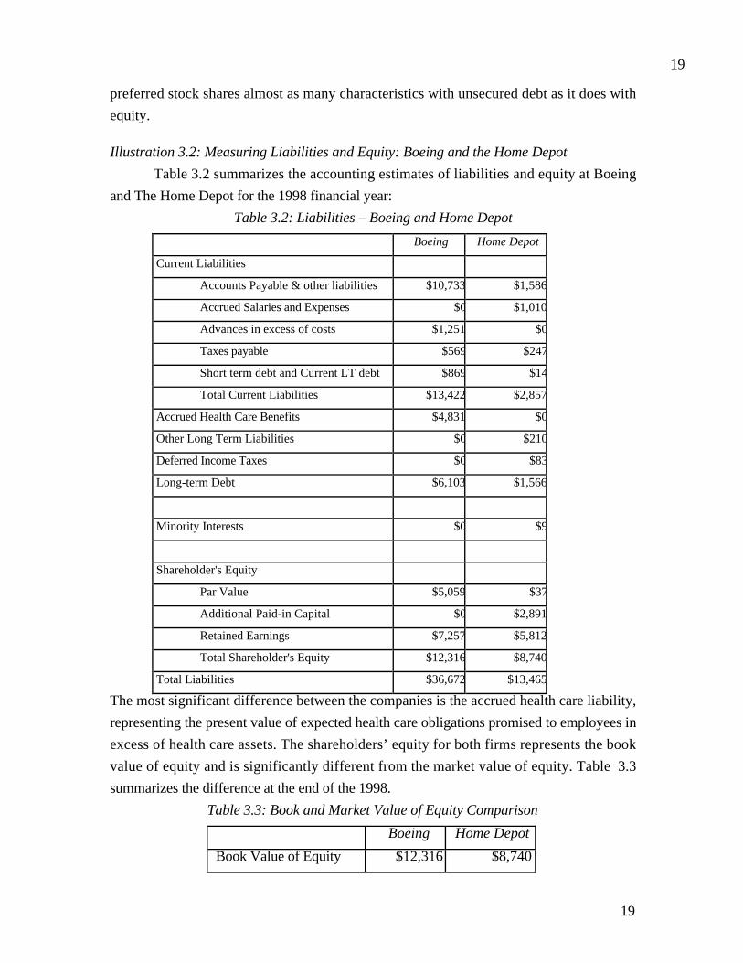
19

19

preferred stock shares almost as many characteristics with unsecured debt as it does with

equity.

Illustration 3.2: Measuring Liabilities and Equity: Boeing and the Home Depot

Table 3.2 summarizes the accounting estimates of liabilities and equity at Boeing

and The Home Depot for the 1998 financial year:

Table 3.2: Liabilities – Boeing and Home Depot

Boeing Home Depot

Current Liabilities

Accounts Payable & other liabilities $10,733 $1,586

Accrued Salaries and Expenses $0 $1,010

Advances in excess of costs $1,251 $0

Taxes payable $569 $247

Short term debt and Current LT debt $869 $14

Total Current Liabilities $13,422 $2,857

Accrued Health Care Benefits $4,831 $0

Other Long Term Liabilities $0 $210

Deferred Income Taxes $0 $83

Long-term Debt $6,103 $1,566

Minority Interests $0 $9

Shareholder's Equity

Par Value $5,059 $37

Additional Paid-in Capital $0 $2,891

Retained Earnings $7,257 $5,812

Total Shareholder's Equity $12,316 $8,740

Total Liabilities $36,672 $13,465

The most significant difference between the companies is the accrued health care liability,

representing the present value of expected health care obligations promised to employees in

excess of health care assets. The shareholders’ equity for both firms represents the book

value of equity and is significantly different from the market value of equity. Table 3.3

summarizes the difference at the end of the 1998.

Table 3.3: Book and Market Value of Equity Comparison

Boeing Home Depot

Book Value of Equity $12,316 $8,740

20

20

Market Value of Equity $32,595 $85,668

One final point needs to be made about the Home Depot’s liabilities. The Home

Depot has substantial operating leases. Because these leases are treated as operating

expenses, they do not show up in the balance sheet. Since they represent commitments to

make payments in the future, we would argue that operating leases should be capitalized and

treated as part of the liabilities of the firm. We will consider how best to do this later in this

book.

Measuring Earnings and ProfitabilityHow profitable is a firm? What did it earn on the assets that it invested in? These are

the fundamental questions we would like financial statements to answer. Accountants use

the income statement to provide information about a firm's operating activities over a

specific time period. In terms of our description of the firm, the income statement is

designed to measure the earnings from assets in place. In this section, we will examine the

principles underlying earnings and return measurement in accounting, and the methods that

they are put into practice.

Accounting Principles Underlying Measurement of Earnings and Profitability

Two primary principles underlie the measurement of accounting earnings and

profitability. The first is the principle of accrual accounting. In accrual accounting, the

revenue from selling a good or service is recognized in the period in which the good is sold

or the service is performed (in whole or substantially). A corresponding effort is made on

the expense side to match7 expenses to revenues. This is in contrast to cash accounting,

where revenues are recognized when payment is received and expenses are recorded when

they are paid.

The second principle is the categorization of expenses into operating, financing and

capital expenses. Operating expenses are expenses that, at least in theory, provide benefits

only for the current period; the cost of labor and materials expended to create products that

are sold in the current period is a good example. Financing expenses are expenses arising

from the non-equity financing used to raise capital for the business; the most common

example is interest expenses. Capital expenses are expenses that are expected to generate

benefits over multiple periods; for instance, the cost of buying land and buildings is treated

as a capital expense.

7 If a cost (such as an administrative cost) cannot be easily linked with a particular revenues, it is usuallyrecognized as an expense in the period in which it is consumed.

21

21

Operating expenses are subtracted from revenues in the current period to arrive at a

measure of operating earnings from the firm. Financing expenses are subtracted from

operating earnings to estimate earnings to equity investors or net income. Capital expenses

are written off over their useful life (in terms of generating benefits) as depreciation or

amortization.

Measuring Accounting Earnings and Profitability

Since income can be generated from a number of different sources, generally

accepted accounting principles (GAAP) require that income statements be classified into

four sections: income from continuing operations, income from discontinued operations,

extraordinary gains or losses and adjustments for changes in accounting principles.

Generally accepted accounting principles require the recognition of revenues when

the service for which the firm is getting paid has been performed in full or substantially and

for which it has received in return either cash or a receivable that is both observable and

measurable. Expenses linked directly to the production of revenues (like labor and

materials) are recognized in the same period in which revenues are recognized. Any

expenses that are not directly linked to the production of revenues are recognized in the

period in which the firm consumes the services.

While accrual accounting is straightforward in firms that produce goods and sell

them, there are special cases where accrual accounting can be complicated by the nature of

the product or service being offered. For instance, firms that enter into long term contracts

with their customers, for instance, are allowed to recognize revenue on the basis of the

percentage of the contract that is completed. As the revenue is recognized on a percentage of

completion basis, a corresponding proportion of the expense is also recognized. When there

is considerable uncertainty about the capacity of the buyer of a good or service to pay for a

service, the firm providing the good or service may recognize the income only when it

collects portions of the selling price under the installment method.

Reverting back to our discussion of the difference between capital and operating

expenses, operating expenses should reflect only those expenses that create revenues in the

current period. In practice, however, a number of expenses are classified as operating

expenses that do not seem to meet this test. The first is depreciation and amortization. While

the notion that capital expenditures should be written off over multiple periods is reasonable,

the accounting depreciation that is computed on the original historical cost often bears little

resemblance to the actual economical depreciation. The second expense is research and

development expenses, which accounting standards in the United States classify as

22

22

operating expenses, but which clearly provide benefits over multiple periods. The rationale

used for this classification is that the benefits cannot be counted on or easily quantified.

Much of financial analysis is built around the expected future earnings of a firm, and

many of these forecasts start with the current earnings. It is therefore important that we

know how much of these earnings come from the ongoing operations of the firm, and how

much can be attributed to unusual or extraordinary events, that are unlikely to recur on a

regular basis. From that standpoint, it is useful that firms categorize expenses into operating

and nonrecurring expenses, since it is the earnings prior to extraordinary items that should

be used in forecasting. Nonrecurring items include the following:

a. Unusual or Infrequent items, such as gains or losses from the divestiture of an asset or

division and write-offs or restructuring costs. Companies sometimes include such items

as part of operating expenses. As an example, Boeing in 1997 took a write-off of

$1,400 million to adjust the value of assets it acquired in its acquisition of McDonnell

Douglas, and it showed this as part of operating expenses.

b. Extraordinary items, which are defined as events that are unusual in nature, infrequent

in occurrence and material in impact. Examples include the accounting gain associated

with refinancing high coupon debt with lower coupon debt, and gains or losses from

marketable securities that are held by the firm.

c. Losses associated with discontinued operations, which measure both the loss from the

phase out period and the estimated loss on the sale of the operations. To qualify,

however, the operations have to be separable separated from the firm.

d. Gains or losses associated with accounting changes, which measure earnings changes

created by accounting changes made voluntarily by the firm (such as a change in

inventory valuation and change in reporting period) and accounting changes mandated

by new accounting standards.

Illustration 3.3: Measures of Earnings

Table 3.4 summarizes the income statements of Boeing and the Home Depot for the

1998 financial year:

Table 3.4: Income Statements: Boeing and Home Depot

Boeing

(in millions)

Home Depot

(in millons)

Sales & Other Operating Revenues $56,154.00 $30,219.00

- Operating Costs & Expenses $51,022.00 $27,185.00

- Depreciation $1,517.00 $373.00

- Research and Development Expenses $1,895.00 $0.00

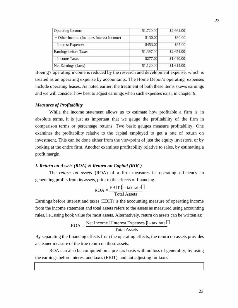
23

23

Operating Income $1,720.00 $2,661.00

+ Other Income (Includes Interest Income) $130.00 $30.00

- Interest Expenses $453.00 $37.00

Earnings before Taxes $1,397.00 $2,654.00

- Income Taxes $277.00 $1,040.00

Net Earnings (Loss) $1,120.00 $1,614.00

Boeing's operating income is reduced by the research and development expense, which is

treated as an operating expense by accountants. The Home Depot’s operating expenses

include operating leases. As noted earlier, the treatment of both these items skews earnings

and we will consider how best to adjust earnings when such expenses exist, in chapter 9.

Measures of Profitability

While the income statement allows us to estimate how profitable a firm is in

absolute terms, it is just as important that we gauge the profitability of the firm in

comparison terms or percentage returns. Two basic gauges measure profitability. One

examines the profitability relative to the capital employed to get a rate of return on

investment. This can be done either from the viewpoint of just the equity investors, or by

looking at the entire firm. Another examines profitability relative to sales, by estimating a

profit margin.

I. Return on Assets (ROA) & Return on Capital (ROC)

The return on assets (ROA) of a firm measures its operating efficiency in

generating profits from its assets, prior to the effects of financing.

( )

Assets Total

rate tax - 1 EBIT ROA =

Earnings before interest and taxes (EBIT) is the accounting measure of operating income

from the income statement and total assets refers to the assets as measured using accounting

rules, i.e., using book value for most assets. Alternatively, return on assets can be written as:

( )Assets Total

rate tax - 1 ExpensesInterest IncomeNet ROA

+=

By separating the financing effects from the operating effects, the return on assets provides

a cleaner measure of the true return on these assets.

ROA can also be computed on a pre-tax basis with no loss of generality, by using

the earnings before interest and taxes (EBIT), and not adjusting for taxes -

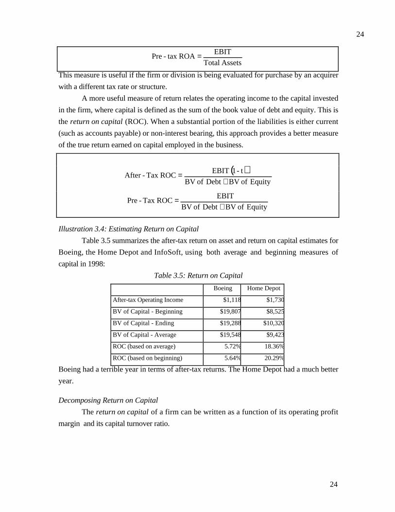
24

24

Assets Total

EBIT ROAtax -Pre =

This measure is useful if the firm or division is being evaluated for purchase by an acquirer

with a different tax rate or structure.

A more useful measure of return relates the operating income to the capital invested

in the firm, where capital is defined as the sum of the book value of debt and equity. This is

the return on capital (ROC). When a substantial portion of the liabilities is either current

(such as accounts payable) or non-interest bearing, this approach provides a better measure

of the true return earned on capital employed in the business.

( )Equity of BV Debt of BV

t-1 EBIT ROCTax -After

+=

Equity of BV Debt of BV

EBIT ROCTax -Pre

+=

Illustration 3.4: Estimating Return on Capital

Table 3.5 summarizes the after-tax return on asset and return on capital estimates for

Boeing, the Home Depot and InfoSoft, using both average and beginning measures of

capital in 1998:

Table 3.5: Return on Capital

Boeing Home Depot

After-tax Operating Income $1,118 $1,730

BV of Capital - Beginning $19,807 $8,525

BV of Capital - Ending $19,288 $10,320

BV of Capital - Average $19,548 $9,423

ROC (based on average) 5.72% 18.36%

ROC (based on beginning) 5.64% 20.29%

Boeing had a terrible year in terms of after-tax returns. The Home Depot had a much better

year.

Decomposing Return on Capital

The return on capital of a firm can be written as a function of its operating profit

margin and its capital turnover ratio.

25

25

After - Tax ROC =EBIT 1-t( )

BV of Capital=

EBIT 1-t( )Sales

X Sales

BV of Capital

= After -Tax Operating Margin * Capital Turnover Ratio

Pre- Tax ROC = Pre -Tax Operating Margin * Capital Turnover Ratio

Thus, a firm can arrive at a high ROC by either increasing its profit margin or more

efficiently utilizing its capital to increase sales. There are likely to be competitive constraints

and technological constraints on increasing sales, but firms still have some freedom within

these constraints to choose the mix of profit margin and capital turnover that maximizes

their ROC. The return on capital varies widely across firms in different businesses, largely

as a consequence of differences in profit margins and capital turnover ratios.

mgnroc.xls: There is a dataset on the web that summarizes the operating margins,

turnover ratios and returns on capital of firms in the United States, classified by industry.

II. Return on Equity

While the return on capital measures the profitability of the overall firm, the return

on equity (ROE) examines profitability from the perspective of the equity investor by

relating profits to the equity investor (net profit after taxes and interest expenses) to the

book value of the equity investment.

EquityCommon of ValueBook

IncomeNet ROE =

Since preferred stockholders have a different type of claim on the firm than do common

stockholders, the net income should be estimated after preferred dividends and the book

value of common equity should not include the book value of preferred stock. This can be

accomplished by using net income after preferred dividends in the numerator and the book

value of common equity in the denominator.

Determinants of ROE

Since the ROE is based upon earnings after interest payments, it is affected by the

financing mix the firm uses to fund its projects. In general, a firm that borrows money to

finance projects and that earns a ROC on those projects exceeding the after-tax interest rate

26

26

it pays on its debt will be able to increase its ROE by borrowing. The ROE can be written as

follows8:

( )( )t-1i-ROCE

DROCROE +=

where,

( )Equity of BV Debt of BV

t-1 EBIT ROC

+=

Equity of BV

Debt of BV

E

D =

Debt of BV

Debton ExpenseInterest i =

t = Marginal tax rate on ordinary income

The second term captures the benefit of financial leverage.

Illustration 3.5: ROE Computations

Table 3.6 summarizes the return on equity for Boeing and the Home Depot in 1998:

Table 3.6: Return on Equity

Return Ratios Boeing Home Depot

Net Income $1,120 $1,614

BV of Equity- Beginning $12,953 $7,214

BV of Equity- Ending $12,316 $8,740

BV of Equity - Average $12,635 $7,977

ROE (based on average) 8.86% 20.23%

ROE (based on beginning) 8.65% 22.37%

The results again indicate that Boeing had a poor year in 1998, while the Home Depot

reported a healthier return on equity. The returns on equity can also be estimated by

decomposing into the components specified above (using the adjusted beginning of the year

numbers):

Boeing Home Depot

After-tax ROC 5.82% 16.37%

8

( )( ) ( ) ( ) ( )

( ) ( ) ( ) ( )ROE

E

NI

E

t-1IE

E

t-1IE

E

NI

E

t-1IE

E

D1

ED

t-1IENI

D

t-1IE

ED

t-1IENI

E

D

ED

t-1IENIt-1i-ROC

E

DROC

==−+=−

+

++=

−

+++

++=+

27

27

Debt/Equity Ratio 35.18% 48.37%

Book Interest Rate (1-tax rate) 4.22% 4.06%

ROE 6.38% 22.33%

Note that we used a tax rate of 35% on both the return on capital and the book interest rate.

This approach results in a return on equity that is different from the one estimated using the

net income and the book value of equity.

rocroe.xls: There is a dataset on the web that summarizes the return on capital,

debt equity ratios, book interest rates and returns on equity of firms in the United States,

classified by industry.

Measuring RiskHow risky are the investments the firm has made over time? How much risk do

equity investors in a firm face? These are two more questions that we would like to find the

answer to in the course of an investment analysis. Accounting statements do not really claim

to measure or quantify risk in a systematic way, other than to provide footnotes and

disclosures where there might be risk embedded in the firm. In this section, we will examine

some of the ways in which accountants try to assess risk.

Accounting Principles Underlying Risk Measurement

To the extent that accounting statements and ratios do attempt to measure risk, there

seem to be two common themes.

a. The first is that the risk being measured is the risk of default, i.e. the risk that a fixed

obligation, such as interest or principal due on outstanding debt, will not be met. The

broader equity notion of risk, which measures the variance of actual returns around

expected returns, does not seem to receive much attention. Thus, an all-equity-financed

firm with positive earnings and few or no fixed obligations will generally emerge as a

low-risk firm from an accounting standpoint, in spite of the fact that its earnings are

unpredictable.

b. Accounting risk measures generally take a static view of risk, by looking at the capacity

of a firm at a point in time to meet its obligations. For instance, when ratios are used to

assess a firm's risk, the ratios are almost always based upon one period's income

statement and balance sheet.

28

28

Accounting Measures of Risk

Accounting measures of risk can be broadly categorized into two groups. The first

is disclosures about potential obligations or losses in values that show up as footnotes on

balance sheets, which are designed to alert potential or current investors to the possibility of

significant losses. The second is the ratios that are designed to measure both liquidity and

default risk.

Disclosures in Financial Statements

In recent years, the number of disclosures that firms have to make about future

obligations has proliferated. Consider, for instance, the case of contingent liabilities.

These refer to potential liabilities that will be incurred under certain contingencies, as is the

case when a firm is the defendant in a lawsuit. The general rule that has been followed is to

ignore contingent liabilities which hedge against risk, since the obligations on the contingent

claim will be offset9 by benefits elsewhere. In recent periods, however, significant losses

borne by firms from supposedly hedged derivatives positions (such as options and futures)

have led to FASB requirements that these derivatives be disclosed as part of a financial

statement. In fact, pension fund and health care obligations have moved from mere footnotes

to actual liabilities for firms.

Financial Ratios

Financial statements have long been used as the basis for estimating financial ratios

that measure profitability, risk and leverage. In the section on earnings, we looked at two of

the profitability ratios – return on equity and return on capital . In this section, we will look

at some of the financial ratios that are often used to measure the financial risk in a firm.

1. Short-Term Liquidity Risk

Short-term liquidity risk arises primarily from the need to finance current

operations. To the extent that the firm has to make payments to its suppliers before it gets

paid for the goods and services it provides, there is a cash shortfall that has to be met,

usually through short-term borrowing. Though this financing of working capital needs is

done routinely in most firms, financial ratios have been devised to keep track of the extent of

the firm's exposure to the risk that it will not be able to meet its short-term obligations. The

two most frequently used to measure short-term liquidity risk are the current ratio and the

quick ratio.

9 This assumes that the hedge is set up competently. It is entirely possible that a hedge, if sloppily set up,can end up costing the firm money.

29

29

The current ratio is the ratio of current assets (cash, inventory, accounts receivable)

to its current liabilities (obligations coming due within the next period).

sLiabilitieCurrent

AssetsCurrent RatioCurrent =

A current ratio below one, for instance, would indicate that the firm has more obligations

coming due in the next year than assets it can expect to turn to cash. That would be an

indication of liquidity risk.

While traditional analysis suggests that firms maintain a current ratio of 2 or greater,

there is a trade-off here between minimizing liquidity risk and tying up more and more cash

in net working capital (Net working capital = Current Assets - Current Liabilities). In fact, it

can be reasonably argued that a very high current ratio is indicative of an unhealthy firm,

which is having problems reducing its inventory. In recent years, firms have worked at

reducing their current ratios and managing their net working capital better.

Reliance on current ratios has to be tempered by a few concerns. First, the ratio can

be easily manipulated by firms around the time of financial reporting dates to give the

illusion of safety; second, current assets and current liabilities can change by an equal

amount, but the effect on the current ratio will depend upon its level10 before the change.

The quick or acid test ratio is a variant of the current ratio. It distinguishes current

assets that can be converted quickly into cash (cash, marketable securities) from those that

cannot (inventory, accounts receivable).

sLiabilitieCurrent

Securities Marketable Cash RatioQuick

+=

The exclusion of accounts receivable and inventory is not a hard and fast rule. If there is

evidence that either can be converted into cash quickly, it can, in fact, be included as part of

the quick ratio.

Turnover ratios measure the efficiency of working capital management by looking

at the relationship of accounts receivable and inventory to sales and to the cost of goods

sold.

Receivable Accounts Average

SalesTurnover Receivable Accounts =

10 If the current assets and current liabilities increase by an equal amount, the current ratio will go down if

30

30

Inventory Average

Sold Goods ofCost TurnoverInventory =

These ratios can be interpreted as measuring the speed with which the firm turns accounts

receivable into cash or inventory into sales. These ratios are often expressed in terms of the

number of days outstanding.

Turnover Receivable

365gOutstandin Receivable Days =

TurnoverInventory

365HeldInventory Days =

A similar pair of ratios can be computed for accounts payable, relative to purchases.

Payable Accounts Average

PurchasesTurnover Payable Accounts =

Turnover Payable Accounts

365gOutstandin Payable Accounts Days =

Since accounts receivable and inventory are assets and accounts payable is a liability, these

three ratios (standardized in terms of days outstanding) can be combined to get an estimate

of how much financing the firm needs to fund working capital needs.

+

+

=gOutstandin

Payable Days

Held

Inventory Days

gOutstandin

Receivable DaysPeriod Financing Required

The greater the financing period for a firm, the greater is its short-term liquidity risk.

wcdata.xls: This is a dataset on the web that summarizes working capital ratios for

firms in the United States, classified by industry.

it was greater than one before the increase and go up if it was less than one.

31

31

finratio.xls: This spreadsheet allows you to compute the working capital ratios for a

firm, based upon financial statement data.

2. Long-term Solvency and Default risk

Measures of long-term solvency attempt to examine a firm's capacity to meet interest

and principal payments in the long term. Clearly, the profitability ratios discussed earlier in

the section are a critical component of this analysis. The ratios specifically designed to

measure long term solvency try to relate profitability to the level of debt payments, to

identify the degree of comfort with which the firm can meet these payments.

Interest Coverage Ratios

The interest coverage ratio measures the capacity of the firm to meet interest

payments from pre-debt, pre-tax earnings.

ExpensesInterest

EBITRatio CoverageInterest =

The higher the interest coverage ratio, the more secure is the firm's capacity to make interest

payments from earnings. This argument however has to be tempered by the recognition that

earnings before interest and taxes is volatile and can drop significantly if the economy

enters a recession. Consequently, two firms can have the same interest coverage ratio but be

viewed very differently in terms of risk.

The denominator in the interest coverage ratio can be easily extended to cover other

fixed obligations such as lease payments. If this is done, the ratio is called a fixed charges

coverage ratio.

Fixed Chargeds Coverage Ratio =EBIT + Fixed Charges

Fixed Charges

Finally, this ratio, while stated in terms of earnings, can be restated in terms of cash flows,

by using earnings before interest, taxes and depreciation (EBITDA) in the numerator and

cash fixed charges in the denominator.

Charges FixedCash

EBITDARatio Coverage Charges FixedCash =

Both interest coverage and fixed charge ratios are open to the criticism that they do not

consider capital expenditures, a cash flow that may be discretionary in the very short term,

32

32

but not in the long term if the firm wants to maintain growth. One way of capturing the

extent of this cash flow, relative to operating cash flows, is to compute a ratio of the two.

esExpenditur Capital

Operations from flowsCash esExpenditur Capital toflowCash Operating =

While there are a number of different definitions of cash flows from operations, the most

reasonable way of defining it is to measure the cash flows from continuing operations,

before interest but after taxes, and after meeting working capital needs.

Cash flow from operations = EBIT (1-tax rate) - ∆ Working Capital

covratio.xls: There is a dataset on the web that summarizes the interest coverage

and fixed charge coverage ratios for firms in the United States, classified by industry.

Illustration 3.6: Interest and Fixed Charge Coverage Ratios

Table 3.7 summarizes interest and fixed charge coverage ratios for Boeing and

Home Depot in 1998:

Table 3.7: Interest and Fixed Charge Coverage Ratios

Boeing Home Depot

EBIT $1,720 $2,661

Interest Expense $453 $37

Interest Coverage Ratio 3.80 71.92

EBIT $1,720 $2,661

Operating Lease Expenses $215 $290

Interest Expenses $453 $37

Fixed Charge Coverage Ratio 2.90 9.02

EBITDA $3,341 $3,034

Cash Fixed Charges $668 $327

Cash Fixed Charge Coverage 5.00 9.28

Cash Flows from Operations $2,161 $1,662

Capital Expenditures $1,584 $2,059

CF/Cap Ex 1.36 0.81

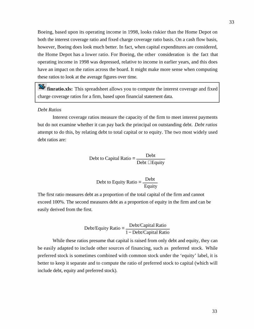
33

33

Boeing, based upon its operating income in 1998, looks riskier than the Home Depot on

both the interest coverage ratio and fixed charge coverage ratio basis. On a cash flow basis,

however, Boeing does look much better. In fact, when capital expenditures are considered,

the Home Depot has a lower ratio. For Boeing, the other consideration is the fact that

operating income in 1998 was depressed, relative to income in earlier years, and this does

have an impact on the ratios across the board. It might make more sense when computing

these ratios to look at the average figures over time.

finratio.xls: This spreadsheet allows you to compute the interest coverage and fixed

charge coverage ratios for a firm, based upon financial statement data.

Debt Ratios

Interest coverage ratios measure the capacity of the firm to meet interest payments

but do not examine whether it can pay back the principal on outstanding debt. Debt ratios

attempt to do this, by relating debt to total capital or to equity. The two most widely used

debt ratios are:

Equity Debt

DebtRatio Capital Debt to

+=

Equity

DebtRatioEquity Debt to =

The first ratio measures debt as a proportion of the total capital of the firm and cannot

exceed 100%. The second measures debt as a proportion of equity in the firm and can be

easily derived from the first.

Ratio alDebt/Capit1

Ratio alDebt/CapitRatioy Debt/Equit

−=

While these ratios presume that capital is raised from only debt and equity, they can

be easily adapted to include other sources of financing, such as preferred stock. While

preferred stock is sometimes combined with common stock under the ‘equity’ label, it is

better to keep it separate and to compute the ratio of preferred stock to capital (which will

include debt, equity and preferred stock).

34

34

a. Variants on Debt Ratios

There are two close variants of debt ratios. In the first, only long-term debt is used

rather than total debt, with the rationale that short-term debt is transitory and will not affect

the long-term solvency of the firm.

Equity Debt termLong

Debt termLongRatio Capital Debt to termLong

+=

Equity

Debt termLongRatioEquity Debt to termLong =

Given the ease with which firms can roll over short-term debt, and the willingness of many

firms to use short-term financing to fund long-term projects, these variants can provide a

misleading picture of the firm's financial leverage risk.

The second variant of debt ratios uses market value (MV) instead of book value,

primarily to reflect the fact that some firms have a significantly greater capacity to borrow

than their book values indicate.

Equity of MV Debt of MV

Debt of MVRatio Capital Debt to ValueMarket

+=

Equity of MV

Debt of MVRatioEquity Debt to ValueMarket =

Many analysts disavow the use of market value in their calculations, contending that market

values, in addition to being difficult to get for debt, are volatile and hence unreliable. These

contentions are open to debate. It is true that the market value of debt is difficult to get for

firms which do not have publicly traded bonds, but the market value of equity is not only

easy to obtain, it is constantly updated to reflect market-wide and firm-specific changes.

Furthermore, using the book value of debt as a proxy for market value in those cases where

bonds are not traded does not significantly shift11 most market-value based debt ratios.

Illustration 3.7: Book Value Debt Ratios and Variants- Boeing and Home Depot

Table 3.8 summarizes different estimates of the debt ratio for Boeing, the Home

Depot and InfoSoft, using book values of debt and equity for all three firms:

Table 3.8: Book Value Debt Ratios

11 Deviations in the market value of equity from book value are likely to be much larger than deviation fordebt and are likely to dominate in most debt ratio calculations.

35

35

Boeing Home Depot

Long Term Debt $6,103 $1,566

Short Term Debt $869 $14

BV of Equity $12,316 $8,740

LT Debt/Equity 49.55% 17.92%

LT Debt / (LT Debt + Equity) 33.13% 15.20%

Debt/Equity 56.61% 18.08%

Debt/ (Debt + Equity) 36.15% 15.31%

Boeing has a much higher book value debt ratio, both long term and total debt, than the

Home Depot.

dbtfund.xls: There is a dataset on the web that summarizes the book value debt

ratios and market value debt ratios for firms in the United States, classified by industry.

Other issues in analyzing financial statementsTwo more issues bear consideration before we conclude this section on financial

statements. The first relates to differences in accounting standards and practices and how

these differences may color comparisons across companies and the second relates to

accounting for acquisitions and how this can affect both the acquisition method and price.

Differences in accounting standards and practices

Differences in accounting standards across countries affect the measurement of

earnings. These differences, however, are not so great as they are made out to be and they

cannot explain away radical departures from fundamental principles of valuation12. Choi

and Levich, in a survey of accounting standards across developed markets, note that most

countries subscribe to basic accounting notions of consistency, realization and historical

cost principles in preparing accounting statements. Table 3.9 summarizes accounting

standards in eight major financial markets and reveals that the common elements vastly

outnumber those areas where there are differences.

12 At the peak of the Japanese market, there were many investors who explained away the price-earningsmultiples of 60 and greater in the market, by noting that Japanese firms were conservative in measuringearnings. Even after taking into account the general provisions and excess depreciation used by many ofthese firms to depress current earnings, the price-earnings multiples were greater than 50 for many firms,suggesting either extraordinary expected growth in the future or overvaluation.

36

36

The two countries that offer the strongest contrast to the United States are Germany

and Japan. The key differences and their implications are as follows. First, companies in the

United States generally maintain separate tax and financial reporting books, which in turn

generates items like deferred taxes to cover differences between the two books. Companies

in Germany and Japan do not maintain separate books. Consequently, depreciation methods

in financial reports are much more likely to be accelerated and hence to reduce stated

income. Second, the requirement that leases be capitalized and shown as a liability is much

more tightly enforced in the United States. In Japan, leases are generally treated as operating

leases and do not show up as liabilities in the balance sheet. In Germany, firms can

capitalize leases, but they have more leeway in classifying leases as operating and capital

leases than U.S. companies. Third, goodwill, once created, can be amortized over 40 years in

the United States and over much shorter time periods in Germany and Japan, again

depressing stated income. Fourth, reserves in the United States can be created only for

specific purposes, whereas German and Japanese companies can use general reserves to

equalize earnings across periods, leading earnings to be understated during the good years,

and overstated during bad years.

Most of these differences can be accounted and adjusted for when comparisons are

made between companies in the U.S. and companies in other financial markets. Ratios such

as price earnings, which use stated and unadjusted earnings, can be misleading when

accounting standards vary widely across the companies being compared.

SummaryFinancial statements remain the primary source of information for most investors

and analysts. There are differences, however, in how accounting and financial analysis

approach answering a number of key questions about the firm. We examine these

differences in this chapter.

The first question that we examined related to the nature and the value of the assets

owned by a firm. Categorizing assets into investments already made (assets in place) and

investments yet to be made (growth assets), we argued that accounting statements provide a

substantial amount of historical information about the former and very little about the latter.

The focus on the original price of assets in place (book value) in accounting statements can

lead to significant differences between the stated value of these assets and their market

value. With growth assets, accounting rules result in low or no values for assets generated

by internal research.

The second issue that we examined was the measurement of profitability. The two

principles that seem to govern how profits are measured are accrual accounting – revenues

37

37

and expenses are shown in the period where transactions occur rather than when the cash is

received or paid – and the categorization of expenses into operating, financing and capital

expenses. Operating and financing expenses are shown in income statements. Capital

expenditures take the form of depreciation and amortization and are spread over several time

periods. Accounting standards miscategorize operating leases and research and development

expenses as operating expenses (when the former should be categorized as financing

expenses and the latter as capital expenses).

In the last part of the chapter, we examine how financial statements deal with short-

term liquidity risk and long-term default risk. While the emphasis in accounting statements

is on examining the risk that firms may be unable to make payments that they have

committed to make, there is very little focus on risk to equity investors.

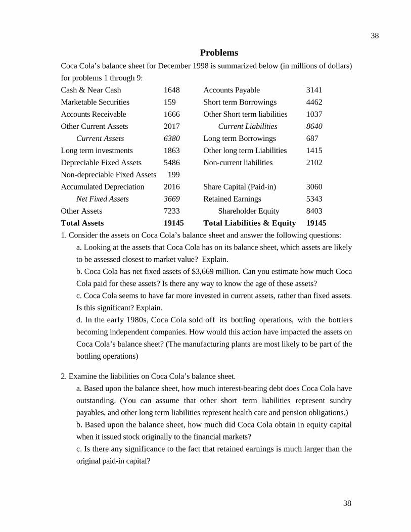
38

38

ProblemsCoca Cola’s balance sheet for December 1998 is summarized below (in millions of dollars)

for problems 1 through 9:

Cash & Near Cash 1648 Accounts Payable 3141

Marketable Securities 159 Short term Borrowings 4462

Accounts Receivable 1666 Other Short term liabilities 1037

Other Current Assets 2017 Current Liabilities 8640

Current Assets 6380 Long term Borrowings 687

Long term investments 1863 Other long term Liabilities 1415

Depreciable Fixed Assets 5486 Non-current liabilities 2102

Non-depreciable Fixed Assets 199

Accumulated Depreciation 2016 Share Capital (Paid-in) 3060

Net Fixed Assets 3669 Retained Earnings 5343

Other Assets 7233 Shareholder Equity 8403

Total Assets 19145 Total Liabilities & Equity 19145

1. Consider the assets on Coca Cola’s balance sheet and answer the following questions:

a. Looking at the assets that Coca Cola has on its balance sheet, which assets are likely

to be assessed closest to market value? Explain.

b. Coca Cola has net fixed assets of $3,669 million. Can you estimate how much Coca

Cola paid for these assets? Is there any way to know the age of these assets?

c. Coca Cola seems to have far more invested in current assets, rather than fixed assets.

Is this significant? Explain.

d. In the early 1980s, Coca Cola sold off its bottling operations, with the bottlers

becoming independent companies. How would this action have impacted the assets on

Coca Cola’s balance sheet? (The manufacturing plants are most likely to be part of the

bottling operations)

2. Examine the liabilities on Coca Cola’s balance sheet.

a. Based upon the balance sheet, how much interest-bearing debt does Coca Cola have

outstanding. (You can assume that other short term liabilities represent sundry

payables, and other long term liabilities represent health care and pension obligations.)

b. Based upon the balance sheet, how much did Coca Cola obtain in equity capital

when it issued stock originally to the financial markets?

c. Is there any significance to the fact that retained earnings is much larger than the

original paid-in capital?

39

39

d. The market value of Coca Cola’s equity is $140 billion. What is the book value of

equity in Coca Cola? Why is there such a large difference between the market value of

equity and the book value of equity?

3. Coca Cola’s most valuable asset is its brand name. Where in the balance sheet do you

see its value? Is there any way to adjust the balance sheet to reflect the value of this asset?

4. Assume that you have been asked to analyze Coca Cola’s working capital management.

a. Estimate the net working capital and non-cash working capital for Coca Cola.

b. Estimate the firm’s current ratio.

c. Estimate the firm’s quick ratio.

d. Would you draw any conclusions about the riskiness of Coca Cola as a firm by

looking at these numbers? Why or why not?

Coca Cola’s income statements for 1997 and 1998 are summarized below (in millions of

dollars):

1997 1998

Net Revenues $18,868 $18,813

Cost of Goods Sold 6,105 5,562

Selling, G & A Expenses 7,852 8,284

Earnings before interest and taxes 5,001 4,967

Interest Expenses 258 277

Non-operating Gains 1,312 508

Income Tax Expenses 1,926 1,665

Net Income 4,129 3,533

Dividends 1,387 1,480

The following questions relate to Coca Cola’s income statement.

5. How much operating income did Coca Cola earn, before taxes, in 1998? How does this

compare to how much Coca Cola earned in 1997? What are the reasons for the differences?

6. The biggest expense for Coca Cola is advertising, which is part of the selling, general and

administrative expenses. A large portion of these expenses are designed to build up Coca

Cola’s brand name. Should advertising expenses be treated as operating expenses or are

they really capital expenses? If they are to be treated as capital expenses, how would you

capitalize them? (Use the capitalization of R&D as a guide.)

40

40

7. What effective tax rate did Coca Cola have in 1998? How does it compare with what they

paid in 1997 as an effective tax rate? What might account for the difference?

8. You have been asked to assess the profitability of Coca Cola, as a firm. To that end,

estimate the pre-tax operating and net margins in 1997 and 1998 for the firm. Are there any

conclusions you would draw from the comparisons across the two years.

9. The book value of equity at Coca Cola in 1997 was $7,274 million. The book value of

interest-bearing debt was $3,875 million. Estimate:

a. the return on equity (beginning of the year) in 1998

b. the pre-tax return on capital (beginning of the year) in 1998

c. the after-tax return on capital (beginning of the year) in 1998, using the effective tax

rate in 1998.

10. SeeSaw Toys reported that it had a book value of equity of $1.5 billion at the end of

1998 and 100 million shares outstanding. During 1999, it bought back 10 million shares at

a market price of $40 per share. The firm also reported a net income of $150 million for

1999, and paid dividends of $50 million.

a. Estimate the book value of equity at the end of 1999

b. Estimate the return on equity, using beginning book value of equity.

c. Estimate the return on equity, using the average book value of equity.

41

41

Table 3.9: International Comparison of Accounting Principles

Accounting Principle UK USA France Germany Netherlands Sweden Switzerland Japan

1. Consistence – accounting principles and

methods are applied on the same basis from

period to period

Yes Yes Yes Yes Yes PP PP Yes

2. Realization – revenue is recognized when

realization is reasonably assured

Yes Yes Yes Yes Yes Yes PP Yes

3. Fair presentation of the financial

statement is required

Yes Yes Yes Yes Yes Yes Yes Yes

4. Historical cost convention – departures

from the historical cost convention are

disclosed

Yes Yes Yes Yes Yes Yes RF Yes

5. Accounting policies – a change in

accounting principles and methods without

a change in circumstances is accounted for

by a prior year adjustment

Yes No Yes MP RF MP MP No

6. Fixed assets – revaluation – in historical

cost statements, fixed assets are stated at an

amount in excess of cost which is

determined at irregular intervals.

MP No Yes No RF PP No No

7. Fixed assets – revaluation – when fixed

assets are stated, in historical cost

statements, at an amount in excess of cost,

depreciation based on the revaluation

amount is charged to income.

Yes No Yes No Yes Yes No No

8. Goodwill amortized MP Yes Yes Yes M Yes MP Yes

42

42

9. Finance leases capitalized Yes Yes No No No Yes RF No

10. Short-term marketablse securities at the

lower of cost or market value

Yes Yes Yes Yes Yes Yes Yes Yes

11. Inventory values at the lower of cost or

market value

Yes Yes Yes Yes Yes Yes Yes Yes

12. Manufacturing overhead allocated to

year-end inventory

Yes Yes Yes Yes Yes Yes Yes Yes

13. Inventory costed using FIFO PP M M M M PP PP M

14. Long-term debt included maturities

longer than one year

Yes Yes Yes No Yes Yes Yes Yes

15. Deferred tax recognized where

accounting income and taxable income arise

at different times

Yes Yes Yes No Yes No No Yes

16. Total pension fund assets and liabilities

excluded from a company’s financial

statements

Yes Yes Yes No Yes Yes Yes Yes

17. Research and development expensed Yes Yes Yes Yes Yes Yes Yes Yes

18. General purpose (purely discretionary)

reserves allowed

No No Yes Yes Yes Yes Yes Yes

19. Offsetting-assets and liabilities are offset

against each other in the balance sheet only

when a legal right of offset exists

Yes Yes Yes Yes Yes Yes PP Yes

20. Unusual and extraordinary gains and

losses are taken in the income statement

Yes Yes Yes Yes Yes Yes Yes Yes

21. Closing rate method of foreign currency

translation employed

Yes Yes Yes Yes Yes No Yes No

43

43

22. Currency translation gains or losses

arising from trading are reflected in current

income

Yes Yes MP MP MP MP MP No

23. Excess depreciation permitted Yes No Yes Yes Yes Yes Yes Yes

24. Basic statements reflect a historical cost

valuation (no price level adjustment)

Yes Yes Yes Yes M Yes Yes Yes

25. Supplementary inflation – adjusted

financial statements adjusted

MP MP No NO MP Yes No No

26. Accounting for long-term investments:

(a) less than 20% ownership - cost

method

(b) 20 - 50% ownership -equity method

(c) More than 50% full consolidation

Yes

Yes

Yes

Yes

Yes

Yes

Yes

Yes

Yes

Yes

No

Yes

No

Yes

Yes

Yes

MP

Yes

Yes

M

Yes

Yes

Yes

Yes

27. Both domestic and foreign subsidiaries

consolidated

Yes Yes Yes M Yes Yes MP Yes

28. Acquisition accounted for under the

purchase cost method

PP PP Yes Yes Yes PP Yes Yes

29. Minority interest excluded from

consolidation income

Yes Yes Yes Yes Yes Yes Yes Yes

30. Minority interest excluded from

consolidated owners’ equity

Yes Yes Yes Yes Yes Yes Yes Yes

Key: PP – Predominant Practice

MP – Minority Practice

M – Mixed Practice

RF – Rarely or not found

44

44

1

CHAPTER 4

THE BASICS OF RISK

When valuing assets and firms, we need to use discount rates that reflect the

riskiness of the cash flows. In particular, the cost of debt has to incorporate a default

spread for the default risk in the debt and the cost of equity has to include a risk premium

for equity risk. But how do we measure default and equity risk, and more importantly,

how do we come up with the default and equity risk premiums?

In this chapter, we will lay the foundations for analyzing risk in valuation. We

present alternative models for measuring risk and converting these risk measures into

“acceptable” hurdle rates. We begin with a discussion of equity risk and present our

analysis in three steps. In the first step, we define risk in statistical terms to be the

variance in actual returns around an expected return. The greater this variance, the more

risky an investment is perceived to be. The next step, which we believe is the central one,

is to decompose this risk into risk that can be diversified away by investors and risk that

cannot. In the third step, we look at how different risk and return models in finance

attempt to measure this non-diversifiable risk. We compare and contrast the most widely

used model, the capital asset pricing model, with other models, and explain how and why

they diverge in their measures of risk and the implications for the equity risk premium.

In the second part of this chapter, we consider default risk and how it is measured

by ratings agencies. In addition, we discuss the determinants of the default spread and

why it might change over time. By the end of the chapter, we should have a methodology

of estimating the costs of equity and debt for any firm.

What is risk?

Risk, for most of us, refers to the likelihood that in life’s games of chance, we will

receive an outcome that we will not like. For instance, the risk of driving a car too fast is

getting a speeding ticket, or worse still, getting into an accident. Webster’s dictionary, in

fact, defines risk as “exposing to danger or hazard”. Thus, risk is perceived almost

entirely in negative terms.

In finance, our definition of risk is both different and broader. Risk, as we see it,

refers to the likelihood that we will receive a return on an investment that is different from

2

the return we expected to make. Thus, risk includes not only the bad outcomes, i.e,

returns that are lower than expected, but also good outcomes, i.e., returns that are higher

than expected. In fact, we can refer to the former as downside risk and the latter is upside

risk; but we consider both when measuring risk. In fact, the spirit of our definition of risk

in finance is captured best by the Chinese symbols for risk, which are reproduced below:

The first symbol is the symbol for “danger”, while the second is the symbol for

“opportunity”, making risk a mix of danger and opportunity. It illustrates very clearly the

tradeoff that every investor and business has to make – between the higher rewards that

come with the opportunity and the higher risk that has to be borne as a consequence of

the danger.

Much of this chapter can be viewed as an attempt to come up with a model that

best measures the “danger” in any investment and then attempts to convert this into the

“opportunity” that we would need to compensate for the danger. In financial terms, we

term the danger to be “risk” and the opportunity to be “expected return”.

What makes the measurement of risk and expected return so challenging is that it

can vary depending upon whose perspective we adopt. When analyzing Boeing’s risk, for

instance, we can measure it from the viewpoint of Boeing’s managers. Alternatively, we

can argue that Boeing’s equity is owned by its stockholders and that it is their

perspective on risk that should matter. Boeing’s stockholders, many of whom hold the

stock as one investment in a larger portfolio, might perceive the risk in Boeing very

differently from Boeing’s managers, who might have the bulk of their capital, human and

financial, invested in the firm.

In this chapter, we will argue that risk in an investment has to be perceived

through the eyes of investors in the firm. Since firms like Boeing often have thousands of

investors, often with very different perspectives, we will go further. We will assert that

risk has to be measured from the perspective of not just any investor in the stock, but of

the marginal investor, defined to be the investor most likely to be trading on the stock

3

at any given point in time. The objective in corporate finance is the maximization of firm

value and stock price. If we want to stay true to this objective, we have to consider the

viewpoint of those who set the stock prices, and they are the marginal investors.

Equity Risk and Expected Return

To demonstrate how risk is viewed in corporate finance, we will present risk

analysis in three steps. First, we will define risk in terms of the distribution of actual

returns around an expected return. Second, we will differentiate between risk that is

specific to one or a few investments and risk that affects a much wider cross section of

investments. We will argue that in a market where the marginal investor is well diversified,

it is only the latter risk, called market risk that will be rewarded. Third, we will look at

alternative models for measuring this market risk and the expected returns that go with it.

I. Defining Risk

Investors who buy assets expect to earn returns over the time horizon that they

hold the asset. Their actual returns over this holding period may be very different from

the expected returns and it is this difference between actual and expected returns that is

source of risk. For example, assume that you are an investor with a 1-year time horizon

buying a 1-year Treasury bill (or any other default-free one-year bond) with a 5%

expected return. At the end of the 1-year holding period, the actual return on this

investment will be 5%, which is equal to the expected return. The return distribution for

this investment is shown in Figure 4.1.

4

Return

Probability =

Expected

Figure 4.1: Probability Distribution for Riskfree Investment

The actual return is always equal to the expected return.

This is a riskless investment.

To provide a contrast to the riskless investment, consider an investor who buys

stock in Boeing. This investor, having done her research, may conclude that she can make

an expected return of 30% on Boeing over her 1-year holding period. The actual return

over this period will almost certainly not be equal to 30%; it might be much greater or

much lower. The distribution of returns on this investment is illustrated in Figure 4.2.

5

ReturnsExpected Return

Figure 4.2: Probability Distribution for Risky Investment

This distribution measures the probabilitythat the actual return will be different

In addition to the expected return, an investor now has to consider the following. First,

note that the actual returns, in this case, are different from the expected return. The

spread of the actual returns around the expected return is measured by the variance or

standard deviation of the distribution; the greater the deviation of the actual returns from

expected returns, the greater the variance. Second, the bias towards positive or negative

returns is represented by the skewness of the distribution. The distribution in Figure 4.2

is positively skewed, since there is a higher probability of large positive returns than large

negative returns. Third, the shape of the tails of the distribution is measured by the

kurtosis of the distribution; fatter tails lead to higher kurtosis. In investment terms, this

represents the tendency of the price of this investment to jump (up or down from current

levels) in either direction.

In the special case, where the distribution of returns is normal, investors do not

have to worry about skewness and kurtosis. Normal distributions are symmetric (no

skewness) and defined to have a kurtosis of zero. Figure 4.3 illustrates the return

distributions on two investments with symmetric returns.

Figure 4.3: Return Distribution Comparisons

6

Expected Return

Low Variance Investment

High Variance Investment

When return distributions take this form, the characteristics of any investment can be

measured with two variables – the expected return, which represents the opportunity in

the investment, and the standard deviation or variance, which represents the danger. In

this scenario, a rational investor, faced with a choice between two investments with the

same standard deviation but different expected returns, will always pick the one with the

higher expected return.

In the more general case, where distributions are neither symmetric nor normal, it

is still conceivable that investors will choose between investments on the basis of only

the expected return and the variance, if they possess utility functions1 that allow them to

do so. It is far more likely, however, that they prefer positive skewed distributions to

negatively skewed ones, and distributions with a lower likelihood of jumps (lower

kurtosis) to those with a higher likelihood of jumps (higher kurtosis). In this world,

investors will trade off the good (higher expected returns and more positive skewness)

against the bad (higher variance and higher kurtosis) in making investments.

1 A utility function is a way of summarizing investor preferences into a generic term called ‘utility’ on thebasis of some choice variables. In this case, for instance, we state the investor’s utility or satisfaction as afunction of wealth. By doing so, we effectively can answer questions such as – Will an investor be twice ashappy if he has twice as much wealth? Does each marginal increase in wealth lead to less additional utilitythan the prior marginal increase? In one specific form of this function, the quadratic utility function, theentire utility of an investor can be compressed into the expected wealth measure and the standard deviationin that wealth.

7

In closing, we should note that the expected returns and variances that we run into

in practice are almost always estimated using past returns rather than future returns. The

assumption we are making when we use historical variances is that past return

distributions are good indicators of future return distributions. When this assumption is

violated, as is the case when the asset’s characteristics have changed significantly over

time, the historical estimates may not be good measures of risk.

In Practice 4.1: Calculation of standard deviation using historical returns: Boeing and the

Home Depot

We will use Boeing and the Home Depot as our investments to illustrate how

standard deviations and variances are computed. To make our computations simpler, we

will look at returns on an annual basis from 1991 to 1998. To begin the analysis, we first

estimate returns for each company for each of these years, in percentage terms,

incorporating both price appreciation and dividends into these returns:

nyear of beginning at the Price

nyear in Dividendnyear of beginningat Price-nyear of end at the Pricenyear in Return

+=

Table 4.1 summarizes returns on the two companies.

Table 4.1: Returns on Boeing and the Home Depot: 1991-1998

Return on Boeing Return on The Home

Depot

1991 5.00% 161%

1992 -16% 50.30%

1993 7.80% -22%

1994 8.70% 16.50%

1995 66.80% 3.80%

1996 35.90% 5.00%

1997 -8.10% 76.20%

1998 -33.10% 107.90%

Sum 67.00% 398.70%

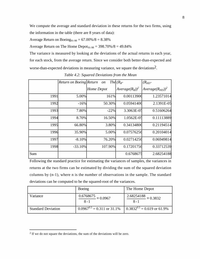
8

We compute the average and standard deviation in these returns for the two firms, using

the information in the table (there are 8 years of data):

Average Return on Boeing91-98 = 67.00%/8 = 8.38%

Average Return on The Home Depot91-98 = 398.70%/8 = 49.84%

The variance is measured by looking at the deviations of the actual returns in each year,

for each stock, from the average return. Since we consider both better-than-expected and

worse-than-expected deviations in measuring variance, we square the deviations2.

Table 4.2: Squared Deviations from the Mean

Return on Boeing Return on The

Home Depot

(RB-

Average(RB))2

(RHD-

Average(RHD))2

1991 5.00% 161% 0.00113906 1.23571014

1992 -16% 50.30% 0.05941406 2.1391E-05

1993 7.80% -22% 3.3063E-05 0.51606264

1994 8.70% 16.50% 1.0562E-05 0.11113889

1995 66.80% 3.80% 0.34134806 0.21194514

1996 35.90% 5.00% 0.07576256 0.20104014

1997 -8.10% 76.20% 0.02714256 0.06949814

1998 -33.10% 107.90% 0.17201756 0.33712539

Sum 0.6768675 2.68254188

Following the standard practice for estimating the variances of samples, the variances in

returns at the two firms can be estimated by dividing the sum of the squared deviation

columns by (n-1), where n is the number of observations in the sample. The standard

deviations can be computed to be the squared-root of the variances.

Boeing The Home Depot

Variance0.0967

1-8

0.6768675 = 0.38321-8

2.68254188 =

Standard Deviation 0.09670.5 = 0.311 or 31.1% 0.38320.5 = 0.619 or 61.9%

2 If we do not square the deviations, the sum of the deviations will be zero.

9

Based upon this data, the Home Depot looks like it was two times more risky than

Boeing between 1991 and 1998. What does this tell us? By itself, it provides a measure of

how much each these companies’ returns in the past have deviated from the average. If we

assume that the past is a good indicator of the future, the Home Depot is a more risky

investment than Boeing.

optvar.xls: There is a dataset on the web that summarizes standard deviations

and variances of stocks in various sectors in the United States.

II. Diversifiable and Non-diversifiable Risk

Although there are many reasons that actual returns may differ from expected

returns, we can group the reasons into two categories: firm-specific and market-wide. The

risks that arise from firm-specific actions affect one or a few investments, while the risk

arising from market-wide reasons affect many or all investments. This distinction is

critical to the way we assess risk in finance.

The Components of Risk

When an investor buys stock or takes an equity position in a firm, he or she is

exposed to many risks. Some risk may affect only one or a few firms and it is this risk

that we categorize as firm-specific risk. Within this category, we would consider a wide

range of risks, starting with the risk that a firm may have misjudged the demand for a

product from its customers; we call this project risk . For instance, in the coming

chapters, we will be analyzing Boeing’s investment in a Super Jumbo jet. This investment

is based on the assumption that airlines want a larger airplane and are will be willing to

pay a higher price for it. If Boeing has misjudged this demand, it will clearly have an

impact on Boeing’s earnings and value, but it should not have a significant effect on other

firms in the market. The risk could also arise from competitors proving to be stronger or

weaker than anticipated; we call this competitive risk. For instance, assume that Boeing

and Airbus are competing for an order from Quantas, the Australian airline. The

possibility that Airbus may win the bid is a potential source of risk to Boeing and

perhaps a few of its suppliers. But again, only a handful of firms in the market will be

10

affected by it. Similarly, the Home Depot recently launched an online store to sell its

home improvement products. Whether it succeeds or not is clearly important to the

Home Depot and its competitors, but it is unlikely to have an impact on the rest of the

market. In fact, we would extend our risk measures to include risks that may affect an

entire sector but are restricted to that sector; we call this sector risk. For instance, a cut

in the defense budget in the United States will adversely affect all firms in the defense

business, including Boeing, but there should be no significant impact on other sectors,

such as food and apparel. What is common across the three risks described above –

project, competitive and sector risk – is that they affect only a small sub-set of firms.

There is other risk that is much more pervasive and affects many if not all

investments. For instance, when interest rates increase, all investments are negatively

affected, albeit to different degrees. Similarly, when the economy weakens, all firms feel

the effects, though cyclical firms (such as automobiles, steel and housing) may feel it

more. We term this risk market risk.

Finally, there are risks that fall in a gray area, depending upon how many assets

they affect. For instance, when the dollar strengthens against other currencies, it has a

significant impact on the earnings and values of firms with international operations. If

most firms in the market have significant international operations, it could well be

categorized as market risk. If only a few do, it would be closer to firm-specific risk. Figure

4.4 summarizes the break down or the spectrum of firm-specific and market risks.

11

Actions/Risk that affect only one firm

Actions/Risk that affect all investments

Firm-specific Market

Projects maydo better orworse thanexpected

Competitionmay be strongeror weaker thananticipated

Entire Sectormay be affectedby action

Exchange rateand Politicalrisk

Interest rate,Inflation & News about Econoomy

Figure 4.4: A Break Down of Risk

Affects fewfirms

Affects manyfirms

Why Diversification reduces or eliminates Firm-specific Risk: An Intuitive

Explanation

As an investor, you could invest your entire portfolio in one asset, say Boeing. If

you do so, you are exposed to both firm-specific and market risk. If, however, you

expand your portfolio to include other assets or stocks, you are diversifying, and by

doing so, you can reduce your exposure to firm-specific risk. There are two reasons why

diversification reduces or, at the limit, eliminates firm specific risk. The first is that each

investment in a diversified portfolio is a much smaller percentage of that portfolio than

would be the case if you were not diversified. Thus, any action that increases or decreases

the value of only that investment or a small group of investments will have only a small

impact on your overall portfolio, whereas undiversified investors are much more exposed

to changes in the values of the investments in their portfolios. The second reason is that

the effects of firm-specific actions on the prices of individual assets in a portfolio can be

either positive or negative for each asset for any period. Thus, in very large portfolios,

this risk will average out to zero and will not affect the overall value of the portfolio.

In contrast, the effects of market-wide movements are likely to be in the same

direction for most or all investments in a portfolio, though some assets may be affected

12

more than others. For instance, other things being equal, an increase in interest rates will

lower the values of most assets in a portfolio. Being more diversified does not eliminate

this risk.

A Statistical Analysis Of Diversification Reducing Risk

We can illustrate the effects of diversification on risk fairly dramatically by

examining the effects of increasing the number of assets in a portfolio on portfolio

variance. The variance in a portfolio is partially determined by the variances of the

individual assets in the portfolio and partially by how they move together; the latter is

measured statistically with a correlation coefficient or the covariance across investments

in the portfolio. It is the covariance term that provides an insight into why and by how

much diversification will reduce risk.

Consider a portfolio of two assets. Asset A has an expected return of A and a

variance in returns of 2A , while asset B has an expected return of B and a variance in

returns of 2B . The correlation in returns between the two assets, which measures how

the assets move together, is AB . The expected returns and variance of a two-asset

portfolio can be written as a function of these inputs and the proportion of the portfolio

going to each asset.

( ) BAAAP ww −+= 1

( ) ( ) ABBAAABAAAP wwww −+−+= 121 22222

where

Aw = Proportion of the portfolio in asset A

The last term in the variance equation is sometimes written in terms of the covariance in

returns between the two assets, which is

ABBAABCov =

The savings that accrue from diversification are a function of the correlation coefficient.

Other things remaining equal, the higher the correlation in returns between the two assets,

the smaller are the potential benefits from diversification.

Why is the marginal investor assumed to be diversified?

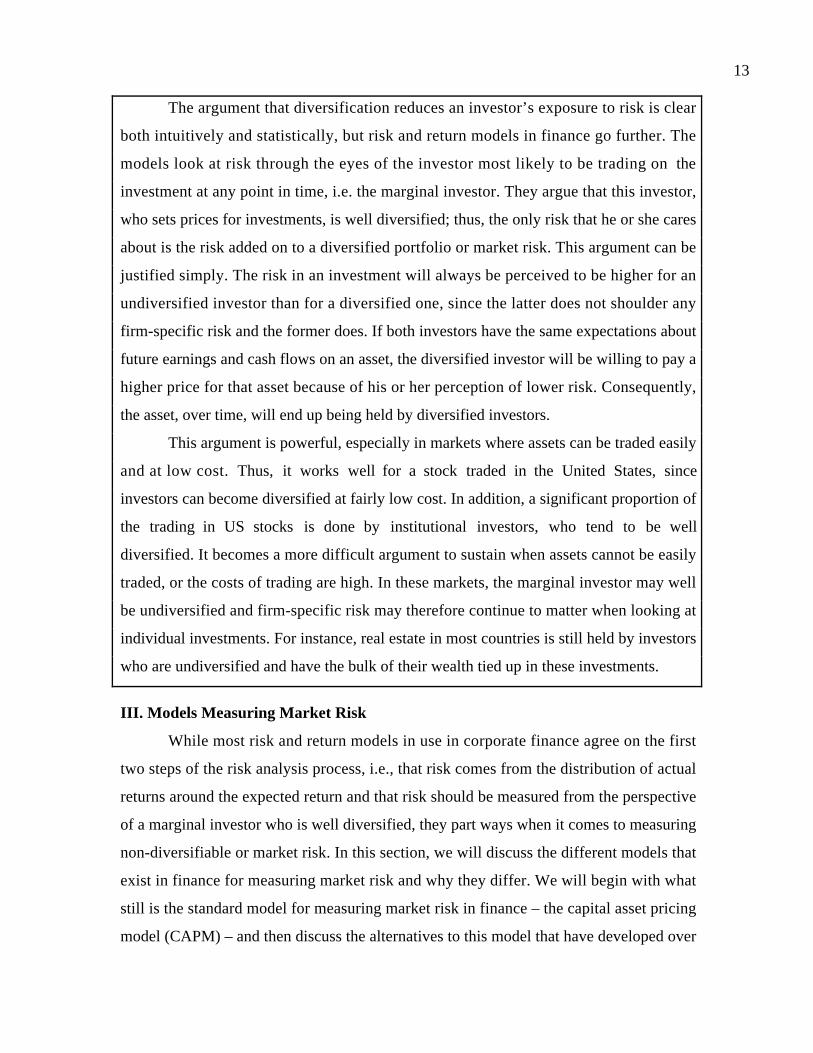
13

The argument that diversification reduces an investor’s exposure to risk is clear

both intuitively and statistically, but risk and return models in finance go further. The

models look at risk through the eyes of the investor most likely to be trading on the

investment at any point in time, i.e. the marginal investor. They argue that this investor,

who sets prices for investments, is well diversified; thus, the only risk that he or she cares

about is the risk added on to a diversified portfolio or market risk. This argument can be

justified simply. The risk in an investment will always be perceived to be higher for an

undiversified investor than for a diversified one, since the latter does not shoulder any

firm-specific risk and the former does. If both investors have the same expectations about

future earnings and cash flows on an asset, the diversified investor will be willing to pay a

higher price for that asset because of his or her perception of lower risk. Consequently,

the asset, over time, will end up being held by diversified investors.

This argument is powerful, especially in markets where assets can be traded easily

and at low cost. Thus, it works well for a stock traded in the United States, since

investors can become diversified at fairly low cost. In addition, a significant proportion of

the trading in US stocks is done by institutional investors, who tend to be well

diversified. It becomes a more difficult argument to sustain when assets cannot be easily

traded, or the costs of trading are high. In these markets, the marginal investor may well

be undiversified and firm-specific risk may therefore continue to matter when looking at

individual investments. For instance, real estate in most countries is still held by investors

who are undiversified and have the bulk of their wealth tied up in these investments.

III. Models Measuring Market Risk

While most risk and return models in use in corporate finance agree on the first

two steps of the risk analysis process, i.e., that risk comes from the distribution of actual

returns around the expected return and that risk should be measured from the perspective

of a marginal investor who is well diversified, they part ways when it comes to measuring

non-diversifiable or market risk. In this section, we will discuss the different models that

exist in finance for measuring market risk and why they differ. We will begin with what

still is the standard model for measuring market risk in finance – the capital asset pricing

model (CAPM) – and then discuss the alternatives to this model that have developed over

14

the last two decades. While we will emphasize the differences, we will also look at what

they have in common.

A. The Capital Asset Pricing Model (CAPM)

The risk and return model that has been in use the longest and is still the standard

in most real world analyses is the capital asset pricing model (CAPM). In this section, we

will examine the assumptions made by the model and the measures of market risk that

emerge from these assumptions.

Assumptions

While diversification reduces the exposure of investors to firm specific risk, most

investors limit their diversification to holding only a few assets. Even large mutual funds

rarely hold more than a few hundred stocks and many of them hold as few as ten to

twenty. There are two reasons why investors stop diversifying. One is that an investor or

mutual fund manager can obtain most of the benefits of diversification from a relatively

small portfolio, because the marginal benefits of diversification become smaller as the

portfolio gets more diversified. Consequently, these benefits may not cover the marginal

costs of diversification, which include transactions and monitoring costs. Another reason

for limiting diversification is that many investors (and funds) believe they can find under

valued assets and thus choose not to hold those assets that they believe to be fairly or

over valued.

The capital asset pricing model assumes that there are no transactions costs, all

assets are traded and investments are infinitely divisible (i.e., you can buy any fraction of

a unit of the asset). It also assumes that everyone has access to the same information and

that investors therefore cannot find under or over valued assets in the market place.

Making these assumptions allows investors to keep diversifying without additional cost.

At the limit, their portfolios will not only include every traded asset in the market but

will have identical weights on risky assets The fact that this diversified portfolio

includes all traded assets in the market is the reason it is called the market portfolio,

which should not be a surprising result, given the benefits of diversification and the

absence of transactions costs in the capital asset pricing model. If diversification reduces

exposure to firm-specific risk and there are no costs associated with adding more assets to

15

the portfolio, the logical limit to diversification is to hold a small proportion of every

traded asset in the market. If this seems abstract, consider the market portfolio to be an

extremely well diversified mutual fund that holds stocks and real assets, and treasury bills

as the riskless asset. In the CAPM, all investors will hold combinations of treasury bills

and the same mutual fund3.

Investor Portfolios in the CAPM

If every investor in the market holds the identical market portfolio, how exactly

do investors reflect their risk aversion in their investments? In the capital asset pricing

model, investors adjust for their risk preferences in their allocation decision, where they

decide how much to invest in a riskless asset and how much in the market portfolio.

Investors who are risk averse might choose to put much or even all of their wealth in the

riskless asset. Investors who want to take more risk will invest the bulk or even all of

their wealth in the market portfolio. Investors, who invest all their wealth in the market

portfolio and are still desirous of taking on more risk, would do so by borrowing at the

riskless rate and investing more in the same market portfolio as everyone else.

These results are predicated on two additional assumptions. First, there exists a

riskless asset, where the expected returns are known with certainty. Second, investors can

lend and borrow at the same riskless rate to arrive at their optimal allocations. While

lending at the riskless rate can be accomplished fairly simply by buying treasury bills or

bonds, borrowing at the riskless rate might be more difficult to do for individuals. There

are variations of the CAPM that allow these assumptions to be relaxed and still arrive at

the conclusions that are consistent with the model.

Measuring the Market Risk of an Individual Asset

The risk of any asset to an investor is the risk added by that asset to the

investor’s overall portfolio. In the CAPM world, where all investors hold the market

portfolio, the risk to an investor of an individual asset will be the risk that this asset adds

on to the market portfolio. Intuitively, if an asset moves independently of the market

3 The significance of introducing the riskless asset into the choice mix, and the implications for portfoliochoice were first noted in Sharpe (1964) and Lintner (1965). Hence, the model is sometimes called the

16

portfolio, it will not add much risk to the market portfolio. In other words, most of the

risk in this asset is firm-specific and can be diversified away. In contrast, if an asset tends

to move up when the market portfolio moves up and down when it moves down, it will

add risk to the market portfolio. This asset has more market risk and less firm-specific

risk. Statistically, this added risk is measured by the covariance of the asset with the

market portfolio.

Measuring the Non-Diversifiable Risk

In a world in which investors hold a combination of only two assets – the riskless

asset and the market portfolio – the risk of any individual asset will be measured relative

to the market portfolio. In particular, the risk of any asset will be the risk that it adds on

to the market portfolio. To arrive at the appropriate measure of this added risk, assume

that 2m is the variance of the market portfolio prior to the addition of the new asset and

that the variance of the individual asset being added to this portfolio is 2i . The market

value portfolio weight on this asset is iw , and the covariance correlation in returns

between the individual asset and the market portfolio is Covim. The variance of the market

portfolio prior to and after the addition of the individual asset can then be written as

Variance prior to asset i being added = 2m

Variance after asset i is added = ( ) ( ) imiimiiim Covwwww −+−+= 121 22222'

The market value weight on any individual asset in the market portfolio should be small

( iw is very close to 0) since the market portfolio includes all traded assets in the economy.

Consequently, the first term in the equation should approach zero, and the second term

should approach 2m , leaving the third term (Covim, the covariance) as the measure of the

risk added by individual asset i.

Standardizing Covariances

The covariance is a percentage value and it is difficult to pass judgment on the

relative risk of an investment by looking at this value. In other words, knowing that the

Sharpe-Lintner model.

17

covariance of Boeing with the Market Portfolio is 55% does not provide us a clue as to

whether Boeing is riskier or safer than the average asset. We therefore standardize the risk

measure by dividing the covariance of each asset with the market portfolio by the variance

of the market portfolio. This yields a risk measure called the beta of the asset:

Beta of an asset i = 2PortfolioMarket theof Variance

PortfolioMarket with iasset of Covariance

m

imCov=

Since the covariance of the market portfolio with itself is its variance, the beta of the

market portfolio, and by extension, the average asset in it, is one. Assets that are riskier

than average (using this measure of risk) will have betas that are greater than 1 and assets

that are less riskier than average will have betas that are less than 1. The riskless asset will

have a beta of 0.

Getting Expected Returns

The fact that every investor holds some combination of the riskless asset and the

market portfolio leads to the next conclusion: the expected return of an asset is linearly

related to the beta of the asset. In particular, the expected return of an asset can be written

as a function of the risk-free rate and the beta of that asset.

( ) ( )( )fmifi RRERRE −+=

where,

E(Ri) = Expected Return on asset i

Rf = Risk-free Rate

E(Rm) = Expected Return on market portfolio

βi= Beta of investment i

To use the capital asset pricing model, we need three inputs. While we will look at the

estimation process in far more detail in the next chapter, each of these inputs is estimated

as follows:

• The riskless asset is defined to be an asset for which the investor knows the expected

return with certainty for the time horizon of the analysis.

18

• The risk premium is the premium demanded by investors for investing in the market

portfolio, which includes all risky assets in the market, instead of investing in a

riskless asset.

• The beta, which we defined as the covariance of the asset divided by the variance of

the market portfolio, measures the risk added on by an investment to the market

portfolio.

In summary, in the capital asset pricing model, all the market risk is captured in the beta,

measured relative to a market portfolio, which at least in theory should include all traded

assets in the market place held in proportion to their market value.

B. The Arbitrage Pricing Model

The restrictive assumptions on transactions costs and private information in the

capital asset pricing model and the model’s dependence on the market portfolio have long

been viewed with skepticism by both academics and practitioners. Ross (1976) suggested

an alternative model for measuring risk called the arbitrage pricing model (APM).

Assumptions

If investors can invest risklessly and earn more than the riskless rate, they have

found an arbitrage opportunity. The premise of the arbitrage pricing model is that

investors take advantage of such arbitrage opportunities, and in the process, eliminate

them. If two portfolios have the same exposure to risk but offer different expected

returns, investors will buy the portfolio that has the higher expected returns, sell the

portfolio with the lower expected returns and earn the difference as a riskless profit. To

prevent this arbitrage from occurring, the two portfolios have to earn the same expected

return.

Like the capital asset pricing model, the arbitrage pricing model begins by breaking

risk down into firm-specific and market risk components. As in the capital asset pricing

model, firm specific risk covers information that affects primarily the firm. Market risk

affects many or all firms and would include unanticipated changes in a number of

economic variables, including gross national product, inflation, and interest rates.

Incorporating both types of risk into a return model, we get:

19

( ) ++= mRER

where R is the actual return, E(R) is the expected return, m is the market-wide component

of unanticipated risk and ε is the firm-specific component. Thus, the actual return can be

different from the expected return, either because of market risk or firm-specific actions.

The Sources of Market-Wide Risk

While both the capital asset pricing model and the arbitrage pricing model make a

distinction between firm-specific and market-wide risk, they measure market risk

differently. The CAPM assumes that market risk is captured in the market portfolio,

whereas the arbitrage pricing model allows for multiple sources of market-wide risk and

measures the sensitivity of investments to changes in each source. In general, the market

component of unanticipated returns can be decomposed into economic factors:

( )( )+++++=

++=

nnjj FFFR

mRER

... 22

where

βj = Sensitivity of investment to unanticipated changes in factor j

Fj = Unanticipated changes in factor j

Note that the measure of an investment’s sensitivity to any macro-economic factor takes

the form of a beta, called a factor beta. In fact, this beta has many of the same properties

as the market beta in the CAPM.

The Effects of Diversification

The benefits of diversification were discussed earlier, in the context of our break

down of risk into market and firm-specific risk. The primary point of that discussion was

that diversification eliminates firm-specific risk. The arbitrage pricing model uses the same

argument and concludes that the return on a portfolio will not have a firm-specific

component of unanticipated returns. The return on a portfolio can be written as the sum

of two weighted averages: the anticipated returns in the portfolio and the market factors.

( ) ( )( ) ......

......

2,22,221,22

1,12,121,112211

+++++

++++++++=

FRwRwRw

FRwRwRwRwRwRwR

nn

nnnnp

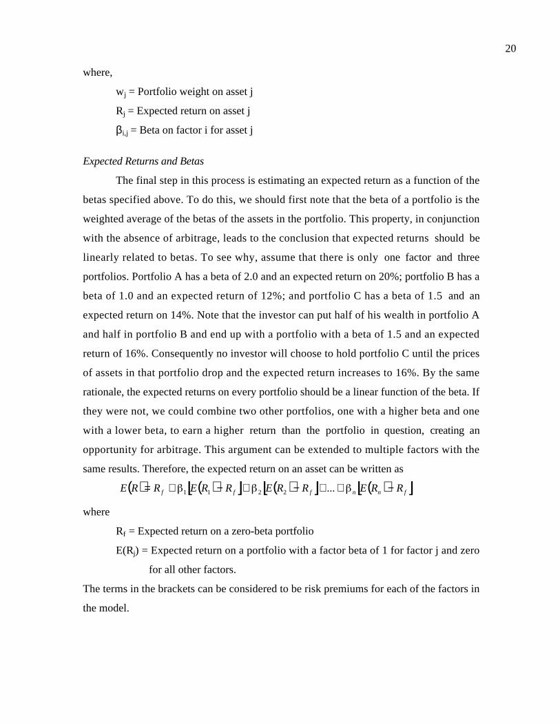
20

where,

wj = Portfolio weight on asset j

Rj = Expected return on asset j

βi,j = Beta on factor i for asset j

Expected Returns and Betas

The final step in this process is estimating an expected return as a function of the

betas specified above. To do this, we should first note that the beta of a portfolio is the

weighted average of the betas of the assets in the portfolio. This property, in conjunction

with the absence of arbitrage, leads to the conclusion that expected returns should be

linearly related to betas. To see why, assume that there is only one factor and three

portfolios. Portfolio A has a beta of 2.0 and an expected return on 20%; portfolio B has a

beta of 1.0 and an expected return of 12%; and portfolio C has a beta of 1.5 and an

expected return on 14%. Note that the investor can put half of his wealth in portfolio A

and half in portfolio B and end up with a portfolio with a beta of 1.5 and an expected

return of 16%. Consequently no investor will choose to hold portfolio C until the prices

of assets in that portfolio drop and the expected return increases to 16%. By the same

rationale, the expected returns on every portfolio should be a linear function of the beta. If

they were not, we could combine two other portfolios, one with a higher beta and one

with a lower beta, to earn a higher return than the portfolio in question, creating an

opportunity for arbitrage. This argument can be extended to multiple factors with the

same results. Therefore, the expected return on an asset can be written as

( ) ( )[ ] ( )[ ] ( )[ ]fnnfff RRERRERRERRE −++−+−+= ...2211

where

Rf = Expected return on a zero-beta portfolio

E(Rj) = Expected return on a portfolio with a factor beta of 1 for factor j and zero

for all other factors.

The terms in the brackets can be considered to be risk premiums for each of the factors in

the model.

21

The capital asset pricing model can be considered to be a special case of the

arbitrage pricing model, where there is only one economic factor driving market-wide

returns and the market portfolio is the factor.

( ) ( )( )fmmf RRERRE −+=

The APM in Practice

The arbitrage pricing model requires estimates of each of the factor betas and

factor risk premiums in addition to the riskless rate. In practice, these are usually

estimated using historical data on asset returns and a factor analysis. Intuitively, in a

factor analysis, we examine the historical data looking for common patterns that affect

broad groups of assets (rather than just one sector or a few assets). A factor analysis

provides two output measures:

1. It specifies the number of common factors that affected the historical return data

2. It measures the beta of each investment relative to each of the common factors and

provides an estimate of the actual risk premium earned by each factor.

The factor analysis does not, however, identify the factors in economic terms. In

summary, in the arbitrage pricing model, the market risk is measured relative to multiple

unspecified macroeconomic variables, with the sensitivity of the investment relative to

each factor being measured by a beta. The number of factors, the factor betas and factor

risk premiums can all be estimated using the factor analysis.

C. Multi-factor Models for risk and return

The arbitrage pricing model's failure to identify the factors specifically in the

model may be a statistical strength, but it is an intuitive weakness. The solution seems

simple: Replace the unidentified statistical factors with specific economic factors and the

resultant model should have an economic basis while still retaining much of the strength of

the arbitrage pricing model. That is precisely what multi-factor models try to do.

Deriving a Multi-Factor Model

Multi-factor models generally are determined by historical data, rather than

economic modeling. Once the number of factors has been identified in the arbitrage pricing

model, their behavior over time can be extracted from the data. The behavior of the

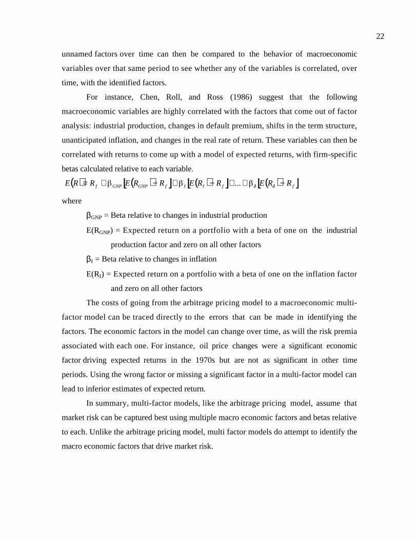
22

unnamed factors over time can then be compared to the behavior of macroeconomic

variables over that same period to see whether any of the variables is correlated, over

time, with the identified factors.

For instance, Chen, Roll, and Ross (1986) suggest that the following

macroeconomic variables are highly correlated with the factors that come out of factor

analysis: industrial production, changes in default premium, shifts in the term structure,

unanticipated inflation, and changes in the real rate of return. These variables can then be

correlated with returns to come up with a model of expected returns, with firm-specific

betas calculated relative to each variable.

( ) ( )[ ] ( )[ ] ( )[ ]ffIIfGNPGNPf RRERRERRERRE −++−+−+= ∂∂...

where

βGNP = Beta relative to changes in industrial production

E(RGNP) = Expected return on a portfolio with a beta of one on the industrial

production factor and zero on all other factors

βI = Beta relative to changes in inflation

E(RI) = Expected return on a portfolio with a beta of one on the inflation factor

and zero on all other factors

The costs of going from the arbitrage pricing model to a macroeconomic multi-

factor model can be traced directly to the errors that can be made in identifying the

factors. The economic factors in the model can change over time, as will the risk premia

associated with each one. For instance, oil price changes were a significant economic

factor driving expected returns in the 1970s but are not as significant in other time

periods. Using the wrong factor or missing a significant factor in a multi-factor model can

lead to inferior estimates of expected return.

In summary, multi-factor models, like the arbitrage pricing model, assume that

market risk can be captured best using multiple macro economic factors and betas relative

to each. Unlike the arbitrage pricing model, multi factor models do attempt to identify the

macro economic factors that drive market risk.

23

D. Regression or Proxy Models

All the models described so far begin by defining market risk in broad terms and

then developing models that might best measure this market risk. All of them, however,

extract their measures of market risk (betas) by looking at historical data. There is a final

class of risk and return models that start with the returns and try to explain differences in

returns across stocks over long time periods using characteristics such as a firm’s market

value or price multiples4. Proponents of these models argue that if some investments earn

consistently higher returns than other investments, they must be riskier. Consequently,

we could look at the characteristics that these high-return investments have in common

and consider these characteristics to be indirect measures or proxies for market risk.

Fama and French, in a highly influential study of the capital asset pricing model in

the early 1990s, noted that actual returns between 1963 and 1990 have been highly

correlated with book to price ratios5 and size. High return investments, over this period,

tended to be investments in companies with low market capitalization and high book to

price ratios. Fama and French suggested that these measures be used as proxies for risk

and report the following regression for monthly returns on stocks on the NYSE:

( )

+−=

MV

BV0.35lnMVln11.0%77.1R t

where

MV = Market Value of Equity

BV/MV = Book Value of Equity / Market Value of Equity

The values for market value of equity and book-price ratios for individual firms, when

plugged into this regression, should yield expected monthly returns.

A Comparative Analysis of Risk and Return Models

Figure 4.5 summarizes all the risk and return models in finance, noting their

similarities in the first two steps and the differences in the way they define market risk.

4 A price multiple is obtained by dividing the market price by its earnings or its book value. Studiesindicate that stocks that have low price to earnings multiples or low price to book value multiples earnhigher returns than other stocks.5 The book to price ratio is the ratio of the book value of equity to the market value of equity.

24

Figure 4.5: Risk and Return Models in Finance

The risk in an investment can be measured by the variance in actual returns around an expected return

E(R)

Riskless Investment Low Risk Investment High Risk Investment

E(R) E(R)

Risk that is specific to investment (Firm Specific) Risk that affects all investments (Market Risk)Can be diversified away in a diversified portfolio Cannot be diversified away since most assets1. each investment is a small proportion of portfolio are affected by it.2. risk averages out across investments in portfolioThe marginal investor is assumed to hold a “diversified” portfolio. Thus, only market risk will be rewarded and priced.

The CAPM The APM Multi-Factor Models Proxy ModelsIf there is 1. no private information2. no transactions costthe optimal diversified portfolio includes everytraded asset. Everyonewill hold this market portfolioMarket Risk = Risk added by any investment to the market portfolio:

If there are no arbitrage opportunities then the market risk ofany asset must be captured by betas relative to factors that affect all investments.Market Risk = Risk exposures of any asset to market factors

Beta of asset relative toMarket portfolio (froma regression)

Betas of asset relativeto unspecified marketfactors (from a factoranalysis)

Since market risk affectsmost or all investments,it must come from macro economic factors.Market Risk = Risk exposures of any asset to macro economic factors.

Betas of assets relativeto specified macroeconomic factors (froma regression)

In an efficient market,differences in returnsacross long periods mustbe due to market riskdifferences. Looking forvariables correlated withreturns should then give us proxies for this risk.Market Risk = Captured by the Proxy Variable(s)

Equation relating returns to proxy variables (from aregression)

Step 1: Defining Risk

Step 2: Differentiating between Rewarded and Unrewarded Risk

Step 3: Measuring Market Risk

As noted in Figure 4.9, all the risk and return models developed in this chapter

make some assumptions in common. They all assume that only market risk is rewarded

and they derive the expected return as a function of measures of this risk. The capital

asset pricing model makes the most restrictive assumptions about how markets work but

arrives at the simplest model, with only one factor driving risk and requiring estimation.

The arbitrage pricing model makes fewer assumptions but arrives at a more complicated

model, at least in terms of the parameters that require estimation. The capital asset pricing

model can be considered a specialized case of the arbitrage pricing model, where there is

only one underlying factor and it is completely measured by the market index. In general,

the CAPM has the advantage of being a simpler model to estimate and to use, but it will

underperform the richer APM when an investment is sensitive to economic factors not

well represented in the market index. For instance, oil company stocks, which derive most

of their risk from oil price movements, tend to have low CAPM betas and low expected

25

returns. Using an arbitrage pricing model, where one of the factors may measure oil and

other commodity price movements, will yield a better estimate of risk and higher expected

return for these firms6.

Which of these models works the best? Is beta a good proxy for risk and is it

correlated with expected returns? The answers to these questions have been debated

widely in the last two decades. The first tests of the CAPM suggested that betas and

returns were positively related, though other measures of risk (such as variance)

continued to explain differences in actual returns. This discrepancy was attributed to

limitations in the testing techniques. In 1977, Roll, in a seminal critique of the model's

tests, suggested that since the market portfolio could never be observed, the CAPM could

never be tested, and all tests of the CAPM were therefore joint tests of both the model

and the market portfolio used in the tests. In other words, all that any test of the CAPM

could show was that the model worked (or did not) given the proxy used for the market

portfolio. It could therefore be argued that in any empirical test that claimed to reject the

CAPM, the rejection could be of the proxy used for the market portfolio rather than of

the model itself. Roll noted that there was no way to ever prove that the CAPM worked

and thus no empirical basis for using the model.

Fama and French (1992) examined the relationship between betas and returns

between 1963 and 1990 and concluded that there is no relationship. These results have

been contested on three fronts. First, Amihud, Christensen, and Mendelson (1992), used

the same data, performed different statistical tests and showed that differences in betas

did, in fact, explain differences in returns during the time period. Second, Kothari and

Shanken (1995) estimated betas using annual data, instead of the shorter intervals used in

many tests, and concluded that betas do explain a significant proportion of the differences

in returns across investments. Third, Chan and Lakonishok (1993) looked at a much

longer time series of returns from 1926 to 1991 and found that the positive relationship

between betas and returns broke down only in the period after 1982. They also find that

betas are a useful guide to risk in extreme market conditions, with the riskiest firms (the

6 Weston and Copeland used both approaches to estimate the cost of equity for oil companies in 1989 andcame up with 14.4% with the CAPM and 19.1% using the arbitrage pricing model.

26

10% with highest betas) performing far worse than the market as a whole, in the ten

worst months for the market between 1926 and 1991 (See Figure 4.6).

Source: Chan and Lakonishok

While the initial tests of the APM suggested that they might provide more

promise in terms of explaining differences in returns, a distinction has to be drawn

between the use of these models to explain differences in past returns and their use to

predict expected returns in the future. The competitors to the CAPM clearly do a much

better job at explaining past returns since they do not constrain themselves to one factor,

as the CAPM does. This extension to multiple factors does become more of a problem

when we try to project expected returns into the future, since the betas and premiums of

each of these factors now have to be estimated. Because the factor premiums and betas

are themselves volatile, the estimation error may eliminate the benefits that could be

gained by moving from the CAPM to more complex models. The regression models that

were offered as an alternative also have an estimation problem, since the variables that

work best as proxies for market risk in one period (such as market capitalization) may not

be the ones that work in the next period.

Figure 4.6: Returns and Betas: Ten Worst Months between 1926 and 1991

Mar

198

8

Oct

198

7

May

194

0

May

193

2

Apr

193

2

Sep

193

7

Feb

193

3

Oct

193

2

Mar

198

0

Nov

197

3

High-beta stocks Whole Market Low-beta stocks

27

Ultimately, the survival of the capital asset pricing model as the default model for

risk in real world applications is a testament to both its intuitive appeal and the failure of

more complex models to deliver significant improvement in terms of estimating expected

returns. We would argue that a judicious use of the capital asset pricing model, without an

over reliance on historical data, is still the most effective way of dealing with risk in

modern corporate finance.

Models of Default Risk

The risk that we have discussed hitherto in this chapter relates to cash flows on

investments being different from expected cash flows. There are some investments,

however, in which the cash flows are promised when the investment is made. This is the

case, for instance, when you lend to a business or buy a corporate bond; the borrower

may default on interest and principal payments on the borrowing. Generally speaking,

borrowers with higher default risk should pay higher interest rates on their borrowing

than those with lower default risk. This section examines the measurement of default risk

and the relationship of default risk to interest rates on borrowing.

In contrast to the general risk and return models for equity, which evaluate the

effects of market risk on expected returns, models of default risk measure the

consequences of firm-specific default risk on promised returns. While diversification can

be used to explain why firm-specific risk will not be priced into expected returns for

equities, the same rationale cannot be applied to securities that have limited upside

potential and much greater downside potential from firm-specific events. To see what we

mean by limited upside potential, consider investing in the bond issued by a company.

The coupons are fixed at the time of the issue and these coupons represent the promised

cash flow on the bond. The best case scenario for you as an investor is that you receive

the promised cash flows; you are not entitled to more than these cash flows even if the

company is wildly successful. All other scenarios contain only bad news, though in

varying degrees, with the delivered cash flows being less than the promised cash flows.

Consequently, the expected return on a corporate bond is likely to reflect the firm-

specific default risk of the firm issuing the bond.

28

The Determinants of Default Risk

The default risk of a firm is a function of two variables. The first is the firm’s

capacity to generate cash flows from operations and the second is its financial obligations

– including interest and principal payments7. Firms that generate high cash flows

relative to their financial obligations should have lower default risk than firms that

generate low cash flows relative to their financial obligations. Thus, firms with significant

existing investments, which generate relatively high cash flows, will have lower default

risk than firms that do not.

In addition to the magnitude of a firm’s cash flows, the default risk is also affected by

the volatility in these cash flows. The more stability there is in cash flows the lower the

default risk in the firm. Firms that operate in predictable and stable businesses will have

lower default risk than will other similar firms that operate in cyclical or volatile

businesses.

Most models of default risk use financial ratios to measure the cash flow coverage

(i.e., the magnitude of cash flows relative to obligations) and control for industry effects

to evaluate the variability in cash flows.

Bond Ratings and Interest rates

The most widely used measure of a firm's default risk is its bond rating, which is

generally assigned by an independent ratings agency. The two best known are Standard

and Poor’s and Moody’s. Thousands of companies are rated by these two agencies and

their views carry significant weight with financial markets.

The Ratings Process

The process of rating a bond usually starts when the issuing company requests a

rating from a bond ratings agency. The ratings agency then collects information from both

publicly available sources, such as financial statements, and the company itself and makes

a decision on the rating. If the company disagrees with the rating, it is given the

7 Financial obligation refers to any payment that the firm has legally obligated itself to make, such asinterest and principal payments. It does not include discretionary cash flows, such as dividend payments ornew capital expenditures, which can be deferred or delayed, without legal consequences, though there maybe economic consequences.

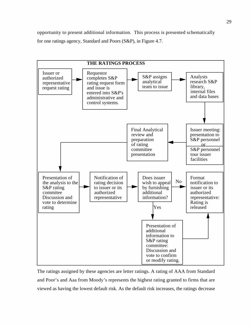
29

opportunity to present additional information. This process is presented schematically

for one ratings agency, Standard and Poors (S&P), in Figure 4.7.

Issuer or authorized representative request rating

Requestor completes S&P rating request form and issue is entered into S&P's administrative and control systems.

S&P assigns analytical team to issue

Analysts research S&P library, internal files and data bases

Issuer meeting: presentation to S&P personnel orS&P personnel tour issuer facilities

Final Analyticalreview and preparationof rating committeepresentation

Presentation of the analysis to the S&P rating commiteeDiscussion and vote to determine rating

Notification of rating decision to issuer or its authorized representative

Does issuer wish to appeal by furnishing additional information?

Presentation of additional information to S&P rating committee: Discussion and vote to confirm or modify rating.

Format notification to issuer or its authorized representative: Rating is releasedYes

No

THE RATINGS PROCESS

The ratings assigned by these agencies are letter ratings. A rating of AAA from Standard

and Poor’s and Aaa from Moody’s represents the highest rating granted to firms that are

viewed as having the lowest default risk. As the default risk increases, the ratings decrease

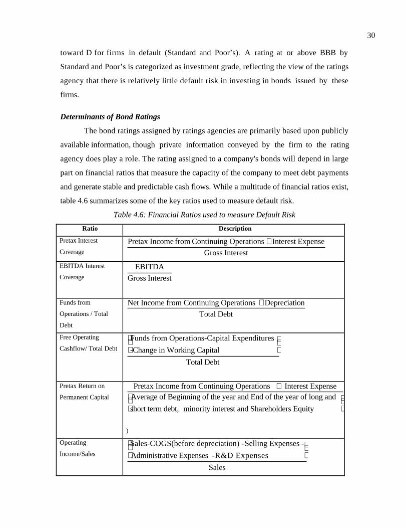
30

toward D for firms in default (Standard and Poor’s). A rating at or above BBB by

Standard and Poor’s is categorized as investment grade, reflecting the view of the ratings

agency that there is relatively little default risk in investing in bonds issued by these

firms.

Determinants of Bond Ratings

The bond ratings assigned by ratings agencies are primarily based upon publicly

available information, though private information conveyed by the firm to the rating

agency does play a role. The rating assigned to a company's bonds will depend in large

part on financial ratios that measure the capacity of the company to meet debt payments

and generate stable and predictable cash flows. While a multitude of financial ratios exist,

table 4.6 summarizes some of the key ratios used to measure default risk.

Table 4.6: Financial Ratios used to measure Default Risk

Ratio Description

Pretax Interest

Coverage Interest Gross

ExpenseInterest Operations Continuing from IncomePretax +

EBITDA Interest

Coverage Interest Gross

EBITDA

Funds from

Operations / Total

Debt

Net Income from Continuing Operations + Depreciation

Total Debt

Free Operating

Cashflow/ Total Debt

Funds from Operations-Capital Expenditures

-Change in Working Capital

Total Debt

Pretax Return on

Permanent Capital

Pretax Income from Continuing Operations + Interest ExpenseAverage of Beginning of the year and End of the year of long and

short term debt, minority interest and Shareholders Equity

)

Operating

Income/Sales

Sales-COGS(before depreciation) -Selling Expenses -

Administrative Expenses -R&D Expenses

Sales

31

Long Term Debt/

Capital

Long Term Debt

Long Term Debt + Equity

Total

Debt/Capitalization

Total Debt

Total Debt + Equity

Source: Standard and Poors

There is a strong relationship between the bond rating a company receives and its

performance on these financial ratios. Table 4.7 provides a summary of the median

ratios8 from 1998 to 2000 for different S&P ratings classes for manufacturing firms.

Table 4.7: Financial Ratios by Bond Rating: 1998-2000

AAA AA A BBB BB B CCC

EBIT interest cov. (x) 17.5 10.8 6.8 3.9 2.3 1.0 0.2

EBITDA interest cov. 21.8 14.6 9.6 6.1 3.8 2.0 1.4

Funds flow/total debt 105.8 55.8 46.1 30.5 19.2 9.4 5.8

Free oper. cash

flow/total debt (%)

55.4 24.6 15.6 6.6 1.9 –4.5 -14.0

Return on capital (%) 28.2 22.9 19.9 14.0 11.7 7.2 0.5

Oper.income/sales

(%)

29.2 21.3 18.3 15.3 15.4 11.2 13.6

Long-term

debt/capital (%)

15.2 26.4 32.5 41.0 55.8 70.7 80.3

Total Debt/ Capital

(%)

26.9 35.6 40.1 47.4 61.3 74.6 89.4

Number of firms 10 34 150 234 276 240 23

Source: Standard and Poors

Note that the pre-tax interest coverage ratio (EBIT) and the EBITDA interest coverage

ratio are stated in terms of times interest earned, whereas the rest of the ratios are stated

in percentage terms.

Not surprisingly, firms that generate income and cash flows significantly higher

than debt payments, that are profitable and that have low debt ratios are more likely to be

32

highly rated than are firms that do not have these characteristics. There will be individual

firms whose ratings are not consistent with their financial ratios, however, because the

ratings agency does add subjective judgments into the final mix. Thus, a firm which

performs poorly on financial ratios but is expected to improve its performance

dramatically over the next period may receive a higher rating than is justified by its

current financials. For most firms, however, the financial ratios should provide a

reasonable basis for guessing at the bond rating.

ratingfins.xls: There is a dataset on the web that summarizes key financial ratios

by bond rating class for the United States in the most recent period for which the data is

available.

Bond Ratings and Interest Rates

The interest rate on a corporate bond should be a function of its default risk,

which is measured by its rating. If the rating is a good measure of the default risk, higher

rated bonds should be priced to yield lower interest rates than would lower rated bonds.

In fact, in chapter 5, we will define the difference between the interest rate on a bond with

default risk and a default-free government bond to be the default spread. This default

spread will vary by maturity of the bond and can also change from period to period,

depending on economic conditions. In chapter 7, we will consider how best to estimate

these default spreads and how they might vary over time.

Summary

Risk, as we define it in finance, is measured based upon deviations of actual

returns on an investment from its' expected returns. There are two types of risk. The

first, which we call equity risk, arises in investments where there are no promised cash

flows, but there are expected cash flows. The second, default risk, arises on investments

with promised cash flows.

On investments with equity risk, the risk is best measured by looking at the

variance of actual returns around the expected returns, with greater variance indicating

8 See the Standard and Poor’s online site: http://www.standardandpoors.com/ratings/criteria/index.htm

33

greater risk. This risk can be broken down into risk that affects one or a few investments,

which we call firm specific risk, and risk that affects many investments, which we refer to

as market risk. When investors diversify, they can reduce their exposure to firm specific

risk. By assuming that the investors who trade at the margin are well diversified, we

conclude that the risk we should be looking at with equity investments is the market risk.

The different models of equity risk introduced in this chapter share this objective of

measuring market risk, but they differ in the way they do it. In the capital asset pricing

model, exposure to market risk is measured by a market beta, which estimates how much

risk an individual investment will add to a portfolio that includes all traded assets. The

arbitrage pricing model and the multi-factor model allow for multiple sources of market

risk and estimate betas for an investment relative to each source. Regression or proxy

models for risk look for firm characteristics, such as size, that have been correlated with

high returns in the past and use these to measure market risk. In all these models, the risk

measures are used to estimate the expected return on an equity investment. This expected

return can be considered the cost of equity for a company.

On investments with default risk, risk is measured by the likelihood that the

promised cash flows might not be delivered. Investments with higher default risk should

have higher interest rates and the premium that we demand over a riskless rate is the

default premium. For most US companies, default risk is measured by rating agencies in

the form of a company rating; these ratings determine, in large part, the interest rates at

which these firms can borrow. Even in the absence of ratings, interest rates will include a

default premium that reflects the lenders’ assessments of default risk. These default-risk

adjusted interest rates represent the cost of borrowing or debt for a business

34

Problems

1. The following table lists the stock prices for Microsoft from 1989 to 1998. The company did

not pay any dividends during the period

Year Price

1989 $ 1.20

1990 $ 2.09

1991 $ 4.64

1992 $ 5.34

1993 $ 5.05

1994 $ 7.64

1995 $ 10.97

1996 $ 20.66

1997 $ 32.31

1998 $ 69.34

a. Estimate the average annual return you would have made on your investment.

b. Estimate the standard deviation and variance in the annual returns.

c. If you were investing in Microsoft today, would you expect the historical standard

deviations and variances to continue to hold? Why or why not?

2. Unicom is a regulated utility serving Northern Illinois. The following table lists the stock

prices and dividends on Unicom from 1989 to 1998.

Year Price Dividends

1989 $ 36.10 $ 3.00

1990 $ 33.60 $ 3.00

1991 $ 37.80 $ 3.00

1992 $ 30.90 $ 2.30

1993 $ 26.80 $ 1.60

1994 $ 24.80 $ 1.60

1995 $ 31.60 $ 1.60

35

1996 $ 28.50 $ 1.60

1997 $ 24.25 $ 1.60

1998 $ 35.60 $ 1.60

a. Estimate the average annual return you would have made on your investment.

b. Estimate the standard deviation and variance in the annual returns.

c. If you were investing in Unicom today, would you expect the historical standard

deviations and variances to continue to hold? Why or why not?

3. The following table summarizes the annual returns you would have made on two companies –

Scientific Atlanta, a satellite and data equipment manufacturer, and AT&T, the telecomm giant,

from 1988 to 1998.

Year Scientific Atlanta AT&T

1989 80.95% 58.26%

1990 -47.37% -33.79%

1991 31% 29.88%

1992 132.44% 30.35%

1993 32.02% 2.94%

1994 25.37% -4.29%

1995 -28.57% 28.86%

1996 0.00% -6.36%

1997 11.67% 48.64%

1998 36.19% 23.55%

a. Estimate the average and standard deviation in annual returns in each company.

b. Estimate the covariance and correlation in returns between the two companies.

c. Estimate the variance of a portfolio composed, in equal parts, of the two investments.

4. You are in a world where there are only two assets, gold and stocks. You are interested in

investing your money in one, the other or both assets. Consequently you collect the following

data on the returns on the two assets over the last six years.

36

Gold Stock Market

Average return 8% 20%

Standard deviation 25% 22%

Correlation -0.4

a. If you were constrained to pick just one, which one would you choose?

b. A friend argues that this is wrong. He says that you are ignoring the big payoffs that you

can get on gold. How would you go about alleviating his concern?

c. How would a portfolio composed of equal proportions in gold and stocks do in terms of

mean and variance?

d. You now learn that GPEC (a cartel of gold-producing countries) is going to vary the

amount of gold it produces with stock prices in the US. (GPEC will produce less gold when

stock markets are up and more when it is down.) What effect will this have on your

portfolios? Explain.

5. You are interested in creating a portfolio of two stocks – Coca Cola and Texas Utilities. Over

the last decade, an investment in Coca Cola stock would have earned an average annual return of

25% with a standard deviation in returns of 36%. An investment in Texas Utilities stock would

have earned an average annual return of 12%, with a standard deviation of 22%. The correlation in

returns across the two stocks is 0.28.

a. Assuming that the average and standard deviation, estimated using past returns, will

continue to hold in the future, estimate the average returns and standard deviation of a

portfolio composed 60% of Coca Cola and 40% of Texas Utilities stock.

b. Estimate the minimum variance portfolio.

c. Now assume that Coca Cola’s international diversification will reduce the correlation to

0.20, while increasing Coca Cola’s standard deviation in returns to 45%. Assuming all of the

other numbers remain unchanged, answer (a) and (b).

6. Assume that you have half your money invested in Times Mirror, the media company, and the

other half invested in Unilever, the consumer product giant. The expected returns and standard

deviations on the two investments are summarized below:

Times Mirror Unilever

Expected Return 14% 18%

37

Standard Deviation 25% 40%

Estimate the variance of the portfolio as a function of the correlation coefficient (Start with –1

and increase the correlation to +1 in 0.2 increments).

7. You have been asked to analyze the standard deviation of a portfolio composed of the

following three assets:

Investment Expected Return Standard Deviation

Sony Corporation 11% 23%

Tesoro Petroleum 9% 27%

Storage Technology 16% 50%

You have also been provided with the correlations across these three investments:

Sony Tesoro Storage Tech

Sony 1.00 -0.15 0.20

Tesoro -0.15 1.00 -0.25

Storage Tech 0.20 -0.25 1.00

Estimate the variance of a portfolio equally weighted across all three assets.

9. Assume that the average variance of return for an individual security is 50 and that the average

covariance is 10. What is the expected variance of a portfolio of 5, 10, 20, 50 and 100 securities.

How many securities need to be held before the risk of a portfolio is only 10% more than the

minimum?

10. Assume you have all your wealth (a million dollars) invested in the Vanguard 500 index fund

and that you expect to earn an annual return of 12% with a standard deviation in returns of 25%.

Since you have become more risk averse, you decide to shift $200,000 from the Vanguard 500

index fund to treasury bills. The T.bill rate is 5%. Estimate the expected return and standard

deviation of your new portfolio.

11. Every investor in the capital asset pricing model owns a combination of the market portfolio

and a riskless asset. Assume that the standard deviation of the market portfolio is 30% and that

the expected return on the portfolio is 15%. What proportion of the following investor’s wealth

38

would you suggest investing in the market portfolio and what proportion in the riskless asset?

(The riskless asset has an expected return of 5%)

a. an investor who desires a portfolio with no standard deviation

b. an investor who desires a portfolio with a standard deviation of 15%

c. an investor who desires a portfolio with a standard deviation of 30%

d. an investor who desires a portfolio with a standard deviation of 45%

e. an investor who desires a portfolio with an expected return of 12%

12. The following table lists returns on the market portfolio and on Scientific Atlanta, each year

from 1989 to 1998.

Year Scientific Atlanta Market Portfolio

1989 80.95% 31.49%

1990 -47.37% -3.17%

1991 31% 30.57%

1992 132.44% 7.58%

1993 32.02% 10.36%

1994 25.37% 2.55%

1995 -28.57% 37.57%

1996 0.00% 22.68%

1997 11.67% 33.10%

1998 36.19% 28.32%

a. Estimate the covariance in returns between Scientific Atlanta and the market portfolio.

b. Estimate the variances in returns on both investments.

c. Estimate the beta for Scientific Atlanta.

13. United Airlines has a beta of 1.50. The standard deviation in the market portfolio is 22% and

United Airlines has a standard deviation of 66%

a. Estimate the correlation between United Airlines and the market portfolio.

b. What proportion of United Airlines’ risk is market risk?

39

14. You are using the arbitrage pricing model to estimate the expected return on Bethlehem Steel,

and have derived the following estimates for the factor betas and risk premia:

Factor Beta Risk Premia

1 1.2 2.5%

2 0.6 1.5%

3 1.5 1.0%

4 2.2 0.8%

5 0.5 1.2%

a. Which risk factor is Bethlehem Steel most exposed to? Is there any way, within the

arbitrage pricing model, to identify the risk factor?

b. If the riskfree rate is 5%, estimate the expected return on Bethlehem Steel.

c. Now assume that the beta in the capital asset pricing model for Bethlehem Steel is 1.1 and

that the risk premium for the market portfolio is 5%. Estimate the expected return using the

CAPM.

d. Why are the expected returns different between the two models?

15. You are using the multi-factor model to estimate the expected return on Emerson Electric, and

have derived the following estimates for the factor betas and risk premia:

Macro-economic Factor Measure Beta Risk Premia (Rfactor-Rf)

Level of Interest rates T.bond rate 0.5 1.8%

Term Structure T.bond rate – T.bill rate 1.4 0.6%

Inflation rate CPI 1.2 1.5%

Economic Growth GNP Growth rate 1.8 4.2%

With a riskless rate of 6%, estimate the expected return on Emerson Electric.

16. The following equation is reproduced from the study by Fama and French of returns between

1963 and 1990.

( )

+−=

MV

BV0.35lnMVln11.00177.0R t

where MV is the market value of equity in hundreds of millions of dollar and BV is the book

value of equity in hundreds of millions of dollars. The return is a monthly return.

40

a. Estimate the expected annual return on Lucent Technologies. The market value of equity

is $240 billion and the book value of equity is $13.5 billion.

b. Lucent Technologies has a beta of 1.55. If the riskless rate is 6%, and the risk premium for

the market portfolio is 5.5%, estimate the expected return.

c. Why are the expected returns different under the two approaches?

1

CHAPTER 5

OPTION PRICING THEORY AND MODELS

In general, the value of any asset is the present value of the expected cash flows on

that asset. In this section, we will consider an exception to that rule when we will look at

assets with two specific characteristics:

• They derive their value from the values of other assets.

• The cash flows on the assets are contingent on the occurrence of specific events.

These assets are called options and the present value of the expected cash flows on these

assets will understate their true value. In this section, we will describe the cash flow

characteristics of options, consider the factors that determine their value and examine how

best to value them.

Basics of Option Pricing

An option provides the holder with the right to buy or sell a specified quantity of

an underlying asset at a fixed price (called a strike price or an exercise price) at or before

the expiration date of the option. Since it is a right and not an obligation, the holder can

choose not to exercise the right and allow the option to expire. There are two types of

options: call options and put options.

Call and Put Options: Description and Payoff Diagrams

A call option gives the buyer of the option the right to buy the underlying asset at

a fixed price, called the strike or the exercise price, at any time prior to the expiration date

of the option. The buyer pays a price for this right. If at expiration, the value of the asset

is less than the strike price, the option is not exercised and expires worthless. If, on the

other hand, the value of the asset is greater than the strike price, the option is exercised -

the buyer of the option buys the asset [stock] at the exercise price. And the difference

between the asset value and the exercise price comprises the gross profit on the option

investment. The net profit on the investment is the difference between the gross profit

and the price paid for the call initially.

A payoff diagram illustrates the cash payoff on an option at expiration. For a call,

the net payoff is negative (and equal to the price paid for the call) if the value of the

2

underlying asset is less than the strike price. If the price of the underlying asset exceeds

the strike price, the gross payoff is the difference between the value of the underlying

asset and the strike price and the net payoff is the difference between the gross payoff

and the price of the call. This is illustrated in figure 5.1 below:

A put option gives the buyer of the option the right to sell the underlying asset at a

fixed price, again called the strike or exercise price, at any time prior to the expiration date

of the option. The buyer pays a price for this right. If the price of the underlying asset is

greater than the strike price, the option will not be exercised and will expire worthless. If

on the other hand, the price of the underlying asset is less than the strike price, the owner

of the put option will exercise the option and sell the stock a the strike price, claiming the

difference between the strike price and the market value of the asset as the gross profit.

Again, netting out the initial cost paid for the put yields the net profit from the

transaction.

A put has a negative net payoff if the value of the underlying asset exceeds the

strike price, and has a gross payoff equal to the difference between the strike price and

the value of the underlying asset if the asset value is less than the strike price. This is

summarized in figure 5.2 below.

Strike Price

Net Payoff on call option

Figure 5.1: Payoff on Call Option

Price of Underlying Asset

If asset value<strike price, you lose is what you paid for the call

3

Determinants of Option Value

The value of an option is determined by a number of variables relating to the

underlying asset and financial markets.

1. Current Value of the Underlying Asset: Options are assets that derive value from an

underlying asset. Consequently, changes in the value of the underlying asset affect the

value of the options on that asset. Since calls provide the right to buy the underlying asset

at a fixed price, an increase in the value of the asset will increase the value of the calls.

Puts, on the other hand, become less valuable as the value of the asset increase.

2. Variance in Value of the Underlying Asset: The buyer of an option acquires the right to

buy or sell the underlying asset at a fixed price. The higher the variance in the value of the

underlying asset, the greater will the value of the option be1. This is true for both calls

and puts. While it may seem counter-intuitive that an increase in a risk measure (variance)

should increase value, options are different from other securities since buyers of options

can never lose more than the price they pay for them; in fact, they have the potential to

earn significant returns from large price movements.

3. Dividends Paid on the Underlying Asset: The value of the underlying asset can be

expected to decrease if dividend payments are made on the asset during the life of the

Price of Underlying Asset

Strike Price

Net Payoff on put

Figure 5.2: Payoff on Put Option

If asset value>strike price, youlose what you paid for the put.

4

option. Consequently, the value of a call on the asset is a decreasing function of the size

of expected dividend payments, and the value of a put is an increasing function of

expected dividend payments. There is a more intuitive way of thinking about dividend

payments, for call options. It is a cost of delaying exercise on in-the-money options. To

see why, consider an option on a traded stock. Once a call option is in the money, i.e, the

holder of the option will make a gross payoff by exercising the option, exercising the call

option will provide the holder with the stock and entitle him or her to the dividends on

the stock in subsequent periods. Failing to exercise the option will mean that these

dividends are foregone.

4. Strike Price of Option: A key characteristic used to describe an option is the strike

price. In the case of calls, where the holder acquires the right to buy at a fixed price, the

value of the call will decline as the strike price increases. In the case of puts, where the

holder has the right to sell at a fixed price, the value will increase as the strike price

increases.

5. Time To Expiration On Option: Both calls and puts become more valuable as the time

to expiration increases. This is because the longer time to expiration provides more time

for the value of the underlying asset to move, increasing the value of both types of

options. Additionally, in the case of a call, where the buyer has to pay a fixed price at

expiration, the present value of this fixed price decreases as the life of the option

increases, increasing the value of the call.

6. Riskless Interest Rate Corresponding To Life Of Option: Since the buyer of an option

pays the price of the option up front, an opportunity cost is involved. This cost will

depend upon the level of interest rates and the time to expiration on the option. The

riskless interest rate also enters into the valuation of options when the present value of

the exercise price is calculated, since the exercise price does not have to be paid (received)

until expiration on calls (puts). Increases in the interest rate will increase the value of calls

and reduce the value of puts.

1 Note, though, that higher variance can reduce the value of the underlying asset. As a call option becomesmore in the money, the more it resembles the underlying asset. For very deep in-the-money call options,higher variance can reduce the value of the option.]

5

Table 5.1 below summarizes the variables and their predicted effects on call and put

prices.

Table 5.1: Summary of Variables Affecting Call and Put Prices

Effect on

Factor Call Value Put Value

Increase in underlying asset’s value Increases Decreases

Increase in strike price Decreases Increases

Increase in variance of underlying asset Increases Increases

Increase in time to expiration Increases Increases

Increase in interest rates Increases Decreases

Increase in dividends paid Decreases Increases

American Versus European Options: Variables Relating To Early Exercise

A primary distinction between American and European options is that American

options can be exercised at any time prior to its expiration, while European options can

be exercised only at expiration. The possibility of early exercise makes American options

more valuable than otherwise similar European options; it also makes them more difficult

to value. There is one compensating factor that enables the former to be valued using

models designed for the latter. In most cases, the time premium associated with the

remaining life of an option and transactions costs makes early exercise sub-optimal. In

other words, the holders of in-the-money options will generally get much more by selling

the option to someone else than by exercising the options.

While early exercise is not optimal generally, there are at least two exceptions to

this rule. One is a case where the underlying asset pays large dividends, thus reducing the

value of the asset, and any call options on that asset. In this case, call options may be

exercised just before an ex-dividend date if the time premium on the options is less than

the expected decline in asset value as a consequence of the dividend payment. The other

exception arises when an investor holds both the underlying asset and deep in-the-money

puts on that asset at a time when interest rates are high. In this case, the time premium on

the put may be less than the potential gain from exercising the put early and earning

interest on the exercise price.

6

Option Pricing Models

Option pricing theory has made vast strides since 1972, when Black and Scholes

published their path-breaking paper providing a model for valuing dividend-protected

European options. Black and Scholes used a “replicating portfolio” –– a portfolio

composed of the underlying asset and the risk-free asset that had the same cash flows as

the option being valued –– to come up with their final formulation. While their derivation

is mathematically complicated, there is a simpler binomial model for valuing options that

draws on the same logic.

The Binomial Model

The binomial option pricing model is based upon a simple formulation for the

asset price process in which the asset, in any time period, can move to one of two

possible prices. The general formulation of a stock price process that follows the binomial

is shown in figure 5.3.

Figure 5.3: General Formulation for Binomial Price Path

S

Su

Sd

Su2

Sd2

Sud

In this figure, S is the current stock price; the price moves up to Su with probability p and

down to Sd with probability 1-p in any time period.

7

Creating A Replicating Portfolio

The objective in a replicating portfolio is to use a combination of risk-free

borrowing/lending and the underlying asset to create a portfolio that has the same cash

flows as the option being valued. The principles of arbitrage apply here and the value of

the option must be equal to the value of the replicating portfolio. In the case of the general

formulation above, where stock prices can either move up to Su or down to Sd in any

time period, the replicating portfolio for a call with strike price K will involve borrowing

$B and acquiring of the underlying asset, where:

∆ = Number of units of the underlying asset bought = Sd-Su

Cu dC−

where,

Cu = Value of the call if the stock price is Su

Cd = Value of the call if the stock price is Sd

In a multi-period binomial process, the valuation has to proceed iteratively, i.e.,

starting with the last time period and moving backwards in time until the current point in

time. The portfolios replicating the option are created at each step and valued, providing

the values for the option in that time period. The final output from the binomial option

pricing model is a statement of the value of the option in terms of the replicating

portfolio, composed of shares (option delta) of the underlying asset and risk-free

borrowing/lending.

Value of the call = Current value of underlying asset * Option Delta - Borrowing needed

to replicate the option

Illustration 5.1: Binomial Option Valuation

Assume that the objective is to value a call with a strike price of 50, which is

expected to expire in two time periods, on an underlying asset whose price currently is 50

and is expected to follow a binomial process:

8

Now assume that the interest rate is 11%. In addition, define

= Number of shares in the replicating portfolio

B = Dollars of borrowing in replicating portfolio

The objective is to combine shares of stock and B dollars of borrowing to replicate the

cash flows from the call with a strike price of 50. This can be done iteratively, starting

with the last period and working back through the binomial tree.

Step 1: Start with the end nodes and work backwards:

9

Thus, if the stock price is $70 at t=1, borrowing $45 and buying one share of the stock

will give the same cash flows as buying the call. The value of the call at t=1, if the stock

price is $70, is:

Value of Call = Value of Replicating Position = ( )( ) 254517070 =−=−∆ B

Considering the other leg of the binomial tree at t=1,

If the stock price is 35 at t=1, then the call is worth nothing.

Step 2: Move backwards to the earlier time period and create a replicating portfolio that

will provide the cash flows the option will provide.

In other words, borrowing $22.5 and buying 5/7 of a share will provide the same cash

flows as a call with a strike price of $50. The value of the call therefore has to be the same

as the value of this position.

10

Value of Call = Value of replicating position =

( ) ( ) 21.135.22507

55.22PriceStock Current

7

5 =−

=−

The Determinants of Value

The binomial model provides insight into the determinants of option value. The

value of an option is not determined by the expected price of the asset but by its current

price, which, of course, reflects expectations about the future. This is a direct

consequence of arbitrage. If the option value deviates from the value of the replicating

portfolio, investors can create an arbitrage position, i.e., one that requires no investment,

involves no risk, and delivers positive returns. To illustrate, if the portfolio that replicates

the call costs more than the call does in the market, an investor could buy the call, sell the

replicating portfolio and guarantee the difference as a profit. The cash flows on the two

positions will offset each other, leading to no cash flows in subsequent periods. The

option value also increases as the time to expiration is extended, as the price movements

(u and d) increase, and with increases in the interest rate.

While the binomial model provides an intuitive feel for the determinants of option

value, it requires a large number of inputs, in terms of expected future prices at each node.

As we make time periods shorter in the binomial model, we can make one of two

assumptions about asset prices. We can assume that price changes become smaller as

periods get shorter; this leads to price changes becoming infinitesimally small as time

periods approach zero, leading to a continuous price process. Alternatively, we can

assume that price changes stay large even as the period gets shorter; this leads to a jump

price process, where prices can jump in any period. In this section, we consider the

option pricing models that emerge with each of these assumptions.

The Black-Scholes Model

When the price process is continuous, i.e. price changes becomes smaller as time

periods get shorter, the binomial model for pricing options converges on the Black-

Scholes model. The model, named after its co-creators, Fischer Black and Myron Scholes,

allows us to estimate the value of any option using a small number of inputs and has been

shown to be remarkably robust in valuing many listed options.

11

The Model

While the derivation of the Black-Scholes model is far too complicated to present

here, it is also based upon the idea of creating a portfolio of the underlying asset and the

riskless asset with the same cashflows and hence the same cost as the option being

valued. The value of a call option in the Black-Scholes model can be written as a function

of the five variables:

S = Current value of the underlying asset

K = Strike price of the option

t = Life to expiration of the option

r = Riskless interest rate corresponding to the life of the option

σ2 = Variance in the ln(value) of the underlying asset

The value of a call is then:

Value of call = S N (d1) - K e-rt N(d2)

where

d1 = ln

S

K

+ ( r +

2

2) t

t

tdd −= 12

Note that e-rt is the present value factor and reflects the fact that the exercise price on the

call option does not have to be paid until expiration. N(d1) and N(d2) are probabilities,

estimated by using a cumulative standardized normal distribution and the values of d1 and

d2 obtained for an option. The cumulative distribution is shown in Figure 5.4:

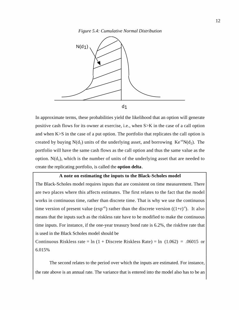
12

Figure 5.4: Cumulative Normal Distribution

d1

N(d1)

In approximate terms, these probabilities yield the likelihood that an option will generate

positive cash flows for its owner at exercise, i.e., when S>K in the case of a call option

and when K>S in the case of a put option. The portfolio that replicates the call option is

created by buying N(d1) units of the underlying asset, and borrowing Ke-rtN(d2). The

portfolio will have the same cash flows as the call option and thus the same value as the

option. N(d1), which is the number of units of the underlying asset that are needed to

create the replicating portfolio, is called the option delta .

A note on estimating the inputs to the Black-Scholes model

The Black-Scholes model requires inputs that are consistent on time measurement. There

are two places where this affects estimates. The first relates to the fact that the model

works in continuous time, rather than discrete time. That is why we use the continuous

time version of present value (exp-rt) rather than the discrete version ((1+r)-t). It also

means that the inputs such as the riskless rate have to be modified to make the continuous

time inputs. For instance, if the one-year treasury bond rate is 6.2%, the riskfree rate that

is used in the Black Scholes model should be

Continuous Riskless rate = ln (1 + Discrete Riskless Rate) = ln (1.062) = .06015 or

6.015%

The second relates to the period over which the inputs are estimated. For instance,

the rate above is an annual rate. The variance that is entered into the model also has to be an

13

annualized variance. The variance, estimated from ln(asset prices), can be annualized easily

because variances are linear in time if the serial correlation is zero. Thus, if monthly

(weekly) prices are used to estimate variance, the variance is annualized by multiplying by

twelve (fifty two).

Illustration 5.2: Valuing an option using the Black-Scholes Model

On March 6, 2001, Cisco Systems was trading at $13.62. We will attempt to

value a July 2001 call option with a strike price of $15, trading on the CBOT on the same

day for $2.00. The following are the other parameters of the options:

• The annualized standard deviation in Cisco Systems stock price over the previous

year was 81.00%. This standard deviation is estimated using weekly stock prices

over the year and the resulting number was annualized as follows:

Weekly standard deviation = 1.556%

Annualized standard deviation =1.556%*52 = 81%

• The option expiration date is Friday, July 20, 2001. There are 103 days to

expiration.

• The annualized treasury bill rate corresponding to this option life is 4.63%.

The inputs for the Black-Scholes model are as follows:

Current Stock Price (S) = $13.62

Strike Price on the option = $15.00

Option life = 103/365 = 0.2822

Standard Deviation in ln(stock prices) = 81%

Riskless rate = 4.63%

Inputting these numbers into the model, we get

( )0212.0

0.2822 81.0

.2822 02

)81.0( + 0.0463

15.00

13.62ln

=d

2

1 =

+

-0.40910.28220.81 -.0212 0=d2 =

Using the normal distribution, we can estimate the N(d1) and N(d2)

14

N(d1) = 0.5085

N(d2) = 0.3412

The value of the call can now be estimated:

Value of Cisco Call = S N (d1) - K e-rt N(d2)

= ( )( ) ( )( )( ) 1.87 0.3412e 15-0.5085 13.62 0.28220.0463- =

Since the call is trading at $2.00, it is slightly overvalued, assuming that the estimate

of standard deviation used is correct.

Implied VolatilityThe only input on which there can be significant disagreement among investors is

the variance. While the variance is often estimated by looking at historical data, the values

for options that emerge from using the historical variance can be different from the market

prices. For any option, there is some variance at which the estimated value will be equal

to the market price. This variance is called an implied variance.

Consider the Cisco option valued in the last illustration. With a standard deviation

of 81%, we estimated the value of the call option with a strike price of $15 to be $1.87.

Since the market price is higher than the calculated value, we tried higher standard

deviations and at a standard deviation 85.40%, the value of the option is $2.00. This is

the implied standard deviation or implied volatility..

Model Limitations and Fixes

The Black-Scholes model was designed to value options that can be exercised only

at maturity and on underlying assets that do not pay dividends. In addition, options are

valued based upon the assumption that option exercise does not affect the value of the

underlying asset. In practice, assets do pay dividends, options sometimes get exercised

early and exercising an option can affect the value of the underlying asset. Adjustments

exist. While they are not perfect, adjustments provide partial corrections to the Black-

Scholes model.

1. Dividends

The payment of a dividend reduces the stock price; note that on the ex-dividend

day, the stock price generally declines. Consequently, call options will become less

15

valuable and put options more valuable as expected dividend payments increase. There

are two ways of dealing with dividends in the Black Scholes:

• Short-term Options: One approach to dealing with dividends is to estimate the

present value of expected dividends that will be paid by the underlying asset

during the option life and subtract it from the current value of the asset to use as S

in the model.

Modified Stock Price = Current Stock Price – Present value of expected dividends

during the life of the option

• Long Term Options: Since it becomes impractical to estimate the present value of

dividends as the option life becomes longer, we would suggest an alternate

approach. If the dividend yield (y = dividends/current value of the asset) on the

underlying asset is expected to remain unchanged during the life of the option, the

Black-Scholes model can be modified to take dividends into account.

C = S e-yt N(d1) - K e-rt N(d2)

where

d1 = ln

S

K

+ (r -y +

2

2) t

t

tdd −= 12

From an intuitive standpoint, the adjustments have two effects. First, the value of

the asset is discounted back to the present at the dividend yield to take into

account the expected drop in asset value resulting from dividend payments.

Second, the interest rate is offset by the dividend yield to reflect the lower

carrying cost from holding the asset (in the replicating portfolio). The net effect

will be a reduction in the value of calls estimated using this model.

stopt.xls: This spreadsheet allows you to estimate the value of a short term option,

when the expected dividends during the option life can be estimated.

ltopt.xls: This spreadsheet allows you to estimate the value of an option, when the

underlying asset has a constant dividend yield.

16

Illustration 5.3: Valuing a short-term option with dividend adjustments – The Black

Scholes Correction

Assume that it is March 6, 2001 and that AT&T is trading at $20.50 a share.

Consider a call option on the stock with a strike price of $20, expiring on July 20, 2001.

Using past stock prices, the variance in the log of stock prices for AT&T is estimated at

60%. There is one dividend, amounting to $0.15, and it will be paid in 23 days. The

riskless rate is 4.63%.

Present value of expected dividend = 15.0

0463.1

15.0

365

23=

Dividend-adjusted stock price = $20.50 - $0.15 = $20.35

Time to expiration = 103/365 = 0.2822

Variance in ln(stock prices) = 0.62=0.36

Riskless rate = 4.63%

The value from the Black-Scholes is:

d1 = 0.2548 N(d1) = 0.6006

d2 = -0.0639 N(d2) = 0.4745

Value of Call = ( )( ) ( ) ( )( )( ) 85.24745.0206006.035.20 2822.00463.0 =− −e

The call option was trading at $2.60 on that day.

Illustration 5.4: Valuing a long term option with dividend adjustments - Primes and

Scores

In recent years, the CBOT has introduced longer term call and put options on

stocks. On AT&T, for instance, you could have purchased a call expiring on January 17,

2003, on March 6, 2001. The stock price for AT&T is $20.50 (as in the previous

example). The following is the valuation of a call option with a strike price of $20. Instead

of estimating the present value of dividends over the next two years, we will assume that

AT&T’s dividend yield will remain 2.51% over this period and that the riskfree rate for a

two-year treasury bond is 4.85%. The inputs to the Black-Scholes model are:

S = Current asset value = $20.50

K = Strike Price = $20.00

Time to expiration = 1.8333 years

17

Standard Deviation in ln(stock prices) = 60%

Riskless rate = 4.85%

Dividend Yield = 2.51%

The value from the Black Scholes is:

( )4894.0

1.8333 6.0

1.83332

6.0 +0.0251-0.0485

20.00

20.50ln

=d

2

1 =

+

N(d1) = 0.6877

3230.08333.16.04894.02 −=−=d N(d2) = 0.6267

Value of Call= ( ) ( )( )( ) ( ) ( )( ) 63.6206877.050.20 8333.10485.08333.10251.0 =− −− ee

The call was trading at $5.80 on March 8, 2001.

2. Early Exercise

The Black-Scholes model was designed to value options that can be exercised only

at expiration. Options with this characteristic are called European options . In contrast,

most options that we encounter in practice can be exercised any time until expiration.

These options are called American options. The possibility of early exercise makes

American options more valuable than otherwise similar European options; it also makes

them more difficult to value. In general, though, with traded options, it is almost always

better to sell the option to someone else rather than exercise early, since options have a

time premium, i.e., they sell for more than their exercise value. There are two exceptions.

One occurs when the underlying asset pays large dividends, thus reducing the expected

value of the asset. In this case, call options may be exercised just before an ex-dividend

date, if the time premium on the options is less than the expected decline in asset value as

a consequence of the dividend payment. The other exception arises when an investor

holds both the underlying asset and deep in-the-money puts, i.e., puts with strike prices

well above the current price of the underlying asset, on that asset and at a time when

interest rates are high. In this case, the time premium on the put may be less than the

potential gain from exercising the put early and earning interest on the exercise price.

There are two basic ways of dealing with the possibility of early exercise. One is

to continue to use the unadjusted Black-Scholes model and regard the resulting value as a

18

floor or conservative estimate of the true value. The other is to try to adjust the value of

the option for the possibility of early exercise. There are two approaches for doing so.

One uses the Black-Scholes to value the option to each potential exercise date. With

options on stocks, this basically requires that we value options to each ex-dividend day

and choose the maximum of the estimated call values. The second approach is to use a

modified version of the binomial model to consider the possibility of early exercise. In

this version, the up and down movements for asset prices in each period can be estimated

from the variance and the length of each period2.

Approach 1: Pseudo-American Valuation

Step 1: Define when dividends will be paid and how much the dividends will be.

Step 2: Value the call option to each ex-dividend date using the dividend-adjusted

approach described above, where the stock price is reduced by the present value of

expected dividends.

Step 3: Choose the maximum of the call values estimated for each ex-dividend day.

Illustration 5.5: Using Pseudo-American option valuation to adjust for early exercise

Consider an option, with a strike price of $35 on a stock trading at $40. The

variance in the ln(stock prices) is 0.05, and the riskless rate is 4%. The option has a

remaining life of eight months, and there are three dividends expected during this period:

Expected Dividend Ex-Dividend Day

$ 0.80 in 1 month

$ 0.80 in 4 months

$ 0.80 in 7 months

The call option is first valued to just before the first ex-dividend date:

2 To illustrate, if σ2 is the variance in ln(stock prices), the up and down movements in the binomial can beestimated as follows:

+

−

=m

TmT

r

eu

22

2

−

−

=m

TmT

r

ed

22

2

where u and d are the up and down movements per unit time for the binomial, T is the life of the optionand m is the number of periods within that lifetime.

19

S = $40 K = $35 t= 1/12 σ2 = 0.05 r = 0.04

The value from the Black-Scholes model is:

Value of Call = $5.1312

The call option is then valued to before the second ex-dividend date:

Adjusted Stock Price = $40 - $0.80/1.041/12 = $39.20

K = $35 t=4/12 σ2 = 0.05 r = 0.04

The value of the call based upon these parameters is:

Value of call = $5.0732

The call option is then valued to before the third ex-dividend date:

Adjusted Stock Price = $40 - $0.80/1.041/12 - $0.80/1.044/12 = $38.41

K = $35 t=7/12 σ2 = 0.05 r = 0.04

The value of the call based upon these parameters is:

Value of call = $5.1285

The call option is then valued to expiration:

Adjusted Stock Price = $40 - $0.80/1.041/12 - $0.80/1.044/12 - $0.80/1.047/12 = $37.63

K = $35 t=8/12 σ2 = 0.05 r = 0.04

The value of the call based upon these parameters is:

Value of call = $4.7571

Pseudo-American value of the call = Maximum ($5.1312, $5.0732, $5.1285, $4.7571) =

$5.1312

Approach 2: Using the binomial

The binomial model is much more capable of handling early exercise because it

considers the cash flows at each time period rather than just the cash flows at expiration.

The biggest limitation of the binomial is determining what stock prices will be at the end

of each period, but this can be overcome by using a variant that allows us to estimate the

up and the down movements in stock prices from the estimated variance. There are four

steps involved.

Step 1: If the variance in ln(stock prices) has been estimated for the Black-Scholes,

convert these into inputs for the Binomial

20

+

−

=m

TmT

r

eu

22

2

−

−

=m

TmT

r

ed

22

2

where u and d are the up and down movements per unit time for the binomial, T is the life

of the option and m is the number of periods within that lifetime.

Step 2: Specify the period in which the dividends will be paid and make the assumption

that the price will drop by the amount of the dividend in that period.

Step 3: Value the call at each node of the tree, allowing for the possibility of early exercise

just before ex-dividend dates. There will be early exercise if the remaining time premium

on the option is less than the expected drop in option value as a consequence of the

dividend payment.

Step 4: Value the call at time 0, using the standard binomial approach.

bstobin.xls: This spreadsheet allows you to estimate the parameters for a binomial

model from the inputs to a Black-Scholes model.

From Black-Scholes to Binomial

The process of converting the continuous variance in a Black-Scholes modesl to a

binomial tree is a fairly simple one. Assume, for instance, that you have an asset that is

trading at $ 30 currently and that you estimate the standard deviation in the asset value to

be 40%; the riskless rate is 5%. For simplicity, let us assume that the option that you are

valuing has a one-year life and that each period is a quarter. To estimate the prices at the

end of each the four quarters, we begin by first estimating the up and down movements in

the binomial:

u = exp.4 1+(.05 −(.4)2

2)1

= 1.4477

d = exp−.4 1+(.05− .402

2)1

= 0.6505

Based upon these estimates, we can obtain the prices at the end of the first node of the

tree (the end of the first quarter):

Up price = $ 30 (1.4477) = $ 43.43

21

Down price = $ 40 (0.6505) = $19.52

Progressing through the rest of the tree, we obtain the following numbers:

30

43.43

19.52

62.88

28.25

12.69

91.03

40.90

18.38

8.26

3. The Impact of Exercise On The Value Of The Underlying Asset

The Black-Scholes model is based upon the assumption that exercising an option

does not affect the value of the underlying asset. This may be true for listed options on

stocks, but it is not true for some types of options. For instance, the exercise of warrants

increases the number of shares outstanding and brings fresh cash into the firm, both of

which will affect the stock price.3 The expected negative impact (dilution) of exercise will

decrease the value of warrants compared to otherwise similar call options. The adjustment

for dilution in the Black-Scholes to the stock price is fairly simple. The stock price is

adjusted for the expected dilution from the exercise of the options. In the case of

warrants, for instance:

Dilution-adjusted S = WS

WS

nnWnSn

++

where

S = Current value of the stock

3 Warrants are call options issued by firms, either as part of management compensation contracts or toraise equity. We will discuss them in chapter 16.

22

nw = Number of warrants outstanding

W = Value of warrants outstanding

ns = Number of shares outstanding

When the warrants are exercised, the number of shares outstanding will increase, reducing

the stock price. The numerator reflects the market value of equity, including both stocks

and warrants outstanding. The reduction in S will reduce the value of the call option.

There is an element of circularity in this analysis, since the value of the warrant is

needed to estimate the dilution-adjusted S and the dilution-adjusted S is needed to

estimate the value of the warrant. This problem can be resolved by starting the process

off with an assumed value for the warrant (say, the exercise value or the current market

price of the warrant). This will yield a value for the warrant and this estimated value can

then be used as an input to re-estimate the warrant’s value until there is convergence.

Illustration 5.6: Valuing a warrant with dilution

MN Corporation has 1 million shares of stock trading at $50, and it is considering

an issue of 500,000 warrants with an exercise price of $60 to raise fresh equity for the

firm. The warrants will have a five-year lifetime. The standard deviation in the value of

equity has been 20%, and the five-year riskless bond rate is 10%. The stock is expected

to pay $1 in dividends per share this year, and is expected to maintain this dividend yield

for the next five years.

The inputs to the warrant valuation model are as follows:

S = (1,000,000 * $50 + 500,000 * $ W )/(1,000,000+500,000)

K = Exercise price on warrant = $60

t = Time to expiration on warrant = 5 years

σ2 = Variance in value of equity = 0.22 = 0.04

y = Dividend yield on stock = $1 / $50 = 2%

Since the value of the warrant is needed as an input to the process, there is an element of

circularity in reasoning. After a series of iterations where the warrant value was used to

re-estimate S, the results of the Black-Scholes valuation of this option are:

d1 = -0.1435 N(d1) = 0.4430

d2 = -0.5907 N(d2) = 0.2774

23

Value of Call= S exp-(0.02) (5) (0.4430) - $60 exp-(0.10)(5) (0.2774) = $ 3.59

Value of warrant = Value of Call * ns /(nw + ns) = $ 3.59 *(1,000,000/1,500,000) = $2.39

Illustration 5.7: Valuing a warrant on Avatek Corporation

Avatek Corporation is a real estate firm with 19.637 million shares outstanding,

trading at $0.38 a share. In March, 2001, the company had 1.8 million options

outstanding, with four years to expiration, with an exercise price of $2.25. The stock paid

no dividends, and the standard deviation in ln(stock prices) is 93%. The four-year

treasury bond rate was 4.90%. (The warrants were trading at $0.12 apiece at the time of

this analysis)

The inputs to the warrant valuation model are as follows:

S = (0.38 * 19.637 + 0.12* 1.8 )/(19.637+1.8) = 0.3582

K = Exercise price on warrant = 2.25

t = Time to expiration on warrant = 4 years

r = Riskless rate corresponding to life of option = 4.90%

σ2 = Variance in value of stock = 0.932

y = Dividend yield on stock = 0.00%

The results of the Black-Scholes valuation of this option are:

d1 = 0.0418 N(d1) = 0.5167

d2 = -1.8182 N(d2) = 0.0345

Value of Warrant= 0.3544 (0.5167) – 2.25 exp-(0.049)(4) (0.0345) = $0.12

The warrant was trading at $0.25.

warrant.xls: This spreadsheet allows you to estimate the value of an option, when

there is a potential dilution from exercise.

The Black-Scholes Model for Valuing Puts

The value of a put can be derived from the value of a call with the same strike

price and the same expiration date.

C – P = S - K e-rt

24

where C is the value of the call and P is the value of the put. This relationship between

the call and put values is called put-call parity and any deviations from parity can be

used by investors to make riskless profits. To see why put-call parity holds, consider

selling a call and buying a put with exercise price K and expiration date t, and

simultaneously buying the underlying asset at the current price S. The payoff from this

position is riskless and always yields K at expiration t. To see this, assume that the stock

price at expiration is S*. The payoff on each of the positions in the portfolio can be

written as follows:

Position Payoffs at t if S*>K Payoffs at t if S*<K

Sell call -(S*-K) 0

Buy put 0 K-S*

Buy stock S* S*

Total K K

Since this position yields K with certainty, the cost of creating this position must be

equal to the present value of K at the riskless rate (K e-rt).

S+P-C = K e-rt

C - P = S - K e-rt

Substituting the Black-Scholes equation for the value of an equivalent call into this

equation, we get:

Value of put = K e-rt (1-N(d2)) - S e-yt (1-N(d1))

where

d1 = ln

S

K

+ (r -y +

2

2) t

t

tdd −= 12

Thus, the replicating portfolio for a put is created by selling short (1-N(d1))) shares of

stock and investing Ke-rt(1-N(d2)) in the riskless asset.

25

Illustration 5.8: Valuing a put using put-call parity: Cisco& AT&T

Consider the call that we valued on Cisco in Illustration 5.2. The call had a strike

price of $15, 103 days left to expiration and was valued at $1.87. The stock was trading

at $13.62 and the riskless rate was 4.63%. We could value the put as follows:

Put Value = C – S + K e-rt = $1.87 - $13.62 + $15 e-(0.0463)(0.2822) = $3.06

The put was trading at $3.38.

We also valued a long term call on AT&T in Illustration 5.4. The call had a strike

price of $20, 1.8333 years left to expiration and a value of $6.63. The stock was trading at

$20.50 and was expected to maintain a dividend yield of 2.51% over the period. The

riskless rate was 4.85%. The put value can be estimated as follows:

Put Value = C – S e-yt + K e-rt = $6.63- $20.5 e-(0.0251)(1.8333) + $20 e-(0.0485)(1.8333) = $5.35

The put was trading at $3.80.

Jump Process Option Pricing Models

If price changes remain larger as the time periods in the binomial are shortened, we

can no longer assume that prices change continuously. When price changes remain large, a

price process that allows for price jumps is much more realistic. Cox and Ross (1976)

valued options when prices follow a pure jump process, where the jumps can only be

positive. Thus, in the next interval, the stock price will either have a large positive jump

with a specified probability or drift downwards at a given rate.

Merton (1976) considered a distribution where there are price jumps

superimposed on a continuous price process. He specified the rate at which jumps occur

(λ) and the average jump size (k), measured as a percentage of the stock price. The model

derived to value options with this process is called a jump diffusion model. In this model,

the value of an option is determined by the five variables specified in the Black Scholes

model and the parameters of the jump process (λ, k). Unfortunately, the estimates of the

jump process parameters are so noisy for most firms that they overwhelm any

advantages that accrue from using a more realistic model. These models, therefore, have

seen limited use in practice.

26

Extensions of Option Pricing

All the option pricing models we have described so far – the Binomial, the Black-

Scholes and the jump process models – are designed to value options, with clearly defined

exercise prices and maturities, on underlying assets that are traded. The options we

encounter in investment analysis or valuation are often on real assets rather than financial

assets, thus leading to them to be categorized as real options, can take much more

complicated forms. In this section, we will consider some of these variations.

Capped and Barrier Options

With a simple call option, there is no specified upper limit on the profits that can be

made by the buyer of the call. Asset prices, at least in theory, can keep going up, and the

payoffs increase proportionately. In some call options, the buyer is entitled to profits up

to a specified price but not above it. For instance, consider a call option with a strike

price of K1 on an asset. In an unrestricted call option, the payoff on this option will

increase as the underlying asset's price increases above K1. Assume, however, that if the

price reaches K2, the payoff is capped at (K2 –K1). The payoff diagram on this option is

shown in Figure 5.5:

Figure 5.5: Payoff on Capped Call

Value of Underlying Asset

K1 K2

Payoff on capped call

When the price of the asset exceeds K2, the payoffon the call is limited to K2-K1

This option is called a capped call. Notice, also, that once the price reaches K2, there

is no time premium associated with the option anymore and the option will therefore be

exercised. Capped calls are part of a family of options called barrier options, where the

payoff on and the life of the options are a function of whether the underlying asset price

reaches a certain level during a specified period.

27

The value of a capped call will always be lower than the value of the same call

without the payoff limit. A simple approximation of this value can be obtained by valuing

the call twice, once with the given exercise price and once with the cap, and taking the

difference in the two values. In the above example, then, the value of the call with an

exercise price of K1 and a cap at K2 can be written as:

Value of Capped Call = Value of call (K=K1) - Value of call (K=K2)

Barrier options can take many forms. In a knockout option, an option ceases to exist

if the underlying asset reaches a certain price. In the case of a call option, this knock-out

price is usually set below the strike price and this option is called a down-and-out

option. In the case of a put option, the knock-out price will be set above the exercise

price and this option is called an up-and-out option . Like the capped call, these options

will be worth less than their unrestricted counterparts. Many real options have limits on

potential upside or knock-out provisions and ignoring these limits can result in the

overstatement of the value of these options.

Compound Options

Some options derive their value not from an underlying asset but from other

options. These options are called compound options. Compound options can take any of

four forms - a call on a call, a put on a put, a call on a put and a put on a call. Geske

(1979) developed the analytical formulation for valuing compound options by replacing

the standard normal distribution used in a simple option model with a bivariate normal

distribution in the calculation.

Consider, for instance, the option to expand a project that we will consider in the

next section. While we will value this option using a simple option pricing model, in

reality there could be multiple stages in expansion, with each stage representing an option

for the following stage. In this case, we will undervalue the option by considering it as a

simple rather than a compound option.

Notwithstanding this discussion, the valuation of compound options become

progressively more difficult as we add more options to the chain. In this case, rather than

wreck the valuation on the shoals of estimation error, it may be better to accept the

28

conservative estimate that is provided with a simple valuation model as a floor on the

value.

Rainbow Options

In a simple option, the uncertainty is about the price of the underlying asset.

Some options are exposed to two or more sources of uncertainty and these options are

rainbow options . Using the simple option pricing model to value such options can lead

to biased estimates of value. As an example, we will consider an undeveloped oil reserve

as an option, where the firm that owns the reserve has the right to develop the reserve.

Here, there are two sources of uncertainty. The first is obviously the price of oil and the

second is the quantity of oil that is in the reserve. To value this undeveloped reserve, we

can make the simplifying assumption that we know the quantity of the reserves with

certainty. In reality, however, uncertainty about the quantity will affect the value of this

option and make the decision to exercise more difficult4.

Conclusion

An option is an asset with payoffs which are contingent on the value of an

underlying asset. A call option provides its holder with the right to buy the underlying

asset at a fixed price, whereas a put option provides its holder with the right to sell at a

fixed price, any time before the expiration of the option. The value of an option is

determined by six variables - the current value of the underlying asset, the variance in this

value, the strike price, life of the option, the riskless interest rate and the expected

dividends on the asset. This is illustrated in both the Binomial and the Black-Scholes

models, which value options by creating replicating portfolios composed of the

underlying asset and riskless lending or borrowing. These models can be used to value

assets that have option-like characteristics.

4 The analogy to a listed option on a stock is the case where you do not know what the stock price is withcertainty when you exercise the option. The more uncertain you are about the stock price, the more marginfor error you have to give yourself when you exercise the option to ensure that you are in fact earning aprofit.

29

Questions and Short Problems: Chapter 5

1. The following are prices of options traded on Microsoft Corporation, which pays no

dividends.

Call Put

K=85 K=90 K=85 K=90

1 month 2.75 1.00 4.50 7.50

3 month 4.00 2.75 5.75 9.00

6 month 7.75 6.00 8.00 12.00

The stock is trading at $83, and the annualized riskless rate is 3.8%. The standard

deviation in ln stock prices (based upon historical data) is 30%.

a. Estimate the value of a three-month call, with a strike price of 85.

b. Using the inputs from the Black-Scholes model, specify how you would replicate

this call.

c. What is the implied standard deviation in this call?

d. Assume now that you buy a call with a strike price of 85 and sell a call with a strike

price of 90. Draw the payoff diagram on this position.

e. Using put-call parity, estimate the value of a three-month put with a strike price of

85.

2. You are trying to value three-month call and put options on Merck, with a strike price

of 30. The stock is trading at $28.75, and expects to pay a quarterly dividend per share of

$0.28 in two months. The annualized riskless interest rate is 3.6%, and the standard

deviation in ln stock prices is 20%.

a. Estimate the value of the call and put options, using the Black-Scholes.

b. What effect does the expected dividend payment have on call values? on put values?

Why?

3. There is the possibility that the options on Merck, described above, could be exercised

early.

a. Use the pseudo-American call option technique to determine whether this will affect

the value of the call.

30

b. Why does the possibility of early exercise exist? What types of options are most

likely to be exercised early?

4. You have been provided the following information on a three-month call:

S = 95 K=90 t=0.25 r=0.04

N(d1) = 0.5750 N(d2) = 0.4500

a. If you wanted to replicate buying this call, how much money would you need to

borrow?

b. If you wanted to replicate buying this call, how many shares of stock would you

need to buy?

5. Go Video, a manufacturer of video recorders, was trading at $4 per share in May 1994.

There were 11 million shares outstanding. At the same time, it had 550,000 one-year

warrants outstanding, with a strike price of $4.25. The stock has had a standard deviation

(in ln stock prices) of 60%. The stock does not pay a dividend. The riskless rate is 5%.

a. Estimate the value of the warrants, ignoring dilution.

b. Estimate the value of the warrants, allowing for dilution.

c. Why does dilution reduce the value of the warrants.

6. You are trying to value a long term call option on the NYSE Composite Index, expiring

in five years, with a strike price of 275. The index is currently at 250, and the annualized

standard deviation in stock prices is 15%. The average dividend yield on the index is 3%,

and is expected to remain unchanged over the next five years. The five-year treasury bond

rate is 5%.

a. Estimate the value of the long term call option.

b. Estimate the value of a put option, with the same parameters.

c. What are the implicit assumptions you are making when you use the Black-Scholes

model to value this option? Which of these assumptions are likely to be violated? What

are the consequences for your valuation?

7. A new security on AT&T will entitle the investor to all dividends on AT&T over the

next three years, limit upside potential to 20%, but also provide downside protection

below 10%. AT&T stock is trading at $50, and three-year call and put options are traded

on the exchange at the following prices

31

Call Options Put Options

K 1 year 3 year 1 year 3 year

45 $8.69 $13.34 $1.99 $3.55

50 $5.86 $10.89 $3.92 $5.40

55 $3.78 $8.82 $6.59 $7.63

60 $2.35 $7.11 $9.92 $10.23

How much would you be willing to pay for this security?

1

CHAPTER 6

MARKET EFFICIENCY – DEFINITION, TESTS AND EVIDENCE

What is an efficient market? What does it imply for investment and valuation

models? Clearly, market efficiency is a concept that is controversial and attracts strong

views, pro and con, partly because of differences between individuals about what it really

means, and partly because it is a core belief that in large part determines how an investor

approaches investing. This chapter provides a simple definition of market efficiency,

considers the implications of an efficient market for investors and summarizes some of the

basic approaches that are used to test investment schemes, thereby proving or disproving

market efficiency. It also provides a summary of the voluminous research on whether

markets are efficient.

Market Efficiency and Investment Valuation

The question of whether markets are efficient, and if not, where the inefficiencies lie,

is central to investment valuation. If markets are, in fact, efficient, the market price provides

the best estimate of value, and the process of valuation becomes one of justifying the market

price. If markets are not efficient, the market price may deviate from the true value, and the

process of valuation is directed towards obtaining a reasonable estimate of this value. Those

who do valuation well, then, will then be able to make 'higher' returns than other investors,

because of their capacity to spot under and over valued firms. To make these higher returns,

though, markets have to correct their mistakes – i.e. become efficient – over time. Whether

these corrections occur over six months or five years can have a profound impact in which

valuation approach an investor chooses to use and the time horizon that is needed for it to

succeed.

There is also much that can be learnt from studies of market efficiency, which

highlight segments where the market seems to be inefficient. These 'inefficiencies' can

provide the basis for screening the universe of stocks to come up with a sub-sample that is

2

more likely to have under valued stocks. Given the size of the universe of stocks, this not

only saves time for the analyst, but increases the odds significantly of finding under and

over valued stocks. For instance, some efficiency studies suggest that stocks that are

'neglected' be institutional investors are more likely to be undervalued and earn excess

returns. A strategy that screens firms for low institutional investment (as a percentage of the

outstanding stock) may yield a sub-sample of neglected firms, which can then be valued

using valuation models, to arrive at a portfolio of undervalued firms. If the research is

correct the odds of finding undervalued firms should increase in this sub-sample.

What is an efficient market?

An efficient market is one where the market price is an unbiased estimate of the true

value of the investment. Implicit in this derivation are several key concepts -

(a) Contrary to popular view, market efficiency does not require that the market price be

equal to true value at every point in time. All it requires is that errors in the market price be

unbiased, i.e., that prices can be greater than or less than true value, as long as these

deviations are random1.

(b) The fact that the deviations from true value are random implies, in a rough sense, that

there is an equal chance that stocks are under or over valued at any point in time, and that

these deviations are uncorrelated with any observable variable. For instance, in an efficient

market, stocks with lower PE ratios should be no more or less likely to under valued than

stocks with high PE ratios.

(c) If the deviations of market price from true value are random, it follows that no group of

investors should be able to consistently find under or over valued stocks using any

investment strategy.

1 Randomness implies that there is an equal chance that stocks are under or over valued at any point in

time.

3

Definitions of market efficiency have to be specific not only about the market that is

being considered but also the investor group that is covered. It is extremely unlikely that all

markets are efficient to all investors, but it is entirely possible that a particular market (for

instance, the New York Stock Exchange) is efficient with respect to the average investor. It

is also possible that some markets are efficient while others are not, and that a market is

efficient with respect to some investors and not to others. This is a direct consequence of

differential tax rates and transactions costs, which confer advantages on some investors

relative to others.

Definitions of market efficiency are also linked up with assumptions about what

information is available to investors and reflected in the price. For instance, a strict definition

of market efficiency that assumes that all information, public as well as private, is reflected

in market prices would imply that even investors with precise inside information will be

unable to beat the market. One of the earliest classifications of levels of market efficiency

was provided by Fama (1971), who argued that markets could be efficient at three levels,

based upon what information was reflected in prices. Under weak form efficiency, the

current price reflects the information contained in all past prices, suggesting that charts and

technical analyses that use past prices alone would not be useful in finding under valued

stocks. Under semi-strong form efficiency, the current price reflects the information

contained not only in past prices but all public information (including financial statements

and news reports) and no approach that was predicated on using and massaging this

information would be useful in finding under valued stocks. Under strong form efficiency,

the current price reflects all information, public as well as private, and no investors will be

able to consistently find under valued stocks.

Implications of market efficiency

An immediate and direct implication of an efficient market is that no group of

investors should be able to consistently beat the market using a common investment

4

strategy. An efficient market would also carry very negative implications for many

investment strategies and actions that are taken for granted -

(a) In an efficient market, equity research and valuation would be a costly task that provided

no benefits. The odds of finding an undervalued stock would always be 50:50, reflecting the

randomness of pricing errors. At best, the benefits from information collection and equity

research would cover the costs of doing the research.

(b) In an efficient market, a strategy of randomly diversifying across stocks or indexing to

the market, carrying little or no information cost and minimal execution costs, would be

superior to any other strategy, that created larger information and execution costs. There

would be no value added by portfolio managers and investment strategists.

(c) In an efficient market, a strategy of minimizing trading, i.e., creating a portfolio and not

trading unless cash was needed, would be superior to a strategy that required frequent

trading.

It is therefore no wonder that the concept of market efficiency evokes such strong reactions

on the part of portfolio managers and analysts, who view it, quite rightly, as a challenge to

their existence.

It is also important that there be clarity about what market efficiency does not imply.

An efficient market does not imply that -

(a) stock prices cannot deviate from true value; in fact, there can be large deviations from

true value. The only requirement is that the deviations be random.

(b) no investor will 'beat' the market in any time period. To the contrary, approximately half2

of all investors, prior to transactions costs, should beat the market in any period.

(c) no group of investors will beat the market in the long term. Given the number of

investors in financial markets, the laws of probability would suggest that a fairly large

2 Since returns are positively skewed, i.e., large positive returns are more likely than large negative returns

(since this is bounded at -100%), less than half of all investors will probably beat the market.

5

number are going to beat the market consistently over long periods, not because of their

investment strategies but because they are lucky. It would not, however, be consistent if a

disproportionately large number3 of these investors used the same investment strategy.

In an efficient market, the expected returns from any investment will be consistent

with the risk of that investment over the long term, though there may be deviations from

these expected returns in the short term.

Necessary conditions for market efficiency

Markets do not become efficient automatically. It is the actions of investors, sensing

bargains and putting into effect schemes to beat the market, that make markets efficient. The

necessary conditions for a market inefficiency to be eliminated are as follows -

(1) The market inefficiency should provide the basis for a scheme to beat the market and

earn excess returns. For this to hold true -

(a) The asset (or assets) which is the source of the inefficiency has to be traded.

(b) The transactions costs of executing the scheme have to be smaller than the expected

profits from the scheme.

(2) There should be profit maximizing investors who

(a) recognize the 'potential for excess return'

(b) can replicate the beat the market scheme that earns the excess return

(c) have the resources to trade on the stock until the inefficiency disappears

The internal contradiction of claiming that there is no possibility of beating the market in an

efficient market and requiring profit-maximizing investors to constantly seek out ways of

beating the market and thus making it efficient has been explored by many. If markets were,

in fact, efficient, investors would stop looking for inefficiencies, which would lead to

3 One of the enduring pieces of evidence against market efficiency lies in the performance records posted by

many of the investors who learnt their lessons from Ben Graham in the fifties. No probability statistics

could ever explain the consistency and superiority of their records.

6

markets becoming inefficient again. It makes sense to think about an efficient market as a

self-correcting mechanism, where inefficiencies appear at regular intervals but disappear

almost instantaneously as investors find them and trade on them.

Propositions about market efficiency

A reading of the conditions under which markets become efficient leads to general

propositions about where investors are most likely to find inefficiencies in financial

markets-

Proposition 1: The probability of finding inefficiencies in an asset market decreases as the

ease of trading on the asset increases. To the extent that investors have difficulty trading on

a stock, either because open markets do not exist or there are significant barriers to trading,

inefficiencies in pricing can continue for long periods.

This proposition can be used to shed light on the differences between different asset

markets. For instance, it is far easier to trade on stocks that it is on real estate, since markets

are much more open, prices are in smaller units (reducing the barriers to entry for new

traders) and the asset itself does not vary from transaction to transaction (one share of IBM

is identical to another share, whereas one piece of real estate can be very different from

another piece, a stone's throw away. Based upon these differences, there should be a greater

likelihood of finding inefficiencies (both under and over valuation) in the real estate market.

Proposition 2: The probability of finding an inefficiency in an asset market increases as

the transactions and information cost of exploiting the inefficiency increases. The cost of

collecting information and trading varies widely across markets and even across investments

in the same markets. As these costs increase, it pays less and less to try to exploit these

inefficiencies.

Consider, for instance, the perceived wisdom that investing in 'loser' stocks, i.e.,

stocks that have done very badly in some prior time period should yields excess returns.

This may be true in terms of raw returns, but transactions costs are likely to be much higher

for these stocks since-

7

(a) they then to be low priced stocks, leading to higher brokerage commissions and

expenses

(b) the bid-ask spread, a transaction cost paid at the time of purchase, becomes a much

higher fraction of the total price paid.

(c) trading is often thin on these stocks, and small trades can cause prices to change

resulting in a higher 'buy' price and a lower 'sell' price.

Corollary 1: Investors who can establish a cost advantage (either in information collection

or transactions costs) will be more able to exploit small inefficiencies than other investors

who do not possess this advantage.

There are a number of studies that look at the effect of block trades on prices, and

conclude that while they affect prices, that investors will not be exploit these inefficiencies

because of the number of times they will have to trade and their transactions costs. These

concerns are unlikely to hold for a specialist on the floor of the exchange, who can trade

quickly, often and at no or very low costs. It should be pointed out, however, that if the

market for specialists is efficient, the value of a seat on the exchange should reflect the

present value of potential benefits from being a specialist.

This corollary also suggests that investors who work at establishing a cost

advantage, especially in relation to information, may be able to generate excess returns on

the basis of these advantages. Thus a John Templeton, who started investing in Japanese

and other Asian markets well before other portfolio managers, might have been able to

exploit the informational advantages he had over his peers to make excess returns on his

portfolio.

Proposition 3: The speed with which an inefficiency is resolved will be directly related to

how easily the scheme to exploit the inefficiency can be replicated by other investors. The

ease with which a scheme can be replicated itself is inversely related to the time, resources

and information needed to execute it. Since very few investors single-handedly possess the

resources to eliminate an inefficiency through trading, it is much more likely that an

8

inefficiency will disappear quickly if the scheme used to exploit the inefficiency is

transparent and can be copied by other investors.

To illustrate this point, assume that stocks are consistently found to earn excess

returns in the month following a stock split. Since firms announce stock splits publicly, and

any investor can buy stocks right after these splits, it would be surprising if this inefficiency

persisted over time. This can be contrasted with the excess returns made by some 'arbitrage

funds' in index arbitrage, where index futures are bought (sold), and stocks in the index are

sold short (bought). This strategy requires that investors be able to obtain information on

index and spot prices instantaneously, have the capacity (in terms of margin requirements

and resources) to buy and sell index futures and to sell short on stocks, and to have the

resources to take and hold very large positions until the arbitrage unwinds. Consequently,

inefficiencies in 'index futures pricing' are likely to persist at least for the most efficient

arbitrageurs, with the lowest execution costs and the speediest execution times.

Testing market efficiency

Tests of market efficiency look at the whether specific investment strategies earn

excess returns. Some tests also account for transactions costs and execution feasibility.

Since an excess return on an investment is the difference between the actual and expected

return on that investment, there is implicit in every test of market efficiency a model for this

expected return. In some cases, this expected return adjusts for risk using the capital asset

pricing model or the arbitrage pricing model, and in others the expected return is based

upon returns on similar or equivalent investments. In every case, a test of market efficiency

is a joint test of market efficiency and the efficacy of the model used for expected returns.

When there is evidence of excess returns in a test of market efficiency, it can indicate that

markets are inefficient or that the model used to compute expected returns is wrong or both.

While this may seem to present an insoluble dilemma, if the conclusions of the study are

insensitive to different model specifications, it is much more likely that the results are being

driven by true market inefficiencies and not just by model misspecifications.

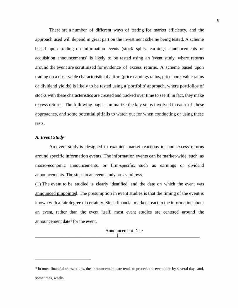
9

There are a number of different ways of testing for market efficiency, and the

approach used will depend in great part on the investment scheme being tested. A scheme

based upon trading on information events (stock splits, earnings announcements or

acquisition announcements) is likely to be tested using an 'event study' where returns

around the event are scrutinized for evidence of excess returns. A scheme based upon

trading on a observable characteristic of a firm (price earnings ratios, price book value ratios

or dividend yields) is likely to be tested using a 'portfolio' approach, where portfolios of

stocks with these characteristics are created and tracked over time to see if, in fact, they make

excess returns. The following pages summarize the key steps involved in each of these

approaches, and some potential pitfalls to watch out for when conducting or using these

tests.

A. Event Study

An event study is designed to examine market reactions to, and excess returns

around specific information events. The information events can be market-wide, such as

macro-economic announcements, or firm-specific, such as earnings or dividend

announcements. The steps in an event study are as follows -

(1) The event to be studied is clearly identified, and the date on which the event was

announced pinpointed. The presumption in event studies is that the timing of the event is

known with a fair degree of certainty. Since financial markets react to the information about

an event, rather than the event itself, most event studies are centered around the

announcement date4 for the event.

Announcement Date___________________________________|___________________________________

4 In most financial transactions, the announcement date tends to precede the event date by several days and,

sometimes, weeks.

10

(2) Once the event dates are known, returns are collected around these dates for each of the

firms in the sample. In doing so, two decisions have to be made. First, the analyst has to

decide whether to collect weekly, daily or shorter-interval returns around the event. This will,

in part, be decided by how precisely the event date is known (the more precise, the more

likely it is that shorter return intervals can be used) and by how quickly information is

reflected in prices (the faster the adjustment, the shorter the return interval to use). Second,

the analyst has to determine how many periods of returns before and after the

announcement date will be considered as part of the 'event window'. That decision also will

be determined by the precision of the event date, since more imprecise dates will require

longer windows.

R-jn ................. Rj0 ..................R+jn_____________|_______________________|________________________|_________

Return window: -n to +n

where,

Rjt = Returns on firm j for period t (t = -n, ...,0, .... +n)

(3) The returns, by period, around the announcement date, are adjusted for market

performance and risk to arrive at excess returns for each firm in the sample. For instance, if

the capital asset pricing model is used to control for risk -

Excess Return on period t = Return on day t – (Riskfree rate + Beta * Return on market on

day t)

ER-jn ................. ERj0 ..................ER+jn_____________|_______________________|________________________|_________

Return window: -n to +n

where,

ERjt = Excess Returns on firm j for period t (t = -n, ...,0, .... +n)

(4) The excess returns, by period, are averaged across all firms in the sample and a standard

error is computed.

Average excess return on day t= ER jt

Nj =1

j= N

∑

where,

11

N = Number of events in the event study

(5) The question of whether the excess returns around the announcement are different from

zero is answered by estimating the t statistic for each n, by dividing the average excess

return by the standard error -

T statistic for excess return on day t = Average Excess Return / Standard Error

If the t statistics are statistically significant5, the event affects returns; the sign of the excess

return determines whether the effect is positive or negative.

Illustration 8.1: Example of an event study - Effects of Option Listing on Stock prices

Academics and practitioners have long argued about the consequences of option

listing for stock price volatility. On the one hand, there are those who argue that options

attract speculators and hence increase stock price volatility. On the other hand, there are

others who argue that options increase the available choices for investors and increase the

flow of information to financial markets, and thus lead to lower stock price volatility and

higher stock prices.

One way to test these alternative hypotheses is to do an event study, examining the

effects of listing options on the underlying stocks' prices. Conrad(1989) did such a study,

following these steps -

Step 1: The date on which the announcement that options would be listed on the Chicago

Board of Options on a particular stock was collected.

5 The standard levels of significance for a t statistics are -

Level One-tailed Two-tailed

1% 2.33 2.55

5% 1.66 1.96

12

Step 2: The prices of the underlying stock(j) were collected for each of the ten days prior to

the option listing announcement date, the day of the announcement, and each of the ten days

after.

Step 3: The returns on the stock (Rjt) were computed for each of these trading days.

Step 4: The beta for the stock (βj) was estimated using the returns from a time period

outside the event window (using 100 trading days from before the event and 100 trading

days after the event).

Step 5: The returns on the market index (Rmt) were computed for each of the 21 trading

days.

Step 6: The excess returns were computed for each of the 21 trading days -

ERjt = Rjt - βj Rmt .......... t = -10,-9,-8,....,+8,+9,+10

The excess returns are cumulated for each trading day.

Step 7: The average and standard error of excess returns across all stocks with option

listings were computed for each of the 21 trading days. The t statistics are computed using

the averages and standard errors for each trading day. Table 6.1 summarizes the average

excess returns and t statistics around option listing announcement dates –

Table 6.1: Excess Returns around Option Listing Announcement DatesTrading Day Average Excess Cumulative T Statistic

Return Excess Return-10 0.17% 0.17% 1.30-9 0.48% 0.65% 1.66-8 -0.24% 0.41% 1.43-7 0.28% 0.69% 1.62-6 0.04% 0.73% 1.62-5 -0.46% 0.27% 1.24-4 -0.26% 0.01% 1.02-3 -0.11% -0.10% 0.93-2 0.26% 0.16% 1.09-1 0.29% 0.45% 1.280 0.01% 0.46% 1.27

13

1 0.17% 0.63% 1.372 0.14% 0.77% 1.443 0.04% 0.81% 1.444 0.18% 0.99% 1.545 0.56% 1.55% 1.886 0.22% 1.77% 1.997 0.05% 1.82% 2.008 -0.13% 1.69% 1.899 0.09% 1.78% 1.9210 0.02% 1.80% 1.91

Based upon these excess returns, there is no evidence of an announcement effect on the

announcement day alone, but there is mild6 evidence of a positive effect over the entire

announcement period.

B. Portfolio Study

In some investment strategies, firms with specific characteristics are viewed as more

likely to be undervalued, and therefore have excess returns, than firms without these

characteristics. In these cases, the strategies can be tested by creating portfolios of firms

possessing these characteristics at the beginning of a time period, and examining returns

over the time period. To ensure that these results are not colored by the idiosyncracies of

one time period, this analysis is repeated for a number of periods. The steps in doing a

portfolio study are as follows -

(1) The variable on which firms will be classified is defined, using the investment strategy as

a guide. This variable has to be observable, though it does not have to be numerical.

Examples would include market value of equity, bond ratings, stock price, price earnings

ratios and price book value ratios.

(2) The data on the variable is collected for every firm in the defined universe7 at the start of

the testing period, and firms are classified into portfolios based upon the magnitude of the

6 The t statistics are marginally significant at the 5% level.

14

variable. Thus, if the price earnings ratio is the screening variable, firms are classified on the

basis of PE ratios into portfolios from lowest PE to highest PE classes. The number of

classes will depend upon the size of the universe, since there have to be sufficient firms in

each portfolio to get some measure of diversification.

(3) The returns are collected for each firm in each portfolio for the testing period, and the

returns for each portfolio are computed, generally assuming that the stocks are equally

weighted.

(4) The beta (if using a single factor model) or betas (if using a multifactor model) of each

portfolio are estimated, either by taking the average of the betas of the individual stocks in

the portfolio or by regressing the portfolio's returns against market returns over a prior time

period (for instance, the year before the testing period).

(5) The excess returns earned by each portfolio are computed, in conjunction with the

standard error of the excess returns.

(6) There are a number of statistical tests available to check whether the average excess

returns are, in fact, different across the portfolios. Some of these tests are parametric8 (they

make certain distributional assumptions about excess returns) and some are non-

parametric9.

(7) As a final test, the extreme portfolios can be matched against each other to see whether

there are statistically significant differences across these portfolios.

7 Though there are practicial limits on how big the universe can be, care should be taken to make sure that

no biases enter at this stage of the process. An obvious one would be to pick only stocks that have done

well over the time period for the universe.

8 One parametric test is an F test, which tests for equality of means across groups. This test can be

conducted assuming either that the groups have the same variance, or that they have different variances.

9 An example of a non-parametric test is a rank sum test, which ranks returns across the entire sample an

then sums the ranks within each group to check whether the rankings are random or systematic.

15

Illustration 8.2: Example of a portfolio study - Price Earnings Ratios

Practitioners have claimed that low price-earnings ratio stocks are generally bargains

and do much better than the market or stocks with high price earnings ratios. This

hypothesis can be tested using a portfolio approach -

Step 1: Using data on price-earnings ratios from the end of 1987, firms on the New York

Stock Exchange were classified into five groups, the first group consisting of stocks with

the lowest PE ratios and the fifth group consisting of stocks with the highest PE ratios.

Firms with negative price-earnings ratios were ignored.

Step 2: The returns on each portfolio were computed using data from 1988 to 1992. Stocks

which went bankrupt or were delisted were assigned a return of -100%.

Step 3: The betas for each stock in each portfolio were computed using monthly returns

from 1983 to 1987, and the average beta for each portfolio was estimated. The portfolios

were assumed to be equally weighted.

Step 4: The returns on the market index was computed from 1988 to 1992.

Step 5: The excess returns on each portfolio were computed using data from 1988 to 1992.

Table 6.2 summarizes the excess returns each year from 1988 to 1992 for each portfolio.

Table 6.2: Excess Returns from 1988 to 1992 for PE Ratio Portfolios

P/E Class 1988 1989 1990 1991 1992 1988-1992

Lowest 3.84% -0.83% 2.10% 6.68% 0.64% 2.61%

2 1.75% 2.26% 0.19% 1.09% 1.13% 1.56%

3 0.20% -3.15% -0.20% 0.17% 0.12% -0.59%

4 -1.25% -0.94% -0.65% -1.99% -0.48% -1.15%

Highest -1.74% -0.63% -1.44% -4.06% -1.25% -1.95%

Step 6: While the ranking of the returns across the portfolio classes seems to confirm our

hypothesis that low PE stocks earn a higher return, we have to consider whether the

differences across portfolios is statistically significant. There are several tests available, but

these are a few:

16

• An F test can be used to accept or reject the hypothesis that the average returns are

the same across all portfolios. A high F score would lead us to conclude that the

differences are too large to be random.

• A chi-squared test is a non-parametric test that can be used to test the hypothesis

that the means are the same across the five portfolio classes.

• We could isolate just the lowest PE and highest PE stocks and estimate a t statistic

that the averages are different across these two portfolios.

The Cardinal Sins in testing Market Efficiency

In the process of testing investment strategies, there are a number of pitfalls that

have to be avoided. Some of them are listed below -

1. Using 'anecdotal evidence' to support/reject an investment strategy: Anecdotal evidence

is a double edged sword. It can be used to support or reject the same hypothesis. Since

stock prices are noisy and all investment schemes (no matter how absurd) will succeed

sometimes and fail at other times, there will always be cases where the scheme works or

does not work.

2. Testing an investment strategy on the same data and time period from which it was

extracted: This is the tool of choice for the unscrupulous investment advisor. An investment

scheme is extracted from hundreds through an examination of the data for a particular time

period. This investment scheme is then tested on the same time period, with predictable

results. (The scheme does miraculously well and makes immense returns.)

An investment scheme should always be tested out on a time period different from the

one it is extracted from or on a universe different from the one used to derive the scheme.

3. Choosing a biased universe: The universe is the sample on which the test is run. Since

there are thousands of stocks that could be considered part of this universe, researchers

often choose to use a smaller universe. When this choice is random, this does limited

damage to the results of the study. If the choice is biased, it can provide results which are

not true in the larger universe.

17

4. Failure to control for market performance: A failure to control for overall market

performance can lead one to conclude that your investment scheme works just because it

makes good returns (Most schemes will make good returns if the overall market does well;

the question is did they make better returns than expected) or does not work just because it

makes bad returns (Most schemes will do badly if the overall market performs poorly). It is

crucial therefore that investment schemes control for market performance during the period

of the test.

5. Failure to control for risk: A failure to control for risk leads to a bias towards accepting

high-risk investment schemes and rejecting low-risk investment schemes, since the former

should make higher returns than the market and the latter lower, without implying any

excess returns.

6. Mistaking correlation for causation: Consider the study on PE stocks cited in the earlier

section. We concluded that low PE stocks have higher excess returns than high PE stocks.

It would be a mistake to conclude that a low price earnings ratio causes excess returns, since

the high returns and the low PE ratio themselves might have been caused by the high risk

associated with investing in the stock. In other words, high risk is the causative factor that

leads to both the observed phenomena – low PE ratios on the one hand and high returns on

the other. This insight would make us more cautious about adopting a strategy of buying

low PE stocks in the first place.

Some lesser sins that can be a problem

1. Survival Bias: Most researchers start with a existing universe of publicly traded

companies and working back through time to test investment strategies. This can create a

subtle bias since it automatically eliminates firms that failed during the period, with obvious

negative consequences for returns. If the investment scheme is particularly susceptible to

picking firms that have high bankruptcy risk, this may lead to an 'overstatement' of returns

on the scheme.

18

For example, assume that the investment scheme recommends investing in stocks

which have very negative earnings, using the argument that these stocks are most likely to

benefit from a turnaround. Some of the firms in this portfolio will go bankrupt, and a failure

to consider these firms will overstate the returns from this strategy.

2. Not allowing for transactions Costs: Some investment schemes are more expensive than

others because of transactions costs - execution fees, bid-ask spreads and price impact. A

complete test will take these into account before it passes judgment on the strategy. This is

easier said than done, because different investors have different transactions costs, and it is

unclear which investor's trading cost schedule should be used in the test. Most researchers

who ignore transactions costs argue that individual investors can decide for themselves,

given their transactions costs, whether the excess returns justify the investment strategy.

3. Not allowing for difficulties in execution: Some strategies look good on paper but are

difficult to execute in practice, either because of impediments to trading or because trading

creates a price impact. Thus a strategy of investing in very small companies may seem to

create excess returns on paper, but these excess returns may not exist in practice because the

price impact is significant.

The Evidence on Market Efficiency

This section of the chapter attempts to summarize the evidence from studies of

market efficiency. Without claiming to be comprehensive, the evidence is classified into four

sections - the study of price changes and their time series properties, the research on the

efficiency of market reaction to information announcements, the existence of return

anomalies across firms and over time and the analysis of the performance of insiders,

analysts and money managers.

Time Series Properties of Price Changes

Investors have used price charts and price patterns as tools for predicting future

price movements for as long as there have been financial markets. It is not surprising,

19

therefore, that the first studies of market efficiency focused on the relationship between

price changes over time, to see if in fact such predictions were feasible. Some of this testing

was spurred by the random walk theory of price movements, which contended that price

changes over time followed a random walk. As the studies of the time series properties of

prices have proliferated, the evidence can be classified into two classes - studies that focus

on short-term (intraday, daily and weekly price movements) price behavior and research that

examines long-term (annual and five-year returns) price movements.

a. Short term Price Movements

The notion that today's price change conveys information about tomorrow's price

change is deep rooted in most investors' psyches. There are several ways in which this

hypotheses can be tested in financial markets -

a. Serial correlation

The serial correlation measures the correlation between price changes in consecutive

time periods, whether hourly, daily or weekly, and is a measure of how much the price

change in any period depends upon the price change over the previous time period. A serial

correlation of zero would therefore imply that price changes in consecutive time periods are

uncorrelated with each other, and can thus be viewed as a rejection of the hypothesis that

investors can learn about future price changes from past ones. A serial correlation which is

positive, and statistically significant, could be viewed as evidence of price momentum in

markets, and would suggest that returns in a period are more likely to be positive (negative)

if the prior period's returns were positive (negative). A serial correlation which is negative,

and statistically significant, could be evidence of price reversals, and would be consistent

with a market where positive returns are more likely to follow negative returns and vice

versa.

From the viewpoint of investment strategy, serial correlations can be exploited to

earn excess returns. A positive serial correlation would be exploited by a strategy of buying

20

after periods with positive returns and selling after periods with negative returns. A negative

serial correlation would suggest a strategy of buying after periods with negative returns and

selling after periods with positive returns. Since these strategies generate transactions costs,

the correlations have to be large enough to allow investors to generate profits to cover these

costs. It is therefore entirely possible that there be serial correlation in returns, without any

opportunity to earn excess returns for most investors.

The earliest studies of serial correlation (Alexander (1964), Cootner (1962)and

Fama (1965) all looked at large U.S. stocks and concluded that the serial correlation in

stock prices was small. Fama, for instance, found that 8 of the 30 stocks listed in the Dow

had negative serial correlations and that most of the serial correlations were less than 0.05.

Other studies confirm these findings not only for smaller stocks in the United States, but

also for other markets. For instance, Jennergren and Korsvold (1974) report low serial

correlations for the Swedish equity market and Cootner (1961) conludes that serial

correlations are low in commodity markets as well. While there may be statistical

significance associated with some of these correlations, it is unlikely that there is enough

correlation to generate excess returns.

The serial correlation in short period returns is affected by market liquidity and the

presence of a bid-ask spread. Not all stocks in an index are liquid, and, in some cases,

stocks may not trade during a period. When the stock trades in a subsequent period, the

resulting price changes can create positive serial correlation. To see why, assume that the

market is up strongly on day 1, but that three stocks in the index do not trade on that day.

On day 2, if these stocks are traded, they are likely to go up in price to reflect the increase in

the market the previous day. The net result is that you should expect to see positive serial

correlation in daily or hourly returns in illiquid market indices.

The bid-ask spread creates a bias in the opposite direction, if transactions prices are

used to compute returns, since prices have a equal chance of ending up at the bid or the ask

21

price. The bounce that this induces in prices will result in negative serial correlations in

returns. Roll (1984) provides a simple measure of this relationship,

Bid-Ask Spread = -√2 (Serial Covariance in returns)

where the serial covariance in returns measures the covariance between return changes in

consecutive time periods. For very short return intervals, this bias induced in serial

correlations might dominate and create the mistaken view that price changes in consecutive

time periods are negatively correlated.

b. Filter Rules

In a filter rule, an investor buys an investment if the price rises X% from a previous

low and holds the investment until the price drops X% from a previous high. The magnitude

of the change (X%) that triggers the trades can vary from filter rule to filter rule. with

smaller changes resulting in more transactions per period and higher transactions costs.

Figure 6.1 graphs out a typical filter rule.

Figure 6.1: Filter Rule

Buy

Sell

Up X%

Down X%

Price

Time

This strategy is based upon the assumption that price changes are serially correlated and

that there is price momentum, i.e., stocks which have gone up strongly in the past are more

likely to keep going up than go down. Table 6.4 summarizes results from a study on

returns, before and after transactions costs, on a trading strategy based upon filter rules

22

ranging from 0.5% to 20%. ( A 0.5% rule implies that a stock is bought when it rises 0.5%

from a previous low and sold when it falls 0.5% from a prior high.)

Table 6.4: Returns on Filter Rule Strategies

Value of X Return with

strategy

Return with Buy

and Hold

# Transactions

with strategy

Return after

transactions

costs

0.5% 11.5% 10.4% 12,514 -103.6%

1.0% 5.5% 10.3% 8,660 -74.9%

2.0% 0..2% 10.3% 4,764 -45.2%

3.0% -1.7% 10.1% 2,994 -30.5%

4.0% 0.1% 10.1% 2,013 -19.5%

5.0% -1.9% 10.0% 1,484 -16.6%

6.0% 1.3% 9.7% 1,071 -9.4%

7.0% 0.8% 9.6% 828 -7.4%

8.0% 1.7% 9.6% 653 -5.0%

9.0% 1.9% 9.6% 539 -3.6%

10.0% 3.0% 9.6% 435 -1.4%

12.0% 5.3% 9.4% 289 2.3%

14.0% 3.9% 10.3% 224 1.4%

16.0% 4.2% 10.3% 172 2.3%

18.0% 3.6% 10.0% 139 2.0%

20.0% 4.3% 9.8% 110 3.0%

The only filter rule that beats the returns from the buy and hold strategy is the 0.5% rule,

but it does so before transactions costs. This strategy creates 12,514 trades during the

period which generate enough transactions costs to wipe out the principal invested by the

investor. While this test is an dated, it also illustrates a basic strategies that require frequent

short term trading. Even though these strategies may earn excess returns prior to

transactions costs, adjusting for these costs can wipe out the excess returns.

One popular indicator among investors that is a variant on the filter rule is the

relative strength measure, which relates recent prices on stocks or other investments to either

average prices over a specified period, say over six months, or to the price at the beginning

of the period. Stocks that score high on the relative strength measure are considered good

23

investments. This investment strategy is also based upon the assumption of price

momentum.

c. Runs Tests

A runs test is a non-parametric variation on the serial correlation, and it is based

upon a count of the number of runs, i.e., sequences of price increases or decreases, in the

price changes. Thus, the following time series of price changes, where U is an increase and

D is a decrease would result in the following runs -

UUU DD U DDD UU DD U D UU DD U DD UUU DD UU D UU D

There were 18 runs in this price series of 33 periods. The actual number of runs in the price

series is compared against the number that can be expected10 in a series of this length,

assuming that price changes are random. If the actual number of runs is greater than the

expected number, there is evidence of negative correlation in price changes. If it is lower,

there is evidence of positive correlation. A study of price changes in the Dow 30 stocks,

assuming daily, four-day, nine-day and sixteen day return intervals provided the following

results -

DIFFERENCING INTERVAL

Daily Four-day Nine-day Sixteen-day

Actual runs 735.1 175.7 74.6 41.6

Expected runs 759.8 175.8 75.3 41.7

Based upon these results, there is evidence of positive correlation in daily returns but no

evidence of deviations from normality for longer return intervals.

Again, while the evidence is dated, it serves to illustrate the point that long strings of

positive and negative changes are, by themselves, insufficient evidence that markets are not

random, since such behavior is consistent with price changes following a random walk. It is

10 There are statistical tables that summarize the expected number of runs, assuming randomness, in a

series of any length.

24

the recurrence of these strings that can be viewed as evidence against randomness in price

behavior.

Long-term Price Movements

While most of the earlier studies of price behavior focused on shorter return

intervals, more attention has been paid to price movements over longer periods (one-year to

five-year) in recent years. Here, there is an interesting dichotomy in the results. When long

term is defined as months rather than years, there seems to be a tendency towards positive

serial correlation. Jegadeesh and Titman present evidence of what they call “price

momentum” in stock prices over time periods of up to eight months when investors winner

and loser stocks. However, when long term is defined in terms of years, there is substantial

negative correlation returns, suggesting that markets reverse themselves over very long

periods.

Fama and French examined five-year returns on stocks from 1931 to 1986 and

present further evidence of this phenomenon. Studies that break down stocks on the basis

of market value have found that the serial correlation is more negative in five-year returns

than in one-year returns, and is much more negative for smaller stocks rather than larger

stocks. Figure 6.2 summarizes one-year and five-years serial correlation by size class for

stocks on the New York Stock Exchange.

25

Figure 6.2: Serial Correlation in Stock Returns

This phenomenon has also been examined in other markets, and the findings have been

similar. There is evidence that returns reverse themselves over long time period.

Winner and Loser portfolios

Since there is evidence that prices reverse themselves in the long term for entire

markets, it might be worth examining whether such price reversals occur on classes of stock

within a market. For instance, are stocks that have gone up the most over the last period

more likely to go down over the next period and vice versa? To isolate the effect of such

price reversals on the extreme portfolios, DeBondt and Thaler constructed a winner

portfolio of 35 stocks, which had gone up the most over the prior year, and a loser portfolio

of 35 stocks, which had gone down the most over the prior year, each year from 1933 to

1978, and examined returns on these portfolios for the sixty months following the creation

of the portfolio. Figure 6.3 summarizes the excess returns for winner and loser portfolios .

Figure 6.3: Excess Returns for Winner and Loser Portfolios

26

This analysis suggests that loser portfolio clearly outperform winner portfolios in the sixty

months following creation. This evidence is consistent with market overreaction and

correction in long return intervals. Jegadeesh and Titman find the same phenomenon

occurring, but present interesting evidence that the winner (loser) portfolios continue to go

up (down) for up to eight months after they are created and it is in the subsequent periods

that the reversals occur.

There are many, academics as well as practitioners, who suggest that these findings

may be interesting but that they overstate potential returns on 'loser' portfolios. For instance,

there is evidence that loser portfolios are more likely to contain low priced stocks (selling

for less than $5), which generate higher transactions costs and are also more likely to offer

heavily skewed returns, i.e., the excess returns come from a few stocks making phenomenal

returns rather than from consistent performance. One study of the winner and loser

portfolios attributes the bulk of the excess returns of loser portfolios to low-priced stocks

and also finds that the results are sensitive to when the portfolios are created. Loser

27

portfolios created every December earn significantly higher returns than portfolios created

every June.

Speculative Bubbles, Crashes and Panics

Historians who have examined the behavior of financial markets over time have

challenged the assumption of rationality that underlies much of efficient market theory.

They point out to the frequency with speculative bubbles have formed in financial markers,

as investors buy into fads or get-rich-quick schemes, and the crashes with these bubbles

have ended, and suggest that there is nothing to prevent the recurrence of this phenomenon

in today's financial markets. There is some evidence in the literature of irrationality on the

part of market players.

a. Experimental Studies of Rationality

Some of the most interesting evidence on market efficiency and rationality in recent

years has come from experimental studies. While most experimental studies suggest that

traders are rational, there are some examples of irrational behavior in some of these studies.

One such study was done at the University of Arizona. In an experimental study,

traders were told that a payout would be declared after each trading day, determined

randomly from four possibilities - zero, eight, 28 or 60 cents. The average payout was 24

cents. Thus the share's expected value on the first trading day of a fifteen day experiment

was $3.60 (24*15), the second day was $3.36 .... The traders were allowed to trade each

day. The results of 60 such experiments is summarized in figure 6.4.

28

Figure 6.4: Trading Price by Trading Day

There is clear evidence here of a 'speculative bubble' forming during periods 3 to 5, where

prices exceed expected values by a significant amount. The bubble ultimately bursts, and

prices approach expected value by the end of the period. If this is feasible in a simple

market, where every investor obtains the same information, it is clearly feasible in real

financial markets, where there is much more differential information and much greater

uncertainty about expected value.

It should be pointed out that some of the experiments were run with students, and

some with Tucson businessmen, with 'real world' experience. The results were similar for

both groups. Furthermore, when price curbs of 15 cents were introduced, the booms lasted

even longer because traders knew that prices would not fall by more than 15 cents in a

period. Thus, the notion that price limits can control speculative bubbles seems misguided.

b. Behavioral Finance

The irrationality sometimes exhibited by investors has given rise to a whole new area

of finance called behavioral finance. Using evidence gathered from experimental

psychology, researchers have tried to both model how investors react to information and

29

predict how prices will change as a consequence. They have been far more successful at the

first endeavor than the second. For instance, the evidence seems to suggest the following:

a. Investors do not like to admit their mistakes. Consequently, they tend to hold on

to losing stocks far too long, or in some cases, double up their bets

(investments) as stocks drop in value.

b. More information does not always lead to better investment decisions. Investors

seem to suffer both from information overload and a tendency to react to the

latest piece of information. Both result in investment decisions that lower returns

in the long term.

If the evidence on how investors behave is so clear cut, you might ask, why are the

predictions that emerge from these models so noisy? The answer, perhaps, is that any model

that tries to forecast human foibles and irrationalities is, by its very nature, unlikely to be a

stable one. Behavioral finance may emerge ultimately as a trump card in explaining why and

how stock prices deviate from true value, but their role in devising investment strategy still

remains questionable.Behavioral Finance and Valuation

In 1999, Robert Shiller made waves in both academia and investment houses with

his book titled Irrational Exuberance. His thesis is that investors are often not just irrational

but irrational in predictable ways- overreacting to some information and buying and selling

in herds. His work forms part of a growing body of theory and evidence of behavioral

finance, which can be viewed as a congruence of psychology, statistics and finance.

While the evidence presented for investor irrationality is strong, the implications for

valuation are less so. You can consider discounted cash flow valuation to be the antithesis of

behavioral finance, because it takes the point of view that the value of an asset is the present

value of the expected cash flows generated by that asset. With this context, there are two

ways in which you can look at the findings in behavioral finance:

• Irrational behavior in finance may explain why prices can deviate from value (as

estimated in a discounted cash flow model). Consequently, it provides the foundation

for the excess returns earned by rational investors who base decisions on estimated

value. Implicit here is the assumption that markets ultimately recognize their irrationality

and correct themselves.

30

• It may also explain why discounted cash flow values can deviate from relative values

(estimated using multiples). Since the relative value is estimated by looking at how the

market prices similar assets, market irrationalities that exist will be priced into the asset.

Market Reaction to Information Events

Some of the most powerful tests of market efficiency are event studies where market

reaction to informational events (such as earnings and takeover announcements) has been

scrutinized for evidence of inefficiency. While it is consistent with market efficiency for

markets to react to new information, the reaction has to be instantaneous and unbiased. This

point is made in Figure 6.5 by contrasting three different market reactions to information

announcements -

TimeNew information is revealed

Asset price

Figure 6.5: Information and Price Adjustment

Notice that the price adjusts instantaneously to the information

TimeNew information is revealed

Asset priceThe price drifts

upwards after the good news comes out.

Time

New information is revealed

Asset price

The price increases too much on the good news announcement, and thendecreases in the period after.

Of the three market reactions pictured here, only the first one is consistent with an efficient

market. In second market, the information announcement is followed by a gradual increase

in prices, allowing investors to make excess returns after the announcement. This is a slow

learning market where some investors will make excess returns on the price drift. In the

third market, the price reacts instantaneously to the announcement, but corrects itself in the

days that follow, suggesting that the initial price change was an over reaction to the

information. Here again, an enterprising investor could have sold short after the

announcement, and expected to make excess returns as a consequence of the price

correction.

a. Earnings Announcements

31

When firms make earnings announcements, they convey information to financial

markets about their current and future prospects. The magnitude of the information, and the

size of the market reaction, should depend upon how much the earnings report exceeds or

falls short of investor expectations. In an efficient market, there should be an instantaneous

reaction to the earnings report, if it contains surprising information, and prices should

increase following positive surprises and down following negative surprises.

Since actual earnings are compared to investor expectations, one of the key parts of

an earnings event study is the measurement of these expectations. Some of the earlier

studies used earnings from the same quarter in the prior year as a measure of expected

earnings, i.e., firms which report increases in quarter-to-quarter earnings provide positive

surprises and those which report decreases in quarter-to-quarter earnings provide negative

surprises. In more recent studies, analyst estimates of earnings have been used as a proxy

for expected earnings, and compared to the actual earnings.

Figure 6.6 provides a graph of price reactions to earnings surprises, classified on the

basis of magnitude into different classes from 'most negative' earnings reports (Group 1) to

'most positive' earnings reports (Group 10).

Figure 6.6: Price Reaction to Quarterly Earnings Report

32

The evidence contained in this graph is consistent with the evidence in most earnings

announcement studies -

(a) The earnings announcement clearly conveys valuable information to financial markets;

there are positive excess returns (cumulative abnormal returns) after positive announcements

and negative excess returns around negative announcements.

(b) There is some evidence of a market reaction in the day immediately prior to the earnings

announcement which is consistent with the nature of the announcement, i.e., prices tend to

go up on the day before positive announcements and down in the day before negative

announcements. This can be viewed either as evidence of insider trading or as a

consequence of getting the announcement date wrong11.

(c) There is some evidence, albeit weak, of a price drift in the days following an earnings

announcement. Thus, a positive report evokes a positive market reaction on the

announcement date, and there are mildly positive excess returns in the days following the

earnings announcement. Similar conclusions emerge for negative earnings reports.

The management of a firm has some discretion on the timing of earnings reports

and there is some evidence that the timing affects expected returns. A study of earnings

reports, classified by the day of the week that the earnings are reported, reveals that earnings

and dividend reports on Fridays are much more likely to contain negative information than

announcements on any other day of the week. This is shown in figure 6.7.

11 The Wall Street Journal or COMPUSTAT are often used as information sources to extract announcement

dates for earnings. For some firms, news of the announcement may actually cross the news wire the day

before the Wall Street Journal announcement, leading to a misidentification of the report date and the drift in

returns the day before the announcement.

33

There is also some evidence that earnings announcements that are delayed, relative to the

expected announcement date, are much more likely to contain bad news than earnings

announcements which are early or on time. This is graphed in Figure 6.8.

Figure 6.7: Earnings and Dividend Reports by Day of the Week

-6.00%

-4.00%

-2.00%

0.00%

2.00%

4.00%

6.00%

8.00%

Monday Tuesday Wednesday Thursday Friday

% Chg(EPS) % Chg(DPS)

34

Earnings announcements that are more than six days late, relative to the expected

announcement date, are much more likely to contain bad news and evoke negative market

reactions than earnings announcements that are on time or early.

b. Investment and Project Announcements

Firms frequently make announcements of their intentions of investing resources in

projects and research and development. There is evidence that financial markets react to

these announcements. The question of whether market have a long term or short term

perspective can be partially answered by looking at these market reactions. If financial

markets are as short term as some of their critics claim, they should react negatively to

announcements by the firm that it plans to invest in research and development. The evidence

suggests the contrary. Table 6.5 summarizes market reactions to various classes of

investment announcements made by the firm.

Table 6.5: Market Reactions to Investment Announcements

Type of Announcement Abnormal Returns on

Announcement Day Announcement Month

Joint Venture Formations 0.399% 1.412%

FIGURE 6.8: CUMULATED ABNORMAL RETURNS AND EARNINGS DELAY

Day 0 is Earnings Announcement Date

CAR

0.006

-0.014

0 +30-30

Delay>6 days

Early>6 days

35

R&D Expenditures 0.251% 1.456%

Product Strategies 0.440% -0.35%

Capital Expenditures 0.290% 1.499%

All Announcements 0.355% 0.984%

This table excludes the largest investments that most make which is acquisitions of other

firms. Here, the evidence is not so favorable. In about 55% of all acquisitions, the stock

price of the acquiring firm drops on the announcement of the acquisition, reflecting the

market’s beliefs that firms tend to overpay on acquisitions.

Market Anomalies

Webster's Dictionary defines an anomaly as a "deviation from the common rule" .

Studies of market efficiency have uncovered numerous examples of market behavior that are

inconsistent with existing models of risk and return and often defy rational explanation. The

persistence of some of these patterns of behavior suggests that the problem, in at least some

of these anomalies, lies in the models being used for risk and return rather than in the

behavior of financial markets. The following section summarizes some of the more widely

noticed anomalies in financial markets in the United States and elsewhere.

Anomalies based upon firm characteristics

There are a number of anomalies that have been related to observable firm

characteristics, including the market value of equity, price earnings ratios and price book

value ratios.

a. The Small Firm Effect

Studies have consistently found that smaller firms (in terms of market value of

equity) earn higher returns than larger firms of equivalent risk, where risk is defined in

terms of the market beta. Figure 6.9 summarizes returns for stocks in ten market value

classes, for the period from 1927 to 1983.

36

Figure 6.9: Annual Returns by Size Class: 1927-83

0.00%2.00%4.00%6.00%8.00%

10.00%12.00%14.00%16.00%18.00%20.00%

Smallest 3 5 7 9

Size Class

Ann

ual R

etur

ns

The size of the small firm premium, while it has varied across time, has been generally

positive. It was highest during the 1970s and lowest during the 1980s. The persistence of

this premium has lead to several possible explanations.

(a) The transactions costs of investing in small stocks is significantly higher than the

transactions cots of investing in larger stocks, and the premiums are estimated prior to these

costs. While this is generally true, the differential transactions costs are unlikely to explain

the magnitude of the premium across time, and are likely to become even less critical for

longer investment horizons. The difficulties of replicating the small firm premiums that are

observed in the studies in real time are illustrated in Figure 6.10, which compares the returns

on a hypothetical small firm portfolio (CRSP Small Stocks) with the actual returns on a

small firm mutual fund (DFA Small Stock Fund), which passively invests in small stocks.

37

Figure 6.10: Returns on CRSP Small Stocks versus DFA Small Stock Fund

-10.00%

-5.00%

0.00%

5.00%

10.00%

15.00%

1982 1983 1984 1985 1986 1987 1988 1989 1990 1991

CRSP Small DFA Small Firm Fund

(b) The capital asset pricing model may not be the right model for risk, and betas under

estimate the true risk of small stocks. Thus, the small firm premium is really a measure of

the failure of beta to capture risk. The additional risk associated with small stocks may come

from several sources. First, the estimation risk associated with estimates of beta for small

firms is much greater than the estimation risk associated with beta estimates for larger firms.

The small firm premium may be a reward for this additional estimation risk. Second, there

may be additional risk in investing in small stocks because far less information is available

on these stocks. In fact, studies indicate that stocks that are neglected by analysts and

institutional investors earn an excess return that parallels the small firm premium.

There is evidence of a small firm premium in markets outside the United States as

well. Dimson and Marsh examined stocks in the United Kingdom from 1955 to 1984 and

found that the annual returns on small stocks exceeded that on large stocks by 7% annually

over the period. Bergstrom, Frashure and Chisholm report a large size effect for French

stocks (Small stocks made 32.3% per year between 1975 to 1989, while large stocks made

38

23.5% a year), and a much smaller size effect in Germany. Chan, Hamao and Lakonishok

reports a small firm premium of 5.1% for Japanese stocks between 1971 and 1988.

b. Price Earnings Ratios

Investors have long argued that stocks with low price earnings ratios are more likely

to be undervalued and earn excess returns. For instance, Ben Graham, in his investment

classic "The Intelligent Investor", uses low price earnings ratios as a screen for finding

under valued stocks. Studies that have looked at the relationship between PE ratios and

excess returns confirm these priors. Figure 6.11 summarizes annual returns by PE ratio

classes for stocks from 1967 to 1988.

Figure 6.11: Annual Returns by PE Ratio Class

0.00%

2.00%

4.00%

6.00%

8.00%

10.00%

12.00%

14.00%

16.00%

18.00%

Lowest 3 5 7 9

F

irms in the lowest PE ratio class earned an average return of 16.26% during the period,

while firms in the highest PE ratio class earned an average return of only 6.64%.

The excess returns earned by low PE ratio stocks also persist in other international

markets. Table 6.6 summarizes the results of studies looking at this phenomenon in markets

outside the United States.Table 6.6: Excess Returns on Low P/E Ratio Stocks by Country: 1989-1994

39

Country Annual Premium earned by lowest P/E Stocks (bottom quintile)Australia 3.03%France 6.40%Germany 1.06%Hong Kong 6.60%Italy 14.16%Japan 7.30%Switzerland 9.02%U.K. 2.40%Annual premium: Premium earned over an index of equally weighted stocks in that marketbetween January 1, 1989 and December 31, 1994. These numbers were obtained from aMerrill Lynch Survey of Proprietary Indices.

The excess returns earned by low price earnings ratio stocks are difficult to justify

using a variation of the argument used for small stocks, i.e., that the risk of low PE ratios

stocks is understated in the CAPM. Low PE ratio stocks generally are characterized by low

growth, large size and stable businesses, all of which should work towards reducing their

risk rather than increasing it. The only explanation that can be given for this phenomenon,

which is consistent with an efficient market, is that low PE ratio stocks generate large

dividend yields, which would have created a larger tax burden in those years where

dividends were taxed at higher rates.

c. Price Book Value Ratios

Another statistic that is widely used by investors in investment strategy is price book

value ratios. A low price book value ratio has been considered a reliable indicator of

undervaluation in firms. In studies that parallel those done on price earnings ratios, the

relationship between returns and price book value ratios has been studied. The consistent

finding from these studies is that there is a negative relationship between returns and price

book value ratios, i.e., low price book value ratio stocks earn higher returns than high price

book value ratio stocks.

Rosenberg, Reid and Lanstein (1985) find that the average returns on U.S. stocks

are positively related to the ratio of a firm's book value to market value. Between 1973 and

1984, the strategy of picking stocks with high book/price ratios (low price-book values)

yielded an excess return of 36 basis points a month. Fama and French (1992), in examining

40

the cross-section of expected stock returns between 1963 and 1990, establish that the

positive relationship between book-to-price ratios and average returns persists in both the

univariate and multivariate tests, and is even stronger than the size effect in explaining

returns. When they classified firms on the basis of book-to-price ratios into twelve

portfolios, firms in the lowest book-to-price (higher P/BV) class earned an average monthly

return of 0.30%, while firms in the highest book-to-price (lowest P/BV) class earned an

average monthly return of 1.83% for the 1963-90 period.

Chan, Hamao and Lakonishok (1991) find that the book-to-market ratio has a

strong role in explaining the cross-section of average returns on Japanese stocks. Capaul,

Rowley and Sharpe (1993) extend the analysis of price-book value ratios across other

international markets, and conclude that value stocks, i.e., stocks with low price-book value

ratios , earned excess returns in every market that they analyzed, between 1981 and 1992.

Their annualized estimates of the return differential earned by stocks with low price-book

value ratios, over the market index, were as follows:

Country Added Return to low P/BV portfolio

France 3.26%

Germany 1.39%

Switzerland 1.17%

U.K 1.09%

Japan 3.43%

U.S. 1.06%

Europe 1.30%

Global 1.88%

A caveat is in order. Fama and French point out that low price-book value ratios may

operate as a measure of risk, since firms with prices well below book value are more likely

to be in trouble and go out of business. Investors therefore have to evaluate for themselves

41

whether the additional returns made by such firms justifies the additional risk taken on by

investing in them.

Temporal Anomalies

There are a number of peculiarities in return differences across calendar time that are

not only difficult to rationalize but are also suggestive of inefficiencies. Furthermore, some

of these temporal anomalies are related to the small firm effect described in the previous

section.

a. The January Effect

Studies of returns in the United States and other major financial markets

consistently reveal strong differences in return behavior across the months of the year.

Figure 6.12 reports average returns by month of the year from 1926 to 1983.

Figure 6.12: Average Return by Month of the Year

-2.00%

-1.00%

0.00%

1.00%

2.00%

3.00%

4.00%

5.00%

Janu

ary

Febr

uary

Mar

ch

Apr

il

May

June

July

Aug

ust

Sept

embe

r

Oct

ober

Nov

embe

r

Dec

embe

r

Month of the Year

Ave

rage

Mon

thly

Ret

urn

Returns in January are significantly higher than returns in any other month of the year. This

phenomenon is called the year-end or January effect, and it can be traced to the first two

weeks in January.

42

The relationship between the January effect and the small firm effect adds to the

complexity of this phenomenon. The January effect is much more accentuated for small

firms than for larger firms, and roughly half of the small firm premium, described in the

prior section, is earned in the first two days of January. Figure 6.13 graphs returns in

January by size and risk class for data from 1935 to 1986.

Figure 6.13: Returns in January by Size and Risk Class - 1935-86

A number of explanations have been advanced for the January effect, but few hold up to

serious scrutiny. One is that there is tax loss selling by investors at the end of the year on

stocks which have 'lost money' to capture the capital gain, driving prices down, presumably

below true value, in December, and a buying back of the same stocks12 in January, resulting

12 Since wash sales rules would prevent an investor from selling and buying back the same stock within 45

days, there has to be some substitution among the stocks. Thus investor 1 sells stock A and investor 2

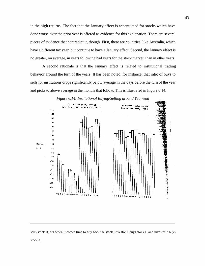
43

in the high returns. The fact that the January effect is accentuated for stocks which have

done worse over the prior year is offered as evidence for this explanation. There are several

pieces of evidence that contradict it, though. First, there are countries, like Australia, which

have a different tax year, but continue to have a January effect. Second, the January effect is

no greater, on average, in years following bad years for the stock market, than in other years.

A second rationale is that the January effect is related to institutional trading

behavior around the turn of the years. It has been noted, for instance, that ratio of buys to

sells for institutions drops significantly below average in the days before the turn of the year

and picks to above average in the months that follow. This is illustrated in Figure 6.14.

Figure 6.14: Institutional Buying/Selling around Year-end

sells stock B, but when it comes time to buy back the stock, investor 1 buys stock B and investor 2 buys

stock A.

44

It is argued that the absence of institutional buying pushes down prices in the days before

the turn of the year and pushes up prices in the days after.

The universality of the January effect is illustrated in Figure 6.15, which examines

returns in January versus the other months of the year in several major financial markets,

and finds strong evidence of a January effect in every market.

Figure 6.15: Returns in January vs Other Months - Major Financial Markets

b. The Weekend Effect

The weekend effect is another return phenomenon that has persisted over

extraordinary long periods and over a number of international markets. It refers to the

differences in returns between Mondays and other days of the week. The significance of the

return difference is brought out in Figure 6.16, which graphs returns by days of the week

from 1962 to 1978.

45

Figure 6.16: Average Daily Returns by Day of the Week: 1962-78

-0.15%

-0.10%

-0.05%

0.00%

0.05%

0.10%

0.15%

Monday Tuesday Wednesday Thursday Friday

Ave

rage

Dai

ly R

etur

n

The returns on Mondays are significantly negative, whereas the returns on every day of the

week are not. There are a number of other findings on the Monday effect that have fleshed I

out. First, the Monday effect is really a weekend effect since the bulk of the negative returns

is manifested in the Friday close to Monday open returns. The returns from intraday returns

on Monday are not the culprits in creating the negative returns. Second, the Monday effect

is worse for small stocks than for larger stocks. Third, the Monday effect is no worse

following three-day weekends than two-day weekends.

There are some who have argued that the weekend effect is the result of bad news

being revealed after the close of trading on Friday and during the weekend. They point to

figure 6.16, which reveals that more negative earnings reports are revealed after close of

trading on Friday. Even if this were a widespread phenomenon, the return behavior would

be inconsistent with a rational market, since rational investors would build in the expectation

of the bad news over the weekend into the price before the weekend, leading to an

elimination of the weekend effect.

The weekend effect is fairly strong in most major international markets, as shown in

Figure 6.17.

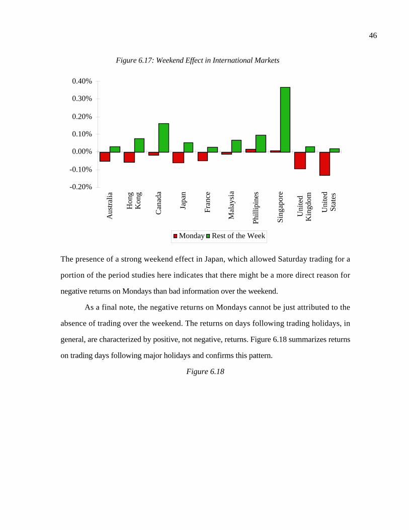
46

Figure 6.17: Weekend Effect in International Markets

-0.20%

-0.10%

0.00%

0.10%

0.20%

0.30%

0.40%

Aus

tral

ia

Hon

gK

ong

Can

ada

Japa

n

Fran

ce

Mal

aysi

a

Phill

ipin

es

Sing

apor

e

Uni

ted

Kin

gdom

Uni

ted

Stat

es

Monday Rest of the Week

The presence of a strong weekend effect in Japan, which allowed Saturday trading for a

portion of the period studies here indicates that there might be a more direct reason for

negative returns on Mondays than bad information over the weekend.

As a final note, the negative returns on Mondays cannot be just attributed to the

absence of trading over the weekend. The returns on days following trading holidays, in

general, are characterized by positive, not negative, returns. Figure 6.18 summarizes returns

on trading days following major holidays and confirms this pattern.

Figure 6.18

47

New Year's Day

President's Day

Good Friday

Memorial Day

Fourth of July

Labor Day

Thanksgiving

Christmas

Average of all days

-0.05% 0.00% 0.05% 0.10% 0.15% 0.20% 0.25% 0.30% 0.35% 0.40%

A Holiday Effect?Average Market Returns on Holidays

Evidence on Insiders and Investment Professionals

There is a sense that insiders, analysts and portfolio managers must possess an

advantage over the average investors in the market and be able to convert this advantage into

excess returns. The evidence on the performance of these investors is actually surprisingly

mixed.

a. Insider Trading

The SEC defines an insider to be a officer or director of the firm or a major

stockholder (holding more than 5% of the outstanding stock in the firm). Insiders are

barred from trading in advance of specific information on the company and are required to

file with the SEC when they buy or sell stock in the company. If it is assumed, as seems

reasonable, that insiders have better information about the company, and consequently better

estimates of value, than other investors, the decisions by insiders to buy and sell stock

should affect stock prices. Figure 6.19, derived from an early study of insider trading by

Jaffe, examines excess returns on two groups of stock, classified on the basis of insider

trades. The "buy group" includes stocks where buys exceeded sells by the biggest margin,

and the "sell group" includes stocks where sells exceed buys by the biggest margin.

48

Figure 6.19: Cumulative Returns Following Insider Trading: Buy vs Sell Group

-0.050

0.050.1

0.15

0.20.250.3

0.35

0.4

1 2 3 4 5 6 7 8 9 10 11 12 13 14 15 16 17 18 19 20

Month following insider trade

CA

R

Buy Group-M Sell Group-M

While it seems like the buy group does significantly better than the sell group in this study,

advances in information technology have made this information on insider trading available

to more and more investors. A more recent study of insider trading examined excess returns

around both the date the insiders report to the SEC and the date that information becomes

available to investors in the official summary. Figure 6.20 presents the contrast between the

two event studies.

Figure 6.20: Abnormal Returns around Reporting Day/ Official Summary Availability Day

49

Given the opportunity to buy on the date the insider reports to the SEC, investors could have

marginal excess returns, but these returns diminish and become statistically insignificant, if

investors are forced to wait until the official summary date.

None of these studies examine the question of whether insiders themselves make

excess returns. The reporting process, as set up now by the SEC, is biased toward legal and

less profitable trades, and away from illegal and more profitable trades. Though direct

evidence cannot be offered for this proposition, insiders trading illegally on private

information must make excess returns.

b. Analyst Recommendations

Analysts clearly hold a privileged position in the market for information, operating at

the nexus of private and public information. Using both types of information, analysts issue

buy and sell recommendations to their clients, who trade on its basis.

While both buy and sell recommendations affect stock prices, sell recommendations affect

prices much more adversely than buy recommendation affect them positively. Interestingly,

Womack (1996) documents that the price effect of buy recommendations tends to be

immediate and there is no evidence of price drifts after the announcement, whereas prices

Figure 6.21: Market Reaction to Recommendations: 1989- 1990

-10.00%

-8.00%

-6.00%

-4.00%

-2.00%

0.00%

2.00%

4.00%

6.00%

8.00%

10.00%

Added to Buy Removed from Buy Added to Sell Removed from SellRet

urns

3 days around recommendation 1 month after 3 months after 6 months after

50

continue to trend down after sell recommendations. Figure 6.21 graphs his findings. Stock

prices increase by about 3% on buy recommendations whereas they drop by about 4% on

sell recommendations at the time of the recommendations (3 days around reports). In the

six months following, prices decline an additional 5% for sell recommendations, while

leveling off for buy recommendations.

Though analysts provide a valuable service in collecting private information, or

maybe because they do, there is a negative relationship in the cross-section between returns

earned by stocks and the number of analysts following the stock. The same kind of

relationship exists between another proxy for interest, institutional ownership, and returns.

c. Money Managers

Professional money managers operate as the experts in the field of investments.

They are supposed to be better informed, smarter, have lower transactions costs and be

better investors overall than smaller investors. The earliest study of mutual funds by Jensen

suggested that this supposition might not hold in practice. His findings, summarized in

Figure 6.22, as excess returns on mutual funds, were that the average portfolio manager

actually underperformed the market between 1955 and 1964.

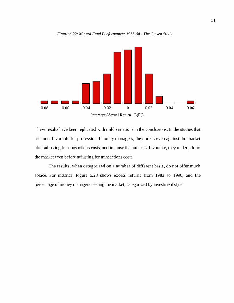
51

Figure 6.22: Mutual Fund Performance: 1955-64 - The Jensen Study

-0.08 -0.06 -0.04 -0.02 0 0.02 0.04 0.06

Intercept (Actual Return - E(R))

These results have been replicated with mild variations in the conclusions. In the studies that

are most favorable for professional money managers, they break even against the market

after adjusting for transactions costs, and in those that are least favorable, they underpeform

the market even before adjusting for transactions costs.

The results, when categorized on a number of different basis, do not offer much

solace. For instance, Figure 6.23 shows excess returns from 1983 to 1990, and the

percentage of money managers beating the market, categorized by investment style.

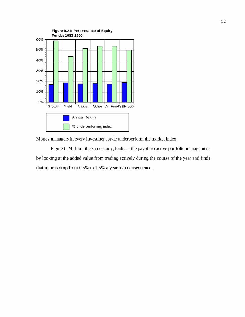
52

Growth Yield Value Other All FundS&P 5000%

10%

20%

30%

40%

50%

60%

Annual Return

% underperfoming index

Figure 9.21: Performance of EquityFunds: 1983-1990

Money managers in every investment style underperform the market index.

Figure 6.24, from the same study, looks at the payoff to active portfolio management

by looking at the added value from trading actively during the course of the year and finds

that returns drop from 0.5% to 1.5% a year as a consequence.

53

Growth Yield Value Other All

-1.60%

-1.40%

-1.20%

-1.00%

-0.80%

-0.60%

-0.40%

-0.20%

0.00%

Figure 9.22: The Payoff to Active Money Management:Equity Funds

This table measures the difference between actual return on

equity funds and return on hypothetical portfolio frozen at

beginning of period.

Finally, the study, like others before it, found no evidence of continuity in performance. It

classified money managers into quartiles and examined the probabilities of movement from

one quartile to another each year from 1983 to 1990. The results are summarized in Table

6.7.

Table 6.7: Probabilities of Transition from One Quartile to Another

Ranking next period

Ranking this period 1 2 3 4

1 26% 24% 23% 27%

2 20% 26% 29% 25%

3 22% 28% 26% 24%

4 32% 22% 22% 24%

This table indicates that a money manager who was ranked in the first quartile in a period

had a 26% chance of being ranked in the first quartile in the next period and a 27% chance

of being ranked in the bottom quartile. There is some evidence of reversal in the portfolio

54

managers in the lowest quartile, though some of that may be a reflection of the higher risk

portfolios that they put together.

While the evidence is depressing for active portfolio management as a whole, there

are a few bright spots. Carhart (1992) looked at mutual funds and concluded that there was

some persistence at the extremes – a small group of exceptional managers who outperform

a passive strategy and another group who consistently underperform, largely because they

have high expenses.Market Inefficiencies and Money Manager Performance

The evidence on markets is contradictory. On the one hand, there seem to be

numerous patterns in stock prices –stock prices reverse course in the long term and returns

are higher in January – and evidence of market anomalies – small market-cap firms with low

price to book and price to earnings ratios seem to handily beat the market. On the other,

there seems to be little evidence of money managers being able to exploit these findings to

beat the market.

There are a number of possible explanations. The most benign one is that the

inefficiencies show up mostly in hypothetical studies and that the transactions costs and

execution problems associated with converting these inefficiencies into portfolios

overwhelms the excess returns. A second possible explanation is that the studies generally

look at the long term – many are over 20 to 50 years. Over shorter periods, there is

substantially more uncertainty about whether small stocks will outperform large stocks and

whether buying losers will generate excess returns. There are no investment strategies that

are sure bets for short periods. Pradhuman (2000) illustrates this phenomenon by noting

that small cap stocks have underperformed large cap stocks in roughly one out of every four

years in the last 50 years. Bernstein (1998) notes that while value investing (buying low PE

and low Price to book value stocks) may earn excess returns over long periods, growth

investing has outperformed value investing over many five-year periods during the last three

decades. A third explanation is that portfolio managers do not consistently follow any one

55

strategy and that they jump from one strategy to another, increasing both their expenses and

reducing the likelihood that the strategy can generate excess returns in the long term.

Conclusion

The question of whether markets are efficient will always be a provocative one, given

the implications that efficient markets have for investment management and research. If an

efficient market is defined as one where the market price is an unbiased estimate of the true

value, it is quite clear that some markets will always be more efficient than others and that

markets will always be more efficient to some investors than to others. The capacity of a

market to correct inefficiencies quickly will depend, in part, on the ease of trading, the

transactions cost and the vigilance of profit-seeking investors in that market.

While market efficiency can be tested in a number of different ways, the two most

widely used tests to test efficiency are 'event studies' which examine market reactions to

information events and 'portfolio studies' which evaluate the returns of portfolios created on

the basis of observable characteristics. It does make sense to be vigilant, because bias can

enter these studies, intentionally or otherwise, in a number of different ways and can lead to

unwarranted conclusions, and, worse still, wasteful investment strategies.

There is substantial evidence of irregularities in market behavior, related to

systematic factors such as size, price-earnings ratios and price book value ratios, as well as

to time - the January and the weekend effects. While these irregularities may be

inefficiencies, there is also the sobering evidence that professional money managers, who

are in a position to exploit these inefficiencies, have a very difficult time consistently beating

financial markets. Read together, the persistence of the irregularities and the inability of

money managers to beat the market is testimony to the gap between empirical tests on paper

and real world money management in some cases, and the failure of the models of risk and

return in others.

190

1. Which of the following is an implication of market efficiency? (There may be more than one right

answer)

(a) Resources are allocated among firms efficiently (i.e. put to best use)

(b) No investor will do better than the market in any time period

(c) No investor will do better than the market consistently

(d) No investor will do better than the market consistently after adjusting for risk

(e) No investor will do better than the market consistently after adjusting for risk and

transactions costs

(f) No group of investors will do better than the market consistently after adjusting for risk and

transactions costs.

2. Suppose you are following a retailing stock which has a strong seasonal pattern to sales. Would you

expect to see a seasonal pattern in the stock price as well?

3. Tests of market efficiency are often referred to as joint tests of two hypotheses - the hypothesis that

the market is efficient and an expected returns model. Explain. Is it ever possible to test market

efficiency alone? (i.e. without jointly testing an asset pricing model)

4. You are in a violent argument with a chartist. He claims that you are violating the fundamental laws of

economics by trying to find intrinsic value. "Price is determined by demand and supply... not by some

intrinsic value'. Is finding an intrinsic value inconsistent with demand and supply?

5. You are testing the effect of merger announcements on stock prices. (This is an event study.). Your

procedure goes through the following steps.

Step 1: You choose the twenty biggest mergers of the year

Step 2: You isolate the date the merger became effective as the key day around which you will

examine the data

Step 3: You look at the returns for the five days after the effective merger date

By looking at these returns (.13%) you conclude that you could not have made money on merger

announcements. Are there any flaws that you can detect in this test? How would you correct for them?

Can you devise a stronger test?

6. In an efficient market, the market price is defined to be an 'unbiased estimate' of the true

value. This implies that

(a) the market price is always equal to true value.

(b) the market price has nothing to do with true value

(c) markets make mistakes about true value, and investors can exploit these mistakes

to make money

191

(d) market prices contain errors, but the errors are random and therefore cannot be

exploited by investors.

(e) no one can beat the market.

7. Evaluate whether the following actions are likely to increase stock market efficiency,

decrease it or leave it unchanged, and explain why.

a. The government imposes a transaction tax of 1% on all stock transactions.

Increase Efficiency___ Decrease Efficiency___ Leave unchanged___

b. The securities exchange regulators impose a restriction on all short sales to prevent

rampant speculation.

Increase Efficiency___ Decrease Efficiency___ Leave unchanged___

c. An options market, trading call and put options, is opened up, with options traded on

many of the stocks listed on the exchange.

Increase Efficiency___ Decrease Efficiency___ Leave unchanged___

d. The stock market removes all restrictions on foreign investors acquiring and holding

stock in companies.

Increase Efficiency___ Decrease Efficiency___ Leave unchanged___

8. The following is a graph of cumulative abnormal returns around the announcement of

asset divestitures by major corporations.

Time (t)

Cumulative Abnormal Returns

How best would you explain the

(a) market behavior before the announcement?

(b) market reaction to the announcement ?

(c) market reaction after the announcement?

9. What is the phenomenon of the size effect in stock performance? How does it relate to the 'turn-of-

the-year' effect? Can you suggest any good reasons why small stocks, after adjusting for beta, still do

192

better than large stocks? What strategy would you follow to exploit this anomaly? What factors do

you have to keep in mind?

10. A study examining market reactions to earnings surprises found that prices tend to drift after

earnings surprises. What does this tell you market's capacity to learn from events and new

information? What cross-sectional differences would you expect to find in this learning behavior?

(i.e. Would you expect to see a greater price drift in some types of firms than in others? Why?) How

would you try to exploit this anomaly? What possible costs would you have to keep in mind?

11. One explanation of the turn-of-the-year or January effect has to do with sales and purchases

related to the tax year.

(a) Present the tax effect hypothesis

(b) Studies have shown that the January effect occurs internationally, even in countries where the tax

year does not start in January. Speculate on a good reason for this.

12. The following are the expected price appreciation and dividend yield components of returns on

two portfolios - a 'high dividend yield' portfolio and a 'low dividend yield' portfolio.

Portfolio Expected Price Appreciation Expected Dividend Yield

High Yield 9% 5%

Low Yield 12% 1%

You are a taxable investor who faces a tax rate of 40% on dividends. What would your tax rate on

capital gains need to be for you to be indifferent between these two portfolios?

13. Answer true or false to the following questions –

a. Low price-earnings stocks, on average, earn returns in excess of expectations, while high price-

earnings stocks earn less than expected. This is primarily because lower P/E ratio stocks have lower

risk. TRUE FALSE

b. The small firm effect, which refers the positive excess returns earned, on average, by small firms, is

primarily caused by a few small firms that make very high positive returns.

TRUE FALSE

c. Investors generally cannot make money on analyst recommendations, because stock prices are not

affected by these recommendations. TRUE FALSE

14. You are examining the performance of two mutual funds. AD VALUE Fund has been in

existence since January 1, 1988 and invests primarily in low Price Earnings Ratio stocks, with high

dividend yields. AD GROWTH Fund has also been in existence since January 1, 1988 but it invests

primarily in high growth stocks, with high PE ratios and low or no dividends. The performance of

these funds over the last five years is summarized below:

Average from 1988-1992

Price Appreciation Dividend Yield Beta

193

NYSE Composite 13% 3% 1.0

AD VALUE 11% 5% 0.8

AD GROWTH 15% 1% 1.2

The average riskfree rate during the period was 6%. The current riskfree rate is 3%.

a. How well or badly did these funds perform after adjusting for risk?

b. Assume that the front-end load on each of these funds is 5% (i.e. if you put $1000 in each

of these funds today, you would only be investing $950 after the initial commission). Assume

also that the excess returns you have calculated in part (a) will continue into the future and

that you choose to invest in the fund that outperformed the market. How many years would

you have to hold this fund to break even?

1

CHAPTER 7

RISKLESS RATES AND RISK PREMIUMS

All models of risk and return in finance are built around a rate that investors can

make on riskless investments and the risk premium or premiums that investors should

charge for investing in the average risk investment. In the capital asset pricing model,

where there is only one source of market risk captured in the market portfolio, this risk

premium becomes the premium that investors would demand when investing in that

portfolio. In multi-factor models, there are multiple risk premiums, each one measuring

the premium demanded by investors for exposure to a specific risk factor. In this chapter,

we examine how best to measure a riskless rate and to estimate a risk premium or

premiums for use in these models.

As noted in chapter 4, risk is measured in terms of default risk for bonds and this

default risk is captured in a default spread that firms have to pay over and above the

riskless rate. We close this chapter by considering how best to estimate these default

spreads and factors that may cause these spreads to change over time.

The Risk Free Rate

Most risk and return models in finance start off with an asset that is defined as

risk free and use the expected return on that asset as the risk free rate. The expected

returns on risky investments are then measured relative to the risk free rate, with the risk

creating an expected risk premium that is added on to the risk free rate. But what makes

an asset risk free? And what do we do when we cannot find such an asset? These are the

questions that we will deal with in this section.

Requirements for an Asset to be Riskfree

In chapter 4, we considered some of the requirements for an asset to be riskfree.

In particular, we argued that an asset is riskfree if we know the expected returns on it

with certainty – i.e. the actual return is always equal to the expected return. Under what

conditions will the actual returns on an investment be equal to the expected returns? In

our view, there are two basic conditions that have to be met. The first is that there can be

no default risk. Essentially, this rules out any security issued by a private firm, since even

2

the largest and safest firms have some measure of default risk. The only securities that

have a chance of being risk free are government securities, not because governments are

better run than corporations, but because they control the printing of currency. At least in

nominal terms, they should be able to fulfill their promises. Even though this assumption

is straightforward , it does not always hold up, especially when governments refuse to

honor claims made by previous regimes and when they borrow in currencies other than

their own.

There is a second condition that riskless securities need to fulfill that is often

forgotten. For an investment to have an actual return equal to its expected return, there

can be no reinvestment risk. To illustrate this point, assume that you are trying to

estimate the expected return over a five-year period and that you want a risk free rate. A

six-month treasury bill rate, while default free, will not be risk free, because there is the

reinvestment risk of not knowing what the treasury bill rate will be in six months. Even a

5-year treasury bond is not risk free, since the coupons on the bond will be reinvested at

rates that cannot be predicted today. The risk free rate for a five-year time horizon has to

be the expected return on a default-free (government) five-year zero coupon bond. This

clearly has painful implications for anyone doing corporate finance or valuation, where

expected returns often have to be estimated for periods ranging from one to ten years. A

purist's view of risk free rates would then require different risk free rates for each period

and different expected returns.

As a practical compromise, however, it is worth noting that the present value

effect of using year-specific risk free rates tends to be small for most well-behaved1 term

structures. In these cases, we could use a duration matching strategy, where the duration

of the default-free security used as the risk free asset is matched up to the duration2 of the

cash flows in the analysis. If, however, there are very large differences, in either

direction, between short term and long term rates, it does pay to stick with year-specific

risk free rates in computing expected returns.

1 By well behaved term structures, I would include a normal upwardly sloping yield curve, where long termrates are at most 2-3% higher than short term rates.2 In investment analysis, where we look at projects, these durations are usually between 3 and 10 years. Invaluation, the durations tend to be much longer, since firms are assumed to have infinite lives. The durationin these cases is often well in excess of ten years and increases with the expected growth potential of thefirm.

3

The Practical Implications when a Default-free Entity exists

In most developed markets, where the government can be viewed as a default free

entity, at least when it comes to borrowing in the local currency, the implications are

simple. When doing investment analysis on longer term projects or valuation, the risk

free rate should be the long term government bond rate. If the analysis is shorter term, the

short term government security rate can be used as the risk free rate. The choice of a risk

free rate also has implications for how risk premiums are estimated. If, as is often the

case, historical risk premiums are used, where the excess return earned by stocks over

and above a government security rate over a past period is used as the risk premium, the

government security chosen has to be same one as that used for the risk free rate. Thus,

the historical risk premium used in the US should be the excess return earned by stocks

over treasury bonds, and not treasury bills, for purposes of long term analysis.

Cash Flows and Risk free Rates: The Consistency Principle

The risk free rate used to come up with expected returns should be measured

consistently with how the cash flows are measured. Thus, if cash flows are estimated in

nominal US dollar terms, the risk free rate will be the US treasury bond rate. This also

implies that it is not where a project or firm is domiciled that determines the choice of a

risk free rate, but the currency in which the cash flows on the project or firm are

estimated. Thus, Nestle can be valued using cash flows estimated in Swiss Francs,

discounted back at an expected return estimated using a Swiss long term government

bond rate or it can be valued in British pounds, with both the cash flows and the risk free

rate being the British pound rates. Given that the same project or firm can be valued in

different currencies, will the final results always be consistent? If we assume purchasing

power parity then differences in interest rates reflect differences in expected inflation

rates. Both the cash flows and the discount rate are affected by expected inflation; thus, a

low discount rate arising from a low risk free rate will be exactly offset by a decline in

expected nominal growth rates for cash flows and the value will remain unchanged.

If the difference in interest rates across two currencies does not adequately reflect

the difference in expected inflation in these currencies, the values obtained using the

different currencies can be different. In particular, projects and assets will be valued more

4

highly when the currency used is the one with low interest rates relative to inflation. The

risk, however, is that the interest rates will have to rise at some point to correct for this

divergence, at which point the values will also converge.

Real versus Nominal Risk free Rates

Under conditions of high and unstable inflation, valuation is often done in real

terms. Effectively, this means that cash flows are estimated using real growth rates and

without allowing for the growth that comes from price inflation. To be consistent, the

discount rates used in these cases have to be real discount rates. To get a real expected

rate of return, we need to start with a real risk free rate. While government bills and

bonds offer returns that are risk free in nominal terms, they are not risk free in real terms,

since expected inflation can be volatile. The standard approach of subtracting an

expected inflation rate from the nominal interest rate to arrive at a real risk free rate

provides at best an estimate of the real risk free rate.

Until recently, there were few traded default-free securities that could be used to

estimate real risk free rates; but the introduction of inflation-indexed treasuries has filled

this void. An inflation-indexed treasury security does not offer a guaranteed nominal

return to buyers, but instead provides a guaranteed real return. Thus, an inflation-indexed

treasury that offers a 3% real return, will yield approximately 7% in nominal terms if

inflation is 4% and only 5% in nominal terms if inflation is only 2%.

The only problem is that real valuations are seldom called for or done in the

United States, which has stable and low expected inflation. The markets where we would

most need to do real valuations, unfortunately, are markets without inflation-indexed

default-free securities. The real risk free rates in these markets can be estimated by using

one of two arguments.

• The first argument is that as long as capital can flow freely to those economies with

the highest real returns, there can be no differences in real risk free rates across

markets. Using this argument, the real risk free rate for the United States, estimated

from the inflation-indexed treasury, can be used as the real risk free rate in any

market.

5

• The second argument applies if there are frictions and constraints in capital flowing

across markets. In that case, the expected real return on an economy, in the long term,

should be equal to the expected real growth rate, again in the long term, of that

economy, for equilibrium. Thus, the real risk free rate for a mature economy like

Germany should be much lower than the real risk free rate for an economy with

greater growth potential, such as Hungary.

Risk free Rates when there is no Default-free Entity

Our discussion, hitherto, has been predicated on the assumption that governments

do not default, at least on local borrowing. There are many emerging market economies

where this assumption might not be viewed as reasonable. Governments in these markets

are perceived as capable of defaulting even on local borrowing. When this is coupled

with the fact that many governments do not borrow long term locally, there are scenarios

where obtaining a local risk free rate, especially for the long term, becomes difficult.

Under these cases, there are compromises that give us reasonable estimates of the risk

free rate.

• Look at the largest and safest firms in that market and use the rate that they pay on

their long term borrowings in the local currency as a base. Given that these firms, in

spite of their size and stability, still have default risk, you would use a rate that is

marginally lower3 than the corporate borrowing rate.

• If there are long term dollar-denominated forward contracts on the currency, you can

use interest rate parity and the treasury bond rate (or riskless rate in any other base

currency) to arrive at an estimate of the local borrowing rate.

( )t

++=

$

FCFC,$

tFC,$ RateInterest 1

RateInterest 1RateSpot Rate Forward

where,

Forward RateFC,$ = Forward rate for foreign currency units/$

Spot RateFC,$ = Spot rate for foreign currency units/$

Interest RateFC = Interest rate in foreign currency

3 I would use 0.50% less than the corporate borrowing rate of these firms as my risk free rate. This isroughly an AA default spread in the US.

6

Interest Rate$ = Interest rate in US dollars

For instance, if the current spot rate is 38.10 Thai Baht per US dollar, the ten-year

forward rate is 61.36 Baht per dollar and the current ten-year US treasury bond rate is

5%, the ten-year Thai risk free rate (in nominal Baht) can be estimated as follows.

61.36 = 38.1( ) 1+ Interest RateThai Baht

1+ 0.05

10

Solving for the Thai interest rate yields a ten-year risk free rate of 10.12%. The

biggest limitation of this approach, however, is that forward rates are difficult to

obtain for periods beyond a year4 for many of the emerging markets, where we would

be most interested in using them.

• You could adjust the local currency government borrowing rate by the estimated

default spread on the bond to arrive at a riskless local currency rate. The default

spread on the government bond can be estimated using the local currency ratings5 that

are available for many countries. For instance, assume that the Indian government

bond rate is 12% and that the rating assigned to the Indian government is A. If the

default spread for A rated bonds is 2%, the riskless Indian rupee rate would be 10%.

Riskless Rupee rate = Indian Government Bond rate – Default Spread

= 12% - 2% = 10%

Equity Risk Premiums

The notion that risk matters and that riskier investments should have a higher

expected return than safer investments to be considered good investments is intuitive.

Thus, the expected return on any investment can be written as the sum of the riskfree rate

and an extra return to compensate for the risk. The disagreement, in both theoretical and

practical terms, remains on how to measure this risk and how to convert the risk measure

into an expected return that compensates for risk. This section looks at the estimation of

4 In cases where only a one-year forward rate exists, an approximation for the long term rate can beobtained by first backing out the one-year local currency borrowing rate, taking the spread over the one-year treasury bill rate and then adding this spread on to the long term treasury bond rate. For instance, witha one-year forward rate of 39.95 on the Thai bond, we obtain a one-year Thai baht riskless rate of 9.04%(given a one-year T.Bill rate of 4%). Adding the spread of 5.04% to the ten-year treasury bond rate of 5%provides a ten-year Thai Baht rate of 10.04%.

7

an appropriate risk premium to use in risk and return models, in general, and in the

capital asset pricing model, in particular.

Competing Views on Risk Premiums

In chapter 4, we considered several competing models of risk ranging from the

capital asset pricing model to multi-factor models. Notwithstanding their different

conclusions, they all share some common views about risk. First, they all define risk in

terms of variance in actual returns around an expected return; thus, an investment is

riskless when actual returns are always equal to the expected return. Second, they all

argue that risk has to be measured from the perspective of the marginal investor in an

asset and that this marginal investor is well diversified. Therefore, the argument goes, it

is only the risk that an investment adds on to a diversified portfolio that should be

measured and compensated. In fact, it is this view of risk that leads models of risk to

break the risk in any investment into two components. There is a firm-specific component

that measures risk that relates only to that investment or to a few investments like it and a

market component that contains risk that affects a large subset or all investments. It is the

latter risk that is not diversifiable and should be rewarded.

While all risk and return models agree on these fairly crucial distinctions, they

part ways when it comes to how measure this market risk. Table 7.1 summarizes four

models and the way each model attempts to measure risk.

Table 7.1: Comparing Risk and Return Models

Assumptions Measure of Market Risk

The CAPM There are no transactions costs orprivate information. Therefore, thediversified portfolio includes alltraded investments, held inproportion to their market value.

Beta measured against thismarket portfolio.

Arbitrage pricingmodel (APM)

Investments with the same exposureto market risk have to trade at thesame price (no arbitrage).

Betas measured againstmultiple (unspecified)market risk factors.

Multi-FactorModel

Same no arbitrage assumption Betas measured againstmultiple specified macro

5 Ratings agencies generally assign different ratings for local currency borrowings and dollar borrowing,with higher ratings for the former and lower ratings for the latter.

8

economic factors.Proxy Model Over very long periods, higher

returns on investments must becompensation for higher market risk.

Proxies for market risk, forexample, include marketcapitalization and Price/BVratios.

In the first three models, the expected return on any investment can be written as:

Expected Return = Riskfree Rate + jj=1

j=k

∑ (Risk Premium j)

where,

βj = Beta of investment relative to factor j

Risk Premiumj = Risk Premium for factor j

Note that in the special case of a single-factor model, such as the CAPM, each

investment’s expected return will be determined by its beta relative to the single factor.

Assuming that the riskfree rate is known, these models all require two inputs. The

first is the beta or betas of the investment being analyzed and the second is the

appropriate risk premium(s) for the factor or factors in the model. While we examine the

issue of beta estimation in the next chapter, we will concentrate on the measurement of

the risk premium in this section.

What we would like to measure

We would like to measure how much market risk (or non-diversifiable risk) there

is in any investment through its beta or betas. As far as the risk premium is concerned, we

would like to know what investors, on average, require as a premium over the riskfree

rate for an investment with average risk, for each factor.

Without any loss of generality, let us consider the estimation of the beta and the

risk premium in the capital asset pricing model. Here, the beta should measure the risk

added on by the investment being analyzed to a portfolio, diversified not only within

asset classes but across asset classes. The risk premium should measure what investors,

on average, demand as extra return for investing in this portfolio relative to the riskfree

asset.

9

What we do in practice…

In practice, however, we compromise on both counts. We estimate the beta of an

asset relative to the local stock market index, rather than a portfolio that is diversified

across asset classes. This beta estimate is often noisy and a historical measure of risk. We

estimate the risk premium by looking at the historical premium earned by stocks over

default-free securities over long time periods. These approaches might yield reasonable

estimates in markets like the United States, with a large and diverisified stock market and

a long history of returns on both stocks and government securities. We will argue,

however, that they yield meaningless estimates for both the beta and the risk premium in

other countries, where the equity markets represent a small proportion of the overall

economy and the historical returns are available only for short periods.

The Historical Premium Approach: An Examination

The historical premium approach, which remains the standard approach when it

comes to estimating risk premiums, is simple. The actual returns earned on stocks over a

long time period is estimated and compared to the actual returns earned on a default-free

asset (usually government security). The difference, on an annual basis, between the two

returns is computed and represents the historical risk premium

While users of risk and return models may have developed a consensus that

historical premium is, in fact, the best estimate of the risk premium looking forward,

there are surprisingly large differences in the actual premiums we observe being used in

practice. For instance, the risk premium estimated in the US markets by different

investment banks, consultants and corporations range from 4% at the lower end to 12% at

the upper end. Given that we almost all use the same database of historical returns,

provided by Ibbotson Associates6, summarizing data from 1926, these differences may

seem surprising. There are, however, three reasons for the divergence in risk premiums.

• Time Period Used: While there are many who use all the data going back to 1926,

there are almost as many using data over shorter time periods, such as fifty, twenty or

even ten years to come up with historical risk premiums. The rationale presented by

those who use shorter periods is that the risk aversion of the average investor is likely

10

to change over time and that using a shorter and more recent time period provides a

more updated estimate. This has to be offset against a cost associated with using

shorter time periods, which is the greater noise in the risk premium estimate. In fact,

given the annual standard deviation in stock prices7 between 1928 and 2000 of 20%,

the standard error8 associated with the risk premium estimate can be estimated as

follows for different estimation periods in Table 7.2.

Table 7.2: Standard Errors in Risk Premium Estimates

Estimation Period Standard Error of Risk Premium Estimate

5 years 20

5= 8.94%

10 years 20

10= 6.32%

25 years 20

25= 4.00%

50 years 20

50= 2.83%

Note that to get reasonable standard errors, we need very long time periods of

historical returns. Conversely, the standard errors from ten-year and twenty-year

estimates are likely to be almost as large or larger than the actual risk premium

estimated. This cost of using shorter time periods seems, in our view, to overwhelm

any advantages associated with getting a more updated premium.

• Choice of Riskfree Security: The Ibbotson database reports returns on both treasury

bills and treasury bonds and the risk premium for stocks can be estimated relative to

each. Given that the yield curve in the United States has been upward sloping for

most of the last seven decades, the risk premium is larger when estimated relative to

shorter term government securities (such as treasury bills). The riskfree rate chosen in

6 See "Stocks, Bonds, Bills and Inflation", an annual edition that reports on the annual returns on stocks,treasury bonds and bills, as well as inflation rates from 1926 to the present. (http://www.ibbotson.com)7 For the historical data on stock returns, bond returns and bill returns, check under "updated data" inwww.stern.nyu.edu/~adamodar.8 These estimates of the standard error are probably understated because they are based upon theassumption that annual returns are uncorrelated over time. There is substantial empirical evidence thatreturns are correlated over time, which would make this standard error estimate much larger.

11

computing the premium has to be consistent with the riskfree rate used to compute

expected returns. Thus, if the treasury bill rate is used as the riskfree rate, the

premium has to be the premium earned by stocks over that rate. If the treasury bond

rate is used as the riskfree rate, the premium has to be estimated relative to that rate.

For the most part, in corporate finance and valuation, the riskfree rate will be a long

term default-free (government) bond rate and not a treasury bill rate. Thus, the risk

premium used should be the premium earned by stocks over treasury bonds.

• Arithmetic and Geometric Averages: The final sticking point when it comes to

estimating historical premiums relates to how the average returns on stocks, treasury

bonds and bills are computed. The arithmetic average return measures the simple

mean of the series of annual returns, whereas the geometric average looks at the

compounded return9. Conventional wisdom argues for the use of the arithmetic

average. In fact, if annual returns are uncorrelated over time and our objectives were

to estimate the risk premium for the next year, the arithmetic average is the best

unbiased estimate of the premium. In reality, however, there are strong arguments

that can be made for the use of geometric averages. First, empirical studies seem to

indicate that returns on stocks are negatively correlated10 over time. Consequently,

the arithmetic average return is likely to over state the premium. Second, while asset

pricing models may be single period models, the use of these models to get expected

returns over long periods (such as five or ten years) suggests that the single period

may be much longer than a year. In this context, the argument for geometric average

premiums becomes even stronger.

In summary, the risk premium estimates vary across users because of differences in time

periods used, the choice of treasury bills or bonds as the riskfree rate and the use of

9 The compounded return is computed by taking the value of the investment at the start of the period(Value0) and the value at the end (ValueN) and then computing the following:

Geometric Average = ValueN

Value0

1/ N

−1

10 In other words, good years are more likely to be followed by poor years and vice versa. The evidence onnegative serial correlation in stock returns over time is extensive and can be found in Fama and French(1988). While they find that the one-year correlations are low, the five-year serial correlations are stronglynegative for all size classes.

12

arithmetic as opposed to geometric averages. The effect of these choices is summarized

in table 7.3 below, which uses returns from 1928 to 2000.

Table 7.3: Historical Risk Premia for the United States

Stocks – Treasury Bills Stocks – Treasury Bonds

Arithmetic

Geometric Arithmetic Geometric

1928 – 2000 8.41% 7.17% 6.53% 5.51%1962 – 2000 6.41% 5.25% 5.30% 4.52%1990 – 2000 11.42% 7.64% 12.67% 7.09%

Note that the premiums can range from 4.52% to 12.67%, depending upon the choices

made. In fact, these differences are exacerbated by the fact that many risk premiums that

are in use today were estimated using historical data three, four or even ten years ago.

There is a dataset on the web that summarizes historical returns on stocks,

T.Bonds and T.Bills in the United States going back to 1926.

The Historical Risk Premium Approach: Some Caveats

Given how widely the historical risk premium approach is used, it is surprising

how flawed it is and how little attention these flaws have attracted. Consider first the

underlying assumption that investors’ risk premiums have not changed over time and that

the average risk investment (in the market portfolio) has remained stable over the period

examined. We would be hard pressed to find anyone who would be willing to sustain this

argument with fervor.

The obvious fix for this problem, which is to use a shorter and more recent time

period, runs directly into a second problem, which is the large noise associated with risk

premium estimates. While these standard errors may be tolerable for very long time

periods, they clearly are unacceptably high when shorter periods are used.

Finally, even if there is a sufficiently long time period of history available and

investors’ risk aversion has not changed in a systematic way over that period, there is a

another problem. Markets that exhibit this characteristic, and let us assume that the US

13

market is one such example, represent "survivor markets”. In other words, assume that

one had invested in the ten largest equity markets in the world in 1928, of which the

United States was one. In the period extending from 1928 to 2000, investments in one of

the other equity markets would have earned as large a premium as the US equity market

and some of them (like Austria) would have resulted in investors earning little or even

negative returns over the period. Thus, the survivor bias will result in historical premiums

that are larger than expected premiums for markets like the United States, even assuming

that investors are rational and factoring risk into prices.

Historical Risk Premiums: Other Markets

If it is difficult to estimate a reliable historical premium for the US market, it

becomes doubly so when looking at markets with short and volatile histories. This is

clearly true for emerging markets, but it is also true for the European equity markets.

While the economies of Germany, Italy and France may be mature, their equity markets

do not share the same characteristic. They tend to be dominated by a few large

companies; many businesses remain private; and trading, until recently, tended to be thin

except on a few stocks.

There are some practitioners who still use historical premiums for these markets.

To capture some of the danger in this practice, I have summarized historical risk

premiums11 for major non-US markets below for 1970-1996 in Table 7.4.

Table 7.4: Historical Risk Premiums in non-US markets

Equity Bonds Risk PremiumCountry Beginning Ending Annual Return Annual Return

Australia 100 898.36 8.47% 6.99% 1.48%Canada 100 1020.7 8.98% 8.30% 0.68%France 100 1894.26 11.51% 9.17% 2.34%Germany 100 1800.74 11.30% 12.10% -0.80%Hong Kong 100 14993.06 20.39% 12.66% 7.73%Italy 100 423.64 5.49% 7.84% -2.35%Japan 100 5169.43 15.73% 12.69% 3.04%Mexico 100 2073.65 11.88% 10.71% 1.17%Netherlands 100 4870.32 15.48% 10.83% 4.65%Singapore 100 4875.91 15.48% 6.45% 9.03%

11 This data is also from Ibbotson Associcates and can be obtained from their web site:http://www.ibbotson.com.

14

Spain 100 844.8 8.22% 7.91% 0.31%Switzerland 100 3046.09 13.49% 10.11% 3.38%UK 100 2361.53 12.42% 7.81% 4.61%Note that a couple of the countries have negative historical risk premiums and a few

others have risk premiums under 1%. Before we attempt to come up with rationale for

why this might be so, it is worth noting that the standard errors on each and every one of

these estimates is larger than 5%, largely because the estimation period includes only 26

years.

If the standard errors on these estimates make them close to useless, consider how

much more noise there is in estimates of historical risk premiums for the equity markets

of emerging economies, which often have a reliable history of ten years or less and very

large standard deviations in annual stock returns. Historical risk premiums for emerging

markets may provide for interesting anecdotes, but they clearly should not be used in risk

and return models.

A Modified Historical Risk Premium

While historical risk premiums for markets outside the United States cannot be

used in risk models, we still need to estimate a risk premium for use in these markets. To

approach this estimation question, let us start with the basic proposition that the risk

premium in any equity market can be written as:

Equity Risk Premium = Base Premium for Mature Equity Market + Country Premium

The country premium could reflect the extra risk in a specific market. This boils down

our estimation to answering two questions:

• What should the base premium for a mature equity market be?

• Should there be a country premium, and if so, how do we estimate the premium?

To answer the first question, we will make the argument that the US equity market is a

mature market and that there is sufficient historical data in the United States to make a

reasonable estimate of the risk premium. In fact, reverting back to our discussion of

historical premiums in the US market, we will use the geometric average premium earned

by stocks over treasury bonds of 5.51% between 1928 and 2000. We chose the long time

period to reduce standard error, the treasury bond to be consistent with our choice of a

15

riskfree rate and geometric averages to reflect our desire for a risk premium that we can

use for longer term expected returns.

On the issue of country premiums, there are some who argue that country risk is

diversifiable and that there should be no country risk premium. We will begin by looking

at the basis for their argument and then consider the alternative view that there should be

a country risk premium. We will present two approaches for estimating country risk

premiums, one based upon country bond default spreads and one based upon equity

market volatility.

Should there be a country risk premium?

Is there more risk in investing in a Malaysian or Brazilian stock than there is in

investing in the United States? The answer, to most, seems to be obviously affirmative.

That, however, does not answer the question of whether there should be an additional risk

premium charged when investing in those markets.

Note that the only risk that is relevant for the purpose of estimating a cost of

equity is market risk or risk that cannot be diversified away. The key question then

becomes whether the risk in an emerging market is diversifiable or non-diversifiable risk.

If, in fact, the additional risk of investing in Malaysia or Brazil can be diversified away,

then there should be no additional risk premium charged. If it cannot, then it makes sense

to think about estimating a country risk premium.

But diversified away by whom? Equity in a Brazilian or Malaysian firm can be

held by hundreds or thousands of investors, some of whom may hold only domestic

stocks in their portfolio, whereas others may have more global exposure. For purposes of

analyzing country risk, we look at the marginal investor – the investor most likely to be

trading on the equity. If that marginal investor is globally diversified, there is at least the

potential for global diversification. If the marginal investor does not have a global

portfolio, the likelihood of diversifying away country risk declines substantially. Stulz

(1999) made a similar point using different terminology. He differentiated between

segmented markets, where risk premiums can be different in each market because

investors cannot or will not invest outside their domestic markets, and open markets,

where investors can invest across markets. In a segmented market, the marginal investor

16

will be diversified only across investments in that market; whereas in an open market, the

marginal investor has the opportunity (even if he or she does not take it) to invest across

markets.

Even if the marginal investor is globally diversified, there is a second test that has

to be met for country risk to not matter. All or much of country risk should be country

specific. In other words, there should be low correlation across markets. Only then will

the risk be diversifiable in a globally diversified portfolio. If, on the other hand, the

returns across countries have significant positive correlation, country risk has a market

risk component and is not diversifiable and can command a premium. Whether returns

across countries are positively correlated is an empirical question. Studies from the 1970s

and 1980s suggested that the correlation was low and this was an impetus for global

diversification. Partly because of the success of that sales pitch and partly because

economies around the world have become increasingly intertwined over the last decade,

more recent studies indicate that the correlation across markets has risen. This is borne

out by the speed at which troubles in one market, say Russia, can spread to a market with

little or no obvious relationship, say Brazil.

So where do we stand? We believe that while the barriers to trading across

markets have dropped, investors still have a home bias in their portfolios and that markets

remain partially segmented. While globally diversified investors are playing an

increasing role in the pricing of equities around the world, the resulting increase in

correlation across markets has resulted in a portion of country risk being non-

diversifiable or market risk. In the next section, we will consider how best to measure this

country risk and build it into expected returns.

Measuring Country Risk Premiums

If country risk matters and leads to higher premiums for riskier countries, the

obvious follow-up question becomes how we measure this additional premium. In this

section, we will look at two approaches. The first builds on default spreads on country

bonds issued by each country whereas the second uses equity market volatility as its

basis.

17

1. Default Risk Spreads

While there are several measures of country risk, one of the simplest and most

easily accessible is the rating assigned to a country’s debt by a ratings agency (S&P,

Moody’s and IBCA all rate countries). These ratings measure default risk (rather than

equity risk), but they are affected by many of the factors that drive equity risk – the

stability of a country’s currency, its budget and trade balances and its political stability,

for instance12. The other advantage of ratings is that they come with default spreads over

the US treasury bond. For instance, table 7.5 summarizes the ratings and default spreads

for Latin American countries on June 2000.

Table 7.5: Ratings and Default Spreads: Latin America

Country Ratinga Typical Spreadb Market Spreadc

Argentina B1 450 433

Bolivia B1 450 469

Brazil B2 550 483

Colombia Ba2 300 291

Ecuador Caa2 750 727

Guatemala Ba2 300 331

Honduras B2 550 537

Mexico Baa3 145 152

Paraguay B2 550 581

Peru Ba3 400 426

Uruguay Baa3 145 174

Venezuela B2 550 571a Ratings are foreign currency ratings from Moody's.b Typical spreads are estimated by looking at the default spreads on bonds issued by all countries with this

rating and are over and above a riskless rate (U.S. treasury or German Euro rate).c Market spread measures the spread difference between dollar-denominated bonds issued by this country

and the U.S. treasury bond rate.

12 The process by which country ratings are obtained is explained on the S&P web site athttp://www.ratings.standardpoor.com/criteria/index.htm.

18

The market spreads measure the difference between dollar-denominated bonds issued by

the country and the U.S. treasury bond rate. While this is a market rate and reflects

current expectations, country bond spreads are extremely volatile and can shift

significantly from day to day. To counter this volatility, we have estimate typical spreads

by averaging the default spreads of all countries in the world with the specified rating

over and above the appropriate riskless. These spreads tend to be less volatile and more

reliable for long term analysis.

Analysts who use default spreads as measures of country risk typically add them

on to both the cost of equity and debt of every company traded in that country. For

instance, the cost of equity for a Brazilian company, estimated in U.S. dollars, will be

4.83% higher than the cost of equity of an otherwise similar U.S. company. If we assume

that the risk premium for the United States and other mature equity markets is 5.51%, the

cost of equity for an average Brazilian company can be estimated as follows (with a U.S.

Treasury bond rate of 5% and a beta of 1.2).

Cost of equity = Riskfree rate + Beta *(U.S. Risk premium) + Default Spread

= 5% + 1.2 (5.51%) + 4.83% = 16..34%

In some cases, analysts add the default spread to the U.S. risk premium and multiply it by

the beta. This increases the cost of equity for high beta companies and lowers them for

low beta firms.

While ratings provide a convenient measure of country risk, there are costs

associated with using them as the only measure. First, ratings agencies often lag markets

when it comes to responding to changes in the underlying default risk. Second, the fact

that the ratings agency focus on default risk may obscure other risks that could still affect

equity markets. What are the alternatives? There are numerical country risk scores that

have been developed by some services as much more comprehensive measures of risk.

The Economist, for instance, has a score that runs from 0 to 100, where 0 is no risk, and

100 is most risky, that it uses to rank emerging markets. Alternatively, country risk can

be estimated from the bottom-up by looking at economic fundamentals in each country.

This, of course, requires significantly more information than the other approaches.

Finally, default spreads measure the risk associated with bonds issued by countries and

19

not the equity risk in these countries. Since equities in any market are likely to be more

risky than bonds, you could argue that default spreads understate equity risk premiums.

The Danger of Double Counting Risk

When assessing country risk, there is a substantial risk that the same risk may be counted

more than once in a valuation. For instance, there are analysts who use the dollar-

denominated bonds issued by a country – the Brazilian C-Bond, for instance – as the

riskfree rate when estimating cost of equity for Brazilian companies. The interest rate on

this bond already incorporates the default spreads discussed in the section above. If the

risk premium is also adjusted upwards to reflect country risk, there has been a double

counting of the risk. This effect is made worse when betas are adjusted upwards and cash

flows are adjusted downwards (a process called “haircutting”) because of country risk.

2. Relative Standard Deviations

There are some analysts who believe that the equity risk premiums of markets

should reflect the differences in equity risk, as measured by the volatilities of these

markets. A conventional measure of equity risk is the standard deviation in stock prices;

higher standard deviations are generally associated with more risk. If you scale the

standard deviation of one market against another, you obtain a measure of relative risk.

Relative Standard Deviation Country X =Standard DeviationCountry X

Standard DeviationUS

This relative standard deviation when multiplied by the premium used for U.S. stocks

should yield a measure of the total risk premium for any market.

Equity risk premiumCountry X = Risk PremumUS *Relative Standard Deviation Country X

Assume, for the moment, that you are using a mature market premium for the United

States of 5.51% and that the annual standard deviation of U.S. stocks is 20%. If the

annual standard deviation of Indonesian stocks is 35%, the estimate of a total risk

premium for Indonesia would be as follows.

Equity Risk PremiumIndonesia = 5.51%*35%

20%= 9.64%

The country risk premium can be isolated as follows:

Country Risk PremiumIndonesia = 9 .64%-5 .51%= 4.13%

20

While this approach has intuitive appeal, there are problems with using standard

deviations computed in markets with widely different market structures and liquidity.

There are very risky emerging markets that have low standard deviations for their equity

markets because the markets are illiquid. This approach will understate the equity risk

premiums in those markets. The second problem is related to currencies since the

standard deviations are usually measured in local currency terms; the standard deviation

in the U.S. market is a dollar standard deviation, whereas the standard deviation in the

Indonesian market is a rupiah standard deviation. This is a relatively simple problem to

fix, though, since the standard deviations can be measured in the same currency – you

could estimate the standard deviation in dollar returns for the Indonesian market.

3. Default Spreads + Relative Standard Deviations

The country default spreads that come with country ratings provide an important

first step, but still only measure the premium for default risk. Intuitively, we would

expect the country equity risk premium to be larger than the country default risk spread.

To address the issue of how much higher, we look at the volatility of the equity market in

a country relative to the volatility of the bond market used to estimate the spread. This

yields the following estimate for the country equity risk premium.

Country Risk Premium =Country Default Spread* Equity

Country Bond

To illustrate, consider the case of Brazil. In March 2000, Brazil was rated B2 by

Moody's, resulting in a default spread of 4.83%. The annualized standard deviation in the

Brazilian equity index over the previous year was 30.64%, while the annualized standard

deviation in the Brazilian dollar denominated C-bond was 15.28%. The resulting country

equity risk premium for Brazil is as follows:

Brazils Country Risk Premium = 4.83%30.64%

15.28%

= 9.69%

Note that this country risk premium will increase if the country rating drops or if the

relative volatility of the equity market increases.

Why should equity risk premiums have any relationship to country bond spreads?

A simple explanation is that an investor who can make 11% on a dollar-denominated

21

Brazilian government bond would not settle for an expected return of 10.5% (in dollar

terms) on Brazilian equity. Playing devil’s advocate, however, a critic could argue that

the interest rate on a country bond, from which default spreads are extracted, is not really

an expected return since it is based upon the promised cash flows (coupon and principal)

on the bond rather than the expected cash flows. In fact, if we wanted to estimate a risk

premium for bonds, we would need to estimate the expected return based upon expected

cash flows, allowing for the default risk. This would result in a much lower default

spread and equity risk premium.

Both this approach and the previous one use the standard deviation in equity of a

market to make a judgment about country risk premium, but they measure it relative to

different bases. This approach uses the country bond as a base, whereas the previous one

uses the standard deviation in the U.S. market. This approach assumes that investors are

more likely to choose between Brazilian bonds and Brazilian equity, whereas the

previous one approach assumes that the choice is across equity markets.

Choosing between the approaches

The three approaches to estimating country risk premiums will generally give you

different estimates, with the bond default spread and relative equity standard deviation

approaches yielding lower country risk premiums than the melded approach that uses

both the country bond default spread and the equity and bond standard deviations. We

believe that the larger country risk premiums that emerge from the last approach are the

most realistic for the immediate future, but that country risk premiums will decline over

time. Just as companies mature and become less risky over time, countries can mature

and become less risky as well.

One way to adjust country risk premiums over time is to begin with the premium

that emerges from the melded approach and to adjust this premium down towards either

the country bond default spread or the country premium estimated from equity standard

deviations. Another way of presenting this argument is to note that the differences

between standard deviations in equity and bond prices narrow over longer periods and the

22

resulting relative volatility will generally be smaller13. Thus, the equity risk premium will

converge to the country bond spread as we look at longer term expected returns. As an

illustration, the country risk premium for Brazil would be 9.69% for the next year but

decline over time to either the 4.83% (country default spread) or 4.13% (relative standard

deviation).

Estimating Asset Exposure to Country Risk Premiums

Once country risk premiums have been estimated, the final question that we have

to address relates to the exposure of individual companies within that country to country

risk. There are three alternative views of country risk.

• Assume that all companies in a country are equally exposed to country risk. Thus, for

Brazil, where we have estimated a country risk premium of 9.69%, each company in

the market will have an additional country risk premium of 9.69% added to its

expected returns. For instance, the cost of equity for Aracruz Celulose, a paper and

pulp manufacturer listed in Brazil, with a beta of 0.72, in US dollar terms would be

(assuming a US treasury bond rate of 5% and a mature market (US) risk premium of

5.59%):

Expected Cost of Equity = 5.00% + 0.72 (5.51%) + 9.69% = 18.66%

Note that the riskfree rate that we use is the US treasury bond rate, and that the 5.51%

is the equity risk premium for a mature equity market (estimated from historical data

in the US market). To convert this dollar cost of equity into a cost of equity in the

local currency, all that we need to do is to scale the estimate by relative inflation. To

illustrate, if the BR inflation rate is 10% and the U.S. inflation rate is 3%, the cost of

equity for Aracruz in BR terms can be written as:

Expected Cost of EquityBR =1.1866 1.10

1.03

-1 = 0 .2672 or 26.72%

This will ensure consistency across estimates and valuations in different currencies.

The biggest limitation of this approach is that it assumes that all firms in a country, no

matter what their business or size, are equally exposed to country risk.

13 Jeremy Siegel reports on the standard deviation in equity markets in his book “Stocks for the very longrun” and notes that they tend to decrease with time horizon.

23

• Assume that a company's exposure to country risk is proportional to its exposure to

all other market risk, which is measured by the beta. For Aracruz, this would lead to a

cost of equity estimate of:

Expected Cost of Equity = 5.00% + 0.72 (5.51% + 9.69%) = 15.94%

This approach does differentiate between firms, but it assumes that betas which

measure exposure to market risk also measure exposure to country risk as well. Thus,

low beta companies are less exposed to country risk than high beta companies.

• The most general, and our preferred approach, is to allow for each company to have

an exposure to country risk that is different from its exposure to all other market risk.

We will measure this exposure with λ and estimate the cost of equity for any firm as

follows:

Expected Return = Rf + Beta (Mature Equity Risk Premium) + λ (County Risk Premium)

How can we best estimate λ? I consider this question in far more detail in the next

chapter on beta estimation but I would argue that commodity companies which get

most of their revenues in US dollars14 by selling into a global market should be less

exposed than manufacturing companies that service the local market. Using this

rationale, Aracruz, which derives 80% or more of its revenues in the global paper

market in US dollars, should be less exposed15 than the typical Brazilian firm to

country risk. Using a λ of 0.25, for instance, we get a cost of equity in US dollar

terms for Aracruz of:

Expected Return = 5% + 0.72 (5.51%) + 0.25 (9.69%) =11.39%

Note that the third approach essentially converts our expected return model to a two

factor model, with the second factor being country risk as measured by the parameter λ

and the country risk premium. This approach also seems to offer the most promise in

analyzing companies with exposures in multiple countries like Coca Cola and Nestle.

While these firms are ostensibly developed market companies, they have substantial

exposure to risk in emerging markets and their costs of equity should reflect this

14 While I have categorized the revenues into dollar, the analysis can be generalized to look at revenues inother stable currencies and revenues in “risky currencies”.

15 0.2580.0

0.20

market local from %

market local from %Aracruz

firmBrazilian average

Aracruz ===

24

exposure. We could estimate the country risk premiums for each country in which they

operate and a λ relative to each country and use these to estimate a cost of equity for

either company.

There is a data set on the website that contains the updated ratings for countries

and the risk premiums associated with each.

An Alternative Approach: Implied Equity Premiums

There is an alternative to estimating risk premiums that does not require historical

data or corrections for country risk, but does assume that the market overall is correctly

priced. Consider, for instance, a very simple valuation model for stocks.

Value = Expected Dividends Next Period

(Required Return on Equity - Expected Growth Rate in Dividends)

This is essentially the present value of dividends growing at a constant rate. Three of the

four variables in this model can be obtained externally – the current level of the market

(i.e., value), the expected dividends next period and the expected growth rate in earnings

and dividends in the long term. The only “unknown” is then the required return on equity;

when we solve for it, we get an implied expected return on stocks. Subtracting out the

riskfree rate will yield an implied equity risk premium.

To illustrate, assume that the current level of the S&P 500 Index is 900, the

expected dividend yield on the index for the next period is 2% and the expected growth

rate in earnings and dividends in the long term is 7%. Solving for the required return on

equity yields the following:

( )

0.07-

02.0900900

r=

Solving for r,

02.007.0 =−r

%909.0 ==r

If the current riskfree rate is 6%, this will yield a premium of 3%.

25

This approach can be generalized to allow for high growth for a period and

extended to cover cash flow based, rather than dividend based, models. To illustrate this,

consider the S&P 500 Index, as of December 31, 1999. The index was at 1469, and the

dividend yield on the index was roughly 1.68%. In addition, the consensus estimate16 of

growth in earnings for companies in the index was approximately 10% for the next 5

years. Since this is not a growth rate that can be sustained forever, we employ a two-stage

valuation model, where we allow growth to continue at 10% for 5 years and then lower

the growth rate to the treasury bond rate of 6.50% after the 5 year period.17 The following

table summarizes the expected cash flows for the next 5 years of high growth and the first

year of stable growth thereafter.

Year Cash Flow on Index

1 27.15

2 29.86

3 32.85

4 36.13

5 39.75

6 42.33aCash flow in the first year = 1.68% of 1469 (1.10)

If we assume that these are reasonable estimates of the cash flows and that the index is

correctly priced, then

Level of the index = ( ) ( ) ( ) ( ) ( )5432 1065.0

33.4275.39

1

13.36

1

85.32

1

86.29

1

15.271469

rr

rrrr +−

++

++

++

++

+=

Note that the term with 42.33 in the last term of the equation is the terminal value of the

index, based upon the stable growth rate of 6.5%, discounted back to the present. Solving

for r in this equation yields us the required return on equity of 8.56%. The treasury bond

rate on December 31, 1999, was approximately 6.5%, yielding an implied equity

premium of 2.06%.

The advantage of this approach is that it is market-driven and current and it does

not require any historical data. Thus, it can be used to estimate implied equity premiums

16 We used the average of the analyst estimates for individual firms (bottom-up). Alternatively, we couldhave used the top-down estimate for the S&P 500 earnings.

26

in any market. It is, however, bounded by whether the model used for the valuation is the

right one and the availability and reliability of the inputs to that model. For instance, the

equity risk premium for the Argentine market on September 30, 1998 was estimated from

the following inputs. The index (Merval) was at 687.50 and the current dividend yield on

the index was 5.60%. Earnings in companies in the index are expected to grow 11% (in

US dollar terms) over the next 5 years and 6% thereafter. These inputs yield a required

return on equity of 10.59%, which when compared to the treasury bond rate of 5.14% on

that day results in an implied equity premium of 5.45%. For simplicity, we have used

nominal dollar expected growth rates18 and treasury bond rates, but this analysis could

have been done entirely in the local currency.

The implied equity premiums change over time much more than historical risk

premiums. In fact, the contrast between these premiums and the historical premiums is

best illustrated by graphing out the implied premiums in the S&P 500 going back to 1960

in Figure 7.1.

17 The treasury bond rate is the sum of expected inflation and the expected real rate. If we assume that realgrowth is equal to the real rate, the long term stable growth rate should be equal to the treasury bond rate.18 The input that is most difficult to estimate for emerging markets is a long term expected growth rate. ForArgentine stocks, I used the average consensus estimate of growth in earnings for the largest Argentinecompanies which have listed ADRs . This estimate may be biased, as a consequence.

27

In terms of mechanics, we used smoothed historical growth rates in earnings and

dividends as our projected growth rates and a two-stage dividend discount model.

Looking at these numbers, we would draw the following conclusions.

• The implied equity premium has seldom been as high as the historical risk premium.

Even in 1978, when the implied equity premium peaked, the estimate of 6.50% is

well below what many practitioners use as the risk premium in their risk and return

models. In fact, the average implied equity risk premium has been between about 4%

over the last 40 years. We would argue that this is because of the survivor bias that

pushes up historical risk premiums.

• The implied equity premium did increase during the seventies, as inflation increased.

This does have interesting implications for risk premium estimation. Instead of

assuming that the risk premium is a constant and unaffected by the level of inflation

and interest rates, which is what we do with historical risk premiums, it may be more

realistic to increase the risk premium as expected inflation and interest rates increase.

Implied Premium for US Equity Market

0.00%

1.00%

2.00%

3.00%

4.00%

5.00%

6.00%

7.00%

1960

1962

1964

1966

1968

1970

1972

1974

1976

1978

1980

1982

1984

1986

1988

1990

1992

1994

1996

1998

2000

Year

Implied P

rem

ium

28

In fact, an interesting avenue of research would be to estimate the fundamentals that

determine risk premiums.

• Finally, the risk premium has been on a downward trend since the early eighties and

the risk premium at the end of 1999 was a historical low. Part of the decline can be

attributed to a decline in inflation uncertainty and lower interest rates and part of it,

arguably, may reflect other changes in investor risk aversion and characteristics over

the period. There is, however, the very real possibility that the risk premium is low

because investors had over priced equity. In fact, the market correction in 2000

pushed the implied equity risk premium up to 2.87% by the end of 2000.

As a final point, there is a strong tendency towards mean reversion in financial markets.

Given this tendency, it is possible that we can end up with a far better estimate of the

implied equity premium by looking at not just the current premium, but also at historical

data. There are two ways in which we can do this.

• We can use the average implied equity premium over longer periods, say ten to

fifteen years. Note that we do not need as many years of data here as we did with the

traditional estimate because the standard errors tend to be smaller.

• A more rigorous approach would require relating implied equity risk premiums to

fundamental macroeconomic data over the period. For instance, given that implied

equity premiums tend to be higher during periods with higher inflation rates (and

interest rates), we ran a regression of implied equity premiums against treasury bond

rates and a term structure variable between 1960 and 2000:

Implied Equity Premium = 1.87% + 0.2903 (T.Bond Rate) - 0.1162 (T.Bond – T.Bill)

(5.94) (1.10)

The regression has significant explanatory power with an R-squared of 49% and the t

statistics (in brackets under the coefficients) indicating the statistical significance of the

independent variables used. Substituting the current treasury bond rate and bond-bill

spread into this equation should yield an updated estimate19 of the implied equity

premium.

19 On June 30, 2001, for instance, I substituted in the treasury bond rate of 5% and a spread of 1.0%between the T.Bond and T.Bill rate into the regression equation to get:

0.0182 +0.2903 (0.05) - 0.1162(0.01) = 0.032 or 3.20%

29

histimpl.xls: This data set on the web shows the inputs used to calculate the

premium in each year for the U.S. market.

implprem.xls: This spreadsheet allows you to estimate the implied equity premium

in a market.

Default Spreads on Bonds

The interest rates on bonds are determined by the default risk that investors

perceive in the issuer of the bonds. This default risk is often measured with a bond rating

and the interest rate that corresponds to the rating is estimated by adding a default spread

to the riskless rate. In chapter 4, we examined the process used by rating agencies to rate

firms. In this chapter, we consider how to estimate default spreads for a given ratings

class and why these spreads may vary over time.

Estimating Default Spreads

The simplest way to estimate default spreads for each ratings class is to find a

sampling of bonds within that ratings class and obtain the current market interest rate on

these bonds. Why do we need a sampling rather than just one bond? A bond can be mis-

rated or the market can make mistakes with a single bond. Using a sample reduces or

eliminates this problem. In obtaining this sample, you should try to focus on the most

liquid bonds with as few special features attached to them as possible. Corporate bonds

are often illiquid and the interest rates on such bonds may not reflect current market rates.

The presence of special features on bonds such as convertibility or callability can affect

the pricing of these bonds and consequently the interest rates estimated on them.

Once a sample of bonds within each ratings class has been identified, you need to

estimate the interest rate on these bonds. There are two measures that are widely used.

The first is the yield on the bond, which is the coupon rate divided by the market price.

The second is the yield to maturity on the bond, which is the interest rate that makes the

present value of the coupons and face value of the bond equal to the market price. In

general, it is the yield to maturity that better measures the market interest rate on the

bond.

30

Having obtained the interest rates on the bonds in the sample, you have two

decisions to make. The first relates to weighting. You could compute a simple average of

the interest rates of the bonds in the sample or a weighted average, with the weights

based upon the trading volume – more liquid bonds will be weighted more than less

liquid bonds. The second relates to the index treasury rate since the average interest rate

for a ratings class is compared to this rate to arrive at a default spread. In general, the

maturity of the treasury should match the average maturity of the corporate bonds chosen

to estimate the average interest rate. Thus, the average interest rate for 5-year BBB rated

corporate bonds should be compared to the average interest rate for 5-year treasuries to

derive the spread for the BBB rated bonds.

While publications like Barron’s have historically provided interest rates on at

least higher rated bonds (BBB or higher), an increasing number of online services

provide the same information today for all rated bonds. The following table is extracted

from one such online service in early 2000 for 10-year bonds.

Table 7.6: Default Spreads by Ratings Class – January 2001 (T.Bond rate=5%)

Rating Spread Interest Rate on Debt

AAA 0.75% 5.75%

AA 1.00% 6.00%

A+ 1.50% 6.50%

A 1.80% 6.80%

A- 2.00% 7.00%

BBB 2.25% 7.25%

BB 3.50% 8.50%

B+ 4.75% 9.75%

B 6.50% 11.50%

B- 8.00% 13.00%

CCC 10.00% 15.00%

CC 11.50% 16.50%

C 12.70% 17.70%

D 14.00% 19.00%

Source: bondsonline.com

31

Determinants of Default Spreads

Table 7.6 provides default spreads at a point in time, but default spreads not only

vary across time but they can vary for bonds with the same rating but different maturities.

In this section, we consider how default spreads vary across time and for bonds with

varying maturities.

Default Spreads and Bond Maturity

From observation, the default spread for corporate bonds of a given ratings class

seems to increase with the maturity of the bond. In Figure 7.2, we present the default

spreads estimated for an AAA, BBB and CCC rated bond for maturities ranging from 1 to

10 years in January 2001.

For every rating, the default spread seems to widen for the longer maturities and it widens

more for the lower rated bonds. Why might this be? It is entirely possible that default risk

is multiplied as we look at longer maturities. A bond investor buying a 10-year bond in a

Figure 7.2: Default Spreads by Maturity

0

200

400

600

800

1000

1200

1400

1 yr 2 yr 3 yr 5 yr 7 yr 10 yr

Maturity

Spre

ad o

ver

Tre

asu

ry B

ond R

ate

Aaa/AAA Baa2/BBB Caa/CCC

32

CCC rated company may feel more exposed to default risk than a bondholder buying a

higher rated bond.

Default Spreads over Time

The default spreads presented in Table 7.6, after a year of declining markets and a

slowing economy, were significantly higher than the default spreads a year prior. This

phenomenon is not new. Historically, default spreads for every ratings class have

increased during recessions and decreased during economic booms. In Figure 7.3, we

graph the spread between 10-year Moody’s Baa rated bonds and the 10-year treasury

bond rate each year from 1960 to 2000.

The default spreads did increase during periods of low economic growth; note the

increase during 1973-74 and 1979-81, in particular. In fact, a regression of default

spreads each year against real economic growth that year bears out this conclusion.

Default SpreadBBB-Treasury = 0.47 – 0.04 GNP GrowthReal

After years of high real growth, default spreads tend to shrink.

Figure 7.3: Default Spread - Baa versus Treasury Bond Rates from 1960 to 2000

0.00%

2.00%

4.00%

6.00%

8.00%

10.00%

12.00%

14.00%

16.00%

18.00%

1960

1961

1962

1963

1964

1965

1966

1967

1968

1969

1970

1971

1972

1973

1974

1975

1976

1977

1978

1979

1980

1981

1982

1983

1984

1985

1986

1987

1988

1989

1990

1991

1992

1993

1994

1995

1996

1997

1998

1999

2000

Year

Baa Rate Treasury Bond rate Baa - T.Bond Rate

33

The practical implication of this phenomenon is that default spreads for bonds

have to be re-estimated at regular intervals, especially if the economy shifts from low to

high growth or vice versa.

ratings.xls: There is a dataset on the web that summarizes default spreads bybond rating class for the most recent period.

ConclusionThe risk free rate is the starting point for all expected return models. For an asset

to be risk free, it has to be free of both default and reinvestment risk. Using these criteria,

the appropriate risk free rate to use to obtain expected returns should be a default-free

(government) zero coupon rate that is matched up to when the cash flow or flows that are

being discounted occur. In practice, however, it is usually appropriate to match up the

duration of the risk free asset to the duration of the cash flows being analyzed. In

corporate finance and valuation, this will lead us towards long term government bond

rates as risk free rates. It is also important that the risk free rate be consistent with the

cash flows being discounted. In particular, the currency in which the risk free rate is

denominated and whether it is a real or nominal risk free rate should be determined by the

currency in which the cash flows are estimated and whether the estimation is done in real

or nominal terms.

The risk premium is a fundamental and critical component in portfolio

management, corporate finance and valuation. Given its importance, it is surprising that

more attention has not been paid in practical terms to estimation issues. In this paper, we

considered the conventional approach to estimating risk premiums, which is to use

historical returns on equity and government securities, and evaluated some of its

weaknesses. We also examined how to extend this approach to emerging markets, where

historical data tends to be both limited and volatile. The alternative to historical

premiums is to estimate the equity premium implied by equity prices. This approach does

require that we start with a valuation model for equities and estimate the expected growth

and cash flows, collectively, on equity investments. It has the advantage of not requiring

historical data and reflecting current market perceptions.

34

Problems and Questions

1. Assume that you are valuing an Indonesian firm in US dollars. What would you useas the riskless rate?

2. Explain why a 6-month treasury bill rate is not an appropriate riskless rate indiscounting a five-year cash flow.

3. You have been asked to estimate a riskless rate in Indonesian Rupiah. The Indonesiangovernment has rupiah denominated bonds outstanding with an interest rate of 17%.S&P has a rating of BB on these bonds, and the typical spread for a BB rated countryis 5% over a riskless rate. Estimate the rupiah riskless rate.

4. You are valuing an Indian company in rupees. The current exchange rate is Rs 45 perdollar and you have been able to obtain a ten-year forward rate of Rs 70 per dollar. Ifthe U.S. treasury bond rate is 5%, estimate the riskless rate in Indian rupees.

5. You are attempting to do a valuation of a Chilean company in real terms. While youhave been unable to get a real riskless rate in Latin America, you know that inflation-index treasury bonds in the United States are yielding 3%. Could you use this as areal riskless rate? Why or why not? What are the alternatives?

6. Assume you have estimated the historical risk premium, based upon 50 years of data,to be 6%. If the annual standard deviation in stock prices is 30%, estimate thestandard error in the risk premium estimate.

7. When you use a historical risk premium as your expected future risk premiums, whatare the assumptions that you are making about investors and markets? Under whatconditions would a historical risk premium give you too high a number (to use as anexpected premium)?

8. You are trying to estimate a country equity risk premium for Poland. You find thatS&P has assigned an A rating to Poland and that Poland has issued Euro-denominatedbonds that yield 7.6% in the market currently. (Germany, an AAA rated country, hasEuro-denominated bonds outstanding that yield 5.1%).

a. Estimate the country risk premium, using the default spread on the countrybond as the proxy.

b. If you were told that the standard deviation in the Polish equity market was25% and that the standard deviation in the Polish Euro bond was 15%,estimate the country risk premium.

9. The standard deviation in the Mexican Equity Index is 48% and the standarddeviation in the S&P 500 is 20%. You use an equity risk premium of 5.5% for theUnited States.

a. Estimate the country equity risk premium for Mexico using the equitystandard deviations.

35

b. Now assume that you are told that Mexico is rated BBB by Standard andPoor’s and that it has dollar denominated bonds outstanding that trade at aspread of about 3% above the treasury bond rate. If the standard deviation inthese bonds is 24%, estimate the country risk premium for Mexico.

10. The S&P 500 is at 1400. The expected dividends and cash flows, next year, on thestocks in the index is expected to be 5% of the index. If the expected growth rate individends and cash flows over the long term is expected to be 6% and the riskless rateis 5.5%, estimate the implied equity risk premium.

11. The Bovespa (Brazilian equity index) is at 15000. The dividends on the index lastyear were 5% of the index value, and analysts expect them to grow 15% a year in realterms for the next 5 years. After the fifth year, the growth is expected to drop to 5% inreal terms in perpetuity. If the real riskless rate is 6%, estimate the implied equity riskpremium in this market.

12. As stock prices go up, implied equity risk premiums will go down. Is this statementalways true?

1

CHAPTER 8

ESTIMATING RISK PARAMETERS AND COSTS OF FINANCING

In the last chapter, we laid the groundwork for estimating the costs of equity and

capital for firms by looking at how best to estimate a riskless rate that operates as a base

for all costs, an equity risk premium for estimating the cost of equity and default spreads

for estimating the cost of debt. We did not, however, consider how to estimate the risk

parameters for individual firms. In this chapter, we will examine the process of estimating

risk parameters for individual firms, both for estimating cost of equity and the cost of

debt.

For the cost of equity, we will look at the standard process of estimating the beta

for a firm and consider alternative approaches. For the cost of debt, we will examine bond

ratings as measures of default risk and the determinants of these ratings.

We will close the chapter by bringing together the risk parameter estimates for

individual firms and the economy-wide estimates of the riskfree rate and risk premia to

estimate a cost of capital for the firm. To do this, we will argue that the sources of capital

have to be weighted by their relative market values.

The Cost of Equity and Capital

Firms raise money from both equity investors and lenders to fund investments.

Both groups of investors make their investments expecting to make a return. In chapter 4,

we argued that the expected return for equity investors would include a premium for the

equity risk in the investment. We label this expected return the cost of equity. Similarly,

the expected return that lenders hope to make on their investments includes a premium

for default risk and we call that expected return the cost of debt. If we consider all of the

financing that the firm takes on, the composite cost of financing will be a weighted average

of the costs of equity and debt and this weighted cost is the cost of capital.

We will begin by estimating the equity risk in a firm and using the equity risk to

estimate the cost of equity and we follow up by measuring the default risk to estimate a

2

cost of debt. We will conclude the chapter by determining the weights we should attach to

each of these costs to arrive at a cost of capital.

Cost of Equity

The cost of equity is the rate of return investors require on an equity investment

in a firm. The risk and return models described in chapter 4 need a riskless rate and a risk

premium (in the CAPM) or premiums (in the APM and multi-factor models), which we

estimated in the last chapter. They also need measures of a firm’s exposure to market risk

in the form of betas. These inputs are used to arrive at an expected return on an equity

investment using the CAPM.

Expected Return = Riskless rate + Beta (Risk Premium)

This expected return to equity investors includes compensation for the market risk in the

investment and is the cost of equity. In this section, we will concentrate on the estimation

of the beta of a firm. While much of our discussion is directed at the CAPM, it can be

extended to apply to the arbitrage pricing and multi factor models, as well.

Betas

In the CAPM, the beta of an investment is the risk that the investment adds to a

market portfolio. In the APM and Multi-factor model, the betas of the investment

relative to each factor have to be measured. There are three approaches available for

estimating these parameters. The first is to use historical data on market prices for

individual investments. The second is to estimate the betas from the fundamental

characteristics of the investment. The third is to use accounting data. We describe all three

approaches in this section.

A. Historical Market Betas

The conventional approach for estimating the beta of an investment is a regression

of the historical returns on the investment against the historical returns on a market index.

For firms that have been publicly traded for a length of time, it is relatively

straightforward to estimate returns that an investor would have made on investing in

stock in intervals (such as a week or a month) over that period. In theory, these stock

returns on the assets should be related to returns on a market portfolio, i.e. a portfolio

3

that includes all traded assets, to estimate the betas of the assets. In practice, we tend to

use a stock index, such as the S&P 500, as a proxy for the market portfolio, and we

estimate betas for stocks against the index.

Regression Estimates of Betas

The standard procedure for estimating betas is to regress1 stock returns (Rj)

against market returns (Rm) -

mj bRaR +=

where

a = Intercept from the regression

b = Slope of the regression = ( )

2

,

m

mj RRCov

The slope of the regression corresponds to the beta of the stock and measures the

riskiness of the stock.

The intercept of the regression provides a simple measure of performance of the

investment during the period of the regression, when returns are measured against the

expected returns from the capital asset pricing model. To see why, consider the following

rearrangement of the capital asset pricing model:

( ) ( ) mffmfj RRRRRR +−=−+= 1

Compare this formulation of the return on an investment to the return equation from the

regression:

mj bRaR +=

Thus, a comparison of the intercept (a) to Rf (1-β) should provide a measure of the

stock's performance, at least relative to the capital asset pricing model.2 In summary,

then:

If a > Rf (1-β) .... Stock did better than expected during regression period.

1 The appendix to this chapter provides a brief overview of ordinary least squares regressions.2 The regression is calculated using returns in excess of the riskless rate for both the stock and the market.In this case, the intercept of the regression should be zero if the actual returns equal the expected returnsfrom the CAPM, greater than zero if the stock does better than expected and less than zero if it does worsethan expected.

4

a = Rf (1-β) .... Stock did as well as expected during regression period.

a < Rf (1-β) .... Stock did worse than expected during regression period.

The difference between a and Rf (1-β) is called Jensen’s alpha3 and provides a measure

of whether the investment in question earned a return greater than or less than its required

return, given both market performance and risk. For instance, a firm that earned 15%

during a period, when firms with similar betas earned 12%, will have earned an excess

return of 3%; its intercept will also exceed Rf (1-β) by 3%.

The third statistic that emerges from the regression is the R squared (R2) of the

regression. While the statistical explanation of the R squared is that it provides a measure

of the goodness of fit of the regression, the economic rationale is that it provides an

estimate of the proportion of the risk of a firm that can be attributed to market risk; the

balance (1 - R2) can then be attributed to firm-specific risk.

The final statistic worth noting is the standard error of the beta estimate. The

slope of the regression, like any statistical estimate, may be different from the true value;

and the standard error reveals just how much error there could be in the estimate. The

standard error can also be used to arrive at confidence intervals for the “true” beta value

from the slope estimate.

Illustration 8.1: Estimating a Regression Beta for Boeing

Boeing is a dominant firm in both the aerospace and defense businesses and has

been traded on the NYSE for decades. In assessing risk parameters for Boeing, we

compute the returns on the stock and the market index as follows.

(1) The returns to a stockholder in Boeing are computed month by month from January

1996 to December 2000. These returns include both dividends and price appreciation are

defined as follows.

3 The terminology is confusing, since the intercept of the regression is sometimes also called the alpha andis sometimes compared to zero as a measure of risk-adjusted performance. The intercept can be compared tozero only if the regression is run with excess returns for both the stock and the index; the riskless rate hasto be subtracted from the raw return in each month for both.

5

Stock ReturnBoeing,j = PriceBoeing,j -Price Boeing,j-1 + Dividends j

PriceBoeing,j-1

where Stock

ReturnBoeing,j = Returns to a stockholder in Boeing in month j

PriceBoeing,j = Price of Boeing stock at the end of month j

PriceBoeing,j-1 = Price of Boeing stock at the end of month j-1 (the previous month)

Dividendsj = Dividends on Boeing stock in month j

Dividends are added to the returns of the month in which stockholders are entitled to the

dividend.4

(2) The returns on the S&P 500 market index are computed for each month of the period,

using the level of the index at the end of each month and the monthly dividend on the

stocks in the index.

Market Return j = Index j -Index j-1 + Dividends t

Index j-1

where Market Returnj = returns of the index in month j

Indexj = the level of the index at the end of month j

Indexj-1 = the level of the index at the end of month j-1 (the previous month)

Dividendj = the dividends paid on the index in month j

While the S&P 500 and the NYSE Composite are the most widely used indices for U.S.

stocks, they are, at best, imperfect proxies for the market portfolio in the CAPM, which

is supposed to include all assets.

Figure 8.1 graphs the monthly returns on Boeing against the monthly returns on

the S&P 500 index from January 1996 to December 2000.

4 The stock has to be bought by the day called the ex-dividend day for investors to be entitled to dividends.The returns in a month include dividends if the ex-dividend day is in that month.

6

The regression statistics for Boeing are as follows:

(a) Slope of the regression = 0.56. This is Boeing's beta, based on monthly returns from

1996 to 2000. Using a different time period for the regression or different return intervals

(weekly or daily) for the same period can result in a different beta.

(b) Intercept of the regression = 0.54%. This is a measure of Boeing's performance, when

it is compared with Rf(1-β). The monthly riskless rate (since the returns used in the

regression are monthly returns) between 1996 and 2000 averaged 0.4%, resulting in the

following estimate for the performance:

Rf (1-β) = 0.4% (1-0.56) = 0.18%

Intercept - Rf (1-β) = 0.54% - 0.18% = 0.36%

This analysis suggests that Boeing performed 0.36% better than expected, when

expectations are based on the CAPM and on a monthly basis between January 1996 and

December 2000. This results in an annualized excess return of approximately 4.41%.

Annualized Excess Return = (1 + Monthly Excess Return)12 – 1

= (1+0.0036)12 – 1 = 4.41%

Figure 8.1: Boeing versus S&P 500: 1/96-12/200

-20.00%

-15.00%

-10.00%

-5.00%

0.00%

5.00%

10.00%

15.00%

-25.00% -20.00% -15.00% -10.00% -5.00% 0.00% 5.00% 10.00% 15.00% 20.00% 25.00%

Returns on Boeing

Ret

urns

on

S&

P 5

00

Beta is slope of this line

Each point represents a monthof data.

Regressionline

7

Note, however, that this does not imply that Boeing would be a good investment in the

future. The performance measure also does not provide a breakdown of how much of this

excess return can be attributed to the performance of the entire sector (aerospace and

defense) and how much is specific to the firm. To make that breakdown, we would need

to compute the excess over the same period for other firms in the aerospace and defense

industry and compare them with Boeing’s excess return. The difference would be then

attributable to firm-specific actions. In this case, for instance, the average annualized

excess return on other aerospace/defense firms between 1996 and 2000 was –0.85%,

suggesting that the firm-specific component of performance for Boeing is actually 5.26%.

(Firm-specific Jensen’s alpha = 4.41% - (-0.85%))

(c) R squared of the regression = 9.43%. This statistic suggests that 9.43% of the risk

(variance) in Boeing comes from market sources and that the balance of 90.57% of the risk

comes from firm-specific components. The latter risk should be diversifiable and therefore

will not be rewarded with a higher expected return. Boeing’s R squared is higher than the

median R squared of companies listed on the New York Stock Exchange, which was

approximately 19% in 2000.

(d) Standard Error of Beta Estimate = 0.23. This statistic implies that the true beta for

Boeing could range from 0.33 to 0.79 (subtracting and adding one standard error to beta

estimate of 0.56) with 67% confidence and from 0.10 to 1.02 (subtracting and adding two

standard error to beta estimate of 0.56) with 95% confidence. While these ranges may

seem large, they are not unusual for most U.S. companies. This suggests that we should

consider estimates of betas from regressions with caution.

Using a Service Beta

Most of us who use betas obtain them from an estimation service; Merrill Lynch,

Barra, Value Line, Standard and Poor’s, Morningstar and Bloomberg are some of the well

known services. All these services begin with the regression beta described above and

adjust them to reflect what they feel are better estimates of future risk. Although many of

these services do not reveal their estimation procedures, Bloomberg is an exception.

8

Figure 8.2 is the beta calculation page from Bloomberg for Boeing, using the same period

as our regression (January 1996 to December 2000):

Figure 8.2: Bloomberg Beta Estimate for Boeing

While the time period used is identical to the one used in our earlier regression, there are

subtle differences between this regression and the earlier one in Figure 8.1. First,

Bloomberg uses price appreciation in the stock and the market index in estimating betas

and ignores dividends5. The fact that dividends are ignored does not make much of a

difference for a company like Boeing, but it could make a difference for a company that

either pays no dividends or pays significantly higher dividends than the market. This

explains the mild differences in the intercept (0.50% versus 0.54%) and the beta (0.57

versus 0.56).

Second, Bloomberg also computes what it calls an adjusted beta, which is

estimated as follows.

Adjusted Beta = Raw Beta (0.67) + 1.00 (0.33)

5 This is done purely for computational convenience.

9

These weights (0.67 and 0.33) do not vary across stocks and this process pushes all

estimated betas toward one. Most services employ similar procedures to adjust betas

towards one. In doing so, they are drawing on empirical evidence that suggests that the

betas for most companies, over time, tend to move towards the average beta, which is

one. This may be explained by the fact that firms get more diversified in their product mix

and client base as they get larger.

Estimation Choices for Beta Estimation

There are three decisions we must make in setting up the regression described

above. The first concerns the length of the estimation period. Most estimates of betas,

including those by Value Line and Standard and Poor’s, use five years of data, while

Bloomberg uses two years of data. The trade-off is simple: A longer estimation period

provides more data, but the firm itself might have changed in its risk characteristics over

the time period. Boeing, during the period of our analysis, acquired both Rockwell and

McDonnell Douglas changing its business mix and its basic risk characteristics.

The second estimation issue relates to the return interval. Returns on stocks are

available on an annual, monthly, weekly, daily and even on an intra-day basis. Using daily

or intra-day returns will increase the number of observations in the regression, but it

exposes the estimation process to a significant bias in beta estimates related to non-

trading.6 For instance, the betas estimated for small firms, which are more likely to suffer

from non-trading, are biased downwards when daily returns are used. Using weekly or

monthly returns can reduce the non-trading bias significantly.7 In this case, using weekly

returns for 2 years yields a beta estimate for Boeing of only 0.88, while the monthly beta

estimate is 0.96. The latter is a much more reliable estimate of the firm’s beta.

The third estimation issue relates to the choice of a market index to be used in the

regression. The standard practice used by most beta estimation services is to estimate the

betas of a company relative to the index of the market in which its stock trades. Thus, the

6 The non-trading bias arises because the returns in non-trading periods are zero (even though the marketmay have moved up or down significantly in those periods). Using these non-trading period returns in theregression will reduce the correlation between stock returns and market returns and, ultimately, the beta ofthe stock.7 The bias can also be reduced using statistical techniques suggested by Dimson and Scholes-Williams.

10

betas of German stocks are estimated relative to the Frankfurt DAX, British stocks

relative to the FTSE, Japanese stocks relative to the Nikkei and U.S. stocks relative to the

NYSE composite or the S&P 500. While this practice may yield an estimate that is a

reasonable measure of risk for the domestic investor, it may not be the best approach for

an international or cross-border investor, who would be better served with a beta

estimated relative to an international index. For instance, Boeing’s beta between 1993 and

1998 estimated relative to the Morgan Stanley Capital Index, an index that is composed of

stocks from different global markets, yields a beta of 0.82.

To the extent that different services use different estimation periods, different

market indices and different beta adjustments, they will often provide different beta

estimates for the same firm at the same point in time. While these beta differences are

troubling, note that the beta estimates delivered by each of these services comes with a

standard error and it is very likely that all the betas reported for a firm fall within the

range of standard errors from the regressions.

Historical Beta Estimate for Companies in Smaller (or Emerging) Markets

The process for estimating betas in markets with fewer stocks listed on them is no

different from the process described above, but the estimation choices on return intervals,

the market index and the return period can make a much bigger difference in the estimate.

• When liquidity is limited, as it often is in many stocks in emerging markets, the

betas estimated using short return intervals tend to be much more biased. In fact,

using daily or even weekly returns in these markets will tend to yield betas that

are not good measures of the true market risk of the company.

• In many emerging markets, both the companies being analyzed and the market

itself change significantly over short periods of time. Using five years of returns,

as we did for Boeing, for a regression may yield a beta for a company (and market)

that bears little resemblance to the company (and market) as it exists today.

• Finally, the indices that measure market returns in many smaller markets tend to

be dominated by a few large companies. For instance, the Bovespa ( the Brazilian

index) was dominated for several years by Telebras, which represented almost half

the index. Nor is this just a problem with emerging markets. The DAX, the equity

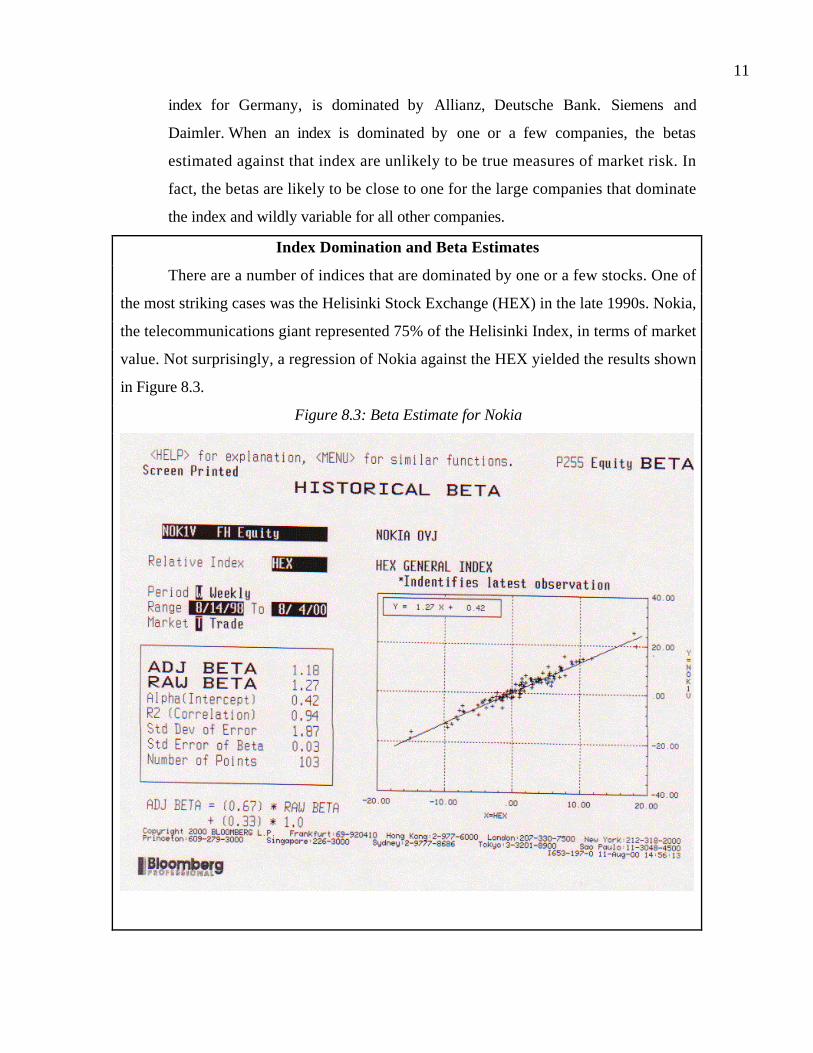
11

index for Germany, is dominated by Allianz, Deutsche Bank. Siemens and

Daimler. When an index is dominated by one or a few companies, the betas

estimated against that index are unlikely to be true measures of market risk. In

fact, the betas are likely to be close to one for the large companies that dominate

the index and wildly variable for all other companies.

Index Domination and Beta Estimates

There are a number of indices that are dominated by one or a few stocks. One of

the most striking cases was the Helisinki Stock Exchange (HEX) in the late 1990s. Nokia,

the telecommunications giant represented 75% of the Helisinki Index, in terms of market

value. Not surprisingly, a regression of Nokia against the HEX yielded the results shown

in Figure 8.3.

Figure 8.3: Beta Estimate for Nokia

12

The regression looks impeccable. In fact, the noise problem that we noted with Boeing,

arising from the high standard errors, disappears. The beta estimate has a standard error of

0.03, but the results are deceptive. The low standard error is the result of a regression of

Nokia on itself, since it dominates the index. The beta is meaningless to a typical investor

in Nokia, who is likely to be diversified, if not globally, at least across European stocks.

Worse still, the betas of all other Finnish stocks against the HEX become betas estimated

against Nokia. In fact, the beta of every other Finnish stock at the time of this regression

was less than 1. How is this possible, you might ask, if the average beta is one? It is the

weighted average beta that is one, and if Nokia which comprises three quarters of the

index has a beta greater than one (which it does), every other stock in the index could well

end up with a beta less than one.

Illustration 8.2: Estimating a Beta for Titan Cements

Titan Cements is a cement and construction company in Greece. Reproduced

below in Figure 8.4 is the beta estimate for Titan obtained from a beta service

(Bloomberg) from January 1996 to December 2000.

Figure 8.4: Beta Estimate for Titan Cement: Athens Stock Exchange Index

13

Note that the index used is the Athens Stock Index. This is a fairly conventional choice

since most services estimate betas against a local index. Based upon this regression, we

arrive at the following equation.

ReturnsTitan Cement = 0.31% + 0.93 ReturnsASE R squared = 57%

(0.08)

The beta for Titan Cements, based upon this regression, is 0.93. The standard error of the

estimate, shown in brackets below, is only 0.08, but the caveats about narrow indices

apply to the Athens Stock Exchange Index.

Drawing on the arguments in the previous section, if the marginal investor in Titan

Cements is, in fact, an investor diversified across European companies, the appropriate

index would have been a European stock index. The Bloomberg beta calculation with the

MS European Index is reported below in Figure 8.5.

Figure 8.5: Beta Estimate for Titan: MSCI Euro Index

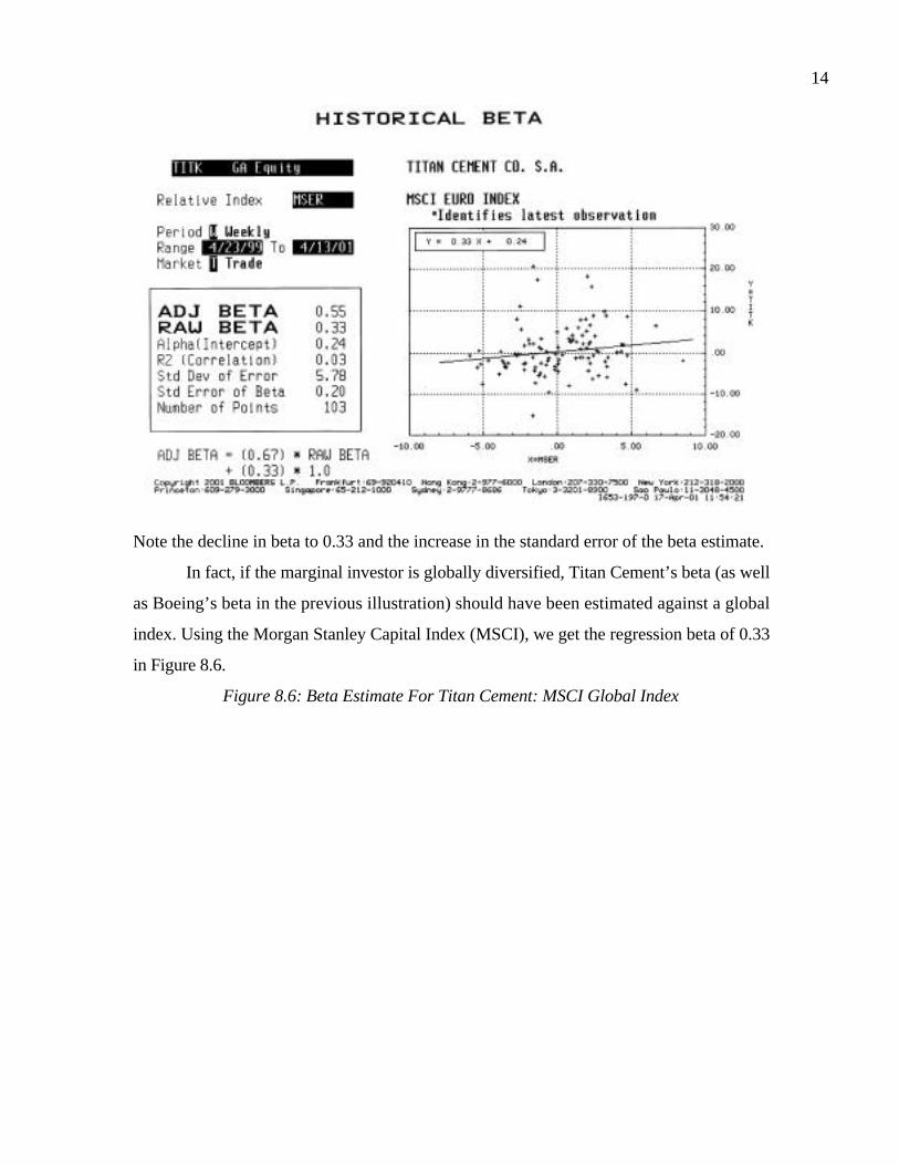
14

Note the decline in beta to 0.33 and the increase in the standard error of the beta estimate.

In fact, if the marginal investor is globally diversified, Titan Cement’s beta (as well

as Boeing’s beta in the previous illustration) should have been estimated against a global

index. Using the Morgan Stanley Capital Index (MSCI), we get the regression beta of 0.33

in Figure 8.6.

Figure 8.6: Beta Estimate For Titan Cement: MSCI Global Index

15

In fact, the beta estimate and the standard error look very similar to the ones estimated

against the European index.

Estimating the Historical Beta for Private Firms

The historical approach to estimating betas works only for assets that have been

traded and have market prices. Private companies do not have a market price history.

Consequently, we cannot estimate a regression beta for these companies. Nevertheless,

we still need estimates of cost of equity and capital for these companies.

You might argue that this is not an issue because you do not value private

companies but you will still be confronted with this issue even when valuing publicly

traded firms. Consider, for instance, the following scenarios.

• If you have to value a private firm for an initial public offering, you will need to

estimate discount rates for the valuation.

• Even after a firm has gone public, there will be a period of time lasting as long as

two years when there will be insufficient data for a regression.

16

• If you are called upon to value the division of a publicly traded firm that is up for

sale, you will not have past prices to draw upon to run a regression.

• Finally, if your firm has gone through significant restructuring – divestitures or

recapitalization – in the recent past, regression betas become meaningless because

the company itself has changed its risk characteristics.

Thus, regression betas are either unavailable or meaningless in a significant number of

valuations.

Some analysts assume that discounted cash flow valuation is not feasible in these

scenarios and use multiples. Others make assumptions about discount rates based upon

rules of thumb. Neither approach is appealing. In the next section, we will develop an

approach for estimating betas that is general enough to apply to all of these companies.

risk.xls.This spreadsheet allows you to run a regression of stock returns against

market returns and estimate risk parameters.

The Limitations of Regression Betas

Much of what we have presented in this section represents an indictment of

regression betas. In the case of Boeing, the biggest problem was that the beta had high

standard error. In fact, this is not a problem unique to Boeing. Figure 8.7 presents the

distribution of standard errors on beta estimates for US companies.

17

With the Nokia regression, we seem to cure the standard error problem but at a very large

cost. The low standard errors reflect the domination of the index by a stock and result in

betas that may be precise but bear no resemblance to true risk.

Changing the market index, the return period and return interval offer no respite. If

the index becomes a more representative index, the standard errors on betas will increase,

reflecting the fact that more of the risk in the stock is firm-specific. If the beta changes as

the return period or interval changes, it creates more uncertainty about the true beta of the

company.

In short, regression betas will almost always be either too noisy or skewed by

estimation choices to be useful measures of the equity risk in a company. The cost of

equity is far too important an input into a discounted cash flow valuation to be left to

statistical chance.

B. Fundamental Betas

A second way to estimate betas is to look at the fundamentals of the business.

The beta for a firm may be estimated from a regression but it is determined by decisions

the firm has made on what business to be in, how much operating leverage to use in the

business and by the degree to which the firm uses financial leverage. In this section, we

Figure 8.7: Distribution of Standard Errors on Beta Estimates

0%

2%

4%

6%

8%

10%

12%

14%

16%

18%

20%

<.10 .10-.15 .15-.20 .20-.25 .25-.30 .30-.40 .40-.50 >.50

Standard Error on Beta Estimate

Perc

ent o

f U

S st

ocks

18

will examine an alternative way of estimating betas for firms, where we are less reliant on

historical betas and more cognizant of their fundamental determinants.

Determinants of Betas

The beta of a firm is determined by three variables -(1) the type of business or

businesses the firm is in, (2) the degree of operating leverage of the firm and (3) the firm's

financial leverage. Although we will use these determinants to find betas in the capital

asset pricing model, the same analysis can be used to calculate the betas for the arbitrage

pricing and the multi-factor models as well.

Type of Business Since betas measure the risk of a firm relative to a market index, the more sensitive a

business is to market conditions, the higher its beta. Thus, other things remaining equal,

cyclical firms can be expected to have higher betas than non-cyclical firms. Companies

involved in housing and automobiles, two sectors of the economy which are very

sensitive to economic conditions, should have higher betas than companies in food

processing and tobacco, which are relatively insensitive to business cycles.

We can extend this view to a company’s products. The degree to which a

product’s purchase is discretionary will affect the beta of the firm manufacturing the

product. Firms whose products are much more discretionary to their customers should

have higher betas than firms whose products are viewed as necessary or less

discretionary. Thus, the beta of Procter and Gamble, which sells diapers and daily

household products, should be lower than the beta of Gucci, which manufactures luxury

products.

Degree of Operating Leverage

The degree of operating leverage is a function of the cost structure of a firm and is

usually defined in terms of the relationship between fixed costs and total costs. A firm

that has high fixed costs relative to total costs is said to have high operating leverage. A

firm with high operating leverage will also have higher variability in operating income than

would a firm producing a similar product with low operating leverage. Other things

remaining equal, the higher variance in operating income will lead to a higher beta for the

firm with high operating leverage.

19

Can firms change their operating leverage? While some of a firm’s cost structure is

determined by the business it is in (an energy utility has to build expensive power plants

and airlines have to lease expensive planes), firms in the United States have become

increasingly inventive in lowering the fixed cost component in their total costs. For

instance, firms have made cost structures more flexible by

• negotiating labor contracts that emphasize flexibility and allow the firm to make its

labor costs more sensitive to its financial success;

• entering into joint venture agreements, where the fixed costs are borne or shared by

someone else; and

• sub-contracting manufacturing and outsourcing, which reduce the need for expensive

plant and equipment.

While the arguments for such actions may be couched in terms of offering competitive

advantage and flexibility, they do also reduce the operating leverage of the firm and its

exposure to market risk.

While operating leverage affects betas, it is difficult to measure the operating leverage

of a firm, at least from the outside, since fixed and variable costs are often aggregated in

income statements. It is possible to get an approximate measure of the operating leverage

of a firm by looking at changes in operating income as a function of changes in sales.

Degree of Operating leverage = % Change in Operating Profit / % Change in Sales

For firms with high operating leverage, operating income should change more than

proportionately when sales change.

Size, Growth and Betas

Generally, smaller firms with higher growth potential are viewed as riskier than

larger, more stable firms. While the rationale for this argument is clear when talking about

total risk, it becomes more difficult to see when looking at market risk or betas. Should a

smaller software firm have a higher beta than a larger software firm? One reason to believe

that it should is operating leverage. If there is a set-up cost associated with investing in

infrastructure or economies of scale, smaller firms will have higher fixed costs than larger

firms, leading in turn to higher betas for these firms.

20

With growth firms, the argument for higher betas rests on the notion of discretionary

versus non-discretionary purchases. For a high growth firm to deliver on its growth, new

customers have to adopt the product or existing customers have to buy more of the

product. Whether they do so or not will depend, in large part, on how well-off they feel.

This, in turn, will make the profits of high growth firms much more dependent on how

well the economy is doing, thus increasing their betas.

Degree of Financial Leverage

Other things remaining equal, an increase in financial leverage will increase the

beta of the equity in a firm. Intuitively, we would expect that the fixed interest payments

on debt result in high net income in good times and low or negative net income in bad

times. Higher leverage increases the variance in net income and makes equity investment

in the firm riskier. If all the firm's risk is borne by the stockholders (i.e., the beta of debt is

zero)8 and debt has a tax benefit to the firm, then,

( )

−+=

ED

tuL 11

where

βL = Levered Beta for equity in the firm

βu = Unlevered beta of the firm (i.e., the beta of the firm without any debt)

t = Corporate tax rate

D/E = Debt/Equity Ratio

Intuitively, we expect that as leverage increases (as measured by the debt to equity ratio),

equity investors bear increasing amounts of market risk in the firm, leading to higher

betas. The tax factor in the equation measures the tax deductibility of interest payments.

8 This formula was originally developed by Hamada in 1972. There are two common modifications. One isto ignore the tax effects and compute the levered beta as:

+=

ED

uL 1

If debt has market risk (i.e., its beta is greater than zero), the original formula can be modified to take itinto account. If the beta of debt is βD, the beta of equity can be written as:

L = u 1+ 1− t( ) D

E

− D 1− t( ) D

E

21

The unlevered beta of a firm is determined by the types of the businesses in

which it operates and its operating leverage. It is often also referred to as the asset beta

since it is determined by the assets owned by the firm. Thus, the levered beta, which is

also the beta for an equity investment in a firm or the equity beta, is determined both by

the riskiness of the business it operates in and by the amount of financial leverage risk it

has taken on.

Since financial leverage multiplies the underlying business risk, it stands to reason

that firms that have high business risk should be reluctant to take on financial leverage. It

also stands to reason that firms that operate in stable businesses should be much more

willing to take on financial leverage. Utilities, for instance, have historically had high debt

ratios but have not had high betas, mostly because their underlying businesses have been

stable and fairly predictable.

Illustration 8.3: Effects of Leverage on betas: Boeing

From the regression for the period from 1996 to 2000, Boeing had a historical beta of

0.56. Since this regression uses stock prices of Boeing over this period, we begin by

estimating the average debt/equity ratio between 1996 and 2000, using market values for

debt and equity.

Average Debt/Equity Ratio between 1996 and 2000 = 15.56%

The beta over the 1996-2000 period reflects this average leverage. To estimate the

unlevered beta over the period, we used a corporate tax rate of 35%.

Unlevered Beta =Current Beta

1 + (1 - tax rate) (Average Debt/Equity)=

0.56

1+ 1− 0.35( ) 0.1556( )= 0.51

The unlevered beta for Boeing over the 1996-2000 period is 0.51. The levered beta at

different levels of debt can then be estimated.

Levered Beta = Unlevered Beta1 + 1 - tax rate( ) Debt/ Equity( )( )For instance, if Boeing were to decrease its debt equity ratio to 10%, its equity beta will

be:

22

Levered Beta (@10% D/E) = 0.511+ 1 - 0.35( ) 0.10( )( ) = 0.543

If the debt equity ratio were raised to 25%, the equity beta would be

Levered Beta (@25% D/E) = 0.511+ 1-0.35( ) 0.25( )( ) = 0.59

Table 8.1 summarizes the beta estimates for different levels of financial leverage ranging

from 0 to 90% debt.

Table 8.1: Financial Leverage and Betas

Debt to Capital Debt/Equity Ratio Beta Effect of Leverage

0.00% 0.00% 0.51 0.00

10.00% 11.11% 0.55 0.04

20.00% 25.00% 0.59 0.08

30.00% 42.86% 0.65 0.14

40.00% 66.67% 0.73 0.22

50.00% 100.00% 0.84 0.33

60.00% 150.00% 1.00 0.50

70.00% 233.33% 1.28 0.77

80.00% 400.00% 1.83 1.32

90.00% 900.00% 3.48 2.98

As Boeing’s financial leverage increases, the beta increases concurrently.

levbeta.xls.This spreadsheet allows you to estimate the unlevered beta for a firm and

compute the betas as a function of the leverage of the firm.

Bottom Up Betas

Breaking down betas into their business risk and financial leverage components

provides us with an alternative way of estimating betas in which we do not need past

prices on an individual firm or asset.

To develop this alternative approach, we need to introduce an additional property

of betas that proves invaluable. The beta of two assets put together is a weighted average

of the individual asset betas, with the weights based upon market value. Consequently,

23

the beta for a firm is a weighted average of the betas of all the different businesses it is in.

We can estimate the beta for a firm in five steps.

• Step 1: We identify the business or businesses the firm operates in.

• Step 2: We find other publicly traded firms in these businesses and obtain

their regression betas, which we use to compute an average beta for the firms,

and their financial leverage.

• Step 3: We estimate the average unlevered beta for the business, by unlevering

the average beta for the firm by their average debt to equity ratio.

Alternatively, we could estimate the unlevered beta for each firm and then

compute the average of the unlevered betas. The first approach is preferable

because unlevering an erroneous regression beta is likely to compound the

error.

( )( )firms rableratiocompa D/E t-11

BetaBeta Unlevered firms comparable

Business +=

• Step 4: To estimate an unlevered beta for the firm that we are analyzing, we

take a weighted average of the unlevered betas for the businesses it operates in,

using the proportion of firm value derived from each business as the weights.

If values are not available, we use operating income or revenues as weights.

This weighted average is called the bottom-up unlevered beta.

Unlevered Betafirm= Unlevered Beta jj=1

j = k

∑ *Value Weight j

where the firm is assumed to operating in k different businesses.

• Step 5: Finally, we estimate the current market values of debt and equity of

the firm and use this debt to equity ratio to estimate a levered beta.

The betas estimated using this process are called bottom-up betas.

The Case for Bottom Up BetasAt first sight, the use of bottom up betas may seem to leave us exposed to all of

the problems we noted with regression betas. After all, the betas for other publicly traded

firms in the business are obtained from regressions. Notwithstanding these bottom up

betas represent a significant improvement on regression betas for the following reasons.

24

• While each regression beta is estimated with standard error, the average across

a number of regression betas will have much lower standard error. The

intuition is simple. A high standard error on a beta estimate indicates that it

can be significantly higher or lower than the true beta. Averaging across these

errors results in an average beta that is far more precise than the individual

betas that went into it. In fact, if the estimation errors on individual firm betas

are uncorrelated across firms, the savings in standard error can be stated as a

function of the average standard error and the number of firms in the sample.

Standard ErrorBottom-up beta =Average Standard Error Comparable firms

n

where n is the number of firms in the sample. Thus, if the average standard error in

beta estimates for software firms is 0.50 and the number of software firms is 100,

the standard error of the average beta is only 0.05 (0.50/ 100 ).

• A bottom-up beta can be adapted to reflect actual changes in a firm’s business

mix and expected changes in the future. Thus, if a firm divested a major

portion of its operations last week, the weights on the businesses can be

modified to reflect the divestiture. The same can be done with acquisitions. In

fact, a firm’s strategic plans to enter new businesses in the future can be

brought into the beta estimates for future periods.

• Firms do change their debt ratios over time. While regression betas reflect the

average debt to equity ratio maintained by the firm during the regression

period, bottom-up betas use the current debt to equity ratio. If a firm plans to

change its debt to equity ratio in the future, the beta can be adjusted to show

these changes.

• Finally, bottom-up betas wean us from our dependence on historical stock

prices. While we do need these prices to get betas for comparable firms, all we

need for the firm being analyzed is a breakdown of the businesses it is in.

Thus, bottom-up betas can be estimated for private firms, divisions of

business and stocks that have just started trading in financial markets.

25

Computational DetailsWhile the idea behind bottom-up betas is fairly simple, there are several

computational details that are deserving of attention.

a. Defining Comparable firms: First, we have to decide how narrowly we want to

define a business. Consider, for instance, a firm that manufactures entertainment

software. We could define the business as entertainment software and consider

only companies that primarily manufacture entertainment software to be

comparable firms. We could go even further and define comparable firms as firms

manufacturing entertainment software with revenues similar to that of the

company being analyzed. While there are benefits to narrowing the comparable

firm definition, there is a large cost. Each additional criterion added on to the

definition of comparable will mean that fewer firms make the list and the savings

in standard error that comprise the biggest benefit to bottom-up betas become

smaller. A common sense principle should therefore come into play. If there are

hundreds of firms in a business, as there are in the software business, you can

afford to be more selective. If there are relatively few firms, not only do you have

to become less selective, you might have to broaden the definition of comparable

to bring in other firms into the mix.

b. Estimating Betas: Once the comparable firms in a business have been defined, you

have to estimate the betas for these firms. While it would be best to estimate the

regressions for all of these firms against a common and well diversified equity

index, it is usually easier to use service betas that are available for each of these

firms. These service betas may be estimated against different indices. For instance,

if you define your business to be global telecommunications and obtain betas for

global telecomm firms from Bloomberg, these betas will be estimated against their

local indices. This is usually not a fatal problem, especially with large samples,

since errors in the estimates tend to average out.

c. Averaging Method: The average beta for the firms in the sector can be computed in

one of two ways. We could use market-weighted averages, but the savings in

standard error that we touted in the earlier section will be muted, especially if

there are one or two very large firms in the sample. We could estimate the simple

26

average of the betas of the companies, thus weighting all betas equally. The

process weighs in the smallest firms in the sample disproportionately but the

savings in standard error are likely to be maximized. There is also the issue of

whether the firm being analyzed should be excluded from the group when

computing the average. While the answer is yes, there will make little or no

difference in the final estimate if there are more than 15 or 20 comparable firms.

d. Controlling for differences: In essence, when we use betas from comparable firms,

we are assuming that all firms in the business are equally exposed to business risk

and have similar operating leverage. Note that the process of levering and

unlevering of betas allows us to control for differences in financial leverage. If

there are significant differences in operating leverage – cost structure – across

companies, the differences in operating leverage can be controlled for as well. This

would require that we estimate a business beta, where we take out the effects of

operating leverage from the unlevered beta.

Business Beta =Unlevered Beta

1+ 1- tax rate( ) Fixed Costs/ Variable Costs( )Note the similarity to the adjustment for financial leverage; the only difference is

that both fixed and variable costs are eligible for the tax deduction and the tax rate

is therefore no longer a factor. The business beta can then be relevered to reflect

the differences in operating leverage across firms.

betas.xls: This dataset on the web has updated betas and unlevered betas by

business sector in the United States.

Illustration 8.3: Estimating a Bottom-up Beta for Vans Shoes – January 2001

Vans Shoes is a shoe manufacturing firm with a market capitalization of $191

million. To estimate the bottom up beta for Vans Shoes, we consider the betas of all

publicly traded shoe manufacturers in Table 8.2.

Table 8.2: Betas and Relevant Statistics: Publicly Traded Shoe Companies

27

Company Name Beta Market D/E Tax Rate Fixed/VariableBarry (R.G.) 1.00 40.51% 36.89% 75.66%Brown Shoe 0.80 106.64% 37.06% 61.41%Candie's Inc. 1.20 75.86% 0.00% 29.78%Converse Inc 0.60 653.46% 0.00% 39.64%Deckers Outdoor Corp 0.80 82.43% 0.00% 62.52%Florsheim Group Inc 0.65 96.79% 32.47% 79.03%K-Swiss Inc. 0.65 0.69% 40.94% 56.92%Kenneth Cole 'A' 1.05 0.29% 39.50% 56.97%LaCrosse Footwear Inc 0.55 81.15% 39.25% 30.36%Maxwell Shoe Inc 0.75 2.24% 33.28% 20.97%NIKE Inc. 'B' 0.90 9.47% 39.50% 46.07%Reebok Int'l 1.05 171.90% 32.28% 35.03%Rocky Shoes & Boots Inc. 0.80 93.51% 0.00% 26.89%Saucony Inc 0.15 34.93% 31.11% 49.33%Shoe Carnival 0.85 2.18% 39.97% 35.03%Stride Rite Corp. 0.80 0.00% 36.80% 48.23%Timberland Co. 'A' 1.10 15.23% 32.00% 49.50%Vulcan Int'L 0.65 3.38% 5.61% 11.92%Wellco Enterprises Inc. 0.60 48.89% 0.00% 11.52%Weyco Group 0.30 11.91% 35.74% 24.69%Wolverine World Wide 1.35 44.37% 32.62% 32.31%Average (Simple) 0.79 75.04% 25.95% 42.08%

[NOTE: I have 42.08% for the Fixed/Variable average. Suggestion: Instead of changing the

calculations, just decrease Wolverine World Wide to 22.00% to make the average

41.59%.]

In addition to the betas for each firm, we report the market debt to equity ratio, the

effective tax rate and a measure of operating leverage obtained by dividing S,G&A

expenses (which we consider fixed) by other operating expenses (which we consider

variable). We can estimate the unlevered beta for the business using the averages for these

values.

Average Beta = 0.79

Average Debt to Equity Ratio = 75.04%

Using the effective tax rate of 25.95%, we can estimate the unlevered beta.

Unlevered Beta Vans =0.79

1 + 1- 0.2595( ) 0.7504( )= 0.5081

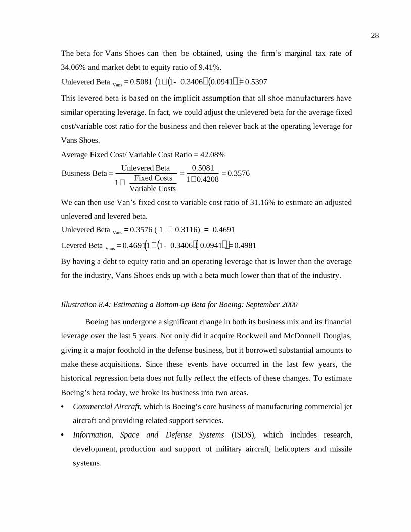
28

The beta for Vans Shoes can then be obtained, using the firm’s marginal tax rate of

34.06% and market debt to equity ratio of 9.41%.

Unlevered Beta Vans = 0.5081 1+ 1- 0.3406( ) 0.0941( )( ) = 0.5397

This levered beta is based on the implicit assumption that all shoe manufacturers have

similar operating leverage. In fact, we could adjust the unlevered beta for the average fixed

cost/variable cost ratio for the business and then relever back at the operating leverage for

Vans Shoes.

Average Fixed Cost/ Variable Cost Ratio = 42.08%

Business Beta =Unlevered Beta

1+ Fixed Costs

Variable Costs

=0.5081

1+ 0.4208= 0.3576

We can then use Van’s fixed cost to variable cost ratio of 31.16% to estimate an adjusted

unlevered and levered beta.

Unlevered Beta Vans = 0.3576 ( 1 + 0.3116) = 0.4691

Levered Beta Vans = 0.46911+ 1- 0.3406( ) 0.0941( )( ) = 0.4981

By having a debt to equity ratio and an operating leverage that is lower than the average

for the industry, Vans Shoes ends up with a beta much lower than that of the industry.

Illustration 8.4: Estimating a Bottom-up Beta for Boeing: September 2000

Boeing has undergone a significant change in both its business mix and its financial

leverage over the last 5 years. Not only did it acquire Rockwell and McDonnell Douglas,

giving it a major foothold in the defense business, but it borrowed substantial amounts to

make these acquisitions. Since these events have occurred in the last few years, the

historical regression beta does not fully reflect the effects of these changes. To estimate

Boeing’s beta today, we broke its business into two areas.

• Commercial Aircraft, which is Boeing’s core business of manufacturing commercial jet

aircraft and providing related support services.

• Information, Space and Defense Systems (ISDS), which includes research,

development, production and support of military aircraft, helicopters and missile

systems.

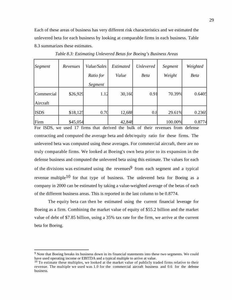
29

Each of these areas of business has very different risk characteristics and we estimated the

unlevered beta for each business by looking at comparable firms in each business. Table

8.3 summarizes these estimates.

Table 8.3: Estimating Unlevered Betas for Boeing’s Business Areas

Segment Revenues Value/Sales

Ratio for

Segment

Estimated

Value

Unlevered

Beta

Segment

Weight

Weighted

Beta

Commercial

Aircraft

$26,929 1.12 30,160 0.91 70.39% 0.6405

ISDS $18,125 0.70 12,688 0.8 29.61% 0.2369

Firm $45,054 42,848 100.00% 0.8774For ISDS, we used 17 firms that derived the bulk of their revenues from defense

contracting and computed the average beta and debt/equity ratio for these firms. The

unlevered beta was computed using these averages. For commercial aircraft, there are no

truly comparable firms. We looked at Boeing's own beta prior to its expansion in the

defense business and computed the unlevered beta using this estimate. The values for each

of the divisions was estimated using the revenues9 from each segment and a typical

revenue multiple10 for that type of business. The unlevered beta for Boeing as a

company in 2000 can be estimated by taking a value-weighted average of the betas of each

of the different business areas. This is reported in the last column to be 0.8774.

The equity beta can then be estimated using the current financial leverage for

Boeing as a firm. Combining the market value of equity of $55.2 billion and the market

value of debt of $7.85 billion, using a 35% tax rate for the firm, we arrive at the current

beta for Boeing.

9 Note that Boeing breaks its business down in its financial statements into these two segments. We couldhave used operating income or EBITDA and a typical multiple to arrive at value.10 To estimate these multiples, we looked at the market value of publicly traded firms relative to theirrevenue. The multiple we used was 1.0 for the commercial aircraft business and 0.6 for the defensebusiness.

30

Equity Beta for Boeing = 0.8774 1+ 1-0.35( ) 7.85

55.2 +7.85

= 0.9585

This is very different from the historical beta of 0.56 that we obtained from the

regression, but it is, in our view, a much truer reflection of the risk in Boeing.

Illustration 8.5: Estimating a Bottom-up Beta for Titan Cements – January 2000

To estimate a beta for Titan Cements, we began by defining comparable firms as

other cement companies in Greece but found only one comparable firm. When we

expanded the list to include cement companies across Europe, we increased our sample to

nine firms. Since we did not see any reason to restrict our comparison to just European

firms, we decided to look at the average beta for cement companies globally. There were

108 firms in this sample with an average beta of 0.99, an average tax rate of 34.2% and an

average debt to equity ratio of 27.06%. We used these numbers to arrive at an unlevered

beta of 0.84.

Unlevered Beta for cement companies =0.99

1+ 1-0.342( ) 0.2706( )= 0.84

We then used Titan’s market values of equity (566.95 million Gdr) and debt (13.38

million GDr) to estimate a levered beta for its equity:

Levered Beta = 0.84 1+ 1- 0.2414( ) 13.38

566.95

= 0.86

We used a tax rate of 24.14% in this calculation.

How well do betas travel?

Often, when analyzing firms in small or emerging markets, we have to estimate

betas by looking at firms in the same business but traded on other markets. This is what

we did when estimating the beta for Titan Cements. Is this appropriate? Should the beta

for a steel company in the United States be comparable to that of a steel company in

Indonesia? We see no reason why it should not. But the company in Indonesia has much

more risk, you might argue. We do not disagree, but the fact that we use similar betas does

not mean that we believe that the costs of equity are identical across all steel companies.

In fact, using the approach described in the last chapter, the risk premium used to

estimate the cost of equity for the Indonesian company will incorporate a country risk

31

premium, whereas the cost of equity for the U.S. company will not. Thus, even if the

betas used for the two companies are identical, the cost of equity for the Indonesian

company will be much higher.

There are a few exceptions to this proposition. Recall that one of the key

determinants of betas is the degree to which a product or service is discretionary. It is

entirely possible that products or services that are discretionary in one market (and

command high betas) may be non-discretionary in another market (and have low betas).

For instance, phone service is viewed as a non-discretionary product in most developed

markets, but is a discretionary product in emerging markets. Consequently, the average

beta estimated by looking at telecom firms in developed markets will understate the true

beta of a telecomm firm in an emerging market. Here, the comparable firms should be

restricted to include only telecomm firms in emerging markets.

Calculating Betas after A Major Restructuring

The bottom-up process of estimating betas provides a solution when firms go

through a major restructuring that change both their business mix and leverage. In these

cases, the regression betas are misleading because they do not reflect fully the effects of

these changes. Boeing’s beta, estimated using the bottom up approach, is likely to

provide a more precise estimate than the historical beta from a regression of Boeing’s

stock prices, given Boeing’s acquisitions of Rockwell and McDonnell Douglas and its

increase in leverage. In fact, a firm’s beta can be estimated even before the restructuring

becomes effective using the bottom-up approach. In the illustration that follows, for

instance, we estimate Boeing’s beta just before and after its acquisition of McDonnell

Douglas, allowing for the changes in both the business mix and the leverage.

Illustration 8.6: Beta of a Firm After an Acquisition: Boeing and McDonnell Douglas

In 1997, Boeing announced that it was acquiring McDonnell Douglas, another

company involved in the aerospace and the defense business. At the time of the

acquisition, the two firms had the following market values and betas:

Company Beta Debt Equity Firm Value

Boeing 0.95 $ 3,980 $ 32,438 $ 36,418

32

McDonnell Douglas 0.90 $ 2,143 $ 12,555 $ 14,698

Note that the market values of equity used for the two firms reflect the market values

after the acquisition announcement and reflect the acquisition price agreed upon for

McDonnell Douglas shares.

In order to evaluate the effects of the acquisition on Boeing’s beta, we first

examine the effects of the merger on the business risk of the combined firm, by estimating

the unlevered betas of the two companies and calculating the combined firm’s unlevered

beta.

Boeings unlevered beta =0.95

1+ 0.65( ) 398032438

= 0.88

McDonnell Douglas unlevered beta =0.90

1+ 0.65( ) 214312555

= 0.81

The unlevered beta for the combined firm can be calculated as the weighted average of the

two unlevered betas, with the weights based upon the market values of the two firms.

Unlevered Beta for combined firm = 0.8836,418

51,116

+ 0.81

14,698

51,116

= 0.86

Boeing’s acquisition of McDonnell Douglas was accomplished by issuing new stock in

Boeing to cover the value of McDonnell Douglas’s equity of $12,555 million. Since no

new debt was used to finance the deal, the debt outstanding in the firm after the

acquisition is just the sum of the debt outstanding at the two companies before the

acquisition.

Debt = McDonnell Douglas Old Debt + Boeing’s Old Debt

= $3,980 + $2,143 = $6,123 million

Equity = Boeing’s Old Equity + New Equity used for Acquisition

= $32,438 + $12,555 = $44,993 million

The debt/equity ratio can then be computed as follows –

D/E Ratio = $ 6,123/44,993 = 13.61%

This debt/equity ratio in conjunction with the new unlevered beta for the combined firm

yields a new beta of

33

New Beta = 0.86 1+ 0.65( ) 0.1361( )( ) = 0.94

C. Accounting Betas

A third approach is to estimate the market risk parameters from accounting

earnings rather than from traded prices. Thus, changes in earnings at a division or a firm,

on a quarterly or annual basis, can be related to changes in earnings for the market, in the

same periods, to arrive at an estimate of an accounting beta to use in the CAPM. While

the approach has some intuitive appeal, it suffers from three potential pitfalls. First,

accounting earnings tend to be smoothed out relative to the underlying value of the

company, as accountants spread expenses and income over multiple periods. This results

in betas that are “biased down”, especially for risky firms, or “biased up”, for safer firms.

In other words, betas are likely to be closer to 1.00 for all firms using accounting data.

Second, accounting earnings can be influenced by non-operating factors, such as

changes in depreciation or inventory methods and by allocations of corporate expenses at

the divisional level. Finally, accounting earnings are measured, at most, once every quarter

and often only once every year, resulting in regressions with few observations and not

much explanatory power (low R-squared, high standard errors).

Illustration 8.7: Estimating Accounting Betas ––Defense Division of Boeing - 1995

Having operated in the defense business for decades, Boeing has a record of its

profitability. These profits are reported in Table 8.4, together with earnings changes for

companies in the S&P 500 going back to 1980.

Table 8.4: Earnings on Defense Business - Boeing

Year S& P 500 Boeing Defense

Business

1980 -2.10% -12.70%

1981 -6.70% -35.56%

1982 -45.50% 27.59%

1983 37.00% 159.36%

1984 41.80% 13.11%

1985 -11.80% -26.81%

34

1986 7.00% -16.83%

1987 41.50% 20.24%

1988 41.80% 18.81%

1989 2.60% -29.70%

1990 -18.00% -40.00%

1991 -47.40% -35.00%

1992 64.50% 10.00%

1993 20.00% -7.00%

1994 25.30% 11.00%

Source: Bloomberg

Regressing the changes in profits in the defense division (∆ EarningsDefense) against

changes in profits for the S&P 500 (∆ EarningsS&P ) yields the following:

∆EarningsDefense =−0.03 + 0.65∆EarningsS&P

Based upon this regression, the beta for the defense division is 0.65. We can now estimate

the cost of equity for the defense division, with a riskless rate of 5% and a risk premium

of 5.5%, as follows.

Cost of Equity for the Defense Division = 5% + 0.65 (5.5%) = 8.58%

accbeta.xls: This spreadsheet allows you to estimate the accounting beta on a

division or firm.

spearn.xls: This dataset on the web has earnings changes, by year, for the S&P

500 going back to 1960.

Market, Bottom-up and Accounting Betas: Which one do we use?

For most publicly traded firms, betas can be estimated using accounting data or

market data or from the bottom-up approach. Since the betas will almost never be the

same using these different approaches, the question is which one do we use? We would

almost never use accounting betas, for all the reasons specified above. We are almost as

35

reluctant to use historical market betas for individual firms because of the standard errors

in beta estimates, the failures of the local indices (as is the case with most emerging

market companies) and the inability of these regressions to reflect the effects of major

changes in the business mix and financial risk at the firm. Bottom-up betas, in our view,

provide us with the best beta estimates because:

1. They allow us to consider changes in business and financial mix, even before they

occur.

2. They use average betas across large numbers of firms, which tend to be less noisy

than individual firm betas.

3. They allow us to calculate betas by area of business for a firm, which is useful both in

the context of investment analysis and valuation.

From Betas to Cost of Equity

Having estimated the riskless rate, the risk premium(s) and the beta(s), we can

now estimate the expected return from investing in equity at any firm. In the CAPM, this

expected return can be written as:

Expected Return = Riskless Rate + Beta * Expected Risk Premium

where the riskless rate would be the rate on a long-term government bond, the beta would

be either the historical, fundamental or accounting betas described above and the risk

premium would be either the historical premium or an implied premium.

In the arbitrage pricing and multi-factor model, the expected return would be

written as follows:

Expected Return = Riskless Rate + jj −1

j= n

∑ *Risk Premium j

where the riskless rate is the long term government bond rate, βj is the beta relative to

factor j estimated using historical data or fundamentals and Risk Premiumj is the risk

premium relative to factor j, estimated using historical data.

The expected return on an equity investment in a firm, given its risk, has strong

implications for both equity investors in the firm and the managers of the firm. For equity

investors, it is the rate they need to earn to be compensated for the risk they have taken

in investing in the equity of the firm. If, after analyzing an investment, they conclude they

36

cannot make this return, they would not buy this investment; alternatively, if they decide

they can make a higher return, they would make the investment. For managers in the firm,

the return that investors need to make to break even on their equity investments becomes

the return they have to try to deliver to keep these investors from becoming restive and

rebellious. Thus, it becomes the rate they have to beat in terms of returns on their equity

investments in projects. In other words, this is the cost of equity to the firm.

Illustration 8.8: Estimating the Cost of Equity for Boeing – June 2000

Now that we have an estimate of beta of 0.9585 for Boeing, based upon the

bottom-up estimates, we can estimate its cost of equity. To make the estimate, we used

the prevailing treasury bond rate of 5% and a historical risk premium of 5.51%.

Cost of Equity = 5.00% + 0.9585 (5.51%) = 10.28%

There are two points making about this estimate. The first is that the cost of equity

would have been significantly lower, if we had chosen to use the implied equity premium

at the time of this analysis which was about 2.87% (See chapter 7).

Cost of Equity = 5.00% + 0.9585 (2.87%) = 7.75%

The second point is that we are not considering the exposure that Boeing has to emerging

market risk from its business. If the exposure is significant, we should be adding a country

risk premium to the cost of equity estimate.

Illustration 8.9: Estimating the Cost of Equity for Embraer – March 2001

Embraer is a Brazilian aerospace firm. To estimate its cost of equity, we first

estimated the unlevered beta by looking at aerospace firms globally.

Unlevered Beta for aerospace firms = 0.87

Embraer’s debt to equity ratio11 at the time of this analysis was 2.45%, resulting in a

levered beta for Embraer:

Levered beta for Embraer = 0.87 (1 + (1-0.33)0.0245) = 0.88

To estimate the cost of equity for Embraer in U.S. dollar terms, we began with the

treasury bond rate of 5% at the time of the analysis, but incorporated the country risk

11 We used net debt (the difference between gross debt and cash) in making this estimate. See the note laterin the chapter about when this practice is appropriate and when it is not.

37

associated with Brazil into the risk premium. Using the approach described in chapter 7,

we estimated a country risk premium of 10.24%. In conjunction with a mature market

risk premium of 5.59%, estimated for the United States, this yields a cost of equity of

18.93%.

Cost of Equity for Embraer = 5% + 0.88 (5.51% + 10.24%) = 18.86%

Again, there are several points that are worth making on this estimate. The first is that

this cost of equity can be expected to change over time as Brazil matures as a market and

country risk declines. The second is that we have assumed that betas measure exposure to

country risk. A company like Embraer that derives the bulk of its revenues outside Brazil

could argue that it is less exposed to country risk. We could have derived λ as a measure

of exposure to country risk for Embraer by looking at the proportion of its revenues that

it derives in Brazil and comparing it to the proportion of revenues derived by a typical

company in Brazil. In 2000, for instance, this would have yielded the following:

λEmbraer = Proportion of Revenues from Brazil Embraer

Proportion of Revenues from Brazil Typical Brazilian firm

=9%

60% = 0.15

Using this measure of exposure to country risk, Embraer would have had a much lower

cost of equity.

Cost of Equity in U.S. dollars

= Riskfree rate + Beta (Mature Market Risk Premium ) + λ (Country Risk Premium)

= 5% + 0.88 (5.51%) + 0.15 (10.24%) = 11.39%

The final point is that the cost of equity in dollar terms can be converted into a nominal

real cost of equity fairly simply by considering the differences in expected inflation rates

in Brazil and the United States. For instance, if the expected inflation rate in Brazil is 10%

and the differential inflation rate in the United States is 2%, the cost of equity in nominal

real is as follows:

Cost of EquityNominal Real = 1 + Cost of Equity$( ) 1+ Inflation Rate Brazil

1+ Inflation Rate US

-1

= 1+ 0.1139( ) 1.10

1.02

−1= 20.12%

Implicitly, we assume that real riskfree rates around that world are the same with this

approach and that the risk premium scales up with inflation as well. The alternative is to

38

estimate a cost of equity from scratch, beginning with a nominal real risk free rate (which

was 14% at the time of this analysis) and adding the premiums from above:

Cost of EquityNominal Real

= Riskfree rate + Beta (Mature Market Risk Premium ) + λ (Country Risk Premium)

= 14% + 0.88 (5.51%) + 0.15 (10.24%) = 20.39%

Substituting in a real riskfree rate in the equation above would yield a real cost of equity.

Cost of Equity and a Small Firm Premium

In chapter 6, we presented evidence of a small firm premium – small market-cap

stocks earn higher returns than large market-cap stocks with equivalent betas. The

magnitude and persistence of the small firm premium can be viewed as evidence that the

capital asset pricing model understates the risk of smaller companies, and that a cost of

equity based purely upon a CAPM beta will therefore yield too low a number for these

firms. There are some analysts who argue that you should therefore add a premium on to

the estimated cost of equity for smaller firms. Since small cap stocks have earned about 2%

more than large cap stocks over the last few decades, you could consider this a reasonable

estimate of the small firm premium. To estimate the cost of equity for a small cap stock with

a beta of 1.2 (assuming a riskfree rate of 5.1% and a market risk premium of 4%), for

instance, you would do the following:

Cost of Equity for small-cap stock = Riskfree Rate + Beta * Market Risk Premium +

Small Cap Premium = 5.1% + 1.2 * 4% + 2% = 11.9%

We would introduce two notes of caution with this approach. First, it opens the door

to a series of adjustments that you could make to the cost of equity, reflecting the numerous

inefficiencies that we cited in chapter 6. For instance, you could estimate a low PE premium,

a low price to book premium and a high dividend yield premium and add them all to the cost

of equity. If our objective in valuation is to uncover market mistakes, it would be a mistake

to start off with the presumption that markets are right in their assessments in the first place.

Second, a better way of considering the small firm premium would be to identify the

reasons for the premium and then develop more direct measures of risk. For instance,

assume that the higher risk of small cap stocks comes from the higher operating leverage

that these firms have, relative to their larger competitors. You could adjust the betas for

operating leverage (as we did a few pages ago for Van Shoes) and use the higher betas for

small firms.

From Cost of Equity to Cost of Capital

39

While equity is undoubtedly an important and indispensable ingredient of the

financing mix for every business, it is but one ingredient. Most businesses finance some or

much of their operations using debt or some security that is a combination of equity and

debt. The costs of these sources of financing are generally very different from the cost of

equity and the cost of financing for a firm should reflect their costs as well, in proportion

to their use in the financing mix. Intuitively, the cost of capital is the weighted average of

the costs of the different components of financing -- including debt, equity and hybrid

securities -- used by a firm to fund its financial requirements. In this section, we examine

the process of estimating the cost of financing other than equity and the weights for

computing the cost of capital.

Calculating the Cost of Debt

The cost of debt measures the current cost to the firm of borrowing funds to

finance projects. In general terms, it is determined by the following variables:

(1) The riskless rate: As the riskless increases, the cost of debt for firms will also

increase.

(2) The default risk (and associated default spread) of the company: As the default risk of

a firm increases, the cost of borrowing money will also increase. In chapter 7, we looked

at how the default spread has varied across time and can vary across maturity.

(3) The tax advantage associated with debt: Since interest is tax deductible, the after-tax

cost of debt is a function of the tax rate. The tax benefit that accrues from paying interest

makes the after-tax cost of debt lower than the pre-tax cost. Furthermore, this benefit

increases as the tax rate increases.

After-tax cost of debt = Pre-tax cost of debt (1 - tax rate)

In this section, we will focus on how best to estimate the default risk in a firm and to

convert that default risk into a default spread that can be used to come up with a cost of

debt.

Estimating the Default Risk and Default Spread of a firm

The simplest scenario for estimating the cost of debt occurs when a firm has long

term bonds outstanding that are widely traded. The market price of the bond, in

conjunction with its coupon and maturity can serve to compute a yield that we use as the

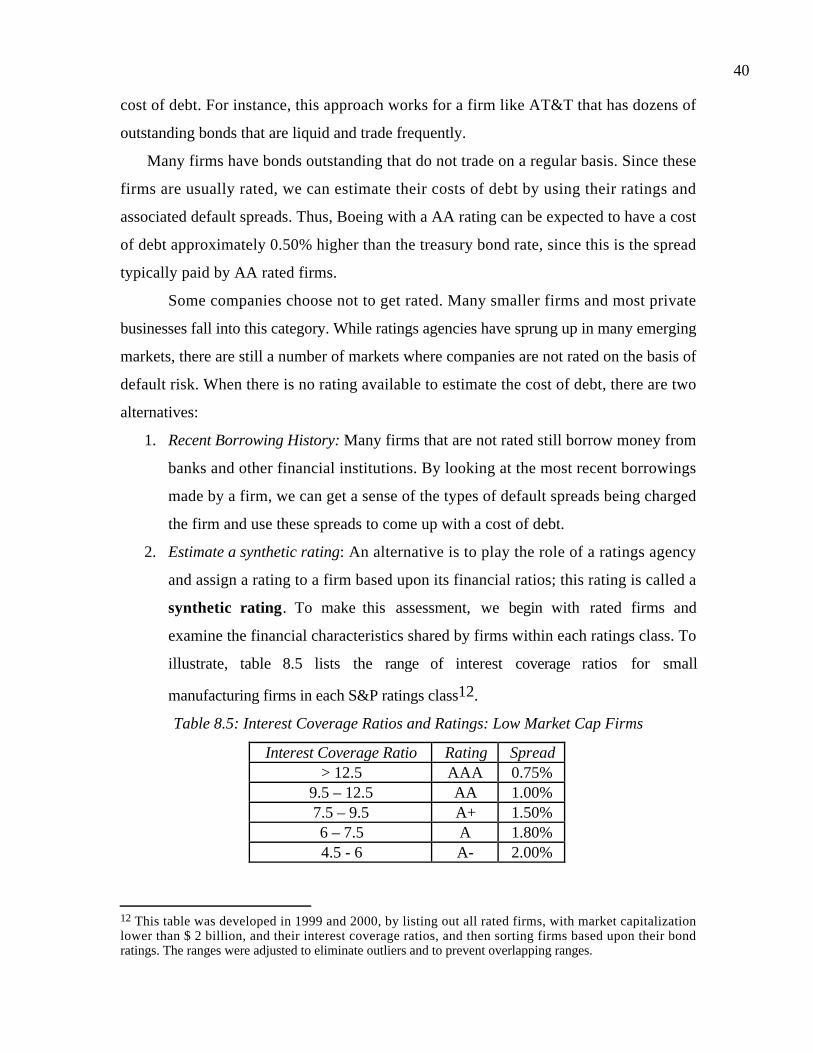
40

cost of debt. For instance, this approach works for a firm like AT&T that has dozens of

outstanding bonds that are liquid and trade frequently.

Many firms have bonds outstanding that do not trade on a regular basis. Since these

firms are usually rated, we can estimate their costs of debt by using their ratings and

associated default spreads. Thus, Boeing with a AA rating can be expected to have a cost

of debt approximately 0.50% higher than the treasury bond rate, since this is the spread

typically paid by AA rated firms.

Some companies choose not to get rated. Many smaller firms and most private

businesses fall into this category. While ratings agencies have sprung up in many emerging

markets, there are still a number of markets where companies are not rated on the basis of

default risk. When there is no rating available to estimate the cost of debt, there are two

alternatives:

1. Recent Borrowing History: Many firms that are not rated still borrow money from

banks and other financial institutions. By looking at the most recent borrowings

made by a firm, we can get a sense of the types of default spreads being charged

the firm and use these spreads to come up with a cost of debt.

2. Estimate a synthetic rating: An alternative is to play the role of a ratings agency

and assign a rating to a firm based upon its financial ratios; this rating is called a

synthetic rating. To make this assessment, we begin with rated firms and

examine the financial characteristics shared by firms within each ratings class. To

illustrate, table 8.5 lists the range of interest coverage ratios for small

manufacturing firms in each S&P ratings class12.

Table 8.5: Interest Coverage Ratios and Ratings: Low Market Cap Firms

Interest Coverage Ratio Rating Spread> 12.5 AAA 0.75%

9.5 – 12.5 AA 1.00%7.5 – 9.5 A+ 1.50%6 – 7.5 A 1.80%4.5 - 6 A- 2.00%

12 This table was developed in 1999 and 2000, by listing out all rated firms, with market capitalizationlower than $ 2 billion, and their interest coverage ratios, and then sorting firms based upon their bondratings. The ranges were adjusted to eliminate outliers and to prevent overlapping ranges.

41

3.5 – 4.5 BBB 2.25%3 – 3.5 BB 3.50%2.5 - 3 B+ 4.75%2 – 2.5 B 6.50%1.5 - 2 B- 8.00%

1.25 –1.5 CCC 10.00%0.8 – 1.25 CC 11.50%0.5 – 0.8 C 12.70%

< 0.5 D 14.00%

Now consider a small firm that is not rated but has an interest coverage ratio of 6.15.

Based on this ratio, we would assess a “synthetic rating” of A for the firm.

The interest coverage ratios tend to be lower for larger firms, for any given rating.

Table 8.6 summarizes these ratios:

Table 8.6: Interest Coverage Ratios and Ratings: High Market Cap Firms

Interest Coverage Ratio Rating Spread> 8.5 AAA 0.75%

6.5-8.5 AA 1.00%5.5 –6.5 A+ 1.50%4.25- 5.5 A 1.80%3- 4.25 A- 2.00%2.5-3 BBB 2.25%2- 2.5 BB 3.50%1.75-2 B+ 4.75%

1.5-1.75 B 6.50%1.25-1.5 B- 8.00%0.8-1.25 CCC 10.00%0.65-0.8 CC 11.50%0.2-0.65 C 12.70%

<0.2 D 14.00%

This approach can be expanded to allow for multiple ratios and qualitative

variables, as well. Once a synthetic rating is assessed, it can be used to estimate a default

spread which when added to the riskfree rate yields a pre-tax cost of debt for the firm.

Extending the Synthetic Ratings Approach

By basing the rating on the interest coverage ratio alone, we run the risk of missing

the information that is available in the other financial ratios used by ratings agencies. The

42

approach described above can be extended to incorporate other ratios. The first step

would be to develop a score based upon multiple ratios. For instance, the Altman Z score,

which is used as a proxy for default risk, is a function of five financial ratios, which are

weighted to generate a Z score. The ratios used and their relative weights are usually

based upon empirical evidence on firm defaults. The second step is to relate the level of

the score to a bond rating, much as we have done in the table above with interest coverage

ratios.

In making this extension, though, note that complexity comes at a cost. While

credit or Z scores may, in fact, yield better estimates of synthetic ratings than those based

upon interest coverage ratios, changes in ratings arising from these scores are much more

difficult to explain than those based upon interest coverage ratios. That is the reason we

prefer the flawed but simpler ratings that we get from interest coverage ratios.

Estimating a Tax Rate

To estimate the after-tax cost of debt, we consider the fact that interest expenses

are tax deductible to the firm. While the computation is fairly simple and requires that we

multiply the pre-tax cost by (1- tax rate), the question of what tax rate to use can be a

difficult one to answer because we have so many choices. For instance, firms often report

an effective tax rate, estimated by dividing the taxes due by the taxable income. The

effective tax rate, though, is usually very different from the marginal tax rate, which is the

rate at which the last or the next dollar of income is taxed. Since interest expenses save

taxes at the margin (they are deducted from the last or the next dollar of income), the right

tax rate to use is the marginal tax rate.

The other caveat to keep in mind is that interest creates a tax benefit only if a firm

has enough income to cover the interest expenses. Firms that have operating losses will

not get a tax benefit, at least in the year of the loss, from interest expenses. The after-tax

cost of debt will be equal to the pre-tax cost of debt in that year. If you expect the firm to

make money in future years, you would need to adjust the after-tax cost of debt for taxes.

We will return to this issue and examine it in more detail in chapter 10, where we

will look at the same issue in the context of estimating after-tax cash flows.

43

Illustration 8.10: Estimating the Cost of Debt: Boeing in June 2000

Boeing is rated AA by S&P. Using the typical default spreads for AA rated firms,

we could estimate the pre-tax cost for Boeing by adding the default spread13 of 1.00% to

the riskless rate of 5%.

Pre-tax cost of debtActual Rating = 5.00% + 1.00% = 6.00%%

Boeing has an effective tax rate of 27% but we use a marginal tax rate of 35%, which is the

federal marginal corporate tax rate to estimate the after-tax cost of debt for Boeing.

After-tax cost of debt = 6.00% (1-.35) = 3.90%

We could also compute a synthetic rating for Boeing, based upon its interest coverage

ratio from 1999. Based upon its operating income of $1,720 million in 1999 and interest

expense of $453 million in of that year, we would have estimated an interest coverage

ratio:

Interest coverage ratioBoeing = 1720/453 = 3.80

Using Table 8.6, we would have assigned a synthetic rating of A- to Boeing. Based upon

default spreads prevailing in June 2000, this would have resulted in a default spread of

2.00% and a pre-tax cost of debt of 7.00% for the firm.

Estimating the Cost of Debt for an Emerging Market firm

In general, there are three problems that we run into when assessing the cost of

debt for emerging market firms. The first is that most of these firms are not rated, leaving

us with no option but to estimate the synthetic rating (and associated costs). The second

is that the synthetic ratings may be skewed by differences in interest rates between the

emerging market and the United States. Interest coverage ratios will usually decline as

interest rates increase and it may be far more difficult for a company in an emerging

market to achieve the interest coverage ratios of companies in developed markets. Finally,

the existence of country default risk level hangs over the cost of debt of firms in that

market.

The second problem can be fixed fairly simply by either modifying the tables

developed using U.S. firms or restating the interest expenses (and interest coverage ratios)

44

in dollar terms. The question of country risk is a thornier one. Conservative analysts

often assume that companies in a country cannot borrow at a rate lower than the country

can borrow at. With this reasoning, the cost of debt for an emerging market company will

include the country default spread for the country.

Cost of debtEmerging Market company= Riskless Rate + Country Default Spread + Company

Default SpreadSynthetic Rating

The counter to this argument is that companies may be safer than the countries that they

operate in and that they bear only a portion or perhaps even none of the country default

spread.

Illustration 8.11: Estimating the Cost of Debt: Embraer in December 2000

To estimate Embraer’s cost of debt, we first estimate a synthetic rating for the

firm. Based upon its operating income of $810 million and interest expenses of $28

million in 2000, we arrived at an interest coverage ratio of 28.93 and an AAA rating.

While the default spread for AAA rated bonds was only 0.75%, there is the added

consideration that Embraer is a Brazilian firm. Since the Brazilian government bond traded

at a spread of 5.37% at the time of the analysis, you could argue that every Brazilian

company should pay this premium, in addition to its own default spread. With this

reasoning, the pre-tax cost of debt for Embraer in U.S. dollars (assuming a treasury bond

rate is 5%) can be calculated:

Cost of Debt = Riskfree rate + Default spread for country + Default Spread for firm

= 5% + 5.37% + 0.75% = 11.12%

Using a marginal tax rate of 33%, we can estimate an after-tax cost of debt for Embraer:

After-tax cost of debt = 11.12% (1- .33) = 7.45%

With this approach, the cost of debt for a firm can never be lower than the cost of debt

for the country in which it operates. Note, though, that Embraer gets a significant portion

of its revenues in dollars from contracts with non-Brazilian airlines. Consequently, it

could reasonably argue that it is less exposed to risk than the Brazilian government and

should therefore command a lower cost of debt.

13 We used the default spread of 1.00% from table 7.6.

45

ratings.xls: This spreadsheet allows you to estimate the synthetic rating and cost of

debt for any firm.

Calculating the Cost of Hybrid Securities

While debt and equity represent the fundamental financing choices available for

firms, there are some types of financing that share characteristics with both debt and

equity. These are called hybrid securities. In this section, we consider how best to

estimate the costs of such securities.

Cost of Preferred Stock

Preferred stock shares some of the characteristics of debt - the preferred dividend

is pre-specified at the time of the issue and is paid out before common dividend - and

some of the characteristics of equity - the payments of preferred dividend are not tax

deductible. If preferred stock is viewed as perpetual, the cost of preferred stock can be

written as follows:

kps =Preferred Dividend per share

Market Price per preferred share

This approach assumes the dividend is constant in dollar terms forever and that the

preferred stock has no special features (convertibility, callability, etc.). If such special

features exist, they will have to be valued separately to estimate the cost of preferred

stock. In terms of risk, preferred stock is safer than common equity, because preferred

dividends are paid before dividends on common equity. It is, however, riskier than debt

since interest payments on debt are made prior to preferred dividend payments.

Consequently, on a pre-tax basis, it should command a higher cost than debt and a lower

cost than equity.

Illustration 8.12: Calculating the Cost Of Preferred Stock: General Motors Co.

In March 1995, General Motors had preferred stock that paid a dividend of $2.28

annually and traded at $26.38 per share. The cost of preferred stock can be estimated as

follows:

Cost of preferred stock =Preferred Dividend per share

Preferred Stock Price=

2.28

26.38= 8.64%

46

At the same time, GM's cost of equity, using the CAPM, was 13%, its pre-tax cost of

debt was 8.25% and its after-tax cost of debt was 5.28%. Not surprisingly, its preferred

stock was less expensive than equity but much more expensive than debt.

Calculating the Cost of Other Hybrid Securities

A convertible bond is a bond that can be converted into equity, at the option of

the bondholder. A convertible bond can be viewed as a combination of a straight bond

(debt) and a conversion option (equity). Instead of trying to calculate the cost of these

hybrid securities individually, we can break down hybrid securities into their debt and

equity components and treat the components separately.

Illustration 8.13: Breaking down a convertible bond into debt and equity components:

Amazon Inc

In 1999, Amazon Inc, the online retailer, issued convertible bonds with a coupon

rate of 4.75% and a ten-year maturity. Since the firm was losing money, it was rated

CCC+ by S&P and would have had to pay 11% if it had issued straight bonds at the same

time. The bonds were issued at a price that was 98% of par and the total par value of the

convertible bond issue was $1.25 billion. The convertible bond can be broken down into

straight bond and conversion option components.

Straight Bond component = Value of a straight 4.75% coupon bond due in 10 years with

an 11% interest rate = $636 (assuming semi-annual coupons)

Conversion Option = $980 - $636 = $344

The straight bond component of $636 is treated as debt and has the same cost as the rest

of debt. The conversion option of $344 is treated as equity and has the same cost of

equity as other equity issued by the firm. For the entire bond issue of $1.25 billion, the

value of debt is $811 million, and the value of equity is $439 million.

Calculating the Weights of Debt and Equity Components

Now that we have the costs of debt, equity and hybrid securities, we have to

estimate the weights that should be attached to each. Before we discuss how best to

estimate weights, we define what we include in debt. We then make the argument that

47

weights used should be based upon market value and not book value. This is so because

the cost of capital measures the cost of issuing securities – stocks as well as bonds – to

finance projects and these securities are issued at market value, not at book value.

What is debt?

The answer to this question may seem obvious since the balance sheet for a firm

shows the outstanding liabilities of a firm. There are, however, limitations with using

these liabilities as debt in the cost of capital computation. The first is that some of the

liabilities on a firm’s balance sheet, such as accounts payable and supplier credit, are not

interest bearing. Consequently, applying an after-tax cost of debt to these items can

provide a misleading view of the true cost of capital for a firm. The second is that there

are items off the balance sheet that create fixed commitments for the firm and provide the

same tax deductions that interest payments on debt do. The most prominent of these off-

balance sheet items are operating leases. In chapter 3, we contrasted operating and capital

leases and noted that operating leases are treated as operating expenses rather than

financing expenses. Consider, though, what an operating lease involves. A retail firms

leases a store space for 12 years and enters into a lease agreement with the owner of the

space agreeing to pay a fixed amount each year for that period. We do not see much

difference between this commitment and borrowing money from a bank and agreeing to

pay off the bank loan over 12 years in equal annual installments.

There are therefore two adjustments we will make when we estimate how much

debt a firm has outstanding.

• We will consider only interest bearing debt rather than all liabilities. We will

include both short term and long term borrowings in debt.

• We will also capitalize operating leases and treat these expenditures as financing

expenses.

Capitalizing Operating Leases

Converting operating lease expenses into a debt equivalent is straightforward. The

operating lease commitments in future years, which are revealed in the footnotes to the

financial statements for US firms, should be discounted back at a rate that reflects their

status as unsecured and fairly risky debt. As an approximation, using the firm’s current

48

pre-tax cost of borrowing as the discount rate yields a good estimate of the value of

operating leases.

Outside the United States, firms do not have to reveal their operating lease

commitments in future periods. When this is the case, you can get a reasonably close

estimate of the estimated debt value of operating leases by assuming that an annuity equal

to the current year’s operating lease payment for a period that reflects a typical lease

period (8 to 10 years).

There is one final issue relating to capitalization. Earlier in this chapter, we argued

that the interest coverage ratio could be used to estimate a synthetic rating for a firm that

is not rated. For firms with little in terms of conventional debt and substantial operating

leases, the interest coverage ratio used to estimate a synthetic rating has to be adapted to

include operating lease expenses.

Modified Interest Coverage Ratio = (EBIT + Current year’s Operating Lease

Expense)/(Interest Expenses + Current year’s Operating Lease Expense)

This ratio can then be used in conjunction with Tables 8.5 and 8.6 to estimate a synthetic

rating.

Illustration 8.14: The Debt Value of Operating Leases: Boeing in June 2000

Boeing has both conventional debt and operating lease commitments. In this

illustration, we will estimate the “debt value” of Boeing’s operating leases by taking the

present value of operating lease expenses over time. To compute the present value of

operating leases in Table 8.7, we use the pre-tax cost of borrowing for the firm which we

estimated to be 6.0% in Illustration 8.10.

Table 8.7: Debt Value of Operating Leases

Year Operating Lease

Expense

Present Value

at 6.0%

1 $ 205 $ 193.40

2 $ 167 $ 146.83

3 $ 120 $ 100.75

4 $ 86 $ 68.12

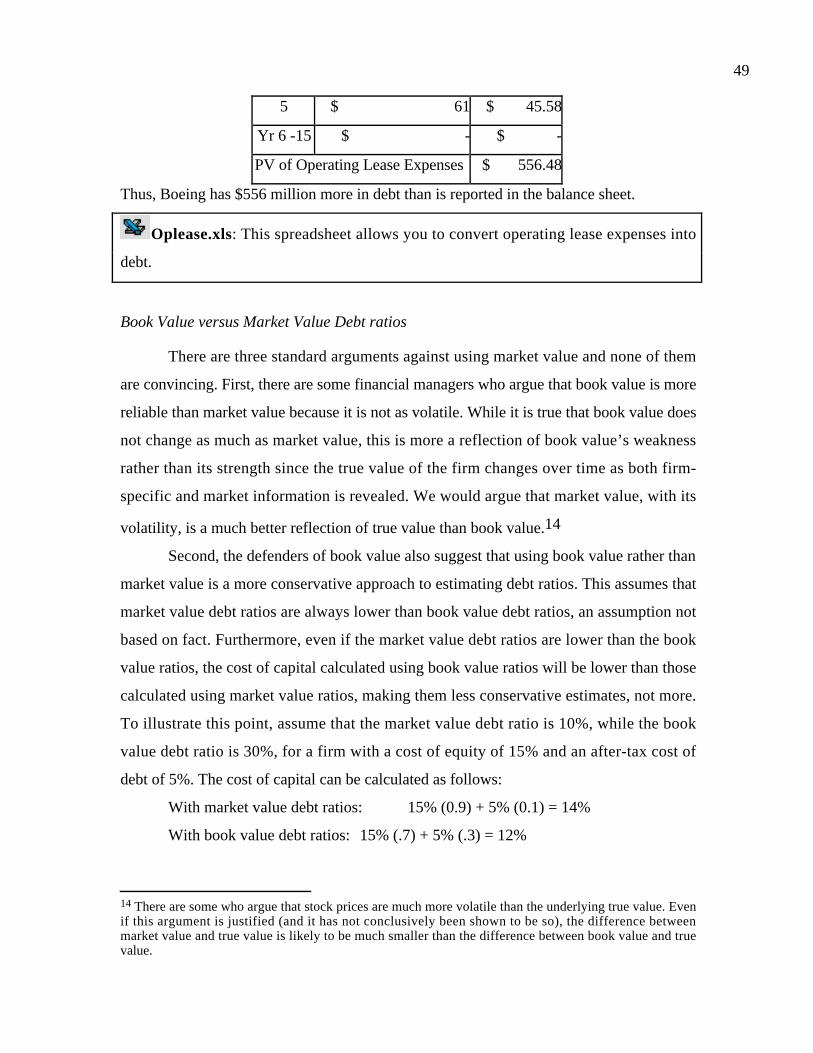
49

5 $ 61 $ 45.58

Yr 6 -15 $ - $ -

PV of Operating Lease Expenses $ 556.48

Thus, Boeing has $556 million more in debt than is reported in the balance sheet.

Oplease.xls: This spreadsheet allows you to convert operating lease expenses into

debt.

Book Value versus Market Value Debt ratios

There are three standard arguments against using market value and none of them

are convincing. First, there are some financial managers who argue that book value is more

reliable than market value because it is not as volatile. While it is true that book value does

not change as much as market value, this is more a reflection of book value’s weakness

rather than its strength since the true value of the firm changes over time as both firm-

specific and market information is revealed. We would argue that market value, with its

volatility, is a much better reflection of true value than book value.14

Second, the defenders of book value also suggest that using book value rather than

market value is a more conservative approach to estimating debt ratios. This assumes that

market value debt ratios are always lower than book value debt ratios, an assumption not

based on fact. Furthermore, even if the market value debt ratios are lower than the book

value ratios, the cost of capital calculated using book value ratios will be lower than those

calculated using market value ratios, making them less conservative estimates, not more.

To illustrate this point, assume that the market value debt ratio is 10%, while the book

value debt ratio is 30%, for a firm with a cost of equity of 15% and an after-tax cost of

debt of 5%. The cost of capital can be calculated as follows:

With market value debt ratios: 15% (0.9) + 5% (0.1) = 14%

With book value debt ratios: 15% (.7) + 5% (.3) = 12%

14 There are some who argue that stock prices are much more volatile than the underlying true value. Evenif this argument is justified (and it has not conclusively been shown to be so), the difference betweenmarket value and true value is likely to be much smaller than the difference between book value and truevalue.

50

Third, it is claimed that lenders will not lend on the basis of market value, but this claim

again seems to be based more upon perception than fact. Any homeowner who has taken

a second mortgage on a house that has appreciated in value knows that lenders do lend on

the basis of market value. It is true, however, that the greater the perceived volatility in

the market value of an asset, the lower is the borrowing potential on that asset.

Estimating the Market Values of Equity and Debt

The market value of equity is generally the number of shares outstanding times the

current stock price. If there other equity claims in the firm such as warrants and

management option, these should also be valued and added on to the value of the equity in

the firm.

The market value of debt is usually more difficult to obtain directly, since very

few firms have all their debt in the form of bonds outstanding trading in the market. Many

firms have non-traded debt, such as bank debt, which is specified in book value terms but

not market value terms. A simple way to convert book value debt into market value debt

is to treat the entire debt on the books as one coupon bond, with a coupon set equal to

the interest expenses on all the debt and the maturity set equal to the face-value weighted

average maturity of the debt, and then to value this coupon bond at the current cost of

debt for the company. Thus, the market value of $1 billion in debt, with interest expenses

of $60 million and a maturity of 6 years, when the current cost of debt is 7.5% can be

estimated as follows:

Estimated Market Value of Debt = 601− 1

1.0756

0.075

+

1,000

1.0756 = $930million

Gross Debt versus Net Debt

Gross debt refers to all debt outstanding in a firm. Net debt is the difference

between gross debt and the cash balance of the firm. For instance, a firm with $1.25

billion in interest bearing debt outstanding and a cash balance of $1 billion has a net debt

balance of $250 million. The practice of netting cash against debt is common in both Latin

America and Europe and the debt ratios are usually estimated using net debt.

51

It is generally safer to value a firm based upon gross debt outstanding and to add

the cash balance outstanding to the value of operating assets to arrive at the firm value.

The interest payment on total debt is then entitled to the tax benefits of debt and we can

assess the effect of whether the company invests its cash balances efficiently on value.

In some cases, especially when firms maintain large cash balances as a matter of

routine, analysts prefer to work with net debt ratios. If we choose to use net debt ratios,

we have to be consistent all the way through the valuation. To begin, the beta for the firm

should be estimated using a net debt ratio rather than a gross debt ratio. The cost of

equity that emerges from the beta estimate can be used to estimate a cost of capital, but

the market value weight on debt should be based upon net debt. Once we discount the

cash flows of the firm at the cost of capital, we should not add back cash. Instead, we

should subtract the net debt outstanding to arrive at the estimated value of equity.

Implicitly, when we net cash against debt to arrive at net debt ratios, we are

assuming that cash and debt have roughly similar risk. While this assumption may not be

outlandish when analyzing highly rated firms, it becomes much shakier when debt

becomes riskier. For instance, the debt in a BB rated firm is much riskier than the cash

balance in the firm and netting out one against the other can provide a misleading view of

the firm’s default risk. In general, using net debt ratios will overstate the value of riskier

firms.

Illustration 8.15: Difference between market value and book value debt ratios – Boeing in

June 2000

In this illustration we contrast the book values of debt and equity with the market

values. For debt, we estimate the market value of debt using the book value of debt, the

interest expense on the debt, the average maturity of the debt and the pre-tax cost of debt

for each firm. For Boeing, the book value of debt is $6,972 million, the interest expense on

the debt is $453 million, the average maturity of the debt is 13.76 years and the pre-tax

cost of debt is 6.00%. The estimated market value is as follows:

52

Estimated MV of Boeing Debt = 4531− 1

1.0613.76

0.06

+6,972

1.0613.76 = $7,291

To this, we need to add the present value of operating leases of $556 million to arrive at a

total market value for debt of $7,847 million.

The book value of equity for Boeing was $12,316 million while the market value

of equity was $55,197 million. The debt ratios in market value and book value terms are

computed.

Market Book

Debt to Equity7847

55197=14.22%

6972

12316= 56.61%

Debt/(Debt + Equity)7847

7847 + 55197=12.45%

6972

6972 +12316= 36.15%

The market debt ratio is significantly lower than the book debt ratio.

wacccalc.xls: This spreadsheet allows you to convert book values of debt into

market values.

Estimating the Cost of Capital

Since a firm can raise its money from three sources -- equity, debt and preferred

stock -- the cost of capital is defined as the weighted average of each of these costs. The

cost of equity (ke) reflects the riskiness of the equity investment in the firm, the after-tax

cost of debt (kd) is a function of the default risk of the firm and the cost of preferred stock

(kps) is a function of its intermediate standing in terms of risk between debt and equity.

The weights on each of these components should reflect their market value proportions

since these proportions best measure how the existing firm is being financed. Thus if E, D

and PS are the market values of equity, debt and preferred stock, respectively, the cost of

capital can be written as follows:

Cost of Capital = k e

E

D+ E + PS

+ kd

D

D + E + PS

+ kps

PS

D+ E + PS

Illustration 8.16: Estimating Cost of Capital - Boeing

53

Having estimated the costs of debt and equity in earlier illustrations and the

market value debt ratio in Illustration 8.15, we can put them together to arrive at a cost of

capital for Boeing.

Cost of Equity = 10.28% (from Illustration 8.8)

Cost of Debt = 3.90% (from Illustration 8.10)

Market Value Debt ratio = 12.45% (from Illustration 8.15)

Cost of capital = 10.28% (0.8755) + 3.90% (0.1245) = 9.49%

Illustration 8.17: Estimating Cost of Capital – Embraer in January 2001

To estimate a cost of capital for Embraer, we again draw on the estimates of cost

of equity and cost of debt we obtained in prior illustrations. The cost of capital will be

estimated using net debt all the way through (for the levered betas, interest coverage ratios

and debt ratios) and in U.S. dollars.

Cost of equity = 18.86% (from illustration 8.9)

After-tax cost of debt = 7.45% (from illustration 8.11)

Market Value of Debt = 1,328 million BR

Cash and Marketable Securities = 1,105 million BR

Market Value of Equity = 9,084 million BR

The cost of capital for Embraer is estimated below:

Net Debt = 1,328 million – 1,105 million = 223 million

Cost of Capital = 18.86% 9084

9084 + 223

+ 7.45%

223

9084 + 223

=18.59%

To convert this into a nominal real cost of capital, we would apply the differential

inflation rates (10% in Brazil and 2% in the US)

Cost of Capital NominalBR = 1 + Cost of Capital$( ) Inflation Rate Brazil

Inflation Rate US

-1

= 1.1859( ) 1.10

1.02

−1= 27.89%

Best Practices at Firms

54

We have spent this chapter discussing what firms should do when it comes to

estimating the cost of capital. What do they actually do? Bruner, Eades, Harris and

Higgins surveyed 27 well regarded corporations and their findings are summarized in

Table 8.8.

Table 8.8: Current Practices for Estimating Cost of Capital

Cost of capital item Current Practices

Cost of Equity • 81% of firms used the capital asset pricing model to estimate

the cost of equity, 4% used a modified capital asset pricing

model and 15% were uncertain about how they estimated the

cost of equity.

• 70% of firms used 10-year treasuries or longer as the riskless

rate, 7% used 3 to 5-year treasuries and 4% used the treasury

bill rate.

• 52% used a published source for a beta estimate, while 30%

estimated it themselves.

• There was wide variation in the market risk premium used,

with 37% using a premium between 5 and 6%.

Cost of Debt • 52% of firms used a marginal borrowing rate and a marginal tax

rate, while 37% used the current average borrowing rate and

the effective tax rate.

Weights for Debt and

Equity

• 59% used market value weights for debt and equity in the cost

of capital, 15% used book value weights and 19% were

uncertain about what weights they used.

Source: Bruner, Eades, Harris and Higgins (1998)

Summary

When we analyze the investments of a firm or assess its value, we need to know

the cost that the firm faces in raising equity, debt and capital. The risk and return models

described in the previous chapter can be used to estimate the costs of equity and capital

for a firm.

55

Building on the premise that the cost of equity should reflect the riskiness of equity

to investors in the firm, there are three basic inputs we need to estimate the cost of equity

for any firm. The riskless rate is the expected return on an investment with no default risk

and no reinvestment risk. Since much of the analysis in corporate finance is long term, the

riskless rate should be the interest rate on a long term government bond. The risk

premium measures what investors demand as a premium for investing in risky

investments instead of riskless investments. This risk premium, which can vary across

investors, can be estimated either by looking at past returns on stocks and government

securities or by looking at how the market prices stocks currently. The beta for a firm is

conventionally measured using a regression of returns on the firm’s stock against returns

on a market index. This approach yields imprecise beta estimates and we are better off

estimating betas by examining the betas of the businesses that the firm operates in.

The cost of capital is a weighted average of the costs of the different components of

financing, with the weights based on the market values of each component. The cost of

debt is the market rate at which the firm can borrow, adjusted for any tax advantages of

borrowing. The cost of preferred stock, on the other hand, is the preferred dividend.

The cost of capital is useful at two levels. On a composite basis, it is what these firms

have to make collectively on their investments to break even. It is also the appropriate

discount rate to use to discount expected future cash flows to arrive at an estimate of firm

value.

56

Problems

1. In December 1995, Boise Cascade’s stock had a beta of 0.95. The treasury bill rate at the time

was 5.8% and the treasury bond rate was 6.4%.

a. Estimate the expected return on the stock for a short term investor in the company.

b. Estimate the expected return on the stock for a long term investor in the company.

c. Estimate the cost of equity for the company.

2. (Continuing problem 1) Boise Cascade also had debt outstanding of $1.7 billion and a market

value of equity of $1.5 billion; the corporate marginal tax rate was 36%.

a. Assuming that the current beta of 0.95 for the stock is a reasonable one, estimate the

unlevered beta for the company.

b. How much of the risk in the company can be attributed to business risk and how much

to financial leverage risk?

3. Biogen Inc., as biotechnology firm, had a beta of 1.70 in 1995. It had no debt outstanding at the

end of that year.

a. Estimate the cost of equity for Biogen, if the treasury bond rate is 6.4%.

b. What effect will an increase in long term bond rates to 7.5% have on Biogen’s cost of

equity?

c. How much of Biogen’s risk can be attributed to business risk?

4. Genting Berhad is a Malaysian conglomerate, with holding in plantations and tourist resorts.

The beta estimated for the firm, relative to the Malaysian stock exchange, is 1.15, and the long

term government borrowing rate in Malaysia is 11.5%.

a. Estimate the expected return on the stock.

b. If you were an international investor, what concerns, if any, would you have about

using the beta estimated relative to the Malaysian Index? If you do, how would you

modify the beta?

5. You have just done a regression of monthly stock returns of HeavyTech Inc., a manufacturer

of heavy machinery, on monthly market returns over the last five years and come up with the

following regression:

57

RHeavyTech = 0.5% + 1.2 RM

The variance of the stock is 50% and the variance of the market is 20%. The current T.Bill rate is

3% (It was 5% one year ago). The stock is currently selling for $50, down $4 over the last year,

and has paid a dividend of $2 during the last year and expects to pay a dividend of $2.50 over the

next year. The NYSE composite has gone down 8% over the last year with a dividend yield of

3%. HeavyTech Inc. has a tax rate of 40%.

a. What is the expected return on HeavyTech over the next year?

b. What would you expect HeavyTech's price to be one year from today?

c. What would you have expected HeavyTech's stock returns to be over the last year?

d. What were the actual returns on HeavyTech over the last year?

e. HeavyTech has $100 million in equity and $5 million in debt. It plans to issue $50 million in

new equity and retire $50 million in debt. Estimate the new beta.

6. Safecorp, which owns and operates grocery stores across the United States, currently has $50

million in debt and $100 million in equity outstanding. Its stock has a beta of 1.2. It is planning a

leveraged buyout, where it will increase its debt/equity ratio to 8. If the tax rate is 40%, what will

the beta of the equity in the firm be after the LBO?

7. Novell, which had a market value of equity of $2 billion and a beta of 1.50, announced that it

was acquiring WordPerfect, which had a market value of equity of $1 billion and a beta of 1.30.

Neither firm had any debt in its financial structure at the time of the acquisition and the corporate

tax rate was 40%.

a. Estimate the beta for Novell after the acquisition, assuming that the entire acquisition was

financed with equity.

b. Assume that Novell had to borrow the $1 billion to acquire WordPerfect. Estimate the beta

after the acquisition.

8. You are analyzing the beta for Hewlett Packard and have broken down the company into four

broad business groups with market values and betas for each group.

Business Group Market Value of Equity Beta

Mainframes $ 2.0 billion 1.10

Personal Computers $ 2.0 billion 1.50

Software $ 1.0 billion 2.00

58

Printers $ 3.0 billion 1.00

a. Estimate the beta for Hewlett Packard as a company. Is this beta going to be equal to the

beta estimated by regressing past returns on HP stock against a market index. Why or Why

not?

b. If the treasury bond rate is 7.5%, estimate the cost of equity for Hewlett Packard.

Estimate the cost of equity for each division. Which cost of equity would you use to value

the printer division?

c. Assume that HP divests itself of the mainframe business and pays the cash out as a

dividend. Estimate the beta for HP after the divestiture. (HP had $1 billion in debt

outstanding.)

9. The following table summarizes the percentage changes in operating income, percentage

changes in revenue and betas for four pharmaceutical firms.

Firm % Change in Revenue % Change in Operating Income Beta

PharmaCorp 27% 25% 1.00

SynerCorp 25% 32% 1.15

BioMed 23% 36% 1.30

Safemed 21% 40% 1.40

a. Calculate the degree of operating leverage for each of these firms.

b. Use the operating leverage to explain why these firms have different betas.

10. A prominent beta estimation service reports the beta of Comcast Corporation, a major cable

TV operator, to be 1.45. The service claims to use weekly returns on the stock over the prior five

years and the NYSE composite as the market index to estimate betas. You replicate the regression

using weekly returns over the same period and arrive at a beta estimate of 1.60. How would you

reconcile the two estimates?

11. Battle Mountain is a mining company, which mines gold, silver and copper in mines in South

America, Africa and Australia. The beta for the stock is estimated to be 0.30. Given the volatility

in commodity prices, how would you explain the low beta?

59

12. You have collected returns on AnaDone Corporation (AD Corp.), a large diversified

manufacturing firm, and the NYSE index for five years:

Year AD Corp NYSE

1981 10% 5%

1982 5% 15%

1983 -5% 8%

1984 20% 12%

1985 -5% -5%

a. Estimate the intercept (alpha) and slope (beta) of the regression.

b. If you bought stock in AD Corp. today, how much would you expect to make

as a return over the next year? [The six-month T.Bill rate is 6%]

c. Looking back over the last five years, how would you evaluate AD's

performance relative to the market?

d. Assume now that you are an undiversified investor and that you have all of

your money invested in AD Corporation. What would be a good measure of the

risk that you are taking on? How much of this risk would you be able to eliminate

if you diversify?

e. AD is planning to sell off one of its divisions. The division under consideration

has assets which comprise half of the book value of AD Corporation and 20% of

the market value. Its beta is twice the average beta for AD Corp (before

divestment). What will the beta of AD Corporation be after divesting this

division?

13. You run a regression of monthly returns of Mapco Inc, an oil and gas producing firm, on the

S&P 500 index and come up with the following output for the period 1991 to 1995.

Intercept of the regression = 0.06%

Slope of the regression = 0.46

Standard error of X-coefficient = 0.20

R squared = 5%

There are 20 million shares outstanding and the current market price is $2 per share. The firm has

$20 million in debt outstanding. (The firm has a tax rate of 36%.)

60

a. What would an investor in Mapco's stock require as a return if the T.Bond rate is 6%?

b. What proportion of this firm's risk is diversifiable?

c. Assume now that Mapco has three divisions, of equal size (in market value terms). It

plans to divest itself of one of the divisions for $20 million in cash and acquire another for

$50 million (It will borrow $30 million to complete this acquisition). The division it is

divesting is in a business line where the average unlevered beta is 0.20 and the division it

is acquiring is in a business line where the average unlevered beta is 0.80. What will the

beta of Mapco be after this acquisition?

14. You have just run a regression of monthly returns of American Airlines (AMR) against the

S&P 500 over the last five years. You have misplaced some of the output and are trying to derive

it from what you have.

a. You know the R squared of the regression is 0.36 and that your stock has a variance of

67%. The market variance is 12%. What is the beta of AMR?

b. You also remember that AMR was not a very good investment during the period of the

regression and that it did worse than expected (after adjusting for risk) by 0.39% a month

for the five years of the regression. During this period, the average riskfree rate was

4.84%. What was the intercept on the regression?

c. You are comparing AMR Inc. to another firm which also has an R squared of 0.48. Will

the two firms have the same beta? If not, why not?

15. You have run a regression of monthly returns on Amgen, a large biotechnology firm, against

monthly returns on the S&P 500 index, and come up with the following output.

Rstock = 3.28%+ 1.65 RMarket R2 = 0.20

The current one-year treasury bill rate is 4.8% and the current thirty-year bond rate is 6.4%. The

firm has 265 million shares outstanding selling for $30 per share.

a. What is the expected return on this stock over the next year?

b. Would your expected return estimate change if the purpose was to get a discount rate

to analyze a thirty-year capital budgeting project?

61

c. An analyst has estimated, correctly, that the stock did 51.10% better than expected,

annually, during the period of the regression. Can you estimate the annualized riskfree

rate that she used for her estimate?

d. The firm has a debt/equity ratio of 3%, and faces a tax rate of 40%. It is planning to

issue $2billion in new debt and acquire a new business for that amount with the same risk

level as the firm's existing business. What will the beta be after the acquisition?

16. You have just run a regression of monthly returns on MAD Inc., a newspaper and

magazine publisher, against returns on the S&P 500 and arrived at the following result.

RMAD = – 0.05% + 1.20 RS&P

The regression has an R-squared of 22%. The current T.Bill rate is 5.5% and the current

T.Bond rate is 6.5%. The riskfree rate during the period of the regression was 6%.

Answer the following questions relating to the regression.

a. Based upon the intercept, how well or badly did MAD do, relative to

expectations, during the period of the regression?

b. You now realize that MAD Inc. went through a major restructuring at the end

of last month (which was the last month of your regression) and made the

following changes:

• The firm sold off its magazine division, which had an unlevered beta of 0.6, for

$20 million.

• It borrowed an additional $20 million and bought back stock worth $40

million.

• After the sale of the division and the share repurchase, MAD Inc. had $40

million in debt and $120 million in equity outstanding.

If the firm’s tax rate is 40%, re-estimate the beta, after these changes.

17. Time Warner Inc., the entertainment conglomerate, has a beta of 1.61. Part of the reason for

the high beta is the debt left over from the leveraged buyout of Time by Warner in 1989, which

amounted to $10 billion in 1995. The market value of equity at Time Warner in 1995 was also

$10 billion. The marginal tax rate was 40%.

a. Estimate the unlevered beta for Time Warner.

62

b. Estimate the effect of reducing the debt ratio by 10% each year for the next two years on

the beta of the stock.

18. Chrysler, the automotive manufacturer, had a beta of 1.05 in 1995. It had $13 billion in debt

outstanding in that year and 355 million shares trading at $50 per share. The firm had a cash

balance of $8 billion at the end of 1995. The marginal tax rate was 36%.

a. Estimate the unlevered beta of the firm.

b. Estimate the effect of paying out a special dividend of $5 billion on this unlevered beta.

c. Estimate the beta for Chrysler after the special dividend.

19. You are trying to estimate the beta of a private firm that manufactures home appliances. You

have managed to obtain betas for publicly traded firms that also manufacture home appliances.

Firm Beta Debt MV of Equity

Black & Decker 1.40 $ 2,500 $ 3,000

Fedders Corp. 1.20 $ 5 $ 200

Maytag Corp. 1.20 $ 540 $ 2250

National Presto 0.70 $ 8 $ 300

Whirlpool 1.50 $ 2900 $ 4000

The private firm has a debt equity ratio of 25%, and faces a tax rate of 40%. The publicly traded

firms all have marginal tax rates of 40% as well.

a. Estimate the beta for the private firm.

b. What concerns, if any, would you have about using betas of comparable firms?

20. As the result of stockholder pressure, RJR Nabisco is considering spinning off its food

division. You have been asked to estimate the beta for the division and decide to do so by

obtaining the beta of comparable publicly traded firms. The average beta of comparable publicly

traded firms is 0.95 and the average debt/equity ratio of these firms is 35%. The division is

expected to have a debt ratio of 25%. The marginal corporate tax rate is 36%.

a. What is the beta for the division?

b. Would it make any difference if you knew that RJR Nabisco had a much higher fixed cost

structure than the comparable firms used here?

63

21. Southwestern Bell, a phone company, is considering expanding its operations into the media

business. The beta for the company at the end of 1995 was 0.90 and the debt/equity ratio was 1.

The media business is expected to be 30% of the overall firm value in 1999 and the average beta

of comparable firms is 1.20; the average debt/equity ratio for these firms is 50%. The marginal

corporate tax rate is 36%.

a. Estimate the beta for Southwestern Bell in 1999, assuming that it maintains its current

debt/equity ratio.

b. Estimate the beta for Southwestern Bell in 1999, assuming that it decides to finance its

media operations with a debt/equity ratio of 50%.

22. The chief financial officer of Adobe Systems, a growing software manufacturing firm, has

approached you for some advice regarding the beta of his company. He subscribes to a service

which estimates Adobe System’s beta each year and he has noticed that the beta estimates have

gone down every year since 1991: 2.35 in 1991 to 1.40 in 1995. He would like the answers to the

following questions:

a. Is this decline in beta unusual for a growing firm?

b. Why would the beta decline over time?

c. Is the beta likely to keep decreasing over time?

23. You are analyzing Tiffany, an upscale retailer, and find that the regression estimate of the

firm’s beta is 0.75; the standard error for the beta estimate is 0.50. You also note that the average

unlevered beta of comparable specialty retailing firms is 1.15.

a. If Tiffany has a debt/equity ratio of 20%, estimate the beta for the company based upon

comparable firms. (The tax rate is 40%.)

b. Estimate a range for the beta from the regression.

c. Assume that Tiffany’s is rated BBB and that the default spread for BBB rated firms is

1% over the treasury bond rate. If the treasury bond rate is 6.5%, estimate the cost of

capital for the firm.

24. You have been asked to estimate the cost of capital for NewTel, a telecomm firm. The firm

has the following characteristics:

• There are 100 million shares outstanding trading at $250 per share.

64

• The firm has a book value of ten-year debt of $10 billion and interest expenses of $600

million on the debt. The firm is not rated, but it had operating income of $2.5 billion last year.

Firms with an interest coverage ratio of 3.5 to 4.5 were rated BBB.

• The unlevered beta of other telecomm firms is 0.80

The treasury bond rate is 6%, and the tax rate for the firm is 35%.

a. Estimate the market value of debt for this firm

b. Based upon the synthetic rating, estimate the cost of debt for this firm.

c. Estimate the cost of capital for this firm.

0

CHAPTER 9

MEASURING EARNINGSTo estimate cash flows, we usually begin with a measure of earnings. Free cash

flows to the firm, for instance, are based upon after-tax operating earnings. Free cashflow

to equity estimates, on the other hand, commence with net income. While we obtain and

use measures of operating and net income from accounting statements, the accounting

earnings for many firms bear little or no resemblance to the true earnings of the firm.

In this chapter, we begin by consider the philosophical difference between the

accounting and financial views of firms. We then consider how the earnings of a firm, at

least as measured by accountants, have to be adjusted to get a measure of earnings that is

more appropriate for valuation. In particular, we examine how to treat operating lease

expenses, which we argue are really financial expenses, and research and development

expenses, which we consider to be capital expenses. The adjustments affect not only our

measures of earnings but our estimates of book value of capital. We also look at

extraordinary items (both income and expenses) and one-time charges, the use of which

has expanded significantly in recent years as firms have shifted towards managing earnings

more aggressively. The techniques used to smooth earnings over periods and beat analyst

estimates can skew reported earnings and, if we are not careful, the values that emerge

from them.

Accounting versus Financial Balance Sheets

When analyzing a firm, what are the questions to which we would like to know

the answers? A firm, as we define it, includes both investments already made -- we will

call these assets-in-place -- and investments yet to be made -- we will call these growth

assets. In addition, a firm can either borrow the funds it needs to make these investments,

in which case it is using debt, or raise it from its owners, in the form of equity. Figure 9.1

summarizes this description of a firm in the form of a financial balance sheet:

1

Figure 9.1: A Financial Balance Sheet

Assets Liabilities

Assets in Place Debt

Equity

Fixed Claim on cash flowsLittle or No role in managementFixed MaturityTax Deductible

Residual Claim on cash flowsSignificant Role in managementPerpetual Lives

Growth Assets

Existing InvestmentsGenerate cashflows todayIncludes long lived (fixed) and

short-lived(working capital) assets

Expected Value that will be created by future investments

Note that while this summary does have some similarities with the accounting balance

sheet, but there are key differences. The most important one is that here we explicitly

consider growth assets when we look at what a firm owns.

When doing a financial analysis of a firm, we would like to be able to answer of

questions relating to each of these items. Figure 9.2 lists the questions.

Figure 9.2: Key Financial Questions

Assets Liabilities

Assets in Place Debt

Equity

What is the value of the debt?How risky is the debt?

What is the value of the equity?How risky is the equity?

Growth Assets

What are the assets in place?How valuable are these assets?How risky are these assets?

What are the growth assets?How valuable are these assets?

As we will see in this chapter, accounting statements allow us to acquire some

information about each of these questions, but they fall short in terms of both the

timeliness with which they provide it and the way in which they measure asset value,

earnings and risk.

Adjusting Earnings

The income statement for a firm provides measures of both the operating and

equity income of the firm in the form of the earnings before interest and taxes (EBIT) and

net income. When valuing firms, there are two important considerations in using this

measure. One is to obtain as updated an estimate as possible, given how much these firms

change over time. The second is that reported earnings at these firms may bear little

2

resemblance to true earnings because of limitations in accounting rules and the firms’ own

actions.

The Importance of Updating Earnings

Firms reveal their earnings in their financial statements and annual reports to

stockholders. Annual reports are released only at the end of a firm’s financial year, but

you are often required to value firms all through the year. Consequently, the last annual

report that is available for a firm being valued can contain information that is sometimes

six or nine months old. In the case of firms that are changing rapidly over time, it is

dangerous to base value estimates on information that is this old. Instead, use more recent

information. Since firms in the United States are required to file quarterly reports with the

SEC (10-Qs) and reveal these reports to the public, a more recent estimate of key items in

the financial statements can be obtained by aggregating the numbers over the most recent

four quarters. The estimates of revenues and earnings that emerge from this exercise are

called “trailing 12-month” revenues and earnings and can be very different from the values

for the same variables in the last annual report.

There is a price paid for the updating. Unfortunately, not all items in the annual

report are revealed in the quarterly reports. You have to either use the numbers in the last

annual report (which does lead to inconsistent inputs) or estimate their values at the end

of the last quarter (which leads to estimation error). For example, firms do not reveal

details about options outstanding (issued to managers and employees) in quarterly

reports, while they do reveal them in annual reports. Since you need to value these

options, you can use the options outstanding as of the last annual report or assume that

the options outstanding today have changed to reflect changes in the other variables. (For

instance, if revenues have doubled, the options have doubled as well.)

For younger firms, it is critical that you stay with the most updated numbers you

can find, even if these numbers are estimates. These firms are often growing exponentially

and using numbers from the last financial year will lead to under valuing them. Even those

that are not are changing substantially from quarter to quarter, updated information might

give you a chance to capture these changes.

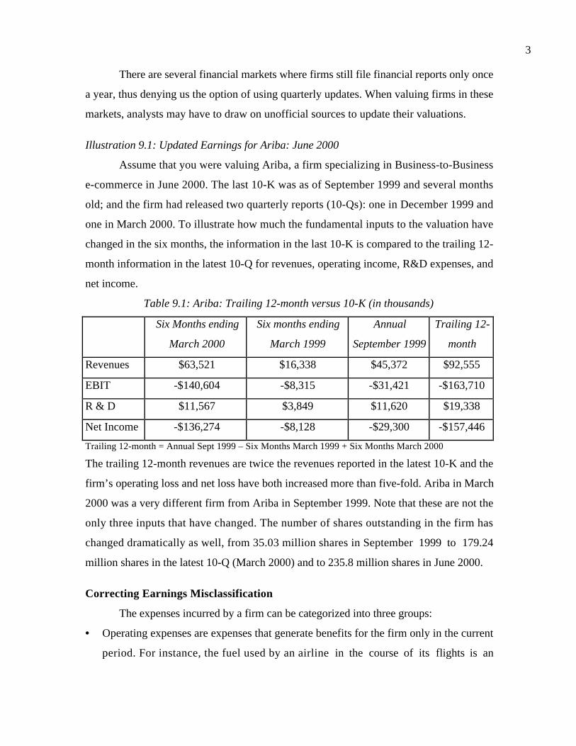
3

There are several financial markets where firms still file financial reports only once

a year, thus denying us the option of using quarterly updates. When valuing firms in these

markets, analysts may have to draw on unofficial sources to update their valuations.

Illustration 9.1: Updated Earnings for Ariba: June 2000

Assume that you were valuing Ariba, a firm specializing in Business-to-Business

e-commerce in June 2000. The last 10-K was as of September 1999 and several months

old; and the firm had released two quarterly reports (10-Qs): one in December 1999 and

one in March 2000. To illustrate how much the fundamental inputs to the valuation have

changed in the six months, the information in the last 10-K is compared to the trailing 12-

month information in the latest 10-Q for revenues, operating income, R&D expenses, and

net income.

Table 9.1: Ariba: Trailing 12-month versus 10-K (in thousands)

Six Months ending

March 2000

Six months ending

March 1999

Annual

September 1999

Trailing 12-

month

Revenues $63,521 $16,338 $45,372 $92,555

EBIT -$140,604 -$8,315 -$31,421 -$163,710

R & D $11,567 $3,849 $11,620 $19,338

Net Income -$136,274 -$8,128 -$29,300 -$157,446

Trailing 12-month = Annual Sept 1999 – Six Months March 1999 + Six Months March 2000

The trailing 12-month revenues are twice the revenues reported in the latest 10-K and the

firm’s operating loss and net loss have both increased more than five-fold. Ariba in March

2000 was a very different firm from Ariba in September 1999. Note that these are not the

only three inputs that have changed. The number of shares outstanding in the firm has

changed dramatically as well, from 35.03 million shares in September 1999 to 179.24

million shares in the latest 10-Q (March 2000) and to 235.8 million shares in June 2000.

Correcting Earnings Misclassification

The expenses incurred by a firm can be categorized into three groups:

• Operating expenses are expenses that generate benefits for the firm only in the current

period. For instance, the fuel used by an airline in the course of its flights is an

4

operating expense, as is the labor cost for an automobile company associated with

producing vehicles.

• Capital expenses are expenses that generate benefits over multiple periods. For

example, the expense associated with building and outfitting a new factory for an

automobile manufacturer is a capital expense, since it will generate several years of

revenues.

• Financial expenses are expenses associated with non-equity capital raised by a firm.

Thus, the interest paid on a bank loan would be a financial expense.

The operating income for a firm, measured correctly, should be equal to its

revenues less its operating expenses. Neither financial nor capital expenses should be

included in the operating expenses in the year that they occur, though capital expenses

may be depreciated or amortized over the period that the firm obtains benefits from the

expenses. The net income of a firm should be its revenues less both its operating and

financial expenses. No capital expenses should be deducted to arrive at net income.

The accounting measures of earnings can be misleading because operating, capital

and financial expenses are sometimes misclassified. We will consider the two most

common misclassifications in this section and how to correct for them. The first is the

inclusion of capital expenses such as R&D in the operating expenses, which skews the

estimation of both operating and net income. The second adjustment is for financial

expenses such as operating leases expenses that are treated as operating expenses. This

affects the measurement of operating income but not net income.

The third factor to consider is the effects of the phenomenon of “managed

earnings” at these firms. Technology firms sometimes use accounting techniques to post

earnings that beat analyst estimates resulting in misleading measures of earnings.

Capital Expenses treated as Operating Expenses

While, in theory, income is not computed after capital expenses, the reality is that

there are a number of capital expenses that are treated as operating expenses. For instance,

a significant shortcoming of accounting statements is the way in which they treat research

and development expenses. Under the rationale that the products of research are too

uncertain and difficult to quantify, accounting standards have generally required that all

5

R&D expenses to be expensed in the period in which they occur. This has several

consequences, but one of the most profound is that the value of the assets created by

research does not show up on the balance sheet as part of the total assets of the firm.

This, in turn, creates ripple effects for the measurement of capital and profitability ratios

for the firm. We will consider how to capitalize R&D expenses in the first part of the

section and extend the argument to other capital expenses in the second part of the

section.

Capitalizing R&D Expenses

Research expenses, notwithstanding the uncertainty about future benefits, should

be capitalized. To capitalize and value research assets, you make an assumption about

how long it takes for research and development to be converted, on average, into

commercial products. This is called the amortizable life of these assets. This life will vary

across firms and reflect the commercial life of the products that emerge from the research.

To illustrate, research and development expenses at a pharmaceutical company should

have fairly long amortizable lives, since the approval process for new drugs is long. In

contrast, research and development expenses at a software firm, where products tend to

emerge from research much more quickly should be amortized over a shorter period.

Once the amortizable life of research and development expenses has been

estimated, the next step is to collect data on R&D expenses over past years ranging back

to the amortizable life of the research asset. Thus, if the research asset has an amortizable

life of 5 years, the R&D expenses in each of the five years prior to the current one have to

be obtained. For simplicity, it can be assumed that the amortization is uniform over time,

which leads to the following estimate of the residual value of research asset today.

∑0=t

1)--(n=tt

n

t)+(nD&R =Asset Research theof Value

Thus, in the case of the research asset with a five-year life, you cumulate 1/5 of the R&D

expenses from four years ago, 2/5 of the R & D expenses from three years ago, 3/5 of the

R&D expenses from two years ago, 4/5 of the R&D expenses from last year and this

year’s entire R&D expense to arrive at the value of the research asset. This augments the

value of the assets of the firm, and by extension, the book value of equity.

6

Adjusted Book Value of Equity = Book Value of Equity + Value of the Research Asset

Finally, the operating income is adjusted to reflect the capitalization of R&D

expenses. First, the R&D expenses that were subtracted out to arrive at the operating

income are added back to the operating income, reflecting their re-categorization as capital

expenses. Next, the amortization of the research asset is treated the same way that

depreciation is and netted out to arrive at the adjusted operating income.

Adjusted Operating Income = Operating Income + R & D expenses –

Amortization of Research Asset

The adjusted operating income will generally increase for firms that have R&D expenses

that are growing over time. The net income will also be affected by this adjustment:

Adjusted Net Income = Net Income + R & D expenses – Amortization of Research Asset

While we would normally consider only the after-tax portion of this amount, the fact that

R&D is entirely tax deductible eliminates the need for this adjustment.1

R&Dconv.xls: This spreadsheet allows you to convert R&D expenses from operating

to capital expenses.

Illustration 9.2: Capitalizing R&D expenses: Amgen in March 2001

Amgen is a bio-technology firm. Like most pharmaceutical firms, it has a

substantial amount of R&D expenses and we will attempt to capitalize it in this section.

The first step in this conversion is determining an amortizable life for R & D expenses.

How long will it take, on an expected basis, for research to pay off at Amgen? Given the

length of the approval process for new drugs by the Food and Drugs Administration, we

will assume that this amortizable life is 10 years.

The second step in the analysis is collecting research and development expenses

from prior years, with the number of years of historical data being a function of the

amortizable life. Table 9.2 provides this information for the firm.

1 If only amortization were tax deductible, the tax benefit from R&D expenses would be:Amortization * tax rateThis extra tax benefit we get from the entire R&D being tax deductible is as follows:(R&D – Amortization) * tax rateIf we subtract out (R&D – Amortization) (1- tax rate) and add the differential tax benefit which iscomputed above, (1- tax rate) drops out of the equation.

7

Table 9.2: Historical R& D Expenses (in millions)

Year R& D Expenses

Current 845.00

-1 822.80

-2 663.30

-3 630.80

-4 528.30

-5 451.70

-6 323.63

-7 255.32

-8 182.30

-9 120.94

-10

[Note that the firm has been in existence for only nine years, and that there is no

information therefore available for year –10.] The current year’s information reflects the

R&D in the last financial year (which was calendar year 2000).

The portion of the expenses in prior years that would have been amortized

already and the amortization this year from each of these expenses is considered. To make

estimation simpler, these expenses are amortized linearly over time; with a 10-year life,

10% is amortized each year. This allows us to estimate the value of the research asset

created at each of these firms and the amortization of R&D expenses in the current year.

The procedure is illustrated in table 9.3:

Table 9.3: Value of Research Asset

Year R&D Expense Unamortized portion

Amortization

this year

Current 845.00 1.00 845.00

-1 822.80 0.90 740.52 $ 82.28

-2 663.30 0.80 530.64 $ 66.33

8

-3 630.80 0.70 441.56 $ 63.08

-4 528.30 0.60 316.98 $ 52.83

-5 451.70 0.50 225.85 $ 45.17

-6 323.63 0.40 129.45 $ 32.36

-7 255.32 0.30 76.60 $ 25.53

-8 182.30 0.20 36.46 $ 18.23

-9 120.94 0.10 12.09 $ 12.09

-10 0.00 0.00 0.00 $ -

[Note that none of the current year’s expenditure has been amortized because it is

assumed to occur at the end of the year but that 50% of the expense from 5 years ago has

been amortized. The sum of the dollar values of unamortized R&D from prior years is

$3.355 billion. This can be viewed as the value of Amgen’s research asset and would be

also added to the book value of equity for computing return on equity and capital

measures. The sum of the amortization in the current year for all prior year expenses is

$397.91 million.

The final step in the process is the adjustment of the operating income to reflect

the capitalization of research and development expenses. We make the adjustment by

adding back R&D expenses to the operating income (to reflect its reclassification as a

capital expense) and subtract out the amortization of the research asset, estimated in the

last step. For Amgen, which reported operating income of $1,549 million in its income

statement for 2000, the adjusted operating earnings would be:

Adjusted Operating Earnings

= Operating Earnings + Current year’s R&D expense – Amortization of Research Asset

= 1,549 + 845 – 398 = $1,996 million

The stated net income of $1,139 million can be adjusted similarly.

Adjusted Net Income

= Net Income + Current year’s R&D expense – Amortization of Research Asset

= 1,139 + 845 – 398 = $1,586 million

9

Both the book value of equity and capital are augmented by the value of the research

asset. Since measures of return on capital and equity are based upon the prior year’s

values, we computed the value of the research asset at the end of 1999, using the same

approach that we used in 2000 and obtained a value of $2,909 million.2

Value of Research Asset1999 = $2,909 million

Adjusted Book Value of Equity1999 = Book Value of Equity1999 + Value of Research Asset

= 3,024 million + 2,909 million = $5,933 million

Adjusted Book Value of Capital1999 = Book Value of Capital1999 + Value of Research

Asset

= 3,347 million + 2909 million = $6,256 million

The returns on equity and capital are reported with both the unadjusted and adjusted

numbers below:

Unadjusted Adjusted for R&D

Return on Equity 1,139

3,024= 37.67%

1,586

5,933= 26.73%

Pre-tax Return on Capital 1,549

3,347= 46.28%

1,996

6,256= 31.91%

While the profitability ratios for Amgen remain impressive even after the adjustment,

they decline significantly from the unadjusted numbers. This is likely to happen for most

firms that earn high returns on equity and capital and have substantial R&D expenses.3

Capitalizing Other Operating Expenses

While R&D expenses are the most prominent example of capital expenses being

treated as operating expenses, there are other operating expenses that arguably should be

treated as capital expenses. Consumer product companies such as Gillette and Coca Cola

could argue that a portion of advertising expenses should be treated as capital expenses,

since they are designed to augment brand name value. For a consulting firm like KPMG,

2 Note that you can arrive at this value using the table above and shifting the amortization numbers by onerow. Thus, $ 822.80 million will become the current year’s R&D, $ 663.3 million will become the R&Dfor year –1 and 90% of it will be unamortized and so on.3 If the return on capital earned by a firm is well below the cost of capital, the adjustment could result in ahigher return.

10

the cost of recruiting and training its employees could be considered a capital expense,

since the consultants who emerge are likely to be the heart of the firm’s assets and

provide benefits over many years. For many new technology firms, including e-tailers

such as Amazon.com, the biggest operating expense item is selling, general and

administrative expenses (SG&A). These firms could argue that a portion of these

expenses should be treated as capital expenses since they are designed to increase brand

name awareness and bring in new presumably long term customers. America Online, for

instance, used this argument to justify capitalizing the expenses associated with the free

trial CDs that it bundled with magazines in the United States.

While this argument has some merit, you should remain wary about using it to

justify capitalizing these expenses. For an operating expense to be capitalized, there

should be substantial evidence that the benefits from the expense accrue over multiple

periods. Does a customer who is enticed to buy from Amazon, based upon an

advertisement or promotion, continue as a customer for the long term? There are some

analysts who claim that this is indeed the case and attribute significant value added to

each new customer.4 It would be logical, under those circumstances, to capitalize these

expenses using a procedure similar to that used to capitalize R&D expenses.

• Determine the period over which the benefits from the operating expense (such as

SG&A) will flow.

• Estimate the value of the asset (similar to the research asset) created by these

expenses. If the expenses are SG&A expenses, this would be the SG&A asset.

• Adjust the operating income for the expense and the amortization of the created

asset.

Adjusted Operating Income = Operating Income + SG&A expenses for the current period

– Amortization of SG&A Asset

• A similar adjustment has to be made to net income:

4 As an example, Jamie Kiggen, an equity research analyst at Donaldson, Lufkin and Jenrette, valued anAmazon customer at $2,400 in an equity research report in 1999. This value was based upon theassumption that the customer would continue to buy from Amazon.com and an expected profit marginfrom such sales.

11

Adjusted Net Income = Net Income + SG&A expenses for the current period –

Amortization of SG&A Asset

• Adjust the book value of equity and capital.

Adjusted BV Equity = BV of Equity + Value SG&A Asset

Adjusted BV Capital = BV of Capital + Value SG&A Asset

Illustration 9.3: Should you capitalize SG&A expense? Analyzing Amazon.com and

America Online

Let use consider SG&A expenses at Amazon and America Online. To make a

judgment on whether you should capitalize this expense, you need to get a sense of what

these expenses are and how long the benefits accruing from these expenses last. For

instance, assume that an Amazon promotion (the expense of which would be included in

SG&A) attracts a new customer to the web site and that customers, once they try

Amazon, continue, on average, to be customers for three years. You would then use a

three year amortizable life for SG&A expenses and capitalize them the same way you

capitalized R& D: by collecting historical information on SG&A expenses, amortizing

them each year, estimating the value of the selling asset and then adjusting operating

income and book value of equity.

We do believe, on balance, that selling, general and administrative expenses should

continue to be treated as operating expenses and not capitalized for Amazon for two

reasons. First, retail customers are difficult to retain, especially online, and Amazon faces

serious competition not only from B&N.com and Borders.com, but also from traditional

retailers like Walmart, setting up their online operations. Consequently, the customers

that Amazon might attract with its advertising or sales promotions are unlikely to stay

for an extended period just because of the initial inducements. Second, as the company

has become larger, its selling, general and administrative expenses seem increasingly

directed towards generating revenues in current periods rather than future periods to

retain current customers.

In contrast, consider the SG&A expenses at America Online. Especially when the

firm was smaller, these expenses primarily related to the cost of the CDs that AOL would

package with magazines to get readers to try its service. The company’s statistics

12

indicated that a customer who tried the service remained a subscriber to it for about 3

years, on average. This makes a case for treating the expense as a capital expense stronger,

with an amortizable life of 3 years.

Illustration 9.4: Capitalizing Recruitment and Training Expenses: Cyber Health

Consulting

Cyber Health Consulting (CHC) is a firm that specializes in offering management

consulting services to health care firms. CHC reported operating income (EBIT) of $51.5

million and net income of $23 million in the most recent year. However, the firm’s

expenses include the cost of recruiting new consultants ($ 5.5 million) and the cost of

training ($8.5 million). A consultant who joins CHC stays with the firm, on average, 4

years.

To capitalize the cost of recruiting and training, we obtained these costs from each

of the prior four years. Table 9.4 reports on these expenses and amortizes each of these

expenses over four years.

Table 9.4: Human Capital Expenses: CHC

Year Training & Recruiting Expenses Unamortized Portion Amortization this year

Current $ 14.00 100% $ 14.00

-1 $ 12.00 75% $ 9.00 $ 3.00

-2 $ 10.40 50% $ 5.20 $ 2.60

-3 $ 9.10 25% $ 2.28 $ 2.28

-4 $ 8.30 - $ 0.00 $ 2.08

Value of Human Capital Asset = $ 30.48 $9.95

The adjustments to operating and net income are as follows:

Adjusted Operating Income = Operating Income + Training and Recruiting expenses –

Amortization of Expense this year = $ 51.5 + $ 14 - $ 9.95 = $ 55.55 million

Net Income = Net Income + + Training and Recruiting expenses – Amortization of

Expense this year = $ 23 million + $ 14 million - $ 9.95 million = $ 27.05 million

As with R&D expenses, the fact that training and recruiting expenses are fully tax

deductible dispenses with the need to consider the tax effect when adjusting net income.

13

Adjustments for Financing Expenses

The second adjustment is for financing expenses that accountants treat as

operating expenses. The most significant example is operating lease expenses, which are

treated as operating expenses, in contrast to capital leases, which are presented as debt.

Converting Operating Leases into Debt

In chapter 3, the basic approach for converting operating leases into debt was

presented. We discount future operating lease commitments back at the firm’s pre-tax

cost of debt. The present value of the operating lease commitments is then added to the

conventional debt of the firm to arrive at the total debt outstanding.

Adjusted Debt = Debt + Present Value of Lease Commitments

Once operating leases are re-categorized as debt, the operating incomes can be

adjusted in two steps. First, the operating lease expense is added back to the operating

income, since it is a financial expense. Next, the depreciation on the leased asset is

subtracted out to arrive at adjusted operating income.

Adjusted Operating Income = Operating Income + Operating Lease Expenses –

Depreciation on leased asset

If you assume that the depreciation on the leased asset approximates the principal

portion of the debt being repaid, the adjusted operating income can be computed by

adding back the imputed interest expense on the debt value of the operating lease expense.

Adjusted Operating Income = Operating Income + (Present Value of Lease

Commitments)*(Pre-tax Interest rate on debt)

Illustration 9.5: Adjusting Operating Income for Operating Leases: The Gap in 2001

As a specialty retailer, the Gap has hundreds of stores that are leased with the

leases being treated as operating leases. For the most recent financial year, the Gap has

operating lease expenses of $705.8 million. Table 9.5 presents the operating lease

commitments for the firm over the next five years and the lump sum of commitments

beyond that point in time.

Table 9.5: The Gap’s Operating Lease Commitments

Year Commitment

14

1 $ 774.60

2 $ 749.30

3 $ 696.50

4 $ 635.10

5 $ 529.70

6 and beyond $ 5,457.90

The Gap has a pre-tax cost of debt of 7%. To compute the present value of the

commitments, you have to make a judgment on the lump sum commitment in year 6.

Based upon the average annual lease commitment over the first five years ($677 million),

we arrive at an annuity of 8 years:

Approximate life of annuity (for year 6 lump sum)5 = $ 5,458/677 = 8.06 years

The present value of the commitments are estimated in Table 9.6:

Table 9.6: Present Value of Operating Lease Commitments: The Gap

Year Commitment Present Value

1 $ 774.60 $ 723.93

2 $ 749.30 $ 654.47

3 $ 696.50 $ 568.55

4 $ 635.10 $ 484.51

5 $ 529.70 $ 377.67

6 and beyond $ 682.24 $ 2,904.59

Debt Value of leases = $ 5,713.72

The present value of operating leases is treated as the equivalent of debt and is added on

to the conventional debt of the firm. The Gap has conventional interest-bearing debt of

$1.56 billion on its balance sheet. The cumulated debt for the firm is:

Adjusted Debt = Interest-bearing Debt + Present Value of Lease Commitments

= $1,560 million + $5,714 million = $ 7,274 million

5 The value is rounded to the nearest integer.

15

To adjust the operating income for the Gap, we first use the full adjustment. To

compute depreciation on the leased asset, we assume straight line depreciation over the

lease life6 (13 years) on the value of the leased asset which is equal to the debt value of

the lease commitments.

million $44013

$5,714

life Lease

Asset Leased of Valueondepreciati lineStraight ===

The Gap’s stated operating income of $1,365 million is adjusted.

Adjusted Operating Income = Operating Income + Operating lease expense in current

year – Depreciation on leased asset = $1,365 million + $706 - $440 = $1,631 million

The approximate adjustment is also estimated, where we add the imputed interest

expense using the pre-tax cost of debt.

Adjusted Operating Income = Operating Income + Debt value of leases * Pre-tax cost of

debt = $1,365 + $5,714 * 0.07 = $1,765 million

Oplease.xls: This spreadsheet allows you to convert operating lease expenses into

debt.

What about other commitments?

The argument made about leases can be made about other long term commitments

where a firm has no escape hatches or cancellations options or where the payment is not

connected to performance/earnings. For instance, consider a professional sports team that

signs a star player to a 10-year contract agreeing to pay $ 5 million a year. If the payment

is not contingent on performance, this firm has created the equivalent of debt by signing

this contract.

The upshot of this argument is that firms that have no debt on their balance sheet

may still be highly levered and subject to default risk, as a consequence. For instance,

Mario Lemieux, a star player for the Pittsburg Penguins, the professional ice-hockey team

was given partial ownership of the team because of its failure to meet contractual

commitments it had made to him.

6 The lease life is computed by adding the estimated annuity life of 8 years for the lump-sum to the initial5 years.

16

Accounting Earnings and True Earnings

Firms have become particularly adept at meeting and beating analyst estimates of

earnings each quarter. While beating earnings estimates can be viewed as a positive

development, some firms adopt accounting techniques that are questionable to accomplish

this objective. When valuing these firms, you have to correct operating income for these

accounting manipulations to arrive at the correct operating income.

The Phenomenon of Managed Earnings

In the 1990s, firms like Microsoft and Intel set the pattern for technology firms.

In fact, Microsoft beat analyst estimates of earnings in 39 of the 40 quarters during the

decade and Intel posted a record almost as impressive. Other technology firms followed in

their footsteps in trying to deliver earnings that were higher than analyst estimates by at

least a few pennies. The evidence is overwhelming that the phenomenon is spreading. For

an unprecedented 18 quarters in a row from 1996 to 2000, more firms beat consensus

earnings estimates than missed them.7 In another indication of the management of

earnings, the gap between the earnings reported by firms to the Internal Revenue Service

and that reported to equity investors has been growing over the last decade.

Given that these analyst estimates are expectations, what does this tell you? One

possibility is that analysts consistently under estimate earnings and never learn from their

mistakes. While this is a possibility, it seems extremely unlikely to persist over an entire

decade. The other is that technology firms particularly have far more discretion in how

they measure and report earnings and are using this discretion to beat estimates. In

particular, the treatment of research expenses as operating expenses gives these firms an

advantage when it comes to managing earnings.

Does managing earnings really increase a firm’s stock price? It might be possible

to beat analysts quarter after quarter, but are markets as gullible? They are not, and the

advent of “whispered earnings estimates” is in reaction to the consistent delivery of

earnings that are above expectations. What are whispered earnings? Whispered earnings

17

are implicit earnings estimates that firms like Intel and Microsoft have to beat to surprise

the market and these estimates are usually a few cents higher than analyst estimates. For

instance, on April 10, 1997, Intel reported earnings per share of $2.10 per share, higher

than analyst estimates of $2.06 per share, but saw its stock price drop 5 points, because

the whispered earnings estimate had been $2.15. In other words, markets had built into

expectations the amount by which Intel had beaten earnings estimates historically.

Why do firms manage earnings?

Firms generally manage earnings because they believe that they will be rewarded

by markets for delivering earnings that are smoother and come in consistently above

analyst estimates. As evidence, the point to the success of firms like Microsoft and Intel

and the brutal punishment meted out, especially at technology firms, for firms that do not

deliver expectations.

Many financial managers also seem to believe that investors take earnings numbers

at face value and work at delivering bottom lines that reflect this belief. This may explain

why any attempts by the Financial Accounting Standards Board (FASB) to change the

way earnings are measured are fought with vigor, even when the changes make sense. For

instance, any attempts by FASB to value the options granted by these firms to their

managers at a fair value and charging them against earnings or change the way to mergers

are accounted for have been consistently opposed by technology firms.

It may also be in the best interests of the managers of firms to manage earnings.

Managers know that they are more likely to be fired when earnings drop significantly,

relative to prior periods. Furthermore, there are firms where managerial compensation is

still built around profit targets and meeting these targets can lead to lucrative bonuses.

Techniques for Managing Earnings

How do firms manage earnings? One aspect of good earnings management is the

care and nurturing of analyst expectations, a practice that Microsoft perfected during the

1990s. Executives at the firm monitored analyst estimates of earnings and stepped in to

7 I/B/E/S Estimates

18

lower expectations when they believed that the estimates were too high.8 There are

several other techniques that are used and we will consider some of the most common

ones in this section. Not all the techniques are harmful to the firm and some may indeed

be considered prudent management.

1. Planning ahead: Firms can plan investments and asset sales to keep earnings rising

smoothly.

2. Revenue Recognition: Firms have some leeway when it comes when revenues have to

be recognized. As an example, Microsoft, in 1995, adopted an extremely conservative

approach to accounting for revenues from its sale of Windows 95 and chose not to

show large chunks of revenues that they were entitled (though not obligated) to

show.9 In fact, the firm had accumulated $1.1 billion in unearned revenues by the end

of 1996 that it could borrow on to supplement earnings in weaker quarter.

3. Book revenues early: In an opposite phenomenon, firms sometimes ship products

during the final days of a weak quarter to distributors and retailers and record the

revenues. Consider the case of MicroStrategy, a technology firm that went public in

1998. In the last two quarters of 1999, the firm reported revenue growth of 20% and

27% respectively, but much of that growth was attributable to large deals announced

just days before each quarter ended. In a more elaborate variant of this strategy, two

technology firms, both of which need to boost revenues, can enter into a transaction

swapping revenues. 10

4. Capitalize operating expenses: Just as with revenue recognition, firms are given some

discretion in whether they classify expenses as operating or capital expenses,

especially for items like software R&D. AOL’s practice of capitalizing and writing

8 Microsoft preserved its credibility with analysts by also letting them know when their estimates were toolow. Firms that are consistently pessimistic in their analyst presentations lose their credibility andconsequently their effectiveness in managing earnings.9 Firms that bought Windows 95 in 1995 also bought the right to upgrades and support in 1996 and1997. Microsoft could have shown these as revenues in 1995.10 Forbes magazine carried an article on March 6, 2000, on MicroStrategy, with this excerpt: “On Oct. 4MicroStrategy and NCR announced what they described as a $52.5 million licensing and technologyagreement. NCR agreed to pay MicroStrategy $27.5 million to license its software. MicroStrategy boughtan NCR unit which had been a competitor for what was then $14 million in stock and agreed to pay $11million cash for a data warehousing system. MicroStrategy reported $17.5 million of the licensing moneyas revenue in the third quarter, which had closed four days earlier.

19

off the cost of the CDs and disks it provided with magazines, for instance, allowed it

to report positive earnings through much of the late 1990s.

5. Write offs: A major restructuring charge can result in lower income in the current

period, but it provides two benefits to the firm taking it. Since operating earnings are

reported both before and after the restructuring charge, it allows the firm to separate

the expense from operations. It also makes beating earnings easier in future quarters.

To see how restructuring can boost earnings, consider the case of IBM. By writing off

old plants and equipment in the year they are closed, IBM was able to drop

depreciation expenses to 5% of revenue in 1996 from an average of 7% in 1990-94.

The difference, in 1996 revenue, was $1.64 billion, or 18% of the company's $9.02

billion in pretax profit last year. Technology firms have been particularly adept at

writing off a large portion of acquisition costs as “in-process R&D” to register

increases in earnings in subsequent quarters. Lev and Deng (1997) studied 389 firms

that wrote off in-process R&D between 1990 and 199611; these write offs amounted,

on average, to 72% of the purchase price on these acquisitions and increased the

acquiring firm’s earnings 22% in the fourth quarter after the acquisition.

6. Use reserves: Firms are allowed to build up reserves for bad debts, product returns

and other potential losses. Some firms are conservative in their estimates in good

years and use the excess reserves that they have built up during these years to smooth

out earnings in other years.

7. Income from Investments: Firms with substantial holdings of marketable securities or

investments in other firms often have these investments recorded on their books at

values well below their market values. Thus, liquidating these investments can result

in large capital gains which can boost income in the period. Technology firms such as

Intel have used this route to beat earnings estimates.

Adjustments to Income

To the extent that firms manage earnings, you have to be cautious about using the

current year’s earnings as a base for projections. In this section, we will consider a series

11 Only 3 firms wrote off in-process R&D during the prior decade (1980-89).

20

of adjustments that we might need to make to stated earnings before using the number as a

basis for projections. We will begin by considering the often subtle differences between

one-time, recurring and unusual items. We will follow up by examining how best to deal

with the debris left over by acquisition accounting. Then we will consider how to deal

with income from holdings in other companies and investments in marketable securities.

Finally, we will look at a series of tests that may help us gauge whether the reported

earnings of a firm are reliable indicators of its true earnings.

Extraordinary, Recurring and Unusual Items

The rule for estimating both operating and net income is simple. The operating

income that is used as a base for projections should reflect continuing operations and

should not include any items that are one-time or extraordinary. Putting this statement to

practice is often a challenge because there are four types of extraordinary items:

• One-time expenses or income that is truly one time: A large restructuring charge

that has occurred only once in the last 10 years would be a good example. These

expenses can be backed out of the analysis and the operating and net income

calculated without them.

• Expenses and income that do not occur every year but seem to recur at regular

intervals: Consider, for instance, a firm that has taken a restructuring charge every

3 years for the last 12 years. While not conclusive, this would suggest that the

extraordinary expenses are really ordinary expenses that are being bundled by the

firm and taken once every three years. Ignoring such an expense would be

dangerous because the expected operating income in future years would be

overstated. What would make sense would be to take the expense and spread it

out on an annual basis. Thus, if the restructuring expense for every 3 years has

amounted to $1.5 billion, on average, the operating income for the current year

should be reduced by $0.5 billion to reflect the annual charge due to this expense.

• Expenses and income that recur every year but with considerable volatility: The

best way to deal with such items is to normalize them by averaging the expenses

across time and reducing this year’s income by this amount.

21

• Items that recur every year which change signs – positive in some years and

negative in others: Consider, for instance, the effect of foreign currency

translations on income. For a firm in the United States, the effect may be negative

in years in which the dollar gets stronger and positive in years in which the dollars

gets weaker. The most prudent thing to do with these expenses would be to ignore

them. This is because income gains or losses from exchange rate movements are

likely to reverse themselves over time, and making them part of permanent income

can yield misleading estimates of value.

To differentiate among these items requires that you have access to a firm’s financial

history. For young firms, this may not be available, making it more difficult to draw the

line between expenses that should be ignored, expenses that should be normalized and

expenses that should be considered in full.

Adjusting for Acquisitions and Divestitures

Acquisition accounting can wreak havoc on reported earnings for years after an

acquisition. The most common by-product of acquisitions, if purchase accounting is used,

is the amortization of goodwill. This amortization can reduce reported net income in

subsequent periods, though operating income should be unaffected. Should we consider

amortization to be an operating expense? We think not, since it is both a non-cash and

often a non-tax deductible charge. The safest route to follow with goodwill amortization is

to look at earnings prior to the amortization.

In recent years, technology companies have used an unusual ploy to get the

goodwill created when a premium is paid over book value off their books. Using the

argument that the bulk of the market value paid for technology companies comes from the

value of the research done by the firm over time, they have written off what they called

“in-process R&D” to preserve consistency. After all, the R&D they do internally is

expensed. As with amortization of goodwill, writing off in-process R&D creates a non-

cash and non-tax deductible charge and we should look at earnings prior to their write off.

When firms divest assets, they can generate income in the form of capital gains.

Infrequent divestitures can be treated as one-time items and ignored, but some firms

divest assets on a regular basis. For such firms, it is best to ignore the income associated

22

with the divestiture, but to consider the cash flows associated with divestiture, net of

capital gains taxes, when estimating net capital expenditures. For instance, a firm with

$500 million in capital expenditures, $300 million in depreciation and $120 million in

divestitures every year would have a net capital expenditure of $80 million.

Net Capital Expenditures = Capital Expenditures – Depreciation – Divestiture Proceeds

= $ 500 - $ 300 - $ 120 = $ 80 million

Income from Investments and Cross Holdings

Investments in marketable securities generate two types of income. The first takes

the form of interest or dividends and the second is the capital gains (losses) associated

with selling securities at prices that are different from their cost bases. In recent years,

when the stock market was booming, several technology firms used the latter to augment

income and beat analyst estimates. In our view, neither type of income should be

considered part of the earnings used in valuation for any firm other than a financial service

firm that defines its business as the buying and selling of securities (such as a hedge fund).

The interest earned on marketable securities should be ignored when valuing the firm,

since it is far easier to add the market value of these securities at the end of the process

rather than mingle them with other assets. For instance, assume that you have a firm that

generates $100 million in after-tax cash flows, but also assume that 20% of these cash

flows come from holdings of riskless marketable securities with a current market value of

$500 million. The remaining 80% of the cash flows come from operating assets and these

cash flows are expected to grow at 5% a year in perpetuity and the cost of capital (based

upon the risk of these assets) is 10%. The value of this firm can be most easily estimated

as follows:

Value of operating assets of the firm = $ 80 (1.05)/(.10-.05) = $1,680 million

Value of marketable securities = = $ 500 million

Value of firm = = $2,180 million

If we had chosen to discount the entire after-tax cash flow of $100 million, we would have

had to adjust the cost of capital (to reflect the appropriate risk of the marketable

securities). The adjustment, done right, should yield the same value as that estimated

23

above.12 The capital gain or loss from the sale of marketable securities should be ignored

for a different reason. If you incorporate this gain into your income and use it in your

forecasts, you are not only counting on being able to sell your securities for higher prices

each period in the future but you risk double counting the value of these securities if you

are adding them on to the value of the operating assets to arrive at an estimate of value.

Firms that have a substantial number of cross holdings in other firms will often

report increases or decreases to earnings reflecting these holdings. The effect on earnings

will vary depending upon how the holding is categorized. In chapter 3, we differentiated

among three classifications.

• A minority, passive holding, where only the dividends received from the holding

are recorded in income.

• A minority, active interest, where the portion of the net income (or loss) from the

subsidiary is shown in the income statement as an adjustment to net income (but

not to operating income).

• A majority, active interest, where the income statements are consolidated and the

entire operating income of the subsidiary (or holding) are shown as part of the

operating income of the firm. In such cases, the net income is usually adjusted for

the portion of the subsidiary owned by others (minority interests).

The safest route to take with the first two types of holdings is to ignore the income

shown from the subsidiary when valuing a firm, to value the subsidiary separately and to

add it on to the value obtained for the parent. As a simple example, consider a firm

(Holding Inc.) that generates $100 million in after-tax cash flows from its operating assets

and assume that these cash flows will grow at 5% a year forever. In addition, assume that

the firm owns 10% of another firm (Subsidiary Inc.) with after-tax cash flows of $50

million growing at 4% a year forever. Finally, assume that the cost of capital for both

firms is 10%. The firm value for Holding Inc. can be estimated as follows.

Value of operating assets of Holding Inc = million $2,1000.05-0.10

1.05100 =

12 This will happen only if the marketable securities are fairly priced and you are earning a fair marketreturn on them. If they are not, you can get different values from the approaches.

24

Value of operating assets of Subsidiary Inc = million $8670.04-0.10

1.0450 =

Value of Holding company’s share of Subsidiary Inc = $2,100 + 0.10 (867) = $2,187

million

When earnings are consolidated, you can value the combined firm with the consolidated

income statement and then subtract out the value of the minority holdings. To do this,

though, you have to assume that the two firms are in the same business and are of

equivalent risk since the same cost of capital will be applied to both firm’s cash flows.

Alternatively, you can strip the entire operating income of the subsidiary from the

consolidated operating income and follow the process laid out above to value the holding.

We will return to examine this issue in more detail in chapter 16.

Illustration 9.6: Adjusting Earnings for One-time Charges

Between 1997 and 1999, Xerox’s reported earnings included a significant number

of one-time, extraordinary and unusual items. The summary of the earnings is provided in

Table 9.7.

Table 9.7: Earnings for Xerox: 1997-1999

1999 1998 1997Sales $10,346 $10,696 $9,881Service & Rentals $7,856 $7,678 $7,257Finance Income $1,026 $1,073 $1,006Total Revenues $19,228 $19,447 $18,144Costs and ExpensesCost of Sales $5,744 $5,662 $5,330Cost of Service and Rentals $4,481 $4,205 $3,778Inventory Charges $113Equipment Financing Interest $547 $570 $520Research and Development Expenses $979 $1,040 $1,065S, G & A Expenses $5,144 $5,321 $5,212Restructuring Charge & Asset Impairment $1,531Other, net $297 $242 $98Total Expenses $17,192 $18,684 $16,003

Earnings before taxes, EquityIncome and Minority Interests $2,036 $763 $2,141- Income Taxes $631 $207 $728

25

+ Equity in Net Income of unconsolidated affiliates $68 $74 $127- Minority Interests in earnings of subsidiaries $49 $45 $88Net Income from continuing operations $1,424 $585 $1,452- Discontinued Operations $0 $190 $0Net Income $1,424 $395 $1,452

There are a few obvious adjustments to income that represent one-time charges and a host

of other issues. Let us consider first the obvious adjustments.

• The inventory charge and restructuring charges in 1998 seem to represent one-time

charges though there is the possibility that they represent more serious underlying

problems that can create charges in future periods. The charge for discontinued

operations in 1998 also affects only one year’s income. These expenses should be

added back to arrive at adjusted operating income and net income.

• The other (net) expenses line item is a recurring but volatile item. We would

average this expense when forecasting future income.

• To arrive at adjusted net income we would also reverse the last two adjustments

concerning subsidiaries by subtracting out the “Equity in Net Income of

unconsolidated affiliates” (reflecting Xerox’s minority holdings in other firms) and

adding back the “Minority Interests in earnings of subsidiaries” (reflecting

minority interests in Xerox’s majority holdings).

The following table adjusts the net income in each of the years for the changes suggested.

Table 9.8: Adjusted Net Income For Xerox

1999 1998 1997Net Income from continuing operations $1,424 $585 $1,452- Equity in Net Income of unconsolidated affiliates $68 $74 $127+ Minority Interests in earnings of subsidiaries $49 $45 $88+ Restructuring Charge (1- tax rate) $0 $1,116 $0+ Inventory Charge (1 - tax rate) $0 $82 $0+ Other, net (1- tax rate) $205 $176 $65- Normalized Other, net (1-tax rate) $147 $155 $140

Adjusted Net Income $1,463 $1,776 $1,338

26

The restructuring and inventory charges were tax deductible and the after-tax portion was

added back; the tax rate was computed based upon taxes paid and taxable income for that

year.

Tax rate in 1998 = 27.13%763

207

Income Taxable

paid Taxes ==

We also add back the after-tax portion of the other expenses (net) and subtract out the

average annual expense over the three years:

Average annual other expenses = million $2123

98242297 =++

Normalized Other, net (1-tax rate) for 1998 = million 155$)2713.01)(212( =−

Similar adjustments would need to be made to operating income. Xerox nets out interest

expenses against interest income on its capital subsidiary to report finance income. You

would need to separate interest expenses from interest income to arrive at an estimate of

operating income for the firm.

What are the other issues? The plethora of one-time charges suggests that there

may be ongoing operational problems at Xerox that may cause future charges. In fact, it is

not surprising that Xerox had to delay its 10K filing in 2000 because of accounting issues.

Warning Signs in Earnings Reports

The most troubling thing about earnings reports is that we are often blindsided not

by the items that get reported (such as extraordinary charges) but by the items that are

hidden in other categories. We would suggest the following checklist that should be

reviewed about any earnings report to gauge the possibility of such shocks.

• Is earnings growth outstripping revenue growth by a large magnitude year after year?

This may well be a sign of increased efficiency, but when the differences are large and

continue year after year, you should wonder about the source of these efficiencies.

• Do one-time or non-operating charges to earnings occur frequently? The charge itself

might be categorized differently each year – an inventory charge one year, a

restructuring charge the next and so on. While this may be just bad luck, it may also

reflect a conscious effort by a company to move regular operating expenses into these

non-operating items.

27

• Do any of the operating expenses, as a percent of revenues, swing wildly from year to

year? This may suggest that the expense item (say SG&A) includes non-operating

expenses that should really be stripped out and reported separately.

• Does the company manage to beat analyst estimates quarter after quarter by a cent or

two? Not every company is a Microsoft. Companies that beat estimates year after

year are involved in earnings management and are moving earnings across time periods.

As growth levels off, this practice can catch up with them.

• Does a substantial proportion of the revenues come from subsidiaries or related

holdings? While the sales may be legitimate, the prices set may allow the firm to move

earnings from unit to the other and give a misleading view of true earnings at the firm.

• Are accounting rules for valuing inventory or depreciation changed frequently?

• Are acquisitions followed by miraculous increases in earnings? An acquisition strategy

is difficult to make successful in the long term. A firm that claims instant success from

such as strategy requires scrutiny.

• Is working capital ballooning out as revenues and earning surge? This can sometimes

let us pinpoint those firms that generate revenues by lending to their own customers.

None of these factors, by themselves, suggest that we lower earnings for these

firms but combinations of the factors can be viewed as a warning signal that the earnings

statement needs to be held up to higher scrutiny.

Summary

Financial statements remain the primary source of information for most investors

and analysts. There are differences, however, in how accounting and financial analysis

approach answering a number of key questions about the firm.

In this chapter we begin our analysis of earnings by looking at the accounting

categorization of expenses into operating, financing and capital expenses. While operating

and financing expenses are shown in income statements, capital expenditures are spread

over several time periods and take the form of depreciation and amortization. Accounting

standards misclassify operating leases and research and development expenses as

operating expenses (the former should be categorized as financing expenses and the latter

28

as capital expenses). We suggest ways in which earnings can be corrected to better

measure the impact of these items.

In the second part of the chapter, we consider the effect of one-time, non-recurring

and unusual items on earnings. While the underlying principle that earnings should include

only normal expenses is put to the test by attempts on the part of companies to move

normal operating expenses into the non-recurring column and non-operating income into

operating earnings.

29

Problems

1. Derra Foods is a specialty food retailer. In its balance sheet, the firm reports $1 billion

in book value of equity and no debt, but it has operating leases on all its stores. In the

most recent year, the firm made $85 million in operating lease payments and its

commitments to make lease payments for the next 5 years and beyond are summarized.

Year Operating Lease Expense

1 $ 90 million

2 $ 90 million

3 $ 85 million

4 $ 80 million

5 $ 80 million

6-10 $ 75 million annually

If the firm's current cost of borrowing is 7%, estimate the debt value of operating leases.

Estimate the book value debt to equity ratio.

12. Assume that Derra Foods, in problem 1, reported earnings before interest and taxes

(with operating leases expensed) of $200 million. Estimate the adjusted operating income,

assuming that operating leases are capitalized.

3. FoodMarkets Inc. is a grocery chain. It reported a debt to capital ratio of 10%, and a

return on capital of 25%, on a book value of capital invested of $1 billion. Assume that

the firm has significant operating leases. If the operating lease expense in the current year

is $100 million and the present value of lease commitments is $750 million, estimate the

FoodMarket's debt to capital and return on capital.

4. Zif Software is a firm with significant research and development expenses. In the most

recent year, the firm had $100 million in research and development expenses. R&D

expenses are amortizable over 5 years and the R& D expenses over the last 5 years are as

follows:

Year R&D expenses

-5 $ 50 million

30

-4 $ 60 million

-3 $ 70 million

-2 $ 80 million

-1 $ 90 million

Current year $ 100 million

Assuming a linear amortization schedule (over 5 years), estimate

a. the value of the research asset.

b. the amount of R&D amortization this year.

c. the adjustment to operating income.

5. Stellar Computers has a well-earned reputation for earning a high return on capital. The

firm had a return on capital of 100%, on capital invested of $1.5 billion, in 1999. Assume

that you have estimated the value of the research asset to be $1 billion. In addition, the

R&D expense this year is $250 million and that the amortization of the research asset is

$150 million. Re-estimate Stellar Computer's return on capital.

1

CHAPTER 10FROM EARNINGS TO CASH FLOWS

The value of an asset comes from its capacity to generate cash flows. When

valuing a firm, these cash flows should be after taxes, prior to debt payments and after

reinvestment needs. When valuing equity, the cash flows should be after debt payments.

There are thus three basic steps to estimating these cash flows. The first is to estimate the

earnings generated by a firm on its existing assets and investments, a process we examined

in the last chapter. The second step is to estimate the portion of this income that would

go towards taxes. The third is to develop a measure of how much a firm is reinvesting

back for future growth.

We will examine the last two steps in this chapter. We will begin by investigating

the difference between effective and marginal taxes at this stage, as well as the effects of

substantial net operating losses carried forward. To examine how much a firm is

reinvesting, we will break it down into reinvestment in tangible and long-lived assets (net

capital expenditures) and short-term assets (working capital). We will use a much broader

definition of reinvestment to include investments in R&D and acquisitions as part of

capital expenditures.

The Tax Effect

To compute the after-tax operating income, you multiply the earnings before

interest and taxes by an estimated tax rate. This simple procedure can be complicated by

three issues that often arise in valuation. The first is the wide differences you observe

between effective and marginal tax rates for these firms and the choice you face between

the two in valuation. The second issue arises usually with younger firms and is caused by

the large losses they often report, leading to large net operating losses that are carried

forward and can save taxes in future years. The third issue arises from the capitalizing of

research and development and other expenses. The fact that these expenditures can be

expensed immediately leads to much higher tax benefits for the firm.

Effective versus Marginal Tax rate

2

You are faced with a choice of several different tax rates. The most widely

reported tax rate in financial statements is the effective tax rate, which is computed from

the reported income statement.

Effective Tax Rate = Income Taxable

Due Taxes

The second choice on tax rates is the marginal tax rate, which is the tax rate the firm faces

on its last dollar of income. This rate depends on the tax code and reflects what firms have

to pay as taxes on their marginal income. In the United States, for instance, the federal

corporate tax rate on marginal income is 35%; with the addition of state and local taxes,

most firms face a marginal corporate tax rate of 40% or higher.

While the marginal tax rates for most firms in the United States should be fairly

similar, there are wide differences in effective tax rates across firms. Figure 10.1 provides

a distribution of effective tax rates for firms in the United States in January 2001.

Note that the number of firms reporting effective tax rates of less than 10% as well as the

number of firms reporting effective tax rates of more than 100%. In addition, it is worth

Figure 10.1: Effective Tax rates for U.S. Firms: January 2001

0

200

400

600

800

1000

1200

1400

0-5% 5-10% 10-15% 15-20% 20-25% 25-30% 30-35% 35-40% 40-45% 45-50% >50%

3

noting that this table does not include about 2000 firms that did not pay taxes during the

most recent financial year or have a negative effective tax rate.1

Reasons for Differences between Marginal and Effective Tax Rates

Given that most of the taxable income of publicly traded firms is at the highest

marginal tax bracket, why would a firm’s effective tax rate be different from its marginal

tax rate? There are at least three reasons:

1. Many firms, at least in the United States, follow different accounting standards for tax

and reporting purposes. For instance, firms often use straight line depreciation for

reporting purposes and accelerated depreciation for tax purposes. As a consequence,

the reported income is significantly higher than the taxable income, on which taxes are

based2.

2. Firms sometimes use tax credits to reduce the taxes they pay. These credits, in turn,

can reduce the effective tax rate below the marginal tax rate.

3. Finally, firms can sometimes defer taxes on income to future periods. If firms defer

taxes, the taxes paid in the current period will be at a rate lower than the marginal tax

rate. In a later period, however, when the firm pays the deferred taxes, the effective

tax rate will be higher than the marginal tax rate.

4. The structure of the tax rates is tiered with the first $X in income taxed at a lower rate

(15%), the subsequent $Y in income taxed at a higher rate (?%) and any amount over

$Z taxed at 35%. As a result, the effective tax rate based on the total tax a firm pays

will be lower than the marginal tax rate which is 35%.

Marginal Tax Rates for Multinationals

When a firm has global operations, its income is taxed at different rates in different

locales. When this occurs, what is the marginal tax rate for the firm? There are three ways

in which we can deal with different tax rates.

1 A negative effective tax rate usually arises because a firm is reporting an income in its tax books (onwhich it pays taxes) and a loss in its reporting books.2 Since the effective tax rate is based upon the taxes paid (which comes from the tax statement), theeffective tax rate will be lower than the marginal tax rate for firms that change accounting methods toinflate reported earnings.

4

• The first is to use a weighted average of the marginal tax rates, with the weights

based upon the income derived by the firm from each of these countries. The

problem with this approach is that the weights will change over time if income is

growing at different rates in different countries.

• The second is to use the marginal tax rate of the country in which the company is

incorporated, with the implicit assumption being that the income generated in

other countries will eventually have to be repatriated to the country of origin, at

which point the firm will have to pay the marginal tax rate. This assumes that the

home country has the highest marginal tax rate of all other countries.

• The third and safest approach is to keep the income from each country separate

and apply a different marginal tax rate to each income stream.

Effects of Tax Rate on Value

In valuing a firm, should you use the marginal or the effective tax rates? If the

same tax rate has to be applied to earnings every period, the safer choice is the marginal

tax rate because none of the reasons noted above can be sustained in perpetuity. As new

capital expenditures taper off, the difference between reported and tax income will

narrow; tax credits are seldom perpetual; and firms eventually do have to pay their

deferred taxes. There is no reason, however, why the tax rates used to compute the after-

tax cash flows cannot change over time. Thus, in valuing a firm with an effective tax rate

of 24% in the current period and a marginal tax rate of 35%, you can estimate the first

year’s cash flows using the effective tax rate of 24% and then increase the tax rate to 35%

over time. It is critical that the tax rate used in perpetuity to compute the terminal value

be the marginal tax rate.

When valuing equity, we often start with net income or earnings per share, which

are after-tax earnings. While it looks like we can avoid dealing with the estimating of tax

rates when using after-tax earnings, appearances are deceptive. The current after-tax

earnings of a firm reflect the taxes paid this year. To the extent that tax planning or

deferral caused this payment to be very low (low effective tax rates) or very high (high

effective tax rates), we run the risk of assuming that the firm can continue to do this in the

future if we do not adjust the net income for changes in the tax rates in future years.

5

Illustration 10.1: Effect of Tax Rate assumptions on value

Convoy Inc. is a telecommunications firm that generated $150 million in pre-tax

operating income and reinvested $30 million in the most recent financial year. As a result

of tax deferrals, the firm has an effective tax rate of 20%, while its marginal tax rate is

40%. Both the operating income and the reinvestment are expected to grow 10% a year

for 5 years and 5% thereafter. The firm’s cost of capital is 9% and is expected to remain

unchanged over time. We will estimate the value of Convoy using three different

assumptions about tax rates – the effective tax rate forever, the marginal tax rate forever

and an approach that combines the two rates.

Approach 1: Effective Tax Rate forever

We first estimate the value of Convoy assuming that the tax rate remains at 20%

forever:

Table 10.1: Value of Convoy: Effective Tax Rate forever

Tax rate 20% 20% 20% 20% 20% 20% 20%

Current year 1 2 3 4 5 Terminal year

EBIT $150.00 $165.00 $181.50 $199.65 $219.62 $241.58 $253.66

EBIT(1-t) $120.00 $132.00 $145.20 $159.72 $175.69 $193.26 $202.92

- Reinvestment $30.00 $33.00 $36.30 $39.93 $43.92 $48.32 $50.73

FCFF $90.00 $99.00 $108.90 $119.79 $131.77 $144.95 $152.19

Terminal value $3,804.83

Present Value $90.83 $91.66 $92.50 $93.35 $2,567.08

Firm Value $2,935.42

This value is based upon the implicit assumption that deferred taxes will never have to be

paid by the firm.

Approach 2: Marginal Tax Rate forever

We next estimate the value of Convoy assuming that the tax rate is the marginal

tax rate of 40% forever.

Table 10.2: Value of Convoy: Marginal Tax Rate forever

Tax rate 20% 40% 40% 40% 40% 40% 40%

Current year 1 2 3 4 5 Terminal year

EBIT $150.00 $165.00 $181.50 $199.65 $219.62 $241.58 $253.66

6

EBIT(1-t) $120.00 $99.00 $108.90 $119.79 $131.77 $144.95 $152.19

- Reinvestment $30.00 $33.00 $36.30 $39.93 $43.92 $48.32 $50.73

FCFF $90.00 $66.00 $72.60 $79.86 $87.85 $96.63 $101.46

Terminal value $2,536.55

Present Value $60.55 $61.11 $61.67 $62.23 $1,711.39

Firm Value $1,956.94

This value is based upon the implicit assumption that the firm cannot defer taxes from

this point on. In fact, an even more conservative reading would suggest that we should

reduce this value by the amount of the cumulated deferred taxes from the past. Thus, if

the firm has $200 million in deferred taxes from prior years and expects to pay these taxes

over the next 4 years in equal annual installments of $50 million, we would first compute

the present value of these tax payments.

Present value of deferred tax payments = $ 50 million (PV of annuity, 9%, 4 years)

= $161.99 million

Firm value after deferred taxes = $1,956.94 - $161.99 million = $ 1,794.96 million

The value of the firm would then be $ 1,794.96 million.

Approach 3: Blended Tax Rates

In the final approach, we will assume that the effective tax will remain 20% for 5

years and we will use the marginal tax rate to compute the terminal value.

Table 10.3: Value of Convoy: Blended Tax Rates

Tax rate 20% 20% 20% 20% 20% 20% 40%

Current year 1 2 3 4 5 Terminal year

EBIT $150.00 $165.00 $181.50 $199.65 $219.62 $241.58 $253.66

EBIT(1-t) $120.00 $132.00 $145.20 $159.72 $175.69 $193.26 $152.19

- Reinvestment $30.00 $33.00 $36.30 $39.93 $43.92 $48.32 $50.73

FCFF $90.00 $99.00 $108.90 $119.79 $131.77 $144.95 $101.46

Terminal value $2,536.55

Present Value $90.83 $91.66 $92.50 $93.35 $1,742.79

Firm Value $2,111.12

Note, however, that the use of the effective tax rate for the first 5 years will increase the

deferred tax liability to the firm. Assuming that the firm ended the current year with a

7

cumulated deferred tax liability of $200 million, we can compute the deferred tax liability

by the end of the fifth year:

Expected Deferred Tax Liability = $200 + ($165 + $181.5+ $199.65 + $219.62+ $241.58)

*(.40 - .20) = $ 401.47 million

We will assume that the firm will pay this deferred tax liability after year 5, but spread

the payments over 10 years, leading to a present value of $167.45 million.

Present value of deferred tax payments =

( )

million $167.451.09

years 10 9%, annuity, of PV10

$401.47

5=

Note that the payments do not start until the sixth year and hence get discounted back an

additional 5 years. The value of the firm can then be estimated.

Value of firm = $2,111.12 - $167.45 = $1,943.67 million

taxrate.xls: There is a dataset on the web that summarizes average effective tax

rates by industry group in the United States for the most recent quarter.

The Effect of Net Operating Losses

For firms with large net operating losses carried forward or continuing operating

losses, there is the potential for significant tax savings in the first few years that they

generate positive earnings. There are two ways of capturing this effect.

One is to change tax rates over time. In the early years, these firms will have a

zero tax rate as losses carried forward offset income. As the net operating losses decrease,

the tax rates will climb toward the marginal tax rate. As the tax rates used to estimate the

after-tax operating income change, the rates used to compute the after-tax cost of debt in

the cost of capital computation also need to change. Thus, for a firm with net operating

losses carried forward, the tax rate used for both the computation of after-tax operating

income and cost of capital will be zero during the years when the losses shelter income.

The other approach is often used when valuing firms that already have positive

earnings but have a large net operating loss carried forward. Analysts will often value the

firm, ignoring the tax savings generated by net operating losses, and then add to this

8

amount the expected tax savings from net operating losses. Often, the expected tax

savings are estimated by multiplying the tax rate by the net operating loss. The limitation

of doing this is that it assumes that the tax savings are both guaranteed and instantaneous.

To the extent that firms have to generate earnings to create these tax savings and there is

uncertainty about earnings, it will over estimate the value of the tax savings.

There are two final points that needs to be made about operating losses. To the

extent that a potential acquirer can claim the tax savings from net operating losses sooner

than the firm generating these losses, there can be potential for tax synergy that we will

examine in the chapter on acquisitions. The other is that there are countries where there

are significant limitations in how far forward or back operating losses can be applied. If

this is the case, the value of these net operating losses may be curtailed.

Illustration 10.2: The Effect of Net Operating Loss on Value- Commerce One

In this illustration, we will consider the effect of both net operating losses carried

forward and expected losses in future periods on the tax rate for Commerce One, a

pioneer in the B2B business, in 2001. Commerce One reported an operating loss of $340

million in 2000 and had an accumulated net operating loss of $454 million by the end of

that year.

While things do look bleak for the firm, we will assume that revenues will grow

significantly over the next decade and that the firm’s operating margin will converge on

the industry average of 16.36% for mature business service firms. Table 10.4 summarizes

our projections of revenues and operating income for Commerce One for the next 10

years.

Table 10.4: Estimated Revenues and Operating Income: Commerce One

Year Revenues

Operating

Income or

Loss

NOL at the

end of the

year

Taxable

Income Taxes Tax Rate

Current $402 -$340 $454 $0 $0 0.00%

1 $603 -$206 $660 $0 $0 0.00%

2 $1,205 -$107 $767 $0 $0 0.00%

3 $2,170 $81 $686 $0 $0 0.00%

9

4 $3,472 $349 $337 $0 $0 0.00%

5 $4,860 $642 $0 $305 $107 16.63%

6 $6,561 $970 $0 $970 $339 35.00%

7 $8,530 $1,328 $0 $1,328 $465 35.00%

8 $10,236 $1,634 $0 $1,634 $572 35.00%

9 $11,259 $1,820 $0 $1,820 $637 35.00%

10 $11,822 $1,922 $0 $1,922 $673 35.00%

Note that Commerce One continues to lose money over the next two years and adds to its

net operating losses. In years 3 and 4, its operating income is positive but it still pays no

taxes because of its accumulated net operating losses from prior years. In year 5, it is able

to reduce its taxable income by the remaining net operating loss ($337 million), but it

begins paying taxes for the first time. We will assume a 35% tax rate and use this as our

marginal tax rate beyond year 5. The benefits of the net operating losses are thus built

into the cash flows and the value of the firm.

The Tax Benefits of R&D Expensing

In the last chapter, we argued that R&D expenses should be capitalized. If we

decide to do so, there is a tax benefit that we might be missing. Firms are allowed to

deduct their entire R&D expense for tax purposes. In contrast, they are allowed to deduct

only the depreciation on their capital expenses. To capture the tax benefit, therefore, you

would add the tax savings on the difference between the entire R&D expense and the

amortized amount of the research asset to the after-tax operating income of the firm.

Additional tax benefitR&D Expensing = (Current year’s R& D expense – Amortization of

Research Asset) * Tax rate

A similar adjustment would need to be made for any other operating expense that you

choose to capitalize. In chapter 9, we noted that the adjustment to pre-tax operating

income from capitalizing R&D.

Adjusted Operating Earnings

= Operating Earnings + Current year’s R&D expense – Amortization of Research Asset

10

To estimate the after-tax operating income, we would multiply this value by (1- tax rate)

and add on the additional tax benefit from above.

Adjusted after-tax Operating Earnings

= (Operating Earnings + Current year’s R&D expense – Amortization of Research Asset)

(1-Tax rate) + (Current year’s R& D expense – Amortization of Research Asset) * Tax

rate

= Operating Earnings (1- tax rate) + Current year’s R&D expense – Amortization of

Research Asset

In other words, the tax benefit from R&D expensing allows us to add the difference

between R&D expense and amortization directly to the after-tax operating income.

Illustration 10.3: Tax Benefit from Expensing: Amgen in 2001

In chapter 9, we capitalized R&D expenses for Amgen and estimated the value of

the research asset to Amgen and adjusted operating income. Reviewing Illustration 9.2, we

see the following adjustments.

Current year’s R&D expense = $845 million

Amortization of Research asset this year = $398 million

To estimate the tax benefit from expensing for Amgen, first assume that the tax rate for

Amgen is 35% and note that Amgen can deduct the entire $845 million for tax purposes.

Tax deduction from R&D Expense = R& D * Tax rate = 845 *0.35 = $295.75 million

If only the amortization had been eligible for a tax deduction in 2000, the tax benefit

would have been:

Tax Deduction from R&D amortization = $398 million *0.35 = $139.30 million

By expensing instead of capitalizing, Amgen was able to derive a much larger tax benefit

($295.75 million versus $139.30 million). The differential tax benefit can be written as:

Differential Tax Benefit = $295.75 - $139.30 = $156.45 million

Thus, Amgen derives a tax benefit that is $156 million higher because it can expense R&D

rather than capitalize them. Completing the analysis, we computed the adjusted after-tax

operating income for Amgen. Note that in Illustration 9.2, we estimated the adjusted pre-

tax operating income.

Adjusted Pre-tax Operating Earnings

11

= Operating Earnings + Current year’s R&D expense – Amortization of Research Asset

= 1,549 + 845 – 398 = $1,996 million

The adjusted after-tax operating income can be written as follows:

Adjusted After-tax Operating Earnings

= After-tax Operating Earnings + Current year’s R&D expense – Amortization of

Research Asset

= 1,549 (1-.35) + 845 – 398 = $1,454 million

Tax Books and Reporting Books

It is no secret that many firms in the United States maintain two sets of books –

one for reporting purposes and one for tax purposes – and that this practice is not only

legal but is also widely accepted. While the details vary from company to company, the

income reported to stockholders generally is much higher than the income reported for tax

purposes. When valuing firms, we generally have access only to the former and not the

latter and this can affect our estimates in a number of ways.

• Dividing the taxes paid, which is computed on the tax income, by the reported

income, which is generally much higher, will yield a tax rate that is lower than the

true tax rate. If we use this tax rate as the forecasted tax rate, we could over value

the company. This is another reason for shifting to marginal tax rates in future

periods.

• If we base the projections on the reported income, we will overstate expected

future income. The effect on cash flows is likely to be muted. To see why,

consider one very common difference between reporting and tax income: straight

line depreciation is used to compute the former and accelerated depreciation is

used for the latter. Since we add depreciation back to after-tax income to get to

cash flows, the drop in depreciation will offset the increase in earnings. The

problem, however, is that we understate the tax benefits from depreciation.

• Some companies capitalize expenses for reporting purposes (and depreciating

them in subsequent periods) but expense them for tax purposes. Here again, using

the income and the capital expenditures from reporting books will result in an

understatement of the tax benefits from the expensing.

12

Thus, the problems created by firms having different standards for tax and accounting

purposes are much greater if you focus on reported earnings (as is the case when you use

earnings multiples) than when you use cash flows. If we did have a choice, however, we

would base our valuations on the tax books rather than the reporting books.

Dealing with Tax Subsidies

Firms sometimes obtain tax subsidies from the government for investing in

specified areas or types of businesses. These tax subsidies can either take the form of

reduced tax rates or tax credits. Either way, these subsidies should increase the value of

the firm. The question, of course, is how best to build in the effects into the cash flows.

Perhaps the simplest approach is to first value the firm, ignoring the tax subsidies, and to

then add on the value increment from the subsidies.

For instance, assume that you are valuing a pharmaceutical firm with operations in

Puerto Rico, which entitle the firm to a tax break in the form of a lower tax rate on the

income generated from these operations. You could value the firm using its normal

marginal tax rate, and then add to that value the present value of the tax savings that will

be generated by the Puerto Rican operations. There are three advantages with this

approach:

• It allows you to isolate the tax subsidy and consider it only for the period over which

you are entitled to it. When the effects of these tax breaks are consolidated with other

cash flows, there is a danger that they can be viewed as perpetuities.

• The discount rate used to compute the tax breaks can be different from the discount

rate used on the other cash flows of the firm. Thus, if the tax break is a guaranteed tax

credit by the government, you could use a much lower discount rate to compute the

present value of the cash flows.

• Building on the theme that there are few free lunches, it can be argued that

governments provide tax breaks for investments only because firms are exposed to

higher costs or more risk in these investments. By isolating the value of the tax breaks,

firms can then consider whether the trade off operates in their favor. For example,

assume that you are a sugar manufacturer that is offered a tax credit for being in the

business by the government. In return, the government imposes sugar price controls.

13

The firm can compare the value created by the tax credit with the value lost because of

the price controls and decide whether it should fight to preserve its tax credit.

Reinvestment Needs

The cash flow to the firm is computed after reinvestments. Two components go

into estimating reinvestment. The first is net capital expenditures, which is the difference

between capital expenditures and depreciation. The other is investments in non-cash

working capital. With technology firms, again, these numbers can be difficult to estimate.

Net Capital Expenditures

In estimating net capital expenditures, we generally deduct depreciation from

capital expenditures. The rationale is that the positive cash flows from depreciation pay

for at least a portion of capital expenditures and it is only the excess that represents a

drain on the firm’s cash flows. While information on capital spending and depreciation are

usually easily accessible in most financial statements, forecasting these expenditures can

be difficult for three reasons. The first is that firms often incur capital spending in chunks

– a large investment in one year can be followed by small investments in subsequent

years. The second is that the accounting definition of capital spending does not

incorporate those capital expenses that are treated as operating expenses such as R&D

expenses. The third is that acquisitions are not classified by accountants as capital

expenditures. For firms that grow primarily through acquisition, this will result in an

understatement of the net capital expenditures.

Lumpy Capital Expenditures and the Need for Smoothing

Firms seldom have smooth capital expenditure streams. Firms can go through

periods when capital expenditures are very high (as is the case when a new product is

introduced or a new plant built) followed by periods of relatively light capital

expenditures. Consequently, when estimating the capital expenditures to use for

forecasting future cash flows, you should normalize capital expenditures. There are at

least two ways in which you can normalize capital expenditures.

• The simplest normalization technique is to average capital expenditures over a

number of years. For instance, you could estimate the average capital expenditures

14

over the last four or five years for a manufacturing firm and use that number rather

the capital expenditures from the most recent year. By doing so, you could

capture the fact that the firm may invest in a new plant every four years. If

instead, you had used the capital expenditures from the most recent year, you

would either have over estimated capital expenditures (if the firm built a new plant

that year) or under estimated it (if the plant had been built in an earlier year).

There are two measurement issues that you will need to confront. One relates to

the number of years of history that you should use. The answer will vary across

firms and will depend upon how infrequently the firm makes large investments.

The other is on the question of whether averaging capital expenditures over time

requires us to average depreciation as well. Since depreciation is spread out over

time, the need for normalization should be much smaller. In addition, the tax

benefits received by the firm reflect the actual depreciation in the most recent

year, rather than an average depreciation over time. Unless depreciation is as

volatile as capital expenditures, it may make more sense to leave depreciation

untouched.

• For firms with a limited history or firms that have changed their business mix over

time, averaging over time is either not an option or will yield numbers that are not

indicative of its true capital expenditure needs. For these firms, industry averages

for capital expenditures are an alternative. Since the sizes of firms can vary across

an industry, the averages are usually computed with capital expenditures as a

percent of a base input – revenues and total assets are common choices. We prefer

to look at capital expenditures as a percent of depreciation and average this

statistic for the industry. In fact, if there are enough firms in the sample, you

could look at the average for a subset of firms that are at the same stage of the life

cycle as the firm being analyzed.

Illustration 10.4: Estimating Normalized Net Capital Expenditures– Reliance India

Reliance Industries is one of India’s largest firms and is involved in a multitude of

businesses ranging from chemicals to textiles. The firm makes substantial investments in

15

these businesses and Table 10.5 summarizes the capital expenditures and depreciation for

the period 1997-2000.

Table 10.5: Capital Expenditures and Depreciation: Reliance India (Millions of Indian

Rupees)

Year

Capital

Expenditures Depreciation

Net Capital

Expenditures

1997 INR 24,077 INR 4,101 INR 19,976

1998 INR 23,247 INR 6,673 INR 16,574

1999 INR 18,223 INR 8,550 INR 9,673

2000 INR 21,118 INR 12,784 INR 8,334

Average INR 21,666 INR 8,027 INR 13,639

The firm’s capital expenditures have been volatile but its depreciation has been trending

upwards. There are two ways in which we can normalize the net capital expenditures.

One is to take the average net capital expenditure over the four year period, which would

result in net capital expenditures of INR 13,639 million. The problem with doing this,

however, is that the depreciation implicitly being used in the calculation is INR 8,027

million, which is well below the actual depreciation of INR 12,784. A better way to

normalize capital expenditures is to use the average capital expenditure over the four-year

period (INR 21,166) and depreciation from the current year (INR 12,784) to arrive at a

normalized net capital expenditure value of

Normalized Net Capital Expenditures = 21,166 – 12,784 = INR 8,882 million

Note that the normalization did not make much difference in this case because the actual

net capital expenditures in 2000 amounted to INR 8,334 million.

Capital Expenses treated as Operating Expenses

In chapter 9, we discussed the capitalization of expenses such as R&D and

personnel training, where the benefits last over multiple periods, and examined the effects

on earnings. There should also clearly be an impact on our estimates of capital

expenditures, depreciation and, consequently, net capital expenditures.

16

• If we decide to recategorize some operating expenses as capital expenses, we

should treat the current period’s value for this item as a capital expenditure. For

instance, if we decide to capitalize R&D expenses, the amount spent on R&D in

the current period has to be added to capital expenditures.

Adjusted Capital Expenditures = Capital Expenditures + R&D Expenses in

current period

• Since capitalizing an operating expense creates an asset, the amortization of this

asset should be added to depreciation for the current period. Thus, capitalizing

R&D creates a research asset, which generates an amortization in the current

period.

Adjusted Depreciation and Amortization = Depreciation & Amortization +

Amortization of the Research Asset

• If we are adding the current period’s expense to the capital expenditures and the

amortization of the asset to the depreciation, the net capital expenditures of the

firm will increase by the difference between the two:

Adjusted Net Capital Expenditure = Net Capital Expenditures + R& D Expenses

in current period – Amortization of the Research Asset

Note that the adjustment that we make to net capital expenditure mirrors the adjustment

we make to operating income. Since net capital expenditures are subtracted from after-tax

operating income, we are, in a sense, nullifying the impact on cash flows of capitalizing

R&D. Why, then, do we expend the time and resources doing it? While we believe that

estimating cash flows is important, it is just as important that we identify how much

firms are earning and reinvesting accurately.

Illustration 10.5: Effect of Capitalizing R&D: Amgen

In Illustration 9.2, we capitalized Amgen’s R&D expense and created a research

asset. In Illustration 10.3, we considered the additional tax benefit generated by the fact

that Amgen can expense the entire amount. In this illustration, we complete the analysis

by looking at the impact of capitalization on net capital expenditures.

Reviewing the numbers again, Amgen had an R&D expense of $845 million in

2000. Capitalizing the R&D expenses, using an amortizable life of 10 years, yields a value

17

for the research asset of $3,355 million and an amortization for the current year (2000) of

$398 million. In addition, note that Amgen reported capital expenditures of $438 million

in 2000 and depreciation and amortization amounting to $212 million. The adjustments to

capital expenditures, depreciation and amortization and net capital expenditures are:

Adjusted Capital Expenditures = Capital Expenditures + R&D Expenses in current period

= $438 million + $845 million = $1,283 million

Adjusted Depreciation and Amortization = Depreciation & Amortization + Amortization

of the Research Asset = $212 million + $398 million = $610 million

Adjusted Net Capital Expenditure = Net Capital Expenditures + R& D Expenses in

current period – Amortization of the Research Asset = ($438 million - $212 million) +

$845 million - $398 million = $673 million

Viewed in conjunction with the adjustment to after-tax operating income in Illustration

10.3, the change in net capital expenditure is exactly equal to the change in after-tax

operating income. Capitalizing R&D thus has no effect on the free cash flow to the firm.

So why bother? Though the bottom-line cash flow does not change, the capitalization of

R&D significantly changes the estimates of earnings and reinvestment. Thus, it helps us

better understand how profitable a firm is and how much it is reinvesting for future

growth.

Acquisitions

Finally, in estimating capital expenditures, you should not distinguish between

internal investments (which are usually categorized as capital expenditures in cash flow

statements) and external investments (which are acquisitions). The capital expenditures of

a firm, therefore, need to include acquisitions. Since firms seldom make acquisitions every

year and each acquisition has a different price tag, the point about normalizing capital

expenditures applies even more strongly to this item. The capital expenditure projections

for a firm that makes an acquisition of $100 million approximately every five years

should therefore include about $20 million, adjusted for inflation, every year.

Should you distinguish between acquisitions funded with cash versus those

funded with stock? We do not believe so. While there may be no cash spend by a firm on

latter, the firm is increasing the number of shares outstanding. In fact, one way to think

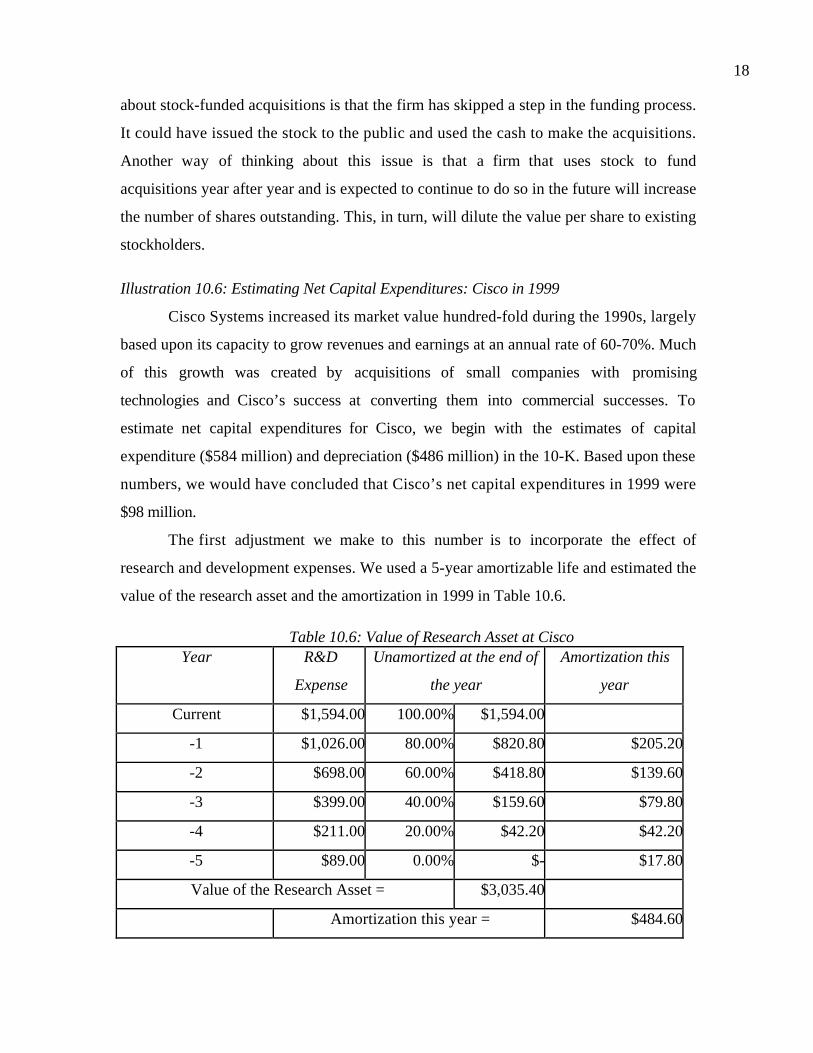
18

about stock-funded acquisitions is that the firm has skipped a step in the funding process.

It could have issued the stock to the public and used the cash to make the acquisitions.

Another way of thinking about this issue is that a firm that uses stock to fund

acquisitions year after year and is expected to continue to do so in the future will increase

the number of shares outstanding. This, in turn, will dilute the value per share to existing

stockholders.

Illustration 10.6: Estimating Net Capital Expenditures: Cisco in 1999

Cisco Systems increased its market value hundred-fold during the 1990s, largely

based upon its capacity to grow revenues and earnings at an annual rate of 60-70%. Much

of this growth was created by acquisitions of small companies with promising

technologies and Cisco’s success at converting them into commercial successes. To

estimate net capital expenditures for Cisco, we begin with the estimates of capital

expenditure ($584 million) and depreciation ($486 million) in the 10-K. Based upon these

numbers, we would have concluded that Cisco’s net capital expenditures in 1999 were

$98 million.

The first adjustment we make to this number is to incorporate the effect of

research and development expenses. We used a 5-year amortizable life and estimated the

value of the research asset and the amortization in 1999 in Table 10.6.

Table 10.6: Value of Research Asset at CiscoYear R&D

Expense

Unamortized at the end of

the year

Amortization this

year

Current $1,594.00 100.00% $1,594.00

-1 $1,026.00 80.00% $820.80 $205.20

-2 $698.00 60.00% $418.80 $139.60

-3 $399.00 40.00% $159.60 $79.80

-4 $211.00 20.00% $42.20 $42.20

-5 $89.00 0.00% $- $17.80

Value of the Research Asset = $3,035.40

Amortization this year = $484.60

19

We adjusted the net capital expenditures for Cisco by adding back the R&D expenses in

the most recent financial year ($1,594 million) and subtracting the amortization of the

research asset ($485 million).

The second adjustment is to bring in the effect of acquisitions that Cisco made

during the last financial year. Table 10.7 summarizes the acquisitions made during the

year and the price paid on these acquisitions.

Table 10.7: Cisco’s Acquisitions: 1999 Financial Year(in millions)

Acquired Method of Acquisition Price Paid

GeoTel Pooling 1344

Fibex Pooling 318

Sentient Pooling 103

American Internet Corporation Purchase 58

Summa Four Purchase 129

Clarity Wireless Purchase 153

Selsius Systems Purchase 134

PipeLinks Purchase 118

Amteva Technologies Purchase 159

$2516

Note that both purchase and pooling transactions are included and that the sum total of

these acquisitions is added on to net capital expenditures in 1999. We are assuming, given

Cisco’s track record, that its acquisitions in 1999 are not unusual and reflect Cisco’s

reinvestment policy. The amortization associated with these acquisitions is already

included as part of depreciation by the firm3. Table 10.8 summarizes the final net capital

expenditures for Cisco.

Table 10.8: Net Capital Expenditures: Cisco in 1999

Capital Expenditures $584.00

- Depreciation $486.00

3 It is only the tax-deductible amortization that really matters. To the extent that amortization is not taxdeductible, you would look at the EBIT before the amortization and not consider it while estimating netcapital expenditures.

20

Net Cap Ex (from

financials)

$98.00

+ R & D Expenditures $1,594.00

- Amortization of R&D $484.60

+ S,G&A Expenditures $-

- Amortization of

S,G&A

$-

+Acquisitions $2,516.00

Adjusted Net Cap Ex $3,723.40

Ignoring Acquisitions in Valuation: A Possibility?

Incorporating acquisitions into net capital expenditures and value can be difficult

and especially so for firms that do large acquisitions infrequently. Predicting whether

there will be acquisitions, how much they will cost and what they will deliver in terms of

higher growth can be close to impossible. There is one way in which you can ignore

acquisitions, but it does come with a cost. If you assume that firms pay a fair price on

acquisitions, i.e. a price that reflects the fair value of the target company and you assume

that the target company stockholders claim any or all synergy or control value,

acquisitions have no effect on value no matter how large they might be and how much

they might seem to deliver in terms of higher growth. The reason is simple. A fair-value

acquisition is an investment that earns it required return – a zero net present value

investment.

If you choose not to consider acquisitions when valuing a firm, you have to remain

internally consistent. The portion of growth that is due to acquisitions should not be

considered in the valuation. A common mistake that is made in valuing companies that

have posted impressive historic growth numbers from an acquisition based strategy is to

extrapolate from this growth and ignore acquisitions at the same time. This will result in

an over valuation of your firm, since you have counted the benefits of the acquisitions but

have not paid for them.

What is the cost of ignoring acquisitions? Not all acquisitions are fairly priced and

not all synergy and control value ends up with the target company stockholders. Ignoring

21

the costs and benefits of acquisitions will result in an under valuation for a firm like Cisco

that has established a reputation for generating value from acquisitions. On the other

hand, ignoring acquisitions can over value firms that routinely over pay on acquisitions.

capex.xls: There is a dataset on the web that summarizes capital expenditures, as

a percent of revenues and firm value, by industry group in the United States for the most

recent quarter.

Investment in Working Capital

The second component of reinvestment is the cash that needs to be set aside for

working capital needs. Increases in working capital tie up more cash and hence generate

negative cash flows. Conversely, decreases in working capital release cash and positive

cash flows.

Defining Working Capital

Working capital is usually defined to be the difference between current assets and

current liabilities. However, we will modify that definition when we measure working

capital for valuation purposes.

• We will back out cash and investments in marketable securities from current

assets. This is because cash, especially in large amounts, is invested by firms in

treasury bills, short term government securities or commercial paper. While the

return on these investments may be lower than what the firm may make on its real

investments, they represent a fair return for riskless investments. Unlike

inventory, accounts receivable and other current assets, cash then earns a fair

return and should not be included in measures of working capital. Are there

exceptions to this rule? When valuing a firm that has to maintain a large cash

balance for day-to-day operations or a firm that operates in a market in a poorly

developed banking system, you could consider the cash needed for operations as a

part of working capital.

• We will also back out all interest bearing debt – short term debt and the portion of

long term debt that is due in the current period – from the current liabilities. This

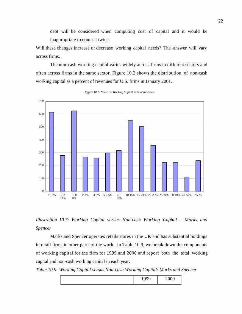
22

debt will be considered when computing cost of capital and it would be

inappropriate to count it twice.

Will these changes increase or decrease working capital needs? The answer will vary

across firms.

The non-cash working capital varies widely across firms in different sectors and

often across firms in the same sector. Figure 10.2 shows the distribution of non-cash

working capital as a percent of revenues for U.S. firms in January 2001.

Illustration 10.7: Working Capital versus Non-cash Working Capital – Marks and

Spencer

Marks and Spencer operates retails stores in the UK and has substantial holdings

in retail firms in other parts of the world. In Table 10.9, we break down the components

of working capital for the firm for 1999 and 2000 and report both the total working

capital and non-cash working capital in each year:

Table 10.9: Working Capital versus Non-cash Working Capital: Marks and Spencer

1999 2000

Figure 10.2: Non-cash Working Capital as % of Revenues

0

100

200

300

400

500

600

700

<-10% -5 to -10%

-5 to0%

0-3% 3-5% 5-7.5% 7.5-10%

10-15% 15-20% 20-25% 25-30% 30-40% 40-50% >50%

23

Cash & Near Cash 282 301

Marketable Securities 204 386

Trade Debtors (Accounts Receivable) 1980 2186

Stocks (Inventory) 515 475

Other Current Assets 271 281

Total Current Assets 3252 3629

Non-Cash Current Assets 2766 2942

Trade Creditors (Accounts Payable) 215 219

Short Term Debt 913 1169

Other Short Term Liabilities 903 774

Total Current Liabilities 2031 2162

Non-debt current liabilities 1118 993

Working Capital 1221 1467

Non-cash Working Capital 1648 1949

The non-cash working capital is substantially higher than the working capital in both

years. We would suggest that the non-cash working capital is a much better measure of

cash tied up in working capital.

Estimating Expected Changes in non-cash Working Capital

While we can estimate the non-cash working capital change fairly simply for any

year using financial statements, this estimate has to be used with caution. Changes in non-

cash working capital are unstable, with big increases in some years followed by big

decreases in the following years. To ensure that the projections are not the result of an

unusual base year, you should tie the changes in working capital to expected changes in

revenues or costs of goods sold at the firm over time. The non-cash working capital as a

percent of revenues can be used, in conjunction with expected revenue changes each

period, to estimate projected changes in non-cash working capital over time. You can

24

obtain the non-cash working capital as a percent of revenues by looking at the firm’s

history or at industry standards.

Should you break working capital down into more detail? In other words, is there

a payoff to estimating individual items such as accounts receivable, inventory and

accounts payable separately? The answer will depend upon both the firm being analyzed

and how far into the future working capital is being projected. For firms where inventory

and accounts receivable behave in very different ways as revenues grow, it clearly makes

sense to break down into detail. The cost, of course, is that it increases the number of

inputs needed to value a firm. In addition, the payoff to breaking working capital down

into individual items will become smaller as we go further into the future. For most firms,

estimating a composite number for non-cash working capital is easier to do and often

more accurate than breaking it down into more detail.

Illustration 10.8: Estimating Non-cash Working Capital Needs – The Gap

As a specialty retailer, the Gap has substantial inventory and working capital

needs. At the end of the 2000 financial year (which concluded January 2001), the Gap

reported $1,904 million in inventory and $335 million in other non-cash current assets. At

the same time, the accounts payable amounted to $1,067 million and other non-interest

bearing current liabilities of $702 million. The non-cash working capital for the Gap in

January 2001 can be estimated.

Non-cash working capital = $1,904 + $335 - $1067 - $ 702 = $470 million

In Table 10.10, we report on the non-cash working capital at the end of the previous year

and the total revenues in each year:

Table 10.10: Working Capital – The Gap

1999 2000 Change

Inventory $1,462 $1,904 $442

Other non-cash CA $285 $335 $50

Accounts Payable $806 $1,067 $261

Other non-interest bearing CL $778 $702 -$76

25

Non-cash Working Capital $163 $470 $307

Revenues $11,635 $13,673 $2,038

Working capital as % of revenues 1.40% 3.44% 15.06%

The non-cash working capital increased by $307 million from last year to this year. When

forecasting the non-cash working capital needs for the Gap, we have several choices.

• One is to use the change in non-cash working capital from the year ($307 million)

and to grow that change at the same rate as earnings are expected to grow in the

future. This is probably the least desirable option because changes in non-cash

working capital from year to year are extremely volatile and last year’s change

may in fact be an outlier.

• The second is to base our changes on non-cash working capital as a percent of

revenues in the most recent year and expected revenue growth in future years. In

the case of the Gap, that would indicate that non-cash working capital changes in

future years will be 3.44% of revenue changes in that year. This is a much better

option than the first one, but the non-cash working capital as a percent of

revenues can also change from one year to the next.

• The third is to base our changes on the marginal non-cash working capital as a

percent of revenues in the most recent year, computed by dividing the change in

non-cash working capital in the most recent year into the change in revenues in the

most recent year, and expected revenue growth in future years. In the case of the

Gap, this would lead to non-cash working capital changes being 15.06% of

revenues in future periods. This approach is best used for firms whose business is

changing and where growth is occurring in areas different from the past. For

instance, a brick and mortar retailer that is growing mostly online may have a very

different marginal working capital requirement than the total.

• The fourth is to base our changes on the non-cash working capital as a percent of

revenues over a historical period. For instance, non-cash working capital as a

percent of revenues between 1997 and 2000 averaged out to 4.5% of revenues.

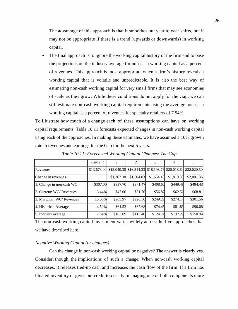
26

The advantage of this approach is that it smoothes out year to year shifts, but it

may not be appropriate if there is a trend (upwards or downwards) in working

capital.

• The final approach is to ignore the working capital history of the firm and to base

the projections on the industry average for non-cash working capital as a percent

of revenues. This approach is most appropriate when a firm’s history reveals a

working capital that is volatile and unpredictable. It is also the best way of

estimating non-cash working capital for very small firms that may see economies

of scale as they grow. While these conditions do not apply for the Gap, we can

still estimate non-cash working capital requirements using the average non-cash

working capital as a percent of revenues for specialty retailers of 7.54%.

To illustrate how much of a change each of these assumptions can have on working

capital requirements, Table 10.11 forecasts expected changes in non-cash working capital

using each of the approaches. In making these estimates, we have assumed a 10% growth

rate in revenues and earnings for the Gap for the next 5 years.

Table 10.11: Forecasted Working Capital Changes: The Gap

Current 1 2 3 4 5

Revenues $13,673.00 $15,040.30 $16,544.33 $18,198.76 $20,018.64 $22,020.50

Change in revenues $1,367.30 $1,504.03 $1,654.43 $1,819.88 $2,001.86

1. Change in non-cash WC $307.00 $337.70 $371.47 $408.62 $449.48 $494.43

2. Current: WC/ Revenues 3.44% $47.00 $51.70 $56.87 $62.56 $68.81

3. Marginal: WC/ Revenues 15.06% $205.97 $226.56 $249.22 $274.14 $301.56

4. Historical Average 4.50% $61.53 $67.68 $74.45 $81.89 $90.08

5. Industry average 7.54% $103.09 $113.40 $124.74 $137.22 $150.94

The non-cash working capital investment varies widely across the five approaches that

we have described here.

Negative Working Capital (or changes)

Can the change in non-cash working capital be negative? The answer is clearly yes.

Consider, though, the implications of such a change. When non-cash working capital

decreases, it releases tied-up cash and increases the cash flow of the firm. If a firm has

bloated inventory or gives out credit too easily, managing one or both components more

27

efficiently can reduce working capital and be a source of positive cash flows into the

immediate future – 3, 4 or even 5 years. The question, however, becomes whether it can

be a source of cash flows for longer than that. At some point in time, there will be no

more inefficiencies left in the system and any further decreases in working capital can

have negative consequences for revenue growth and profits. Therefore, we would suggest

that for firms with positive working capital, decreases in working capital are feasible only

for short periods. In fact, we would recommend that once working capital is being

managed efficiently, the working capital changes from year to year be estimated using

working capital as a percent of revenues. For example, consider a firm that has non-cash

working capital that represent 10% of revenues and that you believe that better

management of working capital could reduce this to 6% of revenues. You could allow

working capital to decline each year for the next 4 years from 10% to 6% and, once this

adjustment is made, begin estimating the working capital requirement each year as 6% of

additional revenues. Table 10.12 provides estimates of the change in non-cash working

capital on this firm, assuming that current revenues are $1 billion and that revenues are

expected to grow 10% a year for the next 5 years.

Table 10.12: Changing Working Capital Ratios and Cashflow Effects

Year Current 1 2 3 4 5

Revenues $1,000.00$1,100.00$1,210.00$1,331.00$1,464.10$1,610.51

Non-Cash WC as % of

Revenues 10% 9% 8% 7% 6% 6%

Non-cash Working Capital $100.00 $99.00 $96.80 $93.17 $87.85 $96.63

Change in Non-cash WC -$1.00 -$2.20 -$3.63 -$5.32 $8.78

Can working capital itself be negative? Again, the answer is yes. Firms whose

current liabilities that exceed non-cash current assets have negative non-cash working

capital. This is a thornier issue that negative changes in working capital. A firm that has a

negative working capital is, in a sense, using supplier credit as a source of capital,

especially if the working capital becomes larger as the firm becomes larger. A number of

28

firms, with Walmart and Dell being the most prominent examples, have used this strategy

to grow. While this may seem like a cost-efficient strategy, there are potential downsides.

The first is that supplier credit is generally not really free. To the extent that delaying

paying supplier bills may lead to the loss of cash discounts and other price breaks, firms

are paying for the privilege. Thus, a firm that decides to adopt this strategy will have to

compare the costs of this capital to more traditional forms of borrowing. The second is

that a negative non-cash working capital has generally been viewed both by accountants

and ratings agencies as a source of default risk. To the extent that a firm’s rating drops and

interest rates paid by the firm increase, there may be costs created for other capital by

using supplier credit as a source. As a practical question, you still have an estimation

problem on your hand when forecasting working capital requirements for a firm that has

negative non-cash working capital. As in the previous scenario, with negative changes in

non-cash working capital, there is no reason why firms cannot continue to use supplier

credit as a source of capital in the short term. In the long term, however, we should not

assume that non-cash working capital will become more and more negative over time. At

some point in time in the future, you have to either assume that the change in non-cash

working capital is zero or that pressure will build for increases in working capital (and

negative cash flows)

wcdata.xls: There is a dataset on the web that summarizes non-cash working

capital needs by industry group in the United States for the most recent quarter.

Summary

When valuing a firm, the cash flows that are discounted should be after taxes and

reinvestment needs but before debt payments. In this chapter, we considered some of the

challenges in coming up with this number for firms.

We began the chapter with the corrected and updated version of operating income

described in chapter 9. To state this operating income in after-tax terms, we need a tax

rate. Firms generally state their effective tax rates in their financial statements, but these

effective tax rates can be different from marginal tax rates. While the effective tax rate can

29

be used to arrive at the after-tax operating income in the current period, the tax rate used

should converge on the marginal tax rate in future periods. For firms that are losing money

and not paying taxes, the net operating losses that they are accumulating will protect

some of their future income from taxation.

The reinvestment that firms make in their own operations is then considered in

two parts. The first part is the net capital expenditure of the firm which is the difference

between capital expenditures (a cash outflow) and depreciation (effectively a cash

inflow). In this net capital expenditure, we include the capitalized operating expenses

(such as R&D) and acquisitions. The second part relates to investments in non-cash

working capital, mainly inventory and accounts receivable. Increases in non-cash working

capital represent cash outflows to the firm, while decreases represent cash inflows. Non-

cash working capital at most firms tends to be volatile and may need to be smoothed out

when forecasting future cash flows.

30

Problems

1. The following is the balance sheet for Ford Motor Company as of December 31, 1994

(in millions).

Assets Liabilities

Cash $ 19,927 Accounts Payable $ 11,635

Receivables $ 132,904 Debt due within 1 year $ 36,240

Inventory $ 10,128 Other Current Liabilities $ 2,721

Current Assets $ 91,524 Current Liabilities $ 50,596

Fixed Assets $ 45,586 Short Term Debt $ 36,200

Long Term Debt $ 37,490

Equity $ 12,824

Total Assets $137,110 Total Liabilities $ 137,110

The firm had revenues of $154,951 million in 1994 and cost of goods sold of $103,817

million.

a. Estimate the net working capital

b. Estimate the non-cash working capital.

c. Why is Ford’s working capital so high? If you were told that Ford Capital (the

financing arm of Ford) was consolidated into this balance sheet, would that help you with

your explanation?

d. Estimate non-cash working capital as a percent of revenues. If you were asked

to estimate the non-cash working capital needs for a new automobile factory that

Ford was constructing, would you use this ratio? Why or why not?

2. You are analyzing the balance sheet for Bed, Bath and Beyond, a retail firm that sells

home furnishings, from February 26, 1995 (in millions).

Assets Liabilities

Cash $ 6.5 Accounts Payable $ 27.5

Receivables $ 0.0 Other Current Liabilities $ 18.6

Inventory $ 108.4

Current Assets $ 118.0 Current Liabilities $ 46.1

Fixed Assets $ 53.8 Long Term Debt $ 16.8

31

Equity $ 108.9

Total Assets $ 171.8 Total Liabilities $ 171.8

The firm had revenues of $440.3 million in 1994 and cost of goods sold of $249.2 million.

a. Estimate the net working capital

b. Estimate the non-cash working capital.

c. Estimate non-cash working capital as a percent of revenues. If you were asked

to estimate the non-cash working capital needs for a new store for Bed, Bath and

Beyond, would you use this ratio? Why or why not?

3. You have been provided with the current assets and current liabilities of a retailing firm

each quarter for the last 5 years, together with the revenues in each quarter.

Period Non-cash current assets Non-debt current liabilities Revenues1990 – 1 $ 300 $ 150 $ 3,0001990 – 2 $ 325 $ 160 $ 3,2201990 – 3 $ 350 $ 180 $ 3,4501990 – 4 $ 650 $ 300 $ 6,3001991 – 1 $ 370 $ 170 $ 3,5501991 – 2 $ 400 $ 200 $ 4,1001991 – 3 $ 420 $ 220 $ 4,3501991 – 4 $ 755 $ 380 $ 7,7501992 – 1 $ 450 $ 220 $ 4,5001992 – 2 $ 480 $ 240 $ 4,7501992 – 3 $ 515 $ 265 $ 5,2001992 – 4 $ 880 $ 460 $ 9,0001993 – 1 $ 550 $ 260 $ 5,4001993 – 2 $ 565 $ 285 $ 5,6001993 – 3 $ 585 $ 300 $ 5,9001993 – 4 $ 1,010 $ 500 $ 10,0001994 – 1 $ 635 $ 330 $ 6,5001994 – 2 $ 660 $ 340 $ 6,7501994 – 3 $ 665 $ 340 $ 6,900

a. Based on this information, estimate the non-cash working capital each quarter.

b. Estimate non-cash working capital as a percent of revenues each quarter.

c. Assume that you are told that there are economies of scale, when it comes to

inventories. How would you test to see if there are any? What would your

conclusions be?

32

1

CHAPTER 11

ESTIMATING GROWTH

The value of a firm is the present value of expected future cash flows generated by

the firm. The most critical input in valuation, especially for high growth firms, is the

growth rate to use to forecast future revenues and earnings. In this chapter, we consider

how best to estimate these growth rates for firms, including those with low revenues and

negative earnings.

There are three basic ways of estimating growth for any firm. One is to look at the

growth in a firm’s past earnings – its historical growth rate. While this can be a useful

input when valuing stable firms, there are both dangers and limitations in using this

growth rate for high growth firms. The historical growth rate can often not be estimated,

and even if it can, it cannot be relied on as an estimate of expected future growth.

The second is to trust the equity research analysts that follow the firm to come up

with the right estimate of growth for the firm and to use that growth rate in valuation.

While many firms are widely followed by analysts, the quality of growth estimates,

especially over longer periods, is poor. Relying on these growth estimates in a valuation

can lead to erroneous and inconsistent estimates of value.

The third is to estimate the growth from a firm’s fundamentals. A firm’s growth

ultimately is determined by how much is reinvested into new assets and the quality of

these investments, with investments widely defined to include acquisitions, building up

distribution channels or even expanding marketing capabilities. By estimating these

inputs, you are, in a sense, estimating a firm’s fundamental growth rate. While the

determinants of fundamental growth remain the same for all firms, estimating these inputs

for high growth firms can pose special challenges.

The Importance of Growth

A firm can be valuable because it owns assets that generate cash flows now or

because it is expected to acquire such assets in the future. The first group of assets is

categorized as assets in place and the second as growth assets. Figure 11.1 presents a

financial balance sheet for a firm:

2

Assets Liabilities

Investments alreadymade

Debt

Equity

Borrowed money

Owner’s fundsInvestments yet tobe made

Existing InvestmentsGenerate cashflows today

Expected Value that will be created by future investments

Figure 11.1: A Financial View of a Firm

Note that an accounting balance sheet can be very different from a financial balance sheet,

since accounting for growth assets tends to be both conservative and inconsistent.

For high growth firms, accounting balance sheets do a poor job of summarizing the

values of the assets of the firm because they completely ignore the largest component of

value, which is future growth. The problems are exacerbated for firms that invest in

research because the book value will not include the most important asset at these firms –

the research asset.

Historical Growth

When estimating the expected growth for a firm, we generally begin by looking at

the firm’s history. How rapidly have the firm’s operations as measured by revenues or

earnings grown in the recent past? While past growth is not always a good indicator of

future growth, it does convey information that can be valuable while making estimates for

the future. In this section, we begin by looking at measurement issues that arise when

estimating past growth and then consider how past growth can be used in projections.

Estimating Historical Growth

Given a firm’s earnings history, estimating historical growth rates may seem like a

simple exercise but there are several measurement problems that may arise. In particular,

the average growth rates can be different, depending upon how the average is estimated,

and whether you allow for compounding in the growth over time. Estimating growth rates

can also be complicated by the presence of negative earnings in the past or in the current

period.

3

Arithmetic versus Geometric Averages

The average growth rate can vary depending upon whether it is an arithmetic

average or a geometric average. The arithmetic average is the simple average of past

growth rates, while the geometric mean takes into account the compounding that occurs

from period to period.

Arithmetic Average =

gtt =−n

t =−1

∑n

where gt = growth rate in year t

Geometric Average =Earnings0

Earnings−n

(1/ n)

−1 where Earnings-n = earnings in n years ago

The two estimates can be very different, especially for firms with volatile earnings. The

geometric average is a much more accurate measure of true growth in past earnings,

especially when year-to-year growth has been erratic.

In fact, the point about arithmetic and geometric growth rates also applies to

revenues, though the difference between the two growth rates tend to be smaller for

revenues than for earnings. For firms with volatile earnings and revenues, the caveats

about using arithmetic growth carry even more weight.

Illustration 11.1: Differences between Arithmetic and Geometric Averages: Motorola

Table 11.1 reports the revenues, EBITDA, EBIT and net income for Motorola for

each year from 1994 to 1999. The arithmetic and geometric average growth rates in each

series are reported at the bottom of the table:

Table 11.1: Arithmetic and Geometric Average Growth Rates: Motorola

Year Revenues % Change EBITDA % Change EBIT % Change

Net

Income % Change

1994 $ 22,245 $ 4,151 $ 2,604 $ 1,560

1995 $ 27,037 21.54% $ 4,850 16.84% $ 2,931 12.56% $ 1,781 14.17%

1996 $ 27,973 3.46% $ 4,268 -12.00% $ 1,960 -33.13% $ 1,154 -35.20%

1997 $ 29,794 6.51% $ 4,276 0.19% $ 1,947 -0.66% $ 1,180 2.25%

1998 $ 29,398 -1.33% $ 3,019 -29.40% $ 822 -57.78% $ 212 -82.03%

4

1999 $ 30,931 5.21% $ 5,398 78.80% $ 3,216 291.24% $ 817 285.38%

Arithmetic Average 7.08% 10.89% 42.45% 36.91%

Geometric Average 6.82% 5.39% 4.31% -12.13%

Standard deviation 8.61% 41.56% 141.78% 143.88%

Geometric Average = (Earnings1999/Earnings1994)1/5-1

The arithmetic average growth rate is higher than the geometric average growth rate

for all four items, but the difference is much larger with net income and operating income

(EBIT) than it is with revenues and EBITDA. This is because the net and operating

income are the most volatile of the numbers, with a standard deviation in year-to-year

changes of almost 140%. Looking at the net and operating income in 1994 and 1999, it is

also quite clear that the geometric averages are much better indicators of true growth.

Motorola’s operating income grew only marginally during the period and this is reflected

in its geometric average growth rate, which is 4.31%, but not in its arithmetic average

growth rate, which indicates much faster growth. Motorola’s net income dropped by

almost 50% during the period. This is reflected in its negative geometric average growth

rate but its arithmetic average growth rate is 36.91%.

Linear and Log-linear Regression Models

The arithmetic mean weights percentage changes in earnings in each period equally

and ignores compounding effects in earnings. The geometric mean considers compounding

but focuses on the first and the last earnings observations in the series - it ignores the

information in the intermediate observations and any trend in growth rates that may have

developed over the period. These problems are at least partially overcome by using OLS1

regressions of earnings per share (EPS) against time. The linear version of this model is:

EPSt = a + b t

where,

EPSt = Earnings per share in period t

t = Time period t

1 An ordinary least squares (OLS) regression estimates regression coefficients by minimizing the squareddifferences of predicted from actual values.

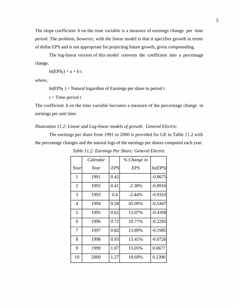
5

The slope coefficient b on the time variable is a measure of earnings change per time

period. The problem, however, with the linear model is that it specifies growth in terms

of dollar EPS and is not appropriate for projecting future growth, given compounding.

The log-linear version of this model converts the coefficient into a percentage

change.

ln(EPSt) = a + b t

where,

ln(EPSt ) = Natural logarithm of Earnings per share in period t

t = Time period t

The coefficient b on the time variable becomes a measure of the percentage change in

earnings per unit time.

Illustration 11.2: Linear and Log-linear models of growth: General Electric.

The earnings per share from 1991 to 2000 is provided for GE in Table 11.2 with

the percentage changes and the natural logs of the earnings per shares computed each year.

Table 11.2: Earnings Per Share: General Electric

Year

Calendar

Year EPS

% Change in

EPS ln(EPS)

1 1991 0.42 -0.8675

2 1992 0.41 -2.38% -0.8916

3 1993 0.4 -2.44% -0.9163

4 1994 0.58 45.00% -0.5447

5 1995 0.65 12.07% -0.4308

6 1996 0.72 10.77% -0.3285

7 1997 0.82 13.89% -0.1985

8 1998 0.93 13.41% -0.0726

9 1999 1.07 15.05% 0.0677

10 2000 1.27 18.69% 0.2390

6

There are a number of ways in which we can estimate the growth rate in earnings per

share at GE between 1991 and 2000. One is to compute the arithmetic and geometric

averages.

Arithmetic average growth rate in earnings per share = 13.79%

Geometric average growth rate in earnings per share = (1.27/0.42)1/9-1 = 13.08%

The second is to run a linear regression of earnings per share against a time variable (where

the earliest year is given a value of 1, the next year a value of 2 and so on):

Linear Regression : EPS = 0.2033 + 0.0952 t R2 = 94.5%

(4.03) (11.70)

This regression would indicate that the earnings per share increased 9.52 cents a year from

1991 to 2000. We can convert it into a percentage growth in earnings per share by

dividing this change by the average earnings per share over the period.

Growth rate in earnings per share =

%10.13727.0

0952.0

EPS Average

regressionlinear on t Coefficien ==

Finally, you can regress ln(EPS) against the time variable.

Log-linear Regression: ln (EPS) = -1.1288 + 0.1335 t R2=96.3%

(19.53) (14.34)

The coefficient on the time variable here can be viewed as a measure of compounded

percent growth in earnings per share; GE’s earnings per share grew at 13.35% a year

based upon this regression.

The numbers are close using all of the approaches because there is so little

variability in the growth rate of earnings per share at GE. For companies with more

volatile earnings, the differences will be much larger.

Negative Earnings

Measures of historical growth are distorted by the presence of negative earnings

numbers. The percentage change in earnings on a year-by-year basis is defined as:

% change in EPS in period t = 1EPS

EPS

EPS

EPS-EPS

1-t

t

1-t

1-tt −=

7

If EPSt-1 is negative or zero, this calculation yields a meaningless number. This extends

into the calculation of the geometric mean. If the EPS in the initial time period is negative

or zero, the geometric mean is not meaningful.

Similar problems arise in log-linear regressions, since the EPS has to be greater

than zero for the log transformation to exist. There are at least two ways of trying to get

meaningful estimates of earnings growth for firms with negative earnings. One is to run

the linear regression of EPS against time specified in the previous regression.

EPS = a + b t

The growth rate can then be approximated as follows:

Growth rate in EPS = regression theof period timeover the EPS Average

b

This assumes that the average EPS over the time period is positive. Another approach to

estimating growth for these firms, suggested by Arnott, is as follows:

% change in EPS = ( )1-tt

1-tt

EPS,EPSMax

EPS-EPS

Alternatively, you could use the absolute value of earnings per share in the previous

period.

Note that these approaches to estimating historical growth rates do not provide

any information on whether these growth rates are useful in predicting future growth. It is

not incorrect and, in fact, it may be appropriate, to conclude that the historical growth

rate is 'not meaningful' when earnings are negative and to ignore it in predicting future

growth. While there are ways of estimating growth even when earnings are negative, the

resulting growth rates are not very useful indicators of past growth and it is best to view

the past growth as not meaningful in those cases.

Illustration 11.3: Negative Earnings: Commerce One and Aracruz Celulose

The problems with estimating earnings growth when earnings are negative can be

seen even for firms that have only negative earnings. For instance, Commerce One, the

B2B firm, reported operating earnings (EBIT) of -$53 million in 1999 and -$340 million in

2000. Clearly, the firm’s earnings deteriorated, but estimating a standard earnings growth

rate would lead us to the following growth rate:

8

Earnings growth for Commerce One in 2000= ( )

541%5.4153-

53--340- ==

Now consider Aracruz, a Brazilian paper and pulp company, susceptible like

other firms in the industry to the ebbs and flows of commodity prices. Table 11.3 reports

the earnings per share at the firm from 1995 to 2000.

Table 11.3: EPS at Aracruz Celulose in Brazilian Real: 1995-2000

Year EPS

1995 0.302

1996 0.041

1997 0.017

1998 -0.067

1999 0.065

2000 0.437

The negative net income (and earnings per share) numbers in 1998 make the estimation of

a growth rate in 1999 problematic. For instance, the firm has a loss per share of 0.067 BR

in 1998 and a profit per share of 0.065 BR in 1999. The growth rate in earnings per share

estimated using the conventional equation, would be:

Earnings growth rate in 1999 = ( )

%19797.10670

06700650 −=−=− .

.--.

This growth rate, a negative number, makes no sense given the improvement in earnings

during the year. There are two fixes to this problem. One is to replace the actual earnings

per share in the denominator with the absolute value:

Earnings growth rate in 1999absolute value = ( )

%19797.1067.0

0.067--0.065 ==

The other is to use the higher of the earnings per share from the two years yielding:

Earnings growth rate in 1999Higher value= ( )

%20303.2065.0

0.067--0.065 ==

While the growth rate is now positive, as you would expect it to be, the values for the

growth rates themselves are not very useful for making estimates for the future.

Time Series Models to predict Earnings per share

9

Time series models use the same historical information as the simpler models

described in the previous section. They attempt to extract better predictions from this

data, however, through the use of sophisticated statistical techniques.

Box-Jenkins Models

Box and Jenkins developed a procedure for analyzing and forecasting univariate

time series data using an autoregressive integrated moving average model. AutoRegressive

Integrated Moving Average (ARIMA) models a value in a time series as a linear

combination of past values and past errors (shocks). Since historical data is used, these

models are appropriate as long as the data does not show deterministic behavior, such as a

time trend or a dependence on outside events or variables. ARIMA models are usually

denoted by the notation:

ARIMA (p, d, q)

where,

p is the degree of the autoregressive part

d is the degree of differencing

q is the degree of the moving average process

The mathematical model can then be written as follows:

tqtqttptptt aaawww +−−−−++++ −−−−−−= ......w 221102111t

where,

wt = Original data series or difference of degree d of the original data

φ1, φ2, ..., φp = Autoregressive parameters

θ0 = Constant term

θ1, θ2, ..., θq = Moving average parameters

εt = Independent disturbances, random error

ARIMA models can also adjust for seasonality in the data, in which case the model is

denoted by the notation.

SARIMA (p,d,q) X (p,d,q) s=n

where,

s = Seasonal parameter of length n

10

Time Series Models in Earnings

Most time series models used in forecasting earnings are built around quarterly

earnings per share. In a survey paper, Bathke and Lorek (1984) pointed out that three

time-series models have been shown to be useful in forecasting quarterly earnings per

share. All three models are seasonal autoregressive integrated moving average (SARIMA)

models, since quarterly earnings per share have a strong seasonal component. The first

model, developed by Foster (1977), allows for seasonality in earnings.

Model 1: SARIMA (1,0,0) X (0,1,0)s=4

t05-t14-t1-t1t EPSEPSEPS EPS ++−+=

This model was extended by Griffin and Watts to allow for a moving average parameter.

Model 2: SARIMA (0,1,1) X (0,1,1)s=4

t 5-t 14-t1-t15-t4-t1-tt - --EPS-EPSEPSEPS +ΘΘ+=

where,

θ1 = First-order moving average (MA(1)) parameter

Θ = First-order seasonal moving average parameter

εt = Disturbance realization at the end of quarter t

The third time series model, developed by Brown and Rozeff (1979), is similar in its use

of seasonal moving average parameter.

Model 3: SARIMA (1,0,0) X (0,1,1)s=4

EPS-EPSEPSEPS 4-t05-t14-t1-t1t Θ−++=

How good are time series models at predicting earnings?

Time series models do better than naive models (using past earnings) in predicting

earnings per share in the next quarter. The forecast error, i.e., the difference between the

actual earnings per share and forecasted earnings per share, from the time series models is,

on average, smaller than the forecast error from naive models (such as simple averages of

past growth). The superiority of the models over naive estimates declines with longer

term forecasts, suggesting that the estimated time series parameters are not stationary.

Among the time series models themselves, there is no evidence that any one model

is dominant, in terms of minimizing forecast error, for every firm in the sample. The gain

11

from using the firm-specific best models relative to using the same model for every firm is

relatively small.

Limitations in using time series models in valuation

In most studies, time series models provide superior forecasts relative to naive

models. There are several concerns, however, in using these models for forecasting

earnings in valuation. First, time series models require a lot of data, which is why most of

them are built around quarterly earnings per share. In most valuation, the focus is on

predicting annual earnings per share and not on quarterly earnings. Second, even with

quarterly earnings per share, the number of observations is limited for most firms to ten

to fifteen years of data (forty to sixty quarters of data), leading to large estimation errors2

in time-series model parameters and in the forecasts. Third, the superiority of earnings

forecasts from time series models declines as the forecasting period is extended. Given

that earnings forecasts in valuation have to be made for several years rather than a few

quarters, the value of time series models may be limited. Finally, studies indicate that

analyst forecasts dominate even the best time series models in forecasting earnings.

In conclusion, time series models are likely to work best for firms which have a

long history of earnings and where the parameters of the models have not shifted

significantly over time. For the most part, however, the cost of using these models is

likely to exceed their benefits, at least in the context of valuation.

The Usefulness of Historical Growth

Is the growth rate in the past a good indicator of growth in the future? Not

necessarily. In this section we consider how good historical growth is as a predictor of

future growth for all firms and why the changing size and volatile businesses of many

firms can undercut growth projections.

Higgledy Piggledy Growth

Past growth rates are useful in forecasting future growth, but they have

considerable noise associated with them. In a study of the relationship between past

2 Time series models generally can be run as long as there at least thirty observations, but the estimation

12

growth rates and future growth rates, Little (1960) coined the term "Higgledy Piggledy

Growth" because he found little evidence that firms that grew fast in one period continued

to grow fast in the next period. In the process of running a series of correlations between

growth rates in earnings in consecutive periods of different length, he frequently found

negative correlations between growth rates in the two periods and the average correlation

across the two periods was close to zero (0.02). If past growth in earnings is not a

reliable indicator of future growth at many firms, it becomes even less so at smaller firms.

The growth rates at smaller firms tend to be even more volatile than growth rates at other

firms in the market. The correlation between growth rates in earnings in consecutive time

periods (five-year, three-year and one-year) for firms in the United States, categorized by

market value, is reported in Figure 11.2.

Figure 11.3: Correlations in Earnings Growth by Market Capitalization

0.00

0.05

0.10

0.15

0.20

0.25

0.30

0.35

0.40

0.45

0.50

Correlation between 90-94 and 95-99 Correlation between 94-96 and 97-99 Correlation between 1998 and 1998

Small Cap firmsMidcap Firms

Large Cap firm

While the correlations tend to be higher across the board for one-year growth rates than

for 3-year or 5-year growth rates in earnings, they are also consistently lower for smaller

firms than they are for the rest of the market. This would suggest that you should be

error declines as the number of observations increases.

13

more cautious about using past growth, especially in earnings, for forecasting future

growth at these firms.

Revenue Growth versus Earnings Growth

In general, revenue growth tends to be more persistent and predictable than

earnings growth. This is because accounting choices have a far smaller effect on revenues

than they do on earnings. Figure 11.4 compares the correlations in revenue and earnings

growth over one-year, three-year and five-year periods at U.S. firms.

Source: Compustat

Revenue growth is consistently more correlated over time than earnings growth. The

implication is that historical growth in revenues is a far more useful number when it

comes to forecasting than historical growth in earnings.

The Effects of Firm Size

Since the growth rate is stated in percentage terms, the role of size has to be

weighed in the analysis. It is easier for a firm with $10 million in earnings to generate a

50% growth rate than it is for a firm with $500 million in earnings to generate the same

Figure 11.4: Correlation in Revenues and Earnings

0

0.05

0.1

0.15

0.2

0.25

0.3

0.35

0.4

0.45

0.5

Correlation between 90-94 and 95-99 Correlation between 94-96 and 97-99 Correlation between 1998 and 1998

Revenues

Earnings

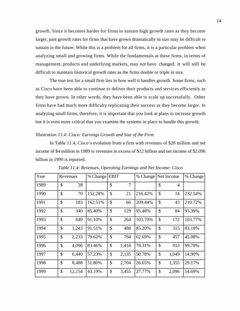
14

growth. Since it becomes harder for firms to sustain high growth rates as they become

larger, past growth rates for firms that have grown dramatically in size may be difficult to

sustain in the future. While this is a problem for all firms, it is a particular problem when

analyzing small and growing firms. While the fundamentals at these firms, in terms of

management, products and underlying markets, may not have changed, it will still be

difficult to maintain historical growth rates as the firms double or triple in size.

The true test for a small firm lies in how well it handles growth. Some firms, such

as Cisco have been able to continue to deliver their products and services efficiently as

they have grown. In other words, they have been able to scale up successfully. Other

firms have had much more difficulty replicating their success as they become larger. In

analyzing small firms, therefore, it is important that you look at plans to increase growth

but it is even more critical that you examine the systems in place to handle this growth.

Illustration 11.4: Cisco: Earnings Growth and Size of the Firm

In Table 11.4, Cisco’s evolution from a firm with revenues of $28 million and net

income of $4 million in 1989 to revenues in excess of $12 billion and net income of $2.096

billion in 1999 is reported.

Table 11.4: Revenues, Operating Earnings and Net Income: Cisco

Year Revenues % Change EBIT % Change Net Income % Change

1989 $ 28 $ 7 $ 4

1990 $ 70 152.28% $ 21 216.42% $ 14 232.54%

1991 $ 183 162.51% $ 66 209.44% $ 43 210.72%

1992 $ 340 85.40% $ 129 95.48% $ 84 95.39%

1993 $ 649 91.10% $ 264 103.70% $ 172 103.77%

1994 $ 1,243 91.51% $ 488 85.20% $ 315 83.18%

1995 $ 2,233 79.62% $ 794 62.69% $ 457 45.08%

1996 $ 4,096 83.46% $ 1,416 78.31% $ 913 99.78%

1997 $ 6,440 57.23% $ 2,135 50.78% $ 1,049 14.90%

1998 $ 8,488 31.80% $ 2,704 26.65% $ 1,355 29.17%

1999 $ 12,154 43.19% $ 3,455 27.77% $ 2,096 54.69%

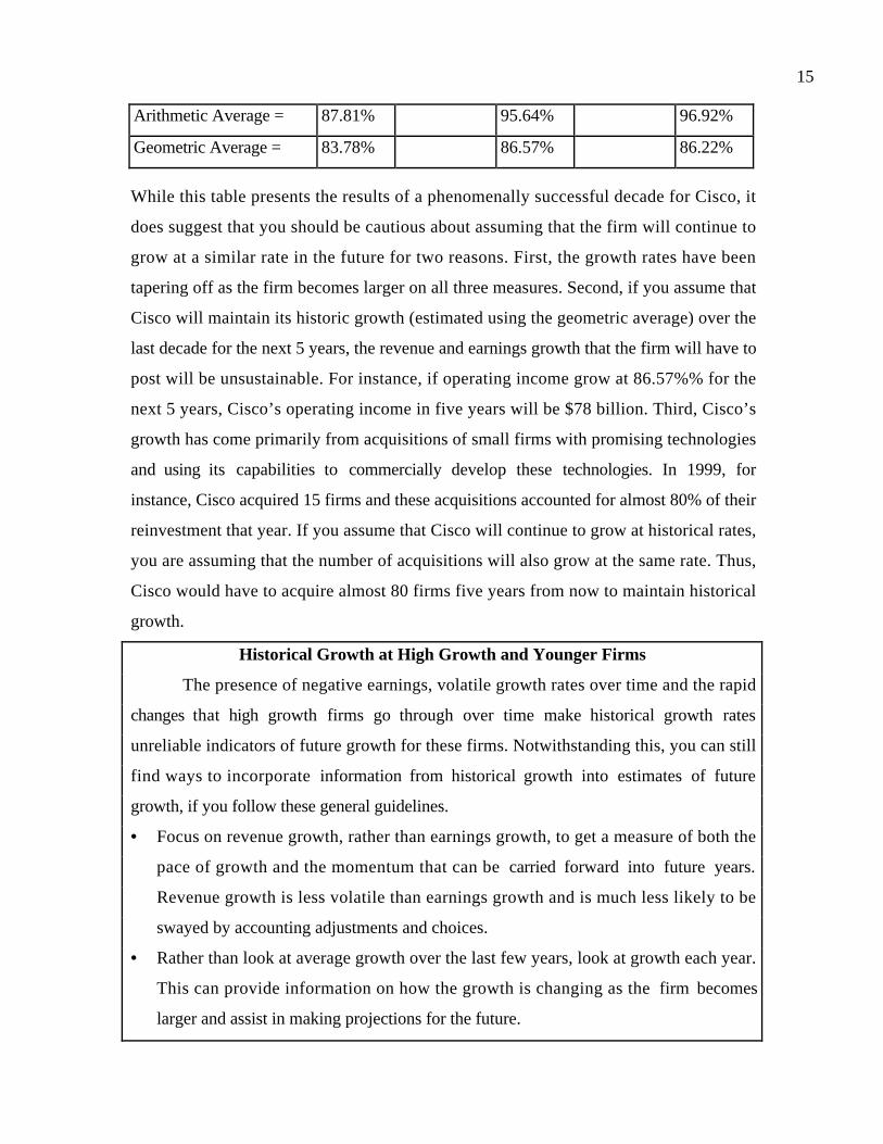
15

Arithmetic Average = 87.81% 95.64% 96.92%

Geometric Average = 83.78% 86.57% 86.22%

While this table presents the results of a phenomenally successful decade for Cisco, it

does suggest that you should be cautious about assuming that the firm will continue to

grow at a similar rate in the future for two reasons. First, the growth rates have been

tapering off as the firm becomes larger on all three measures. Second, if you assume that

Cisco will maintain its historic growth (estimated using the geometric average) over the

last decade for the next 5 years, the revenue and earnings growth that the firm will have to

post will be unsustainable. For instance, if operating income grow at 86.57%% for the

next 5 years, Cisco’s operating income in five years will be $78 billion. Third, Cisco’s

growth has come primarily from acquisitions of small firms with promising technologies

and using its capabilities to commercially develop these technologies. In 1999, for

instance, Cisco acquired 15 firms and these acquisitions accounted for almost 80% of their

reinvestment that year. If you assume that Cisco will continue to grow at historical rates,

you are assuming that the number of acquisitions will also grow at the same rate. Thus,

Cisco would have to acquire almost 80 firms five years from now to maintain historical

growth.

Historical Growth at High Growth and Younger Firms

The presence of negative earnings, volatile growth rates over time and the rapid

changes that high growth firms go through over time make historical growth rates

unreliable indicators of future growth for these firms. Notwithstanding this, you can still

find ways to incorporate information from historical growth into estimates of future

growth, if you follow these general guidelines.

• Focus on revenue growth, rather than earnings growth, to get a measure of both the

pace of growth and the momentum that can be carried forward into future years.

Revenue growth is less volatile than earnings growth and is much less likely to be

swayed by accounting adjustments and choices.

• Rather than look at average growth over the last few years, look at growth each year.

This can provide information on how the growth is changing as the firm becomes

larger and assist in making projections for the future.

16

• Use historical growth rates as the basis for projections only in the near future (next

year or two), since technologies can change rapidly and undercut future estimates.

• Consider historical growth in the overall market and in other firms that are serving it.

This information can be useful in deciding what the growth rates of the firm that you

are valuing will converge over time.

histgr.xls: There is a dataset on the web that summarizes historical growth rates

in earnings and revenues by industry group for the United States.

Analyst Estimates of Growth

Equity research analysts provide not only recommendations on the firms they

follow but also estimates of earnings and earnings growth for the future. How useful are

these estimates of expected growth from analysts and how, if at all, can they be used in

valuing technology firms? In this section, you consider the process that analysts follow to

estimate expected growth and follow up by examining why such growth rates may not be

appropriate when valuing some firms.

Who do analysts follow?

The number of analysts tracking firms varies widely across firms. At one extreme

are firms like GE, Cisco and Microsoft that are followed by dozens of analysts. At the

other extreme, there are hundreds of firms that are not followed by any analysts. Figure

11.5 shows the divergence across firms in the United States, in terms of the number of

analysts following them.

17

Why are some firms more heavily followed than others? These seem to be some of the

determinants:

1. Market Capitalization: The larger the market capitalization of a firm, the more

likely it is to be followed by analysts.

2. Institutional Holding: The greater the percent of a firm’s stock that is held by

institutions, the more likely it is to be followed by analysts. The open question,

though, is whether analysts follow institutions or whether institutions follow

analysts. Given that institutional investors are the biggest clients of equity

research analysts, the causality probably runs both ways.

3. Trading Volume: Analysts are more likely to follow liquid stocks. Here again,

though, it is worth noting that the presence of analysts and buy (or sell)

recommendations on a stock may play a role in increasing trading volume.

The Information in Analyst Forecasts

There is a simple reason to believe that analyst forecasts of growth should be

better than using historical growth rates. Analysts, in addition to using historical data, can

avail themselves of other information that may be useful in predicting future growth.

Figure 11.5: Number of analysts estimating earnings per shar: U.S. firms in January 2001

0

200

400

600

800

1000

1200

1400

1600

1800

2000

No analysts 1 - 2 3 - 4 5 - 8 9 - 12 13-16 17 - 20 21-24 >25

18

1. Firm-specific information that has been made public since the last earnings report

Analysts can use information that has come out about the firm since the last

earnings report, to make predictions about future growth. This information can sometimes

lead to significant re-evaluation of the firm's expected cash flows.

2. Macro-economic information that may impact future growth

The expected growth rates of all firms are affected by economic news on GNP

growth, interest rates and inflation. Analysts can update their projections of future

growth as new information comes out about the overall economy and about changes in

fiscal and monetary policy. Information, for instance, that shows the economy growing at

a faster rate than forecast will result in analysts increasing their estimates of expected

growth for cyclical firms.

3. Information revealed by competitors on future prospects

Analysts can also condition their growth estimates for a firm on information

revealed by competitors on pricing policy and future growth. For instance, a negative

earnings report by one telecommunications firm can lead to a reassessment of earnings for

other telecommunication firms.

4. Private information about the firm

Analysts sometimes have access to private information about the firms they

follow which may be relevant in forecasting future growth. This avoids answering the

delicate question of when private information becomes illegal inside information. There is

no doubt, however, that good private information can lead to significantly better estimates

of future growth. In an attempt to restrict this type of information leakage, the SEC

issued new regulations in 2000 preventing firms from selectively revealing information to

a few analysts or investors. Outside the United States, however, firms routinely convey

private information to analysts following them.

5. Public information other than earnings

Models for forecasting earnings that depend entirely upon past earnings data may

ignore other publicly available information that is useful in forecasting future earnings. It

19

has been shown, for instance, that other financial variables such as earnings retention,

profit margins and asset turnover are useful in predicting future growth. Analysts can

incorporate information from these variables into their forecasts.

The Quality of Earnings Forecasts3

If firms are followed by a large number of analysts and these analysts are indeed

better informed than the rest of the market, the forecasts of growth that emerge from

analysts should be better than estimates based upon either historical growth or other

publicly available information. But is this presumption justified? Are analyst forecasts of

growth superior to other forecasts?

The general consensus from studies that have looked at short-term forecasts (one

quarter ahead to four quarters ahead) of earnings is that analysts provide better forecasts

of earnings than models that depend purely upon historical data. The mean relative

absolute error, which measures the absolute difference between the actual earnings and the

forecast for the next quarter, in percentage terms, is smaller for analyst forecasts than it is

for forecasts based upon historical data. Two other studies shed further light on the value

of analysts' forecasts. Crichfield, Dyckman and Lakonishok (1978) examine the relative

accuracy of forecasts in the Earnings Forecaster, a publication from Standard and Poors

that summarizes forecasts of earnings from more than 50 investment firms. They measure

the squared forecast errors by month of the year and compute the ratio of analyst forecast

error to the forecast error from time-series models of earnings. They find that the time

series models actually outperform analyst forecasts from April until August, but

underperform them from September through January. They hypothesize that this is

because there is more firm-specific information available to analysts during the latter part

of the year. The other study by O'Brien (1988) compares consensus analyst forecasts

from the Institutions Brokers Estimate System (I/B/E/S) with time series forecasts from

one quarter ahead to four quarters ahead. The analyst forecasts outperform the time series

model for one-quarter ahead and two-quarter ahead forecasts, do as well as the time series

3 Sell side analysts work for brokerage houses and investment banks and their research is offered to clientsof these firms as a service. In contrast, buy side analysts work for institutional investors and their researchis generally proprietary.

20

model for three-quarter ahead forecasts and do worse than the time series model for four-

quarter ahead forecasts. Thus, the advantage gained by analysts from firm-specific

information seems to deteriorate as the time horizon for forecasting is extended.

In valuation, the focus is more on long term growth rates in earnings than on next

quarter's earnings. There is little evidence to suggest that analysts provide superior

forecasts of earnings when the forecasts are over three or five years. An early study by

Cragg and Malkiel compared long term forecasts by five investment management firms in

1962 and 1963 with actual growth over the following three years to conclude that

analysts were poor long term forecasters. This view is contested by Vander Weide and

Carleton (1988) who find that the consensus prediction of five-year growth in the I/B/E/S

is superior to historically oriented growth measures in predicting future growth. There is

an intuitive basis for arguing that analyst predictions of growth rates must be better than

time-series or other historical-data based models simply because they use more

information. The evidence indicates, however, that this superiority in forecasting is

surprisingly small for long term forecasts and that past growth rates play a significant role

in determining analyst forecasts.

There is one final consideration. Analysts generally forecast earnings per share and

most services report these estimates. When valuing a firm, you need forecasts of

operating income and the growth in earnings per share will not be equal to the growth in

operating income. In general, the growth rate in operating income should be lower than the

growth rate in earnings per share. Thus, even if you decide to use analyst forecasts, you

will have to adjust them down to reflect the need to forecast operating income growth.

How do you use analyst forecasts in estimating future growth?

The information in the growth rates estimated by other analysts can and should be

incorporated into the estimation of expected future growth. There are several factors that

determine the weight assigned to analyst forecasts in predicting future growth.

1. Amount of recent firm-specific information

Analyst forecasts have an advantage over historical-data based models because

they incorporate more recent information about the firm and its future prospects. This

advantage is likely to be greater for firms where there have been significant changes in

21

management or business conditions in the recent past, for example, a restructuring or a

shift in government policy relating to the firm's underlying business.

2. Number of analysts following the stock

Generally speaking, the larger the number of analysts following a stock, the more

informative is their consensus forecast and the greater should be the weight assigned to it

in analysis. The informational gain from having more analysts is diminished somewhat by

the well-established fact that most analysts do not act independently and that there is a

high correlation across analysts' revisions of expected earnings.

3. Extent of disagreement between analysts

While consensus earnings growth rates are useful in valuation, the extent of

disagreement between analysts, measured by the standard deviation in growth

predictions, is also a useful measure of the reliability of the consensus forecasts. Givoly

and Lakonsihok find that the dispersion of earnings is correlated with other measures of

risk such as beta and is a good predictor of expected returns.

4. Quality of analysts following the stock

This is the hardest of the variables to quantify. One measure of quality is the size

of the forecast error made by analysts following a stock, relative to models which use

only historical data - the smaller this relative error, the larger the weight that should be

attached to analyst forecasts. Another measure is the effect on stock prices of analyst

revisions - the more informative the forecasts, the greater the effect on stock prices. There

are some who argue that the focus on consensus forecasts misses the point that some

analysts are better than others in predicting earnings and that their forecasts should be

isolated from the rest and weighted more.

Analysts forecasts may be useful in coming up with a predicted growth rate for a

firm but there is a danger to blindly following consensus forecasts. Analysts often make

significant errors in forecasting earnings, partly because they depend upon the same data

sources (which might have been erroneous or misleading) and partly because they

sometimes overlook significant shifts in the fundamental characteristics of the firm. The

secret to successful valuation often lies in discovering inconsistencies between analysts'

22

forecasts of growth and a firm's fundamentals. The next section examines this relationship

in more detail.

The Fundamental Determinants of Growth

With both historical and analyst estimates, growth is an exogenous variable that

affects value but is divorced from the operating details of the firm. The soundest way of

incorporating growth into value is to make it endogenous, i.e., to make it a function of

how much a firm reinvests for future growth and the quality of its reinvestment. We will

begin by considering the relationship between fundamentals and growth in equity income,

and then move on to look at the determinants of growth in operating income.

Growth In Equity Earnings

When estimating cash flows to equity, we usually begin with estimates of net

income, if we are valuing equity in the aggregate, or earnings per share, if we are valuing

equity per share. In this section, we will begin by presenting the fundamentals that

determine expected growth in earnings per share and then move on to consider a more

expanded version of the model that looks at growth in net income.

Growth in Earnings Per Share

The simplest relationship determining growth is one based upon the retention

ratio (percentage of earnings retained in the firm) and the return on equity on its projects.

Firms that have higher retention ratios and earn higher returns on equity should have

much higher growth rates in earnings per share than firms that do not share these

characteristics. To establish this, note that

1-t

1-ttt

NI

NI-NIg =

where,

gt = Growth Rate in Net Income

NIt = Net Income in year t

Given the definition of return on equity, the net income in year t-1 can be written as:

1-t2-t1-t ROE*Equity of ValueBook NI =

where,

23

ROEt-1 = Return on equity in year t-1

The net income in year t can be written as:

( ) t1-t2-tt ROE*Earnings RetainedEquity of ValueBook NI +=

Assuming that the return on equity is unchanged, i.e., ROEt = ROEt-1 =ROE,

( ) ( )( ) ( )( )ROEbROERatio RetainedROENI

Earnings Retainedg

1-t

1-tt ==

=

where b is the retention ratio. Note that the firm is not being allowed to raise equity by

issuing new shares. Consequently, the growth rate in net income and the growth rate in

earnings per share are the same in this formulation.

Illustration 11.5: Growth in Earnings Per Share

In this illustration, we will consider the expected growth rate in earnings based

upon the retention ratio and return on equity for three firms – Consolidated Edison, a

regulated utility that provides power to New York City and its environs, Procter &

Gamble, a leading brand-name consumer product firm and Reliance Industries, a large

Indian manufacturing firm. In Table 11.5, we summarize the returns on equity, retention

ratios and expected growth rates in earnings for the three firms.

Table 11.5: Fundamental Growth Rates in Earnings per Share

Return on

Equity

Retention

Ratio

Expected Growth

Rate

Consolidated Edison 11.63% 29.96% 3.49%

Procter & Gamble 29.37% 49.29% 14.48%

Reliance Industries 19.43% 82.57% 16.04%

Reliance has the highest expected growth rate in earnings per share, assuming that it can

maintain its current return on equity and retention ratio. Procter & Gamble also can be

expected to post a healthy growth rate, notwithstanding the fact that it pays out more

than 50% of its earnings as dividends, because of its high return on equity. Co Ed, on the

other hand, has a very low expected growth rate because its return on equity and retention

ratio are anemic.

24

Growth in Net Income

If we relax the assumption that the only source of equity is retained earnings, the

growth in net income can be different from the growth in earnings per share. Intuitively,

note that a firm can grow net income significantly by issuing new equity to fund new

projects while earnings per share stagnates. To derive the relationship between net income

growth and fundamentals, we need a measure of how investment that goes beyond

retained earnings. One way to obtain such a measure is to estimate directly how much

equity the firm reinvests back into its businesses in the form of net capital expenditures

and investments in working capital.

Equity reinvested in business = (Capital Expenditures – Depreciation + Change in

Working Capital – (New Debt Issued – Debt Repaid))

Dividing this number by the net income gives us a much broader measure of the equity

reinvestment rate:

Equity Reinvestment Rate = IncomeNet

reinvestedEquity

Unlike the retention ratio, this number can be well in excess of 100% because firms can

raise new equity. The expected growth in net income can then be written as:

Expected Growth in Net Income = ( )( )Equityon Return Ratent Reinvestmeity Equ

Illustration 11.6: Growth in Net Income

To estimate growth in operating income based upon fundamentals, we look at

three firms – Coca Cola, Nestle and Sony. In Table 11.6, we first estimate the

components of equity reinvestment and use it to estimate the reinvestment rate for each

of the firms. We also present the return on equity and the expected growth rate in net

income at each of these firms.

Table 11.6: Expected Growth in Net Income

Net

Income

Net Cap

Ex

Change in

Working

Capital

Net Debt

Issued

(paid)

Equity

Reinvestment

Rate ROE

Expected

Growth

Rate

Coca

Cola $ 2177 m 468 852 -$104.00 65.41% 23.12% 15.12%

25

Nestle

SFr

5763m 2470 368 272 44.53% 21.20% 9.44%

Sony

JY

30.24b 26.29 -4.1 3.96 60.28% 1.80% 1.09%

The pluses and minuses of this approach are visible in the table above. The approach

much more accurately captures the true reinvestment in the firm by focusing not on what

was retained but on what was reinvested. The limitation of the approach is that the

ingredients that go into the reinvestment – capital expenditures, working capital change

and net debt issued – are all volatile numbers. Note that Coca Cola paid off debt last year,

while reinvesting back into the business and Sony’s working capital dropped. In fact, it

would probably be much more realistic to look at the average reinvestment rate over three

or five years, rather than just the current year. We will return to examine this question in

more depth when we look at growth in operating income.

Determinants of Return on Equity

Both earnings per share and net income growth are affected by the return on

equity of a firm. The return on equity is affected by the leverage decisions of the firm. In

the broadest terms, increasing leverage will lead to a higher return on equity if the pre-

interest, after-tax return on capital exceeds the after-tax interest rate paid on debt. This is

captured in the following formulation of return on equity:

( )( )t-1i-ROCE

DROCROE +=

where,

( )Equity of BVDebt of BV

t-1EBITROC

++=

Equity of BV

Debt of BV

E

D =

Debt of BV

Debton ExpenseInterest i =

t = Tax rate on ordinary income

26

The derivation is simple4. Using this expanded version of ROE, the growth rate

can be written as:

( )( )

+= t-1i-ROC

E

DROCbg

The advantage of this formulation is that it allows explicitly for changes in leverage and

the consequent effects on growth.

Illustration 11.7: Breaking down Return on Equity

To consider the components of return on equity, we look, in Table 11.7, at Con

Ed, Procter & Gamble and Reliance Industries, three firms whose returns on equity we

looked at in Illustration 11.5.

Table 11.7: Components of Return on Equity

ROC Book D/E Book Interest rate Tax Rate ROE

Consolidated

Edison 8.76% 75.72% 7.76% 35.91% 11.63%

Procter & Gamble 17.77% 77.80% 5.95% 36.02% 28.63%

Reliance 10.24% 94.24% 8.65% 2.37% 11.94%

Comparing these numbers to those reported in Illustration 11.5, you will note that the

return on equity is identical for Con Ed but significantly lower here for the other two

firms. This is because both Procter & Gamble and Reliance posted significant non-

operating profits. We have chosen to consider only operating income in the return on

capital computation. To the extent that firms routinely report non-operating income, you

could modify the return on capital.

The decomposition of return on equity for Reliance suggests a couple of areas of

concern. One is that the high return on equity in Illustration 11.5 reported by the firm is

4

( )( ) ( ) ( ) ( )

( ) ( ) ( ) ( )ROE

E

NI

E

t-1Int

E

t-1Int

E

NI

E

t-1Int

E

D1

ED

t-1IntNI

D

t-1Int

ED

t-1IntNI

E

D

ED

t-1IntNIt-1i-ROC

E

DROC

==−+=−

+

++=

−

++

++

+=+

27

driven by three factors – high leverage, a significant non-operating profit and a low tax

rate. If the firm loses its tax breaks and the sources of non-operating income dry up, the

firm could very easily find itself with a return on capital that is lower than its book

interest rate. If this occurs, leverage could bring down the return on equity of the firm.

Average and Marginal Returns

The return on equity is conventionally measured by dividing the net income in the

most recent year by the book value of equity at the end of the previous year.

Consequently, the return on equity measures both the quality of both older projects that

have been on the books for a substantial period and new projects from more recent

periods. Since older investments represent a significant portion of the earnings, the

average returns may not shift substantially for larger firms that are facing a decline in

returns on new investments, either because of market saturation or competition. In other

words, poor returns on new projects will have a lagged effect on the measured returns. In

valuation, it is the returns that firms are making on their newer investments that convey

the most information about a quality of a firm’s projects. To measure these returns, we

could compute a marginal return on equity by dividing the change in net income in the

most recent year by the change in book value of equity in the prior year:

Marginal Return on Equity = 1-t

t

Equity of ValueBook

IncomeNet

∆∆

For example, Reliance Industries reported net income of Rs 24033 million in 2000 on

book value of equity of Rs 123693 million in 1999, resulting in an average return on

equity of 19.43%:

Average Return on Equity = 24033/123693 = 19.43%

The marginal return on equity is computed below:

Change in net income from 1999 to 2000 = 24033- 17037 = Rs 6996 million

Change in Book value of equity from 1998 to 1999 = 123693 – 104006 = Rs 19,687

million

Marginal Return on Equity = 6996/19687 = 35.54%

The Effects of Changing Return on Equity

28

So far in this section, we have operated on the assumption that the return on

equity remains unchanged over time. If we relax this assumption, we introduce a new

component to growth – the effect of changing return on equity on existing investment

over time. Consider, for instance, a firm that has a book value of equity of $100 million

and a return on equity of 10%. If this firm improves its return on equity to 11%, it will

post an earnings growth rate of 10% even if it does not reinvest any money. This

additional growth can be written as a function of the change in the return on equity.

Addition to Expected Growth Rate = 1-t

1-tt

ROE

ROE-ROE

where ROEt is the return on equity in period t. This will be in addition to the fundamental

growth rate computed as the product of the return on equity in period t and the retention

ratio.

Total Expected Growth Rate = 1-t

1-ttt

ROE

ROEROE)(b)(ROE

−+

While increasing return on equity will generate a spurt in the growth rate in the

period of the improvement, a decline in the return on equity will create a more than

proportional drop in the growth rate in the period of the decline.

It is worth differentiating at this point between returns on equity on new

investments and returns on equity on existing investments. The additional growth that we

are estimating above comes not from improving returns on new investments but by

changing the return on existing investments. For lack of a better term, you could consider

it “efficiency generated growth”.

Illustration 11.8: Effects of Changing Return on Equity: Con Ed

In Illustration 11.5, we looked at Con Ed’s expected growth rate based upon its

return on equity of 11.63% and its retention ratio of 29.96%. Assume that the firm will

be able to improve its overall return on equity (on both new and existing investments) to

13% next year and that the retention ratio remains at 29.96%. The expected growth rate in

earnings per share next year can then be written as:

29

Expected Growth rate in EPS =

( )( )

( )( )%43.141443.0

13.0

1163.013.02996.013.0

ROE

ROE-ROERatioRetention ROE

1-t

1-ttt

==

−+=

+

After next year, the growth rate will subside to a more sustainable 3.89% (0.13*0.2996).

How would the answer be different if the improvement in return on equity were

only on new investments but not on existing assets? The expected growth rate in earnings

per share can then be written as:

Expected Growth rate in EPS = ROEt* Retention Ratio= 0.13* 0.2996 = 0.0389

Thus, there is no additional growth created in this case. What if the improvement had

been only on existing assets and not on new investments? Then, the expected growth rate

in earnings per share can be written as:

Expected Growth rate in EPS =

( )( )

( )( )%02.141402.0

13.0

1163.013.02996.01163.0

ROE

ROE-ROERatioRetention ROE

1-t

1-ttt

==

−+=

+

Growth in Operating Income

Just as equity income growth is determined by the equity reinvested back into the

business and the return made on that equity investment, you can relate growth in

operating income to total reinvestment made into the firm and the return earned on capital

invested.

You will consider three separate scenarios, and examine how to estimate growth in

each, in this section. The first is when a firm is earning a high return on capital that it

expects to sustain over time. The second is when a firm is earning a positive return on

capital that is expected to increase over time. The third is the most general scenario, where

a firm expects operating margins to change over time, sometimes from negative values to

positive levels.

A. Stable Return on Capital Scenario

30

When a firm has a stable return on capital, its expected growth in operating income

is a product of the reinvestment rate, i.e., the proportion of the after-tax operating income

that is invested in net capital expenditures and non-cash working capital, and the quality

of these reinvestments, measured as the return on the capital invested.

Expected GrowthEBIT = Reinvestment Rate * Return on Capital

where,

rate) tax - (1 EBIT

cash WC-Non +on Depreciati - eExpenditur Capital= Ratent Reinvestme

∆

Return on Capital = ( )

Invested Capital

t-1EBIT

In making these estimates, you use the adjusted operating income and reinvestment values

that you computed in Chapter 4. Both measures should be forward looking and the return

on capital should represent the expected return on capital on future investments. In the

rest of this section, you consider how best to estimate the reinvestment rate and the

return on capital.

Reinvestment Rate

The reinvestment rate measures how much a firm is plowing back to generate

future growth. The reinvestment rate is often measured using the most recent financial

statements for the firm. Although this is a good place to start, it is not necessarily the

best estimate of the future reinvestment rate. A firm’s reinvestment rate can ebb and

flow, especially in firms that invest in relatively few, large projects or acquisitions. For

these firms, looking at an average reinvestment rate over time may be a better measure of

the future. In addition, as firms grow and mature, their reinvestment needs (and rates)

tend to decrease. For firms that have expanded significantly over the last few years, the

historical reinvestment rate is likely to be higher than the expected future reinvestment

rate. For these firms, industry averages for reinvestment rates may provide a better

indication of the future than using numbers from the past. Finally, it is important that

you continue treating R&D expenses and operating lease expenses consistently. The

R&D expenses, in particular, need to be categorized as part of capital expenditures for

purposes of measuring the reinvestment rate.

31

Return on Capital

The return on capital is often based upon the firm's return on existing investments,

where the book value of capital is assumed to measure the capital invested in these

investments. Implicitly, you assume that the current accounting return on capital is a

good measure of the true returns earned on existing investments and that this return is a

good proxy for returns that will be made on future investments. This assumption, of

course, is open to question for the following reasons.

• The book value of capital might not be a good measure of the capital invested in

existing investments, since it reflects the historical cost of these assets and accounting

decisions on depreciation. When the book value understates the capital invested, the

return on capital will be overstated; when book value overstates the capital invested,

the return on capital will be understated. This problem is exacerbated if the book value

of capital is not adjusted to reflect the value of the research asset or the capital value

of operating leases.

• The operating income, like the book value of capital, is an accounting measure of the

earnings made by a firm during a period. All the problems in using unadjusted

operating income described in Chapter 4 continue to apply.

• Even if the operating income and book value of capital are measured correctly, the

return on capital on existing investments may not be equal to the marginal return on

capital that the firm expects to make on new investments, especially as you go further

into the future.

Given these concerns, you should consider not only a firm’s current return on

capital, but any trends in this return as well as the industry average return on capital. If

the current return on capital for a firm is significantly higher than the industry average, the

forecasted return on capital should be set lower than the current return to reflect the

erosion that is likely to occur as competition responds.

Finally, any firm that earns a return on capital greater than its cost of capital is

earning an excess return. The excess returns are the result of a firm’s competitive

advantages or barriers to entry into the industry. High excess returns locked in for very

long periods imply that this firm has a permanent competitive advantage.

32

Illustration 11.9: Measuring the Reinvestment Rate, Return on Capital and Expected

Growth Rate – Embraer and Amgen

In this Illustration, we will estimate the reinvestment rate, return on capital and

expected growth rate for Embraer, the Brazilian aerospace firm, and Amgen. We begin by

presenting the inputs for the return on capital computation in Table 11.8.

Table 11.8: Return on Capital

EBIT EBIT (1-t) BV of Debt

BV of

Equity

Return on

Capital

Embraer 945 716.54 1321.00 697.00 35.51%

Amgen $1,996 $1,500 $323 $5,933 23.98%

We use the effective tax rate for computing after-tax operating income and the

book value of debt and equity from the end of the prior year. For Amgen, we use the

operating income and book value of equity, adjusted for the capitalization of the research

asset, as described in Illustration 9.2. The after-tax returns on capital are computed in the

last column.

We follow up by estimating capital expenditures, depreciation and the change in

non-cash working capital from the most recent year in Table 11.9.

Table 11.9: Reinvestment Rate

EBIT(1-t)

Capital

expenditures Depreciation

Change in

Working

Capital Reinvestment

Reinvestment

Rate

Embraer 716.54 182.10 150.16 -173.00 -141.06 -19.69%

Amgen $1,500.32 $1,283.00 $610.00 $121.00 $794.00 52.92%

Here again, we treat R&D as a capital expenditure and the amortization of the

research asset as part of depreciation for computing the values for Amgen. In the last

column, we compute the reinvestment rate by dividing the total reinvestment (cap ex –

depreciation + Change in working capital) by the after-tax operating income. Note that

33

Embraer’s reinvestment rate is negative because of non-cash working capital dropped by

173 million in the most recent year.

Finally, we compute the expected growth rate by multiplying the after-tax return

on capital by the reinvestment rate in Table 11.10

Table 11.10: Expected Growth Rate in Operating Income

Reinvestment

Rate

Return on

Capital

Expected Growth

Rate

Embraer -19.69% 35.51% -6.99%

Amgen 52.92% 23.98% 12.69%

If Amgen can maintain the return on capital and reinvestment rate that they had

last year, it would be able to grow at 12.69% a year. Embraer’s growth rate is negative

because its reinvestment rate is negative. In the Illustration that follows, we will look at

the reinvestment rate in more detail.

Illustration 11.10: Current, Historical Average and Industry Averages

The reinvestment rate is a volatile number and often shifts significantly from year

to year. Consider Embraer’s reinvestment rate in Table 11.11 over the last five years.

Table 11.11: Reinvestment and Reinvestment Rate: Embraer

1996 1997 1998 1999 2000 Total

EBIT 75.75 91.86 230.51 588.63 945.00

Tax rate 0.00% 0.00% 8.15% 0.00% 24.17%

EBIT (1-t) 75.75 91.86 211.72 588.63 716.32 1684.46

Capital Expenditures 334.57 9.90 27.62 45.64 182.11

Depreciation 52.90 60.95 100.07 127.50 150.16

Change in Non-cash working

capital -3.00 52.00 279.00 608.00 -205.00

Reinvestment 278.67 0.95 206.55 526.14 -173.05 839.26

Reinvestment Rate 367.88% 1.03% 97.56% 89.38%-24.16% 49.82%

34

The reinvestment rate over the last 5 years has ranged from –24% in 2000 to 368% in

1996. We computed the average reinvestment rate over the five years, by dividing the

total reinvestment over the 5 years by the total after-tax operating income over the last 5

years.5

We also computed Embraer’s return on capital each year for the last 5 years in

Table 11.12:

Table 11.12: Return on Capital: Embraer – 1996-2000

1996 1997 1998 1999 2000 Total

EBIT(1-t) 75.75 91.86 211.72 588.63 716.50 1684.46

Book Value of Capital

(Beginning) 404 578 724 1234 2018 4958

Return on Capital 18.75% 15.89% 29.24% 47.70% 35.51% 33.97%

While the return on capital also shifts significantly over time, the average return on capital

of 33.97% is close to the current return on capital.

Clearly, the estimates of expected growth are a function of what you assume

about future investments. For Embraer, if you assume that the current return on capital

and reinvestment rate are the best indicators for the future, you would obtain a negative

growth rate. If, on the other hand, you assume that the average reinvestment rate and

return on capital were better measures for the future, your expected growth rate would be:

Expected Growth rate = Reinvestment Rate * Return on Capital

= 0.4982*0.3397 = 0.1693 or 16.93%

In the case of Embraer, we believe that this estimate is a much more reasonable

one given what we know about the firm and its growth potential.

Negative Reinvestment Rates: Causes and Consequences

The reinvestment rate for a firm can be negative if its depreciation exceeds its

capital expenditures or if the working capital declines substantially during the course of

the year. For most firms, this negative reinvestment rate will be a temporary phenomenon

5 This tends to work better than averaging the reinvestment rate over 5 years. The reinvestment rate tends tobe much more volatile than the dollar values.

35

reflecting lumpy capital expenditures or volatile working capital. For these firms, the

current year’s reinvestment rate (which is negative) can be replaced with an average

reinvestment rate over the last few years. (This is what we did for Embraer in the

Illustration above.) For some firms, though, the negative reinvestment rate may be a

reflection of the policies of the firms and how we deal with it will depend upon why the

firm is embarking on this path:

• Firms that have over invested in capital equipment or working capital in the past may

be able to live off past investment for a number of years, reinvesting little and

generating higher cash flows for that period. If this is the case, we should not use the

negative reinvestment rate in forecasts and estimate growth based upon improvements

in return on capital. Once the firm has reached the point where it is efficiently using

its resources, though, we should change the reinvestment rate to reflect industry

averages.

• The more extreme scenario is a firm that has decided to liquidate itself over time, by

not replacing assets as they become run down and by drawing down working capital.

In this case, the expected growth should be estimated using the negative reinvestment

rate. Not surprisingly, this will lead to a negative expected growth rate and declining

earnings over time.

fundgrEB.xls: There is a dataset on the web that summarizes reinvestment rates

and return on capital by industry group in the United States for the most recent quarter.

B. Positive and Changing Return on Capital Scenario

The analysis in the previous section is based upon the assumption that the return

on capital remains stable over time. If the return on capital changes over time, the

expected growth rate for the firm will have a second component, which will increase the

growth rate if the return on capital increases and decrease the growth rate if the return on

capital decreases.

Expected Growth Rate = ( )( )t

1-ttt

ROC

ROC-ROCratent ReinvestmeROC +

36

For example, a firm that sees its return on capital improves from 10% to 11% while

maintaining a reinvestment rate of 40% will have an expected growth rate of:

Expected Growth Rate = ( )( ) 14.40%0.10

0.10 - 0.110.400.11 =+

In effect, the improvement in the return on capital increases the earnings on existing assets

and this improvement translates into an additional growth of 10% for the firm.

Marginal and Average Returns on Capital

So far, you have looked at the return on capital as the measure that determines

return. In reality, however, there are two measures of returns on capital. One is the return

earned by firm collectively on all of its investments, which you define as the average

return on capital. The other is the return earned by a firm on just the new investments it

makes in a year, which is the marginal return on capital.

Changes in the marginal return on capital do not create a second-order effect and

the value of the firm is a product of the marginal return on capital and the reinvestment

rate. Changes in the average return on capital, however, will result in the additional impact

on growth chronicled above.

Candidates for Changing Average Return on Capital

What types of firms are likely to see their return on capital change over time? One

category would include firms with poor returns on capital that improve their operating

efficiency and margins, and consequently their return on capital. In these firms, the

expected growth rate will be much higher than the product of the reinvestment rate and

the return on capital. In fact, since the return on capital on these firms is usually low

before the turn-around, small changes in the return on capital translate into big changes in

the growth rate. Thus, an increase in the return on capital on existing assets of 1% to 2%

doubles the earnings (resulting in a growth rate of 100%).

The other category would include firms that have very high returns on capital on

their existing investments but are likely to see these returns slip as competition enters the

business, not only on new investments but also on existing investments.

37

Illustration 11.12: Estimating Expected Growth with Changing Return on Capital: Titan

Cement and Motorola

In 2000, Titan Cement, a Greek cement company, reported operating income of

55,467 million drachmas on capital invested of 135,376 million drachmas. Using its

effective tax rate of 24.5%, we estimate a return on capital for the firm of 30.94%:

Return on Capital = 30.94%135,376

0.245)-55,467(1 =

Assume that the firm will see its return on capital drop on both its existing assets and its

new investments to 29% next year and that its reinvestment rate will stay at 35%. The

expected growth rate next year can be estimated.

Expected growth rate = ( )( ) 3.88%0.3094

0.3094-0.290.350.29 =+

In contrast, consider Motorola. The firm had a reinvestment rate of 52.99% and a

return on capital of 12.18% in 1999. Assume that Motorola’s return on capital will

increase towards the industry average of 22.27%, as the firm sheds the residue of its ill-

fated Iridium investment and returns to its roots. Assume that Motorola’s return on

capital will increase from 12.18% to 17.22% over the next 5 years6. For simplicity, also

assume that the change occurs linearly over the next 5 years. The expected growth rate in

operating income each year for the next 5 years can then be estimated.7

Expected Growth Rate

( )( )

( )( )

%63.131363.0

11218.0

1218.01722.015299.00.1218

1-ROC

ROC-ROC1Ratent ReinvestmeROC

5

1

5

1

current

currentyears 5in currentcurrent

==

−

−++=

++=

The improvement in return on capital over the next five years will result in a higher

growth rate in operating earnings at Motorola over that period.

6 17.22% is exactly halfway between the current return on capital and the industry average of 22.27%.7 You are allowing for a compounded growth rate over time. Thus, if earnings are expected to grow 25%over three years, you estimate the expected growth rate each year to be:Expected Growth Rate each year = (1.25)1/3-1 = 0.0772.

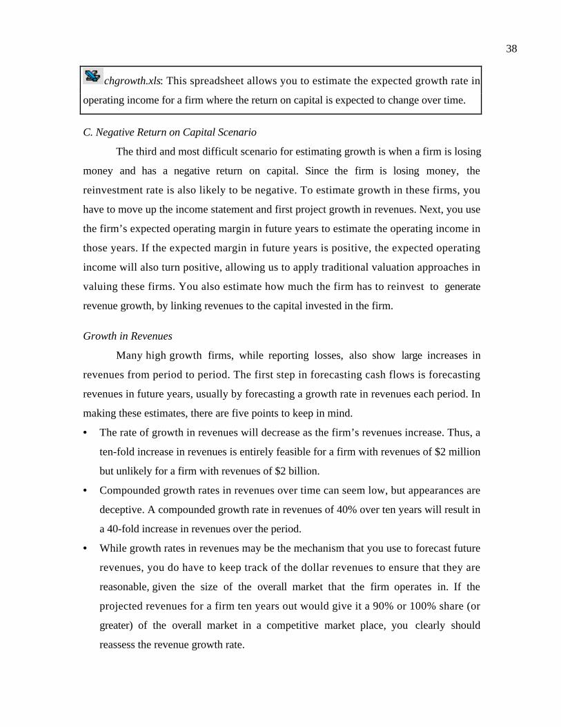
38

chgrowth.xls: This spreadsheet allows you to estimate the expected growth rate in

operating income for a firm where the return on capital is expected to change over time.

C. Negative Return on Capital Scenario

The third and most difficult scenario for estimating growth is when a firm is losing

money and has a negative return on capital. Since the firm is losing money, the

reinvestment rate is also likely to be negative. To estimate growth in these firms, you

have to move up the income statement and first project growth in revenues. Next, you use

the firm’s expected operating margin in future years to estimate the operating income in

those years. If the expected margin in future years is positive, the expected operating

income will also turn positive, allowing us to apply traditional valuation approaches in

valuing these firms. You also estimate how much the firm has to reinvest to generate

revenue growth, by linking revenues to the capital invested in the firm.

Growth in Revenues

Many high growth firms, while reporting losses, also show large increases in

revenues from period to period. The first step in forecasting cash flows is forecasting

revenues in future years, usually by forecasting a growth rate in revenues each period. In

making these estimates, there are five points to keep in mind.

• The rate of growth in revenues will decrease as the firm’s revenues increase. Thus, a

ten-fold increase in revenues is entirely feasible for a firm with revenues of $2 million

but unlikely for a firm with revenues of $2 billion.

• Compounded growth rates in revenues over time can seem low, but appearances are

deceptive. A compounded growth rate in revenues of 40% over ten years will result in

a 40-fold increase in revenues over the period.

• While growth rates in revenues may be the mechanism that you use to forecast future

revenues, you do have to keep track of the dollar revenues to ensure that they are

reasonable, given the size of the overall market that the firm operates in. If the

projected revenues for a firm ten years out would give it a 90% or 100% share (or

greater) of the overall market in a competitive market place, you clearly should

reassess the revenue growth rate.

39

• Assumptions about revenue growth and operating margins have to be internally

consistent. Firms can post higher growth rates in revenues by adopting more

aggressive pricing strategies but the higher revenue growth will then be accompanied

by lower margins.

• In coming up with an estimate of revenue growth, you have to make a number of

subjective judgments about the nature of competition, the capacity of the firm that

you are valuing to handle the revenue growth and the marketing capabilities of the

firm.

Illustration 11.12: Estimating Revenues at Commerce One

In earlier Illustrations, we had considered Commerce One, the B2B pioneer. In

Table 11.13, we forecast revenues for the firm for the next 10 years, as well as for

Ashford.com, an online jewelry and brand-name product retailer.

Table 11.13: Revenue Growth Rates and Revenues: Commerce One

Commerce One Ashford.com

Year

Expected Growth

Rate Revenues

Expected Growth

Rate Revenues

Current $402 $ 70.00

1 50.00% $603 80.00% $126.00

2 100.00% $1,205 60.00% $201.60

3 80.00% $2,170 40.00% $282.24

4 60.00% $3,472 30.00% $366.91

5 40.00% $4,860 20.00% $440.29

6 35.00% $6,561 17.00% $515.14

7 30.00% $8,530 14.00% $587.26

8 20.00% $10,236 11.00% $651.86

9 10.00% $11,259 8.00% $704.01

10 5.00% $11,822 5.00% $739.21

We based our estimates of growth for the firms in the initial years on the growth

in revenues over the last year – we did lower the growth rate for Commerce One in the

40

first year because of the fact that the economy was weak at the time of the valuation and

business spending had slowed.

As a check, we also examined how much the revenues at each of these firms would

be in ten years relative to more mature companies in the sector now.

• We compared revenues at Commerce One in ten years to those of EDS – a leading

provider of business services- today. EDS had revenues of $18.73 billion in 1999,

which would make Commerce One a leading player in this sector but not by an

overwhelming margin.

• Zale, which is the largest retailer of jewelry in the United States, had revenues of

about $1.7 billion in 2000. Our projected growth rate for Ashford would give it

revenues of $739 million.

Operating Margin Forecasts

Before considering how best to estimate the operating margins, let us begin with

an assessment of where many high growth firms, early in the life cycle, stand when the

valuation begins. They usually have low revenues and negative operating margins. If

revenue growth translates low revenues into high revenues and operating margins stay

negative, these firms will not only be worth nothing but are unlikely to survive. For firms

to be valuable, the higher revenues eventually have to deliver positive earnings. In a

valuation model, this translates into positive operating margins in the future. A key input

in valuing a high growth firm then is the operating margin you would expect it to have as

it matures.

In estimating this margin, you should begin by looking at the business that the

firm is in. While many new firms claim to be pioneers in their businesses and some believe

that they have no competitors, it is more likely that they are the first to find a new way

of delivering a product or service that was delivered through other channels before. Thus,

Amazon might have been one of the first firms to sell books online, but Barnes and Noble

and Borders preceded them as book retailers. In fact, one can consider online retailers as

logical successors to catalog retailers such as L.L. Bean or Lillian Vernon. Similarly,

Yahoo! might have been one of the first (and most successful) internet portals but they

are following the lead of newspapers that have used content and features to attract readers

41

and used their readership to attract advertising. Using the average operating margin of

competitors in the business may strike some as conservative. After all, they would point

out, Amazon can hold less inventory than Borders and does not have the burden of

carrying the operating leases that Barnes and Noble does (on its stores) and should,

therefore, be more efficient about generating its revenues and subsequently earnings. This

may be true but it is unlikely that the operating margins for internet retailers can be

persistently higher than their brick-and-mortar counterparts. If they were, you would

expect to see a migration of traditional retailers to online retailing and increased

competition among online retailers on price and products driving the margin down.

While the margin for the business in which a firm operates provides a target value,

there are still two other estimation issues that you need to confront. Given that the

operating margins in the early stages of the life cycle are negative, you first have to

consider how the margin will improve from current levels to the target values. Generally,

the improvements in margins will be greatest in the earlier years (at least in percentage

terms) and then taper off as the firm approaches maturity. The second issue is one that

arises when talking about revenue growth. Firms may be able to post higher revenue

growth with lower margins but the trade off has to be considered. While firms generally

want both higher revenue growth and higher margin, the margin and revenue growth

assumptions have to be consistent.

Illustration 11.13: Estimating Operating Margins

To estimate the operating margins for Commerce One, we begin by estimating the

operating margins of other firms in the business services/software sector. In 2000, the

average pre-tax operating margin for firms in this business was 16.36%. For Ashford.com,

we will use the average pre-tax operating margin of jewelry and brand name product

retailers, which is 10.86%.

We will assume that both Commerce One and Ashford.com will move toward

their target margins, with greater marginal improvements8 in the earlier years and smaller

8 The margin each year is computed as follows:(Margin this year + Target margin)/2

42

ones in the later years. Table 11.14 summarizes the expected operating margins over time

for both firms.

Table 11.14: Expected Operating Margins

Year

Commerce One:

Margin

Ashford.com: Operating

Margin

Current -84.62% -228.57%

1 -34.13% -119.74%

2 -8.88% -60.38%

3 3.74% -28.00%

4 10.05% -10.33%

5 13.20% -0.70%

6 14.78% 4.55%

7 15.57% 7.42%

8 15.97% 8.98%

9 16.16% 9.84%

10 16.26% 10.30%

11 16.36% 10.86%

Since we estimated revenue growth in the last section and the margins in this one, we can

now estimate the pre-tax operating income at each of the firms over the next 10 years in

Table 11.15.

Table 11.15: Expected Operating Income

Commerce One Ashford.com

Year Revenues

Operating

Margin EBIT Revenues

Operating

Margin EBIT

Current $402 -84.62% -$340 $70.00 -228.57% -$160.00

1 $603 -34.13% -$206 $126.00 -119.74% -$150.87

2 $1,205 -8.88% -$107 $201.60 -60.38% -$121.72

3 $2,170 3.74% $81 $282.24 -28.00% -$79.02

4 $3,472 10.05% $349 $366.91 -10.33% -$37.92

43

5 $4,860 13.20% $642 $440.29 -0.70% -$3.08

6 $6,561 14.78% $970 $515.14 4.55% $23.46

7 $8,530 15.57% $1,328 $587.26 7.42% $43.58

8 $10,236 15.97% $1,634 $651.86 8.98% $58.56

9 $11,259 16.16% $1,820 $704.01 9.84% $69.25

10 $11,822 16.26% $1,922 $739.21 10.30% $76.15

As the margins move towards target levels and revenues grow, the operating income at

each of the three firms also increases.

Market Size, Market Share and Revenue Growth

Estimating revenue growth rates for a young firm in a new business may seem like

an exercise in futility. While it is difficult to do, there are ways in which you can make the

process easier.

• One is to work backwards by first considering the share of the overall market that you

expect your firm to have once it matures and then determining the growth rate you

would need to arrive at this market share. For instance, assume that you are analyzing

an online toy retailer with $100 million in revenues currently. Assume also that the

entire toy retail market had revenues of $70 billion last year. Assuming a 3% growth

rate in this market over the next 10 years and a market share of 5% for your firm, you

would arrive at expected revenues of $4.703 billion for the firm in ten years and a

compounded revenue growth rate of 46.98%.

Expected Revenues in 10 years = $70 billion * 1.0310 * 0.05 = $4.703 billion

Expected compounded growth rate = (4,703/100)1/10 – 1 = 0.4698

• The other approach is to forecast the expected growth rate in revenues over the next 3

to 5 years based upon past growth rates. Once you estimate revenues in year 3 or 5,

you can then forecast a growth rate based upon companies with similar revenues

growth currently. For instance, assume that the online toy retailer analyzed above had

revenue growth of 200% last year (revenues went from $33 million to $100 million).

You could forecast growth rates of 120%, 100%, 80% and 60% for the next 4 years,

leading to revenues of $1.267 billion in four years. You could then look at the average

44

growth rate posted by retail firms with revenues between $1 and $1.5 billion last year

and use that as the growth rate commencing in year 5.

Sales to Capital Ratio

High revenue growth is clearly a desirable objective, especially when linked with

positive operating margins in future years. Firms do, however, have to invest to generate

both revenue growth and positive operating margins in future years. This investment can

take traditional forms (plant and equipment) but it should also include acquisitions of

other firms, partnerships, investments in distribution and marketing capabilities and

research and development.

To link revenue growth with reinvestment needs, you look at the revenues that

every dollar of capital that you invest generates. This ratio, called the sales to capital

ratio, allows us to estimate how much additional investment the firm has to make to

generate the projected revenue growth. This investment can be in internal projects,

acquisitions or working capital. To estimate the reinvestment needs in any year, you

divide the revenue growth that you have projected (in dollar terms) by the sales to capital

ratio. Thus, if you expect revenues to grow by $1 billion and you use a sales to capital

ratio of 2.5, you would estimate a reinvestment need for this firm of $400 million ($1

billion/2.5). Lower sales to capital ratios increase reinvestment needs (and reduce cash

flows) while higher sales to capital ratios decrease reinvestment needs (and increase cash

flows).

To estimate the sales to capital ratio, you look at both a firm’s past and the

business it operates in. To measure this ratio historically, you look at changes in revenue

each year and divide it by the reinvestment made that year. You also look at the average

ratio of sales to book capital invested in the business in which the firm operates.

Linking operating margins to reinvestment needs is much more difficult to do,

since a firm’s capacity to earn operating income and sustain high returns comes from the

competitive advantages that it acquires, partly through internal investment and partly

through acquisitions. Firms that adopt a two-track strategy in investing, where one track

focuses on generating higher revenues and the other on building up competitive strengths

45

should have higher operating margins and values than firms that concentrate only on

revenue growth.

Link to Return on Capital

One of the dangers that you face when using a sales-to-capital ratio to generate

reinvestment needs is that you might under-estimate or over-estimate your reinvestment

needs. You can keep tabs on whether this is happening and correct it when it does by also

estimating the after-tax return on capital on the firm each year through the analysis. To

estimate the return on capital in a future year, you use the estimated after-tax operating

income in that year and divide it by the total capital invested in that firm in that year. The

former number comes from your estimates of revenue growth and operating margins,

while the latter can be estimated by aggregating the reinvestments made by the firm all the

way through the future year. For instance, a firm that has $500 million in capital invested

today and is required to reinvest $300 million next year and $400 million the year after

will have capital invested of $1.2 billion at the end of the second year.

For firms losing money today, the return on capital will be a negative number

when the estimation begins but improve as margins improve. If the sales-to-capital ratio is

set too high, the return-on-capital in the later years will be too high, while if it is set too

low, it will be too low. Too low or high relative to what, you ask? There are two

comparisons that are worth making. The first is to the average return-on-capital for

mature firms in the business in which your firm operates – mature specialty and brand

name retailers, in the case of Ashford.com. The second is to the firm’s own cost of

capital. A projected return on capital of 40% for a firm with a cost of capital of 10% in a

sector where returns on capital hover around 15% is an indicator that the firm is investing

too little for the projected revenue growth and operating margins. Decreasing the sales to

capital ratio until the return on capital converges on 15% would be prudent.

Illustration 11.14: Estimated Sales to Capital Ratios

To estimate how much Commerce One and Ashford.com have to invest to

generate the expected revenue growth, we estimate the current sales to capital ratio, the

marginal sales to capital ratio in the last year and the average sales to capital ratio for the

businesses that each operates in.

46

Table 11.16: Sales to Capital Ratio Estimates

Commerce One Ashford.com

Firm's Sales to Capital 3.13 1.18

Marginal Sales to Capital: Most recent year 2.70 1.60

Industry average Sales to Capital 3.18 3.24

Sales to Capital Ratio used in valuation 2.00 2.50

We used a sales to capital ratio of 2.50 for Ashford.com, approximately midway through

their marginal sales to capital ratio from last year and the industry average. For Commerce

One, we set the sales to capital ratio well below the industry average and the firm’s

marginal sales to capital ratio. We feel that as competition increases, Commerce One will

have to invest increasing amounts in technology and in acquisitions to grow.

Based upon these estimates of the sales to capital ratio for each firm, we can now

estimate how much each firm will have to reinvest each year for the next 10 years in Table

11.17.

Table 11.17: Estimated Reinvestment Needs

Commerce One Ashford.com

Year

Increase in

Revenue Reinvestment

Increase in

Revenue Reinvestment

1 $201 $100 $56 $22

2 $603 $301 $76 $30

3 $964 $482 $81 $32

4 $1,302 $651 $85 $34

5 $1,389 $694 $73 $29

6 $1,701 $851 $75 $30

7 $1,968 $984 $72 $29

8 $1,706 $853 $65 $26

9 $1,024 $512 $52 $21

10 $563 $281 $35 $14

47

As a final check, we estimate the return on capital each year for the next 10 years for both

firms in Table 11.18.

Table 11.18: Estimated Return on Capital

Year Commerce

One

Ashford.com

1 -160.23% -254.67%

2 -46.80% -149.09%

3 15.30% -70.62%

4 34.46% -26.31%

5 32.17% -1.73%

6 26.74% 11.31%

7 26.91% 18.36%

8 25.34% 22.00%

9 23.44% 23.72%

10 22.49% 24.34%

Industry

average 20.00% 20.00%

The returns-on-capital at both firms converge to sustainable levels, at least relative to

industry averages, by the terminal year. This suggests that our estimates of sales to

capital ratios are reasonable.

margins.xls: This dataset on the web summarizes operating margins, by

industry, for the United States.

The Qualitative Aspects of Growth

The emphasis on quantitative elements – return on capital and reinvestment rates

for profitable firms and margins, revenue growth and sales to capital ratios for

unprofitable firms – may strike some as skewed. After all, growth is determined by a

number of subjective factors – the quality of management, the strength of a firm’s

marketing, its capacity to form partnerships with other firms and the management’s

48

strategic vision, among many others. Where, you might ask, is there room in the growth

equations that have been presented in this chapter for these factors?

The answer is that qualitative factors matter and that they all ultimately have to

show up in one or more of the quantitative inputs that determine growth. Consider the

following:

• The quality of management plays a significant role in the returns on capital that you

assume firms can earn on their new investments and in how long they can sustain

these returns. Thus, the fact that a firm has a well-regarded management team may be

one reason why you allow a firm’s return on capital to remain well above the cost of

capital.

• The marketing strengths of a firm and its choice of marketing strategy are reflected in

the operating margins and turnover ratios that you assume for firms. Thus, it takes

faith in Coca Cola’s capacity to market its products effectively to assume a high

turnover ratio and a high target margin. In fact, you can consider various marketing

strategies, which trade off lower margins for higher turnover ratios, and consider the

implications for value. The brand name of a firm’s products and the strength of its

distribution system also affect these estimates.

• Defining reinvestment broadly to include acquisitions, research and development and

investments in marketing and distribution allows you to consider different ways in

which firms can grow. For some firms like Cisco, reinvestment and growth come from

acquisitions, while for other firms such as GE, it may take the form of more

traditional investments in plant and equity. The effectiveness of these reinvestment

strategies is captured in the return on capital that you assume for the future, with

more effective firms having higher returns on capital.

• The strength of the competition that firms face is in the background but it does

determine how high excess returns (return on capital – cost of capital) will be, and

how quickly they will slide.

Thus, every qualitative factor is quantified and the corresponding growth implications

are considered. What if you cannot quantify the effects? If you cannot, you should remain

skeptical about whether these factors truly affect value. What about those qualitative

49

factors that do not affect the return on capital, margin or reinvestment rate? At the risk of

sounding dogmatic, these factors cannot affect value.

Why is it necessary to impose this quantitative structure on growth estimate? One

of the biggest dangers in valuing technology firms is that story telling can be used to

justify growth rates that are neither reasonable nor sustainable. Thus, you might be told

that Ashford.com will grow at 60% a year because the online retailing market is huge and

that Coca Cola will grow 20% a year because it has a great brand name. While there is

some truth in these stories, a consideration of how these qualitative views translate into

the quantitative elements of growth is an essential step towards consistent valuations.

Can different investors consider the same qualitative factors and come to different

conclusions about the implications for returns on capital, margins, reinvestment rates,

and, consequently, growth? Absolutely. In fact, you would expect differences in opinion

about the future and different estimates of value. The payoff to knowing a firm and the

sector it operates better than other investors is that your estimates of growth and value

will be better than theirs. Unfortunately, this does not guarantee that your investment

returns will be better than theirs.

Summary

Growth is the key input in every valuation and there are three sources for growth

rates. One is the past, though both estimating and using historical growth rates can be

difficult for most firms with their volatile and sometimes negative earnings. The second is

analyst estimates of growth. Though analysts may be privy to information that is not

available to the rest of the market, this information does not result in growth rates that are

superior to historical growth estimates. Furthermore, the analyst emphasis on earnings

per share growth can be a problem when forecasting operating income. The third and

soundest way of estimating growth is to base it on a firm’s fundamentals.

The relationship of growth to fundamentals will depend upon what growth rate

we are estimating. To estimate growth in earnings per share, we looked at return on equity

and retention ratios. To estimate growth in net income, we replaced the retention ratio

with the equity reinvestment rate. To evaluate growth in operating income, we used

return on capital and reinvestment rate. While the details vary from approach to

50

approach, there are some common themes that emerge from these approaches. The first is

that growth and reinvestment are linked and estimates of one have to be lined with

estimates of the other. Firms that want to grow at high rates over long periods have to

reinvest to create that growth. The second is that the quality of growth can vary widely

across firms and that the best measure of the quality of growth is the returns earned on

investments. Firms that earn higher returns on equity and capital will not only generate

higher growth but that growth will add more to their value.

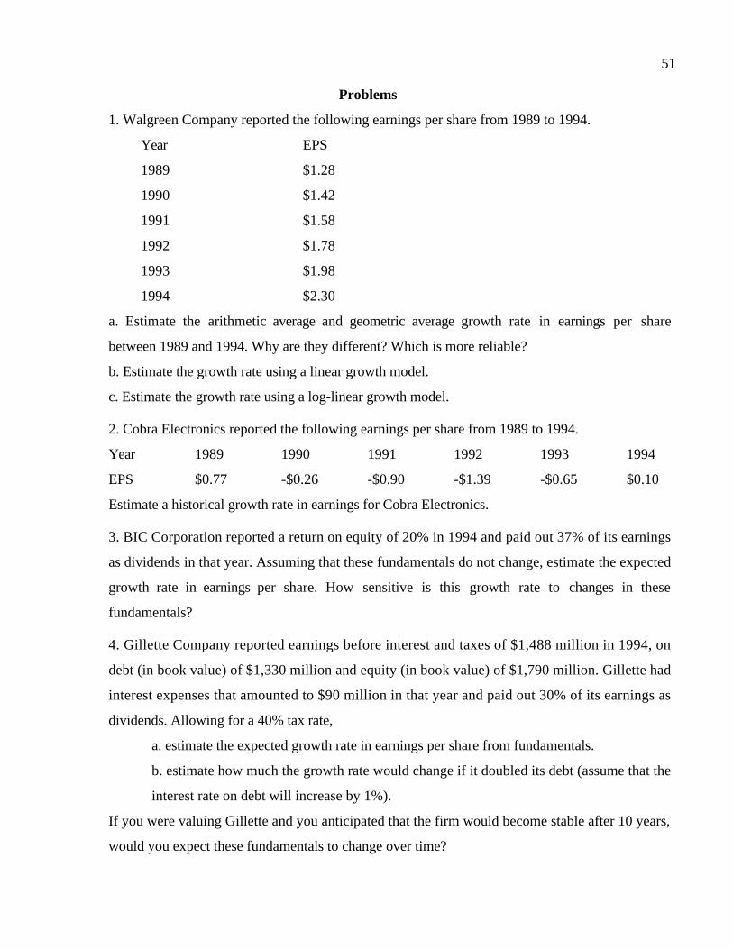
51

Problems

1. Walgreen Company reported the following earnings per share from 1989 to 1994.

Year EPS

1989 $1.28

1990 $1.42

1991 $1.58

1992 $1.78

1993 $1.98

1994 $2.30

a. Estimate the arithmetic average and geometric average growth rate in earnings per share

between 1989 and 1994. Why are they different? Which is more reliable?

b. Estimate the growth rate using a linear growth model.

c. Estimate the growth rate using a log-linear growth model.

2. Cobra Electronics reported the following earnings per share from 1989 to 1994.

Year 1989 1990 1991 1992 1993 1994

EPS $0.77 -$0.26 -$0.90 -$1.39 -$0.65 $0.10

Estimate a historical growth rate in earnings for Cobra Electronics.

3. BIC Corporation reported a return on equity of 20% in 1994 and paid out 37% of its earnings

as dividends in that year. Assuming that these fundamentals do not change, estimate the expected

growth rate in earnings per share. How sensitive is this growth rate to changes in these

fundamentals?

4. Gillette Company reported earnings before interest and taxes of $1,488 million in 1994, on

debt (in book value) of $1,330 million and equity (in book value) of $1,790 million. Gillette had

interest expenses that amounted to $90 million in that year and paid out 30% of its earnings as

dividends. Allowing for a 40% tax rate,

a. estimate the expected growth rate in earnings per share from fundamentals.

b. estimate how much the growth rate would change if it doubled its debt (assume that the

interest rate on debt will increase by 1%).

If you were valuing Gillette and you anticipated that the firm would become stable after 10 years,

would you expect these fundamentals to change over time?

52

5. B.A.T. Industries had a pre-tax operating margin of 10% on revenues of $34,500 million in

1994 and reported a capital turnover ratio of 3.0 in that year.

a. If the tax rate is 36%, estimate the return on capital for B.A.T. Industries.

b. If the pre-tax operating margin drops to 8% of revenues and the asset turnover ratio

remains unchanged, estimate the new return on capital.

1

CHAPTER 12CLOSURE IN VALUATION: ESTIMATING TERMINAL VALUE

In the last chapter, we examined the determinants of expected growth. Firms that

reinvest substantial portions of their earnings and earn high returns on these investments

should be able to grow at high rates. But for how long? In this chapter, we bring closure to

firm valuation by considering this question.

As a firm grows, it becomes more difficult for it to maintain high growth and it

eventually will grow at a rate less than or equal to the growth rate of the economy in

which it operates. This growth rate, labeled stable growth, can be sustained in perpetuity,

allowing us to estimate the value of all cash flows beyond that point as a terminal value

for a going concern. The key question that we confront is the estimation of when and how

this transition to stable growth will occur for the firm that you are valuing. Will the

growth rate drop abruptly at a point in time to a stable growth rate or will it occur more

gradually over time? To answer these questions, we will look at a firm’s size (relative to

the market that it serves), its current growth rate and its competitive advantages.

We also consider an alternate route, which is that firms do not last forever and that

they will be liquidated at some point in time in the future. We will consider how best to

estimate liquidation value and when it makes more sense to use this approach rather than

the going concern approach.

Closure in Valuation

Since you cannot estimate cash flows forever, you generally impose closure in

discounted cash flow valuation by stopping your estimation of cash flows sometime in

the future and then computing a terminal value that reflects the value of the firm at that

point.

Value of a Firm =CFt

(1 + k c )t + t =1

t = n

∑ Terminal Value n

(1 + k c )n

You can find the terminal value in one of three ways. One is to assume a liquidation of

the firm’s assets in the terminal year and estimate what others would pay for the assets

that the firm has accumulated at that point. The other two approaches value the firm as a

going concern at the time of the terminal value estimation. One applies a multiple to

2

earnings, revenues or book value to estimate the value in the terminal year. The other

assumes that the cash flows of the firm will grow at a constant rate forever – a stable

growth rate. With stable growth, the terminal value can be estimated using a perpetual

growth model.

Liquidation Value

In some valuations, we can assume that the firm will cease operations at a point in

time in the future and sell the assets it has accumulated to the highest bidders. The

estimate that emerges is called a liquidation value. There are two ways in which the

liquidation value can be estimated. One is to base it on the book value of the assets,

adjusted for any inflation during the period. Thus, if the book value of assets ten years

from now is expected to be $2 billion, the average age of the assets at that point is 5 years

and the expected inflation rate is 3%, the expected liquidation value can be estimated.

Expected Liquidation value = Book Value of AssetsTerm yr (1+ inflation rate)Average life of

assets

= $ 2 billion (1.03)5 = $2.319 billion

The limitation of this approach is that it is based upon accounting book value and does

not reflect the earning power of the assets.

The alternative approach is to estimate the value based upon the earning power of

the assets. To make this estimate, we would first have to estimate the expected cash

flows from the assets and then discount these cash flows back to the present, using an

appropriate discount rate. In the example above, for instance, if we assumed that the

assets in question could be expected to generate $400 million in after-tax cash flows for 15

years (after the terminal year) and the cost of capital was 10%, your estimate of the

expected liquidation value would be:

Expected Liquidation value = ( ) ( )billion $3.042

0.10

1.10

1-1

million 400$15

=

When valuing equity, there is one additional step that needs to be taken. The

estimated value of debt outstanding in the terminal year has to be subtracted from the

liquidation value to arrive at the liquidation proceeds for equity investors.

3

Multiple Approach

In this approach, the value of a firm in a future year is estimated by applying a

multiple to the firm’s earnings or revenues in that year. For instance, a firm with expected

revenues of $6 billion ten years from now will have an estimated terminal value in that

year of $12 billion if a value to sales multiple of 2 is used. If valuing equity, we use equity

multiples such as price earnings ratios to arrive at the terminal value.

While this approach has the virtue of simplicity, the multiple has a huge effect on

the final value and where it is obtained can be critical. If, as is common, the multiple is

estimated by looking at how comparable firms in the business today are priced by the

market. The valuation becomes a relative valuation rather than a discounted cash flow

valuation. If the multiple is estimated using fundamentals, it converges on the stable

growth model that will be described in the next section.

All in all, using multiples to estimate terminal value, when those multiples are

estimated from comparable firms, results in a dangerous mix of relative and discounted

cash flow valuation. While there are advantages to relative valuation, and we will consider

these in a later chapter, a discounted cash flow valuation should provide you with an

estimate of intrinsic value, not relative value. Consequently, the only consistent way of

estimating terminal value in a discounted cash flow model is to use either a liquidation

value or a stable growth model.

Stable Growth Model

In the liquidation value approach, we are assuming that your firm has a finite life and

that it will be liquidated at the end of that life. Firms, however, can reinvest some of their

cash flows back into new assets and extend their lives. If we assume that cash flows,

beyond the terminal year, will grow at a constant rate forever, the terminal value can be

estimated as.

Terminal Valuet = stable

1t

g -r

FlowCash +

where the cash flow and the discount rate used will depend upon whether you are valuing

the firm or valuing the equity. If we are valuing the equity, the terminal value of equity

can be written as:

4

Terminal value of Equityn = n1n

1n

g-Equity ofCost

Equity toCashflow

+

+

The cashflow to equity can be defined strictly as dividends (in the dividend discount

model) or as free cashflow to equity. If valuing a firm, the terminal value can be written

as:

Terminal valuen = n1n

1n

g-Capital ofCost

Firm toCashflow

+

+

where the cost of capital and the growth rate in the model are sustainable forever.

In this section, we will begin by considering how high a stable growth rate can be,

how to best estimate when your firm will be a stable growth firm and what inputs need to

be adjusted as a firm approaches stable growth.

Constraints on Stable Growth

Of all the inputs into a discounted cash flow valuation model, none can affect the

value more than the stable growth rate. Part of the reason for it is that small changes in the

stable growth rate can change the terminal value significantly and the effect gets larger as

the growth rate approaches the discount rate used in the estimation. Not surprisingly,

analysts often use it to alter the valuation to reflect their biases.

The fact that a stable growth rate is constant forever, however, puts strong

constraints on how high it can be. Since no firm can grow forever at a rate higher than the

growth rate of the economy in which it operates, the constant growth rate cannot be

greater than the overall growth rate of the economy. In making a judgment on what the

limits on stable growth rate are, we have to consider the following questions.

1. Is the company constrained to operate as a domestic company or does it operate

(or have the capacity) to operate multi-nationally? If a firm is a purely domestic

company, either because of internal constraints (such as those imposed by

management) or external (such as those imposed by a government), the growth

rate in the domestic economy will be the limiting value. If the company is a multi-

national or has aspirations to be one, the growth rate in the global economy (or at

least those parts of the globe that the firm operates in) will be the limiting value.

Note that the difference will be small for a U.S. firm, since the U.S economy still

5

represents a large portion of the world economy. It may, however, mean that you

could use a stable growth rate that is slightly higher (say 1/2 to 1%) for a Coca

Cola than a Consolidated Edison.

2. Is the valuation being done in nominal or real terms? If the valuation is a nominal

valuation, the stable growth rate should also be a nominal growth rate, i.e. include

an expected inflation component. If the valuation is a real valuation, the stable

growth rate will be constrained to be lower. Again, using Coca Cola as an example,

the stable growth rate can be as high as 5.5% if the valuation is done in nominal

U.S. dollars but only 3% if the valuation is done in real dollars.

3. What currency is being used to estimate cash flows and discount rates in the

valuation? The limits on stable growth will vary depending upon what currency is

used in the valuation. If a high-inflation currency is used to estimate cash flows

and discount rates, the limits on stable growth will be much higher, since the

expected inflation rate is added on to real growth. If a low-inflation currency is

used to estimate cash flows, the limits on stable growth will be much lower. For

instance, the stable growth rate that would be used to value Titan Cements, the

Greek cement company, will be much higher if the valuation is done in drachmas

than in euros.

While the stable growth rate cannot exceed the growth rate of the economy in which a

firm operates, it can be lower. There is nothing that prevents us from assuming that

mature firms will become a smaller part of the economy and it may, in fact, be the more

reasonable assumption to make. Note that the growth rate of an economy reflects the

contributions of both young, higher-growth firms and mature, stable growth firms. If the

former grow at a rate much higher than the growth rate of the economy, the latter have to

grow at a rate that is lower.

Setting the stable growth rate to be less than or equal to the growth rate of the

economy is not only the consistent thing to do but it also ensures that the growth rate

will be less than the discount rate. This is because of the relationship between the riskless

rate that goes into the discount rate and the growth rate of the economy. Note that the

riskless rate can be written as:

Nominal riskless rate = Real riskless rate + Expected inflation rate

6

In the long term, the real riskless rate will converge on the real growth rate of the economy

and the nominal riskless rate will approach the nominal growth rate of the economy. In

fact, a simple rule of thumb on the stable growth rate is that it should not exceed the

riskless rate used in the valuation.

Can the stable growth rate be negative?

In the previous section, we noted that the stable growth rate has to be less than or

equal to the growth rate of the economy. But can it be negative? There is no reason why

not since the terminal value can still be estimated. For instance, a firm with $100 million

in after-tax cash flows growing at –5% a year forever and a cost of capital of 10% has a

value of:

Value of firm = ( )

( ) million $63305.010.0

0.05-1100 =−−

Intuitively, though, what does a negative growth rate imply? It essentially allows a firm

to partially liquidate itself each year until it just about disappears. Thus, it is an

intermediate choice between complete liquidation and the going concern that gets larger

each year forever.

This may be the right choice to make when valuing firms in industries that are

being phased out because of technological advances (such as the manufacturers of

typewriters with the advent of the personal computer) or where an external and critical

customer is scaling back purchases for the long term (as was the case with defense

contractors after the end of the cold war).

Key Assumptions about Stable Growth

In every discounted cash flow valuation, there are three critical assumptions you

need to make on stable growth. The first relates to when the firm that you are valuing will

become a stable growth firm, if it is not one already. The second relates to what the

characteristics of the firm will be in stable growth, in terms of return on investments and

costs of equity and capital. The final assumption relates to how the firm that you are

valuing will make the transition from high growth to stable growth.

I. Length of the High Growth Period

7

The question of how long a firm will be able to sustain high growth is perhaps one of

the more difficult questions to answer in a valuation, but two points are worth making.

One is that it is not a question of whether but when firms hit the stable growth wall. All

firms ultimately become stable growth firms, in the best case, because high growth makes

a firm larger and the firm’s size will eventually become a barrier to further high growth. In

the worst case scenario, firms may not survive and will be liquidated. The second is that

high growth in valuation, or at least high growth that creates value1, comes from firms

earning excess returns on their marginal investments. In other words, increased value

comes from firms having a return on capital that is well in excess of the cost of capital (or

a return on equity that exceeds the cost of equity). Thus, when you assume that a firm

will experience high growth for the next 5 or 10 years, you are also implicitly assuming

that it will earn excess returns (over and above the required return) during that period. In a

competitive market, these excess returns will eventually draw in new competitors and the

excess returns will disappear.

You should look at three factors when considering how long a firm will be able to

maintain high growth.

1. Size of the firm: Smaller firms are much more likely to earn excess returns and

maintain these excess returns than otherwise similar larger firms. This is because

they have more room to grow and a larger potential market. Small firms in large

markets should have the potential for high growth (at least in revenues) over long

periods. When looking at the size of the firm, you should look not only at its

current market share, but also at the potential growth in the total market for its

products or services. A firm may have a large market share of its current market,

but it may be able to grow in spite of this because the entire market is growing

rapidly

2. Existing growth rate and excess returns: Momentum does matter, when it comes to

projecting growth. Firms that have been reporting rapidly growing revenues are

more likely to see revenues grow rapidly at least in the near future. Firms that are

1 Growth without excess returns will make a firm larger but not more valuable.

8

earnings high returns on capital and high excess returns in the current period are

likely to sustain these excess returns for the next few years.

3. Magnitude and Sustainability of Competitive Advantages: This is perhaps the most

critical determinant of the length of the high growth period. If there are significant

barriers to entry and sustainable competitive advantages, firms can maintain high

growth for longer periods. If, on the other hand, there are no or minor barriers to

entry or if the firm’s existing competitive advantages are fading, you should be far

more conservative about allowing for long growth periods. The quality of existing

management also influences growth. Some top managers2 have the capacity to

make the strategic choices that increase competitive advantages and create new

ones.

Illustration 12.1: Length of High Growth Period

To illustrate the process of estimating the length of the high growth period, we

will consider a number of companies and make subjective judgments about how long each

one will be able to maintain high growth:

Consolidated Edison:

Background: The firm has a monopoly in generating and selling power in the environs of

New York. In return for the monopoly, though, the firm is restricted in both its

investment policy and its pricing policy. A regulatory commission determines how much

Con Ed can raise prices and it makes this decision based upon the returns made by Con

Ed on its investments; if the firm is making high returns on its investments, it is unlikely

to be allowed to increase prices. Finally, the demand for power in New York is stable as

the population levels off.

Implication: The firm is already a stable growth firm. There is little potential for either

high growth or excess returns.

Procter & Gamble

Background: Procter & Gamble comes in with some obvious strengths. Its valuable brand

names have allowed it to earn high excess returns (as manifested in its high return on

9

equity of 29.37% in 2000) and sustain high growth rates in earnings over the last few

decades. The firm faces two challenges. One is that it has a significant market share in a

mature market in the United States and that its brand names are less recognized outside of

the United States and therefore less likely to command premiums abroad. The other is the

increasing assault on brand names in general by generic manufacturers.

Implication: Brand name can sustain excess returns and growth higher than the stable

growth rate for a short period – we will assume five years. Beyond that, we will assume

that the firm will be in stable growth albeit with some residual excess returns. If the firm

is able to take its brand names overseas, its potential for high growth in terms of rate and

period will be significantly higher.

Amgen

Background: Amgen has a stable of drugs, on which it has patent protection, that

generates cash flows currently and several drugs in its R&D pipeline. While it is the

largest biotechnology firm in the world, the market for bio-technology products is

expanding significantly and will continue to do so. Finally, Amgen has had a track record

of delivering high earnings growth.

Implication: The patents that Amgen has will protect it from competition and the

long lead time to drug approval will ensure that new products will take a while getting to

the market. We will allow for ten years of high growth and excess returns. There is clearly

a strong subjective component to making a judgment on how long high growth will last.

Much of what was said about the interrelationships between qualitative variables and

growth towards the end of Chapter 11 has relevance for this discussion as well.

Competitive Advantage Period (CAP)

The confluence of high growth and excess returns which is the source of value has led to

the coining of the term “competitive advantage period” (CAP) to capture the joint effect.

This term, first used by Michael Maboussin at Credit Suisse First Boston, measures the

period for which a firm can be expected to earn excess returns. The value of such a firm

can then be written as the sum of the capital invested today and the present value of the

2 Jack Welch at GE and Robert Goizueta at Coca Cola are good examples of CEOs who made a profounddifference in the growth of their firms.

10

excess returns that the firm will earn over its life. Since there are no excess returns after

the competitive advantage period, there is no additional value added.

In an inventive variant, analysts sometimes try to estimate how long the

competitive advantage period will have to be to sustain a current market value, assuming

that the current return on capital and cost of capital remain unchanged. The resulting

market implied competitive advantage period (MICAP) can then be either compared

across firms in a sector or evaluated on a qualitative basis.

II. Characteristics of Stable Growth Firm

As firms move from high growth to stable growth, you need to give them the

characteristics of stable growth firms. A firm in stable growth is different from that same

firm in high growth on a number of dimensions. In general, you would expect stable

growth firms to be less risky, use more debt, have lower (or even no) excess returns and

reinvest less than high growth firms. In this section, we will consider how best to adjust

each of these variables.

a. Equity Risk

When looking at the cost of equity, high growth firms tend to be more exposed to

market risk (and have higher betas) than stable growth firms. Part of the reason for this is

that they tend to be niche players, providers of discretionary products and services and a

high leverage operation. Thus, firms like Commerce One or NTT Docomo may have betas

that exceed 1.5 or even 2. As these firms and their corresponding markets mature, you

would expect them to have less exposure to market risk and betas that are closer to one –

the average for the market. One option is to set the beta in stable growth to one for all

firms, arguing that firms in stable growth should all be average risk. Another is to allow

for small differences to persist even in stable growth with firms in more volatile

businesses having higher betas than firms in more stable businesses. We would

recommend that, as a rule of thumb, stable period betas should not exceed 1.2.3

But what about firms that have betas well below 1, such as commodity companies?

If you are assuming that these firms will stay in their existing businesses, there is no harm

11

in assuming that the beta remains at existing levels. However, if your estimates of growth

in perpetuity4 will require them to branch out into other business, you should adjust the

beta upwards towards one.

betas.xls: This dataset on the web summarizes the average levered and unlevered

betas, by industry group, for firms in the United States.

b. Project Returns

High growth firms tend to have high returns on capital (and equity) and earn excess

returns. In stable growth, it becomes much more difficult to sustain excess returns. There

are some who believe that the only assumption consistent with stable growth is to

assume no excess returns; the return on capital is set equal to the cost of capital. While, in

principle, excess returns in perpetuity are not feasible, it is difficult in practice to assume

that firms will suddenly lose the capacity to earn excess returns. Since entire industries

often earn excess returns over long periods, assuming a firm’s returns on equity and

capital will move towards industry averages will yield more reasonable estimates of value.

eva.xls: This dataset on the web summarizes the returns on capital (equity),

costs of capital (equity) and excess returns, by industry group, for firms in the United

States.

c. Debt Ratios and Costs of Debt

High growth firms tend to use less debt than stable growth firms. As firms mature,

their debt capacity increases. When valuing firms, this will change the debt ratio that we

use to compute the cost of capital. When valuing equity, changing the debt ratio will

change both the cost of equity and the expected cash flows. The question whether the

debt ratio for a firm should be moved towards a more sustainable level in stable growth

cannot be answered without looking at the incumbent managers’ views on debt and how

3 Two thirds of U.S. firms have betas that fall between 0.8 and 1.2. That becomes the range for stableperiod betas.

12

much power stockholders have in these firms. If managers are willing to change their debt

ratios and stockholders retain some power, it is reasonable to assume that the debt ratio

will move to a higher level in stable growth; if not, it is safer to leave the debt ratio at

existing levels.

As earnings and cash flows increase, the perceived default risk in the firm will also

change. A firm that is currently losing $10 million on revenues of $100 million may be

rated B, but its rating should be much better if your forecasts of $10 billion in revenues

and $1 billion in operating income come to fruition. In fact, internal consistency requires

that you re-estimate the rating and the cost of debt for a firm as you change its revenues

and operating income.

On the practical question of what debt ratio and cost of debt to use in stable

growth, you should look at the financial leverage of larger and more mature firms in the

industry. One solution is to use the industry average debt ratio and cost of debt as the

debt ratio and cost of debt for the firm in stable growth.

wacc.xls: This dataset on the web summarizes the debt ratios and costs of debt,

by industry group, for firms in the United States.

d. Reinvestment and Retention Ratios

Stable growth firms tend to reinvest less than high growth firms and it is critical

that we both capture the effects of lower growth on reinvestment and that we ensure that

the firm reinvests enough to sustain its stable growth rate in the terminal phase. The

actual adjustment will vary depending upon whether we are discounting dividends, free

cash flows to equity or free cash flows to the firm.

In the dividend discount model, note that the expected growth rate in earnings per

share can be written as a function of the retention ratio and the return on equity.

Expected Growth Rate = Retention ratio * Return on Equity

Algebraic manipulation can allow us to state the retention ratio as a function of the

expected growth rate and return on equity:

4 If you are valuing a commodity company and assuming any growth rate that exceeds inflation, you are

13

Retention ratio = Equityon Return

rateGrowth Expected

If we assume, for instance, a stable growth rate of 5% (based upon the growth rate of the

economy) for Procter & Gamble and a return on equity of 15% (based upon industry

averages), we would be able to compute the retention ratio in stable growth:

Retention ratio = 33.33%15%

5% =

Procter & Gamble will have to reinvest 33.33% of its earnings into the firm to generate its

expected growth of 5%; it can pay out the remaining 66.67%.

In a free cash flow to equity model, where we are focusing on net income growth,

the expected growth rate is a function of the equity reinvestment rate and the return on

equity.

Expected Growth Rate = Equity Reinvestment rate * Return on Equity

The equity reinvestment rate can then be computed as follows:

Equity Reinvestment rate = Equityon Return

rateGrowth Expected

If, for instance, we assume that Coca Cola will have a stable growth rate of 5.5% and that

its return on equity in stable growth of 18%, we can estimate an equity reinvestment rate:

Equity Reinvestment rate = 30.56%18%

5.5% =

Finally, looking at free cash flows to the firm, we estimated the expected growth

in operating income as a function of the return on capital and the reinvestment rate:

Expected Growth rate = Reinvestment rate * Return on Capital

Again, algebraic manipulation yields the following measure of the reinvestment

rate in stable growth.

Reinvestment Rate in stable growth = nROC

rategrowth Stable

where the ROCn is the return on capital that the firm can sustain in stable growth. This

reinvestment rate can then be used to generate the free cash flow to the firm in the first

year of stable growth.

assuming that your firm will branch into other businesses and you have to adjust the beta accordingly.

14

Linking the reinvestment rate and retention ratio to the stable growth rate also

makes the valuation less sensitive to assumptions about stable growth. While increasing

the stable growth rate, holding all else constant, can dramatically increase value, changing

the reinvestment rate as the growth rate changes will create an offsetting effect. The gains

from increasing the growth rate will be partially or completely offset by the loss in cash

flows because of the higher reinvestment rate. Whether value increases or decreases as the

stable growth increases will entirely depend upon what you assume about excess returns.

If the return on capital is higher than the cost of capital in the stable growth period,

increasing the stable growth rate will increase value. If the return on capital is equal to the

stable growth rate, increasing the stable growth rate will have no effect on value. This can

be proved quite easily.

RateGrowth StableCapital ofCost

Rate)nt Reinvestme-t)(1(1EBIT=Value Terminal

n

1+n

−−

Substituting in the stable growth rate as a function of the reinvestment rate, from above,

you get:

Capital)on Return *Rateent (ReinvestmCapital ofCost

Rate)nt Reinvestme -t)(1(1EBIT=Value Terminal

n

1+n

−−

Setting the return on capital equal to the cost of capital, you arrive at:

Capital)on Cost *Rateent (ReinvestmCapital ofCost

Rate)nt Reinvestme -t)(1(1EBIT=Value Terminal

n

1+n

−−

Simplifying, the terminal value can be stated as:

n

1+nWACC=ROC

Capital ofCost

t)(1EBIT=Value Terminal

−

You could establish the same proposition with equity income and cash flows and show

that a return on equity equal to the cost of equity in stable growth nullifies the positive

effect of growth.

divfund.xls: This dataset on the web summarizes retention ratios, by industry

group, for firms in the United States.

15

capex.xls: This dataset on the web summarizes the reinvestment rates, by

industry group, for firms in the United States.

Illustration 12.2: Stable Growth rates and Excess Returns

Alloy Mills is a textile firm that is currently reporting after-tax operating income

of $100 million. The firm has a return on capital currently of 20% and reinvests 50% of

its earnings back into the firm, giving it an expected growth rate of 10% for the next 5

years:

Expected Growth rate = 20% * 50% = 10%

After year 5, the growth rate is expected to drop to 5% and the return on capital is

expected to stay at 20%. The terminal value can be estimated as follows:

Expected operating income in year 6 = 100 (1.10)5(1.05) = $169.10 million

Expected reinvestment rate from year 5 = 25%20%

5%

ROC

g ==

Terminal value in year 5 = million 2,537$0.05-0.10

0.25)-$169.10(1 =

The value of the firm today would then be:

Value of firm today =

million $1,8251.10

$2,537

1.10

$80.53

1.10

$73.21

1.10

$66.55

1.10

$60.5

1.10

$5555432

=+++++

If we did change the return on capital in stable growth to 10% while keeping the growth

rate at 5%, the effect on value would be dramatic:

Expected operating income in year 6 = 100 (1.10)5(1.05) = $169.10 million

Expected reinvestment rate from year 5 = 50%10%

5%

ROC

g ==

Terminal value in year 5 = million 691,1$0.05-0.10

0.5)-$169.10(1 =

Value of firm today =

million $1,3001.10

$1,691

1.10

$80.53

1.10

$73.21

1.10

$66.55

1.10

$60.5

1.10

$5555432

=+++++

16

Now consider the effect of lowering the growth rate to 4% while keeping the return on

capital at 10% in stable growth:

Expected operating income in year 6 = 100 (1.10)5(1.04) = $167.49 million

Expected reinvestment rate in year 6 = 40%10%

4%

ROC

g ==

Terminal value in year 5 = million 675,1$0.04-0.10

0.4)-$169.10(1 =

Value of firm today =

million $1,3001.10

$1,675

1.10

$96.63

1.10

$73.21

1.10

$66.55

1.10

$60.5

1.10

$5555432

=+++++

Note that the terminal value decreases by $16 million but the cash flow in year 5 also

increases by $16 million because the reinvestment rate at the end of year 5 drops to 40%.

The value of the firm remains unchanged at $1,600 million. In fact, changing the stable

growth rate to 0% has no effect on value:

Expected operating income in year 6 = 100 (1.10)5 = $161.05 million

Expected reinvestment rate in year 6 = 0%10%

0%

ROC

g ==

Terminal value in year 5 = million 5.610,1$0.00-0.10

0.00)-$161.05(1 =

Value of firm today =

million $1,3001.10

$1,610.5

1.10

$161.05

1.10

$73.21

1.10

$66.55

1.10

$60.5

1.10

$5555432

=+++++

Illustration 12.3: Stable Growth Inputs

To illustrate how the inputs to valuation change as we go from high growth to

stable growth, we will consider three firms – Procter & Gamble, with the dividend

discount model, Coca Cola with a free cashflow to equity model and Amgen.

Consider Procter & Gamble first in the context of the dividend discount model.

While we will do the valuation in the next chapter, note that there are only three real

inputs to the dividend discount model – the payout ratio (which determines dividends),

the expected return on equity (which determines the expected growth rate) and the beta

(which affects the cost of equity). In Illustration 12.1, we argued that Procter & Gamble

17

would have a five-year high growth period. Table 12.1 summarizes the inputs into the

dividend discount model for the valuation of Procter and Gamble.

Table 12.1: Inputs to Dividend Discount Model – Procter & Gamble

High Growth

Period

Stable Growth

Period

Payout ratio 45.67% 66.67%

Return on Equity 25.00% 15.00%

Expected Growth rate 13.58% 5.00%

Beta 0.85 1.00

Note that the payout ratio and the beta for the high growth period are based upon the

current year’s values. The return on equity for the next 5 years is set at 25% which is

below the current return on equity, but reflects the pressures that Procter & Gamble has

been under recently. The expected growth rate of 13.58% for the next 5 years is the

product of the return on equity and retention ratio. In stable growth, we adjust the beta to

one, though the adjustment has little effect on value since the beta is already close to one.

We assume that the stable growth rate will be 5%, just slightly below the nominal growth

rate in the global economy. We also assume that the return on equity will drop to 15%,

about halfway between the cost of equity and the average return on equity earned by

brand name companies similar to Procter & Gamble today. This reflects our assumption

that returns on equity will decline for the entire industry as competition from generics

eats into profit margins. The retention ratio decreases to 33.33%, as both growth and

ROE drop.

To analyze Coca Cola in a free cash flow to equity model, we summarize our

inputs for high growth and stable growth in Table 12.2.

Table 12.2: Inputs to Free Cash flow to Equity Model – Coca Cola

High

Growth

Stable

Growth

Return on Equity 27.83% 20.00%

Equity Reinvestment rate 39.32% 27.50%

18

Expected Growth 10.94% 5.50%

Beta 0.8 0.80

In high growth, the high equity reinvestment rate and high return on equity combine to

generate an expected growth rate of 10.94% a year. In stable growth, we reduce the return

on equity for Coca Cola to the industry average for beverage companies and estimate the

expected equity reinvestment rate based upon a stable growth rate of 5.5%. The beta for

the firm is left unchanged at its existing level, since Coca Cola’s management has been

fairly disciplined in staying focused on their core businesses.

Finally, let us consider Amgen. In Table 12.3, we report on the return on capital,

reinvestment rate and expected growth for the firm in high growth and stable growth

periods.

Table 12.3: Inputs to Free Cash Flow to Firm Valuation: Amgen

High

Growth

Stable

Growth

Return on Capital 23.24% 20.00%

Reinvestment rate 56.27% 25.00%

Expected Growth 13.08% 5.00%

Beta 1.35 1.00

The firm has a high return on capital currently and we assume that this return will

decrease slightly in stable growth to 20%, as the firm becomes larger and patents expire.

Since the stable growth rate drops to 5%, the resulting reinvestment rate at Amgen will

decrease to 25%. We will also assume that the beta for Amgen will converge on the

market average.

For all of the firms, it is worth noting that you are assuming that excess returns

continue in perpetuity by setting the return on capital above the cost of capital. While

this is potentially troublesome, the competitive advantages that these firms have built up

historically or will build up over the high growth phase will not disappear in an instant.

The excess returns will fade over time, but moving them to or towards industry averages

in stable growth seems like a reasonable compromise.

III. The Transition to Stable Growth

19

Once you have decided that a firm will be in stable growth at a point in time in the

future, you have to consider how the firm will change as it approaches stable growth.

There are three distinct scenarios. In the first, the firm will be maintain its high growth

rate for a period of time and then become a stable growth firm abruptly; this is a two-

stage model. In the second, the firm will maintain its high growth rate for a period and

then have a transition period where its characteristics change gradually towards stable

growth levels; this is a three stage model. In the third, the firm’s characteristics change

each year from the initial period to the stable growth period; this can be considered an n-

stage model.

Which of these three scenarios gets chosen depends upon the firm being valued.

Since the firm goes in one year from high growth to stable growth in the two-stage model,

this model is more appropriate for firms with moderate growth rates, where the shift will

not be too dramatic. For firms with very high growth rates in operating income, a

transition phase (in a 2 stage model) allows for a gradual adjustment not just of growth

rates but also of risk characteristics, returns on capital and reinvestment rates towards

stable growth levels. For very young firms or for firms with negative operating margins,

allowing for changes in each year (in an n-stage model) is prudent.

Illustration 12.4: Choosing a Growth Pattern

Consider the three firms analyzed in Illustration 12.3. We assumed a growth rate

of 13.58% and a high growth period of 5 years for P&G, a growth rate of 10.94% and a

high growth period of 10 years for Coca Cola and a growth rate of 13.08% and a high

growth period of 10 years for Amgen. For Procter & Gamble, stepping down to stable

growth at the end of 5 years is not likely to be as abrupt a change as it is for the other two

firms and we will use a two-stage model – growth of 13.58% for 5 years and 5%

thereafter. For both Coca Cola and Amgen, we will allow for a transition phase between

years 6 and 10 where the inputs will change gradually from high growth to stable growth

levels. Figure 12.1 reports on how the payout ratio and expected growth change at Coca

Cola, from years 6 through 10, as well as the change in the return on capital and growth in

operating income at Amgen over the same period.

20

High Growth Periods without a high growth rate or a negative growth rate

Can you have high growth periods for firms that have expected growth rates that

are less than or equal to the growth rate of the economy? The answer is yes, for some

firms. This is because stable growth requires not just that the growth rate be less than the

growth rate of the economy, but that the other inputs into the valuation are also

appropriate for a stable growth firm. Consider, for instance, a firm whose operating

income is growing at 4% a year but whose current return on capital is 20% and whose

beta is 1.5. You would still need a transition period where the return on capital declined to

more sustainable levels (say 12%) and the beta moved towards one.

By the same token, you can have an extraordinary growth period, where the growth

rate is less than the stable growth rate and then moves up to the stable growth rate. For

instance, you could have a firm that is expected to see its earnings grow at 2% a year for the

next 5 years (which would be the extraordinary growth period) and 5% thereafter.

The Survival Issue

Figure 12.1: Fundamentals and Growth in Transition

0.00%

10.00%

20.00%

30.00%

40.00%

50.00%

60.00%

70.00%

80.00%

1- 5 6 7 8 9 10

Forecast Year

Gro

wth

Rat

e in

EPS

and

Ope

ratin

g In

com

e

0.00%

10.00%

20.00%

30.00%

40.00%

50.00%

60.00%

Payo

ut R

atio

and

Rei

nves

tmen

t Rat

e

Coca Cola: Payout Ratio Coca Cola: Growth rate in EPSAmgen: Reinvestment Rate Amgen: Expected Growth in Operating Income

21

Implicit in the use of a terminal value in discounted cash flow valuation is the

assumption that the value of a firm comes from it being a going concern with a perpetual

life. For many risky firms, there is the very real possibility that they might not be in

existence in 5 or 10 years, with volatile earnings and shifting technology. Should the

valuation reflect this chance of failure and, if so, how can the likelihood that a firm will

not survive be built into a valuation?

Life Cycle and Firm Survival

There is a link between where a firm is in the life cycle and survival. Young firms

with negative earnings and cash flows can run into serious cash flow problems and end up

being acquired by firms with more resources at bargain basement prices. Why are new

technology firms more exposed to this problem? The negative cash flows from

operations, when combined with significant reinvestment needs, can result in rapid

depletion of cash reserves. When financial markets are accessible and additional equity can

be raised at will; raising more funds to meet these funding needs is not a problem.

However, when stock prices drop and access to markets becomes more limited, these

firms can be in trouble.

A widely used measure of the potential for a cash flow problem for firms with

negative earnings is the cash-burn ratio, which is estimated as the cash balance of the firm

divided by its earnings before interest, taxes and depreciation (EBITDA).

Cash Burn Ratio =EBITDA

BalanceCash

Thus, a firm with a cash balance of $ 1 billion and EBITDA of -$1.5 billion will burn

through its cash balance in 8 months.

Likelihood of Failure and Valuation

` One view of survival is that the expected cash flows that you use in a valuation

reflect cash flows under a wide range of scenarios from very good to abysmal and the

probabilities of the scenarios occurring. Thus, the expected value already has built into it

the likelihood that the firm will not survive. Any market risk associated with survival or

failure is assumed to be incorporated into the cost of capital. Firms with a high likelihood

of failure will therefore have higher discount rates and lower present values.

22

Another view of survival is that discounted cash flow valuations tend to have an

optimistic bias and that the likelihood that the firm will not survive is not considered

adequately in the value. With this view, the discounted cash flow value that emerges from

the analysis in the prior section overstates the value of operating assets and has to be

adjusted to reflect the likelihood that the firm will not survive to deliver its terminal value

or even the positive cash flows that you have forecast in future years.

Should you or should you not discount value for survival?

For firms like Cisco and Motorola that have substantial assets in place and

relatively small probabilities of distress, the first view is the more appropriate one.

Attaching an extra discount for non-survival is double counting risk.

For firms like Ariba and Rediff.com, it is a tougher call and depends upon whether

expected cash flows consider the probability that these firms may not make it past the

first few years. If they do, the valuation already reflects the likelihood that the firms will

survive past the first few years. If they do not, you do have to discount the value for the

likelihood that the firm will not survive the near future. One way to estimate this discount

is to use the cash burn ratio, described earlier, to estimate a probability of failure and

adjust the operating asset value for this probability.

Adjusted Value = DCF Value of Operating Assets (1 – Probability of distress)

+ Distressed Sale Value (Probability of distress)

For a firm with a discounted cash flow value of $1 billion on its assets, a distress sale

value of $500 million and a 20% probability of default, the adjusted value would be $900

million.

Adjusted Value = $1,000 (0.8) + $500 (0.2) = $900 million

There are two points worth noting here. The first is that it is not the failure to survive per

se that causes the loss of value but the fact that the distressed sale value is at a discount

of the true value. The second is that this approach revolves around estimating the

probability of failure. This probability is difficult to estimate because it will depend upon

both the magnitude of the cash reserves of the firm (relative to its cash needs) and the

state of the market. In buoyant equity markets, even firms with little or no cash can

23

survive because they can access markets for more funds. Under more negative market

conditions, even firms with significant cash balances may find themselves under threat.

There will be no discount for failure for any of the firms being valued for two

reasons. One is that you are using expected cash flows that adequately reflect the

likelihood of failure. The other is that each of these firms has a valuable enough niche in

the market that even in the event of failure there will be other firms interested in buying

their assets at a distressed sale value.

Estimating the Probability of Distress

There are two ways in which we can estimate the probability that a firm will not

survive. One is to draw on the past, look at firms that have failed, compare them to firms

that survived and look for variables that seem to set them apart. For instance, firms with

high debt ratios and negative cash flows from operations may be more likely to fail than

firms without these characteristics. In fact, you can use statistical techniques such as

probits to estimate the probability that a firm will fail. To run a probit, you would begin,

for instance, with all listed firms in 1990 and their financial characteristics. Identify the

firms that failed during the 1991-99 time period and then estimate the probability of

failure as a function of variables that were observable in 1990. The output, which

resembles regression output, will then let you estimate the probability of default for any

firm today.

The other way of estimating the probability of default is to use the bond rating for

the firm, if it is available. For instance, assume that Commerce One has a B rating. An

empirical examination of B rated bonds over the last few decades reveals that the

likelihood of default with this rating is 25%.5 While this approach is simpler, it is limiting

insofar as it can be used only for rated firms and it assumes that the standards used by

ratings agencies have not changed significantly over time.

Closing Thoughts on Terminal Value

5 Professor Altman at NYU estimates these probabilities as part of an annual series that he updates. Thelatest version is available from the Stern School of Business Working paper series.

24

The role played by the terminal value in discounted cash flow valuations has often

been the source of much of the criticism of the discounted cash flow approach. Critics of

the approach argue that too great a proportion of the discounted cash flow value comes

from the terminal value and that it is easy to manipulate the terminal value to yield any

number you want. They are wrong on both counts.

It is true that a large portion of the value of any stock or equity in a business

comes from the terminal value, but it would be surprising if were not so. When you buy a

stock or invest in the equity in a business, consider how you get your returns. Assuming

that your investment is a good investment, the bulk of the returns come not while you

hold the equity (from dividends or other cash flows) but when you sell it (from price

appreciation). The terminal value is designed to capture the latter. Consequently, the

greater the growth potential in a business, the higher the proportion of the value that

comes from the terminal value will be.

Is it easy to manipulate the terminal value? We concede that terminal value is

manipulated often and easily, but it is because analysts either use multiples or because

they violate one or both of two basic propositions in stable growth models. One is that

the growth rate cannot exceed the growth rate of the economy. The other is that firms

have to reinvest in stable growth to generate the growth rate. In fact, as we showed earlier

in the chapter, it is not the stable growth rate that drives value as much as what we

assume about excess returns in perpetuity. When excess returns are zero, changes in the

stable growth rate have no impact on value.

Summary

The value of a firm is the present value of its expected cash flows over its life.

Since firms have infinite lives, you apply closure to a valuation by estimating cash flows

for a period and then estimating a value for the firm at the end of the period – a terminal

value. Many analysts estimate the terminal value using a multiple of earnings or revenues

in the final estimation year. If you assume that firms have infinite lives, an approach

which is more consistent with discounted cashflow valuation is to assume that the cash

flows of the firm will grow at a constant rate forever beyond a point in time. When the

firm that you are valuing will approach this growth rate, labeled stable growth rate, is a

25

key part of any discounted cash flow valuation. Small firms that are growing fast and have

significant competitive advantages should be able to grow at high rates for much longer

periods than larger and more mature firms without these competitive advantages. If you

do not want to assume an infinite life for a firm, you can estimate a liquidation value

based upon what others will pay for the assets that the firm has accumulated during the

high growth phase.

Once the terminal values and operating cash flows have been estimated, they are

discounted back to the present to yield the value of the operating assets of the firm. To

this value, you add the value of cash, near-cash investments and marketable securities as

well as the value of holdings in other firm to arrive at the value of the firm. Subtracting out

the value of non-equity claims yields the value of equity in the firm.

1

CHAPTER 13

DIVIDEND DISCOUNT MODELSIn the strictest sense, the only cash flow you receive from a firm when you buy

publicly traded stock is the dividend. The simplest model for valuing equity is the dividend

discount model -- the value of a stock is the present value of expected dividends on it. While

many analysts have turned away from the dividend discount model and viewed it as

outmoded, much of the intuition that drives discounted cash flow valuation is embedded in

the model. In fact, there are specific companies where the dividend discount model remains

a useful took for estimating value.

This chapter explores the general model as well as specific versions of it tailored for

different assumptions about future growth. It also examines issues in using the dividend

discount model and the results of studies that have looked at its efficacy.

The General Model

When an investor buys stock, she generally expects to get two types of cashflows -

dividends during the period she holds the stock and an expected price at the end of the

holding period. Since this expected price is itself determined by future dividends, the value

of a stock is the present value of dividends through infinity.

Value per share of stock = ∑∞=t

=1tt

e

t

)k+(1

)E(DPS

where,

DPSt = Expected dividends per share

ke = Cost of equity

The rationale for the model lies in the present value rule - the value of any asset is the

present value of expected future cash flows discounted at a rate appropriate to the riskiness

of the cash flows.

There are two basic inputs to the model - expected dividends and the cost on equity.

To obtain the expected dividends, we make assumptions about expected future growth rates

in earnings and payout ratios. The required rate of return on a stock is determined by its

riskiness, measured differently in different models - the market beta in the CAPM, and the

factor betas in the arbitrage and multi-factor models. The model is flexible enough to allow

for time-varying discount rates, where the time variation is caused by expected changes in

interest rates or risk across time.

Versions of the model

2

Since projections of dollar dividends cannot be made through infinity, several

versions of the dividend discount model have been developed based upon different

assumptions about future growth. We will begin with the simplest – a model designed to

value stock in a stable-growth firm that pays out what it can afford in dividends and then

look at how the model can be adapted to value companies in high growth that may be paying

little or no dividends.

I. The Gordon Growth Model

The Gordon growth model can be used to value a firm that is in 'steady state' with

dividends growing at a rate that can be sustained forever.

The Model

The Gordon growth model relates the value of a stock to its expected dividends in

the next time period, the cost of equity and the expected growth rate in dividends.

Value of Stock = g

DPS1

−ek

where,

DPS1 = Expected Dividends one year from now (next period)

ke= Required rate of return for equity investors

g = Growth rate in dividends forever

What is a stable growth rate?

While the Gordon growth model is a simple and powerful approach to valuing

equity, its use is limited to firms that are growing at a stable rate. There are two insights

worth keeping in mind when estimating a 'stable' growth rate. First, since the growth rate in

the firm's dividends is expected to last forever, the firm's other measures of performance

(including earnings) can also be expected to grow at the same rate. To see why, consider the

consequences in the long term of a firm whose earnings grow 6% a year forever, while its

dividends grow at 8%. Over time, the dividends will exceed earnings. On the other hand, if a

firm's earnings grow at a faster rate than dividends in the long term, the payout ratio, in the

long term, will converge towards zero, which is also not a steady state. Thus, though the

model's requirement is for the expected growth rate in dividends, analysts should be able to

substitute in the expected growth rate in earnings and get precisely the same result, if the

firm is truly in steady state.

The second issue relates to what growth rate is reasonable as a 'stable' growth rate.

As noted in Chapter 12, this growth rate has to be less than or equal to the growth rate of the

economy in which the firm operates. This does not, however, imply that analysts will always

3

agree about what this rate should be even if they agree that a firm is a stable growth firm for

three reasons.

• Given the uncertainty associated with estimates of expected inflation and real growth

in the economy, there can be differences in the benchmark growth rate used by

different analysts, i.e., analysts with higher expectations of inflation in the long term

may project a nominal growth rate in the economy that is higher.

• The growth rate of a company may not be greater than that of the economy but it can

be less. Firms can becomes smaller over time relative to the economy.

• There is another instance in which an analyst may be stray from a strict limit

imposed on the 'stable growth rate'. If a firm is likely to maintain a few years of

'above-stable' growth rates, an approximate value for the firm can be obtained by

adding a premium to the stable growth rate, to reflect the above-average growth in

the initial years. Even in this case, the flexibility that the analyst has is limited. The

sensitivity of the model to growth implies that the stable growth rate cannot be more

than 1% or 2% above the growth rate in the economy. If the deviation becomes

larger, the analyst will be better served using a two-stage or a three-stage model to

capture the 'super-normal' or 'above-average' growth and restricting the Gordon

growth model to when the firm becomes truly stable.

Does a stable growth rate have to be constant over time?

The assumption that the growth rate in dividends has to be constant over time is a

difficult assumption to meet, especially given the volatility of earnings. If a firm has an

average growth rate that is close to a stable growth rate, the model can be used with little real

effect on value. Thus, a cyclical firm that can be expected to have year-to-year swings in

growth rates, but has an average growth rate that is 5%, can be valued using the Gordon

growth model, without a significant loss of generality. There are two reasons for this result.

First, since dividends are smoothed even when earnings are volatile, they are less likely to be

affected by year-to-year changes in earnings growth. Second, the mathematical effects of

using an average growth rate rather than a constant growth rate are small.

Limitations of the model

The Gordon growth model is a simple and convenient way of valuing stocks but it is

extremely sensitive to the inputs for the growth rate. Used incorrectly, it can yield

misleading or even absurd results, since, as the growth rate converges on the discount rate,

the value goes to infinity. Consider a stock, with an expected dividend per share next period

of $2.50, a cost of equity of 15%, and an expected growth rate of 5% forever. The value of

this stock is:

4

Value = 25.00 $0.05-0.15

2.50 =

Note, however, the sensitivity of this value to estimates of the growth rate in Figure 13.1.

As the growth rate approaches the cost of equity, the value per share approaches infinity. If

the growth rate exceeds the cost of equity, the value per share becomes negative.

This issue is tied to the question of what comprises a stable growth rate. If an

analyst follows the constraints discussed in the previous chapter in estimating stable growth

rates, this will never happen. In this example, for instance, an analyst who uses a 14%

growth rate and obtains a $250 value would have been violating a basic rule on what

comprises stable growth.

Works best for:

In summary, the Gordon growth model is best suited for firms growing at a rate

comparable to or lower than the nominal growth in the economy and which have well

established dividend payout policies that they intend to continue into the future. The

dividend payout of the firm has to be consistent with the assumption of stability, since stable

Figure 13.1: Value Per Share and Expected Growth Rate

$0.00

$50.00

$100.00

$150.00

$200.00

$250.00

$300.00

0% 1% 2% 3% 4% 5% 6% 7% 8% 9% 10% 11% 12% 13% 14%

5

firms generally pay substantial dividends1. In particular, this model will under estimate the

value of the stock in firms that consistently pay out less than they can afford and accumulate

cash in the process.

.DDMst.xls: This spreadsheet allows you to value a stable growth firm, with stable firm

characteristics (beta and retun on equity) and dividends that roughly match cash flows.

Illustration 13.1: Value a regulated firm: Consolidated Edison in May 2001

Consolidated Edison is the electric utility that supplies power to homes and

businesses in New York and its environs. It is a monopoly whose prices and profits are

regulated by the State of New York.

Rationale for using the model

• The firm is in stable growth; based upon size and the area that it serves. Its rates are also

regulated. It is unlikely that the regulators will allow profits to grow at extraordinary

rates.

• The firm is in a stable business and regulation is likely to restrict expansion into new

businesses.

• The firm is in stable leverage.

• The firm pays out dividends that are roughly equal to FCFE.

• Average Annual FCFE between 1996 and 2000 = $551 million

• Average Annual Dividends between 1996 and 2000 = $506 million

• Dividends as % of FCFE = 91.54%

Background Information

Earnings per share in 2000 = $3.13

Dividend Payout Ratio in 1994 = 69.97%

Dividends per share in 2000 = $2.19

Return on equity = 11.63%

Estimates

We first estimate the cost of equity, using a bottom-up levered beta for electric utilities of

0.90, a riskfree rate of 5.40% and a market risk premium of 4%.

Con Ed Beta = 0.90

Cost of Equity = 5.4% + 0.90*4% = 9%

We estimate the expected growth rate from fundamentals.

Expected growth rate = (1- Payout ratio) Return on equity

= (1-0.6997)(0.1163) = 3.49%

1 The average payout ratio for large stable firms in the United States is about 60%.

6

Valuation

We now use the Gordon growth model to value the equity per share at Con Ed:

Value of Equity = ( )( )15.41$

0349.009.0

0349.119.2$

rategrowth Expected-equity ofCost

yearnext dividends Expected

=−

=

Con Ed was trading for $36.59 on the day of this analysis (May 14, 2001). Based upon this

valuation, the stock would have been under valued.

.DDMst.xlss: This spreadsheet allows you to value a stable growth firm, with stable

firm characteristics (beta and return on equity) and dividends that roughly match cash flows.

Implied Growth Rate

Our value for Con Ed is different from the market price and this is likely to be the

case with almost any company that you value. There are three possible explanations for this

deviation. One is that you are right and the market is wrong. While this may be the correct

explanation, you should probably make sure that the other two explanations do not hold –

that the market is right and you are wrong or that the difference is too small to draw any

conclusions. [

To examine the magnitude of the difference between the market price and your

estimate of value, you can hold the other variables constant and change the growth rate in

your valuation until the value converges on the price. Figure 13.2 estimates value as a

function of the expected growth rate (assuming a beta of 0.90 and current dividends per

share of $2.19).

Figure 13.2: Value per share versus Growth

$0.00

$10.00

$20.00

$30.00

$40.00

$50.00

$60.00

$70.00

5.00% 4.00% 3.00% 2.00% 1.00% 0.00% -1.00% -2.00% -3.00%

Val

ue p

er s

hare

Current Price

Implied Growth Rate

7

Solving for the expected growth rate that provides the current price,

g-0.09

g)$2.19(1$36.59

+=

The growth rate in earnings and dividends would have to be 2.84% a year to justify the

stock price of $36.59. This growth rate is called an implied growth rate. Since we

estimate growth from fundamentals, this allows us to estimate an implied return on equity.

Implied return on equity = %47.93003.0

0284.0

ratioRetention

rategrowth Implied ==

Illustration 13.2: Value a real estate investment trust: Vornado REIT

Real estate investment trusts were created in the early 1970s by a law that allowed

these entities to invest in real estate and pass the income, tax-free, to their investors. In return

for the tax benefit, however, REITs are required to return at least 95% of their earnings as

dividends. Thus, they provide an interesting case study in dividend discount model

valuation. Vornado Realty Trust owns and has investments in real estate in the New York

area including Alexander’s, the Hotel Pennsylvania and other ventures.

Rationale for using the model

Since the firm is required to pay out 95% of its earnings as dividends, the growth in

earnings per share will be modest,2 making it a good candidate for the Gordon growth

model.

Background Information

In 2000, Vornado paid dividends per share of $2.12 on earnings per share of $2.22. The

estimated payout ratio is:

Expected payout ratio = 95.50%2.22

2.12 =

The firm had a return on equity of 12.29%.

Estimates

We use the average beta for real estate investment trusts of 0.69, a riskfree rate of 5.4% and

a risk premium of 4% to estimate a cost of equity:

Cost of equity = 5.4% + 0.69 (4%) = 8.16%

The expected growth rate is estimated from the dividend payout ratio and the return on

equity:

2 Growth in net income may be much higher, since REITs can still issue new equity for investing in newventures.

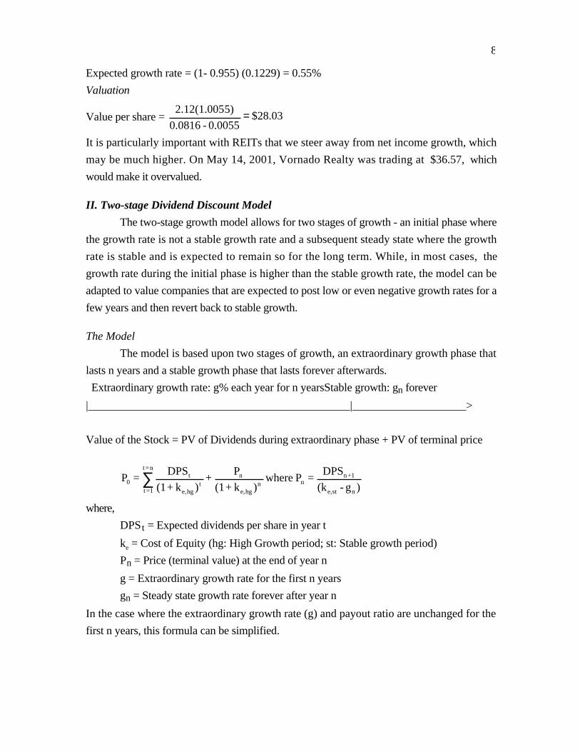
8

Expected growth rate = (1- 0.955) (0.1229) = 0.55%

Valuation

Value per share = $28.030.0055-0.0816

5)2.12(1.005 =

It is particularly important with REITs that we steer away from net income growth, which

may be much higher. On May 14, 2001, Vornado Realty was trading at $36.57, which

would make it overvalued.

II. Two-stage Dividend Discount Model

The two-stage growth model allows for two stages of growth - an initial phase where

the growth rate is not a stable growth rate and a subsequent steady state where the growth

rate is stable and is expected to remain so for the long term. While, in most cases, the

growth rate during the initial phase is higher than the stable growth rate, the model can be

adapted to value companies that are expected to post low or even negative growth rates for a

few years and then revert back to stable growth.

The Model

The model is based upon two stages of growth, an extraordinary growth phase that

lasts n years and a stable growth phase that lasts forever afterwards.

Extraordinary growth rate: g% each year for n yearsStable growth: gn forever

|______________________________________________|____________________>

Value of the Stock = PV of Dividends during extraordinary phase + PV of terminal price

)g-(k

DPS = P where

)k+(1

P +

)k+(1

DPS = P

nste,

1+nnn

hge,

nn=t

1=tt

hge,

t0 ∑

where,

DPS t = Expected dividends per share in year t

ke = Cost of Equity (hg: High Growth period; st: Stable growth period)

Pn = Price (terminal value) at the end of year n

g = Extraordinary growth rate for the first n years

gn = Steady state growth rate forever after year n

In the case where the extraordinary growth rate (g) and payout ratio are unchanged for the

first n years, this formula can be simplified.

9

nhge,nste,

1+n

hge,

nhge,

n

0

0)k+)(1g-(k

DPS +

g-k

)k+(1

g)+(1-1*g)+(1*DPS

= P

where the inputs are as defined above.

Calculating the terminal price

The same constraint that applies to the growth rate for the Gordon Growth Rate

model, i.e., that the growth rate in the firm is comparable to the nominal growth rate in the

economy, applies for the terminal growth rate (gn) in this model as well.

In addition, the payout ratio has to be consistent with the estimated growth rate. If

the growth rate is expected to drop significantly after the initial growth phase, the payout

ratio should be higher in the stable phase than in the growth phase. A stable firm can pay

out more of its earnings in dividends than a growing firm. One way of estimating this new

payout ratio is to use the fundamental growth model described in Chapter 12.

Expected Growth = Retention ratio * Return on equity

Algebraic manipulation yields the following stable period payout ratio:

Stable Payout ratio = equityon return period Stable

rategrowth Stable

Thus, a firm with a 5% growth rate and a return on equity of 15% will have a stable period

payout ratio of 33.33%.

The other characteristics of the firm in the stable period should be consistent with

the assumption of stability. For instance, it is reasonable to assume that a high growth firm

has a beta of 2.0, but unreasonable to assume that this beta will remain unchanged when the

firm becomes stable. In fact, the rule of thumb that we developed in the last chapter – that

stable period betas should be between 0.8 and 1.2 – is worth repeating here. Similarly, the

return on equity, which can be high during the initial growth phase, should come down to

levels commensurate with a stable firm in the stable growth phase. What is a reasonable

stable period return on equity? The industry average return on equity and the firm’s own

stable period cost of equity provide useful information to make this judgment.

Limitations of the model

There are three problems with the two-stage dividend discount model – the first two

would apply to any two-stage model and the third is specific to the dividend discount model.

• The first practical problem is in defining the length of the extraordinary growth period.

Since the growth rate is expected to decline to a stable level after this period, the value of

an investment will increase as this period is made longer. While we did develop criteria

10

that might be useful in making this judgment in Chapter 12, it is difficult in practice to

convert these qualitative considerations into a specific time period.

• The second problem with this model lies in the assumption that the growth rate is high

during the initial period and is transformed overnight to a lower stable rate at the end of

the period. While these sudden transformations in growth can happen, it is much more

realistic to assume that the shift from high growth to stable growth happens gradually

over time.

• The focus on dividends in this model can lead to skewed estimates of value for firms

that are not paying out what they can afford in dividends. In particular, we will under

estimate the value of firms that accumulate cash and pay out too little in dividends.

Works best for:

Since the two-stage dividend discount model is based upon two clearly delineated

growth stages, high growth and stable growth, it is best suited for firms which are in high

growth and expect to maintain that growth rate for a specific time period, after which the

sources of the high growth are expected to disappear. One scenario, for instance, where this

may apply is when a company has patent rights to a very profitable product for the next few

years and is expected to enjoy super-normal growth during this period. Once the patent

expires, it is expected to settle back into stable growth. Another scenario where it may be

reasonable to make this assumption about growth is when a firm is in an industry which is

enjoying super-normal growth because there are significant barriers to entry (either legal or

as a consequence of infra-structure requirements), which can be expected to keep new

entrants out for several years.

The assumption that the growth rate drops precipitously from its level in the initial

phase to a stable rate also implies that this model is more appropriate for firms with modest

growth rates in the initial phase. For instance, it is more reasonable to assume that a firm

growing at 12% in the high growth period will see its growth rate drops to 6% afterwards

than it is for a firm growing at 40% in the high growth period.

Finally, the model works best for firms that maintain a policy of paying out most of

residual cash flows – i.e, cash flows left over after debt payments and reinvestment needs

have been met – as dividends.

Illustration 13.3: Valuing a firm with the two-stage dividend discount model: Procter &

Gamble

Procter & Gamble (P&G) manufactures and markets consumer products all over

the world. Some of its best known brand names include Pampers diapers, Tide detergent,

Crest toothpaste and Vicks cough/cold medicines.

11

A Rationale for using the Model

• Why two-stage? While P&G is a firm with strong brand names and an impressive

track record on growth, it faces two problems. The first is the saturation of the domestic

U.S. market, which represents about half of P&G’s revenues. The second is the

increased competition from generics across all of its product lines. We will assume that

the firm will continue to grow but restrict the growth period to 5 years.

• Why dividends? P&G has a reputation for paying high dividends and it has not

accumulated large amounts of cash over the last decade.

Background Information

• Earnings per share in 2000 = $3.00

• Dividends per share in 2000 = $1.37

• Payout ratio in 2000 = 45.67%3.00

1.37 =

• Return on Equity in 2000 = 29.37%

Estimates

We will first estimate the cost of equity for P&G, based upon a bottom-up beta of 0.85

(estimated using the unlevered beta for consumer product firms and P&G’s debt to equity

ratio), a riskfree rate of 5.4% and a risk premium of 4%.

Cost of equity = 5.4% + 0.85 (4%) = 8.8%

To estimate the expected growth in earnings per share over the five-year high growth period,

we use the retention ratio in the most recent financial year (2000) but lower the return on

equity to 25% from the current value.

Expected growth rate = Retention ratio * Return on Equity

= ( )( ) %58.1325.04567.01 =−

In stable growth, we will estimate that the beta for the stock will rise to 1, leading to a cost of

equity of 9.40%.

Cost of equity in stable growth = 5.4% + 1 (4%) = 9.40%

The expected growth rate will be assumed to be equal to the growth rate of the economy

(5%) and the return on equity will drop to 15%, which is lower than the current industry

average (17.4%) but higher than the cost of equity estimated above. The retention ratio in

stable growth during the stable growth period is calculated.

Retention ratio in stable growth = 33.33%15%

5%

ROE

g ==

The payout ratio in stable growth is therefore 66.67%.

Estimating the value:

12

The first component of value is the present value of the expected dividends during

the high growth period. Based upon the current earnings ($3.00), the expected growth rate

(13.58%) and the expected dividend payout ratio (45.67%), the expected dividends can be

computed for each year in the high growth period.

Table 13.1: Expected Dividends per share: P&G

Year EPS DPS Present Value

1 $3.41 $1.56 $1.43

2 $3.87 $1.77 $1.49

3 $4.40 $2.01 $1.56

4 $4.99 $2.28 $1.63

5 $5.67 $2.59 $1.70

Sum $7.81

The present value is computed using the cost of equity of 8.8% for the high growth period.

Cumulative Present Value of Dividends during high growth (@8.8%) = $7.81

The present value of the dividends can also be computed in short hand using the following

computation:

81.7$0.1358-0.088

(1.088)

(1.1358)-158)$1.37(1.13

=Dividends of PV5

5

=

The price (terminal value) at the end of the high growth phase (end of year 5) can be

estimated using the constant growth model.

Terminal price = nste,

1n

g - k

shareper Dividends Expected +

Expected Earnings per share6 = 3.00 *1.13585*1.05 = $5.96

Expected Dividends per share6 = EPS6*Stable period payout ratio

= $5.96 * 0.6667 = $3.97

Terminal price = $90.230.05- 0.094

$3.97

g-k

Dividends

ste,

6 ==

The present value of the terminal price –is:

18.59$(1.088)

$90.23=Price Terminal of PV

5=

The cumulated present value of dividends and the terminal price can then be calculated.

13

( )

( ) $66.99=$59.18+$7.81=1.088

$90.23+

0.1358-0.088

(1.088)

(1.1358)-11.1358$1.37

= P5

5

5

0

P&G was trading at $63.90 at the time of this analysis on May 14, 2001.

.DDM2st.xlss: This spreadsheet allows you to value a firm with a temporary period of

high earnings followed by stable growth.

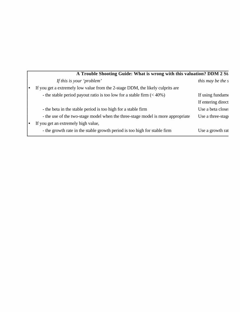
A Trouble Shooting Guide: What is wrong with this valuation? DDM 2 Stage

If this is your ‘problem’ this may be the solution

• If you get a extremely low value from the 2-stage DDM, the likely culprits are

- the stable period payout ratio is too low for a stable firm (< 40%) If using fundamentals,

If entering directly,

- the beta in the stable period is too high for a stable firm Use a beta closer

- the use of the two-stage model when the three-stage model is more appropriate Use a three-stage

• If you get an extremely high value,

- the growth rate in the stable growth period is too high for stable firm Use a growth rate

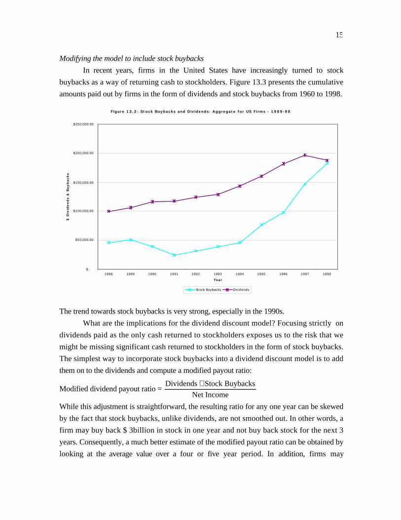
15

Modifying the model to include stock buybacks

In recent years, firms in the United States have increasingly turned to stock

buybacks as a way of returning cash to stockholders. Figure 13.3 presents the cumulative

amounts paid out by firms in the form of dividends and stock buybacks from 1960 to 1998.

The trend towards stock buybacks is very strong, especially in the 1990s.

What are the implications for the dividend discount model? Focusing strictly on

dividends paid as the only cash returned to stockholders exposes us to the risk that we

might be missing significant cash returned to stockholders in the form of stock buybacks.

The simplest way to incorporate stock buybacks into a dividend discount model is to add

them on to the dividends and compute a modified payout ratio:

Modified dividend payout ratio = IncomeNet

BuybacksStock Dividends +

While this adjustment is straightforward, the resulting ratio for any one year can be skewed

by the fact that stock buybacks, unlike dividends, are not smoothed out. In other words, a

firm may buy back $ 3billion in stock in one year and not buy back stock for the next 3

years. Consequently, a much better estimate of the modified payout ratio can be obtained by

looking at the average value over a four or five year period. In addition, firms may

Figure 13.3: Stock Buybacks and Dividends: Aggregate for US Firms - 1989-98

$-

$50,000.00

$100,000.00

$150,000.00

$200,000.00

$250,000.00

1988 1989 1990 1991 1992 1993 1994 1995 1996 1997 1998

Year

$ D

ivid

ends &

Buybacks

Stock Buybacks Dividends

16

sometimes buy back stock as a way of increasing financial leverage. We could adjust for

this by netting out new debt issued from the calculation above:

Modified dividend payout = IncomeNet

issuesDebt Term Long-BuybacksStock Dividends +

Adjusting the payout ratio to include stock buybacks will have ripple effects on the

estimated growth and the terminal value. In particular, the modified growth rate in earnings

per share can be written as:

Modified growth rate = (1 – Modified payout ratio) * Return on equity

Even the return on equity can be affected by stock buybacks. Since the book value of equity

is reduced by the market value of equity bought back, a firm that buys backs stock can

reduce its book equity (and increase its return on equity) dramatically. If we use this return

on equity as a measure of the marginal return on equity (on new investments), we will

overstate the value of a firm. Adding back stock buybacks in recent year to the book equity

and re-estimating the return on equity can sometimes yield a more reasonable estimate of

the return on equity on investments.

Illustration 13.4: Valuing a firm with modified dividend discount mode: Procter & Gamble

Consider our earlier valuation of Procter and Gamble where we used the current

dividends as the basis for our projections. Note that over the last four years, P&G has had

significant stock buybacks each period. Table 13.2 summarizes the dividends and buybacks

over the period.

Table 13.2: Dividends and Stock Buybacks: P&G

1997 1998 1999 2000 Total

Net Income 3415 3780 3763 3542 14500

Dividends 1329 1462 1626 1796 6213

Buybacks 2152 391 1881 -1021 3403

Dividends+Buybacks 3481 1853 3507 775 9616

Payout ratio 38.92% 38.68% 43.21% 50.71% 42.85%

Modified payout ratio 101.93% 49.02% 93.20% 21.88% 66.32%

Buybacks 1652 1929 2533 1766

Net LT Debt issued -500 1538 652 2787

Buybacks net of debt 2152 391 1881 -1021

Over the five-year period, P&G had significant buybacks but it also increased its leverage

dramatically in the last three years. Summing up the total cash returned to stockholders over

17

the last 4 years, we arrive at a modified payout ratio of 66.32%. If we substitute this payout

ratio into the valuation in Illustration 13.3, the expected growth rate over the next 5 years

drops to 8.42%:

Expected growth rate = (1- Modified payout ratio) ROE = (1-0.6632)(0.25) = 8.42%

We will still assume a five year high growth period and that the parameters in stable growth

remain unchanged. The value per share can be estimated.

( )( )$56.75 =

(1.0880)

$71.50 +

0.0842-0.0880

(1.0880)

(1.0842)-11.08420.6632$3.00

= P5

5

5

0

Note that the drop in growth rate in earnings during the high growth period reduces

earnings in the terminal year, and the terminal value per share drops to $71.50.

This value is lower than that obtained in Illustration 13.3 and it reflects our expectation that

P&G does not have as many new profitable new investments (earning a return on equity of

25%).

Valuing an entire market using the dividend discount model

All our examples of the dividend discount model so far have involved individual

companies, but there is no reason why we cannot apply the same model to value a sector or

even the entire market. The market price of the stock would be replaced by the cumulative

market value of all of the stocks in the sector or market. The expected dividends would be

the cumulated dividends of all these stocks and could be expanded to include stock

buybacks by all firms. The expected growth rate would be the growth rate in cumulated

earnings of the index. There would be no need for a beta or betas, since you are looking at

the entire market (which should have a beta of 1) and you could add the risk premium (or

premiums) to the riskfree rate to estimate a cost of equity. You could use a two-stage model,

where this growth rate is greater than the growth rate of the economy, but you should be

cautious about setting the growth rate too high or the growth period too long because it will

be difficult for cumulated earnings growth of all firms in an economy to run ahead of the

growth rate in the economy for extended periods.

Consider a simple example. Assume that you have an index trading at 700 and that

the average dividend yield of stocks in the index is 5%. Earnings and dividends can be

expected to grow at 4% a year forever and the riskless rate is 5.4%. If you use a market risk

premium of 4%, the value of the index can be estimated.

Cost of equity = Riskless rate + Risk premium = 5.4% + 4% = 9.4%

18

Expected dividends next year = (Dividend yield * Value of the index)(1+ expected growth

rate) = (0.05*700) (1.04) = 36.4

Value of the index 67404.0094.0

4.36

rategrowth Expected-equity ofCost

yearnext dividends Expected =−

==

At its existing level of 700, the market is slightly over priced.

Illustration 13.5: Valuing the S&P 500 using a dividend discount model: January 1, 2001

On January 1, 2001, the S&P 500 index was trading at 1320. The dividend yield on

the index was only 1.43%, but including stock buybacks increases the modified dividend

yield to 2.50%. Analysts were estimating that the earnings of the stocks in the index would

increase 7.5% a year for the next 5 years. Beyond year 5, the expected growth rate is

expected to be 5%, the nominal growth rate in the economy. The treasury bond rate was

5.1% and we will use a market risk premium of 4%, leading to a cost of equity of 9.1%:

Cost of equity = 5.1% + 4% = 9.1%

The expected dividends (and stock buybacks) on the index for the next 5 years can be

estimated from the current dividends and expected growth of 7.50%.

Current dividends = 2.50% of 1320 = 33.00

1 2 3 4 5

Expected Dividends = $35.48 $38.14 $41.00 $44.07 $47.38

Present Value = $32.52 $32.04 $31.57 $31.11 $30.65

The present value is computed by discounting back the dividends at 9.1%. To estimate the

terminal value, we estimate dividends in year 6 on the index:

Expected dividends in year 6 = $47.38 (1.05) = $49.74

Terminal value of the index = $12130.05-0.091

$49.74

g-r

Dividends Expected 6 ==

Present value of Terminal value = $7851.091

$12135

=

The value of the index can now be computed:

Value of index = Present value of dividends during high growth + Present value of terminal

value = $32.52+32.04+31.57+$31.11+ $30.65+ $785 = $943

Based upon this, we would have concluded that the index was over valued at 1320.

The Value of Growth

19

Investors pay a price premium when they acquire companies with high growth

potential. This premium takes the form of higher price-earnings or price-book value ratios.

While no one will contest the proposition that growth is valuable, it is possible to pay too

much for growth. In fact, empirical studies that show low price-earnings ratio stocks earning

return premiums over high price-earnings ratio stocks in the long term supports the notion

that investors overpay for growth. This section uses the two-stage dividend discount model

to examine the value of growth and it provides a benchmark that can be used to compare the

actual prices paid for growth.

Estimating the value of growth

The value of the equity in any firm can be written in terms of three components:

)g-(k

DPS-

)k+)(1g-(k

DPS +

g-k

)k+(1

g)+(1-1*g)+(1*DPS

= Pnste,

1n

hge,nste,

1+n

hge,

nhge,

n

0

0

|________________________________________________|

Extraordinary Growth

+ DPS1

(k e,st -g n ) -

DPS0

k e,st

+

DPS0

k e,st

|___________________| |_____________|

Stable Growth Assets in place

where

DPS t = Expected dividends per share in year t

ke = Required rate of return

Pn = Price at the end of year n

g = Growth rate during high growth stage

gn = Growth rate forever after year n

Value of extraordinary growth = Value of the firm with extraordinary growth in first n

years - Value of the firm as a stable growth firm3

Value of stable growth = Value of the firm as a stable growth firm - Value of firm with no

growth

3 The payout ratio used to calculate the value of the firm as a stable firm can be either the current payoutratio, if it is reasonable, or the new payout ratio calculated using the fundamental growth formula.

20

Assets in place = Value of firm with no growth

In making these estimates, though, we have to remain consistent. For instance, to value

assets in place, you would have to assume that the entire earnings could be paid out in

dividends, while the payout ratio used to value stable growth should be a stable period

payout ratio.

Illustration 13.6: The Value of Growth: P&G in May 2001

In illustration 13.3, we valued P&G using a 2-stage dividend discount model at $66.99. We

first value the assets in place using current earnings ($3.00) and assume that all earnings are

paid out as dividends. We also use the stable growth cost of equity as the discount rates.

Value of the assets in place 91.31$094.0

3$

k

EPSCurrent

ste,

===

To estimate the value of stable growth, we assume that the expected growth rate will be 5% and that

the payout ratio is the stable period payout ratio of 66.67%:

Value of stable growth

( )( )( )

( )( )( )81.15$91.31$

05.0094.0

05.16667.000.3$

91.31$1RatioPayout StableEPSCurrent

,

=−−

=

−−

+nste

n

gkg

Value of extraordinary growth = $66.99 - $31.91 - $15.81 = $19.26

The Determinants of the Value of Growth

1. Growth rate during extraordinary period: The higher the growth rate in the

extraordinary period, the higher the estimated value of growth will be. If the growth

rate in the extraordinary growth period had been raised to 20% for the Procter &

Gamble valuation, the value of extraordinary growth would have increased from

$19.26 to $39.45. Conversely, the value of high growth companies can drop

precipitously if the expected growth rate is reduced, either because of disappointing

earnings news from the firm or as a consequence of external events.

2. Length of the extraordinary growth period: The longer the extraordinary

growth period, the greater the value of growth will be. At an intuitive level, this is

fairly simple to illustrate. The value of $19.26 obtained for extraordinary growth is

predicated on the assumption that high growth will last for five years. If this is

revised to last ten years, the value of extraordinary growth will increase to $43.15.

3. Profitability of projects: The profitability of projects determines both the

growth rate in the initial phase and the terminal value. As projects become more

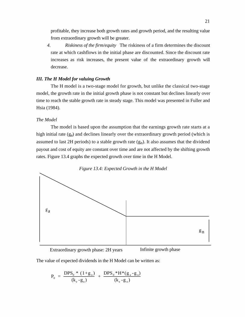
21

profitable, they increase both growth rates and growth period, and the resulting value

from extraordinary growth will be greater.

4. Riskiness of the firm/equity The riskiness of a firm determines the discount

rate at which cashflows in the initial phase are discounted. Since the discount rate

increases as risk increases, the present value of the extraordinary growth will

decrease.

III. The H Model for valuing Growth

The H model is a two-stage model for growth, but unlike the classical two-stage

model, the growth rate in the initial growth phase is not constant but declines linearly over

time to reach the stable growth rate in steady stage. This model was presented in Fuller and

Hsia (1984).

The Model

The model is based upon the assumption that the earnings growth rate starts at a

high initial rate (ga) and declines linearly over the extraordinary growth period (which is

assumed to last 2H periods) to a stable growth rate (gn). It also assumes that the dividend

payout and cost of equity are constant over time and are not affected by the shifting growth

rates. Figure 13.4 graphs the expected growth over time in the H Model.

Figure 13.4: Expected Growth in the H Model

Extraordinary growth phase: 2H years Infinite growth phase

ga

gn

The value of expected dividends in the H Model can be written as:

P0 = DPS0 * (1+g n )

(k e -gn ) +

DPS0 *H*(g a -g n)

(k e -g n )

22

Stable growth Extraordinary growth

where,

P0 = Value of the firm now per share,

DPS t = DPS in year t

ke= Cost of equity

ga = Growth rate initially

gn = Growth rate at end of 2H years, applies forever afterwards

Limitations

This model avoids the problems associated with the growth rate dropping

precipitously from the high growth to the stable growth phase, but it does so at a cost. First,

the decline in the growth rate is expected to follow the strict structure laid out in the model --

it drops in linear increments each year based upon the initial growth rate, the stable growth

rate and the length of the extraordinary growth period. While small deviations from this

assumption do not affect the value significantly, large deviations can cause problems.

Second, the assumption that the payout ratio is constant through both phases of growth

exposes the analyst to an inconsistency -- as growth rates decline the payout ratio usually

increases.

Works best for:

The allowance for a gradual decrease in growth rates over time may make this a

useful model for firms which are growing rapidly right now, but where the growth is

expected to decline gradually over time as the firms get larger and the differential advantage

they have over their competitors declines. The assumption that the payout ratio is constant,

however, makes this an inappropriate model to use for any firm that has low or no dividends

currently. Thus, the model, by requiring a combination of high growth and high payout,

may be quite limited4 in its applicability.

Illustration 13.7: Valuing with the H model: Alcatel

Alcatel is a French telecommunications firm, paid dividends per share of 0.72 Ffr on

earnings per share of 1.25 Ffr in 2000. The firm’s earnings per share had grown at 12%

over the prior 5 years but the growth rate is expected to decline linearly over the next 10

years to 5%, while the payout ratio remains unchanged. The beta for the stock is 0.8, the

riskfree rate is 5.1% and the market risk premium is 4%.

4 Proponents of the model would argue that using a steady state payout ratio for firms which pay little orno dividends is likely to cause only small errors in the valuation.

23

Cost of equity = 5.1% + 0.8*4% = 8.30%

The stock can be valued using the H model:

Value of stable growth = ( )( )

$22.91=0.05-0.083

1.050.72

Value of extraordinary growth = ( )( )( )

7.64=0.05-0.083

0.05-0.1210/20.72

Value of stock = 22.91 + 7.64 = 30.55

The stock was trading at 33.40 Ffr in May 2001.

IV. Three-stage Dividend Discount Model

The three-stage dividend discount model combines the features of the two-stage

model and the H-model. It allows for an initial period of high growth, a transitional period

where growth declines and a final stable growth phase. It is the most general of the models

because it does not impose any restrictions on the payout ratio.

The Model

This model assumes an initial period of stable high growth, a second period of declining

growth and a third period of stable low growth that lasts forever. Figure 13.5 graphs the expected

growth over the three time periods.

Figure 13.5: Expected Growth in the Three-Stage DDM

24

Increasing payout ratio

High Stable growth Declining growth Infinite Stable growth

ga

gn

Low Payout ratio

High payout ratio

EARNINGS GROWTH RATES

DIVIDEND PAYOUTS

The value of the stock is then the present value of expected dividends during the high growth and

the transitional periods and of the terminal price at the start of the final stable growth phase.

P0 = EPS0 *(1+ga )t * Πa

(1+k e,hg)t

t=1

t=n1

∑ + DPSt

(1+k e,t )t

t=n1+1

t=n2

∑ + EPSn2 *(1+g n )* Πn

(k e,st -g n )(1+r)n

High growth phase Transition Stable growth phase

where,

EPSt = Earnings per share in year t

DPS t = Dividends per share in year t

ga = Growth rate in high growth phase (lasts n1 periods)

gn = Growth rate in stable phase

Πa = Payout ratio in high growth phase

Πn = Payout ratio in stable growth phase

ke= Cost of equity in high growth (hg), transition (t) and stable growth (st)

Assumptions

25

This model removes many of the constraints imposed by other versions of the

dividend discount model. In return, however, it requires a much larger number of inputs -

year-specific payout ratios, growth rates and betas. For firms where there is substantial

noise in the estimation process, the errors in these inputs can overwhelm any benefits that

accrue from the additional flexibility in the model.

Works best for:

This model's flexibility makes it a useful model for any firm, which in addition to

changing growth over time is expected to change on other dimensions as well - in particular,

payout policies and risk. It is best suited for firms which are growing at an extraordinary

rate now and are expected to maintain this rate for an initial period, after which the

differential advantage of the firm is expected to deplete leading to gradual declines in the

growth rate to a stable growth rate. Practically speaking, this may be the more appropriate

model to use for a firm whose earnings are growing at very high rates5, are expected to

continue growing at those rates for an initial period, but are expected to start declining

gradually towards a stable rate as the firm become larger and loses its competitive

advantages.

Illustration 13.8: Valuing with the Three-stage DDM model: Coca Cola

Coca Cola, the owner of the most valuable brand name in the world according to

Interbrand, was able to increase its market value ten-fold in the 1980s and 1990s. While

growth has leveled off in the last few years, the firm is still expanding both into other

products and other markets.

A Rationale for using the Three-Stage Dividend Discount Model

• Why three-stage? Coca Cola is still in high growth, but its size and dominant market

share will cause growth to slide in the second phase of the high growth period. The high

growth period is expected to last 5 years and the transition period is expected to last an

additional 5 years.

• Why dividends? The firm has had a track record of paying out large dividends to its

stockholders, and these dividends tend to mirror free cash flows to equity.

• The financial leverage is stable.

Background Information

• Current Earnings / Dividends

• Earnings per share in 2000 = $1.56

5 The definition of a 'very high' growth rate is largely subjective. As a rule of thumb, growth rates over25% would qualify as very high when the stable growth rate is 6-8%.

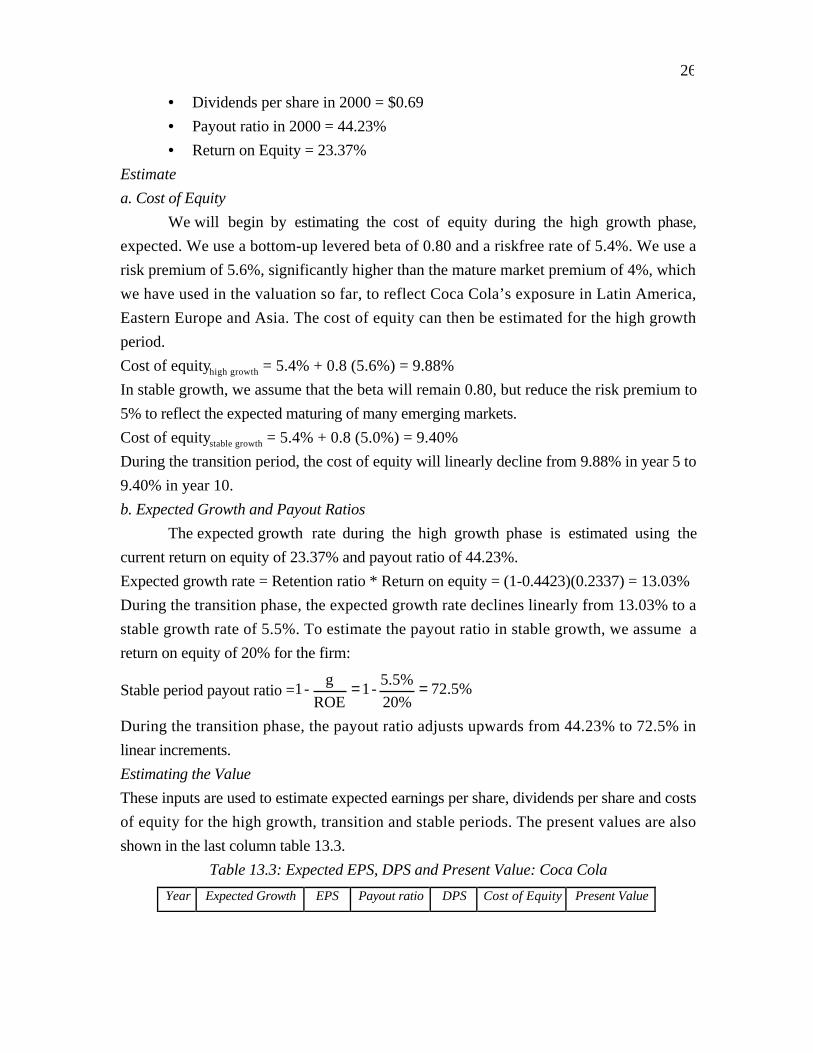
26

• Dividends per share in 2000 = $0.69

• Payout ratio in 2000 = 44.23%

• Return on Equity = 23.37%

Estimate

a. Cost of Equity

We will begin by estimating the cost of equity during the high growth phase,

expected. We use a bottom-up levered beta of 0.80 and a riskfree rate of 5.4%. We use a

risk premium of 5.6%, significantly higher than the mature market premium of 4%, which

we have used in the valuation so far, to reflect Coca Cola’s exposure in Latin America,

Eastern Europe and Asia. The cost of equity can then be estimated for the high growth

period.

Cost of equityhigh growth = 5.4% + 0.8 (5.6%) = 9.88%

In stable growth, we assume that the beta will remain 0.80, but reduce the risk premium to

5% to reflect the expected maturing of many emerging markets.

Cost of equitystable growth = 5.4% + 0.8 (5.0%) = 9.40%

During the transition period, the cost of equity will linearly decline from 9.88% in year 5 to

9.40% in year 10.

b. Expected Growth and Payout Ratios

The expected growth rate during the high growth phase is estimated using the

current return on equity of 23.37% and payout ratio of 44.23%.

Expected growth rate = Retention ratio * Return on equity = (1-0.4423)(0.2337) = 13.03%

During the transition phase, the expected growth rate declines linearly from 13.03% to a

stable growth rate of 5.5%. To estimate the payout ratio in stable growth, we assume a

return on equity of 20% for the firm:

Stable period payout ratio = 72.5%20%

5.5%-1

ROE

g-1 ==

During the transition phase, the payout ratio adjusts upwards from 44.23% to 72.5% in

linear increments.

Estimating the Value

These inputs are used to estimate expected earnings per share, dividends per share and costs

of equity for the high growth, transition and stable periods. The present values are also

shown in the last column table 13.3.

Table 13.3: Expected EPS, DPS and Present Value: Coca Cola

Year Expected Growth EPS Payout ratio DPS Cost of Equity Present Value

27

High Growth Stage

1 13.03% $1.76 44.23% $0.78 9.88% $0.71

2 13.03% $1.99 44.23% $0.88 9.88% $0.73

3 13.03% $2.25 44.23% $1.00 9.88% $0.75

4 13.03% $2.55 44.23% $1.13 9.88% $0.77

5 13.03% $2.88 44.23% $1.27 9.88% $0.79

Transition Stage

6 11.52% $3.21 49.88% $1.60 9.78% $0.91

7 10.02% $3.53 55.54% $1.96 9.69% $1.02

8 8.51% $3.83 61.19% $2.34 9.59% $1.11

9 7.01% $4.10 66.85% $2.74 9.50% $1.18

10 5.50% $4.33 72.50% $3.14 9.40% $1.24

(Note: Since the costs of equity change each year, the present value has to be calculated

using the cumulated cost of equity. Thus, in year 7, the present value of dividends is:

PV of year 7 dividend = $1.02(1.0969) (1.0978)(1.0988)

$1.965

=

The terminal price at the end of year 10 can be calculated based upon the earnings per share

in year 11, the stable growth rate of 5%, a cost of equity of 9.40% and the payout ratio of

72.5% -

Terminal price = ( )( )

$84.830.055-0.094

0.7251.055$4.33 =

The components of value are as follows:

Present Value of dividends in high growth phase:$ 3.76

Present Value of dividends in transition phase:$ 5.46

Present Value of terminal price at end of transition:$ 33.50

Value of Coca Cola Stock :$ 42.72

Coca Cola was trading at $46.29 in May 21, 2001.

.DDM3st.xlss: This spreadsheet allows you to value a firm with a period of high

growth followed by a transition period where growth declines to a stable growth rate.

28

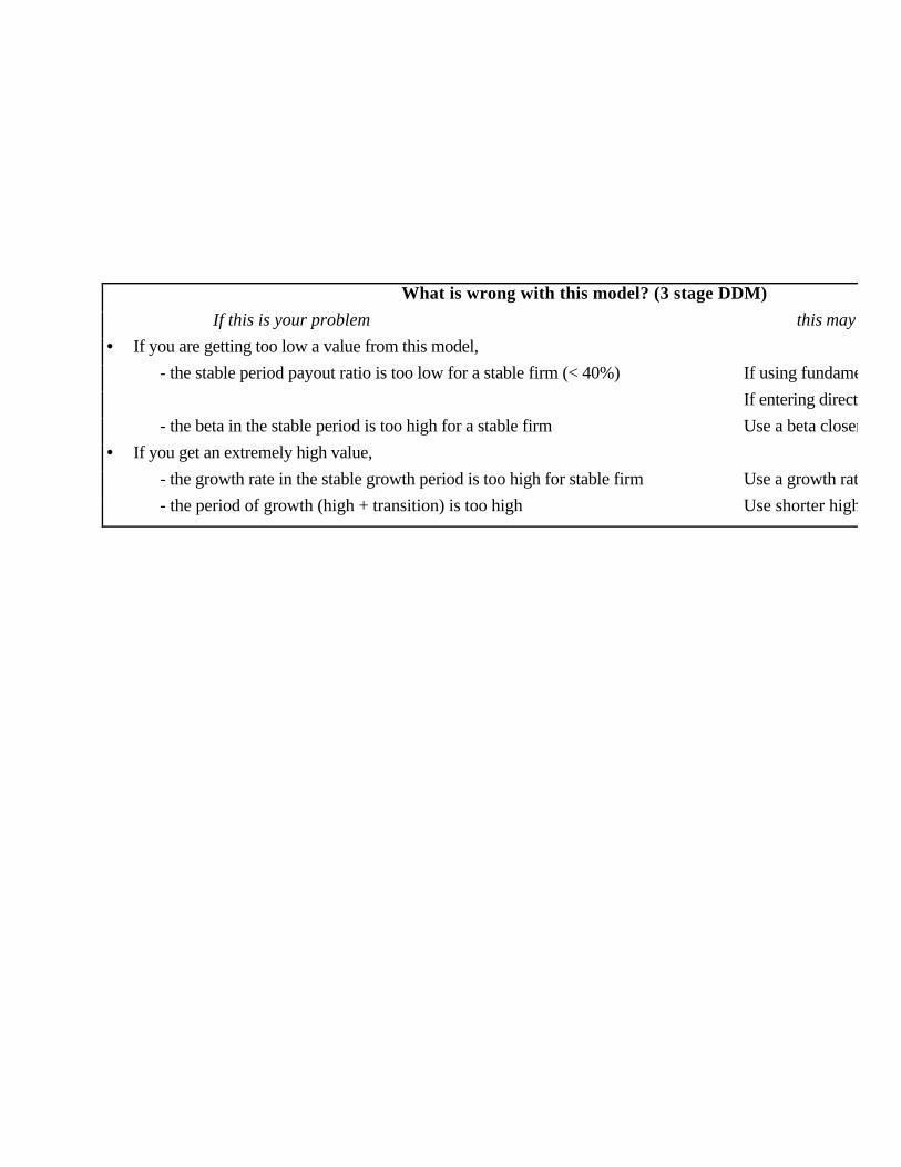
What is wrong with this model? (3 stage DDM)

If this is your problem this may

• If you are getting too low a value from this model,

- the stable period payout ratio is too low for a stable firm (< 40%) If using fundamentals,

If entering directly,

- the beta in the stable period is too high for a stable firm Use a beta closer

• If you get an extremely high value,

- the growth rate in the stable growth period is too high for stable firm Use a growth rate

- the period of growth (high + transition) is too high Use shorter high

30

Issues in using the Dividend Discount Model

The dividend discount model's primary attraction is its simplicity and its intuitive

logic. There are many analysts, however, who view its results with suspicion because of

limitations that they perceive it to possess. The model, they claim, is not really useful in

valuation, except for a limited number of stable, high-dividend paying stocks. This section

examines some of the areas where the dividend discount model is perceived to fall short.

(a) Valuing non-dividend paying or low dividend paying stocks

The conventional wisdom is that the dividend discount model cannot be used to

value a stock that pays low or no dividends. It is wrong. If the dividend payout ratio is

adjusted to reflect changes in the expected growth rate, a reasonable value can be obtained

even for non-dividend paying firms. Thus, a high-growth firm, paying no dividends

currently, can still be valued based upon dividends that it is expected to pay out when the

growth rate declines. If the payout ratio is not adjusted to reflect changes in the growth rate,

however, the dividend discount model will underestimate the value of non-dividend paying

or low-dividend paying stocks.

(b) Is the model too conservative in estimating value?

A standard critique of the dividend discount model is that it provides too

conservative an estimate of value. This criticism is predicated on the notion that the value is

determined by more than the present value of expected dividends. For instance, it is argued

that the dividend discount model does not reflect the value of 'unutilized assets'. There is no

reason, however, that these unutilized assets cannot be valued separately and added on to the

value from the dividend discount model. Some of the assets that are supposedly ignored by

the dividend discount model, such as the value of brand names, can be dealt with simply

within the context of the model.

A more legitimate criticism of the model is that it does not incorporate other ways of

returning cash to stockholders (such as stock buybacks). If you use the modified version of

the dividend discount model, this criticism can also be countered.

(c) The contrarian nature of the model

The dividend discount model is also considered by many to be a contrarian model.

As the market rises, fewer and fewer stocks, they argue, will be found to be undervalued

using the dividend discount model. This is not necessarily true. If the market increase is due

to an improvement in economic fundamentals, such as higher expected growth in the

economy and/or lower interest rates, there is no reason, a priori, to believe that the values

31

from the dividend discount model will not increase by an equivalent amount. If the market

increase is not due to fundamentals, the dividend discount model values will not follow suit,

but that is more a sign of strength than weakness. The model is signaling that the market is

overvalued relative to dividends and cashflows and the cautious investor will pay heed.

Tests of the Dividend Discount Model

The ultimate test of a model lies in how well it works at identifying undervalued and

overvalued stocks. The dividend discount model has been tested and the results indicate that

it does, in the long term, provide for excess returns. It is unclear, however, whether this is

because the model is good at finding undervalued stocks or because it proxies for well-

know empirical irregularities in returns relating to price-earnings ratios and dividend yields.

A Simple Test of the Dividend Discount model

A simple study of the dividend discount model was conducted by Sorensen and

Williamson, where they valued 150 stocks from the S&P 400 in December 1980, using the

dividend discount model. They used the difference between the market price at that time and

the model value to form five portfolios based upon the degree of under or over valuation.

They made fairly broad assumptions in using the dividend discount model.

(a) The average of the earnings per share between 1976 and 1980 was used as the current

earnings per share.

(b) The cost of equity was estimated using the CAPM.

(c) The extraordinary growth period was assumed to be five years for all stocks and the

I/B/E/S consensus forecast of earnings growth was used as the growth rate for this period.

(d) The stable growth rate, after the extraordinary growth period, was assumed to be 8% for

all stocks.

(e) The payout ratio was assumed to be 45% for all stocks.

The returns on these five portfolios were estimated for the following two years

(January 1981-January 1983) and excess returns were estimated relative to the S&P 500

Index using the betas estimated at the first stage and the CAPM. Figure 13.6 illustrates the

excess returns earned by the portfolio that was undervalued by the dividend discount model

relative to both the market and the overvalued portfolio.

32

The undervalued portfolio had a positive excess return of 16% per annum between 1981

and 1983, while the overvalued portfolio had a negative excess return of 15% per annum

during the same time period. Other studies which focus only on the dividend discount

model come to similar conclusions. In the long term, undervalued (overvalued) stocks from

the dividend discount model outperform (under perform) the market index on a risk

adjusted basis.

Caveats on the use of the dividend discount model

The dividend discount model provides impressive results in the long term. There are,

however, three considerations in generalizing the findings from these studies.

The dividend discount model does not beat the market every year

The dividend discount model outperforms the market over five-year time periods,

but there have been individual years where the model has significantly under performed the

market. Haugen reports on the results of a fund that used the dividend discount model to

analyze 250 large capitalization firms and to classify them into five quintiles from the first

quarter of 1979 to the last quarter of 1991. The betas of these quintiles were roughly equal.

The valuation was done by six analysts who estimated an extraordinary growth rate for the

initial high growth phase, the length of the high growth phase and a transitional phase for

each of the firms. The returns on the five portfolios as well as the returns on all 250 stocks

and the S&P 500 from 1979 to 1991 are reported in Table 13.4.

Table 13.4: Returns on Quintiles: Dividend Discount Model

Figure 13.6 Performance of the Dividend Discount Model: 1981-83

-0.3

-0.2

-0.1

0

0.1

0.2

0.3

0.4

Most undervalued 2 3 4 Most overvalued

Annual Return Excess Return

33

Quintile

Under 2 3 4 Over 250 S&P

Valued Valued Stocks 500

1979 35.07% 25.92% 18.49% 17.55% 20.06% 23.21% 18.57%

1980 41.21% 29.19% 27.41% 38.43% 26.44% 31.86% 32.55%

1981 12.12% 10.89% 1.25% -5.59% -8.51% 28.41% 24.55%

1982 19.12% 12.81% 26.72% 28.41% 35.54% 24.53% 21.61%

1983 34.18% 21.27% 25.00% 24.55% 14.35% 24.10% 22.54%

1984 15.26% 5.50% 6.03% -4.20% -7.84% 3.24% 6.12%

1985 38.91% 32.22% 35.83% 29.29% 23.43% 33.80% 31.59%

1986 14.33% 11.87% 19.49% 12.00% 20.82% 15.78% 18.47%

1987 0.42% 4.34% 8.15% 4.64% -2.41% 2.71% 5.23%

1988 39.61% 31.31% 17.78% 8.18% 6.76% 20.62% 16.48%

1989 26.36% 23.54% 30.76% 32.60% 35.07% 29.33% 31.49%

1990 -17.32% -8.12% -5.81% 2.09% -2.65% -6.18% -3.17%

1991 47.68% 26.34% 33.38% 34.91% 31.64% 34.34% 30.57%

1979-91 1253% 657% 772% 605% 434% 722% 654%

The undervalued portfolio earned significantly higher returns than the overvalued portfolio

and the S&P 500 for the 1979-91 period, but it under performed the market in five of the

twelve years and the overvalued portfolio in four of the twelve years.

Is the model just a proxy for low PE ratios and dividend yields?

The dividend discount model weights expected earnings and dividends in near

periods more than earnings and dividends in far periods., It is biased towards finding low

price-earnings ratio stocks with high dividend yields to be undervalued and high price-

earnings ratio stocks with low or no dividend yields to be overvalued. Studies of market

efficiency indicate that low PE ratio stocks have outperformed (in terms of excess returns)

high PE ratio stocks over extended time periods. Similar conclusions have been drawn

about high-dividend yield stocks relative to low-dividend yield stocks. Thus, the valuation

findings of the model are consistent with empirical irregularities observed in the market.

It is unclear how much the model adds in value to investment strategies that use PE

ratios or dividend yields to screen stocks. Jacobs and Levy (1988b) indicate that the

marginal gain is relatively small.

Attribute Average Excess Return per Quarter: 1982-87

34

Dividend Discount Model 0.06% per quarter

Low P/E Ratio 0.92% per quarter

Book/Price Ratio 0.01% per quarter

Cashflow/Price 0.18% per quarter

Sales/Price 0.96% per quarter

Dividend Yield -0.51% per quarter

This suggests that using low PE ratios to pick stocks adds 0.92% to your quarterly returns,

whereas using the dividend discount model adds only a further 0.06% to quarterly returns.

If, in fact, the gain from using the dividend discount model is that small, screening stocks on

the basis of observables (such as PE ratio or cashflow measures) may provide a much larger

benefit in terms of excess returns.

The tax disadvantages from high dividend stocks

Portfolios created with the dividend discount model are generally characterized by

high dividend yield, which can create a tax disadvantage if dividends are taxed at a rate

greater than capital gains or if there is a substantial tax timing6 liability associated with

dividends. Since the excess returns uncovered in the studies presented above are pre-tax to

the investor, the introduction of personal taxes may significantly reduce or even eliminate

these excess returns.

In summary, the dividend discount model's impressive results in studies looking at

past data have to be considered with caution. For a tax-exempt investment, with a long time

horizon, the dividend discount model is a good tool, though it may not be the only one, to

pick stocks. For a taxable investor, the benefits are murkier, since the tax consequences of

the strategy have to be considered. For investors with shorter time horizons, the dividend

discount model may not deliver on its promised excess returns, because of the year-to-year

volatility in its performance.

Conclusion

When you buy stock in a publicly traded firm, the only cash flow you receive

directly from this investment are expected dividends. The dividend discount model builds on

this simple propositions and argues that the value of a stock then has to be the present value

of expected dividends over time. Dividend discount models can range from simple growing

perpetuity models such as the Gordon Growth model, where a stock’s value is a function of

6 Investors do not have a choice of when they receive dividends, whereas they have a choice on the timingof capital gains.

35

its expected dividends next year, the cost of equity and the stable growth rate, to complex

three stage models, where payout ratios and growth rates change over time.

While the dividend discount model is often criticized as being of limited value, it has

proven to be surprisingly adaptable and useful in a wide range of circumstances. It may be a

conservative model that finds fewer and fewer undervalued firms as market prices rise

relative to fundamentals (earnings, dividends, etc.) but that can also be viewed as a strength.

Tests of the model also seem to indicate its usefulness in gauging value, though much of its

effectiveness may be derived from its finding low PE ratio, high dividend yield stocks to be

undervalued.

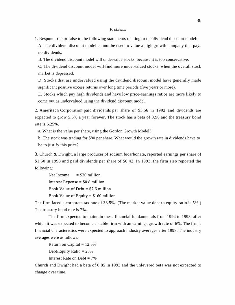
36

Problems

1. Respond true or false to the following statements relating to the dividend discount model:

A. The dividend discount model cannot be used to value a high growth company that pays

no dividends.

B. The dividend discount model will undervalue stocks, because it is too conservative.

C. The dividend discount model will find more undervalued stocks, when the overall stock

market is depressed.

D. Stocks that are undervalued using the dividend discount model have generally made

significant positive excess returns over long time periods (five years or more).

E. Stocks which pay high dividends and have low price-earnings ratios are more likely to

come out as undervalued using the dividend discount model.

2. Ameritech Corporation paid dividends per share of $3.56 in 1992 and dividends are

expected to grow 5.5% a year forever. The stock has a beta of 0.90 and the treasury bond

rate is 6.25%.

a. What is the value per share, using the Gordon Growth Model?

b. The stock was trading for $80 per share. What would the growth rate in dividends have to

be to justify this price?

3. Church & Dwight, a large producer of sodium bicarbonate, reported earnings per share of

$1.50 in 1993 and paid dividends per share of $0.42. In 1993, the firm also reported the

following:

Net Income = $30 million

Interest Expense = $0.8 million

Book Value of Debt = $7.6 million

Book Value of Equity = $160 million

The firm faced a corporate tax rate of 38.5%. (The market value debt to equity ratio is 5%.)

The treasury bond rate is 7%.

The firm expected to maintain these financial fundamentals from 1994 to 1998, after

which it was expected to become a stable firm with an earnings growth rate of 6%. The firm's

financial characteristics were expected to approach industry averages after 1998. The industry

averages were as follows:

Return on Capital = 12.5%

Debt/Equity Ratio = 25%

Interest Rate on Debt = 7%

Church and Dwight had a beta of 0.85 in 1993 and the unlevered beta was not expected to

change over time.

37

a. What is the expected growth rate in earnings, based upon fundamentals, for the high-

growth period (1994 to 1998)?

b. What is the expected payout ratio after 1998?

c. What is the expected beta after 1998?

d. What is the expected price at the end of 1998?

e. What is the value of the stock, using the two-stage dividend discount model?

f. How much of this value can be attributed to extraordinary growth? to stable growth?

4. Oneida Inc, the world's largest producer of stainless steel and silverplated flatware, reported

earnings per share of $0.80 in 1993 and paid dividends per share of $0.48 in that year. The

firm was expected to report earnings growth of 25% in 1994, after which the growth rate was

expected to decline linearly over the following six years to 7% in 1999. The stock was

expected to have a beta of 0.85. (The treasury bond rate was 6.25%)

a. Estimate the value of stable growth, using the H Model.

b. Estimate the value of extraordinary growth, using the H Model.

c. What are the assumptions about dividend payout in the H Model?

5. Medtronic Inc., the world's largest manufacturer of implantable biomedical devices,

reported earnings per share in 1993 of $3.95 and paid dividends per share of $0.68. Its

earnings were expected to grow 16% from 1994 to 1998, but the growth rate was expected to

decline each year after that to a stable growth rate of 6% in 2003. The payout ratio was

expected to remain unchanged from 1994 to 1998, after which it would increase each year to

reach 60% in steady state. The stock was expected to have a beta of 1.25 from 1994 to 1998,

after which the beta would decline each year to reach 1.00 by the time the firm becomes

stable. (The treasury bond rate was 6.25%)

a. Assuming that the growth rate declines linearly (and the payout ratio increases linearly)

from 1999 to 2003, estimate the dividends per share each year from 1994 to 2003.

b. Estimate the expected price at the end of 2003.

c. Estimate the value per share, using the three-stage dividend discount model.

1

CHAPTER 14

FREE CASH FLOW TO EQUITY DISCOUNT MODELS

The dividend discount model is based upon the premise that the only cashflows

received by stockholders is dividends. Even if we use the modified version of the model

and treat stock buybacks as dividends, we may misvalue firms that consistently return

less or more than they can afford to their stockholders.

This chapter uses a more expansive definition of cashflows to equity as the

cashflows left over after meeting all financial obligations, including debt payments, and

after covering capital expenditure and working capital needs. It discusses the reasons for

differences between dividends and free cash flows to equity, and presents the discounted

free cashflow to equity model for valuation.

Measuring what firms can return to their stockholders

Given what firms are returning to their stockholders in the form of dividends or

stock buybacks, how do we decide whether they are returning too much or too little? We

measure how much cash is available to be paid out to stockholders after meeting

reinvestment needs and compare this amount to the amount actually returned to

stockholders.

Free Cash Flows to Equity

To estimate how much cash a firm can afford to return to its stockholders, we

begin with the net income –– the accounting measure of the stockholders’ earnings during

the period –– and convert it to a cash flow by subtracting out a firm’s reinvestment needs.

First, any capital expenditures, defined broadly to include acquisitions, are subtracted

from the net income, since they represent cash outflows. Depreciation and amortization,

on the other hand, are added back in because they are non-cash charges. The difference

between capital expenditures and depreciation is referred to as net capital expenditures

and is usually a function of the growth characteristics of the firm. High-growth firms tend

to have high net capital expenditures relative to earnings, whereas low-growth firms may

have low, and sometimes even negative, net capital expenditures.

2

Second, increases in working capital drain a firm’s cash flows, while decreases in

working capital increase the cash flows available to equity investors. Firms that are

growing fast, in industries with high working capital requirements (retailing, for instance),

typically have large increases in working capital. Since we are interested in the cash flow

effects, we consider only changes in non-cash working capital in this analysis.

Finally, equity investors also have to consider the effect of changes in the levels of

debt on their cash flows. Repaying the principal on existing debt represents a cash

outflow; but the debt repayment may be fully or partially financed by the issue of new

debt, which is a cash inflow. Again, netting the repayment of old debt against the new

debt issues provides a measure of the cash flow effects of changes in debt.

Allowing for the cash flow effects of net capital expenditures, changes in working

capital and net changes in debt on equity investors, we can define the cash flows left over

after these changes as the free cash flow to equity (FCFE).

Free Cash Flow to Equity (FCFE) = Net Income

- (Capital Expenditures - Depreciation)

- (Change in Non-cash Working Capital)

+ (New Debt Issued - Debt Repayments)

This is the cash flow available to be paid out as dividends or stock buybacks.

This calculation can be simplified if we assume that the net capital expenditures

and working capital changes are financed using a fixed mix1 of debt and equity. If δ is the

proportion of the net capital expenditures and working capital changes that is raised from

debt financing, the effect on cash flows to equity of these items can be represented as

follows:

Equity Cash Flows associated with Capital Expenditure Needs = – (Capital Expenditures

- Depreciation)(1 - δ)

Equity Cash Flows associated with Working Capital Needs = - (∆ Working Capital)(1-δ)

Accordingly, the cash flow available for equity investors after meeting capital expenditure

and working capital needs, assuming the book value of debt and equity mixture is

constant, is:

3

Free Cash Flow to Equity = Net Income

- (Capital Expenditures - Depreciation)(1 - δ)

- (∆ Working Capital)(1-δ)

Note that the net debt payment item is eliminated, because debt repayments are

financed with new debt issues to keep the debt ratio fixed. It is particularly useful to

assume that a specified proportion of net capital expenditures and working capital needs

will be financed with debt if the target or optimal debt ratio of the firm is used to forecast

the free cash flow to equity that will be available in future periods. Alternatively, in

examining past periods, we can use the firm’s average debt ratio over the period to arrive

at approximate free cash flows to equity.

What about preferred dividends?

In both the long and short formulations of free cashflows to equity described in

the section above, we have assumed that there are no preferred dividends paid. Since the

equity that we value is only common equity, you would need to modify the formulae

slightly for the existence of preferred stock and dividends. In particular, you would

subtract out the preferred dividends to arrive at the free cashflow to equity:

Free Cash Flow to Equity (FCFE) = Net Income - (Capital Expenditures -

Depreciation) - (Change in Non-cash Working Capital) – (Preferred Dividends + New

Preferred Stock Issued) + (New Debt Issued - Debt Repayments)

In the short form, you would obtain the following:

Free Cash Flow to Equity = Net Income - Preferred Dividend - (Capital

Expenditures - Depreciation)(1 - δ) - (∆ Working Capital)(1-δ)

The non-equity financial ratio (δ) would then have to include the expected financing from

new preferred stock issues.

Illustration 14.1: Estimating Free Cash Flows to Equity – The Home Depot and Boeing

In this illustration, we estimate the free cash flows to equity for the Home Depot,

the home improvement retail giant, and Boeing. We begin by estimating the free cash flow

1 The mix has to be fixed in book value terms. It can be varying in market value terms.

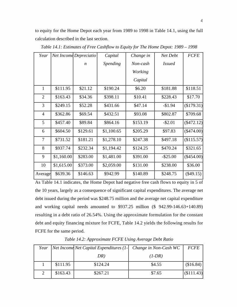
4

to equity for the Home Depot each year from 1989 to 1998 in Table 14.1, using the full

calculation described in the last section.

Table 14.1: Estimates of Free Cashflow to Equity for The Home Depot: 1989 – 1998

Year Net Income Depreciatio

n

Capital

Spending

Change in

Non-cash

Working

Capital

Net Debt

Issued

FCFE

1 $111.95 $21.12 $190.24 $6.20 $181.88 $118.51

2 $163.43 $34.36 $398.11 $10.41 $228.43 $17.70

3 $249.15 $52.28 $431.66 $47.14 -$1.94 ($179.31)

4 $362.86 $69.54 $432.51 $93.08 $802.87 $709.68

5 $457.40 $89.84 $864.16 $153.19 -$2.01 ($472.12)

6 $604.50 $129.61 $1,100.65 $205.29 $97.83 ($474.00)

7 $731.52 $181.21 $1,278.10 $247.38 $497.18 ($115.57)

8 $937.74 $232.34 $1,194.42 $124.25 $470.24 $321.65

9 $1,160.00 $283.00 $1,481.00 $391.00 -$25.00 ($454.00)

10 $1,615.00 $373.00 $2,059.00 $131.00 $238.00 $36.00

Average $639.36 $146.63 $942.99 $140.89 $248.75 ($49.15)

As Table 14.1 indicates, the Home Depot had negative free cash flows to equity in 5 of

the 10 years, largely as a consequence of significant capital expenditures. The average net

debt issued during the period was $248.75 million and the average net capital expenditure

and working capital needs amounted to $937.25 million ($ 942.99-146.63+140.89)

resulting in a debt ratio of 26.54%. Using the approximate formulation for the constant

debt and equity financing mixture for FCFE, Table 14.2 yields the following results for

FCFE for the same period.

Table 14.2: Approximate FCFE Using Average Debt Ratio

Year Net Income Net Capital Expenditures (1-

DR)

Change in Non-Cash WC

(1-DR)

FCFE

1 $111.95 $124.24 $4.55 ($16.84)

2 $163.43 $267.21 $7.65 ($111.43)

5

3 $249.15 $278.69 $34.63 ($64.17)

4 $362.86 $266.64 $68.38 $27.85

5 $457.40 $568.81 $112.53 ($223.95)

6 $604.50 $713.32 $150.81 ($259.63)

7 $731.52 $805.77 $181.72 ($255.98)

8 $937.74 $706.74 $91.27 $139.72

9 $1,160.00 $880.05 $287.23 ($7.28)

10 $1,615.00 $1,238.53 $96.23 $280.24

Average $639.36 $585.00 $103.50 ($49.15)

∂ = Average debt ratio during the period = 26.54%

Note that the approximate formulation yields the same average FCFE for the period.

Since new debt issues are averaged out over the 10 years in the approach, it also smoothes

out the annual FCFE, since actual debt issues are much more unevenly spread over time.

A similar estimation of FCFE was done for Boeing from 1989 to 1998 in Table

14.3

Table 14.3: Approximate FCFE on Boeing from 1989 to 1998

Year Net Income Net Capital Expenditures (1-

DR)

Change in Non-Cash WC

(1-DR)

FCFE

1 $973.00 $423.80 $333.27 $215.93

2 $1,385.00 $523.55 $113.59 $747.86

3 $1,567.00 $590.44 ($55.35) $1,031.92

4 $552.00 $691.34 ($555.26) $415.92

5 $1,244.00 $209.88 $268.12 $766.00

6 $856.00 ($200.08) $6.34 $1,049.74

7 $393.00 ($232.95) ($340.77) $966.72

8 $1,818.00 ($155.68) ($21.91) $1,995.59

9 ($178.00) $516.63 ($650.98) ($43.65)

10 $1,120.00 $754.77 $107.25 $257.98

Average $973.00 $312.17 ($79.57) $740.40

6

∂ = Average debt ratio during the period = 42.34%

During the period, Boeing financed a high proportion of its reinvestment needs with debt,

and its market debt ratio increased from about 1% to approximately 20%. The average

free cash flow to equity during the period was $740.40 million. Note that the 1997 and

1998 capital expenditures include the amount spent by Boeing to acquire McDonnell

Douglas.

Comparing Dividends to Free Cash Flows to Equity

The conventional measure of dividend policy –– the dividend payout ratio ––

gives us the value of dividends as a proportion of earnings. In contrast, our approach

measures the total cash returned to stockholders as a proportion of the free cash flow to

equity.

Dividend Payout Ratio = Earnings

Dividends

Cash to Stockholders to FCFE Ratio = FCFE

sRepurchaseEquity Dividends +

The ratio of cash to FCFE to the stockholders shows how much of the cash available to

be paid out to stockholders is actually returned to them in the form of dividends and

stock buybacks. If this ratio, over time, is equal or close to 1, the firm is paying out all

that it can to its stockholders. If it is significantly less than 1, the firm is paying out less

than it can afford to and is using the difference to increase its cash balance or to invest in

marketable securities. If it is significantly over 1, the firm is paying out more than it can

afford and is either drawing on an existing cash balance or issuing new securities (stocks or

bonds).

We can observe the tendency of firms to pay out less to stockholders than they

have available in free cash flows to equity by examining cash returned to stockholders

paid as a percentage of free cash flow to equity. In 1998, for instance, the average

dividend to free cash flow to equity ratio across all firms on the NYSE was 51.55%.

Figure 14.1 shows the distribution of cash returned as a percent of FCFE across all firms.

7

Source: Compustat database 1998

A percentage less than 100% means that the firm is paying out less in dividends than it

has available in free cash flows and that it is generating surplus cash. For those firms that

did not make net debt payments (debt payments in excess of new debt issues) during the

period, this cash surplus appears as an increase in the cash balance. A percentage greater

than 100% indicates that the firm is paying out more in dividends than it has available in

cash flow. These firms have to finance these dividend payments either out of existing cash

balances or by making new stock and debt issues.

The implications for valuation are simple. If we use the dividend discount model

and do not allow for the build-up of cash that occurs when firms pay out less than they

can afford, we will under estimate the value of equity in firms. The rest of this chapter is

designed to correct for this limitation.

dividends.xls: This spreadsheet allows you to estimate the free cash flow to equity

and the cash returned to stockholders for a period of up to 10 years.

Figure 14.1: Dividends/FCFE: US firms in 2000

0

50

100

150

200

250

300

350

0% 10% 20% 30% 40% 50% 60% 70% 80% 90% 100% > 100%

Dividends/FCFE

Num

ber

of F

irm

s

8

divfcfe.xls: There is a dataset on the web that summarizes dividends, cash

returned to stockholders and free cash flows to equity, by sector, in the United States.

Why Firms may pay out less than is available

Many firms pay out less to stockholders, in the form of dividends and stock

buybacks, than they have available in free cash flows to equity. The reasons vary from

firm to firm and we list some below.

1. Desire for Stability

Firms are generally reluctant to change dividends; and dividends are considered

'sticky' because the variability in dividends is significantly lower than the variability in

earnings or cashflows. The unwillingness to change dividends is accentuated when firms

have to reduce dividends and, empirically, increases in dividends outnumber cuts in

dividends by at least a five-to-one margin in most periods. As a consequence of this

reluctance to cut dividends, firms will often refuse to increase dividends even when

earnings and FCFE go up, because they are uncertain about their capacity to maintain

these higher dividends. This leads to a lag between earnings increases and dividend

increases. Similarly, firms frequently keep dividends unchanged in the face of declining

earnings and FCFE. Figure 14.2 reports the number of dividend changes (increases,

decreases, no changes) between 1989 and 1998:

9

Source: Compustat

The number of firms increasing dividends outnumbers that decreasing dividends, seven to

one. The number of firms, however, that do not change dividends outnumbers firms that

do, about four to one. Dividends are also less variable than either FCFE or earnings, but

this reduced volatility is a result of keeping dividends significantly below the FCFE.

2. Future Investment Needs

A firm might hold back on paying its entire FCFE as dividends, if it expects

substantial increases in capital expenditure needs in the future. Since issuing securities is

expensive (from a flotation cost standpoint), it may choose to keep the excess cash to

finance these future needs. Thus, to the degree that a firm may be unsure about its future

financing needs, it may choose to retain some cash to take on unexpected investments or

meet unanticipated needs.

3. Tax Factors

If dividends are taxed at a higher tax rate than capital gains, a firm may choose to

retain the excess cash and pay out much less in dividends than it has available. This is

likely to be accentuated if the stockholders in the firm are in high tax brackets, as is the

case with many family-controlled firms. If on the other hand, investors in the firm like

Figure 14.2: Dividend Changes : 1989-1998

0.00%

10.00%

20.00%

30.00%

40.00%

50.00%

60.00%

1989 1990 1991 1992 1993 1994 1995 1996 1997 1998

Year

% o

f al

l fir

ms

Increasing dividends Decreasing dividends Not changing dividends

10

dividends or tax laws favor dividends, the firm may pay more out in dividends than it has

available in FCFE, often borrowing or issuing new stock to do so.

4. Signaling Prerogatives

Firms often use dividends as signals of future prospects, with increases in

dividends being viewed as positive signals and decreases as negative signals. The empirical

evidence is consistent with this signaling story, since stock prices generally go up on

dividend increases, and down on dividend decreases. The use of dividends as signals may

lead to differences between dividends and FCFE.

5. Managerial Self-interest

The managers of a firm may gain by retaining cash rather than paying it out as a

dividend. The desire for empire building may make increasing the size of the firm an

objective on its own. Or, management may feel the need to build up a cash cushion to tide

over periods when earnings may dip; in such periods, the cash cushion may reduce or

obscure the earnings drop and may allow managers to remain in control.

FCFE Valuation Models

The free cash flow to equity model does not represent a radical departure from the

traditional dividend discount model. In fact, one way to describe a free cash flow to

equity model is that it represents a model where we discount potential dividends rather

than actual dividends. Consequently, the three versions of the FCFE valuation model

presented in this section are simple variants on the dividend discount model, with one

significant change - free cashflows to equity replace dividends in the models.

Underlying Principle

When we replace the dividends with FCFE to value equity, we are doing more

than substituting one cash flow for another. We are implicitly assuming that the FCFE

will be paid out to stockholders. There are two consequences.

1. There will be no future cash build-up in the firm, since the cash that is available

after debt payments and reinvestment needs is paid out to stockholders each

period.

11

2. The expected growth in FCFE will include growth in income from operating assets

and not growth in income from increases in marketable securities. This follows

directly from the last point.

How does discounting free cashflows to equity compare with the modified dividend

discount model, where stock buybacks are added back to dividends and discounted? You

can consider stock buybacks to be the return of excess cash accumulated largely as a

consequence of not paying out their FCFE as dividends. Thus, FCFE represent a

smoothed out measure of what companies can return to their stockholders over time in

the form of dividends and stock buybacks.

Estimating Growth in FCFE

Free cash flows to equity, like dividends, are cash flows to equity investors and

you could use the same approach that you used to estimate the fundamental growth rate

in dividends per share.

Expected Growth rate = Retention Ratio * Return on Equity

The use of the retention ratio in this equation implies that whatever is not paid out as

dividends is reinvested back into the firm. There is a strong argument to be made, though,

that this is not consistent with the assumption that free cash flows to equity are paid out

to stockholders which underlies FCFE models. It is far more consistent to replace the

retention ratio with the equity reinvestment rate, which measures the percent of net

income that is invested back into the firm.

Equity Reinvestment Rate =

IncomeNet

IssuesDebt Net -Capital in Working ChangeEx CapNet 1

+−

The return on equity may also have to be modified to reflect the fact that the conventional

measure of the return includes interest income from cash and marketable securities in the

numerator and the book value of equity also includes the value of the cash and marketable

securities. In the FCFE model, there is no excess cash left in the firm and the return on

equity should measure the return on non-cash investments. You could construct a

modified version of the return on equity that measures the non-cash aspects.

12

Non-cash ROE = Securities Marketable andCash -Equity of ValueBook

securities marketable andcash from incomeAfter tax -IncomeNet

The product of the equity reinvestment rate and the modified ROE will yield the expected

growth rate in FCFE.

Expected Growth in FCFE = Equity Reinvestment Rate * Non-cash ROE

I. The constant growth FCFE model

The constant growth FCFE model is designed to value firms that are growing at a

stable rate and are hence in steady state.

The Model

The value of equity, under the constant growth model, is a function of the

expected FCFE in the next period, the stable growth rate and the required rate of return.

P0 =FCFE1

k e − gn

where,

P0 = Value of stock today

FCFE1 = Expected FCFE next year

ke = Cost of equity of the firm

gn = Growth rate in FCFE for the firm forever

Caveats

The model is very similar to the Gordon growth model in its underlying

assumptions and works under some of the same constraints. The growth rate used in the

model has to be reasonable, relative to the nominal growth rate in the economy in which

the firm operates. As a general rule, a 'stable' growth rate cannot exceed the growth rate of

the economy in which the firm operates by more than one or two percent.

The assumption that a firm is in steady state also implies that it possesses other

characteristics shared by stable firms. This would mean, for instance, that capital

expenditures, relative to depreciation, are not disproportionately large and the firm is of

'average' risk. (If the capital asset pricing model is used, the beta of the equity should not

13

significantly different from one.) To estimate the reinvestment for a stable growth firm,

you can use one of two approaches.

• You can use the typical reinvestment rates for firms in the industry to which the

firm belongs. A simple way to do this is to use the average capital expenditure to

depreciation ratio for the industry (or better still, just stable firms in the industry)

to estimate a normalized capital expenditure for the firm.

• Alternatively, you can use the relationship between growth and fundamentals

developed in Chapter 12 to estimate the required reinvestment. The expected

growth in net income can be written as:

Expected growth rate in net income = Equity Reinvestment Rate * Return on equity

This allows us to estimate the equity reinvestment rate:

Equity reinvestment rate = Equityon Return

rategrowth Expected

To illustrate, a firm with a stable growth rate of 4% and a return on equity of 12%

would need to reinvest about a third of its net income back into net capital

expenditures and working capital needs. Put another way, the free cash flows to

equity should be two thirds of net income.

Best suited for firms

This model, like the Gordon growth model, is best suited for firms growing at a

rate comparable to or lower than the nominal growth in the economy. It is, however, the

better model to use for stable firms that pay out dividends that are unsustainably high

(because they exceed FCFE by a significant amount) or are significantly lower than the

FCFE. Note, though, that if the firm is stable and pays outs its FCFE as dividend, the

value obtained from this model will be the same as the one obtained from the Gordon

growth model.

Illustration 14.2: FCFE Stable Growth Model: Singapore Airlines

Rationale for using Model

• Singapore Airlines is a large firm in a mature industry. Given the competition for air

passengers and the limited potential for growth, it seems reasonable to assume stable

14

growth for the future. Singapore Air’s revenues have grown about 3% a year for the

last 5 years.

• Singapore Airlines has maintained a low book debt ratio historically and its

management seems inclined to keep leverage low.

Background Information

In the financial year ended March 2001, Singapore Airlines reported net income of

S$1,164 million on revenues of S$7,816 million, representing a non-cash return on equity

of 10% for the year. The capital expenditures during the year amounted to S$2,214

million, but the average capital expenditures between 1997 and 2000 were S$1,520

million. The depreciation in 2000 was S$1,205 million. The firm has no working capital

requirements. The book value debt to capital ratio at the end of 2000 was 5.44%.

Estimation

We begin by estimating a normalized free cash flow to equity for the current year.

We will assume that earnings will grow 5% over the next year. To estimate net capital

expenditures, we will use the average capital expenditures between 1997 and 2000 (to

smooth out the year-to-year jumps) and the depreciation from the most recent year.

Finally, we will assume that the 5.44% of future reinvestment needs will come from debt,

reflecting the firm’s current book debt ratio.2

Net Income this year = $1,164 m

Net Cap Ex (1- Debt Ratio) = (1520-1205)(1-.0544) = $ 298 m

Change in Working Capital (1- Debt Ratio) = 303 (1-.0544) = $ 287 m

Normalized FCFE for current year = $ 580 m

As a check, we also computed the equity reinvestment rate that Singapore Airlines would

need to maintain to earn a growth of 5%, based upon its return on equity of 10%:

Equity reinvestment rate = 50%%10

%5

ROE

g ==

With this reinvestment rate, the free cash flows to equity would have been half the net

income. The reinvestment we used in the calculation above is very close to this value:

2 In making estimates for the future, you can go with either book or market debt ratios, depending uponwhat you think about firm financing policy.

15

Equity reinvestment rate used = 50.20%1164

287298 =+

To estimate the cost of equity, we used the bottom-up unlevered beta for airlines (0.81),

Singapore Airlines’ market debt to equity ratio of 3.63% and tax rate of 38%.

Levered Beta = 0.81 (1 + (1-0.38) (.0363)) = 0.83

Using a riskless rate of 6% based upon a 10-year S$ denominated bond issued by the

Singapore Government, and using a risk premium of 5% (4% for mature market risk plus

1% for additional country risk), we estimate a cost of equity:

Cost of equity = 6% + 0.83*(5%) = 10.14%

Valuation

With the normalized FCFE estimated above, a perpetual growth rate of 5% and a cost of

equity of 10.14%, we can estimate the value of equity below:

Value of equity ( )S$11,838

05.01014.0

05.1580

growth expected-equity ofCost

yearnext FCFE Expected

=−

=

=

The equity in the firm had a market value of S$14,627 million in May 2001.

.FCFEst.xls: This spreadsheet allows you to value the equity in a firm in stable

growth, with all of the inputs of a stable growth firm.

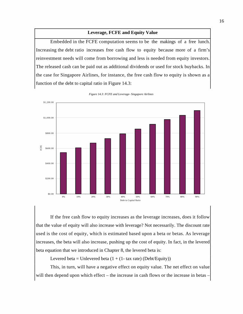
16

Leverage, FCFE and Equity Value

Embedded in the FCFE computation seems to be the makings of a free lunch.

Increasing the debt ratio increases free cash flow to equity because more of a firm’s

reinvestment needs will come from borrowing and less is needed from equity investors.

The released cash can be paid out as additional dividends or used for stock buybacks. In

the case for Singapore Airlines, for instance, the free cash flow to equity is shown as a

function of the debt to capital ratio in Figure 14.3:

If the free cash flow to equity increases as the leverage increases, does it follow

that the value of equity will also increase with leverage? Not necessarily. The discount rate

used is the cost of equity, which is estimated based upon a beta or betas. As leverage

increases, the beta will also increase, pushing up the cost of equity. In fact, in the levered

beta equation that we introduced in Chapter 8, the levered beta is:

Levered beta = Unlevered beta (1 + (1- tax rate) (Debt/Equity))

This, in turn, will have a negative effect on equity value. The net effect on value

will then depend upon which effect – the increase in cash flows or the increase in betas –

Figure 14.3: FCFE and Leverage- Singapore Airlines

$0.00

$200.00

$400.00

$600.00

$800.00

$1,000.00

$1,200.00

0% 10% 20% 30% 40% 50% 60% 70% 80% 90%

Debt to Capital Ratio

FCFE

17

dominates. Figure 14.4 graphs out the value of Singapore as a function of the debt to

capital ratio

The value of equity is maximized at a debt ratio of 30%, but beyond that level, debt’s

costs outweigh its benefits.

Figure 14.4: Singapore Air- Leverage and Value of Equity

0.00

1.00

2.00

3.00

4.00

5.00

6.00

0% 10% 20% 30% 40% 50% 60% 70% 80% 90%

Debt Ratio

Bet

a

$0.00

$2,000.00

$4,000.00

$6,000.00

$8,000.00

$10,000.00

$12,000.00

$14,000.00

Val

ue o

f Equ

ity

Value of Equity Beta

18

What is wrong with this valuation? FCFE Stable

• If you get a low value from this model, it may be because Solution

- capital expenditures are too high relative to depreciation Use a smaller Cap Ex or use the 2-stage model.

- working capital as a percent of revenues is too high Normalize this ratio, using historical averages.

- the beta is high for a stable firm Use a beta closer to one

• If you get too high a value, it is because

- Capital expenditures are lower than depreciation Estimate a reinvestment rate, given growth

- Working capital ratio as % of revenue is negative Set equal to zero

- the expected growth rate is too high for a stable firm Use a growth rate less than or equal to GNP growth.

19

II. The Two-stage FCFE Model

The two stage FCFE model is designed to value a firm which is expected to grow

much faster than a stable firm in the initial period and at a stable rate after that.

The Model

The value of any stock is the present value of the FCFE per year for the

extraordinary growth period plus the present value of the terminal price at the end of the

period.

Value

( ) ( )∑ ++

+=

+=

nn

t

P

ee

t

k1k1

FCFE

price terminalof PV FCFE of PV

where,

FCFEt = Free Cashflow to Equity in year t

Pn = Price at the end of the extraordinary growth period

ke = Cost of equity in high growth (hg) and stable growth (st) periods

The terminal price is generally calculated using the infinite growth rate model,

Pn ngr −

= +1nFCFE

where,

gn = Growth rate after the terminal year forever.

Calculating the terminal price

The same caveats that apply to the growth rate for the stable growth rate model,

described in the previous section, apply here as well. In addition, the assumptions made

to derive the free cashflow to equity after the terminal year have to be consistent with the

assumption of stability. For instance, while capital spending may be much greater than

depreciation in the initial high growth phase, the difference should narrow as the firm

enters its stable growth phase. We can use the two approaches described for the stable

growth model – industry average capital expenditure requirements or the fundamental

growth equation (equity reinvestment rate = g/ROE) to make this estimate.

20

The beta and debt ratio may also need to be adjusted in stable growth to reflect the

fact that stable growth firms tend to have average risk (betas closer to one) and use more

debt than high growth firms.

Illustration 14.3: Capital Expenditure, Depreciation and Growth Rates

Assume you have a firm that is expected to have earnings growth of 20% for the

next five years and 5% thereafter. The current earnings per share is $2.50. Current capital

spending is $2.00 and current depreciation is $1.00. We assume that capital spending and

depreciation grow at the same rate as earnings and there are no working capital

requirements or debt.

Earnings in year 5 = 2.50 * (1.20)5 = $ 6.22

Capital spending in year 5 = 2.00 * (1.20)5 = $ 4.98

Depreciation in year 5 = 1.00 * (1.20)5 = $ 2.49

Free cashflow to equity in year 5 = $6.22 + 2.49 - 4.98 = $3.73

If we use the infinite growth rate model, but fail to adjust the imbalance between capital

expenditures and depreciation, the free cashflow to equity in the terminal year is --

Free cashflow to equity in year 6 = 3.73* 1.05 = $ 3.92

This free cashflow to equity can then be used to compute the value per share at the end of

year 5, but it will understate the true value. There are two ways in which you can adjust

for this:

1. Adjust capital expenditures in year 6 to reflect industry average capital

expenditure needs: Assume, for instance, that capital expenditures are 150% of

depreciation for the industry in which the firm operates. You could compute the

capital expenditures in year 6 as follows:

Depreciation in year 6 = 2.49 (1.05) = $2.61

Capital expenditures in year 6 = Depreciation in year 6* Industry average capital

expenditures as percent of depreciation = $2.61 *1.50 = $3.92

FCFE in year 6 = $6.53 + $2.61 - $3.92 = $5.23

2. Estimate the equity reinvestment rate in year 6, based upon expected growth and

the firm’s return on equity. For instance, if we assume that this firm’s return on

21

equity will be 15% in stable growth, the equity reinvestment rate would need to

be:

Equity reinvestment rate = g/ ROE = 5%/15% = 33.33%

Net Capital expenditures in year 6 = Equity reinvestment rate * Earnings per

share

= 0.3333* $ 6.53 = $2.18

FCFE in year 6 = $6.53 - $2.18 = $4.35

Works best for:

This model makes the same assumptions about growth as the two-stage dividend

discount model, i.e., that growth will be high and constant in the initial period and drop

abruptly to stable growth after that. It is different because of its emphasis on FCFE

rather than dividends. Consequently, it provides much better results than the dividend

discount model when valuing firms which either have dividends which are unsustainable

(because they are higher than FCFE) or which pay less in dividends than they can afford

to (i.e., dividends are less than FCFE).

Illustration 14.4: Two-Stage FCFE Model: Nestle

Nestle has operations all over the world, with 97% of its revenues coming from

markets outside Switzerland, where it is headquartered. The firm, like many large

European corporations, has a weak corporate governance system and stockholders have

little power over managers.

A Rationale for using the Model

• Why two-stage? Nestle has a long and impressive history of growth, and while we

believe that its growth will be moderate, we assume that it will be able to maintain

high growth for 10 years.

• Why FCFE? Given its weak corporate governance structure and a history of

accumulating cash, the dividends paid by Nestle bear little resemblance to what the

firm could have paid out.

Background Information

Current Net Income =Sfr 5,763 million Earnings per share =Sfr 148.33

Current Capital Spending= Sfr 5,058 million Capital Expenditures/sh = Sfr 130.18

22

Current Depreciation = Sfr 3,330 million Depreciation / share = Sfr 85.71

Current Revenues = Sfr 81,422 million Revenue/ share = Sfr 2,095.64

Non-cash Working Capital= Sfr 5,818 million Working Capital/share = Sfr 149.74

Change in Working capital = Sfr 368 million Chg. Working Capital/share Sfr 9.47

Estimates

We will begin by estimating the cost of equity for Nestle during the high growth

period in Swiss francs. We will use the 10-year Swiss Government Sfr bond rate of 4% as

the riskfree rate. To estimate the risk premium, we used the breakdown of Nestle’s

revenues by region in Table 14.4.

Table 14.4: Risk Premium for Nestle: Regional Breakdown

Region Revenues Weight Risk Premium

North America 20.21 24.82% 4.00%

South America 4.97 6.10% 12.00%

Switzerland 1.27 1.56% 4.00%

Germany/France/UK 21.25 26.10% 4.00%

Italy/Spain 7.39 9.08% 5.50%

Asia 6.70 8.23% 9.00%

Rest of W. Europe 15.01 18.44% 4.00%

Eastern Europe 4.62 5.67% 8.00%

Total 81.42 100.00% 5.26%

The risk premiums for each region represent an average of the risk premiums of the

countries in the region. Using a bottom-up beta of 0.85 for Nestle, we estimated a cost of

equity of

Cost of Equity = 4% + 0.85 (5.26%) = 8.47%

To estimate the expected growth rate in free cash flows to equity, we first computed the

free cash flows to equity in the current year.

FCFE

= Net Income-(Cap Ex – Depreciation) – Change in working capital + Net Debt Issues

= 5763 – (5058 –3330) –368 + 272 = Sfr 3,939 million

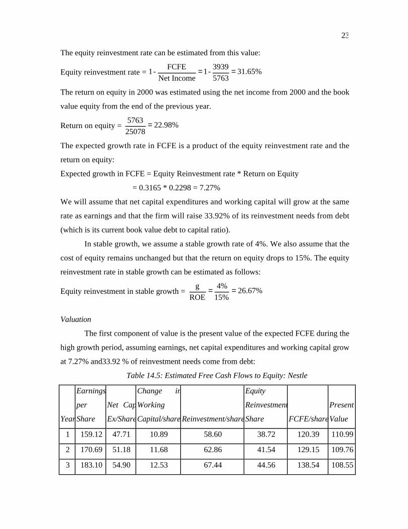
23

The equity reinvestment rate can be estimated from this value:

Equity reinvestment rate = 31.65%5763

3939-1

IncomeNet

FCFE-1 ==

The return on equity in 2000 was estimated using the net income from 2000 and the book

value equity from the end of the previous year.

Return on equity = 22.98%25078

5763 =

The expected growth rate in FCFE is a product of the equity reinvestment rate and the

return on equity:

Expected growth in FCFE = Equity Reinvestment rate * Return on Equity

= 0.3165 * 0.2298 = 7.27%

We will assume that net capital expenditures and working capital will grow at the same

rate as earnings and that the firm will raise 33.92% of its reinvestment needs from debt

(which is its current book value debt to capital ratio).

In stable growth, we assume a stable growth rate of 4%. We also assume that the

cost of equity remains unchanged but that the return on equity drops to 15%. The equity

reinvestment rate in stable growth can be estimated as follows:

Equity reinvestment in stable growth = 26.67%15%

4%

ROE

g ==

Valuation

The first component of value is the present value of the expected FCFE during the

high growth period, assuming earnings, net capital expenditures and working capital grow

at 7.27% and33.92 % of reinvestment needs come from debt:

Table 14.5: Estimated Free Cash Flows to Equity: Nestle

Year

Earnings

per

Share

Net Cap

Ex/Share

Change in

Working

Capital/share Reinvestment/share

Equity

Reinvestment

Share FCFE/share

Present

Value

1 159.12 47.71 10.89 58.60 38.72 120.39 110.99

2 170.69 51.18 11.68 62.86 41.54 129.15 109.76

3 183.10 54.90 12.53 67.44 44.56 138.54 108.55

24

4 196.42 58.90 13.44 72.34 47.80 148.62 107.35

5 210.71 63.18 14.42 77.60 51.28 159.43 106.17

6 226.03 67.77 15.47 83.25 55.01 171.02 105.00

7 242.47 72.70 16.60 89.30 59.01 183.46 103.84

8 260.11 77.99 17.80 95.80 63.30 196.81 102.69

9 279.03 83.67 19.10 102.76 67.91 211.12 101.56

10 299.32 89.75 20.49 110.24 72.85 226.48 100.44

Sum of present value of FCFE = 1056.34

Note that the change in working capital each year is computed based upon the current

working capital of Sfr 149.74 per share. The present value of FCFE is computed using the

cost of equity of 8.47%.

To estimate the terminal value, we first estimate the free cash flows to equity in

year 11.

Expected Earnings per share in year 11 = ( ) 311.304)299.32(1.01EPS10 ==+ g

Equity Reinvestment in year 11 = EPS11*Stable Equity reinvestment rate

= 311.30 * 0.2667 = 83.02

Expected FCFE in year 11 = EPS11-Equity Reinvestment11

= 311.30 – 83.02 = 228.28

Terminal value of equity per share = FCFE11/(Cost of equity11-g)

= 5,105.880.04-0.0847

228.28 =

The value per share can be estimated as the sum of the present value of FCFE during the

high growth phase and the present value of the terminal value of equity:

Value per share Sfr 3320.65

1.0847

5105.881056.34

)k(1

Price Terminalphasegrowth high during dividend of PV

10

ne

=+=

++=

The stock was trading 3390 Sfr per share in May 2001, at the time of this valuation.

25

.FCFE2st..xls: This spreadsheet allows you to value a firm with a temporary period

of high growth in FCFE, followed by stable growth.

Reinvestment Assumptions, Terminal Value and Equity Value

We have repeatedly emphasized the importance of linking growth assumptions to

assumptions about reinvestment and especially so in stable growth. A very common

assumption in many discounted cash flow valuations is that capital expenditures offset

depreciation in stable growth. When combined with the assumption of no working capital

changes, this translates into zero reinvestment. While this may be a reasonable

assumption for a year or two, it is not consistent with the assumption that operating

income will grow in perpetuity. How much of a difference can one assumption make? In

the Nestle valuation above, we re-estimated terminal value of equity per share assuming

no reinvestment.

Estimated terminal value of equity per share= 6962.570.04-0.0847

311.30 =

Keeping all of our other assumptions intact, this results in an increase in the estimated

value of equity per share to 4144 Sfr per share.

26

What is wrong with this valuation? FCFE 2 Stage

• If you get a extremely low value from the 2-stage FCFE, the likely culprits are

- earnings are depressed due to some reason (economy...) Use normalized earnings

- capital expenditures are significantly higher than depreciation in Reduce the difference for stable growth period

stable growth phase

- the beta in the stable period is too high for a stable firm Use a beta closer to one.

- working capital as % of revenue is too high to sustain Use a working capital ratio closer to industry

- the use of the 2-stage model when the 3-stage model is more appropriate Use a three-stage model

• If you get an extremely high value,

- earnings are inflated above normal levels Use normalized earnings

- capital expenditures offset or lag depreciation during high growth period Capital expenditures should be set higher

- the growth rate in the stable growth period is too high for stable firm Use a growth rate closer to GNP growth

27

What is wrong with this valuation? FCFE 3 Stage

• If you get a extremely low value from the 3-stage FCFE, the likely culprits are

- capital expenditures are significantly higher than depreciation in Reduce net cap ex in stable growth

stable growth phase Cap Ex grows slower than depreciation during

transition period

- the beta in the stable period is too high for a stable firm Use a beta closer to one.

- working capital as % of revenue is too high to sustain Use working capital ratio closer to industry average

• If you get an extremely high value,

- capital expenditures offset depreciation during high growth period Capital expenditures should be set higher

- capital expenditures are less than depreciation Set capital expenditures equal to depreciation.

- Growth Period (High growth + transition) is too long Use a shorter growth period

- the growth rate in the stable growth period is too high for stable firm Use a growth rate closer to GNP growth

28

III. The E-Model - A Three Stage FCFE Model

The E model is designed to value firms that are expected to go through three stages

of growth - an initial phase of high growth rates, a transitional period where the growth

rate declines and a steady state period where growth is stable.

The Model

The E model calculates the present value of expected free cash flow to equity over

all three stages of growth:

n,

n2n2t

1n1tt

,

tn1t

1tt

,

t0

)k(1

P

)k(1

FCFE

)k(1

FCFEP

stetehge ++

++

+= ∑∑

=

+=

=

=

where,

P0 = Value of the stock today

FCFEt = FCFE in year t

ke = Cost of equity

Pn2 = Terminal price at the end of transitional period = n

1n2

g-r

FCFE +

n1 = End of initial high growth period

n2 = End of transition period

Caveats in using model

Since the model assumes that the growth rate goes through three distinct phases -

high growth, transitional growth and stable growth - it is important that assumptions

about other variables are consistent with these assumptions about growth.

1. Capital Spending versus Depreciation

It is reasonable to assume that as the firm goes from high growth to stable growth,

the relationship between capital spending and depreciation will change. In the high growth

phase, capital spending is likely to be much larger than depreciation. In the transitional

phase, the difference is likely to narrow. Finally, the difference between capital spending

29

and depreciation will be lower still in stable growth, reflecting the lower expected growth

rate.

Figure 14.5: Three Stage FCFE Model: Reinvestment Needs

High Growth

Stable Growth

Transition

Cap Ex

DepreciationCap Ex is high relative to depreciation

Difference between cap ex and depreciation narrows.

Difference between cap exand depreciation reflects growth

2. Risk

As the growth characteristics of a firm change, so do its risk characteristics. In the

context of the CAPM, as the growth rate declines, the beta of the firm can be expected to

change. The tendency of betas to converge towards one in the long term has been

confirmed by empirical observation of portfolios of firms with high betas. Over time, as

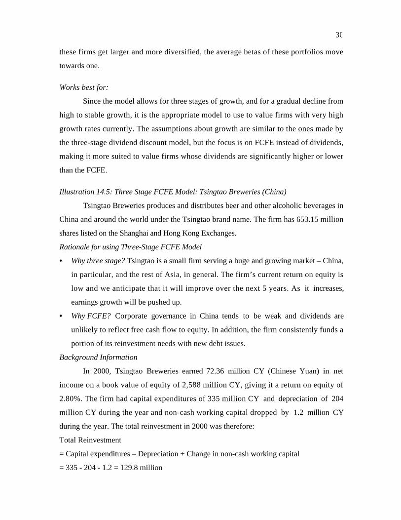
30

these firms get larger and more diversified, the average betas of these portfolios move

towards one.

Works best for:

Since the model allows for three stages of growth, and for a gradual decline from

high to stable growth, it is the appropriate model to use to value firms with very high

growth rates currently. The assumptions about growth are similar to the ones made by

the three-stage dividend discount model, but the focus is on FCFE instead of dividends,

making it more suited to value firms whose dividends are significantly higher or lower

than the FCFE.

Illustration 14.5: Three Stage FCFE Model: Tsingtao Breweries (China)

Tsingtao Breweries produces and distributes beer and other alcoholic beverages in

China and around the world under the Tsingtao brand name. The firm has 653.15 million

shares listed on the Shanghai and Hong Kong Exchanges.

Rationale for using Three-Stage FCFE Model

• Why three stage? Tsingtao is a small firm serving a huge and growing market – China,

in particular, and the rest of Asia, in general. The firm’s current return on equity is

low and we anticipate that it will improve over the next 5 years. As it increases,

earnings growth will be pushed up.

• Why FCFE? Corporate governance in China tends to be weak and dividends are

unlikely to reflect free cash flow to equity. In addition, the firm consistently funds a

portion of its reinvestment needs with new debt issues.

Background Information

In 2000, Tsingtao Breweries earned 72.36 million CY (Chinese Yuan) in net

income on a book value of equity of 2,588 million CY, giving it a return on equity of

2.80%. The firm had capital expenditures of 335 million CY and depreciation of 204

million CY during the year and non-cash working capital dropped by 1.2 million CY

during the year. The total reinvestment in 2000 was therefore:

Total Reinvestment

= Capital expenditures – Depreciation + Change in non-cash working capital

= 335 - 204 - 1.2 = 129.8 million

31

The working capital changes over the last 4 years have been volatile and we normalize the

change using non-cash working capital as a percent of revenues in 1999.

Normalized change in non-cash working

capital

( )

( ) CYmillion 52.31598-22532253

180

Revenues-RevenuessRevenues

capital ngcash worki-Non19981999

1999

1999

=

=

=

The normalized reinvestment in 1999 can then be estimated.

Normalized Reinvestment

= Capital expenditures – Depreciation + Normalized Change in non-cash working capital

= 335 - 204 + 52.3 = 183.3 million CY

As with working capital, debt issues have been volatile. We estimate the firm’s book debt

to capital ratio of 40.94% at the end of 1999 and use it to estimate the normalized equity

reinvestment in 1999.

Equity Reinvestment in 2000 = Reinvestment (1- Debt ratio)

= 183.3 (1-0.4094) = 108.27million CY

As a percent of net income,

Equity Reinvestment rate in 2000 = 108.27

72.36=149.97%

Estimation

To estimate free cash flows to equity for the high growth period, we make the

assumption that the return on equity, which is 2.80% today, will drift up to 12% by the

fifth year. In addition, we will assume that new investments from now on will earn a

return on equity of 12%. Finally, we will assume that the equity reinvestment rate will

remain at its current level (149.97%) each year for the next 5 years. The expected growth

rate over the next 5 years can then be estimated.

Expected growth rate- next 5 years

= Equity reinvestment rate( ) ROENew( ) +ROE5 -ROE today

ROE today

1

5

-1

= 1.4997( ) 0.12( ) + 0.12 − 0.02800.0280

1

5−1= 44.91%

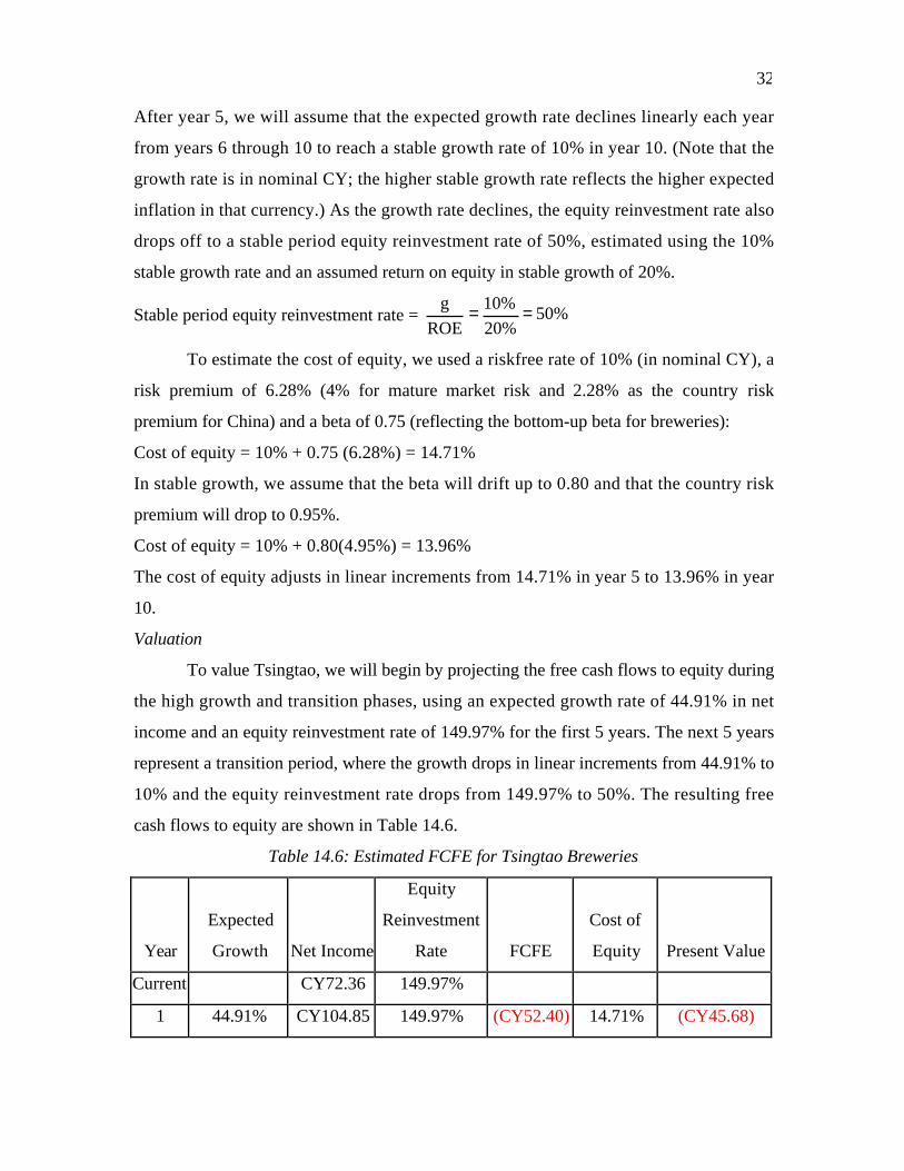
32

After year 5, we will assume that the expected growth rate declines linearly each year

from years 6 through 10 to reach a stable growth rate of 10% in year 10. (Note that the

growth rate is in nominal CY; the higher stable growth rate reflects the higher expected

inflation in that currency.) As the growth rate declines, the equity reinvestment rate also

drops off to a stable period equity reinvestment rate of 50%, estimated using the 10%

stable growth rate and an assumed return on equity in stable growth of 20%.

Stable period equity reinvestment rate = 50%20%

10%

ROE

g ==

To estimate the cost of equity, we used a riskfree rate of 10% (in nominal CY), a

risk premium of 6.28% (4% for mature market risk and 2.28% as the country risk

premium for China) and a beta of 0.75 (reflecting the bottom-up beta for breweries):

Cost of equity = 10% + 0.75 (6.28%) = 14.71%

In stable growth, we assume that the beta will drift up to 0.80 and that the country risk

premium will drop to 0.95%.

Cost of equity = 10% + 0.80(4.95%) = 13.96%

The cost of equity adjusts in linear increments from 14.71% in year 5 to 13.96% in year

10.

Valuation

To value Tsingtao, we will begin by projecting the free cash flows to equity during

the high growth and transition phases, using an expected growth rate of 44.91% in net

income and an equity reinvestment rate of 149.97% for the first 5 years. The next 5 years

represent a transition period, where the growth drops in linear increments from 44.91% to

10% and the equity reinvestment rate drops from 149.97% to 50%. The resulting free

cash flows to equity are shown in Table 14.6.

Table 14.6: Estimated FCFE for Tsingtao Breweries

Year

Expected

Growth Net Income

Equity

Reinvestment

Rate FCFE

Cost of

Equity Present Value

Current CY72.36 149.97%

1 44.91% CY104.85 149.97% (CY52.40) 14.71% (CY45.68)

33

2 44.91% CY151.93 149.97% (CY75.92) 14.71% (CY57.70)

3 44.91% CY220.16 149.97% (CY110.02) 14.71% (CY72.89)

4 44.91% CY319.03 149.97% (CY159.43) 14.71% (CY92.08)

5 44.91% CY462.29 149.97% (CY231.02) 14.71% (CY116.32)

6 37.93% CY637.61 129.98% (CY191.14) 14.56% (CY84.01)

7 30.94% CY834.92 109.98% (CY83.35) 14.41% (CY32.02)

8 23.96% CY1,034.98 89.99% CY103.61 14.26% CY34.83

9 16.98% CY1,210.74 69.99% CY363.29 14.11% CY107.04

10 10.00% CY1,331.81 50.00% CY665.91 13.96% CY172.16

Sum of the present values of FCFE during high growth = ($186.65)

To estimate the terminal value of equity, we used the net income in the year 11, reduce it

by the equity reinvestment needs in that year and then assume a perpetual growth rate to

get to a value.

Expected stable growth rate =10%

Equity reinvestment rate in stable growth = 50%

Cost of equity in stable growth = 13.96%

Expected FCFE in year 11

= Net Income11( ) 1-Stable period equity reinvestment rate( )= 1331.81( ) 1.10( ) 1−0.5( ) = 732.50 million

Terminal Value of equity in Tsingtao Breweries:

= FCFE11

Stable period cost of equity Stable growth rate

= 732.500.1396 − 0.10

=18,497 million

To estimate the value of equity today, we sum up the present value of the FCFE over the

high growth period and transition period and add to it the present value of the terminal

value of equity.

Value of Equity

= PV of FCFE during the high growth period + PV of terminal value

=−186.65 +18,497

1.1471( )51.1456( ) 1.1441( ) 1.1426( ) 1.1411( ) 1.1396( )

= 4,596 million

34

Value of Equity per share = Value of Equity

Number of Shares

= 4,596653.15

= CY 7.04 per share

The stock was trading at 10.10 Yuan per share, which would make it overvalued, based

upon this valuation.

.FCFE3st..xls: This spreadsheet allows you to value a firm with a temporary period

of high growth in FCFE, followed by a transition period, followed by stable growth.

Negative FCFE, Equity Dilution and Value per Share

Unlike dividends, free cash flows to equity can be negative. This can occur either

because net income is negative or because a firm’s reinvestment needs are significant – this

is the case with Tsingtao in the illustration above. The resulting net capital expenditure

and working capital needs may be much larger than the net income. In fact, this is likely to

occur fairly frequently with high growth firms.

The model that we have described above is flexible enough to deal with this issue.

The free cash flows to equity will be negative as the firm reinvests substantial amounts to

generate high growth. As the growth declines, the reinvestment needs also drop off and

free cash flows to equity turn positive.

Intuitively, though, consider what a negative free cash flow to equity implies. It

indicates that the firm does not generate enough cash flows from current operations to

meet its reinvestment needs. Since the free cash flow to equity is after net debt issues, the

firm will have to issue new equity in years where the cash flow is negative. This expected

dilution in future years will reduce the value of equity per share today. In the FCFE

model, the negative free cash flows to equity in the earlier years will reduce the estimated

value of equity today. Thus, the dilution effect is captured in the present value and no

additional consideration is needed of new stock issues in future years and the effect on

value per share today.

FCFE Valuation versus Dividend Discount Model Valuation

35

The discounted cash flow model that uses FCFE can be viewed as an alternative to

the dividend discount model. Since the two approaches sometimes provide different

estimates of value, it is worth examining when they provide similar estimates of value,

when they provide different estimates of value and what the difference tells us about the

firm.

a. When they are similar

There are two conditions under which the value from using the FCFE in

discounted cashflow valuation will be the same as the value obtained from using the

dividend discount model. The first is the obvious one, where the dividends are equal to

the FCFE. The second condition is more subtle, where the FCFE is greater than

dividends, but the excess cash (FCFE - Dividends) is invested in projects with net present

value of zero. (For instance, investing in financial assets which are fairly priced should

yield a net present value of zero.)

b. When they are different

There are several cases where the two models will provide different estimates of

value. First, when the FCFE is greater than the dividend and the excess cash either earns

below-market interest rates or is invested in negative net present value projects, the value

from the FCFE model will be greater than the value from the dividend discount model.

There is reason to believe that this is not as unusual as it would seem at the outset. There

are numerous case studies of firms, which having accumulated large cash balances by

paying out low dividends relative to FCFE, have chosen to use this cash to finance

unwise takeovers (where the price paid is greater than the value received from the

takeover). Second, the payment of dividends less than FCFE lowers debt-equity ratios

and may lead the firm to become underlevered, causing a loss in value.

In the cases where dividends are greater than FCFE, the firm will have to issue

either new stock to pay these dividends leading to at least three negative consequences for

value. One is the flotation cost on these security issues, which can be substantial for

equity issues and creates an unnecessary expenditure that decreases value. Second, if the

firm borrows the money to pay the dividends, the firm may become overlevered (relative

to the optimal) leading to a loss in value. Finally, paying too much in dividends can lead

36

to capital rationing constraints where good projects are rejected, resulting in a loss of

value.

There is a third possibility and it reflects different assumptions about

reinvestment and growth in the two models. If the same growth rate used in the dividend

discount and FCFE models, the FCFE model will give a higher value than the dividend

discount model whenever FCFE are higher than dividends and a lower value when

dividends exceed FCFE. In reality, the growth rate in FCFE should be different from the

growth rate in dividends, because the free cash flow to equity is assumed to be paid out to

stockholders. This will affect the reinvestment rate of the firm. In addition, the return on

equity used in the FCFE model should reflect the return on equity on non-cash

investments, whereas the return on equity used in the dividend discount model should be

the overall return on equity. Table 14.7 summarizes the differences in assumptions

between the two models.

Table 14.7: Differences between DDM and FCFE Model

Dividend Discount Model FCFE Model

Implicit Assumption Only dividends are paid.

Remaining portion of earnings

are invested back into the firm,

some in operating assets and

some in cash & marketable

securities.

The FCFE is paid out to

stockholders. The remaining

earnings are invested only in

operating assets.

Expected Growth Measures growth in income

from both operating and cash

assets. In terms of

fundamentals, it is the product

of the retention ratio and the

return on equity

Measures growth only in

income from operating assets.

In terms of fundamentals, it is

the product of the equity

reinvestment rate and the non-

cash return on equity.

Dealing with cash and

marketable securities

The income from cash and

marketable securities is built

into earnings and ultimately

You have two choices:

1. Build in income from cash

and marketable securities

37

into dividends. Therefore, cash

and marketable securities do

not need to be added in

into projections of income

and estimate the value of

equity.

2. Ignore income from cash

and marketable securities,

and add their value to

equity value in model

In general, when firms pay out much less in dividends than they have available in FCFE,

the expected growth rate and terminal value will be higher in the dividend discount model,

but the year-to-year cash flows will be higher in the FCFE model. The net effect on value

will vary from company to company.

3. What does it mean when they are different?

When the value using the FCFE model is different from the value using the

dividend discount model, with consistent growth assumptions, there are two questions

that need to be addressed - What does the difference between the two models tell us?

Which of the two models is the appropriate one to use in evaluating the market price?

The more common occurrence is for the value from the FCFE model to exceed the

value from the dividend discount model. The difference between the value from the FCFE

model and the value using the dividend discount model can be considered one component

of the value of controlling a firm - it measures the value of controlling dividend policy. In

a hostile takeover, the bidder can expect to control the firm and change the dividend

policy (to reflect FCFE), thus capturing the higher FCFE value.

As for which of the two values is the more appropriate one for use in evaluating

the market price, the answer lies in the openness of the market for corporate control. If

there is a sizable probability that a firm can be taken over or its management changed, the

market price will reflect that likelihood and the appropriate benchmark to use is the value

from the FCFE model. As changes in corporate control become more difficult, either

because of a firm's size and/or legal or market restrictions on takeovers, the value from the

dividend discount model will provide the appropriate benchmark for comparison.

38

Illustration 14.6: Comparing the DDM and FCFE Models: Coca Cola

In Chapter 13, we valued Coca Cola using a three-stage dividend discount model at

$42.72 a share. Here, we will value Coca Cola using a three stage free cash flow to equity

model.

Rationale for using Three-Stage FCFE Model

• Why three stage? Coca Cola’s strong brand name will allow it to overcome some of

the constraints that may exist on its high growth rate – the saturation of its domestic

market and its high market share in the market. However, we believe that this growth

will come under assault from competition in future years, leading us to allow for a

transition to stable growth.

• Why FCFE? While the firm does have a history of returning cash to stockholders, we

wanted to examine the differences in value, if any, estimated with the dividend and

FCFE models.

• The firm has used debt a little more liberally in the last few years, but it remains a

firm that uses equity for much of its reinvestment needs.

Background Information

Net Income =$3,878

Number of shares outstanding =2487.03

Current Capital Expenditures =$992.00

Current Depreciation =$773.00

Increase in non-cash Working capital in most recent year =$852.00

Net Debt Issued (Paid) during the year =($585.00)

Based upon these values, we can estimate the free cash flows to equity in the most recent

year as follows:

Free Cash flow to equity = Net Income – (Cap Expenditures – Depreciation) – Change in

non-cash working capital + Net Debt Issued = 3878 – (992- 773) – 852 + (-585) = $2,222

million

The return on equity in the most recent year was estimated to be 23.37% in the dividend

discount model. We re-estimated the return on equity excluding the income from cash and

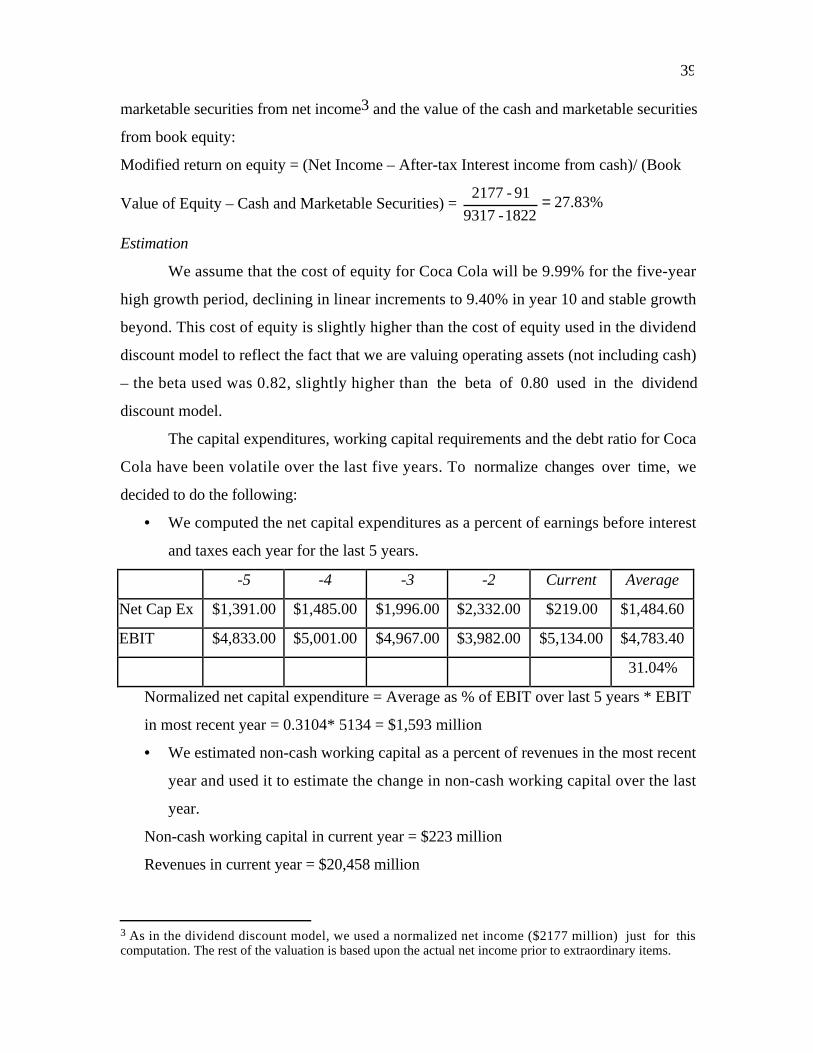
39

marketable securities from net income3 and the value of the cash and marketable securities

from book equity:

Modified return on equity = (Net Income – After-tax Interest income from cash)/ (Book

Value of Equity – Cash and Marketable Securities) = 27.83%1822-9317

91-2177 =

Estimation

We assume that the cost of equity for Coca Cola will be 9.99% for the five-year

high growth period, declining in linear increments to 9.40% in year 10 and stable growth

beyond. This cost of equity is slightly higher than the cost of equity used in the dividend

discount model to reflect the fact that we are valuing operating assets (not including cash)

– the beta used was 0.82, slightly higher than the beta of 0.80 used in the dividend

discount model.

The capital expenditures, working capital requirements and the debt ratio for Coca

Cola have been volatile over the last five years. To normalize changes over time, we

decided to do the following:

• We computed the net capital expenditures as a percent of earnings before interest

and taxes each year for the last 5 years.

-5 -4 -3 -2 Current Average

Net Cap Ex $1,391.00 $1,485.00 $1,996.00 $2,332.00 $219.00 $1,484.60

EBIT $4,833.00 $5,001.00 $4,967.00 $3,982.00 $5,134.00 $4,783.40

31.04%

Normalized net capital expenditure = Average as % of EBIT over last 5 years * EBIT

in most recent year = 0.3104* 5134 = $1,593 million

• We estimated non-cash working capital as a percent of revenues in the most recent

year and used it to estimate the change in non-cash working capital over the last

year.

Non-cash working capital in current year = $223 million

Revenues in current year = $20,458 million

3 As in the dividend discount model, we used a normalized net income ($2177 million) just for thiscomputation. The rest of the valuation is based upon the actual net income prior to extraordinary items.

40

Revenues last year = $19,805 million

Normalized change in non-cash working capital last year =

( ) million $7.1219805-2045820458

223 =

• We normalized the net debt issued by assuming that Coca Cola would continue to

fund its reinvestment needs with its market debt to capital ratio. To estimate the

market debt to capital ratio, we used the total interest bearing debt outstanding at

the end of 2000 and the current market value of equity.

Debt Ratio

%68.41151255651

5651

equity of ueMarket valdebt bearingInterest

debt bearingInterest

=+

=

+=

Normalized debt issued in current year = (Normalized net capital expenditures +

Normalized change in non-cash working capital) * Debt Ratio

= (1593+7.12)*(0.0468) =$74.89 million

The normalized free cash flow to equity can then be computed.

Normalized FCFE = Net Income – Normalized Net Cap Ex – Normalized change in

working capital + Normalized net debt issued = 3878 – 1593 – 7.12 + 74.89 = $2,353

million

This normalized FCFE also lets us compute the equity reinvestment rate for the firm:

Equity reinvestment rate = 39.3%3878

2353-1

IncomeNet

FCFE-1 ==

With the current return on equity of 27.83%, this yields an expected growth rate in net

income at Coca Cola of 10.94%.

Expected Growth = Equity reinvestment rate * Return on Equity = 0.393*0.2783 =

0.1094

In stable growth, we assume that the return on equity drops to 20% and that the growth

rate in perpetuity in net income is 5.5%. The equity reinvestment rate can then be

estimated as follows:

Equity Reinvestment rate in stable growth = 27.5% 20%

%5.5

ROE

g ==

Valuation

41

To value Coca Cola, we will begin by projecting the free cash flows to equity

during the high growth and transition phases, using an expected growth rate of 10.94% in

non-cash net income and an equity reinvestment rate of 39.3% for the first 5 years.

Non-cash Net Income = Net Income – After-tax Interest income from cash and marketable

securities = $3,878 million – 89 million = $3,789 million

The next 5 years represent a transition period, where the growth drops in linear

increments from 10.94% to 5.5% and the equity reinvestment rate drops from 39.3% to

27.5%. The resulting free cash flows to equity are shown in Table 14.8.

Table 14.8: Estimated FCFE for Coca Cola

Year

Expected

Growth

Net

Income

Equity

Reinvestment

Rate FCFE

Cost of

Equity Present Value

High Growth Stage

1 10.94% $4,203.28 39.32% $2,550.42 9.99% $2,318.73

2 10.94% $4,663.28 39.32% $2,829.53 9.99% $2,338.80

3 10.94% $5,173.61 39.32% $3,139.18 9.99% $2,359.03

4 10.94% $5,739.79 39.32% $3,482.72 9.99% $2,379.44

5 10.94% $6,367.93 39.32% $3,863.86 9.99% $2,400.03

Steady Growth Stage

6 9.85% $6,995.48 36.96% $4,410.06 9.87% $2,493.13

7 8.77% $7,608.71 34.59% $4,976.57 9.76% $2,563.34

8 7.68% $8,192.87 32.23% $5,552.37 9.64% $2,608.54

9 6.59% $8,732.68 29.86% $6,124.69 9.52% $2,627.34

10 5.50% $9,212.97 27.50% $6,679.40 9.40% $2,619.11

Sum of the present values of FCFE during high growth = $24,707.49

To estimate the terminal value of equity, we used the net income in the terminal year

(Year 11), reduce it by the equity reinvestment needs in that year and then assume a

perpetual growth rate to get to a value.

Expected stable growth rate = 5.5%

42

Equity reinvestment rate in stable growth = 27.5%

Cost of equity in stable growth = 9.40%

Expected FCFE in year 11

( )( )( )( )( ) million 047,7275.01055.19212.97

ratent reinvestmeequity period Stable-1IncomeNet 11

=−==

Value of equity in Coca Cola

686,180055.0094.0

047,7

rategrowth Stableequity ofcost period Stable

FCFE11

=−

=

=

To estimate the value of equity today, we sum up the present value of the FCFE over the

high growth period and add to it the present value of the terminal value of equity.

Value of Equity ( ) ( )( )( )( )( )million 558,95

0940.10952.10964.10976.10987.11.0988

180,68624,707

value terminalof PVperiodgrowth high theduring FCFE of PV

5

=

+=

+=

Adding in the value of the cash and marketable securities that Coca Cola had on hand at

the end of 2001, we obtain the total value of equity:

Value of Equity including cash = $95,558 + $1,892 = $97,447 million

Value of Equity per share 19.39$

03.487,2

447,97

Shares ofNumber

Equity of Value

==

=

The FCFE model yields a lower value than the dividend discount model value of $42.72 a

share. This may seem surprising since the FCFE each year for the high growth period are

greater than the dividends, but this effect is more than offset by the decline in the

expected growth rate which is generated by the equity reinvestment rate being lower than

the retention ratio. We would argue that this valuation is probably more realistic than the

dividend discount model because it keeps investments in cash and marketable securities

separate from investments in operating assets. The dividend discount model overstates

the expected growth rate because it does not consider the fact that the low return earned

by cash investments will bring the return on equity down over time (and the growth rate

down with it).

43

Conclusion

The primary difference between the dividend discount models described in the

previous chapter and the free cashflow to equity models described in this one lies in the

definition of cash flows - the dividend discount model uses a strict definition of cashflow

to equity, i.e., the expected dividends on the stock, while the FCFE model uses an

expansive definition of cashflow to equity as the residual cashflow after meeting all

financial obligations and investment needs. When firms have dividends that are different

from the FCFE, the values from the two models will be different. In valuing firms for

takeovers or in valuing firms where there is a reasonable chance of changing corporate

control, the value from the FCFE provides the better estimate of value.

44

Problems

1. Respond true or false to the following statements relating to the calculation and use of

FCFE.

A. The free cash flow to equity will generally be more volatile than dividends.

B. The free cash flow to equity will always be higher than the dividends.

C. The free cash flow to equity will always be higher than net income.

D. The free cash flow to equity can never be negative.

2. Kimberly-Clark, a household product manufacturer, reported earnings per share of

$3.20 in 1993 and paid dividends per share of $1.70 in that year. The firm reported

depreciation of $315 million in 1993 and capital expenditures of $475 million. (There

were 160 million shares outstanding, trading at $51 per share.) This ratio of capital

expenditures to depreciation is expected to be maintained in the long term. The working

capital needs are negligible. Kimberly-Clark had debt outstanding of $1.6 billion and

intends to maintain its current financing mix (of debt and equity) to finance future

investment needs. The firm is in steady state and earnings are expected to grow 7% a

year. The stock had a beta of 1.05. (The treasury bond rate is 6.25%.)

a. Estimate the value per share, using the Dividend Discount Model.

b. Estimate the value per share, using the FCFE Model.

c. How would you explain the difference between the two models and which one would

you use as your benchmark for comparison to the market price?

3. Ecolab Inc. sells chemicals and systems for cleaning, sanitizing and maintenance. It

reported earnings per share of $2.35 in 1993 and expected earnings growth of 15.5% a

year from 1994 to 1998 and 6% a year after that. The capital expenditure per share was

$2.25 and depreciation was $1.125 per share in 1993. Both are expected to grow at the

same rate as earnings from 1994 to 1998. Working capital is expected to remain at 5% of

revenues and revenues, which were $1,000 million in 1993, are expected to increase 6% a

year from 1994 to 1998, and 4% a year after that. The firm currently has a debt ratio

(D/(D+E)) of 5%, but plans to finance future investment needs (including working capital

investments) using a debt ratio of 20%. The stock is expected to have a beta of 1.00 for

the period of the analysis and the treasury bond rate is 6.50%. (There are 63 million

shares outstanding)

a. Assuming that capital expenditures and depreciation offset each other after 1998,

estimate the value per share.

b. Assuming that capital expenditures continue to be 200% of depreciation even after

1998, estimate the value per share.

45

c. What would the value per share have been, if the firm had continued to finance new

investments with its old financing mix (5%)? Is it fair to use the same beta for this

analysis?

4. Dionex Corporation, a leader in the development and manufacture of ion chromography

systems (used to identify contaminants in electronic devices), reported earnings per share

of $2.02 in 1993 and paid no dividends. These earnings are expected to grow 14% a year

for five years (1994 to 1998) and 7% a year after that. The firm reported depreciation of

$2 million in 1993 and capital spending of $4.20 million, and had 7 million shares

outstanding. The working capital is expected to remain at 50% of revenues, which were

$106 million in 1993, and are expected to grow 6% a year from 1994 to 1998 and 4% a

year after that. The firm is expected to finance 10% of its capital expenditures and

working capital needs with debt. Dionex had a beta of 1.20 in 1993, and this beta is

expected to drop to 1.10 after 1998. (The treasury bond rate is 7%)

a. Estimate the expected free cash flow to equity from 1994 to 1998, assuming that

capital expenditures and depreciation grow at the same rate as earnings.

b. Estimate the terminal price per share (at the end of 1998). Stable firms in this

industry have capital expenditures which are 150% of revenues and maintain working

capital at 25% of revenues.

c. Estimate the value per share today, based upon the FCFE model.

5. Biomet Inc. designs, manufactures and markets reconstructive and trauma devices and

reported earnings per share of $0.56 in 1993, on which it paid no dividends (It had

revenues per share in 1993 of $2.91). It had capital expenditures of $0.13 per share in

1993 and depreciation in the same year of $0.08 per share. The working capital was 60%

of revenues in 1993 and will remain at that level from 1994 to 1998, while earnings and

revenues are expected to grow 17% a year. The earnings growth rate is expected to decline

linearly over the following five years to a rate of 5% in 2003. During the high growth and

transition periods, capital spending and depreciation are expected to grow at the same rate

as earnings, but are expected to offset each other when the firm reaches steady state.

Working capital is expected to drop from 60% of revenues during the 1994-1998 period

to 30% of revenues after 2003. The firm has no debt currently, but plans to finance 10%

of its net capital investment and working capital requirements with debt.

The stock is expected to have a beta of 1.45 for the high growth period (1994-

1998) and it is expected to decline to 1.10 by the time the firm goes into steady state (in

2003). The treasury bond rate is 7%.

a. Estimate the value per share, using the FCFE model.

46

b. Estimate the value per share, assuming that working capital stays at 60% of revenues

forever.

c. Estimate the value per share, assuming that the beta remains unchanged at 1.45

forever.

6. Which of the following firms is likely to have a higher value from the dividend discount

model, a higher value from the FCFE model or the same value from both models?

(a) A firm that pays out less in dividends than it has available in FCFE, but which

invests the balance in treasury bonds.

(b) A firm which pays out more in dividends than it has available in FCFE, and then

issues stock to cover the difference.

(c) A firm which pays out, on average, its FCFE as dividends.

(d) A firm which pays out less in dividends that it has available in FCFE, but which

uses the cash at regular intervals to acquire other firms, with the intent of diversifying.

(e) A firm which pays out more in dividends than it has available in FCFE, but borrows

money to cover the difference. (The firm is over-levered to begin with.)

0

CHAPTER 15

FIRM VALUATION: COST OF CAPITAL AND APV APPROACHES

In the last two chapters, we examined two approaches to valuing the equity in the

firm -- the dividend discount model and the FCFE valuation model. This chapter develops

another approach to valuation where the entire firm is valued, by either discounting the

cumulated cashflows to all claim holders in the firm by the weighted average cost of

capital (the cost of capital approach) or by adding the marginal impact of debt on value

to the unlevered firm value (adjusted present value approach).

In the process of looking at firm valuation, we also look at how leverage may or

may not affect firm value. We note that in the presence of default risk, taxes and agency

costs, increasing leverage can sometimes increase firm value and sometimes decrease it. In

fact, we argue that the optimal financing mix for a firm is the one that maximizes firm

value.

The Free Cashflow to the Firm

The free cashflow to the firm is the sum of the cashflows to all claim holders in

the firm, including stockholders, bondholders and preferred stockholders. There are two

ways of measuring the free cashflow to the firm (FCFF).

One is to add up the cashflows to the claim holders, which would include cash

flows to equity (defined either as free cash flow to equity or dividends), cashflows to

lenders (which would include principal payments, interest expenses and new debt issues)

and cash flows to preferred stockholders (usually preferred dividends).

FCFF = Free Cashflow to Equity

+ Interest Expense (1 - tax rate) + Principal Repayments - New Debt Issues

+ Preferred Dividends

Note, however, that we are reversing the process that we used to get to free cash flow to

equity, where we subtracted out payments to lenders and preferred stockholders to

estimate the cash flow left for stockholders. A simpler way of getting to free cash flow to

the firm is to estimate the cash flows prior to any of these claims. Thus, we could begin

1

with the earnings before interest and taxes, net out taxes and reinvestment needs and

arrive at an estimate of the free cash flow to the firm.

FCFF = EBIT (1 - tax rate) + Depreciation - Capital Expenditure - ∆ Working Capital

Since this cash flow is prior to debt payments, it is often referred to as an unlevered cash

flow. Note that this free cash flow to the firm does not incorporate any of the tax benefits

due to interest payments. This is by design, because the use of the after-tax cost of debt

in the cost of capital already considers this benefit and including it in the cash flows

would double count it.

FCFF and other cashflow measures

The differences between FCFF and FCFE arise primarily from cashflows

associated with debt -- interest payments, principal repayments, new debt issues and

other non-equity claims such as preferred dividends. For firms at their desired debt level,

which finance their capital expenditures and working capital needs with this mix of debt

and equity. As for the use of debt issues to finance principal repayments, the free

cashflow to the firm will exceed the free cashflow to equity.

One measure that is widely used in valuation is the earnings before interest, taxes,

depreciation and amortization (EBITDA). The free cashflow to the firm is a closely

related concept but it takes into account the potential tax liability from the earnings as

well as capital expenditures and working capital requirements.

Three measures of earnings are also often used to derive cash flows. The earnings

before interest and taxes (EBIT) or operating income comes directly from a firm’s income

statements. Adjustments to EBIT yield the net operating profit or loss after taxes

(NOPLAT) or the net operating income (NOI). The net operating income is defined to be

the income from operations, prior to taxes and non-operating expenses.

Each of these measures is used in valuation models and each can be related to the

free cashflow to the firm. Each, however, makes some assumptions about the relationship

between depreciation and capital expenditures that are made explicit in the Table 15.1.

Table 15.1: Free Cash Flows to the Firm: Comparison to other measures

Cashflow used Definition Use in valuation

2

FCFF Free Cashflow to firm Discounting free cash flow

to the firm at the cost of

capital will yield the value

of the operating assets of

the firm. To this, you

would add on the value of

non-operating assets to

arrive at firm value.

FCFEFCFF - Interest (1-t) – Principal

repaid + New Debt Issued –

Preferred Dividend

Discounting free cash flows

to equity at the cost of

equity will yield the value

of equity in a business.

EBITDAFCFF + EBIT(t) + Capital

Expenditures + Change in

working capital

If you discount EBITDA at

the cost of capital to value

an asset, you are assuming

that there are no taxes and

that the firm will actively

disinvest over time. It

would be inconsistent to

assume a growth rate or an

infinite life for this firm.

EBIT (1-t)

(NOPLAT is a slightly

modified version of this

estimate and it removes

any non-operating

items that might affect

the reported EBIT.)

FCFF + Capital Expenditures –

Depreciation + Change in

working capital

If you discount after-tax

operating income at the

cost of capital to value a

firm, you are assuming no

reinvestment. The

depreciation is reinvested

back into the firm to

maintain existing assets.

You can assume an infinite

3

life but no growth.

Growth in FCFE versus Growth in FCFF

Will equity cashflows and firm cashflows grow at the same rate? Consider the

starting point for the two cash flows. Equity cash flows are based upon net income or

earnings per share – measures of equity income. Firm cash flows are based upon operating

income – i.e. income prior to debt payments. As a general rule, you would expect growth

in operating income to be lower than growth in net income, because financial leverage can

augment the latter. To see why, let us go back to the fundamental growth equations we

laid out in Chapter 11.

Expected growth in net income = Equity Reinvestment rate * Return on Equity

Expected growth in operating income = Reinvestment Rate * Return on Capital

We also defined the return on equity in terms of the return on capital:

Return on Equity =

( )debt ofcost tax -After - capitalon Return Equtiy

DebtCapitalon Return

+

When a firm borrows money and invests in projects that earn more than the after-tax cost

of debt, the return on equity will be higher than the return on capital. This, in turn, will

translate into a higher growth rate in equity income at least in the short term.

In stable growth, though, the growth rates in equity income and operating income

have to converge. To see why, assume that you have a firm whose revenues and operating

income and growing at 5% a year forever. If you assume that the same firm’s net income

grows at 6% a year forever, the net income will catch up with operating income at some

point in time in the future and exceed revenues at a later point in time. In stable growth,

therefore, even if return on equity exceeds the return on capital, the expected growth will

be the same in all measures of income.1

Firm Valuation: The Cost of Capital Approach

1 The equity reinvestment rate and firm reinvestment rate will adjust to ensure that this happens. The equityreinvestment rate will be a lower number than the firm reinvestment rate in stable growth for any leveredfirm.

4

The value of the firm is obtained by discounting the free cashflow to the firm at

the weighted average cost of capital. Embedded in this value are the tax benefits of debt

(in the use of the after-tax cost of debt in the cost of capital) and expected additional risk

associated with debt (in the form of higher costs of equity and debt at higher debt ratios).

Just as with the dividend discount model and the FCFE model, the version of the model

used will depend upon assumptions made about future growth.

Stable Growth Firm

As with the dividend discount and FCFE models, a firm that is growing at a rate

that it can sustain in perpetuity – a stable growth rate – can be valued using a stable

growth model.

The Model

A firm with free cashflows to the firm growing at a stable growth rate can be

valued using the following equation:

Value of firm = n

1

g - WACC

FCFF

where,

FCFF1 = Expected FCFF next year

WACC = Weighted average cost of capital

gn = Growth rate in the FCFF (forever)

The Caveats

There are two conditions that need to be met in using this model. First, the growth

rate used in the model has to be less than or equal to the growth rate in the economy –

nominal growth if the cost of capital is in nominal terms, or real growth if the cost of

capital is a real cost of capital. Second, the characteristics of the firm have to be consistent

with assumptions of stable growth. In particular, the reinvestment rate used to estimate

free cash flows to the firm should be consistent with the stable growth rate. The best way

of enforcing this consistency is to derive the reinvestment rate from the stable growth

rate.

5

Reinvestment rate in stable growth = capitalon Return

rateGrowth

If reinvestment is estimated from net capital expenditures and change in working capital,

the net capital expenditures should be similar to those other firms in the industry

(perhaps by setting the ratio of capital expenditures to depreciation at industry averages)

and the change in working capital should generally not be negative. A negative change in

working capital creates a cash inflow and while this may, in fact, be viable for a firm in the

short term, it is dangerous to assume it in perpetuity.2 The cost of capital should also be

reflective of a stable growth firm. In particular, the beta should be close to one – the rule

of thumb presented in the earlier chapters that the beta should be between 0.8 and 1.2 still

holds. While stable growth firms tend to use more debt, this is not a pre-requisite for the

model, since debt policy is subject to managerial discretion.

Limitations

Like all stable growth models, this one is sensitive to assumptions about the

expected growth rate. This is accentuated, however, by the fact that the discount rate

used in valuation is the WACC, which is significantly lower than the cost of equity for

most firms. Furthermore, the model is sensitive to assumptions made about capital

expenditures relative to depreciation. If the inputs for reinvestment are not a function of

expected growth, the free cashflow to the firm can be inflated (deflated) by reducing

(increasing) capital expenditures relative to depreciation. If the reinvestment rate is

estimated from the return on capital, changes in the return on capital can have significant

effects on firm value.

Illustration 15.1: Valuing a firm with a stable growth FCFF Model: Tube Investments of

India (TI)

Tube Investments of India is a diversified manufacturing firm, with its

headquarters in South India. In 1999, the firm reported operating income of Rs. 632.2

million and paid faced a tax rate of 30% on income. The firm had a book value of equity of

2 Carried to its logical extreme, this will push net working capital to a very large (potentially infinite)negative number.

6

Rs 3432.1 million rupees and book value of debt of Rs. 1377.2 million at the end of 1998.

The firm’s return on capital can be estimated as follows:

Return on capital

( )

( )%20.9

2.13771.3432

30.012.632

Equity of Book valuedebt of Book value

t-1EBIT

=+−=

+=

The firm is in stable businesses and expects to grow only 5% a year.3 Assuming that it

maintains its current return on capital, the reinvestment rate for the firm will be:

Reinvestment rate = 54.34%9.20%

5%

ROC

g ==

The firm’s expected free cash flow to the firm next year can be estimated as follows:

Expected EBIT (1-t) next year = 632.2 (1-0.30) (1.05) = 464.7

- Expected Reinvestment next year = EBIT(1-t) (Reinvestment rate)

= 464.7 (0.5435) = 252.5

Expected Free Cash flow to the firm = 212.2

To estimate the cost of capital, we use a bottom-up beta (adjusted to 1.17 to reflect TI’s

additional leverage), a nominal rupee riskfree rate of 10.50% and a risk premium of 9.23%

(4% for the mature market premium and 5.23% for country risk in India). The cost of

equity can then be estimated as follows:

Cost of Equity = 10.5% + 1.17 (9.23%) = 21.30%

The cost of debt for Tube Investments is 12%, which in conjunction with their market

debt to capital ratio of 44.19% - the market value of equity at the time of the valuation

was Rs.2282 million and the market value of debt was Rs. 1807.3 million - yields a cost

of capital of 15.60%:

Cost of capital ( ) ( )

( )( ) ( )( )( ) 15.60%0.44190.3-112%0.558121.30%

ED

DDebt ofCost tax -After

ED

EEquity ofCost

=+=

++

+=

With the perpetual growth of 5%, the expected free cash flow to the firm shown above

(Rs 212.2 million) and the cost of capital of 15.60%, we obtain a value for the firm of:

3 Note that while this resembles growth rates we have used for other firms, it is a low growth rate giventhat this valuation is in Indian rupees. As a simple check, note that the riskfree rate that we use is 10.50%.

7

Value of the operating assets of firm = million 2002 Rs0.05-0.156

212.2 =

Adding back cash and marketable securities with a value of Rs 1365.3 million and

subtracting out the debt outstanding of Rs 1807.3 million yields a value for the equity of

Rs 1560 million and a value per share of Rs. 63.36 (based upon the 24.62 million shares

outstanding). The stock was trading at Rs 92.70 at the time of this valuation.

An interesting aspect of this valuation is that the return on capital used to

compute the reinvestment rate is significantly lower than the cost of capital. In other

words, we are locking in this firm into investing in negative excess return projects forever.

If we assume that the firm will find a way to earn its cost of capital of 15.6% on

investments, the reinvestment rate would be much lower.

Reinvestment rateROC=Cost of capital = 32.05%0.156

0.05

ROC

g ==

Value of operating assets =( )

0.05-0.1560

0.3205-1464.7 = Rs. 2979 million

+ Value of cash and marketable securities = Rs 1365 million

- Debt = Rs 1807 million

Value of equity = Rs 2537 million

Value per share =24.62

2537= Rs 103.04 per share

Market Value Weights, Cost of Capital and Circular Reasoning

To value a firm, you first need to estimate a cost of capital. Every textbook is

categorical that the weights in the cost of capital calculation be market value weights. The

problem, however, is that the cost of capital is then used to estimate new values for debt

and equity that might not match the values used in the original calculation. One defense

that can be offered for this inconsistency is that if you went out and bought all of the debt

and equity in a publicly traded firm, you would pay current market value and not your

estimated value and your cost of capital reflects this.

To those who are bothered by this inconsistency, there is a way out. You could

do a conventional valuation using market value weights for debt and equity, but then use

the estimated values of debt and equity from the valuation to re-estimate the cost of

8

capital. This, of course, will change the values again, but you could feed the new values

back and estimate cost of capital again. Each time you do this, the differences between the

values you use for the weights and the values you estimate will narrow, and the values

will converge sooner rather than later.

How much of a difference will it make in your ultimate value? The greater the

difference between market value and your estimates of value, the greater the difference

this iterative process will make. In the valuation of Tube Investments above, we began

with a market price of Rs 92.70 per share and estimated a value of Rs 63.36. If we

substituted back this estimated value and iterated to a solution, we would arrive at an

estimate of value of Rs 70.66 per share.4

The General Version of the FCFF Model

Rather than break the free cash flow model into two-stage and three-stage models

and risk repeating what was said in the last chapter, we present the general version of the

model in this section. We follow up by examining a range of companies – a traditional

manufacturing firm, a firm with operating leases and a firm with substantial R&D

investments – to illustrate the differences and similarities between this approach and the

FCFE approach.

The Model

The value of the firm, in the most general case, can be written as the present value

of expected free cashflows to the firm.

Value of Firm = FCFF t

(1+ WACC)tt =1

t =∞

∑

where,

FCFFt = Free Cashflow to firm in year t

WACC = Weighted average cost of capital

4 In Microsoft Excel, it is easy to set this process up. You should first go into calculation options and puta check in iteration box. You can then make the cost of capital a function of your estimated values for debtand equity.

9

If the firm reaches steady state after n years and starts growing at a stable growth rate gn

after that, the value of the firm can be written as:

Value of Firm =FCFF t

(1+ WACC) tt =1

t =n

∑ +[FCFFn+1 / (WACC − gn )]

(1+ WACC)n

Best suited for:

Firms that have very high leverage or are in the process of changing their leverage

are best valued using the FCFF approach. The calculation of FCFE is much more difficult

in these cases because of the volatility induced by debt payments (or new issues) and the

value of equity, which is a small slice of the total value of the firm, is more sensitive to

assumptions about growth and risk. It is worth noting, though, that in theory, the two

approaches should yield the same value for the equity. Getting them to agree in practice is

an entirely different challenge and we will return to examine it later in this chapter.

Best suited for:

There are three problems that we see with the free cash flow to the firm model.

The first is that the free cash flows to equity are a much more intuitive measure of cash

flows than cash flows to the firm. When asked to estimate cash flows, most of us look at

cash flows after debt payments (free cash flows to equity), because we tend to think like

business owners and consider interest payments and the repayment of debt as cash

outflows. Furthermore, the free cash flow to equity is a real cash flow that can be traced

and analyzed in a firm. The free cash flow to the firm is the answer to a hypothetical

question: What would this firm’s cash flow be, if it had no debt (and associated

payments)?

The second is that its focus on pre-debt cash flows can sometimes blind us to real

problems with survival. To illustrate, assume that a firm has free cash flows to the firm of

$100 million but because of its large debt load makes the free cash flows to equity equal

to -$50 million. This firm will have to raise $50 million in new equity to survive and, if it

cannot, all cash flows beyond this point are put in jeopardy. Using free cash flows to

equity would have alerted you to this problem, but free cash flows to the firm are

unlikely to reflect this.

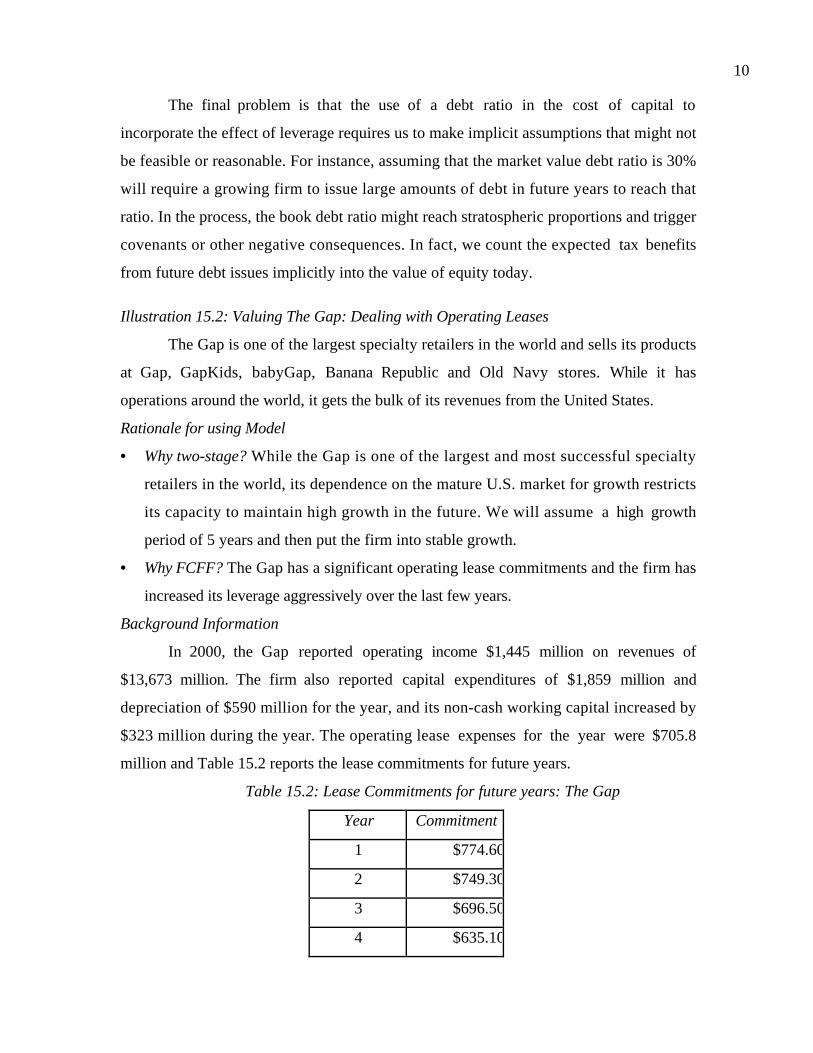
10

The final problem is that the use of a debt ratio in the cost of capital to

incorporate the effect of leverage requires us to make implicit assumptions that might not

be feasible or reasonable. For instance, assuming that the market value debt ratio is 30%

will require a growing firm to issue large amounts of debt in future years to reach that

ratio. In the process, the book debt ratio might reach stratospheric proportions and trigger

covenants or other negative consequences. In fact, we count the expected tax benefits

from future debt issues implicitly into the value of equity today.

Illustration 15.2: Valuing The Gap: Dealing with Operating Leases

The Gap is one of the largest specialty retailers in the world and sells its products

at Gap, GapKids, babyGap, Banana Republic and Old Navy stores. While it has

operations around the world, it gets the bulk of its revenues from the United States.

Rationale for using Model

• Why two-stage? While the Gap is one of the largest and most successful specialty

retailers in the world, its dependence on the mature U.S. market for growth restricts

its capacity to maintain high growth in the future. We will assume a high growth

period of 5 years and then put the firm into stable growth.

• Why FCFF? The Gap has a significant operating lease commitments and the firm has

increased its leverage aggressively over the last few years.

Background Information

In 2000, the Gap reported operating income $1,445 million on revenues of

$13,673 million. The firm also reported capital expenditures of $1,859 million and

depreciation of $590 million for the year, and its non-cash working capital increased by

$323 million during the year. The operating lease expenses for the year were $705.8

million and Table 15.2 reports the lease commitments for future years.

Table 15.2: Lease Commitments for future years: The Gap

Year Commitment

1 $774.60

2 $749.30

3 $696.50

4 $635.10

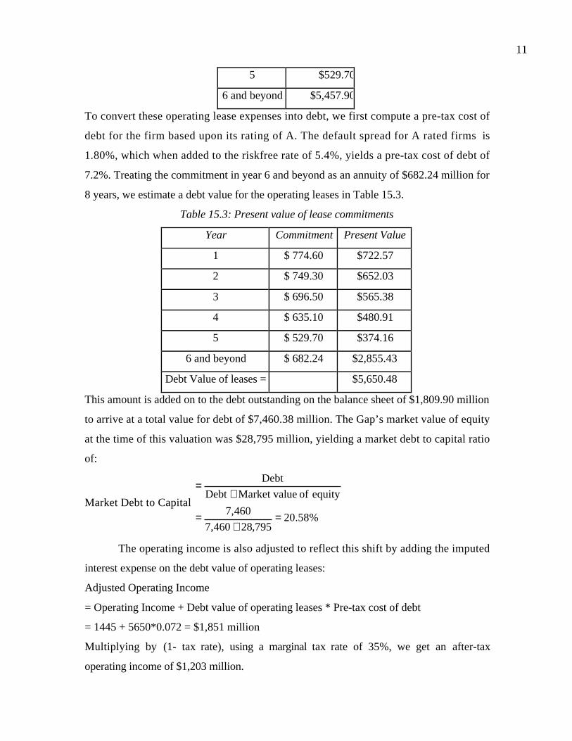
11

5 $529.70

6 and beyond $5,457.90

To convert these operating lease expenses into debt, we first compute a pre-tax cost of

debt for the firm based upon its rating of A. The default spread for A rated firms is

1.80%, which when added to the riskfree rate of 5.4%, yields a pre-tax cost of debt of

7.2%. Treating the commitment in year 6 and beyond as an annuity of $682.24 million for

8 years, we estimate a debt value for the operating leases in Table 15.3.

Table 15.3: Present value of lease commitments

Year Commitment Present Value

1 $ 774.60 $722.57

2 $ 749.30 $652.03

3 $ 696.50 $565.38

4 $ 635.10 $480.91

5 $ 529.70 $374.16

6 and beyond $ 682.24 $2,855.43

Debt Value of leases = $5,650.48

This amount is added on to the debt outstanding on the balance sheet of $1,809.90 million

to arrive at a total value for debt of $7,460.38 million. The Gap’s market value of equity

at the time of this valuation was $28,795 million, yielding a market debt to capital ratio

of:

Market Debt to Capital %58.20

795,28460,7

460,7

equity of ueMarket valDebt

Debt

=+

=

+=

The operating income is also adjusted to reflect this shift by adding the imputed

interest expense on the debt value of operating leases:

Adjusted Operating Income

= Operating Income + Debt value of operating leases * Pre-tax cost of debt

= 1445 + 5650*0.072 = $1,851 million

Multiplying by (1- tax rate), using a marginal tax rate of 35%, we get an after-tax

operating income of $1,203 million.

12

Adjusted after-tax operating income

= Adjusted Operating Income (1- tax rate)

= 1851 (1-0.35) = $1,203 million

Dividing this value by the book value of debt (including capitalized operating leases) and

the book value of equity at the end of the previous year yields an adjusted return on

capital of 13.61% in 2000 for the firm.

ROC2000

( )

%61.1322336604

1203

Equity of BVDebt of BV

t-1EBIT

19991999

2000

=+

=

+=

We will assume that the firm will be able to maintain this return on capital in perpetuity.

Valuation

We will begin with a cost of equity estimate for the Gap, using a bottom-up beta

of 1.20 (based upon the betas of specialty retailers) for the high growth period, a riskfree

rate of 5.4% and a mature market premium of 4%. In stable growth, we will lower the

beta to 1.00, keeping the riskfree rate and risk premium unchanged.

Cost of equityHigh Growth = 5.4% + 1.2 (4%) = 10.2%

Cost of equityStable Growth = 5.4% + 1.0 (4%) = 9.4%

To estimate the cost of capital during the high growth and stable growth phases, we will

assume that the pre-tax cost of debt will remain at 7.2% in perpetuity and that the current

market debt ratio of 20.58% will remain the debt ratio.

Cost of capitalHigh Growth = 10.2%(0.7942)+ 7.2% (1-0.35)(0.2058) = 9.06%

Cost of capitalStable Growth = 9.4%(0.7942)+ 7.2% (1-0.35)(0.2058) = 8.43%

To estimate the expected growth in operating earnings during the high growth period, we

will assume that the firm will continue to earn 13.61% as its return on capital and that its

reinvestment rate will equal its average reinvestment rate over the last 4 years.5

Average reinvestment rate over last 4 years = 93.53%

Expected Growth rate = Reinvestment rate * Return on Capital = 0.9353*0.1361 =

12.73%

5 The Gap has had volatile capital expenditures and working capital changes. This is our attempt to averageout this volatility.

13

Table 15.4 summarizes the expected cash flows for the high growth period.

Table 15.4: Estimated FCFF: The Gap

Year EBIT(1-t)

Reinvestment

rate Reinvestment FCFF Present Value

Current $1,203

1 $1,356 93.53% $1,269 $88 $80

2 $1,529 93.53% $1,430 $99 $83

3 $1,732 93.53% $1,620 $112 $86

4 $1,952 93.53% $1,826 $126 $89

5 $2,190 93.53% $2,049 $142 $92

Sum of present values of cash flows = $430

Note that the cash flows during the high growth period are discounted back at 9.06%. To

estimate the terminal value at the end of year 5, we assume that this cash flow will grow

forever at 5%. The reinvestment rate can then be estimated and used to measure the free

cash flow to the firm in year 6:

Expected growth rate =5%

Reinvestment rate in stable growth = 36.73%13.61%

5%

ROC period Stable

g ==

FCFF6 ( )( )( )

( )( ) 14553673.0105.12190

Ratent Reinvestme-11t-1EBIT Period Stable5

=−=+= g

The terminal value is:

Terminal value

million 441,42$05.00843.0

1455

rateGrowth -growth stablein capital ofCost

FCFF11

=−

=

=

Discounting the terminal value to the present and adding it to the present value of the

cash flows over the high growth period yields a value for the operating assets of the firm.

Value of Operating assets = PV of cash flows during high growth + PV of terminal value

= million $27,9331.0906

$42,441$430

5=+

14

Adding back the firm’s cash and marketable securities (estimated to be $409 million at the

end of 2000) and subtracting out the value of the debt yields a value for the equity in the

firm:

Value of the equity

= Value of the operating assets + Cash and Marketable securities – net debt

= 27,933 + 409 – 7460 = $20,882 million

Note that the debt subtracted out includes the present value of operating leases. At its

prevailing market value of equity of $27,615 million, the Gap is overvalued.

Illustration 15.3: Valuing Amgen: Effects of R&D

As a leading biotechnology firm, Amgen has substantial research and development

expenses and we capitalized these expenses earlier in this book. In this valuation, we will

consider the implications of this capitalization for firm and equity values.

Rationale for using Model

• Why three-stage? Amgen, in spite of being one of the largest biotechnology firms has

significant potential for future growth, both because of drugs that it has in commercial

production and other drugs in the pipeline. We will assume that the firm will continue

to grow for 10 years, five at a high growth rate followed by five year in transition to

stable growth.

• Why FCFF? The firm has little debt on its books currently but will come under

increasing pressure to increase its leverage as its cash flows become larger and more

stable.

Background Information

In 2000, Amgen reported operating income $1,549 million on revenues of $3,629

million. The firm also reported capital expenditures of $437 million and depreciation of

$212 million for the year, and its non-cash working capital increased by $146 million

during the year. Recapping the analysis of Amgen’s R&D from Chapter 9, we will use a

10-year amortizable life to estimate the value of the research asset in Table 15.5.

Table 15.5: Capitalizing the Research Asset

Year R&D Expense Unamortized portion

Amortization

this year

15

Current 845.00 1.00 845.00

-1 822.80 0.90 740.52 $82.28

-2 663.30 0.80 530.64 $66.33

-3 630.80 0.70 441.56 $63.08

-4 528.30 0.60 316.98 $52.83

-5 451.70 0.50 225.85 $45.17

-6 323.63 0.40 129.45 $32.36

-7 255.32 0.30 76.60 $25.53

-8 182.30 0.20 36.46 $18.23

-9 120.94 0.10 12.09 $12.09

-10 0.00 0.00 0.00 $0.00

Value of Research Asset = $3,355.15 $397.91

The operating income is adjusted by adding back the current year’s R& D expense and

subtracting out the amortization of the research asset.

Adjusted operating income

= Operating income + Current year’s R&D – Amortization of Research asset

= $1,549+ $845 - $398 = $1996 million

To get to the after-tax operating income, we also consider the tax benefits from expensing

R&D (as opposed to just the amortization of the research asset).

Adjusted after-tax operating income

= Adjusted Operating Income (1- tax rate) + (Current year R&D – Amortization) Tax rate

= 1996 (1-0.35) + (845-398) (0.35) = $1,454 million

The current year’s R&D expense is added to the capital expenditures for the year, and the

amortization to the depreciation. In conjunction with an increase in working capital of

$146 million, we estimate an adjusted reinvestment rate for the firm of 56.27%.

Adjusted Capital expenditures = 437+ 845 = $1,282 million

Adjusted Depreciation = 212 + 398 = $610 million

Adjusted Reinvestment rate

16

( )%27.56

1454

1466101282

t-1EBIT Adjusted

WConDepreciati-esExpenditur Capital

=+−=

∆+=

To estimate the return on capital, we estimated the value of the research asset at

the end of the previous year and added it to the book value of equity. The resultant return

on capital for the firm is shown.

Return on capital

( )

%24.233235932

1454

debt of Book valueasset)research (includesequity of book value Adjusted

t-1EBIT Adjusted

=+

=

+=

Valuation

To value Amgen, we will begin with the estimates for the 5-year high growth

period. We use a bottom-up beta estimate of 1.35, a riskfree rate of 5.4% and a risk

premium of 4% to estimate the cost of equity:

Cost of equity = 5.4% + 1.35 (4%) = 10.80%

We estimate a synthetic rating of AAA for the firm, and use it to come up with a pre-tax

cost of borrowing of 6.15% by adding a default spread of 0.75% to the treasury bond rate

of 5.4%. With a marginal tax rate of 35% and a debt ratio of 0.55%, the firm’s cost of

capital closely tracks its cost of equity.

Cost of capital = 13.08% (0.9945) + 6.15%(1-0.35)(0.0055) = 10.76%

To estimate the expected growth rate during the high growth period, we will assume that

the firm can maintain its current return on capital and reinvestment rate estimated in the

section above.

Expected Growth rate = Reinvestment rate * Return on capital = 0.5627*0.2324 =

13.08%

Before we consider the transition period, we estimate the inputs for the stable

growth period. First, we assume that the beta for Amgen will drop to 1, and that the firm

will raise its debt ratio to 10%. Keeping the cost of debt unchanged, we estimate a cost of

capital of

Cost of equity = 5.4% + 1(4%) = 9.4%

17

Cost of capital = 9.4% (0.9) + 6.15% (1-0.35) (0.1) = 8.86%

We assume that the stable growth rate will be 5% and that the firm will have a return on

capital of 20% in stable growth. This allows us to estimate the reinvestment rate in stable

growth.

Reinvestment rate in stable growth = 25%20%

5%

ROC

g ==

During the transition period, we adjust growth, reinvestment rate and the cost of

capital from high growth levels to stable growth levels in linear increments. Table 15.6

summarizes the inputs and cash flows for both the high growth and transition period.

Table 15.6: Free Cashflows to Firm: Amgen

Year

Expected

Growth EBIT(1-t)

Reinvestment

Rate FCFF

Cost of

Capital Present Value

Current $1,454

1 13.08% $1,644 56.27% $719 10.76% $649

2 13.08% $1,859 56.27% $813 10.76% $663

3 13.08% $2,102 56.27% $919 10.76% $677

4 13.08% $2,377 56.27% $1,040 10.76% $691

5 13.08% $2,688 56.27% $1,176 10.76% $705

6 11.46% $2,996 50.01% $1,498 10.38% $814

7 9.85% $3,291 43.76% $1,851 10.00% $914

8 8.23% $3,562 37.51% $2,226 9.62% $1,003

9 6.62% $3,798 31.25% $2,611 9.24% $1,077

10 5.00% $3,988 25.00% $2,991 8.86% $1,133

Sum of the present value of the FCFF during high growth = $8,327 m

Finally, we estimate the terminal value, based upon the growth rate, cost of capital and

reinvestment rate estimated above.

FCFF11 = ( )( ) ( )( ) million $3,1400.25-11.053988ratent Reinvestme-1t-1EBIT11 ==

Terminal value10

million 364,81$05.00886.0

3140

rateGrowth -growth stablein capital ofCost

FCFF11

=−

=

=

18

Adding the present value of the terminal value to the present value of the free cash flows

to the firm in the first 10 years, we get:

Value of the operating assets of the firm

( )( )( )( )( )( )million 161,39$

1.08861.09241.09621.101.10381.1076

$81,364million $8,327

5

=

+=

Adding the value of cash and marketable securities ($2,029 million) and subtracting out

debt ($323 million) yields a value for the equity of $40,867 million. At the time of this

valuation in May 2001, the equity was trading at a market value of $58,000 million.

Illustration 15.4: Valuing Embraer: Dealing with Country Risk

Embraer is a Brazilian aerospace firms that manufactures and sells both

commercial and military aircraft. In this valuation, we will consider the implications of

valuing the firm in the context of country risk and uncertainty about expected inflation.

Rationale for using Model

• Why two-stage? Embraer has done exceptionally well in the last few years though it

operates in a mature business with strong competition from giants such as Boeing and

Airbus. We believe that it can sustain growth for a long period (10 years) and that

there will be a transition to stable growth in the second half of this growth period.

• Why FCFF? The firm’s debt ratio has been volatile. While it does not use much debt

to fund its operations currently, it does have the capacity to raise more debt now,

especially in the United States.

• Why real cash flows? We had two choices when it came to valuation – to work with

U.S. dollars or work in real cash flows. We avoided working with nominal real, largely

because of the difficulties associated with getting a riskfree rate in that currency.

Background Information

In 2000, Embraer reported operating income of 810.32 million BR on revenues of

4560 million BR, and faced a marginal tax rate of 33% on its income. At the end of 2000,

the firm had net debt (debt minus cash) of 215.5 million BR on which their net interest

expenses for 2000 were 28.20 million BR. The firm’s non-cash working capital at the end

19

of 2000 amounted to 915 million BR, an increase of 609.7 million BR over the previous

year’s amount.

The firm’s capital expenditures were 233.5 million BR and depreciation was 127.5

million for the year, yielding a reinvestment rate of 131.83% for the year.

Reinvestment Rate2000 = ( ) 131.83%0.33-1810.32

609.7127.5-233.5 =+

Normalizing the non-cash working capital component6 yields a change in non-cash

working capital of 239.59 million BR and a normalized reinvestment rate.

Normalized Reinvestment Rate2000 = ( ) 63.65%0.33-1810.32

239.59127.5-233.5 =+

Based upon the capital invested of 1,470 million BR in the firm at the beginning of

2000, the return on capital at Embraer in 2000 was 36.94%.

Return on capital = ( )

36.94%1470

0.33-1810.32 =

Valuation

We first have to estimate a country risk premium for Brazil. Drawing on the

approach developed in Chapter 7, we estimate a country risk premium for Brazil of

10.24%.

Country rating for Brazil = B1

Default spread on Brazilian Government C-bond (U.S. dollar denominated) = 5.37%

To estimate the country equity risk premium, we estimated the standard deviation in

weekly returns over the last 2 years in both the Bovespa (the Brazilian equity index) and

the C-Bond.

Standard deviation in the Bovespa = 32.6%

Standard deviation in the C-Bond = 17.1%

Country risk premium

( )

( ) %24.10%1.17

%6.32%37.5

Deviation Standard

Deviation StandardSpreadDefault

Bond-C

Equity

=

=

=

6 The normalized change in non-cash working capital was computed as follows:Normalized change = (Non-cash WC2000/Revenues2000)*(Revenues2000-Revenues1999)

20

To make an estimate of Embraer’s beta, we used a bottom-up unlevered beta of 0.87 and

Embraer’s market net debt to equity ratio (to stay consistent with our use of net debt in

the valuation) of 2.45%.

Levered beta = 0.87 (1 + (1-0.33) (0.0245)) = 0.88

Finally, to estimate the cost of equity, we used a real riskless rate of 4.5% and a mature

market risk premium of 4% (in addition to the country risk premium of 10.24%):

Cost of equity = 4.5% + 0.88 (4%+10.24%) = 17.03%

We estimate a synthetic rating of AAA for Embraer and use it to come up with a pre-tax

cost of borrowing of 10.62% by adding a default spread of 0.75% to the real riskless rate

of 4.5%, and then adding the country default spread of 5.37%.7

Pre-tax cost of debt = Real riskfree rate + Country default spread + Company default

spread = 4.5% + 5.37% + 0.75% = 10.62%

With a marginal tax rate of 33% and a net debt to capital ratio of 2.40%, the firm’s cost of

capital is shown below:

Cost of capital = 17.03% (0.976) + 0.1062(1-0.33)(0.024) = 16.79%

To estimate the expected growth rate during the high growth period, we will

assume that the firm can maintain its current return on capital and use the normalized

reinvestment rate.

Expected Growth rate = Normalized Reinvestment rate * Return on capital

= 0.6365*0.3694 = 23.51%

In stable growth, we assume that the beta for Embrarer will rise slightly to 0.90,

that its net debt ratio will remain unchanged at 2.40% and that the country risk premium

will drop to 5.37%. We also assume that the pre-tax cost of debt will decline to 7.50%

Cost of equity = 4.5% + 0.9(4%+ 5.37%) = 12.93%

Cost of capital = 12.93% (0.976) + 7.5% (1-0.33) (0.024) = 12.74%

We assume that the stable real growth rate will be 3% and that the firm will have a return

on capital of 15% in stable growth. This is a significant drop from its current return on

7 This is a conservative estimate. It is entirely possible that the market will not assess Embraer with all ofthe country risk and may view Embraer as safer than the Brazilian government.

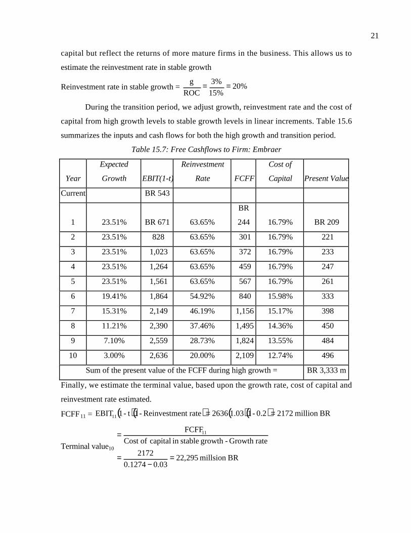
21

capital but reflect the returns of more mature firms in the business. This allows us to

estimate the reinvestment rate in stable growth

Reinvestment rate in stable growth = 20%15%

3%

ROC

g ==

During the transition period, we adjust growth, reinvestment rate and the cost of

capital from high growth levels to stable growth levels in linear increments. Table 15.6

summarizes the inputs and cash flows for both the high growth and transition period.

Table 15.7: Free Cashflows to Firm: Embraer

Year

Expected

Growth EBIT(1-t)

Reinvestment

Rate FCFF

Cost of

Capital Present Value

Current BR 543

1 23.51% BR 671 63.65%

BR

244 16.79% BR 209

2 23.51% 828 63.65% 301 16.79% 221

3 23.51% 1,023 63.65% 372 16.79% 233

4 23.51% 1,264 63.65% 459 16.79% 247

5 23.51% 1,561 63.65% 567 16.79% 261

6 19.41% 1,864 54.92% 840 15.98% 333

7 15.31% 2,149 46.19% 1,156 15.17% 398

8 11.21% 2,390 37.46% 1,495 14.36% 450

9 7.10% 2,559 28.73% 1,824 13.55% 484

10 3.00% 2,636 20.00% 2,109 12.74% 496

Sum of the present value of the FCFF during high growth = BR 3,333 m

Finally, we estimate the terminal value, based upon the growth rate, cost of capital and

reinvestment rate estimated.

FCFF11 = ( )( ) ( )( ) BRmillion 21720.2-11.032636ratent Reinvestme-1t-1EBIT11 ==

Terminal value10

BRmillsion 295,2203.01274.0

2172

rateGrowth -growth stablein capital ofCost

FCFF11

=−

=

=

22

Adding the present value of the terminal value to the present value of the free cash flows

to the firm in the first 10 years, we get:

Value of the operating assets of the firm

( ) ( )( )( )( )( )BRmillion 578,8

1.12741.13551.14361.15171.15981.1679

22,295BRmillion 3,333

5

=

+=

We do not add back cash and marketable securities, because we are using net debt (and the

cash has therefore already been netted out against debt). Adding the value of non-

operating assets ($510 million) and subtracting out net debt ($223 million) yields a value

for the equity of 8,865 million BR and a per-share value of 14.88 BR. At the time of this

valuation in March 2001, the equity was trading at a market price of 15.2 BR per share.

Doing a valuation is only the first part of the process. Presenting it to others is the

second and perhaps just as important. Valuations can be complicated and it is easy to lose

your audience (and yourself) in the details. Presenting a big picture of the valuation often

helps. In Figure 15.1, for instance, the valuation of Embraer is presented in a picture. The

valuation contains all of the details presented in the Amgen and Gap valuations but they

are presented both in a more concise format and the connections between the various

inputs are much more visible.

fcffginzu.xls: This spreadsheet allows you to estimate the value of a firm using the

FCFF approach.

Net Debt versus Gross Debt

In valuing Embrarer, we used net debt where cash was netted out against debt. In

all of the earlier valuations, we used gross debt. What is the difference between the two

approaches and will the valuations from the two approaches agree?

A comparison of the Embraer and the earlier valuations reveals the differences in

the way we approach the calculation of key inputs to the valuation. We summarize these.

23

While working with net debt in valuation is not difficult to do, the more interesting

question is whether the value that emerges will be different from the value that would

have been estimated using gross debt. In general, the answer is no and the reason usually

lies in the cost of debt used in the net debt valuation. Intuitively, what you are doing

when you use net debt is break the firm into two parts – a cash business, which is funded

100% with riskless debt, and an operating business, funded partly with risky debt.

Carrying this to its logical conclusion, the cost of debt you would have for the operating

business would be significantly higher than the firm’s current cost of debt. This is because

the current lenders to the firm will factor in the firm’s cash holdings when setting the cost

of debt.

To illustrate, assume that you have a firm with an overall value of $1 billion -

$200 million in cash and $800 million in operating assets – with $400 million in debt and

$600 million in equity. The firm’s cost of debt is 7%, a 2% default spread over the

riskfree rate of 5%; note that this cost of debt is set based upon the firm’s substantial

cash holdings. If you net debt against cash, the firm would have $200 million in net debt

and $600 million in equity. If you use the 7% cost of debt to value the firm now, you will

overstate its value. Instead, the cost of debt you should use in the valuation is 9%.

Gross Debt Net Debt

Levered Beta Unlevered beta is levered

using gross debt to market

equity ratio.

Unlevered beta is levered

using net debt to market

equity ratio.

Cost of capital Debt to capital ratio used is

based upon net debt.

Debt to capital ratio used is

based upon gross debt.

Treatment of cash & debt Cash is added to value of

operating assets and net

debt is subtracted out to get

to equity value.

Cash is not added back to

operating assets and gross

debt is subtracted out to get

to equity value.

24

Cost of debt on net debt

( )( ) ( )( )

( )( ) ( )( )0.09

200-400

20005.040007.0

DebtNet -Debt Gross

DebtNet debt ofcost tax -Pre-Debt Grossdebt ofcost tax -Pre DebtNet Debt Gross

=−=

=

In general, we would recommend using gross debt rather than net debt for two

other reasons. First, the net debt can be a negative number, if cash exceeds the gross debt.

If this occurs, you should set the net debt to zero and consider the excess cash just as you

would cash in a gross debt valuation. Second, maintaining a stable net debt ratio in a

growing firm will require that cash balances increase as the firm value increases.

25

Current Cashflow to FirmEBIT(1-t) : 543- Nt CpX 36- Chg WC 610= FCFF -173Reinvestment Rate =131.8%

Expected Growth in EBIT (1-t).6356*.3694= .235123.51 %

Stable Growthg = 3%; Beta = 0.90;Country Premium= 5.37% ROC= 15%Reinvestment Rate=20%

Terminal Value 10= 2172/(.1274-.03) = 22,295

Cost of Equity17.03%

Cost of Debt(4.5%+ 5.37%+.75%)(1-.33)= 7.12%

WeightsE =97.6% D = 2.4%

Discount at Cost of Capital (WACC) = 17.03% (.974) + 7.12% (0.024) = 16.79%

Firm Value: 8,578+ NO Assets 510- Net Debt: 223=Equity 8,865-Options 0Value/Share 14.88

Riskfree Rate :Riskfree rate = 4.5%(Real Riskfree rate)

+Beta 0.88 X

Risk Premium14.24%

Unlevered Beta for Sectors: 0.87

Firm’s D/ERatio: 2.45%

Mature riskpremium4%

Country RiskPremium10.24%

Figure 15.1: Embraer Reinvestment Rate63.56%

Return on Capital36.94%

Term Yr2715 5432172

Synthetic rating = AAA

Transition Period

Norm. WC Reinv Rate = 63.56%

1 2 3 4 5 6 7 8 9 10EBIT(1-t) R$ 671 828 1023 1264 1561 1864 2149 2390 2559 2636 - ReinvestmentR$ 427 527 651 804 993 1024 993 895 735 527 = FCFF R$ 244 301 372 459 567 840 1156 1495 1824 2109

26

Will equity value be the same under firm and equity valuation?

This model, unlike the dividend discount model or the FCFE model, values the

firm rather than equity. The value of equity, however, can be extracted from the value of

the firm by subtracting out the market value of outstanding debt. Since this model can be

viewed as an alternative way of valuing equity, two questions arise - Why value the firm

rather than equity? Will the values for equity obtained from the firm valuation approach

be consistent with the values obtained from the equity valuation approaches described in

the previous chapter?

The advantage of using the firm valuation approach is that cashflows relating to

debt do not have to be considered explicitly, since the FCFF is a pre-debt cashflow, while

they have to be taken into account in estimating FCFE. In cases where the leverage is

expected to change significantly over time, this is a significant saving, since estimating

new debt issues and debt repayments when leverage is changing can become increasingly

messy the further into the future you go. The firm valuation approach does, however,

require information about debt ratios and interest rates to estimate the weighted average

cost of capital.

The value for equity obtained from the firm valuation and equity valuation

approaches will be the same if you make consistent assumptions about financial leverage.

Getting them to converge in practice is much more difficult. Let us begin with the

simplest case – a no-growth, perpetual firm. Assume that the firm has $166.67 million in

earnings before interest and taxes and a tax rate of 40%. Assume that the firm has equity

with a market value of $600 million, with a cost of equity of 13.87% debt of $400 million

and with a pre-tax cost of debt of 7%. The firm’s cost of capital can be estimated.

Cost of capital = ( ) ( )( ) 10%1000

4000.4-17%

1000

60013.87% =

+

Value of the firm = ( ) ( )

$1,0000.10

0.4-1166.67

capital ofCost

t-1EBIT ==

Note that the firm has no reinvestment and no growth. We can value equity in this firm

by subtracting out the value of debt.

Value of equity = Value of firm – Value of debt = $ 1,000 - $400 = $ 600 million

27

Now let us value the equity directly by estimating the net income:

Net Income = (EBIT – Pre-tax cost of debt * Debt) (1-t) = (166.67 - 0.07*400) (1-0.4) =

83.202 million

The value of equity can be obtained by discounting this net income at the cost of equity:

Value of equity = million 600 $0.1387

83.202

equity ofCost

IncomeNet ==

Even this simple example works because of the following assumptions that we made

implicitly or explicitly during the valuation.

1. The values for debt and equity used to compute the cost of capital were equal to

the values that we obtained in the valuation. Notwithstanding the circularity in

reasoning – you need the cost of capital to obtain the values in the first place – it

indicates that a cost of capital based upon market value weights will not yield the

same value for equity as an equity valuation model, if the firm is not fairly priced

in the first place.

2. There are no extraordinary or non-operating items that affect net income but not

operating income. Thus, to get from operating to net income, all we do is subtract

out interest expenses and taxes.

3. The interest expenses are equal to the pre-tax cost of debt multiplied by the

market value of debt. If a firm has old debt on its books, with interest expenses

that are different from this value, the two approaches will diverge.

If there is expected growth, the potential for inconsistency multiplies. You have to ensure

that you borrow enough money to fund new investments to keep your debt ratio at a

level consistent with what you are assuming when you compute the cost of capital.

fcffvsfcfe.xls: This spreadsheet allows you to compare the equity values obtained

using FCFF and FCFE models.

Firm Valuation: The APV approach

In the adjusted present value (APV) approach, we begin with the value of the firm

without debt. As we add debt to the firm, we consider the net effect on value by

considering both the benefits and the costs of borrowing. To do this, we assume that the

28

primary benefit of borrowing is a tax benefit and that the most significant cost of

borrowing is the added risk of bankruptcy.

The Mechanics of APV Valuation

We estimate the value of the firm in three steps. We begin by estimating the value

of the firm with no leverage. We then consider the present value of the interest tax savings

generated by borrowing a given amount of money. Finally, we evaluate the effect of

borrowing the amount on the probability that the firm will go bankrupt, and the expected

cost of bankruptcy.

Value of Unlevered Firm

The first step in this approach is the estimation of the value of the unlevered firm.

This can be accomplished by valuing the firm as if it had no debt, i.e., by discounting the

expected free cash flow to the firm at the unlevered cost of equity. In the special case

where cash flows grow at a constant rate in perpetuity, the value of the firm is easily

computed.

Value of Unlevered Firm = ( )g -

g1FCFF

u

o +

where FCFF0 is the current after-tax operating cash flow to the firm, ρu is the unlevered

cost of equity and g is the expected growth rate. In the more general case, you can value

the firm using any set of growth assumptions you believe are reasonable for the firm.

The inputs needed for this valuation are the expected cashflows, growth rates and

the unlevered cost of equity. To estimate the latter, we can draw on our earlier analysis

and compute the unlevered beta of the firm.

( )E

tD

11

currentunlevered

−+=

where

βunlevered = Unlevered beta of the firm

βcurrent = Current equity beta of the firm

t = Tax rate for the firm

D/E = Current debt/equity ratio

29

This unlevered beta can then be used to arrive at the unlevered cost of equity.

Expected Tax Benefit from Borrowing

The second step in this approach is the calculation of the expected tax benefit

from a given level of debt. This tax benefit is a function of the tax rate of the firm and is

discounted at the cost of debt to reflect the riskiness of this cash flow. If the tax savings

are viewed as a perpetuity,

Value of Tax Benefits

( )( )( )

( )( )Dtc=

=

=

DebtRateTax Debt ofCost

DebtDebt ofCost RateTax

The tax rate used here is the firm’s marginal tax rate and it is assumed to stay constant

over time. If we anticipate the tax rate changing over time, we can still compute the

present value of tax benefits over time, but we cannot use the perpetual growth equation

cited above.

Estimating Expected Bankruptcy Costs and Net Effect

The third step is to evaluate the effect of the given level of debt on the default risk

of the firm and on expected bankruptcy costs. In theory, at least, this requires the

estimation of the probability of default with the additional debt and the direct and indirect

cost of bankruptcy. If πa is the probability of default after the additional debt and BC is

the present value of the bankruptcy cost, the present value of expected bankruptcy cost

can be estimated.

PV of Expected Bankruptcy cost ( )( )

BCa== Cost Bankruptcy of PVBankruptcy ofy Probabilit

This step of the adjusted present value approach poses the most significant estimation

problem, since neither the probability of bankruptcy nor the bankruptcy cost can be

estimated directly.

There are two basic ways in which the probability of bankruptcy can be estimated

indirectly. One is to estimate a bond rating, as we did in the cost of capital approach, at

each level of debt and use the empirical estimates of default probabilities for each rating.

30

For instance, Table 15.8, extracted from a study by Altman and Kishore, summarizes the

probability of default over ten years by bond rating class in 1998.8

Table 15.8: Default Rates by Bond Rating Classes

Bond Rating Default Rate

D 100.00%

C 80.00%

CC 65.00%

CCC 46.61%

B- 32.50%

B 26.36%

B+ 19.28%

BB 12.20%

BBB 2.30%

A- 1.41%

A 0.53%

A+ 0.40%

AA 0.28%

AAA 0.01%

Source: Altman and Kishore (1998)

The other is to use a statistical approach, such as a probit to estimate the probability of

default, based upon the firm’s observable characteristics, at each level of debt.

The bankruptcy cost can be estimated, albeit with considerable error, from studies

that have looked at the magnitude of this cost in actual bankruptcies. Research that has

looked at the direct cost of bankruptcy concludes that they are small9, relative to firm

value. The indirect costs of bankruptcy can be substantial, but the costs vary widely

8 This study estimated default rates over ten years only for some of the ratings classes. We extrapolated therest of the ratings.9 In Warner’s study of railroad bankruptcies, the direct cost of bankruptcy seems to be about 5%.

31

across firms. Shapiro and Titman speculate that the indirect costs could be as large as

25% to 30% of firm value but provide no direct evidence of the costs.

Illustration 15.5: Valuing a firm with the APV approach: Tube Investments

In Illustration 15.1, we valued Tube Investments, using a cost of capital approach.

Here, we re-estimate the value of the firm using an adjusted present value approach in

three steps.

Step 1: Unlevered firm value

To estimate the unlevered firm value, we first compute the unlevered beta. Tube

Investment’s beta is 1.17, its current market debt to equity ratio is 79% and the firm’s tax

rate is 30%.

Unlevered beta = ( )( ) 0.750.790.3-11

1.17 =+

Using the rupee riskfree rate of 10.5% and the risk premium of 9.23% for India, we

estimate an unlevered cost of equity.

Unlevered cost of equity = 10.5% + 0.75(9.23%) = 17.45%

Using the free cash flow to the firm that we estimated in Illustration 15.1 of Rs 212.2

million and the stable growth rate of 5%, we estimate the unlevered firm value:

Unlevered firm value= million $1704.60.05-0.1745

212.2 =

Step 2: Tax benefits from debt

The tax benefits from debt are computed based upon Tube Investment’s existing dollar

debt of Rs. 1807.3 million and the tax rate of 30%:

Expected tax benefits in perpetuity = Tax rate (Debt) = 0.30 (1807.3) = Rs 542.2 million

Step 3: Expected bankruptcy costs

To estimate this, we made two assumptions. First, based upon its existing rating, the

probability of default at the existing debt level is 10%. Second,the cost of bankruptcy is

40% of unlevered firm value.

Expected bankruptcy cost =Probability of bankruptcy * Cost of bankruptcy * Unlevered

firm value = 0.10*0.40*1704.6 = Rs 68.2 million

The value of the operating assets of the firm can now be estimated.

32

Value of the operating assets

= Unlevered firm value + PV of tax benefits – Expected Bankruptcy Costs

= 1704.6 + 542.2 – 68.2 = Rs 2178.6 million

Adding to this the value of cash and marketable securities of Rs. 1365.3 million, we obtain

a value for the firm of Rs 3543.9 million. In contrast, we valued the firm at Rs. 3367.3

million with the cost of capital approach.

Cost of Capital versus APV Valuation

In an APV valuation, the value of a levered firm is obtained by adding the net

effect of debt to the unlevered firm value.

Value of Levered Firm = ( )

BC-Dtg-

g1FCFFac

u

o ++

In the cost of capital approach, the effects of leverage show up in the cost of capital, with

the tax benefit incorporated in the after-tax cost of debt and the bankruptcy costs in both

the levered beta and the pre-tax cost of debt. Will the two approaches yield the same

value? Not necessarily. The first reason for the differences is that the models consider

bankruptcy costs very differently, with the adjusted present value approach providing

more flexibility in allowing you to consider indirect bankruptcy costs. To the extent that

these costs do not show up or show up inadequately in the pre-tax cost of debt, the APV

approach will yield a more conservative estimate of value. The second reason is that the

APV approach considers the tax benefit from a dollar debt value, usually based upon

existing debt. The cost of capital approach estimates the tax benefit from a debt ratio that

may require the firm to borrow increasing amounts in the future. For instance, assuming a

market debt to capital ratio of 30% in perpetuity for a growing firm will require it to

borrow more in the future and the tax benefit from expected future borrowings is

incorporated into value today.

APV, without bankruptcy costs

There are many who believe that adjusted present value is a more flexible way of

approaching valuation than traditional discounted cash flow models. This may be true in a

generic sense, but APV valuation in practice has significant flaws. The first and most

important is that most practitioners who use the adjusted present value model ignore

33

expected bankruptcy costs. Adding the tax benefits to unlevered firm value to get to the

levered firm value makes debt seem like an unmixed blessing. Firm value will be

overstated, especially at very high debt ratios, where the cost of bankruptcy is clearly not

zero and, in some instances, the cost of bankruptcy is higher than the tax benefit of debt.

The Effect of Leverage in Firm Value

Both the cost of capital approach and the APV approach make the value of a firm

a function of its leverage. It follows directly, then, that there is some mix of debt and

equity at which firm value is maximized. In the rest of this chapter, we consider how best

to make this link.

Cost of Capital and Optimal Leverage

In order to understand the relationship between the cost of capital and optimal

capital structure, we rely on the relationship between firm value and the cost of capital. In

the earlier section, we noted that the value of the entire firm can be estimated by

discounting the expected cash flows to the firm at the firm’s cost of capital. The cash

flows to the firm can be estimated as cash flows after operating expenses, taxes and any

capital investments needed to create future growth in both fixed assets and working

capital, but before financing expenses.

Cash Flow to Firm = EBIT (1-t) - (Capital Expenditures - Depreciation) - Change

in Working Capital

The value of the firm can then be written as:

Value of Firm = CF to Firmt

(1+WACC) tt=1

t=n

∑

and is a function of the firm’s cash flows and its cost of capital. If we assume that the

cash flows to the firm are unaffected by the choice of financing mix and the cost of capital

is reduced as a consequence of changing the financing mix, the value of the firm will

increase. If the objective in choosing the financing mix for the firm is the maximization of

firm value, we can accomplish it, in this case, by minimizing the cost of capital. In the

34

more general case where the cash flows to the firm are a function of the debt-equity mix,

the optimal financing mix is the mix that maximizes firm value.10

Illustration 15.6: WACC, Firm Value, and Leverage

Assume that you are given the costs of equity and debt at different debt levels for

Strunks Inc., a leading manufacturer of chocolates and other candies, and that the cash

flows to this firm are currently $200 million. Strunks is in a relatively stable market. The

cash flows are expected to grow at 6% forever and are unaffected by the debt ratio of the

firm. The cost of capital schedule is provided in Table 15.9, along with the value of the

firm at each level of debt.

Table 15.9: Cost of Capital, Firm Value and Debt Ratios

D/(D+E) Cost of Equity Cost of Debt WACC Firm Value

0 10.50% 4.80% 10.50% $4,711

10% 11.00% 5.10% 10.41% $4,807

20% 11.60% 5.40% 10.36% $4,862

30% 12.30% 5.52% 10.27% $4,970

40% 13.10% 5.70% 10.14% $5,121

50% 14.00% 6.30% 10.15% $5,108

60% 15.00% 7.20% 10.32% $4,907

70% 16.10% 8.10% 10.50% $4,711

80% 17.20% 9.00% 10.64% $4,569

90% 18.40% 10.20% 11.02% $4,223

100% 19.70% 11.40% 11.40% $3,926

Note that the value of the firm

( )

( )0.06-Capital ofCost

06.1200

g-Capital ofCost

g1firm toflowsCash

=

+=

10 In other words, the value of the firm might not be maximized at the point that cost of capital isminimized, if firm cash flows are much lower at that level.

35

The value of the firm increases as the cost of capital decreases, and decreases as

the cost of capital increases. This is illustrated in Figure 15.2.

While this illustration makes the choice of an optimal financing mix seem easy, it obscures

problems that may arise in its practice. First, we typically do not have the benefit of

having the entire schedule of costs of financing prior to an analysis. In most cases, the

only level of debt at which we have information on the cost of debt and equity financing

is the current level. Second, the analysis assumes implicitly that the level of operating

income of the firm is unaffected by the financing mix of the firm and, consequently, by

the default risk (or bond rating) for the firm. While this may be reasonable in some cases,

it might not be in others. Firms that borrow too much might find that there are indirect

bankruptcy costs that affect revenues and operating income.

Steps in Cost of Capital Approach

We need three basic inputs to compute the cost of capital – the cost of equity, the

after-tax cost of debt and the weights on debt and equity. The costs of equity and debt

Figure 15.2: Cost of Capital and Firm Value

9.40%

9.60%

9.80%

10.00%

10.20%

10.40%

10.60%

10.80%

11.00%

11.20%

11.40%

11.60%

0 10% 20% 30% 40% 50% 60% 70% 80% 90% 100%

Debt Ratio

Cos

t of

Cap

ital

$0

$1,000

$2,000

$3,000

$4,000

$5,000

$6,000

Firm

Val

ue

WACCFirm Value

36

change as the debt ratio changes, and the primary challenge of this approach is in

estimating each of these inputs.

Let us begin with the cost of equity. We argued that the beta of equity will change as

the debt ratio changes. In fact, we estimated the levered beta as a function of the market

debt to equity ratio of a firm, the unlevered beta and the firm’s marginal tax rate:

( )

−+=

ED

tunleveredlevered 11

Thus, if we can estimate the unlevered beta for a firm, we can use it to estimate the

levered beta of the firm at every debt ratio. This levered beta can then be used to compute

the cost of equity at each debt ratio.

Cost of Equity = Riskfree rate + βlevered (Risk Premium)

The cost of debt for a firm is a function of the firm’s default risk. As firms borrow

more, their default risk will increase and so will the cost of debt. If we use bond ratings as

our measure of default risk, we can estimate the cost of debt in three steps. First, we

estimate a firm’s dollar debt and interest expenses at each debt ratio; as firms increase

their debt ratio, both dollar debt and interest expenses will rise. Second, at each debt level,

we compute a financial ratio or ratios that measures default risk and use the ratio(s) to

estimate a rating for the firm; again, as firms borrow more, this rating will decline. Third,

a default spread, based upon the estimated rating, is added on to the riskfree rate to arrive

at the pre-tax cost of debt. Applying the marginal tax rate to this pre-tax cost yields an

after-tax cost of debt.

Once we estimate the costs of equity and debt at each debt level, we weight them

based upon the proportions used of each to estimate the cost of capital. While we have

not explicitly allowed for a preferred stock component in this process, we can have

preferred stock as a part of capital. However, we have to keep the preferred stock portion

fixed, while changing the weights on debt and equity. The debt ratio at which the cost of

capital is minimized is the optimal debt ratio.

In this approach, the effect on firm value of changing the capital structure is

isolated by keeping the operating income fixed and varying only the cost of capital. In

practical terms, this requires us to make two assumptions. First, the debt ratio is

decreased by raising new equity and/or retiring debt; conversely, the debt ratio is

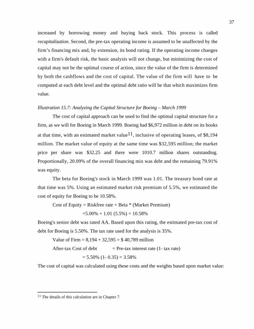
37

increased by borrowing money and buying back stock. This process is called

recapitalization. Second, the pre-tax operating income is assumed to be unaffected by the

firm’s financing mix and, by extension, its bond rating. If the operating income changes

with a firm's default risk, the basic analysis will not change, but minimizing the cost of

capital may not be the optimal course of action, since the value of the firm is determined

by both the cashflows and the cost of capital. The value of the firm will have to be

computed at each debt level and the optimal debt ratio will be that which maximizes firm

value.

Illustration 15.7: Analyzing the Capital Structure for Boeing – March 1999

The cost of capital approach can be used to find the optimal capital structure for a

firm, as we will for Boeing in March 1999. Boeing had $6,972 million in debt on its books

at that time, with an estimated market value11, inclusive of operating leases, of $8,194

million. The market value of equity at the same time was $32,595 million; the market

price per share was $32.25 and there were 1010.7 million shares outstanding.

Proportionally, 20.09% of the overall financing mix was debt and the remaining 79.91%

was equity.

The beta for Boeing's stock in March 1999 was 1.01. The treasury bond rate at

that time was 5%. Using an estimated market risk premium of 5.5%, we estimated the

cost of equity for Boeing to be 10.58%.

Cost of Equity = Riskfree rate + Beta * (Market Premium)

=5.00% + 1.01 (5.5%) = 10.58%

Boeing's senior debt was rated AA. Based upon this rating, the estimated pre-tax cost of

debt for Boeing is 5.50%. The tax rate used for the analysis is 35%.

Value of Firm = 8,194 + 32,595 = $ 40,789 million

After-tax Cost of debt = Pre-tax interest rate (1- tax rate)

= 5.50% (1- 0.35) = 3.58%

The cost of capital was calculated using these costs and the weights based upon market value:

11 The details of this calculation are in Chapter 7.

38

WACC

( ) ( )

( ) ( ) %17.9789,40

194,8%58.3

789,40

595,32%58.10

Debt Equity

DebtDebt ofCost tax -After

Debt Equity

EquityEquity ofCost

=

+

=

+

+

+

=

I. Boeing's Cost of Equity and Leverage

The cost of equity for Boeing at different debt ratios can be computed using the unlevered

beta of the firm and the debt equity ratio at each level of debt. We use the levered betas that

emerge to estimate the cost of equity. The first step in this process is to compute the firm’s

current unlevered beta, using the current market debt to equity ratio and a tax rate of 35%.

Unlevered Beta

( )

( )

87.0

595,32

194,835.011

014.1E

Dt-11

BetaCurrent

=

−+=

+=

The recomputed betas are reported in Table 15.10. We use the treasury bond rate of 5%

and the market premium of 5.5% to compute the cost of equity. Note that the tax rate above a

50% debt ratio is adjusted to reflect the fact that Boeing does not have enough operating income

to cover its interest expenses.

Table 15.10: Leverage, Betas And The Cost Of Equity

Debt Ratio Beta Cost of Equity

0% 0.87 9.79%

10% 0.93 10.14%

20% 1.01 10.57%

30% 1.11 11.13%

40% 1.25 11.87%

50% 1.51 13.28%

60% 1.92 15.54%

70% 2.56 19.06%

80% 3.83 26.09%

39

90% 7.67 47.18%

In calculating the levered beta in this table, we assumed that all market risk is borne by the

equity investors; this may be unrealistic especially at higher levels of debt. We could also

consider an alternative estimate of levered betas that apportions some of the market risk

to the debt:

( )E

Dt-1-

E

Dt)-(11 debtlevered

+= u

The beta of debt is based upon the rating of the bond and is estimated by regressing past

returns on bonds in each rating class against returns on a market index. The levered betas

estimated using this approach will generally be lower than those estimated with the

conventional model.

II. Boeing's Cost of Debt and Leverage

We assume that bond ratings are determined solely by the interest coverage ratio,

which is defined as:

Interest Coverage Ratio = ExpenseInterest

taxes&interest before Earnings

We chose the interest coverage ratio for three reasons. First, it is a ratio12 used by both

Standard and Poor's and Moody's to determine ratings. Second, there is significant

correlation not only between the interest coverage ratio and bond ratings, but also

between the interest coverage ratio and other ratios used in analysis, such as the debt

coverage ratio and the funds flow ratios. Third, the interest coverage ratio changes as a

firm changes is financing mix and decreases as the debt ratio increases. The ratings

agencies would argue, however, that subjective factors, such as the perceived quality of

management, are part of the ratings process. One way to build these factors into the

analysis would be to modify the ratings obtained from the financial ratio analysis across

the board to reflect the ratings agencies' subjective concerns13.

12 S&P lists interest coverage ratio first among the nine ratios that it reports for different ratings classes onits web site.13 For instance, assume that a firm's current rating is AA, but that its financial ratios would result in an Arating. It can then be argued that the ratings agencies are, for subjective reasons, rating the company one

40

The data in Table 15.11 were obtained based upon an analysis of the interest

coverage ratios of large manufacturing firms in different ratings classes.

Table 15.11: Bond Ratings and Interest Coverage Ratios

Interest Coverage Ratio Rating

> 8.5 AAA

6.50 - 8.50 AA

5.50 – 6.50 A+

4.25 – 5.50 A

3.00 – 4.25 A-

2.50 – 3.00 BBB

2.00 – 2.50 BB

1.75 – 2.00 B+

1.50 - 1.75 B

1.25 – 1.50 B-

0.80 – 1.25 CCC

0.65 – 0.80 CC

0.20 – 0.65 C

< 0.65 D

Source: Compustat

Using this table as a guideline, a firm with an interest coverage ratio of 1.65 would have a

rating of B for its bonds.

The relationship between bond ratings and interest rates in February 1999 was

obtained by looking at the typical default spreads14 for bonds in different ratings classes.

Table 15.12 summarizes the interest rates/rating relationship and reports the spread for

these bonds over treasury bonds and the resulting interest rates, using the treasury bond

rate of 5%.

notch higher than the rating obtained from a purely financial analysis. The ratings obtained for each debtlevel can then be increased by one notch across the board to reflect these subjective considerations.14 These default spreads were estimated from bondsonline.com, a service that provides, among other data onfixed income securities, updated default spreads for each ratings class.

41

Table 15.12: Bond Ratings And Market Interest Rates, February 1999

Rating Spread Interest Rate on Debt

AAA 0.20% 5.20%

AA 0.50% 5.50%

A+ 0.80% 5.80%

A 1.00% 6.00%

A- 1.25% 6.25%

BBB 1.50% 6.50%

BB 2.00% 7.00%

B+ 2.50% 7.50%

B 3.25% 8.25%

B- 4.25% 9.25%

CCC 5.00% 10.00%

CC 6.00% 11.00%

C 7.50% 12.50%

D 10.00% 15.00%

Source: bondsonline.com

Table 15.13 summarizes Boeing's projected operating income statement for the financial

year 1998. It shows that Boeing had earnings before interest, taxes, and depreciation

(EBITDA) of $3,237 million and paid interest expenses of $453 million.

Table 15.13: Boeing’s Income Statement for 1998

Sales & Other Operating Revenues $56,154.00

- Operating Costs & Expenses $52,917.00

EBITDA $3,237.00

- Depreciation $1,517.00

EBIT $1,720.00

+ Extraordinary Income $130.00

EBIT with extraordinary income $1,850.00

42

- Interest Expenses $453.00

Earnings before Taxes $1,397.00

- Income Taxes $277.00

Net Earnings (Loss) $1,120.00

Based upon the current earnings before interest and taxes (EBIT) of $1,720 million

and interest expenses of $453 million, Boeing has an interest coverage ratio of 3.80 and

should command a rating of A-. Boeing’s earnings before interest, taxes and deprecation

(EBITDA) for the year was $3,237 million. The actual rating of the firm which is AA

reflects the ratings agency view that Boeing had sub-par years in both 1997 and 1998, and

is capable of earning more on a regular basis. In our analysis, we adjust the EBIT and

EBITDA for the imputed interest expenses on Boeing’s operating leases15; this results in

an increase of $31 million in both numbers – to $1,751 million in EBIT and $3,268 million

in EBITDA.

Finally, to compute Boeing’s ratings at different debt levels, we redo the operating

income statement at each level of debt, compute the interest coverage ratio at that level of

debt and find the rating that corresponds to that level of debt. For example, Table 15.14

estimates the interest expenses, interest coverage ratios and bond ratings for Boeing at 0%

and 10% debt ratios, at the existing level of operating income.

Table 15.14: Effect of Moving to Higher Debt Ratios, Boeing

D/(D+E) 0.00% 10.00%

D/E 0.00% 11.11%

$ Debt $0 $4,079

EBITDA $3,268 $3,268

Depreciation $1,517 $1,517

EBIT $1,751 $1,751

Interest Expense $0 $227

Pre-tax Int. cov ∞ 7.80

15 The details of this adjustment are provided in Chapter 4.

43

Likely Rating AAA AA

Interest Rate 5.20% 5.50%

Eff. Tax Rate 35.00% 35.00%

The dollar debt is computed to be 10% of the current value of the firm, which we

compute by adding the market values of debt and equity.

Dollar Debt at 10% debt ratio = (Debt Ratio)(Market Value of Equity + Market Value of

Debt) = 0.10 (32,595 + 8,194) = $4,079 million

There is circular reasoning involved in estimating the interest expense. The interest rate is

needed to calculate the interest coverage ratio and the coverage ratio is necessary to

compute the interest rate. To get around the problem, we began our analysis by assuming

that you could borrow $4,079 million at the AAA rate of 5.20%; we computed an interest

expense and interest coverage ratio using that rate; we estimated a new rating of AA for

Boeing. We recomputed the interest expense using the AA rate16 of 5.50% as our cost of

debt. This process is repeated for each level of debt from 10% to 90%, and the after-tax

costs of debt are obtained at each level of debt in Table 15.15.

Table 15.15: Boeing: Cost of Debt and Debt Ratios

Debt

Ratio

$ Debt Interest

Expense

Interest

Coverage

Ratio

Bond

Rating

Pre-tax

Cost of

Debt

Tax

Rate

After-tax

Cost of

Debt

0.00% $0 $0 ∞ AAA 5.20% 35.00% 3.38%

10.00% $4,079 $224 7.80 AA 5.50% 35.00% 3.58%

20.00% $8,158 $510 3.43 A- 6.25% 35.00% 4.06%

30.00% $12,237 $857 2.04 BB 7.00% 35.00% 4.55%

40.00% $16,316 $1,632 1.07 CCC 10.00% 35.00% 6.50%

50.00% $20,394 $2,039 0.86 CCC 10.00% 30.05% 7.00%

60.00% $24,473 $2,692 0.65 CC 11.00% 22.76% 8.50%

70.00% $28,552 $3,569 0.49 C 12.50% 17.17% 10.35%

16 Since the interest expense rises, it is possible that for the rating to drop again. Thus, a third iterationmight be necessary in some cases.

44

80.00% $32,631 $4,079 0.43 C 12.50% 15.02% 10.62%

90.00% $36,710 $4,589 0.38 C 12.50% 13.36% 10.83%

There are two points to make about this computation. We assume that at every

debt level, all existing debt will be refinanced at the new interest rate that will prevail after

the capital structure change. For instance, Boeing's existing debt, which has an AA rating,

is assumed to be refinanced at the interest rate corresponding to a BB rating when Boeing

moves to a 30% debt ratio. This is done for two reasons. The first is that existing debt-

holders might have protective puts that enable them to put their bonds back to the firm

and receive face value.17 The second is that the refinancing eliminates “wealth

expropriation” effects –– the effects of stockholders expropriating wealth from

bondholders when debt is increased and vice versa when debt is reduced. If firms can

retain old debt at lower rates, while borrowing more and becoming riskier, the lenders of

the old debt will lose wealth. If we lock in current rates on existing bonds and recalculate

the optimal debt ratio, we will allow for this wealth transfer.18

While it is conventional to leave the marginal tax rate unchanged as the debt ratio is

increased, we adjust the tax rate to reflect the potential loss of the tax benefits of debt at

higher debt ratios, where the interest expenses exceed the earnings before interest and

taxes. To illustrate this point, note that the earnings before interest and taxes at Boeing is

$1,751 million. As long as interest expenses are less than $1,751 million, interest expenses

remain fully tax deductible and earn the 35% tax benefit. For instance, at a 40% debt ratio,

the interest expenses are $1,632 million and the tax benefit is therefore 35% of this

amount. At a 50% debt ratio, however, the interest expenses balloon to $2,039 million,

which is greater than the earnings before interest and taxes of $1,751 million. We consider

the tax benefit on the interest expenses up to this amount.

Tax Benefit = $1,751 million * 0.35 = $612.85 million

As a proportion of the total interest expenses, the tax benefit is now less than 35%.

17 If they do not have protective puts, it is in the best interests of the stockholders not to refinance the debt(as in the leveraged buyout of RJR Nabisco) if debt ratios are increased.18 This will have the effect of reducing interest cost, when debt is increased, and thus interest coverageratios. This will lead to higher ratings, at least in the short term, and a higher optimal debt ratio.

45

Effective Tax Rate 30.05%35.0

$2,039

$1,751

expenseinterest

EBIT

==

= t

This, in turn, raises the after-tax cost of debt. This is a conservative approach, since

losses can be carried forward. Given that this is a permanent shift in leverage, it does

make sense to be conservative.

III. Leverage and Cost of Capital

Now that we have estimated the cost of equity and the cost of debt at each debt

level, we can compute Boeing’s cost of capital. This is done for each debt level in Table

15.16. The cost of capital, which is 9.79%, when the firm is unlevered, decreases as the

firm initially adds debt, reaches a minimum of 9.16% at 30% debt and then starts to

increase again.

Table 15.16: Cost of Equity, Debt and Capital, Boeing

Debt Ratio Beta Cost of Equity Cost of Debt (After-

tax)

Cost of

Capital

0% 0.87 9.79% 3.38% 9.79%

10% 0.93 10.14% 3.58% 9.48%

20% 1.01 10.57% 4.06% 9.27%

30% 1.11 11.13% 4.55% 9.16%

40% 1.25 11.87% 6.50% 9.72%

50% 1.48 13.15% 7.00% 10.07%

60% 1.88 15.35% 8.50% 11.24%

70% 2.56 19.06% 10.35% 12.97%

80% 3.83 26.09% 10.62% 13.72%

90% 7.67 47.18% 10.83% 14.47%

The optimal debt ratio is shown graphically in Figure 15.3.

46

To illustrate the robustness of this solution to alternative measures of levered betas, we

re-estimate the costs of debt, equity and capital under the assumption that debt bears

some market risk. The results are summarized in Table 15.17.

Table 15.17: Costs of Equity, Debt and Capital with Debt carrying Market Risk, Boeing

Debt

Ratio Beta

Cost of

Equity

Beta of

Debt

Bond

Rating

Interest rate on

debt

Tax

Rate

Cost of Debt

(after-tax)

Cost of

Capital

0% 0.89 9.92% 0.02 AAA 5.20% 35.00% 3.38% 9.92%

10% 0.96 10.26% 0.05 AA 5.50% 35.00% 3.58% 9.59%

20% 1.02 10.62% 0.11 A- 6.25% 35.00% 4.06% 9.31%

30% 1.10 11.04% 0.18 BB 7.00% 35.00% 4.55% 9.09%

40% 1.11 11.08% 0.45 CCC 10.00% 35.00% 6.50% 9.25%

50% 1.24 11.80% 0.45 CCC 10.00% 29.81% 7.02% 9.41%

60% 1.24 11.80% 0.68 C 12.50% 19.87% 10.02% 10.73%

Figure 15.3: Costs of Equity, Debt and Capital: Boeing

0.00%

5.00%

10.00%

15.00%

20.00%

25.00%

30.00%

35.00%

40.00%

45.00%

50.00%

0% 10% 20% 30% 40% 50% 60% 70% 80% 90%

Debt Ratio

Cost

of

Debt/

Equit

y

8.00%

9.00%

10.00%

11.00%

12.00%

13.00%

14.00%

15.00%

Cost

of

Capit

al

Cost of Equity Cost of Debt (After-tax) Cost of Capital

Optimal Debt Ratio

47

70% 1.44 12.94% 0.68 C 12.50% 17.03% 10.37% 11.14%

80% 1.86 15.24% 0.68 C 12.50% 14.91% 10.64% 11.56%

90% 3.11 22.13% 0.68 C 12.50% 13.25% 10.84% 11.97%

If the debt holders bear some market risk19, the cost of equity is lower at higher levels of

debt and Boeing’s optimal debt ratio is still 30%, which is unchanged from the optimal

calculated under the conventional calculation of the levered beta.

IV. Firm Value and Cost of Capital

The reason for minimizing the cost of capital is that it maximizes the value of the

firm. To illustrate the effects of moving to the optimal on Boeing’s firm value, we use the

model described earlier in the chapter designed to value a firm in stable growth.

Firm Value = g- WACC

FCFF Expected yearnext

where

g = Stable growth rate

We begin by computing Boeing’s current free cash flow using its current earnings before

interest and taxes of $1,753 million, its tax rate of 35% and its reinvestments in 1998 in

working capital and net fixed assets:

EBIT (1- tax rate) = $ 1,138

+ Depreciation & Amortization = $ 1,517

- Capital Expenditures = $ 1,584

- Change in Working Capital = $ (105)

Free Cash Flow to the Firm = $ 1,176

The market value of the firm at the time of this analysis was obtained by adding up the

estimated market values of debt and equity:

19 To estimate the beta of debt, we used the default spread at each level of debt and assumed that half thisrisk is market risk. Thus, at a C rating, the default spread is 9%. Based upon the market risk premium of5.5% and the riskfree rate of 5% that we used elsewhere, we estimated the beta at a C rating to be:

Imputed Debt Beta at a C rating =(9%/5.5%)*0.5 = 0.8182

48

Market Value of Equity = $ 32,595

+ Market Value of Debt = $ 8,194

= Value of the Firm $ 40,789

Based upon the current cost of capital of 9.17%, we solve for the implied growth rate.

Growth rate

( )( )

( )( )%11.60611.0

176,1789,40

176,10917.0789,40

Firm toCFValue Firm

Firm toCF-Capital ofCost Value Firm

==+

−=

+=

Now assume that Boeing shifts to 30% Debt and a WACC of 9.16%. The firm can now

be valued using the following parameters.

Cash flow to Firm = $1,176 million

WACC = 9.16%

Growth rate in Cash flows to Firm = 6.11%

Firm Value = ( )( )

million 40,990 $0.0611-0.0916

1.06111,176 =

The value of the firm20 will increase from $40,789 million to $40,990 million if the firm

moves to the optimal debt ratio.

Increase in firm value = $ 40,990 mil - $ 40,789 mil = $201 million

With 1010.7 million shares outstanding, assuming that stockholders can evaluate the

effect of this refinancing, we can calculate the increase in the stock price.

Increase in stock price

20.0$7.1010

201

goutstandin shares ofNumber

Value Firmin Increase

==

=

Since the current stock price is $32.25, the stock price can be expected to increase to

$32.45, which translates into a 0.62% increase in the price. The change is negligible

20 This approach works best for firms with growth rates close to or below the growth rate of the economy,since this is a model that assumes perpetual growth. When this is not the case, i.e., when implied growthis much higher than 6%, we would suggest a modified approach, in which the present value of savings infirm value each year from going to the lower cost of capital is computed using a stable growth rate cappedat about 6%. In the case of Boeing, this calculation would have yielded the following:Savings each year = $ 40,789 (0.0917 - 0.0916) = $ 6.14 millionPresent Value of Savings = $ 6.14 /(0.0916 - 0.06) = $ 206 millionIncrease in value per share = $206 million/1010.7 = $ 0.20 million

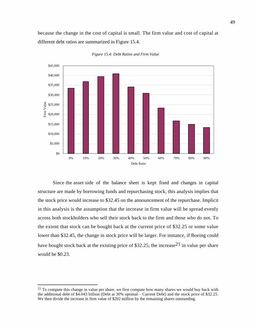
49

because the change in the cost of capital is small. The firm value and cost of capital at

different debt ratios are summarized in Figure 15.4.

Since the asset side of the balance sheet is kept fixed and changes in capital

structure are made by borrowing funds and repurchasing stock, this analysis implies that

the stock price would increase to $32.45 on the announcement of the repurchase. Implicit

in this analysis is the assumption that the increase in firm value will be spread evenly

across both stockholders who sell their stock back to the firm and those who do not. To

the extent that stock can be bought back at the current price of $32.25 or some value

lower than $32.45, the change in stock price will be larger. For instance, if Boeing could

have bought stock back at the existing price of $32.25, the increase21 in value per share

would be $0.23.

21 To compute this change in value per share, we first compute how many shares we would buy back withthe additional debt of $4.043 billion (Debt at 30% optimal – Current Debt) and the stock price of $32.25.We then divide the increase in firm value of $202 million by the remaining shares outstanding.

Figure 15.4: Debt Ratios and Firm Value

$0

$5,000

$10,000

$15,000

$20,000

$25,000

$30,000

$35,000

$40,000

$45,000

0% 10% 20% 30% 40% 50% 60% 70% 80% 90%

Debt Ratio

Firm

Val

ue

50

captstr.xls: This spreadsheet allows you to compute the optimal debt ratio firm value

for any firm, using the same information used for Boeing. It has updated interest coverage

ratios and default spreads built in.

Default Risk, Operating Income and Optimal Leverage

In the analysis we just completed on Boeing, we assumed that operating income

would remain constant while the debt ratios changed. While this assumption simplifies

our analysis substantially, it is not realistic. The operating income, for many firms, will

drop as the default risk increases; this, in fact, is the cost we labeled as an indirect

bankruptcy cost earlier in this chapter. The drop is likely to become more pronounced as

the default risk falls below an acceptable level; for instance, a bond rating below

investment grade may trigger significant losses in revenues and increases in expenses.

A general model for optimal capital structure would allow both operating income

and cost of capital to change as the debt ratio changes. We have already described how we

can estimate cost of capital at different debt ratios, but we could also attempt to do the

same with operating income. For instance, we could estimate how the operating income

for the Boeing would change as debt ratios and default risk changes by looking at the

effects of rating downgrades on the operating income of other retailers.

If both operating income and cost of capital change, the optimal debt ratio may no

longer be the point at which the cost of capital is minimized. Instead, the optimal has to

be defined as that debt ratio at which the value of the firm is maximized.

APV and Financial Leverage

In the adjusted present value (APV) approach, we begin with the value of the firm

without debt. As we add debt to the firm, we consider the net effect on value by

considering both the benefits and the costs of borrowing. The value of the levered firm can

Change in stock price = shareper $0.23

32.25

4043-1010.7

million $202 =

51

then be estimated at different levels of the debt and the debt level that maximizes firm

value is the optimal debt ratio.

Steps in the Adjusted Present Value approach

The unlevered firm value is not a function of expected leverage and can be

estimated as described in the earlier section – by discounting the free cash flows to the

firm at the unlevered cost of equity. In fact, if you do not want to estimate this value and

take the market value of the firm as correct, you could back out the unlevered firm value

by subtracting out the tax benefits and adding back the expected bankruptcy cost from the

existing debt.

Current Firm Value = Value of Unlevered firm + PV of tax benefits – Expected

Bankruptcy cost

Value of Unlevered firm = Current Firm Value – PV of tax benefits + Expected

Bankruptcy costs

The only components that change as a firm changes its leverage are the expected

tax benefits and the expected bankruptcy costs. To obtain these values as you change

leverage, you would go through the following steps.

1. Estimate the dollar debt outstanding at each debt ratio. This process mirrors what

was done in the cost of capital approach. Keeping firm value fixed, we consider

how much debt the firm will have at 20% debt, 30% debt and so on.

2. Estimate the tax benefits of debt by multiplying the dollar debt by the tax rate.

This essentially assumes that the debt is permanent and that the tax benefits will

continue in perpetuity.

3. Estimate the rating, interest rate and interest expense at each debt ratio. This

process again replicates what was done in the cost of capital approach.

4. Use the rating to estimate a probability of default. Note that Table 15.8 provides

these probabilities for each rating.

5. Estimate the expected bankruptcy cost by multiplying the probability of

bankruptcy by the cost of bankruptcy, stated as a percent of unlevered firm value.

We compute the value of the levered firm at different levels of debt. The debt level that

maximizes the value of the levered firm is the optimal debt ratio.

52

Illustration 15.8: Using the Adjusted Present Value Approach to calculate Optimal Debt

Ratio for Boeing in 1999.

This approach can be applied to estimating the optimal capital structure for

Boeing. The first step is to estimate the value of the unlevered firm. To do so, we start

with the firm value of Boeing in 1999 and net the effect of the tax savings and bankruptcy

costs arising from the existing debt.

Value of Boeing in 1999 = Value of Equity + Value of Debt = $32,595+$8,194 = $40,789

We compute the present value of the tax savings from the existing debt, assuming that the

interest payments on the debt constitute a perpetuity.

PV of Tax Savings from Existing Debt = Existing Debt * Tax Rate

= $8,194 * 0.35 = $ 2,868 million

Based upon Boeing’s current rating of AA, we estimate a probability of bankruptcy of

0.28% from Table 15.8. The bankruptcy cost is assumed to be 30% of the unlevered firm

value.22 The cost is high because the perception of default risk is likely to be very

damaging for a firm like Boeing, whose customers depend upon it for long-term service

and support, and whose sales contracts are often spread out over a decade or more.

PV of Expected Bankruptcy Cost = Probability of Default * Bankruptcy cost

= 0.28% * (30% * (40,789-2,868)) = $ 32

We then compute the value of Boeing as an unlevered firm.

Value of Boeing as an Unlevered Firm

= Current Market Value – PV of Tax Savings + Expected Bankruptcy Costs

= $ 40,789 - $ 2,868 + $ 32

= $ 37,953 million

The next step in the process is to estimate the tax savings at different levels of

debt in Table 15.18. While we use the standard approach of assuming that the present

value is calculated over a perpetuity, we reduce the tax rate used in the calculation if

interest expenses exceed the earnings before interest and taxes. The adjustment to the tax

rate was described more fully earlier in the cost of capital approach.

22 This estimate is based upon the Warner study, which estimates bankruptcy costs for large companies tobe 10% of the value and upon the qualitative analysis of indirect bankruptcy costs in Shapiro and Cornell.

53

Table 15.18: Tax Savings From Debt (tcD): Boeing

Debt Ratio $ Debt Tax Rate Tax Benefits

0% $0 35.00% $0

10% $4,079 35.00% $1,428

20% $8,158 35.00% $2,855

30% $12,237 35.00% $4,283

40% $16,316 35.00% $5,710

50% $20,394 30.05% $6,128

60% $24,473 22.76% $5,571

70% $28,552 17.17% $4,903

80% $32,631 15.02% $4,903

90% $36,710 13.36% $4,903

The final step in the process is to estimate the expected bankruptcy cost, based upon the

bond ratings, the probabilities of default and the assumption that the bankruptcy cost is

30% of firm value. Table 15.19 summarizes these probabilities and the expected

bankruptcy cost, computed based on the unlevered firm value.

Table 15.19: Expected Bankruptcy Cost, Boeing

Debt Ratio Bond Rating Probability of Default Expected Bankruptcy Cost

0% AA 0.28% $32

10% AA 0.28% $32

20% A- 1.41% $161

30% BB 12.20% $1,389

40% CCC 50.00% $5,693

50% CCC 50.00% $5,693

60% CC 65.00% $7,401

70% C 80.00% $9,109

80% C 80.00% $9,109

90% C 80.00% $9,109

54

The value of the levered firm is estimated in Table 15.20 by aggregating the effects of the

tax savings and the expected bankruptcy costs.

Table 15.20: Value of Boeing with Leverage

Debt Ratio Unlevered Firm

Value

Tax Benefits Expected

Bankruptcy Cost

Value of Levered

Firm

0% $37,953 $0 $32 $37,921

10% $37,953 $1,428 $32 $39,349

20% $37,953 $2,855 $161 $40,648

30% $37,953 $4,283 $1,389 $40,847

40% $37,953 $5,710 $5,693 $37,970

50% $37,953 $6,128 $5,693 $38,388

60% $37,953 $5,571 $7,401 $36,123

70% $37,953 $4,903 $9,109 $33,747

80% $37,953 $4,903 $9,109 $33,747

90% $37,953 $4,903 $9,109 $33,747

The firm value is optimized at between 20% and 30% debt, which is consistent with the

results of the other approaches. These results are, however, very sensitive to both the

estimate of bankruptcy cost as a percent of firm value and the probabilities of default.

apv.xls: This spreadsheet allows you to compute the value of a firm, with leverage,

using the adjusted present value approach.

Benefits and Limitations of the Adjusted Present Value Approach

The advantage of this approach is that it separates the effects of debt into

different components and allows the analyst to use different discount rates for each

component. In this method, we do not assume that the debt ratio stays unchanged

forever, which is an implicit assumption in the cost of capital approach. [NOTE: This is

not true. In the CoC approach, I could adjust the debt ratio at any stage (year). The

cumulative discount rate will be messy though.] Instead, we have the flexibility to keep

the dollar value of debt fixed and to calculate the benefits and costs of the fixed dollar

debt.

55

These advantages have to be weighed against the difficulty of estimating

probabilities of default and the cost of bankruptcy. In fact, many analyses that use the

adjusted present value approach ignore the expected bankruptcy costs leading them to the

conclusion that firm value increases as firms borrow money. Not surprisingly, they

conclude that the optimal debt ratio for a firm is 100% debt.

In general, with the same assumptions, the APV and the Cost of Capital

conclusions give identical answers. However, the APV approach is more practical when

firms are evaluating a dollar amount of debt, while the cost of capital approach is easier

when firms are analyzing debt proportions.23

Valuing the pieces rather than the whole

In the adjusted present value model, we value debt separately from the operating

assets and firm value is the sum of the two components. In fact, one of the strongest

benefits of discounted cash flow valuation is that breaking up cash flows into individual

components and valuing them separately should not change the value. Thus, you could

value a firm like General Electric by valuing each of its divisions separately and adding

them up or Coca Cola by valuing its operations in each country separately and summing

those up.

The advantage of piece-wise valuation is that you can estimate cash flows and

discount rates separately for each piece and thus get more precise estimates of value. For

example, you would use very different assumptions about operating margins,

reinvestment needs and costs of capital when valuing the appliance and aircraft engine

divisions of GE. Similarly, you could apply different country risk premiums for each

country that Coca Cola operates in to value the firm. Since this is always the case, you

might wonder why we do not do this for all firms. The problem is with the information.

Many firms do not break down their earnings and cash flows in sufficient detail to allow

for piece-wise valuation. Even firms that do, like GE, they often have large centralized

expenses that get allocated, often arbitrarily, to individual divisions.

23 See Inselbag and Kaufold (1997).

56

The benefits of breaking a firm down into pieces clearly increase as a firm becomes

more diverse in its operations. These benefits have to be weighed off against the costs

associated with more imprecise information and greater estimation problems.

Conclusion

This chapter develops an alternative approach to discounted cashflow valuation.

The cashflows to the firm are discounted at the weighted average cost of capital to obtain

the value of the firm, which when reduced by the market value of outstanding debt, yields

the value of equity. Since the cashflow to the firm is a cashflow prior to debt payments,

this approach is more straightforward to use when there is significant leverage or when

leverage changes over time, though the weighted average cost of capital, used to discount

free cashflows to the firm, has to be adjusted for changes in leverage. Finally, the costs of

capital can be estimated at different debt ratios and used to estimate the optimal debt ratio

for a firm.

The alternative approach to firm valuation is the APV approach, where we add

the effect on value of debt (tax benefits – bankruptcy costs) to the unlevered firm value.

This approach can also be used to estimate the optimal debt ratio for the firm.

57

Problems

1. Respond true or false to the following statements about the free cash flow to the firm.

A. The free cash flow to the firm is always higher than the free cash flow to equity.

B. The free cash flow to the firm is the cumulated cash flow to all investors in the firm,

though the form of their claims may be different.

C. The free cash flow to the firm is a pre-debt, pre-tax cash flow.

D. The free cash flow to the firm is an after-debt, after-tax cash flow.

E. The free cash flow to the firm cannot be estimated without knowing interest and

principal payments, for a firm with debt.

2. Union Pacific Railroad reported net income of $770 million in 1993, after interest

expenses of $320 million. (The corporate tax rate was 36%.) It reported depreciation of

$960 million in that year, and capital spending was $1.2 billion. The firm also had $4

billion in debt outstanding on the books, rated AA (carrying a yield to maturity of 8%),

trading at par (up from $3.8 billion at the end of 1992). The beta of the stock is 1.05, and

there were 200 million shares outstanding (trading at $60 per share), with a book value of

$5 billion. Union Pacific paid 40% of its earnings as dividends and working capital

requirements are negligible. (The treasury bond rate is 7%.)

a. Estimate the free cash flow to the firm in 1993.

b. Estimate the value of the firm at the end of 1993.

c. Estimate the value of equity at the end of 1993 and the value per share, using the

FCFF approach.

3. Lockheed Corporation, one of the largest defense contractors in the US, reported

EBITDA of $1290 million in 1993, prior to interest expenses of $215 million and

depreciation charges of $400 million. Capital Expenditures in 1993 amounted to $450

million and working capital was 7% of revenues (which were $13,500 million). The firm

had debt outstanding of $3.068 billion (in book value terms), trading at a market value of

$3.2 billion and yielding a pre-tax interest rate of 8%. There were 62 million shares

outstanding trading at $64 per share and the most recent beta is 1.10. The tax rate for the

firm is 40%. (The treasury bond rate is 7%.)

The firm expects revenues, earnings, capital expenditures and depreciation to grow

at 9.5% a year from 1994 to 1998, after which the growth rate is expected to drop to 4%.

(Capital spending will offset depreciation in the steady state period.) The company also

plans to lower its debt/equity ratio to 50% for the steady state (which will result in the

pre-tax interest rate dropping to 7.5%).

a. Estimate the value of the firm.

58

b. Estimate the value of the equity in the firm, and the value per share.

4. In the face of disappointing earnings results and increasingly assertive institutional

stockholders, Eastman Kodak was considering a major restructuring in 1993. As part of

this restructuring, it was considering the sale of its health division, which earned $560

million in earnings before interest and taxes in 1993, on revenues of $5.285 billion. The

expected growth in earnings was expected to moderate to 6% between 1994 and 1998, and

to 4% after that. Capital expenditures in the health division amounted to $420 million in

1993, while depreciation was $350 million. Both are expected to grow 4% a year in the

long term. Working capital requirements are negligible.

The average beta of firms competing with Eastman Kodak's health division is

1.15. While Eastman Kodak has a debt ratio (D/(D+E)) of 50%, the health division can

sustain a debt ratio (D/(D+E)) of only 20%, which is similar to the average debt ratio of

firms competing in the health sector. At this level of debt, the health division can expect

to pay 7.5% on its debt, before taxes. (The tax rate is 40% and the treasury bond rate is

7%.)

a. Estimate the cost of capital for the division.

b. Estimate the value of the division.

c. Why might an acquirer pay more than this estimated value for the division?

5. You are analyzing a valuation done on a stable firm by a well-known analyst. Based

upon the expected free cash flow to firm, next year, of $30 million and an expected

growth rate of 5%. The analyst has estimated a value of $750 million. However, he has

made the mistake of using the book values of debt and equity in his calculation. While you

do not know the book value weights he used, you know that the firm has a cost of equity

of 12% and an after-tax cost of debt of 6%. You also know that the market value of

equity is three times the book value of equity, while the market value of debt is equal to

the book value of debt. Estimate the correct value for the firm.

6. Santa Fe Pacific, a major rail operator with diversified operations, had earnings before

interest, taxes and depreciation, of $637 million in 1993, with depreciation amounting to

$235 million (offset by capital expenditure of an equivalent amount). The firm is in

steady state and expected to grow 6% a year in perpetuity. Santa Fe Pacific had a beta of

1.25 in 1993 and debt outstanding of $1.34 billion. The stock price was $18.25 at the end

of 1993, and there were 183.1 million shares outstanding. The expected ratings and the

costs of debt at different levels of debt for Santa Fe are shown in the following table (The

treasury bond rate is 7% and the firm faced a tax rate of 40%.).

D/(D+E) Rating Cost of Debt (Pre-tax)

59

0% AAA 6.23%

10% AAA 6.23%

20% A+ 6.93%

30% A- 7.43%

40% BB 8.43%

50% B+ 8.93%

60% B- 10.93%

70% CCC 11.93%

80% CCC 11.93%

90% CC 13.43%

The earnings before interest and taxes are expected to grow 3% a year in perpetuity with

capital expenditures offset by depreciation. (The tax rate is 40%, the treasury bond rate

is 7% and the market risk premium is 5.5%.)

a. Estimate the cost of capital at the current debt ratio.

b. Estimate the costs of capital at debt ratios ranging from 0% to 90%.

c. Estimate the value of the firm at debt ratios ranging from 0% to 90%.

1

CHAPTER 16

ESTIMATING EQUITY VALUE PER SHARE

In Chapter 15, we considered how best to estimate the value of the operating

assets of the firm. To get from that value to the firm value, you have to consider cash,

marketable securities and other non-operating assets held by a firm. In particular, you

have to value holdings in other firms and deal with a variety of accounting techniques used

to record such holdings. To get from firm value to equity value, you have to determine

what should be subtracted out from firm value – i.e, the value of the non-equity claims in

the firm.

Once you have valued the equity in a firm, it may appear to be a relatively simple

exercise to estimate the value per share. All it seems you need to do is divide the value of

the equity by the number of shares outstanding. But, in the case of some firms, even this

simple exercise can become complicated by the presence of management and employee

options. In this chapter, we will measure the magnitude of this option overhang on

valuation and then consider ways of incorporating the effect into the value per share.

The Value of Non-operating Assets

Firms have a number of assets on their books that can be categorized as non-

operating assets. The first and obvious one is cash and near-cash investments –

investments in riskless or very low-risk investments that most companies with large cash

balances make. The second is investments in equities and bonds of other firms, sometimes

for investment reasons and sometimes for strategic ones. The third is holdings in other

firms, private and public, which are categorized in a variety of ways by accountants.

Finally, there are assets that firms own that do not generate cash flows but nevertheless

could have value – for instance undeveloped land in New York or Tokyo.

Cash and Near Cash Investments

Investments in short-term government securities or commercial paper, which can

be converted into cash quickly and with very low cost, are considered near-cash

investments. In this section, we will consider how best to deal with these investments in

valuation.

2

Operating Cash Requirements

If a firm needs cash for its operations – an operating cash balance – you should

consider such cash part of working capital requirements rather than as a source of

additional value. Any cash and near-cash investments that exceed the operating cash

requirements can be then added on to the value of operating assets. How much cash does

a firm need for its operations? The answer depends upon both the firm and the economy

in which the firm operates. A small retail firm in an emerging market, where cash

transactions are more common than credit card transactions, may require an operating

cash balance that is substantial. In contrast, a manufacturing firm in a developed market

may not need any operating cash. In fact, if the cash held by a firm is interest-bearing and

the interest earned on the cash reflects a fair rate of return1, you would not consider that

cash to be part of working capital. Instead, you would add it to the value of operating

assets to value the firm.

Dealing with Non-operating Cash holdings

There are two ways in which we can deal with cash and marketable securities in

valuation. One is to lump them in with the operating assets and value the firm (or equity)

as a whole. The other is to value the operating assets and the cash and marketable

securities separately.

Consolidated Valuation

Is it possible to consider cash as part of the total assets of the firm and to value it

on a consolidated basis? The answer is yes and it is, in a sense, what we do when we

forecast the total net income for a firm and estimate dividends and free cash flows to

equity from those forecasts. The net income will then include income from investments in

government securities, corporate bonds and equity investments2. While this approach has

the advantage of simplicity and can be used when financial investments comprise a small

1 Note that if the cash is invested in riskless assets such as treasury bills, the riskless rate is a fair rate ofreturn.2 Thus, if cash represents 10% of the firm value, the unlevered beta used will be a weighted average of thebeta of the operating assets and the beta of cash (which is zero).

3

percent of the total assets, it becomes much more difficult to use when financial

investments represent a larger proportion of total assets for two reasons.

• The cost of equity or capital used to discount the cash flows has to be adjusted on an

ongoing basis for the cash. In specific terms, you would need to use an unlevered beta

that represents a weighted average of the unlevered beta for the operating assets of the

firm and the unlevered beta for the cash and marketable securities. For instance, the

unlevered beta for a steel company where cash represents 10% of the value would be

a weighted average of the unlevered beta for steel companies and the beta of cash

(which is usually zero). If the 10% were invested in riskier securities, you would need

to adjust the beta accordingly. While this can be done if you use bottom-up betas, you

can see that it would be much more difficult to do if you obtain a beta from a

regression.3

• As the firm grows, the proportion of income that is derived from operating assets is

likely to change. When this occurs, you have to adjust the inputs to the valuation

model – cash flows, growth rates and discount rates – to maintain consistency.

What will happen if you do not make these adjustments? You will tend to misvalue the

financial assets. To see why, assume that you were valuing the steel company described

above, with 10% of its value coming from cash. This cash is invested in government

securities and earns an appropriate rate – say 5%. If this income is added on to the other

income of the firm and discounted back at a cost of equity appropriate for a steel

company – say 11% - the value of the cash will be discounted. A billion dollars in cash

will be valued at $800 million, for instance, because the discount rate used is incorrect.

Separate Valuation

It is safer to separate cash and marketable securities from operating assets and to

value them individually. We do this almost always when we use the firm valuation

approaches described in the last chapter. This is because we use operating income to

estimate free cash flows to the firm and operating income generally does not include

3 The unlevered beta that you can back out of a regression beta reflects the average cash balance (as apercent of firm value) over the period of the regression. Thus, if a firm maintains this ratio at a constantlevel, you might be able to arrive at the correct unlevered beta.

4

income from financial assets. If, however, this is not the case and some of the investment

income has found its way into the operating income, you would need to back it out before

you did the valuation. Once you value the operating assets, you can add the value of the

cash and marketable securities to it to arrive at firm value.

Can this be done with the FCFE valuation models described in Chapter 14? While

net income includes income from financial assets, we can still separate cash and

marketable securities from operating assets, if we wanted to. To do this, we would first

back out the portion of the net income that represents the income from financial

investments (interest on bonds, dividends on stock) and use this adjusted net income to

estimate free cash flows to equity. These free cash flows to equity would be discounted

back using a cost of equity that would be estimated using a beta that reflected only the

operating assets. Once the equity in the operating assets has been valued, you could add

the value of cash and marketable securities to it to estimate the total value of equity.

Illustration 16.1: Consolidated versus Separate Valuation

To examine the effects of a cash balance on firm value, consider a firm with

investments of $1,200 million in non-cash operating assets and $200 million in cash. For

simplicity, let us assume the following.

• The non-cash operating assets have a beta of 1.00 and are expected to earn $120

million in net income each year in perpetuity and there are no reinvestment needs.

• The cash is invested at the riskless rate, which we assume to be 4.5%.

• The market risk premium is assumed to be 5.5%

Under these conditions, we can value the equity, using both the consolidated and separate

approaches.

Let us first consider the consolidated approach. Here, we will estimate a cost of

equity for all of the assets (including cash) by computing a weighted average beta of the

non-cash operating and cash assets.

Beta of the firm = BetaNon-cash assets( ) Weight Non-cash assets( ) + BetaCash assets( ) Weight Cash assets( )

= 1.00( ) 1200

1400

+ 0.00( ) 200

1400

= 0.8571

Cost of Equity for the firm = 4.5% + 0.8571 (5.5%) = 9.21%

5

Expected Earnings for the firm

needs)nt reinvestme no are theresince FCFE thealso is(which million 129

200)* .0450(120

cash from incomeInterest assets operating from IncomeNet

=+=

+=

Value of the equity

million $14000.0921

129

equity ofCost

FCFE

=

=

=

The equity is worth $1,400 million.

Now, let us try to value them separately, beginning with the non-cash

investments.

Cost of Equity for non-cash investments ( ) %105.5%1.004.5%

PremiumRisk *Betarate Riskless

=+=+=

Expected earnings from operating assets = $120 million (which is the FCFE from these

assets)

Value of non-cash assets

million $1,2000.10

120

assetscash -nonfor Equity ofCost

Earnings Expected

=

=

=

To this, we can add the value of the cash, which is $ 200 million, to get a value for the

equity of $1,400 million.

To see the potential for problems with the consolidated approach, note that if you

had discounted the total FCFE of $129 million at the cost of equity of 10% (which

reflects only the operating assets) you would valued the firm at $1,290 million. The loss

in value of $110 million can be traced to the mishandling of cash.

Interest income from cash = 4.5% *200 = $ 9 million

If you discount the cash at 10%, you would value the cash at $90 million instead of the

correct value of $200 million – hence the loss in value of $ 110 million.

Should you ever discount cash?

6

In the illustration above, cash was reduced in value for the wrong reason – a

riskless cash flow was discounted at a discount rate that reflects risky investments.

However, there two conditions under which you might legitimately apply a discount to a

cash balance.

1. The cash held by a firm is invested at a rate that is lower than the market rate, given

the riskiness of the investment

2. The management is not trusted with the large cash balance because of its past track

record on investments.

1. Cash Invested at below-market Rates

The first and most obvious condition occurs when much or all the cash balance

does not earn a market interest rate. If this is the case, holding too much cash will clearly

reduce the firm’s value. While most firms in the United States can invest in government

bills and bonds with ease today, the options are much more limited for small businesses

and for firms outside the United States. When this is the case, a large cash balance earning

less than a fair return can destroy value over time.

Illustration 16.2: Cash Invested at below market rates

In Illustration 16.1, we assumed that cash was invested at the riskless rate.

Assume, instead, that the firm was able to earn only 3% on its cash balance, while the

riskless rate is 4.5%. The estimated value of the cash kept in the firm would then be

Estimated value of cash invested at 3% ( )( )

133.330.045

200.030 ==

The value of cash that is invested at a lower rate is $133.33 million. In this scenario, if the

cash is returned to stockholders, it would yield them a surplus value of $66.67 million. In

fact, liquidating any asset that has a return less than the required return would yield the

same result, as long as the entire investment can be recovered on liquidation4.

2. Distrust of Management:

4 While this assumption is straight forward with cash, it is less so with real assets, where the liquidationvalue may reflect the poor earning power of the asset. Thus, the potential surplus from liquidation may notbe as easily claimed.

7

While making a large investment in low-risk or no-risk marketable securities by

itself is value neutral, the burgeoning cash balance can tempt managers to accept large

investments or make acquisitions even if these investments earn sub-standard returns. In

some cases, these actions may be taken to prevent the firm from becoming a takeover

target5. To the extent that stockholders anticipate such sub-standard investments, the

current value of the firm may reflect the cash at a discounted level. The discount is likely

to be largest at firms with few investment opportunities and poor management and there

may be no discount at all in firms with significant investment opportunities and good

management.

Illustration 16.3: Discount for Poor Investments in the Future

Return now to the firm described in Illustration 16.1, where the cash is invested at

the riskless rate of 4.5%. Normally, we would expect this firm to trade at a total value of

$1,400 million. Assume, however, that the managers of this firm have a history of poor

acquisitions and that the presence of a large cash balance increases the probability from

0% to 30% that the management will try to acquire another firm. Further, assume that the

market anticipates that they will overpay by $50 million on this acquisition. The cash

will then be valued at $185 million.

Estimated Discount on Cash Balance

( ) ( )( )( )( )

million 15$

million 50$3.0

tOverpaymenExpectedyProbabilit nacquisitionacquisitio

==

∆=

Value of Cash = Cash Balance – Estimated Discount = $ 200 million - $ 15 million

= $ 185 million

The two factors that determine this discount – the incremental likelihood of a poor

investment and the expected net present value of the investment – are likely to be based

upon investors’ assessments of management quality.

Investments in Risky Securities

5 Firms with large cash balances are attractive targets, since the cash balance reduces the cost of making theacquisition.

8

So far in this chapter, we have looked at how much firms should hold in the form

of cash and near-cash investments. In some cases, firms invest in risky securities, which

can range from investment-grade bonds to high-yield bonds to publicly traded equity in

other firms. In this section, we examine the motivation, consequences and accounting for

such investments.

Reasons for holding risky securities

Why do firms invest in risky securities? Some firms do so for the allure of the

higher returns they can expect to make investing in stocks and corporate bonds, relative to

treasury bills. In recent years, there has also been a trend for firms to take equity

positions in other firms to further their strategic interests. Still other firms take equity

positions in firms they view as under valued by the market. And finally, investing in

risky securities is part of doing business for banks, insurance companies and other

financial service companies.

To make a higher return

Near-cash investments such as treasury bills and commercial paper are liquid and

have little or no risk, but they also earn low returns. When firms have substantial amounts

invested in marketable securities, they can expect to earn considerably higher returns by

investing in riskier securities. For instance, investing in corporate bonds will yield a higher

interest rate than investing in treasury bonds and the rate will increase with the riskiness

of the investment. Investing in stocks will provide an even higher expected return, though

not necessarily a higher actual return, than investing in corporate bonds. Figure 16.1

summarizes returns on risky investments – corporate bonds, high-yield bonds and

equities – and compares them to the returns on near-cash investments between 1989-98.

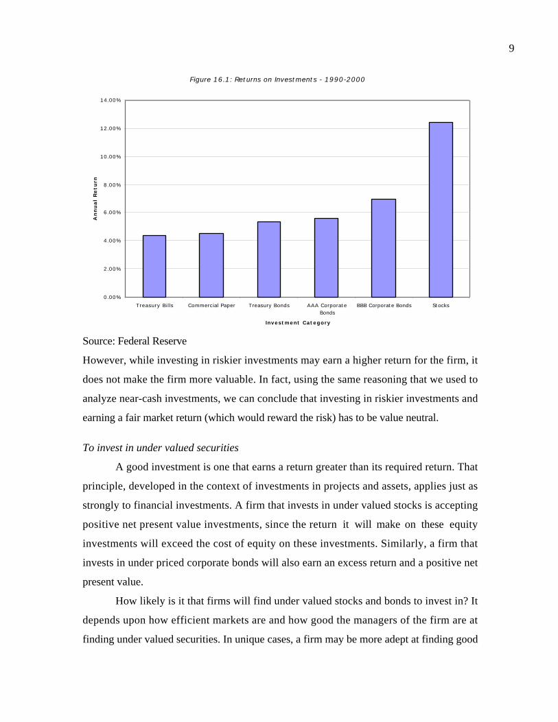
9

Source: Federal Reserve

However, while investing in riskier investments may earn a higher return for the firm, it

does not make the firm more valuable. In fact, using the same reasoning that we used to

analyze near-cash investments, we can conclude that investing in riskier investments and

earning a fair market return (which would reward the risk) has to be value neutral.

To invest in under valued securities

A good investment is one that earns a return greater than its required return. That

principle, developed in the context of investments in projects and assets, applies just as

strongly to financial investments. A firm that invests in under valued stocks is accepting

positive net present value investments, since the return it will make on these equity

investments will exceed the cost of equity on these investments. Similarly, a firm that

invests in under priced corporate bonds will also earn an excess return and a positive net

present value.

How likely is it that firms will find under valued stocks and bonds to invest in? It

depends upon how efficient markets are and how good the managers of the firm are at

finding under valued securities. In unique cases, a firm may be more adept at finding good

Figure 16.1: Returns on Investments - 1990-2000

0.00%

2.00%

4.00%

6.00%

8.00%

10.00%

12.00%

14.00%

Treasury Bills Commercial Paper Treasury Bonds AAA CorporateBonds

BBB Corporate Bonds Stocks

Investment Category

Annual Retu

rn

10

investments in financial markets than it is at competing in product markets. Consider the

case of Berkshire Hathaway, a firm which has been a vehicle for Warren Buffet’s

investing acumen over the last few decades. At the end of the second quarter of 1999,

Berkshire Hathaway had $69 billion invested in securities of other firms. Among its

holdings were investments of $12.4 billion in Coca Cola, $6.6 billion in American Express

and $3.9 billion in Gillette. While Berkshire Hathaway also has real business interests,

including ownership of a well regarded insurance company (GEICO), investors in the firm

get a significant portion of their value from the firm’s passive equity investments.

Notwithstanding Berkshire Hathaway’s success, most firms in the United States

steer away from looking for bargains among financial investments. Part of the reason for

this is their realization that it is difficult to find under valued securities in financial

markets. Part of the reluctance on the part of firms to make investments can be traced to a

recognition that investors in firms like Proctor and Gamble and Coca Cola invest in them

because of these firms’ competitive advantages in product markets (brand name,

marketing skills, etc.) and not for their perceived skill at picking stocks.

Strategic Investments

During the 1990s, Microsoft accumulated a huge cash balance in excess of $20

billion. It used this cash to make a series of investments in the equity of software,

entertainment and internet related firms. It did so for several reasons6. First, it gave

Microsoft a say in the products and services these firms were developing and pre-empted

competitors from forming partnerships with the firms. Second, it allowed Microsoft to

work on joint products with these firms. In 1998 alone, Microsoft announced

investments in 14 firms including ShareWave, General Magic, RoadRunner and Qwest

Communications. In an earlier investment in 1995, Microsoft invested in NBC to create

the MSNBC network to give it a foothold in the television and entertainment business.

6 One of Microsoft’s oddest investments was in one of its primary competitors, Apple Computer, early in1998. The investment may have been intended to fight the anti-trust suit brought against Microsoft by theJustice Department.

11

Can strategic investments be value enhancing? As with all investments, it depends

upon how much is invested and what the firm receives as benefits in return. If the side-

benefits and synergies that are touted in these investments exist, investing in the equity of

other firms can earn much higher returns than the hurdle rate and create value. It is clearly

a much cheaper option than acquiring the entire equity of the firm.

Business Investments

Some firms hold marketable securities not as discretionary investments, but

because of the nature of their business. For instance, insurance companies and banks often

invest in marketable securities in the course of their business, the former to cover

expected liabilities on insurance claims and the latter in the course of trading. While these

financial service firms have financial assets of substantial value on their balance sheets,

these holdings are not comparable to those of the firms described so far. In fact, they are

more akin to the raw material used by manufacturing firms than to discretionary financial

investments.

Dealing with marketable securities in valuation

Marketable securities can include corporate bonds, with default risk embedded in

them, and traded equities, which have even more risk associated with them. As the

marketable securities held by a firm become more risky, the choices on how to deal with

them become more complex. You have three ways of accounting for marketable securities.

1. The simplest and most direct approach is to estimate the current market value of

these marketable securities and add the value on to the value of operating assets.

For firms valued on a going-concern basis, with a large number of holdings of

marketable securities, this may be the only practical option.

2. The second approach is to estimate the current market value of the marketable

securities and net out the effect of capital gains taxes that may be due if those

securities were sold today. [NOTE: I removed this sentence because the structure

is very confusing and I think everyone knows what is capital gain tax.] This is the

best way of estimating value when valuing a firm on a liquidation basis.

3. The third and most difficult way of incorporating the value of marketable

securities into firm value is to value the firms that issued these securities and

12

estimate the value of these securities. This approach tends to work best for firms

that have relatively few, but large, holdings in other publicly traded firms.

Illustration 16.4: Microsoft’s cash and marketable securities

Over the last decade, Microsoft has accumulated a huge cash balance, largely as a

consequence of holding back on free cash flows to equity that could have been paid to

stockholders. In June 2000, for instance, the firm reported the following holdings of near-

cash investments:

Table 16.1: Cash and Near-cash Investments: Microsoft

1999 2000

Cash and equivalents:Cash $635 $849Commercial paper $3,805 $1,986Certificates of deposit $522 $1,017U.S. government and agency securities $0 $729Corporate notes and bonds $0 $265Money market preferreds $13 $0Cash and equivalents $4,975 $4,846Short-term investments:Commercial paper $1,026 $612U.S. government and agency securities $3,592 $7,104Corporate notes and bonds $6,996 $9,473Municipal securities $247 $1,113Certificates of deposit $400 $650Short-term investments $12,261 $18,952Cash and short-term investments $17,236 $23,798

When valuing Microsoft, we should clearly consider this $24 billion investment as part of

the firm’s value. The interesting question is whether there should be a discount, reflecting

investor’s fears about poor investments in the future. Over its life, Microsoft has not

been punished for holding on to cash, largely as a consequence of its impeccable track

record in both delivering ever-increasing profits on the one hand and high stock returns on

the other. The last two years have not been good ones for the firm, but investors will

probably give the firm the benefit of the doubt at least for the near future. We would add

the cash balance at face value to the value of Microsoft’s operating assets.

13

The more interesting component is the $17.7 billion in 2000 that Microsoft shows

as investments in riskier securities. Microsoft reports the following information about

these investments.

Table 16:2: Investments in Risky Securities and Investments

Unrealized Cost Basis Gains Losses Recorded Basis

Debt securities recorded at market: Within one year $498 $27 $0 $525Between 2 and 10 years $388 $11 -$3 $396Between 10 and 15 years $774 $14 -$93 $695Beyond 15 years $4,745 -$933 $3,812Debt securities recorded at market $6,406 $52 -$1,029 $5,429Equities Common stock and warrants $5,815 $5,655 -$1,697 $9,773Preferred stock $2,319 $2,319Other investments $205 $205Equity and other investments $14,745 $5,707 -$2,726 $17,726

Microsoft has generated a paper profit of almost $3 billion on its original cost of $14.745

billion and reports a current value of $17.726 billion. Most of these investments are

traded in the market and are recorded at market value. The easiest way to deal with these

investments is to add the market value on to the value of the operating assets of the firm

to arrive at firm value. The most volatile item is the investment in common stock of other

firms. The value of these holdings has almost doubled, as reflected in the recorded basis of

$9,773 million. Should we reflect this at current market value when we value Microsoft?

The answer is generally yes. However, if these investments are overvalued, we risk

building in this overvaluation into the valuation. The alternative is to value each of the

equities that the firm has invested in, using a discounted cash flow model, but this will

become increasingly cumbersome as the number of equity holdings increases.

In summary, then, you would add the values of both the near-cash investments of

$23.798 billion and the equity investments of $17,726 billion to the value of the operating

assets of Microsoft.

Premiums or Discounts on Marketable Securities?

14

As a general rule, you should not attach a premium or discount for marketable

securities. Thus, you would add the entire value of $17,726 million to the value of

Microsoft. There is an exception to this rule, though, and it relates to firms that make it

their business to buy and sell financial These are the closed-end mutual funds, of which

there are several hundred listed on the US stock exchanges, and investment companies,

such as Fidelity and T. Rowe Price. Closed-end mutual funds sell shares to investors and

use the funds to invest in financial assets. The number of shares in a closed-end fund

remains fixed and the share price changes. Since the investments of a closed-end fund are

in publicly traded securities, this sometimes creates a phenomenon where the market

value of the shares in a closed-end fund is greater than or less than the market value of the

securities owned by the fund. For these firms, it is appropriate to attach a discount or

premium to the marketable securities to reflect their capacity to generate excess returns on

these investments.

A closed-end mutual fund that consistently finds undervalued assets and delivers

much higher returns than expected (given the risk) should be valued at a premium on the

value of their marketable securities. The amount of the premium will depend upon how

large the excess return is and how long you would expect the firm to continue to make

these excess returns. Conversely, a closed-end fund that delivers returns that are much

lower than expected should trade at a discount on the value of the marketable securities.

The stockholders in this fund would clearly be better off if it were liquidated, but that

may not be a viable option.

Illustration 16.5: Valuing a closed-end fund

The Pierce Regan Asia fund is a closed-end fund with investments in traded Asian

stocks, valued at $4 billion at today’s market prices. The fund has earned a return of 13%

over the last 10 years, but based upon the riskiness of its investments and the

performance of the Asian market over the period, it should have earned 15%. Looking

forward, your expected return for the Asian market for the future is 12%, but you expect

the Pierce Regan fund to continue to under perform the market by 2%.

15

To estimate the discount from its net assets you would expect to see on the fund,

let us begin by assuming that the fund will continue in perpetuity and earning 2% less

than the return on the market index also in perpetuity.

Estimated discount

( )( )

( )( )

million 667$12.0

400012.010.0

market on thereturn Expected

Value FundReturn Excess

−=

−=

=

On a percent basis, the discount represents 16.67% of the market value of the

investments. [NOTE: There is a short cut: % discount = %67.1612.0

12.010.0 −=−]

If you assume that the fund will either be liquidated or begin earning the expected

return at a point in the future – say 10 years from now – the expected discount will

become smaller.

Holdings in Other Firms

In this category, you consider a broader category of non-operating assets, where

you look at holdings in other companies, public as well as private. You begin by looking

at the differences in accounting treatment of different holdings and how this treatment can

affect the way they are reported in financial statements.

Accounting Treatment

The way in which these assets are valued depends upon the way the investment is

categorized and the motive behind the investment. In general, an investment in the

securities of another firm can be categorized as a minority, passive investment; a

minority, active investment; or a majority, active investment, and the accounting rules

vary depending upon the categorization.

Minority, Passive Investments

If the securities or assets owned in another firm represent less than 20% of the

overall ownership of that firm, an investment is treated as a minority, passive investment.

These investments have an acquisition value, which represents what the firm originally

paid for the securities, and often a market value. Accounting principles require that these

assets be sub-categorized into one of three groups - investments that will be held to

16

maturity, investments that are available for sale and trading investments. The valuation

principles vary for each.

• For investments that will be held to maturity, the valuation is at historical cost or

book value and interest or dividends from this investment are shown in the income

statement.

• For investments that are available for sale, the valuation is at market value, but the

unrealized gains or losses are shown as part of the equity in the balance sheet and not

in the income statement. Thus, unrealized losses reduce the book value of the equity

in the firm and unrealized gains increase the book value of equity.

• For trading investments, the valuation is at market value and the unrealized gains and

losses are shown in the income statement.

Firms are allowed an element of discretion in the way they classify investments and,

subsequently, in the way they value these assets. This classification ensures that firms

such as investment banks, whose assets are primarily securities held in other firms for

purposes of trading, revalue the bulk of these assets at market levels each period. This is

called marking-to-market and provides one of the few instances in which market value

trumps book value in accounting statements.

Minority, Active Investments

If the securities or assets owned in another firm represent between 20% and 50%

of the overall ownership of that firm, an investment is treated as a minority, active

investment. While these investments have an initial acquisition value, a proportional share

(based upon ownership proportion) of the net income and losses made by the firm in

which the investment was made is used to adjust the acquisition cost. In addition, the

dividends received from the investment reduce the acquisition cost. This approach to

valuing investments is called the equity approach.

The market value of these investments is not considered until the investment is

liquidated, at which point the gain or loss from the sale, relative to the adjusted

acquisition cost is shown as part of the earnings in that period.

17

Majority, Active Investments

If the securities or assets owned in another firm represent more than 50% of the

overall ownership of that firm, an investment is treated as a majority active investment7.

In this case, the investment is no longer shown as a financial investment but is instead

replaced by the assets and liabilities of the firm in which the investment was made. This

approach leads to a consolidation of the balance sheets of the two firms, where the assets

and liabilities of the two firms are merged and presented as one balance sheet. The share

of the firm that is owned by other investors is shown as a minority interest on the

liability side of the balance sheet. A similar consolidation occurs in the other financial

statements of the firm as well, with the statement of cash flows reflecting the cumulated

cash inflows and outflows of the combined firm. This is in contrast to the equity

approach, used for minority active investments, in which only the dividends received on

the investment are shown as a cash inflow in the cash flow statement.

Here again, the market value of this investment is not considered until the

ownership stake is liquidated. At that point, the difference between the market price and

the net value of the equity stake in the firm is treated as a gain or loss for the period.

Valuing Cross Holdings in other Firms

Given that the holdings in other firms can accounted for in three different ways,

how do you deal with each type of holding in valuation? The best way to deal with each

of them is exactly the same. You would value the equity in each holding separately and

estimate the value of the proportional holding. This would then be added on to the value

of the equity of the parent company. Thus, to value a firm with minority holdings in

three other firms, you would value the equity in each of these firms, take the percent

share of the equity in each and add it to the value of equity in the parent company.

When income statements are consolidated, you would first need to strip the

income, assets and debt of the subsidiary from the parent company’s financials before

you do any of the above. If you do not do so, you will double count the value of the

subsidiary.

18

Why, you might ask, do we not value the consolidated firm? You could, and in

some cases because of the absence of information, you might have to. The reason we

would suggest separate valuations is that the parent and the subsidiaries may have very

different characteristics – costs of capital, growth rates and reinvestment rates. Valuing

the combined firm under these circumstances may yield misleading results. There is

another reason. Once you have valued the consolidated firm, you will have to subtract out

the portion of the equity in the subsidiary that the parent company does not own. If you

have not valued the subsidiary separately, it is not clear how you would do this. Note

that the conventional practice of netting out the minority interest does not accomplish

this, because minority interest reflects book rather than market value.

As a firm’s holdings become more numerous, estimating the values of the holdings

will become more onerous. If the holdings are publicly traded, substituting in the market

values of the holdings for estimated value is an alternative worth exploring. While you risk

building into your valuation any mistakes the market might be making in valuing these

holdings, this approach is more time efficient.

Estimating the Value of Holdings in Private Companies

When a publicly traded firm has a cross holding in a private company, it is often

difficult to obtain information on the private company and to value it. Consequently,

you might have to make your best estimate of how much this holding is worth, with the

limited information that you have available. One way to do this is to estimate the multiple

of book value at which firms in the same business (as the private business in which you

have holdings) typically trade at and apply this multiple to the book value of the holding

in the private business. . Assume for instance that you are trying to estimate the value of

the holdings of a pharmaceutical firm in 5 privately held biotechnology firms, and that

these holdings collectively have a book value of $ 50 million. If biotechnology firms

typically trade at 10 times book value, the estimated market value of these holdings

would be $ 500 million.

7 Firms have evaded the requirements of consolidation by keeping their share of ownership in other firmsbelow 50%.

19

In fact, this approach can be generalized to estimate the value of complex

holdings, where you lack the information to estimate the value for each holding or if there

are too many such holdings. For example, you could be valuing a Japanese firm with

dozens of cross holdings. You could estimate a value for the cross holdings by applying a

multiple of book value to their cumulative book value.

Illustration 16.6: Valuing Holdings in other company

Segovia Entertainment is an entertainment firm that operates in a wide range of

entertainment businesses. The firm reported $300 million in operating income (EBIT) on

capital invested of $1,500 million in the current year; the total debt outstanding is $500

million. A portion of the operating income ($100 million), capital invested ($400 million)

and debt outstanding ($150 million) represent Segovia’s holdings in Seville Televison, a

television station owner. Segovia owns only 51% of Seville and Seville’s financials are

consolidated with Segovia.8 In addition, Segovia owns 15% of LatinWorks, a record and

CD company. These holdings have been categorized as minority passive investments and

the dividends from the investment are shown as part of Segovia’s net income but not as

part of its operating income. LatinWorks reported operating income of $75 million on

capital invested of $250 million in the current year; the firm has $ 100 million in debt

outstanding. We will assume the following:

• The cost of capital for Segovia Entertainment, without considering either its

holdings in either Seville or LatinWorks, is 10%. The firm is in stable growth, with

operating income (again not counting the holdings) growing 5% a year in

perpetuity.

• Seville Television has a cost of capital of 9% and it is also in stable growth, with

operating income growing 5% a year in perpetuity

• LatinWorks has a cost of capital of 12% and it is in stable growth, with operating

income growing 4.5% a year in perpetuity.

• None of the firms has a significant balance of cash and marketable securities

8 Consolidation in the U.S. requires that you consider 100% of the subsidiary, even if you own less. Thereare other markets in the world where consolidation requires only that you consider the portion of the firmthat you own.

20

• The tax rate for all of these firms is 40%.

We can value Segovia Entertainment in three steps:

1. Value the equity in the operating assets of Segovia, without counting any of the

holdings. To do this, we first have to cleanse the operating income of the

consolidation.

Operating income from Segovia’s operating assets = $ 300 - $ 100 = $ 200 million

Capital invested in Segovia’s operating assets = $1500 - $ 400 = $ 1100 million

Debt in Segovia’s operating assets = $ 500 – $ 150 = $ 350 million

Return on capital invested in Segovia’s operating assets ( )

10.91%1100

0.4-1200 ==

Reinvestment rate 45.83%10.91%

5%

ROC

g ===

Value of Segovia’s operating assets

( )( )( )

( )( )( )

million 365,1$05.010.0

05.14583.014.01200

g-capital ofCost g1ratent Reinvestme-1t-1EBIT

=−−−=

+=

Value of equity million $1,015350-1365

debt of Value-assets operating of Value

===

2. Value the 51% of equity in Seville Enterprises.

Operating income from Seville’s operating assets = $ 100 million

Capital invested in Seville’s operating assets = $ 400 million

Debt invested in Seville = $ 150 million

Return on capital invested in Seville’s operating assets ( )

15%400

0.4-1100 ==

Reinvestment rate 3%3.3315%

5%

ROC

g ===

21

Value of Seville’s operating assets

( )( )( )

( )( )( )

million 050,1$05.009.0

05.13333.014.01100

g-capital ofCost

g1ratent Reinvestme-1t-1EBIT

=−−−=

+=

Value of Seville’s equity million $900150-1050

debt of Value-assets operating of Value

===

Value of Segovia’ equity stake in Seville = 0.51 (900) = $ 459 million

3. Value the 15% stake in LatinWorks

Operating income from LatinWorks’s operating assets = $ 75 million

Capital invested in LatinWorks’s operating assets = $ 250 million

Return on capital invested in LatinWorks’s operating assets ( )

18%250

0.4-157 ==

Reinvestment rate %2518%

4.5%

ROC

g ===

Value of LatinWorks’s operating assets

( )( )( )

( )( )( )

million 25.470$045.012.0

045.125.014.0175

g-capital ofCost

g1ratent Reinvestme-1t-1EBIT

=−−−=

+=

Value of LatinWork’s’s equity million $370.25100-470.25

debt of Value-assets operating of Value

===

Value of Segovia’ equity stake in LatinWorks= 0.15 (370.25) = $ 55 million

The value of Segovia as a firm can now be computed (assuming that it has no cash

balance).

Value of equity in Segovia

million 1,529 $$55$459$1,015

LatinWorksin equity of 15%Sevillein equity of 51%Segoviain equity of Value

=++=++=

To provide a contrast, consider what would have happened if we had used the

consolidated income statement and Segovia’s cost of capital to do this valuation. We

would have valued Segovia and Seville together.

Operating income from Segovia’s consolidated assets = $ 300 million

Capital invested in Segovia’s consolidated assets = $1,500 million

22

Consolidated Debt = $ 500 million

Return on capital invested in Segovia’s operating assets ( )

12%1500

0.4-1300 ==

Reinvestment rate %67.4112%

5%

ROC

g ===

Value of Segovia’s operating assets

( )( )( )

( )( )( )

million 205,2$05.010.0

05.14167.014.01300

g-capital ofCost

g1ratent Reinvestme-1t-1EBIT

=−−−=

+=

Value of equity in Segovia:

= Value of operating assets– Consolidated debt – Minority Interests in Seville +

Minority interest in LatinWorks

= 2205 – 500 – 122.5 + 22.5 = $1,605 million

Note that the minority interests in Seville are computed as 49% of the book value of

equity at Seville.

Book Value of Equity in Seville = Capital invested in Seville – Seville’s debt

= 400 – 150 = 250

Minority interest = (1 – Parent company holding) Book value of equity

= (1-0.51) 250 = $122.5 million

The minority interests in LatinWorks are computed as 15% of the book value of

equity in LatinWorks which is $250 million (Capital invested – Debt outstanding). It

would be pure chance if the value from this approach were equal to the true value of

equity, estimated above, of $1,529 million.

You can see from the discussion of how best to value holdings in other firms that

you need a substantial amount of information to value holdings correctly. This

information may be difficult to come by when the holdings are in private companies.

The Value of Transparency

The difficulty we often face in identifying and valuing holdings in other companies

highlights a cost faced by firms that have complicated cross-holding structures and that

make little or no effort to explain what they own to investors. In fact, many companies

23

seem to have adopted a strategy of making it difficult for their own stockholders to see

what they own, lest they be questioned about the wisdom of their choices. Not

surprisingly, the values of these firms often understate the value of these hidden holdings.

Many firms outside the United States use, as an excuse, the argument that the

disclosure laws are not as strict in their countries as they are in the United States; but

disclosure laws provide a floor for information that has to be revealed to markets and not

a ceiling. For instance, InfoSys, an Indian software company has one of the most

informative financial reports of any company anywhere in the world. In fact, the firm has

reaped substantial financial rewards because of its openness, as investors are better able

to gauge how the firm is doing and tend to be much more willing to listen to management

views.

So, what can firms that find themselves in these straits do to improve their value?

First, they can break down complicated holdings structures that impede understanding

and valuation. Second, they can adopt a strategy of revealing as much as they can to

investors about their holdings – private as well as public. Third, they need to stick with

this strategy when they have bad news to report. A firm that is generous with positive

information and stingy with negative information will rapidly lose credibility as an

information source.

Other Non-Operating Assets

Firms can have other non-operating assets, but they are likely to be of less

importance than those listed above. In particular, firms can have unutilized assets that do

not generate cash flows and have book values that bear little resemblance to market

values. An example would be prime real estate holdings that have appreciated

significantly in value since the firm acquired them, but produce little if any cash flows. An

open question also remains about overfunded pension plans. Do the excess funds belong

to stockholders and, if so, how do you incorporate the effect into value?

Unutilized Assets

The strength of discounted cash flow models is that they estimate the value of

assets based upon expected cash flows that these assets generate. In some cases, however,

24

this can lead to assets of substantial value being ignored in the final valuation. For

instance, assume that a firm owns a plot of land that has not been developed and that the

book value of the land reflects its original acquisition price. The land obviously has

significant market value but does not generate any cash flow for the firm yet. If a

conscious effort is not made to bring the expected cash flows from developing the land

into the valuation, the value of the land will be left out of the final estimate.

How do you reflect the value of such assets in firm value? An inventory of all

such assets (or at least the most valuable ones) is a first step, followed up by estimates of

market value for each of the assets. These estimates can be obtained by looking at what

the assets would fetch in the market today or by projecting the cash flows that could be

generated if the assets were developed and discounting the cash flows at the appropriate

discount rate.

The problem with incorporating unutilized assets into firm value is an

informational one. Firms do not reveal their unutilized assets as part of their financial

statements. While it may sometimes be possible to find out about such assets as investors

or analysts, it is far more likely that they will be uncovered only when you have access to

information about what the firm owns and uses.

Pension Fund Assets

Firms with defined pension liabilities sometimes accumulate pension fund assets

in excess of these liabilities. While the excess does belong to stockholders, they usually

face a tax liability if they claim it. The conservative rule in dealing with overfunded

pension plans would be to assume that the social and tax costs of reclaiming the excess

funds are so large that few firms would ever even attempt to do it. The more realistic

approach would be to add the after-tax portion of the excess funds into the valuation.

As an illustration, consider a firm that reports pension fund assets that exceed its

liabilities by $ 1 billion. Since a firm that withdraws excess assets from a pension fund is

taxed at 50% on these withdrawals (in the United States), you would add $ 500 million to

the estimated value of the operating assets of the firm. This would reflect the 50% of the

excess assets that the firm will be left with after paying the taxes.cash.xls: There is a

25

dataset on the web that summarizes the value of cash and marketable securities by

industry group in the United States for the most recent quarter.

Firm Value and Equity Value

Once you have estimates of the values of the operating assets, cash and

marketable securities and the other non-operating assets owned by a firm, you can

estimate the value of the firm as the sum of the three components. To get to the value of

the equity from the firm value, you subtract out the non-equity claims on the firm. Non-

equity claims would include debt and preferred stock, though the latter are often treated

as equity in financial statements. What debt should you subtract out and should you

subtract out future debt issues? We will consider these questions now.

What non-equity claims should be subtracted out?

The general rule that you should use is that the debt you subtract from the value

of the firm should be at least equal to the debt that you use to compute the cost of

capital. Thus, if you decide to capitalize operating leases as debt, as we did with the Gap

in the last chapter, to compute the cost of capital, you should subtract out the debt value

of operating leases from the value of operating assets to estimate the value of equity. If

the firm you are valuing has preferred stock, you would use the market value of the stock

(if it is traded) or estimate a market value9 (if it is not) and deduct it from firm value to

get to the value of common equity.

There may be other claims on the firm that do not show up in debt that you

should subtract out from firm value.

• Expected liabilities on lawsuits: You could be analyzing a firm that is the defendant

in a lawsuit, where it potentially could have to pay tens of millions of dollars in

damages. You should estimate the probability that this will occur and use this

probability to estimate the expected liability. Thus, if there is a 10% chance that

9 Estimating market value for preferred stock is relatively simple. Preferred stock generally is perpetual andthe estimated market value of the preferred stock is therefore:

Value of preferred stock stock preferred ofCost

Dividend Preferred=

26

you could lose a case that you are defending and the expected damage award is $1

billion, you would reduce the value of the firm by $100 million (probability *

expected damages). If the expected liability is not anticipated until several years

from now, you would compute the present value of the payment.

• Unfunded Pension and Health Care Obligations: If a firm has significantly

underfunded a pension or a health plan, it will need to set aside cash in future

years to meet these obligations. While it would not be considered debt for cost of

capital purposes, it should be subtracted from firm value to arrive at equity value.

• Deferred Tax Liability: The deferred tax liability that shows up on the financial

statements of many firms reflects the fact that firms often use tax deferral

strategies that reduce their taxes in the current year while increasing their taxes in

the future years. Of the three items listed here, this one is the least clearly defined,

since it is not clear when or even whether the obligation will come due. Ignoring it,

though, may be foolhardy, since the firm could find itself making these tax

payments in the future. The most sensible way of dealing with this item is to

consider it an obligation, but one that will come due only when the firm’s growth

rate moderates. Thus, if you expect your firm to be in stable growth in 10 years,

you would discount the deferred tax liability back ten years and deduct this

amount from the firm value to get to equity value.

What about future claims?

As you forecast earnings growth for your firm, you generally also assume that the

firm will increase its debt as it grows. A question that arises then is whether you should

be subtracting out the value of these future debt issues when estimating equity value

today. The answer is no, since the value of the equity is a current value and these future

claims do not exist today. To illustrate, assume that you have a firm with no debt today

and that you assume that it will have a 30% debt ratio in stable growth. Assume further

that your estimate of the terminal value for this firm is $10 billion in 5 years. You are

implicitly assuming that your firm will borrow $3 billion in 5 years to raise its debt ratio

The cost of preferred stock should be higher than the pre-tax cost of debt, since debt has a prior claim on thecash flows and assets of the firm.

27

to 30%. This higher debt ratio may affect your firm value today, but the value of equity

today is the firm value less the current debt.

Management and Employee Options

Firms use options to reward managers as well as other employees. There are two

effects that these options have on value per share. One is created by options that have

already been granted. These options, most of which have exercise prices well below the

stock price, reduce the value of equity per share, since a portion of the existing equity in

the firm has to be set aside to meet these eventual option exercises. The other is the

likelihood that these firms will use options on a continuing basis to reward employees or

to compensate them. These expected option grants reduce the portion of the expected

future cash flows that accrue to existing stockholders.

The Magnitude of the Option Overhang

The use of options in management compensation packages is not new to firms.

Many firms in the 1970s and 1980s initiated option-based compensation packages to

induce top managers to think like stockholders in their decision making. In most cases,

though, the drain on value created by these options was small enough that you could

ignore it and not affect the value per share substantially. In the last decade, however, the

surge in both the number and the value of technology firms has highlighted the importance

of dealing with these options in valuation.

What is different about technology firms? One is that management contracts at

these firms are much more heavily weighted towards options than are those at other

firms. The second is that the paucity of cash at these firms has meant that options are

granted not just to top managers but to employees all through the organization, making

the total option grants much larger. The third is that some of the smaller firms have used

options to meet operating expenses and pay for supplies.

Figure 16.2 summarizes the number of options outstanding as a percent of

outstanding stock at technology firms and compares them to options outstanding at non-

technology firms.

28

As Figure 16.2 makes clear, the overhang is larger for younger new technology firms.

Characteristics of Option Grants

Firms that use employee options usually restrict when and whether these options

can be exercised. It is standard, for instance, that the options granted to an employee

cannot be exercised until they are vested. For this to occur, the employee usually has to

remain for a period that is specified with the contract. While firms do this to keep

employee turnover low, it also has implications for option valuation that are examined

later. Firms that issue options do not face any tax consequences in the year in which they

make the issue. When the options are exercised, however, they are allowed to treat the

difference between the stock price and the exercise price as an employee expense. This tax

deductibility also has implications for option value.

Options in Existence

Given the large number of options outstanding at many technology firms, your

first task is to consider ways in which you can incorporate their effect into value per

share. The section begins by presenting the argument for why these outstanding options

Figure 16.2: Options as % of outstanding stock

0.00%

2.00%

4.00%

6.00%

8.00%

10.00%

12.00%

14.00%

16.00%

18.00%

20.00%

New Technology Old Technology Other Firms

29

matter when computing value per share and then considering four ways in which you can

incorporate their effect on value.

Why they affect value per share?

Why do existing options affect value per share? Note that not all options do. In

fact, options issued and listed by the options exchanges have no effect on the value per

share of the firms on which they are issued. The options issued by firms do have an effect

on value per share, since there is a chance that they will be exercised in the near or far

future. Given that these options offer the right to individuals to buy stock at a fixed price,

they will be exercised only if the stock price rises above that exercise price. When they

are exercised, the firm has two choices, both of which have negative consequences for

existing stockholders. It can issue additional shares to cover the option exercise. But this

increases the number of shares outstanding and reduces the value per share to existing

stockholders.10 Alternatively, it can use cashflows from operations to buy back shares in

the open market and use these shares to meet the option exercise. This reduces the cash

flows available to current equity investors in future periods and makes their equity less

valuable today.

Ways of Incorporating existing options into value

There are four approaches that are used to incorporate the effect of options that

are already outstanding into the value per share. However, the first three approaches can

lead to misleading estimates of value.

I. Use fully diluted number of shares to estimate per-share value

The simplest way to incorporate the effect of outstanding options on value per share

is to divide the value of equity by the number of shares that will be outstanding if all

options are exercised today – the fully diluted number of shares. While this approach has

10 This would be dilution in the true sense of the word, rather than the term that is used to describe anyincrease in the number of shares outstanding. The reason there is dilution is the additional shares are issuedonly to the option holders at a price below the current price. In contrast, the dilution that occurs in a rightsissue where every stockholder gets the right to buy additional shares at a lower price is value neutral. Theshares will trade at a lower price but everyone will have more shares outstanding.

30

the virtue of simplicity, it will lead to too low of an estimate of value per share for two

reasons.

• It considers all options outstanding, not just the ones that are in the money and

vested. To be fair, there are variants of this approach where the shares outstanding are

adjusted to reflect only in-the-money and vested options.

• It does not incorporate the expected proceeds from exercise, which will comprise a

cash inflow to the firm.

Finally, this approach does not take into consideration the time premium of the options

into the valuation.

Illustration 16.7: Fully Diluted Approach to estimating Value per Share: Commerce One

Commerce One, as a young and fast-growting B2B business, used options

liberally in the period 1996 to 2000 to compensate employees. Table 16.3 summarizes

the options granted, exercised and canceled each year and also provides information on the

total number of options outstanding at the firm at the end of each of these years.

Table 16.3: Options Granted, Exercised and Canceled: Commerce One (in ‘000s)

Granted Exercised Canceled Outstanding1998 7336 462 1338 113341999 26288 7431 2995 171952000 29023 8033 2275 45911

At the end of 2000, Commerce One had options on 45.911 million shares outstanding,

with a wide range of exercise prices and expiration dates. Table 16.4 summarizes the

details of these options.

Table 16.4; Details of Options outstanding: Commerce One

Exercise Price

Range

Number of

options

Remaining

life

Average

exercise price

Exercisable &

Vested

Average

Exercise price

$ 0.00 - $ 0.40 4,771,451 7.26 $0.19 1,889,590 $0.13

$ 0.67 - $ 3.50 7,414,524 8.38 $2.33 1,672,662 $2.32

$ 4.71 - $

24.61 5,498,253 8.75 $15.42 1,036,632 $14.07

$25.31 - $ 2,746,602 9.73 $27.88 274,724 $27.56

31

28.81

$30.00 - $

33.00 4,851,300 9.29 $32.70 1,053,513 $32.80

$34.17 - $

54.69 5,032,969 9.38 $42.75 631,181 $42.48

$54.88 - $

62.81 7,926,752 9.39 $59.75 919,951 $56.86

$64.19 - $

75.07 5,000,268 9.36 $72.12 837,853 $73.15

$78.50 -

$101.81 2,103,829 9.2 $86.94 387,099 $89.94

$104.44 565,275 9.16 $104.44 117,755 $104.44

Total 45,911,223 8.92 $35.49 8,820,960 $28.16

For the number of options, the total for remaining life and average exercise price is the

weighted average. For the exercisable and vested options, the total for average exercise

price is the weighted average.

To apply the fully diluted approach to estimate the per share value, we first

estimated the total value of equity for Commerce One using a discounted cash flow

model. The value we obtained was $4,941 million11. At the end of 2000, Commerce One

had 228.32 million shares outstanding. To estimate the value of equity per share, we use

the total number of shares that would be outstanding if all options were exercised.

Value of Equity per share

= Value of Equity

Shares outstanding+ Shares in options

=4941

228.32 + 45.911= $18.02

Note, though, that some of these options are not vested or exercisable. If we considered

only exercisable options, we would estimate a value of equity per share that is higher.

11 The details of this valuation are in Chapter 23.

32

Value of Equity per share

= Value of Equity

Shares outstanding+ Exercisable options

=4941

228.32 + 8.821= $20.84

II. Estimate expected option exercises in the future and build in expected dilution

In this approach, you forecast when in the future options will be exercised and

build in the expected cash outflows associated with the exercise by assuming that the firm

will go out and buy back stock to cover the exercise. The biggest limitation of this

approach is that it requires estimates of what the stock price will be in the future and

when options will be exercised on the stock. Given that your objective is to examine

whether the price today is correct, forecasting future prices to estimate the current value

per share seems circular. In general, this approach is neither practical nor is it particularly

useful in coming up with reasonable estimates of value.

III. Treasury Stock Approach

This approach is a variant of the fully diluted approach. Here, the number of

shares is adjusted to reflect options that are outstanding, but the expected proceeds from

the exercise (exercise price * number of options) are added to the value of equity. Similar

to the fully diluted approach, this approach does not consider the time premium on the

options and there is no effective way of dealing with vesting. Generally, this approach,

by under estimating the value of options granted, will over estimate the value of equity

per share.

The biggest advantage of this approach is that it does not require a value per share

(or stock price) to incorporate the option value into per-share value. As you will see with

the last (and recommended) approach, there is a circularity that is created when the stock

price is used in estimating value per share.

Illustration 16.8: Treasury Stock Approach: Commerce One

To estimate the value per share with the treasury stock approach for Commerce

One, we consider the expected proceeds for the exercise of the options today. To

33

simplify calculations, we use the total number of options outstanding and the weighted

average exercise price from Table 16.4.

Expected proceeds from option exercise

( )( )( )( )

million 629,1$

49.35911.45

price Exercise Weightedoptions ofNumber

===

We add the expected proceeds from option exercise to the value of equity that we

estimated for Commerce One and then divide by the total number of shares outstanding to

estimate the value of equity per share:

Value per share

= Value of Equity + Expected Proceeds

Shares outstanding+ Shares underlying options

=4941+1629

228.32 + 45.911= $23.96

Here again, we could have used the modified approach of looking only at in-the-money

options.

Expected proceeds from option exercise

( )( )( )( )

million 248$

16.28821.8

price Exercise Weightedoptions eexercisabl ofNumber

===

Value per share

= Value of Equity + Expected Proceeds from in -the -money options

Shares outstanding + Exercisable options

=4941+ 248

228.32 + 8.821= $21.88

Note that the value per share using this approach is higher than the value per share using

the fully diluted approach. The difference is greatest when options have a higher exercise

price relative to the current stock price. The estimated value per share still ignores the

time premium of the options.

IV. Value Options using option pricing model

34

The correct approach to dealing with options is to estimate the value of the

options today, given today’s value per share and the time premium on the option. Once

this value has been estimated, it is subtracted from the equity value and divided by the

number of shares outstanding to arrive at value per share.

Value of Equity per share = goutstandin shares ofnumber Primary

goutstandin Options of Value-Equity of Value=

In valuing these options, however, there are four measurement issues that you

have to confront. One relates to the fact that not all of the options outstanding are vested,

and that some of the non-vested options might never be vested. The second relates to the

stock price to use in valuing these options. As the description in the last paragraph , the

value per share is an input to the process as well as the output. The third issue is

taxation. Since firms are allowed to deduct a portion of the expense associated with

option exercises, there may be a potential tax saving when the options are exercised. The

final issue relates to private firms or firms on the verge of a public offering, like

Rediff.com. Key inputs to the option pricing model, including the stock price and the

variance, cannot be obtained for these firms, but the options have to be valued

nevertheless.

Dealing with Vesting

As noted earlier in the chapter, firms granting employee options usually require

that the employee receiving the options stay with the firm for a specified period for the

option to be vested. Consequently, when you examine the options outstanding at a firm,

you are looking at a mix of vested and non-vested options. The non-vested options

should be worth less than the vested options, but the probability of vesting will depend

upon how in-the-money the options are and the period left for an employee to vest.

While there have been attempts12 to develop option pricing models that allow for the

possibility that employees may leave a firm before vesting and forfeit the value of their

options, the likelihood of such an occurrence when a manager’s holdings are substantial

should be small. Carpenter (1998) developed a simple extension of the standard option

12 Cuny and Jorion (1995) examine the valuation of options when there is the possibility of forfeiture.

35

pricing model to allow for early exercise and forfeiture and used it to value executive

options.

Which stock price?

The answer to this question may seem obvious. Since the stock is traded and you

can obtain a stock price, it would seem that you should be using the current stock price to

value options. However, you are valuing these options to arrive at a value per share that

you will then compare to the market price to decide whether a stock is under or over

valued. Thus, using the current market price to arrive at the value of the options and then

using this option value to estimate an entirely different value per share seems

inconsistent.

There is a solution. You can value the options using the estimated value per share.

This creates circular reasoning in your valuation. In other words, you need the option

value to estimate value per share and value per share to estimate the option value. We

would recommend that the value per share be initially estimated using the treasury stock

approach and that you then converge on the proper value per share by iteration.13

There is another related issue. When options are exercised, they increase the

number of shares outstanding and, by doing so, there can have an effect on the stock

price. In conventional option pricing models, the exercise of the option does not affect the

stock price. These models have to be adapted to allow for the dilutive effect of option

exercise. This can be done fairly simply by adjusting the current stock price for the

expected effects of dilution.

Taxation

When options are exercised, the firm can deduct the difference between the stock

price at the time and the exercise price as an employee expense for tax purposes. This

potential tax benefit reduces the drain on value created by having options outstanding.

One way in which you could estimate the tax benefit is to multiply the difference

between the stock price today and the exercise price by the tax rate; clearly, this would

make sense only if the options are in-the-money. While this does not allow for the

13 The value per share, obtained using the treasury stock approach, will become the stock price in theoption pricing model. The option value that results from using this price is used to compute a new valueper share which is fed back into the option pricing model and so on.

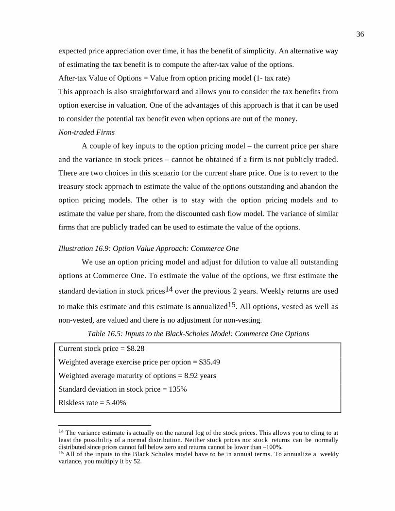
36

expected price appreciation over time, it has the benefit of simplicity. An alternative way

of estimating the tax benefit is to compute the after-tax value of the options.

After-tax Value of Options = Value from option pricing model (1- tax rate)

This approach is also straightforward and allows you to consider the tax benefits from

option exercise in valuation. One of the advantages of this approach is that it can be used

to consider the potential tax benefit even when options are out of the money.

Non-traded Firms

A couple of key inputs to the option pricing model – the current price per share

and the variance in stock prices – cannot be obtained if a firm is not publicly traded.

There are two choices in this scenario for the current share price. One is to revert to the

treasury stock approach to estimate the value of the options outstanding and abandon the

option pricing models. The other is to stay with the option pricing models and to

estimate the value per share, from the discounted cash flow model. The variance of similar

firms that are publicly traded can be used to estimate the value of the options.

Illustration 16.9: Option Value Approach: Commerce One

We use an option pricing model and adjust for dilution to value all outstanding

options at Commerce One. To estimate the value of the options, we first estimate the

standard deviation in stock prices14 over the previous 2 years. Weekly returns are used

to make this estimate and this estimate is annualized15. All options, vested as well as

non-vested, are valued and there is no adjustment for non-vesting.

Table 16.5: Inputs to the Black-Scholes Model: Commerce One Options

Current stock price = $8.28

Weighted average exercise price per option = $35.49

Weighted average maturity of options = 8.92 years

Standard deviation in stock price = 135%

Riskless rate = 5.40%

14 The variance estimate is actually on the natural log of the stock prices. This allows you to cling to atleast the possibility of a normal distribution. Neither stock prices nor stock returns can be normallydistributed since prices cannot fall below zero and returns cannot be lower than –100%.15 All of the inputs to the Black Scholes model have to be in annual terms. To annualize a weeklyvariance, you multiply it by 52.

37

Number of options outstanding = 45.911

Number of shares outstanding = 228.32

Value of options outstanding = $349 million

After-tax value of options outstanding = 3491− 0.35( ) = $227 million

In estimating the after-tax value of the options at Commerce One, we have used their

prospective marginal tax rate of 35%. If the options are exercised prior to these firms

reaching their marginal tax rates, the tax benefit is lower since the expenses are carried

forward and offset against income in future periods.

The value per share can now be computed by subtracting the value of the options

outstanding from the value of equity and dividing by the primary number of shares

outstanding. Again, using Commerce One, we estimate a value for equity per share.

Value of equity per share

= Value of Equity -Value of options outstandingNumber of shares outstanding

= 4941-227228.32

= $ 20.65 per share

The inconsistency averred to earlier is clear when you compare the value per share that is

estimated here ($20.65) to the price per share ($8.28) that we used to estimate the value

of the options. For instance, Commerce One’s value per share is $20.65, whereas the

price per share used in the option valuation is $8.28. If you choose to iterate, you would

revalue the options using the estimated value of $20.65, which would increase the value of

the options and decrease the value per share, leading to a second iteration and a third one

and so on. The values converge to yield a consistent estimate.

Estimated value of options with estimated value per share = $543 million

Value per share =

= Value of Equity -Value of options outstanding

Number of shares outstanding

=4941-8351-0.35( )

228.32= $19.26 per share

The options are also valued using the same value per share.

The Repricing of Options: Effects on Value

In recent years, firms that have seen their stock price drop have often reset their

exercise prices on options closer to the market price to make them more attractive to

38

management. This practice is obviously hazardous to stockholders since it increases the

value of the option overhang. In face, if this practice is egregious at a firm, you should

value the options with an exercise price of zero which would make them each worth as

much as a regular share. In effect, the fully diluted estimate of value per share will be the

value you get even if you used the option pricing model.

Future Option Grants

While incorporating options that are already outstanding is fairly straightforward,

incorporating the effects of future option grants is much more complicated. In this

section, the argument for why these option issues affect value is presented and how to

incorporate these effects into value.

Why future options issues affect value

Just as options outstanding currently represent potential dilution or cash outflows

to existing equity investors, expected option grants in the future will affect value per

share by increasing the number of shares outstanding in future periods. The simplest way

of thinking about this expected dilution is to consider the terminal value in the discounted

cash flow model. As constructed in the last chapter, the terminal value is discounted to

the present and divided by the shares outstanding today to arrive at the value per share.

However, expected option issues in the future will increase the number of shares

outstanding in the terminal year and therefore reduce the portion of the terminal value that

belongs to existing equity investors.

Ways of Incorporating Effect into Value per Share

It is much more difficult to incorporate the effect of expected option issues into

value than existing options outstanding. This is because you have to forecast not only

how many options will be issued by a firm in future periods, but also what the terms of

these options will be. While this may be possible for a couple of periods with proprietary

information (the firm lets you know how much it plans to issue and at what terms), it will

become more difficult in circumstances beyond that point. You will consider a way in

which you can obtain an estimate of the option value and look at two ways of dealing

with this estimate.

39

Estimate option value as an operating or capital expense

You can estimate the value of options that will be granted in future periods as a

percentage of revenues or operating income. By doing so, you can avoid having to

estimate the number and terms of future option issues. Estimation will also become easier

since you can draw on the firm’s own history (by looking at the value of option grants in

previous years as a proportion of firm value) and the experiences of more mature firms in

the sector. Generally, as firms become larger, the value of options granted as a percent of

revenues should become smaller.

Having estimated the value of expected future option issues, you are left with another

choice. You can consider this value each period as an operating expense and compute the

operating income, after the expense. You are assuming, then, that option issues form part

of annual compensation. Alternatively, you can treat it as a capital expense and amortize

it over multiple periods. While the cash flow in the current period is unaffected by this

distinction, it has consequences for the return on capital and reinvestment rates that you

measure for a firm.

It is important that you do not double count future option issues. The current

operating expenses of the firm already include the expenses associated with option

exercises in the current period. The operating margins and returns on capital that you

might derive by looking at industry averages reflect the effects of option exercise in the

current period for the firms in the industry. If the effect on operating income of option

exercise in the current period is less than the expected value of new option issues, you

have to allow for an additional expense associated with option issues. Conversely, if a

disproportionately large number of options were exercised in the last period, you have to

reduce the operating expenses to allow for the fact that the expected effect of option

issues in future periods will be smaller.

Value per Share when voting rights vary

When you divide the value of the equity by the number of shares outstanding, you

assume that the shares all have the same voting rights. If different classes of shares have

different voting rights, the value of equity per share has to reflect these differences, with

the shares with more voting rights having higher value. Note, though, that the total value

40

of equity is still unchanged. To illustrate, assume that the value of equity in a firm is $500

million and that there are 50 million shares outstanding; 25 million of these shares have

voting rights and 25 million do not. Furthermore, assume that the voting shares will have a

value 10% higher than the non-voting shares. To estimate the value per share:

Value per non-voting share ( )( )52.9$

million 251.10million 25

million $500

=+

=

Value per voting share = $ 9.52 (1.10) = $ 10.48

The key issue that you face in valuation then is in coming up with the discount to apply

for non-voting shares or, alternatively, the premium to attach to voting shares.

Voting Shares versus Non-voting Shares

What premium should be assigned to the voting shares? You have two choices.

One is to look at studies that empirically examine the size of the premium for voting

rights and to assign this premium to all voting shares. Lease, McConnell and

Mikkelson(1983) examined 26 firms that had two classes of common stock outstanding;

they concluded that the voting shares traded at a premium relative to non-voting

shares.16 The premium, on average, amounted to 5.44% and the voting shares sold at a

higher price in 88% of the months for which data were available. In four firms that also

had voting preferred stock, however, the voting common stock traded at a discount of

about 1.17% relative to non-voting shares.

The other option is to be more discriminating and vary the premium depending

upon the firm. Voting rights have value because they give shareholders a say in the

management of the firm. To the extent that voting shares can make a difference –– by

removing incumbent management, forcing management to change policy, or selling to a

hostile bidder in a takeover –– their price will reflect the possibility of a change in the

16 The two classes of stock received the same dividend.

41

way the firm is run.17 Non-voting shareholders, on the other hand, do not participate in

these decisions.

Estimating the Premium for Voting Rights

If one class of shares has significantly more voting rights than another, you would

expect it to trade at a higher price. Estimating the premium for voting rights can be fairly

complicated. While many analysts prefer to use ad hoc approaches, you can estimate a

more precise estimate of the relative value of voting shares by valuing the firm twice –

once under incumbent management and once with a new (and better) management. For

instance, assume that you value a firm at $ 800 million with existing management and

$1,200 million with new management. The value of control at this firm is $ 400 million. If

you assume that this firm has 10 million voting shares and 10 million non-voting shares,

you could estimate the voting share premium by estimating two per-share values:

Value per share for non-voting shares = Status Quo Value/ (Voting + Non-voting shares)

= 800 / (10 + 10) = $ 40

Value per share for voting shares = Value per share without voting rights + (Value of firm

with superior management – Value of Firm- Status Quo)/ Number of Voting Shares

= $ 40 + (1200 – 800)/10 = $ 80 per share

The voting share premium will decrease as the difference between optimal and current

value decreases and also if the likelihood of a hostile takeover lessens.

The voting share premium will decrease as the difference between optimal and current

value decreases and also if the likelihood of a hostile takeover lessens.

warrants.xls: This spreadsheet allows you to value the options outstanding in a firm,

allowing for the dilution effect.

Summary

Incorporating the value of non-operating assets into firm value can be very simple

to do in some cases – cash and near-cash investments – and very complicated in other

cases – holdings in private companies. The principle, though, should remain the same.

17In some cases, the rights of non-voting stockholders are protected in the specific instance of a takeover byforcing the bidder to buy the non-voting shares as well.

42

You want to estimate a fair value for these non-operating assets and bring them into value.

As we noted, it is often better to value non-operating assets separately from operating

assets, but the absence of information may impede this process.

The existence of options and the possibility of future option grants make getting

from equity value to value per share a complicated exercise. To deal with options

outstanding at the time of the valuation, there are four approaches. The simplest is to

estimate the value per share by dividing the value of equity by the fully diluted number of

shares outstanding. This approach ignores both the expected proceeds from exercising the

options and the time value of the options. The second approach of forecasting expected

option exercises in the future and estimating the effect on value per share is not only

tedious but unlikely to work. In the third (treasury stock) approach, you add the

expected proceeds from option exercise to the value of equity and then divide by the fully

diluted number of shares outstanding. While this approach does consider the expected

proceeds from exercise, it still ignores the option time premium. In the final and the

preferred approach, the options are valued using an option pricing model and the value is

subtracted from the value of equity. The resulting estimate is divided by the primary

shares outstanding to arrive at the value of equity per share. While the current price of the

stock is usually used in option pricing models, the value per share estimated from the

discounted cash flow valuation can be substituted to arrive at a more consistent estimate.

To deal with expected option grants in the future, the current operating income has to be

dissected to consider how much of an effect option exercises in the current period had on

operating expenses. If the options granted during the period had more value than the

option expense resulting form exercise of options granted in prior periods, the current

operating income has to be adjusted down to reflect the difference. Industry average

margins and returns on capital will also have to be adjusted for the same reason.

Once the value per share of equity has been estimated, that value may need to be

adjusted for differences in voting rights. Shares with disproportionately high voting rights

will sell at a premium relative to shares with low or no voting rights. The difference will

be larger for firms that are badly managed and smaller for well-managed firms.

43

Problems

1. ABV Inc. has earnings before interest and taxes of $250 million, expected to grow 5% a

year forever; the tax rate is 40%. Its cost of capital is 10%, reinvestment rate is 33.33%

and it has 200 million shares outstanding. If the firm has $500 million in cash and

marketable securities, and $750 million in debt outstanding, estimate the value of equity

per share.

2. How would your answer to the previous problem change if you were told that ABV

had options outstanding, for 50 million shares, and that each option had a value of $5.

3. If you were told that the average exercise price of the 50 million options in the previous

problem was $6, estimate the value per share for ABV, using the treasury stock

approach.

4. LSI Logic has 1 billion shares outstanding, trading at $25 per share. The firm also has

$5 billion in debt outstanding. The cost of equity is 12.5% and the cost of debt, after-

taxes, is 5%. If the firm has $3 billion in cash outstanding and is fairly valued, estimate

how much the firm earned in operating income in the current year. (The return on capital

is 15%, the tax rate is 30% and earnings are growing 6% a year in perpetuity)

5. Lava Lamps Inc. had $800 million in earnings before interest and taxes last year. It has

just acquired a 50% stake in General Lamps Inc., which had $400 million in earnings

before interest and taxes last year. Because Lava Lamps has a majority active stake, it has

been asked to consolidate last year’s income statements for the two firms. What earnings

before interest and taxes would you see in the consolidated statement?

6. Genome Sciences is a bio-technology firm that had after-tax operating income of$ 300

million last year; these earnings are expected to grow 6% a year forever. The reinvestment

rate is 40% and the firm has a cost of capital of 12%. Genome also owns 10% of the

stock of Gene Therapies Inc., another publicly traded firms. Gene Therapies has 100

million shares outstanding, trading at $50 per share. If Genome has $800 million in debt

outstanding, estimate the value of equity per share in Genome Sciences. (Genome has 50

million shares outstanding.)

44

1

CHAPTER 17

FUNDAMENTAL PRINCIPLES OF RELATIVE VALUATION

In discounted cash flow valuation, the objective is to find the value of assets, given

their cash flow, growth and risk characteristics. In relative valuation, the objective is to

value assets, based upon how similar assets are currently priced in the market. While

multiples are easy to use and intuitive, they are also easy to misuse. Consequently, a

series of tests will be developed in this chapter that can be used to ensure that multiples

are correctly used.

There are two components to relative valuation. The first is that to value assets on

a relative basis, prices have to be standardized, usually by converting prices into

multiples of earnings, book values or sales. The second is to find similar firms, which is

difficult to do since no two firms are identical and firms in the same business can still

differ on risk, growth potential and cash flows. The question of how to control for these

differences, when comparing a multiple across several firms, becomes a key one.

Use of Relative Valuation

The use of relative valuation is widespread. Most equity research reports and

many acquisition valuations are based upon a multiple such as a price to sales ratio or the

value to EBITDA multiple and a group of comparable firms. In fact, firms in the same

business as the firm being valued are called comparable, though as you see later in this

chapter, that is not always true. In this section, the reasons for the popularity of relative

valuation are considered first, followed by some potential pitfalls.

Reasons for Popularity

Why is relative valuation so widely used? There are several reasons. First, a

valuation based upon a multiple and comparable firms can be completed with far fewer

assumptions and far more quickly than a discounted cash flow valuation. Second, a

relative valuation is simpler to understand and easier to present to clients and customers

than a discounted cash flow valuation. Finally, a relative valuation is much more likely to

reflect the current mood of the market, since it is an attempt to measure relative and not

intrinsic value. Thus, in a market where all internet stocks see their prices bid up, relative

valuation is likely to yield higher values for these stocks than discounted cash flow

2

valuations. In fact, relative valuations will generally yield values that are closer to the

market price than discounted cash flow valuations. This is particularly important for

those whose job it is to make judgments on relative value and who are themselves judged

on a relative basis. Consider, for instance, managers of technology mutual funds. These

managers will be judged based upon how their funds do relative to other technology

funds. Consequently, they will be rewarded if they pick technology stocks that are under

valued relative to other technology stocks, even if the entire sector is over valued.

Potential Pitfalls

The strengths of relative valuation are also its weaknesses. First, the ease with

which a relative valuation can be put together, pulling together a multiple and a group of

comparable firms, can also result in inconsistent estimates of value where key variables

such as risk, growth or cash flow potential are ignored. Second, the fact that multiples

reflect the market mood also implies that using relative valuation to estimate the value of

an asset can result in values that are too high, when the market is over valuing comparable

firms, or too low, when it is under valuing these firms. Third, while there is scope for bias

in any type of valuation, the lack of transparency regarding the underlying assumptions in

relative valuations make them particularly vulnerable to manipulation. A biased analyst

who is allowed to choose the multiple on which the valuation is based and to choose the

comparable firms can essentially ensure that almost any value can be justified.

Standardized Values and Multiples

The price of a stock is a function both of the value of the equity in a company and

the number of shares outstanding in the firm. Thus, a stock split that doubles the number

of units will approximately halve the stock price. Since stock prices are determined by the

number of units of equity in a firm, stock prices cannot be compared across different

firms. To compare the values of “similar” firms in the market, you need to standardize the

values in some way. Values can be standardized relative to the earnings firms generate, to

the book value or replacement value of the firms themselves, to the revenues that firms

generate or to measures that are specific to firms in a sector.

1. Earnings Multiples

3

One of the more intuitive ways to think of the value of any asset is the multiple of

the earnings that asset generates. When buying a stock, it is common to look at the price

paid as a multiple of the earnings per share generated by the company. This price/earnings

ratio can be estimated using current earnings per share, yielding a current PE, earnings

over the last 4 quarters, resulting in a trailing PE, or an expected earnings per share in the

next year, providing a forward PE.

When buying a business, as opposed to just the equity in the business, it is

common to examine the value of the firm as a multiple of the operating income or the

earnings before interest, taxes, depreciation and amortization (EBITDA). While, as a

buyer of the equity or the firm, a lower multiple is better than a higher one. These

multiples will be affected by the growth potential and risk of the business being acquired.

2. Book Value or Replacement Value Multiples

While markets provide one estimate of the value of a business, accountants often

provide a very different estimate of the same business. The accounting estimate of book

value is determined by accounting rules and is heavily influenced by the original price paid

for assets and any accounting adjustments (such as depreciation) made since. Investors

often look at the relationship between the price they pay for a stock and the book value

of equity (or net worth) as a measure of how over- or undervalued a stock is; the

price/book value ratio that emerges can vary widely across industries, depending again

upon the growth potential and the quality of the investments in each. When valuing

businesses, you estimate this ratio using the value of the firm and the book value of all

assets (rather than just the equity). For those who believe that book value is not a good

measure of the true value of the assets, an alternative is to use the replacement cost of the

assets; the ratio of the value of the firm to replacement cost is called Tobin’s Q.

3. Revenue Multiples

Both earnings and book value are accounting measures and are determined by

accounting rules and principles. An alternative approach, which is far less affected by

accounting choices, is to use the ratio of the value of an asset to the revenues it generates.

For equity investors, this ratio is the price/sales ratio (PS), where the market value per

share is divided by the revenues generated per share. For firm value, this ratio can be

4

modified as the value/sales ratio (VS), where the numerator becomes the total value of the

firm. This ratio, again, varies widely across sectors, largely as a function of the profit

margins in each. The advantage of using revenue multiples, however, is that it becomes far

easier to compare firms in different markets, with different accounting systems at work,

than it is to compare earnings or book value multiples.

4. Sector-Specific Multiples

While earnings, book value and revenue multiples are multiples that can be

computed for firms in any sector and across the entire market, there are some multiples

that are specific to a sector. For instance, when Internet firms first appeared on the

market in the later 1990s, they had negative earnings and negligible revenues and book

value. Analysts looking for a multiple to value these firms divided the market value of

each of these firms by the number of hits generated by that firm’s web site. Firms with a

low market value per customer hit were viewed as more under valued. More recently, e-

tailers have been judged by the market value of equity per customer in the firm, regardless

of the longevity and the profitably of the customers.

While there are conditions under which sector-specific multiples can be justified,

they are dangerous for two reasons. First, since they cannot be computed for other

sectors or for the entire market, sector-specific multiples can result in persistent over or

under valuations of sectors relative to the rest of the market. Thus, investors who would

never consider paying 80 times revenues for a firm might not have the same qualms about

paying $2000 for every page hit (on the web site), largely because they have no sense of

what high, low or average is on this measure. Second, it is far more difficult to relate

sector specific multiples to fundamentals, which is an essential ingredient to using

multiples well. For instance, does a visitor to a company’s web site translate into higher

revenues and profits? The answer will not only vary from company to company, but will

also be difficult to estimate looking forward.

The Four Basic Steps to Using Multiples

Multiples are easy to use and easy to misuse. There are four basic steps to using

multiples wisely and for detecting misuse in the hands of others. The first step is to

ensure that the multiple is defined consistently and that it is measured uniformly across

5

the firms being compared. The second step is to be aware of the cross sectional

distribution of the multiple, not only across firms in the sector being analyzed but also

across the entire market. The third step is to analyze the multiple and understand not

only what fundamentals determine the multiple but also how changes in these

fundamentals translate into changes in the multiple. The final step is finding the right

firms to use for comparison and controlling for differences that may persist across these

firms.

A. Definitional Tests

Even the simplest multiples can be defined differently by different analysts.

Consider, for instance, the price earnings ratio (PE). Most analysts define it to be the

market price divided by the earnings per share but that is where the consensus ends.

There are a number of variants on the PE ratio. While the current price is conventionally

used in the numerator, there are some analysts who use the average price over the last six

months or a year. The earnings per share in the denominator can be the earnings per share

from the most recent financial year (yielding the current PE), the last four quarters of

earnings (yielding the trailing PE) and expected earnings per share in the next financial

year (resulting in a forward PE). In addition, earnings per share can be computed based

upon primary shares outstanding or fully diluted shares and can include or exclude

extraordinary items. Figure 17.1 provides some of the PE ratios for Cisco in 1999 using

variants of these measures.

6

Not only can these variants on earnings yield vastly different values for the price

earnings ratio, but the one that gets used by analysts depends upon their biases. For

instance, in periods of rising earnings, the forward PE yields consistently lower values

than the trailing PE, which, in turn, is lower than the current PE. A bullish analyst will

tend to use the forward PE to make the case that the stock is trading at a low multiple of

earnings, while a bearish analyst will focus on the current PE to make the case that the

multiple is too high. The first step when discussing a valuation based upon a multiple is

to ensure that everyone in the discussion is using the same definition for that multiple.

Consistency

Every multiple has a numerator and a denominator. The numerator can be either an

equity value (such as market price or value of equity) or a firm value (such as enterprise

value, which is the sum of the values of debt and equity, net of cash). The denominator

can be an equity measure (such as earnings, net income or book value of equity) or a firm

measure (such as operating income, EBITDA or book value of capital).

Figure 17.1: Estimate of Cisco's PE Ratio

0.00

50.00

100.00

150.00

200.00

250.00

Current Trailing Forward Diluted beforeExtraordinary

Diluted afterExtraordinary

7

One of the key tests to run on a multiple is to examine whether the numerator and

denominator are defined consistently. If the numerator for a multiple is an equity value,

then the denominator should be an equity value as well. If the numerator is a firm value,

then the denominator should be a firm value as well. To illustrate, the price earnings ratio

is a consistently defined multiple, since the numerator is the price per share (which is an

equity value) and the denominator is earnings per share (which is also an equity value). So

is the Enterprise value to EBITDA multiple, since the numerator and denominator are

both firm value measures.

Are there any multiples in use that are inconsistently defined? Consider the price

to EBITDA multiple, a multiple that has acquired adherents in the last few years among

analysts. The numerator in this multiple is an equity value and the denominator is a

measure of earnings to the firm. The analysts who use this multiple will probably argue

that the inconsistency does not matter since the multiple is computed the same way for

all of the comparable firms; but they would be wrong. If some firms on the list have no

debt and others carry significant amounts of debt, the latter will look cheap on a price to

EBITDA basis, when in fact they might be over or correctly priced.

Uniformity

In relative valuation, the multiple is computed for all of the firms in a group and

then compared across these firms to make judgments on which firms are over priced and

which are under priced. For this comparison to have any merit, the multiple has to be

defined uniformly across all of the firms in the group. Thus, if the trailing PE is used for

one firm, it has to be used for all of the others as well. In fact, one of the problems with

using the current PE to compare firms in a group is that different firms can have different

fiscal-year ends. This can lead to some firms having their prices divided by earnings from

July 1999 to June 2000, with other firms having their prices divided by earnings from

January 1999 to December 1999. While the differences can be minor in mature sectors,

where earnings do not make quantum jumps over six months, they can be large in high-

growth sectors.

With both earnings and book value measures, there is another component to be

concerned about and that is the accounting standards used to estimate earnings and book

8

values. Differences in accounting standards can result in very different earnings and book

value numbers for similar firms. This makes comparisons of multiples across firms in

different markets, with different accounting standards, very difficult. Even within the

United States, the fact that some firms use different accounting rules (on depreciation and

expensing) for reporting purposes and tax purposes and others do not can throw off

comparisons of earnings multiples1.

B. Descriptional Tests

When using a multiple, it is always useful to have a sense of what a high value, a low

value or a typical value for that multiple is in the market. In other words, knowing the

distributional characteristics of a multiple is a key part of using that multiple to identify

under or over valued firms. In addition, you need to understand the effects of outliers on

averages and unearth any biases in these estimates, introduced in the process of estimating

multiples.

Distributional Characteristics

Many analysts who use multiples have a sector focus and have a good sense of

how different firms in their sector rank on specific multiples. What is often lacking,

however, is a sense of how the multiple is distributed across the entire market. Why, you

might ask, should a software analyst care about price earnings ratios of utility stocks?

Because both software and utility stocks are competing for the same investment dollar,

they have to, in a sense, play by the same rules. Furthermore, an awareness of how

multiples vary across sectors can be very useful in detecting when the sector you are

analyzing is over or under valued.

What are the distributional characteristics that matter? The standard statistics –

the average and standard deviation – are where you should start, but they represent the

beginning of the exploration. The fact that multiples such as the price earnings ratio can

never be less than zero and are unconstrained in terms of a maximum results in

distributions for these multiples that are skewed towards the positive values.

1 Firms that adopt different rules for reporting and tax purposes generally report higher earnings to theirstockholders than they do to the tax authorities. When they are compared on a price earnings basis to firms

9

Consequently, the average values for these multiples will be higher than median values2,

and the latter are much more representative of the typical firm in the group. While the

maximum and minimum values are usually of limited use, the percentile values (10th

percentile, 25 th percentile, 75th percentile, 90th percentile, etc.) can be useful in judging

what a high or low value for the multiple in the group is.

Outliers and Averages

As noted earlier, multiples are unconstrained on the upper end and firms can have

price earnings ratios of 500 or 2000 or even 10000. This can occur not only because of

high stock prices but also because earnings at firms can sometime drop to a few cents.

These outliers will result in averages that are not representative of the sample. In most

cases, services that compute and report average values for multiples either throw out

these outliers when computing the averages or constrain the multiples to be less than or

equal to a fixed number. For instance, any firm that has a price earnings ratio greater than

500 may be given a price earnings ratio of 500.

When using averages obtained from a service, it is important that you know how

the service dealt with outliers in computing the averages. In fact, the sensitivity of the

estimated average to outliers is another reason for looking at the median values for

multiples.

Biases in Estimating Multiples

With every multiple, there are firms for which the multiple cannot be computed.

Consider again the price-earnings ratio. When the earnings per share are negative, the price

earnings ratio for a firm is not meaningful and is usually not reported. When looking at the

average price earnings ratio across a group of firms, the firms with negative earnings will

all drop out of the sample because the price earnings ratio cannot be computed. Why

should this matter when the sample is large? The fact that the firms that are taken out of

the sample are the firms losing money creates a bias in the selection process. In fact, the

that do not maintain different reporting and tax books, they will look cheaper (lower PE).2 With the median, half of all firms in the group fall below this value and half lie above.

10

average PE ratio for the group will be biased upwards because of the elimination of these

firms.

There are three solutions to this problem. The first is to be aware of the bias and

build it into the analysis. In practical terms, this will mean adjusting the average PE down

to reflect the elimination of the money-losing firms. The second is to aggregate the market

value of equity and net income (or loss) for all of the firms in the group, including the

money-losing ones, and compute the price earnings ratio using the aggregated values.

Figure 17.2 summarizes the average PE ratio, the median PE ratio and the PE ratio based

upon aggregated earnings for specialty retailers.

Note that the median PE ratio is much lower than the average than the PE ratio.

Furthermore, the PE ratio based upon the aggregate values of market value of equity and

net income is lower than the average across firms where PE ratios could be computed. The

third choice is to use a multiple that can be computed for all of the firms in the group. The

inverse of the price earning ratio, which is called the earnings yield, can be computed for

all firms, including those losing money.

Figure 17.2: PE Ratio for Specialty Retailers

0.00

5.00

10.00

15.00

20.00

25.00

Aerage PE ratio Median PE ratio PE ratio based upon aggregate

11

C. Analytical Tests

In discussing why analysts were so fond of using multiples, it was argued that relative

valuations require fewer assumptions than discounted cash flow valuations. While this is

technically true, it is only so on the surface. In reality, you make just as many

assumptions when you do a relative valuation as you make in a discounted cash flow

valuation. The difference is that the assumptions in a relative valuation are implicit and

unstated, whereas those in discounted cash flow valuation are explicit and stated. The two

primary questions that you need to answer before using a multiple are: What are the

fundamentals that determine at what multiple a firm should trade? How do changes in the

fundamentals affect the multiple?

Determinants

In the introduction to discounted cash flow valuation, you observed that the value

of a firm is a function of three variables – it capacity to generate cash flows, its expected

growth in these cash flows and the uncertainty associated with these cash flows. Every

multiple, whether it is of earnings, revenues or book value, is a function of the same three

variables – risk, growth and cash flow generating potential. Intuitively, then, firms with

higher growth rates, less risk and greater cash flow generating potential should trade at

higher multiples than firms with lower growth, higher risk and less cash flow potential.

The specific measures of growth, risk and cash flow generating potential that are

used will vary from multiple to multiple. To look under the hood, so to speak, of equity

and firm value multiples, you can go back to fairly simple discounted cash flow models

for equity and firm value and use them to derive the multiples.

In the simplest discounted cash flow model for equity, which is a stable growth

dividend discount model, the value of equity is:

Value of Equity = P0 =DPS1

k e − gn

where DPS1 is the expected dividend in the next year, ke is the cost of equity and gn is the

expected stable growth rate. Dividing both sides by the earnings, you obtain the

discounted cash flow equation specifying the PE ratio for a stable growth firm.

12

P0

EPS0

= PE = Payout Ratio*(1 + gn)

k e-gn

Dividing both sides by the book value of equity, you can estimate the price/book value

ratio for a stable growth firm.

P0

BV0

= PBV = ROE*Payout Ratio*(1 + gn )

k e -gn

where ROE is the return on equity. Dividing by the Sales per share, the price/sales ratio

for a stable growth firm can be estimated as a function of its profit margin, payout ratio,

risk and expected growth.

P0

Sales0

= PS = Profit Margin*Payout Ratio*(1 + gn)

k e-gn

You can do a similar analysis to derive the firm value multiples. The value of a

firm in stable growth can be written as:

Value of Firm = V0 =FCFF1

kc − gn

Dividing both sides by the expected free cash flow to the firm yields the Value/FCFF

multiple for a stable growth firm.

V0

FCFF1

=1

k c − gn

Since the free cash flow the firm is the after-tax operating income netted against

the net capital expenditures and working capital needs of the firm, the multiples of EBIT,

after-tax EBIT and EBITDA can also be estimated similarly.

The point of this analysis is not to suggest that you go back to using discounted

cash flow valuation, but to understand the variables that may cause these multiples to

vary across firms in the same sector. If you ignore these variables, you might conclude

that a stock with a PE of 8 is cheaper than one with a PE of 12 when the true reason may

be that the latter has higher expected growth or you might decide that a stock with a P/BV

13

ratio of 0.7 is cheaper than one with a P/BV ratio of 1.5 when the true reason may be that

the latter has a much higher return on equity.

Relationship

Knowing the fundamentals that determine a multiple is a useful first step, but

understanding how the multiple changes as the fundamentals change is just as critical to

using the multiple. To illustrate, knowing that higher growth firms have higher PE ratios is

not a sufficient insight if you are called upon to analyze whether a firm with a growth rate

that is twice as high as the average growth rate for the sector should have a PE ratio that is

1.5 times or 1.8 times or two times the average price earnings ratio for the sector. To

make this judgment, you need to know how the PE ratio changes as the growth rate

changes.

A surprisingly large number of analyses are based upon the assumption that there

is a linear relationship between multiples and fundamentals. For instance, the PEG ratio,

which is the ratio of the PE to the expected growth rate of a firm and widely used to

analyze high growth firms, implicitly assumes that PE ratios and expected growth rates

are linearly related.

One of the advantages of deriving the multiples from a discounted cash flow

model, as was done in the last section, is that you can analyze the relationship between

each fundamental variable and the multiple by keeping everything else constant and

changing the value of that variable. When you do this, you will find that there are very

few linear relationships in valuation.

Companion Variable

While the variables that determine a multiple can be extracted from a discounted

cash flow model and the relationship between each variable and the multiple can be

developed by holding all else constant and asking what-if questions, there is one variable

that dominates when it comes to explaining each multiple. This variable, which is called

the companion variable, can usually be identified by looking at how multiples are different

across firms in a sector or across the entire market. In the next two chapters, the

companion variables for the most widely used multiples from the price earnings ratio to

the value to sales multiples are identified and then used in analysis.

14

D. Application Tests

When multiples are used, they tend to be used in conjunction with comparable

firms to determine the value of a firm or its equity. But what is a comparable firm? While

the conventional practice is to look at firms within the same industry or business as

comparable firms, this is not necessarily always the correct or the best way of identifying

these firms. In addition, no matter how carefully you choose comparable firms,

differences will remain between the firm you are valuing and the comparable firms.

Figuring out how to control for these differences is a significant part of relative valuation.

What is a comparable firm?

A comparable firm is one with cash flows, growth potential, and risk similar to the

firm being valued. It would be ideal if you could value a firm by looking at how an exactly

identical firm - in terms of risk, growth and cash flows - is priced. Nowhere in this

definition is there a component that relates to the industry or sector to which a firm

belongs. Thus, a telecommunications firm can be compared to a software firm, if the two

are identical in terms of cash flows, growth and risk. In most analyses, however, analysts

define comparable firms to be other firms in the firm’s business or businesses. If there are

enough firms in the industry to allow for it, this list is pruned further using other criteria;

for instance, only firms of similar size may be considered. The implicit assumption being

made here is that firms in the same sector have similar risk, growth, and cash flow profiles

and therefore can be compared with much more legitimacy.

This approach becomes more difficult to apply when there are relatively few

firms in a sector. In most markets outside the United States, the number of publicly

traded firms in a particular sector, especially if it is defined narrowly, is small. It is also

difficult to define firms in the same sector as comparable firms if differences in risk,

growth and cash flow profiles across firms within a sector are large. Thus, there may be

hundreds of computer software companies listed in the United States, but the differences

across these firms are also large. The tradeoff is therefore a simple one. Defining an

industry more broadly increases the number of comparable firms, but it also results in a

more diverse group.

15

There are alternatives to the conventional practice of defining comparable firms.

One is to look for firms that are similar in terms of valuation fundamentals. For instance,

to estimate the value of a firm with a beta of 1.2, an expected growth rate in earnings per

share of 20% and a return on equity of 40%3, you would find other firms across the

entire market with similar characteristics4. The other is consider all firms in the market

as comparable firms and to control for differences on the fundamentals across these firms,

using statistical techniques such as multiple regressions.

Controlling for Differences across Firms

No matter how carefully you construct your list of comparable firms, you will

end up with firms that are different from the firm you are valuing. The differences may be

small on some variables and large on others and you will have to control for these

differences in a relative valuation. There are three ways of controlling for these

differences:

1. Subjective Adjustments

Relative valuation begins with two choices - the multiple used in the analysis and

the group of firms that comprises the comparable firms. The multiple is calculated for

each of the comparable firms and the average is computed. To evaluate an individual firm,

you then compare the multiple it trades at to the average computed; if it is significantly

different, you make a subjective judgment about whether the firm’s individual

characteristics (growth, risk or cash flows) may explain the difference. Thus, a firm may

have a PE ratio of 22 in a sector where the average PE is only 15, but you may conclude

that this difference can be justified because the firm has higher growth potential than the

average firm in the industry. If, in your judgment, the difference on the multiple cannot be

explained by the fundamentals, the firm will be viewed as over valued (if its multiple is

higher than the average) or undervalued (if its multiple is lower than the average).

3 The return on equity of 40% becomes a proxy for cash flow potential. With a 20% growth rate and a 40%return on equity, this firm will be able to return half of its earnings to its stockholders in the form ofdividends or stock buybacks.4 Finding these firms manually may be tedious when your universe includes 10000 stocks. You could drawon statistical techniques such as cluster analysis to find similar firms.

16

2. Modified Multiples

In this approach, you modify the multiple to take into account the most

important variable determining it – the companion variable. Thus, the PE ratio is divided

by the expected growth rate in EPS for a company to determine a growth-adjusted PE

ratio or the PEG ratio. Similarly, the PBV ratio is divided by the ROE to find a Value

Ratio and the price sales ratio is divided by the net margin. These modified ratios are then

compared across companies in a sector. The implicit assumption you make is that these

firms are comparable on all the other measures of value, other than the one being

controlled for. In addition, you are assuming that the relationship between the multiples

and fundamentals is linear.

Illustration 17.1: Comparing PE ratios and growth rates across firms: Beverage

Companies

The PE ratios and expected growth rates in EPS over the next 5 years, based on

consensus estimates from analysts, for the firms that are categorized as beverage firms are

summarized in Table 17.1.

Table 17.1: Beverage Companies

Company Name

Trailing

PE

Expected

Growth

Standard

Deviation PEG

Coca-Cola Bottling 29.18 9.50% 20.58% 3.07

Molson Inc. Ltd. 'A' 43.65 15.50% 21.88% 2.82

Anheuser-Busch 24.31 11.00% 22.92% 2.21

Corby Distilleries Ltd. 16.24 7.50% 23.66% 2.16

Chalone Wine Group

Ltd. 21.76 14.00% 24.08% 1.55

Andres Wines Ltd. 'A' 8.96 3.50% 24.70% 2.56

Todhunter Int'l 8.94 3.00% 25.74% 2.98

Brown-Forman 'B' 10.07 11.50% 29.43% 0.88

Coors (Adolph) 'B' 23.02 10.00% 29.52% 2.30

PepsiCo, Inc. 33.00 10.50% 31.35% 3.14

17

Coca-Cola 44.33 19.00% 35.51% 2.33

Boston Beer 'A' 10.59 17.13% 39.58% 0.62

Whitman Corp. 25.19 11.50% 44.26% 2.19

Mondavi (Robert) 'A' 16.47 14.00% 45.84% 1.18

Coca-Cola Enterprises 37.14 27.00% 51.34% 1.38

Hansen Natural Corp 9.70 17.00% 62.45% 0.57

Average 22.66 12.60% 33.30% 2.00

Source: Value Line

Is Andres Wine under valued on a relative basis? A simple view of multiples would lead

you to conclude this because its PE ratio of 8.96 is significantly lower than the average for

the industry.

In making this comparison, we are assuming that Andres Wine has growth and risk

characteristics similar to the average for the sector. One way of bringing growth into the

comparison is to compute the PEG ratio, which is reported in the last column. Based on

the average PEG ratio of 2.00 for the sector and the estimated growth rate for Andres

Wine, you obtain the following value for the PE ratio for Andres.

PE Ratio = 2.00 * 3.50% = 7.00

Based upon this adjusted PE, Andres Wine looks overvalued even though it has a low PE

ratio. While this may seem like an easy adjustment to resolve the problem of differences

across firms, the conclusion holds only if these firms are of equivalent risk. Implicitly,

this approach assumes a linear relationship between growth rates and PE.

3. Sector Regressions

When firms differ on more than one variable, it becomes difficult to modify the

multiples to account for the differences across firms. You can run regressions of the

multiples against the variables and then use these regressions to find predicted values for

each firm. This approach works reasonably well when the number of comparable firms is

large and the relationship between the multiple and the variables is stable. When these

conditions do not hold, a few outliers can cause the coefficients to change dramatically

and make the predictions much less reliable.

18

Illustration 17.2: Revisiting the Beverage Sector: Sector Regression

The price earnings ratio is a function of the expected growth rate, risk and the

payout ratio. None of the firms in the beverage sector pay significant dividends but they

differ in terms of risk and growth. Table 17.2 summarizes the price earnings ratios, betas

and expected growth rates for the firms on the list.

Table 17.2: Beverage Firms: PE, Growth and Risk

Company Name

Trailing

PE

Expected

Growth

Standard

Deviation

Coca-Cola Bottling 29.18 9.50% 20.58%

Molson Inc. Ltd. 'A' 43.65 15.50% 21.88%

Anheuser-Busch 24.31 11.00% 22.92%

Corby Distilleries Ltd. 16.24 7.50% 23.66%

Chalone Wine Group

Ltd. 21.76 14.00% 24.08%

Andres Wines Ltd. 'A' 8.96 3.50% 24.70%

Todhunter Int'l 8.94 3.00% 25.74%

Brown-Forman 'B' 10.07 11.50% 29.43%

Coors (Adolph) 'B' 23.02 10.00% 29.52%

PepsiCo, Inc. 33.00 10.50% 31.35%

Coca-Cola 44.33 19.00% 35.51%

Boston Beer 'A' 10.59 17.13% 39.58%

Whitman Corp. 25.19 11.50% 44.26%

Mondavi (Robert) 'A' 16.47 14.00% 45.84%

Coca-Cola Enterprises 37.14 27.00% 51.34%

Hansen Natural Corp 9.70 17.00% 62.45%

Source: Value Line Database

Since these firms differ on both risk and expected growth, a regression of PE ratios on

both variables is presented.

PE = 20.87 - 63.98 Standard deviation + 183.24 Expected Growth R2 = 51%

19

(3.01) (2.63) (3.66)

The numbers in brackets are t-statistics and suggest that the relationships between PE

ratios and both variables in the regression are statistically significant. The R-squared

indicates the percentage of the differences in PE ratios that is explained by the

independent variables. Finally, the regression5 itself can be used to get predicted PE

ratios for the companies in the list. Thus, the predicted PE ratio for Coca Cola, based

upon its standard deviation of 35.51% and the expected growth rate of 19%, would be:

Predicted PECisco = 20.87 - 63.98 (0.3551) + 183.24 (0.19) = 32.97

Since the actual PE ratio for Coca Cola was 44.33, this would suggest that the stock is

overvalued, given how the rest of the sector is priced.

If you are uncomfortable with the assumption that the relationship

between PE and growth is linear, which is what we have implicitly assumed in the

regression above, you could either run non-linear regressions or modify the variables in

the regression to make the relationship more linear. For instance, using the ln(growth rate)

instead of the growth rate in the regression above yields much better behaved residuals.

4. Market Regression

Searching for comparable firms within the sector in which a firm operates is fairly

restrictive, especially when there are relatively few firms in the sector or when a firm

operates in more than one sector. Since the definition of a comparable firm is not one that

is in the same business but one that has the same growth, risk and cash flow

characteristics as the firm being analyzed, you need not restrict your choice of comparable

firms to those in the same industry. The regression introduced in the previous section

controls for differences on those variables that you believe cause multiples to vary across

firms. Based upon the variables that determine each multiple, you should be able to

regress PE, PBV and PS ratios against the variables that should affect them:

Price Earnings = f (Growth, Payout ratios, Risk)

Price to Book Value = f (Growth, Payout ratios, Risk, ROE)

5 Both approaches described above assume that the relationship between a multiple and the variables drivingvalue are linear. Since this is not always true, you might have to run non-linear versions of theseregressions.

20

Price to Sales = f (Growth, Payout ratios, Risk, Margin)

It is, however, possible that the proxies that you use for risk (beta), growth (expected

growth rate), and cash flow (payout) may be imperfect and that the relationship may not

be linear. To deal with these limitations, you can add more variables to the regression -

e.g., the size of the firm may operate as a good proxy for risk - and use transformations of

the variables to allow for non-linear relationships.

The first advantage of this approach over the “subjective” comparison across

firms in the same sector, described in the previous section, is that it does quantify, based

upon actual market data, the degree to which higher growth or risk should affect the

multiples. It is true that these estimates can be noisy, but noise is a reflection of the

reality that many analysts choose not to face when they make subjective judgments.

Second, by looking at all firms in the market, this approach allows you to make more

meaningful comparisons of firms that operate in industries with relatively few firms.

Third, it allows you to examine whether all firms in an industry are under- or overvalued,

by estimating their values relative to other firms in the market.

Reconciling Relative and Discounted Cash Flow Valuations

The two approaches to valuation – discounted cash flow valuation and relative

valuation – will generally yield different estimates of value for the same firm.

Furthermore, even within relative valuation, you can arrive at different estimates of value

depending upon which multiple you use and what firms you based the relative valuation

on.

The differences in value between discounted cash flow valuation and relative

valuation come from different views of market efficiency, or put more precisely, market

inefficiency. In discounted cash flow valuation, you assume that markets make mistakes,

that they correct these mistakes over time, and that these mistakes can often occur across

entire sectors or even the entire market. In relative valuation, you assume that while

markets make mistakes on individual stocks, they are correct on average. In other words,

when you value InfoSoft relative to other small software companies, you are assuming

that the market has priced these companies correctly, on average, even though it might

have made mistakes in the pricing of each of them individually. Thus, a stock may be over

21

valued on a discounted cash flow basis but under valued on a relative basis, if the firms

used in the relative valuation are all overpriced by the market. The reverse would occur, if

an entire sector or market were underpriced.

Summary

In relative valuation, you estimate the value of an asset by looking at how similar

assets are priced. To make this comparison, you begin by converting prices into multiples

– standardizing prices – and then comparing these multiples across firms that you define

as comparable. Prices can be standardized based upon earnings, book value, revenue or

sector-specific variables.

While the allure of multiples remains their simplicity, there are four steps in using

them soundly. First, you have to define the multiple consistently and measure it

uniformly across the firms being compared. Second, you need to have a sense of how the

multiple varies across firms in the market. In other words, you need to know what a high

value, a low value and a typical value are for the multiple in question. Third, you need to

identify the fundamental variables that determine each multiple and how changes in these

fundamentals affect the value of the multiple. Finally, you need to find truly comparable

firms and adjust for differences between the firms on fundamental characteristics.

22

Problems

1. You can compute the PE ratio using current earnings, trailing earnings and forward

earnings.

a. What is the difference between the ratios?

b. Which one is likely to yield the highest value and why?

2. An analyst has computed a ratio of firm value (which he has defined as the market

value of equity plus long term debt – cash) to earnings before all interest expenses

and taxes.

a. Explain why this ratio is not consistently estimated.

b. Explain why this might be a problem when comparing firms using this

multiple.

3. We noted in the chapter that multiples have skewed distributions.

a. What do we mean be skewed distributions?

b. Why do multiples generally have skewed distributions?

c. What are the implications for analysts who might use industry averages to

compare firms?

4. Generally, we cannot compute a PE ratio for firms that have negative earnings.

What are the implications for statistics such as industry average PE ratios?

1

CHAPTER 18

EARNINGS MULTIPLES

Earnings multiples remain the most commonly used measures of relative value. In

this chapter, we begin with a detailed examination of the price earnings ratio and then

move on to consider variants of the multiple – the PEG ratio and relative PE. We will also

look at value multiples and, in particular, the value to EBITDA multiple in the second

part of the chapter. We will use the four-step process described in Chapter 17 to look at

each of these multiples.

Price Earnings Ratio (PE)

The price-earnings multiple (PE) is the most widely used and misused of all

multiples. Its simplicity makes it an attractive choice in applications ranging from pricing

initial public offerings to making judgments on relative value, but its relationship to a

firm's financial fundamentals is often ignored, leading to significant errors in applications.

This chapter provides some insight into the determinants of price-earnings ratios and how

best to use them in valuation.

Definitions of PE ratio

The price earnings ratio is the ratio of the market price per share to the earnings

per share.

shareper Earnings

shareper PriceMarket PE =

The PE ratio is consistently defined, with the numerator being the value of equity per

share and the denominator measuring earnings per share, both of which is a measure of

equity earnings. The biggest problem with PE ratios is the variations on earnings per share

used in computing the multiple. In Chapter 17, we saw that PE ratios could be computed

using current earnings per share, trailing earnings per share, forward earnings per share,

fully diluted earnings per share and primary earnings per share.

Especially with high growth firms, the PE ratio can be very different depending

upon which measure of earnings per share is used. This can be explained by two factors.

2

• The high growth in earnings per share at these firms: Forward earnings per share can

be substantially higher (or lower) than trailing earnings per share, which, in turn, can

be significantly different from current earnings per share.

• Management Options: Since high growth firms tend to have far more employee

options outstanding, relative to the number of shares, the differences between diluted

and primary earnings per share tend to be large.

When the PE ratios of firms are compared, it is difficult to ensure that the earnings per

share are uniformly estimated across the firms for the following reasons.

• Firms often grow by acquiring other firms and they do not account for with

acquisitions the same way. Some do only stock-based acquisitions and use only

pooling, others use a mixture of pooling and purchase accounting, still others use

purchase accounting and write of all or a portion of the goodwill as in-process R&D.

These different approaches lead to different measures of earnings per share and

different PE ratios.

• Using diluted earnings per share in estimating PE ratios might bring the shares that are

covered by management options into the multiple, but they treat options that are

deep in-the-money or only slightly in-the-money as equivalent.

• Firm often have discretion in whether they expense or capitalize items, at least for

reporting purposes. The expensing of a capital expense gives firms a way of shifting

earnings from period to period and penalizes those firms that are reinvesting more.

For instance, technology firms that account for acquisitions with pooling and do not

invest in R&D can have much lower PE ratios than technology firms that use purchase

accounting in acquisitions and invest substantial amounts in R&D.

Cross Sectional Distribution of PE ratios

A critical step in using PE ratios is to understand how the cross sectional multiple

is distributed across firms in the sector and the market. In this section, the distribution of

PE ratios across the entire market is examined.

Market Distribution

Figure 18.1 presents the distribution of PE ratios for U.S. stocks in July 2000.

The current PE, trailing PE and forward PE ratios are all presented in this figure.

3

Table 18.1 presents summary statistics on all three measures of the price earnings ratio

starting with the mean and the standard deviation, and including the median, 10th and 90th

percentile values. In computing these values, the PE ratio is set at 200 if it is greater than

200 to prevent outliers from having too large of an influence on the summary statistics1.

Table 18.1: Summary Statistics – PE Ratios for U.S. Stocks

Current PE Trailing PE Forward PE

Mean 31.30 28.49 27.21

Standard Deviation 44.13 40.86 41.21

Median 14.47 13.68 11.52

Mode 12.00 7.00 7.50

10th percentile 5.63 5.86 5.45

90th percentile 77.87 63.87 64.98

Skewness 17.12 25.96 19.59

1 The mean and the standard deviation are the summary statistics that are most likely to be affected by theseoutliers.

Figure 18.1: Current, Trailing and Forward PE RatiosU.S. Stocks - July 2000

0

100

200

300

400

500

600

700

800

900

1000

< 4 4 - 8 8 - 12 12 - 16 16 - 20 20 - 25 25 - 30 30 -40 40 -50 50 -75 75 -100

>100

PE

Current PE

Trailing PEForward PE

4

Looking at all three measures of the PE ratio, the average is consistently higher than the

median, reflecting the fact that PE ratios can be very high numbers but cannot be less than

zero. This asymmetry in the distributions is captured in the skewness values. The current

PE ratios are also higher than the trailing PE ratios, which, in turn, are higher than the

forward PE ratios.

pedata.xls: There is a dataset on the web that summarizes price earnings ratios

and fundamentals by industry group in the United States for the most recent year

Determinants of the PE ratio

In Chapter 17, the fundamentals that determine multiples were extracted using a

discounted cash flow model – an equity model like the dividend discount model for equity

multiples and a firm value model for firm multiples. The price earnings ratio, being an

equity multiple, can be analyzed using an equity valuation model. In this section, the

fundamentals that determine the price earnings ratio for a high growth firm are analyzed.

A Discounted Cashflow Model perspective on PE ratios

In Chapter 17, we derived the PE ratio for a stable growth firm from the stable

growth dividend discount model.

( )( )ne

n

gkg

−+== 1RatioPayout

PEEPS

P

0

0

If the PE ratio is stated in terms of expected earnings in the next time period, this can be

simplified.

ne gk −= RatioPayout

=PE ForwardEPS

P

1

0

The PE ratio is an increasing function of the payout ratio and the growth rate and a

decreasing function of the riskiness of the firm. In fact, we can state the payout ratio as a

function of the expected growth rate and return on equity.

5

Payout ratio n

n

ROE

g-1

equityon Return

rategrowth Expected-1 ==

Substituting back into the equation above,

ne gk −= n

n

1

0 ROEg

-1=PE Forward

EPS

P

The price-earnings ratio for a high growth firm can also be related to fundamentals.

In the special case of the two-stage dividend discount model, this relationship can be

made explicit fairly simply. When a firm is expected to be in high growth for the next n

years and stable growth thereafter, the dividend discount model can be written as follows:

P0 =EPS0( ) Payout Ratio( )(1+g) 1−

(1+g) n

(1+k e,hg)n

k e,hg -g+

EPS0( ) Payout Ratio n( )(1+g)n (1+gn )

(k e,st -gn )(1+k e,hg)n

where,

EPS0 = Earnings per share in year 0 (Current year)

g = Growth rate in the first n years

ke,hg = Cost of equity in high growth period

ke,st = Cost of equity in stable growth period

Payout = Payout ratio in the first n years

gn = Growth rate after n years forever (Stable growth rate)

Payout Ration = Payout ratio after n years for the stable firm

Divide both sides of the equation by EPS0.

P0

EPS0

=

Payout Ratio *(1+g)* 1−(1+g)n

(1+k e,hg )n

ke,hg -g+

Payout Ratio n *(1+g)n *(1+gn )

(ke,st -gn )(1+k e,hg )n

Here again, we can substitute in the fundamental equation for payout ratios.

P0

EPS0

=

1-g

ROEhg

1+g( ) 1−

(1+g) n

(1+k e,hg)n

k e,hg -g+

1-gn

ROE st

1+g( )n

1+g n( )

(k e,st -gn )(1+k e,hg)n

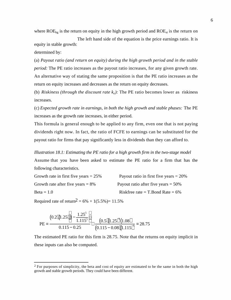
6

where ROEhg is the return on equity in the high growth period and ROEst is the return on

equity in stable growth:The left hand side of the equation is the price earnings ratio. It is

determined by:

(a) Payout ratio (and return on equity) during the high growth period and in the stable

period: The PE ratio increases as the payout ratio increases, for any given growth rate.

An alternative way of stating the same proposition is that the PE ratio increases as the

return on equity increases and decreases as the return on equity decreases.

(b) Riskiness (through the discount rate ke): The PE ratio becomes lower as riskiness

increases.

(c) Expected growth rate in earnings, in both the high growth and stable phases: The PE

increases as the growth rate increases, in either period.

This formula is general enough to be applied to any firm, even one that is not paying

dividends right now. In fact, the ratio of FCFE to earnings can be substituted for the

payout ratio for firms that pay significantly less in dividends than they can afford to.

Illustration 18.1: Estimating the PE ratio for a high growth firm in the two-stage model

Assume that you have been asked to estimate the PE ratio for a firm that has the

following characteristics.

Growth rate in first five years = 25% Payout ratio in first five years = 20%

Growth rate after five years = 8% Payout ratio after five years = 50%

Beta = 1.0 Riskfree rate = T.Bond Rate = 6%

Required rate of return2 = 6% + 1(5.5%)= 11.5%

PE =0.2( ) 1.25( ) 1− 1.255

1.1155

0.115 − 0.25+

0.5( ) 1.25( )51.08( )

0.115 − 0.08( ) 1.115( )5 = 28.75

The estimated PE ratio for this firm is 28.75. Note that the returns on equity implicit in

these inputs can also be computed.

2 For purposes of simplicity, the beta and cost of equity are estimated to be the same in both the highgrowth and stable growth periods. They could have been different.

7

Return on equity in first 5 years 31.25%.80

0.25

ratiopayout -1

rateGrowth ===

Return on equity in stable growth 16%0.5

0.08 ==

Illustration 18.2: Estimating a Fundamental PE ratio for Procter and Gamble

The following is an estimation of the appropriate PE ratio for Procter and Gamble

in May 2001. The assumptions on the growth period, growth rate and cost of equity are

identical to those used in the discounted cash flow valuation of P&G in Chapter 13. The

assumptions are summarized in Table 18.2.

Table 18.2: Summary Inputs for P& G

High Growth Period Stable Growth

Length 5 Forever after year 5

Cost of Equity 8.80% 9.40%

Expected Growth Rate 13.58% 5.00%

Payout Ratio 45.67% 66.67%

The current payout ratio of 45.67% is used for the entire high growth period. After year

5, the payout ratio is estimated based upon the expected growth rate of 5% and a return

on equity of 15% (based upon industry averages).

Stable period payout ratio 66.67%15%

5%-1

equityon Return

rateGrowth -1 ===

The price-earnings ratio can be estimated based upon these inputs.

PE =

0.4567( ) 1.1358( ) 1− (1.1358)5

(1.0880)5

0.0880-0.1358( )+

0.6667( ) 1.1358( )51.05( )

0.094 -0.05( ) 1.0880( )5 =22.33

Based upon its fundamentals, you would expect P&G to be trading at 22.33 times

earnings. Multiplied by the current earnings per share, you get a value per share of

$66.99, which is identical to the value obtained in Chapter 13, using the dividend discount

model.

PE Ratios and Expected Extraordinary Growth

8

The PE ratio of a high growth firm is a function of the expected extraordinary

growth rate - the higher the expected growth, the higher the PE ratio for a firm. In

Illustration 18.1, for instance, the PE ratio that was estimated to be 28.75, with a growth

rate of 25%, will change as that expected growth rate changes. Figure 18.2 graphs the PE

ratio as a function of the extraordinary growth rate during the high growth period.

As the firm's expected growth rate in the first five years declines from 25% to 5%, the PE

ratio for the firm also decreases from 28.75 to just above 10.

The effect of changes in the expected growth rate varies depending upon the level

of interest rates. In Figure 18.3, the PE ratios are estimated for different expected growth

rates at four levels of riskless rates – 4%, 6%, 8% and 10%.

Figure 18.2: PE Ratios and Expected Growth

0

10

20

30

40

50

60

70

80

5% 10% 15% 20% 25% 30% 35% 40% 45% 50%

Expected Growth: Next 5 years

PE

Ra

tio

9

The PE ratio is much more sensitive to changes in expected growth rates when interest

rates are low than when they are high. The reason is simple. Growth produces cash flows

in the future and the present value of these cash flows is much smaller at high interest

rates. Consequently the effect of changes in the growth rate on the present value tend to

be smaller.

There is a possible link between this finding and how markets react to earnings

surprises from technology firms. When a firm reports earnings that are significantly higher

than expected (a positive surprise) or lower than expected (a negative surprise), investors’

perceptions of the expected growth rate for this firm can change concurrently, leading to a

price effect. You would expect to see much greater price reactions for a given earnings

surprise, positive or negative, in a low-interest rate environment than you would in a

high-interest rate environment.

PE ratios and Risk

Figure 18.3: PE Ratios and Expected Growth: Interest Rate Scenarios

0

20

40

60

80

100

120

140

160

180

200

5% 10% 15% 20% 25% 30% 35% 40% 45% 50%

Expected Growth Rate

PE

r=4%r=6%

r=8%r=10%

10

The PE ratio is a function of the perceived risk of a firm and the effect shows up

in the cost of equity. A firm with a higher cost of equity will trade at a lower multiple of

earnings than a similar firm with a lower cost of equity.

Again, the effect of higher risk on PE ratios can be seen using the firm in

Illustration 18.1. Recall that the firm, which has an expected growth rate of 25% for the

next 5 years and 8% thereafter, has an estimated PE ratio of 28.75, if its beta is assumed

to be 1.

PE =0.2( ) 1.25( ) 1− 1.255

1.1155

0.115 − 0.25+

0.5( ) 1.25( )51.08( )

0.115 − 0.08( ) 1.115( )5 = 28.75

If you assume that the beta is 1.5, the cost of equity increases to 14.25%, leading

to a PE ratio of 14.87:

PE =0.2( ) 1.25( ) 1− 1.255

1.14255

0.1425 − 0.25+

0.5( ) 1.25( )51.08( )

0.1425 − 0.08( ) 1.1425( )5 =14.87

The higher cost of equity reduces the value created by expected growth.

In Figure 18.4, you can see the impact of changing the beta on the price earnings

ratio for four high growth scenarios – 8%, 15%, 20% and 25% for the next 5 years.

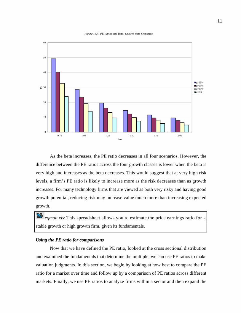
11

As the beta increases, the PE ratio decreases in all four scenarios. However, the

difference between the PE ratios across the four growth classes is lower when the beta is

very high and increases as the beta decreases. This would suggest that at very high risk

levels, a firm’s PE ratio is likely to increase more as the risk decreases than as growth

increases. For many technology firms that are viewed as both very risky and having good

growth potential, reducing risk may increase value much more than increasing expected

growth.

eqmult.xls: This spreadsheet allows you to estimate the price earnings ratio for a

stable growth or high growth firm, given its fundamentals.

Using the PE ratio for comparisons

Now that we have defined the PE ratio, looked at the cross sectional distribution

and examined the fundamentals that determine the multiple, we can use PE ratios to make

valuation judgments. In this section, we begin by looking at how best to compare the PE

ratio for a market over time and follow up by a comparison of PE ratios across different

markets. Finally, we use PE ratios to analyze firms within a sector and then expand the

Figure 18.4: PE Ratios and Beta: Growth Rate Scenarios

0

10

20

30

40

50

60

0.75 1.00 1.25 1.50 1.75 2.00

Beta

PE

g=25%g=20%g=15%g=8%

12

analysis to the entire market. In doing so, note that PE ratios vary across time, markets,

industries and firms because of differences in fundamentals - higher growth, lower risk and

higher payout generally result in higher PE ratios. When comparisons are made, you have

to control for these differences in risk, growth rates and payout ratios.

Comparing a Market’s PE ratio across time

Analysts and market strategists often compare the PE ratio of a market to its

historical average to make judgments about whether the market is under or over valued.

Thus, a market which is trading at a PE ratio which is much higher than its historical

norms is often considered to be over valued, whereas one that is trading at a ratio lower is

considered under valued.

While reversion to historic norms remains a very strong force in financial markets,

we should be cautious about drawing too strong a conclusion from such comparisons. As

the fundamentals (interest rates, risk premiums, expected growth and payout) change over

time, the PE ratio will also change. Other things remaining equal, for instance, we would

expect the following.

• An increase in interest rates should result in a higher cost of equity for the market and

a lower PE ratio.

• A greater willingness to take risk on the part of investors will result in a lower risk

premium for equity and a higher PE ratio across all stocks.

• An increase in expected growth in earnings across firms will result in a higher PE ratio

for the market.

• An increase in the return on equity at firms will result in a higher payout ratio for any

given growth rate (g = (1- Payout ratio)ROE) and a higher PE ratio for all firms.

In other words, it is difficult to draw conclusions about PE ratios without looking at these

fundamentals. A more appropriate comparison is therefore not between PE ratios across

time, but between the actual PE ratio and the predicted PE ratio based upon fundamentals

existing at that time.

Illustration 18.3: PE Ratios across time

13

The following are the summary economic statistics at two points in time for the

same stock market. The interest rates in the first period were significantly higher than the

interest rates in the second period.

Period 1 Period 2

T. Bond rate 11.00% 6.00%

Market premium 5.50% 5.50%

Expected inflation 5.00% 4.00%

Expected growth in real GNP 3.00% 2.50%

Average payout ratio 50% 50%

Expected PE ratio( )( )

0.08-0.165

1.080.5 ( )( )0.065-0.115

1.0650.5

= 6.35 = 10.65

The PE ratio in the second time period will be significantly higher than the PE ratio in the

first period, largely because of the drop in interest rates.

Illustration 18.4: PE Ratios across time for the S&P 500

Figure 18.5 summarizes the Earnings/Price ratios for S&P 500 and treasury bond

rates at the end of each year from 1960 to 2000.

14

There is a strong positive relationship between E/P ratios and T.Bond rates, as evidenced

by the correlation of 0.6854 between the two variables. In addition, there is evidence that

the term structure also affects the E/P ratio. In the following regression, we regress E/P

ratios against the level of T.Bond rates and the yield spread (T.Bond - T.Bill rate), using

data from 1960 to 2000.

E/P = 0.0188 + 0.7762 T.Bond Rate - 0.4066 (T.Bond Rate-T.Bill Rate) R2 = 0.495

(1.93) (6.08) (-1.37)

Other things remaining equal, this regression suggests that

• Every 1% increase in the T.Bond rate increases the E/P ratio by 0.7762%. This is not

surprising but it quantifies the impact that higher interest rates have on the PE ratio.

• Every 1% increase in the difference between T.Bond and T.Bill rates reduces the E/P

ratio by 0.4066%. Flatter or negative sloping term yield curves seem to correspond to

lower PE ratios and upwards sloping yield curves to higher PE ratios. While, at first

sight, this may seem surprising, the slope of the yield curve, at least in the United

Figure 18.5: S&P 500- Earnings Yield, T.Bond rate and Yield spread

-2.00%

0.00%

2.00%

4.00%

6.00%

8.00%

10.00%

12.00%

14.00%

16.00%

1960

1961

1962

1963

1964

1965

1966

1967

1968

1969

1970

1971

1972

1973

1974

1975

1976

1977

1978

1979

1980

1981

1982

1983

1984

1985

1986

1987

1988

1989

1990

1991

1992

1993

1994

1995

1996

1997

1998

1999

2000

Year

T.Bond Rate T.Bond-T.Bill E/P Ratios

15

States, has been a leading indicator of economic growth with more upward sloped

curves going with higher growth.

Based upon this regression, we predict E/P ratio at the beginning of 2001, with the T.Bill

rate at 4.9% and the T.Bond rate at 5.1%.

E/P2000 = 0.0188 + 0.7762 (0.054) – 0.4066 (0.051-0.049) = 0.0599 or 5.99%

PE2000 16.690.0599

1

E/P

1

2000

===

Since the S&P 500 was trading at a multiple of 25 times earnings in early 2001, this would

have indicated an over valued market.This regression can be enriched by adding other

variables, which should be correlated to the price-earnings ratio, such as expected growth

in GNP and payout ratios, as independent variables. In fact, a fairly strong argument can

be made that the influx of technology stocks into the S&P 500 over the last decade, the

increase in return on equity at U.S. companies over the same period and a decline in risk

premiums could all explain the increase in PE ratios over the period.

Comparing PE ratios across Countries

Comparisons are often made between price-earnings ratios in different countries

with the intention of finding undervalued and overvalued markets. Markets with lower PE

ratios are viewed as under valued and those with higher PE ratios are considered over

valued. Given the wide differences that exist between countries on fundamentals, it is

clearly misleading to draw these conclusions. For instance, you would expect to see the

following, other things remaining equal:

• Countries with higher real interest rates should have lower PE ratios than countries

with lower real interest rates.

• Countries with higher expected real growth should have higher PE ratios than

countries with lower real growth.

• Countries that are viewed as riskier (and thus command higher risk premiums) should

have lower PE ratios than safer countries

• Countries where companies are more efficient in their investments (and earn a higher

return on these investments) should trade at higher PE ratios.

Illustration 18.5: PE Ratios in markets with different fundamentals

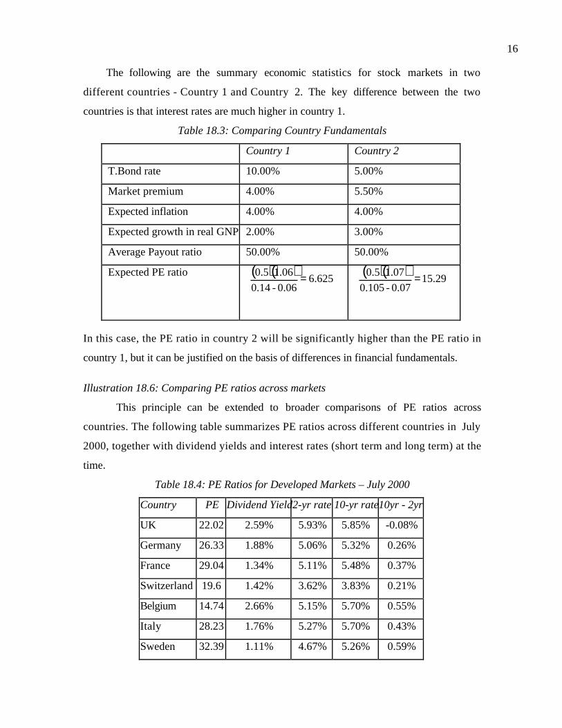
16

The following are the summary economic statistics for stock markets in two

different countries - Country 1 and Country 2. The key difference between the two

countries is that interest rates are much higher in country 1.

Table 18.3: Comparing Country Fundamentals

Country 1 Country 2

T.Bond rate 10.00% 5.00%

Market premium 4.00% 5.50%

Expected inflation 4.00% 4.00%

Expected growth in real GNP 2.00% 3.00%

Average Payout ratio 50.00% 50.00%

Expected PE ratio ( )( )

625.60.06-0.14

1.060.5 = ( )( )

29.150.07-0.105

1.070.5 =

In this case, the PE ratio in country 2 will be significantly higher than the PE ratio in

country 1, but it can be justified on the basis of differences in financial fundamentals.

Illustration 18.6: Comparing PE ratios across markets

This principle can be extended to broader comparisons of PE ratios across

countries. The following table summarizes PE ratios across different countries in July

2000, together with dividend yields and interest rates (short term and long term) at the

time.

Table 18.4: PE Ratios for Developed Markets – July 2000

Country PE Dividend Yield2-yr rate 10-yr rate10yr - 2yr

UK 22.02 2.59% 5.93% 5.85% -0.08%

Germany 26.33 1.88% 5.06% 5.32% 0.26%

France 29.04 1.34% 5.11% 5.48% 0.37%

Switzerland 19.6 1.42% 3.62% 3.83% 0.21%

Belgium 14.74 2.66% 5.15% 5.70% 0.55%

Italy 28.23 1.76% 5.27% 5.70% 0.43%

Sweden 32.39 1.11% 4.67% 5.26% 0.59%

17

Netherlands 21.1 2.07% 5.10% 5.47% 0.37%

Australia 21.69 3.12% 6.29% 6.25% -0.04%

Japan 52.25 0.71% 0.58% 1.85% 1.27%

United

States 25.14 1.10% 6.05% 5.85% -0.20%

Canada 26.14 0.99% 5.70% 5.77% 0.07%

A naive comparison of PE ratios suggests that Japanese stocks, with a PE ratio of 52.25,

are overvalued, while Belgian stocks, with a PE ratio of 14.74, are undervalued. There is,

however, a strong negative correlation between PE ratios and 10-year interest rates (-0.73)

and a positive correlation between the PE ratio and the yield spread (0.70). A cross-

sectional regression of PE ratio on interest rates and expected growth yields the following.

PE Ratio = 42.62 – 360.9 (10-year rate) + 846.6 (10-year rate– 2-year rate) R2=59%

(2.78) (-1.42) (1.08)

The coefficients are of marginal significance, partly because of the small size of the

sample. Based upon this regression, the predicted PE ratios for the countries are shown in

Table 18.5.

Table 18.5:Predicted PE Ratios for Developed Markets – July 2000

Country Actual PE Predicted PE

Under or Over

Valued

UK 22.02 20.83 5.71%

Germany 26.33 25.62 2.76%

France 29.04 25.98 11.80%

Switzerland 19.6 30.58 -35.90%

Belgium 14.74 26.71 -44.81%

Italy 28.23 25.69 9.89%

Sweden 32.39 28.63 13.12%

Netherlands 21.1 26.01 -18.88%

Australia 21.69 19.73 9.96%

Japan 52.25 46.70 11.89%

18

United

States 25.14 19.81 26.88%

Canada 26.14 22.39 16.75%

From this comparison, Belgian and Swiss stocks would be the most undervalued, while

U.S. stocks would have been most over valued.

Illustration 18.7: An Example with Emerging Markets

This example is extended to examine PE ratio differences across emerging markets at

the end of 2000. In this table, the country risk factor is estimated by The Economist for

the emerging markets. It is scaled from zero (safest) to one hundred (riskiest).

Table 18.6: PE Ratios and Key statistics: Emerging Markets

Country PE Ratio Interest Rates GDP Real Growth Country Risk

Argentina 14 18.00% 2.50% 45

Brazil 21 14.00% 4.80% 35

Chile 25 9.50% 5.50% 15

Hong Kong 20 8.00% 6.00% 15

India 17 11.48% 4.20% 25

Indonesia 15 21.00% 4.00% 50

Malaysia 14 5.67% 3.00% 40

Mexico 19 11.50% 5.50% 30

Pakistan 14 19.00% 3.00% 45

Peru 15 18.00% 4.90% 50

Phillipines 15 17.00% 3.80% 45

Singapore 24 6.50% 5.20% 5

South Korea 21 10.00% 4.80% 25

Thailand 21 12.75% 5.50% 25

Turkey 12 25.00% 2.00% 35

Venezuela 20 15.00% 3.50% 45

Interest Rates: Short term interest rates in these countries

19

The regression of PE ratios on these variables provides the following –

PE = 16.16 – 7.94 Interest Rates + 154.40 Real Growth - 0.112 Country Risk R2=74%

(3.61) (-0.52) (2.38) (-1.78)

Countries with higher real growth and lower country risk have higher PE ratios, but the

level of interest rates seems to have only a marginal impact. The regression can be used to

estimate the price earnings ratio for Turkey.

Predicted PE for Turkey = 16.16 – 7.94 (0.25) + 154.40 (0.02) - 0.112 (35) = 13.35

At a PE ratio of 12, the market can be viewed as slightly under valued.

Comparing PE Ratios across firms in a sector

The most common approach to estimating the PE ratio for a firm is to choose a

group of comparable firms, to calculate the average PE ratio for this group and to

subjectively adjust this average for differences between the firm being valued and the

comparable firms. There are several problems with this approach. First, the definition of a

'comparable' firm is essentially a subjective one. The use of other firms in the industry as

the control group is often not the solution because firms within the same industry can

have very different business mixes and risk and growth profiles. There is also plenty of

potential for bias. One clear example of this is in takeovers, where a high PE ratio for the

target firm is justified, using the price-earnings ratios of a control group of other firms that

have been taken over. This group is designed to give an upward biased estimate of the PE

ratio and other multiples. Second, even when a legitimate group of comparable firms can

be constructed, differences will continue to persist in fundamentals between the firm

being valued and this group. It is very difficult to subjectively adjust for differences

across firms. Thus, knowing that a firm has much higher growth potential than other firms

in the comparable firm list would lead you to estimate a higher PE ratio for that firm, but

how much higher is an open question.

The alternative to subjective adjustments is to control explicitly for the one or two

variables that you believe account for the bulk of the differences in PE ratios across

companies in the sector in a regression. The regression equation can then be used to

estimate predicted PE ratios for each firm in the sector and these predicted values can be

20

compared to the actual PE ratios to make judgments on whether stocks are under or over

priced.

Illustration 18.8: Comparing PE ratios for Global telecomm firms

The following table summarizes the trailing PE ratios for global telecomm firms

with ADRs listed in the United States in September 2000. The earnings per share used are

those estimated using generally accepted accounting principles in the United States and

thus should be much more directly comparable than the earnings reported by these firms

in their local markets.

Table 18.7: PE Ratios, Expected Growth and Market Status

Company Name PE Growth

Emerging Market

Dummy

APT Satellite Holdings ADR 31.00 33.00% 1

Asia Satellite Telecom Holdings ADR 19.60 16.00% 1

British Telecommunications PLC ADR 25.70 7.00% -

Cable & Wireless PLC ADR 29.80 14.00% -

Deutsche Telekom AG ADR 24.60 11.00% -

France Telecom SA ADR 45.20 19.00% -

Gilat Communications 22.70 31.00% 1

Hellenic Telecommunication Organization SA

ADR 12.80 12.00% 1

Korea Telecom ADR 71.30 44.00% 1

Matav RT ADR 21.50 22.00% 1

Nippon Telegraph & Telephone ADR 44.30 20.00% -

Portugal Telecom SA ADR 20.80 13.00% -

PT Indosat ADR 7.80 6.00% 1

Royal KPN NV ADR 35.70 13.00% -

Swisscom AG ADR 18.30 11.00% -

Tele Danmark AS ADR 27.00 9.00% -

Telebras ADR 8.90 7.50% 1

21

Telecom Argentina Stet - France Telecom SA

ADR B 12.50 8.00% 1

Telecom Corporation of New Zealand ADR 11.20 11.00% -

Telecom Italia SPA ADR 42.20 14.00% -

Telecomunicaciones de Chile ADR 16.60 8.00% 1

Telefonica SA ADR 32.50 18.00% -

Telefonos de Mexico ADR L 21.10 14.00% 1

Telekomunikasi Indonesia ADR 28.40 32.00% 1

Telstra ADR 21.70 12.00% -

The earnings per share represent trailing earnings and the price earnings ratios for each

firm are reported in the second column. The analyst estimates of expected growth in

earnings per share over the next 5 years are shown in the next column. In the last column,

we introduce a dummy variable indicating whether the firm is from an emerging market or

a developed one, since emerging market telecomm firms are likely to be exposed to far

more risk. Not surprisingly, the firms with the lowest PE ratios, such as Telebras and

Indosat, are from emerging markets.

Regressing the PE ratio for the sector against the expected growth rate and the

emerging market dummy yields the following results.

PE Ratio = 13.12 + 121.22 Expected Growth – 13.85 Emerging Market R2 =66%

(3.78) (6.29) (-3.84)

Firms with higher growth have significantly higher PE ratios than firms with lower

expected growth. In addition, this regression indicates that an emerging market telecomm

firm should trade at a much lower PE ratio than one in a developed market. Using this

regression to get predicted values, we get the predicted PE ratios.

Table 18.8: Predicted PE ratios – Global Telecomm firms

Company Name PE Predicted PE Under or Over

Valued

APT Satellite Holdings ADR 31 39.27 -21.05%

Asia Satellite Telecom Holdings ADR 19.6 18.66 5.05%

22

British Telecommunications PLC ADR 25.7 21.60 18.98%

Cable & Wireless PLC ADR 29.8 30.09 -0.95%

Deutsche Telekom AG ADR 24.6 26.45 -6.99%

France Telecom SA ADR 45.2 36.15 25.04%

Gilat Communications 22.7 36.84 -38.38%

Hellenic Telecommunication Organization SA

ADR

12.8 13.81 -7.31%

Korea Telecom ADR 71.3 52.60 35.55%

Matav RT ADR 21.5 25.93 -17.09%

Nippon Telegraph & Telephone ADR 44.3 37.36 18.58%

Portugal Telecom SA ADR 20.8 28.87 -27.96%

PT Indosat ADR 7.8 6.54 19.35%

Royal KPN NV ADR 35.7 28.87 23.64%

Swisscom AG ADR 18.3 26.45 -30.81%

Tele Danmark AS ADR 27 24.03 12.38%

Telebras ADR 8.9 8.35 6.54%

Telecom Argentina Stet - France Telecom SA

ADR B

12.5 8.96 39.51%

Telecom Corporation of New Zealand ADR 11.2 26.45 -57.66%

Telecom Italia SPA ADR 42.2 30.09 40.26%

Telecomunicaciones de Chile ADR 16.6 8.96 85.27%

Telefonica SA ADR 32.5 34.94 -6.97%

Telefonos de Mexico ADR L 21.1 16.23 29.98%

Telekomunikasi Indonesia ADR 28.4 38.05 -25.37%

Telstra ADR 21.7 27.66 -21.55%

Based upon the predicted PE ratios, Telecom Corporation of New Zealand is the most

under valued firm in this group and Telecom de Chile is the most overvalued firm.

Comparing PE ratios across firms in the market

23

In the last section, comparable firms were narrowly defined to be other firms in

the same business. In this section, we consider ways in which we can expand the number

of comparable firms by looking at an entire sector or even the market. There are two

advantages in doing this. The first is that the estimates may become more precise as the

number of comparable firms increase. The second is that it allows you to pinpoint when

firms in a small sub-group are being under or over valued relative to the rest of the sector

or the market. Since the differences across firms will increase when you loosen the

definition of comparable firms, you have to adjust for these differences. The simplest

way of doing this is with a multiple regression, with the PE ratio as the dependent

variable and proxies for risk, growth and payout forming the independent variables.

A. Past studies

One of the earliest regressions of PE ratios against fundamentals across the entire

market was done by Kisor and Whitbeck in 1963. Using data from the Bank of New York

as of June 1962 for 135 stocks, they arrived at the following regression.

P/E = 8.2 + 1.5 (Growth rate in Earnings) + 6.7 (Payout ratio) - 0.2 (Standard

Deviation in EPS changes)

Cragg and Malkiel followed up by estimating the coefficients for a regression of the price-

earnings ratio on the growth rate, the payout ratio and the beta for stocks for the time

period from 1961 to 1965.

Year Equation R2

1961 P/E = 4.73 + 3.28 g + 2.05 π - 0.85 β 0.70

1962 P/E = 11.06 + 1.75 g + 0.78 π - 1.61 β 0.70

1963 P/E = 2.94 + 2.55 g + 7.62 π - 0.27 β 0.75

1964 P/E = 6.71 + 2.05 g + 5.23 π - 0.89 β 0.75

1965 P/E = 0.96 + 2.74 g + 5.01 π - 0.35 β 0.85

where,

P/E = Price/Earnings Ratio at the start of the year

g = Growth rate in Earnings

π = Earnings payout ratio at the start of the year

β = Beta of the stock

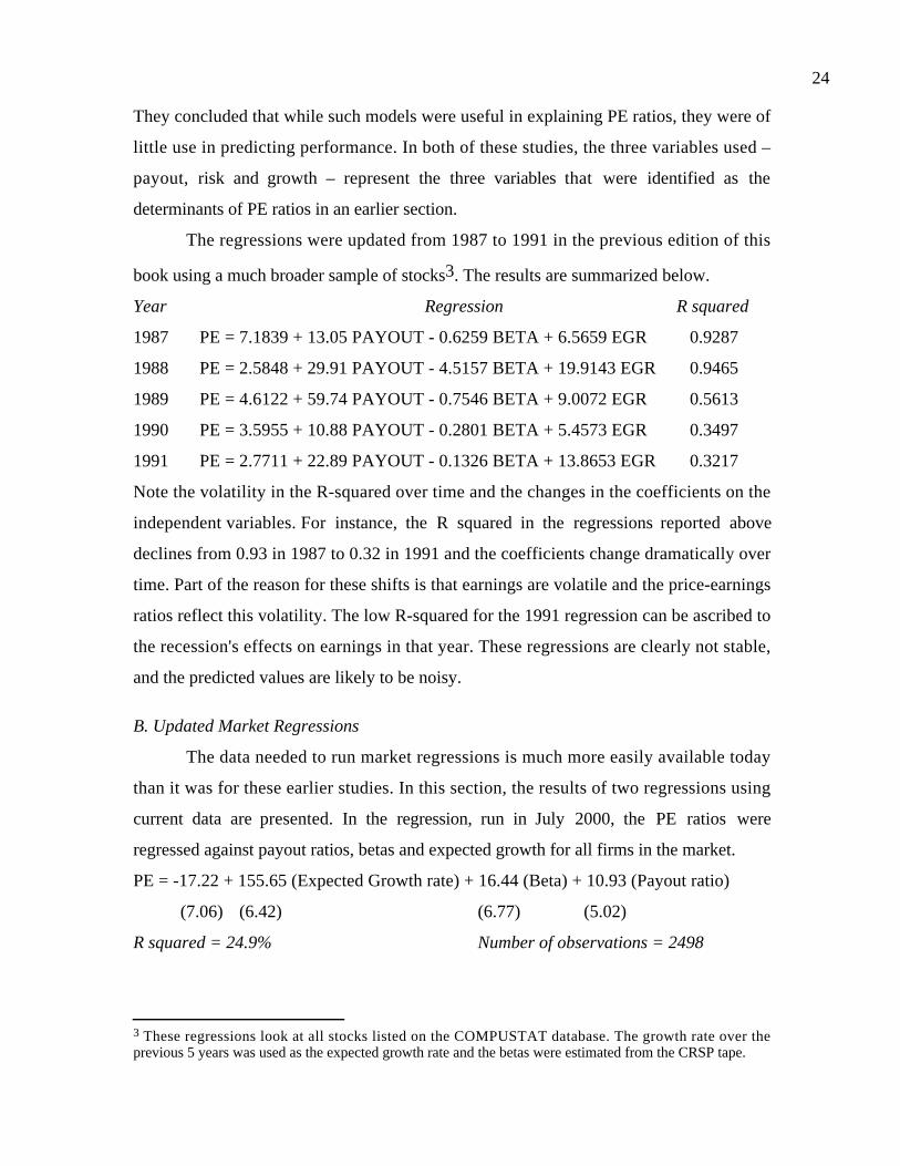
24

They concluded that while such models were useful in explaining PE ratios, they were of

little use in predicting performance. In both of these studies, the three variables used –

payout, risk and growth – represent the three variables that were identified as the

determinants of PE ratios in an earlier section.

The regressions were updated from 1987 to 1991 in the previous edition of this

book using a much broader sample of stocks3. The results are summarized below.

Year Regression R squared

1987 PE = 7.1839 + 13.05 PAYOUT - 0.6259 BETA + 6.5659 EGR 0.9287

1988 PE = 2.5848 + 29.91 PAYOUT - 4.5157 BETA + 19.9143 EGR 0.9465

1989 PE = 4.6122 + 59.74 PAYOUT - 0.7546 BETA + 9.0072 EGR 0.5613

1990 PE = 3.5955 + 10.88 PAYOUT - 0.2801 BETA + 5.4573 EGR 0.3497

1991 PE = 2.7711 + 22.89 PAYOUT - 0.1326 BETA + 13.8653 EGR 0.3217

Note the volatility in the R-squared over time and the changes in the coefficients on the

independent variables. For instance, the R squared in the regressions reported above

declines from 0.93 in 1987 to 0.32 in 1991 and the coefficients change dramatically over

time. Part of the reason for these shifts is that earnings are volatile and the price-earnings

ratios reflect this volatility. The low R-squared for the 1991 regression can be ascribed to

the recession's effects on earnings in that year. These regressions are clearly not stable,

and the predicted values are likely to be noisy.

B. Updated Market Regressions

The data needed to run market regressions is much more easily available today

than it was for these earlier studies. In this section, the results of two regressions using

current data are presented. In the regression, run in July 2000, the PE ratios were

regressed against payout ratios, betas and expected growth for all firms in the market.

PE = -17.22 + 155.65 (Expected Growth rate) + 16.44 (Beta) + 10.93 (Payout ratio)

(7.06) (6.42) (6.77) (5.02)

R squared = 24.9% Number of observations = 2498

3 These regressions look at all stocks listed on the COMPUSTAT database. The growth rate over theprevious 5 years was used as the expected growth rate and the betas were estimated from the CRSP tape.

25

With the sample size expanding to about 2500 firms, this regression represents the

broadest measure of relative value.

This regression has a low R-squared, but it is more a reflection of the noise in PE

ratios than it is on the regression methodology. As you will see, the market regressions

for Price to book value and Price to sales ratios tend to be better behaved and have higher

R-squared than PE ratio regressions. The other disquieting finding is that the coefficients

on the variables do not always have the signs you would expect them to have. For

instance, higher risk stocks (higher betas) have higher PE ratios, when fundamentals

would lead you to expect the opposite.

C. Problems with the regression methodology

The regression methodology is a convenient way of compressing large amounts of

data into one equation capturing the relationship between PE ratios and financial

fundamentals. But it does have its limitations. First, the independent variables are

correlated with each other4. For example, high growth firms tend to have high risk and

low payout ratios, as is clear from Table 18.9, which summarizes the correlation between

beta, growth and payout ratios for all U.S. firms:

Table 18.9: Correlations between Independent Variables

PE Growth Beta Payout Ratio

PE 1.000

Growth rate 0.288 1.000

Beta 0.141 0.292** 1.000

Payout Ratio -0.087 -0.404** -0.183** 1.000

** Significant at 1% level

Note the negative correlation between payout ratios and growth and the positive

correlation between beta and growth. This “multi-colinearity” makes the coefficients of

the regressions unreliable and may explain the 'wrong' signs on the coefficients and the

large changes in these coefficients from period to period. Second, the regression is based

on a linear relationship between PE ratios and the fundamentals and that might not be

4 In a multiple regression, the independent variables should be independent of each other.

26

appropriate. An analysis of the residuals from a regression may suggest transformations

of the independent variables (squared, natural logs) that work better in explaining PE

ratios. Third, the basic relationship between PE ratios and financial variables itself might

not be stable and, if it shifts from year to year, the predictions from the regression

equation may not be reliable for extended periods. For all these reasons, the regression

approach is useful but it has to be viewed as one more tool in the search for true value.

Illustration 18.9: Valuing Procter and Gamble using the market regression

To value P&G using the broader regressions, you would first have to estimate the

values, for P&G, of the independent variables in the regression.

P&G’s Beta = 0.85

P&G’s Payout ratio = 45.67%

P&G’s Expected Growth rate = 13.58%

Note that these variables have been defined consistently with the variables in the

regression. Thus, the growth rate over the next 5 years, the beta over the last 5 years and

the payout ratio over the most recent four quarters are used to make the prediction.

Based upon the price-earnings ratio regression for all stocks in the market, you would get

a predicted PE ratio.

Predicted PEP&G= -17.22 + 155.65 (Growth) + 16.44 (Beta) + 10.93 (Payout)

= -17.22 + 155.65 (0.1358) + 16.44 (0.85) + 10.93 (0.4567)

= 22.88

Based upon the market regression, you would expect P&G to be trading at 22.88 times

earnings.

pereg.htm: This reports the results of the latest regression of PE ratios against

fundamentals, using all firms in the market.

Normalizing Earnings for PE ratios

The dependence of PE ratios on current earnings makes them particularly

vulnerable to the year-to-year swings that often characterize reported earnings. In making

comparisons, therefore, it may make much more sense to use normalized earnings. The

process used to normalize earnings varies widely but the most common approach is a

27

simple averaging of earnings across time. For a cyclical firm, for instance, you would

average the earnings per share across a cycle. In doing so, you should adjust for inflation.

If you do decide to normalize earnings for the firm you are valuing, consistency demands

that you normalize it for the comparable firms in the sample as well.

The PEG Ratio

Portfolio managers and analysts sometimes compare PE ratios to the expected

growth rate to identify undervalued and overvalued stocks. In the simplest form of this

approach, firms with PE ratios less than their expected growth rate are viewed as

undervalued. In its more general form, the ratio of PE ratio to growth is used as a measure

of relative value, with a lower value believed to indicate that a firm is under valued. For

many analysts, especially those tracking firms in high-growth sectors, these approaches

offer the promise of a way of controlling for differences in growth across firms, while

preserving the inherent simplicity of a multiple.

Definition of the PEG Ratio

The PEG ratio is defined to be the price earnings ratio divided by the expected

growth rate in earnings per share:

PEG ratio RateGrowth Expected

ratio PE=

For instance, a firm with a PE ratio of 20 and a growth rate of 10% is estimated to have a

PEG ratio of 2. Consistency requires the growth rate used in this estimate be the growth

rate in earnings per share, rather than operating income, because this is an equity multiple.

Given the many definitions of the PE ratio, which one should you use to estimate

the PEG ratio? The answer depends upon the base on which the expected growth rate is

computed. If the expected growth rate in earnings per share is based upon earnings in the

most recent year (current earnings), the PE ratio that should be used is the current PE

ratio. If it based upon trailing earnings, the PE ratio used should be the trailing PE ratio.

The forward PE ratio should never be used in this computation, since it may result in a

double counting of growth. To see why, assume that you have a firm with a current price

of $30 and current earnings per share of $1.50. The firm is expected to double its earnings

per share over the next year (forward earnings per share will be $3.00) and then have

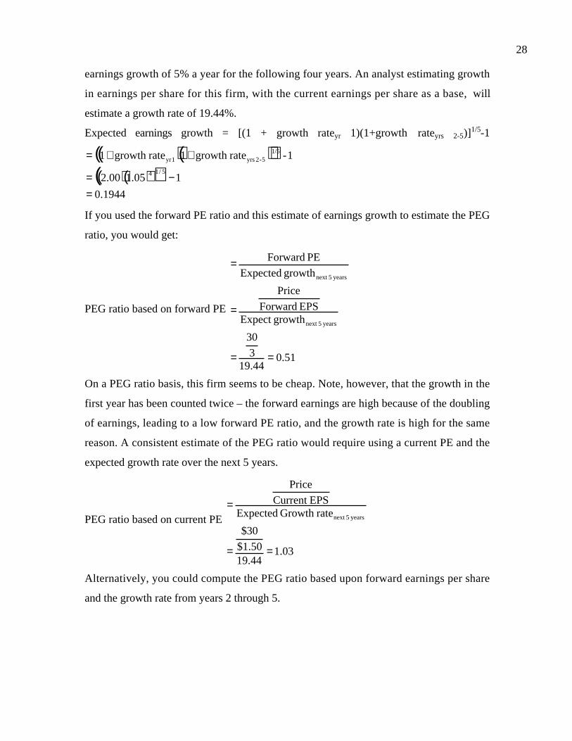
28

earnings growth of 5% a year for the following four years. An analyst estimating growth

in earnings per share for this firm, with the current earnings per share as a base, will

estimate a growth rate of 19.44%.

Expected earnings growth = [(1 + growth rateyr 1)(1+growth rateyrs 2-5)]1/5-1

( )( )( )( )( )( )

1944.0

105.100.2

1-rategrowth 1rategrowth 15/14

1/55-2 yrs1yr

=−=

++=

If you used the forward PE ratio and this estimate of earnings growth to estimate the PEG

ratio, you would get:

PEG ratio based on forward PE

51.044.19

3

30

growthExpect EPS Forward

Price

growth Expected

PE Forward

years 5next

years 5next

==

=

=

On a PEG ratio basis, this firm seems to be cheap. Note, however, that the growth in the

first year has been counted twice – the forward earnings are high because of the doubling

of earnings, leading to a low forward PE ratio, and the growth rate is high for the same

reason. A consistent estimate of the PEG ratio would require using a current PE and the

expected growth rate over the next 5 years.

PEG ratio based on current PE

03.144.1950.1$

30$

rateGrowth ExpectedEPSCurrent

Price

years 5next

==

=

Alternatively, you could compute the PEG ratio based upon forward earnings per share

and the growth rate from years 2 through 5.

29

PEG ratio based upon forward PE

00.253$

30$

growth ExpectedEPS Forward

Price

5-2 yrs

==

=

If this approach is used, the PEG ratio would have to be estimated uniformally for all of

the other comparable firms as well, using the forward PE and the expected growth rate

from years 2 through 5.

Building upon the theme of uniformity, the PEG ratio should be estimated using

the same growth estimates for all firms in the sample. You should not, for instance, use 5-

year growth rates for some firms and 1-year growth rates for others. One way of ensuring

uniformity is to use the same source for earnings growth estimates for all the firms in the

group. For instance, both I/B/E/S and Zacks provide consensus estimates from analysts of

earnings per share growth over the next 5 years for most U.S. firms.

Cross Sectional Distribution of the PEG Ratio

Now that the PEG ratio has been defined, the cross sectional distribution of PEG

ratios across all U.S. firms is examined in Figure 18.6.

Figure 18.6: PEG RatiosU.S. Stocks- July 2000

0

50

100

150

200

250

300

350

400

450

<0.25 0.25-0.5 0.5-0.75 0.75-1.00 1-1.25 1.25-1.5 1.5-1.75 1.75-2.00 2-2.5 2.5-3 3 - 4 4 - 5 >5

30

In estimating these PEG ratios, the analyst estimates of growth in earnings per share over

the next 5 years is used in conjunction with the current PE. Any firm, therefore, that has

negative earnings per share or lacks an analyst estimate of expected growth is dropped

from the sample. This may be a source of bias, since larger and more liquid firms are more

likely to be followed by analysts.

PEG ratios are most widely used in analyzing technology firms. Figure 18.7

contains the distribution of PEG ratios for technology stocks, using analyst estimates of

growth again to arrive at the PEG ratios.

Note that of the 448 firms for which PE ratios were estimated, only 335 have PEG ratios

available; the 113 firms for which analyst estimates of growth were not available have

been dropped from the sample.

Finally, Table 18.10 includes the summary statistics for PEG ratios for

technology stocks and non-technology stocks5.

5 The PEG ratio is capped at 10.

Figure 18.7: PEG Ratios for Technology StocksUnited States - July 2000

0

5

10

15

20

25

30

35

<0.25 0.25-0.5 0.5-0.75 0.75-1.00 1-1.25 1.25-1.5 1.5-1.75 1.75-2.00 2-2.5 2.5-3 3 - 4 4 - 5 >5

31

Table 18.10: PEG Ratios: Technology versus Non-technology Stocks

Technology Stocks Non-technology stocks All Stocks

Mean 5.83 2.99 3.31

Standard Error 1.03 0.36 0.34

Median 2.03 1.13 1.18

Standard Deviation 18.05 17.68 17.74

Skewness 7.81 22.09 20.33

Range 198.62 569.73 569.73

Minimum 0.08 0.00 0.00

Maximum 198.70 569.73 569.73

Number of firms 309 2454 2763

The mean PEG ratio for technology stocks is much higher than the mean PEG ratio for

non-technology stocks. In addition, the mean is much higher than the median for both

groups.

pedata.xls: This dataset summarizes the PEG ratios by industry for firms in the

United States.

Determinants of the PEG Ratio

The determinants of the PEG ratio can be extracted using the same approach used

to estimate the determinants of the PE ratio. The value per share in a two-stage dividend

discount model can be written as:

P0 =

EPS0( ) Payout Ratio( ) 1+g( ) 1− 1+g( )n

1+k e,hg( )n

k e,hg -g+

EPS0( ) Payout Ration( ) 1+g( )n1+g n( )

k e,st -g n( ) 1+k e,hg( )n

Dividing both sides of the equation by the earnings per share (EPS0) first and the expected

growth rate over the high growth period (g) next, you can estimate the PEG ratio.

32

PEG =

Payout Ratio( ) 1+g( ) 1−1+g( )n

1+k e,hg( )n

g k e,hg -g( ) + Payout Ratio n( ) 1+g( )n

1+g n( )g k e,st -g n( ) 1+k e,hg( )n

Even a cursory glance at this equation suggests that analysts who believe that using the

PEG ratio neutralizes the growth effect are mistaken. Instead of disappearing, the growth

rate becomes even more deeply entangled in the multiple. In fact, as the growth rate

increases, the effects on the PEG ratio can be both positive and negative and the net effect

can vary depending upon the level of the growth rate.

Illustration 18.10: Estimating the PEG ratio for a firm

Assume that you have been asked to estimate the PEG ratio for a firm which has

the same characteristics as the firm described in Illustration 18.1.

Growth rate in first five years = 25% Payout ratio in first five years = 20%

Growth rate after five years = 8% Payout ratio after five years = 50%

Beta = 1.0 Riskfree rate = T.Bond Rate = 6%

Required rate of return = 6% + 1(5.5%)= 11.5%

The PEG ratio can be estimated as follows:

PEG =

0.2( ) 1.25( ) 1−1.25( )5

1.115( )5

0.25 0.115-0 .25( )+

0.5( ) 1.25( )51.08( )

0.25 0.115-0.08( ) 1.115( )5 =115 or 1.15

The PEG ratio for this firm, based upon fundamentals, is 1.15.

Exploring the relationship with fundamentals

Consider first the effect of changing the growth rate during the high growth period

(next 5 years) from 25%. Figure 18.8 presents the PEG ratio as a function of the expected

growth rate:

33

As the growth rate increases, the PEG ratio initially decreases, but then starts increasing

again. This U-shaped relationship between PEG ratios and growth suggests that

comparing PEG ratios across firms with widely different growth rates can be complicated.

Next, consider the effect of changing the riskiness (beta) of this firm on the PEG

ratio. Figure 18.9 presents the PEG ratio as a function of the beta.

Figure 18.8: PEG Ratios, Expected Growth and Interest Rates

0.00

0.50

1.00

1.50

2.00

2.50

3.00

5% 10% 15% 20% 25% 30% 35% 40% 45% 50%

Expected Growth Rate

PEG

Rat

io r=6%r=8%

r=10%

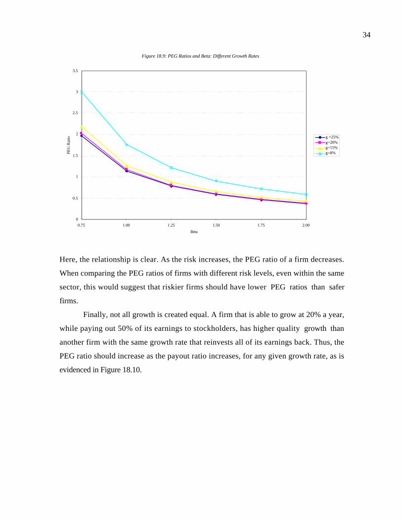
34

Here, the relationship is clear. As the risk increases, the PEG ratio of a firm decreases.

When comparing the PEG ratios of firms with different risk levels, even within the same

sector, this would suggest that riskier firms should have lower PEG ratios than safer

firms.

Finally, not all growth is created equal. A firm that is able to grow at 20% a year,

while paying out 50% of its earnings to stockholders, has higher quality growth than

another firm with the same growth rate that reinvests all of its earnings back. Thus, the

PEG ratio should increase as the payout ratio increases, for any given growth rate, as is

evidenced in Figure 18.10.

Figure 18.9: PEG Ratios and Beta: Different Growth Rates

0

0.5

1

1.5

2

2.5

3

3.5

0.75 1.00 1.25 1.50 1.75 2.00

Beta

PEG

Rat

io g =25%g=20%g=15%g=8%

35

The growth rate and the payout ratio are linked by the firm’s return on equity. In fact, the

expected growth rate of a firm can be written as:

Expected Growth rate = (Return on equity)(1 – Payout ratio)

The PEG ratio should therefore be higher for firms with higher returns on equity.

eqmult.xls: This spreadsheet allows you to estimate the price earnings ratio for a

stable growth or high growth firm, given its fundamentals.

Using the PEG Ratio for Comparisons

As with the PE ratio, the PEG ratio is used to compare the valuations of firms

that are in the same business. As noted in the last section, the PEG ratio is a function of

the risk, growth potential and the payout ratio of a firm. In this section, you look at ways

of using the PEG ratio and examine some of the problems in comparing PEG ratios across

firms.

Direct Comparisons

Figure 18.10: PEG Ratios and Retention Ratios

0

0.2

0.4

0.6

0.8

1

1.2

1.4

1.6

0% 20% 40% 60% 80% 100%

Payout Ratio

PEG

Rat

io

PEG

36

Most analysts who use PEG ratios compute them for firms within a business (or

comparable firm group) and compare these ratios. Firms with lower PEG ratios are

usually viewed as undervalued, even if growth rates are different across the firms being

compared. This approach is based upon the incorrect perception that PEG ratios control

for differences in growth. In fact, direct comparisons of PEG ratios work only if firms are

similar in terms of growth potential, risk and payout ratios (or returns on equity). If this

were the case, however, you could just as easily compare PE ratios across firms.

When PEG ratios are compared across firms with different risk, growth and

payout characteristics and judgments are made about valuations based on this

comparison, you will tend to find that:

• Lower growth firms will have higher PEG ratios and look more over valued than

higher growth firms, because PEG ratios tend to decrease as the growth rate decreases,

at least initially (see Figure 18.8).

• Higher risk firms will have lower PEG ratios and look more under valued than higher

risk firms, because PEG ratios tend to decrease as a firm’s risk increases (see Figure

18.9).

• Firms with lower returns on equity (or lower payout ratios) will have lower PEG

ratios and look more under valued than firms with higher returns on equity and higher

payout ratios (see Figure 18.10).

In short, firms that look under valued based upon direct comparison of the PEG ratios

may in fact be firms with higher risk, higher growth or lower returns on equity that are, in

fact, correctly valued.

Controlled Comparisons

When comparing PEG ratios across firms, then, it is important that you control

for differences in risk, growth and payout ratios when making the comparison. While you

can attempt to do this subjectively, the complicated relationship between PEG ratios and

these fundamentals can pose a challenge. A far more promising route is to use the

regression approach suggested for PE ratios and to relate the PEG ratios of the firms being

compared to measures of risk, growth potential and the payout ratio.

37

As with the PE ratio, the comparable firms in this analysis can be defined

narrowly (as other firms in the same business), more expansively as firms in the same

sector or as all firms in the market. In running these regressions, all the caveats that were

presented for the PE regression continue to apply. The independent variables continue to

be correlated with each other and the relationship is both unstable and likely to be non-

linear. In fact, Figure 18.11, which provides a scatter plot of PEG ratios against growth

rates, for all U.S. stocks in July 2000, indicates the degree of non-linearity.

Figure 18.11: PEG Ratios versus Expected Growth Rates

1

2

3

4

5

0.2 0.4 0.6 0.8

Expected Growth in EPS: next 5…

PEG

In running the regression, especially when the sample contains firms with very different

levels of growth, you should transform the growth rate to make the relationship more

linear. A scatter plot of PEG ratios against the natural log of the expected growth rate, for

instance, yields a much more linear relationship.

Figure 18.12: PEG Ratios versus ln(Expected Growth Rate)

38

1

2

3

4

5

-5.00 -3.75 -2.50 -1.25

lnGrowth

PEG

The results of the regression of PE ratios against ln(expected growth), beta and payout

ratio is reported below for the entire market and for technology stocks.

Entire Market

PEG Ratio = -0.25 – 0.44 ln(Growth) + 0.95 (Beta) + 0.71 (Payout)

(1.76) (10.40) (9.66) (7.95)

R squared = 9.0% Number of firms = 2594

Only Technology Stocks

PEG Ratio = 1.24 + 0.80 ln(Growth) + 2.45 (Beta) – 1.96 (Payout)

(1.27) (2.20) (4.15) (0.73)

R squared = 11.0% Number of firms = 274

The low R-squared is indicative of the problems with this multiple and the difficulties

you will run into in using it in comparisons across firms.

39

Illustration 18.11: Estimating and Using the PEG ratio for Data Networking firms

The following table summarizes the PEG ratios of the firms that are considered

data networking firms as of June 2000.

Table 18.11: PEG Ratios for Data Networking Firms

Company Name PE Beta Projected Growth PEG

3Com Corp. 37.20 1.35 11.00% 3.38

ADC Telecom. 78.17 1.40 24.00% 3.26

Alcatel ADR 51.50 0.90 24.00% 2.15

Ciena Corp. 94.51 1.70 27.50% 3.44

Cisco 133.76 1.43 35.20% 3.80

Comverse Technology 70.42 1.45 28.88% 2.44

E-TEK Dynamics 295.56 1.55 55.00% 5.37

JDS Uniphase 296.28 1.60 65.00% 4.56

Lucent Technologies 54.28 1.30 24.00% 2.26

Nortel Networks 104.18 1.40 25.50% 4.09

Tellabs, Inc. 52.57 1.75 22.00% 2.39

Average 115.31 1.44 31.10% 3.38

Consider Cisco. Cisco with a PEG ratio of 3.80 is trading at a higher PEG ratio than the

average for the sector, suggesting, at least on a preliminary basis, an over valued stock.

Regressing the PEG ratio against the ln(expected growth rate) in this sector yields:

PEG Ratio = 5.06 + 1.33 ln(Expected Growth Rate) R squared = 29.6%

For Cisco, with an expected growth rate of 35.20%, the predicted PEG ratio based upon

this regression is:

Predicted PEG ratio = 5.06 + 1.33 ln(0.352) = 4.02

Cisco’s actual PEG ratio is very close to this predicted value.

The predicted PEG ratio for Cisco can also be estimated using the broader

regressions, across the technology sector and the market, reported in the last section.

Predicted PEGMarket = -0.25 – 0.44 ln(0.352) + 0.95 (1.43) + 0.71 (0) =1.57

Predicted PEGTechnology = 1.24 + 0.80 ln(0.352) + 2.45 (1.43) – 1.96 (0) = 3.91

40

Cisco looks over valued when compared with the rest of the market, but is fairly valued

when compared to just technology stocks.

pegreg.xls: This summarizes the results of the most recent regression of PEG

ratios against fundamentals for U.S. stocks.

Whose Growth rate?

In computing PEG ratios, we are often faced with the question of whose growth rate we

will use in estimating the PEG ratios. If the number of firms in the sample is small, you

could estimate expected growth for each firm yourself. If the number of firms increases,

you will have no choice but to use analyst estimates of expected growth for the firms.

Will this expose your analyses to all of the biases in these estimates? Not necessarily. If

the bias is uniform – for instance, analysts over estimate growth for all of the firms in the

sector – you will still be able to make comparisons of PEG ratios across firms and draw

reasonable conclusions.

Other Variants on the PE ratio

While the PE ratio and the PEG ratio may be the most widely used earnings

multiples, there are other equity earnings multiples that are also used by analysts. In this

section, three variants are considered. The first is the relative PE ratio, the second is a

multiple of price to earnings in a future year (say 5 or 10 years from now) and the third is

a multiple of price to earnings prior to R&D expenses (used primarily for technology

firms).

Relative PE Ratios

Relative price earnings ratios measure a firm’s PE ratio relative to the market

average. It is obtained by dividing a firm’s current PE ratio by the average for the market.

Relative PE market

firm

ratio PECurrent

ratio PECurrent =

Not surprisingly, the distribution of relative PE ratios mimics the distribution of the

actual PE ratios, with one difference – the average relative PE ratio is one.

41

To analyze relative PE ratios, we will draw on the same model that we used to

analyze the PE ratio for a firm in high growth, but we will use a similar model to estimate

the PE ratio for the market. Brought together, we obtain the following.

Relative PE j =

Payout Ratio j( ) 1+g j( ) 1−1+g j( )n

1+r j( )n

rj -g j

+ Payout Ratio j,n( ) 1+g j( )n

1+g j,n( )rj -g j,n( ) 1+r j( )n

Payout Ratio m( ) 1+g m( ) 1−1+gm( )n

1+rm( )n

rm -gm

+ Payout Ratiom,n( ) 1+g m( )n

1+g m,n( )rm -g m,n( ) 1+rm( )n

Note that the relative PE ratio is a function of all of the variables that determine the PE

ratio – the expected growth rate, the risk of the firm and the payout ratio – but stated in

terms relative to the market. Thus, a firm’s relative PE ratio is a function of its relative

growth rate in earnings per share (Growth Ratefirm/Growth Ratemarket), its relative cost of

equity (Cost of Equityfirm/Cost of Equitymarket) and its relative return on equity

(ROEfirm/ROEmarket). Firms with higher relative growth, lower relative costs of equity and

higher relative returns on equity should trade at higher relative PE ratios.

There are two ways in which they are used in valuation. One is to compare a

firm’s relative PE ratio to its historical norms; Ford, for instance, may be viewed as under

valued because its relative PE ratio of 0.24 today is lower than the relative PE that it has

historically traded at. The other is to compare relative PE ratios of firms in different

markets; this allows comparisons when PE ratios in different markets vary significantly.

For instance, we could have divided the PE ratios for each telecom firm in Illustration 18.8

by the PE ratio for the market in which this firm trades locally to estimate relative PE

ratios and compared those ratios.

Illustration 18.12: Comparing Relative PE ratios for automobile stock – December 2000

In December 2000, the S&P 500 was trading at a multiple of 29.09 times earnings.

At the same time, Ford, Chrysler and GM were trading at 7.05, 8.95 and 6.93 times

earnings, respectively. Their relative PE ratios are reported.

Relative PE for Ford 0.2429.09

7.05 ==

42

Relative PE for Chrysler 0.3029.09

8.95 ==

Relative PE for GM 0.2429.09

6.93 ==

Does this mean that GM and Ford are more under valued than Chrysler? Not necessarily,

since there are differences in growth and risk across these firms. In fact, Figure 18.13

graphs the relative PE ratios of the three firms going back to the early 1990s.

In 1993, GM traded at a significantly higher relative PE ratio than the other two firms. In

fact, the conventional wisdom until that point in time was that GM was less risky than

the other two firms because of its dominance of the auto market and should trade at a

higher multiple of earnings. During the 1990s, the premium paid for GM largely

disappeared and the three automobile firms traded at roughly the same relative PE ratios.

Relative PE Ratios and Market Growth

As the expected growth rate on the market increases, the divergence in PE ratios

increases, resulting in a bigger range for relative PE ratios. This can be illustrated very

simply, if you consider the relative PE for a company that grows at half the rate as the

Figure 18.13: Relative PE Ratios: Auto Stocks

0.00

0.20

0.40

0.60

0.80

1.00

1.20

1993 1994 1995 1996 1997 1998 1999 2000

FordChryslerGM

43

market. When the market growth rate is 4%, this firm will trade at a PE that is roughly

80% of the market PE. When the market growth rate increases to 10%, the firm will trade

at a PE that is 60% of the market PE.

This has consequences for analysts who use relative PE ratios. Stocks of firms

whose earnings grow at a rate much lower than the market growth rate, will often look cheap

on a relative PE basis when the market growth rate is high, and expensive when the market

growth rate is low.

Price to Future Earnings

The price earnings ratio cannot be estimated for firms with negative earnings per

share. While there are other multiples, such as the price to sales ratio, that can still be

estimated for these firms, there are analysts who prefer the familiar ground of PE ratios.

One way in which the price earnings ratio can be modified for use in these firms is to use

expected earnings per share in a future year in computing the PE ratio. For instance,

assume that a firm has earnings per share currently of -$2.00 but is expected to report

earnings per share in 5 years of $1.50 per share. You could divide the price today by the

expected earnings per share in five years to obtain a PE ratio.

How would such a PE ratio be used? The PE ratio for all of the comparable firms

would also have to be estimated using expected earnings per share in 5 years and the

resulting values can be compared across firms. Assuming that all of the firms in the

sample share the same risk, growth and payout characteristics after year 5, firms with low

price to future earnings ratios will be considered undervalued. An alternative approach is

to estimate a target price for the negative earnings firm in five years, divide that price by

earnings in that year and compare this PE ratio to the PE ratio of comparable firms today.

While this modified version of the PE ratio increases the reach of PE ratios to

cover many firms that have negative earnings today, it is difficult to control for

differences between the firm being valued and the comparable firms, since you are

comparing firms at different points in time.

Illustration 18.13: Analyzing Amazon using Price to Future Earnings per share

Amazon.com has negative earnings per share in 2000. Based upon consensus

estimates, analysts expect it to lose $0.63 per share in 2001 but is expected to earn $1.50

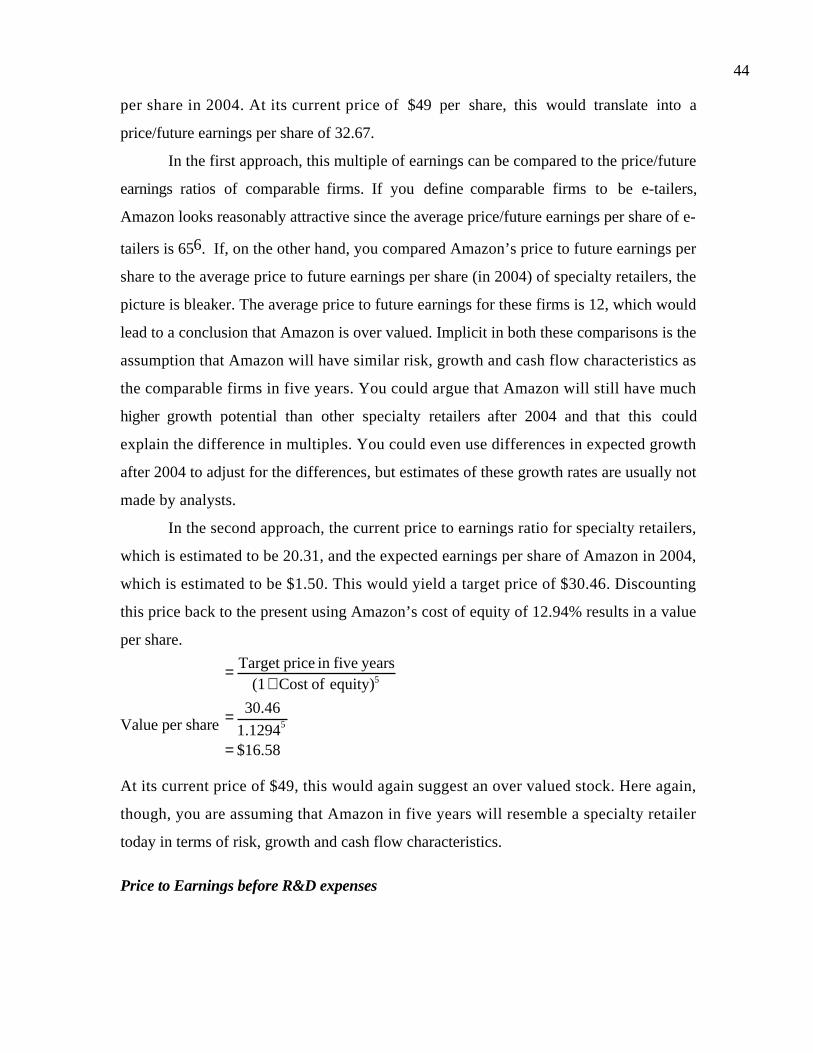
44

per share in 2004. At its current price of $49 per share, this would translate into a

price/future earnings per share of 32.67.

In the first approach, this multiple of earnings can be compared to the price/future

earnings ratios of comparable firms. If you define comparable firms to be e-tailers,

Amazon looks reasonably attractive since the average price/future earnings per share of e-

tailers is 656. If, on the other hand, you compared Amazon’s price to future earnings per

share to the average price to future earnings per share (in 2004) of specialty retailers, the

picture is bleaker. The average price to future earnings for these firms is 12, which would

lead to a conclusion that Amazon is over valued. Implicit in both these comparisons is the

assumption that Amazon will have similar risk, growth and cash flow characteristics as

the comparable firms in five years. You could argue that Amazon will still have much

higher growth potential than other specialty retailers after 2004 and that this could

explain the difference in multiples. You could even use differences in expected growth

after 2004 to adjust for the differences, but estimates of these growth rates are usually not

made by analysts.

In the second approach, the current price to earnings ratio for specialty retailers,

which is estimated to be 20.31, and the expected earnings per share of Amazon in 2004,

which is estimated to be $1.50. This would yield a target price of $30.46. Discounting

this price back to the present using Amazon’s cost of equity of 12.94% results in a value

per share.

Value per share

58.16$1294.1

46.30

equity) ofCost (1years fivein priceTarget

5

5

=

=

+=

At its current price of $49, this would again suggest an over valued stock. Here again,

though, you are assuming that Amazon in five years will resemble a specialty retailer

today in terms of risk, growth and cash flow characteristics.

Price to Earnings before R&D expenses

45

In the discussion of cash flows and capital expenditures in Chapter 4, it was

argued that research and development expenses should be capitalized, since they

represent investments for the future. Since accounting standards require that R&D be

expensed, rather than capitalized, the earnings of high growth firms with substantial

research expenses is likely to be under stated and the PE ratio is, therefore, likely to be

overstated. This will especially be true if you are comparing technology firms, which have

substantial research expenditures, to non-technology firms, which usually do not. Even

when comparing only across technology stocks, firms that are growing faster with larger

R&D expenses will end up with lower earnings and higher PE ratios than more stable

firms in the sector with lower R&D expenses. There are some analysts who argue that the

PE ratio should be estimated using earnings prior to R&D expenses:

PEpre R&D Expenses D&RIncomeNet

Equity of ValueMarket

+=

The PE ratios that emerge from this calculation are likely to be much lower than the PE

ratios using conventional definitions of earnings per share.

While the underlying logic behind this approach is sound, adding back R&D to

earnings represents only a partial adjustment. To complete the adjustment, you would

need to capitalized R&D expenses and compute the amortization of R&D expenses, as

was done in Chapter 4. The adjusted PE would then be:

PER&D Adjusted D&R ofon Amortizati-Expenses D&RIncomeNet

Equity of ValueMarket

+=

These adjusted PE ratios can then be computed across firms in the sample.

This adjustment to the PE ratio, while taking care of one problem – the expensing

of R&D – will still leave you exposed to all of the other problems associated with PE

ratios. Earnings will continue to be volatile and affected by accounting choices and

differences in growth, risk and cashflow characteristics will still cause price earnings ratios

to be different across firms. In addition, you will also have to estimate expected growth in

earnings (pre-R&D) on your own, since consensus estimates from analysts will not be

available for this growth rate.

6 The earnings per share in 2004 of e-tailers were obtained from consensus estimates of analysts following

46

Enterprise Value to EBITDA multiples

Unlike the earnings multiples discussed so far in this chapter, the enterprise value

to EBITDA multiple is a firm value multiple. In the last two decades, this multiple has

acquired a number of adherents among analysts for a number of reasons. First, there are

far fewer firms with negative EBITDA than there are firms with negative earnings per

share and thus fewer firms are lost from the analysis. Second, differences in depreciation

methods across different companies – some might use straight line while others use

accelerated depreciation – can cause differences in operating income or net income but will

not affect EBITDA. Third, this multiple can be compared far more easily across firms

with different financial leverage – the numerator is firm value and the denominator is a

pre-debt earnings – than other earnings multiples. For all of these reasons, this multiple is

particularly useful for firms in sectors that require large investments in infrastructure with

long gestation periods. Good examples would be cable firms in the 1980s and cellular

firms in the 1990s. In this section, we will analyze this multiple.

Definition

The enterprise value to EBITDA multiple relates the total market value of the

firm, net of cash, to the earnings before interest, taxes and depreciation of the firm.

EV/EBITDA EBITDA

Cash-Debt of ValueMarket Equity of ValueMarket +=

Why is cash netted out of firm value for this calculation? Since the interest income from

the cash is not counted as part of the EBITDA, not netting out the cash will result in an

overstatement of the true value to EBITDA multiple. The asset (cash) is added to value,

but the income from the asset is excluded from the income measure (EBITDA).

The enterprise value to EBITDA multiple can be difficult to estimate for firms

with cross-holdings. To see why, note that cross holdings can be categorized as majority

active, minority active or minority passive holdings. When a holding is categorized as a

minority holding, the operating income of a firm does not reflect the income from the

holding. The numerator, on the other hand, includes the market value of equity which

should incorporate the value of the minority holdings. Consequently, the value to

these firms and the current price was divided by the expected earnings per share.

47

EBITDA multiple will be too high for these firms, leading a casual observer to conclude

that they were over valued. When a holding is categorized as a majority holding, a

different problem arises. The EBITDA includes 100% of the EBITDA of the holding, but

the numerator reflects only the percentage (not 100%) of the holding that belongs to the

firm. Thus, the value to EBITDA will be too low, leading it to be categorized as an

undervalued stock.

The correction for cross-holdings is tedious and difficult to do when the holdings

are in private firms. With passive investments, you can either subtract the estimated value

of the holdings from the numerator or add the portion of the EBITDA of the subsidiary

to the denominator. With active investments, you can subtract the proportional share of

the value of the holding from the numerator and the entire EBITDA of the holding from

the denominator.

Illustration 18.14: Estimating Value to EBITDA with cross holdings

In Illustration 16.6, we estimated a discounted cash flow value for Segovia, a firm

with two holdings – a 51% stake in Seville Televison, and a 15% stake of LatinWorks, a

record and CD company. The first holding was categorized as a majority, active holding

(resulting in consolidation) and the second as a minority, passive holding. Here, we will

try to estimate an enterprise value to EBITDA multiple for Seville, using the following

information.

• The market value of equity at Segovia is $1,529 million and the consolidated debt

outstanding at the firm is $500 million. The firm reported $500 million in

EBITDA on its consolidated income statement. A portion of the EBITDA ($180

million) and debt outstanding ($150 million) represent Segovia’s holdings in Seville

Televison.

• Seville Television is a publicly traded firm with a market value of equity of $459

million.

• LatinWorks is a private firm with an EBITDA of $120 million on capital invested

of $250 million in the current year; the firm has $100 million in debt outstanding.

• None of the firms have significant cash balances.

48

If we estimate an enterprise value to EBITDA multiple for Segovia using its consolidated

financial statements, we would obtain the following.

EV/EBITDA

06.4500

05001529EBITDA

CashDebt of Valueequity of ueMarket val

=

−+=

+=

This multiple is contaminated by the cross holdings. There are two ways we can correct

for these holdings. One is to net out from the market value of equity of Segovia the value

of the equity in the holdings and from the debt of the consolidated holding from Segovia’s

debt and then divide by the EBITDA of just the parent company. To do this, you would

first need to estimate the market value of equity in LatinWorks, which is a private

company. We will use the estimate of equity value that we obtained in Illustration16.6.

Value of equity in LatinWorks = 370.25 million

EV/EBITDANo holdings = 70.5180-500

150)-(500370.25)*0.15-459*0.51-(1529 =+

The alternative is to adjust just the denominator to make it consistent with the numerator.

In other words, the EBITDA should include only 51% of the majority, active holding’s

EBITDA and should add in the 15% of the EBITDA in the minority holdings.

EV/EBITDAHoldings = 72.4120*.150180*.49 0-500

500+1529 =+

We prefer the first approach, since it results in multiples that can be more easily

compared across firms. The latter yields an enterprise value to EBITDA multiple that is a

composite of three different firms.

Description

Figure 18.14 summarizes the enterprise value to EBITDA multiples for U.S. firms

in January 2001.

Figure 18.14: EV/EBITDA for U.S. firms – January 2001

49

As with the price earnings ratio, you have a heavily skewed distribution. The average

EV/EBITDA multiple across U.S. firms in January 2001 was 11.7, while the median value

is closer to 8. Note also the large number of firms that trade at very low multiples of

EBITDA, suggesting that rules of thumb should be used with caution.

Analysis

To analyze the determinants of Enterprise value to EBITDA multiples, we will

revert back to a free cashflow to the firm valuation model that we developed in Chapter

15. Specifically, we estimated the value of the operating assets (or enterprise value) of a

firm.

g-WACC

FCFF=V 1

0

We can write the free cash flow to the firm in terms of the EBITDA.

FCFF = EBIT (1-t) – (Cap Ex – DA +∆ Working Capital)

EV/EBITDA

800

600

400

200

0

Std. Dev = 12.18

Mean = 11.7

N = 4181.00

50

= (EBITDA – DA) (1-t) – (Cap Ex – DA +∆ Working Capital)

= EBITDA (1-t) - DA (1-t) – Reinvestment

Substituting back into the equation above, we get:

g-WACC

ntReinvestme–t)-(1DA-t)-(1EBITDA=V 111

0

Dividing both sides by the EBITDA and removing the subscripts yields:

g-WACC

EBITDAntReinvestme

–t)-(1EBITDA

DA-t)-(1

=EBITDA

V0

The determinants of the enterprise value to EBITDA multiple are visible in this equation.

1. Tax rate: Other things remaining equal, firms with lower tax rates should command

higher enterprise value to EBITDA multiples than otherwise similar firms with

higher tax rates.

2. Depreciation and amortization: Other things remaining equal, firms that derive a

greater portion of their EBITDA from depreciation and amortization should trade

at lower multiples of EBITDA than otherwise similar firms.

3. Reinvestment requirements: Other things remaining equal, the greater the portion

of the EBITDA that needs to be reinvested to generate expected growth, the lower

the value to EBITDA will be for firms.

4. Cost of capital: Other things remaining equal, firms with lower costs of capital

should trade at much higher multiples of EBITDA.

5. Expected growth: Other things remaining equal, firms with higher expected growth

should trade at much higher multiples of EBITDA.

This can be generalized to consider firms in high growth. The variables will remain

unchanged but will need to be estimated for each phase of growth.

Illustration 18.15: Analyzing Value to EBITDA multiples

Castillo Cable is a cable and wireless firm with the following characteristics:

• The firm has a cost of capital of 10% and faces a tax rate of 36% on its operating

income.

• The firm has capital expenditures that amount to 45% of EBITDA and depreciation

that amounts to 20% of EBITDA. There are no working capital requirements

51

• The firm is in stable growth and its operating income is expected to grow 5% a year in

perpetuity.

To estimate the enterprise value to EBITDA, we first estimate the reinvestment needs as

a percent of EBITDA.

Reinvestment/EBITDA

.2500-0.20-.450EBITDA

Capital Working

EBITDA

onDepreciati-

EBITDA

Ex Cap ==∆+=

( ) ( )( )5.24=

0.05-0.10

0.25-0.36-10.2-0.36-1=

EBITDA

EV

This multiple is sensitive to the tax rate, as evidenced in Figure 18.15.

It is also sensitive to the reinvestment rate (stated as a percent of EBITDA).

Figure 18.15: VEBITDA Multiples and Tax Rates

0

2

4

6

8

10

12

0% 10% 20% 30% 40% 50%

Tax Rate

Val

ue/E

BIT

DA

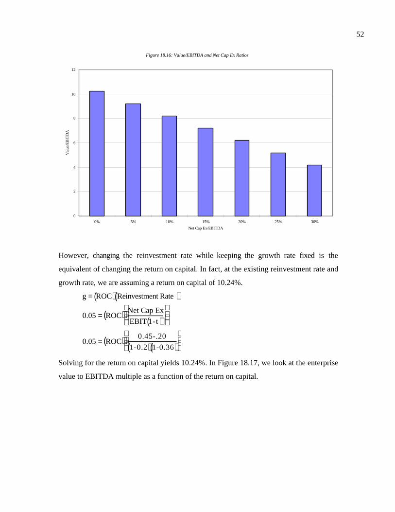
52

However, changing the reinvestment rate while keeping the growth rate fixed is the

equivalent of changing the return on capital. In fact, at the existing reinvestment rate and

growth rate, we are assuming a return on capital of 10.24%.

g = ROC( ) Reinvestment Rate( )

0.05 = ROC( ) Net Cap Ex

EBIT 1-t( )

0.05 = ROC( ) 0.45-.20

1-0.2( ) 1-0.36( )

Solving for the return on capital yields 10.24%. In Figure 18.17, we look at the enterprise

value to EBITDA multiple as a function of the return on capital.

Figure 18.16: Value/EBITDA and Net Cap Ex Ratios

0

2

4

6

8

10

12

0% 5% 10% 15% 20% 25% 30%

Net Cap Ex/EBITDA

Val

ue/E

BIT

DA

53

In short, firms with low returns on capital and high reinvestment rates should trade at

very low multiples of EBITDA.

firmmult.xls: This spreadsheet allows you to estimate firm value multiples for a

stable growth or high growth firm, given its fundamentals.

Application

Having established the fundamentals that determine the enterprise value to

EBITDA multiple, we can now examine how best to apply the multiple. The multiple is

most widely used in capital-intensive firms with heavy infrastructure investments. The

rationale that is given for using the multiple – that EBITDA is the operating cash flow of

the firm – does not really hold up, because many of these firms also tend to have capital

expenditure needs that drain cash flows. There are, however, good reasons for using this

multiple when depreciation methods vary widely across firms and the bulk of the

investment in infrastructure has already been made.

Illustration 18.16: Comparing the Value to EBITDA Multiple: Steel companies

Figure 18.17: Value/EBITDA and Return on Capital

0

2

4

6

8

10

12

6% 7% 8% 9% 10% 11% 12% 13% 14% 15%

Return on Capital

Val

ue/E

BIT

DA

WACC=10%WACC=9%

WACC=8%

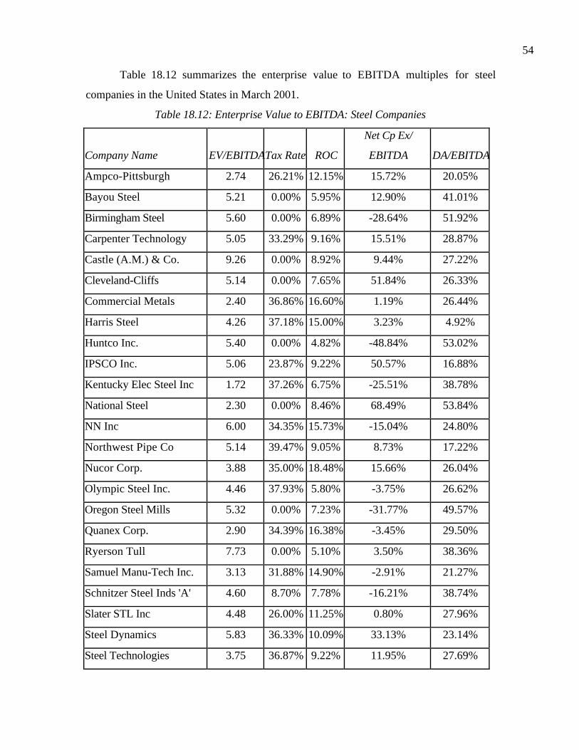
54

Table 18.12 summarizes the enterprise value to EBITDA multiples for steel

companies in the United States in March 2001.

Table 18.12: Enterprise Value to EBITDA: Steel Companies

Company Name EV/EBITDATax Rate ROC

Net Cp Ex/

EBITDA DA/EBITDA

Ampco-Pittsburgh 2.74 26.21% 12.15% 15.72% 20.05%

Bayou Steel 5.21 0.00% 5.95% 12.90% 41.01%

Birmingham Steel 5.60 0.00% 6.89% -28.64% 51.92%

Carpenter Technology 5.05 33.29% 9.16% 15.51% 28.87%

Castle (A.M.) & Co. 9.26 0.00% 8.92% 9.44% 27.22%

Cleveland-Cliffs 5.14 0.00% 7.65% 51.84% 26.33%

Commercial Metals 2.40 36.86% 16.60% 1.19% 26.44%

Harris Steel 4.26 37.18% 15.00% 3.23% 4.92%

Huntco Inc. 5.40 0.00% 4.82% -48.84% 53.02%

IPSCO Inc. 5.06 23.87% 9.22% 50.57% 16.88%

Kentucky Elec Steel Inc 1.72 37.26% 6.75% -25.51% 38.78%

National Steel 2.30 0.00% 8.46% 68.49% 53.84%

NN Inc 6.00 34.35% 15.73% -15.04% 24.80%

Northwest Pipe Co 5.14 39.47% 9.05% 8.73% 17.22%

Nucor Corp. 3.88 35.00% 18.48% 15.66% 26.04%

Olympic Steel Inc. 4.46 37.93% 5.80% -3.75% 26.62%

Oregon Steel Mills 5.32 0.00% 7.23% -31.77% 49.57%

Quanex Corp. 2.90 34.39% 16.38% -3.45% 29.50%

Ryerson Tull 7.73 0.00% 5.10% 3.50% 38.36%

Samuel Manu-Tech Inc. 3.13 31.88% 14.90% -2.91% 21.27%

Schnitzer Steel Inds 'A' 4.60 8.70% 7.78% -16.21% 38.74%

Slater STL Inc 4.48 26.00% 11.25% 0.80% 27.96%

Steel Dynamics 5.83 36.33% 10.09% 33.13% 23.14%

Steel Technologies 3.75 36.87% 9.22% 11.95% 27.69%

55

STEEL-GENERAL 4.14 38.37% 9.80% 21.69% 28.75%

Unvl Stainless & Alloy

Prods 4.28 37.52% 14.51% 12.73% 15.15%

Worthington Inds. 4.80 37.50% 12.54% 0.16% 22.79%

The enterprise value to EBITDA multiples vary widely across these firms and many of

these firms have negative net capital expenditures, partly reflecting the industry’s

maturity and partly the lumpy nature of reinvestments. Many of them also pay no taxes

because they lose money. We regressed the EV/EBITDA multiple against the tax rate and

depreciation as a percent of EBITDA.

EV/EBITDA = 8.65 – 7.20 Tax Rate – 8.08 DA/EBITDA

We did not use expected growth or cost of capital as independent variables because they

are very similar across these firms. Using this regression, the predicted value to EBITDA

multiple for Birmingham Steel would be:

Predicted EV/EBITDABirminham Steel = 8.65 – 7.20 (0.00) – 8.08 (0.5192) = 4.45

At 5.60 times EBITDA, the firm is over valued.

vebitda.xls: There is a dataset on the web that summarizes value to earnings

multiples and fundamentals by industry group in the United States for the most recent

year

Value Multiples: Variants

While enterprise value to EBITDA may be the most widely used value multiple,

there are close variants that are sometimes used by analysts – Value/EBIT, Value/After-

tax EBIT and Value/FCFF. Each of these multiples is determined by many of the same

variables that determine the EV/EBITDA multiple but the actual relationship is slightly

different. In particular, note that for a stable growth firm, these multiples can be written

as follows:

Value/FCFF RateGrowth Expected-capital ofCost

1=

56

Value/EBIT RateGrowth Expected-capital ofCost

RIR-1=

Value/ EBIT ( )( )

Growth Expected-Capital ofCost

RIR-1t-1=

where RIR is the reinvestment rate and t is the tax rate. In other words, higher costs of

capital and lower expected growth decrease all of these multiples. A higher reinvestment

rate lowers the last two multiples but does not affect the multiple of FCFF (since FCFF

is already after reinvestment). A higher tax rate will affect just the last multiple, since the

first two look at earnings after taxes.

Conclusion

The price-earnings ratio and other earnings multiples, which are widely used in

valuation, have the potential to be misused. These multiples are ultimately determined by

the same fundamentals that determine the value of a firm in a discounted cash flow model

- expected growth, risk and cash flow potential. Firms with higher growth, lower risk and

higher payout ratios, with other things remaining equal, should trade at much higher

multiples of earnings than other firms. To the extent that there are differences in

fundamentals across countries, across time and across companies, the multiples will also

be different. A failure to control for these differences in fundamentals can lead to

erroneous conclusions based purely upon a direct comparison of multiples.

There are several ways in which earnings multiples can be used in valuation. One

way is to compare earnings multiples across a narrowly defined group of comparable

firms and to control for differences in growth, risk and payout subjectively. Another is to

expand the definition of a comparable firm to the entire sector (such as technology) or the

market and to control for differences in fundamentals using statistical techniques, such as

regression.

57

Problems

1. National City Corporation, a bank holding company, reported earnings per share of

$2.40 in 1993 and paid dividends per share of $1.06. The earnings had grown 7.5% a year

over the prior five years and were expected to grow 6% a year in the long term (starting in

1994). The stock had a beta of 1.05 and traded for ten times earnings. The treasury bond

rate was 7%.

a. Estimate the PE Ratio for National City Corporation.

b. What long term growth rate is implied in the firm's current PE ratio?

2. On March 11, 1994, the New York Stock Exchange Composite was trading at 16.9

times earnings and the average dividend yield across stocks on the exchange was 2.5%.

The treasury bond rate on March 11, 1994 was 6.95%. The economy was expected to

grow 2.5% a year, in real terms in the long term, and the consensus estimate for inflation,

in the long term, was 3.5%.

a. Based upon these inputs, estimate the 'appropriate' PE ratio for the exchange.

b. What growth rate in dividends/earnings would justify the PE ratio on March 11,

1994?

c. Would it matter whether this higher growth comes from higher inflation or higher real

growth? Why?

3. International Flavors and Fragrances, a leading creator and manufacturer of flavors and

fragrances, paid out dividends of $0.91 per share on earnings per share of $1.64 in 1992.

The firm is expected to have a return on equity of 20% between 1993 and 1997, after

which the firm is expected to have stable growth of 6% a year. The return on equity is

expected to drop to 15% in the stable growth phase. The dividend payout ratio is

expected to remain at the current level from 1993 to 1997. The stock has a beta of 1.10,

which is not expected to change. The treasury bond rate is 7%.

a. Estimate the PE ratio for International Flavors, based upon fundamentals.

b. Estimate how much of this PE ratio can be ascribed to the extraordinary growth in

earnings that the firm expects to have between 1993 and 1997.

4. Cracker Barrel, which operates restaurants and gift shops, reported dramatic growth in

earnings and revenues between 1983 and 1992. During this period, earnings grew from

$0.08 per share in 1983 to $0.78 per share in 1993. The dividends paid in 1993 amounted

to only $0.02 per share. The earnings growth rate was expected to ease to 15% a year

from 1994 to 1998 and to 6% a year after that. The payout ratio is expected to increase to

10% from 1994 to 1998 and to 50% after that. The beta of the stock is currently 1.55, but

58

it is expected to decline to 1.25 for the 1994-98 time period and to 1.10 after that. The

treasury bond rate is 7%.

a. Estimate the PE ratio for Cracker Barrel.

b. Estimate how much higher the PE ratio would have been, if it had been able to

maintain the growth rate in earnings that it had posted between 1983 and 1993.

(Assume that the dividend payout ratios are unaffected.)

c. Now assume that disappointing earnings reports in the near future lower the expected

growth rate between 1994 and 1998 to 10%. Estimate the PE ratio. (Again, assume that

the dividend payout ratio is unaffected.)

5. The S & P 500 was trading at 21.2 times earnings on December 31, 1993. On the same

day, the dividend yield on the index was 2.74% and the treasury bond rate was 6%. The

expected growth rate in real GNP was 2.5%.

a. Assuming that the S&P 500 is correctly priced, what is the inflation rate implied in

the PE ratio?

b. By February 1994, treasury bond rates had increased to 7%. If payout ratios and

expected growth remain unchanged, what would the effect on the PE ratio be?

c. Does an increase in interest rates always imply lower prices (and PE ratios)?

6. The following were the PE ratios of firms in the aerospace/defense industry at the end

of December 1993, with additional data on expected growth and risk.

Company PE Ratio Expected Beta Payout

Growth

Boeing 17.3 3.5% 1.10 28%

General Dynamics 15.5 11.5% 1.25 40%

General Motors - Hughes 16.5 13.0% 0.85 41%

Grumman 11.4 10.5% 0.80 37%

Lockheed Corporation 10.2 9.5% 0.85 37%

Logicon 12.4 14.0% 0.85 11%

Loral Corporation 13.3 16.5% 0.75 23%

Martin Marietta 11.0 8.0% 0.85 22%

McDonnell Douglas 22.6 13.0% 1.15 37%

Northrop 9.5 9.0% 1.05 47%

Raytheon 12.1 9.5% 0.75 28%

Rockwell 13.9 11.5% 1.00 38%

Thiokol 8.7 5.5% 0.95 15%

United Industrial 10.4 4.5% 0.70 50%

59

a. Estimate the average and median PE ratios. What, if anything, would these averages

tell you?

b. An analyst concludes that Thiokol is undervalued, because its PE ratio is lower than

the industry average. Under what conditions is this statement true? Would you agree

with it here?

c. Using a regression, control for differences across firms on risk, growth and payout.

Specify how you would use this regression to spot under and over valued stocks. What

are the limitations of this approach?

7. The following was the result of a regression of PE ratios on growth rates, betas and

payout ratios, for stocks listed on the Value Line Database, in April 1993.

PE = 18.69 + 0.0695 GROWTH - 0.5082 BETA - 0.4262 PAYOUT R2 =0.35

Thus, a stock with an earnings growth rate of 20%, a beta of 1.15 and a payout ratio of

40%, would have had an expected PE ratio of:

PE = 18.69 + 0.0695 * 20 - 0.5082 (1.15) - 0.4262 * 0.40 = 19.33[NOTE: Is it 20 or

0.20?]

You are attempting to value a private firm, with the following characteristics:

(a) The firm had net profits of $10 million. It did not pay dividends, but had depreciation

allowances of $5 million and capital expenditures of $12 million, in the most recent year.

Working capital requirements were negligible.

(b) The earnings had grown 25% over the previous five years and are expected to grow at

the same rate over the next five years.

(c) The average beta of publicly traded firms, in the same line of business, is 1.15, and the

average debt/equity ratio of these firms is 25%. The tax rate is 40%. The private firm is an

all-equity financed firm, with no debt.

a. Estimate the appropriate PE ratio for this private firm, using the regression.

b. What would some of your concerns be, in using this regression in valuation?

1

CHAPTER 19BOOK VALUE MULTIPLES

The relationship between price and book value has always attracted the attention

of investors. Stocks selling for well below the book value of equity have generally been

considered good candidates for undervalued portfolios, while those selling for more than

book value have been targets for overvalued portfolios. This chapter begins by examining

the price/book value ratio in more detail, the determinants of this ratio and how best to

evaluate or estimate the ratio.

In the second part of the chapter, we will turn our attention to variants of the

price to book ratio. In particular, we focus on the value to book ratio and Tobin’s Q – a

ratio of market value of assets to their replacement cost.

Price to Book Equity

The market value of the equity in a firm reflects the market’s expectation of the

firm’s earning power and cashflows. The book value of equity is the difference between

the book value of assets and the book value of liabilities, a number that is largely

determined by accounting conventions. In the United States, the book value of assets is

the original price paid for the assets reduced by any allowable depreciation on the assets.

Consequently, the book value of an asset decreases as it ages. The book value of liabilities

similarly reflects the "at-issue" values of the liabilities. Since the book value of an asset

reflects its original cost, it might deviate significantly from market value if the earning

power of the asset has increased or declined significantly since its acquisition.

Why analysts use book value and the down side…

There are several reasons why investors find the price-book value ratio useful in

investment analysis. The first is that the book value provides a relatively stable, intuitive

measure of value that can be compared to the market price. For investors who

instinctively mistrust discounted cashflow estimates of value, the book value is a much

simpler benchmark for comparison. The second is that, given reasonably consistent

accounting standards across firms, price-book value ratios can be compared across similar

firms for signs of under or over valuation. Finally, even firms with negative earnings,

which cannot be valued using price-earnings ratios, can be evaluated using price-book

2

value ratios; there are far fewer firms with negative book value than there are firms with

negative earnings.

There are several disadvantages associated with measuring and using price-book

value ratios. First, book values, like earnings, are affected by accounting decisions on

depreciation and other variables. When accounting standards vary widely across firms, the

price-book value ratios may not be comparable. A similar statement can be made about

comparing price-book value ratios across countries with different accounting standards.

Second, book value may not carry much meaning for service and technology firms which

do not have significant tangible assets. Third, the book value of equity can become

negative if a firm has a sustained string of negative earnings reports, leading to a negative

price-book value ratio.

Definition

The price to book ratio is computed by dividing the market price per share by the

current book value of equity per share.

Price to Book Ratio = PBV = Price per share

Book value of equity per share

While the multiple is fundamentally consistent – the numerator and denominator are both

equity values – there is a potential for inconsistency if you are not careful about how you

compute book value of equity per share. In particular,

• If there are multiple classes of shares outstanding, the price per share can be

different for different classes of shares and it is not clear how the book equity

should be apportioned among shares.

• You should not include the portion of the equity that is attributable to preferred

stock in computing the book value of equity, since the price per share refers only

to common equity.

Some of the problems can be alleviated by computing the price to book ratio using the

total market value of equity and book value of equity, rather than per share values.

Price to Book Ratio = PBV = Market Value of Equity

Book value of equity

The safest way to measure this ratio when there are multiple classes of equity is to use

the composite market value of all classes of common stock in the numerator and the

3

composite book value of equity in the denominator – you would still ignore preferred

stock for this computation.

There are two other measurement issues that you have to confront in computing

this multiple. The first relates to the book value of equity, which as an accounting

measure, gets updated infrequently – once every quarter for U.S, companies and once

every year for European companies. While most analysts use the most current book value

of equity, there are some who use the average over the last year or the book value of

equity at the end of the latest financial year. Consistency demands that you use the same

measure of book equity for all firms in your sample. The second and more difficult

problem concerns the value of options outstanding. Technically, you would need to

compute the estimated market value of management options and conversion options (in

bonds and preferred stock) and add them to the market value of equity before computing

the price to book value ratio.1 If you have a small sample and options represent a large

portion of equity value, you should do this. With larger samples and less significant

option issues, you can stay with the conventional measure of market value of equity.

Accounting standards can affect book values of equity and price to book ratios

and skew comparisons made across firms. For instance, assume that you are comparing

the price to book ratios of technology firms in two markets and that one of them allows

research expenses to be capitalized and the other does not. You should expect to see

lower price to book value ratios in the former, since the book value of equity will be

augmented by the value of the research asset.

Adjusting Book Equity for Buybacks and Acquisitions

In recent years, firms in the United States have increasing turned to buying back

stock as a way of returning cash to stockholders. When a firm buys back stock, the book

equity of the firm declines by the amount of the buyback. While this is precisely what

happens when firms pay a cash dividend as well, buybacks tend to be much larger than

regular dividends and thus have a bigger impact on book equity. To illustrate, assume that

1 If you do not do this and compare price to book ratios across firms with widely different amounts ofoptions outstanding, you could mis-identify firms with more options outstanding as undervalued – themarket value of traded common stock at these firms will be lower because of the option overhang.

4

you have a firm that has a market value of equity of $100 million and a book value of

equity of $50 million; its price to book ratio is 2.00. If the firm borrows $25 million and

buys back stock, its book equity will decline to $25 million and its market equity will

drop to $75 million. The resulting price to book ratio is three.

With acquisitions, the effect on price to book ratios can vary dramatically

depending upon how the acquisition is accounted for. If the acquiring firm uses purchase

accounting, the book equity of the firm will increase by the market value of the acquired

firm. If, on the other hand, it uses pooling, the book equity will increase by the book

value of the acquired firm. Given that the book value is less than the market value for

most firms, the price to book ratio will be much higher for firms that use pooling on

acquisitions than purchase accounting.

To compare price to book ratios across firms, when some firms in the sample buy

back stocks and some do not or when there are wide differences in both the magnitude and

the accounting for acquisitions, can be problematic. One way to adjust for the differences

is to take out the goodwill from acquisitions and to add back the market value of

buybacks to the book equity to come up with an adjusted book value of equity. The price

to book ratios can then be computed based upon this adjusted book value of equity.

Description

To get a sense of what comprises a high, low or average price to book value ratio,

we computed the ratio for every firm listed in the United States and Figure 19.1

summarizes the distribution of price to book ratios in July 2000.

5

Note that this distribution is heavily skewed, as is evidenced by the fact that the average

price to book value ratio of firms is 3.25 while the median price to book ratio is much

lower at 1.85.

Another point worth making about price to book ratios is that there are firms with

negative book values of equity – the result of continuously losing money – where price to

book ratios cannot be computed. In this sample of 5903 firms, there were 728 firms

where this occurred. In contrast, though, 2045 firms had negative earnings and PE ratios

could not be computed for them.

pbvdata.xls: There is a dataset on the web that summarizes price to book ratios

and fundamentals by industry group in the United States for the most recent year

Analysis

The price-book value ratio can be related to the same fundamentals that determine

value in discounted cashflow models. Since this is an equity multiple, we will use an

equity discounted cash flow model – the dividend discount model – to explore the

Figure 19.1: Price to Book Value Ratios

0

100

200

300

400

500

600

700

800

900

1000

0-0.5 0.5- 1 1-1.5 1.5-2 2- 2.5 2.5 - 3 3 - 3.5 3.5 - 4 4 - 4.5 4.5 - 5 5- 10 >10

Price to Book Ratio

Num

ber

of f

irm

s

6

determinants. The value of equity in a stable growth dividend discount model can be

written as:

P0 =DPS1

k e −gn

where,

P0 = Value of equity per share today

DPS1 = Expected dividends per share next year

ke = Cost of equity

gn = Growth rate in dividends (forever)

Substituting in for DPS1 = (EPS1)(Payout ratio), the value of the equity can be written as:

( )( )n

10

g-r

RatioPayout EPSP =

Defining the return on equity (ROE)0

1

Equity of ValueBook

EPS= , the value of equity can be

written as:

( )( )( )n

00

g-r

RatioPayout ROEBVP =

Rewriting in terms of the PBV ratio,

( )( )n0

0

g-r

RatioPayout ROE=PBV

BV

P =

If we define return on equity using contemporaneous earnings,

ROE0

0

Equity of ValueBook

EPS= , the price to book ratio can be written as:

( ) ( )n0

0

g-r

RatioPayout g)+(1ROE

BV

P =

7

The PBV ratio is an increasing function of the return on equity, the payout ratio and the

growth rate and a decreasing function of the riskiness of the firm.

This formulation can be simplified even further by relating growth to the return on

equity.

g = (1 - Payout ratio) * ROE

Substituting back into the P/BV equation,

n

n

0

0

g-r

g-ROEPBV

BV

P ==

The price-book value ratio of a stable firm is determined by the differential between the

return on equity and its cost of equity. If the return on equity exceeds the cost of equity,

the price will exceed the book value of equity; if the return on equity is lower than the

cost of equity, the price will be lower than the book value of equity. The advantage of

this formulation is that it can be used to estimate price-book value ratios for private firms

that do not pay out dividends.

Illustration 19.1: Estimating the PBV ratio for a stable firm - Volvo

Volvo had earnings per share of 11.04 Swedish Kroner (SEK) in 2000 and paid out

a dividend of 7 SEK per share, which represented 63.41% of its earnings. The growth rate

in earnings and dividends, in the long term, is expected to be 5%. The return on equity at

Volvo is expected to be 13.66%. The beta for Volvo is 0.80 and the riskfree rate in

Swedish Kroner is 6.1%.

Current Dividend Payout Ratio = 63.41%

Expected Growth Rate in Earnings and Dividends = 5%

Return on Equity = 13.66%

Cost of Equity = 6.1% + 0.80*4% = 9.30%

PBV Ratio based on fundamentals

( )( )

( )( )

01.205.0093.0

6341.01366.0

g-k

RatioPayout ROE=

ne

=−

=

8

Since the expected growth rate in this case is consistent with that estimated by

fundamentals, the price to book ratio could also have been estimated from the return

differences.

Fundamental growth rate = (1 – payout ratio)(ROE) = (1-0.6341)(0.1366) = .05 or 5%

PBV ratio

01.205.0094.0

05.01366.0

rateGrowth -equity ofCost rategrowth -ROE

=−−=

=

Volvo was selling at a P/BV ratio of 1.10 on the day of this analysis (May 2001),

making it significantly under valued. The alternative interpretation is that the market is

anticipating a much lower return on equity in the future and pricing Volvo based upon

this expectation.

Illustration 19.2: Estimating the price-book value ratio for a 'privatization' candidate -

Jenapharm (Germany)

One of the by-products of German reunification was the Treuhandanstalt, the

German privatization agency set up to sell hundreds of East German firms to other

German companies, individual investors and the public. One of the handful of firms that

seemed to be a viable candidate for privatization was Jenapharm, the most respected

pharmaceutical manufacturer in East Germany. Jenapharm, which was expected to have

revenues of 230 million DM in 1991, also was expected to report net income of 9 million

DM in that year. The firm had a book value of assets of 110 million DM and a book value

of equity of 58 million DM at the end of 1990.

The firm was expected to maintain sales in its niche product, a contraceptive pill,

and grow at 5% a year in the long term, primarily by expanding into the generic drug

market. The average beta of pharmaceutical firms traded on the Frankfurt Stock exchange

was 1.05, though many of these firms had much more diversified product portfolios and

less volatile cashflows. Allowing for the higher leverage and risk in Jenapharm, a beta of

1.25 was used for Jenapharm. The ten-year bond rate in Germany at the time of this

valuation in early 1991 was 7% and the risk premium for stocks over bonds is assumed to

be 3.5%.

9

Expected Net Income = 9 mil DM

Return on Equity 15.52%58

9

Equity of ValueBook

IncomeNet Expected ===

Coat of Equity = 7% + 1.25 (3.5%) = 11.375%

Price/Book Value Ratio 1.650.05-0.11375

0.05-0.1552

g-r

g-ROE ===

Estimated MV of equity

( )( ) ( )( ) DMmillion 95.701.6558ratio Price/BVEquity of BV ===

PBV Ratio for a high growth firm

The price-book value ratio for a high growth firm can also be related to

fundamentals. In the special case of the two-stage dividend discount model, this

relationship can be made explicit simply. The value of equity of a high growth firm in the

two-stage dividend discount model can be written as:

Value of Equity = Present Value of expected dividends + Present value of terminal price

When the growth rate is assumed to be constant after the initial high growth

phase, the dividend discount model can be written as follows:

P0 =

EPS0( ) Payout Ratio( ) 1+g( ) 1−1+g( )n

1+k e,hg( )n

k e,hg -g+

EPS0( ) Payout Ratio n( ) 1+g( )n1+g n( )

k e,st -gn( ) 1+k e,hg( )n

where,

g = Growth rate in the first n years

Payout = Payout ratio in the first n years

gn = Growth rate after n years forever (Stable growth rate)

Payoutn = Payout ratio after n years for the stable firm

ke = Cost of equity (hg: high growth period; st: stable growth period)

Rewriting EPS0 in terms of the return on equity, EPS0 = (BV0)(ROE), and bringing BV0

to the left hand side of the equation, we get:

10

P0

BV0

= ROEhg( )Payout Ratio( ) 1+g( ) 1−

1+g( )n

k e,hg -g+ ROE st( ) Payout Ratio n( ) 1+g( )n

1+g n( )k e,st -g n( ) 1+k e,hg( )n

where ROE is the return on equity and ke is the cost of equity.

The left hand side of the equation is the price book value ratio. It is determined

by:

(a) Return on equity: The price-book value ratio is an increasing function of the

return on equity.

(b) Payout ratio during the high growth period and in the stable period: The PBV

ratio increases as the payout ratio increases, for any given growth rate.

(c) Riskiness (through the discount rate r): The PBV ratio becomes lower as

riskiness increases; the increased risk increases the cost of equity.

(d) Growth rate in Earnings, in both the high growth and stable phases: The PBV

increases as the growth rate increases, in either period, holding the payout ratio

constant.

This formula is general enough to be applied to any firm, even one that is not paying

dividends right now. Note, in addition, that the fundamentals that determine the price to

book ratio for a high growth firm are the same as the ones for a stable growth firm – the

payout ratio, the return on equity, the expected growth rate and the cost of equity.

In Chapter 14, we noted that firms may not always pay out what they can afford

to and recommended that the free cashflows to equity be substituted in for the dividends

in those cases. You can, in fact, modify the equation above to state the price to book ratio

in terms of free cashflows to equity.

P0

BV0

= ROE hg( )*

FCFEEarnings

hg

1+g( ) 1−1+g( )n

1+r( )n

r -g+ ROE st( )

FCFEEarnings

n

1+g( )n1+g n( )

r -gn( ) 1+r( )n

The only substitution that we have made is the replacement of the payout ratio by the

FCFE as a percent of earnings.

11

Illustration 19.3: Estimating the PBV ratio for a high growth firm in the two-stage model

Assume that you have been asked to estimate the PBV ratio for a firm that is expected to

be in high growth for the next five years. The firm has the following characteristics:

EPS Growth rate in first five years = 20% Payout ratio in first five years = 20%

EPS Growth rate after five years = 8% Payout ratio after five years = 68%

Beta = 1.0 Riskfree rate = T.Bond Rate = 6%

Return on equity = 25%

Cost of equity = 6% + 1(5.5%)= 11.5%

PBV = 0.25

0.2( ) 1.20( ) 1− 1.205

1.1155

0.115 − 0.20+ 0.25

0.68( ) 1.205( ) 1.08( )0.115 − 0.08( ) 1.1155( ) = 7.89

The estimated PBV ratio for this firm is 7.89.

Illustration 19.4: Estimating the Price/Book Value Ratio for a high growth firm using

FCFE - Nestle

In Chapter 14, we valued Nestle using a two-stage FCFE model. We summarize

the inputs we used for that valuation in the Table 19.1.

Table 19.1: Nestle – Summary of Inputs

High Growth Stable Growth

Length 10 years Forever after year 10

ROE 22.98% 15%

FCFE/Earnings 68.35% 73.33%

Growth rate 7.27% 4%

Cost of Equity 8.47% 8.47%

The price-book value ratio, based upon these inputs, is calculated below:

12

PBV = 0.2298( )0.6835( ) 1.0727( ) 1−

1.0727( )10

1.0847( )10

0.0847-0.0727+ 0.15( ) 0.7333( ) 1.0727( )10

1.04( )(0.0847-0.0727) 1.0847( )10 =3.77

Nestle traded at a price-book value ratio of 4.40 in May 2001, which would make it over

valued.

Again, in this valuation, we have preserved consistency by setting the growth rate

equal to the product of the return on equity and the equity reinvestment rate (1- FCFE/

Earnings).

Growth rate during high growth = ROE (1- FCFE/Earnings)

= 1.2298 (1 - 0.6835) = 0.0727

Growth rate during stable growth = ROE (1- FCFE/Earnings) = 0.15 (1-0.7333) = 0.04

PBV Ratios and Return on Equity

The ratio of price to book value is strongly influenced by the return on equity. A

lower return on equity affects the price-book value ratio directly through the formulation

specified in the prior section and indirectly by lowering the expected growth or payout.

Expected growth rate = Retention Ratio * Return on Equity

The effects of lower return on equity on the price-book value ratio can be seen by going

back to Illustration 19.3 and changing the return on equity for the firm that we valued in

that example.

Illustration 19.5: Return on Equity and Price-Book Value

In Illustration 19.3, we estimated a price to book ratio for the firm of 7.89, based

upon a return on equity of 25%. This return on equity, in turn, allowed the firm to

generate growth rates of 20% in high growth and 8% in stable growth.

Growth rate in first five years ( )( ) ( )( ) 20%25%0.8ROEratioRetention ===

Growth rate after year 5 ( )( ) ( )( ) 8%25%0.32ROEratioRetention ===

If the firm's return on equity drops to 12%, the price/book value will reflect the drop. The

lower return on equity will also lower expected growth in the initial high growth period:

13

Expected growth rate (first five years)

( )( )( )( )

%6.9

%1280.0

ROEratioRetention

===

After year 5, either the retention ratio has to increase or the expected growth rate has to

be lower than 8%. If the retention ratio is adjusted,

New retention ratio after year 5 66.67%12%

8%

ROE

growth Expected ===

New payout ratio after year 5 = 1 - Retention ratio = 33.33%

The new price-book value ratio can then be calculated as follows:

PBV = 0.12( )0.2( ) 1.096( ) 1−

1.096( )5

1.115( )5

0.115 − 0.096+ 0.12( ) 0.3333( ) 1.096( )5

1.08( )0.115 −0.08( ) 1.115( )5 =1.25

The drop in the ROE has a two-layered impact. First, it lowers the growth rate in

earnings and/or the expected payout ratio, thus having an indirect effect on the P/BV ratio.

Second, it reduces the P/BV ratio directly.

The price-book value ratio is also influenced by the cost of equity, with higher

costs of equity leading to lower price-book value ratios. The influence of the return on

equity and the cost of equity can be consolidated in one measure by taking the difference

between the two – a measure of excess equity return. The larger the return on equity

relative to the cost of equity, the greater is the price-book value ratio. In the illustration

above for instance, the firm, which had a cost of equity of 11.5%, went from having a

return on equity that was 13.5% greater than the required rate of return to a return on

equity that barely broke even (0.5% greater than the required rate of return).

Consequently, its price-book value ratio declined from 7.89 to 1.25. The following graph

shows the price-book value ratio as a function of the difference between the return on

equity and required rate of return.

14

Note that when the return on equity is equal to the cost of equity, the price is equal to the

book value.

The Determinants of Return on Equity

The difference between return on equity and the required rate of return is a

measure of a firm's capacity to earn excess returns in the business in which it operates.

Corporate strategists have examined the determinants of the size and expected duration of

these excess profits (and high ROE) using a variety of frameworks. One of the better

known is the "five forces of competition" framework developed by Porter. In his

approach, competition arises not only from established producers producing the same

product but also from suppliers of substitutes and from potential new entrants into the

market. Figure 19.3 summarizes the five forces of competition:

Figure 19.2: Price-Book Value as a Function of Return Differential

0

1

2

3

4

5

6

7

8

9

13.50% 11.50% 9.50% 7.50% 5.50% 3.50% 1.50% -0.50% -2.50%

ROE - Cost of Equity

P/B

V R

atio

15

Figure 19.3: Forces of Competition and Return on Equity

Supplier Power

Threat of Entry

• Economies of scale• Cost Advantages• Capital Requirements• Product Differentiation• Access to distribution channels• Government and legal barriers• Retaliation by established producers

Threat of substitutes

• Buyer propensity to substitute• Relative price perf- ormance of substitutes

Buyer Power

Price Sensitivity• Cost ofpurchasesrelative to total costs• Profitability of buyers• Importance of theproduct to qualityof buyer's product

Bargaining Power• Size and concent-ration of buyersrelative to suppliers• Buyers' switchingcosts• Buyers' information• Buyers' abilityto backward integrate

IndustryCompetitiveness• Concentration• Product differentiation• Excess Capacity• Ratio of fixed to variable costs• Demand Growth• Cyclical fluctuations• Exit barriers

In Porter's framework, a firm is able to maintain a high return on equity because there are

significant barriers to entry by new firms or because the firm has significant advantages

over its competition. The analysis of the return on equity of a firm can be made richer and

much more informative by examining the competitive environment in which it operates.

There may also be clues in this analysis to the future direction of the return on equity.

eqmult.xls: This spreadsheet allows you to estimate the price earnings ratio for a

stable growth or high growth firm, given its fundamentals.

Applications

16

There are several potential applications for the principles developed in the last

section and we will consider three in this section. We will first look at what causes price

to book ratios for entire markets to change over time and when a low (high) price to book

ratio for a market can be viewed as a sign of under (over) valuation. We will next compare

the price to book ratios of firms within a sector and extend this to look at firms across the

market and what you need to control for in making these comparison. Finally, we will

look at the factors that cause the price to book ratio of an individual firm to change over

time and how this can be used as a tool for analyzing restructurings.

PBV ratios for a Market

The price to book value ratio for an entire market is determined by the same

variables that determine the price to book value ratio for an individual firm. Other things

remaining equal, therefore, you would expect the price to book ratio for a market to go up

as the equity return spread (ROE – Cost of equity) earned by firms in the market

increases. Conversely, you would expect the price to book ratio for the market to

decrease as the equity return spread earned by firms decreases.

In Chapter 18, we noted the increase in the price earnings ratio for the S&P 500

from 1960 to 2000. Over that period, the price to book value ratio for the market has also

increased. In Figure 19.4, we report on the price to book ratio for the S&P 500 on one axis

and the return on equity for S&P 500 firms on the other.

17

The increase in the price to book ratio over the last two decades can be at least partially

explained by the increase in return on equity over the same period.

Comparisons across firms in a Sector

Price-book value ratios vary across firms for a number of reasons - different

expected growth, different payout ratios, different risk levels and most importantly,

different returns on equity. Comparisons of price-book value ratios across firms that do

not take into account these differences are likely to be flawed.

The most common approach to estimating PBV ratios for a firm is choose a group

of comparable firms, to calculate the average PBV ratio for this group and to base the

PBV ratio estimate for a firm on this average. The adjustments made to reflect differences

in fundamentals between the firm being valued and the comparable group are usually

subjectively. There are several problems with this approach. First, the definition of a

'comparable' firm is essentially a subjective one. The use of other firms in the industry as

the control group is often not a complete solution because firms within the same industry

can have very different business mixes, risk and growth profiles. There is also plenty of

Figure 19.4: Price to Book Ratios and ROE - S&P 500

0

0.5

1

1.5

2

2.5

3

3.5

4

4.5

1980 1981 1982 1983 1984 1985 1986 1987 1988 1989 1990 1991 1992 1993 1994 1995 1996 1997 1998 1999 2000

Year

Pric

e to

Boo

k R

atio

0.00%

5.00%

10.00%

15.00%

20.00%

25.00%

RO

E PBVROE

18

potential for bias. Second, even when a legitimate group of comparable firms can be

constructed, differences will continue to persist in fundamentals between the firm being

valued and this group. Adjusting for differences subjectively does not provide a

satisfactory solution to this problem, since these judgments are only as good as the

analysts making them.

Given the relationship between price-book value ratios and returns on equity, it is

not surprising to see firms which have high returns on equity selling for well above book

value and firms which have low returns on equity selling at or below book value. The

firms that should draw attention from investors are those that provide mismatches of

price-book value ratios and returns on equity - low P/BV ratios and high ROE or high

P/BV ratios and low ROE. There are two ways in which we can bring home these

mismatches – a matrix approach and a sector regression.

Matrix Approach

If the essence of misvaluation is finding firms that have price to book ratios that

do not go with their equity return spreads, the mismatch can be brought home by plotting

the price to book value ratios of firms against their returns on equity. Figure 19.5 presents

such a plot.

Figure 19.5: Price to Book Ratios and Returns on Equity

19

If we assume that firms within a sector have similar costs of equity, we could replace the

equity return spread with the raw return on equity.

Regression Approach

If the price to book ratio is largely a function of the return on equity, we could

regress the former against the latter.

PBV = a + b ROE

If the relationship is strong, we could use this regression to obtain predicted price to book

ratios for all of the firms in the sector, separating out those firms that are under from

those that are over valued.

This regression can be enriched in two ways. The first is to allow for non-linear

relationships between price to book and return on equity - this can be done by either

transforming the variables (natural logs, exponentials, etc.) or by running non-linear

regressions. The second is to expand the regression to include other independent variables

such as risk and growth.

Return on Equity - Cost of Equity

High Price to BookHigh Equity return spread

Low Price to BookLow Equity return spread

Low Price to BookHigh Equity return spread

Undervalued

High Price to BookLow Equity return spread

Overvalued

20

Illustration 19.6: Comparing Price to Book Value Ratios: Integrated Oil companies

In Table 19.2, we report on the price to book ratios for integrated oil companies

listed in the United States in September 2000.

Table 19.2: Price to Book Ratios and Returns on Equity

Company Name

Ticker

Symbol PBV ROE

Std

Deviation

Crown Cent. Petr.'A' CNPA 0.29 -14.60% 59.36%

Giant Industries GI 0.54 7.47% 38.87%

Harken Energy Corp. HEC 0.64 -5.83% 56.51%

Getty Petroleum Mktg. GPM 0.95 6.26% 58.34%

Pennzoil-Quaker State PZL 0.95 3.99% 51.06%

Ashland Inc. ASH 1.13 10.27% 21.77%

Shell Transport SC 1.45 13.41% 31.61%

USX-Marathon Group MRO 1.59 13.42% 45.31%

Lakehead Pipe Line LHP 1.72 13.28% 19.56%

Amerada Hess AHC 1.77 16.69% 26.89%

Tosco Corp. TOS 1.95 15.44% 34.51%

Occidental Petroleum OXY 2.15 16.68% 39.47%

Royal Dutch Petr. RD 2.33 13.41% 29.81%

Murphy Oil Corp. MUR 2.40 14.49% 27.80%

Texaco Inc. TX 2.44 13.77% 27.78%

Phillips Petroleum P 2.64 17.92% 29.51%

Chevron Corp. CHV 3.03 15.69% 26.44%

Repsol-YPF ADR REP 3.24 13.43% 26.82%

Unocal Corp. UCL 3.53 10.67% 34.90%

Kerr-McGee Corp. KMG 3.59 28.88% 42.47%

Exxon Mobil Corp. XOM 4.22 11.20% 19.22%

BP Amoco ADR BPA 4.66 14.34% 27.00%

Clayton Williams CWEI 5.57 31.02% 26.31%

21

Energy

Average 2.30 12.23%

The average price to book ratio for the sector is 2.30, but the range in price to book ratios

is large, with Crown Central trading at 0.29 times book value and Clayton Williams

Energy trading at 5.57 times book value.

We will begin by plotting price to book ratios against returns on equity for these

firms in Figure 19.6.

Figure 19.6: Price to Book versus ROE: Oil Companies

ROE

.4.3.2.10.0-.1-.2

6

5

4

3

2

1

0

CWEI

BPA

XOM

KMGUCL

REPCHV

PMUR

OXY

AHC

SC

ASHGPM

HEC GICNPA

While there are no firms that show up in the over valued quadrant, firms such as Pennzoil

(P), Occidental (OXY), Amerada Hess (AMC) and Murphy (MUR) look under valued

relative to the rest of the sector.

Regressing the price to book against return on equity for oil companies, we

obtained the following:

22

PBV = 1.043 + 10.24 ROE R2 = 48.6%

(2.97) (4.46)

If we extend this regression to include standard deviation in stock prices as a measure of

risk, we get:

PBV = 2.21 + 8.22 ROE - 2.63 Std Dev R2 = 52%

(2.16) (2.92) (-1.21)

This regression can be used to estimate predicted price to book ratios for these companies

in Table 19.3.

Table 19.3: Predicted Price to Book Ratios – Oil Companies

Company Name PBV Predicted PBV Under/Over Valued

Crown Cent. Petr.'A' 0.29 -0.56 NMF

Giant Industries 0.54 1.80 -69.74%

Harken Energy Corp. 0.64 0.24 166.59%

Getty Petroleum Mktg. 0.95 1.19 -19.67%

Pennzoil-Quaker State 0.95 1.19 -19.93%

Ashland Inc. 1.13 2.48 -54.28%

Shell Transport 1.45 2.48 -41.56%

USX-Marathon Group 1.59 2.12 -25.11%

Lakehead Pipe Line 1.72 2.78 -38.03%

Amerada Hess 1.77 2.87 -38.33%

Tosco Corp. 1.95 2.57 -24.09%

Occidental Petroleum 2.15 2.54 -15.27%

Royal Dutch Petr. 2.33 2.52 -7.66%

Murphy Oil Corp. 2.40 2.67 -10.07%

Texaco Inc. 2.44 2.61 -6.47%

Phillips Petroleum 2.64 2.90 -9.17%

Chevron Corp. 3.03 2.80 8.20%

Repsol-YPF ADR 3.24 2.60 24.53%

Unocal Corp. 3.53 2.17 63.05%

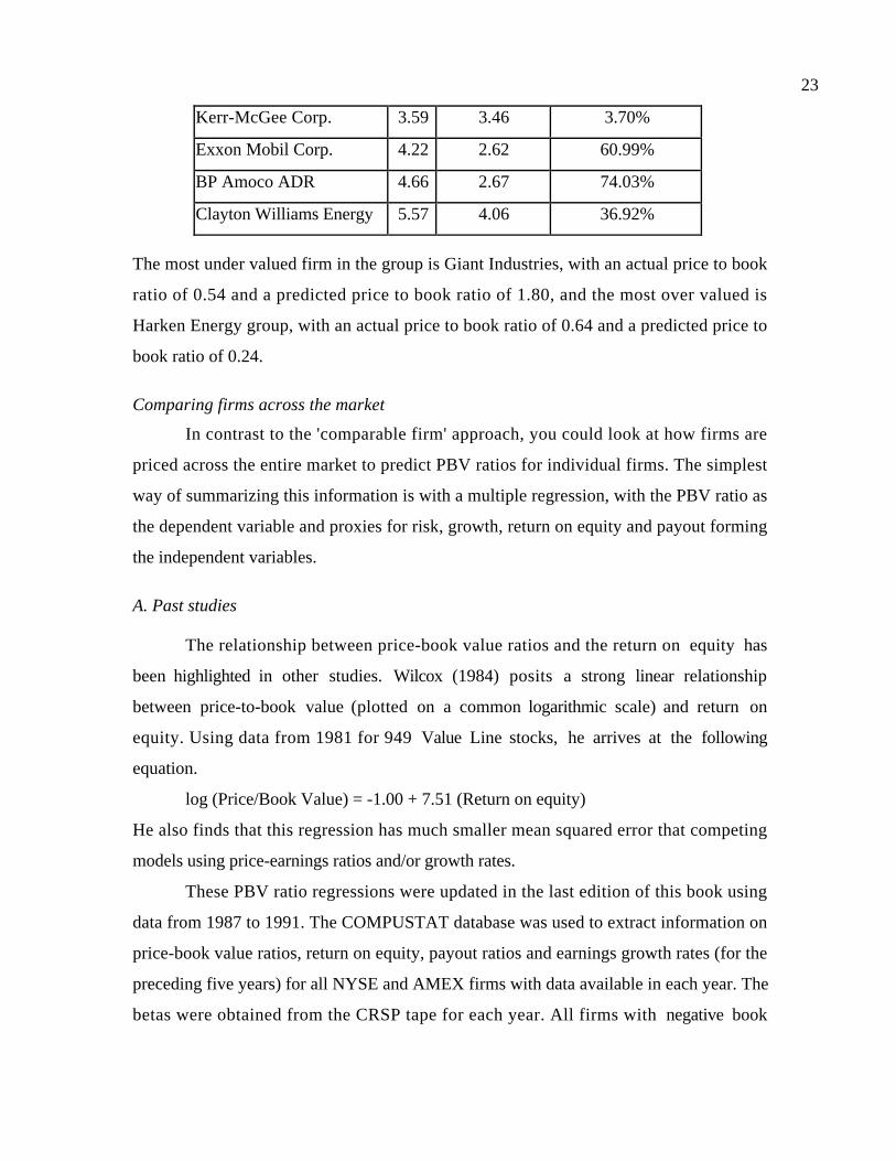
23

Kerr-McGee Corp. 3.59 3.46 3.70%

Exxon Mobil Corp. 4.22 2.62 60.99%

BP Amoco ADR 4.66 2.67 74.03%

Clayton Williams Energy 5.57 4.06 36.92%

The most under valued firm in the group is Giant Industries, with an actual price to book

ratio of 0.54 and a predicted price to book ratio of 1.80, and the most over valued is

Harken Energy group, with an actual price to book ratio of 0.64 and a predicted price to

book ratio of 0.24.

Comparing firms across the market

In contrast to the 'comparable firm' approach, you could look at how firms are

priced across the entire market to predict PBV ratios for individual firms. The simplest

way of summarizing this information is with a multiple regression, with the PBV ratio as

the dependent variable and proxies for risk, growth, return on equity and payout forming

the independent variables.

A. Past studies

The relationship between price-book value ratios and the return on equity has

been highlighted in other studies. Wilcox (1984) posits a strong linear relationship

between price-to-book value (plotted on a common logarithmic scale) and return on

equity. Using data from 1981 for 949 Value Line stocks, he arrives at the following

equation.

log (Price/Book Value) = -1.00 + 7.51 (Return on equity)

He also finds that this regression has much smaller mean squared error that competing

models using price-earnings ratios and/or growth rates.

These PBV ratio regressions were updated in the last edition of this book using

data from 1987 to 1991. The COMPUSTAT database was used to extract information on

price-book value ratios, return on equity, payout ratios and earnings growth rates (for the

preceding five years) for all NYSE and AMEX firms with data available in each year. The

betas were obtained from the CRSP tape for each year. All firms with negative book

24

values were eliminated from the sample and the regression of PBV on the independent

variables yielded the following for each year.

Year Regression R squared

1987 PBV = 0.1841 + .00200 PAYOUT - 0.3940 BETA + 1.3389 EGR

+ 9.35 ROE 0.8617

1988 PBV = 0.7113 + 0.00007 PAYOUT - 0.5082 BETA + 0.4605 EGR

+ 6.9374 ROE 0.8405

1989 PBV = 0.4119 + 0.0063 PAYOUT - 0.6406 BETA + 1.0038 EGR

+ 9.55 ROE 0.8851

1990 PBV = 0.8124 + 0.0099 PAYOUT - 0.1857 BETA + 1.1130 EGR

+ 6.61 ROE 0.8846

1991 PBV = 1.1065 + 0.3505 PAYOUT - 0.6471 BETA + 1.0087 EGR

+ 10.51 ROE 0.8601

where,

PBV = Price / Book Value Ratio at the end of the year

PAYOUT = Dividend Payout ratio at the end of the year

BETA = Beta of the stock

EGR = Growth rate in earnings over prior five years

ROE = Return on Equity = Net Income / Book Value of Equity

B. Updated Regressions

In July 2000, we regressed the price to book ratio against the fundamentals

identified in the last section – the return on equity, the payout ratio, the beta and the

expected growth rate over the next 5 years (from analyst forecasts).

PBV = -0.59 + 8.93 ROE +0.0809 Payout ratio + 0.917 Beta + 7.55 Growth rate

(3.76) (32.22) (3.06) (5.68) (18.37)

The regression has an R-squared of 43.2%.

The strong positive relationship between price to book ratios and returns on

equity is not unique to the United States. In fact, the following table summarizes

regression for other countries of price to book against returns on equity.

25

Table 19.4: Price to Book and Returns on Equity: Market Regressions

Country Regression Details Regression Equation

Greece May 2001

Entire market:

272firms

PBV = 2.11 + 11.63 ROE (R2=17.5%)

Brazil October 2000

(Entire market:

PBV = 0.77 + 3.78 (ROE) (R2=17.3%)

Portugal June 1999

(Entire market – 74

firms)

PBV = -1.94 + 16.34 ROE + 2.83 Beta

(R2=78%)

India November 1997

(50 largest firms)

PBV = -1.68 + 24.03 ROE (R2=51%)

In each of the markets, firms with higher returns on equity have higher price to book

ratios, though the strength of the relationship is greater in Portugal and India and weaker

in Greece and Brazil.

Illustration 19.7: Valuing a private firm using the cross-sectional regression

Assume that you had been asked to value a private firm early in 2001 and that

you had obtained the following data on the company:

Book Value of Equity = 100 million

Net Income in 2000 = 20 million

Beta based upon comparable firms = 1.20

First compute the variables in the desired units.

Payout = 8/20 = 40% (assuming free cashflow to equity is paid out as dividend)

Earnings Growth Rate = 25%

Return on Equity = 20 / 100 = 20%

Beta = 1.20

Predicted Price/Book Value Ratio = -0.59 + 8.93 (0.20)+ 0.0809 (0.40)+ 0.917 (1.20)

+7.55 (0.25) = 4.2162

Predicted Market Value of firm = 4.2162 * 100 = 421.62 million

26

pbvreg.htm: This reports the results of the latest regression of PBV ratios

against fundamentals, using all firms in the market.

Current versus Expected Returns on Equity

In all of the comparisons that we have made in this section, we have used a firm’s

current return on equity to make judgments about valuation. While it is convenient to

focus on current returns, the market value of equity is determined by expectations of

future returns on equity.

To the extent that there is a strong positive correlation between current ROE and

future ROE, using the current return on equity to identify under or over valued companies

is appropriate. Focusing on the current ROE can be dangerous, however, when the

competitive environment is changing, and can lead to significant errors in valuation. In

such cases, you should use a forecast return on equity that can be very different from the

current return on equity. There are several ways in which you can obtain this forecast.

• You could compute a historical average (over the last 3 or 5 years) of the return on

equity earned by the firm and substitute this value for the current return on equity,

when the latter is volatile.

• You could use the push the firm’s current return on equity towards the industry

average to reflect competitive pressures. For instance, assume that you are analyzing a

computer software firm with a current return on equity of 35% and that the industry

average return on equity is 20%. The forecast return on equity for this firm would be

a weighted average of 20% and 35%, with the weight on the industry average

increasing with the speed with which you expect the firm’s return to converge on

industry norms.

Comparing a firm’s price to book ratio across time

As a firm’s return on equity changes over time, you would expect its price to

book ratio to also change. Specifically, firms that increase their returns on equity should

increase their price to book ratios and firms that see their returns on equity deteriorate

should see a fall in their price to book ratios as well. Another way of thinking about this

27

is in terms of the matrix presented in Figure 19.7, where we argued that firms with low

(high) returns on equity should have low (high) price to book ratios.

Figure 19.7: Changes in ROE and Changes in PBV Ratio

Return on Equity - Cost of Equity

High Price to BookHigh Equity return spread

Low Price to BookLow Equity return spread

As return on equityincreases, the priceto book ratio willincrease

As return on equitydrops, the price tobook ratio willdrop

Thus, one way to measure the effect of the restructuring of a poorly performing firm

(with low return on equity and low price to book ratio) is to see where it moves on the

matrix. If it succeeds in its endeavor, it should move from the low PBV/low ROE

quadrant towards the high PBV/high ROE quadrant.

Illustration 19.8: ROE and P/BV Ratios - The case of IBM

IBM provides a classic example of the effects of returns on equity on price-book

value ratios. In 1983, IBM had a price which was three times its book value, one of the

highest price-book value multiples among the Dow 30 stocks at that time. By 1992, the

stock was trading at roughly book value, significantly lower than the average ratio for

Dow 30 stocks. This decline in the price-book value ratio was triggered by the decline in

return on equity at IBM, from 25% in 1983 and 1984, to negative levels in 1992 and

28

1993. In the years following Lou Gerstner becoming CEO, the firm has recovered

dramatically and was trading at 9 times book value in 1999. Figure 19.8 illustrates both

variables between 1982 and 2000 for IBM.

An investor buying IBM at its low point would have obtained a stock with a low price to

book and a low return on equity, but her bet would have paid off. As the return on equity

improved, IBM migrated from the bottom left quadrant to the top right quadrant in the

matrix above. As its price to book ratio improved, the investor would have seen

substantial price appreciation and profits.

Use in Investment Strategies

Investors have used the relationship between price and book value in a number of

investment strategies, ranging from the simple to the sophisticated. Some have used low

price-book value ratios as a screen to pick undervalued stocks. Others combine price to

book value ratios with other fundamentals to make the same judgment. Finally, the sheer

persistent of higher returns earned by low price to book stocks is viewed by some as an

indication that price to book value ratio is a proxy for equity risk.

Figure 19.8: IBM: The Fall and Rise again

0.00

1.00

2.00

3.00

4.00

5.00

6.00

7.00

8.00

9.00

10.00

1983 1984 1985 1986 1987 1988 1989 1990 1991 1992 1993 1994 1995 1996 1997 1998 1999 2000

Year

Pric

e to

Boo

k

-40.00%

-30.00%

-20.00%

-10.00%

0.00%

10.00%

20.00%

30.00%

40.00%

50.00%

Ret

urn

on E

quity

PBV ROE

29

The Link to Excess Returns

Several studies have established a relationship between price-book value ratios and

excess returns. Rosenberg, Reid and Lanstein (1985) find that the average returns on U.S.

stocks are positively related to the ratio of a firm's book value to market value. Between

1973 and 1984, the strategy of picking stocks with high book/price ratios (low price-book

values) yielded an excess return of 36 basis points a month. Fama and French (1992), in

examining the cross-section of expected stock returns between 1963 and 1990, establish

that the positive relationship between book-to-price ratios and average returns persists in

both the univariate and multivariate tests and is even stronger than the small firm effect in

explaining returns. When they classified firms on the basis of book-to-price ratios into

twelve portfolios, firms in the lowest book-to-price (higher P/BV) class earned an average

monthly return of 0.30%, while firms in the highest book-to-price (lowest P/BV) class

earned an average monthly return of 1.83%, for the 1963-90 period.

Chan, Hamao and Lakonishok (1991) find that the book-to-market ratio has a

strong role in explaining the cross-section of average returns on Japanese stocks. Capaul,

Rowley and Sharpe (1993) extend the analysis of price-book value ratios across other

international markets and conclude that value stocks, i.e., stocks with low price-book

value ratios, earned excess returns in every market that they analyzed, between 1981 and

1992. Their annualized estimates of the return differential earned by stocks with low

price-book value ratios, over the market index, were as follows:

Country Added Return to low P/BV portfolio

France 3.26%

Germany 1.39%

Switzerland 1.17%

U.K 1.09%

Japan 3.43%

U.S. 1.06%

Europe 1.30%

Global 1.88%

30

While this study is dated, the conclusion that lower price to book stocks earn higher

returns than higher price to book stocks is unlikely to be challenged.

Using Price-Book Value Ratios as Investment Screens

The excess returns earned by firms with low price-book value ratios has been

exploited by investment strategies that use price/book value ratios as a screen. Ben

Graham, for instance, in his classic on security analysis, listed price being less than two-

thirds of book value as one of the criteria to be used to pick stocks.

The discussion in the preceding section emphasized the importance of return on

equity in determining the price/book value ratio and noted that only firms with high return

on equity and low price-book value ratio could be considered undervalued. This

proposition was tested by screening all NYSE stocks from 1981 to 1990, on the basis of

both price-book value ratios and returns on equity and creating two portfolios - an

'undervalued' portfolio with low price-book value ratios (in bottom 25% of universe) and

high returns on equity (in top 25% of universe) and an overvalued portfolio with high

price-book value ratios (in top 25% of universe) and low returns on equity (in bottom

25% of universe) - each year, and then estimating excess returns on each portfolio in the

following year. The following table summarizes returns on these two portfolios for each

year from 1982 to 1991.

Year Undervalued Overvalued S & P 500

Portfolio Portfolio

1982 37.64% 14.64% 40.35%

1983 34.89% 3.07% 0.68%

1984 20.52% -28.82% 15.43%

1985 46.55% 30.22% 30.97%

1986 33.61% 0.60% 24.44%

1987 -8.80% -0.56% -2.69%

1988 23.52% 7.21% 9.67%

1989 37.50% 16.55% 18.11%

1990 -26.71% -10.98% 6.18%

31

1991 74.22% 28.76% 31.74%

1982-91 25.60% 10.61% 17.49%

The undervalued portfolios significantly outperformed the overvalued portfolios in eight

out of ten years, earning an average of 14.99% more per year between 1982 and 1991, and

also had an average return significantly higher than the S&P 500.

Price to Book as a proxy for risk

The persistence of excess returns earned by firms with lower price to book ratios

indicates either that the market is inefficient or that the price to book ratio is a proxy for

equity risk. In other words, if lower price to book ratio stocks are viewed by the market

as riskier than firms with higher price to book ratios, the higher returns earned by these

stocks would be a fair return for this risk. In fact, this is the conclusion that Fama and

French (1992) reached after examining the returns earned by lower price to book stocks.

While you cannot reject this hypothesis out of hand, you would need to put it to

the test. What is the additional risk that low price to book stocks are exposed to? It is

true that some low price to book ratio companies are highly levered and may not stay in

business. For the most part, though, a portfolio composed of low price to book ratio

stocks does not seem any more risky than a portfolio of high price to book stocks – their

leverage and earnings variability are similar.

Value to Book Ratios

Instead of relating the market value of equity to the book value of equity, the

value to book ratio relates the firm value to the book value of capital of the firm.

Consequently, it can be viewed as the firm value analogous to the price to book ratio.

Definition

The value to book ratio is obtained by dividing the market value of both debt and

equity by the book value of capital invested in a firm.

Value to Book Ratio = Debt of Book value+Equity of Book value

Debt of ueMarket val+equity of ueMarket val

32

If the market value of equity is unavailable, the book value of equity can be used in the

numerator as well. Needless to say, debt has to be consistently defined for both the

numerator and denominator. For instance, if you choose to convert operating leases to

debt for computing market value of debt, you have to add the present value of operating

leases to the book value of debt as well.

There are two common variants of this multiple that do not pass the consistency

test. One uses the book value of assets, which will generally exceed the book value of

capital by the magnitude of current liabilities, in the denominator. This will result in price

to book ratios that are biased down for firms with substantial current liabilities. The other

uses the enterprise value in the numerator, with cash netted from the market values of

debt and equity. Since the book value of equity incorporates the cash holdings of the firm,

this will also bias the multiple down. If you decide to use enterprise value in the

numerator, you would need to net cash out of the denominator as well.

Enterprise Value to Book = Cash-Debt of ValueBook +Equity of Book value

Cash-Debt of ueMarket val+equity of ueMarket val

In addition, the multiple will need to be adjusted for a firm’s cross holdings. The

adjustment was described in detail for the enterprise value to EBITDA multiple in

Chapter 18 and will require that you net out the portion of the market value and book

value of equity that is attributable to subsidiaries.

Description

The distribution of the value to book ratio resembles that of the price to book

ratio. In Figure 19.9, we present this distribution for U.S. companies in July 2000.

33

As with the other multiples, it is a heavily skewed distribution. The average value to book

ratio is 2.93, slightly lower than the average price to book ratio computed for the same

firms. The median value to book ratio is 1.40, which is also lower than the median price to

book ratio.

One of the interesting by-products of switching from price to book ratios to value

to book is that we lose no firms in the sample. In other words, the book value of equity

can be negative but the book value of capital is always positive.

pbvdata.xls: There is a dataset on the web that summarizes value to book

multiples and fundamentals by industry group in the United States for the most recent

year

Analysis

The value to book ratio is a firm value multiple. To analyze it, we go back to a free

cash flow to the firm valuation model and use it to value a stable growth firm.

g-capital ofCost

FCFF=Value 1

Figure 19.9: Value to Book Value

0

200

400

600

800

1000

1200

1400

0-0.5 0.5- 1 1-1.5 1.5-2 2- 2.5 2.5 - 3 3 - 3.5 3.5 - 4 4 - 4.5 4.5 - 5 5- 10 >10

Value to Book Ratio

Num

ber

of f

irm

s

34

Substituting in FCFF = EBIT1(1-t) (1 – Reinvestment Rate), we get:

( )( )g-capital ofCost

Ratent Reinvestme-1t1EBIT=Value 1 −

Dividing both sides by the book value of capital, we get:2

( )g-capital ofCost

Ratent Reinvestme-1ROC=

Capital of Book value

Value

The value to book ratio is fundamentally determined by its return on capital – firms with

high returns on capital tend to have high value to book ratios. In fact, the determinants of

value to book mirror the determinants of price to book equity, but we replace equity

measures with firm value measures – the ROE with the ROC, the cost of equity with the

cost of capital and the payout ratio with (1- Reinvestment rate). In fact, if we substitute

in the fundamental equation for the reinvestment rate:

Reinvestment rate ROC

g=

g-capital ofCost

g-ROC=

Capital of Book value

Value

The analysis can be extended to cover high growth firms, with the value to book capital

ratio determined by the cost of capital, growth rate and reinvestment – in the high growth

and stable growth periods.

Value 0

BV0

= ROChg( )1−RIRhg( ) 1+g( ) 1−

1+g( )n

1+k c,hg( )n

k c,hg -g+ ROCst( ) 1− RIRst( ) 1+g( )n

1+g n( )k c,st -gn( ) 1+k c,hg( )n

where,

ROC = Return on capital (hg: high growth period; st: stable growth period)

RIR = Reinvestment rate (hg: high growth period; st: stable growth period)

kc = Cost of capital (hg: high growth period; st: stable growth period)

firmmult.xls: This spreadsheet allows you to estimate firm value multiples for a

stable growth or high growth firm, given its fundamentals.

2 As with the return on equity, if return on capital is defined in terms of contemporaneous earnings (ROC =EBIT0/ Book Capital), there will be an extra (1+ g) in the numerator.

35

Application

The value to book ratios can be compared across firms just as the price to book

value of equity ratio was in the last section. The key variable to control for in making this

comparison is the return on capital. The value matrix developed for price to book ratios

can be adapted for the value to book ratio in Figure 19.10.

Figure 19.10: Valuation Matrix: Value to Book and Excess Returns

Return on Capital - Cost of Capital

High Value to BookHigh Return Spread

Low Value to BookLow Return Spread

Low Value to BookHigh Return spread

Undervalued

High Value to BookLow Return Spread

Overvalued

Firms with high return on capital will tend to have high value to book ratios, whereas

firms with low return on capital will generally have lower value to book ratios.

This matrix also yields an interesting link to a widely used value enhancement

measure– economic value added (EVA). One of the biggest sales pitches for EVA, which

is computed as the product of the return spread (ROC – Cost of capital) and Capital

Invested, is its high correlation with MVA (which is defined as the difference between

market value and book value of capital). This is not surprising since MVA is a variant on

the value to book ratio and EVA is a variant on the return spread.

Is the link between value to book and return on capital stronger or weaker than the

link between price to book and return on equity? To examine this question, we regressed

36

the value to book ratio against return on capital using data on all U.S. firms from January

2001.

Value/Book = -0.40 + 4.78 ROC + 11.48 Expected Growth + 0.39 σoi R2=41%

(2.33) (24.0) (16.8) (1.39)

The regression yields results similar to those obtained for price to book ratios.

If the results from using value to book and price to book ratios parallel each other,

why would you choose to use one multiple over the other? The case for using value to

book ratios is stronger for firms that have high and/or shifting leverage. Firms can use

leverage to increase their returns on equity, but in the process, they also increase the

volatility in the measure – in good times, they report very high returns on equity and in

bad times, very low or negative returns on equity. For such firms, the value to book ratio

and the accompanying return on capital will yield more stable and reliable estimates of

relative value. In addition, the value to book ratio can be computed even for firms that

have negative book values of equity and is thus less likely to be biased.

pbvreg.htm: This reports the results of the latest regression of PE ratios against

fundamentals, using all firms in the market.

Tobin's Q: Market Value/Replacement Cost

James Tobin presented an alternative to traditional financial measures of value by

comparing the market value of an asset to its replacement cost. His measure, called

Tobin’s Q, has several adherents in academia but still has not broken through into

practical use, largely because of informational problems.

Definition

Tobin's Q is estimated by dividing the market value of a firm’s assets by the

replacement cost of these assets.

Tobin's Q placein Assets ofCost t Replacemen

placein Assets of ueMarket val=

In cases where inflation has pushed up the replacement cost of the assets or where

technology has reduced the cost of the assets, this measure may provide a more updated

37

measure of the value of the assets than accounting book value. The rationale for the

measure is simple. Firms that earn negative excess returns and do not utilize their assets

efficiently will have a Tobin’s Q that is less than one. Firms that utilize their assets more

efficiently will trade at a Tobin’s Q that exceeds one.

While this measure has some advantages in theory, it does have some practical

problems. The first is that the replacement value of some assets may be difficult to

estimate, especially if assets are not traded on a market. The second is that even where

replacement values are available, substantially more information is needed to construct

this measure than the traditional price-book value ratio. In practice, analysts often use

short cuts to arrive at Tobin's Q, using book value of assets as a proxy for replacement

value and market value of debt and equity as a proxy for the market value of assets. In

these cases, Tobin’s Q resembles the value to book value ratio described in the last

section.

Description

If we use the strict definition of Tobin’s Q, we cannot get a cross sectional

distribution of the multiple because the information to estimate it is neither easily

accessible nor is it even available. This is a serious impediment to using the multiple

because we have no sense of what a high, low or average number for the multiple would

be. For instance, assume that you find a firm trading at 1.2 times the replacement cost of

the assets. You would have no way of knowing whether you were paying too much or

too little for this firm, without knowing the summary statistics for the market.

Analysis

The value obtained from Tobin's Q is determined by two variables - the market

value of the firm and the replacement cost of assets in place. In inflationary times, where

the cost of replacing assets increases over time, Tobin's Q will generally be lower than the

unadjusted price-book value ratio and the difference will increase for firms with older

assets. Conversely, if the cost of replacing assets declines much faster than the book value

(because of technological changes), Tobin's Q will generally be higher than the unadjusted

price-book value ratio.

38

Tobin’s Q is also determined by how efficiently a firm manages its assets and

extracts value from them, relative to the next best bidder. To see why, note that the

market value of an asset will be equal to its replacement cost, when assets earn their

required return. (If the return earned on capital is equal to the cost of capital, investments

have a zero net present value and the present value of the cash flows from the investment

will be equal to the investment made). Carrying this logic forward, Tobin’s Q will be less

than one, if a firm earns less than its required return on investments, and more than one, if

its earns positive excess returns.

Applications

Tobin’s Q is a practical measure of value for a mature firm with most or all of its

assets in place, where replacement cost can be estimated for the assets. Consider, for

example, a steel company with little or no growth potential. The market value of this firm

can be used as a proxy for the market value of its assets and you could adjust the book

value of the assets owned by the firm for inflation. In contrast, estimating the market

value of assets owned would be difficult for a high growth firm, since the market value of

equity for this firm will include a premium for future growth.

Tobin’s Q is more a measure of the perceived quality of a firm’s management than

it is of mis-valuation, with poorly managed firms trading at market values that are lower

than the replacement cost of the assets that they own. In fact, several studies have

examined whether such firms are more likely to be taken over. Lang, Stulz and Walkling

(1989) conclude that firms with low Tobin's Q are more likely to be taken over for

purposes of restructuring and increasing value. They also find that shareholders of high q

bidders gain significantly more from successful tender offers than shareholders of low q

bidders.

Conclusion

The relationship between price and book value is much more complex than most

investors realize. The price-book value ratio of a firm is determined by its expected

payout ratio, its expected growth rate in earnings and its riskiness. The most important

determinant, however, is the return on equity earned by the firm - higher (lower) returns

lead to higher (lower) price-book value ratios. The mismatch that should draw investor

39

attention is the one between return on equity and price-book value ratios -- high price-

book value ratios with low returns on equity (overvalued) and low price-book value ratios

with high returns on equity (undervalued).

The value to book ratio is the firm value analogy to the price to book ratio and it is

a function of the return on capital earned by the firm, its cost of capital and reinvestment

rate. Again, though, firms with low value to book ratios and high expected returns on

capital can be viewed as under valued.

40

Problems

1. Answer true or false to the following statements, with a short explanation.

A. A stock that sells for less than book value is undervalued.

B. If a company's return on equity drops, its price/book value ratio will generally drop

more than proportionately, i.e., if the return on equity drops by half, the price/book

value ratio will drop by more than half.

C. A combination of a low price-book value ratio and a high expected return on equity

suggests that a stock is undervalued.

D. Other things remaining equal, a higher growth stock will have a higher price-book

value ratio than a lower growth stock.

E. In the Gordon Growth model, firms with higher dividend payout ratios will have

higher price/book value ratios.

2. NCH Corporation, which markets cleaning chemicals, insecticides and other products,

paid dividends of $2.00 per share in 1993 on earnings of $4.00 per share. The book value

of equity per share was $40.00 and earnings are expected to grow 6% a year in the long

term. The stock has a beta of 0.85 and sells for $60 per share. (The treasury bond rate is

7%.)

a. Based upon these inputs, estimate the price/book value ratio for NCH.

b. How much would the return on equity have to increase to justify the price/book

value ratio at which NCH sells for currently?

3. You are analyzing the price/book value ratios for firms in the trucking industry, relative

to returns on equity and required rates of return. The data on the companies is provided

below:

Company PBV ROE Beta

Builders Transport 2.00 11.5% 1.00

Carolina Freight 0.60 5.5% 1.20

Consolidated Freight 2.60 12.0% 1.15

J.B. Hunt 2.50 14.5% 1.00

M.S. Carriers 2.50 12.5% 1.15

Roadway Services 3.00 14.0% 1.15

Ryder System 2.25 13.0% 1.05

Xtra Corporation 2.80 16.5% 1.10

The treasury bond rate is 7%.

a. Compute the average PBV ratio, return on equity and beta for the industry.

41

b. Based upon these averages, are stocks in the industry under or over valued relative to

book values.

4. United Healthcare, a health maintenance organization, is expected to have earnings

growth of 30% for the next five years and 6% after that. The dividend payout ratio will

be only 10% during the high growth phase, but will increase to 60% in steady state. The

return on equity was 21% in the most recent time period. The stock has a beta of 1.65

currently, but the beta is expected to drop to 1.10 in steady state. (The treasury bond rate

is 7.25%.)

(a) Estimate the price/book value ratio for United Healthcare, given the inputs above.

(b) How sensitive is the price/book value ratio to estimates of growth during the high

growth period?

(c) United Healthcare trades at a price/book value ratio of 7.00. How long would

extraordinary growth have to last (at a 30% annual rate) to justify this PBV ratio.

5. Johnson and Johnson, a leading manufacturer of health care products, had a return on

equity of 31.5% in 1993 and paid out 37% of its earnings as dividends. The stock had a

beta of 1.25. (The treasury bond rate is 6%.) The extraordinary growth is expected to last

for ten years, after which the growth rate is expected to drop to 6% and the return on

equity to 15%. (The beta will move to 1.)

a. Assuming the return on equity and dividend payout ratio continue at current levels

for the high growth period, estimate the PBV ratio for Johnson and Johnson.

b. If health care reform passes, it is believed that Johnson and Johnson's return on

equity will drop to 20% for the high growth phase. If they choose to maintain their

existing dividend payout ratio, estimate the new PBV ratio for Johnson and Johnson.

(You can assume that the inputs for the steady state period are unaffected.)

6. Assume that you have done a regression of PBV ratios for all firms on the New York

Stock Exchange and arrived at the following result.

PBV = 0.88 +0.82 PAYOUT +7.79 GROWTH -0.41 BETA + 13.81 ROE{R2=0.65}

where,

Payout = Dividend Payout ratio during most recent period

Beta = Beta of the stock in most current period

Growth = Projected Growth rate in Earnings over next five years

To illustrate, a firm with a payout ratio of 40%, a beta of 1.25, a ROE of 25% and

expected growth rate of 15%, would have had a price/book value ratio of:

PBV = 0.88 +0.82 (0.4) +7.79 (0.15) - 0.41 (1.25)+ 13.81 (0.25) = 5.3165

a. What, if any, use would you put the R squared of the regression to?

42

b. Assume that you have also run a sector regression on a company and estimated a price to

book ratio based upon that regression. Why might your result from the market regression

yield a different result from the sector regression?

1

CHAPTER 20

REVENUE MULTIPLES AND SECTOR-SPECIFIC MULTIPLES

While earnings and book value multiples are intuitively appealing and widely used,

analysts in recent years have increasingly turned to alternative multiples to value

companies. For new economy firms that have negative earnings, multiples of revenues

have replaced multiples of earnings in many valuations. In addition, these firms are being

valued on multiples of sector-specific measures such as the number of customers,

subscribers or even web-site visitors. In this chapter, the reasons for the increased use of

revenue multiples are examined first, followed by an analysis of the determinants of these

multiples and how best to use them in valuation. This is followed by a short discussion of

the sector specific multiples, the dangers associated with their use and the adjustments

that might be needed to make them work.

Revenue Multiples

A revenue multiple measures the value of the equity or a business relative to the

revenues that it generates. As with other multiples, other things remaining equal, firms

that trade at low multiples of revenues are viewed as cheap relative to firms that trade at

high multiples of revenues.

Revenue multiples have proved attractive to analysts for a number of reasons.

First, unlike earnings and book value ratios, which can become negative for many firms

and thus not meaningful, revenue multiples are available even for the most troubled firms

and for very young firms. Thus, the potential for bias created by eliminating firms in the

sample is far lower. Second, unlike earnings and book value, which are heavily influenced

by accounting decisions on depreciation, inventory, R&D, acquisition accounting and

extraordinary charges, revenue is relatively difficult to manipulate. Third, revenue

multiples are not as volatile as earnings multiples and hence are less likely to be affected

by year-to-year swings in firm’s fortune. For instance, the price-earnings ratio of a

cyclical firm changes much more than its price-sales ratios, because earnings are much

more sensitive to economic changes than revenues.

The biggest disadvantage of focusing on revenues is that it can lull you into

assigning high values to firms that are generating high revenue growth while losing

2

significant amounts of money. Ultimately, a firm has to generate earnings and cash flows

for it to have value. While it is tempting to use price-sales multiples to value firms with

negative earnings and book value, the failure to control for differences across firms in

costs and profit margins can lead to misleading valuations.

Definition of Revenue Multiple

As noted in the introduction to this section, there are two basic revenue multiples

in use. The first, and more popular one, is the multiple of the market value of equity to

the revenues of a firm – this is termed the price to sales ratio. The second, and more

robust ratio, is the multiple of the value of the firm (including both debt and equity) to

revenues – this is the enterprise value to sales ratio.

Revenues

Equity of ValueMarket =Ratio Sales toPrice

Revenues

Cash-Debt of ValueMarket +Equity of ValueMarket =Ratio Sales toValue Enterprise

As with the EBITDA multiple, we net cash out of firm value, because the income from

cash is not treated as part of revenue. The enterprise value to sales ratio a more robust

multiple than the price to sales ratio because it is internally consistent. It divides the total

value of the firm by the revenues generated by that firm. The price to sales ratio divides

an equity value by revenues that are generated for the firm. Consequently, it will yield

lower values for more highly levered firms and may lead to misleading conclusions when

price to sales ratios are compared across firms in a sector with different degrees of

leverage.

Accounting standards across different sectors and markets are fairly similar when

it comes to how revenues are recorded. There have been firms, in recent years though, that

have used questionable accounting practices in recording installment sales and intra-

company transactions to make their revenues higher. Notwithstanding these problems,

revenue multiples suffer far less than other multiples from differences across firms.

3

Cross Sectional Distribution

As with the price earning ratio, the place to begin the examination of revenue

multiples is with the cross sectional distribution of price to sales and value to sales ratios

across firms in the United States. Figure 20.1 summarizes this distribution.

There are two things worth noting in this distribution. The first is that revenue multiples

are even more skewed towards positive values than earnings multiples. The second is that

the price to sales ratio is generally lower than the value to sales ratio, which should not be

surprising since the former includes only equity while the latter considers firm value.

Table 20.1 provides summary statistics on both the price to sales and the value to

sales ratios.

Table 20.1:Summary Statistics on Revenue Multiples: July 2000

Price to Sales Ratio Value to Sales Ratio

Number of firms 4940 4940

Average 13.22 13.89

Median 1.06 1.32

Figure 20.1: Revenue Multiples

0

100

200

300

400

500

600

700

800

<0.05

0..05

-0.1

0.1-0

.15

0.150

.25

0.25-

0.5

0.5-0

.75

0.75-

11-

1.51.5

-2 2

- 3 3 -4

4 -5

5 -

7.5

7.5 -

10 >10

Revenue Multiple

Num

ber

of f

irm

s

Price to SalesValue to Sales

4

Standard Deviation 131.32 127.26

10th percentile 0.15 0.27

90th percentile 13.25 12.89

The average values for both multiples are much higher than the median values, largely as

the result of outliers – there are firms that trade at multiples that exceed 100 or more. The

price to sales ratio is slightly lower than the value to sales ratio but that is not surprising

since the former uses only the value of equity in the numerator whereas the latter looks at

firm value.

psdata.xls: There is a dataset on the web that summarizes price to sales and

value to sales ratios and fundamentals by industry group in the United States for the most

recent year.

Analysis of Revenue Multiples

The variables that determine the revenue multiples can be extracted by going back

to the appropriate discounted cash flow models – dividend discount model (or a FCFE

valuation model) for price to sales and a firm valuation model for value to sales ratios.

Price to Sales Ratios

The price to sales ratio for a stable firm can be extracted from a stable growth

dividend discount model.

P 0 =DPS1

r − gn

where,

P0 = Value of equity

DPS1 = Expected dividends per share next year

r = Required rate of return on equity

gn = Growth rate in dividends (forever)

Substituting in for DPS1 = EPS0 (1+gn) (Payout ratio), the value of the equity can be

written as:

5

( )( )( )n

n

gg

P-r

1RatioPayout EPS00

+=

Defining theshareper Sales

EPSMarginProfit Net 0= , the value of equity can be written as:

( )( )( )( )n

n00 g-r

g1RatioPayout MarginNet SalesP

+=

Rewriting in terms of the Price/Sales ratio,

( )( )( )n

n

0

0

g-r

g1RatioPayout MarginNet =PS=

Sales

P +

The PS ratio is an increasing function of the profit margin, the payout ratio and the

growth rate and a decreasing function of the riskiness of the firm.

The price-sales ratio for a high growth firm can also be related to fundamentals. In

the special case of the two-stage dividend discount model, this relationship can be made

explicit fairly simply. With two stages of growth, a high growth stage and a stable growth

phase, the dividend discount model can be written as follows:

( )( )( ) ( )( ) ( ) ( )( ) ( )

( )( )nhge,nste,

nn

n0

hge,

n

hge,

n

0

0k+1g-k

g+1g+1RatioPayout *EPS+

g-k

k+1

g+11g+1RatioPayout EPS

=P

−

where,

g = Growth rate in the first n years

ke,hg = Cost of equity in high growth

Payout = Payout ratio in the first n years

gn = Growth rate after n years forever (Stable growth rate)

ke,hg = Cost of equity in stable growth

Payoutn = Payout ratio after n years for the stable firm

Rewriting EPS0 in terms of the profit margin, EPS0 = (Sales0) (Profit Margin) and

bringing Sales0 to the left hand side of the equation, you get:

6

Price

Sales= Net Margin( )

Payout Ratio( ) 1+g( ) 1− 1+g( )n

1+k e,hg( )n

k e,hg -g+ Payout Ratio n( ) 1+g( )n

1+g n( )k e,st -g n( ) 1+k e,hg( )n

The left hand side of the equation is the price-sales ratio. It is determined by--

(a) Net Profit Margin: Net Income / Revenues. The price-sales ratio is an increasing

function of the net profit margin. Firms with higher net margins, other things remaining

equal, should trade at higher price to sales ratios.

(b) Payout ratio during the high growth period and in the stable period: The PS ratio

increases as the payout ratio increases, for any given growth rate.

(c) Riskiness (through the discount rate ke,hg in the high growth period and ke,st in the

stable period): The PS ratio becomes lower as riskiness increases, since higher risk

translates into a higher cost of equity.

(d) Expected growth rate in Earnings, in both the high growth and stable phases: The PS

increases as the growth rate increases, in both the high growth and stable growth period.

You can apply this equation to estimate the price to sales ratio, even for a firm

that is not paying dividends currently. As with the price to book ratio, you can substitute

in the free cash flows to equity for the dividends in making this estimate. Doing so will

yield a more reasonable estimate of the price to sales ratio for firms that pay out

dividends that are far lower than what they can afford to pay out.

Price

Sales= Net Margin( )

FCFEEarnings

1+g( ) 1− 1+g( )n

1+k e,hg( )n

k e,hg -g+

FCFEEarnings

n

1+g( )n1+g n( )

k e,st -g n( ) 1+k e,hg( )n

Illustration 20.1: Estimating the PS ratio for a high growth firm in the two-stage model

Assume that you have been asked to estimate the PS ratio for a firm that is

expected to be in high growth for the next 5 years. The following is a summary of the

inputs for the valuation.

Growth rate in first five years = 25% Payout ratio in first five years = 20%

7

Growth rate after five years = 8% Payout ratio after five years = 50%

Beta = 1.0 Riskfree rate = T.Bond Rate = 6%

Net Profit Margin = 10%

Cost of Equity = 6% + 1(5.5%)= 11.5%

This firm’s price to sales ratio can be estimated as follows:

PS=0.10

0.2( ) 1.25( ) 1−1.25( )5

1.115( )5

0.115-0.25+

0.50( ) 1.25( )51.08( )

0.115-0.08( ) 1.115( )5

=2.87

Based upon this firm’s fundamentals, you would expect its equity to trade at 2.87 times

revenues.

Illustration 20.2: Estimating the price to sales ratio for Unilever

Unilever is a U.K. based company that sells consumer products globally. To

estimate the price to sales ratio for Unilever, we used the following inputs for the high

growth and stable growth periods. The costs of equity and growth rates are estimated in

British pounds. Table 20.2 summarizes the inputs used in the valuation.

Table 20.2: Inputs for Estimating Price to Sales: Unilever

High Growth Period Stable Growth Period

Length 5 years Forever after year 5

Growth Rate 8.67% 5%

Net Profit Margin 5.82% 5.82%

Beta 1.10 1.10

Cost of Equity 10.5% 9.4%

Payout Ratio 51.17% 66.67%

The riskfree rate used in the analysis is 5% (long term British government bond rate) and

the risk premium is 5% in the high growth period (due to Unilever’s exposure in emerging

markets) and 4% in stable growth.

8

PS= 0.0582( )0.5117( ) 1.0867( ) 1−

1.0867( )5

1.1050( )5

0.1050-0.0867+

0.6667( ) 1.0867( )51.05( )

0.094-0.05( ) 1.1050( )5

=0.99

Based upon its fundamentals, you would expect Unilever to trade at 0.99 times revenues.

The stock was trading at 1.15 times revenues in May 2001.

Value to Sales Ratio

To analyze the relationship between value and sales, consider the value of a stable

growth firm:

n

10

gCapital ofCost

Rate)nt Reinvestmet)(1(1EBITValue Firm

−−−=

Dividing both sides by the revenue, you get

n

10

gCapital ofCost

Rate)nt Reinvestme1t)/Sales)((1(EBIT

Sales

Value Firm

−−−=

( )( )n

0

gCapital ofCost

Ratent Reinvestme1Margin Operatingtax -After

Sales

Value Firm

−−=

Just as the price to sales ratio is determined by net profit margins, payout ratios

and costs of equity, the value to sales ratio is determined by after-tax operating margins,

reinvestment rates and the cost of capital. Firms with higher operating margins, lower

reinvestment rates (for any given growth rate) and lower costs of capital will trade at

higher value to sales multiples.

This equation can be expanded to cover a firm in high growth by using a two-stage

firm valuation model.

Firm Value 0

Sales= AT Oper Margin( )

1-RIR( ) 1+ g( ) 1− 1+ g( )n

1+k c,hg( )n

k c,hg -g+ 1-RIR n( ) 1+ g( )n

1+g n( )k c,st -g n( ) 1+k c,hg( )n

9

where

AT Oper Margin = After-tax operating margin ( )

Sales

t-1EBIT=

RIR = Reinvestment Rate (RIRn is for stable growth period)

kc = Cost of capital (hg: high growth and st: stable growth periods)

g = Growth rate in operating income in high growth and stable growth periods

Note that the determinants of the value to sales ratio remain the same as they were in the

stable growth model – the growth rate, the reinvestment rate, the operating margin and the

cost of capital – but the number of estimates increases to reflect the existence of a high

growth period.

Illustration 20.3: Estimating the value to sales ratio for Coca Cola

Coca Cola has one of the highest operating margins of any large U.S. firm and it

should command a high value to sales ratio, as a consequence. To estimate the value to

sales ratio at which Coca Cola should trade at, we used the following inputs.

Table 20.3: Inputs for Estimating Value to Sales: Coca Cola

High Growth Period Stable Growth Period

Length 10 years Forever after year 10

Growth Rate 8.92% 5%

After-tax Operating Margin 16.31% 16.31%

Cost of Capital 9.71% 8.85%

Reinvestment Rate 40% 31.25%

The return on capital during the high growth period is expected to be 22.30% and to drop

to 16% during stable growth. Based upon these inputs, we can estimate the value to sales

ratio for Coca Cola.

VS = 0.1631( )1−0.40( ) 1.0892( ) 1−

1.0892( )10

1.0971( )10

0.0971− 0.0892

+ 0.1631( ) 1− 0.3125( ) 1.0892( )101.05( )

0.0885 − 0.05( ) 1.0971( )10

= 3.79

Based upon its fundamentals, you would expect Coca Cola to trade at 3.79 times

revenues. The firm was trading at 5.9 times revenues in May 2001.

10

firmmult.xls: This spreadsheet allows you to estimate the value to sales ratio for a

stable growth or high growth firm, given its fundamentals.

Revenue Multiples and Profit Margins

The key determinant of revenue multiples is the profit margin – the net margin for

price to sales ratios and operating margin for value to sales ratios. Firms involved in

businesses that have high margins can expect to sell for high multiples of sales. However,

a decline in profit margins has a two-fold effect. First, the reduction in profit margins

reduces the revenue multiple directly. Second, the lower profit margin can lead to lower

growth and hence lower revenue multiples.

The profit margin can be linked to expected growth fairly easily if an additional

term is defined - the ratio of sales to book value, which is also called a turnover ratio. This

turnover ratio can be defined in terms of book equity (Equity Turnover = Sales/ Book

value of equity) or book capital (Capital Turnover = Sales/ Book value of capital). Using a

relationship developed between growth rates and fundamentals, the expected growth rates

in equity earnings and operating income can be written as a function of profit margins and

turnover ratios.

Expected growthEquity

= Retention ratio( ) Return on Equity( ) =

= Retention ratio( ) Net Profit

Sales

Sales

BV of Equity

= Retention ratio( ) Net Margin( ) Sales/BV of Equity( )For example, in the valuation of Unilever in Illustration 20.2, the expected growth rate of

earnings is 8.67%. This growth rate can be derived from Unilever’s net margin (5.82%)

and sales/equity ratio (3.0485).

Expected Growth rate

= Retention ratio( ) Net ProfitSales

SalesBV of Equity

= 0.4883( ) 0.0582( ) 3.0485( )= 8.67%

For growth in operating income,

Expected growthFirm

11

= Reinvestment Rate( ) Return on Capital( )

= Reinvestment Rate( ) EBIT 1-t( )Sales

Sales

BV of Capital

= Reinvestment Rate( ) After -tax Operating Margin( ) Sales/BV of Capital( )In the valuation of Coca Cola in Illustration 20.3, the expected growth rate of operating

income is 8.92%. This growth rate can be derived from Coca Cola’s after-tax operating

margin (16.31%) and sales/capital ratio (1.37).

Expected growthfirm

( )( )( )( )( )( )

%92.8

37.11631.04.0

Capital of Sales/BVMargin Operatingtax -AfterRatent Reinvestme

===

As the profit margin is reduced, the expected growth rate will decrease, if the sales do not

increase proportionately.

Illustration 20.4: Estimating the effect of lower margins of price-sales ratios

Consider again the firm analyzed in Illustration 20.1. If the firm's profit margin

declines and total revenue remains unchanged, the price/sales ratio for the firm will decline

with it. For instance consider the effect if the firm's profit margin declines from 10% to

5%, and the sales/BV remains unchanged.

New Growth rate in first five years

( )( )( )( )( )( )

%10

50.205.08.0

Sales/BVMarginProfit RatioRetention

===

The new price sales ratio can then be calculated as follows:

PS=0.05

0.2( ) 1.10( ) 1−1.10( )5

1.115( )5

0.115-0.10+

0.50( ) 1.10( )51.08( )

0.115-0.08( ) 1.115( )5

=0.77

12

The relationship between profit margins and the price-sales ratio is illustrated more

comprehensively in the following graph. The price-sales ratio is estimated as a function of

the profit margin, keeping the sales/book value of equity ratio fixed.

This linkage of price-sales ratios and profit margins can be utilized to analyze the value

effects of changes in corporate strategy as well as the value of a 'brand name'.

Marketing Strategy and Value

Every firm has a pricing strategy. At the risk of over-simplifying the choice, you

can argue that firms have to decide whether they want to go with a low-price, high volume

strategy (volume leader) or with a high price, lower volume strategy (price leader). In

terms of the variables that link growth to value, this choice will determine the profit

margin and turnover ratio to use in valuation.

You could analyze the alternative pricing strategies that are available to a firm by

examining the impact that each strategy will have on margins and turnover and valuing the

firm under each strategy. The strategy that yields the highest value for the firm is, in a

sense, the optimal strategy.

Note that the effect of price changes on turnover ratios will depend in large part

on how elastic or inelastic the demand for the firm’s products are. Increases in the price of

Figure 20.2: P/S Ratios and Profit Margins

0.00

0.50

1.00

1.50

2.00

2.50

10% 9% 8% 7% 6% 5% 4% 3% 2% 1% 0%

Profit Margin

P/S

Rat

io

13

a product will have a minimal effect on turnover ratios if demand is inelastic. In this case,

the value of the firm will generally be higher with a price leader strategy. On the other

hand, the turnover ratio could drop more than proportionately if the product price in

increased and demand is elastic. In this case, firm value will increase with a volume leader

strategy.

Illustration 20.5: Choosing between a high-margin and a low-margin strategy.

Assume that a firm has to choose between the two pricing strategies. In the first strategy,

the firm will charge higher prices (resulting in higher net margins) and sell less (resulting in

lower turnover ratios). In the second strategy, the firm will charge lower prices and sell

more. Assume that the firm has done market testing and arrived at the following inputs:

High-Margin Low-Margin

Low Volume High Volume

Profit Margin 10% 5%

Sales/Book Value 2.5 4.0

Assume, in addition, that the firm is expected to pay out 20% of its earnings as dividends

over the next five years, and 50% of earnings as dividends after that. The growth rate after

year 5 is expected to be 8%. The book value of equity per share is $10. The cost of

equity for the firm is 11.5%.

High Margin Strategy

Expected Growth rate in first five yearsHigh margin

( )( )( )( )( )( )20%

0.82.50.10

ratioRetention Sales/BVMarginProfit

===

Price/Sales Ratio High margin = 0.10( )

0.2( ) 1.20( ) 1−1.20( )5

1.115( )5

0.115 − 0.20+

0.50( ) 1.20( )51.08( )

0.115 − 0.08( ) 1.115( )5

= 2.35

Sales/Book ValueHigh margin = 2.50

PriceHigh margin ( )( )( ) ( )( )( ) 58.83 $102.52.35Equity of BVSales/BVsPrice/Sale ===

14

Low Margin Strategy

Expected Growth rate in first five yearsLow margin

( )( )( )( )( )( )

%16

0.840.05

ratioRetention Sales/BVMarginProfit

===

Price/Sales RatioLow margin =

= 0.05( )0.2( ) 1.16( ) 1−

1.16( )5

1.115( )5

0.115 − 0.16+

0.50( ) 1.16( )51.08( )

0.115 − 0.08( ) 1.115( )5

= 0.9966

Sales/Book ValueLow margin = 4.00

PriceLow margin ( )( )( ) ( )( )( ) $39.861040.9966Equity of BVSales/BVsValue/Sale ===

The high margin strategy is clearly the better one to follow here, if the objective is value

maximization.

Illustration 20.6: Examining the effects of moving to a lower-margin, higher volume

strategy: Philip Morris in 1993

Philip Morris had sales of $59,131 million, earned $4,939 million in net income

and had a book value of equity of $12,563 million in 1992. The firm paid 42% of its

earnings as dividends in 1992. The beta for the stock was 1.10.

Based upon 1992 figures, the inputs for the price/sales ratio calculation would be:

Profit Margin = 8.35% Beta for the stock = 1.10

Sales / Book Value of Equity = 4.71 Expected Return = 7% + 1.1 (5.5%)

Book Value per share = $14.10 = 13.05%

Retention Ratio = 58%

Expected growth rate over next five years

( )( )( )( )( )( )22.80%

4.710.08350.58

Value Sales/BookMarginProfit RatioRetention

===

15

Expected growth rate after five years = 6% Expected payout ratio after five years =

65%

Price/Sales Ratio1992 Margins

= 0.0835( )0.42( ) 1.2280( ) 1−

1.2280( )5

1.1305( )5

0.1305 − 0.2280+

0.65( ) 1.2280( )51.06( )

0.1305 − 0.06( ) 1.1305( )5

=1.46

Sales/Book Value1992 Margins = 4.71

In April 1993, Philip Morris announced that it was cutting prices on its Marlboro Brand

of cigarettes because of increasing competition from low-priced competitors. This was

viewed by many analysts as a precursor of further price cuts and as a signal of a move to

a lower-margin strategy. Assume that the profit margin will decline to 7% from 8.35%, as

a consequence. If we assume that the sales/book value of equity ratio will remain

unchanged at 4.71, we can estimate the expected growth.

Expected growth rate over next five years

= Retention Ratio( ) Profit Margin( ) Sales/Book Value( )= 0.58( ) 0.07( ) 4.71( )=19.11%

Expected growth rate after five years = 6% Expected payout ratio after five years =

65%

Price/Sales Ratio1992 Margins

= 0.07( )0.42( ) 1.1911( ) 1−

1.1911( )5

1.1305( )5

0.1305 − 0.1911+

0.65( ) 1.1911( )51.06( )

0.1305 − 0.06( ) 1.1305( )5

=1.06

16

As a consequence of the new lower-price strategy, the price-sales ratio will decline from

1.46 to 1.06. Unless the sales/book value ratio increases by an equivalent proportion

(16.19%), the value of Philip Morris will decrease. In the case where profit margins

decline by this magnitude and the sales/book value is not expected to increase, the value

will decline by 27.41%.

The market reacted negatively to the announcement of price cuts and the stock

price dropped approximately 20% on the announcement.

Pricing Strategy, Market Share and Competitive Dynamics

All too often, firms analyze the effects of changing prices in a static setting, where

only the firm is acting and the competition stays still. The problem, though, is that every

action (especially when it comes to pricing) generates reactions from competition and the

net effects can be unpredictable.

Consider, for instance, a firm that cuts prices, hoping to increase market share and

sales. If the competition does nothing, the firm may be able to accomplish its objectives.

If, on the other hand, the competition reacts by also cutting prices, the firm may find

itself with lower margins and the same turnover ratios that it had before the price cut – a

recipe for lower firm value. In competitive industries, you have to assume that the latter

will happen and plan accordingly.

There are some firms that have focused on maximizing market share as their

primary objective function. The linkage between increased market share and market value

is a tenuous one and can be examined using the profit-margin/revenue multiple framework

developed above. If increasing market share leads to higher margins, either because of

economies of scale driving down costs or increased market power driving out competitors,

it will lead to higher value. If the increase in the market share is accompanied by lower

prices and profit margins, the net effect on value can be negative.

The Value of a Brand Name

One of the critiques of traditional valuation is that it fails to consider the value of

brand names and other intangibles. Hiroyumi Itami, in his book "Mobilizing Invisible

Assets", provides a summary of this criticism. He says:

17

"Analysts have tended to define assets too narrowly, identifying only those that can be

measured, such as plant and equipment. Yet the intangible assets, such as a particular

technology, accumulated consumer information, brand name, reputation and corporate

culture, are invaluable to the firm's competitive power. In fact, these invisible assets are

the only real source of competitive edge that can be sustained over time."

While this criticism is clearly overstated, the approaches used by analysts to value

brand names are often ad-hoc and may significantly overstate or understate their value.

Firms with well known brand names often sell for higher multiples than lesser-known

firms. The standard practice of adding on a 'brand name premium', often set arbitrarily, in

relationship to discounted cashflow value, can lead to erroneous estimates. Instead, the

value of a brand name can be estimated using the approach that relates profit margins to

price-sales ratios.

One of the benefits of having a well-known and respected brand name is that firms

can charge higher prices for the same products, leading to higher profit margins and hence

to higher price-sales ratios and firm value. The larger the price premium that a firm can

charge, the greater is the value of the brand name. In general, the value of a brand name can

be written as:

Value of brand name ( )( )SalesV/S-V/S gb=

where,

(V/S)b = Value-Sales ratio of the firm with the benefit of the brand name

(V/S)g = Value-Sales ratio of the firm with the generic product

Illustration 20.7: Valuing a brand name using price-sales ratio

Consider two firms which produce similar products that compete in the same

market place. Famous Inc. has a well-known brand name and has an after-tax operating

profit margin of 10%, while NoFrills Inc. makes a generic version and has an after-tax

operating margin of 5%. Both firms have the same sales-book capital ratio (2.50) and the

cost of capital of 11.5%. In addition, both firms are expected to reinvest 80% of their

operating income in the next five years and 50% of earnings after that. The growth rate

after year 5 for both firms, is 8%.

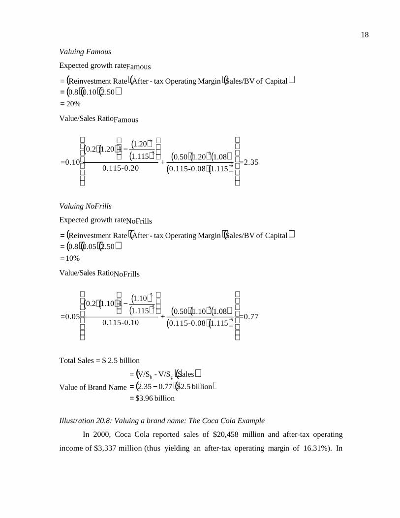
18

Valuing Famous

Expected growth rateFamous

( )( )( )( )( )( )

%20

50.210.08.0

Capital of Sales/BVMargin Operatingtax -AfterRatent Reinvestme

===

Value/Sales RatioFamous

=0.10

0.2( ) 1.20( ) 1−1.20( )5

1.115( )5

0.115-0.20+

0.50( ) 1.20( )51.08( )

0.115-0.08( ) 1.115( )5

=2.35

Valuing NoFrills

Expected growth rateNoFrills

( )( )( )( )( )( )

%10

50.205.08.0

Capital of Sales/BVMargin Operatingtax -AfterRatent Reinvestme

===

Value/Sales RatioNoFrills

=0.05

0.2( ) 1.10( ) 1−1.10( )5

1.115( )5

0.115-0.10+

0.50( ) 1.10( )51.08( )

0.115-0.08( ) 1.115( )5

=0.77

Total Sales = $ 2.5 billion

Value of Brand Name

( )( )( )( )

billion 96.3$

billion 5.2$77.035.2

SalesV/S-V/S gb

=−=

=

Illustration 20.8: Valuing a brand name: The Coca Cola Example

In 2000, Coca Cola reported sales of $20,458 million and after-tax operating

income of $3,337 million (thus yielding an after-tax operating margin of 16.31%). In

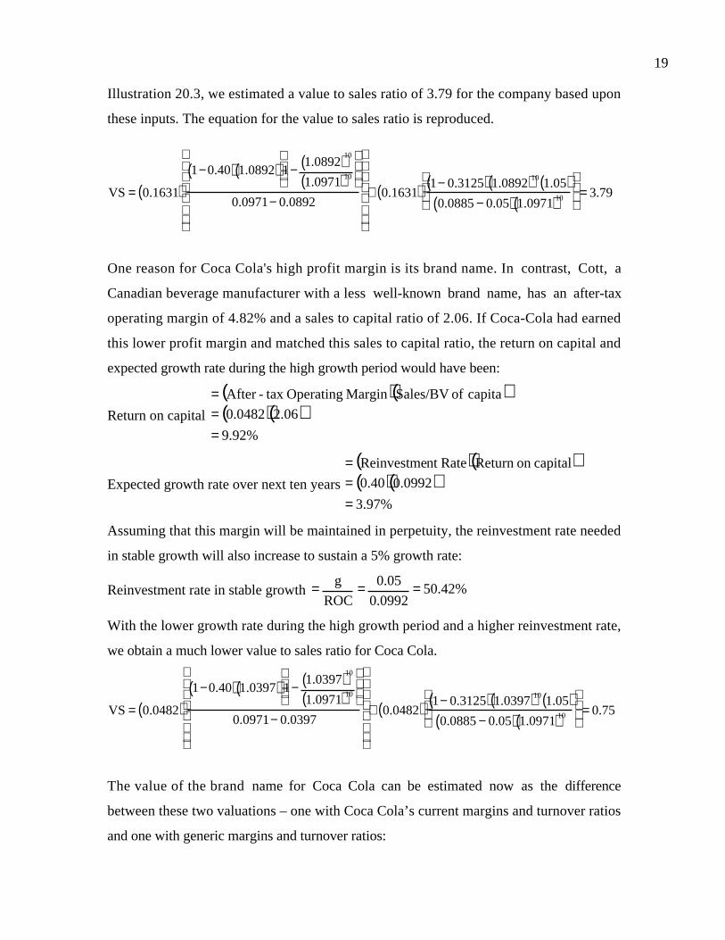
19

Illustration 20.3, we estimated a value to sales ratio of 3.79 for the company based upon

these inputs. The equation for the value to sales ratio is reproduced.

VS = 0.1631( )1−0.40( ) 1.0892( ) 1− 1.0892( )10

1.0971( )10

0.0971− 0.0892

+ 0.1631( ) 1− 0.3125( ) 1.0892( )10 1.05( )0.0885 − 0.05( ) 1.0971( )10

= 3.79

One reason for Coca Cola's high profit margin is its brand name. In contrast, Cott, a

Canadian beverage manufacturer with a less well-known brand name, has an after-tax

operating margin of 4.82% and a sales to capital ratio of 2.06. If Coca-Cola had earned

this lower profit margin and matched this sales to capital ratio, the return on capital and

expected growth rate during the high growth period would have been:

Return on capital

( )( )( )( )

%92.9

06.20482.0

capita of Sales/BVMargin Operatingtax -After

===

Expected growth rate over next ten years

( )( )( )( )

%97.3

0992.040.0

capitalon Return Ratent Reinvestme

===

Assuming that this margin will be maintained in perpetuity, the reinvestment rate needed

in stable growth will also increase to sustain a 5% growth rate:

Reinvestment rate in stable growth 50.42%0.0992

.050

ROC

g ===

With the lower growth rate during the high growth period and a higher reinvestment rate,

we obtain a much lower value to sales ratio for Coca Cola.

VS = 0.0482( )1−0.40( ) 1.0397( ) 1− 1.0397( )10

1.0971( )10

0.0971− 0.0397

+ 0.0482( ) 1− 0.3125( ) 1.0397( )10 1.05( )0.0885 − 0.05( ) 1.0971( )10

= 0.75

The value of the brand name for Coca Cola can be estimated now as the difference

between these two valuations – one with Coca Cola’s current margins and turnover ratios

and one with generic margins and turnover ratios:

20

Value of Coca Cola

= Value/Sales 2000 Margins( ) SalesCoca Cola( )= 3.79( ) $20,458( )= $ 77,536 million

Value of Coca Cola as a generic firm

( )( )( )( )

million $15,344

$20,4580.75

SalessValue/Sale Cola CocaGeneric

===

Value of brand name

= Value/Sales 2000 Margins-Value/Sales Generic( ) Salescoca Cola( )= 3.79 − 0.75( ) $20,458 million( )= $ 62,192 million

Of Coca Cola’s estimated value of $77536 million, 80.21% stems from its brand name,

which provides it with the market power to earn higher margins and to grow faster.

An aside on brand name value

It is common to see brand name premiums attached to discounted cash flow

valuations. As you can see from the example above, this is a mistake. Done right, the

value of a brand name is already built into the valuation in a number of places – higher

operating margins, higher turnover ratios and, consequently, higher returns on capital.

These, in turn, have ripple effects, increasing expected growth rates and value. Adding a

brand name premium to this value would be double counting.

What about firms that do not exploit a valuable brand name? You might add a

premium to the values of these firms, but the premium is not for the brand name but for

control. In fact, you could estimate similar premiums for any underutilized or mismanaged

assets, but you would pay the premiums only if you could acquire control of the firm.

Using Revenue Multiples in Investment Analysis

The key determinants of the revenue multiples of a firm are its expected margins

(net and operating), risk, cashflow and growth characteristics. To use revenue multiples in

analysis and to make comparisons across firms, you would need to control for differences

on these characteristics. In this section, we examine different ways of comparing revenue

multiples across firms.

21

Looking for Mismatches

While growth, risk and cash flow characteristics affect revenue multiples, the key

determinants of revenue multiples are profit margins – net profit margin for equity

multiples and operating margins for firm value multiples. Thus, it is not surprising to find

firms with low profit margins and low revenue multiples and firms with high profit

margins and high revenue ratios. However, firms with high revenue ratios and low profit

margins as well as firms with low revenue ratios and high profit margins should attract

investors' attention as potentially overvalued and undervalued securities, respectively.

This is presented in a matrix in Figure 20.3.

Figure 20.3: Value/Sales and Margins

Margin

Low Revenue MultipleLow Margin

Undervalued

High Revenue MultipleLow Margin

Overvalued

Low Revenue MultipleHigh Margin

High Revenue MultipleHigh Margin

You can identify under or over valued firms in a sector or industry by plotting them on

this matrix and looking for potential mismatches between margins and revenue multiples.

While intuitively appealing, there are at least three practical problems associated

with this approach. The first is that data is more easily available on historical (current)

22

profit margins than on expected profit margins. If a firm’s current margins are highly

correlated with future margins – a firm that has earned high margins historically will

continue to do so and one that have earned low margins historically will also continue to

do so – using current margins and current revenue multiples to identify under or over

valued securities is reasonable. If the current margins of firms are not highly correlated

with expected future margins, it is no longer appropriate to argue that firms are over

valued just because they have low current margins and trade at high price to sales ratios.

The second problem with this approach is that it assumes that revenue multiples are

linearly related to margins. In other words, as margins double, you would expect revenue

multiples to double as well. The third problem is that it ignores differences on other

fundamentals, especially risk. Thus, a firm that looks under valued because it has a high

current margin and is trading at a low multiple of revenues may in fact be a fairly valued

firm with very high risk.

Illustration 20.9: Revenue Multiples and Margins: Specialty Retailers

In the first comparison, we look at specialty retailers with positive earnings in the

most recent financial year. In Figure 20.4, the value to sales ratios of these firms are

plotted against the operating margins of these firms (with the stock symbols for each firm

next to each observation).

23

Figure 20.4: Value to Sales Ratios and Operating Margins

MSELGDYS RET.TO MLG

MHCOZANYPSRC

FINLROSIFLWS LVC TWMCSPGLASAH RUSH MDADBRNGADZ WLSNCELL FNLYJILLIBICLWYANIC VOXX CHRS PSS BKEZMTMC HMYPBY

URBNROST AEOSPGDACC BEBEITNCAOGBIZ DAP RUS

MNROSCHS HLYWMENSLE LIN MDLKRAYS PIR GLBEZQKMIKECWTR IPAR ANNAZONSITBBY

LTDZLCORLY

FOSLPSUN CLEPLCEJWLSATH

PCCC WSM

TLB

HOTTCPWM

TWTR

SCC

BFCI

TOOVVTV MBAY

BIDDABRISEE

CHCSCDWC LUX

-0.0

0.5

1.0

1.5

2.0

-0.000 0.075 0.150 0.225

Operating Margin

V/Sales

Firms with higher operating margins tend to have higher value to sales ratios, while firms

with lower margin have lower value to sales ratios. Note, though, that there is a

considerable amount of noise even in this sub-set of firms in the relationship between

value to sales ratios and operating margins.

Illustration 20.10: Revenue Multiples and Margins: Internet Retailers

In the second comparison, the price to sales ratios of internet retailers are plotted

against the net margins earned by these firms in the most recent year in Figure 20.5.

24

Figure 20.5: Price to Sales Ratios versus Net Margins: Internet Stocks

ROWEGSVIPPODTURF BUYX ELTXGEEKRMIIFATB TMNTONEM ABTL INFO ANETITRAIIXLBIZZ EGRPACOMALOYBIDSSPLN EDGRPSIX ATHY AMZNCLKS PCLNAPNT SONENETO

CBIS NTPACSGPINTW RAMP

DCLKCNETATHMMQST FFIV

SCNT MMXIINTMSPYGLCOS

PKSI

-0

10

20

30

-0.8 -0.6 -0.4 -0.2

AdjMargin

AdjPS

Here, there seems to be almost no relationship between price to sales ratios and net

margins. This should not be surprising. Most internet firms have negative net income and

net margins. The market values of these firms are based not upon what they earn now but

what they are expected to earn in the future and there is little correlation between current

and expected future margins.

Statistical Approaches

When analyzing price earnings and price to book value ratios, we used regressions

to control for differences in risk, growth and payout ratios across firms. We could also

use regressions to control for differences across firms to analyze revenue multiples. In

this section, we begin by applying this approach to comparables defined narrowly as

firms in the same business and then expanded to cover the entire sector and the market.

A. Comparable Firms in the Same Business

In the last section, we examined firms in the same business looking for mismatches –

firms with high margins and low revenue multiples were viewed as under valued. In a

25

simple extension of this approach, we could regress revenue multiples against profit

margins across firms in a sector.

Price to Sales Ratio = a + b (Net Profit Margin)

Value to Sales Ratio = a + b (After-tax Operating Margin)

These regressions can be used to estimate predicted values for firms in the sample,

helping to identify under and over valued firms.

If the number of firms in the sample is large enough to allow for it, this regression

can be extended to add other independent variables. For instance, the standard deviation in

stock prices or the beta can be used as an independent variable to capture differences in

risk and analyst estimates of expected growth can control for differences in growth. The

regression can also be modified to account for non-linear relationships between revenue

multiples and any or all of these variables.

Can this approach be used for sectors such as the internet where there seems to be

little or no relationship between revenue multiples and fundamentals? It can, but only if

you adapt it to consider the determinants of value in these sectors.

Illustration 20.11: Regression Approach – Specialty Retailers

Consider again the scatter plot of value to sales ratios and operating margins for

retailers in Illustration 20.9. There is clearly a positive relationship and a regression of

value to sales ratios against operating margins for specialty retailers yields the following.

Value to Sales Ratio = 0.0563+ 6.6287 After-tax Operating Margin R2= 39.9%

(10.39)

This regression has 162 observations and the t-statisics are reported in brackets. The

predicted value to sales ratio for Talbots, one of the specialty retailers in the group, which

has an after-tax operating margin of 11.22%, can be estimated.

Predicted Value to Sales Ratio = 0.0563 + 6.6287(0.1122) = 0.80

With an actual value to sales ratio of 1.27, Talbot’s can be considered over valued.

This regression can be modified in two ways. One is to regress the value to sales ratio

against the ln(operating margins) to allow for the non-linear logarithmic relationship

between the two variables.

Value to Sales Ratio = 1.8313 + 0.4339 ln(After-tax Operating Margin) R2= 22.40%

26

(6.89)

The other is to expand the regression to include proxies for risk and growth.

Value to Sales = -0.6209 + 7.21 (At Op Mgn) – 0.0209 σOpInc + 3.1460 Growth

(10.34) (0.22) (4.91)

Where

AT Op Mgn = After-tax operating margin

σOpInc = Standard deviation in operating income over previous 5 years

Growth = Expected Growth Rate in earnings over next 5 years

This regression has fewer observations (124) than the previous two but a higher R

squared of 50.09%. The predicted value to sales ratio for Talbot’s using this regression

can be estimated.

Predicted Value to Sales = -0.6209 + 7.21 (0.1122) – 0.0209 (0.7391) + 3.1460 (0.225)

= 0.88

Talbot’s remains over valued even after adjusting for differences in growth and risk.

Illustration 20.12: Regression Approach – Internet Retailers

In the case of the internet stocks graphed in Illustration 20.10, the regression of

price to sales ratios against net margins yields the following.

Price to Sales Ratio = 44.4495 - 0.7331 (Net Margin) R2 = 0.22%

Not only is the R-squared close to zero, but the relationship between current net margins

and price to sales ratios is negative. Thus, there is little relationship between the pricing

of these stocks and their current profitability.

What variables might do a better job of explaining the differences in price to sales

ratios across internet stocks? Consider the following propositions.

• Since this sample contains some firms with very little in revenues and other firms

with much higher revenues, you would expect the firms with less in revenues to trade

at a much higher multiple of revenues than firms with higher revenues. Thus, Amazon

with revenues of almost $2 billion can be expected to trade at a lower multiple of this

value than iVillage with revenues of less than $60 million.

• There is a high probability that some or many of these internet firms will not survive

because they will run out of cash. A widely used measure of this potential for cash

27

problems is the cash burn ratio, which is the ratio of the cash balance to the absolute

value of EBITDA (which is usually a negative number). Firms with a low cash burn

ratio are at higher risk of running into a cash crunch and should trade at lower

multiples of revenues.

• Revenue growth is a key determinant of value at these firms. Firms that are growing

revenues more quickly are likely to reach profitability sooner, other things remaining

equal.

The following regression relates price to sales ratios to the level of revenues

(ln(Revenues)), the cash burn ratio (Absolute value of Cash/EBITDA) and revenue

growth over the last year for internet firms.

Price to Sales Ratio = 37.18- 4.34 ln(Revenue)+ 0.75 (Cash/EBITDA) + 8.37 GrowthRev

(1.85) (0.95) (4.18) (1.06)

The regression has 117 observations and an R-squared of 13.83%. The coefficients all

have the right signs, but are of marginal statistical significance. You could obtain a

predicted price to sales ratio for Amazon.com in July 2000 in this regression of.

PSAshford.com= 37.18 - 4.34 ln(1,920) + 0.75 (2.12) + 8.37 (1.4810) = 18.36

At its actual price to sales ratio of 6.69, Amazon looks significantly under valued relative

to other internet firms.

In any case, the regressions are much too noisy to attach much weight to the

predictions. In fact, the low explanatory power with fundamentals and the huge

differences in measures of relative value should sound a note of caution on the use of

multiples in sectors such as this one, where firms are in transition and changing

dramatically from period to period.

B. Market Regressions

If you can control for differences across firms using a regression, you can extend

this approach to look at much broader cross sections of firms. Here, the cross-sectional

data is used to estimate the price to sales ratio as a function of fundamental variables -

profit margin, dividend payout, beta and growth rate in earnings.

28

Consider first the technology sector. Regressing the price to sales ratio against net

margins, growth rate in earnings, payout ratios and betas in July 2000 yields the following

result.

PS = -8.48 + 30.37 (Net Margin) + 20.98 (Growth Rate) + 4.68 Beta + 3.79 Payout

(7.19) (10.2) (10.0) (4.64) (0.85)

There are 273 observations in this regression and the R-squared is 53.8%.

This approach can be extended to cover the entire market. In the first edition of

this book, regressions of price-sales ratios on fundamentals - dividend payout ratio,

growth rate in earnings, profit margin and beta – were run for each year from 1987 to

1991.

Year Regression R squared

1987 PS = 0.7894 + .0008 PAYOUT - 0.2734 BETA

+ 0.5022 EGR + 6.46 MARGIN 0.4434

1988 PS = 0.1660 + .0006 PAYOUT - 0.0692 BETA

+ 0.5504 EGR + 10.31 MARGIN 0.7856

1989 PS = 0.4911 + .0393 PAYOUT - 0.0282 BETA

+ 0.2836 EGR + 10.25 MARGIN 0.4601

1990 PS = 0.0826 + .0105 PAYOUT - 0.1073 BETA

+ 0.5449 EGR + 10.36 MARGIN 0.8885

1991 PS = 0.5189 + 0.2749 PAYOUT - 0.2485 BETA

+ 0.4948 EGR + 8.17 MARGIN 0.4853

where,

PS = Price /Sales Ratio at the end of the year

MARGIN = Profit Margin for the year = Net Income / Sales for the year (in %)

PAYOUT = Payout Ratio = Dividends / Earnings at the end of the year

BETA = Beta of the stock

EGR = Earnings Growth rate over the previous five years

This regression is updated for the entire market in July 2000.

PS = -2.36 + 17.43 ( Net Margin) + 8.72 (Growth Rate) + 1.45 Beta + 0.37 Payout

(16.5) (35.5) (23.9) (10.1) (3.01)

There are 2235 observations in this regression and the R-squared is 52.5%.

29

The regression can also be run in terms of the value to sales ratio, with the

operating margin, standard deviation in operating income and reinvestment rate used as

independent variables:

VS = -1.67 + 8.82 (Operating Margin) + 7.66 (Growth Rate) + 1.50 σoi + 0.08 RIR

(14.4) (30.7) (19.2) (8.35) (1.44)

This regression also has 2235 observations but the R-squared is slightly lower at 42%.

Illustration 20.13: Valuing Cisco and Motorola using Sector and Market Regressions-

July 2000

These sector and market regressions can be used to estimate predicted price to

sales ratios for Cisco and Motorola. In Table 20.4, the values of the independent variables

are reported for both firms.

Table 20.4: Regression Variables

Cisco Motorola

Net Margin 17.25% 2.64%

Expected Growth Rate (Analyst projection over 5 years) 36.39% 21.26%

Beta 1.43 1.21

Payout Ratio 0 35.62%

Using these values, you can estimate predicted price to sales ratios for the two firms from

the sector regression.

PSCisco = -8.48 + 30.37 (0.1725) + 20.98 (0.3639) + 4.68 (1.43) + 3.79 (0) = 11.09

PSMotorola = -8.48 + 30.37 (0.0264) + 20.98 (0.2126) + 4.68 (1.21) + 3.79 (0.3562) = 3.79

You can also estimate predicted price to sales ratios from the market regression.

PSCisco = -2.36 + 17.43 (0.1725) + 8.72 (0.3639) + 1.45 (1.43) + 0.37 (0) = 5.89

PSMotorola = -2.36 + 17.43 (0.0264) + 8.72 (0.2126) + 1.45 (1.21) + 0.37 (0.3562) = 1.84

Cisco at its existing price to sales ratio of 27.77 looks significantly over valued relative to

both the market and the technology sector. In contrast, Motorola with a price to sales

ratio of 2.27 is slightly over valued relative to the rest of the market, but is significantly

under valued relative to other technology stocks.

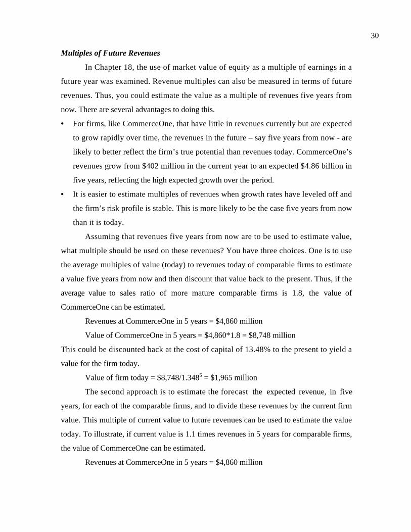
30

Multiples of Future Revenues

In Chapter 18, the use of market value of equity as a multiple of earnings in a

future year was examined. Revenue multiples can also be measured in terms of future

revenues. Thus, you could estimate the value as a multiple of revenues five years from

now. There are several advantages to doing this.

• For firms, like CommerceOne, that have little in revenues currently but are expected

to grow rapidly over time, the revenues in the future – say five years from now - are

likely to better reflect the firm’s true potential than revenues today. CommerceOne’s

revenues grow from $402 million in the current year to an expected $4.86 billion in

five years, reflecting the high expected growth over the period.

• It is easier to estimate multiples of revenues when growth rates have leveled off and

the firm’s risk profile is stable. This is more likely to be the case five years from now

than it is today.

Assuming that revenues five years from now are to be used to estimate value,

what multiple should be used on these revenues? You have three choices. One is to use

the average multiples of value (today) to revenues today of comparable firms to estimate

a value five years from now and then discount that value back to the present. Thus, if the

average value to sales ratio of more mature comparable firms is 1.8, the value of

CommerceOne can be estimated.

Revenues at CommerceOne in 5 years = $4,860 million

Value of CommerceOne in 5 years = $4,860*1.8 = $8,748 million

This could be discounted back at the cost of capital of 13.48% to the present to yield a

value for the firm today.

Value of firm today = $8,748/1.3485 = $1,965 million

The second approach is to estimate the forecast the expected revenue, in five

years, for each of the comparable firms, and to divide these revenues by the current firm

value. This multiple of current value to future revenues can be used to estimate the value

today. To illustrate, if current value is 1.1 times revenues in 5 years for comparable firms,

the value of CommerceOne can be estimated.

Revenues at CommerceOne in 5 years = $4,860 million

31

Value today

( )( )( )

million $5,346

(1.1)4,860

enues today/RevValueyears 5in Revenuesfirms Comparable5year

==

=

In the third approach, you can adjust the multiple of future revenues for

differences in operating margin, growth and risk for differences between the firm and

comparable firms. For instance, CommerceOne, five years from now, will have an

expected operating margin of 14.83% and an expected growth rate of 19.57% over the

following 5 years (years 6 through 10). A regression of value to sales ratio against

operating margins and expected growth rates run across comparable firms today yields the

following.

Value to Sales = 1.0834 + 3.0387 Operating Margin + 8.1555 Growth R2 = 73%

Plug in CommerceOne’s predicted values for expected growth and operating margins into

this regression.

Value to SalesCommerceOne in 5 years = 1.0834 + 3.0387 (0.1483)+ 8.1555 (0.1957) = 3.13

The value of CommerceOne in five years can now be estimated using this multiple.

Revenues at CommerceOne in 5 years = $4,860 million

Value of CommerceOne in 5 years = $4,860*3.13 = $15,212 million

Value of CommerceOne today = $15,212/1.13485 = $8,083 million

Sector-specific Multiples

The value of a firm can be standardized using a number of sector specific

multiples. The value of steel companies can be compared based upon market value per

ton of steel produced and the value of electricity generators can be computed on the basis

of kwh of power produced. In the last few years, analysts following new technology

firms have become particularly inventive with multiples that range from value per

subscriber for internet service providers to value per web site visitor for internet portals

to value per customer for internet retailers.

Why analysts use sector-specific multiples and their limitations

The increase in the use of sector specific multiples in the last few years has

opened up a debate about whether they are a good way to compare relative value. There

are several reasons why analysts use sector-specific multiples.

32

• They link firm value to operating details and output. For analysts who begin with

these forecasts – predicting the number of subscribers for an internet service provider,

for instance – they provide a much more intuitive way of estimating value.

• Sector specific multiples can often be computed with no reference to accounting

statements or measures. Consequently, they can be estimated for firms where

accounting statements are non-existent, unreliable or just not comparable. Thus, you

could compute the value per kwh sold for Latin American power companies and not

have to worry about accounting differences across these countries.

• Though this is usually not admitted to, sector-specific multiples are sometimes

employed in desperation because none of the other multiples can be estimated or

used. For instance, an impetus for the use of sector-specific multiples for new

economy firms was that they often had negative earnings and little in terms of book

value or revenues.

Though it is understandable that analysts sometimes turn to sector specific multiples,

there are two significant problems associated with their use.

• They feed into the tunnel vision that plagues analysts who are sector focused and

thus allow entire sectors to become overpriced. Thus, a cable company trading at

$50 a subscriber might look cheap next to another one trading at $125 a subscriber,

but it is entirely possible that they are both over priced or under priced.

• As we will show later in this section, the relationship of sector-specific multiples

to fundamentals is complicated and it is very difficult, consequently, to control for

differences across firms when comparing them on these multiples.

Definitions of Sector-specific Multiples

The essence of sector specific multiples is that the way they are measured vary

from sector to sector. In general, though, they share some general characteristics.

• The numerator is usually enterprise value – the market values of both debt and

equity netted out against cash and marketable securities.

• The denominator is defined in terms of the operating units that generate revenues

and profits for the firm.

33

For commodity companies such as oil refineries and gold mining companies, where

revenue is generated by selling units of the commodity, the market value can be

standardized by dividing by the value by the reserves that these companies have of the

commodity.

reservesin commodity theof units ofNumber

Debt of ValueMarket +Equity of ValueMarket =unitcommodity per Value

Oil companies can be compared on enterprise value per barrel of oil in reserves and gold

mining companies on the basis of enterprise value per ounce of gold in reserves.

For manufacturing firms that produce a homogeneous product (in terms of quality

and units), the market value can be standardized by dividing by the number of units of the

product that the firm produces or has the capacity to produce.

capacity)(or produced units ofNumber

Debt of ValueMarket +Equity of ValueMarket =productunit per Value

For instance, steel companies can be compared based upon their enterprise value per ton

of steel produced or in capacity.

For subscription-based firms such as cable companies, internet service providers

and information providers (such as TheStreet.com), revenues come from the number of

subscribers to the base service provided. Here, the value of a firm can be stated in terms

of the number of subscribers.

sSubscriber ofNumber

Debt of ValueMarket +Equity of ValueMarket =Subscriberper Value

In each of the above cases, you could make an argument for the use of a sector-

specific multiple because the units (whether they be barrels of oil, kwh of electricity or a

subscriber) generate the similar revenues. Sector multiples become much more problematic

when the units used to scale value are not homogeneous. Let us consider two examples.

For retailers such as Amazon that generate revenue from customers who shop at

their site, the value of the firm can be stated in terms of the number of regular customers.

Customers ofNumber

Debt of ValueMarket +Equity of ValueMarket =Customerper Value

34

The problem, here, is that amount spent by each customer can vary widely across the

customers and it is not clear that a firm that looks cheap on this basis is under valued.

For internet portals that generate revenue from advertising revenues that are based

upon traffic to the site, the revenues can be stated in terms of the number of visitors to

the site.

iteVisitors/S ofNumber

Debt of ValueMarket +Equity of ValueMarket =Visitor Siteper Value

Here, again, the link between visitors and advertising revenues is neither clearly

established nor obvious.

Determinants of Value

What are the determinants of value for these sector-specific multiples? Not

surprisingly, they are the same as the determinants of value for other multiples – cash

flows, growth and risk - though the relationship can be complex. The fundamentals that

drive these multiples can be derived by going back to a discounted cash flow model stated

in terms of these sector-specific variables.

Consider an internet service provider that has NX existing subscribers and assume

that each subscriber is expected to remain with the provider for the next n years. In

addition, assume that the firm will generate net cash flows per customer (Revenues from

each customer – Cost of serving the customer) of CFX per year for these n years1. The

value of each existing customer to the firm can then be written as:

Value per customer = VX = CFX

(1+r) tt=1

t=n

∑

The discount rate used to compute the value per customer can range from close to

the riskless rate, if the customer has signed a contract to remain a subscriber for the next n

1 For purposes of simplicity, it has been assumed that the cash flow is the same in each year. This can begeneralized to allow cash flows to grow over time.

35

years, to the cost of capital, if the estimate is just an expectation based upon past

experience.

Assume that the firm expects to continue to add new subscribers in future years

and that the firm will face a cost (advertising and promotion) of Ct for each new

subscriber added in period t. If the new subscribers (∆ NX t) added in period t will

generate the a value VXt per subscriber, the value of this firm can be written as:

Value of Firm = NX( ) VX( ) +∆NX t(VX t -C t)

(1+ k c)t

t=1

t=∞

∑

Note that the first term in this valuation equation represents the value generated by

existing subscriber and that the second is the value of expected growth. The subscribers

added generate value only if the cost of adding a new subscriber (Ct) is less than the

present value of the net cash flows generated by that subscriber for the firm.

Dividing both sides of this equation by the number of existing subscribers (NX).

Value per existing subscriber = Value of Firm

NX=VX +

∆NX t(VX t -C t )(1+ k c)

tt=1

t=∞

∑NX

In the most general case, then, the value of a firm per subscriber will be a function not

only of the expected value that will be generated by existing subscribers, but by the

potential for value creation from future growth in the subscriber base. If you assume a

competitive market, where the cost of adding new subscribers (Ct) converges on the value

that is generated by that customer, the second term in the equation drops out and the

value per subscriber becomes just the present value of cash flows that will be generated

by each existing subscriber.

Value per existing subscriberC=VX = VX

A similar analysis can be done to relate the value of an internet retailer to the number of

customers it has, though it is generally much more difficult to estimate the value that will

be created by a customer. Unlike subscribers who pay a fixed fee, retail customers buying

habits are more difficult to predict.

In either case, you can see the problems associated with comparing these

multiples across firms. Implicitly, you have to assume competitive markets and conclude

that the firms with the lowest market value per subscriber are the most under valued.

36

Alternatively, you have to assume that the value of growth is the same proportion of the

value generated by existing customers for all of the firms in your analysis. Either way, it

leads to the same conclusion.

Value can also be related to the number of site visitors, but only if the link

between revenues and the number of site visitors is made explicit. For instance, if an

internet portal’s advertising revenues are directly tied to the number of visitors at its site,

the value of the internet portal can be stated in terms of the number of visitors to the site.

Since sites have to spend money (on advertising) to attract visitors, it is the net value

generated by each visitor that ultimately determines value.

Illustration 20.14: Estimating the Value per Subscriber: Internet Portal

Assume that you are valuing GOL, an internet service provider with 1 million

existing subscribers. Each subscriber is expected to remain for 3 years and GOL is

expected to generate $100 in net after-tax cash flow (Subscription revenues – Costs of

providing subscription service) per subscriber each year. GOL has a cost of capital of

15%. The value added to the firm by each existing subscriber can be estimated.

Value per subscriber = 100

(1.15)t =t=1

t=3

∑ $228.32

Value of existing subscriber base = $228.32 million

Furthermore, assume that GOL expects to add 100,000 subscribers each year for the next

10 years and that the value added by each subscriber will grow from the current level

($228.32) at the inflation rate of 3% every year. The cost of adding a new subscriber is

$100 currently, assumed to be growing at the inflation rate.

Table 20.5: Value Added by New Subscribers

Year Value

added/Subscriber

Cost of acquiring

subscriber

Number of

subscribers added

Present Value at

15%

1 $ 235.17 $ 103.00 100,000 $ 11,493,234

2 $ 242.23 $ 106.09 100,000 $ 10,293,940

3 $ 249.49 $ 109.27 100,000 $ 9,219,789

4 $ 256.98 $ 112.55 100,000 $ 8,257,724

37

5 $ 264.69 $ 115.93 100,000 $ 7,396,049

6 $ 272.63 $ 119.41 100,000 $ 6,624,287

7 $ 280.81 $ 122.99 100,000 $ 5,933,057

8 $ 289.23 $ 126.68 100,000 $ 5,313,956

9 $ 297.91 $ 130.48 100,000 $ 4,759,456

10 $ 306.85 $ 134.39 100,000 $ 4,262,817

$ 73,554,309

The cumulative value added by new subscribers is $73.55 million. The total value of the

firm is the sum of the value generated by existing customers and the value added by new

customers.

Value of Firm = Value of existing subscriber base + Value added by new customers

= $ 228.32 million + $ 73.55 million = $ 301.87 million

Value per existing subscriber

subscriberper 87.301$million 1

million 87.301$ssubscriber ofNumber

Firm of Value

=

=

=

Note, though, that a portion of this value per subscriber is attributable to future growth.

As the cost of acquiring a subscriber converges on the value added by each subscriber, the

value per subscriber will converge on $228.32.

Analysis using Sector-Specific Multiples

To analyze firms using sector-specific multiples, you have to control for the

differences across firms on any or all of the fundamentals that you identified as affecting

these multiples in the last part.

With value-per–subscriber, for instance, you have to control for differences in the

value generated by each subscriber. In particular -

• Firms that are more efficient in delivering a service for a given subscription price

(resulting in lower costs) should trade at a higher value per subscriber than comparable

firms. This would also apply if a firm has significant economies of scale. In

Illustration 20.14 above, the value per subscriber would be higher if each existing

subscriber generated $120 in net cash flows for the firm each year instead of $100.

38

• Firms that can add new subscribers at a lower cost (advertising and promotion) should

trade at a higher value per subscriber than comparable firms.

• Firms with higher expected growth in the subscriber base (in percentage terms) should

trade at a higher value per subscriber than comparable firms.

You could make similar statements about value-per-customer.

With value per site visitor, you have to control for the additional advertising

revenue that is generated by each visitor – the greater the advertising revenue, the higher

the value per site visitor – and the cost of attracting each visitor – the higher the costs, the

lower the value per site visitor.

Illustration 20.15: Comparing Value per Site Visitor

In Table 20.6, the market value per site visitor is presented for internet firms that

generate the bulk of their revenues from advertising. The number of visitors per site was

from July 1, 2000 to July 31, 2000 and the market value is as of July 31, 2000.

Table 20.6: Value per Visitor

Company Name Firm Value Visitors Value per

visitor

Lycos, Inc. $ 5,396.00 5,858 $ 0.92

MapQuest.com Inc $ 604.80 6,621 $ 0.09

iVillage Inc $ 250.40 7,346 $ 0.03

CNET Networks $ 1,984.30 10,850 $ 0.18

Ask Jeeves Inc $ 643.50 11,765 $ 0.05

Go2Net Inc $ 1,468.60 12,527 $ 0.12

LookSmart, Ltd. $ 1,795.30 13,374 $ 0.13

About.com Inc $ 541.90 18,282 $ 0.03

Excite@Home $ 7,008.20 27,115 $ 0.26

Yahoo! Inc. $ 65,633.40 49,045 $ 1.34

Source: Media Metrix

Note the differences in value per site visitor across Yahoo, Excite and Lycos. Excite looks

much cheaper than either of the other two firms, but the differences could also be

attributable to differences across the firms on fundamentals. It could be that Yahoo earns

39

more in advertising revenues than Excite and Lycos and that its prospects of earning

higher profits in the future are brighter.

Conclusion

The price to sales multiple and value to sales are widely used to value technology

firms and to compare value across these firms. An analysis of the fundamentals highlights

the importance of profit margins in determining these multiples, in addition to the

standard variables - the dividend payout ratio, the required rate of return, the expected

growth rates for price to sales, the reinvestment rate and the risk for value to sales.

Comparisons of revenue multiples across firms have to take into account differences in

profit margins. One approach is to look for mismatches – low margins and high revenue

multiples suggesting over valued firms and high margins and low revenue multiples

suggesting under valued firms. Another approach that controls for differences in

fundamentals is the cross-sectional regression approach, where revenue multiples are

regressed against fundamentals across firms in a business, an entire sector or the market.

Sector-specific multiples relate value to sector specific variables but they have to

be used with caution. It is often difficult to compare these multiples across firms without

making stringent assumptions about their operations and growth potential.

40

Problems

1. Longs Drug, a large US drugstore chain operating primarily in Northern California, had

sales per share of $122 in 1993, on which it reported earnings per share of $2.45 and paid

a dividend per share of $1.12. The company is expected to grow 6% in the long term and

has a beta of 0.90. The current T.Bond rate is 7%.

a. Estimate the appropriate price/sales multiple for Longs Drug.

b. The stock is currently trading for $34 per share. Assuming the growth rate is

estimated correctly, what would the profit margin need to be to justify this price per

share.

2. You are examining the wide differences in price/sales ratios that you can observe among

firms in the retail store industry and trying to come up with a rationale to explain these

differences.

Per-Share

Company Price Sales Earnings Expected Beta Payout

Growth

Bombay Co. $ 38 $ 9.70 $ 0.68 29.00% 1.45 0 %

Bradlees 15 168.60 1.75 12.00% 1.15 34

Caldor 32 147.45 2.70 12.50% 1.55 0

Consolidated 21 23.00 0.95 26.50% 1.35 0

Dayton Hudson 73 272.90 4.65 12.50% 1.30 38

Federated 22 58.90 1.40 10.00% 1.45 0

Kmart 23 101.45 1.75 11.50% 1.30 59

Nordstrom 36 43.85 1.60 11.50% 1.45 20

Penney 54 81.05 3.50 10.50% 1.10 41

Sears 57 150.00 4.55 11.00% 1.35 36

Tiffany's 32 35.65 1.50 10.50% 1.50 19

Wal-Mart 30 29.35 1.05 18.50% 1.30 11

Woolworth 23 74.15 1.35 13.00% 1.25 65

a. There are two companies that sell for more than revenues, the Bombay company and

Wal-Mart. Why?

b. What is the variable that is most highly correlated with price-sales ratios?

c. Which of these companies is most likely to be over/under valued? How did you arrive

at this judgment?

3. Walgreen, a large retail drugstore chain in the United States, reported net income of

$221 million in 1993 on revenues of $8,298 million. It paid out 31% of its earnings as

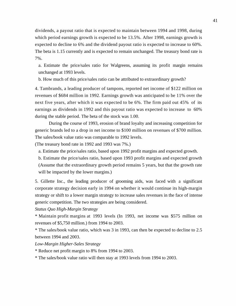
41

dividends, a payout ratio that is expected to maintain between 1994 and 1998, during

which period earnings growth is expected to be 13.5%. After 1998, earnings growth is

expected to decline to 6% and the dividend payout ratio is expected to increase to 60%.

The beta is 1.15 currently and is expected to remain unchanged. The treasury bond rate is

7%.

a. Estimate the price/sales ratio for Walgreens, assuming its profit margin remains

unchanged at 1993 levels.

b. How much of this price/sales ratio can be attributed to extraordinary growth?

4. Tambrands, a leading producer of tampons, reported net income of $122 million on

revenues of $684 million in 1992. Earnings growth was anticipated to be 11% over the

next five years, after which it was expected to be 6%. The firm paid out 45% of its

earnings as dividends in 1992 and this payout ratio was expected to increase to 60%

during the stable period. The beta of the stock was 1.00.

During the course of 1993, erosion of brand loyalty and increasing competition for

generic brands led to a drop in net income to $100 million on revenues of $700 million.

The sales/book value ratio was comparable to 1992 levels.

(The treasury bond rate in 1992 and 1993 was 7%.)

a. Estimate the price/sales ratio, based upon 1992 profit margins and expected growth.

b. Estimate the price/sales ratio, based upon 1993 profit margins and expected growth

(Assume that the extraordinary growth period remains 5 years, but that the growth rate

will be impacted by the lower margins.)

5. Gillette Inc., the leading producer of grooming aids, was faced with a significant

corporate strategy decision early in 1994 on whether it would continue its high-margin

strategy or shift to a lower margin strategy to increase sales revenues in the face of intense

generic competition. The two strategies are being considered.

Status Quo High-Margin Strategy

* Maintain profit margins at 1993 levels (In 1993, net income was $575 million on

revenues of $5,750 million.) from 1994 to 2003.

* The sales/book value ratio, which was 3 in 1993, can then be expected to decline to 2.5

between 1994 and 2003.

Low-Margin Higher-Sales Strategy

* Reduce net profit margin to 8% from 1994 to 2003.

* The sales/book value ratio will then stay at 1993 levels from 1994 to 2003.

42

The book value per share at the end of 1993 is $9.75. The dividend payout ratio, which

was 33% in 1993, is expected to remain unchanged from 1994 to 2003 under either

strategy, as is the beta, which was 1.30 in 1993. (The T.Bond rate is 7%)

After 2003, the earnings growth rate is expected to drop to 6% and the dividend

payout ratio is expected to be 60% under either strategy. The beta will decline to 1.0.

a. Estimate the price/sales ratio under the status quo strategy.

b. Estimate the price/sales ratio under the low margin strategy.

c. Which strategy would you recommend and why.

d. How much would sales have to drop under the status quo strategy for the two

strategies to be equivalent?

6. You have regressed price/sales ratios against fundamentals for NYSE stocks in 1994

and come up with the following regression.

PS = 0.42 + 0.33 PAYOUT + 0.73 GROWTH - 0.43 BETA + 7.91 MARGIN

For instance, a firm with a 35% payout, a 15% growth rate, a beta of 1.25 and a profit

margin of 10% would have had a price/sales ratio of:

PS = 0.42 + 0.33 * 0.35 + 0.73 * 0.15 - 0.43 * 1.25 + 7.91 * 0.10

= 0.8985

a. What do the coefficients on this regression tell you about the independent variables

relationship with the dependent variable? What statistical concerns might you have with

this regression?

b. Estimate the price/sales ratios for all the drugstore chains described in question 2.

Why might this answer be different from the one obtained from the regression of only

the drug store firms? Which one would you consider more reliable and why?

1

CHAPTER 21

VALUING FINANCIAL SERVICE FIRMS

Banks, insurance companies and other financial service firms pose particular

challenges for an analyst attempting to value them for two reasons. The first is the nature

of their businesses makes it difficult to define both debt and reinvestment, making the

estimation of cash flows much more difficult. The other is that they tend to be heavily

regulated and the effects of regulatory requirements on value have to be considered.

In this chapter, we begin by considering what makes financial service firms unique

and ways of dealing with the differences. We then look at how best we can adapt

discounted cash flow models to value financial service firms and look at three alternatives

– a traditional dividend discount model, a cash flow to equity discount model and an

excess return model. With each, we look at a variety of examples from the financial

services arena. We move on to look at how relative valuation works with financial service

firms and what multiples may work best with these firms.

In the last part of the chapter, we examine a series of issues that, if not specific to,

are accentuated in financial service firms ranging from the effect of changes in regulatory

requirements on risk and value to how best to consider the quality of loan portfolios at

banks.

Categories of financial service firms

Any firm that provides financial products and services to individuals or other

firms can be categorized as a financial service firm. We would categorize financial service

businesses into four groups from the perspective of how they make their money. A bank

makes money on the spread between the interest it pays to those from whom it raises

funds and the interest it charges those who borrow from it, and from other services it

offers it depositors and its lenders. Insurance companies make their income in two ways.

One is through the premiums they receive from those who buy insurance protection from

them and the other is income from the investment portfolios that they maintain to service

the claims. An investment bank provides advice and supporting products for other firms

to raise capital from financial markets or to consummate deals such as acquisitions or

divestitures. Investment firms provide investment advice or manage portfolios for clients.

2

Their income comes from advisory fees for the advice and management and sales fees for

investment portfolios.

With the consolidation in the financial services sector, an increasing number of

firms operate in more than one of these businesses. For example, Citigroup, created by

the merger of Travelers and Citicorp operates in all four businesses. At the same time,

however, there remain a large number of small banks, boutique investment banks and

specialized insurance firms that still derive the bulk of their income from one source.

How big is the financial services sector in the United States? Figure 21.1

summarizes the number of publicly traded banks, insurance companies, brokerage houses,

investment firms and thrifts in the United States at the end of 2000.

Even more striking than the sheer number of financial service firms is their diversity in

terms of size and growth. Table 21.1 provides a measure of the range on each measure

across different sectors.

Table 21.1: Cross Sectional Distribution: Financial Service Firms

Market Value of Equity(in millions) Expected Growth Rate

Figure 21.1: Financial Service Firms

0

50

100

150

200

250

Banks Insurance Companies Investment Companies Investment banks &Security Brokers

Thrift

Category

Num

ber

of f

irm

s

3

Industry

Number

of firms AverageMaximumMinimum

Standard

DeviationAverageMaximumMinimum

Standard

Deviation

Banks 211 $4,836 $96,910 $10 $12,642 10.60% 19.00% 4.50% 2.82%

Insurance

companies 86 $3,975 $90,317 $8 $11,663 11.24% 37.00% 1.50% 5.31%

Investment

Companies 45 $476 $2,707 $9 $500 9.50% 14.50% 6.50% 3.35%

Securities

Brokerage 27 $10,524 $97,987 $3 $23,672 17.56% 32.75% 10.00% 7.19%

Thrift 124 $707 $25,751 $5 $2,533 11.89% 38.33% 5.00% 5.00%

In emerging markets, financial service firms tend to have an even higher profile and

account for a larger proportion of overall market value than they do in the United States.

If we bring these firms into the mix, it is quite clear that no one template will value all

financial service firms and that we have to be able to be flexible in how we design the

model to allow for all types of financial service firms.

What is unique about financial service firms?

Financial service firms have much in common with non-financial service firms.

They attempt to be as profitable as they can, have to worry about competition and want

to grow rapidly over time. If they are publicly traded, they are judged by the total return

they make for their stockholders, just as other firms are. In this section, though, we focus

on those aspects of financial service firms that make them different from other firms and

consider the implications for valuation.

Debt: Raw Material or Source of Capital

When we talk about capital for non-financial service firms, we tend to talk about

both debt and equity. A firm raises funds from both equity investor and bondholders (and

banks) and uses these funds to make its investments. When we value the firm, we value

the value of the assets owned by the firm, rather than just the value of its equity.

With a financial service firm, debt seems to take on a different connotation. Rather

than view debt as a source of capital, most financial service firms seem to view it as a raw

4

material. In other words, debt is to a bank what steel is to General Motors, something to

be molded into other financial products which can then be sold at a higher price and yield

a profit. Consequently, capital at financial service firms seems to be more narrowly

defined as including only equity capital. This definition of capital is reinforced by the

regulatory authorities who evaluate the equity capital ratios of banks and insurance firms.

The definition of what comprises debt also seems to be murkier with a financial

service firm than it is with a non-financial service firm. For instance, should deposits

made by customers into their checking accounts at a bank be treated as debt by that bank?

Especially on interest-bearing checking accounts, there is little distinction between a

deposit and debt issued by the bank. If we do categorize this as debt, the operating

income for a bank should be measured prior to interest paid to depositors, which would

be problematic since interest expenses are usually the biggest single expense item for a

bank.

The Regulatory Overlay

Financial service firms are heavily regulated all over the world, though the extent

of the regulation varies from country to country. In general, these regulations take three

forms. First, banks and insurance companies are required to maintain capital ratios to

ensure that they do not expand beyond their means and put their claimholders or

depositors at risk. Second, financial service firms are often constrained in terms of where

they can invest their funds. For instance, until recently, the Glass-Steagall act in the

United States restricted commercial banks from investment banking activities and from

taking active equity positions in manufacturing firms. Third, entry of new firms into the

business is often restricted by the regulatory authorities, as are mergers between existing

firms.

Why does this matter? From a valuation perspective, assumptions about growth

are linked to assumptions about reinvestment. With financial service firms, these

assumptions have to be scrutinized to ensure that they pass regulatory constraints. There

might also be implications for how we measure risk at financial service firms. If regulatory

restrictions are changing or are expected to change, it adds a layer of uncertainty (risk) to

the future, which can have an effect on value.

5

Reinvestment at Financial Service Firms

In the last section, we noted that financial service firms are often constrained by

regulation in both where they invest their funds and how much they invest. If, as we have

so far in this book, define reinvestment as necessary for future growth, there are other

problems associated with measuring reinvestment with financial service firms. Note that

in Chapter 10, we consider two items in reinvestment – net capital expenditures and

working capital. Unfortunately, measuring either of these items at a financial service firm

can be problematic.

Consider net capital expenditures first. Unlike manufacturing firms that invest in

plant, equipment and other fixed assets, financial service firms invest primarily in

intangible assets such as brand name and human capital. Consequently, their investments

for future growth often are categorized as operating expenses in accounting statements.

Not surprisingly, the statement of cash flows to a bank show little or no capital

expenditures and correspondingly low depreciation. With working capital, we run into a

different problem. If we define working capital as the different between current assets and

current liabilities, a large proportion of a bank’s balance sheet would fall into one or the

other of these categories. Changes in this number can be both large and volatile and may

have no relationship to reinvestment for future growth.

As a result of this difficulty in measuring reinvestment, we run into two practical

problems in valuing these firms. The first is that we cannot estimate cash flows without

estimating reinvestment. In other words, if we cannot identify net capital expenditures

and changes in working capital, we cannot identify cash flows either. The second is that

estimating expected future growth becomes more difficult, if the reinvestment rate cannot

be measured.

General Framework for Valuation

Given the unique role of debt at financial service firms, the regulatory restrictions

that they operate under and the difficulty of identifying reinvestment at these firms, how

can we value these firms? In this section, we suggest some broad rules that can allow us to

deal with these issues. First, it makes far more sense to value equity directly at financial

service firms, rather than the entire firm. Second, we either need a measure of cashflow

6

that does not require us to estimate reinvestment needs or we need to redefine

reinvestment to make it more meaningful for a financial service firm.

Equity versus Firm

Early in this book, we noted the distinction between valuing a firm and valuing the

equity in the firm. We value firms by discounting expected after tax cash flows prior to

debt payments at the weighted average cost of capital. We value equity by discounting

cash flows to equity investors at the cost of equity.

Estimating cash flows prior to debt payments or a weighted average cost of capital

is problematic when debt and debt payments cannot be easily identified, which, as we

argued earlier, is the case with financial service firms. Equity can be valued directly,

however, by discounting cashflows to equity at the cost of equity. Consequently, we

would argue for the latter approach for financial service firms. We would extend this

argument to multiples as well. Equity multiples such as price to earnings or price to book

ratios are a much better fit for financial service firms than value multiples such as value to

EBITDA.

Estimating Cash Flows

To value the equity in a firm, we normally estimate the free cashflow to equity. In

Chapter 10, we defined the free cash flow to equity.

Free Cashflow to Equity = Net Income – Net Capital Expenditures – Change in non-cash

working capital – (Debt repaid – New debt issued)

If we cannot estimate the net capital expenditures or non-cash working capital, we clearly

cannot estimate the free cashflow to equity. Since this is the case with financial service

firms, we have two choices. The first is to use dividends as cash flows to equity and

assume that firms over time pay out their free cash flows to equity as dividends. Since

dividends are observable, we therefore do not have to confront the question of how much

firms reinvest. The second is to adapt the free cashflow to equity measure to allow for the

types of reinvestment that financial service firms make. For instance, given that banks

operate under a capital ratio constraint, it can be argued that these firms have to reinvest

equity capital in order to make more loans in the future.

7

Discounted Cashflow Valuation

In a discounted cash flow model, we consider the value of an asset to be the

present value of the expected cash flows generated by that asset. In this section, we will

first consider the use of dividend discount models to value banks and other financial

service firms, then move on to analyze cashflow to equity models and conclude with an

examination of excess return models.

Dividend Discount Models

In Chapter 13, we considered how to value the equity in a firm based upon

dividend discount models. Using the argument that the only cash flows that a stockholder

in a publicly traded firm receives are dividends, we valued equity as the present value of

the expected dividends. We looked at the range of dividend discount models, ranging from

stable to high growth, and considered how best to estimate the inputs. While much of

what was said in that chapter applies here as well, we will consider some of the unique

aspects of financial service firms in this section.

Basic Models

In the basic dividend discount model, the value of a stock is the present value of

the expected dividends on that stock. Assuming that equity in a publicly traded firm has

an infinite life, we arrive at:

Value per share of equity =∑∞=

= +

t

tt

e

t

kDPS

1 )1(

where

DPSt = Expected dividend per share in period t

ke = Cost of equity

In the special case where the expected growth rate in dividends is constant forever, this

model collapses into the Gordon Growth model.

Value per share of equity in stable growth =DPS1

(ke − g)

where g is the expected growth rate in perpetuity. In the more general case, where

dividends are growing at a rate which is not expected to be sustainable or constant forever

during a period (called the extraordinary growth period), we can still assume that the

8

growth rate will be constant forever at some point in the future. This allows us to then

estimate the value of a stock, in the dividend discount model, as the sum of the present

values of the dividends over the extraordinary growth period and the present value of the

terminal price, which itself is estimated using the Gordon growth model.

Value per share of equity in extraordinary growth = DPSt

(1+ ke ,hg) tt=1

t= n

∑ +DPSn +1

(ke ,st − gn )(1+ ke,hg )n

The extraordinary growth is expected to last n years, gn is the expected growth rate after n

years and ke is the cost of equity (hg: high growth period and st: stable growth period).

Inputs to Model

In this section, we will focus purely on the estimation issues relating to financial

service firms when it comes to the inputs to these models. In general, to value a stock

using the dividend discount model, we need estimates of the cost of equity, the expected

payout ratios and the expected growth rate in earnings per share over time.

a. Cost of Equity

In keeping with the way we have estimated the cost of equity for firms so far in

this book, the cost of equity for a financial service firm has to reflect the portion of the

risk in the equity that cannot be diversified away by the marginal investor in the stock.

This risk is estimated using a beta (in the capital asset pricing model) or betas (in a multi-

factor or arbitrage pricing model).

In our earlier discussions of betas, we argued against the use of regression betas

because of the noise in the estimates (standard errors) and the possibility that the firm has

changed over the period of the regression. How relevant are these arguments with financial

service firms? The regression beta estimates of large and more mature financial service

firms often are far more precise than the estimates for firms in other sectors. If regulatory

restrictions have remained unchanged over the period and are not expected to change in

the future, this may be one of the few sectors where regression betas can continue to be

used with some confidence. In periods where the rules are changing and regulatory

environments are shifting, the caveat about not using regression betas continues to hold.

There is a second area of difference. When estimating betas for non-financial

service firms, we emphasized the importance of unlevering betas (whether they be

9

historical or sector averages) and then relevering them, using a firm’s current debt to

equity ratio. With financial service firms, we would skip this step for two reasons. First,

financial service firms tend to be much more homogeneous in terms of capital structure –

they tend to have similar financial leverage primarily due to regulations. Second, and this

is a point made earlier, debt is difficult to measure for financial service firms. In practical

terms, this will mean that we will use the average levered beta for comparable firms as the

bottom-up beta for the firm being analyzed.

b. Payout Ratios

The expected dividend per share in a future period can be written as the product

of the expected earnings per share in that period and the expected payout ratio. There are

two advantages of deriving dividends from expected earnings. The first is that it allows us

to focus on expected growth in earnings, which is both more reasonable and more

accessible than growth in dividends. The second is that the payout ratio can be changed

over time, to reflect changes in growth and investment opportunities.

The payout ratio for a bank, as it is for any other firm, is the dividend divided by

the earnings. This said, financial service firms have conventionally paid out more in

dividends than other firms in the market, as is clear from Figure 21.2.

10

The dividend payout ratios and dividend yields for banks, insurance companies,

investment banks and investment firms are much higher than similar statistics for the rest

of the market.

Why do financial service firms pay out more in dividends than other firms? An

obvious response would be that they operate in much more mature businesses than firms

in sectors such as telecommunications and software, but this is only part of the story.

Even if we control for differences in expected growth rates, financial service firms pay out

far more in dividends than other firms for two reasons. One is that banks and insurance

companies need to invest far less in capital expenditures, at least as defined by

accountants, than other firms. This, in turn, means that far more of the net income of

these firms can be paid out as dividends than for a manufacturing firm. A second factor is

history. Banks and insurance companies have developed a reputation as reliable payers of

high dividends. Over time, they have attracted investors who like dividends, making it

difficult for them to change dividend policy.

In recent years, in keeping with a trend that is visible in other sectors as well,

financial service firms have increased stock buybacks as a way of returning cash to

stockholders. In this context, focusing purely on dividends paid can provide a misleading

Figure 21.2: Payout Ratios and Yields: Financial versus Non-financal service firms

0.00%

10.00%

20.00%

30.00%

40.00%

50.00%

60.00%

70.00%

80.00%

90.00%

Banks InsuranceCompanies

Investment firms Security Brokerage Thrift Non-financialservice firms

0.00%

0.50%

1.00%

1.50%

2.00%

2.50%

3.00%

3.50%

Payout RatioDividend Yield

11

picture of the cash returned to stockholders. An obvious solution is to add the stock

buybacks each year to the dividends paid and to compute the composite payout ratio. If

we do so, however, we should look at the number over several years, since stock

buybacks vary widely across time – a buyback of billions in one year may be followed by

three years of relatively meager buybacks, for instance.

c. Expected Growth

If dividends are based upon earnings, the expected growth rate that will determine

value is the expected growth rate in earnings. For financial service firms, as with other

firms, earnings growth can be estimated in one of three ways.

• Historical growth in earnings: Many banks and insurance companies have very

long histories and estimating historical growth is usually feasible. Furthermore, the

correlation between past earnings growth and expected future growth is much

higher for financial service firms than it is for other firms.

Note, in this figure, that the correlation between earnings growth over five-year

periods is 0.35 for financial service firms, while it is only 0.17 for other firms.

Figure 21.3: Correlation between past and expected growth

0

0.05

0.1

0.15

0.2

0.25

0.3

0.35

0.4

Financial Service Firms Non-financial service firms

12

This would suggest that historical growth in earnings is a much better predictor of

future earnings at these firms. If the regulatory environment is changing, however,

we have to be cautious about projecting past growth into the future.

• Analyst Estimates in Growth in Earnings: Analysts estimate expected growth rates

in earnings for many publicly traded firms, though the extent of coverage varies

widely. Many large banks and insurance companies are widely followed, allowing

us to get these estimates of future growth. As noted in Chapter 11, it is an open

question as to whether the long term forecasts from analysts are any better than

historical growth for estimating future growth.

• Fundamental Growth: In Chapter 11, we suggested that the expected growth in

earnings per share can be written as a function of the retention ratio and the return

on equity.

Expected Growth in EPS = Retention ratio * Return on equity

This equation allows us to estimate the expected growth rate for firms with stable

returns on equity. If we consider stock buybacks in addition to dividends when

looking at payout, the retention ratio should be defined consistently as well.

If the return on equity is expected to change over time, the expected

growth rate in earnings per share can be written as:

Expected GrowthEPS ( )( )t

t1t1t

ROE

ROE-ROEROERatioRetention +

+ +=

In both formulations, the expected growth rate is a function of the retention ratio,

which measures the quantity of reinvestment, and the return on equity, which

measures their quality. How well do fundamental growth models work for

financial service firms? Surprisingly well. The retention ratio in a bank measures

the equity reinvested back into the firms, which in turn, given the regulatory focus

on capital ratios, determines, in large part, how much these firms can expand in the

future. The return on equity is also a more meaningful measure of investment

quality because financial assets are much more likely to be marked up to market.

d. Stable Growth

13

To get closure with dividend discount models, we have to assume that the

financial service firms that we are valuing will be in stable growth at some point in the

future, where stable growth is defined to be growth that is less than or equal to the growth

rate of the economy. In some cases, especially with larger firms in more mature

businesses, the expected growth rate today may already be a stable growth rate.

In making the judgment of when a financial service firm will become a stable

growth firm, we have to consider three factors. The first is the size of the firm, relative to

the market that it serves. Larger financial service firms will find it more difficult to sustain

high growth for long periods, especially in mature markets. The second is the nature of

the competition. If competition is intense, stable growth will arrive sooner rather than

later. If competition is restricted, high growth and excess returns can last for much longer.

Finally, the way in which financial service firms are regulated can affect the convergence

to stable growth, since regulation can operate both as a help and a hindrance. By

restricting new entrants, regulations may help financial service firms maintain high growth

for long. At the same time, though, regulatory restrictions may prevent firms from

entering new and potentially lucrative businesses, which can reduce the length of the high

growth period.

As noted in prior chapters, it is not only the growth rate that changes in stable

growth. The payout ratio has to adjust to reflect the stable growth rate, and can be

estimated from the payout ratio

Payout ratio in stable growth growth stableROE

g-1=

The risk of the firm should also adjust to reflect the stable growth assumption. In

particular, if betas are used to estimate the cost of equity, they should converge towards

one in stable growth.

Illustration 21.1: Stable Growth Dividend Discount Model – Citigroup

Citigroup, created by the merger of Citicorp and Travelers Group, is one of the

giants in the financial service business. In 1999, Citigroup paid out dividends of $1,973

million on net income of $9,867 million; the return on equity for the year was 22%. The

14

low payout ratio and high return on equity would normally lead us to allow for a period

of high growth for the firm but there are two other factors to consider.

• Citigroup bought back $4.3 billion of its own stock in 1999 and $4.1 billion in

1998. If we consider the sum of dividends and stock buybacks over both periods

as a percent of net income, we arrive at a modified dividend payout ratio.

Modified dividend payout ratio

= 19991998

1999199819991998

IncomeNet IncomeNet

Dividends+Dividends+BuybacksBuybacks

++

= (4125+4294+1846+1973)/(5807+9867)

= 78.07%

If we go back over the last 4 years, rather then just the last 2 years, the modified

payout ratio is 56.40%. Over the same period, the return on equity at the firm has

averaged out to 17%.

• Citigroup has a significant market share in almost every business that it competes

it. While overall market growth may be high in some segments – emerging market

investment banking, for instance – the firm faces strong competition in each of

these segments.

With these factors in mind, we will assume that Citigroup is in stable growth and

that its current earnings (estimated for 2000) of $13.993 billion will grow 5% in

perpetuity. In addition, we will assume that the payout ratio looking forward will be

56.40% (the average modified payout ratio over last 4 years) and that the beta for the

stock based upon its business mix is 1.00. With these inputs, a riskfree rate of 5.1% and a

risk premium of 4%, we would value Citigroup as follows:

Cost of equity for Citigroup = 5.1% + 1.00 (4%) = 9.1%

Value of Citigroup’s equity ( )( )

billion $202.1130.05-0.091

0.5641.05$13.993 ==

There is an alternative approach we could have used to value Citigroup. Given its

return on equity of 17%, we could have estimated a dividend payout ratio and used this

ratio to value the stock.

Estimated Dividend payout ratio 70.59%0.17

0.05-1

ROE

g-1 ===

15

Value of Citigroup’s equity ( )( )

billion $2530.05-0.091

0.70591.05$13.993 ==

Which is the more reasonable value? It depends upon whether we believe that the 17%

return on equity that Citigroup earned between 1996 and 1999 can be maintained in

perpetuity. If the answer is yes, the $253 billion value estimate is the better one. If, on

the other hand, we assume that Citigroup’s return on equity will decline over time, the

initial estimate of $202 billion is more credible. At the time of this valuation in January

2001, Citicorp’s market value of equity was $ 256 billion.

Illustration 21.2: A High Growth Dividend Discount Model – State Bank of India

Valuation as of: January 2001 Stock price at time of valuation: Rs 235

State Bank of India is India’s largest bank, created in the aftermath of a

nationalization of all banks in India in 1971. For the two decades that followed, it

operated as a monopoly and was entirely government owned. In the 1990s, the Indian

governments privatized portions of the bank while retaining control of its management

and operations.

In 1999, State Bank of India earned 205 million Indian rupees on a book value of

equity of 1,042 million rupees (at the beginning of 1999), resulting in a return on equity of

19.72%. The bank also paid out dividends of Rs 2.50 per share from earnings per share of

Rs. 38.98; this yields a payout ratio of 6.41%. The high retention ratio suggests that the

firm is investing substantial amounts in the expectation of high growth in the future. We

will analyze its value over three phases – an initial period of sustained high growth, a

transition period where growth drops towards stable growth and a stable growth phase.

High Growth Phase

If State Bank can maintain the current return on equity of 19.72% and payout

ratio of 6.41%, the expected growth rate in earnings per share will be 18.46%.

Expected Growth rate = ROE * Retention ratio = 19.72% (1-0.0641) = 18.46%

The key question is how long the bank can sustain this growth. Given the large potential

size of the Indian market, we assume that this growth will continue for 4 years. During

this period, we also allow for the fact that there will be substantial risk associated with

the Indian economy by allowing for a country risk premium in estimating the cost of

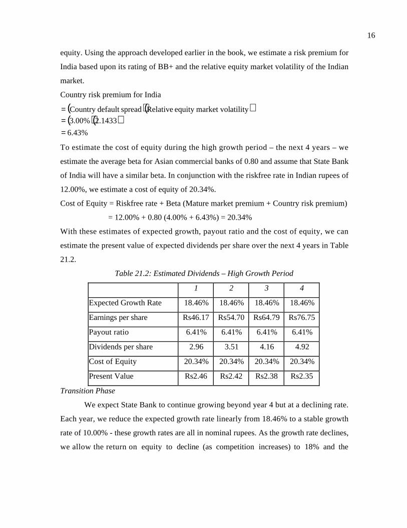
16

equity. Using the approach developed earlier in the book, we estimate a risk premium for

India based upon its rating of BB+ and the relative equity market volatility of the Indian

market.

Country risk premium for India

( )( )( )( )

%43.6

2.14333.00%

atilitymarket volequity Relativespreaddefault Country

===

To estimate the cost of equity during the high growth period – the next 4 years – we

estimate the average beta for Asian commercial banks of 0.80 and assume that State Bank

of India will have a similar beta. In conjunction with the riskfree rate in Indian rupees of

12.00%, we estimate a cost of equity of 20.34%.

Cost of Equity = Riskfree rate + Beta (Mature market premium + Country risk premium)

= 12.00% + 0.80 (4.00% + 6.43%) = 20.34%

With these estimates of expected growth, payout ratio and the cost of equity, we can

estimate the present value of expected dividends per share over the next 4 years in Table

21.2.

Table 21.2: Estimated Dividends – High Growth Period

1 2 3 4

Expected Growth Rate 18.46% 18.46% 18.46% 18.46%

Earnings per share Rs46.17 Rs54.70 Rs64.79 Rs76.75

Payout ratio 6.41% 6.41% 6.41% 6.41%

Dividends per share 2.96 3.51 4.16 4.92

Cost of Equity 20.34% 20.34% 20.34% 20.34%

Present Value Rs2.46 Rs2.42 Rs2.38 Rs2.35

Transition Phase

We expect State Bank to continue growing beyond year 4 but at a declining rate.

Each year, we reduce the expected growth rate linearly from 18.46% to a stable growth

rate of 10.00% - these growth rates are all in nominal rupees. As the growth rate declines,

we allow the return on equity to decline (as competition increases) to 18% and the

17

payout ratio to rise to reflect the lesser need for reinvestment1. To illustrate, the payout

ratio in year 8, when the expected growth rate is 10% can be computed.

Payout ratio in year 8 44.44%or 0.44440.18

0.10-1

ROE

rategrowth Expected1 ==−=

We also adjust the country risk premium down from 6.43% to 3.00% to reflect our

expectation that there will be less risk in investing in India as the country’s economy

matures. Table 21.3 summarizes expected dividends during the transition phase.

Table 21.3: Expected Dividends per share – Transition Phase

5 6 7 8

Expected Growth Rate 16.34% 14.23% 12.11% 10.00%

Earnings per share Rs89.29 Rs102.00 Rs114.35 Rs125.79

Payout ratio 15.92% 25.43% 34.94% 44.44%

Dividends per share 14.22 25.94 39.95 55.91

Cost of Equity 19.66% 18.97% 18.29% 17.60%

Cumulative Cost of Equity 250.98% 298.60% 353.20% 415.36%

Present Value Rs5.66 Rs8.69 Rs11.31 Rs13.46

Note that the cost of equity in year 8 reflects the lower country risk premium.

Cost of equity in year 8 = 12.00% + 0.80 (4.00% + 3.00%) = 17.60%

The beta and the mature market risk premium of 4% have been left unchanged. To

compute the present values of the expected dividends over the transition period, we

compound the cost of equity and discount the cash flows at the compounded cost2.

Stable Growth

In stable growth, we assume that State Bank’s earnings and dividends will grow in

perpetuity at 10% a year and discount them at the stable period cost of equity of

1 The adjustment in the payout ratio is linear. The current payout ratio is 6.41% and the stable periodpayout ratio is 44.44%. Dividing the difference of 38.03% over four years yields an increase in the payoutratio of 9.51% each year.2 When the cost of equity changes each year, as it does between years 5 and 8, the compounded cost ofequity has to be computed. For instance, the cashflow in year 6 will be discounted back using the followingcompounded cost:Compounded cost = (1.2034)4 (1.1966) (1.1897) = 2.9860

18

17.60%. The present value of these dividends in perpetuity, which yield the terminal

price per share, can be computed to be:

Terminal price per share

( )( )

( )( )

809.18 Rs0.10-0.176

0.44441.10125.79

g-equity ofCost

Payoutshareper Earnings Expected 99

=

=

=

Final Valuation

The final value per share for State Bank can be computed by adding the present

values of the dividends during the high growth phase, the dividends during the transition

period and the terminal price at the end of the transition period.

Value per share

= PV of dividends: high growth + PV of dividends: transition phase + PV of terminal

price

= 4.1536

809.1813.4611.318.695.662.352.382.422.46 ++++++++

= Rs 243.55

Note that the terminal price is discounted back at the compounded cost of equity for the

8th year.

Valuing a Non-dividend Paying Financial Service Firm

While many financial service firms do pay dividends, a large number of young,

high growth financial service firms in recent years have chosen not to pay dividends and

reinvest all of their earning back into their operations. In fact, some of these firms lose

money. While it may seem inappropriate to use the dividend discount model to value

such firms, we will argue that the model is flexible enough to deal with them. How, if

dividends are zero, will we ever be able to get a positive value for a share? The answer is

simple, at least for firms that have positive earnings currently. While dividends are zero

currently and are expected to be zero for the foreseeable future, when the firm is growing,

the growth will ultimately subside. As the growth drops, the firm’s capacity to pay out

dividends will increase. In fact, using the fundamental equation for growth from the last

section, we can estimate the expected payout ratio in future periods.

19

Expected Payout ratio ROE

g-1=

The equity will derive its value from expected future dividends.

If earnings are negative currently, the mechanics become a little more involved. We

first have to estimate earnings in future periods. Presumably, we would expect earnings to

become positive some period in the future. (If we did not, the value of equity would be

zero and the valuation exercise would be unnecessary.) Once earnings become positive,

the rest of the analysis resembles what we did above.

Illustration 21.3: Valuing a Non-dividend Paying Financial Service Firm – NetBank

Valuation as of: January 2001 Stock Price: $ 9.50

NetBank is a virtual bank that offers banking services to customers. At the time of

this valuation, the bank had just made the turn to profitability and reported net income of

$3.05 million on a beginning book value of equity of $38.76 million; this amounted to

earnings per share of $0.246. The bank paid no dividends but we anticipate significant

growth in earnings both from growth in deposits and economies of scale (which should

improve the return on equity). The expected growth rate in earnings is 30% for the next 6

years and it is then expected to decline linearly to a stable growth rate of 5% in the 12th

year.

NetBank is not expected to pay dividends during the first 6 years of high growth.

During this period, the bank is also exposed to significant risk. We use a beta of 1.70 to

reflect the risk of e-commerce ventures and estimate a cost of equity of 11.80%, based

upon a treasury bond rate of 5% and a risk premium of 4%.

Cost of equity = 5% + 1.70 (4%) = 11.80%

Table 21.4 summarizes the expected earnings during this high growth period.

Table 21.4: Expected Earnings and Dividends during high growth phase

1 2 3 4 5 6

Expected Growth Rate 30.00% 30.00% 30.00% 30.00% 30.00% 30.00%

Earnings per share $0.32 $0.42 $0.54 $0.70 $0.91 $1.19

Payout ratio 0.00% 0.00% 0.00% 0.00% 0.00% 0.00%

Dividends per share $0.00 $0.00 $0.00 $0.00 $0.00 $0.00

20

Cost of Equity 11.80% 11.80% 11.80% 11.80% 11.80% 11.80%

Present Value $0.00 $0.00 $0.00 $0.00 $0.00 $0.00

In stable growth (after the 12th year), the bank is expected to earn a return on

equity of 12% which will allow it to pay out 58.33% of its earnings as dividends during

the period:

Expected dividend payout ratio in 12th year %33.5818%

5%-1

ROE

g1 ==−=

Between years 6 and 12, as the growth rate tapers off, we will assume that the payout

ratio will increase from 0% to 58.33% in linear increments. We will also assume that the

risk in the equity will also decline, with the beta dropping from 1.70 to 1.00 in stable

growth. Table 21.5 summarizes the expected earnings and dividends during this transition

period.

Table 21.5: Expected Earnings and Dividends during transition phase

7 8 9 10 11 12

Expected Growth Rate 25.83% 21.67% 17.50% 13.33% 9.17% 5.00%

Earnings per share $1.49 $1.82 $2.14 $2.42 $2.64 $2.77

Payout ratio 9.72% 19.44% 29.17% 38.89% 48.61% 58.33%

Dividends per share $0.15 $0.35 $0.62 $0.94 $1.28 $1.62

Cost of Equity 11.33% 10.87% 10.40% 9.93% 9.47% 9.00%

Cumulative Cost of

Equity 217.41% 241.03% 266.10% 292.53% 320.23% 349.05%

Present Value $0.07 $0.15 $0.23 $0.32 $0.40 $0.46

The dividends begin in year 6 and grow at a much faster rate than earnings because the

payout ratio increases.

The terminal price at the end of the 12th year can be estimated using the dividends

in year 13, the stable period cost of equity and the expected growth rate in perpetuity.

Terminal price per share

( )( )

( )( )( )

49.42$05.009.0

5833.005.177.2

g-equity ofCost

ratioPayout g1EPS

stable13

13stable12

=−

=

+=

21

The value per share today can then be computed as the sum of the present values of the

dividends during high growth and the present value of the terminal price:

Value per share $13.813.4905

$42.490.46$$0.400.32$$0.23$0.15$0.07 =++++++=

The terminal price per share is discounted at the compounded cost of equity of 3.4905 in

year 12.

Cashflow to Equity Models

At the beginning of this discussion, we noted the difficulty in estimating

cashflows when net capital expenditures and non-cash working capital cannot be easily

identified. It is possible, however, to estimate cashflows to equity even for financial

service firms if we define reinvestment differently.

Defining Cashflow to Equity

The cashflow to equity is the cashflow left over for equity investors after debt

payments have been made and reinvestment needs met. With financial service firms, the

reinvestment generally does not take the form of plant, equipment or other fixed assets.

Instead, the investment is in human capital and regulatory capital; the latter is the capital

as defined by the regulatory authorities, which, in turn, determines the limits on future

growth. There are ways in which we could incorporate both of these items into the

reinvestment.

Capitalize Training and Employee Development Expenses

If human capital is a large factor in determining the success or failure of a financial

service firm, we could capitalize the expenses associated with developing this capital. The

process for doing so closely mirrors the process for capitalizing research and development

expenses for technology firms and involves the following steps.

1. Identify the amortizable life for the asset: To determine the period over which

these expenses will be written off, we have to begin with how long a typical

employee that the firm has invested its resources in stays with the firm.

2. Collect information on employee expenses in prior years: The amount spent

by the firm on employee training and development in prior years is collected,

22

with the number of years matching the amortizable life specified in the first

step.

3. Compute the current year’s amortization expense: The expenses in each of the

prior years is amortized. With a linear amortization schedule, the expense will

be spread equally over the amortizable life. The sum total of the amortization

of all of the expenses in previous years will become the current year’s

amortization expense.

4. Adjust the net income for the firm: The net income for the firm is adjusted for

the capitalization of employee expenses.

Adjusted Net Income = Reported Net income + Employee development

expense in the current year – Amortization of the employee expenses (from

step 3)

5. Compute the value of the human capital: The value of human capital in the firm

can be computed by adding up the unamortized portion of the employee

development expenses in each of the prior years.

Employee development expenses are more difficult to capitalize than research and

development expenses for two reasons. The first is that while research expenses are

usually consolidated and reported as one item on a financial statement, employee

development expenses tend to be widely spread across the firm and may be included in

several different items in an income statement. Disentangling these expenses from

employee salary and benefits may be difficult to do. The second is that the patents and

licenses that emerge from research belong to the firm and often give it exclusive rights in

commercial use. A firm’s employees, on the other hand, are mobile and may, and often

do, move to competitors who offer them better terms.

Assuming that we can get over these practical difficulties in valuing human capital,

let us consider the factors that determine the value that human capital adds to a firm. The

first is the employee turnover ratio; as this ratio rises, the amortizable life for employee

expenses will fall and with it the value of human capital. The second relates to the

resources spent by the firm in employee development and training; the greater the

resources, the greater the value assigned to human capital. There is a third and often

ignored factor. If we consider human capital as an asset, it is the excess returns that we

23

make on the asset that create value. To create excess returns, a firm will have to pay an

employee less than what he or she generates in value to the firm. To illustrate, an

investment bank will generate value from a bond trader that works for it only if it pays

that trader less than what he or she generates in profits for the firm. Why might the trader

settle for less? One reason might be that the investment bank has some unique capability

that allows the trader to earn these profits; this unique capability might come from

proprietary information, client lists or market position. Another reason might be non-

economic; the trader may have enough goodwill towards the investment bank that he or

she might be willing to give up higher compensation elsewhere. Firms that treat their

employees well and are loyal to them in bad times are much likely to earn this goodwill

and have higher value as a consequence.

Investments in Regulatory Capital

For a financial service firm that is regulated based upon capital ratios, equity

earnings that are not paid out increase the equity capital of the firm and allow it to expand

its activities. For instance, a bank that has a 5% equity capital ratio can make $100 in

loans for every $5 in equity capital. When this bank reports net income of $15 million and

pays out only $5 million, it is increasing its equity capital by $10 million. This, in turn,

will allow it to make $200 million in additional loans and presumably increase its growth

rate in future periods.

Using this argument, the portion of net income that does not get paid out can be

viewed as reinvestment. It works, however, only if the firm takes advantage of its larger

capital base and grows. If it does not, the equity retained is more akin to cash

accumulating in the firm rather than reinvestment. One way to measure this usage is to

look at the equity capital ratios of the firm over time and compare them to the regulatory

constraints. A firm that reports an equity capital ratio that rises over time, well above the

regulatory constraint, is not using its equity capital to grow.

Why Earnings are not cash flows?

There are some analysts who value banks by discounting their earnings back to the

present. They make the argument that banks have little or no net capital expenditure

24

needs and that working capital needs– inventory, accounts receivable etc. – are non-

existent. The problem, though, is that they couple the discounting of earnings with an

expected growth rate in these earnings. This is clearly not feasible.

To see why, consider a bank that does pay out 100% of its earnings as dividends.

If this firm issues no new equity, its book equity will stay frozen at current levels

forever. If this bank continues to grow its loan portfolio, it will end up with capital ratios

that are lower than the regulatory minimum sooner rather than latter.

That is why reinvestment has to include investments in regulatory capital,

acquisitions and other such investments that banks need to make to continue to grow.

That is also why even mature banks with low growth rates cannot afford to pay out

100% of their earnings as dividends.

Excess Return Models

The third approach to valuing financial service firms is to use an excess return

model. In such a model, the value of a firm can be written as the sum of capital invested

currently in the firm and the present value of dollar excess returns that the firm expects to

make in the future. In this section, we will consider how this model can be applied to

valuing equity in a bank.

Basic Model

Given the difficulty associated with defining total capital in a financial service

firm, it makes far more sense to focus on just equity when using an excess return model to

value a financial service firm. The value of equity in a firm can be written as the sum of

the equity invested in a firm’s current investments and the expected excess returns to

equity investors from these and future investments.

Value of Equity = Equity Capital invested currently + Present Value of Expected Excess

Returns to Equity investors

The most interesting aspect of this model is its focus on excess returns. A firm that

invests its equity and earns just the fair-market rate of return on these investments should

see the market value of its equity converge on the equity capital currently invested in it.

25

A firm that earns a below-market return on its equity investments will see its equity

market value dip below the equity capital currently invested.

The other point that has to be emphasized is that this model considers expected

future investments as well. Thus, it is up to the analyst using the model to forecast not

only where the financial service firm will direct its future investments but also the returns

it will make on those investments.

Inputs to Model

There are two inputs needed to value equity in the excess return model. The first

is a measure of equity capital currently invested in the firm. The second and more difficult

input is the expected excess returns to equity investors in future periods.

The equity capital invested currently in a firm is usually measured as the book

value of equity in the firm. While the book value of equity is an accounting measure and is

affected by accounting decisions, it should be a much more reliable measure of equity

invested in a financial service firm than in a manufacturing firm for two reasons. The first

is that the assets of a financial service firm are often financial assets that are marked up to

market; the assets of manufacturing firms are real assets and deviations between book and

market value are usually much larger. The second is that depreciation, which can be a big

factor in determining book value for manufacturing firms, is often negligible at financial

service firms. Notwithstanding this, the book value of equity can be affected by stock

buybacks and extraordinary or one-time charges. The book value of equity for financial

service firms that have one or both may understate the equity capital invested in the firm.

The excess returns, defined in equity terms, can be stated in terms of the return on

equity and the cost of equity.

Excess Equity return = (Return on equity – Cost of equity) (Equity capital invested)

Here again, we are assuming that the return on equity is a good measure of the economic

return earned on equity investments. When analyzing a financial service firm, we can

obtain the return on equity from the current and past periods, but the return on equity

that is required is the expected future return. This requires an analysis of the firm’s

strengths and weaknesses as well as the competition faced by the firm. Figure 21.4

26

summarizes the return on equity, cost of equity and equity return spread for financial

service firms.

In making estimates of expected equity return spreads, we have to allow for the fact that

the presence of large excess returns is likely to attract competition. These excess returns

will fade over time and this should be reflected in the forecasts.

Illustration 21.4: Excess Return Valuation – Morgan Stanley Dean Witter

Morgan Stanley Dean Witter (MSDW) is one of the leading investment banks in

the world. In 2000, the firm was earning a return on equity of 30.86% on its equity

capital of $17.997 billion. Based upon comparable firms, we estimate the beta of the firm

to be 1.15, which results in a cost of equity of 9.60% (with a treasury bond rate of 5%

and a risk premium of 4%).

Cost of equity = 5% + 1.15 (4%) = 9.60%

We assume that the return on equity over the next 5 years will average 25%, reflecting the

competitive pressures as MSDW expands globally, and that the cost of equity will be

unchanged over that period. In addition, we assume that MSDW will maintain its existing

Figure 21.4: Return Spreads for Financial Service Firms

0.00%

5.00%

10.00%

15.00%

20.00%

25.00%

Banks Life Insurance Companies Property Insurance Security Brokers/InvestmentBanks

Thrift

ROE Cost of Equity Equity Return Spread

27

dividend payout ratio of 19.37%. The excess returns to equity investors are computed in

the Table 21.6.

Table 21.6: Excess Returns – High Growth Period

1 2 3 4 5

Net Income $4,499.25 $5,406.20 $6,495.98 $7,805.43 $9,378.85

- Equity Cost (see below) $1,727.71 $2,075.98 $2,494.46 $2,997.29 $3,601.48

Excess Equity Return $2,771.54 $3,330.22 $4,001.52 $4,808.15 $5,777.37

Cumulated Cost of Equity 1.09600 1.20122 1.31653 1.44292 1.58144

Present Value $2,528.78 $2,772.38 $3,039.44 $3,332.23 $3,653.23

Estimating Equity Cost Each year

Beginning BV of Equity (see

below) $17,997.00$21,624.82 $25,983.92$31,221.74 $37,515.38

Cost of Equity 9.60% 9.60% 9.60% 9.60% 9.60%

Equity Cost $1,727.71 $2,075.98 $2,494.46 $2,997.29 $3,601.48

Estimating Book Value of Equity

Return on Equity 25.00% 25.00% 25.00% 25.00% 25.00%

Net Income $4,499.25 $5,406.20 $6,495.98 $7,805.43 $9,378.85

Dividend Payout Ratio 19.37% 19.37% 19.37% 19.37% 19.37%

Dividends paid $871.43 $1,047.10 $1,258.17 $1,511.79 $1,816.53

Retained Earnings $3,627.82 $4,359.11 $5,237.81 $6,293.64 $7,562.31

The net income each year is computed by multiplying the return on equity each year by

the beginning book value of equity. The book value of equity each year is augmented by

the portion of earnings that is not paid out as dividends – the retained earnings. To put

closure on this valuation, we have to make assumptions about excess returns after year 5.

If we assume that excess returns are zero, the value of Morgan Stanley’s equity would be

the sum of the present values of the excess returns computed in Table 21.6 and the

existing book value of equity.

We assumed that the net income would grow 5% a year beyond year 5, that the

return on equity would drop to 15% and that the beta for the stock would decline to 1.10.

Net Income6 = $9378.85 *1.05 = $9847.79

28

Cost of equity in stable growth period = 5% + 1.1 (4%) = 9.40%

Book value of Equity at beginning of year 6

92.651,65$15.0

79.9847

ROE

IncomeNet

6

6

=

=

=

Note that this book value of equity is significantly higher than the book value of equity in

year 5 and reflects the much lower return on equity in stable growth3. The terminal value

of excess returns to equity investors can then be computed.

Terminal value of excess returns

( )( )

( )( )

98.556,83$05.0094.0

0.09465,651.92-9,847.79

rategrowth Expected-equity ofCost

Equity of BVequity ofCost -IncomeNet 666

=−

=

=

The value of equity can then be computed as the sum of the three components – the book

value of equity invested today, the present value of excess equity returns over the next 5

years and the present value of the terminal value of equity.

Book value of Equity Invested currently =$17,997.00

PV of Equity Excess Return – next 5 years =$15,326.06

PV of terminal value of excess returns =$52,836.01 {83,556.98/1.0965}

Value of Equity =$86,159.07

Number of shares =1120.713

Value Per Share =$76.88

At the time of this valuation in January 2001, Morgan Stanley was trading at $ 75 a share.

Asset Based Valuation

In asset based valuation, we value the existing assets of a financial service firm, net

out debt and other outstanding claims and report the difference as the value of equity. For

example, with a bank, this would require valuing the loan portfolio of the bank (which

would comprise its assets) and subtracting outstanding debt to estimate the value of

29

equity. For an insurance company, you would value the policies that the company has in

force and subtract out the expected claims resulting from these policies and other debt

outstanding to estimate the value of the equity in the firm.

How would you value the loan portfolio of a bank or the policies of an insurance

company? One approach would be to estimate the price at which the loan portfolio can

be sold to another financial service firm, but the better approach is to value it based upon

the expected cash flows. Consider, for instance, a bank with a $1 billion loan portfolio

with a weighted average maturity of 8 years, on which it earns interest income of $70

million. Furthermore, assume that the default risk on the loans is such that the fair market

interest rate on the loans would be 6.50%; this fair market rate can be estimated by either

getting the loan portfolio rated by a ratings agency or by measuring the potential for

default risk in the portfolio. The value of the loans can be estimated.

Value of loans = $ 70 million (PV of annuity, 8 years, 6.5%) + 81.065

million $1,000

= $ 1,030 million

This loan portfolio has a fair market value that exceeds its book value because the bank is

charging an interest rate that exceeds the market rate. The reverse would be true if the

bank charged an interest rate that is lower than the market rate. To value the equity in this

book, you would subtract out the deposits, debt and other claims on the bank.

This approach has merit if you are valuing a mature bank or insurance company

with little or no growth potential but it has two significant limitations. First, it does not

assign any value to expected future growth and the excess returns that flow from that

growth. A bank, for instance, that consistently is able to lend at rates higher than justified

by default risk should be able to harvest value from future loans as well. Second, it is

difficult to apply when a financial service firm enters multiple businesses. A firm like

Citigroup that operates in multiple businesses would prove to be difficult to value

because the assets in each business – insurance, commercial banking, investment banking,

3 This is an adjustment that is needed to make the book value of equity consistent with our assumptionsabout a lower return on equity in stable growth. The alternative is to drop the net income in year 6 to 15%of the book value of equity at the beginning of year 6.

30

portfolio management – would need to be valued separately, with different income

streams and different discount rates.

Relative Valuation

In our chapters on relative valuation, we examined a series of multiples that are

used to value firms, ranging from earnings multiples to book value multiples to revenue

multiples. In this section, we consider how relative valuation can be used for financial

service firms.

Choices in Multiples

Firm value multiples such as Value to EBITDA or Value to EBIT cannot be easily

adapted to value financial service firms, because neither value nor operating income can be

easily estimated for banks or insurance companies. In keeping with our emphasis on

equity valuation for financial service firms, the multiples that we will work with to

analyze financial service firms are equity multiples. The three most widely used equity

multiples are price earnings ratios, price to book value ratios and price to sales ratios.

Since sales or revenues are not really measurable for financial service firms, price to sales

ratios cannot be estimated or used for these firms. We will look, in this section, at the use

of price earnings and price to book value ratios for valuing financial service firms.

Price Earnings Ratios

The price earnings ratio for a bank or insurance companies is measured much the

same as it is for any other firm.

Price Earnings Ratio shareper Earnings

shareper Price=

In Chapter 18, we noted that the price earnings ratio is a function of three variables – the

expected growth rate in earnings, the payout ratio and the cost of equity. As with other

firms, the price earnings ratio should be higher for financial service firms with higher

expected growth rates in earnings, higher payout ratios and lower costs of equity.

An issue that is specific to financial service firms is the use of provisions for

expected expenses. For instance, banks routinely set aside provisions for bad loans. These

provisions reduce the reported income and affect the reported price earnings ratio.

31

Consequently, banks that are more conservative about categorizing bad loans will report

lower earnings and have higher price earnings ratios, whereas banks that are less

conservative will report higher earnings and lower price earnings ratios.

Another consideration in the use of earnings multiples is the diversification of

financial service firms into multiple businesses. The multiple that an investor is willing to

pay for a dollar in earnings from commercial lending should be very different than the

multiple that the same investor is will to pay for a dollar in earnings from trading. When a

firm is in multiple businesses with different risk, growth and return characteristics, it is

very difficult to find truly comparable firms and to compare the multiples of earnings

paid across firms. In such a case, it makes far more sense to break the firm’s earnings

down by business and assess the value of each business separately.

Illustration 21.5: Comparing PE ratios: Insurance Companies

In Table 21.7, we compare the current price earnings ratios of life insurance

companies in January 2001.

Table 21.7: PE Ratios and Expected Growth Rates – Life Insurance Companies

Company Name PE Ratio

Expected Growth

Rate

Standard

Deviation

AEGON Ins. Group 32.96 11.50% 36.61%

AFLAC Inc. 34.53 19.00% 43.23%

AmerUs Group Co 12.76 10.00% 33.46%

Delphi Fin'l `A' 10.50 10.50% 39.72%

Great West Lifeco

Inc. 22.00 15.00% 35.09%

Jefferson-Pilot

Corp. 13.93 9.00% 30.49%

Lincoln Nat'l Corp. 13.01 9.50% 38.07%

Nationwide

Financial 2.65 14.53% 42.84%

Penn Treaty 6.47 15.00% 43.18%

32

American

Protective Life 12.36 12.00% 50.64%

Reinsurance Group 29.80 13.30% 50.79%

The MONY Group

Inc. 6.22 9.50% 72.16%

Torchmark Corp. 13.53 9.50% 37.64%

U I C I 9.40 18.00% 63.38%

UNUMProvident

Corp. 9.51 6.00% 56.42%

The PE ratios vary widely and range from 2.65 for Nationwide Financial to 34.53

for AFLAC. We also report the consensus estimates by analysts of the growth rate in

earnings per share over the next 5 years and the standard deviation in stock prices over

the previous five years. Some of the variation in PE ratios can be explained by differences

in the expected growth rate – higher growth firms tend to have higher PE ratios - and some

of it is due to differences in risk – more risky firms have lower PE ratios. Regressing PE

ratios against the expected growth rate and the standard deviation yields the following:

PE Ratio = 15.72 + 91.67 Expected Growth Rate – 25.72 Standard deviation R2=19%

(1.21) (1.28) (-1.17)

While the regression has limited explanatory power and the coefficients are of marginal

statistical significance, it confirms the intuition that higher growth and lower risk firms

have higher PE ratios than other firms. Figure 21.5 uses this regression to estimate

predicted PE ratios for the companies in the table and reports on whether the firms are

under or over valued.

33

Based upon this regression, Reinsurance Group looks significantly overvalued while Penn

Treaty and Nationwide Financial look significantly undervalued.

Illustration 21.6: Earnings Multiples for Business: Citigroup

Citigroup is in multiple businesses – commercial banking, investment banking and

asset management. In Table 21.8, we summarize the income that Citigroup earned from

each business in 2000.

Table 21.8: Citigroup – Business Valuations

Business Net Income PE Ratio for Business Estimated Value of Equity

Investment Banking $5,800 21.44 $124,352

Commercial Banking $5,200 15.61 $81,172

Asset Management $500 28.7 $14,350

Entire firm $11,500 $219,874

Figure 21.5: Actual versus Predicted PE Ratios

0.00

5.00

10.00

15.00

20.00

25.00

30.00

35.00

40.00

AE

GO

N Ins. G

roup

AFL

AC

Inc.

Am

erUs G

roup Co

Delphi F

in'l `A'

Great W

est Lifeco Inc.

Jefferson-Pilot Corp.

Lincoln N

at'l Corp.

Nationw

ide Financial

Penn Treaty A

merican

Protective Life

Reinsurance G

roup

The M

ON

Y G

roup Inc.

Torchm

ark Corp.

U I C

I

UN

UM

Provident Corp.

Actual PEPredicted PE

34

The value of each business is estimated using the average price earnings multiple of other

firms that operate only in that business.

This approach can be generalized to allow the multiples of earnings used in each

business to reflect the differences between that business and other firms that operate only

in that business. For instance, if Citigroup’s asset management business has higher growth

and lower risk than other asset management firms, you would use a higher earnings

multiple for the income from the business.

Price to Book Value Ratios

The price to book value ratio for a financial service firm is the ratio of the price

per share to the book value of equity per share.

Price to Book Ratio shareper equity of Book value

shareper Price=

This definition is identical to the one presented in Chapter 19 and it is determined by the

variables specified in that chapter – the expected growth rate in earnings per share, the

dividend payout ratio, the cost of equity and the return on equity. Other thing remaining

equal, higher growth rates in earnings, higher payout ratios, lower costs of equity and

higher returns on equity should all result in higher price to book ratios. Of these four

variable, the return on equity has the biggest impact on the price to book ratio, leading us

to identify it as the companion variable for the ratio.

If anything, the strength of the relationship between price to book ratios and

returns on equity should be stronger for financial service firms than for other firms,

because the book value of equity is much more likely to track the market value of equity

invested in existing assets. Similarly, the return on equity is less likely to be affected by

accounting decisions. The strength of the relationship between price to book ratios and

returns on equity can be seen when we plot the two on a scatter plot for commercial

banks in the United States in Figure 21.6.

Figure 21.6: Price to Book Ratios and Returns on Equity: Banks

35

Banks such as North Fork Bancorp (NFB) and WestAmerica Bancorp (WABC) that have

high price to book value ratios tend to have high returns on equity. Banks such as City

Holding (CHCO) and Eldorado Bancshares (ELBI) that have low returns on equity tend

to have low price to book value ratios. The correlation between price to book ratios and

returns on equity is 0.70.

While emphasizing the relationship between price to book ratios and returns on

equity, we should not ignore the other fundamentals. For instance, banks vary in terms of

risk, and we would expect for any given return on equity that riskier banks should have

lower price to book value ratios. Similarly, banks with much greater potential for growth

should have much higher price to book ratios, for any given level of the other

fundamentals.

Illustration 21.7: Price to Book Value Ratios: Investment Banks

In Table 21.9, we report the price to book ratios and returns on equity for

security brokerage houses and investment banks.

ROE

.5.4.3.2.10.0-.1

10

8

6

4

2

0

WABC

STT

SIVB

RGFCPFSL

NFB

NCBC

JPM

MEL

GBCBBUSE

ELBI

CYN

CHCOCNBKA

BK

AROWAMBC

36

Table 21.9: Price to Book Ratios and Returns on Equity: Investment Banks & Brokers

Company Name

Ticker

Symbol Market CapPBV Ratio ROE

Advest Group ADV $283.00 2.09 15.25%

Annaly Mortgage

Mgmt NLY $141.40 1.37 16.26%

Bear Stearns BSC $6,056.50 1.46 20.92%

Brantley Capital BBDC $31.40 0.60 7.44%

Dain Rauscher DRC $1,237.60 3.17 23.27%

DLJdirect Com DIR $86.30 0.37 0.35%

Edwards (A.G.) AGE $3,843.20 2.24 21.98%

Fahnestock Viner 'A' FVH $272.10 1.45 22.15%

Firebrand Finl Group

Inc FFGI $3.40 0.13 9.26%

Goldman Sachs GS $52,108.60 5.14 32.04%

H. D. Vest Inc HDVS $29.80 2.76 27.78%

Jefferies Group JEF $683.50 1.72 14.02%

Kirlin Hldg Corp KILN $12.10 0.68 -6.21%

Legg Mason LM $3,287.30 4.37 21.36%

Lehman Bros.

Holdings LEH $18,771.30 3.36 31.72%

M H Meyerson & Co

Inc MHMY $19.30 0.93 14.98%

Merrill Lynch & Co. MER $58,235.50 4.71 35.81%

Morgan Keegan Inc. MOR $762.30 2.95 18.29%

Morgan S. Dean

Witter MWD $97,986.70 6.15 34.22%

Olympic Cascade Finl OLY $8.40 1.05 20.00%

37

Paulson Capital PLCC $16.40 0.65 47.24%

Raymond James Fin'l RJF $1,811.00 3.24 24.33%

Schwab (Charles) SCH $37,823.80 16.63 34.21%

Southwest Secs

Group SWS $442.90 1.52 34.32%

Stifel Finanical Corp. SF $79.10 1.34 16.75%

While the relationship between price to book ratios and returns on equity is weaker for

this sample than it is for commercial banks, higher price to book value ratios tend to go

with higher returns on equity. Regressing the price to book ratios against the return on

equity yields the following:

Price to Book Ratio = 0.1314 + 12.41 (Return on Equity) R2 = 20%

(0.11) (2.40)

Using this regression yields predicted price to book ratios for any firm in the same. For

instance, the predicted price to book ratio for Merrill Lynch would be:

Predicted price to book ratio for Merrill Lynch = 0.1314 + 12.41 (0.3581) = 4.58

With an actual price to book ratio of 4.71, Merrill is close to fairly priced.

Issues in Valuing Financial Service Firms

Up till this point in this chapter, we have emphasized the similarities between

financial service firms and other firms. In this section, we will consider some of the

special issues that arise in the context of valuing financial service firms and how best to

incorporate them into the value.

Provisions for Losses

Banks and insurance companies often set aside provisions to meet future losses.

These provisions reduce net income in the current period but are used to meet expected

losses in future periods. Thus, a provision for bad debts reduces a bank’s income in the

current period but allows the bank to cover bad debts when they do occur. In general,

while the actual bad debts that occur in any year will not match the provision set aside for

that year exactly, the cumulative provisions over time should be equal to the cumulated

bad debts over the same period. If this is the case, the provisions smooth out earnings

38

over time, making them lower than the true earnings in years when the economy does well

– when default rates are lower – and higher than true earnings in years when the economy

does badly –when default rates are higher.

There can be a problem, however, when firms consistently set aside more or less

in provisions than they expect to lose. If they set aside too much, the net income will be

understated which will also lower the return on equity and the retention ratio. If expected

growth is the product of these two, the value of equity in the firm will be reduced. If too

little is set aside, the net income will be overstated (at least for the moment) and you

could over estimate the value of equity. The quickest fix for this problem is to look at the

provisions set aside over time and the actual losses over time. If the numbers do not

match, the provision should be reestimated, based upon the actual loss ratio and the net

income should be restated. To illustrate, if a bank sets aside 8% of its loans into a reserve

for bad debts, when its actual bad debt ratio is only 4%, the net income should be

recomputed using a 4% provision for bad debts. This will increase the net income, the

return on equity and the equity value of the bank. The reverse will be true if too little is

set aside.

Regulatory Risk and Value

As we have noted in this chapter, financial service firms are much more likely to

be regulated. This regulation can affect the perceived risk of investing in these firms as

well as the expected cash flows. Consequently, they should affect the value of these

firms. When valuing financial service firms using discounted cash flow models, the

regulatory effects can be built explicitly into both the discount rate as well as the expected

future cash flows.

• To incorporate regulatory risk into the discount rate, we first need to decide

whether such risk is diversifiable in a portfolio. For the most part, we would argue

that regulatory risk is diversifiable and should not affect the discount rate. In

exceptional cases, where financial service firms dominate a market and the

regulatory risk is large, the cost of equity will include a premium for this risk.

• It is the cashflows, in our view, where regulatory concerns have the biggest

impact. The expected growth rate, which was derived from the retention ratio and

39

the return on equity, will be affected by regulatory restrictions on where financial

service firms can invest. If the restrictions on investments are severe, for instance,

financial service firms may be destined to earn low returns on equity for the

foreseeable future, which will negatively affect their values.

If we use relative valuation models and are comparing financial service firms that operate

under different regulatory regimes, either because they are from different countries

(European banks versus U.S. banks) or are in different businesses (investment banks

versus commercial banks), the multiples may vary across firms because of the regulatory

differences.

Financing Mix and Value

When analyzing manufacturing firms, we looked at the effect of changing the mix

of debt and equity used by the firm for funding on value. With financial service firms, we

generally do not examine the financing mix question for two reasons. One is the afore-

mentioned difficulty of defining and measuring debt. The other is that financial service

firms tend to use as much debt as they can afford to carry, making it very unlikely that

they will be significantly underlevered or overlevered.

There is the danger, though, that arises from regulatory considerations driving the

choice of financial mix. Regulatory requirements are often based upon book values of debt

and equity and may not always be rational. For instance, if the regulatory capital ratios

are set too low for risky loan portfolios, banks that meet regulatory requirements may be

borrowing too much. Conversely, banks that do not use their debt capacity will be worth

less than banks that do. However, if the inability to use debt capacity is engrained in the

regulations that cover banks, there is little that can be done to use it.

Subsidies and Constraints

In many markets, banks and insurance companies operate under systems where

they derive special benefits because of subsidies and exclusive rights that they are granted,

while at the same time being forced to make investments at below-market rates in what

are viewed as socially desirable investments. Both subsidies and social investments affect

value and can be incorporated into cash flows.

40

The best approach to bringing in the effect of subsidies into the value is to project

the expected positive excess returns or cash flows that will be generated as a consequence

of the subsidy or exclusive right and to separate this excess return from the rest of the

valuation. The same process can be repeated with social investments, though the effect

will usually be negative. The present value of the negative excess returns can be computed

and netted from the value of the firm.

There are two advantages in separating the subsidy benefit value and the social

investment cost from the rest of the valuation. The first is that it allows us to make

specific assumptions that apply only to these items. For instance, the subsidy that the

government grants may be expected to last only ten years and be guaranteed, in which

case, we would compute the value of the subsidy using ten years of expected cash flows

and the riskfree rate as the discount rate. The second is that it allows firms to determine

whether the tradeoff is a favorable one for value, since the social investment requirements

are often tied to the subsidy grants. In other words, a bank that is provided a subsidy by

the government in return for providing below-market interest rate loans to small

businesses may find that the loss in value associated with the latter exceeds the subsidy

benefits.

Illustration 21.8: Valuing Subsidies and Social Investment

Consider the valuation of the State Bank of India in Illustration 21.2. Over the last

three decades, the State Bank has been given both special privileges (exclusive entry in

some markets) and unique responsibilities (such as lending to high-risk businesses at

below-market rates). The value of the bank is enhanced by the first and reduced by the

latter and the effect on value of each can be computed. Consider for instance, the effect of

exclusivity in some businesses. By itself, this will allow the bank to earn excess returns in

these businesses and the value added will be the present value of these excess returns. On

the other side of the coin, the requirement that the bank lend at below market rates results

in a loss in value that come computed as the present value of the negative excess returns

in these markets.

Assume, for example, that State Bank is given the exclusive right to lend money to

other Indian government enterprises and that the bank uses the exclusivity to charge 1%

41

more than the market interest rate that would be charged these enterprises in a

competitive environment. If the bank has 1 billion rupees in loans outstanding to these

enterprises and the fair market interest rate for these enterprises is 10%, the present value

of the excess returns in perpetuity can be computed.

Present value of above-market rate loans ( )( )

rupeesmillion 1000.10

100001.0 ==

If the exclusivity is expected not to be perpetual, but disappear after 10 years, the

present value of the excess returns will be lower and can be computed as the present value

of an annuity over 10 years.

A similar value can be attached to the requirement that the bank lend at below

market rates. For instance, if State Bank is required to loan 800 million rupees to small

farmers at 8%, when a fair market interest rate for such loans would be 14%, the effect on

value of this requirement can be computed.

Value effect of below market loans ( )( )

rupeesmillion 3430.14

0.14-0.08million 800 −==

While this value is computed on the assumption that the below market rates will continue

in perpetuity, the analysis can also be modified to allow for shorter periods.

Deposit Insurance and Bank Value

In most countries, the state provides insurance to bank depositors by guaranteeing

the deposits up to a specified limit. What effect will such deposit insurance have on

value? If banks are charged a fair price for the insurance, it should have no effect on value.

In practice, though, deposit insurance can skew value in two ways.

• In many countries, including the U.S, the deposit insurance rate does not vary across

banks. Thus, banks with safe loan portfolios are charged the same rate as banks with

risky loan portfolios. If the rate set is based upon average default, this will result in

the former being over charged and the latter being under charged. It will also create an

incentive system for banks to take on more and more risk. In fact, you can consider

deposit insurance to be a put option provided to the bank – the bank can put its

deposit liabilities to the insurance agency if the value of its loan portfolio drops below

the value of the liabilities. If the put price does not vary with the volatility in the

42

value of the loan portfolio, banks with riskier portfolios will become more valuable

(the value of the put will exceed the price paid) and banks with safer portfolios will

become less valuable.

• Even if deposit insurance rates vary across banks, the price of the insurance may not

fully reflect the risk of the bank’s assets for two reasons. The first is that the risk can

change from period to period and the pricing may not keep up. The second is that the

insurance may be subsidized by taxpayers, in which case all banks will become more

valuable as a result of the insurance.

Conclusion

The basic principles of valuation apply just as much for financial service firms as

they do for other firms. There are, however, a few aspects relating to financial service

firms that can affect how they are valued. The first is that debt, for a financial service

firm, is difficult to define and measure, making it difficult to estimate firm value or costs

of capital. Consequently, it is far easier to value the equity directly in a financial service

firm, by discounting cash flows to equity at the cost of equity. The second is that capital

expenditures and working capital, which are required inputs to estimating cash flows, are

often not easily estimated at financial service firms. In fact, much of the reinvestment that

occurs at these firms is categorized under operating expenses. To estimate cashflows to

equity, therefore, we either have to use dividends (and assume that what is not paid out

as dividend is the reinvestment) or modify our definition of reinvestment.

Even if we choose to use multiples, we run into many of the same issues. The

difficulties associated with defining debt make equity multiples such as price earnings or

price to book value ratios better suited for comparing financial service firms than value

multiples. In making these comparisons, we have to control for differences in

fundamentals – risk, growth, cash flows, loan quality – that affect value.

Finally, regulatory considerations and constraints overlay financial firm

valuations. In some cases, regulatory restrictions on competition allow financial service

firms to earn excess returns and increase value. In other case, the same regulatory

authorities may restrict the potential excess returns that a firm may be able to make by

preventing the firm from entering a business.

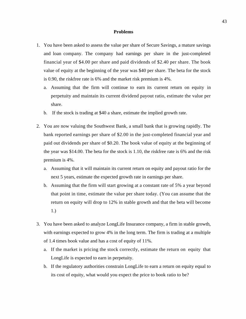
43

Problems

1. You have been asked to assess the value per share of Secure Savings, a mature savings

and loan company. The company had earnings per share in the just-completed

financial year of $4.00 per share and paid dividends of $2.40 per share. The book

value of equity at the beginning of the year was $40 per share. The beta for the stock

is 0.90, the riskfree rate is 6% and the market risk premium is 4%.

a. Assuming that the firm will continue to earn its current return on equity in

perpetuity and maintain its current dividend payout ratio, estimate the value per

share.

b. If the stock is trading at $40 a share, estimate the implied growth rate.

2. You are now valuing the Southwest Bank, a small bank that is growing rapidly. The

bank reported earnings per share of $2.00 in the just-completed financial year and

paid out dividends per share of $0.20. The book value of equity at the beginning of

the year was $14.00. The beta for the stock is 1.10, the riskfree rate is 6% and the risk

premium is 4%.

a. Assuming that it will maintain its current return on equity and payout ratio for the

next 5 years, estimate the expected growth rate in earnings per share.

b. Assuming that the firm will start growing at a constant rate of 5% a year beyond

that point in time, estimate the value per share today. (You can assume that the

return on equity will drop to 12% in stable growth and that the beta will become

1.)

3. You have been asked to analyze LongLife Insurance company, a firm in stable growth,

with earnings expected to grow 4% in the long term. The firm is trading at a multiple

of 1.4 times book value and has a cost of equity of 11%.

a. If the market is pricing the stock correctly, estimate the return on equity that

LongLife is expected to earn in perpetuity.

b. If the regulatory authorities constrain LongLife to earn a return on equity equal to

its cost of equity, what would you expect the price to book ratio to be?

44

4. Now assume that you are comparing the price to book ratios of the 13 largest banks in

the United States in 2000. The following table summarizes the price to book ratios

and the returns on equity earned by these firms.

Company Name P/BV ROE

Wachovia Corp. 2.05 18.47%

PNC Financial Serv. 2.54 21.56%

SunTrust Banks 1.91 15.35%

State Street Corp. 6.63 19.52%

Mellon Financial Corp. 4.59 23.95%

Morgan (J.P.) & Co 1.74 19.39%

First Union Corp. 1.52 19.66%

FleetBoston Fin'l 2.25 20.15%

Bank of New York 7.01 25.36%

Chase Manhattan Corp. 2.60 24.60%

Wells Fargo 3.07 17.72%

Bank of America 1.69 19.31%

Bank of Montreal 1.23 18.08%

a. If you were valuing SunTrust Banks, relative to these firms, would you expect it

to have a higher or lower price to book ratio than the average for the group?

Explain why.

b. If you regress price to book ratios against returns on equity, what would your

predicted price to book ratios be for each of these companies?

5. Signet Bank has asked you to estimate the value of their loan portfolio. The bank has

$1 billion in loans outstanding, with an average maturity of 6 years, and expected

interest income of $75 million a year. You have been able to get a synthetic rating of A

for the entire loan portfolio and the current market interest rate on A rated bonds is

6.5%.

a. Estimate the value of the loan portfolio.

45

b. If Signet bank has $800 million in debt outstanding, estimate the value of the

equity in the bank based upon the loans it has in place.

1

CHAPTER 22

VALUING FIRMS WITH NEGATIVE EARNINGS

In most of the valuations thus far in this book, we have looked at firms that have

positive earnings. In this chapter, we consider a subset of firms with negative earnings or

abnormally low earnings that we categorize as troubled firms. We begin by looking at why

firms have negative earnings in the first place and look at the ways that valuation has to

be adapted to reflect these underlying reasons.

For firms with temporary problems – a strike or a product recall, for instance –

we argue that the adjustment process is a simple one, where we back out of current

earnings the portion of the expenses associated with the temporary problems. For

cyclical firms, where the negative earnings are due to a deterioration of the overall

economy, and for commodity firms, where cyclical movements in commodity prices can

affect earnings, we argue for the use of normalized earnings in valuation. For firms with

long-term strategic problems, operating problems – outdated plants, a poorly trained

workforce or poor investments in the past – or financial problems – too much debt – the

process of valuation becomes more complicated because we have to make assumptions

about whether the firm will be able to outlive its problems and restructure itself or

whether it will go bankrupt. Finally, we look at firms that have negative earnings because

they have borrowed too much and consider how best to deal with the potential for

default.

Negative Earnings: Consequences and Causes

A firm with negative earnings or abnormally low earnings is more difficult to value

than a firm with positive earnings. In this section, we look at why such firms create

problems for analysts in the first place and then follow up by examining the reasons for

negative earnings.

The Consequences of Negative or Abnormally Low Earnings

Firms that are losing money currently create several problems for the analysts who

are attempting to value them. While none of these problems are conceptual, they are

significant from a measurement standpoint.

2

1. Earnings growth rates cannot be estimated or used in valuation: The first and most

obvious problem is that we can no longer estimate an expected growth rate to earnings

and apply it to current earnings to estimate future earnings. When current earnings are

negative, applying a growth rate will just make it more negative. In fact, even

estimating an earnings growth rate becomes problematic, whether one uses historical

growth, analyst projections or fundamentals.

• Estimating historical growth when current earnings are negative is difficult and

the numbers, even if estimated, often are meaningless. To see why, assume

that a firm’s operating earnings have gone from -$200 million last year to -

$100 million in the current year. The traditional historical growth equation

yields the following:

Earnings growth rate

-50%

1-200-

100-

1-Earnings

Earnings

yearlast

today

=

=

=

This clearly does not make sense since this firm has improved its earnings over

the period.

• An alternative approach to estimating earnings growth is to use analyst

estimates of projected growth in earnings, especially over the next 5 years.

The consensus estimate of this growth rate, across all analysts following a

stock, is generally available as public information for many US companies and

is often used as the expected growth rate in valuation. For firms with negative

earnings in the current period, this estimate of a growth rate will not be

available or meaningful.

• A third approach to estimating earnings growth is to use fundamentals. This

approach is also difficult to apply for firms that have negative earnings, since

the two fundamental inputs – the return made on investments (return on

equity or capital) and the reinvestment rate (or retention ratio) are usually

computed using current earnings. When current earnings are negative, both

3

these inputs become meaningless from the perspective of estimating expected

growth.

2. Tax computation becomes more complicated: The standard approach to estimating

taxes is to apply the marginal tax rate on the pre-tax operating income to arrive at the

after-tax operating income.

After-tax Operating Income = Pre-tax Operating Income (1 – tax rate)

This computation assumes that earnings create tax liabilities in the current period.

While this is generally true, firms that are losing money can carry these losses forward

in time and apply them to earnings in future periods. Thus, analysts valuing firms

with negative earnings have to keep track of the net operating losses of these firms

and remember to use them to shield income in future periods from taxes.

3. The Going Concern Assumption: The final problem associated with valuing companies

that have negative earnings is the very real possibility that these firms will go

bankrupt if earnings stay negative. And the assumption of infinite live that underlies

the estimation of terminal value may not apply in these cases.

The problems are less visible but exist nevertheless for firms that have abnormally

low earnings, i.e, the current earnings of the firm are much lower than what the firm has

earned historically. Though you can compute historical growth and fundamental growth

for these firms, they are likely to be meaningless because current earnings are depressed.

The historical growth rate in earnings will be negative and the fundamentals will yield

very low estimates for expected growth.

The Causes of Negative Earnings

There are several reasons why firms have negative or abnormally low earnings.

Some of which can be viewed as temporary, some of which are long term and some of

which relate to where a firm stands in the life cycle.

Temporary Problems

For some firms, negative earnings are the result of temporary problems,

sometimes affecting the firm alone, sometimes affecting an entire industry and sometimes

the result of a downturn in the economy.

4

• Firm-specific reasons for negative earnings can include a strike by the firm’s

employees, an expensive product recall or a large judgment against the firm in a

lawsuit. While these will undoubtedly lower earnings, the effect is likely to be

one-time and not affect future earnings.

• Sector-wide reasons for negative earnings can include a downturn in the price of a

commodity for a firm that produces that commodity. It is common, for instance,

for paper and pulp firms to go through cycles of high paper prices (and profits)

followed by low paper prices (and losses). In some cases, the negative earnings

may arise from the interruption of a common source of supply for a necessary

raw material or a spike in its price. For instance, an increase in oil prices will

negatively affect the profits of all airlines.

• For cyclical firms, a recession will affect revenues and earnings. It is not

surprising, therefore, that automobile companies report low or negative earnings

during bad economic times.

The common thread for all of these firms is that we expect earnings to recover sooner

rather than later as the problem dissipates. Thus, we would expect a cyclical firm’s

earnings to bounce back once the economy revives and an airline’s profits to improve

once oil prices level off.

Long Term Problems

Negative earnings are sometimes reflections of deeper and much more long-term

problems in a firm. Some of these are the results of poor strategic choices made in the

past, some reflect operational inefficiencies and some are purely financial, the result of a

firm borrowing much more than it can support with its existing cash flows.

• A firm’s earnings may be negative because its strategic choices in terms of product

mix or marketing policy might have backfired. For such a firm, financial health is

generally not around the corner and will require a substantial makeover and, often,

new management.

• A firm can have negative earnings because of inefficient operations. For instance,

the firm’s plant and equipment may be obsolete or its work force may be poorly

trained. The negative earnings may also reflect poor decisions made in the past by

5

management and the continuing costs associated with such decisions. For instance,

firms that have gone on acquisition binges and overpaid on a series of acquisitions

may face several years of poor earnings as a consequence.

• In some cases, a firm that is in good health operationally can end up with negative

equity earnings because it has chosen to use too much debt to fund its operations.

For instance, many of the firms that were involved in leveraged buyouts in the

1980s reported losses in the first few years after the buyouts.

Life Cycle

In some cases, a firm’s negative earnings may not be the result of problems in the

way it is run but because of where the firm is in its life cycle. We can think of at least

three examples.

• Firms in businesses that require huge infrastructure investments up front will often

lose money until these investments are in place. Once they are made and the firm is

able to generate revenues, the earnings will turn positive. You can argue that this was

the case with the phone companies in the early part of the twentieth century in the

United States, the cable companies in the 1980s and the cellular companies in the

early 1990s.

• Small biotechnology or pharmaceutical firms often spend millions of dollars on

research and come up with promising products that they patent, but then have to wait

years for FDA approval to sell the drugs. In the meantime, they continue to have

research and development expenses and report large losses.

• The third group includes young, start-up companies. Often these companies have

interesting and potentially profitable ideas, but they lose money until they convert

these ideas into commercial products. Until the late 1990s, these companies seldom

went public but relied instead of venture capital financing for their equity needs. One

of the striking features of the boom in new technology companies from 1997 to 2000

was the number of such firms that chose to bypass the venture capital route and go to

the markets directly.

Making the Call: Short term versus Long term Problems

6

In practice, it is often difficult to disentangle temporary or short-term problems

from long term ones. There is no simple rule of thumb that works and accounting

statements are not always forthcoming about the nature of the problems. Most firms,

when reporting negative earnings, will claim that their problems are transitory and that

recovery is around the corner. Analysts have to make their own judgments on whether

this is the case and they should consider the following.

- The credibility of the management making the claim: The managers of some firms are

much more forthcoming than others in revealing problems and admitting their

mistakes, and their claims should be given much more credence.

- The amount and timeliness of information provided with the claim: A firm that

provides detailed information backing up its claim that the problem is temporary is

more credible than a firm that does not provide such information. In addition, a firm

that reveals its problems promptly is more believable than one that delays reporting

problems until its hand is forced.

- Confirming reports from other companies in industry: A cyclical company that claims

that its earnings are down because of an economic slowdown will be more believable if

other companies in the sector also report similar slowdowns.

- The persistence of the problem: If poor earnings persist over multiple periods, it is

much more likely that the firm is facing a long-term problem. Thus, a series of

restructuring charges should be viewed with suspicion.

Valuing Negative Earnings Firms

The way we deal with negative earnings will depend upon why the firm has

negative earnings in the first place. In this section, we explore the alternatives that are

available for working with negative earnings firms.

Firms with temporary problems

When earnings are negative because of temporary or short-term problems, the

expectation is that earnings will recover in the near term. Thus, the solutions we devise

will be fairly simple ones, which for the most part will replace the current earnings (which

7

are negative) with normalized earnings (which will be positive). How we normalize

earnings will vary depending upon the nature of the problem.

Firm-Specific

A firm can have a bad year in terms of earnings, but the problems may be isolated

to that firm, and be short-term in nature. If the loss can be attributed to a specific event –

a strike or a lawsuit judgment, for instance – and the accounting statements report the

cost associated with the event, the solution is fairly simple. You should estimate the

earnings prior to these costs and use these earnings not only for estimating cash flows but

also for computing fundamentals such as return on capital. In making these estimates,

though, note that you should remove not just the expense but all of the tax benefits

created by the expense as well, assuming that it is tax deductible.

If the cause of the loss is more diffuse or if the cost of the event causing the loss is

not separated out from other expenses, you face a tougher task. First, you have to ensure

that the loss is in fact temporary and not the symptom of long term problems at the firm.

Next, you have to estimate the normal earnings of the firm. The simplest and most direct

way of doing this is to compare each expense item for the firm for the current year with

the same item in previous years, scaled to revenues. Any item that looks abnormally high,

relative to prior years, should be normalized (by using an average from previous years).

Alternatively, you could apply the operating margin that the firm earned in prior years to

the current year’s revenues and estimate an operating income to use in the valuation.

In general, you will have to consider making adjustments to the earnings of firms

after years in which they have made major acquisitions, since the accounting statements in

these years will be skewed by large items that are generally non-recurring and related to

the acquisition.

Illustration 22.1: Normalizing Earnings for a Firm after a Poor Year: Daimler Benz in

1995

In 1995, Daimler Benz reported an operating loss of DM 2,016 million and a net loss

of DM 5,674 million. Much of the loss could be attributed to firm-specific problems

including a large write off of a failed investment in Fokker Aerospace, an aircraft

manufacturer. To estimate normalized earnings at Daimler Benz, we eliminated all charges

8

related to these items and estimated a pre-tax operating income of DM 5,693 million. To

complete the valuation, we made the following additional assumptions.

• Revenues at Daimler had been growing 3-5% a year prior to 1995 and we anticipated

that the long term growth rate would be 5% in both revenues and operating income.

• The firm had a book value of capital invested of DM 43,558 million at the beginning

of 1995, and was expected to maintain its return on capital (based upon the adjusted

operating income of DM 5,693 million)

• The firm’s tax rate is 44%.1

To value Daimler, we first estimated the return on capital at the firm, using the adjusted

operating income.

Return on capital

( )

( )

%32.743558

44.015693

invested capital of Book value

t-1EBIT

=

−=

=

Based upon the expected growth rate of 5%, this would require a reinvestment rate of

68.31%.

Reinvestment rate %31.68%32.7

%5

ROC=== g

With these assumptions, we were able to compute Daimler’s expected free cash flows in

1996.

EBIT1995 (1+g) (1-t) = 5,693 (1.05) (1-0.44) = 3,347 Mil DM

- Reinvestment = 5,693 (1.05) (1-0.44) (0.6831)= 2,287 Mil DM

Free Cash Flow to Firm = 1,061 Mil DM

To compute the cost of capital, we used a bottom-up beta of 0.95, estimated using

automobile firms listed globally. The long-term bond rate (on a German government bond

denominated in DM) was 6%, and Daimler Benz could borrow long term at 6.1%. We

1 Germany has a particularly complicated tax structure since it has different tax rates for retained earningsand dividends, which makes the tax rate a function of a firm’s dividend policy.

9

assumed that a market risk premium of 4%. The market value of equity was 50,000

million DM, and there was 26,281 million DM in debt outstanding at the end of 1995.

Cost of Equity = 6%+ 0.95(4%)= 9.8%

Cost of Debt = 6.1%(1-.44) = 3.42%

Debt Ratio = 26,281/(50,000+26,281) = 34.45%

Cost of Capital = 9.8%(.6555) + 3.42% (.3445) = 7.60%

Note that all of the costs are computed in DM terms to be consistent with our cash

flows. The firm value can now be computed, if we assume that earnings and cash flows

will grow at 5% a year in perpetuity.

Value of the operating assets

DMmillion 40,787

0.05-0.076

1061

g-capital ofCost

FCFF

rategrowth Expected-capital ofCost

1996in FCFF Expected

1996

=

=

=

=

Adding to this the value of the cash and marketable securities (13,500 million DM) held

by Daimler at the time of this valuation and netting out the market value of debt yields an

estimated value of 28,006 million for equity, significantly lower than the market value of

50,000 million DM.

Value of equity = Value of operating assets + Cash and Marketable securities – Debt

= 40787+13500 – 26281 = 28,006 million DM

As in all firm valuations, there is an element of circular reasoning2 involved in this

valuation.

Sector Wide or Market Driven Problems

The earnings of cyclical firms are, by definition, volatile and dependent upon the

state of the economy. In economic booms, the earnings of these firms are likely to

increase, while, in recessions, the earnings will be depressed. The same can be said of

2 The circular reasoning comes in because we use the current market value of equity and debt to computethe cost of capital. We then use the cost of capital to estimate the value of equity and debt. If this is

10

commodity firms that go through price cycles, where periods of high prices for the

commodity are often followed by low prices. In both cases, you can get misleading

estimates of value if you use the current year’s earnings.

Valuing Cyclical Firms

In most discounted cashflow valuations, the current year is used as the base year

and growth rates are used to project future earnings and cashflows. Depending upon what

stage of the economic cycle a valuation is done at, the current year's earnings may be too

low (if you are in a recession) or too high (if the economy is at a peak) to use as a base

year. The failure to adjust the base year's earnings for cyclical effects can lead to

significant errors in valuation, since the earnings are likely to adjust as the economic cycle

changes. There are two potential solutions – one is to adjust the expected growth rate in

the near periods to reflect cyclical changes and the other is to value the firm based upon

normalized rather than current earnings.

a. Adjust Expected Growth

Cyclical firms often report low earnings at the bottom of an economic cycle, but the

earnings recover quickly when the economy recovers. One solution, if earnings are not

negative, is to adjust the expected growth rate in earnings, especially in the near term, to

reflect expected changes in the economic cycle. This would imply using a higher growth

rate in the next year or two, if both the firm’s earnings and the economy are depressed

currently but are expected to recover quickly. The strategy would be reversed if the

current earnings are inflated (because of an economic boom) and if the economy is

expected to slow down. The disadvantage of this approach is that it ties the accuracy of

the estimate of value for a cyclical firm to the precision of the macro-economic

predictions of the analyst doing the valuation. The criticism, though, may not be

avoidable since it is difficult to value a cyclical firm without making assumptions about

future economic growth. The actual growth rate in earnings in 'turning-point' years (years

unacceptable, the process can be iterated, with the cost of capital being recomputed using the estimatedvalues of debt and equity and continued until there is convergence.

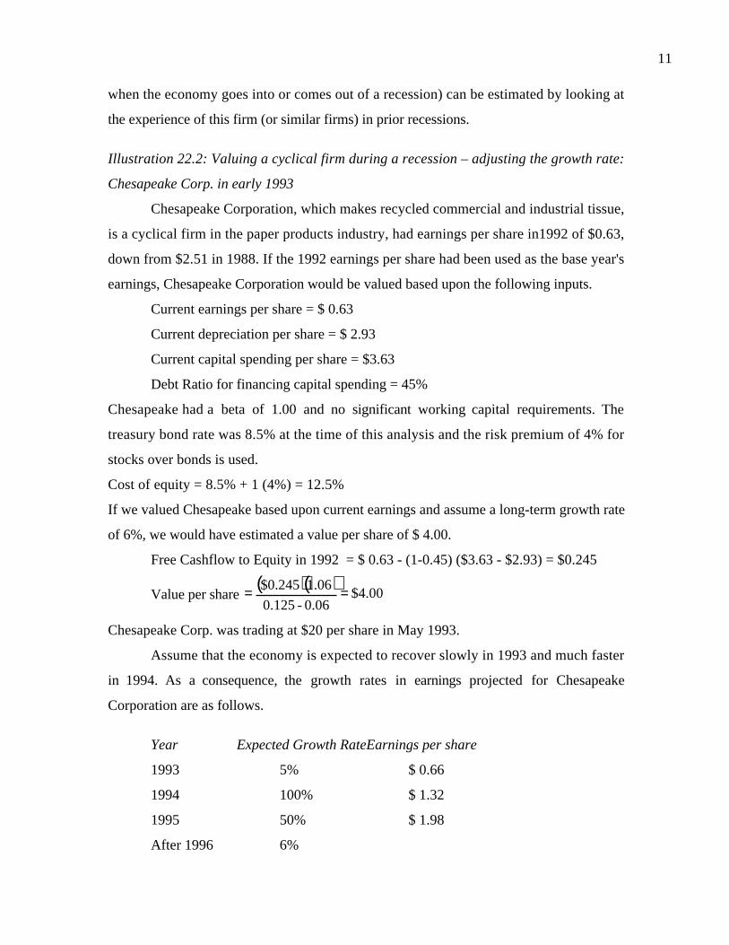
11

when the economy goes into or comes out of a recession) can be estimated by looking at

the experience of this firm (or similar firms) in prior recessions.

Illustration 22.2: Valuing a cyclical firm during a recession – adjusting the growth rate:

Chesapeake Corp. in early 1993

Chesapeake Corporation, which makes recycled commercial and industrial tissue,

is a cyclical firm in the paper products industry, had earnings per share in1992 of $0.63,

down from $2.51 in 1988. If the 1992 earnings per share had been used as the base year's

earnings, Chesapeake Corporation would be valued based upon the following inputs.

Current earnings per share = $ 0.63

Current depreciation per share = $ 2.93

Current capital spending per share = $3.63

Debt Ratio for financing capital spending = 45%

Chesapeake had a beta of 1.00 and no significant working capital requirements. The

treasury bond rate was 8.5% at the time of this analysis and the risk premium of 4% for

stocks over bonds is used.

Cost of equity = 8.5% + 1 (4%) = 12.5%

If we valued Chesapeake based upon current earnings and assume a long-term growth rate

of 6%, we would have estimated a value per share of $ 4.00.

Free Cashflow to Equity in 1992 = $ 0.63 - (1-0.45) ($3.63 - $2.93) = $0.245

Value per share ( )( )

$4.000.06-0.125

1.06$0.245 ==

Chesapeake Corp. was trading at $20 per share in May 1993.

Assume that the economy is expected to recover slowly in 1993 and much faster

in 1994. As a consequence, the growth rates in earnings projected for Chesapeake

Corporation are as follows.

Year Expected Growth RateEarnings per share

1993 5% $ 0.66

1994 100% $ 1.32

1995 50% $ 1.98

After 1996 6%

12

The capital spending and depreciation are expected to grow at 6%. The free cashflow to

equity can be estimated as follows.

1993 1994 1995 1996

EPS $0.66 $1.32 $1.98 $2.10

- (Cap Ex - Deprecn) ( 1- Debt Ratio) $0.41 $0.43 $0.46 $0.49

= FCFE $0.25 $0.89 $1.53 $1.62

Terminal price (at the end of 1995) $24.880.06- 0.125

$1.62 ==

Present Value per share =0.25

1.125+

0.89

1.1252 +1.53 + 24.88

1.1253 =19.47

b. Normalize Earnings

For cyclical firms, the easiest solution to the problem of volatile earnings over time

and negative earnings in the base period is to normalize earnings. When normalizing

earnings for a firm with negative earnings, we are simply trying to answer the question:

“What would this firm earn in a normal year?” Implicit in this statement is the

assumption that the current year is not a normal year and that earnings will recover

quickly to normal levels. This approach, therefore, is most appropriate for cyclical firms

in mature businesses. There are a number of ways in which earnings can be normalized.

• Average the firm’s dollar earnings over prior periods: The simplest way to

normalize earnings is to use the average earnings over prior periods. How many

periods should you go back in time? For cyclical firms, you should go back long

enough to cover an entire economic cycle – between 5 and 10 years. While this

approach is simple, it is best suited for firms that have not changed in scale (or

size) over the period. If it is applied to a firm that has become larger or smaller (in

terms of the number of units it sells or total revenues) over time, it will result in a

normalized estimate that is incorrect.

• Average the firm’s return on investment or profit margins over prior periods: This

approach is similar to the first one, but the averaging is done on scaled earnings

instead of dollar earnings. The advantage of the approach is that it allows the

normalized earnings estimate to reflect the current size of the firm. Thus, a firm

13

with an average return on capital of 12% over prior periods and a current capital

invested of $1,000 million would have normalized operating income of $120

million. Using average return on equity and book value of equity yields normalized

net income. A close variant of this approach is to estimate the average operating or

net margin in prior periods and apply this margin to current revenues to arrive at

normalized operating or net income. The advantage of working with revenues is

that they are less susceptible to manipulation by accountants.

There is one final question that we have to deal with when normalizing earnings and it

relates to when earnings will be normalized. Replacing current earnings with normalized

earnings essentially is equivalent to assuming that normalization will occur

instantaneously (i.e., in the very first time period of the valuation). If earnings will be

normalized over several periods, the value obtained by normalizing current earnings will

be too high. A simple correction that can be applied is to discount the value back by the

number of periods it will take to normalize earnings.

Illustration 22.3: Normalizing Earnings for a Cyclical Firm in a Recession: Historical

Margin

In 1992, towards the end of a recession in Europe and the United States, Volvo

reported an operating loss of 2,249 million Swedish Kroner (Sk) on revenues of 83,002

million Sk. To value the firm, we first had to normalize earnings. We used Volvo’s average

pre-tax operating margin from 1988 to 1992 of 4.1% as a measure of the normal margin

and applied it to revenues in 1992 to estimate normalized operating income.

Normalized operating income in 1992

( )( )( )( )

Skmillion 403,3

041.0002,83

\Margin Normalized92Revenues19

===

To value the operating assets of the firm, we assumed that Volvo was in stable growth, a

reasonable assumption given its size and the competitive nature of the automobile

industry, and that the expected growth rate in perpetuity would be 4%. To estimate the

firm’s reinvestment needs, we assumed that Volvo’s return on capital in the future would

be equal to the average return on capital that the firm earned between 1988 and 1992,

14

which was 12.2%. This allowed use to estimate a reinvestment rate for the firm of

32.78%.

Reinvestment rate in stable growth 32.78%ROC

4%

ROC

g ===

The expected free cash flow to the firm in 1993, based upon the normalized pre-tax

operating income of 3,403 million Sk, an estimated tax rate of 35%, the expected growth

rate of 4% and the reinvestment rate of 32.78% can be estimated.

Expected free cash flow to the firm in 1993

= 3403 (1.04) (1-.35) (1 - .3278) = 1,546 million Sk

To estimate the cost of capital for Volvo, we computed weights upon the market value of

equity of 22,847 million Sk at the end of 1992 and the debt outstanding of 42641 million

Sk. We used a bottom-up beta of 1.20 for Volvo and a pre-tax cost of debt of 8.00%,

reflecting its high leverage at the time of the analysis. The riskfree rate in Swedish kroner

was 6.6% and the risk premium used was 4%:

Cost of equity = 6.6% + 1.2 (4%) = 11.40%

Cost of capital = 11.40%( ) 22847

22847 + 42641

+ 8%( ) 1−0.35( ) 42641

22847 + 42641

= 7.36%

The value of the operating assets of Volvo can now be estimated.

Value of operating assets

= Expected FCFF in 1993

Cost of capital -Expected growth

=1546

0.0736 − 0.04= 45,977 million Sk

Adding to this the value of cash and marketable securities (20,760 million Sk) held by the

firm at the end of 1992 and subtracting out debt yields an estimated value for equity.

Value of equity = Value of operating assets + Cash & marketable securities – Debt

= 45977 + 20760 – 42641 = 24,096 million Sk

Based upon this estimate, Volvo was slightly undervalued at the end of 1992.

Implicitly, we are assuming that Volvo’s earnings will rebound quickly to

normalized levels and that the recession will end in the very near future. If we assume that

the recovery will take time, we can incorporate the effect into value by discounting the

15

value estimated in the analysis above back by the number of years that it will take Volvo

to return to normal earnings. For instance, if we assume that adjustment will take 2 years,

we could discount the value of the firm back two years at the cost of capital and then add

cash and subtract out the debt outstanding:

Value of the operating assets assuming 2-year recovery = 45977/1.07362 = 39,889

+ Cash and marketable securities + 20,760

- Value of Debt outstanding - 42641

= Value of Equity =18,008

If we assume that the recovery will take two years or more, Volvo’s equity is overvalued.

normearn.xls: This spreadsheet allows you to normalize the earnings for a firm,

using a variety of approaches.

Macro-economic views and Valuation

The earnings of cyclical firms tend to be volatile, with the volatility linked to how

well or badly the economy is performing. One way to incorporate these effects into value

is to build in expectations of when future recessions and recoveries will occur into the

cashflows. This exercise is fraught with danger, since the error in such predictions is likely

to be very large. Economists seldom agree on when a recovery is imminent, and most

categorizations of recessions occur after the fact. Furthermore, a valuation that is based

upon specific macro-economic forecasts makes it difficult for users to separate how much

of the final recommendation, i.e. that the firm is under or over valued, comes from the firm

being mis-priced and how much reflects the analyst’s optimism or the pessimism about

the overall economy.

The other way to incorporate earnings variability into the valuation is through the

discount rate - cyclical firms tend to be more risky and require higher discount rates. This

is what we do when we use higher unlevered betas and/or costs of debt for cyclical firms.

Valuing Commodity and Natural Resource Firms

Commodity prices are not only volatile but go through cycles – periods of high

prices followed by periods with lower prices. Figure 22.1 summarizes the levels of three

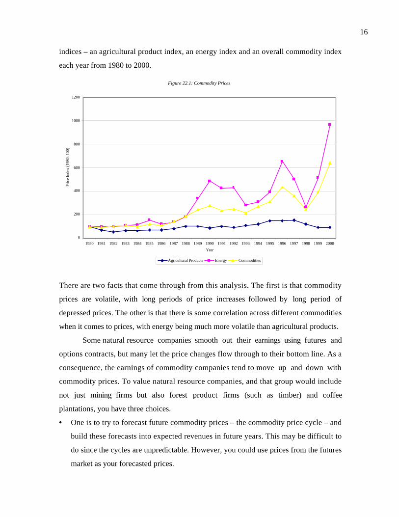
16

indices – an agricultural product index, an energy index and an overall commodity index

each year from 1980 to 2000.

There are two facts that come through from this analysis. The first is that commodity

prices are volatile, with long periods of price increases followed by long period of

depressed prices. The other is that there is some correlation across different commodities

when it comes to prices, with energy being much more volatile than agricultural products.

Some natural resource companies smooth out their earnings using futures and

options contracts, but many let the price changes flow through to their bottom line. As a

consequence, the earnings of commodity companies tend to move up and down with

commodity prices. To value natural resource companies, and that group would include

not just mining firms but also forest product firms (such as timber) and coffee

plantations, you have three choices.

• One is to try to forecast future commodity prices – the commodity price cycle – and

build these forecasts into expected revenues in future years. This may be difficult to

do since the cycles are unpredictable. However, you could use prices from the futures

market as your forecasted prices.

Figure 22.1: Commodity Prices

0

200

400

600

800

1000

1200

1980 1981 1982 1983 1984 1985 1986 1987 1988 1989 1990 1991 1992 1993 1994 1995 1996 1997 1998 1999 2000

Year

Pric

e In

dex

(198

0: 1

00)

Agricultural Products Energy Commodities

17

• You could value the firms using a normalized commodity price, estimated by looking

at the average price of the commodity over a cycle. Thus, the average price of coffee

over the last decade can be used to estimate the value of a coffee plantation. The

danger, of course, is that the price of coffee may stay well above or below this average

price for an extended period, throwing off estimates of value.

• You could value the firm’s current production using the current price for the

commodity, low though it might be, and add to it the value of the option that the

company possesses, which is to produce more if prices go up and less if they go

down. We will look at this approach in more detail in Chapter 28.

Illustration 22.4: Valuing a Commodity company: Aracruz Celulose

Aracruz Celulose is a Brazilian paper and pulp manufacturer and, like all firms in

this sector, it is susceptible to the ups and downs of the price of paper and pulp. In

Figure 22.2, we report on the revenues and operating income at Aracruz over the last

decade and, in the same graph, we provide an index of the price of paper and pulp each

year.

18

Note the correlation between Aracruz’s fortunes and the price of paper and pulp. The

years with low or negative earnings for Aracruz generally are also the years when paper

prices decline.

In May 2001, when we valued Aracruz, the firm had just emerged from a year of

high paper prices and profitability to report 666 million BR of operating income on

revenues of 1,342 million BR in 2000; the firm faced a tax rate of 33%. If we use this

operating income to value Aracruz, we are assuming that paper prices will continue to

remain high. To prevent this from biasing the valuation, we re-estimated revenues and

operating income in 2000, using the average price of paper over the last decade.

Restated revenues = Revenues2000*(Average Paper Price91-00/Paper

= 1342 * (102.58/109.39) = 1258 million BR

Restated operating income = Restated revenues – Operating expenses

= 1258 - (1342-666) = 582 million BR

This operating income was used to compute a normalized return on capital for the firm of

10.55%, based upon the book values of debt ($1549 million) and equity ($2149 million)

invested at the end of the previous year:

Figure 22.2: Aracruz Celulose: Revenues, Profits and the Price of Paper

-$200.00

$0.00

$200.00

$400.00

$600.00

$800.00

$1,000.00

$1,200.00

$1,400.00

$1,600.00

1991 1992 1993 1994 1995 1996 1997 1998 1999 2000

Year

Rev

enue

s &

Ope

ratin

g In

com

e

80

85

90

95

100

105

110

115

Pric

e of

pap

er (

1992

: 100

)

RevenuesOperating IncomePrice of pulp

19

Normalized Return on capital

=Operating Income 2000 1-t( )

Book value of debt 1999 + Book value of equity 1999

=582 1−0.33( )1549 + 2149

=10.55%

We assumed that the firm would maintain this return on capital and grow 10% a year, in

real terms, for the next 5 years and 3% a year in real terms in perpetuity after that. Table

22.1 summarizes projections of free cash flows to the firm for Aracruz for the next 5

years and for the first year of stable growth (6 years from now).

Table 22.1: Operating Income and Expected Free Cashflows to the Firm

1 2 3 4 5

Terminal

year

Expected Growth 10% 10% 10% 10% 10% 3%

Reinvestment rate 94.79% 94.79% 94.79% 94.79% 94.79% 28.44%

EBIT $644 $712 $787 $870 $961 $1,063

EBIT (1-t) $431 $477 $527 $583 $644 $712

- Reinvestment $409 $452 $500 $552 $611 $203

= FCFF $22 $25 $27 $30 $34 $510

Note that the reinvestment rate each year is computed based upon the expected growth

rate and return on capital,

Reinvestment rate capitalon return Normalized

g=

As expected growth declines in year 6 (the terminal year), the reinvestment rate also

declines.

The cost of capital was estimated in real terms, using a bottom-up beta of 0.70

estimated by looking at paper and pulp firms and an additional risk premium for exposure

to Brazilian country risk – 10.24% for the next 5 years and 5% after 5 years. This is in

addition to the equity risk premium of 4%. We use a real riskfree rate of 4%: To estimate

20

the real cost of debt, we assume a pre-tax real cost of borrowing of 7.5% for Aracruz for

both the high growth and stable growth periods.

Real after-tax cost of debt = 7.5% (1-0.33) = 5.03%

The current market values of equity (3749 million BR) and debt (1395 million BR) were

used to compute a market debt to capital ratio of 27.11% and the costs of capital for both

periods are shown in Table 22.2.

Table 22.2; Costs of capital – High Growth and Stable growth periods

High Growth Stable Growth

Beta 0.7 0.7

Riskfree Rate 4% 4%

Mature Market Premium 4% 4%

Country premium 10.24% 5%

Cost of equity = 4%+0.7(4%+10.24%) =13.97%4%+0.7(4%+5%) =10.30%

Cost of debt = 5.03% 5.03%

Debt ratio = 27.11% 27.11%

Cost of capital = 11.54% 8.87%

The terminal value is first estimated using the terminal year’s cash flows estimated in

Table 22.1 and the perpetual growth rate of 3%.

Terminal value = FCFFTerminal year/ (Cost of capitalstable – g)

= 510/(.0887- .03) = 8,682 million BR

The value of the operating assets of firm can be computed today as the present value of

the cash flows for the next 5 years and the present value of the terminal value, using the

high growth period cost of capital as the discount rate:

Value of operating assets = 22/1.1154 + 25/1.11542+ 27/1.11543+ 30/1.11544+

34/1.11545+ 8682/1.11545 = 5,127 million BR

We added back the value of cash and marketable securities (849 million BR) and

subtracted outstanding debt (1395 million) to estimate a value of equity:

Value of equity = 5127 + 849 – 1395 = 4,581 million BR

This would suggest that the firm is under valued at its current value of 2,149 million BR.

Multiples and Normalized Earnings

21

Would you have to make these adjustments to earnings if you were doing relative

valuation rather than discounted cash flow valuation? The answer is generally yes and

when adjustments are not made, you are implicitly assuming normalization of earnings.

To see why, assume that you are comparing steel companies using price earnings

ratios and that one of the firms in your group has just reported very low earnings because

of a strike during the last year. If you do not normalize the earnings, this firm will look

over valued relative to the sector, because the market price will probably be based upon

the expectation that the labor troubles, though costly, are in the past. If you use a

multiple such as price to sales to make your relative valuation judgments and you

compare this firm’s price to sales ratio to the industry average, you are assuming that the

firm’s margins will converge on industry averages sooner rather than later.

What if an entire sector’s earnings are affected by an event? Would you still need

to normalize? We believe so. Though the earnings of all automobile stocks may be

affected by a recession, the degree to which they are affected can vary widely depending

upon differences in operating and financial leverage. Furthermore, you will find yourself

unable to compute multiples such as price earnings ratios for many of the firms in the

group that lose money during recessions. Using normalized earnings will yield multiples

that are more reliable measures of true value.

Firms with long-term problems

In all of the valuations that we presented in the last section, we adjusted earnings

either instantaneously to reflect normal levels or very quickly, reflecting our belief that

the negative earnings will soon pass. In some cases, though, the negative earnings are a

manifestation of more long-term problems at the firm. In such cases, we will be forced to

make judgments on whether the problem will be overcome and, if so, when this will occur.

In this section, we present a range of solutions for companies in this position.

Strategic Problems

Firms can sometimes make mistakes in terms of the product mix they offer, the

marketing strategies they adopt or even the markets that they choose to target. They

22

often end up paying a substantial cost in terms of negative or lower earnings and perhaps

a permanent loss of market share. Consider the following examples.

• IBM found its dominant position in the mainframe computer business and the

extraordinary profitability of that business challenged by the explosion of the

personal computer market in the 1980s. While IBM could have developed the

operating system for personal computers early in the process, it ceded that

business to an upstart called Microsoft. By 1989, IBM had lost more than half its

market value and its return on equity had dropped into the single digits.3

• For decades, Xerox dominated the copier business to the extent that its name

became synonymous with the product. In the 1970s and 1980s, it was challenged

by Asian firms, with lower cost structures, like Ricoh and Canon for the market.

After initial losses, Xerox was able to recoup some of its market share. However

the last part of the 1990s saw a steady decline in Xerox’s fortunes as technology

(in the form of emails, faxes and low cost printers) took its toll. By the end of

2000, there were questions about whether Xerox had a future.

• Under the leadership of Michael Armstrong, AT&T tried to shed its image as a

stodgy phone company and became a technology firm. After some initial

successes, a series of miscues and poor acquisitions saw the firm enter the new

millennium with a vastly reduced market capitalization and no clear vision on

where to go next.

When firms have low or negative earnings that can be traced to strategic missteps, you

have to determine whether the shift is a permanent one. If it is, you will have to value the

firm on the assumption that it will never recover lost ground and scale down your

expectations of revenue growth and expected margins. If, on the other hand, you are more

optimistic about the firm’s recovery or its entry into new markets, you can assume that

the firm will be able to revert back to its traditional margins and high growth.

Operating Problems

3 It is worth noting that IBM made a fulsome recovery in the following decades by going back to basics,cutting costs and refocusing its efforts on business services.

23

Firms that are less efficient in the delivery of goods and services than their

competitors will also be less profitable and less valuable. But how and why do firms

become less efficient? In some cases, it can be traced to a failure to keep up with the times

and replenish existing assets and keep up with the latest technology. A steel company

whose factories are decades old and whose equipment is outdated will generally bear

higher costs for every ton of steel that it produces than its newer competitors. In other

cases, the problem may be labor costs. A steel company with plants in the United States

faces much higher labor costs than a similar company in Asia.

The variable that best measures operating efficiency is the operating margin, with

firms that have operating problems tending to have much lower margins than their

competitors. One way to build in the effect of operating improvements over time is to

increase the margin towards the industry average, but the speed with which the margins

will converge will depend upon several factors.

- Size of the firm: Generally, the larger the firm, the longer it will take to eliminate

inefficiencies. Not only is inertia a much stronger force in large firms, but the absolute

magnitude of the changes that have to be made are much larger. A firm with $10 billion

in revenues will have to cut costs by $300 million to achieve a 3% improvement in

pre-tax operating margin, whereas a firm with $100 million in revenues will have to

cut costs by $3 million to accomplish the same objective.

- Nature of the inefficiency: Some inefficiencies can be fixed far more quickly than

others. For instance, a firm can replace outdated equipment or a poor inventory

system quickly, but retraining a labor force will take much more time.

- External constraints: Firms are often restricted in terms of how much and how quickly

they can move to fix inefficiencies by contractual obligations and social pressure. For

instance, laying off a large portion of the work force may seem to obvious solution for

a firm that is overstaffed, but union contracts and the potential for negative publicity

may make firms reluctant to do so.

- Management Quality: A management that is committed to change is a critical

component of a successful turnaround. In some cases, a replacement of top

management may be necessary for a firm to resolve its operating problems.

24

Illustration 22.5: Valuing a firm with operating problems: Marks and Spencer

Marks and Spencer, a multinational retailer headquartered in the U.K, saw is

operating income halved from 1996 to 2000, partly because of a high cost structure and

partly because of ill-conceived expansion. In 2000, the firm reported £552 million in

operating income on revenues of £8,196 million - a pre-tax operating margin of 6.73%. In

contrast, the average operating margin for department stores in the U.K. and U.S. is 12%

and Market and Spencer’s own historical margin (over the previous decade) is 11%. To

value Marks and Spencer, we will assume the following.

- Revenues will grow 5% a year in perpetuity. The firm is a large firm in a mature

market and it does seem unrealistic to assume much higher growth in revenues.

- The firm reported capital expenditures of £448 million and depreciation of £262

million for the 2000 financial year. In addition, the non-cash working capital at the end

of the year was £1948 million. We will assume that net capital expenditures and non-

cash working capital will continue to grow at the same rate as revenues, i.e., 5% a year

forever.

- We will assume that the pre-tax operating margin of the firm will improve over the

next 10 years from 6.73% to 11.50%, with more significant improvements occurring

in the next 2 years and smaller improvements thereafter.

- We will use a tax rate of 33% to estimate after-tax cash flows. The cost of capital for

the firm is estimated using its current market debt to capital ratio of 20%, a cost of

equity of 9.52% and a pre-tax cost of debt of 6%.

Cost of capital = 9.52% (0.80) + 6% (1-0.33) (0.2) = 8.42%

Table 22.3 summarizes the forecasts of revenues, operating income and free cash flows to

the firm every year for the next 6 years.

Table 22.3: Forecasts of free cash flow to the firm

Year Revenues

Operating

Margin EBIT EBIT(1-t)Net Cap Ex

Change in

Working Capital FCFF

Current $8,196 6.73% $552 $370 $186

1 $8,606 8.32% $716 $480 $195 $97 $187

2 $9,036 9.38% $848 $568 $205 $102 $261

25

3 $9,488 10.09% $957 $641 $215 $107 $319

4 $9,962 10.56% $1,052 $705 $226 $113 $366

5 $10,460 10.87% $1,137 $762 $237 $118 $406

6 $10,983 11.08% $1,217 $815 $249 $124 $442

7 $11,533 11.22% $1,294 $867 $262 $131 $475

8 $12,109 11.31% $1,370 $918 $275 $137 $506

9 $12,715 11.38% $1,446 $969 $289 $144 $537

10 $13,350 11.42% $1,524 $1,021 $303 $151 $567

Term

year $14,018 11.50% $1,612 $1,080

After year 10, we assume that revenues and operating income will continue to grow 5% a

year forever, and that Marks and Spencer will earn an industry average return on capital

of 15%. This allows us to estimate a stable period reinvestment rate and terminal value.

Reinvestment rate in stable growth 33.33%15%

5%

ROC

g ===

Terminal value

( )( )

( )

million 054,21£05.00842.0

3333.011080

g-capital ofCost

ratent Reinvestme-1t-1EBIT11

=−

−=

=

Adding the present value of the cash flows in Table 22.3 to the present value of the

terminal value, using the cost of capital of 8.42% as the discount rate, yields a value for

the operating assets of £11,879 million. Adding the value of cash and marketable

securities at the end of 2000 to this amount and subtracting out the debt yields a value of

equity of £10,612 million.

Value of operating assets = £11,879 million

+ Cash & Securities = £687 million

- Debt = £1,954 million

Value of equity = £10,612 million

Dividing by the 2875 million shares outstanding yields a value per share of £3.69, higher

than the stock price of £2.72 prevailing at the time of this analysis in May 2001.

26

The Special Case of Privatizations

In many privatizations, we are called upon to value firms with long financial

histories but not very profitable ones. The lack of profitability is not surprising, however,

since many of these firms have been run with objectives other than maximizing value or

profitability. In some cases, employment in these firms has been viewed as a source of

political patronage. Consequently, they end up over-staffed and inefficient.

Will this all change as soon as they are privatized? Not necessarily, and certainly

not immediately. The power of unions to preserve existing jobs, the power that

governments continue to have on how they are run and the sheer size of these firms

makes change both daunting and slow. While it is reasonable to assume that these firms

will, in fact, become more efficient once they are privatized, the speed of the

improvement will vary from firm to firm. In general, you would expect the adjustment to

be much quicker if the government relinquishes its power to control the management of

the firm and if there are strong competitive pressures to become more efficient. It will be

slower if the firm is a monopoly and the government continues to handpick the top

management of the firm.

Illustration 22.6: Valuing a privatization – CVRD

In 1995, the Brazilian government privatized Compahnia Vale Dio Roce (CVRD),

Latin America’s biggest mining company. In the year the firm was privatized, it reported

after-tax operating income of 717 million BR on revenues of 4714 million BR. Based on

the capital invested in the firm at the beginning of the year of 14,722 million BR, the

after-tax return on capital earned by the firm was 5.33%.

If we assumed a stable real growth rate of 3% and a real cost of capital of 10%,

and valued CVRD on the basis of these inputs, we would have estimated the following

value for the firm.

Reinvestment rate 56.29%5.33%

3%

ROC

g ===

27

Value of the firm

( )( )( )

( )( )( )

BRmillion 611,403.010.0

5629.0103.1717

g-capital ofCost

ratent Reinvestme-11t-1EBIT

=−

−=

+= g

Note, though, that this assumes that CVRD’s return on capital will remain at existing

levels in perpetuity. If privatization leads to operating efficiencies at the firm, its margins

and return on capital can be expected to improve. For instance, if we valued CVRD using

the real return on capital of 7% earned by mining companies in the United States, we

would have estimated the following.

Reinvestment rate %86.247%

3%

ROC

g ===

Value of the firm

( )( )( )

( )( )( )

BRmillion 029,603.010.0

4286.0103.1717

g-capital ofCost

ratent Reinvestme-11t-1EBIT

=−

−=

+= g

Is it reasonable to assume this improvement in margins? It depends upon which

side of the transaction you are on. If you were an investor interested in buying the stock,

you might argue that the firm is too entrenched in its ways to make the changes needed

for higher profitability and use the value estimated with current margins. If you are the

government and want to obtain the highest value you can, you would argue for the latter.

Golden Shares and the Value of Privatized firms

While governments are always eager to receive the cash proceeds from privatizing

the firms that they own, they are generally not as eager to give up control of these firms.

One way they attempt to preserve power is by maintaining what is called a golden share

in the firm that gives them veto power and control over some or many aspects of the

firm’s management.

For instance, the Brazilian government maintains a golden share in CVRD,

allowing it the final decision on whether mines can be closed and other major financial

decisions. While governments often view these golden shares as a costless way to

privatize and preserve control at the same time, there is a cost that they will bear.

28

Investors valuing firms with golden shares will generally be much less willing to assume

radical changes in management and improvements in efficiency. Consequently, the values

attached to these firms by the market will be much lower. The more inefficient the firm

being privatized and the more restrictive the golden share, the greater will be the loss in

value to the government.

Financial Leverage

In some cases firms get into trouble because they borrow too much and not

because of operating or strategic problems. In these cases, it will be the equity earnings

that will be negative while operating earnings will be positive. The solution to the

problem depends, in large part, on how distressed the firm really is. If the distress is not

expected to push the firm into bankruptcy, there are a variety of potential solutions. If on

the other hand, the distress is likely to be terminal, finding a solution is much more

difficult.

Overlevered with no immediate threat of bankruptcy

Firms that borrow too much are not always on the verge of bankruptcy. In fact,

firms with valuable operating assets and substantial operating cash flows can service

much more debt than is optimal for them, even though they might not do so comfortably.

So, what are the costs of being overlevered? First, the firm might end up with a large

enough exposure to default risk that it affects its operations – customers might not buy

its products, suppliers might demand speedier payment and it might have trouble

retaining valued employees. Second, the higher beta and cost of debt that goes with the

higher leverage may increase the firm’s cost of capital and reduce its value. It is therefore

in the best interests of the firm to reduce its debt ratio, if not immediately, at least over

time. There are two choices when it comes to valuing levered firms as going concerns.

a. You can estimate free cashflows to the firm and value the firm. If the firm is

operationally healthy (the operating margins are both positive and similar to those

of comparable firms), the only modification you have to make is to reduce the

debt ratio over time – in practical terms, a disproportionate share of the

reinvestment each year has to come from equity – and compute costs of capital

29

that change with the debt ratio. If the firm’s operating margins have suffered

because it borrowed too much, you might need to adjust the operating margins

over time towards industry averages as well.

b. You can use the adjusted present value approach and value the firm as an

unlevered firm and subtract from this unlevered firm value the costs (expected

bankruptcy costs) and add to it the benefits (tax benefits) of debt. As noted in

Chapter 15, though, estimating the expected bankruptcy cost can be difficult to

do.

Illustration 22.7: Adjust debt ratio over time: Hyundai

Hyundai Corporation is a Korean company that is part of the Hyundia group and

handles the trading operations for the firm. Like many other Korean companies, Hyundai

borrowed large amounts to fund expansion until the late 1990s. By the end of 2000,

Hyundai had debt outstanding of 848 billion Korean Won (krw) and had a market value of

equity of 163 billion krw, resulting a debt to capital ratio of 83.85%. The high leverage

has three consequences.

- The bottom-up beta for the firm is 2.60, reflecting the firm’s high debt to equity ratio.

With a riskfree rate of 9% and the risk premium of 7% - 4% as the mature market

premium and 3% for Korean country risk - we estimate a cost of equity in Korean

won for the firm of 27.20%.

Cost of equity = 9% + 2.6 (7%) = 27.20%

- The firm has high default risk, leading to a pre-tax cost of borrowing in Korean won

terms of 12.5%; the tax rate for the firm is 30%.

- The firm reported pre-tax operating income of 89.42 billion krw, but the interest

expenses of the firm amounted to 99 billion krw, resulting in a loss for the firm. Note,

though, that the firm is still obtaining the tax benefits of almost all of its interest

payments.4

4 Without interest expenses, Hyundai would have paid taxes on its operating income of 93 billion won.Because of its interest payments, Hyundai was able to not pay taxes. Of the 99 billion won in interestpayments, Hyundai is receiving tax benefits on 93 billion won.

30

We will assume that the operating income will grow 10% a year for the next 6 years and

8% a year beyond that point in time. Over that period, we will assume that the firm’s

capital expenditures (which are currently 12 billion won), depreciation (which is currently

4 billion won) and that non-cash working capital (which is currently 341 billion won) will

grow at the same rate as operating income, yielding the following estimates for the cash

flows.

Table 22.4: Expected Cash Flow: Hyundai

1 2 3 4 5 6

EBIT (1-t) $68.86 $75.74 $83.32 $91.65 $100.81 $110.89

+ Depreciation $4.40 $4.84 $5.32 $5.86 $6.44 $7.09

- Capital Spending $13.20 $14.52 $15.97 $17.57 $19.33 $21.26

- Chg. Working

Capital $34.11 $37.52 $41.27 $45.40 $49.94 $54.93

Free CF to Firm $25.95 $28.54 $31.40 $34.54 $37.99 $41.79

Over the next 6 years, we will assume that the firm will reduce its debt ratio from 83.85%

to 50%, which will result in the beta decreasing from 2.60 to 1.00 and the pre-tax cost of

debt from 12.5% to 10.5% - we assume that the changes occur linearly over the period.

The costs of capital for Hyundai are estimated each year for the next 6 years.

Table 22.5: Costs of capital: Hyundai

1 2 3 4 5 6

Beta 2.60 2.28 1.96 1.64 1.32 1.00

Cost of Equity 27.20% 24.96% 22.72% 20.48% 18.24% 16.00%

Cost of Debt (After-

tax) 8.75% 8.47% 8.19% 7.91% 7.63% 7.35%

Debt Ratio 83.85% 77.08% 70.31% 63.54% 56.77% 50.00%

Cost of Capital 11.73% 12.25% 12.50% 12.49% 12.22% 11.68%

31

To estimate the terminal value, we assume a growth rate of 8% in perpetuity, after year 6,

and a return on capital of 16%. This allows us to estimate a reinvestment rate and

terminal value for the firm at the end of year 6.

Reinvestment rate 50%16%

8%

ROC=== g

Terminal value ( )( )( )

krwbillion 1,6260.08-0.1168

0.50-11.08110.89 ==

Discounting the cash flows over the next 6 years and the terminal value using the

cumulated cost of capital yields the following.

Present Value of FCFF in high growth phase = 132.34 billion krw

Present Value of Terminal Value = 819.19

Value of the operating assets = 951.52

+ Cash and Marketable Securities = 80.46

- Market Value of Debt = 847.73

Market Value of Equity = 184.25 billion krw

Dividing by the number of shares results in an estimated value of equity for the firm of

2504 won per share, a little higher than the actual trading price of 2220 won per share.

Can equity value be negative?

We generally subtract out the value of outstanding debt from firm value to get to

the value of equity. But can the value of the outstanding debt exceed the value of the firm?

If you are using market values for both the firm (obtained by adding the market values of

debt and equity) and debt, this will never occur. This is because the market value of

equity can never be less than zero. However, if you are using your estimated value for the

firm, obtained by discounting cash flows to the firm at the cost of capital, the estimated

firm value can be less than the market value of the outstanding debt. When this occurs,

there are three possible interpretations.

- The first and most obvious reading is that you have made a mistake in estimating firm

value and that your estimate is too low. In this case, the obvious solution is to redo

the firm valuation.

- The second possibility is that the market value of debt is overstated. This can happen

if you are using the book value of debt as a proxy for market value for troubled firms

32

or if the bond market is making a mistake in pricing the debt. Estimating the correct

market value of debt5 will eliminate the problem.

- The third and most intriguing possibility is that your estimate of firm value and the

market value of debt are both correct, in which case the equity value is, in fact,

negative. Since the market price of equity cannot be less than zero, the implication is

that the equity in this firm is worth nothing. However, as you will see below, equity

may still continue to command value, even under these circumstances, if it is viewed

as a call option on the firm’s assets.

Overlevered with high probability of bankruptcy

Discounted cashflow valuation is conditioned on a firm being a going concern, with

cashflows continuing into the future. When a firm’s financial problems are severe enough

to suggest a strong likelihood of bankruptcy, other approaches may need to be used to

value a firm and the equity claim in it. There are two possible approaches – one is to

estimate a liquidation value for the assets today and the other is to continue to treat the

firm as a going concern and value the equity in it as an option.

a. Liquidation Value

The liquidation value of a firm is the aggregate of the value that the assets of the

firm would command on the market, net of transactions and legal costs. The value of

equity can be obtained by subtracting the value of the outstanding debt from the asset

value.

Value of Equity = Liquidation Value of Assets - Outstanding Debt

Estimating liquidation value is complicated when the assets of the firm are not easily

separated and thus cannot be valued individually. Furthermore, the likelihood that assets

will fetch their fair market value will decrease as the urgency of the liquidation increases.

A firm in a hurry to liquidate its assets may have to accept a discount on fair market value

as a price for speedy execution.

5 You could discount the expected cash flows on the debt at a pre-tax cost of debt that reflects the firm’scurrent standing.

33

As a note of caution, it is almost never appropriate to treat the book value of the

assets as the liquidation value. Most distressed firms earn sub-par returns on their assets,

and the liquidation value will reflect the earning capacity of the assets rather than the

price paid for the assets (which is what the book value measures, net of depreciation).

b. Option Pricing Models

The liquidation value approach presumes that the market value of the assets

currently exceeds the face value of outstanding debt. When this assumption is violated,

the only approach left to value the equity in a distressed firm may be to use option

pricing models. Equity in heavily levered firm, where the value of the assets is lower than

the face value of the debt can be viewed an out-of-the-money call option on the

underlying firm and can be valued as such. We will return to examine this concept in more

detail in Chapter 30.

dbtfund.xls: There is a dataset on the web that summarizes book and market

value debt ratios by industry group in the United States for the most recent year

Life Cycle Earnings

As noted earlier in the chapter, it is normal for firms to lose money at certain

stages in their life cycles. When valuing such firms, you cannot normalize earnings, as we

did with cyclical firms or firms with temporary problems. Instead, you have to estimate

the cash flows of the firm over its lifecycle and let them turn positive at the right stage of

the cycle. In this section, we will consider one group of firms – those with large

infrastructure investments – in detail. The other two – pharmaceutical firms that derive

the bulk of their value from a patent or patents and young start up companies – will be

considered in more detail in the coming chapters.

Infrastructure Firms

If the business that a firm is in requires large infrastructure investments early in

the life cycle and the firm has to wait for a long period before it can generate earnings, it is

entirely possible that the firm will report large losses in the initial periods when the

investments are made. In fact, as an added complication, many of these firms have to

34

borrow large amounts to fund their infrastructure investments, creating a fairly toxic

combination – negative earnings and high leverage.

Given this combination, how can an infrastructure firms – a telecom firm or cable

company – ever be valuable? Consider one possible path to success. A firm borrows

money and makes large investments in infrastructure. Having made these investments,

though, it has a secure market where entry is prohibitively expensive. In some cases, the

firm may have a legally sanctioned monopoly to provide the service. No further

investments are needed in infrastructure but depreciation on the existing investments

continues to generate large tax benefits. The net effect is that the firm will be sitting on a

cash machine that allows it to not only pay off its debt but ready itself for the next

generation of investments. In a sense, phone companies and power companies, as well as

some cable and cellular firms, have followed this path to success.

In the 1990s, we saw an explosion both in the number of telecom firms and the

capital raised by telecom firms in a variety of ventures. While they followed the time-

worn path of high debt and large up-front infrastructure investments laid by their

predecessors, we believe that there are two critical ingredients that are missing with this

generation of firms. The first is that technology has become a wild card and large

investments in infrastructure do not guarantee future profitability or even the existence of

a market. The second is that the protection from competition that allowed the old-time

technology firms to generate large and predictable profits is unlikely to be there for this

new generation of telecom firms. As a consequence, we would predict that far more of

these firms will go bankrupt and that they might be well advised to rethink their policies

on financial leverage as a consequence.

Illustration 22.8: Valuing an infrastructure firm – Global Crossing

Global Crossing provides managed data and voice products over a fiber optic

network. Over its three-year history, the firm has increased revenues from $420 million in

1998 to $3,789 million in 2000, but it has gone from an operating income of $120 million

in 1998 to an operating loss of $1,396 million in 2000. In addition, the firm is capital

intensive and reported substantial capital expenditures ($4,289 million) and depreciation

($1,381 million) in 2000.

35

In making the valuation, we assume that there will be no revenue growth in the

first year (to reflect a slowing economy) and that revenue growth will be brisk for the next

4 years and then taper off to a stable growth rate of 5% in the terminal phase, that

EBITDA as a percent of sales will move from the current level (of close to 0%) to a

industry average of 33% by the end of the tenth year and that capital expenditures will be

ratcheted down over the next two years to maintenance levels. Table 22.6 summarizes our

assumptions on revenue growth, EBITDA/Sales and reinvestment needs over the next 10

years.

Table 22.6: Assumptions used to value Global Crossing

Year Growth Rate inEBITDA/Revenue Growth Rate in Growth Rate inWorking Capital

Revenue Capital Spending Depreciation as % of Revenue

1 0.00% 0.00% -20% 10% 3.00%

2 30.00% 7.50% -50% 10% 3.00%

3 25.00% 15.00% -50% 10% 3.00%

4 20.00% 22.50% -50% 10% 3.00%

5 10.00% 30.00% 5% -50% 3.00%

6 10.00% 30.60% 5% -50% 3.00%

7 10.00% 31.20% 5% 5% 3.00%

8 8.00% 31.80% 5% 5% 3.00%

9 6.00% 32.40% 5% 5% 3.00%

10 5.00% 33.00% 5% 5% 3.00%

For both revenue growth and improvement in EBITDA margins, we assume that the

larger changes occur in the earlier years. Note that the changes in depreciation lag the

changes in capital spending – the capital spending is cut first and depreciation drops later.

Finally, we assume that the firm will need to set aside 3% of the revenue change each year

into working capital based upon the industry averages.

With these forecasts, we estimated revenues, operating income and after-tax

operating income each year for the high growth period in Table 22.7. To estimate taxes,

we consider the net operating losses carried forward into 2001 of $2,075 million and add

on the additional losses that we expect in the first few years of the projection.

36

Table 22.7: Expected free cash flows to firm: Global Crossing

Year Revenues EBITDA Depreciation EBIT

NOL atbeginning of

year Taxes EBIT (1-t)1 $3,789 $0 $1,519 -$1,519 $2,075 0 -$1,5192 $4,926 $369 $1,671 -$1,302 $3,594 $0 -$1,3023 $6,157 $924 $1,838 -$915 $4,896 $0 -$9154 $7,389 $1,662 $2,022 -$359 $5,810 $0 -$3595 $8,127 $2,438 $1,011 $1,427 $6,170 $0 $1,4276 $8,940 $2,736 $505 $2,230 $4,742 $0 $2,2307 $9,834 $3,068 $531 $2,538 $2,512 $9 $2,5298 $10,621 $3,314 $557 $2,756 $0 $965 $1,7929 $11,258 $3,580 $585 $2,995 $0 $1,048 $1,94710 $11,821 $3,830 $614 $3,216 $0 $1,125 $2,090

Term. Year $12,412 $4,096 $645 $3,451 $0 $1,208 $2,243The accumulated losses over the first few years shield the firm from paying taxes until

ninth year. After that point, we assume a marginal tax rate of 35%.

Finally, we estimated free cash flows to the firm with our assumptions about

capital expenditures and working capital.

Table 22.8: Expected free cashflows to the firm: Global Crossing

Year EBIT (1-t) Capital Expenditures Depreciation Change in working capital FCFF

1 -$1,519 $3,431 $1,519 $0 -$3,4312 -$1,302 $1,716 $1,671 $34 -$1,3803 -$915 $858 $1,838 $37 $294 -$359 $429 $2,022 $37 $1,1975 $1,427 $450 $1,011 $22 $1,9666 $2,230 $473 $505 $24 $2,2387 $2,529 $497 $531 $27 $2,5368 $1,792 $521 $557 $24 $1,8049 $1,947 $547 $585 $19 $1,96510 $2,090 $575 $614 $17 $2,113

Term.Year $2,243 $1,562 $645 $18 $1,308

The firm uses debt liberally to fund these investments and had debt outstanding of

$7,271 million at the end of 2000. Based upon its market capitalization of $11,142 million

at the time of this valuation, we estimated a market debt to capital ratio for the firm.

Debt to capital 39.49%111427271

7271 =+

=

Equity to capital %51.06111427271

11142 =+

=

37

Using a bottom-up beta of 2.00 for the equity and a cost of debt of 8.9% based upon the

current rating for the firm, we can estimate a cost of capital for the next 5 years. (The

riskfree rate is 5.4% and the risk premium is 4%.)

Cost of equity = 5.4% + 2 (4%) = 13.40%

After-tax cost of debt = 8.9% (1-0) = 8.9% (The firm does not pay taxes)

Cost of capital = 13.40% (0.6051) + 8.9% (0.3949) = 11.62%

In stable growth, after year 10, we assume that the beta will decrease to 1.00 and that the

pre-tax cost of debt will decrease to 8%. The adjustment occurs in linear increments from

years 6 through 10 as shown in Table 22.9.

Table 22.9: Cost of capital – Global Crossing

Year 1-5 6 7 8 9 10

Tax Rate 15% 35%

Beta 2.00 1.80 1.60 1.40 1.20 1.00

Cost of Equity 13.40% 12.60% 11.80% 11.00% 10.20% 9.40%

After-tax Cost of Debt 8.90% 8.72% 8.51% 5.43% 5.32% 5.20%

Debt Ratio 39.49% 39.49% 39.49% 39.49% 39.49% 39.49%

Cost of Capital 11.62% 11.07% 10.50% 8.80% 8.27% 7.74%

To estimate the reinvestment rate in the terminal year, we assume that Global Crossing

would earn a 12% return on capital in perpetuity after year 10, and that the expected

growth rate would be 5%. This yields a reinvestment rate of 41.67%.

Reinvestment rate in stable growth 41.67%12%

5% ==

Expected FCFF in terminal year

= EBIT10 1+ g( ) 1-t( ) 1-reinvestment rate( )= 32161.05( ) 1− 0.35( ) 1−0.4167( )= $1,308 million

Terminal value =FCFF11

Cost of capital -g=

1308

0.0774 -0.05= $47,762 million

Adding the present value of the cash flows over the high growth period to the present

value of the terminal value, we obtain the value of the operating assets.

Value of operating assets = $20,127 million

38

+ Cash & Marketable securities = $ 1,477 million

- Debt = $ 7,271 million

Value of Equity = $14,033 million

In May 2001, Global Crossing’s market value of equity of $11,143 million suggests that

the stock is undervalued.

Firms with patents

The value of a firm generally comes from two sources - assets in place and

expected future growth opportunities. The value of the former is generally captured in

current cashflows, while the value of the latter is reflected in the expected growth rate. In

the special case of a firm that derives a large portion of its value from a product patent or

patents, expected growth will be from developing the patents. Ignoring them in a

discounted cash flow valuation will understate the value of the firm.

There are three possible solutions to the problems associated with valuing firms

with product options.

(a) Value the product options on the open market and add them on to the value from DCF

valuation: If there is an active market trading in product options, this offers a viable and

simple way of valuing these options. In the absence of such a market, or when the

product options are not separable and tradable, this approach becomes difficult to apply.

(b) Use a higher growth rate than the one justified by existing projects and assets, to

capture the additional value from product options. While this keeps the analysis within

the traditional discounted cashflow valuation framework, the increase in the growth rate is

essentially subjective and it converts contingent cashflows (i.e., the product option will

be exercised if and only if makes economic sense) to expected cashflows.

(c) Use an option pricing model to value product options and add on the value to that

obtained from DCF valuation of assets in place. The advantage of this approach is that it

mirrors the cashflow profile of a product option much more precisely.

The primary problem in valuing firms with product options is not that these

options are ignored, but that they are often double counted. Analysts, all too frequently,

use a higher growth rate to reflect the product options that a firm owns, but then add on a

39

premium to the DCF value for the same product options. We will return to examine the

valuation of these firms in Chapter 28.

Young, Start-up Firms

Many firms begin as ideas in the mind of entrepreneurs and develop into

commercial ventures over time. During this transition from idea companies to commercial

ventures, it is not unusual for these firms to lose money. This does not make them

worthless. In fact, the boom in the market value of new economy companies in the late

1990s brought home the fact that good ideas can have substantial values, though the

correction in 2000 also illustrated how volatile these values can be.

Valuing young, start-up firms is perhaps the most difficult exercise in valuation

and one that was, until very recently, the domain of venture capitalists and private equity

investors, who are often compensated for uncertainty by demand extremely high returns

on these investments. The challenge becomes much more daunting if a young, start-up

firm is publicly traded. In the next chapter, we will examine the estimation issues that we

face in valuing such a firm.

Conclusion

There are many cases where traditional discounted cashflow valuation has to be

modified or adapted to provide reasonable estimates of value. Some of these cases are

presented in this chapter. Cyclical firms can be difficult to value because their earnings

track the economy. The same can be said about commodity firms in relation to the

commodity price cycle. A failure to adjust the earnings for these cyclical ups and downs

can lead to significant undervaluation of these firms at the depth of a recession and a

significant overvaluation at the peak of a recovery.

When a firm’s earnings are negative because of long term strategic, operating or

financial problems, the process of valuing these firms becomes more complicated. You

have to make a judgment of whether the firm’s problems will be solved, and if so, when.

For those firms where there is a significant chance of bankruptcy, you might have to

consider the liquidation value of the assets. Valuing firms early in their life cycles poses

similar problems, but they are accentuated when earnings, cashflow and book value all

40

turn negative. In most of these cases, discounted cashflow valuation is flexible enough to

be used to estimate value.

41

Problems

1. Intermet Corporation, the largest independent iron foundry organization in the country,

reported a deficit per share of $0.15 in 1993. The earnings per share from 1984 to 1992,

were as follows:

Year EPS

1984 $0.69

1985 $0.71

1986 $0.90

1987 $1.00

1988 $0.76

1989 $0.68

1990 $0.09

1991 $0.16

1992 <$0.07>

The firm had capital expenditures of $1.60 per share and depreciation per share of $1.20

in 1993. Working capital was expected to increase $0.10 per share in 1994. The stock has

a beta of 1.2, which is expected to remain unchanged, and finances its capital expenditure

and working capital requirements with 40% debt (D/(D+E)). The firm is expected, in the

long term, to grow at the same rate as the economy (6%).

a. Estimate the normalized earnings per share in 1994, using the average earnings

approach.

b. Estimate the normalized free cash flow to equity per share in 1994, using the average

earnings approach.

2. General Motors Corporation reported a deficit per share in 1993 of $4.85, following

losses in the two earlier years (The average earnings per share is negative.) The company

had assets, with a book value of $25 billion, and spent almost $7 billion on capital

expenditures in 1993, which was partially offset by a depreciation charge of $6 billion.

The firm had $19 billion in debt outstanding, on which it paid interest expenses of $1.4

billion. It intends to maintain a debt ratio (D/(D+E)) of 50%. The working capital

requirements of the firm are negligible and the stock has a beta of 1.10. In the last normal

period of operations for the firm between 1986 and 1989, the firm earned an average

return on assets of 12%. (Return on Assets = Earnings before interest and taxes (1- tax

rate)/ Total Assets; The tax rate was 40%.) The treasury bond rate is 7%.

Once earnings are normalized, GM expects them to grow 5% a year forever and

capital expenditures and depreciation to keep track.

42

a. Estimate the value per share for GM, assuming earnings are normalized

instantaneously.

b. How would your valuation be affected if GM is not going to reach its normalized

earnings until 1995 (in two years)?

3. Toro Corporation, which manufactures lawn mowers and tractors, had revenues of

$635 million in 1992, on which it reported a loss of $7 million (largely as a consequence

of the recession). It had interest expenses of $17 million in 1992 and its bonds were rated

BBB. (A typical BBB rated company had an interest coverage ratio (EBIT/Interest

Expenses) of 3.10.) The company faced a 40% tax rate. The stock had a beta of 1.10.

(The treasury bond rate is 7%.)

Toro spent $25 million on capital expenditures in 1992, and had depreciation of

$20 million. Working capital amounted to 25% of sales. The company expects to maintain

a debt ratio of 25%. In the long term, growth in revenues and profits is expected to be 4%,

once earnings return to normal levels.

a. Assuming that the bond rating reflects normalized earnings, estimate the normalized

earnings for Toro Corporation.

b. Allowing for the long term growth rate on normalized earnings, estimate the value of

equity for Toro Corporation.

4. Kollmorgen Corporation, a diversified technology company, reported sales of $194.9

million in 1992 and had a net loss of $1.9 million in that year. Its net income had traced a

fairly volatile course over the previous five years.

Year Net Income

1987 $0.3 million

1988 $11.5 million

1989 -$2.4 million

1990 $7.2 million

1991 -$4.6 million

The stock had a beta of 1.20 and the normalized net income is expected to increase 6% a

year until 1996, after which the growth rate is expected to stabilize at 5% a year (The

beta will drop to 1.00). The depreciation amounted to $8 million in 1992 and capital

spending amounted to $10 million in that year. Both items are expected to grow 5% a

year in the long term. The firm expects to maintain a debt ratio of 35%. (The treasury

bond rate is 7%.)

a. Assuming that the average earnings from 1987 to 1992 represents the normalized

earnings, estimate the normalized earnings and free cash flow to equity.

43

b. Estimate the value per share.

5. OHM Corporation, an environmental service provider, had revenues of $209 million in

1992 and reported losses of $3.1 million. It had earnings before interest and taxes of $12.5

million in 1992 and had debt outstanding of $104 million (in market value terms). There

are 15.9 million shares outstanding, trading at $11 per share. The pre-tax interest rate on

debt owed by the firm is 8.5% and the stock has a beta of 1.15. The firm's EBIT is

expected to increase 10% a year from 1993 to 1996, after which the growth rate is

expected to drop to 4% in the long term. Capital expenditures will be offset by

depreciation and working capital needs are negligible. (The corporate tax rate is 40% and

the treasury bond rate is 7%.)

a. Estimate the cost of capital for OHM.

b. Estimate the value of the firm.

c. Estimate the value of equity (both total and on a per share basis).

6. You have been asked by the owner of a small firm, that produces and sells computer

software, to come up with an estimate of value for his firm. The firm had revenues of $20

million in the most recent year, on which it made earnings before interest and taxes of $2

million. The firm had debt outstanding of $10 million, on which pre-tax interest expenses

amounted to $ 1million. The book value of equity is $10 million. The average beta of

publicly traded firms that are in the same business is 1.30 and the average debt-equity

ratio if 0.2 (based upon the market value of equity). The market value of equity of these

firms is, on average, three times the book value of equity.) All firms face a 40% tax rate.

Capital expenditures amounted to $1 million in the most recent year and were twice the

depreciation charge in that year. Both items are expected to grow at the same rate as

revenues for the next five years and to offset each other in steady state.

The revenues of this firm are expected to grow 20% a year for the next five years

and 5% after that. Net income is expected to increase 25% a year for the next five years

and 8% after that. The treasury bond rate is 7%.

a. Estimate the cost of equity for this private firm.

b. Estimate the cost of capital for this private firm.

c. Estimate the value of the owner's stake in this private firm, using both the firm

approach and the equity approach.

7. You have been provided the following information on CEL Inc, a manufacturer of high-

end stereo systems.

44

• In the most recent year, which was a bad one, the company made only $40 million in

net income. It expects next year to be more normal. The book value of equity at the

company is $1 billion and the average return on equity over the previous 10 years

(assumed to be a normal period) was 10%.

• The company expects to make $80 million in new capital expenditures next year. It

expects depreciation, which was $60 million this year, to grow 10% next year.

• The company had revenues of $1.5 billion this year and it maintained a non-cash

working capital investment of 10% of revenues. It expects revenues to increase 20%

next year and working capital to decline to 9.5% of revenues.

• The firm expects to maintain its existing debt policy (in market value terms). The

market value of equity is $1.5 billion and the book value of equity is $500 million.

The debt outstanding (in both book and market terms) is $500 million.

Estimate the FCFE next year.

1

CHAPTER 23

VALUING YOUNG OR START-UP FIRMS

Many of the firms that we have valued in this book are publicly traded firms with

established operations. But what about young firms that have just started operations?

There are many analysts who argue that these firms cannot be valued because they have

no history and, in some cases, no products or services to sell. In this chapter, we will

present a dissenting point of view. While conceding that valuing young firms is more

difficult to do than valuing established firms, we will argue that the fundamentals of

valuation do not change. The value of a young, start-up firm is the present value of the

expected cash flows from its operations, though estimates of these expected cash flows

may require us to go outside of our normal sources of information which include historical

financial statements and the valuation of comparable firms.

Information Constraints

When valuing a firm, you draw on information from three sources. The first is the

current financial statements for the firm. You use these to determine how profitable a

firm’s investments are or have been, how much it reinvests back to generate future growth

and for all of the inputs that are required in any valuation. The second is the past history

of the firm, both in terms of earnings and market prices. A firm’s earnings and revenue

history over time lets you make judgments on how cyclical a firm’s business has been and

how much growth it has shown, while a firm’s price history can help you measure its

risk. Finally, you can look at the firm’s competitors or peer group to get a measure of

how much better or worse a firm is than its competition, and also to estimate key inputs

on risk, growth and cash flows.

While you would optimally like to have substantial information from all three

sources, you may often have to substitute more of one type of information for less of the

other, if you have no choice. Thus, the fact that there exists 75 years or more of history

on each of the large automakers in the United States compensates for the fact that there

2

are only three of these automakers.1 In contrast, there may be only five years of

information on Abercombie and Fitch, but the firm is in a sector (specialty retailing)

where there are more than 200 comparable firms. The ease with which you can obtain

industry averages and the precision of these averages compensates for the lack of history

at the firm.

There are some firms, especially in new sectors of the market, where you might

run into information problems. First, these firms usually have not been in existence for

more than a year or two, leading to a very limited history. Second, their current financial

statements reveal very little about the component of their assets – expected growth – that

contributes the most to their value. Third, these firms often represent the first of their

kind of business. In many cases, there are no competitors or a peer group against which

they can be measured. When valuing these firms, therefore, you may find yourself

constrained on all three counts, when it comes to information. How have investors

responded to this absence of information? Some have decided that these stocks cannot be

valued and should not therefore be held in a portfolio. Others have argued that while these

stocks cannot be valued with traditional models, the fault lies in the models. They have

come up with new and inventive ways, based upon the limited information available, of

justifying the prices paid for them. We will argue in this chapter that discounted cash

flow models can be used to value these firms.

New Paradigms or Old Principles: A Life Cycle Perspective

The value of a firm is based upon its capacity to generate cash flows and the

uncertainty associated with these cash flows. Generally speaking, more profitable firms

have been valued more highly than less profitable ones. However, young start-up firms

often lose money but still sometimes have high values attached to them. This seems to

contradict the proposition about value and profitability going hand in hand. There seems

to be, at least from the outside, one more key difference between young, start-up firms

and other firms in the market. A young firm does not have significant investments in land,

1 The big three automakers are GM, Chrysler and Ford. In fact, with the acquisition of Chrysler byDaimler, only two are left.

3

buildings or other fixed assets and seem to derive the bulk of its value from intangible

assets.

The negative earnings and the presence of intangible assets are used by analysts as

a rationale for abandoning traditional valuation models and developing new ways that can

be used to justify investing in young firms. For instance, as we noted in Chapter 20,

internet companies in their infancy were compared based upon their value per site visitor,

computed by dividing the market value of a firm by the number of viewers to their web

site. Implicit in these comparisons is the assumptions that more visitors to your site

translate into higher revenues, which, in turn, it is assumed will lead to greater profits in

the future. All too often, though, these assumptions are neither made explicit nor tested,

leading to unrealistic valuations.

This search for new paradigms is misguided. The problem with young firms is not

that they lose money, have no history or do not have substantial tangible assets. It is that

they are far earlier in their life cycles than established firms and often have to be valued

before they have an established market for their product. In fact, in some cases, the firms

being valued have an interesting idea that could be commercial but has not been tested yet.

The problem, however, is not a conceptual problem but one of estimation. The value of a

firm is still the present value of the expected cash flows from its assets, but those cash

flows are likely to be much more difficult to estimate.

Figure 23.1 offers a view of the life cycle of the firm and how the availability of

information and the source of value change over that life cycle.

• Start-up: This represents the initial stage after a business has been formed. The

product is generally still untested and does not have an established market. The firm

has little in terms of current operations, no operating history and no comparable

firms. The value of this firm rests entirely on its future growth potential. Valuation

poses the most challenges at this firm, since there is little useful information to go on.

The inputs have to be estimated and are likely to have considerable error associated

with them. The estimates of future growth are often based upon assessments of the

competence of existing managers and their capacity to convert a promising idea into

commercial success. This is often the reason why firms in this phase try to hire

4

managers with a successful track record in converting ideas into dollars, because it

gives them credibility in the eyes of financial backers.

• Expansion: Once a firm succeeds in attracting customers and establishing a presence in

the market, its revenues increase rapidly, though it still might be reporting losses. The

current operations of the firm provide useful clues on pricing, margins and expected

growth, but current margins cannot be projected into the future. The operating history

of the firm is still limited and shows large changes from period to period. Other firms

generally are in operation, but usually are at the same stage of growth as the firm being

valued. Most of the value for this firm also comes from its expected growth. Valuation

becomes a little simpler at this stage, but the information is still limited and unreliable,

and the inputs to the valuation model are likely to be shifting substantially over time.

• High Growth: While the firm’s revenues are growing rapidly at this stage, earnings are

likely to lag behind revenues. At this stage, both the current operations and operation

history of the firm contain information that can be used in valuing the firm. The

number of comparable firms is generally be highest at this stage and these firms are

more diverse in where they are in the life cycle, ranging from small, high growth

competitors to larger, lower growth competitors. The existing assets of this firm have

significant value, but the larger proportion of value still comes from future growth.

There is more information available at this stage and the estimation of inputs becomes

more straightforward.

• Mature Growth: As growth starts leveling off, firms generally find two phenomena

occurring. The earnings and cash flows continues to increase rapidly, reflecting past

investments, and the need to invest in new projects declines. At this stage in the

process, the firm has current operations that are reflective of the future, an operating

history that provides substantial information about the firm’s markets and a large

number of comparable firms at the same stage in the life cycle. Existing assets

contribute as much or more to firm value than expected growth and the inputs to the

valuation are likely to be stable.

• Decline: The last stage in this life cycle is decline. Firms in this stage find both

revenues and earnings starting to decline, as their businesses mature and new

competitors overtake them. Existing investments are likely to continue to produce

5

cash flows, albeit at a declining pace, and the firm has little need for new investments.

Thus, the value of the firm depends entirely on existing assets. While the number of

comparable firms tends to become smaller at this stage, they are all likely to be either

in mature growth or decline as well. Valuation is easiest at this stage.

Is valuation easier in the last stage than in the first? Generally, yes. Are the

principles that drive valuation different at each stage? Probably not. In fact, valuation is

clearly more of a challenge in the earlier stages in a life cycle and estimates of value are

much more likely to contain errors for start-up or high growth firms, the payoff to

valuation is also likely to be highest with these firms for two reasons. The first is that the

absence of information scares many analysts away, and analysts who persist and end up

with a valuation, no matter how imprecise, are likely to be rewarded. The second is that

these are the firms that are most likely to be coming to the market in the form of initial

public offerings and new issues and need estimates of value.

6

Mostly future growth

More from existing assets than growth

Entirelhy from existing assets

Figure 23.1: Valuation Issues across the Life Cycle

Comparable firms

Revenues

Earnings

None Some, but in same stage of growth

Large number of comparables, at different stages

Declining number of comparables, mostly mature

Revenues/Current Operations

Non-existent or low revenues/ Negative operating income

Revenues increasing/ Income still low or negative

Revenue growth slows/ Operating income still growing

Operating History

Revenues and Operating income growtth drops off

More comparable, at different stages

Portion from existing assets/ Growth still dominates

None Very limited

Some operating history

Operating history can be used in valuation

Substantial operating history

Source of Value

$ Revenues/Earnings

Time

Revenues in high growth/ Operating income also growing

Entirely future growth

Start-upor Ideacompanies

Rapid Expansion

High Growth Mature Growth Decline

7

Venture Capital Valuation

Until very recently, young, start-up firms raised additional equity primarily from

venture capitalists. It is useful to begin by looking at how venture capitalists assess the

value of these firms. While venture capitalists sometimes use discounted cash flow

models to value firms, they are much more likely to value private businesses using what is

called the venture capital method. Here, the earnings of the private firm are forecast in a

future year, when the company can be expected to go public. These earnings, in

conjunction with a price-earnings multiple, estimated by looking at publicly traded firms

in the same business, is used to assess the value of the firm at the time of the initial public

offering; this is called the exit or terminal value. Alternatively, you could forecast

revenues for the firm in a future year and apply a revenue multiple to estimate terminal

value.

For instance, assume that you are valuing InfoSoft, a small, software firm that is

expected to have an initial public offering in 3 years and that the net income in three years

for the firm is expected to be $4 million. If the price-earnings ratio of publicly traded

software firms is 25, this would yield an estimated exit value of $100 million. This value

is discounted back to the present at what venture capitalists call a target rate of return,

which measures what venture capitalists believe is a justifiable return, given the risk that

they are exposed to. This target rate of return is usually set at a much higher level2 than

the traditional cost of equity for the firm.

Discounted Terminal Value nreturn)Target (1

exit value Estimated

+=

Using the software firm example again, if the venture capitalist requires a target return on

30% on his or her investment, the discounted terminal value for InfoSoft would be $45.52

million.

Discounted Terminal value for InfoSoft million 52.45$(1.30)

million 1003

==

2 By 1999, for instance, the target rate of return for private equity investors was in excess of 30%.

8

While this approach works for venture capitalist, it is unlikely to work for investors who

are valuing young, start-up companies that are publicly traded, for two reasons. First,

investors generally do not have the luxury of setting target returns of 35% or 40%, since

they compete with other investors for the stock. Furthermore, there is an argument that

can be made that a young-start up company should be less risky to an investor who holds

a diversified portfolio that to a venture capitalist who might have fewer holdings. Second,

venture capitalists have access to the firm’s internal projections and usually can play a

role in the management of the firm. In contrast, investors have to rely on information that

the firm makes publicly available and generally have little or no say in the way the

company is run.

The venture capital approach is also exposed to another problem. To the extent

that exit multiples are based upon how comparable firms are priced today, they can result

in serious misevaluations if the market is wrong. For instance, venture capitalists who

valued internet firms in 2000 on the assumption that they would be able to sell these

firms at 80 times revenues (which was what the market was pricing small, publicly traded

internet firms at that time) would have overestimated the value of these firms.

Venture Capital, Private Equity and Diversification

Venture capitalists historically have been sector focused – they tend to

concentrate their investments in one or two industries. Part of the reason for this is that

the demand for venture capital tends to be concentrated in a few sectors at any point in

time – new technology stocks in the late 1990s, biotechnology stocks in the late 1980s –

and part of the reason is that venture capitalists draw on their knowledge of the industry

both to value firms that ask for equity capital and to help in the management of these

firms.

There is a cost to not being diversified, however, and it affects how these

companies get valued in the first place. The cost of equity in a firm to a diversified

investor will be lower than the cost of equity in the same firm to an undiversified

investor, and this will result in a lower value being assigned to the firm by the latter.

In recent years, private equity investors have emerged as competition for

traditional venture capitalists. Since these investors tend to be more diversified, they can

settle for lower costs of equity and thus will attach a much higher value for the same

9

private firm. In the long term, will private equity funds drive out venture capitalists? As

long as localized knowledge about an industry matters in valuing firms in that industry,

we do not believe so.

A General Framework for Analysis

To value firms with negative earnings, little or no historical data and few

comparables, the steps involved are essentially the same as in any valuation. In this

section, we will look at some of the issues that are likely to come up at each step when

valuing young companies.

Step 1:Assess the firm’s Current Standing: The Importance of Updated Information

It is conventional, when valuing firms, to use data from the most recent financial year

to obtain the current year’s inputs. For firms with negative earnings and high growth in

revenues, the numbers tend to change dramatically from period to period. Consequently,

it makes more sense to look at the most recent information that one can obtain, at least on

revenues and earnings, for firms that are growing at very high rates. Using the revenues

and earnings from the trailing twelve months, for instance, will provide a much better

estimate of value than using earnings from the last financial year. It is true that some

items, such as capital expenditures and depreciation, may not be updated as frequently.

Even so, we would argue for using estimates3 for these inputs and valuing firms with

more recent data.

Illustration 23.1: Commerce One: Last Financial Year versus Trailing 12 Months

Commerce One provides services and software to businesses that are interested in

setting up electronic marketplaces, a process that arguably reduces costs to these

businesses. In May 2001, when we valued Commerce One, its last annual report was

only three months old and represented information through December 2000. The firm has

released one more quarterly report since, containing information for the first quarter of

2001. We constructed trailing 12-month values for each of the key inputs into the

valuation. The results are summarized in Table 23.1.

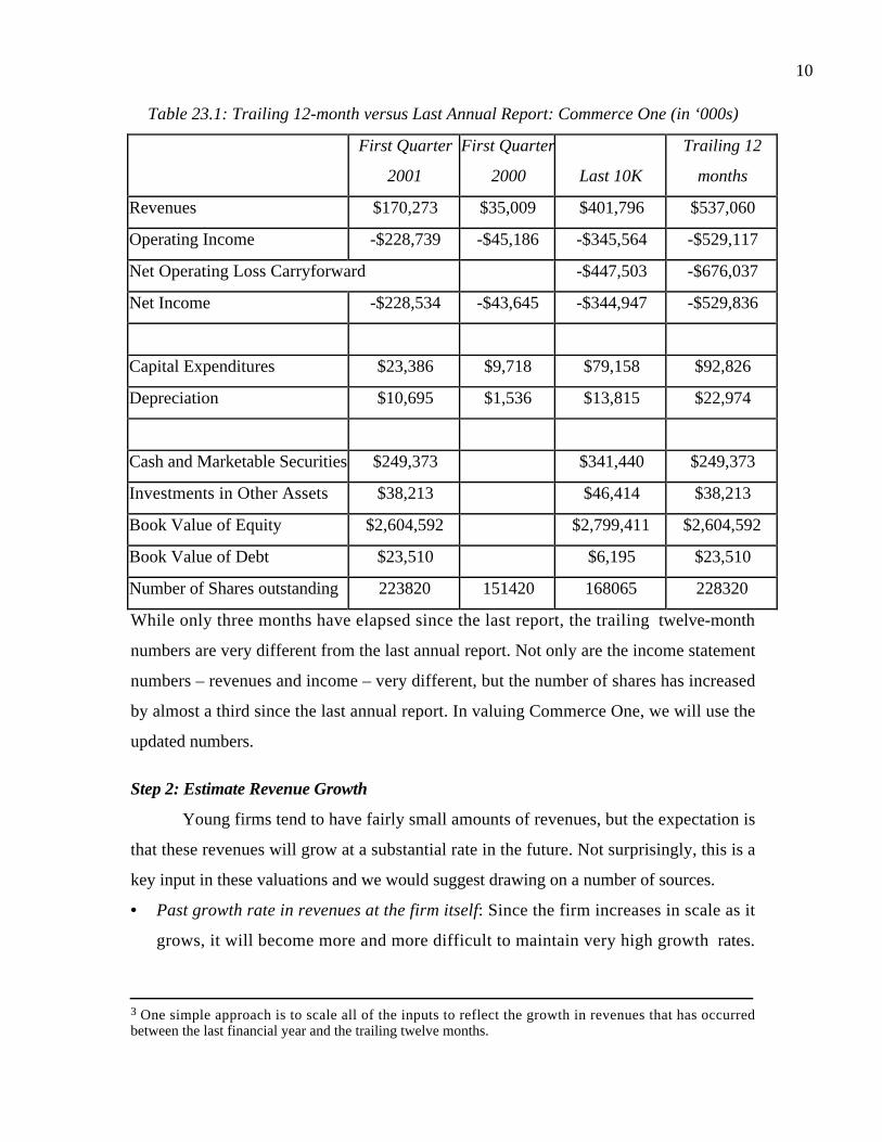
10

Table 23.1: Trailing 12-month versus Last Annual Report: Commerce One (in ‘000s)

First Quarter

2001

First Quarter

2000 Last 10K

Trailing 12

months

Revenues $170,273 $35,009 $401,796 $537,060

Operating Income -$228,739 -$45,186 -$345,564 -$529,117

Net Operating Loss Carryforward -$447,503 -$676,037

Net Income -$228,534 -$43,645 -$344,947 -$529,836

Capital Expenditures $23,386 $9,718 $79,158 $92,826

Depreciation $10,695 $1,536 $13,815 $22,974

Cash and Marketable Securities $249,373 $341,440 $249,373

Investments in Other Assets $38,213 $46,414 $38,213

Book Value of Equity $2,604,592 $2,799,411 $2,604,592

Book Value of Debt $23,510 $6,195 $23,510

Number of Shares outstanding 223820 151420 168065 228320

While only three months have elapsed since the last report, the trailing twelve-month

numbers are very different from the last annual report. Not only are the income statement

numbers – revenues and income – very different, but the number of shares has increased

by almost a third since the last annual report. In valuing Commerce One, we will use the

updated numbers.

Step 2: Estimate Revenue Growth

Young firms tend to have fairly small amounts of revenues, but the expectation is

that these revenues will grow at a substantial rate in the future. Not surprisingly, this is a

key input in these valuations and we would suggest drawing on a number of sources.

• Past growth rate in revenues at the firm itself: Since the firm increases in scale as it

grows, it will become more and more difficult to maintain very high growth rates.

3 One simple approach is to scale all of the inputs to reflect the growth in revenues that has occurredbetween the last financial year and the trailing twelve months.

11

Thus, a firm that grew 300% two years ago and 200% last year is likely to grow a

lower rate this year.

• Growth rate in the overall market that the firm serves: It is far easier for firms to

maintain high growth rates in markets that are themselves growing at high rates than it

is for them to do so in stable markets.

• Barriers to Entry and Competitive Advantages possessed by the firm: For a firm to be

able to sustain high growth rates, it has to have some sustainable competitive

advantage. This may come from legal protection (as is the case with a patent), a

superior product or service, brand name and from being the first mover into a market.

If the competitive advantage looks sustainable, high growth is much more likely to last

for a long period. If it is not, it will taper off much faster.

We looked at the process of estimating revenue growth in far more detail in Chapter 11.

Illustration 23.2: Commerce One: Estimating Revenue Growth

Commerce One has grown at an extraordinary rate since it began operations just

about three years ago. The revenues of the firm have increased from $2.5 million in 1998

to $33.6 million in 1999 to $401 million in 2000. The compounded revenue growth rate

over the two years has been 1166% a year and the growth rate just in the last year was

1093%.

The market that Commerce One serves – business software and services – is a

very large market, potentially allowing us much more room to allow for growth in future

years. The primary competition for Commerce One comes both from other B2B firms

like Ariba and from larger and more established firms such as Electronic Data Systems

(EDS).

As a final consideration, the economy was weak at the time of this valuation and

business spending had slowed down. Consequently, we will be conservative about our

estimate of revenue growth for the next year. Table 23.2 summarizes our forecasts of

revenue growth and dollar revenues at Commerce One for the next 10 years.

Table 23.2: Revenue Growth and Revenues: Commerce One

Year Expected Growth Rate Revenues

Current $537

12

1 50.00% $806

2 100.00% $1,611

3 80.00% $2,900

4 60.00% $4,640

5 40.00% $6,496

6 35.00% $8,770

7 30.00% $11,401

8 20.00% $13,681

9 10.00% $15,049

10 5.00% $15,802

Note first that all projections are based upon the trailing 12-month revenues, rather than

revenues last year. Note also that while the growth rate in revenues is expected to decline

over time, the dollar increase in revenues each year is larger than the previous year until

we get to year 9. By the end of the tenth year, Commerce One’s revenues of $15.8 billion

would make it a very large player in the business services/software business. As

comparison, note that the EDS, the largest firm in this business currently, reported

revenues of $19.6 billion in 2000.

Step 3: Estimate a Sustainable Operating Margin in Stable Growth

For a firm losing money, high revenue growth alone will accomplish little more

than make the losses become larger over time. A key component for a young firm to be

valuable is the expectation that the operating margin, while negative now, will become

positive in the future. In many ways the true test in valuation is being able to visualize

what a young, high-growth firm will look like when growth stabilizes. In the absence of

comparables, the difficulty of this task is magnified. Again, a few guidelines will help.

• Looking at the underlying business that this firm is in, consider its true competitors.

For instance, while Commerce One is considered to be a B2B or e-commerce firm, it is

ultimately a provider of business services and software. At least from the perspective

of margins, it seems reasonable to argue that Commerce One’s margins will approach

those of other business service providers.

13

• Deconstruct the firm’s current income statement to get a truer measure of its operating

margin. Many young start-up firms that report negative earnings do so, not because

their operating expenses from generating current revenues are large, but because

accounting convention requires them to report capital expenses as operating expenses.

Since many of these capital expenses are treated as S,G&A expenses in income

statements, estimating margins and profitability prior to these expenses is a useful

exercise in figuring out how profitable a company’s products truly are.

Illustration 23.3: Estimating Sustainable Margin and Path to Margin: Commerce One

In 2000, Commerce One reported an operating loss of $518 million on revenues of

$537 million. When we capitalize research and development expenses, the operating loss

narrows to $427 million. As the firm matures, these margins will surely improve, but to

what level? The average pre-tax operating margin of established business service providers

in 2000 was 15.73%. Over the 1996-2000 period, the margin has averaged 14.72%. We

assumed that Commerce One’s margins would reach 14.72% by year 10. There are some

who would argue that Commerce One as a B2B business will have higher margins, because

it does not have the same cost structure as traditional service providers. We do not agree

for two reasons. The first is that the high growth rates in revenues that we have assumed

will require aggressive pricing from Commerce One and, therefore, lower margins. The

second is that as long as anticipated margins for e-commerce firms are higher than they are

for traditional competitors, there will be increased competition coming from the latter,

pushing margins towards convergence.

To move from current margins to the sustainable margins, we assumed that the

marginal improvement will be greater in the first few years, but we do not forecast

operating profits until 5 years from now. Table 23.3 summarizes the forecasted operating

margins and earnings before interest and taxes for the next ten years and for the terminal

year (year 11).

Table 23.3: Operating Margins and Income – Commerce One

Year Revenues

Operating

Margin EBIT

Current $537 -79.45% -$427

14

1 $806 -48.06% -$387

2 $1,611 -27.14% -$437

3 $2,900 -13.18% -$382

4 $4,640 -3.88% -$180

5 $6,496 2.32% $151

6 $8,770 6.45% $566

7 $11,401 9.21% $1,050

8 $13,681 11.05% $1,511

9 $15,049 12.27% $1,847

10 $15,802 13.09% $2,068

Terminal

year $16,592 14.72% $2,442

Note that the growth rate in the terminal year is 5%. If the improvement in margins is

much faster (slower) than we forecast, our estimates of value will need to be adjusted

upwards (downwards).

To get from operating income to after-tax operating income, we generally apply

the marginal tax rate, which we assume to be 35% for most U.S. firms. With Commerce

One, though, there are two considerations. The first is that the firm is losing money

currently and does not pay taxes, and in fact, will not be paying taxes for the next 4 years.

The other is that the losses accumulate and may save the firm taxes even after it starts

making money in year 5. At the time of this valuation, Commerce One had already

accumulated losses from the last 3 years amounting to $676 million. Table 23.4

summarizes the net operating losses, taxable income and effective tax rates for the forecast

period.

Table 23.4: Net Operating Losses and Tax Rates

Year EBIT

NOL at beginning of

year

Taxable

Income Taxes PaidTax Rate

1 -$387 $676 $0 0 0.00%

2 -$437 $1,063 $0 0 0.00%

15

3 -$382 $1,500 $0 0 0.00%

4 -$180 $1,883 $0 0 0.00%

5 $151 $2,063 $0 0 0.00%

6 $566 $1,912 $0 0 0.00%

7 $1,050 $1,346 $0 0 0.00%

8 $1,511 $297 $1,215 $425 28.13%

9 $1,847 $0 $1,847 $646 35.00%

10 $2,068 $0 $2,068 $724 35.00%

Terminal

year $2,442 $0 $2,442 $855 35.00%

Note that Commerce One starts making money in year 5 but does not start paying taxes

until year 8, which the year in which the net operating losses run out.4

Step 4: Estimate Reinvestment To Generate Growth

To grow, firms have to reinvest, and this principle cannot be set aside when you

are looking a young firm. Unlike a mature firm, though, there is likely to be little in the

firm’s history that will help in determining how much the firm will need to reinvest. As

the firm grows, the nature of its reinvestment and the amount reinvested will probably

change, and the challenge is to estimate this amount.

In Chapter 11, we stated that growth in operating income ultimately is a function

of how much a firm reinvests and how well it reinvests (measured by the return on

capital).

Expected growth = Reinvestment rate * Return on capital

In fact, we have used this equation to estimate growth in most of the valuations that we

have done so far in this book. However, we also noted that this equation becomes

inoperable when operating earnings are negative, which is the position we are in when

valuing young firms. In those cases, we argued that the growth in revenues be estimated

first, and that the reinvestment be based upon the revenue growth. To make this link, we

4 The tax rate is computed by dividing the taxes by the earnings before interest and taxes.

16

used a sales/capital ratio, i.e, a ratio that specifies how many additional dollars of revenue

will be generated by each additional dollar of capital.

Expected Reinvestment ratio talSales/Capi

Revenuein change Expected=

For instance, to grow revenues by $1 billion, with a sales to capital ratio of 4, would

require a reinvestment of $250 million. The key input required for this formulation is the

sales to capital ratio and it can be estimated by looking at the firm’s history, limited

though it might be, and at industry averages, with the industry defined broadly to reflect

the business the firm is in.

In steady state, however, the reinvestment needs can be computed using the

expected growth rate and the expected return on capital.

Expected Reinvestment Ratestable stable

stable

ROC

Growth Expected=

An alternative approach is to use the industry-average reinvestment rates (broken up into

capital expenditures and working capital needs) to estimate cash flows.

Illustration 23.4: Estimating Reinvestment Needs: Commerce One

Even over its brief history, Commerce One has reinvested in a number of different

ways – R&D, acquisitions and traditional capital expenditures – and has reinvested large

amounts relative to its size. To estimate future reinvestment needs, we used two pieces of

information.

• In 2000, Commerce One had net capital expenditures, including capitalized R&D,

of $160 million and an increase in working capital of $73 million. The revenues for

the firm increased from $34 million to $ 537 million. Based upon this, we can

estimate a marginal sales/marginal capital ratio for the year.

Sales / Capital 2.1673160

34-537

ntReinvestme

Salesin Change

2000

2000 =+

==

• The average sales to capital ratio for the industry – business services and software

– is approximately 2.0. This includes more mature firms that are not e-commerce

firms like EDS. For smaller firms in the business, the ratio is 2.21.

17

We assumed that the sales to capital ratio for Commerce One would be 2.20 for the

forecast period. In conjunction with the revenues estimated in Table 23.2, we were able to

estimate the total reinvestment needed each year in Table 23.5.

Table 23.5: Reinvestment Needs and Forecast Return on Capital: Commerce One

Year Revenues

Change in

Revenues ReinvestmentTotal CapitalEBIT(1-t) ROC

Current $537 $2,744 -$427

1 $806 $269 $122 $2,866 -$387 -14.11%

2 $1,611 $806 $366 $3,232 -$437 -15.26%

3 $2,900 $1,289 $586 $3,818 -$382 -11.83%

4 $4,640 $1,740 $791 $4,609 -$180 -4.72%

5 $6,496 $1,856 $844 $5,452 $151 3.27%

6 $8,770 $2,274 $1,033 $6,486 $566 10.38%

7 $11,401 $2,631 $1,196 $7,682 $1,050 16.19%

8 $13,681 $2,280 $1,036 $8,718 $1,086 14.14%

9 $15,049 $1,368 $622 $9,340 $1,200 13.77%

10 $15,802 $752 $342 $9,682 $1,344 14.39%

By adding the total reinvestment to the capital invested at the beginning of the period, we

estimate the total capital invested in the firm. In the last column, we divide our projected

after-tax operating income each year by the capital invested at the end of the previous

year to compute the return on capital. By year 10, the return on capital at Commerce One

is 14.39%, just a shade below the average return on capital for the industry of 15%.5 In

year 11, which is the first year of stable growth, we assume that Commerce One’s return

on capital will move to the industry average return on capital. Assuming a stable growth

rate of 5% allows us to estimate the reinvestment rate in stable growth.

Reinvestment rate in stable growth 33.33%15%

5%

ROC

g ===

5 If the return on capital had become much larger than the industry average in year 10, we would havelowered the sales to capital ratio used in the valuation.

18

We will use this reinvestment rate to estimate the terminal value in a few pages.

Reinvestment and Growth: Lagged Effects

In our valuation of Commerce One, we have assumed that reinvestment and

growth occur contemporaneously. In other words, the increase in revenues and the

reinvestment that creates that increase occur simultaneously. This may seem like a radical

assumption but it is realistic in service businesses or when growth occurs through

acquisitions.

If, in fact, there is a lag between reinvestment and growth, it is relatively simple to

build this lag into the analysis. In the Commerce One valuation, assuming a one-year lag ,

you could estimate the reinvestment in year one from expected revenue growth in year 2.

The length of the lag will depend upon the firm being valued – it will be longer for firms

that have to make capital-intensive and infrastructure investments – and the form of the

reinvestment – whether it is internal or external (acquisitions).

Step 5: Estimating Risk Parameters and Discount Rates

In the standard approaches for estimating beta, we regress stock returns against

market returns. Young, start-up firms, even when publicly traded, have little historical

data, and we cannot use the conventional approaches6 to estimate risk parameters. In

Chapter 7, though, we suggested alternative approaches for estimating betas that are

useful to bridge this gap. One is the bottom-up approach. If there are comparable firms

that have been listed for two or more years, the current risk parameters for the firm can be

estimated by looking at the averages for these firms. If such firms do not exist, risk

parameters can be estimated using the financial characteristics7 of the firm – the volatility

in earnings, their size, cash flow characteristics and financial leverage.

If a young firm has debt, we run into a different problem when estimating the cost

of debt. The firm will generally not be rated, thus denying us a chance to estimate a cost

of debt based upon the rating. We could try estimating a synthetic rating, but the negative

6 The conventional approach is to regress returns on a stock against returns on a market index over a pastperiod, say two to five years.7 For a description of this approach, refer back to Chapter 7.

19

operating income will yield a negative interest coverage ratio and a default rating for the

firm. One solution is to estimate an expected interest coverage ratio for the firm based

upon expected operating income in future periods – note that these forecasts were already

made in steps 2 and 3 – and to use this expected interest coverage ratio to estimate a

synthetic rating.

Whatever approach we use to estimate costs of equity and debt, they should not

be left unchanged over the estimation period. As the firm matures and moves towards its

sustainable margin and stable growth, the risk parameters should also approach those of

an average firm – the betas should move towards one and the cost of debt should adjust

towards the industry average cost of debt.

In addition to estimating the cost of equity for these firms, we have to estimate how

leverage will change over time. Again, targeting an industry-average or an optimal debt

ratio for this firm (as it will look in steady state) should yield reasonable estimates for the

cost of capital over time.

Operating Leverage and Risk

One argument that can be made for why young firms should have much higher

betas than larger, more mature firms in their business is that they have much higher

operating leverage. The costs for young firms are for the most part fixed and do not vary

with revenues. If you are estimating a bottom-up beta for a young firm by looking at

comparable firms, you have two choices:

a. You can use only small, publicly traded firms as your comparable firms. This will

work only if there are a significant number of publicly traded firms in the business.

b. The other and more promising approach is to adjust the bottom-up beta for

differences in operating leverage. In chapter 7, we noted how betas can be adjusted for

differences in fixed cost structures

Unlevered Beta = Business Beta ( 1 + (Fixed Costs/ Variable Costs))

Illustration 23.5: Estimating Risk Parameters and Costs of Capital: Commerce One

Commerce One does not have sufficient historical data for us to estimate risk

parameters with any degree of accuracy. A regression of stock returns against a market

20

index since the stock’s listing in June 1999 yields a beta of 3.06 but the standard error in

the estimate is 2.23, rendering it useless.

To estimate the current beta for the firm, we had a choice between using the

average unlevered beta of other B2B firms (which is approximately 2.00) and the average

unlevered beta of business service providers (0.98). At the moment, Commerce One’s

fundamental characteristics seem to reflect the former more than the latter; its growth

potential is tied to the success of e-commerce. We therefore chose to use an unlevered

beta of 2.00 to estimate the current beta for the firm. At the time of this analysis,

Commerce One had debt outstanding of $25.1 million and the present value of operating

leases at the firm amounted to $131.12 million. Based upon the prevailing market price of

$8.28 and the number of shares (228.32 million) from Table 23.1, we estimated a market

value of equity of $1.89 billion and a debt to equity ratio of 8.26%.

Debt to Equity ratio 8.26%1890

131.1225.1 =+=

Levered Beta

( ) ( )( )( )( ) ( )( )( )2.17

0.08260.00-112

D/Et-11beta Unlevered

=+=

+=

This will be the beta that we use for the first five years and the tax rate is set to zero to

reflect the fact that the firm will not be paying taxes. With a riskfree rate of 5.4% and a

risk premium of 4%, we estimate a cost of equity for the first five years.

Cost of equity = 5.4% + 2.17 (4%) = 14.06%

To estimate the cost of debt, we computed the average operating income over the

next 7 years using the projections in Table 23.4 (obtaining a value of $54 million) and

divided this by the current interest expenses (including the operating lease expenses from

the current year)

Predicted Interest coverage ratio

3.1714.412.5

54

expense lease yearsCurrent expenseInterest

EBIT Average =+

=+

=

This yields a rating of BB and a default spread of 3.50% and a pre-tax cost of debt of

8.90% for the next 5 years. Since the firm pays no taxes over this period, its after tax

cost of debt is equal to the pre-tax cost.

21

Beyond year 5, as the firm matures, we feel that Commerce One’s risk will

approach those of other business service providers and that its beta will decline to 1.2 in

year 10, which will still make it riskier than the typical firm in the sector. The pre-tax

cost of debt will also decline towards an industry average of 7%, while the debt ratio will

increase towards the average for the industry of 12%. The following table summarizes the

resulting estimates of cost of equity, debt and capital for Commerce One.

Table 23.6: Costs of Debt, Equity and Capital: Commerce One

Year Beta

Cost of

Equity

Pre-tax cost of

debt Tax Rate

After-tax cost

of debt Debt Ratio

Cost of

Capital

1 2.17 14.06% 8.90% 0.00% 8.90% 7.63% 13.67%

2 2.17 14.06% 8.90% 0.00% 8.90% 7.63% 13.67%

3 2.17 14.06% 8.90% 0.00% 8.90% 7.63% 13.67%

4 2.17 14.06% 8.90% 0.00% 8.90% 7.63% 13.67%

5 2.17 14.06% 8.90% 0.00% 8.90% 7.63% 13.67%

6 1.97 13.29% 8.52% 0.00% 8.52% 8.51% 12.88%

7 1.78 12.52% 8.43% 0.00% 8.43% 8.72% 12.16%

8 1.59 11.74% 8.27% 27.93% 5.96% 9.09% 11.22%

9 1.39 10.97% 7.95% 35.00% 5.17% 9.82% 10.40%

10 1.20 10.20% 7.00% 35.00% 4.55% 12.00% 9.52%

[NOTE: The original pre-tax cost of debt does not decline linearly from year 6 to year 10.

It had a very strange pattern.]

Note that the beta declines linearly from the current level of 2.17 in year 5 to 1.20 in year

10 and the pre-tax cost of debt declines linearly from 8.90% in year 5 to 7% in year 10.

The cost of capital beyond year 10 will be 9.52%.

Step 6: Estimate the value of the firm

With the inputs on earnings, reinvestment rates and risk parameters over time, this

valuation becomes much more conventional. In many cases, the cash flows in the early

years will be negative, in keeping with the negative earnings, but turn positive in later

22

years as margins improve. The bulk of the value will generally be in the terminal value.

Consequently, our assumptions about what the firm will look like in stable growth are

significant.

Having valued the operating assets of the firm, you need to consider two other

factors – the possibility that the firm will not survive to become a going concern and the

value of non-operating assets – to value the firm.

Survival

When we value firms using discounted cash flow valuation, we tend to assume

that the firm will be a going concern and continue to generate cash flows in perpetuity.

This assumption might be suspect when valuing young companies, since many of them

will not survive the tests that they will be put to over the next few years. If we ignore

this possibility and consider only the best case scenario of expansion and profitability,

we will over estimate the value of these firms. We have two choices when it comes to

dealing with this possibility.

• The first is to build into the expected growth rates and earnings the likelihood of

unfavorable outcomes. Thus, the growth rate used in revenues will be the expected

growth rate over all scenarios, both optimistic and pessimistic. For young firms,

this will become progressively more difficult to do as you get further and further

into the future.

• The second is to estimate a discounted cash flow value across only the scenarios

where the firm is a going concern and then apply a probability that the firm will be

a going concern to this value. In Chapter 12, we suggested a couple of approaches

that can help in coming up with this probability including statistical probits and

Monte Carlo simulations. Once we have estimated the probability of surviving as

a going concern, the value of a firm can then be estimated.

Value of firm = Probability of surviving as a going concern * Discounted Cash flow value

of firm + (1- Probability of surviving as a going concern) * Distress or Liquidation sale

value

Value of non-operating assets

23

As with the valuation of any firm, you have to consider cash, marketable

securities and holdings in other companies when you value a firm. The only note of

caution that we would add is that young firms can burn through significant cash balances

in short periods because their operation drain cash rather than generate it. Thus, the cash

balance from the last financial statements, especially if those statements are more than a

few months old, can be very different from the current cash balances.

To the extent that young firms often have holdings in other young firms, there is

also the danger that investments in other firms may be shown on the books that are not

reflective of their true value. If there are only one or two large holdings, you should value

those holdings using cash flow based approaches as well.

Illustration 23.6: Estimating Firm Value: Commerce One

Having estimated the cash flows and the discount rates, we are now in a position

to estimate the firm value for Commerce One as a firm. While estimating cash flows, we

consider the fact that the firm will have net operating losses to carry forward and that this

will reduce their tax burden when they initially start making money. Table 23.7

summarizes the cash flows to the firm after reinvestment needs for each of the next 10

years and the discount rate applied to these cash flows.

Table 23.7: Expected Cashflows to the firm and Present Value

Year EBIT(1-t)Reinvestment FCFF Cost of Capital

Cumulated cost of

capital Present Value

1 -$388 $122 -$510 13.67% 1.1367 -$449

2 -$438 $366 -$805 13.67% 1.2920 -$623

3 -$384 $586 -$970 13.67% 1.4686 -$660

4 -$182 $791 -$973 13.67% 1.6693 -$583

5 $149 $844 -$694 13.67% 1.8975 -$366

6 $565 $1,033 -$469 12.88% 2.1419 -$219

7 $1,049 $1,196 -$147 12.16% 2.4024 -$61

8 $1,089 $1,036 $52 11.22% 2.6719 $19

9 $1,200 $622 $578 10.40% 2.9498 $196

24

10 $1,344 $342 $1,002 9.52% 3.2307 $310

Sum of the present value of the cash flows over high growth period = -$2,435

There is one very significant cash flow that is not reported on this table and that is

the terminal value of the firm. To estimate the terminal value, at the end of year 10, we

first estimated the free cash flow to the firm in year 11.

Free cash flow to the firm

= EBIT11 1-t( ) 1-Reinvestment Rate Stable( )= ($2,442)(1− .35) 1−0.3333( )= $1,058 million

We use the stable growth rate of 5% and the reinvestment rate of 33.33% that we

estimated earlier. The terminal value can now be estimated.

Terminal value

=FCFF11

Cost of capital Stable -Stable growth rate

=1058

0.0952 − 0.05= $23,404 million

The value of the operating assets of the firm can be estimated.

Value of operating assets

= PV of cashflows during high growth + PV of terminal value

= -$2,435 +$23,404

3.2279= $4,809 million

To this, we add the most recent estimate that we have of cash, marketable securities and

other investments.

Value of firm = Value of operating assets + Cash and marketable securities + Other

investments = $4,809 million + $249 million + $ 38 million = $5,097 million

This would be the value that we would assign the firm as a going concern.

How much of a discount should be applied for the likelihood that Commerce One

may not survive? The firm has a cash balance that will cover its operating cash needs for

about 6 months, which increases the chances of failure, especially if the equity markets

remain weak. In addition, we expect the firm to continue to lose money for the next 5

years, which will increase its need for external financing. On the positive side, the firm is

not heavily levered and is not under immediate pressure to meet debt payments. Assume,

25

for instance, that these facts lead you to assign a 25% probability that the firm will not

survive and that the distress sale value in the event of failure will be 50% of book value of

$2,744 billion. The value of Commerce One can then be estimated as follows.

Value of Commerce One = Going Concern value * probability of going concern + Distress

sale value * probability of failure = $5,097 * .75 + $2,744*.5 *.25 = $4,166 million

Clearly, the probability estimate and the distress sale value in this example are arbitrary

values, but they can be fine tuned when the probability of default is high.

Step 7: Estimate the value of equity and Per-Share value

To get from firm value to equity value, we generally subtract out all non-equity

claims on the firm. For mature firms, the non-equity claims take the form of bank debt

and bonds outstanding. For young firms, there can also be preferred equity claims that

have to be valued and subtracted out to get to the value of the common equity.

To get from equity value to value per share, you have to consider all options

outstanding on the firm. In Chapter 16, we argued that this is something that needs to be

done for all firms, but it becomes particularly important with young, start-up firms,

because the value of the options outstanding can be a much larger share of the overall

equity value. Given the importance of these claims, we would suggest that the options

–vested as well as non-vested – be valued using an option pricing model and that the value

of the options be subtracted out from the value of the equity to arrive at the value of

equity in common stock. This value should then be divided by the actual number of

shares outstanding to arrive at the equity value per share.

Illustration 23.7: Valuing Equity per Share: Commerce One

Having estimated the value of Commerce One to be $5.097 million, we first

estimate the value of equity by subtracting out the value of the debt claims on the firm.

The debt claims that we consider include both the debt outstanding of $25.1 million and

the present value of operating lease commitments of $131 million.

Value of Commerce One Equity = Value of firm – Debt = 5097 – (25 + 131) = $4,941

million

As of December 2000, the firm had options outstanding on 45.911 million shares, with a

weighted average life of 8.92 years and a weighted exercise price of $35.49. Using a Black-

26

Scholes option pricing model, allowing for dilution, the value of these options were

computed using Commerce One’s market price of $8.28 per share as of May 2001. The

total value of the options outstanding was estimated to be $349 million. Assuming that

Commerce One will be able to claim this expense as a tax deduction, the value of equity in

common stock was computed.

Value of Equity = $4,941 million

Value of Equity in Options Outstanding = - $227 million : ($349 (1-.35))

= Value of Equity in Common Stock $ 4,714 million

Commerce One had 228.32 million shares outstanding as of May 2001, leading to a per

share value of

Value of Equity in Common Stock $4,714 million

/ Number of Shares outstanding 228.32million

= Value of Equity per Share $ 20.65

This value per share is at variance with the value used to price the options. If we iterated

back, using this estimated value per share to value the options, we would obtain a value of

$835 million (pre-tax) for the options and a value per share of $19.26. [NOTE: I am

unable to confirm this since I do not have all the parameters for the option pricing.]

Should there be a discount for float?

Some publicly traded stocks are lightly traded and the number of shares available for trade

(often referred to as the float) is small relative to the total number of shares outstanding8.

Investors who want to sell their stock quickly in these companies often have a price

impact when they sell and the impact will increase with the size of the transaction.

Investors with longer time horizons and a lesser need to convert their holdings into

cash quickly have a smaller problem associated with illiquidity than investors with

shorter time horizons and a greater need for cash. Investors should consider the

possibility that they will need to convert their holdings quickly into cash when they look

at lightly traded stocks as potential investments and require much larger discounts on

value before they take large positions. Assume, for instance, that an investor is looking at

27

a young firm that she has valued at $19.05 per share. The stock would be under priced if

it were trading at $17, but it might not be under priced enough for a short term investor to

take a large position in it. In contrast, a long-term investor may find the stock an

attractive buy at that price.

Value Drivers

What are the key inputs that determine the value of a young, high-growth firm

with negative earnings? In general, the inputs that have the greatest impact on value are

the estimates of sustainable margins and revenue growth. To a lesser extent, assumptions

about how long it will take the firm to reach a sustainable margin and reinvestment needs

in stable growth have an impact on value, as well.

In practical terms, the bulk of the value of these firms is derived from the terminal

value. While this will trouble some, it mirrors how an investor makes returns in these

firms. The payoff to these investors takes the form of price appreciation rather than

dividends or stock buybacks. Another way of explaining the dependence on terminal

value and the importance of the sustainable growth assumption is in terms of assets in

place and future growth. The value of any firm can be written as the sum of the two.

Value of Firm = Value of Assets in Place + Value of Growth Potential

For start-up firms with negative earnings, almost all of the value can be attributed to the

second component. Not surprisingly, the firm value is determined by assumptions about

the latter.

Illustration 23.8: Value Drivers for Commerce One

There are two key value drivers that affect the value of Commerce One as a firm.

The first is the expected compounded growth rate in revenues. We have assumed it to be

approximately 40% compounded over the next 10 years. If revenue growth were higher,

the value per share would also be higher, as evidenced in the figure below.

8 The float is estimated by subtracting out from the shares outstanding, shares that are owned by insiders,5% owners and rule 144 shares. (Rule 144 refers to restricted stock which cannot be traded.)

28

Note, though, that we are talking about compounded growth. At a 50% compounded

growth rate, the value per share would be in excess of $40, but revenues in year 10 would

have to be $30 billion. This is in contrast to our base case assumption where revenues

grow to $15.8 billion in year 10.

The second is the sustainable operating margin. We assumed that it would

converge on the industry average of 14.72%. The value per share is extremely sensitive to

this assumption.

Figure 23.2: Revenue Growth and Value per share

$0.00

$5.00

$10.00

$15.00

$20.00

$25.00

$30.00

$35.00

5% 10% 15% 20% 25% 30% 35% 40% 45%

Compounded Revenue Growth - Next 10 years

Val

ue p

er s

hare

29

If the pre-tax operating margin were to be 16% instead of 14.72%, the value per share

would increase to $23. For this to happen, however, the competition would essentially

have to collapse. If, on the other hand, this market turns out to have fewer barriers to

entry than anticipated and competition drives margins to 10%, the value per share will

drop to single digits.

In conclusion, it is worth noting that we can justify Commerce One’s price per

share (of $8.28 at the time of this analysis) under certain circumstances, just as we can

justify the market price of any security. For instance, assuming a lower compounded

growth rate in revenues for the next 10 years or a lower pre-tax operating margin or some

combination of the two would lead us to a value of $8.28. For any investor or analyst, the

follow-up question then becomes a pragmatic one: What are the odds of such an

occurrence and do you feel confident enough that this is too pessimistic a view of the

world to buy the stock today?

Estimation Noise

Figure 23.3: Value per share and Sustainable Margins

$0.00

$5.00

$10.00

$15.00

$20.00

$25.00

10% 11% 12% 13% 14% 15% 16%

Pre-tax operating margin

Val

ue p

er s

hare

30

The framework for valuation provided in this section should not be considered a

recipe for precision. The valuation of a firm with negative earnings, high growth and

limited information will always be noisy. One way to present this noise is in terms of a

valuation range and the range on the value of these firms will be large. This is often used

as an excuse by analysts who do not want to go through the process of valuing such

firms. It also provides critics with a simplistic argument against trusting the numbers that

emerge from these models.

We have a different view. The noise in the valuation is not a reflection of the

quality of the valuation model, or the analyst using it, but of the underlying real

uncertainty about the future prospects of the firm. This uncertainty is a fact of life when

it comes to investing in these firms. In a valuation, we attempt to grapple with this

uncertainty and make our best estimates about the future. Note that those who disdain

valuation models for their potential errors end up using far cruder approaches, such as

comparing price/sales ratios across firms. The difference, as we see it, is that they choose

to sweep the uncertainties under the rug and act as if they do not exist.

There are two other points to make about the precision in these valuations. First,

even if a valuation is imprecise, it provides a powerful tool to answer the question of what

has to occur for the current market price of a firm to be justified. Investors can then decide

whether they are comfortable with these assumptions and make their decisions on buying

and selling stock. Second, even if individual valuations are noisy, portfolios constructed

based upon these valuations will be more precisely valued. Thus, an investor who buys

40 stocks that he or she has found to be undervalued using traditional valuation models,

albeit with significant noise, should find noise averaging out across the portfolio. The

ultimate performance of the portfolio then should reflect the valuation skills, or the

absence of them, of the analyst.

Implications for Investors

From a valuation perspective, there are a number of useful lessons that emerge for

investors in young firms with negative earnings and limited information.

Ø Focus on sustainable margins and survival, rather than quarter-to-quarter or even

year-to-year swings in profitability. Understanding what a firm’s operating margins

31

will look like when it reaches financial health might be the single most important

determinant of whether one is successful investing, in the long term, in such firms.

Separating those firms that have a greater chance of surviving and reaching financial

health from those that will not survive is a closely connected second determinant.

After all, most start-up firms never survive to enjoy their vaunted growth prospects.

Ø Earnings reports can be misleading, especially when reinvestment costs are expensed

(as is the case with research, development and long-term marketing expenses). Thus,

when a firm with high-growth potential and poor earnings reports a significant

improvement in earnings, investors should examine the report for the reasons. If the

earnings are improving because the costs of generating current revenues are coming

down (due to economies of scale or pricing power), this is clearly good news. If,

however, the earnings are increasing because the firm has reduced or eliminated

discretionary reinvestment expenditures (such as development costs), the net effect

on value can be very negative, since future growth is being put at risk.

Ø Diversify. This age-old rule of investing becomes even more critical when investing in

stocks that derive the bulk of their value from uncertain future growth. The antidote

to estimation noise is often a more diversified portfolio9 both across firms and across

sectors.

Ø Keep track of barriers of entry and competitive advantages; they will, in large part,

determine whether the firm will continue to maintain high growth.

Ø Be ready to be wrong. The noise in these valuations is such that no matter how much

information is brought into the process and how carefully a valuation is done, the

value obtained is an estimate. Thus, investors in these stocks will be spectacularly

wrong sometimes and it is unfair to judge them on individual valuations. They will

also be spectacularly right in other cases; and all that we can hope for is that with time

as an ally, the successes outweigh the failures.

Implications for Managers

9 The simple rules of diversification that suggest 20 stocks are enough may not apply here. Since theseinvestments tend to come from the same sector, and have higher correlations with each other, and since

32

If the future growth potential for a firm is uncertain, what are the implications for

managers? The first is that the uncertainty about future growth will almost certainly

translate into more uncertainty in traditional investment analysis. It is far more difficult to

estimate cash flows and discount rates for individual projects in young, start-up firms

than in more stable sectors. While the reaction of some managers at these firms is to give

up and fall back on more intuitive approaches, the managers who persevere and attempt

to estimate cash flows will have a much better sense of what they need to do to make new

investments pay off.

The Expectations Game

As the proportion of value determined by future growth increases, expectations

become a more critical determinant of how markets react to new information. In fact, the

expectations game largely explains why stock prices change in ways that do not seem

consistent with the news being announced (good earnings news leading to stock price

drops, bad earnings news resulting in stock price increases) and the volatility of young

start-up firms, in general.

Expectations, Information and Value

The value of a firm is the present value of the expected cash flows on the firm, and

implicit in these expected cash flows and the discount rates used to discount the cash

flows are investors’ views about the firm, its management and the potential for excess

returns. While this is true for all firms, the larger proportion of value that comes from

future growth potential at young, start-up firms makes them particularly vulnerable to

shifts in expectations about the future.

How are these expectations formed? While the past history of these firms and

industry averages are sometimes used as the basis for estimates, the firms and the

industries themselves both evolve and change over time. The fact that information is both

noisy and limited suggests that expectations can change relatively quickly and in response

to small shifts in information. An earnings announcement, for instance, that suggests that

there is so much noise in estimation, more stocks will be needed to accomplish the same degree ofdiversification that one would have got by buying 20 large-capitalization, mature companies.

33

a firm’s strategy is not working as well as anticipated may lead to a reassessment of

expectations and a share drop in value.

Lessons for Investors

The power of expectations in determining the value of a stock has to be considered

when investors choose stocks for their portfolios and when they assess new information

about the firm. There are several important implications.

• Risk is always relative to expectations. The risk in a firm does not come from whether

it performs well or badly but from how it does relative to expectations. Thus, a firm

that reports earnings growth of 35% a year when it was expected to grow 50% a year

is delivering bad news and will probably see its stock price drop. In contrast, a firm

that reports a 20% drop in earnings when it was expected to report a 40% drop will

generally see its stock price increase.

• Good companies do not always make good investments. It is not how well or badly a

company is managed that determines stock returns; it is how well or badly managed

relative to expectations. A company that meets every financial criteria for excellence

may be a poor investment, if markets are expecting too much of it. Conversely, a firm

that is universally viewed as a poorly managed, poorly run company may be a good

investment, if expectations have been set too low10.

• Small news leads to big price jumps. As noted in the last section, you should expect

to see what seem like disproportionate stock price responses to relatively small

pieces of information. A report from a high growth firm that earnings in the most

recent quarter were a few cents less than expected may lead to a significant drop in the

stock price.

• Focus on information about value drivers. On a positive note, investors can assess

what it is that drives value the most at a firm, and get a sense of what they should

focus on when looking at new information. Looking past the aggregate earnings

10 The empirical evidence backs up this proposition. Studies of investments seem to indicate thatcompanies that are viewed as well managed under perform companies that are less well regarded asinvestments.

34

numbers for information on these value drivers may provide clues of both upcoming

trouble and potential promise.

Lessons for Managers

If the expectation game affects investors, it is even more critical to managers at

young firms. One of the ironies that emerges from this game is that it is far easier to

manage a firm that is perceived to be a poor performer than it is to manage one that is

perceived to be a star11.

• Find out what is expected of you: If you are going to be judged against expectations, it

is critical that you gauge what these expectations are. While this translates, for many

firms, into keeping track of what analysts are estimating earnings per share to be in

the next quarter, there is more to it than this. Understanding why investors value your

firm the way they do and what they think are your competitive advantages is much

more important, in the long term.

• Learn to manage expectations: When firms first go public, managers and insiders sell

the idea that their firm has great potential and should be valued highly. While this is

perfectly understandable, managers have to change roles after they go public and learn

to manage expectations. Specifically, they have to talk down expectations when they

feel that their firm is being set up to do things that it cannot accomplish. Again,

though, some firms damage their credibility when they talk down expectations

incessantly, even when they know the expectations are reasonable12.

• Do not delay the inevitable: No matter how well a firm manages expectations, there are

times when managers realize that they cannot meet expectations any more, because of

changes in the sector or the overall economy. While the temptation is strong to delay

revealing this to financial markets, often by shifting earnings from future periods into

the current one or using accounting ploys, it is far better to deal with the

consequences immediately. This may mean reporting lower earnings than expected

11 Steve Job’s job at Apple Computer was far easier when he took over in 1998 (when the stock price hadhit a ten-year low) than it was two years later, when he had succeeded in changing investor perceptions ofthe company (and pushed the stock price up ten-fold, in the process).12 Steve Ballmer at Microsoft has developed a reputation for talking down expectations and then beatingthem on a consistent basis.

35

and a lower stock price, but firms that delay their day of reckoning tend to be

punished much more.

Summary

Valuation, fundamentally, remains the same no matter what type of firm one is

analyzing. There are three groups of firms where the exercise of valuation becomes more

difficult and estimates of value more noisy. The first group includes firms that have

negative earnings. Given the dependence of most models on earnings growth to make

projections for the future, analysts have to consider approaches that allow earnings to

become positive, at least over time. They can do so by normalizing earnings in the current

period or by adjusting margins from current levels to sustainable levels over time or by

reducing leverage. The approach used will depend upon why the firm has negative

earnings in the first place. The second group of firms where estimates are difficult to make

are young firms, with little or no financial history. Here, information on comparable firms

can substitute for historical data and allow analysts to estimate the inputs needed for

valuation. The third group of firms where valuation can be difficult includes unique firms

with few or no comparable firms.

If all three problems come together for the same firm – negative earnings, limited

history and few comparables – the difficulty is compounded. In this essay, we have laid

out a broad framework that can be used to value such firms. It should be noted again that

the question is not whether these firms can be valued – they certainly can – but whether

we are willing to live with noisy estimates of value. To those who argue that these

valuations are too noisy to be useful, our counter would be that much of this noise stems

from real uncertainty about the future. As we see it, investors who attempt to measure

and confront this uncertainty are better prepared for the volatility that comes with

investing in these stocks. While some view multiples as a painless way of analyzing these

firms, we have pointed out some of the inherent constraints with coming up with usable

multiples and comparables for such firms, and the dangers of trusting the market to be

right, on average.

36

Problems

1. Intellitech is a technology firm that has been in operating for two years. In the

most recent year, the firm reported revenues of $500 million, five times revenues

in the previous year. The firm also reported an operating loss of $400 million. You

expect revenues to grow 100% next year, 80% the year after and 40% a year for

the following three years and the pre-tax operating margin to improve – in linear

increments – to 10% by the fifth year. Estimate the revenues and operating

income each year for the next 5 years.

2. You are trying to estimate the trailing 12-month earnings for Fiber Networks. The

firm has just reported an operating loss for the first quarter of 2001 of $180

million on revenues of $600 million, a jump from the operating loss of $30 million

on revenues of $120 million in the first quarter of 2000. In its annual report for

2000, Fiber Networks reported an operating loss of $330 million on revenues of

$1.1 billion. Estimate the operating loss and revenues for the last four quarters.

3. Verispace Software sells inventory management software and reported revenues of

$25 million in the most recent financial year. You estimate that the total market

for inventory management software to be $25 billion, growing at 5% a year for the

foreseeable future. If you expect Verispace to have 10% market share of this

market in 10 years, estimate the compounded revenue growth rate over that

period.

4. Lumin Telecommunications produces specialized telecommunication equipment

and has made losses each year over the three years it has been in existence – it has

an accumulated net operating loss of $180 million. In the most recent year, the

firm reported an operating loss of $90 million on revenues of $1 billion. If you

expect the growth rate in revenues to be 20% a year for the next 5 years, and the

pre-tax operating margin to be –6% next year, -3% two years from now, 0% the

year after, 6% in four years and 10% in five years, estimate

a. The revenues and pre-tax operating income each year for the next 5 years.

37

b. The taxes you would have to pay and your after-tax operating income each

year for the next 5 years..

5. In problem 4, assume that Lumin Telecommunications has a beta of 2.0 currently

and that you expect it to drop in linear increments to 1.2 by year 5. If the current

cost of borrowing is 9% and you expect this to remain unchanged over the next 5

years, estimate the cost of capital for the firm each year for the next 5 years. (The

riskfree rate is 5.6% and the risk premium is 4%.)

6. You have estimated the value of Vitale Systems, an internet software firm, to be

$700 million as a going concern, seven times its book value. However, you are

concerned that Vitale might not survive the next 5 years and you estimate the

probability of failure at 40%. If the firm fails, you expect that its assets to sell for

1.5 times book value. If there are 30 million shares outstanding, estimate the value

per share.

1

CHAPTER 24

VALUING PRIVATE FIRMS

So far in this book, we have concentrated on the valuation of publicly traded

firms. In this chapter, we turn our attention to the thousands of firms that are private

businesses. These businesses range in size from small family businesses to some that rival

large publicly traded firms. The principles of valuation remain the same, but there are

estimation problems that are unique to private businesses. The information available for

valuation tends to be much more limited, both in terms of history and depth, since private

firms are often not governed by the strict accounting and reporting standards of publicly

traded firms. In addition, the standard techniques for estimating risk parameters (such as

beta and standard deviation) require market prices for equity, an input that is lacking for

private firms.

When valuing private firms, the motive for the valuation matters and can affect the

value. In particular, the value that is attached to a publicly traded firm may be different

when it is being valued for sale to an individual, for sale to a publicly traded firm or for an

initial public offering. In particular, whether there should be a discount on value for

illiquidity and non-diversifiable risk or a premium for control will depend upon the

motive for the valuation. We will consider each of these components over the course of

this chapter.

What makes private firms different?

There are a number of common characteristics shared by private firms with

publicly traded firms, but there are four significant differences that can affect both how

we estimate inputs for valuation.

• Publicly traded firms are governed by a set of accounting standards that allow us

to identify what each item in a financial statement includes but to also compare

earnings across firms. Private firms, especially if they are not incorporated,

operate under far looser standards and there can be wide differences between firms

on how items are accounted.

• There is far less information about private firms, both in terms of the number of

years of data that is typically available and, more importantly, the amount of

2

information available each year. For instance, publicly traded firms have to break

down operations by business segments in their filings with the SEC and provide

information on revenues and earnings by segment. Private firms do not have to,

and usually do not, provide this information.

• A constantly updated price for equity and historical data on this price is a very

useful piece of information that we can obtain easily for publicly traded firms but

not for private firms. In addition, the absence of a ready market for private firm

equity also means that liquidating an equity position in a private business can be

far more difficult (and expensive) than liquidating a position in a publicly traded

firm.

• In publicly traded firms, the stockholders tend to hire managers to run the firm

and most stockholders hold equity in several firms in their portfolios. The owner

of a private firm tends to be intimately involved with management and often has

all of his or her wealth invested in the firm. The absence of separation between the

owner and management can result in an intermingling of personal expenses with

business expenses and a failure to differentiate between management salary and

dividends (or their equivalent).

Each of the differences cited above can change value by affecting discount rates, cash

flows and expected growth rates.

To examine the issues that arise in the context of valuing private firms, we will

consider two firms. The first firm is the New York Yankees, a fabled baseball franchise

and the second is a private software firm called InfoSoft. We will value the Yankees for

sale in a private transaction, whereas we will value InfoSoft for sale in an initial public

offering.

Estimating Valuation Inputs at Private Firms

The value of a private firm is the present value of expected cash flows discounted

back at an appropriate discount rate. Since this construct is not different from the one we

used to value publicly traded firms, the differences between private firms and publicly

traded firms have to show up in how we estimate these inputs to the discounted cash

flow model.

3

Discount Rates

If we choose to value equity, we discount cashflows to equity at the cost of

equity, whereas if we choose to value the firm, we discount cashflows at the cost of

capital. While the fundamental definitions of these costs have not changed, the process of

estimating them may have to be changed given the special circumstances surrounding

private firms.

Cost of Equity

In assessing the cost of equity for publicly traded firms, we looked at the risk of

investments through the eyes of the marginal investors in these firms. With the added

assumption that these investors were well diversified, we were able to define risk in terms

of risk added on to a diversified portfolio or market risk. The beta (in the CAPM) and

betas (in the multi-factor models) that measure this risk are usually estimated using

historical stock prices. The absence of historical price information for private firm equity

and the failure on the part of many private firm owners to diversify can create serious

problems with estimating and using betas for these firms.

Approaches to Estimating Market Betas

The standard process of estimating the beta in the capital asset pricing model

involves running a regression of stock returns against market returns. Multi-factor models

use other statistical techniques, but they also require historical price information. In the

absence of such information, as is the case with private firms, there are three ways in

which we can estimate betas.

1. Accounting Betas

While price information is not available for private firms, accounting earnings

information is. We could regress changes in a private firm’s accounting earnings against

changes in earnings for an equity index (such as the S&P 500) to estimate an accounting

beta.

∆ EarningsPrivate firm = a + b ∆ EarningsS&P 500

The slope of the regression (b) is the accounting beta for the firm. Using operating

earnings would yield an unlevered beta, whereas using net income would yield a levered or

equity beta.

4

There are two significant limitations with this approach. The first is that private

firms usually measure earnings only once a year, leading to regressions with few

observations and limited statistical power. The second is that earnings are often smoothed

out and subject to accounting judgments, leading to mismeasurement of accounting betas.

Illustration 24.1: Estimating Accounting Betas –– InfoSoft

InfoSoft, even though it is a private business, has been in existence since 1992 and

has accounting earnings going back to that year. Table 24.1 summarizes the quarterly

accounting earnings changes at InfoSoft and for the S&P 500 for each quarter between

1992 and 1998.

Table 24.1: Earnings for InfoSoft versus S&P 500

Period InfoSoft S&P 500 Period InfoSoft S&P 500

1992: Q1 7.50% -1.30% 1995: Q2 24.10% 8.50%

1992: Q2 8.30% 2.20% 1995: Q3 17.50% 6.00%

1992: Q3 8.80% 2.50% 1995: Q4 16.00% 5.00%

1992: Q4 7.90% 3.00% 1996: Q1 27.00% 8.10%

1993: Q1 14.30% 3.60% 1996: Q2 21.30% 7.00%

1993: Q2 16.50% 5.10% 1996: Q3 22.50% 7.20%

1993: Q3 17.10% 5.50% 1996: Q4 20.00% 6.00%

1993: Q4 13.50% 6.20% 1997: Q1 17.10% 5.80%

1994: Q1 11.50% 4.30% 1997: Q2 22.20% 8.00%

1994: Q2 12.30% 4.70% 1997: Q3 17.80% 6.10%

1994: Q3 13.00% 4.50% 1997: Q4 14.50% 4.50%

1994: Q4 11.10% 4.20% 1998: Q1 8.50% 1.30%

1995: Q1 18.60% 7.10% 1998: Q2 3.50% -0.50%

a Earnings changes are over same quarter of previous year

Regressing the changes in earnings at InfoSoft against changes in profits for the S&P 500

yields the following.

InfoSoft Earnings Change = 0.05 + 2.15 (S & P 500 Earnings Change)

5

Based upon this regression, the beta for InfoSoft is 2.15. In calculating this beta, we used

net income to arrive at an equity beta. Using operating earnings for both the firm and the

S&P 500 should yield the equivalent of an unlevered beta.

2. Fundamental Betas

There have been attempts made by researchers to relate the betas of publicly

traded firms to observable variables such as earnings growth, debt ratios and variance in

earnings. Beaver, Kettler, and Scholes (1970) examined the relationship between betas and

seven variables - dividend payout, asset growth, leverage, liquidity, asset size, earnings

variability and the accounting beta. Rosenberg and Guy (1976) also attempted a similar

analysis. The following is a regression that we ran relating the betas of NYSE and AMEX

stocks in 1996 to four variables: coefficient of variation in operating income (CVOI), book

debt/equity (D/E), historical growth in earnings (g) and the book value of total assets

(TA).

Beta = 0.6507 + 0.25 CVOI + 0.09 D/E + 0.54 g - 0.000009 TA R2=18%

where

CVOI = Coefficient of Variation in Operating Income

= Standard Deviation in Operating Income/ Average Operating Income

We could measure each of these variables for a private firm and use these to estimate the

beta for the firm. While this approach is simple, it is only as good as the underlying

regression. The low R2 suggests that the beta estimates that emerge from it are likely to

have large standard errors.

Illustration 24.2: Estimating a Fundamental Beta: InfoSoft

To use the cross sectional regression that we reported earlier to estimate a beta for

InfoSoft, we have to estimate the values for each of the independent variables for the firm.

Variable Value

Coefficient of Variation in Operating Income 0.40

Book Debt to Equity Ratio 128.57%

Growth in earnings (previous 5 years) 30%

Book Value of Total Assets $ 9 million

6

Inputting these values into the regression, we obtain a predicted value for the beta:

Beta = 0.6507 + 0.25 (0.40) + 0.09 (1.2857) + 0.54 (0.3) - 0.000009 (9) = 1.03

This would yield an estimate of 1.03 for InfoSoft’s beta. The standard error on this

estimate is 0.18, resulting in a range of 0.85 to 1.21 for the beta, with 67% probability.

3. Bottom-up Betas

When valuing publicly traded firms, we used the unlevered betas of the businesses

that the firms operated in to estimate bottom-up betas – the costs of equity were based

upon these betas. We did so because of the low standard errors on these estimates (due to

the averaging across large numbers of firms) and the forward looking nature of the

estimates (because the business mix used to weight betas can be changed). We can

estimate bottom-up betas for private firms and these betas have the same advantages that

they do for publicly traded firms. Thus, the beta for a private steel firm can be estimated

by looking at the average betas for publicly traded steel companies. Any differences in

financial or even operating leverage can be adjusted for in the final estimate.

In making the adjustment of unlevered betas for financial leverage, we do run into a

problem with private firms, since the debt to equity ratio that should be used is a market

value ratio. While many analysts use the book value debt to equity ratio to substitute for

the market ratio for private firms, we would suggest one of the following alternatives.

a. Assume that the private firm’s market leverage will resemble the average for the

industry. If this is the case, the levered beta for the private firm can be written as:

β private firm = βunlevered (1 + (1 - tax rate) (Industry Average Debt/Equity))

b. Use the private firm’s target debt to equity ratio (if management is willing to

specify such a target) or its optimal debt ratio (if one can be estimated) to estimate

the beta.

β private firm = βunlevered (1 + (1 - tax rate) (Optimal Debt/Equity))

The adjustment for operating leverage is simpler and is based upon the proportion of the

private firm’s costs that are fixed. If this proportion is greater than is typical in the

industry, the beta used for the private firm should be higher than the average for the

industry.

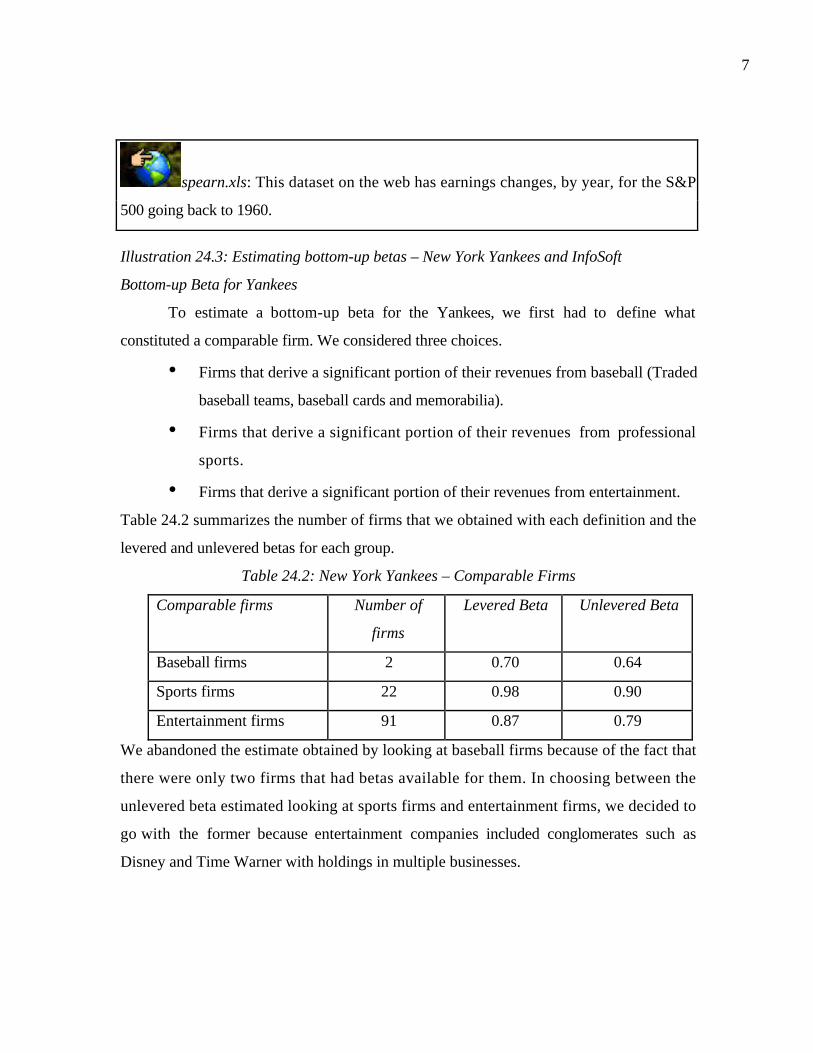
7

spearn.xls: This dataset on the web has earnings changes, by year, for the S&P

500 going back to 1960.

Illustration 24.3: Estimating bottom-up betas – New York Yankees and InfoSoft

Bottom-up Beta for Yankees

To estimate a bottom-up beta for the Yankees, we first had to define what

constituted a comparable firm. We considered three choices.

• Firms that derive a significant portion of their revenues from baseball (Traded

baseball teams, baseball cards and memorabilia).

• Firms that derive a significant portion of their revenues from professional

sports.

• Firms that derive a significant portion of their revenues from entertainment.

Table 24.2 summarizes the number of firms that we obtained with each definition and the

levered and unlevered betas for each group.

Table 24.2: New York Yankees – Comparable Firms

Comparable firms Number of

firms

Levered Beta Unlevered Beta

Baseball firms 2 0.70 0.64

Sports firms 22 0.98 0.90

Entertainment firms 91 0.87 0.79

We abandoned the estimate obtained by looking at baseball firms because of the fact that

there were only two firms that had betas available for them. In choosing between the

unlevered beta estimated looking at sports firms and entertainment firms, we decided to

go with the former because entertainment companies included conglomerates such as

Disney and Time Warner with holdings in multiple businesses.

8

With an unlevered beta estimate of 0.90 for the Yankees from Table 24.2, we used

a target debt to equity ratio1 of 25% and a private firm tax rate of 40% to arrive at a

levered beta estimate of 1.04.

Levered Beta for Yankees = 0.90 (1 + (1-0.4) (0.25)) = 1.04

Bottom-up Beta for InfoSoft

To estimate a beta for InfoSoft, we obtained the betas and market debt/equity

ratios for publicly traded software firms. Since there are 264 software firms in the sample,

with wide variations in market capitalization and growth prospects, we also look, in

Table 24.3, at sub-classes of these firms that might be more comparable to InfoSoft.

Table 24.3: Betas and Leverage of Publicly Traded Software Firms

Grouping Number of Firms Beta D/E Ratio Unlevered Beta

All Software Firms 264 1.15 3.70% 1.13

Small-cap Software Firms 125 1.29 7.09% 1.23

Entertainment Software Firms 31 1.50 7.56% 1.43

Note that the debt/equity ratios are market value debt/equity ratios. Note also that the

difference in the size of the firms should not affect the betas directly, but it might have an

indirect effect, since smaller firms tend to have higher operating leverage. We will use an

unlevered beta of 1.23 for InfoSoft, based upon the average beta of small cap software

firms.

To estimate a levered beta, we have assumed that InfoSoft is close to the industry

average for small-cap software firms (7.09%) in terms of financial leverage. We also use

the corporate marginal tax rate of 35%, since InfoSoft is being priced to go public, to

estimate a beta of 1.29 for InfoSoft.

Bottom-up Beta for InfoSoft = 1.23 (1 + (1-0.35) (0.0709)) = 1.29

Adjusting for Non-Diversification

Betas measure the risk added by an investment to a diversified portfolio.

Consequently, they are best suited for firms where the marginal investor is diversified.

With private firms, the owner is often the only investor and thus can be viewed as the

1 If you are valuing a private firm, the target debt ratio may be supplied to you by management. In this

9

marginal investor. Furthermore, in most private firms, the owner tends to have much of

his or her wealth invested in the private business and does not have an opportunity to

diversify. Consequently, it can be argued that betas will understate the exposure to

market risk in these firms.

At the limit, if the owner has all of his or her wealth invested in the private

business and is completely undiversified, that owner is exposed to all risk in the firm and

it is not just the market risk (which is what the beta measures). There is a fairly simple

adjustment that can allow us to bring in this non-diversifiable risk into the beta

computation. To arrive at this adjustment, assume that the standard deviation in the

private firm’s equity value (which measures total risk) is σj and that the standard

deviation in the market index is σm. If the correlation between the stock and the index is

defined to be ρjm, the market beta can be written as:

Market beta m

jjm=

To measure exposure to total risk (σj), we could divide the market beta by ρjm. This

would yield the following.

m

j

jm

BetaMarket =

This is a relative standard deviation measure, where the standard deviation of the private

firm’s equity value is scaled against the market index’s standard deviation to yield what

we will call a total beta.

Total Beta =Market Beta

jm

The total beta will be higher than the market beta and will depend upon the correlation

between the firm and the market – the lower the correlation, the higher the total beta.

You might wonder how a total beta can be estimated for a private firm, where the

absence of market prices seems to rule out the calculation of either a market beta or a

correlation coefficient. Note though, that we were able to estimate the market beta of the

sector by looking at publicly traded firms in the business. We can obtain the correlation

case, we assumed a target debt to equity ratio of 25%.

10

coefficient by looking at the same sample and use it to estimate a total beta for a private

firm.

The question of whether the total beta adjustment should be made cannot be

answered without examining why the valuation of the private firm is being done in the

first place. If the private firm is being valued for sale, whether and how much the market

beta should be adjusted will depend upon the potential buyer or buyers. If the valuation

is for an initial public offering, there should be no adjustment for non-diversification, since

the potential buyers are stock market investors. If the valuation is for sale to another

individual or private business, the extent of the adjustment will depend upon the degree to

which the buyer’s portfolio is diversified; the more diversified the buyer, the higher the

correlation with the market and the smaller the total beta adjustment.

Illustration 24.4: Adjusting bottom-up beta for non-diversification

Consider the estimate of market beta that we obtained for the New York Yankees

in the previous illustration. Using firms that derive the bulk of their revenues from sports

as our comparable firms, we obtained an unlevered beta of 0.90 for the Yankees. The

average correlation coefficient for these publicly traded firms with the markets is 0.50.

(The R squared is 25%.) The total unlevered beta for the Yankees can be estimated as

follows:

Total Unlevered Beta 1.800.5

0.90 ==

Using the Yankee’s tax rate of 40% and a debt to equity ratio of 25% yields a total

levered beta of 2.07.

Total Levered Beta = 1.80 (1 + (1-0.4)(0.25)) = 2.07

This total beta estimate, in a sense, takes the limiting view that the potential buyer will

own only the Yankees. To the extent that the buyer has some diversification, the

correlation coefficient will be adjusted upwards; if the buyer has a diversified portfolio,

the correlation coefficient will approach one and the total beta will converge on the market

beta.

11

An Alternative Adjustment for Private Firm Risk

There is an alternative approach that is sometimes used to estimate the additional

risk premium that should be charged a private firm. In this approach, you compare the

historical returns earned by venture capital and private equity funds with the historical

returns on publicly traded stocks. The difference between the two can be considered a

premium for private company risk. For instance, private equity funds reported an average

annual return of 24% from 1990 to 2000. In contrast, the average annual return on stocks

from 1990 to 2000 was 15%. The difference of 9% can be viewed as the premium for

private firm risk and it should be added on to the cost of equity estimated with a market

beta or betas.

There are three limitations with this approach. First, most venture capitalists and

private equity investors do not publicly report their annual returns and there is a selection

and survival bias among those who do; successful private equity funds are more likely to

reveal their returns. Second, the standard errors in the annual returns are likely to be very

large and this noise will affect the risk premium estimate as well. Third, all private firms

are treated equivalently in this approach and no attempt is made to assess larger

premiums for some firms and smaller premiums for others.

From Cost of Equity to Cost of Capital

To get from the cost of equity to the cost of capital, we need two additional

inputs – the cost of debt, which measures the rate at which firms can borrow, and the

debt ratio that determines the weights in the cost of capital computation. In this section,

we consider how best to estimate each of these inputs for a private firm.

Cost of Debt

The cost of debt represents the rate at which a firm can borrow money. To

estimate it for publicly traded firms, we generally use either the yields on bonds issued by

these firms or the ratings for these bonds to get default spreads. Private firms generally

are not rated and do not have bonds outstanding. Consequently, we have to use one of the

following alternative approaches.

12

• If the private firm has borrowed money recently (in the last few weeks or

months), we can use the interest rate on the borrowing as a cost of debt. Since the

cost of debt has to be current, the book interest rate2 on debt issued in the past is

generally not a good measure of the cost of debt.

• If the private firm is being valued for an initial public offering, we can assume that

the cost of debt for the private firm will move towards the average cost of debt for

the industry to which the firm belongs. We are essentially assuming that the

private firm, once public, will structure its debt policy to resemble those of

comparable firms.

• When estimating the cost of debt for publicly traded firms in Chapter 8, we used

the interest coverage ratios of these firms to estimate ‘synthetic ratings’ and then

used the default spreads on these ratings to arrive at the costs of debt. To allow

for the fact that private firms tend to be smaller and riskier than most publicly

traded firms, we would use the relationship between interest coverage ratios and

ratings for a sub-set of smaller, publicly traded firms, summarized in Table 24.4

below.

Table 24.4: Interest coverage Ratios and Bond Ratings

Interest Coverage Ratio Rating

> 12.5 AAA

9.50 - 12.50 AA

7.50 – 9.50 A+

6.00 – 7.50 A

4.50 – 6.00 A-

3.50 – 4.50 BBB

3.00 – 3.50 BB

2.50 – 3.00 B+

2.00 - 2.50 B

1.50 – 2.00 B-

2 Book interest rate = Interest expenses / Book value of debt

13

1.25 – 1.50 CCC

0.80 – 1.25 CC

0.50 – 0.80 C

< 0.65 D

To estimate the cost of debt for a private firm with an interest coverage ratio of

5.1, for instance, we would use a synthetic rating of A- and the default spread

associated with that rating. Thus, if A- rated firms typically pay 1.25% above the

riskless rate to borrow, we would add that default spread to the riskless rate to

estimate the cost of debt for the private firm.

This approach may underestimate the cost of debt if banks charge higher

interest rates for private firms than for otherwise similar publicly traded firms. In

that case, you would add an additional spread to reflect this difference, if you

were valuing the firm for sale in a private transaction, but not if you were valuing

it for sale to a publicly traded firm or an initial public offering.

Illustration 24.5: Estimating Cost of Debt

We will use different approaches to estimate the cost of debt for the Yankees and

Infosoft. For the Yankee’s, we will use the interest rate from the most recent loans that

the firm has taken.

Interest rate on debt = 7.00%

Using the Yankee’s tax rate of 40%, we obtain an after-tax cost of debt

After-tax cost of debt = 7% (1-0.4) = 4.2%

For InfoSoft, we will use the interest coverage ratio estimated using the operating income

and interest expenses from the most recent year. Infosoft had earnings before interest and

taxes of $2 million and had interest expenses of $265,000.

Interest coverage ratio = EBIT/ Interest expenses 7.55265

2000 ==

Using Table 24.4 above, we estimate a synthetic rating of A+ for InfoSoft

Rating based upon interest coverage ratio = A+

The default spread associated with A+ rated bonds in the market at the time of this

valuation was 0.80% and the treasury bond rate was 6%. Since we are valuing Infosoft for

14

an initial public offering, we assume that there is no additional private firm spread.

Interest rate on debt = 6% + 0.80% = 6.80%

Finally, we attach a corporate marginal tax rate of 35%, rather than Infosoft’s current tax

rate, because the initial public offering will change the firm’s tax status, to yield an after-

tax cost of debt.

After-tax cost of debt = 6.80% (1-.35) = 4.42%

Debt Ratios

The debt ratio represents the proportion of the market value of a firm that comes

from debt financing. For publicly traded firms, we use the market prices of publicly

traded stocks and bonds to arrive at this ratio. Since neither input will be available for

private firms, we have to consider one of the following options.

• In estimating levered betas, we suggested that the industry-average or target debt

ratios could be used in the computation. Consistency demands that we use the

same debt ratio for computing the cost of capital. Thus, if the industry-average

debt to equity ratio is used to estimate the levered beta, the industry-average debt

to capital ratio should be used to estimate the cost of capital. If the target debt to

equity ratio is used for the levered beta computation, the target debt to capital

ratio should be used in the cost of capital calculation.

• While market values of equity and debt are not available for private firms, we can

use our estimated values of equity and debt from the valuation, though this creates

circular reasoning in the analysis. You need the cost of capital (and the debt ratio)

to estimate firm and equity value and we need the equity value to estimate the

cost of capital. You could overcome this problem by iterating towards a value –

you could start with the book debt ratio and cost of capital, estimate a firm and

equity value, use these values to arrive at a new debt ratio and cost of capital, and

re-estimate firm and equity value. You would continue until the debt and equity

values in the cost of capital computation converge on the estimated values.3

Illustration 24.6: Estimating Cost of Capital

15

To estimate the cost of capital for the New York Yankees and InfoSoft, we will

stay consistent with the assumptions we have made about leverage so far in this chapter.

The Yankees, we assumed, would stay close to a management target debt to equity ratio

of 25%, which translates into a market debt to capital ratio of 20%. For InfoSoft, we used

the industry average debt to equity of 7.09%, which results in a debt to capital ratio of

6.62%.4

For the Yankees, given that we are valuing the firm for sale to a private entity, we

estimated a total beta of 2.07. Using the treasury bond rate of 6% prevalent at the time of

this valuation and a market risk premium of 4%, we estimate a cost of equity of 14.28%.

Cost of Equity = 6% + 2.07 (4%) = 14.28%

Using the cost of debt of 4.2% estimated in Illustration 24.5, we can estimate the cost of

capital.

Cost of capital = 14.28% (0.80) + 4.2% (0.20) = 12.26%

For InfoSoft, where we are pricing an initial public offering, we use the market

beta estimate of 1.29. Using the treasury bond rate of 6% and a risk premium of 4%

yields a cost of equity of 11.16%.

Cost of equity = 6% + 1.29 (4%) = 11.16%

With the after-tax cost of debt of 4.42% estimated in Illustration 24.5 and the industry

average debt ratio of 6.62%, we estimate a cost of capital of 10.71% for InfoSoft.

Cost of capital = 11.16% (0.9338) + 4.42% (0.0662) = 10.71%

Cash Flows

The definitions of the cashflows to equity and cash flows to the firm are identical

for both private and publicly traded firms. The cash flow to equity is the cash flow after

taxes, debt payments and issues and reinvestment needs. The cash flow to the firm is the

cash flow after taxes and reinvestment needs, but before debt payments. There are three

issues that do affect estimation of cash flows with private firms. The first is that many

private firms do not adequately consider the salaries for owner-managers, since many

3 The values will always converge.

16

owners do not distinguish between income that they receive as dividends and income that

they receive as salaries. The second is the intermingling of personal and business expenses

that often occurs at small private businesses that can cause income to be mismeasured.

The third is the effect of taxes on value, since individual tax status and tax rates vary

much more widely than corporate tax rates.

Owner Salaries and Equity Cash flows

In valuing firms, we draw a simple distinction between salaries and dividends.

Salaries are compensation for professional services rendered to the firm and should be

treated as operating expenses. Dividends or other equity cash withdrawals from the firm

are returns on equity capital invested and determine the value of equity. The separation

between managers and stockholders in publicly traded firms resulting in a distinction

between salaries (which are paid to managers) and dividends (which are paid to

stockholders) that is clear. In a private business, the owner is often the firm’s manager

and its only equity investor. If the private firm is not incorporated, the income earned by

the owner is taxed at the same rate, whether it is categorized as a salary or as a dividend.

Consequently, an owner will be indifferent between receiving a salary of $10,000 and a

dividend of $90,000 and a salary of $90,000 and a dividend of $10,000. As a consequence,

owners do not pay themselves a salary in many small private firms, or even if they do,

the salary does not reflect the services they render to the firm.

When valuing a private firm, we generally make forecasts based upon the

operating income reported by the firm. If that operating income does not reflect a salary

adjustment for the owner, it will be overstated and result in a value that is too high. To get

a more precise estimate of operating income, we have to estimate the appropriate

compensation for the owners/managers, based upon the role they play in the firm and the

cost of hiring replacements for them. Thus, the owner of a bookstore might play several

roles – cashier, accountant, stockperson and sales person, and the management salary

would have to include the cost of hiring a person or two to provide the same services.

4 Debt to capital RatioEquity Debt to1

RatioEquity Debt to

+=

17

Intermixing Business and Personal Expenses

The intermingling of business and personal expenses is a particular problem in

small private business, since owners often have absolute power over many aspects of the

business. Many private business owners maintain offices in their residences, have

vehicles that they maintain for personal and business use and share other services –

phone, internet – between work and home. In some cases, family members are hired to fill

phantom positions in order to distribute income or to reduce taxes.

If personal expenses are consolidated with business expenses or are otherwise a

part of business expenses, the operating income for a private firm has to be estimated

prior to these expenses. The problem with making these adjustments, however, is that

private firm owners are usually not forthcoming about the extent of these expenses and

there may be tax consequences.

Tax Effects

When valuing publicly traded firms, the tax rate that we use in valuation is defined

to be the marginal corporate tax rate. While different firms may face different marginal tax

rates, the differences in tax rates across potential buyers of a private firm can be much

larger. In fact, the tax rate can vary from the corporate tax rate (if the potential buyer is a

corporation) to the highest marginal tax rate for individuals (if the potential buyer is a

wealthy individual) to a lower marginal tax rate if the potential buyer is an individual with

lower income. The tax rate will affect both the cash flows (through the after-tax operating

income) and the cost of capital (though the cost of debt). As a consequence, the value of a

private firm can vary across different buyers.

Illustration 24.7: Estimating Operating Income

To estimate the cashflows for the Yankees, we reconstruct the operating income

statement based upon publicly available information5. We begin in Table 24.5, by

estimating the revenue of the Yankees and contrasting them with the revenues of two

other baseball teams.

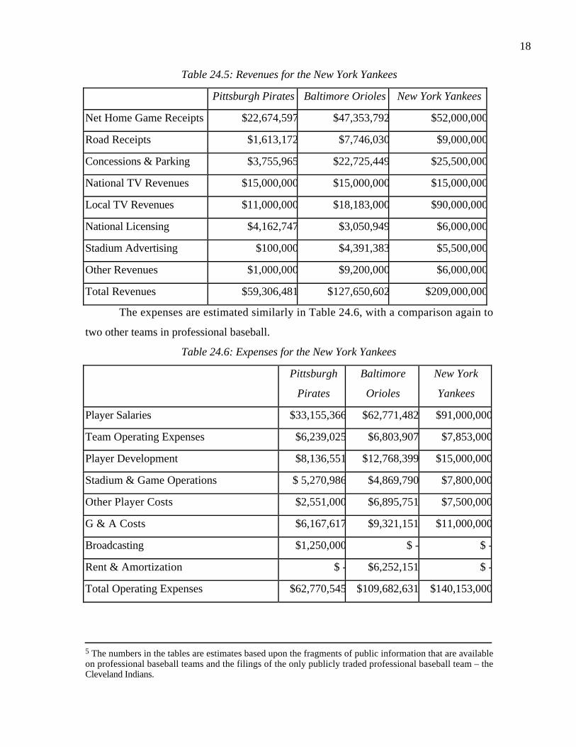
18

Table 24.5: Revenues for the New York Yankees

Pittsburgh Pirates Baltimore Orioles New York Yankees

Net Home Game Receipts $22,674,597 $47,353,792 $52,000,000

Road Receipts $1,613,172 $7,746,030 $9,000,000

Concessions & Parking $3,755,965 $22,725,449 $25,500,000

National TV Revenues $15,000,000 $15,000,000 $15,000,000

Local TV Revenues $11,000,000 $18,183,000 $90,000,000

National Licensing $4,162,747 $3,050,949 $6,000,000

Stadium Advertising $100,000 $4,391,383 $5,500,000

Other Revenues $1,000,000 $9,200,000 $6,000,000

Total Revenues $59,306,481 $127,650,602 $209,000,000

The expenses are estimated similarly in Table 24.6, with a comparison again to

two other teams in professional baseball.

Table 24.6: Expenses for the New York Yankees

Pittsburgh

Pirates

Baltimore

Orioles

New York

Yankees

Player Salaries $33,155,366 $62,771,482 $91,000,000

Team Operating Expenses $6,239,025 $6,803,907 $7,853,000

Player Development $8,136,551 $12,768,399 $15,000,000

Stadium & Game Operations $ 5,270,986 $4,869,790 $7,800,000

Other Player Costs $2,551,000 $6,895,751 $7,500,000

G & A Costs $6,167,617 $9,321,151 $11,000,000

Broadcasting $1,250,000 $ - $ -

Rent & Amortization $ - $6,252,151 $ -

Total Operating Expenses $62,770,545 $109,682,631 $140,153,000

5 The numbers in the tables are estimates based upon the fragments of public information that are availableon professional baseball teams and the filings of the only publicly traded professional baseball team – theCleveland Indians.

19

While deducting operating expenses from revenues would normally yield operating

income, the operating expenses for the Yankees include $4.5 million in expenses that we

are not considering to be part of operations.6 Table 24.7 summarizes these adjustments

for the Yankees.

Table 24.7: Adjusted Operating Income

Pittsburgh Pirates Baltimore Orioles New York Yankees

Total Revenues $59,306,481 $127,650,602 $209,000,000

Total Operating Expenses $62,770,545 $109,682,631 $140,153,000

EBIT ($3,464,064) $17,967,971 $68,847,000

Adjustments $1,500,000 $2,200,000 $4,500,000

Adjusted EBIT ($1,964,064) $20,167,971 $73,347,000

Taxes (at 40%) ($785,626) $8,067,189 $29,338,800

EBIT (1-tax rate) ($1,178,439) $12,100,783 $44,008,200

InfoSoft, though a private firm, has essentially been run like a public firm,

probably as a lead-in to the initial public offering. Table 24.8 reflects the operating income

for InfoSoft and corrects the operating income for the capitalization of R&D expenses;

this is a correction we employed for publicly traded high technology firms as well. Note

that the after-tax operating income is adjusted to reflect the additional tax benefit of

expensing R&D.7

Table 24.8: Adjusted Operating Income – InfoSoft (in ‘000s)

Sales & Other Operating Revenues $20,000.00

- Operating Costs & Expenses $13,000.00

- Depreciation $1,000.00

- Research and Development Expenses $4,000.00

6 Delicately put, these would include what we categorize as personal expenses that the owner/managercharges to the firm and could include employees who owe their employment status to their relationship tothe owner/manager.7 If you multiply the operating income of $3,633 by (1- tax rate), you would obtain a value of $2,362million. The higher value that we obtain of $2,933 million includes the additional tax benefit from theR&D expensing.Additional tax benefit = (4000 – 2367) * .35 = 571 million

20

Operating Income $2,000.00

Pre-tax After-tax

Operating Income $2,000.00 $1,300

+ R& D Expenses $4,000.00 $4,000

- Amortization of Research Asset $2,367.00 $2,367

Adjusted Operating Income $3,633.00 $2,933

Growth

The growth rate for a private firm can be estimated by looking at the past

(historical growth) or from fundamentals (the reinvestment rate and return on capital). In

this section, we will consider some of the issues in estimating private firm growth.

Estimating Growth

In estimating growth for publicly traded firms, we noted that we could draw on

three sources – historical growth, analyst estimates and fundamentals. With private firms,

we will not find analyst estimates of growth and historical growth numbers have to be

used with caution. The shifting accounting standards that characterize many private firms

will mean that reported earnings changes over time may not reflect actual earnings

changes. Furthermore, the fact that earnings are measured annually, rather than quarterly,

and the reality that private firms tend to be younger than publicly traded firms will mean

far less data in the historical growth estimate.

As a consequence of these gaps in past growth and analyst estimates, there is an

even greater reliance on fundamentals in private firms. The expected growth rate in

operating income is the product of the reinvestment rate and the return on capital, though

changes in return on capital in existing assets can create an additional impact.

Expected Growth Rate = Reinvestment Rate * Return on Capital

In making the estimates of reinvestment rates and returns on capital for private firms, we

can draw on the experience of publicly traded firms in the business.

Illustration 24.8: Estimating Growth

21

The process of estimating growth is different for the two firms under

consideration in this chapter. With the Yankees, we are looking at a valuable asset, but

one whose cashflows are unlikely to grow at rate higher than the inflation rate in

perpetuity. Consequently, we will assume a growth rate of 3% in nominal terms in

perpetuity. While this might seem unduly low for a team that has won the World Series

three of the last five years8, the current revenues and operating income reflect these

successes. Depressing though it might be to fans, the Yankees will not always be world

champions and there will be lean years ahead. The expected growth rate of 3% can be

considered a smoothed growth rate over good times and bad. To estimate how much they

will need to reinvest to generate this growth, we will assume a return on capital of 20%.9

This yields a reinvestment rate of

Reinvestment Rate 15%20%

3%

Capitalon Return

RateGrowth ===

To estimate the growth rate at InfoSoft, we follow a more conventional route. We

first estimate the return that they earn on their capital invested currently, by dividing the

after-tax operating income from the most recent year by the adjusted capital invested10 at

the beginning of the year. We use the adjusted operating income from Table 24.8 and used

the corporate marginal tax rate of 35%.

Return on Capital =After − tax Operating Income

BV of Capital

$2,933

$12,933= 23.67%

We then estimate InfoSoft’s reinvestment rate by dividing their reinvestments in capital

expenditures (including R&D)11 and working capital in the most recent year by the after-

tax operating income.

Reinvestment Rate = ($ 2,633+ 500)/ $2,933= 106.82%

8 This statement will clearly date this book. As a Yankees fan, I hope it remains true in future years.9 This is the weak link in this valuation. Since the book value of capital at the Yankees does not reallyreflect the true capital invested, it cannot be used to obtain the return on capital. We are assuming that themost valuable franchise in sports earns an excess return, partly due to brand name and partly due to location– it helps to be in the biggest media market in the nation.10 The capital invested reflects the value of the research asset.11 Reinvestment = Net Cap Ex + R& D expense – Amortization = $ 1,000 + $ 4,000 - $ 2,367 = $ 2,633

22

The expected growth rate in operating income for InfoSoft for the immediate future is

based upon the assumption that the return on capital and reinvestment rate will remain

unchanged over the next 5 years.

Expected Growth Rate = 23.67% * 1.0682 = 25.28%

If we had expected the return on capital or the reinvestment rate to change over time, we

would have reflected those changes in this growth rate.

The Persistence of Growth

In valuing publicly traded firms, we generally assumed infinite lives, even though

we did allow for the risk that the firm would not survive. With private firms, the

perpetual life assumption has to be made with far more caution. Unlike publicly traded

firms, where the transition from one CEO to another is common, the transition is much

more complicated in a private firm since the owner/manager generally does not want to

pass the reins of power to an outsider. Instead, the owner looks to the next generation in

his or her family for the successor, a process that is not always successful.

What are the implications for valuation? One is that the terminal value for a

private firm will be lower than the terminal value for a publicly traded firm. If we assume,

in fact, that the firm will cease operations at some point in time in the future – say when

the current owner retires – we would use a liquidation value for the assets as the terminal

value. In general, liquidation values are lower than the value of continuing operations. The

other is that private firms where owners plan for the transition to the next generation will

be worth more than private firms that do not make these arrangements.

Some private firms, especially as they get larger, resemble publicly traded firms in

terms of having professional managers. With these firms, the assumption of infinite

growth that we used with publicly traded firms can be sustained.

Illustration 24.9: Closure in Valuation and Terminal Values

Neither of the two firms is valued with finite lives. With InfoSoft, the reason is

simple. We are assuming a growing and healthy publicly traded firm, based upon our

projections over the next 10 years. The firm should be worth more based upon continuing

operations than from liquidation. Consequently, we assume an expected growth rate of

5% beyond year 10 for the firm. As the firm becomes larger, it will become more and

23

more difficult for it to sustain its current return on capital of 23.67%. We will assume that

the return on capital will drop to the industry average of 17.20%. These two assumptions

yield a reinvestment rate of 29.07% after year 10.

Reinvestment rate 29.07%17.2%

5%

Capitalon Return

RateGrowth Expected ===

While we do value the Yankees for sale in a private transaction, it remains a

valuable franchise and should not lack for potential buyers, even if the owner or owners

no longer are interested in running it. That is why we assumed a growth rate of 3% in

perpetuity.

Illiquidity Discounts

When you take an equity position in an entity, you generally would like to have

the option to liquidate that position if you need to. The need for liquidity arises not only

because of cash flow considerations but also because you might want to change your

portfolio holdings. With publicly traded firms, liquidation is simple and generally has a

low cost – the transactions costs for liquid stocks are a small percent of the value. With

equity in a private business, liquidation costs as a percent of firm value can be substantial.

Consequently, the value of equity in a private business may need to be discounted for

this potential illiquidity. In this section, we will consider the determinants of this

discount and how best to estimate it.

Determinants of Illiquidity Discount

The illiquidity discount is likely to vary across both firms and buyers, which

renders rules of thumb useless. Let us consider first some of the factors that may cause

the discount to vary across firms.

1. Liquidity of assets owned by the firm: The fact that a private firm is difficult to sell

may be rendered moot if its assets are liquid and can be sold with no significant loss in

value. A private firm with significant holdings of cash and marketable securities

should have a lower illiquidity discount than one with factories or other assets for

which there are relatively few buyers.

2. Financial Health and cashflows of the firm: A private firm that is financially

healthy should be easier to sell than one that is not healthy. In particular, a firm with

24

strong income and positive cash flows should be subject to a smaller illiquidity

discount than one with negative income and cash flows.

3. Possibility of going public in the future: The greater the likelihood that a private firm

can go public in the future, the lower should be the illiquidity discount attached to its

value. In effect, the probability of going public is built into the valuation of the private

firm. To illustrate, the owner of a private e-commerce firm in 1998 or 1999 would not

have had to apply much of a illiquidity discount to his firm’s value, if at all, because

of the ease with which these firms could be taken public in those years.

4. Size of the Firm: If we state the illiquidity discount as a percent of the value of the

firm, it should become smaller as the size of the firm increases. In other words, the

illiquidity discount should be smaller as a percent of firm value for firms like Cargill

and Koch Industries, which are worth billions of dollars, than it should be for a small

firm worth $15 million.

The illiquidity discount is also likely to vary across potential buyers because the

desire for liquidity varies among individuals. It is likely that those buyers who have deep

pockets and see little or no need to cash out their equity positions will attach much lower

illiquidity discounts to value, for similar firms, than buyers that have less of a safety

margin.

Empirical Evidence and Typical Practice

How large is the illiquidity discount attached to private firm valuations? This is a

very difficult question to answer empirically because the discount itself cannot be

observed. Even if we were able to obtain the terms of all private firm transactions, note

that what is reported is the price at which private firms are bought and sold. The value of

these firms is not reported and the illiquidity discount is the difference between the value

and the price.

In fact, much of the evidence on illiquidity discounts comes from examining

“restricted stock” at publicly traded firms. Restricted securities are securities issued by a

publicly traded company, but not registered with the SEC, that can be sold through

private placements to investors, but cannot be resold in the open market for a two-year

holding period, and limited amounts can be sold after that. When this stock is issued, the

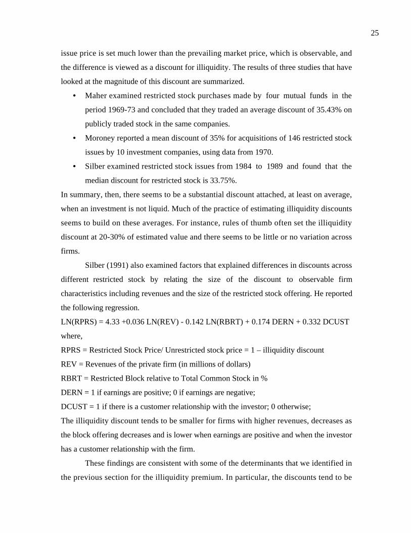
25

issue price is set much lower than the prevailing market price, which is observable, and

the difference is viewed as a discount for illiquidity. The results of three studies that have

looked at the magnitude of this discount are summarized.

• Maher examined restricted stock purchases made by four mutual funds in the

period 1969-73 and concluded that they traded an average discount of 35.43% on

publicly traded stock in the same companies.

• Moroney reported a mean discount of 35% for acquisitions of 146 restricted stock

issues by 10 investment companies, using data from 1970.

• Silber examined restricted stock issues from 1984 to 1989 and found that the

median discount for restricted stock is 33.75%.

In summary, then, there seems to be a substantial discount attached, at least on average,

when an investment is not liquid. Much of the practice of estimating illiquidity discounts

seems to build on these averages. For instance, rules of thumb often set the illiquidity

discount at 20-30% of estimated value and there seems to be little or no variation across

firms.

Silber (1991) also examined factors that explained differences in discounts across

different restricted stock by relating the size of the discount to observable firm

characteristics including revenues and the size of the restricted stock offering. He reported

the following regression.

LN(RPRS) = 4.33 +0.036 LN(REV) - 0.142 LN(RBRT) + 0.174 DERN + 0.332 DCUST

where,

RPRS = Restricted Stock Price/ Unrestricted stock price = 1 – illiquidity discount

REV = Revenues of the private firm (in millions of dollars)

RBRT = Restricted Block relative to Total Common Stock in %

DERN = 1 if earnings are positive; 0 if earnings are negative;

DCUST = 1 if there is a customer relationship with the investor; 0 otherwise;

The illiquidity discount tends to be smaller for firms with higher revenues, decreases as

the block offering decreases and is lower when earnings are positive and when the investor

has a customer relationship with the firm.

These findings are consistent with some of the determinants that we identified in

the previous section for the illiquidity premium. In particular, the discounts tend to be

26

smaller for large firms (at least as measured by revenues) and for healthy firms (with

positive earnings being the measure of financial health). This would suggest that the

conventional practice of using constant discounts across private firms is wrong and that

we should be adjusting for differences across firms.

Estimating the Illiquidity Discount

If we do decide to adjust the illiquidity discount to reflect the differences across

private firms, we are faced with an estimation question. How are we going to measure

these differences and build them into an estimate? There are two ways of doing this. The

first is to extend the analysis done for restricted securities into the illiquidity discount; in

other words, we could adjust the discount factor for the magnitude of a firm’s revenues

and whether it has positive earnings. The second is to apply some of the empirical work

that has been done examining the magnitude of the bid-ask spread for publicly traded

firms to estimating illiquidity discounts.

1. Adjusted Discount Factors

Consider again the regression that Silber presents on restricted stock. Not only

does it yield a result specific to restricted stock, but it provides a measure of how much

lower the discount should be as a function of revenues. A firm with revenue of $20

million should have an illiquidity discount which is 1.19% lower than a firm with

revenues of $10 million. Thus, we could establish a benchmark discount for a profitable

firm with specified revenues (say $100 million) and adjust this benchmark discount for

individual firms that have revenues much higher or lower than this number. The regression

can also be used to differentiate between profitable and unprofitable firms. Figure 24.1

presents the difference in illiquidity discounts across both profitable and unprofitable

firms with different revenues, using a benchmark discount of 25% for a firm with positive

earnings and $10 million revenues.

27

There are clearly dangers associated with extending a regression run on a small number of

restricted stocks to estimating discounts for private firms, but it does provide at least a

road map for adjusting discount factors.

2. Bid-Ask Spread Approach

The biggest limitation of using studies based upon restricted stock is that the

samples are small. We would be able to make far more precise estimates if we could

obtain a large sample of firms with illiquidity discounts. We would argue that such a

sample exists, if we consider the fact that an asset that is publicly traded is not

completely liquid. In fact, liquidity varies widely across publicly traded stock. A small

company listed over-the-counter is much less liquid that a company listed on the New

York Stock Exchange which in turn is much less liquid that a large capitalization company

that is widely held. In fact, the difference between the bid price and the ask price that we

observe on publicly traded assets can be viewed as a measure of the cost of instant

liquidity. An investor who buys an asset, changes her mind and decides to sell the asset

immediately will pay the bid-ask spread.

Figure 24.1: Illiquidity Discounts: Base Discount of 25% for profitable firm with $ 10 million in revenues

0.00%

5.00%

10.00%

15.00%

20.00%

25.00%

30.00%

35.00%

40.00%

5 10 15 20 25 30 35 40 45 50 100 200 300 400 500 1000

Revenues

Dis

coun

t as

% o

f V

alue

Profitable firm Unprofitable firm

28

While the bid-ask spread might only be a quarter or half a dollar, it looms as a

much larger cost when it is stated as a percent of the price per unit. For a stock that is

trading at $2, with a bid-ask spread of 1/4, this cost is 12.5%. For higher price and very

liquid stocks, the illiquidity discount may be less than 0.5% of the price, but it is not

zero.

What relevance does this have for illiquidity discounts on private companies?

Think of equity in a private company as a stock that never trades. On the continuum

described above, you would expect the bid-ask spread to be high for such a stock and this

would essentially measure the illiquidity discount.

To make estimates of the illiquidity discounts using the bid-ask spread as the

measure, you would need to relate the bid-ask spread of publicly traded stocks to

variables that can be measured for a private business. For instance, you could regress the

bid-ask spread against the revenues of the firm and a dummy variable, reflecting whether

the firm is profitable or not, and extend the regression done on restricted stocks to a much

larger sample. You could even consider the trading volume for publicly traded stocks as an

independent variable and set it to zero for a private firm. Using data from the end of 2000,

for instance, we regressed the bid-ask spread against annual revenues, a dummy variable

for positive earnings (DERN: 0 if negative and 1 if positive), cash as a percent of firm

value and trading volume.

Spread = 0.145 – 0.0022 ln (Annual Revenues) -0.015 (DERN) – 0.016 (Cash/Firm

Value) – 0.11 ($ Monthly trading volume/ Firm Value)

Plugging in the corresponding values – with a trading volume of zero – for a private firm

should yield an estimate of the bid-ask spread for the firm.

Illustration 24.10: Estimating the Illiquidity Discount for the New York Yankees

We can use both approaches described above to estimate the illiquidity discount

on the Yankees.

1. Restricted Stock Approach: To estimate the illiquidity discount for the Yankees, we

assume that the base discount for a firm with $10 million in revenues would be 25%. The

Yankee’s revenues of $209 million should result in a lower discount on their value. We

estimate the difference in the illiquidity discount between a firm with $10 million in

29

revenue and $209 million in revenue to be 19.10%. To do this, we first estimated the

illiquidity discount in the Silber equation for a firm with $10 million in revenues.

Expected illiquidity discount

( )48.94%

100

0.174(1)0)0.142ln(l0-.036ln(10)04.33exp-100 =++=

We then reestimated the illiquidity discount with revenues of $ 209 million:

Expected illiquidity discount

( )43.04%

100

0.174(1)0)0.142ln(l0-).036ln(20904.33exp-100 =++=

Difference in discount = 48.94% - 43.04% = 5.90%

The estimated illiquidity discount for the Yankees would therefore be 19.10%, which is

the base discount of 25% adjusted for the revenue difference.

2. Bid-Ask Spread Approach: We could substitute in the revenues of the Yankees ($209

million), the fact that it has positive earnings and the cash as a percent of revenues held

by the firm (3%):

Spread = 0.145 – 0.0022 ln (Annual Revenues) -0.015 (DERN) – 0.016 (Cash/Firm

Value) – 0.11 ($ Monthly trading volume/ Firm Value)

= Spread = 0.145 – 0.0022 ln (209) -0.015 (1) – 0.016 (.03) – 0.11 (0) = .1178 or 11.78%

Based on this approach, we would estimate an illiquidity discount of 11.78%.

Valuation Motives and Value Estimates

In the last section, we considered how best to estimate the inputs to use in valuing

a private firm. As we considered each input, though, we noted that the process of

estimation might be different depending upon the potential buyer of the firm. With betas,

for instance, we argued that the market beta should be used if the potential buyer is a

publicly traded firm or a stock market investor (in an initial public offering) and that a

total beta should be used if the potential buyer is a private party. We made similar

arguments about the cost of debt and cash flows. Table 24.9 summarizes the differences

in the way we estimate the inputs to valuation for different valuation motives.

Table 24.9: Estimation of Inputs for Valuation: Valuation Motives

Valuation for sale to a private Valuation for sale to a publicly

30

entity traded firm or for an initial

public offering

Cost of Equity Based upon total beta, with

correlation reflecting the

diversification of potential

buyer.

Based upon market beta, since

marginal investor is diversified.

Cost of Debt May reflect additional spread

associated with being a private

business.

Based upon synthetic rating,

estimated by looking at

publicly traded firms.

Operating Cash

Flows

Tax rate used should be that of

private business.

Corporate marginal tax rates

used in valuation.

Firm life Finite life terminal value or

liquidation value.

Perpetual life, when estimating

terminal value.

Illiquidity Discount Value discounted for illiquidity. No illiquidity discount

The results of using different approaches to estimating discount rates and cash

flows, depending upon the potential buyer, can have significant effects on value. In

general, a private business that is up for sale will be valued much more highly by a

publicly traded firm than by a private entity. This can be traced to the fact that the

discount rates are higher, when we assume that the buyer is not diversified. Thus, the

owners of private businesses who are interested in selling their businesses at the highest

price possible will be well served looking for potential buyers who are publicly traded

firms. While they might not be able to extract the entire value, they can try to obtain at

least a share of the additional value created because the marginal investors are diversified.

The same implications arise when looking at the alternative of going public. The

value that a firm can obtain from a public offering will exceed the value that it will receive

from a private entity. The values obtained from an initial public offering and sale to a

publicly traded firm will be based upon similar discount rates, but may vary because of

cost and revenue synergies. If the potential for these synergies is large, selling to a

publicly traded firm may result in a higher value than going public.

Illustration 24.11: Valuing the New York Yankees for a private sale

31

The inputs for valuing the Yankees as a business are in place. We have estimated

the cost of capital of 12.26% in Illustration 24.6, the adjusted after-tax operating income

of $44.008 million in Illustration 24.7, an expected growth rate of 3% and reinvestment

rate of 15% in Illustration 24.8. These estimates yield a value of $ 415 million for the

Yankees.

Value of the Yankees

=EBIT 1-t( ) 1-Reinvestment Rate( ) 1+ g( )

Cost of capital -g

=$44.008( ) 1−0.15( ) 1.03( )

0.1226 −0.03= $415 million

Since this a valuation for a private sale, we would apply the illiquidity discount of

11.78% estimated in Illustration 24.10.

Value of the Yankees with discount = $ 415 million (1-0.1178) = $ 366.1 million

This valuation is a conservative one and the actual value may well exceed this for

two reasons. The first is that publicly traded television and cable companies have

expressed interest in the Yankees. Following up, if we substitute in the market beta of

1.03 for the total beta of 2.07, we obtain a cost of capital of 8.95%. This results in a value

of $ 647 million, which no longer has to be discounted for illiquidity.

Value to diversified buyer = $ 44.008 million (1-.15)(1.03)/(.0895-.03) = $ 647 million

The second is the power that sports teams seem to have to extort subsidies and financial

assistance from the cities that they represent. For instance, if the Yankees can get New

York City to pick up the tab for the reinvestment needs (15% of the after-tax operating

income), the value of the Yankees would increase to $762 million.

Value with subsidies = $ 44.008 million (1.03)/(.0895-.03) = $ 762 million

Of course, the presence of synergies to the buyer may cause the value to increase even

further.

Illustration 24.12: Valuing InfoSoft

The inputs for valuing InfoSoft are summarized in Table 24.10. We assume that

InfoSoft will maintain a reinvestment rate of 112.17% and a return on capital of 23.67%

for the next five years, allowing its operating earnings to grow 25.28% a year. At the end

of 5 years, we assume that the firm will be in stable growth, growing 5% a year.

32

Table 24.10: Summary of Inputs – Valuation of InfoSoft

High Growth Phase Stable Growth Phase

Length 5 years Forever after year 5

Growth Inputs

- Reinvestment Rate

- Return on Capital

- Expected Growth rate

106.82%

23.67%

25.28%

29.07%

17.2%

5.00%

Cost of Capital Inputs

- Beta

- Cost of Debt

- Debt Ratio

- Cost of Capital

1.29

6.80%

6.62%

10.71%

1.20

6.80%

6.62%

10.38%

As noted in an earlier section, we use the corporate tax rate of 35% in this valuation

because InfoSoft is being valued for an initial public offering. In addition, we added the

cash and marketable securities, valued at $ 500,000, to the value of the operating assets of

the firm. The valuation is summarized in Figure 24.2. Based upon our assumptions, we

would value the equity in InfoSoft at $ 69.826 million.

33

Current Cashflow to FirmEBIT(1-t) : 2,933- Nt CpX 2,633- Chg WC 500= FCFF <200>Reinvestment Rate = 106.82%

Expected Growth in EBIT (1-t)1.1217*.2367 = .252825.28 %

Stable Growthg = 5%; Beta = 1.20; D/(D+E) = 6.62%;ROC=17.2%Reinvestment Rate=29.07%

Terminal Value 10= 6743/(.1038-.05) = 125,391

Cost of Equity11.16%

Cost of Debt(6+0.80%)(1-.35)= 4.42%

WeightsE = 93.38% D = 6.62%

Discount at Cost of Capital (WACC) = 13.2% (0.9338) + 4.42% (0.0662) = 10.71%

Firm Value: 73,909+ Cash: 500- Debt: 4,583=Equity 69,826

Riskfree Rate :Government Bond Rate = 6%

+Beta 1.29 X

Risk Premium4%

Unlevered Beta for Sectors: 1.24

Firm’s D/ERatio: 7.09%

Historical US Premium4%

Country RiskPremium0%

Figure 24.2: InfoSoft: A ValuationReinvestment Rate106.82%

Return on Capital23.67%

EBIT(1-t)- ReinvFCFF

36753926 -251

46044918 -314

57686161 -393

72277720 -493

9054 9671 -617

950727646743

34

Control Issues

When valuing a firm, you always need to consider the competence and strengths

of the management of the firm. With private firms, where the owner is also the manager,

this consideration carries special weight, since the owner has absolute control. In contrast,

in a publicly traded firm, incompetent management can often be replaced, if enough

stockholders can be convinced that it is in their best interests to do so.

There are implications for valuation, if a portion of a private firm is offered for

sale. If that portion provides a controlling interest, i.e, the right to pick the firm’s

management, it should have a substantially higher value than if it does not provide this

power. Normally, this would mean that 51% of a private firm’s equity should trade at a

substantial premium over 49%. This applies whether a firm is being sold to a private

entity or a publicly traded firm, and may arise in an initial public offering. If, for instance,

only non-voting shares or shares with diluted voting rights are offered to investors in the

public offering, they should trade at a discount on shares with full voting rights.

While the intuition about the value of control is simple, estimating how much it is

worth is a little more difficult. We will defer a full discussion of the topic until we get to

the chapter on acquisitions, but we will value it as the difference between two values –

the value of the firm run optimally and the value of the firm with the incumbent

management. For instance, if the value of a private firm run by incumbent management is

$100 million and the value of the firm run optimally is $150 million, the difference in

values between the 51% and 49% shares can be computed.

Value of controlling interest = 51% of Optimal Value = 0.51* 150 = $ 76.5 million

Value of non-controlling interest = 49% of Status Quo Value = 0.49 * 100 = $ 49 million

The additional 2% interest (from 49% to 51%) has a disproportionate effect on value

because of control. This value of control will be greatest for private firms that are poorly

run and will be close to zero for well run firms.

In fact, the same approach can be used to compute the discount that non-voting

shares will trade at, relative to voting shares in initial public offerings. For instance,

assume that the private firm described above creates 10 million voting shares and offers

70% to the public. Since the potential for changing management is created by this offering,

35

the value per share will fall between $10 and $15, depending upon the probability that is

attached to the management change. Thus, if the probability of the management change is

60%, the value per share will be $13.00.

Value/Shr ( )( )

00.13$10

6.0100150

10

100$Shares ofNumber

change ofy Probabilit*Value) Quo Status-(Optimal+

shares ofNumber

Value Quo Status

=

−+=

=

Now assume that this firm had issued 9 million non-voting shares, with management

retaining 1 million voting shares with complete control. In this case, the non-voting shares

will get little or none of the estimated value change from optimal management. In fact, the

values of the two classes can be estimated.

Value: non-voting share

shareper $1019

$100

shares voting-non shares+# voting#

Value Quo Status

=+

=

=

Value per voting share =

( )( )

00.40$1

6.0100150

19

100$

Shares Voting #

change ofy Probabilit*Value) Quo Status - (Optimal+

shares voting-non shares+# voting#

Value Quo Status

=

−++

=

The voting shares in this case would trade at an enormous premium over the non-voting

shares, but that is because we have assumed that the probability of change is still 60%. If

the incumbent managers are much more likely to fight a change in management, this

probability will drop and reduce the premium with it.

Illustration 24.13: Estimating a per-share value for InfoSoft

In the last illustration, we valued the equity in InfoSoft at $ 69.826 million.

Assume that the firm decides to create 5 million shares – 4 million shares will be non-

36

voting shares and 1 million will be voting shares. In the initial offering, only the non-

voting shares will be sold to the public and the current owners will retain all of the voting

shares.

To value the voting and non-voting shares, we need to value InfoSoft under

optimal management. Assume that the firm would be worth $ 75 million under optimal

management.12 The value of the voting and non-voting shares can then be computed.

Value: non-voting share

= Status Quo Value

# voting shares+# non-voting shares

=$69.826

4 +1= $13.97

Assume that the fact that incumbent managers will retain the voting shares reduces the

probability of management change to 25%.

Value per voting share =

Status Quo Value# voting shares+# non- voting shares

+(Optimal - Status Quo Value) *Probability of change

# Voting Shares

=$69.826

4 +1+

75 − 69.826( ) 0.25( )1

= $15.26

Pre-cash and post-cash valuations

When valuing private companies, many analysts draw a distinction between pre-

cash and post-cash valuations. In general, this is done especially when an infusion of cash

is anticipated either from venture capitalists or from an initial public offering. The pre-

cash valuation values the firm before the cash influx and the post-cash valuation values it

after.

There are two reasons why the two valuations may be different. The first is that

the firm may face capital rationing constraints without the infusion of the cash, resulting

37

in a scaling down of how much the firm can reinvest. If the firm’s return on capital is

greater than the cost of capital, this will cause the value to be lower before the cash influx.

The second is that the value of cash and marketable securities will be added on to the

value of the operating assets to arrive at firm value. After a large cash influx, firms may

have excess cash to invest in marketable securities, which when added to the value of

operating assets, will increase value. If the cash is taken out of the firm, though, by the

existing owners, you should not add the cash to the firm value.

Which of these two values should be used to estimate the value per share in a

public offering? Since stockholders in the firm will hold stock in the post-cash firm, the

post-cash value should be used. In the case of a venture capitalist, though, the answer

may be different. If the venture capitalist has bargaining power – she is the only person

who is interested in providing venture capital – she can ask for a share of the firm value

based upon the pre-cash valuation, arguing that the increase in value is feasible only with

the additional venture capital. If two or more venture capitalists are interested in the firm,

odds are that the post-cash valuations will be basis for deciding how much of the firm will

be yielded to the venture capitalist.

Valuing Private Equity

Earlier in this chapter, we considered how venture capitalists value firms. In the last

decade, private equity has emerged as competition to traditional venture capital. Private

equity can come from a variety of sources – wealthy individual investors, private equity

funds and corporations with excess funds to invest. Like venture capitalists, private equity

investors invest in private firms (often early in the life cycle) in return for a share in the

ownership in the firm.

In valuing a private equity stake, we confront many of the issues that we have raised

in the chapter:

• While private equity investors tend to be more diversified than venture capitalists, the

cost of equity used to value a private equity investment may still be higher than the

cost of equity used to value a publicly traded firm. The degree of non-diversification

can vary across investors. A publicly traded firm like Microsoft that makes private

equity investments should not use a higher cost of equity, whereas an investor who

12 InfoSoft was revalued at its optimal debt ratio. We assumed that the existing investment policy was

38

is not diversified may have to make an adjustment similar to the one described for

the owners of private firms.

• Private equity investors often provide cash to cash-starved firms in return for a

minority stake in the firms. Consequently, the issues of pre-cash versus post-cash

valuations and the value of control often come up with private equity valuations.

Illustration 24.14: Valuing a Private Equity Stake

Assume that you work for a publicly traded firm and have been asked to value a

potential stake in a small, privately held firm that wants you to invest $ 10 million in its

equity, which it plans to use to expand operations.

First, you would value the private firm assuming that you do not invest the $ 10

million. Based upon the projected cash flows, assume that you value the equity in the

firm at $ 30 million:

Pre-cash Valuation = $ 30 million

Now assume that your investment of $ 10 million will allow the firm to grow faster and that

the present value of the expected cash flows is $ 50 million for the equity. (This present

value does not include the cash inflow of $ 10 million from the private equity investment.)

Post-cash Valuation = $ 50 million + $ 10 million = $ 60 million

The key question, assuming that you decide to make this investment, is the percentage of the

private firm you should demand in return for the $ 10 million investment. At the minimum,

you would demand a share of the post-cash valuation

Share of ownershipMinimum = Cash Invested/ Post-cash Valuation = 10/60 = 16.66%

However, you would bargain for a larger share. At the limit, you could argue for a share of

the pre-cash valuation:

Share of ownershipMaximium = Cash Investment / (Pre-cash valuation + Cash Investment)

=10/(30 + 10) = 25%

Conclusion

The value of a private firm is the present value of the cash flows it is expected to

generate, discounted back at a rate that reflects both the risk in the private firm and the

mix of debt and equity it uses. While this statement is identical to the one we used to

describe the value of a publicly traded firm, there are differences in the way we estimate

optimal.

39

these inputs for private firms, and even among private firms, depending upon the motive

for the valuation.

When valuing a private firm for sale to an individual or private entity, we have to

consider three specific issues. The first is that the cost of equity, which we have hitherto

assumed to be determined purely by the risk that cannot be diversified, might have to be

adjusted for the fact that the potential buyer is not well diversified. The second is that

equity holdings in private businesses are illiquid, leading to a discount on the estimated

value. The discounts on restricted stock issues made by publicly traded firms or the bid-

ask spreads of these firms may provide us with useful information on how large this

discount should be. The third is that a controlling interest in equity of a private firm can

trade at a significant premium over a minority interest.

The valuation of a private firm for sale to a publicly traded firm or initial public

offering follows a much more conventional route. We can continue to assume that the cost

of equity should be based only upon non-diverisifiable risk and there is no need for an

illiquidity discount. There can still be a control value, if less than a controlling interest is

sold to the publicly trade firm or if non-voting shares are issued in the initial public

offering.

40

Problems

1. You have been asked to value Barrista Espresso, a chain of espresso coffee shops that

have opened on the east coast of the United States. You have collected the following

information.

• The company had earnings before interest and taxes of $10.50 million in the most

recent year. However, the founders of the company had never charged themselves a

salary, which would have amounted to $1 million, if based upon comparable

companies.

• The tax rate is 36%

• The capital expenditures in the most recent year amounted to $4.5 million, while

depreciation was only $1 million.

• Working capital is expected to remain at 10% of revenues.

• Earnings, revenues and net capital expenditures are expected to grow 30% a year for 5

years, and 6% after that forever.

• There are three comparable companies, which are publicly traded.

Beta D/E kd

Starbucks: 1.74 9.53% 9.00%

Au Bon Pain: 1.21 31.43% 8.50%

Sbarro: 1.12 0.00% NA

Barrista Espresso is expected to maintain a debt ratio of 12% and face a cost of debt of

8.75%.

a. Estimate the value of Barrista Espresso as a firm.

b. Estimate the value of equity in Barrista Espresso.

c. Would your valuation be any different if you were valuing the company for an

initial public offering rather than a private valuation.

2. What are some of the determinants of the size of the liquidity discount? Answer true or

false to the following statements.

a. There should be no liquidity discount attached to the value, if the valuation is

being done for an initial public offering.

41

b. The liquidity discount should be larger for a high-growth firm, with no current

cash flows, than for a stable firm with positive cash flows.

c. The liquidity discount will become smaller for firms, when they start losing

money.

d. The size of the liquidity discount will depend partly upon the buyer’s

characteristics.

3. You have valued a business, using discounted cash flow models, at $250 million, for a

private sale. The business, which does make money, had revenues of $200 million in the

most recent year. How much of a liquidity discount would you apply to this firm:

a. based upon the Silber regression.

b. based upon correcting the average discount (25%) for the size of the firm.

4. You are trying to value a bed-and-breakfast business in Vermont for its owner based

upon the following information.

• The business had pre-tax operating income of $100,000 in the most recent year. This

income has grown 5% a year for the last three years and is expected to continue

growing at that rate for the foreseeable future.

• About 40% of this operating income can be attributed to the fact that the owner is a

master chef. He does not plan to stay on if the business is sold.

• The business is financed equally with debt and equity. The pre-tax cost of borrowing

is 8.00%. The beta for publicly traded firms in the hospitality business is 1.10. The

treasury bond rate is 7.00%.

• The capital maintenance expenditure, net of depreciation, was $10,000 in the most

recent year and it is expected to grow at the same rate as operating income.

• The business is expected to have an operating life of 10 years, after which the building

will be sold at an anticipated price of $1.5 million, net of capital gains taxes.

a. Value the business, for sale.

b. How much would the value change if the owner offered to stay on for the next

three years?

1

1

CHAPTER 25

ACQUISITIONS AND TAKEOVERS

Firms are acquired for a number of reasons. In the 1960s and 1970s, firms such as

Gulf and Western and ITT built themselves into conglomerates by acquiring firms in other

lines of business. In the 1980s, corporate giants like Time, Beatrice and RJR Nabisco

were acquired by other firms, their own management or wealthy raiders, who saw

potential value in restructuring or breaking up these firms. In the 1990s, we saw a wave of

consolidation in the media business as telecommunications firms acquired entertainment

firms and entertainment firms acquired cable businesses. Through time, firms have also

acquired or merged with other firms to gain the benefits of synergy, in the form of either

higher growth, as in the Disney acquisition of Capital Cities, or lower costs.

Acquisitions seem to offer firms a short cut to their strategic objectives, but the

process has its costs. In this chapter, we examine the four basic steps in an acquisition,

starting with establishing an acquisition motive, continuing with the identification and

valuation of a target firm, and following up with structuring and paying for the deal. The

final and often the most difficult step is making the acquisition work after the deal is

consummated.

Background on Acquisitions

When we talk about acquisitions or takeovers, we are talking about a number of

different transactions. These transactions can range from one firm merging with another

firm to create a new firm to managers of a firm acquiring the firm from its stockholders

and creating a private firm. We begin this section by looking at the different forms taken

by acquisitions, continue the section by providing an overview on the acquisition process

and conclude by examining the history of the acquisitions in the United States.

Classifying Acquisitions

There are several ways in which a firm can be acquired by another firm. In a

merger, the boards of directors of two firms agree to combine and seek stockholder

approval for the combination. In most cases, at least 50% of the shareholders of the target

and the bidding firm have to agree to the merger. The target firm ceases to exist and

2

2

becomes part of the acquiring firm; Digital Computers was absorbed by Compaq after it

was acquired in 1997. In a consolidation, a new firm is created after the merger and both

the acquiring firm and target firm stockholders receive stock in the new firm; Citigroup,

for instance, was the firm created after the consolidation of Citicorp and Travelers’

Insurance Group.

In a tender offer, one firm offers to buy the outstanding stock of the other firm at

a specific price and communicates this offer in advertisements and mailings to

stockholders. By doing so, it bypasses the incumbent management and board of directors

of the target firm. Consequently, tender offers are used to carry out hostile takeovers. The

acquired firm will continue to exist as long as there are minority stockholders who refuse

the tender. From a practical standpoint, however, most tender offers eventually become

mergers, if the acquiring firm is successful in gaining control of the target firm.

In a purchase of assets, one firm acquires the assets of another, though a formal

vote by the shareholders of the firm being acquired is still needed.

There is a one final category of acquisitions that does not fit into any of the four

described above. Here, a firm is acquired by its own management or by a group of

investors, usually with a tender offer. After this transaction, the acquired firm can cease

to exist as a publicly traded firm and become a private business. These acquisitions are

called management buyouts, if managers are involved, and leveraged buyouts, if the

funds for the tender offer come predominantly from debt. This was the case, for instance,

with the leveraged buyouts of firms such as RJR Nabisco in the 1980s. Figure 25.1

summarizes the various transactions and the consequences for the target firm.

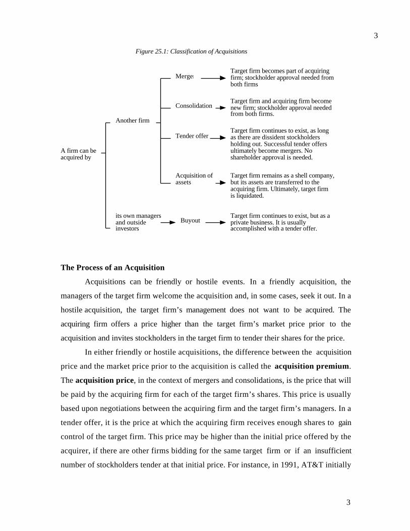
3

3

The Process of an Acquisition

Acquisitions can be friendly or hostile events. In a friendly acquisition, the

managers of the target firm welcome the acquisition and, in some cases, seek it out. In a

hostile acquisition, the target firm’s management does not want to be acquired. The

acquiring firm offers a price higher than the target firm’s market price prior to the

acquisition and invites stockholders in the target firm to tender their shares for the price.

In either friendly or hostile acquisitions, the difference between the acquisition

price and the market price prior to the acquisition is called the acquisition premium.

The acquisition price, in the context of mergers and consolidations, is the price that will

be paid by the acquiring firm for each of the target firm’s shares. This price is usually

based upon negotiations between the acquiring firm and the target firm’s managers. In a

tender offer, it is the price at which the acquiring firm receives enough shares to gain

control of the target firm. This price may be higher than the initial price offered by the

acquirer, if there are other firms bidding for the same target firm or if an insufficient

number of stockholders tender at that initial price. For instance, in 1991, AT&T initially

A firm can beacquired by

Another firm

its own managersand outside investors

Merger

Consolidation

Tender offer

Acquisition ofassets

Buyout

Target firm becomes part of acquiringfirm; stockholder approval needed fromboth firms

Target firm and acquiring firm becomenew firm; stockholder approval neededfrom both firms.

Target firm continues to exist, as longas there are dissident stockholdersholding out. Successful tender offersultimately become mergers. No shareholder approval is needed.

Target firm remains as a shell company,but its assets are transferred to the acquiring firm. Ultimately, target firmis liquidated.

Target firm continues to exist, but as aprivate business. It is usuallyaccomplished with a tender offer.

Figure 25.1: Classification of Acquisitions

4

4

offered to buy NCR for $80 per share, a premium of $ 25 over the stock price at the time

of the offer. AT&T ultimately paid $110 per share to complete the acquisition.

There is one final comparison that can be made and that is between the price paid

on the acquisition and the accounting book value of the equity in the firm being acquired.

Depending upon how the acquisition is accounted for, this difference will be recorded as

goodwill on the acquiring firm’s books or not be recorded at all. Figure 25.2 presents the

break down of the acquisition price into these component parts.

Empirical Evidence on the Value Effects Of Takeovers

Many researchers have studied the effects of takeovers on the value of both the

target and bidder firms. The evidence indicates that the stockholders of target firms are the

clear winners in takeovers –– they earn significant excess returns1 not only around the

announcement of the acquisitions, but also in the weeks leading up to it. Jensen and

Ruback (1983) reviewed 13 studies that look at returns around takeover announcements

1 Excess returns represent returns over and above the returns you would have expected an investment tomake after adjusting for risk and market performance.

Book Value of Equity ofTarget firm

Acquisition Price of target firm

Market Price of target firm priorto acquisition

Acquisition Premium

Book Value of Equity

Figure 25.2: Breaking down the Acquisition Price

Goodwill

5

5

and reported an average excess return of 30% to target stockholders in successful tender

offers and 20% to target stockholders in successful mergers. Jarrell, Brickley, and Netter

(1988) reviewed the results of 663 tender offers made between 1962 and 1985 and noted

that premiums averaged 19% in the 1960s, 35% in the 1970s and 30% between 1980 and

1985. Many of the studies report an increase in the stock price of the target firm prior to

the takeover announcement, suggesting either a very perceptive financial market or leaked

information about prospective deals.

Some attempts at takeovers fail, either because the bidding firm withdraws the

offer or because the target firm fights it off. Bradley, Desai, and Kim(1983) analyzed the

effects of takeover failures on target firm stockholders and found that, while the initial

reaction to the announcement of the failure is negative, albeit statistically insignificant, a

substantial number of target firms are taken over within 60 days of the first takeover

failing, earning significant excess returns (50% to 66%).

The effect of takeover announcements on bidder firm stock prices is not clear cut.

Jensen and Ruback report excess returns of 4% for bidding firm stockholders around

tender offers and no excess returns around mergers. Jarrell, Brickley and Netter, in their

examination of tender offers from 1962 to 1985, note a decline in excess returns to bidding

firm stockholders from 4.4% in the 1960s to 2% in the 1970s to -1% in the 1980s. Other

studies indicate that approximately half of all bidding firms earn negative excess returns

around the announcement of takeovers, suggesting that shareholders are skeptical about

the perceived value of the takeover in a significant number of cases.

When an attempt at a takeover fails, Bradley, Desai and Kim (1983) report

negative excess returns of 5% to bidding firm stockholders around the announcement of

the failure. When the existence of a rival bidder is figured in, the studies indicate

significant negative excess returns (of approximately 8%) for bidder firm stockholders

who lose out to a rival bidder within 180 trading days of the announcement, and no excess

returns when no rival bidder exists.

Steps in an Acquisition

There are four basic and not necessarily sequential steps, in acquiring a target firm.

The first is the development of a rationale and a strategy for doing acquisitions, and the

6

6

understanding of what the strategy requires in terms of resources. The second is the

choice of a target for the acquisition and the valuation of the target firm, with premiums

for the value of control and any synergy. The third is the determination of how much to

pay on the acquisition, how best to raise funds to do it, and whether to use stock or cash.

This decision has significant implications for the choice of accounting treatment for the

acquisition. The final step in the acquisition, and perhaps the most challenging one, is to

make the acquisition work after the deal is complete.

Developing an Acquisition Strategy

Not all firms that make acquisitions have acquisition strategies, and not all firms

that have acquisition strategies stick with them. In this section, we consider a number of

different motives for acquisitions and suggest that a coherent acquisition strategy has to

be based on one or another of these motives.

Acquire undervalued firms

Firms that are undervalued by financial markets can be targeted for acquisition by

those who recognize this mispricing. The acquirer can then gain the difference between the

value and the purchase price as surplus. For this strategy to work, however, three basic

components need to come together.

1. A capacity to find firms that trade at less than their true value: This capacity

would require either access to better information than is available to other

investors in the market, or better analytical tools than those used by other market

participants.

2. Access to the funds that will be needed to complete the acquisition: Knowing a firm

is undervalued does not necessarily imply having capital easily available to carry

out the acquisition. Access to capital depends upon the size of the acquirer – large

firms will have more access to capital markets and internal funds than smaller

firms or individuals – and upon the acquirer’s track record – a history of success

at identifying and acquiring under valued firms will make subsequent acquisitions

easier.

3. Skill in execution: If the acquirer, in the process of the acquisition, drives the stock

price up to and beyond the estimated value, there will be no value gain from the

7

7

acquisition. To illustrate, assume that the estimated value for a firm is $100

million and that the current market price is $75 million. In acquiring this firm, the

acquirer will have to pay a premium. If that premium exceeds 33% of the market

price, the price exceeds the estimated value, and the acquisition will not create any

value for the acquirer.

While the strategy of buying under valued firms has a great deal of intuitive appeal, it is

daunting, especially when acquiring publicly traded firms in reasonably efficient markets,

where the premiums paid on market prices can very quickly eliminate the valuation

surplus. The odds are better in less efficient markets or when acquiring private

businesses.

Diversify to reduce risk

We made a strong argument in Chapter 6 that diversification reduces an investor’s

exposure to firm-specific risk. In fact, the risk and return models that we have used in this

book have been built on the presumption that the firm-specific risk will be diversified

away and hence will not be rewarded. By buying firms in other businesses and

diversifying, acquiring firms’ managers believe, they can reduce earnings volatility and risk

and increase potential value.

Although diversification has benefits, it is an open question whether it can be

accomplished more efficiently by investors diversifying across traded stocks, or by firms

diversifying by acquiring other firms. If we compare the transactions costs associated

with investor diversification with the costs and the premiums paid by firms doing the

same, investors in most publicly traded firms can diversify far more cheaply than firms

can.

There are two exceptions to this view. The first is in the case of a private firm, where

the owner may have all or most of his or her wealth invested in the firm. Here, the

argument for diversification becomes stronger, since the owner alone is exposed to all risk.

This risk exposure may explain why many family-owned businesses in Asia, for instance,

diversified into multiple businesses and became conglomerates. The second, albeit weaker

case, is the closely held firm, whose incumbent managers may have the bulk of their

wealth invested in the firm. By diversifying through acquisitions, they reduce their

8

8

exposure to total risk, though other investors (who presumably are more diversified) may

not share their enthusiasm.

Create Operating or Financial Synergy

The third reason to explain the significant premiums paid in most acquisitions is

synergy. Synergy is the potential additional value from combining two firms. It is

probably the most widely used and misused rationale for mergers and acquisitions.

Sources of Operating Synergy

Operating synergies are those synergies that allow firms to increase their operating

income, increase growth or both. We would categorize operating synergies into four

types.

1. Economies of scale that may arise from the merger, allowing the combined firm to

become more cost-efficient and profitable.

2. Greater pricing power from reduced competition and higher market share, which

should result in higher margins and operating income.

3. Combination of different functional strengths, as would be the case when a firm with

strong marketing skills acquires a firm with a good product line.

4. Higher growth in new or existing markets, arising from the combination of the two

firms. This would be case when a US consumer products firm acquires an emerging

market firm, with an established distribution network and brand name recognition, and

uses these strengths to increase sales of its products.

Operating synergies can affect margins and growth, and through these the value of the

firms involved in the merger or acquisition.

Sources of Financial Synergy

With financial synergies, the payoff can take the form of either higher cash flows

or a lower cost of capital (discount rate). Included are the following.

• A combination of a firm with excess cash, or cash slack , (and limited project

opportunities) and a firm with high-return projects (and limited cash) can yield a

payoff in terms of higher value for the combined firm. The increase in value comes

from the projects that were taken with the excess cash that otherwise would not have

9

9

been taken. This synergy is likely to show up most often when large firms acquire

smaller firms, or when publicly traded firms acquire private businesses.

• Debt capacity can increase, because when two firms combine, their earnings and cash

flows may become more stable and predictable. This, in turn, allows them to borrow

more than they could have as individual entities, which creates a tax benefit for the

combined firm. This tax benefit can take the form of either higher cash flows or a

lower cost of capital for the combined firm.

• Tax benefits can arise either from the acquisition taking advantage of tax laws or from

the use of net operating losses to shelter income. Thus, a profitable firm that acquires

a money-losing firm may be able to use the net operating losses of the latter to reduce

its tax burden. Alternatively, a firm that is able to increase its depreciation charges

after an acquisition will save in taxes and increase its value.

Clearly, there is potential for synergy in many mergers. The more important issues are

whether that synergy can be valued and, if so, how to value it.

Empirical Evidence on Synergy

Synergy is a stated motive in many mergers and acquisitions. Bhide (1993)

examined the motives behind 77 acquisitions in 1985 and 1986 and reported that

operating synergy was the primary motive in one-third of these takeovers. A number of

studies examine whether synergy exists and, if it does, how much it is worth. If synergy

is perceived to exist in a takeover, the value of the combined firm should be greater than

the sum of the values of the bidding and target firms, operating independently.

V(AB) > V(A) + V(B)

where

V(AB) = Value of a firm created by combining A and B (Synergy)

V(A) = Value of firm A, operating independently

V(B) = Value of firm B, operating independently

Studies of stock returns around merger announcements generally conclude that the value

of the combined firm does increase in most takeovers and that the increase is significant.

Bradley, Desai, and Kim (1988) examined a sample of 236 inter-firms tender offers

between 1963 and 1984 and reported that the combined value of the target and bidder

10

10

firms increased 7.48% ($117 million in 1984 dollars), on average, on the announcement of

the merger. This result has to be interpreted with caution, however, since the increase in

the value of the combined firm after a merger is also consistent with a number of other

hypotheses explaining acquisitions, including under valuation and a change in corporate

control. It is thus a weak test of the synergy hypothesis.

The existence of synergy generally implies that the combined firm will become

more profitable or grow at a faster rate after the merger than will the firms operating

separately. A stronger test of synergy is to evaluate whether merged firms improve their

performance (profitability and growth) relative to their competitors, after takeovers. On

this test, as we show later in this chapter, many mergers fail.

Take over poorly managed firms and change management

Some firms are not managed optimally and others often believe they can run them

better than the current managers. Acquiring poorly managed firms and removing

incumbent management, or at least changing existing management policy or practices,

should make these firms more valuable, allowing the acquirer to claim the increase in

value. This value increase is often termed the value of control.

Prerequisites for Success

While this corporate control story can be used to justify large premiums over the

market price, the potential for its success rests on the following.

1. The poor performance of the firm being acquired should be attributable to the

incumbent management of the firm, rather than to market or industry factors

that are not under management control.

2. The acquisition has to be followed by a change in management practices, and

the change has to increase value. As noted in the last chapter, actions that

enhance value increase cash flows from existing assets, increase expected

growth rates, increase the length of the growth period, or reduce the cost of

capital.

3. The market price of the acquisition should reflect the status quo, i.e, the

current management of the firm and their poor business practices. If the

11

11

market price already has the control premium built into it, there is little

potential for the acquirer to earn the premium.

In the last two decades, corporate control has been increasingly cited as a reason for

hostile acquisitions.

Empirical Evidence on the Value of Control

The strongest support for the existence of a market for corporate control lies in

the types of firms that are typically acquired in hostile takeovers. Research indicates that

the typical target firm in a hostile takeover has the following characteristics.

(1) It has under performed other stocks in its industry and the overall market, in terms of

returns to its stockholders in the years preceding the takeover.

(2) It has been less profitable than firms in its industry in the years preceding the

takeover.

(3) It has a much lower stock holding by insiders than do firms in its peer groups.

In a comparison of target firms in hostile and friendly takeovers, Bhide illustrates

their differences. His findings are summarized in Figure 25.3.

Target Characteristics - Hostile vs. Friendly Takeovers

-5.00%

0.00%

5.00%

10.00%

15.00%

20.00%

Target ROE -Industry ROE

Target 5-yr stockreturns - Market

Returns% of Stock held

by insiders

Hostile Takeovers Friendly Takeovers

As you can see, target firms in hostile takeovers have earned a 2.2% lower return on

equity, on average, than other firms in their industry; they have earned returns for their

12

12

stockholders which are 4% lower than the market; and only 6.5% of their stock were held

by insiders.

There is also evidence that firms make significant changes in the way they operate

after hostile takeovers. In his study, Bhide examined the consequences of hostile

takeovers and noted the following changes.

1. Many of the hostile takeovers were followed by an increase in debt, which resulted in

a downgrading of the debt. The debt was quickly reduced with proceeds from the sale

of assets, however.

2. There was no significant change in the amount of capital investment in these firms.

3. Almost 60% of the takeovers were followed by significant divestitures, in which half

or more of the firm was divested. The overwhelming majority of the divestitures were

units in business areas unrelated to the company's core business (i.e., they constituted

reversal of corporate diversification done in earlier time periods).

4. There were significant management changes in 17 of the 19 hostile takeovers, with the

replacement of the entire corporate management team in seven of the takeovers.

Thus, contrary to popular view2, most hostile takeovers are not followed by the acquirer

stripping the assets of the target firm and leading it to ruin. Instead, target firms refocus

on their core businesses and often improve their operating performance.

Cater to Managerial Self Interest

In most acquisitions, it is the managers of the acquiring firm who decide whether to

carry out the acquisition and how much to pay for it, rather than the stockholders of the

firm. Given these circumstances, the motive for some acquisitions may not be stockholder

wealth maximization, but managerial self-interest, manifested in any of the following

motives for acquisitions.

• Empire building: Some top managers interests’ seem to lie in making their firms

the largest and most dominant firms in their industry or even in the entire market.

This objective, rather than diversification, may explain the acquisition strategies of

2 Even if it is not the popular view, it is the populist view that has found credence in Hollywood, inmovies such as Wall Street, Barbarians at the Gate and Other People’s Money.

13

13

firms like Gulf and Western and ITT3 in the 1960s and 1970s. Note that both

firms had strong-willed CEOs, Charles Bludhorn in the case of Gulf and Western,

and Harold Geneen, in the case of the ITT, during their acquisitive periods.

• Managerial Ego: It is clear that some acquisitions, especially when there are

multiple bidders for the same firm, become tests of machismo4 for the managers

involved. Neither side wants to lose the battle, even though winning might cost

their stockholders billions of dollars.

• Compensation and side-benefits: In some cases, mergers and acquisitions can result

in the rewriting of management compensation contracts. If the potential private

gains to the managers from the transaction are large, it might blind them to the

costs created for their own stockholders.

In a paper titled “The Hubris Hypothesis”, Roll (1981) suggests that we might be under

estimating how much of the acquisition process and the prices paid can be explained by

managerial pride and ego.

Should there be an ego discount?

If managerial self-interest and egos can cause firms to pay too much on

acquisitions, should the values of firms run by strong-willed CEOs be discounted? In a

sense, this discount is probably already applied if the firm’s current return on capital and

reinvestment rate reflect the failed acquisitions of the past, and we assume that the firm

will continue to generate the same return on capital in the future.

By the same token, though, this is a good reason to revisit a firm valuation when

there is a change at the top. If the new CEO does not seem to have the same desire to

empire build or overpay on acquisitions as the old one, the firm’s future return on capital

can be expected to be much higher than its past return on capital, and its value will rise.

3 In a delicious irony, ITT itself became the target of a hostile acquisition bid by Hilton Hotels andresponded by shedding what it termed its non-core businesses, i.e., all the businesses it had acquired duringits conglomerate period.4 An interesting question that is whether these bidding wars will become less likely as more women rise tobecome CEOs of firms. They might bring in a different perspective on what winning and losing in a mergermeans.

14

14

Choosing a Target firm and valuing control/synergy

Once a firm has an acquisition motive, there are two key questions that need to be

answered. The first relates to how to best identify a potential target firm for an

acquisition, given the motives described in the last section. The second is the more

concrete question of how to value a target firm, again given the different motives that we

have outlined in the last section.

Choosing a target firm

Once a firm has identified the reason for its acquisition program, it has to find the

appropriate target firm.

• If the motive for acquisitions is under valuation, the target firm must be under

valued. How such a firm will be identified depends upon the valuation approach

and model used. With relative valuation, an under valued stock is one that trades at

a multiple (of earnings, book value or sales) well below that of the rest of the

industry, after controlling for significant differences on fundamentals. Thus, a

bank with a price to book value ratio of 1.2 would be an undervalued bank, if other

banks have similar fundamentals (return on equity, growth, and risk) but trade at

much higher price to book value ratios. In discounted cash flow valuation

approaches, an under valued stock is one that trades at a price well below the

estimated discounted cash flow value.

• If the motive for acquisitions is diversification, the most likely target firms will be

in businesses that are unrelated to and uncorrelated with the business of the

acquiring firm. Thus, a cyclical firm should try to acquire counter-cyclical or, at

least, non-cyclical firms to get the fullest benefit from diversification.

• If the motive for acquisitions is operating synergy, the typical target firm will

vary depending upon the source of the synergy. For economies of scale, the target

firm should be in the same business as the acquiring firm. Thus, the acquisition of

Security Pacific by Bank of America was motivated by potential cost savings

from economies of scale. For functional synergy, the target firm should be

strongest in those functional areas where the acquiring firm is weak. For financial

synergy, the target firm will be chosen to reflect the likely source of the synergy –

15

15

a risky firm with limited or no stand-alone capacity for borrowing, if the motive is

increased debt capacity, or a firm with significant net operating losses carried

forward, if the motive is tax benefits.

• If the motive for the merger is control, the target firm will be a poorly managed

firm in an industry where there is potential for excess returns. In addition, its

stock holdings will be widely dispersed (making it easier to carry out the hostile

acquisition) and the current market price will be based on the presumption that

incumbent management will continue to run the firm.

• If the motive is managerial self-interest, the choice of a target firm will reflect

managerial interests rather than economic reasons.

In Table 25.1, we summarize the typical target firm, given the motive for the take over.

Table 25.1: Target Firm Characteristics given Acquisition Motive

If motive is then the target firm…

Undervaluation trades at a price below the estimated value.

Diversification is in a business different from the acquiring firm’s business.

Operating Synergy has the characteristics that create the operating synergy

Cost Savings: in same business to create economies of scale.

Higher growth: with potential to open up new markets or expand

existing ones.

Financial Synergy has the characteristics that create financial synergy

Tax Savings: provides a tax benefit to acquirer.

Debt Capacity: is unable to borrow money or pay high rates.

Cash slack: has great projects/no funds.

Control is a badly managed firm whose stock has under performed the

market.

Manager’s Interests has characteristics that best meet CEO’s ego and power needs.

There are two final points worth making here before we move on to valuation. The first is

that firms often choose a target firm and a motive for the acquisition simultaneously,

rather than sequentially. That does not change any of the analysis in these sections. The

other point is that firms often have more than one motive in an acquisitions, say, control

16

16

and synergy. If this is the case, the search for a target firm should be guided by the

dominant motive.

Valuing the Target Firm

The valuation of an acquisition is not fundamentally different from the valuation of

any firm, although the existence of control and synergy premiums introduces some

complexity into the valuation process. Given the inter-relationship between synergy and

control, the safest way to value a target firm is in steps, starting with a status quo

valuation of the firm, and following up with a value for control and a value for synergy.

a. Status Quo Valuation

We start our valuation of the target firm by estimating the firm value with existing

investing, financing and dividend policies. This valuation, which we term the status quo

valuation, provides a base from which we can estimate control and synergy premiums.

All of the basic principles presented in earlier chapters on valuation continue to apply

here. In particular, the value of the firm is a function of its cash flows from existing assets,

the expected growth in these cash flows during a high growth period, the length of the

high growth period and the firm’s cost of capital.

Illustration 25.1: A Status Quo Valuation of Digital

In 1997, Digital Equipment, a leading manufacturer of mainframe computers, was

the target of an acquisition bid by Compaq, which was at that time the leading personal

computer manufacturer in the world. The acquisition was partly motivated by the belief

that Digital was a poorly managed firm and that Compaq would be a much better manager

of Digital’s assets. In addition, Compaq expected synergies, in the form of both cost

savings (from economies of scale) and higher growth (from Compaq selling to Digital’s

customers).

To analyze the acquisition, we begin with a status quo valuation of Digital. At the

time of the acquisition, Digital had the following characteristics.

• Digital had earnings before interest and taxes of $391.38 million in 1997, which

translated into a pre-tax operating margin of 3% on revenues of $13,046 million and an

after-tax return on capital of 8.51%; the firm had a tax rate of 36%.

17

17

• Based upon its beta of 1.15, an after-tax cost of borrowing of 5% and a debt ratio of

approximately 10%, the cost of capital for Digital in 1997 was 11.59%. (The treasury

bond rate at the time of the analysis was 6%.)

1. Cost of Equity = 6% + 1.15 (5.5%) = 12.33%

2. Cost of Capital = 12.33% (0.9) + 5% (0.1) = 11.59%

• Digital had capital expenditures5 of $475 million, depreciation of $461 million, and

working capital is 15% of revenues.

4. Operating income, net capital expenditures and revenues were expected to grow 6% a

year for the next 5 years.

5. After year 5, operating income and revenues were expected to grow 5% a year forever.

After year 5, capital expenditures were expected to be 110% of depreciation with

depreciation growing at 5%. The debt ratio remained at 10%, but the after-tax cost of

debt dropped to 4% and the beta dropped to 1.

The value of Digital, based upon these inputs, was estimated to be $2,110.41 million.

Year EBIT (1-t) Net Cap Ex Chg in WC FCFF

Terminal

Value PV

1 $265.51 $14.84 $117.41 $133.26 $119.42

2 $281.44 $15.73 $124.46 $141.25 $113.43

3 $298.33 $16.67 $131.93 $149.73 $107.75

4 $316.23 $17.67 $139.84 $158.71 $102.35

5 $335.20 $18.74 $148.23 $168.24 $2,717.35 $1,667.47

Terminal Year $351.96 $64.78 $130.94 $156.25 $2,110.41

Note that the terminal value is computed using the free cash flow to the firm in year 6 and

the new cost of capital after year 5.

New cost of equity after year 5 = 6% + 1.00 (5.5%) = 11.5%

New cost of capital after year 5 = 11.50%(0.9) + 4% (0.1) = 10.75%

18

18

Terminal value $2,717.350.05-0.1075

$156.25 ==

b. The Value of Corporate Control

Many hostile takeovers are justified on the basis of the existence of a market for

corporate control. Investors and firms are willing to pay large premiums over the market

price to control the management of firms, especially those that they perceive to be poorly

run. This section explores the determinants of the value of corporate control and attempts

to value it in the context of an acquisition.

Determinants of the Value of Corporate Control

The value of wresting control of a firm from incumbent management is inversely

proportional to the perceived quality of that management and its capacity to maximize

firm value. In general, the value of control will be much greater for a poorly managed firm

that operates at below optimum capacity than for a well managed firm.

The value of controlling a firm comes from changes made to existing management

policy that can increase the firm value. Assets can be acquired or liquidated, the financing

mix can be changed and the dividend policy reevaluated, and the firm can be restructured

to maximize value. If we can identify the changes that we would make to the target firm,

we can value control. The value of control can then be written as:

Value of Control = Value of firm, optimally managed - Value of firm with current

management

The value of control is negligible for firms that are operating at or close to their optimal

value, since a restructuring will yield little additional value. It can be substantial for firms

operating at well below optimal, since a restructuring can lead to a significant increase in

value.

Illustration 25.2: The Value of Control at Digital

We said earlier that one of the reasons Digital was targeted by Compaq was that it

was viewed as poorly managed. Assuming that Compaq was correct in its perceptions,

we valued control at Digital by making the following assumptions.

5 The reinvestment rate is therefore artificially low when we look at net capital expenditures. This is

19

19

• Digital will raise its debt ratio to 20%. The beta will increase, but the cost of capital

will decrease.

New Beta = 1.25 (Unlevered Beta = 1.07; Debt/Equity Ratio = 25%)

Cost of Equity = 6% + 1.25 (5.5%) = 12.88%

New After-tax Cost of Debt = 5.25%; the firm is riskier, and its default risk will

increase

Cost of Capital = 12.88% (0.8) + 5.25% (0.2) = 11.35%

• Digital will raise its return on capital to 11.35%, which is its cost of capital. (Pre-tax

Operating margin will go up to 4%, which is close to the industry average)

• The reinvestment rate remains unchanged, but the increase in the return on capital will

increase the expected growth rate in the next 5 years to 10%.

• After year 5, the beta will drop to 1, and the after-tax cost of debt will decline to 4%,

as in the previous example.

The effect of these assumptions on the cash flows and present values is listed in the

following table.

Year EBIT (1-t) Net Cap Ex Chg in WC FCFF

Terminal

Value PV

1 $367.38 $15.40 $195.69 $156.29 $140.36

2 $404.11 $16.94 $215.26 $171.91 $138.65

3 $444.52 $18.63 $236.78 $189.11 $136.97

4 $488.98 $20.50 $260.46 $208.02 $135.31

5 $537.87 $22.55 $286.51 $228.82 $6,584.62 $3,980.29

Terminal Year $564.77 $77.96 $157.58 $329.23 $4,531.59The lower cost of capital and higher growth rate increase the firm value from the status

quo valuation of $2,110.41 million to $4,531.59 million. We can then estimate the value of

control.

Value of firm (optimally managed) = $4,531.59 million

because R&D expenses are not capitalized.

20

20

Value of firm (status quo) = $2,110.41 million

Value of control = $2,421.18 million

c. Valuing Operating Synergy

There is a potential for operating synergy, in one form or the other, in many

takeovers. Some disagreement exists, however, over whether synergy can be valued and, if

so, what that value should be. One school of thought argues that synergy is too nebulous

to be valued and that any systematic attempt to do so requires so many assumptions that

it is pointless. If this is true, a firm should not be willing to pay large premiums for

synergy if it cannot attach a value to it.

While valuing synergy requires us to make assumptions about future cash flows

and growth, the lack of precision in the process does not mean we cannot obtain an

unbiased estimate of value. Thus we maintain that synergy can be valued by answering

two fundamental questions.

(1) What form is the synergy expected to take? Will it reduce costs as a percentage of sales

and increase profit margins (e.g., when there are economies of scale)? Will it increase

future growth (e.g., when there is increased market power) or the length of the growth

period? Synergy, to have an effect on value, has to influence one of the four inputs into

the valuation process – cash flows from existing assets, higher expected growth rates

(market power, higher growth potential), a longer growth period (from increased

competitive advantages), or a lower cost of capital (higher debt capacity).

(2) When will the synergy start affecting cash flows? –– Synergies can show up

instantaneously, but they are more likely to show up over time. Since the value of

synergy is the present value of the cash flows created by it, the longer it takes for it to

show up, the lesser its value.

Once we answer these questions, we can estimate the value of synergy using an

extension of discounted cash flow techniques. First, we value the firms involved in the

merger independently, by discounting expected cash flows to each firm at the weighted

average cost of capital for that firm. Second, we estimate the value of the combined firm,

with no synergy, by adding the values obtained for each firm in the first step. Third, we

build in the effects of synergy into expected growth rates and cash flows and we value the

21

21

combined firm with synergy. The difference between the value of the combined firm with

synergy and the value of the combined firm without synergy provides a value for

synergy.

Figure 25.4 summarizes the effects of synergy and control in valuing a target firm

for an acquisition. Notice the difference between Figure 25.2, which is based upon the

market price of the target firm before and after the acquisition, and Figure 25.4, where we

are looking at the value of the target firm with and without the premiums for control and

synergy. A fair-value acquisition, which would leave the acquiring firm neither better nor

worse off, would require that the total price (in Figure 25.2) be equal to the consolidated

value (in Figure 25.4) with the synergy and control benefits built in.

22

22

Status QuoValuation

ControlPremium

Synergy

Value the company as is, with existing inputsfor investment, financing and dividend policy.

Value the company as if optimally managed. Thiswill usually mean altering investment, financing anddividend policy:Investment Policy: Earn higher returns on projects and

divest unproductive projects.Financing Policy: Move to a better financing

structure; eg. optimal capital structureDividend Policy: Return cash for which the firm has no need.Practically,1. Look at industry averages for optimal (if lazy)2. Do a full-fledged corporate financial analysis

Value the combined firm with synergy built in. This value may includea. a higher growth rate in revenues: growth synergyb. higher margins, because of economies of scalec. lower taxes, because of tax benefits: tax synergyd. lower cost of debt: financing synergye. higher debt ratio because of lower risk: debt capacitySubtract the value of the target firm (with control premium) + value of the bidding firm (pre-acquisition). This is the value of the synergy.

Component Valuation Guidelines Should you pay?

If motive is undervaluation, the status quo value is the maximum you should pay.

If motive is control or in a stand-alone valuation, this is themaximium you should pay.

Which firm is indispensable for synergy?- If it is the target, you should be willing to pay up to thevalue of synergy. - If it is the bidder, you should not.

Figure 25.4: Valuing an Acquisition

23

23

Illustration 25.4: Valuing Synergy: Compaq and Digital

Returning to the Compaq/Digital merger, note that synergy was one of the stated

reasons for the acquisition. To value this synergy, we needed to first value Compaq as a

stand-alone firm. To do this, we made the following assumptions.

• Compaq had earnings before interest and taxes of $2,987 million on revenues of

$25,484 million. The tax rate for the firm is 36%.

• The firm had capital expenditures of $ 729 million and depreciation of $545 million in

the most recent year; working capital is 15% of revenues.

• The firm had a debt to capital ratio of 10%, a beta of 1.25, and an after-tax cost of

debt of 5%.

• The operating income, revenues and net capital expenditures are all expected to grow

10% a year for the next 5 years.

• After year 5, operating income and revenues are expected to grow 5% a year forever,

and capital expenditures are expected to be 110% of depreciation. In addition, the firm

will raise its debt ratio to 20%, the after-tax cost of debt will drop to 4% and the beta

will drop to 1.00.

Based upon these inputs, the value of the firm can be estimated as follows.

Year EBIT (1-t) Net Cap Ex Chg in WC FCFF

Terminal

Value PV

1 $2,102.85 $202.40 $382.26 $1,518.19 $1,354.47

2 $2,313.13 $222.64 $420.49 $1,670.01 $1,329.24

3 $2,544.45 $244.90 $462.53 $1,837.01 $1,304.49

4 $2,798.89 $269.39 $508.79 $2,020.71 $1,280.19

5 $3,078.78 $296.33 $559.67 $2,222.78 $56,654.81 $33,278.53

Terminal Year $3,232.72 $92.16 $307.82 $2,832.74 $38,546.91

The value of Compaq is $38.547 billion.

24

24

The value of the combined firm (Compaq+Digital), with no synergy, should be the

sum of the values of the firms valued independently. To avoid double counting the value

of control, we add the value of Digital, optimally managed, that we estimated in

Illustration 25.2, to the value of Compaq to arrive at the value of the combined firm:

Value of Digital (optimally managed)= $4,531.59 million

Value of Compaq (status quo) = $38,546.91 million

Value of combined firm = $43,078.50 million

This would be the value of the combined firm in the absence of synergy.

To value the synergy, we made the following assumptions about the way in which

synergy would affect cash flows and discount rates at the combined firm.

• The combined firm will have some economies of scale, allowing it to increase its

current after-tax operating margin slightly. The annual dollar savings will be

approximately $100 million. This will translate into a slightly higher pre-tax operating

margin.

• Current Operating Margin 9.11%1304625484

5222987

SalesSales

EBITEBIT

DigitalCompaq

DigitalCompaq =++=

++

=

• New Operating Margin 9.36%1304625484

1005222987 =+

++=

• The combined firm will also have a slightly higher growth rate of 10.50% over the next

5 years, because of operating synergies.

• The beta of the combined firm was computed in three steps. We first estimated the

unlevered betas for Digital and Compaq.

Digital’s Unlevered Beta 1.07)0.36)(0.25-(11

1.25 =+

=

Compaq’s Unlevered Beta 1.17/0.90)0.36)(0.10-(11

.251 =+

=

25

25

We then weighted these unlevered betas by the values of these firms to estimate an

unlevered beta for the combined firm; Digital has a firm value6 of $4.5 billion and

Compaq’s firm value was $38.6 billion.

Unlevered Beta for combined firm ( ) ( ) 1.1643.1

38.61.17

43.1

4.51.07 =

+

=

We then used the debt to equity ratio for the combined firm to estimate a new levered

beta and cost of capital for the firm. The debt to equity ratio for the combined firm,

estimated by cumulating the outstanding debt and market value of equity at the two

firms is 13.64%.

3. New Levered Beta 1.2664))0.36)(0.13-(11.16(1 =+=

4. Cost of Capital = 12.93% (0.88) + 5% (0.12) = 11.98%

Based on these assumptions, the cash flows and value of the combined firm, with

synergy, can be estimated.

Year EBIT (1-t) Net Cap Ex Chg in WC FCFF

Terminal

Value PV

1 $2,552.28 $218.79 $606.85 $1,726.65 $1,541.95

2 $2,820.27 $241.76 $670.57 $1,907.95 $1,521.59

3 $3,116.40 $267.15 $740.98 $2,108.28 $1,501.50

4 $3,443.63 $295.20 $818.78 $2,329.65 $1,481.68

5 $3,805.21 $326.19 $904.75 $2,574.26 $66,907.52 $39,463.87

Terminal Year $3,995.47 $174.02 $476.07 $3,345.38 $45,510.58

The value of the combined firm, with synergy, is $45,510.58 million. This can be

compared to the value of the combined firm, without synergy, of $43,078.50 million, and

the difference is the value of the synergy in the merger.

Value of combined firm (with synergy) = $45,510.58 million

6 The values that we used were the values immediately before the acquisition announcement. This is toprevent the biases that may be created when target prices increase once an acquisition is announced.

26

26

Value of combined firm (with no synergy) = $43,078.50 million

Value of Synergy = $ 2,422.08 million

This valuation is based on the presumption that synergy will be created instantaneously.

In reality, it can take years before the firms are able to see the benefits of synergy. A

simple way to account for the delay is to consider the present value of synergy. Thus, if

it will take Compaq and Digital three years to create the synergy, the present value of

synergy can be estimated, using the combined firm’s cost of capital as the discount rate.

Present Value of Synergy million $1724.861.1198

million $2,4223

==

synergy.xls: This spreadsheet allows you to estimate the approximate value of

synergy in a merger or acquisition.

d. Valuing Financial Synergy

Synergy can also be created from purely financial factors. We will consider three

legitimate sources of financial synergy - a greater “tax benefit” from accumulated losses or

tax deductions, an increase in debt capacity and therefore firm value and better use for

“excess” cash or cash slack. We will begin the discussion, however, with diversification,

which though a widely used rationale for mergers, is not a source of increased value by

itself.

Diversification

A takeover motivated only by diversification considerations has no effect on the

combined value of the two firms involved in the takeover, when the two firms are both

publicly traded and when the investors in the firms can diversify on their own. Consider

the following example. Dalton Motors, which is in an automobile parts manufacturing

firm in a cyclical business, plans to acquire Lube & Auto, which is an automobile service

firm whose business is non-cyclical and high growth, solely for the diversification benefit.

The characteristics of the two firms are as follows:

Lube & Auto Dalton Motors

Current Free cash flow to the firm $100 million $200 million

Expected growth rate -next 5 years 20% 10%

27

27

Expected growth rate – after year 5 6% 6%

Debt /(Debt + Equity) 30% 30%

After-tax cost of debt 6% 5.40%

Beta for equity - next 5 years 1.20 1.00

Beta for equity - after year 5 1.00 1.00

The treasury bond rate is 7% and the market premium is 5.5%. The calculations for the

weighted average cost of capital and the value of the firms are shown in Table 25.2.

Table 25.2: Value of Lube & Auto, Dalton Motors and Combined Firm

Lube & Auto Dalton Motor Lube & Auto +

Dalton Motor

Combined

Firm

Debt (%) 30% 30% 30%

Cost of debt 6.00% 5.40% 5.65%

Equity (%) 70% 70% 70%

Cost of equity 13.60% 12.50% 12.95%

Cost of capital - Yr 1 11.32% 10.37% 10.76%

Cost of capital- Yr 2 11.32% 10.37% 10.76%

Cost of capital- Yr 3 11.32% 10.37% 10.77%

Cost of capital- Yr 4 11.32% 10.37% 10.77%

Cost of capital- Yr 5 11.32% 10.37% 10.77%

Cost of capital after 10.55% 10.37% 10.45%

FCFF in year 1 $120.00 $220.00 $340.00

FCFF in year 2 $144.00 $242.00 $386.00

FCFF in year 3 $172.80 $266.20 $439.00

FCFF in year 4 $207.36 $292.82 $500.18

FCFF in year 5 $248.83 $322.10 $570.93

Terminal Value $5,796.97 $7,813.00 $13,609.97

Present Value $4,020.91 $5,760.47 $9,781.38 $9,781.38

The cost of equity and debt for the combined firm is obtained by taking the

weighted average of the individual firm's costs of equity (debt); the weights are based

28

28

upon the relative market values of equity (debt) of the two firms. Since these relative

market values change over time, the costs of equity and debt for the combined firm also

change over time. The value of the combined firm is exactly the same as the sum of the

values of the independent firms, indicating that there is no value gain from diversification.

This equality does not imply, however, that the shareholders in the bidding and

target firms are indifferent about such takeovers, since the bidding firm pays a significant

premium over the market price. To the extent that these firms were correctly valued

before the merger (Market Value of Lube & Auto = $4,020.91, Market Value of Dalton

Motors = $5,760.47), the payment of a premium over the market price will transfer

wealth from the bidding firm to the target firm.

The absence of added value from this merger may seem puzzling, given the fact

that the two firms are in unrelated businesses and thus should gain some diversification

benefit. In fact, if the earnings of the two firms are not highly correlated, the variance in

earnings of the combined firm should be significantly lower than the variance in earnings

of the individual firms operating independently. This reduction in earnings variance does

not affect value, however, because it is firm-specific risk, which is assumed to have no

effect on expected returns. (The betas, which are measures of market risk, are always

value-weighted averages of the betas of the two merging firms.) But what about the

impact of reduced variance on debt capacity? Firms with lower variability in earnings can

increase debt capacity and thus value. This can be a real benefit of conglomerate mergers,

and we consider it separately later in this section.

Cash Slack

Managers may reject profitable investment opportunities if they have to raise new

capital to finance them. Myers and Majluf (1984) suggest that since managers have more

information than investors about prospective projects, new stock may have to be issued

at less than true value to finance these projects, leading to the rejection of good projects

and to capital rationing for some firms. It may therefore make sense for a company with

excess cash and no investment opportunities to take over a cash-poor firm with good

investment opportunities, or vice versa. The additional value of combining these two

29

29

firms is the present value of the projects that would not have been taken if they had

stayed apart, but can now be taken because of the availability of cash.

Cash slack can be a potent rationale for publicly traded firms that have more

access to capital and want to acquire small, private firms that have capital constraints. It

may also explain why acquisition strategies concentrating on buying smaller, private firms

have worked fairly well in practice. Blockbuster video (video rental), Browning and Ferris

(waste disposal) and Service Merchandise (funeral homes) are good examples.

Tax Benefits

Several possible tax benefits accrue from takeovers. If one of the firms has tax

deductions that it cannot use because it is losing money, whereas the other firm has income

on which it pays significant taxes, combining the two firms can result in tax benefits that can

be shared by the two firms. The value of this synergy is the present value of the tax savings

that result from this merger. In addition, the assets of the firm being taken over can be

written up to reflect new market values in some forms of mergers, leading to higher tax

savings from depreciation in future years.

Illustration 25.5: Tax Benefits of writing up Asset Values after Takeover: Congoleum Inc.

One of the earliest leveraged buyouts (LBOs) occurred in 1979 and involved

Congoleum Inc., a diversified firm in ship building flooring, and automotive accessories.

Congoleum’s own management bought out the firm. The favorable treatment that would

be accorded the firm’s assets by tax authorities was a major reason behind the takeover.

After the takeover –– estimated to cost approximately $400 million –– the firm was

allowed to write up its assets to reflect their new market values and to claim depreciation

on these new values. The estimated change in depreciation and the present value effect of

this depreciation based on a tax rate of 48%, discounted at the firm's cost of capital of

14.5%, are shown in Table 25.3.

Table 25.3: Depreciation Tax Benefits: Before and After Leveraged Buyout

Year Depreciation Depreciation Change in Tax Savings Present Value

before after Depreciation

1980 $8.00 $35.51 $27.51 $13.20 $11.53

1981 $8.80 $36.26 $27.46 $13.18 $10.05

30

30

1982 $9.68 $37.07 $27.39 $13.15 $8.76

1983 $10.65 $37.95 $27.30 $13.10 $7.62

1984 $11.71 $21.23 $9.52 $4.57 $2.32

1985 $12.65 $17.50 $4.85 $2.33 $1.03

1986 $13.66 $16.00 $2.34 $1.12 $0.43

1987 $14.75 $14.75 $0.00 $0.00 $0.00

1988 $15.94 $15.94 $0.00 $0.00 $0.00

1989 $17.21 $17.21 $0.00 $0.00 $0.00

1980-89 $123.05 $249.42 $126.37 $60.66 $41.76

Note that the increase in depreciation occurs in the first seven years, primarily as a

consequence of higher asset values and accelerated depreciation. After year seven,

however, the old and new depreciation schedules converge. The present value of the

additional tax benefits from the higher depreciation amounted to $41.76 million, about

10% of the overall price paid on the transaction.

In recent years, the tax code covering asset revaluations has been significantly

tightened. While acquiring firms can still reassess the value of the acquired firm’s assets,

they can do so only up to fair value.

Debt Capacity

If the cash flows of the acquiring and target firms are less than perfectly

correlated, the cash flows of the combined firm will be less variable than the cash flows of

the individual firms. This decrease in variability can result in an increase in debt capacity

and in the value of the firm. The increase in value, however, has to be weighed against the

immediate transfer of wealth to existing bondholders in both firms from the stockholders

of both the acquiring and target firms. The bondholders in the pre-merger firms find

themselves lending to a safer firm after the takeover. The coupon rates they are receiving

are based upon the riskier pre-merger firms, however. If the coupon rates are not

renegotiated, the bonds will increase in price, increasing the bondholders’ wealth at the

expense of the stockholders.

There are several models available for analyzing the benefits of higher debt ratios

as a consequence of takeovers. Lewellen analyzes the benefits in terms of reduced default

31

31

risk, since the combined firm has less variable cash flows than do the individual firms. He

provides a rationale for an increase in the value of debt after the merger, but at the expense

of equity investors. It is not clear, therefore, that the value of the firm will increase after

the merger. Stapleton evaluates the benefits of higher debt capacity after mergers using

option pricing. He shows that the effect of a merger on debt capacity is always positive,

even when the earnings of the two firms are perfectly correlated. The debt capacity

benefits increase as the earnings of the two firms become less correlated and as investors

become more risk averse.

Consider again the merger of Lube & Auto and Dalton Motor. The value of the

combined firm was the same as the sum of the values of the independent firms. The fact

that the two firms were in different business lines reduced the variance in earnings, but

value was not affected, because the capital structure of the firm remain unchanged after

the merger, and the costs of equity and debt were the weighted averages of the individual

firms' costs.

The reduction in variance in earnings can increase debt capacity, which can

increase value. If, after the merger of these two firms, the debt capacity for the combined

firm were increased to 40% from 30% (leading to an increase in the beta to 1.21 and no

change in the cost of debt), the value of the combined firm after the takeover can be

estimated as shown in Table 25.4.

Table 25.4: Value of Debt Capacity – Lube & Auto and Dalton Motors

Firm A Firm B AB -No new debt AB - Added Debt

Debt (%) 30% 30% 30% 40%

Cost of debt 6.00% 5.40% 5.65% 5.65%

Equity(%) 70% 70% 70% 60%

Cost of equity 13.60% 12.50% 12.95% 13.65%

Cost of Capital- Yr 1 11.32% 10.37% 10.76% 10.45%

Cost of Capital- Yr 2 11.32% 10.37% 10.76% 10.45%

Cost of Capital- Yr 3 11.32% 10.37% 10.77% 10.45%

Cost of Capital- Yr 4 11.32% 10.37% 10.77% 10.45%

Cost of Capital- Yr 5 11.32% 10.37% 10.77% 10.45%

32

32

Cost of Capital after 10.55% 10.37% 10.45% 9.76%

FCFF in year 1 $120.00 $220.00 $340.00 $340.00

FCFF in year 2 $144.00 $242.00 $386.00 $386.00

FCFF in year 3 $172.80 $266.20 $439.00 $439.00

FCFF in year 4 $207.36 $292.82 $500.18 $500.18

FCFF in year 5 $248.83 $322.10 $570.93 $570.93

Terminal Value $5,796.97 $7,813.00 $13,609.97 $16,101.22

Present Value $4,020.91 $5,760.47 $9,781.38 $11,429.35

As a consequence of the added debt, the value of the firm will increase from $9,781.38

million to $11,429.35 million.

Increase Growth and Price-Earnings Multiples

Some acquisitions are motivated by the desire to increase growth and price-cash

flow (or price-earnings) multiples. Though the benefits of higher growth are undeniable,

the price paid for that growth will determine whether such acquisitions make sense. If the

price paid for the growth exceeds the fair market value, the stock price of the acquiring

firm will decline even though the expected future growth in its cash flows may increase as

a consequence of the takeover.

This can be seen in the previous example. Dalton Motor, with projected growth in

cash flows of 10%, acquires Lube & Auto, which is expected to grow 20%. The fair

market value for Lube & Auto is $4,020.91. If Dalton Motor pays more than this amount

to acquire Lube & Auto, its stock price will decline, even though the combined firm will

grow at a faster rate than Dalton Motor alone. Similarly, Dalton Motor, which sells at a

lower multiple of cash flow than Lube & Auto, will increase its value as a multiple of cash

flow after the acquisition, but the effect on the stockholders in the firm will still be

determined by whether or not the price paid on the acquisition exceeds the fair value.

How often does synergy actually show up?

McKinsey and Co. examined 58 acquisition programs between 1972 and 1983 for

evidence on two questions: (1) Did the return on the amount invested in the acquisitions

33

33

exceed the cost of capital? (2) Did the acquisitions help the parent companies outperform

the competition? They concluded that 28 of the 58 programs failed both tests, and six

failed at least one test. In a follow-up study7 of 115 mergers in the U.K. and the U.S. in

the 1990s, McKinsey concluded that 60% of the transactions earned returns on capital

less than the cost of capital and that only 23% earned excess returns. In 1999, KPMG

examined 700 of the most expensive deals between 1996 and 1998 and concluded that

only 17% created value for the combined firm, 30% were value neutral and 53%

destroyed value8.

A study9 looked at the eight largest bank mergers in 1995 and concluded that only

two (Chase/Chemical, First Chicago/NBD) subsequently outperformed the bank-stock

index. The largest, Wells Fargo’s acquisition of First Interstate, was a significant failure.

Sirower (1996) takes a detailed look at the promises and failures of synergy and draws the

gloomy conclusion that synergy is often promised but seldom delivered.

The most damaging piece of evidence on the outcome of acquisitions is the large

number of acquisitions that are reversed within fairly short time periods. Mitchell and

Lehn note that 20.2% of the acquisitions made between 1982 and 1986 were divested by

1988. Studies that have tracked acquisitions for longer time periods (ten years or more)

have found the divestiture rate of acquisitions rises to almost 50%, suggesting that few

firms enjoy the promised benefits from acquisitions. In another study, Kaplan and

Weisbach (1992) found that 44% of the mergers they studied were reversed, largely

because the acquirer paid too much or because the operations of the two firms did not

mesh.

Takeover Valuation: Biases and Common Errors

The process of takeover valuation has potential pitfalls and biases that arise from

the desire of the management of both the bidder and target firms to justify their points of

7 This study was referenced in an article titled “Merger Mayhem” that appeared in Barrons on April 20,1998.8 KPMG measured the success at creating value by comparing the post-deal stock price performance of thecombined firm to the performance of the relevant industry segment for a year after the deal was completed.9 This study was done by Keefe, Bruyette and Woods, an investment bank. It was referenced in an articletitled "Merger Mayhem" in Barrons, April 20, 1998.

34

34

view to their stockholders. The bidder firm aims to convince its stockholders that it is

getting a bargain (i.e., that it is paying less than what the target firm is truly worth). In

friendly takeovers, the target firm attempts to show its stockholders that the price it is

receiving is a fair price (i.e., it is receiving at least what it is worth). In hostile takeovers,

there is a role reversal, with bidding firms trying to convince target firm stockholders that

they are not being cheated out of their fair share and target firms arguing otherwise. Along

the way, there are a number of common errors and biases in takeover valuation.

Use of Comparable Firms and Multiples

The prices paid in most takeovers are justified using the following sequence of

actions: the acquirer assembles a group of firms comparable to the one being valued,

selects a multiple to value the target firm, computes an average multiple for the

comparable firms and then makes subjective adjustments to this “average”. Each of these

steps provides an opening for bias to enter into the process. Since no two firms are

identical, the choice of comparable firms is a subjective one and can be tailored to justify

the conclusion we want to reach. Similarly, in selecting a multiple, there are a number of

possible choices - price-earnings ratios, price-cash flow ratios, price-book value ratios,

and price-sales ratios, among others - and the multiple chosen will be the one that best

suits our biases. Finally, once the average multiple has been obtained, subjective

adjustments can be made to complete the story. In short, there is plenty of room for a

biased firm to justify any price, using reasonable valuation models.

In some acquisition valuation, only firms that have been target firms in

acquisitions are used as comparable firms, with the prices paid on the acquisitions being

used to estimate multiples. The average multiple paid, which is called a transaction

multiple, is then used to justify the price paid in an acquisition. This clearly creates a

biased sample and the values estimated using transactions multiples will generally be too

high.

Mismatching Cash Flows and Discount Rates

One of the fundamental principles of valuation is that cash flows should be

discounted using a consistent discount rate. Cash flows to equity should be discounted at

the cost of equity and cash flows to the firm at the cost of capital, nominal cash flows

35

35

should be discounted at the nominal discount rate and real cash flows at the real rate,

after-tax cash flows at the after-tax discount rate, and pre-tax cash flows at the pre-tax

rate. The failure to match cash flows with discount rates can lead to significant under or

over valuation. Some of the more common mismatches include:

(1) Using the bidding firm's cost of equity or capital to discount the target firm's cash

flows: If the bidding firm raises the funds for the takeover, it is argued, its cost of equity

should be used. This argument fails to take into account the fundamental investment

principle that it is not who raises the money that determines the cost of equity as much

as what the money is raised for. The same firm will face a higher cost of equity for funds

raised to finance riskier projects and a lower cost of equity to finance safer projects.

Thus, the cost of equity in valuing the target will reflect that firm’s riskiness, i.e., it is the

target firm's cost of equity. Note, also, that since the cost of equity, as we have defined it,

includes only non-diversifiable risk, arguments that the risk will decrease after the merger

cannot be used to reduce the cost of equity, if the risk being decreased is firm-specific

risk.

(2) Using the cost of capital to discount the cash flows to equity: If the bidding firm uses a

mix of debt and equity to finance the acquisition of a target firm, the argument goes, the

cost of capital should be used in discounting the target firm's cash flows to equity (cash

flows left over after interest and principal payments). By this reasoning, the value of a

share in IBM to an investor will depend upon how the investor finances his or her

acquisition of the share - increasing if the investor borrows to buy the stock (since the

cost of debt is less than the cost of equity) and decreasing if the investor buys the stock

using his or her own cash. The bottom line is that discounting the cash flows to equity at

the cost of capital to obtain the value of equity is always wrong and will result in a

significant overvaluation of the equity in the target firm.

Subsiding the Target Firm

The value of the target firm should not include any portion of the value that

should be attributed to the acquiring firm. For instance, assume that a firm with excess

debt capacity or a high debt rating uses a significant amount of low-cost debt to finance an

acquisition. If we estimated a low cost of capital for the target firm, with a high debt ratio

36

36

and a low after-tax cost of debt, we would over estimate the value of the firm. If the

acquiring firm paid this price on the acquisition, it would represent a transfer of wealth

from the acquiring firm’s stockholders to the target firm’s stockholders. Thus, it is never

appropriate to use the acquiring firm’s cost of debt or debt capacity to estimate the cost

of capital for the target firm.

Structuring the Acquisition

Once the target firm has been identified and valued, the acquisition moves forward

into the structuring phase. There are three interrelated steps in this phase. The first is the

decision on how much to pay for the target firm, given that we have valued it, with

synergy and control built into the valuation. The second is the determination of how to

pay for the deal, i.e., whether to use stock, cash or some combination of the two, and

whether to borrow any of the funds needed. The final step is the choice of the accounting

treatment of the deal because it can affect both taxes paid by stockholders in the target

firm and how the purchase is accounted for in the acquiring firm’s income statement and

balance sheets

Deciding on an Acquisition Price

In the last section, we explained how to value a target firm, with control and

synergy considerations built into the value. This value represents a ceiling on the price

that the acquirer can pay on the acquisition rather than a floor. If the acquirer pays the

full value, there is no surplus value to claim for the acquirer’s stockholders and the target

firm’s stockholders get the entire value of the synergy and control premiums. This

division of value is unfair, if the acquiring firm plays an indispensable role in creating the

synergy and control premiums.

Consequently, the acquiring firm should try to keep as much of the premium as it

can for its stockholders. Several factors, however, will act as constraints. They include

1. The market price of the target firm, if it is publicly traded, prior to the acquisition:

Since acquisitions have to based on the current market price, the greater the current

market value of equity, the lower the potential for gain to the acquiring firm’s

stockholders. For instance, if the market price of a poorly managed firm already

37

37

reflects a high probability that the management of the firm will be changed, there is

likely to be little or no value gained from control.

2. The relative scarcity of the specialized resources that the target and the acquiring firm

bring to the merger: Since the bidding firm and the target firm are both contributors to

the creation of synergy, the sharing of the benefits of synergy among the two parties

will depend in large part on whether the bidding firm's contribution to the creation of

the synergy is unique or easily replaced. If it can be easily replaced, the bulk of the

synergy benefits will accrue to the target firm. If it is unique, the benefits will be

shared much more equitably. Thus, when a firm with cash slack acquires a firm with

many high-return projects, value is created. If there are a large number of firms with

cash slack and relatively few firms with high-return projects, the bulk of the value of

the synergy will accrue to the latter.

3. The presence of other bidders for the target firm: When there is more than one bidder

for a firm, the odds are likely to favor the target firm’s stockholders. Bradley, Desai,

and Kim (1988) examined an extensive sample of 236 tender offers made between

1963 and 1984 and concluded that the benefits of synergy accrue primarily to the

target firms when multiple bidders are involved in the takeover. They estimated the

market-adjusted stock returns around the announcement of the takeover for the

successful bidder to be 2% in single bidder takeovers and -1.33% in contested

takeovers.

Payment for the Target Firm

Once a firm has decided to pay a given price for a target firm, it has to follow up

by deciding how it is going to pay for this acquisition. In particular, a decision has to be

made about the following aspects of the deal.

1. Debt versus Equity: A firm can raise the funds for an acquisition from either debt or

equity. The mix will generally depend upon both the excess debt capacities of the

acquiring and the target firm. Thus, the acquisition of a target firm that is significantly

under levered may be carried out with a larger proportion of debt than the acquisition

of one that is already at its optimal debt ratio. This, of course, is reflected in the value

of the firm through the cost of capital. It is also possible that the acquiring firm has

38

38

excess debt capacity and that it uses its ability to borrow money to carry out the

acquisition. Although the mechanics of raising the money may look the same in this

case, it is important that the value of the target firm not reflect this additional debt. As

we noted in the last section, the cost of capital used in valuing the acquisition should

not reflect this debt raised. The additional debt has nothing to do with the target firm

and building it into the value will only result in the acquiring firm paying a premium

for a value enhancement that rightfully belongs to its own stockholders.

2. Cash versus Stock: There are three ways in which a firm can use equity in a

transaction. The first is to use cash balances that have been built up over time to

finance the acquisition. The second is to issue stock to the public, raise cash and use

the cash to pay for the acquisition. The third is to offer stock as payment for the

target firm, where the payment is structured in terms of a stock swap – shares in the

acquiring firm in exchange for shares in the target firm. The question of which of these

approaches is best utilized by a firm cannot be answered without looking at the

following factors.

• The availability of cash on hand: Clearly, the option of using cash on hand is available

only to those firms that have accumulated substantial amounts of cash.

• The perceived value of the stock: When stock is issued to the public to raise new

funds or when it is offered as payment on acquisitions, the acquiring firm’s managers

are making a judgment about what the perceived value of the stock is. In other words,

managers who believe that their stock is trading at a price significantly below value

should not use stock as currency on acquisitions, since what they gain on the

acquisitions can be more than what they lost in the stock issue. On the other hand,

firms that believe their stocks are overvalued are much more likely to use stock as

currency in transactions. The stockholders in the target firm are also aware of this and

may demand a larger premium when the payment is made entirely in the form of the

acquiring firm’s stock.

• Tax factors; When an acquisition is a stock swap, the stockholders in the target firm

may be able to defer capital gains taxes on the exchanged shares. Since this benefit can

be significant in an acquisition, the potential tax gains from a stock swap may be large

enough to offset any perceived disadvantages.

39

39

The final aspect of a stock swap is the setting of the terms of the stock swap, i.e., the

number of shares of the acquired firm that will be offered per share of the acquiring firm.

While this amount is generally based upon the market price at the time of the acquisition,

the ratio that results may be skewed by the relative mispricing of the two firm’s

securities, with the more overpriced firm gaining at the expense of the more underpriced

(or at least, less overpriced) firm. A fairer ratio would be based upon the relative values of

the two firm’s shares. This can be seen quite clearly in the illustration below.

Illustration 25.6: Setting the Exchange Ratio

We will begin by reviewing our valuation for Digital in Figure 25.5. The value of

Digital with the synergy and control components is $6,964 million. This is obtained by

adding the value of control of $2422 million and the value of synergy of $2421 million to

the status quo value of $2,110 million. Digital also has $1,006 million in debt and 146.789

million shares outstanding. The maximum value per share for Digital can then be

estimated.

Maximum value per share for Digital

59.40$789.146

006,1$964,6$

goutstandin shares ofNumber

Debt Value Firm

=

−=

=

The estimated value per share for Compaq is $27, based upon the total value of the firm

of $38,546.91 million, the debt outstanding of $3.2 billion and 1,305.76 million shares.

Value per share for Compaq $27.001,305.76

3,200-38,546.91 ==

The appropriate exchange ratio, based upon value per share, can be estimated.

Exchange ratioCompaq, Digital

share italshares/Dig Compaq 50.1

00.27$

59.40$

shareper Value

shareper Value

Compaq

Digital

=

=

=

40

40

If the exchange ratio is set above this number, Compaq stockholders will lose at the

expense of Digital stockholders. If it is set below, Digital stockholders will lose at the

expense of Compaq stockholders.

In fact, Compaq paid $ 30 in cash and offered 0.945 shares of Compaq stock for

every Digital share. Assessing the value of this offer,

Value per Digital share (Compaq offer) = $ 30 + 0.945 ($27.07) = $55.58

Value per Digital share (Assessed value) = $40.59

Over payment by Compaq = $14.99

Based on our assessments of value and control, Compaq over paid on this acquisition for

Digital.

exchratio.xls: This spreadsheet allows you to estimate the exchange ratio on an

acquisition, given the value of control and synergy.

41

41

Status QuoValuation

ControlPremium

Synergy

Value Digital as is, with existing inputsfor investment, financing and dividend policy.

Value Digital as if optimally managed. Thiswas done by assuming1. Higher margins and a return on capital equal to the cost of capital2. Higher debt ratio and a lower cost of capital

Value the combined firm with synergy built in. In the case of Compaq/Digital, the synergy comes from1. Annual cost savings, expected to be $100 million2. Slightly higher growth rate

Component Valuation Guidelines Value

$ 2,110 million

$ 2,421 million

$ 2,422 million

Figure 25.5: Valuing Digital with Control and Synergy

42

42

Accounting Considerations

There is one final decision that, in our view, seems to play a disproportionate role in

the way in which acquisitions are structured and in setting their terms, and that is the

accounting treatment. In this section, we describe the accounting choices and examine why

firms choose one over the other.

Purchase versus Pooling

There are two basic choices in accounting for a merger or acquisition. In purchase

accounting, the entire value of the acquisition is reflected on the acquiring firm’s balance

sheet and the difference between the acquisition price and the restated10 value of the

assets of the target firm is shown as goodwill for the acquiring firm. The goodwill is then

written off (amortized) over a period of 40 years, reducing reported earnings in each year.

The amortization is not tax deductible and thus does not affect cash flows. If an

acquisition qualifies for pooling , the book values of the target and acquiring firms are

aggregated. The premium paid over market value is not shown on the acquiring firm’s

balance sheet.

For an acquisition to qualify for pooling, the merging firms have to meet the

following conditions.

• Each of the combining firms has to be independent; pooling is not allowed when one

of the firms is a subsidiary or division of another firm in the two years prior to the

merger.

• Only voting common stock can be issued to cover the transaction; the issue of

preferred stock or multiple classes of common stock is not allowed.

• Stock buybacks or any other distributions that change the capital structure prior to

the merger are prohibited.

• No transactions that benefit only a group of stockholders are allowed.

• The combined firm cannot sell a significant portion of the existing businesses of the

combined companies, other than duplicate facilities or excess capacity.

10 The acquiring firm is allowed to restate the assets that are on the books at fair value. This changes thetax basis for the assets and can affect depreciation in subsequent periods.

43

43

The question whether an acquisition will qualify for pooling seems to weigh

heavily on the managers of acquiring firms. Some firms will not make acquisitions if they

do not qualify for pooling, or they will pay premiums to ensure that they do qualify.

Furthermore, as the conditions for pooling make clear, firms are constrained in what they

can do after the merger. Firms seem to be willing to accept these constraints, such as

restricting stock buybacks and major asset divestitures, just to qualify for pooling.

The bias toward pooling may seem surprising, since this choice does not affect

cash flows and value, but it is really not surprising, when we consider the source of the

bias. Firms are concerned about the effects of the goodwill amortization on their earnings

and about stockholder reactions to the lower earnings. Are firms that use purchase

accounting punished by markets when they report lower earnings in subsequent periods?

Hong, Kaplan and Mandelkar (1978) examined the monthly excess returns of 122 firms

that acquired other firms between 1954 and 1964 using the pooling technique for 60

months after the acquisition. They compared these findings to 37 acquisitions that used

the purchase approach to see if markets were fooled by the pooling technique. They

found no evidence that the pooling raised stock prices or that the purchase technique

lowered prices. The results are shown in Figure 25.6.

Figure 25.6: Pooling versus Purchase Accounting: Effect on Excess Returns

Panel A: Excess Returns for 122 firms that used Pooling

Panel B: Excess Returns for 37 firms that used Purchase Accounting

44

44

Note that there are no positive excess returns associated with pooling in the 60

months following the merger, nor are there negative excess returns associated with

purchase in the same time period. Lindenberg and Ross (1999) studied 387 pooling and

1055 purchase transactions between 1990 and 1999. They find that the stock price

reaction to the acquisition announcement is more positive for purchase transactions than

for pooling transactions and that the market value of firms that use purchase accounting is

not adversely affected by the reduction in earnings associated with amortization. They

conclude that the earnings multiples of firms that use purchase accounting adjust to offset

the decrease in earnings caused by amortization. To illustrate, a 10% decrease in earnings

because of goodwill amortization is accompanied by a 12.1% increase in the price earnings

ratio; the net effect is that stock price does not drop. Thus, markets seem to discount the

negative earnings effect of amortizing goodwill.

There is another consideration, as well. When pooling is used, the shareholders of

the acquired firm can transfer their cost basis11 to the shares they receive in the acquiring

firm and not pay taxes until they sell these shares. When purchase accounting is used, the

stockholders of the acquired firm have to recognize the capital gain at the time of the

transaction, even if they receive stock in the acquiring firm. Given the substantial

premiums paid on acquisitions, this may be a significant factor in why firms choose to

use pooling.

In-process R&D

In the last few years, another accounting choice has entered the mix, especially for

acquisitions in the technology sector. Here, firms that qualify can follow up an acquisition

by writing off all or a significant proportion of the premium paid on the acquisition as in-

process R&D. The net effect is that the firm takes a one-time charge at the time of the

acquisition that does not affect operating earnings12, and it eliminates or drastically

reduces the goodwill that needs to be amortized in subsequent periods. The one-time

11 For tax purposes, the cost basis reflects what you originally paid for the shares. When pooling is used,the stockholders in the target firm can transfer the cost basis of the shares they have in the target firm tothose that they receive in exchange. This allows them to defer the capital gains tax until they sell the stock.12 The write-off of in-process R&D is viewed as a non-recurring charge and is shown separately fromoperating income.

45

45

expense is not tax deductible and has no cash flow consequences. In acquisitions such as

Lotus by IBM and MCI by Worldcom, the in-process R&D charge allowed the acquiring

firms to write off a significant portion of the acquisition price at the time of the deal.

The potential to reduce the dreaded goodwill amortization with a one-time charge

is appealing for many firms and studies find that firms try to take maximum advantage of

this option. Lev (1998) documented this tendency and also noted that firms that qualify

for this provision tend to pay significantly larger premiums on acquisitions than firms

that do not.

In early 1999, as both the accounting standards board and the SEC sought to crack

down on the misuse of in-process R&D, the top executives at high technology firms

fought back, claiming that many acquisitions that were viable now would not be in the

absence of this provision. It is revealing of managers’ obsession with reported earnings

that a provision that has no effects on cash flows, discount rates and value is making such

a difference in whether acquisitions get done.

Final Considerations

The managers of acquiring firms clearly weigh in the accounting effects of

acquisitions, even when accounting choices have little or no effect on cash flows. This

behavior is rooted in a fear of how much financial markets will punish firms that report

lower earnings, largely as a consequence of the write off of goodwill. Given the

transparency of this write off (firms report earnings before and after goodwill

amortization), we believe that this fear is misplaced and the empirical evidence backs us

up.

When accounting choices weigh disproportionately in the outcome, the results can

be expensive for stockholders in the acquiring firm. In particular,

• Firms will reject some good acquisitions simply because they fail to meet the pooling

test or because in-process R&D cannot be written off.

• Firms will overpay on acquisitions, just to qualify for favorable accounting treatment.

• To meet the requirements for pooling, firms will often acquire entire firms rather than

the divisions that they are interested in and defer asset divestitures that make

economic sense.

46

46

If the signals emerging from both the SEC and FASB have any basis, the rules for

both pooling and writing off in-process R&D will be substantially tightened. In fact, it

looks likely that firms will not be able to use pooling past 2001 and that they will have to

write off goodwill over a much shorter period than the current 40 years13. These changes,

though bitterly opposed by many top managers, should be welcomed by stockholders.

Improving the odds of success on mergers

The evidence on mergers adding value is murky at best and negative at worst.

Considering all the contradictory evidence contained in different studies14, we conclude

that:

• Mergers of equals (firms of equal size) seem to have a lower probability of succeeding

than acquisitions of a smaller firm by a much larger firm15.

• Cost saving mergers, where the cost savings are concrete and immediate, seem to have

a better chance of delivering on synergy than mergers based upon growth synergy.

• Acquisition programs that focus on buying small private businesses for consolidations

have had more success than acquisition programs that concentrate on acquiring

publicly traded firms.

• Hostile acquisitions seem to do better at delivering improved post-acquisition

performance than friendly mergers.

Analyzing Management and Leveraged Buyouts

In the first section, when describing the different types of acquisitions, we

pointed out two important differences between mergers and buyouts. The first is that,

unlike a merger, a buyout does not involve two firms coming together and creating a

consolidated entity. Instead, the target firm is acquired by a group of investors that may

include the management of the firm. The second is that the target firm in a buyout usually

becomes a private business. Some buyouts in the 1980s also used large proportions of

13 Given the formidable lobbying skills of incumbent managers, we would not be surprised to see thischange modified or delayed.14 Some of this evidence is anecdotal and is based upon the study of just a few mergers.

47

47

debt, leading to their categorization as leveraged buyouts. Each of these differences does

have an effect on how we approach the valuation of buyouts.

The Valuation of a Buyout

The fact that buyouts involve only the target firm and that there is no acquiring

firm to consider makes valuation much more straightforward. Clearly, there is no potential

for synergy and therefore no need to value it. However, the fact that the managers of a

firm are also the acquirers of the firm does create two issues. The first is that managers

have access to information that investors do not have. This information may allow

managers to conclude, with far more certainty than would an external acquirer, that their

firm is under valued. This may be one reason for the buyout. The second is that the

management of the firm remains the same after the buyout, but the way in which

investment, financing and dividend decisions are made may change. This happens because

managers, once they become owners, may become much more concerned about

maximizing firm value.

The fact that firms that are involved in buyouts become private businesses can

also have an effect on value. In Chapter 24, we noted that investments in private

businesses are much more difficult to liquidate than investments in publicly traded firms.

This can create a significant discount on value. One reason this discount may be smaller in

the case of buyouts is that many of them are done with the clear intention, once the

affairs of the firm have been put in order, of taking the firm public again.

If going private is expected to increase managers’ responsiveness to value

maximization in the long term –– since they are part owners of the firm –– the way to

incorporate this in value is to include it in the cash flows. The increased efficiency can be

expected to increase cash flows if it increases operating margins. The emphasis on long-

term value should be visible in investment choices and should lead to a higher return on

capital and higher growth. This advantage has to be weighed against the capital rationing

the firm might face because of limited access to financial markets, which might reduce

future growth and profits. The net effect will determine the change in value. The empirical

15 This might well reflect the fact that failures of mergers of equal are much more visible than failures ofthe small firm/large firm combinations.

48

48

evidence on going-private transactions, however, is clear cut. DeAngelo, DeAngelo and

Rice (1984) report, for example, an average abnormal return of 30% for 81 firms in their

sample that went private. Thus, financial markets, at least, seem to believe that there is

value to be gained for some public firms in going private.

Valuing a Leveraged Buyout

We have seen that leveraged buyouts are financed disproportionately with debt.

This high leverage is justified in several ways. First, if the target firm initially has too little

debt relative to its optimal debt ratio, the increase in debt can be explained partially by

the increase in value moving to the optimal ratio provides. The debt level in most

leveraged buyouts exceeds the optimal debt ratio, however, which means that some of the

debt will have to be paid off quickly in order for the firm to reduce its cost of capital and

its default risk. A second explanation is provided by Michael Jensen, who proposes that

managers cannot be trusted to invest free cash flows wisely for their stockholders; they

need the discipline of debt payments to maximize cash flows on projects and firm value.

A third rationale is that the high debt ratio is temporary and will disappear once the firm

liquidates assets and pays off a significant portion of the debt.

The extremely high leverage associated with leveraged buyouts creates two

problems in valuation, however. First, it significantly increases the riskiness of the cash

flows to equity investors in the firm by increasing the fixed payments to debt holders in

the firm. Thus, the cost of equity has to be adjusted to reflect the higher financial risk the

firm will face after the leveraged buyout. Second, the expected decrease in this debt over

time, as the firm liquidates assets and pays off debt, implies that the cost of equity will

also decrease over time. Since the cost of debt and debt ratio will change over time as well,

the cost of capital will also change in each period.

In valuing a leveraged buyout, then, we begin with the estimates of free cash flow

to the firm, just as we did in traditional valuation. However, instead of discounting these

cash flows back at a fixed cost of capital, we discount them back at a cost of capital that

will vary from year to year. Once we value the firm, we then can compare the value to the

total amount paid for the firm.

49

49

Illustration 25.7: Valuing A Leveraged Buyout: Congoleum Inc.16

The managers of Congoleum Inc targeted the firm for a leveraged buyout in 1979.

They planned to buy back the stock at $38 per share (it was trading at $24 prior to the

takeover) and to finance the acquisition primarily with debt. The breakdown of the cost

and financing of the deal.

Cost of Takeover:

Buy back stock: $38 * 12.2 million shares : $463.60 million

Expenses of takeover: : $ 7.00 million

Total Cost : $ 470.60 million

Financing Mix for takeover:

Equity: : $ 117.30 million

Debt: : $ 327.10 million

Preferred Stock (@13.5%): : $ 26.20 million

Total Proceeds : $ 470.60 million

There were three sources of debt:

1. Bank debt of $125 million, at a 14% interest rate, to be repaid in annual installments of

$16.666 million, starting in 1980.

2. Senior notes of $115 million, at 11.25% interest rate, to be repaid in equal annual

installments of $7.636 million each year from 1981.

3. Subordinated notes of $92 million, at 12.25% interest, to be repaid in equal annual

installments of $7.636 million each year from 1989.

The firm also assumed $12.2 million of existing debt, at the advantageous rate of 7.50%;

this debt would be repaid in 1982. The debt value exceeds the transaction amount

reflecting transaction costs.

The firm projected operating income (EBIT), capital spending, depreciation and

change in working capital from 1980 to 1984 as shown in Table 25.5 (in millions of

dollars):

16 The numbers in this illustration were taken from the Harvard Business School case titled “Congoleum”.The case is reprinted in Fruhan, Kester, Mason, Piper and Ruback (1992).

50

50

Table 25.5: EBIT, Net Cap Ex and Changes in Working Capital – Congoleum

Year EBIT Capital Spending Depreciation ∆ Working Capital

Current $ 89.80 $ 6.80 $ 7.5 $ 4.0

1980 $ 71.69 $ 15.0 $ 35.51 $ 2.0

1981 $ 90.84 $ 16.2 $ 36.26 $ 14.0

1982 $115.73 $ 17.5 $ 37.07 $ 23.3

1983 $133.15 $ 18.9 $ 37.95 $ 11.2

1984 $137.27 $ 20.4 $ 21.93 $ 12.8

The earnings before interest and taxes were expected to grow 8% after 1984, and the

capital spending is expected to be offset by depreciation17.

Congoleum had a beta of 1.25 in 1979, prior to the leveraged buyout. The treasury

bond rate at the time of the leveraged buyout was 9.5%.

We begin the analysis by estimating the expected cash flows to the firm from 1980

to 1985. To obtain these estimates, we subtract the net capital expenditures and changes

in working capital from the after-tax operating income.

Table 25.6: Projected Cash Flows to Equity and Firm: Congoleum

1980 1981 1982 1983 1984 1985

EBIT $71.69 $90.84 $115.73 $133.15 $137.27 $148.25

- EBIT (t) $34.41 $43.60 $55.55 $63.91 $65.89 $71.16

= EBIT (1-t) $37.28 $47.24 $60.18 $69.24 $71.38 $77.09

+ Depreciation $35.51 $36.26 $37.07 $37.95 $21.93 $21.62

- Capital Exp. $15.00 $16.20 $17.50 $18.90 $20.40 $21.62

- ∆ WC $2.00 $14.00 $23.30 $11.20 $12.80 $5.00

= FCFF $55.79 $53.30 $56.45 $77.09 $60.11 $72.09

We follow up by estimating the cost of capital for the firm each year, based upon our

estimates of debt and equity each year. The value of debt for future years is estimated

based upon the repayment schedule and it decreases over time. The value of equity in

17 We have used the assumptions provided by the investment banker, in this case. It is troubling, however,that the firm has an expected growth rate of 8% a year forever without reinvesting any money back.

51

51

each of the future years is estimated by discounting the expected cash flows in equity

beyond that year at the cost of equity.

Table 25.7: Cost of Capital – Congoleum

1980 1981 1982 1983 1984 1985

Debt $327.10 $309.96 $285.17 $260.62 $236.04 $211.45

Equity $275.39 $319.40 $378.81 $441.91 $504.29 $578.48

Preferred Stock $26.20 $26.20 $26.20 $26.20 $26.20 $26.20

Debt/Capital 52.03% 47.28% 41.32% 35.76% 30.79% 25.91%

Equity/Capital 43.80% 48.72% 54.89% 60.64% 65.79% 70.88%

Preferred

Stock/Capital

4.17% 4.00% 3.80% 3.60% 3.42% 3.21%

Beta 2.02547 1.87988 1.73426 1.62501 1.54349 1.4745

Cost of Equity 20.64% 19.84% 19.04% 18.44% 17.99% 17.61%

After-tax cost of debt 6.53% 6.53% 6.53% 6.53% 6.53% 5.00%

Cost of preferred

stock

13.51% 13.51% 13.51% 13.51% 13.51% 13.51%

Cost of Capital 13.00% 13.29% 13.66% 14.00% 14.31% 14.21%

An alternative approach to estimating equity, which does not require iterations or circular

reasoning, is to use the book value of equity rather than the estimated market value in

calculating debt-equity ratios.18

The cash flows to the firm and the cost of capital in the terminal year (1985), in

conjunction with the expected growth rate of 8%19, are used to estimate the terminal

value of equity (at the end of 1984):

18 The book value of equity can be obtained as follows:BV of Equityt = BV of Equityt-1 + Net IncometIt is assumed that there will be no dividends paid to equity investors in the initial years of a leveragedbuyout.19 While this may seem to be a high growth rate to sustain forever, it would have been appropriate in1979. Inflation and interest rates were much higher then than in the 1990s.

52

52

Terminal value of firm (end of 1984)

million 1161$08.01421.0

09.72$

0.08)-(k

FCFE

e,1985

1985

=−

=

=

The expected cash flows to the firm and the terminal value were discounted back to the

present at the cost of capital to yield a present value of $820.21 million20. Since the

acquisition of Congoleum cost only $470.6 million, this acquisition creates value for the

acquiring investors.

merglbo.xls: This spreadsheet allows you to evaluate the cash flows and the value of

a leveraged buyout.

Summary

Acquisitions take several forms and occur for different reasons. Acquisitions can

be categorized, based upon what happens to the target firm after the acquisition. A target

firm can be consolidated into the acquiring entity (merger), create a new entity in

combination with the acquiring firm or remain independent (buyout).

There are four steps in analyzing acquisitions. First, we specify the reasons for

acquisitions and list five: the undervaluation of the target firm, benefit from

diversification, the potential for synergy, the value created by changing the way the target

firm is run and management self-interest. Second, we choose a target firm whose

characteristics make it the best candidate, given the motive chosen in the first step. Third,

we value the target firm, assuming it would continue to be run by its current managers and

then revalue it assuming better management. We define the difference between these two

values as the value of control. We also value each of the different sources of operating and

financial synergy and considered the combined value as the value of total synergy. Fourth,

20 When the cost of capital changes on a year-to-year basis, the discounting has to be based upon acumulative cost. For instance, the cash flow in year 3 will be discounted back as follows:

PV of cash flow in year 3 6)329)(1.136(1.13)(1.1

56.45=

53

53

we look at the mechanics of the acquisition. We examine how much the acquiring firm

should consider paying, given the value estimated in the prior step for the target firm,

including control and synergy benefits. We also look at whether the acquisition should be

financed with cash or stock and how the choice of the accounting treatment of the

acquisition affects this choice.

Buyouts share some characteristics with acquisitions, but they also vary on a

couple of important ones. The absence of an acquiring firm, the fact that the managers of

the firm are its acquirers and the conversion of the acquired firm into a private business all

have implications for value. If the buyout is financed predominantly with debt, making it

a leveraged buyout, the debt ratio will change in future years, leading to changes in the

costs of equity, debt and capital in those years.

54

54

Problems

1. The following are the details of two potential merger candidates, Northrop and

Grumman, in 1993.

Northrop Grumman

Revenues $4,400.00 $3,125.00

Cost of Goods Sold (w/o Depreciation) 87.50% 89.00%

Depreciation $200.00 $74.00

Tax Rate 35.00% 35.00%

Working Capital 10% of Revenue 10% of Revenue

Market Value of Equity $2,000.00 $1,300.00

Outstanding Debt $160.00 $250.00

Both firms are expected to grow 5% a year in perpetuity. Capital spending is expected to

be offset by depreciation. The beta for both firms is 1 and both firms are rated BBB, with

an interest rate on their debt of 8.5% (the treasury bond rate is 7%).

As a result of the merger, the combined firm is expected to have a cost of goods

sold of only 86% of total revenues. The combined firm does not plan to borrow additional

debt.

a. Estimate the value of Grumman, operating independently.

b. Estimate the value of Northrop, operating independently.

c. Estimate the value of the combined firm, with no synergy.

d. Estimate the value of the combined firm, with synergy.

e. How much is the operating synergy worth?

2. In the Grumman-Northrop example described in the previous question, the combined

firm did not take on additional debt after the acquisition. Assume that, as a result of

the merger, the firm's optimal debt ratio increases to 20% of total capital from current

levels. (At that level of debt, the combined firm will have an A rating, with an interest

rate on its debt of 8%.) If it does not increase debt, the combined firm's rating will be

A+ (with an interest rate of 7.75%.)

a. Estimate the value of the combined firm if it stays at its existing debt ratio.

55

55

b. Estimate the value of the combined firm if it moves to its optimal debt ratio.

c. Who gains this additional value if the firm moves to the optimal debt ratio?

3. In April 1994, Novell, Inc. announced its plan to acquire WordPerfect Corporation for

$1.4 billion. At the time of the acquisition, the relevant information about the two

companies was as follows:

Novell WordPerfect

Revenues $1,200.00 $600.00

Cost of Goods Sold (w/o Depreciation) 57.00% 75.00%

Depreciation $42.00 $25.00

Tax Rate 35.00% 35.00%

Capital Spending $75.00 $40.00

Working Capital (as % of Revenue) 40.00% 30.00%

Beta 1.45 1.25

Expected Growth Rate in Revenues/EBIT 25.00% 15.00%

Expected Period of High Growth 10 years 10 years

Growth rate After High-Growth Period 6.00% 6.00%

Beta After High-Growth period 1.10 1.10

Capital spending will be offset by depreciation after the high-growth period. Neither firm

has any debt outstanding. The treasury bond rate is 7%.

a. Estimate the value of Novell, operating independently.

b. Estimate the value of WordPerfect, operating independently.

c. Estimate the value of the combined firm, with no synergy.

d. As a result of the merger, the combined firm is expected to grow 24% a year for the

high-growth period. Estimate the value of the combined firm with the higher growth.

e. What is the synergy worth? What is the maximum price Novell can pay for

WordPerfect?

4. Assume, in the Novell-WordPerfect merger described above, that it will take five years

for the firms to work through their differences and start realizing their synergy benefits.

What is the synergy worth, under this circumstance?

56

56

5. In 1996, Aetna, a leading player in health insurance, announced its intentions to acquire

U.S. Healthcare, the nation’s largest HMO, and provided synergy as a rationale. On the

announcement of the merger, Aetna’s stock price which was $57 dropped to $52.50,

while U.S. Healthcare’s stock price surged from $31 to $37.50. Aetna had 400 million

shares and U.S. Healthcare had 50 million shares outstanding at the time of the

announcement.

a. Estimate the value, if any, that financial markets are attaching to synergy in this merger.

b. How would you reconcile the market reaction to the rationale presented by

management for the acquisition?

6. IH Corporation, a farm equipment manufacturer, has accumulated almost $2 billion in

losses over the last seven years of operations and is in danger of not being able to carry

forward these losses. EG Corporation, an extremely profitable financial service firm,

which had $3 billion in taxable income in its most recent year, is considering acquiring IH

Corporation. The tax authorities will allow EG Corporation to offset its taxable income

with the carried-forward losses. The tax rate for EG Corporation is 40% and the cost of

capital is 12%.

a. Estimate the value of the tax savings that will occur as a consequence of the merger.

b. What is the value of the tax savings, if the tax authorities allow EG Corporation to

spread the carried-forward losses over four years, i.e., allow $200 million of the carried

forward losses to offset income each year for the next four years.

7. You are considering a takeover of PMT Corporation, a firm that has significantly

underperformed its peer group over the last five years and you wish to estimate the value

of control. The data on PMT Corporation, the peer group, and the best managed firm in

the group are given below.

PMT Peer Group Best

Corp. Managed

Return on Assets (After-tax) 8.00% 12.00% 18.00%

Dividend Payout Ratio 50.00% 30.00% 20.00%

Debt Equity Ratio 10.00% 50.00% 50.00%

Interest Rate on Debt 7.50% 8.00% 8.00%

57

57

Beta Not Available 1.30 1.30

PMT Corporation reported earnings per share of $2.50 in the most recent time period and

is expected to reach stable growth in five years, after which the growth rate is expected to

be 6% for all firms in this group. The beta during the stable growth period is expected to

be 1 for all firms. There are 100 million shares outstanding and the treasury bond rate is

7% (the tax rate is 40% for all firms).

a. Value the equity in PMT Corporation, assuming that the current management

continues in place.

b. Value the equity in PMT Corporation, assuming that it improves its performance to

peer group levels.

c. Value the equity in PMT Corporation, assuming that it improves its performance to

the level of the best managed firm in the group.

7. You are attempting to do a leveraged buyout of Boston Turkey but have run into some

roadblocks. You have some partially completed projected cash flow statements and need

help to complete them.

Year 1 2 3

Revenues $1,100,000 $1,210,000 $1,331,000

(Less) Expenses $440,000 $484,000 $532,400

(Less) Deprec'n $100,000 $110,000 $121,000

= EBIT $560,000 $616,000 $677,600

(Less) Interest $360,000 $324,000 $288,000

Taxable Income $200,000 $292,000 $389,600

(Less) Tax $80,000 $116,800 $155,840

= Net Income $120,000 $175,200 $233,760

Year 4 5 Term. Year

Revenues $1,464,100 $1,610,510 $1,707,141

(Less) Expenses $585,640 $644,204 $682,856

(Less) Deprec'n $133,100 $146,410 $155,195

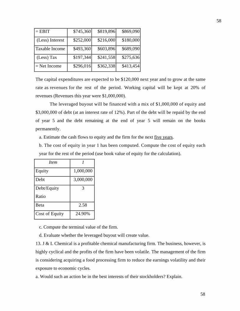
58

58

= EBIT $745,360 $819,896 $869,090

(Less) Interest $252,000 $216,000 $180,000

Taxable Income $493,360 $603,896 $689,090

(Less) Tax $197,344 $241,558 $275,636

= Net Income $296,016 $362,338 $413,454

The capital expenditures are expected to be $120,000 next year and to grow at the same

rate as revenues for the rest of the period. Working capital will be kept at 20% of

revenues (Revenues this year were $1,000,000).

The leveraged buyout will be financed with a mix of $1,000,000 of equity and

$3,000,000 of debt (at an interest rate of 12%). Part of the debt will be repaid by the end

of year 5 and the debt remaining at the end of year 5 will remain on the books

permanently.

a. Estimate the cash flows to equity and the firm for the next five years.

b. The cost of equity in year 1 has been computed. Compute the cost of equity each

year for the rest of the period (use book value of equity for the calculation).

Item 1

Equity 1,000,000

Debt 3,000,000

Debt/Equity

Ratio

3

Beta 2.58

Cost of Equity 24.90%

c. Compute the terminal value of the firm.

d. Evaluate whether the leveraged buyout will create value.

13. J & L Chemical is a profitable chemical manufacturing firm. The business, however, is

highly cyclical and the profits of the firm have been volatile. The management of the firm

is considering acquiring a food processing firm to reduce the earnings volatility and their

exposure to economic cycles.

a. Would such an action be in the best interests of their stockholders? Explain.

59

59

b. Would your analysis be any different if they were a private firm? Explain.

c. Is there any condition under which you would argue for such an acquisition for a

publicly traded firm?

1

CHAPTER 26

VALUING REAL ESTATE

The valuation models developed for financial assets are applicable for real assets

as well. Real estate investments comprise the most significant component of real asset

investments. For many years, analysts in real estate have used their own variants on

valuation models to value real estate. Real estate is too different an asset class, they argue,

to be valued with models developed to value publicly traded stocks.

In this chapter, we present a different point of view. We argue that while real

estate and stocks may be different asset classes, the principles of valuation should not

differ across the classes. In particular, the value of real estate property should be the

present value of the expected cash flows on the property. That said, there are serious

estimation issues that we still have to confront that are unique to real estate and we will

deal with those in this chapter.

Real versus Financial Assets

Real estate and financial assets share several common characteristics - their value

is determined by the cash flows they generate, the uncertainty associated with these cash

flows and the expected growth in the cash flows. Other things remaining equal, the higher

the level and growth in the cash flows and the lower the risk associated with the cash

flows, the greater is the value of the asset.

There are also significant differences between the two classes of assets. There are

many who argue that the risk and return models used to evaluate financial assets cannot

be used to analyze real estate because of the differences in liquidity across the two

markets and in the types of investors in each market. The alternatives to traditional risk

and return models will be examined in this chapter. There are also differences in the nature

of the cash flows generated by financial and real estate investments. In particular, real

estate investments often have finite lives and have to be valued accordingly. Many

financial assets, such as stocks, have infinite lives. These differences in asset lives

manifest themselves in the value assigned to these assets at the end of the ‘estimation

period’. The terminal value of a stock, five or ten years hence, is generally much higher

than the current value because of the expected growth in the cash flows and because these

2

cash flows are expected to continue forever. The terminal value of a building may be lower

than the current value because the usage of the building might depreciate its value.

However, the land component will have an infinite life and, in some cases, may be the

overwhelming component of the terminal value.

The Effect of Inflation: Real versus Financial Assets

For the most part, real and financial assets seem to move together in response to

macro economic variables. A downturn in the economy seems to affect both adversely, as

does a surge in real interest rates. There is one variable, though, that seems to have

dramatically different consequences for real and financial assets and that is inflation.

Historically, higher than anticipated inflation has had negative consequences for financial

assets, with both bonds and stocks being adversely impacted by unexpected inflation.

Fama and Schwert, for instance, in a study on asset returns report that a 1% increase in

the inflation rate causes bond prices to drop by 1.54% and stock prices by 4.23%. In

contrast, unanticipated inflation seems to have a positive impact on real assets. In fact,

the only asset class that Fama and Schwert tracked that was positively affected by

unanticipated inflation was residential real estate.

Why is real estate a potential hedge against inflation? There are a variety of

reasons, ranging from more favorable tax treatment when it comes to depreciation to the

possibility that investors lose faith in financial assets when inflation runs out of control

and prefer to hold real assets. More importantly, the divergence between real estate and

financial assets in response to inflation indicates that the risk of real estate will be very

different if viewed as part of a portfolio that includes financial assets than as a stand-

alone investment.

Discounted Cash Flow Valuation

The value of any cash-flow producing asset is the present value of the expected

cash flows on it. Just as discounted cash flow valuation models, such as the dividend

discount model, can be used to value financial assets, they can also be used to value cash

flow producing real estate investments.

3

To use discounted cash flow valuation to value real estate investments it is

necessary

• to measure the riskiness of real estate investments and to estimate a discount rate

based on the riskiness.

• to estimate expected cash flows on the real estate investment for the life of the asset.

The following section examines these issues.

A. Estimating Discount Rates

In Chapters 6 and 7, we presented the basic models that are used to estimate the

costs of equity, debt and capital for an investment. Do those models apply to real estate

as well? If so, do they need to be modified? If not, what do we use instead?

In this section, we examine the applicability of risk and return models to real

estate investments. In the process, we consider whether the assumption that the marginal

investor is well diversified is a justifiable one for real estate investments, and if so, how

best to measure the parameters of the model – riskfree rate, beta and risk premium – to

estimate the cost of equity. We also consider other sources of risk in real estate

investments that are not adequately considered by traditional risk and return models and

how to incorporate these into valuation.

Cost of Equity

The two basic models used to estimate the cost of equity for financial assets are

the capital asset and the arbitrage pricing models. In both models, the risk of any asset,

real or financial, is defined to be that portion of that asset’s variance that cannot be

diversified away. This non-diversifiable risk is measured by the market beta in the capital

asset pricing model and by multiple factor betas in the arbitrage pricing model. The

primary assumptions that both models make to arrive at these conclusions are that the

marginal investor in the asset is well diversified and that the risk is measured in terms of

the variability of returns.

If one assumes that these models apply for real assets as well, the risk of a real

asset should be measured by its beta relative to the market portfolio in the CAPM and by

its factor betas in the APM. If we do so, however, we are assuming, as we did with

publicly traded stocks, that the marginal investor in real assets is well diversified.

4

Are the marginal investors in real estate well diversified?

Many analysts argue that real estate investments require investments that are so

large that investors in it may not be able to diversify sufficiently. In addition, they note

that real estate investments require localized knowledge and that those who develop this

knowledge choose to invest primarily or only in real estate. Consequently, they note that

the use of the Capital Asset Pricing Model or the Arbitrage Pricing Model, which assume

that only non-diversifiable risk is rewarded, is inappropriate as a way of estimating cost

of equity.

There is a kernel of truth to this argument, but we believe that it can be countered

fairly easily by noting that -

• Many investors who concentrate their holdings in real estate do so by choice. They

see it as a way of leveraging their specialized knowledge of real estate. Thus, we

would view them the same way we view investors who choose to hold only

technology stocks in their portfolios.

• Even large real estate investments can be broken up into smaller pieces, allowing

investors the option of holding real estate investments in conjunction with financial

assets.

• Just as the marginal investor in stocks is often an institutional investor, with the

resources to diversify and keep transactions costs low, the marginal investor in many

real estate markets today has sufficient resources to diversify.

If real estate developers and private investors insist on higher expected returns, because

they are not diversified, real estate investments will increasingly be held by real estate

investment trusts, limited partnerships and corporations, which attract more diversified

investors with lower required returns. This trend is well in place in the United States and

may spread over time to other countries as well.

Measuring Risk for Real Assets in Asset Pricing Models

Even if it is accepted that the risk of a real asset is its market beta in the CAPM

and its factor betas in the APM, there are several issues related to the measurement and

use of these risk parameters that need to be examined. To provide some insight into the

measurement problems associated with real assets, consider the standard approach to

5

estimating betas in the capital asset pricing model for a publicly traded stock. First, the

prices of the stock are collected from historical data, and returns are computed on a

periodic basis (daily, weekly or monthly). Second, these stock returns are regressed

against returns on a stock index over the same period to obtain the beta. For non-traded

real assets, these steps are not as straightforward.

a. Individual Assets: Prices and Risk Parameters

The betas of individual stocks can be estimated fairly simply because stock prices

are available for extended time periods. The same cannot be said for individual real estate

investments. A piece of property does not get bought and sold very frequently, though

similar properties might. Consequently, price indices are available for classes of assets

(Example: Downtown Manhattan Office Buildings) and risk parameters can be estimated

for these classes.

Even when price indices are available for classes of real estate investments,

questions remain about the comparability of assets within a class (Is one downtown

building the same as any other? How does one control for differences in age and quality of

construction? What about location?) and about the categorization itself (Office Buildings

versus Residential Buildings; Single Family versus Multi Family Residences)?

There have been attempts to estimate market indices and risk parameters for

classes of real estate investments. The obvious and imperfect solution to the non-trading

problem in real estate is to construct indices of real estate investment trusts (REITs) and

commingled real estate equity funds (CREFs), which are traded and have market prices.

The reason this might not be satisfactory is because the properties owned by real estate

investment trusts may not be representative of the real estate property market and the

securitization of real estate may result in differences between real estate and REIT/CREF

returns. An alternative and more comprehensive solution is The Frank Russell Company

Index of real estate values that is based upon approximately 1000 properties owned by

real estate funds. While many of these properties are not traded in every period, the index

is based upon appraised values for these properties. In addition, Ibbotson and Siegal

(I&S) have estimated annual returns on an index of unlevered properties. Finally, Case

and Shiller constructed an index using actual transactions prices, rather than appraised

6

valued, to estimate the value of residential real estate. The following table summarizes the

returns on real estate indices, the S&P 500 and an index of bonds.

Table 26.1: Returns on Real Estate, Stocks and Bonds

Period

Compound

annual return

Arithmetic mean

return

Standard

Deviation

Serial

correlation

CREF

(commercial) 1969-87 10.80% 10.90% 2.60% 43.00%

REIT

(commercial) 1972-99 14.20% 15.70% 15.40% 11.00%

I&S (commercial) 1960-69 8.70% 8.70% 4.90% 73.00%

C&S (residential) 1970-89 8.50% 8.50% 3.00% 17.00%

HOME

(residential) 1947-89 9.80% 9.80% 4.70% 54.00%

HARRIS

(residential) 1926-89 8.50% 8.50% 5.40% 55.00%

FARM

(farmland) 1947-89 9.90% 9.90% 7.80% 64.00%

S&P 500 1928-00 10.46% 12.38% 20.02% -5.00%

T. Bonds 1928-00 4.95% 5.21% 7.68% 16.00%

T.Bills 1928-00 3.97% 3.93% 3.18% 86.00%

Inflation rate 1928-00 3.21% 3.30% 3.05% 66.00%

There are several interesting results that emerge from this table. First, not all real estate

series behave the same way. The returns on CREFs have much lower volatility associated

with them than REITs, perhaps because CREF values are based upon appraisals whereas

REITs represent market prices. Second, returns on REITs seem to have more in common

with returns on the stock market than returns on other real estate indices. Third, there is

high positive serial correlation in many of the real estate return series, especially those

based upon appraised data. This can be attributed to the smoothing of appraisals that are

used in these series.

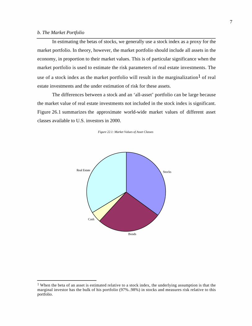
7

b. The Market Portfolio

In estimating the betas of stocks, we generally use a stock index as a proxy for the

market portfolio. In theory, however, the market portfolio should include all assets in the

economy, in proportion to their market values. This is of particular significance when the

market portfolio is used to estimate the risk parameters of real estate investments. The

use of a stock index as the market portfolio will result in the marginalization1 of real

estate investments and the under estimation of risk for these assets.

The differences between a stock and an ‘all-asset’ portfolio can be large because

the market value of real estate investments not included in the stock index is significant.

Figure 26.1 summarizes the approximate world-wide market values of different asset

classes available to U.S. investors in 2000.

1 When the beta of an asset is estimated relative to a stock index, the underlying assumption is that themarginal investor has the bulk of his portfolio (97%..98%) in stocks and measures risk relative to thisportfolio.

Figure 22.1: Market Values of Asset Classes

Stocks

Bonds

Cash

Real Estate

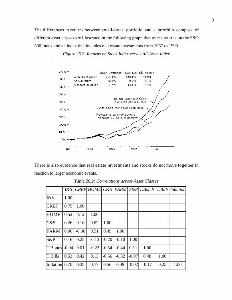
8

The differences in returns between an all-stock portfolio and a portfolio compose of

different asset classes are illustrated in the following graph that traces returns on the S&P

500 Index and an index that includes real estate investments from 1967 to 1990.

Figure 26.2: Returns on Stock Index versus All-Asset Index

There is also evidence that real estate investments and stocks do not move together in

reaction to larger economic events.

Table 26.2: Correlations across Asset Classes

I&S CREF HOME C&S FARM S&P T.Bonds T.Bills Inflation

I&S 1.00

CREF 0.79 1.00

HOME 0.52 0.12 1.00

C&S 0.26 0.16 0.62 1.00

FARM 0.06 -0.06 0.51 0.49 1.00

S&P 0.16 0.25 -0.13 -0.20 -0.10 1.00

T.Bonds -0.04 0.01 -0.22 -0.54 -0.44 0.11 1.00

T.Bills 0.53 0.42 0.13 -0.56 -0.32 -0.07 0.48 1.00

Inflation 0.70 0.35 0.77 0.56 0.49 -0.02 -0.17 0.25 1.00

9

Source: Ibbotson and Brinson (1996)

As noted earlier in this chapter, the differences between real asset and financial asset

returns widen when inflation rates change. In fact, three of the five real estate indices are

negatively correlated with stocks and the other two have low correlations. As a

consequence, adding real estate investments to a portfolio composed primarily of financial

assets will create substantial savings in terms of reduced volatility. In addition, the returns

on a market portfolio which includes both financial and real assets can be very different

from the returns on a market portfolio that is composed entirely of stocks.

While few economists would argue with the value of incorporating real estate

investments into the market portfolio, most are stymied by the measurement problems.

These problems, while insurmountable until recently, are becoming more solvable as real

estate investments get securitized and traded. For instance, exchanges that trade real estate

master limited partnerships and real estate business trusts have opened.

Some practical solutions

If one accepts the proposition that the risk of a real estate investment should be

measured using traditional risk and return models, there are some practical approaches

that can be used to estimate risk parameters.

• The risk of a class of real estate investments can be obtained by regressing returns on

the class (using the Ibbotson series, for instance, on commercial and residential

property) against returns on a consolidated market portfolio. The primary problems

with this approach are - (a) these returns series are based upon smoothed appraisals

and may understate the true volatility in the market and (b) the returns are available

only for longer return intervals (annual or quarterly).

• The risk parameters of traded real estate securities (REITs and MLPs) can be used as

a proxy for the risk in real estate investment. The limitations of this approach are that

securitized real estate investments may behave differently from direct investments

and that it is much more difficult to estimate risk parameters for different classes of

real estate investment (unless one can find REITs that restrict themselves to one class

of investments - such as commercial property).

• The demand for real estate is in some cases a derived demand. For instance, the value

of a shopping mall is derived from the value of retail space, which should be a

10

function of how well retailing is doing as a business. It can be argued, in such a case,

that the risk parameters of a mall should be related to the risk parameters of publicly

traded retail stores. Corrections should obviously be made for differences in operating

and financial leverage.

Other Risk Factors

Does investing in real estate investments expose investors to more (and different)

types of risk than investing in financial assets? If so, how is this risk measured and is it

rewarded? The following are some of the issues related to real estate investments that

might affect the risk and expected returns.

A. Diversifiable versus Non-Diversifiable Risk

We made the argument earlier that using risk and return models that assume that

the marginal investor is well diversified is reasonable even though many investors in real

estate choose not to be diversified. Part of the justification that we offered was the

presence of firms with diversified investors, such as real estate investment trusts and

master limited partnerships, in the real estate market. But what if no such investors exist

and the marginal investor in real estate is not well diversified? How would we modify our

estimates of cost of equity?

In Chapter 24, we examined how to adjust the cost of equity for a private

business for the fact that its owner was not diversified. In particular, we recommended

the use of a total beta that reflected not just the market risk but also the extent of non-

diversification on the part of the owner:

Total Beta market theand portfolio ownersbetween n Correlatio

BetaMarket =

We could adapt this measure to estimate a total beta for private businesses. For instance,

assume that the marginal investor in commercial real estate has a portfolio that has a

correlation of 0.50 with the market and that commercial real estate as a property class has

a beta of 0.40. The beta you would use to estimate the cost of equity for the investment

would be 0.80.

Total beta 80.050.0

40.0 =

11

Using this higher beta would result in a higher cost of equity and a lower value for the real

estate investment.

B. Lack of Liquidity

Another critique of traditional risk measures is that they assume that all assets are

liquid (or, at least, that there are no differences in liquidity across assets). The markets for

many real estate investments are less liquid than markets for financial assets - transactions

occur less frequently, transactions costs are higher and there are far fewer buyers and

sellers. The less liquid an asset, it is argued, the more risky it is.

The link between lack of liquidity and risk is much more difficult to quantify for

several reasons. One is that it depends upon the time horizon of the investor. An investor

who intends to hold long term will care less about liquidity than one who is uncertain

about his or her time horizon or wants to trade short term. Another is that it is affected

by the external economic conditions. For instance, real estate is much more liquid during

economic booms, when prices are rising, than during recessions, when prices are

depressed.

The alternative to trying to view the absence of liquidity as an additional risk

factor and building into discount rates is to value the illiquid asset conventionally (as if it

were liquid) and then applying a liquidity discount to it. This is often the practice in

valuing closely held and illiquid businesses and allows for the liquidity discount to be a

function of the investor and external economic conditions at the time of the valuation. We

examined the question of estimating the liquidity discount in more detail in Chapter 24.

C. Exposure to Legal Changes

The values of all investments are affected by changes in the tax law - changes in

depreciation methods and changes in tax rates on ordinary income and capital gains. Real

estate investments are particularly exposed to changes in the tax law, because they derive

a significant portion of their value from depreciation and tend to be highly levered.

Unlike manufacturing or service businesses which can move operations from one

locale to another to take advantage of locational differences in tax rates and other legal

restrictions, real estate is not mobile and is therefore much more exposed to changes in

local laws (such as zoning requirements, property taxes and rent control).

12

The question becomes whether this additional sensitivity to changes in tax and

local laws is an additional source of risk, and, if so, how this risk should be priced. Again,

the answer will depend upon whether the marginal investor is diversified not only across

asset classes but also across real estate investments in different locations. For instance, a

real estate investor who holds real estate in New York, Miami, Los Angeles and Houston

is less exposed to legal risk than one who holds real estate in only one of these locales.

The trade off, however, is that the localized knowledge that allows a real estate investor

to do well in one market may not carry well into other markets.

D. Information Costs and Risk

Real estate investments often require specific information about local conditions

that is difficult (and costly) to obtain. The information is also likely to contain more

noise. There are some who argue that this higher cost of acquiring information and the

greater noise in this information should be built into the risk and discount rates used to

value real estate. This argument is not restricted to real estate. It has been used as an

explanation for the small stock premium - i.e., small stocks make higher returns than larger

stocks, after adjusting for risk (using the CAPM). Small stocks, it is argued, generally

have less information available on them than larger stocks and the information tends to be

more noisy.

Diversification in Real Estate: Trends and Implications

As we look at the additional risk factors – estimation errors, legal and tax changes,

volatility in specific real estate markets – that are often built into discount rates and

valuations, the rationale for diversification becomes stronger. A real estate firm that is

diversified across holdings in multiple locations will be able to diversify away some of

this risk. If the firm attracts investors who are diversified into other asset classes, it

diversifies away even more risk, thus reducing its exposure to risk and its cost of equity.

Inexorably then, you would expect to see diversified real estate investors – real

estate corporations, REITs and MLPS – drive local real estate investors who are not

diversified (either across locations or asset classes) out of the market by bidding higher

prices for the same properties. If this is true, you might ask, why has it not happened

already? We believe that there are two reasons. The first is that knowledge of local real

estate market conditions is still a critical component driving real estate values and real

13

estate investors with this knowledge may be able to compensate for their failure to

diversify. The second is that a significant component of real estate success still comes

from personal connections – to other developers, to zoning boards and to politicians. Real

estate investors with the right connections may be able to get much better deals on their

investments than corporations bidding for the same business.

As real estate corporations and REITs multiply, you should expect to see much

higher correlation in real estate prices across different regions and a drop-off in the

importance of local conditions. Furthermore, you should also expect to see these firms

become much more savvy at dealing with the regulatory authorities in different regions.

An Alternative Approach to estimating Discount Rates: The Survey Approach

The problems with the assumptions of traditional risk and return models and the

difficulties associated with the measurement of risk for non-traded real assets in these

models have lead to alternative approaches to estimating discount rates for these real

estate investments. In the context of real estate, for instance, the costs of equity and

capital are often obtained by surveying potential investors in real estate on what rate of

return they would demand for investing in different types of property investments. Table

26.3 summarizes the results of such a survey done by Cushman and Wakefield, a real

estate firm, of investors in various real estate properties.

Table 26.3 : Survey Results from Cushman Wakefield

This approach is justified on the following grounds.

14

• These surveys are not based upon some abstract models of risk and return (which

may ignore risk characteristics that are unique to the real estate market) but on what

actual investors in real want to make as a return.

• These surveys allow for the estimation of discount rates for specific categories of

properties (hotels, apartments, etc.) by region, without requiring a dependence upon

past prices like risk and return models.

• There are relatively few large investors who invest directly in real estate (rather than

in securitized real estate). It is therefore feasible to do such a survey.

There are however grounds for contesting this approach, as well.

• Surveys, by their very nature, yield different ‘desired rates of return’ for different

investors for the same property class. Assuming that a range of desired returns can be

obtained for a class of investments, it is not clear where one goes next. Presumably,

those investors who demand returns at the high end of the scale will find themselves

priced out of the market and those whose desired returns are at the low end of the

scale will find plenty of undervalued properties. The question of who the marginal

investor in an investment should be is not answered in these surveys.

• The survey approach bypasses the issue of risk but it does not really eliminate it.

Clearly, investors demand the returns that they do on different property classes

because they perceive them to have different levels of risk.

• The survey approach works reasonably well when there are relatively few and fairly

homogeneous investors in the market. While this might have been true a decade ago, it

is becoming less so as new institutional investors enter the market and the number of

investors increases and becomes more heterogeneous.

• The survey approach also becomes suspect when the investors who are surveyed act

as pass-throughs - they invest in real estate, securitize their investments and sell them

to others and move on. If they do so, it is the desired returns of the ultimate investor

(the buyer of the securitized real estate) that should determine value, not the desired

return of the intermediate investor.

There are several advantages to using a model that measures risk and estimates a

discount rate based on the risk measure, rather than using a survey.

15

• A risk and return model, properly constructed, sets reasonable bounds for the

expected returns. For instance, the expected return on a risky asset in both the CAPM

and the APM will exceed the expected return on a riskless asset. There is no such

constraint on survey responses.

• A risk and return model, by relating expected return to risk and risk to pre-specified

factors allows an analyst to be proactive in estimating discount rates rather than

reactive. For instance, in the context of the CAPM, the expected return on an

investment is determined by its beta, which in turn is determined by the cyclicality of

the business (in which the investment is made) and the financial leverage taken on.

Thus, an analyst who knows how the financial leverage in an investment is expected

to change over time can adjust the beta of that investment accordingly and use it in

valuation. There is no such mechanism available, when the survey approach is used.

• Where the ultimate investor is not known at the time of the analysis, as is the case in

real estate investments that are securitized, a risk and return model provides the

framework for estimating the discount rate for a hypothetical marginal investor.

As real estate markets become more accessible to institutional investors and more

investments are made with the objective of eventual securitization, the need for a good

risk and return model becomes more acute. These same trends will also make real estate

investments more like financial investments (by making them more liquid). Sooner rather

than latter, the same models used to estimate risk and discount rates for financial assets

will also be used to estimate risk and discount rates for real estate investments.

From Cost of Equity to Cost of Capital

Once you have estimated a cost of equity, there are two other inputs needed to

estimate the cost of capital. The first is the cost of debt and estimating it is much more

straightforward than estimating the cost of equity. You have three choices.

• If you are raising capital for a new real estate investment, you could use the stated

interest rate on bank loans used to fund the investment. In making this estimate,

though, you have to be aware of the terms of the bank loan and whether there will

be other costs created to the real estate firm. For instance, a requirement that a

16

compensating balance be maintained over the life of the loan will increase the

effective cost of debt.

• You could look at the capacity that the real estate investment has to cover bank

payments – this is the equivalent of an interest coverage ratio, estimate a synthetic

rating and use this rating to estimate a pre-tax cost of debt. In fact, you could

modify the numerator to include depreciation, since the investment is a finite life

investment and should not require significant reinvestment.

To estimate an after-tax cost of debt, you would use the marginal tax rate of the individual

or entity investing in the property.

The debt ratio in most real estate investments is usually estimated by looking at

the proportion of the funds raised from debt and equity. Thus, if a property costs $4

million to build and the investor borrows $3 million to fund it, the debt ratio used is 75%.

While we will stick with this convention, it is worth bearing in mind that the ratios should

be based upon the value of the property rather than the funding needs. Thus, if the value

of the property is expected to be $5 billion after it is built, the debt ratio used should be

60% ($3 billion / $5 billion). This, of course, requires circular reasoning since the cost of

capital is necessary to estimate the value of the property in the first place.

The distinction between cost of equity and the cost of capital, drawn in Chapter

7, is significant. If the cash flows being discounted are pre-debt cashflows, i.e., cash flows

to the firm, the appropriate discount rate is the cost of capital. If you use this approach,

you will value the property and if you are the equity investor, you would then subtract

out the value of the outstanding debt to arrive at the value of the equity in the real estate

investment. If the cash flows being discounted on a real estate deal are cash flows to

equity, the appropriate discount rate is the cost of equity. You would then value the

equity in the real estate investment directly.

B. Estimating Cash Flows

Not all real estate investments generate cash flows. For those that do, cash flows

can be estimated in much the same way that they can be estimated for financial

investments. The ultimate objective is to estimate cash flows after taxes. Just as with

financial assets, these cash flows can be estimated to equity investors. This is the cash

17

flow left over after meeting all operating expenses, debt obligations (interest expenses and

principal payments) and capital expenditures. The cash flows can also be estimated for all

investors in the real estate investment. This is the equivalent of cash flows to the firm,

which is the cash flow prior to meeting debt obligations.

1. Cash Inflows

The cash flows from a real estate investment generally take the form of rents and

lease payments. In estimating rents for future years, you have to consider past trends in

rents, demand and supply conditions for space provided by the property and general

economic conditions.

In office/multiple residential buildings all space may not be rented at a particular

time. Thus, the vacancy rate (i.e., the percentage of the space that will not be rented out

at any point in time) has to be projected in conjunction with market rents. Even in tight

markets, there will be periods of time where space cannot be rented out, leading to a

vacancy rate. Thus, no building, no matter how sought after, can be expected to have a

100% occupancy rate. With new buildings, the projections have to factor in how long it

will take initially to get occupants to rent/lease space. Clearly, the longer it takes, the less

is the discounted cash flow value of the building.

In the case of leased property, the terms of the lease can affect the projected lease

revenues. If income properties are subject to existing leases, the terms of the lease such as

the length of the lease, the contracted lease payments with future increases, additional

reimbursable expenses and provisions on lease renewal will determine cash flow

estimates. The leases may also be net leases, where the tenant is responsible for paying

taxes, insurance and maintenance.

2. Cash Outflows

Expenses on real estate investments include items such as property taxes,

insurance, repairs and maintenance and advertising - which are unrelated to occupancy and

are fixed, as well as items such as utility expenses, which are a function of occupancy and

are variable. In addition, the following factors will affect projected expenses.

• Reimbursability: Some expenses incurred in connection with a property by the owner

may be reimbursed by the tenant, as part of a contractual agreement.

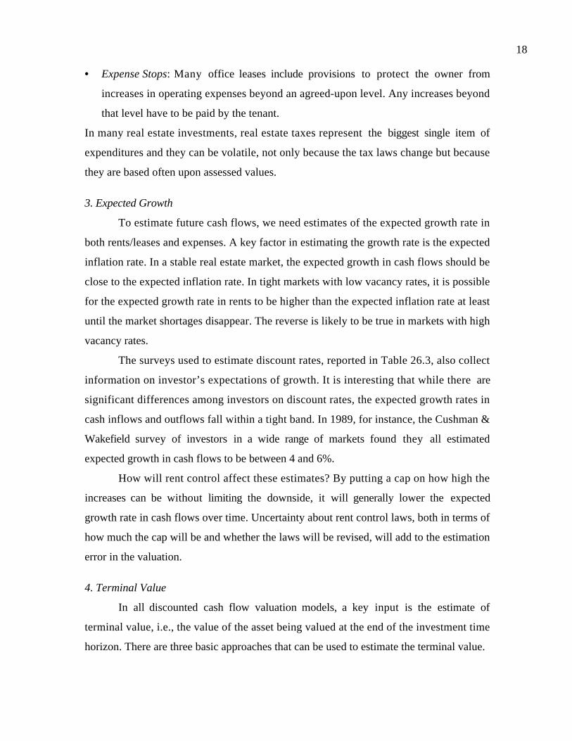
18

• Expense Stops: Many office leases include provisions to protect the owner from

increases in operating expenses beyond an agreed-upon level. Any increases beyond

that level have to be paid by the tenant.

In many real estate investments, real estate taxes represent the biggest single item of

expenditures and they can be volatile, not only because the tax laws change but because

they are based often upon assessed values.

3. Expected Growth

To estimate future cash flows, we need estimates of the expected growth rate in

both rents/leases and expenses. A key factor in estimating the growth rate is the expected

inflation rate. In a stable real estate market, the expected growth in cash flows should be

close to the expected inflation rate. In tight markets with low vacancy rates, it is possible

for the expected growth rate in rents to be higher than the expected inflation rate at least

until the market shortages disappear. The reverse is likely to be true in markets with high

vacancy rates.

The surveys used to estimate discount rates, reported in Table 26.3, also collect

information on investor’s expectations of growth. It is interesting that while there are

significant differences among investors on discount rates, the expected growth rates in

cash inflows and outflows fall within a tight band. In 1989, for instance, the Cushman &

Wakefield survey of investors in a wide range of markets found they all estimated

expected growth in cash flows to be between 4 and 6%.

How will rent control affect these estimates? By putting a cap on how high the

increases can be without limiting the downside, it will generally lower the expected

growth rate in cash flows over time. Uncertainty about rent control laws, both in terms of

how much the cap will be and whether the laws will be revised, will add to the estimation

error in the valuation.

4. Terminal Value

In all discounted cash flow valuation models, a key input is the estimate of

terminal value, i.e., the value of the asset being valued at the end of the investment time

horizon. There are three basic approaches that can be used to estimate the terminal value.

19

• The current value of the property can be assumed to increase at the expected inflation

rate to arrive at a terminal value. Thus, the terminal value of a property, worth $10

million now, in ten years will be $13.44 million, if the expected inflation rate is 3%

(Terminal Value = $10 * 1.0310). The danger of this approach is that it starts of with

the assumption that the current value of the asset is reasonable and then tries to

assess the true value of the asset.

• An alternative to this approach is to assume that the cash flows in the terminal year

(the last year of the investment horizon) will continue to grow at a constant rate

forever after that. If this assumption is made, the terminal value of the asset is:

Terminal Value of Equity/Assetn g-r

CF Expected 1n+=

where r is the discount rate (cost of equity if it is the terminal value of equity and cost

of capital if it is the terminal value of the asset) and CFn+1 is the cash flow (cash flow

to equity if terminal value is for equity and to firm if terminal value is total terminal

value).

Thus, if the property described in the previous example had produced a net cash

flow, prior to debt payments, of $1.2 million in year 10, this cash flow was expected

to grow 3% a year forever after that and the cost of capital was 13%, the terminal

value of the property can be written as follows:

Terminal Value of Asset ( )( )

million 36.12$03.013.0

03.12.1

g-WACC

FCFF11

=−

=

=

The assumption of perpetual cash flows may make some analysts uncomfortable but

one way to compensate is to require that more cash be set aside each year to ensure

that the property life can be extended. If you use this approach, for instance, you

could assume that the cash flow from depreciation be reinvested back into the building

in the form of maintenance capital expenditures.

• A close variation on the infinite growth model is the ‘capitalization rate’ (cap rate)

used by many real estate appraisers to value properties. In its most general form, the

20

cap rate is the rate by which operating income is divided to get the value of the

property.

Property value ratetion Capitaliza

safter taxe income Operating=

The capitalization rate is, in fact, the inverse of the value to EBIT multiple that we

used to value publicly traded companies in Chapter 18.

There are three ways in which capitalization rates are estimated. One is to use the

average capitalization rate at similar properties that have sold recently. This is the

equivalent of using the industry-average earnings multiple to estimate terminal value in

a publicly traded company. The second is to use the surveys mentioned earlier to

obtain an estimate of the cap rates used by other real estate investors. The third is to

estimate the cap rate from a discounted cashflow model. To see the linkage with the

infinite growth model, assume that the net operating income (prior to debt payments)

is also the free cash flow to the firm – note that this essentially is the equivalent of

assuming that capital maintenance expenditures equal depreciation. Then the

capitalization rate can be written as a function of the discount rate and the expected

growth rate.

Capitalization Rate ggr

+−=

1

where r is the discount rate (the cost of equity if net income is being capitalized and

the cost of capital if net operating income is being capitalized) and g is the expected

growth rate forever. In the above example, the capitalization rate would have been:

Capitalization Rate

%70.903.1

03.013.0

=

−=

If the capitalization rate is being applied to next year’s operating income, rather than

this year’s value, you can ignore the denominator and use a cap rate of 10%.

A Speculative Investment in Undeveloped Land

Developers sometimes buy undeveloped land, not with the intention of

developing it, but hold on in the hope that the value of the land will appreciate

significantly over the holding period. An investment in undeveloped land does not

21

generate positive cash flows during the holding period. The only positive cash flow, in

fact, is the estimated value at the end of the holding period and this value will reflect the

expected value of the land. If you have to pay property taxes and other expenses during

the holding period, you will have negative cash flows during the holding period.

There are two ways you can approach the analysis of this investment. The first is

the traditional discounted cash flow approach. You could discount the expected property

taxes and other expenses during the holding period and the estimated value of the land at

the end of the period back to the present at the cost of capital and see if it exceeds the

cost of the land today. In fact, the expected appreciation in the price of the land will have

to be greater than the cost of capital and the expected annual property tax rate for this

investment to have a positive net present value. To illustrate, if your cost of capital is

10% and the annual property tax rate is 2% of land value, you would need a price

appreciation rate of 12% a year for the present value of the inflow to exceed the present

value of the outflows.2

The other is to view the land as an option and developing the land as exercising the

option. You would then consider the cost of the land as the price of the option. The

interesting implication is that you might choose to buy the land even if the expected price

appreciation rate is lower than your cost of capital, if there is substantial volatility in land

prices. We will consider this application in more detail in Chapter 28.

C. DCF Valuation Models

Once a discount rate has been chosen and cash flows estimated, the value of an

income-producing real asset can be estimated either in whole (by discounting cash flows

to the firm at the weighted average cost of capital) or to its equity investors (by

discounting cash flows to equity at the cost of equity). The following illustrations

provide examples of DCF valuation in real estate.

Illustration 26.1: Valuing an office building

2 We are assuming that the property taxes are based upon the estimated value of the land each year and notthe original cost. If it is the latter, the price appreciation rate can be lower.

22

In this illustration, we will be valuing an office building located at 711 Third

Avenue in New York City. The operating details of the building are as follows:

• The building has a capacity of 528,357 square feet of rentable space. While 95%

of this space is rented out for the next year, the occupancy rate is expected to

climb 0.5% a year for the following four years to reach 97% of capacity in year 5.

This is expected to be the occupancy rate in steady state.

• The average rent per square foot3 was $28.07 in the most recent year and is

expected to grow 3% a year in perpetuity. Historically, there has been a credit

loss, associated with tenants failing to make payments, of 2.5% of rental revenues.

• The building has a garage that generated $800,000 in income for the most recent

year. This income is also expected to grow 3% a year in perpetuity.

• Real estate taxes were $5.24 a square foot in the most recent year and are expected

to grow 4% a year for the next 5 years and 3% a year thereafter.

• The land under the building is rented under a long-term lease and the ground rent in

the most recent year was $1.5 million. This rent is expected to remain unchanged

for the next 5 years and grow 3% a year thereafter.

• Other expenses, including insurance, maintenance and utilities, amounted to $6.50

a square foot in the most recent year and are expected grow 3% a year in

perpetuity. Approximately 10% of these expenses will be reimbursed by tenants

each year (and thus will become a part of the revenues).

• The management fee for the most recent year was $300,000 and is expected to

grow 3% a year in perpetuity.

• The depreciation in the building is expected to be $2 million a year for the next 5

years. The capital maintenance and upgrade expenditures (including leasehold

improvements for new tenants) last year amounted to $1.5 million and are

expected to grow 3% a year for the next 5 years. Beyond year 5, depreciation is

expected to increase 3% a year in perpetuity and capital maintenance expenditures

will offset depreciation.

3 The rents vary depending upon location in the building, with lower rents in the basement and lower floorsand higher rents on the top floors.

23

The potential buyer of the building is a corporation that faces a marginal tax rate of 38%

and expects to finance the building with a mix of 60% debt and 40% equity. Then debt

will take the form of a long-term balloon payment loan with an interest rate of 6.50%.

Step 1:Estimating a cost of capital

We begin by trying to estimate a cost of equity. While we had access to a survey

that provided typical hurdle rates used by real estate investors for office buildings in New

York, we chose to estimate the cost of equity from the capital asset pricing model,

because the potential buyer is a corporation (whose investors presumably are

diversified).4 To make this estimate, we began with the unlevered beta of 0.62 of equity

real estate investment trusts with office properties. We estimated a levered beta using the

debt equity mix proposed for the building:

Levered beta

( )

( )

20.1

4.0

6.00.38-110.62

Equity

Debtratetax -11beta Unlevered

=

+=

+=

To estimate the cost of equity, we used a riskfree rate of 5.4% and a risk premium of 4%:

Cost of equity = Riskfree rate + Beta * Risk Premium

= 5.4% + 1.20 (4%) = 10.20%

Using the interest rate on the debt as the pre-tax cost of debt, we estimated a cost of

capital.

Cost of capital = 10.20% (.40) + 6.5% (1-.38) (.60) = 6.49%

We assumed that this would be the cost of capital in perpetuity.5

Step 2: Estimating cash flows on the building

We used the operating information specified above to estimate the cash flows

prior to debt payments on the building for the next 5 years in Table 26.4. Since all of the

items grow at 3% beyond year 5, we estimated a cash flow for year 6 as the terminal year.

The terminal value of the building was calculated based on this cash flow, a perpetual

growth rate of 3% and a cost of capital of 6.49%:

4 Note that it is the investors in the corporation that need to be diversified and not the corporation itself.

24

Terminal value

9116,810,65$03.00649.0

682,079,4

rategrowth Expected-capital ofCost

FCFF6

=−

=

=

[NOTE: There is a significant difference in the result of my calculation.

The present value of the expected cashflows for the next five years and the terminal value,

summarized in Table 26.5, yields the value of the building.

Table 26.5: Value of Building: 711 Third Avenue

1 2 3 4 5

Cash flow to firm $3,617,845$3,761,185$3,909,538$4,063,068 $4,221,946

Terminal value $116,810,659

Present value

@6.49% $3,397,275$3,316,547$3,237,186$3,159,199 $88,370,242

The sum of the present value of the cash flows is $101.48 million. This is the estimated

value of the building.

5 This implies that the existing loan will be refinanced with a new loan when it comes due.

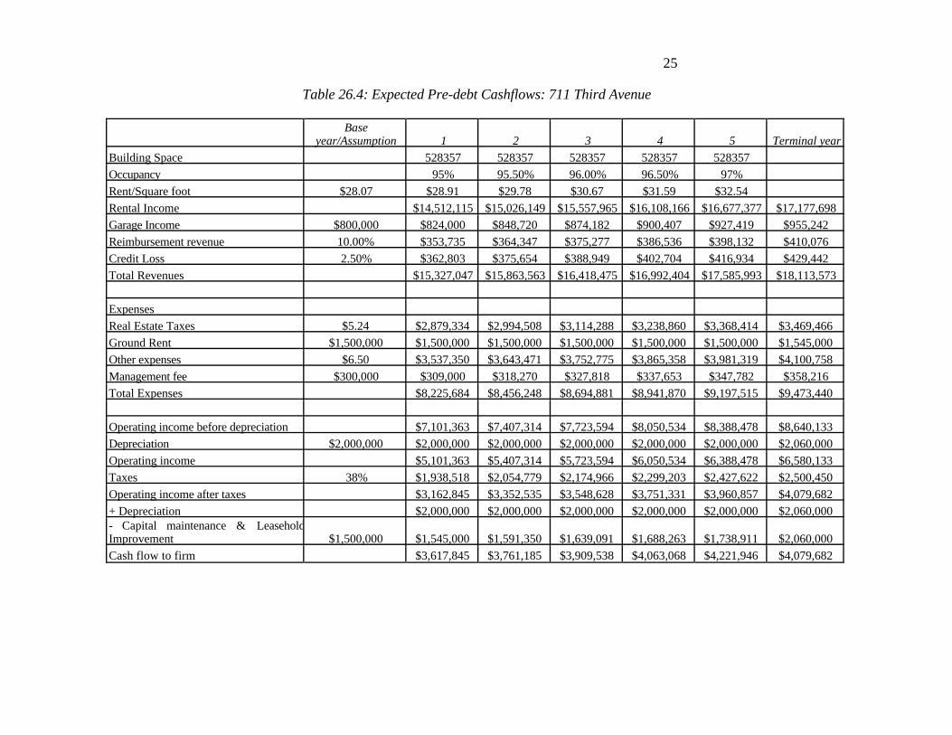
25

Table 26.4: Expected Pre-debt Cashflows: 711 Third Avenue

Baseyear/Assumption 1 2 3 4 5 Terminal year

Building Space 528357 528357 528357 528357 528357

Occupancy 95% 95.50% 96.00% 96.50% 97%

Rent/Square foot $28.07 $28.91 $29.78 $30.67 $31.59 $32.54

Rental Income $14,512,115 $15,026,149 $15,557,965 $16,108,166 $16,677,377 $17,177,698

Garage Income $800,000 $824,000 $848,720 $874,182 $900,407 $927,419 $955,242

Reimbursement revenue 10.00% $353,735 $364,347 $375,277 $386,536 $398,132 $410,076

Credit Loss 2.50% $362,803 $375,654 $388,949 $402,704 $416,934 $429,442

Total Revenues $15,327,047 $15,863,563 $16,418,475 $16,992,404 $17,585,993 $18,113,573

Expenses

Real Estate Taxes $5.24 $2,879,334 $2,994,508 $3,114,288 $3,238,860 $3,368,414 $3,469,466

Ground Rent $1,500,000 $1,500,000 $1,500,000 $1,500,000 $1,500,000 $1,500,000 $1,545,000

Other expenses $6.50 $3,537,350 $3,643,471 $3,752,775 $3,865,358 $3,981,319 $4,100,758

Management fee $300,000 $309,000 $318,270 $327,818 $337,653 $347,782 $358,216

Total Expenses $8,225,684 $8,456,248 $8,694,881 $8,941,870 $9,197,515 $9,473,440

Operating income before depreciation $7,101,363 $7,407,314 $7,723,594 $8,050,534 $8,388,478 $8,640,133

Depreciation $2,000,000 $2,000,000 $2,000,000 $2,000,000 $2,000,000 $2,000,000 $2,060,000

Operating income $5,101,363 $5,407,314 $5,723,594 $6,050,534 $6,388,478 $6,580,133

Taxes 38% $1,938,518 $2,054,779 $2,174,966 $2,299,203 $2,427,622 $2,500,450

Operating income after taxes $3,162,845 $3,352,535 $3,548,628 $3,751,331 $3,960,857 $4,079,682

+ Depreciation $2,000,000 $2,000,000 $2,000,000 $2,000,000 $2,000,000 $2,060,000- Capital maintenance & LeaseholdImprovement $1,500,000 $1,545,000 $1,591,350 $1,639,091 $1,688,263 $1,738,911 $2,060,000

Cash flow to firm $3,617,845 $3,761,185 $3,909,538 $4,063,068 $4,221,946 $4,079,682

26

Table 26.6: Expected cash flows to equity: 711 Third Avenue

1 2 3 4 5

Building Space 528357 528357 528357 528357 528357

Occupancy 95.00% 95.50% 96.00% 96.50% 97.00%

Rent/Square foot $28.91 $29.78 $30.67 $31.59 $32.54

Rental Income $14,512,115 $15,026,149 $15,557,965 $16,108,166 $16,677,377

Garage Income $824,000 $848,720 $874,182 $900,407 $927,419

Reimbursement revenue $353,735 $364,347 $375,277 $386,536 $398,132

Credit Loss $362,803 $375,654 $388,949 $402,704 $416,934

Total Revenues $15,327,047 $15,863,563 $16,418,475 $16,992,404 $17,585,993

Expenses

Real Estate Taxes $2,879,334 $2,994,508 $3,114,288 $3,238,860 $3,368,414

Ground Rent $1,500,000 $1,500,000 $1,500,000 $1,500,000 $1,500,000

Other expenses $3,537,350 $3,643,471 $3,752,775 $3,865,358 $3,981,319

Management fee $309,000 $318,270 $327,818 $337,653 $347,782

Interest expenses $3,957,737 $3,957,737 $3,957,737 $3,957,737 $3,957,737

Total Expenses $12,183,422 $12,413,986 $12,652,618 $12,899,608 $13,155,252

Net income before depreciation & taxes $3,143,625 $3,449,577 $3,765,856 $4,092,797 $4,430,741

Depreciation $2,000,000 $2,000,000 $2,000,000 $2,000,000 $2,000,000

Operating income $1,143,625 $1,449,577 $1,765,856 $2,092,797 $2,430,741

Taxes $434,578 $550,839 $671,025 $795,263 $923,682

Net income $709,048 $898,738 $1,094,831 $1,297,534 $1,507,059

+ Depreciation $2,000,000 $2,000,000 $2,000,000 $2,000,000 $2,000,000

- Capital maintenance & Leasehold Improvement $1,545,000 $1,591,350 $1,639,091 $1,688,263 $1,738,911

Cash flow to equity $1,164,048 $1,307,388 $1,455,741 $1,609,271 $1,768,148

27

Illustration 26.2: Valuing the Equity Stake in a building

The analysis above can be done for just the equity stake in 711 Third Avenue. To

do so, we will first estimate the dollar debt that will be borrowed to buy this building.

Assuming that the building has a value of $101.48 million (from the previous illustration)

and using a debt ratio of 60%, we estimate debt to be $60.89 million.

Debt = Value of building * Debt ratio = 101.48 * 0.6 = $60.89 million

Since this is a balloon payment loan, the interest payments on the debt will remain the

same each year, based upon the 6.5% interest rate.

Annual Interest expenses = Dollar debt * interest rate = $60.89 * 0.065 = $3.96 million

The appropriate discount rate to use while valuing the equity stake in the building is the

cost of equity, estimated to be 10.20% in this analysis.

Estimating Cash Flows to Equity

The estimated cash flows to equity are estimated each year by netting out interest

expenses from income and adjusting the taxes accordingly. Table 26.6 summarizes cash

flows to equity each year for the next 5 years.

In year 5, we also estimate the terminal value of equity by subtracting the debt

due from the terminal value of the building estimated in the previous illustration.

Terminal value of equity

million 55.92

million 60.89 -million 116.81

Debt-Building of valueTerminal

===

Estimating the value of equity

The present value of the cash flows to equity for the next 5 years and the terminal value

are computed in Table 26.7 below.

Table 26.7: Value of Equity stake in 711 Third Avenue

1 2 3 4 5

Cash flow to equity $1,164,048 $1,307,388 $1,455,741 $1,609,271 $1,768,148

Terminal value $55,922,390

Present value

@10.20%

$1,056,305 $1,076,567 $1,087,775 $1,091,196 $35,519,318

28

The value of the equity stake in the building is $$39.83 million. Adding this value to the

value of the debt raised of $60.89 million gives us an estimate for the value of the building.

Estimated value of building = $ 60.89 million + $39.83 million = $100.72 million

Why is there a difference between this estimate of the property value and the one we

arrived at in the previous illustration? The reason is simple. The debt ratio of 60% that

we assumed and kept constant when estimating cost of capital will require us to borrow

an additional amount each year for the next 5 years, since the building’s value will

appreciate by about 3% a year. The tax benefits from this additional debt were implicitly

built into the valuation of the building in the last illustration but were ignored while

valuing equity in this one. If we consider those tax benefits, we will arrive at the same

value.

Real Estate Valuation in Practice: A Comparison

The building on 711 Seventh Avenue was valued for sale by an appraiser, using

discounted cash flow valuation. While many of the base assumptions in our valuation

were borrowed from that appraisal, the estimate of value in the appraisal was $70 million,

about a third below our estimate. The main differences between our valuation and the

appraiser’s valuation are as follows.

• The appraisal was done entirely in terms of pre-tax cash flows. Depreciation was

therefore not considered and the tax benefits from it were ignored.

• The discount rate used was 11.5%, based upon a proprietary survey of real estate

investors done by the appraiser. While nothing was mentioned in the appraisal, this

discount rate presumably was in pre-tax terms (to ensure consistency with how the

cash flows were estimated) and stated as a return on the overall investment (and not

just the equity investment).

• The terminal value was estimated based upon a capitalization rate of 9.0%, which was

also based upon the survey. (The operating income in year 5 was divided by 9.0% to

arrive at terminal value)

We believe that using pre-tax cash flows and pre-tax discount rates will miss the segment

of value that comes from depreciation and interest expenses being tax deductible and

understate the value of the building. Assuming that the discount rate is defined correctly

29

as a pre-tax cost of capital, the use of surveys to estimate both this number and the

terminal multiple makes us uncomfortable, especially given the fact that the buyer of this

building is a corporation with diversified investors.

D. Limitations of Discounted Cash flow

There are many reasons given for why discounted cash flow valuation is not

appropriate for real estate. First, it is argued the discount rates are difficult, if not

impossible, to estimate for most real estate investments. In the discussion of this topic,

we have pointed out that this is not necessarily true. Second, it is argued that estimating

cash flows for the time horizon is tedious and difficult to do, as is the estimation of the

terminal value. We would argue that it is much easier to estimate cash flows for real estate

than for some financial investments (for instance, a high growth stock). Third, it is argued

that discounted cash flow valuation does not reflect market conditions - that the market is

strong or weak at the time of the valuation. We would reject this argument at two levels.

On one level, the cash flows should reflect the market conditions, since they will be higher

(higher rents and lower vacancy rates) and grow faster in strong market conditions. On the

other level, any additional value being assigned by the market beyond the cash flow levels

can be considered to be ‘overvaluation’ and should not be built into the appraised value in

the first place.

Comparable/Relative Valuation

Just as price/earnings and price/book value ratios are used to value financial assets,

real estate investments can be valued using standardized value measures and comparable

assets. There are several reasons for doing so.

• It provides a mechanism for valuing non-cash flow producing assets. For instance, the

value of a single family residential building bought as a primary residence can be

estimated by looking at similar properties in the same area.

• It takes into account market trends that might not be reflected in the cash flows yet

for a number of reasons. Leases might have frozen lease payments in place, while

market values have risen, and rent control laws might prevent rents from rising with

market values.

30

• It is also argued that valuing based upon comparables is much simpler to do than

discounted cash flow valuation since it does not require, at least explicitly, the

estimation of discount rates and cash flows.

What is a comparable asset?

The key limitation of all comparable based approaches is in the definition of

‘comparable’. In the case of stocks, differences in growth, risk and payout ratios between

stocks have to be adjusted before price/earnings ratios are compared. Many analysts

choose to restrict their comparisons of stocks to those within the same industry group to

keep it relatively homogeneous. In the case of real estate, differences in income

production, size, scale, location, age and quality of construction have to be accounted for

before comparisons are made. Some of these adjustments are simple (such as differences

in size) and others are subjective (such as differences in location).

Use of Standardized Value Estimates

When valuing assets based upon comparable assets, the value has to be

standardized for the comparison. In stocks, this standardization is often done by dividing

the price per share by the earnings per share (P/E) or the book value per share (P/BV). In

the case of real estate, this adjustment is made by –

(a) Size: The simplest standardized measure is the price per square foot, which

standardizes value using the size of the building. In office rentals, where square footage is

a key factor determining rental revenues, this may by a useful adjustment. It does not,

however, factor in differences on any of the other dimensions.

(b) Income: The value of an asset can be standardized using its income. For instance, the

Gross Income Multiplier (Price of property/Gross Annual Income) is an income-

standardized value measure. The advantage of this approach is that the income

incorporates differences in scale, construction quality and location6. The gross income

should be prior to debt payments, since differences in leverage can cause large differences

in the income available to equity investors.

6 Buildings of better quality in better locations should command higher rents/leases and higher expectedincome than other buildings.

31

Why comparables may work better for real estate than stocks

One of the difficulties in using comparables to value stocks is that risk and growth

characteristics can vary widely across stocks even in the same industry class. In the case

of real estate properties in the same locale, the argument can be made that the growth and

risk characteristics are very similar across these properties and that the only differences

are therefore differences in the capacity to generate income.

Illustration 26.3: Valuing a property based upon comparables

Consider the property at 711 Third Avenue that was valued using discounted cash

flow valuation. The appraisal also noted eight other properties in that part of Manhattan

with roughly the same characteristics as the building being appraised that had sold

recently. The following table summarizes the details of these properties and the prices

that they were sold for.

Table 26.8: Comparable Properties

Property Size

Occupancy

rate Price for sale

Price/Square

foot NOI/SFPrice/NOI

900 Third Avenue 560000 99% $182,000,000 $325.00 26.98 12.05

767 Third Avenue 456007 95% $95,000,000 $208.33 NA

350 Madison

Avenue 310000 97% $70,060,000 $226.00 17.6 12.84

888 Seventh Avenue 838680 96% $154,500,000 $184.22 NA

622 Third Avenue 874434 97% $172,000,000 $196.70 NA

150 East 58th Street 507178 95% $118,000,000 $232.66 16.52 14.08

1065 Avenue of the

Americas 580000 95% $59,000,000 $101.72 NA

810 Seventh Avenue 646000 95% $141,000,000 $218.27 15.17 14.39

Average 96.13% $211.61 13.34

The property at 711 Third Avenue has 528,357 square feet of rental space, had an

occupancy rate of 95% and generated net operating income of $6.107 million in the most

recent year. Based upon the average price/square foot, the value of the property is;

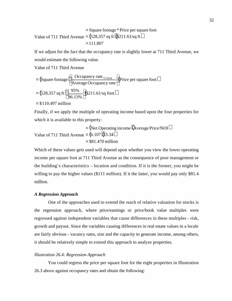
32

Value of 711 Third Avenue ( )( )111.807

ft /sq61.211$ft sq 528,357

foot squareper Price*footage Square

===

If we adjust for the fact that the occupancy rate is slightly lower at 711 Third Avenue, we

would estimate the following value.

Value of 711 Third Avenue

( ) ( )

( ) ( )

million 110.497 $

foot $211.61/sq96.13%

95%ft sq 528,357

foot squareper PricerateOccupancy Average

rateOccupancy footage Square third711

=

=

=

Finally, if we apply the multiple of operating income based upon the four properties for

which it is available to this property:

Value of 711 Third Avenue

( )( )( )( )

million 470.81$

34.13107.6

Price/NOI Averageincome OperatingNet

===

Which of these values gets used will depend upon whether you view the lower operating

income per square foot at 711 Third Avenue as the consequence of poor management or

the building’s characteristics – location and condition. If it is the former, you might be

willing to pay the higher values ($111 million). If it the latter, you would pay only $81.4

million.

A Regression Approach

One of the approaches used to extend the reach of relative valuation for stocks is

the regression approach, where price/earnings or price/book value multiples were

regressed against independent variables that cause differences in these multiples - risk,

growth and payout. Since the variables causing differences in real estate values in a locale

are fairly obvious - vacancy rates, size and the capacity to generate income, among others,

it should be relatively simple to extend this approach to analyze properties.

Illustration 26.4: Regression Approach

You could regress the price per square foot for the eight properties in Illustration

26.3 above against occupancy rates and obtain the following:

33

Price per square foot = -2535.50 + 2857.86 Occupancy rate R2 = 46%

(-2.07) (2.25)

Using this regression, we would obtain an estimated price per square foot for 711 Seventh

Avenue, with its 95% occupancy rate.

Price per square foot = -2535.70 + 2857.86 (0.95) = $179.46

Value of 711 Third Avenue = 528,357 * $179.46 = $94.820 million

This regression is clearly limited in its power because there only eight observations and

the occupancy rates are very similar. If we can obtain information on more properties and

include variables on which there are bigger differences – a variable measuring the age of the

building, for instance – we would be able to get much stronger predictions.

Valuing Real Estate Businesses

We have focused on valuing real estate properties through much of this chapter. In

this section, we consider extending this analysis to value a real estate business. To value

such a business, you have to consider its sources of income and then look at its

organization structure.

Sources of Income

Real estate businesses vary widely in terms of how they generate income and how

you approach valuation will vary as well. In particular, we could categorize real estate

firms into four businesses.

Service Income: Some firms generate income from providing just management services or

support services to the owners of real estate – for instance, selling, security or

maintenance. Valuing these firms is relatively straight forward and requires assumptions

about how fees will be assessed – many management service contracts, for instance, are

stated as a percent of the gross income on a property – and how much the fee income will

increase over time. More efficient firms or firms with better reputations (brand name)

may be able to charge higher fees and be worth more.

Real Estate Construction: These businesses make their income from real estate

construction – building residential or commercial properties. They usually agree to deliver

the units at a contractually fixed price and generate profits from being able to construct

them at a lower cost. Firms that are more cost-efficient will generally earn higher profits

34

and be worth more. Here again, though, reputation can make a difference and firms that

are associated with quality construction may be able to charge premium prices.

Real Estate Development: These businesses usually buy vacant or under utlitized land,

put up new construction and sell the units to real estate investors. They generally do not

hold on to the properties for purposes of generating on-going income. The values of these

businesses will be determined by their capacity to gauge market demand and complete

construction both quickly and at low cost.

Real Estate Investment: These are businesses that buy real estate property as income-

generating investments. The simplest way of valuing these businesses is to value each of

the properties that they own and to aggregate them. However, a premium may be

attached to this value, if a business has shown the capacity to repeatedly buy under

valued properties.

Thus, the factors we should think about when valuing real estate businesses are

the same factors we think about in any valuation – the capacity to generate not just cash

flows but also excess returns and the uncertainty associated with these cash flows.

Organizational Structure

There are four basic organizational forms available to real estate business – real

estate investment trusts (REIT), limited partnerships (MLP), business trusts and real

estate corporations. They differ in two major areas.

Structure of Taxation

Single taxation is a characteristic of REITs and MLPs, since both are taxed at the

investor level, but not at the firm level. This tax benefit is given to REITs to compensate

for certain investment and dividend policy restrictions to which REITs must adhere.

MLPs receive single-taxation status only if they invest in certain activities, such as real

estate or oil and gas. Otherwise, for tax purposes, MLPs are treated as a corporation.

This tax advantage does not exist for business trusts and corporations that are taxed at

both the entity level on income and at the investor level on dividends.

What are the implications for valuation? When valuing real estate investment

trusts and master limited partnerships, the tax rate used to estimate cash flows and

discount rates is zero. That does not mean that there are no tax benefits from depreciation

35

or interest expenses, since these benefits still flow through to the ultimate investors.

When valuing real estate corporations, the marginal corporate tax rate should be used for

estimating cash flows and discount rates.

Restrictions on Investment and Dividend Policy

The tax code requires REITs to distribute 95% of their taxable income to

shareholders, which effectively limits REITs’ use of internal financing. Consequently,

REITs must return to the capital markets on a regular basis, which in turn tends to impart

discipline and monitoring. The code further requires that a minimum of 75% of a REIT’s

gross income come from real estate. A REIT must also be a passive investment conduit,

i.e., less than 30 percent of a REIT’s income must come from the operation of real estate

held less than four years and income from the sale of securities held less than one year.

REITs cannot engage in active real estate operations. They cannot operate a business,

develop or trade properties for sale, or sell more than five properties per year. A REIT is

prohibited from entering into tax-free exchanges to acquire properties. Although no

dividend payout restrictions exist for MLPs, a high payout ratio is likely, since partners

are taxed regardless of whether they actually receive the income or the MLP retains it.

This fact has to be weighed off against the investment opportunities of an MLP. The

empirical evidence suggests that MLPs pay out a high proportion of their earnings as

dividends. Although MLPs are restricted in engaging in real estate activities (or oil and

gas), there are no restrictions on the nature or management of these activities.

Consequently, MLPs can actively and directly engage in the real estate trade or business.

There are no MLP restrictions on the number of properties that can be sold in any given

year. Business trusts and corporations have no restrictions on dividend payout, they can

engage in any real estate or non-real estate activity except those prohibited in the

declaration of trust or corporate charter, respectively.

The implications for valuation are significant. When valuing REITs and MLPs,

you have to assume much of the earnings will be paid out in dividends. If you do not

assume external financing, your estimates of expected growth will be low, not matter how

well managed the entities are. If you do allow for external financing, you can have high

expected growth but the number of shares in the firm will have to increase

proportionately, thus limiting the potential price appreciation on a per-share basis. The

36

restrictions on investment policy will constrain how much returns on capital can be

changed over time.

Conclusion

There is much that is said in this chapter that repeats what was said in earlier

chapters on stock valuation. This is because a real estate investment can (and, in our view,

should) be valued with the same approaches used to value financial assets. While the

structure and caveats of discounted cash flow models remain unchanged for real estate

investments, there are some practical problems that have to be faced and overcome. In

particular, real estate investments do not trade regularly and risk parameters (and discount

rates) are difficult to estimate. A real estate investment can also be valued using

comparable investments, but the difficulties in identifying ‘comparable’ assets and

controlling for differences across them remain significant problems.

37

Problems

Questions and Short Problems: Chapter 26

1. An analyst who looks at real estate decides to apply the Capital Asset Pricing Model

to estimate the risk (beta) for real estate. He regresses returns on a real estate index (based

upon appraised values) against returns on a stock index and estimates a beta of 0.20 for

real estate. Would you agree with this estimate? If you do not, what might be the sources

of your disagreement?

2. An alternative way of estimating risk for real estate is to use prices on traded REITs to

compute returns and to regress these returns against a stock index to arrive at a beta

estimate. Would this beta be a more reliable estimate of risk? Why or why not?

3. The risk for real estate can be viewed as a derived demand. If this is the case, the risk of

real estate can be estimated from the underlying business it supports. Under this view,

what would be the appropriate proxy to use for risk in the following types of real estate

investments?

a. Commercial real estate in New York.

b. Commercial real estate in Houston.

c. Commercial real estate in San Jose (Silicon Valley).

d. Hotel complex in Orlando.

4. Would your valuation of real estate be affected by who the potential investors in the

property are? [For instance, would your analysis be any different if the primary investors

were individuals, involved primarily in real estate, or if they were institutional investors?]

5. How would you factor in the absence of liquidity into your valuation?

6. You have been asked to value an office building in Orlando, Florida with the following

characteristics.

• The building was built in 1988 and has 300,000 square feet of rentable area.

• There would be an initial construction and renovation cost of $3.0 million.

• It will take two years to fill the building. The expected vacancy rates in the first two

years are as follows.

Year Vacancy Rate

38

1 30%

2 20%

After year 2 10%

• The market rents in the building were expected to average $15.00 per square foot in

the current year based upon average rents in the surrounding buildings.

• The market rents were assumed to grow 5% a year for five years and at 3% a year

forever afterwards.

• The variable operating expenses were assumed to be $3.00 per square foot and are

expected to grow at the same rate as rents. The fixed operating expense in 1994

amounted to $300,000 and was expected to grow at 3% forever.

• The real estate taxes are expected to amount to $300,000 in the first year and grow at

3% a year after that. It is assumed that all tenants will pay their pro rate share of

increases in real estate taxes that exceed 3% a year.

• The tax rate on income was assumed to be 42%.

• The cost of borrowing was assumed to be 8.25%, pre-tax. It was also assumed that

the building would be financed with 30% equity and 70% debt.

• A survey suggests that equity investors in real estate require a return of 12.5% of

their investments.

a. Estimate the value of the building, based upon expected cash flows.

b. Estimate the value of just the equity stake in this building.

7. You are trying to value the same building based upon “comparable properties” sold in

recent years. There have been six property sales of buildings of comparable size in the

surrounding area.

Property Sale Price Size (Sq. Ft) Gross Rent

A $ 20,000,000 400,000 $ 5,000,000

B $ 18,000,000 425,000 $ 4,750,000

C $ 22,000,000 450,000 $ 5,100,000

D $ 25,000,000 400,000 $ 5,500,000

E $ 15,000,000 350,000 $ 4,000,000

39

F $ 12,000,000 300,000 $ 3,000,000

a. Estimate the value of the building, based upon price/square foot.

b. Estimate the value of the building, based upon price/gross rent.

c. What are some of the assumptions you make when you value a building based upon

comparable buildings.

1

1

CHAPTER 27

VALUING OTHER ASSETS

One of the fundamental precepts of this book is that all assets, financial as well as

real, can be valued systematically using traditional valuation models. The bulk of this

book examines the valuation of stocks, but in the last chapter, we extended the reach of

valuation models to cover real estate. In this chapter, we consider other assets that are

usually considered as unique and different and attempt to value them using the principles

we have developed in the earlier chapters. Consequently, we examine how to value a wide

range of assets from franchises to a five-star restaurant.

While the assets covered in this chapter have very different characteristics and

attract different investors, they can be broadly classified into three categories.

• Assets that are expected to generate cash flows over time and can be valued with

discounted cash flow models.

• Assets that do not generate cash flows but attain value because they are scarce and

either are perceived to be valuable (collectibles, coins) and/or generate utility to their

owners (antiques, paintings). These assets can be valued using ‘comparable’ assets.

• Assets that do not generate cash flows but could be valuable in the event of a

contingency - they have option characteristics. These assets can be valued using

contingent claim valuation models.

Within each category, there are a surprising number of commonalties both across different

assets and with the financial assets described in the earlier chapters.

Cash Flow Producing Assets

A number of assets derive their value from their capacity to generate cash flows to

their owners. The value of such assets is a function of their capacity to generate cash

flows in the future and the uncertainty associated with these cash flows. The basic

principles of discounted cash flow valuation, described in earlier chapters, apply for any

of these assets and require the following steps.

• Estimate cash flows on the asset for the estimation period. These cash flows can

either be pre-debt (cash flows to the firm) or after-debt cash flows (cash flows to

equity).

2

2

• Estimate the value of the asset, if any, at the end of the estimation period. This value

will deplete over time if the asset loses value with use or has a limited life and may, in

some cases, be zero.

• Estimate a discount rate that reflects the riskiness of the cash flows. This discount

rate will be the cost of equity if the cash flows discounted are cash flows to equity

and the cost of capital if the cash flows are cash flows to the firm.

• Calculate the present value of the cash flows to arrive at the value of the asset or the

value of the equity in the assets.

There are several practical problems associated with applying these steps to assets when

cash flows are difficult to estimate and risk cannot be easily quantified (and converted

into a discount rate). In most cases, these problems are not insurmountable and can be

overcome. Since the problems and the solutions vary from case to case, we consider a

series of examples, ranging from the valuation of a simple franchise to more complex

businesses.

Valuing a Franchise

A franchise gives you the right to market or sell a product or service of a brand-

name company. Examples of franchises would include the thousands of McDonald’s

around the world, dealerships for the automobile companies and, loosely defined, even a

New York City cab medallion. In each case, the franchisee (the person who buys the

franchise) pays the franchisor (McDonald’s or Ford) either an up-front fee or an annual

fee for running the franchise. In return, he or she gets the power of the brand name,

corporate support and advertising backing.

Franchise value and Excess Returns

The acquisition of a franchise provides the franchisee with the opportunity to earn

above-market returns for the life of the franchise. While the sources of these above-market

returns vary from case to case, they can arise from a number of different factors.

• Brand Name Value: The franchise might have a brand name value that enables the

franchisee to charge higher prices and attract more customers than an otherwise similar

business. Thus, an investor may be willing to pay a significant up-front fee to acquire

3

3

a McDonald’s franchise, in order to take advantage of the brand name value associated

with the company.

• Exclusivity: In some cases, a franchise has value because it enables a franchisee to

produce a product, the rights to which are owned by the franchisor. For instance, an

investor may pay a fee to Disney for the right to manufacture Mickey Mouse

watches or toys and hope to recoup the fee by selling more of the product or charging

a higher price for it.

• Legal Monopolies: Sometimes, a franchise may have value because the franchisee is

given the exclusive right to provide a service. For instance, a company may pay a large

fee for the right to operate concession stands in a baseball stadium, knowing that they

will face no competition within the stadium. In a milder variant of this, multiple

franchises are sometimes sold but the number of franchises is kept limited to insure

that the franchisees earn excess returns. New York City, for example, sells cab

medallions that are a pre-requisite for operating a yellow cab in the city. They also

have tight restrictions on non-medallion owners offering the same service.

Consequently, a market where cab medallions are bought and sold exists.

In essence, the value of a franchise is directly tied to the capacity to generate excess

returns. Any action or event that affects these excess returns will affect the value of the

franchise.

Special Issues in Valuing Franchises

Buying a franchise is often a mixed blessing. While the franchisee gets the backing

of a well-known firm with significant resources to back up his or her efforts, there are

some costs that may affect the value of the franchise. Among these costs are the

following.

a. The problems of the franchisor can spill over into the franchisee. For instance,

when Daewoo, the Korean automaker, borrowed too much and got into financial

trouble, their dealers around the world felt the repercussions. Similarly,

McDonald’s franchisees around the world were picketed by anti-globalization

activists. Thus, an efficient and well-run franchise’s value can be affected by

actions that it has little or no control over.

4

4

b. Since franchisors tend to be large corporations and franchisees tend to be small

business people, the former often have much more bargaining power and

sometimes take advantage of it to change the terms of franchise agreements in their

favor. Franchisees can increase their power by banding together and bargaining as a

collective unit.

c. The value of a franchise derives from the exclusive rights it grants the franchisor to

sell the products of a firm. This value can be diluted if a franchise is granted to a

competitor. For instance, the value of a Days Inn franchise may be diluted if

another Days Inn is allowed to open five miles down the highway.

Illustration 27.1: Valuing a New York City Cab Medallion: June 1994

Background

• In 1994, New York City had 11,787 cab medallions outstanding1. The owner of a cab

medallion has the right to operate a yellow cab in the five boroughs of New York City

– Manhattan, Brooklyn, the Bronx, Queens and Staten Island.

• New York City restricts non-medallion owners from picking up customers on the

street, though they can still be summoned in other ways.

• All yellow cabs in the city are regulated by the Taxi and Limousine commission,

which sets fares and reserves the right to fine owners who do not follow its numerous

requirements.

Cash Flows on a Cab Medallion

• The typical New York City cab is a Chevrolet Caprice. The cost of acquiring one in

1994 was approximately $15,000 and it has an expected life of ten years. The cab can

be depreciated over the life down to a salvage value of zero.

• A cab can be expected to be on the road 330 days of the years, with an expected down

time (for maintenance) of 35 days, and make $250 a day prior to meeting operating

expenses, maintenance expenses and covering the cost of time for the driver.

• The annual cost of fuel and operating expenses is expected to be 25% of revenues and

the maintenance expenses are expected to amount to $1,500 a year.

5

5

• The cost of automobile insurance, covering the cost of collision, theft and bodily

harm, is $2,000 per year.

• The annual fee to be paid to the Taxi and Limousine commission is $500. Other

licensing costs are expected to amount to $500 a year.

• The total cost per day, inclusive of benefits, of the driver of the cab is expected to

amount to $100. (This also includes the 35 days where the car is down for

maintenance.)

Estimating Risk and Discount Rates

• The capacity of a cab to pull in the expected revenues is a function of several

variables.

• The state of the city’s economy: The more buoyant the economy of the city,

the greater are the potential revenues from owning and operating a cab in it.

Since the state of New York City’s economy is, in large part, driven by the

state of the financial services sector, there is in all likelihood a positive

correlation between cab revenues and financial service sector health.

• The scarcity of cabs: The value of a cab medallion is derived directly from the

fact that there are only a limited number of medallions out there. To the extent

that the city can either issue more medallions or allows gypsy cabs (unlicensed

taxis) to operate within the environs of the city, it can affect the expected

revenues.

• The fare structure: Since the fare structure is regulated, the expected revenues

from owning a cab in the future will be dependent on the generosity of raises

that the Taxi and Limousine Commission allows.

• There are a number of other potential sources of risk including collision and theft

which have already been built into the cost structure. To the extent that these are

estimates, they could also create swings in the cash flows.

Assuming that the expected revenues factors in the number of medallions outstanding and

the expected changes in the fare structure already, the primary source of risk in owning a

cab medallion is expected to be from shifts in the city’s economy. If the health of the

1 The number of cab medallions had been frozen at this level since 1937. A proposal in 1995 planned to

6

6

city’s economy is a function of the financial service sector, the risk of owning a cab

medallion should be similar to the risk of investing in a financial service firm. The average

beta of financial service firms headquartered in New York City is 1.25. At the end of

1994, with treasury bond rates at 8% and using a market risk premium of 5.5%, the cost

of equity can be calculated.

Cost of Equity = 8% + 1.25 (5.5%) = 14.88%

This will be used as the cost of equity in valuing a cab medallion.

Financing Mix

Assume that the medallion will be financed half with equity and half with debt,

and that the debt will carry an interest rate of 10% per annum. Allowing for a marginal tax

rate (federal, state and city) of 40%, the cost of capital for valuing the medallion is:

Cost of Capital = 14.88% (0.5) + 10% (1-0.4) (0.5) = 10.44%

Estimating Future Growth and Value

It is assumed that the expected operating income from owning a cab will keep up

with expected inflation, which is assumed to be 3%, in the long term. The pre-debt cash

flow from owning a cab medallion is provided in Table 27.1.

Table 27.1: Expected Cash flows from Operating a Cab

Item Calculation Amount

Revenues (330 * 250) $ 82,500

Expenses

a. Driver (365 * 100) $ 36,500

b. Fuel & Operating (25% of Revenues) $ 20,625

c. Maintenance ($1500/year) $ 1,500

d. Depreciation ($1500/year) $ 1,500

e. Fees & License Costs ($1000/year) $ 1,000

EBIT $ 21,375

raise this number by 400, and faced stiff opposition from existing medallion owners.

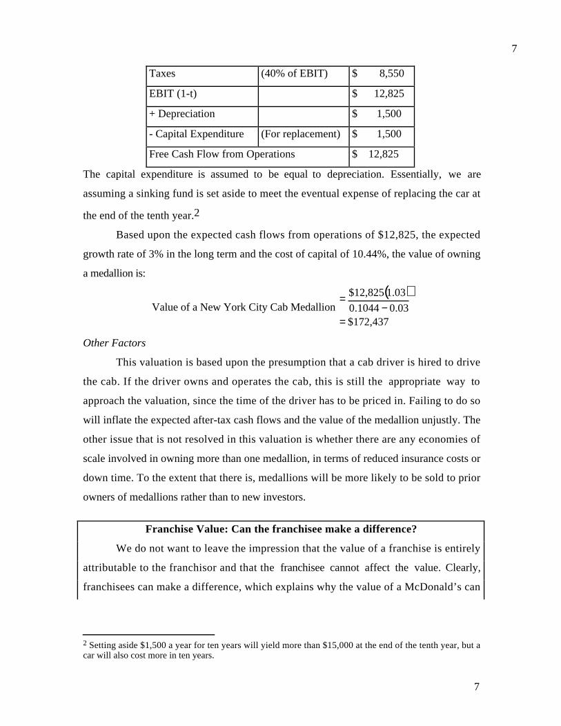
7

7

Taxes (40% of EBIT) $ 8,550

EBIT (1-t) $ 12,825

+ Depreciation $ 1,500

- Capital Expenditure (For replacement) $ 1,500

Free Cash Flow from Operations $ 12,825

The capital expenditure is assumed to be equal to depreciation. Essentially, we are

assuming a sinking fund is set aside to meet the eventual expense of replacing the car at

the end of the tenth year.2

Based upon the expected cash flows from operations of $12,825, the expected

growth rate of 3% in the long term and the cost of capital of 10.44%, the value of owning

a medallion is:

Value of a New York City Cab Medallion ( )

172,437$03.01044.0

1.03$12,825

=−

=

Other Factors

This valuation is based upon the presumption that a cab driver is hired to drive

the cab. If the driver owns and operates the cab, this is still the appropriate way to

approach the valuation, since the time of the driver has to be priced in. Failing to do so

will inflate the expected after-tax cash flows and the value of the medallion unjustly. The

other issue that is not resolved in this valuation is whether there are any economies of

scale involved in owning more than one medallion, in terms of reduced insurance costs or

down time. To the extent that there is, medallions will be more likely to be sold to prior

owners of medallions rather than to new investors.

Franchise Value: Can the franchisee make a difference?

We do not want to leave the impression that the value of a franchise is entirely

attributable to the franchisor and that the franchisee cannot affect the value. Clearly,

franchisees can make a difference, which explains why the value of a McDonald’s can

2 Setting aside $1,500 a year for ten years will yield more than $15,000 at the end of the tenth year, but acar will also cost more in ten years.

8

8

increase when it passes from one franchisee to another. There are several factors that

explain these differences.

Efficiency: Some franchisees do a much better job in controlling costs and generating higher

margins than others. To illustrate, a large proportion of low-cost hotels and inns in the

United States is owned by a small immigrant group from India. Since the owner’s entire

family often works at the hotel, at low or no pay, their employee costs tend to be lower,

allowing them to turn a larger profit than a passive owner would have.

Personal component: There remains a personal component in many franchises that can

make a significant difference to value. For instance, while there are thousands of Ford and

GM dealers around the country, a handful of them account for a significant portion of the

sales.

Economies of scale: There are economies of scale associated with owning several

franchises from the same firm. For instance, you often see franchisees who own more

than one franchise of the same company. By pooling several franchises, you might be able

to reduce your administrative costs and increase the profitability of each.

Valuing Businesses with a Personal Component

Many businesses derive a significant portion of their value from a ‘key person’,

who is often the owner, and may be worth significantly less if run by someone else. In

these cases, it is important that the consequences of losing this key person is built into

the valuation. It is also important that the additional risk associated with the dependence

upon an individual be factored into the analysis.

There are a number of examples we can offer for businesses with personal

components. Consider the following.

• Expensive restaurants are identified closely with the chefs that run their

kitchens. Thus, when a chef is incapacitated or moves to a competitor, the

number of customers may drop off dramatically.

• Many service businesses, ranging from plumbing to dentistry to tax

accounting, have a personal component. Hence, when the person providing the

service moves on, a large portion of the value of the business could be lost.

Thus, a dentist who pays a large amount for a thriving dental practice of

9

9

another dentist may see a drop in business after the purchase. This effect will

be accentuated if the seller can start a competing business.

• A mutual fund company may derive its value from its most recognized fund

managers. If they move to a competitor or start their own funds, they could

take a large portion of the money they manage with them.

So, how should we value these businesses and the component of value that is attributable

to the “key person”? The answer depends upon why you are doing the valuation in the

first place. If the objective is to value the business for the existing owner, you may

separate out the portion of value due to the owner’s personal connections and skills, if

there are no immediate consequences. If the objective is to value the business for a

potential buyer, the simplest way to avoid overpaying is to do two valuations – one with

the business as is, with the existing owner, and one, without the existing owner, making

reasonable assumptions about the degree to which business will drop. The latter will be

much lower than the former and will represent the price you would be willing to pay.

There are intermediate steps that can be taken to minimize the slippage in value.

First, you could contract with the owner to remain with the firm after you buy it, which

should reduce the drop off in customers. Second, you could apprentice or help the owner

for a transition period before you buy the business. This will allow customers or patients

to get used to you before the business passes hands and may reduce the number that

leaves after the transaction. Third, you should ensure that the owner cannot start a

competing business and extract business from you for the foreseeable future.

Illustration 27.2: Valuing a dental practice

Assume that you are a young dentist, specializing in pediatric dentistry, and that

you are interested in buying a dental practice located in Chatham, New Jersey. The

dentist who owns the practice has built it up over the last two decades and the practice

generated $500,000 in revenues last year. The expenditures associated with running this

practice last year include the following.

• Employee expenses (including dental hygienists and secretarial help) amounted to

$150,000 last year and are expected to grow 3% a year for the next 10 years.

10

10

• The annual rent for the facilities last year was $50,000 and is expected to grow 3% a

year for the next 10 years.

• Rentals of medical equipment cost $40,000 last year and this expense is expected to

grow 3% for the next 10 years.

• The cost of medical insurance last year was $60,000 and is expected to grow 3% a

year for the next 10 years.

• The tax rate on the income, including state and local taxes, is 40%.

• The cost of capital is 10%.

To value the practice, we will assume that revenues would have grown 3% a year for the

next 10 years if the current dentist continued to run the practice, but that there will be a

drop off of 20% in the first year’s revenues if a new dentist comes into the practice. The

growth rate of 3% will still occur in the following years but on the lower base revenues.

We will first value the practice with the current dentist. To make this estimate, we

will begin by estimating the cash flows in the first year to the practice.

Cash flow in year 1

( )( )( )( ) ( )( )( )( )

600,123$

40.0103.1000,60000,40000,50000,15003.1000,500

ratetax -1Expenses Operating-Revenues 11

=−+++−=

=

Using the cost of capital as the discount rate and the growing annuity equation for a 10-

year period, we can estimate the value of the practice.

Value of practice 850,831$)03.010.0(

)10.1(

)03.1(1

600,123)(

)1(

)1(1

CF10

10

1 =

−

−=

−++−

=grrg

n

n

We assume that the value of the practice fades after ten years and therefore attach no

terminal value.

We will follow up by valuing the practice with a new dentist in place. The cash

flow in year 1 will be lower because the revenues will be lower.

Cash flow in year 1

11

11

( )( )( )( )( ) ( )( )( )( )

800,61$

40.0103.1000,60000,40000,50000,15003.18.0000,500

ratetax -1Expenses Operating-Revenues 11

=−+++−=

=

Value of practice 425,415$)03.010.0(

)10.1(

)03.1(1

61,80010

10

=

−

−=

Notice that the value is halved and the difference can be viewed as the value of the key

person.

As a potential buyer, the new dentist should offer the latter value for the practice.

However, if he can arrange for a transition period where the current dentist stays with the

practice after the transaction, he or she may be willing to pay a higher price.

Illustration 27.3: Valuing a five-star restaurant – Lutece in 1994

Lutece is a renowned restaurant located at 249 East 50th Street in Manhattan. In

1994, Lutece was sold by its owner/chef Andre Soltner to Ark Restaurants, a publicly

traded restaurant chain, for an undisclosed amount. The New York Times, blanching as a

result of the sale ran the headline, “Lutece, a Dining Landmark, Is Sold to a Chain

Operator”, which was then followed by an article detailing the surprise marriage of the

classic French restaurant to Ark, a company largely known for operating theme concepts.

Bryan Miller, the Times' former restaurant reviewer and writer of the piece, likened the

addition of Lutece to Ark's portfolio to "hanging a Van Gogh in a community art exhibit."

Background

Lutece was founded in 1961 by Andre Soltner and quickly acquired a reputation

for serving food of exceptional quality. It has received a five-star rating from Mobil for 24

consecutive years and is one of five New York City restaurants that gets a four-star rating

(the highest) from the New York Times. In a sign of slippage, however, its ranking in the

Zagat Survey of New York City restaurants dropped to eighth from being perennially at

or near the top for much of the seventies and eighties.

Estimating Cash Flows

The following are some of the background facts on Lutece.

12

12

• The restaurant can seat 92 diners. It has one seating for lunch and two seatings for

dinner. It fills in 70% of its seats at lunchtime and 80% of its seats at dinner.

• The restaurant stays open 340 days every year, and is closed for the remaining 25

days.

• The average price of a lunch is $30 and the average price of a dinner is $66.

Approximately, one third of this is for liquor.

• There are 42 employees on the staff of the restaurant. The cost of food is

approximately 30% of the price of the meal and the payroll amounts to $1.25 million

a year.

• The annual rent for the space used by the Lutece is $600,000.

Table 27.2 is an estimation of the after-tax operating cash flows in 1994 for Lutece.

Table 27.2: Expected cash flows from Lutece - 1994

Assumption Base Year

Revenues

Lunch (70% occupancy; $30 per person) $ 656,880

Dinner (80% occupancy; $66 per person) $ 3,303,168

Total $ 3,960,048

Expenses

Food (30% of revenues) $ 1,188,014

Staff ($1,250,000 for staff expenses) $ 1,250,000

Rent $ 600,000

Total $ 3,038,014

EBIT $ 922,034

Taxes (Assumed tax rate of 40%) $ 368,813

EBIT (1-t) $ 553,220

These cash flows are expected to grow 6% a year for three years and 3% a year after that.

The following table summarizes the expected cash flows over the next three years.

Table 27.3: Expected cash flows from Lutece – next 5 years

Base Year 1 2 3

13

13

Revenues 3,960,048 4,197,651 4,449,510 4,716,481

Expenses 3,038,014 3,220,295 3,413,513 3,618,324

EBIT 922,034 977,356 1,035,997 1,098,157

Taxes 368,813 390,942 414,399 439,263

EBIT (1-t) 553,220 586,413 621,598 658,894

Estimating Discount Rates

The acquirer in this case, Ark Restaurants, has a relatively low beta (0.7), and gets

only about 10% of its financing needs from debt. Assuming that the underlying risk in

investing in Lutece is similar, the cost of equity can be estimated as follows.

Cost of Equity = 8% + 0.7 (5.5%) = 11.85%

(This assumes that the long term treasury bond rate is 8%.)

If Ark Restaurants can borrow money at 9% and faces a 40% tax rate, the cost of capital

can be calculated.

Cost of Capital = 11.85% (.90) + 9% (1-0.4) (.10) = 11.20%

Estimating Value

The value of Lutece can be estimated by discounting the cash flows at the

weighted average cost of capital. Allowing for a growth rate of 6% over the next three

years and 3% after that, the value of the restaurant can be estimated as follows.

Value at the end of the high growth period

( )

( )

8,271,309$03.01120.0

1.03658,894

g-WACC

t-1EBIT

n

4

=−

=

=

Value of Lutece 7,524,559

1.1120

8,271,309658,894

1.1120

621,598

1120.1

86,413532

=

+++=

Valuing the ‘Key Person’

There would be probably no argument that much of Lutece’s value derives from

Andre Soltner’s presence as chef. It would be worth examining how much this value

would change if he were to be replaced by somebody else. The simplest way to evaluate

this effect is to:

14

14

• Estimate the effect on occupancy of replacing Mr. Soltner with another chef, and

through this on cash flows. To the extent that occupancy and cash flows decline, the

value of the restaurant will decline.

• Calculate the value of the restaurant based on the discounted cash flows.

In extreme cases, where the entire value of an enterprise depends upon one person, the

value can drop to essentially zero if the key person were to leave or die. In less extreme

cases, the value of the key person can be estimated to be the difference between the

values of the enterprise with and without that person in place3.

Valuing Trademarks, Copyrights and Licenses

Trademarks, copyrights and licenses all give the owner the exclusive right to

produce a product or provide a service. Fundamentally, then, their value is derived from

the cash flows that can be generated from the exclusive right. To the extent that there is a

cost associated with production, the value comes from the excess returns that come from

having the exclusive right.

As with other assets, you can value trademarks or copyrights in one of two ways.

You can estimate the expected cash flows from owning the asset, attach a discount rate to

these cash flows that reflects their uncertainty and take the present value, which will

yield a discounted cash flow valuation of the asset. Alternatively, you can attempt a

relative valuation, where you apply a multiple to the revenues or income that you believe

that you can generate from the trademark or copyright. The multiple is usually estimated

by looking at what similar products have sold for in the past.

In making these estimates, you are likely to run into estimation issues that are

unique to these assets. First, you have to consider the fact that a copyright or trademark

provides you exclusive rights for a finite period. Consequently, the cash flows you will

estimate will be for only this period and there will generally be no terminal value. Second,

you have to factor in the expected costs of violations of the copyright and trademark.

These costs can include at least two items. The first is the legal and monitoring cost

3 Consider the value of David Letterman to CBS. One estimate in the New York Times claimed that 20%of the profits at CBS could be traced to the success of David Letterman’s show. If this is true, CBS may begetting an incredible bargain, even at $5 million a year.

15

15

associated with enforcing exclusivity. The second is the fact that no matter how careful

you are with the monitoring, you cannot ensure that there will be no violations, and the

lost revenues (profits) that arise as a consequence will lower the value of the right.

Illustration 27.4: Valuing the Copyright on “Investment Valuation”

Assume that John Wiley has been approached by another publisher who is

interested in buying the copyright to this book (Investment Valuation). To estimate the

value of the copyright, we will make the following assumptions.4

• The book is expected to generate $150,000 in after-tax cash flows for the next three

years and $100,000 a year for the next two years. These are the cash flows after

author royalties, promotional expenses and production costs.

• About 40% of these cash flows are from large organizations that make bulk orders and

are considered predictable and stable. The cost of capital applied to these cash flows

is 7%.

• The remaining 60% of the cash flows are to the general public and this segment of the

cash flows is considered much more volatile. The cost of capital applied to these cash

flows is 10%.

The value of the copyright can be estimated using these cash flows and the cost of capital

that has been supplied in Table 27.4:

Table 27.4: Value of Copyright

Year Stable Cashflows Present value @ 7%

Volatile

Cashflows Present value @ 10%

1 $60,000 $56,075 $90,000 $81,818

2 $60,000 $52,406 $90,000 $74,380

3 $60,000 $48,978 $90,000 $67,618

4 $40,000 $30,516 $60,000 $40,981

5 $40,000 $28,519 $60,000 $37,255

$216,494 $302,053

4 I am intentionally making these assumptions as optimistic as I can. I hope you, as the reader, can makethe actual cashflows resemble my estimates.

16

16

The value of the copyright, with these assumptions, is $518,547 (which is the sum of

$216,494 and $302,053).

Non Cash Flow Producing Assets

Assets that do not produce cash flows cannot be valued using discounted cash

flow models. They derive their value from a combination of factors – a scarcity of supply

relative to demand, consumption utility and individual perceptions. While they can be

valued relative to comparables, their values are also much more volatile since they are

based entirely upon perceptions. There is a wide range of assets that fall under this

category from limited edition Barbie dolls to rare coins and wine.

Special Issues in valuing non-cash flow producing assets

The biggest difference between these assets and cashflow generating assets is that

there is no intrinsic value backing up the price. Consequently, the only way to value these

assets is by using relative valuation – i.e., by looking at how similar assets are priced in

the market.

The process of using comparables in valuing an asset is fairly straightforward, at least

in the abstract. The first step in the process is to collect a group of comparable assets.

The second is to estimate a measure of standardized value for this group. The third is to

control for differences between assets in this group and the asset being valued to arrive at

a measure of reasonable value for the asset. The problems in applying this approach are

as follows.

• Finding comparable assets may be difficult to do for some non-cash-flow producing

assets. While there are indices compiled on various unconventional assets, there are

substantial differences between the assets within each index.

• The markets for many of these assets are neither liquid nor public. Many transactions

are private and the reported prices are therefore unreliable.

• It is not clear how one controls for differences across assets which are comparable,

when these differences are not quantitative but relate to perception.

• The prices of many of these assets are directly related to how scarce the supply of

the asset is. For instance, the reason that the Honus Wagner T-206 baseball card is the

most highly valued card on the market is that there are only 58 known cards in

17

17

existence and only one in mint condition.5 The flip side of this is that any event that

alters this balance will affect the price. Thus, a surprise find of another mint condition

Honus Wagner card in someone’s attic can cause the price to change dramatically.

Art and Collectibles

There are many investors who view investments in art and collectibles as part of

their overall portfolio. In that context, it is worth asking the following questions.

• The first relates to the type of returns that these investments generate for investors

over long periods. There are a number of studies that have looked at this question. In

one of the more comprehensive analysis of art as an investment, Mei and Moses

constructed an index based upon repeated sales of artwork between 1875 and 2000

and their results are summarized in Table 27.5.

Table 27.5: Returns from Art versus S&P 500

Art Stocks

Mean

Standard

Deviation Mean

Standard

Deviation

1875-1999 5.60% 25.60% 11.10% 19.00%

1900-1999 4.70% 20.30% 12.20% 19.80%

1950-1999 5.30% 9.30% 14.60% 16.50%

As a stand alone investment, art has earned low returns historically. In the last 50

years, the returns on art have become less volatile but that may reflect the fact that

there are more transactions in this period than in earlier ones. Does the low return

make art a bad investment? Not necessarily. In Table 27.6, we examine the correlation

between the returns on art, stocks and treasury bonds:

Table 27.6: Correlation between investmentsArt S&P 500 T.Bonds

Art 1

5 This is the card that sold for $640,000 in 1996 to Michael Gidwitz, an investor from Chicago. The cardhad been earlier owned by Wayne Gretzky, the hockey great, who bought it for $451,000 in 1991.

18

18

S&P 500 0.13 1

T.Bonds -0.01 0.05 1

The low correlation between the returns of art and stocks may give it a place in a well

diversified portfolio of financial assets, but only at the margin.

• The second relates to how best to value investments in art and collectibles. In

practice, they are almost always valued on a relative basis. Thus, a Picasso is usually

valued by looking at what other Picassos have sold for recently.

Generally speaking, there are at least three problems that we run into in the context of

valuation. The first is that this is not a very liquid market and there are relatively few

transactions. Thus, the most recent sale of a Picasso might have been three years ago and

a great deal might have changed in the art market since then. The second is that no two

Picassos are alike and there are substantial differences (both in style and value) across

different paintings. The third problem is that there is the very real possibility of forgery

and fraud and much of it can be detected only by an expert eye. Consequently, the

relative valuation of art and collectibles remains the province of expert appraisers, who

try to overcome these problems (though not always successfully) and estimate a fair

value. Like all analysts, however, they are susceptible to market moods and bubbles and

busts are just as common in this market as they are in other ones.

So, what are the lessons for individual investors? The first is that while art and

collectibles, as a class, may balance a portfolio, you have to spend substantially more

time acquiring specialized knowledge to be successful with these investments than you

would with financial investments. The second is that you should expect to have much

higher transactions costs with investments in art and collectibles, especially at the high

end of the market. The third is that you should collect baseball cards or Old Master

paintings because you enjoy them and not just as investments. The psychic returns that

you receive will then compensate for the sub-standard financial returns that you may well

earn.

Other Assets

As any regular visitor to Ebay will attest, even the most unconventional assets

have to be priced and often the prices are based upon comparable assets. Thus, you can

19

19

attach a value to a baseball card (for instance, a Mickey Mantle rookie card) by looking at

the prices at which similar cards have sold. In fact, there are publications that list out

prices for traded cards, categorized by the condition of the card.

One case where a model for comparables seems to have fairly remarkably well is in

the area of valuing wine vintages. Professor Orley Ashenfelter at Princeton University has

developed a regression model, which factors in temperature and rainfall in wine growing

regions, to evaluate wine vintages (Bordeaux, California cabernet sauvignon, red

Burgundy, Sauternes and Port wines) and come up with estimates of value per bottle,

which is published in his newsletter titled “Liquid Assets”. The analog from stock

valuation would be to compare price earnings ratios across firms, controlling for risk and

growth characteristics.

Assets with Option Characteristics

Some assets derive their value not from the cash flows that they generate or from

highly valued comparables, but from the potential that they possess to be valuable in the

future, contingent on an event occurring. The values of these assets will exceed their

discounted cash flow or relative values, with the difference coming from the option

component.

One example would be art produced by an unknown artist that could be valuable if

the artist is discovered. Another example would be the copyrights and trademarks that we

valued using traditional valuation approaches in an earlier section. You might be willing to

pay a premium for some licenses or trademarks because of the option component. For

instance, a publisher bidding for a book has to consider the possibility that the book could

be a runaway success: think of Bloomsbury, the publisher who brought out the first

Harry Potter book. A final example would be investing in an off-Broadway show or low-

budget movie. While the expected cash flows from the investment may be lower than the

cost – making it a poor investment on a discounted cash flow basis – there is a chance,

albeit small, that the show could be successful enough to make it to Broadway and

perhaps even into a movie. In each of these cases, you could value these assets as options

and we will consider a few applications in the next three chapters.

Conclusion

20

20

This chapter provides an insight into the breadth of use that valuation models can

be put to, ranging from valuing a New York City Cab Medallion to a five-star restaurant.

The basic models remain unchanged, but the inputs may be more difficult to get and have

more noise associated with them. That should however not be viewed as a barrier to their

use.

21

21

Problems

1. Cool Café is a well-regarded restaurant in the Denver area, owned and operated by

Joanne Arapacio, a star chef specializing in Southwestern cuisine. You are interested in

buying the restaurant and have been provided the income statement for the firm for the

most recent year (in ‘000s).

Revenues $ 5,000

- Operating Expenses $ 3,500

EBIT $ 1,500

- Interest Expenses $ 300

- Taxes $ 480

Net Income $ 720

The owner did not pay herself a salary last year, but you believe that you will have to

pay $200,000 a year for a new chef. The restaurant is in stable growth and is expected to

grow 5% a year for the next decade. You estimate the unlevered beta of publicly traded

restaurants to be 0.80. The average debt to capital ratio for these firms is 30% and you

believe that Cool Café will have to operate at close to this average. The riskfree rate is

6%, the market risk premium is 4% and the cost of debt is 7%.

a. Estimate the value of Cool Café

b. Now assume that you will see a drop off in revenues of 15% if Joanne Arapacio

leaves the restaurant. Assuming that 70% of the current operating expenses are

variable and that the remaining 30% is fixed, estimate the value Ms. Arapacio to

the restaurant.

2. Sick and tired of the investment banking grind, you decide to quit and buy a franchise

for a fast-growing bagel chain in your town. You have been able to get information on

what another franchise for the same chain is generating in revenues in the neighboring

town.

a. The franchise has revenues of $1 million and earnings before interest and taxes of

$150,000 last year but the owner did not assess a salary for himself. He does the

accounting and oversees the bagel shop and you believe that hiring someone else to

do what he does will cost you $50,000 annually.

22

22

b. The revenues and operating income are expected to grow 3% a year in perpetuity.

c. You expect to pay 35% of your income in taxes and use all of your investment

savings to buy the shop. The unlevered beta for franchise food chains is 0.80.

d. The owner has a bank loan outstanding of $300,000 and the book value of equity

in the business is $700,000. However, the average market debt to capital ratio of

publicly traded restaurants is 20% and the average pre-tax cost of debt for

restaurants is 8%.

e. The riskless rate is 5% and the market risk premium is 4%.

Estimate the value of the bagel shop to you.

3. You work for a publishing company and are considering bidding for the copyright to a

“Cook Light, Cook Right”, a cookbook of low-fat recipes. While the book was out-of-

print last year, you believe that you can generate $120,000 in after-tax cash flows next

year, $100,000 the year after and $80,000 in the following three years. If your cost of

capital is 12%, estimate the value of the copyright.

4. You have been asked to value the practice of Dr. Vong, a pediatrician in your town and

are provided with the following facts.

• The practice generated $800,000 in revenues last year and these revenues are expected

to grow 4% a year for the next 10 years.

• Employee expenses (including nurses and secretarial help) amounted to $200,000 last

year and are expected to grow 4% a year for the next 10 years.

• The annual rent for the facilities last year was $100,000 and is expected to grow 4% a

year for the next 10 years.

• Rentals of medical equipment cost $75,000 last year and this expense is expected to

grow 5% for the next 10 years.

• The cost of medical insurance last year was $75,000 and is expected to grow 7% a

year for the next 10 years.

• The tax rate on the income, including state and local taxes, is 40%.

• The cost of capital is 11%.

Assuming that there will be no drop-off in revenues if a new pediatrician takes over the

practice, estimate the value of the practice.

23

23

5. You are trying to decide how much you should bid on a Ken Griffey Jr. rookie baseball

card in good condition on Ebay. You notice that there have been 8 transactions involving

Ken Griffey Jr. cards in the last month on Ebay.

Transaction # Condition of card Price paid for card

1 Excellent $ 800

2 Poor $ 200

3 Good $ 550

4 Good $ 500

5 Excellent $ 850

6 Good $ 400

7 Poor $ 350

8 Excellent $ 650

a. Estimate how much you would be willing to pay for the card.

b. Now assume that the seller of the card has been rated poorly by other buyers

because he has misrepresented other items he has sold to them. What effect would

this information have on how much you would be willing to bid for the card?

6. Assume that you are a wealthy investor with your entire portfolio invested in stocks.

Your financial advisor has suggested that you buy some fine art to balance the portfolio

and based this suggestion on the low correlation between returns on stocks and returns on

fine art (ρ=0.10).

a. If the standard deviation of stock returns is 20% and the standard

deviation in fine art returns is 15%, estimate what the standard deviation

of your portfolio would be if you invested 10% of your portfolio in fine

art.

b. If the expected return on stocks is 12.5% and the expected return on fine

art is only 5%, would you add fine art to your portfolio? Explain why or

why not. (The riskfree rate is 6%.)

1

CHAPTER 28

THE OPTION TO DELAY AND VALUATION IMPLICATIONS

In traditional investment analysis, a project or new investment should be accepted

only if the returns on the project exceed the hurdle rate; in the context of cash flows and

discount rates, this translates into investing in projects with positive net present values.

The limitation of this view of the world, which analyzes projects on the basis of expected

cash flows and discount rates, is that it fails to consider fully the options that are usually

associated with many investments.

In this chapter, we will consider an option that is embedded in many projects,

namely the option to wait and take the project in a later period. Why might a firm want to

do this? If the present value of the cash flows on the project are volatile and can change

over time, a project with a negative net present value today may have a positive net

present value in the future. Furthermore, a firm may gain by waiting on a project even

after a project has a positive net present value, because the option has a time premium

that exceeds the cash flows that can be generated in the next period by accepting the

project. We will argue that this option is most valuable in projects where a firm has the

exclusive right to invest in a project and becomes less valuable as the barriers to entry

decline.

There are three cases where the option to delay can make a difference when

valuing a firm. The first is undeveloped land in the hands of real estate investor or

company. The choice of when to develop rests in the hands of the owner and presumably

development will occur when real estate values increase. The second is a firm that owns a

patent or patents. Since a patent provides a firm with the exclusive rights to produce the

patented product or service, it can and should be valued as an option. The third is a

natural resource company that has undeveloped reserves that it can choose to develop at a

time of its choosing – presumably when the price of the resource is high.

The Option to Delay a Project

Projects are typically analyzed based upon their expected cash flows and discount

rates at the time of the analysis; the net present value computed on that basis is a measure

of its value and acceptability at that time. Expected cash flows and discount rates change

2

over time, however, and so does the net present value. Thus, a project that has a negative

net present value now may have a positive net present value in the future. In a

competitive environment, in which individual firms have no special advantages over their

competitors in taking projects, the fact that net present values can be positive in the

future may not be significant. In an environment in which a project can be taken by only

one firm because of legal restrictions or other barriers to entry to competitors, however,

the changes in the project’s value over time give it the characteristics of a call option.

The Payoff on the Option to Delay

Assume that a project requires an initial up-front investment of X and that the

present value of expected cash inflows from investing in the project, computed today, is

V. The net present value of this project is the difference between the two.

NPV = V - X

Now assume that the firm has exclusive rights to this project for the next n years and that

the present value of the cash inflows may change over that time, because of changes in

either the cash flows or the discount rate. Thus, the project may have a negative net

present value right now, but it may still be a good project if the firm waits. Defining V

again as the present value of the cash flows, the firm’s decision rule on this project can be

summarized as follows:

If V > X Invest in the project: Project has positive net present value

V < X Do not invest in the project: Project has negative net present value

If the firm does not invest in the project over its life, it incurs no additional cash flows,

though it will lose what it invested to get exclusive rights to the project. This relationship

can be presented in a payoff diagram of cash flows on this project, as shown in Figure

28.1, assuming that the firm holds out until the end of the period for which it has

exclusive rights to the project.

3

Present Value of ExpectedCash Flows

PV of Cash Flows

Initial Investment in Project

Figure 28.1: The Option to Delay a Project

Project has negativeNPV in this range

Project's NPV turnspositive in this range

Note that this payoff diagram is that of a call option –– the underlying asset is the

project, the strike price of the option is the initial investment needed to take the project;

and the life of the option is the period for which the firm has rights to the project. The

present value of the cash flows on this project and the expected variance in this present

value represent the value and variance of the underlying asset.

Inputs for Valuing the Option to Delay

The inputs needed to apply option pricing theory to value the option to delay are

the same as those needed for any option using the Black-Scholes model. We need the

value of the underlying asset, the variance in that value, the time to expiration on the

option, the strike price, the riskless rate and the equivalent of the dividend yield.

Value Of The Underlying Asset

In the case of product options, the underlying asset is the project to which the

firm has exclusive rights. The current value of this asset is the present value of expected

cash flows from initiating the project now, not including the up-front investment. This

present value can be obtained by doing a standard investment analysis. There is likely to

be a substantial amount of error in the cash flow estimates and the present value,

however. Rather than being viewed as a problem, this uncertainty should be viewed as the

reason the project delay option has value. If the expected cash flows on the project were

4

known with certainty and were not expected to change, there would be no need to adopt

an option pricing framework, since there would be no value to the option.

Variance in the value of the asset

As noted in the prior section, there is likely to be considerable uncertainty

associated with the cash flow estimates and the present value that measures the value of

the project now. This is partly because the potential market size for the product may be

unknown and partly because technological shifts can change the cost structure and

profitability of the product. The variance in the present value of cash flows from the

project can be estimated in one of three ways.

• If we have invested in similar projects in the past, the variance in the cash flows

from those projects can be used as an estimate. This may be the way that a

consumer product company like Gillette might estimate the variance associated

with introducing a new blade for its razors.

• We can assign probabilities to various market scenarios, estimate cash flows and a

present value under each scenario and then calculate the variance across present

values. Alternatively, the probability distributions can be estimated for each of the

inputs into the project analysis - the size of the market, the market share and the

profit margin, for instance - and simulations used to estimate the variance in the

present values that emerge. This approach tends to work best when there are only

one or two sources1 of significant uncertainty about future cash flows.

• We can use the variance in the value of firms involved in the same business (as the

project being considered) as an estimate of the variance. Thus, the average variance

in the value of firms involved in the software business can be used as the variance

in present value of a software project.

The value of the option is largely derived from the variance in cash flows - the

higher the variance, the higher the value of the project delay option. Thus, the value of an

option to invest in a project in a stable business will be less than the value of one in an

environment where technology, competition and markets are all changing rapidly.

5

Exercise Price on Option

The option to delay a project is exercised when the firm owning the rights to the

project decides to invest in it. The cost of making this initial investment is the exercise

price of the option. The underlying assumption is that this cost remains constant (in

present value dollars) and that any uncertainty associated with the investment is reflected

in the present value of cash flows on the product.

Expiration of the Option and the Riskless Rate

The project delay option expires when the rights to the project lapse. Investments

made after the project rights expire are assumed to deliver a net present value of zero as

competition drives returns down to the required rate. The riskless rate to use in pricing

the option should be the rate that corresponds to the expiration of the option. While

expiration dates can be estimated easily when firms have the explicit right to a project

(through a license or a patent, for instance), it becomes far more difficult to obtain if the

right is less clearly defined. If, for instance, a firm has a competitive advantage on a

product or project, the option life can be defined as the expected period over which the

advantage can be sustained.

Cost of Delay

In Chapter 5, we noted that an American option generally will not be exercised

prior to expiration. When you have the exclusive rights to a project, though, and the net

present value turns positive, you would not want the owner of the rights to wait until the

rights expire to exercise the option (invest in the project). Note that there is a cost in

delaying investing in a project, once the net present value turns positive. If you wait an

additional period, you may gain if the variance pushes value higher but you also lose one

period of protection against competition. You have to consider this cost when analyzing

the option and there are two ways of estimating it.

• Since the project rights expire after a fixed period and excess profits (which are the

source of positive present value) are assumed to disappear after that time as new

1 In practical terms, the probability distributions for inputs like market size and market share can often beobtained from market testing.

6

competitors emerge, each year of delay translates into one less year of value-

creating cash flows.2 If the cash flows are evenly distributed over time and the life

of the patent is n years, the cost of delay can be calculated.

Annual cost of delay = 1

n

Thus, if the project rights are for 20 years, the annual cost of delay works out to

5% a year for the very first year. Note, though, that this cost of delay rises each

year, to 1/19 in year 2, 1/18 in year 3 and so on, making the cost of delaying

exercise larger over time.

• If the cash flows are uneven, the cost of delay can be more generally defined in

terms of the change in present value that can be expected to occur over the next

period as a percent of the present value today.

Cost of delay = Present value next period − Present value Now

Present value Now

In either case, the likelihood that a firm will delay investing in a project is higher early in

the exclusive rights period rather than later and the cost will increase as the loss in present

value from waiting a period increases.

optvar.xls: There is a dataset on the web that summarizes standard deviations in

firm value and equity value by industry group in the United States.

Illustration 28.1: Valuing the Option to Delay a Project

Assume that you are interested in acquiring the exclusive rights to market a new

product that will make it easier for people to access their email on the road. If you do

acquire the rights to the product, you estimate that it will cost you $50 million up-front

to set up the infrastructure needed to provide the service. Based upon your current

projections, you believe that the service will generate only $10 million in after-tax cash

2 A value-creating cashflow is one that adds to the net present value because it is in excess of the requiredreturn for investments of equivalent risk.

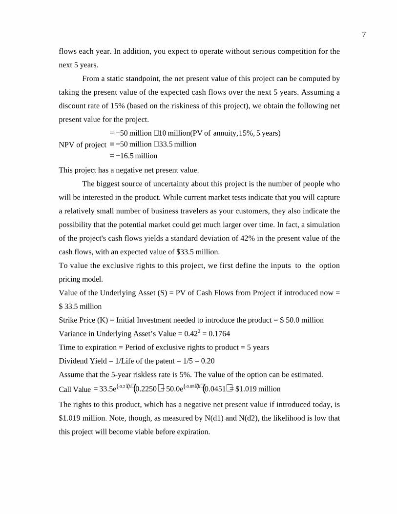
7

flows each year. In addition, you expect to operate without serious competition for the

next 5 years.

From a static standpoint, the net present value of this project can be computed by

taking the present value of the expected cash flows over the next 5 years. Assuming a

discount rate of 15% (based on the riskiness of this project), we obtain the following net

present value for the project.

NPV of project

million 5.16

million 33.5 million 50

years) 5 15%, annuity, of million(PV 10million 50

−=+−=+−=

This project has a negative net present value.

The biggest source of uncertainty about this project is the number of people who

will be interested in the product. While current market tests indicate that you will capture

a relatively small number of business travelers as your customers, they also indicate the

possibility that the potential market could get much larger over time. In fact, a simulation

of the project's cash flows yields a standard deviation of 42% in the present value of the

cash flows, with an expected value of $33.5 million.

To value the exclusive rights to this project, we first define the inputs to the option

pricing model.

Value of the Underlying Asset (S) = PV of Cash Flows from Project if introduced now =

$ 33.5 million

Strike Price (K) = Initial Investment needed to introduce the product = $ 50.0 million

Variance in Underlying Asset’s Value = 0.422 = 0.1764

Time to expiration = Period of exclusive rights to product = 5 years

Dividend Yield = 1/Life of the patent = 1/5 = 0.20

Assume that the 5-year riskless rate is 5%. The value of the option can be estimated.

Call Value ( )( )( ) ( )( )( ) million 019.1$0451.0e0.502250.0e5.33 5-0.055-0.2 =−=

The rights to this product, which has a negative net present value if introduced today, is

$1.019 million. Note, though, as measured by N(d1) and N(d2), the likelihood is low that

this project will become viable before expiration.

8

delay.xls: This spreadsheet allows you to estimate the value of an option to delay an

investment.

Arbitrage Possibilities and Option Pricing Models

In our discussion of option pricing models in chapter 5, we noted that they are based

upon two powerful constructs – the idea of replicating portfolios and arbitrage. Models

such as the Black Scholes and the Binomial assume that you can create a replicating

portfolio, using the underlying asset and riskless borrowing or lending, that has cashflows

identical to those on an option. Furthermore, these models assume that since investors can

then create riskless positions by buying the underlying option and selling the replicating

portfolio, or vice versa, the value of the call should converge on the cost of creating the

replicating portfolio. If it does not, investors should be able to create riskless positions and

walk away with guaranteed profits – the essence of arbitrage. This is why the interest rate

used in option pricing models is the riskless rate.

With listed options on traded stocks or assets, arbitrage is clearly feasible at least

for some investors. With options on non-traded assets, it is almost impossible to trade the

replicating portfolio though you can create it on paper. In the illustration above, for

instance, you would need to buy 0.225 units (the option delta) of the underlying project ( a

non-traded asset) to create a portfolio that replicates the call option.

There are some who argue that the impossibility of arbitrage makes it inappropriate

to use option pricing models to value real options, whereas other try to adjust for this

limitation by using an interest rate higher than the riskless rate in the option pricing model.

We do not think that either of these responses is appropriate. Note that while you cannot

trade on the replicating portfolios in many real options, you still can create them on paper

(as we did in illustration 28.1) and value the options. The difficulties in creating arbitrage

positions may result in prices that deviate by a large amounts from this value, but that is an

argument for using real option pricing models and not for avoiding them. Increasing the

9

riskless rate to reflect the higher risk associated with real options may seem like an obvious

fix, but doing this will only make call options (such as the one valued in illustration 28.1)

more valuable, not less.

If you want to be more conservative in your estimate of value for real options to

reflect the difficulty of arbitrage, you have two choices. One is to use a higher discount rate

in computing the present value of the cash flows that you would expect to make from

investing in the project today, thus lowering the value of the underlying asset (S) in the

model. In illustration 28.1, using a 20% discount rate rather than a 15% rate would result in

a present value of $29.1 million, which would replace the $33.5 million as S in the model.

The other is to value the option and then apply an illiquidity discount to it (similar to the one

we used in valuing private companies) because you cannot trade it easily.

Problems in valuing the Option to Delay

While it is quite clear that the option to delay is embedded in many projects,

several problems are associated with the use of option pricing models to value these

options. First, the underlying asset in this option, which is the project, is not traded,

making it difficult to estimate its value and variance. We have argued that the value can be

estimated from the expected cash flows and the discount rate for the project, albeit with

error. The variance is more difficult to estimate, however, since we are attempting the

estimate a variance in project value over time.

Second, the behavior of prices over time may not conform to the price path

assumed by the option pricing models. In particular, the assumption that value follows a

diffusion process and that the variance in value remains unchanged over time, may be

difficult to justify in the context of a project. For instance, a sudden technological change

may dramatically change the value of a project, either positively or negatively.

Third, there may be no specific period for which the firm has rights to the project.

Unlike the case of a patent, for instance, in which the firm has exclusive rights to produce

the patented product for a specified period, the firm’s rights often are less clearly defined,

in terms of both exclusivity and time. For instance, a firm may have significant advantages

over its competitors, which may, in turn, provide it with the virtually exclusive rights to a

10

project for a period of time. An example would be a company with strong brand name

recognition in retailing or consumer products. The rights are not legal restrictions,

however, and will erode over time. In such cases, the expected life of the project itself is

uncertain and only an estimate. In the valuation of the rights to the product, in the

previous section, we used a life of 5 years for the option, but competitors could in fact

enter sooner than we anticipated. Alternatively, the barriers to entry may turn out to be

greater than expected and allow the firm to earn excess returns for longer than 5 years.

Ironically, uncertainty about the expected life of the option can increase the variance in

present value and through it the expected value of the rights to the project.

Implications and Extensions of Delay Options

Several interesting implications emerge from the analysis of the option to delay a

project as an option. First, a project may have a negative net present value currently

based upon expected cash flows, but the rights to it may still be valuable because of the

option characteristics.

Second, a project may have a positive net present value but still not be accepted

right away. This can happen because the firm may gain by waiting and accepting the

project in a future period, for the same reasons that investors do not always exercise an

option that is in the money. A firm is more likely to wait if it has the rights to the project

for a long time and the variance in project inflows is high. To illustrate, assume a firm has

the patent rights to produce a new type of disk drive for computer systems and building a

new plant will yield a positive net present value today. If the technology for

manufacturing the disk drive is in flux, however, the firm may delay investing in the

project in the hopes that the improved technology will increase the expected cash flows

and consequently the value of the project. It has to weigh this benefit against the cost of

delaying the project, which will be the cash flows that will be forsaken by not investing in

it.

Third, factors that can make a project less attractive in a static analysis can

actually make the rights to the project more valuable. As an example, consider the effect

of uncertainty about the size of the potential market and the magnitude of excess returns.

In a static analysis, increasing this uncertainty increases the riskiness of the project and

11

may make it less attractive. When the project is viewed as an option, an increase in the

uncertainty may actually make the option more valuable, not less. We will consider two

cases, product patents and natural resource reserves, where we believe that the project

delay option allows us to estimate value more precisely.

Option Pricing Models

Once you have identified the option to delay a project as a call option and

identified the inputs needed to value the option, it may seem like a trivial task to actually

value the option. There are, however, some serious estimation issues that we have to deal

with in valuing these options. In Chapter 5, we noted that while the more general model

for valuing options is the Binomial model, many practitioners use the Black-Scholes

model, which makes far more restrictive assumptions about price processes and early

exercise to value options. With listed options on traded assets, options can be exercised

early at fairly low cost. With real options, there can be a substantial cost for the following

reasons.

• Unlike listed options, real options tend to be exercised early, if they are in the

money. While there are ways in which the Black-Scholes can be adjusted to allow

for this early exercise, the Binomial allows for much more flexibility.

• The binomal option pricing model allows for a much wider range of price

processes for the underlying asset than the Black-Scholes, which assumes that

prices are not only continuous but log-normally distributed. With real options,

where the present value of the cashflows is often equivalent to the price, the

assumptions of non-normality and continuous distribution may be difficult to

sustain.

The biggest problem with the binomial model is that the prices at each node of the

binomial tree have to be estimated. As the number of periods expands, this will become

more and more difficult to do. You can, however, use the variance estimate to come up

with rough measures of the magnitude of the up and down movements, which can be used

to obtain the binomial tree.

Having made a case for the binomial model, you may find it surprising that we use

the Black-Scholes model to value any real options. We do so not only because the model

12

is more compact and elegant to present, but because we believe that it will provide a

lower bound on the value in most cases. To provide a frame of reference, we will present

the values that we would have obtained using a binomial model in each case.

From Black-Scholes to Binomial

It is a fairly simple exercise to convert the inputs to the Black-Scholes model into

a binomial model. To make the adjustment, you have to assume a multiplicative binomial

process, where the magnitude of the jumps, in percent terms, remains unchanged from

period to period. If you assume symmetric probabilities, the up (u) and down (d)

movements can be estimated as a function of the annualized variance in the price process

and how many periods you decide to break each year into (t).

u = dtyr

−−+

2dt

2

e

d = dtyr

−−+−

2dt

2

e

where dt yeareach periods ofnumber

1=

To illustrate, consider the project delay option that we valued in Illustration 28.1. The

standard deviation in the value was assumed to be 42%, the riskfree rate was 5% and the

dividend yield was 20%. To convert the inputs into a binomial model, we will assume

that each year is a time period and estimate the up and down movements.

u = 1.1994e1

2

42.020.005.0142.0

2

=

−−+

d = 0.5178e1

2

42.020.005.0142.0

2

=

−−+−

The value today is $33.5 million. To estimate the end values for the first branch:

Value with up movement = $33.5 (1.1994) = $40.20 million

Value with down movement = $33.5 (0.5178) = $17.35 million

You could use these values then to get the three potential values at the second branch.

Note that the value of $17.35 million growing at 19.94% is exactly equal to the value of

$40.20 million dropping by 48.22%. The binomial tree for the five periods is shown

below in Figure 28.2.

13

Figure 28.2: Binomial tree for delay option

33.5

40.18

17.35

48.19

20.80

8.98

57.80

24.95

10.77

4.65

69.32

29.93

12.92

5.58

2.41

83.14

35.89

15.50

6.69

2.89

1.25

You could estimate the value of the option from this binomial tree to be $1.58 million,

slightly higher than the estimate obtained from the Black Scholes model of $1.019 million.

The differences will narrow as the option becomes more in the money and the time period

used in the binomial model shortens.

14

Valuing a Patent

A number of firms, especially in the technology and pharmaceutical sectors, can

patent products or services. A product patent provides a firm with the right to develop

and market a product and thus can be viewed as an option.

Patents as call options

The firm will develop a patent only if the present value of the expected cash flows

from the product sales exceeds the cost of development, as shown in Figure 28.3. If this

does not occur, the firm can shelve the patent and not incur any further costs. If I is the

present value of the costs of commercially developing the patent and V is the present

value of the expected cash flows from development, then:

Payoff from owning a product patent = V - I if V> I

= 0 if V ≤ I

Thus, a product patent can be viewed as a call option, where the product is the

underlying asset.

Figure 28.3: Payoff to Introducing Product

Present value of expectedcashflows on product

Net Payoff to introducing product

Cost of productintroduction

Illustration 28.2: Valuing a Patent: Avonex in 1997

Biogen is a bio-technology firm with a patent on a drug called Avonex, which has

received FDA approval for use in treating multiple sclerosis. Assume you are trying to

15

value the patent and that you have the following estimates for use in the option pricing

model.

• An internal analysis of the financial viability of the drug today, based upon the

potential market and the price that the firm can expect to charge for the drug, yields a

present value of cash flows of $3.422 billion, prior to considering the initial

development cost.

• The initial cost of developing the drug for commercial use is estimated to be $2.875

billion, if the drug is introduced today.

• The firm has the patent on the drug for the next 17 years and the current long-term

treasury bond rate is 6.7%.

• The average variance in firm value for publicly traded bio-technology firms is 0.224.

We assume that the potential for excess returns exists only during the patent life and that

competition will eliminate excess returns beyond that period. Thus, any delay in

introducing the drug, once it becomes viable, will cost the firm one year of patent-

protected returns. (For the initial analysis, the cost of delay will be 1/17, next year it will

be 1/16, the year after 1/15 and so on.)

Based on these assumptions, we obtain the following inputs to the option pricing model.

Present Value of Cash Flows from Introducing the Drug Now = S = $ 3.422 billion

Initial Cost of Developing Drug for Commercial Use (today) = K = $ 2.875 billion

Patent Life = t = 17 years

Riskless Rate = r = 6.7% (17-year Treasury Bond rate)

Variance in Expected Present Values =σ2 = 0.224

Expected Cost of Delay = y = 1/17 = 5.89%

These yield the following estimates for d and N(d):

d1 = 1.1362 N(d1) = 0.8720

d2 = -0.8152 N(d2) = 0.2076

Plugging back into the dividend-adjusted Black-Scholes option pricing model3, we get:

Value of the patent ( )( )( ) ( )( )( ) million 907$2079.0e875,28720.0e422,3 17-0.06717-0.0589 =−=

To provide a contrast, the net present value of this project is only $547 million.

16

NPV = $3,422 million - $ 2,875 million = $ 547 million

The time premium of $360 million on this option ($907-$547) suggests that the firm will

be better off waiting rather than developing the drug immediately, the cost of delay

notwithstanding. However, the cost of delay will increase over time and make exercise

(development) more likely in future years.

To illustrate, we will value the call option, assuming that all of the inputs, other

than the patent life, remain unchanged. For instance, assume that there are 16 years left on

the patent. Holding all else constant, the cost of delay increases as a result of the shorter

patent life.

Cost of delay = 1/16

The decline in the present value of cash flows (which is S) and the increase in the cost of

delay (y) reduce the expected value of the patent. Figure 28.4 graphs the option value and

the net present value of the project each year.

3 With a binomial model, we estimate a value of $915 million for the same option.

Figure 28.4: Patent value versus Net Present value

0

100

200

300

400

500

600

700

800

900

1000

17 16 15 14 13 12 11 10 9 8 7 6 5 4 3 2 1

Number of years left on patent

Val

ue

Value of patent as option Net present value of patent

Exercise the option here: Convert patent to commercial product

17

Based upon this analysis, if nothing changes, you would expect Avonex to be worth more

as a commercial product than as a patent four years from now, which would also then be

the optimal time to commercially develop the product.

product.xls: This spreadsheet allows you to estimate the value of a patent.

Competitive Pressures and Option ValuesIn the section above, we have taken the view that a firm is protected from

competition for the life of the patent. This is generally true only for the patented product

or process, but the firm may still face competition from other firms that come up with

their own products to serve the same market. More specifically, Biogen can patent

Avonex, but Merck or Pfizer can come up with their own drugs to treat multiple sclerosis

and compete with Biogen.

What are the implications for the value of the patent as an option? First, the life of

the option will no longer be the life of the patent but the lead time that the firm has until a

competing product is developed. For instance, if Biogen knows that another

pharmaceutical firm is working on a drug to treat MS and where this drug is in the

research pipeline (early research or the stage in the FDA approval process), it can use its

estimate of how long it will take before the drug is approved for use as the life of the

option. This will reduce the value of the option and make it more likely that the drug will

be commercially developed earlier rather than later.

The presence of these competitive pressures may explain why commercial

development is much quicker with some drugs than with others and why the value of

patents is not always going to be greater than a discounted cash flow valuation. Generally

speaking, the greater the number of competing products in the research pipeline, the less

likely it is that the option pricing model will generate a value that is greater than the

traditional discounted cash flow model.

Valuing a firm with patents

If the patents owned by a firm can be valued as options, how can this estimate be

incorporated into firm value? The value of a firm that derives its value primarily from

18

commercial products that emerge from its patents can be written as a function of three

variables.

• the cash flows it derives from patents that it has already converted into

commercial products,

• the value of the patents that it already possesses that have not been commercially

developed and

• the expected value of any patents that the firm can be expected to generate in

future periods from new patents that it might obtain as a result of its research.

Value of Firm = Value of commercial products + Value of existing patents + (Value of

New patents that will be obtained in the future – Cost of obtaining these patents)

The value of the first component can be estimated using traditional cash flow

models. The expected cash flows from existing products can be estimated for their

commercial lives and discounted back to the present at the appropriate cost of capital to

arrive at the value of these products. The value of the second component can be obtained

using the option pricing model described earlier to value each patent. The value of the

third component will be based upon perceptions of a firm’s research capabilities. In the

special case, where the expected cost of research and development in future periods is

equal to the value of the patents that will be generated by this research, the third

component will become zero. In the more general case, firms such as Cisco and Pfizer that

have a history of generating value from research will derive positive value from this

component as well.

How would the estimate of value obtained using this approach contrast with the

estimate obtained in a traditional discounted cash flow model? In traditional discounted

cash flow valuation, the second and the third components of value are captured in the

expected growth rate and the expected time in such an expected growth rate in cash flows.

Firms such as Cisco are allowed to grow at much higher rates for longer periods because

of the technological edge they possess and their research prowess. In contrast, the

approach described in this section looks at each patent separately and allows for the

option component of value explicitly.

The biggest limitation of the option-based approach is the information that is

needed to put it in practice. To value each patent separately, you need access to

19

proprietary information that is usually available only to managers of the firm. In fact,

some of the information, such as the expected variance to use in option pricing may not

even be available to insiders and will have to be estimated for each patent separately.

Given these limitations, the real option approach should be used to value small

firms with one or two patents and little in terms of established assets. A good example

would be Biogen in 1997, which was valued in the last section. For firms such as Cisco

and Lucent that have significant assets in place and hundreds of patents, discounted cash

flow valuation is a more pragmatic choice. Viewing new technology as options provides

insight into Cisco’s successful growth strategy over the last decade. Cisco has been

successful at buying firms with nascent and promising technologies (options) and

converting them into commercial success (exercising these options).

Illustration 28.3: Valuing Biogen as a firm

In Illustration 28.2, the patent that Biogen owns on Avonex was valued as a call

option and the estimated value was $907 million. To value Biogen as a firm, two other

components of value would have to be considered.

• Biogen had two commercial products (a drug to treat Hepatitis B and Intron) at

the time of this valuation that it had licensed to other pharmaceutical firms. The

license fees on these products were expected to generate $50 million in after-tax

cash flows each year for the next 12 years. To value these cash flows, which were

guaranteed contractually, the pre-tax cost of debt of 7% of the licensing firms was

used.

Present Value of License Fees = $50 million1-

11.0712

0.07

= $397.13 million

• Biogen continued to fund research into new products, spending about $100 million

on R&D in the most recent year. These R&D expenses were expected to grow

20% a year for the next 10 years and 5% thereafter. While it was difficult to

forecast the specific patents that would emerge from this research, it was assumed

20

that every dollar invested in research would create $1.25 in value in patents4

(valued using the option pricing model described above) for the next 10 years and

break even after that (i.e., generate $1 in patent value for every $1 invested in

R&D). There was a significant amount of risk associated with this component and

the cost of capital was estimated to be 15%.5 The value of this component was

then estimated as follows:

Value of Future Research = ∑∞=

= +

t

ttr1

tt

)1(

D&R-Patents of Value

The table below summarizes the value of patents generated each period and the R&D

costs in that period. Note that there is no surplus value created after the tenth year.

Table 28.1: Value of New Research

Year Value of Patents

generated

R&D Cost Excess Value Present Value at

15%

1 $ 150.00 $ 120.00 $ 30.00 $ 26.09

2 $ 180.00 $ 144.00 $ 36.00 $ 27.22

3 $ 216.00 $ 172.80 $ 43.20 $ 28.40

4 $ 259.20 $ 207.36 $ 51.84 $ 29.64

5 $ 311.04 $ 248.83 $ 62.21 $ 30.93

6 $ 373.25 $ 298.60 $ 74.65 $ 32.27

7 $ 447.90 $ 358.32 $ 89.58 $ 33.68

8 $ 537.48 $ 429.98 $ 107.50 $ 35.14

9 $ 644.97 $ 515.98 $ 128.99 $ 36.67

10 $ 773.97 $ 619.17 $ 154.79 $ 38.26

$ 318.30

4 To be honest, this is not an estimate based upon any significant facts other than Biogen’s history ofsuccess in coming up with new products. You can estimate this value created from the return and cost ofcapital for a firm. For instance, if you assume that you can earn a return on capital of 15% in perpetuitywith a cost of capital of 10%, you would obtain the following value created for every dollar of investment:Value Created = $ 1 + (ROC – Cost of Capital)/ Cost of Capital = 1 +(.15-.10)/.10 = $ 1.505 This discount rate was estimated by looking at the costs of equity of young publicly traded bio-technology firms with little or no revenue from commercial products.

21

The total value created by new research is $318.3 million.

The value of Biogen as a firm is the sum of all three components – the present

value of cash flows from existing products, the value of Avonex (as an option) and the

value created by new research.

Value = CF: Commerical products + Value: Undeveloped patents + Value: Future R&D

= $ 397.13 million + $ 907 million + $ 318.30 million = $1622.43 million

Since Biogen had no debt outstanding, this value was divided by the number of shares

outstanding (35.50 million) to arrive at a value per share.

Value per share =$1,622.43 million

35.5= $45.70

Is there life after the patent expires?

In our valuations, we assumed that the excess returns are restricted to the patent

life and that they disappear the instant the patent expires. In the pharmaceutical sector,

the expiration of a patent does not necessarily mean the loss of excess returns. In fact,

many firms continue to be able to charge a premium price for their products and earn

excess returns even after the patent expires, largely as a consequence of the brand name

image that they built up over the project life. A simple way of adjusting for this reality is

to increase the present value of the cash flows on the project (S) and decrease the cost of

delay (y) to reflect this reality. The net effect is a greater likelihood that firms will delay

commercial development, while they wait to collect more information and assess market

demand.

The other thing that might increase the value of the patent is the capacity that

drug companies have shown to lobby legislators to extend the patent life of profitable

drugs. If we consider this as a possibility when we value a patent, it will increase the

expected life of the patent and its value as an option.

Natural Resource Options

Natural resource companies, such as oil and mining companies, generate cash

flows from their existing reserves but also have undeveloped reserves that they can

develop if they choose to do so. They will be much more likely to develop these reserves

if the price of the resource (oil, gold, copper) increases and these undeveloped reserves

22

can be viewed as call options. In this section, we will begin by looking at the value of an

undeveloped reserve and then consider how we can extend this to look at natural resource

companies that have both developed and undeveloped reserves.

Undeveloped Reserves as Options

In a natural resource investment, the underlying asset is the natural resource and

the value of the asset is based upon the estimated quantity and the price of the resource.

Thus, in a gold mine, the underlying asset is the value of the estimated gold reserves in the

mine, based upon the price of gold. In most such investments, there is an initial cost

associated with developing the resource; the difference between the value of the estimated

reserves and the cost of the development is the profit to the owner of the resource (see

Figure 28.5). Defining the cost of development as X and the estimated value of the

resource as V makes the potential payoffs on a natural resource option the following:

Payoff on natural resource investment = V - X if V > X

= 0 if V≤ X

Thus, the investment in a natural resource option has a payoff function similar to a call

option.

Figure 28.5: Payoff from Developing Natural Resource Reserves

Value of estimated reserveof natural resource

Net Payoff on extracting reserve

Cost of Developing reserve

23

Inputs for valuing a natural resource option

To value a natural resource investment as an option, we need to make

assumptions about a number of variables.

1. Available reserves of the resource and estimated value if extracted today: Since this is

not known with certainty at the outset, it has to be estimated. In an oil tract, for instance,

geologists can provide reasonably accurate estimates of the quantity of oil available in the

tract. The value of the reserves is then the product of the estimated reserves and the

contribution (market price of the resource – variable cost of extraction) per unit of

reserve.

2. Estimated cost of developing the resource: The estimated cost of developing the

resource reserve is the exercise price of the option. In an oil reserve, this would be the

fixed cost of installing the rigs to extract oil from the reserve. With a mine, it would be the

cost associated with making the mine operational. Since oil and mining companies have

done this before in a variety of settings, they can use their experience to come up with a

reasonable measure of development cost.

3. Time to expiration of the option: The life of a natural resource option can be defined in

one of two ways. First, if the ownership of the investment has to be relinquished at the

end of a fixed period of time, that period will be the life of the option. In many off-shore

oil leases, for instance, the oil tracts are leased to the oil company for a fixed period. The

second approach is based upon the inventory of the resource and the capacity output

rate, as well as estimates of the number of years it would take to exhaust the inventory.

Thus, a gold mine with a reserve of 3 million ounces and a capacity output rate of

150,000 ounces a year will be exhausted in 20 years, which is defined as the life of the

natural resource option.

4. Variance in value of the underlying asset: The variance in the value of the underlying

asset is determined by the variability in the price of the resource and the variability in the

estimate of available reserves. In the special case where the quantity of the reserve is

known with certainty, the variance in the underlying asset's value will depend entirely

upon the variance in the price of the natural resource.

5. Cost of Delay: The net production revenue is the annual cash flow that will be

generated, once a resource reserve has been developed, as a percentage of the market value

24

of the reserve. This is the equivalent of the dividend yield and is treated the same way in

calculating option values. An alternative way of thinking about this cost is in terms of a

cost of delay. Once a natural resource option is in the money (Value of the reserves >

Cost of developing these reserves), by not developing the reserve the firm is costing itself

the production revenue it could have generated by doing so.

An important issue in using option pricing models to value natural resource

options is the effect of development lags on the value of these options. Since oil or gold or

any other natural resource reserve cannot be developed instantaneously, a time lag has to

be allowed between the decision to extract the resources and the actual extraction. A

simple adjustment for this lag is to reduce the value of the developed reserve for the loss

of cash flows during the development period. Thus, if there is a one-year lag in

development and you can estimate the cash flow you would make over that year, you can

estimate the cash flow as a percent of your reserve value and discount the current value of

the developed reserve at that rate. This is the equivalent of removing the first year’s cash

flow from your investment analysis and lowering the present value of your cash flows.

In Practice 28.4: Valuing an Oil Reserve6

Consider an offshore oil property with an estimated oil reserve of 50 million

barrels of oil; the cost of developing the reserve is expected to be $600 million, and the

development lag is two years. Exxon has the rights to exploit this reserve for the next 20

years, and the marginal value (price per barrel - marginal cost per barrel) per barrel of oil is

currently $127. Once developed, the net production revenue each year will be 5% of the

value of the reserves. The riskless rate is 8%, and the variance in oil prices is 0.03.

Given this information, the inputs to the Black-Scholes can be estimated

Current Value of the asset = S = Value of the developed reserve discounted back the

length of the development lag at the dividend yield ( )( )

$544.221.05

50122

==

6 The following is a simplified version of the illustration provided by Siegel, Smith and Paddock to valuean offshore oil property.7 For simplicity, we will assume that while this marginal value per barrel of oil will grow over time, thepresent value of the marginal value will remain unchanged at $12 per barrel. If we do not make this

25

Exercise Price = Cost of developing reserve = $ 600 million

Time to expiration on the option = 20 years

Variance in the value of the underlying asset8 = 0.03

Riskless rate =8%

Dividend Yield = Net production revenue / Value of reserve = 5%

Based upon these inputs, the Black-Scholes model provides the following values.

d1 = 1.0359 N(d1) = 0.8498

d2 = 0.2613 N(d2) = 0.6030

Call Value ( )( )( ) ( )( )( ) million 10.97$6030.0e6008498.0e22.544 20-0.0820-0.05 =−=

This oil reserve, though not viable at current prices, is still valuable because of its

potential to create value if oil prices go up.9

natres.xls: This spreadsheet allows you to estimate the value of an undeveloped

natural resource reserve.

Multiple Sources of Uncertainty

In the example above, we assumed that there was no uncertainty about the

quantity of the reserve. Realistically, the oil company has an estimate of the reserve of 50

million barrels but does not know it with certainty. If we introduce uncertainty about the

quantity of the reserve into the analysis, there will be two sources of variance and both

can affect value. There are two ways we can address this problem.

1. Combine the uncertainties into one value: If we consider the value of the reserves to be

the product of the price of oil and the oil reserves, the variance in the value should reflect

the combined effect of the variances in each input. In fact, if the variance in the

ln(estimated reserve quantity) is σq2 and the variance in ln(oil prices) is σp

2 , the

variance10 in the value of the reserve can be calculated.

assumption, we will have to estimate the present value of the oil that will be extracted over the extractionperiod.8 In this example, we assume that the only uncertainty is in the price of oil and the variance thereforebecomes the variance in ln(oil prices).9 With a binomial model, we arrive at an estimate of value of $99.15 million.10 This is the variance of a product of two variables. If c = ab, then σc

2 = σa2+ σb

2+

26

2

2

2

22

elprice/barrbarrels #

elprice/barr

elprice/barrbarrels #

barrels #

++

+= pqres

We are assuming that there is no correlation between the estimated quantity of oil in a

reserve and the price per barrel of oil. Thus, in the above example, if we introduced a

variance of 0.05 in the estimated reserve of 50 million barrels, we obtain the following

estimate for the variance in the value of the reserve.

0.03361250

1203.0

1250

5005.0

222 =

++

+=res

This would be the variance we would use in the option pricing model to estimate a new

value for the reserve.

2. Keep the variances separate and value the option as a rainbow option: A rainbow

option allows explicitly for more than one source of variance and allows us to keep the

variances separate and still value the option. While option pricing becomes more

complicated, you may need to do this if you expect the two sources of uncertainty to

evolve differently over time – the variance from one source (say, market conditions) may

increase over time whereas the variance from the other source (say, technology) may

decrease over time.

Valuing a firm with undeveloped reserves

The examples provided above illustrate the use of option pricing theory in valuing

individual mines and oil tracts. Since the assets owned by a natural resource firm can be

viewed primarily as options, the firm itself can be valued using option pricing models.

Individual Reserves versus Aggregate Reserves

The preferred approach would be to consider each option separately, value it and

cumulate the values of the options to get the value of the firm. Since this information is

likely to be difficult to obtain for large natural resource firms, such as oil companies,

which own hundreds of such assets, a variant of this approach is to value the entire firm

as one option. A purist would probably disagree, arguing that valuing an option on a

portfolio of assets (as in this approach) will provide a lower value than valuing a portfolio

27

of options (which is what the natural resource firm really own) because aggregating the

assets that are correlated yields a lower variance which will lower the value of the

portfolio of the aggregated assets. Nevertheless, the value obtained from the model still

provides an interesting perspective on the determinants of the value of natural resource

firms.

Inputs to option valuation

If you decide to apply the option pricing approach to estimate the value of

undeveloped reserves, you have to estimate the inputs to the model. In general terms,

while the process resembles the process used to value an individual reserve, there are a

few differences.

Value of underlying asset: You should cumulate all of the undeveloped reserves owned by

a company and estimate the value of these reserves, based upon the price of the resource

today and the average variable cost of extracting these reserves today. The variable costs

are likely to be higher for some reserves and lower for others, and weighting the variable

costs at each reserve by the quantity of the resource of that reserve should give you a

reasonable approximation of this value. At least hypothetically, we are assuming that the

company can decide to extract all of its undeveloped reserves at one time and not affect

the price of the resource.

Exercise Price: For this input, you should consider what it would cost the company

today to develop all of its undeveloped reserves. Again, the costs might be higher for

some reserves than for others, and you can use a weighted average cost.

Life of the option: A firm will probably have different lives for each of its reserves. As a

consequence, you will have to use a weighted average of the lives of the different

reserves.11

Variance in the value of the asset: Here, there is a strong argument for looking at only the

oil price as the source of variance, since a firm should have a much more precise estimate

of its total reserves than it does of any one of its reserves.

11 If you own some reserves in perpetuity, you should cap the life of the reserve at a large value – say, 30years – in making this estimate.

28

Dividend Yield (cost of delay): As with an individual reserve, a firm with viable reserves

will be giving up the cash flows it could receive in the next period from developing these

reserves if it delays exercise. This cash flow, stated as a percent of the value of the

reserves, becomes the equivalent of the dividend yield.

The development lag reduces the value of this option just as it reduces the value of an

individual reserve. The logical implication is that undeveloped reserves will be worth more

at oil companies that can develop their reserves quicker than at less efficient companies.

Illustration 28.5: Valuing an oil company - Gulf Oil in 1984

Gulf Oil was the target of a takeover in early 1984 at $70 per share (It had 165.30

million shares outstanding and total debt of $9.9 billion). It had estimated reserves of

3038 million barrels of oil and the average cost of developing these reserves at that time

was estimated to be $30.38 billion dollars (The development lag is approximately two

years). The average relinquishment life of the reserves is 12 years. The price of oil was

$22.38 per barrel, and the production cost, taxes and royalties were estimated at $7 per

barrel. The bond rate at the time of the analysis was 9.00%. If Gulf chooses to develop

these reserves, it was expected to have cash flows next year of approximately 5% of the

value of the developed reserves. The variance in oil prices is 0.03.

Value of underlying asset = Value of estimated reserves discounted back for period of

development lag ( )( )

million $42,3801.05

7-22.3830382

==

Note that you could have used forecasted oil prices and estimated cash flows over the

production period to estimate the value of the underlying asset, which is the present value

of all of these cash flows. We have used as short cut of assuming that the current

contribution margin of $15.38 a barrel will remain unchanged in present value terms over

the production period.

Exercise price = Estimated cost of developing reserves today= $30,380 million

Time to expiration = Average length of relinquishment option = 12 years

Variance in value of asset = Variance in oil prices = 0.03

Riskless interest rate = 9%

Dividend yield = Net production revenue/ Value of developed reserves = 5%

29

Based upon these inputs, the Black-Scholes model provides the following value for the

call.12

d1 = 1.6548 N(d1) = 0.9510

d2 = 1.0548 N(d2) = 0.8542

Call Value ( )( )( ) ( )( )( ) million 13,306$0.854230,380e0.9510e380,42 12-0.0912-0.05 =−=

This stands in contrast to the discounted cash flow value of $12 billion that you obtain

by taking the difference between the present value of the cash flows of developing the

reserve today ($42.38 billion) and the cost of development ($30.38 billion). The

difference can be attributed to the option possessed by Gulf to choose when to develop

its reserves.

This represents the value of the undeveloped reserves of oil owned by Gulf Oil. In

addition, Gulf Oil had free cashflows to the firm from its oil and gas production from

already developed reserves of $915 million and assume that these cashflows are likely to

be constant and continue for ten years (the remaining lifetime of developed reserves). The

present value of these developed reserves, discounted at the weighted average cost of

capital of 12.5%, yields:

Value of already developed reserves $5,0660.125

1.125

1-1915 10

=

=

Adding the value of the developed and undeveloped reserves of Gulf Oil provides the

value of the firm.

Value of undeveloped reserves = $ 13,306 million

Value of production in place = $ 5,066 million

Total value of firm = $ 18,372 million

Less Outstanding Debt = $ 9,900 million

Value of Equity = $ 8,472 million

Value per share = $51.25165.3

$8,472 =

This analysis would suggest that Gulf Oil was overvalued at $70 per share.

12 With a binomial model, we estimate the value of the reserves to be $13.73 billion.

30

Price Volatility and Natural Resource Company Valuation

An interesting implication of this analysis is that the value of a natural resource

company depends not just on the price of the natural resource but also on the expected

volatility in that price. Thus, if the price of oil goes from $25 a barrel to $40 a barrel, you

would expect all oil companies to become more valuable. If the price drops back to $25,

the values of oil companies may not decline to their old levels, since the perceived

volatility in oil prices may have changed. If investors believe that the volatility in oil

prices has increased, you would expect an increase in values but the increase will be

greatest for companies that derive a higher proportion of their value from undeveloped

reserves.

If you regard undeveloped reserves as options, discounted cash flow valuation will

generally under estimate the value of natural resource companies, because the expected

price of the commodity is used to estimate revenues and operating profits. As a

consequence, you miss the option component of value. Again, the difference will be

greatest for firms with significant undeveloped reserves and with commodities where

price volatility is highest.

Other Applications

While patents and undeveloped reserves of natural resource companies lend

themselves best to applying option pricing, there are other assets that we have referenced

in earlier chapters that can also be valued as options.

• In Chapter 26, in the context of real estate valuation, we noted that vacant land

could be viewed as an option on commercial development.

• In Chapter 27, we presented an argument that copyrights and licenses could be

viewed as options, even if they are not commercially viable today.

The following table presents the inputs you would use to value each of these options in

an option pricing model.

Table 28.2: Inputs to value other options to delay

Undeveloped Land License/ copyright

Value of the Present value of the cash flows Present value of the

31

underlying asset that would be obtained from

commercial development of

land today.

cashflows that would be

obtained from

commercially utilizing the

license or copyright today.

Variance in value of

underlying asset

Variance in the values of

commercial property in the area

where the real estate is located.

Variance in the present

values from commercial

utilization of copyright or

license.

Exercise Price Cost of commercially

developing land today.

Up-front cost of

commercially utilizing

copyright or license today.

Life of the option If land is under long-term lease,

you could use the lease period.

If not, you should set the

option life equal to the period

when the loan that you used to

buy the land comes due.

Period for which you have

rights to copyright or

license.

Cost of delay Interest payments you have to

make on the loan each year.

Cashflow you could

generate in next year as a

percent of present value of

the cash flows today.

Much of what we have said about the other option applications apply here as well. The

value is derived from the exclusivity that you have to commercially develop the asset.

That exclusivity is obtained by legal sanction in the case of licenses and copyrights and

from the scarcity of land in the case of undeveloped land.

Summary

In traditional investment analysis, we compute the net present value of a project’s

cash flows and conclude that firms should not invest in a project with a negative net

present value. This is generally good advice, but it does not imply that the rights to this

32

project are not valuable. Projects that have negative net present values today may have

positive net present values in the future, and the likelihood of this occurring is directly a

function of the volatility in the present value of the cash flows from the project.

In this chapter, we valued the option to delay an investment and considered the

implications of this option for three valuation scenarios – the value of a firm that derives

all or a significant portion of value from patents that have not been commercially

exploited yet, the value of a natural resource company with undeveloped reserves of the

resource and the value of a real estate firm with undeveloped land. In each case, we

showed that using discounted cash flow valuation would result in an understatement of

the values for these firms.

33

Problems

1. A company is considering delaying a project which with after-tax cash flows of

$25 million but costs $300 million to take (the life of the project is 20 years and

the cost of capital is 16%). A simulation of the cash flows leads you to conclude

that the standard deviation in the present value of cash inflows is 20%. If you can

acquire the rights to the project for the next ten years, what are the inputs for the

option pricing model? (The six-month T.Bill rate is 8%, the ten year bond-rate is

12% and the 20-year bond rate is 14%.)

2. You are examining the financial viability of investing in some abandoned copper

mines in Chile, which still have significant copper deposits in them. A geologist

survey suggests that there might be 10 million pounds of copper in the mines still

and that the cost of opening up the mines will be $3 million (in present value

dollars). The capacity output rate is 400,000 pounds a year and the price of

copper is expected to increase 4% a year. The Chilean Government is willing to

grant a twenty-five year lease on the mine. The average production cost is

expected to be 40 cents a pound and the current price per pound of copper is 85

cents. (The production cost is expected to grow 3% a year, once initiated.) The

annualized standard deviation in copper prices is 25% and the twenty-five year

bond rate is 7%.

a. Estimate the value of the mine using traditional capital budgeting techniques.

b. Estimate the value of the mine based upon an option pricing model.

c. How would you explain the difference between the two values?

3. You have been asked to analyze the value of an oil company with substantial oil

reserves. The estimated reserves amount to 10,000,000 barrels and the estimated

present value of the development cost for each barrel is $12. The current price of

oil is $20 per barrel and the average production cost is estimated to be $6 per

barrel. The company has the rights to these reserves for the next twenty years and

the twenty year bond rate is 7%. The company also proposes to extract 4% of its

reserves each year to meet cashflow needs. The annualized standard deviation in

the price of the oil is 20%. What is the value of this oil company?

4. You are analyzing a capital budgeting project. The project is expected to have a

PV of cash inflows of $250 million and will cost $200 million (in present value

dollars) to take on. You have done a simulation of the project cashflows and the

34

simulation yields a variance in present value of cash inflows of 0.04. You have the

rights to this project for the next five years, during which period you have to pay

$12.5 million a year to retain the project rights. The five-year treasury bond rate is

8%.

a. What is the value of project, based upon traditional NPV?

b. What is the value of the project as an option?

c. Why are the two values different? What factor or factors determine the

magnitude of this difference?

5. Cyclops Inc, a high technology company specializing in state-of-the-art visual

technology, is considering going public. While the company has no revenues or

profits yet on its products, it has a ten-year patent to a product that will enable

contact lens users to get no-maintenance lens that will last for years. While the

product is technically viable, it is exorbitantly expensive to manufacture and the

potential market for it will be relatively small initially. (A cash flow analysis of

the project suggests that the present value of the cash inflows on the project, if

adopted now, would be $250 million, while the cost of the project will be $500

million.) The technology is rapidly evolving and a simulation of alternative

scenarios yields a wide range of present values, with an annualized standard

deviation of 60%. To move towards this adoption, the company will have to

continue to invest $10 million a year in research. The ten-year bond rate is 6%.

a. Estimate the value of this company.

b. How sensitive is this value estimate to the variance in project cash flows?

What broader lessons would you draw from this analysis?

1

CHAPTER 29

THE OPTIONS TO EXPAND AND ABANDON: VALUATION

IMPLICATIONS

In the last chapter, we noted that traditional discounted cash flow valuation does

not consider the value of the option that many firms have to delay making an investment

and consequently understates the value of these firms. In this chapter, we consider two

other options that are often embedded in investments (and consequently in the values of

the firms that possess them). The first of these is the option to expand an investment, not

only in new markets but in new products, to take advantage of favorable conditions. We

argue that this option may sometimes make young, start-up firms significantly more

valuable than the present value of their expected cash flows. The second option is the

option to abandon or scale down investments, which can reduce the risk and downside

from large investments and therefore make them more valuable.

The Option to Expand

Firms sometimes invest in projects because the investments allow them either to

make further investments or to enter other markets in the future. In such cases, we can

view the initial projects as options allowing the firm to invest in other projects and we

should therefore be willing to pay a price for such options. Put another way, a firm may

accept a negative net present value on the initial project because of the possibility of high

positive net present values on future projects.

The Payoff on the Option to Expand

The option to expand can be evaluated at the time the initial project is analyzed.

Assume that this initial project will give the firm the right to expand and invest in a new

project in the future. Assessed today, the expected present value of the cash flows from

investing in the future project is V and the total investment needed for this project is X.

The firm has a fixed time horizon, at the end of which it has to make the final decision on

whether or not to make the future investment. Finally, the firm cannot move forward on

this future investment if it does not take the initial project. This scenario implies the

option payoffs shown in Figure 29.1.

2

Present Value ofExpected Cash Flows

PV of Cash Flows

Cost of Expansion

Figure 29.1: The Option to Expand a Project

Expansion has negative NPVin this range Expansion NPV turns positive

in this range

As you can see, at the expiration of the fixed time horizon, the firm will expand into the

new project if the present value of the expected cash flows at that point in time exceeds

the cost of expansion.

Inputs to value the option to expand

To understand how to estimate the value of the option to expand, let us begin by

recognizing that there are two projects usually that drive this option. The first project

generally has a negative net present value and is recognized as a poor investment, even by

the firm investing in it. The second project is the potential to expand that comes with the

first project. It is the second project that represents the underlying asset for the option.

The inputs have to be defined accordingly.

• The present value of the cash flows that you would generate if you were to invest

in the second project today (the expansion option) is the value of the underlying

asset – S in the option pricing model.

• If there is substantial uncertainty about the expansion potential, the present value

is likely to be volatile and change over time as circumstances change. It is the

variance in this present value that you would want to use to value the expansion

option. Since projects are not traded, you have to either estimate this variance

3

from simulations or use the variance in values of publicly traded firms in the

business.

• The cost that you would incur up front, if you invest in the expansion today, is

the equivalent of the strike price.

• The life of the option is fairly difficult to define, since there is usually no

externally imposed exercise period. (This is in contrast to the patents we valued in

the last chapter which have a legal life which can be used as the option life.) When

valuing the option to expand, the life of the option will be an internal constraint

imposed by the firm on itself. For instance, a firm that invests on a small scale in

China might impose a constraint that it either will expand within 5 years or pull

out of the market. Why might it do so? There may be considerable costs

associated with maintaining the small presence or the firm may have scarce

resources that have to be committed elsewhere.

• As with other real options, there may be a cost to waiting, once the expansion

option becomes viable. That cost may take the form of cash flows that will be lost

on the expansion project if it is not taken or a cost imposed on the firm until it

makes its final decision. For instance, the firm may have to pay a fee every year

until it makes its final decision.

Illustration 29.1: Valuing an Option to Expand: Ambev and Guarana

Guarana is a very popular caffeine-based soft drink in Brazil and Ambev is the

Brazilian beverage manufacturer that is the largest producer of Guarana in the world.

Assume that Ambev is considering introducing the drink into the United States and that it

has decided to do so in two steps.

• Ambev will initially introduce Guarana in just the large metropolitan areas of the

United States to gauge potential demand. The expected cost of this limited

introduction is $500 million and the estimated present value of the expected cash

flows is only $400 million. In other words, Ambev expects to have a negative net

present value of $100 million on this first investment.

• If the limited introduction turns out to be a success, Ambev expects to introduce

Guarana to the rest of the U.S. market. At the moment, though, the firm is not

4

optimistic about this expansion potential and believes that while the cost of the

full-scale introduction will be $1 billion, the expected present value of the cash

flows is only $750 million (making this a negative net present value investment as

well).

At first sight, investing in a poor project to get a chance to invest in an even poorer

project may seem like a bad deal, but the second investment does have a redeeming

feature. It is an option and Ambev will not make the second investment (of $1 billion) if

the expected present value of the cash flows stays below that number. Furthermore, there

is considerable uncertainty about the size and potential for this market and the firm may

well find itself with a lucrative investment.

To estimate the value of the second investment as an option, we begin by first

identifying the underlying asset – the expansion project – and using the current estimate

of expected value ($750 million) as the value of the underlying asset. Since the investment

needed for the investment of $1 billion is the exercise price, this option is an out-of-the-

money option. The two most problematic assumptions relate to the variance in the value

of the underlying asset and the life of the option:

• We estimated the average standard deviation of 35% in firm values of small,

publicly traded beverage companies in the United States and assumed that this

would be a good proxy for the standard deviation in the value of the expansion

option.

• We assumed that Ambev would have a five-year window to make their decision.

We admit that this is an arbitrary constraint but, in the real world, it may be

driven by any of the following.

o financing constraints (loans coming due)

o strategic prerogatives (you have to choose where your resources will be

invested)

o personnel decisions (management has to be hired and put in place).

Based upon these inputs, we had the following inputs to the option pricing model.

S = Present value of cash flows from expansion option today = $750

K = Exercise Price = $ 1000

t = 5 years

5

Standard deviation in value = 35%

We used a riskless rate of 5% and derived the expected up and down movements from the

standard deviation.

u = 1.4032

d = 0.6968

The binomial tree is presented in Figure 29.2.

Figure 29.2: Binomial Tree – Ambev Expansion Option

750

1052

523

1477

733

364

2072

1029

511

254

2908

1444

717

356

177

4080

2026

1006

500

248

123

6

Using the replicating portfolio framework described in Chapter 5, we estimate the value

of the expansion option to be $203 million. This value can be added on to the net present

value of the original project under consideration.

NPV of limited introduction = -500 + 400 = - $ 100 million

Value of Option to Expand = $ 203 million

NPV with option to expand = -$ 100 million + $ 203 million = $ 103 million

Ambev should go ahead with the limited introduction, even though it has a negative net

present value, because it acquires an option of much greater value, as a consequence.

Estimating variances from Monte Carlo Simulations

We have suggested a couple of times in the last two chapters that the variances to

be used in real option pricing models be derived from simulations. A Monte Carlo

simulation requires the following steps.

1. You define probability distributions for each of the key inputs that underlie the cash

flows and the parameters of the distributions – the average and the standard deviation,

if it is a normal distribution, for instance.

2. In each simulation, you draw one outcome from each distribution and estimate the

present value of the cash flows based upon these draws.

3. After repeated simulations, you should have a distribution of present values. The

mean of this distribution should be the expected value of the project and the standard

deviation of the distribution can be used as the variance in the value to value options

on the project.

While the process of running these simulations is straight forward and there are a number

of software packages1 that exist that allow you to do this, we would add the following

notes of caution.

• The most difficult step is estimating the probability distributions and parameters for

the key variables. It is easier to do when a firm has had experience with similar

projects in the past – a retail store considering a new store, for instance – than for a

1 Crystal Ball and @Risk are both add-on packages to Excel that allow you to run simulations.

7

new product or a new market. If the distributions that feed into a simulation are

random, the output, impressive though it might look on paper, is meaningless.

• The standard deviation or variance that you want to use in option pricing models is a

variance in value over time and not at a point in time. What is the difference, you

might ask? Market testing, for instance, provide a distribution for the market potential

today and reflect estimation uncertainty. The market itself will evolve over time and it

is the variance in that distribution that we would like to estimate.2

• You should estimate the standard deviation in the value of the project – the sum of the

present value of the cash flows – rather than the standard deviation in annual income

or annual cash flows.

expand.xls: This spreadsheet allows you to estimate the value of the option to

expand a project to cover new markets or new products, using the Black-Scholes model.

Problems in valuing the Option to Expand

The practical considerations associated with estimating the value of the option to

expand are similar to those associated with valuing the option to delay. In most cases,

firms with options to expand have no specific time horizon by which they have to make

an expansion decision, making these open-ended options, or, at best, options with

arbitrary lives. Even in those cases where a life can be estimated for the option, neither

the size nor the potential market for the product may be known and estimating either can

be problematic. To illustrate, consider the Ambev example discussed above. While we

adopted a period of five years, at the end of which the Ambev has to decide one way or

another on its future expansion in United States, it is entirely possible that this time

frame is not specified at the time the first store is opened. Futhermore, we have assumed

that both the cost and the present value of expansion are known at the time of the initial

investment. In reality, the firm may not have good estimates for either input before

opening the first store, since it does not have much information on the underlying market.

8

Extensions and Implications of Expansion Options

The option to expand can be used by firms to rationalize investing in projects that

have negative net present values but provide significant opportunities to enter new

markets or to sell new products. The option pricing approach adds rigor to this argument

by estimating the value of this option and it also provides insight into those occasions

when it is most valuable. The option to expand is clearly more valuable for more volatile

businesses with higher returns on projects (such as biotechnology or computer software)

than it is for stable businesses with lower returns (such as automobile production). We

will consider three cases where the expansion option may yield useful insights – strategic

considerations in acquisitions, research and development expenses and multi-stage

projects.

Strategic Considerations in Acquisitions

In many acquisitions or investments, the acquiring firm believes that the

transaction will give it competitive advantages in the future. These competitive

advantages include:

• Entry into a Large or Growing Market: An investment or acquisition may allow the

firm to enter a large or potentially large market much sooner than it otherwise would

have been able to do so. A good example of this is the acquisition of a Mexican retail

firm by a US firm, with the intent of expanding into the Mexican market.

• Technological Expertise: In some cases, the acquisition is motivated by the desire to

acquire a proprietary technology that will allow the acquirer to either expand its

existing market or enter a new market.

• Brand Name: Firms sometimes pay large premiums over market price to acquire firms

with valuable brand names, because they believe that these brand names can be used

for expansion into new markets and products in the future.

While all these potential advantages may be used to justify large acquisition premiums,

not all of them create valuable options. Even if these advantages can be viewed as valuable

2 You could, for instance, be fairly certain about the size of the market today – the variance would be lowor even zero – but be uncertain about what the market will look like a year from now or three years fromnow. It is the latter variance that determines the value of the option.

9

expansion options, the value has to be greater than the acquisition premium for

stockholders to gain.

Research, Development and Test Market Expenses

Firms that spend considerable amounts of money on research and development

and test marketing are often stymied when they try to evaluate these expenses, since the

payoffs are in terms of future projects. At the same time, there is the very real possibility

that after the money has been spent, the products or projects may turn out not to be

viable; consequently, the expenditure must be treated as a sunk cost. In fact, R & D has

the characteristics of a call option –– the amount spent on the R&D is the cost of the call

option and the projects or products that might emerge from the research provide the

payoffs on the options. If these products are viable (i.e., the present value of the cash

inflows exceeds the needed investment), the payoff is the difference between the two. If

not, the project will not be accepted and the payoff will be zero.

Several logical implications emerge from this view of R & D. First, research

expenditures should provide much higher value for firms that are in volatile businesses,

since the variance in the product or project cash flows is positively correlated with the

value of the call option. Thus, Minnesota Mining and Manufacturing (3M), which

expends a substantial amount on R&D on basic office products, such as the Post-it pad,

should receive less value3 for its dollar of research than does Amgen, whose research

primarily concerns bio-technology products. Second, the value of research and the

optimal amount to be spent on research will change over time as businesses mature. The

best example is the pharmaceutical industry - pharmaceutical companies spent most of

the 1980s investing substantial amounts in research and earning high returns on new

products, as health care costs expanded. In the 1990s, however, as health care costs

started leveling off and the business matured, many of these companies found that they

were not getting the same payoffs on research and started cutting back. Some companies

3 This statement is based on the assumption that the quality of research is the same at both firm, thoughthe research is in different businesses, and that the only difference is in the volatility of the underlyingbusinesses.

10

moved research dollars from conventional drugs to bio-technology products, where

uncertainty about future cash flows remains high.

Multi-Stage Projects/Investments

When entering new businesses or taking new investments, firms sometimes have

the option to move in stages. While doing so may reduce potential upside, it also protects

the firm against downside risk, by allowing it at each stage to gauge demand and decide

whether to go on to the next stage. In other words, a standard project can be recast as a

series of options to expand, with each option being dependent on the previous one. There

are two propositions that follow.

• Some projects that are unattractive on a full investment basis may be value creating if

the firm can invest in stages.

• Some projects that look attractive on a full investment basis may become even more

attractive if taken in stages.

The gain in value from the options created by multi-stage investments has to be weighed

against the cost. Taking investments in stages may allow competitors who decide to enter

the market on a full scale to capture the market. It may also lead to higher costs at each

stage, since the firm is not taking full advantage of economies of scale.

Several implications emerge from viewing this choice between multi-stage and one-

time investments in an option framework. The projects where the gains will be largest

from making the investment in multiple stages include:

• Projects where there are significant barriers to entry to competitors entering the

market and taking advantage of delays in full-scale production: Thus, a firm with a

patent on a product or other legal protection against competition pays a much smaller

price for starting small and expanding as it learns more about the market.

• Projects where there is uncertainty about the size of the market and the eventual

success of the project: Here, starting small and expanding in stages allows the firm to

reduce its losses if the product does not sell as well as anticipated and to learn more

about the market at each stage. This information can be useful in both product design

and marketing in subsequent stages.

11

• Projects where there is a substantial investment needed in infrastructure and high

operating leverage (fixed costs): Since the savings from doing a project in multiple

stages can be traced to the investments needed at each stage, the benefit is likely to be

greater in firms where those costs are large. Capital intensive projects as well as

projects that require large initial marketing expenses (a new brand name product for a

consumer product company), for example, will gain more from the options created by

investing in the projects in multiple stages.

Sequential and Compound Options: Some Thoughts

A compound option is an option on an option. A simple example would be a call

option on a small company that has only one asset – a patent. Last chapter, we argued

that a patent could be viewed as an option and thus the call option on the company

becomes a compound option. You can also have a sequence of options, where the value of

each option is dependent upon whether the previous option is exercised or not. For

instance, a five-stage project has sequential options. Whether you reach the fifth stage or

not is obviously a function of whether you make it through the first four stages – the

value of the fifth option in the sequence is determined by what happens to the first four

options.

Needless to say, option pricing becomes more complicated when you have

sequential and compound options. There are two choices. One is to value these options as

simple options and accept the fact that the value that you obtain will be an

approximation. The other is to modify the option pricing model to allow for the special

characteristics of these options. While we do not consider these models in this book, you

can modify both the Black Scholes and binomial models to allow them to price compound

and sequential options.

When are expansion options valuable?

While the argument that some or many investments have valuable strategic or

expansion options embedded in them has great allure, there is a danger that this argument

can be used to justify poor investments. In fact, acquirers have long justified huge

premiums on acquisitions on synergistic and strategic grounds. We need to be more

12

rigorous in our measurement of the value of real options and in our use of real options as

justification for paying high prices or making poor investments.

Quantitative Estimation

When real options are used to justify a decision, the justification has to be in more

than qualitative terms. In other words, managers who argue for investing in a project with

poor returns or paying a premium on an acquisition on the basis of the real options

generated by this investment should be required to value these real options and show that

the economic benefits exceed the costs. There will be two arguments made against this

requirement. The first is that real options cannot be easily valued, since the inputs are

difficult to obtain and often noisy. The second is that the inputs to option pricing models

can be easily manipulated to back up whatever the conclusion might be. While both

arguments have some basis, an estimate is better than no estimate at all and the process of

trying to estimate the value of a real option is, in fact, the first step to understanding what

drives it value.

Tests for Expansion Option to have Value

Not all investments have options embedded in them and not all options, even if

they do exist, have value. To assess whether an investment creates valuable options that

need to be analyzed and valued, we need to understand three key questions.

1. Is the first investment a pre-requisite for the later investment/expansion? If not, how

necessary is the first investment for the later investment/expansion? Consider our

earlier analysis of the value of a patent or the value of an undeveloped oil reserve as

options. A firm cannot generate patents without investing in research or paying

another firm for the patents and it cannot get rights to an undeveloped oil reserve

without bidding on it at a government auction or buying it from another oil company.

Clearly, the initial investment here (spending on R&D, bidding at the auction) is

required for the firm to have the second investment. Now consider the Ambev

investment in a limited introduction and the option to expand into the U.S. market

later. The initial investment provides Ambev with information about market potential,

without which presumably it is unwilling to expand into the larger market. Unlike the

patent and undeveloped reserves examples, the initial investment is not a pre-requisite

13

for the second, though management might view it as such. The connection gets even

weaker and the option value lower when we look at one firm acquiring another to have

the option to be able to enter a large market. Acquiring an internet service provider to

have a foothold in the internet retailing market or buying a Chinese brewery to

preserve the option to enter the Chinese beer market would be examples of less

valuable options.

2. Does the firm have an exclusive right to the later investment/expansion? If not, does

the initial investment provide the firm with significant competitive advantages on

subsequent investments? The value of the option ultimately derives not from the cash

flows generated by the second and subsequent investments, but from the excess

returns generated by these cash flows. The greater the potential for excess returns on

the second investment, the greater the value of the expansion option in the first

investment. The potential for excess returns is closely tied to how much of a

competitive advantage the first investment provides the firm when it takes subsequent

investments. At one extreme, again, consider investing in research and development to

acquire a patent. The patent gives the firm that owns it the exclusive rights to produce

that product and, if the market potential is large, the right to the excess returns from

the project. At the other extreme, the firm might get no competitive advantages on

subsequent investments, in which case, it is questionable as to whether there can be

any excess returns on these investments. In reality, most investments will fall in the

continuum between these two extremes, with greater competitive advantages being

associated with higher excess returns and larger option values.

3. How sustainable are the competitive advantages? In a competitive market place,

excess returns attract competitors and competition drives out excess returns. The

more sustainable the competitive advantages possessed by a firm, the greater will be

the value of the options embedded in the initial investment. The sustainability of

competitive advantages is a function of two forces. The first is the nature of the

competition; other things remaining equal, competitive advantages fade much more

quickly in sectors where there are aggressive competitors. The second is the nature of

the competitive advantage. If the resource controlled by the firm is finite and scarce

(as is the case with natural resource reserves and vacant land), the competitive

14

advantage is likely to be sustainable for longer periods. Alternatively, if the

competitive advantage comes from being the first mover in a market or from having

technological expertise, it will come under assault far sooner. The most direct way of

reflecting this competitive advantage in the value of the option is its life; the life of the

option can be set to the period of competitive advantage and only the excess returns

earned over this period counts towards the value of the option.

If the answer is yes to all three questions, then the option to expand can be

valuable. Applying the last two tests to the Ambev expansion option, you can see the

potential problems. While Ambev is the largest producer of Guarana in the world, it does

not have a patent on the product. If the initial introduction proves successful, it is

entirely possible that Coke and Pepsi could produce their own versions of Guarana for

the national market. If this occurs, Ambev will have expended $100 million of its funds to

provide market information to its competitors. Thus, if Ambev gets no competitive

advantage in the expansion market because of its initial investment, the option to expand

ceases to have value and cannot be used to justify the initial investment. Now consider

two intermediate scenarios. If Ambev gets a lead time on the expansion investment

because of its initial investment, you could build in higher cash flows for that lead time

and a fading off to lower cashflows thereafter. This will lower the present value of the

cash flows for the expansion and the value of the option. A simpler adjustment would be

to cap the present value of the cash flows, the argument being that competition will

restrict how large the net present value can become and value the option with the cap. For

instance, if you assume that the present value of the cashflows from the expansion option

cannot exceed $2 billion, the value of the expansion option drops to $142 million.4

Valuing a firm with the option to expand

Is there an option to expand embedded in some firms that can lead to these firms

to trade at a premium over their discounted cash flow values? At least in theory, there is a

4 You can value the capped call by valuing the expansion option twice in the Black Scholes model, oncewith a strike price of $1,000 (yielding the original expansion option value of $218 million) and one withthe strike price of $2000 (yielding an option value of $76 million). The difference between the two is thevalue of the expansion option with a cap on the present value. You could also value it explicitly in the

15

rationale for making this argument for a small, high-growth firm in a large and evolving

market. The discounted cash flow valuation is based upon expected cash flows and

expected growth and these expectations should reflect the probability that the firm could

be hugely successful (or a huge failure). What the expectations might fail to consider is

that, in the event of success, the firm could invest more, add new products or expand into

new markets and augment this success. This is the real option that is creating the

additional value.

Relationship to Discounted Cashflow Valuation

If the value of this option to expand is estimated, the value of a firm can be

written as the sum of two components – a discounted cash flow value based upon

expected cash flows and a value associated with the option to expand.

Value of firm = Discounted Cash flow Value + Option to Expand

The option pricing approach adds rigor to this argument by estimating the value of

the option to expand and it also provides insight into those occasions when it is most

valuable. In general, the option to expand is clearly more valuable for more volatile

businesses with higher returns on projects (such as biotechnology or computer software)

than in stable businesses with lower returns (such as housing, utilities or automobile

production).

Again, though, you have to be careful not to double count the value of the option.

If you use a higher growth rate than would be justified based upon expectations because

of the option to expand, you have already counted the value of the option in the

discounted cash flow valuation. Adding an additional component to reflect the value of

the option would be double counting.

Inputs for valuing Expansion Option

To value a firm with the option to expand, you have to begin by defining the

market that the firm has the option to enter and specify the competitive advantages that

you believe will give it some degree of exclusivity to make this entry. Once you are

binomial by setting the value to $2,000 whenever it exceeds that number in the binomial tree. [NOTE: Theproblem calls for a cap on the PV of cash flow or S, not the exercise price.]

16

convinced that there is this exclusivity, you should then estimate the expected cashflows

you would get if you entered the market today and the cost of entering that market.

Presumably, the costs will exceed the expected cash flows or you would have entered the

market already. The cost of entering the market will become the exercise price of the

option and the expected cashflows from entering the market today will become the value

of the underlying asset.

To estimate the variance in the value, you can either run simulations on how the

market will evolve over time or use the variances of publicly traded firms that service that

market today and assume that this variance is a good proxy for the volatility in the

underlying market. You also have to specify a period by which you have to make the

decision of whether to enter the market or not – this will become the life of the option.

You may tie this assumption to the assumptions you made about competitive advantages.

For instance, if you have the exclusive license to enter a market for the next 10 years, you

would use 10 years as your option life.

Illustration 29.2: Considering the value of the option to expand

Rediff.com is an internet portal serving the Indian sub-continent. In June 2000, the

firm had only a few million in revenues, but had tremendous growth potential as a portal

and electronic marketplace. Using a discounted cashflow model, we valued Rediff.com at

$474 million, based upon its expected cash flows in the internet portal business. Assume

that in buying Rediff.com, you are in fact buying an option to expand in the online market

in India. This market is a small one now, but could potentially be much larger in five or

ten years.

In more specific terms, assume that Rediff.com has the option to enter the internet

retailing business in India in the future. The cost of entering this business is expected to

be $1 billion and, based on current expectations, the present value of the cash flows that

would be generated by entering this business today is only $500 million. Based upon

current expectations of the growth in the Indian e-commerce business, this investment

clearly does not make sense.

There is substantial uncertainty about future growth in online retailing in India and

the overall performance of the Indian economy. If the economy booms and the online

17

market grows faster than expected over the next 5 years, Rediff.com might be able to

create value from entering this market. If you leave the cost of entering the online retailing

business at $1 billion, the present value of the cash flows would have to increase above

this value for Rediff to enter this business and add value. The standard deviation in the

present value of the expected cash flows (which is currently $500 million) is assumed to

be 50%.

The value of the option to expand into internet retailing can now be estimated

using an option pricing model, with the following parameters.

S = Present Value of the expected cash flows from entering market today = $ 500 million

K = Cost of entering the market today = $ 1 billion

σ2 = Variance in the present value of expected cash flows = 0.52 = 0.25

r = 5.8% (This is a five year treasury bond rate: the analysis is being done in U.S dollar

terms)

t = 5 years

The value of the option to expand can be estimated.

Option to Expand ( ) ( )( )( ) million 155.47$0.1789e10005786.0500 5-0.058 =−=

Why does the option expire in 5 years? If the online retail market in India expands

beyond this point in time, it is assumed that there will be other potential entrants into

this market and that Rediff.com will have no competitive advantages and hence no good

reason for entering this market. If the online retail market in India expands sooner than

expected, it is assumed that Rediff.com, as one of the few recognized names in the market,

will be able to parlay its brand name and the visitors to its portal to establish competitive

advantages.

The value of Rediff.com as a firm can now be estimated as the sum of the

discounted cash flow value of $474 million and the value of the option to expand into the

retail market ($155 million). It is true that the discounted cash flow valuation is based

upon a high growth rate in revenues, but all of this growth is assumed to occur in the

internet portal business and not in online retailing.

In fact, the option to enter online retailing is only one of several options available

to Rediff. Another path it might embark is to become a development exchange for

18

resources - software developers and programmers in India looking for programming work

in the United States and other developed markets. The value of this option can also be

estimated using an approach similar to the one shown above.

expand.xls: This spreadsheet allows you to estimate the value of the option to

expand an investment or project.

Value of Financial Flexibility

When making financial decisions, managers consider the effects of such decisions

on their capacity to make new investments or meet unanticipated contingencies in future

periods. Practically, this translates into firms maintaining excess debt capacity or larger

cash balances than are warranted by current needs to meet unexpected future

requirements. While maintaining this financing flexibility has value to firms, it also has a

cost; the large cash balances might earn below market returns and excess debt capacity

implies that the firm is giving up some value and has a higher cost of capital.

Determinants of the Value of Financial Flexibility

One reason that a firm maintains large cash balances and excess debt capacity is to

have the future option to take unexpected projects with high returns. To value financial

flexibility as an option, assume that a firm has expectations about how much it will need

to reinvest in future periods, based upon its own past history and current conditions in

the industry. Assume also that a firm has expectations about how much it can raise from

internal funds and its normal access to capital markets in future periods. There is

uncertainty about future reinvestment needs; for simplicity, we will assume that the

capacity to generate funds is known with certainty to the firm. The advantage (and value)

of having excess debt capacity or large cash balances is that the firm can meet any

reinvestment needs, in excess of funds available, using its debt capacity. The payoff from

these projects, however, comes from the excess returns the firm expects to make on them.

To value financial flexibility on an annualized basis, therefore, we will use the following

measures.

Input to Model Measure Estimation Approach

S Expected Annual Use historical average of

19

Reinvestment Needs as %

Firm Value Firm of ValueMarket

cash WC-NonEx CapNet ∆+

K Annual Reinvestment

Needs as percent of firm

value that can be raised

without financing

flexibility

If firm does not want to or cannot use

external financing:

Firm of ValueMarket

onDepreciatiDividendIncomeNet ++

If firm uses external capital (bank debt,

bonds or equity) regularly:

Net Income+ Depreciation + Net External FinancingMarket Value of Firm

σ2 Variance in reinvestment

needs

Variance in the reinvestment as percent of

firm value (using historical data)

t 1 year To get an annual estimate of the value of

flexibility

Illustration 29.3: Valuing Financial Flexibility at the Home Depot

The Home Depot is a giant retail chain that sells home improvement products,

primarily in the United States. This firm traditionally has not been a heavy user of

leverage and has also grown at an extraordinary rate over the last decade. To estimate the

value of financial flexibility for the Home Depot, we began by estimating reinvestments as

a percent of firm value from 1989 to 1998 in Table 29.1.

Table 29.1: Reinvestment Needs as percent of firm value

Year Reinvestment Needs Firm Value Reinvestment Needs as

percent of Firm Value

ln(Reinvestment

Needs)

1989 $175 $2,758 6.35% -2.7574751

1990 $374 $3,815 9.80% -2.3224401

1991 $427 $5,137 8.31% -2.4874405

1992 $456 $7,148 6.38% -2.7520951

1993 $927 $9,239 10.03% -2.2992354

1994 $1,176 $12,477 9.43% -2.3617681

20

1995 $1,344 $15,470 8.69% -2.4432524

1996 $1,086 $19,535 5.56% -2.8897065

1997 $1,589 $24,156 6.58% -2.7214279

1998 $1,817 $30,219 6.01% -2.8112841

Average Reinvestment needs as % of Firm Value = 7.71%

Standard Deviation in ln(Reinvestment Needs) = 22.36%

We followed up by estimating internal funds as a percent of firm value, using the sum of

net income and depreciation as a measure of internal funds.

Table 29.2: Internal Funds as percent of firm value

Year Net Income Depreciation Firm Value Internal Funds/Value

1989 $112 $21 $2,758 4.82%

1990 $163 $34 $3,815 5.16%

1991 $249 $52 $5,137 5.86%

1992 $363 $70 $7,148 6.06%

1993 $457 $90 $9,239 5.92%

1994 $605 $130 $12,477 5.89%

1995 $732 $181 $15,470 5.90%

1996 $938 $232 $19,535 5.99%

1997 $1,160 $283 $24,156 5.97%

1998 $1,614 $373 $30,219 6.58%

Internal funds, on average, were 5.82% of firm value between 1989 and 1998. Since the

firm uses almost no external debt, the firm made up the difference between its average

reinvestment needs (7.71%) and the average internal fund generation (5.82%) by issuing

equity. We will assume, looking forward, that the Home Depot will no longer issue new

equity.

The Home Depot’s current debt ratio is 4.55% and its current cost of capital is

9.51%. Using the cost of capital framework developed in Chapter 15, we estimated its

optimal debt ratio to be 20%, and its cost of capital at that debt level is 9.17%. Finally,

the Home Depot in 1998, earned a return on capital of 16.37% and we will assume that

this is the expected return on new projects, as well.

21

S = Expected Reinvestment Needs as percent of Firm Value = 7.71%

K = Reinvestment needs that can be financed without flexibility = 5.82%

t = 1 year

σ2 = Variance in ln(Net Capital Expenditures) = (.2237)2 = .05

With a riskfree rate of 6%, the option value that we estimate using these inputs is 0.0228

or 2.28%. We then converted this option value into a measure of value over time by

multiplying the value by the annual excess return and then assuming that the firm foregoes

this excess returns forever5.

Value of Flexibility

1.64%0.0164

0951.0

0951.01637.00228.0

Capital ofCost

Capital ofCost -Capitalon Return .02280

==

−=

=

On an annual basis, the flexibility generated by the excess debt capacity is worth 1.64%

of firm value at the Home Depot, which is well in excess of the savings (9.51% - 9.17% =

0.34%) in the cost of capital that would be accomplished, if it used up the excess debt

capacity.

The one final consideration here is that this estimate does not consider the fact

that the Home Depot does not have unlimited financial flexibility. In fact, assume that

excess debt capacity of the Home Depot (which is 15.45%, the difference between the

optimal debt ratio and the current debt ratio) is the upside limit on financial flexibility. We

can value the effect of this limit, by valuing a call with the same parameters as the call

described above, but with a strike price of 21.27% (15.45% + 5.82%). In this case, the

effect of imposing this constraint on the value of flexibility is negligible.

finflex.xls: This spreadsheet allows you to estimate the value of financial flexibility as

an option.

5 We are assuming that the project that a firm is unable to take because it lacks financial flexibility is lostforever and that the excess returns on this project would also have lost forever. Both assumptions are strongand may result in overstatement of the lost value.

22

Implications of Financial Flexibility Option

Looking at financial flexibility as an option yields valuable insights on when

financial flexibility is most valuable. Using the approach developed above, for instance,

we would argue that:

• Other things remaining equal, firms operating in businesses where projects earn

substantially higher returns than their hurdle rates should value flexibility more than

those that operate in stable businesses where excess returns are small. This would

imply that firms such as Microsoft and Dell, which earn large excess returns on their

projects, can use the need for financial flexibility as justification for holding large cash

balances and maintaining excess debt capacity.

• Since a firm’s ability to fund these reinvestment needs is determined by its capacity

to generate internal funds, other things remaining equal, financial flexibility should be

worth less to firms with large and stable earnings, as a percent of firm value. Firms

that have small or negative earnings, and therefore have much lower capacity to

generate internal funds, will value flexibility more.

• Firms with limited internal funds can still get away with little or no financial flexibility

if they can tap external markets for capital – bank debt, bonds and new equity issues.

Other things remaining equal, the greater the capacity (and the willingness) of a firm to

raise funds from external capital markets, the less should be the value of flexibility.

This may explain why private or small firms, which have far less access to capital,

will value financial flexibility more than larger firms. The existence of corporate bond

markets can also make a difference in how much flexibility is valued. In markets where

firms cannot issue bonds and have to depend entirely upon banks for financing, there

is less access to capital and a greater need to maintain financial flexibility. In the Home

Depot example above, a willingness to tap external funds – debt or equity – would

reduce the value of flexibility substantially.

• The need for and the value of flexibility is a function of how uncertain a firm is about

future reinvestment needs. Firms with predictable reinvestment needs should value

flexibility less than firms in businesses where reinvestment needs are volatile on a

period-to-period basis.

23

In our analysis of Home Depot, we considered the firm’s gross debt ratio, which cannot

be less than 0%. If we consider a firm’s net debt ratio (gross debt minus cash), it is

entirely possible for firms to have negative net debt ratios. Extending the financing

flexibility argument, you could argue that in extreme circumstances – low or negative

internal cash flows and no access to capital markets – firms will not only not use their

debt capacity (thus driving the gross debt ratio to zero) but accumulate cash. This may

explain why many emerging market firms and young technology firms use no debt and

accumulate large cash balances.

The Option to Abandon

When investing in new projects, firms worry about the risk that the investment

will not pay off and that actual cash flows will not measure up to expectations. Having

the option to abandon a project that does not pay off can be valuable, especially on

projects with a significant potential for losses. In this section, we examine the value of the

option to abandon and its determinants.

The Payoff on the Option to Abandon

The option pricing approach provides a general way of estimating and building in

the value of abandonment. To illustrate, assume that V is the remaining value on a project

if it continues to the end of its life and L is the liquidation or abandonment value for the

same project at the same point in time. If the project has a remaining life of n years, the

value of continuing the project can be compared to the liquidation (abandonment) value. If

the value from continuing is higher, the project should be continued; if the value of

abandonment is higher, the holder of the abandonment option could consider abandoning

the project. The payoffs can be written as:

Payoff from owning an abandonment option = 0 if V > L

= L-V if V ≤ L

These payoffs are graphed in Figure 29.3, as a function of the expected stock price.

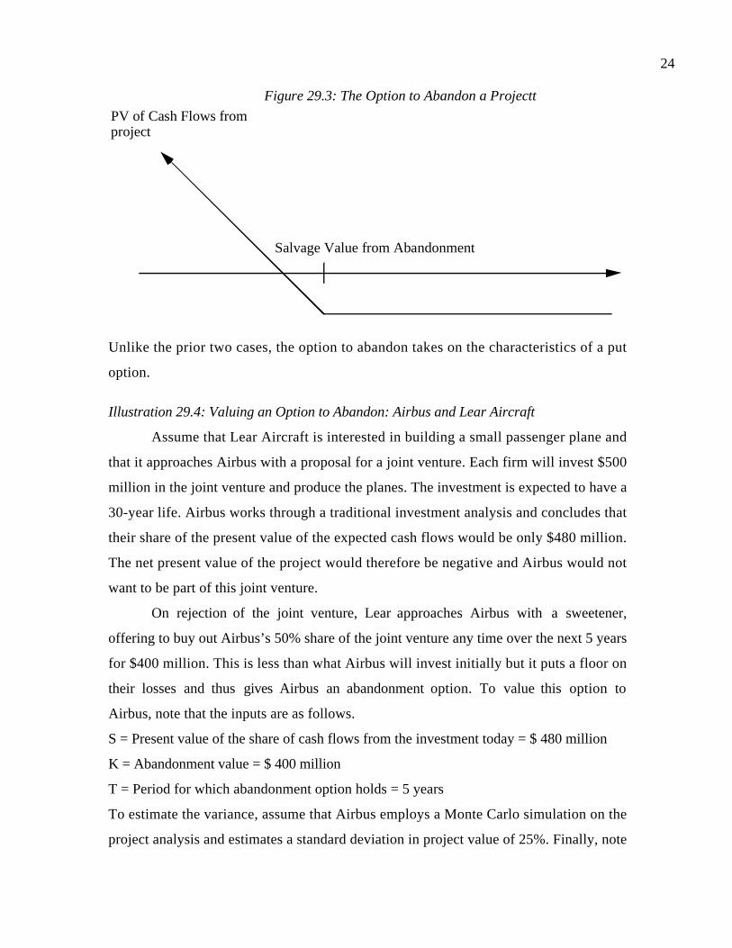
24

PV of Cash Flows fromproject

Salvage Value from Abandonment

Figure 29.3: The Option to Abandon a Projectt

Unlike the prior two cases, the option to abandon takes on the characteristics of a put

option.

Illustration 29.4: Valuing an Option to Abandon: Airbus and Lear Aircraft

Assume that Lear Aircraft is interested in building a small passenger plane and

that it approaches Airbus with a proposal for a joint venture. Each firm will invest $500

million in the joint venture and produce the planes. The investment is expected to have a

30-year life. Airbus works through a traditional investment analysis and concludes that

their share of the present value of the expected cash flows would be only $480 million.

The net present value of the project would therefore be negative and Airbus would not

want to be part of this joint venture.

On rejection of the joint venture, Lear approaches Airbus with a sweetener,

offering to buy out Airbus’s 50% share of the joint venture any time over the next 5 years

for $400 million. This is less than what Airbus will invest initially but it puts a floor on

their losses and thus gives Airbus an abandonment option. To value this option to

Airbus, note that the inputs are as follows.

S = Present value of the share of cash flows from the investment today = $ 480 million

K = Abandonment value = $ 400 million

T = Period for which abandonment option holds = 5 years

To estimate the variance, assume that Airbus employs a Monte Carlo simulation on the

project analysis and estimates a standard deviation in project value of 25%. Finally, note

25

that since the project is a finite life project, the present value will decline over time,

because there will be fewer years of cash flows left. For simplicity, we will assume that

this will be proportional to the time left on the project:

Dividend yield 3.33%30

1

project theof life Remaining

1 ===

Inputting these values into the Black-Scholes model and using a 5% riskless rate, we value

the put option.

Value of abandonment option ( )( )( ) ( )( )( )

million 09.40$

0.7748-1480e-0.5776-100e4 5-0.0335-0.05

==

Since this is greater than the negative net present value of the investment, Airbus should

enter into this joint venture. On the other hand, Lear needs to be able to generate a

positive net present value of at least $40.09 million to compensate for giving up this

option.6

abandon.xls: This spreadsheet allows you to estimate the value of the option to

abandon an investment.

Problems in valuing the Option to Abandon

In Illustration 29.4, we assumed, rather unrealistically, that the abandonment value

was clearly specified and did not change during the life of the project. This may be true in

some very specific cases, in which an abandonment option is built into the contract. More

often, however, the firm has the option to abandon and the salvage value from

abandonment can only be estimated. Further, the abandonment value may change over the

life of the project, making it difficult to apply traditional option pricing techniques.

Finally, it is entirely possible that abandoning a project may not bring in a liquidation

value but may create costs instead; a manufacturing firm may have to pay severance to its

workers, for instance. In such cases, it would not make sense to abandon, unless the cash

flows on the project are even more negative.

6 The binomial model yields a value of $34.74 million for this option.

26

Extensions and Implications of Abandonment Option

The fact that the option to abandon has value provides a rationale for firms to

build the operating flexibility to scale back or terminate projects if they do not measure

up to expectations. It also indicates that firms that try to generate more revenues by

offering their customers the option to walk away from commitments will have to weigh

the higher revenues against the cost of the options that have been granted to these

customers.

Escape Clauses in Contracts

The first and most direct way of creating an abandonment option is to build

operating flexibility contractually with other parties that are involved in a project. Thus,

contracts with suppliers may be written on an annual basis rather than be long term and

employees may be hired on a temporary basis rather than permanently. The physical

plant used for a project may be leased on a short term basis rather than bought and the

financial investment may be made in stages rather than as an initial lump sum. While there

is a cost to building in this flexibility, the gains may be much larger, especially in volatile

businesses.

Customer Incentives

On the other side of the transaction, offering abandonment options to customers

and partners in joint ventures can have a negative impact on value. As an example, assume

that a firm that sells its products on multi-year contracts offers customers the option to

cancel the contract at any time. While this may increase sales, there is likely to be a

substantial cost. In the event of a recession, firms that are unable to meet their obligations

are likely to cancel their contracts. Any benefits gained by the initial sale (obtained by

offering the inducement of cancellation by the buyer) may be offset by the cost of the

option provided to customers.

Reconciling net present value and real option valuations

Why does an investment sometimes have higher value when you value it using real

option approaches than with traditional discounted cash flow models? The answer lies in

the flexibility that firms have to change the way they invest in and run a project, based

27

upon what they observe in the market. Thus, an oil company will not produce the same

amount of oil or drill as many new wells if oil prices go to $15 a barrel as it would if oil

prices go up to $ 35 a barrel.

In traditional net present value, we consider the expected actions and the cash

flow consequences of those actions to estimate the value of an investment. If there is a

potential for further investments, expansion or abandonment down the road, all you can

do is consider the probabilities of such actions and build it into your cash flows. Analysts

often allow for flexibility by using decision trees and mapping out the optimal path, given

each outcome. You can then estimate the value of a project today, using the probabilities

of each branch and estimating the present value of the cash flows from each branch. For

instance, you have a decision tree for a new investment for the Home Depot in the Figure

29.4.

(1000)0.75

Invest (2,500)

Invest(15,000)

0.50

0.25

Stop

t=0 t=1 t=2 t=3 t=4 t=5 t=6

12,000 15,000 18,000 21,000

0.25

8,000 10,000 12,000 16,000

0.50

(2,000) (4,000) (6,000) (8,000)

0.25

0.50

Stop

Prob NPV

.09375 $23.066

.1875 $7,978

.09375 -$26,252

-$3,222

0.25 -$1000

MarketTest

PartialIntroduction

FullIntroduction

Year 1 Year 2 Year 3 Year 4

.375

Figure 10.9: Decision Tree for The Home Depot Home Shopping

This decision tree does bear a significant resemblance to the binomial tree approach that

we use to value real options, but there are two differences. The first is that the

probabilities of the outcomes are not used directly to value the real option and the second

is that you have only two branches at each node in the binomial tree. Notwithstanding

this, you might wonder why the two approaches will yield different values for the

project. The answer is surprisingly simple. It lies in the discount rate assumptions we

make to compute the value. In the real options approach, you use a replicating portfolio

to compute value. In the decision tree above, you used the cost of capital for the project

28

as the discount rate all through the process. If the exposure to market risk, which is what

determines the cost of capital, changes at each node, you can argue that using the same

cost of capital all the way through is incorrect and that you should be modifying the

discount rate as you move through time. If you do, you will obtain the same value with

both approaches. The real options approach does allow for far more complexity and is

simpler to employ with continuous distributions (as opposed to the discrete outcomes

that we assume in decision trees).

Summary

In this chapter, we consider two options that are embedded in many investments

– the option to expand an investment and the option to abandon it. When a firm has an

option to expand an investment, the value of this expansion option may sometimes allow

it to override the fact that the initial investment has a negative net present value.

Extending this concept to firm valuation, you may sometimes add a premium to the value

obtained from a discounted cash flow valuation for a firm that has the potential to enter

new markets or create new products. This expansion option has maximum value when the

firm has the exclusive right to make these investments and the value decreases as the

competitive advantages enjoyed by the firm decline.

The option to abandon refers to the right that firms often possess to walk away

from poor investments. To the extent that this reduces the firm’s exposure to the worst

outcomes, it can make the difference between investing in a new project and not.

29

Problems

1. NBC has the rights to televise the Winter Olympics in 2 years and is trying to

estimate the value of these rights for possible sale to another network. NBC expects it

to cost $40 million (in present value terms) to televise the Olympics and based upon

current assessments expects to have a Nielsen rating7 of 15 for the games. Each rating

point is expected to yield net revenue of $2 million to NBC (in present value terms).

There is substantial variability in this estimate and the standard deviation in the

expected net revenues is 30%. The riskless rate is 5%.

a. What is the net present value of these rights, based upon current assessments?

b. Estimate the value of these rights for sale to another network.

2. You are analyzing Skates Inc., a firm that manufactures skateboards. The firm is

currently unlevered and has a cost of equity of 12%. You estimate that Skates would

have a cost of capital of 11% at its optimal debt ratio of 40%. The management,

however, insists that it will not borrow the money because of the value of maintaining

financial flexibility and they have provided you with the following information.

• Over the last 10 years, reinvestments (net capital expenditures + working capital

investments) have amounted to 10% of firm value, on an annual basis. The

standard deviation in this reinvestment has been 0.30.

• The firm has traditionally used only internal funding (net income + depreciation)

to meet these needs and these have amounted to 6% of firm value.

• In the most recent year, the firm earned $180 million in net income on a book

value of equity of $1 billion and it expects to earn these excess returns on new

investments in the future.

• The riskless rate is 5%.

a. Estimate the value of financial flexibility as a percent of firm value, on an annual

basis.

7 There are 99.4 million households in the United States. Each rating point represents 1% of roughly994,000 households.

30

b. Based upon part a, would you recommend that Skates use its excess debt

capacity?

3. Disney is considering entering into a joint venture to build condominiums in Vail,

Colorado, with a local real estate developer. The development is expected to cost $1

billion overall and, based on Disney’s estimate of the cashflows, generate $900 million

in present value cash flows. Disney will have a 40% share of the joint venture

(requiring it to put up $400 million of the initial investment and entitling it to 40% of

the cashflows) but it will have the right to sell its share of the venture back to the

developer for $300 million.

a. If the standard deviation in real estate values in Vail is 30% and the riskless

rate is 5%, estimate the value of the abandonment option to Disney.

b. Would you advice Disney to enter into the joint venture?

c. If you were advising the developer, how much would he need to generate in

present value cashflows from the investment to make this a good investment?

4. Quality Wireless is considering making an investment in China. While it knows that

the investment will cost $1 billion and generate only $800 million in cashflows (in

present value terms), the proponents of expansion are arguing that the potential

market is huge and that Quality should go ahead with its investment.

a. Under what conditions will the expansion potential have option value?

b. Assume now that there is an option value to expansion that exactly offsets the

negative net present value on the initial investment. If the cost of the

subsequent expansion in 5 years is $2.5 billion, what is your current estimate

of the present value of the cash flows from expansion? (You can assume that

the standard deviation in the present value of the cashflows is 25% and that

the riskless rate is 6%.)

5. Reliable Machinery Inc. is considering expanding its operations in Thailand. The

initial analysis of the projects yields the following results.

• The project is expected to generate $85 million in after-tax cash flows every year for

the next 10 years.

31

• The initial investment in the project is expected to be $750 million.

• The cost of capital for the project is 12%.

If the project generates much higher cash flows than anticipated, you will have the

exclusive right for the next 10 years (from a manufacturing license) to expand operations

into the rest of South East Asia. A current analysis suggests the following about the

expansion opportunity.

• The expansion will cost $2 billion (in current dollars).

• The expansion is expected to generate $150 million in after tax cash flows each year

for 15 years. There is substantial uncertainty about these cash flows and the standard

deviation in the present value is 40%.

• The cost of capital for this investment is expected to be 12% as well. The riskfree rate

is 6.5%.

a. Estimate the net present value of the initial investment.

b. Estimate the value of the expansion option.

1

CHAPTER 30

VALUING EQUITY IN DISTRESSED FIRMS

In Chapter 22, we examined how discounted cash flow models could be adapted to

value firms with negative earnings. In most of our solutions, we estimated the expected

cash flows into the future and assumed that an improvement in margins or earnings would

result in positive cash flows and firm value. In the special case where the firm has

substantial amounts of debt, we argued that there is a very real possibility of defaulting

on the debt and going bankrupt. In these cases, discounted cash flow valuation may be an

inadequate tool for estimating value. In this chapter, we look at firms with negative

earnings, significant assets in place and substantial debt. We argue that the equity

investors in this firm, given limited liability, have the option to liquidate the firm and pay

off the debt. This call option on the underlying firm can add value to equity, especially

when there is significant uncertainty about the value of the assets.

Equity in Highly Levered distressed firms

In most publicly traded firms, equity has two features. The first is that the equity

investors run the firm and can choose to liquidate its assets and pay off other claim

holders at any time. The second is that the liability of equity investors in some private

firms and almost all publicly traded firms is restricted to their equity investments in these

firms. This combination of the option to liquidate and limited liability allows equity to

have the features of a call option. In firms with substantial liabilities and negative

earnings, the option value of equity may be in excess of the discounted cash flow value.

The Payoff on Equity as an Option

The equity in a firm is a residual claim, that is, equity holders lay claim to all cash

flows left after other financial claimholders (debt, preferred stock, etc.) have been

satisfied. If a firm is liquidated, the same principle applies; equity investors receive the

cash that is left in the firm after all outstanding debt and other financial claims have been

paid off. With limited liability, if the value of the firm is less than the value of the

outstanding debt, equity investors cannot lose more than their investment in the firm. The

payoff to equity investors on liquidation can therefore be written as:

2

Payoff to equity on liquidation = V - D if V > D

= 0 if V ≤ D

where

V = Liquidation Value of the firm

D = Face Value of the outstanding debt and other external claims

Equity can thus be viewed as a call option on the firm, where exercising the option

requires that the firm be liquidated and the face value of the debt (which corresponds to

the exercise price) be paid off. The firm is the underlying asset and the option expires

when the debt comes due. The payoffs are shown in Figure 30.1.

Figure 30.1: Payoff on Equity as Option on a Firm

Value of firm

Net Payoffon Equity

Face Valueof Debt

Illustration 30.1: Valuing Equity as an Option

Assume that you are valuing the equity in a firm whose assets are currently valued

at $100 million; the standard deviation in this asset value is 40%. The face value of debt is

$80 million (it is zero coupon debt with 10 years left to maturity). The 10-year treasury

bond rate is 10%. We can value equity as a call option on the firm, using the following

inputs for the option pricing model.

Value of the underlying asset = S = Value of the firm = $ 100 million

Exercise price = K = Face Value of outstanding debt = $ 80 million

Life of the option = t = Life of zero-coupon debt = 10 years

3

Variance in the value of the underlying asset = σ2 = Variance in firm value = 0.16

Riskless rate = r = Treasury bond rate corresponding to option life = 10%

Based upon these inputs, the Black-Scholes model provides the following value for the

call.

d1 = 1.5994 N(d1) = 0.9451

d2 = 0.3345 N(d2) = 0.6310

Value of the call ( ) ( )( )( ) million 94.75$6310.0e809451.0100 10-0.10 =−=

Since the call value represents the value of equity and the firm value is $100 million, the

estimated value of the outstanding debt can be calculated.

Value of the outstanding debt = $100 - $75.94 = $24.06 million

Since the debt is a 10-year zero coupon bond, the market interest rate on the bond can be

calculated.

Interest rate on debt 12.77%1-$24.06

$80 10

1

=

=

Thus, the default spread on this bond should be 2.77%.

The Importance of Limited Liability

The argument that equity is a call option holds only if equity has limited liability – i.e.,

the most that an equity investor can lose is what he or she has invested in a firm. This is

clearly the case in publicly traded companies. In private companies, however, the owners

often have unlimited liability. If these firms get into financial trouble and are unable to

make their debt payments, the owner’s personal assets can be put at risk. You should not

value equity as a call option in these cases.

Implications of viewing Equity as an Option

When the equity in a firm takes on the characteristics of a call option, you have to

change the way you think about its value and what determines its value. In this section,

we will consider a number of potential implications for equity investors and bondholders

in the firm.

4

When will equity be worthless?

In discounted cash flow valuation, we argue that equity is worthless if what you

own (the value of the firm) is less than what you owe. The first implication of viewing

equity as a call option is that equity will have value, even if the value of the firm falls well

below the face value of the outstanding debt. While the firm will be viewed as troubled by

investors, accountants and analysts, its equity is not worthless. In fact, just as deep out-

of-the-money traded call options command value because of the possibility that the value

of the underlying asset may increase above the strike price in the remaining lifetime of the

option, equity commands value because of the time premium on the option (the time until

the bonds mature and come due) and the possibility that the value of the assets may

increase above the face value of the bonds before they come due.

Illustration 30.2: Firm Value and Equity Value

Revisiting the preceding example, assume that the value of the firm drops to $50

million, below the face value of the outstanding debt ($80 million). Assume that all the

other inputs remain unchanged. The parameters of equity as a call option are as follows:

Value of the underlying asset = S = Value of the firm = $ 50 million

Exercise price = K = Face Value of outstanding debt = $ 80 million

Life of the option = t = Life of zero-coupon debt = 10 years

Variance in the value of the underlying asset = σ2 = Variance in firm value = 0.16

Riskless rate = r = Treasury bond rate corresponding to option life = 10%

Based upon these inputs, the Black-Scholes model provides the following value for the

call.

d1 = 1.0515 N(d1) = 0.8534

d2 = -0.2135 N(d2) = 0.4155

Value of the call (equity) = 50 (0.8534) - 80 exp(-0.10)(10) (0.4155) = $30.44 million

Value of the bond= $50 - $30.44 = $19.56 million

As you can see, the equity in this firm retains value, because of the option characteristics

of equity. In fact, equity continues to have value in this example even if the firm value

drops to $10 million or below, as shown in Figure 30.2.

5

Value of Equity as Firm Value Changes

0

10

20

30

40

50

60

70

80

100 90 80 70 60 50 40 30 20 10

Value of Firm ($ 80 Face Value of Debt)

Val

ue o

f Equity

Increasing Risk can increase Equity Value

In traditional discounted cash flow valuation, higher risk almost always translates

into lower value for equity investors. When equity takes on the characteristics of a call

option, you should not expect this relationship to continue to hold. Risk can become your

ally, when you are an equity investor in a troubled firm. In essence, you have little to lose

and much to gain from swings in firm value.

Illustration 30.3: Equity Value and Volatility

Let us revisit the valuation in Illustration 30.1. The value of the equity is a

function of the variance in firm value, which we assumed to be 40%. If we change this

variance, holding all else constant, the value of the equity will change as evidenced in

Figure 30.3.

6

Note that the value of equity increases, if we hold firm value constant, as the standard

deviation increases. The interest rate on debt also increases as the standard deviation

increases.

Probability of Default and Default Spreads

One of the more interesting pieces of output from the option pricing model is the

risk-neutral probability of default that you can obtain for the firm. In the Black-Scholes

model, you can estimate this value from N(d2), which is the risk-neutral probability that

S>K, which in this model is the probability that the value of the firm’s asset will exceed

the face value of the debt.

Risk-neutral probability of default = 1 – N(d2)

In addition, the interest rate from the debt allows us to estimate the appropriate default

spread to charge on bonds.

You can see the potential in applying this model to bank loan portfolios to extract

both the probability of default and to measure whether you are charging an interest rate

that is high enough on the debt. In fact, there are commercial services that use fairly

sophisticated option pricing models to estimate both values for firms.

Figure 30.3: Equity Value and Standard Deviation in Firm Value

0

10

20

30

40

50

60

70

80

90

100

0% 10% 20% 30% 40% 50% 60% 70% 80%

Standard deviation in firm value

Val

ue o

f E

quity

0%

5%

10%

15%

20%

25%

Inte

rest

rat

e on

deb

t

Equity ValueInterest rate on debt

7

Illustration 30.4: Probabilities of default and Default Spreads

We return to Illustration 30.1 and estimate the probability of default as N(d2) and

the default spread, measured as the difference between the interest rate on a firm’s debt

and the riskfree rate, as a function of the variance. These values are graphed in Figure

30.4.

Note that the probability of default climbs very quickly as the standard deviation in firm

value increases and the default spread follows it along.

Estimating the Value of Equity as an Option

The examples we have used thus far to illustrate the application of option pricing

to value equity have included some simplifying assumptions. Among them are the

following.

1. There are only two claimholders in the firm - debt and equity.

2. There is only one issue of debt outstanding and it can be retired at face value.

3. The debt has a zero coupon and no special features (convertibility, put clauses, etc.)

4. The value of the firm and the variance in that value can be estimated.

Figure 30.4: Risk Neutral Probability of default and Default spreads

0%

2%

4%

6%

8%

10%

12%

14%

0% 10% 20% 30% 40% 50% 60% 70% 80%

Standard Deviation in firm value

Def

ault

Spre

ad

0%

10%

20%

30%

40%

50%

60%

70%

80%

90%

prob

abili

ty o

f de

faul

t

Default Spread

1-N(d2)

8

Each of these assumptions is made for a reason. First, by restricting the claimholders to

just debt and equity, we make the problem more tractable; introducing other claimholders

such as preferred stock makes it more difficult to arrive at a result, albeit not impossible.

Second, by assuming only one zero-coupon debt issue that can be retired at face value any

time prior to maturity, we align the features of the debt more closely to the features of the

strike price on a standard option. Third, if the debt is coupon debt, or more than one debt

issue is outstanding, the equity investors can be forced to exercise (liquidate the firm) at

these earlier coupon dates if they do not have the cash flows to meet their coupon

obligations.

Finally, knowing the value of the firm and the variance in that value makes the

option pricing possible, but it also raises an interesting question about the usefulness of

option pricing in equity valuation. If the bonds of the firm are publicly traded, the market

value of the debt can be subtracted from the value of the firm to obtain the value of equity

much more directly. The option pricing approach does have its advantages, however.

Specifically, when the debt of a firm is not publicly traded, option pricing theory can

provide an estimate of value for the equity in the firm. Even when the debt is publicly

traded, the bonds may not be correctly valued and the option pricing framework can be

useful in evaluating the values of debt and equity. Finally, relating the values of debt and

equity to the variance in firm value provides some insight into the redistributive effects of

actions taken by the firm.

Inputs for Valuing Equity as an Option

Since most firms do not fall into the neat framework developed above (such as

having only one zero-coupon bond outstanding), we have to make some compromises to

use this model in valuation.

Value of the Firm

We can obtain the value of the firm in one of four ways. In the first, we cumulate

the market values of outstanding debt and equity, assuming that all debt and equity are

traded, to obtain firm value. The option pricing model then reallocates the firm value

between debt and equity. This approach, while simple, is internally inconsistent. We start

9

with one set of market values for debt and equity and, using the option pricing model, end

up with entirely different values for each.

In the second, we estimate the market values of the assets of the firm by

discounting expected cash flows at the cost of capital. The one consideration that we need

to keep in mind is that the value of the firm in an option pricing model should be the value

obtained on liquidation. This may be less than the total firm value, which includes

expected future investments and it may also be reduced to reflect the cost of liquidation.

If we estimate the firm value using a discounted cash flow model, then this would suggest

that only existing investments1 should be considered while estimating firm value. The

biggest problem with this approach is that financial distress can affect operating income

and thus the value that you obtain by using current operating income may be too low.

In the third approach, we estimate a multiple of revenues by looking at healthy

firms in the same business and apply this multiple to the revenues of the firm you are

valuing. Implicitly, we are assuming that a potential buyer, in the event of liquidation, will

pay this value.

We can use the third approach for firms that have separable assets that are

individually traded. For example, we can value a troubled real estate firm that owns five

properties by valuing each property separately and then aggregating the values.

Variance in Firm value

We can obtain the variance in firm value directly if both stocks and bonds in the

firm are traded. Defining σe2 as the variance in the stock price and σd2 as the variance in

the bond price, we as the market-value weight of equity and wd as the market-value

weight of debt, we can write the variance in firm value as:2

deeddeddeefirm wwww 222222 ++=

where ρed is the correlation between the stock and the bond prices. When the bonds of

the firm are not traded, we can use the variance of similarly rated bonds as the estimate of

1 Technically, this can be done by putting the firm into stable growth and valuing it as a stable growthfirm, where reinvestments are used to either preserve or augment existing assets.2 This is an extension of the variance formula for a two-asset portfolio.

10

σd2 and the correlation between similarly rated bonds and the firm's stock as the estimate

of ρed.

When companies get into financial trouble, this approach can yield misleading

results as both its stock prices and its bond prices become more volatile. An alternative

that often yields more reliable estimates is to use the average variance in firm value for

other firms in the sector. Thus, the value of equity in a deeply troubled steel company

can be estimated using the average variance in firm value of all traded steel companies.

optvar.xls: There is a dataset on the web that summarizes standard deviations in

equity and firm value, by industry, for firms in the United States.

Maturity of the Debt

Most firms have more than one debt issue on their books and much of the debt

comes with coupons. Since the option pricing model allows for only one input for the

time to expiration, we have to convert these multiple bonds issues and coupon payments

into one equivalent zero-coupon bond.

• One solution, which takes into account both the coupon payments and the

maturity of the bonds, is to estimate the duration of each debt issue and calculate a

face-value-weighted average of the durations of the different issues. This value-

weighted duration is then used as a measure of the time to expiration of the

option.

• An approximation is to use the face-value weighted maturity of the debt converted

to the maturity of the zero-coupon bond in the option pricing model.

Face Value of Debt

When a distressed firm has multiple debt issues outstanding, you have three

choices when it comes to what you use as the face value of debt:

• You could add up the principal due on all of the debt of the firm and consider it to

be the face value of the hypothetical zero coupon bond that you assume that the

firm has issued. The limitation of this approach is that it will understate what the

11

firm will truly have to pay out over the life of the debt, since there will be coupon

payments and interest payments during the period.

• At the other extreme, you could add the expected interest and coupon payments

that will come due on the debt to the principal payments to come up with a

cumulated face value of debt. Since the interest payments occur in the near years

and the principal payments are due only when the debt comes due, you are mixing

cash flows up at different points in time when you do this. This is, however, the

simplest approach of dealing with intermediate interest payments coming due.

• You can consider only the principal due on the debt as the face value of the debt

and the interest payments each year, specified as a percent of firm value, can take

the place of the dividend yield in the option pricing model. In effect, each year

that the firm remains in existence, you would expect to see the value of the firm

decline by the expected payments on the debt.

Illustration 30.5: Valuing Equity as an option – Eurotunnel in 1997

Eurotunnel was the firm that was created to build and ultimately profit from the

tunnel under the English Channel, linking England and France. While the tunnel was

readied for operations in the early 1990s, it was never a commercial success and reported

significant losses each year after opening. In early 1998, Eurotunnel had a book value of

equity of -£117 million, and in 1997, the firm had reported earnings before interest and

taxes of -£3.45 million and net income of -£611 million on revenues of £456 million. By

any measure, it was a firm in financial trouble.

Much of the financing for the tunnel had come from debt and, at the end of 1997,

Eurotunnel had debt obligations in excess of £5,000 million, raised from a variety of bond

issues and bank debt. Adding the expected interest payments and coupon payments on

the debt brings the total obligations of the firm up to £8,865 million. The following table

summarizes the outstanding debt at the firm, with our estimates of the expected duration

for each class of debt.

Table 30.1: Debt Breakdown for Eurotunnel

Debt Type Face Value (including cumulated coupons) Duration

Short term £ 935 0.50

12

10 year £ 2435 6.7

20 year £ 3555 12.6

Longer £ 1940 18.2

Total £8,865 mil 10.93 years

The firm’s only significant asset is its ownership of the tunnel and we estimated

the value of this asset from its expected cash flows and the appropriate cost of capital.

The assumptions we made were as follows.

1. Revenues will grow 10% a year for the next 5 years and 3% a year in perpetuity after

that.

2. The cost of goods sold which was 72% of revenues in 1997 will drop to 60% of

revenues by 2002 in linear increments and stay at that level.

3. Capital spending and depreciation will grow 3% a year for the next 5 years. Note that

the net capital expenditure is negative for each of these years – we are assuming that

the firm will be able to not make significant reinvestments for the next 5 years.

Beyond year 5, capital expenditures will offset depreciation.

4. There are no working capital requirements.

5. The debt ratio, which was 95.35% at the end of 1997, will drop to 70% by 2002. The

cost of debt is 10% for the next 5 years and 8% after that.

6. The beta for the stock will be 2.00 for the next five years, and drop to 0.8 thereafter

(as the leverage decreases).

The long-term bond rate at the time of the valuation was 6% and the tax rate was 35%.

Based on these assumptions, we estimated the cash flows in Table 30.2.

Table 30.2: Estimated FCFF: Eurotunnel

1 2 3 4 5Terminal

YearRevenues $501.60 $551.76 $606.94 $667.63 $734.39 $756.42- COGS $361.15 $380.71 $400.58 $420.61 $440.64 $453.85- Depreciation $141.11 $145.34 $149.70 $154.19 $158.82 $163.59EBIT ($0.66) $25.70 $56.65 $92.83 $134.94 $138.98- EBIT*t $0.00 $9.00 $19.83 $32.49 $47.23 $48.64EBIT (1-t) ($0.66) $16.71 $36.83 $60.34 $87.71 $90.34+ Depreciation $141.11 $145.34 $149.70 $154.19 $158.82 $163.59- Capital Spending $46.35 $47.74 $49.17 $50.65 $52.17 $163.59

13

- Chg. WorkingCapital $0.00 $0.00 $0.00 $0.00 $0.00 $0.00Free CF to Firm $94.10 $114.31 $137.36 $163.89 $194.36 $90.34Terminal Value $2,402.66 Present Value $87.95 $99.86 $112.16 $125.08 $1,852.67 Value of firm = $2,277.73

The value of the assets of the firm is £2,278 million.

The final input we estimated was the standard deviation in firm value. Since there

are no directly comparable firms, we estimated the standard deviations in Eurotunnel

stock and debt using the data over the previous years.

Standard deviation in Eurotunnel stock price (ln) = 41%

Standard deviation in Eurotunnel bond price (ln) = 17%

We also estimated a correlation of 0.50 between Eurotunnel stock and bond prices and the

average market debt to capital ratio during the two-year period was 85%. Combining

these inputs, we estimated the standard deviation in firm value to be:

( ) ( ) ( ) ( ) ( )( )( )( )( ) 0.033517.041.05.085.015.0217.085.041.015.0 22222firm =++=

In summary, the inputs to the option pricing model were as follows.

Value of the underlying asset = S = Value of the firm = £2,278 million

Exercise price = K = Face Value of outstanding debt = £8,865 mil

Life of the option = t = Weighted average duration of debt = 10.93 years

Variance in the value of the underlying asset = σ2 = Variance in firm value = 0.0335

Riskless rate = r = Treasury bond rate corresponding to option life = 6%

Based upon these inputs, we estimate the following value for the call:

d1 = -0.8582 N(d1) = 0.1955

d2 = -1.4637 N(d2) = 0.0717

Value of the call = 2,278 0.1955( ) −8,865e -0.06( ) 10.93( ) 0.0717( ) = $116 million

Eurotunnel's equity was trading at £150 million in 1997.

The option pricing framework, in addition to yielding a value for Eurotunnel

equity, yields some valuable insight into the drivers of value for this equity. While it is

certainly important that the firm try to bring costs under control and increase operating

margins, the two most critical variables determining equity value are the duration of the

14

debt and the variance in firm value. Any action that increases (decreases) the debt

duration will have a positive (negative) effect on equity value. For instance, when the

French government put pressure on the bankers who had lent money to Eurotunnel to

ease restrictions and allow the firm more time to repay its debt, equity investors benefited

as their options became more long term. Similarly, an action that increases the volatility of

expected firm value will increase the value of the option.

equity.xls: This spreadsheet allows you to estimate the value the equity in a troubled

firm as an option.

Vulture Investing and Option Pricing

Vulture investing refers to an investment strategy of buying the securities of firms that are

in severe financial distress. In a sense, you are investing in deep out of the money options

and hoping that some of these options pay off handsomely. Using the option pricing

framework allows us to draw some conclusions about when and how this strategy can

pay off.

• As with any portfolio of deep out-of-the-money options, you should expect a

considerable proportion of the portfolio to end up worthless. The relatively few

investments that do pay off, however, will earn huge returns and you could still end

up with a portfolio with impressive returns.

• You should direct your equity investments to equity in deeply troubled firms in

volatile sectors. Risk is your ally when you invest in options; and the equity in these

firms should be worth more than equity in deeply troubled stable firms.

• If you are buying equity in deeply troubled firms, you should direct your investments

towards troubled firms with longer term debt rather than shorter tem debt. As the life

of the option increases, you will see the value of the option also increase.

• If you are investing in the debt issued by financially troubled firms, you cannot be a

passive bondholder. You have to take an active role in the management and obtain an

equity stake in the companies you invest in, perhaps by making the debt convertible.

15

Consequences for decision making

Option pricing theory can be applied to illustrate the conflict between

stockholders and bondholders when it comes to investment analysis and conglomerate

mergers. In this section, we will argue that decisions that make stockholders better off are

not necessarily value maximizing for the firm and can hurt bondholders.

The Conflict between Bondholders and Stockholders

Stockholder and bondholders have different objective functions, and this can lead

to agency problems, whereby stockholders expropriate wealth from bondholders. The

conflict can manifest itself in a number of ways. For instance, stockholders have an

incentive to invest in riskier projects than bondholders and to pay more out in dividends

than bondholders would like them to. The conflict between bondholders and stockholders

can be illustrated dramatically using the option pricing methodology developed in the

previous section.

Investing in Risky Projects

Since equity is a call option on the value of the firm, other things remaining equal,

an increase in the variance in the firm value will lead to an increase in the value of equity.

It is therefore conceivable that stockholders can invest in risky projects with negative net

present values, which, while making them better off, may make the bonds and the firm

less valuable. To illustrate, consider the firm in Illustration 30.1 with a value of assets of

$100 million, a face value of zero-coupon ten-year debt of $80 million and a standard

deviation in the value of the firm of 40%. The equity and debt in this firm were valued as

follows:

Value of Equity = $75.94 million

Value of Debt = $24.06 million

Value of Firm == $100 million

Now assume that the stockholders have the opportunity to invest in a project with a net

present value of -$2 million; the project is a very risky one that will push up the standard

deviation in firm value to 50%. The equity as a call option can then be valued using the

following inputs.

16

Value of the underlying asset = S = Value of the firm = $ 100 million - $2 million = $ 98

million (The value of the firm is lowered because of the negative net present value

project.)

Exercise price = K = Face Value of outstanding debt = $ 80 million

Life of the option = t = Life of zero-coupon debt = 10 years

Variance in the value of the underlying asset = σ2 = Variance in firm value = 0.25

Riskless rate = r = Treasury bond rate corresponding to option life = 10%

Based upon these inputs, the Black-Scholes model provides the following value for the

equity and debt in this firm.

Value of Equity = $77.71

Value of Debt = $20.29

Value of Firm = $98.00

The value of equity rises from $75.94 million to $ 77.71 million, even though the firm

value declines by $2 million. The increase in equity value comes at the expense of

bondholders, who find their wealth decline from $24.06 million to $20.29 million.

Conglomerate Mergers

Bondholders and stockholders may also be affected differently by conglomerate

mergers, where the variance in earnings and cash flows of the combined firm can be

expected to decline because the merging firms have earning streams that are not perfectly

correlated. In these mergers, the value of the combined equity in the firm will decrease

after the merger because of the decline in variance; consequently, bondholders will gain.

Stockholders can reclaim some or all of this lost wealth by utilizing their higher debt

capacity and issuing new debt. To illustrate, suppose you are provided with the following

information on two firms, Lube and Auto (auto service) and Gianni Cosmetics (a

cosmetics manufacturer) that hope to merge.

Lube & Auto Gianni Cosmetics

Value of the firm $100 million $ 150 million

Face Value of Debt $ 80 million $ 50 million (Zero-coupon debt)

Maturity of debt 10 years 10 years

Std. Dev. in firm value 40 % 50 %

17

Correlation between firm cash flows 0.4

The ten-year bond rate is 10%.

We calculate the variance in the value of the firm after the acquisition as follows:

Variance in combined firm value ( ) ( ) ( ) ( ) ( )( )( )( )( )154.0

5.04.04.06.04.025.06.04.04.0

22222

2222

=++=

++= deeddeddee wwww

We estimate the values of equity and debt in the individual firms and the combined firm

using the option pricing model.

Lube & Auto Gianni Combined firm

Value of equity in the firm $75.94 $134.48 $ 207.58

Value of debt in the firm $24.06 $ 15.52 $ 42.42

Value of the firm $100.00 $150.00 $ 250.00

The combined value of the equity prior to the merger is $ 210.42 million; it declines to

$207.58 million after that. The wealth of the bondholders increases by an equal amount.

There is a transfer of wealth from stockholders to bondholders, as a consequence of the

merger. Thus, conglomerate mergers that are not followed by increases in leverage are

likely to result in a wealth transfer from stockholders to bondholders.

Is equity not a call option in every firm?

Looking at the framework that we have employed in this chapter, you are probably

wondering why equity in every firm cannot be viewed as a call option and why therefore

we should not add a premium to discounted cash flow values for all firms. It is true that

equity is a call option in every firm, but in most firms, the value of the firm as a going

concern will be greater than the value you obtain from a liquidation option. Consider, for

instance, a high growth firm with very little in assets in place and a high proportion of

value from growth potential. If this firm liquidates, it will get the value of its asset in

place – this will become the value of the underlying asset in the option pricing model and

determine the value of equity as a call option on the firm. This value will be much lower

than the value you would obtain if you valued the firm as a going concern and considered

the cash flows from expected growth.

18

Value of equity = Maximum (Equity value as a going concern from a discounted cashflow

valuation, Equity value as a call option on liquidation)

For some mature firms that derive most of their value coming from assets in place and

substantial debt, the call option can be the higher value. For other firms, though, the going

concern will be greater.

Summary

The value of equity in deeply troubled firms - firms with negative earnings and

high leverage - can be viewed as a call option. The option rests in the hands of equity

investors, who can choose to liquidate the firm and claim the difference between firm

value and debt outstanding. With limited liability, they do not have to make up the

difference if firm value falls below the value of the outstanding debt. The equity will

retain value even when the value of the assets of the firm is lower than the debt

outstanding, because of the time premium on the option.

19

Problems

1. Designate the following statements as true or false.

a. Equity can be viewed as an option because equity investors have limited

liability (limited to their equity investment in the firm).

b. Equity investors will sometimes take bad projects (with negative net present

value) because they can add to the value of the firm.

c. Investing in a good project (with positive NPV) -- which is less risky than the

average risk of the firm -- can negatively impact equity investors.

d. The value of equity in a firm is an increasing function of the duration of the debt

in the firm (i.e., equity will be more valuable in a firm with longer term debt than

an otherwise similar firm with short term debt).

e. In a merger in which two risky firms merge and do not borrow more money,

equity can become less valuable because existing debt will become less risky.

2. XYZ Corporation has $500 million in zero-coupon debt outstanding, due in five years.

The firm had earnings before interest and taxes of $40 million in the most recent year (the

tax rate is 40%). These earnings are expected to grow 5% a year in perpetuity and the

firm paid no dividends. The firm had a cost of equity of 12% and a cost of capital of 10%.

The annualized standard deviation in firm values of comparable firms is 12.5%. The five-

year bond rate is 5%.

a. Estimate the value of the firm.

b. Estimate the value of equity, using an option pricing model.

c. Estimate the market value of debt and the appropriate interest rate on the debt.

3. McCaw Cellular Communications reported earnings before interest and taxes of $850

million in 1993 and had a depreciation allowance of $400 million in that year (which was

offset by capital spending of an equivalent amount). The earnings before interest and

taxes are expected to grow 20% a year for the next five years and 5% a year after that.

The cost of capital is 10%. The firm has $10 billion in debt outstanding with the

following characteristics.

Duration Debt

1 year $2 billion

20

2 years $4 billion

5 years $4 billion

The annualized standard deviation in the firm's stock price is 35%, while the annualized

standard deviation in the traded bonds is 15%. The correlation between stock and bond

prices has been 0.5. The firm has a debt/equity ratio of 50% and the after-tax cost of debt

is 6%. (The beta of the stock is 1.50; the 30-year treasury bond rate is 7%.) The three-

year bond rate is 5%.

a. Estimate the value of the firm.

b. Estimate the value of the equity.

c. The stock was trading at $60 and there were 210 million shares outstanding in

January 1994. Estimate the implied standard deviation in firm value.

d. Estimate the market value of the debt.

4. You have been asked to analyze the value of equity in a company that has the

following features.

• The earnings before interest and taxes is $25 million and the corporate tax rate is 40%.

There is no net capital expenditures or working capital requirements and the earnings

are expected to grow 5% a year in perpetuity. The cost of capital of comparable firms

is 10%.

• The firm has two types of debt outstanding - 2-year zero-coupon bonds with a face

value of $250 million and bank debt with ten years to maturity with a face value of

$250 million (The duration of this debt is 4 years.).

• The firm is in two businesses - food processing and auto repair. The average standard

deviation in firm value for firms in food processing is 25%, whereas the standard

deviation for firms in auto repair is 40%. The correlation between the businesses is

0.5.

• The riskless rate is 7%.

Use the option pricing model to value equity as an option.

5. You are valuing the equity in a firm with $800 million (face value) in debt with an

average duration of 6 years and assets with an estimated value of $400 million. The

21

standard deviation in asset value is 30%. With these inputs (and a riskless rate of 6%) we

obtain the following values (approximately) for d1 and d2.

d1 = - 0.15 d2 = - 0.90

Estimate the default spread (over and above the riskfree rate) that you would charge for

the debt in this firm.

1

CHAPTER 31

VALUE ENHANCEMENT: A DISCOUNTED CASHFLOW

VALUATION FRAMEWORK

In much of this book, we have taken on the role of a passive investor valuing going

concerns. In this chapter, we switch roles and look at valuation from the perspective of

those who can make a difference in the way a company is run and hence its value. Our

focus is therefore on how actions taken by managers and owners can change the value of a

firm.

We will use the discounted cash flow framework that we have developed in earlier

parts of the book to explore the requirements for an action to be value creating and then

go on to examine the different ways in which a firm can create value. In the process, we

will also examine the role that marketing decisions, production decisions, and strategic

decisions have in value creation.

Value Creating and Value Neutral Actions

The value of a firm is the present value of the expected cash flows from both

assets in place and future growth, discounted at the cost of capital. For an action to create

value, it has to do one or more of the following.

1. increase the cash flows generated by existing investments

2. increase the expected growth rate in earnings

3. increase the length of the high growth period

4. reduce the cost of capital that is applied to discount the cash flows

Conversely, an action that does not affect cash flows, the expected growth rate, the length

of the high growth period or the cost of capital cannot affect value.

While this might seem obvious, a number of value-neutral actions taken by firms

receive disproportionate attention from both managers and analysts. Consider four

examples.

• Stock dividends and stock splits change the number of units of equity in a firm but do

not affect cash flows, growth or value. These actions can have price effects, though,

because they alter investors’ perceptions of the future of the company.

2

• Accounting changes in inventory valuation and depreciation methods that are

restricted to the reporting statements and do not affect tax calculations have no effect

on cash flows, growth or value. In recent years, firms have spent an increasing amount

of time on the management and smoothing of earnings and seem to believe that there is

a value payoff in doing this.

• When making acquisitions, firms often try to structure the deals in such a way that

they can pool their assets and not show the market premium paid in the acquisition.

When they fail and they are forced to show the difference between market value and

book value as goodwill, their earnings are reduced by the amortization of the goodwill

over subsequent periods. This amortization is not tax deductible, however, and thus

does not affect the cash flows of the firm. So, whether a firm adopts purchase or

pooling accounting and the length of time it takes to write off the goodwill should not

really make any difference to value.

• In the late 1990s, a number of firms that have issued tracking stock on their high-

growth divisions. Since these divisions remain under the complete control of the

parent company, we would argue that the issue of tracking stock, by itself, should not

create value.

Some would take issue with some of these propositions. When a stock splits or a

firm issues tracking stock, they would argue, the stock price often goes up1 significantly.

While this is true, we would emphasize that it is value, not price, that we claim is

unaffected by these actions.

While paying stock dividends, splitting stock and issuing tracking stock are value

neutral actions, they can still be useful tools for a firm that perceives itself to be

undervalued by the market. These actions can change market perceptions about growth or

cash flows and thus act as signals to financial markets. Alternatively, they might provide

more information about undervalued assets owned by the firm and the price may react as

a consequence. In some cases, these actions may even lead to changes in operations; tying

the compensation of managers to the price of stock tracking the division in which they

work may improve efficiency and thus increase cash flows, growth and value.

1 This is backed up empirically. Stock prices do tend to increase, on average, when stocks are split.

3

Ways of Increasing Value

The value of a firm can be increased by increasing cash flows from assets in place,

increasing expected growth and the length of the growth period and by reducing the cost

of capital. In reality, however, none of these is easily accomplished or likely to reflect all

the qualitative factors that we, as financial analysts, are often accused of ignoring in

valuation. In this section, we will consider how actions taken by a firm on a variety of

fronts – marketing, strategic and financial – can have an effect on value.

1. Increase Cash Flows from Existing Investments

The first place to look for value is in the firm’s existing assets. These assets

represent investments the firm has already made and they generate the current operating

income for the firm. To the extent that these investments earn less than their cost of

capital or are earning less than they could if optimally managed, there is potential for

value creation.

1.1: Poor Investments: Keep, Divest or Liquidate

Every firm has some investments that earn less than necessary to break even (the

cost of capital) and sometimes even lose money. At first sight, it would seem to be a

simple argument to make that investments that do not earn their cost of capital should

either be liquidated or divested. If, in fact, the firm could get back the original capital on

liquidation, this statement would be true. But that assumption is not generally true and

there are three different measures of value for an existing investment that we need to

consider.

The first is the continuing value and it reflects the present value of the expected

cash flows from continuing the investment through the end of its life. The second is the

liquidation or salvage value, which is the net cash flow that the firm will receive if it

terminated the project today. Finally, there is the divestiture value, which is the price that

will be paid by the highest bidder for this investment.

Whether a firm should continue with an existing project, liquidate the project, or

sell it to someone else will depend upon which of the three is highest. If the continuing

value is the highest, the firm should continue with the project to the end of the project

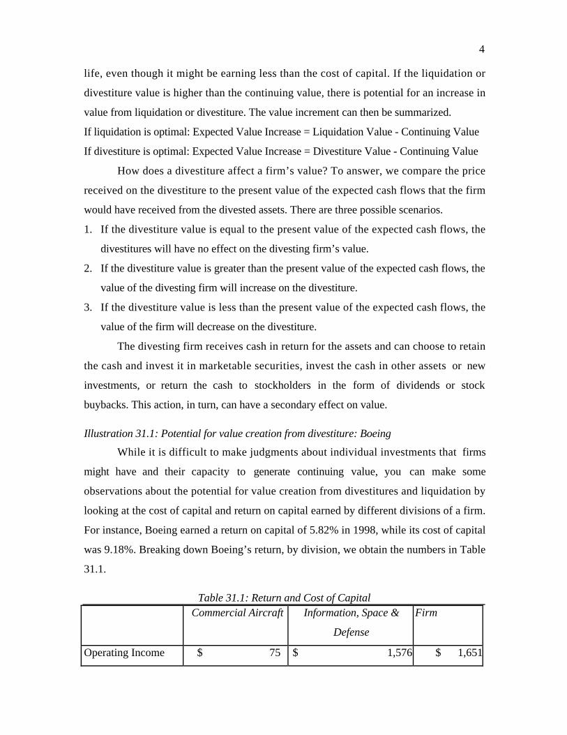
4

life, even though it might be earning less than the cost of capital. If the liquidation or

divestiture value is higher than the continuing value, there is potential for an increase in

value from liquidation or divestiture. The value increment can then be summarized.

If liquidation is optimal: Expected Value Increase = Liquidation Value - Continuing Value

If divestiture is optimal: Expected Value Increase = Divestiture Value - Continuing Value

How does a divestiture affect a firm’s value? To answer, we compare the price

received on the divestiture to the present value of the expected cash flows that the firm

would have received from the divested assets. There are three possible scenarios.

1. If the divestiture value is equal to the present value of the expected cash flows, the

divestitures will have no effect on the divesting firm’s value.

2. If the divestiture value is greater than the present value of the expected cash flows, the

value of the divesting firm will increase on the divestiture.

3. If the divestiture value is less than the present value of the expected cash flows, the

value of the firm will decrease on the divestiture.

The divesting firm receives cash in return for the assets and can choose to retain

the cash and invest it in marketable securities, invest the cash in other assets or new

investments, or return the cash to stockholders in the form of dividends or stock

buybacks. This action, in turn, can have a secondary effect on value.

Illustration 31.1: Potential for value creation from divestiture: Boeing

While it is difficult to make judgments about individual investments that firms

might have and their capacity to generate continuing value, you can make some

observations about the potential for value creation from divestitures and liquidation by

looking at the cost of capital and return on capital earned by different divisions of a firm.

For instance, Boeing earned a return on capital of 5.82% in 1998, while its cost of capital

was 9.18%. Breaking down Boeing’s return, by division, we obtain the numbers in Table

31.1.

Table 31.1: Return and Cost of CapitalCommercial Aircraft Information, Space &

Defense

Firm

Operating Income $ 75 $ 1,576 $ 1,651

5

Capital Invested $ 18,673 $ 9,721 $ 28,394

After-tax ROC 0.40% 16.21% 5.82%

At Boeing’s annual meeting in 1999, Phil Condit, Boeing’s CEO, was candid in

admitting that 35% of Boeing’s capital was in investments that earned less than the cost

of capital. He revealed little, however, about whether it would be feasible to liquidate2 or

divest these investments and get more than continuing value from such actions.

Assume that Boeing is interested in selling its information, space and defense

systems division and that it has found a potential buyer who is willing to pay $11 billion

for the division. The division reported cash flows before debt payments, but after

reinvestment needs and taxes, of $393 million in the most recent year and the cash flows

are expected to grow 5% a year in the long term. The cost of capital for the division is

9%, a little lower than the cost of capital for the entire firm. The division, as a continuing

part of Boeing, can be valued.

Value of Division ( )( )( ) million 316,10$

05.009.0

05.1393$ =−

=

With the divestiture value of $11 billion, the net effect of the divestiture will be an

increase in Boeing’s value of $684 million.

Net Effect on Value = Divestiture Value – Continuing Value = $11,000 mil - $10,316 mil

= $ 684 million

Reasons for Divestitures

Why would a firm sell assets or a division? There are at least three reasons. The

first is that the divested assets may have a higher value to the buyer of these assets. For

assets to have a higher value, they have to either generate higher cash flows for the buyers

or result in lower risk (leading to a lower discount rate). The higher cash flows can occur

because the buyer is more efficient at utilizing the assets or because the buyer finds

synergies with its existing businesses. The lower discount rate may reflect the fact that

the owners of the buying firm are more diversified that the owners of the firm selling the

2 In 1999, Lockheed, Boeing’s leading competitor in the sector, announced plans to divest itself ofapproximately 15% of its assets as a remedy for its poor stock price performance.

6

assets. In either case, both sides can gain from the divestiture and share in the increased

value.

The second reason for divestitures is less value-driven and more a result of the

immediate cash flow needs of the divesting firm. Firms that find themselves unable to

meet their current operating or financial expenses may have to sell assets to raise cash.

For instance, many leveraged acquisitions in the 1980s were followed by divestitures of

assets. The cash generated from these divestitures was used to retire and service debt.

The third reason for divestitures relates to the assets not sold by the firm, rather

than the divested assets. In some cases, a firm may find the cash flows and values of its

core businesses affected by the fact that it has diversified into unrelated businesses. This

lack of focus can be remedied by selling assets or businesses that are peripheral to the

main business of a firm.

1.2: Improve Operating Efficiency

A firm’s operating efficiency determines its operating margin and, thus, its

operating income; more efficient firms have higher operating margins, other things

remaining equal, than less efficient firms in the same business. If a firm can increase its

operating margin on existing assets, it will generate additional value. There are a number

of indicators of the potential to increase margins, but the most important is a measure of

how much a firm's operating margin deviates from its industry. Firms whose current

operating margins are well below their industry average must locate the source of the

difference and try to fix it.

In most firms, the first step in value enhancement takes the form of cost cutting

and layoffs. These actions are value enhancing only if the resources that are pruned do not

contribute sufficiently either to current operating income or to future growth. Companies

can easily show increases in current operating income by cutting back on expenditures

(such as research and training), but they may sacrifice future growth in doing so.

Illustration 31.2: Operating Margin Comparisons

In Chapter 22, we valued Marks and Spencer in 2000 and noted that its value was

depressed because its operating margins had dropped over the previous two years. In

7

Figure 31.1, we compare the after-tax operating margins at Marks and Spencer in 2000

with the average after-tax margin earned by the firm over the previous five years and the

average after-tax margin in 2000 for other firms in the sector.

Marks and Spencer’s current margins lag both its own historical levels and the average for

the sector. We estimated the effect on value per share, at Marks and Spencer, of

improvements in the operating margin from the current level. Figure 31.2 summarizes the

effect of these changes.

Figure 31.1: Marks and Spencer: Margin Comparisons

0.00%

2.00%

4.00%

6.00%

8.00%

10.00%

12.00%

14.00%

Pre-tax Operating Margin After-tax Operating Margin Net Margin

Current

Five-year average

Industry average

8

While it is not surprising that the value per share is sensitive to changes in the operating

margin, you can see that the decline in operating margins from historical levels to the

current one have had a significant impact on value. Any value enhancement the firm plans,

therefore, has to be centered on improving operating margins.

Some Thoughts on Cost Cutting

Firms embark on cost cutting with a great deal of fanfare but seem to have trouble

carrying through. Cost cutting is often promised by firms, especially after acquisitions or

new management comes into the firm, but seldom delivered. We would make the following

general conclusions about cost cutting.

• The greater the absolute magnitude of the cost cuts promised, the more likely it is that

they will not be delivered.

• Cost cutting is never painless – not only is the human cost associated with layoffs

large, but there is an associated loss of morale that can be just as expensive.

• The initial phases of cost cuts go much more smoothly than the later phases. Part of

the reason for this is that the easy cost cuts come first and the tough ones come later.

Figure 31.2: Operating Margin and Value per Share: Marks and Spencer

0

1

2

3

4

5

6

3.00% 4.00% 5.00% 6.00% 7.00% 8.00% 9.00% 10.00% 11.00% 12.00% 13.00% 14.00%

Pre-tax Operating Margin

Val

ue /

Shar

e

9

• It is far more difficult to separate those costs that do not generate benefits for the firm

from those that do than it seems at the outset, especially if we think of benefits in the

long term.

• Cost cutting that is promised in the abstract is less likely to happen than cost cutting

that is described in detail – an example would be a bank merger where the branches

that will be closed after the merger are specified as opposed to one where the bank

just specified that economies of scale will lower costs.

From a valuation perspective, you should first evaluate the credibility of the management

that is making the cost cutting claims and, even if you believe the managers, you should

phase the costs cuts in over a long period – the larger the firm and the bigger the cost cuts,

the longer the period.

1.3: Reduce the Tax Burden

The value of a firm is the present value of its after-tax cash flows. Thus, any action

that can reduce the tax burden on a firm for a given level of operating income will increase

value. Although there are some aspects of the tax code that offer no flexibility to the firm,

the tax rate can be reduced over time by doing any or all of the following.

• Multinational firms that generate earnings in different markets may be able to move

income from high-tax locations to low-tax or no-tax locations. For instance, the prices

that divisions of these firms charge each other for intra-company sales (transfer

prices) can allow profits to be shifted from one part of the firm to another3.

• A firm may be able to acquire net operating losses that can be used to shield future

income. In fact, this might be why a profitable firm acquires an unprofitable one.

• A firm can use risk management to reduce the average tax rate paid on income over

time because the marginal tax rate on income tends to rise, in most tax systems, as

income increases. By using risk management to smooth income over time, firms can

make their incomes more stable and reduce their exposure to the highest marginal tax

3 Taxes are only one aspect of transfer pricing. Brickley, Smith and Zimmerman (1995) look at the broaderissue of how to best set transfer prices.

10

rates4. This is especially the case when a firm faces a windfall or supernormal profit

taxes.

Illustration 31.3: Tax Burden and Valuation

In Chapter 22, we valued Daimler Chrysler, using a tax rate of 44%, which is

much higher than the tax rates we have used for other companies that we have valued. As

a German company, Daimler is clearly much more exposed to high tax rates, but there are

two forces that may change this tax rate.

• With the acquisition of Chrysler and the increasing globalization of its business,

Daimler Chrysler has far more options when it comes to moving income to lower

tax locales.

• As a result of expected changes in German law, the tax rate in Germany will

decline over the next 5 years.

We show the impact on the value of equity at Daimler Chrysler of changes in the tax rate

from 0% to 50% in Figure 31.3.

4 Stulz (1996) makes this argument for risk management. He also presents other ways in which riskmanagement can be value enhancing.

11

The value of equity changes dramatically as the tax rate changes and would triple from the

base case value, if the tax rate were zero. This is notwithstanding the fact that the tax

benefits from depreciation and interest expenses also decline as the tax rate drops.

1.4: Reduce net capital expenditures on existing investments

The net capital expenditures is the difference between capital expenditures and

depreciation. As a cash outflow, it reduces the free cash flow to the firm. Part of the net

capital expenditure is designed to generate future growth, but part is to maintain existing

assets. If a firm can reduce its net capital expenditures on existing assets, it will increase

value. During short periods, the capital expenditures can even be lower than depreciation

for those assets, creating a cash inflow from net capital expenditures.

There is generally a trade off between capital maintenance expenditures and the

life of existing assets. A firm that does not make any capital expenditures on its assets

will generate much higher after-tax cash flows from these assets, but the assets will have a

far shorter life. At the other extreme, a firm that reinvests all the cash flows it gets from

depreciation into capital maintenance may be able to extend the life of its assets in place

Figure 31.3: Daimler Chrysler: Tax Rate versus Value of Equity

0 DM

10,000 DM

20,000 DM

30,000 DM

40,000 DM

50,000 DM

60,000 DM

70,000 DM

80,000 DM

90,000 DM

100,000 DM

0% 5% 10% 15% 20% 25% 30% 35% 40% 45% 50%

Tax Rate

Val

ue o

f E

quity

12

significantly. Firms often ignore this trade-off when they embark on cost cutting and

reduce or eliminate capital maintenance expenditures. Although these actions increase

current cash flows from existing assets, the firm might actually lose value as it depletes

these assets at a faster rate.

1.5: Reduce non-cash Working capital

The non-cash working capital in a firm is the difference between non-cash current

assets, generally inventory and accounts receivable, and the non-debt portion of current

liabilities, generally accounts payable. Money invested in non-cash working capital is tied

up and cannot be used elsewhere; thus, increases in non-cash working capital are cash

outflows, whereas decreases are cash inflows. For retailers and service firms, non-cash

working capital may be a much larger drain on cash flows than traditional capital

expenditures.

The path to value creation seems simple. Reducing non-cash working capital as a

percent of revenues should increase cash flows and therefore, value. This assumes,

however, that there are no negative consequences for growth and operating income. Firms

generally maintain inventory and provide credit because it allows them to sell more. If

cutting back on one or both causes lost sales, the net effect on value may be negative.

The availability of updated reliable data has made it easier for firms to plan and

reduced the need for inventory and working capital. In fact, the average non-cash working

capital as a percent of revenues at major U.S. corporations has dropped from 17.6% in

1988 to 14.5% in 1998.

Illustration 31.4: Non-Cash Working Capital: The Home Depot

Consider a large retail firm like the Home Depot. It has significant investments in

working capital and changes in this input can make a significant difference to the value of

equity in the firm. In Figure 31.4, we compare non-cash working capital as a percent of

revenues, operating income and book value of capital invested for the Home Depot for

1998 with the previous five years and the average for the sector.

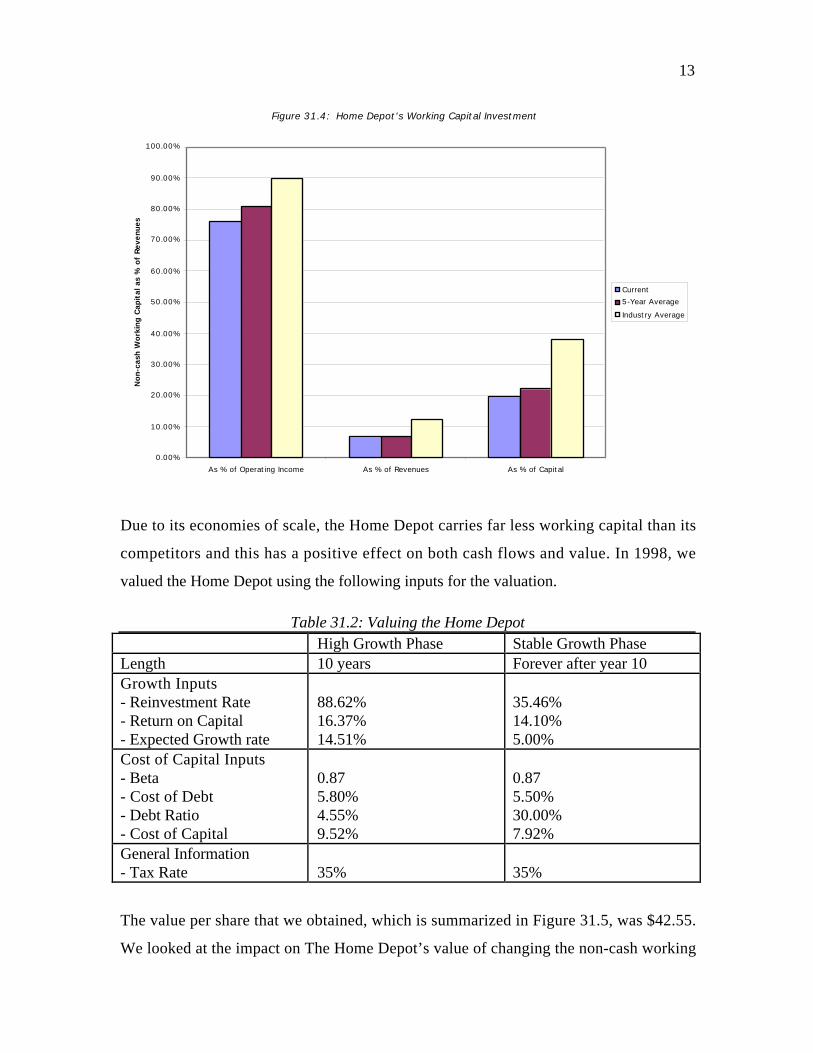
13

Due to its economies of scale, the Home Depot carries far less working capital than its

competitors and this has a positive effect on both cash flows and value. In 1998, we

valued the Home Depot using the following inputs for the valuation.

Table 31.2: Valuing the Home DepotHigh Growth Phase Stable Growth Phase

Length 10 years Forever after year 10Growth Inputs- Reinvestment Rate- Return on Capital- Expected Growth rate

88.62%16.37%14.51%

35.46%14.10%5.00%

Cost of Capital Inputs- Beta- Cost of Debt- Debt Ratio- Cost of Capital

0.875.80%4.55%9.52%

0.875.50%30.00%7.92%

General Information- Tax Rate 35% 35%

The value per share that we obtained, which is summarized in Figure 31.5, was $42.55.

We looked at the impact on The Home Depot’s value of changing the non-cash working

Figure 31.4: Home Depot's Working Capital Investment

0.00%

10.00%

20.00%

30.00%

40.00%

50.00%

60.00%

70.00%

80.00%

90.00%

100.00%

As % of Operating Income As % of Revenues As % of Capital

Non-

cash

Work

ing C

apit

al a

s %

of

Rev

enue

s

Current

5-Year Average

Industry Average

14

capital as a percent of revenues. As non-cash working capital increases, the value of

equity decreases and the results are graphed in Figure 31.6.

As the non-cash working capital increases from 0% to 20% of revenues, the value per

share decreases by approximately 20%.

cfbasics.xls: There is a dataset on the web that summarizes operating margins,

tax rates and non-cash working capital as a percent of revenues by industry group for the

United States.

Figure 31.6: The Home Depot: Working Capital and Value/Share

$0.00

$5.00

$10.00

$15.00

$20.00

$25.00

$30.00

$35.00

$40.00

$45.00

$50.00

0% 5% 10% 15% 20%

Non-Cash Working Capital as % of Revenues

Val

ue/S

hare

15

Current Cashflow to FirmEBIT(1-t) : 1,829- Nt CpX 1,799- Chg WC 190= FCFF <160>Reinvestment Rate =108.75%

Expected Growth in EBIT (1-t).8862*.1637= .145114.51 %

Stable Growthg = 5%; Beta = 0.87; D/(D+E) = 30%;ROC=14.1%Reinvestment Rate=35.46%

Terminal Value 10= 4806 / (.0792-.05) = 164,486

Cost of Equity9.79%

Cost of Debt(5%+ 0.80%)(1-.35)= 3.77%

WeightsE = 95.55% D = 4.45%

Discount at Cost of Capital (WACC) = 9.79% (0.9555) + 3.77% (0.0445) = 9.52%

Firm Value: 68,949+ Cash: 62- Debt: 4,081=Equity 64,930-Options 2,021Value/Share $42.55

Riskfree Rate :Government Bond Rate = 5%

+Beta 0.87 X

Risk Premium5.5%

Unlevered Beta for Sectors: 0.86

Firm’s D/ERatio: 4.76%

Historical US Premium5.5%

Country RiskPremium0%

Figure 31.5: The Home Depot: A ValuationReinvestment Rate88.62%

Return on Capital16.37%

EBIT(1-t)- ReinvFCFF

20951857 238

23992126 273

27472434 313

31462788 358

36023192 410

41253655 469

47234186 538

54094793 616

61945489 705

70926285 807

16

2. Increase Expected Growth

A firm with low current cash flows can still have high value if it is able to grow

quickly. For profitable firms, the growth will be defined in terms of earnings but for

money-losing firms, you have to consider the nexus of revenue growth and higher margins.

I. Profitable Firms

Higher growth either arises from increases in reinvestment or a higher return on

capital. It does not always translate into higher value, though, since higher growth can be

offset by changes elsewhere in the valuation. Thus, higher reinvestment rates usually

result in higher expected growth but at the expense of lower cash flows, since

reinvestment reduces the free cash flows. Higher returns on capital also cause expected

growth to increase, but value can still go down if the new investments are in riskier

businesses and there is a more than proportionate increase in the cost of capital.

The trade off from increasing the reinvestment rate is listed in Table 31.3. The

positive effect of reinvesting more, higher growth, has to be compared to the negative

effect of reinvesting more, the drop in free cash flows:

Table 31.3: Trade off on Reinvestment RateNegative Effects Positive Effects

Reduces free cash flow to firm:

FCFF

= EBIT (1- tax rate) ( 1- Reinvestment

Rate)

Increases Expected Growth:

Expected Growth

= Reinvestment Rate * Return on Capital

We could work through the entire valuation and determine whether the present value of

the additional cash flows created by higher growth is greater than the present value of the

actual reinvestments made, in cash flow terms. There is, however, a far simpler test to

determine the effect on value. Note that the net present value of a project measures the

value added by the project to overall firm value and that the net present value is positive

only if the internal rate of return on the project exceeds the cost of capital. If we make the

assumption that the accounting return on capital on a project is a reasonable estimate for

the internal rate of return, then increasing the reinvestment rate will increase value if and

17

only if the return on capital is greater than the cost of capital. If the return on capital is

less than the cost of capital, the positive effects of growth will be less than the negative

effects of making the reinvestment.

Note that the return on capital that we are talking about is the marginal return on

capital, i.e., the return on capital earned on the actual reinvestment, rather than the average

return on capital. Given that firms tend to accept their most attractive investment first

and their less attractive investments later, the average returns on capital will tend to be

greater than the marginal returns on capital. Thus, a firm with a return on capital of 18%

and a cost of capital of 12% may really be earning only 11% on its marginal projects. In

addition, the marginal return on capital will be much lower if the increase in the

reinvestment rate is substantial. Thus, we have to be cautious about assuming large

increases in the reinvestment rate while keeping the current return on capital constant.

A firm that is able to increase its return on capital, while keeping the cost of

capital fixed, will increase its value. The increase in growth will increase value, and there

are generally no offsetting effects. If, however, the increase in return on capital comes

from the firm entering new businesses that are far riskier than its existing business, there

might be an increase in the cost of capital that offsets the increase in growth. The general

rule for value creation remains simple, however. As long as the projects, no matter how

risky they are, have a marginal return on capital that exceeds their cost of capital, they

will create value.

Using the comparison between return on capital and cost of capital, a firm that

earns a return on capital that is less than its cost of capital can get an increase in value by

accepting higher return investments, but it would get an even greater increase in value by

not investing at all and returning the cash to the owners of the business. Liquidation or

partial liquidation might be the most value enhancing strategy for firms trapped in

businesses where it is impossible to earn the cost of capital.

Illustration 31.5: Reinvestment Rates, Return on Capital and Value

In 1998, Boeing earned a return on capital of 6.59% and had a reinvestment rate of

65.98%. If you assume a cost of capital of 9.17% for the firm, you would value the

equity in the firm at $13.14 a share. In the same year, the Home Depot had a return on

18

capital of 16.38%, a reinvestment rate of 88.62% and a cost of capital of 9.51%, resulting

in a value per share of $42.55.

Table 31.4: Value per ShareBoeing The Home Depot

Cost of Capital 9.17% 9.51%

Return on Capital 6.59% 16.38%

Reinvestment Rate 65.98% 88.62%

Expected Growth Rate 4.35% 14.51%

Value Per Share $13.14 $42.55

If the Home Depot could increase its reinvestment rates, without affecting its returns on

capital, the effect on value will be positive, because it is earning excess returns. For

Boeing, the effect of increasing the reinvestment rate at the current return on capital will

be negative, since the firm’s return on capital is less than its cost of capital. In Figure

31.7, we summarize the impact on the value of equity of changing the reinvestment rate at

both firms, keeping the cost of capital.

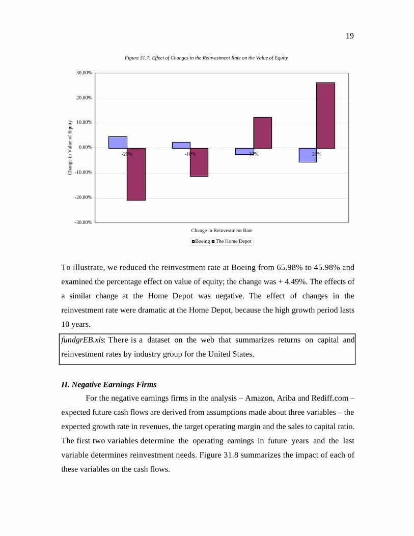
19

To illustrate, we reduced the reinvestment rate at Boeing from 65.98% to 45.98% and

examined the percentage effect on value of equity; the change was + 4.49%. The effects of

a similar change at the Home Depot was negative. The effect of changes in the

reinvestment rate were dramatic at the Home Depot, because the high growth period lasts

10 years.

fundgrEB.xls: There is a dataset on the web that summarizes returns on capital and

reinvestment rates by industry group for the United States.

II. Negative Earnings Firms

For the negative earnings firms in the analysis – Amazon, Ariba and Rediff.com –

expected future cash flows are derived from assumptions made about three variables – the

expected growth rate in revenues, the target operating margin and the sales to capital ratio.

The first two variables determine the operating earnings in future years and the last

variable determines reinvestment needs. Figure 31.8 summarizes the impact of each of

these variables on the cash flows.

Figure 31.7: Effect of Changes in the Reinvestment Rate on the Value of Equity

-30.00%

-20.00%

-10.00%

0.00%

10.00%

20.00%

30.00%

-20% -10% 10% 20%

Change in Reinvestment Rate

Cha

nge

in V

alue

of

Equ

ity

Boeing The Home Depot

20

Free Cashflow to Firm (FCFF) = EBIT (1 - tax rate) - Reinvestment Needs

Revenue Growth Target Operating Margin

Sales to Capital Ratio

Figure 31.8: Determinants of Growth

Other things remaining equal, the expected cash flows in future years will be higher if any

of the three variables – revenue growth, target margins and sales to capital ratios –

increase. Increasing revenue growth and target margins will increase operating earnings,

while increasing the sales to capital ratio will reduce reinvestment needs.

In reality, though, firms have to make a trade off between higher revenue growth

and higher margins. When firms increase prices for their products, they improve operating

margins but reduce revenue growth. Michael Porter, one of the leading thinkers in

corporate strategy, suggests that when it comes to pricing strategy, there are two basic

routes a firm can take5. It can choose to be a volume leader, reducing price and hoping to

increase revenues sufficiently to compensate for the lower margins. For this strategy to

work, the firm needs a cost advantage over its competitors to prevent pricing wars that

may make all firms in the industry worse off. Alternatively, it can attempt to be a price

leader, increasing prices and hoping that the effect on volume will be smaller than the

increased margins. The extent to which revenue growth will drop depends upon how

elastic the demand for the product is and how competitive the overall product market is.

The net effect will determine value.

While a higher sales to capital ratio reduces reinvestment needs and increases cash

flow, there are both internal and external constraints on the process. As the sales to

capital ratio increases, the return on capital on the firm in future years will also increase.

If the return on capital substantially exceeds the cost of capital, new competitors will

5 “Competitive Strategy”, Michael Porter

21

enter the market, making it more difficult to sustain the expected operating margins and

revenue growth.

Illustration 31.6: Revenue Growth, Operating Margins and Sales to Capital Ratios

In Chapter 23, we valued Commerce One, a firm with an operating loss of $529

million and only $537 million in revenues. Using a compounded revenue growth rate of

40.24%, a target operating margin of 14.72% in ten years and a sales to capital ratio of

2.20, we estimated a value for the firm of $4.8 billion and value per share of $19.26.

Changes in these inputs can have a dramatic effect on the value of the firm, as we noted in

Chapter 23.

As you would expect, higher revenue growth translates into higher values per

share. Figure 31.9 graphs the change in value per share for Commerce One as a function of

the change in expected growth rate in revenues over the next decade.

Thus, Commerce One’s value per share increases by 50% if the compounded revenue

growth over the next 10 years is 45% instead of 40%. By the same token, the value per

share drops by a third if the growth rate is 35%.

Figure 31.9: Revenue Growth and Value per share

$0.00

$5.00

$10.00

$15.00

$20.00

$25.00

$30.00

$35.00

5% 10% 15% 20% 25% 30% 35% 40% 45%

Compounded Revenue Growth - Next 10 years

Val

ue p

er s

hare

22

While higher revenue growth clearly increases value, we assumed that the target

margin would remain unchanged as we change the growth rate. The target margin is just as

important, if not more so, than revenue growth in determining value. In Figure 31.10, we

estimate the value per share, holding revenue growth at 40.24% and changing the target

margin.

Every 1% change in the target operating margin changes the value by approximately $3

per share.

The trade off between revenue growth and margins is made more explicit in Table

31.5, which shows value per share as a function of both variables.

Table 31.5: Margin versus Revenue Growth: Commerce One

Target Pre-tax Operating Margin in 10 years8% 10% 12% 14% 16%

10% $0.00 $0.00 $0.00 $0.47 $1.08

20% $0.00 $0.18 $1.46 $2.91 $4.29

Compounded

Revenue

Growth over

next 10 years30% $0.02 $2.98 $5.74 $8.47 $11.18

Figure 31.10: Value per share and Sustainable Margins

$0.00

$5.00

$10.00

$15.00

$20.00

$25.00

10% 11% 12% 13% 14% 15% 16%

Pre-tax operating margin

Val

ue

per

shar

e

23

40% $3.51 $8.94 $14.36 $19.77 $25.17next 10 years

50% $10.31 $20.74 $31.16 $41.56 $51.97

Commerce One’s value varies widely depending upon the combination of revenue growth

and margins that you assume. In practical terms, this also provides the firm with a sense

of the trade off between higher revenue growth and lower target margins.

Finally, a higher sales to capital ratio (which translates into a higher return on

capital in 10 years) leads to a higher value per share, because it determines both how

much Commerce One has to reinvest to generate its expected growth rate. Figure 31.11

presents the effects on value per share of changing the sales to capital ratio over the high

growth period for Commerce One. As we change the sales to capital ratio, we also change

the return on capital in stable growth – it increases as the sales to capital ratio increases.

As the sales to capital ratio (and the terminal return on capital) increases, the value per

share of Commerce One also increases.

Figure 31.11: Value per Share versus Sales to Capital

$0.00

$5.00

$10.00

$15.00

$20.00

$25.00

$30.00

1.60 1.80 2 2.2 2.4 2.6

Sales to Capital Ratio

Val

ue p

er S

hare

24

3. Lengthen the Period of High Growth

Every firm, at some point in the future, will become a stable growth firm, growing

at a rate equal to or less than that of the economy in which it operates. In addition,

growth creates value only if the firm earns excess returns on its investments. With excess

returns, the longer the high growth period lasts, other things remaining equal, the greater

the value of the firm. No firm should be able to earn excess returns for any length of time

in a competitive product market, since competitors will be attracted to the business by

the excess returns. Thus, implicit in the assumption that there will be high growth with

excess returns is the assumption that there also exist some barriers to entry that prevent

competing firms from entering the market and eliminating the excess returns that prevail.

One way firms can increase value is by increasing existing barriers to entry and

erecting new ones. Another way to express this idea is that companies earning excess

returns have significant competitive advantages. Nurturing these advantages can increase

value.

3.1: The Brand Name Advantage

As we noted earlier in the book, the inputs to the traditional discounted cash flow

valuation incorporate the effects of brand name. In particular, firms with more valuable

brand names are either able to charge higher prices than the competition for the same

products (leading to higher margins) or sell more than the competitors at the same price

(leading to higher turnover ratios). They usually have higher returns on capital and greater

value than their competitors in the industry.

Creating a brand name is a difficult and expensive process that may take years to

achieve, but firms can often build on existing brand names and make them valuable. Brand

management and advertising can contribute in value creation. Consider the extraordinary

success that Coca Cola has had in increasing its market value over the last two decades.

Some attribute its success to its high return on equity or capital, yet these returns are not

the cause of its success but the consequence of it. The high returns can be traced to the

25

company's relentless focus on making its brand name more valuable globally6.

Conversely, the managers of a firm who take over a valuable brand name and then

dissipate its value will reduce the values of the firm substantially. The near-death

experience of Apple Computers in 1996 and 1997 and the travails of Quaker Oats after

the Snapple acquisition suggest that managers can quickly squander the advantage that

comes from valuable brand names.

3.2: Patents, Licenses and Other Legal Protection

The second competitive advantage that companies can possess is a legal one.

Firms may enjoy exclusive rights to produce and market a product because they own the

patent rights on the product, as is often the case in the pharmaceutical industry.

Alternatively, firms may have exclusive licensing rights to service a market, as is the case

with utilities in the United States.

The key to value enhancement is not just to preserve but to increase any

competitive advantages that the firm possesses. If the competitive advantage comes from

its existing patents, the firm has to work at developing new patents that allow it to

maintain this advantage over time. While spending more money on research and

development (R&D) is clearly one way, the efficiency of reinvestment also applies here.

The companies that have the greatest increases in value are not necessarily those that

spend the most on R&D, but those that have the most productive R&D departments not

only in generating patents but also in converting patents into commercial products.

The competitive advantage from exclusive licensing or a legal monopoly is a mixed

blessing and may not lead to value enhancement. When a firm is granted these rights by

another entity, say the government, that entity usually preserves the right to control the

prices charged and margins earned through regulation. In the United States, for instance,

much of the regulation of power and phone utilities was driven by the objective of

ensuring that these firms did not earn excess returns. In these circumstances, firms may

actually gain in value by giving up their legal monopolies, if they get pricing freedom in

6 Companies like Coca Cola have taken advantage of the global perception that they represent Americanculture, and used it to grow strongly in other markets.

26

return. We could argue that this has already occurred, in great part, in the airline and long-

distance telecommunications businesses and will occur in the future in other regulated

businesses. In the aftermath of deregulation, the firms that retain competitive advantages

will gain value at the expense of others in the business.

3.3: Switching Costs

There are some businesses where neither brand name nor a patent provides

adequate protection against competition. Products have short life cycles, competition is

fierce and customers develop little loyalty to companies or products. This describes the

computer software business in the 1980s and it still applies to a significant portion of

that business today. How, then, did Microsoft succeed so well in establishing its presence

in the market? Although many would attribute its success entirely to its ownership of the

operating system needed to run the software, there is another reason. Microsoft

recognized earlier than most other firms that the most significant barrier to entry in the

software business is the cost to the end-user of switching from one product to a

competitor. In fact, Microsoft Excel, early in its life, had to overcome the obstacle that

most users were working with Lotus spreadsheets and did not want to bear the switching

cost. Microsoft made it easy for end-users to switch to its products (by allowing Excel to

open Lotus spreadsheets, for instance), and it made it more and more expensive for them

to switch to a competitor by creating the Microsoft Office Suite. Thus, a user who has

Microsoft Office installed on his or her system and who wants to try to switch from

Microsoft Word to WordPerfect has to overcome multiple barriers - Will the conversion

work well on the hundreds of Word files that exist already? Will the user still be able to

cut and paste from Microsoft Excel and Power Point into WordPerfect documents? The

end result, of course, is that it becomes very difficult for competitors who do not have

Microsoft’s resources to compete with it in this arena.

There are a number of other businesses where the switching cost concept can be

used to augment an argument for value enhancement or debunk it. For instance, there are

many who argue that the high valuations of Internet companies such as Amazon.com and

eToys reflect their first-mover advantage, i.e, the fact that they are pioneers in the online

business. However, the switching costs in online retailing seem to be minimal, if any, and

27

these companies have to come up with a way of increasing switching costs if they want

to earn high returns in the future.

3.4: Cost Advantages

There are several ways in which firms can establish a cost advantage over their

competitors and use it as a barrier to entry.

• In businesses where scale can be used to reduce costs, economies of scale can give

bigger firms advantages over smaller firms. This is the advantage, for instance, that the

Home Depot has used to gain market share at the expense of its smaller and often

local competitors.

• Owning or having exclusive rights to a distribution system can provide firms with a

cost advantage over its competitors. For instance, American Airlines’ ownership of

the Sabre airline reservation system gave it an advantage over its competitors in

attracting customers.

• Having access to lower-cost labor or resources can also provide cost advantages. Thus

Southwest Airlines, with its non-unionized labor force, has an advantage over its

unionized competitors, as do natural resource companies with access to reserves that

are less expensive to exploit.

These cost advantages will influence value in one of two ways: The firm with the cost

advantage may charge the same price as its competitors but have a much higher operating

margin. Or the firm may charge lower prices than its competitors and have a much higher

capital turnover ratio. In fact, the net effect of increasing margins or turnover ratios (or

both) will increase the return on capital and through it expected growth.

The cost advantage of economies of scale can create high capital requirements that

prevent new firms from entering the business. In businesses such as aerospace and

automobiles, the competition is almost entirely among existing competitors. The absence

of new competitors may allow these firms to maintain above-normal returns, though the

competition between existing firms will constrain the magnitude of these returns.

28

Illustration 31.7: Potential for Increasing the Length of the High Growth Period

We examine the potential for increasing barriers to entry and by extension the

excess returns and the length of the high growth period at Cisco and Motorola. The

competitive advantages are different for the two firms and the potential for building on

these advantages is different as well.

• Cisco’s most significant differential advantage seems to be its capacity to generate

much larger excess returns on its new investments than its competitors. Since most of

these investments take the form of acquisitions of other firms, Cisco’s excess returns

rest on whether it can continue to maintain its success in this area. The primary

challenge, however, is that as Cisco continues to grow, it will need to do even more

acquisitions each year to maintain the growth rate it had the previous year. It is

possible that there might be both external and internal constraints on this process. The

number of firms that are potential takeover targets is limited and the firm may not

have the resources to replicate its current success if the number of acquisitions

doubles or triples.

• Motorola’s research capabilities and the patents that emerge from the research

represent its most significant competitive advantage. However, it is not viewed as the

technological leader in either of the two businesses that it operates in. Firms like

Nokia are viewed as more innovative when it comes to mobile communications

(cellular phones) and Intel is considered the leading innovator among large semi-

conductor manufacturers.

We begin by valuing each of these firms using their current returns on capital and

estimated reinvestment rates as inputs for the high growth period. Table 31.6 summarizes

the inputs used in the base case valuations and the value per share estimated with these

assumptions.

Table 31.6: Inputs for valuing Cisco and Motorola

Cisco MotorolaHigh Growth Stable Growth High Growth Stable Growth

Beta 1.43 1.00 1.21 1.00

29

Cost of Equity 11.72% 10.00% 10.85% 10.00%

After-tax Cost of

Debt

4.03% 4.03% 4.23% 4.23%

Debt Ratio 0.18% 10.00% 6.86% 6.86%

Cost of Capital 11.71% 9.40% 10.39% 9.58%

Return on Capital 34.07% 16.52% 12.12% 12.12%

Reinvestment Rate 106.8% 30.27% 52.99% 41.07%

Expected Growth

Rate

36.39% 5.00% 6.45% 5.00%

Value per share $44.13 $20.99

In the base case, we assume 12 years of high growth for Cisco – six years of high growth

and six years of transition – and 5 years of high growth for Motorola. We then consider

how much the value per share changes as we change the growth period in Figure 31.12.

Figure 31.12: Value per Share and Length of High Growth

$0.00

$10.00

$20.00

$30.00

$40.00

$50.00

$60.00

$70.00

0 2 4 6 8 10 12 14

Length of High Growth

Val

ue p

er s

hare

CiscoMotorola

30

The effect of changing the length of the growth period is very different for the two firms.

For Cisco, the value per share changes significantly as the length of the growth period

change, increasing as it gets longer. For Motorola, the effect is muted and the value per

share is relatively insensitive to changes in the length of the growth period. The reason

lies in the excess returns that we are assuming for the two firms over the length of the

growth period. For Cisco, the excess returns are very large and thus the impact on value is

also large. For Motorola, we assume that the excess returns are relatively small and the

effect on value is also much lower.

Lead Times from Competitive Advantages

A key question that we often face when looking at the effects of a competitive

advantage on value is how long a competitive advantage lasts. This is a difficult question

to answer because there are a number of firm specific factors but there are few interesting

studies in corporate strategy that try to address the issue. Levin, Klevorick, Nelson and

Winter (1987) estimate, for instance, that it takes between 3-5 years to duplicate a

patented product or process and 1-3 years to duplicate an unpatented product or

process. In the same study, they find that patenting is often much less effective at

preventing imitation that moving quickly down the learning curve (producing more

advanced versions of the product at lower cost) and establishing efficient sales and service

networks. For example, Intel was able to maintain its competitive advantages even as its

computer chips were being cloned by AMD by using the lead time it had to move quickly

to the next generation chips.

4. Reduce the cost of financing

The cost of capital for a firm is a composite cost of debt and equity financing. The

cash flows generated over time are discounted to the present at the cost of capital.

Holding the cash flows constant, reducing the cost of capital will increase the value of the

firm. In this section, we will explore the ways in which a firm may reduce its cost of

capital, or more generally, increase its firm value by changing both financing mix and type.

31

4.1. Change Operating Risk

The operating risk of a firm is a direct function of the kinds of products or

services it provides and the degree to which these products or services are discretionary

to the customer. The more discretionary they are, the greater the operating risk faced by

the firm. Both the cost of equity and cost of debt of a firm are affected by the operating

risk of the business or businesses in which it operates. In the case of equity, only that

portion of the operating risk that is not diversifiable will affect value.

Firms can reduce their operating risk by making their products and services less

discretionary to their customers. Advertising clearly plays a role, but finding new uses for

a product or service is another.

4.2: Reduce Operating Leverage

The operating leverage of a firm measures the proportion of its costs that are

fixed. Other things remaining equal, the greater the proportion of the costs of a firm that

are fixed, the more volatile its earnings and the higher its cost of capital. Reducing the

proportion of the costs that are fixed will make firms much less risky and reduce their

cost of capital. Firms can reduce their fixed costs by using outside contractors for some

services; if business does not measure up, the firm is not stuck with the costs of

providing this service. They can also tie expenses to revenues; for instance, tying wages

paid to revenues made will reduce the proportion of costs that are fixed.

This basic idea of tying expenses to revenues is often described as making the cost

structure more flexible. A more flexible cost structure influences three inputs in a

valuation. It leads to a lower unlevered beta (due to the lower operating leverage), reduces

the cost of debt (because of the reduction in default risk) and increases the optimal debt

ratio. All three reduce the cost of capital and increase firm value.

4.3: Change the Financing Mix

A third way to reduce the cost of capital is to change the mix of debt and equity

used to finance the firm. As we argued in the chapters on capital structure, debt is always

cheaper than equity, partly because lenders bear less risk and partly because of the tax

advantage associated with debt. This benefit has to be weighed off against the additional

32

risk of bankruptcy created by the borrowing; this higher risk increases both the beta for

equity and the cost of borrowing. The net effect will determine whether the cost of capital

will increase or decrease as the firm takes on more debt.

Note, however, that firm value will increase as the cost of capital decreases, if and

only if the operating cash flows are unaffected by the higher debt ratio. If, as the debt

ratio increases, the riskiness of the firm increases, and this, in turn, affects the firm's

operations and cash flows; the firm value may decrease even as cost of capital declines. If

this is the case, the objective function when designing the financing mix for a firm has to

be restated in terms of firm value maximization rather than cost of capital minimization.

wacc.xls: There is a dataset on the web that summarizes debt ratios and costs of

capital by industry group for the United States.

Illustration 31.8: The Effect of Financing Mix on Value

To analyze the effect of changing the financing mix on value, you would need to

estimate the costs of equity and debt at each debt ratio. In Table 31.7, the costs of equity

and debt are estimated for Motorola for debt ratios from 0% to 90%.

Table 31.7: Cost of Capital and Firm Value: MotorolaDebt

Ratio

Beta Cost of

Equity

Bond

Rating

Interest rate

on debt

Tax Rate Cost of Debt

(after-tax)

WACC

0% 1.16 10.63% AAA 6.20% 35.00% 4.03% 10.63%

10% 1.24 10.96% A- 7.25% 35.00% 4.71% 10.33%

20% 1.34 11.38% B- 10.25% 35.00% 6.66% 10.43%

30% 1.48 11.91% CC 12.00% 35.00% 7.80% 10.68%

40% 1.72 12.90% C 13.50% 26.34% 9.94% 11.72%

50% 2.07 14.28% C 13.50% 21.07% 10.66% 12.47%

60% 2.63 16.54% D 16.00% 14.82% 13.63% 14.79%

70% 3.51 20.05% D 16.00% 12.70% 13.97% 15.79%

80% 5.27 27.07% D 16.00% 11.11% 14.22% 16.79%

90% 10.54 48.14% D 16.00% 9.88% 14.42% 17.79%

33

Note that the cost of equity is estimated based upon the levered beta. As the debt ratio

increases, the beta increases as well.7 The cost of debt is estimated based upon a

synthetic rating that is determined by the interest coverage ratio at each debt ratio. As the

debt ratio increases, the interest expense increases leading to a drop in the ratings and

higher costs of debt. As Motorola moves from a 0% debt ratio to a 10% debt ratio, the

cost of capital decreases (and firm value increases). At a 10% debt ratio, Motorola’s cost

of capital is 10.33%, which is lower than the current cost of capital of 10.39%. Beyond

10%, though, the trade off operates against debt, the cost of capital increases as the debt

ratio increases.

4.4: Change Financing Type

A fundamental principle in corporate finance is that the financing of a firm should

be designed to ensure, as far as possible, that the cash flows on debt match as closely as

possible the cash flows on the asset. By matching cash flows on debt to cash flows on the

asset, a firm reduces its risk of default and increases its capacity to carry debt, which, in

turn, reduces its cost of capital and increases value.

Firms that mismatch cash flows on debt and cash flows on assets (by using short-

term debt to finance long-term assets, debt in one currency to finance assets in a different

currency or floating-rate debt to finance assets whose cash flows tend to be adversely

impacted by higher inflation) will have higher default risk, higher costs of capital and

lower firm value. Firms can use derivatives and swaps to reduce these mismatches and, in

the process, increase firm value. Alternatively, they can replace their existing debt with

debt that is more closely matched to their assets. Finally, they can use innovative

securities that allow them to pattern cash flows on debt to cash flows on investments.

The use of catastrophe bonds by insurance companies and commodity bonds by natural

resource firms are good examples.

What about Miller-Modigliani?

7 Levered Beta = Unlevered Beta (1 + (1- tax rate) (Debt/ Equity))

34

One of corporate finance’s best known and most enduring propositions – the

Miller-Modigliani theorem – argues that the value of a firm is independent of its capital

structure. In other words, changing your financing mix should have no effect on your firm

value. How would we reconcile our arguments in this section with the Miller Modigliani

theorem? Note that the original version of the theorem was derived for a world with no

taxes and default. With these assumptions, debt creates no tax advantages and no

bankruptcy costs and does not affect value. In a world with taxes and default risk, you are

much more likely to have to make trade offs and debt can increase value, decrease value or

leave it unaffected depending upon how the trade offs operate.

The Value Enhancement Chain

We can categorize the range of actions firms can take to increase value in several

ways. One is in terms of whether they affect cash flows from assets in place, growth, the

cost of capital or the length of the growth period. There are two other levels at which we

can distinguish between actions that create value.

a. Does an action create a value trade off or is it a pure value creator? Very few

actions increase value without any qualifications. Among these are the

divestitures of assets when the divestiture value exceeds the continuing value

and the elimination of deadweight costs that contribute nothing to the firm’s

earnings or future growth. Most actions have both positive and negative

effects on value and it is the net effect that determines whether these actions

are value enhancing. In some cases, the tradeoff is largely internal and the odds

are much better for value creation. An example is a firm changing its mix of

debt and equity to reduce the cost of capital. In other cases, however, the net

effect on value will be a function of how competitors react to a firm’s actions.

As an example, changing pricing strategy to increase margins may not work as

a value enhancement measure, if competitors react and change prices as well.

b. How quickly do actions pay off? Some actions generate an immediate increase

in value. Among these are divestitures and cost cutting. Many actions,

however, are designed to create value in the long term. Thus, building up a

35

respected brand name clearly creates value in the long term but is unlikely to

affect value today.

Table 31.8 summarizes a value enhancement chain, where actions that create value are

categorized both on how quickly they create value and on how much control the firm has

over the value creation. Under the first column, titled “Quick Fixes”, we have listed

actions in which the firm has considerable control over the outcome and the benefit in

terms of value creation is immediate. Under the second column, titled "Odds on", we have

included actions that are likely to create value in the near or medium term and where the

firm still continues to exercise significant control over the outcome. The third column,

titled "Long Term", includes actions designed to create value in the long term. This is

where the major strategic initiatives of the firm show up.

Illustration 31.9: A Value Enhancement Plan

In Illustration 31.7, we valued Motorola at $22.05 using its current return on

capital of 12.18% and debt ratio of 6.86% in the valuation. Figure 31.13 summarizes this

valuation. Note, though, that the current return on capital is well below what the firm has

earned historically and lags the industry average (of 22.36%) by almost 10%. If Motorola

could increase its return on capital to 17.22% on its new investments (leaving its existing

investments earning 12.18%) and increase its debt ratio to its optimal of 10%, its value

per share would increase to $23.86. The restructured valuation is summarized in Figure

31.14.

valenh.xls: This spreadsheet allows you to estimate the approximate effect of

changing the way a firm is run on its value.

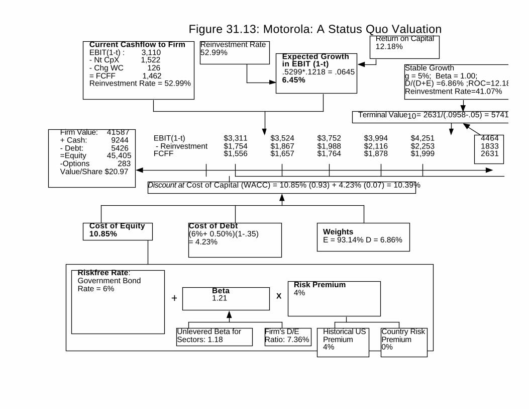
Current Cashflow to FirmEBIT(1-t) : 3,110- Nt CpX 1,522- Chg WC 126= FCFF 1,462Reinvestment Rate = 52.99%

Expected Growth in EBIT (1-t).5299*.1218 = .06456.45%

Stable Growthg = 5%; Beta = 1.00; D/(D+E) =6.86% ;ROC=12.18%Reinvestment Rate=41.07%

Terminal Value10= 2631/(.0958-.05) = 57418

Cost of Equity10.85%

Cost of Debt(6%+ 0.50%)(1-.35)= 4.23%

WeightsE = 93.14% D = 6.86%

Discount at Cost of Capital (WACC) = 10.85% (0.93) + 4.23% (0.07) = 10.39%

Firm Value: 41587+ Cash: 9244- Debt: 5426=Equity 45,405-Options 283Value/Share $20.97

Riskfree Rate:Government Bond Rate = 6%

+Beta 1.21 X

Risk Premium4%

Unlevered Beta for Sectors: 1.18

Firm’s D/ERatio: 7.36%

Historical US Premium4%

Country RiskPremium0%

Figure 31.13: Motorola: A Status Quo ValuationReinvestment Rate52.99%

Return on Capital12.18%

446418332631

EBIT(1-t) $3,311 $3,524 $3,752 $3,994 $4,251 - Reinvestment $1,754 $1,867 $1,988 $2,116 $2,253 FCFF $1,556 $1,657 $1,764 $1,878 $1,999

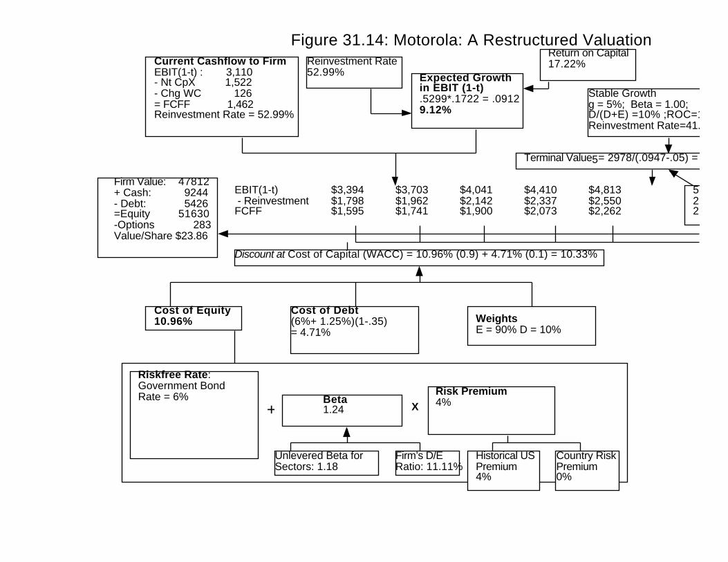
Current Cashflow to FirmEBIT(1-t) : 3,110- Nt CpX 1,522- Chg WC 126= FCFF 1,462Reinvestment Rate = 52.99%

Expected Growth in EBIT (1-t).5299*.1722 = .09129.12%

Stable Growthg = 5%; Beta = 1.00; D/(D+E) =10% ;ROC=12.18%Reinvestment Rate=41.07%

Terminal Value5= 2978/(.0947-.05) = 66606

Cost of Equity10.96%

Cost of Debt(6%+ 1.25%)(1-.35)= 4.71%

WeightsE = 90% D = 10%

Discount at Cost of Capital (WACC) = 10.96% (0.9) + 4.71% (0.1) = 10.33%

Firm Value: 47812+ Cash: 9244- Debt: 5426=Equity 51630-Options 283Value/Share $23.86

Riskfree Rate:Government Bond Rate = 6%

+Beta 1.24 X

Risk Premium4%

Unlevered Beta for Sectors: 1.18

Firm’s D/ERatio: 11.11%

Historical US Premium4%

Country RiskPremium0%

Figure 31.14: Motorola: A Restructured ValuationReinvestment Rate52.99%

Return on Capital17.22%

505320752978

EBIT(1-t) $3,394 $3,703 $4,041 $4,410 $4,813 - Reinvestment $1,798 $1,962 $2,142 $2,337 $2,550 FCFF $1,595 $1,741 $1,900 $2,073 $2,262

Table 31.8: The Value Enhancement Chain

More control Less control

Payoff quickly Payoff in long term

Quick Fixes Odds on.. Long Term

Existing Investmentsa. Divest assets/projects with

Divestiture Value >Continuing Value.

b. Terminate projects withLiquidation Value >Continuing Value.

c. Eliminate operatingexpenses that generate norevenues and no growth.

d. Take advantage of tax lawto increase cash flow.

1. Reduce net working capitalrequirements, by reducinginventory and accountsreceivable, or by increasingaccounts payable.

2. Reduce capital maintenanceexpenditures on assets inplace.

3. Reduce marginal tax rate.

1. Change pricing strategy tomaximize the product ofprofit margins and turnoverratio.

2. Move to more efficienttechnology for operationsto reduce expenses andimprove margins..

Expected Growth Eliminate new capitalexpenditures that are expectedto earn less than the cost ofcapital.

Increase reinvestment rate ormarginal return on capital orboth in firm’s existingbusinesses.

Increase reinvestment rate ormarginal return on capital orboth in new businesses.

Length of High Growth Period If any of the firm’s products orservices can be patented andprotected, do so.

Use economies of scale or costadvantages to create higherreturn on capital.

a. Build up brand name.b. Increase the cost of switchingfrom product and reduce cost ofswitching to it.

Cost of Financing a. Use swaps and derivativesto match debt more closelyto firm’s assets.

b. Recapitalize to move thefirm towards its optimaldebt ratio.

a. Change financing type anduse innovative securities toreflect the types of assets beingfinanced.b. Use the optimal financingmix to finance new investments.c. Make cost structure moreflexible to reduce operatingleverage.

Reduce the operating risk of thefirm, by making products lessdiscretionary to customers.

39

Closing Thoughts on Value Enhancement

Almost all firms claim to be interested in value enhancement but very few are able

to increase value consistently. If value enhancement is as simple as it is made out to be in

this chapter, you might wonder why this is so. There are four basic propositions you

need to consider in the context of value enhancement.

1. Value enhancement is hard work, takes time and may make life uncomfortable for

existing managers: There are no magic bullets that increase value painlessly.

Increasing cash flows requires hard decisions on layoffs and cost cutting and, in

some cases, admitting past mistakes. Increasing the reinvestment rate will require

that you analyze new investments with more care and that you invest in the

infrastructure you need to manage these investments. Increasing your debt ratio

may also create new pressures to make interest payments and to deal with ratings

agencies and banks.

2. For a firm to enhance value, all of its component parts need to buy into the value

enhancement plan: You cannot increase value by edict and you cannot do it from

the executive offices (or the finance department). As you probably noted in the

discussion, every part of the firm has a role to play in increasing value. Table 31.9

summarizes the role of each part of the firm in the value enhancement actions that

we have described in this chapter. Departments have to cooperate for value

enhancement to become a reality.

Table 31.9: Value Enhancement Actions: Who is responsible?

Value enhancing action Primary responsibility

Increasing operating efficiency Operating managers and personnel, from

shop-floor stewards to factory managers.

Reducing working capital needs Inventory personnel

Credit personnel

Increasing revenue growth Sales and marketing personnel

Increasing return on capital/ reinvestment

rate

Strategic Teams, with help from financial

analysts

40

Build brand name

Other competitive advantages

Advertising personnel

Strategic analysts

Reduce cost of financing Finance department

3. Value enhancement has to be firm-specific: No two firms in trouble share the same

problems and using a cook-book approach seldom works in value enhancement.

You have to begin by diagnosing the specific problems faced by the firm you are

analyzing and tailor a response to these problems. Thus, the value enhancement

plan you would devise for a mature firm with cost overruns will be very different

from the plan you would devise for a young firm that has a product that no longer

meets market needs.

4. Price enhancement may not always follow value enhancement: This is perhaps the

most disappointing aspect of value enhancement. A firm that takes all the right

actions may not necessarily be rewarded immediately by financial markets. In

some cases, markets may even punish such firms because of the effects of these

actions on reported earnings. We remain convinced that in the long terms, markets

will recognize value enhancing actions and reward them, but the manager who took

these actions may not be around to share in the rewards.

Summary

Value enhancement is clearly on the minds of many managers today. Building on

the discounted cash flow principles developed in the last chapter, the value of a firm can

be increased by changing one of the four primary inputs into valuation: the cash flows

from assets in place, the expected growth rate during the high growth period, the length of

the high growth period and the cost of capital. Conversely, actions that do not change any

of these variables cannot create value. Cash flows from assets in place can be increased by

cost cutting and more efficient operations, as well as by lowering taxes paid on income

and reducing investment needs (capital maintenance and non-cash working capital

investments). Expected growth can be increased by increasing the reinvestment rate or the

return on capital, but increases in the reinvestment rate will generate value only if the

return on capital exceeds the cost of capital. High growth, at least the value creating kind,

41

can be made to last longer by generating new competitive advantages or augments existing

ones. Finally, the cost of capital can be lowered by moving towards an optimal debt ratio,

using debt that is more suited for the assets being financed and by reducing market risk.

42

Problems

1. Marion Manufacturing, a steel company, announces that it will be taking a major

restructuring charge that will lower earnings this year by $500 million. Assume that

the charge is not tax deductible and has no effects on operations.

a. What will the effect of this charge be on the value of the firm?

a. When the firm announces the charge, what effect would you expect it to have

on the stock price? Is your answer consistent with your response to (a)?

2. Universal Health Care (UHC) is a company whose stock price has declined by 40% in

the last year. In the current year, UHC earned $300 million in pre-tax operating income on

revenues of $10 billion. The new CEO of the firm has proposed cost-cutting measures she

anticipates will save the firm $100 million in expenses, without any effect on revenues.

Assume the firm is growing at a stable rate of 5% a year and its cost of capital is 10%;

neither number is expected to change as a consequence of the cost cutting. The firm’s tax

rate is 40%. (You can assume that the firm reinvests $100 million each year and that this

reinvestment will not change as the firm cuts costs.)

• What effect will the cost cutting have on value?

• What effect will the cost cutting have on value, if the expected growth rate

will drop to 4.5% as a consequence? (Some of the costs cut were designed

to generate future growth)

3. Atlantic Cruise Lines operates cruise ships and is headquartered in Florida. The firm

had $100 million in pre-tax operating income in the current year, of which it

reinvested $25 million. The firm expects its operating income to grow 4% in

perpetuity and maintain its existing reinvestment rate. Atlantic has a capital structure

composed 60% of equity and 40% of debt. Its cost of equity is 12% and it has a pre-

tax cost of borrowing of 8%. The firm currently faces a tax rate of 40%.

a. Estimate the value of the firm.

b. Assume now that Atlantic Cruise Lines will move its headquarters to the

Cayman Islands. If its tax rate drops to 0% as a consequence, estimate the effect

on value of the shift.

43

4. Furniture Depot is a retail chain selling furniture and appliances. The firm has after-tax

operating income of $250 million in the current year on revenues of $5 billion. The firm

also has non-cash working capital of $1 billion. The net capital expenditures this year is

$100 million and expects revenues, operating income and net capital expenditures to grow

5% a year forever. The firm’s cost of capital is 9%.

a. Assume that non-cash working capital remains at the existing percent of

revenues, estimate the value of the firm.

b. Assume now that the firm is able to reduce its non-cash working capital

requirement by 50%. Estimate the effect on value of this change.

c. If as a consequence of this non-cash working capital change, earnings growth

declines to 4.75%, what would the effect on value be of the drop in non-cash

working capital?

5. General Systems is a firm that manufactures personal computers. As a top manager in

the firm, you are considering changes in the way the firm is run. Currently, the firm has

after-tax operating income of $50 million on capital invested of $250 million (at the

beginning of the year). The firm also reinvests $25 million in net capital expenditures and

working capital.

a. Estimate the expected growth rate in earnings, given the firm’s current return on

capital and reinvestment rate.

b. Holding the return on capital constant, what would happen to the expected

growth rate if the firm increased its reinvestment rate to 80%?

c. What would the effect on growth be, if as the reinvestment rate increases to

80%, the return on capital on investments drops by 5%? (For instance, if the

return on capital is currently 18%, it will drop to 13%.)

6. Compaq Computers has seen its stock price decline from $45 to $24. The firm is

expected to reinvest 50% of its expected after-tax operating income of $2 billion in new

investments and to earn a return on capital of 10.69%. The firm is all equity financed and

has a cost of equity of 11.5%.

a. What is the firm’s expected growth rate, assuming that it maintains its existing

reinvestment rate and return on capital?

44

b. Assuming that this growth is perpetual, what is the value of the firm?

c. How much value is being created or destroyed by the firm’s new investments?

7. (Refer to problem 6) Now assume that Compaq’s optimal debt ratio is 20%. Its cost of

equity will increase to 12.5% and its after-tax cost of debt will be 4.5% at the optimal

debt ratio.

a. What is the firm’s expected growth rate, assuming it maintains its existing

reinvestment rate and return on capital?

b. Assuming this growth is perpetual, what is the value of the firm?

c. How much value is being created or destroyed by the firm’s new investments?

8. Coca Cola is considered to have one of the most valuable brand names in the world.

The firm has an after-tax operating margin of 20% on revenues of $25 billion. The capital

invested in the firm is $10 billion. In addition, Coca Cola reinvests 50% of its after-tax

operating earnings.

a. Estimate the expected growth in operating earnings, assuming Coca Cola can

sustain these values for the foreseeable future.

b. Assume generic soft drink manufacturers have after-tax operating margins of

only 7.5%. If Coca Cola maintains its existing reinvestment rate but loses its brand

name value, estimate the expected growth rate in operating earning. (You can

assume that, with the loss in brand name value, Coca Cola’s operating margins

would drop to 7.5%, as well.)

9. BioMask Genetics is a biotechnology firm with only one patent to its name. The after-

tax operating earnings in the current year is $100 million and the firm has no reinvestment

needs. The patent will expire in 3 years and the firm will have a 15% growth rate in

earnings during that period. After year 3, operating earnings are expected to remain

constant forever. The firm’s management is considering an advertising plan designed to

build up the brand name of its patented product. The advertising campaign will cost $50

million (pre-tax) a year over the next 3 years; the firm’s tax rate is 40%. The firm believes

this campaign will allow it to maintain a 15% growth rate for 10 years, as the brand name

45

compensates for the loss of the patent protection. After year 10, the operating earnings

are expected to remain constant forever. The firm has a cost of capital of 10%.

a. Estimate the value of the firm, assuming it does not embark on the advertising

campaign.

b. Estimate the value of the firm, with the advertising campaign.

c. Assume there is no guarantee the growth rate will last 10 years as a result of the

campaign. What would the probability of success need to be for the campaign to be

financially viable?

10. Sunmask is a cosmetics firm that has seen its stock price fall and its earnings decline in

the last year. You have been hired as the new CEO of the company and a careful analysis

of Sunmask’s current financials reveals the following.

- The firm currently has after-tax operating earnings of $300 million on revenues of $10

billion and a capital turnover ratio (sales/book value of capital) of 2.5.

- The firm is expected to reinvest 60% of its after-tax operating income.

- The firm is all equity financed and has a cost of capital of 10%.

a. Estimate the value of the firm, assuming existing policies continue forever. (Returns

on capital and reinvestment rates remain constant forever, as well.)

b. Assume that you can increase operating margins from 3% to 5% without affecting

the capital turnover ratio, that you can lower the reinvestment rate to 40%, and that

the cost of capital will become 9%, if you shift to your optimal debt ratio. How much

would your firm value increase if you were able to make these changes?

1

CHAPTER 32

VALUE ENHANCEMENT: EVA, CFROI AND OTHER TOOLS

The traditional discounted cash flow model provides for a rich and thorough

analysis of all the different ways in which a firm can increase value; but it can become

complex, as the number of inputs increases. It is also very difficult to tie management

compensation systems to a discounted cash flow model, since many of the inputs need to

be estimated and can be manipulated to yield the results management wants.

If we assume that markets are efficient, we can replace the unobservable value

from the discounted cash flow model with the observed market price and reward or

punish managers based upon the performance of the stock. Thus, a firm whose stock

price has gone up is viewed as having created value, whereas one whose stock price has

fallen has destroyed value. Compensation systems based upon the stock price, including

stock grants and warrants, have become a standard component of most management

compensation package.

While market prices have the advantage of being up to date and observable, they

are also noisy. Even if markets are efficient, stock prices tend to fluctuate around the true

value and markets sometimes do make mistakes. Thus, a firm may see its stock price go

up and its top management rewarded, even as it destroys value. Conversely, the managers

of a firm may be penalized as its stock price drops, even though the managers may have

taken actions that increase firm value. The other problem with stock prices as the basis

for compensation is that they are available only for the entire firm. Thus, stock prices

cannot be used to analyze the managers of individual divisions of a firm or for their

relative performance.

In the last decade, while firms have become more focused on value creation, they

have remained suspicious of financial markets. While they might understand the notion of

discounted cash flow value, they are unwilling to tie compensation to a value that is based

upon dozens of estimates. In this environment, new mechanisms for measuring value that

are simple to estimate and use, do not depend too heavily on market movements and do

not require a lot of estimation, find a ready market. The two mechanisms that seem to

have made the most impact are:

2

1. Economic Value Added, which measures the dollar surplus value created by a firm

on its existing investment, and

2. Cash Flow Return on Investment, which measured the percentage return made by a

firm on its existing investments

In this chapter, we look at how each is related to discounted cash flow valuation. We also

look at the conditions under which firms using these approaches to judge performance and

evaluate managers may end up making decisions that destroy value rather than create it.

Economic Value Added

The economic value added (EVA) is a measure of the dollar surplus value created

by an investment or a portfolio of investments. It is computed as the product of the

"excess return" made on an investment or investments and the capital invested in that

investment or investments.

Economic Value Added = (Return on Capital Invested – Cost of Capital) (Capital

Invested) = After tax operating income – (Cost of Capital) (Capital Invested)

In this section, we will begin by looking at the measurement of economic value added,

then consider its links to discounted cash flow valuation and close with a discussion of its

limitations as a value enhancement tool.

Calculating EVA

The definition of EVA outlines three basic inputs we need for its computation -

the return on capital earned on investments, the cost of capital for those investments and

the capital invested in them. In measuring each of these, we will make many of the same

adjustments we discussed in the context of discounted cash flow valuation.

How much capital is invested in existing assets? One obvious answer is to use the

market value of the firm, but market value includes capital invested not just in assets in

place but in expected future growth1. Since we want to evaluate the quality of assets in

place, we need a measure of the market value of just these assets. Given the difficulty of

estimating market value of assets in place, it is not surprising that we turn to the book

3

value of capital as a proxy for the market value of capital invested in assets in place. The

book value, however, is a number that reflects not just the accounting choices made in the

current period, but also accounting decisions made over time on how to depreciate assets,

value inventory and deal with acquisitions. At the minimum, the three adjustments we

made to capital invested in the discounted cashflow valuation – converting operating

leases into debt, capitalizing R&D expenses and eliminating the effect of one-time or

cosmetic charges – have to be made when computing EVA as well. The older the firm, the

more extensive the adjustments that have to be made to book value of capital to get to a

reasonable estimate of the market value of capital invested in assets in place. Since this

requires that we know and take into account every accounting decision over time, there

are cases where the book value of capital is too flawed to be fixable. Here, it is best to

estimate the capital invested from the ground up, starting with the assets owned by the

firm, estimating the market value of these assets and cumulating this market value.

To evaluate the return on this invested capital, we need an estimate of the after-tax

operating income earned by a firm on these investments. Again, the accounting measure of

operating income has to be adjusted for operating leases, R&D expenses and one-time

charges to compute the return on capital.

The third and final component needed to estimate the economic value added is the

cost of capital. In keeping with our arguments both in the investment analysis and the

discounted cash flow valuation sections, the cost of capital should be estimated based

upon the market values of debt and equity in the firm, rather than book values. There is

no contradiction between using book value for purposes of estimating capital invested and

using market value for estimating cost of capital, since a firm has to earn more than its

market value cost of capital to generate value. From a practical standpoint, using the book

value cost of capital will tend to understate cost of capital for most firms and will

understate it more for more highly levered firms than for lightly levered firms.

Understating the cost of capital will lead to overstating the economic value added.

1 As an illustration, computing the return on capital at Microsoft using the market value of the firm,instead of book value, results in a return on capital of about 3%. It would be a mistake to view this as asign of poor investments on the part of the firm's managers.

4

EVA Computation in Practice

During the 1990s, EVA was promoted most heavily by Stern Stewart, a New

York based consulting firm. The firm’s founders Joel Stern and Bennett Stewart became

the foremost evangelists for the measure. Their success spawned a whole host of

imitators from other consulting firms, all of which were variants on the excess return

measure.

Stern Stewart, in the process of applying this measure to real firms found that it

had to modify accounting measures of earnings and capital to get more realistic estimates

of surplus value. Bennett Stewart, in his book titled “The Quest for Value” mentions

some of the adjustments that should be made to capital invested including adjusting for

goodwill (recorded and unrecorded). He also suggests adjustments that need to be made to

operating income including the conversion of operating leases into financial expenses.

Many firms that adopted EVA during this period also based management

compensation upon measured EVA. Consequently, how it was defined and measured

became a matter of significant concern to managers at every level.

Economic Value Added, Net Present Value and Discounted Cashflow Valuation

One of the foundations of investment analysis in traditional corporate finance is

the net present value rule. The net present value (NPV) of a project, which reflects the

present value of expected cash flows on a project, netted against any investment needs, is

a measure of dollar surplus value on the project. Thus, investing in projects with positive

net present value will increase the value of the firm, while investing in projects with

negative net present value will reduce value. Economic value added is a simple extension

of the net present value rule. The net present value of the project is the present value of

the economic value added by that project over its life2.

( )∑ +

n=t

1=t

t

k1

EVA=NPV t

c

2 This is true, though, only if the expected present value of the cash flows from depreciation is assumed tobe equal to the present value of the return of the capital invested in the project. A proof of this equality canbe found in my paper on value enhancement in the Contemporary Finance Digest in 1999.

5

where EVAt is the economic value added by the project in year t and the project has a life

of n years.

This connection between economic value added and NPV allows us to link the

value of a firm to the economic value added by that firm. To see this, let us begin with a

simple formulation of firm value in terms of the value of assets in place and expected

future growth.

Firm Value = Value of Assets in Place + Value of Expected Future Growth

Note that in a discounted cash flow model, the values of both assets in place and expected

future growth can be written in terms of the net present value created by each component.

∑∞=

=

t

1t tProjects, FuturePlacein AssetsPlacein Assets NPV+NPV+Invested Capital=Value Firm

Substituting the economic value added version of net present value into this equation, we

get:

( ) ( )∑∑∞=

=

∞ t

1t c

Projects Future t,=t

=1t c

Placein Assets t,Placein Assets

k+1

EVA+

k+1

EVA+Invested Capital=Value Firm tt

Thus, the value of a firm can be written as the sum of three components, the

capital invested in assets in place, the present value of the economic value added by these

assets and the expected present value of the economic value that will be added by future

investments.

Illustration 32.1: Discounted Cashflow Value and Economic Value Added

Consider a firm that has existing assets in which it has capital invested of $100

million. Assume these additional facts about the firm.

1. The after-tax operating income on assets in place is $15 million. This return on capital

of 15% is expected to be sustained in the future and the company has a cost of capital

of 10%.

2. At the beginning of each of the next 5 years, the firm is expected to make investments

of $10 million each. These investments are also expected to earn 15% as a return on

capital and the cost of capital is expected to remain 10%.

6

3. After year 5, the company will continue to make investments and earnings will grow

5% a year, but the new investments will have a return on capital of only 10%, which

is also the cost of capital.

4. All assets and investments are expected to have infinite lives3. Thus, the assets in

place and the investments made in the first five years will make 15% a year in

perpetuity, with no growth.

This firm can be valued using an economic value added approach, as shown in Table 32.1.

Table 32.1: Economic Value Added Valuation of Firm

Capital Invested in Assets in Place $100

+ EVA from Assets in Place ( )( )

10.0

1000.10-0.15= $ 50

+ PV of EVA from New Investments in Year 1 ( )( )

( )10.0

100.10-0.15= $ 5

+ PV of EVA from New Investments in Year 2 ( )( )

( )( )110.110.0

100.10-0.15= $ 4.55

+ PV of EVA from New Investments in Year 3 ( )( )( )( )210.110.0

100.10-0.15= $ 4.13

+ PV of EVA from New Investments in Year ( )( )( )( )310.110.0

100.10-0.15= $ 3.76

+ PV of EVA from New Investments in Year 5 ( )( )( )( )410.110.0

100.10-0.15= $ 3.42

Value of Firm $ 170.85

Note that the present values are computed assuming that the cash flows on investments

are perpetuities. In addition, the present value of the economic value added by the

investments made in future years are discounted to the present, using the cost of capital.

To illustrate, the present value of the economic value added by investments made at the

3 Note that this assumption is purely for convenience, since it makes the net present value easier tocompute.

7

beginning of year 2 is discounted back two years. The value of the firm, which is $170.85

million, can be written using the firm value equation.

Firm Value = Capital Invested Assets in Place + EVA t, Assets in Place

(1+k c )tt=1

t= ∞

∑ +EVA t, Future Projects

(1+k c)t

t=1

t =∞

∑

$170.85 mil= $100 mil + $50 mil + $20.85 mil

The value of existing assets is therefore $150 million and the value of future growth

opportunities is $ 20.85 million.

Another way of presenting these results is in terms of Market Value Added

(MVA). The market value added, in this case, is the difference between the firm value of

$170.85 million and the capital invested of $100 million, which yields $70.85 million.

This value will be positive only if the return on capital is greater than the cost of capital

and will be an increasing function of the spread between the two numbers. Conversely,

the number will be negative if the return on capital is less than the cost of capital.

Note that although the firm continues to grow operating income and makes new

investments after the fifth year, these marginal investments create no additional value

because they earn the cost of capital. A direct implication is that it is not growth that

creates value, but growth in conjunction with excess returns. This provides a new

perspective on the quality of growth. A firm can be increasing its operating income at a

healthy rate, but if it is doing so by investing large amounts at or below the cost of

capital, it will not be creating value and may actually be destroying it.

This firm could also have been valued using a discounted cash flow valuation, with

free cashflows to the firm discounted at the cost of capital. Table 32.2 shows expected

free cash flows and the firm value, using the cost of capital of 10% as the discount rate. In

looking at this valuation, note the following.

• The capital expenditures occur at the beginning of each year and thus are shown in the

previous year. The investment of $10 million in year 1 is shown in year 0, the year 2

investment in year 1 and so on.

• In year 5, the net investment needed to sustain growth is computed by using two

assumptions – that growth in operating income would be 5% a year beyond year 5,

and that the return on capital on new investments starting in year 6 (which is shown

in year 5) would be 10%.

8

Net Investment5 ( ) ( )

million 25.11$10.0

50.22$625.23$

ROC

1EBIT1EBIT

6

56 =−=−−−= tt

The value of the firm obtained by discounting free cash flows to the firm at the

cost of capital is $170.85, which is identical to the value obtained using the economic

value added approach.

9

Table 32.2: Firm Value using DCF Valuation

0 1 2 3 4 5 Term. Year

EBIT (1-t) from Assets in Place $0.00 $ 15.00 $ 15.00 $ 15.00 $ 15.00 $ 15.00

EBIT(1-t) from Investments - Yr 1 $ 1.50 $ 1.50 $ 1.50 $ 1.50 $ 1.50

EBIT(1-t) from Investments - Yr 2 $ 1.50 $ 1.50 $ 1.50 $ 1.50

EBIT(1-t) from Investments - Yr 3 $ 1.50 $ 1.50 $ 1.50

EBIT(1-t) from Investments - Yr 4 $ 1.50 $ 1.50

EBIT(1-t) from Investments - Yr 5 $ 1.50

Total EBIT(1-t) $ 16.50 $ 18.00 $ 19.50 $ 21.00 $ 22.50 $ 23.63

- Net Capital Expenditures $10.00 $ 10.00 $ 10.00 $ 10.00 $ 10.00 $ 11.25 $ 11.81

FCFF ($10) $ 6.50 $ 8.00 $ 9.50 $ 11.00 $ 11.25 $ 11.81

PV of FCFF ($10) $ 5.91 $ 6.61 $ 7.14 $ 7.51 $ 6.99

Terminal Value $ 236.25

PV of Terminal Value $ 146.69

Value of Firm $170.85

Return on Capital 15% 15% 15% 15% 15% 15% 10%

Cost of Capital 10% 10% 10% 10% 10% 10% 10%

10

Illustration 32.2: An EVA Valuation of Boeing - 1998

The equivalence of traditional DCF valuation and EVA valuation can be illustrated

for Boeing. We begin with a discounted cash flow valuation of Boeing and summarize the

inputs we used in Table 32.3.

Table 32.3: Summary of Inputs: Boeing

High Growth Phase Stable Growth PhaseLength 10 years Forever after year 10Growth Inputs- Reinvestment Rate- Return on Capital- Expected Growth rate

65.98%6.59%4.35%

59.36%8.42%5.00%

Cost of Capital Inputs- Beta- Cost of Debt- Debt Ratio- Cost of Capital

1.015.50%19.92%9.18%

1.005.50%30.00%8.42%

General Information- Tax Rate 35% 35%

With these inputs, we can estimate the free cashflows to the firm in Table 32.4.

Table 32.4: Expected Free Cashflows to the Firm: Boeing

Year EBIT(1-t) Reinvestment FCFF Present Value at 9.18%

Current $1,651

1 $1,723 $1,137 $586 $537

2 $1,798 $1,186 $612 $513

3 $1,876 $1,238 $638 $490

4 $1,958 $1,292 $666 $469

5 $2,043 $1,348 $695 $448

6 $2,132 $1,407 $725 $428

7 $2,225 $1,468 $757 $409

8 $2,321 $1,532 $790 $391

9 $2,422 $1,598 $824 $374

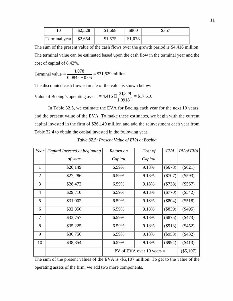
11

10 $2,528 $1,668 $860 $357

Terminal year $2,654 $1,575 $1,078

The sum of the present value of the cash flows over the growth period is $4,416 million.

The terminal value can be estimated based upon the cash flow in the terminal year and the

cost of capital of 8.42%.

Terminal value million 31,529$05.00842.0

078,1 =−

=

The discounted cash flow estimate of the value is shown below:

Value of Boeing’s operating assets 17,516$0918.1

529,31416,4

10=+=

In Table 32.5, we estimate the EVA for Boeing each year for the next 10 years,

and the present value of the EVA. To make these estimates, we begin with the current

capital invested in the firm of $26,149 million and add the reinvestment each year from

Table 32.4 to obtain the capital invested in the following year.

Table 32.5: Present Value of EVA at Boeing

Year Capital Invested at beginning

of year

Return on

Capital

Cost of

Capital

EVA PV of EVA

1 $26,149 6.59% 9.18% ($678) ($621)

2 $27,286 6.59% 9.18% ($707) ($593)

3 $28,472 6.59% 9.18% ($738) ($567)

4 $29,710 6.59% 9.18% ($770) ($542)

5 $31,002 6.59% 9.18% ($804) ($518)

6 $32,350 6.59% 9.18% ($839) ($495)

7 $33,757 6.59% 9.18% ($875) ($473)

8 $35,225 6.59% 9.18% ($913) ($452)

9 $36,756 6.59% 9.18% ($953) ($432)

10 $38,354 6.59% 9.18% ($994) ($413)

PV of EVA over 10 years = ($5,107)

The sum of the present values of the EVA is -$5,107 million. To get to the value of the

operating assets of the firm, we add two more components.

12

• The capital invested in assets in place at the beginning of year 1 (current), which is

$26,149 million.

• The present value of the EVA in perpetuity on assets in place in year 10, which is

computed as follows:

[(EBIT11(1-t) – Capital Invested11*Cost of Capital11)/Cost of Capital11]/(1+Current Cost

of Capital)10

( ) ( )( )( )( )

( )( )( )( )

million 536,3$

0918.10842.0

0842.0022,4093.653,2

Capital ofCost 1Capital ofCost

Capital ofCost Invested Capital1EBIT

10

1011

111111

−=

−=

+−− t

Note that while the marginal return on capital on new investments is equal to the cost of

capital after year 10, the existing investments continue to make 6.59%, which is lower

than the cost of capital of 8.42%, in perpetuity.

The total value of the firm can then be computed as follows:

Capital Invested in Assets in Place = $ 26,149 million

PV of EVA from Assets in Place = -$ 8,643 million

Value of Operating Assets = $17,506 million

fcffeva.xls: This spreadsheet allows you to convert a discounted cash flow valuation

into an EVA valuation and vice versa.

EVA Valuation versus DCF valuation: Whey will they disagree?

To get the same value from discounted cashflow and EVA valuations, you have to

ensure that the following conditions hold.

• The after-tax operating income that you use to estimate free cash flows to the firm

should be equal to the after-tax operating income that you use to compute economic

value added. Thus, if you decide to adjust the operating income for operating leases

and research and development expenses, when doing discounted cashflow valuation,

you have to adjust it for computing EVA as well.

• The growth rate you use to estimate after-tax operating income in future periods

should be estimated from fundamentals when doing discounted cash flow valuation. In

other words, it should be set to

13

Growth rate = Reinvestment rate * Return on capital

If growth is an exogenous input into a DCF model and the relationship between growth

rates, reinvestments and return on capital outlined above does not hold, you will get

different values from DCF and EVA valuations.

• The capital invested, which is used to compute EVA in future periods, should be

estimated by adding the reinvestment in each period to the capital invested at the

beginning of the period. The EVA in each period should be computed as follows:

EVAt = After-tax Operating Incomet – Cost of capital* Capital Investedt-1

• You have to make consistent assumptions about terminal value in your discounted

cash flow and EVA valuations. In the special case, where the return on capital on all

investments – existing and new - is equal to the cost of capital after your terminal

year, this is simple to do. The terminal value will be equal to your capital invested at

the beginning of your terminal year. In the more general case, you will have to ensure

that the capital invested at the beginning of your terminal year is consistent with your

assumption about return on capital in perpetuity. In other words, if your after-tax

operating income in your terminal year is $1.2 billion and you are assuming a return

on capital of 10% in perpetuity, you will have to set your capital invested at the

beginning of your terminal year to be $12 billion.

EVA and Firm Value: Potential Conflicts

Assume that a firm adopts economic value added as its measure of value and

decides to judge managers on their capacity to generate greater-than-expected economic

value added. What is the potential for abuse? Is it possible for a manager to deliver greater

than expected economic value added, while destroying firm value at the same time? If so,

how can we protect stockholders against these practices?

To answer these questions, let us go back to the earlier equation where we

decomposed firm value into capital invested, the present value of economic value added

by assets in place and the present value of economic value added by future growth.

∑∑∞=

=

∞ t

1t c

Projects Future t,=t

=1t c

Placein Assets t,Placein Assets

)k+(1

EVA+

)k+(1

EVA+Invested Capital=Value Firm tt

14

The Capital Invested Game

The first two terms in the equation above, the capital invested and the present

value of economic value added by these investments, are both sensitive to the

measurement of capital invested. If capital invested is reduced, keeping the operating

income constant, the first term in the equation will drop but the present value of

economic value added will increase proportionately. To illustrate, consider the firm we

valued in Illustration 32.1. Assume that the capital invested is estimated to be $50 million

rather than $100 million and that the operating income on these investments stays at $15

million. The assumptions about future investments remain unchanged. The firm value can

then be written as shown in Table 32.6.

Table 32.6: EVA Valuation of Firm: EVA and Assets in PlaceCapital Invested in Assets in Place $ 50

+ EVA from Assets in Place ( )( )

10.0

500.10-0.30= $ 100

+ PV of EVA from New Investments in Year 1 ( )( )

10.0

1010.015.0 −= $ 5

+ PV of EVA from New Investments in Year 2 ( )( )

( )( )110.110.0

1010.015.0 −= $ 4.55

+ PV of EVA from New Investments in Year 3 ( )( )

( )( )210.110.0

1010.015.0 −= $ 4.13

+ PV of EVA from New Investments in Year 4 ( )( )

( )( )310.110.0

1010.015.0 −= $ 3.76

+ PV of EVA from New Investments in Year 5 ( )( )

( )( )410.110.0

1010.015.0 −= $ 3.42

Value of Firm $ 170.85

The value of the firm is unchanged, but it is redistributed to the economic value added

component. When managers are judged on the economic value added, there will be strong

incentives to reduce the capital invested, at least as measured for EVA computations.

There are some actions managers can take to reduce capital invested that truly

create value. Thus, in the above example, if the reduction in capital invested came from

closing down a plant that does not (and is not expected to) generate any operating income,

15

the cash flow generated by liquidating the plant’s assets will increase value. Some actions,

however, are purely cosmetic in terms of their effects on capital invested and thus do not

create and may even destroy value. For instance, firms can take one-time restructuring

charges, reducing capital or lease assets rather than buy them, because the capital impact

of leasing may be smaller.

To illustrate the potential destructiveness of these actions, assume that the managers

of the firm in Illustration 32.1 are able to replace half their assets with leased assets.

Assume further that the estimated capital invested in these leased assets is only $40

million, which is lower than the capital invested in the replaced assets of $50 million. In

addition, assume that the action actually reduces the adjusted annual operating income

from these assets from $15 million to $14.8 million. The value of the firm can now be

written in Table 32.7.

Table 32.7: Value Reduction with Higher EVA

Capital Invested in Assets in Place $ 90

+ EVA from Assets in Place ( )( )

10.0

900.10-0.1644= $ 58

+ PV of EVA from New Investments in Year 1 ( )( )

10.0

1010.015.0 −= $ 5

+ PV of EVA from New Investments in Year 2 ( )( )

( )( )110.110.0

1010.015.0 −= $ 4.55

+ PV of EVA from New Investments in Year 3 ( )( )

( )( )210.110.0

1010.015.0 −= $ 4.13

+ PV of EVA from New Investments in Year 4 ( )( )

( )( )310.110.0

1010.015.0 −= $ 3.76

+ PV of EVA from New Investments in Year 5 ( )( )

( )( )410.110.0

1010.015.0 −= $ 3.42

Value of Firm $ 168.85

Note that the firm value declines by $ 2 million, but the economic value added increases

by $ 8 million.

When economic value added is estimated for divisions, the capital invested at the

divisional level is a function of a number of allocation decisions made by the firm, with

16

the allocation based upon pre-specified criteria (such as revenues or number of

employees). While we would like these rules to be objective and unbiased, they are often

subjective and over allocate capital to some divisions and under-allocate it to others. If

this misallocation were purely random, we could accept it as error and use changes in

economic value added to measure success. Given the natural competition that exists

among divisions in a firm for the marginal investment dollar, however, these allocations

are also likely to reflect the power of individual divisions to influence the process. Thus,

the economic value added will be over-estimated for those divisions that are under

allocated capital and under-estimated for divisions that are over-allocated capital.

The Future Growth Game

The value of a firm is the value of its existing assets and the value of its future

growth prospects. When managers are judged on the basis of economic value added in the

current year, or on year-to-year changes, the economic value added that is being measured

is just from assets in place. Thus, managers may trade off the economic value added from

future growth for higher economic value added from assets in place.

Again, this point can be illustrated simply using the firm in Illustration 32.1. The

firm earned a return on capital of 15% on both assets in place and future investments.

Assume that there are actions the firm can take to increase the return on capital on assets

in place to 16%, but that this action reduces the return on capital on future investments to

12%. The value of this firm can then be estimated in Table 32.8:

Table 32.8: Trading Off Future Growth for Higher EVACapital Invested in Assets in Place $ 100

+ EVA from Assets in Place ( )( )

10.0

1000.10-0.16= $ 60

+ PV of EVA from New Investments in Year 1 ( )( )

10.0

1010.012.0 −= $ 2

+ PV of EVA from New Investments in Year 2 ( )( )

( )( )1.110.0

1010.012.0 −= $ 1.82

+ PV of EVA from New Investments in Year 3 ( )( )

( )( )21.110.0

1010.012.0 −= $ 1.65

17

+ PV of EVA from New Investments in Year 4 ( )( )

( )( )31.110.0

1010.012.0 −= $ 1.50

+ PV of EVA from New Investments in Year 5 ( )( )

( )( )41.110.0

1010.012.0 −= $ 1.37

Value of Firm $ 168.34

Note that the value of the firm has decreased, but the economic value added in year 1 is

higher now than it was before. In fact, the economic value added at this firm for each of

the next five years is graphed in Figure 32.1 for both the original firm and this one.

The growth trade off, while leading to a lower firm value, results in economic value added

in each of the first three years that is larger than it would have been without the trade off.

Compensation mechanisms based upon EVA are sometimes designed to punish

managers who give up future growth for current EVA. Managers are partly compensated

based upon the economic value added this year, but another part is held back in a

compensation bank and is available to the manager only after a period (say three or four

years). There are significant limitations with these approaches. First, the limited tenure

that managers have with firms implies that this measure can at best look at economic

Figure 32.1: Annual EVA: With and Without Growth Trade-Off

$-

$1.00

$2.00

$3.00

$4.00

$5.00

$6.00

$7.00

$8.00

1 2 3 4 5

Year

EV

A EVA (Original)EVA (Growth Trade-Off)

18

value added only over the next 3 or 4 years. The real costs of the growth trade off are

unlikely to show up until much later. Second, these approaches are really designed to

punish managers who increase economic value added in the current period while reducing

economic value added in future periods. In the more subtle case, where the economic value

added continues to increase but at a rate lower than it otherwise would have, it is difficult

to devise a punishment for managers who trade off future growth. In the example above,

for instance, the economic value added with the growth trade off increases over time. The

increases are smaller than they would have been without the trade off, but that number

would not have been observed anyway.

The Risk Shifting Game

The value of a firm is the sum of the capital invested and the present value of the

economic value added. The latter term is therefore a function not just of the dollar

economic value added but also of the cost of capital. A firm can invest in projects to

increase its economic value added but still end up with a lower value, if these investments

increase its operating risk and cost of capital.

Again, using the firm in Illustration 32.1, assume that the firm is able to increase

its return on capital on both assets in place and future investments from 15% to 16.25%.

Simultaneously, assume that the cost of capital increases to 11%. The economic value

added in each year for the next five years is contrasted with the original economic value

added in each year in Figure 32.2.

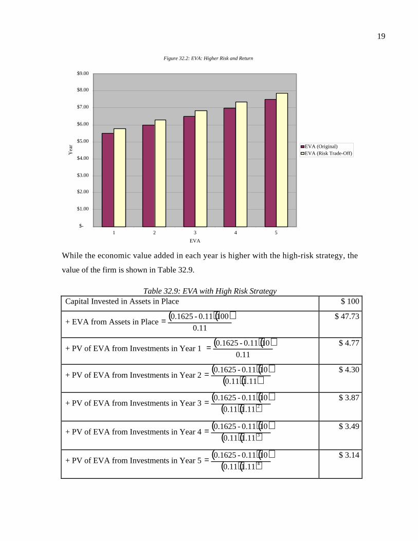
19

While the economic value added in each year is higher with the high-risk strategy, the

value of the firm is shown in Table 32.9.

Table 32.9: EVA with High Risk StrategyCapital Invested in Assets in Place $ 100

+ EVA from Assets in Place ( )( )

11.0

1000.11-0.1625= $ 47.73

+ PV of EVA from Investments in Year 1 ( )( )

11.0

100.11-0.1625= $ 4.77

+ PV of EVA from Investments in Year 2 ( )( )

( )( )11.111.0

100.11-0.1625= $ 4.30

+ PV of EVA from Investments in Year 3 ( )( )

( )( )211.111.0

100.11-0.1625= $ 3.87

+ PV of EVA from Investments in Year 4 ( )( )

( )( )311.111.0

100.11-0.1625= $ 3.49

+ PV of EVA from Investments in Year 5 ( )( )

( )( )411.111.0

100.11-0.1625= $ 3.14

Figure 32.2: EVA: Higher Risk and Return

$-

$1.00

$2.00

$3.00

$4.00

$5.00

$6.00

$7.00

$8.00

$9.00

1 2 3 4 5

EVA

Yea

r EVA (Original)EVA (Risk Trade-Off)

20

Value of Firm $ 167.31

Note that the risk effect dominates the higher excess dollar returns and the value of the

firm decreases.

This risk shifting can be dangerous for firms that adopt economic value added

based on objective functions. When managers are judged based upon year-to-year

economic value added changes, there will be a tendency to shift into riskier investments.

This tendency will be exaggerated if the measured cost of capital does not reflect the

changes in risk or lags4 it.

In closing, economic value added is an approach skewed toward assets in place

and away from future growth. It should not be surprising, therefore, that when economic

value added is computed at the divisional level of a firm, the higher growth divisions end

up with the lowest economic value added and in some cases with negative economic value

added. Again, while these divisional managers may still be judged based upon changes in

economic value added from year to year, the temptation at the firm level to reduce or

eliminate capital invested in these divisions will be strong, since it will make the firm’s

overall economic value added look much better.

EVA and Market Value

Will increasing economic value added cause market value to increase? While an

increase in economic value added will generally lead to an increase in firm value, barring

the growth and risk games described earlier, it may or may not increase the stock price.

This is because the market has built into its expectations of future economic value added.

Thus, a firm like Microsoft is priced on the assumption that it will earn large and

increasing economic value added over time. Whether a firm’s market value increases or

decreases on the announcement of higher economic value added will depend in large part

on what the expected change in economic value added was. For mature firms, where the

market might have expected no increase or even a decrease in economic value added, the

announcement of an increase will be good news and cause the market value to increase.

4 In fact, beta estimates that are based upon historical returns will lag changes in risk. With a five-yearreturn estimation period, for instance, the lag might be as long as three years and the full effect will notshow up for five years after the change.

21

For firms that are perceived to have good growth opportunities and are expected to report

an increase in economic value added, the market value will decline if the announced

increase in economic value added does not measure up to expectations. This should be no

surprise to investors, who have recognized this phenomenon with earnings per share for

decades; the earnings announcements of firms are judged against expectations and the

earnings surprise is what drives prices.

We would therefore not expect any correlation between the magnitude of the

economic value added and stock returns or even between the change in economic value

added and stock returns. Stocks that report the biggest increases in economic value added

should not necessarily earn high returns for their stockholders5. These priors are

confirmed by a study done by Richard Bernstein at Merrill Lynch, who examined the

relationship between EVA and stock returns.

• A portfolio of the 50 firms which had the highest absolute levels6 of economic value

added earned an annual return on 12.9% between February 1987 and February 1997,

while the S&P index returned 13.1% a year over the same period.

• A portfolio of the 50 firms that had the highest growth rates7 in economic value

added over the previous year earned an annual return of 12.8% over the same time

period.

eva.xls: There is a dataset on the web that summarizes economic value added by

industry group for the United States.

Equity Economic Value Added

While EVA is usually calculated using total capital, it can easily be modified to be

an equity measure.

Equity EVA = (Return on Equity - Cost of Equity) (Equity Invested in Project or Firm)

= Net Income – (Cost of Equity)(Equity Invested in Project or Firm)

5 A study by Kramer and Pushner found that differences in operating income (NOPAT) explained differencesin market value better than differences in EVA. O'Byrne (1996), however, finds that changes in EVAexplain more than 55% of changes in market value over 5-year periods.6 See Quantitative Viewpoint, Merrill Lynch, December 19, 1997.

22

Again, a firm that earns a positive equity EVA is creating value for its stockholders while

a firm with a negative equity EVA is destroying value for its stockholders.

Why might a firm use this measure rather than the traditional measure? In Chapter

21, when we looked at financial service firms, we noted that defining debt (and therefore

capital) may create measurement problems, since so much of the firm could potentially be

categorized as debt. Consequently, we argued that financial service firms should be valued

using equity valuation models and multiples. Extending that argument to economic value

added, we believe that equity EVA is a much better measure of performance for financial

service firms than the traditional EVA measure.

We would hasten to add that all of the issues that we raised in the context of the

traditional EVA measure affect the equity EVA measure as well. Banks and insurance

companies can play the capital invested, growth and risk games to increase equity EVA

just as other firms can with traditional EVA.

EVA for High Growth firms

The fact that the value of a firm is a function of the capital invested in assets in

place, the present value of economic value added by those assets and the economic value

added by future investments, points to some of the dangers of using it as a measure of

success or failure for high growth and especially high-growth technology firms. In

particular, there are three problems.

• We have already noted many of the problems associated with how accountants

measure capital invested at technology firms. Given the centrality of capital invested

to economic value added, these problems have a much bigger effect when firms use

EVA than when discounted cash flow valuation.

• When 80% to 90% of value comes from future growth potential, the risks of managers

trading off future growth for current EVA are magnified. It is also very difficult to

monitor these trade offs at young firms.

7 See Quantitative Viewpoint, Merrill Lynch, February 3, 1998.

23

• The constant change that these firms go through also makes them much better

candidates for risk shifting. In this case, the negative effect (of a higher discount rate)

can more than offset the positive effect of a higher economic value added.

Finally, it is unlikely that there will be much correlation between actual changes in

economic value added at technology firms and changes in market value. The market value

is based upon expectations of economic value added in future periods and investors

expect an economic value added that grows substantially each year. Thus, if the economic

value added increases, but by less than expected, you could see its market value drop on

the report.

Cash Flow Return on Investment

The cash flow return on investment (CFROI) for a firm is the internal rate of

return on existing investments, based upon real cash flows. Generally, it should be

compared to the real cost of capital to make judgments about the quality of these

investments.

Calculating CFROI

The cash flow return on investment for a firm is calculated using four inputs. The

first is the gross investment (GI) the firm has in its existing assets, obtained by adding

back cumulated depreciation and inflation adjustments to the book value. The second

input is the gross cash flow (GCF) earned in the current year on gross investment, which

is usually defined as the sum of the after-tax operating income of a firm and the non-cash

charges against earnings, such as depreciation and amortization. The third input is the

expected life of the assets (n) in place at the time of the original investment, which varies

from sector to sector but reflects the earning life of the investments in question. The

expected value of the assets (SV) at the end of this life, in current dollars, is the final input.

This is usually assumed to be the portion of the initial investment, such as land and

building, that is not depreciable, adjusted to current dollar terms. The CFROI is the

internal rate of return of these cash flows, i.e, the discount rate that makes the net present

value of the gross cash flows and salvage value equal to the gross investment and it can

thus be viewed as a composite internal rate of return, in current dollar terms.

24

An alternative formulation of the CFROI allows for setting aside an annuity to

cover the expected replacement cost of the asset at the end of the project life. This

annuity is called the economic depreciation.

( ) 1k+1

)(k dollarsCurrent in Cost t Replacemen=onDepreciati Economic

nc

c

−

where n is the expected life of the asset. The expected replacement cost of the asset is

defined in current dollar terms to be the difference between the gross investment and the

salvage value. The CFROI for a firm or a division can then be written as follows:

Investment Gross

onDepreciati Economic-FlowCash Gross=CFROI

For instance, assume that you have existing assets with a book value of $2,431 million, a

gross cash flow of $390 million, an expected salvage value (in today’s dollar terms) of

$607.8 million and a life of 10 years. The conventional measure of CFROI is 11.71% and

the real cost of capital is 8%. The estimate using the alternative approach is computed.

( )( )million 86.125$

11.08

0.08$607.8 - $2,431onDepreciati Economic

10=

−=

10.87%2,431

125.86-390CFROI ==

The differences in the reinvestment rate assumption accounts for the difference in CFROI

estimated using the two methods. In the first approach, intermediate cash flows get

reinvested at the internal rate of return, while in the second, at least the portion of the

cash flows that are set aside for replacement get reinvested at the cost of capital. In fact, if

we estimated that the economic depreciation using the internal rate of return of 11.71%,

the two approaches would yield identical results8.

8 With an 11.71% rate, the economic depreciation works out to $105.37 million and the CFROI to11.71%.

25

Cashflow Return on Investment, Internal Rate of Return and Discounted Cashflow

Value

If net present value provides the genesis for the economic value added approach to

value enhancement, the internal rate of return is the basis for the CFROI approach. In

investment analysis, the internal rate of return on a project is computed using the initial

investment on the project and all cash flows over the project’s life.

InitialInvestment

ATCF ATCF ATCF ATCF ATCF

1 2 3 4 n

SV

Where the ATCF is the after-tax cash flow on the project and SV is the expected salvage

value of the project assets. This analysis can be done entirely in nominal terms, in which

case the internal rate of return is a nominal IRR and is compared to the nominal cost of

capital, or in real terms, in which case it is a real IRR and is compared to the real cost of

capital.

At first sight, the CFROI seems to do the same thing as IRR. It uses the gross

investment in the project (in current dollars) as the equivalent of the initial investment,

assumes that the gross current-dollar cash flow is maintained over the project life and

computes a real internal rate of return. There are, however, some significant differences.

The internal rate of return does not require the after-tax cash flows to be constant

over a project’s life, even in real terms. The CFROI approach assumes that real cash

flows on assets do not increase over time. This may be a reasonable assumption for

investments in mature markets, but will understate project returns if there is real growth.

Note, however, that the CFROI approach can be modified to allow for real growth.

The second difference is that the internal rate of return on a project or asset is

based upon incremental future cash flows. It does not consider cash flows that have

occurred already, since these are viewed as “sunk.” The CFROI, on the other hand, tries

to reconstruct a project or asset, using both cash flows that have occurred already and

cashflows that are yet to occur. To illustrate, consider the project described in the

previous section. At the time of the original investment, assuming that the inputs for

initial investment, after-tax cash flows and salvage value are unchanged, both the internal

26

rate of return and the CFROI of this project would have been 11.71%. The CFROI is,

however, being computed three years into the project life and remains at 11.71%, since

none of the original inputs have changed. The IRR of this project will change, though. It

will now be based upon the current market value of the asset, the expected cash flows

over the remaining life of the asset and a life of seven years. Thus, if the market value of

the asset has increased to $2.5 billion, the internal rate of return on this project would be

computed to be only 6.80%.

$ 3,000 mil

$390 mil $390 mil $390 mil $390 mil $ 390 mil

1 2 3 4 7

$607.8 mil

Given the real cost of capital of 8%, this would mean that the CFROI is greater than the

cost of capital, while the internal rate of return is lower. Why is there a difference

between the two measures and what are the implications? The reason for the difference is

that IRR is based entirely on expected future cash flows, whereas the CFROI is not. A

CFROI that exceeds the cost of capital is viewed as a sign that a firm is deploying its

assets well. If the IRR is less than the cost of capital, that interpretation is false, because

the owners of the firm would be better off selling the asset and getting the market value

for it rather than continuing its operation.

To link the cash flow return on investment with firm value, let us begin with a

simple discounted cash flow model for a firm in stable growth.

nc

1

gk

FCFF=Value Firm

−

where FCFF is the expected free cash flow to the firm, kc is the cost of capital and gn is

the stable growth rate. Note that this can be rewritten, approximately, in terms of the

CFROI.

( )( )( )( ) ( )nc gk

WC-DA-CXt-1DA-GICFROI=Value Firm

−∆−

where CFROI is the cash flow return on investment, GI is the gross investment, DA is

the depreciation and amortization, CX is the capital expenditure and ∆WC is the change in

27

working capital. To illustrate, consider a firm with a CFROI of 30%, a gross investment

of $100 million, capital expenditures of $15 million, depreciation of $10 million and no

working capital requirements. If we assume a 10% cost of capital, a 40% tax rate and a

5% stable growth rate, it would be valued as follows:

( )( )( )( ) ( )million $140=

05.00.10

)0-10-15-0.4-110-1000.30=Value Firm

−

More important than the mechanics, however, is the fact that the firm value, while a

function of the CFROI is also a function of the other variables in the equation – the gross

investment, the tax rate, the growth rate, the cost of capital and the firm’s reinvestment

needs.

Again, sophisticated users of CFROI do recognize the fact that value comes from

the CFROI not just on assets in place but also on future investments. In fact, Holt

Associates, one of CFROI’s leading proponents, allows for a fade factor in CFROI,

where the current CFROI fades towards the real cost of capital over time. The "fade

factor" is estimated empirically by looking at firms in different CFROI classes and

tracking them over time. Thus, a firm that has a current CFROI of 20% and real cost of

capital of 8% will be projected to have lower CFROI over time. The value of the firm, in

this more complex format, can then be written as a sum of the following.

• The present value of the cash flows from assets in place over their remaining life,

which can be written as ( )( )

( )∑=

= +

nt

tt

c

aipaip

k

GICFROI

1 1, where CFROIaip is the CFROI on

assets in place, GIaip is the gross investment in assets in place and kc is the real cost of

capital.

• The present value of the excess cash flows from future investments, which can be

written in real terms as ( )( )

( ) t

t

tt

c

tNIt GIk

GICFROI∆−

+∆∑

∞=

=1

,

1, where CFROIt,NI is the CFROI

on new investments made in year t and ∆GIt is the new investment made in year t.

Note that if CFROIt,NI = kc, this present value is equal to zero.

28

Thus, a firm's value will depend upon the CFROI it earns on assets in place and both the

abruptness and the speed with which this CFROI fades towards the cost of capital. Thus,

a firm can therefore potentially increase its value by doing any of the following.

• Increase the CFROI from assets in place, for a given gross investment.

• Reduce the speed at which the CFROI fades towards the real cost of capital.

• Reduce the abruptness with which CFROI fades towards the cost of capital.

Note that this is no different from our earlier analysis of firm value in the

discounted cash flow approach, in terms of cash flows from existing investments (increase

current CFROI), the length of the high growth period (reduce fade speed) and the growth

rate during the growth period (keep excess returns from falling as steeply).

cfroi.xls: This spreadsheet allows you to estimate the cash flow return on investment

for a firm or project.

CFROI Innovations: The Fade Factor and Implied Cost of Capital

The biggest contribution made by practitioners who use CFROI has been the

work that they have done on how returns on capital fade over time towards the cost of

capital. Madden (1999) makes the argument that not only is this phenomenon wide

spread but that it is at least partially predictable. He presents evidence done by Holt

Associates, a leading proponent of CFROI, who sorted the largest 1000 firms by CFROI,

from highest to lowest and tracked them over time, to find a convergence towards an

average. We should note that we have used fade factors, without referring to them as such,

in the chapters on discounted cash flow valuation. The fade to a lower return on capital

occurred either precipitously in the terminal year or over a transition period. We noted

that the return on capital could converge to the cost of capital or to the industry average.

To compute the cost of capital, CFROI practitioners look to the market instead of

the risk and return models that we have used to compute DCF value. Using the current

market values of stocks and their estimates of expected aggregate cash flows, they

compute internal rates of return that they use as the cost of capital in analysis. In Chapter

7, we used a very similar approach to estimate an implied risk premium, though we use

this premium as an input into traditional risk and return models.

29

CFROI and Firm Value: Potential Conflicts

The relationship between CFROI and firm value is less intuitive than the

relationship between EVA and firm value, partly because it is a percentage return.

Notwithstanding this fundamental weakness, managers can take actions that increase

CFROI while reducing firm value.

a. Reduce Gross Investment: If the gross investment in existing assets is reduced,

the CFROI may be increased. Since it is the product of CFROI and Gross

Investment that determines value, it is possible for a firm to increase CFROI

and end up with a lower value.

b. Sacrifice Future Growth: CFROI, even more than EVA, is focused on existing

assets and does not look at future growth. To the extent that managers increase

CFROI at the expense of future growth, the value can decrease while CFROI

goes up.

c. The Risk Trade Off: While the CFROI is compared to the real cost of capital

to pass judgment on whether a firm is creating or destroying value, it

represents only a partial correction for risk. The value of a firm is still the

present value of expected future cash flows. Thus, a firm can increase its

spread between the CFROI and cost of capital but still end up losing value if

the present value effect of having a higher cost of capital dominates the higher

CFROI.

In general, then, an increase in CFROI does not, by itself, indicate that the firm value has

increased, since it might have come at the expense of lower growth and/or higher risk.

CFROI and Market Value

There is a relationship between CFROI and market value. Firms with high CFROI

generally have high market value. This is not surprising, since it mirrors what we noted

about economic value added earlier. However, it is changes in market value that create

returns, not market value per se. When it comes to market value changes, the relationship

between EVA changes and value changes tends to be much weaker. Since market values

reflect expectations, there is no reason to believe that firms that have high CFROI will

earn excess returns.

30

The relationship between changes in CFROI and excess returns is more intriguing. To the

extent that any increase in CFROI is viewed as a positive surprise, firms with the biggest

increases in CFROI should earn excess returns. In reality, however, the actual change in

CFROI has to be measured against expectations; if CFROI increases, but less than

expected, the market value should drop; if CFROI drops but by less than expected, the

market value should increase.

A Postscript on Value Enhancement

The value of a firm has three components. The first is its capacity to generate cash

flows from existing assets, with higher cash flows translating into higher value. The

second is its willingness to reinvest to create future growth and the quality of these

reinvestments. Other things remaining equal, firms that reinvest well and earn significant

excess returns on these investments will have higher value. The final component of value

is the cost of capital, with higher costs of capital resulting in lower firm values. To create

value then a firm has to:

• Generate higher cash flows from existing assets, without affecting its growth

prospects or its risk profile.

• Reinvest more and with higher excess returns, without increasing the riskiness of its

assets.

• Reduce the cost of financing its assets in place or future growth, without lowering the

returns made on these investments.

All value enhancement measures are variants on these simple themes. Whether these

approaches measure dollar excess returns, as does economic value added, or percentage

excess returns, like CFROI, they have acquired followers because they seem simpler and

less subjective than discounted cash flow valuation. This simplicity comes at a cost, since

these approaches make subtle assumptions about other components of value that are

often not visible or not recognized by many users. Approaches that emphasize economic

value added and reward managers for increasing the same, often assume that increases in

economic value added are not being accomplished at the expense of future growth or by

increasing risk. Practitioners who judge performance based upon the cash flow return on

investment make similar assumptions.

31

Is there something of value in the new value enhancement measures? Absolutely,

but only in the larger context of valuation. One of the inputs we need for traditional

valuation models is the return on capital (to get expected growth). Making the

adjustments to operating income suggested by those who use economic value added and

augmenting it with a cash flow return, with CFROI, may help us come up with a better

estimate of this number. The terminal value computation in traditional valuation models,

where small changes in assumptions can lead to large changes in value, becomes much

more tractable if we think in terms of excess returns on investments rather than just

growth and discount rates. Finally, the empirical evidence that has been collected by

practitioners who use CFROI on fade factors can be invaluable in traditional valuation

models, where practitioners sometimes make the mistake of assuming that current project

returns will continue forever.

Summary

In this chapter, we consider two widely used value enhancement measures.

Economic value added measures the dollar excess return on existing assets. The cash flow

return on investment is the internal rate of return on existing assets, based upon the

original investment in these assets and the expected future cash flows. While both

approaches can lead to conclusions consistent with traditional discounted cash flow

valuation, their simplicity comes at a cost. Managers can take advantage of measurement

limitations in both approaches to make their firms look better with either approach, while

reducing firm value. In particular, they can trade off less growth in the future for higher

economic value added today and shift to riskier investments.

As we look at various approaches to value enhancement, we should consider a few

facts. The first is that no value enhancement mechanism will work at generating value

unless there is a commitment on the part of managers to making value maximization their

primary objective. If managers put other goals first, then no value enhancement

mechanism will work. Conversely, if managers truly care about value maximization, they

can make almost any mechanism work in their favor. The second is that while it is

sensible to connect whatever value enhancement measure we have chosen to management

compensation, there is a down side. Managers, over time, will tend to focus their

32

attention on making themselves look better on that measure even if it leads to reducing

firm value. Finally, there are no magic bullets that create value. Value creation is hard

work in competitive markets and almost involves a trade off between costs and benefits.

Everyone has a role in value creation and it certainly is not the sole domain of financial

analysts. In fact, the value created by financial engineers is smaller and less significant

than the value created by good strategic, marketing, production or personnel divisions.

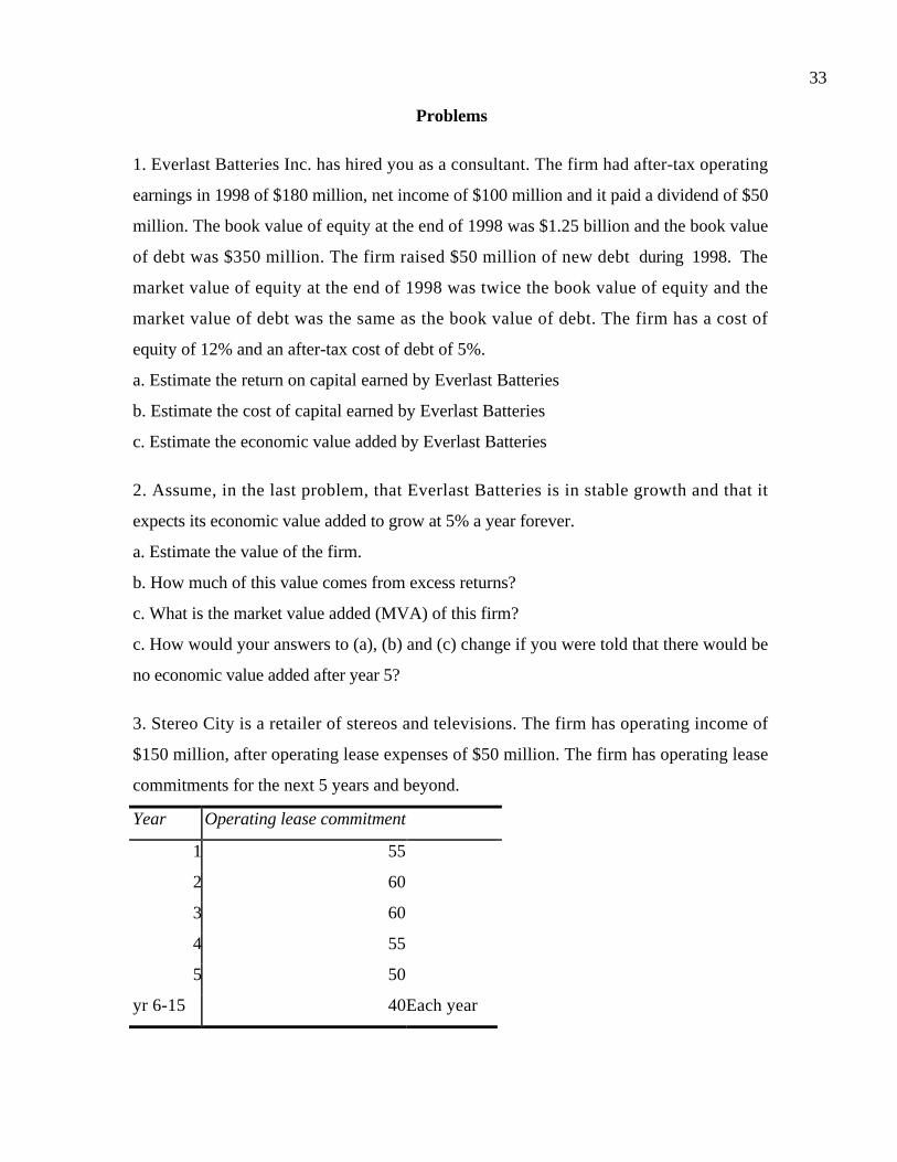
33

Problems

1. Everlast Batteries Inc. has hired you as a consultant. The firm had after-tax operating

earnings in 1998 of $180 million, net income of $100 million and it paid a dividend of $50

million. The book value of equity at the end of 1998 was $1.25 billion and the book value

of debt was $350 million. The firm raised $50 million of new debt during 1998. The

market value of equity at the end of 1998 was twice the book value of equity and the

market value of debt was the same as the book value of debt. The firm has a cost of

equity of 12% and an after-tax cost of debt of 5%.

a. Estimate the return on capital earned by Everlast Batteries

b. Estimate the cost of capital earned by Everlast Batteries

c. Estimate the economic value added by Everlast Batteries

2. Assume, in the last problem, that Everlast Batteries is in stable growth and that it

expects its economic value added to grow at 5% a year forever.

a. Estimate the value of the firm.

b. How much of this value comes from excess returns?

c. What is the market value added (MVA) of this firm?

c. How would your answers to (a), (b) and (c) change if you were told that there would be

no economic value added after year 5?

3. Stereo City is a retailer of stereos and televisions. The firm has operating income of

$150 million, after operating lease expenses of $50 million. The firm has operating lease

commitments for the next 5 years and beyond.

Year Operating lease commitment

1 55

2 60

3 60

4 55

5 50

yr 6-15 40Each year

34

The book value of equity is $1 billion and the firm has no debt outstanding. The firm has

a cost of equity of 11% and a pre-tax cost of borrowing of 6%. The tax rate is 40%.

a. Estimate the capital invested in the firm, before and after adjusting for operating

leases.

b. Estimate the return on capital, before and after adjusting for operating leases.

c. Estimate the economic value added, before and after adjusting for operating

leases. (The market value of equity is $2 billion.)

4. Sevilla Chemicals earned $1 billion in after-tax operating income on capital invested of

$5 billion last year. The firm’s cost of equity is 12%, its debt to capital ratio is 25% and

the after-tax cost of debt is 4.5%.

a. Estimate the economic value added by Sevilla Chemicals last year.

b. Assume now that the entire chemical industry earned $40 billion after taxes on capital

invested of $180 billion and that the cost of capital for the industry is 10%. Estimate the

economic value added by the entire industry.

c. Based on economic value added, how did Sevilla do, relative to the industry?

5. Jeeves Software is a small software firm in high growth. The firm is all equity financed.

In the current year, the firm earned $20 million in after-tax operating income on capital

invested of $60 million. The firm’s cost of equity is 15%.

a. Assume that the firm will be able to grow its economic value added 15% a year for the

next 5 years and that there will be no excess returns after year 5. Estimate the value of the

firm. How much of this value comes from the EVA and how much from capital invested?

b. Now, assume the firm is able to reduce its capital invested this year by $20 million by

selling its assets and leasing them back. Assuming operating income and cost of capital do

not change as a result of the sale-lease back, estimate the value of the firm now. How

much of the value of the firm now comes from EVA and how much from capital invested?

6. Healthy Soups is a company that manufactures canned soups made without

preservatives. The firm has assets that have a book value of $100 million. The assets are 5

years old and have been depreciated $50 million over that period. In addition, the inflation

rate over those 5 years has averaged 2% a year. The assets are currently earning $15

35

million in after-tax operating income. They have a remaining life of 10 years and the

depreciation each year is expected to be $5 million. At the end of these 10 years, the

assets will have an expected salvage value, in current dollars, of $50 million.

a. Estimate the CFROI of Healthy Foods, using the conventional CFROI approach.

b. Estimate the CFROI of Healthy Foods, using the economic depreciation approach.

c. If Healthy Foods has a cost of capital in nominal terms of 10% and the expected

inflation rate is 2%, evaluate whether Healthy Foods’ existing investments are value

creating or destroying.

1

CHAPTER 33

VALUING BONDS

The value of a bond is the present value of the expected cash flows on the bond,

discounted at an interest rate that is appropriate to the riskiness of that bond. Since the

cash flows on a straight bond are fixed at issue, the value of a bond is inversely related to

the interest rate that investors demand for that bond. The interest rate charged on a bond

is determined by both the general level of interest rates, which applies to all bonds and

financial investments, and the default premium specific to the entity issuing the bond.

This chapter examines the determinants of both the general level of interest rates and the

magnitude of the default premia on specific bonds. The general level of interest rates

incorporates expected inflation and a measure of real return and reflects the term

structure, with bonds of different maturities carrying different interest rates. The default

premia varies across time, depending in large part on the health of the economy and

investors' risk preferences.

Bonds often have special features embedded in them that have to be factored into

the value. Some of these features are options - to convert into stock (convertible bonds),

to call the bond back if interest rates go down (callable bonds) and to put the bond back to

the issuer at a fixed price under specific circumstances (putable bonds). Other bond

characteristics, such as interest rate caps and floors, have option features. Some of these

options reside with the issuer of the bond, some with the buyer of the bond, but they all

have to be priced. Option pricing models can be used to value these special features and

price complex fixed income securities. Some special features in bonds such as sinking

funds, subordination of further debt and the type of collateral may affect the prices of

bonds, as well.

Bond Prices and Interest Rates

The value of a straight bond is determined by the level of and changes in interest

rates. As interest rates rise, the price of a bond will decrease and vice versa. This inverse

relationship between bond prices and interest rates arises directly from the present value

relationship that governs bond prices.

2

a. The Present Value Relationship

The value of a bond, like all financial investments, is derived from the present

value of the expected cash flows on that bond, discounted at an interest rate that reflects

the default risk associated with the cash flows. There are two features that set bonds

apart from equity investments. First, the cash flows on a bond, i.e., the coupon payments

and the face value of the bond, are usually set at issue and do not change during the life of

the bond. Even when they do change, as in floating rate bonds, the changes are generally

linked to changes in interest rates. Second, bonds usually have fixed lifetimes, unlike

stocks, since most bonds1 specify a maturity date. As a consequence, the present value

of a 'straight bond' with fixed coupons and specified maturity is determined entirely by

changes in the discount rate, which incorporates both the general level of interest rates and

the specific default risk of the bond being valued.

The present value of a bond, expected to mature in N time periods, with coupons

every period can be calculated.

PV of Bond =

Coupon t

(1+r)tt=1

t=N

∑ +Face Value

(1+r)N

where,

Coupont = Coupon expected in period t

Face Value = Face value of the bond

r = Discount rate for the cash flows

The discount rate used to calculate the present value of the bond will vary from bond to

bond depending upon default risk, with higher rates used for riskier bonds and lower rates

for safer ones.

If the bond is traded, and a market price is therefore available for it, the internal

rate of return can be computed for the bond, i.e., the discount rate at which the present

value of the coupons and the face value is equal to the market price. This internal rate of

return is called the yield to maturity on the bond.

1 Console bonds are the exception to this rule, since they are perpetuities.

3

There are several details, relating to both the magnitude and timing of cash flows,

that can affect the value of a bond and its yield to maturity. First, the coupon payment on

a bond may be semi-annual, in which case the discounting has to allow for the semi-annual

cash flows. (The first coupon will be discounted back half a year, the second one year, the

third a year and a half and so on.) Second, once a bond has been issued, it accrues coupon

interest between coupon payments and this accrued interest has to be added on to the

price of the bond, when valuing the bond.

Illustration 33.1: Valuing a straight bond at issue

The following is a valuation of a thirty-year U.S. Government Bond at the time of

issue. The coupon rate on the bond is 7.50%, and the market interest rate is 7.75%. The

price of the bond can be calculated.

PV of Bond =

75.00

(1.0775) tt=1

t=30

∑ +1,000

(1.0775)30 = $971.18

This is based upon annual coupons. If the calculation is based upon semi-annual coupons,

the value of the bond is:

PV of Bond =37.50

(1.0775) tt=0.5

t=30

∑ +1,000

(1.0775)30 = $987.62

Illustration 33.2: Valuing a seasoned straight bond

The following is a valuation of a seasoned Government bond, with twenty years

left to expiration and a coupon rate of 11.75%. The next coupon is due in two months.

The current twenty-year bond rate is 7.5%. The value of the bond can be calculated.

PV of Bond =58.75

(1.075) tt=0.5

t=19.5

∑ +58.75

(1.075)2/12 +1,000

(1.075)19.67 = $1505.31

This bond trades at well above face value, because of its high coupon rate. Note that the

second term of the equation is the present value of the next coupon.

b. A Measure of Interest Rate Risk in Bonds

When the fact that the cash flows on a bond are fixed at issue is combined with the

present value relationship governing bond prices, there is a clear rationale for why interest

4

changes affect bond prices so directly. Any increase in interest rates, either at the

economy wide level or because of an increase in the default risk of the company issuing

the bond, will lower the present value of the stream of expected cash flows and hence the

value of the bond. Any decrease in interest rates will have the opposite impact.

The effect of interest rate changes on bond prices will vary from bond to bond and

will depend upon a number of characteristics of the bond.

(a) the maturity of the bond - Holding coupon rates and default risk constant, increasing

the maturity of a straight bond will increase its sensitivity to interest rate changes. The

present value of cash flows changes much more for cash flows further in the future, as

interest rates change, than for cash flows which are nearer in time. Figure 33.1 illustrates

the present values of six bonds - a 5-year, a 10-year, a 15-year, a 20-year, a 30-year and a

50-year bonds, all with 8% coupons for a range of interest rates.

The longer-term bonds are much more sensitive to interest rate changes than the shorter

term bonds. For instance, an increase in interest rates from 8% to 10% results in a decline

in value of 7.61% for the five-year bond and of 19.83% for the fifty-year bonds.

(b) the coupon rate of the bond - Holding maturity and default risk constant, increasing the

coupon rate of a straight bond will decrease its sensitivity to interest rate changes. Since

higher coupons result in more cash flows earlier in the bond's life, the present value will

Figure 33.1: Bond Values and Interest Rates

$0.00

$200.00

$400.00

$600.00

$800.00

$1,000.00

$1,200.00

$1,400.00

5 year 10 year 15 years 20 years 30 years 50 years

Bond Maturities

r=6%r=7%r=8%r=9%r=10%

5

change less as interest rates change. At the extreme, if the bond is a 'zero-coupon' bond,

the only cash flow is the face value at maturity, and the present value is likely to vary

much more as a function of interest rates. Figure 33.2 illustrates the percentage changes in

bond prices for six thirty-year bonds with coupon rates ranging from 0% to 10% for a

range of interest rates.

The bonds with the lower coupons are much more sensitive, in percentage terms, to

interest rate changes than those with higher coupons.

While the maturity and the coupon rate are the key determinants of how sensitive

the price of a bond is to interest rate changes, a number of other factors impinge on this

sensitivity. Any special features that the bond has, including convertibility and callability,

make the maturity of the bond less definite and can therefore affect the bond price's

sensitivity to interest rate changes. If there is any relationship between the level of

interest rates and the default premia on bonds, the default risk of a bond can affect its

price sensitivity.

c. A More Formal Measure of Interest Rate Risk - Duration

Figure 33.2: Percent Change in Bond Price - Interest rate changes from 8%

-60.00%

-40.00%

-20.00%

0.00%

20.00%

40.00%

60.00%

80.00%

100.00%

0% 2% 4% 6% 8% 10%

Coupon Rate

Perc

ent

Change in B

ond P

rice

Interest rate drops 2% Interest rate drops 1% Interest rate rises 1% Interest rate rises 2%

6

Since the interest rate risk of a bond is a significant component of its total risk, a

more formal measure of interest risk is needed, which consolidates the effects of maturity,

coupon rates and the bond's special features. To arrive at this measure, consider the

present value relationship developed earlier in this chapter.–

PV of Bond =

Coupon t

(1+r)tt=1

t=N

∑ +Face Value

(1+r)N

Differentiating the bond price with respect to interest rate should provide a formal

measure of bond price sensitivity to interest rate changes.

+

+

∑

∑

N

N=t

=1tt

t

N

N=t

=1tt

t

r)+(1

Value Face

r)+(1

Coupon

r)+(1

Value Face*

r)+(1

Coupon*t

=dr/r

dP/P=Bond ofDuration

N

The bond price differential, rdrPdP

/

/, is called the duration of the bond and measures the

interest rate sensitivity of the bond.

The duration of a bond is a weighted maturity of all the cash flows on the bond

including the coupons, where the weights are based upon both the timing and the

magnitude of the cash flows. Larger and earlier cash flows are weighted more than smaller

and later cash flows. By incorporating the magnitude and timing of all the cash flows on

the bond, duration encompassed all the variables that affect bond price sensitivity in one

measure. The higher the duration of a bond, the more sensitive it is to changes in interest

rates.

The duration of a bond will always be less than the maturity for a coupon bond

and equal to the maturity for a zero-coupon bond, with no special features. In general, the

duration of a bond will decrease as the coupon rate on the bond increases.

The measure of duration described here is called 'Macaulay duration' and it is the

simplest version, based upon yields to maturity. It is based upon the assumption of a flat

term structure and modified versions of duration, which are more flexible in their

assumptions about the term structure and its shifts over time

Illustration 33.3: Estimating durations for coupon bonds

7

In this example, we estimate the duration of a seasoned Government bond, with

twenty years left to expiration and a coupon rate of 11.75%. The interest rate is 7.5%.

The duration of the bond, assuming annual coupon payments, can be calculated as

follows.

t Cashflow PV of Cashflow t * PV of Cashflow1 $117.50 $109.30 $109.302 $117.50 $101.68 $203.353 $117.50 $94.58 $283.754 $117.50 $87.98 $351.945 $117.50 $81.85 $409.236 $117.50 $76.14 $456.817 $117.50 $70.82 $495.778 $117.50 $65.88 $527.069 $117.50 $61.29 $551.5710 $117.50 $57.01 $570.1011 $117.50 $53.03 $583.3612 $117.50 $49.33 $591.9913 $117.50 $45.89 $596.5814 $117.50 $42.69 $597.6515 $117.50 $39.71 $595.6716 $117.50 $36.94 $591.0517 $117.50 $34.36 $584.1718 $117.50 $31.97 $575.3819 $117.50 $29.74 $564.9820 $1,117.50 $263.07 $5,261.48

$1,433.27 $14,501.21

Duration of the Bond 0.121$1,433

$14,501 ==

Determinants of Interest Rates

The discount rate used to discount cash flows on a bond is determined by a

number of variables - the general level of interest rates in the economy, the term structure

of interest rates and the default risk of the bond. Figure 33.3 provides the building blocks

for arriving at the interest rate on a straight corporate bond.

8

Figure 33.3: Building Blocks for Interest Rates

Instantaneous (Short-TermDefault-free Rate)

Maturity Premium

Default Premium

The first block is the level of short-term default free interest rates and it captures the

overall level of rates in the economy. The second block is a maturity premium, which

reflects the difference between longer-term default free rates and short-term default free

rates, and is generally positive. The third block is a default premium, which is related to

the default risk of the bond is question. This section takes a closer look at these blocks.

a. Level of Interest Rates

The short-term default free rate can be decomposed into two components - an

expected inflation rate during the period and an expected real rate of return.

Short-term default free rate = Expected Inflation + Expected Real Rate of Return

This identity is known as the Fisher equation and essentially implies that changes in

short-term rates can be traced to changes in either expected inflation or the expected real

rate of return. The more precise version of the Fisher equation allows for the

compounding effect.

(1+r) = (1+I) (1+R)

where,

r = Nominal interest rate

I = Expected Inflation

9

R = Expected real rate of return

It should be emphasized that the Fisher equation is an identity and there is no question of

it being proved or disproved. The real questions that arise from the equation are the

specific assumptions about the real rate and expected inflation.

I. Expected Inflation

Expected inflation is clearly the dominant variable determining interest rates.

Generally speaking, a forecaster who can predict changes in inflation well should also

post a good track record in predicting interest rate changes. The first step in forecasting

inflation is the understanding of its determinants.

The Determinants of Inflation

There is consensus on the determinants of inflation, though there is little

agreement about the consequences of specific actions on inflation. To understand both the

determinants of inflation and the sources of disagreement between the different schools of

thought on inflation, consider another identity.

Y

MVP =

Where

P = Price level

M = Money supply in the economy

V = Velocity of money circulation in the economy

Y = Real Output in the economy

The velocity of money measures how often the currency, used to define the money

supply 'M', circulates in the economy and how much is created in terms of transactions

for every unit of currency created. Thus, if a $1 in additional currency created $3 in

transactions, the velocity of money is 3. While the money supply used in the equation

can be defined in a number of different ways, ranging from just currency to broader

aggregates, the velocity has to be defined consistently.

This identity can be stated in terms of changes as follows -

Y

VMP

ddd

d =

10

The left hand side of this identity is the inflation rate and the right hand side provides the

three determinants of the inflation rate.

(a) the change in the money supply (dM): If the money supply increases, with no

concurrent change in real output and money velocity, the inflation rate will increase. This

is the basis for the argument by many monetarists, who believe that there is no linkage

between real output and money supply and that money velocity is stable over long

periods, that loose monetary policy (increasing money supply) is the reason for high

inflation. While some monetarists will concede that monetary policy can have short term

effects on real output, most argue that it cannot impact real output in the long term. They

also argue that while money velocity may change over time, that these changes occur over

the very long term and are unlikely to have a major impact on inflation.

(b) the change in money velocity (dV): If the money velocity increases, with no concurrent

change in money supply and real output, the inflation rate will increase. Economists have

long debated why money velocity changes over time. One determinant is technology,

since changes in the way people save (from checking accounts to money market accounts)

and in the way they spend (from cash transactions to credit card transactions) affect the

money velocity. Another is the faith the public has in the currency. In hyper-inflationary

environments, individuals are much less willing to hold currency (because it depreciates in

value so quickly) and therefore attempt to convert the currency into real goods. This

unwillingness to hold currency translates into higher money velocity. Thus, if the central

bank is viewed as having eased the reins on money supply, there is often a concurrent

increase in money velocity, leading to a surge in inflation.

(c) the change in real output: If the real output increases, with no concurrent change in

money supply and money velocity, the inflation rate will decrease. This is often the basis

of the argument used by Keynesians for easing monetary policy during economic

downturns. Increasing the money supply, they argue, results in a concomitant increase in

real output, since there is excess capacity, and the effects on inflation are therefore muted

or non-existent.

Measuring Inflation

11

A true measure of inflation would consider changes in the prices of all goods and

services used in an economy, weighted by their usage values. The reported measures of

inflation, either at the consumer or the producer level, attempt to do so, but often lag

changes in true inflation because of a number of reasons. The first is that not all goods and

services are traded in a market place, where prices are easily available and goods are fairly

standardized. Thus, it is easy to gauge the inflation in medical prescription prices, but

much more difficult to gauge the inflation in the prices of medical services. The second is

that all inflation indices are based upon samplings of prices of goods, rather than the

universe of all goods traded. Even if the sample is not biased, there is the possibility of

sampling error that enters into the numbers. The third is the issue of weighting on the

basis of usage value. Due to practical considerations of time and resources, the weights are

not adjusted every time the inflation index is computed to allow for changes in usage.

Instead index weights are adjusted infrequently, leading to biased in the measured

inflation. Thus, the inflation indices which kept the usage of gasoline by households

constant in the late seventies while oil prices were climbing (and people were cutting back

on the use of gasoline) tended to overstate the inflation rate during that period. The final

consideration is about the level at which inflation is to be measured, since counting goods

at every level of the process (from commodity to manufactured good to retailed good)

would result in double or even triple counting the same good. Different inflation indices

examine inflation at different stages in the process and can lead to different conclusions

about whether inflation is increasing, decreasing or staying unchanged.

Forecasting Inflation

Since changes in inflation signal changes in interest rates, economists and analysts

have expended considerable time and resources forecasting inflation, with mixed results.

The forecasting models used range from the naive to the sophisticated and are based upon

everything from gut feeling to elaborate mathematics. The output from these models can

be contrasted with predictions based purely upon past inflation - either the inflation in

the last time period or time-series models that examine trends and shifts in past inflation -

and the results for the most part are mixed. Elaborate forecasting models do no better than

time series models in the short term, but may better capture changes in inflation in the

12

long term because they consider information beyond what’s available in past inflation

rates.

The introduction of inflation-adjusted treasury bonds a few years ago has

provided an interesting alternative for those who would rather rely on markets for their

inflation estimates than economists. In particular, if we view the market interest rate on

an inflation indexed treasury bond as a riskless real rate and the market interest rate on a

nominal treasury bond of equal maturity as a nominal rate, the expected inflation rate can

be estimated as follows:

Expected Inflation Rate = (1+ Nominal Rate)

(1+ Real Rate) - 1 = Expected Inflation Rate

For instance, if the nominal rate is 5.1% and the real rate is 2.7%, you can estimate the

expected inflation rate as follows:

Expected Inflation Rate = 1.051/1.027 = .0233 or 2.33%

Testing the Fisher Equation

As mentioned earlier, the Fisher equation is an identity that cannot be proved or

disproved. There have, however, been numerous attempts to impose additional

constraints on the model, to test the usefulness of the model in explaining changes in

interest rates over time. These studies go back to Fisher's own work on interest rates and

inflation, where he found that the correlation between the rate of inflation and the

commercial paper rate was low in both his sample periods – 1890 to 1914 and 1915 to

1927. The correlation between inflation and the commercial paper rate did not improve as

various leads and lags on inflation were tried.

Fama (1976) made the assumption that real rates do not change much over time

and that changes in interest rates should therefore almost entirely be caused by changes in

inflation. He tested this proposition by regressing interest rates against expected inflation.

It = a + b Rt

where,

Rt = Nominal interest rate during period t

It = Expected inflation during period t

13

He argued that if his initial assumption about constant real rates was true, this regression

would yield the following:

(a) The intercept would be equal to the constant real rate over the period.

(b) The slope of the regression would be one, since all changes in interest rates would be a

consequence of changes in inflation.

Lacking an adequate measure of expected inflation, he used the one-month treasury bill

rate at the start of each month as a measure of expected inflation during the month and the

one and three-month treasury bill rates as measures of nominal rates. His results, for the

period 1953 to 1971, were as follows -

CPI regressed against one-month T.Bills

It = 0.0007 - 0.98 Rt R2 = 0.29

(0.0003) (0.10)

CPI regressed against three-month T.Bills

It = 0.0023 - 0.92 Rt R2 = 0.48

(0.0011) (0.11)

Based upon this regression, he concluded that the hypothesis of constant real rates was

supported and that the slope was statistically indistinguishable from one, suggesting that

there was a one-to-one relationship between changes in interest rates and expected

inflation.

The studies that followed up have generally not been as encouraging. Wood, for

instance, updates Fama's regression, after adding a lagged measure of inflation and

contrasts the results for two periods – 1953 to 1971 and 1974 to 1981.

It = a + b Rt + c It-1

Period Regression R2

1953-71 It = 0.0006 - 0.84 Rt + 0.09 It-1 0.309

(0.0003) (0.111) (0.064)

1974-81 It = - 0.0023 - 0.25 Rt + 0.47 It-1 0.371

(0.0008) (0.12) (0.11)

The coefficient on nominal interest rates (Rt) which was close to one for the 1953-71 time

period, used by Fama in his study, drops to 0.25 for the 1974-81 time period.

14

The reason for the surprisingly good results from 1953 to 1971 may be traceable

to the fact that inflation was very stable during this period and that changes in inflation

tended to be small. Thus, it seems likely that the hypothesis of stable real rates and a one-

to-one relationship between interest rates and inflation will be rejected in any period or

any economy where there is volatility in interest rates and inflation. Since the importance

of forecasting increases with the volatility of interest rates and inflation, the cautionary

notes on forecasting short-term interest rates based only upon expected inflation should

be taken to heart.

II. Expected Real Rate of Return

The other component of the Fisher equation is the expected real rate of return. On

an intuitive level, the expected real rate of return is the rate at which individuals are willing

to trade off current consumption for future consumption. Given the human preference for

present consumption, the expected real rate of return should be positive, but can vary

widely across time and across economies. If individuals in a society have a strong desire

for current consumption, the expected real rate of return will have to be high to induce

them to defer consumption.

a. Realized Real Rates of Return

Since the expected real rate of return is based upon the preference functions of

individuals, which are difficult to observe, we are reduced to observing realized real rates

of return, which can be defined to be –

Realized Real Rate of Return = Nominal Interest Ratet - Actual Inflationt

where,

Nominal Interest Ratet = Nominal interest rate at the beginning of period t

Actual Inflationt = Actual Inflation during period t

While the expected real rate of return should be positive, the realized real rate of return

can be positive or negative, depending upon the period under observation. During the

1970s, for instance, bond investors in the United States earned negative real rates of

return as actual inflation outstripped expected inflation.

b. Expected Real Return and Expected Real Growth

15

Ultimately, real returns to investors in an economy comes from real growth in the

economy. One way to approach the estimation of expected real return is to estimate the

expected real growth rate in the economy. Thus, the expected real return in an economy

growing in the long term at 2.5% a year, should be approximately 2.5%. If the expected

real return increases above the long term growth rate in the economy, the imbalance will

lead to a depletion of savings and a shortfall in investments. Alternatively, if the real

return decreases below the long term growth rate, the imbalance will lead to an

accumulation of savings and over-investment.

The Role of the Central Bank

Central banks do not set interest rates, but they certainly can influence them in

two ways. On a short term basis, central banks can tighten or loosen its reins on the

money supply and try to slow an overheated economy or regenerate a sluggish economy.

In either case, though, we should not attribute more power to central banks than they

actually have. The only interest rate that the Federal Reserve in the United States, for

instance, directly controls is the Federal funds rate. By raising or lowering this rate, it can

hope to affect other rates but the market does not always cooperate. It is generally true

that market interest rates tend to move with the Federal funds rate, but there are two

caveats. The first is that markets tend to lead the Federal reserve as bond investors build

in expectations of changes in Fed policy. And the second is that the correlation tends to

be strongest for short term rates (treasury bills and commercial paper) and weaker for

long maturity bonds.

On a long-term basis, central banks can have a much bigger impact on interest rates

through their conduct of monetary policy and the resolution that they show about

fighting inflation. It is no coincidence that high inflation occurs most often when central

banks are undisciplined when it comes to monetary policy and show no resolve when it

comes to taking tough measures to fight inflation.

b. Maturity Premium

The maturity premium refers to the difference in interest rates between a short-

term (or instantaneous) default-free bond and a longer-maturity default-free bond. In the

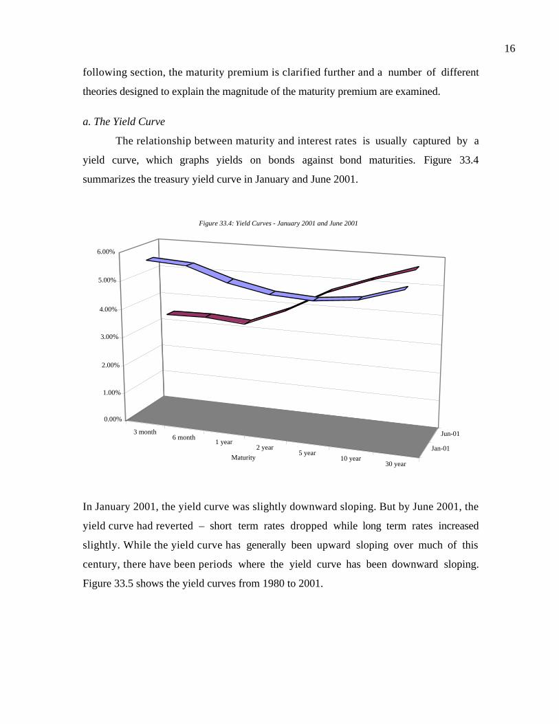
16

following section, the maturity premium is clarified further and a number of different

theories designed to explain the magnitude of the maturity premium are examined.

a. The Yield Curve

The relationship between maturity and interest rates is usually captured by a

yield curve, which graphs yields on bonds against bond maturities. Figure 33.4

summarizes the treasury yield curve in January and June 2001.

In January 2001, the yield curve was slightly downward sloping. But by June 2001, the

yield curve had reverted – short term rates dropped while long term rates increased

slightly. While the yield curve has generally been upward sloping over much of this

century, there have been periods where the yield curve has been downward sloping.

Figure 33.5 shows the yield curves from 1980 to 2001.

3 month6 month

1 year2 year

5 year10 year

30 year

Jan-01

Jun-01

0.00%

1.00%

2.00%

3.00%

4.00%

5.00%

6.00%

Maturity

Figure 33.4: Yield Curves - January 2001 and June 2001

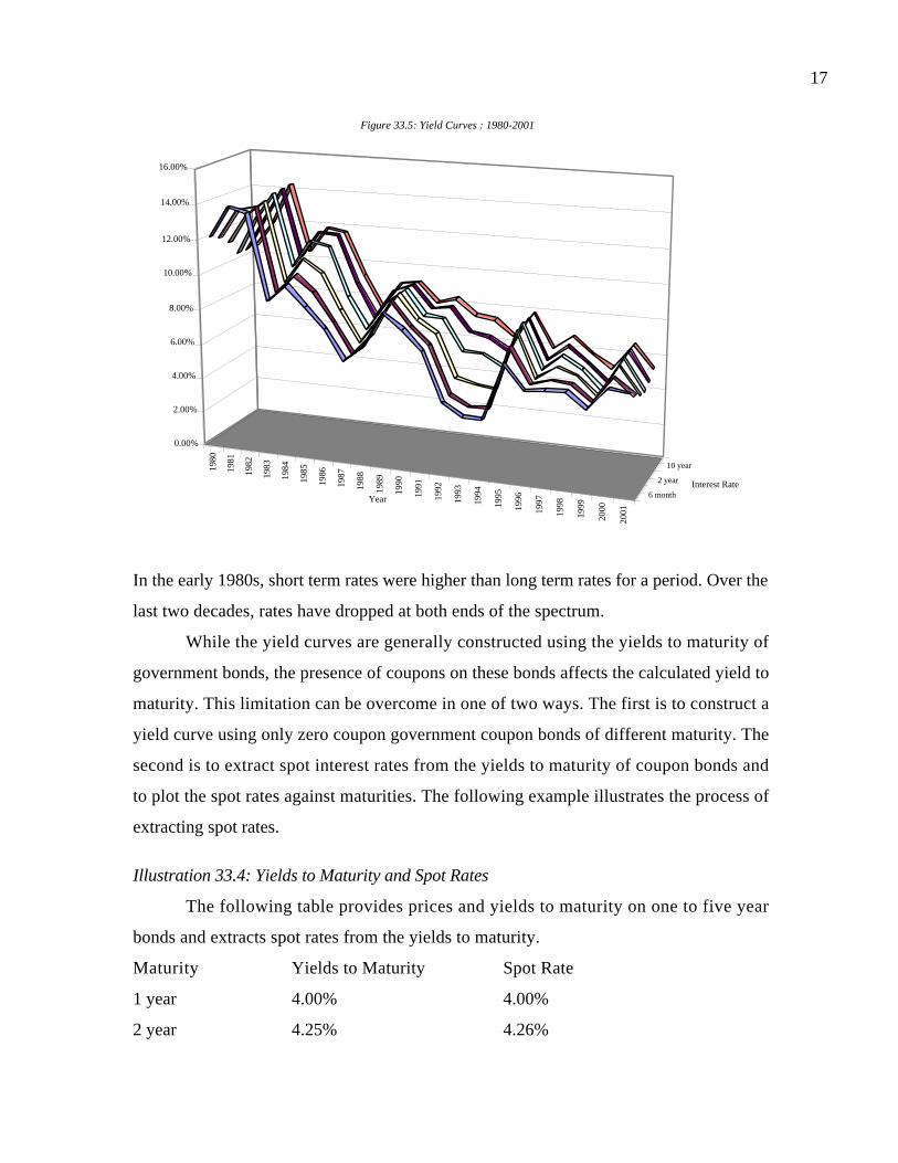
17

In the early 1980s, short term rates were higher than long term rates for a period. Over the

last two decades, rates have dropped at both ends of the spectrum.

While the yield curves are generally constructed using the yields to maturity of

government bonds, the presence of coupons on these bonds affects the calculated yield to

maturity. This limitation can be overcome in one of two ways. The first is to construct a

yield curve using only zero coupon government coupon bonds of different maturity. The

second is to extract spot interest rates from the yields to maturity of coupon bonds and

to plot the spot rates against maturities. The following example illustrates the process of

extracting spot rates.

Illustration 33.4: Yields to Maturity and Spot Rates

The following table provides prices and yields to maturity on one to five year

bonds and extracts spot rates from the yields to maturity.

Maturity Yields to Maturity Spot Rate

1 year 4.00% 4.00%

2 year 4.25% 4.26%

1980

1981

1982

1983

1984

1985

1986

1987

1988

1989

1990

1991

1992

1993

1994

1995

1996

1997

1998

1999

2000

2001

6 month

2 year

10 year

0.00%

2.00%

4.00%

6.00%

8.00%

10.00%

12.00%

14.00%

16.00%

Year

Interest Rate

Figure 33.5: Yield Curves : 1980-2001

18

3 year 4.40% 4.41%

4 year 4.50% 4.514%

5 year 4.58% 4.60%

The spot rate is estimated from the two year rate as follows –

Price of two year bond ( )220

2

10

1

r1

CouponValue Face

r1

Coupon

+++

+=

Assuming the bond is priced at par,

( )220r1

50.1042

04.1

50.421000

++=

Solve for0r2.

%26.41

04.1

50.421000

50.1042r

5.0

20 =−

−=

The other rates are extracted using a similar process,

( )330

2 r1

00.1044

0426.1

00.44

04.1

00.441000

+++=

( )440

32 r1

00.1045

0441.1

00.45

0426.1

00.45

04.1

00.451000

++++=

( )550

432 r1

80.1045

0451.1

80.45

0441.1

80.45

0426.1

80.45

04.1

80.451000

+++++=

The difference between yields to maturity and spot rates increases as the bond maturity

increases.

b. Spot and Forward Rates

The spot rate on a multi-period bond is an average rate that applies over the

periods. The forward rate is a one-period rate for a future period and can be extracted

from the spot rates. For instance, if 0S2 is the two-period spot rate and 0S1 is the one-

period spot rate, the forward rate for the second period, 1F2, can be obtained.

( )10

220

21S1

S1F

++=

19

The forward rate for period three can be extracted using the spot rates for periods 2 and 3.

In general, the forward rate for period n can be written as:

( )( ) 1

1-n0

n0n1

S1

S1F −− +

+= n

n

n

If the yield curve for spot rates is upward sloping, the yield curve using forward rates will

be even more so. Alternatively, if the spot rate yield curve is downward sloping, the

forward rate yield curve will be even more so. The following illustration builds on the

previous one and extracts forward rates from spot rates.

Illustration 33.5: Spot Rates and Forward Rates

The forward rates are extracted from the spot rates for one to five year bonds.

This is illustrated in the following table.

YTM Spot Rate Forward Rate

1 4.00% 4.00% 4.00%

2 4.25% 4.26% 4.52%

3 4.40% 4.41% 4.71%

4 4.50% 4.51% 4.81%

5 4.58% 4.60% 4.96%

Forward rate for year 2 %52.4104.1

0426.1 2

=−=

Forward rate for year 3 %71.410426.1

0441.12

3

=−=

Forward rate for year 4 %81.410441.1

0451.13

4

=−=

Forward rate for year 5 %96.410451.1

0460.14

5

=−=

c. Determinants of the Maturity Premium

The magnitude of the maturity premium is determined by a number of factors

including expectations about inflation, investor preferences for liquidity and demands

from specific market segments. Each of these factors is examined in more detail in the

following section.

20

1. Expected Inflation

Expectations about future inflation are a key determinant of longer term rates. In

general, if inflation is expected to go up in future periods, longer term rates will be higher

than shorter term rates. Alternatively, if inflation is expected to go down in future period,

longer term rates will be lower than short term rates.

An extreme version of this story is the 'pure expectations hypothesis', where the

term structure is driven entirely by the expectations on inflation. Under this hypothesis,

the yield curve will be upward sloping if investors expect inflation to rise in future

periods, flat if investors expect inflation to remain unchanged in future periods, and

downward sloping if investors expect inflation to decline in future periods. This is

illustrated in Figure 33.6.

Figure 33.6: Pure Expectations Hypothesis

No change in inflation Increasing Inflation Decreasing Inflation

Maturity Maturity Maturity

SpotRate

SpotRate

SpotRate

The pure expectations hypothesis can also be stated in terms of forward rates and

expected spot rates. If the hypothesis is correct, the forward rate for period n should be

the best predictor of the expected spot rate in that period.

n-1Fn = Exp(n-1Sn)

where,

n-1Fn = Forward rate for period n

Exp(n-1Sn) = Expected one-period spot rate in period n

While the pure expectations hypothesis may be extreme in assuming that forward rates

are determined entirely by expected spot rates, it does highlight the importance of

expected inflation in determining the maturity premium.

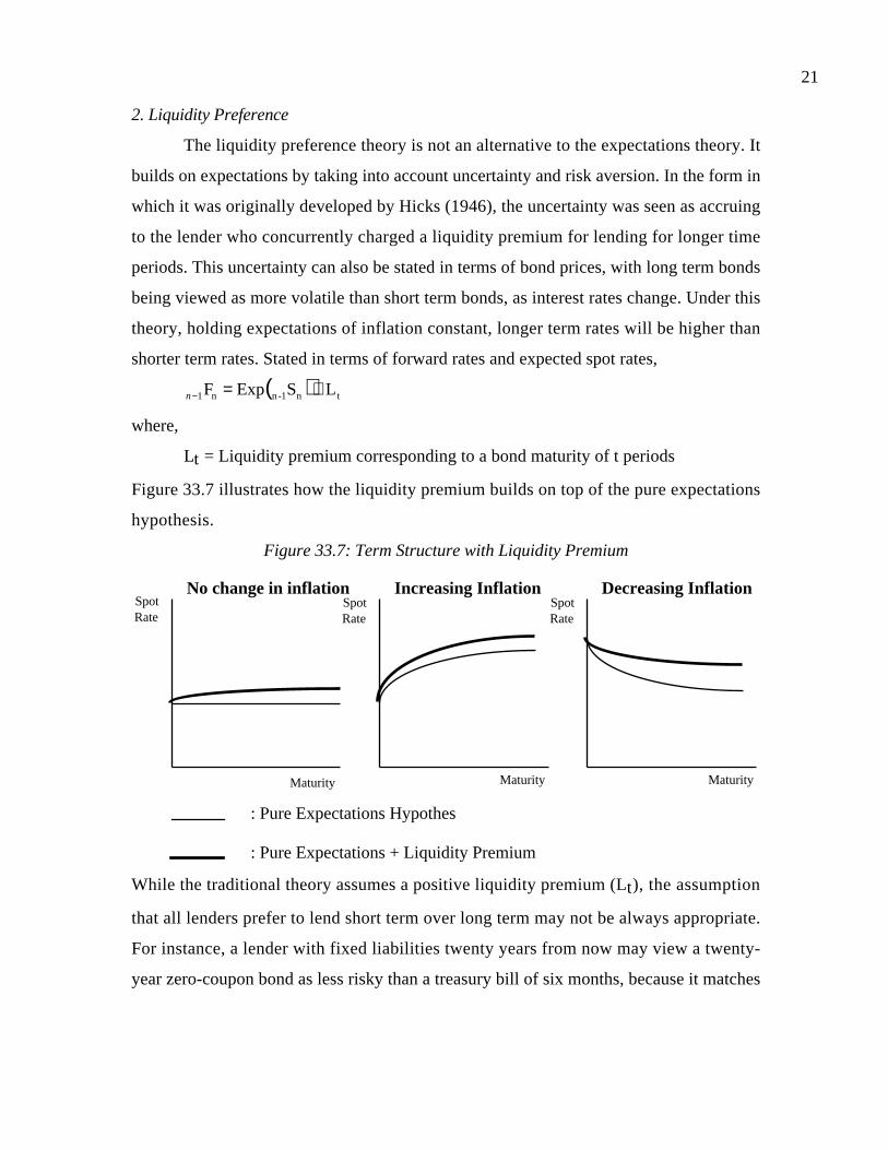
21

2. Liquidity Preference

The liquidity preference theory is not an alternative to the expectations theory. It

builds on expectations by taking into account uncertainty and risk aversion. In the form in

which it was originally developed by Hicks (1946), the uncertainty was seen as accruing

to the lender who concurrently charged a liquidity premium for lending for longer time

periods. This uncertainty can also be stated in terms of bond prices, with long term bonds

being viewed as more volatile than short term bonds, as interest rates change. Under this

theory, holding expectations of inflation constant, longer term rates will be higher than

shorter term rates. Stated in terms of forward rates and expected spot rates,

( ) tn1-nn1 LSExpF +=−n

where,

Lt = Liquidity premium corresponding to a bond maturity of t periods

Figure 33.7 illustrates how the liquidity premium builds on top of the pure expectations

hypothesis.

Figure 33.7: Term Structure with Liquidity Premium

No change in inflation Increasing Inflation Decreasing Inflation

Maturity Maturity Maturity

SpotRate

SpotRate

SpotRate

: Pure Expectations Hypothes

: Pure Expectations + Liquidity Premium

While the traditional theory assumes a positive liquidity premium (Lt), the assumption

that all lenders prefer to lend short term over long term may not be always appropriate.

For instance, a lender with fixed liabilities twenty years from now may view a twenty-

year zero-coupon bond as less risky than a treasury bill of six months, because it matches

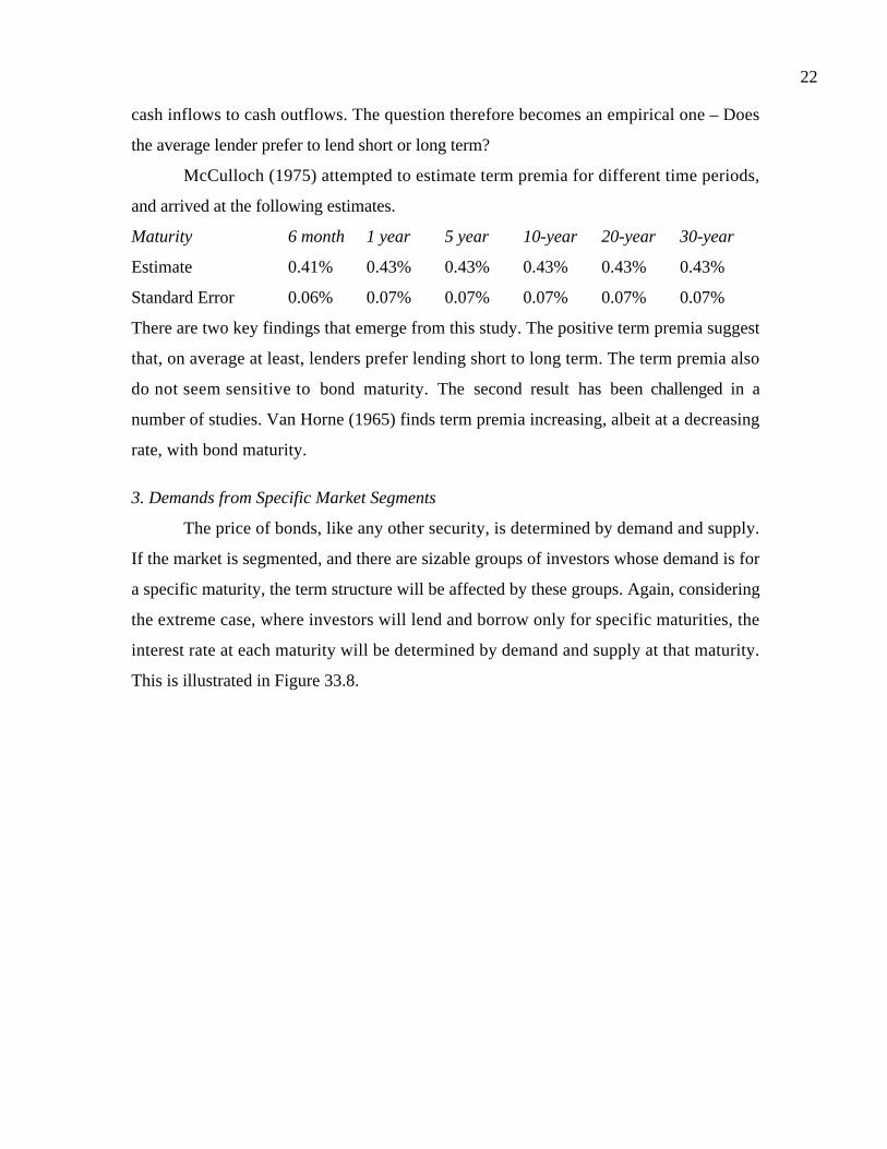
22

cash inflows to cash outflows. The question therefore becomes an empirical one – Does

the average lender prefer to lend short or long term?

McCulloch (1975) attempted to estimate term premia for different time periods,

and arrived at the following estimates.

Maturity 6 month 1 year 5 year 10-year 20-year 30-year

Estimate 0.41% 0.43% 0.43% 0.43% 0.43% 0.43%

Standard Error 0.06% 0.07% 0.07% 0.07% 0.07% 0.07%

There are two key findings that emerge from this study. The positive term premia suggest

that, on average at least, lenders prefer lending short to long term. The term premia also

do not seem sensitive to bond maturity. The second result has been challenged in a

number of studies. Van Horne (1965) finds term premia increasing, albeit at a decreasing

rate, with bond maturity.

3. Demands from Specific Market Segments

The price of bonds, like any other security, is determined by demand and supply.

If the market is segmented, and there are sizable groups of investors whose demand is for

a specific maturity, the term structure will be affected by these groups. Again, considering

the extreme case, where investors will lend and borrow only for specific maturities, the

interest rate at each maturity will be determined by demand and supply at that maturity.

This is illustrated in Figure 33.8.

23

Figure 33.8: Market Segmentation and Term Structure

SpotRate

Maturity

Under this scenario, the term structure can take any shape, depending upon the demand

and supply at each maturity.

The assumption that investors will lend or borrow only for specific maturities and

not substitute other maturities even when it is extremely favorable for them to do so is an

extreme one. In reality, market segments do exist and do affect the term structure but only

at the margin and for one or two maturities. For instance, the demand from Japanese

investors in the late eighties for the just-issued thirty year bonds resulted in a slight kink

in the term structure, where the thirty-year bond rates were slightly lower than twenty-

nine year bond rates, even though the rest of the yield curve was upward sloping.

The Empirical Evidence on Maturity Premia

Empirical studies of the term structure have examined several questions including

the relative frequency of upward and downward sloping term structures, the magnitude of

liquidity premia and the presence of market segments. The evidence can be summarized as

follows.

• The yield curve, at least in this century, has been more likely to be upward sloping

than downward sloping. Examining yield curves at the beginning of each year from

1900 to 2000, the yield curve has been downward sloping in only 29 of the 100 years.

24

This is inconsistent2 with a pure expectations hypothesis, where downward sloping

yield curves should be just as likely as flat or upward sloping yield curves. It is,

however, consistent with a combination of the expectation and liquidity preference

hypotheses, where positive liquidity premia are demanded over and above expected

inflation.

• The term structure is much more likely to be downward sloping when the level of

interest rates is high, relative to historical rates. The table below3 summarizes the

frequency of downward-sloping yield curves as a function of the level of interest

rates.

1-year Corporate Bond Rate Slope of Yield Curve

Positive Flat Negative

Above 4.40% 0 0 20

1900-70 3.25% - 4.40% 10 10 5

Below 3.25% 26 0 0

1971-00 Above 8.00% 4 2 3

Below 8.00% 13 6 0

This evidence is consistent with the expectations and liquidity preference hypotheses,

but it is also consistent with a hypothesis that interest rates move within a normal

range. When they approach the upper end (lower end) of the normal range, the yield

curve is more likely to be downward sloping (upward sloping).

• Studies have generally found that expectations about future interest rates are

important in shaping the term structure. Meiselman computed high positive

correlations between forecasting errors and changes in various forward rates, and

stable term premiums. In contrast, there are many researchers who argue that the

volatility in interest rates is much too great to be explained by just expectations about

future rates and constant term premia. Shiller (1979) concludes that the greater the

volatility in interest rates, the larger the term premium.

2 Prior to the abandonment of the Gold Standard in the 1930s, negatively sloped yield curves were just aslikely to occur as positively sloped yield curves.3 Some of the data table is extracted from Wood (1984).

25

• Attempts by the government to alter the shape of the yield curve by adjusting the

maturity of issues have largely been unsuccessful in the long term. For instance,

"Operation Twist" in 1962 was designed to make the yield curve flatter4 by lowering

long term rates and raising short term rates, by issuing short term debt to finance

deficits. Though the yield curve did flatten, long term yields did not decline. This can

be viewed as evidence of the weakness of the market segmentation hypothesis.

• There is evidence that the shape of the term structure has strong predictive power for

future changes in the real economy. Harvey (1991) examined the G-7 countries

(Canada, France, Germany, Italy, Japan, U.K., U.S.A.) and concluded that 54% of

world economic growth could be explained the term structure.

c. Default Premium

While there is no possibility of default for bond issues made by the United States

Treasury, corporate bonds or state/local bonds can default on interest or principal

payments. If there is any possibility of default on a bond, there will be a default premium

in addition to the maturity premium on the bond. The default premium will increase with

the perceived default risk of the bond and is generally also a function of the maturity and

terms of the specific bond. We examined this issue in detail in Chapter 7, as part of the

discussion of how best to estimate the cost of debt for a firm. Reviewing that discussion,

we concluded that:

• The most direct measure of default risk is the default rate which measures

defaulted issues as a percentage of the par value of debt outstanding. Hickman

investigated the default experience of fixed-income corporate bonds between 1900

and 1943, as a function of the bond rating.

Ratings

Size of Issue I II III IV V-IX No Rating

> $ 5 millions 5.9% 6.0% 13.4% 19.1% 42.4% 28.6%

≤ $ 5 millions 10.2% 15.5% 9.9% 25.2% 32.6% 27.0%

4 A similar, though less formal, attempt was made in 1993 by the Treasury Department to raise short termrates and lower long term rates by issuing more short term bonds and less long term bonds. It wassuccessful at raising short term rates, but long term rates increased concomitantly.

26

Hickman's study have been extended by several researchers and data availability

has made this easier to do. Altman computes default rates for high yield bonds

from 1970 to the present, on an annual basis and relates them to bond ratings.

• Default spreads on bonds tend to increase during economic downturns and

decrease during economic booms.

• Default spreads are generally larger for longer term bonds than they are for shorter

term bonds, for any given level of default risk. There may be specific

circumstances, though, where the reverse is true. Johnson defines a "crisis-at-

maturity" scenario, usually in the midst of a recession or a depression, where a

firm is perceived to have insufficient funds to meet its immediate debt servicing

needs, though it is expected to revert to health in the long term. In this scenario,

the default premia will be lower for longer maturity bonds than for shorter

maturity bonds. Johnson found evidence of inverted default premia term

structures during 1934, in the midst of the depression.

Corporate Bonds in Emerging Markets

In the framework that we have developed, you build up to the rate on a corporate

bond by adding a default spread to the government bond rate. This process works only

when the government is viewed as having no default risk. When governments have default

risk, as is often the case in emerging markets, the process becomes more complicated. To

estimate the appropriate interest rate on a corporate bond in an emerging market, you

have to begin by estimating a riskless rate. The best way to do it is to build it up from the

Fisher equation – add an expected inflation rate to the real rate of return in that market.

The latter can be set equal to the expected real growth rate in the economy, but the former

can be a volatile number in high inflation markets. An alternative approach is to begin

with the government bond rate and subtract out the estimated default spread for the

government – this default spread can be obtained using the rating for the government.

You could alternatively estimate the corporate bond rate for a company in an

emerging market in a different currency – U.S. dollars or Euros. In this case, the riskless

rate will be defined in that currency – the treasury bond rate in the U.S. for dollars and the

27

German Euro-denominated government bond rate. The default spread for the company

can then be added on to this riskless rate to estimate the corporate bond rate.

There is one final point that needs to be confronted with corporate bonds in

emerging markets and it relates to whether you should incorporate the country default

risk spread into the corporate bond rate. For instance, should the interest rate on a bond

issued by Embraer, the Brazilian aerospace firm, incorporate the default spread on

Brazilian government bonds? For smaller firms, the answer should generally be yes. For

larger firms with substantial operations outside the country, we have a little more leeway.

These firms may be able to borrow at rates lower than the sovereign rate.

Special Feature in Bonds and Pricing Effects

In the last section, we examined the question of how to price a government or a

corporate bond based upon the expected coupons and the appropriate interest rate for the

bond. Most bonds though have other features added on, some of which make the bonds

more valuable and some less valuable. In this section, we consider how best to value these

special features.

I. Convertibility

A convertible bond is a bond that can be converted into a pre-determined number

of shares, at the option of the bondholder. While it generally does not pay to convert at

the time of the bond issue, conversion becomes a more attractive option as stock prices

increase. Firms generally add conversions options to bonds to lower the interest rate paid

on the bonds.

The Conversion Option

In a typical convertible bond, the bondholder is given the option to convert the

bond into a specified number of shares of stock. The conversion ratio measures the

number of shares of stock for which each bond may be exchanged. Stated differently, the

market conversion value is the current value of the shares for which the bonds can be

exchanged. The conversion premium is the excess of the bond value over the conversion

value of the bond.

28

Thus a convertible bond with a par value of $1,000, which is convertible into 50

shares of stock, has a conversion ratio of 50. The conversion ratio can also be used to

compute a conversion price - the par value divided by the conversion ratio, yielding a

conversion price of $20. If the current stock price is $25, the market conversion value is

$1,250 (50 * $25). If the convertible bond is trading at $1,300, the conversion premium is

$50.

The effect of including a conversion option in a bond is illustrated in Figure 33.9.

Figure 33.9: Bond Value and Conversion Option

Determinants of Value

The conversion option is a call option on the underlying stock and its value is

therefore determined by the variables that affect call option values – the underlying stock

price, the conversion ratio (which determines the strike price), the life of the convertible

bond, the variance in the stock price and the level of interest rates. The payoff diagrams

on a call option and on the conversion option in a convertible bond are illustrated in

Figure 33.10.

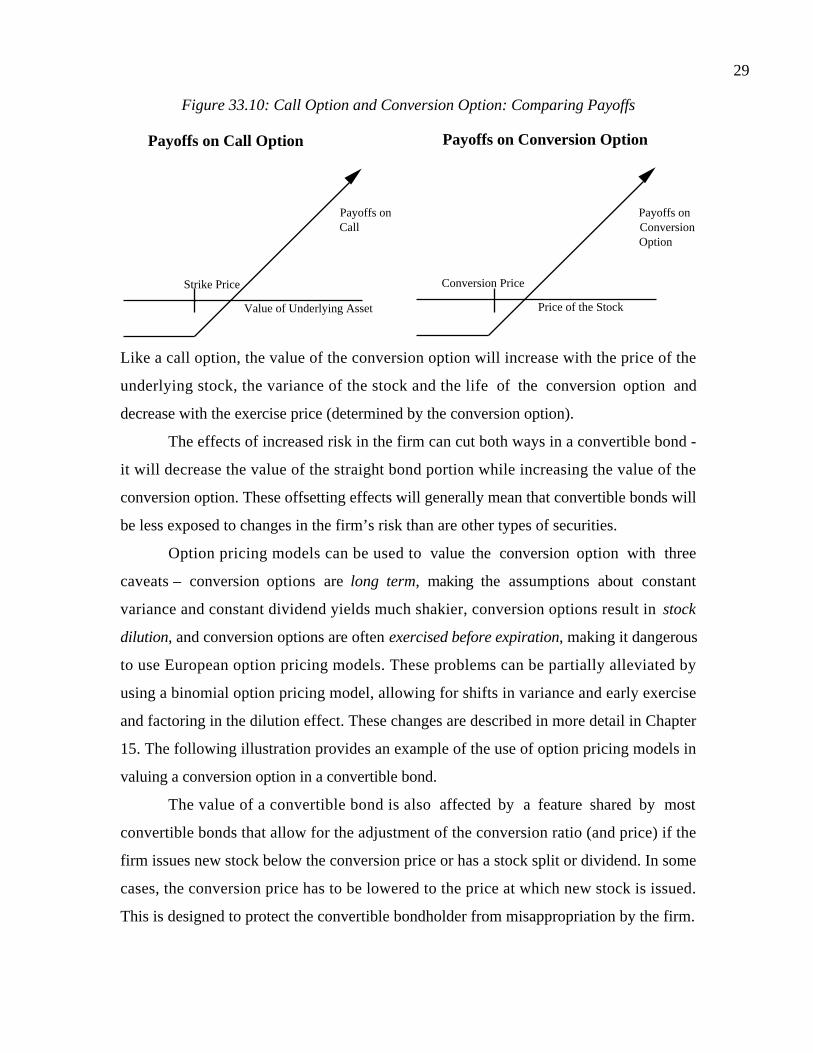
29

Figure 33.10: Call Option and Conversion Option: Comparing Payoffs

Value of Underlying Asset

Payoffs on Call Option

Strike Price

Price of the Stock

Payoffs on Conversion Option

Conversion Price

Payoffs onCall

Payoffs onConversionOption

Like a call option, the value of the conversion option will increase with the price of the

underlying stock, the variance of the stock and the life of the conversion option and

decrease with the exercise price (determined by the conversion option).

The effects of increased risk in the firm can cut both ways in a convertible bond -

it will decrease the value of the straight bond portion while increasing the value of the

conversion option. These offsetting effects will generally mean that convertible bonds will

be less exposed to changes in the firm’s risk than are other types of securities.

Option pricing models can be used to value the conversion option with three

caveats – conversion options are long term, making the assumptions about constant

variance and constant dividend yields much shakier, conversion options result in stock

dilution, and conversion options are often exercised before expiration, making it dangerous

to use European option pricing models. These problems can be partially alleviated by

using a binomial option pricing model, allowing for shifts in variance and early exercise

and factoring in the dilution effect. These changes are described in more detail in Chapter

15. The following illustration provides an example of the use of option pricing models in

valuing a conversion option in a convertible bond.

The value of a convertible bond is also affected by a feature shared by most

convertible bonds that allow for the adjustment of the conversion ratio (and price) if the

firm issues new stock below the conversion price or has a stock split or dividend. In some

cases, the conversion price has to be lowered to the price at which new stock is issued.

This is designed to protect the convertible bondholder from misappropriation by the firm.

30

Illustration 33.6: Valuing a conversion option / convertible bond

In December 1994, General Signal had convertible bonds outstanding with the

following features.

• The bonds matured in June 2002. There were 100,000 shares of convertible bonds

outstanding.

• They had a face value of $1000, and were convertible into 25.32 shares per bond until

June 2002.

• The coupon rate on the bond was set at 5.75%.

• The company was rated A-. Straight bonds of similar rating and similar maturity were

yielding 9.00%.

• The stock price in December 1994 was $32.50. The volatility (standard deviation in ln

stock prices) based upon historical data was 50.00%.

• There were 47.35 million shares of equity outstanding. Exercising the convertible

bonds will create 2.532 million additional shares (100,000 * 25.32 shares).

The two components of the convertible bond can be valued as follows.

A. Straight Bond Component

If this bond had been a straight bond, with a coupon rate of 5.75% and a yield to

maturity of 9.00% (based upon the bond rating), the value of this straight bond can be

calculated.

PV of Bond =28.75

(1.09) tt=1

t=7.5

∑ +1,000

(1.09)7.5 = $834.79

This is based upon semi-annual coupon payments (of $28.75 for semi-annual periods).

B. Valuing the Conversion Option

The value of the conversion option is estimated using the Black-Scholes model,

with the following parameters for the conversion option.

Type of Option = Call Number of Calls/Bond = 25.32

Stock Price = $32.50 Strike Price = $1000/25.32 = $39.49

Time to Expiration = 7.5 years Standard Deviation in Stock Prices (ln) = 0.5

Riskless rate = 7.75% (Rate on 7.5 year Treasury Bond)

Dividend yield on Stock = 3.00%

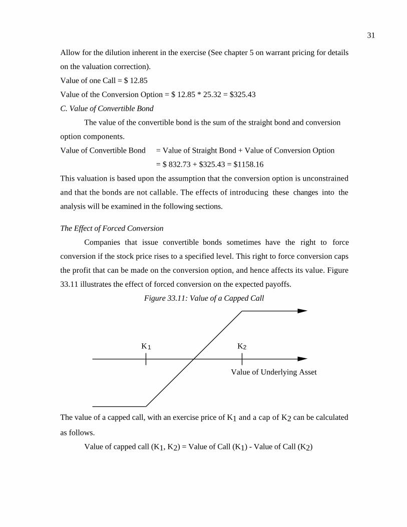
31

Allow for the dilution inherent in the exercise (See chapter 5 on warrant pricing for details

on the valuation correction).

Value of one Call = $ 12.85

Value of the Conversion Option = $ 12.85 * 25.32 = $325.43

C. Value of Convertible Bond

The value of the convertible bond is the sum of the straight bond and conversion

option components.

Value of Convertible Bond = Value of Straight Bond + Value of Conversion Option

= $ 832.73 + $325.43 = $1158.16

This valuation is based upon the assumption that the conversion option is unconstrained

and that the bonds are not callable. The effects of introducing these changes into the

analysis will be examined in the following sections.

The Effect of Forced Conversion

Companies that issue convertible bonds sometimes have the right to force

conversion if the stock price rises to a specified level. This right to force conversion caps

the profit that can be made on the conversion option, and hence affects its value. Figure

33.11 illustrates the effect of forced conversion on the expected payoffs.

Figure 33.11: Value of a Capped Call

K2K1

Value of Underlying Asset

The value of a capped call, with an exercise price of K1 and a cap of K2 can be calculated

as follows.

Value of capped call (K1, K2) = Value of Call (K1) - Value of Call (K2)

32

This is because the cash flows on a capped call can be replicated by buying the call with a

strike price of K1 and selling the call with a strike price of K2.

II. Callability

The issuer of a callable bond preserves the right to call back the bond and pay a

fixed price (generally at a premium over the par value) for it. Thus, if interest rates decline

(bond prices rise) after the initial issue, the firm can refund the bonds at the fixed price

instead of the market value. Adding the call option to a bond should make it less

attractive to buyers, since it reduces the potential upside on the bond. As interest rates go

down, and the bond price increases, the bonds are more likely to be called back.

The distinction between a straight bond and a callable bond are illustrated in the

Figure 33.12.

Figure 33.12: Callable versus Straight Bonds

The difference on the upside between straight and callable bonds is quite clearly

illustrated in Figure 33.12. As interest rates decline, the values of the two bonds diverge,

whereas they converge as interest rates increase.

There are several common features shared by most callable bonds. Most callable

bonds come with an initial period of call protection, during which the bonds cannot be

called back. Such bonds are called deferred callable bonds. The call price on most callable

33

bonds is set at an initial level above par value plus one annual coupon payment, but

declines as time passes and approaches the par value.

Valuing the Callability Option

The issuer's right to call back a bond if interest rates drop (or bond prices rise) to

an attractive level is a call option on the bond and can be valued as such. The payoffs on a

callable bond are shown in Figure 33.13.

Figure 33.13: Payoffs on Call Feature on Bond to Seller of Bond

Value of Underlying Asset

Payoffs on Call Option

Strike Price

Value of Bond

Payoffs on Call Feature on Bond

Call Price

Payoffs onCall

Payoffs onCall Feature

The value of the callable feature on a callable bond will increase as interest rates decline,

and as the volatility of interest rates increases. Since the callable feature is held by the

issuer of the bond, the value of a callable bond can be written as follows:

Value of Callable Bond = Value of Straight Bond - Value of Call Feature in Bond

A callable bond should therefore sell for less than an otherwise similar straight bond.

Traditional Analysis

The traditional approach to analyzing callable bonds is to estimate yields to call

as well as yields to maturity. The former is based upon the assumption that the bond will

be called at the first call date while the latter assumes holding the bond until maturity. The

two yields are compared and the investor chooses the lower of the two as a measure of

his expected return on the bond. This approach can also be extended to calculate the yield

to all possible call dates and picking the lowest of these yields as the expected yield on

the callable bond. This yield is called the yield to worst.

While this approach may give the investor some sense of the potential downside

from the callability of the bond, it suffers from all the standard problems of the ‘yield to

34

maturity’ calculation. First, it assumes that the investor can reinvest all coupons until the

bond is called at the yield to call, which is not a realistic assumption since calls are much

more likely if interest rates go down. Second, it does not examine the rate at which the

proceeds from the called bond can be reinvested by the investor. Third, it assumes that

the bond will be called on the call date, which takes away the option characteristics of the

call feature.

Illustration 33.7: Estimating yields to maturity and call on a callable bond

Consider a corporate bond, with 20 years to maturity and a 12% coupon rate that

is callable in two years at 105% of the face value. The bond is trading at 98 currently. The

yields to maturity and the yields to call on the corporate bond are as follows:

Price =60.00

(1+r) tt=0.5

t=20

∑ +1,000

(1+r)20 = $980

The yield to maturity, r, is approximately 12.26%.

The yield to call can be similarly calculated.

Price =60.00

(1+r) tt=0.5

t=2

∑ +1,000

(1+r)2 = $1050

The yield to call is approximately 13.25%.

Price/Yield Relationship for a Callable Bond

The price/yield relationship on a callable bond is different because the potential

that the bond will be called back puts an upper limit on the price. This makes the

relationship between price and yield convex, for some range of the yields. The difference

is illustrated in Figure 33.14.

35

Figure 33.14: Callable Bond Prices and Interest Rates

The section of the price/yield relationship on the callable bond when the yield falls below

y* has negative convexity - i.e., the price appreciation on this bond will be less than the

price depreciation for a given change (down or up) in interest rates.

Determinants of Value - Option Pricing Approach

The call feature in a callable bond can be valued using option pricing models. It is a

series of call options on the underlying bond and its value is determined by the level and

volatility of interest rates. There are some modifications that need to be made to the

standard option pricing models before they can be applied in this context.

Once the call feature is valued as a series of option, the yield on a callable bond

can be adjusted for the option features and the difference between this adjusted yield and

treasuries of equivalent maturity is called the option adjusted spread. This approach is a

more realistic way of considering the effects of the call feature on expected yields than the

traditional yield to call approach.

The following illustration values the call feature on a callable bond.

Illustration 33.8: Valuing a callable bond

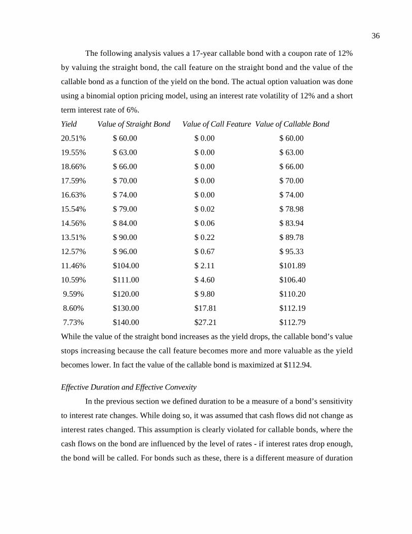
36

The following analysis values a 17-year callable bond with a coupon rate of 12%

by valuing the straight bond, the call feature on the straight bond and the value of the

callable bond as a function of the yield on the bond. The actual option valuation was done

using a binomial option pricing model, using an interest rate volatility of 12% and a short

term interest rate of 6%.

Yield Value of Straight Bond Value of Call Feature Value of Callable Bond

20.51% $ 60.00 $ 0.00 $ 60.00

19.55% $ 63.00 $ 0.00 $ 63.00

18.66% $ 66.00 $ 0.00 $ 66.00

17.59% $ 70.00 $ 0.00 $ 70.00

16.63% $ 74.00 $ 0.00 $ 74.00

15.54% $ 79.00 $ 0.02 $ 78.98

14.56% $ 84.00 $ 0.06 $ 83.94

13.51% $ 90.00 $ 0.22 $ 89.78

12.57% $ 96.00 $ 0.67 $ 95.33

11.46% $104.00 $ 2.11 $101.89

10.59% $111.00 $ 4.60 $106.40

9.59% $120.00 $ 9.80 $110.20

8.60% $130.00 $17.81 $112.19

7.73% $140.00 $27.21 $112.79

While the value of the straight bond increases as the yield drops, the callable bond’s value

stops increasing because the call feature becomes more and more valuable as the yield

becomes lower. In fact the value of the callable bond is maximized at $112.94.

Effective Duration and Effective Convexity

In the previous section we defined duration to be a measure of a bond’s sensitivity

to interest rate changes. While doing so, it was assumed that cash flows did not change as

interest rates changed. This assumption is clearly violated for callable bonds, where the

cash flows on the bond are influenced by the level of rates - if interest rates drop enough,

the bond will be called. For bonds such as these, there is a different measure of duration

37

that is more appropriate called the effective duration. The duration of any bond can be

approximated as follows, for a small change in interest rates.

Duration ( )-0

-

yyP

PP

−−=+

+

where P- = Price of the bond if yield drop by x basis points

P+ = Price of the bond if yield increases by x basis points

P0 = Price of the bond initially

y+ = Initial yield + x basis points

y - = Initial yield - x basis points

This approach can be used to estimate the effective duration of callable bonds for any

segment of the yield curve. It can also be used for any other bonds with embedded

options, such as putable bonds, or mortgage backed securities, which have the

prepayment option embedded in them.

A similar adjustment can be made to the standard convexity measure to arrive at

the effective convexity of any bond with embedded options. [NOTE: There was no

equation for convexity.]

Effective Convexity ( )( )2-0

0-

yy5.0P

P2PP

−−+=

+

+

Valuing a Callable-Convertible Bond

Many convertible bonds have embedded call features. The presence of two

options in the bond, one possessed by the buyer of the bond and the other possessed by

the seller of the bond, and the interaction between the two options, implies that the two

options have to be valued together. Brennan and Schwartz (1977, 1980) provide an

analysis of convertible bonds with call features, default risk and stock price dilution. The

simplest approach for illustrating the interaction between the various options is a

binomial option pricing model.

Empirical Evidence on Call Feature

When a convertible bond is callable, holders of the convertible bond lose the

opportunity to make further returns on the bond as stock prices increase. Companies can

establish a variety of call policies such as calling the instant the market value of the

38

convertible rises above the call price or waiting until the market value is well in excess of

the call price. Ingersoll (1977) argues that a bond should be called when its conversion

value equals its call price. Given that a thirty-day notice has to be given to bondholders of

a call, firms may prefer to build a cushion to protect against risk during this period.

The empirical evidence however suggests that firms do not usually follow the

optimal policy. Ingersoll, for instance, finds that between 1968 and 1975, the average

conversion value was 43.9% above the call price for bonds and 38.5% for preferred

stocks. The call policy chosen by a firm and communicated to financial markets implicitly

through its actions, has an effect on the value of the convertible bond.

III. Pre-payment Option

Mortgage backed securities, which came of age in the eighties, securitized

residential mortgages, by packaging them and issuing marketable securities of various

types on them – either as flow through investments where holders receive a share of the

total cash flows on the pool of mortgages or as derivative products, where holders receive

customized packages of cash flows depending upon their preferences. The latter, called

collateralized mortgage obligations, in its simplest form, divide cash flows on the mortgage

pool into four tranches, with cash flows on each tranche starting as the cash flows on the

prior tranche are completed. Figure 33.15 illustrates this type of security.

Figure 33.15: Cash flows on a Mortgage Pool

39

In recent years, CMOs have been refined further and even more specialized products have

been created including stripped mortgage-backed securities (where cash flows are divided

on the basis of principal and interest), floating rate classes and inverse floaters (where the

interest rate on the security increases as the index rate decreases).

Mortgages can be pre-paid by borrowers, if interest rates decline. This

prepayment option that resides with borrowers affects the cash flows, and therefore the

value, of all mortgage-backed securities.

The Prepayment Option

The homeowner may prepay a loan for any number of reasons, but the level of

interest rates is a critical variable. If interest rates declines sufficiently, the potential gain

from pre-payment may exceed the cost of pre-payment. The following graph illustrates

the percentage of homeowners who prepay as a function of the difference between

interest rate and the coupon rate, based upon historical data.

40

If the level of interest rates were the only determinant of prepayment and homeowners

were rational about prepayment decisions, the prepayment option could be valued very

similarly to the call option in a callable bond (as a function of the level and volatility of

interest rates).

There are, however, other variables besides the level of interest rates that

determine whether homeowners prepay. For instance, there is a correlation between

prepayment and the age of a mortgage, irrespective of interest rates. Furthermore, some

homeowners may never prepay their mortgages no matter how much interest rates drop.

There are also seasonal factors that affect prepayment. Consequently, option pricing

models alone fall short in pricing prepayment options in mortgage backed securities.

A number of researchers have attempted to develop models that explain

prepayment, as a basis for pricing the prepayment option, with characteristics such as

age and coupon rate as inputs, in addition to specific characteristics of the borrowers in

the pool. In cases where a specific rather than a generic pool of mortgages is being priced,

the historical payment record of the specific5 pool is useful and is often the basis for

estimating prepayments.

5 A number of variables have been found to be useful in explaining prepayments - the market price relativeto the original purchase price and geographical differences, for instance.

41

Valuing the prepayment option

The effect of the prepayment option on value will vary with the type of mortgage

backed security. Consider, for instance, the price behavior of interest-only and principal-

only securities, as interest rates changes. As interest rates increase, the interest payments

on the interest-only securities goes up, leading to a higher value for the security, at least

initially, though the present value effects (which are negative) start to dominate beyond a

certain point. As interest rates decrease, the prepayments lead to lower interest payments

and a lower value for the security. The principal-only securities behave more like

conventional bonds, increasing in value as interest rates decline and decreasing in value as

they increase. Figure 33.16 illustrates this relationship.

Figure 33.16: Mortgage Rates and Security Values

IO: Interest Only Security PO: Principal Only Security

IV. Interest Rate Caps and Floors

A floating rate bond is a bond which has an interest rate linked up to an index -

either a government bond rate (treasury bond or bill) or to the LIBOR. The rationale for

issuing such bonds is to reduce the interest rate risk for both the issuer and the buyer of

the bond. Most floating rate bond issuers, however, cap their floating rate obligations to

ensure that interest rates do not rise above a pre-specified rate (the cap). Some floating

rate bonds offer buyers some compensation by providing a floor, below which interest

rates will not decline. If a floating rate bond has a cap and a floor, a collar is created.

42

Caps, Floors and Collars

The presence of a cap on a floating rate bond can be illustrated best by contrasting

a bond with a cap against a floating rate bond without one, as shown in Figure 33.17.

Figure 33.17: Effects of Caps on Floating Rate Loans

EffectiveIn teres tRate (%)

Index Rate(for Cap)

Float ing RateBond

Cap

Float ing Rate+ Cap

K(c)

The cap on a floating rate bond has the same effect as a call option on interest rates with a

strike price of Kc, with the issuer of the bond holding the option. A call option on

interest rates translates6 into a put option on the underlying bond. The price of a floating

rate bond with a cap can then be written as:

Price of floating rate bond with cap = Price of floating rate bond without cap

- Value of put on bond

The presence of a floor on interest rates can also be illustrated using a similar comparison

of a bond with a floor against a bond without one in Figure 33.18.

6 The translation is not one to one. A call option on interest rates is the equivalent of α options on theunderlying bill or bond, where α = 1/ Exercise price of equivalent bill.

43

Figure 33.18: Effects of Caps on Floating Rate Loans

EffectiveInterestRate (%)

Floating RateBond

Floor

Cap

K(f)

Floating Rate+ Floor

The floor on a floating rate bond has the same effect as adding a put option on interest

rates with a strike price of Kf, with the buyer of the bond holding the put. A put option

on interest rates can be translated into a call option on the underlying bond. The price of a

floating rate bond with a floor can then be written as:

Price of floating rate bond with floor = Price of floating rate bond without cap

+ Value of call on bond

Finally, the presence of both a cap and a floor can be illustrated in Figure 33.19.

Figure 33.19: Effects of Caps on Floating Rate Loans

44

EffectiveInterestRate (%)

Index Rate(for Cap)

Floating RateBond

Floor

Cap

Collared Bond

K(f) K(c)

The presence of a collar on a floating rate bond creates two options - a call option with a

strike price of Kc for the issuer of the bond and a put option with a strike price of Kf for

the buyer of the bond. These options on interest rates can be stated again in terms on

options on the underlying bond.

Price of floating rate bond with collar = Price of floating rate bond without collar

+ Value of call on bond

- Value of put on bond

Valuing caps and floors

Option pricing models can be used to value caps, floors and collars with some

caveats. The key assumption in the Black Scholes model of constant volatility over the

life of the option is likely to be violated for interest rate options, both because of the long

term nature of these options and because the variance in the bond price is likely to change

as the bond approaches maturity. There have been attempts to use yield instead of price

and assume that it conforms to a lognormal distribution.

45

Subrahmanyam (1990) notes that the value of a cap on interest rates can be

written as a series of put options on the price of an equivalent bill or bond. Briys, Crouhy

and Schobel (1991) provide a framework for pricing caps, floors and collars. They argue

that caps and floors can be modeled as a series of independent options on zero coupon

bonds. They allow for the fact that bond prices do not follow the geometric Brownian

motion used by Black and Scholes (1973), but adopt a different stochastic process to

price caps, floors and collars.

Illustration 33.9: Valuing a 2-year Cap/Floor on 6 Month LIBOR

Assume that the current 6-month LIBOR rate is 8%, and that the cap/floor has an

exercisable price of 8%. The cap consists of three options which are exercisable at the end

of 6 months (183 days), 12 months (365 days) and 18 months (548 days). Each of these

options is on the $LIBOR rate (of 183 days for the first, 182 days for the second and 183

days for the third).

The options can be valued using the bill prices (rather than interest rates) and the

inputs used in the Black-Scholes Model are as follows.

Option Maturity Bill price Exercise Price Forward Price Volatility

183 0.9609 0.9611 0.9626 0.0100

365 0.9250 0.9609 0.9609 0.0100

548 0.8890 0.9611 0.9615 0.0100

The first column provides the maturity period for each of the three options. The second

column is the value of a zero-coupon bond with a maturity equal to the maturity of the

zero-coupon bond - $1 discounted back 183 days at 8% is $0.9609, $1 discounted back

365 days at 8% is $0.9250 and so on. The third column is the strike price, based upon the

cap rate, for each option. The fourth column is the forward price of the bill at the option

expiration date. The final column is the assumed annualized volatility in bill prices of 1%.

The values of the call and puts options with these maturities on bills is provided

in the following table in basis points. These can be converted into option values for

options on interest rates by multiplying by the number of put options on bills that is

equivalent to one call option on the interest rate.

Adjustment Factor = α = 1/Exercise price of equivalent bill option

46

T. Bill Option Interest Rate Options

Put Call Call Put

183 19.6133 33.6639 20.4065 35.0254

365 34.6903 36.4439 36.1010 37.9259

548 39.8620 43.5135 41.4742 45.2734

Value of the Cap = 97.9817

Value of the Floor = 120.2237

To illustrate the calculation, the values of the interest rate options for the 183 day option

can be estimated as follows.

Adjustment factor for 183 day option 1.04050.9611

1 ==

Value of 183-day put on T.Bill = 19.6133

Value of 183-day call on interest rate = 19.6133 * 1.0405 = 20.4065

Valuing Options Embedded in Bonds

A corporate bond can often have three or four options embedded in it and to value the

bonds, you have to value the options. While conventional option pricing models can be

used to value fixed income options, you should note the following.

• The assumption of constant volatility that we often use to value options on stocks

cannot be used to value options on bonds such as callability. Bonds are finite life

instruments and their volatility will decrease as they approach maturity. You will

have to model the change in volatility over time to price the option.

• When multiple options exist in a bond, you will have to examine the relationship

between the options to price them. For instance, consider a callable, convertible bond.

While both callability and convertibility are options – one is held by the bond issuer

and the other by the bond buyer – the exercise of one of these options voids the other.

This will become a factor when the options will be exercised and how much they are

worth.

• The key underlying variable for some bond options – such as interest rate caps and

floors – is the interest rate process and how it is modeled can have a significant impact

on the value of the options.

47

V. Other Features

There are a number of other bond features which affect the value of the bond - a

sinking fund provision, where the firm plans to retire a specified face value of the bonds

outstanding each year, provisions relating to the subordination of future debt issues and

bond covenants on investment and dividend policy.

Sinking Funds

Most industrial bond issues come with sinking fund provisions, requiring the

issuer to retire a specified portion of the bond issue each year, starting a period of time

(five or ten years) after the initial issue. The sinking fund provision can take one of two

forms.

(a) A trustee collects a cash payment from the bond issuer and calls bonds for redemption

at the sinking-fund call price, usually based upon a lottery.

(b) The bond issuer can buy back bonds in the open market and deliver the specified

number of bonds to the trustee in the periods specified.

If the bond issuer has the option to do the latter, bonds will be bought back and delivered

if the market price is less than the call price and cash will be delivered to the trustee to

make the call if the market price is greater than the call price.

Sinking funds usually relate to a single issue, but they can sometimes cover

multiple issues ("funnel sinking fund"). Most sinking funds also allow the bond issuer to

accelerate call backs if it is in the issuer's favor to do so (i.e., interest rates have gone

down since the issue).

A sinking fund has two effects, one of which benefits the issuer of the bond and

the other which benefits the buyer of the bond. The issuer of the bond gets a delivery

option, because he has an option to either deliver the cash for the call price or to buy the

bonds at the market price. The value of this call option (similar to the option in a callable

bond) will increase with the volatility of interest rates and decrease with the level of

interest rates. The buyer of the bond has less default risk because of the requirement that

some of the debt be retired each period. The net effect will determine whether a sinking

fund provision adds or detracts from the value of a bond.

48

The empirical evidence on the sinking fund provision is mixed. While some of the

earlier studies concluded that a sinking fund provision added to bond value, Ho and Lee

(1985) find that its net value is insignificant overall, but that it adds more value as default

risk increases than it does as interest rate volatility increases.

Subordination of Further Debt and Collateral

Existing debt holders are negatively affected by the issue of new debt, especially if

the new debt has superior claims on the assets of the issuer. Therefore, some bond issues

have subordination clauses, which put restrictions on the issue of additional debt.

Additional debt might have to be subordinated to existing debt; i.e., in the event of

bankruptcy, subordinated debt will be paid off after existing debt is fully paid. The

presence of subordination clauses in a bond agreement should make it less risky and

therefore more valuable.

Some bonds are issued with specific collateral issued behind them, with a specific

asset of the firm backing up the promised payments on the bond. If the collateral is

property, the bond is called a mortgage bond, whereas, if it is securities, it is a collateral

trust bond. Other bonds are issued without specific collateral and are called unsecured

bonds. Other things remaining equal, secured bonds should be viewed as less risky and

more valuable than equivalent unsecured bonds.

The Effect of Bond Covenants

Most bond issues are accompanied by a set of covenants that restrict the

investment and dividend policies of the firm. These covenants are designed to protect

bondholders from stockholders, who might try to expropriate wealth from them by:

(a) investing in much riskier projects, especially if the firm is highly levered, or

(b) paying significantly higher dividends than expected.

Bond covenants should reduce the risk of expropriation on a bond and increase the value

of the bond.

Conclusion

The price of a bond is the present value of the cashflows on the bond – coupons

and face value – discounted back at an appropriate interest rate. To estimate that interest

49

rate, we began with the instantaneous riskless interest rate and added a maturity premium

and a default premium to it.

Bonds become increasingly complex as special features are added to them, since

these special features affect the cash flows, risk and value of these bonds. Many of these

special features have option characteristics - the chance to convert the bond into other

securities or assets, the option to call the bond back if interest rates go down and the

option to put the bond back to the issuer if contractual obligations are not met.

Traditional option pricing models can be used to value these options, some of which

reside with the buyer (thus increasing the value of the bond) and some of which reside

with the seller (which would reduce value). The presence of more than one of these

options in the same bond (for example, a callable convertible bond) does add to the

complexity of the process, but it can be overcome.

50

Problems

1. Estimate the value of a just-issued 20-year government bond with an 8% coupon rate if

interest rates are at 9%. How much will this value change if interest rates go up by 2%?

if they go down by 2%? (Coupons are paid semi-annually.)

2. Estimate the value of seasoned government bond with a 7.5% coupon rate and twelve

years to maturity, if interest rates are at 8.0%. (Coupons are paid semi-annually, and

the next coupon is due in three months.)

3. Estimate the duration of a government bond with a coupon rate of 10% and a 5-year

maturity, if the yield to maturity on the bond is 8%. (You can assume, for purposes of

simplicity, that the coupons are paid annually.)

4. Why are longer-term bonds more sensitive to a given change in interest rates than

shorter term bonds? Why are zero-coupon bonds more sensitive than coupon bonds of

equal maturity?

5. If the nominal interest rate is 8% and the expected inflation is 5%, estimate the expected

real rate of return. Why might the actual real rate of return deviate from this

expectation?

6. You are provided with the following information on government bonds of different

maturities.

Maturity Yield to Maturity

1 year 5.0%

2 years 5.5%

3 years 6.0%

4 years 6.5%

5 years 7.0%

You can assume that the bonds are trading at par and, therefore, the coupon rates are equal

to the yields to maturity.

a. Plot the yield curve using the yields to maturity.

b. Estimate the spot rates for the different maturities.

c. Estimate the forward rates for each of the four one-year periods.

51

7. If lenders demand a liquidity premium for lending long term, yield curves will always be

upward sloping. Is this statement true? Why or why not?

8. Some studies that looked at low-rated bonds in the 1980s found that the default

premiums received on these bonds were much larger than the default rate on them. (In

other words, investors in these bonds made more over the period, even after adjusting

for actual defaults, than investors in higher-rated or default free bonds.) They then

concluded that the default premiums were too high. Would you agree? Why or why

not?

9. You are analyzing a convertible bond with a face value of $1000 and an annual coupon

of 4%, which is convertible into 30 shares of stock anytime over the next 20 years. The

current stock price is $27 and the convertible is trading at $1177. Estimate the

following:

a. the conversion ratio and conversion price.

b. the conversion premium.

c. if the interest rate on straight bonds issued by the same company is 8%,

estimate the value of the conversion option.

10. ITC Corporation has convertible bonds outstanding with the following features:

• The bonds mature in fifteen years; there are 100,000 bonds outstanding.

• Each bond can be converted into 50 shares of stock any time until expiration.

• The coupon rate on the bond is 5%; straight bonds issued by the company are

yielding 10%.

• The current stock price is $15 per share and the standard deviation in ln(stock

prices return) is 40%.

• There are 20 million shares outstanding.

a. Value the conversion option.

b. Estimate the value of the straight bond portion.

c. If these bonds were issued at par, who would be gaining? Who would be losing?

d. What impact would forced conversion have on the value of this convertible

bond?

52

11. A company has two issues of bonds outstanding - they both have the same maturities

and coupon rates, but differ in one respect. The first issue (Issue A) is callable, while

the second is not. Respond true or false to the following statements.

a. The callable bonds will trade for a higher price than the non-callable bonds.

b. The callable bonds have a shorter duration than the non-callable bonds.

c. The callable bonds will have a higher yield than the non-callable bonds.

d. The callable bonds will be more sensitive to interest rate changes than the non-

callable bonds.

12. You are evaluating the yield on a callable bond, with a 10-year maturity and a 9%

coupon rate. The bonds can be called back at 110% of par in 3 years. The bond is

trading at $950.

a. Estimate the yield to maturity.

b. Estimate the yield to call.

c. Which of the two would you use in analyzing the bond?

13. Collateralized Mortgage Obligations (CMOs) provide investors with the opportunity

to invest in cash flows from mortgage obligations. These cash flows are affected by

mortgage prepayments. Assume that you have valued (and bought) CMOs on the

assumption that homeowners will prepay as soon as it is rational for them to do so.

What would be the effect on your returns if:

i. homeowners consistently waited too long before prepaying mortgages.

ii. homeowners consistently prepaid mortgages at the right time.

14. Answer true or false to the following statements and explain.

a. A floating rate loan with no cap or floor has very low or no duration.

b. A floating rate loan with a cap will have a higher interest rate than a similar

floating rate loan with no cap.

c. A floating rate loan with a floor will have a higher interest rate than a similar

floating rate loan with no floor.

d. A loan with a sinking fund provision will have a lower interest rate than a similar

loan with no sinking fund provision.

1

CHAPTER 34

VALUING FUTURES AND FORWARD CONTRACTS

A futures contract is a contract between two parties to exchange assets or services

at a specified time in the future at a price agreed upon at the time of the contract. In most

conventionally traded futures contracts, one party agrees to deliver a commodity or

security at some time in the future, in return for an agreement from the other party to pay

an agreed upon price on delivery. The former is the seller of the futures contract, while

the latter is the buyer.

This chapter explores the pricing of futures contracts on a number of different

assets - perishable commodities, storable commodities and financial assets - by setting up

the basic arbitrage relationship between the futures contract and the underlying asset. It

also examines the effects of transactions costs and trading restrictions on this relationship

and on futures prices. Finally, the chapter reviews some of the evidence on the pricing of

futures contracts.

Futures, Forward and Option Contracts

Futures, forward and option contracts are all viewed as derivative contracts

because they derive their value from an underlying asset. There are however some key

differences in the workings of these contracts.

How a Futures Contract works

There are two parties to every futures contract - the seller of the contract, who

agrees to deliver the asset at the specified time in the future, and the buyer of the contract,

who agrees to pay a fixed price and take delivery of the asset.

2

Figure 34.1: Cash Flows on Futures Contracts

Spot Price onUnderlying Asset

Buyer'sPayoffs

Seller'sPayoffs

FuturesPrice

While a futures contract may be used by a buyer or seller to hedge other positions in the

same asset, price changes in the asset after the futures contract agreement is made provide

gains to one party at the expense of the other. If the price of the underlying asset

increases after the agreement is made, the buyer gains at the expense of the seller. If the

price of the asset drops, the seller gains at the expense of the buyer.

Futures versus Forward Contracts

While futures and forward contracts are similar in terms of their final results, a

forward contract does not require that the parties to the contract settle up until the

expiration of the contract. Settling up usually involves the loser (i.e., the party that

guessed wrong on the direction of the price) paying the winner the difference between the

contract price and the actual price. In a futures contract, the differences is settled every

period, with the winner's account being credited with the difference, while the loser's

account is reduced. This process is called marking to the market. While the net settlement

is the same under the two approaches, the timing of the settlements is different and can

3

lead to different prices for the two types of contracts. The difference is illustrated in the

following example, using a futures contract in gold.

Illustration 34.1: Futures versus Forward Contracts - Gold Futures Contract

Assume that the spot price of gold is $400, and that a three-period futures

contract on gold has a price of $415. The following table summarizes the cash flow to the

buyer and seller of this contract on a futures and forward contract over the next 3 time

periods, as the price of the gold futures contract changes.

Time Period Gold Futures

Contract

Buyer's CF:

Forward

Seller's CF:

Forward

Buyer's CF:

Futures

Seller's CF:

Futures

1 $420 $0 $0 $5 -$5

2 $430 $0 $0 $10 -$10

3 $425 $10 -$10 -$5 $5

Net $10 -$10 $10 -$10

The net cash flow from the seller to the buyer is $10 in both cases, but the timing of the

cash flows is different. On the forward contract, the settlement occurs at maturity. On the

futures contract, the profits or losses are recorded each period.

Futures and Forward Contracts versus Option Contracts

While the difference between a futures and a forward contract may be subtle, the

difference between these contracts and option contracts is much greater. In an options

contract, the buyer is not obligated to fulfill his side of the bargain, which is to buy the

asset at the agreed upon strike price in the case of a call option and to sell the asset at the

strike price in the case of a put option. Consequently the buyer of an option will exercise

the option only if it is in his or her best interests to do so, i.e., if the asset price exceeds

the strike price in a call option and vice versa in a put option. The buyer of the option, of

course, pays for this privilege up front. In a futures contract, both the buyer and the seller

are obligated to fulfill their sides of the agreement. Consequently, the buyer does not gain

an advantage over the seller and should not have to pay an up front price for the futures

contract itself. Figure 34.2 summarizes the differences in payoffs on the two types of

contracts in a payoff diagram.

Figure 34.2: Buying a Futures Contract versus Buying a Call Option

4

Spot Price onUnderlying Asset

FuturesPrice

Futures Contract

Call Option

Traded Futures Contracts - Institutional Details

A futures contract is an agreement between two parties. In a traded futures

contract, an exchange acts as an intermediary and guarantor, and also standardizes and

regulates how the contract is created and traded.

Buyer of Contract ----------->Futures Exchange <---------- Seller of Contract

In this section, we will examine some of the institutional features of traded futures

contracts.

1. Standardization

Traded futures contracts are standardized to ensure that contracts can be easily

traded and priced. The standardization occurs at a number of levels.

(a) Asset Quality and Description: The type of asset that can be covered by the

contract is clearly defined. For instance, a lumber futures contract traded on the

Chicago Mercantile Exchange allows for the delivery of 110,000 board feet of

lumber per contract. A treasury bond futures contract traded on the Chicago

5

Board of Trade requires the delivery of bonds with a face value of $100,000 with a

maturity of greater than 15 years1.

(b) Asset Quantity: Each traded futures contract on an asset provides for the

delivery of a specified quantity of the asset. For instance, a gold futures contract

traded on the Chicago Board of trade requires the delivery of 100 ounces of gold at

the contracts expiration.

The purpose of the standardization is to ensure that the futures contracts on an asset are

perfect substitutes for each other. This allows for liquidity and also allows parties to a

futures contract to get out of positions easily.

2. Price Limits

Futures exchanges generally impose ‘price movement limits’ on most futures

contracts. For instance, the daily price movement limit on orange juice futures contract on

the New York Board of Trade is 5 cents per pound or $750 per contract (which covers

15,000 pounds). If the price of the contract drops or increases by the amount of the price

limit, trading is generally suspended for the day, though the exchange reserves the

discretion to reopen trading in the contract later in the day. The rationale for introducing

price limits is to prevent panic buying and selling on an asset, based upon faulty

information or rumors, and to prevent overreaction to real information. By allowing

investors more time to react to extreme information, it is argued, the price reaction will be

more rational and reasoned.

3. Marking to Market

One of the unique features of futures contracts is that the positions of both

buyers and sellers of the contracts are adjusted every day for the change in the market

price that day. In other words, the profits or losses associated with price movements are

credited or debited from an investor’s account even if he or she does not trade. This

process is called marking to market.

4. Margin Requirements for Trading

1 The reason the exchange allows equivalents is to prevent investors from buying a significant portion of

6

In a futures agreement, there is no payment made by the buyer to the seller, nor

does the seller have to show proof of physical ownership of the asset at the time of the

agreement. In order to ensure, however, that the parties to the futures contract fulfill their

sides of the agreement, they are required to deposit funds in a margin account. The

amount that has to be deposited at the time of the contract is called the initial margin. As

prices move subsequently, the contracts are marked to market, and the profits or losses

are posted to the investor’s account. The investor is allowed to withdraw any funds in

the margin account in excess of the initial margin. Table 34.1 summarizes price limits and

contract specifications for many traded futures contracts as of June 2001.

Table 34.1: Futures Contracts: Description, Price Limits and Margins

Contract Exchange Specifications Tick Value InitialMargin/Contract

DailyLimit/unit

SoftsCoffee NYBOT 37,500 lbs $18.75/0.05¢ $2,450 noneSugar NYBOT 112,000 lbs $11.20/0.01¢ $840 noneCocoa NYBOT 10 metric

tons$10/1¢ $980 none

Cotton NYBOT 50,000 lbs $5/0.01¢ $1,000 3¢Orange Juice NYBOT 15,000 lbs $7.50/0.05¢ $700 5¢

MetalsGold NYMEX 100 troy ozs $10/10¢ $1,350 $75Kilo Gold CBOT 1 gross kgm $3.22/10¢ $473 $50Silver NYMEX 5000 troy

ozs$25/0.5¢ $1,350 $1.50

5000oz Silver CBOT 5000 troyozs

$5/0.1¢ $270 $1

Copper NYMEX 25,000 lbs $12.50/0.05¢ $4,050 $0.20Platinum NYMEX 50 troy ozs $5/10¢ $2,160 $25Palladium NYMEX 100 troy ozs $5/5¢ $67,500 none

EnergyCrude NYMEX 1,000 barrels $10/1¢ $3,375 $7.50

firstUnleaded NYMEX 42,000

gallons$4.20/0.01¢ $3,375 20¢ first

Heating Oil NYMEX 42,000gallons

$4.20/0.01¢ $3,375 20¢ first

Natural Gas NYMEX 10,000 mm $10/0.01¢ $4,725 $1

the specified treasury bonds and cornering the market.

7

BtuAgriculture

Live Cattle CME 40,000 lbs $10/2.5¢ $810 1.5¢Feeder Cattle CME 50,000 lbs $12.50/2.5¢ $945 1.5¢Lean Hogs CME 40,000 lbs $10/2.5¢ $999 2¢Pork Bellies CME 40,000 lbs $10/2.5¢ $1,620 3¢Lumber CME 110,000 ft $11/10¢ $1,013 $10

CurrenciesEuroCurrency CME 125,000

Euros$12.50/0.01¢ $2,349 400 ticks

Swiss Franc CME 125,000 Sfr $12.50/0.01¢ $1,755 400 ticksJapanese Yen CME 12,500,000

Yen$12.50/0.0001¢ $2,835 400 ticks

British Pound CME 62,500 Bp $6.25/0.02¢ $1,418 800 ticksCanadian Dlr CME 100,000 C$ $10/0.01¢ $608 400 ticksAustralianDlr

CME 100,000 A$ $10/0.01¢ $1,215 400 ticks

MexicanPeso CME 500,000pesos

$12.50/0.0025¢ $2,500 2000ticks

Dollar Index NYBOT $1,000 timesdollar index

$10/0.01¢ $1,995 2 pts

Interest RateT-Bond CBOT $100,000

face value$31.25/1/32 $2,363 None

T-Note (10) CBOT $100,000face value

$31.25/1/32 $1,620 None

T-Note (5) CBOT $100,000face value

$31.25/1/32 $1,080 None

Muni Bond CBOT $1,000 timesthe closingvalue of TheBondBuyer™ 40Index

$31.25/1/32 $1,350 None

Midam Bond MIDAM $50,000 facevalue

$15.62/1/32 $878 3pts

T-Bills CME $1,000,000 $25/0.05¢ $540 NoneEurodollars CME $1,000,000 $25/0.05¢ $810 None

IndicesS&P 500 CME $250 times

S&P 500Index

$25/0.10 Pts. $21,563 None

NYSE Index NYBOT $250 timesS&P 500

$25/0.05 Pts. $19,000 None

8

IndexNasdaq 100 CME $100 times

NASDAQ$5/0.05 Pts. $33,750 None

Mini Nasdaq CME $20 timesNASDAQ

$10/0.50 Pts. $6,750 None

Mini S&P CME $50 timesS&P 500Index

$12.50/0.25Pts

$4,313 None

DowJonesFut

CBOT $10 times DJIndex

$10/1 Pt. $6,750 None

Value Line KCBT $100 timesVL Index

$25/0.05 Pts. $3,500 None

Nikkei CME $ 5 timesNikkei Index

$25/5 Pts. $6,750 None

GSCI CME $250 timesGSCI

$12.50/0.05Pts.

$3,750 None

CRB NYBOT $25/0.05 Pts. $1,500 NoneGrains Soybeans CBOT 5000 bushels $12.50/0.25¢ $945 50¢Soymeal CBOT 100 tons $10/10¢ $810 $20Bean Oil CBOT 60,000 lbs $6/0.01¢ $473 2¢Wheat CBOT 5000 bushels $12.50/0.25¢ $743 30¢Corn CBOT 5000 bushels $12.50/0.25¢ $473 20¢Oats CBOT 5000 bushels $12.50/0.25¢ $270 20¢CBOT: Chicago Board of TradeKCBT: Kansas City Board of TradeNYBOT: New York Board of TradeNYNEX: New York Mercantile ExchangeCME: Chicago Mercantile ExchangeMIDAM: Mid American Exchange

If the investor has a string of losses, because of adverse price movements, his margin will

decrease. To ensure that there are always funds in the account, the investor is expected to

maintain a maintenance margin, which is generally lower than the initial margin. If the

funds in the margin account fall below the maintenance margin, the investor will receive a

margin call to replenish the funds in the account. These extra funds that have to be

brought in is known as a variation margin. Maintenance margins can vary across

contracts and even across different customers. Table 34.2, for instance, shows the

relationship between maintenance and initial margins for a sampling of futures contracts

from the Chicago Mercantile Exchange.

9

Table 34.2: Initial versus Maintenance Margins

Agricultural Group Maintenance

Margin (per

contract)

Initial Margin Mark

Up Percentage

Initial Margin (per

contract)

Corn $350 135% $473

Oats $200 135% $270

Rough Rice $500 135% $675

Soybeans $700 135% $945

Soybean Meal $600 135% $810

Soybean Oil $350 135% $473

Wheat $550 135% $743

Illustration 34.2: Calculating Equity and Maintenance Margins

Assume that you buy 100 wheat futures contracts on the CME and that the spot

price of wheat today is $3.15. Your initial margin can be computed based upon the $743

per contract specified by the exchange.

Initial margin = $743 * 100 contracts = $74,300

Assume that the price of wheat drops to $3.14 per bushel tomorrow. [NOTE: The

solution was incorrect. It implied a drop of only 1 cent, not 10 cents. It was easier to

change the question than the solution.] The contract will be marked to market, resulting in

a loss to you.

Loss from marking to market

( )( )( )( )( )( )

000,5$

100500014.3$15.3$

contracts ofNumber ntractBushels/copricein change

=−=

=

The equity in your account is now $69,300.

Equity after marking to market = $74,300 - $ 5,000 = $69,300

You are still safely above the maintenance margin requirement, but a series of price drops

can cause your equity to drop below the maintenance margin.

Maintenance margin = $ 550 * 100 = $ 55,000

If you drop below this level, you will get a margin call. Failure to meet the margin call will

result in the position being liquidated.

10

Price Limits: Effects on Liquidity

The logic of price limits is that they act as a brake on the market and prevent

panic buying or selling. Implicit in their use is the assumption that trading can sometimes

exacerbate volatility and cause prices to swing to unjustifiably high or low levels. The

problem with price limits, however, is that they do not discriminate between rational

price movements (caused by shifts in the underlying demand or supply of a commodity)

and irrational ones. Consequently, price limits can limit liquidity when investors need it

the most and slow down the process of price adjustment.

An interesting way to frame the question on price limits is to ask whether you

would be willing to pay more or less for an asset that has price limits associated with

trading than for an asset without those price limits. The trade off between lower volatility

(from restrictions on trading) and less liquidity will determine how you answer the

question.

Pricing of Futures Contracts

Most futures contracts can be priced on the basis of arbitrage, i.e., a price or range

of prices can be derived at which investors will not be able to create positions involving

the futures contract and the underlying asset that make riskless profits with no initial

investment. The following sections examine the pricing relationships for a number of

futures contracts.

a. Perishable Commodities

Perishable commodities offer the exception to the rule that futures contracts are

priced on the basis of arbitrage, since the commodity has to be storable for arbitrage to be

feasible. On a perishable futures contract, the futures price will be influenced by:

(a) the expected spot price of the underlying commodity: If the spot price on the

underlying commodity is expected to increase before the expiration of the futures

contract, the futures prices will be greater than the current spot price of the commodity.

If the spot price is expected to decrease, the futures price will be lower than the spot

price.

11

(b) any risk premium associated taking the futures position: Since there is a buyer and a

seller on a futures contract, the size and the direction of the risk premium will be vary

from case to case and will depend upon whether the buyer is viewed as providing a

service to the seller or vice versa. In an agricultural futures contract, where farmers or

producers are the primary sellers of futures contracts and individual investors are the

buyers, it can be argued that the latter are providing a service to the former and thus

should be rewarded. In this scenario, the futures price will be lower than the expected

spot price.

Futures price = Spot Price - Expected Risk Premium

In this type of relationship between futures and spot prices, prices are said to exhibit

'normal backwardation'.

In a futures contract, where buyers of the futures contract are industrial users (a

good example would be Hershey's, a chocolate manufacturer, buying sugar futures to lock

in favorable prices) and the sellers are individual investors, the buyers are being provided

the service and the sellers could demand a reward, leading to a risk premium that is

positive. In this case, the futures price will be greater than the expected spot price

(assuming flat expectations) and futures prices are said to exhibit 'normal contango'.

In most modern commodity futures markets, neither sellers nor buyers are likely

to be dominated by users or producers, and the net benefit can accrue to either buyers or

sellers and there is no a priori reason to believe that risk premiums have to be positive or

negative. In fact, if buyers and sellers are both speculating on the price, rather than

hedging output or input needs, the net benefit can be zero, leading to a zero risk premium.

In such a case the futures price should be equal to the expected spot price.

These three possible scenarios for the futures price, relative to the expected spot

price, are graphed in Figure 34.3. The empirical evidence from commodity futures markets

is mixed. An early study by Houthaker found that futures prices for commodities were

generally lower than the expected spot prices, a finding that is consistent with a ‘normal

backwardation’. Telser and Gray, however, report contradictory evidence from the wheat

and corn futures markets.

12

Figure 34.3:Futures on Perishable Commodities

F = E (St) + Risk premium

________________________________________________________

Expectations Hypothesis Normal Backwardation Normal Contango

Assumptions 1. Investors are risk-neutral 1. Hedgers are net short 1. Hedgers are net long

2. Speculators are net long 2. Speculators are net short

Futures price F = E (St) F < E (St) F > E (St)

F vs S

F

E(spot)

F

E(spot)

t t

F

E(spot)

13

b. Storable Commodities

The distinction between storable and perishable goods is that storable goods can

be acquired at the spot price and stored till the expiration of the futures contract, which is

the practical equivalent of buying a futures contract and taking delivery at expiration.

Since the two approaches provide the same result, in terms of having possession of the

commodity at expiration, the futures contract, if priced right, should cost the same as a

strategy of buying and storing the commodity. The two additional costs of the latter

strategy are as follows.

(a) Since the commodity has to be acquired now, rather than at expiration, there is an

added financing cost associated with borrowing the funds needed for the acquisition now.

Added Interest Cost ( )( )( )1-RateInterest 1priceSpot contract Futures of Life+=

(b) If there is a storage cost associated with storing the commodity until the expiration of

the futures contract, this cost has to be reflected in the strategy as well. In addition, there

may be a benefit to having physical ownership of the commodity. This benefit is called

the convenience yield and will reduce the futures price. The net storage cost is defined to

be the difference between the total storage cost and the convenience yield.

If F is the futures contract price, S is the spot price, r is the annualized interest

rate, t is the life of the futures contract and k is the net annual storage costs (as a

percentage of the spot price) for the commodity, the two equivalent strategies and their

costs can be written as follows.

Strategy 1: Buy the futures contract. Take delivery at expiration. Pay $F.

Strategy 2: Borrow the spot price (S) of the commodity and buy the commodity. Pay the

additional costs.

(a) Interest cost ( )( )1-r1S t+=

(b) Cost of storage, net of convenience yield = S k t

If the two strategies have the same costs,

F* ( )( )( )( )ktr1S

Skt1-r1St

t

++=

++=

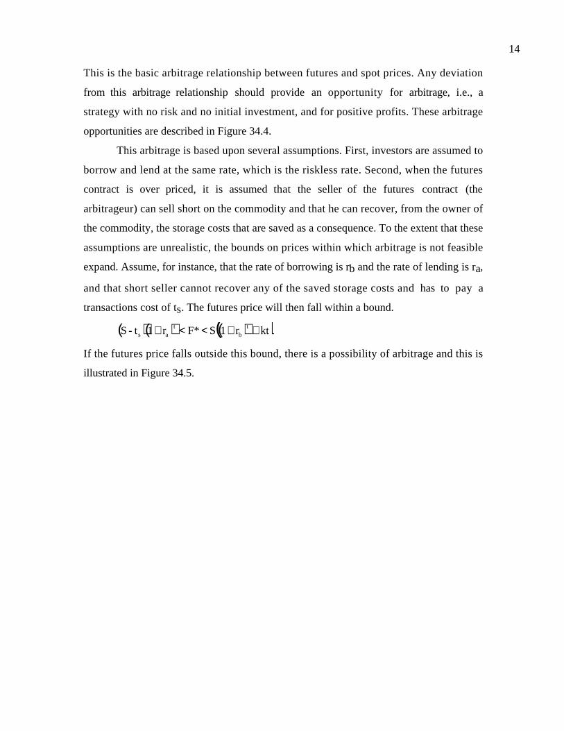
14

This is the basic arbitrage relationship between futures and spot prices. Any deviation

from this arbitrage relationship should provide an opportunity for arbitrage, i.e., a

strategy with no risk and no initial investment, and for positive profits. These arbitrage

opportunities are described in Figure 34.4.

This arbitrage is based upon several assumptions. First, investors are assumed to

borrow and lend at the same rate, which is the riskless rate. Second, when the futures

contract is over priced, it is assumed that the seller of the futures contract (the

arbitrageur) can sell short on the commodity and that he can recover, from the owner of

the commodity, the storage costs that are saved as a consequence. To the extent that these

assumptions are unrealistic, the bounds on prices within which arbitrage is not feasible

expand. Assume, for instance, that the rate of borrowing is rb and the rate of lending is ra,

and that short seller cannot recover any of the saved storage costs and has to pay a

transactions cost of ts. The futures price will then fall within a bound.

( )( ) ( )( )ktr1SF*r1t-S tb

tas ++<<+

If the futures price falls outside this bound, there is a possibility of arbitrage and this is

illustrated in Figure 34.5.

15

Figure 34.4: Storable Commodity Futures: Pricing and Arbitrage

F* = S ((1+r)t + k t)

____________________________________________________________

If F > F* If F < F*

Time Action Cashflows Action CashflowsNow: 1. Sell futures contract 0 1. Buy futures contract 0

2. Borrow spot price at riskfree r S 2. Sell short on commodity S3. Buy spot commodity -S 3. Lend money at riskfree rate -S

At t: 1. Collect commodity; Pay storage cost. -Skt 1. Collect on loan S(1+r)t

2. Deliver on futures contract F 2. Take delivery of futures contract -F

3. Pay back loan -S(1+r)t 3. Return borrowed commodity; Collect storage costs +Skt

NCF= F-S((1+r)t - kt) > 0 S((1+r)t + kt) - F > 0

Key inputs:F* = Theoretical futures price r= Riskless rate of interest (annualized)F = Actual futures price t = Time to expiration on the futures contractS = Spot price of commodity k = Annualized carrying cost, net of convenience yield (as % of spot price)Key assumptions1. The investor can lend and borrow at the riskless rate.2. There are no transactions costs associated with buying or selling short the commodity.3. The short seller can collect all storage costs saved because of the short selling.

16

Figure 34.5: storable commodity futures: pricing and arbitrage with modified assumptionsModified Assumptions1. Investor can borrow at rb (rb > r) and lend at ra (ra < r).2. The transactions cost associated with selling short is ts (where ts is the dollar transactions cost).3. The short seller does not collect any of the storage costs saved by the short selling.______________________________________________________________________________________________________

Fh* = S ((1+rb)t + k t)

Fl* = (S-ts) (1+ra)t

____________________________________________________________

If F > Fh* If F < Fl*

Time Action Cashflows Action CashflowsNow: 1. Sell futures contract 0 1. Buy futures contract 0

2. Borrow spot price at rb S 2. Sell short on commodity S - ts3. Buy spot commodity -S 3. Lend money at ra -(S - ts)

At t: 1. Collect commodity from storage -Skt 1. Collect on loan (S-ts)(1+ra)t

2. Delivery on futures contract F 2. Take delivery of futures contract -F

3. Pay back loan -S(1+rb)t 3. Return borrowed commodity; Collect storage costs 0

NCF= F-S((1+rb)t - kt)> 0 (S-ts) (1+ra)t - F > 0

Fh = Upper limit for arbitrage bound on futures prices Fl = Lower limit for arbitrage bound on futures prices

17

c. Stock Index Futures

Futures on stock indices have become an important and growing part of most

financial markets. Today, you can buy or sell futures on the Dow Jones, the S&P 500, the

NASDAQ and the Value Line indices.

An index future entitles the buyer to any appreciation in the index over and above

the index futures price and the seller to any depreciation in the index from the same

benchmark. To evaluate the arbitrage pricing of an index future, consider the following

strategies.

Strategy 1: Sell short on the stocks in the index for the duration of the index futures

contract. Invest the proceeds at the riskless rate. (This strategy requires that the owners

of the index be compensated for the dividends they would have received on the stocks.)

Strategy 2: Sell the index futures contract.

Both strategies require the same initial investment, have the same risk and should provide

the same proceeds. Again, if S is the spot price of the index, F is the futures prices, y is

the annualized dividend yield on the stock and r is the riskless rate, the cash flows from

the two contracts at expiration can be written.

F* = S (1 + r - y)t

If the futures price deviates from this arbitrage price, there should be an opportunity from

arbitrage. This is illustrated in Figure 34.6.

This arbitrage is conditioned on several assumptions. First, it, like the commodity

futures arbitrage, assumes that investors can lend and borrow at the riskless rate. Second,

it ignores transactions costs on both buying stock and selling short on stocks. Third, it

assumes that the dividends paid on the stocks in the index are known with certainty at the

start of the period. If these assumptions are unrealistic, the index futures arbitrage will be

feasible only if prices fall outside a band, the size of which will depend upon the

seriousness of the violations in the assumptions.

Assume that investors can borrow money at rb and lend money at ra and that the

transactions costs of buying stock is tc and selling short is ts. The band within which the

futures price must stay can be written as:

( )( ) ( )( )tc

ts y-rb1tSF*y-ra1t-S ++<<+

18

The arbitrage that is possible if the futures price strays outside this band is illustrated in

Figure 34.7.

In practice, one of the issues that you have to factor in is the seasonality of

dividends since the dividends paid by stocks tend to be higher in some months than

others. Figure 34.8 graphs out dividends paid as a percent of the S&P 500 index on U.S.

stocks in 2000 by month of the year.

Thus, dividend yields seem to peak in February, May, August and November.

Figure 34.8: Dividend Yields by Month of Year- 2000

0.0000%

0.0200%

0.0400%

0.0600%

0.0800%

0.1000%

0.1200%

0.1400%

0.1600%

Janu

ary

Febru

ary

Marc

hApr

ilM

ayJu

ne July

Augus

t

Septem

ber

Octobe

r

Novem

ber

Decem

ber

Month

Div

iden

ds in

mon

th/ I

ndex

at s

tart

of

mon

th

Dividend Yield

19

Figure 34.6: Stock Index Futures: Pricing and Arbitrage

F* = S (1+r-y)t

____________________________________________________________

If F > F* If F < F*

Action Cashflows Action Cashflows1. Sell futures contract 0 1. Buy futures contract 02. Borrow spot price of index at riskfree r S 2. Sell short stocks in the index S3. Buy stocks in index -S 3. Lend money at riskfree rate -S

1. Collect dividends on stocks S((1+y)t-1) 1. Collect on loan S(1+r)t

2. Delivery on futures contract F 2. Take delivery of futures contract -F

3. Pay back loan -S(1+r)t 3. Return borrowed stocks; Pay foregone dividends - S((1+y)t-1)

F-S(1+r-y)t > 0 S (1+r-y)t - F > 0

inputs:Theoretical futures price r= Riskless rate of interest (annualized)

Actual futures price t = Time to expiration on the futures contractSpot level of index y = Dividend yield over lifetime of futures contract as % of current index level

assumptionsinvestor can lend and borrow at the riskless rate.

There are no transactions costs associated with buying or selling short stocks.vidends are known with certainty.

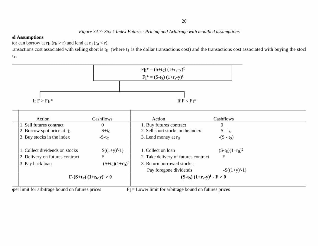
20

Figure 34.7: Stock Index Futures: Pricing and Arbitrage with modified assumptionsModified Assumptions

Investor can borrow at rb (rb > r) and lend at ra (ra < r).transactions cost associated with selling short is ts (where ts is the dollar transactions cost) and the transactions cost associated with buying the stocks tc.

______________________________________________________________________________________________________

Fh* = (S+tc) (1+rb-y)t

Fl* = (S-ts) (1+ra-y)t

____________________________________________________________

If F > Fh* If F < Fl*

Action Cashflows Action Cashflows1. Sell futures contract 0 1. Buy futures contract 02. Borrow spot price at rb S+tc 2. Sell short stocks in the index S - ts3. Buy stocks in the index -S-tc 3. Lend money at ra -(S - ts)

1. Collect dividends on stocks S((1+y)t-1) 1. Collect on loan (S-ts)(1+ra)t

2. Delivery on futures contract F 2. Take delivery of futures contract -F

3. Pay back loan -(S+tc)(1+rb)t 3. Return borrowed stocks; Pay foregone dividends -S((1+y)t-1)

F-(S+tc) (1+rb-y)t > 0 (S-ts) (1+ra-y)t - F > 0

Upper limit for arbitrage bound on futures prices Fl = Lower limit for arbitrage bound on futures prices

21

d. Treasury Bond Futures

The treasury bond futures traded on the CBOT require the delivery of any

government bond with a maturity greater than fifteen years, with a no-call feature for at

least the first fifteen years. Since bonds of different maturities and coupons will have

different prices, the CBOT has a procedure for adjusting the price of the bond for its

characteristics. The conversion factor itself is fairly simple to compute and is based upon

the value of the bond on the first day of the delivery month, with the assumption that the

interest rate for all maturities equals 8% per annum (with semi-annual compounding). The

following example calculates the conversion factor for a 9% coupon bond with 18 years to

maturity.

Illustration 34.3: Calculation Conversion Factors for T.Bond futures

Consider a 9% coupon bond with 20 years to maturity. Working in terms of a

$100 face value of the bond, the value of the bond can be written as follows, using the

interest rate of 8%.

PV of Bond =4.50

(1.08) tt=0.5

t=20

∑ +100

(1.08)20 = $111.55

The conversion factor for this bond is 109.90. Generally speaking, the conversion factor

will increase as the coupon rate increases and with the maturity of the delivered bond.

The Delivery Option and the Wild Card Play

This feature of treasury bond futures, i.e., that any one of a menu of treasury bonds can

be delivered to fulfill the obligation on the bond, provides an advantage to the seller of the

futures contract. Naturally, the cheapest bond on the menu, after adjusting for the

conversion factor, will be delivered. This delivery option has to be priced into the futures

contract.

There is an additional option embedded in treasury bond futures contracts that

arises from the fact that the T.Bond futures market closes at 2 p.m., whereas the bonds

themselves continue trading until 4 p.m. The seller does not have to notify the clearing

house until 8 p.m. about his intention to deliver. If bond prices decline after 2 p.m., the

22

seller can notify the clearing house of intention to deliver the cheapest bond that day. If

not, the seller can wait for the next day. This option is called the wild card play.

Valuing a T.Bond Futures Contract

The valuation of a treasury bond futures contract follows the same lines as the

valuation of a stock index future, with the coupons of the treasury bond replacing the

dividend yield of the stock index. The theoretical value of a futures contract should be –

( )( )tr1PVC-SF* +=

where,

F* = Theoretical futures price for Treasury Bond futures contract

S = Spot price of Treasury bond

PVC = Present Value of coupons during life of futures contract

r = Riskfree interest rate corresponding to futures life

t = Life of the futures contract

If the futures price deviates from this theoretical price, there should be the opportunity

for arbitrage. These arbitrage opportunities are illustrated in Figure 34.8.

This valuation ignores the two options described above - the option to deliver the

cheapest-to-deliver bond and the option to have a wild card play. These give an advantage

to the seller of the futures contract and should be priced into the futures contract. One

way to build this into the valuation is to use the cheapest deliverable bond to calculate

both the current spot price and the present value of the coupons. Once the futures price

is estimated, it can be divided by the conversion factor to arrive at the standardized

futures price.

23

Figure 34.8: Treasury Bond Futures: Pricing And Arbitrage

F* = (S - PVC) (1+r)t

____________________________________________________________

If F > F* If F < F*

Time Action Cashflows Action CashflowsNow: 1. Sell futures contract 0 1. Buy futures contract 0

2. Borrow spot price of bond at riskfree r S 2. Sell short treasury bonds S3. Buy treasury bonds -S 3. Lend money at riskfree rate -S

Till t: 1. Collect coupons on bonds; Invest PVC(1+r)t 1. Collect on loan S(1+r)t

2. Deliver the cheapest bond on contract F 2. Take delivery of futures contract -F

3. Pay back loan -S(1+r)t 3. Return borrowed bonds; Pay foregone coupons w/interest - PVC(1+r)t

NCF= F-(S-PVC)(1+r)t > 0 (S-PVC) (1+r)t - F > 0

Key inputs:F* = Theoretical futures price r= Riskless rate of interest (annualized)F = Actual futures price t = Time to expiration on the futures contractS = Spot level of treasury bond PVC = Present Value of Coupons on Bond during life of futures contract

Key assumptions1. The investor can lend and borrow at the riskless rate.2. There are no transactions costs associated with buying or selling short bonds.

24

e. Currency Futures

In a currency futures contract, you enter into a contract to buy a foreign currency

at a price fixed today. To see how spot and futures currency prices are related, note that

holding the foreign currency enables the investor to earn the risk-free interest rate (Rf)

prevailing in that country while the domestic currency earn the domestic riskfree rate

(Rd). Since investors can buy currency at spot rates and assuming that there are no

restrictions on investing at the riskfree rate, we can derive the relationship between the

spot and futures prices. Interest rate parity relates the differential between futures and

spot prices to interest rates in the domestic and foreign market.

)1(

)1(

PriceSpot

Price Futures

fd,

fd,

f

d

RR

++=

where Futures Priced,f is the number of units of the domestic currency that will be

received for a unit of the foreign currency in a forward contract and Spot Priced,f is the

number of units of the domestic currency that will be received for a unit of the same

foreign currency in a spot contract. For instance, assume that the one-year interest rate in

the United States is 5% and the one-year interest rate in Germany is 4%. Furthermore,

assume that the spot exchange rate is $0.65 per Deutsche Mark. The one-year futures

price, based upon interest rate parity, should be as follows:

Futures Priced,f

$ 0.65=

(1.05)

(1.04)

resulting in a futures price of $0.65625 per Deutsche Mark.

Why does this have to be the futures price? If the futures price were greater than

$0.65625, say $0.67, an investor could take advantage of the mispricing by selling the

futures contract, completely hedging against risk and ending up with a return greater than

the riskfree rate. When a riskless position yields a return that exceeds the riskfree rate, it

is called an arbitrage position. The actions the investor would need to take are

summarized in Table 34.3, with the cash flows associated with each action in brackets

next to the action.

25

Table 34.3: Arbitrage when currency futures contracts are mispriced

Forward Rate

Mispricing

Actions to take today Actions at expiration of futures

contract

If futures price >

$0.65625

e.g. $0.67

1. Sell a futures contract at

$0.67 per Deutsche Mark.

($0.00)

2. Borrow the spot price in the

U.S. domestic markets @ 5%.

(+$0.65)

3. Convert the dollars into

Deutsche Marks at spot price.

(-$0.65/+1 DM)

4. Invest Deustche Marks in

the German market @ 4%. (-1

DM)

1. Collect on Deutsche Mark

investment. (+1.04 DM)

2. Convert into dollars at

futures price. (-1.04 DM/

+$0.6968)

3. Repay dollar borrowing with

interest. (-$0.6825)

Profit = $0.6968 - $0.6825 = $

0.0143

If futures price <

$0.65625

e.g. $0.64

1. Buy a futures price at $0.64

per Deutsche Mark. ($0.00)

2. Borrow the spot rate in the

German market @4%. (+1

DM)

3. Convert the Deutsche

Marks into Dollars at spot

rate. (-1 DM/+$0.65)

4. Invest dollars in the U.S.

market @ 5%. (-$0.65)

1. Collect on Dollar

investment. (+$0.6825)

2. Convert into dollars at

futures price. (-$0.6825/1.0664

DM)

3. Repay DM borrowing with

interest. (1.04 DM)

Profit = 1.0664-1.04 = 0.0264

DM

The first arbitrage of Table 34.3 results in a riskless profit of $0.0143, with no initial

investment. The process of arbitrage will push down futures price towards the

equilibrium price.

If the futures price were lower than $0.65625, the actions would be reversed, with

the same final conclusion. Investors would be able to take no risk, invest no money and

26

still end up with a positive cash flow at expiration. In the second arbitrage of Table 34.3,

we lay out the actions that would lead to a riskless profit of .0164 DM.

Effects of Special Features in Futures Contracts

The arbitrage relationship provides a measure of the determinants of futures prices

on a wide range of assets. There are however some special features that affect futures

prices. One is the fact that futures contracts require marking to the market, while forward

contracts do not. Another is the existence of trading restrictions, such as price limits on

futures contracts. The following section examines the pricing effects of each of these

special features.

a. Futures versus Forward Contracts

As described earlier in this section, futures contracts require marking to market

while forward contracts do not. If interest rates are constant and the same for all

maturities, there should be no difference between the value of a futures contract and the

value of an equivalent forward contract. When interest rates vary unpredictably, forward

prices can be different from futures prices. This is because of the reinvestment

assumptions that have to be made for intermediate profits and losses on a futures

contract, and the borrowing and lending rates assumptions that have to be made for

intermediate losses and profits, respectively. The effect of this interest rate induced

volatility on futures prices will depend upon the relationship between spot prices and

interest rates. If they move in opposite directions (as is the case with stock indices and

treasury bonds), the interest rate risk will make futures prices greater than forward prices.

If they move together (as is the case with some real assets), the interest rate risk can

actually counter price risk and make futures prices less than forward prices. In most real

world scenarios, and in empirical studies, the difference between futures and forward

prices is fairly small and can be ignored.

There is another difference between futures and forward contracts that can cause

their prices to deviate and it relates to credit risk. Since the futures exchange essentially

guarantees traded futures contracts, there is relatively little credit risk. Essentially, the

exchange has to default for buyers or sellers of contracts to not be paid. Forward

contracts are between individual buyers and sellers. Consequently, there is potential for

27

significant default risk which has to be taken into account when valuing a forward

contract.

b. Trading Restrictions

The existence of price limits and margin requirements on futures contract are

generally ignored in the valuation and arbitrage conditions described in this chapter. It is

however possible that these restrictions on trading, if onerous enough, could impact value.

The existence of price limits, for instance, has two effects. One is that it might reduce the

volatility in prices, by protecting against market overreaction to information and thus

make futures contracts more valuable. The other is that it makes futures contracts less

liquid and this may make them less valuable. The net effect could be positive, negative or

neutral.

Conclusion

The value of a futures contract is derived from the value of the underlying asset.

The opportunity for arbitrage will create a strong linkage between the futures and spot

prices; and the actual relationship will depend upon the level of interest rates, the cost of

storing the underlying asset and any yield that can be made by holding the asset. In

addition the institutional characteristics of the futures markets, such as price limits and

‘marking to market’, as well as delivery options, can affect the futures price.

28

Problems

1. The following is an excerpt from the Wall Street Journal futures page. It includes the

futures prices of gold. The current cash (spot) price of gold is $403.25. Make your best

estimates of the implied interest rates (from the arbitrage relationship) in the futures prices.

(You can assume zero carrying costs for gold.)

Contract expiring in Trading at

1 month $404.62

2 months $406.11

3 months $407.70

6 months $412.51

12 months $422.62

2. You are a portfolio manager who has just been exposed to the possibilities of stock index

futures. Respond to the following situations.

(a) Assume that you have the resources to buy and hold the stocks in the S&P 500. You are

given the following data. (Assume that today is January 1.)

Level of the S&P 500 index = 258.90

June S&P 500 futures contract = 260.15

Annualized Rate on T.Bill expiring June 26 (expiration date) = 6%

Annualized Dividend yield on S&P 500 stocks = 3%

Assume that dividends are paid out continuously over the year. Is there potential for

arbitrage? How would you go about setting up the arbitrage?

(b) Assume now that you are known for your stock selection skills. You have 10,000 shares

of Texaco in your portfolio (now selling for 38) and are extremely worried about the

direction of the market until June. You would like to protect yourself against market risk by

using the December S&P 500 futures contract (which is at 260.15). If Texaco's beta is 0.8,

how would you go about creating this protection?

3. Assume that you are a mutual fund manager with a total portfolio value of $100 million.

You estimate the beta of the fund to be 1.25. You would like to hedge against market

movements by using stock index futures. You observe that the S&P 500 June futures are

selling for 260.15 and that the index is at 258.90. Answer the following questions.

29

(a) How many stock index futures would you have to sell to protect against market risk?

(b) If the riskfree rate is 6% and the market risk premium is 8%, what return would you

expect to make on the mutual fund? (Assuming you don't hedge.)

(c) How much would you expect to make if you hedge away all market risk?

4. Given the following information on gold futures prices, the spot price of gold, the riskless

interest rate and the carrying cost of gold, construct an arbitrage position. (Assume that it is

December 1987 now.)

December 1988 futures contract price = 515.60/troy oz

Spot price of gold = 481.40/troy oz

Interest rate (annualized) = 6%

Carrying cost (annualized) = 2%

a. What would you have to do right now to set up the arbitrage?

b. What would you have to do in December to unwind the position? How much arbitrage

profit would you expect to make?

c. Assume now that you can borrow at 8%, but you can lend at only 6%. Establish a price

band for the futures contract, within which arbitrage is not feasible.

5. The following is a set of prices for stock index futures on the S&P 500.

Maturity Futures price

March 246.25

June 247.75

The current level of the index is 245.82 and the current annualized T.Bill rate is 6%. The

annualized dividend yield is 3%. (Today is January 14. The March futures expire on March

18 and the June futures on June 17.)

(a) Estimate the theoretical basis and actual basis in each of these contracts.

(b) Using one of the two contracts, set up an arbitrage. Also show how the arbitrage will be

resolved at expiration. [You can assume that you can lend or borrow at the riskfree rate and

that you have no transaction costs or margins.]

(c) Assume that a good economic report comes out on the wire. The stock index goes up to

247.82 and the T.Bill rate drops to 5%. Assuming arbitrage relationships hold and that the

dollar dividends paid do not change, how much will the March future go up by?

30

6. You are provided the following information.

Current price of wheat = $19,000 for 5000 bushels

Riskless rate = 10 % (annualized)

Cost of storage = $200 a year for 5000 bushels

One-year futures contract price = $20,400 (for a contract for 5000 bushels)

a. What is F* (the theoretical price)?

b. How would you arbitrage the difference between F and F*? (Specify what you do now and at

expiration and what your arbitrage profits will be.)

c. If you can sell short (Cost $100 for 5000 bushels) and cannot claim any of the storage cost for

yourself on short sales2, at what rate would you have to be able to lend for this arbitrage to be

feasible?

2 In theory, we make the unrealistic assumption that a person who sells short (i.e. borrows somebody else'sproperty and sells it now) will be able to collect the storage costs saved by the short sales from the otherparty to the transaction.

1

CHAPTER 35

OVERVIEW AND CONCLUSION

The problem in valuation is not that there are not enough models to value an asset,

it is that there are too many. Choosing the right model to use in valuation is as critical to

arriving at a reasonable value as understanding how to use the model. This chapter

attempts to provide an overview of the valuation models introduced in this book and a

general framework that can be used to pick the right model for any task.

Choices in valuation models

In the broadest possible terms, firms or assets can be valued in one of four ways –

asset based valuation approaches where you estimate what the assets owned by a firm are

worth currently, discounted cashflow valuation approaches that discount cashflows to

arrive at a value of equity or the firm, relative valuation approaches that base value upon

multiples and option pricing approaches that use contingent claim valuation. Within each

of these approaches, there are further choices that help determine the final value.

There are at least two ways in which you can value a firm using asset based

valuation techniques. One is liquidation value, where you consider what the market will

be willing to pay for assets, if the assets were liquidated today. The other is replacement

cost, where you evaluate how much it would cost you to replicate or replace the assets

that a firm has in place today.

In the context of discounted cashflow valuation, cashflows to equity can be

discounted at the cost of equity to arrive at a value of equity or cashflows to the firm can

be discounted at the cost of capital to arrive at the value for the firm. The cashflows to

equity themselves can be defined in the strictest sense as dividends or in a more expansive

sense as free cashflows to equity. These models can be further categorized on the basis of

assumptions about growth into stable growth, two-stage and three-stage models. Finally,

the measurement of earnings and cashflows may be modified to match the special

characteristics of the firm/asset - current earnings for firms/assets which have normal

earnings or normalized earnings for firms/assets whose current earnings may be distorted

either by temporary factors or cyclical effects.

2

In the context of multiples, you can use either equity or firm value as your

measure of value and relate it to a number of firm-specific variables – earnings, book value

and sales. The multiples themselves can be estimated by using comparable firms in the

same business or from cross-sectional regressions that use the broader universe. For other

assets, such as real estate, the price can similarly expressed as a function of gross income

or per square foot of space. Here, the comparables would be other properties in the same

locale with similar characteristics.

Contingent claim models can also be used in a variety of scenarios. When you

consider the option that a firm has to delay making investment decisions, you can value a

patent or an undeveloped natural resource reserve as an option. The option to expand

may make young firms with potentially large markets trade at a premium on their

discounted cashflow values. Finally, equity investors may derive value from the option to

liquidate troubled firms with substantial debt.

3

Figure 35.1: The Choices in Valuation Models

Valuation Models

Asset BasedValuation

Discounted CashflowModels

Relative Valuation Contingent Claim Models

LiquidationValue

ReplacementCost

Equity ValuationModels

Firm ValuationModels

Cost of capitalapproach

APVapproach

Excess ReturnModels

Stable

Two-stage

Three-stageor n-stage

Current

Normalized

Equity

Frim

Earnings BookValue

Revenues Sectorspecific

Sector

Market

Option todelay

Option toexpand

Option toliquidate

Patent UndevelopedReserves

Youngfirms

Undevelopedland

Equity introubledfirm

Dividends

Free Cashflowto Firm

4

Which approach should you use?

The values that you obtain from the four approaches described above can be very

different and deciding which one to use can be a critical step. This judgment, however,

will depend upon several factors, some of which relate to the business being valued but

many of which relate to you, as the analyst.

Asset or Business Characteristics

The approach that you use to value a business will depend upon how marketable

its assets are, whether it generates cash flows and how unique it is in terms of its

operations.

Marketability of Assets

Liquidation valuation and replacement cost valuation are easiest to do for firms

that have assets that are separable and marketable. For instance, you can estimate the

liquidation value for a real estate company because its properties can be sold individually

and you can estimate the value of each property easily. The same can be said about a

closed end mutual fund. At the other extreme, consider a brand name consumer product

like Gillette. Its assets are not only intangible but difficult to separate out. For instance,

you cannot separate the razor business easily from the shaving cream business and brand

name value is inherent in both businesses.

You can also use this same analysis to see why the liquidation or replacement cost

value of a high growth business may bear little resemblance to true value. Unlike assets in

place, growth assets cannot be easily identified or sold.

Mature businessesSeparable & marketable assets

Growth businessesLinked and non-marketable assets

Liquidation &Replacement costvaluation

Other valuation models

Figure 35.2: Asset Marketability and Valuation Approaches

Cash Flow Generating Capacity

5

You can categorize assets into three groups based upon their capacity to generate

cash flows – assets that are either generating cash flows currently or are expected to do so

in the near future, assets that are not generating cash flows currently but could in the

future in the event of a contingency and assets that will never generate cash flows.

• The first group includes most publicly traded companies and these firms can be

valued using discounted cash flow models. Note that we do not draw a distinction

between negative and positive cash flows and young, start-up companies that

generate negative cash flow can still be valued using discounted cash flow models.

• The second group includes assets such as drug patents, promising (but not viable)

technology, undeveloped oil or mining reserves and undeveloped land. These

assets may generate no cash flows currently and could generate large cash flows in

the future but only under certain conditions – if the FDA approves the drug

patent, if the technology becomes commercially viable, if oil prices and

commercial property values go up. While you could estimate expected values

using discounted cash flow models by assigning probabilities to these events, you

will understate the value of the assets if you do so. You should value these assets

using option pricing models.

• Assets that are never expected to generate cash flows include your primary

residence, a baseball card collection or fine art. These assets can only be valued

using relative valuation models.

Cashflows currently orexpected in near future

Assets that will never generate cashflows

Discounted cashflow or relative valuation models

Relative valuation models

Figure 35.3: Cash Flows and Valuation Approaches

Cashflows if a contingencyoccurs

Option pricing models

Uniqueness (or presence of comparables)

In a market where thousands of stocks are traded and tens of thousands of assets

are bought and sold every day, it may be difficult to visualize an asset or business that is

so unique that you cannot find comparable assets. On a continuum, though, some assets

6

and businesses are part of a large group of similar assets, with no or very small differences

across the assets. These assets are tailor-made for relative valuation, since assembling

comparable assets (businesses) and controlling for differences is simple. The further you

move from this ideal, the less reliable is relative valuation. For businesses that are truly

unique, discounted cash flow valuation will yield much better estimates of value.

Unique asset or businessLarge number of similar assets that are priced

Discounted cashflow or option pricing models

Relative valuation models

Figure 35.4: Uniqueness of Asset and Valuation Approaches

Analyst Characteristics and Beliefs

The valuation approach that you choose to use will depend upon your time

horizon, the reason that you are doing the valuation in the first place and what you think

about markets – whether they are efficient and if they are not, what form the inefficiency

takes.

Time Horizon

At one extreme, in discounted cash flow valuation you consider a firm as a going

concern that may last into perpetuity. At the other extreme, with liquidation valuation,

you are estimating value on the assumption that the firm will cease operations today.

With relative valuation and contingent claim valuation, you take an intermediate position

between the two. Not surprisingly, then, you should be using discounted cash flow

valuation, if you have a long time horizon, and relative valuation, if you have a shorter

time horizon. This may explain why discounted cash flow valuation is more prevalent in

valuing a firm for an acquisition and relative valuation is more common in equity research

and portfolio management.

7

Very short time horizonLong Time Horizon

Liquidation value Discounted Cashflow value

Figure 35.5 Investor Time Horizon and Valuation Approaches

Option pricing models

Relative valuation

Reason for doing the valuation

Analysts value businesses for a number of reasons and the valuation approach

used will vary depending upon the reason. If you are an equity research analyst following

steel companies, your job description is simple. You are asked to find the most under and

over valued companies in the sector and not to take a stand on whether the sector overall

is under or over valued. You can see why multiples would be your weapon of choice

when valuing companies. This effect is likely to be exaggerated if the way you are judged

and rewarded is on a relative basis, i.e., your recommendations are compared to those

made by other steel company analysts. If you are an individual investor setting money

aside for retirement or a private businessperson valuing a business for purchase, on the

other hand, you want to estimate intrinsic value. Consequently, discounted cash flow

valuation is likely to be more appropriate for your needs.

Market NeutralJudged on relative basis

Discounted Cashflow value

Figure 35.6: Market Neutrality and Valuation Approaches

Option pricing models

Relative valuation

Can take view on marketJudged on absolute basis

Beliefs about Markets

Embedded in each approach are assumptions about markets and how they work or

fail to work. With discounted cash flow valuation, you are assuming that market prices

deviate from intrinsic value but that they correct themselves over long periods. With

relative valuation, you are assuming that markets are on average right and that while

8

individual firms in a sector or market may be mispriced, the sector or overall market is

fairly priced. With asset-based valuation models, you are assuming that the markets for

real and financial assets can deviate and that you can take advantage of these differences.

Finally, with option pricing models, you are assuming that markets are not very efficient

at assessing the value of flexibility that firms have and that option pricing models will

therefore give you an advantage. In each and every one of these cases, though, you are

assuming that markets will eventually recognize their mistakes and correct them.

Markets are correct on average but make mistakes on individual assets

Discounted Cashflow value

Figure 35.7: Views on market and Valuation Approaches

Option pricing models

Relative valuation

Markets make mistakes but correct them over time

Asset markets and financialmarkets may diverge

Liquidation value

Bridging the Philosophical Divide

Philosophically, there is a big gap between discounted cash flow valuation and

relative valuation. In discounted cash flow valuation, we take a long term perspective,

evaluate a firm’s fundamentals in detail and try to estimate a firm’s intrinsic value. In

relative valuation, we assume that the market is right on average and estimate the value of

a firm by looking at how similar firms are priced. There is something of value in both

approaches and it would be useful if we could borrow the best features of relative

valuation while doing discounted cash flow valuation or vice versa.

Assume that your instincts lead you to discounted cash flow valuation, but that

you are expected, as an analyst, to be market neutral. You can stay market neutral in a

discounted cash flow framework, if you use the implied risk premium for the market

(which we described in Chapter 7) to estimate the cost of equity for the valuation. You

can also bring in information about comparable firm margins and betas, when estimating

fundamentals for your firm. Your estimate of intrinsic value will then be market-neutral

and include information about comparables.

Alternatively, assume that you prefer relative valuation. Your analysis can carry

the rigor of a discounted cash flow valuation, if you can bring in the details of the

9

fundamentals into your comparisons. We attempted to do this in the chapters on relative

valuation by noting the link between multiples and fundamentals and also by examining

how best to control for these differences in our analysis.

Choosing the Right Discounted Cash flow Model

The model used in valuation should be tailored to match the characteristics of the

asset being valued. The unfortunate truth is that the reverse is often true. Time and

resources are wasted trying to make assets fit a pre-specified valuation model, either

because it is considered to be the 'best' model or because not enough thought goes into the

process of model choice. There is no one 'best' model. The appropriate model to use in a

particular setting will depend upon a number of the characteristics of the asset or firm

being valued.

Choosing a cashflow to discount

With consistent assumptions about growth and leverage, you should get the same

value for your equity using the firm approach (where you value the firm and subtract

outstanding debt) and the equity approach (where you value equity directly). If this is the

case, you might wonder why you would pick one approach over the other. The answer is

purely pragmatic. For firms that have stable leverage, i.e., they have debt ratios that are

not expected to change during the period of the valuation, there is little to choose between

the models in terms of the inputs needed for valuation. You use a debt ratio to estimate

free cashflows to equity in the equity valuation model and to estimate the cost of capital

in the firm valuation model. Under these circumstances, you should stay with the model

that you are more intuitively comfortable with.

For firms that have unstable leverage, i.e., they have too much or too little debt

and want to move towards their optimal or target debt ratio during the period of the

valuation, the firm valuation approach is much simpler to use because it does not require

cashflow projections from interest and principal payments and is much less sensitive to

errors in estimating leverage changes. The calculation of the cost of capital requires an

estimate of the debt ratio, but the cost of capital itself does not change as much as a

consequence of changing leverage as the cost of equity. If you prefer to work with

10

assumptions about dollar debt rather than debt ratios, you can switch to the adjusted

present value approach.

In valuing equity, you can discount dividends or free cashflows to equity. You

should consider using the dividend discount model under the following circumstances.

• You cannot estimate cashflows with any degree of precision either because you have

insufficient or contradictory information about debt payments and reinvestments or

because you have trouble defining what comprises debt. This was our rationale for

using dividend discount models for valuing financial service firms.

• There are significant restrictions on stock buybacks and other forms of cash return,

and you have little or no control over what the management of a firm does with the

cash. In this case, the only cashflows you can expect to get from your equity

investment are the dividends that managers choose to pay out.

In all other cases, you will get much more realistic estimates of a firm’s value using the

free cashflow to equity, which may be greater than or lower than the dividend.

Should you use current or normalized earnings?

In most valuations, we begin with the current financial statements of the firm and

use the reported earnings in those statements as the base for projections. There are some

firms, though, where you may not be able to do this, either because the firm’s earnings are

negative or because these earnings are abnormally high or low - a firm’s earnings are

abnormal if they do not fit in with the firm’s own history of earnings.

When earnings are negative or abnormal, you can sometimes replace current

earnings with a normalized value, estimated by looking at the company’s history or

industry averages and value the firm based upon these normalized earnings. This is the

easiest route to follow if the causes for the negative or abnormal earnings are temporary or

transitory, as in the following cases.

(a) A cyclical firm will generally report depressed earnings during an economic downturn

and high earnings during an economic boom. Neither may capture properly the true

earnings potential of the firm.

(b) A firm may report abnormally low earnings in a period during which it takes an

extraordinary charge.

11

(c) A firm in the process of restructuring may report low earnings during the restructuring

period, as the changes made to improve firm performance are put into effect.

The presumption here is that earnings will quickly bounce back to normal levels and that

little will be lost by assuming that it will occur immediately.

For some firms, though, the negative or low earnings may reflect factors that are

unlikely to disappear quickly. There are at least three groups of firms where the negative

earnings are likely to be a long term phenomena and may even threaten the firm’s survival.

a. Firms with long term operating, strategic or financial problems can have extended

periods of negative or low earnings. If you replace current earnings with normalized

earnings and value these firms, you will over value them.

• If a firm seems to be in a hopeless state, and likely to go bankrupt, the only

models that are likely to provide meaningful measures of value are the option

pricing model (if financial leverage is high) or a model based upon liquidation

value.

• If on the other hand, the firm is troubled but unlikely to go bankrupt, you will

have to nurse it back to financial health. In practical terms, you will have to

adjust the operating margins over time to healthier levels and value the firm

based upon its expected cash flows.

b. An infrastructure firm may report negative earnings in its initial periods of growth, not

because it is unhealthy but because the investments it has made take time to pay off. The

cashflows to the firm and equity are often also negative, because the capital expenditure

needs for this type of firm tend to be disproportionately large relative to depreciation.

For these firms to have value, capital expenditure has to drop once the infrastructure

investments have been made and operating margins have to improve. The net result will

be positive cashflows in future years and a value for the firm today.

c. Young start-up companies often report negative earnings early in their life cycles, as

they concentrate on turning interesting ideas into commercial products. To value such

companies, you have to assume a combination of high revenue growth and improving

operating margins over time.

12

Growth Patterns

In general, when valuing a firm, you can assume that your firm is already in stable

growth, assume a period of constant high growth and then drop the growth rate to stable

growth (two-stage growth) or allow for a transition phase to get to stable growth (3-stage

or n-stage models). There are several factors you should consider in making this judgment.

a. Growth Momentum

The choice of growth pattern will influence the level of current growth in earnings

and revenues. You can categorize firms, based upon growth in recent periods, into three

groups.

(a) Stable growth firms report earnings and revenues growing at or below the nominal

growth rate in the economy that they operate in.

(b) Moderate growth firms report earnings and revenues growing at a rate moderately

higher than the nominal growth rate in the economy – as a rule of thumb, we would

consider any growth rate within 8-10% of the growth rate of the economy as a moderate

growth rate.

(c) High growth firms report earnings and revenues growing at a rate much higher than the

nominal growth rate in the economy.

For firms growing at the stable rate, the steady state models that assume constant growth

provide good estimates of value. For firms growing at a 'moderate' rate, the two-stage

discounted cashflow model should provide enough flexibility in terms of capturing

changes in the underlying characteristics of the firm, while a three-stage or n-stage model

may be needed to capture the longer transitions to stable growth that are inherent in 'high'

growth rate firms.

b. Source of growth (Barriers to entry)

The higher expected growth for a firm can come from either 'general' competitive

advantages acquired over time such as a brand name or reduced costs of production (from

economies of scale) or 'specific' advantages that are the result of legal barriers to entry –

such as licenses or product patents. The former are likely to erode over time as new

competitors enter the market place, while the latter are more likely to disappear abruptly

when the legal barrier to entry are removed. The expected growth rate for a firm that has

13

specific sources of growth is likely to follow the two-stage process where growth is high

for a certain period (for instance, the period of the patent) and drops abruptly to a stable

rate after that. The expected growth rate for a firm that has 'general' sources of growth is

more likely to decline gradually over time, as new competitors come in. The speed with

which this competitive advantage is expected is a function of several factors, including:

a. The nature of the competitive advantage: Some competitive advantages, such as brand

name in consumer products – seem to be more difficult to overcome and consequently are

likely to generate growth for longer periods. Other competitive advantages, such as a first-

mover advantage, seem to erode much faster.

b. Competence of the firm's management - More competent management will be able to

slow, though not stop, the loss of competitive advantage over time by creating strategies

that find new markets to exploit the firm's current competitive advantage and new sources

of competitive advantage.

c. Ease of entry into the firm's business -- The greater the barriers to industry in entering

the firm's business, either because of capital requirements or technological factors, the

slower will be the loss of competitive advantage.

These factors are summarized and presented in the Figure 35.8, with the appropriate

discounted cashflow model highlighted for each combination of the factors.

Status Quo versus Optimal Management

In the chapters on valuing acquisitions and troubled firms, we noted that the value of a

firm can be substantially higher if you assume that it is optimally run than if it is run by

incumbent management. A question that you are often faced with in valuation is whether

you should value the firm with incumbent management or with the optimal management.

The answer is simple in some cases and complicated in others.

• If you are interested in acquiring the firm and intend to change the management, you

should value the firm with the optimal management policies in place. Whether you

will pay that amount in the acquisition will depend upon your bargaining power and

how long you think it will take you change the way the firm is run.

• If you are a small investor looking at buying stock in the firm, you cannot change

incumbent management yourself but you can still pay a premium if you believe that

14

there is a possibility of change. If there are strong mechanisms for corporate

governance – hostile takeovers are common and poor managers get replaced quickly –

you can assume that the value will quickly converge on the optimal value. If, on the

other hand, it is difficult to dislodge incumbent management, you should value the

firm based upon their continue stewardship of the firm.

• If you are an institutional investor, you fall between these two extremes. While you

may not intend to take over the firm and change the way it is run, you could play a

role in making this change happen.

15

Figure 35.8: Discounted Cashflow Models

Can you estimate cash flows?

Yes No

Use dividend discount model

Is leverage stable or likely to change over time?

Stable leverage

Unstable leverage

Are the current earnings positive & normal?

Yes

Use current earnings as base

No

Is the cause temporary?

Yes No

Replace current earnings with normalized earnings

Is the firm likely to survive?

Yes No

Adjust margins over time to nurse firm to financial health

Does the firm have a lot of debt?

Yes No

Value Equity as an option to liquidate

Estimate liquidation value

What rate is the firm growing at currently?

< Growth rate of economy

Stable growth model

> Growth rate of economy

Are the firm’s competitive advantges time limited?

Yes No

2-stage model

3-stage or n-stage model

FCFE FCFF

16

Choosing the Right Relative Valuation Model

Many analysts choose to value assets using relative valuation models. In making

this choice, two basic questions have to be answered -- Which multiple will be used in the

valuation? Will this multiple be arrived at using the sector or the entire market?

Which multiple should I use?

In the chapters on multiples, we presented a variety of multiples. Some were

based upon earnings, some on book value and some on revenues. For some multiples, we

used current values and for others, we used forward or forecast values. Since the values

you obtain are likely to be different using different multiples, deciding which multiple to

use can make a big difference to your estimate of value. There are three ways you can

answer this question –the first is to adopt the cynical view that you should use the

multiple that reflects your biases, the second is to value your firm with different

multiples and try to use all of the values that you obtain and the third is to pick the best

multiple and base your valuation on it.

The Cynical View

You can always use the multiple that best fits your story. Thus, if you are trying

to sell a company, you will use the multiple which gives you the highest value for your

company. If you are buying the same company, you will choose the multiple that yields

the lowest value. While this clearly crosses the line from analysis into manipulation, it is a

more common practice than you might realize. Even if you never plan to employ this

practice, you should consider ways in which how you can protect yourself from being

victimized by it. First, you have to recognize that conceding the choice of multiple and

comparables to an analyst is the equivalent of letting him or her write the rules of the

game. You should play an active role in deciding which multiple should be used to value a

company and what firms will be viewed as comparable firms. Second, when presented

with a value based upon one multiple, you should always ask what the value would have

been if an alternative multiple had been used.

The Bludgeon View

17

You can always value a company using a dozen or more multiples and then use all

of the values, different thought they might be, in your final recommendation. There are

three ways in which can present the final estimate of value. The first is in terms of a range

of values, with the lowest value that you obtained from a multiple being the lower end of

the range and the highest value being the upper limit. The problem with this approach is

that the range is usually so large that it becomes useless for any kind of decision-making.

The second approach is a simple average of the values obtained from the different

multiples. While this approach has the virtue of simplicity, it gives equal weight to the

values from each multiple, even though some multiples may yield more precise answers

than others. The third approach is a weighted average, with the weight on each value

reflecting the precision of the estimate. This weight can either be a subjective one or a

statistical measure – you can, for instance, use the standard error on a prediction from a

regression.

The Best Multiple

While we realize that you might be reluctant to throw away any information, the

best estimates of value are usually obtained by using the one multiple that is best suited

for your firm. There are three ways in which you can find this multiple.

• The Fundamentals approach: You should consider using the variable that is most

highly correlated with your firm’s value. For instance, current earnings and value

are much more highly correlated in consumer product companies than in

technology companies. Using price earnings ratios makes more sense for the

former than for the latter.

• The Statistical approach: You could run regressions of each multiple against the

fundamentals that we determined affected the value of the multiple in earlier

chapters and use the R-squared of the regression as a measure of how well that

multiple works in the sector. The multiple with the highest R-squared is the

multiple that you can best explain using fundamentals and should be the multiple

you use to value companies in that sector.

• The Conventional Multiple approach: Over time, we usually see a specific

multiple become the most widely used one for a specific sector. For instance,

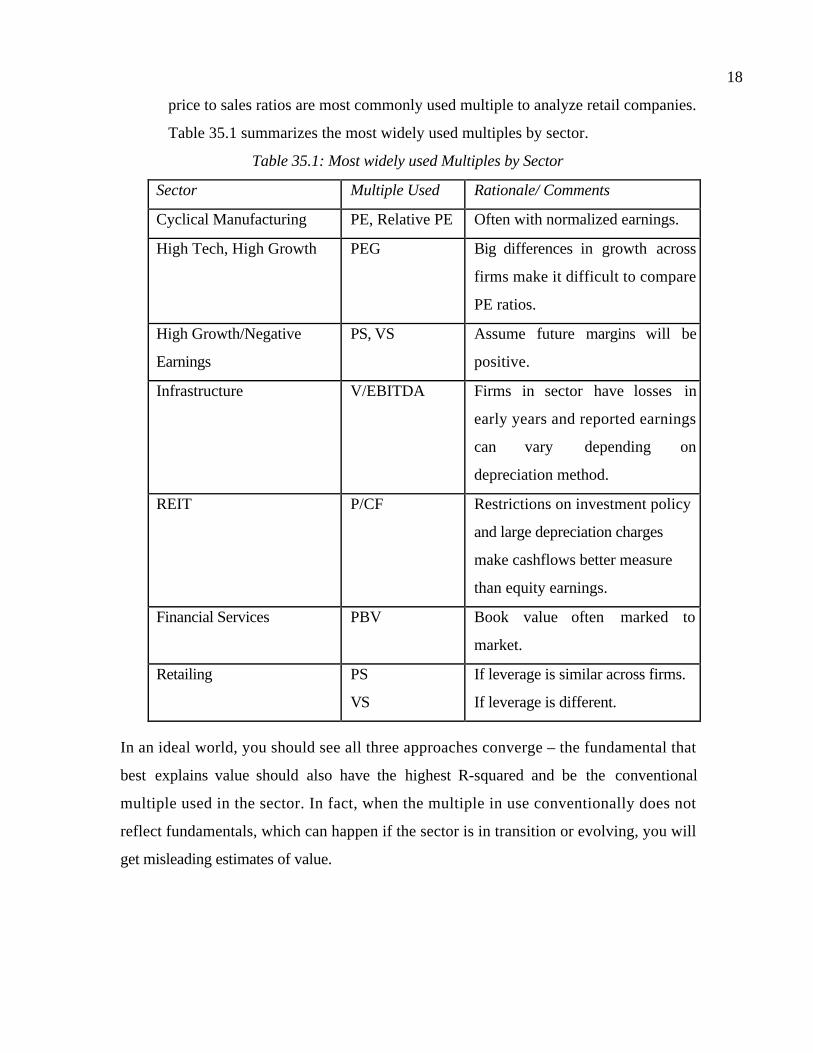
18

price to sales ratios are most commonly used multiple to analyze retail companies.

Table 35.1 summarizes the most widely used multiples by sector.

Table 35.1: Most widely used Multiples by Sector

Sector Multiple Used Rationale/ Comments

Cyclical Manufacturing PE, Relative PE Often with normalized earnings.

High Tech, High Growth PEG Big differences in growth across

firms make it difficult to compare

PE ratios.

High Growth/Negative

Earnings

PS, VS Assume future margins will be

positive.

Infrastructure V/EBITDA Firms in sector have losses in

early years and reported earnings

can vary depending on

depreciation method.

REIT P/CF Restrictions on investment policy

and large depreciation charges

make cashflows better measure

than equity earnings.

Financial Services PBV Book value often marked to

market.

Retailing PS

VS

If leverage is similar across firms.

If leverage is different.

In an ideal world, you should see all three approaches converge – the fundamental that

best explains value should also have the highest R-squared and be the conventional

multiple used in the sector. In fact, when the multiple in use conventionally does not

reflect fundamentals, which can happen if the sector is in transition or evolving, you will

get misleading estimates of value.

19

Market or Sector Valuation

In most relative valuations, you value a firm relative to other firms in the industry

that the firm operates and attempt to answer a simple question: Given how other firms in

the business (sector) are priced by the market, is this firm under or over valued? Within

this approach, you can define comparable firms narrowly as being firms that not only

operate in the business in which your firm operates but also look like your firm in terms

of size or market served, or broadly in which case you will have far more comparable

firms. If you are attempting to control for differences across firms subjectively, you

should stick with the narrower group. If, on the other hand, you plan to control for

differences statistically – with a regression, for instance – you should go with the broader

definition.

In the chapters on relative valuation, we presented an alternative approach to

relative valuation, where we valued firms relative to the entire market. When we do this,

we are not only using a much larger universe of questions, but asking a different question:

Given how other firms in the market are priced, is this firm under or over valued? A firm

can be under valued relative to its sector but overvalued relative to the market (or vice

versa), if the entire sector is mispriced.

The approach you use for relative valuation will depend again upon what your

task is defined to be. If you want to stay narrowly focused on your sector and make

judgments on which stocks are under or over valued, you should stick with sector based

relative valuation. If you have more leeway and are trying to find under or overvalued

stocks across the market, you should look at the second approach – perhaps in addition

to the first one.

Can a firm be under and over valued at the same time?

If you value a firm using both discounted cash flow and relative valuation models, you

may very well get different answers using the two – the firm may be under valued using

relative valuation models but over valued using discounted cash flow models. What do we

make of these differences and why do they occur? If a firm is overvalued using a

discounted cash flow model and undervalued using relative valuation, it is usually an

indication that the sector is over valued, relative to its fundamentals. For instance, in

20

March 2000, we valued Amazon at $30 a share using a discounted cash flow model, when

it was trading at $70 a share – it was clearly overvalued. At the same time, a comparison

of Amazon to other dot com firms suggested that it was undervalued relative to these

firms.

If a firm is undervalued using a discounted cashflow model and overvalued using

relative valuation, it usually indicates that the sector is under valued. By March 2001,

Amazon’s stock price had dropped to $15 but the values of other internet stocks

dropped by almost 90%. In March 2001, a discounted cash flow valuation suggested that

Amazon was under valued but a relative valuation indicated that it was now over valued

relative to the sector.

As an investor, you can use both discounted cash flow and relative valuation to

value a company. Optimally, you would like to buy companies that are under valued

using both approaches. That way, you benefit from market corrections both across time

(which is the way you make money in discounted cash flow valuation) and across

companies.

When should you use the option pricing models?

In the chapters on applying option pricing models to valuation, we presented a

number of scenarios where option pricing may yield a premium on traditional discounted

cash flow valuation. We do not intend to revisit those scenarios, but offer the following

general propositions that you should keep in mind when using option pricing models.

• Use Options sparingly: Restrict your use of options to where they make the

biggest difference in valuation. In general, options will affect value the most at

smaller firms that derive the bulk of their value form assets that resemble options.

Therefore, valuing patents as options to estimate firm value makes more sense for

a small biotechnology firm than it does for a drug giant like Merck. While Merck

may have dozens of patents, it derives much of its value from a portfolio of

developed drugs and the cash flows they generate.

• Opportunities are not always options: You should be careful not to mistake

opportunities for options. Analysts often see a firm with growth potential and

assume that there must be valuable options embedded in the firm. For

21

opportunities to become valuable options, you need some degree of exclusivity for

the firm in question – this can come from legal restrictions on competition or a

significant competitive edge.

• Do not double count options: All too often, analysts incorporate the effect of

options on fundamentals in the company value and then proceed to add on

premiums to reflect the same options. Consider, for instance, the undeveloped oil

reserves owned by an oil company. While it is legitimate to value these reserves as

options, you should not add this value to a discounted cashflow valuation of the

company, if your expected growth rate in the valuation is set higher because of the

firm’s undeveloped reserves.

Conclusion

The analyst faced with the task of valuing a firm/asset or its equity has to choose

among three different approaches -- discounted cashflow valuation, relative valuation and

option pricing models; and within each approach, they must also choose among different

models. These choices will be driven largely by the characteristics of the firm/asset being

valued - the level of its earnings, its growth potential, the sources of earnings growth, the

stability of its leverage and its dividend policy. Matching the valuation model to the asset

or firm being valued is as important a part of valuation as understanding the models and

having the right inputs.

Once you decide to go with one or another of these approaches, you have further

choices to make – whether to use equity or firm valuation in the context of discounted

cashflow valuation, which multiple you should use to value firms or equity and what

type of option is embedded in a firm.

ReferencesChapter 1Buffett, W.E. and L.A. Cunningham, 2001, The Essays of Warren Buffett: Lessons ofCorporate America, The Cunningham Group.Cottle, S., R. Murray and F. Bloch, 1988, Security Analysis, McGraw-Hill.Graham, B., D.L. Dodd and S. Cottle, 1962, Security Analysis, Fourth Edition, McGraw-Hill.

Chapter 2Black, F. and M. Scholes, 1972, The Valuation of Option Contracts and a Test of MarketEfficiency, Journal of Finance, v27, 399-417.Damodaran, A., 1994, Damodaran on Valuation, John Wiley and Sons.Hooke, J.C., 2001, Security Analysis on Wall Street, John Wiley and Sons.

Chapter 3Choi, F.D.S. and R.M. Levich, 1990, The Capital Market Effects of InternationalAccounting Diversity, Dow Jones Irwin, New York.Stickney, C.P., 1993, Financial Statement Analysis, Dryden, Fort WorthWhite, G.I, A. Sondhi and D. Fried, 1997, The Analysis and Use of Financial Statements,Wiley, New York.Williams, J. R., 1998, GAAP guide, Harcourt Brace, New York.

Chapter 4Amihud, Y., B. Christensen and H. Mendelson, 1992, Further Evidence on the Risk-Return Relationship, Working Paper, New York University.Bernstein, P., 1992, Capital Ideas, The Free Press, New York.Bernstein, P., 1996, Against the Gods, John Wiley & Sons, New York.Chan, L.K. and J. Lakonsihok, 1993, Are the reports of Beta's death premature?, Journalof Portfolio Management, v19, 51-62.Chen, N., R. Roll and S.A. Ross, 1986, Economic Forces and the Stock Market, Journalof Business, 1986, v59, 383-404.Elton, E.J. and M.J. Gruber, 1995, Modern Portfolio Theory and InvestmentManagement, John Wiley & Sons, New York.Fama, E.F. and K.R. French, 1992, The Cross-Section of Expected Returns, Journal ofFinance, v47, 427-466.Jensen, M.C, 1969, Risk, the Pricing of Capital Assets, and the Evaluation of InvestmentPortfolios, Journal of Business, v42, pp 167-247.Kothari, S.P. and J. Shanken, 1995, In Defense of Beta, Journal of Applied CorporateFinance, v8(1), 53-58.Lintner, J., 1965, The Valuation of Risk Assets and the Selection of Risky Investments inStock Portfolios and Capital Budgets, Review of Economics and Statistics, v47, 13-37.Markowitz, Harry M., Foundations Of Portfolio Theory, Journal of Finance, 1991,v46(2), 469-478.Roll, R., 1977, A Critique of the Asset Pricing Theory's Tests: Part I: On Past andPotential Testability of Theory, Journal of Financial Economics, v4, 129-176.Ross, Stephen A., 1976, The Arbitrage Theory Of Capital Asset Pricing, Journal ofEconomic Theory, v13(3), 341-360.

Seyhun, H.N., 1986, Insiders’ Profits, Costs of Trading and Market Efficiency, Journal ofFinancial Economics, v16, pp 189-212.Sharpe, W.F, 1964, Capital Asset Prices: A Theory of Market Equilibrium underConditions of Risk, Journal of Finance, v19, 425-442.Weston, J.F. and T.E. Copeland, 1992, Managerial Finance, Dryden Press.

Chapter 5: Option PricingBlack, F. and M. Scholes, 1972, The Valuation of Option Contracts and a Test of MarketEfficiency, Journal of Finance, v27, 399-417.Cox, J.C. and M. Rubinstein, 1985, Options Markets, Prentice-Hall.Cox, J.C. and S.A. Ross, 1976, The Valuation of Options for Alternative StochasticProcesses, Journal of Financial Economics, v3, 145-166.Cox, J.C., S.A. Ross and M.Rubinstein, 1979, Option Pricing: A Simplified Approach,Journal of Financial Economics, v7, 229-264.Geske, R., 1979, The Valuation of Compound Options, Journal of Finance, v7, 63-82.Hull, J.C., 1999, Options, Futures and Other Derivatives, Prentice Hall.Hull, J.C., Introduction to Futures and Options Markets, Prentice Hall, New Jersey.Merton, R. C., 1973, The Theory Of Rational Option Pricing, Bell Journal of Economics,v4(1), 141-183.Merton, R.C., Option Pricing when the Underlying Stock Returns are Discontinuous,Journal of Financial Economics, v3, 125-144.

Chapter 6: Market EfficiencyAlexander, S.S., 1964, Price Movements in Speculative Markets: Trends or RandomWalks, in The Random Character of Stock Market Prices, MIT Press.Arbel, A. and P.J. Strebel, 1983, Pay attention to neglected stocks, Journal of PorfolioManagement,Banz, R., 1981, The Relationship between Return and Market Value of Common Stocks,Journal of Financial Economics, v9.Basu, S., 1977, The Investment Performance of Common Stocks in Relation to theirPrice-Earnings: A Test of the Efficient Market Hypothesis, Journal of Finance, v32, 663-682.Basu, S., 1983, The Relationship between Earnings Yield, Market Value and Return forNYSE Common Stocks: Further Evidence, Journal of Financial Economics, v12.Bernstein, R., 1995, Style Investing, John Wiley and Sons.Capaul, C., I. Rowley and W.F. Sharpe, 1993, International Value and Growth StockReturns, Financial Analysts Journal, 27-36.Carhart,M.M., 1997, On the Persistence of Mutual Fund Performance, Journal ofFinance, v52, 57-82.Chambers, A.E. and S.H. Penman, 1984, Timeliness of Reporting and the Stock PriceReaction to Earnings Announcements, Journal of Accounting Research, v22, 21-47.Chan, L.K., Y. Hamao, and J. Lakonishok, 1991, Fundamentals and Stock Returns inJapan, Journal of Finance. v46. 1739-1789.Chan, S.H, J. Martin and J. Kensinger, 1990, Corporate Research and DevelopmentExpenditures and Share Value, Journal of Financial Economics, v26, 255-276.Conrad, J., 1989, The Price Effect of Option Introduction, Journal of Finance, v44, pp487-498.

Cootner, P. H. 1961, Common Elements In Futures Markets For Commodities AndBonds, American Economic Review, 1961, v51(2), 173-183.Cootner, P.H., 1962, Stock Prices: Random versus Systematic Changes, IndustrialManagement Review, v3, 24-45.Damodaran, A., 1989, The Weekend Effect in Information Releases: A Study of Earningsand Dividend Announcements, Review of Financial Studies, v2, 607-623.DeBondt , W.F.M. & R. Thaler, 1987, Further Evidence on Investor Overreaction andStock Market Seasonality, Journal of Finance, v42, pp 557-581.DeBondt, W.F.M. & R. Thaler, 1985, Does the Stock Market Overreact?, Journal ofFinance, v40, pp 793-805.Dimson, E. and P.R. Marsh, 1984, An Analysis of Brokers' and Analysts' UnpublishedForecasts of UK Stock Returns, Journal of Finance, 1257-1292.Dimson, E. and P.R. Marsh, 1986, Event Studies and the Size Effect: The Case of UKPress Recommendations, Journal of Financial Economics, v17, 113-142.Dimson, E. and P.R. Marsh, 2001, Murphy’s Law and Market Anomalies, Journal ofPortfolio Management, v25, 53-69.Fama, E.F. and K.R. French, 1988, Permanent and Temporary Components of StockPrices, Journal of Political Economy, v96, 246-273.Fama, E.F. and K.R. French, 1992, The Cross-Section of Expected Returns, Journal ofFinance, v47, 427-466.Fama, E.F. and M. Blume, 1966, Filter Rules and Stock Market Trading Profits, Journalof Business, v39, 226-241.Fama, E.F., 1965, The Behavior of Stock Market Prices, Journal of Business, v38, pp 34-105.Fama, E.F., 1970, Efficient Capital Markets: A Review of Theory and Empirical Work,Journal of Finance, v25, pp 383-417.Gultekin, M.N. and B.N. Gultekin, 1983, Stock Market Seasonality: InternationalEvidence, Journal of Financial Economics,Haugen, R.A. and Lakonishok, J., 1988, The Incredible January Effect, Homewood Ill,,Dow Jones-Irwin.Haugen, R.A., 1990, Modern Investment Theory, Prentice Hall.Jaffe, J., 1974, Special Information and Insider Trading, Journal of Business, v47, pp410-428.Jegadeesh, N. and S. Titman, 1993, Returns to Buying Winners and Selling Losers:Implications for Stock Market Efficiency, Journal-of-Finance; 48(1), 65-91.Jegadeesh, N. and S. Titman, 2001, Profitability of Momentum Strategies: An Evaluationof Alternative Explanations, Journal-of-Finance; 56(2), 699-720.Jennergren, L.P., 1975, Filter Tests of Swedish Share Prices, in International CapitalMarkets, North-Holland, 55-67.Jennergren, L.P., and P.E. Korsvold, 1974, Price Formation in the Norwegian andSwedish Stock Markets - Some Random Walk Tests, Swedish Journal of Economics, 76,171-185.Jensen, M. and G.A. Bennington, 1970, Random Walks and Technical Theories, SomeAdditional Evidence, Journal of Finance, v25, 469-482.Jensen, M., 1968, The Performance of Mutual Funds in the period 1945-64, Journal ofFinance, v2, 389-416.

Kaplan, R.S. and R. Roll, 1972, Investor Evaluation of Accounting Information: SomeEmpirical Evidence, Journal of Business, 225-257.Keim, D., 1983, Size Related Anomalies and Stock Return Seasonality: FurtherEmpirical Evidence, Journal of Financial Economics, v12McConnell, J.J. and C.J. Muscarella, 1985, Corporate Capital Expenditure Decisions andthe Market Value of the Firm, Journal of Financial Economics, v14, 399-422.Michaely, R. and K.L. Womack, 1999, Conflict of Interest and the Credibility ofUnderwriter Analyst Recommendations, Review of Financial Studies, v12, 653-686.Niederhoffer, V. and M.F.M. Osborne, 1966, Market Making and Reversal on the StockExchange, Journal of the American Statistical Association, v61, 891-916.Peters, E.E., 1991, Chaos and Order in the Capital Markets, John Wiley & Sons.Praduhman, S., 2000, Small Cap Dynamics, Bloomberg Press.Praetz, Peter D., The Distribution Of Share Price Changes, Journal of Business, 1972,v45(1), 49-55.Reinganum, M.R., 1983, The Anomalous Stock Market Behavior of Small Firms inJanuary: Empirical Tests for Tax-Loss Effects, Journal of Financial Economics, v12.Rendleman, R.J., C.P. Jones and H.A. Latene, 1982, Empirical Anomalies based onUnexpected Earnings and the Importance of Risk Adjustments, Journal of FinancialEconomics,Richards, R.M. and J.D. Martin, 1979, Revisions in Earnings Forecasts: How muchresponse?, Journal of Portfolio Management, v5, 47-52.Ritter, J. and N. Chopra, 1989, Portfolio Rebalancing and the Turn of the Year Effect,Journal of Finance, v44, 149-166.Roll, R., 1983, Vas ist das?, Journal of Portfolio Management, v9, 18-28.Roll, R., 1984, A Simple Implicit Measure of the Bid-Ask Spread in an Efficient Market,Journal of Finance, Vl 39, pp 1127-1139.Rosenberg, B., K. Reid, and R. Lanstein, 1985, Persuasive Evidence of MarketInefficiency, Journal of Portfolio Management, v11, 9-17.Seyhun, H.N., 1998, Investment Intelligence from Insider Trading, MIT Press,Cambridge.Shiller, R., 1999, Irrational Exuberance, Princeton University Press, Princeton.Sunder, S., 1973, Relationship between Accounting Changes and Stock Prices: Problemsof Measurement and some Empirical Evidence, Empirical Research in Accounting:Selected Studies, 1-45.Sunder, S., 1975, Stock Price and Risk Related Accounting Changes in InventoryValuation, Accounting Review, 305-315.Womack, K., 1996, Do brokerage analysts’ recommendations have investment value?,Journal of Finance, v51, 137-167.Woodruff, Catherine S. and A. J. Senchack, Jr., Intradaily Price-Volume Adjustments OfNYSE Stocks To Unexpected Earnings, Journal of Finance, 1988, v43(2), 467-491.

Chapter 7Altman, E.I., 1968, Financial Ratios, Discriminant Analysis and the Prediction ofCorporate Bankruptcy, Journal of Finance, v23, pp 589-609.Altman, E.I. and V. Kishore, 2000, The Default Experience of U.S. Bonds, WorkingPaper, Salomon Center, New York University.

Booth, L., 1999, Estimating the Equity Risk Premium and Equity Costs: New Way ofLooking at Old Data, Journal of Applied Corporate Finance, v12(1), 100-112.Bruner, R.F., K.M. Eades, R.S. Harris and R.C. Higgins, 1998, Best Practices inEstimating the Cost of Capital: Survey and Synthesis, Financial Practice and Education,14-28.Chan, K.C., G.A. Karolyi and R.M. Stulz, 1992, Global Financial Markets and the RiskPremium on U.S. Equity, Journal of Financial Economics, v32, 132-167.Damodaran, A., Estimating the Equity Risk Premium, Working paper,www.stern.nyu.edu/~adamodar/New_Home_Page/papers.html.Elton, E., M.J. Gruber and J. Mei, 1994, Cost of Capital using Arbitrage Pricing Theory:A Case Study of Nine New York Utilities, Financial Markets, Institutions and Instruments,v3, 46-73.Godfrey, S. and R. Espinosa, 1996, A Practical Approach to Calculating the Cost ofEquity for Investments in Emerging Markets, Journal of Applied Corporate Finance,v9(3), 80-81.Ibbotson and Brinson, 1993, Global Investing, McGraw-Hill, New York.Indro, D.C. and W. Y. Lee, 1997, Biases in Arithmetic and Geometric Averages asEstimates of Long-run Expected Returns and Risk Premium, Financial Management, v26,81-90.Pettit, J., 1999, Corporate Capital Costs: A Practitioner's Guide, Journal of AppliedCorporate Finance, v12(1), 113-120.Rosenberg, B. and V. Marathe, 1979, "Tests of Capital Asset Pricing Hypotheses",Research in Finance, v1, 115-124.Stocks, Bonds, Bills and Inflation, 1999, Ibbotson AssociatesStulz, R.M., 1999, Globalization, Corporate finance, and the Cost of Capital, Journal ofApplied Corporate Finance, v12(1).

Chapter 8Blume, M., 1979, Betas and Their Regression Tendencies: Some Further Evidence,Journal of Finance, v34(1), 265-67.Brown, S.J and J.B. Warner, 1980, Measuring Security Price Performance, Journal-of-Financial-Economics; v8(3), 205-58.Brown, S.J and J.B. Warner, 1985, Using Daily Stock Returns: The Case of EventStudies, Journal-of-Financial-Economics; v14(1), 3-31.Bruner, R.F., K.M. Eades, R.S. Harris and R.C. Higgins, 1998, Best Practices inEstimating the Cost of Capital: Survey and Synthesis, Financial Practice and Education,14-28.Dimson, E., 1979, Risk Measurement When Shares are Subject to Infrequent Trading,Journal of Financial-Economics; v7(2), 197-226.Hamada, R.S., The Effect of the Firm's Capital Structure on the Systematic Risk ofCommon Stocks, Journal of Finance, v27, 435-452.Scholes, M. and J.T. Williams, 1977, Estimating Betas from Nonsynchronous Data,Journal-of-Financial-Economics; v5(3), 309-27.

Chapter 9: Measuring EarningsAboody, D. and B. Lev, 1998, The Value Relevance of Intangibles: The Case of SoftwareCapitalization. Journal of Accounting Research, v36(0), 161-191.Bernstein, L.A. and J.G. Siegel, 1979, The Concept of Earnings Quality, FinancialAnalysts Journal, v35, 72-75.Damodaran, A., 1999, The Treatment of Operating Leases, Working paper,www.stern.nyu.edu/~adamodar/New_Home_Page/papers.html.Damodaran, A., 1999, The Treatment of R&D, Working paper,www.stern.nyu.edu/~adamodar/New_Home_Page/papers.html.

Chapter 10: From Earnings to CashflowsBrennan, M.J., 1970, "Taxes, Market Valuation and Corporation Financial Policy",National Tax Journal, 417-427Graham, J.R., How big are the tax benefits of debt?, Journal of Finance, v55(5), 1901-1941.Graham, J.R., Proxies for the Corporate Marginal Tax Rate, Journal of FinancialEconomics, v42(2), 187-221.

Chapter 11: Estimating GrowthArnott, R.D., 1985, The Use and Misuse of Consensus Earnings, Journal of PortfolioManagement. 18-27.Bathke, A.W., Jr. and K.S. Lorek, 1984, The Relationship between Time-Series Modelsand the Security Market's Expectation of Quarterly Earnings, The Accounting Review,163-176.Box, G. and G. Jenkins, 1976, Time Series Analysis: Forecasting and Control, HoldenDay.Brown, L.D. and M.S. Rozeff, 1979, Univariate Time Series Models of QuarterlyAccounting Earnings per share: A Proposed Model, Journal of Accounting Research,178-189.Brown, L.D. and M.S. Rozeff, 1980, Analysts can forecast accurately!, Journal ofPortfolio Management, v6, 31-34.Collins, W. and W. Hopwood, 1980, A Multivariate Analysis of Annual EarningsForecasts generated from Quarterly Forecasts of Financial Analysts and UnivariateTime Series Models, Journal of Accounting Research.Cragg, J.G., and B.G. Malkiel, 1968, The Consensus and Accuracy of Predictions of theGrowth of Corporate Earnings, Journal of Finance, v23, 67-84.Crichfield, T., T. Dyckman and J. Lakonishok, 1978, An Evaluation of Security AnalystsForecasts, Accounting Review.Foster, G., 1977, Quarterly Accounting Data: Time Series Properties and PredictiveAbility Results, The Accounting Review.Fried, D. and D. Givoly, 1982, Financial Analysts Forecasts of Earnings: A BetterSurrogate for Earnings Expectations, Journal of Accounting and Economics, 85-107.Fuller, R.J., L.C. Huberts and M. Levinson, 1992, Its not Higgledy-Piggledy Growth!Journal of Portfolio Management, 38-46.Givoly. D. and J. Lakonishok, 1984, The Quality of Analysts' Forecasts of Earnings,Financial Analysts Journal, v40, 40-47.

Hawkins, E.H., S.C. Chamberlin and W.E. Daniel, 1984, Earnings Expectations andSecurity Prices, Financial Analysts Journal, v40, 24-27, 30-38, 74.Little, I.M.D., 1962, Higgledy Piggledy Growth, Institute of Statistics, Oxford.O'Brien, P., 1988, Analyst's Forecasts as Earnings Expectations, Journal of Accountingand Economics.Vander Weide, J.H., and W.T. Carleton, 1988, Investor Growth Expectations: AnalystsVs. History, Journal of Portfolio Management, v14, 78-83.Watts, R., 1975, The Time Series Behavior of Quarterly Earnings, Working Paper,University of Newcastle.

Chapter 12: Closure in ValuationAltman, E.I., 1968, Financial Ratios, Discriminant Analysis and the Prediction ofCorporate Bankruptcy, Journal of Finance, v23, pp 589-609.Grant, R.M., 1998, Contemporary Strategy Analysis, Blackwell.Mauboussin, M. and P. Johnson, Competitive Advantage Period: The Neglected ValueDriver, Financial Management, 26(2), 67-74.Porter, M.E., 1980, Competitive Strategy: Techniques for analyzing Industries andCompetitors, Free Press, New York.

Chapter 13: Dividend Discount ModelsBethke, W.M. and S.E. Boyd, 1983, Should Dividend Discount Models be Yield-Tilted?,Journal of Portfolio Management, v9, 23-27.Estep, T., 1987, Security Analysis and Stock Selection: Turning Financial Informationinto Return Forecasts, Financial Analysts Journal, v43, 34-43.Estep, T., 1985, A New Method for Valuing Common Stocks, Financial Analysts Journal.Fuller, R.J. and C. Hsia, 1984, A Simplified Common Stock Valuation Model, FinancialAnalysts Journal, v40, 49-56.Gordon, M., 1962, The Investment, Financing and Valuation of the Corporation, Irwin &Co.Haugen, R., 1997, Modern Investment Theory, Prentice Hall, New Jersey.Jacobs, B.I. and K.N. Levy, 1988a, Disentangling Equity Return Irregularities: NewInsights and Investment Opportunities, Financial Analysts Journal, Vol 44, 18-44.Jacobs, B.I. and K.N. Levy, 1988b, On the Value of 'Value’, Financial Analysts Journal,Vol 44, 47-62.Litzenberger, R.H. and K. Ramaswamy, 1979, The Effect of Personal Taxes andDividends on Capital Asset Prices: Theory and Empirical Evidence, Journal of FinancialEconomics, v7, 163-196.Sorensen, E.H. and D.A. Williamson, 1985, Some Evidence on the Value of the DividendDiscount Model, Financial Analysts Journal, v41, 60-69.

Chapter 14: Free Cashflow to Equity ModelsDamodaran, A., 2001, Corporate Finance: Theory and Practice, Second Edition, JohnWiley and Sons, New York.

Chapter 15: Firm ValuationAltman, E.I. and V. Kishore, 2000, The Default Experience of U.S. Bonds, WorkingPaper, Salomon Center, New York University.

Barclay, M.J., C.W. Smith and R.L. Watts, 1995, The Determinants of CorporateLeverage and Dividend Policies, Journal of Applied Corporate Finance, v7(4), 4-19.Bhide, A., 1993, Reversing Corporate Diversification, in The New Corporate Finance-Where Theory meets Practice, ed. D.H. Chew Jr., McGraw Hill.Damodaran, A., 2001, Corporate Finance: Theory and Practice, Second Edition, JohnWiley and Sons, New York.Davis, D. and K. Lee, 1997, A Practical Approach to Capital Structure for Banks,Journal of Applied Corporate Finance, v10(1), 33-43.Denis, David J. and Diane K. Denis. Leveraged Recaps In The Curbing Of CorporateOverinvestment, Journal of Applied Corporate Finance, 1993, v6(1), 60-71.Graham, J., 1996, Debt and the Marginal Tax Rate, Journal of Financial Economics, v41,41-73.Inselbag, I. and H. Kaufold, 1997, Two DCF Approaches and Valuing Companies underAlternative Financing Strategies, Journal of Applied Corporate Finance, v10(1), 115-122.Jensen, M.C., Agency Costs of Free Cash Flow, Corporate Finance, and Takeovers,American Economic Review, v76, 323-329.Kaplan, S.N.,1989, Campeau's Acquisition of Federated: Value Destroyed or ValueAdded, Journal of Financial Economics, v25, 191-212.Mackie-Mason, Jeffrey, 1990, Do taxes affect corporate financing decisions?, Journal ofFinance, v45, 1471-1494.Miller, M., 1977, Debt and Taxes, Journal of Finance, v32, 261-275.Modigliani, F. and M. Miller, 1958, The Cost of Capital, Corporation Finance and theTheory of Investment, American Economic Review, v48, 261-297.Myers, S.C. and N.S. Majluf, 1984, Corporate Financing and Investment Decisions whenFirms have Information that Investors do not have, Journal of Financial Economics, v13,187-221.Myers, S.C., Determinants of Corporate Borrowing, Journal of Financial Economics, v5,147-175.Opler, T., M. Saron and S. Titman, 1997, Designing Capital Structure to CreateStockholder Value, Journal of Applied Corporate Finance, v10, 21-32.Palepu, K. G., Consequences of Leveraged Buyouts, Journal of Financial Economics,v26, 247-262.Palepu, Krishna G., Predicting Takeover Targets: A Methodological And EmpiricalAnalysis, Journal of Accounting and Economics, 1986, v8(1), 3-35.Pinegar, J. Michael and Lisa Wilbricht. 1989, What Managers Think Of Capital StructureTheory: A Survey, Financial Management, v18(4), 82-91.Shapiro, A., 1989, Modern Corporate Finance, Macmillan, New York.Smith, A.J., 1990, Corporate Ownership Structure and Performance: The Case ofManagement Buyouts, Journal of Financial Economics, v27, 143-164.Smith, C.W., 1986, Investment Banking and the Capital Acquisition Process, Journal ofFinancial Economics, v15, 3-29.Titman, S., 1984, The Effect of Capital Structure on a Firm's Liquidation Decision,Journal of Financial Economics, v13, 1371-51.Warner, J.N., 1977, Bankruptcy Costs: Some Evidence, Journal of Finance, v32, 337-347.

Chapter 16: Estimating Equity Value per shareCuny, C.C. and P. Jorion, 1995, Valuing Executive Stock Options with EndogenousDeparture, Journal of Accounting and Economics, v20, 193-205.Carpenter , J. , 1998, The Valuation of Executive Stock Options, Journal of Finance, vDamodaran, A., 1999, Dealing with Cash, Marketable Securities and Cross Holdings,Working paper, www.stern.nyu.edu/~adamodar/New_Home_Page/papers.html.Lease, R.C., J.J. McConnell and W.H. Mikkelson, 1983, The Market Value of Control inPublicly-Traded Corporations, Journal of Financial Economics, v11, 439-471.

Chapter 17: Fundamental Principles of Relative ValuationDamodaran, A., 2001, Its all Relative: First Principles of Relative Valuation, Workingpaper, www.stern.nyu.edu/~adamodar/New_Home_Page/papers.html.

Chapter 18: Earnings MultiplesCragg, J.G., and B.G. Malkiel, 1968, The Consensus and Accuracy of Predictions of theGrowth of Corporate Earnings, Journal of Finance, v23, 67-84.Goodman, D.A. and J.W. Peavy, III., 1983, Industry Relative Price-Earnings Ratios asIndicators of Investment Returns, Financial Analysts Journal, v39, 60-66.Kisor, M., Jr., and V.S. Whitbeck, 1963, A New Tool in Investment Decision-Making,Financial Analysts Journal, v19, 55-62.Leibowitz, M.L. and S. Kogelman, 1992, Franchise Value and the Growth Process,Financial Analysts Journal, 53-62.Levy, H. and Z. Lerman, Testing P/E Ratio Filters with Stochastic Dominance, Journal ofPortfolio Management, v11, 31-40.Peters, D.J., 1991, Valuing a Growth Stock, Journal of Portfolio Mangement, 49-51.

Chapter 19: Book Value MultiplesCapaul, C., I. Rowley and W.F. Sharpe, 1993, International Value and Growth StockReturns, Financial Analysts Journal, 27-36.Chan, L.K., Y. Hamao, and J. Lakonishok, 1991, Fundamentals and Stock Returns inJapan, Journal of Finance. v46. 1739-1789.Jacobs, B.I. and K.N. Levy, 1988b, On the Value of 'Value’, Financial Analysts Journal,v44, 47-62.Lang, L.H.P,, R.M. Stulz and R.A. Walkling, 1991, A Test of the Free Cash FlowHypothesis: The Case of Bidder Returns, Journal of Financial Economics, v29, pp 315-335.Porter, M.E., 1980, Competitive Strategy: Techniques for analyzing Industries andCompetitors, Free Press, New York.Porter, M.E., 1980, Competitive Strategy: Techniques for analyzing Industries andCompetitors, Free Press, New YorkWilcox, J.W., The P/B-ROE Valuation Model, Financial Analysts Journal, v40, 58-66.

Chapter 20: Revenue MultiplesHiroyumi Itami, 1987, Mobilizing Invisible Assets, Boston, Harvard University Press.Jacobs, B.I. and K.N. Levy, 1988a, Disentangling Equity Return Irregularities: NewInsights and Investment Opportunities, Financial Analysts Journal, v44, 18-44.

Senchack, A.J., Jr., and J.D. Martin, 1987, The Relative Performance of the PSR and PERInvestment Strategies, Financial Analysts Journal, v43, 46-56.

Chapter 21: Valuing Financial Service FirmsCopeland, T.E., T. Koller and J. Murrin, 1999, Valuation: Measuring and Managing theValue of Companies, John Wiley and Sons.

Chapter 22: Valuing Negative Earnings FirmsDamodaran, A., 2001, Dealing with Negative Earnings, Working Paper,www.stern.nyu.edu/~adamodar/New_Home_Page/papers.html.

Chapter 23: Valuing Young and Start-up FirmsDamodaran, A 2001, The Dark Side of Valuation, Prentice Hall.

Chapter 24: Valuing Private CompaniesBeaver, W. H., P. Kettler and M. Scholes, 1970, The Association Between MarketDetermined And Accounting Determined Risk Measures, The Accounting Review,v45(4), 654-682.Kim, S.H., T. Crick and S.H. Kim, 1986, Do Executives Practice what AcademicsPreach?, Management Accounting, Vol 68, 49-52.Pratt, S. R.F. Reilly and R.P. Schweihs, 2000, Valuing a Business: The Analysis andAppraisal of Closely Held Companies, McGraw Hill.Rosenberg, B. and J. Guy. 1976, Beta And Investment Fundamentals - II, FinancialAnalyst Journal, v32(4), 62-70.Rosenberg, B. and J. Guy. 1976, Beta And Investment Fundamentals, Financial AnalystJournal, v32(3), 60-72.Rosenberg, B. and J. Guy. 1995, Prediction Of Beta From Investment Fundamentals,Financial Analyst Journal, v51(1), 101-112.Silber, W.L., 1991, Discounts on Restricted Stock: The Impact of Illiquidity on StockPrices, Financial Analysts Journal, 60-64.

Chapter 25: Valuing acquisitionsBhide, A., 1989, The Causes and Consequences of Hostile Takeovers, Journal of AppliedCorporate Finance, v2, 36-59.Bhide, A., 1993, Reversing Corporate Diversification, in The New Corporate Finance-Where Theory meets Practice, ed. D.H. Chew Jr., McGraw Hill.Bradley, M., A. Desai and E.H. Kim, 1983, The Rationale behind Interfirm TenderOffers, Journal of Financial Economics, v11, 183-206.Bradley, M., A. Desai and E.H. Kim, 1988, Synergistic Gains from CorporateAcquisitions and their Division between the Stockholders of Target and Acquiring Firms,Journal of Financial Economics, v21, 3-40.Dann, L.Y. and H. DeAngelo, 1983, Standstill Agreements, Privately Negotiated StockRepurchases, and the Market for Corporate Control, Journal of Financial Economics,v11, 275-300.Dann, L.Y. and H. DeAngelo, 1988, Corporate Financial Policy and Corporate Control:A study of Defensive Adjustments in Asset and Ownership Structure, Journal of FinancialEconomics, v20, 87-128.

DeAngelo, H. and E.M. Rice, 1983, Antitakeover Charter Amendments and StockholderWealth, Journal of Financial Economics, v11, 329-360.DeAngelo, H., L. DeAngelo and E.M. Rice, 1984, Going Private: The Effects of achange in Corporate Ownership Structure, Midland Corporate Finance Journal, 35-43.Deng, Z. and B. Lev, 1998, The Valuation of Acquired R&D, Working Paper, New YorkUniversity.Dubofsky, P. and P.R. Varadarajan, 1987, Diversification and Measures of Performance:Additional Empirical Evidence, Academy of Management Journal, 597-608.Fruhan, W.E., W.C. Kester, S.P. Mason, T.R. Piper and R.S. Ruback, 1992, Congloeum,Case Problems in Finance, Irwin.Healy, P.M., K.G. Palepu and R.S. Ruback, 1992, Does Corporate Performance improveafter Mergers?, Journal of Financial Economics, v31, 135-176.Hong, Hai, Robert S. Kaplan and Gershon Mandelker. Pooling Vs. Purchase: The EffectsOf Accounting For Mergers On Stock Prices, The Accounting Review, 1978, v53(1), 31-47.Jarrell, G.A., J.A. Brickley and J.M. Netter, 1988, The Market for Corporate Control:The Empirical Evidence since 1980, Journal of Economic Perspectives, v2, 49-68.Jensen, M.C. and R.S. Ruback, 1983, The Market for Corporate Control, Journal ofFinancial Economics, v11, 5-50.Jensen, M.C., 1986, Agency Costs of Free Cashflow, Corporate Finance and Takeovers,American Economic Review, v76, 323-329.Kaplan, S. and M.S. Weisbach, 1992, The Success of Acquisitions: The Evidence fromDivestitures, Journal of Finance, v47, 107-138.Karpoff, J.M. and P.H. Malatesta, 1990, The Wealth Effects of Second-Generation StateTakeover Legislation, Journal of Financial Economics, v25, 291-322.KPMG, 1999, Unlocking Shareholder Value: The Keys to Success, KPMG GlobalResearch Report.Lewellen, W.G., 1971, A Pure Financial Rationale for the Conglomerate Merger,Journal of Finance, v26, 521-537.Lindenberg, E. and M.P. Ross, 1999, To Purchase or to Pool: Does it Matter?, Journalof Applied Corporate Finance, v 12, 32-47.Linn, S. and J.J. McConnell, 1983, An Empirical Investigation of the Impact of Anti-Takeover Amendments on Common Stock Prices, Journal of Financial Economics, v11,361-399.Michel, A. and I. Shaked, 1984, Does Business Diversification affect Performance?,Financial Management, Vvol 13, 5-14.Mitchell, M.L. and K. Lehn, 1990, Do Bad Bidders make Good Targets?, Journal ofApplied Corporate Finance, v3, 60-69.Myers, S.C. and N.S. Majluf, 1984, Corporate Financing and Investment Decisions whenFirms have Information that Investors do not have, Journal of Financial Economics, v13,187-221.Nail, L.A. , W.L. Megginson and C. Maquieira, 1998, Wealth Creation versus WealthRedistributions in Pure Stock-for-Stock Mergers, Journal of Financial Economics, v48, 3-33.

Parrino, J.D. and R.S. Harris, Takeovers, Management Replacement and Post-AcquisitionOperating Performance: Some Evidence from the 1980s, Journal of Applied CorporateFinance, v11, 88-97.Sirower, M.L., 1996, The Synergy Trap, Simon & Schuster.Stapleton, R.C., 1985, A Note on Default Risk, Leverage and the MM Theorem, Journalof Financial Economics, v2, 377-381.Varadarajan, P.R., and V. Ramanujam, 1987, Diversification and Performance: AReexamination using a new two-dimensional conceptualization of diversity in firms,Academy of Management Journal, v30, 369-380.Gaughan, P.A., 1999, Mergers, Acquisitions and Corporate Restructurings, John Wiley& Sons.Weston, J.F., K.S. Chung and J.A. Siu, 1998, Takeovers, Restructuring and CorporateGovernance, Simon and Schuster.Krallinger, J.C., 1997, Mergers and Acquisitions: Managing the Transaction, McGraw-Hill.

Chapter 26: Valuing real estateFama, E.F. and G.W. Schwert, 1977, Asset Returns and Inflation, Journal of FinancialEconomics, v5, 115-146.Ibbotson and Brinson, 1993, Global Investing, McGraw-Hill, New York.

Chapter 27: Valuing unconventional assetsMei, J. and M. Moses, 2001, Art as an Investment and the Underperformance ofMasterpieces: Evidence from 1875-2000, Working Paper, Stern School of Business.

Chapter 28: The Option to DelayAvellaneda, M. and P. Lawrence, 2000, Quantitative Modeling of Derivative Securities,Chapman and Hall.Brennan, M.J. and E.S. Schwartz, 1985, "Evaluating Natural Resource Investments,"Journal of Business, v58, 135-158.Siegel, D., J. Smith and J. Paddock, 1993, "Valuing Offshore Oil Properties with OptionPricing Models," in The New Corporate Finance, ed. D.H. Chew, Jr., McGraw Hill.

Chapter 29: The Option to ExpandAmram, M. and N. Kulantilaka, 1998, Real Options: Managing Strategic Investments inan Uncertain World, Oxford University Press.Mauboussin, M., 1998, Get Real, Credit Suisse First Boston.Copeland, T.E. and V. Antikarov , 2001, Real Options: A Practitioners Guide, Texere.

Chapter 30: The Liquidation OptionCopeland, T.E. and V. Antikarov , 2001, Real Options: A Practitioners Guide, Texere.

Chapter 31: DCF Value EnhancementRappaport, A., 1998, Creating Shareholder Value, The Free Press, New York.Copeland, T.E., T. Koller and J. Murrin, 1999, Valuation: Measuring and Managing theValue of Companies, John Wiley and Sons.

Damodaran, A., 1999, Value Enhancement: Back to the Future, Contemporary FinanceDigest.Fruhan, W.E., 1979, Financial Strategy: Studies in the Creation, Transfer andDestruction of Shareholder Value, Homewood, Ill., Irwin.Grant, R.M., 1998, Contemporary Strategy Analysis, Blackwell.McConnell, J.J. and C.J. Muscarella, 1985, Corporate Capital Expenditure Decisions andthe Market Value of the Firm, Journal of Financial Economics, v14, 399-422.Schipper, K. and A. Smith, 1983, Effects of Recontracting on Shareholder Wealth: TheCase of Voluntary Spin-Offs, Journal of Financial Economics, v12, 437-468.Schipper, K. and A. Smith, 1986, A Comparison of Equity Carve-Outs and SeasonedEquity Offerings: Share Price Effects and Corporate Restructuring, Journal of FinancialEconomics, v15, 153-186.Shapiro, A., 1985, Corporate Strategy and the Capital BudgetingDecision, MidlandCorporate Finance Journal, 22-36.Shapiro, A., 1989, Modern Corporate Finance, Macmillan, New York.Weston, J.F. and T.E. Copeland, 1992, Managerial Finance, Ninth Edition, HarcourtBrace Jovanovich.Woolridge, R., 1993, Competitive Decline and Corporate Restructuring, in The NewCorporate Finance, ed. D.H. Chew, Jr..

Chapter 32: EVA, CFROI and other Value Enhancement MeasuresBernstein, R., 1997, EVA and Market Returns, Merrill Lynch, December 19, 1997.Bernstein, R., 1997, EVA and Market Returns, Merrill Lynch, February 3, 1998.Brickley, J., C. Smith and J. Zimmerman, 1995, Transfer Pricing and the Control ofInternal Corporate Transactions, Journal of Applied Corporate Finance, v8(2), 60-67.Ehrbar, A., 1998, EVA: The Real Key to Creating Wealth, John Wiley & Sons, NewYork.Kramer, J.R. and G. Pushner, 1997, An Empirical Analysis of Economic Value Added asa proxy for Market Value Added, Financial Practice and Education, v7, 41-49.Madden. B.L., 1998, CFROI Cash Flow Return on Investment Valuation: A Total SystemApproach to Valuing a Firm, Butterworth-Heinemann.O"Byrne, S.F., 1996, EVA and Market Value, Journal of Applied Corporate Finance,v9(1), 116-125.O’Byrne, S.F. and S.D. Young, 2000, EVA and Value-Based Management, McGraw Hill.Stewart, M.L., 1990, The Quest for Value, Harper, New York.Stulz, R., 1996, Rethinking Risk Management, Journal of Applied Corporate Finance,v9(3), 8-24.

Chapter 33: Fixed Income SecuritiesAtkinson, T.R., 1967, Trends in Corporate Bond Quality, National Bureau of EconomicResearch.Brennan, M.J. and E. S. Schwartz, 1977, Savings Bonds, Retractable Bonds and CallableBonds, Journal of Financial Economics, v5, 67-88.Brennan, M.J. and E. S. Schwartz, 1980, Analyzing Convertible Bonds, Journal ofFinancial and Quantitative Analysis, v15, 907-929.Fabozzi, F.J., 1994, Investment Management, Prentice Hall.

Fama, E.F., 1975, Short Term Interest Rates as Predictors of Inflation, AmericanEconomic Review, pp 269-282.Figlewski, S., W.L. Silber and M.G. Subrahmanyam, 1990, Financial Options, BusinessOne Irwin.Fraine, H.G., and R.H. Mills, 1961, Effect of Defaults and Credit Deterioration on Yieldsof Corporate Bonds, Journal of Finance, v16, 423-434.Harvey, C.R., 1988, The Real Term Structure and Consumption Growth, Journal ofFinancial Economics, v22, pp 305-333.Hempel, G.H., 1971, The Postwar Quality of State and Local Debt, National Bureau ofEconomic Research.Hickman, W.B., 1958, Corporate Bond Quality and Investor Experience, NationalBureau of Economic Research.Hicks, J.R., 1946, The Value of Capital, Oxford University Press.Ho, T.S.Y. and S.B.Lee, 1989, Pricing of the Call and Sinking Fund Provisions onCorporate Bonds under Interest Rate Risk: Empirical Evidence, International Journal ofFinance, v2, 1-17.Ingersoll, J., 1977, An Examination of Corporate Call Policies on Convertible Securities,Journal of Finance, v32, pp 463-478.Johnson, R.E., 1967, Term Structures of Corporate Bond Yields as a Function of the Riskof Default, Journal of Finance, v22, 313-345.McCulloch, J.H., 1975, An Estimate of the Liquidity Premium, Journal of PoliticalEconomy, pp 95-119.Meiselman, D., 1962, The Term Structure of Interest Rates, Prentice Hall.Park, S.Y. and M.G. Subrahmanyam, 1990, Option Features of Corporate Securities, inFinancial Options, Business One Irwin.Sarig, O. and A.Warga, 1989, Some Empirical Estimate of the Term Structure of InterestRates, Journal of Finance, v44, pp 1351-1360.Van Horne, J.C., 1965, Interest-Rate Risk and the Term Structure of Interest Rates,Journal of Political Economy, v73, pp 344-351.Wood, J.H. and N.L.Wood, 1985, Financial Markets, Harcourt Brace Jovanovich

Chapter 34: Futures and ForwardsHull, J.C., 1999, Options, Futures and Derivative Securities, Prentice Hall.

Chapter 35: The Grand FinaleDamodaran, A., 2001, Choosing the Right Valuation Model, Working paper,www.stern.nyu.edu/~adamodar/New_Home_Page/papers.html.