asa_bvreview_spring17.pdf - Business Valuation Resources
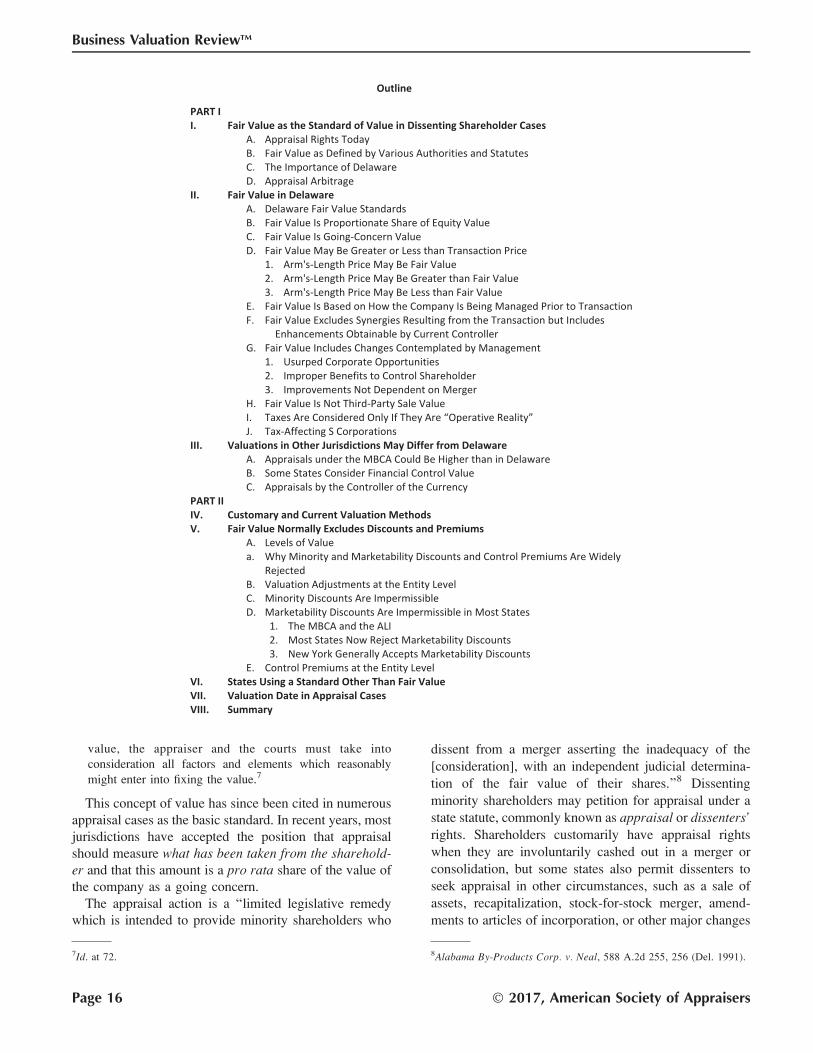
45
Volume 36 Issue 1 Spring 2017 1 Editor’s Column Dan McConaughy, PhD, ASA 3 American Society of Appraisers Business Valuation Committee Special Topics Paper #3 The Use of Management’s Prospective Financial Information by a Valuation Analyst 7 Petroleum Property Income and Market Valuation Approaches (Transactions Beware!) Louis R. Posgate, ASA, PE, CMA 9 A Primer on Bargain Purchases and Negative Goodwill Dan Daitchman, ASA 15 Statutory Fair Value in Dissenting Shareholder Cases— Part I Gilbert E. Matthews, MBA, CFA 32 Comparing Three Convertible Debt Valuation Models Dwight Grant, PhD 42 From the Chair of the Business Valuation Committee William A. Johnston, ASA Quarterly Journal of the Business Valuation Committee of the American Society of Appraisers
-
Upload
khangminh22 -
Category
Documents
-
view
2 -
download
0
Transcript of asa_bvreview_spring17.pdf - Business Valuation Resources

Volume 36
Issue 1
Spring 2017
1 Editor’s Column Dan McConaughy, PhD, ASA
3 American Society of Appraisers Business Valuation Committee Special Topics Paper #3 The Use of Management’s Prospective Financial Information by a Valuation Analyst
7 Petroleum Property Income and Market Valuation Approaches (Transactions Beware!) Louis R. Posgate, ASA, PE, CMA
9 A Primer on Bargain Purchases and Negative Goodwill Dan Daitchman, ASA
15 Statutory Fair Value in Dissenting Shareholder Cases—Part I Gilbert E. Matthews, MBA, CFA
32 Comparing Three Convertible Debt Valuation Models Dwight Grant, PhD
42 From the Chair of the Business Valuation Committee William A. Johnston, ASA
Quar
terly
Jour
nal o
f the
Bus
ines
s Val
uatio
n Co
mm
ittee
of t
he A
mer
ican
Socie
ty o
f App
raise
rs
Published by the American Society of Appraisers Copyright © 2017 American Society of Appraisers
Business Valuation Review™ – Spring 2017
The Business Valuation Committee
Chair William A. Johnston, ASA – Empire Valuation Consultants, LLC
Vice Chair Jeffrey S. Tarbell, ASA – Houlihan Lokey
Secretary Erin Hollis, ASA – Marshall & Stevens, Inc.
Treasurer Kenneth J. Pia, Jr., ASA – Meyers, Harrison & Pia, LLC
Past Chair Robert B. Morrison, ASA – Morrison Valuation & Forensic Services, LLC
Members At-Large Gregory Ansel, ASA – Financial Strategies Consulting Group LLC Arlene Ashcraft, ASA – Columbia Financial Advisors, Inc. KC Conrad, ASA – American Business Appraisers Matthew R. Crow, ASA – Mercer Capital Nancy M. Czaplinski, ASA – Duff & Phelps Erin Hollis, ASA – Marshall & Stevens, Inc. Bruce Johnson, ASA – Munroe, Park & Johnson, Inc. Curtis T. Johnson, ASA – Ernst & Young Timothy Meinhart, ASA – Willamette Management Associates Susan Saidens, ASA – SMS Valuation & Financial Forensics Ronald L. Seigneur, ASA – Seigneur Gustafson LLP Gary R. Trugman, ASA – Trugman Valuation Associates, Inc. Mark Zyla, ASA – Acuitas, Inc.
Ex Officio James O. Brown, ASA – Perisho Tombor Brown, PC R. Chris Rosenthal, ASA – Ellin & Tucker Linda B. Trugman, ASA – Trugman Valuation Associates, Inc.
Emeritus Jay E. Fishman, FASA – Financial Research Associates Shannon P. Pratt, FASA – Shannon Pratt Valuations, LLC
HQ Advisor Bonny Price
BUSINESS VALUATION REVIEW TM —Published quarterly by the Business Valuation Committee of the American Society of Appraisers. Editor: Daniel L. McConaughy, PhD, ASA. Managing Editor: Rita Janssen, [email protected].
INTERNATIONAL STANDARD SERIAL NUMBER—The Library of Congress, National Serials Data Pro = ISSN 0897-1781.SUBSCRIPTION RATES—PRINT AND ELECTRONIC ACCESS: Members of American Society of Appraisers-$60 if paid with annual dues;
all others—$140 per year. Direct any questions and/or subscription changes to Bonny F. Price (703) 733-2110 or [email protected]—Authors should submit their articles (including charts, graphs, pictures, etc.) for publication in Business Valuation Review™
at http://www.editorialmanager.com/bvr/. Follow the new user registration login instructions, at the Register Now hotlink. Since we use a double-blind peer review system, authors should provide the author’s name (as it would appear if published), and a short one-paragraph description of professional activities when completing the registration process. An abstract should appear at the beginning of the paper submitted for review. Authors are asked to not submit manuscripts currently under review by other publications or that have been published elsewhere. All manuscripts are reviewed by the Editorial Review Board and may be accepted, rejected, or returned for additional work. Editor’s notes may be included with the printing of accepted articles. All authors will be so notified. No manuscripts will be returned, and no critiques or reasons for rejection will be given for material not selected for publication.
CLASSIFIED ADS—Accepted for publication in one issue only and should reach the Publisher no later than the 10th of the month prior to publication. Rates: full page—$500, 2/3 page—$375, 1/2 page—$300, 1/3 page—$200, 1/4 page—$150. Payable in U.S. funds. Direct any questions to Bonny F. Price (703) 733-2110 or [email protected]
LETTERS TO THE EDITOR & COMMENTS—Letters from readers are encouraged on any valuation subject. BVR™ reserves the right to edit letters for length, taste and/or clarity. No guarantee of publica tion is given. Please direct critique or comments to the Editor. All Letters to the Editor should be submitted at http://www.editorialmanager.com/bvr/.
STATEMENTS & OPINIONS—Statements expressed herein by the authors and contributors to Business Valuation Review™ are their own and not necessarily those of the American Society of Appraisers or its Business Valuation Committee.
Copyright, © American Society of Appraisers—2017All rights reserved. For permission to reproduce in whole or part, and for quotation privilege, contact International Headquarters of ASA. Neither the Society nor its Editor accepts responsibility for statements or opinions advanced in articles appearing herein, and their appearance does not necessarily constitute an endorsement.
EditorDaniel L. McConaughy, PhD, ASA
California State University Northridge
Managing EditorRita Janssen
Lawrence, Kansas
Business ManagerJames O. Brown, ASA Campbell, California
ReviewersAshok Abbott*, PhD
Morgantown, West Virginia
John D. Finnerty, PhD New York, New York
Stillian Ghaidarov
Roger Grabowski*, FASA Chicago, Illinois
*Editorial Board Member
Editors EmeritusJames H. Schilt, ASA (1982–2001)
San Francisco, California
Jay E. Fishman, FASA (2002–2007) Bala Cynwyd, Pennsylvania
Roger J. Grabowski, FASA (2008–2012) Chicago, Illinois
Publishers EmeritusJohn E. Bakken, FASA (1982–2003)
Granby, Colorado
Ralph Arnold, III, ASA (2004–2007) Portland, Oregon
BVR™ Editorial Review Board
© 2017, American Society of Appraisers

Editor’s Column
Dan McConaughy, PhD, ASA
Hello Everyone,
Recently, I reviewed a valuation report with a
sensitivity analysis matrix. Such a matrix is a common
feature in valuation reports.
This time I looked at it a little differently, thinking
about the relationship between the expected cost of
capital and expected growth. The traditional interpretation
of this matrix, taken from the valuation and edited to
disguise the real numbers and shown below, gives the
range as the best case to worst case range, where best case
is high growth and low discount rate, and worst case is
high discount rate and low growth.
The Gordon Growth Model suggests that r and g are
related: r ¼ (D1 / P) þ g. If they are related and the
Gordon Growth Model reflects an expectation, would a
more reasonable range be read along the diagonal from
lower right to upper left?
Please let me know your thoughts.
Dan McConaughy
Business Valuation ReviewTM — Spring 2017 Page 1
Business Valuation Reviewe
Volume 36 � Number 1
� 2017, American Society of Appraisers

American Society of Appraisers Business ValuationCommittee Special Topics Paper #3
The Use of Management’s Prospective Financial Informationby a Valuation Analysta
According to AICPA Professional Standards: AT Section 301 Financial Forecasts
and Projections, ‘‘financial forecast is the prospective financial statements that present,
to the best of the responsible party’s knowledge and belief, an entity’s expected
financial position, results of operations, and cash flows. A financial forecast is based on
the responsible party’s assumptions reflecting the conditions it expects to exist and the
course of action it expects to take.’’ In order for a valuation analyst to objectively
perform the valuation analysis, the analyst has to judge whether or not management’s
prospective financial information is reasonable and can be relied upon in the valuation
analysis. This white paper will focus on the valuation analyst’s role in using
management’s forecast financial information and suggest a few useful analytical tools
available to the valuation analyst.
Introduction
Business valuation is the process of determining the
economic value of a business entity, which is based on
the ability of the business to generate future cash flows.
One common method used in estimating the value of the
entity, the discounted cash flow (DCF) method, utilizes
free cash flow expected in the future and discounts those
prospective cash flows at a risk-adjusted rate to arrive at a
net present value of or for the business. The DCF method
is particularly useful when future profit margins and
growth are expected to vary significantly from historical
operating results.
The two common components of the DCF method are:
� an estimate of future cash flows, and� an estimate of an appropriate risk-adjusted required
rate of return used to discount the estimated future
cash flows back to net present value.
The credibility of the DCF method lies in both a
reliable forecast and a well-developed discount rate.
Much has already been written about discount rate
development. This white paper will focus on the valuation
analyst’s role in using management’s forecast financial
information.
Management’s Prospective Financial Information
(PFI): Difference between a Forecast and a
Projection
Even though forecast and projection are used inter-
changeably by valuation analysts, they are actually
different concepts in accounting literature.
According to AICPA, ‘‘financial forecast is the prospec-
tive financial statements that present, to the best of the
responsible party’s knowledge and belief, an entity’s
expected financial position, results of operations, and cash
flows. A financial forecast is based on the responsible
party’s assumptions reflecting the conditions it expects to
exist and the course of action it expects to take.’’1
‘‘Financial projection is the prospective financial
statements that present, to the best of the responsible
party’s knowledge and belief, given one or more
hypothetical assumptions, an entity’s expected financial
position, results of operations, and cash flows. A financial
projection is sometimes prepared to present one or more
hypothetical courses of action for evaluation, as in
response to a question such as ‘What would happen
if. . .?’ A financial projection is based on the responsible
party’s assumptions reflecting conditions it expects would
exist and the course of action it expects would be taken,
given one or more hypothetical assumptions.’’2
aThis white paper is for education purposes and should not be consideredas authoritative. It has been provided for discussion of a concept and isnot being offered as professional advice. Each set of circumstances mayrequire a different analysis to be performed.
1American Institute of Certified Public Accountants, AICPA Profes-sional Standards, ‘‘AT Section 301 Financial Forecasts and Projections.’’2Ibid.
Business Valuation ReviewTM — Spring 2017 Page 3
Business Valuation Reviewe
Volume 36 � Number 1
� 2017, American Society of Appraisers
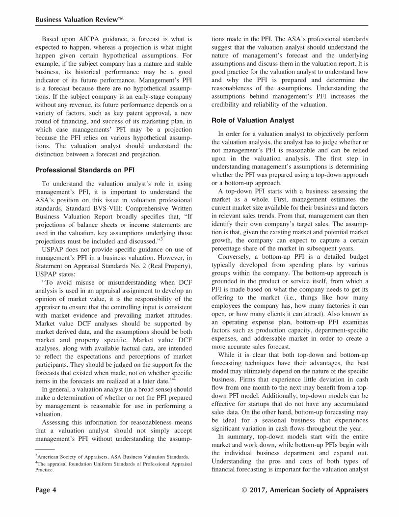
Based upon AICPA guidance, a forecast is what is
expected to happen, whereas a projection is what might
happen given certain hypothetical assumptions. For
example, if the subject company has a mature and stable
business, its historical performance may be a good
indicator of its future performance. Management’s PFI
is a forecast because there are no hypothetical assump-
tions. If the subject company is an early-stage company
without any revenue, its future performance depends on a
variety of factors, such as key patent approval, a new
round of financing, and success of its marketing plan, in
which case managements’ PFI may be a projection
because the PFI relies on various hypothetical assump-
tions. The valuation analyst should understand the
distinction between a forecast and projection.
Professional Standards on PFI
To understand the valuation analyst’s role in using
management’s PFI, it is important to understand the
ASA’s position on this issue in valuation professional
standards. Standard BVS-VIII: Comprehensive Written
Business Valuation Report broadly specifies that, ‘‘Ifprojections of balance sheets or income statements are
used in the valuation, key assumptions underlying those
projections must be included and discussed.’’3
USPAP does not provide specific guidance on use of
management’s PFI in a business valuation. However, in
Statement on Appraisal Standards No. 2 (Real Property),
USPAP states:
‘‘To avoid misuse or misunderstanding when DCF
analysis is used in an appraisal assignment to develop an
opinion of market value, it is the responsibility of the
appraiser to ensure that the controlling input is consistent
with market evidence and prevailing market attitudes.
Market value DCF analyses should be supported by
market derived data, and the assumptions should be both
market and property specific. Market value DCF
analyses, along with available factual data, are intended
to reflect the expectations and perceptions of market
participants. They should be judged on the support for the
forecasts that existed when made, not on whether specific
items in the forecasts are realized at a later date.’’4
In general, a valuation analyst (in a broad sense) should
make a determination of whether or not the PFI prepared
by management is reasonable for use in performing a
valuation.
Assessing this information for reasonableness means
that a valuation analyst should not simply accept
management’s PFI without understanding the assump-
tions made in the PFI. The ASA’s professional standards
suggest that the valuation analyst should understand the
nature of management’s forecast and the underlying
assumptions and discuss them in the valuation report. It is
good practice for the valuation analyst to understand how
and why the PFI is prepared and determine the
reasonableness of the assumptions. Understanding the
assumptions behind management’s PFI increases the
credibility and reliability of the valuation.
Role of Valuation Analyst
In order for a valuation analyst to objectively perform
the valuation analysis, the analyst has to judge whether or
not management’s PFI is reasonable and can be relied
upon in the valuation analysis. The first step in
understanding management’s assumptions is determining
whether the PFI was prepared using a top-down approach
or a bottom-up approach.
A top-down PFI starts with a business assessing the
market as a whole. First, management estimates the
current market size available for their business and factors
in relevant sales trends. From that, management can then
identify their own company’s target sales. The assump-
tion is that, given the existing market and potential market
growth, the company can expect to capture a certain
percentage share of the market in subsequent years.
Conversely, a bottom-up PFI is a detailed budget
typically developed from spending plans by various
groups within the company. The bottom-up approach is
grounded in the product or service itself, from which a
PFI is made based on what the company needs to get its
offering to the market (i.e., things like how many
employees the company has, how many factories it can
open, or how many clients it can attract). Also known as
an operating expense plan, bottom-up PFI examines
factors such as production capacity, department-specific
expenses, and addressable market in order to create a
more accurate sales forecast.
While it is clear that both top-down and bottom-up
forecasting techniques have their advantages, the best
model may ultimately depend on the nature of the specific
business. Firms that experience little deviation in cash
flow from one month to the next may benefit from a top-
down PFI model. Additionally, top-down models can be
effective for startups that do not have any accumulated
sales data. On the other hand, bottom-up forecasting may
be ideal for a seasonal business that experiences
significant variation in cash flows throughout the year.
In summary, top-down models start with the entire
market and work down, while bottom-up PFIs begin with
the individual business department and expand out.
Understanding the pros and cons of both types of
financial forecasting is important for the valuation analyst
3American Society of Appraisers, ASA Business Valuation Standards.4The appraisal foundation Uniform Standards of Professional AppraisalPractice.
Page 4 � 2017, American Society of Appraisers
Business Valuation ReviewTM

so they can assess the reasonableness and credibility of
management’s PFI.
In addition to understanding the approach management
used to develop the PFI, a valuation analyst should
understand who actually prepared the PFI to consider any
potential biases. For example, if the marketing and sales
department prepared the PFI, is it potentially too
optimistic? Conversely, if the finance and accounting
department prepared the PFI, is it too pessimistic?
Typically, the greater amount of time and company
personnel dedicated to the forecast planning process, the
more detailed and accurate the forecast will be.
Additionally, if the valuation analyst has access to
previous forecasts prepared by management, the analyst
should compare the previous forecasts to actual results to
consider the accuracy of management with those PFI
reports.
The valuation analyst should also understand the
fundamental assumptions that drive the forecast. If the
assumptions in the PFI prepared by management are not
readily apparent, the valuation analyst may consider
asking questions of management regarding the underlying
assumptions.
Examples of questions that the valuation analyst may
consider in understanding the assumptions behind the PFI
include:
� Is expected growth in revenue due to an increase in
price or volume or both?� How does expected growth in revenue of the
company compare to industry growth?� Is revenue growth achievable given the current
conditions of company operations?� How are new products or services considered in
forecasted revenue? If so, are corresponding expens-
es reasonable?� Are new products under development? What is the
basis for research and development expenses? Are
forecasted capital expenditures consistent with the
revenue growth assumptions?� Are operating expenses consistent with historical
levels? Did management differentiate between fixed
and variable costs?� If there are variable costs, what do costs vary
against?� Are forecasted results consistent with historical
results? If not, why?� In a business combination, do the forecasts consider
any synergies from revenue enhancement and/or cost
savings?� Is it reasonable for management to forecast a much
higher or lower growth rate compared to guideline
companies or other industry metrics?
� Is it reasonable for management to forecast a much
higher or lower profit margin compared to guideline
companies or other industry metrics?
A good benchmark with which to evaluate the
reasonableness of management’s PFI is industry data.
The valuation analyst should compare the subject
company’s historical performance and management’s
PFI to those of the guideline publicly traded companies.
Comparison with guideline publicly traded companies
can also provide the valuation analyst with detailed
industry information, such as normalized working capital
level, average industry growth rate, and average capital
expenditures. In addition, the valuation analyst might
research market and industry research reports and
relevant government data as additional information to
determine whether or not the PFI is reasonable for use in
a valuation.
Furthermore, when utilizing more than one approach in
valuation, if the valuation results from use of the PFI are
significantly different from other valuation methods, it
may be good practice to reevaluate the reasonableness of
management’s PFI.
What if Management Doesn’t Prepare a PFI?
In certain circumstances, management may not prepare
a PFI. In those circumstances, a PFI may be available
from other sources, such as the company’s outside
financial advisors. If the subject company is a public
company, equity analysts may prepare prospective
information in research reports. The valuation analyst
should consider reconciling multiple sources of PFI in
preparing for valuation analysis.
Occasionally, there is no PFI available to valuation
analyst. This is particularly common when dealing with
small, privately held companies. In these circumstances,
the valuation analyst may ask management to develop the
PFI specifically for the valuation. In such case,
management still ultimately takes responsibility for the
PFI.
If management prepares a PFI, but a valuation analyst
finds management’s PFI to be unreasonable, the valuation
analyst should first make recommendations for any
revisions in the PFI to management. Otherwise, the
valuation analyst should consider any additional risk in
achieving the PFI company-specific risk premium in the
cost of capital to perhaps capture any additional forecast
risk. If the valuation analyst finds that management’s PFI
is not reasonable for use in the valuation, the analyst may
also consider using only valuation methods that do not
require the use of PFI. In these situations, a valuation
analyst may consider making clear in the analysis the
limitations of the data available for the analysis. In
Business Valuation ReviewTM — Spring 2017 Page 5
Use of Management’s Prospective Financial Information by a Valuation Analyst

extreme circumstances, the valuation analyst should
consider resigning from the engagement due to lack of
appropriate data.
Finally, it may be good practice for the valuation
analyst to have representations that the PFI provided to
the valuation analyst is management’s best estimate of
expected future performance of the company through a
management representation letter. Management represen-
tation letters are commonly used by third-party auditing
firms in their financial reporting engagements.
Analytical Tools
Whether the goal is to evaluate the reasonableness of
management’s PFI or to assist management to prepare for
a PFI, there are a few useful analytical tools available to
the valuation analyst. It is common for historical results to
be used as a starting point in any forecast. One way to
statistically evaluate PFI is for the analyst to perform a
regression analysis comparing the company’s historical
financial performance to certain economic indicators. One
key to this approach is to identify the salient economic
variable(s) that correlate with historical revenue. Once the
trending line is fitted, it is much easier to forecast for the
future.
Some business valuation analysts perform scenario
analysis or sensitivity analysis when evaluating manage-
ment’s PFI. The analyst may consider utilizing three
scenarios, such as best, worst, and neutral, representing
management’s optimistic, pessimistic, and status-quo
outlook for the company to identify key value drivers
in the PFI. Sensitivity analysis on specific assumptions is
another powerful tool that may be used by valuation
analysts to understand the reasonableness of manage-
ment’s PFI.
Powerful analytical tools such as Monte Carlo
simulation may be helpful in determining the reasonable-
ness in using management’s PFI in the valuation.
Traditional DCF analysis is based upon single-point
estimates of the variables. Monte Carlo simulation
produces distributions of possible outcome values based
upon distributions of underlying variables. Monte Carlo
simulations calculate thousands of scenarios having
different combinations of inputs. The simulation captures
numerous ‘‘what-if’’ scenarios related to the company’s
future performance.
Summary and Conclusion
The valuation analyst should determine that any PFI
prepared by management is reasonable for use in a
valuation analysis. Assessing for reasonableness means
that the valuation analyst should not simply accept
management’s PFI without understanding the assump-
tions made in the PFI. The ASA’s professional standards
suggest that the valuation analyst should understand the
nature of management’s forecast and the underlying
assumptions and discuss them in the valuation report.
Good practice dictates that the valuation analyst under-
stand how and why the PFI was prepared and determine
the reasonableness of the assumptions. Assessing reason-
ableness can take many forms, But determining the
reasonableness of management’s PFI increases the
credibility and reliability of the valuation.
Page 6 � 2017, American Society of Appraisers
Business Valuation ReviewTM
Petroleum Property Income and Market ValuationApproaches (Transactions Beware!)
Louis R. Posgate, ASA, PE, CMA
Characteristics exhibited by producing liquid-rich shale formations often cause
inaccurate forecasts of natural gas and oil production when multistage hydraulic
fracking is used for extraction. Poor cash flow estimates can be avoided by practicing
due diligence when appraising petroleum property value and income. Due diligence is
satisfied by comparing volumes recorded on actual royalty check stubs or monthly
statements to state-reported production volumes, by relying on petroleum reserve
appraisals instead of transaction multipliers or rules of thumb, and by using nearby
analog wells in proximity found in subscription databases for good ‘‘type’’ well decline
curves. In addition, properly referencing the contributing work of other appraisers,
maps, and analyses improves understanding and reduces errors.
Introduction
A band of Eagle Ford Shale fields is being developed
(e.g., Sugarkane [Eagle Ford] and Eagleville [Eagle Ford-
1, Eagle Ford-2]) in quality regimes or ‘‘tiers’’ near San
Antonio, Texas. Producing counties, such as Atascosa,
Live Oak, Lavaca, Gonzales, La Salle, and contiguous or
nearby counties through Fayette and Lee (west of
Houston), contain tracts where wells were drilled
vertically through untapped shales, rich in liquids, to
targeted chalk and sandstone traps. However, relatively
recently, wells have been drilled horizontally and snake
through the shale beds. Shale is composed of overburden-
compressed hydrocarbon-imbedded clays that are the
source rock providing the hydrocarbons. The hydrocar-
bons migrate through natural and hydraulically induced
fractures to conventionally completed sandstone sedi-
mentary and carbonate reef-like reservoirs. Connected
(permeable) pores in such reservoirs are produced by
solution gas depletion. An example would be shaking up
canned soda.
Over a decade ago in the Newark East Barnett Shale
Field (a Mississippian-aged, 8,000 ft deep shale) south
and west of Dallas, expansion of multistaged hydraulic
fracking through horizontal drainage was performed by
Mitchell Energy and other operators with longer (now up
to 2 mi long) horizontal, sometimes multilateral bores,
thereby increasing the effective shale thicknesses from
100 ft (30 meters vertically) to many thousands of feet.
Under pressure, oil flushes through fractures in shale,
then seeps through the shale walls that have 1/1000th of
the permeability of sandstones.
This causes the production (and cash flow profile) to
decline hyperbolically (initially steeply and then stabiliz-
ing at a lower rate, often five to six years or more later,
exponentially (a straight line on a semilog plot) like
conventional reservoirs. This makes the oil and gas priceassumptions for the first two years critical to anappraiser’s reserves and present values, drilling, androyalty property economics.
Specific factors, such as if the wells are ‘‘choked back’’
(to flatten the decline; e.g., like holding a thumb over a
shaken soda can), if petroleum vapors that condense are
captured (e.g., by natural gas liquids extraction plants
downstream paying owners for their share of extracted
product), and if the length of laterals and sand/proppant
treatment (millions of lbs) and number of gallons
(hundreds of thousands) in the frack effectively prop open
fractures to facilitate flow, point to the importance of using
analog wells in close proximity for good ‘‘type’’ well
decline curves. These data may be found in subscription
databases used by petroleum engineers/appraisers.
Sometimes unstable pressure declines in an early stage
of production, with higher gathering system pressure and
high (62þ) condensate gravity (API number indicating
volatility), can pose a production prediction error. This is
Louis R. Posgate is an Accredited Senior Apprais-er, designated in both business valuation and oil andgas valuation, by the American Society of Apprais-ers. He is a licensed professional engineer andcertified minerals appraiser (CMA), and a valuationconsultant in Driftwood, Texas, d.b.a. LRP BusinessAppraisal, an affiliate of Mineral Valuation Special-ists.
Business Valuation ReviewTM — Spring 2017 Page 7
Business Valuation Reviewe
Volume 36 � Number 1
� 2017, American Society of Appraisers
due to gas and oil volume shrinkage—I have seen up to
40% volume shrinkage from reported production to
volumes on which owners are paid.
Statistical regression techniques applied by analysts
without reviewing actual purchased production for
shrinkage, shut-in wells being worked on, or drilling
well buildup in a lease can indicate a different prospectivefield decline rate and can cause valuation inaccuracy. In
Texas, a pooled unit can have several completed wells
constituting a lease, often with planned ‘‘PUD’’ additionsto be included. Since high well-stream pressures in gassy
oil- or liquids-rich reservoir windows can cause signif-
icant condensate and gas volume shrinkage from
wellhead-measured (state-reported) volumes, cash flow
streams evaluation software must reflect this adjustment.
Comparison of state-reported volumes to actual royalty
check stub volumes is required to estimate not only
shrinkage, but 23 to 33 the gas equivalent price when
natural gas liquid revenues are included. This practitioner
has dealt with this in producing fields in Live Oak,
Gonzales, Atascosa, and other Texas counties hosting
Eagle Ford Shale fields.
One problem regarding business valuators using
transaction multiples as a proxy for reserves appraisal is
not using volume adjustments, i.e., gas BTU equivalence
with one barrel oil. This is magnified if the thumb rule for
dollars per equivalent barrel of daily production multiple
is relied on to avoid reserves or royalty appraisal costs,
without the necessary BTU or similar equivalence
adjustments. Usually nothing other than a good petroleum
appraisal is acceptable for users valuing companies,
partnerships, and business components. This appraiser
has observed this misuse of market multiples, assuming
$/BTU-equivalence and similar volume shrinkage, when
thumb rules are applied for valuing oil and gas reserves,
and questionably comparable acquisition multiples are
used in such a transaction method. This was noted in
energy papers presented in ASA conference speeches,
and by reviewing court case decisions (analysis in ‘‘Oil
and Gas Federal Tax Case Review: Fair Market Values
with Volatility,’’ Business Valuation Review 21, 4
[December 2002, pp. 181–185]), and in articles on web
sites.
Due diligence is practiced by comparing royalty
statement monthly volumes to state-reported production,
asking about the subject’s oil API gravity and if any
shrinkage exists, and then reducing, if necessary,
production volumes by shrinkage when fitting data to
decline curves. This is significant in volatile-rich gas
windows of the Eagle Ford Shale, and any other volatile
crude and condensate nonconventional shales. Without
the petroleum appraisals, transfers such as estate asset
values or capital gains basis, sometimes being estimated
retrospectively, could cause a client to have a costly
challenge or misstatement of fair market value, or an
unreasonable acquisition purchase price of reserves,
royalty property, or asset value. This satisfies the
competency requirement under USPAP.
Other competency and ethics items to consider involve
properly referencing appraisers who contribute (signifi-cantly) to opinions stated in the report. When such an
opinion of value is formed by reference in part to any
other appraiser’s work or research, its provider or source
should be listed in the report references. That applies to
persons doing any contributing work subcontracted for an
appraisal, such as running production decline curves for
reserves estimation, doing market analysis, calculating
discount rate of company stock versus asset valuations,
sharing maps or privately developed data, and referencing
papers or presentations. When quoting papers or
footnoting, such as another appraiser’s published docu-
ment on lease bonus multiples applied to nonproducing
acreage, a mineral parcel, or lease transaction compara-
bility, etc., the referencing author should contact the
original appraiser to understand the original context and
whether it is appropriate to apply it to the current
valuation. This applies when citing it in published
valuation documents, magazines, etc., to avoid errors.
Page 8 � 2017, American Society of Appraisers
Business Valuation ReviewTM
A Primer on Bargain Purchases and Negative Goodwill
Dan Daitchman, ASA
When a change of company control occurs, such as an acquisition, a valuation of the
assets acquired must be performed to be compliant with generally accepted
accounting principles, as mandated by the Financial Accounting Standards Board
(FASB) and addressed in Accounting Standards Codification (ASC) 805: Business
Combinations. This type of exercise is commonly referred to as a purchase price
allocation, since the purchase price of the subject company is allocated across all
tangible and intangible assets and liabilities acquired. Generally, the value of the
subject company is greater than the value of the acquired assets, or in other words,
‘‘the whole is greater than the sum of the parts.’’ However, what if the sum of the parts
is greater than the whole? This paper looks at transactions involving fair value and
bargain purchases, the differences between the two, and how bargain purchases
should be addressed.
Background
When a change of company control occurs, such as an
acquisition, a valuation of the assets acquired must be
performed to be compliant with generally accepted
accounting principles, as mandated by the Financial
Accounting Standards Board (FASB) and addressed in
Accounting Standards Codification (ASC) 805: Business
Combinations.1 This type of exercise is commonly
referred to as a purchase price allocation, since the
purchase price of the subject company is allocated
across all tangible and intangible assets and liabilities
acquired. Generally, the value of the subject company is
greater than the value of the acquired assets, or in other
words, ‘‘the whole is greater than the sum of the parts.’’
That additional value is referred to as goodwill.
However, what if the sum of the parts is greater than
the whole? There are certain transactions in which the
total value of the individual assets acquired in a
transaction exceeds the price paid for the total company.
This is often referred to as a ‘‘bargain purchase.’’ The
scope of this paper is to look at transactions involving
fair value and bargain purchases, the differences
between the two, and how bargain purchases should be
addressed.
Transactions with Positive Goodwill
In a typical acquisition, acquired tangible assets may
include working capital (accounts receivable, inventory,
etc.), personal property (machinery and equipment), and
real property. In addition, there are a number of intangible
assets that are often acquired, which are seen as the
‘‘value-drivers’’ of the company. An asset must pass one
of two tests to have allocated value: (a) It must be of a
legal or contractual nature; or (b) it must be separable
from the business. Such intangible assets can include a
brand name, patented or unpatented technology, certifi-
cations or licenses, noncompetition agreements, customer
relationships, as well as industry-specific forms of
intangible assets, such as broadcast licenses or distribu-
tion rights.
In this exercise, after allocating value to all of these
assets, the residual difference between the fair value of
the acquired assets and liabilities versus the purchase
price is considered goodwill. Hence, the aggregate fair
value of the acquired assets plus the fair value of
goodwill equals the purchase price of the transaction,
assuming the overall transaction itself is conducted at
fair value.
Dan Daitchman is a manager with Great AmericanGroup in their Corporate Valuation Services practice.Dan provides valuations of assets, including businessinterests, intellectual property, and various other intan-gible assets. His valuation work is primarily used forfinancial reporting, tax, asset-based lending, transactionadvisory, as well as fairness and solvency opinions. Danis also an Accredited Senior Appraiser of the AmericanSociety of Appraisers. He can be reached [email protected].
1ASC 805: Business Combinations.
Business Valuation ReviewTM — Spring 2017 Page 9
Business Valuation Reviewe
Volume 36 � Number 1
� 2017, American Society of Appraisers

Purchase accounting requires the use of the standard of
fair value, which is defined in ASC 8202 as: ‘‘. . . the price
that would be received to sell an asset or paid to transfer a
liability in an orderly transaction between market
participants at the measurement date.’’An important concept of this definition is that of a
‘‘market participant,’’ which is an actual or theoretical
potential buyer of the business or asset (or assumer of the
liability). ASC 805 does not require that specific market
participants be identified, only that their characteristics be
described.
The difference between the carrying values of the
assets (CVA) acquired and the fair values of those assets
represents a step-up in the basis for the acquired assets. A
diagram showing CVA, the step-up from CVA to fair
value, and goodwill as components of the purchase price
is shown in Figure 1.
Goodwill is an asset representing the future economic
benefits arising from other assets acquired in a business
combination that are not individually identified and
separately recognized.3 There are many ways to more
explicitly describe what comprises goodwill, but often it
includes the acquired company’s workforce, prospects for
future growth, market participant synergies with the target
company, and ‘‘going concern value’’ from the assem-
blage of the assets. Table 1 shows a sample of what a
purchase price allocation might look like for a $60
million acquisition.
As you can see, the fair value of the acquired assets
sums up to $42.5 million, which means that the residual
$17.5 million represents goodwill. It is also important to
note that while the trained and assembled workforce
(TAW) is listed separately, it is not viewed as separable
from the company and hence is bundled into goodwill on
the subject company’s balance sheet. For purchase price
allocation purposes, it is listed separately because it is
used as an input in valuing intangible assets under the
Multi-Period Excess Earnings Method (MPEEM). This
valuation method will be discussed later in the paper.
Transactions with Negative Goodwill
While most transactions have positive goodwill,
occasionally the fair value of the acquired assets exceeds
the purchase price. This scenario results in a nontaxable
gain and is commonly referred to as a bargain purchase.
Using the previous example, if the purchase price were
only $40 million instead of $60 million, Table 2 shows
how the allocation would look. This type of scenario
creates a significant amount of additional analysis, which
will be described in further detail.
Figure 1Purchase Price Diagram
Table 1Purchase Price Allocation with Positive Goodwill ($ in
000s)
Assets Fair Value % of Total
Net Working Capital $15,000 25.0
Personal Property 10,000 16.7
Real Property 1,000 1.7
Identified Intangible Assets
Patents and Technology 5,000 8.3
Trade Name 7,000 11.7
Customer Relationships 4,000 6.7
Unallocated Intangible Assets
Trained and Assembled Workforce 500 0.8
Goodwill 17,500 29.2
Purchase Price $60,000 100.0
Table 2Purchase Price Allocation with Negative Goodwill ($
in 000s)
Assets Fair Value % of Total
Net Working Capital $15,000 37.5
Personal Property 10,000 25.0
Real Property 1,000 2.5
Identified Intangible Assets
Patents and Technology 5,000 12.5
Trade Name 7,000 17.5
Customer Relationships 4,000 10.0
Unallocated Intangible Assets
Trained and Assembled Workforce 500 1.3
Fair Value of Identified Assets $42,500 106.3
Goodwill (2,500) �6.3
Purchase Price $40,000 100.02ASC 820-10-20: Fair Value Measurements and Disclosures.3ASC 805-10-20.
Page 10 � 2017, American Society of Appraisers
Business Valuation ReviewTM

Characteristics—Initial Screening
There are several telltale signs that a transaction may be
a bargain purchase. Two common themes are company
distress and information asymmetry. Some earmarks of
bargain purchases include:
� The seller was compelled to sell the business.� The subject company has incurred financial losses in
recent years.� The transaction was not well marketed (i.e., a limited
number of potential buyers were contacted).� There was only one bid for the subject company.� The subject company was acquired over a very short
time frame.� There was information asymmetry, in which the
buyer knew more about the future prospects of the
business than the seller.� The net book value of the acquired assets exceeded
the purchase price.
As with any purchase price allocation, there should
be a detailed explanation associated with the transaction
as to why it was a bargain purchase, and steps should be
taken to document why the purchase price is not
representative of fair value. If you cannot clearly
articulate why the purchase price allocation represents
a bargain purchase, you may need to revalue each asset,
or conclude that the fair value of the overall business is
more than the purchase price (i.e., the transaction did
not occur at fair value). In that case, the concluded fair
value is the amount allocated to the acquired assets, and
the excess of the fair value of the business above the
purchase price would be recorded as an extraordinary
gain.
Valuation Characteristics
Since a bargain purchase often implies that the subject
company has endured some form of financial distress, the
fair value of the acquired assets is often depressed as well.
A few examples are stated below.
Inventory
Occasionally, the fair value of the subject company’s
inventory will be required, particularly if inventory
comprises a large portion of the company’s assets. If the
fair value of the inventory is greater than its net book
value (NBV), it is referred to as an ‘‘inventory step-up.’’
In a bargain purchase scenario, however, the fair value
of the inventory could be lower than its NBV, which
would be referred to as an inventory step-down. For
example, the inventory’s fair value might be less than its
NBV due to low gross margins, low turnover, product
obsolescence, raw material price changes, or high fixed
costs.
Fixed assets
One common characteristic of a company acquired
under a bargain purchase is that the company has excess,
underutilized, or nonoperating fixed assets on the balance
sheet. In such a case, it can be inferred that the cash flows
of the subject company do not support the fair values of
the fixed assets as a going concern. This situation can be
rectified by applying economic obsolescence to the fixed
assets, thereby writing the assets down to create a fair
value in which the cash flows of the business do support
the fixed assets. One must be aware of both the macro-
and micro-impacts of applying this analysis. Applying too
much economic obsolescence to fixed assets can push a
bargain purchase into a positive goodwill scenario. When
applying economic obsolescence to fixed assets, typically
the lower-end constraint is orderly liquidation value, also
known as value in-exchange. The case for economic
obsolescence is that there are not enough cash flows to
support ownership of the fixed assets. Therefore, it would
be self-contradicting to state that there is insufficient cash
flow to support the full value of the fixed assets in-use,
and yet also conclude that there is cash flow beyond that
generated by the aggregate assets. In other words,
economic obsolescence and residual goodwill do not
typically both exist in the same operating unit in a
transaction setting.
Customer relationships
One intangible asset that is present in nearly every
purchase price allocation is customer relationships. As
one may infer, this asset represents the value of the
company’s power to generate future sales from its
existing customers. This asset is often valued using the
MPEEM. The MPEEM attempts to isolate the value of
the customer relationships by assuming a scenario in
which the buyer would only own the customer relation-
ships, and all other assets (i.e., working capital, fixed
assets, trade name, etc.) are rented. The cash flows of the
business are therefore reduced by economic rents, or
‘‘contributory asset charges,’’ which are the theoretical
costs of renting all of the other assets. The excess cash
flow that remains is referred to as the ‘‘excess earnings,’’
which are then discounted to calculate the fair value of
customer relationships.
Another characteristic often found in bargain purchases
is that, since the company frequently does not generate
enough cash flows to support the assets of the business,
the contributory asset charges applied in the MPEEM
Business Valuation ReviewTM — Spring 2017 Page 11
A Primer on Bargain Purchases and Negative Goodwill

often end up consuming all of the cash flows used in
calculating the fair value of customer relationships. In
such cases, it is often necessary to explore other valuation
methods for the customer relationships, so that the value
of the customers reflects economic assumptions a market
participant typically would have made regarding those
assets. While it is very rare to have both economic
obsolescence and residual goodwill, it is not uncommon
to have both economic obsolescence and value within the
identified intangible assets such as customer relationships,
trademarks, or patented technology.
Rates of return
Commonly, as part of a purchase price allocation
analysis, it would be expected that three rates of return
would be in alignment: weighted average cost of capital
(WACC, or a hypothetical return on the subject company
calculated by the appraiser), implied rate of return (IRR,
the rate of return determined based on the projections
used to price the acquisition and the ultimate purchase
price), and weighted average return on assets (WARA,
the aggregate rate of return required for each acquired
asset weighted in proportion to the fair value of that asset
to the purchase price).
In a bargain purchase scenario, however, these rates
would often initially not be in alignment without further
efforts to reconcile them. This scenario typically observes
the following relationship: IRR . WACC . WARA. The
IRR tends to be the highest because the subject company
was purchased at a low price (hence a ‘‘bargain purchase’’),and this indicates that the buyer is requiring an above
market rate of return on the investment. The WACC is in
the middle because it is calculated without regard to the
purchase price and reflects return requirements of market
participants; hence, it is unaffected by the nature of the
acquisition. The WARA tends to be the lowest rate of
return because in a bargain purchase, there is no goodwill,
which typically has the highest required rate of return of
the acquired assets due to its inherent riskiness, while
goodwill would be present in the normal market
assumptions associated with the WACC. This difference
in the asset mix pushes toward a lower WACC, with all
else being equal. In a bargain purchase scenario, the
reconciliation of these differences can be a complex
process.
Independent valuation
To further support the evidence of a bargain purchase,
the appraiser may calculate his/her own fair value of the
business enterprise using market participant data. If the
appraiser determines that the future cash flows of the
business are market participant cash flows (i.e., exclude
buyer-specific synergies), he/she can determine the fair
value of the subject company using a market participant
WACC. Using the same two scenarios of an acquisition
representing fair value with residual goodwill, and a
bargain purchase scenario with negative goodwill, he/she
can demonstrate that the purchase price is not represen-
tative of fair value.
One method of calculating an independent fair value of
the subject company is through a discounted cash flow
(DCF) analysis. Table 3 shows the forecasted debt-free
net cash flow (DFNCF) of the subject company. Using
the DFNCF, a long-term growth rate of 2.5%, and the
Table 3IRR Using the Market Participant Cash Flows and the Purchase Price
2016 2017 2018 2019 2020 2021 2022 2023 2024 2025
DFNCF $6,939 $7,633 $8,015 $8,415 $8,792 $9,055 $9,327 $9,607 $9,895 $10,192
Present Value Factor 0.8981 0.7245 0.5844 0.4714 0.3803 0.3068 0.2475 0.1996 0.1610 0.1299
Present Value of DFNCF 6,232 5,530 4,684 3,967 3,343 2,778 2,308 1,918 1,593 1,324
Total Present Value of Discrete Period DFNCF 33,679
Calculation of Terminal Value
Normalized Terminal Year 10,447
Capitalization Rate 21.5%
Terminal Value of DFNCF 48,665
Present Value Factor at 24.0% 0.1299
Present Value of Terminal Value 6,321
Valuation Summary
Total Present Value of Discrete Period DFNCF 33,679
Present Value of Terminal Value 6,321
Fair Value of Invested Capital $40,000
IRR 24.0%
Page 12 � 2017, American Society of Appraisers
Business Valuation ReviewTM

purchase price of $40 million, we see that the IRR is
24.0%. Let’s assume that the appraiser calculated a
WACC of 16.6% for the subject company. If we assume
that these cash flows are market participant cash flows,
Table 4 shows that using the same DFNCF, a long-term
growth rate of 2.5%, and the WACC, we find that the fair
value of the subject company is $60 million. The IRR of
24.0% versus the WACC of 16.6% demonstrates that the
acquirer of the subject company purchased the company
at a bargain price, because the IRR is an above-market
return when compared to the WACC.
In addition to a DCF analysis, the appraiser could
calculate the fair value of the subject company through a
market-based approach. By looking at the trading
multiples of public comparable companies, or transaction
multiples of similar acquired companies, the appraiser
could determine that the implied multiples of the
transaction are below the range of multiples that are
representative of fair value.
As previously mentioned, reconciling the rates of
return in a bargain purchase scenario can be a complex
process. Tables 5 and 6 show the WARA under each
scenario. In Table 5, using the appraiser’s independent
valuation of $60 million, the WARA is equal to the
WACC, and the return on goodwill has the highest return
of all of the acquired assets. When using the purchase
price in Table 6, the WARA is much lower than the
WACC, and the previously mentioned relationship holds.
It is important to note that the selected rates of return in
Tables 5 and 6 are illustrative only; the return on goodwill
Table 4Fair Value of Invested Capital using the Market Participant Cash Flows and the WACC
2016 2017 2018 2019 2020 2021 2022 2023 2024 2025
DFNCF $6,939 $7,633 $8,015 $8,415 $8,792 $9,055 $9,327 $9,607 $9,895 $10,192
Present Value Factor 0.9262 0.7945 0.6815 0.5846 0.5014 0.4301 0.3690 0.3165 0.2715 0.2329
Present Value of DFNCF 6,427 6,064 5,462 4,920 4,409 3,895 3,441 3,041 2,686 2,374
Total Present Value of Discrete Period DFNCF 42,718
Calculation of Terminal Value
Normalized Terminal Year 10,447
Capitalization Rate 14.1%
Terminal Value of DFNCF 74,206
Present Value Factor at 16.6% 0.2329
Present Value of Terminal Value 17,282
Valuation Summary
Total Present Value of Discrete Period DFNCF 42,718
Present Value of Terminal Value 17,282
Fair Value of Invested Capital $60,000
WACC 16.6%
Long Term Growth Rate 2.5%
Table 5WARA with Positive Goodwill
Assets Fair Value % of Total Rate of Return, %
Net Working Capital $15,000 25.0 5.0
Personal Property 10,000 16.7 6.0
Real Property 1,000 1.7 7.0
Identified Intangible Assets
Patents and Technology 5,000 8.3 20.0
Trade Name 7,000 11.7 20.0
Customer Relationships 4,000 6.7 20.0
Unallocated Intangible Assets
Trained and Assembled Workforce 500 0.8 17.0
Goodwill 17,500 29.2 30.0
Purchase Price $60,000 100.0 16.6
Business Valuation ReviewTM — Spring 2017 Page 13
A Primer on Bargain Purchases and Negative Goodwill
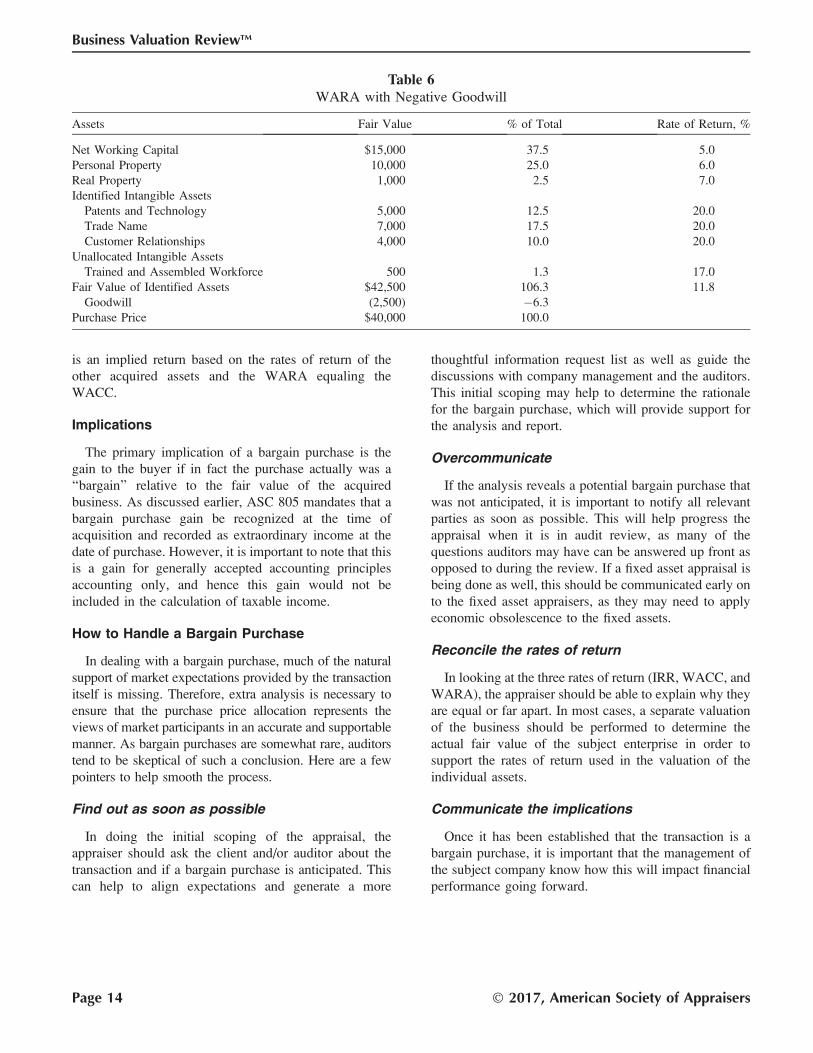
is an implied return based on the rates of return of the
other acquired assets and the WARA equaling the
WACC.
Implications
The primary implication of a bargain purchase is the
gain to the buyer if in fact the purchase actually was a
‘‘bargain’’ relative to the fair value of the acquired
business. As discussed earlier, ASC 805 mandates that a
bargain purchase gain be recognized at the time of
acquisition and recorded as extraordinary income at the
date of purchase. However, it is important to note that this
is a gain for generally accepted accounting principles
accounting only, and hence this gain would not be
included in the calculation of taxable income.
How to Handle a Bargain Purchase
In dealing with a bargain purchase, much of the natural
support of market expectations provided by the transaction
itself is missing. Therefore, extra analysis is necessary to
ensure that the purchase price allocation represents the
views of market participants in an accurate and supportable
manner. As bargain purchases are somewhat rare, auditors
tend to be skeptical of such a conclusion. Here are a few
pointers to help smooth the process.
Find out as soon as possible
In doing the initial scoping of the appraisal, the
appraiser should ask the client and/or auditor about the
transaction and if a bargain purchase is anticipated. This
can help to align expectations and generate a more
thoughtful information request list as well as guide the
discussions with company management and the auditors.
This initial scoping may help to determine the rationale
for the bargain purchase, which will provide support for
the analysis and report.
Overcommunicate
If the analysis reveals a potential bargain purchase that
was not anticipated, it is important to notify all relevant
parties as soon as possible. This will help progress the
appraisal when it is in audit review, as many of the
questions auditors may have can be answered up front as
opposed to during the review. If a fixed asset appraisal is
being done as well, this should be communicated early on
to the fixed asset appraisers, as they may need to apply
economic obsolescence to the fixed assets.
Reconcile the rates of return
In looking at the three rates of return (IRR, WACC, and
WARA), the appraiser should be able to explain why they
are equal or far apart. In most cases, a separate valuation
of the business should be performed to determine the
actual fair value of the subject enterprise in order to
support the rates of return used in the valuation of the
individual assets.
Communicate the implications
Once it has been established that the transaction is a
bargain purchase, it is important that the management of
the subject company know how this will impact financial
performance going forward.
Table 6WARA with Negative Goodwill
Assets Fair Value % of Total Rate of Return, %
Net Working Capital $15,000 37.5 5.0
Personal Property 10,000 25.0 6.0
Real Property 1,000 2.5 7.0
Identified Intangible Assets
Patents and Technology 5,000 12.5 20.0
Trade Name 7,000 17.5 20.0
Customer Relationships 4,000 10.0 20.0
Unallocated Intangible Assets
Trained and Assembled Workforce 500 1.3 17.0
Fair Value of Identified Assets $42,500 106.3 11.8
Goodwill (2,500) �6.3
Purchase Price $40,000 100.0
Page 14 � 2017, American Society of Appraisers
Business Valuation ReviewTM

STATUTORY FAIR VALUE IN DISSENTING SHAREHOLDER CASES: PART I
Gilbert E. Matthews, MBA, CFA
The predominant standard of value employed by state courts to determine the value
of minority shares in appraisal cases is fair value, which is determined by state law. In
most states, fair value is the shareholder’s pro rata portion of the value of a company’s
equity. This measure of value differs from fair market value, third-party sale value, and
fair value for GAAP purposes. This article discusses the valuation approaches
accepted by the courts, focusing on the Delaware courts’ views as to how fair value is
assessed, and contrasts Delaware’s views with those of other jurisdictions that differ
from Delaware in their approach to fair value.
I. Fair Value as the Standard of Value inDissenting Shareholder Cases
In this article I address the predominant standard of
value, fair value, employed by state courts to determine
the value of minority shares in appraisal (dissent)
cases.1Appraisal statutes in most states expressly or
effectively stipulate that the minority’s shares are to be
valued at ‘‘fair value.’’ To understand fair value as a
standard of measurement, it must be contrasted to the
standards of value called fair market value and third-party sale value, as will be discussed in this article and
continued in the next issue (Part II).2 Please refer to the
article outline on page 16.
Appraisal cases are governed by state law, that is,
relevant corporate law statutes, the judicial interpretations
of those statutes, and the courts’ holdings under their
general equitable authority, even when the state lacks
corresponding statutes.3 Although fair value is now the
state-mandated or accepted standard for judicial valua-
tions for appraisal in almost all states, differing
interpretations of its meaning and measurement have
evolved through legislative changes and judicial inter-
pretation.
The model statutes proposed by the American Bar
Association (ABA) and the American Law Institute
(ALI), together with Delaware corporate laws on
appraisals, have greatly influenced a majority of state
statutes. The ABA and the ALI have developed
definitions of fair value that are set forth in the ABA’s
Model Business Corporation Act (MBCA)4and the ALI’s
Principles of Corporate Governance.5 Although statutes
and legal organizations have both contributed to the
development of the fair value standard, the courts’
decisions in dissenting shareholder cases are central to
its definition.
Delaware’s appraisal statute explicitly mandates fair
value as the measure of value, and the Delaware Supreme
Court clarified its meaning in Tri-Continental6 in 1950.
Fair value was defined as the value that had been taken
from the dissenting shareholder:
The basic concept of value under the appraisal statute is that
the stockholder is entitled to be paid for that which has been
taken from him, viz., his proportionate interest in a going
concern. By value of the stockholder’s proportionate interest
in the corporate enterprise is meant the true or intrinsic value
of his stock which has been taken by the merger. In
determining what figure represents this true or intrinsic
Gilbert E. Matthews, MBA, CFA, is Chairman ofSutter Securities Incorporated in San Francisco,California. He headed the fairness opinion practiceat Bear Stearns in New York for twenty-five years. Heis on the editorial review board of Business ValuationResources.
1Since shareholders who dissent from a transaction are entitled toappraisal of their shares, the terms dissenters’ rights and appraisalrights are interchangeable.2Fair value for appraisal is distinct from fair value for US GAAP. Asdefined in FAS 157, fair value for accounting purpose is a form of fairmarket value.3Douglas K. Moll, ‘‘Shareholder Oppression and ‘Fair Value’: OfDiscounts, Dates, and Dastardly Deeds in the Close Corporation,’’ 54Duke L.J. 293 (2004): 310.
4The MBCA is a model code designed for use by state legislatures inrevising and updating their corporation statutes. It was initially publishedby the ABA in 1950 and revised in 1971, 1984, and 1999. There wereamendments with respect to appraisals in 1969, 1978, and 2008.5The Principles of Corporate Governance were written to ‘‘clarify theduties and obligations of corporate directors and officers and to provideguidelines for discharging those responsibilities in an efficient manner,with minimum risks of personal liability.’’ ALI, Principles of CorporateGovernance (Philadelphia: American Law Institute Publishers, 1992) atPresident’s Foreword, xxi.6Tri-Continental v. Battye, 74 A.2d 71 (Del. 1950) (‘‘Tri-Continental’’).
Business Valuation ReviewTM — Spring 2017 Page 15
Business Valuation Reviewe
Volume 36 � Number 1
� 2017, American Society of Appraisers
value, the appraiser and the courts must take into
consideration all factors and elements which reasonably
might enter into fixing the value.7
This concept of value has since been cited in numerous
appraisal cases as the basic standard. In recent years, most
jurisdictions have accepted the position that appraisal
should measure what has been taken from the sharehold-er and that this amount is a pro rata share of the value of
the company as a going concern.
The appraisal action is a ‘‘limited legislative remedy
which is intended to provide minority shareholders who
dissent from a merger asserting the inadequacy of the
[consideration], with an independent judicial determina-
tion of the fair value of their shares.’’8 Dissenting
minority shareholders may petition for appraisal under a
state statute, commonly known as appraisal or dissenters’rights. Shareholders customarily have appraisal rights
when they are involuntarily cashed out in a merger or
consolidation, but some states also permit dissenters to
seek appraisal in other circumstances, such as a sale of
assets, recapitalization, stock-for-stock merger, amend-
ments to articles of incorporation, or other major changes
7Id. at 72. 8Alabama By-Products Corp. v. Neal, 588 A.2d 255, 256 (Del. 1991).
Page 16 � 2017, American Society of Appraisers
Business Valuation ReviewTM

to the nature of their investment. In an appraisal action,
the exclusive remedy is cash.
Importantly, defining fair value as a proportionate
share of a company’s value, as Delaware did in Tri-Continental, differentiates it from the other two relevant
standards of value: fair market value and third-party salevalue. Professors Hamermesh and Wachter write:
‘‘[T]he measure of ‘fair value’ in share valuation proceed-
ings is superior, in both fairness and efficiency, to its two
main competitors, [fair] market value and third-party sale
value.’’9
Fair market value is ‘‘the price at which the property
would change hands between a willing buyer and a
willing seller when the former is not under any
compulsion to buy and the latter is not under any
compulsion to sell, both parties having reasonable
knowledge of relevant facts.’’10 In contrast, fair value is
used in statutory appraisals where the seller is not a
willing seller, is compelled to sell, and has less
knowledge of the relevant facts than does the buyer.
When fair market value is used in (for example) tax
cases, substantial discounts for the minority’s lack of
control and lack of marketability are often applied to the
value of minority shares. Courts have noted that a fair
market value valuation based on such discounts would be
less than the value of the minority shareholders’
proportionate interest in the company. With a fair market
valuation, the controller (or majority) would reap a
windfall at the expense of the minority. Consequently,
statutes and judicial interpretations in most states now
reject minority or marketability discounts in the determi-
nation of fair value.
On the other hand, if the courts used the standard of
third-party sale value, those shares may be valued at a
level that would usually be higher than fair value. An
augmented value results when third-party sale price
includes additional elements of value resulting from the
transaction, such as synergies. Minority shareholders are
not entitled to those incremental values. Hamermesh and
Wachter explain:
Third-party sale value necessarily derives from transactions
in which corporate control is acquired. The Delaware cases
establish, however, that it is the nature of the enterprise itselfat the time of the merger that is the key parameter in the
valuation exercise [emphasis in original]. Because the prices
paid in such transactions reflect elements of value created by
the transaction—notably synergies—that would not other-
wise exist in the enterprise itself, the use of such prices in
determining fair value conflicts with the statutory mandate
that ‘‘any element of value arising from the accomplishment
or expectation of the merger or consolidation’’ must be
excluded.11
These writers maintain that the fair value standard is
fairer to opposing parties in a dispute than either fair
market value or third-party sale value because fair value
attempts to balance the dangers that lie in either direction:
on one side, the danger of awarding a windfall to an
opportunistic controller who has forced out the minority
shareholders; on the other side, the danger of incentiv-
izing litigation by minority shareholders attempting to
capture value from controllers whose energies and
abilities have resulted in increased company value
through a synergistic transaction. They posit that fair
value strikes the best balance for valuing what was taken
from the minority by awarding them the pro rata share of
the existing company’s going-concern value, that is, the
present value of the cash flows to be generated from the
corporation’s existing assets plus its reinvestment oppor-tunities.12
To further understand the issues and complexity
surrounding fair value in appraisal and fiduciary duty
cases, this article examines what elements of value are
addressed by the courts in their determination of fair
value, and looks at how various courts address current
valuation concepts and techniques.
A. Appraisal rights today
Currently, the ABA and the ALI recognize various
events that can trigger dissenters’ rights. States have
adopted their own triggering events in their statutes, and
these may have developed differently from those of the
MBCA and the Principles of Corporate Governancebecause of each state’s corporate law history. Some
common triggers contained in the MBCA and the state
statutes include:
� Merger� Share exchange� Disposition of assets� Amendment to the articles of incorporation that
creates fractional shares� Any other amendment to the articles from which
shareholders may dissent� Change of state of incorporation� Conversion to a flow-through, unincorporated or
nonprofit entity9Lawrence A. Hamermesh and Michael L. Wachter, ‘‘RationalizingAppraisal Standards in Compulsory Buyouts,’’ 50 Boston College L. Rev.1021 (2009): 1021 (‘‘Rationalizing Appraisal Standards’’). In this article,we extensively cite these professors’ expert writings on appraisal and fairvalue.10IRS Rev. Ruling 59-60, §2.02.
11Hamermesh and Wachter, ‘‘Rationalizing Appraisal Standards’’ at1028, quoting 8 DEL. CODE ANN. §262(h).12Id. at 1022.
Business Valuation ReviewTM — Spring 2017 Page 17
STATUTORY FAIR VALUE IN DISSENTING SHAREHOLDER CASES: PART I

In practice, a majority of appraisal cases today arise
when control shareholders squeeze out minority share-
holders for cash.
Professor Robert Thompson points out that the
appraisal remedy serves as a check against opportunism:
Now the remedy serves as a check against opportunism by a
majority shareholder in mergers and other transactions in
which the majority forces minority shareholders out of the
business and requires them to accept cash for their shares. In
earlier times, policing transactions in which those who
controlled the corporation had a conflict of interest was left
to the courts through the use of fiduciary duty or statues that
limited corporate powers. Today, that function is left for
appraisal in many cases.13
Thompson makes the case that that several statutory
appraisal provisions work counter to providing fairness in
the opportunism context:
� Excluding from the fair value calculation any appreciation
or depreciation attributable to the merger transaction;� Requiring minority shareholders seeking appraisal to take
four or more separate legal steps to perfect the remedy
(and withdrawing relief if the actions are not perfect);� Excluding appraisal when shares are traded on a public
market;14 and� Making appraisal an exclusive remedy even when the
valuation remedy does not include loss from breaches of
fiduciary duty.15
Dissenters are required to follow precisely the complex
timing and other requirements of state law in a process
referred to as perfecting dissenters’ rights. The process
and timetable of these events vary from state to state, but
in most cases are strictly enforced. A company’s board of
directors is required to give notice (commonly in a proxy
or information statement) of a contemplated corporate
action from which shareholders may dissent. Dissenters
must then decline the consideration and demand payment
of their shares in a notice to the board prior to the action.
This dissent triggers an appraisal. Upon notice of dissent,
dissenters relinquish all rights except the right to receive
payment of the fair value of their shares (plus interest
from the valuation date) and, in many states, will receive
no payment until the conclusion or settlement of
litigation. (In some states, however, the company must
[or may elect to] pay or put into escrow, the amount that it
contends to be fair value, as recommended by the
MBCA.) Furthermore, dissenters become unsecured
creditors of the company or its successor, which often
is a highly leveraged entity. In an unpublished 1999
Alabama appraisal, Delchamps, Inc. v. Kuykeldall, in
which the author was an expert witness, petitioners were
awarded an amount materially above the transaction
price, but the highly leveraged acquirer filed for
bankruptcy shortly after the verdict without paying
petitioners.
B. Fair Value as defined by various authoritiesand statutes
‘‘Fair value’’ is the standard of value for statutory
appraisal in forty-eight states and the District of Colum-
bia.16 State statutes vary, but most draw inspiration from
the MCBA (1969) and the later revised MBCAs (1984,
1999, and 2008). The definitions in the various iterations
illustrate the evolution of the fair value standard.
The 1969 MBCA set out that ‘‘fair value’’ was to be the
measure by which the minority shareholder was to be
paid for his or her shares, but it provided no details on fair
value’s definition. It stated that:
[S]uch corporation shall pay to such shareholder, upon
surrender of the certificate or certificates representing such
shares, the fair value thereof as of the day prior to the date on
which the vote was taken approving the proposed corporate
action, excluding any appreciation or depreciation in
anticipation of such corporate action.17
In 1984, the ABA issued a revised MBCA, adding
important additional concepts to the definition of fair
value. It excluded from the value of minority shares
the synergy value of the objected-to transaction
‘‘unless exclusion would be inequitable.’’ It reads:
‘‘The value of the shares immediately before the
effectuation of the corporate action to which the
dissenter objects, excluding any appreciation or
depreciation in anticipation of the corporate action
unless exclusion would be inequitable [newly added
language in italics].’’18
The 1984 definition provided a guideline, however
nonspecific, by which fair value should be determined.
The company should be valued without any of the effects
of the transaction unless that exclusion would be unfair.
The passage did not give instructions on what method or13Robert B. Thompson, ‘‘Exit, Liquidity, and Majority Rule: Appraisal’sRole in Corporate Law,’’ 84 Georgetown L. Rev. 1 (Nov. 1995): 4.14Shareholders of publicly traded companies are denied appraisal rightsin all transactions in thirteen states, in transactions other than interestedparty transactions in eleven states, and in stock-for-stock transactions inDelaware and twelve other states. See Gilbert E. Matthews and MichellePatterson, ‘‘Public Shareholders, Fair Value, and the ‘Market-OutException’ in Appraisal Statutes,’’ 21 Business Valuation Update 17,Feb. 2015: 17–25.15Thompson at 5.
16The exception are California, whose appraisal statute specifies fairmarket value, and Ohio, whose statute uses the phrase fair cash value.Wisconsin uses fair value for most transactions but uses market value forcertain related party transactions. See ‘‘States Using a Standard Otherthan Fair Value’’ in Part II.171969 MBCA §13.01.181984 MBCA. This provision is currently in many state statutes. See,e.g., COLO. REV. STAT. §7-113-101(4).
Page 18 � 2017, American Society of Appraisers
Business Valuation ReviewTM

valuation technique should be utilized to determine the
fair value, nor does it define inequitable. The intentional
ambiguity in this definition allowed for wide interpreta-
tion of the assumptions that underlie this standard of
value. Comments published by the ABA explained that
this definition left the matter to the courts to determine
‘‘the details by which fair value is to be determined within
the broad outlines of the definition.’’19
Although most state statutes use a definition of fair
value from a version of the MBCA, some states have
utilized the definition provided by the ALI. In its
Principles of Corporate Governance, published in 1992,
the ALI defined fair value as
the value of the eligible holder’s proportionate interest in the
corporation, without any discount for minority status or,
absent extraordinary circumstances, lack of marketability. Fair
value should be determined using the customary valuation
concepts and techniques generally employed in the relevant
securities and financial markets for similar businesses in the
context of the transaction giving rise to appraisal.20
Following the development of substantial case law on
valuation of dissenters’ shares, as well as the publication of
the ALI’s Principles of Corporate Governance, the MBCA
was revised in 1999 so that the definition of fair value reads:
The value of the shares immediately before the effectuation
of the corporate action to which the shareholder objects
using customary and current valuation concepts and
techniques generally employed for similar businesses in
the context of the transaction requiring appraisal, and
without discounting for lack of marketability or minority
status except, if appropriate, for amendments to the
certificate of incorporation.21
This definition (unchanged in 2008) affords a more
inclusive view of opportunities, which may affect the
determination of fair value. It mirrors the ALI’s
Principles of Corporate Governance in that it adds
important concepts to the framework: the use of
customary and current valuation techniques, and the
explicit rejection of the use of marketability and minority
discounts.22
Other states, including Delaware, have developed their
own definitions of fair value23 or have used different
standards of value in their statutes. It should be recognized
that ‘‘there has been a constructive symbiosis between the
MBCA and Delaware.’’24 The amended MBCA’s language
calling for ‘‘using customary and current valuation
concepts and techniques generally employed’’ is substan-
tially the standard that Delaware had adopted in Wein-berger25 in 1983. A review of published appraisal
decisions indicates that, in practice, many state courts
had already been following the Weinberger standard.
The diversity among states in their definitions of fair
value combined with the complexity of each state’s
statutes compels the valuation expert to closely consult
counsel for guidance before undertaking either appraisal
testimony or a fairness assessment.
C. The importance of Delaware
More than half of all publicly traded US corporations
and about two-thirds of the Fortune 500 are incorporated
in Delaware,26 and a major portion of corporate litigation
takes place in Delaware. Delaware has by far the most
extensive body of case law. The Delaware General
Corporation Law is comprehensive and widely under-
stood. Delaware has a trial court, the Court of Chancery,
which is dedicated to equity cases and is knowledgeable
and widely respected.
D. Appraisal arbitrage
Much of the rise in appraisal petitions is attributable to
‘‘appraisal arbitrage,’’ in which investors, primarily hedge
funds, purchase shares eligible for appraisal to obtain
returns through an appraisal proceeding rather than
through the merger itself.27 This practice has been
particularly effective in related party transactions.
In 2007 the Court of Chancery held in Transkaryotic28
that appraisal rights are available to investors who hold
shares in ‘‘street name’’ at the date of the stockholder
meeting, even if they had purchased shares after the
record date:
[S]tockholders . . . [learn] key information that will help
them evaluate the merger . . . only when they see the
company’s proxy statement, which also . . . is generally
19ABA, A Report of the Committee of Corporate Laws, ‘‘Changes in theRevised Model Business Corporation Act: Amendments Pertaining toClose Corporations,’’ 54 Bus. Lawyer 209 (Nov. 1998).20Principles of Corporate Governance at §7.22.211999 MBCA §13.01.22The exception permitting discounts for certain amendments to thecertificate of incorporation has minimal impact.23Some states have explicitly accepted the Delaware definition in theircase law. See, e.g., Vortex Corp. v. Denkewicz, 334 P.3d 734 (Ariz. App.2014).
24Jeffrey M. Gorris, Lawrence A. Hamermesh, and Leo E. Strine, Jr.,‘‘Delaware Corporate Law and the Model Business Corporation Act: AStudy in Symbiosis,’’ 74 Law & Contemp. Prob. 107 (2011): 107.25Weinberger v. UOP, Inc., 457 A.2d 701 (Del. 1983) (‘‘Weinberger’’).26John L. Reed and Ashley R. Altschuler, ‘‘Delaware Corporate Law andLitigation: What Happened in 2014 and What It Means for You in2015, ’’ available at https://www.dlapiper.com/en/us/insights/publications/2015/01/delaware-corporate-litigation-review-2014-2015/.27Charles R. Korsmo and Minor Myers, ‘‘Appraisal Arbitrage and theFuture of Public Company M&A,’’ 92 Wash. U. L. Rev. 1551 (2015).28In re Appraisal of Transkaryotic Therapies, Inc., 2007 Del. Ch. LEXIS57 (May 2, 2007).
Business Valuation ReviewTM — Spring 2017 Page 19
STATUTORY FAIR VALUE IN DISSENTING SHAREHOLDER CASES: PART I

when they learn of the record date—and that record date is
almost always publicly disclosed after it has passed.29
As a result of Transkaryotic, hedge funds and others
can evaluate potential appraisal claims and choose to
accumulate shares between the record date and the
closing date.30 The decision widened the door for
appraisal arbitrage. Numerous hedge funds have actively
pursued this activity, and some hedge funds have been
created specifically for this purpose.
Another factor is the interest rate applicable to
Delaware appraisals. Shareholders are awarded interest
at a rate of 5% over the Federal Reserve discount rate,
compounded quarterly, on the fair value of their shares.
This generous interest rate has contributed to the rise of
appraisal arbitrage in the low-interest-rate environment
that has prevailed since 2008. As of August 1, 2016,
Delaware amended its appraisal statute to permit
companies to reduce interest accruals by prepaying to
petitioners an amount chosen by the company.
In the past decade, appraisal arbitrage has resulted not
only in an increase in the portion of eligible Delaware
transactions where appraisal is sought, but also in a
material increase in the aggregate number of shares
involved in appraisals of public companies. The increase
is attributable not only to hedge fund activity but also to
an increased proclivity of mutual funds to seek appraisal
in related party transactions.
II. Fair Value in Delaware
A. Delaware fair value standards
The concept of fair value under Delaware law is not
equivalent to the economic concept of fair market value.
Rather, the concept of fair value for purposes of
Delaware’s appraisal statute is a largely judge-made
creation, freighted with policy considerations.31
The Delaware Supreme Court developed the standards
for valuations in appraisal cases in four seminal cases:
Tri-Continental (1950), Sterling v. Mayflower (1952),32
Weinberger (1983), and Cavalier (1989):33
� Tri-Continental described fair value as that which
has been taken from the shareholder and stated that
fair value should be determined based on facts
known or knowable at the valuation date.34
� Sterling v. Mayflower stated that the proper test of
fairness was whether the ‘‘minority stockholder will
receive the substantial equivalent in value of theshares he held [emphasis added].’’35
� Weinberger permitted the use of valuation tech-
niques customarily accepted in the financial com-
munity and endorsed forward-looking valuation
approaches.36
� Cavalier confirmed that discounts for lack of
marketability or minority interest should not be
applied in calculating fair value.37
Subsequent case law is based on these principles.
Delaware’s appraisal statute38 has been further clarified in
numerous decisions interpreting how fair value is to be
determined and explaining which factors should be
considered and excluded. We discuss these developments
in this section.
B. Fair value is proportionate share of equityvalue
The Delaware appraisal statute states that ‘‘the Court
shall determine the fair value of the shares exclusive of
any element of value arising from the accomplishment or
expectation of the merger or consolidation. . . . In
determining such fair value, the Court shall take into
account all relevant factors.’’39 Interpreting the statute, the
Delaware Court of Chancery ruled in 1988 that a
dissenting shareholder was entitled to a pro rata share
of the equity value of the company:
Under §262 [of the Delaware General Corporation Law], the
dissenting shareholder is entitled to his proportionate interest
in the overall fair value of the corporation, appraised as a
going concern. The amount of the holdings of a particular
dissenting stockholder is not relevant, except insofar as they
represent that shareholder’s proportionate interest in the
corporation’s overall ‘‘fair value.’’ That a particular dissent-
ing stockholder’s ownership represents only a minority stock
interest in a corporation is, therefore, legally immaterial in
determining the corporation’s ‘‘fair value.’’40
The Delaware Supreme Court upheld the lower court
decision, explaining that if minority shareholders did not29Korsmo and Myers, ‘‘Reforming Modern Appraisal Litigation,’’ 41Del. J. Corp. L. (2017) [forthcoming], available at http:ssrn.com/abstract=2712088, p. 70.30Shareholders as of the record date are eligible for appraisal even if theybought their shares after the announcement date.31Finkelstein v. Liberty Media, Inc., 2005 Del. Ch. LEXIS 53 (Apr. 25,2005) at *39.32Sterling v. Mayflower Hotel Corp., 93 A.2d 107 (Del. 1952).33Cavalier Oil Corp. v. Harnett, 564 A.2d 1137 (Del. 1989)(‘‘Cavalier’’). See discussion of Cavalier in ‘‘Fair value is proportionateshare of equity value’’ below.
34Tri-Continental at 72.35Sterling v. Mayflower at 110.36Weinberger at 713.37Cavalier at 1145.388 DEL. CODE ANN. §262.398 DEL. CODE ANN. §262(h).40Cavalier Oil Corp. v. Harnett, 1988 Del. Ch. LEXIS 28 (Feb. 22,1988) at *27; aff’d, 564 A.2d 1137 (Del. 1989).
Page 20 � 2017, American Society of Appraisers
Business Valuation ReviewTM

receive ‘‘the full proportionate value’’ of their shares, the
majority shareholders would ‘‘reap a windfall’’:
[T]o fail to accord to a minority shareholder the full
proportionate value of his shares imposes a penalty for lack
of control, and unfairly enriches the majority shareholders
who may reap a windfall from the appraisal process by chasing
out a dissenting shareholder, a clearly undesirable result.41
This decision clearly supports the pro rata share concept,
ruling that in an appraisal the minority shareholder should
not receive a lesser price for his shares because he or she
does not share in the exercise of control of the corporation.
Because minority shareholders are entitled to proportionate
value, the controller cannot benefit disproportionately from
forcing out the minority at a diminished price.
C. Fair value is going-concern value
The Delaware courts have consistently held that the best
measure of fair value is going-concern value.42 In Delaware,
the concept of going-concern value is based on earnings
from existing assets plus the value of anticipated reinvest-ment opportunities: ‘‘[G]oing concern value must include
not only the discounted free cash flow to be generated by the
corporation’s current assets, but also the discounted free cash
flow to be generated by the reinvestment opportunities
anticipated by the corporation.’’43
A Delaware company is appraised as it exists at thetransaction date, inclusive of its anticipated reinvest-
ments. This concept of going-concern value is often
referred to as operative reality. In the 2012 Just Caredecision, the court cited precedent and wrote:
In an appraisal proceeding, ‘‘the corporation must be valued
as a going concern based upon the ‘operative reality’ of the
company as of the time of the merger.’’ The Court should
consider ‘‘all factors known or knowable as of the Merger
Date that relate to the future prospects of the Companies,’’
but should avoid including speculative costs or revenues.44
D. Fair value may be greater or less than thetransaction price
1. Arm’s-length price may be fair value
When considering fair value, the court may elect to give
substantial weight to a price negotiated in an arm’s-length
transaction. The Delaware Supreme Court wrote in 1999
that ‘‘a merger price resulting from arm’s-length negotia-
tions where there are no claims of collusion is a very strong
indication of fair value.’’45 The court wrote in 2004:
In view of the market’s opportunity to price UFG directly as
an entity, the use of alternative valuation techniques like a
DCF [discounted cash flow] analysis is necessarily a second-
best method to derive value. A DCF analysis depends
heavily on an assumption about the cost of capital that
rational investors would use in investing in UFG, and
assumptions about the accuracy of UFG’s cash-flow
projections. The benefit of the active market for UFG as
an entity that the sales process generated is that several
buyers with a profit motive, were able to assess these factors
for themselves and to use those assessments to make bids
with actual money behind them.46
In 2010 it ruled that the Court of Chancery can decide
whether or not to give any weight to the transaction price:
Requiring the Court of Chancery to defer—conclusively or
presumptively—to the merger price, even in the face of a
pristine, unchallenged transactional process, would contravene
the unambiguous language of the statute and the reasoned
holdings of our precedent. . . . [I]nflexible rules governing
appraisal provide little additional benefit in determining ‘‘fair
value.’’ . . . Appraisal is, by design, a flexible process.47
In a 2013 decision involving an acquisition by a
financial buyer, Vice Chancellor Sam Glasscock III
rejected the experts’ analyses and appraised the dissent-
ers’ shares at the transaction price less ‘‘the synergy value
of the transaction, if any.’’48
Four 2015 Delaware decisions appraised companies at
or minimally below arm’s-length transaction prices. Vice
Chancellor Glasscock appraised a company at the
transaction price, writing:
I note that my DCF value . . . is still below that paid by the
actual acquiror without apparent synergies; it would be
hubristic indeed to advance my estimate of value over that of
an entity for which investment represents a real—not merely
an academic—risk.49
Vice Chancellor John Noble stated that ‘‘the Merger
price appears to be the best estimate of value’’ and
41Cavalier at 1145.42Hamermesh and Wachter, ‘‘Rationalizing Appraisal Standards’’ at1022.43Id.44Gearreald v. Just Care, Inc., 2012 Del. Ch. LEXIS 91 (Apr. 30, 2012)(‘‘Just Care’’) at *21, citing M.G. Bancorp., Inc. v. LeBeau, 737 A.2d513, 525 (Del. 1999) and In re U. S. Cellular Operating Co., 2005 Del.Ch. LEXIS 1 (Jan. 6, 2005) at *56.
45M.P.M. Enterprises., Inc. v. Gilbert, 731 A.2d 790, 797 (Del. 1999). See alsoMiller Bros. Industries, Inc. v. Lazy River Inv. Co., 272 A.D. 2d (N.Y. App.2000); Dermody v. Sticco, 465 A.2d 948, 951 (N.J. Super. 1983).46Union Ill. v. Union Financial, 847 A.2d 340, 359, citing Barry M.Wertheimer, ‘‘The Shareholders’ Appraisal Remedy and How CourtsDetermine Fair Value,’’ 47 Duke Law Journal 613 (1998): 655 (‘‘Thebest evidence of value, if available, is third-party sales value. If suchevidence is not available, there is no choice but to resort to less precisevaluation techniques.’’).47Golden Telecom, Inc. v. Global GT LP, 11 A.3d 214, 218 (Del. 2010).48Huff Investment Fund v. CKx, Inc., 2013 Del. Ch. LEXIS 262 (Nov. 1,2013) at *48-*49; aff’d, 2015 Del. LEXIS 77 (Del., Feb. 12, 2015).49In Re Appraisal of Ancestry.com, Inc., 2015 Del. Ch. LEXIS 21 (Jan.30, 2015) at *76.
Business Valuation ReviewTM — Spring 2017 Page 21
STATUTORY FAIR VALUE IN DISSENTING SHAREHOLDER CASES: PART I
determined that the company’s appraised value was the
price negotiated in a transaction that was negotiated after
an extensive marketing process.50
Vice Chancellor Donald Parsons, Jr. rejected DCF
because ‘‘the management projections that provide the
key inputs to the petitioner’s DCF analysis [were] not
reliable;’’ he valued the company at 99% of the price paid
in a hostile transaction51 and commented that ‘‘hypothet-
ical statements about how much money someone
allegedly would have paid, if they actually had the
money to do so, . . . are significantly less probative’’ than
‘‘bids with actual money behind them.’’52
Later in 2015, Vice Chancellor Glasscock valued a
company acquired in an arm’s-length transaction at the
acquisition price even though it was 4% lower than his
calculated DCF value:
I undertook my own DCF analysis that resulted in a
valuation of BMC at $48.00 per share. . . .
Taking these uncertainties in the DCF analysis—in light of
the wildly-divergent DCF valuation of the experts—together
with my review of the record as it pertains to the sales
process that generated the Merger, I find the Merger price of
$46.25 per share to be the best indicator of fair value of
BMC as of the Merger date.53
In December 2016, Vice Chancellor Laster wrote:
If the merger giving rise to appraisal rights ‘‘resulted from an
arm’s-length process between two independent parties, and
if no structural impediments existed that might materially
distort the ‘crucible of objective market reality,’’’ then ‘‘a
reviewing court should give substantial evidentiary weight
to the merger price as an indicator of fair value.’’54
He concluded:
Small changes in the assumptions that drive the DCF analysis,
however, generate a range of prices that starts below the
merger price and extends far above it. My best effort to
resolve the differences between the experts resulted in a DCF
valuation that is within 3% of the Final Merger Consideration.
As noted, a DCF analysis depends heavily on assumptions.
Under the circumstances, as in AutoInfo and BMC, I give
100% weight to the transaction price.55
Laster did not adjust valuation for synergies because
the respondent’s expert ‘‘declined to offer any opinion on
the quantum of synergies or to propose an adjustment to
the merger price.’’56
Vice Chancellor Joseph Slights rejected the projections
underlying the petitioners’ DCF analysis and appraised
the company at the deal price. He concluded:
In the wake of a robust pre-signing auction among informed,
motivated bidders, and in the absence of any evidence that
market conditions impeded the auction, I can find no basis to
accept the Petitioners’ flawed, post-hoc valuation and ignore
the deal price. Nor can I find a path in the evidence to reach
a fair value somewhere between the values proffered by the
parties. And so I ‘‘defer’’ to deal price, not to restore balance
after some perceived disruption in the doctrinal Force, but
because that is what the evidence presented in this case
requires.57
A major law firm recently commented:
These cases suggest that the court is likely to apply a
‘‘merger price minus synergies’’ valuation if the sales
process is thorough, effective and free from conflicts of
interest. Additionally, the court has been more willing to
defer to the merger price if the other evidence, such as the
petitioners’ expert valuation evidence, is seen as problem-
atic. For example, the court has viewed discounted cash flow
analyses as less persuasive than the merger price when the
reliability of the projections, discount rates and other inputs
to the financial analysis are effectively called into question.58
If the court determines that a purported third-party
transaction was not arm’s-length due to conflict of interest
and/or improper actions by the buyer, the merger price is
not credible evidence of fair value.59
2. Arm’s-length price may be greater than fair value
Fair value is going-concern value, while third-party
sale value is the price that results from arm’s-length
negotiations. Because of synergies, as well as a buyer’s
ability to make changes to the operations and financial
structure of a company, fair value is often less than third-
party sale value:
Since the [appraisal] remedy provides going concern value
and the shareholders [in an arm’s-length transaction] are in
fact receiving the higher amount, third-party sale value, the
likely award in appraisal will be a lower amount than the50Merlin Partners LP v. AutoInfo, Inc., 2015 Del. Ch. LEXIS 128 (Apr.30, 2015) at *48.51Longpath Capital, LLC v. Ramtron Intl. Corp., 2015 Del. Ch. LEXIS177 (June 30, 2015) at *2.52Id. at *87.53Merion Capital LP v. BMC Software, Inc., 2015 Del. Ch. LEXIS 265(Oct. 21, 2015) at *64–*65.54Merion Capital LP v. Lender Processing, 2016 Del. Ch. LEXIS 189 at*40-*41, quoting Highfields Capital, Inc. v. AXA Financial, Inc., 939 A.2d 34, 42 (Del. Ch. 2007).55Id. at *89.
56Id. at *90.57In Re Appraisal of PetSmart, Inc., 2017 Del. Ch. LEXIS 89 (May 26,2017) at *88.58Ronald N. Brown, III, and Keenan D. Lynch, ‘‘Recent OpinionsHighlight Different Appraisal Valuation Methods Employed in MergerTransactions by Delaware Courts,’’ in Insights: The Delaware Edition,Skadden, Arps, Slate, Meagher & Flom LLP, Nov. 17, 2016, p. 1.59See, e.g., Just Care at *15, n. 26; Laidler v. Hesco BastionEnvironmental, Inc., 2014 Del. Ch. LEXIS 75 (May 12, 2014) at *22.
Page 22 � 2017, American Society of Appraisers
Business Valuation ReviewTM

dissenting shareholder will receive by voting in favor of the
merger and taking the merger price.60
Dissenting shareholders seek appraisal when they
believe that the fair value of their shares is greater than
the consideration that they were offered in the transaction.
Dissenters have sometimes been awarded far more than
the price they were originally offered, but this rarely
happens when the buyer was a third party. The Supreme
Court wrote in 1999:
A fair merger price in the context of a breach of fiduciary
duty claim will not always be a fair value in the context of
determining going concern value.
A merger price resulting from arms-length negotiations where
there are no claims of collusion is a very strong indication of
fair value. But in an appraisal action, that merger price must be
accompanied by evidence tending to show that it represents the
going concern value of the company rather than just the value
of the company to one specific buyer.61
Importantly, dissenting shareholders have been awarded
amounts lower than an arm’s-length transaction price when
the court determined that the transaction price included
synergies and/or a control premium that should not have
been included in fair value under Delaware law. A 2005
case concluded that the fair value of a company was $2.74
per share, even though the minority shares had been
acquired for $3.31 in stock.62 A 2003 decision awarded the
petitioner ‘‘the value of the Merger Price net of syner-
gies,’’63 which gave the dissenters only 86% of the merger
price. In 2012 a company acquired by a competitor was also
appraised at 86% of the purchase price.64 In 2017, a
company was appraised using DCF at 82% of the value of
the consideration at the time of the acquisition agreement
(92% of the value of the consideration at closing).65
3. Arm’s-length price may be less than fair value
Although the Delaware courts have often equated fair
value in appraisal with fair value in ‘‘entire fairness’’
cases,66 there are several decisions in which the Court of
Chancery stated appraisal valuations could be higher than
transaction prices that were deemed to meet the entire
fairness standard.
In the long-running Technicolor case, in which there
were more than twenty decisions over a twenty-one-year
period, the Court concluded that ‘‘the $23 per share
received constituted the highest value reasonably available
to the Technicolor shareholders’’67 and that the ‘‘transaction
was in all respects fair to the shareholders of Technicolor.68
In the appraisal case, however, the Supreme Court
determined that the fair value of Technicolor was
$28.41.69 This difference resulted in part because the
valuation date for the appraisal was several months after the
date that the transaction had been approved by Techni-
color’s board and because (as discussed in the next section)
new higher projections were deemed relevant.
The Court of Chancery explained in 2014:
The entire fairness test is a standard of review, and the fair
process aspect of the unitary entire fairness test is flexible
enough to accommodate the reality that ‘‘[t]he value of a
corporation is not a point on a line, but a range of reasonable
values.’’70 A price may fall within the range of fairness for
purposes of the entire fairness test even though the point
calculation demanded by the appraisal statute yields an
award in excess of the merger price.71
A clear-cut example of the value for entire fairness
being lower than appraised value is the 2016 Delldecision.72 In this prominent case, Dell, Inc. was taken
private in a leveraged buyout (LBO) led by the founder,
Michael Dell. The transaction price was $13.88 per share,
and Vice Chancellor J. Travis Laster awarded $17.62 to
the eligible dissenting shareholders based on his DCF
analysis.73 He wrote:
In this case, the Company’s process easily would sail
through if reviewed under enhanced scrutiny. The Commit-
tee and its advisors did many praiseworthy things. . . . In a
60Hamermesh and Wachter, ‘‘The Fair Value of Cornfields in DelawareAppraisal Law,’’ 31 J. Corp. Law 119 (2005): 142 (‘‘Cornfields’’).61M.P.M. Enterprises, Inc. v. Gilbert, 731 A.2d 790, 797 (Del. 1999).62Finkelstein v. Liberty Media, 2005 Del. Ch. LEXIS 53 at *84.63Union Ill. 1995 Investment LP v. Union Financial Group, Ltd., 847A.2d 340, 364 (Del. Ch. 2003).64Just Care at *1.65In Re Appraisal of SWS Group, Inc., 2017 Del. Ch. LEXIS 90 (May30, 2017) at *3-*4, *23. The value of the consideration was lower atclosing because of a decline in the market price of the acquiror’s stock.66Hamermesh and Wachter, ‘‘Rationalizing Appraisal Standards’’ at1030.
67Cinerama, Inc. v. Technicolor, Inc., 663 A.2d 1134, 1142 (Del. Ch.1994), aff’d in relevant part, Cede, Inc. v. Technicolor, Inc., 663 A.2d1156 (Del. 1995).68Id. at 1154.69Cede, Inc. v. Technicolor, Inc., 884 A.2d 26, 30 (Del. 2005).70Quoting Cede & Co. v. Technicolor, 2003 Del. Ch. LEXIS 146 (Dec.31, 2003) (‘‘Technicolor 2003’’) at *2; aff’d in part, rev’d in part onother grounds, 884 A.2d 26.71In re Orchard Enterprises, Inc. Sh’holder Litig., 88 A.3d 1, 30 (Del.Ch. 2014). See also Reis v. Hazelett Strip-Casting Corp., 28 A. 3d 442,466 (Del. Ch. 2011) (‘‘Reis’’); In re Trados Inc. Sh’holder Litig., 73 A.3d17, 78 (Del. Ch. 2013); Ancestry.com, 2015 Del. Ch. LEXIS 21 at *50(‘‘[A] conclusion that a sale was conducted by directors who compliedwith their duties of loyalty is not dispositive of the question of whetherthat sale generated fair value.’’); Merion Capital v. Lender Processing ,2016 Del. Ch. LEXIS 189 at *43 (‘‘Because the two inquiries aredifferent, a sale process might pass muster for purposes of a breach offiduciary claim and yet still constitute a sub-optimal process of anappraisal.’’).72In re Appraisal of Dell Inc., 2016 Del. Ch. LEXIS 81 (May 31, 2016).73Id. at *167.
Business Valuation ReviewTM — Spring 2017 Page 23
STATUTORY FAIR VALUE IN DISSENTING SHAREHOLDER CASES: PART I
liability proceeding, this court could not hold that the
directors breached their fiduciary duties or that there could
be any basis for liability. But that is not the same as proving
that the deal price provides the best evidence of the
Company’s fair value.74
He observed the fairness opinions on which the
directors relied were based on the values determined by
the LBO models, and the valuations were constrained by
the 20% minimum target internal rate of return used by
LBO buyers.75
E. Fair value is based on how the company isbeing managed prior to transaction
An important part of operative reality is how the company
is being managed at the time of the transaction. A Delaware
company being appraised is valued ‘‘as is’’ under its current
management, not as it might be run by a different party:
The company, with all of its warts and diamonds, is valued in
terms of the discounted free cash flow generated by the
company’s assets and reinvestment opportunities. In measur-
ing the value of the warts and diamonds, the warts are valued
as warts and the diamonds as diamonds. . . . The minority’s
claim is equal to the value of the shares into the future, and
that value is a mix of the existing warts and diamonds.76
It is important to note, however, that some ‘‘warts’’ can
be disregarded; see ‘‘Fair value includes changescontemplated by management’’ below.
Management’s plans, not those of an independent
acquiror, are a company’s operative reality. When a third-
party buyer projected a higher growth rate for the target
than did the target’s management, the court determined that
the appropriate input for the court’s DCF calculation in an
appraisal was the growth rate expected by the target’s CEO,
not the buyer’s expectation.77 Similarly, a company should
be valued on its existing capital structure rather than on an
optimal capital structure or the buyer’s plans.78
Actions planned by existing management prior to a
squeeze-out merger are part of operative reality. Delaware
normally excludes actions planned by a third-partyacquiror before it acquires control. However, if control
actually changes hands before a second-stage merger (a
merger that squeezes out any minority shareholders
whose shares were not acquired in an initial tender or
exchange offer), the new control party’s plans may be
taken into account. The Delaware Supreme Court ruled in
its 1996 Technicolor decision that dissenting shareholders
were entitled to benefit from changes being made or
planned by a new management that had assumed control
prior to the valuation date.79In that case, nontendering
shareholders were squeezed out in the second-stage
merger at the same price that had been paid for the bulk
of the shares in November 1982 pursuant to a friendly
tender offer by MacAndrews & Forbes. By the time the
squeeze-out merger was consummated in January 1983,
MacAndrews & Forbes had taken operating control. The
Supreme Court ruled that MacAndrews & Forbes’ plan,
which involved disposing of certain unprofitable opera-
tions and increasing profit margins, was the operative
reality and that the projections based on the buyer’s plan
should be the basis for the valuation.
The Court of Chancery’s 2006 Delaware Open MRIdecision stated, ‘‘The expansion plans for [additional MRI
Centers] were clearly part of the operative reality of
Delaware Radiology as of the merger date and under
Technicolor and its progeny must be valued in the
appraisal.’’80 It ruled:
The decision of [the control group] to cash out the
[dissenters] at a price that did not afford it any of the value
of the gains expected from [the additional MRI Centers]
clearly bears on the fairness of the merger. Not only that, if
the concept of opening [them] was part of the business plans
of Delaware Radiology as of the merger date, then the value
of those expansion plans must be taken into account in
valuing Delaware Radiology as a going concern.81
The court added that ‘‘when a business has opened a
couple of facilities and has plans to replicate those
facilities as of the merger date, the value of its expansion
plans must be considered in . . . determining fair value.’’82
The court may, however, reject the projected benefits
of a planned expansion if it deems the project to be too
speculative. In Just Care, a case appraising a company
that operated a prison health-care facility in South
Carolina, the financial projections included renovating a
Georgia prison as a medical detention facility, the Court
of Chancery distinguished this expansion from DelawareOpen MRI and rejected the portion of the projection that
related to a potential Georgia facility:
74Id. at *88–*89.75Id. at *90–*91.76Hamermesh and Wachter, ‘‘Cornfields’’ at 143–144.77 Crescent/Mach I Partnership, L.P. v. Dr Pepper Bottling Co. ofTexas, 2007 Del. Ch. LEXIS 63 (May 2, 2007) at *16–*17 and *38.78In re Radiology Associates, Inc. Litig., 611 A.2d 485, 493 (Del. Ch.1991).
79Cede & Co. v. Technicolor, 684 A.2d 289, 298-299 (Del. 1996)(‘‘Technicolor 1996’’). The MBCA now concurs with Delaware thatchanges prior to the squeeze-out merger in a two-step transaction shouldbe included in fair value: ‘‘[I]n a two-step transaction culminating in amerger, the corporation is valued immediately before the second stepmerger, taking into account any interim changes in value.’’ (OfficialComments to MBCA, §13.01 (2008), citing Technicolor 1996.).80Delaware Open MRI Radiology Associates v. Kessler, 898 A.2d 290,316 (Del. Ch. 2006) (‘‘Delaware Open MRI’’).81Id. at 313.82Id. at 314–315.
Page 24 � 2017, American Society of Appraisers
Business Valuation ReviewTM
I find that the Georgia Case was too speculative to be
included in the valuation of the Company as of the merger
date. . . . [E]ven if the new facility was successful, there was
a risk that Georgia would move its prisoners currently
housed at the Columbia Center back to Georgia, thereby
reducing the value of the Columbia Center.83
Just Care could not undertake the expansion unilater-
ally without a decision by Georgia to move forward. The
fact that the company was focused on expanding into
Georgia and had taken actions in furtherance of that goal
is insufficient to make the Georgia Case part of Just
Care’s operative reality.84
The court did consider Just Care’s planned expansion
of its existing South Carolina facility but probability-
weighted the calculated DCF value because of the
uncertainty as to whether the state’s Department of
Correction would proceed with the project. To risk-adjust
the planned expansion, the court deducted 33.3% from
the calculated value.85
F. Fair value excludes synergies resulting fromthe transaction but includes enhancementsobtainable by current controller
In Delaware, the fair value standard does not permit the
benefits of synergies resulting from a transaction to be
included in a going-concern valuation:
[S]ynergies dependent on the consummation of an arm’s-
length acquisition or combination may not contribute to ‘‘fair
value’’ in appraisal proceedings. Similarly, we conclude that
operating efficiencies that arise from the acquiror’s new
business plans are not properly included in determining ‘‘fair
value,’’ as long as they are not operationally implemented
before the merger, even though they derive solely from the
enterprise’s own assets.86
The Delaware Supreme Court has stressed that the
value of synergies imbedded in a third-party purchase
price should be excluded: ‘‘In performing its valuation,
the Court of Chancery is free to consider the price
actually derived from the sale of the company being
valued, but only after the synergistic elements of valueare excluded from that price’’ [emphasis added].87
Under the going-concern ‘‘operative reality’’ concept,
the court did not include the benefits to a near-bankrupt
airline of the transaction’s cancellation of preferred stock,
a debt restructuring, and a planned capital infusion.88 The
court declined to credit the existing shareholders for
benefits that could not have been achieved without the
transaction. The acquiror’s future plans and projectionsassumed the completion of the merger, which was
conditioned on concessions from creditors and the
infusion of new capital. The court followed the practice
of excluding from fair value any gains that would nothave occurred but for the transaction. The court noted:
[T]he Concessions were not being implemented—and thus
were not an ‘‘operative reality’’—as of the merger date. On
that date the only ‘‘operative reality’’ was that the parties had
entered into a contract which provided that the Concessions
would become operative if and when the merger closed.89
Another example of a situation where the dissenter could
not benefit from the consequences of the transaction was
when a shareholder who refused to consent to the conversion
of a C corporation into an S corporation was squeezed out.90
The prospective tax benefits from the conversion were
excluded from fair value because they could not have been
achieved without the transaction: ‘‘Heng Sang’s conversionto an S corporation cannot be considered for valuation
purposes, because without Ng’s consent it was not possible
for Heng Sang to convert to subchapter S status before the
merger, and Ng never granted his consent.’’91
In contrast, if the controller can achieve the benefits
without the transaction, the court may include the presentvalue of those enhancements in fair value. In the 2004
Emerging Communications decision, the court concluded
that the substantial posttransaction benefits that defen-dants attributed to the merger were in fact contemplated
and achievable before the transaction. It ruled that the
control shareholder could have achieved the benefits
without the merger by other means, such as entering intoa contract between his wholly owned private company
and the public company he controlled:
The cost savings attributed to the consolidation were
properly includable in the June projections, because they
were contemplated well before the going private merger and
could have been achieved without it. Prosser had identified
potential consolidation savings before the Privatization
occurred. Because Prosser controlled both ECM and ICC,
he had the power to accomplish those savings without abusiness combination, such as by intercompany contractualarrangements [emphasis added]. To put it differently, the
value achieved by Prosser’s existing pre-merger ability to
effect those cost savings was an asset of ECM at the time of
the Privatization merger.92
83Just Care at *21–*22.814Id. at *24.85Id. at *30.86Id. at 151.87Montgomery Cellular Holding Co. v. Dobler, 880 A.2d 206, 220 (Del.2005).88Allenson v. Midway Airlines Corp., 789 A.2d 572, 585-6 (Del. Ch. 2001).
89Id. at 583.90An election to become an S corporation requires the unanimousapproval of its shareholders (INT. REV. CODE §1362(a)(2)).91Ng v. Heng Sang Realty Corp., 2004 Del. Ch. LEXIS 69 (Apr. 22,2004) at *18. The benefits of converting a C corporation to an Scorporation were also excluded in In re Sunbelt Beverage Corp.Sh’holder Litig., 2010 Del. Ch. LEXIS 1 (Jan. 5, 2010) at *53.92In re Emerging Communications, Inc. Sh’holders Litig., 2004 Del. Ch.LEXIS 70 (Del. Ch. May 3, 2004) at *48–*49.
Business Valuation ReviewTM — Spring 2017 Page 25
STATUTORY FAIR VALUE IN DISSENTING SHAREHOLDER CASES: PART I

The court decided that the fact that the controller’s ability
to accomplish the cost savings before the merger was an
asset of the public company at the merger date and that all
shareholders were entitled to share pro rata in that benefit.
G. Fair value includes changes contemplated bymanagement
If management is contemplating changes in the
company at the time the relevant transaction is completed,
or if new management has begun implementing its plans
prior to a squeeze-out merger, the Court of Chancery will
deem these changes to be operative reality. Professors
Hamermesh and Wachter explain certain adjustments that
Delaware will recognize in an appraisal:
[I]n appropriate circumstances in which a controlling
shareholder is acquiring the minority shares, the courts have
interpreted ‘‘fair value’’ to include elements of value that
arise from assets or plans that were not in place operationally
at the time of the merger. Those three areas . . . involve:
(1) pro forma inclusion of assets not formally owned by the
corporation at the time of the merger, but constructively
attributed to the corporation because they had represent-
ed a corporate opportunity wrongfully usurped prior to
the merger;
(2) projections of post-merger returns in which actual costs
are disregarded and excluded because they represent
improper benefits to the controlling shareholder; and
(3) operating improvements that the controlling shareholder
implements following the merger but that do not depend
causally upon the consummation of the merger.93
The next three subsections discuss the three categories
listed by Hamermesh and Wachter. They include
examples of adjustments rejected by the court as
unacceptable under the fair value standard in Delaware
appraisals, even though they might be considered by a
financial buyer under the third-party sale value standard.
1. Usurped corporate opportunities
If a corporate opportunity is wrongfully usurped prior
to the transaction, the court will constructively attribute
the corporate opportunity to the corporation and adjust
fair value to reflect this misconduct. Misappropriation of
a corporate opportunity by a control shareholder has been
addressed in appraisal cases when the misconduct was not
known to the dissenters until after the transaction that
triggered the appraisal.
In its seminal 1989 Cavalier decision, the Supreme
Court discussed a diversion of assets to a related company
and stated:
The . . . corporate opportunity claim, if considered on its
derivative merits, would inure almost entirely to the benefit
of the alleged wrongdoers, an inequitable result at variance
with the fair value quest of the appraisal proceeding. . . .
[T]he Vice Chancellor found that [petitioner] did not have
knowledge of the basis for the corporate opportunity claim
prior to the institution of the appraisal proceeding and that,
as a matter of credibility, those claims were based on
misrepresentations by the principal shareholders. We
conclude that, under the unusual configuration of facts
present here, the corporate opportunity claim was assertable
in the [appraisal] proceeding.94
ONTI v. Integra Bank also involved an abuse of corporate
opportunity. Within days of closing the squeeze-out cash
merger, the control shareholder merged his company with a
publicly traded company. Plaintiffs asked that the appraisal
valuation take into consideration their pro rata portion of the
market value of shares that the defendant received in the
later merger. The court ruled in favor of the plaintiffs,
stating, ‘‘I think it is clear that it is ‘not the product of
speculation’ that the [subsequent] Transaction was effec-
tively in place at the time of the Cash-Out Mergers.’’95
2. Improper benefits to control shareholder
The court may make adjustments to eliminate the
agency costs of improper actions by a control party that
were not known to shareholders before the transaction
and that affect current and future cash flow. For example,
in ONTI, the court adjusted the projection underlying the
DCF calculation by doubling the fees receivable from an
affiliate of the controller, which had been paying less than
the contractual rate.96
In another case, the court accepted adjustments to
eliminate the adverse consequences of the abusive actions
of the Controller. The court adjusted for ‘‘excessive
management fees, an unexplained inter-company loan, an
unexplained corporate allocation, and an overcharge by a
vendor’’97 as well as ‘‘the sale and leaseback of
Montgomery’s cell sites and towers,’’ which ‘‘was clearly
an inappropriate exaction by [the controller] due to its
corporate control.’’98
The court may also make adjustments when it can be
shown that payments to inside shareholders were not for
services rendered. In 1991 the court accepted a DCF
93Hamermesh and Wachter, ‘‘Cornfields’’ at 159.
94Cavalier at 1143–1144.95ONTI, Inc. v. Integra Bank, 751 A.2d 904, 930 (Del. Ch. 1999).96Id. at 910.97Dobler v. Montgomery Cellular Holding Co., 2004 Del. Ch. LEXIS139 (Oct. 4, 2004) at *69; aff’d in part, rev’d in part on other grounds,Montgomery Cellular v. Dobler, 880 A.2d 206 (Del. 2005). The Court ofChancery stated, ‘‘The management fee charged by [parent] can bereasonably interpreted to be a corporate charade by which the parentremoved money from its subsidiary.’’98Id. at *71.
Page 26 � 2017, American Society of Appraisers
Business Valuation ReviewTM
analysis in which officers’ salaries were adjusted to
exclude a portion that, because compensation was
proportional to equity ownership, was deemed to be a
return on equity.99 That decision was cited in a 2011
decision where the court pointed out that ‘‘Delaware law
on fair value . . . empower[s] a court to make normalizing
adjustments to account for expenses that reflect controller
self-dealing when the plaintiff/petitioner provides an
adequate evidentiary basis for the adjustment.’’100
Claims relating to the control shareholder’s improper
conduct that were known (and thus could have been
challenged) prior to a squeeze-out have been excluded
from consideration in Delaware appraisals. For example,
in two cases where the petitioners claimed that improp-
erly issued shares had diluted their interests, the court
determined that it could not address these claims in an
appraisal context.101
3. Improvements not dependent on merger
The court considers future events that were not
speculative as part of going-concern value under the fair
value standard. Hamermesh and Wachter summarize this
concept:
In fact, we believe that both finance theory and Delaware
case law are consistent with our view that minority
shareholders have a right to ‘‘fair value’’ that incorporates
not only current assets but also future reinvestmentopportunities, so long as those reinvestment opportunitiesreflect pre-merger plans or policies of the corporation andits controlling shareholder [emphasis added]. . . . These
reinvestment opportunities will not have been taken at the
time of the merger, because they are to be funded with future
free cash flow. Consequently, the assets purchased as part of
the reinvestment opportunities will not exist at the time of
the merger. However, these assets are as much a part of the
present value of the corporation as are the value of the
existing assets.102
Consistent with this view and with customary valuation
practice, income should be normalized so that nonrecur-
ring items should be excluded from valuation calcula-
tions. The Court of Chancery has faulted an expert for not
normalizing earnings data, pointing out, ‘‘The earnings
figures used to derive the earnings base should be
adjusted to eliminate non-recurring gains and losses.’’103
Normalizing adjustments include not only items
classed as ‘‘extraordinary’’ under GAAP, but also
nonrecurrent items in the income account such as gains
or losses from litigation and (if truly nonrecurrent)
restructuring costs. The normalizing adjustments accepted
in Delaware include the adjustments described in Chris
Mercer’s ‘‘Business Valuation: An Integrated Theory’’ as
‘‘Type 1 Normalizing Adjustments’’: ‘‘These adjustments
eliminate one-time gains and losses, other unusual items,
discontinued business operations, expenses of non-
operating assets, and the like. . . . [T]here is virtually
universal acceptance that Type 1 Normalizing Adjust-
ments are appropriate.’’104
The cost of reinvestment opportunities should be taken
into account. The court decided in a 2005 appraisal that it
was not speculative to consider the cost of a cellular
telephone company’s prospective conversion of its
network to higher future industry standards. It ruled that
the expert ‘‘should have incorporated the effects of this
expected capital improvement in his projections.’’105
H. Fair value is not third-party sale value
Fair value in Delaware is not hypothetical third-party
sale value. The Delaware Supreme Court wrote in 2010:
‘‘Importantly, this Court has defined ‘fair value’ as the
value to a stockholder of the firm as a going concern, asopposed to the firm’s value in the context of [a strategic]acquisition or other transaction [emphasis added].106
For this reason, some normalizing adjustments that an
analyst might normally consider in performing a
valuation are rejected in Delaware appraisals. These are
the adjustments that Mercer describes as ‘‘Type 2
Normalizing Adjustments’’:
These adjustments normalize officer/owner compensation
and other discretionary expense that would not exist in a
reasonably well-run, publicly traded company. Type 2
Normalizing Adjustments should not be confused with the
control adjustments or Type 1 Normalizing Adjustments.107
The position of the Delaware courts is that a company
should be valued as it is being run and that such
adjustments as normalizing officer/owner compensation
would reflect third-party sale value. In addition, pro forma
adjustments that Mercer describes as ‘‘Financial Control
Adjustments’’ and ‘‘Strategic Control Adjustments’’108
clearly reflect value to an acquiror and therefore are
rejected in Delaware appraisals.
In 1997 the Delaware Supreme Court rejected
petitioner’s claim that earnings and projections should
be adjusted because the control shareholder had been and
99Radiology Associates, 611 A.2d 485, 491–492.100Reis at 472.101Cavalier at 1146; Gentile v. SinglePoint Financial, 2003 Del. Ch.LEXIS 21 (Del. Ch. Mar. 5, 2003) at *17–*21.102Hamermesh and Wachter, ‘‘Cornfields’’ at 158.103Reis at 470.
104Z. Christopher Mercer and Travis W. Harms, Business Valuation: AnIntegrated Theory, 2d ed. (New York; John Wiley & Sons, 2007), p. 113.105U. S. Cellular, 2005 Del. Ch. LEXIS 1 at *56.106Golden Telecom, 11 A.3d 214 at 217.107Mercer & Harms at 113.108Id. at 117–120.
Business Valuation ReviewTM — Spring 2017 Page 27
STATUTORY FAIR VALUE IN DISSENTING SHAREHOLDER CASES: PART I

continued to be materially overpaid. It noted that there
was no plan prior to the merger to adjust that
compensation. The court ruled that ‘‘in the absence of a
derivative claim attacking excessive compensation, the
underlying issue of whether such costs may be adjusted
may not be considered in an appraisal proceeding.’’109 It
concluded that ‘‘going business value of the corporation
at the moment before the merger . . . does not include the
capitalized value of possible changes which may be made
by new management [emphasis added].’’110
A 2011 decision rejected an adjustment to earnings
premised on the assertion that that the company was
overspending on research. The Court of Chancery ruled,
‘‘Because a reduction in R&D expense only could be
made by a new controller of Hazelett Strip-Casting,
adjustments to reflect those changes would generate a
third-party sale value, not going concern value.’’111 The
court stated that its conclusion was based on ‘‘the well-
established principle of Delaware law that minority
shareholders have no legal right to demand that the
controlling shareholder achieve—and that they be paid—
the value that might be obtained in a hypothetical third-
party sale.’’112
Similarly, the Court of Chancery declined in ISNSoftware (2016) to make adjustments for challenged
expenditures that it did not deem to be wasteful:
I do not make separate adjustments for executive compen-
sation, charitable contributions, or private jet usage. Those
expenditures were a part of the Company’s operative reality
on the date of the Merger, and there is no evidence
sufficient, in my opinion, to demonstrate that they represent
waste or actionable breaches of fiduciary duty; as such, they
would have likely continued in a going-concern ISN.113
I. Taxes are considered only if they are‘‘operative reality’’
The operative reality concept has also been used to
justify the exclusion of deferred taxes on investment
assets (built-in capital gains) that management does not
currently intend to sell. In Paskill, the Supreme Court
ruled:
The record reflects that a sale of its appreciated investment
assets was not part of Okeechobee’s operative reality on the
date of the merger. Therefore, the Court of Chancery should
have excluded any deduction for the speculative future tax
liabilities that were attributed by Alcoma to those uncon-
templated sales.114
This differs from the Supreme Court’s ruling that
accepted deferred taxes in Technicolor because in that
case, Technicolor’s management had already decided to
sell the relevant assets. The built-in gain on that asset sale
was the operative reality on the date of the merger.115
In a 2006 decision, the Court of Chancery used the
operative reality concept when it accepted taxes and other
expenses paid as a result of an asset sale directly related to
a merger. Carter-Wallace sold the assets of its consumer
products business simultaneously with the merger into
MedPointe Healthcare of its health-care business. Each
transaction was contingent on the other. The asset sale
resulted in substantial capital gains taxes and expenses.
The petitioner unsuccessfully argued that the taxes and
expenses should not be deducted in determining appraisal
value because the asset sale was not completed prior to
the date of the merger. The court said, ‘‘There is no
principled distinction between an asset sale occurring a
few hours before the merger and a sale on the day before
the merger’’ and based its appraisal of Carter-Wallace on
the company’s value after the asset sale, giving effect to
all related expenses including taxes on the asset sales.116
A 2011 decision rejected the deduction of potential
taxes and selling expenses and ‘‘add[ed] the full appraised
value of the non-operating real estate’’ that the company
had no current intent to sell.117 Moreover, since the
company expected to utilize its net operating losses, the
Court of Chancery also added the potential tax benefit of
the carryforward:
Hazelett Strip-Casting has a history of generating taxable
earnings, and the capitalized earnings valuation anticipates
that it will continuing doing so in a manner that will enable
the Hazelett family to take advantage of the NOL. I therefore
add $258,000, representing the full value of the NOL.118
J. Tax-affecting S corporations
Since a company is valued in a Delaware appraisal as it
is being run by its current management, not as it might be
run by the buyer, a C corporation is valued based on C
corporation taxes even if the buyer intends to convert it to
an S corporation, and an S corporation is valued inclusive
109Gonsalves v. Straight Arrow Publishers, 701 A.2d 357, 363 (Del.1997).110Id.111Reis at 471.112Id., quoting Hamermesh and Wachter, ‘‘Cornfields’’ at 154.113In re ISN Software Corp. Appraisal Litig., 2016 Del. Ch. LEXIS 125(Aug, 11, 2016) at *17, fn. 46.
114Paskill Corp. v. Alcoma Corp., 747 A.2d 549, 552 (Del. 2000).115Technicolor 1996 at 298.116Cede & Co., Inc. v. MedPointe Healthcare, 2004 Del. Ch. LEXIS 124(Aug. 16, 2004) at *29 (‘‘The inquiry here is not one of hours, but ofwhether one two-step transaction, with all components occurring in acertain order and substantially simultaneously, may (or must) be dividedfor valuation purposes.’’).117Reis at 476.118Id.
Page 28 � 2017, American Society of Appraisers
Business Valuation ReviewTM

of the tax benefits of being an S corporation. In Delaware
Open MRI (2006), then-Vice Chancellor Leo Strine, Jr.
(now Chief Justice of the Delaware Supreme Court)
explained that ‘‘an S corporation structure can produce a
material increase in economic value for a stockholder and
should be given weight in a proper valuation of the
stockholder’s interest.’’119 He ruled: ‘‘[W]hen minority
stockholders have been forcibly denied the future benefits
of S corporation status, they should receive compensation
for those expected benefits and not an artificially
discounted value that disregards the favorable tax
treatment available to them.’’120
He determined the implied effective S corporation tax
rate in a 2006 appraisal case. Using a 40% corporate tax
rate, a 40% personal tax rate, and a 15% tax on S
corporation dividends, he calculated the implied pro
forma S corporation tax rate at the corporate level that
would give shareholders the same after-tax earnings that
C corporation shareholders would receive after both
corporate taxes and taxes on corporate dividends to be
29.4% (Table 1).
The 29.4% effective pro forma S corporation tax rate
was calculated by taking the amount available to S
corporation shareholders, grossing it pro forma for a 15%
dividend tax, and then determining the implied effective
tax rate.
Chancellor Andre Bouchard applied the same method
in a C corporation appraisal in 2015.122 He used the
dissenter’s ‘‘actual tax rates as a Maine resident’’ and
calculated the taxes applicable to C corporation dividends
as 31.75%: ‘‘the sum of the 20% federal tax on dividends,
the 3.8% Net Income Investment Tax (NIIT) imposed by
the Affordable Care Act, and the 7.95% Maine state tax
on dividends.’’123
The Strine formula can be expressed in a mathematical
formula that can be applied using different tax rates. If P
is the relevant marginal personal tax rate, D is the tax rate
applicable to C corporation dividends, and E is implied
effective tax rate on the S corporation, then
E ¼ 1� ð1� PÞ=D:
When applying this formula, the valuator should consider
the impact of state personal income taxes. Interestingly, the
formula is independent of the C corporation tax rate.
III. Valuations in Other Jurisdictions May Differfrom Delaware
A. Appraisals under the MBCA could be higherthan in Delaware
The Delaware statute excludes appreciation ‘‘arising
from the accomplishment or expectation’’ of the transac-
tion without the ‘‘inequitable’’ qualification that had been
included in the pre-1999 MBCA. The Official Comments
to the 1999 MBCA point out: ‘‘[T]he exclusionary clause
in the prior Model Act definition, including the
qualification for cases where the exclusion would be
inequitable, has been deleted. Those provisions have not
been susceptible to meaningful judicial interpretation.’’124
The Official Comments further state:
Customary valuation concepts and techniques will typically
take into account numerous relevant factors, including
assigning a higher valuation to corporate assets that would
be more productive if acquired in a comparable transaction
but excluding any element of value attributable to the uniquesynergies of the actual purchaser [emphasis added].
For example, if the corporation’s assets include undeveloped
real estate . . . the court should consider the value that would
be attributed to the real estate . . . in a comparable
transaction. The court should not, however, assign any
additional value based upon the specific plans or special use
of the actual purchaser.125
The revised MBCA is thus more expansive than
Delaware in that it includes in fair value any improvement
Table 1Court’s Calculation from Delaware Open MRI121
C Corporation S Corporation S Corporation Valuation
Income before Tax $100 $100 $100
Corporate Tax Rate 40% – 29.4%
Available Earnings $60 $100 $70.60
Dividend or Personal Income Tax Rate 15% 40% 15%
Available after Dividends $51 $60 $60
119Delaware Open MRI at 327.120Id. at 328121Id. at 328.122Owen v. Cannon, 2015 Del. Ch. LEXIS 165 (June 17, 2015) at *72.123Id. at *71.
124Official Comments to MBCA, §13.01 (1999).125Id.
Business Valuation ReviewTM — Spring 2017 Page 29
STATUTORY FAIR VALUE IN DISSENTING SHAREHOLDER CASES: PART I
that could be made without unique input from a third-
party acquiror. While Delaware includes any improve-
ments that are planned or contemplated by existing
management, it excludes ‘‘the capitalized value of
possible changes which may be made by new manage-
ment.’’126 In contrast to Delaware, the 1999 MBCA
would determine fair value adjusted for business
opportunities which management has not yet planned toexploit or for excessive compensation paid to manage-
ment. Thus, states that adopt the language in the 1999
MBCA could accept Mercer’s ‘‘Type 2 Normalizing
Adjustments’’ that Delaware rejects.127
B. Some states consider financial control value
Most states follow the Delaware interpretation of fair
value, valuing a company as it exists at the valuation date.
The case law of some states, however, defines going-
concern value more expansively. In 1986, the Supreme
Judicial Court of Massachusetts ruled:
As a going concern, the value of an enterprise such as the
Old Patriots is the price a knowledgeable buyer would payfor the entire corporation, including the National Football
League (NFL) franchise, the stadium lease, various con-
tracts, goodwill, and other assets and liabilities [emphasisadded].128
Three years later, in the widely cited McLoon case, the
Supreme Judicial Court of Maine concluded:
Especially in fixing the appraisal remedy in a closely held
corporation, the relevant inquiry is what is the highest pricea single buyer would reasonably pay for the wholeenterprise, not what a willing buyer and a willing seller
would bargain out as the sales price of a dissenting
shareholder’s share in a hypothetical market transaction
[emphasis added].129
New York similarly defines ‘‘fair value’’ as the amount
that would be paid by an arm’s length non-synergistic
buyer, that is, financial control value:
[I]n fixing fair value, courts should determine the minority
shareholder’s proportionate interest in the going concern
value of the corporation as a whole, that is, ‘‘what a willing
purchaser, in an arm’s length transaction, would offer for
corporation as an operating business’’ [emphasis in origi-nal].130
In the recent AriZona Beverages case, the New York
trial court stated:
[The Court] value[d] AriZona using the ‘‘financial control’’
measurement, that is, ‘‘the value of a company exposed to a
representative group of buyers who are not expecting
synergies, who are looking at the value of the business on
a standalone basis, who may not be able to run the company
a little differently . . . a little better but not differently like the
synergies.’’131
Other states where decisions have cited the above
language from McLoon include Connecticut,132 Florida,133
Indiana,134 Iowa,135 Missouri,136 Vermont,137 and Virgin-
ia.138 In these states that define fair value as financial
control value, nonsynergistic changes that a new manage-
ment might undertake would be relevant to an appraisal.
Thus, normalizing for these potential changes, described
by Mercer as Type 2 Normalizing Adjustments,139 would
be generally be accepted in those states, as would the use
of a normalized capital structure rather than a company’s
actual capital structure. These adjustments would have a
positive impact on valuations in most situations.
However, a financial control standard could have a
negative effect on valuations of flow-through entities such
as S corporations. If the likely acquiror of a C corporation
is an S corporation, the appropriate pro forma tax rate for
valuation purposes would be a C corporation tax rate.
When the standard is going-concern value as the
company is being run, the valuation includes the tax
benefits of an S corporation, as was done in DelawareOpen MRI.140
Similarly, a court using a financial control standard
could arrive at a lower value than a Delaware court when
a company has significant built-in capital gains on
marketable assets. Delaware does not accept deductions
for taxes on built-in gains unless there is an intent to sell
the assets,141 but a financial control buyer would be
126Gonsalves v. Straight Arrow, 701 A.2d 357, 363.127See ‘‘Fair value is not third-party sale value’’ above.128Sarrouf v. New England Patriots Football Club, Inc., 492 N.E.2d1122, 1125 (Mass. 1986).129In re Val. of Common Stock of McLoon Oil Co., 565 A.2d 997, 1004(Me. 1989) (‘‘McLoon’’).130Friedman v. Beway Realty Corp., 87 N.Y.2d 161, 168 (N.Y. 1995)(‘‘Beway’’), quoting Matter of Blake v. Blake Agency, 107 A.D.2d139,146 (N.Y. App. 1985) (‘‘Blake’’).
131Ferolito v. AriZona Beverages USA LLC, 2014 N.Y. Misc. LEXIS4709 (N.Y. Supr., Oct. 14, 2014) at *19–*20, quoting Chris Mercer’strial testimony.132Devivo v. Devivo, 2001 Conn. Super. LEXIS 1285 (May 8, 2001) at*16.133G & G Fashion Design, Inc. v. Garcia, 870 So. 2d 870, 872 (Fla. App.2004).134Lees Inns of America, Inc. v. Lee, 924 N.E.2d 143, 156 (Ind. App.2010).135Northwest Investment Corp. v Wallace, 741 N.W.2d 782,791 (Iowa2007).136Swope v. Siegel-Robert, Inc., 243 F.3d 486, 492 (8th Cir. 2001).137In re 75,629 Shares of Common Stock of Trapp Family Lodge, Inc.,725 A.2d 927, 931 (Vt. 1999).138U.S. Inspect, Inc. v. McGreevy, 57 Va. Cir. 511, 526, 2000 Va. Cir.LEXIS 524, at *33–*34 (Nov. 7, 2000).139Mercer & Harms at 113.140Delaware Open MRI at 330.141See ‘‘Taxes are considered only if they are ‘operative reality’’’ above.
Page 30 � 2017, American Society of Appraisers
Business Valuation ReviewTM

highly likely to bid a lower price for such a company than
for an otherwise identical company whose marketable
assets had a higher tax basis.
C. Appraisals by the Controller of the Currency
National banks are incorporated under federal law.
Shareholders dissenting from mergers of national banks
or conversion of national banks into state banks are not
entitled to a judicial appraisal, but instead are granted the
right to an appraisal by the majority of a three-person
panel.142 The panel consists of one person chosen by
holders of a majority of the dissenting shares, one chosen
by the bank, and a third person chosen by the first two.
Either party may appeal and ask the Controller of the
Currency for a binding reappraisal.143 However, in stock-
for-stock mergers, the shares that would have been
delivered to the dissenters must be sold in a public
auction. If the auction price is higher than the appraised
value, the dissenters are entitled to the higher price.144
This article will be continued in the next issue of
Business Valuation Review.
This article is materially revised and updated from
Chapter 3 in Standards of Value: Theory and Application,2nd ed. (New York: Wiley, 2013) and is published with
permission of John Wiley & Sons, Inc. Michelle
Patterson, JD, PhD, assisted with the conceptualization,
organization, and writing.
14212 U.S.C. § 214a, § 215, § 215a.143Valuations by the OCC use the Delaware block method and do not useDCF. (OCC, Business Combinations, Dec. 2006, pp. 39–40, available athttp://www.occ.gov/publications/publications-by-type/licensing-manuals/bizcombo.pdf.). 14412 U.S.C § 215(d), § 215a(d).
Business Valuation ReviewTM — Spring 2017 Page 31
STATUTORY FAIR VALUE IN DISSENTING SHAREHOLDER CASES: PART I
Comparing Three Convertible Debt Valuation Models
Dwight Grant, PhD
In this article, I (a) describe and illustrate the implementation of three convertible
debt valuation models, (b) show how their values for convertible debt respond to
changes in the underlying valuation parameters, (c) examine the effects of changing
each of the models such that the credit spread and the probability of default are not
constant but vary inversely with the stock price, and (d) measure and compare the
accuracy of each model when it is calibrated to convertible debt issuance prices and
then used to forecast the convertible debt price one year later.
Introduction
Appraisers frequently value nontraded convertible
debt, either to estimate the fair value of the debt
component of the convertible or to estimate the value of
one or more derivatives embedded in the convertible debt.
There is an extensive literature on the valuation of
convertible debt, and many models have been proposed.
In my experience, appraisers most frequently use a credit
spread model developed by Tsiveriotis and Fernandes
when they were at Morgan Stanley (the ‘‘TF’’ model1).
Less frequently, appraisers use a probability-weighted
discount rate model developed by Bardhan et al. when
they were at Goldman Sachs & Company (the ‘‘GS’’model2). These two models were developed independent-
ly in the same time period as practical approaches to the
valuation of a complex hybrid security. The TF model
figures much more prominently in the literature, having
been cited 295 times as compared to 28 times for the GS
model. More recently, appraisers have begun to use
‘‘jump-to-default’’ models. A paper by Milanov and
Kounchev (the ‘‘MK’’ model3) describes one good
example of such a model.
The TF model values the conversion feature in an option-
pricing risk-neutral framework and values the principal and
interest payments in a ‘‘real-world’’ discounted cash flow
framework. Consequently, the model discounts conversion
valuesat the risk-free rateandprincipaland interest payments
at a credit-adjusted rate. The GS model differs in that it
discounts all cashflowsbya weightedaverageof the risk-free
rate and the credit-adjusted rate, with the weights determined
by the probabilities of conversion to common stock and
redemption. Both models implement the calculation of cash
flows and their discounting with sets of lattices as described
later herein. The foundation for these lattices is a common
stock price lattice.4 In contrast, the MK model values all
payments in a risk-neutral framework. The foundation of this
model is a CRR stock price lattice that adds a jump to default
at each date. Necessarily, this model is augmented with
assumptions about recovery rates in the event of default.
The purpose of this article is to demonstrate the
implementation of the models, illustrate how they
respond to changes in inputs, and compare their
performance. My perspective on performance is that of
an appraiser who is pricing nontraded convertible debt by
calibrating a model to the issuance price and is concerned
with the performance of the developed model at a later
date. This contrasts with previous empirical studies that
examined the performance of models in pricing traded
convertible debt based on inputs derived independently of
the convertible debt trading price.5
I first describe the mechanics of each model and
illustrate each with a numerical example. Second, I
compare how the values of the three models vary with
changes in the valuation parameters. Third, I examine the
effects of changing each of the models such that the credit
spread and the probability of default are not constant but
vary inversely with the stock price. Put another way, I
introduce a credit spread lattice and a probability of
default lattice instead of using constant values for all
Dwight Grant is a managing director in PwC’sValue Analytics and Derivatives Practice. He isbased in San Francisco, California. He thanks DmitryKosorukov, Xinajian Zou, Yusu Ziang, and especiallySeema Ranka for their assistance.
1Tsiveriotis and Fernandes (1998).2Bardhan et al. (1994).3Milanov and Kounchev (2012). Hull (2011) presents a similar model.See also de Spiegeleer and Schoutens (2011).
4The TF model uses a Cox, Ross, and Rubinstein (1979) lattice, whilethe GS model uses a Jarrow and Rudd (1983) model. To facilitatecomparisons, we employ the CRR lattice for the GS model.5See Zabolotnyuk, Jones, and Veld (2010).
Page 32 � 2017, American Society of Appraisers
Business Valuation Reviewe
Volume 36 � Number 1
� 2017, American Society of Appraisers
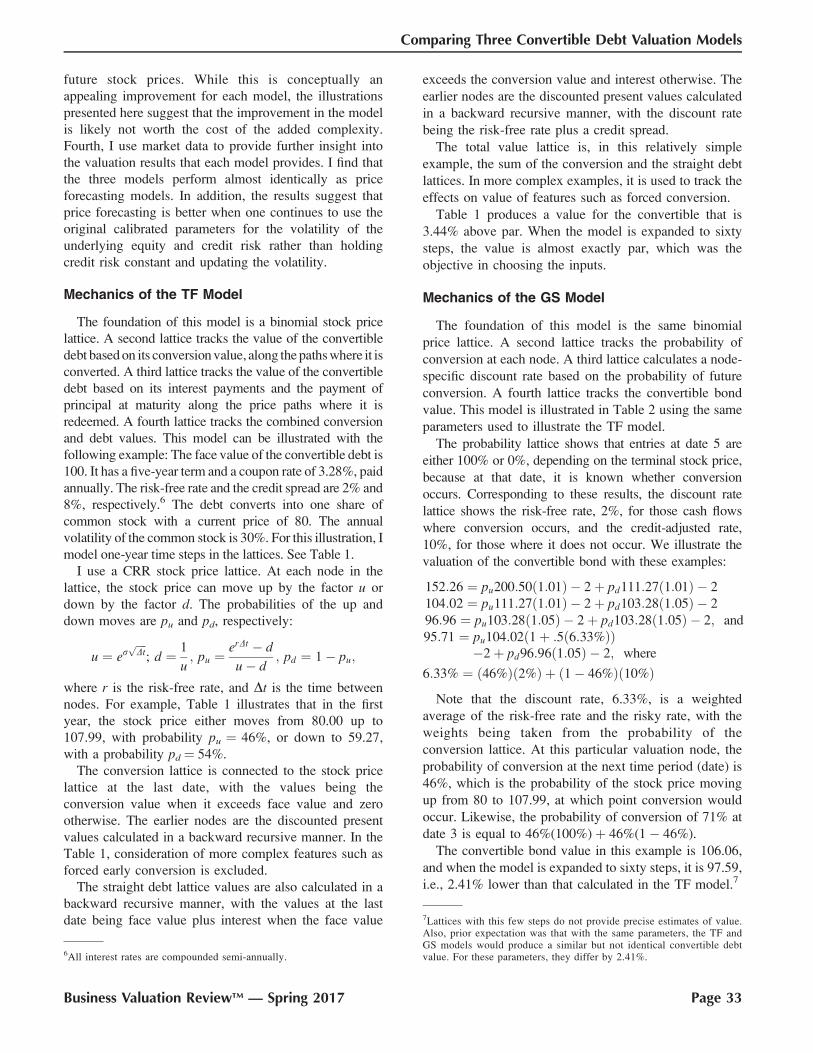
future stock prices. While this is conceptually an
appealing improvement for each model, the illustrations
presented here suggest that the improvement in the model
is likely not worth the cost of the added complexity.
Fourth, I use market data to provide further insight into
the valuation results that each model provides. I find that
the three models perform almost identically as price
forecasting models. In addition, the results suggest that
price forecasting is better when one continues to use the
original calibrated parameters for the volatility of the
underlying equity and credit risk rather than holding
credit risk constant and updating the volatility.
Mechanics of the TF Model
The foundation of this model is a binomial stock price
lattice. A second lattice tracks the value of the convertible
debt based on its conversion value, along the paths where it is
converted. A third lattice tracks the value of the convertible
debt based on its interest payments and the payment of
principal at maturity along the price paths where it is
redeemed. A fourth lattice tracks the combined conversion
and debt values. This model can be illustrated with the
following example: The face value of the convertible debt is
100. It has a five-year term and a coupon rate of 3.28%, paid
annually. The risk-free rate and the credit spread are 2% and
8%, respectively.6 The debt converts into one share of
common stock with a current price of 80. The annual
volatility of the common stock is 30%. For this illustration, I
model one-year time steps in the lattices. See Table 1.
I use a CRR stock price lattice. At each node in the
lattice, the stock price can move up by the factor u or
down by the factor d. The probabilities of the up and
down moves are pu and pd, respectively:
u ¼ erffiffiffiffiDtp
; d ¼ 1
u; pu ¼
erDt � d
u� d; pd ¼ 1� pu;
where r is the risk-free rate, and Dt is the time between
nodes. For example, Table 1 illustrates that in the first
year, the stock price either moves from 80.00 up to
107.99, with probability pu ¼ 46%, or down to 59.27,
with a probability pd ¼ 54%.
The conversion lattice is connected to the stock price
lattice at the last date, with the values being the
conversion value when it exceeds face value and zero
otherwise. The earlier nodes are the discounted present
values calculated in a backward recursive manner. In the
Table 1, consideration of more complex features such as
forced early conversion is excluded.
The straight debt lattice values are also calculated in a
backward recursive manner, with the values at the last
date being face value plus interest when the face value
exceeds the conversion value and interest otherwise. The
earlier nodes are the discounted present values calculated
in a backward recursive manner, with the discount rate
being the risk-free rate plus a credit spread.
The total value lattice is, in this relatively simple
example, the sum of the conversion and the straight debt
lattices. In more complex examples, it is used to track the
effects on value of features such as forced conversion.
Table 1 produces a value for the convertible that is
3.44% above par. When the model is expanded to sixty
steps, the value is almost exactly par, which was the
objective in choosing the inputs.
Mechanics of the GS Model
The foundation of this model is the same binomial
price lattice. A second lattice tracks the probability of
conversion at each node. A third lattice calculates a node-
specific discount rate based on the probability of future
conversion. A fourth lattice tracks the convertible bond
value. This model is illustrated in Table 2 using the same
parameters used to illustrate the TF model.
The probability lattice shows that entries at date 5 are
either 100% or 0%, depending on the terminal stock price,
because at that date, it is known whether conversion
occurs. Corresponding to these results, the discount rate
lattice shows the risk-free rate, 2%, for those cash flows
where conversion occurs, and the credit-adjusted rate,
10%, for those where it does not occur. We illustrate the
valuation of the convertible bond with these examples:
152:26 ¼ pu200:50ð1:01Þ � 2þ pd111:27ð1:01Þ � 2
104:02 ¼ pu111:27ð1:01Þ � 2þ pd103:28ð1:05Þ � 2
96:96 ¼ pu103:28ð1:05Þ � 2þ pd103:28ð1:05Þ � 2; and
95:71 ¼ pu104:02ð1þ :5ð6:33%ÞÞ�2þ pd96:96ð1:05Þ � 2; where
6:33% ¼ ð46%Þð2%Þ þ ð1� 46%Þð10%Þ
Note that the discount rate, 6.33%, is a weighted
average of the risk-free rate and the risky rate, with the
weights being taken from the probability of the
conversion lattice. At this particular valuation node, the
probability of conversion at the next time period (date) is
46%, which is the probability of the stock price moving
up from 80 to 107.99, at which point conversion would
occur. Likewise, the probability of conversion of 71% at
date 3 is equal to 46%(100%) þ 46%(1� 46%).
The convertible bond value in this example is 106.06,
and when the model is expanded to sixty steps, it is 97.59,
i.e., 2.41% lower than that calculated in the TF model.7
6All interest rates are compounded semi-annually.
7Lattices with this few steps do not provide precise estimates of value.Also, prior expectation was that with the same parameters, the TF andGS models would produce a similar but not identical convertible debtvalue. For these parameters, they differ by 2.41%.
Business Valuation ReviewTM — Spring 2017 Page 33
Comparing Three Convertible Debt Valuation Models
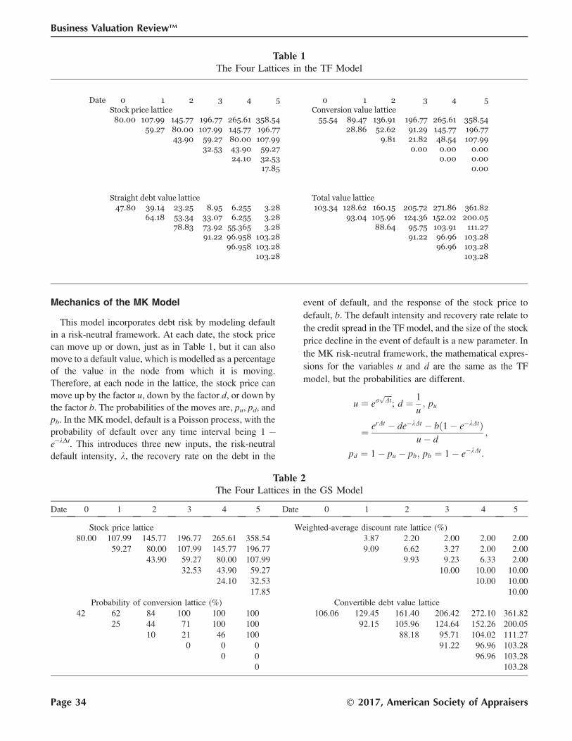
Mechanics of the MK Model
This model incorporates debt risk by modeling default
in a risk-neutral framework. At each date, the stock price
can move up or down, just as in Table 1, but it can also
move to a default value, which is modelled as a percentage
of the value in the node from which it is moving.
Therefore, at each node in the lattice, the stock price can
move up by the factor u, down by the factor d, or down by
the factor b. The probabilities of the moves are, pu, pd, and
pb. In the MK model, default is a Poisson process, with the
probability of default over any time interval being 1 �e�kDt. This introduces three new inputs, the risk-neutral
default intensity, k, the recovery rate on the debt in the
event of default, and the response of the stock price to
default, b. The default intensity and recovery rate relate to
the credit spread in the TF model, and the size of the stock
price decline in the event of default is a new parameter. In
the MK risk-neutral framework, the mathematical expres-
sions for the variables u and d are the same as the TF
model, but the probabilities are different.
u ¼ erffiffiffiffiDtp
; d ¼ 1
u; pu
¼ erDt � de�kDt � bð1� e�kDtÞu� d
;
pd ¼ 1� pu � pb; pb ¼ 1� e�kDt:
Table 1The Four Lattices in the TF Model
Table 2The Four Lattices in the GS Model
Date 0 1 2 3 4 5 Date 0 1 2 3 4 5
Stock price lattice Weighted-average discount rate lattice (%)
80.00 107.99 145.77 196.77 265.61 358.54 3.87 2.20 2.00 2.00 2.00
59.27 80.00 107.99 145.77 196.77 9.09 6.62 3.27 2.00 2.00
43.90 59.27 80.00 107.99 9.93 9.23 6.33 2.00
32.53 43.90 59.27 10.00 10.00 10.00
24.10 32.53 10.00 10.00
17.85 10.00
Probability of conversion lattice (%) Convertible debt value lattice
42 62 84 100 100 100 106.06 129.45 161.40 206.42 272.10 361.82
25 44 71 100 100 92.15 105.96 124.64 152.26 200.05
10 21 46 100 88.18 95.71 104.02 111.27
0 0 0 91.22 96.96 103.28
0 0 96.96 103.28
0 103.28
Page 34 � 2017, American Society of Appraisers
Business Valuation ReviewTM

The stock price lattice in Table 3 is built with the same
inputs as those used for Table 1 and the addition of a
default intensity of 14.6%, a recovery rate of 40%, and a
jump to default of �70%, meaning b ¼ 0.30. To make
Tables 1 and 2 comparable, the default intensity is based
on the risk-free rate and the credit spread used in the TF
model; namely, it is the risk-neutral default intensity
consistent with a five-year, 3.28% coupon debt with a
40% recovery rate that is priced to yield 10% (2%þ 8%).
In Table 3, the stock price moves from 80.00 either up to
107.99 or down to 59.27 or into bankruptcy with a value
of 24.00¼0.30(80).8 Likewise, at date 1, if the stock price
moved down to 59.27, it can next move up to 80.00, down
to 43.90, or into bankruptcy at 17.78¼ 0.30(59.27). In the
bankruptcy states, the value of the convertible debt is the
higher of its conversion value or the recovery value,
which is 40.
Because all of the discounting in this model is at the
risk-free rate, the model requires only one other lattice,
one that tracks the value of the convertible debt. At date
5, the value of the convertible debt is the higher of its
value in conversion or its face value, plus interest. At
each of the other nodes, the value of the convertible is
calculated in a backward recursive manner as the
discounted probability-weighted values it can assume at
the next date. In this illustration, the value of the
convertible debt is 101.30, and for the sixty-step version
of the model, the value is 102.94, i.e., 2.94% higher than
the value produced by the TF model.
Comparison of the Changes in Values of theThree Models as Parameters Change
Having illustrated the mechanics of the models, I now
compare the changes in their values when their
parameters are varied. To increase the precision of the
results discussed here, they are based on sixty-step
implementations of each model. I adopt the parameters
discussed in the previous section as a base case. I measure
the effect on the price of the convertible for two
additional credit spreads, 4% and 12%, for levels of
price decline �70% and �100% (b ¼ 0.30 and b ¼ 0.0)
and for two tenors, five years and ten years. For the ten-
year tenor, the coupon rate is decreased to 2.93%, so that
the TF model calibrates to par. Table 4 presents the
results.
I discuss the results for the TF and GS models first. For
both the five-year term and the ten-year term, the base case
value of the convertible debt is par for TS by design and close
to par for the other two models. For each term, I increase and
decrease the credit spread by 400 basis points. As would be
expected, the value of the convertible increases when the
credit spread declines and decreases when the credit spread
increases. For these parameters, the changes in values are
10.8% and �8.6% for the five-year term and 15.0% and
�10.4% for the ten-year term. For the GS models, the
corresponding changes in value are similar, but somewhat
larger in both directions, 11.6% and�10.0% for the five-year
term and 17.8% and�14.0% for the ten-year term.
The MK model values the convertible at very close to par
for the base case when the equity jump is�70%, i.e., 102.94
and 100.60 for the five-year and ten-year terms, respectively.
Table 3The Two Lattices in the MK Model
8This feature tends to offset the undesirable effect of the probability ofdefault being unchanged as the stock price increases.
Business Valuation ReviewTM — Spring 2017 Page 35
Comparing Three Convertible Debt Valuation Models

However, if an equity jumpof�100% isselected, the value of
the convertible is substantially larger, 114.59 and 123.85 for
the five-year and ten-year terms, respectively. It is important
to understand this counterintuitive result. The total volatility
of the common stock price is a function of the familiar
volatility used in the TF model,r¼30% in this example, and
the size of the equity jump and the probability of default.
Specifically, total stock price volatility for the MK model9 isffiffiffiffiffiffiffiffiffiffiffiffiffiffiffiffiffiffir2 þ kb2p
. When b is 0.30, total volatility is 42.5%, and
when b is 0.00, total volatility is 55.5%. This increase in
volatility explains why the value of the convertible debt
increases when the equity price jump is�100% rather than
�70%. This point also highlights that the two models are not
comparable with respect to volatility. For the MK model to
have a total volatility in the base case with a stock price jump
of�70%, the usual volatility term, referred to as r, would
have to be 13.6%. For those parameters, the value of the
convertible would decrease from 102.94 to 96.48. I will
return to this subject when I discuss the estimation of the
parameters for the models and the models’ relative merits.
When the credit spread is decreased by 400 basis points,
the corresponding default intensity decreases from 14.60%
to 8.36%; when the credit spread is increased by 400 basis
points, the default intensity increases from 14.60% to
57.28%. The effect on the value of the convertible is not as
straightforward as for the TF and GS models and depends
on the size of the equity price jump because of its effect on
volatility, as just discussed. I highlight one case: When the
equity jump is �100%, a decrease and an increase in the
credit spread of 400 basis points increases the value of the
convertible debt by almost equal amounts, 1.67 and 1.98.
The increase in the value of the convertible in the MK
model in response to an increase in the credit spread is a
clear and important difference between the MK model and
the TF and GS models, and I view it as a negative feature
of the MK model.
The values produced by the models can also be
compared for different degrees of moneyness. Table 5
reports the values of the convertible debt for the five-year
and ten-year terms, the two equity jumps, �70% and
�100%, and three levels of moneyness, 60%, 80% (the
base case), and 100%. The changes in values attributable
to the change in moneyness (common stock price) are
both reasonable and consistent among the three models.
Addressing a Common Shortcoming of theModels
All three of these models implicitly assume that the
probability of bankruptcy is independent of the price of the
underlying common stock price. In general, that is an
unreasonable assumption. I would expect the credit spread
in the TF and the GS models and the default intensity in
Table 4Convertible Debt Values for the TF and MK Models for Combinations of Parameters
S/X ¼ 80/100 80% 80%
Term (years) 5.00 10.00
Coupon Rate (%) 3.28 2.93
Model TF GS MK TF GS MK
Recovery Rate (%) 40.00 40.00
Credit Spread/Default Intensity (%) 4.00 4.00 8.36 4.00 4.00 7.27
Equity Jump (%) �70 �100 �70 �100
Volatility (%) 30.0 30.0 35.1 43.7 30.0 30.0 35.4 44.5
Pure Bond 88.40 88.40 88.40 88.40 77.15 77.15 77.15 77.15
Conversion Value 22.18 21.26 22.93 27.86 37.84 35.60 36.75 47.22
Convertible 110.58 109.66 111.33 116.26 114.98 112.75 113.90 124.37Credit Spread/Default Intensity (%) 8.00 8.00 14.60 8.00 8.00 18.57
Equity Jump (%) �70 �100 �70 �100
Volatility (%) 30.0 30.0 40.2 55.5 30.0 30.0 42.5 60.6
Pure Bond 74.05 74.05 74.05 74.05 55.93 55.93 55.93 55.93
Conversion Value 25.96 23.63 28.89 40.54 44.07 38.12 44.67 67.91
Convertible 100.00 97.68 102.94 114.59 100.00 94.05 100.60 123.85Credit Spread/Default Intensity (%) 12.00 12.00 57.28 12.00 12.00 93.56
Equity Jump (%) �70 �100 �70 �100
Volatility (%) 30.0 30.0 45.7 67.2 30.0 30.0 74.1 121.8
Pure Bond 62.35 62.35 62.35 62.35 41.35 41.35 41.35 41.35
Conversion Value 29.02 25.07 35.08 54.22 48.24 38.17 47.17 80.56
Convertible 91.37 87.42 97.44 116.57 89.59 79.52 88.52 121.91
9See Milanov and Kounchev (2012), who derive this relationship basedon the assumption that default and stock price are uncorrelated.
Page 36 � 2017, American Society of Appraisers
Business Valuation ReviewTM

the MK model to be inversely related to the price of the
common stock. In this section of the paper, I examine the
effects on value of introducing this relationship.
The results for the TF and GS models are similar, and so I
discuss the TF model in detail. The credit spread is
expressed as a modified power function with the degree of
moneyness as the independent variable. This produces a
credit spread lattice in which the credit spread at each node
is determined by the power function and the stock price at
the corresponding node in the stock price lattice. Credit
adjustment of debt cash flows is node (stock price) specific.
I identify parameters of the modified power function such
that the credit spread for a stock price of 80 is approximately
the 8% used in the base case. Figure 1 displays the function.
For the MK model, I follow a similar process. In this case,
I develop a default intensity lattice that is a function of the
stock price. This gives rise to corresponding probability
lattices for the each of the three possible price moves, u, d,
and b, and the default intensity and the probabilities are all
node (stock price) specific. I identify a function such that the
default intensity for a price of 80 is approximately the 14.6%
used in the base case. Figure 2 displays the function.10
The operative question is whether these changes in the
models, which are complex and require judgment with
respect to the functional form of the credit spread and
default intensity equations, are worth the effort. The
results in Table 6 suggest that they are not. For the five-
year convertible debt, the price differences caused by the
more complex models range from less than 1% to a
maximum of 4%. To illustrate this result, consider the
base case. With a constant credit spread or default
intensity, the values of the five-year debt are 100.00,
102.94, and 114.59 for the TF model and the two versions
of the MK model, respectively. When the price-varying
spread and default intensity are introduced, the values are
98.02, 103.79, and 111.62, respectively, i.e., differences
of only 2.0%,�0.8%, and 2.6%.
Examining the Pricing Performance of the ThreeModels
I collected data on convertible debt issued by
companies with publicly traded common stock from
Table 5Convertible Debt Values for the TF and MK Models for Degrees of Moneyness
Term 5.00 10.00
Coupon Rate (%) 3.28 2.93
Model TF GS MK TF GS MK
Recovery Rate (%) 40.00 40.00
Credit Spread/Default Intensity (%) 8.00 8.00 14.60 8.00 8.00 18.57
Equity Jump (%) �70 �100 �70 �100
Volatility (%) 30.0 30.0 40.2 55.5 30.0 30.0 42.5 60.6
S/X Convertible Value Convertible Value
60/100 ¼ 60% 87.99 86.79 89.54 97.53 80.29 75.32 85.55 104.03
80/100 ¼ 80% 100.01 97.68 102.94 114.59 100.00 94.05 101.04 123.77
100/100 ¼ 100% 115.10 111.83 118.45 132.96 114.23 104.93 117.83 143.64
For S/X ¼ 60%: % Change from 80% �12.0 �11.1 �13.0 �14.9 �19.7 �19.9 �15.3 �15.9
For S/X ¼100%: % Change from 80% 15.1 14.5 15.1 16.0 14.2 11.6 16.6 16.1
Table 6Convertible Debt Values for the TF and MK Models
for Degrees of Moneyness
S/X ¼ 80/100 80%
Term 5.00
Coupon Rate (%) 3.28
Model TF MK
Credit Spread/Default
Intensity (%) 4.00 8.36
Equity Jump (%) �70 �100
Constant 109.66 111.33 116.26
Inverse Function of
Stock Price 110.21 112.14 114.92
Credit Spread/Default
Intensity (%) 8.00 14.60
Equity Jump (%) �70 �100
Constant 97.68 102.94 114.59
Inverse Function of
Stock Price 98.02 103.79 111.62
Credit Spread/Default
Intensity (%) 12.00 57.28
Equity Jump (%) �70 �100
Constant 87.42 97.44 116.57
Inverse Function of
Stock Price 88.49 98.94 112.05
10I selected the functional forms in Figures 1 and 2 numerically such thatthe price effect of the credit adjustment went to zero as the convertibledebt was very deep in the money and to 100% when it was deep out ofthe money.
Business Valuation ReviewTM — Spring 2017 Page 37
Comparing Three Convertible Debt Valuation Models
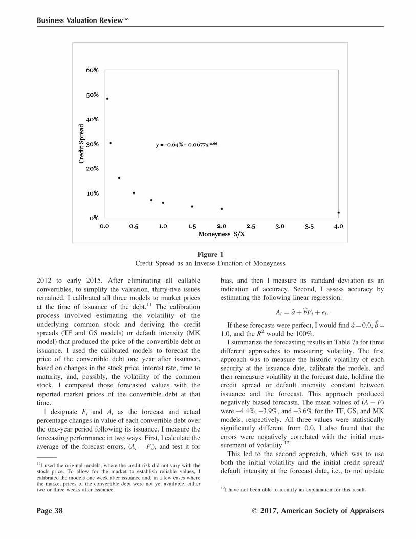
2012 to early 2015. After eliminating all callable
convertibles, to simplify the valuation, thirty-five issues
remained. I calibrated all three models to market prices
at the time of issuance of the debt.11 The calibration
process involved estimating the volatility of the
underlying common stock and deriving the credit
spreads (TF and GS models) or default intensity (MK
model) that produced the price of the convertible debt at
issuance. I used the calibrated models to forecast the
price of the convertible debt one year after issuance,
based on changes in the stock price, interest rate, time to
maturity, and, possibly, the volatility of the common
stock. I compared those forecasted values with the
reported market prices of the convertible debt at that
time.
I designate Fi and Ai as the forecast and actual
percentage changes in value of each convertible debt over
the one-year period following its issuance. I measure the
forecasting performance in two ways. First, I calculate the
average of the forecast errors, (Ai � Fi), and test it for
bias, and then I measure its standard deviation as an
indication of accuracy. Second, I assess accuracy by
estimating the following linear regression:
Ai ¼ baþ bbFi þ ei:
If these forecasts were perfect, I would find a¼0.0, b¼1.0, and the R2 would be 100%.
I summarize the forecasting results in Table 7a for three
different approaches to measuring volatility. The first
approach was to measure the historic volatility of each
security at the issuance date, calibrate the models, and
then remeasure volatility at the forecast date, holding the
credit spread or default intensity constant between
issuance and the forecast. This approach produced
negatively biased forecasts. The mean values of (A � F)
were�4.4%,�3.9%, and�3.6% for the TF, GS, and MK
models, respectively. All three values were statistically
significantly different from 0.0. I also found that the
errors were negatively correlated with the initial mea-
surement of volatility.12
This led to the second approach, which was to use
both the initial volatility and the initial credit spread/
default intensity at the forecast date, i.e., to not update
Figure 1Credit Spread as an Inverse Function of Moneyness
11I used the original models, where the credit risk did not vary with thestock price. To allow for the market to establish reliable values, Icalibrated the models one week after issuance and, in a few cases wherethe market prices of the convertible debt were not yet available, eithertwo or three weeks after issuance. 12I have not been able to identify an explanation for this result.
Page 38 � 2017, American Society of Appraisers
Business Valuation ReviewTM

the volatility estimate. The mean values of (A � F) for
this approach were 0.6%, 0.3%, and 0.0% for the TF,
GS, and MK models, respectively, and none was
statistically significantly different from 0.0. The
standard deviations of (A � F) for the second approach
were also smaller than those for the first approach,
indicating that it was not only unbiased, but also more
accurate.
The results for the case with constant volatility suggest
that consistency in the two inputs may be more important
than the precision of their individual estimations. To
investigate that, I tested a third approach to volatility,
namely, assuming a single constant volatility of 30% for
all securities at both dates. This approach also produced
unbiased forecasts with mean values of (A� F) of 0.3%,
0.3%, and �0.2% for the TF, GS, and MK models,
respectively. The accuracy of this third approach, as
indicated by the standard deviations of the forecast error,
is essentially identical to the accuracy of the second
approach. This supports the idea that consistency in the
two inputs is more important than the precision of their
estimations.
Figure 2Default Intensity as a Function of Moneyness
Table 7aResults of Price Forecasting Models
Alternative Volatility
Choices
TF GS MK
(A – F) (%)
Forecast
Regression (A – F) (%)
Forecast
Regression (A – F) (%)
Forecast
Regression
Mean
Standard
Deviation b R2 (%) Mean
Standard
Deviation b R2 Mean
Standard
Deviation b R2 (%)
Two Different Volatilities �4.39 8.02 0.91 90 �3.86 7.33 0.86 89 �3.55 6.76 0.93 87
One Volatility 0.65 6.93 0.97 93 0.29 5.90 0.92 93 �0.01 5.83 1.01 91
Volatility of 30% 0.30 6.41 0.88 93 0.27 6.48 0.88 91 �0.18 5.87 0.91 91
Business Valuation ReviewTM — Spring 2017 Page 39
Comparing Three Convertible Debt Valuation Models
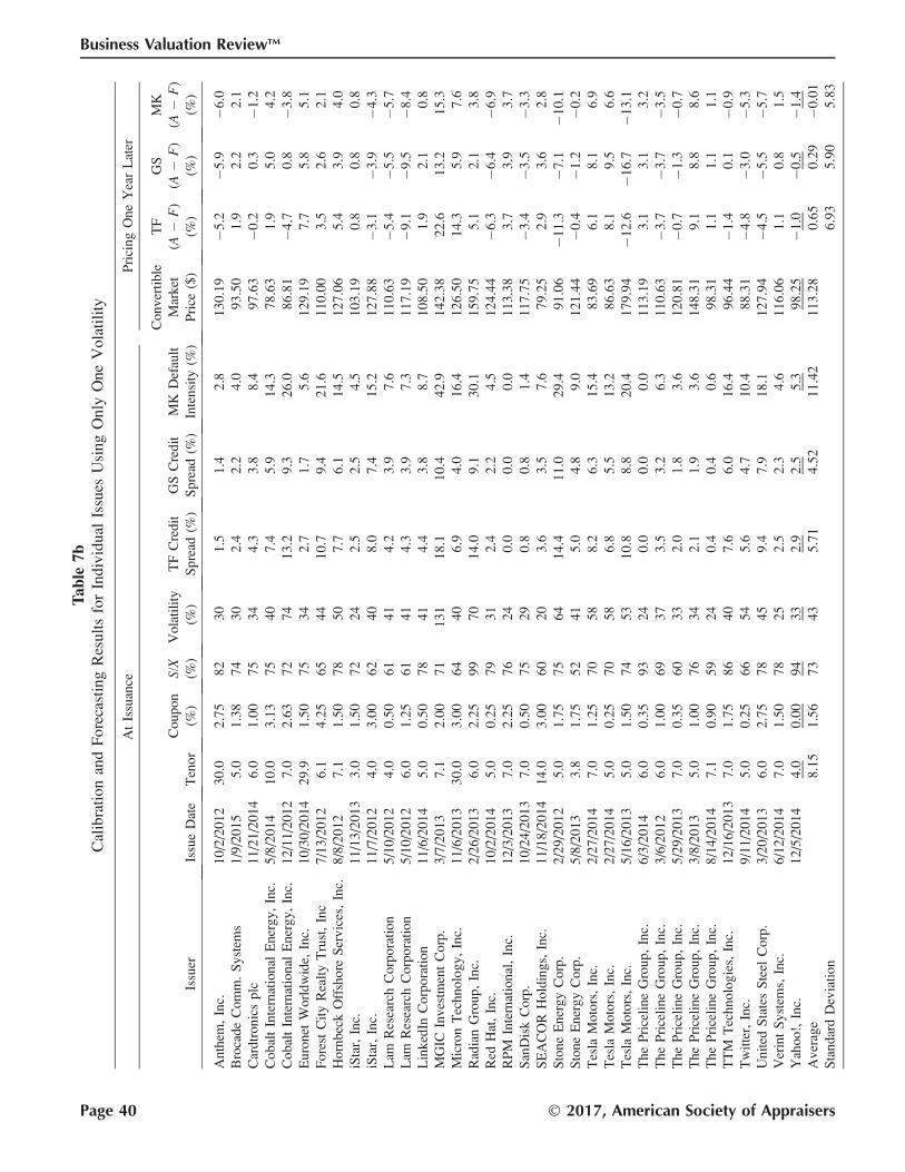
Tab
le7b
Cal
ibra
tion
and
Fore
cast
ing
Res
ult
sfo
rIn
div
idual
Issu
esU
sing
Only
One
Vola
tili
ty
At
Issu
ance
Pri
cin
gO
ne
Yea
rL
ater
Issu
erIs
sue
Dat
eT
eno
r
Co
up
on
(%)
S/X
(%)
Vo
lati
lity
(%)
TF
Cre
dit
Sp
read
(%)
GS
Cre
dit
Sp
read
(%)
MK
Def
ault
Inte
nsi
ty(%
)
Co
nv
erti
ble
Mar
ket
Pri
ce($
)
TF
(A�
F)
(%)
GS
(A�
F)
(%)
MK
(A�
F)
(%)
An
them
,In
c.1
0/2
/20
12
30
.02
.75
82
30
1.5
1.4
2.8
13
0.1
9�
5.2
�5
.9�
6.0
Bro
cad
eC
om
m.
Sy
stem
s1
/9/2
01
55
.01
.38
74
30
2.4
2.2
4.0
93
.50
1.9
2.2
2.1
Car
dtr
on
ics
plc
11
/21
/20
14
6.0
1.0
07
53
44
.33
.88
.49
7.6
3�
0.2
0.3
�1
.2
Co
bal
tIn
tern
atio
nal
En
erg
y,
Inc.
5/8
/20
14
10
.03
.13
75
40
7.4
5.9
14
.37
8.6
31
.95
.04
.2
Co
bal
tIn
tern
atio
nal
En
erg
y,
Inc.
12
/11
/20
12
7.0
2.6
37
27
41
3.2
9.3
26
.08
6.8
1�
4.7
0.8
�3
.8
Eu
ron
etW
orl
dw
ide,
Inc.
10
/30
/20
14
29
.91
.50
75
34
2.7
1.7
5.6
12
9.1
97
.75
.85
.1
Fo
rest
Cit
yR
ealt
yT
rust
,In
c7
/13
/20
12
6.1
4.2
56
54
41
0.7
9.4
21
.61
10
.00
3.5
2.6
2.1
Ho
rnb
eck
Off
sho
reS
erv
ices
,In
c.8
/8/2
01
27
.11
.50
78
50
7.7
6.1
14
.51
27
.06
5.4
3.9
4.0
iSta
r,In
c.1
1/1
3/2
01
33
.01
.50
72
24
2.5
2.5
4.5
10
3.1
90
.80
.80
.8
iSta
r,In
c.1
1/7
/20
12
4.0
3.0
06
24
08
.07
.41
5.2
12
7.8
8�
3.1
�3
.9�
4.3
Lam
Res
earc
hC
orp
ora
tio
n5
/10
/20
12
4.0
0.5
06
14
14
.23
.97
.61
10
.63
�5
.4�
5.5
�5
.7
Lam
Res
earc
hC
orp
ora
tio
n5
/10
/20
12
6.0
1.2
56
14
14
.33
.97
.31
17
.19
�9
.1�
9.5
�8
.4
Lin
ked
InC
orp
ora
tio
n1
1/6
/20
14
5.0
0.5
07
84
14
.43
.88
.71
08
.50
1.9
2.1
0.8
MG
ICIn
ves
tmen
tC
orp
.3
/7/2
01
37
.12
.00
71
13
11
8.1
10
.44
2.9
14
2.3
82
2.6
13
.21
5.3
Mic
ron
Tec
hn
olo
gy
,In
c.1
1/6
/20
13
30
.03
.00
64
40
6.9
4.0
16
.41
26
.50
14
.35
.97
.6
Rad
ian
Gro
up
,In
c.2
/26
/20
13
6.0
2.2
59
97
01
4.0
9.1
30
.11
59
.75
5.1
2.1
3.8
Red
Hat
,In
c.1
0/2
/20
14
5.0
0.2
57
93
12
.42
.24
.51
24
.44
�6
.3�
6.4
�6
.9
RP
MIn
tern
atio
nal
,In
c.1
2/3
/20
13
7.0
2.2
57
62
40
.00
.00
.01
13
.38
3.7
3.9
3.7
San
Dis
kC
orp
.1
0/2
4/2
01
37
.00
.50
75
29
0.8
0.8
1.4
11
7.7
5�
3.4
�3
.5�
3.3
SE
AC
OR
Ho
ldin
gs,
Inc.
11
/18
/20
14
14
.03
.00
60
20
3.6
3.5
7.6
79
.25
2.9
3.6
2.8
Sto
ne
En
erg
yC
orp
.2
/29
/20
12
5.0
1.7
57
56
41
4.4
11
.02
9.4
91
.06
�1
1.3
�7
.1�
10
.1
Sto
ne
En
erg
yC
orp
.5
/8/2
01
33
.81
.75
52
41
5.0
4.8
9.0
12
1.4
4�
0.4
�1
.2�
0.2
Tes
laM
oto
rs,
Inc.
2/2
7/2
01
47
.01
.25
70
58
8.2
6.3
15
.48
3.6
96
.18
.16
.9
Tes
laM
oto
rs,
Inc.
2/2
7/2
01
45
.00
.25
70
58
6.8
5.5
13
.28
6.6
38
.19
.56
.6
Tes
laM
oto
rs,
Inc.
5/1
6/2
01
35
.01
.50
74
53
10
.88
.82
0.4
17
9.9
4�
12
.6�
16
.7�
13
.1
Th
eP
rice
lin
eG
rou
p,
Inc.
6/3
/20
14
6.0
0.3
59
32
40
.00
.00
.01
13
.19
3.1
3.1
3.2
Th
eP
rice
lin
eG
rou
p,
Inc.
3/6
/20
12
6.0
1.0
06
93
73
.53
.26
.31
10
.63
�3
.7�
3.7
�3
.5
Th
eP
rice
lin
eG
rou
p,
Inc.
5/2
9/2
01
37
.00
.35
60
33
2.0
1.8
3.6
12
0.8
1�
0.7
�1
.3�
0.7
Th
eP
rice
lin
eG
rou
p,
Inc.
3/8
/20
13
5.0
1.0
07
63
42
.11
.93
.61
48
.31
9.1
8.8
8.6
Th
eP
rice
lin
eG
rou
p,
Inc.
8/1
4/2
01
47
.10
.90
59
24
0.4
0.4
0.6
98
.31
1.1
1.1
1.1
TT
MT
ech
no
log
ies,
Inc.
12
/16
/20
13
7.0
1.7
58
64
07
.66
.01
6.4
96
.44
�1
.40
.1�
0.9
Tw
itte
r,In
c.9
/11
/20
14
5.0
0.2
56
65
45
.64
.71
0.4
88
.31
�4
.8�
3.0
�5
.3
Un
ited
Sta
tes
Ste
elC
orp
.3
/20
/20
13
6.0
2.7
57
84
59
.47
.91
8.1
12
7.9
4�
4.5
�5
.5�
5.7
Ver
int
Sy
stem
s,In
c.6
/12
/20
14
7.0
1.5
07
82
52
.52
.34
.61
16
.06
1.1
0.8
1.5
Yah
oo
!,In
c.1
2/5
/20
14
4.0
0.0
09
43
32
.92
.55
.39
8.2
5�
1.0
�0
.5�
1.4
Av
erag
e8
.15
1.5
67
34
35
.71
4.5
21
1.4
21
13
.28
0.6
50
.29
�0
.01
Sta
nd
ard
Dev
iati
on
6.9
35
.90
5.8
3
Page 40 � 2017, American Society of Appraisers
Business Valuation ReviewTM

When I measure forecast performance in terms of a
regression of actual percentage change on forecast
percentage change, I find the results are very similar for
the three methods of measuring volatility and for the three
models. Using two different volatilities produces slightly
lower R2 values for the TF and GS models, and given that
its forecasts are biased, I would tend to reject the idea of
trying to update the volatility when holding the measure
of credit risk constant. The TF and GS models have
slightly higher R2 values than the MK model, but the
differences are so small that all three models perform
essentially identically. This conclusion is further rein-
forced by the fact that the pair-wise R2 values between the
three forecasts using a single volatility are greater than
99.5%.
In Table 7b, I provide summary statistics and
individual results for the thirty-five convertible debt
securities in this sample for the analysis using a single
volatility. The average tenor of the convertibles at
issuance was 8.15 years, the average coupon was
1.56%, the average degree of moneyness was 73%, and
the average volatility was 43%.13 The average credit
spreads were 5.85% for the TF model and 4.61% for
the GS model. It appears that the credit spread for the
TF model is consistently larger than that for the GS
model. This means that in the context of partitioning
the debt value for financial reporting purposes, the TF
model will consistently identify a smaller debt value
and higher yield than the GS model. The average
default intensity was 11.42%. In general, this value
translates to an effective yield that is higher and bond
value that is lower than either of the credit spread
models.
Conclusions
In three important respects, the convertible debt
models are very similar. First, the base case example
illustrated that the three models produce quite similar
prices for the same inputs and a jump in the stock price of
�70% in the event of default. Second, I showed that there
is little effect on the value of the convertible if the credit
spread or default intensity is a function of stock price.
Third, I provide evidence that the three models perform
well in forecasting convertible debt prices one year after
calibrating each of the models to market data. In the
context of estimating convertible debt prices for non-
traded securities for financial reporting purposes, this is
reassuring. I also identified one important difference in
the comparative responses of the TF and GS models and
the MK model to changes in credit quality. Contrary to
expectations, the convertible debt price produced by the
MK model increased when credit quality decreased. This
is because there is a complex relationship between credit
quality and volatility of equity, such that the decrease in
credit quality increased stock price volatility and
increased the value of the conversion feature. This
observation highlights an important underlying differ-
ence in the assumptions of the TF and GS models as
compared to the MK model. The TF and GS models
assume that the stock price follows a geometric
Brownian motion, while the MK model assumes the
stock price follows a jump-diffusion process. This
difference should be considered in estimating the
volatilities to use in each model. In particular, volatility
estimation is more complex if you assume stock prices
follow a jump-diffusion process. That said, on the whole,
I find that the models are sufficiently similar that all three
can reasonably be used to estimate the value of nontraded
convertible debt and will provide very similar valuations
of the convertible debt. If these models are used to
partition the debt component, the debt component will
generally be largest for the TF model and smallest for the
MK model.
References
Cox, J. C., S. A. Ross, and M. E. Rubinstein. ‘‘Option
Pricing: A Simplified Approach.’’ Journal of FinancialEconomics 3 (September 1979):229–263.
Bardhan, I., A. Bergier, E. Derman, C. Dosembet, and I.
Kani. 1994. ‘‘Valuing Convertible Bonds as Deriva-
tives.’’ In Quantitative Strategies Research Notes. New
York: Goldman Sachs.
de Spiegeleer, J., and W. Schoutens. 2011. The Handbookof Convertible Bonds: Pricing, Strategies and RiskManagement. West Sussex, United Kingdom: John
Wiley & Sons Limited.
Hull, J. 2011. Options, Futures and Other Derivatives.
8th ed. Upper Saddle River, NJ: Prentice-Hall.
Jarrow, R. A., and A. Rudd. 1983. Option Pricing.
Homewood, IL: Irwin.
Milanov, Krasimir, and Ognyan Kounchev. June 2012.
Binomial Tree Model for Convertible Bond Pricingwithin Equity to Credit Risk Framework. Working
Paper of the Institute of Mathematics and Informatics.
Sofia, Bulgaria: Bulgarian Academy of Science.
Tsiveriotis, K., and C. Fernandes. ‘‘Valuing Convertible
Bonds with Credit Risk.’’ Journal of Fixed Income 8
(September 1998):95–102.
Zabolotnyuk, Y., R. Jones, and C. Veld. ‘‘An
Empirical Comparison of Convertible Bond Valua-
tion Models.’’ Financial Management 39 (Summer
2010):675–706.
13For two of the securities, the historical volatility implied negativecredit spreads and default intensity, and in those two cases, I adjusted thevolatilities until the credit spreads and default intensity were 0.0%.
Business Valuation ReviewTM — Spring 2017 Page 41
Comparing Three Convertible Debt Valuation Models

From the Chair
William A. Johnston, ASA
Hello again! Time certainly goes by fast, and this is my
last letter as Chair of the Business Valuation Committee.
Thank you for the opportunity to serve.
It’s Not Always Where You End, It’s the Journey . . .
Often I am asked the benefits of getting involved with
ASA. There are countless tangible benefits that are
obvious: the networking, the education, building your
credentials, etc. However, let me tell you another
reason—the challenges you face and how you deal with
them. You learn a lot from these experiences and are a
much better person and professional as a result.
So, you can choose to sit in your office and not expand
your horizons, or you can try new endeavors. When you
take on these challenges, sometimes you are going to fail.
Sometimes you do not know how you will get there or
what is waiting for you when you do. It is really the
journey getting there that I find most rewarding and what
has made me (I hope) a better person and professional.
Get outside of your comfort zone and push yourself, and
good things will happen as a result—trust me!
Fair Value Quality Initiative—CEIVTM Credential
The CEIVTM has launched. The three Valuation
Profession Organizations involved with this effort begun
offering the credential Certified in Entity and Intangible
ValuationsTM or CEIVTM. Do not worry if you do not
have the credential yet, as many people are just starting
the process or evaluating how to proceed.
Also remember that anyone can get the credential,
regardless whether you have a BV credential or not. The
pathway is longer, of course, but it can nonetheless be
done. Please be in touch with any questions.
Enhanced Equivalency for CFA Designation
I want to keep mentioning that the BV committee
approved increased equivalency for individuals with the
CFA designation, provided that they have at least five
years of full-time business valuation experience. Now, if
an individual has at least five years of full-time business
valuation experience and the CFA designation, he or she
is not required to take ASA’s BV 201 to BV 204 classes.
This decision was arrived at after a thorough review and
comparison of the CFA designation versus the ASA
designation. Candidates will still need to meet the other
requirements (e.g., submitting a report and our USPAP/
ethics requirements). If you are interested in learning
more about this, please be in touch with me directly
([email protected]) or contact ASA.
Last Words
I could not be more pleased to have such a high-quality
professional follow me as Chair as Jeff Tarbell. Our
committee could not be in any better hands, and if he
needs my help I will be there to provide it.
What a ride! What sets ASA apart the most in my
opinion is how much our members really care about the
profession and the quality of the work that they do—you
take it so seriously. Continue being proud and being
proud of ASA!
Page 42 � 2017, American Society of Appraisers
Business Valuation Reviewe
Volume 36 � Number 1
� 2017, American Society of Appraisers

Business Valuation Review™ – Spring 2017
The Business Valuation Committee
Chair William A. Johnston, ASA – Empire Valuation Consultants, LLC
Vice Chair Jeffrey S. Tarbell, ASA – Houlihan Lokey
Secretary Erin Hollis, ASA – Marshall & Stevens, Inc.
Treasurer Kenneth J. Pia, Jr., ASA – Meyers, Harrison & Pia, LLC
Past Chair Robert B. Morrison, ASA – Morrison Valuation & Forensic Services, LLC
Members At-Large Gregory Ansel, ASA – Financial Strategies Consulting Group LLC Arlene Ashcraft, ASA – Columbia Financial Advisors, Inc. KC Conrad, ASA – American Business Appraisers Matthew R. Crow, ASA – Mercer Capital Nancy M. Czaplinski, ASA – Duff & Phelps Erin Hollis, ASA – Marshall & Stevens, Inc. Bruce Johnson, ASA – Munroe, Park & Johnson, Inc. Curtis T. Johnson, ASA – Ernst & Young Timothy Meinhart, ASA – Willamette Management Associates Susan Saidens, ASA – SMS Valuation & Financial Forensics Ronald L. Seigneur, ASA – Seigneur Gustafson LLP Gary R. Trugman, ASA – Trugman Valuation Associates, Inc. Mark Zyla, ASA – Acuitas, Inc.
Ex Officio James O. Brown, ASA – Perisho Tombor Brown, PC R. Chris Rosenthal, ASA – Ellin & Tucker Linda B. Trugman, ASA – Trugman Valuation Associates, Inc.
Emeritus Jay E. Fishman, FASA – Financial Research Associates Shannon P. Pratt, FASA – Shannon Pratt Valuations, LLC
HQ Advisor Bonny Price
BUSINESS VALUATION REVIEW TM —Published quarterly by the Business Valuation Committee of the American Society of Appraisers. Editor: Daniel L. McConaughy, PhD, ASA. Managing Editor: Rita Janssen, [email protected].
INTERNATIONAL STANDARD SERIAL NUMBER—The Library of Congress, National Serials Data Pro = ISSN 0897-1781.SUBSCRIPTION RATES—PRINT AND ELECTRONIC ACCESS: Members of American Society of Appraisers-$60 if paid with annual dues;
all others—$140 per year. Direct any questions and/or subscription changes to Bonny F. Price (703) 733-2110 or [email protected]—Authors should submit their articles (including charts, graphs, pictures, etc.) for publication in Business Valuation Review™
at http://www.editorialmanager.com/bvr/. Follow the new user registration login instructions, at the Register Now hotlink. Since we use a double-blind peer review system, authors should provide the author’s name (as it would appear if published), and a short one-paragraph description of professional activities when completing the registration process. An abstract should appear at the beginning of the paper submitted for review. Authors are asked to not submit manuscripts currently under review by other publications or that have been published elsewhere. All manuscripts are reviewed by the Editorial Review Board and may be accepted, rejected, or returned for additional work. Editor’s notes may be included with the printing of accepted articles. All authors will be so notified. No manuscripts will be returned, and no critiques or reasons for rejection will be given for material not selected for publication.
CLASSIFIED ADS—Accepted for publication in one issue only and should reach the Publisher no later than the 10th of the month prior to publication. Rates: full page—$500, 2/3 page—$375, 1/2 page—$300, 1/3 page—$200, 1/4 page—$150. Payable in U.S. funds. Direct any questions to Bonny F. Price (703) 733-2110 or [email protected]
LETTERS TO THE EDITOR & COMMENTS—Letters from readers are encouraged on any valuation subject. BVR™ reserves the right to edit letters for length, taste and/or clarity. No guarantee of publica tion is given. Please direct critique or comments to the Editor. All Letters to the Editor should be submitted at http://www.editorialmanager.com/bvr/.
STATEMENTS & OPINIONS—Statements expressed herein by the authors and contributors to Business Valuation Review™ are their own and not necessarily those of the American Society of Appraisers or its Business Valuation Committee.
Copyright, © American Society of Appraisers—2017All rights reserved. For permission to reproduce in whole or part, and for quotation privilege, contact International Headquarters of ASA. Neither the Society nor its Editor accepts responsibility for statements or opinions advanced in articles appearing herein, and their appearance does not necessarily constitute an endorsement.
EditorDaniel L. McConaughy, PhD, ASA
California State University Northridge
Managing EditorRita Janssen
Lawrence, Kansas
Business ManagerJames O. Brown, ASA Campbell, California
ReviewersAshok Abbott*, PhD
Morgantown, West Virginia
John D. Finnerty, PhD New York, New York
Stillian Ghaidarov
Roger Grabowski*, FASA Chicago, Illinois
*Editorial Board Member
Editors EmeritusJames H. Schilt, ASA (1982–2001)
San Francisco, California
Jay E. Fishman, FASA (2002–2007) Bala Cynwyd, Pennsylvania
Roger J. Grabowski, FASA (2008–2012) Chicago, Illinois
Publishers EmeritusJohn E. Bakken, FASA (1982–2003)
Granby, Colorado
Ralph Arnold, III, ASA (2004–2007) Portland, Oregon
BVR™ Editorial Review Board
© 2017, American Society of Appraisers

Volume 36
Issue 1
Spring 2017
1 Editor’s Column Dan McConaughy, PhD, ASA
3 American Society of Appraisers Business Valuation Committee Special Topics Paper #3 The Use of Management’s Prospective Financial Information by a Valuation Analyst
7 Petroleum Property Income and Market Valuation Approaches (Transactions Beware!) Louis R. Posgate, ASA, PE, CMA
9 A Primer on Bargain Purchases and Negative Goodwill Dan Daitchman, ASA
15 Statutory Fair Value in Dissenting Shareholder Cases—Part I Gilbert E. Matthews, MBA, CFA
32 Comparing Three Convertible Debt Valuation Models Dwight Grant, PhD
42 From the Chair of the Business Valuation Committee William A. Johnston, ASA
Quar
terly
Jour
nal o
f the
Bus
ines
s Val
uatio
n Co
mm
ittee
of t
he A
mer
ican
Socie
ty o
f App
raise
rs
Published by the American Society of Appraisers Copyright © 2017 American Society of Appraisers