
Calibration and Verification Test of Lily Bulb Simulation ... - MDPI
Upload
khangminh22Category
view
0download
0
Citation: Ernst, Dietmar. 2022.
Simulation-Based Business Valuation:
Methodical Implementation in the
Valuation Practice. Journal of Risk and
Financial Management 15: 200.
https://doi.org/10.3390/jrfm15050200
Academic Editor: Xiaofei Pan
Received: 23 March 2022
Accepted: 20 April 2022
Published: 26 April 2022
Publisher’s Note: MDPI stays neutral
with regard to jurisdictional claims in
published maps and institutional affil-
iations.
Copyright: © 2022 by the author.
Licensee MDPI, Basel, Switzerland.
This article is an open access article
distributed under the terms and
conditions of the Creative Commons
Attribution (CC BY) license (https://
creativecommons.org/licenses/by/
4.0/).
Journal of
Risk and FinancialManagement
Article
Simulation-Based Business Valuation: MethodicalImplementation in the Valuation PracticeDietmar Ernst
International School of Finance (IFS), Nuertingen-Geislingen University, Sigmaringer Straße 25,72622 Nürtingen, Germany; [email protected]; Tel.: +49-7022-201-1021
Abstract: The simulation-based company valuation values a company on the basis of the risks actuallypresent in the company without having to derive them from the capital market data. The simulation-based company valuation takes into account the market imperfections, such as the probability ofinsolvency or the lack of diversification, and fulfils the legal requirements and auditing standards fora company valuation. The simulation-based company valuation is an alternative to the CAPM-basedcompany valuation, which, under the assumption of perfect capital markets, derives the risks throughcapital market comparisons. A simulation-based business valuation has many advantages and isparticularly suitable for valuing medium-sized companies, start-ups, companies in a crisis, and forintegrating country-specific risks into business valuations. Due to the internationally widespread useof the CAPM, a simulation-based company valuation is still rarely used in practice. This article showswhich valuation formulas are necessary for the application of a simulation-based company valuation.These are used for both the certainty equivalent method and for the risk premium method. In aconcrete and valuation example, the simulation-based business planning and company valuation iscarried out, and the derived valuation formulas are applied in a way that allows a transfer to concretevaluation cases in practice. It is shown that the certainty equivalent method and the risk premiummethod lead to identical company values.
Keywords: company valuation; simulation; Gordon Growth Model; certainty equivalent; risk premium
1. Introduction
Simulation-based business valuations have been in discussion for some time as analternative to the CAPM-based business valuation (see Gleißner and Ernst 2019 for anEnglish summary of the research and the literature cited there). The simulation-basedbusiness valuation has the advantage of capturing the company-specific risk positionby means of an unbiased planning (Gleißner 2021). This makes it possible to derive acompany value that reflects the actual risk situation in the company (Gleißner 2020). Thesimulation-based company valuation is especially suitable for the valuation of medium-sized companies, start-up companies, companies in a crisis, and for the integration ofcountry-specific risks in the company valuation. A CAPM-based company valuation, onthe other hand, calculates the risk in a company via the capital market route under theassumption of perfect capital markets, and is particularly suitable for the valuation oflisted companies. Despite the methodological superiority of the simulation-based companyvaluation, it is, still, rarely used in practice and applied to valuation examples.
The value of a company corresponds to the market price only in perfect and completecapital markets (Shiller 1981; Brennan and Wang 2010); therefore, business valuationtechniques are necessary to assign a value to the future cash flows graded as higher risk.The Discounted Cash Flow (DCF) method is the most common and important method forthis purpose. The DCF method does not require a utility function. It is based on the idealmarket calculations in a complete (e.g., arbitrage-free) and perfect capital market. Thisallows a perfect duplication of the cash flow streams to be valued; however, this approach
J. Risk Financial Manag. 2022, 15, 200. https://doi.org/10.3390/jrfm15050200 https://www.mdpi.com/journal/jrfm

J. Risk Financial Manag. 2022, 15, 200 2 of 17
requires that an infinite number of possible future conditions are modelled in order toobtain a perfect replication of cash flows.
The reason for the high importance of the CAPM in capital market-oriented valuationtheory is that it does not assume completeness of the capital market. Furthermore, theCAPM provides with the Beta factor a simple risk parameter which is based on the (µ,σ)-principle (Dorfleitner and Gleißner 2018, pp. 4–5). The risk is derived from the historicalfluctuations in stock returns incorporated in the beta factor. Empirical research shows,however, that neither the realized nor the expected stock returns can be explained bythe beta factor alone (see the critique by Dempsey 2013). Although there are approachesto explain market imperfections such as bankruptcy costs, transaction costs, asymmetri-cally distributed information, boundedly rational behavior, and non-diversified portfolios(Shleifer 2000; Haugen 2002), a closed theory of the imperfect capital market does not yetexist. Alternatives to the CAPM, such as the well-known three-factor model of Fama andFrench (Fama and French 1993) and the five-factor model (Fama and French 2015), are onlyof limited use for the company valuation, as they lack a clear theoretical foundation (forempirical results, see Fama and French 2008; Fama and French 2012). It is important for thefuture development of the valuation theory that the mentioned “new” multi-factor modelsare no longer limited to evaluating only the capital market data. These models also take intoaccount the characteristics of the companies to be valued (Zhang 2009; Novy-Marx 2013),such as profitability (return on equity), growth, or the probability of insolvency (distressfactor), when deriving expected returns and the risk-adjusted discount rates; however, thespecific relevant company characteristics remain to be critically analyzed, such as the risksassociated with the company’s cash flows, which have so far still received little attention inthe field of capital market research.
Due to the increasing imperfections in capital markets and the growing influence ofrisk management in companies, some valuation approaches have burgeoned in the recentyears that, on the one hand, derive the risk scope of companies through risk analysis, andon the other hand, take into account the imperfections of real markets. These approachesinclude investment-theoretical valuation theory (Smith 1998; Hazen 2009 for extensivereferences) and simulation-based valuation theory (Gleißner and Ernst 2019 and the litera-ture cited there). The investment-theoretical valuation theory assumes that the preferencesof a decision-maker can be described as a neoclassical decision function. In practical ap-plications, however, it is problematic that the valuation with the so-called “total models”presupposes a simultaneous optimization of all the options for action, and thus requiresunrealistic demands on the level of information (for example Fishburn 1977; Tversky andKahneman 1979). The simplifying “partial models” make it possible to reduce complexity,but they do not provide a method for deriving the risk-adequate discount rates (and inparticular, no link to risk simulation and risk aggregation).
Based on the fundamental ideas of investment-theoretical valuation theory, “semi-investment-theoretical” valuation methods have been developed in recent years, whichare also referred to as simulation-based methods. In practice, these methods are used toevaluate investments, companies, determine the rating, risk-bearing capacity, and riskcoverage. The simulation-based methods also do not require the assumption of a perfectcapital market, but they are much more practical than investment theory valuation methods.Simulation-based methods make it possible to use the DCF methods, commonly used in thevaluation practice. Instead of information on the (historical) stock return fluctuations, suchas the beta factor of the CAPM, the company-specific information from the risk analysisand risk aggregation is used to calculate unbiased planned values of cash flows and therisk-adequate cost of capital. The insolvency scenarios, possibly as a result of the risks, andthus the insolvency risk, can also be easily reflected in the valuation calculation.
Dorfleitner and Gleißner (2018), and Dorfleitner (2020), have presented the formalframework of the simulation-based valuation. It has not yet been shown how the connectionto the DCF models used in the valuation practice can be established. Gleißner and Ernst(2019) describe important basics of the simulation-based valuation and demonstrate them

J. Risk Financial Manag. 2022, 15, 200 3 of 17
with a simple example, which, however, does not answer questions of implementationin a concrete valuation example. Furthermore, they do not discuss which formulas areused in the certainty equivalent method and the risk premium method to arrive at identicalcompany values. In this paper, the necessary formulas are derived. They show how riskinformation from the simulation as well as the simulated insolvency probability and thegrowth rate are taken into account in the terminal value formula. Furthermore, through aretrograde valuation in the certainty equivalent method, the certainty equivalent of eachperiod will be included in the formula in order to be able to discount with the risk-freeinterest rate. In order to increase the acceptance of the simulation-based business valuationin practice, the application of the formulas presented here is demonstrated in a practicalvaluation case.
The paper is structured as follows. First, the simulation-based business valuationis briefly introduced, and it is shown how the valuation can be carried out using thecertainty equivalent method and the risk premium method. The relationship between thetwo methods is explained by deriving the cost of capital for the risk premium methodfrom the certainty equivalent method. Subsequently, the valuation equations for thecertainty equivalent method and the risk premium method are calculated with the helpof a retrograde valuation; thereafter, the valuation formula for the terminal value and thevaluation formula for the detailed planning period are presented for both methods. In apractical example, we demonstrate how a professional simulation-based business valuationcan be carried out. Finally, the results are summarized, the limitations of the approach arediscussed, and further fields of research are identified.
2. The Concept of the Simulation-Based Company Valuation
A simulation-based business valuation relies on information about the risks of thecompany itself, which are determined by means of risk analysis. Here, a distinction ismade, not between systematic and unsystematic risks as is customary in the CAPM, butbetween the risks hedged and non-hedged in the company (Ernst and Häcker 2021). Theserisks are modelled within the business plan using suitable distribution functions, and theyform the basis of unbiased business planning. After carrying out a Monte Carlo simulation,the risk measures are selected for the aggregated risks within the framework of a riskanalysis. These risk measures provide the basis for risk processing in a simulation-basedbusiness valuation.
From this approach, the core features of a simulation-based business valuation canbe derived:
1. consideration of the corporate risks,2. and application of a Monte Carlo simulation for risk aggregation.
A simulation-based valuation does not initially imply a commitment to a specific valu-ation theoretical framework. If one chooses, as is in common practice, a semi-investment-theoretical valuation by means of an “imperfect replication” (Gleißner 2019; Dorfleitnerand Gleißner 2018), all market constellations are from a high degree of market imperfectionto a perfect and complete capital market (also the CAPM as a special case) can be modelled(Gleißner and Ernst 2019).
The frequency distributions resulting from the Monte Carlo simulation are each con-densed to the expected value in the simulation-based valuation and the risk of the cashflows is expressed by a risk measure, such as standard deviation or value-at-risk. A risk-value model and the imperfect replication method can be used to calculate the risk-adequatepresent value of the cash flows, taking into account their (a) amount, (b) risk, and (c) timing.
The essential features and advantages of a simulation-based business valuation basedon the analysis of the business risks can be summarized as follows (Gleißner 2021):
1. Only simulation-based planning can derive the comprehensible, unbiased, expectedvalues of cash flows.
2. A plausibility check of the planning and planning logic is carried out through riskidentification, risk quantification, and risk aggregation.

J. Risk Financial Manag. 2022, 15, 200 4 of 17
3. With a simulation-based valuation, the effects of insolvency risk on the companyvalue can be easily incorporated into the valuation model.
4. A simulation-based business valuation enables the derivation of a risk-adequate costof capital directly from the risk analysis of the simulation results.
5. The simulation-based valuation is also a suitable basis for the preparation of en-trepreneurial decisions.
6. A simulation-based valuation is the only valuation method that meets the legalrequirements and auditing standards for risk management.
The simulation-based company valuation can now be carried out with
• the certainty equivalent method or• the risk premium method.
We start with the certainty equivalent method, since without this, the cost of capitalfor the risk premium method cannot be derived.
3. Valuation with the Certainty Equivalent Method
In the certainty equivalent method, a risk discount is deducted from the expected valueof the cash flow. In this process, the expected future (uncertain) cash flows are transformedinto certain cash flows. The resulting certainty equivalents are then discounted at therisk-free interest rate to obtain the present value of the cash flows or the enterprise value.
The certainty equivalent CE is the certain payment that provides the same utility asthe uncertain cash flow (C̃F). A risk discount of the valuation-relevant cash flow RD
(C̃F)
is deducted from the expected value of the uncertain cash flows E(
C̃F)
.
CE(
C̃F)= E
(C̃F)− RD
(C̃F)
(1)
The risk discount itself is calculated as follows:
RD(
C̃F)= R
(C̃F)·λ·d (2)
and is composed of the risk measure R(
C̃F)
, the market price per unit of risk λ, and thedegree of diversification d.
R(
C̃F)
is the risk associated with the cash flow, which is determined via the frequencydistribution of the cash flow. The frequency distribution of the cash flow is determinedwith the help of a Monte Carlo simulation, which aggregates the non-hedged risks existingin a company via an integrated income statement and balance sheet planning. This makes itpossible to carry out the following risk analysis from the company’s risk structure withouthaving to rely on capital market data.
R(
C̃F)
is the risk measure and it reflects the (aggregated) total risk of the cash flows,valued in monetary units. This can be the standard deviation of the cash flows or a value-at-risk measure. The risk measure of the cash flows is converted into a price of aggregaterisk by multiplying it by the market price per unit risk λ. The price of the aggregated totalrisk is then multiplied by the share of the risks of the valuation object that the valuationsubject has to bear.
The calculated certainty equivalents can now be used to calculate the enterprise valueV. In the certainty equivalent method, the certainty equivalents in the numerator arediscounted with the risk-free interest rate r f in the denominator. The risk-free interest rateis used because the aggregated total risk has already been captured with the risk discountin the certainty equivalent.

J. Risk Financial Manag. 2022, 15, 200 5 of 17
Let us consider the certainty equivalent method in a single-period case.
Value(
C̃F0
)=
CE(
C̃F1
)(
1 + r f
) =E(
C̃F1
)− RD
(C̃F1
)(
1 + r f
) =E(
C̃F1
)− R
(C̃F1
)·λ·d(
1 + r f
) (3)
As we can see, the certainty equivalent method clearly distinguishes between therisk preference (in the numerator) and the time preference (risk-free interest rate in thedenominator). This is not the case with the risk premium method commonly used inpractice, which we will address below.
4. Valuation with the Risk Premium Method
In the risk premium method, which is widely used in practice, the cash flows in thenumerator are discounted with the risk-adjusted interest rate in the denominator. Therisk premium rP is added to the risk-free interest rate r f to obtain cost of capital c fordiscounting the future expected cash flows (c = r f + rP).
Value(
C̃F0
)=
E(
C̃F1
)(1 + c)
=E(
C̃F1
)(
1 + r f + rP
) =E(
C̃F1
)(
1 + r f +R(C̃F1)
Value(C̃F1)·λ·d
) =E(
C̃F1
)(
1 + r f + Rnorm.(C̃F1)
·λ·d) (4)
Rnorm.(C̃F1)
is the normalised, aggregated total risk (in % of value =R(C̃F1)
Value(C̃F1)), i.e., a
measure of the return risk (like the standard deviation of the stock return). This is multipliedby the market price of the risk λ and the diversification factor d of the valuation subject, asalready explained above.
5. A Comparison between the Certainty Equivalent Method and the RiskPremium Method
The certainty equivalent method and the risk premium method are two approachesthat incorporate the risk measure at different points in the valuation equation, but theyresult in identical company values. The application of the certainty equivalent methodand the risk premium method have strengths and weaknesses for the practice of businessvaluation, which will be pointed out here.
First of all, it is very important to mention that the risk premium method is thecommonly used method in business valuation practices. This is because the discountedcash flow (DCF) method originates from investment appraisal, in which one determinesthe net present value of an investment by discounting the future cash flows with a risk-adjusted interest rate; therefore, the risk premium method is applied here. This was thenincorporated into the company valuation theory. Another important reason for using therisk premium method is that it is a standard method within the Capital Asset PricingModel (CAPM) (for the use of a less common certainty equivalent variant of the CAPM, seeRobichek and Myers 1966; Rubinstein 1973). As the CAPM has been the preferred modelworldwide for calculating the premium risk, the risk premium method is also consideredto be widely acceptable. Furthermore, the cost of capital is often used in the context ofvalue-based management to control companies; therefore, there is a connection here interms of the content. From an investor’s point of view, the cost of capital reflects theexpected return on capital, so that here, too, a use of the risk premium method is popular.
A weakness of the risk premium method is the lack of separation between the riskand time preference. This can lead to valuation errors in certain valuation cases. Theseerrors occur when the expected value of the cash flows is small or even negative comparedwith the risks (standard deviations). In such cases, the discounting of negative cash flowsmay occur. If the negative payments are discounted with a positive discount rate, thediscounted value will erroneously be greater (less negative) than the expected value. In thecertainty equivalent method, on the other hand, the certainty equivalent of a payment with

J. Risk Financial Manag. 2022, 15, 200 6 of 17
a negative expected value will be less than the expected value. The separation of the riskand time preference in the certainty equivalent method leads to correct valuation resultsfor negative cash flows.
Another weakness of the risk premium method is that the risk is difficult to interpretas a relative risk measure. It would be more helpful to indicate it as an absolute monetaryunit, as we know it from the value at risk. This is made possible by the certainty equivalentmethod. It is interesting to observe to what extent the aggregated total risk reduces theexpected cash flow. With the certainty equivalent method, well-known risk measures suchas the value at risk, which plays an important role in risk management, can be used inaddition to the standard deviation.
A further strength of the certainty equivalent method is the fact that in simulation-based company valuations, the cost of capital for the risk premium method can onlybe derived via the certainty equivalents; therefore, a stand-alone application of the riskpremium method with the help of a simulation-based valuation is not possible (seeEquations (5) and (6)). This means that in the simulation-based valuation, the resultsof the risk analysis are first taken into account via the certainty equivalent method. If thecapital costs have been derived from this, the certainty equivalent method and the riskpremium method can be applied alternately.
However, it is important to mention that a company valuation with the certaintyequivalent method is more complex and unfamiliar to practitioners. We will see this laterwhen we derive the formula for the terminal value in the certainty equivalent method. Thiscan lead to problems of understanding and acceptance.
As we have seen, both methods have advantages and disadvantages. The interestingthing is that both methods are not mutually exclusive, but can be used in parallel, so thatyou can benefit from the advantages of both. This is what we will do in the followingsections. In the next step, we will calculate the cost of capital for the risk premium methodfrom the certainty equivalence method.
6. Calculation of Simulation-Based Cost of Capital for the Risk Premium Method
As we have already learned, the certainty equivalents are the basis for the calculationof the simulation-based cost of capital. Furthermore, we know that the company valueshould be identical for the certainty equivalent method and the risk premium method. Sincewe can derive the company value via the certainty equivalent method with Formula (3),we will equate the formula of the certainty equivalent method with the formula of the riskpremium method in the following and then dissolve it, according to the cost of capital.
E(
C̃F1
)− R
(C̃F1
)·λ·d(
1 + r f
) =E(
C̃F1
)(1 + c)
(5)
By diligent rearrangement, we obtain the following equation for the cost of capital:
c =1 + r f
1 − R(C̃F1)E(C̃F1)
·λ·d− 1 =
1 + r f
1 − V(
C̃F1
)·λ·d
− 1 =r f + V
(C̃F1
)·λ·d
1 − V(
C̃F1
)·λ·d
, (6)
where V stands for the coefficient of variation.The result of this calculation is a cost of capital derived from the aggregated total
risk volume. These are the period-specific costs of capital. They reflect the risks actuallyidentified, quantified, and then aggregated in the business plan. In contrast to the CAPM,the focus here is not on purely on systematic risks, but also on those risks that are relevantto the company and not hedged by hedging instruments. The cost of capital determinedin this way, therefore, shows the true risk inherent to the company without the need forcomparisons with listed companies.
J. Risk Financial Manag. 2022, 15, 200 7 of 17
7. Calculating the Simulation-Based Enterprise Value
We now want to calculate the company value. Since this is easier for the risk premiummethod, we will start with that. After that, we perform the calculations for the certaintyequivalent method.
The company value is calculated in retrograde for both the risk premium method andthe certainty equivalent method. In this context, ‘retrograde’ means that we first calculatethe terminal value of the continuation phase, and then, successively, calculate the companyvalue for the detailed planning phase, taking into account the terminal value, the respectivecash flows, and the period-specific costs of capital for each period, until we arrive at thevaluation date. The retrograde approach is always used when a period-specific varyingrisk volume—either expressed in the cost of capital or in the cash flows—is expected.
However, it should be emphasized once again that the risk premium method and thecertainty equivalent method must result in identical company values in each case.
7.1. Valuation Equations for the Risk Premium Method7.1.1. Calculation of the Terminal Value in the Continuation Phase
In the continuation phase, the value of the company (for example for the periodst6, t7, . . . , ∞) is calculated with the help of the terminal value. Behind the general terminalvalue formula, also known as the Gordon Growth Model (Gordon 1962), there is nothingother than the perpetuity of a payment formula with the growth rate g.
TV =C̃FTV
cTV − g(7)
The terminal value formula will now be extended by the insolvency probability p.
TV =C̃FTV
cTV − g + p·(1 + g)(8)
The C̃FTV is the unbiased cash flow to the capital providers derived from the simula-tion, which already takes into account the probability of insolvency; therefore, no furtheradjustments need to be made to the numerator. In addition to the cost of capital, thegrowth rate g and the insolvency probability p can be found in the denominator. From theformula, it can be seen that the insolvency probability acts like a negative growth rate ofthe (uncertain) cash flow to be valued, and thus reduces the terminal value. One can argueagainst the presented approach, that in the C̃FTV , the insolvency probability has alreadybeen correctly taken into account and double counting should be avoided. This is correct,but in the formula of the terminal value, we do not only consider the situation in the firstplanning period, but the effects of the insolvency probability over the entire payment series.This is a conditional insolvency probability, which is additionally subject to the growth ofthe payment series.
7.1.2. Calculating the Enterprise Value in the Detailed Planning Phase
After the terminal value has been calculated, the value of the company can then bedetermined retrogradely for each period. It should be noted that the terminal value refersto 31.12. of the last plan year t. This means that the terminal value occurs at the same timeas the cash flow of the last planning year t.
The value as at 31.12. of the last planning year t is obtained by adding the cash flow ofthe last planning year to the terminal value.
Value31.12.t = TV + C̃F31.12.t (9)

J. Risk Financial Manag. 2022, 15, 200 8 of 17
This results in the value as of 1.1.t
Value1.1.t =TV + C̃F31.12.t
(1 + ct)(10)
In a generalized form, the value as of 1.1.t results as
Value1.1.t =Value01.01.t+1 + C̃F31.12.t
(1 + ct)(11)
This formula can now be used to discount the value of the company up to the valuationdate.
7.2. Valuation Equations for the Certainty Equivalent Method7.2.1. Calculating the Terminal Value in the Continuation Phase
In the certainty equivalent method, the numerator of the terminal value formulacontains the certainty equivalent CE. As we already know, the certainty equivalent iscalculated by subtracting a risk discount RD from the expected value of the uncertain cashflows E
(C̃F)
.
CE(
C̃F1
)= E
(C̃F1
)− RD
(C̃F1
)(12)
The risk discount RD is, again, the expected value of an uncertain cash flow E(
C̃F)
multiplied by the coefficient of variation V, the risk aversion parameter λ, and the diversifi-cation factor d. The coefficient of variation V is defined as the risk of the cash flow dividedby the expected value of the cash flow.
RD(
C̃F1
)= E
(C̃F1
)·V·λ·d = E
(C̃F1
)·R(
C̃F1
)E(
C̃F1
) ·λ·d = E(
C̃F1
)·RR
(C̃F1
), (13)
where RR(
C̃F1
)stands for the risk rate of the cash flow, which reflects the share of the risk
discount in the expected cash flow.Substituting Equation (13) into Equation (12), we obtain the following equation for the
certainty equivalent CE.
CE(
C̃F1
)= E
(C̃F1
)− E
(C̃F1
)·V·λ·d = E
(C̃F1
)·(1 − V·λ·d) = E
(C̃F1
)·(
1 − RR(
C̃F1
))(14)
Based on the certainty equivalent, the terminal value for the certainty equivalentmethod can now be calculated, taking into account the risk rate RR, the probability ofinsolvency p and the growth rate g.
Before we start with the calculation of the terminal value, we would like to take a lookat the valuation methodology behind the terminal value. The calculation of the terminalvalue is based on the Gordon Growth Model. This in turn is based on a geometric series.A geometric series is characterized by the fact that the sequence links are each created bymultiplication of the preceding link with a constant rate. Each sequence element (exceptthe first) is the geometric mean of its two neighboring elements.
The cash flows used to calculate the terminal value are a geometric series, which webriefly introduce in its general form. The sum of a data series, which starts in t0 with thefactor a and is then multiplied by a rate q in each case up to period n, has the followingequation.
n
∑t=0
a·qt = a + a·q + a·q2 + . . . + a·qn−1 =a·(1 − qn)
1 − q(15)

J. Risk Financial Manag. 2022, 15, 200 9 of 17
For the case when the geometric series runs towards infinity, the rate qn tends towardszero, resulting in the following formula:
∞
∑t=1
a·qt =a
1 − q(16)
In the certainty equivalent method, we are dealing with three different rates in ageometric series:
Rate 1: the risk rate RR, which reduces the factor a in each period, acts like a negativegrowth rate, and leads to a decreasing geometric sequence.Rate 2: the insolvency probability p, which reduces the factor a in each period, acts similarlyto a negative growth rate, and leads to a decreasing geometric sequence.Rate 3: the growth rate g, which increases the factor a in each period and leads to anincreasing geometric sequence.
The cash flow in t + 1 is calculated from the cash flow in t by decreasing it by the riskrate RR and the probability of insolvency p, and simultaneously increasing it by the growthrate g. The calculations of the cash flows can be continued for the subsequent periods asfollows:
CE(
C̃Ft+1
)= CE
(C̃Ft
)·(1 − RR)·(1 − p)·(1 + g)
CE(
C̃Ft+2
)= CE
(C̃Ft
)·(1 − RR)2·(1 − p)2·(1 + g)2
. . . ∞
(17)
If the present value of this series is now calculated, the future cash flows must bediscounted with the risk-free interest rate r f .
TV =CE(
C̃Ft
)·(1 − RR)·(1 − p)·(1 + g)(
1 + r f
) +CE(
C̃Ft
)·(1 − RR)2·(1 − p)2·(1 + g)2(
1 + r f
)2 + . . . ∞ (18)
If we apply the findings from the geometric series to our cash flow series, we obtainfor a und q:
a =CE(
C̃Ft
)·(1 − RR)·(1 − p)·(1 + g)
1 + r f(19)
and
q =(1 − RR)·(1 − p)·(1 + g)
1 + r f(20)
Substituting the equations of Formulas (19) and (20) into Formula (18), we get
TV =
CE(C̃Ft)·(1−RR)·(1−p)·(1+g)1+r f
1− (1−RR)·(1−p)·(1+g)1+r f
=CE(C̃Ft)·(1−RR)·(1−p)·(1+g)
(1+r f )·(
1− (1−RR)·(1−p)·(1+g)1+r f
) =CE(C̃Ft)·(1−RR)·(1−p)·(1+g)
1+r f −(1−RR)·(1−p)·(1+g) =
CE(C̃Ft)·(1−RR)·(1−p)·(1+g)r f +RR·(1+g)·(1−p)−g+p·(1+g) =
CE(C̃Ft+1)r f +RR·(1+g)·(1−p)−g+p·(1+g) .
(21)
The denominator in the certainty equivalent method has a similar structure to that inthe risk premium method. Since the risk has already been priced into the numerator, therisk-free interest rate r f is used as the interest rate in the denominator. We must be awarethat among all the periods of the terminal value, only one period is discounted with therisk-free interest rate; therefore, the risk in the further cash flow series tending towardsinfinity has to be taken into account for the calculation of the terminal value. This is doneby adding the risk premium to the risk-free interest rate add-on, which in turn, is subjectto a growth rate g and the probability of insolvency p. The overall risk premium has avalue-reducing effect. The denominator contains the growth rate g, which is deducted from

J. Risk Financial Manag. 2022, 15, 200 10 of 17
the risk-free rate and has a value-increasing effect. The probability of insolvency p, whichis itself subject to growth, also reduces value.
7.2.2. Calculating the Value of the Company in the Detailed Planning Phase
The value, as of 31 December of the last planning year t, is obtained by first subtractingfrom the terminal value, the risk associated with the terminal value in the last planningyear, and then adding the certainty equivalent of the last planning year. The reason for thisapproach is that the certainty equivalent already includes the risk in the period t, althoughthe risk of the TV in the period t has not yet been taken into account.
Value31.12.t = TV − TV·λ·Vt·d + CE(
C̃F31.12.t
)(22)
When discounted, the value at 1.1.t is calculated as
Value1.1.t =TV − TV·λ·VT ·d + CE
(C̃F31.12.t
)(
1 + r f
) . (23)
In a generalized form, the value at 1.1.t is given as
Value1.1.t =Value01.01.t+1 − Value01.01.t+1·λ·Vt·d + CE
(C̃F31.12.t
)(
1 + r f
) . (24)
This formula can now be used to discount the value of the company up to the valuationdate.
8. Application of the Valuation Formulas
In the following, we show how the simulation-based business valuation can be appliedin practice. For this purpose, we use the slightly modified business valuation exampleby Ernst and Häcker (2017), and based on this, carry out the simulation-based businessvaluation with the risk premium method and the certainty equivalent method. As a DCFmethod, we use the equity approach, in which the cash flows to equity represent therelevant cash flows, and the cost of equity represents the relevant cost of capital.
We proceed in the following steps:
1. Creation of the distribution functions of the risk parameters for the Monte Carlosimulation.
2. Integration of the risk parameters into the planning of the income statement and thebalance sheet.
3. Calculation of the probability of insolvency.4. Calculation of cash flows to equity as a target values of the Monte Carlo simulation.5. Risk analysis of the cash flows to equity.6. Pricing of the risk.7. Derivation of the cost of equity for the risk premium method.8. Calculation of the risk-adjusted cash flow to equity for the certainty equivalent
method.9. Calculation of the company value with the risk premium method.10. Calculation of the company value with the certainty equivalent method.
In step 1, as a result of a risk workshop, the risks that have not been hedged orcan be hedged by the company are identified. These are quantified by assigning them adistribution function (Ernst and Wehrspohn 2022). Figure 1 shows the distribution functionsfor modelling total sales, COGS, and general administrative expenses. Figure 2 contains thedistribution functions for modelling the other operating expenses. The cells with the green

J. Risk Financial Manag. 2022, 15, 200 11 of 17
background colour are input cells for the Monte Carlo simulation and contain randomnumbers from the specified distribution functions.
J. Risk Financial Manag. 2022, 15, x FOR PEER REVIEW 11 of 17
Figure 1. Distribution functions for modelling total sales, COGS, and general administra-tive expenses.
Figure 2. Distribution functions for other operating expenses.
In the second step, the Monte Carlo parameters are built into the income statement and balance sheet planning. This results in unbiased planning. Figure 3 shows an excerpt of the income statement planning.
Risk Assumptions
Plan Plan Plan Plan Plan Plant1 t2 t3 t4 t5 TV
Triangular distribution Distribution Distribution Distribution Distribution Distribution DistributionSales growth 2.00% 2.25% 1.72% 2.51% 0.21% 0.96% Minimum value 0.00% 0.00% 0.00% 0.00% 0.00% 0.00% Most likely value 2.00% 2.00% 2.00% 2.00% 1.00% 1.00% Maximum value 3.00% 3.00% 3.00% 3.00% 2.00% 2.00%
Normal distribution Distribution Distribution Distribution Distribution Distribution DistributionCOGS 0.27% 2.09% −5.95% −4.42% 6.15% 6.99% Expected value 0.00% 0.00% 0.00% 0.00% 0.00% 0.00% Standard deviation 5.00% 5.00% 5.00% 5.00% 5.00% 5.00%Selling expenses 5.90% 1.93% 0.38% −2.46% −2.83% −5.71% Expected value 0.00% 0.00% 0.00% 0.00% 0.00% 0.00% Standard deviation 3.00% 3.00% 3.00% 3.00% 3.00% 3.00%General administration expenses 3.13% −0.27% −2.29% −0.06% −1.07% −3.21% Expected value 0.00% 0.00% 0.00% 0.00% 0.00% 0.00% Standard deviation 2.00% 2.00% 2.00% 2.00% 2.00% 2.00%
Risk Assumptions
Plan Plan Plan Plan Plan Plant1 t2 t3 t4 t5 TV
Uniform distribution Distribution Distribution Distribution Distribution Distribution DistributionOther operating expensesSmall defaults 76.74% 80.07% 25.20% 60.53% 24.55% 93.64% Probability of occurence (minimum) 0.00% 0.00% 0.00% 0.00% 0.00% 0.00% Probability of occurence (maximum) 100.00% 100.00% 100.00% 100.00% 100.00% 100.00% Likelihood of damage 30.00% 30.00% 30.00% 30.00% 30.00% 30.00% Amount of damages in % of sales 0.50% 0.50% 0.50% 0.50% 0.50% 0.50% Expected amount of damages in % of sales 0.00% 0.00% 0.50% 0.00% 0.50% 0.00%Medium defaults 83.34% 91.77% 21.75% 85.43% 89.05% 4.11% Probability of occurence (minimum) 0.00% 0.00% 0.00% 0.00% 0.00% 0.00% Probability of occurence (maximum) 100.00% 100.00% 100.00% 100.00% 100.00% 100.00% Likelihood of damage 5.00% 5.00% 5.00% 5.00% 5.00% 5.00% Amount of damages in % of sales 3.00% 3.00% 3.00% 3.00% 3.00% 3.00% Expected amount of damages in % of sales 0.00% 0.00% 0.00% 0.00% 0.00% 3.00%Large defaults 75.80% 0.78% 14.83% 85.21% 30.92% 60.91% Probability of occurence (minimum) 0.00% 0.00% 0.00% 0.00% 0.00% 0.00% Probability of occurence (maximum) 100.00% 100.00% 100.00% 100.00% 100.00% 100.00% Likelihood of damage 1.00% 1.00% 1.00% 1.00% 1.00% 1.00% Amount of damages in % of sales 5.00% 5.00% 5.00% 5.00% 5.00% 5.00% Expected amount of damages in % of sales 0.00% 5.00% 0.00% 0.00% 0.00% 0.00%Loss of key accounts 16.23% 81.05% 71.39% 50.73% 93.28% 66.49% Probability of occurence (minimum) 0.00% 0.00% 0.00% 0.00% 0.00% 0.00% Probability of occurence (maximum) 100.00% 100.00% 100.00% 100.00% 100.00% 100.00% Likelihood of damage 5.00% 5.00% 5.00% 5.00% 5.00% 5.00% Amount of damages in % of sales 20.00% 20.00% 20.00% 20.00% 20.00% 20.00% Expected amount of damages in % of sales 20.00% 0.00% 0.00% 0.00% 0.00% 0.00%
Figure 1. Distribution functions for modelling total sales, COGS, and general administrative expenses.
J. Risk Financial Manag. 2022, 15, x FOR PEER REVIEW 11 of 17
Figure 1. Distribution functions for modelling total sales, COGS, and general administra-tive expenses.
Figure 2. Distribution functions for other operating expenses.
In the second step, the Monte Carlo parameters are built into the income statement and balance sheet planning. This results in unbiased planning. Figure 3 shows an excerpt of the income statement planning.
Risk Assumptions
Plan Plan Plan Plan Plan Plant1 t2 t3 t4 t5 TV
Triangular distribution Distribution Distribution Distribution Distribution Distribution DistributionSales growth 2.00% 2.25% 1.72% 2.51% 0.21% 0.96% Minimum value 0.00% 0.00% 0.00% 0.00% 0.00% 0.00% Most likely value 2.00% 2.00% 2.00% 2.00% 1.00% 1.00% Maximum value 3.00% 3.00% 3.00% 3.00% 2.00% 2.00%
Normal distribution Distribution Distribution Distribution Distribution Distribution DistributionCOGS 0.27% 2.09% −5.95% −4.42% 6.15% 6.99% Expected value 0.00% 0.00% 0.00% 0.00% 0.00% 0.00% Standard deviation 5.00% 5.00% 5.00% 5.00% 5.00% 5.00%Selling expenses 5.90% 1.93% 0.38% −2.46% −2.83% −5.71% Expected value 0.00% 0.00% 0.00% 0.00% 0.00% 0.00% Standard deviation 3.00% 3.00% 3.00% 3.00% 3.00% 3.00%General administration expenses 3.13% −0.27% −2.29% −0.06% −1.07% −3.21% Expected value 0.00% 0.00% 0.00% 0.00% 0.00% 0.00% Standard deviation 2.00% 2.00% 2.00% 2.00% 2.00% 2.00%
Risk Assumptions
Plan Plan Plan Plan Plan Plant1 t2 t3 t4 t5 TV
Uniform distribution Distribution Distribution Distribution Distribution Distribution DistributionOther operating expensesSmall defaults 76.74% 80.07% 25.20% 60.53% 24.55% 93.64% Probability of occurence (minimum) 0.00% 0.00% 0.00% 0.00% 0.00% 0.00% Probability of occurence (maximum) 100.00% 100.00% 100.00% 100.00% 100.00% 100.00% Likelihood of damage 30.00% 30.00% 30.00% 30.00% 30.00% 30.00% Amount of damages in % of sales 0.50% 0.50% 0.50% 0.50% 0.50% 0.50% Expected amount of damages in % of sales 0.00% 0.00% 0.50% 0.00% 0.50% 0.00%Medium defaults 83.34% 91.77% 21.75% 85.43% 89.05% 4.11% Probability of occurence (minimum) 0.00% 0.00% 0.00% 0.00% 0.00% 0.00% Probability of occurence (maximum) 100.00% 100.00% 100.00% 100.00% 100.00% 100.00% Likelihood of damage 5.00% 5.00% 5.00% 5.00% 5.00% 5.00% Amount of damages in % of sales 3.00% 3.00% 3.00% 3.00% 3.00% 3.00% Expected amount of damages in % of sales 0.00% 0.00% 0.00% 0.00% 0.00% 3.00%Large defaults 75.80% 0.78% 14.83% 85.21% 30.92% 60.91% Probability of occurence (minimum) 0.00% 0.00% 0.00% 0.00% 0.00% 0.00% Probability of occurence (maximum) 100.00% 100.00% 100.00% 100.00% 100.00% 100.00% Likelihood of damage 1.00% 1.00% 1.00% 1.00% 1.00% 1.00% Amount of damages in % of sales 5.00% 5.00% 5.00% 5.00% 5.00% 5.00% Expected amount of damages in % of sales 0.00% 5.00% 0.00% 0.00% 0.00% 0.00%Loss of key accounts 16.23% 81.05% 71.39% 50.73% 93.28% 66.49% Probability of occurence (minimum) 0.00% 0.00% 0.00% 0.00% 0.00% 0.00% Probability of occurence (maximum) 100.00% 100.00% 100.00% 100.00% 100.00% 100.00% Likelihood of damage 5.00% 5.00% 5.00% 5.00% 5.00% 5.00% Amount of damages in % of sales 20.00% 20.00% 20.00% 20.00% 20.00% 20.00% Expected amount of damages in % of sales 20.00% 0.00% 0.00% 0.00% 0.00% 0.00%
Figure 2. Distribution functions for other operating expenses.
In the second step, the Monte Carlo parameters are built into the income statementand balance sheet planning. This results in unbiased planning. Figure 3 shows an excerptof the income statement planning.

J. Risk Financial Manag. 2022, 15, 200 12 of 17J. Risk Financial Manag. 2022, 15, x FOR PEER REVIEW 12 of 17
Figure 3. Excerpt of the income statement planning.
In step 3, the insolvency risk is linked to the planning model and the insolvency prob-ability is calculated via a heuristic function using the equity ratio and the return on equity employed (ROCE) (see Figure 4). The cells with the yellow background colour are output cells of the Monte Carlo simulation.
Figure 4. Insolvency risk.
In step 4, the cash flows to equity are calculated as the target values of the Monte Carlo simulation (see Figure 5). The result of the Monte Carlo simulation is a frequency distribution of the cash flow to equity (see Figure 6), which is the basis for the following risk analysis. The tail risks in the frequency distribution are striking. They show that the combined occurrence of risks can threaten the existence of the company. These tail risks would be overlooked in the absence of simulation-based planning.
Figure 5. Calculation of the cash flow to equity.
Actual Actual Actual Plan Plan Plan Plan Plan Plan€ million t−2 t−1 t0 t1 t2 t3 t4 t5 TV
Total sales (random) 39,625 40,493 41,149 41,882 42,184 42,702 Total sales (plan) 34,943 35,015 39,586 40,378 41,185 42,009 42,849 43,278 43,710 Total sales (risk) −753 −692 −860 −967 −1094 −1008
− COGS (random) 14,211 12,818 15,013 14,825 14,611 16,446 − COGS (plan) 11,756 11,382 17,010 14,687 14,980 15,280 15,586 15,741 15,899 − COGS (risk) 476 2,162 267 761 1,130 −547
Gross profit on sales (random) 23,187 23,633 22,576 25,414 27,675 26,136 27,057 27,573 26,256
− Selling expenses (random) 13,005 12,672 13,479 13,894 13,128 12,921 − Selling expenses (plan) 11,148 11,116 12,751 12,902 13,160 13,423 13,692 13,829 13,967 − Selling expenses (risk) −103 488 −56 −202 701 1,046
− Research and development expenses 4,405 4,504 5,246 5,212 5,316 5,422 5,531 5,586 5,642
− General administration expenses (random) 2,369 2,399 2,416 2,459 2,462 2,509 − General administration expenses (plan) 1,804 2,026 2,728 2,401 2,449 2,498 2,548 2,574 2,599 − General administration expenses (risk) 32 50 82 89 112 90
+ Other operating income 787 864 5,057 2,355 2,402 2,450 2,499 2,524 2,549
− Other operating expenses (random) 1,689 1,726 1,754 1,785 1,798 1,820 − Other operating expenses (plan) 879 948 2,994 1,721 1,755 1,790 1,826 1,845 1,863 − Other operating expenses (risk) 32 29 36 41 47 43
Operating result (EBIT) (random) 5,494 7,964 5,515 5,887 7,123 5,913 Operating result (EBIT) (plan) 5,738 5,903 3,914 5,810 5,926 6,045 6,166 6,227 6,289 Operating result (EBIT) (risk) −315 2,038 −530 −279 896 −376
Insolvency Risk t1 t2 t3 t4 t5 TV Insolvency likelihood 1.42% 1.35% 1.38% 1.14% 1.23% 1.20% Likelihhood of survival 98.58% 98.65% 98.62% 98.86% 98.77% 98.80% Equity ratio 38.22% 38.40% 38.59% 39.54% 39.84% 40.33% Return on capital employed (ROCE) 4.16% 4.50% 4.12% 5.34% 4.39% 4.31%
Figure 3. Excerpt of the income statement planning.
In step 3, the insolvency risk is linked to the planning model and the insolvencyprobability is calculated via a heuristic function using the equity ratio and the return onequity employed (ROCE) (see Figure 4). The cells with the yellow background colour areoutput cells of the Monte Carlo simulation.
J. Risk Financial Manag. 2022, 15, x FOR PEER REVIEW 12 of 17
Figure 3. Excerpt of the income statement planning.
In step 3, the insolvency risk is linked to the planning model and the insolvency prob-ability is calculated via a heuristic function using the equity ratio and the return on equity employed (ROCE) (see Figure 4). The cells with the yellow background colour are output cells of the Monte Carlo simulation.
Figure 4. Insolvency risk.
In step 4, the cash flows to equity are calculated as the target values of the Monte Carlo simulation (see Figure 5). The result of the Monte Carlo simulation is a frequency distribution of the cash flow to equity (see Figure 6), which is the basis for the following risk analysis. The tail risks in the frequency distribution are striking. They show that the combined occurrence of risks can threaten the existence of the company. These tail risks would be overlooked in the absence of simulation-based planning.
Figure 5. Calculation of the cash flow to equity.
Actual Actual Actual Plan Plan Plan Plan Plan Plan€ million t−2 t−1 t0 t1 t2 t3 t4 t5 TV
Total sales (random) 39,625 40,493 41,149 41,882 42,184 42,702 Total sales (plan) 34,943 35,015 39,586 40,378 41,185 42,009 42,849 43,278 43,710 Total sales (risk) −753 −692 −860 −967 −1094 −1008
− COGS (random) 14,211 12,818 15,013 14,825 14,611 16,446 − COGS (plan) 11,756 11,382 17,010 14,687 14,980 15,280 15,586 15,741 15,899 − COGS (risk) 476 2,162 267 761 1,130 −547
Gross profit on sales (random) 23,187 23,633 22,576 25,414 27,675 26,136 27,057 27,573 26,256
− Selling expenses (random) 13,005 12,672 13,479 13,894 13,128 12,921 − Selling expenses (plan) 11,148 11,116 12,751 12,902 13,160 13,423 13,692 13,829 13,967 − Selling expenses (risk) −103 488 −56 −202 701 1,046
− Research and development expenses 4,405 4,504 5,246 5,212 5,316 5,422 5,531 5,586 5,642
− General administration expenses (random) 2,369 2,399 2,416 2,459 2,462 2,509 − General administration expenses (plan) 1,804 2,026 2,728 2,401 2,449 2,498 2,548 2,574 2,599 − General administration expenses (risk) 32 50 82 89 112 90
+ Other operating income 787 864 5,057 2,355 2,402 2,450 2,499 2,524 2,549
− Other operating expenses (random) 1,689 1,726 1,754 1,785 1,798 1,820 − Other operating expenses (plan) 879 948 2,994 1,721 1,755 1,790 1,826 1,845 1,863 − Other operating expenses (risk) 32 29 36 41 47 43
Operating result (EBIT) (random) 5,494 7,964 5,515 5,887 7,123 5,913 Operating result (EBIT) (plan) 5,738 5,903 3,914 5,810 5,926 6,045 6,166 6,227 6,289 Operating result (EBIT) (risk) −315 2,038 −530 −279 896 −376
Insolvency Risk t1 t2 t3 t4 t5 TV Insolvency likelihood 1.42% 1.35% 1.38% 1.14% 1.23% 1.20% Likelihhood of survival 98.58% 98.65% 98.62% 98.86% 98.77% 98.80% Equity ratio 38.22% 38.40% 38.59% 39.54% 39.84% 40.33% Return on capital employed (ROCE) 4.16% 4.50% 4.12% 5.34% 4.39% 4.31%
Figure 4. Insolvency risk.
In step 4, the cash flows to equity are calculated as the target values of the MonteCarlo simulation (see Figure 5). The result of the Monte Carlo simulation is a frequencydistribution of the cash flow to equity (see Figure 6), which is the basis for the followingrisk analysis. The tail risks in the frequency distribution are striking. They show that thecombined occurrence of risks can threaten the existence of the company. These tail riskswould be overlooked in the absence of simulation-based planning.
J. Risk Financial Manag. 2022, 15, x FOR PEER REVIEW 12 of 17
Figure 3. Excerpt of the income statement planning.
In step 3, the insolvency risk is linked to the planning model and the insolvency prob-ability is calculated via a heuristic function using the equity ratio and the return on equity employed (ROCE) (see Figure 4). The cells with the yellow background colour are output cells of the Monte Carlo simulation.
Figure 4. Insolvency risk.
In step 4, the cash flows to equity are calculated as the target values of the Monte Carlo simulation (see Figure 5). The result of the Monte Carlo simulation is a frequency distribution of the cash flow to equity (see Figure 6), which is the basis for the following risk analysis. The tail risks in the frequency distribution are striking. They show that the combined occurrence of risks can threaten the existence of the company. These tail risks would be overlooked in the absence of simulation-based planning.
Figure 5. Calculation of the cash flow to equity.
Actual Actual Actual Plan Plan Plan Plan Plan Plan€ million t−2 t−1 t0 t1 t2 t3 t4 t5 TV
Total sales (random) 39,625 40,493 41,149 41,882 42,184 42,702 Total sales (plan) 34,943 35,015 39,586 40,378 41,185 42,009 42,849 43,278 43,710 Total sales (risk) −753 −692 −860 −967 −1094 −1008
− COGS (random) 14,211 12,818 15,013 14,825 14,611 16,446 − COGS (plan) 11,756 11,382 17,010 14,687 14,980 15,280 15,586 15,741 15,899 − COGS (risk) 476 2,162 267 761 1,130 −547
Gross profit on sales (random) 23,187 23,633 22,576 25,414 27,675 26,136 27,057 27,573 26,256
− Selling expenses (random) 13,005 12,672 13,479 13,894 13,128 12,921 − Selling expenses (plan) 11,148 11,116 12,751 12,902 13,160 13,423 13,692 13,829 13,967 − Selling expenses (risk) −103 488 −56 −202 701 1,046
− Research and development expenses 4,405 4,504 5,246 5,212 5,316 5,422 5,531 5,586 5,642
− General administration expenses (random) 2,369 2,399 2,416 2,459 2,462 2,509 − General administration expenses (plan) 1,804 2,026 2,728 2,401 2,449 2,498 2,548 2,574 2,599 − General administration expenses (risk) 32 50 82 89 112 90
+ Other operating income 787 864 5,057 2,355 2,402 2,450 2,499 2,524 2,549
− Other operating expenses (random) 1,689 1,726 1,754 1,785 1,798 1,820 − Other operating expenses (plan) 879 948 2,994 1,721 1,755 1,790 1,826 1,845 1,863 − Other operating expenses (risk) 32 29 36 41 47 43
Operating result (EBIT) (random) 5,494 7,964 5,515 5,887 7,123 5,913 Operating result (EBIT) (plan) 5,738 5,903 3,914 5,810 5,926 6,045 6,166 6,227 6,289 Operating result (EBIT) (risk) −315 2,038 −530 −279 896 −376
Insolvency Risk t1 t2 t3 t4 t5 TV Insolvency likelihood 1.42% 1.35% 1.38% 1.14% 1.23% 1.20% Likelihhood of survival 98.58% 98.65% 98.62% 98.86% 98.77% 98.80% Equity ratio 38.22% 38.40% 38.59% 39.54% 39.84% 40.33% Return on capital employed (ROCE) 4.16% 4.50% 4.12% 5.34% 4.39% 4.31%
Figure 5. Calculation of the cash flow to equity.

J. Risk Financial Manag. 2022, 15, 200 13 of 17
Figure 6. Frequency distribution and statics of the cashflow to equity in the TV.
In step 5, the cash flow to equity risk analysis is carried out. The risk measures,standard deviation, and coefficient of variation are calculated (see Figure 7). The furthercalculations refer to the standard deviation for the certainty equivalent method and thecoefficient of variation for the risk premium method.
J. Risk Financial Manag. 2022, 15, x FOR PEER REVIEW 13 of 17
Figure 6. Frequency distribution and statics of the cashflow to equity in the TV.
In step 5, the cash flow to equity risk analysis is carried out. The risk measures, stand-ard deviation, and coefficient of variation are calculated (see Figure 7). The further calcu-lations refer to the standard deviation for the certainty equivalent method and the coeffi-cient of variation for the risk premium method.
Figure 7. Calculation of the risk measures, standard deviation, and coefficient of variation.
In step 6, the risk parameter—in our case the standard deviation—is adequately priced in order to determine risk-adjusted cash flows for the certainty equivalent method (see Figure 8). In addition to the risk parameter itself, this requires the market price of the risk and the diversification factor. The parameter lambda 𝜆 describes the “market price of the risk” and expresses the risk aversion. The lambda is calculated by setting the market risk premium in relation to one unit of market risk. The diversification factor 𝑑 depends on the investor’s diversification factor. In order to be able to take into account the entire risk scope of the company, the diversification factor is set at the value of one; however, the diversification factor can be adjusted individually.
Risk Parameters
Plan Plan Plan Plan Plan Plant1 t2 t3 t4 t5 TV
Standard deviation An input/output cell has to be definedbe definedbe definedbe definedbe definedStandard Deviation 969 1,632 1,614 1,661 1,641 1,728
Coefficient of Variation 0.32 0.36 0.44 0.45 0.45 0.47Control 0.32 0.36 0.44 0.45 0.45 0.47
Figure 7. Calculation of the risk measures, standard deviation, and coefficient of variation.
In step 6, the risk parameter—in our case the standard deviation—is adequately pricedin order to determine risk-adjusted cash flows for the certainty equivalent method (seeFigure 8). In addition to the risk parameter itself, this requires the market price of the riskand the diversification factor. The parameter lambda λ describes the “market price of therisk” and expresses the risk aversion. The lambda is calculated by setting the market riskpremium in relation to one unit of market risk. The diversification factor d depends onthe investor’s diversification factor. In order to be able to take into account the entire riskscope of the company, the diversification factor is set at the value of one; however, thediversification factor can be adjusted individually.

J. Risk Financial Manag. 2022, 15, 200 14 of 17J. Risk Financial Manag. 2022, 15, x FOR PEER REVIEW 14 of 17
Figure 8. Pricing of the risk.
In step 7, the cost of capital for the risk premium method is derived from the certainty equivalents according to Equations (5) and (6). For the risk premium method, the risk is expressed in the cost of capital, in this case the cost of equity. The risk itself is the result of a risk analysis of the company, for which the coefficient of variation is calculated as the risk parameter. Figure 9 shows the cost of equity derived with the help of the coefficient of variation, the market price of the risk (lambda), and the diversification factor.
Figure 9. Derivation of the cost of equity for the risk premium method.
In step 8, the calculation of the risk-adjusted cash flow to equity for the certainty equivalent method, according to Equation (1), takes place. For the certainty equivalent method, the risk is calculated at the level of the cash flows. Figure 10 shows the risk-ad-justed cash flows to equity underlying the valuation, which are also referred to as certainty equivalents.
Figure 10. Calculation of the risk-adjusted cash flow to equity for the certainty equivalent method.
In step 9, the company value can be calculated retrogradely for the risk premium method starting from the terminal value (see Figure 11). The formulas derived above for the terminal value and the period-specific company value are used.
Price of the Risk for the Risk Parameter Standard Deviation
Plan Plan Plan Plan Plan Plant1 t2 t3 t4 t5 TV
Standard deviation 969 1632 1614 1661 1641 1728Lambda 26.55% 26.55% 26.55% 26.55% 26.55% 26.55%Diversification factor (d) 100.00% 100.00% 100.00% 100.00% 100.00% 100.00%Price of the risk 257 433 429 441 436 459
Risk-free rate of return 0.70% 0.70% 0.70% 0.70% 0.70% 0.70%Expected return of the market 6.01% 6.01% 6.01% 6.01% 6.01% 6.01%Market risk premium 5.31% 5.31% 5.31% 5.31% 5.31% 5.31%Standard deviation of the market return 20.00% 20.00% 20.00% 20.00% 20.00% 20.00%Lambda 26.55% 26.55% 26.55% 26.55% 26.55% 26.55%
Cost of equity
Plan Plan Plan Plan Plan Plant1 t2 t3 t4 t5 TV
Risk-free rate of return 0.70% 0.70% 0.70% 0.70% 0.70% 0.70%Coefficient of variation 32.02% 35.57% 44.10% 44.69% 44.56% 46.78%Lambda 26.55% 26.55% 26.55% 26.55% 26.55% 26.55%Diversification factor 100% 100% 100% 100% 100% 100%Cost of equity (levered) 10.06% 11.20% 14.05% 14.26% 14.21% 14.98%
Certainty Equivalent = Risk adjusted Cash flow to Equity (CFtE)
Plan Plan Plan Plan Plan Plant1 t2 t3 t4 t5 TV
Unbiased CFtE with insolvency likelihood 3,026 4,589 3,659 3,716 3,683 3,694Standard deviation 969 1,632 1,614 1,661 1,641 1,728Lambda 27% 27% 27% 27% 27% 27%Diversification factor 100% 100% 100% 100% 100% 100%Risk adjusted CFtE = Certainty equivalent 2,769 4,156 3,230 3,275 3,247 3,235
Figure 8. Pricing of the risk.
In step 7, the cost of capital for the risk premium method is derived from the certaintyequivalents according to Equations (5) and (6). For the risk premium method, the risk isexpressed in the cost of capital, in this case the cost of equity. The risk itself is the resultof a risk analysis of the company, for which the coefficient of variation is calculated as therisk parameter. Figure 9 shows the cost of equity derived with the help of the coefficient ofvariation, the market price of the risk (lambda), and the diversification factor.
J. Risk Financial Manag. 2022, 15, x FOR PEER REVIEW 14 of 17
Figure 8. Pricing of the risk.
In step 7, the cost of capital for the risk premium method is derived from the certainty equivalents according to Equations (5) and (6). For the risk premium method, the risk is expressed in the cost of capital, in this case the cost of equity. The risk itself is the result of a risk analysis of the company, for which the coefficient of variation is calculated as the risk parameter. Figure 9 shows the cost of equity derived with the help of the coefficient of variation, the market price of the risk (lambda), and the diversification factor.
Figure 9. Derivation of the cost of equity for the risk premium method.
In step 8, the calculation of the risk-adjusted cash flow to equity for the certainty equivalent method, according to Equation (1), takes place. For the certainty equivalent method, the risk is calculated at the level of the cash flows. Figure 10 shows the risk-ad-justed cash flows to equity underlying the valuation, which are also referred to as certainty equivalents.
Figure 10. Calculation of the risk-adjusted cash flow to equity for the certainty equivalent method.
In step 9, the company value can be calculated retrogradely for the risk premium method starting from the terminal value (see Figure 11). The formulas derived above for the terminal value and the period-specific company value are used.
Price of the Risk for the Risk Parameter Standard Deviation
Plan Plan Plan Plan Plan Plant1 t2 t3 t4 t5 TV
Standard deviation 969 1632 1614 1661 1641 1728Lambda 26.55% 26.55% 26.55% 26.55% 26.55% 26.55%Diversification factor (d) 100.00% 100.00% 100.00% 100.00% 100.00% 100.00%Price of the risk 257 433 429 441 436 459
Risk-free rate of return 0.70% 0.70% 0.70% 0.70% 0.70% 0.70%Expected return of the market 6.01% 6.01% 6.01% 6.01% 6.01% 6.01%Market risk premium 5.31% 5.31% 5.31% 5.31% 5.31% 5.31%Standard deviation of the market return 20.00% 20.00% 20.00% 20.00% 20.00% 20.00%Lambda 26.55% 26.55% 26.55% 26.55% 26.55% 26.55%
Cost of equity
Plan Plan Plan Plan Plan Plant1 t2 t3 t4 t5 TV
Risk-free rate of return 0.70% 0.70% 0.70% 0.70% 0.70% 0.70%Coefficient of variation 32.02% 35.57% 44.10% 44.69% 44.56% 46.78%Lambda 26.55% 26.55% 26.55% 26.55% 26.55% 26.55%Diversification factor 100% 100% 100% 100% 100% 100%Cost of equity (levered) 10.06% 11.20% 14.05% 14.26% 14.21% 14.98%
Certainty Equivalent = Risk adjusted Cash flow to Equity (CFtE)
Plan Plan Plan Plan Plan Plant1 t2 t3 t4 t5 TV
Unbiased CFtE with insolvency likelihood 3,026 4,589 3,659 3,716 3,683 3,694Standard deviation 969 1,632 1,614 1,661 1,641 1,728Lambda 27% 27% 27% 27% 27% 27%Diversification factor 100% 100% 100% 100% 100% 100%Risk adjusted CFtE = Certainty equivalent 2,769 4,156 3,230 3,275 3,247 3,235
Figure 9. Derivation of the cost of equity for the risk premium method.
In step 8, the calculation of the risk-adjusted cash flow to equity for the certaintyequivalent method, according to Equation (1), takes place. For the certainty equivalentmethod, the risk is calculated at the level of the cash flows. Figure 10 shows the risk-adjusted cash flows to equity underlying the valuation, which are also referred to ascertainty equivalents.
J. Risk Financial Manag. 2022, 15, x FOR PEER REVIEW 14 of 17
Figure 8. Pricing of the risk.
In step 7, the cost of capital for the risk premium method is derived from the certainty equivalents according to Equations (5) and (6). For the risk premium method, the risk is expressed in the cost of capital, in this case the cost of equity. The risk itself is the result of a risk analysis of the company, for which the coefficient of variation is calculated as the risk parameter. Figure 9 shows the cost of equity derived with the help of the coefficient of variation, the market price of the risk (lambda), and the diversification factor.
Figure 9. Derivation of the cost of equity for the risk premium method.
In step 8, the calculation of the risk-adjusted cash flow to equity for the certainty equivalent method, according to Equation (1), takes place. For the certainty equivalent method, the risk is calculated at the level of the cash flows. Figure 10 shows the risk-ad-justed cash flows to equity underlying the valuation, which are also referred to as certainty equivalents.
Figure 10. Calculation of the risk-adjusted cash flow to equity for the certainty equivalent method.
In step 9, the company value can be calculated retrogradely for the risk premium method starting from the terminal value (see Figure 11). The formulas derived above for the terminal value and the period-specific company value are used.
Price of the Risk for the Risk Parameter Standard Deviation
Plan Plan Plan Plan Plan Plant1 t2 t3 t4 t5 TV
Standard deviation 969 1632 1614 1661 1641 1728Lambda 26.55% 26.55% 26.55% 26.55% 26.55% 26.55%Diversification factor (d) 100.00% 100.00% 100.00% 100.00% 100.00% 100.00%Price of the risk 257 433 429 441 436 459
Risk-free rate of return 0.70% 0.70% 0.70% 0.70% 0.70% 0.70%Expected return of the market 6.01% 6.01% 6.01% 6.01% 6.01% 6.01%Market risk premium 5.31% 5.31% 5.31% 5.31% 5.31% 5.31%Standard deviation of the market return 20.00% 20.00% 20.00% 20.00% 20.00% 20.00%Lambda 26.55% 26.55% 26.55% 26.55% 26.55% 26.55%
Cost of equity
Plan Plan Plan Plan Plan Plant1 t2 t3 t4 t5 TV
Risk-free rate of return 0.70% 0.70% 0.70% 0.70% 0.70% 0.70%Coefficient of variation 32.02% 35.57% 44.10% 44.69% 44.56% 46.78%Lambda 26.55% 26.55% 26.55% 26.55% 26.55% 26.55%Diversification factor 100% 100% 100% 100% 100% 100%Cost of equity (levered) 10.06% 11.20% 14.05% 14.26% 14.21% 14.98%
Certainty Equivalent = Risk adjusted Cash flow to Equity (CFtE)
Plan Plan Plan Plan Plan Plant1 t2 t3 t4 t5 TV
Unbiased CFtE with insolvency likelihood 3,026 4,589 3,659 3,716 3,683 3,694Standard deviation 969 1,632 1,614 1,661 1,641 1,728Lambda 27% 27% 27% 27% 27% 27%Diversification factor 100% 100% 100% 100% 100% 100%Risk adjusted CFtE = Certainty equivalent 2,769 4,156 3,230 3,275 3,247 3,235
Figure 10. Calculation of the risk-adjusted cash flow to equity for the certainty equivalent method.
In step 9, the company value can be calculated retrogradely for the risk premiummethod starting from the terminal value (see Figure 11). The formulas derived above forthe terminal value and the period-specific company value are used.
J. Risk Financial Manag. 2022, 15, 200 15 of 17J. Risk Financial Manag. 2022, 15, x FOR PEER REVIEW 15 of 17
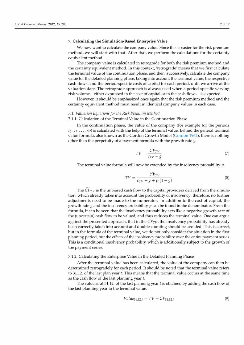
Figure 11. Calculation of the company value with the risk premium method.
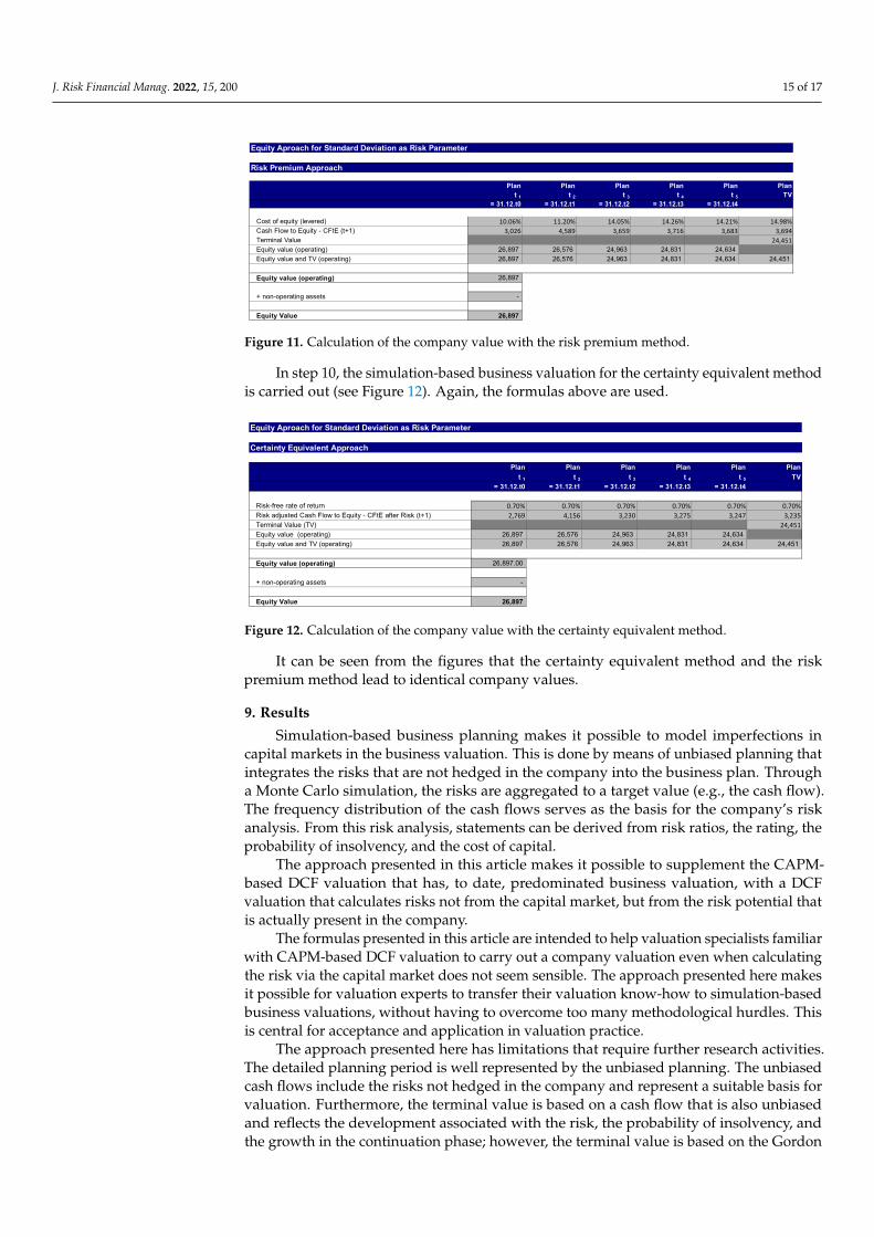
In step 10, the simulation-based business valuation for the certainty equivalent method is carried out (see Figure 12). Again, the formulas above are used.
Figure 12. Calculation of the company value with the certainty equivalent method.
It can be seen from the figures that the certainty equivalent method and the risk pre-mium method lead to identical company values.
9. Results Simulation-based business planning makes it possible to model imperfections in cap-
ital markets in the business valuation. This is done by means of unbiased planning that integrates the risks that are not hedged in the company into the business plan. Through a Monte Carlo simulation, the risks are aggregated to a target value (e.g., the cash flow). The frequency distribution of the cash flows serves as the basis for the company’s risk analysis. From this risk analysis, statements can be derived from risk ratios, the rating, the probability of insolvency, and the cost of capital.
The approach presented in this article makes it possible to supplement the CAPM-based DCF valuation that has, to date, predominated business valuation, with a DCF val-uation that calculates risks not from the capital market, but from the risk potential that is actually present in the company.
The formulas presented in this article are intended to help valuation specialists fa-miliar with CAPM-based DCF valuation to carry out a company valuation even when calculating the risk via the capital market does not seem sensible. The approach presented here makes it possible for valuation experts to transfer their valuation know-how to sim-ulation-based business valuations, without having to overcome too many methodological hurdles. This is central for acceptance and application in valuation practice.
The approach presented here has limitations that require further research activities. The detailed planning period is well represented by the unbiased planning. The unbiased cash flows include the risks not hedged in the company and represent a suitable basis for valuation. Furthermore, the terminal value is based on a cash flow that is also unbiased and reflects the development associated with the risk, the probability of insolvency, and the growth in the continuation phase; however, the terminal value is based on the Gordon
Equity Aproach for Standard Deviation as Risk Parameter
Risk Premium Approach
Plan Plan Plan Plan Plan Plant 1 t 2 t 3 t 4 t 5 TV
= 31.12.t0 = 31.12.t1 = 31.12.t2 = 31.12.t3 = 31.12.t4
Cost of equity (levered) 10.06% 11.20% 14.05% 14.26% 14.21% 14.98% Cash Flow to Equity - CFtE (t+1) 3,026 4,589 3,659 3,716 3,683 3,694 Terminal Value 24,451 Equity value (operating) 26,897 26,576 24,963 24,831 24,634 Equity value and TV (operating) 26,897 26,576 24,963 24,831 24,634 24,451
Equity value (operating) 26,897
+ non-operating assets -
Equity Value 26,897
Equity Aproach for Standard Deviation as Risk Parameter
Certainty Equivalent Approach
Plan Plan Plan Plan Plan Plant 1 t 2 t 3 t 4 t 5 TV
= 31.12.t0 = 31.12.t1 = 31.12.t2 = 31.12.t3 = 31.12.t4
Risk-free rate of return 0.70% 0.70% 0.70% 0.70% 0.70% 0.70% Risk adjusted Cash Flow to Equity - CFtE after Risk (t+1) 2,769 4,156 3,230 3,275 3,247 3,235 Terminal Value (TV) 24,451 Equity value (operating) 26,897 26,576 24,963 24,831 24,634 Equity value and TV (operating) 26,897 26,576 24,963 24,831 24,634 24,451
Equity value (operating) 26,897.00
+ non-operating assets -
Equity Value 26,897
Figure 11. Calculation of the company value with the risk premium method.
In step 10, the simulation-based business valuation for the certainty equivalent methodis carried out (see Figure 12). Again, the formulas above are used.
J. Risk Financial Manag. 2022, 15, x FOR PEER REVIEW 15 of 17
Figure 11. Calculation of the company value with the risk premium method.
In step 10, the simulation-based business valuation for the certainty equivalent method is carried out (see Figure 12). Again, the formulas above are used.
Figure 12. Calculation of the company value with the certainty equivalent method.
It can be seen from the figures that the certainty equivalent method and the risk pre-mium method lead to identical company values.
9. Results Simulation-based business planning makes it possible to model imperfections in cap-
ital markets in the business valuation. This is done by means of unbiased planning that integrates the risks that are not hedged in the company into the business plan. Through a Monte Carlo simulation, the risks are aggregated to a target value (e.g., the cash flow). The frequency distribution of the cash flows serves as the basis for the company’s risk analysis. From this risk analysis, statements can be derived from risk ratios, the rating, the probability of insolvency, and the cost of capital.
The approach presented in this article makes it possible to supplement the CAPM-based DCF valuation that has, to date, predominated business valuation, with a DCF val-uation that calculates risks not from the capital market, but from the risk potential that is actually present in the company.
The formulas presented in this article are intended to help valuation specialists fa-miliar with CAPM-based DCF valuation to carry out a company valuation even when calculating the risk via the capital market does not seem sensible. The approach presented here makes it possible for valuation experts to transfer their valuation know-how to sim-ulation-based business valuations, without having to overcome too many methodological hurdles. This is central for acceptance and application in valuation practice.
The approach presented here has limitations that require further research activities. The detailed planning period is well represented by the unbiased planning. The unbiased cash flows include the risks not hedged in the company and represent a suitable basis for valuation. Furthermore, the terminal value is based on a cash flow that is also unbiased and reflects the development associated with the risk, the probability of insolvency, and the growth in the continuation phase; however, the terminal value is based on the Gordon
Equity Aproach for Standard Deviation as Risk Parameter
Risk Premium Approach
Plan Plan Plan Plan Plan Plant 1 t 2 t 3 t 4 t 5 TV
= 31.12.t0 = 31.12.t1 = 31.12.t2 = 31.12.t3 = 31.12.t4
Cost of equity (levered) 10.06% 11.20% 14.05% 14.26% 14.21% 14.98% Cash Flow to Equity - CFtE (t+1) 3,026 4,589 3,659 3,716 3,683 3,694 Terminal Value 24,451 Equity value (operating) 26,897 26,576 24,963 24,831 24,634 Equity value and TV (operating) 26,897 26,576 24,963 24,831 24,634 24,451
Equity value (operating) 26,897
+ non-operating assets -
Equity Value 26,897
Equity Aproach for Standard Deviation as Risk Parameter
Certainty Equivalent Approach
Plan Plan Plan Plan Plan Plant 1 t 2 t 3 t 4 t 5 TV
= 31.12.t0 = 31.12.t1 = 31.12.t2 = 31.12.t3 = 31.12.t4
Risk-free rate of return 0.70% 0.70% 0.70% 0.70% 0.70% 0.70% Risk adjusted Cash Flow to Equity - CFtE after Risk (t+1) 2,769 4,156 3,230 3,275 3,247 3,235 Terminal Value (TV) 24,451 Equity value (operating) 26,897 26,576 24,963 24,831 24,634 Equity value and TV (operating) 26,897 26,576 24,963 24,831 24,634 24,451
Equity value (operating) 26,897.00
+ non-operating assets -
Equity Value 26,897
Figure 12. Calculation of the company value with the certainty equivalent method.
It can be seen from the figures that the certainty equivalent method and the riskpremium method lead to identical company values.
9. Results
Simulation-based business planning makes it possible to model imperfections incapital markets in the business valuation. This is done by means of unbiased planning thatintegrates the risks that are not hedged in the company into the business plan. Througha Monte Carlo simulation, the risks are aggregated to a target value (e.g., the cash flow).The frequency distribution of the cash flows serves as the basis for the company’s riskanalysis. From this risk analysis, statements can be derived from risk ratios, the rating, theprobability of insolvency, and the cost of capital.
The approach presented in this article makes it possible to supplement the CAPM-based DCF valuation that has, to date, predominated business valuation, with a DCFvaluation that calculates risks not from the capital market, but from the risk potential thatis actually present in the company.
The formulas presented in this article are intended to help valuation specialists familiarwith CAPM-based DCF valuation to carry out a company valuation even when calculatingthe risk via the capital market does not seem sensible. The approach presented here makesit possible for valuation experts to transfer their valuation know-how to simulation-basedbusiness valuations, without having to overcome too many methodological hurdles. Thisis central for acceptance and application in valuation practice.
The approach presented here has limitations that require further research activities.The detailed planning period is well represented by the unbiased planning. The unbiasedcash flows include the risks not hedged in the company and represent a suitable basis forvaluation. Furthermore, the terminal value is based on a cash flow that is also unbiasedand reflects the development associated with the risk, the probability of insolvency, andthe growth in the continuation phase; however, the terminal value is based on the Gordon

J. Risk Financial Manag. 2022, 15, 200 16 of 17
Growth formula, which is commonly used in practice. One area of research for the continu-ation phase would be to model the development of the cash flow via a stochastic processgenerated by a Monte Carlo simulation. This would have the advantage of applying acoherent approach to simulation-based planning and valuation for the entire planninghorizon.
Another area of research is the determination of the diversification factor in simulation-based valuation. So far, CAPM-based company valuations assume a fully diversifiedinvestor. The counterpart to this is the total beta approach, which assumes an investorconcentrated on one company. The degree of diversification depends on the individualasset situation of the investor; therefore, when determining the diversification factor, theinvestor’s overall asset situation must be determined. In order to be able to determinethis, the Copula approach is required, which maps the correlation of the assets takinginto account the correlations in the tails of the distribution functions of the assets. Theconnection of the Copula approach with simulation-based valuation is still an open areaof research.
Since simulation-based planning and business valuation depicts the risks of manyKPIs via frequency distributions, the fat tails of the distributions that can lead to risks, thusthreatening the existence of the company, should be evaluated in particular. The extremevalue theory can be used for this purpose.
Funding: The article processing charge was funded by the Baden-Württemberg Ministry of Sci-ence, Research and the Arts and Nürtingen-Geislingen University in the funding programme OpenAccess Publishing.
Institutional Review Board Statement: Not applicable.
Informed Consent Statement: Not applicable.
Data Availability Statement: Not applicable.
Conflicts of Interest: The author declares no conflict of interest.
ReferencesBrennan, Michael J., and Ashley W. Wang. 2010. The mispricing return premium. Review of Financial Studies 23: 3437–68. [CrossRef]Dempsey, Mike. 2013. The Capital Asset Pricing Model (CAPM): The History of a Failed Revolutionary Idea in Finance? Abacus 49:
7–23. [CrossRef]Dorfleitner, Gregor. 2020. On the use of the terminal-value approach in risk-value models. Annals of Operations Research, 1–21. Available
online: https://epub.uni-regensburg.de/43131/1/Dorfleitner2020_Article_OnTheUseOfTheTerminal-valueApp.pdf (accessedon 22 February 2022). [CrossRef]
Dorfleitner, Gregor, and Werner Gleißner. 2018. Valuing streams of risky cashflows with risk-value models. Journal of Risk 20: 1–27.[CrossRef]
Ernst, Dietmar, and Joachim Häcker. 2017. Financial Modeling: An Introduction Guided to Excel and VBA Applications in Finance. London:Palgrave Macmillan.
Ernst, Dietmar, and Joachim Häcker. 2021. Risikomanagement im Unternehmen. Bandar Seri Begawan: UTB.Ernst, Dietmar, and Uwe Wehrspohn. 2022. When Do I Take which Distribution? Berlin: Springer.Fama, Eugene F., and Kenneth R. French. 1993. Common risk factors in the returns on stocks and bonds. Journal of Financial Economics
33: 3–56. [CrossRef]Fama, Eugene F., and Kenneth R. French. 2008. Dissecting Anomalies. Journal of Finance 63: 1653–78. [CrossRef]Fama, Eugene F., and Kenneth R. French. 2012. Size, Value, and Momentum in international Stock Returns. Journal of Financial Economics
105: 457–72. [CrossRef]Fama, Eugene F., and Kenneth R. French. 2015. A five-factor asset pricing model. Journal of Financial Economics 116: 1–22. [CrossRef]Fishburn, Peter C. 1977. Mean-risk analysis with risk associated with below target returns. American Economic Review 67: 116–28.Gleißner, Werner. 2019. Cost of capital and probability of default in value-based risk management. Management Research Review 42:
1243–58. [CrossRef]Gleißner, Werner. 2020. Risikoanalyse und moderne Unternehmensbewertungsverfahren als Alternative zum CAPM. Controlling 32:
35–37. [CrossRef]Gleißner, Werner. 2021. Unternehmensbewertung: Methode und Nutzen. BewertungsPraktiker 3: 84–87.Gleißner, Werner, and Dietmar Ernst. 2019. Company valuation as result of risk analysis: Replication approach as an alternative to the
CAPM. Business Valuation OIV Journal 1: 3–18. [CrossRef]

J. Risk Financial Manag. 2022, 15, 200 17 of 17
Gordon, Myron. 1962. The Investment, Financing, and Valuation of the Corporation. Publisher Homewood, IL: Irwin.Haugen, Robert A. 2002. The Inefficient Stock Market: What Pays Off and Why. Hoboken: Prentice Hall.Hazen, Gordon. 2009. An extension of the internal rate of return to stochastic cashflows. Management Science 55: 1030–34. [CrossRef]Novy-Marx, Robert. 2013. The other side of value: The gross profitability premium. Journal of Financial Economics 108: 1–28. [CrossRef]Robichek, Alexander A., and Stewart C. Myers. 1966. Conceptual problems in the use of risk-adjusted discount rates. The Journal of
Finance 21: 727–30.Rubinstein, Mark E. 1973. The Fundamental Theorem of Parameter Preference security valuation. Journal of Financial and Quantitative
Analysis 8: 61–69. [CrossRef]Shiller, Robert J. 1981. The use of volatility measures in assessing market efficiency. Journal of Finance 36: 291–304. [CrossRef]Shleifer, Andrei. 2000. Inefficient Markets: An Introduction to Behavioral Finance. OUP Catalogue. Oxford: Oxford University Press.Smith, James E. 1998. Evaluating income streams:a decision analysis approach. Management Science 44: 1690–708. [CrossRef]Tversky, Amos, and Daniel Kahneman. 1979. Prospect theory: An analysis of decision under risk. Econometrica 47: 280–84. [CrossRef]Zhang, Chu. 2009. On the explanatory power of firm-specific variables in cross-sections of expected returns. Journal of Empirical Finance
16: 306–17. [CrossRef]
Copyright © 2022 FDOKUMEN