Equity Valuation of

Equinor ASA

Freddy León Mujica (152417057)

Dissertation written under the supervision of

José Carlos Tudela Martins

Dissertation submitted in partial fulfilment of requirement for Msc in

Finance, at the Universidad Católica Portuguesa, January 7th, 2019.

Financial

Data 2018 2019E 2020E 2021E

Revenue

(Bill $) $76,28 $82,33 $82,64 $80,03

EBITDA

(Bill $) $27,77 $27,23 $27,75 $28,03

EBITDA

mg (%) 36,4% 33,1% 33,6% 35,0%

ROA (%) 3,31% 4,11% 2,96% 2,79%

EPS $1,15 $1,41 $1,03 $1,05

Methodology Segment Price/share

DCF Operations Kr. 80,41

Real Option Reserves Kr. 136,82

Sum of the parts Kr. 217,23

EV / EBITDAX Kr. 227,52

EV / Annual Production Kr. 235,77

Multiples Average Kr. 231,65

Equinor ASA – Investment Summary Ticker: EQNR.OL Operating Industry: Integrated Oil & Gas Current Price: kr. 191,75 Price Target: kr. 217,23 ($23,15)*

0

200

400

600

800

1000

1200

0

50

100

150

200

Osl

o S

tock

Exch

an

ge I

nd

ex

Eq

uin

or A

SA

Sh

are P

ric

e

Equinos ASA Oslo Stock Exchange

We issue a hold recommendation for Equinor ASA, with a target price of kr.217,23 per share, which

represents a 13% upside over the coming year. This recommendation is based on a combination of

macroeconomic and company-specific expected events and given the uncertainty that shadow the Oil &

Gas industry we believe that the upside is not substantial enough for a different recommendation.

Equinor’s priority is to maximize and develop its unique

Norwegian Continental Shelf (NCS) position, new asset

and resource positions in Brazil and its international gas

business. Despite of new investment being directed at new

energy solutions by 2030, it is still an upstream-dominated

company with activities in Norway and 29 other countries.

Equinor also has a dominant, flexible and cost-advantaged

position in European gas supply and a relevant North

America shale position.

With a relatively intense reinvestment commitment to

support longer-term growth post 2020E, investors could

choose to wait for de-risked ‘next generation’ project

delivery and earnings momentum.

After considerable losses in 2015 and

2016, the pressure in the business unit to

respond made them focus in cost

management and reach their objective of

achieving a break-even price below $50

per barrel by 2022 on their onstream

operations.

Thanks to several new fields starting

production and the recent acquisition of a

25% stake in the producing field

Roncador in Brazil, production will grow

somewhat over the next few years.

However, post 2025, the production is

likely to start declining relatively sharply

if no more new fields are added to the

portfolio through exploration or

acquisitions.

Expectation to reach a break-even price of

$20 per barrel in future development, as

stated by their CEO, will position Equinor

at a competitive position, to better

mitigate the different risk they are expose

to.

*Note: NOK/USD rate 8,64

II

Equity Valuation – Equinor ASA

Freddy León Mujica

Abstract

This dissertation has the objective of valuing the Norwegian oil & gas company Equinor

ASA, previously known as Statoil. The purpose is to reach the fair value of a single

share of the company and issue a buy, hold or sell recommendation, by contrasting the

target price with the current market price. The valuation performed is based in an oil &

gas industry analysis, as well as a company analysis, so that well informed assumptions

could be formed to forecast future performance. Equinor ASA’s valuation is performed

as a sum of the parts, where the current operations where valued following a DCF

approach and the undeveloped proven reserves where valued using the Real Option

methodology, the sum of the part approach was also complemented by multiples

valuation. Equinor ASA’s fair value reached with these methodologies was kr.203,17,

that has a 10,56% upside against market price, given that the price difference is not

significant given the industry’s volatility, a hold recommendation was issued. This

recommendation is consistent with Handelsbanken’s report.

Keywords:

Company valuation, Fair value calculation, Oil & Gas, LNG, DCF, Real Option,

Multiple valuation

Resumo

Esta dissertação tem como objetivo avaliar a empresa norueguesa de petróleo e gás

Equinor ASA, antes conhecida como Statoil. O objetivo é atingir o valor justo de uma

única ação da empresa e emitir uma recomendação para comprar, manter ou vender,

contrastando o preço alvo com o preço de mercado atual. A avaliação realizada baseia-

se numa análise da indústria do petróleo e gás, bem como numa análise da empresa,

para que com suposições bem informadas se possa prever o desempenho futuro. A

avaliação da Equinor ASA é realizada como uma soma de partes, onde as operações

atuais são valorizadas seguindo uma abordagem DCF e as reservas provadas não

desenvolvidas foram avaliadas usando a metodologia da Opção Real. A metodologia da

soma das partes também foi complementada por uma avaliação de múltiplos. O valor

justo da Equinor ASA alcançado com essas metodologias foi de kr.203,17, que tem um

aumento de 10,56% em relação ao preço do mercado. Dado que a diferença de preço

não é significativa, e tendo em conta a volatilidade da indústria, uma recomendação de

retenção é emitida. Esta recomendação é consistente com o relatório do Handelsbanken.

Keywords:

Avaliação de empresas, Cálculo do valor justo, Petróleo e gás, GNL, DCF, Opção Real,

Avaliação múltiplos.

III

Acknowledgment

I would like to thank my parents for the unconditional and endless support provided,

without whom none of this would have been possible. Also, I would like to thank Paula

Gutierrez, for the constant encouragement and words of motivation throughout this

process. I would also like to extend my gratitude to Max Berninghaus and Julian

Klotzner, for the comradery they provided, that made the process of the equity valuation

considerably more dynamic. I would like to thank Adriano Granadeiro as well, for the

help and availability to answer industry related questions, early-on in this dissertation

process. And last, but certainly not least, I would like to thank Professor Tudela Martins

for his continuous guidance and insightful feedback throughout the dissertation process.

IV

Table of Content

Abstract ........................................................................................................................................ II

Acknowledgment ........................................................................................................................ III

List of Formulas ......................................................................................................................... VI

List of Tables .............................................................................................................................. VI

List of figures ............................................................................................................................. VII

1. Introduction ............................................................................................................................. 1

1.1 Topic Relevance and Motivation ..................................................................................... 1

1.2 Methodology ...................................................................................................................... 1

2. Literature review ..................................................................................................................... 2

2.1 Introduction ....................................................................................................................... 2

2.2 Intrinsic Valuation Methods ............................................................................................ 2

2.2.1 The Discount Rate ...................................................................................................... 2

2.2.1.1 The Risk-Free Rate ............................................................................................. 3

2.2.1.2 Cost of Equity ...................................................................................................... 3

2.2.1.2.1 CAPM ................................................................................................................ 3

2.2.1.4 Weighted Average Cost of Capital ..................................................................... 4

2.2.2 Discounted Cash Flow Valuation Models ................................................................ 4

2.2.2.1 Free Cash Flows to Firm..................................................................................... 5

2.2.2.2 Free Cash Flow to Equity ................................................................................... 5

2.2.2.3 Adjusted Present Value (APV) ........................................................................... 6

2.2.2.4 Dividend Discount Model ................................................................................... 8

2.2.2.5 Conclusions .......................................................................................................... 8

2.2.3 The Terminal Value ................................................................................................... 8

2.2.3.1 Growth Rate......................................................................................................... 9

2.3 Real Option Valuation .................................................................................................... 10

2.4 The Relative Valuation Method ..................................................................................... 11

2.5 Sum of the Part Valuation .............................................................................................. 12

3. Industry Analysis .................................................................................................................. 13

3.1 Oil & Gas Industry .............................................................................................................. 13

3.1.1 Oil Industry ............................................................................................................... 13

3.1.1.1 Oil Supply........................................................................................................... 13

3.1.1.2 Oil Demand ........................................................................................................ 14

3.1.2 Gas Industry ............................................................................................................. 15

V

3.1.2.1 Gas Demand ....................................................................................................... 15

3.1.2.2 Gas Supply ......................................................................................................... 16

3.2 Conclusions ...................................................................................................................... 17

4. Company Analysis ................................................................................................................. 19

4.1 Company Overview ......................................................................................................... 19

4.1.1 Activities .................................................................................................................... 19

4.2 Share Price Evolution ..................................................................................................... 20

4.3 Company shareholder structure .................................................................................... 20

4.4 Operational & Financial Performance .......................................................................... 20

5. Valuation of Equinor ASA ................................................................................................... 22

5.1 Intrinsic Valuation .......................................................................................................... 22

5.1.1 Future Cash Flow Forecast ..................................................................................... 22

5.1.1.1 Equinor ASA Revenue ...................................................................................... 22

5.1.1.2 Equinor ASA Operational Costs ...................................................................... 24

5.1.1.3 Equinor ASA CAPEX and Depreciation ......................................................... 24

5.1.1.4 Equinor ASA Working Capital ........................................................................ 25

5.1.1.5 Equinor ASA Cost of Capital ........................................................................... 26

5.1.1.6 Equinor ASA Free Cash Flows and Terminal Value ..................................... 28

5.1.2 Real Option Valuation Method ............................................................................... 29

5.1.3 Sum of the Parts ....................................................................................................... 30

5.1.4 Sensitivity Analysis ................................................................................................... 30

5.2 Relative Valuation ........................................................................................................... 32

5.2.1 Multiples Valuation .................................................................................................. 32

6. Comparison with investment bank ...................................................................................... 34

7. Conclusion .............................................................................................................................. 36

Appendixes ................................................................................................................................. 37

Appendix 1: Financial Statements ....................................................................................... 37

Appendix 2: Energy Outlook ............................................................................................... 41

Appendix 3: Extended Peer Group ...................................................................................... 42

Bibliography .............................................................................................................................. 45

VI

List of Formulas

Formula 1: Present Value Formula

Formula 2: CAPM Formula

Formula 3: Levered Beta formula

Formula 4: Beta adjustment

Formula 5: Market Risk Premium formula

Formula 6: Relative Equity market Volatility

Formula 7: Weighted Average Cost of Capital

Formula 8: Unlevered Cost of Equity

Formula 9: Present Value of Interest Tax Shields

Formula 10: Expected Bankruptcy Cost

Formula 11: Adjusted Present Value

Formula 12: Dividend Discount Model

Formula 13: Terminal Value

Formula 14: Firm Value with explicit period and terminal value

Formula 15: Perpetuity Growth Rate

Formula 16: Option Pricing Computation

Formula 17: Linear Regression

List of Tables

Table 1: FFCF Inputs

Table 2: FCFE Inputs

Table 3: Example Analysis Debt Level APV (Damodaran, 2002)

Table 4: Inputs for Reserves Valuation

Table 5: Regression Equinor Revenue vs. Oil Prices

Table 6: Country Risk Premium

VII

List of figures

Figure 1: Share of world oil supply, BP Energy Outlook 2018

Figure 2: Outlook Oil Demand per region, BP Energy Outlook 2018

Figure 3: Natural Gas Consumption per Sector, EIA Energy Outlook 2018

Figure 4: Natural gas Producer by Region

Figure 5: Equinor ASA Share Price vs. Oslo SE Index

Figure 6: Financial Indicators Summary

Figure 7: Historical and Forecasted Revenue

Figure 8: Total Operating Cost & Brent Price Evolution

Figure 9: Evolution of CAPEX and Depreciation & Amortization

Figure 10: Net Working Capital Computation

Figure 11: Net debt Ratio

Figure 12: Free Cash Flow to Firm

Figure 13: Dissemination of the Firm Value

Figure 14: Sensitivity Analysis

Figure 15: Equinor’s Peer Group

Figure 16: Peer Group’s Multiples

Figure 17: Equinor’s Multiple Valuation

Figure 18: Valuation Summary, Price per Share (Kr./share)

Figure 19: Summary of differences between this report’s and Handelsbanken’s

valuation

Figure 20: Analyst Recommendation Consensus on Equinor ASA, The Wall Street

Journal

1

1. Introduction

1.1 Topic Relevance and Motivation

In an environment of high uncertainty and volatility that has been witnessed the past years

in the Oil & Gas industry, oil prices reached record levels during the period 2014-2016.

This downward trend was attributed to misestimation of energy demand by the OPEC,

which were not willing to decreases their level of oil production, the lack of balance in

the market lead the Brent oil price to plummet from a price of 115$ per barrel to a record

low of 26$ per barrel.

The situation forced the players of the market to re-assess their cost structures and shuffle

their portfolio, not only by pursuing low carbon energy but also by including renewable

sources of energy into their operations. Equinor ASA, put in practice these initiatives to

maintain and even improve its competitive position in the market. This report aims to

analyze the macroeconomics, industry specific and operation characteristics to access the

fair value of Equinor ASA.

1.2 Methodology

As a first step, of the process of assessing how to best value Equinor ASA, a discussion

of the most used methodologies of firm valuation is presented in the literature review.

Then the oil & gas industry environment is analyzed, discussing both the supply and

demand side, as well as their expected evolution for the foreseeable future.

As a third step Equinor ASA’s businesses and strategy are discussed to better understand

their motivations and their competitive position in the market.

In the final step, the equity valuation of Equinor ASA is developed based on the

forecasted financial performance using the valuation methods the best suited the

company. This valuation is later compared with an investment bank report,

Handelsbanken, discussing the differences in the assumptions and methodologies used in

each of the reports. In the conclusions section of this report, the limitation and

recommendation issued are discussed.

2

2. Literature review

2.1 Introduction

This section addresses the different valuation methodologies, where its advantages and

limitation will be discussed to determine which of them are best suited to determine the

fair value of Equinor ASA. The methodologies explained in the following sections, where

chosen in accordance to its relevance to the company subject of this dissertation.

A combination of industry understanding with the selection of the proper valuation model

is always important to yield a reliable fair value for any investment valuation.

2.2 Intrinsic Valuation Methods

Every asset that has cash flows associated to its activities, has an intrinsic value that

encompasses both its cash flow potential and its risk. Intrinsic value can be considered

the value that would be attached to a firm by an unbiased analyst, given the information

available at the time.

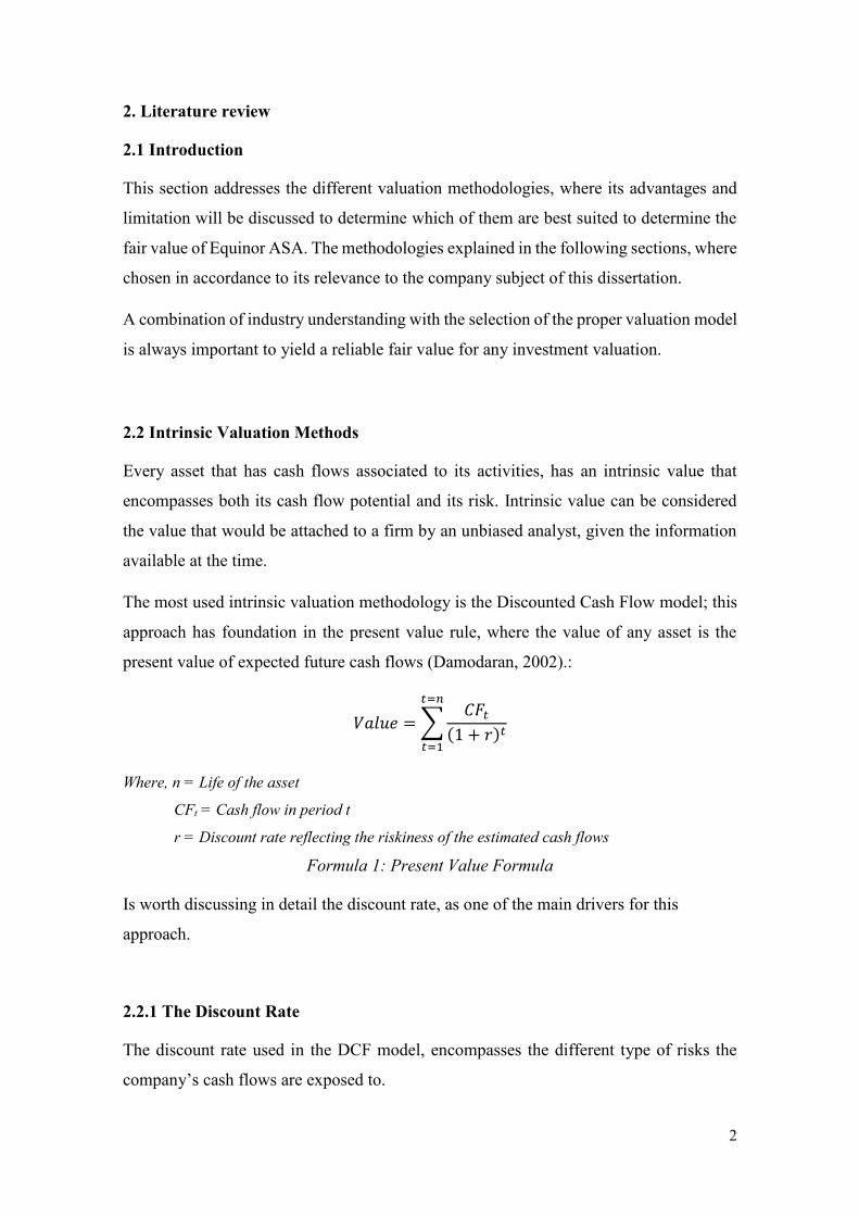
The most used intrinsic valuation methodology is the Discounted Cash Flow model; this

approach has foundation in the present value rule, where the value of any asset is the

present value of expected future cash flows (Damodaran, 2002).:

𝑉𝑎𝑙𝑢𝑒 = ∑𝐶𝐹𝑡

(1 + 𝑟)𝑡

𝑡=𝑛

𝑡=1

Where, n = Life of the asset

CFt = Cash flow in period t

r = Discount rate reflecting the riskiness of the estimated cash flows

Formula 1: Present Value Formula

Is worth discussing in detail the discount rate, as one of the main drivers for this

approach.

2.2.1 The Discount Rate

The discount rate used in the DCF model, encompasses the different type of risks the

company’s cash flows are exposed to.

3

2.2.1.1 The Risk-Free Rate

The risk-free rate is the return of a risk-free asset, which are those assets where the actual

return should always be equal to the expected return.

Given that these types of asset are incredibly difficult to find in the market, for valuation

purposes the only securities that have a chance of being risk free are government

securities, mainly because they are in control of printing of currency, in other words they

control the cash that circulates their given economy.

However, the maturity of the bonds has to be taken into account, for 5-year treasury bonds

the coupons on the bond will be reinvested at rates that cannot be predicted, for that reason

the most common proxy for a risk-free rate used in valuations is the 10-year government

bond(Damodaran, 2008). For Equinor ASA, the most suitable risk-rate chosen was the

10-year U.S. Treasury bond.

2.2.1.2 Cost of Equity

Equity risk premium are a central component of every risk and return model and refers to

the additional return investors demand for holding equities(Damodaran, 2018). The most

commonly used methodology to compute cost of equity, Capital Asset Pricing Model

(CAPM).

2.2.1.2.1 CAPM

The Capital Asset Pricing Model, states that the risk premium equals the investment’s

beta times the market risk premium:

𝐾𝑒 = 𝑟𝑓 + 𝛽𝑒(𝑟𝑚 − 𝑟𝑓)

Where, Ke = Cost of Equity

rf = Risk-free rate

βe = Equity beta

rm= Market return rate

Formula 2: CAPM Formula

4

This tells the investor the amount of return they should expect for holding a risky asset,

which exist in the efficient frontier.

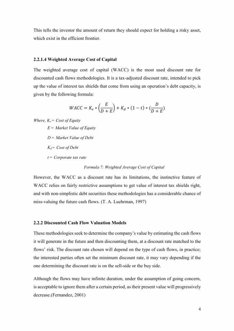
2.2.1.4 Weighted Average Cost of Capital

The weighted average cost of capital (WACC) is the most used discount rate for

discounted cash flows methodologies. It is a tax-adjusted discount rate, intended to pick

up the value of interest tax shields that come from using an operation’s debt capacity, is

given by the following formula:

𝑊𝐴𝐶𝐶 = 𝐾𝑒 ∗ (𝐸

𝐷 + 𝐸) + 𝐾𝑑 ∗ (1 − 𝑡) ∗ (

𝐷

𝐷 + 𝐸)

Where, Ke = Cost of Equity

E = Market Value of Equity

D = Market Value of Debt

Kd = Cost of Debt

t = Corporate tax rate

Formula 7: Weighted Average Cost of Capital

However, the WACC as a discount rate has its limitations, the instinctive feature of

WACC relies on fairly restrictive assumptions to get value of interest tax shields right,

and with non-simplistic debt securities these methodologies has a considerable chance of

miss-valuing the future cash flows. (T. A. Luehrman, 1997)

2.2.2 Discounted Cash Flow Valuation Models

These methodologies seek to determine the company’s value by estimating the cash flows

it will generate in the future and then discounting them, at a discount rate matched to the

flows’ risk. The discount rate chosen will depend on the type of cash flows, in practice;

the interested parties often set the minimum discount rate, it may vary depending if the

one determining the discount rate is on the sell-side or the buy side.

Although the flows may have infinite duration, under the assumption of going concern,

is acceptable to ignore them after a certain period, as their present value will progressively

decrease.(Fernandez, 2001)

5

2.2.2.1 Free Cash Flows to Firm

These are the cash flows generated by operations after tax, in order to calculate the free

cash flow; we must ignore financing for the company’s operation and concentrate on the

financial return on the company’s assets, viewed from a perspective of going concern.

Earnings Before Interest and Tax

(EBIT)

( - ) Tax paid on EBIT

( = ) Net Income without debt

( + ) Depreciation

( - ) Increased in fixed assets

( - ) Increase in Working Capital Requirement

( = ) Free Cash Flows to the Firm

Table 1: FFCF Inputs

Under the assumption that the company has no debt or other non-operational obligation

to fulfill, the FCFF is the amount of cash available to distribute to investors.

2.2.2.2 Free Cash Flow to Equity

These cash flows are the ones distributed to investors after covering fixed asset

investment and working capital requirements, and after paying the financial charges and

repaying the corresponding part of the debt’s principal.

Free Cash Flow to Firm

( - ) Interest Payments * ( 1 – Corporate Tax Rate)

( - ) Principal Repayments

( + ) New Debt

( = ) Free Cash Flow to Equity

Table 2: FCFE Inputs

These cash flows assume the existence of a certain financing structure in each period,

where the interest and the principal of the corresponding debt are paid, and new debt is

hired. With the flows the valuation is of the company’s equity, which is why the most

appropriate discount rate would be the cost of equity. (Fernandez, 2001)

6

2.2.2.3 Adjusted Present Value (APV)

APV is designed to value operations or assets in place. This approach analyzes financial

maneuvers separately and add their value together. (Timothy A Luehrman, 1997)

The model starts with the value of the unlevered firm that can be computed by discounting

the free cash flows of the firm by its unlevered cost of equity. The unlevered cost of equity

can be reverse engineered using the observed cost of equity, the cost of debt and the

market debt-to-equity ratio. The resulting equation is the levered cost of equity for a

company whose debt can take any value but whose interest tax shields have the same risk

as the company’s debt. (Koller, Goefhart, & Wessels, 2010)

𝐾𝑒 = 𝐾𝑢 +𝐷 − 𝑉𝑡𝑥𝑠

𝐸∗ (𝐾𝑢 − 𝐾𝑑)

Where, Ke = Cost of Equity

E = Value of Equity

D = Value of Debt

Kd = Cost of Debt

Ku = Unlevered cost of equity

Vtxs = Present Value of tax shields

Formula 8: Unlevered Cost of Equity

Once the value of the company as an all equity firm is establish, the value of tax shields and the

expected bankruptcy cost should be included, to determine the current firm value. To estimate the

tax benefits of debt, the total debt should be multiplied by its corporate tax rate, assuming that

debt is permanent, and the tax benefits will continue in perpetuity, taking into account possible

limitations in the amount of tax shields that are allowed within regulations. However, to compute

the present value of interest tax shields for each of the period forecasted the following formula

should be use: (Fernandez, 2001)

𝑃𝑉𝐼𝑇𝑆 =𝐷 ∗ 𝐾𝑑 ∗ 𝑡

(1 + 𝐾𝑑)𝑛

Where, D = Value of Debt

Kd = Cost of Debt

t = Corporate tax rate

Formula 9: Present Value of Interest Tax Shields

7

The final step of the process is to estimate the expected bankruptcy cost, this is usually

computed by multiplying the probability of default by the bankruptcy cost. The ratings of

corporate bonds can be used as a proxy to establish the probability of default for company.

However, when it comes to bankruptcy cost, understood as percentage of the value for

the unlevered firm, there is no consensus in regards of how it should be computed, given

that is very difficult to measure indirect bankruptcy cost.

𝐸𝑥𝑝𝑒𝑐𝑡𝑒𝑑 𝐵𝑎𝑛𝑘𝑟𝑢𝑝𝑐𝑦 𝐶𝑜𝑠𝑡 = 𝑃𝑟𝑜𝑏𝑎𝑏𝑖𝑙𝑖𝑡𝑦 𝑜𝑓 𝐷𝑒𝑓𝑎𝑢𝑙𝑡 ∗ 𝐵𝑎𝑛𝑘𝑟𝑢𝑝𝑡𝑐𝑦 𝐶𝑜𝑠𝑡

Formula 10: Expected Bankruptcy Cost

In the end the current value of the company will be:

𝐶𝑢𝑟𝑟𝑒𝑛𝑡 𝑉𝑎𝑙𝑢𝑒 𝑜𝑓 𝑡ℎ𝑒 𝐹𝑖𝑟𝑚 = 𝑉𝑢 + 𝑃𝑉𝐼𝑇𝑆 − 𝐸𝐵𝐶

Where, Vu = Value of the unlevered firm

PVITS = Present Value of Interest Tax Shields

EBC = Expected Bankrupcy Cost

Formula 11: Adjusted Present Value

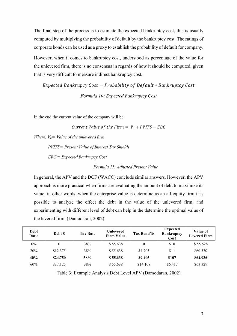
In general, the APV and the DCF (WACC) conclude similar answers. However, the APV

approach is more practical when firms are evaluating the amount of debt to maximize its

value, in other words, when the enterprise value is determine as an all-equity firm it is

possible to analyze the effect the debt in the value of the unlevered firm, and

experimenting with different level of debt can help in the determine the optimal value of

the levered firm. (Damodaran, 2002)

Debt

Ratio Debt $ Tax Rate

Unlevered

Firm Value Tax Benefits

Expected

Bankruptcy

Cost

Value of

Levered Firm

0% 0 38% $ 55.638 0 $10 $ 55.628

20% $12.375 38% $ 55.638 $4.703 $11 $60.330

40% $24.750 38% $ 55.638 $9.405 $107 $64.936

60% $37.125 38% $ 55.638 $14.108 $6.417 $63.329

Table 3: Example Analysis Debt Level APV (Damodaran, 2002)

8

2.2.2.4 Dividend Discount Model

This is one of the simplest models for valuing equity, where the value of the stock is

understood as the present value of the expected dividend on it. The rationale of the model

lies in the present value rule, with two basic inputs: expected dividends and the cost of

equity.

𝑉𝑎𝑙𝑢𝑒 𝑝𝑒𝑟 𝑠ℎ𝑎𝑟𝑒 𝑠𝑡𝑜𝑐𝑘 = ∑𝐸(𝐷𝑃𝑆𝑇)

(1 + 𝐾𝐸)𝑇

𝑇=∞

𝑇=1

Where, DPS = Expected dividend per share

Ke = Cost of Equity

Formula 12: Dividend Discount Model

“This model is flexible enough to allow for time varying discount rates, where the time

variation is because of expected changes in interest rates or risk across time” (Damodaran,

2002). This approach is most suitable when the company has a well stablish dividend

policy, that bears consistency with the its profitability.(Pinto, Robinson, & Stowe, 2018)

2.2.2.5 Conclusions

Overall the chosen approach for Equinor ASA valuation will be to discount the FCFF by

the WACC. Even though APV provides the flexibility to account for changes in the

company’s level of debt, given that, historically, capital structure has not change

significantly from year-to-year, this approach will not provide additional value in

comparison to the cost of capital approach.

2.2.3 The Terminal Value

As a way to wrap up the valuation, to determine the terminal value it can be considered a

going concern approach, by computing it under the assumptions that the last cash flow

forecasted will grow in perpetuity at a stable growth rate. The terminal value is a crucial

input of any discounted cash flow methodology, since it can account for a significant

amount of the Enterprise Value. An adaptation of the Gordon Growth model is most used

formula for this approach:

9

𝑇𝑉 =𝐹𝐶𝐹𝑛

𝑟 − 𝑔

Where, TV = Terminal Value

r = Discount rate chosen

g = growth rate in perpetuity

Formula 13: Terminal Value

Because is not possible to forecast the cash flows into infinity, the common practice is to

estimate an explicit period and add the terminal value based on the Formula 13. In the

end the value of the firm using the cost of capital approach, for example, will be as follow:

𝐹𝑖𝑟𝑚 𝑉𝑎𝑙𝑢𝑒 = ∑𝐹𝐶𝐹𝐹𝑡

(1 + 𝑊𝐴𝐶𝐶)𝑡

𝑛

𝑡=1

+𝐹𝐶𝐹𝐹𝑛+1

(𝑊𝐴𝐶𝐶 − 𝑔)∗

1

(1 + 𝑊𝐴𝐶𝐶)𝑛

Formula 14: Firm Value with explicit period and terminal value

2.2.3.1 Growth Rate

While the determination of a growth rate can vary depending on the approaches, there are

common themes among them, the main one is that growth and reinvestment rate are

linked, which is why is common to compute growth rate as:

𝑃𝑒𝑟𝑝𝑒𝑡𝑢𝑖𝑡𝑦 𝐺𝑟𝑜𝑤𝑡ℎ 𝑅𝑎𝑡𝑒 = 𝑅𝑒𝑖𝑛𝑣𝑒𝑠𝑡𝑚𝑒𝑛𝑡 𝑟𝑎𝑡𝑒 ∗ 𝑅𝑒𝑡𝑢𝑟𝑛 𝑜𝑛 𝐶𝑎𝑝𝑖𝑡𝑎𝑙

Formula 15: Perpetuity Growth Rate

However, this approach is mainly valid for company that have a constant reinvestment

rate throughout the analyzed period. And given that is not realistic for a company, under

the assumption of going concern, to grow at higher rate than the nominal GDP of its main

region of operation. Nevertheless, for natural resource companies, as it is the case of

Equinor ASA, since there is a limited amount of resource in the planet, the common

assumption in practice is to establish a nominal growth rate between 1% and 3%.

10

2.3 Real Option Valuation

One critique of conventional approach is that they fail to consider adequately the relation

between the commodity prices and financing actions of companies. In other words,

conventional valuation approaches fail to consider the option embedded within

investments.

The fact that a project does not have a positive NPV, does not mean that right to the

project are not valuable, this is something that is capture by the real option model. For the

sake of this dissertation, the approach will be discussed from the point of view a natural

resource company, so that the applicability to Equinor ASA can be more evident.

The simplest application of the option approach is in the valuation of natural resource

reserves, where the company has the right to develop the reserve over a specific period

and will be a function of the quantity of resources and the current price. As prices of the

commodity rises and falls, the company will assess the viability of developing the

reserves. Under the premise of natural resource reserves as options, the following inputs

must be considered for its valuation:

Value of Underlying Asset S Quantity of resources time current price

Strike Price K Cost of developing the reserve

Life of the Option T Number of years of production it would take to

deplete the reserve

Variance of underlying asset σ2 Variance of the price of the underlying asset

Dividend Yield R Annual Cash flow as a percentage of the value

of the underlying asset

Development lag n Number of years from the decision to develop

until actual extraction of the reserves

Table 4: Inputs for Reserves Valuation

Since extraction cannot be done instantaneously, once the value of the reserve is

computed, it must be discounted to account for the development lag. The discount rate in

11

this case should be the dividend yield, to adjust for those cash flow loss during the

development lag period. (Damodaran, 2009)

The option pricing model used is this approach is based on the Black-Scholes model,

assuming the option of developing or not the reserve resembles a call option.

𝑑1 =ln (

𝑆𝐾

) + (𝑅 −𝜎2

2) ∗ 𝑇

𝜎 ∗ √𝑇

𝑑2 = 𝑑1 − 𝜎 ∗ √𝑇

𝐶 =𝑆 ∗ 𝑛 ∗ 𝑁(𝑑1) − 𝐾 ∗ 𝑒−𝑟∗𝑇 ∗ 𝑁(𝑑2)

(1 + 𝑅)𝑛

Formula 16: Option Pricing Computation

2.4 The Relative Valuation Method

Relative valuation approach can provide an insight and help in summarizing and test a

valuation, however their use should be superficial, since it may lead to erroneous

conclusions. The basic rationale behind multiples for valuation is that similar assets

should sell at similar prices, this approach can also be used to value non listed companies,

or division of traded companies, to see how they compared against their peers. (Koller et

al., 2010)

To properly apply the multiples approach there are four basic principle worth mentioning:

- Use the right peer group, usually industrial classification are loosely defined, as

an alternative could be to use the standard industrial classification codes issued

by the U.S. Government. After this first list of market competitors, each of the

company must be investigated to determine if they have similar prospect of ROIC

and growth.

- Use forward-looking multiples, aside for the principles of valuation, empirical

evidence shows that forward-looking multiples are more accurate predictors of

value.

- Use enterprise value multiples, although P/E is widely used it is distorted by

capital structure and nonoperating gains and losses. The alternative to this ratio is

EV to EBITDA, in general this ratio is less susceptible to manipulation, since EV

12

already include debt and equity and EBITDA includes the profitability to

investors, so a change in capital structure will affect this multiple.

- Adjust EV/EBITDA for nonoperating items, items like excess cash and pension

items embedded in the EBITDA can distort this multiple. (Koller, Goedhart, &

Wessels, 2005)

Given the peculiarities of the oil & gas sector, the multiples used are slightly different

than the ones commonly used in other markets, for the valuation of Equinor ASA, the

multiple used were:

- EV / EBITDAX: the “X” stands for the Exploration Expenses that are added back

to the EBITDA, since recognition of these type of expenses and earning could

vary significantly from one company to the other, it will depend if the company

uses a successful effort or full cost accounting method. It’s an approach to

standardize the accounting treatment of exploration expenses.

- EV / Annual Production: annual production is measure in “barrels of oil

equivalent”, and this ratio gives an indication on how much their fields are worth

on per barrel basis.

2.5 Sum of the Part Valuation

A valuation that sums the estimated values of each of the company’s businesses, is known

as sum-of-the-parts valuation (Pinto et al., 2018). For the case of Equinor ASA, the value

of the company was divided in two, current operations were valued using the DCF

(WACC) approach, and the proven undeveloped reserves were valued using the real

option approach, the assumptions taken for each of the approaches will be discussed later

on.

13

3. Industry Analysis

Any reliable valuation requires a thorough understanding of the industry in which the

company operates, so that the assumptions made in each of the approaches used for the

valuation are in line with the industry dynamics. In this section we will address, mainly

the oil & gas industry, as it is the sector in which Equinor ASA operates.

3.1 Oil & Gas Industry

Throughout 2017 and the first half of 2018, economy delivered a high growth rate, where

consumer spending, driven by higher employment rates, combined by low inflation

delivered an estimated GDP growth of 2,2% for regions like UK, US and Europe. A

robust demand picture and solid economics fundamentals should allow the expansion to

continue. The rising prosperity drives an increase in energy demand, although it expected

that it will be counterbalance by in increase in energy efficiency

3.1.1 Oil Industry

Global oil demand grew by 1,5 mmbl per day in 2017 and global supply grew by 0,4

mmbbl per day. However, decreasing oil prices in the first half of 2017 made OPEC and

Non-OPEC countries adjust their production, to facilitate gradual rebalancing of the oil

market. This recovery has been a result of various factors, including sustained success of

the production restraint agreement between OPEC and non-OPEC countries before

mentioned, less oil entering the market from challenged producers, and a strong global

oil demand growth estimated by the Energy Information Administration (EIA) at about

1.6million b/d in 2018.

3.1.1.1 Oil Supply

On the supply side, the Organization of Petroleum Exporting Countries (OPEC) has been

crucial to this market adjustment. In November 2017, an agreement made by OPEC and

non-OPEC countries, to cut production by 1,8 million barrels per day, throughout 2018

helped to rebalance the market after the continued downward trend of 2016.

Despite the signs of recovery, the industry has to face several challenges in regards of the

supply.

“A decrease in discoveries was aggravated the slowness of the rise in exploration

spending after the downturn of oil prices of 2014–16. Globally, spending plummeted by

more than 60 percent, from a high of US$153 billion in 2014 to about $58 billion in 2017.

14

The investment slump in traditional supply sources looks like it will continue to have an

effect on new production”. (Biscardini, Morrison, Branson & Del Maestro, 2018)

However, the outlook of global market for liquids expands with growing demands from

developing economies met by increase in supply from low-cost producers. The increase

in supply in 2017 was marginal, given that the market was still bearing part of the excess

supple from 2016. Future supply increases are expected to be driven initially by US tight

oil, with OPEC taking over by the end of the 2020s.

Figure 1: Share of world oil supply, BP Energy Outlook 2018

3.1.1.2 Oil Demand

Even though there is no foreseeable peak in the demand of oil, after an expansion of

consumption by 1,4 mb/d in 2018 it is expected to for the growth to plateau to 1mb/d in

the next 5 years. Several countries are starting to take initiatives to find alternative sources

of energy as a substitute of oil, so demand management will require business models

throughout the industry to evolve.

United States and China continue to be main sources of the oil demand growth, said

growth is mainly driven by the petrochemical industry. Around a fourth of the total

demand expected for 2023, is taken up by ethane and naphtha. The economic growth that

has been experienced worldwide, is increasing the percentage of the population in the

middle-class threshold, in particular in developing countries. This trend is increasing the

demands of consuming goods and services, many of which require derivation of oil in

order to be manufacture.

0%

5%

10%

15%

20%

25%

30%

35%

40%

45%

200

0

200

1

200

2

200

3

200

4

200

5

200

6

200

7

200

8

200

9

201

0

201

1

201

2

201

3

201

4

201

5

201

6

202

0

202

5

203

0

203

5

204

0

Shar

e o

f W

orl

Sup

ply

OPEC

Saudi Arabia

US Tight Oil

US crude

Russia

15

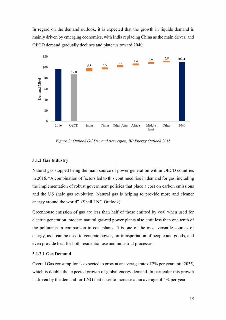
In regard on the demand outlook, it is expected that the growth in liquids demand is

mainly driven by emerging economies, with India replacing China as the main driver, and

OECD demand gradually declines and plateaus toward 2040.

Figure 2: Outlook Oil Demand per region, BP Energy Outlook 2018

3.1.2 Gas Industry

Natural gas stopped being the main source of power generation within OECD countries

in 2016. “A combination of factors led to this continued rise in demand for gas, including

the implementation of robust government policies that place a cost on carbon emissions

and the US shale gas revolution. Natural gas is helping to provide more and cleaner

energy around the world”. (Shell LNG Outlook)

Greenhouse emission of gas are less than half of those emitted by coal when used for

electric generation, modern natural gas-red power plants also emit less than one tenth of

the pollutants in comparison to coal plants. It is one of the most versatile sources of

energy, as it can be used to generate power, for transportation of people and goods, and

even provide heat for both residential use and industrial processes.

3.1.2.1 Gas Demand

Overall Gas consumption is expected to grow at an average rate of 2% per year until 2035,

which is double the expected growth of global energy demand. In particular this growth

is driven by the demand for LNG that is set to increase at an average of 4% per year.

87,0

109,41

5,8 3,53,9

3,4 2,9 2,8

0

20

40

60

80

100

120

2016 OECD India China Other Asia Africa Middle

East

Other 2040

Dem

and

Mb

/d

16

Over the next twenty years 40% of the growth of demand of the energy mix is expected

to be allocated to gas. Even though gas will continue as a power generation source, most

the energy demand growth will arise from sectors like steel and cement production, which

are difficult to electrify.

“In 2017, demand for LNG was strong with a clear “pull” from countries instead of a

“push” of volumes seeking a home. This was similar to 2016, but during 2017 the demand

pull was from legacy gas and LNG importers in Asia and Southern Europe; whereas 2016

was characterized by a pull from new areas of demand. Asian demand grew by more than

17 million tonnes, beating industry predictions going into the year. That is nearly as much

as the total volume that Indonesia, the world’s fifth largest exporter, produced in 2017”.

(Shell LNG Outlook)

Figure 3: Natural Gas Consumption per Sector, EIA Energy Outlook 2018

3.1.2.2 Gas Supply

An increase in the number of countries that supply LNG, helped significantly the

flexibility and the strength of the market, where China alone imported LNG from 20

different countries. With an expansion of planned capacity partially completed, the

market size of LNG grew by 29 million tonnes.

0

20

40

60

80

100

0

5

10

15

20

25

30

35

40

2000 2010 2020 2030 2040 2050B

illi

on

Cu

bic

Fee

t p

er d

ay

Tri

llio

n C

ub

ic f

eet

power industrial transportation commercial residential

2017

History Projections

17

Figure 4: Natural gas Producer by Region

“Significant LNG exports came from new supplies in the USA and Australia, with

increased output from existing LNG supply facilities in Africa. Domestic natural gas

production is expected to continue being the dominant source of gas supply – especially

in North America and parts of Europe where well-connected pipelines are already in

place. In regions such as Asia and the Middle East, where cross-border pipelines are

limited, LNG is expected to play a more significant role. Floating storage and

regasification units (FSRUs) continue to enable fast, flexible and economically

competitive options for countries looking to import LNG. These vessels can be docked in

a port to re-gasify LNG and feed gas into a transmission or distribution network”. (Shell

LNG Outlook)

3.2 Conclusions

Uncertainty and volatility are the two main characteristic that are being used to describe

the Oil & Gas industry, not only because of high variance of commodities prices, but also

because of the increasing talks of energy transition among governments to empower

cleaner sources of energy. This environment is forcing companies in the industry to

rethink their approach on competition with its peers.

After the downturn of oil prices in 2014, big players in the industry adopted an “always-

low” policy, where there was a general trend of disinvestment of non-strategic assets and

a continuous cost efficiency of their operational expenses. In other words, companies are

starting to manage their portfolio at a lower break-even price, in order to maintain their

0 100 200 300 400 500

2016

2040

N America Europe

China India & Emerging Asia

Middle East CIS

Africa Others

18

profitability at any given oil price. The cleaning of inefficiencies within operation is

expected to become a mantra in the industry, even if oil prices rise.

This trend of continuous efficiency will have to be combined with an initiative to develop

new businesses to expand their portfolio. This has already been seen in some of the mayor

players, with significant investments in renewable energy and shifting their portfolio to

natural gas, as it is considered to be the bridge between fossil fuels to a low-carbon

emission source.

Despite highs and lows of the industry, demand keeps exceeding annual forecasts,

inventories are being reduced, and reserves are not being replaced due to lack of

investment in exploration. Nonetheless, the world remains dependent on oil and gas.

“The need to find more of both resources will become more pressing over the short to

medium term. Portfolios have to be resilient, innovation needs to thrive, and productivity

and capital efficiency must remain the bedrock of operations. Looking further out,

companies will need a robust strategy for hydrocarbon weighting: a strategy that will

serve them no matter what the future brings. Only those companies who can do all this

will prevail”. (Biscardini, Morrison, Branson & Del Maestro, 2018)

19

4. Company Analysis

4.1 Company Overview

Equinor ASA was founded as Den Norske Stats Oljeselskap AS, the Norwegian State Oil

company in 1972. Equinor ASA became listed on the Oslo Børs (Norway) and New York

Stock Exchange (US) in June 2001. Equinor ASA is engaged in exploration, development

and production of oil and gas in addition to renewables. They are the leading operator on

the Norwegian continental shelf and have substantial international activities. Equinor

ASA sells crude oil and is a major supplier of natural gas. Processing, refining, offshore

wind and carbon capture and storage is also part of our operations.

4.1.1 Activities

Equinor ASA’s operations are managed through six business unit:

- Development & Production, this area manages upstream activities in charge of

exploring for and extracting crude oil, natural gas and natural gas liquid. This

business unit is sub-divided by D&P Norway, which is in charge of the Norwegian

Continental Shell (NCS); D&P USA is in charge of upstream activities in USA

and Mexico; and D&P International is in charge of worldwide upstream activities

excluding activities of Norway and USA.

- Marketing, Midstream and Processing this area is in charge of marketing and

trading activities related to oil products and natural gas, transportation, processing

and manufacturing, and development of oil and gas.

- Technology, Projects & Drilling (TDP) is responsible for the global project

portfolio, well delivery, new technologies and sourcing across Equinor ASA. TPD

seeks to provide safe and secure, efficient and cost-competitive global well and

project delivery, technological excellence, and research and development.

- Exploration, this business unit is in charge of exploration activities worldwide,

their aim is to position Equinor ASA as a leading exploration company by

accessing high potential new acreage and drilling more significant wells in growth

and frontier basis.

- New Energy Solutions (NES), reflects the long-term commitment of Equinor

ASA to complement their oil and gas portfolio, with profitable renewable energy

and low-carbon energy solutions. This area is in charge of wind farms and carbon

capture and storage.

20

- Global Strategy & Business Development (GSB), this business area is

responsible of developing the corporate strategy and merger & acquisition

activities for Equinor ASA.

In regards of financial reporting, the different segments reported as source of revenues

are D&P Norway, D&P International (includes D&P USA), Marketing, Midstream &

Processing, and Others, this last segment compiles TDP, NES, GSB and Exploration.

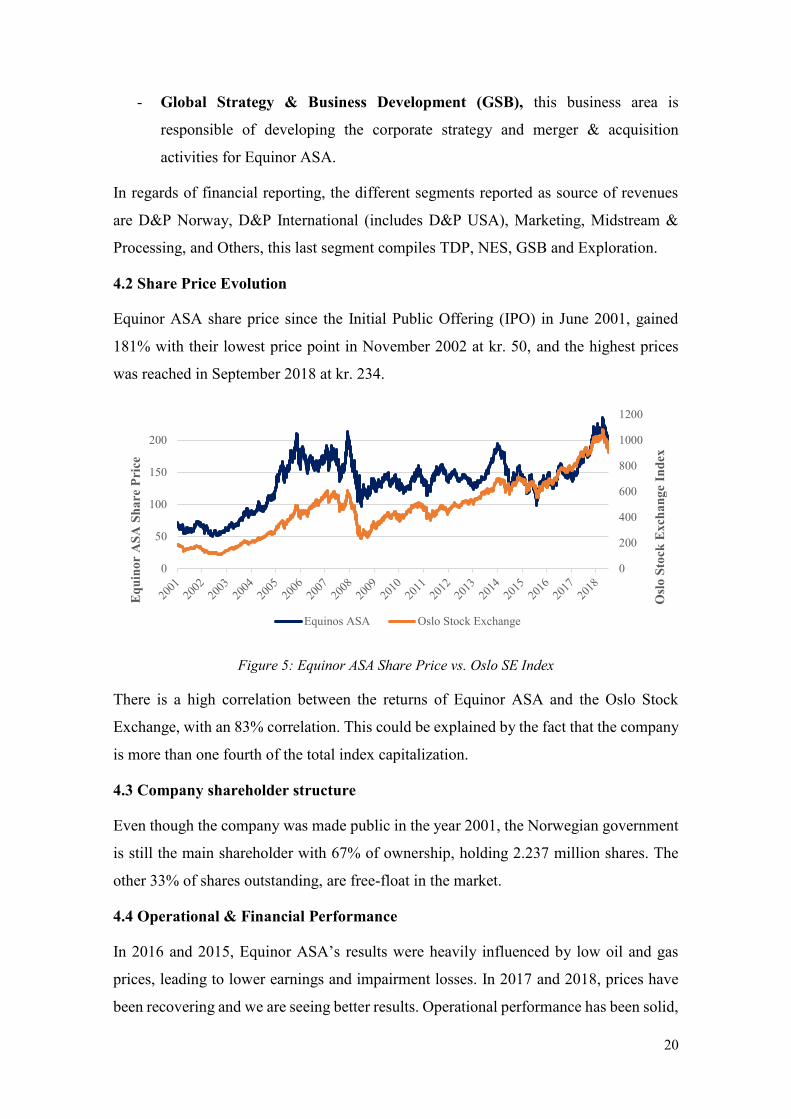
4.2 Share Price Evolution

Equinor ASA share price since the Initial Public Offering (IPO) in June 2001, gained

181% with their lowest price point in November 2002 at kr. 50, and the highest prices

was reached in September 2018 at kr. 234.

Figure 5: Equinor ASA Share Price vs. Oslo SE Index

There is a high correlation between the returns of Equinor ASA and the Oslo Stock

Exchange, with an 83% correlation. This could be explained by the fact that the company

is more than one fourth of the total index capitalization.

4.3 Company shareholder structure

Even though the company was made public in the year 2001, the Norwegian government

is still the main shareholder with 67% of ownership, holding 2.237 million shares. The

other 33% of shares outstanding, are free-float in the market.

4.4 Operational & Financial Performance

In 2016 and 2015, Equinor ASA’s results were heavily influenced by low oil and gas

prices, leading to lower earnings and impairment losses. In 2017 and 2018, prices have

been recovering and we are seeing better results. Operational performance has been solid,

0

200

400

600

800

1000

1200

0

50

100

150

200

Osl

o S

tock

Exch

an

ge

Ind

ex

Eq

uin

or

AS

A S

ha

re P

rice

Equinos ASA Oslo Stock Exchange

21

and production was up by 5% in 2017. Cost discipline and efficiency improvements have

contributed to the reduced operating costs. Supported by increasing prices and better

operational performance, several previous impairments have been reversed.

(USD

Billion) 2010 2011 2012 2013 2014 2015 2016 2017 2018

Revenues $87,68 $119,47 $124,22 $108,53 $98,78 $59,64 $45,87 $61,19 $76,28

EBITDA $31,10 $46,91 $45,87 $38,77 $33,46 $18,08 $11,63 $22,42 $27,77

EBIT $22,71 $37,75 $35,48 $26,44 $17,37 $1,37 $0,08 $13,77 $19.04

Net Profit $6,23 $13,98 $11,93 $6,66 $3,51 -$6,05 -$3,88 $4,60 $3,2

Profit Margin 7,11% 11,70% 9,61% 6,13% 3,55% -10,14% -8,46% 7,51% 5,01%

ROIC 7,6% 15,1% 11,4% 5,8% 3,4% -5,1% -3,2% 5,1% 7,2%

Figure 6: Financial Indicators Summary

The analysis of Equinor ASA, went several years back to understand the magnitude of

the effect that fluctuation in oil prices have had in the profitability and the operations of

the company. As it can be seen in Figure 6, during the period of low oil prices that started

in mid-2014, the company suffered considerable losses that could only be recovered after

a combination of cost efficiency implantation and rising commodities prices.

This exposure to fluctuation in oil prices is trying to be reduced by an expansion of their

portfolio, with investment in low carbon energy and improvement in the efficiency of

their processes, reaching solutions that could be both cost efficient and at the same time

less detrimental to the environment.

22

5. Valuation of Equinor ASA

In order to compute Equinor ASA fair value, the value of the company was segmented

between current operations and proven undeveloped reserved, using different approaches

for each of the segments.

5.1 Intrinsic Valuation

For the current operations of the company, the approach used was the Discounted Cash

Flow model, and in particular, de cost of capital approach.

5.1.1 Future Cash Flow Forecast

The explicit period for the estimation of the company’s cash flows ranges from 2019 to

2025, due to the current uncertainty of Brent oil prices, and the high exposure of Equinor’s

revenues to these changes, a longer explicit period was not forecasted.

Data collection date is 31st of December 2018, and at this date Equinor ASA had only

published the results for the first nine months, which why the results of the last quarter

were estimated based on the year-date-trend of the historical Q4 results, always taking

into account the prices of Brent oil at that point in time.

5.1.1.1 Equinor ASA Revenue

Equinor business revenues is comprised of income from four different segment,

Exploration & Production Norway, Exploration & Production International, Marketing,

Midstream & Processing (MMP) and Other, already explained in the Company review.

“The eliminations section includes the elimination of inter-segment sales and related

unrealized profits, mainly from the sale of crude oil and products. Inter-segment revenues

are based upon estimated market prices” (Equinor ASA, annual report)

(USD Billion) 2016 2017 2018 2019E 2020E 2021E 2022E 2023E 2024E 2025E

E&P Norway $13,08 $17,69 $21,90 $23,64 $23,73 $22,98 $23,51 $22,92 $22,92 $22,92

E&P International $6,66 $9,26 $11,57 $12,49 $12,53 $12,14 $12,42 $12,11 $12,11 $12,11

MMP $44,98 $59,07 $74,18 $80,07 $80,37 $77,83 $79,62 $77,64 $77,64 $77,64

Other $0,04 $0,09 $0,13 $0,14 $0,14 $0,13 $0,14 $0,13 $0,13 $0,13

Elimination -$18,88 -$24,92 -$31,50 -$34,00 -$34,13 -$33,05 -$33,81 -$32,97 -$32,97 -$32,97

Total revenues $45,87 $61,19 $76,28 $82,33 $82,64 $80,03 $81,87 $79,83 $79,83 $79,83

Growth -23,09% 33,39% 24,66% 7,94% 0,38% -3,16% 2,30% -2,49% 0,00% 0,00%

Figure 7: Historical and Forecasted Revenue

23

The incomes are heavily influenced by fluctuation in oil and gas prices, and recovering

prices throughout 2017 and 2018, helped significantly the operational performance with

considerable increases in revenues in the las two years. For the forecast of the explicit

period, revenue was forecasted as regression of the Brent oil prices given the exposure of

the main segments to the commodity price. To make sure that this variable is of enough

significant to use for the forecast we ran a regression of the revenue against the Brent oil

prices.

R2 P-value Intercept Slope

94% 0,00000018 7.880,9 999,35

Table 5: Regression Equinor Revenue vs. Oil Prices

The results of the regression run, showed that the Brent oil price is a significant variable

to use in the regression model for the forecast. The formula used to compute the revenues

in the periods forecasted was a simple linear regression:

𝑦 = 𝑥 ∗ 𝛽 + 𝛼

Where, x = oil price

Β = slope

α = intercept

y = revenue for the period

Formula 17: Linear Regression

For the estimation of oil prices in the explicit period, the main source used was the Reuters

Crude Oil Price Poll, which consists in a poll performed to the main analyst and

companies where they are asked to provide a forecast on the price of Brent and WTI oil

for the next 5 years (See Appendix 2). This poll was contrasted with a Price Forecast

Report published by Deloitte, and both sources established that for the medium-term

Brent Oil Prices are expected to maintain within a range of high $60s and low $70s. On

regard of Equinor ASA’s production, they estimated a CAGR of 1%-2% for the next 5

years, when taken into account in projection of revenue, it did not have a significant

impact on the result of the forecast.

24

5.1.1.2 Equinor ASA Operational Costs

After the crash of oil prices on late 2014, most oil companies in the sector cut down non-

essential and non-strategic asset and started to implement cost discipline and efficiency

improvement to reduce operating cost.

Figure 8: Total Operating Cost & Brent Price Evolution

Equinor ASA is investing heavily in automation of their operational processes and in the

reduction of their climate emissions. Although, they are expected to reach a “break-even”

price of 21$ in their future developments, as stated by the CEO in the Annual Report, this

implementation is not expected to be realized in the short to medium-term.

5.1.1.3 Equinor ASA CAPEX and Depreciation

Equinor ASA’s CAPEX, understood as PP&E, capitalized exploration expenditures,

intangible assets, long-term share investments and investment in equity accounted firms,

reached a level of almost $11 Billion in 2018, and is expected to maintain a similar level

throughout the explicit period.

$73

$97

$62

$80

$112 $112 $110

$99

$52

$43$54

$71 $69 $71 $71 $71 $73 $72 $72

$0

$20

$40

$60

$80

$100

$0

$10.000

$20.000

$30.000

$40.000

$50.000

$60.000

$70.000

$80.000

$90.000

$100.000

Bre

nt

Oil

Pri

ces

($/B

bl)

To

tal

Op

era

tin

g C

ost

(M

ill

$)

25

Figure 9: Evolution of CAPEX and Depreciation & Amortization

Depreciation & Amortization saw a downward trend during the period of low oil prices

and stables out from the year 2017 onwards; it is expected for the company to reach steady

state in the year 2024 where CAPEX is equal to Depreciation & Amortization. Estimation

of the CAPEX was based in the variation PP&E plus depreciation. In the case of PP&E

was projected as percentage of sales, since these items are largely driven by company’s

operation, and in general the more revenue the more capital expenditure is expected. Since

fluctuation Depreciation and Amortization are highly related to assets, D&A was

forecasted as percentage of PP&E.

5.1.1.4 Equinor ASA Working Capital

For the computation of net working capital, the approach used was to use the Non-Cash

Working capital. With this approach, cash is taken away from the current asset side of the

equation, given that if companies do not require cash for their day-to-day operations it is

a common practice to invest said cash in treasury bills or short-term government

securities. Account receivables were forecasted as percentage of sales, while inventories

was projected as percentage of Cost of Goods Sold.

On the other hand, from the liabilities side of the working capital equation, short-term

interest baring debt is also dismissed from the computation, and all account payable items

where projected as percentage of Cost of Goods Sold. Given that we are using the DCF

approach in the valuation, financial debt will be included in the computation of the

$0

$5.000

$10.000

$15.000

$20.000

2013 2014 2015 2016 2017 2018 2019E 2020E 2021E 2022E 2023E 2024E 2025E

CAPEX Depreciation & Amortization

26

Weighted Average Cost Capital, so including it in the working capital would be double

counting.

WC (USD Billion) 2016 2017 2018 2019E 2020E 2021E 2022E 2023E 2024E 2025E

Inventories $3,23 $3,40 $3,82 $3,75 $3,82 $3,86 $3,85 $3,95 $3,88 $3,88

Account receivables $7,84 $9,43 $11,36 $11,14 $11,36 $11,47 $11,45 $11,74 $11,55 $11,55

Current Asset $11,07 $12,82 $15,18 $14,89 $15,17 $15,33 $15,29 $15,69 $15,44 $15,44

Deferred Tax Assets $2,20 $2,44 $3,05 $3,00 $3,05 $3,08 $3,08 $3,16 $3,11 $3,11

Account Payable -$9,67 -$9,74 -$11,25 -$11,03 -$11,24 -$11,35 -$11,33 -$11,62 -$11,43 -$11,43

Current tax payable -$2,18 -$4,06 -$9,04 -$8,85 -$9,93 -$10,03 -$10,01 -$10,27 -$10,10 -$10,10

Current Liabilities -$11,85 -$13,80 -$20,29 -$19,87 -$21,17 -$21,38 -$21,34 -$21,89 -$21,54 -$21,54

Deferred Tax

Liabilities -$6,43 -$7,65 -$9,48 -$9,29 -$9,47 -$9,57 -$9,55 -$9,79 -$9,64 -$9,64

WC Determination -$5,02 -$6,19 -$11,53 -$11,28 -$12,41 -$12,54 -$12,51 -$12,84 -$12,63 -$12,63

% Revenue -10,94% -10,11% -15,11% -13,70% -15,02% -15,67% -15,28% -16,08% -15,82% -15,82%

Changes in WC $1,37 $0,51 -$3,81 $1,16 -$1,09 -$0,52 $0,32 -$0,64 $0,21 $0,00

Figure 10: Net Working Capital Computation

Deferred tax assets are forecasted as percentage of growth of revenue, given that this item

is usually tied to operations. In the case of deferred tax liabilities, it relates to the

differences between tax depreciation methodologies and the book value, so in the in long

run it grows with operations, in other word with revenues.

5.1.1.5 Equinor ASA Cost of Capital

5.1.1.5.1 Capital Structure

Equinor ASA has a target Net Debt to EBITDA ratio of 30% for the short term, and for

the medium to long-term, they aim to maintain this ration between 20% and 30%. These

targets were used to stablish the target level for the explicit period.

(US Billion) 2016 2017 2018 2019E 2020E 2021E 2022E 2023E 2024E 2025E

EBITDA $11,63 $22,42 $27,77 $27,23 $27,75 $28,03 $27,97 $28,69 $28,23 $28,23

Net debt $18,37 $15,44 $17,17 $13,56 $15,30 $11,05 $11,07 $8,62 $7,43 $6,32

Net debt to

EBITDA 158,00% 68,86% 61,84% 49,79% 55,13% 39,40% 39,57% 30,04% 26,30% 22,39%

Figure 11: Net debt Ratio

Even though Equinor ASA started trading in the Norwegian stock exchange in 2001, it

only began distributing dividends in 2014, maintaining a steady level of dividend despite

27

the results of the company. This can explain the increasing level of the Net Debt Ration

in 2016, for this reason for the forecast was assumed a constant level of dividend for the

explicit period.

5.1.1.5.2 Cost of Debt

Equinor has a big percentage of debt trading in the market in US dollars, representing

83% of the total debt outstanding, for this tranche of debt the cost of debt assumed was

the average YTM of the bonds outstanding. For the other 17% of total debt, which

correspond to bank loans that was also hired in US dollars, the cost of debt considered

was the spread of the rating given by Standard & Poor’s, given that the detailed

information of the rate negotiated for those loans was not available.

The overall cost of debt of Equinor ASA was considered as weighted average of the YTM

times the percentage of the total debt traded in the market, and the spread of the rating

assigned by the agencies time the amount of debt that corresponded to loans.

Considering that the rating issued by S&P on July 2018 was AA-/Stable, that correspond

to a synthetic spread of 0,74% according to Damodaran’s database, and that the average

YTM of bonds issued was of 4,02%; by computing a weighted average of both tranches

of the debt a cost of debt of 3,46% was reached.

5.1.1.5.3 Cost of Equity

The cost of equity was computed using the CAPM model, as a risk-free proxy the most

used rate is the 10-year bond. Despite that Equinor ASA’s has reported almost 75% of its

revenues are allocated in Norway, all of the transactions from their operations are in U.S.

dollars as the main currency of commodities prices, which is why the 10-year treasury

bond of the United State government was considered to be most suitable indicator of risk-

free for this firm, at the data collection point the rate of this bond was 2,91%.

For the market risk premium, the return of the Norwegian stock exchange market, the risk

free and the country risk premium (CRP), were considered. The country risk premium of

Equinor ASA was estimated as a weighted average of each of the countries where the

company has assets allocated, reaching a CRP of 0.90%. The country risk for each of the

countries were extracted from Damodaran’s data base. The market return of the

Norwegian Stock Exchange was 9,78% for 2018.

28

Country Country Risk Premium Assets allocated

Norway 0,00% 46,24%

USA 0,00% 25,76%

UK 0,57% 6,13%

Brazil 3,46% 5,64%

Angola 6,34% 3,86%

Canada 0,00% 2,29%

Azerbaijan 3,46% 1,97%

Algeria 5,19% 1,49%

Other 4,28% 6,63%

Table 6: Country Risk Premium

The beta of the company was derived from data on equity returns, by regression analysis.

By conducting a regression of the excess return of the market against the excess return of

the stock, we got a raw beta of 1,54. The raw beta yielded by the regression was adjusted

by mean reversion, using the Blume adjustment, where the raw beta of the company is

assigned weight of 2/3 and the beta of the market is assigned a weight of 1/3. After the

adjustment the beta obtained was 1,36.

Using the CAPM model as the approach to reach a cost of equity for Equinor ASA

provided a 13,45%.

5.1.1.5.4 Weighted Average Cost of Capital

For the market value of debt, we applied the debt-to-market ratio of the traded bonds to

the tranche of debt that is not traded as an estimation of market value of the loans. Taking

into account the market value of debt the and the market value of equity, and its respective

costs, we arrived at WACC of 10,17%.

5.1.1.6 Equinor ASA Free Cash Flows and Terminal Value

Based on the assumptions discussed in the previous sections the computation of the free

cash flow of the firm, are as follows:

29

(USD Billion) 2016 2017 2018 2019E 2020E 2021E 2022E 2023E 2024E 2025E

(+) Revenue $45,87 $61,19 $78,90 $77,36 $78,84 $79,65 $79,47 $81,53 $80,21 $80,21

(-) Operating

Costs -$45,79 -$47,42 -$59,86 -$58,69 -$59,82 -$60,43 -$60,29 -$61,86 -$60,86 -$60,86

(*) 1 - Tax Rate 22,00% 34,26% 26,51% 27,07% 19,44% 19,62% 19,64% 19,74% 19,77% 19,82%

= NOPAT $0,02 $4,72 $5,05 $5,05 $3,70 $3,77 $3,77 $3,88 $3,83 $3,84

(+) Dep. &

Amort. $11,55 $8,64 $8,74 $8,56 $8,73 $8,82 $8,80 $9,03 $8,88 $8,88

(-) CAPEX $12,19 $10,76 $19,79 $7,07 $10,17 $9,60 $8,62 $11,02 $7,61 $8,88

(-) Changes in

WC $1,37 $0,51 -$3,81 $1,16 -$1,09 -$0,52 $0,32 -$0,64 $0,21 $0,00

= FCFF -$1,99 $2,10 -$2,19 $5,39 $3,35 $3,51 $3,62 $2,52 $4,89 $3,84

Figure 12: Free Cash Flow to Firm

The terminal value was computed using the adaptation of Gordon Growth Model

discussed in the Literature Review (Formula 13). For the perpetuity growth rate, the

estimation was based in the world nominal GDP and the outlook of the oil and natural

gas demand for the explicit period, yielding a growth rate of 1,85%.

5.1.2 Real Option Valuation Method

Real option approach was used for the valuation of the proved undeveloped reserves, as

an attempt to consider the optionality of this assets, they will exploited or not depending

in the price of the underlying asset, in this case the price of Brent oil.

To estimate the total value of the underlying assets, the number of barrels associated to

the undeveloped reserve was multiplied by the average Brent oil price for 2018, $71,09.

The cost of developing the reserves would be considered the strike price of the option,

taking into account the cost of production per barrel, for the life of the option it is assumed

to be the number of years that it will take to deplete the reserve, based on annual

production.

The dividend yield was considered to be the net production revenue as a percentage of

the values of the asset, as the last input to determine the price the “option”, we estimated

the variance of the distribution as the variance of the prices of Brent oil.

Once the value of the reserves was determine using the Black-Scholes pricing model, it

was discounted, considering a development lag of three years and the dividend yield. This

gave us a total value for the proven undeveloped reserves of $72,81 billion.

30

5.1.3 Sum of the Parts

To reach the fair value of the company per share, we used the sum of the part approach,

where the value of the current operations was computed using the discounted cash flow

approach, and the value of the undeveloped reserves by the real option approach.

Figure 13: Dissemination of the Firm Value

After subtracting the market value of debt from the enterprise value to obtain the fair

value of the firm, it was divided by the number of outstanding shares giving us the fair

value per share.

Since the analysis of the historical accounts and its projection were done in US dollars,

in order to determine the fair price per share for the Norwegian Stock Exchange, the price

given was multiplied by the exchange rate at the data collection point, at the 31st of

December 2018 the exchange rate of NOK to USD was kr.8,64, this yielded a price per

share of kr.217,23.

5.1.4 Sensitivity Analysis

A sensitivity analysis consists in stressing the value of dependent variables of the model

and see how fluctuations in the chosen variable will affect the price of the share. For this

model, the analysis was performed in key variables, in particular those variables that are

susceptible to a higher degree of volatility, and those that are crucial inputs in the

approach used to determine the fair value of Equinor ASA.

The variables included are exchange rate NOK/USD, the terminal growth rate, weighted

average cost of capital, and Brent oil prices. The variation from the central case to

$18,97

$23,82

$72,81 $115,60$31,93

$83,67

Discounted

Cash Flows

Terminal Value Value of

Undeveloped

Reserves

Enterprise Value Market Value Firm Value

(US

Do

lla

rs B

illi

on

)

31

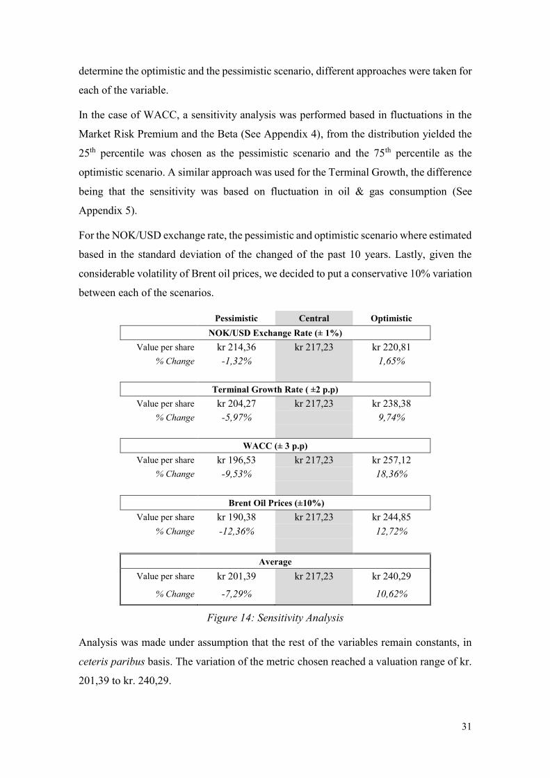
determine the optimistic and the pessimistic scenario, different approaches were taken for

each of the variable.

In the case of WACC, a sensitivity analysis was performed based in fluctuations in the

Market Risk Premium and the Beta (See Appendix 4), from the distribution yielded the

25th percentile was chosen as the pessimistic scenario and the 75th percentile as the

optimistic scenario. A similar approach was used for the Terminal Growth, the difference

being that the sensitivity was based on fluctuation in oil & gas consumption (See

Appendix 5).

For the NOK/USD exchange rate, the pessimistic and optimistic scenario where estimated

based in the standard deviation of the changed of the past 10 years. Lastly, given the

considerable volatility of Brent oil prices, we decided to put a conservative 10% variation

between each of the scenarios.

Pessimistic Central Optimistic

NOK/USD Exchange Rate (± 1%)

Value per share kr 214,36 kr 217,23 kr 220,81

% Change -1,32% 1,65%

Terminal Growth Rate ( ±2 p.p)

Value per share kr 204,27 kr 217,23 kr 238,38

% Change -5,97% 9,74%

WACC (± 3 p.p)

Value per share kr 196,53 kr 217,23 kr 257,12

% Change -9,53% 18,36%

Brent Oil Prices (±10%)

Value per share kr 190,38 kr 217,23 kr 244,85

% Change -12,36% 12,72%

Average

Value per share kr 201,39 kr 217,23 kr 240,29

% Change -7,29% 10,62%

Figure 14: Sensitivity Analysis

Analysis was made under assumption that the rest of the variables remain constants, in

ceteris paribus basis. The variation of the metric chosen reached a valuation range of kr.

201,39 to kr. 240,29.

32

5.2 Relative Valuation

Peer group selection is one of the first steps, and a crucial one to begin a relative valuation

using the multiples approach. Equinor ASA’s peers were selected based on area of

activities, focusing mainly in integrated oil & gas companies, those that were mostly

dedicated to refining activities were discarded from the group. The Return on Invested

Capital (ROIC) was used as second metric to filter potential peers, as a measure of

profitability for the comparable companies.

(USD Billion) Enterprise

Value

Market

Capitalization ROIC

Long-Term

Growth

Equinor ASA $94,12 $73,78 11,18% 16,9%

Canadian Natural Resources Ltd $60,17 $0,86 9,00% 34,2%

Occidental Petroleum Corp $73,19 $12,27 7,60% 74,1%

Anadarko Petroleum Corp $42,70 $25,00 8,00% 12,0%

ConocoPhillips $76,13 $54,44 13,37% 120,3%

Total SA $137,82 $57,36 9,54% 19,7%

BP PLC $111,55 $82,20 8,40% 37,1%

Royal Dutch Shell PLC $270,20 $128,39 8,87% 21,5%

Repsol SA $35,95 $145,04 9,15% 5,4%

Exxon Mobil Corp $400,52 $15,16 6,47% 23,2%

Figure 15: Equinor’s Peer Group

The main assumptions in the relative valuation approach, is that the value of the firm is

based on the value of other, comparable firms that are expected to generate similar cash

flows in the future. (Berk & DeMarzo, 2014)

5.2.1 Multiples Valuation

By expressing the value of a firm in terms of a multiple, we can adjust the differences

that may be observable among the peers. For the case of Equinor ASA, the two multiples

chosen to best reflect the value of the firm where the EV/EBITDAX and EV/Annual

Production, already discussed in the literature review.

For the multiple approach, the values used were the forecasted financial metrics for

Equinor ASA and its peers. Given that a principle of any valuation is to estimate the value

of the firm based its capacity to generate future cash flow, it was logical to use forward-

looking multiples.

EV to EBITDAX EV to Annual Production

Peer Group’s Average 4,53x $178,51

33

Figure 16: Peer roup’s Multiples

Applying the peer group’s multiples to Equinor ASA financial metrics, we reach the

enterprise value and in order to obtain the equity value of the firm, the market value of

net debt is subtracted.

EV to EBITDAX EV to Annual Production

Equinor’s value per share (kr.) 227,52 235,77

Figure 17: Equinor’s Multiple Valuation

The results from this approach, help to assure the results from the value obtain using

the intrinsic valuations methodologies.

Figure 18: Valuation Summary, Price per Share (Kr./share)

kr 235,77

kr 227,52

kr 217,23

EV / ANNUAL PROD

EV / EBITDAX

DCF Approach

34

6. Comparison with investment bank

The comparison was made against Handelsbanken valuation issued in July 31st, 2018.

The methodologies and main inputs are summarized in the following table:

This report’s Valuation Handelsbanken’s Valuation

Estimated fair price kr 217,23 Kr 240,00

Recommendation Hold Hold

Explicit forecast period 2018-2025 2017-2022

Method - Overall Sum of the Part DCF

Cost of equity without CRP 12,55% 7,60%

Overall WACC 10,17% 6,60%

Perpetuity growth rate 1,85% 1,22%

Figure 19: Summary of differences between this report’s and Handelsbanken’s valuation

Handelsbanken issued a hold recommendation with a target fair-value price of Kr.240 per

share, which represented an upside of only 11% from the market price at 31st of July 2018

of Kr.216.60 per share. This recommendation is in line with 33% of the total 34 analysts

that cover Equinor ASA issued a hold recommendation, as shown in Figure 20.

Buy Hold Sell Consensus

17 12 4 Overweight

Figure 20: Analyst Recommendation Consensus on Equinor ASA, The Wall Street Journal

One of the main differences between the report is the explicit period chosen, at the

moment of Handelsbanken’s valuation, only the results of the first quarter of 2018 was

available making this year part of the explicit period.

In regards of the approach used for the valuation, there is a slight difference between the

report, as we used a sum of the parts approach, where DCF model was used for the current

operations and a real option model for the proved reserves, in the case of Handelsbanken’s

report they value the company as whole was based on the DCF model, in both valuations

sales and earnings where forecasted based in historical financial performance and derived

from expectation of micro and macroeconomics factors.

The most significant differences are in reference of WACC calculation, despite using the

same proxy for the risk-free rate, Handelsbanken used a 2,5% which correspond to the

10-year US Treasury Bond. However, in the case of the equity risk premium it was based

35

on the return of the NYSE, as the beta used the same benchmark as the equity risk

premium. These assumptions can easily explain the differences in the cost of equity and

overall WACC of both models, and at the same time the different prices yielded by each

of the models. As explained in the previous section, for the computation of equity risk

premium and the beta in this report, we took the Norwegian Stock Exchange as the

benchmark, given the majority of operations and revenues of Equinor ASA are coming

from this region.

Despite all the differences found, the overall conclusion was the same given the point in

time in which each of the valuation where done, as both present an upside of around 11%

of the fair value reached against the market value, that is not significant enough

considering the volatility at which the business is exposed to, both reports stand by a hold

recommendation.

36

7. Conclusion

By applying a DCF approach for the valuation of Equinor ASA, we reach a value per

share of Kr.217,23. A hold recommendation is issues, since the upside is only 13,29%

from the market price and given the exposure of the company exposure to Brent oil prices

volatility, we do not find suitable a buy recommendation, in spite of the potential upside

found in the fair value. The assumptions used throughout this model are supported by

industry factors, such as the expected trend of oil prices fluctuations, average

development lag for fields production, estimation of perpetual growth rate driven by

expected increment of oil and gas consumption. Multiple valuation reassure that Equinor

ASA is undervalued in respect to its peers. This report has a limitation the assumptions

taken throughout the valuation process, despite the sensitivity performed.

37

Appendixes

Appendix 1: Financial Statements

Balance Sheet I (USD Billion) 2016 2017 2018 2019E 2020E 2021E 2022E 2023E 2024E 2025E

Property, Plants & Equipment $59,56 $63,64 $76,58 $75,08 $76,52 $77,30 $77,13 $79,13 $77,85 $77,85

Intangible Assets $9,24 $8,62 $11,23 $11,01 $11,22 $11,33 $11,31 $11,60 $11,42 $11,42

Equity Accounted Investments $2,25 $2,55 $2,72 $2,64 $2,55 $2,48 $2,40 $2,32 $2,25 $2,18

Deferred Tax Assets $2,20 $2,44 $3,05 $3,00 $3,05 $3,08 $3,08 $3,16 $3,11 $3,11

Pension Assets $0,84 $1,31 $1,15 $1,10 $1,06 $1,01 $0,97 $0,93 $0,90 $0,86

Derivatives Financial Instruments $1,82 $1,60 $1,14 $1,12 $1,14 $1,15 $1,15 $1,18 $1,16 $1,16

Financial Investments $2,34 $2,84 $2,78 $2,78 $2,78 $2,78 $2,78 $2,78 $2,78 $2,78

Prepayments and Financial Receivables $0,89 $0,91 $1,46 $1,43 $1,45 $1,47 $1,47 $1,50 $1,48 $1,48

Total Non-Current Assets $79,13 $83,91 $100,11 $98,15 $99,78 $100,61 $100,28 $102,61 $100,94 $100,84

Inventories $3,23 $3,40 $3,82 $3,75 $3,82 $3,86 $3,85 $3,95 $3,88 $3,88

Trade and other receivables $7,84 $9,43 $11,36 $11,14 $11,36 $11,47 $11,45 $11,74 $11,55 $11,55

Derivatives Financial Instrument $0,49 $0,16 $0,28 $0,28 $0,28 $0,29 $0,29 $0,29 $0,29 $0,29

Financial Investments $8,21 $8,45 $7,31 $7,31 $7,31 $7,31 $7,31 $7,31 $7,31 $7,31

Cash and Cash equivalents $5,09 $4,39 $2,72 $3,90 $4,60 $8,93 $9,78 $13,03 $14,99 $16,94

Total Current Assets $24,86 $25,82 $25,50 $26,37 $27,37 $31,86 $32,67 $36,32 $38,03 $39,97

Assets held for sale $0,54 $1,37 $0,00 $0,00 $0,00 $0,00 $0,00 $0,00 $0,00 $0,00

TOTAL ASSETS $104,53 $111,10 $125,61 $124,52 $127,15 $132,47 $132,95 $138,93 $138,97 $140,81

38

Balance Sheet II (USD Billion) 2016 2017 2018 2019E 2020E 2021E 2022E 2023E 2024E 2025E

Shareholders’ Equity $35,07 $39,86 $42,67 $44,19 $41,89 $44,30 $45,43 $46,63 $47,84 $49,15

Non-Controlling Interests $0,03 $0,02 $0,02 $0,03 $0,03 $0,03 $0,03 $0,03 $0,03 $0,03

Total Equity $35,10 $39,89 $42,69 $44,22 $41,92 $44,32 $45,46 $46,66 $47,87 $49,19

Finance Debt $28,00 $24,18 $24,69 $21,70 $20,57 $21,75 $22,31 $22,90 $23,49 $24,14

Deferred tax liabilities $6,43 $7,65 $9,48 $9,29 $9,47 $9,57 $9,55 $9,79 $9,64 $9,64

Pension liabilities $3,38 $3,90 $3,96 $3,80 $3,65 $3,50 $3,36 $3,23 $3,10 $2,97

Provisions $13,41 $15,56 $18,80 $18,43 $18,79 $18,98 $18,93 $19,43 $19,11 $19,11

Derivative Financial Instruments $1,42 $0,90 $1,21 $1,18 $1,20 $1,22 $1,21 $1,25 $1,23 $1,23

Total Non-Current Liabilities $52,63 $52,20 $58,13 $54,41 $53,68 $55,01 $55,36 $56,59 $56,56 $57,08

Trade, othey payable and provision $9,67 $9,74 $11,25 $11,03 $11,24 $11,35 $11,33 $11,62 $11,43 $11,43

Current tax payable $2,18 $4,06 $9,04 $8,85 $9,93 $10,03 $10,01 $10,27 $10,10 $10,10

Finance debt $3,67 $4,09 $2,60 $3,31 $6,89 $5,72 $5,99 $6,24 $6,41 $6,70

Dividend Payable $0,71 $0,73 $0,77 $0,77 $0,77 $0,77 $0,77 $0,77 $0,77 $0,77

Derivatives Financial Instruments $0,51 $0,40 $1,21 $1,19 $1,21 $1,23 $1,22 $1,25 $1,23 $1,23

Total Current Liabilities $16,75 $19,02 $24,87 $25,14 $30,04 $29,09 $29,31 $30,14 $29,95 $30,24

TOTAL EQUITY AND LIABILITIES $104,53 $111,10 $125,69 $123,77 $125,64 $128,43 $130,13 $133,40 $134,38 $136,51

39

Income Statement (USD Billion) 2016 2017 2018 2019E 2020E 2021E 2022E 2023E 2024E 2025E

Exploration & Production Norway $13,08 $17,69 $22,65 $22,21 $22,63 $22,86 $22,81 $23,40 $23,03 $23,03

Exploration & Production International $6,66 $9,26 $11,99 $11,75 $11,98 $12,10 $12,07 $12,39 $12,19 $12,19

Marketing, Mid-Stream & Processing $44,98 $59,07 $76,75 $75,25 $76,69 $77,47 $77,30 $79,30 $78,02 $78,02

Other $0,04 $0,09 $0,13 $0,13 $0,13 $0,13 $0,13 $0,13 $0,13 $0,13

Elimination -$18,88 -$24,92 -$32,61 -$31,97 -$32,59 -$32,92 -$32,85 -$33,70 -$33,15 -$33,15

Total revenues and other income $45,87 $61,19 $78,90 $77,36 $78,84 $79,65 $79,47 $81,53 $80,21 $80,21

Purchases (net of inventory variation) -$21,51 -$28,21 -$39,48 -$38,70 -$39,45 -$39,85 -$39,76 -$40,79 -$40,13 -$40,13

Operating expenses -$9,03 -$8,76 -$9,64 -$9,45 -$9,63 -$9,73 -$9,71 -$9,96 -$9,80 -$9,80

Selling, general and administrative

expenses -$0,76 -$0,74 -$0,78 -$0,76 -$0,78 -$0,79 -$0,79 -$0,81 -$0,79 -$0,79

Depreciation, amortization and

impairment losses -$11,55 -$8,64 -$8,74 -$8,56 -$8,73 -$8,82 -$8,80 -$9,03 -$8,88 -$8,88

Exploration expenses -$2,95 -$1,06 -$1,23 -$1,21 -$1,23 -$1,25 -$1,24 -$1,28 -$1,26 -$1,26

Net operating income (loss) $0,08 $13,77 $19,04 $18,66 $19,02 $19,22 $19,17 $19,67 $19,35 $19,35

Net foreign exchange gains (losses) -$0,12 $0,13 -$0,30 -$0,30 -$0,30 -$0,31 -$0,31 -$0,31 -$0,31 -$0,31

Interest income and other financial items $0,44 $0,49 $0,32 $0,35 $0,38 $0,42 $0,45 $0,49 $0,53 $0,58

Gain (losses) derivative fin instruments $0,47 -$0,06 -$0,43 -$0,42 -$0,43 -$0,43 -$0,43 -$0,44 -$0,43 -$0,43

Interest expense -$0,98 -$0,94 -$0,84 $0,00 $0,00 $0,00 $0,00 $0,00 $0,00 $0,00

Impairment loss recognized $0,00 $0,00 $0,00 $0,00 $0,00 $0,00 $0,00 $0,00 $0,00 $0,00

Other financial expenses -$0,07 $0,04 -$0,18 $0,00 $0,00 $0,00 $0,00 $0,00 $0,00 $0,00

Net financial items -$1,24 -$0,35 -$2,27 -$1,30 -$1,37 -$1,35 -$1,34 -$1,35 -$1,33 -$1,31

Income/(loss) before tax -$1,16 $13,42 $16,77 $17,36 $17,65 $17,87 $17,83 $18,32 $18,03 $18,04

Current Income Tax Expense -$4,03 -$7,81 -$11,91 -$11,65 -$13,08 -$13,22 -$13,19 -$13,53 -$13,31 -$13,31

Deferred Tax Expense $1,30 -$1,02 -$1,03 -$1,01 -$1,13 -$1,15 -$1,14 -$1,17 -$1,15 -$1,15

Net income / (loss) -$3,88 $4,60 $3,82 $4,70 $3,43 $3,51 $3,50 $3,62 $3,56 $3,57

40

Cash Flow Statement (USD Billion) 2016 2017 2018 2019E 2020E 2021E 2022E 2023E 2024E 2025E

Income for the period -$3,88 $4,60 $3,82 $4,70 $3,43 $3,51 $3,50 $3,62 $3,56 $3,57

DD&A $11,55 $8,64 $8,74 $8,56 $8,73 $8,82 $8,80 $9,03 $8,88 $8,88

Inventories -$0,73 -$0,17 -$0,42 $0,07 -$0,07 -$0,04 $0,01 -$0,10 $0,06 $0,00

Trade and other receivables -$1,17 -$1,59 -$1,94 $0,22 -$0,21 -$0,12 $0,03 -$0,30 $0,19 $0,00

Trade and other payables $0,33 $0,07 $1,51 -$0,22 $0,21 $0,11 -$0,03 $0,29 -$0,19 $0,00

Deferred tax and Tax receivables and

payables -$1,72 $2,85 $6,19 -$0,32 $1,21 $0,17 -$0,04 $0,43 -$0,27 $0,00

Others $0,92 $0,04 -$0,33 -$0,08 -$0,14 -$0,12 -$0,10 -$0,13 -$0,07 -$0,09

(Increase) decrease in net derivative

financial instruments $1,31 -$0,08 $1,46 -$0,02 $0,02 $0,01 $0,00 $0,03 -$0,02 $0,00

Cash flow from operations $6,61 $14,37 $19,02 $12,92 $13,17 $12,34 $12,17 $12,86 $12,15 $12,37

Capital expenditure -$10,72 -$10,76 -$19,79 -$7,07 -$10,17 -$9,60 -$8,62 -$11,02 -$7,61 -$8,88

Intangible assets $0,21 $0,62 -$2,61 $0,22 -$0,21 -$0,11 $0,03 -$0,29 $0,19 $0,00

Investments in associated companies -$1,42 -$0,31 -$0,17 $0,08 $0,08 $0,08 $0,08 $0,07 $0,07 $0,07

Financial investments -$0,01 -$0,50 $0,06 $0,00 $0,00 $0,00 $0,00 $0,00 $0,00 $0,00

(Increase) decrease in current financial

investments $1,61 -$0,24 $1,14 $0,00 $0,00 $0,00 $0,00 $0,00 $0,00 $0,00

Other $0,50 $1,27 $4,61 -$0,37 $0,35 $0,19 -$0,04 $0,49 -$0,31 $0,00

Cash flow from investing -$9,83 -$9,91 -$16,76 -$7,13 -$9,94 -$9,44 -$8,56 -$10,75 -$7,66 -$8,81

Free cash flow -$3,22 $4,47 $2,27 $5,79 $3,23 $2,90 $3,61 $2,11 $4,49 $3,56

Net proceeds from debt issuance -$0,62 -$3,40 -$0,98 -$2,28 $2,45 $0,00 $0,82 $0,84 $0,77 $0,94

Dividends paid -$1,92 -$1,53 -$2,30 -$2,30 -$2,30 -$2,30 -$2,30 -$2,30 -$2,30 -$2,30

Repurchase of shares and other equity

transactions -$0,03 -$0,02 -$0,01 $0,00 $0,00 $0,00 $0,00 $0,00 $0,00 $0,00

Unrealized (losses)/gains on securities $0,00 -$0,06 $0,06 $0,00 $0,00 $0,00 $0,00 $0,00 $0,00 $0,00

Other comprehensive Income -$0,37 $0,10 $0,01 $0,00 $0,00 $0,00 $0,00 $0,00 $0,00 $0,00

Cash flow from financing activities -$2,94 -$4,92 -$3,21 -$4,58 $0,15 -$2,29 -$1,47 -$1,46 -$1,53 -$1,36

Currency translation differences -$0,17 -$0,38 -$0,23 $0,00 $0,00 $0,00 $0,00 $0,00 $0,00 $0,00

Change in cash and cash equivalents -$6,33 -$0,84 -$1,18 $1,21 $3,38 $0,60 $2,14 $0,65 $2,96 $2,19

41

Appendix 2: Energy Outlook

Primary Energy

Consumption (Mill toe) 1970 1980 1990 2000 2010 2020 2030 2040

Average annual

change 2000-2040

Oil 2.252,97 2.985,75 3.152,50 3.579,58 4.021,41 4.563,94 4.863,89 4.835,58 0,88%

Gas 890,02 1.291,47 1.767,44 2.181,72 2.874,25 3.534,25 4.148,30 4.706,51 2,89%

Coal 1.482,76 1.812,74 2.246,41 2.384,72 3.635,64 3.697,04 3.821,24 3.761,60 1,44%

Nuclear 17,73 160,96 452,97 584,28 625,91 673,65 772,13 911,67 1,40%

Hydro 265,82 384,56 487,49 601,11 778,67 1.014,73 1.159,92 1.241,11 2,66%

Renewables 2,31 6,82 35,02 59,02 234,11 794,05 1.551,89 2.526,99 104,53%

Commodities Price Forecast 2018 2019E 2020E 2021E 2022E 2023E 2024E 2025E

Brent Price

($/barrel) $71,09 $69,13 $70,62 $71,43 $71,25 $73,32 $72,00 $72,00

West Texas Intermediate

($/barrel) $66,37 $61,05 $64,38 $65,09 $65,51 $66,83 $70,00 $70,00

Henry Hub Price

($/mmBtus) $2,90 $2,90 $3,10 $3,30 $3,40 $3,55 $3,75 $3,90

National Balancing Point

(£/therm) £0,60 £0,61 £0,57 £0,53 £0,53 £0,53 £0,53 £0,54

42

Appendix 3: Extended Peer Group

Company Name Enterprise Value

($ USD Bn)

Market Capitalization

($ USD Bn) ROIC Long Term Growth

Equinor ASA $94,12 $73,78 11,18% 16,90%

YPF SA $17,65 $0,67 3,60% -6,40%

Canadian Natural Resources Ltd $60,17 $0,86 9,00% 34,20%

Frontera Energy Corp $1,83 $5,40 0,00% 0,00%

Marathon Oil Corp $19,32 $5,46 2,75% 0,00%

Encana Corp $19,80 $11,45 0,00% 46,00%

Galp Energia SGPS SA $19,81 $11,94 23,90% 19,90%

Apache Corp $24,27 $12,24 0,00% 127,60%

Occidental Petroleum Corp $73,19 $12,27 7,60% 74,10%

Devon Energy Corp $34,32 $14,74 1,00% 63,00%

Exxon Mobil Corp $400,52 $15,16 6,47% 23,20%

Anadarko Petroleum Corp $42,70 $25,00 8,00% 12,00%

OMV AG $27,48 $25,40 29,70% 3,80%

Chevron Corp $273,43 $29,83 6,43% 58,10%

Hess Corp $18,39 $37,19 1,87% 0,00%

NK Lukoil PAO $46,13 $48,40 14,65% 0,00%

ConocoPhillips $76,13 $54,44 13,37% 120,30%

Eni SpA $93,48 $57,29 8,73% 27,70%

Total SA $137,82 $57,36 9,54% 19,70%

Petroleo Brasileiro SA Petrobras $0,00 $72,67 0,00% 24,10%

BP PLC $111,55 $82,20 8,40% 37,10%

Royal Dutch Shell PLC $270,20 $128,39 8,87% 21,50%

Repsol SA $35,95 $145,04 9,15% 5,40%

Gazprom PAO $98,36 $195,37 10,20% 11,70%

PetroChina Co Ltd $340,40 $214,87 7,14% 35,80%

Ecopetrol SA $63,85 $241,70 40,00% 0,00%

Premier Oil PLC $3,01 $313,47 3,00% 0,00%

43

Appendix 4: Sensitivity Weighted Average Cost of Capital (WACC)

WACC Market Risk Premium

2,81% 3,81% 4,81% 5,81% 6,81% 7,81% 8,81% 9,81% 10,81% 11,81% 12,81% 13,81% 14,81% B

eta

0,76 3,34% 3,90% 4,46% 5,03% 5,59% 6,15% 6,71% 7,27% 7,83% 8,39% 8,95% 9,51% 10,07%

0,86 3,47% 4,11% 4,75% 5,38% 6,02% 6,65% 7,29% 7,92% 8,56% 9,19% 9,83% 10,46% 11,10%

0,96 3,61% 4,32% 5,03% 5,73% 6,44% 7,15% 7,86% 8,57% 9,28% 9,99% 10,70% 11,41% 12,12%

1,06 3,74% 4,52% 5,31% 6,09% 6,87% 7,66% 8,44% 9,22% 10,01% 10,79% 11,57% 12,36% 13,14%

1,16 3,87% 4,73% 5,59% 6,44% 7,30% 8,16% 9,02% 9,87% 10,73% 11,59% 12,45% 13,31% 14,16%

1,26 4,00% 4,93% 5,87% 6,80% 7,73% 8,66% 9,59% 10,53% 11,46% 12,39% 13,32% 14,25% 15,19%

1,36 4,13% 5,14% 6,15% 7,15% 8,16% 9,16% 10,17% 11,18% 12,18% 13,19% 14,20% 15,20% 16,21%

1,46 4,27% 5,35% 6,43% 7,51% 8,59% 9,67% 10,75% 11,83% 12,91% 13,99% 15,07% 16,15% 17,23%

1,56 4,40% 5,55% 6,71% 7,86% 9,02% 10,17% 11,33% 12,48% 13,63% 14,79% 15,94% 17,10% 18,25%

1,66 4,53% 5,76% 6,99% 8,22% 9,44% 10,67% 11,90% 13,13% 14,36% 15,59% 16,82% 18,05% 19,28%

1,76 4,66% 5,96% 7,27% 8,57% 9,87% 11,18% 12,48% 13,78% 15,09% 16,39% 17,69% 18,99% 20,30%

1,86 4,79% 6,17% 7,55% 8,92% 10,30% 11,68% 13,06% 14,43% 15,81% 17,19% 18,57% 19,94% 21,32%

1,96 4,92% 6,38% 7,83% 9,28% 10,73% 12,18% 13,63% 15,08% 16,54% 17,99% 19,44% 20,89% 22,34%

44

Appendix 5: Sensitivity Terminal Growth Rate

Terminal Growth

Rate

Oil Production

321.859 328.428 335.130 341.970 348.949 356.070 363.337 374.237 385.464 397.028 408.939 421.207 433.843

Ga

s P

rod

uct

ion

298.313 1,85% 1,84% 1,83% 1,82% 1,81% 1,80% 1,79% 1,77% 1,76% 1,74% 1,73% 1,71% 1,70%

304.401 1,86% 1,85% 1,84% 1,83% 1,82% 1,81% 1,80% 1,78% 1,77% 1,75% 1,74% 1,72% 1,71%

310.614 1,87% 1,86% 1,85% 1,84% 1,83% 1,82% 1,81% 1,79% 1,78% 1,76% 1,75% 1,73% 1,72%

316.953 1,88% 1,87% 1,86% 1,85% 1,84% 1,83% 1,82% 1,80% 1,79% 1,77% 1,76% 1,74% 1,73%

323.421 1,89% 1,88% 1,87% 1,86% 1,85% 1,84% 1,83% 1,81% 1,80% 1,78% 1,77% 1,75% 1,74%

330.022 1,90% 1,89% 1,88% 1,87% 1,86% 1,85% 1,84% 1,82% 1,81% 1,79% 1,78% 1,76% 1,75%

336.757 1,91% 1,90% 1,89% 1,88% 1,87% 1,86% 1,85% 1,83% 1,82% 1,80% 1,79% 1,77% 1,76%

346.859 1,92% 1,91% 1,90% 1,89% 1,88% 1,87% 1,86% 1,85% 1,83% 1,82% 1,80% 1,79% 1,77%

357.265 1,94% 1,93% 1,92% 1,91% 1,90% 1,89% 1,88% 1,86% 1,85% 1,83% 1,82% 1,80% 1,79%

367.983 1,95% 1,94% 1,93% 1,92% 1,91% 1,90% 1,89% 1,88% 1,86% 1,85% 1,83% 1,82% 1,80%

379.023 1,97% 1,96% 1,95% 1,94% 1,93% 1,92% 1,91% 1,89% 1,88% 1,86% 1,85% 1,83% 1,82%

390.393 1,98% 1,97% 1,96% 1,95% 1,94% 1,93% 1,92% 1,91% 1,89% 1,88% 1,86% 1,85% 1,83%

402.105 2,00% 1,99% 1,98% 1,97% 1,96% 1,95% 1,94% 1,92% 1,91% 1,89% 1,88% 1,86% 1,85%

45

Bibliography

Berk, J., & DeMarzo, P. (2014). Corporate finance; Corporate finance. The Prentice

Hall series in finance. https://doi.org/10.1016/S1574-0102(03)01011-2

Biscardini, G,, Morrison R., Branson, D., Del Maestro, A. (2018). Oil and Gas Trends

2018-19: Strategy shaped by volatility.

https://www.strategyand.pwc.com/trend/2018-oil-gas

Blume, M. E. (1975). BETAS AND THEIR REGRESSION TENDENCIES. The

Journal of Finance. https://doi.org/10.1111/j.1540-6261.1975.tb01850.x

Bodnar, G. M., Dumas, B., & Marston, R. (2004). Cross-border valuation: The

international cost of equity capital. In The INSEAD-Wharton Alliance on

Globalizing: Strategies for Building Successful Global Businesses.

https://doi.org/10.1017/CBO9780511522093.012

BP Energy Economics. (2018). BP Energy Outlook 2018. 2018 BP Energy Outlook.

https://doi.org/10.1088/1757-899X/342/1/012091

Clark, J., Hill, S., Mago, N., Zenner, M. (2008). The Most Important Number in

Finance: The Quest for the Market Risk Premium - J.P Morgan

Damodaran, A. (2002). Investment Valuation: Second Edition. Wiley Finance.

https://doi.org/10.1016/B978-0-7020-2797-0.00001-1

Damodaran, A. (2008). What is the Riskfree Rate? A Search for the Basic Building

Block. SSRN. https://doi.org/10.2139/ssrn.1317436

Damodaran, A. (2009). Ups and Downs: Valuing Cyclical and Commodity Companies.

SSRN. https://doi.org/10.2139/ssrn.1466041

Damodaran, A. (2018). Equity Risk Premiums (ERP): Determinants, Estimation and

Implications – The 2018 Edition. SSRN. https://doi.org/10.2139/ssrn.3140837

Damodaran, A. (2010). The Dark Side of Valuation. Journal of Chemical Information

and Modeling. https://doi.org/10.1016/B978-0-7020-2797-0.00001-1

Deloite. (2017). 2018 Outlook on Oil and Gas. Deloitte Center for Energy Solutions.

Equinor, 2018. Second quarter 2018: Financial statements and review

Equinor, 2018. Third quarter 2018: Financial statements and review

ExxonMovile. (2018). 2018 Outlook for Energy.

Fernandez, P. (2001). Company Valuation Methods. SSRN.

https://doi.org/10.2139/ssrn.274973

Fernández, P. (2001). Company Valuation Methods. The Most Common Errors in

Valuations. Social Science Research Network. https://doi.org/10.2139/ssrn.274973

46

Fernandez, P. (2001). Valuation Using Multiples: How Do Analysts Reach Their

Conclusions? SSRN. https://doi.org/10.2139/ssrn.274972

IMF. (2018). World Economic Outlook Database April 2018.

https://doi.org/10.1111/ajpy.12157

James, M., James, M., Koller, T. M., & Koller, T. M. (2000). Valuation in emerging

markets. Working Paper. https://doi.org/10.1073/pnas.0832308100

Koller, T., Goedhart, M., & Wessels, D. (2005). The right Role for Multiples in

Valuation. McKinsey on Finance.

Koller, T., Goefhart, M., & Wessels, D. (2010). Measuring and managing the value of

company. McKinsey & Company.

LNG Outlook, 2018 Shell. (2018). Definitions & Cautionary Note. 2018 Shell LNG

Outlook.

Luehrman, T. A. (1997). Using APV: A better tool for valuing operations. Harvard

Business Review.

Luehrman, T. A. (1997). What’s it worth? A general manager’s guide to valuation.

Harvard Business Review. https://doi.org/Article

Pinto, J. E., Robinson, T. R., & Stowe, J. D. (2018). Equity valuation: A survey of

professional practice. Review of Financial Economics.

https://doi.org/10.1002/rfe.1040

Rosenbaum, J., & Pearl, J. (2009). Investment Banking - Valuation, Leveraged Buyouts,

and Mergers & Aqcusitions. Modern healthcare.

https://doi.org/10.1002/9781118267943

Samuelsen, J. (2018). A Guide to Norwegian Petroleum Taxation - KPMG,

https://assets.kpmg/content/dam/kpmg/no/pdf/2018/a-guide-to-petroleum-taxation-

2018-print.pdf

Statoil, 2017. 2017 Annual Report and Form 20-F

Statoil, 2018. First Quarter 2018: Financial statements and review

U.S. EIA. (2018). Annual Energy Outlook 2018 with projections to 2050. Annual

Energy Outlook 2018 with Projections to 2050. https://doi.org/DOE/EIA-

0383(2012) U.S.

Weimer, J., & Marsal, R. (2018). Equity Market Risk Premium Research Summary.

MRP Research Summary- KPMG. https://doi.org/10.1038/sj.ejcn.1601913