Non-oriented MLS Gradient Field

Volume 0 (1981), Number 0 pp. 1–12 COMPUTER GRAPHICS forum

Non-oriented MLS Gradient Fields

Jiazhou Chen1,2 Gaël Guennebaud 2 Pascal Barla2 Xavier Granier2

1 College of Computer Science - Zhejiang University of Technology2 Inria - LaBRI (CNRS, Univ. Bordeaux) - LP2N (CNRS, Univ. Bordeaux, IOGS)

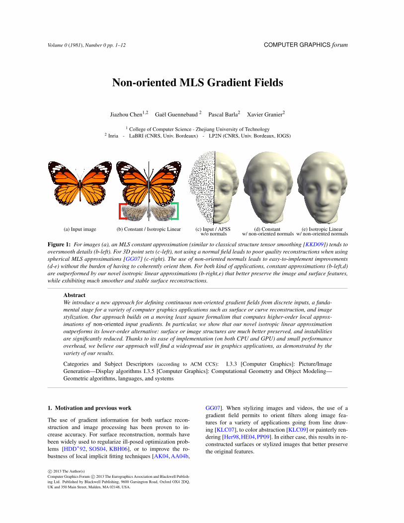
(a) Input image (b) Constant / Isotropic Linear (c) Input / APSS (d) Constant (e) Isotropic Linearw/o normals w/ non-oriented normals w/ non-oriented normals

Figure 1: For images (a), an MLS constant approximation (similar to classical structure tensor smoothing [KKD09]) tends tooversmooth details (b-left). For 3D point sets (c-left), not using a normal field leads to poor quality reconstructions when usingspherical MLS approximations [GG07] (c-right). The use of non-oriented normals leads to easy-to-implement improvements(d-e) without the burden of having to coherently orient them. For both kind of applications, constant approximations (b-left,d)are outperformed by our novel isotropic linear approximations (b-right,e) that better preserve the image and surface features,while exhibiting much smoother and stable surface reconstructions.

AbstractWe introduce a new approach for defining continuous non-oriented gradient fields from discrete inputs, a funda-mental stage for a variety of computer graphics applications such as surface or curve reconstruction, and imagestylization. Our approach builds on a moving least square formalism that computes higher-order local approx-imations of non-oriented input gradients. In particular, we show that our novel isotropic linear approximationoutperforms its lower-order alternative: surface or image structures are much better preserved, and instabilitiesare significantly reduced. Thanks to its ease of implementation (on both CPU and GPU) and small performanceoverhead, we believe our approach will find a widespread use in graphics applications, as demonstrated by thevariety of our results.

Categories and Subject Descriptors (according to ACM CCS): I.3.3 [Computer Graphics]: Picture/ImageGeneration—Display algorithms I.3.5 [Computer Graphics]: Computational Geometry and Object Modeling—Geometric algorithms, languages, and systems

1. Motivation and previous work

The use of gradient information for both surface recon-struction and image processing has been proven to in-crease accuracy. For surface reconstruction, normals havebeen widely used to regularize ill-posed optimization prob-lems [HDD∗92, SOS04, KBH06], or to improve the ro-bustness of local implicit fitting techniques [AK04, AA04b,

GG07]. When stylizing images and videos, the use of agradient field permits to orient filters along image fea-tures for a variety of applications going from line draw-ing [KLC07], to color abstraction [KLC09] or painterly ren-dering [Her98,HE04,PP09]. In either case, this results in re-constructed surfaces or stylized images that better preservethe original features.

c© 2013 The Author(s)Computer Graphics Forum c© 2013 The Eurographics Association and Blackwell Publish-ing Ltd. Published by Blackwell Publishing, 9600 Garsington Road, Oxford OX4 2DQ,UK and 350 Main Street, Malden, MA 02148, USA.

J. Chen, G. Guennebaud P. Barla, & X. Granier / Non-oriented MLS Gradient Fields

(a) Oriented gradient smoothing (b) Structure tensor smoothing

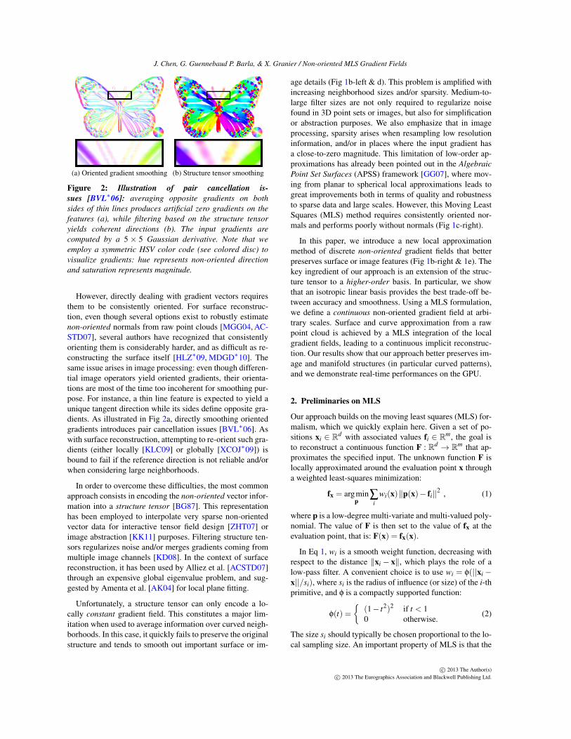
Figure 2: Illustration of pair cancellation is-sues [BVL∗06]: averaging opposite gradients on bothsides of thin lines produces artificial zero gradients on thefeatures (a), while filtering based on the structure tensoryields coherent directions (b). The input gradients arecomputed by a 5× 5 Gaussian derivative. Note that weemploy a symmetric HSV color code (see colored disc) tovisualize gradients: hue represents non-oriented directionand saturation represents magnitude.

However, directly dealing with gradient vectors requiresthem to be consistently oriented. For surface reconstruc-tion, even though several options exist to robustly estimatenon-oriented normals from raw point clouds [MGG04, AC-STD07], several authors have recognized that consistentlyorienting them is considerably harder, and as difficult as re-constructing the surface itself [HLZ∗09, MDGD∗10]. Thesame issue arises in image processing: even though differen-tial image operators yield oriented gradients, their orienta-tions are most of the time too incoherent for smoothing pur-pose. For instance, a thin line feature is expected to yield aunique tangent direction while its sides define opposite gra-dients. As illustrated in Fig 2a, directly smoothing orientedgradients introduces pair cancellation issues [BVL∗06]. Aswith surface reconstruction, attempting to re-orient such gra-dients (either locally [KLC09] or globally [XCOJ∗09]) isbound to fail if the reference direction is not reliable and/orwhen considering large neighborhoods.

In order to overcome these difficulties, the most commonapproach consists in encoding the non-oriented vector infor-mation into a structure tensor [BG87]. This representationhas been employed to interpolate very sparse non-orientedvector data for interactive tensor field design [ZHT07] orimage abstraction [KK11] purposes. Filtering structure ten-sors regularizes noise and/or merges gradients coming frommultiple image channels [KD08]. In the context of surfacereconstruction, it has been used by Alliez et al. [ACSTD07]through an expensive global eigenvalue problem, and sug-gested by Amenta et al. [AK04] for local plane fitting.

Unfortunately, a structure tensor can only encode a lo-cally constant gradient field. This constitutes a major lim-itation when used to average information over curved neigh-borhoods. In this case, it quickly fails to preserve the originalstructure and tends to smooth out important surface or im-

age details (Fig 1b-left & d). This problem is amplified withincreasing neighborhood sizes and/or sparsity. Medium-to-large filter sizes are not only required to regularize noisefound in 3D point sets or images, but also for simplificationor abstraction purposes. We also emphasize that in imageprocessing, sparsity arises when resampling low resolutioninformation, and/or in places where the input gradient hasa close-to-zero magnitude. This limitation of low-order ap-proximations has already been pointed out in the AlgebraicPoint Set Surfaces (APSS) framework [GG07], where mov-ing from planar to spherical local approximations leads togreat improvements both in terms of quality and robustnessto sparse data and large scales. However, this Moving LeastSquares (MLS) method requires consistently oriented nor-mals and performs poorly without normals (Fig 1c-right).

In this paper, we introduce a new local approximationmethod of discrete non-oriented gradient fields that betterpreserves surface or image features (Fig 1b-right & 1e). Thekey ingredient of our approach is an extension of the struc-ture tensor to a higher-order basis. In particular, we showthat an isotropic linear basis provides the best trade-off be-tween accuracy and smoothness. Using a MLS formulation,we define a continuous non-oriented gradient field at arbi-trary scales. Surface and curve approximation from a rawpoint cloud is achieved by a MLS integration of the localgradient fields, leading to a continuous implicit reconstruc-tion. Our results show that our approach better preserves im-age and manifold structures (in particular curved patterns),and we demonstrate real-time performances on the GPU.

2. Preliminaries on MLS

Our approach builds on the moving least squares (MLS) for-malism, which we quickly explain here. Given a set of po-sitions xi ∈ Rd with associated values fi ∈ Rm, the goal isto reconstruct a continuous function F : Rd → Rm that ap-proximates the specified input. The unknown function F islocally approximated around the evaluation point x througha weighted least-squares minimization:

fx = argminp

∑i

wi(x)‖p(x)− fi‖2 , (1)

where p is a low-degree multi-variate and multi-valued poly-nomial. The value of F is then set to the value of fx at theevaluation point, that is: F(x) = fx(x).

In Eq 1, wi is a smooth weight function, decreasing withrespect to the distance ‖xi− x‖, which plays the role of alow-pass filter. A convenient choice is to use wi = φ(||xi−x||/si), where si is the radius of influence (or size) of the i-thprimitive, and φ is a compactly supported function:

φ(t) ={

(1− t2)2 if t < 10 otherwise.

(2)

The size si should typically be chosen proportional to the lo-cal sampling size. An important property of MLS is that the

c© 2013 The Author(s)c© 2013 The Eurographics Association and Blackwell Publishing Ltd.


continuity of the reconstruction depends on the continuity ofthe weight functions wi [Lev98]. For instance, the aforemen-tioned choice yields C1 reconstructions.

This formalism is directly amenable to the reconstructionof 3D images [LGM∗08], or oriented vector fields such asdeformation fields [SMW06]. For the reconstruction of d−1manifolds, a common approach is to seek an implicit scalarfield such that its zero iso-contour approximates the inputpositions xi. In the MLS formalism, this means we are seek-ing local approximations such that fx(xi) ≈ 0. To avoid theunwanted trivial solution fx = 0, additional constraints basedon oriented input normals are commonly employed.

The MLS approach contrasts with variational globalmethods such as [ACSTD07] in that it does not require anypreprocess and involves only local computations, making itsuitable to the handle real-time settings and time-varying in-puts [GGG08]. It produces continuous and analytically dif-ferentiable reconstructions, and does not require to define asomewhat arbitrary discretization. The weight function per-mits to elegantly control the amount of smoothing in a localfashion. The price to pay for these benefits is that since re-gressions are performed locally, a MLS approach is poten-tially less robust to disambiguate tricky configurations (e.g.,close sheets) than techniques working globally.

3. Non-oriented MLS gradient fields

The MLS formalism presented in the previous section is notdirectly amenable to the reconstruction of non-oriented gra-dient fields since it is sensitive to the sign of input valuesfi. As motivated in Section 1, this is necessary for a numberof applications including filtering, stylization, simplificationand reconstruction. The main contribution of this paper isto explain how to adapt the MLS formalism to handle non-oriented input normals. Our approach starts by reconstruct-ing a non-oriented gradient field matching the input normals,and then integrates it to recover a local implicit field if re-quired by the application. We first describe the general ap-proach (Sec 3.1), then discuss the choices of appropriate reg-ularization (Sec 3.2), higher-order basis (Sec 3.3) and how tocompute differential properties (Sec 3.4).

3.1. General approach

Our algorithm takes as input a set of non-oriented and unitvectors gi ∈Rd specified at sample positions xi ∈Rd , with dthe dimension of the ambient space (see Fig 3a for an exam-ple in R2). The samples are either pixels of an image or comefrom an arbitrary scattered point cloud. In this work, we fur-ther assume the directions gi come from the normalized gra-dient of an unknown continuous scalar potential. Their ori-entation (i.e., signs) are either unknown and/or irrelevant.

Given an arbitrary evaluation point x ∈ Rd and an Eu-clidean neighborhood Ns(x) = {y∈Rd ; ||x−y|| ≤ s} of size

pi

ui

gx

x

{y ; f x(y)=0}

u

(a) (b)

F

(c)

Figure 3: Overview of our MLS approach. (a) In green,the local approximation gx of the input vectors ui aroundthe evaluation point x. (b) Streamlines of the global recon-struction of the continuous non-oriented vector field u (inblue), and of its respective 2D tangent field (in light red). (c)The reconstructed continuous and unsigned scalar potentialF, and its 0-isovalue (in orange). Note that this iso-contourdoes not correspond to the tangent field streamlines. Thisfigure has been made using the isotropic linear basis.

s, we assume all gradients gi (with xi ∈ Ns) may be wellapproximated by a low degree polynomial gradient field gxdefined in matrix form as (Fig 3a):

gx(·) = B(·)T u(x) , (3)

where B is a polynomial basis matrix with d columns, and uis the vector of unknown polynomial coefficients. For localgradient approximation, B must represent an integrable ba-sis, and its particular choice will be discussed in section 3.3.

The key idea to determine the polynomial coefficients uis to consider the sum of the squared dot products betweenthe local gradient field and the prescribed input gradients gi,which is maximized when they are aligned, independentlyof their orientation:

u(x) = argmaxu

∑i

wi(x)(

gTi (B(xi−x)T u)

)2. (4)

Taken together, Eq 3 and 4 provide an analog to Eq 1 that isinvariant to the sign of gi.

In matrix form, the maximization becomes:

u(x) = argmaxu

uT A(x)u , (5)

with the covariance matrix A defined as:

A(x) = ∑i

wi(x)B(xi−x)gigTi B(xi−x)T . (6)

From these local approximations, we reconstruct a continu-ous, but non-oriented, vector field G : Rd → Rd that glob-ally approximates the discrete vectors gi (Fig 3b). Sincewe are using a centered basis, G is classically defined asG(x) = gx(0). Although the gx are proper gradient fields(i.e., curl-free vector fields), this might not be the case ofG in general (see Figure 17). This MLS reconstruction ofthe gradient field is used directly for image stylization.



When the input samples are supposed to lie on an un-known manifold, the goal is to recover a local scalar poten-tial fx = c+ hx. Since ∇ fx = gx, hx is directly obtained byintegrating gx. The constant term c is recovered such thatthe 0-isosurface of fx best approximates the input samplepositions xi nearby x (Fig 3a). To this end, we minimize thepotentials fx(xi) in a moving least square sense, yielding:

c =−∑i wi(x)hx(xi−x)∑i wi(x)

. (7)

As before, the sought-for manifold is implicitly definedas the 0-isosurface of a continuous unsigned scalar potentialF : Rd → R. It is computed by evaluating the local approxi-mation fx at x: F(x) = fx(0), as illustrated in Fig 3c.

Two questions remain open though. Indeed, the maxi-mization of Eq 5 is an under-constrained problem which hasto be regularized in order to avoid the trivial solution of avector field with infinite magnitude. This question will beaddressed in the next sub-section, after which we will dis-cuss the critical choice of a higher order polynomial basisfor the local gradient fields.

3.2. Problem regularization

Before presenting our regularization constraint for a higher-order basis, we briefly study the case of a constant local ap-proximation.

Regularization for constant approximations

In the case where gx is a constant function, B is the identitymatrix and gx(·) = u(x). Since we assume unit input vec-tors, a natural regularization is then to constrain u(x) to bea unit vector. Under such a constraint, the solution u(x) ofEq 5 is directly found as the eigenvector v of the maximaleigenvalue λ of the following eigenvalue problem [All07]:

A(x)v = λv . (8)

This formulation corresponds to a continuous definition ofthe structure tensor built from discrete and possibly scat-tered inputs. In the context of MLS surface reconstruction, ithas already been suggested by Amenta et al. [AK04], thoughto our knowledge no result has been shown yet.

Generic regularization

In order to overcome the limitations of constant approxima-tions, we study the possibility to locally approximate thevector field by higher order polynomials. In this case, theprevious regularization term (‖gx(y)‖2 = 1, ∀y ∈ Rd) doesnot apply: if gx is a polynomial of arbitrary degree, then itsmagnitude is not constant anymore. Nevertheless, one couldbe tempted to enforce this in a least squares sense by mini-mizing ∑i wi(x)(‖gx(xi−x)‖−1)2. To our knowledge, thereis no direct method to solve for Eq 5 with such additional

Figure 4: Constraint comparisons. Fitted curves obtainedwith the naive constraint ‖u(x)‖ = 1 (in red), and our con-straint given in Eq 9 (in green). The only difference betweenleft and right images is the choice of origin.

least squares constraints. Moreover, this strategy would ex-hibit the undesirable effect to favor local solutions close toa constant gradient field because this is the only solutionthat can fully satisfy such a constraint in general. Naivelyconstraining the Euclidean norm of the solution vector (i.e.,‖u(x)‖ = 1) is not an option either. Indeed, as depicted inFig 4, for a general basis, such a normalization is clearly notinvariant to similarity transformations, and introduces a hugebias in the optimization process [Pra87].

Alliez et al. [ACSTD07] addresses a similar issue by solv-ing over the solution space of unit biharmonic energy. Intheir approach, this regularization is applied to the final solu-tion (i.e.,

∫‖∆F‖2 = 1), thus leading to an expensive global

problem that we strive to avoid here. Applying the same reg-ularization to individual fits (i.e.,

∫‖∆ fx‖2 = 1) enforces the

solutions to have non-zero high-order terms, thus prevent-ing the approximation of constant gradient fields, and areasnearby inflection points.

Our key observation here is that, in average, the norm ofgx should be equal to 1 nearby the considered samples. Thisis achieved by a quadratic normalization constraint:

u(x)T Qu(x) = 1 , (9)

with Q a symmetric positive-definite matrix:

Q(x) = ∑i wi(x)B(xi−x)B(xi−x)T

∑i wi(x). (10)

Equation 9 reduces the space of solutions to the set of unitaryvectors with respect to our data-dependent quadratic normdefined by the matrix Q. Note that the choice of the targetmagnitude, here 1, is totally arbitrary and does not affect thedirections of the fitted gradient. Strictly speaking, our normQ is obviously not affine invariant. However, by constructionit is both invariant to the choice of a basis frame, and to simi-larity transformations of the input data. The solution u(x) ofEq 5 is now directly found as the eigenvector v of the max-imal eigenvalue λ of the following generalized eigenvalueproblem [Tau91]:

A(x)v = λQ(x)v . (11)

When gx represents a constant vector field, then Q is theidentity matrix, and our generalized approach gently boilsdown to the previous structure tensor.



(a) (b) (c)

x

Figure 5: Illustration of the overfitting issue of the fully inte-grable linear basis (g1, f 1), with (a) the local gradient fieldand best fitted isoline for the given red point, and (b) theglobal MLS reconstruction of the gradient field and isocurve.(c) Comparison of various MLS variants: planar fit withoutnormals (magenta) and with non-oriented normals (our f 0,blue), spherical fit without normals (green) and with non-oriented normals (our f ∗, orange), and for comparison pur-pose, spherical fit with consistently oriented normals (red).Note that these last two curves match almost exactly.

3.3. Choice of basis

The choice of basis for gx is critical since it characterizesthe quality of the approximation. For the sake of clarity, weexplicitly develop Eq 3 for constant and linear basis. Moreprecisely, we consider constant g0, linear isotropic g∗, andgeneral linear g1 gradient fields whose expression and re-spective scalar potential are given below:

g0(y) = r → f 0(y) = c+ rT yg∗(y) = r+ ly → f ∗(y) = c+ rT y+ 1

2 l yT yg1(y) = r+L ·y → f 1(y) = c+ rT y+ 1

2 yT Ly

where the scalar c is a constant term, and the vector r storesthe coefficients of the linear term. For the quadratic term,we either use a scalar value l, or a symmetric matrix L toensure that g1 is an integrable gradient field. To better seethe link with the formulation of Eq 3, observe that g∗ is ob-tained using BT = (I, y) and u = (rT , l)T . Once integrated,they represent a hyper-plane, a hyper-sphere, and a generalquadric respectively. g∗ and f ∗ are illustrated in Fig 3, com-pared to others in Fig 5 for sparse data, and in Fig 6 foran image. As already noticed in Section 1, the constant ba-sis cannot approximate well highly-curved regions, yieldingover-smoothing of the features and even instabilities (Fig 5c,6b). On the other hand, the general linear basis of g1 alreadypresents too many degrees of freedom (d-o-f) (5 in 2D, and9 in 3D), and leads to over-fitting issues in the form of thegeneration of oscillations and details which are not presentin the input data (Fig 5a, 5b, 6c).

The isotropic basis g∗ clearly appears to be the best trade-off. Compared to a constant basis it only increases by onethe number of d-o-f while offering a much richer space ofsolutions. Keeping the number of d-o-f as low as possibleis highly desirable, not only for performance reasons, but

(a) Input image (b) Constant

(c) Full linear (d) Isotropic linear

Figure 6: Comparisons using a noisy image. The inputnoisy image (400× 400) in (a) requires a large smoothingneighborhood (s = 16). The gradient field is visualized us-ing line-integral convolution, and the color code of Fig. 2.The constant approximation (b) tends to oversmooth the dataat line extremities and dot centers. The full linear approxi-mation (c) leads to over-fitting issues. Our isotropic linearsolution provides the best trade-off (d).

also to keep high stability with small neighborhoods. Enlarg-ing the neighborhood increases both the computation costsand the risk to take into account different and/or inconsis-tent parts of the input data. Moreover, it should be noted thatin the case of manifold reconstruction, our approach worksbest if the norm of the gradient along a given isovalue ofthe respective local scalar potential is constant. Since this isnot the case of the full linear gradient, this basis also suffersfrom a slight bias in the fitting process.

Figure 5c shows that the non-oriented normal informationhas a greater impact on spherical MLS (isotropic basis) thanon planar MLS. Our intuition is that the non-oriented normalinformation is required to avoid the fitted spheres to sink in-between the input samples, thus producing a high qualitysmooth surface that well preserves the features. Finally, itshould be noted that in this example, our MLS reconstructionwith non-oriented normals works very closely to the APSSmethod which can fit spheres with oriented normals only.

3.4. Differential quantities

Assuming differentiable weight functions wi, our global gra-dient and scalar fields G and F can be analytically differ-entiated. In particular, the computation of surface or curve



normals requires to first compute the gradient∇F of our re-constructed scalar field, which is given by:

∇F(x) =∇c(x)+(1, xT , xT x

)∇u(x) + B(x)T u(x) . (12)

The computation of ∇c is straightforward, as well as BT usince it corresponds to our global gradient G. In contrast,the computation of∇u is more involved since it requires thedifferentiation of a generalized eigenvalue problem:

∇u = V(Σ−λI)+VT (∇A−λQ)u−12

(uT∇Qu

)u ,

where V and Σ are the eigenvectors and eigenvalues of equa-tion 11, and (.)+ denote the Moore-Penrose inverse of thesingular matrix Σ−λI (see Magnus [Mag85] for details).

Another useful differential quantity is the tangential cur-vature κt of the tangential field. This requires to computethe Jacobian of our reconstructed gradient field, which couldbe obtained as above. However, in our applications we havefound sufficient to neglect the variations of gx with respectto x. κt thus boils down to the curvature of the local gradientfield gx, that is: κt ≈ l/||G||.

4. Applications

4.1. Image stylization

This section demonstrates our non-oriented MLS gradientfields on a variety of image stylization techniques. We showhow our approach improves them by systematically compar-ing the results obtained with our Constant Approximations(CA) and Isotropic Linear Approximations (ILA).

Implementation details

In this paper, we employed a 5×5 Gaussian derivative filterto compute the image gradient ∇I from which we get inputunit vectors ui. For fast implementation, we use the follow-ing alternative separable and compactly supported weightfunction:

wi(x,y) = φ

(||x− xi||

s

)φ

(||y− yi||

s

)‖∇I(xi,yi)‖2 .

where the last factor is employed to favor gradients withlarge magnitudes.

Multi-channel (e.g., color) images yield multiple gradientvectors per pixels which are all taken into account and ap-proximated during the construction of the covariance matrixA (Eq 6). Our image processing system is entirely imple-mented on the GPU, and our results are obtained using anNVIDIA GeForce GTX 460 with 1GB of memory.

Thanks to the separability and GPU implementation, oursystem easily achieves real-time performance. For instance,on a 512× 512 image, our non-optimized implementationof the ILA costs 5.1 ms (resp. 11.5 ms) for a neighborhoodof size s = 5 (resp. 20) pixels. Compared to a structure ten-sor, we observe a slowdown factor of about 1.5 to 2 becauseof the need to solve a slightly larger eigenvalue problem(3×3 instead of 2×2). Our ILA implementation extracts the

maximal eigenvalue using the iterative Power method, whilewe use a direct solver for CA. Better performance may beachieved using a direct 3×3 eigensolver.

Results

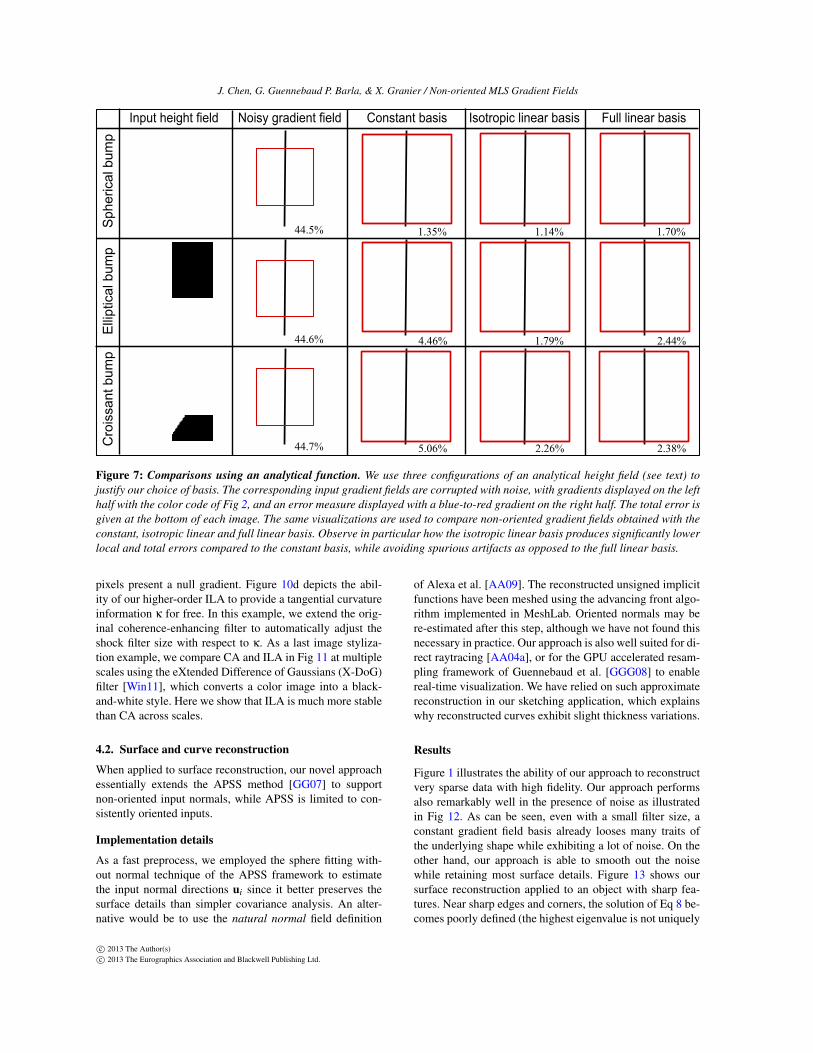
We first provide in Fig 7 a formal comparison between thethree basis functions we have considered in this paper. Tothis end, we have generated three configurations of an an-

alytic height field h(x,y) = exp(− x2

r2x− (y+α exp(−x2/r2

x ))2

r2y

):

spherical (rx = ry = 1,α = 0), elliptical (rx = 2,ry = 1,α =0) and croissant-shaped (rx = 2,ry = 1,α = 1). We havethen created images of their corresponding gradients, cor-rupted them with additive white noise and reconstructednon-oriented gradients with each of the three basis. We in-troduce the following local error measure for comparison:err = |sin(θ∗ − θ)|, where θ

∗ and θ are the angles of theground truth and reconstructed gradient directions respec-tively (this formula is used to discard differences in orien-tation). The total error measure is simply obtained by sum-ming up local error measurements. This comparison showsthe superiority of the isotropic linear basis compared to theother two: it produces the lowest errors without introducingany spurious artifact.

Figure 8 illustrates our approach applied to the flow-basedcolor abstraction (F-Abs) filter [KLC09]. This filter employsa 1D bilateral filter [TM98] along the tangential field (or-thogonal to the gradient field) to preserve image structurethrough abstraction. In comparison to CA, it can be seen thatILA much better preserves important structures of the inputimage. This filter can also be seen in the supplemental video,where our method naturally exhibits good temporal coher-ence even when processing each frame independently. Theadvantage of our ILA is further illustrated in Fig 9, wherecontinuous glass patterns [PP09] are guided by our gradientfields to mimic brush painting. Smoothing directly orienteddirections completely loses the original image structure, ourCA tends to over-smooth the round shape of the eye, whileour ILA preserves well its roundness.

As already noted, our CA method can be seen as a contin-uous variant of classical structure tensor smoothing [KD08].This is a key advantage for enabling high-quality dynamiczooms without any particular overhead since the cost of ourapproach is linear in term of number of evaluations, i.e., interm of the number of pixels of the output image. This con-trasts with approaches based on a global formulation (e.g.,harmonic smoothing) for which the whole input image al-ways has to be considered. This ability is visible in Fig 6,but also in the insets of Fig 10, and in the video wherethe lines produced by coherence-enhancing filtering [KK11]naturally separate or merge depending on the zooming level.This filter applies a 1D shock filter [OR90] along the gradi-ent field to sharpen edges and a 1D bilateral filter along thetangent field to abstract colors. Note that the line-drawingin Fig 10a provides a sparse information since most of the



1.14%1.35% 1.70%

1.79%4.46%

2.26%5.06%

2.44%

2.38%

44.5%

44.6%

44.7%

Input height field Noisy gradient field Constant basis Isotropic linear basis Full linear basisS

pher

ical

bum

pE

llipt

ical

bum

pC

rois

sant

bum

p

Figure 7: Comparisons using an analytical function. We use three configurations of an analytical height field (see text) tojustify our choice of basis. The corresponding input gradient fields are corrupted with noise, with gradients displayed on the lefthalf with the color code of Fig 2, and an error measure displayed with a blue-to-red gradient on the right half. The total error isgiven at the bottom of each image. The same visualizations are used to compare non-oriented gradient fields obtained with theconstant, isotropic linear and full linear basis. Observe in particular how the isotropic linear basis produces significantly lowerlocal and total errors compared to the constant basis, while avoiding spurious artifacts as opposed to the full linear basis.

pixels present a null gradient. Figure 10d depicts the abil-ity of our higher-order ILA to provide a tangential curvatureinformation κ for free. In this example, we extend the orig-inal coherence-enhancing filter to automatically adjust theshock filter size with respect to κ. As a last image styliza-tion example, we compare CA and ILA in Fig 11 at multiplescales using the eXtended Difference of Gaussians (X-DoG)filter [Win11], which converts a color image into a black-and-white style. Here we show that ILA is much more stablethan CA across scales.

4.2. Surface and curve reconstruction

When applied to surface reconstruction, our novel approachessentially extends the APSS method [GG07] to supportnon-oriented input normals, while APSS is limited to con-sistently oriented inputs.

Implementation details

As a fast preprocess, we employed the sphere fitting with-out normal technique of the APSS framework to estimatethe input normal directions ui since it better preserves thesurface details than simpler covariance analysis. An alter-native would be to use the natural normal field definition

of Alexa et al. [AA09]. The reconstructed unsigned implicitfunctions have been meshed using the advancing front algo-rithm implemented in MeshLab. Oriented normals may bere-estimated after this step, although we have not found thisnecessary in practice. Our approach is also well suited for di-rect raytracing [AA04a], or for the GPU accelerated resam-pling framework of Guennebaud et al. [GGG08] to enablereal-time visualization. We have relied on such approximatereconstruction in our sketching application, which explainswhy reconstructed curves exhibit slight thickness variations.

Results

Figure 1 illustrates the ability of our approach to reconstructvery sparse data with high fidelity. Our approach performsalso remarkably well in the presence of noise as illustratedin Fig 12. As can be seen, even with a small filter size, aconstant gradient field basis already looses many traits ofthe underlying shape while exhibiting a lot of noise. On theother hand, our approach is able to smooth out the noisewhile retaining most surface details. Figure 13 shows oursurface reconstruction applied to an object with sharp fea-tures. Near sharp edges and corners, the solution of Eq 8 be-comes poorly defined (the highest eigenvalue is not uniquely



Input image Constant @ 79 fps Isotropic linear @ 66 fps

Figure 8: Flow-based abstraction on a 500× 327 image using a neighborhood of size s = 16. Note the general improvementin shape preservation using our isotropic linear approximation, especially for water droplets.

(a) Input image (b) Oriented gradient @ 77 fps

(c) Constant @ 70 fps (d) Isotropic Linear @ 65 fps

Figure 9: Continuous glass pattern on the eye of Lena im-age (394× 510) using a neighborhood of size s = 12 forthe MLS gradient field. We use a factor of 2.0 for tangen-tial smoothing, and a 10 pixel-wide brush thickness. Di-rectly smoothing oriented gradients quickly loses the origi-nal shape (b). In contrast to CA (c), our ILA (d) better pre-serves the structures in the original image.

(a) Input image (b) Constant @ 88 fps

(d) Isotropic Linear @ 79 fps (c) Isotropic Linear @ 76 fpsCurvature-dependent Shock size Uniform Shock size

Figure 10: Coherence-enhancing filtering for line draw-ing simplification on a 422× 499 image using a neighbor-hood of size s = 11 for the MLS gradient field. We use afactor of 2.0 for tangential smoothing, and a 10 pixel-wideshock filter size. Compared to CA (b), our ILA (c) improvesthe overall sharpness. Furthermore, it permits to locally ad-just the shock size based on curvature to vary stylization (d).

CA

ILA

s = 10 s = 20 s = 30

Figure 11: X-DoG at multiple scales. We compare CA and ILA on a region around the eyes of the Mandril image at threescales. Observe how round features are better preserved through increasing scales with our approach.


J. Chen, G. Guennebaud P. Barla, & X. Granier / Non-oriented MLS Gradient FieldsC

onst

ant

Isot

ropi

c lin

ear

Small filter Large filter

Figure 12: Noisy surface reconstruction. Reconstruction ofthe Stanford bunny model with 1% additional noise usingour non-oriented isotropic linear (top) and constant (bot-tom) gradient field approximations, and using two differentfilter sizes (1.7, and 2.3%).

(a) (b) (c) (d)

Figure 13: The fandisk model corrupted with noise (a), andreconstructed using non-oriented constant gradients (b), ourisotropic linear basis (c), and the APSS method (d). Our so-lution (c) is free of artifacts, and sharper than (d).

defined), and so using a constant basis to reconstruct the gra-dient field leads to jagged edges. This issue is addressed byour approach that even exhibits sharper edges compared tothe fitting of spheres using oriented normals (APSS). Fig-ure 14 illustrates our approach on a very challenging sam-pling obtained using a Kreon laser scanning device. Mullenet al. [MDGD∗10] present a reconstruction of this modelwith their global non-oriented approach. As discussed in sec-tion 5, their solution is generally more robust to topologicalambiguities. On the other hand, it is also one or two ordersof magnitude slower compared to our purely local solution.

Figure 15 illustrates the natural stroke simplification abil-ity of our approach. Here the 2D real-time reconstructiontakes place in the background while the input gradient infor-mation directly comes from the stroke directions. Coherently

Figure 14: A highly non-uniformly sampled model is chal-lenging for purely local methods, yet we obtain a satisfyingreconstruction using our method.

Sketched strokes Reconstructed curves

Sketched strokes Reconstructed curves Varying thickness

Figure 15: Curve from sketched strokes. Our approach forreconstructing of a 2D curve from drawn strokes is quiterobust to the drawing style, like straight lines (top row) orscribbling (middle row). In the bottom row, the reconstructedcurves are further re-stylized with varying thickness depend-ing on the approximate tangential curvature.

orienting the gradients between the different strokes wouldbe particularly challenging on these examples. We furthershow at the bottom of Fig 15 that the approximate tangen-tial curvature κ can be used to vary line thickness, hencere-stylizing the input line drawing.

5. Discussion

Joint interpolation. Both our constant and higher-order gra-dient fields are defined at any location, thus allowing for in-finite zoom at a cost which is independent of the zoom level.On the other hand, our implementations of the presentedstylization filters currently make use of simple bilinear inter-polation of the color information. We believe sharper results



(a) Input image (b) Uniform weights (c) User-drawn masks (d) Non-uniform weights

Figure 16: Non-uniform weights for adaptive flow-based abstraction By adjusting the neighborhood size using a hand-drawnscale image (c-top) and hand-selected segmentation (c-bottom), we locally improve the preservation of small features (e.g., onthe peacock body and head) and the preservation of original discontinuities (e.g., between the body and tail feathers), as seenwhen comparing (b) and (d). A comparison with constant approximations is given in supplemental materials.

could be obtained by using more elaborated color interpola-tion techniques. Our gradient fields could certainly help herefor better edge preservation.

Extensions. In this paper we focused on the approximationof smooth gradient fields mainly ignoring the junctions, oc-clusions and sharp edges that may arises in images or 3Dpoint clouds. This is however an orthogonal problem. In-deed, to deal with discontinuities, many extensions of MLShave already been proposed (e.g., [FCOS05, OGG09]), andmany of them could be directly applied to our approachwithout major difficulties. In the same vein, we considerthe choice of the neighborhood size s as a separate andmore general problem. For instance, Fig 16 illustrates theuse of masks to clip the neighborhoods at discontinuities,and locally adjust their size. In future work, we would liketo investigate the adaptation of the Growing Least-Squaresapproach [MBG∗12] to identify pertinent scales of non-oriented gradient fields automatically. For videos, we thinkthat the use of motion flow could increase temporal smooth-ing, and help deal more properly with occluding contours.

Residual curl. As shown in Figure 17, the reconstructedMLS field G might not be curl-free. Strictly speaking, it isnot a pure gradient field. Nevertheless, in practice, regionswith non-zero curls are restricted to singularities (in red) andto locations where there is no meaningful information, i.e.,regions where the magnitude of the input gradient is verysmall (in blue).

Sheet separation. It is worth noting that if the input nor-mals are known to be consistently oriented, then our novelMLS surface approach has no real advantages compared tothe APSS method. In particular, oriented normals combinedwith sphere fitting performs remarkably well at sheet sep-aration under very sparse sampling (Fig 18d), whereas ourapproach will collapse the two sheets more like any planarapproximations would do (Fig 18b). Of course, this remarkonly applies if the normal orientations can be known in ad-vance without any ambiguity (Fig 18c). We believe that aglobal integration of our MLS gradient field could probablyovercome this difficulty at the cost of significantly more ex-pensive computations [ACSTD07].

Figure 17: Our reconstructed MLS fields locally have non-zero curl (red/blue pixels), as illustrated on the noisy andbutterfly images. Locations where the input gradient magni-tude is smaller (resp. larger) than a threshold value (we use0.0005) are shown in blue (resp. red).

Extra zeros. As usual with MLS surface reconstruction, theglobal scalar field F might present some unwanted extra ze-ros [AA06]. Since, by definition, they happen far away fromthe input points, they are not a problem for smoothing, re-sampling, or meshing with an advancing front. If evaluationshappen in the whole space (e.g., for raytracing) then solutionsuch as the one proposed by Guennebaud and Gross [GG07]may be used.

6. Conclusion

We have demonstrated how the classical structure tensorcan be advantageously generalized to achieve higher-orderapproximations of non-oriented gradient fields. In particu-lar, we have shown that the best trade-off between stabil-ity and reconstruction fidelity lies in local isotropic linearapproximations, provided our appropriate regularization isemployed. The presented MLS formalism provides contin-uous solutions at arbitrary scales with a low computationalcomplexity. Our approach is particularly effective for localsurface and curve reconstructions from sparse and/or noisydata sets, as well as for image abstraction and stylization.They constitute two kinds of applications for which it is sel-dom possible to orient gradients consistently. A potentialalternative would be to consider non-oriented fields as ori-ented vector fields on the covering space [NP09]. Such anapproach deserves further investigations, and would present



Figure 18: A highly downsampled version of the HappyBuddha presents some very thin undersampled layers (a),and yields to collapsing artefacts with our approach (b).On this difficult test case, the normal orienter of MeshLab(based on [HDD∗92]) fails to correctly orient the computednormals, thus making a correct reconstruction impossiblefor APSS (c), unless using the normals of the original highresolution model (d).

the benefit of enabling classic vector field processing ontonon-oriented fields.

We believe that our approach could benefit to many othertypes of data and applications. Since our MLS formulationworks for arbitrary dimensions, it could be used for scien-tific visualization (e.g., 3D medical imaging). It may serve asa basis for multi-scale image decomposition, using increas-ing MLS support sizes [MBG∗12]. For videos, optic flowsmay be used to combine corresponding gradients across sub-sequent frames, for instance by advecting the MLS weightfunctions. Finally, global surface reconstruction methodsthat rely on analytic gradient fields [KBH06, ACSTD07]could also benefit from our approach.

Acknowledgments

This work has been supported by the ANR SeARCH project(ANR-09-CORD-019), and ANR DRAO project (12-JS02-003 01). The models of figures 12 and 18 are courtesy ofthe Stanford Computer Graphics Laboratory, and the modelof figure 14 is courtesy of the AIM@SHAPE Shape Repos-itory.

References[AA04a] ADAMSON A., ALEXA M.: Approximating bounded,

non-orientable surfaces from points. In Shape Modeling Interna-

tional (2004), pp. 243–252. 7

[AA04b] ALEXA M., ADAMSON A.: On normals and projectionoperators for surfaces defined by point sets. In Proc. Eurograph-ics Symposium on Point-Based Graphics (2004), pp. 149–156. 1

[AA06] ADAMSON A., ALEXA M.: Anisotropic point set sur-faces. In Afrigraph ’06: Proc. international conference on Com-puter graphics, virtual reality, visualisation and interaction inAfrica (2006), ACM, pp. 7–13. 10

[AA09] ALEXA M., ADAMSON A.: Interpolatory point setsurfaces-convexity and hermite data. ACM Transactions onGraphics (TOG) 28, 2 (2009), 20. 7

[ACSTD07] ALLIEZ P., COHEN-STEINER D., TONG Y., DES-BRUN M.: Voronoi-based variational reconstruction of unori-ented point sets. In Proc. Eurographics Symposium on GeometryProcessing 2007 (2007), pp. 39–48. 2, 3, 4, 10, 11

[AK04] AMENTA N., KIL Y. J.: Defining point-set surfaces.ACM Trans. Graph. 23, 3 (2004), 264–270. 1, 2, 4

[All07] ALLAIRE G.: Numerical Analysis and Optimization: AnIntroduction to Mathematical Modelling and Numerical Simula-tion. 2007. 4

[BG87] BIGÜN J., GRANLUND G. H.: Optimal orientation detec-tion of linear symmetry. In Proc. IEEE International Conferenceon Computer Vision (1987), pp. 433–438. 2

[BVL∗06] BROX T., VAN DEN BOOMGAARD R., LAUZE F.,VAN DE WEIJER J., WEICKERT J., KORNPROBST P.: Adap-tive structure tensors and their applications. In Visualization andimage processing of tensor fields, Weickert J., Hagen H., (Eds.),vol. 1. Springer, Jan. 2006, ch. 2, pp. 17–47. 2

[FCOS05] FLEISHMAN S., COHEN-OR D., SILVA C. T.: Ro-bust moving least-squares fitting with sharp features. ACM Trans.Graph. 24, 3 (2005), 544–552. 10

[GG07] GUENNEBAUD G., GROSS M.: Algebraic point set sur-faces. ACM Trans. Graph. 26, 3 (2007). 1, 2, 7, 10

[GGG08] GUENNEBAUD G., GERMANN M., GROSS M.: Dy-namic sampling and rendering of algebraic point set surfaces.Computer Graphics Forum 27, 2 (2008). 3, 7

[HDD∗92] HOPPE H., DEROSE T., DUCHAMP T., MCDONALDJ., STUETZLE W.: Surface reconstruction from unorganizedpoints. In Proc. SIGGRAPH ’92 (1992), ACM, pp. 71–78. 1,11

[HE04] HAYS J., ESSA I.: Image and video based painterly an-imation. In NPAR’04: Proc. symposium on Non-photorealisticanimation and rendering (2004), ACM/Eurographics, pp. 113–120. 1

[Her98] HERTZMANN A.: Painterly rendering with curved brushstrokes of multiple sizes. In Proc. SIGGRAPH ’98 (1998), ACM,pp. 453–460. 1

[HLZ∗09] HUANG H., LI D., ZHANG H., ASCHER U., COHEN-OR D.: Consolidation of unorganized point clouds for surfacereconstruction. ACM Trans. Graph. 28, 5 (2009). 2

[KBH06] KAZHDAN M., BOLITHO M., HOPPE H.: Poisson sur-face reconstruction. In Proc. Eurographics Symposium on Ge-ometry Processing 2006 (2006), pp. 43–52. 1, 11

[KD08] KYPRIANIDIS J., DÖLLNER J.: Image abstraction bystructure adaptive filtering. Proc. EG UK Theory and Practiceof Computer Graphics (2008), 51–58. 2, 6

[KK11] KYPRIANIDIS J., KANG H.: Image and video abstractionby coherence-enhancing filtering. Computer Graphics Forum 30,2 (2011), 593–602. 2, 6



[KKD09] KYPRIANIDIS J., KANG H., DÖLLNER J.: Image andvideo abstraction by anisotropic kuwahara filtering. ComputerGraphics Forum 28, 7 (2009), 1955–1963. 1

[KLC07] KANG H., LEE S., CHUI C.: Coherent line drawing.In NPAR’07: Proc. symposium on Non-photorealistic animationand rendering (2007), ACM/Eurographics, pp. 43–50. 1

[KLC09] KANG H., LEE S., CHUI C. K.: Flow-based imageabstraction. IEEE Trans. Visualization and Comput. Graph. 15,1 (2009), 62–76. 1, 2, 6

[Lev98] LEVIN D.: The approximation power of moving least-squares. Mathematics of Computation 67 (1998), 1517–1531. 2

[LGM∗08] LEDERGERBER C., GUENNEBAUD G., MEYER M.,BACHER M., PFISTER H.: Volume MLS Ray Casting. IEEETransactions on Visualization and Computer Graphics 14, 6(2008), 1372–1379. 3

[Mag85] MAGNUS J. R.: On differentiating eigenvalues andeigenvectors. Econometric Theory 24, 1 (1985), 179–191. 6

[MBG∗12] MELLADO N., BARLA P., GUENNEBAUD G.,REUTER P., SCHLICK C.: Growing Least Squares for the Con-tinuous Analysis of Manifolds in Scale-Space. Computer Graph-ics Forum (July 2012). 10, 11

[MDGD∗10] MULLEN P., DE GOES F., DESBRUN M., COHEN-STEINER D., ALLIEZ P.: Signing the Unsigned: Robust SurfaceReconstruction from Raw Pointsets. Computer Graphics Forum29, 5 (2010), 1733–1741. 2, 9

[MGG04] MITRA N., GUYEN N., GUIBAS: Estimating surfacenormals in noisy point cloud data. International Journal of Com-putational Geometry and Applications (2004). 2

[NP09] NIESER M., POLTHIER K.: Parameterizing singularitiesof positive integral index. In 13th IMA International Conferenceon Mathematics of Surfaces XIII (2009), pp. 265–277. 10

[OGG09] OZTIRELI C., GUENNEBAUD G., GROSS M.: Featurepreserving point set surfaces based on non-linear kernel regres-sion. Computer Graphics Forum 28, 2 (2009), 493–501. 10

[OR90] OSHER S., RUDIN L. I.: Feature-oriented image en-hancement using shock filters. SIAM J. Numer. Anal. 27, 4 (Aug.1990), 919–940. 6

[PP09] PAPARI G., PETKOV N.: Continuous glass patterns forpainterly rendering. Image Processing, IEEE Transactions on18, 3 (2009), 652–664. 1, 6

[Pra87] PRATT V.: Direct least-squares fitting of algebraic sur-faces. In Proc. SIGGRAPH ’87 (1987), ACM, pp. 145–152. 4

[SMW06] SCHAEFER S., MCPHAIL T., WARREN J.: Image de-formation using moving least squares. ACM Trans. Graph. 25, 3(2006), 533–540. 3

[SOS04] SHEN C., O’BRIEN J. F., SHEWCHUK J. R.: Interpo-lating and approximating implicit surfaces from polygon soup.ACM Trans. Graph. 23, 3 (2004), 896–904. 1

[Tau91] TAUBIN G.: Estimation of planar curves, surfaces, andnonplanar space curves defined by implicit equations with ap-plications to edge and range image segmentation. IEEE Trans.Pattern Anal. Mach. Intell. 13, 11 (Nov. 1991), 1115–1138. 4

[TM98] TOMASI C., MANDUCHI R.: Bilateral filtering for grayand color images. In Computer Vision, 1998. Sixth InternationalConference on (1998), IEEE, pp. 839–846. 6

[Win11] WINNEMÖLLER H.: XDoG: advanced image styliza-tion with eXtended Difference-of-Gaussians. In NPAR ’11:Proc. symposium on Non-Photorealistic Animation and Render-ing (2011), ACM/Eurographics, pp. 147–156. 7

[XCOJ∗09] XU K., COHEN-OR D., JU T., LIU L., ZHANG H.,ZHOU S., XIONG Y.: Feature-aligned shape texturing. ACMTrans. Graph. 28, 5 (Dec. 2009), 108:1–108:7. 2

[ZHT07] ZHANG E., HAYS J., TURK G.: Interactive tensor fielddesign and visualization on surfaces. IEEE Trans. Visualizationand Computer Graphics 13, 1 (2007), 94–107. 2


Non-oriented MLS Gradient Field

Documents

Transcript of Non-oriented MLS Gradient Field