The maximum spacing estimation for multivariate observations

The Maximum Spacing Estimation forMultivariate Observations

Bo RannebyCentre of Biostochastics, The Swedish University of Agricultural Sciences, Sweden

S. Rao JammalamadakaDepartment of Statistics and Applied Probability, University of California at

Santa Barbara, USA

Alex TeterukovskiyCentre of Biostochastics, The Swedish University of Agricultural Sciences, Sweden

Abstract

For i.i.d. univariate observations a new estimation method, the max-imum spacing (MSP) method, was defined in Ranneby (1984) and inde-pendently by Cheng and Amin (1983). The idea behind the method, asdescribed by Ranneby (1984), is to approximate the Kullback-Leibler infor-mation so each contribution is bounded from above. In the present paperthe MSP-method is extended to multivariate observations. Since we do nothave any natural order relation in Rd when d > 1 the approach has to bemodified. Essentially, there are two different approaches, the geometric orprobabilistic counterpart to the univariate case. If we to each observationattach its Dirichlet cell, the geometrical correspondence is obtained. Theprobabilistic counterpart would be to use the nearest neighbor balls. This,as the random variable, giving the probability for the nearest neighbor ball,is distributed as the minimum of (n − 1) i.i.d. uniformly distributed vari-ables on the interval (0, 1), regardless of the dimension d. Both approachesare discussed in the present paper.

Key words and phrases: Estimation, spacings, consistency, multivariateobservations

1

1 Introduction

For independently and identically distributed (i.i.d.) univariate observa-tions, a new estimation method called the “Maximum Spacings (MSP)”method, was developed in Ranneby (1984) and independently by Chengand Amin (1983). The idea behind the method, as described by Ranneby(1984), is to approximate the Kullback-Leibler information so each contri-bution is bounded from above. The estimation method obtained from thisapproximation is called the maximum spacing method and it works also insituations when the ML-method breaks down. The method is also discussedin Titterington (1985), where he states that “in principle, of course, it wouldbe possible to treat multivariate data by grouping: although definition ofthe multinomial cells would be more awkward.”

In the present paper our goal is to extend the MSP-method to multi-variate observations. Since we do not have any natural order relation inRd when d > 1 , we have to modify the approach. Essentially, there aretwo different approaches to choose between, namely the geometric and theprobabilistic counterparts to the univariate spacings. Let ξ1, ξ2, ..., ξn be asequence of independent and identically distributed d-dimensional randomvectors with true distribution P0 and define the nearest neighbor distanceto the point ξi, namely:

Rn(i) = minj 6=i

|ξi − ξj |

and letB(x, r) = y : |x− y| ≤ r

denote the ball of radius r with center at x.The Dirichlet cells Vn(ξi) attached to each observation ξi may be in-

terpreted as the geometrical correspondence. The Dirichlet cell Vn(ξi) sur-rounding ξi consists of all points x ∈ Rd which are closer to ξi than toany other observation, and the Dirichlet cells split Rd into n identicallydistributed random sets. The main advantage with this approach is thatthe probabilities for the Dirichlet cells always add up to one. The Dirichletcells are cumbersome to handle, both from a practical and theoretical pointof view. The probabilistic counterpart to univariate spacings would be touse the nearest neighbor balls, as the random variable P0(B(ξi, Rn(i)) isdistributed as the minimum of (n− 1) i.i.d. uniformly distributed variableson the interval (0, 1), regardless of the dimension d. The latter approach isour main focus in this paper, but the geometric approach is also discussed.Goodness of fit tests based on nearest neighbor balls have been considered

2

earlier by Bickel and Breiman (1983) as well as Jammalamadaka and Zhou(1993) but our goal here is estimation and not testing hypotheses.

2 Definitions

In this section the definitions of the two different extensions of the MSP-method to the multivariate case will be given.

2.1 MSP based on NN-balls

Let ξ1, ξ2, . . . , ξn be i.i.d. random vectors with an absolutely continuousdistribution P0 with density function g(x) and suppose that we assign amodel with density functions f(x, θ), θ ∈ Θ, where Θ ⊂ Rq. Define,

zi(n, θ) = nPθ(B(ξi, Rn(i))),

z(n, θ) =1n

n∑

i=1

zi(n, θ),

I(A) = indicator function of the set A.

A natural generalization of the univariate definition of the spacing func-tion is to define it in multivariate case as

1n

n∑

i=1

log zi(n, θ).

However, there are serious shortcomings of this approach, mainly that undersome probability measures the sum of the probabilities of the nearest neigh-bor balls may be too large (as for instance when Pθ has the same locationas P0 but much smaller variance). As a consequence there is no guaranteethat the estimator will be consistent.

To overcome this problem, we will normalize the probabilities for thenearest neighbor balls when the sum of their probabilities exceeds one. Whenthe sum is less than one it seems natural to let the remaining probabilityenter the spacing function in the same way as the probabilities for the near-est neighbor balls. This leads us to the following definition of the spacingfunction Sn(θ).

Sn(θ) =1n

∑log(zi(n, θ)) +

(1n

log(1− z(n, θ)))

I(z(n, θ) ≤ 1)

−I(z(n, θ) > 1) log z(n, θ).

3

Remark 1: This means that when the sum of the probabilities exceeds onethe spacing function is defined as

Sn(θ) =1n

∑

i

log

[nPθ(B(ξi, Rn(i)))∑

j Pθ(B(ξj , Rn(j))

].

Definition: The parameter value which maximizes Sn(θ) is called the max-imum spacing estimate (MSP-estimate) of θ.

Remark 2: If supSn(θ) is not attained for any θ belonging to the admissibleset Θ, we define the MSP-estimate θn as any point belonging to the set Θand satisfying

Sn(θn) ≥ log cn

n+ sup

θ∈ΘSn(θ).

In this expression 0 < cn < 1 and cn → 1 as n →∞.For mixtures of continuous distributions it happens that the likelihood

function tends to infinity for certain parameter combinations and then theML-method breaks down.

Example 1 Let ξ1, ξ2, . . . be i.i.d. observations from a mixture of two bi-variate normal distributions. The density function f(x, y, θ) is given by

f(x, y, θ) = ph(x, y, µ1, µ2, σ1, σ2, ρ1) + (1− p)h(x, y, µ3, µ4, σ3, σ4, ρ2)

where h is the density function for a bivariate normal distribution with pa-rameters indicated by the notation. Say that we have observations (x1, y1),(x2, y2), . . . , (xn, yn). If we put µ1 = x1, µ2 = y1 and let σ1 (or σ2) go to zero,then the likelihood function tends to infinity. Consequently, the ML-methodis not suitable. The maximum spacing estimate obtained by maximizingSn(θ), defined above will be consistent.

Remark 3: It may be argued that if the σi’s are bounded away from zeroby some small number the ML method performs well. Theoretically thatis true but quite frequently the numerical maximization breaks down, as aconsequence of the unboundedness of the likelihood function when the σi’sare not bounded away from zero.

2.2 MSP based on Dirichlet tesselation

Before we give an alternative definition of the spacing function, consider thefollowing definitions.

4

Given an open set Ω ⊂ Rd, the set Vini=1 is called a tesselation of Ω if

Vi ∩ Vj = ® for i 6= j and ∪ni=1V i = Ω. Let | · | denote the Euclidean norm

on Rd. Given a set of points ξini=1 belonging to Ω, the Dirichlet cell V (ξi)

corresponding to the point ξi is defined by

V (ξi) = y ∈ Ω : |y − ξi| ≤ |y − ξj |, forj = 1, . . . , n, j 6= i.The probabilities of the Dirichlet cells, of course, always add up to theprobability of Ω.

Now we consider the following alternative definition of the spacing func-tion based on the Dirichlet tesselation. Let

vi(n, θ) = nPθ(V (ξi)).

The spacing function S∗n(θ) is defined as follows.

S∗n(θ) =1n

∑log(vi(n, θ)).

The MSP-estimate of θ is now defined as the maximizer of S∗n(θ).This approach has been used in Ranneby (1996) and it is also discussed

in Jimenez and Yukich (2002).

3 Consistency of MSP based on NN-balls

Before the main results will be stated some results of independent interestwill be given

3.1 Preliminaries

Let ξ1, ξ2, ..., ξn be a sequence of independent d-dimensional random vec-tors. Then, for each fixed i , we can make the transformation P0(B(ξi, |ξi−ξj |)), j 6= i . The (n−1) random variables are not only uniformly distributed,but they are also mutually independent. As the following proposition shows,it is also possible to let the random vectors ξ1, ξ2, . . . , ξn have different dis-tributions.

Proposition 1 Let ξ1, ξ2, ..., ξn be independent random variables with therespective distributions Pj(·), j = 1, 2, . . . , n which are absolutely continuousw.r.t. Lebesgue measure. Then for each fixed i it holds that the randomvariables Pj(B(ξi, |ξi− ξj |)), j 6= i, j = 1, 2, . . . , n have the same distributionas the joint distribution of (n−1) independent and uniformly distributed (onthe interval (0, 1)) random variables.

5

Lemma 1 Under the assumptions in Proposition 1 it holds that the randomvariable minj 6=i Pj(B(ξi, |ξi−ξj |)) has the same distribution as Y1/

∑nj=1 Yj,

where Y1, Y2, . . . , Yn are i.i.d. random variables with an exponential distri-bution with mean 1. Furthermore, n minj 6=i Pj(B(ξi, |ξi − ξj |)) converges indistribution to an exponential distribution with mean 1.

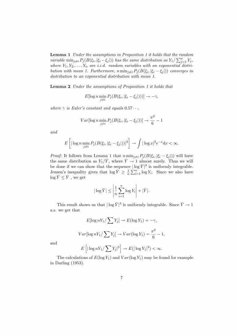
Lemma 2 Under the assumptions of Proposition 1 it holds that

E[log nminj 6=i

Pj(B(ξi, |ξi − ξj |)))] → −γ,

where γ is Euler’s constant and equals 0.57 · · ·,

V ar[log n minj 6=i

Pj(B(ξi, |ξi − ξj |))] → π2

6− 1

and

E

[| log n min

j 6=iPj(B(ξi, |ξi − ξj |))|3

]→

∫| log x|3e−xdx < ∞.

Proof: It follows from Lemma 1 that nminj 6=i Pj(B(ξi, |ξi − ξj |)) will havethe same distribution as Y1/Y , where Y → 1 almost surely. Thus we willbe done if we can show that the sequence | log Y |3 is uniformly integrable.Jensen’s inequality gives that log Y ≥ 1

n

∑ni=1 log Yi. Since we also have

log Y ≤ Y , we get

| log Y | ≤∣∣∣∣∣1n

n∑

i=1

log Yi

∣∣∣∣∣ + |Y |.

This result shows us that | log Y |3 is uniformly integrable. Since Y → 1a.s. we get that

E[log nY1/∑

Yj ] → E(log Y1) = −γ,

V ar[log nY1/∑

Yj ] → V ar(log Y1) =π2

6− 1,

andE

[| log nY1/

∑Yj |3

]→ E(| log Y1|3) < ∞.

The calculations of E(log Y1) and V ar(log Y1) may be found for examplein Darling (1953).

7

In the following we will assume that the random vectors ξ1, ξ2, . . . , ξn

have the same distribution P0 with density function g(x). In the rest of thepaper, we use the following notation (see also Section 4 of Jammalamadakaand Janson (1986)):

‖B(x, r)‖ = volume of the ball B(x, r) = cdrd,

where cd = πd/2/Γ(d/2 + 1).

Proposition 2 Let ξ1, ξ2, . . . , ξn be i.i.d. random vectors with an abso-lutely continuous distribution P0 with density function g(x). Then (ξi, ηi(n)),where

ηi(n) = n‖B(ξi, Rn(i))‖ = ncdRdn(i),

converges in distribution to (X,Y ) where X has density function g(x) andY given X = x has an exponential distribution with parameter g(x).

Proof: As the volume of the ball B(x, r) exceeds y/n if and only if none of thevariables ξj , j 6= i, j ≤ n falls in the ball B(x, V −1(y/n)). (Here V −1(y/n)denotes the radius giving the volume y/n, i.e. r = (y/n)1/dc

−1/dd ). Thus

Pr(n‖B(ξi, Rn(i)‖ > y|ξi = x) = (1− P0(ξ1 ∈ B(x, V −1(y/n))))n−1.

AsP0(ξ1 ∈ B(x, V −1(y/n))

y/n→ g(x),

(see Mattila (1995, p.36)), it follows that

(1− P0(ξ1 ∈ B(x, V −1(y/n))))n−1 → e−yg(x).

Next we prove that (ξi, ηi(n)) and (ξj , ηj(n)) are asymptotically inde-pendent.

Proposition 3 When n tends to infinity it holds that

Pr(ηi(n) > yi, ηj(n) > yj |ξi = xi, ξj = xj) → e−yig(xi)e−yjg(xj)

Proof: Since the random variables (ξi, ηi(n)), i = 1, 2, . . . , n are exchangeableit is sufficient to prove the proposition for i = 1 and j = 2. Instead of provingthe convergence for η1(n) and η2(n) we shall prove it for η1(n) and η2(n),where

ηk(n) = minj≥3

ncd|ξk − ξj |d for k = 1, 2.

8

By symmetry ηk(n) and ηk(n) differs only on a set having probability1/(n− 1). Thus

ηk(n)− ηk(n)p−→ 0, k = 1, 2

which implies that (η1(n), η2(n) and η1(n), η2(n)) have the same limit dis-tribution. By conditioning on ξ1 = x1 and ξ2 = x2 we get

Pr(η1(n) > y1, η2(n) > y2| ξ1 = x1, ξ2 = x2)= Pr(E(x1, n) > y1, E(x2, n) > y2),

whereE(xi, n) = n‖B(xi, min

j≥3|xi − ξj |)‖, i = 1, 2.

The event E(xi, n) > yi occurs if all ξj , j ≥ 3 falls outside the ballB(xi, V

−1(yi/n)) = B(xi).Thus

Pr(η1(n) > y1, η2(n) > y2| ξ1 = x1, ξ2 = x2) = (1− Pr(B(x1) ∪B(x2)))n−2.

But, as x1 6= x2, B(x1) and B(x2) are disjoint if n is sufficiently large so

limn→∞(1− Pr(B(x1) ∪B(x2)))n−2 = e−yig(xi)e−yjg(xj).

As the set ξ1 = ξ2 has probability zero this gives us the asymptoticindependence of (ξi, ηi(n)) and (ξj , ηj(n)).

Proposition 4 Let the distribution P0 of the sequence ξ1, ξ2, . . . , ξn of in-dependent random vectors be absolutely continuous w.r.t. Lebesgue measure.Then it holds that

1n

n∑

i=1

log nP0(B(ξi, Rn(i)))p−→ −γ

as n tends to infinity.

Proof: DefineEi(n) = nP0(B(ξi, Rn(i)).

The exchangeability of (ξi, ηi(n)) gives

E

[1n

n∑

i=1

log Ei(n)

]= E(log E1(n)),

9

and

V ar

[1n

n∑

i=1

log Ei(n)

]

=V ar(log E1(n))

n+ 2

n2 − n

n2Cov(log E1(n), log E2(n)).

Since, see Lemma 2E(log E1(n)) → −γ

and

V ar(log E1(n)) → π2

6− 1 < ∞,

an application of Chebychev’s inequality will give the desired result if wecan show that Cov(log E1(n), log E2(n)) → 0 as n → ∞. Since E1(n) andE2(n) are asymptotically independent we will be through if we show thatthe sequence log E1(n) log E2(n)∞n=1 is uniformly integrable. We have

E2| log E1(n) log E2(n)|1.5 ≤ E| log E1(n)|3E| log E2(n)|3.

The right hand side of this expression converges to (∫ | log x|3e−xdx)2,

which is finite, giving us

supn

E |log E1(n) log E2(n)|1+0.5 < ∞.

Consequently, the sequence log E1(n) log E2(n)∞n=1 has to be uniformlyintegrable, which completes the proof.

Proposition 5 Let the distribution P0 of the sequence ξ1, ξ2, . . . , ξn of in-dependent random vectors be absolutely continuous w.r.t. Lebesque measure.Then it holds that

1n

n∑

i=1

nP0(B(ξi, Rn(i)))p−→ 1

as n tends to infinity.

Proof: Follows in a similar way from Corollary 1 and Proposition 3.

10

3.2 Consistency

To prove the consistency of the MSP-estimate, we need some kind of con-tinuity and identifiability condition. If we allow the distributions for pa-rameter values close to each other to be too different, we cannot expectour estimation procedure to produce consistent estimators. This is clearlydemonstrated by an example in Basu (1955). Our continuity condition isinspired by the Arzela-Ascoli theorem.

Define

z(n, θ, x, y) = nB(x, rn) where rn = (c−1d y/n)1/d,

P (x, y) = the distribution function of (X,Y )with density function p(x, y) defined by

p(x, y) = g2(x) exp(−yg(x)), y > 0.

Condition C1: Let (X,Y ) have the distribution P (x, y). For each ε > 0and η > 0 there exists an integer m, sets Kj ⊂ Rd+1, j = 1, 2, . . . ,m, apartition of Θ into disjoint sets Θ1, Θ2, . . . , Θm and parameter values ψj ∈Θj , j = 1, 2, . . . ,m, such that for each for each j = 1, 2, . . . , m,

(i) the boundary ∂Kj of the set Kj has Lebesgue measure zero;

(ii) P ((X, Y ) ∈ Kj) > 1− η;

(iii) supθ∈Θj|z(n, θ, x, y)− z(n, ψj , x, y)| < ε for all (x, y) ∈ Kj and for all

n ≥ N(ε, η).

Remark 4: All or some of the sets K1,K2, . . . , Km may be equal.The mixture distribution in Example 1 satisfies Condition C1. The tech-

nique used in Ranneby (1984) to verify Condition C1 is also applicable in themultivariate situations. It follows that the continuity condition C1 usuallyis satisfied.

The identifiability condition we are going to use is called, according to theterminology in Rao (1973), a strong identifiability condition. However, whenweak identifiability conditions are used, these conditions are usually usedin combination with other conditions implying that a strong identifiabilitycondition is satisfied.

Let T (M, θ) denote the expected value of max(−M, log Y fθ(X)), where(X, Y ) has the distribution P (x, y).

11

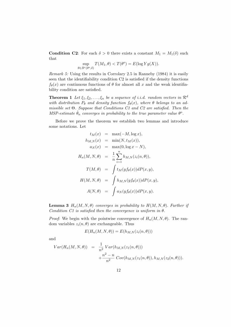
Condition C2: For each δ > 0 there exists a constant M1 = M1(δ) suchthat

supθ∈Bc(θo,δ)

T (M1, θ) < T (θo) = E(log Y g(X)).

Remark 5: Using the results in Corrolary 2.5 in Ranneby (1984) it is easilyseen that the identifiability condition C2 is satisfied if the density functionsfθ(x) are continuous functions of θ for almost all x and the weak identifia-bility condition are satisfied.

Theorem 1 Let ξ1, ξ2, . . . , ξn be a sequence of i.i.d. random vectors in Rd

with distribution Pθ and density function fθ(x), where θ belongs to an ad-missible set Θ. Suppose that Conditions C1 and C2 are satisfied. Then theMSP-estimate θn converges in probability to the true parameter value θo.

Before we prove the theorem we establish two lemmas and introducesome notations. Let

tM (x) = max(−M, log x),hM,N (x) = min(N, tM (x)),

aN (x) = max(0, log x−N),

Hn(M, N, θ) =1n

n∑

i=1

hM,N (zi(n, θ)),

T (M, θ) =∫

tM (yfθ(x))dP (x, y),

H(M, N, θ) =∫

hM,N (yfθ(x))dP (x, y),

A(N, θ) =∫

aN (yfθ(x))dP (x, y).

Lemma 3 Hn(M, N, θ) converges in probability to H(M, N, θ). Further ifCondition C1 is satisfied then the convergence is uniform in θ.

Proof: We begin with the pointwise convergence of Hn(M, N, θ). The ran-dom variables zi(n, θ) are exchangeable. Thus

E(Hn(M, N, θ)) = E(hM,N (zi(n, θ)))

and

V ar(Hn(M, N, θ)) =1n2

V ar(hM,N (z1(n, θ)))

+n2 − n

n2Cov(hM,N (z1(n, θ)), hM,N (z2(n, θ))).

12

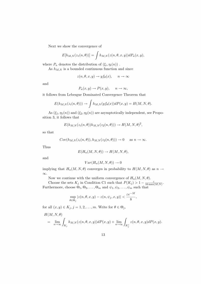
Next we show the convergence of

E[hM,N (z1(n, θ))] =∫

hM,N (z(n, θ, x, y))dPn(x, y),

where Pn denotes the distribution of (ξi, ηi(n)) .As hM,N is a bounded continuous function and since

z(n, θ, x, y) → yfθ(x), n →∞and

Pn(x, y) → P (x, y), n →∞,

it follows from Lebesgue Dominated Convergence Theorem that

E(hM,N (zi(n, θ))) →∫

hM,N (yfθ(x))dP (x, y) = H(M,N, θ).

As (ξ1, η1(n)) and (ξ2, η2(n)) are asymptotically independent, see Propo-sition 3, it follows that

E(hM,N (zi(n, θ))hM,N (z2(n, θ))) → H(M,N, θ)2,

so that

Cov(hM,N (zi(n, θ)), hM,N (z2(n, θ))) → 0 as n →∞.

ThusE(Hn(M, N, θ)) → H(M,N, θ),

andV ar(Hn(M,N, θ)) → 0

implying that Hn(M,N, θ) converges in probability to H(M,N, θ) as n →∞.

Now we continue with the uniform convergence of Hn(M, N, θ).Choose the sets Kj in Condition C1 such that P (Kj) > 1− ε

16max(M,N) .Furthermore, choose Θ1, Θ2, . . . ,Θm and ψ1, ψ2, . . . , ψm such that

supθ∈Θj

|z(n, θ, x, y)− z(n, ψj , x, y)| < εe−M

8,

for all (x, y) ∈ Kj , j = 1, 2, . . . ,m. Write for θ ∈ Θj ,

H(M, N, θ)

= limn→∞

∫

Kj

hM,N (z(n, θ, x, y))dP (x, y) + limn→∞

∫

Kcj

z(n, θ, x, y)dP (x, y).

13

Let θ ∈ Θj . We have, for n sufficiently large,

|hM,N (z(n, θ, x, y))− hM,N (z(n, ψj , x, y))| ≤

ε/8 on Kj ,2max(M, N) on Kc

j .(2)

Thussupθ∈Θj

|H(M,N, θ)−H(M,N, ψj)| < ε

8+

ε

8=

ε

4. (3)

We have

|Hn(M,N, θ)−Hn(M,N,ψj)|<

1n

∑|hM,N (zi(n, θ))− hM,N (zi(n, ψj)|I(ξi, ηi(n) ∈ Kj)

+1n

∑|hM,N (zi(n, θ))− hM,N (zi(n, ψj)|I(ξi, ηi(n) ∈ Kc

j ).

Since the boundary ∂Kj has P -measure zero we get

1n

∑I((ξi, ηi(n)) ∈ Kc

j ) →p P ((X, Y ) ∈ Kcj ) <

ε

16 max(M,N)

and then it follows from (2) that

P (|Hn(M,N, θ)−Hn(M,N,ψj)| < ε

4) → 1 as n →∞. (4)

Combining (3) and (4) we get that

Hn(M, N, θ)p−→ H(M, N, θ)

uniformly in θ.

Lemma 4 Define

zi(n, θ) =

zi(n, θ) if z(n, θ) ≤ 1,zi(n, θ)/z(n, θ) if z(n, θ) > 1.

Then the random function

An(N, θ) =1n

n∑

i=1

max(0, log zi(n, θ)−N)

converges to zero for all elementary events, uniformly in n and θ as N →∞.

14

Proof: Obviously,∑

zi(n, θ) ≤ n. The rest of the proof is only a slightmodification of Lemma 2 in Ranneby and Ekstrom (1997).

Proof of Theorem 1: Recall the definition of Sn(θ) as

Sn(θ) =1n

∑log zi(n, θ)

+1n

log(1− z(n, θ))I(z(n, θ) ≤ 1)− log z(n, θ)I(z(n, θ) > 1).

We have

Sn(θ) ≤ 1n

∑log zi(n, θ)− log z(n, θ)I(z(n, θ) > 1)

≤ 1n

∑hM,N (zi(n, θ)) +

1n

∑max(0, log zi(n, θ)−N).

Obviously,∑

zi(n, θ) ≤ n, so Lemma 4 gives that

An(N, θ)p−→ 0,

uniformly in θ and n. As zi(n, θ) ≤ zi(n, θ) and hM,N (x) is a non-decreasingfunction we get that

Sn(θ) ≤ Hn(M,N, θ) + An(N, θ).

Lemma 3 gives that Hn(M, N, θ)p−→ H(M, N, θ), uniformly in θ as

n →∞. Note that

H(M, N, θ) + A(N, θ) = T (M, θ),

and let θn denote the MSP-estimate. For N large the following holds withprobability going to one as n tends to infinity:

Sn(θn) ≤ 1n

∑hM,N (zi(n, θn) +

ε

4≤ H(M, N, θn) +

ε

2≤ H(M, N, θn) + A(N, θn) +

ε

2= T (M, θn) +

ε

2.

As Sn(θo)p−→ −γ we get

T (M, θn) +ε

2> Sn(θn) > Sn(θo) > T (θo)− ε

2,

15

which implies thatT (M, θn) > T (θo)− ε.

Now the identifiability condition C2 gives

|θn − θo| < δ

which completes the proof.

4 Simulation results

Here we present the results of the simulation study we conducted in order toconfirm and support our hypothesis about the consistency and asymptoticnormality of the MSP-estimates for multivariate observations. It was also ofinterest to compare the estimation based on Dirichlet tesselation with thatbased on nearest-neighbor balls. In all the figures and tables, MSPE standsfor MSP-estimate.

4.1 Gaussian density

We simulated bivariate Gaussian random variables with the following meanvector and covariance matrix:

µ =(

µ1

µ2

)=

(00

), Γ =

(σ2

1 ρρ σ2

2

)=

(1 0.5

0.5 1

).

Then we constructed two spacing functions - one based on nearest neighborballs and one based on Dirichlet cells. These functions were subsequentlymaximized by random search algorithm. As the starting point in the pa-rameter space, to speed up the convergence, the true value of the param-eter vector was chosen. We have also experimented with different startingpoints, and always the outcomes (e.g. the maximizers) were identical. Eachspacing function was maximized twice - first based on 50, then on 200 ob-servations, and both experiments were repeated 500 times. The mean andthe covariance matrix of the outcomes were calculated and averaged over500 repetitions (see Tables 1 and 2). The estimated covariance matrix wascompared to the Cramer-Rao bound:

I−1 =

1 0.5 0 0 00.5 1 0 0 00 0 0.5 0.125 0.50 0 0.125 0.5 0.50 0 0.5 0.5 1.25

.

16

-3 -2 -1 0 1 2 3

NN MSPE (50 observations)

-20

24

-3 -2 -1 0 1 2 3


-20

24

-3 -2 -1 0 1 2 3

Dirichlet MSPE (50 observations)

-3-2

-10

12

3

-3 -2 -1 0 1 2 3


-20

2Figure 1: Quantile-quantile plots of the MSPE for σ2 (Gaussian density)

The results confirm the consistency of the MSP estimates. Besides, wenote that the MSP-estimate based on Dirichlet cells is much closer to beingefficient than the estimate based on the nearest neighbor balls. Figure 1displays the normal quantile-quantile plots of the estimates of one of theparameters. We note that the plots support the conjecture of asymptoticnormality of the MSP-estimates.

4.2 Mixture of two Gaussian densities

The second simulation was performed for the mixture of two bivariate Gaus-sian densities. This is a well-known example, where the ML-method breaksdown. Particularly, if we set the mean of the first (say) component of themixture equal to one of the observations, e.g. µ1 = x1, µ2 = y1 then the ML-function will tend to infinity as σ1 goes to zero. We simulated the bivariateobservations with the following density:

g(x, y, θ) = 0.8× f1(x, y, µ1, µ2, σ1, σ2, ρ1) + 0.2× f2(x, y, µ3, µ4, σ3, σ4, ρ2),

where µ1 = µ2 = 0, σ1 = σ2 = 1, ρ1 = 0.5, µ3 = µ4 = 2, σ3 = σ4 = 2 andρ2 = 0. Only the parameters of f1 were considered unknown. We constructedthe spacing functions for 50 and 200 observations. Each experiment wasagain repeated 500 times as in the previous example. The results can beseen in Tables 3 and 4. The estimated covariance matrix was again compared

17

-3 -2 -1 0 1 2 3

-0.5

0.0

0.5


-3 -2 -1 0 1 2 3

-0.6

-0.2

0.2

0.4

0.6


-3 -2 -1 0 1 2 3

-0.4

0.0

0.4

0.8


-3 -2 -1 0 1 2 3

-0.2

0.0

0.1

0.2


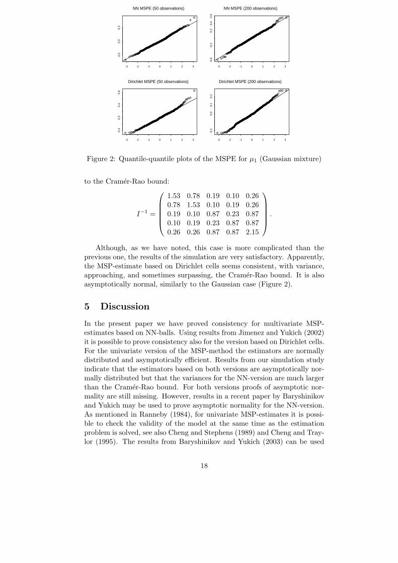
Figure 2: Quantile-quantile plots of the MSPE for µ1 (Gaussian mixture)

to the Cramer-Rao bound:

I−1 =

1.53 0.78 0.19 0.10 0.260.78 1.53 0.10 0.19 0.260.19 0.10 0.87 0.23 0.870.10 0.19 0.23 0.87 0.870.26 0.26 0.87 0.87 2.15

.

Although, as we have noted, this case is more complicated than theprevious one, the results of the simulation are very satisfactory. Apparently,the MSP-estimate based on Dirichlet cells seems consistent, with variance,approaching, and sometimes surpassing, the Cramer-Rao bound. It is alsoasymptotically normal, similarly to the Gaussian case (Figure 2).

5 Discussion

In the present paper we have proved consistency for multivariate MSP-estimates based on NN-balls. Using results from Jimenez and Yukich (2002)it is possible to prove consistency also for the version based on Dirichlet cells.For the univariate version of the MSP-method the estimators are normallydistributed and asymptotically efficient. Results from our simulation studyindicate that the estimators based on both versions are asymptotically nor-mally distributed but that the variances for the NN-version are much largerthan the Cramer-Rao bound. For both versions proofs of asymptotic nor-mality are still missing. However, results in a recent paper by Baryshinikovand Yukich may be used to prove asymptotic normality for the NN-version.As mentioned in Ranneby (1984), for univariate MSP-estimates it is possi-ble to check the validity of the model at the same time as the estimationproblem is solved, see also Cheng and Stephens (1989) and Cheng and Tray-lor (1995). The results from Baryshinikov and Yukich (2003) can be used

18

to give confidence limits for Sn(θ0). Thus for multivariate MSP-estimatesbased on NN-balls it is possible to check the validity of the model. Anotheradvantage with the NN-version is that it is much easier to handle, especiallyin higher dimensions. The drawback is of course the lack of efficiency. In sit-uations where the maximum likelihood method fails that is usually becauseof global reasons. Locally the method may still give satisfactory results.To be specific for mixture distributions it should be possible to use the MLmethod if the starting values for the maximization are in the neighborhoodof the true values. Thus in these situations it should be possible to use theMSP-method based on NN-balls to get consistent estimators which can beused as starting values for the ML estimation.

Acknowledgements

This research was conducted using the resources of High Performance Com-puting Center North (HPC2N) in Sweden. The authors would like to thankProf. Yuri Belyaev and Dr. Jun Yu for valuable comments and discussion.

References

[1] Baryshnikov, Y. and Yukich, J.E. (2003) “Generalized spacing statisticsand Gaussian fields”.

[2] Basu, D. (1955) “An inconsistency of the method of maximum likeli-hood,” Ann. Math. Statist., 26, 144-145.

[3] Bickel, P.J. and Breiman, L. (1983) “Sum of functions of nearest neigh-bor distances, moment bounds, limit theorems, and a goodness of fittest,” Ann. of Probab., 11, 185-214.

[4] Cheng, R.C.H. and Amin, N.A.K. (1983) “Estimating parameters incontinuous univariate difstributions with a shifted origin,” J. R. Statist.Soc. B, 45, 394-403.

[5] Cheng, R.C.H. and Stephens, M.A. (1989) “A goodness-of-fit test usingMoran’s statistic with estimated parameters,” Biometrika 76, 385-392.

[6] Cheng, R.C.H. and Traylor, L. (1995) “Non-regular maximum likeli-hood problems (with discussions),” J. Roy. Staist. Soc. B, 57, 3-44.

[7] Darling, D.A. (1953) “On a class of problems related to the randomdivision of an interval,” Ann. Math. Statist., 24, 239-253.

19

[8] Jammalamadaka, S. Rao and Janson, S. (1986) “Limit theorems for atriangular scheme of U-statistics with applications to inter-point dis-tances,” Ann. of Probab., 14, 1347-1358.

[9] Jammalamadaka, S. Rao and Zhou, S. (1993) “Goodness of fit in mul-tidimensions based on nearest neighbor distances,” Jour. of Nonpara-metric Statistics, 2, 271-284.

[10] Jimenez, R. and Yukich, J.E. (2002) “Asymptotics for statistical dis-tances based on Voronoi tesselation,” J. Theor. Prob., 15, 503–541.

[11] Mattila, P. (1995) Geometry of Sets and Measures in Euclidean Spaces,Fractals and rectifiability, Cambridge University Press, Cambridge, UK.

[12] Pyke, R. (1965) “Spacings (with discussion),” J. R. Statist. Soc. B, 27,395-449.

[13] Ranneby, B. (1984) “The maximum spacing method. An estimationmethod related to the maximum likelihood method,” Scand. J. Statist.,11, 93-112.

[14] Ranneby, B. (1996) “Spatial and temporal models in contextual classi-fication,”, In Todd Mowrer, H. and Czaplewski, R. L. and Hamre, R.H., editors, Spatial Accuracy Assessment in Natural Resources and En-vironmental Sciences: Second International Symposium, pages 451-458,Fort Collins, Colorado.

[15] Ranneby, B. and Ekstrom, M. (1997) “Maximum spacing estimatesbased on different metrics,” Research Report No. 5, Dept. of Mathe-matical Statistics, Umea University.

[16] Rao, C.R. (1973) Linear Statistical Inference and its Applications, 2nded., Wiley, New York.

[17] Reiss, R.D. (1989) Approximate Distributions of Order Statistics, withApplications to Nonparametric Statistics, Springer-Verlag, New York.

[18] Renyi, A. (1953) “On the theory of order statistics,” Acta Math. Acad.Sci. Hungar., 4, 191-231.

[19] Titterington, D.M. (1985) “Comment on ‘estimating parameters in con-tinuous univariate distribution’,” J. R. Statist. Soc. B, 47, 115-116.

20

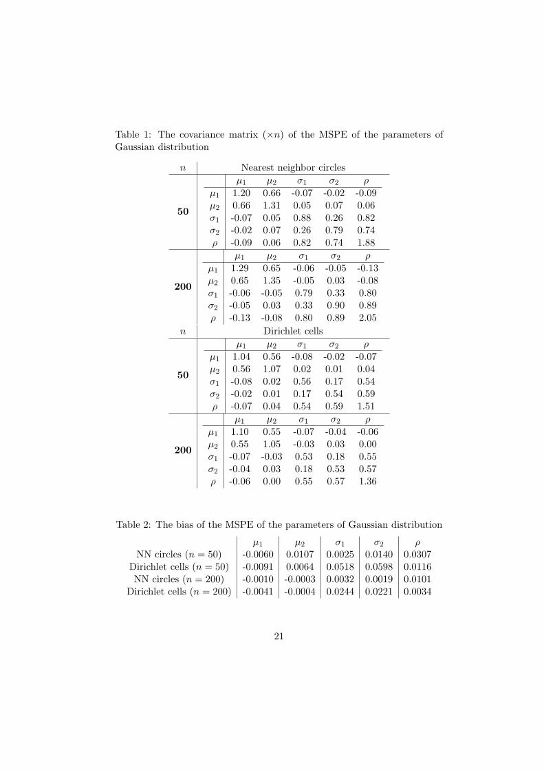
Table 1: The covariance matrix (×n) of the MSPE of the parameters ofGaussian distribution

n Nearest neighbor circles

50

µ1 µ2 σ1 σ2 ρ

µ1 1.20 0.66 -0.07 -0.02 -0.09µ2 0.66 1.31 0.05 0.07 0.06σ1 -0.07 0.05 0.88 0.26 0.82σ2 -0.02 0.07 0.26 0.79 0.74ρ -0.09 0.06 0.82 0.74 1.88

200

µ1 µ2 σ1 σ2 ρ

µ1 1.29 0.65 -0.06 -0.05 -0.13µ2 0.65 1.35 -0.05 0.03 -0.08σ1 -0.06 -0.05 0.79 0.33 0.80σ2 -0.05 0.03 0.33 0.90 0.89ρ -0.13 -0.08 0.80 0.89 2.05

n Dirichlet cells

50

µ1 µ2 σ1 σ2 ρ

µ1 1.04 0.56 -0.08 -0.02 -0.07µ2 0.56 1.07 0.02 0.01 0.04σ1 -0.08 0.02 0.56 0.17 0.54σ2 -0.02 0.01 0.17 0.54 0.59ρ -0.07 0.04 0.54 0.59 1.51

200

µ1 µ2 σ1 σ2 ρ

µ1 1.10 0.55 -0.07 -0.04 -0.06µ2 0.55 1.05 -0.03 0.03 0.00σ1 -0.07 -0.03 0.53 0.18 0.55σ2 -0.04 0.03 0.18 0.53 0.57ρ -0.06 0.00 0.55 0.57 1.36

Table 2: The bias of the MSPE of the parameters of Gaussian distribution

µ1 µ2 σ1 σ2 ρNN circles (n = 50) -0.0060 0.0107 0.0025 0.0140 0.0307

Dirichlet cells (n = 50) -0.0091 0.0064 0.0518 0.0598 0.0116NN circles (n = 200) -0.0010 -0.0003 0.0032 0.0019 0.0101

Dirichlet cells (n = 200) -0.0041 -0.0004 0.0244 0.0221 0.0034

21

Table 3: The covariance matrix (×n) of the MSPE of the parameters ofGaussian mixture

n Nearest neighbor circles

50

µ1 µ2 σ1 σ2 ρ

µ1 2.61 1.11 0.39 0.04 0.49µ2 1.11 1.72 0.16 0.12 0.25σ1 0.39 0.16 1.02 0.22 1.02σ2 0.04 0.12 0.22 1.14 1.04ρ 0.49 0.25 1.02 1.04 2.53

200

µ1 µ2 σ1 σ2 ρ

µ1 2.50 1.16 0.41 0.06 0.51µ2 1.16 1.99 0.14 0.10 0.22σ1 0.41 0.14 1.12 0.26 0.84σ2 0.06 0.10 0.26 1.12 0.87ρ 0.51 0.22 0.84 0.87 2.71

n Dirichlet cells

50

µ1 µ2 σ1 σ2 ρ

µ1 1.96 0.86 0.25 -0.09 0.24µ2 0.86 1.59 0.16 0.16 0.32σ1 0.25 0.16 1.04 0.27 0.95σ2 -0.09 0.16 0.27 1.10 0.89ρ 0.24 0.32 0.95 0.89 2.43

200

µ1 µ2 σ1 σ2 ρ

µ1 1.61 0.88 0.20 0.03 0.25µ2 0.88 1.69 0.06 0.11 0.13σ1 0.20 0.06 0.91 0.19 0.82σ2 0.03 0.11 0.19 0.87 0.80ρ 0.25 0.13 0.82 0.80 2.10

Table 4: The bias of the MSPE of the parameters of Gaussian mixture

µ1 µ2 σ1 σ2 ρNN circles (n = 50) 0.0060 -0.0044 -0.0313 -0.0287 0.0057

Dirichlet cells (n = 50) -0.0051 -0.0416 0.0198 0.0391 0.0125NN circles (n = 200) 0.0021 -0.0009 0.0191 0.0302 0.0025

Dirichlet cells (n = 200) -0.0055 -0.0017 0.0179 0.0124 0.0096

22

The maximum spacing estimation for multivariate observations

Documents

Transcript of The maximum spacing estimation for multivariate observations