Maximum likelihood principal component analysis

MAXIMUM LIKELIHOOD PRINCIPAL COMPONENT ANALYSIS

PETER D. WENTZELL,1 DARREN T. ANDREWS,1 DAVID C. HAMILTON,2 KLAAS FABER3 ANDBRUCE R. KOWALSKI3

1 Trace Analysis Research Centre, Department of Chemistry, Dalhousie University, Halifax, Nova Scotia B3H 4J3,Canada

2 Department of Mathematics, Statistics and Computing Science, Dalhousie University, Halifax, Nova Scotia B3H 3J5,Canada

3 Center for Process Analytical Chemistry, University of Washington, Seattle, WA 98195, U.S.A.

SUMMARY

The theoretical principles and practical implementation of a new method for multivariate data analysis, maximumlikelihood principal component analysis (MLPCA), are described. MLCPA is an analog to principal componentanalysis (PCA) that incorporates information about measurement errors to develop PCA models that are optimalin a maximum likelihood sense. The theoretical foundations of MLPCA are initially established using aregression model and extended to the framework of PCA and singular value decomposition (SVD). An efficientand reliable algorithm based on an alternating regression method is described. Generalization of the algorithmallows its adaptation to cases of correlated errors provided that the error covariance matrix is known. Models withintercept terms can also be accommodated. Simulated data and near-infrared spectra, with a variety of errorstructures, are used to evaluate the performance of the new algorithm. Convergence times depend on the errorstructure but are typically around a few minutes. In all cases, models determined by MLPCA are found to besuperior to those obtained by PCA when non-uniform error distributions are present, although the level ofimprovement depends on the error structure of the particular data set. © 1997 by John Wiley & Sons, Ltd.

Journal of Chemometrics, Vol. 11, 339–366 (1997) (No. of Figures: 4 No. of Tables: 5 No. of References: 22)

KEY WORDS principal component analysis; maximum likelihood; measurement errors; multivariate analysis;near-infrared spectroscopy; errors in variables

1. INTRODUCTION

In general the primary goal of chemometrics is to develop and utilize models for chemicalmeasurements. Principal component analysis (PCA) has been perhaps the most powerful tool of thechemometrician in this regard. Initially employed by statisticians to describe the variance andcovariance of random variables, PCA is more commonly used in chemometrics to describedeterministic relationships among variables, especially in cases where a high degree of collinearityexists. In this context the advantage of PCA is that it allows multivariate data to be represented by asmaller number of variables, called principal components, factors or latent variables. In applicationssuch as mixture analysis and curve resolution the object is to develop a p-dimensional linear model(i.e. a p-dimensional hyperplane) to describe the data within experimental error. In this case p issometimes called the chemical rank, pseudorank or true rank of the data set to distinguish it from themathematical rank, which is nearly always maximized owing to the presence of experimental error.The chemical rank is typically related to the number of underlying chemical factors or chemicalcomponents present and in this paper will be referred to simply as the ‘rank’. Although there are otherapplications of PCA, such as dimensionality reduction and preprocessing, this paper will consider the

Correspondence to: Peter D. Wentzell.

JOURNAL OF CHEMOMETRICS, VOL. 11, 339–366 (1997)

CCC 0886–9383/97/040339–28 $17.50 Received 2 July 1996© 1997 by John Wiley & Sons, Ltd. Accepted 24 October 1996

technique from a modeling perspective.PCA has been very successfully applied to modeling in chemistry, as evidenced by the large number

of papers on mixture analysis and related topics. The objective of the chemist is generally twofold: (i)to determine the correct form of the model (the rank p as well as the presence of any model offsets);(ii) to obtain the best estimate of parameters associated with the model (in the form of eigenvectors,scores, etc.). Usually the hyperplane described by the model is of more interest than the eigenvectorsthemselves, since it typically describes the space containing the real factors, such as pure componentspectra. Unfortunately, PCA is often not an optimal procedure for the estimation of model parametersand can lead to poor models in certain cases. Of course, there are a variety of optimization criteria tobe considered when evaluating parameter estimation methods (e.g. robustness, bias and variance of theestimators) and none is universally the best. One widely used approach is to employ a maximumlikelihood criterion. Simply put, for a given p-dimensional model the maximum likelihood solution forthe model parameters is the one that is most likely to give rise to the observed mesurements.Maximum likelihood estimates are generally recognized as having desirable statistical properties andtheir use has become commonplace.1 For example, ordinary least squares is a maximum likelihoodmethod when measurement errors in the x-variable(s) are negligible and the errors in y are independentand normally distributed. Likewise, PCA can be considered to be a maximum likelihood method if allmeasurement error standard deviations have the same normal distribution (i.e. independent andidentically distributed (i.i.d.)). This is one reason for the widespread use of PCA for modelingapplications. When minor variations from the assumptions for maximum likelihood estimation areobserved, PCA can still be useful, but when the violations become large, it becomes ineffective. Thishas been remedied in part by incorporating various scaling techniques to reduce the data to i.i.d., butthis will not work in the general case.2 A maximum likelihood method which is more general in itsapproach to modeling is needed.

This paper establishes the theoretical foundations for maximum likelihood principal componentanalysis (MLPCA). MLPCA is an errors-in-variables modeling method in that it accounts formeasurement errors in the estimation of model parameters. It is an optimal modeling method in amaximum likelihood sense for functional models with no errors in the model equations. The methodis first presented in terms of a classical measurement error regression model and then transformed toprincipal component space to provide a closer relationship with PCA and a more tractable formulation.The mathematical aspects of the algorithm are described in detail to allow the principles to be readilyapplied.

A number of assumptions have been made in the development of the MLPCA method and theseshould be made clear from the outset. First, it is assumed that there is a true underlying p-dimensionalmodel for the data (possibly with the inclusion of row and column offsets). Second, deviations of themeasurements from this model are the result only of random measurement errors (no model errors oroutliers). Third, these random errors are normally distributed around the true measurements withknown standard deviations and covariance structure. Although the assumption of normally distributederrors may be violated in practice and does not strictly preclude the application of the maximumlikelihood principle, mathematical tractability demanded that this assumption be made for thedevelopment of this algorithm and limits its generality to a small degree. However, correlated errorscan be accommodated by the method as long as the error covariance matrix can be estimated. Finally,as noted, the method assumes that the true values of the measurement standard deviations (or errorcovariance matrices) are known, while in practice only estimates of these values are normallyavailable. Although this will no doubt affect the quality of the parameter estimates, it does not affectthe development of the principles here or the utility of the approach. It is the premise of this work thata modeling method which includes some knowledge of the measurement errors, however incomplete,is better than one which includes no information other than its implicit assumptions.

P. D. WENTZELL ET AL.340

© 1997 by John Wiley & Sons, Ltd. Journal of Chemometrics, Vol. 11, 339–366 (1997)

2. BACKGROUND

The need for some form of PCA which is weighted according to measurement errors has beenrecognized for some time. Informally this has been addressed through a variety of scaling procedures,such as range scaling and autoscaling as well as more elaborate schemes.2–5 Under the right conditionsthese can reduce PCA to a maximum likelihood method. However, Paatero and Tapper2 showed thatfor this to happen, the matrix of measurement standard deviations needs to be of rank one. If thiscondition is not met, as it will not be in the general case, any weighting scheme developed will besuboptimal.

A number of researchers have developed methods to more rigorously incorporate measurementerrors into the modeling process.6,7 This is normally done by minimizing the usual weighted residualsum of squares in accordance with some p-dimensional model. Mathematically, if X is an m3n datamatrix, this corresponds to minimization of

S2 =Om

i=1On

j=1

(xij 2 xij)2

s2ij

(1)

where xij corresponds to the estimated value of the measurement. In the general case where there areno offsets in the model, this is given by

X=AB (2)

where A is m3p and B is p3n. By analogy to PCA, A and B correspond to score and loading matrices,but in equation (2) the individual vectors are not required to be orthogonal. A variety of methods havebeen devised to obtain A and B through minimization of equation (1) and these differ largely in theirrepresentation of the problem, the constraints applied to the solution and their approach to the non-linear optimization. Gabriel and Zamir6 describe a method based on ‘criss-cross regressions’ as ameans to obtain lower-rank approximations of the matrix X. Paatero and Tapper7 have described whatthey call ‘positive matrix factorization’ (PMF) and have applied this to environmental problems. Inaddition to satisfying the minimization criterion, PMF also requires A and B to be positive.

In this work, MLPCA is presented as an alternative to the above methods. Although MLPCA issimilar to these methods in that it seeks to minimize equation (1), it has some important differences.First, it is formulated in terms of singular value decomposition (SVD), which is a very commonmethod for implementing PCA. Second, the standard MLPCA algorithm consists of an alternatingleast squares procedure which is robust, easy to implement and very efficient compared withconventional gradient search methods. Finally, unlike the methods described in the precedingparagraph, which require measurement errors to be independent, MLPCA allows the inclusion of errorcovariance in virtually any form.

The MLPCA method described here should not be confused with maximum likelihood commonfactor analysis (MLCFA) that appears frequently in the literature outside of chemistry. Although theterms are often used interchangeably by chemists, PCA and factor analysis are distinctly differentapproaches to multivariate analysis.8 The principles of MLCFA were originally developed by Lawleyand Maxwell8 and later employed in programs such as LISREL.9,10 More recently, MLCFA hasappeared in the chemical literature with claims that it performs better than PCA.11,12 However, MLCFAwas developed with the intention of finding structural models for random variables. As such, itestimates covariance matrices for random variables and does not generally use information aboutmeasurement errors.

Another errors-in-variables method that has become popular recently is total least squares (TLS).13

MAXIMUM LIKELIHOOD PCA 341


This method uses SVD for the purpose of developing a regression model and is similar to MLPCAin some ways. However, it is less general in its ability to obtain maximum likelihood estimates ofmodel parameters. To our knowledge, the method described in this work is unique in its approach toPCA model estimation.

The objective of the work presented here is to develop the MLPCA approach in a manner consistentwith the PCA formulation and present algorithms which are computationally practical. A completeanalysis of the statistical properties of the method is beyond the scope of this treatment, but examplesare presented to validate the method and demonstrate some of its features. Additional applications willbe presented in future work.

3. THEORY

The development of the theoretical aspects of MLPCA is presented here in four subsections. First, theparametric models are developed and extended to a PCA framework and a strategy for gradientoptimization of the model parameters is discussed. In the second subsection a more efficientoptimization procedure based on an alternating least squares approach is described. This procedureassumes that the model contains no intercept terms and the measurements have uncorrelated errors.This algorithm will be referred to as the ‘standard’ MLPCA algorithm since it represents the simplestcase. The more general case which accommodates correlated errors is discussed in Section 3.3.Finally, as an analog to mean centering in traditional PCA, the incorporation of intercept terms intothe MLPCA procedure is treated in Section 3.4.

3.1. MLPCA with no intercept terms

Starting with the m3n matrix of measurements, X, the MLPCA problem can be regarded simply asone of finding the equation for the optimum p-dimensional hyperplane to fit n points in the m-dimensional row space or, alternatively, m points in the n-dimensional column space. In the analysispresented here, the former approach is used, but it will become apparent that this is not important.Maximum likelihood model estimation is an iterative two-step procedure. First, for a set of givenhyperplanar model parameters (i.e. slopes) the maximum likelihood estimates for the points (thecolumn vectors of the observed data matrix X) are found. These are then used to calculate theobjective function in equation (1) (or an analogous equation). In the second step the model parametersare adjusted in an attempt to minimize S2. The new model parameters are used to calculate newmaximum likelihood estimates of the points and a new S2 and the process continues until the objectivefunction is minimized. Thus there are two problems to address: (i) how to calculate the maximumlikelihood estimates for a given set of model parameters; (ii) how to optimize the model parameters.These problems are treated in order.

In accordance with the assumptions stated earlier, each column of the data matrix X can beconsidered to represent a point in the m-dimensional row space, with the true measurements corruptedby normally distributed errors:

x=xo +« (3)

Here x is a column vector of X, xo represents the error-free column vector and « is the vector ofmeasurement errors, which has an error covariance matrix

C=cov(«)=E(««T) (4)

where ‘E( · )’ denotes an expectation value. Note that each column of X can have a different errorcovariance matrix. In the development of an MLPCA model it is assumed that the error-free



measurements lie on a p-dimensional hyperplane that can be modeled by a set of parametric equationswith p independent variables. The independent variables for these parametric equations will bearbitrarily chosen to be the first p rows of X. For example, the parametric equations for a two-dimensional (planar) model in a four-dimensional space would be

xo3 =a31x

o1 +a32x

o2, xo

4 =a41xo1 +a42x

o2 (5)

where the as are the model parameters and the x0s are the error-free measurements. In matrix form theequation for the observation is

x1

x2

x3

x4

=

10

a31

a41

01

a32

a42

Fxo1

xo2G+

«1

«2

«3

«4

(6)

or in general

x=Axop +« (7)

where xop is the vector containing the first p elements of xo. In this equation, A is the m3p matrix of

model coefficients (slope parameters) and the upper p3p submatrix of A is the identity matrix. Ourproblem here is to find the best estimate for xo

p given the vector of observations, x, a matrix ofestimated model coefficients, A, and an error covariance matrix C. Note that this problem is similarin form (but different in objective) to the classical regression problem, which uses the model

y=Xb+d (8)

In this equation, y and X are the observations, b is the regression vector and d is the measurementerror vector for y. In the regression case we assume no errors in X and try to estimate b, whereas inthe case of equation (7) we would like to estimate xp for a given A. The form of the solution isanalogous to that for generalized least squares regression and yields

xp =(ATC21A)21ATC21x (9)

Here xp is the maximum likelihood estimate of xp. Substitution back into the model equation gives themaximum likelihood estimates for the remaining elements of x:

x= Axp = A(ATC21A)21ATC21x (10)

A more formal derivation of equation (10) is given in Appendix II.Equation (10) solves the first of the problems posed, allowing maximum likelihood estimates of the

measurements to be obtained for a given set of model parameters. However, to obtain the maximumlikelihood fit, it is necessary to adjust the model coefficients (A) to minimize the objective functionS2. In the case of uncorrelated errors this objective function is given by equation (1). In the case whereerrors are correlated among the rows, a more general form of equation (1) is minimized

S2 =On

j=1

(xj 2 xj)TC21

j (xj 2 xj)=On

j=1

DxTj C21

j Dxj (11)

where, as before, xj represents a column vector of X. Equation (11) reduces to equation (1) for adiagonal covariance matrix. For the case where the error covariance matrix C is the same for eachcolumn of X, Fuller has given a closed-form solution for A that minimizes S2 (Reference 14, p. 292).



If C is also diagonal, this is equivalent to the solution obtained by SVD if appropriate row scaling isused. However, in the general case where the error covariance matrix varies with the columns of X,there is no closed-form solution for A. Fuller suggests an iterative solution in this case (Reference 14,p. 217). We have successfully employed both simplex and gradient-based algorithms to optimize thecoefficients of A, but in general convergence is slow and prone to local minima. Furthermore,depending on which rows are used for the ‘independent’ variables, the numerical stability of thesolution algorithm is questionable. Another drawback to this approach is that the equations developedthus far are in the form of a regression model rather than the PCA model which is sought. For thesereasons it would be more convenient to represent equation (10) in terms of a PCA decomposition, i.e.in terms of scores and loadings. To do this, consider the form of the PCA model normally arrived atthrough SVD:

X= USVT (12)

where X is m3n, U is m3p, S is p3p and V is n3p. The caret on X denotes that these are themaximum likelihood estimates of the measurements in accordance with the p-dimensional model andU, S and V are obtained from the singular value decomposition of X, which is constrained to be rankp. Now X and U are partitioned into the upper p rows (X1 and U1) and the lower m2p rows (X2 andU2) to give

X=FX1

X2G=FU1

U2GSVT =SFU1

U2GU21

1 DU1SVT =F Ip

U2U211GX1 (13)

or, with reference to equation (10),

A= UU211 (14)

Thus there is a direct relationship between the parametric equations and SVD form of the model inthe absence of intercepts. Substituting this into equation (10) yields

xj = A(ATC21j A)21ATC21

j xj

= UU211 [(UU21

1 )TC21j UU21

1 ]21(UU211 )TC21

j xj

= UU211 [(U21

1 )TUTC21j UU21

1 ]21(U211 )TUTC21

j xj

= UU211 U1(U

TC21j U)21UT

1(UT1)21UTC21

j xj

= U(UTC21j U)21UTC21

j xj

=Pjxj (15)

where the projection matrix Pj is given by

Pj = U(UTC21j U)21UTC21

j (16)

Like equation (10), equation (15) allows the maximum likelihood values for the matrix ofmeasurements to be calculated, but in accordance with a given SVD model rather than a regressionmodel. It is also similar to an equation developed by Bartlett in the psychometrics literature as earlyas 193715,16 and discussed later by Lawley and Maxwell,8 who describe it as an unbiased method forestimating factor scores. It should be noted that because S is diagonal the score matrix R (= US) canbe substituted for U in equations (14)–(16). In order for equation (15) to provide maximum likelihoodestimates, the measurement errors should be normally distributed and the error covariance matrix



needs to be available. In the case of uncorrelated errors, C will be a diagonal matrix with the diagonalelements equal to the measurement variances.

As before, equation (15) is used to optimize the elements of U in accordance with the objectivefunction given in equation (11). In this case, however, there should be fewer parameters to optimize.While the matrix A has p(m2p) variable coefficients, the columns of U define an orthonormal set ofvectors in the row space and it is only necessary to optimize m21 angles in this space to define theoptimum hyperplane.

To optimize the SVD model, an initial estimate for U, designated U0, is first obtained. The columnvectors of U0 are then rotated in the m-dimensional space by applying an m3m rotation matrix T. Thisgives a new estimate for U:

U=TU0 (17)

One easy way to define the rotation matrix is in terms of successive rotations about each axis. In anm-dimensional space there are m21 rotation angles to be specified, so we have

T=T1T2 . . . Tm21 = Pm21

i=1

Ti (18)

where

cos a1 2sin a1 0 . . . 0 1 0 0 . . . 0

sin a1 cos a1 0 . . . 0 0 cos a2 2sin a2 . . . 0

T1 = 0 0 1 . . . 0 , T2 = 0 sin a2 cos a2 . . . 0 , etc.

: : : · · . : : : : · · . :

0 0 0 . . . 1 0 0 0 . . . 1

(19)

The problem now is one of optimizing the rotation angles a1, . . . , am21 to minimize the objectivefunction in equation (11).

The optimization of the rotation angles can be carried out by a number of methods, but gradientmethods are generally regarded as being the most efficient. These require the calculation of derivativesof S2 with respect to the rotation angles. Since this is a nontrivial calculation, the derivation is includedas Appendix III. The result is given as

S2

ai

=22On

j=1

(DxTj C21

j GiPjxj 2xTj C21

j PjGiPjDxj 2DxTj C21

j PjGiPjxj +xTj C21

j GiPjDxj) (20)

where the matrix Gi is defined in Appendix III. This equation has been checked against numericallycalculated derivatives and found to be correct. It can be used in conjunction with standard gradienttechniques to find the optimum rotation of eigenvectors to minimize the objective function in equation(11). In practice this procedure is faster and more reliable than using the regression form of theequation, but it is still relatively slow and susceptible to local minima. Therefore an alternativeapproach was sought. This is described in the next subsection.

3.2. An efficient MLPCA algorithm

In order to be useful with large data sets, an MLPCA procedure is needed which converges relativelyquickly. Among the most efficient methods in this regard are iterative procedures, such as alternatingregression approaches. Such a solution was developed for the MLPCA problem and was based on the



following rationale.It will be assumed for the moment that all measurement errors are independent so that error

covariance matrices in both the row and column spaces are diagonal. If this is true, the p-dimensionalmodel obtained by maximum likelihood estimation must be equivalent in both spaces. This followsbecause the objective function in both cases reduces to the same summation given by equation (1).Mathematically,

S2 =Om

i=1On

j=1

(xij 2 xij)2

s2ij

=On

j=1

DxTj C21

j Dxj =Om

i=1

DxTi S21

i Dxi (21)

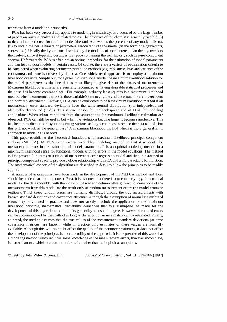
Here Dxj is a column vector of DX, Dxi is a column vector of (DX)T, and Cj and Si are thecorresponding column and row error covariance matrices for X, both of which are diagonal. For easeof visualization, some of the matrices are represented pictorially in Figure 1(a). In order to developthe alternating regression algorithm, equation (12) will be rewritten as

XT = VSUT (22)

This suggests that the maximum likelihood estimates of the measurements in the column space aregiven by an equation which is analogous to equation (15):

xi = V(VTS21i V)21VTS21

i xi (23)

where, as before, xi is a column vector of XT and Si is the corresponding error covariance matrix.When the maximum likelihood solution has been obtained, the estimates of X in the row and columnspaces will be identical. This implies that an alternating regression approach can be developed byalternately transposing the maximum likelihood estimates and performing SVD.

The algorithm for the alternating regression procedure is given in Table 1. It should be noted thatthe algorithm has been expanded to show a full iteration for clarity, but there are some redundanciesin the procedure that can be exploited to make the actual code more compact. The algorithmalternately uses the maximum likelihood estimates in the original row space to update the estimatesin the column space (i.e. the row space of the transposed matrix) and vice versa. This procedure hasbeen found to be simple, fast and reliable. It does not appear to be susceptible to local minima, as isthe case for gradient methods. Convergence time will depend on the dimensionality of the problem,the accuracy of the initial SVD estimate and the structure of the errors. The algorithm is easily appliedto cases where there are missing data simply by incorporating large variances for the missingmeasurements. Convergence is somewhat slower in these cases, owing to the poor initial estimatesobtained when the missing measurements are replaced with zeros, but is still reliable. Somecomparative data on convergence times are given in Secton 5.1.

The algorithm presented in Table 1 does impose certain restrictions. First, it is assumed that thereare no offsets in the row or column space. Normally this would be equivalent to saying that the datahave been mean centered but in the case of non-uniform measurement errors, mean centering is notgenerally equivalent to eliminating offsets. The topic of row and column offsets is discussed in Section3.4.

Another restriction to the algorithm presented here is that it assumes uncorrelated errors in the rowand column spaces. The algorithm will not converge to a common solution if the covariance matricesused are not diagonal in both spaces. This raises an interesting question. Suppose, for example, thatone is dealing with a series of m samples whose spectra are measured at n different wavelengths. Also



imagine that, because of instrumental characteristics, errors are correlated in the wavelength directionbut there is no correlation in the errors among the samples. Under these conditions the m3m errorcovariance matrices in the row space, Cj, are diagonal and minimization of S2 should lead to the samesolution regardless of whether the n3n error covariance matrices in the column space, Si, are diagonalor not, since there is no information about wavelength correlation in the Cj. However, it is apparentthat the maximum likelihood estimates of X obtained by equation (23) depend on whether or not theSi are diagonal and will not be the same as the maximum likelihood estimates obtained by equation(15) if there are correlated errors. Therefore it seems that the maximum likelihood solution found inone space is not generally equivalent to that found in the alternate space in the presence of correlatederrors. The reason for this apparent paradox is that the points in the row space are assumed to beindependent, which will not be true if errors are correlated in the wavelength direction, so the modelis invalid. The subject of correlated measurement errors is addressed in the next subsection.

Figure 1. Pictorial representation of some MLPCA matrices: (a) matrices used in standard algorithm; (b) matricesused in algorithm which incorporates error covariance; (c) composition of background matrix in algorithm

incorporating intercept terms.



3.3. Error covariance

When measurements are made during the course of an experiment, there is a realistic possibility thatrandom errors in these measurements will be correlated with one another because of the design of theexperiment or the nature of the samples. Even if the original measurement errors are not correlated,it is possible that preprocessing methods such as digital filtering can introduce such correlation. To ourknowledge, no one has attempted to develop PCA models which deal with correlated measurementerrors, although there has been recognition of the importance of correlated errors in the literature.17

Earlier works cited6,7 attempt to develop algorithms to minimize equation (1), which assumesuncorrelated errors for maximum likelihood estimation. In the more general case we wish to minimizeequation (11), which incorporates the non-diagonal error covariance matrix. Furthermore, the modeldeveloped should be consistent with an SVD formulation such that the maximum likelihood estimatesobtained in either the row or the column space will be the same. In practice one is fortunate to haveindividual measurement standard deviations available, while information on error covariance is rare.

Table 1. Standard MLPCA algorithm (uncorrelated errors, no intercepts)

1. Given an m3n data matrix X and a corresponding m3n matrix Q of measurement error variances, use SVDto obtain an initial approximation to the MLPCA solution. The SVD solution is truncated to rank p as indicatedby the notation svd(X, p). This means that U, S and V are truncated to m3p, p3p and n3p respectively.

[U, S, V]⇐svd(X, p) (T1)

2. Transpose X and Q and calculate the maximum likelihood estimates in the alternate space using V.

X⇐XT, Q⇐QT, Si⇐diag(qi) (T2)

xi = V(VTS21i V)21VTS21

i xi (T3)

Here xi is a column vector of the now transposed X. From this result the objective function can be calculatedusing equation (T4).

S21 =Om

i=1

(xi 2 xj)TS21

i (xi 2 xi)=Om

i=1On

j=1

(xji 2 xji)2

s2ji

(T4)

3. Compute the SVD of X from step 2 and, as before, truncate the results to obtain a new V.

[U, S, V]⇐svd(X, p) (T5)

4. Repeat step 2 to estimate the model in the original space.

X⇐XT, Q⇐QT, Cj⇐diag(qj) (T6)

xj = V(VTC21j V)21VTC21

j xj (T7)

S22 =On

j=1

(xj 2 xj)TC21

j (xj 2 xj)=Om

i=1On

j=1

(xij 2 xij)2

s2ij

(T8)

5. Compute the SVD of X to obtain a new estimate of the MLPCA solution in the original space.

[U, S, V]⇐svd(X, p) (T9)

6. Calculate the convergence parameter l.

l=(S21 2S2

2)/S22 (T10)

If l is less than the convergence limit (typically 10210 in this work), terminate. Otherwise return to step 2.



Nevertheless, it is useful to develop a theoretical framework for using such information if for no otherreason than to assess its value.

There are essentially three common cases of error correlation that can be distinguished: (i) allmeasurement errors are uncorrelated; (ii) correlations among errors exist along either the rows orcolumns of the data matrix, but the errors are uncorrelated in the other direction; (iii) there is somedegree of possible correlation among all the measurement errors. The first case was dealt with in thepreceding two subsections and the third is the completely general case which has yet to be addressed.To begin, however, it is helpful to examine the second case, which is more restricted.

An example of the second case was presented earlier and will be considered again here. Considera series of spectra whose errors are correlated in the wavelength direction (e.g. by source fluctuations)but not correlated among samples. If this were true, the error covariance matrix for column j of X (msamples by n wavelengths), Cj, would be diagonal, but that for row i, Si, would not. Varianceinformation is carried in both spaces, but covariance information is only carried in the column spacein this case. Therefore it would seem logical to compute the maximum likelihood estimates usingequation (23) and minimize the objective function by rotating the columns of V0 . In principle this canbe done and will lead to the correct result. However, it would have to be done using the gradientmethods described in Section 3.1 rather than the much more efficient algorithm described in Section3.2, since we can no longer interchange the row and column spaces. Furthermore, when the finalsolution is obtained, the maximum likelihood estimates of X computed by equation (23) in the columnspace will not be the same as those calculated in the row space using equation (15). This is an apparentcontradiction, since there should only be one set of maximum likelihood projections which are thesame in either space. The reason for this paradox is that there is no information about wavelengthcorrelation in the row space, so the maximum likelihood estimates generated there are wrong.Realizing this, one could simply use the estimates obtained from equation (23), but this does notaddress the more general problem of incorporating the error covariance information in both spaces.

To arrive at a more general solution for correlated errors, it is necessary to realize that any pair ofmeasurement errors could be correlated and redefine the problem accordingly. Rather than consideringit as modeling n points in an m-dimensional space or m points in an n-dimensional space, it will beviewed as modeling a single point in an mn-dimensional space. To do this, X is vectorized by applyingthe ‘vec’ operator and the equations are adapted as necessary. The generalizations of equations (15)and (11) are

vec(X)=U(UTV21U)21UTV21 vec(X) (24)

S2 =vec(DX)TV21 vec(DX) (25)

where

U=In ^ U (26)

V=E[(vec(X2Xo)) · (vec(X2Xo))T] (27)

Here the ‘vec’ operator gives an mn31 vector with the column vectors of X arranged in sequence.18

The symbol ‘^ ’ indicates the Kronecker product such that each element of In is multiplied by U.18

Thus U is an mn3np matrix with U (m3p) repeating along the diagonal. V is the full covariancematrix for vec(X), providing the error covariance among all the measurements. Xo represents the true(or expectation) values for X. For greater clarity, some of these matrices are shown pictorially inFigure 1(b). Note that the column variance matrices of X, represented as C, fall along the diagonalof V. The remainder of V is made up with the row covariance information (S) and othercovariances.

With these definitions an alternating regression algorithm similar to the one in the preceding



subsection can be developed and is given in Table 2. As before, the algorithm above uses themaximum likelihood estimates in one space to estimate the solution in the alternate space. As thesolutions are exchanged, the error covariance matrix for vec(X) (given by V) needs to be modified togive the covariance matrix for vec(XT) (given by J). This can be done on an element-by-elementbasis, but it is easier to use the commutation matrix K.18 The commutation matrix is an orthonormalmatrix that has the property

vec(AT)=K vec(A) (28)

When combined with the definition in equation (25), this leads to the use of equation (55) (AppendixIII) to transform the error covariance matrix into the alternate space. In practice the commutationmatrix can be computed as follows. Begin with an mn31 vector a such that ai = i. Reshape a so thatit forms the m3n matrix A and then set b=vec(AT). Now the corresponding elements of a and b arethe row and column indices respectively of the elements of the mn3mn commutation matrix K thatshould be set to one. The remaining elements of K should be set to zero, making it a sparse matrixwith mn non-zero elements.

The algorithm in Table 2 represents a completely general treatment for the case of correlatedmeasurement errors and therefore is a significant advance in multivariate modeling. It convergesrapidly to an optimal solution (unless the matrices involved are numerically unstable) and yields

Table 2. MLPCA algorithm for correlated measurement errors

1. Given an m3n data matrix X, a corresponding mn3mn matrix V of measurement error covariances forvec(X) and a commutation matrix K for X, use a truncated SVD to obtain an initial approximation to theMLPCA solution.

[U, S, V]⇐svd(X, p) (T11)

2. Transpose X and calculate the maximum likelihood estimates in the alternate space using V.

X⇐XT, J21⇐KV21KT (T12)

V=Im ^ V (T13)

vec(X)= V(VTJ21V)21VTJ21vec(X) (T14)

From this result the objective function can be calculated using equation (T16).

S21 =vec(DX)TJ21 vec(DX) (T15)

3. Reconstruct X from vec(X) and compute the truncated SVD of X.

[U, S, V]⇐svd(X, p) (T16)

4. Repeat step 2 to estimate the model in the original space.

X⇐XT, V21⇐KTJ21K (T17)

V=In ^ V (T18)

vec(X)= V(VTV21V)21VTV21 vec(X) (T19)

S22 =vec(DX)TV21 vec(DX) (T20)

5. Reconstruct X (original dimensions) and compute the truncated SVD of X in the original space.

[U, S, V]⇐svd(X, p) (T21)

6. Compute the convergence parameter (equation (T10)) and terminate if it is less than the convergence limit.Otherwise return to step 2.



results identical to the earlier algorithm in the presence of uncorrelated erors. In practice, use of thealgorithm is currently limited to some extent by the size and stability of the matrices. In the completelygeneral case the covariance matrix will have m2n2 elements and easily exceeds the storage capacity ofmost machines for large matrices unless special measures are used. The matrices also tend to becomeill-conditioned as X becomes large, causing convergence problems. However, for many chemicalproblems, error covariance is limited to either the row or column directions. In these cases either Vor J will block diagonal and can be stored as a sparse matrix. The diagonal blocks of these matrices(C or S) can be inverted individually and the covariance matrix in the alternate space can becalculated with the commutation matrix. In this way the algorithm can be extended to a much widerset of problems.

3.4. MLPCA with intercepts

In models for chemical systems it is common for row and column offsets to be present for the matrixof measurements. Returning to the earlier example from spectroscopy, one can imagine a situation inwhich a constant background spectrum is present for all the samples. If X is m samples by nwavelengths, this can be considered a vector of column offsets. Since this is invariant for all samples,it is often desirable to subtract it from each sample spectrum prior to decomposition of the data matrix,thereby achieving a reduction rank. Likewise, one can imagine a vector of row offsets that arises from,say, variations in cell position or sample preparation. This can also be removed. Models which includesuch effects in chemistry are the same as that developed by Mandel for analysis of variance,19

namely

xij =m+ri +gj +Op

k=1

uikskknjk (29)

Here m is the grand mean of X, ri and gj represent row and column offsets respectively and u, s andn are individual elements of the SVD of the matrix with the offsets removed. The elements of thevectors r and g are often taken to be the means of the rows and columns after the grand mean issubtracted. Note that equation (29) is a general formulation. In a given application the row and/orcolumn offsets could be set to zero (as they often are) or could even be constrained, for example, toeach have identical elements (a situation rarely imposed in chemistry). Also note that the grand mean,since it is constant, can be incorporated into either or both of the offset terms and so can be excludedfrom equation (29). For the purposes of this discussion an alternate form of equation (29) will beused:

X= USVT +1mcT +d1Tn = USVT +B (30)

In this equation, c and d are column vectors of the row and column offsets respectively and 1m and1n are column vectors of ones of length m and n. This representation of the matrix of offsets, B, isshown pictorially in Figure 1(c). It is clear from the figure that the presence of row or column offsetswill increase the rank of an untreated data matrix by one, while the presence of both will increase therank by two.

In chemistry, realization of a model of the form of equation (30) is normally accomplished bycolumn and/or row mean centering to determine c and d. If only one of these is to be used, the meansof the columns or rows can be used directly as c or d. If both are used, the grand mean must first besubtracted from the data matrix or one set of offsets needs to be calculated after the other has beensubtracted from X.

It should be pointed out that there are an infinite number of row and column offset vectors which



will provide equivalent models in terms of quality of fit. This is illustrated in Figure 2 for the case ofrank-one data (with an offset) in a two-dimensional space. Note that a zero intercept for the model canbe obtained in at least three ways and there are infinitely more. In fact, the illustration shows that anyone of the offset terms (x or y) can be set to zero without changing the quality of the fit. In general,any p offset terms can be set to zero for both c and d, which is why the degrees of freedom are reducedby n2p and/or m2p when mean centering is used.

When all the measurements in X have normal i.i.d. errors, mean centering to remove offsets is aconvenient approach to use because the characteristics of PCA guarantee that the mean will fall onthe optimum model, so forcing the mean to zero ensures that all the intercept terms will also be zerofor the centrered data. However, for MLPCA the presence of non-uniform and/or correlated errordistributions means that this is no longer generally true, although it may be a good approximation. Forthis reason the row and column offset vectors need to be optimized along with the scores and loadingsin order to obtain a true maximum likelihood solution. Attempts to include these parameters in thealternating regression algorithms already presented have not been successful thus far and generallyresult in convergence to a suboptimal solution. As an alternative, more traditional gradient methodshave been coupled with the alternating regression procedure to yield the MLPCA solution. Althoughthis is slower than the standard MLPCA algorithm, it converges reliably.

The procedure begins by finding intial estimates for the row and/or column offset vectors. One wayto do this would be to use the corresponding means, but we chose an alternate procedure. The data arefirst analyzed using the algorithm with no intercepts, but increasing the model rank by one or two toaccount for the offset vectors. The row and/or column means of the maximum likelihood estimates arethen used as a starting point for the offset parameters. As noted above, the procedure should requirethe optimization of only n–p row offsets and/or m2p column offsets. However, the full vectors ineach direction (n and/or m parameters) have been used in this work to simplify the conversion fromand comparison with the row and column means. This will lead to degenerate solutions but does notseem to affect convergence.

Once initial estimates for c and d have been obtained, these are used to calculate B (see equation(30)) and this is subtracted from X. The alternating regression algorithm is then applied to the adjustedmatrix. As soon as the convergence criterion has fallen below an acceptable value, a gradient searchis implemented to optimize c and/or d. The results of this are used to calculate a new B, which is thensubtracted from the original X, and the process is repeated until the change in the objective function

Figure 2. Representation of equivalent translations for removing model intercepts: (a) original data; (b) meancentered in x and y; (c) offset of zero in x; (d) offset of zero in y.



is acceptably small. In order to carry out the gradient optimization, the derivative of S2 with respectto the intercept parameters is needed. For uncorrelated errors this can be obtained by using theequation for Dx in the presence of intercepts:

Dxj = [I2 U(UTC21j U)21UTC21

j ](xj 2bj) (31)

Here bj is a column vector of B. This gives

S2

cj

=DxTj C21

j [I2 U(UTC21j U)21UTC21

j ]1m (32)

S2

d=On

j=1

{DxTj C21

j [I2 U(UTC21j U)21UTC21

j ]}T (33)

These equations were employed for the gradient optimization.

4. EXPERIMENTAL

All the calculations performed in this work were carried out on a DEC 3000/300X Unix-basedworkstation with a clock speed of 175 MHz and 96 MB of memory (Digital Equipment Corp.,Maynard, MA). Programs were written in Matlab v. 4.2a (The Maths Works Inc., Natick, MA). Sevendata sets were used to evaluate the algorithms.

Data set 1 was a simulated rank-two data set of dimensions 10320. The error-free data matrix wasgenerated by multiplying a 1032 matrix of elements from a uniform distribution of random numbersbetween zero and one (U(0, 1)) by a 2320 matrix that was also drawn from U (0, 1). Measurementstandard deviations corresponding to this 10320 matrix were determined by generating a 10320matrix of random numbers from U(0, 0·01). This ensured that there was no pattern in the standarddeviations. Finally, the 10320 matrix of measurement errors was generated by taking 10320 matrixof normally distributed random numbers (mean=0, standard deviation=1, or N(0, 1)) and multiplyingthis on an element-by-element basis by the matrix of standard deviations. The result was added to theerror-free matrix to give the noisy data matrix X. The matrix of variances, Q, was obtained bysquaring the elements of the standard deviation matrix. The matrices X and Q were passed to theMLPCA algorithm for uncorrelated errors.

Data sets 2 and 3 were also rank-two matrices generated in the same manner as data set 1, exceptthat their dimensions were 20320 and 203100.

Data set 4 was simulated rank-three spectral data. Pure component spectra were simulated as threeGaussian profiles spaced 20 nm apart, each with a standard deviation of 20 nm and a maximum heightof unity. The maximum of the center profile was at 500 nm and 41 equally spaced points werecalculated for each spectrum in the range 400–600 nm. A 2033 concentration matrix was generatedby drawing random numbers form a U(0, 1) distribution. The 20341 error-free matrix was the productof the concentration matrix and the 3341 matrix of spectral profiles. To provide a matrix of standarddeviations that was unstructured (i.e. rank greater than one) but still realistic, constant and proportionalerrors were used. The constant part was taken to be 1% of the maximum value of the noise-free datamatrix. The 20341 matrix of proportional standard deviations was calculated as 5% of the elementsin the error-free data matrix. The overall matrix of standard deviations was the square root of the sumof the squares of the proportional part and the constant part. Finally, random numbers from an N(0, 1)distribution were multiplied by each element of the standard deviation matrix to give the error matrix,which was added to the error-free data to give the noisy data matrix X.



Data set 5 was generated in exactly the same manner as data set 4, except that random offsets drawnfrom an N(0, 0·1) distribution were added to each row and column of the final X. This was intendedto test the version of the MLPCA algorithm designed to fit intercept terms.

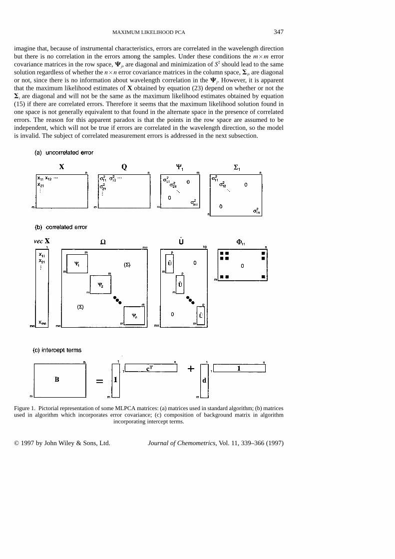
Data set 6 consisted of near-infrared spectroscopic data for three-component mixtures containingtoluene, chlorobenzene and heptane and was part of the Infomertix (Seattle, WA) calibration transferstudy.20 The 31 samples derived from an augmented, three-level, three-factor, full factorial design. Theconcentration was varied between 20% and 70% by weight for toluene and chlorobenzene andbetween 2% and 10% by weight for heptane. The mixtures were sealed into standard 1 cm path lengthcuvettes. Spectra were obtained over the range 400–2500 nm on an NIRSystems Model 6500(NIRSystems, Silver Spring, MD) grating spectrometer at intervals of 2 nm and were the averageresult of 32 scans. The spectrometer employed a Si detector in the range 400–1100 nm and a PbSdetector at longer wavelengths. A typical spectrum is shown in Figure 3(a). Clearly there are someregions above 1600 nm which are essentially opaque and are not meaningful, but these were retainedin this study for the purpose of illustrating the features of MLPCA. Unfortunately, replicate data wereonly available for the first sample, for which 400 spectra had been obtained, so a complete matrix ofstandard deviations could not be constructed. Instead, the standard deviation data for the first sample,shown in Figure 3(b), was used for all the samples. Although this is not completely accurate, it shouldserve as a reasonable approximation, especially for regions where the standard deviation is very largeowing to high absorbance.

Data set 7 was a 5310 matrix constructed in the same manner as a data set 1, except that correlatederrors were introduced. To produce error covariance, a 333 moving average filter (coefficients=1/9)was applied to the 5310 matrix of errors before it was added to the error-free measurements. At theboundaries of the error matrix the filter was wrapped around to the opposite side in order to eliminate

Figure 3. (a) Typical near-infrared spectrum of three-component mixture. (b) Standard deviation of absorbancemeasurements.



edge effects. Although this approach is not particularly realistic, it represents a general case for whichthe covariance structure could be easily predicted. The covariance matrix for this data set wascalculated using the definitions

F=[vec(F11) vec(F21) . . . vec(Fmn)] (34)

V=FT diag(vec(Q))F (35)

Here Q is the 5310 matrix of error variances prior to the application of the moving average filter. The5310 matrix Fij contains the nine filter coefficients applied to the error matrix to give the filtered errorcorresponding to measurement ij., This is illustrated in Figure 1(b) for F11, where the filled squaresshow the positions of the filter coefficients. For F12 the squares shift right and for F21 they shift down.Expressed another way, if E represents the 5310 matrix of uncorrelated errors generated inaccordance with the variances in Q and if «ij represents the error added to element ij of the pure datamatrix, we have

«ij = [vec(Fij)]T vec(E) (36)

The errors generated in this way were added to the pure data matrix. The noisy data matrix X and theerror covariance matrix V were passed to the MLPCA algorithm.

5. RESULTS AND DISCUSSION

5.1. Algorithm performance

Table 3 summarizes the results of applying the various MLPCA algorithms to the data sets describedin the preceding section. For data sets 1–4 and 6 the standard algorithm (Table 1) was used. Theversion which incorporates intercept terms (Section 3.4) was used for data set 5 and the routine forcorrelated errors (Table 2) was employed for data set 7. In all cases the MLPCA model rank wasvaried from one to p+1, where p is the true rank of the data set. All the data sets were also analyzedby PCA, with mean centering used as a pretreatment step for data set 5. The models generated by PCAand MLPCA were used to estimate the error-free measurements (X) by orthogonal and maximumlikelihood projections of the measurements respectively. These were used to calculate the objectivefunction S2 in each instance. For this purpose, equation (1) was used for data sets 1–6 and equation(25) was used for data set 7. For cases with no intercept terms, S2 for the model with correct rankshould approximate a x2-distribution with (m2p)(n2p) degrees of freedom. In accordance with this,the last two columns of Table 3 give the probability of realizing a value of S2 below that observed ifthe model were correct. In other words, values of P below 0·025 or above 0·975 would constituterejection of the null hypothesis that the model is correct (a=0·05). For data set 5 the same test wasdone using (m2p21)(n2p21) degrees of freedom to account for row and column intercepts.

The convergence times given in Table 3 are the result of single runs that were carried out with nocompeting tasks running on the computer. The results are ‘typical’ in the sense that no attempt wasmade to adjust the random number seeds to improve performance. Note that there is a separateconvergence time listed for each rank analyzed by MLPCA. This is because, unlike conventionalPCA, the MLPCA solutions are not generally nested (i.e. the rank-p model does not contain the rank-(p21) model). Convergence times listed are generally reasonable, with most cases requiring no morethan a few minutes and all but one case requiring less than 1 h. Although size seems to play some rolein convergence time, a much more important factor is the structure of the errors. Experience hasindicated that the totally random error structure, such as that in data sets 1–3, is the most difficult caseand this observation is supported by the results in Table 3. This case is therefore useful in estimating



Table 3. Results of MLPCA on test data sets

S2 Pa

Data set Error True Model Convergencenumber Size type Offset? rank rank time (min) PCA MLPCA PCA MLPCA

1 10320 Random N 2 1 3·00 3·903106 4·533105 1·00 1·002 1·46 3·293104 123·04 1·00 0·103 2·12 5209·0 88·48 1·00 0·02

2 20320 Random N 2 1 1·21 7·173106 4·073105 1·00 1·002 1·65 1·513104 311·82 1·00 0·323 2·56 1·863104 267·29 1·00 0·18

3 203100 Random N 2 1 700·50 8·713109 7·133106 1·00 1·002 48·46 2·833107 1757·3 1·00 0·463 40·10 2·673108 1548·3 1·00 0·04

4 20341 Proportional N 3 1 0·03 8419·2 7100·9 1·00 1·00+constant 2 0·03 1240·2 1217·0 1·00 1·00

3 0·03 724·90 683·43 0·98 0·854 0·24 654·99 571·85 0·96 0·28

5 20341 Proportional Y 3 1 13·73 8138·4 6592·5 1·00 1·00+constant 2 5·35 1094·4 953·02 1·00 1·00

3 4·21 677·40 622·28 0·99 0·814 12·78 603·87 512·46 0·97 0·20

6 3131050 ? N 3 1 3·35 1·723108 8.883107 1·00 1·002 8·13 1·633108 1·443107 1·00 1·003 5·45 1·273108 3·383105 1·00 1·004 10·84 5·393107 1·433105 1·00 1·00

7 5310 Random, N 2 1 0·02 2·593106 1·533106 1·00 1·00correlated 2 0·11 199·92 23·01 1·00 0·48

3 0·06 129·45 9·97 1·00 0·24

a P is the probability that a value less than the corresponding S2 would be observed for a x2-distribution with the appropriate degrees of freedom.

P. D. W

EN

TZ

EL

L E

T A

L.

356

© 1997 by John W

iley & Sons, L

td.Journal of C

hemom

etrics, Vol. 11, 339–366 (1997)

upper limits for the convergence time. The rank-one model for data set 3 (the largest of the ‘random’error models) proved to be unusually difficult to solve, requiring nearly 12 h. It is not clear at this pointwhether the slow convergence is the result of the error structure itself or poor initial estimates thatarise from it. However, convergence seems to be considerably faster for other error structures, suchas data set 4, where the convergence time is typically a few seconds. This case is likely to be muchmore typical of experimental data than the random structure. Data set 5, which is the same as data set4 except for the presence of row and column offsets, required considerably more time because of thegradient optimization of intercept vectors as described in Section 3.4. Data set 6 represents a typicalexperimental data set and demonstrates that MLPCA is a practical alternative to PCA for such cases.Relatively slow convergence in this instance was probably due to poor initial estimates resulting fromthe inclusion of very noisy measurements in the data set. Finally, data set 7 shows that convergencetime is not a problem for correlated errors.

Analysis of the objective function values in Table 3 shows that MLPCA always produces a lowerS2 than the corresponding PCA model. This is expected, since PCA does not optimize the samecriterion. It is interesting to note, however, that for data sets 2 and 3 the value of S2 obtained by PCAactually increases in going from a rank-two to a rank-three model. At first this may seemcontradictory, since the general rule is that increasing the rank of a model improves the fit to the data.However, accounting for a greater amount of variance in the data set by increasing the number offactors in PCA does not necessarily decrease the value of S2. This seems to be especially true for thecase of unstructured errors.

With reference to the last two columns of Table 3 it is expected that P should drop significantlybelow unity when a model of the correct rank is found, since that is the point at which S2 should followa x2-distribution. For MLPCA this is true for all cases but one. The one exception is the experimentaldata, data set 6. In this case it is not surprising that P remains at unity for several reasons: (a) thematrix of standard deviations was approximated using only information from the first sample andtherefore is incorrect for the remaining samples; (b) the variance estimates are the results of replicatescans and do not account for other sources of variance, such as cell positioning; (c) the varianceestimates appear to reflect truncation of the signal in some places; (d) the noise is known to becorrelated; (e) although there are only three known components in the system, there is a real possibilityof row and/or column offsets. This example highlights some of the difficulties in using this sensitivestatistical measure to estimate the rank in practical cases but does not diminish the utility of MLPCAfor model estimation. (Note that the objective function for the rank-three model is more than twoorders of magnitude smaller for MLPCA.) In contrast with MLPCA, the PCA models almost alwaysgive P-values of unity in the table, indicating an incorrect model even when the rank is overestimated.The only exceptions are data sets 4 and 5, where the error structure is closer to uniform, but even inthose cases P does not fall below 0·98 for models of the correct rank.

5.2. Statistical validation

Although the cases in the preceding subsection indicate that MLPCA produces smaller values of theobjective function than does PCA, it does not guarantee that the procedure converges on the optimumsolution, since local optima are always possible. One way to test for a global optimum is to use adifferent initial estimate and compare the final solutions, but this method is not foolproof. A bettermethod in this case is to exploit the statistical characteristics of S2 for the correct model. This is doneby analyzing replicate data sets, each with the same matrix of error-free data and standard deviationsbut with different errors. If the distribution of the S2-values for these replicates follows a x2-distribution with the appropriate degrees of freedom, then it can be concluded that the method isfinding the maximum likelihood solution.



A convenient way to make this comparison is to use probability plots. First the replicate data sets(100 in this case) are analyzed and the S2-values are stored. The S2-values are then sorted and assigneda cumulative probability according to their position in the list (the observed probability). For example,the second element in the list would be assigned an observed probability of 2/n, where n is the numberof replicates. Then an expected probability is calculated using the x2-distribution. The cumulativeprobability density function for x2 can be calculated using the incomplete gamma function:21

P(S2 |n)=GincSn

2,

S2

2D (37)

where n is the number of degrees of freedom. If the two distributions are the same, a plot of theexpected probabilities against observed probabilities should yield a straight line with a slope of unity.If the model is insufficient to account for the systematic variance, either because the form of the modelis incorrect or the parameters are suboptimal, then the points of the plot will lie above the ideal line.This means that the distribution of S2 is shifted right from the x2-distribution. If the model accountsfor an excessive amount of variance (i.e. the estimated rank is too high and measurement variance ismodeled), the points will lie below the ideal line.

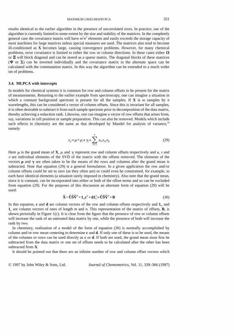
Figure 4 shows probability plots for four of the data sets used in this study: data sets 2, 4, 5 and 7.These data sets were chosen to reflect the different error structures and algorithms used. It is clear fromthe figure that in all cases the results from MLPCA follow the expected distribution, with only minor

Figure 4. Probability plots of S2 for replicate runs of simulated data sets: (a) data set 2; (b) data set 4; (c) dataset 5; (d) data set 7.



deviations attributable to the statistical limitations of this study. Therefore it can be concluded thateach of the algorithms is converging on a global optimum (the quality of the optimum is discussed inSection 5.5). Furthermore, to varying degrees, the models generated by PCA do not adequatelyaccount for the systematic variance in the data sets and are therefore likely to be inferior. Additionalcomments on these plots are made in the following two subsections.

5.3. MLPCA with intercepts

The results shown in Figure 4(c) confirm that the gradient optimization method used to determine theintercept vectors for MLPCA performed as expected. However, an additional analysis was done usingthe standard MLPCA algorithm after the data were column and row mean centered. While thisapproach always produced S2-values which were higher than those for which the intercepts wereoptimized, the difference is barely distinguishable in the figure. This implies that the interceptsdetermined are very close to the mean values for this particular error structure. Therefore, although theuse of mean centering may mean that the models obtained by the standard MLPCA algorithm aresuboptimal, the differences may be negligibly small in many cases and justify the use of the fasteralgorithm. Larger differences are likely to be observed for cases where the standard deviations becomevery large or where the data matrix is small. Such cases justify efforts to improve the efficiency of themodified algorithm.

5.4. Correlated errors

Figure 4(d) reveals some interesting characteristics of MLPCA when applied to cases of correlatederrors. It is clear from the figure that the version of the MLPCA algorithm that incorporates errorcovariance provides the optimum model according to the maximum likelihood criterion and that PCAmodels are inferior in this regard. An additional analysis was also carried out using the standardMLPCA algorithm by assuming no correlation among the errors and using the diagonal elements ofthe full covariance matrix (V) for the variances. The models generated by this approach were notvisibly any better than the PCA models, although the plot does not allow a direct comparison of thesetwo sets of results. Further studies have shown that PCA and the standard MLPCA algorithm produceinferior results for correlated errors even when the standard deviations are the same for allmeasurements (in this case these two algorithms are equivalent). This indicates the importance of theerror covariance information. Since many chemical measurements and data-preprocessing methodsgive rise to correlated errors, future studies need to be carried out to assess the importance of thiscontribution to model estimation and to improve the numerical reliability of the algorithmincorporating covariance.

5.5. Model quality

Although MLPCA generates models with smaller values of the objective function than does PCA, thekey questions have yet to be answered. Are the MLPCA models closer to the true model and do theyoffer significant advantages over the PCA models? The second part of this question cannot beanswered outside the context of particular applications, since the advantages gained by MLPCA willundoubtedly depend on the type and magitude of errors involved as well as the indended use of themodel (regression, mixture analysis, etc.). However, the first part of the question is readily answeredusing simulated data.

One way to compare the MLPCA and PCA models is to project the original vectors used to generatethe error-free data onto the row space (U) or column space (V) of the model. The angle between theprojected vector and the original vector then gives an indication of the agreement between the true



model and the fitted model. Mathematically, the angular deviations for the left-hand vectors are givenby

ui =cos21S aTi UUTai

||aTi || · ||UUTai ||

D (38)

where ui is the angular deviation of the left-hand vector ai from the space of the model. A similarexpression can be used for the right-hand vectors. In order to be able to draw statistically validconclusions, 100 replicates were run for data sets 2, 4 and 7. The results are reported in Table 4. Notethat since equation (38) always gives positive values, the results in the table are the mean values ofthe absolute angular deviations. Also given are the standard deviations of the distributions.

Application of the t-test to the results in Table 4 clearly indicates that the MLPCA algorithmproduces models with smaller angular deviations for all three data sets. The extent of improvementvaries considerably with the nature of the data and the errors, however. Although these differences arestatistically significant, the practical significance of the differences remain as a subject for futureresearch.

To further assess the quality of MLPCA model estimation, the experimental data set, data set 6, wasused. Of course, in this case, replicate data sets were unavailable, as were pure component spectra.However, the deviations of the concentration vectors from the model space could be measured. Theconcentrations for this data set were determined gravimetrically and so were accurately known. Table5 shows that when the full wavelength range is used, the model obtained by MLPCA is far superior

Table 4. Comparison of vector angle accuracies for PCA and MLPCA. Results are based on 100 replicates anduncertainties are given as standard deviations

Mean angular deviation (PCA) (deg) Mean angular deviation (MLPCA) (deg)Data setnumber Rank U V U V

2 2 0·41±0·08 0·39±0·06 0·22±0·04 0·21±0·050·42±0·08 0·41±0·06 0·22±0·04 0·23±0·04

4 3 3·1±0·6 3·4±0·6 2·3±0·4 3·0±0·54·7±1·0 3·8±0·7 3·8±0·7 3·1±0·53·0±0·7 3·5±0·6 2·3±0·4 2·9±0·4

7 2 0·10±0·05 0·16±0·05 0·023±0·012 0·10±0·040·11±0·06 0·16±0·06 0·027±0·016 0·12±0·04

Table 5. Angular deviations of concentration vectors from PCA space for data set 6

Angular deviation (deg)Wavelengthrange (nm) Component PCA MLPCA

400–2500 Toluene 13·7 0·127Chlorobenzene 13·6 0·135Heptane 25·8 0·688

700–1600 Toluene 0·281 0·281Chlorobenzene 0·359 0·359Heptane 0·792 0·792



to that obtained by PCA. This is not surprising, since PCA attempts to model the variance due tomeasurement errors in the high-absorbance regions. Normally in a situation like this one wouldpreselect wavelengths prior to analysis by PCA. If the wavelength region used is 700–1600 nm, thevariance is essentially uniform and PCA and MLPCA produce equivalent results. However, it will benoted that the angular deviation of the concentration vectors is smaller when MLPCA is used with thefull wavelength region as opposed to the truncated data set, even though the error estimates in this caseare only approximate. This illustrates that information can be lost when data are excluded from themodeling process. MLPCA uses the measurement error variance to optimize the amount ofinformation extracted from the data and in that sense represents a significant advance in multivariateanalysis.

6. CONCLUSIONS

In this work the theoretical foundations of MLPCA have been established using the framework ofPCA (and SVD). By incorporating information about the measurement errors, the procedure has beenshown to be optimal for principal component modeling in accordance with a maximum likelihoodcriterion. The algorithm presented here is particularly efficient in its use of alternating regression toachieve rapid convergence. Modifications to the algorithm also permit the incorporation of interceptterms consistent with a maximum likelihood model. Furthermore, generalization of the method allowsthe incorporation of correlated measurement errors. To our knowledge, this is the first time that a PCAprocedure has been developed that has the capability of dealing with mesurement error covariance.Results using simulated data show that the objective function minimized by the algorithmapproximates a x2-distribution with (m2p)(n2p) degrees of freedom (in the absence of interceptterms) provided that the measurement error covariance matrix is known and the form of the model iscorrect. Results using simulated and experimental data also demonstrate that model estimation byMLPCA is superior to models produced by PCA in cases where non-uniform or correlated errors arepresent.

The practical implications of the theoretical aspects of MLPCA put forward here will no doubt bethe subject of future research. This work has clearly demonstrated the positive features of MLPCA andanswered many questions related to optimal scaling for PCA models. The advantages of MLPCA overPCA are balanced to some degree by the greater computational efficiency of the latter. As long asmeasurement errors are approximately uniform or are very small in the context of the intendedapplication, PCA results may be sufficient, if suboptimal. However, there are many cases in chemistrywhere these conditions do not hold. Applications in a wide range of areas, including calibration, curveresolution and data fusion, can no doubt benefit from the optimal modeling features of MLPCA andare fertile grounds for future research. This work has demonstrated the importance of measurementerror data for maximizing the information available from chemical data sets and MLPCA should serveas an important archetype for optimal modeling by PCA.

ACKNOWLEDGEMENTS

This work was supported by the Natural Sciences and Engineering Research Council of Canada andthe Center for Process Analytical Chemistry.

APPENDIX I: NOTATION AND LIST OF SYMBOLS

In general the conventions used in this paper are as follows. Matrices are represented as bolduppercase letters and column vectors are represented as bold lowercase letters. Italic upper- andlowercase letters are used for scalars. Greek and italic fonts are used with no particular pattern, but



where possible we have tried to adhere to symbols commonly used in the literature. Symbols whichrepresent estimates of unknown quantities are designated with a caret. A matrix transpose is indicatedby a superscript ‘T’ and the Euclidean norm of a vector by ‘|| · ||’. The Kronecker product of twomatrices is indicated ‘^ ’.

A list of important symbols in the paper follows.

1m m31 vector of onesaij model coefficient (element of A)ai left-hand vector of true modelA (i) left-hand matrix of p-dimensional model (equation (2)) (ii) matrix of model coefficients

(equation (7))A matrix of estimated model coefficientsB (i) right-hand matrix of p-dimensional model (equation (2)) (ii) matrix of model offsets (equation

(30))bj column vector of B (offsets)c vector of column offsets for MLPCA modeld vector of row offsets for MLPCA modelE unfiltered measurement errors for XF matrix of filter coefficients (mn3mn) for calculating V of filtered dataGi intermediate matrix in calculation of dS2/dai

Hj substitution equal to (UTC21j U)21UTC21

j

In n3n identity matrixJi derivative of rotation matrix T with respect to angle ai

K commutation matrix for Xl function minimized for maximum likelihood projectionL probability density function for measurement vector xLi exchange matrix with property Ji =LiTi

m number of rows in Xn number of columns in Xp rank of data matrix (pseudorank)P probability of observing a x2-value less than a given valuePj maximum likelihood projection matrix for xj

S2 objective functionT1, T2, . . . individual rotation matricesT overall rotation matrixu, s, n elements of U, S and VU, S, V estimated MLPCA matrices (SVD form)U1, U2 upper and lower matrices of U (p3p and (m2p)3p)U0, V0 initial estimates for U and VU, V supermatrices for U and Vxij, xij, xo

ij elements of X, X and Xo

xj, xj, xoj column vectors of X, X and Xo

xp, xop upper p31 vectors of x and xo

Dxj residual vector for column j of X (=xj 2 xj)X measurement data matrixX matrix of maximum likelihood estimates of Xo

X1, X2 upper and lower matrices of X (p3n and (m2p)3n)Xo matrix of true measurementsy vector of dependent variables in classical regressiona significance level for hypothesis testingai rotation angle about axis ib vector of regression coefficients in classical regressiond vector of errors in y in classical regression«j column vector of measurement errors for column j of X«ij measurement error for xij after filteringFij matrix of filter coefficients for errors corresponding to measurement xij

g vector of row offsets for Mandel model



Ginc incomplete gamma functionl convergence criterion for MLPCA algorithmm grand mean for Xn degrees of freedomui angular deviation of eigenvector i from true model spacer vector of column offsets for Mandel modelSi error covariance matrix for row i of X (or column i of XT)V full error covariance matrix of vec(X)J full covariance matrix of vec(XT)Cj error covariance matrix for column vector j of Xs2

ij measurement variance for xij

APPENDIX II: DERIVATION OF MAXIMUM LIKELIHOOD PREDICTION EQUATION

Given a vector x of length m of observed measurements and the corresponding error covariance matrixC, the multivariate probability density function at x is given by

L=1

(2p)m/2 |C |1/2 exp[212 (x2xo)TC21(x2xo)] (39)

where xo represents the (unknown) vector of true values. The vector of maximum likelihood estimatesof xo for a given A, designated x, is obtained by maximizing the probability density function subjectto the parametric model x= Axp. This corresponds to minimizing the function

l=(x2 x)TC21(x2 x) (40)

with respect to x. Substitution of the parametric model gives

l=(x2 Axp)TC21(x2 Axp)

=xTC21x2xTC21Axp 2 xTpATC21x+ xT

pATC21Axp (41)

Using standard relations for derivatives of vectors,22 this gives

lxp

=02 ATC21T x2 ATC21x+2ATC21Axp (42)

Setting this equal to zero to find the minimum leads to

xp =(ATC21A)21ATC21x (43)

which is the same as equation (9) and leads directly to equation (10).

APPENDIX III: DERIVATIVES OF S2

The calculation of the derivative of S2 with respect to the rotation angles (in the absence of interceptterms) begins by finding the differential of S2.

dS2 =On

j=1

d(DxTj C21

j Dxj)

=O [d(DxTj )C21

j Dxj +DxTj C21

j d(Dxj)]



=2O DxTj C21

j d(Dxj) (44)

It will be assumed that the symmetric error covariance matrix C is known for each x. Forconvenience, from this point on, the subscript ‘j’ in equation (44) will be dropped but will be implied.Also, for simplicity we will use U in place of U. We can write Dx as

Dx=[I2U(UTC21U)21UTC21]x

={I2TU0[(TU0)TC21TU0]

21(TU0)TC21}x

=[I2TU0(UT0TTC21TU0)

21UT0TTC21]x (45)

This gives

DxTC21 d(Dx)=2{DxTC21(dT)U0(UTC21UT)21UTC21x+DxTC21U[d(UT

0TTC21TU0)21]UTC21x

+DxTC21U(UTC21UT)21UT0(dTT)C21x} (46)

If we make the substitution H=(UTC21U)21UTC21, equation (46) can be further expanded byconventional means18 to give

DxTC21d(Dx)=2 [DxTC21(dT)U0Hx2xTC21UH(dT)U0HDx

2DxTC21UH(dT)U0Hx+xTC21(dT)U0HDx] (47)

The differential of the transformation matrix can be expanded as

dT=(dT1)T2T3 . . . Tm21 +T1(dT2)T3 . . . Tm21 + . . . (48)

where

dTi =dTi

dai

dai =Ji dai (49)

Here Ji is the derivative of the rotation matrix corresponding to ai. For example,

2sin a1 2cos a1 0 . . . 0 0 0 0 . . . 0

cos a1 2sin a1 0 . . . 0 0 2sin a2 2cos a2 . . . 0

J1 = 0 0 0 . . . 0 , J2 = 0 cos a2 2sin a2 . . . 0 , etc.

: : : . . . : : : : . . . :

0 0 0 . . . 0 0 0 0 . . . 0

(50)

Furthermore, it is easily shown that

Ji =LiTi (51)

where

0 21 0 . . . 0 0 0 0 . . . 0

1 0 0 . . . 0 0 0 21 . . . 0

L1 = 0 0 0 . . . 0 , L2 = 0 1 0 . . . 0 , etc.

: : : . . . : : : : . . . :

0 0 0 . . . 0 0 0 0 . . . 0

(52)



From this we can write

dT=J1(T2T3 . . . ) da1 +T1J2(T3T4 . . .) da2 + . . .

=L1T1(T2T3 . . . ) da1 +T1L2T2(T3T4 . . .) da2 + . . .

=L1T da1 +T1L2T211 T1T2(T3T4 . . .) da2 + . . .

=L1T da1 +(T1L2TT1)T da2 + . . .

=G1T da1 +G2T da2 + . . . +Gm21T dam21 (53)

where

Gi = (T1T2 . . . Ti21)Li(TTi21T

Ti22 . . . T1) (54)

Substitution of equation (53) into equation (47) and recognizing that U=TU0 and P=UH gives

DxTC21 d(Dx)=2O (DxTC21GiPx2xTC21PGiPDx2DxTC21PGiPx+xTC21GiPDx) dai (55)

This result leads to equation (20) in the paper. Although this equation is correct and faster thannumerical evaluation of the derivatives, it is somewhat cumbersome. Each of the m21 parameters tobe optimized requires the calculation and storage of an m3m matrix Gi, which is the product of 2i21matrices that are m3m. Even though these matrices are sparse, the calculations are still time-consuming and awkward. Some simplification of equation (55) is possible by examining thecharacteristics of G. The matrix Gi is antisymmetric with zero elements everywhere except for the firsti elements of column i+1 and row i+1. If the rotation angles are small, the rotation matrices approachthe identity matrix and a good approximation is

Gi ÅLi (56)

We have found that this approximation works well in practice, particularly if U0 is updated asconvergence is approached so that the angles remain small.

REFERENCES

1. R. J. Larsen and M. L. Marx, An Introducton to Mathematical Statistics and Its Applications, 2nd edn,Prentice-Hall, Englewood Cliffs, NJ (1986).

2. P. Paatero and U. Tapper, Chemometrics Intell. Lab. Syst. 18, 183 (1993).3. R. N. Cochran and F. H. Horne, Anal. Chem. 49, 846 (1977).4. H. R. Halvorson, Biophys. Chem. 14, 177 (1984).5. V. Simeon and D. Pavkovic, J. Chemometrics 6, 257 (1992).6. K. R. Gabriel and S. Zamir, Technometrics 21, 489 (1979).7. P. Paatero and U. Tapper, Environmetrics 5, 111 (1994).8. D. N. Lawley and A. E. Maxwell, Factor Analysis as a Statistical Method, 2nd edn, p. 109, Butterworths,

London (1971).9. K. G. Jöreskog, in Systems Under Indirect Observation, Part I, ed. by K. G. Jöreskog and H. Wold, Chap.

4, North-Holland, Amsterdam (1982).10. K. A. Bollen, Structural Equations with Latent Variables, Wiley, New York (1989).11. P. Moens, P. De Volder, R. Hoogewijs, F. Callens and R. Verbeeck, J. Magn. Reson. A, 101, 1 (1993).12. P. Persoone, R. De Gryse and P. De Volder, J. Electron Spectrosc. Relat. Phenom. 71, 225 (1995).13. S. Van Huffel and J. Vandewalle, The Total Least Squares Problem, SIAM, Philadelphia, PA (1991).14. W. A. Fuller, Measurement Error Models, Wiley, New York (1987).15. M. S. Bartlett, Br. J. Psychol. 28, 97 (1937).16. M. S. Bartlett, Nature 141, 609 (1938).



https://www.researchgate.net/publication/243774909_Factor_Analysis_As_A_Statistical_Method?el=1_x_8&enrichId=rgreq-106d270c712df139cfc4b1991104ad39-XXX&enrichSource=Y292ZXJQYWdlOzI1MTUxNjc5MDtBUzoxMDEwNzIyNDkwMzI3MjNAMTQwMTEwODkxMTAwMg==

https://www.researchgate.net/publication/243774909_Factor_Analysis_As_A_Statistical_Method?el=1_x_8&enrichId=rgreq-106d270c712df139cfc4b1991104ad39-XXX&enrichSource=Y292ZXJQYWdlOzI1MTUxNjc5MDtBUzoxMDEwNzIyNDkwMzI3MjNAMTQwMTEwODkxMTAwMg==

https://www.researchgate.net/publication/224773289_Structural_Equations_With_Latent_Variables?el=1_x_8&enrichId=rgreq-106d270c712df139cfc4b1991104ad39-XXX&enrichSource=Y292ZXJQYWdlOzI1MTUxNjc5MDtBUzoxMDEwNzIyNDkwMzI3MjNAMTQwMTEwODkxMTAwMg==

https://www.researchgate.net/publication/242462643_An_Introduction_to_Mathematical_Statistics_and_Its_Applications_Prentice-Hall_Inc?el=1_x_8&enrichId=rgreq-106d270c712df139cfc4b1991104ad39-XXX&enrichSource=Y292ZXJQYWdlOzI1MTUxNjc5MDtBUzoxMDEwNzIyNDkwMzI3MjNAMTQwMTEwODkxMTAwMg==

https://www.researchgate.net/publication/242462643_An_Introduction_to_Mathematical_Statistics_and_Its_Applications_Prentice-Hall_Inc?el=1_x_8&enrichId=rgreq-106d270c712df139cfc4b1991104ad39-XXX&enrichSource=Y292ZXJQYWdlOzI1MTUxNjc5MDtBUzoxMDEwNzIyNDkwMzI3MjNAMTQwMTEwODkxMTAwMg==

17. L. J. Gleser and H. Yang, Anal. Chim. Acta 277, 405 (1993).18. J. R. Magnus and H. Neudecker, Matrix Differential Calculus with Applications in Statistics and

Econometrics, Wiley, Chichester (1988).19. J. Mandel, Technometrics 13, 1 (1971).20. T. Dean, B. Kowalski and R. Pell, Appl. Spectrosc. submitted.21. W. H. Press, S. A. Teukolsky, W. T. Vetterling and B. P. Flannery, Numerical Recipes in FORTRAN, 2nd edn,

p. 215, Cambridge University Press, New York (1992).22. W. H. Beyer (ed.), CRC Handbook of Tables for Probability and Statistics, p. 26, Chemical Rubber Co.,

Cleveland, OH (1996).



https://www.researchgate.net/publication/245813526_CRC_Handbook_of_Tables_of_Probability_and_Statistics?el=1_x_8&enrichId=rgreq-106d270c712df139cfc4b1991104ad39-XXX&enrichSource=Y292ZXJQYWdlOzI1MTUxNjc5MDtBUzoxMDEwNzIyNDkwMzI3MjNAMTQwMTEwODkxMTAwMg==

https://www.researchgate.net/publication/245813526_CRC_Handbook_of_Tables_of_Probability_and_Statistics?el=1_x_8&enrichId=rgreq-106d270c712df139cfc4b1991104ad39-XXX&enrichSource=Y292ZXJQYWdlOzI1MTUxNjc5MDtBUzoxMDEwNzIyNDkwMzI3MjNAMTQwMTEwODkxMTAwMg==

Maximum likelihood principal component analysis

Documents

Transcript of Maximum likelihood principal component analysis