an exact maximum likelihood non-parametric test for meta ...

Paul Emerg Themes Epidemiol (2018) 15:9 https://doi.org/10.1186/s12982-018-0077-7

METHODOLOGY

Cannons and sparrows: an exact maximum likelihood non-parametric test for meta-analysis of k 2 × 2 tablesLawrence M. Paul*

Abstract

Background: The use of meta-analysis to aggregate multiple studies has increased dramatically over the last 30 years. For meta-analysis of homogeneous data where the effect sizes for the studies contributing to the meta-anal-ysis differ only by statistical error, the Mantel–Haenszel technique has typically been utilized. If homogeneity cannot be assumed or established, the most popular technique is the inverse-variance DerSimonian–Laird technique. How-ever, both of these techniques are based on large sample, asymptotic assumptions and are, at best, an approximation especially when the number of cases observed in any cell of the corresponding contingency tables is small.

Results: This paper develops an exact, non-parametric test based on a maximum likelihood test statistic as an alter-native to the asymptotic techniques. Further, the test can be used across a wide range of heterogeneity. Monte Carlo simulations show that for the homogeneous case, the ML-NP-EXACT technique to be generally more powerful than the DerSimonian–Laird inverse-variance technique for realistic, smaller values of disease probability, and across a large range of odds ratios, number of contributing studies, and sample size. Possibly most important, for large values of heterogeneity, the pre-specified level of Type I Error is much better maintained by the ML-NP-EXACT technique rela-tive to the DerSimonian–Laird technique. A fully tested implementation in the R statistical language is freely available from the author.

Conclusions: This research has developed an exact test for the meta-analysis of dichotomous data. The ML-NP-EXACT technique was strongly superior to the DerSimonian–Laird technique in maintaining a pre-specified level of Type I Error. As shown, the DerSimonian–Laird technique demonstrated many large violations of this level. Given the various biases towards finding statistical significance prevalent in epidemiology today, a strong focus on maintaining a pre-specified level of Type I Error would seem critical.

Keywords: Meta-analysis, Categorical analysis, Mantel–Haenszel, DerSimonian–Laird, Exact solution, Inverse variance

© The Author(s) 2018. This article is distributed under the terms of the Creative Commons Attribution 4.0 International License (http://creat iveco mmons .org/licen ses/by/4.0/), which permits unrestricted use, distribution, and reproduction in any medium, provided you give appropriate credit to the original author(s) and the source, provide a link to the Creative Commons license, and indicate if changes were made. The Creative Commons Public Domain Dedication waiver (http://creat iveco mmons .org/publi cdoma in/zero/1.0/) applies to the data made available in this article, unless otherwise stated.

Little experience is sufficient to show that the traditional machinery of statistical processes is wholly unsuited to the needs of practical research. Not only does it take a cannon to shoot a sparrow, but it misses the sparrow. The elaborate mechanism built on the theory of infinitely large samples is not accurate enough for simple laboratory data.” (R. A. Fisher, 1925).

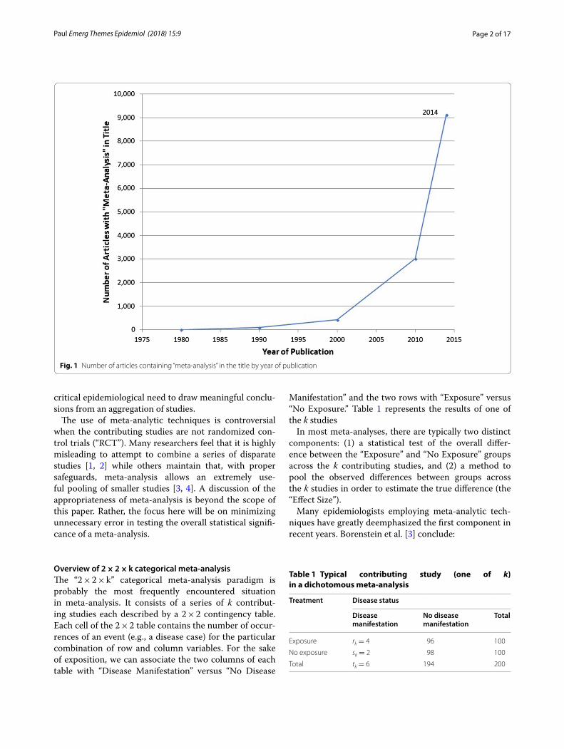
BackgroundThe use of meta-analysis in epidemiological research has been increasing at a very rapid rate. A review of the National Library of Medicine’s online database (“Pub Med”) shows that in 1980 there were only five research articles with the phrase “meta-analysis” in their titles. The number had increased to 92 in 1990, 422 in 2000, and to 9125 in 2014 (see Fig. 1).

While part of this growth may be due to the widespread availability of powerful personal computer software mak-ing meta-analysis techniques easier to perform and more feasible to implement, this growth also likely represents a

Open Access

Emerging Themes inEpidemiology

*Correspondence: [email protected] Somerset, NJ, USA

http://creativecommons.org/licenses/by/4.0/

http://creativecommons.org/publicdomain/zero/1.0/

http://creativecommons.org/publicdomain/zero/1.0/

http://crossmark.crossref.org/dialog/?doi=10.1186/s12982-018-0077-7&domain=pdf

of 17Paul Emerg Themes Epidemiol (2018) 15:9

critical epidemiological need to draw meaningful conclu-sions from an aggregation of studies.

The use of meta-analytic techniques is controversial when the contributing studies are not randomized con-trol trials (“RCT”). Many researchers feel that it is highly misleading to attempt to combine a series of disparate studies [1, 2] while others maintain that, with proper safeguards, meta-analysis allows an extremely use-ful pooling of smaller studies [3, 4]. A discussion of the appropriateness of meta-analysis is beyond the scope of this paper. Rather, the focus here will be on minimizing unnecessary error in testing the overall statistical signifi-cance of a meta-analysis.

Overview of 2 × 2 × k categorical meta‑analysisThe “2 × 2 × k” categorical meta-analysis paradigm is probably the most frequently encountered situation in meta-analysis. It consists of a series of k contribut-ing studies each described by a 2 × 2 contingency table. Each cell of the 2 × 2 table contains the number of occur-rences of an event (e.g., a disease case) for the particular combination of row and column variables. For the sake of exposition, we can associate the two columns of each table with “Disease Manifestation” versus “No Disease

Manifestation” and the two rows with “Exposure” versus “No Exposure.” Table 1 represents the results of one of the k studies

In most meta-analyses, there are typically two distinct components: (1) a statistical test of the overall differ-ence between the “Exposure” and “No Exposure” groups across the k contributing studies, and (2) a method to pool the observed differences between groups across the k studies in order to estimate the true difference (the “Effect Size”).

Many epidemiologists employing meta-analytic tech-niques have greatly deemphasized the first component in recent years. Borenstein et al. [3] conclude:

Fig. 1 Number of articles containing “meta-analysis” in the title by year of publication

Table 1 Typical contributing study (one of k) in a dichotomous meta-analysis

Treatment Disease status

Disease manifestation

No disease manifestation

Total

Exposure rk = 4 96 100

No exposure sk = 2 98 100

Total tk = 6 194 200


“… However, meta-analysis also allows us to move beyond the question of statistical significance, and address questions that are more interesting and also more relevant.” (pp. 11–12).

Similarly, Higgins and Green [4] rather dismissively state:

“… If review authors decide to present a P value with the results of a meta-analysis, they should report a precise P value, together with the 95% confidence interval” (pp. 371–372).

This study addresses only the first of these two compo-nents. A method is developed that attempts to maintain the Type I error (“false alarm rate”) at the desired level but has good power to detect true differences across a large range of event probability, number of contributing studies, sample size and level of heterogeneity.

An argument can be made that maintaining the Type I error at a pre-specified level is more important than the power (1—Type II error rate) to detect true differences between conditions. The framers of modern statistical testing called such errors “Errors of the First Kind” and placed a special emphasis on them. Neyman & Pearson in 1933 stated:

“A new basis has been introduced for choosing among criteria available for testing any given sta-tistical hypothesis, H0, with regard to an alternative Ht. If ϴ1 and ϴ2 are two such possible criteria and if in using them there is the same chance, ε, of reject-ing H0 when it is in fact true, we should choose that one of the two which assures the minimum chance of accepting H0 when the true hypothesis is Ht.” [5] [p. 336]

Thus, while Neyman and Pearson supported the effort to choose criteria that yield the greatest power to detect true differences, this effort is secondary to maintaining a pre-specified level of Type I error. Estimating the Effect Size particularly for rare events is well covered in a num-ber of recent studies (see in particular [6, 7]).

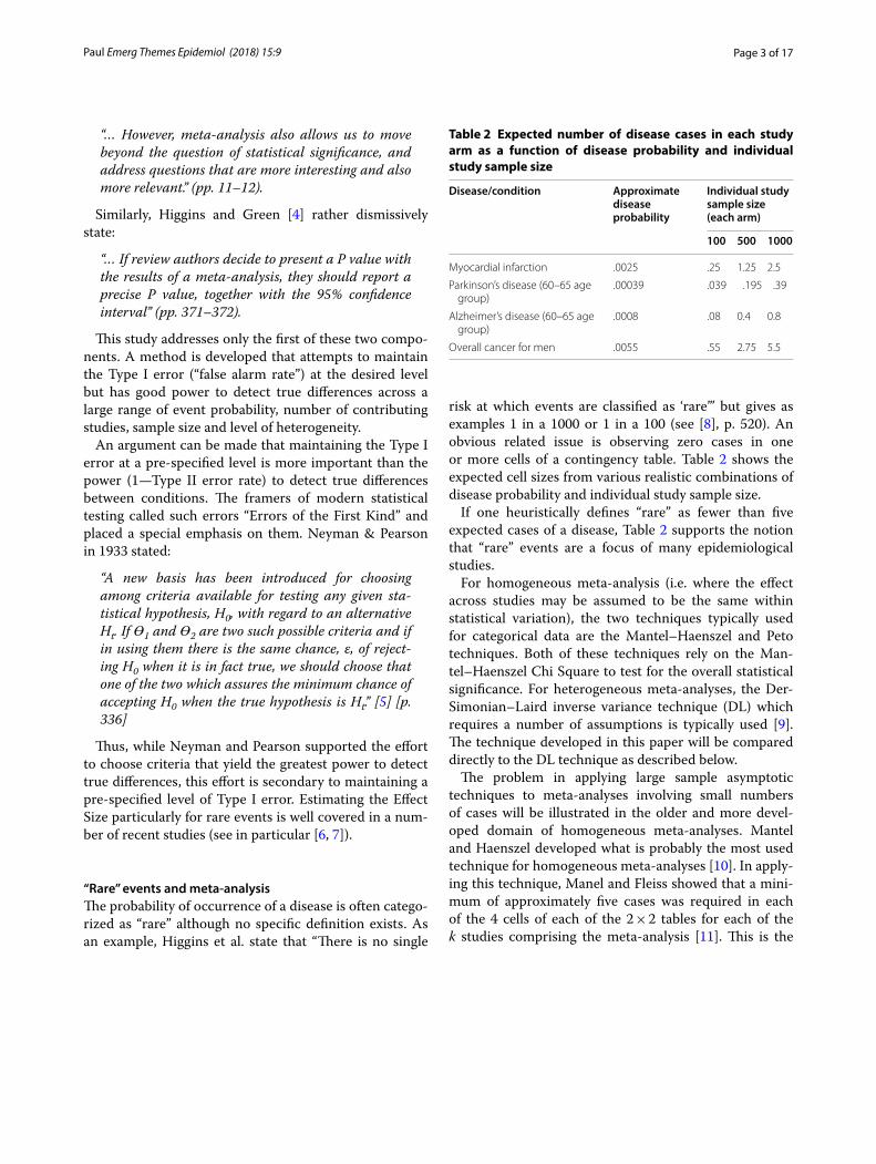
“Rare” events and meta‑analysisThe probability of occurrence of a disease is often catego-rized as “rare” although no specific definition exists. As an example, Higgins et al. state that “There is no single

risk at which events are classified as ‘rare’” but gives as examples 1 in a 1000 or 1 in a 100 (see [8], p. 520). An obvious related issue is observing zero cases in one or more cells of a contingency table. Table 2 shows the expected cell sizes from various realistic combinations of disease probability and individual study sample size.

If one heuristically defines “rare” as fewer than five expected cases of a disease, Table 2 supports the notion that “rare” events are a focus of many epidemiological studies.

For homogeneous meta-analysis (i.e. where the effect across studies may be assumed to be the same within statistical variation), the two techniques typically used for categorical data are the Mantel–Haenszel and Peto techniques. Both of these techniques rely on the Man-tel–Haenszel Chi Square to test for the overall statistical significance. For heterogeneous meta-analyses, the Der-Simonian–Laird inverse variance technique (DL) which requires a number of assumptions is typically used [9]. The technique developed in this paper will be compared directly to the DL technique as described below.

The problem in applying large sample asymptotic techniques to meta-analyses involving small numbers of cases will be illustrated in the older and more devel-oped domain of homogeneous meta-analyses. Mantel and Haenszel developed what is probably the most used technique for homogeneous meta-analyses [10]. In apply-ing this technique, Manel and Fleiss showed that a mini-mum of approximately five cases was required in each of the 4 cells of each of the 2 × 2 tables for each of the k studies comprising the meta-analysis [11]. This is the

Table 2 Expected number of disease cases in each study arm as a function of disease probability and individual study sample size

Disease/condition Approximate disease probability

Individual study sample size (each arm)

100 500 1000

Myocardial infarction .0025 .25 1.25 2.5

Parkinson’s disease (60–65 age group)

.00039 .039 .195 .39

Alzheimer’s disease (60–65 age group)

.0008 .08 0.4 0.8

Overall cancer for men .0055 .55 2.75 5.5


same requirement typically used without any particular justification for the simple Chi square test. All but one of the combinations of individual study sample size and dis-ease probability shown in Table 2 would yield fewer than five cases per cell leading to violations of the minimum cell size in the asymptotic Mantel–Haenszel (MH) Chi Square test, and thus the test would be potentially flawed.

R. A. Fisher addressed the limitations of using asymp-totic large sample methods in 1925 in the preface to the first edition of his well-known “Statistical Methods for Research Workers” [12]:

Little experience is sufficient to show that the tra-ditional machinery of statistical processes is wholly unsuited to the needs of practical research. Not only does it take a cannon to shoot a sparrow, but it misses the sparrow. The elaborate mechanism built on the theory of infinitely large samples is not accu-rate enough for simple laboratory data. Only by sys-tematically tackling small sample problems on their merits does it seem possible to apply accurate tests to practical data.

The continued use asymptotic tests in situations not suited for their use is unacceptable given the computer power that is now available to all researchers.

Heterogeneity versus homogeneity in meta‑analysesThe term “heterogeneity” refers to the fact that stud-ies done at different times and by different researchers might be expected to have different treatment effects. The expectation is that a variable of interest may owe its effect, at least in part, to one or more other variables. The meta-analysis researcher, J. P. T. Higgins stated: “Het-erogeneity is to be expected in a meta-analysis: it would be surprising if multiple studies, performed by differ-ent teams in different places with different methods, all ended up estimating the same underlying parameter.” ([13], p. 1158). While researchers may agree that heter-ogeneity is to be expected, there is very little agreement on how to quantify this variability. The most obvious and direct candidate is τ2, the assumed variability between studies. However, τ2 is not invariant across study designs and its interpretation may not be intuitive. Alternatives include I2, the ratio of the inter-study variability to the total variability and the Q statistic, which is mathemati-cally related to I2 (see, e.g., [14]).

In the technique described in this paper, heterogeneity will be mathematically manipulated through τ2 and the logit function using the same approach as Bhaumik et al. [15]. Namely,

where B is the Binomial Distribution, N is the Normal Distribution, xic, xit are the observed number of cases in the control and exposure groups respectively of the ith study, pic, pit are the event probabilities in the con-trol and exposure groups respectively of the ith study, nic, nit are the sample sizes in the two groups of the ith study, µ corresponds to the background event probabil-ity in the treatment and control groups, θ corresponds to the overall Odds Ratio for the Exposure Group rela-tive to the Control Group or the “log of the odds ratio”, τ 2 is a variance corresponding to the heterogeneity or the “heterogeneity parameter”, εi is the deviation in the treat-ment group of each of the contributing studies due to heterogeneity.

The basic principles of the DerSimonian–Laird (DL) methodAs stated above, this research specifically contrasts an exact method for conducting meta-analyses in k 2 × 2 tables with heterogeneity with the most popular approach which was developed by DerSimonian and Laird [9] (DL).

For each contributing study, the DL technique calcu-lates the logarithm of the sample odds ratio and a cor-responding estimate of the variance of this measure based on the asymptotic distribution of these logarithms. Adjustments are made for entries in the individual 2 × 2 tables that contain a zero-cell count. Equations 2–5 below capture the core DL approach. In Eq. 2, an esti-mate of the interstudy variability, τ 2 , is first derived from Cochran’s Q statistic and the weights assigned to each of the k contributing studies, ωi . These weights are equal to the inverse of the square of the standard error of the esti-mate of the odds ratio, θ̂i, in each of the k contributing studies.

(1)

xic ∼ B(

pic,nic)

, xit ∼ B(

pit,nit)

,

logit(pic) = µ, logit(pit) = µ+ θ + εi

εi ∼ N(

0, τ 2)

(2)τ̂ 2 =

Q − (k − 1)

∑

ωi −

(

∑

ω2i

∑

ωi

)


As shown in Eq. 3, a new set of weights, ω′i , are then

calculated based on the estimated value of τ̂ 2 from Eq. 2 and the standard errors of the contributing studies.

These new weights are then used to calculate estimates of both the overall log odds ratio, θDL and its standard error as shown in Eq. 4 and 5.

A test of statistical significance is then based on a large sample normal distribution. The DL technique requires asymptotic assumptions regarding both the Q statistic used to estimate the interstudy variability, τ 2, and the normal distribution required to test for statistical signif-icance. A more subtle issue is the possibility of distort-ing correlations between the individual estimates of the effect size for each contributing study, θi , and the indi-vidual weights used for each of these contributing effect sizes.

The ML‑NP‑EXACT: an exact maximum likelihood non‑parametric test of 2 × 2 × k dichotomous dataBasic approachAn exact approach to developing a maximum likelihood test of independence for k 2 × 2 tables logically starts by first addressing the simple k = 1 2 × 2 table case. An exact method would use maximum likelihood estimates of the cell counts and associated cell probabilities and then use a “goodness of fit” test sensitive to violations of independ-ence. Agresti and Wackerly [16] argued that “exact con-ditional tests can be simply formulated by using other criteria for ranking the tables according to the deviation each exhibits from independence.” [pp. 113–114] and go on to mention likelihood ratio statistics.

One such statistic is the G Test “goodness of fit” statis-tic strongly advocated by Sokal and Rohlf [17] to test for

(3)ω′i =

1

SE(

θ̂i

)2+ τ 2

(4)θ̂DL =

∑

ω′iθ̂i

∑

ω′i

(5)SE(

θ̂DL

)

=1

√∑

ω′i

independence between the row and column variables. Sokal and Rohlf cite Kullback and Leibler’s “Divergence” measure which is mathematically identical to the G Test [18]. The probability distribution of the G Test statistic is asymptotically χ2 which would be adequate for tables with large numbers in each of the cells. However, for the case of sparse tables being developed in this paper, this would not be satisfactory. For this simple k = 1 case, Fish-er’s Exact Test would be appropriate [19]. Fisher’s Exact Test exploits the fact that if one conditions on any of the marginal totals, the cell frequency of interest will be a suf-ficient statistic. Then, the associated frequency distribu-tion of the cell frequency of interest may be determined exactly using the hypergeometric distribution. Fisher’s Exact approach has been extended by Thomas [20] and others. Among other advantages, such conditioning eliminates the effect of any nuisance variable identi-cally affecting both exposure categories. Using Table 1 nomenclature, the number of individuals manifesting the disease being studied in the Exposure Group, rk, condi-tionalized on the total number of individuals manifesting the disease, tk is a sufficient statistic. This approach can be directly extended to 2 × 2 × k designs by again using the G Test “goodness of fit” statistic and testing for con-ditional independence in each of the k tables comprising the overall meta-analysis.

In the 3-way 2 × 2 × k meta-analysis, one approach is to first test for independence among the two factors (Disease Status and Treatment in the terminology of Table 1) in each of the k strata (e.g. using the Breslow-Day test of interaction [21]). If such a test of interaction supported independence of the two factors, the notion of a Common Odds Ratio (COR) could be entertained. Then the overall COR averaged across the k strata could be tested against the null hypothesis of 1.0 using the Cochran-Mantel–Haenszel test or equivalent.

Alternatively, Yao and Tritchler [22] developed an exact conditional independence test for 2 × 2 × k cat-egorical data. Although they derived an exact null hypothesis frequency distribution, they chose to use the standard Chi Square test statistic:

where k is the number of contributing studies. The present author programmed their test in the R

statistical language based on Yao’s dissertation [23]. Preliminary Monte Carlo simulations showed, however, that this implementation yielded a test with limited power compared to the DL method. With the advantage

(6)χ2 = χ21 + χ2

2 + · · ·χ2k


of the hindsight provided by this simulation, the use of a Chi Square statistic for this exact test is probably sub-optimal and is not necessary given their derivation of an exact null hypothesis frequency distribution.

A straightforward utilization of G Test per [17] would thus be:

where k is the number of contributing studies, Oi is the number of observed cases in the Exposure Group of the ith contributing study, Ei is the number of expected cases in the Exposure Group of the ith contributing study assuming conditional independence.

Table 1 which shows the data for a particular one of the k contributing studies will be used to help clarify this approach. There are two sources of cases, cases from the “Exposure” group and cases from the “No Exposure” group. The number of observed cases in the Exposure Group (rk of Table 1) per Eq. 3 is 4. The num-ber of expected cases under Fisher’s conditional inde-pendence approach would be the total number of cases of 6 multiplied by the proportion of the overall sample size corresponding to the Exposure Group which in this case would be .5. Thus, the number of expected cases in the Exposure Group would be 6 *.5 = 3 cases.

The approach being developed in this paper attempts to deal with “rare” events including the possibility of no disease events in either the Exposure group or in the No Exposure group. However, when the number of cases in the Exposure Group, Oi, is zero, the ln Oi

Ei

G2 = 2

k∑

i=1

Oi ln

(

Oi

Ei

)

term would not be calculable. Simply eliminating such studies would likely lead to an anti-conservative bias in Type I Error. Thus, the following modified G Test statis-tic was used and will be referred to as G*:

This transformation permits calculation of the test statistic when the number of cases in one of the two groups equals zero, but where there are a positive num-ber of cases in the other group. This issue and a similar approach of adding a constant to both the number of Observed and Expected cases was more fully explored in a recent Ph.D. dissertation [24].

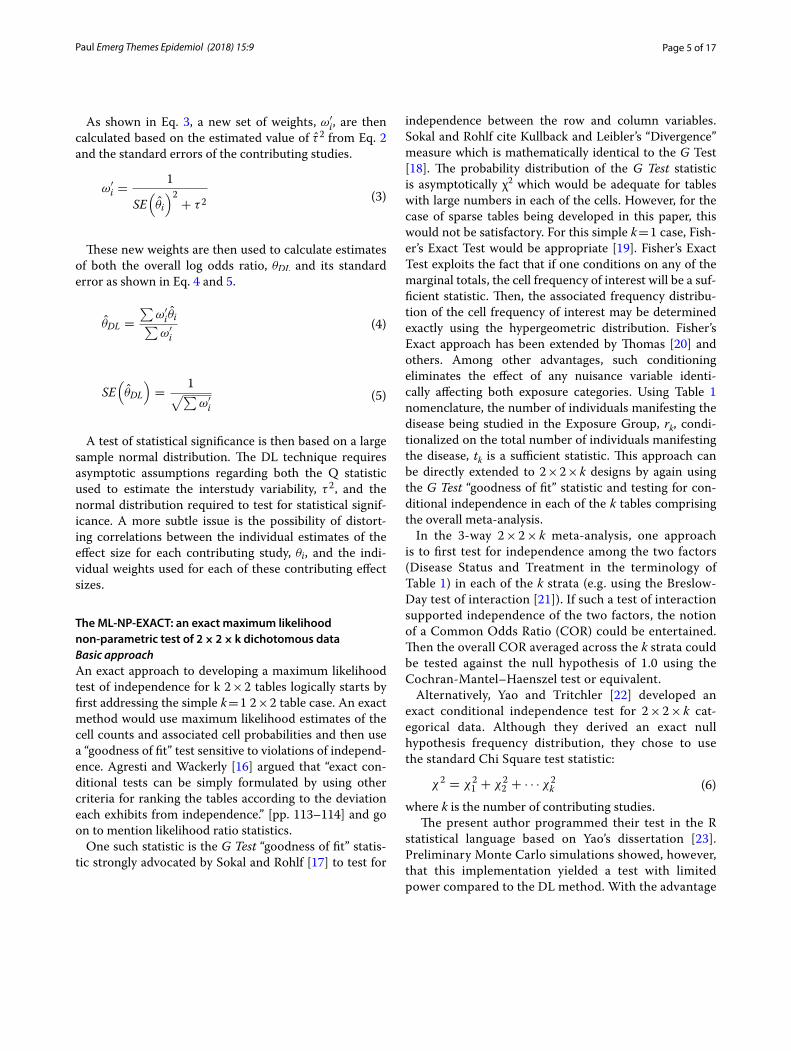
Two special cases under large heterogeneityProtocols were developed to handle two special situations under large heterogeneity. The first situation involves the event probabilities in the control and exposure groups respectively of the ith study, pic, pit, as originally pre-sented in Eq. 1 and shown for convenience below:

As shown in Fig. 2 plotted with p as a function of the logit variable, p has a slope of exactly .25 at p = .5 with the slope approaching zero as p approaches both zero and 1.0. In addition, the curve is only symmetric in the logit variable at exactly p =.5.

For realistic values of event probability such as .01, positive event probability excursions will be much larger than negative ones for large values of heterogeneity

G∗ = 2

k∑

i=1

(Oi + 1) ln

(

Oi + 1

Ei + 1

)

logit(pic) = µ, logit(pit) = µ+ θ + εi

Fig. 2 Plot of event probability, p, as a function of the logit variable


across studies. This problem manifests itself in artificially large violations of the pre-specified level of Type I Error. Therefore, negative values of the test statistic G which corresponds to observing fewer cases in the Exposure Group than expected were increased in magnitude (made more negative) by multiplying them by a correction fac-tor based on the derivative of p with respect to the logit variable:

As required, the correction factor equals one when p = .5 and becomes appropriately large as p approaches zero. This correction factor was applied when the G∗ sta-tistic was negative and when the treatment variance rela-tive to the control variance was greater than or equal to 3.0.

A second problem concerns meta-analyses in which there are only a small number of contributing studies. As shown by InHout and colleagues [25], there is a mono-tonic and large positive effect on Type I Error as the number of contributing studies decreases. This is not a problem of inadequate replications, but one of bias. The author conducted a separate analysis that showed that

Correction Factorlogit =.25

(

dp(logit)dlogit

) =.25

exp (logit)

{1+exp (logit)}2

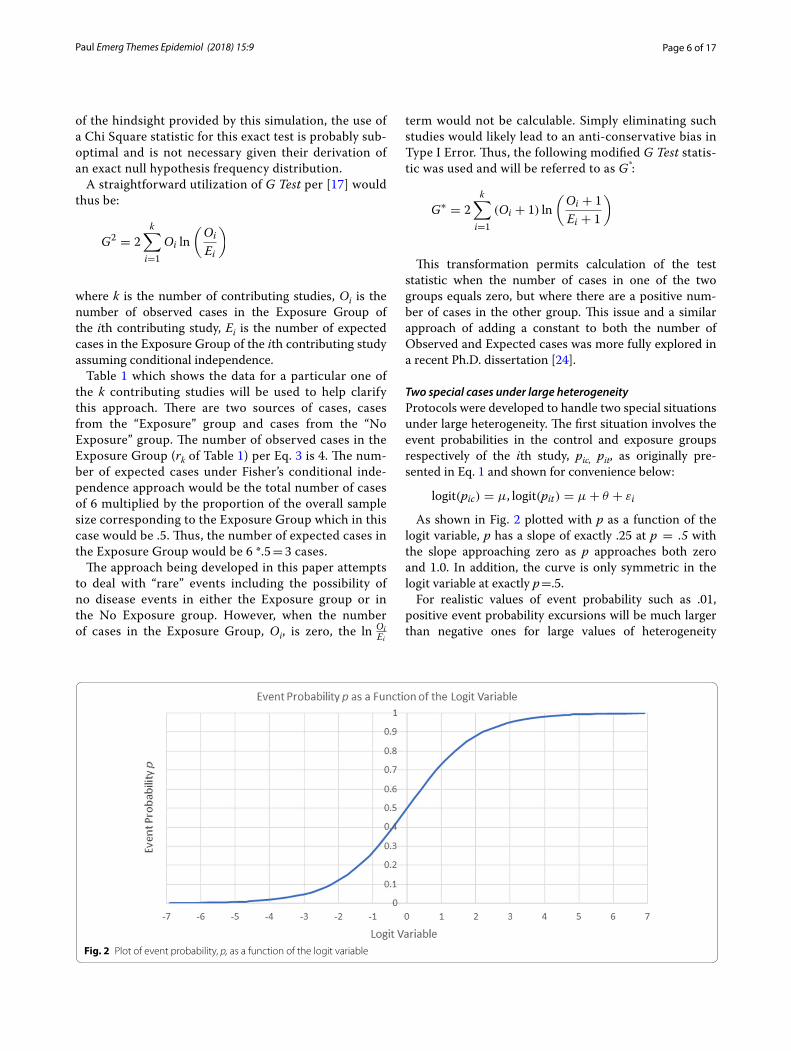
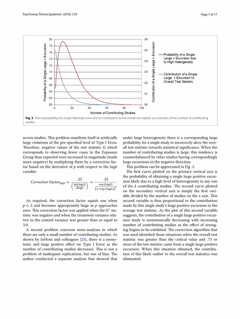
under large heterogeneity there is a corresponding large probability for a single study to incorrectly skew the over-all test statistic towards statistical significance. When the number of contributing studies is large, this tendency is counterbalanced by other studies having correspondingly large excursions in the negative direction.

This problem can be appreciated in Fig. 3.The first curve plotted on the primary vertical axis is

the probability of obtaining a single large positive excur-sion likely due to a high level of heterogeneity in any one of the k contributing studies. The second curve plotted on the secondary vertical axis is simply the first vari-able divided by the number of studies on the x axis. This second variable is thus proportional to the contribution made by this single study’s large positive excursion to the average test statistic. As the plot of this second variable suggests, the contribution of a single large positive excur-sion study is monotonically decreasing with increasing number of contributing studies as the effect of averag-ing begins to be exhibited. The correction algorithm that was used identified those situations when the overall test statistic was greater than the critical value and .75 or more of the test statistic came from a single large positive excursion. When this situation obtained, the contribu-tion of this likely outlier to the overall test statistics was eliminated.

Fig. 3 Plot of probability of a single “skewing” event and its contribution to the overall test statistic as a function of the number of contributing studies


Implementation of the test in the R statistical languageThis conditional-independence maximum likelihood exact test was implemented in the R Statistical Language. Each of the k contributing studies has a discrete prob-ability distribution which is a function of the background event probability and odds ratio of that study. The joint probability distribution of the k discrete probability dis-tributions is the convolution of these k distributions which will also be a discrete distribution. Directly per-forming this convolution would be extremely time con-suming even for relatively small values of k. However, it can be readily shown that if each of the k distributions is first transformed into the “frequency domain” using the Fourier Transform, the simple multiplicative prod-uct of these k transformations is the Fourier transform of the joint probability distribution. A single inverse Fou-rier transform then yields the joint probability distribu-tion (see, e.g., [26]). This was the approach used by Yao & Tritchler [22]. The development of the Fast Fourier Transform (FFT) for generation of the Fourier Transform in discrete situations [see, e.g. [27] for a relatively early presentation] such as the categorical meta-analysis pre-sented here permits quickly determining the joint prob-ability distribution using almost any PC-type computer. The program has been extensively tested across a large range of heterogeneity, odds ratios, disease probability, number of contributing studies and sample size.

Monte Carlo simulation of the ML‑NP‑EXACT and DerSimonian–Laird techniquesPopulation‑based odds ratio simulationA series of Monte Carlo simulations was conducted to evaluate the ML-NP-EXACT technique and compare it directly to the typically used DerSimonian–Laird Inverse Variance technique [9] for population-based odds ratio scenarios. The simulation was written and executed in “R: A Programming Environment for Data Analysis and Graphics.” [28]. The DerSimonian–Laird results were cal-culated using the “meta” package in R [29].

Five levels of odds ratio were chosen (1.0, 1.25, 1.5, 1.75, and 2.0) which were crossed with three levels of background event probability (.005, .01, and .05), and three levels of sample size (50,100 and 200) in each arm of each contributing study. Finally, the number of studies entering into each meta-analysis was chosen to be 5, 10, 20, or 40 studies.

In addition, the heterogeneity between the contribut-ing studies, τ2, was evaluated at 0 (homogeneity), .4, and .8. This last value of .8 represents a very large variance among the studies and was partially chosen to be able to compare the results with previous work [15]. To put such a large inter-study variance into some perspective, a background event probability (e.g. disease probability) of .01 would be expected to fluctuate between .0017 and .057, a ratio of 33:1 under a heterogeneity of τ2 = .8.

Finally, the common variability in both the exposure and control groups was chosen to be .5 and an error term, εi = N (0, .5) was added to both the logit transformed probabilities of Eq. 1 above per Bhaumik’s [15] desire to “imply that both the control and treatment groups have varying rates of events” (p. 9) allowing direct compari-sons to be made to this earlier research. For each simu-lation, the overall treatment effect was evaluated using both the ML-NP-EXACT and DerSimonian–Laird tech-niques. All simulation runs were conducted with 2000 replications. A value of .05 was used as the pre-specified level of Type I Error.

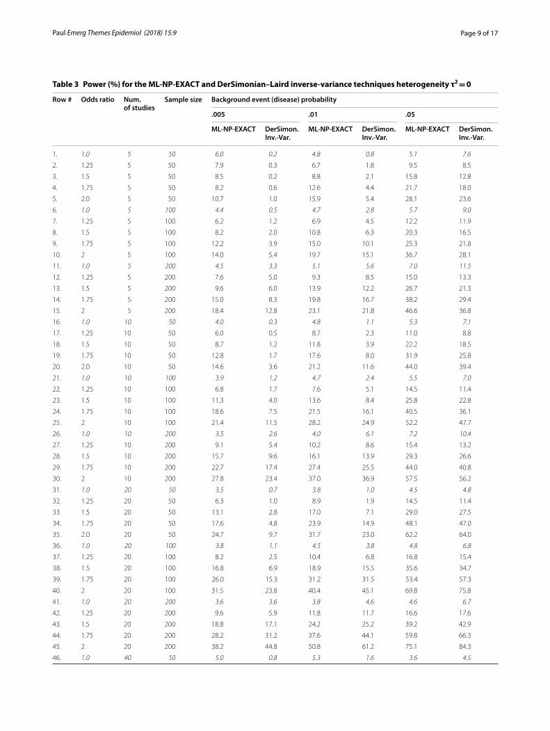
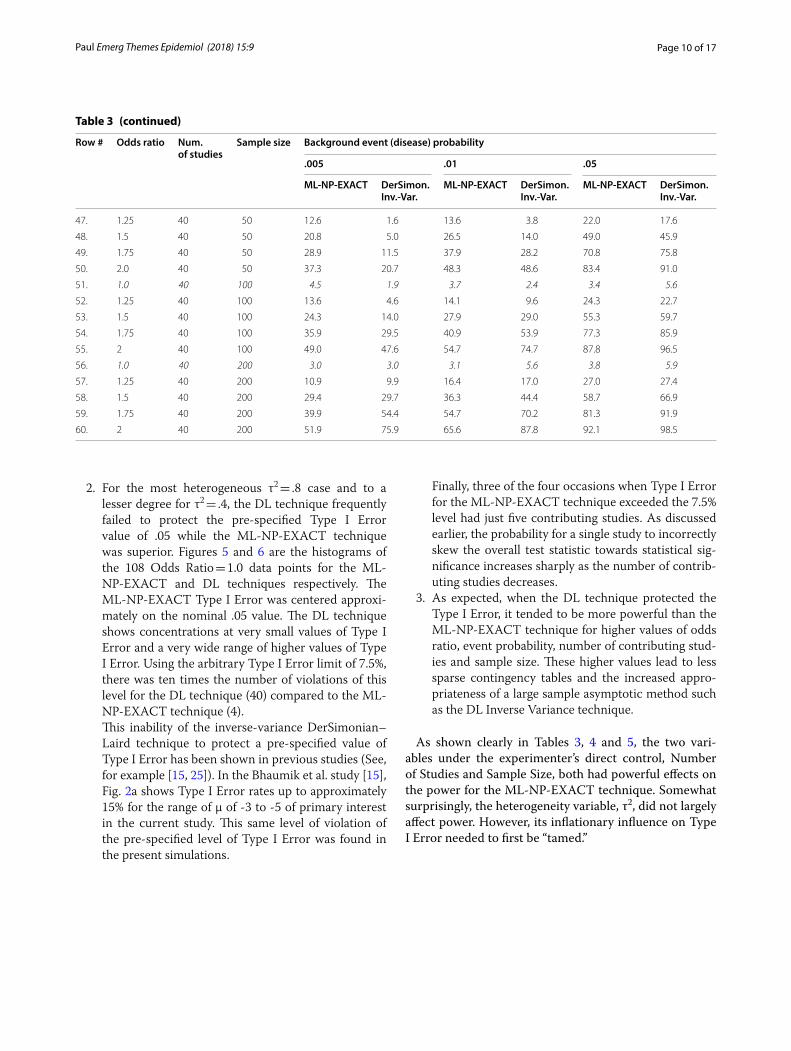
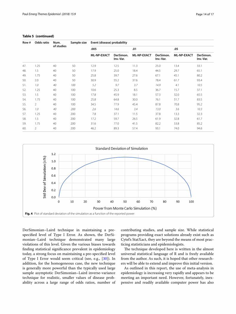
The Monte Carlo simulation results are shown below in Tables 3, 4 and 5 corresponding to heterogeneity val-ues τ2 of 0, .4, and .8. respectively. The 108 variable com-binations with an Odds Ratio of 1.0 (i.e. no treatment effect) are shown in italics for purposes of exposition. The standard deviation as a function of reported power is shown in Fig. 4.

There are three general findings from the direct com-parison of the ML-NP-EXACT technique with the DL technique.

1. For the homogeneous case of τ2 = 0, the ML-NP-EXACT technique yielded a Type I Error value cen-tered on the pre-specified level of .05 for practically all combinations of event probability, number of con-tributing studies and sample size as show in Table 3. However, as shown in Table 3, the DL technique con-sistently returned a Type I Error value well below .05 and correspondingly low levels of power for Odds Ratios greater than 1.0. In order to compare the power for Odds Ratios > 1.0, an upper limit on Type I Error needs to be established. Using a Type I Error level of 7.5%, the ML-NP-EXACT technique dem-onstrated a larger power in over 73% of the compari-sons.


Table 3 Power (%) for the ML-NP-EXACT and DerSimonian–Laird inverse-variance techniques heterogeneity τ2 = 0

Row # Odds ratio Num. of studies

Sample size Background event (disease) probability

.005 .01 .05

ML‑NP‑EXACT DerSimon. Inv.‑Var.


ML‑NP‑EXACT DerSimon.Inv.‑Var.

1. 1.0 5 50 6.0 0.2 4.8 0.8 5.1 7.6

2. 1.25 5 50 7.9 0.3 6.7 1.8 9.5 8.5

3. 1.5 5 50 8.5 0.2 8.8 2.1 15.8 12.8

4. 1.75 5 50 8.2 0.6 12.6 4.4 21.7 18.0

5. 2.0 5 50 10.7 1.0 15.9 5.4 28.1 23.6

6. 1.0 5 100 4.4 0.5 4.7 2.8 5.7 9.0

7. 1.25 5 100 6.2 1.2 6.9 4.5 12.2 11.9

8. 1.5 5 100 8.2 2.0 10.8 6.3 20.3 16.5

9. 1.75 5 100 12.2 3.9 15.0 10.1 25.3 21.8

10. 2 5 100 14.0 5.4 19.7 15.1 36.7 28.1

11. 1.0 5 200 4.5 3.3 5.1 5.6 7.0 11.5

12. 1.25 5 200 7.6 5.0 9.3 8.5 15.0 13.3

13. 1.5 5 200 9.6 6.0 13.9 12.2 26.7 21.3

14. 1.75 5 200 15.0 8.3 19.8 16.7 38.2 29.4

15. 2 5 200 18.4 12.8 23.1 21.8 46.6 36.8

16. 1.0 10 50 4.0 0.3 4.8 1.1 5.3 7.1

17. 1.25 10 50 6.0 0.5 8.7 2.3 11.0 8.8

18. 1.5 10 50 8.7 1.2 11.8 3.9 22.2 18.5

19. 1.75 10 50 12.8 1.7 17.6 8.0 31.9 25.8

20. 2.0 10 50 14.6 3.6 21.2 11.6 44.0 39.4

21. 1.0 10 100 3.9 1.2 4.7 2.4 5.5 7.0

22. 1.25 10 100 6.8 1.7 7.6 5.1 14.5 11.4

23. 1.5 10 100 11.3 4.0 13.6 8.4 25.8 22.8

24. 1.75 10 100 18.6 7.5 21.5 16.1 40.5 36.1

25. 2 10 100 21.4 11.5 28.2 24.9 52.2 47.7

26. 1.0 10 200 3.5 2.6 4.0 6.1 7.2 10.4

27. 1.25 10 200 9.1 5.4 10.2 8.6 15.4 13.2

28. 1.5 10 200 15.7 9.6 16.1 13.9 29.3 26.6

29. 1.75 10 200 22.7 17.4 27.4 25.5 44.0 40.8

30. 2 10 200 27.8 23.4 37.0 36.9 57.5 56.2

31. 1.0 20 50 3.5 0.7 3.8 1.0 4.5 4.8

32. 1.25 20 50 6.3 1.0 8.9 1.9 14.5 11.4

33. 1.5 20 50 13.1 2.8 17.0 7.1 29.0 27.5

34. 1.75 20 50 17.6 4.8 23.9 14.9 48.1 47.0

35. 2.0 20 50 24.7 9.7 31.7 23.0 62.2 64.0

36. 1.0 20 100 3.8 1.1 4.5 3.8 4.8 6.8

37. 1.25 20 100 8.2 2.5 10.4 6.8 16.8 15.4

38. 1.5 20 100 16.8 6.9 18.9 15.5 35.6 34.7

39. 1.75 20 100 26.0 15.3 31.2 31.5 53.4 57.3

40. 2 20 100 31.5 23.8 40.4 45.1 69.8 75.8

41. 1.0 20 200 3.6 3.6 3.8 4.6 4.6 6.7

42. 1.25 20 200 9.6 5.9 11.8 11.7 16.6 17.6

43. 1.5 20 200 18.8 17.1 24.2 25.2 39.2 42.9

44. 1.75 20 200 28.2 31.2 37.6 44.1 59.8 66.3

45. 2 20 200 38.2 44.8 50.8 61.2 75.1 84.3

46. 1.0 40 50 5.0 0.8 5.3 1.6 3.6 4.5


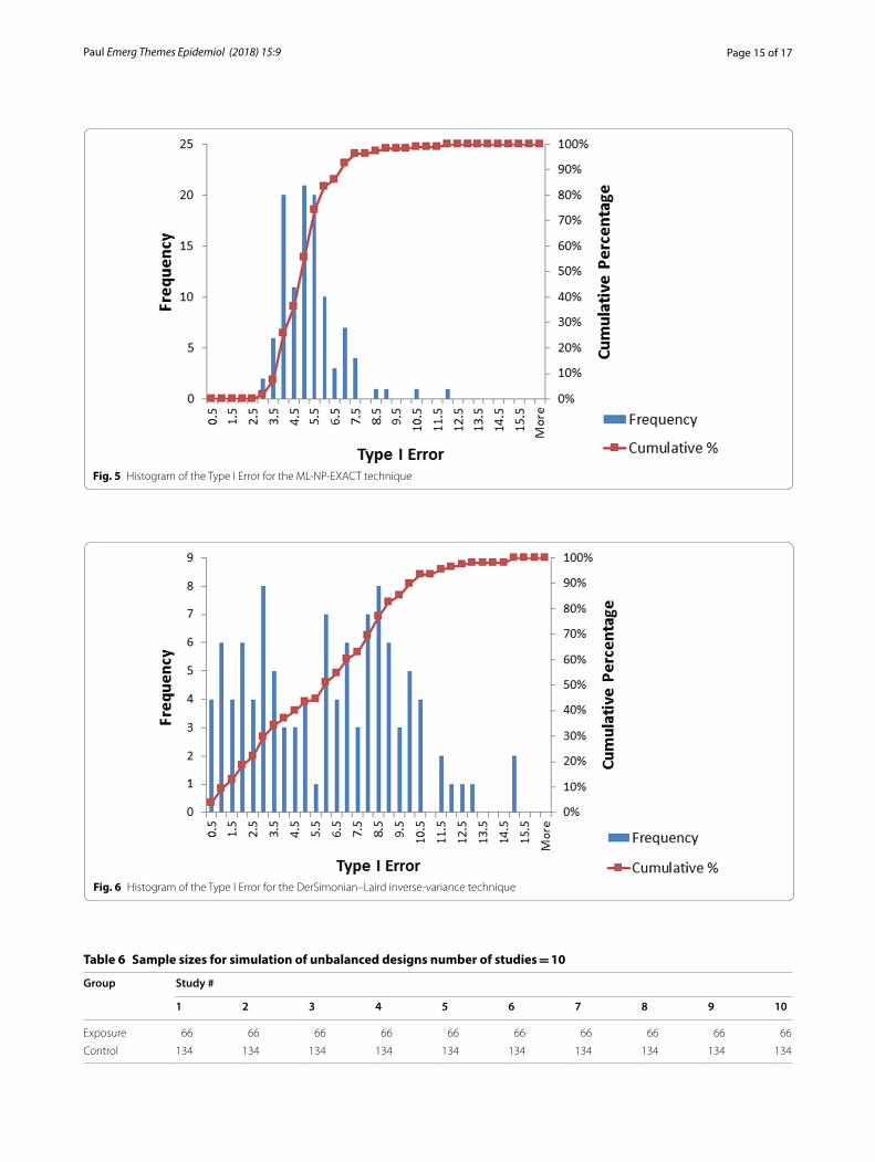
2. For the most heterogeneous τ2 = .8 case and to a lesser degree for τ2 = .4, the DL technique frequently failed to protect the pre-specified Type I Error value of .05 while the ML-NP-EXACT technique was superior. Figures 5 and 6 are the histograms of the 108 Odds Ratio = 1.0 data points for the ML-NP-EXACT and DL techniques respectively. The ML-NP-EXACT Type I Error was centered approxi-mately on the nominal .05 value. The DL technique shows concentrations at very small values of Type I Error and a very wide range of higher values of Type I Error. Using the arbitrary Type I Error limit of 7.5%, there was ten times the number of violations of this level for the DL technique (40) compared to the ML-NP-EXACT technique (4).

This inability of the inverse-variance DerSimonian–Laird technique to protect a pre-specified value of Type I Error has been shown in previous studies (See, for example [15, 25]). In the Bhaumik et al. study [15], Fig. 2a shows Type I Error rates up to approximately 15% for the range of µ of -3 to -5 of primary interest in the current study. This same level of violation of the pre-specified level of Type I Error was found in the present simulations.

Finally, three of the four occasions when Type I Error for the ML-NP-EXACT technique exceeded the 7.5% level had just five contributing studies. As discussed earlier, the probability for a single study to incorrectly skew the overall test statistic towards statistical sig-nificance increases sharply as the number of contrib-uting studies decreases.

3. As expected, when the DL technique protected the Type I Error, it tended to be more powerful than the ML-NP-EXACT technique for higher values of odds ratio, event probability, number of contributing stud-ies and sample size. These higher values lead to less sparse contingency tables and the increased appro-priateness of a large sample asymptotic method such as the DL Inverse Variance technique.

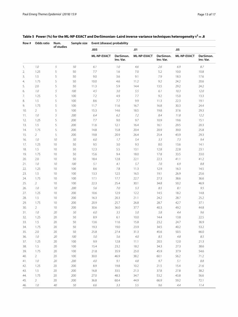
As shown clearly in Tables 3, 4 and 5, the two vari-ables under the experimenter’s direct control, Number of Studies and Sample Size, both had powerful effects on the power for the ML-NP-EXACT technique. Somewhat surprisingly, the heterogeneity variable, τ2, did not largely affect power. However, its inflationary influence on Type I Error needed to first be “tamed.”

Table 3 (continued)


Sample size Background event (disease) probability

.005 .01 .05




47. 1.25 40 50 12.6 1.6 13.6 3.8 22.0 17.6

48. 1.5 40 50 20.8 5.0 26.5 14.0 49.0 45.9

49. 1.75 40 50 28.9 11.5 37.9 28.2 70.8 75.8

50. 2.0 40 50 37.3 20.7 48.3 48.6 83.4 91.0

51. 1.0 40 100 4.5 1.9 3.7 2.4 3.4 5.6

52. 1.25 40 100 13.6 4.6 14.1 9.6 24.3 22.7

53. 1.5 40 100 24.3 14.0 27.9 29.0 55.3 59.7

54. 1.75 40 100 35.9 29.5 40.9 53.9 77.3 85.9

55. 2 40 100 49.0 47.6 54.7 74.7 87.8 96.5

56. 1.0 40 200 3.0 3.0 3.1 5.6 3.8 5.9

57. 1.25 40 200 10.9 9.9 16.4 17.0 27.0 27.4

58. 1.5 40 200 29.4 29.7 36.3 44.4 58.7 66.9

59. 1.75 40 200 39.9 54.4 54.7 70.2 81.3 91.9

60. 2 40 200 51.9 75.9 65.6 87.8 92.1 98.5


Table 4 Power (%) for the ML-NP-EXACT and DerSimonian–Laird inverse-variance techniques heterogeneity τ2 = .4


Sample size Event (disease) probability

.005 .01 .05




1. 1.0 5 50 7.1 0.4 5.0 1.6 6.1 8.7

2. 1.25 5 50 7.9 0.5 7.6 3.2 10.3 10.9

3. 1.5 5 50 9.0 1.4 9.1 4.7 15.7 15.5

4. 1.75 5 50 9.6 2.0 11.0 7.3 22.3 19.8

5. 2.0 5 50 12.4 2.9 13.3 8.6 29.9 27.3

6. 1.0 5 100 5.0 1.9 4.7 3.9 6.7 10.0

7. 1.25 5 100 7.4 3.1 8.2 6.2 14.4 13.2

8. 1.5 5 100 9.0 4.7 11.3 9.3 20.7 17.3

9. 1.75 5 100 11.8 6.2 13.8 11.9 30.9 25.7

10. 2 5 100 13.5 9.1 19.6 18.5 38.0 30.1

11. 1.0 5 200 4.0 4.1 4.8 7.1 8.8 10.5

12. 1.25 5 200 8.7 7.6 8.3 9.7 18.3 15.6

13. 1.5 5 200 11.2 9.3 13.6 14.3 27.5 21.0

14. 1.75 5 200 14.6 13.6 17.5 17.8 38.3 28.0

15. 2 5 200 18.0 17.9 24.8 24.2 46.2 34.7

16. 1.0 10 50 4.6 0.7 5.2 2.6 5.7 7.4

17. 1.25 10 50 7.5 1.5 7.9 3.7 13.0 12.5

18. 1.5 10 50 11.1 3.0 12.8 7.7 21.1 20.7

19. 1.75 10 50 13.7 5.2 18.2 13.1 28.4 28.6

20. 2.0 10 50 17.8 8.5 22.4 18.2 40.1 39.6

21. 1.0 10 100 5.8 1.8 4.8 4.9 5.9 8.2

22. 1.25 10 100 8.3 4.4 8.5 8.7 14.5 14.6

23. 1.5 10 100 12.1 7.7 15.0 15.7 24.8 23.7

24. 1.75 10 100 16.7 13.6 20.9 22.3 36.2 33.3

25. 2 10 100 22.1 18.0 28.0 30.3 48.5 46.2

26. 1.0 10 200 5.1 5.1 4.8 7.7 6.6 8.2

27. 1.25 10 200 7.9 9.2 9.9 12.9 15.5 15.5

28. 1.5 10 200 14.5 15.4 16.6 18.7 28.0 25.1

29. 1.75 10 200 20.0 21.4 25.7 27.5 39.4 38.5

30. 2 10 200 27.5 30.6 34.2 38.1 51.7 49.3

31. 1.0 20 50 5.5 1.5 4.9 2.4 3.9 6.9

32. 1.25 20 50 9.2 3.4 8.7 6.9 12.4 15.8

33. 1.5 20 50 13.3 6.2 14.7 15.1 24.1 33.6

34. 1.75 20 50 18.9 12.9 22.5 25.8 38.3 49.6

35. 2.0 20 50 24.0 18.6 27.4 36.7 54.2 66.0

36. 1.0 20 100 4.8 2.8 4.2 4.9 3.9 7.7

37. 1.25 20 100 9.5 6.4 9.0 13.5 14.2 19.7

38. 1.5 20 100 14.4 16.2 16.0 25.6 27.8 37.6

39. 1.75 20 100 20.8 24.8 26.2 40.4 42.0 57.3

40. 2 20 100 27.9 37.3 35.2 53.7 57.3 72.8

41. 1.0 20 200 4.5 5.9 5.1 8.3 5.1 7.8

42. 1.25 20 200 9.3 13.4 9.7 16.6 14.3 20.7

43. 1.5 20 200 16.4 25.7 17.8 31.8 27.5 37.5

44. 1.75 20 200 25.1 41.3 28.8 49.8 44.8 59.7

45. 2 20 200 34.5 55.5 43.6 66.5 61.9 77.4

46. 1.0 40 50 7.0 2.1 5.5 3.0 5.5 8.5


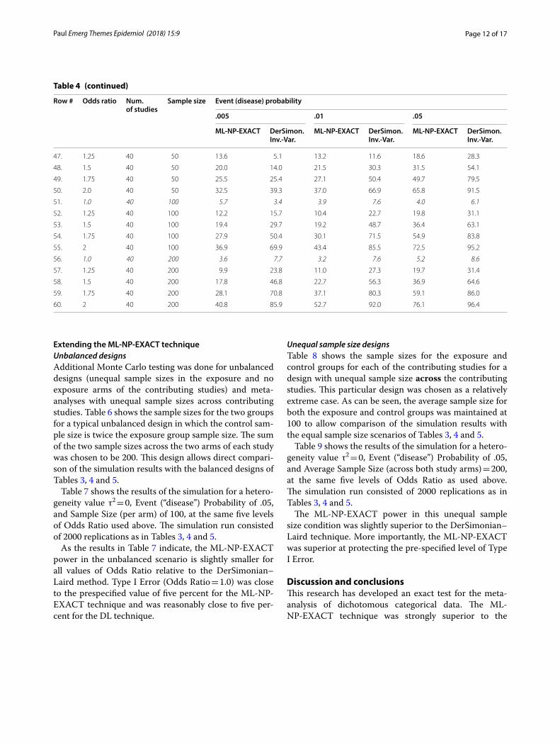
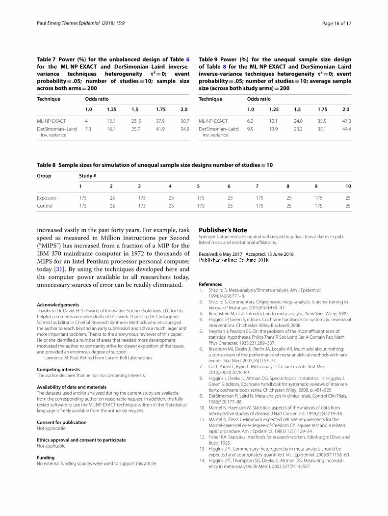
Extending the ML‑NP‑EXACT techniqueUnbalanced designsAdditional Monte Carlo testing was done for unbalanced designs (unequal sample sizes in the exposure and no exposure arms of the contributing studies) and meta-analyses with unequal sample sizes across contributing studies. Table 6 shows the sample sizes for the two groups for a typical unbalanced design in which the control sam-ple size is twice the exposure group sample size. The sum of the two sample sizes across the two arms of each study was chosen to be 200. This design allows direct compari-son of the simulation results with the balanced designs of Tables 3, 4 and 5.

Table 7 shows the results of the simulation for a hetero-geneity value τ2 = 0, Event (“disease”) Probability of .05, and Sample Size (per arm) of 100, at the same five levels of Odds Ratio used above. The simulation run consisted of 2000 replications as in Tables 3, 4 and 5.

As the results in Table 7 indicate, the ML-NP-EXACT power in the unbalanced scenario is slightly smaller for all values of Odds Ratio relative to the DerSimonian–Laird method. Type I Error (Odds Ratio = 1.0) was close to the prespecified value of five percent for the ML-NP-EXACT technique and was reasonably close to five per-cent for the DL technique.

Unequal sample size designsTable 8 shows the sample sizes for the exposure and control groups for each of the contributing studies for a design with unequal sample size across the contributing studies. This particular design was chosen as a relatively extreme case. As can be seen, the average sample size for both the exposure and control groups was maintained at 100 to allow comparison of the simulation results with the equal sample size scenarios of Tables 3, 4 and 5.

Table 9 shows the results of the simulation for a hetero-geneity value τ2 = 0, Event (“disease”) Probability of .05, and Average Sample Size (across both study arms) = 200, at the same five levels of Odds Ratio as used above. The simulation run consisted of 2000 replications as in Tables 3, 4 and 5.

The ML-NP-EXACT power in this unequal sample size condition was slightly superior to the DerSimonian–Laird technique. More importantly, the ML-NP-EXACT was superior at protecting the pre-specified level of Type I Error.

Discussion and conclusionsThis research has developed an exact test for the meta-analysis of dichotomous categorical data. The ML-NP-EXACT technique was strongly superior to the

Table 4 (continued)



.005 .01 .05




47. 1.25 40 50 13.6 5.1 13.2 11.6 18.6 28.3

48. 1.5 40 50 20.0 14.0 21.5 30.3 31.5 54.1

49. 1.75 40 50 25.5 25.4 27.1 50.4 49.7 79.5

50. 2.0 40 50 32.5 39.3 37.0 66.9 65.8 91.5

51. 1.0 40 100 5.7 3.4 3.9 7.6 4.0 6.1

52. 1.25 40 100 12.2 15.7 10.4 22.7 19.8 31.1

53. 1.5 40 100 19.4 29.7 19.2 48.7 36.4 63.1

54. 1.75 40 100 27.9 50.4 30.1 71.5 54.9 83.8

55. 2 40 100 36.9 69.9 43.4 85.5 72.5 95.2

56. 1.0 40 200 3.6 7.7 3.2 7.6 5.2 8.6

57. 1.25 40 200 9.9 23.8 11.0 27.3 19.7 31.4

58. 1.5 40 200 17.8 46.8 22.7 56.3 36.9 64.6

59. 1.75 40 200 28.1 70.8 37.1 80.3 59.1 86.0

60. 2 40 200 40.8 85.9 52.7 92.0 76.1 96.4


Table 5 Power (%) for the ML-NP-EXACT and DerSimonian–Laird inverse-variance techniques heterogeneity τ2 = .8



.005 .01 .05




1. 1.0 5 50 6.1 1.0 4.6 2.6 6.9 8.7

2. 1.25 5 50 7.7 1.6 7.0 5.2 10.0 10.8

3. 1.5 5 50 9.0 3.6 9.1 7.9 18.3 17.6

4. 1.75 5 50 10.0 4.6 11.2 9.2 24.2 20.6

5. 2.0 5 50 11.3 5.9 14.4 13.5 29.2 24.2

6. 1.0 5 100 4.5 3.0 5.5 6.1 10.3 12.0

7. 1.25 5 100 7.2 4.9 7.7 9.2 15.0 13.3

8. 1.5 5 100 8.6 7.7 9.9 11.3 22.3 19.1

9. 1.75 5 100 11.7 11.6 16.7 16.8 30.3 24.4

10. 2 5 100 15.3 14.6 18.5 19.8 37.6 29.3

11. 1.0 5 200 6.4 6.2 7.2 8.4 11.8 12.2

12. 1.25 5 200 7.7 9.0 9.7 10.9 19.6 15.1

13. 1.5 5 200 11.6 12.1 16.4 16.1 29.5 20.3

14. 1.75 5 200 14.8 15.8 20.4 20.9 39.0 25.8

15. 2 5 200 19.8 20.9 26.4 25.4 43.9 29.3

16. 1.0 10 50 6.0 1.7 5.4 3.3 7.3 9.4

17. 1.25 10 50 9.5 3.0 9.3 8.0 13.6 14.1

18. 1.5 10 50 12.3 5.5 13.1 12.8 22.8 23.1

19. 1.75 10 50 15.6 9.4 18.0 17.8 33.5 33.0

20. 2.0 10 50 18.4 12.8 22.1 22.3 41.1 41.2

21. 1.0 10 100 5.1 4.1 5.7 7.0 6.9 8.8

22. 1.25 10 100 8.6 7.8 11.3 12.9 16.3 14.5

23. 1.5 10 100 13.3 12.5 16.5 19.1 26.9 25.6

24. 1.75 10 100 17.1 17.7 22.7 27.3 38.6 36.6

25. 2 10 100 22.3 25.4 30.1 34.8 50.2 46.9

26. 1.0 10 200 5.6 7.0 5.3 8.5 8.1 9.5

27. 1.25 10 200 10.6 12.9 12.2 14.5 18.2 14.8

28. 1.5 10 200 16.3 20.3 21.1 24.2 28.7 25.2

29. 1.75 10 200 20.9 25.7 26.8 28.7 42.7 37.1

30. 2 10 200 30.6 36.0 37.7 40.3 49.2 44.8

31. 1.0 20 50 6.0 3.5 5.0 5.8 4.4 9.6

32. 1.25 20 50 8.9 6.1 10.0 14.4 13.8 22.5

33. 1.5 20 50 13.6 11.6 15.8 23.2 24.7 36.9

34. 1.75 20 50 19.3 19.0 23.9 34.5 40.2 53.2

35. 2.0 20 50 25.8 27.4 31.3 45.6 50.5 66.0

36. 1.0 20 100 5.0 5.6 4.0 8.5 4.8 8.5

37. 1.25 20 100 9.9 12.8 11.1 20.5 12.0 21.3

38. 1.5 20 100 15.4 23.2 18.2 34.3 27.3 38.6

39. 1.75 20 100 21.8 35.9 25.0 45.9 37.9 54.6

40. 2 20 100 30.0 46.9 38.2 60.1 56.2 71.2

41. 1.0 20 200 4.0 9.1 4.8 9.7 5.1 8.8

42. 1.25 20 200 8.9 19.8 10.2 21.5 15.4 21.6

43. 1.5 20 200 16.8 33.5 21.3 37.8 27.8 38.2

44. 1.75 20 200 27.0 48.3 34.7 53.2 43.8 56.6

45. 2 20 200 36.8 60.4 44.9 66.9 59.2 72.1

46. 1.0 40 50 6.6 3.3 5.5 9.6 4.4 11.4


DerSimonian–Laird technique in maintaining a pre-specified level of Type I Error. As shown, the DerSi-monian–Laird technique demonstrated many large violations of this level. Given the various biases towards finding statistical significance prevalent in epidemiology today, a strong focus on maintaining a pre-specified level of Type I Error would seem critical (see, e.g., [30]). In addition, for the homogeneous case, the new technique is generally more powerful than the typically used large sample asymptotic DerSimonian–Laird inverse-variance technique for realistic, smaller values of disease prob-ability across a large range of odds ratios, number of

contributing studies, and sample size. While statistical programs providing exact solutions already exist such as Cytel’s StatXact, they are beyond the means of most prac-ticing statisticians and epidemiologists.

The technique developed here is written in the almost universal statistical language of R and is freely available from the author. As such, it is hoped that other research-ers will be able to extend and improve this initial version.

As outlined in this report, the use of meta-analysis in epidemiology is increasing very rapidly and appears to be meeting an important need. However, fortunately, inex-pensive and readily available computer power has also

Table 5 (continued)



.005 .01 .05




47. 1.25 40 50 12.9 12.5 11.3 25.0 13.4 33.1

48. 1.5 40 50 17.9 25.0 18.4 44.5 29.7 65.1

49. 1.75 40 50 25.8 39.7 27.6 67.1 45.1 80.2

50. 2.0 40 50 30.9 55.2 37.6 78.4 61.7 93.4

51. 1.0 40 100 5.2 9.7 3.7 14.9 4.1 10.5

52. 1.25 40 100 10.6 25.3 8.5 36.7 15.7 37.1

53. 1.5 40 100 17.8 45.9 18.1 57.3 32.0 65.5

54. 1.75 40 100 25.8 64.8 30.0 76.1 51.7 83.5

55. 2 40 100 34.5 77.9 45.4 87.8 70.8 95.2

56. 1.0 40 200 2.6 14.6 3.4 13.0 3.6 10.3

57. 1.25 40 200 7.8 37.1 11.5 37.8 13.3 32.3

58. 1.5 40 200 17.2 59.7 26.5 61.9 32.8 61.7

59. 1.75 40 200 31.6 77.0 41.5 82.2 53.8 85.2

60. 2 40 200 46.2 89.3 57.4 93.1 74.0 94.6

Fig. 4 Plot of standard deviation of the simulation as a function of the reported power


Fig. 5 Histogram of the Type I Error for the ML-NP-EXACT technique

Fig. 6 Histogram of the Type I Error for the DerSimonian–Laird inverse-variance technique

Table 6 Sample sizes for simulation of unbalanced designs number of studies = 10

Group Study #

1 2 3 4 5 6 7 8 9 10

Exposure 66 66 66 66 66 66 66 66 66 66

Control 134 134 134 134 134 134 134 134 134 134


increased vastly in the past forty years. For example, task speed as measured in Million Instructions per Second (“MIPS”) has increased from a fraction of a MIP for the IBM 370 mainframe computer in 1972 to thousands of MIPS for an Intel Pentium processor personal computer today [31]. By using the techniques developed here and the computer power available to all researchers today, unnecessary sources of error can be readily eliminated.

AcknowledgementsThanks to Dr. David. H. Schwartz of Innovative Science Solutions, LLC for his helpful comments on earlier drafts of this work. Thanks to Dr. Christopher Schmid as Editor in Chief of Research Synthesis Methods who encouraged the author to reach beyond an early submission and solve a much larger and more important problem. Thanks to the anonymous reviewer of this paper. He or she identified a number of areas that needed more development, motivated the author to constantly strive for clearer exposition of the issues, and provided an enormous degree of support.

Lawrence M. Paul: Retired from Lucent Bell Laboratories.

Competing interestsThe author declares that he has no competing interests.

Availability of data and materialsThe datasets used and/or analyzed during the current study are available from the corresponding author on reasonable request. In addition, the fully tested software to use the ML-NP-EXACT technique written in the R statistical language is freely available from the author on request.

Consent for publicationNot applicable.

Ethics approval and consent to participateNot applicable.

FundingNo external funding sources were used to support this article.

Publisher’s NoteSpringer Nature remains neutral with regard to jurisdictional claims in pub-lished maps and institutional affiliations.

Received: 6 May 2017 Accepted: 13 June 2018

References 1. Shapiro S. Meta-analysis/Shmeta-analysis. Am J Epidemiol.

1994;140(9):771–8. 2. Shapiro S. Commentary. Oligognostic mega-analysis. Is archie turning in

his grave? Maturitas. 2015;81(4):439–41. 3. Borenstein M, et al. Introduction to meta-analysis. New York: Wiley; 2009. 4. Higgins JP, Green S, editors. Cochrane handbook for systematic reviews of

interventions. Chichester: Wiley-Blackwell; 2008. 5. Neyman J, Pearson ES. On the problem of the most efficient tests of

statistical hypotheses. Philos Trans R Soc Lond Ser A Contain Pap Math Phys Character. 1933;231:289–337.

6. Bradburn MJ, Deeks JJ, Berlin JA, Localio AR. Much ado about nothing: a comparison of the performance of meta-analytical methods with rare events. Stat Med. 2007;26(1):53–77.

7. Cai T, Parast L, Ryan L. Meta-analysis for rare events. Stat Med. 2010;29(20):2078–89.

8. Higgins J, Deeks JJ, Altman DG. Special topics in statistics. In: Higgins J, Green S, editors. Cochrane handbook for systematic reviews of interven-tions: cochrane book series. Chichester: Wiley; 2008. p. 481–529.

9. DerSimonian R, Laird N. Meta-analysis in clinical trials. Control Clin Trials. 1986;7(3):177–88.

10. Mantel N, Haenszel W. Statistical aspects of the analysis of data from retrospective studies of disease. J Natl Cancer Inst. 1959;22(4):719–48.

11. Mantel N, Fleiss J. Minimum expected cell size requirements for the Mantel-Haenszel one-degree-of-freedom Chi square test and a related rapid procedure. Am J Epidemiol. 1980;112(1):129–34.

12. Fisher RA. Statistical methods for research workers. Edinburgh: Oliver and Boyd; 1925.

13. Higgins JPT. Commentary: heterogeneity in meta-analysis should be expected and appropriately quantified. Int J Epidemiol. 2008;37:1158–60.

14. Higgins JPT, Thompson SG, Deeks JJ, Altman DG. Measuring inconsist-ency in meta-analyses. Br Med J. 2003;327(7414):557.

Table 7 Power (%) for the unbalanced design of Table 6 for the ML-NP-EXACT and DerSimonian–Laird inverse-variance techniques heterogeneity τ2 = 0; event probability = .05; number of studies = 10; sample size across both arms = 200

Technique Odds ratio

1.0 1.25 1.5 1.75 2.0

ML-NP-EXACT 4 12.1 23. 5 37.9 50.7

DerSimonian–Laird inv. variance

7.3 16.1 25.7 41.9 54.9

Table 8 Sample sizes for simulation of unequal sample size designs number of studies = 10

Group Study #

1 2 3 4 5 6 7 8 9 10

Exposure 175 25 175 25 175 25 175 25 175 25

Control 175 25 175 25 175 25 175 25 175 25

Table 9 Power (%) for the unequal sample size design of Table 8 for the ML-NP-EXACT and DerSimonian–Laird inverse-variance techniques heterogeneity τ2 = 0; event probability = .05; number of studies = 10; average sample size (across both study arms) = 200

Technique Odds ratio

1.0 1.25 1.5 1.75 2.0

ML-NP-EXACT 6.2 12.1 24.0 35.5 47.0

DerSimonian–Laird inv. variance

9.5 13.9 23.2 35.1 44.4


• fast, convenient online submission

•

thorough peer review by experienced researchers in your field

• rapid publication on acceptance

• support for research data, including large and complex data types

•

gold Open Access which fosters wider collaboration and increased citations

maximum visibility for your research: over 100M website views per year •

At BMC, research is always in progress.

Learn more biomedcentral.com/submissions

Ready to submit your research ? Choose BMC and benefit from:

15. Bhaumik DK, Amatya A, Normand SLT, Greenhouse J, Kaizar E, Neelon B, et al. Meta-analysis of rare binary adverse event data. J Am Stat Assoc. 2012;107(498):555–67.

16. Agresti A, Wackerly D. Some exact conditional tests of independence for r × c cross-classification tables. Psychometrika. 1977;42(1):111–24.

17. Sokal RR, Rohlf FJ. Biometry: the principles and practice of statistics in biological research. 3rd ed. New York: WH Freeman; 1994.

18. Kullback S. Information theory and statistics. Reprint of the 2nd (1968) ed. Mineola: Dover Publications, Inc.; 1997.

19. Agresti A. A survey of exact inference for contingency tables. Stat Sci. 1992;7(1):131–53.

20. Thomas DG. Exact and asymptotic methods for the combination of 2 × 2 tables. Comput Biomed Res. 1975;8(5):423–46.

21. Breslow NE, Day NE. Statistical methods in cancer research, vol. 1. The analysis of case-control studies. 132nd ed. Geneva: Distributed for IARC by WHO; 1980.

22. Yao Q, Tritchler D. An exact analysis of conditional independence in several 2 × 2 contingency tables. Biometrics. 1993;49(1):233–6.

23. Yao Q. An exact analysis for several 2 × 2 contingency tables. Disserta-tion ed, University of Toronto; 1991.

24. Mcelvenny DM. Meta-analysis of rare diseases in occupational epide-miology. Doctoral dissertation, London School of Hygiene & Tropical Medicine; 2017.

25. IntHout J, Ioannidis JP, Borm GF. The Hartung-Knapp-Sidik-Jonkman method for random effects meta-analysis is straightforward and consid-erably outperforms the standard DerSimonian-Laird method. BMC Med Res Methodol. 2014;14(1):25.

26. Hogg RV, McKean JW, Craig AT. Introduction to mathematical statistics. 6th ed. Upper Saddle River: Prentice Hall; 2004.

27. Cooley JW, Tukey JW. An algorithm for the machine calculation of com-plex Fourier series. Math Comput. 1965;19(90):297–301.

28. The R Project for Statistical Computing. https ://www.r-proje ct.org/. 29. Schwarzer G. Meta: an R package for meta-analysis. R News.

2007;7(3):40–5. 30. Ioannidis JPA. Why most published research findings are false. PLoS Med.

2005;2(8):e124. 31. Mollick E. Establishing Moore’s law. IEEE Ann History Comput.

2006;28(3):62–75.

https://www.r-project.org/

an exact maximum likelihood non-parametric test for meta ...

Documents

Transcript of an exact maximum likelihood non-parametric test for meta ...