Robust Parametric Image Registration using

Genetic Algorithms and Newton Levenberg

Marquardt

Felix Calderon, Juan J. Flores, and Leonardo Romero

Division de Estudios de Posgrado, Facultad de Ingenieria Electrica

Universidad Michoacana de San Nicolas de Hidalgo

{calderon, juanf, lromero}@umich.mx

March 15, 2006

Abstract

We present a hybrid method to perform parametric image registration.The objective is to find the best set of parameters of an affine transfor-mation, which applied to the original image yields the closest match toa target image (possibly with noise). Hybridization occurs when GeneticAlgorithms are able to determine rough areas of the parameter optimiza-tion space, but fail to produce fine tunings for those parameters. In thatcase, the Newton–Levenberg–Marquardt method is used to refine results.Another important combination of techniques results when we want tocompare images. In this case, the fitness function needs to be robustenough to discard misleading information contained in outliers. Statis-tical techniques are employed in this case to be able to compare imagesin the presence of noise. The resulting implementation, called GA–SSD–ARC+ was compared against robust registration methods used in the areaof image processing. GA–SSD–ARC+ outperforms the RANSAC and theLorentzian Estimator methods when images are noisy or corrupted byoutliers.

1 Introduction

The parametric image registration problem [19] consists of finding a parameterset for an Affine Transformation, which allows us to match an origin image witha target image as closely as possible. Occluded areas and noise (outliers) in-crease the complexity of the registration task, and some parametric registrationtechniques exhibit poor results under these circumstances.

There are basically two sources of hybridization we are using in our proposedmethod: A gradient-based method is used to fine tune the results of Genetic

1

Algorithms (GAs), and a stochastic method is used to produce a better evalua-tion function (i.e. a function that does not take into account outliers producedby noise).

It is well known in the evolutionary computation community, that GAs aregood tools to produce a rough estimate of the region where optima appear, butthey are not good at producing results with a high level of accuracy [8]. Withthat in mind, we made a combination of GAs and the Newton–Levenberg–Marquardt (NLM) method [4]. GAs find quickly a set of parameters arounda global minimum, in a searching region, and then NLM refines the results tomore accurately reach the minimum.

NLM, as a gradient-based method, suffers of getting stuck at local extrema.NLM fails if the initial parameters are not close enough to the right parameters(which minimize a given cost function). This problem is avoided by the use ofGAs, which are not gradient-based, and perform better on multimodal problems.On the other hand, GAs fail to give accurate results. So, the combination ofGAs + NLM succeeded in finding accurate results in a huge parameter space,avoiding the disadvantages of GAs and NLM.

Now, talking about the fitness function, many algorithms try to minimizethe Sum of Squared Differences (SSD) between the origin and target images.Successful SSD applications, including the classical Least Squared method (LS),are presented in [15, 14, 16]. Nevertheless, the SSD-based algorithms have poorperformances in cases of noisy images. The problem with LS is that outliershave a heavy weight in the cost function and pull the solution towards them;robust methods try to exclude outliers in some way.

Three well known robust methods in the computer vision literature are theLeast Median of Squares (LMedS [12]), the Lorentzian Estimator [6] (LE) andthe Random Sample Consensus method (RANSAC) [7]. LMedS is a robustmethod which can deal with outliers (up to 50%); examples of its applicationto optical flow computation are presented in [1]. Some authors, instead of usingSSD, use the Lorentzian Estimator [2] in cases of noisy images, getting goodresults. The RANSAC method is a stochastic technique which presents goodresults with outliers.

An application of SSD for an non-parametric image registration called SSD-ARC, is presented in [3]. The SSD–ARC cost function is minimized using acoarse to fine strategy and the Newton Algorithm. We take the core idea fromSSD–ARC, and incorporate it in the fitness function, producing a function ableto compare noisy images, discarding the differences produced by noise.

This chapter describes a new robust method named GA–SSD–ARC+ thatcombines the explicit outlier rejection idea of SSD–ARC [3] into a new costfunction with a searching process in two steps. The first step is done witha Genetic Algorithm (GA), where the goal is to find an approximate solutioninside a bounded parameter space. The second step refines the solution, reachedby GA, using the NLM method. Both searching processes consider an AffineTransformation to match the origin and target images, and try to minimize thesame SSD–ARC cost function and compensate the disadvantages of one another.

Experimental results show the robustness of GA–SSD–ARC+ for noise im-

2

ages and provides a comparison with the RANSAC and LE methods. The LEmethod was selected because it punishes outliers and its behavior is similarto the SSD–ARC cost function. The RANSAC method is a robust method,commonly used in the literature [7], which does not use a SSD-based method.

This chapter is organized as follows: Section 2 presents the image registra-tion problem using an affine transformation; Section 3 describes the problemof estimating a good transformation in the presence of outliers (noisy data),and presents alternative solutions to that problem (the Lorentzian Estimatorand RANSAC method); Section 4 presents the genetic coding scheme used torepresent affine transformations and describes the general framework for the ex-periments; it also describes how the hybrid NLM–GA search process takes place;Section 5 presents the results, and a comparison against LE and RANSAC; Fi-nally, Section 6 presents the conclusions.

2 Registration using an Affine Transformation

The Affine Transformation (AT) [9, 18] allows us to compute, at the sametime, translation, rotation, scaling, and sharing of images. An AT uses a six-parameter vector Θ, and maps a pixel at position ri (with coordinates [xi, yi])to new position ri (with coordinates [xi, yi]) given by

ri(Θ) =

[xi

yi

]=

[xi yi 1 0 0 00 0 0 xi yi 1

]

θ0θ1θ2θ3θ4θ5

(1)

In matrix notation the AT transformation can be expressed as

ri (Θ) = M(ri)Θ (2)

where M(ri) and Θ are the matrix of coordinates and the parameter vector,respectively.

Let I2 be the image computed by applying an affine transformation, givenby Θ, to an input image I1. The image registration problem is to find Θ givenimages I1 and I2. However, in practical cases, both images are corrupted bynoise and the problem is to find the best AT to match the transformed originimage I1 to the target image I2.

To assign a value of how good the matching is, a common strategy, is tomeasure the distance between the source and target images, pixel by pixel, asin Equation (3).

E (Θ) =N∑

i=1

[I1(ri (Θ)) − I2(ri)]2 (3)

=N∑

i=1

ei (Θ)2

3

where ei (Θ) = I1(ri (Θ)) − I2(ri), N is the number of pixels, and I(ri) is thegray level value of pixel ri in image I . Using this error measurement, the regis-tration image task consists of finding Θ∗ that makes E reach a minimum value.This method is named Least Squared (LS) and some strategies to minimizeEquation 3 are presented in [4].

3 Outliers and Parameter Estimation

Assuming that ei(Θ) has a normal distribution with zero mean and constantvariance, the optimal method to determine Θ∗ is LS [10]. In this case, thelikelihood p (Θ) is given by Equation 4 and Θ∗ is called the maximum likelihoodestimator.

p (Θ) =

N∏

i=1

1

2πexp−[ei(θ)]2 (4)

The objective, for Equation (4), is to find a Θ vector that maximizes theprobability p(Θ), taking the logarithm in Equation (4), one can see that this isequivalent to minimize Equation (3) for the same data set.

E (θ) =

N∑

i=1

ρ(ei (θ)) (5)

The influence function ρ is defined as the derivative of the error functionand helps seeing the contribution of the errors to the right solution (see [6]).In the LS case, the influence function is ρ (ei) = 2ei. This means that bigerrors have a big contribution to the overall error function. So when using agradient-based search algorithm, this fact contributes to reach a solution biasedby outliers. The problem with LS is its notorious sensibility to outliers, becausethey contribute too much to the general error term ELS , as Hampel describedin [6]. To overcome the LS behavior, other interesting influence functions canbe used.

The following subsections present alternative solutions to the problem ofproducing a wrong estimation, biased by outliers.

3.1 Robust Statistical Estimation

Robust Statistics [6] present the following main advantages: provide a betterparameter set describing most of the input data and identify outliers.

M. J. Black (in [2]) uses the T–student distribution with two degrees offreedom, instead of the normal distribution for maximum likelihood estimation,because the T–student distribution is used in populations with non appropriatevariance estimation. The T–student distribution is defined by Equation (6) (see[17]).

h(t) =Γ [(υ + 1) /2]

Γ (υ/2)√πυ

(1 +

t2

υ

)−(υ+1)/2

(6)

4

where Γ is the gamma function and υ is the degrees of freedom. The T–studentdistribution with two degrees of freedom and its logarithm is given by Equations(7) and (8), respectively.

h(t) =1

2√

2

(1 +

t2

2

)−1.5

(7)

log(h(t)) = log(1

2√

2) − 1.5 log

(1 +

t2

2

)(8)

Black [2] substitutes t = e/σ in the second term of Equation (8). Eliminatingthe associated factor, the resulting term is known as Lorentzian Estimator (9),which has an influence function given by Equation (10).

ELE(e) = log

(1 +

e2

2σ2

)(9)

ρLE(e) =2e

2σ2 + e2(10)

The main advantage of using LE instead of the SSD is its ρLE function(Equation (10)), in which the factor 1/(2σ2 + e2) reduces the outliers contri-bution, yielding, in cases of large error terms, derivatives near zero. Parameterσ controls the boundaries between inliers and outliers for LE, nevertheless theoutliers estimation is not clear and Black and Rangarajan [2] proposed an EMalgorithm extension.

3.2 RANSAC for Image Registration

The RANSAC algorithm [5] is an algorithm for robust fitting of models in thepresence of multiple data outliers. Automatic Homography estimation using theRANSAC method is presented in [7]. A similar version for mosaic is presentedin [11].

RANSAC–based algorithms for Image Registration compute a Homographygiven at least four point correspondences ri ↔ r′i which are related by r′i =Hri. This equation may be expressed in terms of the vector cross productas r′i × Hri = 0, and the solution must be found using the singular valuedecomposition [7].

The steps for Automatic Homography estimation for image registration,given two images are:

1. Interest points: Compute interest points on each image using the KLTalgorithm [13].

2. Putative Correspondences: Compute a set of interest points that matchbased on proximity and similarity of their intensity neighborhood (forinstance using correlation).

3. RANSAC robust estimation: Repeat for M samples

5

• Select a random sample of four correspondence points and computethe homography H(k), solving r′i ×H(k)ri = 0

• Given H(k), calculate the distance for each putative correspondence

• Compute the number of inliers consistent with H (k)

• Choose the H(k) with the largest number of inliers

4. Optimal estimation: re-estimate H (∗) from all correspondence points clas-sified as inliers (consensus set) using any error function (v.g. LS).

3.3 SSD-ARC

The Sum of Squared Differences with Adaptive Rest Condition for non–parametricImage Registration was presented in [3] as the minimization of a quadratic en-

ergy function ESSD−ARC with a term hili to reduce the huge error contributiongiven by

ESSD−ARC (Θ, l) =

N∑

i=1

(ei (Θ) − hili)2 + µ

N∑

i=1

l2i (11)

where hi is desirable to be error dependent in order to weigh the error, andli ∈ [0, 1] is an indicator function under the control of parameter µ. Assuminghi = ei, a particular SDD-ARC function can be obtained as

ESSD−ARC (Θ, l) =

N∑

i=1

e2i (Θ)(1 − li)2 + µ

N∑

i=1

l2i (12)

For this new SDD-ARC function (Equation 12), the term (1 − li)2 allows us to

discard outliers; one would expect values between zero and one for the variableli, zero for inliers, and one for outliers. The second term in Equation (12)restricts the number of outliers by means of µ. For instance, µ = 0 meansthat all image pixels are outliers in contrast with µ = ∞, meaning that all theimage pixels are inliers and the solution is near to LS. The minimizer l∗i forEquation (12) can be computed by solving the independent system of equations∂ESSD−ARC(Θ,l)

∂li= −2e2i (Θ)(1−li)+2µli = 0 for each image pixel, so the solution

is given by Equation (13).

l∗i =e2i (Θ)

µ+ e2i (Θ)(13)

The variable l∗i is bounded on the interval [0, 1], an indispensable condition toestimate and reject outliers. Replacing the value of l∗i in Equation (12), a newerror function E (Θ) results.

ESSD−ARC (Θ) =

N∑

i=1

µe2i (Θ)

µ+ e2i (Θ)(14)

6

The resulting function error is unimodal respect to e, and the first and secondderivatives are given by ψSSD−ARC (e) and ϕSSD−ARC (e)

ψSSD−ARC (e) =2µ2e

(µ+ e2)2 (15)

ϕSSD−ARC (e) =2µ2

(µ− 3e2

)

(µ+ e2)3 (16)

and the influence function, for SSD–ARC error function is given by Equa-tion (15).

The error functions for ELS , ELE and ESSD−ARC are unimodal with respectto the error term, as shown in Figures 1(a), 1(c), and 1(e). LS does not havethe possibility to reject outliers because its derivative function is proportionalto the error term (see Figure 1(b)). Note that the SSD–ARC ρ function exhibitsa behavior similar to the Lorentzian Estimator’s derivative. In both functions,large errors yield derivative values close to zero, as shown in Figures 1(d) and1(f). This means that no matter how large the error provided by an outlier is,its contribution to the searching process is very low.

The SSD–ARC ρ function has a maximum value located at e =√µ/3;

that value can be used as threshold for data rejection; for instance, an errorvalue greater than 2e will have a derivative value near to zero. This conditioncan be used to reject outliers further away than a given error threshold. µ canbe computed as µ = 3e2 for a given error threshold. Nevertheless, there is nogradient-based algorithm capable to reach the minimum if the initial value gives

an error greater than 2µ. The algorithm converges only for values∣∣∣√µ/3

∣∣∣ > e.

In experiments done, the parameter vector computed by LS was taken as theinitial value for SSD–ARC; for small µ values, the solution given by LS could notbe improved by SSD-ARC. Therefore a two-step hybrid minimization algorithmis proposed:

1. First a GA search is used and then

2. Refinement of the GA solution is done, using NLM

where the SSD-ARC error function, given by equation (14), is used in bothsteps. The next section provides more detail for this two-step minimizationalgorithm.

4 Hybrid Genetic/Gradient-based Optimization

In this section we provide a description of the components of the two-step algo-rithm (GA–SSD–ARC+) used to minimize the error function given by Equation(14).

The problem to be solved is the determination of the vector Θ that bestapproximates the transformation that maps the source image I1 to the target

7

−100 −80 −60 −40 −20 0 20 40 60 80 1000

1000

2000

3000

4000

5000

6000

7000

8000

9000

10000

e

E

(a) LS error function

−100 −80 −60 −40 −20 0 20 40 60 80 100−200

−150

−100

−50

0

50

100

150

200

e

dE/d

e

(b) Derivative of the LS error

function

−100 −80 −60 −40 −20 0 20 40 60 80 1000

1

2

3

4

5

6

7

8

e

dE/d

e

(c) LE error function with σ =

2

−100 −80 −60 −40 −20 0 20 40 60 80 100−0.8

−0.6

−0.4

−0.2

0

0.2

0.4

0.6

0.8

e

dE/d

e

(d) Derivative of the LE error

function

−100 −80 −60 −40 −20 0 20 40 60 80 1000

1

2

3

4

5

6

7

e

E

(e) SSD–ARC error function

with µ = 10

−100 −80 −60 −40 −20 0 20 40 60 80 100−1.5

−1

−0.5

0

0.5

1

1.5

e

dE/d

e

(f) Derivative of the SSD-ARC

error function

Figure 1: Error Function Examples and their Influence Functions

8

image I2. We propose to start the search for an optimal vector Θ using GAs andthen to refine the results using a gradient-based algorithm, namely, the NewtonLevenberg–Marquardt (NLM) method. NLM is convenient in cases where asemipositive definite symmetric Hessian matrix exists [4].

4.1 Genetic Algorithms

Genetic Algorithms is an optimization technique inspired in the biological pro-cess of evolution and survival of the fittest individuals in a population. Given aninitial population, GA provides the means for this population to reach a state ofmaximum fitness in successive generations. The general optimization procedureis: Define a cost function, encode an individual in a chromosome (in our case,an individual represents an AT – encoded by a parameter vector), and createa random starting population. Evaluate the cost function for each individual,allow them to mate, reproduce, and mutate. Repeat these last four steps for asmany generations as needed in order to reach a stopping criteria (v.g., a smallenough error, or a fixed number of generations).

Haupt and Haupt [8] describe the steps to minimize a continuous parameterfunction cost using GAs. In our case, the function cost given by Equation 14is optimized and the six-vector parameter Θ will be the chromosome for eachindividual. Thus, the chromosome is represented by a real-valued vector of sixelements. GA needs a search interval for each one of the parameters.

To establish the initial population, the jth parameter is randomly computedby Equation (17).

θj = (θmaxj − θmin

j ) ∗ α+ θminj (17)

where θmaxj and θmin

j are the upper an lower bounds, and α is a number randomlyselected in the interval [0, 1].

This strategy is applied for newly generated genes in an individual’s chro-mosome. The same strategy is used for determining new values for genes ofindividuals during the mutation process.

In each generation, a fitness-based selection process indicates which indi-viduals from the population will mate and reproduce, yielding new offsprings.Once we have selected two individuals Θ1, and Θ2 for mating, cross-over isaccomplished according to the following formulae

θ1,j = θm,j − β(θm,j − θp,j) (18)

θ2,j = θp,j + β(θm,j − θp,j)

where β is a random number between zero and one.Newly born offsprings (Θ1 and Θ2) are incorporated to the population, their

fitness is computed, and the population is cut to maintain the same size acrossgenerations. To maintain the population size, the worst individuals are dis-carded.

9

4.2 SSD–ARC Minimization by NLM

In order to find the minimizer Θ∗ for the general error function E (Θ), givenby Equation 14, a gradient-based algorithm, namely the Newton LevembergMarquart algorithm is used. Equation 19 gives the steps to find the minimumusing NLM.

Θ(k+1) = Θ(k) −[H

(Θ(k)

)+ λ(k)I

]−1

∇E(Θ(k)

)(19)

where ∇E(Θ(k)

)is the gradient at each iteration, computed by

∇E (Θ) = 2

N−1∑

i=0

J(ri (Θ))µe2iµ+ e2i

(20)

and the Hessian matrix is

H (Θ) = 2

N−1∑

i=0

JT (ri (Θ))J(ri (Θ))2µ2

(µ− 3e2i

)

(µ+ e2i )3 (21)

Finally J(ri (Θ)) is the Jacobian matrix given by

J(ri (Θ)) = [∇I1(ri (Θ))]TM(ri) (22)

and M(ri) is defined by Equation (1)A new Θ(k+1) is accepted only when EΘ(k+1) < EΘ(k) which is evaluated

using Equation (14). At the beginning λ takes a small values and the search islike the Newton method. During the iterative process λ is adjusted. Large λvalues perform a Gradient based search.

5 Results

In the rest of the chapter, the following name convention is used to distinguishbetween the different optimization methods used to minimize the SSD–ARCequation. If only the NLM algorithm is used, the minimization process is namedSSD–ARC; if we use only GA, the minimization procedure will be named GA–SSD–ARC; when we use a combination, performing first GA and then NLM,the process will be called GA–SSD–ARC+.

In this section, we compare the results of image registration using the GA–SSD–ARC+ method against LE error function and RANSAC method; resultsare presented for both synthetic and real experiments. For LE, a minimizationscheme similar to GA–SSD–ARC+ (using GA and NLM) is used in order to givesimilar minimization conditions given that LE and SSD–ARC present a similarbehavior in their derivative functions.

In synthetic experiments, we know the parameter vector Θ used by the affinetransformation that produced the target image. Since different algorithms use

10

different error functions, which exhibit different ranges, the error of the solu-tions are non–comparable. Under those circumstances, we use the Euclideandistance |∆Θ| between the known parameter vector Θ and the estimated pa-rameter vector Θ as a proximity measure (for comparison purposes, only, not foroptimization). Algorithms with better performance will have smaller proximitymeasures.

5.1 Synthetic Experiments

In the synthetic experiments (which are performed using real images), the NLMuses the vector Θ = [1, 0, 0, 0, 1, 0]T as the initial value, and the stop criterion

was∣∣∣E(k+1)

−E(k)

E(k+1)

∣∣∣ < 1e − 5 or 1000 iterations. For GA, a population of 3000

individuals and 100 generations was used; in order to accelerate the convergenceprocedure, in some cases the error function was evaluated only on 50% of theimage pixels. The GA search boundaries, for each of the affine transformationparameters, are shown in Table 1.

θminj θmax

j

θ0 0.5 1.5θ1 -0.5 0.5θ2 -10.0 10.0θ3 -0.5 0.5θ4 0.5 1.5θ5 -10.0 10.0

Table 1: GA Search Boundaries

The parameters µ for SSD–ARC and σ for LE were hand-picked in orderto give the better performance for both algorithms, these values are 20 and 25,respectively, and they remain constants in all the experiments.

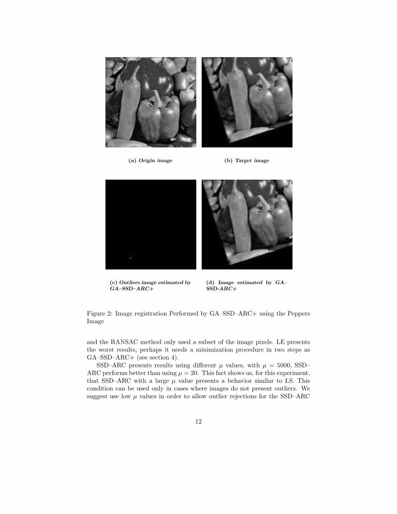
5.1.1 Peppers Image

The main goal of this experiment is to present an example of how the two mini-mization steps for SSD–ARC improved the solution obtained using the gradientbased method only. With this goal in mind, first the experiment was done us-ing NLM for LS, LE, and SSD–ARC error functions. Next, a combination ofGA and NLM is introduced for the LE and SSD–ARC error functions. In thisexperiment, a rotation of 18o, given as Θ = [0.9511, -0.3090, 0.0000, 0.3090,0.9511, 0.0000] is applied to the Peppers image (the origin and target imagesare shown in Figures 2(a) and 2(b), respectively).

The results from LS, LE and SSD–ARC, when their respective error func-tions were minimized using only NLM, are presented in Table 2; the same tablepresents the results for the RANSAC method using the same images. Accord-ing with the results presented in Table 2, LS has a better performance thanRANSAC, due to the fact that the origin and target images do not have outliers

11

(a) Origin image (b) Target image

(c) Outliers image estimated by

GA–SSD–ARC+

(d) Image estimated by GA–

SSD-ARC+

Figure 2: Image registration Performed by GA–SSD–ARC+ using the PeppersImage

and the RANSAC method only used a subset of the image pixels. LE presentsthe worst results, perhaps it needs a minimization procedure in two steps asGA–SSD–ARC+ (see section 4).

SSD–ARC presents results using different µ values, with µ = 5000, SSD–ARC performs better than using µ = 20. This fact shows us, for this experiment,that SSD–ARC with a large µ value presents a behavior similar to LS. Thiscondition can be used only in cases where images do not present outliers. Wesuggest use low µ values in order to allow outlier rejections for the SSD–ARC

12

algorithm parameters Θ |∆Θ|LS 0.9511 -0.3090 0.0000 0.0000

0.3090 0.9511 0.0000SSD-ARC µ = 20 1.0106 -0.0002 -1.2631 1.4054

-0.0043 1.0090 0.4235SSD-ARC µ = 5000 0.9511 -0.3090 0.0000 0.0000

0.3090 0.9511 0.0000LE σ = 25 1.1127 -0.1655 -5.8382 12.7373

-0.0443 0.7131 11.3104RANSAC 0.9591 -0.3107 -0.2383 0.3156

0.3140 0.9595 -0.2065

Table 2: Results for Peppers Image using LS, LE, SSD–ARC and RANSAC

function.

algorithm parameters Θ |∆Θ|GA-SSD-ARC µ = 20 0.9537 -0.3097 -0.0970 0.1003

0.3090 0.9509 0.0254GA-SSD-ARC+ µ = 20 0.9511 -0.3089 0.0000 0.0001

0.3090 0.9511 0.0000GA-LE σ = 25 0.9508 -0.3088 0.0092 0.1316

0.3077 0.9505 0.1313GA-LE+ σ = 25 0.9511 -0.3089 0.0000 0.0001

0.3090 0.9511 0.0000

Table 3: Performance for Peppers Image when SSD–ARC and LE when GA areused

In the second part of this experiment, the minimization of the SSD–ARCand LE error functions was done using first GA and then NLM (as it wasproposed in section 4 for the GA–SSD–ARC+ algorithm). The same images(Figure 2) and AT, were used for this experiment, and the results are shownin Table 3. Comparing these results against the results presented in Table 2one can observe, for this images how the two steps (GA, NLM) improved thesolution reach by SSD–ARC using only NLM and µ = 20. For LE one canobserve the same behavior. In conclusion the algorithm GA–SSD–ARC+ hasobtained the best parameter set for these images, using µ = 20, outperformingRANSAC’s solution.

5.1.2 Peppers Images with Outliers

In this experiment, in contrast with the previous one, 10% of the image pixelswere set to black color (zero value) in order to simulate an outlier field. Usingthe same AT as the previous experiment, the target image is shown in Fig-ure 3(b). The registration image task was performed using LS, LE, SSD–ARC

13

(a) Origin Image (b) Target Image

(c) Outliers Image (d) Resulting Image

Figure 3: Image Registration Performed by MS–SSD–ARC+ using the PeppersImage and a Regular Outliers Field

14

and RANSAC with combination of GA and NLM minimization algorithms.The results are presented in Table 4. In this table, the SSD–ARC error functionpresents a similar behavior than in the last experiment; the best result is reachedagain when GA-NLM are used. Note that the vector parameter estimated byGA–SSD–ARC+ is the nearest to the real vector value. The resulting imageafter applying the vector parameters estimated with GA–SSD–ARC+ is shownin Figure 3(d) and the outlier field (presented as image) is shown in Figure 3(c).The outlier field is computed as the product of Equation l∗i (see Equation (13))and the resulting image (fig 3(d)).

algorithm parameters Θ |∆Θ|LS 1.2861 -0.3763 -5.3277 7.3660

0.0980 0.8820 5.0703SSD-ARC µ = 20 1.0116 -0.0008 -1.2478 1.4106

-0.0057 1.0099 0.4813GA-SSD-ARC µ = 20 0.9546 -0.3086 -0.2383 0.7731

0.2990 0.9502 0.7354GA-SSD-ARC+ µ = 20 0.9513 -0.3089 -0.0097 0.0097

0.3091 0.9511 0.0007LE σ = 25 1.2394 -0.1746 -9.3068 10.7903

0.1004 0.8587 5.4461GA-LE σ = 25 0.9530 -0.3084 -0.0963 0.1023

0.3091 0.9506 0.0346GA-LE+ σ = 25 0.9530 -0.3084 -0.0963 0.1023

0.3091 0.9506 0.0346RANSAC 0.9532 -0.3053 -0.2267 0.3047

0.3127 0.9556 -0.2035

Table 4: Comparative Results for the Peppers Image with a Regular OutlierField

5.1.3 Gatinburg Images with Outliers

In this experiment the complement of a circular-shaped outlier field and an affinetransformation, given by Θ = [1.2, 0, 0, 0, 1.2, 0] are applied to the picture inFigure 4(a), yielding the picture in Figure 4(b). The solutions for the differentminimization schemes are shown in Table 5. GA–SSD–ARC+ again presents thebest result. Figure 4(c) shows the outlier field computed by GA–SSD–ARC+.Figure 4(d) shows the outlier field, which is computed by the product of (li)and the estimated image. Note the accuracy between the outliers and the targetimage.

5.1.4 Earth Image with Outliers

In this experiment we use an image of the earth (see Figure 5). An affine

transformation given by Θ =[0.65, 0.15, 0, 0.15, 0.65, 0] and a random outlier

15

(a) Origin Image (b) Target Image

(c) Outliers Image computed

by GA–SSD–ARC+

(d) Estimated Image by GA–

SSD–ARC+

Figure 4: Image Registration Performance by GA–SSD–ARC+ using the Gat-inburg Image with a Regular Outlier Field

16

algorithm parameters Θ |∆Θ|LS 1.3115 -0.1439 1.2116 8.2119

-0.0061 0.8401 8.1120SSD-ARC µ = 20 1.0000 0.0000 0.0000 0.2828

0.0000 1.0000 0.0000GA-SSD-ARC µ = 20 1.2009 -0.0044 0.1778 0.2064

-0.0007 1.2037 -0.1046GA-SSD-ARC+ µ = 20 1.2000 0.0000 0.0000 0.0000

0.0000 1.2000 0.0000LE σ = 25 1.3487 -0.1384 -6.8888 14.5518

0.0599 0.2555 12.7813GA-LE σ = 25 1.2000 -0.0004 0.0287 0.0699

0.0000 1.2011 -0.0637GA-LE+ σ = 25 1.2000 -0.0004 0.0287 0.0699

0.0000 1.2011 -0.0637RANSAC 1.2003 0.0009 0.0740 0.1392

0.0013 1.2019 -0.1179

Table 5: Results for Gatinburg images

field are applied to the earth image. For the outlier field, one image pixel isreplaced by zero if a random uniform variable is between 0 and 0.05; the finaloutlier image, computed by this way, is shown in Figure 5(e). The target image,Figure 5(b) is the resulting image after applying the affine transformation andthe outlier field to the origin image.

For this couple of images, the affine transformations computed by the dif-ferent algorithms are presented in Table 6; again, the best result is reachedby GA–SSD–ARC+. In contrast, the RANSAC method presents one of theworst result for these images. The resulting image, show in Figure 5(d), wascomputed using the origin image and the parameter vector computed by theGA–SSD–ARC+ algorithms. LE also gives good results.

Finally, Figure 5(f) shows the difference between the given outlier field(Figure 5(e)) and the estimated outliers (Figure 5(c)), computed using Equa-tion (13).

The poor performance of RANSAC is due to the characteristics of the KLTalgorithm, which is derivative-based; the outlier field creates false putative cor-respondences, for this couple of images. If the RANSAC algorithm has poorputative correspondences, the algorithm is not capable to find a good consensusset, resulting in a poor affine transformation model. This experiment shows thehigh sensitivity of the RANSAC method to this kind of noise, and the robustnessof the GA–SSD–ARC+ method under the same circumstances.

17

(a) Origin image (b) Target image

(c) Computed outlier

image

(d) Computed image

(e) Original outlier im-

age

(f) Difference between

target and computed

outlier fields

Figure 5: Image Registration Performed by GA–SSD–ARC+ using the EarthImage and a Random Outlier Field—

18

algorithm parameters Θ |∆Θ|LS 0.8598 -0.0103 6.4877 18.2152

0.0799 0.9595 -17.0157SSD-ARC µ = 20 0.9931 0.0118 -1.3534 7.0285

0.0368 1.0305 -6.8756GA-SSD-ARC µ = 20 0.6505 0.1497 -0.0191 0.2650

0.1448 0.6535 0.2642GA-SSD-ARC+ µ = 20 0.6500 0.1500 0.0002 0.0004

0.1500 0.6500 0.0004LE σ = 25 0.8593 -0.0106 6.4833 18.7994

0.0867 0.9536 -17.6414GA-LE σ = 25 0.6472 0.1514 0.0612 0.4667

0.1511 0.6529 -0.4626GA-LE+ σ = 25 0.6501 0.1500 -0.0067 0.0084

0.1500 0.6500 0.0051RANSAC 0.6368 0.1431 1.2729 2.3624

0.1451 0.6296 1.9900

Table 6: Results for the Earth Experiment with Random Outlier Field

5.2 Image Registration with Real Images

The comparison between the different algorithms presented in this article usingreal images can only be done in a qualitative way. In all synthetic experimentsGA–SSD–ARC+ presents the best results. In general, second place was reachedby the RANSAC method. For this reason, we only present a comparison betweenGA–SSD–ARC+ and RANSAC for cases with real images.

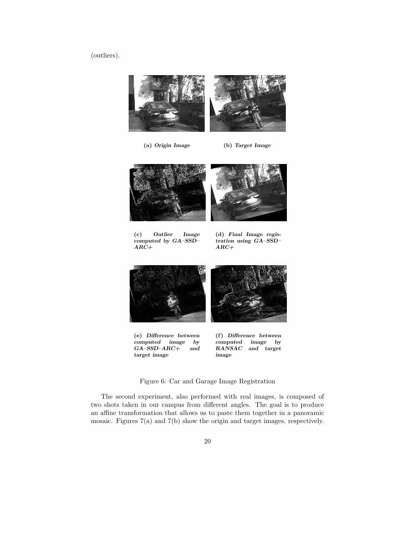
The first experiment uses the images shown in Figure 6, a photograph ofa car in the garage. These images show some differences that can be modeledusing an affine transformation. Additionally, the camera was rotated, and thetarget image has a boy in front of the car, in order to introduce more complexityin the outliers field. The goal is to obtain the image of the boy as part of theoutlier field and the affine transformation introduced by the camera rotation.

The transformations computed by GA–SSD–ARC+ and RANSAC are shownin Table 7. Note the proximity between the parameter vectors computed by bothalgorithms; nevertheless, these values do not allow us to conclude much aboutthe results. Using Equation (13) the outlier field is computed and the imageof them is presented in Figure 6(c). Note in this figure the contour of the boyin front of the car and Figure 6(d) shows the resulting image computed by thevector parameter determined by GA–SSD–ARC+. Finally Figures 6(e) and 6(f)give a clear idea of the accuracy of both AT computed. In both Figures theabsolute value of the difference between the target image and the computedimage by GA–SSD–ARC+ and RANSAC is computed; dark areas correspondto low difference. Note the quality for the AT computed by GA–SSD–ARC+,for Figure 6(e), one can see only the details and noise not present in both images

19

(outliers).

(a) Origin Image (b) Target Image

(c) Outlier Image

computed by GA–SSD–

ARC+

(d) Final Image regis-

tration using GA–SSD–

ARC+

(e) Difference between

computed image by

GA–SSD–ARC+ and

target image

(f) Difference between

computed image by

RANSAC and target

image

Figure 6: Car and Garage Image Registration

The second experiment, also performed with real images, is composed oftwo shots taken in our campus from different angles. The goal is to producean affine transformation that allows us to paste them together in a panoramicmosaic. Figures 7(a) and 7(b) show the origin and target images, respectively.

20

algorithm parameters Θ

GA–SSD–ARC+ µ = 20 0.9700 -0.2280 42.73230.2413 0.9768 -20.6006

RANSAC 0.9166 -0.2473 47.11520.2151 0.9249 -15.3065

Table 7: Resulting AT for RANSAC and GA–SSD–ARC+ Method using Carand Garage Images

The parameter vector computed by RANSAC and GA–SSD–ARC+ are shownin Table 8; comparing the results, there does not exist a significant differencebetween them. The mosaic image (Figure 7(d)) is computed as the linearcombination of the origin and target images, and the outlier field Equation (13)by Equation (23)

I1(ri(Θ)) × l∗(ri) + I2(ri) × (1 − l∗(ri)) (23)

Finally the image of the outlier field is shown in Figure 7(c).

Algorithm Parameters Θ

GA–SSD–ARC+ µ = 20 0.9703 0.042 56.04550.0139 0.9758 0.0051

RANSAC 0.9558 0.0380 57.1481-0.0167 0.9986 0.1160

Table 8: Comparative Results between RANSAC and GA–SSD–ARC+

6 Conclusions

In this paper, we report results on how hybrid computation between GAs andconventional techniques outperforms both of them in the domain of image regis-tration. Hybridization takes place at two levels: combining GAs with a gradient-based search, namely NLM, incorporate ideas from statistics and image process-ing to the fitness function, namely the SSD–ARC function.

Combining GAs with NLM, has proven to improve the search, taking thestrong properties of both algorithms and discarding their weaknesses. GA–SSD–ARC+ does not get stuck in local optima, and is capable of refining results toa high level of accuracy.

GA–SSD–ARC+ performs parametric image registration, based on the non–parametric SSD–ARC algorithm. The function is minimized in two steps, us-ing GAs and NLM. The final algorithm improved the solution using only GAsand/or NLM and it is robust when the images are corrupted by noise. A com-parison of GA–SSD–ARC+ with other registration algorithms, such RANSACand LE, was presented in order to provide experimental proof of the robustnessof GA–SSD–ARC+.

21

(a) Origin Image (b) Target Image

(c) OutlierImage

(d) Mosaic Image

Figure 7: Example of a Panoramic Mosaic

22

We tested GA–SSD–ARC+ using different images and outlier fields; in allthe experiments GA–SSD–ARC+ outperformed the RANSAC and LE methods.Our method is similar to GA–LE+ but it is less sensitive to the particularparameter µ (or σ for LE), and it is easier to find better solutions. Additionallythe GA–SSD–ARC+ provides an explicit way to compute the outliers and doesnot need additional image processing.

In synthetic experiments, we tested the robustness of GA–SSD–ARC+ andpresented how the two minimization steps improved the solution using NLMfor SSD–ARC function alone. In case of real images, the comparison was doneusing only the final parameter vector and the difference between the computedimage and the target image, computed by GA–SSD–ARC+ and RANSAC; bothalgorithms exhibited similar results.

Furthermore, GA–SSD–ARC+ has the advantage of computing the outlierswith accuracy and the experiments proved it, even in case of random outlierfields. In contrast with RANSAC, GA–SSD–ARC+ computes outliers for thewhole image using a simple equation. This outlier equation is implicit on theparametric SSD–ARC function and the outlier field is computed when the al-gorithms converges.

A disadvantage of this algorithms is that GA needs the boundaries of theparameters to be specified. In future works, we plan to compute good valuesfor µ parameter, given a pair of images. Also it is interesting to use RANSACmethods as a way to define the boundaries of the parameters.

References

[1] Alireza Bab-Hadiashar and David Suter. Robust optic flow estimationusing least median of squares. IEEE International Conference on ImageProcessing ICIP96, 1996.

[2] Michael J. Black and Anand Rangarajan. On the unification of line pro-cesses, outlier rejection, and robust statistics with applications in earlyvision. International Journal of Computer Vision, 19:57–92, July 1996.

[3] Felix Calderon and Jose L. Marroquin. Un nuevo algoritmo para el calculode flujo optico y su aplicacion al registro de imagenes. Computacion ySistemas, 6(3):213–226, January-March 2003.

[4] J. E. Dennis and Robert B. Schnabel. Numerical Methods for UnconstrainedOptimization and Nonlinear Equiations. Society for Industrial and AppliedMathematics. siam, Philadelphia, 1996.

[5] M. A. Fischler and R. C. Bolles. Random sample consensus: A paradigmfor model fitting with applications to image analysis and automated car-tography, comm. ACM, 24(6):381–395, 1981.

23

[6] F. R. Hampel, E. M. Ronchetti, P. J. Rousseeuw, and W. A. Stahel. RobustStatistics: The Approach Based on Influence Functions. John Wiley andSons, New York, N.Y, 1986.

[7] Richard Hartley and Andrew Zisserman. Multiple View Geometry in Com-puter Vision. Cambridge University Press, University of Oxford, UK, sec-ond edition, 2003.

[8] Randy L. Haupt and Sue Ellen Haupt. Practical Genetic Algorithms. JohnWiley and Sons, New York, N.Y, 1998.

[9] Donald Hearn and M. Pauline Baker. Computer Graphics C Version. Pren-tice Hall, Inc., Simon and Schuster / A Viacom Upper Saddle River, NewJersey 07458, second edition, 1997.

[10] Geoffrey J. McLachlan. Mixture Models, volume 84. Dekker, 270 MadisonAvenue, New York, New York 10016, 1988.

[11] Kenji Okuma. Mosaic based representation of motion. ACCV, 2004.

[12] P. J. Rousseeuw and A. M. Leroy. Robust Regression and Outlier Detection.Jhon Whiley and Sons, New York, 1987.

[13] J Shi and C Tomasi. Good features to track. In IEEE Conference onComputer Vision and Pattern Recognition (CVPR94), Seatle USA, June94. IEEE.

[14] R Szeliski. Video mosaics for virtual environments. In IEEE ComputerGraphics and Applications, volume 16, pages 22–30. IEEE, March 1996.

[15] Richard Szeliski and James Coughlan. Spline-based image registration.Technical Report 94/1, Harvard University, Department of Physics, Cam-bridge, Ma 02138, April 1994.

[16] Baba C. Vemuri, Shuangying, Huang, Sartaj Sahni, Christiana M. Leonard,Cecile Mohr, Robin Gilmore, and Jeffrey Fitzsimmons. An efficient motionestimator with application to medical image registration. Medical ImageAnalysis, 2:79–98, 1998.

[17] R. E. Walpole and R. H. Myers. Probabilidad y Estadistica para Ingenieros.Inteamericana, Mexico. D.F, 1987.

[18] Allan Watt. 3D Computer Graphics. Pearson Education Limited, 3rdedition, 2000.

[19] Barbara Zitova and Jan Flusser. Image registration methods: A survey.Image and vision computing, 2004.

24