
Optimization techniques for image registration applied to ...
224
Université Paris-Est Laboratoire d’Informatique Gaspard-Monge UMR 8049 A thesis submitted for the degree of Doctor of Philosophy Optimization techniques for image registration applied to remote sensing Bruno Conejo supervised by Prof. Pascal Monasse February 3, 2018
-
Upload
khangminh22 -
Category
Documents
-
view
0 -
download
0
Transcript of Optimization techniques for image registration applied to ...

Université Paris-EstLaboratoire d’Informatique Gaspard-Monge
UMR 8049
A thesis submitted for the degree ofDoctor of Philosophy
Optimization techniques for imageregistration applied to remote
sensing
Bruno Conejo
supervised byProf. Pascal Monasse
February 3, 2018
Abstract
This thesis studies the computer vision problem of image registration in thecontext of geological remote sensing surveys. More precisely we dispose in thiswork of two images picturing the same geographical scene but acquired from twodifferent view points and possibly at a different time. The task of registration isto associate to each pixel of the first image its counterpart in the second image.
While this problem is relatively easy for human-beings, it remains an openproblem to solve it with a computer. Numerous approaches to address thistask have been proposed. The most promising techniques formulate the taskas a numerical optimization problem. Unfortunately, the number of unknownsalong with the nature of the objective function make the optimization problemextremely difficult to solve. This thesis investigates two approaches along with acoarsening scheme to solve the underlying numerical problem.
Each approach makes use of a different assumption to simplify the originalproblem. The convex approach is computationally faster while the non-convex ap-proach delivers more precise solutions. On top of both approaches, we investigatecoarsening frameworks to speed-up the computations.
In our context, we study the First order Primal-Dual techniques for convexoptimization. After a progressive introduction of underlying mathematics, westudy the dual optimal solution space of the TV-regularized problems. Weprove a new theorem that greatly facilitates the demonstration of previouslyestablished theorems. We also provide a new algorithm to optimize the famousROF-model.
As a second approach, we survey the graph-cuts techniques. We also in-vestigate different mincut-maxflow solvers since they are an essential buildingblock of the graph-cuts techniques. We propose a new implementation of thecelebrated Fast-PD solver that drastically outperform the initial implementationprovided by original authors.
We also study coarsening methods for both optimization approaches. Weexperiment with image and energy pyramid coarsening scheme for graph-cuttechniques. In this context we propose a novel framework that drasticallyspeeds-up the inference run-time while maintaining remarkable accuracy.
Finally, we experiment with different remote sensing problems to demonstratethe versatility and efficiency of our approaches. Especially, we investigate thecomputation of depth maps from stereo-images acquired from aerial and spacesurveys. Using LiDAR acquisitions we also propose an algorithm to automaticallyinfer the damages due to earthquakes and soil liquefaction. Finally, we alsomonitor the ground deformation induced by earthquake using realistic simulatedmodel.

Résumé
Dans le contexte de la vision par ordinateur cette thèse étudie le problèmed’appariement d’images dans le cadre de la télédétection pour la géologie. Plusprécisément, nous disposons dans ce travail de deux images de la même scènegéographique, mais acquises à partir de deux points de vue différents et éven-tuellement à un autre moment. La tâche d’appariement est d’associer à chaquepixel de la première image un pixel de la seconde image.
Bien que ce problème soit relativement facile pour les êtres humains, il restedifficile à résoudre par un ordinateur. De nombreuses approches pour traitercette tâche ont été proposées. Les techniques les plus prometteuses formulentla tâche comme un problème d’optimisation numérique. Malheureusement, lenombre d’inconnues ainsi que la nature de la fonction à optimiser rendent ceproblème extrêmement difficile à résoudre. Cette thèse étudie deux approchesavec un schéma multi-échelle pour résoudre le problème numérique sous-jacent.
Chaque approche utilise une hypothèse différente pour simplifier le problèmeinitial. L’approche convexe est plus rapide, tandis que l’approche non convexeoffre des solutions plus précises. En plus des deux approches, nous étudions lesschéma multi-échelle pour accélérer les calculs.
Dans notre contexte, nous étudions les techniques Primal-Dual de premièreordre pour l’optimisation convexe. Après une introduction progressive des ma-thématiques sous-jacentes, nous étudions l’espace dual de solution optimale desproblèmes régularisés par a priori tv. Nous prouvons un nouveau théorème quifacilite grandement la démonstration d’autres théorèmes précédemment établis.Nous proposons également un nouvel algorithme pour optimiser le célèbre modèleROF.
Pour la seconde seconde approche nous examinons les techniques de graph-cut. Nous étudions également différents algorithmes de mincut-maxflow car ilsconstituent un élément essentiel des techniques de graph-cut. Nous proposonsune nouvelle implémentation du célèbre algorithme Fast-PD qui amélioredrastiquement les performances.
Nous étudions également les méthodes multi-échelles pour les deux approchesd’optimisation. Nous expérimentons les schémas de pyramide d’image et d’énergiepour les techniques graph-cut. Dans ce contexte, nous proposons une nouvelleapproche qui accélère considérablement le temps d’exécution de l’inférence touten conservant remarquablement la précision des solutions.
Enfin, nous étudions différents problèmes de télédétection pour démontrerla polyvalence et l’efficacité de nos approches. En particulier, nous étudions lecalcul des cartes de profondeur à partir d’images stéréo aériennes et spatiales. Enutilisant les acquisitions de LiDAR, nous proposons également un algorithme pourdéduire automatiquement les dommages causés par les séismes et la liquéfaction

des sols. Enfin, nous étudions également la déformation du sol induite partremblement de terre en utilisant une simulation sismique réaliste.
2

Acknowledgment
To the most important person in my life, Louise Naud, I would to say thank youfor bearing with me during this journey. I would like to thank my parents fortheir unconditional support and affection.
I would like to acknowledge, Pascal Monasse, Jean-Philippe Avouac, SebastienLeprince, Francois Ayoub and Nikos Komodakis for their guidance and numerouspieces of advice. A special thank you to Heather Steele, Lisa Christiansen,Brigitte Mondou and Sylvie Cash.
I would like to thank Arwen Bradley, Hugues Talbot, Francois Malgouyresand Andrés Almansa for their time and deep review of my work. Finally, I wouldalso like to thank people from the GPS division at Caltech and from the imagelab of LIGM.

Contents
1 Introduction partielle (en français) 61.1 Contexte . . . . . . . . . . . . . . . . . . . . . . . . . . . . . . . . 6
1.1.1 Vue du ciel . . . . . . . . . . . . . . . . . . . . . . . . . . 61.1.2 Applications à la géologie . . . . . . . . . . . . . . . . . . 111.1.3 Un problème d’appariement d’images. . . . . . . . . . . . 13
2 Introduction (English language) 152.1 Context . . . . . . . . . . . . . . . . . . . . . . . . . . . . . . . . 15
2.1.1 Monitoring from above . . . . . . . . . . . . . . . . . . . . 152.1.2 Application to geology . . . . . . . . . . . . . . . . . . . . 202.1.3 An image registration problem . . . . . . . . . . . . . . . 22
2.2 Reviewing previous work . . . . . . . . . . . . . . . . . . . . . . . 232.2.1 Priors . . . . . . . . . . . . . . . . . . . . . . . . . . . . . 232.2.2 Framework . . . . . . . . . . . . . . . . . . . . . . . . . . 24
2.3 An approximate modeling . . . . . . . . . . . . . . . . . . . . . . 242.3.1 Mathematical modeling . . . . . . . . . . . . . . . . . . . 242.3.2 Approximations . . . . . . . . . . . . . . . . . . . . . . . . 26
2.4 Thesis overview . . . . . . . . . . . . . . . . . . . . . . . . . . . . 282.4.1 Document organization . . . . . . . . . . . . . . . . . . . 282.4.2 Contributions . . . . . . . . . . . . . . . . . . . . . . . . . 292.4.3 List of publications . . . . . . . . . . . . . . . . . . . . . . 29
3 First order Primal-Dual techniques for convex optimization 313.1 Introduction and contributions . . . . . . . . . . . . . . . . . . . 31
3.1.1 Introduction . . . . . . . . . . . . . . . . . . . . . . . . . 313.1.2 Chapter organization . . . . . . . . . . . . . . . . . . . . . 323.1.3 Contributions . . . . . . . . . . . . . . . . . . . . . . . . . 32
3.2 Problem formulation . . . . . . . . . . . . . . . . . . . . . . . . . 323.2.1 Basics of convex optimization in a tiny nutshell . . . . . . 323.2.2 Problem of interest . . . . . . . . . . . . . . . . . . . . . . 343.2.3 From a primal to a primal dual form . . . . . . . . . . . . 35
3.3 First order Primal Dual techniques . . . . . . . . . . . . . . . . . 363.3.1 Smoothing: Moreau envelope and the proximal operator . 363.3.2 Decoupling: Fenchel transform . . . . . . . . . . . . . . . 38
2

3.3.3 Primal Dual algorithm . . . . . . . . . . . . . . . . . . . . 403.3.4 Conditioning and Auto tuning of step sizes . . . . . . . . 45
3.4 Reformulating `1 based functions, Proximal operators, and Fencheltransformations . . . . . . . . . . . . . . . . . . . . . . . . . . . . 463.4.1 On reformulating `1 based functions . . . . . . . . . . . . 473.4.2 Proximal operators . . . . . . . . . . . . . . . . . . . . . . 483.4.3 Fenchel transform . . . . . . . . . . . . . . . . . . . . . . 54
3.5 TV regularized problems . . . . . . . . . . . . . . . . . . . . . . . 543.5.1 Notations . . . . . . . . . . . . . . . . . . . . . . . . . . . 543.5.2 Some classic TV regularized problems . . . . . . . . . . . 553.5.3 Truncation theorem for convex TV regularized problems . 573.5.4 A hierarchy of optimal dual spaces for TV-`2 . . . . . . . 593.5.5 Intersection of optimal dual space . . . . . . . . . . . . . 593.5.6 A new primal-dual formulation of the ROF model . . . . 623.5.7 Fused Lasso approximation on pairwise graph for various
sparsifying strength . . . . . . . . . . . . . . . . . . . . . 653.5.8 ROF model with a Global regularization term . . . . . . . 68
3.6 Examples of application . . . . . . . . . . . . . . . . . . . . . . . 693.6.1 Mincut/Maxflow . . . . . . . . . . . . . . . . . . . . . . . 693.6.2 Image denoising . . . . . . . . . . . . . . . . . . . . . . . 733.6.3 L-ROF model vs ROF model for denoising . . . . . . . . 75
3.7 Conclusion . . . . . . . . . . . . . . . . . . . . . . . . . . . . . . 81
4 Maxflow and Graph cuts techniques 824.1 Introduction and contributions . . . . . . . . . . . . . . . . . . . 82
4.1.1 Introduction . . . . . . . . . . . . . . . . . . . . . . . . . 824.1.2 Chapter organization . . . . . . . . . . . . . . . . . . . . . 824.1.3 Contributions . . . . . . . . . . . . . . . . . . . . . . . . . 83
4.2 Discrete optimization in a tiny nutshell . . . . . . . . . . . . . . . 834.2.1 Sub-modularity . . . . . . . . . . . . . . . . . . . . . . . . 834.2.2 Problems of interest . . . . . . . . . . . . . . . . . . . . . 844.2.3 Representation of pairwise binary sub-modular functions . 844.2.4 A link between discrete and convex optimization through
TV regularization . . . . . . . . . . . . . . . . . . . . . . . 854.2.5 Primal dual scheme for integer Linear programming . . . 86
4.3 Max-flow and min-cut problems . . . . . . . . . . . . . . . . . . . 884.3.1 The max-flow / min-cut . . . . . . . . . . . . . . . . . . . 894.3.2 From a min-cut problem to a max-flow problem . . . . . . 894.3.3 Simplified equations . . . . . . . . . . . . . . . . . . . . . 924.3.4 Characterization of obvious partial primal solutions . . . 974.3.5 ROF and Maxflow . . . . . . . . . . . . . . . . . . . . . . 98
4.4 Solvers for min-cut / max-flow problems . . . . . . . . . . . . . . 994.4.1 Solver for chain graphs . . . . . . . . . . . . . . . . . . . . 994.4.2 Iterative solvers . . . . . . . . . . . . . . . . . . . . . . . . 1014.4.3 Augmenting path solvers . . . . . . . . . . . . . . . . . . 104
4.5 Graph-cuts for non convex problems . . . . . . . . . . . . . . . . 104
3

4.5.1 Alpha-expansion . . . . . . . . . . . . . . . . . . . . . . . 1054.5.2 Fast-PD . . . . . . . . . . . . . . . . . . . . . . . . . . . . 1064.5.3 A note on Fast-PD implementation . . . . . . . . . . . . . 111
4.6 Experiments . . . . . . . . . . . . . . . . . . . . . . . . . . . . . . 1134.6.1 The stereo-Matching Problem . . . . . . . . . . . . . . . . 1144.6.2 Maxflow experiments for 4 connected graph . . . . . . . . 1164.6.3 Fast PD implementation experiments . . . . . . . . . . . 1184.6.4 Fast PD vs Alpha-expansion . . . . . . . . . . . . . . . . 124
4.7 Conclusion . . . . . . . . . . . . . . . . . . . . . . . . . . . . . . 125
5 Coarsening schemes for optimization techniques 1275.1 Introduction and contributions . . . . . . . . . . . . . . . . . . . 127
5.1.1 Introduction . . . . . . . . . . . . . . . . . . . . . . . . . 1275.1.2 Chapter organization . . . . . . . . . . . . . . . . . . . . . 1275.1.3 Contributions . . . . . . . . . . . . . . . . . . . . . . . . . 128
5.2 Smoothing and Coarsening scheme for first order primal dualoptimization techniques . . . . . . . . . . . . . . . . . . . . . . . 1285.2.1 Preliminary work . . . . . . . . . . . . . . . . . . . . . . . 1285.2.2 Approach . . . . . . . . . . . . . . . . . . . . . . . . . . . 1385.2.3 Surrogate function via Filtering scheme . . . . . . . . . . 1385.2.4 Surrogate function via coarsening . . . . . . . . . . . . . . 1405.2.5 Experiments . . . . . . . . . . . . . . . . . . . . . . . . . 141
5.3 Coarsening scheme for Graph-Cuts solvers . . . . . . . . . . . . . 1505.3.1 Pairwise undirected discrete MRF . . . . . . . . . . . . . 1505.3.2 Image pyramid . . . . . . . . . . . . . . . . . . . . . . . . 1505.3.3 Energy pyramid . . . . . . . . . . . . . . . . . . . . . . . 1505.3.4 Inference by Learning . . . . . . . . . . . . . . . . . . . . 1545.3.5 Experiments . . . . . . . . . . . . . . . . . . . . . . . . . 158
5.4 Conclusion . . . . . . . . . . . . . . . . . . . . . . . . . . . . . . 175
6 Applications 1766.1 Introduction and chapter organization . . . . . . . . . . . . . . . 176
6.1.1 Introduction . . . . . . . . . . . . . . . . . . . . . . . . . 1766.1.2 Chapter organization . . . . . . . . . . . . . . . . . . . . . 176
6.2 Notations and Preliminaries . . . . . . . . . . . . . . . . . . . . . 1766.2.1 Images . . . . . . . . . . . . . . . . . . . . . . . . . . . . . 1766.2.2 Graph . . . . . . . . . . . . . . . . . . . . . . . . . . . . . 1776.2.3 LiDAR as elevation maps . . . . . . . . . . . . . . . . . . 1776.2.4 Matching criterion . . . . . . . . . . . . . . . . . . . . . . 178
6.3 Stereo-matching . . . . . . . . . . . . . . . . . . . . . . . . . . . . 1796.3.1 Camera models and Epipolar geometry . . . . . . . . . . 1806.3.2 The stereo matching problem . . . . . . . . . . . . . . . . 1826.3.3 Experiments . . . . . . . . . . . . . . . . . . . . . . . . . 185
6.4 Simulated Earth crust deformation . . . . . . . . . . . . . . . . . 1946.4.1 Context . . . . . . . . . . . . . . . . . . . . . . . . . . . . 1956.4.2 Model . . . . . . . . . . . . . . . . . . . . . . . . . . . . . 196
4

6.4.3 Experiments . . . . . . . . . . . . . . . . . . . . . . . . . 1976.5 Damage detection in New-Zealand . . . . . . . . . . . . . . . . . 198
6.5.1 Context . . . . . . . . . . . . . . . . . . . . . . . . . . . . 1986.5.2 Model . . . . . . . . . . . . . . . . . . . . . . . . . . . . . 2006.5.3 Experiments . . . . . . . . . . . . . . . . . . . . . . . . . 202
6.6 Chapter conclusion . . . . . . . . . . . . . . . . . . . . . . . . . . 202
7 Conclusions, limits and future work 204
5

Chapitre 1
Introduction partielle (enfrançais)
Nous débutons ce chapitre en introduisant le contexte de nos travaux 2.1. Nousexpliquons comment la télédétection est utilisée dans les études géologiques. Enparticulier, nous expliquons le lien avec la vision par ordinateur et plus particu-lièrement l’appariement d’images. Les travaux précédents sont présentés dans lasection 2.2. Nous introduisons dans la section 2.3 le model mathématique utilisédans ce document. Finalement, dans la section 2.4 nous présentons un résumédu contenu technique de cette thèse ainsi que nos contributions scientifiques.
1.1 Contexte
1.1.1 Vue du cielLe siècle dernier a connu un nombre croissant de techniques et de dispositifspour observer la Terre. Un développement majeur est l’utilisation de satellites etd’avions équipés de capteur d’imagerie pour observer la Terre vue du ciel. Avecle développement des technologie spatiales, les satellites ont largement contribuéà l’étude de la Terre et d’autres planètes telles que Mars. Nous disposonsmaintenant de nombreuses images haute résolution de multiple planètes et deleurs satellites naturels.
On peut classer les capteurs d’observation en deux familles principales. Lescapteurs actifs tels que le LiDAR et le Radar enregistrent le reflet du signal qu’ilsont émis. Au contraire, les capteurs passifs tels que les caméras panchromatiques,couleurs ou hyper-spectrales enregistrent directement le signal émis par la scèneobservée.
Observing sensors Dans ce travail, nous étudions des acquisitions à partirde caméras panchromatiques et de capteurs LiDAR.
6

Photogrammetry La photogrammétrie est l’ensemble des techniques quiutilisent la photographie pour mesurer les distances entre les objets. De 1850 à1900, le goniographe était l’outil de référence pour dessiner des cartes commeillustré par la figure 1.1. La photogrammétrie analogique utilisée de 1900 à1960 s’appuie sur le concept de vision stéréo-métrique. Cependant, un opérateurexécutait toujours la tâche essentielle d’appariement comme illustré dans la figure1.2. À partir de 1960, la disponibilité des ordinateurs a progressivement diminuéla nécessité d’une implication humaine. À partir de 2000, la photogrammétriemoderne repose entièrement sur des données numérisées et requiert très peud’intervention humaine. Pour plus de détails, nous proposons au lecteur curieuxles travaux de [73], [66], [115] et [80] pour une analyse historique, et [76] pourles fondements mathématiques.
Figure 1.1 – Operateur manipulant ungoniographe. Propriété NOAA.
Figure 1.2 – Opera-teur dessinant une carteen utilisant les tech-niques de photogram-métrie analogique. Pro-priété WSP group.
LiDAR La NASA a investi pendant les années 1970 dans le développementde techniques modernes de télédétection à base de laser. Cette étude initialevisait principalement à mesurer les propriétés de l’atmosphère et de l’océan, lacanopée forestière ou les couches de glace. Dans les années 1990, l’accessibilitéaux dispositifs de positionnement tels que GPS, Global Positioning System etles centrales inertielles, permet d’utiliser le LiDAR à des fins de cartographie.Enfin, dans les années 2000, les logiciels de traitement et la diminution du coûtdes infrastructures informatiques a fait du LiDAR un outil de cartographieprécis et efficace, comme illustré dans les figures 1.3 and 1.4. Pour plus dedetails, nous conseillons la lecture de [144], [5], [11] et [31] pour une revue destechnologies LiDAR et ses applications, mais également [6] pour une introductiondes fondations mathématiques.
7

Figure 1.3 – Acquisition Li-DAR de Mars, Propriété NASA.
Figure 1.4 – Nuage de points3d de New-York City, PropriétéNYC.
Plateformes d’observation Les techniques d’observation de la Terre sontun sujet de recherche et de développement critique pour les forces militaires.Des données historiques [52] indiquent l’utilisation de photos aériennes parBritish Royal Air Force à des fins de reconnaissance pendant la Première Guerremondiale. Ces approches se sont généralisées lors de la seconde guerre mondiale[104] et [123]. En conséquence, la photographie aérienne et la photogrammétrieont bénéficié d’énormes progrès.
Le 7 mars 1947, une caméra montée sur une fusée allemande V-2 modifiéea capturé la première image de la Terre à partir de l’espace. Cependant, étantdonné que la fusée ne pouvait atteindre qu’une altitude légèrement supérieureà 150 kilomètres, elle n’a pas pu mettre en orbite sa charge utile. Néanmoins,un panorama jusque-là inédit 1.5 a pu être créé en raccordant plusieurs images.Nous conseillons l’ouvrage [39] pour une perspective historique de l’imageriespatiale.
Débutant en 1960, le programme TIROS [154], Television InfraRed Observa-tion Satellite, dirigé par la NASA, a prouvé l’efficacité des satellites d’observationpour étudier la Terre. L’objectif principal de ce programme était de développerun système d’information météorologique par satellite. Lancé le 1er avril 1960,TIROS-1 embarquait deux caméras de télévision 1.6 qui ont capturé des milliersd’images lors des 78 jours de mission 1.7. Une revue technique du satelliteTIROS-1 est disponible dans [159].
Le succès du programme TIROS a été suivi de nombreuses autres missionsimportantes. Par exemple, le populaire programme Landsat [107] qui a débutéau début des années 1970 est toujours en activité. Il offre à ce jour l’enregistre-ment global continu le plus long de la surface terrestre [106]. Des programmescommerciaux ou publics plus récents tels que Worldview, Pleiades ou DubaiSatoffrent une qualité et une résolution d’imagerie sans précédent. De plus, l’agilitéde petits satellites tels que la constellation RapidEye ou les satellites SkySatpermet une réponse rapide à des demandes d’acquisitions.
Nous avons également observé au cours de cette dernière décennie une démo-
8

Figure 1.5 – Premiere image de la Terre vu de l’espace, Propriété NASA.
Figure 1.6 – Equipments dusatellite TIROS-1, PropriétéNOAA.
Figure 1.7 – Image de la Terre aquisepar le satellite TIROS-1, PropriétéNASA.
cratisation progressive des drones, créant une troisième option pour l’imagerievue du ciel. Cependant, à ce jour, les drones restent plus adaptés à une image-rie locale et très précise. Par conséquent, ils semblent moins adaptés à notretâche où de vastes zones doivent être cartographiées. En conséquence, nous nousconcentrons uniquement sur l’imagerie aérienne et satellitaire.
9

Comparaison entre l’imagerie aerienne et satellitaire L’imagerie aé-rienne et satellitaire présente différent avantages et inconvéniants comme expliquédans [61] and [164] :
Couverture : les images aériennes sont acquises grâce à des avions survolantune zone d’intérêt. Cela signifie que les endroits reclus peuvent être po-tentiellement difficiles à observer avec l’imagerie aérienne. En revanche,l’imagerie satellitaire offre généralement une couverture plus globale. Deplus, la télédétection satellitaire permet d’observer des paysages de plusgrande taille que l’enquête aérienne.
Réponse à un demande d’observation : Les orbites satellitaires définissentquand une zone géographique peut être observée. En fonction des positionset du cycle de l’orbite de la constellation satellitaire, la réponse à unerequête d’observation peut prendre des heures, des jours ou même dessemaines. Avec une planification appropriée, un avion peut se trouver àun endroit au moment désiré. En outre, si différents endroits doivent êtreimagés en même temps il est possible utiliser plus d’avions.
Météorologie : Un manteau nuageux important ou une forte pluie limite l’ap-plicabilité des deux types d’acquisition. Les observations satellitaires sontplus sensible à la météorologie du fait que la lumière traverse l’intégralité del’atmosphère terrestre. En revanche, les acquisitions aériennes sont moinssusceptibles d’être affectées par des nuages haute altitude.
Données historiques : L’imagerie satellitaire bénéficie d’importantes archiveshistoriques qui permettent parfois aux scientifiques de surveiller l’évolutiontemporelle d’un emplacement souhaité. Malheureusement de telles basesde données n’existent pas pour l’imagerie aérienne.
Precision d’acquisition : L’imagerie aérienne fournit généralement des imagesavec une résolution jusqu’à 6,50 cm. En revanche, l’imagerie satellitaireprocure des images avec une résolution de 50 cm pour les applicationsnon-militaire.
Le choix entre l’utilisation de l’imagerie satellitaire ou aérienne repose trèslargement sur l’application finale.
Comparaison entre la photogrammétrie et les acquisitions LiDARLes techniques de cartographie par photogrammétrie et acquisition LiDARprésentent différents avantages et inconvénients comme détaillé dans [7] et [9] :
Observer à travers la cannopée : Les acquisitions LiDAR ont la possibilitéde pénétrer les forêts denses [10]. Cela permet au LiDAR de cartographieravec une précision élevée la topographie du relief terrestre. Les techniques dephotogrammétrie doivent utiliser des algorithmes pour estimer et soustrairela hauteur de la canopée [158].
10

Précision : La cartographie générée par acquisition LiDAR est généralementplus précise et plus dense. Cela est dû au fait que le LiDAR mesure direc-tement les distances alors que la photogrammétrie mesure indirectementles distances.
Photographie : Les techniques de photogrammétrie peuvent produire en plusde la cartographie une image de la scène. Nous notons que certains capteursLiDAR sont associés avec la caméra pour produire également une imagede la scène.
Couverture : Bien que des bases de données d’acquisition LiDAR existent, ellesdemeurent limitées par rapport aux bases de données de photogrammétrie.
Comme pour la comparaison entre la l’imagerie aérienne et satellitaire,l’application finale définit quel type d’acquisition est le plus approprié.
1.1.2 Applications à la géologieLes géologues ont rapidement adopté l’utilisation de la photogrammétrie et desacquisitions de LiDAR comme illustré dans [43], [69] et [167]. Nous examinonsdans ces sections certaines de ces applications.
Cartographie de la topographie L’obtention d’une cartographie précise dupaysage est extrêmement importante pour les géologues. Le modèle d’élévationnumérique, DEM, peut être produit soit par des techniques de photogrammétrie,soit par traitement d’acquisitions de LiDAR [120]. Les DEM sont généralementdes données d’entrée requises pour beaucoup de tâches différentes. Par exemple,les géologues peuvent surveiller l’évolution du paysage en profitant des bases dedonnées d’images satellites. Le DEM aide également les géologues à préparer leursondage sur le sol où seules des mesures éparses et locales peuvent être réalisées.
Catastrophes naturelles Les catastrophes naturelles se produisent de ma-nière imprévisible et peuvent entraîner des dégâts et des pertes de vie. Ilsperturbent généralement la surface terrestre et les environnements urbainscomme expliqué dans [86]. Une mesure précise de cette perturbation ne permetpas seulement d’améliorer notre compréhension scientifique, mais également demieux organiser les secours. En utilisant une série temporelle de DEMs acquisesavant et après l’événement catastrophique, il est possible d’obtenir de précieusesinformations.
Tremblement de terre Les caractéristiques du paysage et la déformationde la surface le long des failles actives fournissent des informations sur la tecto-nique [59]. Il existe différents types de failles comme illustré dans la figure 1.8.Les séismes sont généralement mesurés à l’aide de sysmomètres. Cependant, lesstations GPS peuvent fournir une mesure précise mais locale de la déformationdu sol [84]. Les progrès de la télédétection permettent également d’estimer cette
11

déformation à plus grande échelle mais au détriment de la précision [112]. L’uti-lisation d’un DEM pré et post-événement permet aux scientifiques de créer descartes de la déformation. Ces cartes peuvent ensuite être combinées avec desmesures GPS ou des relevés au sol. L’ensemble de ces mesures fournissent desdonnées importantes pour modéliser la physique du système de plaques.
Figure 1.8 – Differents types defailles, Propriété USGS.
Figure 1.9 – Diagramme de glisse-ment de terrain, Propriété USGS.
Liquéfaction du sol La liquéfaction du sol est la déformation du reliefinduite par un stress extérieur tel qu’un tremblement de terre [139]. Pendant laliquéfaction, le sol perd de sa rigidité conduisant à des dommages massifs. Parexemple, des bâtiments se sont inclinés lors du séisme de Niigata de 1964. Laliquéfaction du sol est principalement un phénomène local. Par conséquent, desDEM de haute résolution sont nécessaires pour capturer cette déformation durelief.
Glissement de terrain Les glissements de terrain surviennent dans unemasse de terre ou de roche d’une montagne ou d’une falaise, comme l’illustre lafigure 1.9. Les géologues surveillent les glissements de terrain à trois niveaux[103] :
• En identifiant quelles pentes risquent d’être instables [77]. Cela fournit lesinformations nécessaires pour la prévention et le renforcement strucuturelde la pente.
• En surveillant les pentes instables pour déclencher des avertissementsquelques minutes ou secondes avant un glissement de terrain [89]. C’estune préoccupation majeure pour l’exploitation minière à ciel ouvert.
• En mesurant la déformation de la pente due à un glissement de terrain[121]. Cela permet d’étalonner et d’améliorer les modèles numériques deglissement de terrain.
Dans ce contexte, autant les acquistions LiDAR que la photogrammétriehaute résolution sont pertinents pour extraire les informations.
12
Phénomène naturel Bien que les désastres naturels provoquent une dé-formation soudaine du paysage, de nombreux phénomènes naturels modifientprogressivement la topographie des planètes.
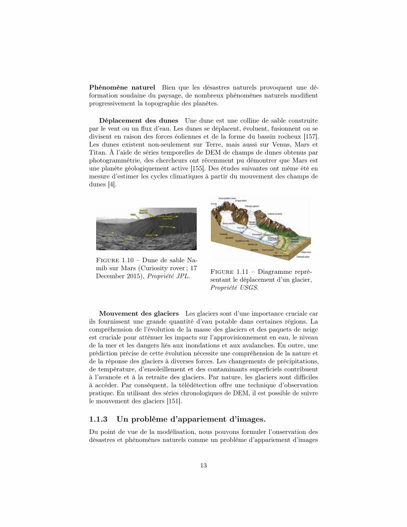
Déplacement des dunes Une dune est une colline de sable construitepar le vent ou un flux d’eau. Les dunes se déplacent, évoluent, fusionnent ou sedivisent en raison des forces éoliennes et de la forme du bassin rocheux [157].Les dunes existent non-seulement sur Terre, mais aussi sur Venus, Mars etTitan. À l’aide de séries temporelles de DEM de champs de dunes obtenus parphotogrammétrie, des chercheurs ont récemment pu démontrer que Mars estune planète géologiquement active [155]. Des études suivantes ont même été enmesure d’estimer les cycles climatiques à partir du mouvement des champs dedunes [4].
Figure 1.10 – Dune de sable Na-mib sur Mars (Curiosity rover ; 17December 2015), Propriété JPL.
Figure 1.11 – Diagramme repré-sentant le déplacement d’un glacier,Propriété USGS.
Mouvement des glaciers Les glaciers sont d’une importance cruciale carils fournissent une grande quantité d’eau potable dans certaines régions. Lacompréhension de l’évolution de la masse des glaciers et des paquets de neigeest cruciale pour atténuer les impacts sur l’approvisionnement en eau, le niveaude la mer et les dangers liés aux inondations et aux avalanches. En outre, uneprédiction précise de cette évolution nécessite une compréhension de la nature etde la réponse des glaciers à diverses forces. Les changements de précipitations,de température, d’ensoleillement et des contaminants superficiels contribuentà l’avancée et à la retraite des glaciers. Par nature, les glaciers sont difficilesà accéder. Par conséquent, la télédétection offre une technique d’observationpratique. En utilisant des séries chronologiques de DEM, il est possible de suivrele mouvement des glaciers [151].
1.1.3 Un problème d’appariement d’images.Du point de vue de la modélisation, nous pouvons formuler l’onservation desdésastres et phénomènes naturels comme un problème d’appariement d’images
13

dense. Un problème d’appariement d’image dense est la tâche de trouver pourchaque pixel d’une image donnée son homologue dans une autre image. Selonl’application finale, le problème d’appariement aura un degré de liberté dif-férent. Si les homologues doivent être sur une certaine ligne, nous obtenonsun problème d’appariement mono-dimmensionnel. Si les homologues sont dansun plan donné, nous obtenons un problème d’appariement bi-dimmensionnel.Si aucune hypothèse n’est possible, nous avons un problème d’appariementtri-dimmensionnel.
Hypothèse sur les DEM
Comme nos observations proviennent d’un avion ou d’un satellite, nous proposonsde transformer avec très peu de perte d’information le DEM acquis en unecarte d’élévation d’image [105]. La position des pixels définit les coordonnéesgéographiques locales tandis que leurs intensités encodent l’élévation au-dessusd’une référence. Nous détaillons cela dans le chapitre 6.2.3 de cette thèse.
Appariement 1D
Pour la photogrammétrie aérienne, nous recevons deux images acquises par unecaméra de type frame. Après avoir prise en compte la géométrie d’acquisition,le calcul de la carte d’élévation repose principalement sur la résolution d’unproblème d’appariement dense 1D appelé appariement stéréo. Nous présentonsdans la section 6.3 le concept d’appariement stéréo.
Appariement 2D
Pour la photogrammétrie satellitaire, nous recevons deux images acquises parun capteur de type push-broom. Cela complexifie la géométrie de l’acquisition.Par conséquent, le calcul de la carte d’élévation repose sur la résolution d’unproblème d’appariement dense 2D. Nous en discutons dans la section 6.3.1.
Appariement 3D
Etant donné une série chronologique de cartes d’élévations du même paysage,nous pouvons effectuer un appariement 3D pour estimer la déformation induitepar un phénomène d’intérêt. Dans ce contexte, les cartes d’élévations peuventêtre produites par photogrammétrie ou par maillage d’une acquisition LiDAR.Nous en discutons dans la section 6.4.
14

Chapter 2
Introduction (Englishlanguage)
We begin this first chapter by introducing in section 2.1 the context of our work.In particular, we explain how remote sensing techniques are used for geologicalstudies and how this relates to the computer vision task of image registration.We review in section 2.2 some of the past work. The section 2.3 describes themathematical modeling we use through this document. Finally, in section 2.4 wepresent a summary of the technical content of this thesis and our contributions.
2.1 Context
2.1.1 Monitoring from aboveThe last century has seen an increasing number of techniques and devices tomonitor Earth. One major development is the use of satellites and airplanesequipped with imaging sensors to monitor the Earth from above. With thedevelopment of space technology satellites have extensively surveyed Earth andother planets such as Mars with an increasing accuracy. We now dispose of manyhigh resolution pictures of many planets and their natural satellites.
One can classify monitoring sensors in two main families. The active sensorssuch as LiDAR and Radar that record the reflection of the signal they emitted.On the contrary, the passive sensors such as panchromatic, color or hyper-spectralcameras directly record the signal emitted by the observed scene.
Observing sensors In this work we consider acquisitions from panchromaticcameras and LiDAR sensors.
Photogrammetry Photogrammetry refers to the set of techniques thatuse photography to measure the distances between objects. From 1850 to 1900,
15

people relied on techniques such as those of the plane tables to draw maps.This is illustrated by figure 2.1. The analog photogrammetry which spannedthe period from 1900 to 1960 relied on the concept of stereo-metric vision.However, an operator was still performing the essential registration task asdepicted in figure 2.2. From 1960 the availability of computers progressively hasdecreased the need for human involvement. Starting from 2000’s the modernphotogrammetry completely relies on fully digitalized data and requires verylittle human intervention. For more detail, we refer the curious reader to [73],[66], [115] and [80] for an historical review, and to [76] for an introduction tothe mathematical foundations.
Figure 2.1 – Operator manipulating aplane table. Courtesy NOAA.
Figure 2.2 – Operatordrawing maps duringthe analog photogram-metry era. CourtesyWSP group.
LiDAR The NASA invested in the 1970s in the development of modernlaser-based remote sensing acquisition techniques. This initial study was mainlyaimed at measuring the properties of the atmosphere and the ocean water, theforest canopy or the ice sheets. In the 1990s the accessibility to positioningdevices such as GPS, Global Positioning Systeme, and IMU, Inertial MeasurementUnit, allowed to use LiDAR for mapping purposes. Finally, in the 2000s theavailability of processing software coupled with the decreased cost of computinginfrastructures made the LiDAR a precise and efficient mapping tool as illustratedin figures 2.3 and 2.4. For more detail, we refer the curious reader to [144], [5],[11] and [31] for a review of the technology and its application, and to [6] for anintroduction to the mathematical foundations.
Observing platforms Earth observation techniques have been a major re-search and development study for military forces. Records indicate that aerialphotos used by British R.A.F. for reconnaissance helped to review militarytactics during World War I [52]. Such practice was generalized during World
16

Figure 2.3 – Rendered LiDARacquisitions of Mars.
Figure 2.4 – 3d points cloud ofNew-York City acquired by a Li-DAR device augmented with acolor camera.
War II [104] and [123]. As a result aerial photography and photogrammetrymade tremendous strides.
On March 7, 1947, a camera mounted on a modified German V-2 rocketcaptured the first picture of Earth from space. However, since the rocket couldonly reach an altitude slightly above 100 miles, it was unable to place into orbitits payload. Nevertheless, stitching several pictures together as illustrated in 2.5created unseen before panoramas. We advise the reader to [39] for an historicalperspective of imaging from space .
Figure 2.5 – The first picture of Earth from space, Courtesy NASA.
Starting in 1960, the TIROS Program [154], Television InfraRed ObservationSatellite, directed by NASA proved the efficiency of observation satellites tostudy Earth. The main focus of this program was to develop a meteorological
17

satellite information system. Launched on April 1, 1960, TIROS-1 embarked twotelevision cameras 2.6 that captured thousands of pictures during its 78 daysmission 2.7. A technical review of the TIROS-1 satellite is given in [159].
Figure 2.6 – Equipments ofthe TIROS-1 satellite, CourtesyNOAA.
Figure 2.7 – Picture of Earth from theTIROS-1 satellite, Courtesy NASA.
The success of the TIROS program was followed by many other importantmissions. For instance, the popular Landsat program [107] that started in theearly 1970s is still operating. It offers to this day the longest continuous globalrecord of the Earth surface [106]. More recent commercial or public programssuch as Worldview, Pleiades or DubaiSat offer unprecedented imaging qualityand resolution. Moreover, the agility of small satellites such as the RapidEyeconstellation or the SkySat satellites allow for quick response to on demandacquisitions.
We also observed over the last decade a progressive democratization of drones,creating a third option for imaging from above. However, to this day dronesremain more suited to very precise and local imaging. Hence, they appear lesssuited to our task where large areas need to be mapped. As a result we onlyfocus on aerial and satellite imaging.
Aerial vs Satellite imaging Aerial and satellite imaging present differentstrong points and weaknesses as explained in [61] and [164]:
Coverage : aerial images are mainly gathered through the use of airplanesflying over the landscape of interest. This means that remote places canbe difficult to survey with aerial imaging while satellite imaging generallyoffer a global coverage. Moreover, remote sensing satellite allows imagingof way larger landscapes than aerial survey.
18

Timing : the satellite orbits defines a time frame when a defined location canbe imaged. Depending on the positions and the orbit cycle of the satelliteconstellation, the response to survey at a given location can take hours,days or even weeks. With proper planning an airplane can be at a certainlocation at the desired time. Moreover, if different locations need to beimaged at the same time one can always use more planes.
Weather : severe cloud coverage or rain nullify both types of acquisition. Sincethe light reaching the satellite is affected by the entire atmosphere, spacesurvey tends to be more sensitive to the weather. For instance, aerialacquisitions are less likely to be affected by high altitude clouds.
Historical data : satellite imaging benefits from massive historical archivesthat sometimes allows observers to monitor the evolution of a desiredlocation through time. Such large databases do not exist for aerial survey.
Image resolution : an aerial survey generally provides images with a resolutiondown to 6.50cm. Satellite survey captures images with resolution down to50cm for the public viewing.
As it should always be, the final task is the one driving the choice betweenaerial and satellite imaging.
Photogrammetry vs Lidar Photogrammetry and Lidar mapping techniquespresent different benefits and drawbacks as detailed in [7] and [9]:
Canopy penetration : LiDAR has the ability to penetrate even dense forestcanopies [10]. This allows the LiDAR to map with high accuracy thebare earth topography. The photogrammetry techniques have to rely onalgorithms to remove the estimated canopy height [158].
Precision : As a rule of thumb, the mapping generated from LiDAR is generallymore precise and dense. This is because the LiDAR directly measuresdistances while photogrammetry uses a proxy measurement (image regis-tration) to estimate those distances.
Photography : The photogrammetry techniques can produce along with themapping a picture of the scene. We note that some LiDAR are augmentedwith camera to also produce a picture of the scene.
Coverage : While LiDAR databases exist they do not compare in extent withphotogrammetry databases.
As for the previous discussion comparing the aerial and satellite imaging, thefinal task will drive which type of acquisition is the most relevant.
19

2.1.2 Application to geologyGeologists and Earth scientists were among the early users of photogrammetryand LiDAR acquisitions as illustrated in [43], [69] and [167]. We review in thissections some of their applications.
Mapping topography Obtaining precise mapping of the landscape is ex-tremely important to geologists. Digital Elevation Model, DEM, can be producedusing either by photogrammetry techniques or by processing LiDAR acquisitions[120]. DEMs are generally required inputs for a lot of different tasks. For in-stance, geologists can monitor the evolution of the landscape by taking advantageof the satellite images databases. DEM also helps geologists to prepare theirground survey where only sparse and local measurements can be made.
Natural hazards Natural hazards occur unpredictably and can cause widespreaddamage and loss of life. They usually disrupt the Earth surface or built environ-ment as explain in depth in [86]. Accurate measurement of this disruption nononly helps to improve our scientific understanding but allows to better organizethe emergency response. Using a time series of DEMs spanning before and afterthe catastrophic event one can automatically derive precious information.
Earthquake Landscape features and surface deformation along activefaults provide insights into faulting and tectonics [59]. There exists differenttype of faults as illustrated in figure 2.8. Earthquakes are generally measuredusing seismometers. However, GPS stations can provide accurate but localmeasurement of the ground deformation [84]. The progress of remote sensingimagery also allows to estimate this deformation at a larger scale at the expenseof precision [112]. The use of a pre and post-event DEMs allows researcherto create maps of the deformation. Those maps can then be used to augmentGPS point measurements or ground surveys. All those measurements provideimportant data to estimate the physical modeling of fault systems.
Figure 2.8 – Different types offaults. Figure 2.9 – Landslide diagram.
Soil liquefaction Soil liquefaction is the deformation of the landscapeinduced by an external stress such as an earthquake [139]. During liquefaction,
20

The soil loses strength and stiffness creating massive damages. For instancebuildings were tilted during the 1964 Niigata earthquake. Soil liquefaction ismainly a local phenomenon. Hence, high resolution DEMs are necessary tocapture landscape deformation induced by soil liquefaction
Landslides Landslides are sliding down of a mass of earth or rock from amountain or cliff as illustrated by figure 2.9. Geologists monitor landslides atthree levels [103]:
• Identifying which slopes are likely to be unstable [77]. This provides thenecessary information for prevention and potential structural reinforcementof the slope.
• Monitoring at high-frequency unstable slopes to trigger early landslidewarnings [89]. This is a main concern for open-pit mining.
• Measuring the slope deformation due to a landslide [121]. This help tocalibrate and improve numerical landslide models.
In this context, one can rely on LiDAR processing or high resolution pho-togrammetry to extract the pertinent information.
Natural processes While natural hazards trigger sudden deformation of thelandscape, many slow natural processes progressively alter planets topography.
Motion of dunes A dune is a hill of loose sand built by wind or the flow ofwater. Dunes move, evolve, merge or divide due to eolian forces and the shape ofthe bed rock [157]. Dunes non-only exist on Earth but also on Venus, Mars andTitan. Using time series of DEMs of dune fields obtained with photogrammetry,researchers have recently been able to demonstrate that Mars is geologicallyactive [155]. Furthermore, follow-up studies were even able to estimate climatecycles from the motion of dune fields [4].
Figure 2.10 – Namib sand dune(downwind side) on Mars (Curiosityrover; 17 December 2015). Figure 2.11 – Glacier diagram.
21

Motion of glaciers and ice Glaciers are of critical importance sincethey provide large quantity of drinking water in some areas. Understandingthe changing mass balances of mountain glaciers and snow packs is crucialfor mitigating impacts to water supplies, sea level, and hazards from outburstfloods and avalanches. Moreover, accurate prediction of future mass balancechanges requires an understanding of the nature and rate of glacier response tovarious forces. Changes in precipitation, temperature, solar input and surfacecontaminants contribute to glaciers advance and retreat. By nature, glaciers aredifficult to access. Hence, remote sensing provides a handy observation technique.Using time series of DEMs, one can track the motion of glaciers or the changein ice coverage [151].
2.1.3 An image registration problemFrom a modeling standpoint, we can formulate the monitoring of natural hazardsand processes as a dense image registration problem. A dense image registrationproblem is the task of finding for each pixel of a given image its counterpart in another image. Depending on the task the registration problem will have differentdegrees of freedom. If we know that the counterparts have to be on a certainline we get a 1D registration problem. If the know that the counterparts are ona given plane, we end-up with a 2D registration problem. If no assumption canbe made, then we have a 3D registration problem.
Assumption for DEM
Since our observations originate from a plane or a satellite, we propose to trans-form with very little loss of information the acquired DEM to an image elevationmap [105]. The position of the pixels refers to local geographic coordinates whiletheir intensities encode the elevation above a reference. We detail this in thechapter 6.2.3 of this thesis.
1D Registration
For aerial photogrammetry we are given two images acquired by a frame camera.After accounting for the geometry of acquisition, the computation of the elevationmap mainly relies on solving a 1D dense registration problem called stereo-matching. We will in the last chapter 6.3 present the stereo-matching concept.
2D Registration
For satellite photogrammetry we are given two images acquired by a push-broomsensor. This complexifies the geometry of acquisition. Hence, the computationof the elevation map relies on solving a 2D dense registration problem apparentto optical-flow. We will discuss this in the last chapter 6.3.1.
22

3D Registration
Given a time series of elevation maps of the same landscape, we can perform a3D registration to estimate the deformation induced by a phenomenon of interest.In this context the elevation maps could have been produced by photogrammetryor by griding a LiDAR. We will discuss this in the last chapter 6.4.
2.2 Reviewing previous workDense image registration has been extensively studied since the inception ofcomputer vision. We can find dense image registration problems in many fieldssuch as medical and biology imagery, planetary sciences, industrial verificationor video surveillance. We point the curious reader toward [23], [178], [45] and[138] for an extensive review on image registration.
2.2.1 PriorsIndependently on their approach, all registration methods try to enforce amatching prior and a regularization prior.
Matching priors
The goal of the matching prior is to measure the similarity between parts of twoimages. There exist many different approaches as illustrated in [67], [29], [163],[149], [150] and [176]. The simplest technique is to directly compare the valueof pixels, eventually on a patch centered around the points of interest. Moreadvanced technique computes descriptors that encode non only the informationcontained by the pixel of interest but also its neighborhood. These descriptorsor features are then compared to estimate a similarity score. Unfortunately,relying only on matching priors is insufficient to register images. For instance,noisy regions or geometric deformations deteriorate the quality of the similarityestimation. Moreover, texture-less areas or repetitive patterns create ambiguities.Finally, in some context some pixels have no corresponding counterparts due toocclusion.
Regularization priors
The role of the regularization prior is to enforce some a-priori information onhow the pixels should register. In most tasks, one can assume that the geometrictransformation that registers the images should follow some structure. Theregularization priors simply define the properties that geometric transformationsshould follow. This helps to correct some of the errors or uncertainty of thematching prior. The most popular regularization favors geometric transformationthat have a smooth gradient. The choice of the regularization priors mainlydepends on the task and the ability to enforce it to a desired accuracy. One
23
can refer to [30] and [156] for examples of different regularization priors in thecontext of image registration.
2.2.2 FrameworkWe distinguish two main frameworks to enforce both the matching and regular-ization priors. While both frameworks have the same intent, their theoreticalfoundations differ.
Heuristic framework
The heuristic based framework relies on alternate application of heuristics toenforce the priors. Generally, the matching prior is enforced first giving a noisyand possibly sparse estimation of the registration. Then, the regularization prioris applied to obtain a dense and denoized registration. For instance, the medianfilter has been extensively used as a regularization prior. Eventually, one canproceed with multiple rounds of alternating between the priors. The decouplingof the prior’s enforcement in successive steps leads to simple algorithm. However,in this setting it is unclear what is globally enforced. Indeed, alternating betweenpriors is different than directly enforcing both priors at the same time.
Optimization framework
The optimization based framework formulates the registration task as an energyminimization problem. This framework makes use of a global energy obtainedby modeling both priors with their respective energies. The main challengeremains to find a registration that minimizes this energy. We remind thatone can link an energy to a probability through the use of Gibb’s free energyfunction. Hence, the energy minimization problem is in fact equivalent tofinding the most probable registration given the inputs. This connection givesstrong theoretical foundation to this framework. Moreover, in some cases, theoptimization problem can generalize a heuristic. For instance, it is well knownthat the median filter is equivalent to solving a certain `1-norm problem. Thisframework gives more precise results than its heuristic base counterpart (see anexample in the context of 2D image registration [8]). However, this comes withan added computational complexity. In this work, we will investigate differentapproaches for the optimization framework.
2.3 An approximate modeling
2.3.1 Mathematical modelingWe now assume that we are given two images: a reference image and a targetimage. The goal of the dense image registration task is to find for each pixel ofthe reference image its counterpart in the target image. Without loss of generality
24

we can model this problem as finding the apparent pixel motion between thereference image and the target image.
Notations We introduce the following notations:
• Ω is the finite set t1, . . . , nu with n P N˚ that represents the pixels of thereference image.
• Xi with i P Ω is a convex subset of Rd with d P N˚ that defines theadmissible range of motions for a given pixel.
• X is a convex subset formed by X0ˆ . . .ˆXn: that represent the admissibleregistrations.
• x is an element of X and represents a potential registration.
• xi is the ith element of x and represents the motion of a given pixel.
• Mi : xi P Xi Ñ R encodes the matching prior as an energy.
• L is a continuous linear operator mapping space X to a vector space Ythat encodes the dependency between the pixel motions. This is the firstpart of the regularization prior.
• R : y P Y Ñ R encodes as an energy the second part of the regularizationprior.
Optimization model We now need to optimize the following model:
arg minxPX
ÿ
iPΩ
Mipxiq `RpLxq (2.1)
This mathematical problem is extremely difficult to solve. Indeed, theobjective function exhibits the following properties:
• Non convexity: there is no convexity assumption on the functions pMiqi
and R, hence the objective function can be non-convex.
• Non smoothness: there is no smoothness assumption on the functionspMiqi and R, hence the objective function can be non-smooth.
• Continuous variables: we assume that each variable xi lives in a continuousconvex space.
• High order terms: the operator L can create dependencies between variablesin sub-sets of x.
• Large number of variables: since we work in the image registration context,the size of x is in the order of millions of elements.
For all these reasons, the problem (2.1) is generally NP-hard and only approx-imate solution may be sought. Notice however that in practice an approximatesolution is good enough because there is no guarantee that the mathematicalmodel is entirely faithful to the reality.
25

2.3.2 ApproximationsDirectly attempting to solve (2.1) is extremely challenging. We need to makefurther assumptions on the objective function to decrease its optimization com-plexity. By using various simplification strategies we obtain different classesof optimization problems that become tractable. However, this simplificationmakes the modeling of the registration task less accurate.
Discarding non convexity
We propose to use convex functions to approximate the matching and regular-ization functions pMiqi and R around the current solution. The quality of theapproximation generally quickly deteriorates with an increased distance to thecurrent solution. However, this approximation gives us a convex function thatrepresents locally the original objective function. In this settings we can usevarious optimization schemes.
Majorization minimization The majorization minimization scheme relieson using a convex surrogate function [82]. The surrogate function needs tocoincide with the objective function at the current solution and should majorizethe objective function everywhere else. Since we have some freedom to definethe surrogate function, we have interest to choose one that is easy to minimize.The most appealing surrogate functions are those that can be minimized witha close-form formula. The minimization of the surrogate function gives a newsolution. We iterate between these two steps until no further progress can bemade.
The majorization minimization scheme is easy to apply and implement.However, it suffers of two main drawbacks. If the function is not smooth, thenthis scheme can terminate in a sub-optimal solution. Moreover, the convergencerate generally slows drastically when it approaches a minimum solution.
Splitting techniques The splitting techniques rely on auxiliary variablesthat are introduced to decouple the matching and regularization parts of theenergy (see [33] and [32] for a detailed introduction). In our context, thismeans to add a set of variables y in place of the term Lx. Then, an additionalconstraint is added to the objective function to enforce that y “ Lx. We can usepenalty terms, Lagrangian multipliers or ADDM, Alternating Direction MultiplierMethod, schemes to enforce this new constraint. This creates different splittingtechniques. In most cases the splitting scheme alternates between 3 optimizingsteps: optimizing the matching variables x, optimizing the regularization variablesy, and enforcing the constraint y “ Lx.
The splitting techniques scheme is generally more difficult to apply andimplement than the majorization minimization scheme. However, this schemehas the ability to minimize non smooth functions. Unfortunately, enforcing theconstraint slows down the convergence of the splitting techniques.
26

Primal-dual techniques The primal dual scheme of [27] relies on the conceptof duality to add auxiliary variables that dynamically approximate the regular-ization function R by a set of linear terms. In our context, this means to add aset of variables y that model RpLxq by the scalar product ă y, Lx ą. We noticethat the auxiliary variables make the optimization over each xi independent.Hence, the optimization over x is easy as long as the functions pMiqi are reason-ably complex. This creates a very appealing scheme where we iterate betweenminimizing for each xi and update the variable y to get a better approximation.
The primal dual scheme can handle non-smooth objective functions and hassuperior convergence properties than the splitting techniques. For these reasonswe elect to choose the primal-dual scheme.
Discretization of the solution space and first order regularization
Another approach to simplify the problem (2.1) is to discretize the solution spaceX and to limit the linear operator L to a first order operator like a gradient.These two assumptions make the problem (2.1) belong to the class of first orderpairwise MRF, Markov Random Field if the regularization function R does notrely on input images, or CRF, Conditional Random Field if it does. In thiscontext, we can use different optimization schemes. Unfortunately, even withthis simplification the problem remains generally NP-Hard. Hence, we are onlyguaranteed to obtain an approximate solution.
Message passing The message passing method builds on dynamic program-ming schemes (see [129] and [171] for a detailed introduction). It relies onpropagating information through the variables to update their respective proba-bilities of being assigned to a given discrete value. There exist many approachesto propagate the information. However in the context of image based problems,the belief propagation with the checkerboard update rule of [49] and the tree-reweighted message passing scheme of [93] obtain the best results. Moreover, ifthe problem takes the form of a chain we can use the famous Viterbi algorithm[56] to compute an optimal solution.
The message passing unfortunately does not always obtain good approxi-mations as demonstrated in [161] and [90]. Moreover, the procedure of thesealgorithms is quadratic with respect to the average number of discrete possiblevalues for variables pxiqi. We note that for some regularization functions R, thiscomplexity can be reduced to a linear one as explained in [48].
Dual decomposition The dual decomposition scheme relies on duplicatingsome variables of the original problem to obtain a set of sub-problems that canbe optimally solved. The duplicated variables are constrained through the use ofauxiliary variables to converge to the same discrete value. This scheme alternatesbetween solving each sub-problem and updating the auxiliary variables to enforcethe constraints. Two main variations exist. The original dual decompositionalgorithm of [99] used Lagrangian multipliers to enforce the constraints while
27

the alternative direction dual decomposition algorithm of [119] makes use of theADMM scheme. In our context the most natural and efficient decomposition isto create a chain per line and column.
The dual decomposition scheme obtains excellent approximations as demon-strated in [98]. However, it is slow to converge since it has the same complexityas the underlying algorithm used to solve the sub problems. Moreover, manyiterations are needed to enforce the constraint on the auxiliary variables.
Graph-Cuts The Graph-Cuts approach of [18] also known as the making moveapproach, relies on iteratively updating a current solution by solving a binaryproblem. During an iteration, each variable can choose between maintaining itscurrent solution or choosing a proposed one. By cycling the proposed solutionthrough the list of admissible discrete solutions, the making move approachprogressively obtains a better solution. Interestingly, the associated binaryproblem is in fact a maxflow-mincut problem which can be solved very efficiently.Different approaches exist and result in different making move algorithms suchas [19], [20] or [152].
The making move proposes a good balance between speed and the qualityof approximations. Moreover, the complexity of algorithm such as the alphaexpansion of [17] and Fast-PD [102] is linear with respect to the average numberof discrete possible values for variable pxiqi. For these reasons we elect toinvestigate the alpha expansion and Fast-PD .
2.4 Thesis overview
2.4.1 Document organizationBesides the current introduction and conclusion, this manuscript articulatesaround three technical chapters 3, 4, 5 and one applications chapter 6.
First order Primal-Dual techniques for convex optimization In thisfirst technical chapter 3 we start with the basis of convex optimization. We followwith a didactic review of first order primal dual scheme for convex optimization.Then, we study the dual optimal space of TV regularized problems. Finally, weperform experiments to illustrate the techniques presented in this chapter.
Maxflow and Graph cuts techniques The second technical chapter 4 in-troduces the basis of discrete optimization. We then review the maxflow-mincutproblem in the context of graph cuts techniques. Then, we provide an extensivediscussion around the implementation of the Fast-PD algorithm. Finally, wejustify the superiority of our implementation in numerous experiments.
28
Coarsening schemes for optimization techniques The last technical chap-ter 5 compares various coarsening schemes for the first order Primal-Dual tech-niques and graph cuts schemes. We also introduce a new pyramidal scheme forgraph cuts that drastically speeds-up the computation without compromising onthe quality of the obtained solutions.
Applications The last chapter of this manuscript 6 revolves around the appli-cations of techniques presented in chapters 3, 4 and 5. We perform experimentswith tasks such as stereo-matching, monitoring Earth crust deformation anddamage detection due to an earthquake.
2.4.2 ContributionsWe present here a summary of our contributions that we further detail in eachtechnical chapter.
First order Primal-Dual techniques for convex optimization We derivetheorems that explain how dual optimal solution spaces relate to one anotherfor TV regularized problems. This understanding helps to derive a new proof toa variety of theorems.
Maxflow and Graph cuts techniques We completely re-implemented theFast-PD algorithm to obtain a drastic reduction of the memory footprint whileproviding faster run-time. This allows us to use Fast-PD on large scale problemson a modern laptop computer.
Coarsening scheme for optimization techniques We propose a coarseningscheme that speeds up the optimization of Graph-Cuts techniques. We extendthis coarsening scheme with a novel framework that drastically speeds-up theinference run-time while maintaining remarkable accuracy.
2.4.3 List of publications• Inference by learning: Speeding-up graphical model optimization via acoarse-to-fine cascade of pruning classifiers, B. Conejo, N. Komodakis,S. Leprince, J.P. Avouac in Advances in Neural Information ProcessingSystems, 2014
• Fast global stereo matching via energy pyramid minimization, B. Conejo, S.Leprince, F. Ayoub, J.P. Avouac in ISPRS Annals of the Photogrammetry,Remote Sensing, 2014
• A 2D and 3D registration framework for remote-sensing data, B. Conejo,S. Leprince, F. Ayoub, J. Avouac in AGU Fall Meeting 2013
29

• Emerging techniques to quantify 3D ground deformation using high resolu-tion optical imagery and multi-temporal LiDAR, S. Leprince, F. Ayoub, B.Conejo, J. Avouac in AGU Fall Meeting 2012
30

Chapter 3
First order Primal-Dualtechniques for convexoptimization
3.1 Introduction and contributions
3.1.1 IntroductionThis chapter introduces an extremely powerful and versatile framework: theFirst Order Primal Dual convex optimization technique. Sometimes referred asthe Primal Dual Hybrid Gradient method or the Primal Dual Proximal Pointmethod, this technique is well suited for a large class of convex optimizationproblems with smooth and non-smooth objective function. This framework hasbeen successfully applied to problems such as image denoising (ROF, TV-L1, ...),inpainting, debluring, image segmentation, dense registration, mincut/maxflow,and linear programming.
The underlying mathematical mechanism can appear quite frightening at firstglance, with terms such as “Moreau envelope”, “Proximity operator” or “Flencheltransform”. However, the framework is in fact fairly easy to understand. Alarge quantity of published materials or technical reports extensively cover thesubject. As a personal preference, I would recommend the seminal paper ofChambolle and Pock [27] for its clarity and exhaustive list of experiments relatedto computer vision. Another great source of information is the technical reportof Parikh and Boyd [141] that covers in more depth the proximal operators.
Finally, implementing a first order primal dual algorithm is relatively straight-forward on both CPU and GPU based architectures. For instance, the core ofthe Mincut/Maxflow algorithm is only 10 lines of Matlab code and barely morein C++. Furthermore, many components can be reused from one algorithm
31

to the next, which makes this technique well suited for quick prototyping ormodular framework.
3.1.2 Chapter organizationIn section 3.2 we introduce the basics of convex optimization and we describethe problems of interest. We progressively explain and detail in section 3.3 thedifferent components of the first order primal dual algorithms. The section 3.4presents frequently used proximal operators and Fenchel transformations. Insection 3.5 we introduce various TV-regularized problems and we study therelationship between the optimal dual solution spaces of the TV-regularizedproblems. The section 3.6 illustrates the application of the first order primaldual techniques with different examples.
3.1.3 ContributionsIn this chapter we demonstrate some TV regularized problems share a particularconnexion through their optimal dual solution space. We prove that there existsa hierarchy of optimal dual solution spaces connecting the ROF model to a linearTV model. Furthermore, we establish that the intersection of the optimal dualsolution space of a set of ROF models defines the optimal dual space of somelinear TV model. To the best of our knowledge these are new results.
Building on these theorems, we state and prove a generalization of theFriedmann’s theorems for Fused Lasso approximation. We also propose a newproof for quickly finding the solution of a ROF model with various globalregularization terms. Finally, we introduce a new primal-dual formulation tosolve the ROF model that experimentally outperform the traditional primal-dualscheme.
3.2 Problem formulation
3.2.1 Basics of convex optimization in a tiny nutshellAs a preamble, we remind some mathematical definitions useful in the contextof this chapter. For an extended introduction on convex optimization, werefer the curious reader to Fundamentals of Convex Analysis by Hiriart-Urrutyand Lemaréchal [78], Convex Optimization by Boyd and Vandenberghe [15] orOptimization. Applications in image processing. by Nikolova [133] from whichwe borrow the following definitions and theorems.
Existence of minimums
Before even thinking of searching for the minimums of a function, we need toestablish the conditions of their existence. To this end, we need the followingdefinitions:
32

Definition 1. A function f on a normed real vector space V is proper if f :V Ñ s´8,`8s and if it is not identically equal to `8.
Definition 2. A function f on a normed real vector space V is coercive iflimuÑ`8 fpuq “ `8.
Definition 3. A function f on a real topological space X , say f : V Ñ s´8,8sis lower semi-continuous (l.s.c.) if @λ P R the set tu P V : fpuq ď λu is closed inV .
Now, we can state the following theorem:
Theorem 1. Let U Ă Rn be non-empty and closed, and f : Rn Ñ R be l.s.c.and proper. In the case that U is not bounded, we also suppose that f is coercive.Then, Du P U such that fpuq “ infuPU fpuq.
Gradient and subgradient
For the following definitions we assume that V is normed real vector space.
Definition 4. A function f : U Ă V Ñ R is said differentiable at v P U if thefollowing limit exists:
limhÑ0
fpv ` hq ´ fpvq
h(3.1)
Definition 5. A function f : U Ă V Ñ R is smooth if it is differentiable @u P U .
Definition 6. A function f : U Ă V Ñ R is not smooth if Du P U where f isnot differentiable.
When f is not smooth we can extend the notion of derivative with subderiva-tive (also refereed to as subgradient):
Definition 7. The subderivative of function f : U Ă V Ñ R at u P U is the setof p P R verifying @v P U :
fpuq ´ fpvq ě 〈p, u´ v〉 (3.2)
We note Bfpuq the subderivative of f at u P U .
Convexity
Let us properly introduce the notion of convexity for spaces and functions.
Definition 8. Let V be any real vector space. U Ă V is convex if @pu, vq P UˆUand @θ P s0, 1r, we have:
θu` p1´ θqv P U. (3.3)
33

Definition 9. A proper function f : U Ă V Ñ R is convex if @pu, vq P U ˆ Uand @θ P p0, 1q, we have:
fpθu` p1´ θqvq ď fpuq ` p1´ θqfpvq (3.4)
f is strictly convex when the inequality is strict whenever u ‰ v.
The space of strong convex functions is a subset of convex functions.
Definition 10. A proper function f : U Ă V Ñ R is strongly convex withconvexity parameter α P R` if @pu, vq P U ˆ U and @p P Bfpvq we have:
fpuq ě fpvq` ă p, u´ v ą `α
2u´ v22 (3.5)
The uniform convexity generalizes the concept of strongly convex function:
Definition 11. A proper function f : U Ă V Ñ R is uniformly convex withmodulus φ if @pu, vq P U ˆ U and @t P r0, 1s we have:
fptx` p1´ tqyq ď tfpxq ` p1´ tqfpyq ´ tp1´ tqφpx´ yq (3.6)
where φ is a function that is increasing and vanishes only at 0.
Characterization of minimums in convex optimization
Supposing that the condition stated in theorem 1 are met, we can define theproperties that characterize minimums for convex functions defined on a convexset. We now state a central theorem in convex optimization:
Theorem 2. For U Ă V a convex space and f : U Ă V Ñ R a proper l.s.c.convex function.
1. If f has a local minimum at u P U , then it is a global minimum w.r.t U .
2. The set of minimizers of f w.r.t U is convex and closed.
3. If f is strictly convex, then f admits at most one minimum.
4. If f is also coercive or U bounded then he set of minimizers of f w.r.t Uis non empty.
We note that the theorem 2 makes use of all hypotheses of theorem 1 andadds the key hypothesis of convexity.
3.2.2 Problem of interestAs stated in the introduction chapter our goal is to optimize functions of thefollowing prototype:
arg minxPX
ÿ
iPΩ
Mipxiq `RpLxq (3.7)
with:
34

• Ω the finite set t1, . . . , nu with n P N˚.
• X is a convex subset of Rn.
• x is a vector of X .
• xi is the ith element of x.
In this chapter, we assume the following hypotheses:
• All functions Mi : xi P Rd Ñ R are (not necessarily smooth) proper l.s.c.convex functions over Rd with d P N`.
• L is a continuous linear operator mapping space X to Y.
• R : y P Y Ñ R is a (not necessarily smooth) proper l.s.c. convex functionover Y.
As a sum of proper l.s.c. convex functions, the functionř
iPΩMipxiq`RpLxqis a proper l.s.c. convex function over X . Hence, it admits at least one minimizerw.r.t. X 2, which is unique in the case of strict convexity. We call (3.7) theprimal formulation of our problem.
3.2.3 From a primal to a primal dual formSolving (3.7) presents two main challenges. First, if any of the tMiu and Rfunctions is not smooth, the problem (3.7) is not a smooth optimization problem.Consequently, we need a technique that is not solely based on pure gradientdescent. Secondly, the linear operator L and the function R generally couple thevariables of x, i.e., elements of x interact one with another. This, again, makesthe optimization harder.
However, by exploiting two brilliant yet simple ideas, primal dual optimizationtechniques overcome the stated challenges. For the lack of smoothness, weoptimize a slightly different problem than (3.7) by operating on the Moreauenvelope of
ř
iPΩMipxiq `RpLxq. It turns out that the Moreau envelope of anyconvex function is always smooth and shares the exact same set of minimizers.For the coupling of variables, we proceed by computing the Fenchel Conjugateof R. This removes the coupling at the cost of adding a new set of variablesnamed dual variables.
These two ideas, using the Moreau envelope and applying the Fenchel trans-formation, are instrumental in establishing a fast iterative optimization algorithm.They transform (3.7) into a saddle point smooth problem where each variable xican be optimized independently.
35

3.3 First order Primal Dual techniques
3.3.1 Smoothing: Moreau envelope and the proximal op-erator
Definition Given a proper lsc convex function F : X Ă V Ñ R, the Moreauenvelope [126, 127] constructs a smoothed version of function F where the degreeof smoothing is controlled by a parameter τ P R`. The Moreau envelope isdefined as the unique solution of the optimization problem:
MF,τ pxq “ minxPX
F pxq `1
2τx´ x22. (3.8)
We note that this problem is smooth and it admits a unique minimizer dueto the added smoothing `2 norm term. Moreover, the domain of functionMF,τ
is V independently of the initial domain X of function F .
At this stage, it is important to remind that a strictly convex optimizationproblem can still be very hard to solve. As a rule of thumb, if F is a difficultfunction to optimize, its Moreau envelope might still be challenging to compute.However, for a lot of interesting functions such as the `1 or Huber norm, one canderive close form formulas for the Moreau envelope. Figure 3.1 illustrates theMoreau envelope of a non smooth function, and Figure 3.2 the inner optimizationproblem solved during the Moreau envelope computation.
Associated to the Moreau envelope is the proximal operator that returns itsunique minimizer:
proxτF pxq “ arg minxPX
F pxq `1
2τx´ x22. (3.9)
We also make use of the proximal function:
PτF px, xq “ F pxq `1
2τx´ x22. (3.10)
Some properties of the Moreau envelope From figure 3.1 we see thatoptimizing F or its Moreau envelope leads to the same minimizer. This is acritical property of the Moreau envelope. One can easily prove the followingproperties [110] for any proper lsc convex function F , for any smoothing factorsτ P R` and for any point x P X :
minxPX
F pxq ďMf,τ pxq (3.11)
Mf,τ pxq ď F pxq (3.12)Mf,τ pxq “ F pxq ðñ x “ arg min
xPXF pxq (3.13)
Hence, minimizing the Moreau envelope of the function F provides an enticingalternative to the direct optimization of F .
36
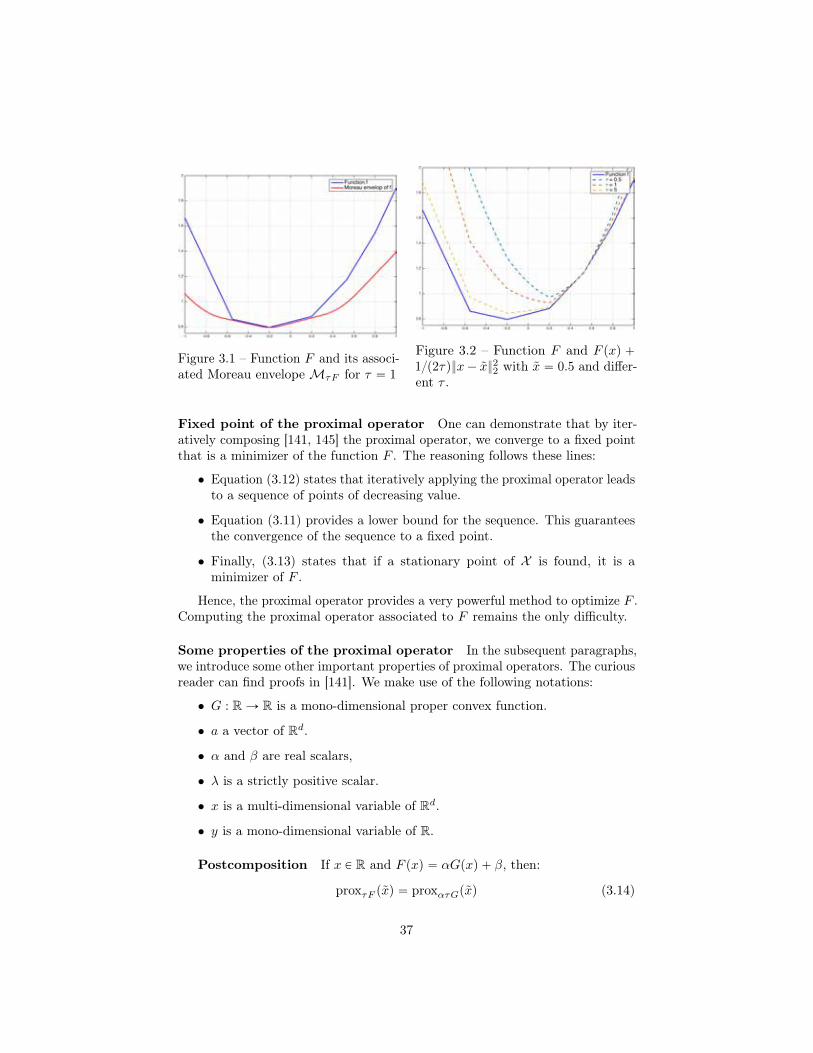
Figure 3.1 – Function F and its associ-ated Moreau envelopeMτF for τ “ 1
Figure 3.2 – Function F and F pxq `1p2τqx´ x22 with x “ 0.5 and differ-ent τ .
Fixed point of the proximal operator One can demonstrate that by iter-atively composing [141, 145] the proximal operator, we converge to a fixed pointthat is a minimizer of the function F . The reasoning follows these lines:
• Equation (3.12) states that iteratively applying the proximal operator leadsto a sequence of points of decreasing value.
• Equation (3.11) provides a lower bound for the sequence. This guaranteesthe convergence of the sequence to a fixed point.
• Finally, (3.13) states that if a stationary point of X is found, it is aminimizer of F .
Hence, the proximal operator provides a very powerful method to optimize F .Computing the proximal operator associated to F remains the only difficulty.
Some properties of the proximal operator In the subsequent paragraphs,we introduce some other important properties of proximal operators. The curiousreader can find proofs in [141]. We make use of the following notations:
• G : RÑ R is a mono-dimensional proper convex function.
• a a vector of Rd.
• α and β are real scalars,
• λ is a strictly positive scalar.
• x is a multi-dimensional variable of Rd.
• y is a mono-dimensional variable of R.
Postcomposition If x P R and F pxq “ αGpxq ` β, then:
proxτF pxq “ proxατGpxq (3.14)
37

Figure 3.3 – Level set of a non smoothfunction. Alternating optimizationmethods ala Gauss Seidel can get stuckin acute corners.
Figure 3.4 – Smoothing of previouslevel sets. The corners have been re-moved but the level sets are impacted.
Affine addition If x P R and F pxq “ Gpxq ` αx` β, then:
proxτF pxq “ proxτGpx´ ταq (3.15)
This property is very handy for the primal dual algorithm.
Affine reduction If F pxq “ GpaTx` βq, then:
proxτF pxq “ proxτGpaT x` βqa (3.16)
with τ “ τaTa.This property is instrumental in computing the proximal operator for 2D
and 3D registration problems.
Sum of functions The proximal operator is not a linear operator. Conse-quently, calculating the proximal operator of the sum of functions is generallycomputationally expensive even if the proximal operator of each function com-posing the sum is simple. However, in the latter case, one can take advantageof the ADMM technique to compute the proximal operator by formulating theoptimization as a consensus problem [14]
3.3.2 Decoupling: Fenchel transformThe coupling issue Another difficulty of our optimization problem (3.7) isthe coupling of variables pxiq due to the linear operator L and the function R.Combined to the eventual non smoothness of R, this imposes to optimize allvariables xi jointly. The figure (3.3) illustrates the problem.
One solution is to smooth the objective function R to make corners disappear.However, this changes the objective function as seen in figure 3.4 which might
38
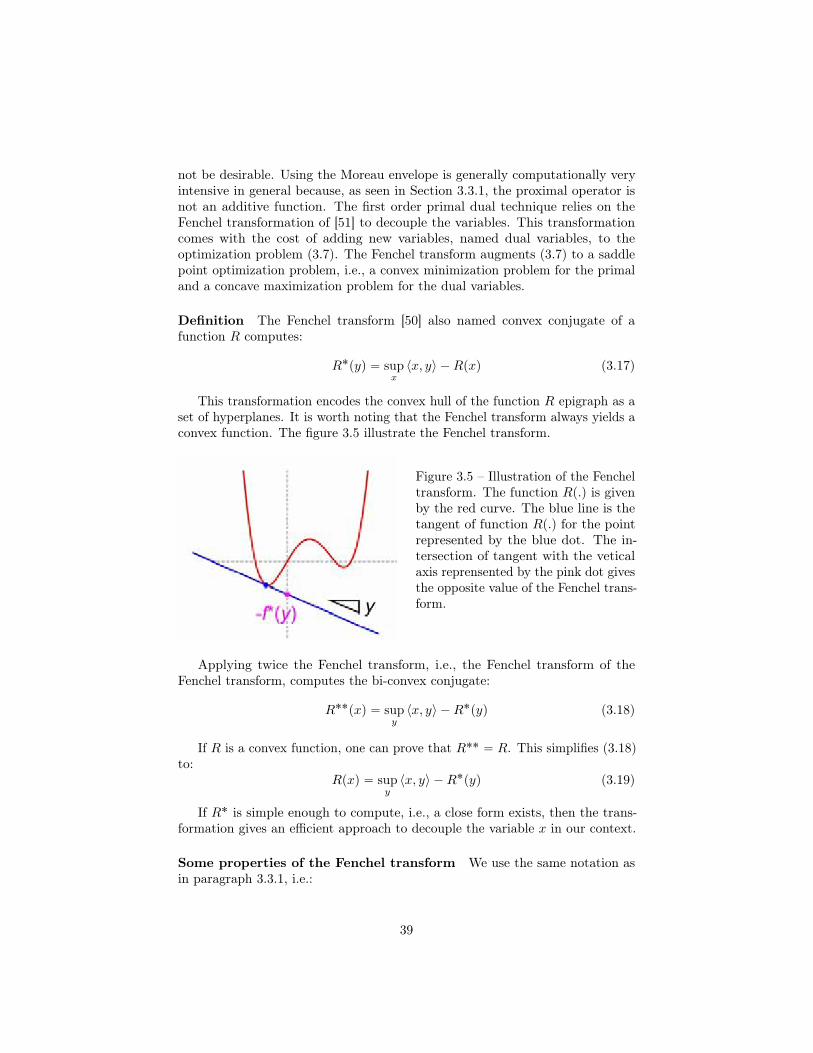
not be desirable. Using the Moreau envelope is generally computationally veryintensive in general because, as seen in Section 3.3.1, the proximal operator isnot an additive function. The first order primal dual technique relies on theFenchel transformation of [51] to decouple the variables. This transformationcomes with the cost of adding new variables, named dual variables, to theoptimization problem (3.7). The Fenchel transform augments (3.7) to a saddlepoint optimization problem, i.e., a convex minimization problem for the primaland a concave maximization problem for the dual variables.
Definition The Fenchel transform [50] also named convex conjugate of afunction R computes:
R˚pyq “ supx〈x, y〉´Rpxq (3.17)
This transformation encodes the convex hull of the function R epigraph as aset of hyperplanes. It is worth noting that the Fenchel transform always yields aconvex function. The figure 3.5 illustrate the Fenchel transform.
Figure 3.5 – Illustration of the Fencheltransform. The function Rp.q is givenby the red curve. The blue line is thetangent of function Rp.q for the pointrepresented by the blue dot. The in-tersection of tangent with the veticalaxis reprensented by the pink dot givesthe opposite value of the Fenchel trans-form.
Applying twice the Fenchel transform, i.e., the Fenchel transform of theFenchel transform, computes the bi-convex conjugate:
R˚˚pxq “ supy〈x, y〉´R˚pyq (3.18)
If R is a convex function, one can prove that R˚˚ “ R. This simplifies (3.18)to:
Rpxq “ supy〈x, y〉´R˚pyq (3.19)
If R˚ is simple enough to compute, i.e., a close form exists, then the trans-formation gives an efficient approach to decouple the variable x in our context.
Some properties of the Fenchel transform We use the same notation asin paragraph 3.3.1, i.e.:
39
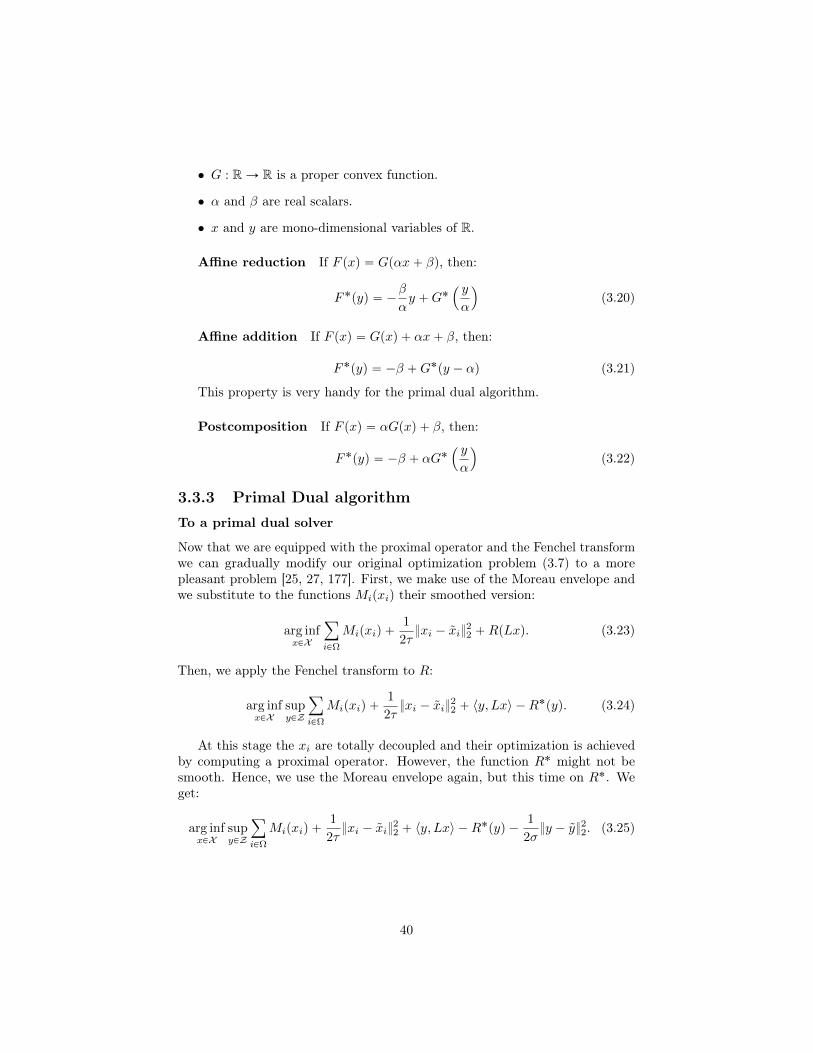
• G : RÑ R is a proper convex function.
• α and β are real scalars.
• x and y are mono-dimensional variables of R.
Affine reduction If F pxq “ Gpαx` βq, then:
F˚pyq “ ´β
αy `G˚
´ y
α
¯
(3.20)
Affine addition If F pxq “ Gpxq ` αx` β, then:
F˚pyq “ ´β `G˚py ´ αq (3.21)
This property is very handy for the primal dual algorithm.
Postcomposition If F pxq “ αGpxq ` β, then:
F˚pyq “ ´β ` αG˚´ y
α
¯
(3.22)
3.3.3 Primal Dual algorithmTo a primal dual solver
Now that we are equipped with the proximal operator and the Fenchel transformwe can gradually modify our original optimization problem (3.7) to a morepleasant problem [25, 27, 177]. First, we make use of the Moreau envelope andwe substitute to the functions Mipxiq their smoothed version:
arg infxPX
ÿ
iPΩ
Mipxiq `1
2τxi ´ xi
22 `RpLxq. (3.23)
Then, we apply the Fenchel transform to R:
arg infxPX
supyPZ
ÿ
iPΩ
Mipxiq `1
2τxi ´ xi
22 ` 〈y, Lx〉´R˚pyq. (3.24)
At this stage the xi are totally decoupled and their optimization is achievedby computing a proximal operator. However, the function R˚ might not besmooth. Hence, we use the Moreau envelope again, but this time on R˚. Weget:
arg infxPX
supyPZ
ÿ
iPΩ
Mipxiq `1
2τxi ´ xi
22 ` 〈y, Lx〉´R˚pyq ´
1
2σy ´ y22. (3.25)
40
Writing x and y as time series pxnqn and pynqn, we obtain for each time stepn:
arg infxnPX
supynPY
ÿ
iPΩ
Mipxni q`
1
2τxni ´x
n´1i 22`〈yn, Lxn〉´R˚pynq´
1
2σyn´yn´122.
(3.26)For all time steps, the problem (3.24) is convex with respect to xn and
concave with respect to yn. The two series converge to a fixed saddle point.Moreover, we can carry the optimization by alternating on xn and yn since thefunctional is now smooth.
One last trick, that we do not develop in this document is the smoothingof the sequence xn. When optimizing with respect to yn, we substitute xnby xn “ xn ` θpxn ´ xn´1q with θ P r0, 1s. This trick greatly improves theconvergence rate in general.
Hypothesis for convergence and convergence rate
As the first order primal dual optimization algorithm is iterative, we need topay a particular attention to the values of τ and σ to ensure its convergence[27]. As illustrated by figure 3.1, τ and σ control the step size of primal anddual variables updates. While smaller steps slow down the convergence, toolarge steps make the algorithm unstable, leading to a possible divergence of thesequences pxnq and pynq. We notice that at each iteration xn and yn exchangeinformation through an interface expressed as the linear operator L. Hence, thenature of L plays a critical role on the range of τ and σ.
In our context, the linear operator L is generally the weighted gradient(possibly oriented and non local) or the laplacian operator. Hence, the value ofL can easily be precomputed or closely upper-bounded.
The Algorithm 1 can be slightly modified to make use of strong convexity toachieve Op1N2q and even Op1eN q convergence rate. We refer the reader toAlgorithms 2 and 3 in [27] for more details.
Algorithm description for non smooth problems
When neither the sum of pMiqi nor R is smooth, we make use of the generalfirst order primal dual algorithm:
It was proved in [27] that to guarantee convergence τ and σ have to satisfythe following inequality:
τσL ă 1 (3.30)
with:L “ maxtLx : x P X with x ď 1u (3.31)
It has been demonstrated in [27] that the Algorithm 1 converges to an optimalprimal-dual saddle point in Op1Nq. This convergence rate is optimal for firstorder algorithm and non smooth function [131].
41

Algorithm 1: First order primal dual algorithmData: Inputs: pMiqi, R, LResult: xCompute the Fenchel transform: Ñ R˚.Initialize primal and dual variable Ñ x0 “ 0, y0 “ 0.Set x “ x0
while Stopping criterion is not verified doOptimize the dual variables:
yn`1 “ proxσp〈y,Lx〉´R˚pynqqpynq (3.27)
Optimize the primal variables:
xn`1 “ proxτpřiPΩ Mipxiq`〈LT yn,x〉qpxnq (3.28)
Smooth variable:x “ xn`1 ` θ
`
xn`1 ´ xn˘
(3.29)
Algorithm description for half-uniformly convex problems
If the sum of pMiqi or R˚ is uniformly convex, we can make use of an acceleratedalgorithm. For simplicity we assume that the sum of pMiqi is γ-uniformly convexfunction.
It was proved in [27] that to guarantee convergence τ0 and σ0 have to satisfythe following inequality:
τ0σ0L ă 1 (3.36)
It has been demonstrated in [27] that Algorithm 2 converges to an optimalprimal-dual saddle point in Op1N2q. This convergence rate is optimal for firstorder algorithm and uniformly convex problem with respect to either the primalor dual variables [131].
Algorithm description for uniformly convex problems
It was proved in [27] that Algorithm 3 converges if µ satisfies the followinginequality:
µ ď 2
?γδ
L(3.41)
It has been demonstrated in [27] that Algorithm 3 converges to an optimalprimal-dual saddle point in Op1eN q. This convergence rate is optimal for firstorder algorithm and uniformly convex problem [131].
42

Algorithm 2: First order primal dual algorithm for half smooth problemData: Inputs: pMiqi, R, L, τ , σResult: xCompute the Fenchel transform: Ñ R˚.Initialize primal and dual variable Ñ x0 “ 0, y0 “ 0.Set x “ x0
while Stopping criterion is not verified doOptimize the dual variables:
yn`1 “ proxσnp〈y,Lx〉´R˚pynqqpynq (3.32)
Optimize the primal variables:
xn`1 “ proxτnpřiPΩ Mipxiq`〈LT yn,x〉qpxnq (3.33)
Update the smoothing and steps size parameters:
θn “1
?1` 2γτn
, τn`1 “ θnτn, σn`1 “σnθn
(3.34)
Smooth variable:
x “ xn`1 ` θn`
xn`1 ´ xn˘
(3.35)
43
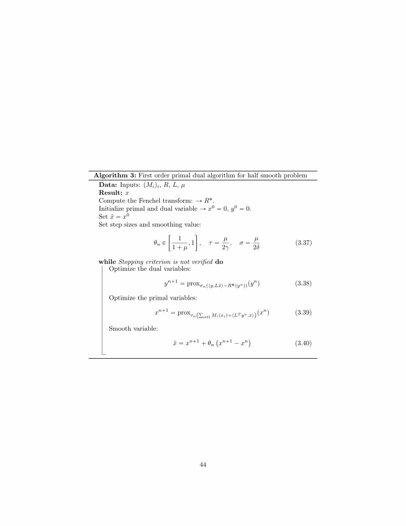
Algorithm 3: First order primal dual algorithm for half smooth problemData: Inputs: pMiqi, R, L, µResult: xCompute the Fenchel transform: Ñ R˚.Initialize primal and dual variable Ñ x0 “ 0, y0 “ 0.Set x “ x0
Set step sizes and smoothing value:
θn P
„
1
1` µ, 1
, τ “µ
2γ, σ “
µ
2δ(3.37)
while Stopping criterion is not verified doOptimize the dual variables:
yn`1 “ proxσnp〈y,Lx〉´R˚pynqqpynq (3.38)
Optimize the primal variables:
xn`1 “ proxτnpřiPΩ Mipxiq`〈LT yn,x〉qpxnq (3.39)
Smooth variable:
x “ xn`1 ` θn`
xn`1 ´ xn˘
(3.40)
44

3.3.4 Conditioning and Auto tuning of step sizesImproving conditioning
The convergence speed of Algorithm 1 is tightly linked to the conditioning of thelinear operator L since its norm impacts the step size parameters τ and σ. Wecan always make one of τ or σ larger, but this comes at the expense of reducingthe other. Hence, improving the conditioning of L is critical.
Fortunately, conditioning improvement has been studied for a long time andsuccessfully applied to primal dual problems [143, 162]. In our context, we onlyinvestigate the simple case where the operator L can be written as a diagonalmatrix D with strictly positive elements and a well conditioned linear operator G:
L “ DG (3.42)
Here, the diagonal matrix D deteriorates the condition number of G, leadingto the badly conditioned operator L. However, by applying a simple change ofvariable in the functional to optimize we can recover a well conditioned problem.By defining, y “ D´1z, we transform (3.26) to:
arg minxnPX
maxznPDY
ÿ
iPΩ
Mipxni q `
1
2τxni ´ x
n´1i 22 ` 〈zn, Gxn〉
´R˚pD´1znq ´1
2σD´1pzn ´ zn´1q22.
(3.43)
Hence, we can now have larger step sizes τ and σ. Moreover, the overall problemretains the same complexity since the computation of proximal operators arenot made more complicated by linear scaling.
If necessary, the same transformation can be applied to primal variables x.We refer the curious reader to [143].
Auto tuning of step sizes and stopping criterion
At this stage, defining correctly the step sizes τ and σ remains of criticalimportance to obtain a fast convergence. As a rule of thumb, we want thealgorithm to make as much progress in the primal space as it does in the dualspace. We can measure such progress by tracking the primal and dual residuals.If the primal residual is large compared to the dual residual, then we want tomake more progress in the primal space at the next iteration. To this end, weneed to increase τ . An analogue reasoning stands if the dual residual is largerthan the primal residual. If both residuals are roughly equally large, then weare on course and no update of τ or σ is necessary.
Hence, we now make use of sequences pτnqn and pσnqn to describe theevolution of τ and σ through time. Moreover, it has been demonstrated in [65]that the convergence of algorithm 1 is achieved only if the sequences pτnqn and
45

pσnqn also converge. To this end, we introduce another sequence pαnqn thatstrictly decreases over time and controls how much pτnqn and pσnqn are updated.
The primal residual of (3.26) is defined as:
pn`1 “1
τnpxn ´ xn`1q ´ LT pyn ´ yn`1q (3.44)
Similarly, the dual residual of (3.26) is defined as:
dn`1 “1
σnpyn ´ yn`1q ´ Lpxn ´ xn`1q (3.45)
Algorithm 4 describes the update rules for pτnqn and pσnqn.
Algorithm 4: Auto tuning of step sizesData: Inputs: pn`1, dn`1, τn, σn, αn, ηResult: τn`1, σn`1, αn`1
if ρpn`1 ă dn`1 thenWe need to increase dual variables convergence speed:
τn`1 “ τnp1´ αnq, σn`1 “σn
1´ αn, αn`1 “ ηαn (3.46)
else if ρdn`1 ă pn`1 thenWe need to increase primal variables convergence speed:
τn`1 “τn
1´ αn, σn`1 “ σnp1´ αnq, αn`1 “ ηαn (3.47)
else
τn`1 “ τn, σn`1 “ σn, αn`1 “ αn (3.48)
With:
• ρ is a parameter in r1,`8q controlling when a correction needs to beapplied.
• η is a parameter in r0, 1q enforcing the convergence of the sequences pαnqn,pτnqn and pσnqn.
3.4 Reformulating `1 based functions, Proximaloperators, and Fenchel transformations
Before diving in the computations of proximal operators and Fenchel transforms,we introduce an important reformulation of `1 based functions.
46

3.4.1 On reformulating `1 based functionsReformulation formula
We assume we are given an `1 based function f : R Ñ R parametrized bypw´, w`q P Rˆ R of the following prototype:
fpxq “ w´maxp´x, 0q ` w`maxpx, 0q. (3.49)
We show that for any a P R we can reformulate the equation as
fpxq “`
w´ ´ a˘
maxp´x, 0q ``
w` ` a˘
maxpx, 0q ´ ax (3.50)
The proof follows from:
ax “ a pminpx, 0q `maxpx, 0qq , (3.51)ax “ ´amaxp´x, 0q ` amaxpx, 0q, (3.52)
0 “ ´amaxp´x, 0q ` amaxpx, 0q ´ ax. (3.53)
By adding (3.53) to (3.49) and rearranging terms, we obtain (3.50), thus,completing the proof.
Some examples of reformulations
Using (3.50) we can transform fp.q to a symmetric function plus a linear termby choosing:
a “w´ ´ w`
2(3.54)
fpxq “w` ` w´
2maxp´x, 0q `
w` ` w´
2maxpx, 0q `
w` ´ w´
2x (3.55)
“w` ` w´
2|x| `
w` ´ w´
2x (3.56)
We can also transform fp.q to half linear term and a linear term by choosingeither:
a “ w´ (3.57)
fpxq “`
w´ ´ w´˘
maxp´x, 0q ``
w` ` w´˘
maxpx, 0q ´ w´x (3.58)
“`
w` ` w´˘
maxpx, 0q ´ w´x (3.59)
or:
a “ ´w` (3.60)
fpxq “`
w´ ` w`˘
maxp´x, 0q ``
w` ´ w`˘
maxpx, 0q ` w`x (3.61)
“`
w` ` w´˘
maxp´x, 0q ` w`x (3.62)
We illustrate these three reformulations in figure 3.6.
47

Figure 3.6 – Example of a reformulations of the same function: left is a symmetricreformulation, center is a half negative reformulation, and right is a half positivereformulation.
3.4.2 Proximal operatorsWe present here some useful proximal operators.
Asymmetric `1
The asymmetric `1 function illustrated in figure 3.7 has the following prototype:
F pxq “
#
´w´x if x ă 0
w`x if x ě 0(3.63)
“ w´maxp´x, 0q ` w`maxpx, 0q (3.64)
with pw´, w`q P Rˆ R and w´ ` w` ě 0 to ensure convexity.
Figure 3.7 – Various instances of asym-metric `1 functions
The proximal operator associated to the asymmetric `1 function is:
proxF,τ pxq “
$
&
%
x` τw´ if x ă ´τw´
0 if x P r´τw´, τw`sx´ τw` if x ą `τw`
(3.65)
One can recognize in (3.65) a generalization of the soft-thresholding operator.
48

Sum of asymmetric `1
We now examine a function F , illustrated in figure 3.8, of the following prototype:
F pxq “Nÿ
i“1
w´i maxp´x` bi, 0q ` w`i maxpx´ bi, 0q (3.66)
where each pair of pw´i , w`i q P Rˆ R verifies w´i ` w
`i ě 0 and each bi P R.
Figure 3.8 – The function F , a sumof asymmetric `1 functions. Each seg-ments composing F is plotted in a dif-ferent color.
Figure 3.9 – The function P that needsto be minimized to obtain the proximaloperator of function F with x “ 0.7and τ “ 0.1
Without any loss of generality we reformulate F as a sum of half linear termsusing example from (3.59):
F pxq “ c` ax`Nÿ
i“1
wi maxpx´ bi, 0q (3.67)
with: c “řNi“1 w
´i bi, a “
řNi“1 w
´i and, each wi “ w`i ` w
´i
To compute the proximal operator we need to minimize the following functionillustrated in figure 3.9:
P pxq “ F pxq `1
2τpx´ xq2 (3.68)
“
Nÿ
i“1
wi maxpx´ bi, 0q `1
2τpx´ px´ τaqq
2` constant (3.69)
“
Nÿ
i“1
wi maxpx´ bi, 0q `Gpxq (3.70)
with τ P R` and x P R.
49

The function F is a piecewise linear function composed of N ` 1 segmentsas illustrated in figure 3.8. Since P is a convex function, its derivative is amonotonic increasing function. Hence, by identifying a segment that has anegative gradient at one hand and a positive derivative at the other hand wehave found that an interval that contains the minimizer of P . Finally, over thisinterval the function P is purely quadratic. Hence, computing the minimumis then trivial. We describe this procedure in algorithm 5. One can obtain asimpler algorithm if the tbiuiPt1,...,Nu are given sorted.
Asymmetric Huber
The asymmetric Huber illustrated in figure 3.10 naturally extends both Huberand `1 norms, and it remains a convex function:
F pxq “
$
’
’
’
&
’
’
’
%
´apx` α2q if x ă ´αax2p2αq if x P r´α, 0sbx2p2βq if x P p0, βsbpx´ β2q if x ą β
(3.72)
with α, β, a and b all positive real scalars.The proximal operator associated to the asymmetric Huber function is:
proxF,τ pxq “
$
’
’
&
’
’
%
x` τa if x ă ´α´ τa´αxpα` τaq if x P r´α´ τa, 0s´βxpβ ` τbq if x P p0, β ` τbs
x´ τb if x ą β ` τb
(3.73)
Figure 3.10 – Various instances ofasymmetric Huber functions
Convex second order form
Another very interesting class of functions with simple proximal operator arethe convex quadratic functions:
F pxq “ xTHx` aTx` c, (3.74)
50

Algorithm 5: Computation of proximal operator for piecewise linearfunctionsData: Inputs: tbiuiPt1,...,Nu, twiuiPt1,...,Nu, G, and xResult: x˚
Initialize variables:x “ x,l “ minpdompF qq, u “ minpdompF qq,wcur “ 0, Σw “ 0.B “ tbiui, W “ twiui,
for i P t1, ..., Nu do
if Σw ` wcur `dG
dxpuq ą 0 then
Exit for loopelse
Get bounds of next segment:lÐ uj Ð indice of minimun element of BuÐ Brjs
Update gradient:Σw Ð Σw ` wcurwcur “W rjs
Update B and W:B Ð B ´BrjsW ÐW ´W rjs
if i ““ N thenGet bounds of last segment:lÐ uuÐ `8
Σw Ð Σw ` wcur
Find minimizer on found segment:
x˚ “ arg minrl,us
Σw `Gpxq (3.71)
return x˚
51

with H a semi-definite positive matrix to ensure convexity.Their proximal operator is given by:
proxτF pxq “ pI ` τHq´1px´ τaq (3.75)
Note that evaluating the proximal operator relies on computing the inverseof I` τH. If H is diagonal, then evaluating this proximal operator is trivial. Forothers cases, we can rely on computing once and caching the inverse of operatorpI ` τHq.
Localization technique for complicated mono-dimensional variable
When F is a complicated function of a mono-dimensional variable, one canapply the localization technique [16] that iteratively reduces the search space ofthe minimum. This technique shares similarity with the bisection method butyields faster convergence by integrating topological information provided by thesub-gradients of the proximal function.
At each iteration, the localization technique defines a search direction bycomputing g, an element of the sub-derivative of the proximal function at currentpoint x. Hence, any point situated in the opposite direction can be removed fromthe search space since the function to optimize is convex. Using the monotonicityof the sub-derivative of the proximal operator we can demonstrate that theminimum cannot be further to the current point x than |τg|. Hence, this givesus another bound to truncate the search space. Finally, we move x to the middleof the search space and iterate as illustrated in figure 3.11.
The range of the search space gives us an upper bound on the precision of xwith respect to optimality. We can stop the algorithm iterations when a desiredprecision of ε has been reached. The algorithm 6 describes the localizationprocedure illustrated by figure 3.11.
This technique is a special case of the cutting plane algorithm. One caneasily apply cutting plane to a multi-dimensional variable but the computationalcomplexity becomes greatly increased.
Figure 3.11 – The doted segments showthe trajectory followed by x to computethe minimizer of F pxq`1p2τqx´x22splotted as a red curve.
52

Algorithm 6: Localization techniqueData: Inputs: F , x, τ and εResult: xInitialize variables:
x “ x, l “ minpdompF qq, u “ maxpdompF qq (3.76)
while u´ l ě ε doCompute an element of the sub-gradient of F at point x:
h PBF
Bx(3.77)
Compute an element of the sub-gradient of the proximal function:
g “ h`1
τpx´ xq (3.78)
if g ą 0 then
l “ maxpl, x´ τgq, u “ minpu, xq (3.79)
else if g ă 0 then
l “ maxpl, xq, u “ minpu, x´ τgq (3.80)
Update position of x:
x “l ` u
2(3.81)
53
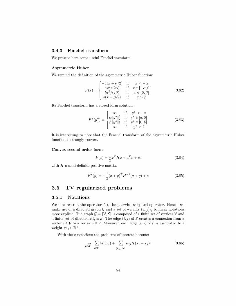
3.4.3 Fenchel transformWe present here some useful Fenchel transform.
Asymmetric Huber
We remind the definition of the asymmetric Huber function:
F pxq “
$
’
’
&
’
’
%
´apx` α2q if x ă ´αax2p2αq if x P r´α, 0sbx2p2βq if x P p0, βsbpx´ β2q if x ą β
(3.82)
Its Fenchel transform has a closed form solution:
F˚py˚q “
$
’
’
&
’
’
%
8 if y˚ ă ´aαy˚22 if y˚ P ra, 0sβy˚22 if y˚ P r0, bs8 if y˚ ą b
(3.83)
It is interesting to note that the Fenchel transform of the asymmetric Huberfunction is strongly convex.
Convex second order form
F pxq “1
2xTHx` aTx` c, (3.84)
with H a semi-definite positive matrix.
F˚pyq “ ´1
2pa` yqTH´1pa` yq ` c (3.85)
3.5 TV regularized problems
3.5.1 NotationsWe now restrict the operator L to be pairwise weighted operator. Hence, wemake use of a directed graph G and a set of weights twijuij to make notationsmore explicit. The graph G “ rV, Es is composed of a finite set of vertices V anda finite set of directed edges E . The edge pi, jq of E creates a connexion from avertex i P V to a vertex j P V. Moreover, each edge pi, jq of E is associated to aweight wij P R`.
With these notations the problems of interest become:
minxPX
ÿ
iPVMipxiq `
ÿ
pi,jqPEwijR pxi ´ xjq . (3.86)
54
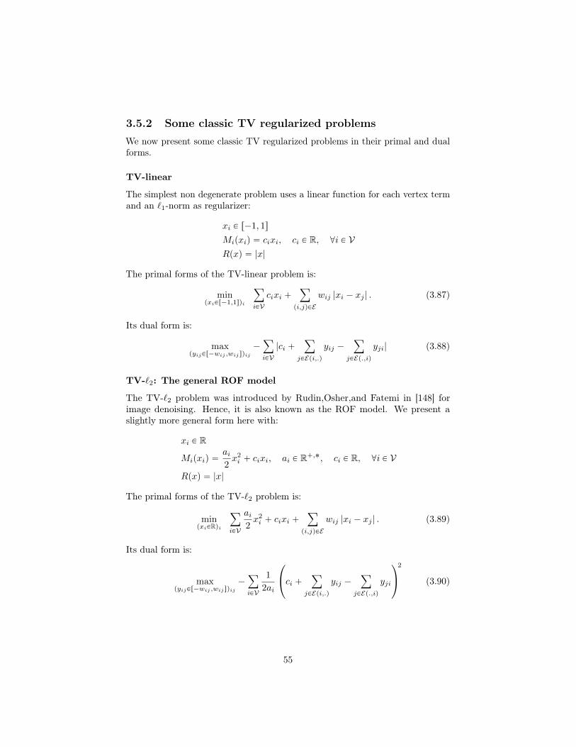
3.5.2 Some classic TV regularized problemsWe now present some classic TV regularized problems in their primal and dualforms.
TV-linear
The simplest non degenerate problem uses a linear function for each vertex termand an `1-norm as regularizer:
xi P r´1, 1s
Mipxiq “ cixi, ci P R, @i P VRpxq “ |x|
The primal forms of the TV-linear problem is:
minpxiPr´1,1sqi
ÿ
iPVcixi `
ÿ
pi,jqPEwij |xi ´ xj | . (3.87)
Its dual form is:
maxpyijPr´wij ,wijsqij
´ÿ
iPV|ci `
ÿ
jPEpi,.q
yij ´ÿ
jPEp.,iq
yji| (3.88)
TV-`2: The general ROF model
The TV-`2 problem was introduced by Rudin,Osher,and Fatemi in [148] forimage denoising. Hence, it is also known as the ROF model. We present aslightly more general form here with:
xi P R
Mipxiq “ai2x2i ` cixi, ai P R`,˚, ci P R, @i P V
Rpxq “ |x|
The primal forms of the TV-`2 problem is:
minpxiPRqi
ÿ
iPV
ai2x2i ` cixi `
ÿ
pi,jqPEwij |xi ´ xj | . (3.89)
Its dual form is:
maxpyijPr´wij ,wijsqij
´ÿ
iPV
1
2ai
¨
˝ci `ÿ
jPEpi,.q
yij ´ÿ
jPEp.,iq
yji
˛
‚
2
(3.90)
55

TV-`1
The famous TV-`1 improves the ROF model by making the vertices terms lesssensitive to outliers:
xi P RMipxiq “ ai|x` ci|, ai P R`,˚, ci P R, @i P VRpxq “ |x|
The primal form of the TV-`1 problem is:
minpxiPRqi
ÿ
iPVai|xi ` ci| `
ÿ
pi,jqPEwij |xi ´ xj | . (3.91)
Its dual form is (up to a constant term):
maxpyijPr´wij ,wijsqij
´ÿ
iPVci
¨
˝
ÿ
jPEpi,.q
yij ´ÿ
jPEp.,iq
yji
˛
‚
subject to.
ˇ
ˇ
ˇ
ˇ
ˇ
ˇ
ÿ
jPEpi,.q
yij ´ÿ
jPEp.,iq
yji
ˇ
ˇ
ˇ
ˇ
ˇ
ˇ
ď ai @i P V
(3.92)
TV-Huber
The TV-Huber model smoothes the TV-`1 vertices and edges terms:
xi P RMipxiq “ ai|x` ci|α, ai P R`,˚, ci P R, α P R`, @i P VRpxq “ |x|β β P R`
where |.|β is the symmetric Huber norm defined by (3.72) with smoothingparameter β.
The primal forms of the TV-Huber problem is:
minpxiPRqi
ÿ
iPVai|xi ` ci|α `
ÿ
pi,jqPEwij |xi ´ xj |β . (3.93)
Its dual form is (up to a constant term):
maxpyijPr´wij ,wijsqij
´α
2
ÿ
iPV
¨
˝
ciα`
ÿ
jPEpi,.q
yij ´ÿ
jPEp.,iq
yji
˛
‚
2
´β
2
ÿ
pi,jqPE
y2ij
subject to.
ˇ
ˇ
ˇ
ˇ
ˇ
ˇ
ÿ
jPEpi,.q
yij ´ÿ
jPEp.,iq
yji
ˇ
ˇ
ˇ
ˇ
ˇ
ˇ
ď ai @i P V
(3.94)
56

3.5.3 Truncation theorem for convex TV regularized prob-lems
Theorem 3. Truncation theorem for TV regularized problemsWe suppose we have solved the following problem:
pz˚i qi “ arg minpziPrα,βsqi
ÿ
iPVfipziq `
ÿ
pi,jqPEwij max pzi ´ zj , 0q . (3.95)
where:
• α P ´8Y R, β P RY`8, and α ď β,
• The function fi : RÑ R is a proper, l.s.c convex function @i P V.
For all ra, bs Ď rα, βs, the following problem shares a special relationship with(3.95):
zti “ arg minpziPra,bsqi
ÿ
iPVfipziq `
ÿ
pi,jqPEwij max pzi ´ zj , 0q . (3.96)
Indeed, a solution of (3.96) is simply the truncation of a solution of (3.95):
zti “`
rz˚i sra,bs˘
i, @i P V (3.97)
where r.sra,bs is the truncation operator:
rxsra,bs “
$
&
%
a if x ď ax if x P ra, bsb if x ě b
(3.98)
Lemma 1. Let py˚ijqij the optimal dual variables of the dual problem associatedto (3.95). Then, py˚ijqij are also optimal for the dual problem associated to(3.96).
Proof
The demonstration relies on the proof that a primal dual fixed point of equation(3.96) is obtained from a primal-dual fixed point of equation (3.95).
We first express the primal dual problems of equation (3.95):
pz˚i qi, py˚ijqij “ arg min
pziPrα,βsqimax
pyijPr0,wijsqij
ÿ
iPVfipziq `
ÿ
pi,jqPEyij pzi ´ zjq .
(3.99)and equation (3.96):
pztiqi, pytijqij “ arg min
pziPra,bsqimax
pyijPr0,wijsqij
ÿ
iPVfipziq `
ÿ
pi,jqPEyij pzi ´ zjq .
(3.100)
57

We initialize the variables of problem (3.100) to:
zi “ rz˚i sra,bs, @i P Vyij “ y˚ij @ pi, jq P E
(3.101)
We show that the optimal dual variables of (3.99) are also optimal dualvariables for (3.100). Using the dual update rule of the primal-dual algorithm 1we have @ pi, jq P E :
ynij ““
y˚ij ` σ`
rz˚i sra,bs ´ rz˚j sra,bs
˘‰
r0,wijs(3.102)
Supposing that z˚i ´ z˚j ą 0 we have:
rz˚i sra,bs ´ rz˚j sra,bs ě 0
y˚ij “ wij(3.103)
Hence, we obtain:ynij “ wij
“ y˚ij(3.104)
The same reasoning holds for z˚i ´ z˚j ă 0:
ynij “ 0
“ y˚ij(3.105)
Finally, if z˚i ´ z˚j “ 0, we trivially obtain:
ynij “ y˚ij (3.106)
Hence, the dual variables py˚ijqij are fixed points of the equation (3.100).
We now look at the primal variables. Using the primal update rules ofalgorithm 1 we have:
zni “ arg minxiPra,bs
fipxiq ` xi
˜
ÿ
j
y˚ij ´ y˚ji
¸
`1
2τrz˚i sra,bs ´ xi
22
“
«
arg minxiPR
fipxiq ` xi
˜
ÿ
j
y˚ij ´ y˚ji
¸
`1
2τrz˚i sra,bs ´ xi
22
ff
ra,bs
“ rz˚i sra,bs
(3.107)
The second equality holds since we are optimizing a mono dimensional convexfunction. Hence, the primal variables prz˚i sra,bsqi are fixed points of the equation(3.100).
This completes the proof.
58

3.5.4 A hierarchy of optimal dual spaces for TV-`2Theorem 4. Let Y˚`2 be the space of optimal solutions for equation:
maxyijPrw
´ij ,w
`ijs
´ÿ
iPV
1
2aici `
ÿ
jPEpi,.q
fij ´ÿ
jPEp.,iq
fji22, (3.108)
and let Y˚α be the space of optimal solutions for equation:
maxyijPrw
´ij ,w
`ijs
´ÿ
iPV
1
2ai
ˇ
ˇ
ˇ
ˇ
ˇ
ˇ
ci `ÿ
jPEpi,.q
fij ´ÿ
jPEp.,iq
fji
ˇ
ˇ
ˇ
ˇ
ˇ
ˇ
α
(3.109)
Then, for any pα, βq P R` ˆ R` and α ě β we have:
Y˚`2 Ď Y˚α Ď Y˚β Ď Y˚0 “ Y˚`1 (3.110)
Proof
We recognize that (3.108) solves the dual of the general ROF model. Theproblem solved by (3.109) is simply the general ROF model with additional boxconstraints of the form xi P r´α, αs:
minpxiPr´α,αsqi
ÿ
iPV
ai2x2i ` cixi `
ÿ
pi,jqPEwij |xi ´ xj | .
minpxiPr´α,αsqi
maxpyijPr´wij ,wijsqij
ÿ
iPV
ai2x2i ` xi
¨
˝ci `ÿ
jPEpi,.q
yij ´ÿ
jPEp.,iq
yji
˛
‚
maxpyijPr´wij ,wijsqij
´ÿ
iPV
1
2ai
ˇ
ˇ
ˇ
ˇ
ˇ
ˇ
ci `ÿ
jPEpi,.q
yij ´ÿ
jPEp.,iq
yji
ˇ
ˇ
ˇ
ˇ
ˇ
ˇ
α
To obtain the last equation, we simply recognize the equation of the Fencheltransform for a Huber function with smoothness α .
The proof is a simple application of the lemma of the truncation theorem.Indeed the lemma states that the optimal dual variables of the less constrainedproblem are also optimal for the more constrained problem. This concludes theproof.
3.5.5 Intersection of optimal dual spaceTheorem 5. Let Y˚`2 be the space of optimal solutions for:
maxyijPrw
´ij ,w
`ijs
´ÿ
iPV
1
2aici `
ÿ
jPEpi,.q
yij ´ÿ
jPEp.,iq
yji22 (3.111)
59

and λ be a real valued scalar and Y˚`1,λ be the space of optimal solution for:
maxyij“rw
´ij ,w
`ijs
´ÿ
iPV
1
2ai
ˇ
ˇ
ˇ
ˇ
ˇ
ˇ
ci ` λai `ÿ
jPEpi,.q
yij ´ÿ
jPEp.,iq
yji
ˇ
ˇ
ˇ
ˇ
ˇ
ˇ
(3.112)
ThenY˚`2 “
č
λPRY˚`1,λ (3.113)
First lemma
We demonstrate a first intermediate result:
Lemma 2. Let α be a real valued scalar and Y˚`2,α be the space of optimalsolution for:
arg maxyij“rw
´ij ,w
`ijs
´ÿ
iPV
1
2aici ` αai `
ÿ
jPEpi,.q
fij ´ÿ
jPEp.,iq
fji22 (3.114)
and β be a real valued scalar and Y˚`2,β be the space of optimal solution for:
arg maxyij“rw
´ij ,w
`ijs
´ÿ
iPV
1
2aici ` βai `
ÿ
jPEpi,.q
fij ´ÿ
jPEp.,iq
fji22 (3.115)
Then,Y˚`2,α “ Y
˚`2,β
(3.116)
Proof of first Lemma
The proof of the previous lemma is straightforward:
y˚ “ arg maxyij“rw
´ij ,w
`ijs
´ÿ
iPV
1
2aici ` βai `
ÿ
jPEpi,.q
fij ´ÿ
jPEp.,iq
fji22
“ arg maxyij“rw
´ij ,w
`ijs
´ÿ
iPV
1
2aici `
ÿ
jPEpi,.q
fij ´ÿ
jPEp.,iq
fji22 ´
ÿ
iPVβ
¨
˝
ÿ
jPEpi,.q
fij ´ÿ
jPEp.,iq
fji
˛
‚
“ arg maxyij“rw
´ij ,w
`ijs
´ÿ
iPV
1
2aici `
ÿ
jPEpi,.q
fij ´ÿ
jPEp.,iq
fji22
Hence, for all couple of real scalars pα, βq we have: Y˚`2,α “ Y˚`2,0 andY˚`2,β “ Y
˚`2,0
. Therefore, we have Y˚`2,α “ Y˚`2,β
. This concludes the proof of thelemma.
60

Second lemma
We demonstrate another intermediate result:
Lemma 3. There exist a positive real scalar α such that:č
λPRY˚`1,λ “
č
λPr´α,αs
Y˚`1,λ (3.117)
Proof of Lemma
Since, a is positive vector, ci is fixed and y is bounded, we can find α P R` suchthat for a y:
ci ` αai `ÿ
jPEpi,.q
yij ´ÿ
jPEp.,iq
yji ě 0, @i P V (3.118)
andci ´ αai `
ÿ
jPEpi,.q
yij ´ÿ
jPEp.,iq
yji ď 0, @i P V (3.119)
Hence, for any λ ď ´α or λ ě α the solution space Y˚`1,λ is the space“
pyijqij | @pi, jq P E , yij P“
w´ij , w`ij
‰‰
. Therefore, we have:č
λď´α
Y˚`1,λ “ Y˚`1,´α
andč
λěα
Y˚`1,λ “ Y˚`1,α
, (3.120)
from which we easily derive the lemma.
Proof of Theorem
We start by proving Y˚`2 ĎŞ
λPR Y˚`1,λ.Thanks to theorem (4) and lemma (2) we have for all λ P R:
Y˚`2,λ Ď Y˚`1,λ
ô Y˚`2 Ď Y˚`1,λ
(3.121)
Hence, we have Y˚`2 ĎŞ
λPR Y˚`1,λ.
Let us now proveŞ
λPR Y˚`1,λ Ď Y˚`2
From the lemma (3) we get
Y˚`2 “č
λPr´α,αs
Y˚`1,λ (3.122)
Let y˚ PŞ
λPr´α,αs Y˚`1,λ. We have:
y˚ “ arg maxyij“rw
´ij ,w
`ijs
´
ż α
´α
ÿ
iPV
1
2ai|ci ` λai `
ÿ
jPEpi,.q
fij ´ÿ
jPEp.,iq
fji|dλ (3.123)
“ arg maxyij“rw
´ij ,w
`ijs
´ÿ
iPV
1
2ai
ż α
´α
|ci ` λai `ÿ
jPEpi,.q
fij ´ÿ
jPEp.,iq
fji|dλ (3.124)
61

We remind the anti-derivative formula for the absolute value:ż α
β
|λ|dλ “1
2pα|α| ´ β|β|q (3.125)
Hence, we get:
y˚ “ arg maxyij“rw
´ij ,w
`ijs
´ÿ
iPV
1
2ai
¨
˝ci ` αai `ÿ
jPEpi,.q
fij ´ÿ
jPEp.,iq
fji
˛
‚
ˆ|ci ` αai `ÿ
jPEpi,.q
fij ´ÿ
jPEp.,iq
fji|
´
¨
˝ci ´ αai `ÿ
jPEpi,.q
fij ´ÿ
jPEp.,iq
fji
˛
‚
ˆ|ci ´ αai `ÿ
jPEpi,.q
fij ´ÿ
jPEp.,iq
fji|
But since we have chosen α large enough the last equation simplifies to:
y˚ “ arg maxyij“rw
´ij ,w
`ijs
´ÿ
iPV
1
2ai
¨
˝ci ` αai `ÿ
jPEpi,.q
fij ´ÿ
jPEp.,iq
fji
˛
‚
2
`
¨
˝ci ´ αai `ÿ
jPEpi,.q
fij ´ÿ
jPEp.,iq
fji
˛
‚
2
Hence, we recognize that:
y˚ P Y˚`2,´α X Y˚`2,α
y˚ P Y˚`2The last equation stands thanks to lemma (2). Therefore we have
Ş
λPR Y˚`1,λ ĎY˚`2 which completes the proof.
3.5.6 A new primal-dual formulation of the ROF modelWe now consider optimizing the ROF model. We propose a new primal dualformulation of the ROF model that we label L-ROF for short of linear ROF:
minpxiPRqi
ÿ
iPVcixi `
ÿ
pi,jqPEwij |xi ´ xj | . (3.126)
The primal dual form of the L-ROF model is:
minxiPR
maxpyijPrw
´ij ,w
`ijsqij
´ÿ
iPVxi
¨
˝ci `ÿ
jPEpi,.q
yij ´ÿ
jPEp.,iq
yji
˛
‚ (3.127)
The following theorem achieves the connexion with the ROF model:
62
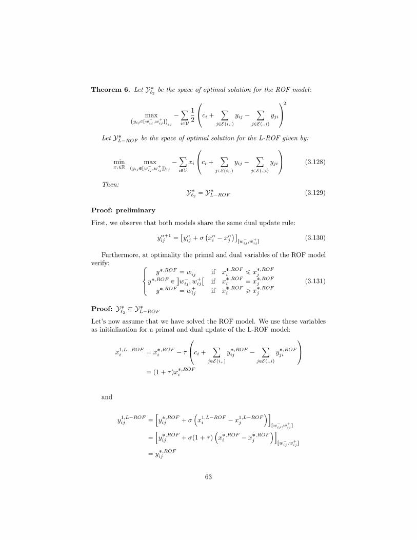
Theorem 6. Let Y˚`2 be the space of optimal solution for the ROF model:
maxpyijPrw
´ij ,w
`ijsqij
´ÿ
iPV
1
2
¨
˝ci `ÿ
jPEpi,.q
yij ´ÿ
jPEp.,iq
yji
˛
‚
2
Let Y˚L´ROF be the space of optimal solution for the L-ROF given by:
minxiPR
maxpyijPrw
´ij ,w
`ijsqij
´ÿ
iPVxi
¨
˝ci `ÿ
jPEpi,.q
yij ´ÿ
jPEp.,iq
yji
˛
‚ (3.128)
Then:Y˚`2 “ Y
˚L´ROF (3.129)
Proof: preliminary
First, we observe that both models share the same dual update rule:
yn`1ij “
“
ynij ` σ`
xni ´ xnj
˘‰
rw´ij ,w`ijs
(3.130)
Furthermore, at optimality the primal and dual variables of the ROF modelverify:
$
’
&
’
%
y˚,ROF “ w´ij if x˚,ROFi ď x˚,ROFj
y˚,ROF P‰
w´ij , w`ij
“
if x˚,ROFi “ x˚,ROFj
y˚,ROF “ w`ij if x˚,ROFi ě x˚,ROFj
(3.131)
Proof: Y˚`2 Ď Y˚L´ROF
Let’s now assume that we have solved the ROF model. We use these variablesas initialization for a primal and dual update of the L-ROF model:
x1,L´ROFi “ x˚,ROFi ´ τ
¨
˝ci `ÿ
jPEpi,.q
y˚,ROFij ´ÿ
jPEp.,iq
y˚,ROFji
˛
‚
“ p1` τqx˚,ROFi
and
y1,L´ROFij “
”
y˚,ROFij ` σ´
x1,L´ROFi ´ x1,L´ROF
j
¯ı
rw´ij ,w`ijs
“
”
y˚,ROFij ` σp1` τq´
x˚,ROFi ´ x˚,ROFj
¯ı
rw´ij ,w`ijs
“ y˚,ROFij
63

We obtain the last equation thanks to (3.131).By induction we obtain:
xn,L´ROFi “ p1` τqnx˚,ROFi
and
yn,L´ROFij “ y˚,ROFij
Hence, the dual optimal variables of the ROF model are also optimal for theL-ROF model.
Proof: Y˚L´ROF Ď Y˚`2Let us assume we have optimized the L´ROF up to a point (k updates) wherethe dual variables are optimal (un-changed by any further updates). We usethese dual variables as initialization for a primal and dual update of the ROFmodel:
x1,ROFi “
xk,L´ROFi ´ τ´
ci `ř
jPEpi,.q y˚,L´ROFij ´
ř
jPEp.,iq y˚,L´ROFji
¯
1` τ
“xk`1,L´ROFi
1` τ
and
y1,ROFij “
”
y˚,L´ROFij ` σ´
x1,ROFi ´ x1,ROF
j
¯ı
rw´ij ,w`ijs
“
„
y˚,L´ROFij `σ
p1` τq
´
xk`1,L´ROFi ´ xk`1,L´ROF
j
¯
rw´ij ,w`ijs
“ y˚,L´ROFij
The last equation stands from the assumption that optimizing further theL´ROF model does not modify its dual variables and from (3.131).
By induction we obtain:
xn,L´ROFi “xk`n,L´ROFi
p1` τqn
and
yn,L´ROFij “ y˚,L´ROFij
Hence, the dual optimal variables of the L-ROF model are also optimal forthe ROF model. This concludes the proof.
64

Properties of the L-ROF model
Property 1. Let us consider the global affine transforms of the following form:zi “ axi`b for any i P V and pa, bq P R`,˚ˆR. Then, the global affine transformlets the optimal dual space of the L-ROF model unchanged.
The proof follows from simple calculus using equation (3.127).
Property 2. Once the optimal dual variables of the L-ROF model have beencomputed then, the optimal primal variable of the ROF model can be obtainedin linear time:
x˚,ROFi “ ´
¨
˝ci `ÿ
jPEpi,.q
y˚,L´ROFij ´ÿ
jPEp.,iq
y˚,L´ROFji
˛
‚
The proof follows from the equality of optimal dual spaces given by Theorem 6and from the optimal primal-dual relationship of the ROF model.
Primal scaling
To optimize the L-ROF model we propose to modify Algorithm 1 by introducinga linear scaling of the primal variables every k iterations. Thanks to Property 1this has no impact on the dual variables.
The scaling guarantees the primal variables remain bounded. It also allowsto give more weight to the current updates by progressively forgetting the past.One can think of it as a more gentle way to restart the smoothing of primalvariables.
The L-ROF optimization is described in Algorithm 7.
3.5.7 Fused Lasso approximation on pairwise graph forvarious sparsifying strength
The fused lasso approximation problem
We now consider a direct application of the hierarchy of optimal dual spaceswith the following problem:
xi P R
Mipxiq “1
2x2i ` cixi ` λ|xi|, ci P R, λ P R`, @i P V
Rpxq “ |x|
(3.132)
The primal form of the fused lasso is:
minpxiPRqi
ÿ
iPV
1
2x2i ` cixi ` λ|xi| `
ÿ
pi,jqPEwij |xi ´ xj | . (3.133)
65

Algorithm 7: L-ROF primal dual optimizationData: Inputs: pciqi, pwijqij , τ , σ, δResult: xInitialize primal and dual variable Ñ x0 “ 0, y0 “ 0.Set x “ x0 and n “ 0while n ď max iteration do
Optimize the dual variables:
yn`1ij “
“
ynij ` σ`
xni ´ xnj
˘‰
r´wij ,wijs, @ pi, jq P E
Optimize the primal variables:
xn`1i “ xni ´ τ
¨
˝ci `ÿ
jPEpi,.q
yn`1ij ´
ÿ
jPEp.,iq
yn`1ji
˛
‚, @i P V
Smooth variable:
xn`1i “ xn`1
i ` θ`
xn`1i ´ xni
˘
, @i P V
Primal scaling:if modpn, kq is 0 then
xn`1i “ δxn`1
i
xn`1i “ δxn`1
i
Increment iteration counter: n “ n` 1
An extended dual form is:
maxpyijPr´wij ,wijsqij
maxpziPr´λ,λsqi
´1
2
ÿ
iPV
¨
˝ci ` zi `ÿ
jPEpi,.q
yij ´ÿ
jPEp.,iq
yji
˛
‚
2
(3.134)
and
x˚i “ ´
¨
˝ci ` z˚i `
ÿ
jPEpi,.q
y˚ij ´ÿ
jPEp.,iq
y˚ji
˛
‚ (3.135)
66

Which simplifies to:
maxpyijPr´wij ,wijsqij
´1
2
ÿ
iPV
¨
˝ci `ÿ
jPEpi,.q
yij ´ÿ
jPEp.,iq
yji
˛
‚
2
`
ˇ
ˇ
ˇ
ˇ
ˇ
ˇ
ci `ÿ
jPEpi,.q
yij ´ÿ
jPEp.,iq
yji
ˇ
ˇ
ˇ
ˇ
ˇ
ˇ
λ
(3.136)
Generalization of Friedmann Theorem
We generalize the theorem of Friedmann [57] to any pairwise graph:
Theorem 7. Once the ROF model (3.133), with λ “ 0, has been solved, onecan compute in linear time the solution of (3.133) for any λ P R`.
Proof
We notice that the dual problem of the fused lasso (3.136) is composed of `2and huber terms. Hence, thanks to theorem (4), we know that the optimal dualvariables of the ROF model are also optimal for the fused lasso (and for any λ).
Let suppose we dispose of y˚,ROF by having solved the dual problem associ-ated to the ROF model. We have to solve the remaining problem:
minpxiPRqi
ÿ
iPV
1
2x2i ` xi
¨
˝ci `ÿ
jPEpi,.q
y˚,ROFij ´ÿ
jPEp.,iq
y˚,ROFji
˛
‚` λ|xi|. (3.137)
The problem (3.137) entirely decouples with respect to pxiqi. We obtain thesolution of each subproblem by applying the soft-thresholding operator.
On the other hand, let us suppose we dispose of x˚,ROF by having solvedthe primal problem associated to the ROF model. We will have a bit more workto do.
First, we obtain in linear time:
x˚,ROFi “ ´
¨
˝ci `ÿ
jPEpi,.q
y˚,ROFij ´ÿ
jPEp.,iq
y˚,ROFji
˛
‚ (3.138)
We then introduce the Fenchel transform for the huber terms in (3.136):
maxpziPr´λ,λsqi
´1
2
ÿ
iPV
¨
˝ci ` zi `ÿ
jPEpi,.q
y˚,ROFij ´ÿ
jPEp.,iq
y˚,ROFji
˛
‚
2
. (3.139)
67

We obtain in linear time:
z˚i “
»
–´
¨
˝ci `ÿ
jPEpi,.q
y˚,ROFij ´ÿ
jPEp.,iq
y˚,ROFji
˛
‚
fi
fl
r´λ,λs
(3.140)
Hence, using equation (3.135) we obtain in linear time the optimal primalvariables of (3.133). This concludes the proof.
3.5.8 ROF model with a Global regularization termWe now consider optimizing an ROF model with an additional global regulariza-tion term: The primal forms of the TV-`2 problem is:
minpxiPRqi
ÿ
iPV
1
2x2i ` cixi `
ÿ
pi,jqPEwij |xi ´ xj | `G
˜
ÿ
iPVxi
¸
. (3.141)
where Gp.q : RÑ R is a convex function possibly not smooth acting as a globalregularizer.
Theorem 8. A solution of problem (3.141) can be obtained in linear time froma solution of the associated ROF model if the global regularizer dual functionG˚p.q has a proximal operator which can be computed in linear time.
Proof
The dual form of problem (3.141) is:
maxpyijPr´wij ,wijsqij
maxzPR
´1
2
ÿ
iPV
¨
˝ci ` z `ÿ
jPEpi,.q
yij ´ÿ
jPEp.,iq
yji
˛
‚
2
´G˚pzq
(3.142)
and the optimal primal variables verify:
x˚i “ ´
¨
˝ci ` z˚ `
ÿ
jPEpi,.q
y˚ij ´ÿ
jPEp.,iq
y˚ji
˛
‚ (3.143)
We develop the dual form to:
maxpyijPr´wij ,wijsqij
maxzPR
´1
2
ÿ
iPV
¨
˝ci `ÿ
jPEpi,.q
yij ´ÿ
jPEp.,iq
yji
˛
‚
2
(3.144)
`ÿ
iPV´
1
2z2 ` z
¨
˝ci `ÿ
jPEpi,.q
yij ´ÿ
jPEp.,iq
yji
˛
‚´G˚pzq
(3.145)
68

Since we have:
ÿ
iPV
¨
˝
ÿ
jPEpi,.q
yij ´ÿ
jPEp.,iq
yji
˛
‚“ 0, (3.146)
we can simplifies the dual to:
maxpyijPr´wij ,wijsqij
maxzPR
´1
2
ÿ
iPV
¨
˝ci `ÿ
jPEpi,.q
yij ´ÿ
jPEp.,iq
yji
˛
‚
2
(3.147)
´N
2z2 ´ z
˜
ÿ
iPV
ciN
¸
´G˚pzq (3.148)
where N is the number of elements in V.The optimization over pyijqij and z is decoupled. Solving with respect to
pyijqij is the same than solving a ROF model. The optimization with respect toz is nothing more than computing the proximal operator of G˚.
Assuming the proximal operator of G˚ is simple to compute, we obtain inlinear time the primal solution of (3.141):
x˚i “ x˚,ROFi ´ z˚ (3.149)
This concludes the proof.
3.6 Examples of applicationWe illustrate features of algorithms 1 and 4 with two classic computer visiontasks: maxflow/mincut and image denoising. We could also have experimentedwith formulating image ressampling as an optimization problem as in [68].
3.6.1 Mincut/MaxflowMincut/Maxflow is ubiquitous in computer science [55, 74]. Indeed tasks suchas edge-disjoint paths, vertex-disjoint paths, maximum matchings in bipartitegraphs and some assignment problems can be formulated as either a maxflowor a mincut problem [47]. In our registration context, it is a key component ofgraph-cut for multi-label optimization.
Mincut as a non smooth continuous optimization problem
We are given a directed graph, G “ rV, Es, where V is the set of vertices andE Ă V ˆ V is a set of directed edges. A binary variable xi P t0, 1u defines theconfiguration of each vertex i P V. The potential of the configuration of eachvertex i is φi P R. The potential of the configuration of each edge pi, jq P E isψi,j P R`. We will present in more detail the mincut and maxflow problem in
69

the next chapter 4.3. To solve the mincut problem [173] proved that we cancompute:
arg minxiPt0,1u
ÿ
iPVφixi `
ÿ
pi,jqPEψi,j maxpxi ´ xj , 0q (3.150)
The authors of [173] show that one can relax the support of all xi from t0, 1uto r0, 1s and still recover the optimal binary solution of (3.150). This leads tocompute:
arg minxiPr0,1s
ÿ
iPVφixi `
ÿ
pi,jqPEψi,j maxpxi ´ xj , 0q (3.151)
To recover previously introduced notation we identify:
• Mipxq “ φixi for @i P V
• Rpxq “ maxpx, 0q which is a special case of the point wise asymmetricHuber function.
• L “WG the weighted adjacency matrix representing the directed edges ofE with potential ψ. Hence, we have Lij “ ψij .
Hence, we can use algorithm 1 to solve problem (3.151).
Experiments
Settings We generate random mincut problems where the vertices are arrangedon a grid of size r100, 100s and the edges follow the 4-connectivity of the grid.We draw pφiq from a normal distribution N p0, 1q and we draw pψi,jq uniformlyin rρ, λs with pρ, λq P R` ˆR` and ρ ď λ.
For all experiments, we initialize all primal variables randomly in r0, 1s andall dual variables to 0. We monitor the primal dual gap throughout the iterationsof algorithm 1.
Conditioning In this first set of experiments, we investigate how conditioningaffects the convergence rate. We generate 6 problems with rρ, λs P tp0.99, 1.01q,p0.9, 1.1q, p0.75, 1.25q, p0.5, 1.5q, p0.25, 1.75q, p0, 2qu. This progressively deterio-rates the conditioning number of operator L. For each problem we run thealgorithm with and without conditioning improvement as defined in Section 3.3.4.We hand pick step sizes τ and σ to ensure a fast convergence.
Figure 3.12 exemplifies the importance of conditioning for ensuring a fastconvergence of algorithm 1. The simple diagonal preconditioning techniquedescribed in Section 3.3.4 helps to maintain a good conditioning. This resultsin a faster convergence illustrated by a smaller primal-dual gap (red curves)when compared with the initial problem (blue curves). In all circumstances, thepreconditioning yields a lower primal-dual gap.
70

L “ 2.8153 L “ 2.8650
L “ 3.0755 L “ 3.5190
L “ 3.9347 L “ 4.5107
Figure 3.12 – Primal dual gap for various conditioned operator L: red curveswith conditioning improvement, blue curves without.
Auto tuning of step sizes We now investigate the tuning of step sizes.To this end, we set ρ “ 1 and λ “ 1 and we run the algorithm with andwithout auto-tuning as defined in Section 3.3.4 for a collection of initial τ Pt0.001, 0.01, 0.1, 1, 10, 100u. The other step size σ is set to the highest possiblethat guarantees convergence as defined by (3.30). We run the algorithm for 200iterations.
Figure 3.13 pictures the sensitivity of algorithm 1 with respect to step size
71
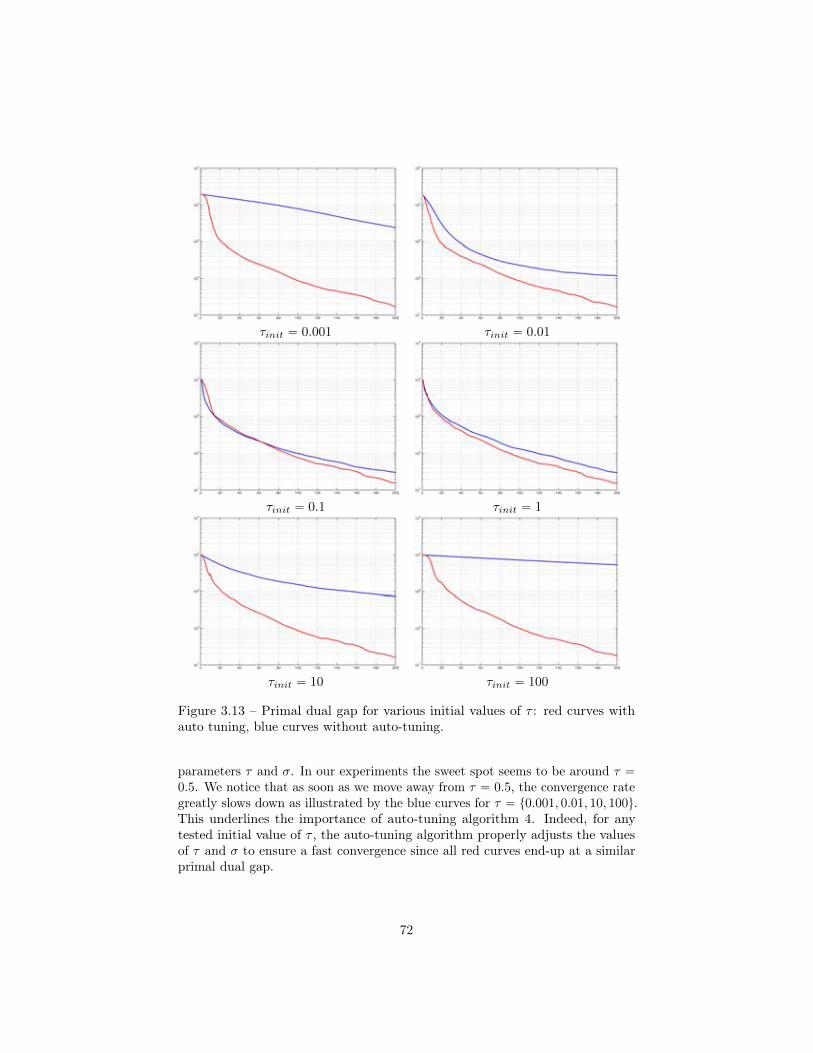
τinit “ 0.001 τinit “ 0.01
τinit “ 0.1 τinit “ 1
τinit “ 10 τinit “ 100
Figure 3.13 – Primal dual gap for various initial values of τ : red curves withauto tuning, blue curves without auto-tuning.
parameters τ and σ. In our experiments the sweet spot seems to be around τ “0.5. We notice that as soon as we move away from τ “ 0.5, the convergence rategreatly slows down as illustrated by the blue curves for τ “ t0.001, 0.01, 10, 100u.This underlines the importance of auto-tuning algorithm 4. Indeed, for anytested initial value of τ , the auto-tuning algorithm properly adjusts the valuesof τ and σ to ensure a fast convergence since all red curves end-up at a similarprimal dual gap.
72

3.6.2 Image denoisingImage denoising is generally one of the first components of many vision system.It has been studied for decades by the computer vision community [70, 128, 24].In our context, we sometimes have to process images contaminated by variousdegrees of additive or multiplicative noise. We can use denoising techniqueseither as a pre-processing step to improve the quality of image to process. But,we can also use denoising as a post-processing step to improve the quality ofa disparity map for instance. Hence, in this chapter we present a very generalformulation of denoising.
Image denoising as an optimization problem
In this task we are given an image r : Ω Ñ r0, 1s contaminated by Gaussiannoise and we attempt to estimate the uncontaminated image x. To this end, weoptimize the following equation:
arg minxiPr0,1s
ÿ
iPΩ
H1,αpxi ´ riq `ÿ
iPΩ
ÿ
jPNipρq
Hwij ,βpxi ´ xjq (3.152)
Where:
• Ha,α is a symmetric Huber function with a a-slope and α-curvature:
Ha,α “
#
ax2p2αq if x P r´α, αsap|x| ´ α2q otherwise
(3.153)
• Ni is the set of neighbor pixels of i within a ρ-radius.
• wij are positive real scalars.
The equation (3.152) enforces two fundamental properties. First, the valueof each pixel of the denoised image needs to be somehow close to the value ofthe pixel of the contaminated image. This is achieved by penalizing the distanceof xi to ri under the Huber norm H1,α. Second, natural images exhibit somenotion of smoothness. Therefore, for each pixel i P Ω we penalize a weighteddisagreement with its neighbors Ni through another Huber norm Hwij ,β .
The neighborhood Ni of a pixel i is the set of pixels of Ω within a givenradius ρ:
Nipρq “ rj P Ω | i´ j2 ď ρs . (3.154)
The weights wij are defined as:
wij “ λ exp p´β|ri ´ rj |q , (3.155)
where λ and β are real positive scalar used to tune the regularization strength.
73

Experiments
As a toy example, we proceed to denoise an image contaminated with a moderatewhite Gaussian noise. We perform a first denoising with the neighborhood radiusρ set to 1 and another denoising with ρ “ 3. All other parameters are adjustedto produce pleasant looking results.
Noise free image Image contaminated with noise
1-radius denoised image 3-radius denoised image
Figure 3.14 – Denoising of an image contaminated with white Gaussian noise.
We observe in figure 3.14 that both denoised images look smooth but exhibitthe noise-free image structure. However, most of the fine details are lost. Wenotice that increasing the neighborhood radius creates a smoother result whilepreserving strong edges.
We could easily improve this simple yet effective denoising formulation.We point the curious reader to recent work that solely focus on denoising[22, 81, 136, 3, 116, 118, 117].
74

3.6.3 L-ROF model vs ROF model for denoisingWe investigate the convergence rate of the L-ROF model through several nu-merical experiments. To this end, we consider the denoising task of an imagec : Ω Ñ r0, 1s contaminated with white Gaussian noise, and we solve the followingL-ROF optimization problem:
minxiPR
maxyijPr´w,ws
ÿ
iPΩ
´cixi `ÿ
iPΩ
ÿ
jPNipρq
yij |xi ´ xj | (3.156)
As a baseline we use the ROF model optimized with Algorithm 2 that yields a1
N2convergence rate:
minxiPR
ÿ
iPΩ
1
2x2i ´ cixi `
ÿ
iPΩ
ÿ
jPNipρq
w |xi ´ xj | (3.157)
Settings
For all experiments, we always set the regularization parameter w to be equal tothe standard deviation σn of the Gaussian noise. We consider three noise levels,low with σn “ 0.02, medium with σn “ 0.1 and high σn “ 0.25 as illustratedin figure 3.15. We set the smoothing parameter θ to 1 for both primal-dualoptimization algorithms. The primal and dual variables are initialized to 0 forboth algorithms.
Experiments with no scaling
In this first set of experiments we compare the L-ROF model without any scaling,δ “ 0, to the ROF model. We sweep space of the initial primal update step sizeτ from 1000 to 1 and set the dual step size accordingly to ensure convergence.We remind that internally the algorithm optimizing the ROF model adjusts boththe primal-dual step sizes along with the smoothing parameter θ. The L-ROFmodel maintains the initial values throughout the optimization.
For each noise level, we run each algorithm for 500 iterations and we displaythe primal dual gap at iterations 100, 250 and 500 in figures 3.16, 3.17 and 3.18.
For the L-ROF model, due to Property 1 and the constant initializationof the primal variable, the algorithm is insensitive to the primal update stepsize. We observe this behavior for the three noise regimes as all red curves offigures 3.16, 3.17 and 3.18 are constant. Since primal dual algorithms convergenceare sensitive to rightly tuning the update step sizes, this is a nice property ofthe L-ROF model.
In terms of convergence, we see that without scaling the L-ROF model slightlyoutperforms the ROF model. This is somehow unexpected since the ROF modelbenefits of a 1N2 convergence rate while the L-ROF model converges with 1Nrate. However, it has been observed in [27] that algorithm (1) from which theL-ROF optimization algorithm is derived obtains 1N2 convergence rate if the
75

Noise free image Image contaminated with low noise
Image contaminated with medium noise Image contaminated with high noise
Figure 3.15 – Reference image and different levels of noise contamination.
primal-dual update step-sizes are properly tuned. Since the L-ROF model isinsensitive to update step-size tuning, the optimization algorithm might alwaysperform in its optimal regime. This could explain the observed exponentialconvergence rate.
Experiments with scaling
We now proceed with a second set of experiments where we compare the L-ROFmodel with scaling to the ROF model. We set the initial primal update stepsize τ to 5 since it seems optimal in the last set of experiments, and we set thedual step size accordingly to ensure convergence. We sweep space of the scalingfactor δ from 0.5 to 1 by 0.1 increments and the space of scaling period from 2to 12 by 1 increments.
For each noise level, we run each algorithm for 500 iterations and we display
76

Figure 3.16 – Primal dual gap for low noise experiment without scaling atiteration 100, 200 and 500
the difference of log in base 10 of the primal dual gap at iterations 100, 250 and500 in figures 3.20, 3.21 and3.22 between the L-ROF and ROF model. Negativevalues mean that the L-ROF model converges faster than the ROF model.
We see that the scaling greatly im-proves the convergence of the L-ROFmodel to up to two orders of magnitude.A typical primal dual gap evolution ofthe L-ROF model is shown in figure3.19. Initially the convergence followsthe one of the ROF model. Then, it sta-bilizes to an exponential convergence(linear trend in the log domain) whilethe ROF model keeps its quadratic con-vergence.
Figure 3.19 – Primal dual gap for theL-ROF model with scaling (δ “ 0.7and scaling period of 10) and the ROFmodel
The optimal scaling factor varies with the scaling period. The more we scale
77

Figure 3.17 – Primal dual gap for medium noise experiment without scaling atiteration 100, 200 and 500
the less frequent we should do it. This is in line with the role of scaling. Indeed,the scaling decreases the influence of the past updates. A possible interpretationis that since the early updates are far from being optimal they can and shouldbe progressively discarded. However, discarding too much of the past is counterproductive. We let to future work the study of an optimal or heuristic criterionto dynamically tune the scaling factor parameter δ and the scaling period.
To conclude, the L-ROF model provides an interesting alternative to theclassic ROF model when highly accurate solutions are required.
78

Figure 3.18 – Primal dual gap for high noise experiment without scaling atiteration 100, 200 and 500
79

Figure 3.20 – Primal dual gap for low noise experiment without scaling atiteration 100, 200 and 500 (left to right)
Figure 3.21 – Primal dual gap for medium noise experiment without scaling atiteration 100, 200 and 500 (left to right)
Figure 3.22 – Primal dual gap for high noise experiment without scaling atiteration 100, 200 and 500 (left to right)
80

3.7 ConclusionThis first technical chapter introduced the basic of convex optimization. Weprogressively yet precisely introduce the fundamentals of the First order Primal-Dual techniques for convex optimization. We thoroughly studied the dual solutionspace of TV regularized problems and we propose through some theorems abetter understanding of how different TV models relate one to another.
However, not all tasks can be formulated as a convex optimization problemwithout scarifying to much modeling accuracy. To this end, we present in thenext chapter techniques for non-convex optimization.
81

Chapter 4
Maxflow and Graph cutstechniques
4.1 Introduction and contributions
4.1.1 IntroductionIn this chapter we consider the optimization of a non convex discrete energy.To this end we quickly introduce some basic background related to discreteoptimization. Then, we introduce a key algorithm in computer science: mincut/ maxflow. We study four different algorithms to solve the mincut / maxflowproblem.
Finally, we study graph-cuts techniques for their known efficiency to optimizepairwise non convex discrete energies. We introduce two algorithms: AlphaExpansion and Fast PD. Fast PD is known to be significantly faster than theAlpha Expansion. However, its current implementation requires a large amountof memory which makes it unsuitable to our context. Hence, we investigate indetails the implementation of the Fast-PD algorithm.
4.1.2 Chapter organizationThe section 4.2 introduces the basics of discrete optimization and we describe theproblem of interest. We discuss in section 4.3 the mincut and maxflow problemsas the primal and dual form of the same task. The section 4.4 presents dedicatedsolver for the mincut and maxflow problems. The section 4.5 introduces thealpha-expansion and the Fast-PD algorithms for solving multi-label pairwiseproblems. In the section 4.6 we perform numerous experiments to comparedifferent mincut / maxflow solvers and we evaluate our own implementation ofFast-PD.
82
4.1.3 ContributionsThe main contribution of this chapter is the complete re-implementation of thefamous Fast-PD algorithm. Our implementation non only drastically reducesthe amount of memory required but it also runs faster than the implementationproposed by the original authors of Fast-PD. We also propose an even fasterimplementation dedicated to grid-like problems.
This allows us for instance to perform discrete optimization in the context ofstereo-matching with large images while only using a recent laptop.
4.2 Discrete optimization in a tiny nutshellWe start by presenting the necessary knowledge to further study both mincut/ maxflow algorithms and graph-cuts techniques. We refer the reader to [142],[130] and [140] for more details.
4.2.1 Sub-modularitySub-modularity plays a central role for discrete optimization in the same waythat convexity is crucial for convex optimization [153].
In this work we make extensive use of binary functions. In this settings, thesub-modularity simplifies to:
Definition 12. Let φ : t0, 1u ˆ t0, 1u Ñ R be a 2-binary function. We say thatφ is sub-modular if and only if:
φp0, 0q ` φp1, 1q ď φp0, 1q ` φp1, 0q (4.1)
We introduce some useful properties about sub-modular functions.
Property 3. If φ is a sub-modular function, then @α P R` and @β P R thefollowing function:
αφp.q ` β (4.2)
is also sub-modular.
Property 4. If φ and ψ are sub-modular functions, then φ`ψ is a sub-modularfunction.
Property 5. Any finite positive weighted sum of sub-modular functions is asub-modular function.
Theorem 9. If φ is a sum of binary sub-modular functions, then one cancompute its minimum in polynomial time by solving a min-cut problem.
Hence, if we can formulate our discrete optimization problems as a sum ofbinary sub-modular functions to optimize, or as a sequence of sums of binarysub-modular functions to optimize, we can derive a polynomial time optimizationscheme.
83

4.2.2 Problems of interestWe remind the problems studied in this chapter.
Notations
We make use of the following notations:
• The graph G is a directed graph G “ rV, Es composed of a finite set ofvertices V and a finite set of directed edges E . The edge pi, jq of E createsa connexion from the vertex i to another vertex j.
• The discrete variable xi defines the configuration of each vertex i P V . Thedomain of xi is L “ t0, . . . , L´ 1u with L P N.
• A discrete unary potential function φi defines the configuration cost ofeach vertex i P V: φi : LÑ R.
• A discrete potential function φij defines the configuration cost of eachdirected edge pi, jq of E : φij : L ˆ L Ñ R`. We assume that φijpl, lq “0, @l P L.
Canonical problems
We are interested in solving the following problem:
px˚i qi “ arg minpxiPLqi
ÿ
iPVφipxiq `
ÿ
pi,jqPEφijpxi, xjq. (4.3)
4.2.3 Representation of pairwise binary sub-modular func-tions
We suppose we are given a pairwise binary sub-modular function ψij : t0, 1u ˆt0, 1u Ñ R:
ψij “
„
A BC D
(4.4)
where pA,B,C,Dq P Rˆ Rˆ Rˆ R
Theorem 10. Any pairwise binary sub-modular function ψij : t0, 1uˆt0, 1u Ñ Rcan be represented as:
ψijpxi, xjq “ cixi ` cjxj ` wij maxpxi ´ xj , 0q ` d (4.5)
with: ci “ C ´A, cj “ D ´ C, wij “ B ` C ´A´D, and d “ A.
84

Proof
The proof, given in [95], derives from basic calculus:
cixi ` cjxj ”
ˇ
ˇ
ˇ
ˇ
0 D ´ CC ´A D ´A
ˇ
ˇ
ˇ
ˇ
cixi ` cjxj ` wij maxpxi ´ xj , 0q ”
ˇ
ˇ
ˇ
ˇ
0 B ´AC ´A D ´A
ˇ
ˇ
ˇ
ˇ
cixi ` cjxj ` wij maxpxi ´ xj , 0q ` d ”
ˇ
ˇ
ˇ
ˇ
A BC D
ˇ
ˇ
ˇ
ˇ
cixi ` cjxj ` wij maxpxi ´ xj , 0q ` d ” ψijpxi, xjq
(4.6)
4.2.4 A link between discrete and convex optimizationthrough TV regularization
Theorem 11. Let pz˚i qi be the solution of the following problem:
pz˚i qi “ arg minpziPr0,1sqi
ÿ
iPVcizi `
ÿ
pi,jqPEwij max pzi ´ zj , 0q . (4.7)
Then, @t P r0, 1r:
x˚i “
"
0 if z˚i ď t1 if z˚i ą t
(4.8)
The set of variables px˚i qi are a solution of the associated binary problem:
px˚i qi “ arg minpxiPt0,1uqi
ÿ
iPVcixi `
ÿ
pi,jqPEwij max pxi ´ xj , 0q . (4.9)
Proof
We introduce the following change of variables for a P R˚,` and t P r0, 1r:
zai “1
apzi ´ tq, @i P V (4.10)
We apply this change of variable to (4.7):ˆ
1
apz˚i ´ tq
˙
i
“ arg min˜
ziP
«
´t
a,1´ t
a
ff¸
i
ÿ
iPVcizi `
ÿ
pi,jqPEwij max pzi ´ zj , 0q .
(4.11)We notice that Da ą 0 such that:
$
’
&
’
%
1
apz˚i ´ tq ě 1 and
1´ t
aě 1 if z˚i ą t
1
apz˚i ´ tq ď 0 and
´t
aď 0 if z˚i ď t
(4.12)
85
We apply the truncation theorem of TV regularized problems 3 with ther0, 1s interval to equation (4.11):˜
„
1
apz˚i ´ tq
r0,1s
¸
i
“ arg minpxiPr0,1sqi
ÿ
iPVcixi `
ÿ
pi,jqPEwij max pxi ´ xj , 0q .
px˚i qi “ arg minpxiPt0,1uqi
ÿ
iPVcixi `
ÿ
pi,jqPEwij max pxi ´ xj , 0q .
(4.13)
This completes the proof.
4.2.5 Primal dual scheme for integer Linear programmingTo study Fast-PD, we need to introduce the fundamental of linear programmingand the approximate primal-dual scheme of [64] and [125] for integer Linearprogramming optimization. We refer the curious reader to [40] for more details.
Primal and dual forms of a linear programming problem
Definition 13. A Linear Programming, LP, problem consists of minimizing alinear combination of variables under inequality constraints that can be expressedin canonical primal form as:
minpxiqi
Iÿ
i“1
cixi
s.t.Iÿ
i“1
ajixi ď bj , @j P r1, Js
xi ě 0, @i P r1, Is
with: pI, Jq P Nˆ N, pciqi P R, pajiqij P R, and pbjqj P R.
Definition 14. The dual canonical form of LP is:
maxpyjqj
Jÿ
j“1
bjyj
s.t.Jÿ
j“0
ajiyj ď ci, @i P r1, Is
yj ě 0, @j P r1, Js
We note that any LP can be easily transformed into either a canonical primalor dual form.
86

Complementary slackness conditions
The complementary slackness plays a central role to certify the optimality of aprimal-dual solution.
Property 6. The primal complementary slackness condition is:
@i P r1, Is , xi ą 0 ñ
Jÿ
j“0
ajiyj “ ci
Property 7. The dual complementary slackness condition is:
@j P r1, Js , yj ą 0 ñ
Iÿ
i“1
ajixi “ bj
Theorem 12. If a pair px, yq of primal-dual pair verifies the primal and dualcomplementary slackness conditions, then x and y are solutions of the primaland dual LP problem.
Hence, the primal and dual complementary slackness conditions can be usedas an optimality certificate.
Relaxed complementary slackness conditions
Interestingly, we can also derive a more general definition for the complementaryslackness conditions by relaxing the equality in the second term of each conditions.
Property 8. For a given α P r1,`8s the primal relaxed complementary slack-ness condition is:
@i P r1, Is , xi ą 0 ñciαď
Jÿ
j“0
ajiyj ď ci
Property 9. For a given β P r1,`8s the dual relaxed complementary slacknesscondition is:
@j P r1, Js , yj ą 0 ñ bj ďIÿ
i“1
ajixi ď βbj
Theorem 13. If a pair px, yq of primal-dual solution verifies the primal anddual relaxed complementary slackness conditions with factor α and β:
Iÿ
i“1
cixi ď αβJÿ
j“1
bjyj
then x and y are αβ optimal solutions of the primal and dual LP problem
87
Primal dual scheme for binary LP
We now give a general framework to optimize approximately a given Binary LP,BLP, B. The key idea is to relax this BLP to an LP, and to compute the dualproblem. The framework makes use of both the primal and dual problems byiteratively improving the dual solution while generating integer primal solutionsuntil no dual improvement can be made. The quality of the approximation ofthe integer primal solution is controlled by factors α and β. The algorithm 8sums up the primal dual scheme for binary LP.
Algorithm 8: Approximate primal dual scheme for Binary Linear Pro-gramming problemsData: Inputs: B, α and βResult: pxiqi, pyjqjRelax the ILP to an LP: Ñ P.Compute the dual of P : Ñ D.Initialize the primal variables to be binary.Initialize the dual variables to be feasible.while Relaxed complementary slackness conditions are not all statisfied do
Select a subset of dual variables that does not satisfy the relaxedcomplementary slackness conditions.
Update this subset of dual variables with a method of choice.
Use the primal relaxed complementrary slackness conditions to updatethe primal variables by an integer quantity.
4.3 Max-flow and min-cut problemsIn 1956, two research teams composed of P. Elias, A. Feinstein, and C.E. Shannonfor the first one [46], and L.R. Ford, Jr. and D.R. Fulkerson [54] for the seconddemonstrated the celebrated max-flow / min-cut theorem. This theorem derivesfrom the strong duality in linear programming problems [108].
In this section, we start by proving the max-flow / min-cut theorem, then weintroduce simply equations for both the primal (min-cut), the primal-dual, andthe dual (max-flow) problems. Those simplified equations ease the creation ofmax-flow / min-cut solvers dedicated to image processing tasks.
88

4.3.1 The max-flow / min-cut
4.3.2 From a min-cut problem to a max-flow problemUsing the representation defined by theorem (10), we can formulate, up to aconstant term, any sum of binary pairwise sub-modular functions as :
ÿ
iPVφip0q p1´ xiq ` φip1qxi `
ÿ
pi,jqPEwij max pxi ´ xj , 0q (4.14)
The min-cut problem
The binary min-cut problem is simply the configuration of minimum cost of theprevious equation 4.14:
px˚i qi “ arg minpxiPt0,1uqi
ÿ
iPVφip0q p1´ xiq ` φip1qxi `
ÿ
pi,jqPEwij max pxi ´ xj , 0q
(4.15)
Relaxing primal variables
Thanks to theorem 11 we can solve the relaxed problem while still being able toretrieve by a simple truncation an optimal solution of (4.15).
minpliPr0,1sqi
ÿ
iPVφip0q p1´ liq ` φip1qli `
ÿ
pi,jqPEwij max pli ´ lj , 0q . (4.16)
where s-indexed variables are connected to the source and t indexed variablesare linked to the sink.
We observe that we now deal with a non smooth convex optimization problem.This transformation was observed by [28] and then [174].
Dualizing the potentials
We transform the previous problem by dualizing the potentials. We formulateboth unary and pairwise potentials using the techniques of previous chapter:
φip0q “ maxρsiPr0,φip0qs
ρsi
φip1q “ maxρitPr0,φip1qs
ρit
wij max pxi ´ xj , 0q “ maxfijPr0,wijs
fij pxi ´ xjq
(4.17)
89

We obtain the following primal dual problem:
minpxiq
maxpρsiq,pρitq,pfijq
ÿ
iPVρsi p1´ xiq ` ρitxi `
ÿ
pi,jqPEfij pxi ´ xjq .
subject to xi P r0, 1s, @i P Vfij P r0, wijs , @ pi, jq P Eρsi P r0, φip0qs , @i P Vρit P r0, φip1qs , @i P V
(4.18)
We introduce the following notations to minimize clutter in equations:
Epi, .q “ tj P V | pi, jq P Eu. (4.19)Ep., iq “ tj P V | pj, iq P Eu (4.20)
After factorization with respect to each xi we obtain:
minpxiq
maxpρsiq,pρitq,pfijq
ÿ
iPVρsi
`ÿ
iPVxi
»
–ρit ´ ρsi `ÿ
jPEpi,.q
fij ´ÿ
jPEp.,iq
fji
fi
fl
subject to xi P r0, 1s, @i P Vfij P r0, wijs , @ pi, jq P Eρsi P r0, φip0qs , @i P Vρit P r0, φip1qs , @i P V
(4.21)
Dualizing the constraints on primal variables
For each vertex i P V, we introduce two variables pki, siq P R` ˆ R` to enforcexi P r0, 1s. Hence, we can drop the domain constraint for all pxiqi
minpxiq
maxpρsiq,pρitq,pfijq,pkiq,psiq
ÿ
iPVρsi
`ÿ
iPVxi
»
–ρit ´ si ´ ρsi ` ki `ÿ
jPEpi,.q
fij ´ÿ
jPEp.,iq
fji
fi
fl
`ÿ
iPVpxi ´ 1q ki ´ xisi
subject to fij P r0, wijs , @ pi, jq P Eρsi P r0, φip0qs , @i P Vρit P r0, φip1qs , @i P Vki ě 0, @i P Vsi ě 0, @i P V
(4.22)
90

We factorize again with respect to xi to obtain:
minpxiq
maxpρsiq,pρitq,pfijq,pkiq,psiq
ÿ
iPVρsi ´ ki
`ÿ
iPVxi
»
–ρit ´ si ´ ρsi ` ki `ÿ
jPEpi,.q
fij ´ÿ
jPEp.,iq
fji
fi
fl
subject to fij P r0, wijs , @ pi, jq P Eρsi P r0, φip0qs , @i P Vρit P r0, φip1qs , @i P Vki ě 0, @i P Vsi ě 0, @i P V
(4.23)
Introducing the source and sink flows
We introduce the flow variables from the source and the sink:
fsi “ ρsi ´ ki, @i P V.fit “ ρit ´ si, @i P V.
(4.24)
We observe that:fsi ď φip0q, @i P V.fit ď φip1q, @i P V.
(4.25)
Hence, we obtain:
minpxiq
maxpfsiq,pfitq,pfijq
ÿ
iPVfsi
`ÿ
iPVxi
»
–fit ´ fsi `ÿ
jPEpi,.q
fij ´ÿ
jPEp.,iq
fji
fi
fl
subject to fij P r0, wijs , @ pi, jq P Efsi ď φip0q, @i P Vfit ď φip1q, @i P V
(4.26)
Solving for primal variables and refactoring
We recognize that each variables xi acts as a Lagrangian multiplier to enforcethe following equality constraint:
fit ´ fsi `ÿ
jPEpi,.q
fij ´ÿ
jPEp.,iq
fji “ 0 (4.27)
91

The maxflow equations
Finally we get the Maxflow equations:
maxpfsiq,pfitq,pfijq
ÿ
iPVfsi
subject to fij P r0, wijs , @ pi, jq P Efsi ď φip0q, @i P Vfit ď φip1q, @i P V
fit ´ fsi `ÿ
jPEpi,.q
fij ´ÿ
jPEp.,iq
fji “ 0, @i P V
(4.28)
The last constraint enforces the conservation of the flow.
4.3.3 Simplified equationsWe now introduce simplified equations for primal, primal-dual and dual problemsmodeling the maxflow-mincut.
The primal problem
We start from the relaxed mincut equations. We introduce the following simplefactorizations:
ci “ φip1q ´ φip0q, @i P V. (4.29)
φΣp0q “ÿ
iPVφip0q (4.30)
E˚ “ minpxiPr0,1sqi
ÿ
iPVφip0q p1´ xiq ` φip1qxi `
ÿ
pi,jqPEwij max pxi ´ xj , 0q .
(4.31)
“ minpxiPr0,1sqi
ÿ
iPVpφip1q ´ φip0qqxi ` φip0q `
ÿ
pi,jqPEwij max pxi ´ xj , 0q .
(4.32)
“ minpxiPr0,1sqi
ÿ
iPVcixi `
ÿ
pi,jqPEwij max pxi ´ xj , 0q ` φΣp0q. (4.33)
During optimization we can discard the constant φΣp0q. The primal variablesare the same as in (4.16). Hence, we can use the truncating technique 11 werecover an optimal solution for (4.15).
The primal-dual problem
We get the simplified primal dual problem by simply dualizing the pairwiseterms:
E˚ “ minxiPr0,1s
maxfijPr0,wijs
ÿ
iPVcixi `
ÿ
pi,jqPEfij pxi ´ xjq ` φΣp0q. (4.34)
92

The dual variable fij represents the flow from vertex i to vertex j.
The dual problem
For the simplified Maxflow problem we start by factorizing (4.34) with respectto each primal variable i and then we solve for the primal variables.
E˚ “ minxiPr0,1s
maxfijPr0,wijs
ÿ
iPV
¨
˝ci `ÿ
jPEpi,.q
fij ´ÿ
jPEp.,iq
fji
˛
‚xi ` φΣp0q. (4.35)
“ maxfijPr0,wijs
ÿ
iPVmin
xiPr0,1s
¨
˝ci `ÿ
jPEpi,.q
fij ´ÿ
jPEp.,iq
fji
˛
‚xi ` φΣp0q. (4.36)
“ maxfijPr0,wijs
ÿ
iPVmin
¨
˝ci `ÿ
jPEpi,.q
fij ´ÿ
jPEp.,iq
fji, 0
˛
‚` φΣp0q. (4.37)
“ maxfijPr0,wijs
´1
2
»
–
ÿ
iPV
ˇ
ˇ
ˇ
ˇ
ˇ
ˇ
ci `ÿ
jPEpi,.q
fij ´ÿ
jPEp.,iq
fji
ˇ
ˇ
ˇ
ˇ
ˇ
ˇ
´ ci
fi
fl` φΣp0q. (4.38)
The last equation is obtained by applying the `1 reformulation presented in 3.4.1and noting that the terms out of the absolute values cancel out. We also notethat the simplified equation of the Maxflow does not contain the flow from thesource and the flow to the sink.
Max-flow / min-cut as a reparametrization
Suppose that we obtain dual variables pfijqij by solving, for instance, the problem(4.37). We can apply the following re-parametrization:
c1i “ ci `ÿ
jPEpi,.q
fij ´ÿ
jPEp.,iq
fji (4.39)
This gives use the following primal dual problem:
E˚ “ minpxiPr0,1sqi
maxf 1ijPr´fij ,wij´fijs
ÿ
iPVc1ixi `
ÿ
pi,jqPEf 1ij pxi ´ xjq ` φΣp0q.
(4.40)And the following primal problem:
E˚ “ minpxiPr0,1sqi
ÿ
iPVc1ixi `
ÿ
pi,jqPEpwij ´ fijqmaxpxi ´ xj , 0q
`fij maxpxj ´ xi, 0q ` φΣp0q.
(4.41)
Hence, solving the max-flow problem is equivalent to finding a re-parametrizationof the min-cut problem where its sum of unary potentials has a minimum `1norm. It is also equivalent to find a re-parametrization of the dual problemwhere the new optimal dual variables are equal to 0.
93

Recovering primal variables from dual variables
To obtain optimal primal variables from optimal dual variables we can solve thefollowing problem:
minpxiq
ÿ
iPVRpxiq
subject to xi P r0, 1s , @i P V
xi “ 0, if ci `ÿ
jPEpi,.q
f˚ij ´ÿ
jPEp.,iq
f˚ji ą 0
xi “ 1, if ci `ÿ
jPEpi,.q
f˚ij ´ÿ
jPEp.,iq
f˚ji ă 0
xi “ xj if f˚ij P s0, wijr
xi ď xj if f˚ji “ 0
xi ě xj if f˚ji “ wij
(4.42)
where Rp.q : RÑ R is a convex function acting as a regularizer.We note that if Rp.q “ 0, then the problem (4.42) can be solved very easily
by applying a depth first search scheme as described in the Ford-Fulkersonmax-flow algorithm as explain in section 26.2 of [36]. For other regularizationfunctions one can use the primal dual techniques of the previous chapter forinstance.
Proof: The primal update rule states that @i P V:
x˚i “
»
–x˚i ´ τ
¨
˝ci `ÿ
jPEpi,.q
f˚ij ´ÿ
jPEp.,iq
f˚ji
˛
‚
fi
fl
r0,1s
(4.43)
Hence, we can recover a partial set of optimal primal variables pxiq˚:
x˚i “
$
&
%
0 if ci `ř
jPEpi,.q f˚ij ´
ř
jPEp.,iq f˚ji ą 0
1 if ci `ř
jPEpi,.q f˚ij ´
ř
jPEp.,iq f˚ji ă 0
P r0, 1s if ci `ř
jPEpi,.q f˚ij ´
ř
jPEp.,iq f˚ji “ 0
(4.44)
The dual update rule states that @ pi, jq P E :
f˚ij ““
f˚ij ` σpx˚i ´ x
˚j q‰
r0,wijs(4.45)
Hence, we gather the following additional constraints:$
&
%
x˚i “ x˚j if f˚ij P s0, wijr
x˚i ď x˚j if f˚ji “ 0
x˚i ě x˚j if f˚ji “ wij
(4.46)
Therefore, the optimal primal variable belongs to the space verifying con-straints (4.44) and (4.46). Since, this space is not necessarily a singleton, wecan enforce a particular solution by adding a regularization cost. This concludesthe proof.
94

Recovering dual variables from primal variables
To obtain optimal dual variables from optimal primal variables we can solve thefollowing problem:
minpfijq
ÿ
pi,jqPE
Rpfijq
subject to fij P r0, wijs , @ pi, jq P Efij “ wij , if x˚i ´ x
˚j ą 0
fij “ 0, if x˚i ´ x˚j ă 0
ci `ÿ
jPEpi,.q
fij ´ÿ
jPEp.,iq
fji ă 0, if x˚i ą 0
ci `ÿ
jPEpi,.q
fij ´ÿ
jPEp.,iq
fji ą 0, if x˚i “ 0
(4.47)
where Rp.q : RÑ R is a convex function acting as a regularizer.
The problem (4.47) can be solved with primal dual techniques presented inthe previous chapter.
Proof: The dual update rule states that @ pi, jq P E :
f˚ij ““
f˚ij ` σpx˚i ´ x
˚j q‰
r0,wijs(4.48)
Hence, we can easily derive a partial set of dual variables:
f˚ij P
$
&
%
twiju if x˚i ´ x˚j ą 0,
t0u if x˚i ´ x˚j ă 0,
r0, wijs if x˚i ´ x˚j “ 0.
(4.49)
However, for any couple pi, jq P E where x˚i “ x˚j we have to find another set ofconstraints.
The primal update rule states that @i P V:
x˚i “
»
–x˚i ´ τ
¨
˝ci `ÿ
jPEpi,.q
f˚ij ´ÿ
jPEp.,iq
f˚ji
˛
‚
fi
fl
r0,1s
(4.50)
Therefore, we deduce additional constraints for pfijqij :
ci `ÿ
jPEpi,.q
f˚ij ´ÿ
jPEp.,iq
f˚ji ă 0, if x˚i ą 0
ci `ÿ
jPEpi,.q
f˚ij ´ÿ
jPEp.,iq
f˚ji ą 0, if x˚i “ 0(4.51)
Hence, the optimal dual variable belongs to the space verifying constraints(4.49) and (4.51). Since, this space is not necessarily a singleton, we can enforcea particular solution by adding a regularization cost. This concludes the proof.
95

Recovering the flow from the source and to the sink
The optimal flow from the source and to the sink is given by:
f˚it “ minpφip0q ´ÿ
jPEpi,.q
f˚ij `ÿ
jPEp.,iq
f˚ji, φip1qq (4.52)
f˚si “ minpφip1q `ÿ
jPEpi,.q
f˚ij ´ÿ
jPEp.,iq
f˚ji, φip0qq (4.53)
Proof: For each vertex i P V we know from equation (4.28) that:
f˚it ´ f˚si `
ÿ
jPEpi,.q
f˚ij ´ÿ
jPEp.,iq
f˚ji “ 0 (4.54)
f˚si ´ f˚it “
ÿ
jPEpi,.q
f˚ij ´ÿ
jPEp.,iq
f˚ji (4.55)
f˚si ´ f˚it “ f˚sit (4.56)
Since we already know the optimal flow between vertices, the canonicalmaxflow problem simplifies to:
maxpfsiq,pfitq
ÿ
iPVfsi
subject to fsi ď φip0q, @i P Vfit ď φip1q, @i P Vfsi “ f˚sit ` fit, @i P V
(4.57)
We can easily solve for all pfsiq:
maxpfitq
ÿ
iPVf˚sit ` fit
subject to f˚sit ` fit ď φip0q, @i P Vfit ď φip1q, @i P V
(4.58)
We can reformulate to:
maxpfitq
ÿ
iPVf˚sit ` fit
subject to fit ď φip0q ´ f˚sit, @i P V
fit ď φip1q, @i P V
(4.59)
Finally, we obtain:
f˚it “ minpφip0q ´ f˚sit, φip1qq (4.60)
f˚si “ minpφip1q ` f˚sit, φip0qq (4.61)
This completes the proof.
96

4.3.4 Characterization of obvious partial primal solutionsWe study some sufficient conditions for a primal variable xk to be equal to either0 or 1. One can show that for a given vertex k P V, there exists an optimalsolution that verifies:
x˚k “
"
0 if ck ěř
jPEp.,kq wjk1 if ck ď ´
ř
jPEpk,.q wkj(4.62)
Figure 4.1 – Example of function fpxkqfor ck ě
ř
jPEp.,kq wjk.Figure 4.2 – Example of function fpxkqfor ck ď ´
ř
jPEpk,.q wkj .
Proof for x˚k “ 0
Let us assume that ck ěř
jPEp.,kq wjk. We can write for a certain δ` P R`:
ck “ δ` `ÿ
jPEp.,kq
wjk (4.63)
We apply the reformulation trick of (3.59) introduced in previous chapter,we have:
fpxkq “ ckxk `ÿ
jPEp.,kq
wjk max pxj ´ xk, 0q `ÿ
jPEpk,.q
wkj max pxk ´ xj , 0q
(4.64)
“ ckxk `ÿ
jPEp.,kq
wjk pxj ´ xkq `ÿ
jPEpk,.q
pwkj ` wjkqmax pxk ´ xj , 0q
(4.65)
“ δ`xk `ÿ
jPEpk,.q
pwkj ` wjkqmax pxk ´ xj , 0q `ÿ
jPEp.,kq
wjkxj (4.66)
Hence, fpxkq is an increasing function and we have x˚k “ 0 an optimal solution.This is illustrated by figure 4.1.
97

Proof for x˚k “ 1
Let us assume that ck ď ´ř
jPEpk,.q wkj . We can write for a certain δ´ P R´:
ck “ δ´ ´ÿ
jPEpk,.q
wkj (4.67)
We apply the reformulation trick of (3.59) introduced in previous chapter:
fplkq “ ckxk `ÿ
jPEp.,kq
wjk max pxj ´ xk, 0q `ÿ
jPEpk,.q
wkj max pxk ´ xj , 0q
(4.68)
“ ckxk `ÿ
jPEp.,kq
pwjk ` wkjqmax pxj ´ xk, 0q `ÿ
jPEpk,.q
wkj pxk ´ xjq
(4.69)
“ δ´xk `ÿ
jPEp.,kq
pwjk ` wkjqmax pxj ´ xk, 0q ´ÿ
jPEpk,.q
wkjxj (4.70)
Hence, fpxkq is an decreasing function and we have x˚k “ 1 an optimal solution.This is illustrated by figure 4.2.
4.3.5 ROF and MaxflowThe previous chapter gives us a surrogate set of problems that give an optimalsolution for the max-flow. Indeed, we see that the optimal solution space ofthe simplified max-flow problem (4.38) corresponds to Y˚`1 of theorem (4). Thetheorem (4) guaranties any optimal dual solution of ROF model also gives asolution of the associated max-flow problem. This was previously observed in[26].
Hence, we can directly solve the following ROF in its dual form:
maxpfijPr0,wijsqij
´1
2
ÿ
iPV
¨
˝ci `ÿ
jPEpi,.q
fij ´ÿ
jPEp.,iq
fji
˛
‚
2
(4.71)
However, if we solve the primal form of the ROF model:
minpxiPRqi
ÿ
iPV
1
2x2i ` cixi `
ÿ
pi,jqPEwij max pxi ´ xj , 0q , (4.72)
we can then recover the optimal dual variable by slightly adjusting problem (4.47)
98

to:
minpfijq
ÿ
pi,jqPE
Rpfijq
subject to fij P r0, wijs , @ pi, jq P Efij “ wij , if x˚i ´ x
˚j ą 0
fij “ 0, if x˚i ´ x˚j ă 0
ci `ÿ
jPEpi,.q
fij ´ÿ
jPEp.,iq
fji “ ´xROF,˚i , @i P V
(4.73)
where Rp.q : RÑ R is a convex function acting as a regularizer.
4.4 Solvers for min-cut / max-flow problemsWe now present solvers that optimally solve the min-cut / max-flow problem.
4.4.1 Solver for chain graphsWe devise a first solver when the graph G is a chain of C vertices. We describealgorithms that solve in OpCq the primal and dual forms.
Primal algorithm
In its primal form, we need to optimize the following problem:
E˚ “ minpxiPt0,1uqi
ÿ
iPt1,..,Nu
cixi `ÿ
iPt2,..,Cu
wi max pxi`1 ´ xi, 0q ` φΣp0q. (4.74)
The problem (4.74) can be solved by the Viterbi algorithm [72], a dynamicprograming algorithm [44]. We present in algorithm 9 a simplified version wherethe inner loops are unrolled since we work with binary variables.
Dual algorithm
For the dual form, we have to solve:
E˚ “ maxfiPr0,wis
´1
2
»
–
ÿ
iPt1,..,Cu
|ci ` fi ´ fi´1| ´ ci
fi
fl` φΣp0q. (4.75)
where we introduce f0 “ 0 and w0 “ 0 to ease the notations.The problem (4.75) can also be solved by dynamic programing as in algo-
rithm 10.
99

Algorithm 9: Primal algorithm for min-cut on chain graphData: Inputs: pciqi, pwiqiResult: pxiqiInitialization: cn0 “ t0, c1uMessage passing on chain:for i P t2, . . . , Cu do
Compute minimum cost for transition to next node:if cn0p1q ă cn0p2q ` wi´1q then
cn1p1q Ð cn0p1qlabelspi´ 1, 1q Ð 0
elsecn1p1q Ð cn0p2q ` wi´1
labelspi´ 1, 1q Ð 1
if cn0p1q ă cn0p2q thencn1p2q Ð cn0p1qlabelspi´ 1, 2q Ð 0
elsecn1p2q Ð cn0p2qlabelspi´ 1, 2q Ð 1
Add unary term: cn1p2q Ð cn1p2q ` ciCopy temporary buffer: cn0 Ð cn1
Decoding:if cn0p1q ă cn0p2q then
xC “ 0
elsexC “ 1
for i P tC ´ 1, . . . , 1u doxi “ labelspi, xi`1 ` 1q
Algorithm 10: Algorithm for max-flow on chain graphData: Inputs: pciqi, pwiqiResult: pfiqifor i “ 1, C ´ 1 do
Compute excess of flow:eÐ ci ´ fi´1
if e ď 0 thenfi Ð minpwi,´eq
elsefi Ð 0q
100

Dual algorithm with backtracking
We can even improve the dual algorithm to also return the optimal primalvariables. To this end, we run the depth-first-search algorithm while computingthe dual variables. As soon as we saturate a dual variable, we can backtrack tolabel the primal variables accordingly. This leads to algorithm 11.
Algorithm 11: Algorithm for max-flow on chain graph with backtrackingData: Inputs: pciqi, pwiqiResult: pfiqiInitialization for backtracking sÐ 1backtrackÐ 0for i “ 1, C ´ 1 do
Compute excess of flow:eÐ ci ´ fi´1
if e ď 0 thenif wpiq ă ´e then
fi Ð wixi Ð 1backtrackÐ 1
elsefi Ð ´e
elsefi Ð 0xi Ð 0backtrackÐ 1
Backtrack to set optimal primal variables:if backtrack then
for j P ti´ 1, . . . , su doxj Ð xj`1
sÐ i` 1backtrackÐ 0
4.4.2 Iterative solversTV-linear
We know focus on general graph. The primal dual formulation of the min-cut /max-flow problem is given by:
E˚ “ minxiPr0,1s
maxfijPr0,wijs
ÿ
iPVcixi `
ÿ
pi,jqPEfij pxi ´ xjq ` φΣp0q. (4.76)
We can apply the primal dual techniques of the last chapter to solve theproblem (4.76) using algorithm (12). This techniques returns both the (relaxed)
101

primal and dual variables. It can also be warm-started when we dispose of aninitial guess of the primal and dual variables.
The convergence rate to an optimal solution in guaranteed in Oˆ
1
N
˙
, where
N is the number of iterations. However, the algorithm (12) does neither guarantyto decrease the primal energy nor increase the dual energy at each iteration. Thealgorithm 12 describes the TV-linear method for solving the maxflow / mincutproblem.
Algorithm 12: Primal dual algorithm for min-cut / max-flow as TV-linearproblemData: Inputs: pciqi, pwijqij , G, τ , σResult: pxiqi, pfijqijInitialize primal and dual variable Ñ x0 “ 0, f0 “ 0.Set x “ x0
while Stopping criterion is not verified doOptimize the dual variables, @pi, jq P E :
fn`1ij “
“
fnij ` σpxi ´ xjq‰
r0,wijs(4.77)
Optimize the primal variables, @i P V:
xn`1i “
»
–xni ´ τ
¨
˝ci `ÿ
jPEpi,.q
fij ´ÿ
jPEp.,iq
fji
˛
‚
fi
fl
r0,1s
(4.78)
Smooth variable, @i P V:
xi “ xn`1i ` θ
`
xn`1i ´ xni
˘
(4.79)
TV-l2: ROF
We have demonstrated that the ROF model gives an alternative approach tosolve the min-cut / max-flow problem. Hence, we make use of the primal-dualform of the ROF model:
minpxiPRqi
maxfijPr0,wijs
ÿ
iPV
1
2x2i ` cixi `
ÿ
pi,jqPEfij pxi ´ xjq (4.80)
As for the TV-linear problem, we apply the primal dual technique of thelast chapter. Therefore, we directly recover optimal dual variables that solvethe max-flow problem (from which we can easily obtain optimal binary primalvariables). The algorithm 13 describes the TV-`2 method for solving maxflow /mincut problems.
102

Algorithm 13: Primal dual algorithm for min-cut / max-flow as TV-`2problemData: Inputs: pciqi, pwijqij , G, τ , σResult: pxiqi, pfijqijInitialize primal and dual variable Ñ x0 “ 0, f0 “ 0.Set x “ x0
while Stopping criterion is not verified doOptimize the dual variables, @pi, jq P E :
fn`1ij “
“
fnij ` σnpxi ´ xjq‰
r0,wijs(4.81)
Optimize the primal variables, @i P V:
xn`1i “
xn`1i ` τn
´
ci `ř
jPEpi,.q fij ´ř
jPEp.,iq fji
¯
1` τn(4.82)
Update the smoothing and steps size parameters:
θn “1
?1` 2γτn
, τn`1 “ θnτn, σn`1 “σnθn
(4.83)
Smooth variable, @i P V:
xi “ xn`1i ` θn
`
xn`1i ´ xni
˘
(4.84)
103

For algorithm (13) the convergence rate to an optimal solution in guaranteed
in Oˆ
1
N2
˙
, where N is the number of iterations.
4.4.3 Augmenting path solversAugmenting path solvers [147] are algorithms designed to solve the dual form ofthe max-flow / min-cut, i.e., problem (4.28). Here, we describe the augmentingpath method of [17] that experimentally outperforms other variant for computervision problems [166]. It sequentially alternates three stages:
1. Find an augmenting path: a chain subgraph A of the main graph G whosedual variables can be further optimized. For computer vision problems,this is generally done by growing two binary trees simultaneously fromthe source and sink by following edges that have positive capacities. Anaugmenting path is found when the two trees meet. If no augmenting pathcan be found, then the algorithm terminates.
2. The augmenting phase: optimize the dual variables of the chain subgraph A.Apply a re-parametrization of the problem as describe in paragraph 4.3.3.
3. Adopt orphan: An optional step that greatly speeds up augmenting pathis to update dynamically the growing trees after the augmentation phase.During the augmentation the re-parametrization might have set the ca-pacities of some edge to 0, potentially invalidating parts of the source andsink trees. The adoption phase corrects this phenomenon.
The efficiency of augmenting path algorithms resides in their ability to quicklyfind augmenting paths. The celebrated BK algorithm uses a heuristic that delivergreat performance for computer vision related maxflow problems. We refer thereader to its original publication [17] for more details.
4.5 Graph-cuts for non convex problemsWe now look at graph-cuts techniques to optimize a sub class of non convexproblems given by equation (4.3):
px˚i qi “ arg minpxiPLqi
ÿ
iPVφipxiq `
ÿ
pi,jqPEφijpxi, xjq.
Unfortunately, such problems are known to be NP-hard [101]. Hence, theo-retically the best we can get is an approximate solution with some mathematicalguaranties on the goodness of the approximation.
104

4.5.1 Alpha-expansionOverview of the method
A first technique to optimize equation (4.3) is to use the alpha expansionalgorithm [20]. Instead of optimizing for all possible labels at the same time, thealpha expansion selects at a given time a unique label, that we refer to as alpha.Then, it tries to substitute (expand) the alpha label to some variables xi of thecurrent solution. Since the goal remains to decrease the energy represented byequation (4.3), the expansion is obtained by solving a binary problem where thezero values represent the choice to keep the current labeling and the one valuesindicate substitution by the alpha label.
The Alpha-expansion method requires that the functions pφijp., .qqij aremetric:
φijpa, aq “ 0, @a P Lφijpa, bq ě 0, @pa, bq P Lˆ L
φijpa, cq ď φijpa, bq ` φijpb, cq @pa, b, cq P Lˆ Lˆ L
Expansion as a maxflow problem
Let us assume we are given a current solution pxiqi and a label to expand α P L.We make use of the following binary functions: for each i P V:
ψip0q “ φipxiq
ψip1q “ φipαq
for each pi, jq P E :
ψij “
ˇ
ˇ
ˇ
ˇ
φi,jpxi, xjq φi,jpxi, αqφi,jpα, xjq φi,jpα, αq
ˇ
ˇ
ˇ
ˇ
The functions pψiqi are obviously submodular and since the functions pφijqijare metric, they make the functions pψijqij submodular:
φi,jpxi, xjq ` φi,jpα, αq ď φi,jpxi, αq ` φi,jpα, xjq
Finally the binary function
ψpzq “ÿ
iPVψipziq `
ÿ
pi,jqPEψijpzi, zjq
is submodular thanks to property (4).The theorem (10) informs us that optimizing ψp.q is equivalent to solving
a mincut-maxflow problem. Hence, we can solve the expansion in polynomialtime.
Alpha expansion algorithm
We now have a sub-routine to perform the expansion. The alpha expansionalgorithm simply cycles through each possible label of L until no expansionchanges the current solution. We summarize this method in algorithm 14.
105

Algorithm 14: Alpha expansionData: Inputs: pφiqi, pφijqij , G, pxiqiResult: pxiqiwhile Until no expansion improves the solution do
for α P L doCreate binary function for expansion:
ψi “
ˇ
ˇ
ˇ
ˇ
φipxiqφipαq
ˇ
ˇ
ˇ
ˇ
and ψij “
ˇ
ˇ
ˇ
ˇ
φi,jpxi, xjq φi,jpxi, αqφi,jpα, xjq φi,jpα, αq
ˇ
ˇ
ˇ
ˇ
Solve mincut - maxflow problem using the representationforumula (4.5) of theorem (10):
z˚ “ arg minzit0,1u
ÿ
iPVψipziq `
ÿ
pi,jqPEψijpzi, zjq
Update current solution:
xi “ p1´ z˚i qxi ` z
˚i α, @i P V.
4.5.2 Fast-PDOverview of the method
We now move on to a different graph-cut technique: Fast-PD [102]. Fast-PDrelies on first transforming the original multi-labels problem (4.3) to a binarylinear programming problem as in [63] or [100]. Then, it makes use of theapproximate primal dual scheme presented at the beginning of this chapterto derive a sub-optimal solution. Fast-PD shares similarity with the alphaexpansion, since it also relies on solving a series of maxflow problems in a cyclingfashion. However, Fast-PD can handle a larger set of pairwise functions since itonly requires the following assumptions on the functions pφijp., .qqij :
φijpa, bq “ 0 ô a “ b @pa, bq P Lˆ Lφijpa, bq ě 0, @pa, bq P Lˆ L
A binary LP formulation
As preliminary work, we formulate problem (4.3):
px˚i qi “ arg minpxiPLqi
ÿ
iPVφipxiq `
ÿ
pi,jqPEφijpxi, xjq.
as a binary linear programing problem.
106

Potentials: We make use of vectors pθiqi to represent the value of each discretefunction φip.q and vectors pθijqi to represent the φijp., .q:
θi “ rφip0q, φip1q, . . . , φipL´ 2q, φipL´ 1qs
θij “ rφijp0, 0q, . . . , φijp0, L´ 1q, . . . , φijpL´ 1, 0q, . . . φijpL´ 1, L´ 1qs
θ “ rθ0, . . . , θi, . . . , θN , . . . , θij , . . .s
Each vector θi has length of L and each vector θij has L2 elements. This makesthe length of vector θ equal to NL` EL2.
Variables: We also make use of binary indicator variables pziqi and pzijqij torepresent a solution x:
zi “ rzi,0, zi,1, . . . , zi,L´1, zi,Ls
zij “ rzij,0,0, . . . , zij,0,L, zij,1,0, . . . , zij,L´1,L, zij,L,0, . . . zij,L,Ls
z “ rz0, . . . , zi, . . . , zN , . . . , zij , . . .s
We need to add constraint to the solution space of z. The uniqueness of labelassignment constraint forces that an unique element of each zi is equal to 1:
ÿ
lPLzi,l “ 1, @i P V
We make use of a sparse matrix U of size N ˆ pNL` EL2q to enforce theuniqueness constraints.
The consistency constraints enforce for any edge pi, jq and any label pa, bq PLˆL that if zi,a “ 1 and zj,b “ 1 then, we need to have zij,a,b “ 1 and all otherelements of zij must be equal to 0:
ÿ
lPLzij,a,l ´ zi,a “ 0 and
ÿ
lPLzij,l,b ´ zj,b “ 0
We make use of sparse matrix C of size 2ELˆ pNL`EL2q to enforce theconsistency constraint.
Binary problem: Putting everything together we get the following binaryLinear Programming problem:
pz˚i qi “ arg minzPt0,1uˆ...ˆt0,1u
θTz
s.t. Uz “ 1, (uniqueness constraints)Cz “ 0, (consistency constraints)
107

A primal LP formulation
Solving the previous binary LP problem is very challenging. Hence, Fast-PDproceeds with the primal dual approximation framework by relaxing the domainof variables z to the real positive half space. Since, we also have the uniquenessconstraints the feasible domain of each element of z is in fact r0, 1s. We get thefollowing LP that we refer as the primal form of our problem:
minz
θTz
s.t. Uz “ 1, (uniqueness constraints)Cz “ 0, (consistency constraints)z ě 0
A dual LP formulation
We proceed to a second transformation by computing the dual of the primal LP.To this end, we introduce a set of NL variables, s, for the uniqueness constraints.We use a set of 2EL variables y for the consistency constraints. The dual formof the LP problem is given by:
maxs,y
„
10
T „
sy
s.t.
„
UC
T „
sy
ď θ
that we can simplify to:
maxs,y
ÿ
iPVsi
s.t. si ď θi,a `ÿ
jPEpiq
yij,a, @pi, aq P V ˆ L
yij,a ` yji,b ď θij,a,b @pij, a, bq P E ˆ Lˆ L
where Epiq “ Epi, .q Y Ep., iq is the set of all nodes of V linked to i by an edgesin E .
Using the relaxed complementary slackness conditions
Since we work in an approximate primal dual scheme, we only make use of binaryprimal solution. Assuming we start from a feasible binary primal solution, it istrivial during any primal update to maintain primal feasibility.
Hence, we can simplify the primal relaxed complementary slackness conditionsassociated to variables pziqi to:
zi,l “ 1 ñθi,lα1`
ÿ
jPEpiq
yij,l ď si ď θi,l `ÿ
jPEpiq
yij,l, @a P L
108

We can simplify the primal relaxed complementary slackness conditionsassociated to variables pzijqij to:
zi,a “ 1 or zj,b “ 1 ñθij,a,bα2
ď yij,a ` yji,b ď θij,a,b, @pa, bq P Lˆ L
Due to the assumption on the regularization functions we have θij,l,l “φijpl, lq “ 0 for any l P L. Hence, we get:
zi,l “ 1 and zj,l “ 1 ñ yij,l ` yji,l “ 0, @l P L
In the approximate primal dual framework, we seek to find a pair of binaryprimal and dual feasible solutions that satisfy these slackness conditions for somevalues of α1 and α2.
By setting yij,a “ ´yji,a for any pair pa, bq P Lˆ L and any edge pi, jq P E ,we simplify the optimization problem and the dual variables are now alwaysguaranteed to verify the last complementary slackness condition.
Loosen up the dual constraints
A key observation is to note that we can always easily obtain dual feasible vari-ables from in-feasible dual variables, i.e. variables not verifying their associatedconstraints, as long as the in-feasibility is bounded. Obtaining dual feasiblevariables from in-feasible dual variables is often refereed as dual-fitting by theLP community. The dual-fitting operation simply divides the dual variables bya certain amount to make them feasible.
The authors of Fast-PD make use of this scheme. They seek a solution thatenforces the primal complementary slackness conditions with α1 “ 1 and α2 “ 1while only imposing the dual constraints on variables s and simply controllingthe in-feasibility of dual variables y. Hence, they look for primal dual solutionverifying:
px˚i qi “ arg minxiPL
ÿ
iPVθi,xi `
ÿ
jPEpiq
yij,xi
yij,x˚i` yji,x˚j
“ θij,x˚i ,x˚j
yij,a ` yji,b ď 2 maxpc,dqPLˆL
θij,c,d @pij, a, bq P E ˆ Lˆ L
Once such a solution is found, one can simply apply dual fitting by scaling
each yij with factor1
δijwith:
δij “ maxpa,bqPLˆL,a‰b
yij,a ` yji,bθij,a,b
It turns out that the fitted dual solution verifies the relaxed complementaryslackness conditions with α1 “ δ and α2 “ δ for δ “ maxpi,jqPE δij . Hence, the
109

primal solution is a δ-approximation of the optimal primal solution. In theoriginal publication the authors derive different approximation bounds of Fast-PD for regularization functions such as weighted Potts or weighted `1. Whilethose bounds are quite large, they show that in practice the approximation isless than 1 percent.
A primal dual problem
We now have to optimize the following problem:
px˚i qi “ arg minpxiPLqi
maxy
ÿ
iPVθi,xi `
ÿ
jPEpiq
yij,xi
s.t. yij,x˚i` yji,x˚j
“ θij,x˚i ,x˚j, @pi, jq P E
yij,a ` yji,b ď 2 maxpc,dqPLˆL
θij,c,d @pij, a, bq P E ˆ Lˆ L
To do so, we proceed by iteratively picking a label α P L, and optimizesimultaneously the dual variables belonging to this label and the primal variables.This scheme shares a lot of similarity with the Alpha-Expansion algorithmpreviously presented. Hence, we refer to this step as expansion.
Expansion
It turns out that by properly setting the capacities of a maxflow problem, onecan jointly optimize the primal and dual variables for a given label l. The curiousreader can find proof of correctness in the original publication [102].
Pre-editing dual variables: We need to ensure that after the maxflow thefollowing constraints are verified whether xi or xj are updated or not:
yij,x˚i` yji,x˚j
“ θij,x˚i ,x˚j, @pi, jq P E
yij,a ` yji,b ď 2 maxpc,dqPLˆL
θij,c,d, @pij, a, bq P E ˆ xi, xj , l ˆ xi, xj , l
To this end, and before maxflow, we always force the dual variables pyij,lqijto verify:
´θij,xj ,l ` yij,xi ď yij,l ď θij,l,xj ` yji,xj
Setting-up the maxflow problem: We set the capacities between nodespi, jq P E to:
capij “ rθij,l,xj ´ pyij,l ` yji,xj qsR`
capji “ rθij,xj ,l ´ pyij,xi ` yji,lqsR`
To simplify notations we introduce the height variable for each vertex i P Vand each label l P L:
hi,l “ θi,l `ÿ
jPEpiq
yij,l
110

The capacities from the source to each vertex i P V are given by:
capsi “ rhi,xi ´ hi,lsR`
while the capacities from each vertex i P V to the sink are given by:
capit “ rhi,xi ´ hi,lsR`
Post-updating primal and dual variables: Once the maxflow has beencomputed the outer flow variables pfsiqi and the inner flow variables pfijqijindicate the update for the primal and dual variables.
The primal variables are updated to label l only if there is an unsaturatedpath from the source to the node:
xi Ð l if capsi ą 0 & capsi ´ fsi ą 0, @piq P V.
We update the dual variables using the inner flow pfijqij as follow:
yij,l Ð yij,l ` capij ´ fij , @pi, jq P E .yij,l Ð ´yij,l, @pi, jq P E .
The Fast PD algorithm
Finally, we put everything together to get the method Fast-PD that we summarizein algorithm 15.
4.5.3 A note on Fast-PD implementationWe decided to implement Fast-PD from scratch in C++ for two main reasons:(1) the current implementation [96] is using way too much memory to run onour remote sensing tasks, and (2) both the architecture and readability need tobe improved to allow others to easily tailor to their needs a custom version ofFast-PD.
We have to make several design choices when implementing Fast-PD. We wantto make the implementation as fast as possible while maintaining a reasonablememory footprint since we are going to process large problems. Hence, weare making different choices than the implementation provided by the originalauthors.
Conjugate dual variables
The algorithm always enforces and maintains conjugacy between yij,l and yji,l:
yij,l “ ´yji,l, @pi, jq P E and l P L
Hence, in the implementation of Fast-PD we only maintain in memory halfof the dual variables: pyij,lqpij,lq. When we need the other half we simply returnminus its conjugate. This reduces the memory footprint of the dual variablesby half at the price of a minor computation. The original implementation alsomade use of this.
111

Algorithm 15: Fast-PDData: Inputs: pφiqi, pφijqij , G, pxiqiResult: pxiqiInitialize dual variables to verify:
yij,xi ` yji,xj “ φijpxi, xjq, @pi, jq P E
while Until no expansion improves the solution dofor l P L do
Pre-edit dual variables such that:
´θij,xj ,l ` yij,xi ď yij,l ď θij,l,xj ` yji,xj @pi, jq P E
Setup and solve maxflow problem.Post-updating primal variables:
xi Ð l if capsi ą 0 & capsi ´ fsi ą 0, @piq P V.
Post-updating dual variables:
yij,l Ð yij,l ` capij ´ fij , @pi, jq P E .yij,l Ð ´yij,l, @pi, jq P E .
Maintaining the height variables
During the expansion sub-routine of Fast PD, we make use of the height variables:
hi,l “ θi,l `ÿ
jPEpiq
yij,l
“ φiplq `ÿ
jPEpi,.q
yij,l ´ÿ
jPEp.,iq
yij,l
Since, we need to have access to the pθiqi we are going to store in memory allthe phi,lqi,l. However, contrary to the original implementation that uses the spaceallocated to the pθiqi to store the phi,lqi,l, we are going to allocate the phi,lqi,l intheir own space. This is much better in terms of software architecture. If the pθiqiare not needed by another process, the class that owns them can deallocate theirspace. In case they are needed after Fast-PD, we provide a method to retrievethe pθiqi from the phi,lqi,l. This way, we keep a clean architecture, maintain thesame memory footprint, and only add the cost of copying the pθiqi (which isnegligible).
112

Updating the source and sink trees for each maxflow
As previously explained the maxflow algorithm finds an augmenting path bysimultaneously growing two trees, one from the source and one from the sink.This is efficient if we expect the amounts of nodes connected to the source andthe sink to be balanced. However, as Fast-PD progresses, fewer nodes are goingto be connected to the source. Hence, the original implementation makes use ofa modified maxflow that only grows the source tree to find augmenting paths.This potentially avoids to grow a very large sink tree which could slow down themaxflow computation.
Unfortunately, to the best of our knowledge, no experiment quantifies theimprovement gained by only growing the source tree. Hence, we investigate thisduring our experiments.
Maintaining the trees and capacities of each maxflow
As Fast-PD progresses fewer modifications are made to primal and dual variables.Hence, the original implementation proposed to keep in memory the capacities ofeach maxflow problem along with the tree structures for finding the augmentingpath. This allows to only recompute the capacities that might have changedduring a full cycle of expansion. Furthermore, the trees can also be used towarm start the computation of the maxflow since only a small part is likely tobe obsolete.
However, the down side is that a large amount of extra memory is required forstoring the capacities and the trees. Hence, we elect to recompute from scratchthe capacities for each expansion. We maintain in memory only one maxflowthat we reinitialize before each expansion. This allows us to avoid allocating andde-allocating at each iteration.
Cache friendly indexation
During each expansion phase of Fast-PD, the algorithm goes through all edgesto pre-edit dual variables, computes the capacities, and then post-updates thedual variables. Hence, we need to pay attention that the pattern used to accessthe variables maximizes cache friendliness. Hence, we perform experiments toinvestigate and quantify the benefit of different memory layouts.
4.6 ExperimentsIn our context we mainly deal with neighborhood structures defined on a grid.Moreover, due to the nature of our applications, our problem tends to be quitelarge. For instance, a satellite image is generally of the order of ten thousandpixel per dimension. Hence, we limit our experiments to 4-connected grid.
113

We make use of the stereo matching task to illustrate the differences betweenmaxflow solvers on the one hand, and between the Alpha Expansion and thedifferent implementations of Fast PD on the other hand.
4.6.1 The stereo-Matching ProblemIn the stereo-matching task [111] we are given a stereo-pair in epipolar geometrycomposed of a reference image Ir and a target image It, and a finite set of potentialdisparitiesD “ rd0, d1, ...dDs, i.e., a one-dimensional apparent displacement alongthe epipolar line. The goal is to retrieve the most likely disparity map, i.e., theapparent motion of the pixel from the reference image to the target image. Foreach stereo-pair, the support graph G “ rV, Es is inherited from the 4-connectivityof the reference image. The node i directly corresponds to pixels pi “ pri, ciqof row ri and column ci. The label set L simply indexes the set of potentialdisparities D.
Defining the potentials: For the unary potential we rely on the ZNCC, ZeroNormalized Cross Correlation, coefficient [113]. For each label l P L and eachnode i P V, we compute:
φiplq “ 1´ ZNCCW pIr, It, i,Dplqq
where ZNCC computes the ZNCC coefficient between the square patch of widthW extracted from image Ir around pixel pri, ciq and the patch of width Wextracted from image It around pixel rri, ci`Dplqs. We setW “ 5 to get patchesof size 5ˆ 5.
For the pairwise potential, we used the popular weighted l1-distance to favora piecewise constant disparity maps. For each edge pi, jq P E and each pair oflabels pa, bq P Lˆ L we define:
φijpa, bq “ pw0 ` w1 expp´w2||Irpiq ´ Irpjq||22qq ˆ |Dpaq ´Dpbq|
where w0, w1 and w3 are positive real scalars.
Remote sensing stereo-pairs: We use a large stereo pair acquired with theUltracam camera during an aerial survey above an urban environment to extract4 subsets of size 1500ˆ 1500. The figure 4.3 displays the reference image of eachsubset. The stereo pair has been beforehand calibrated and globally registered.Hence, the remaining registration only consists of an horizontal offset rangingfrom ´50 to 50 pixels. We remind that the goal of this experiments is to studythe optimization algorithms with realistic problems and not to get the bestdisparity maps. The figure 4.4 displays the obtained disparity maps.
We create 3 different sizes of stereo matching problems by sampling if neededthe stereo pair subsets:
• Small: the graph is 500ˆ 500 nodes and 21 labels are to be optimized.
114

Factory subset Church subset
Buildings subset Industry subset
Figure 4.3 – Reference images of stereo pair subsets for the stereo-matchingexperiments.
• Medium: the graph is 1000ˆ 1000 nodes and 51 labels are to be optimized.
• Large: the graph is 1500ˆ 1500 nodes and 101 labels are to be optimized.
Implementations: We consider only CPU C++ implementations compiledwith Clang (Apple LLVM version 8.0.0) on the same device: Mac-book Pro mid2015 with 2.2 GHz Intel Core i7, 16GB of RAM, and a 64bits operating system.All programs are compiled in 64bits.
115

Factory subset Church subset
Buildings subset Industry subset
Figure 4.4 – Disparity maps: Brighter grays represent higher elevation.
4.6.2 Maxflow experiments for 4 connected graphWe start by investigating the maxflow algorithm since it is a building block forthe expansion phase of Fast PD.
Solvers
We evaluate 4 different maxflow-mincut algorithms: BK maxflow, GridCut (GC),TV-linear and the TV-L2 (ROF).
Augmenting path solvers: The first two belong to the class of AugmentingPath techniques. The famous BK maxflow [94], a standard in the computer
116
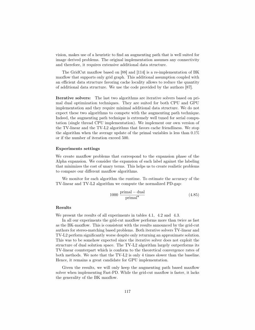
vision, makes use of a heuristic to find an augmenting path that is well suited forimage derived problems. The original implementation assumes any connectivityand therefore, it requires extensive additional data structure.
The GridCut maxflow based on [88] and [114] is a re-implementation of BKmaxflow that supports only grid graph. This additional assumption coupled withan efficient data structure favoring cache locality allows to reduce the quantityof additional data structure. We use the code provided by the authors [87].
Iterative solvers: The last two algorithms are iterative solvers based on pri-mal dual optimization techniques. They are suited for both CPU and GPUimplementation and they require minimal additional data structure. We do notexpect these two algorithms to compete with the augmenting path technique.Indeed, the augmenting path technique is extremely well tuned for serial compu-tation (single thread CPU implementation). We implement our own version ofthe TV-linear and the TV-L2 algorithms that favors cache friendliness. We stopthe algorithm when the average update of the primal variables is less than 0.1%or if the number of iteration exceed 500.
Experiments settings
We create maxflow problems that correspond to the expansion phase of theAlpha expansion. We consider the expansion of each label against the labelingthat minimizes the cost of unary terms. This helps us to create realistic problemsto compare our different maxflow algorithms.
We monitor for each algorithm the runtime. To estimate the accuracy of theTV-linear and TV-L2 algorithm we compute the normalized PD-gap:
1000primal´ dual
primal˚(4.85)
Results
We present the results of all experiments in tables 4.1, 4.2 and 4.3.In all our experiments the grid-cut maxflow performs more than twice as fast
as the BK-maxflow. This is consistent with the results announced by the grid-cutauthors for stereo-matching based problems. Both iterative solvers TV-linear andTV-L2 perform significantly worse despite only returning an approximate solution.This was to be somehow expected since the iterative solver does not exploit thestructure of dual solution space. The TV-L2 algorithm largely outperforms itsTV-linear counterpart which is conform to the theoretical convergence rates ofboth methods. We note that the TV-L2 is only 4 times slower than the baseline.Hence, it remains a great candidate for GPU implementation.
Given the results, we will only keep the augmenting path based maxflowsolver when implementing Fast-PD. While the grid-cut maxflow is faster, it lacksthe generality of the BK maxflow.
117

Small size problemsChurch Factory Buildings Industry Average
BK (baseline)Runtime (ms) 45.16 44.68 45.40 43.38 44.66Speed-up vs baseline 1 1 1 1 1GCRuntime (ms) 20.37 20.34 19.97 18.90 19.90Speed-up vs baseline 2.22 2.20 2.27 2.29 2.24TV-linearRuntime (ms) 271.42 248.34 242.41 259.11 255.32Speed-up vs baseline 0.17 0.18 0.19 0.17 0.17Normalized PD-gap 4.79 2.10 5.80 3.76 4.11TV-L2Runtime (ms) 175.60 177.34 173.82 169.81 174.14Speed-up vs baseline 0.26 0.25 0.26 0.26 0.26Normalized PD-gap 0.91 1.21 1.10 0.99 1.05
Table 4.1 – Comparing maxflow algorithm on small scale problems.
Medium size problemsChurch Factory Buildings Industry Average
BK (baseline)Runtime (ms) 187.31 188.95 187.03 190.22 188.38Speed-up vs baseline 1 1 1 1 1GCRuntime (ms) 187.31 188.95 187.03 190.22 188.38Speed-up vs baseline 2.26 2.29 2.32 2.14 2.25TV-linearRuntime (ms) 2430.40 2221.84 2270.64 2413.98 2334.21Speed-up vs baseline 0.08 0.09 0.08 0.08 0.08Normalized PD-gap 5.41 4.90 5.95 4.22 5.12TV-L2Runtime (ms) 667.76 680.63 659.60 658.90 666.73Speed-up vs baseline 0.28 0.28 0.28 0.29 0.28Normalized PD-gap 0.74 0.78 0.78 0.81 0.78
Table 4.2 – Comparing maxflow algorithm on medium scale problems.
4.6.3 Fast PD implementation experimentsWe propose to compare three different implementations of Fast-PD. As a baseline,we use the C++ implementation provided by the original authors based on amodified BK maxflow, we refer to it as Fast PD (NK). We propose two alternativeimplementations: one also based on the BK maxflow, named Fast PD (BK),and one based on the Grid-Cut maxflow, called Fast PD (GC). We note that
118

Large size problemsChurch Factory Buildings Industry Average
BK (baseline)Runtime (ms) 462.92 454.19 451.51 490.31 464.74Speed-up vs baseline 1 1 1 1 1GCRuntime (ms) 204.19 199.41 199.14 227.83 207.64Speed-up vs baseline 2.27 2.28 2.27 2.15 2.24TV-linearRuntime (ms) 10282.85 9234.86 9718.06 10679.88 9978.91Speed-up vs baseline 0.05 0.05 0.05 0.05 0.05Normalized PD-gap 5.82 6.52 6.69 4.08 5.78TV-L2Runtime (ms) 1494.28 1506.16 1486.56 1501.95 1497.24Speed-up vs baseline 0.31 0.30 0.30 0.33 0.31Normalized PD-gap 0.76 0.76 0.79 0.80 0.78
Table 4.3 – Comparing maxflow algorithm on large scale problems.
an implementation using the BK maxflow can handle any graph architecturewhile the implementation based on the Grid-Cut maxflow can only handle 4-connectivity grid. However, we note that it is relatively easy to extend theGrid-Cut version to 8-connectivity for instance.
Implementation memory footprint limitations
Since we work with large images in our context, we need to pay a close attentionto the memory footprint of our algorithms. Hence, our first experiment quantifiesthe memory footprint of the different implementations. The table 4.4 gives thememory required by each algorithm.
The memory footprint required by the original implementation of Fast-PDmakes it unsuitable in our context. Our implementations only needs on averageless than 10% of the original implementation memory requirement. The Fast PD(GC) requires less memory than the Fast PD (BK) since the grid-cut maxflowcan take advantage of the implicit grid structure to avoid storing the neighborsconnectivity in memory. While our implementations still require a significantamount of memory, they can easily run even on modern laptops.
Cache friendly indexation
We now proceed to exhibit the importance of cache friendliness when implement-ing algorithm such as Fast-PD. To this end, we propose two experiments.
Fast PD (BK) experiment: The first one makes use of Fast PD (BK). Wecompare the runtime when the edges are randomly ordered and when they are
119

Fast PD (NK) Fast PD (BK) Fast PD (GC)(baseline)
Small size problems:Memory footprint 981 MB 115 MB 92 MBRatio vs baseline 1 0.1172 0.0938
Medium size problems:Memory footprint 9066 MB 774 MB 648 MBRatio vs baseline 1 0.0854 0.0715
Large size problems:Memory footprint 40.02 GB 2.91 GB 2.61 GBRatio vs baseline 1 0.0727 0.0652
Table 4.4 – Memory footprint for different Fast PD implementations.
ordered to maximize cache friendliness. For both cases the memory layout ofall edge related variables (weights and dual variables) matches the order of theedges. All node related variables (the primal and height variables) are stored asa continuous vector that follows the vertical lines of the graph.
The main cases for cache misses happen during the pre-edit phase of theexpansion. In this phase the algorithm computes the inner capacities of themaxflow problem by scanning the dual variables following the order of the edges.It also needs to fetch the two primal variables associated to the edge, and it mightalso update the two height variables associated to the edge. If from one edge tothe next, those two primal and two height variables are far away in memory (notin the same cache line), then a cache miss occurs, forcing to load a new cacheline. Sometime this loading time can be hidden by some others computations.However, we illustrate that ordering the edges such that they follow the nodememory layout favors cache hits, and as a result boosts performance. The resultsare presented in table 4.5.
Hence, just by properly ordering the memory layout we obtain up to 1.7speed-up. Hence, from now on we only use the proper memory layout for ourexperiments.
Fast PD (GC) experiment: For our second experiment we propose twomemory layouts for the node and edge related variables. The first layout isexactly the one we used for the Fast PD (BK) with proper ordering. However,the grid-cut maxflow algorithm uses a particular memory layout to favor cachelocality during the growing and augmenting phases. Hence, we derive a secondversion of Fast PD (GC) that matches the grid-cut memory layout. The resultsare reported in the table 4.6.
As for the Fast PD (BK) experiment, the proper memory layout leads toimproved performances up to 1.3. We note that for the pre-edit dual phase of
120

Random ordering Proper ordering(baseline)
Small size problems:Average runtime (sec) 1.7 1.1Average speed-up vs baseline 1 1.52
Medium size problems:Average runtime (sec) 49.0 28.2Average speed-up vs baseline 1 1.73
Large size problems:Average runtime (sec) 330.2 189.6Average speed-up vs baseline 1 1.74
Table 4.5 – Cache friendliness experiments for Fast PD (BK)
BK layout Grid-cut layout(baseline)
Small size problems:Average execution time (sec) 1.2 1.0Average speed-up vs baseline 1 1.24
Medium size problems:Average execution time (sec) 24.2 18.2Average speed-up vs baseline 1 1.33
Large size problems:Average execution time (sec) 144.6 116.4Average speed-up vs baseline 1 1.24
Table 4.6 – Cache friendliness experiments for Fast PD (GC)
Fast-PD the grid-cut memory layout is a bit less efficient than the BK layout.However, this is largely compensated by the gain obtained when filling themaxflow capacities. Therefore, for Fast PD (GC) we elect to use the samememory layout than grid-cut.
Growing source and sink trees
We now verify the claim of the original authors of Fast PD about growing onlythe source tree. To this end, we perform a simple experiment. We solve each ofour stereo matching problem twice, once growing only the source tree and oncegrowing both source and sink trees. We carry-out this experiment for both FastPD (BK) and Fast PD (GC). The results are reported in table 4.7 and 4.8.
For Fast PD (BK) the results illustrates that as the problems grow larger
121

Source and sink Source only(baseline)
Small size problems:Average runtime (sec) 1.2 1.1Average speed-up vs baseline 1 1.04
Medium size problems:Average runtime (sec) 32.2 28.5Average speed-up vs baseline 1 1.13
Large size problems:Average runtime (sec) 267.5 191.6Average speed-up vs baseline 1 1.40
Table 4.7 – Growing tree experiments for Fast PD (BK)
Source and sink Source only(baseline)
Small size problems:Average runtime (sec) 1.0 0.9Average speed-up vs baseline 1 1.05
Medium size problems:Average runtime (sec) 21.2 18.5Average speed-up vs baseline 1 1.15
Large size problems:Average runtime (sec) 136.4 117.9Average speed-up vs baseline 1 1.16
Table 4.8 – Growing tree experiments for Fast PD (GC)
the speed-up increases up to 1.4. For Fast PD (GC) the results follow the sametrend but the speed up stalls around 1.15. Both experiments support the claimof the original authors of Fast-PD. Hence, we elect to only grow the source tree.
Comparing Fast PD implementations
We now compare the run time between the different implementations of FastPD. For Fast PD (NK) we did not run the experiments for large problems dueto the memory footprint. For the medium size problem, it is possible that theOS decided to compress the memory allocated to Fast PD (NK). This wouldhave an impact on the runtime but we decided not to discard this experimentsince it is a normal behavior and we can expect our users to run in the samesituation. We remind that compressing the memory penalizes the runtime far
122

less than swapping to hardrive even for SSD. We report the results in table 4.9.
Small size problemsChurch Factory Buildings Industry Average
Fast PD (NK) (baseline)Runtime (sec) 1.65 1.41 1.24 1.40 1.42Speed-up vs baseline 1 1 1 1 1Fast PD (BK)Runtime (sec) 1.48 1.10 1.08 1.29 1.24Speed-up vs baseline 1.11 1.28 1.14 1.08 1.15Fast PD (GC)Runtime (sec) 1.26 0.89 0.96 1.04 1.04Speed-up vs baseline 1.30 1.57 1.29 1.35 1.37
Medium size problemsChurch Factory Buildings Industry Average
Fast PD (NK) (baseline)Runtime (sec) 28.35 25.96 18.73 23.24 24.07Speed-up vs baseline 1 1 1 1 1Fast PD (BK)Runtime (sec) 24.01 35.11 23.09 28.69 27.73Speed-up vs baseline 1.18 0.74 0.81 0.81 0.87Fast PD (GC)Runtime (sec) 15.80 22.05 15.86 18.37 18.02Speed-up vs baseline 1.79 1.18 1.18 1.26 1.34
Large size problemsChurch Factory Buildings Industry Average
Fast PD (NK)Runtime (sec) - - - - -Fast PD (BK)Runtime (sec) 171.37 212.90 139.71 218.52 185.63Fast PD (GC)Runtime (sec) 108.88 118.24 96.60 137.57 115.32Speed-up vs Fast PD (BK) 1.57 1.80 1.45 1.59 1.61
Table 4.9 – Comparison of Fast PD different implementations
For all experiments, Fast PD (GC) outperforms the other two implementa-tions. This is an ideal situation since it is also the implementation that requiresthe less memory. Hence, for 4-connected problems and in our context, Fast PD(GC) should always be the algorithm of choice.
It was a bit surprising to us that for small size problems Fast PD (NK), theoriginal implementation, is the slowest version. In fact, the extra allocation timeneeded by Fast PD (NK) cannot be compensated by the speed-up obtained in
123

the last expansion phases. For medium size problem, we witness no evidencethat the OS decided to compress memory. In these settings, Fast PD (NK)outperforms Fast PD (BK) by 10%. Given the amount of memory saved by FastPD (BK), this is good trade-off since we reduce the memory consumption by90% to only increase the computation by 10%. For large problems, Fast PD(GC) is on average 1.6 time faster than Fast PD (BK). This is mainly thanks toa faster maxflow algorithm. However, it is important to keep in mind that FastPD (BK) can handle any graph connectivity.
To conclude, our two implementations are suitable for large size problems. Interm of running time both are very competitive since they outperform the originalproblem except for the medium size problems for Fast PD (BK). For 4-connectedproblems, we elect to use Fast PD (GC). For any other graph connectivity, weuse Fast PD (BK).
4.6.4 Fast PD vs Alpha-expansionWe now need to compare our implementation against the Alpha-expansionalgorithm. To this end, for the Alpha-expansion we use the C++ implementationprovided by [165] that we compile with the same optimization flags as ourimplementations. As stated in [102], both Alpha-expansion and Fast-PD obtainsimilar results in term of energy and solution. Hence, we only provide the resultsof our experiments on running time in table 4.10.
Both Fast PD (BK) and Fast PD (GC) outperform Alpha Expansion sig-nificantly. This is conform with the experiments of [102]. Fast PD (BK) is onaverage twice as fast as the Alpha Expansion and Fast PD (GC) runs between 3and 4 times faster than Alpha Expansion. Moreover, Fast-PD is also capable ofsolving a larger class of problems than the Alpha Expansion. Hence, since thememory footprint of both Fast PD (BK) and Fast PD (GC) is suitable to ourcontext, we elect to use Fast PD (BK) and Fast PD (GC) over Alpha Expansion.
124

Small size problemsChurch Factory Buildings Industry Average
Alpha Expansion (baseline)Runtime (sec) 3.49 2.55 3.22 3.39 3.16Speed-up vs baseline 1 1 1 1 1Fast PD (BK)Runtime (sec) 1.56 1.03 1.11 1.30 1.25Speed-up vs baseline 2.24 2.47 2.90 2.60 2.53Fast PD (GC)Runtime (sec) 1.28 0.90 0.96 1.14 1.07Speed-up vs baseline 2.73 2.84 3.36 2.98 2.96
Medium size problemsChurch Factory Buildings Industry Average
Alpha Expansion (baseline)Runtime (sec) 77.74 86.83 71.37 69.14 76.27Speed-up vs baseline 1 1 1 1 1Fast PD (BK)Runtime (sec) 23.84 35.11 23.71 32.75 28.85Speed-up vs baseline 3.26 2.47 3.01 2.11 2.64Fast PD (GC)Runtime (sec) 16.13 22.10 16.49 19.57 18.57Speed-up vs baseline 4.82 3.93 4.33 3.53 4.11
Large size problemsChurch Factory Buildings Industry Average
Alpha Expansion (baseline)Runtime (sec) 409.76 399.50 354.75 557.20 430.30Speed-up vs baseline 1 1 1 1 1Fast PD (BK)Runtime (sec) 171.78 213.84 140.24 227.14 188.25Speed-up vs baseline 2.39 1.87 2.53 2.45 2.29Fast PD (GC)Runtime (sec) 108.47 118.44 97.02 143.02 116.74Speed-up vs baseline 3.78 3.37 3.66 3.90 3.69
Table 4.10 – Comparing Fast PD and graph cuts.
4.7 ConclusionThis second technical chapter introduced the basic of non-convex optimization.We presented and demonstrated the link between the maxflow and mincutproblems. We surveyed different algorithm to solve either a maxflow or mincutproblem. Then, we presented the α expansion algorithm along with Fast-PD. Weextensively experiment with our own implementation of Fast-PD in the context
125

of stereo-matching where it drastically outperforms the original implementation.
Despite these improvement non convex optimization techniques remainscomputationally intensive. Hence, we investigate in the next chapter coarseningscheme for non convex optimization. We also provide a comparison in the contextof remote sensing between the non convex optimization techniques of this chapterand the First order Primal-Dual methods of the previous chapter.
126

Chapter 5
Coarsening schemes foroptimization techniques
5.1 Introduction and contributions
5.1.1 IntroductionIn this chapter we consider coarsening scheme for the optimization techniquespresented in the two previous chapters 3 and 4.
Hence, we study coarsening schemes suited for the First order Primal-Dualtechniques for convex optimization. In this context, we review how to transformour initial non convex problem to a series of convex surrogate problems. Weuse the stereo-matching task of last chapter 4 to evaluate the performances andtrade-offs of different schemes.
We also investigate coarsening schemes for Graph-Cuts techniques. In thiscontext, the goal is to reduce the overall computational complexity. To this end,we present a new coarsening scheme that uses machine learning techniques todeliver impressive trade-off between speeding-up and precise optimization. Asfor the First order Primal-Dual techniques, we perform experiments with thestereo-matching task.
5.1.2 Chapter organizationThe section 5.2 introduces and compares the smoothing and coarsening schemefor first order primal-dual techniques. We discuss in section 5.3 the imageand energy pyramid schemes for graph-cuts optimization techniques. We alsointroduce a powerful optimization framework named Inference by learning.
127

5.1.3 ContributionsThe main contribution of this chapters related to the coarsening scheme forGraph-Cuts techniques where we present different approaches to coarsen anMRF model. None only our coarsening scheme speeds up the optimization butit also delivers more accurate solution. Finally, we present a novel frameworkbuilt on top of the coarsening scheme that drastically speeds-up the inferencewhile maintaining impressive accuracy.
5.2 Smoothing and Coarsening scheme for firstorder primal dual optimization techniques
The first order primal dual scheme assumes that the function to optimize isconvex. However, we can not guaranty the convexity of the functions of interest.Hence, we detail a scheme to approximate any given function with a convexsurrogate function.
To this end, we first survey the causes of non convexity. Then, we show thatwe can easily create a convex surrogate function that locally approximates thegiven function. Finally, we analyze two schemes, smoothing and coarsening, toextend the approximation to larger support.
5.2.1 Preliminary workApproximation measure
We propose to make use of the approximation measure to evaluate the qualityof the approximation of the surrogate function. We use the following definitionto measure how close a function f approximates a reference function fref :
100
ş
|fpxq ´ fref pxq|dxş
|fref pxq|dx(5.1)
We note that many other approximation measures exist.
Origin of the non convexity
The non convexity can arise in both the matching and the regularization termsof the given function.
Non convex matching term The matching term is the main culprit of non-convexity for registration problems. The non convexity comes from the spatialressampling and is amplified by the matching criterion. We also note that thematching criteria such as census, ZNCC or truncated norms are also non convexfunctions.
128

Image ressampling The spatial ressampling of an image I at point pi “pri, ciq P Ω, the spatial support of image, of row ri and column ci with adisplacement vector di “ pdri , dciq defines the following function:
fI,pipdiq “ Ipri ` dri , ci ` dciq
The spatial ressampling of any natural digital image is almost statisticallyguaranteed to yield a non convex function. We exemplify this phenomenonby ressampling along the horizontal axis images of aerial survey acquired withthe UltraCam camera. We use the same images than in the stereo matchingapplication of the previous chapter. The figure 5.1 illustrates typical ressam-pling functions pfI,piqi at four different points with the following ressamplingtechniques: nearest, linear and cubic. We point the interested reader to [2] for adetailed definition of these ressampling techniques.
Point 1 Point 2
Point 3 Point 4
Figure 5.1 – Non convexity and image ressampling.
The curves highlights the non convexity of the ressampling function indepen-dently of the method. The non convexity is directly linked to image content.Hence, it generally drastically varies within the same image. The main differencebetween ressampling techniques is the smoothness. The cubic method alwaysgenerates smooth curves while the nearest and linear methods generate nonsmooth curves with the nearest methods being the least smooth. We also note
129

that the algorithmic complexity increases between methods, with the nearestmethod being the fastest and the cubic method being the slowest. Yet, inour context this only accounts for a negligible part of the total computationalcomplexity.
Matching criterion We survey how much the matching criterion amplifiesthe non convexity. To this end, in the context of stereo matching introducedin the last chapter we make use of the `1 and ZNCC matching criteria. Wedisplay with figures 5.2 and 5.3 for the same points that figure 5.1 the curvesassociated to each matching criterion with the different ressampling methods.
Point 1 Point 2
Point 3 Point 4
Figure 5.2 – Non convexity and ZNCC matching criterion.
We observe that the matching criterion amplifies the non convexity. Moreover,the ZNCC being a non-convex function accentuates the non-convexity more thanthe `1 matching criterion. For both criteria, we observe the function maintainsthe smoothness property of the ressampling method. The matching criterionalso increases the difference between ressampling methods. We quantify thisphenomenon by taking the cubic ressampling as reference and computing theapproximation measure for the nearest and linear ressampling methods.
The table 5.1 details the approximation measure for all 4 subsets of thestereo matching application of the previous chapter. The figure 5.4 displays the
130
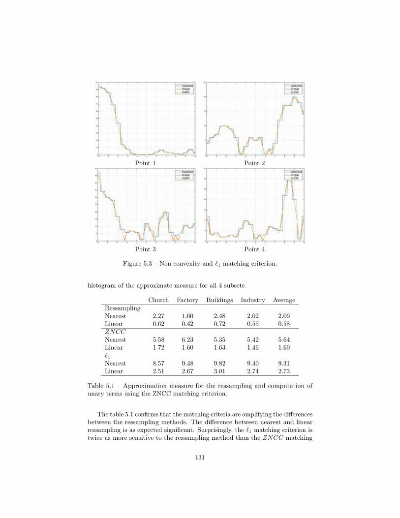
Point 1 Point 2
Point 3 Point 4
Figure 5.3 – Non convexity and `1 matching criterion.
histogram of the approximate measure for all 4 subsets.
Church Factory Buildings Industry AverageRessamplingNearest 2.27 1.60 2.48 2.02 2.09Linear 0.62 0.42 0.72 0.55 0.58ZNCCNearest 5.58 6.23 5.35 5.42 5.64Linear 1.72 1.60 1.63 1.46 1.60`1Nearest 8.57 9.48 9.82 9.40 9.31Linear 2.51 2.67 3.01 2.74 2.73
Table 5.1 – Approximation measure for the ressampling and computation ofunary terms using the ZNCC matching criterion.
The table 5.1 confirms that the matching criteria are amplifying the differencesbetween the ressampling methods. The difference between nearest and linearressampling is as expected significant. Surprisingly, the `1 matching criterion istwice as more sensitive to the ressampling method than the ZNCC matching
131

Ressampling
ZNCC `1
Figure 5.4 – Histogram of approximation measures for ressampling methods andmatching criteria.
criterion.
Non convex regularization terms In our context the regularization termφij : RdˆRd Ñ R is generally a multi-dimensional bi-variate function composedof a weighting term wij P R` and a non linear function ψ : RÑ R`:
φijpa, bq “ wij ψp||a´ b||εq, @pa, bq P Rd ˆ Rd
Hence, the non-convexity actually entirely comes from the function ψp.q whenit takes for instance one of the following forms:
Truncated: ψpxq “ minpx, γq, @px, γq P Rˆ R`
Cauchy: ψpxq “1
1`
ˆ
x
γ
˙α , @px, γ, αq P Rˆ R` ˆ R`
Welsch: ψpxq “ exp
ˆ
´
ˆ
x
γ
˙α˙
, @px, γ, αq P Rˆ R` ˆ R`
We display the regularization functions in figure 5.5.
132

Figure 5.5 – Non convex regularizationterms
• Truncated with γ “ 3,
• Cauchy with γ “ 7 and α “ 2,
• Welsch with γ “ 8 and α “ 1.5.
Taylor approximation for unary terms
When we are only interested to get a convex surrogate function on a smallinterval we can rely on Taylor series.
Taylor series An infinite differentiable function f can be represented as aninfinite sum of terms, a Taylor series, computed from its derivatives:
fpxq “8ÿ
n“0
f pnqpaq
n!px´ aqn
We note that the high order terms progressively vanish as x gets closer to theneighborhood of a. This property allows us to build a polynomial of small orderthat approximately represents a function around a certain point of interest.
For the unary term, we can exploit this idea in two different ways dependingon the convexity of the matching criterion.
1st order approximation Here, we assume that the matching criterion ρ isa convex non decreasing function. Moreover, we limit ourself to the first orderpolynomial functions to approximate the image ressampling. We obtain for agiven point of interest a P Rd:
Ipa` xq « Ipaq ` p∇Ipaqqt x
This approximation is also sometimes referred to as linearization.
Hence, we obtain for a convex function ρ the resulting approximation:
ρpIpa` xqq « ρpIpaq ` p∇Ipaqqt xq
The resulting function is a convex function since it is composed of a convexfunction, the linear term, with a convex non decreasing function, the matchingcriterion.
133

2nd order approximation If we can’t make the previous assumption onthe matching criterion, then we proceed with a second order approximation.We define as fp.q the composition of the image ressampling and the matchingcriterion. By limiting the Taylor series of f to the second order we get:
fpxq « fpaq ` p∇fpaqqt x` xt∇2fpaqx
We note that this approximation is guaranteed to yield a convex functiononly if the Hessian matrix ∇2fpaq is semi definite positive for any point a.Hence, we not only set to zero all non diagonal elements but also the negativediagonal elements of the Hessian matrix as in[170]. We refer to this modifiedHessian matrix as ∇2
`fpaq. Finally, we obtain the following 2nd order convexapproximation:
fpxq « fpaq ` p∇fpaqqt x` xt∇2`fpaqx
Discretization of derivative operators The computation of a Taylor seriesheavily relies on calculating derivatives of different orders. Considering we workwith discretized images we need to define the discretized counterparts of thecontinuous derivative operators. Different discretization schemes exist. We limitthe definition to the case of a mono-dimensional function defined on a rectangularuniform grid. The extension of each scheme to multi-dimensional variables isstraight forward. Since we always assume that our data are uniform gridded,we will not discuss the extension of these definitions to non uniform grid or ungridded space. However, we point the curious reader to the following works [124]for more details on discretization.
For the following definitions we make use of the discrete function fp., .q :Rˆ C Ñ R where R Ă N and C Ă N index respectively the row and columns ofthe grid.
First order derivatives The forward, backward and central schemes arethe most used approximations to calculate the first order derivatives.
The forward method computes:
∇fpi, jq “„
fpi` 1, jq ´ fpi, jqfpi, j ` 1q ´ fpi, jq
The backward method computes:
∇ifpi, jq “„
fpi, jq ´ fpi´ 1, jqfpi, jq ´ fpi, j ´ 1q
The central method computes:
∇fpi, jq “„
fpi` 0.5, jq ´ fpi´ 0.5, jqfpi, j ` 0.5q ´ fpi, j ´ 0.5q
“
»
—
–
fpi` 1, jq ´ fpi´ 1, jq
2fpi, j ` 1q ´ fpi, j ´ 1q
2
fi
ffi
fl
(with linear interpolation)
134

We display in figure 5.6 and 5.7 examples of each discretization scheme.
Discretization scheme
Backward Central Forward
Figure 5.6 – Examples of discretization of the first order derivative: the red lineplots the derivative of the blue curve at the point marked by the red diamondshape.
Discretization scheme
Backward Central Forward
Figure 5.7 – Analytic derivatives vs discretized derivatives for xÑ 1´ cosp0.2xq:the red line plots the derivative estimated by the discretization scheme while theblue curve displays the analytic derived derivative.
In agreement with their respective equations, the forward and backwardschemes are slightly out of phase. The central discretization scheme seems toperform better. During our experiments, we will pursue this investigation inmore depth with functions derived from realistic unary terms.
Second order derivatives The forward, backward and central schemealso extend to second order derivatives. We only gives the diagonals elements
135
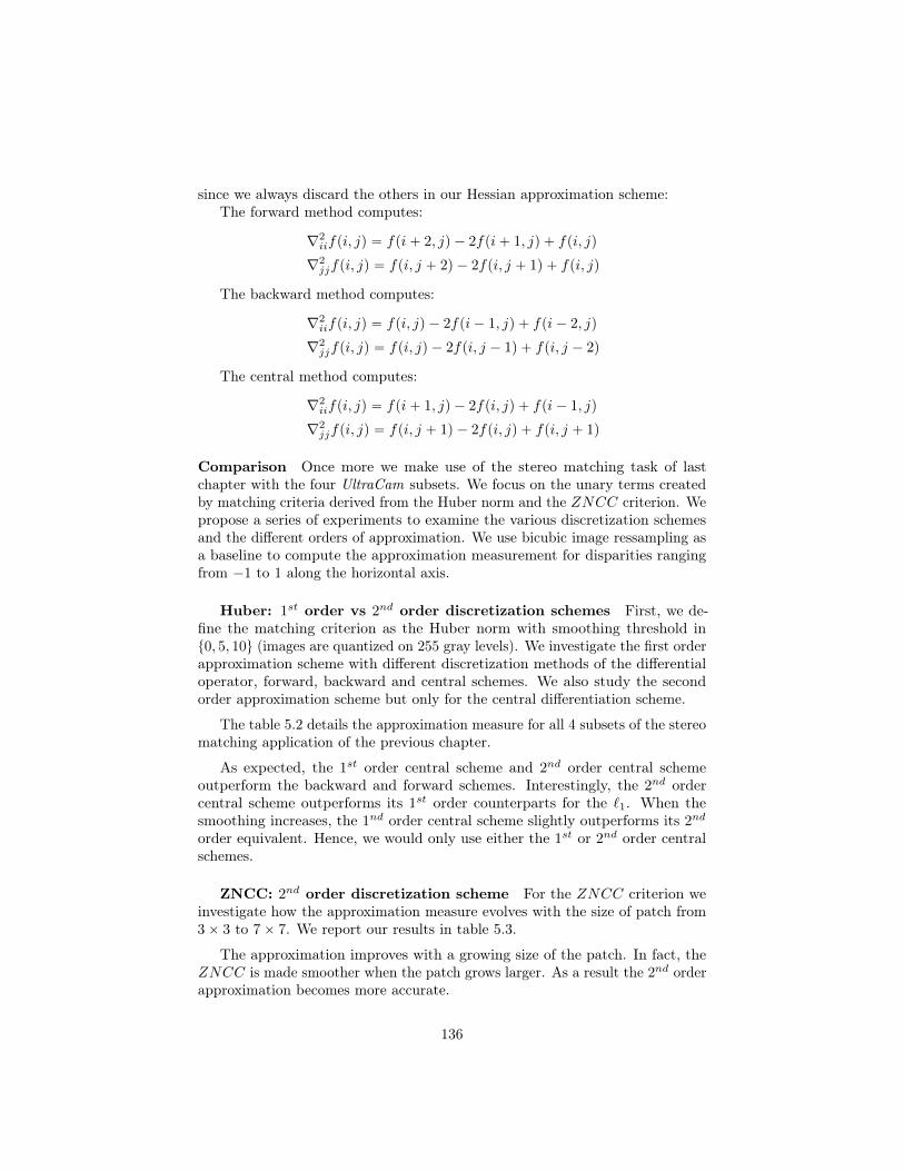
since we always discard the others in our Hessian approximation scheme:The forward method computes:
∇2iifpi, jq “ fpi` 2, jq ´ 2fpi` 1, jq ` fpi, jq
∇2jjfpi, jq “ fpi, j ` 2q ´ 2fpi, j ` 1q ` fpi, jq
The backward method computes:
∇2iifpi, jq “ fpi, jq ´ 2fpi´ 1, jq ` fpi´ 2, jq
∇2jjfpi, jq “ fpi, jq ´ 2fpi, j ´ 1q ` fpi, j ´ 2q
The central method computes:
∇2iifpi, jq “ fpi` 1, jq ´ 2fpi, jq ` fpi´ 1, jq
∇2jjfpi, jq “ fpi, j ` 1q ´ 2fpi, jq ` fpi, j ` 1q
Comparison Once more we make use of the stereo matching task of lastchapter with the four UltraCam subsets. We focus on the unary terms createdby matching criteria derived from the Huber norm and the ZNCC criterion. Wepropose a series of experiments to examine the various discretization schemesand the different orders of approximation. We use bicubic image ressampling asa baseline to compute the approximation measurement for disparities rangingfrom ´1 to 1 along the horizontal axis.
Huber: 1st order vs 2nd order discretization schemes First, we de-fine the matching criterion as the Huber norm with smoothing threshold int0, 5, 10u (images are quantized on 255 gray levels). We investigate the first orderapproximation scheme with different discretization methods of the differentialoperator, forward, backward and central schemes. We also study the secondorder approximation scheme but only for the central differentiation scheme.
The table 5.2 details the approximation measure for all 4 subsets of the stereomatching application of the previous chapter.
As expected, the 1st order central scheme and 2nd order central schemeoutperform the backward and forward schemes. Interestingly, the 2nd ordercentral scheme outperforms its 1st order counterparts for the `1. When thesmoothing increases, the 1nd order central scheme slightly outperforms its 2nd
order equivalent. Hence, we would only use either the 1st or 2nd order centralschemes.
ZNCC: 2nd order discretization scheme For the ZNCC criterion weinvestigate how the approximation measure evolves with the size of patch from3ˆ 3 to 7ˆ 7. We report our results in table 5.3.
The approximation improves with a growing size of the patch. In fact, theZNCC is made smoother when the patch grows larger. As a result the 2nd orderapproximation becomes more accurate.
136

Smoothing threshold of 0: `1 normChurch Factory Buildings Industry Average
Discretization1st order backward 20.14 28.42 19.06 19.30 21.731st order central 17.99 24.95 16.89 17.12 19.241st order forward 20.02 28.36 18.88 19.21 21.622nd order central 16.97 24.96 15.96 16.28 18.54
Smoothing threshold of 10Church Factory Buildings Industry Average
Discretization1st order backward 37.15 55.40 34.49 36.07 40.781st order central 28.96 40.46 26.87 28.08 31.091st order forward 36.78 53.48 34.25 36.05 40.142nd order central 29.90 44.98 27.87 29.28 33.01
Smoothing threshold of 20Church Factory Buildings Industry Average
Discretization1st order backward 39.13 57.44 36.82 37.74 42.781st order central 30.10 41.38 28.17 29.18 32.211st order forward 38.86 54.92 36.59 37.84 42.052nd order central 31.33 46.43 29.42 30.57 34.44
Table 5.2 – Approximation measurement for different discretization schemes withHuber based matching criterion.
Church Factory Buildings Industry AveragePatch size3ˆ 3 14.13 20.97 11.91 10.86 14.475ˆ 5 8.12 15.05 5.98 4.97 8.537ˆ 7 6.34 13.81 4.18 3.20 6.88
Table 5.3 – Approximation measurement for different patch sizes with ZNCCbased matching criterion.
Taylor approximation for pairwise terms
For the pairwise terms and the regularization criterion that we investigate, the1st and 2nd order approximation lead to exactly the same results. Indeed, sincethe functions of interest are non convex the 2nd order term is always set to 0.
137
5.2.2 ApproachIdeally, we want to represent with as much accuracy as possible the energymanifold with a convex function around a current solution. This clearly lookslike a chicken and egg problem. On the one hand we need a current solution todefine the locality where to represent the energy manifold. On the other hand,we need to get a current solution that is as close as possible to the unknownminimum of the energy manifold. Hence, we rely on an iterative scheme that:
1. Creates a surrogate function that approximate the energy manifold withina certain range around the current solution.
2. Computes the minimum of this surrogate functions to get an updatedsolution.
3. Defines a new range for the next approximation.
Moreover, we also need to quickly compute the convex surrogate functionotherwise any computational speed-up gained by using a primal-dual schemeover the graph-cut scheme will be negated. To this end, we propose to workdirectly on the images used to compute the energy manifold with two classicapproaches: Filtering and Coarsening.
5.2.3 Surrogate function via Filtering schemeThe first approach, that we refer to as the Filtering scheme, only modifies theunary terms.
Filtering
We suppose we are given a function f : RÑ R to smooth and a continuous filterk : RÑ R. The convolution of f by k gives the filtered function fs : RÑ R:
fspxq “
ż
kpyqfpx´ yqdy, @x P R
Since we mainly work with discretized functions we remind the definitionof the discrete convolution operator. The convolution of a discrete functionf : ZÑ R by a filter k : KÑ R with limited support K Ď Z computes:
fspiq “ÿ
jPKkpjqfpi´ jq, @i P Z
To simplify notations, we use the operator ‹ to indicate convolution in-differently of the continuous and discrete domain. For instance the convolu-tion of the function fp.q by filter kp.q is noted k ‹ f and we also write for alli P Z, fspiq “ pk ‹ fqpiq.
If we assume that kp.q is a low pass filter, it reduces the average curvatureof the function it is convoluted to. Indeed, the second order derivatives gives
138

the curvature along each directions. Since the second order derivative is a linearoperator we have:
pk ‹ fq2 “ k ‹ pf2q
Gaussian filtering
We choose to use a Gaussian filter as low pass filter. The Gaussian filterminimizes group delay making it an ideal time domain filter as explained in[13]. We remind the impulse response function of a Gaussian filter for a real ddimensional variables x:
gpxq “1
a
det p2πΣqexp
ˆ
´1
2xtΣ´1x
˙
(5.2)
The matrix Σ is a SDP d ˆ d matrix controlling the filtering in each ofthe d direction. For our filtering scheme, we only use some diagonal matrixΣ “ diagpσ2
1 , σ22 , . . . , σ
2dq. Hence, the Gaussian filter simplifies to:
gpxq “1
a
p2πqdśdj“1 σd
exp
˜
´
dÿ
j“1
x2j
2σ2j
¸
(5.3)
By nature the Gaussian filter has an infinite support. However, we noticethat when x grows large the value of gpxq tends to 0. Hence, in our contextwe only use a limited support for the Gaussian filter. However, we properlyrenormalize the output of filtering such that a constant signal is unmodified.
Figure 5.8 – 1-dimensionalGaussian filters for differentvalues of σ.
We display in figure 5.8the impulse response of 1-dimensional Gaussian filtersfor different values of σ. We no-tice that as sigma grows larger,the Gaussian filter has a largerspread, and hence, a lower lowpass frequency cut-off.
Reducing curvature and non convexity
Filtering with a low pass filter helps to reduce the curvature. If we now assumethat the function fp.q is close to be convex, we can find a low pass filter kp.q thatafter convolution creates a convex function. And, then we can use this createdconvex function as a surrogate function in the first order primal dual scheme.
139

We note that if the function fp.q is far from being convex we then need thefilter kp.q to be low pass filter with a potentially very low frequency cut-off toget a convex function. The worst case scenario is when fp.q is strongly concave.The only convex function we can obtain with filtering is the constant functionwith value corresponding to the average of fp.q over its entire domain.
However, in our context, we are going to filter the images instead of filteringthe energy to maintain a low computational complexity. Hence, after filtering wedo not seek to obtain a fully convex function but only attempt to reduce the initialnon convexity. Moreover, even if the images are smooth, the matching criterioncan potentially create matching potentials with high curvature. The figure 5.9displays the matching term obtained with the ZNCC matching criterion in thecontext of stereo matching.
Figure 5.9 – ZNCC matching cost. From blue to red the images used to computethe ZNCC are more and more smoothed. While the smoothing can reduce thenon convexity it also creates poor approximation of the original curve (bluestcurve).
The filtering scheme
To simplify notations in the algorithm 16 description we use the functionφi,Ir,It,di : r´1, 1s ˆ r´1, 1s Ñ R to represent the combination of the Taylorapproximation of image It around di and the matching criterion φ.
5.2.4 Surrogate function via coarseningThe second approach, referred as the coarsening scheme, is well established inthe computer vision community. Hence, we only give a brief description of it.We refer the curious reader to [1] for more details.
Coarsening
The coarsening scheme simply downsamples the images used to compute theenergy manifold by a given factor, and then computes a coarsen energy manifoldfrom the downsampled images. We remind that image downsampling simplyconsists of a low pass filtering followed by a decimation. Hence, the coarseningscheme can be seen as an extension of the Filtering scheme. To simplify the
140

Algorithm 16: Image filtering schemeData: Inputs: Ir, It, pφiqi, ψ, ΣlistResult: pdiqi
Initialize displacement field Ñ d “ 0
Compute weights of regularization pwijqij from Ir.for σ P Σlist do
Compute the Gaussian filter Ñ gσ
Apply filtering on both image:
Ir,σ “ gσ ‹ Ir and It,σ “ gσ ‹ It
while pdiqi is updated doCompute the Taylor approximation of unary term Ñ φi,Ir,σ,It,σ,di
Solve optimization problem:
minxiPr´1,1s2
ÿ
iPVφi,Ir,σ,It,σ,dipxiq `
ÿ
pi,jqPE
wijψp||di ` xi ´ dj ´ xj ||εq
Update displacement:
di Ð di ` xi, @i P V
notations we denote the upsampling by the Ò symbol and the downsamplingwith the Ó symbol.
We describe the Coarsening scheme in algorithm 17.
5.2.5 ExperimentsWe proceed to evaluate the Filtering and the Coarsening schemes. We make useof the stereo matching application of last chapter. Since we optimize non-convexenergy we use a baseline reference the solution obtained with the graph-cutsoptimization technique of chapter 4. For both schemes, we monitor the energyratio with respect to the energy obtained with Fast-PD. We also compute themean error in pixel using `1 norm with respect to the solution of Fast-PD.
Filtering vs coarsening
Our first experiment directly compares the filtering scheme to the coarseningscheme.
141

Algorithm 17: Coarsening schemeData: Inputs: Ir, It, pφiqi, ψ, ΣlistResult: pdiqi
Initialize displacement field at coarsest scale Ñ d “ 0for σ P Σlist do
Compute the Gaussian filter Ñ gσ
Downsample both image:
Ir,σ “Ó pgσ ‹ Irq and It,σ “Ó pgσ ‹ Itq
Compute weights of regularization pwij,σqij from Ir,σ.while pdiqi is updated do
Solve optimization problem:
minxiPr´1,1s2
ÿ
iPVσ
φi,Ir,σ,It,σ,dipxiq`ÿ
pi,jqPEσ
wij,σψp||di`xi´dj´xj ||εq
Update displacement field:
di Ð di ` xi, @i P Vσ
Upsample displacement field for next scale:
dÐÒ d
For both schemes, we compute 3 successive Taylor approximations per scaleand we perform 30 iterations of the Primal-Dual solver for each Taylor approxi-mation. We found that increasing the number of iterations of the Primal-Dualsolver is only slightly modifying the results. For the filtering scheme we use a 2DGaussian filter with standard deviation ranging from 7 to 0.5 with a decrement of0.5. A last iteration is performed with the unfiltered image. For the coarseningscheme we use a 0.66 downsampling factor with 8 scales. We use the bicubicfilter to interpolate the images.
Table 5.4 summarizes the results.From table 5.4 we see that for both schemes the energy ratio is mostly under
1.10 and the mean error is under 0.6. Both schemes are always out-performed bythe Fast-PD baseline. Hence, the non-convexity of the energy manifold clearlyneeds to be taken into account by the optimization scheme. The figure 5.10highlights the difference between the two schemes and the baseline.
For most experiments the Filtering scheme yields a lower energy than theCoarsening scheme. However, we see that Mean Error criterion is often sig-nificantly better for the Coarsening scheme. This indicates that the Filtering
142

Small size problemsChurch Factory Buildings Industry Average
FilteringEnergy (ratio) 1.02 1.03 1.04 1.02 1.03Mean Error 0.30 0.28 0.27 0.27 0.28CoarseningEnergy (ratio) 1.13 1.12 1.15 1.11 1.13Mean Error 0.33 0.30 0.30 0.30 0.31
Medium size problemsChurch Factory Buildings Industry Average
FilteringEnergy (ratio) 1.03 1.06 1.04 1.03 1.04Mean Error 0.40 0.45 0.40 0.40 0.41CoarseningEnergy (ratio) 1.09 1.08 1.12 1.08 1.09Mean Error 0.44 0.34 0.42 0.42 0.40
Large size problemsChurch Factory Buildings Industry Average
FilteringEnergy (ratio) 1.05 1.11 1.07 1.03 1.06Mean Error 0.62 0.93 0.65 0.59 0.70CoarseningEnergy (ratio) 1.08 1.07 1.10 1.06 1.08Mean Error 0.53 0.42 0.57 0.57 0.52
Table 5.4 – Comparing the filtering and coarsening scheme.
scheme has found a solution of relative low energy, but higher than Fast-PD,that significantly differs from the Fast-PD solution.
A visual inspection of the disparity maps confirms this phenomenon. Forinstance, we see in figure 5.10 that the roof of the church is poorly estimated bythe filtering scheme.
The filtering scheme creates artifacts for the church and factory subsets.Hence, for the following experiments we discard the filtering scheme to onlyretain the coarsening scheme.
143

Graph-Cuts Filtering scheme Coarsening scheme
Figure 5.10 – Comparing the filtering and coarsening schemes for the subsetsat full resolution. We notice that neither the Filtering and Coarsening schemeresolve fine details such as the church’s bell tower or the factory chimney.Moreover, the Filtering scheme produces unacceptable artifacts.
Coarsening 1D vs 2D
We now investigate the differences between the 1D and 2D coarsening. In thecontext of the stereo-matching, we deal with a 1D problem. Hence, instead of 2D
144

filtering and decimation we can only filter and decimate in the axis confoundedwith the epipolar lines.
Small size problemsChurch Factory Buildings Industry Average
Coarsening 1DEnergy (ratio) 1.12 1.13 1.17 1.12 1.13Mean Error 0.33 0.31 0.30 0.30 0.31Coarsening 2DEnergy (ratio) 1.13 1.12 1.15 1.11 1.13Mean Error 0.33 0.30 0.30 0.30 0.31
Medium size problemsChurch Factory Buildings Industry Average
Coarsening 1DEnergy (ratio) 1.09 1.08 1.13 1.08 1.09Mean Error 0.44 0.35 0.44 0.41 0.41Coarsening 2DEnergy (ratio) 1.09 1.08 1.12 1.08 1.09Mean Error 0.44 0.34 0.42 0.42 0.40
Large size problemsChurch Factory Buildings Industry Average
Coarsening 1DEnergy (ratio) 1.08 1.07 1.12 1.06 1.08Mean Error 0.57 0.43 0.65 0.55 0.55Coarsening 2DEnergy (ratio) 1.08 1.07 1.10 1.06 1.08Mean Error 0.53 0.42 0.57 0.57 0.52
Table 5.5 – Comparing 1D and 2D coarsening schemes.
For both coarsening scheme the results are very similar. Both the visualinspection of figure 5.11 and the review of table 5.5 show no significant improve-ment of the 1D coarsening scheme over the 2D coarsening scheme. From nowon, we only retain the latter because of its better computational cost.
145

Graph-Cuts 1D coarsening 2D coarsening
Figure 5.11 – Comparing 1D and 2D coarsening scheme. Both schemes giveessentially the same results.
Downsampling
We perform a last experiment that investigates the impact of the downsamplingfactor. We vary the downsampling ratio from 0.5 to 0.8 with 0.1 increment. Foreach ratio we adequately tune the number of scales such that the coarsest scale
146

represents approximately the same downsampling factor with respect to the fullresolution images.
Small size problemsChurch Factory Buildings Industry Average
Coarsening 0.5Energy (ratio) 1.13 1.13 1.17 1.12 1.14Mean Error 0.33 0.31 0.30 0.30 0.31Coarsening 0.6Energy (ratio) 1.13 1.12 1.16 1.12 1.13Mean Error 0.33 0.30 0.30 0.30 0.31Coarsening 0.7Energy (ratio) 1.13 1.12 1.16 1.11 1.13Mean Error 0.33 0.30 0.30 0.30 0.31Coarsening 0.8Energy (ratio) 1.12 1.12 1.15 1.11 1.12Mean Error 0.33 0.30 0.30 0.30 0.31
Table 5.6 – Comparing downsampling factor of the coarsening scheme for smallsize problems.
Medium size problemsChurch Factory Buildings Industry Average
Coarsening 0.5Energy (ratio) 1.10 1.09 1.13 1.09 1.10Mean Error 0.45 0.36 0.43 0.44 0.42Coarsening 0.6Energy (ratio) 1.10 1.09 1.12 1.08 1.09Mean Error 0.44 0.35 0.42 0.42 0.41Coarsening 0.7Energy (ratio) 1.09 1.08 1.11 1.07 1.09Mean Error 0.43 0.33 0.41 0.41 0.40Coarsening 0.8Energy (ratio) 1.09 1.07 1.11 1.07 1.08Mean Error 0.43 0.33 0.41 0.40 0.39
Table 5.7 – Comparing downsampling factor of the coarsening scheme for mediumsize problems.
The tables 5.6, 5.7 and 5.8 all indicate that a progressive downsamplingyields better results. However, the improvement is relatively small as we can seein figure 5.12. Moreover, high value downsampling factors require more scaleswhich lead to larger computational complexity. For those reasons we advocateto choose a downsampling factor between 0.5 and 0.6.
147

Large size problemsChurch Factory Buildings Industry Average
Coarsening 0.5Energy (ratio) 1.09 1.08 1.11 1.07 1.09Mean Error 0.57 0.46 0.60 0.60 0.56Coarsening 0.6Energy (ratio) 1.09 1.07 1.10 1.07 1.08Mean Error 0.54 0.44 0.57 0.58 0.53Coarsening 0.7Energy (ratio) 1.08 1.07 1.09 1.06 1.07Mean Error 0.53 0.41 0.56 0.58 0.52Coarsening 0.8Energy (ratio) 1.07 1.06 1.08 1.06 1.07Mean Error 0.52 0.40 0.56 0.58 0.51
Table 5.8 – Comparing downsampling factor of the coarsening scheme for largesize problems.
148

Graph-Cuts coarsening 0.5 coarsening 0.8
Figure 5.12 – Impact of downsampling factor for the coarsening scheme.
149

5.3 Coarsening scheme for Graph-Cuts solversWe now introduce coarsening schemes for Graph-Cuts solvers.
5.3.1 Pairwise undirected discrete MRFLet us recall the notations. We represent a pairwise undirected discrete MRFmodelM as follow:
M “`
V, E ,L, tφiuiPV , tφijupi,jqPE˘
. (5.4)
The support graph G “ pV, Eq is composed of a set of nodes V and a setof undirected edges E . The random variable x “ pxiqiPV defines the state ofeach node of V, and takes values in the discrete label space L Ă N: we assumewithout loss of generality the same state space for all random variables with eachlabel of L representing one of these possible states. For each node i P V, thepotential function φi : LÑ R encodes the unary cost of variables xi. For eachedge pi, jq P E , the potential function φij : L2 Ñ R encodes the pairwise cost ofvariable xi and xj . The collection of functions tφiuiPV and tφijupi,jqPE form theunary potentials and, respectively, the pairwise potential. We also assume thatthe unary and pairwise potentials are computed from the reference and targetimages as for the stereo-matching application.
The energy of the MRF, given a solution x, computes the sum of the potentials:
Epx|Mq “ÿ
iPV
φipxiq `ÿ
pi,jqPE
φijpxi, xjq (5.5)
The MAP inference computes a configuration of minimum energy over theentire solution space L|V|:
xMAP “ arg minxPL|V|
Epx|Mq (5.6)
5.3.2 Image pyramidThis first coarsening scheme mimics the image pyramid scheme for first orderprimal dual method. The key idea is to create a coarse MRF model by computingthe potentials from downsampled reference and target images as in [146] or [62].
5.3.3 Energy pyramidAnother coarsening method introduced in [35], [34], [49] or [97] relies on firstcomputing the potential of the MRF model at the finest scale, and then directlyapply the coarsening on the MRF model.
Coarsening
To coarsen an MRF model, we need to define how to coarsen the nodes (spatialcomponent) but also how to coarsen the labels (domain component).
150

Algorithm 18: Image coarsening scheme for Graph-Cuts optimizationData: Inputs: Ir, It, ΣlistResult: pdiqi
Initialize displacement field at coarsest scale Ñ d “ 0for σ P Σlist do
Compute the Gaussian filter Ñ gσ
Downsample both image:
Ir,σ “Ó pgσ ‹ Irq and It,σ “Ó pgσ ‹ Itq
Compute coarsen MRF modelMσ from Ir,σ and It,σ.
Convert the displacement field d to label xσ
Optimize MRF model to obtain updated labeling xσ
Update displacement field d from labeling xσ
Upsample displacement field for next scale:
dÐÒ d
Node coarsening The nodes coarsening reduces the solution space by group-ing together nodes of the input MRF’s support graph. From the support graphG of an input modelM, the node grouping function gn : V Ñ V 1 constructs thecoarsen support graph G1 “ pV 1, E 1q:
V 1 “tgnpiq : i P Vu (5.7)E 1 “tpgnpiq, gnpjq : pi, jq P E , gnpiq ‰ gnpjqu (5.8)
An example of grouping function and its associated coarsening is shown inFig. 5.13.
The coarse model M1 “`
V 1, E 1,L, tφ1iuiPV 1 , tφ1ijupi,jqPE 1˘
naturally inheritsthe original support graph and its potentials are computed from the potentialsof the input model M and the node coarsening function. The coarse unarypotentials are computed as:
p@i1 P V 1q, φ1i1plq “ÿ
iPV|i1“gnpiq
φiplq `ÿ
pi,jqPE|i1“gnpiq,i1“gnpjq
φijpl, lq (5.9)
The coarse pairwise potentials are defined as:
p@pi1, j1q P E 1q, φ1i1j1pl0, l1q “ÿ
pi,jqPE|i1“gnpiq,j1“gnpjq
φijpl0, l1q (5.10)
151

Figure 5.13 – The blue circles and the green square represent the unary poten-tials attached to nodes of V and the pairwise potentials associated to edges Erespectively. The blue squares represent the coarse unary potentials of nodes inV 1 and the green rectangle are the coarse pairwise potentials of edges belongingto E 1.
Slightly abusing mathematical notation, we denote the coarse model gnpMq “M1. We also make use of g´1
n px1q “ x, where xi “ x1gnpiq for each i P V, to
“upsample” a solution x1 ofM1 to a solution of x ofM.The node coarsening implies that the nodes of V grouped together are assigned
the same state.
Label coarsening The label space coarsening reduces the solution space bycoarsening the label space of each random variables. From the input label spaceL we make use of a label grouping function gl : LÑ N to compute the coarselabel space L1:
L1 “tglplq : l P Lu . (5.11)
The coarse model M1 “`
V, E ,L1, tφ1iuiPV , tφ1ijupi,jqPE˘
inherits the coarselabel space L1 and its potentials are computed from the potentials of the inputmodelM and the label coarsening function gl. The coarse unary potentials arecomputed as:
p@l1 P L1q, φ1ipl1q “
ÿ
l1PL|l1“glplq
φiplq (5.12)
The coarse pairwise potentials computation follows:
p@pl0, l1q P Lˆ Lq, φ1ijpl10, l11q “
ÿ
pl0,l1qPLˆL|l10“glpl0q,l11“glpl1q
φijpl0, l1q (5.13)
Composing node and label coarsenings One interesting property of thenode and label coarsening operators is that they are commutative with respectto the composition operator. This means that applying the node coarsening
152

before the label coarsening gives exactly the same coarse model as applyingthe label coarsening before the node coarsening. In the following paragraph,we will simply use the term of coarsening and the coarsening function g whereg “ gn ˝ gl.
Energy pyramid scheme
Label pruning In this coarsening framework we keep track of the status ofeach label of each node with the pruning matrix A : V ˆLÑ t0, 1u. This matrixindicates whether a label of a node is active or pruned. Only active label can bepart of the optimization solution.
Api, lq “
"
1 if label l is active at vertex i0 if label l is pruned at vertex i (5.14)
During the coarse-to-fine scheme, we also make use of a pruned solutionspace that restricts the initial solution space to solutions formed with only activelabels:
SpM, Aq “!
x P L|V| | p@iq, Api, xiq “ 1)
.
Pruning function To define whether a label is active or pruned we makeuse of the heuristically defined pruning function p. For instance, in the stereo-matching context, for a given node, labels that represent a potential displacementthat are far from the current solution is good pruning candidates.
Coarse-to-fine optimization Given an input modelM and a sequence of Ngrouping functions pgpsqq0ďsăN , our framework first computes a series of N ` 1progressively coarser models pMpsqq0ďsďN :
Mp0q “M and p@sq, Mps`1q “ gpsqpMpsqq . (5.15)
This builds a coarse-to-fine representation of the input model, where eachscale s P 0 ď s ă N is populated by a modelMpsq and a pruning matrix Apsq.Each coarse model is defined as:
Mpsq “
´
Vpsq, Epsq,L, tφpsqi uiPVpsq , tφpsqij upi,jqPEpsq
¯
(5.16)
Our progressive MAP estimation framework starts with the coarsest scale N ,and initializes all elements of its pruning matrix ApNq to 1, i.e., all labels areactive. From this point, we repeat an iterative procedure at each scale from thecoarsest to the finest scale. At scale s, our framework applies the following steps:
i. Compute the MAP-solution or its approximation (via any existing MRFoptimization method) of the modelMpsq over the reduced solution spaceSpMpsq, Apsqq:
xpsq « arg minxPSpMpsq,ApsqqEpx|Mpsqq .
153

ii. Given the estimated MAP-solution xpsq, compute the feature map, definedin 5.3.4, f psq : Vpsq ˆ LÑ RK
iii. Label pruning: Update the pruning matrix Apsq with the pruning function.
iv. Upsample the pruning matrix Apsq to the next scale:
p@i P Vps´1q, @l P Lq, Aps´1qpi, lq “ Apsqpgps´1qn piq, g
ps´1ql plqq .
v. Upsample solution xpsq to the next scale to warm start next MAP-inference@i P Vps´1q: xps´1q
i Ð xpsq
gps´1qpiq
The Energy pyramid scheme algorithm
The pseudocode of the resulting algorithm appears in Algo. 19.
Algorithm 19: Energy pyramid schemeData: ModelM, grouping functions pgpsqq0ďsăN , classifiers pzpsqq0ăsďNResult: xp0qCompute the coarse to fine sequence of MRFs:Mp0q ÐMfor s “ r0 . . . N ´ 1s doMps`1q Ð gpsqpMpsqq
Optimize the coarse to fine sequence of MRFs over pruned solution spaces:Initialize xpNq and ApNq ” 1for s “ rN...0s do
Update xpsq by MAP inference: xpsq « arg minxPSpMpsq,ApsqqEpx|Mpsqq
if s ‰ 0 thenLabel pruning: update current pruning matrix ApsqUpsample to next finest pruning matrix: Aps´1q Ð rgps´1qs´1pApsqqUpsample xpsq to initialize solution xps´1q of next scale:xps´1q Ð rgps´1qs´1pxpsqq
5.3.4 Inference by LearningWe propose the enhance the energy pyramid scheme by revisiting how the labelsare pruned. Instead of relying on pruning heuristics we make use of learningtechniques to define the pruning function as in [35].
Pruning: features and classifiers
Rightly deciding on which label to prune at each scale is essential for the energypyramid scheme. Wrongly pruning labels belonging to the MAP solution leads todecreasing the accuracy of the estimated solution at the finest scale. Maintaining
154
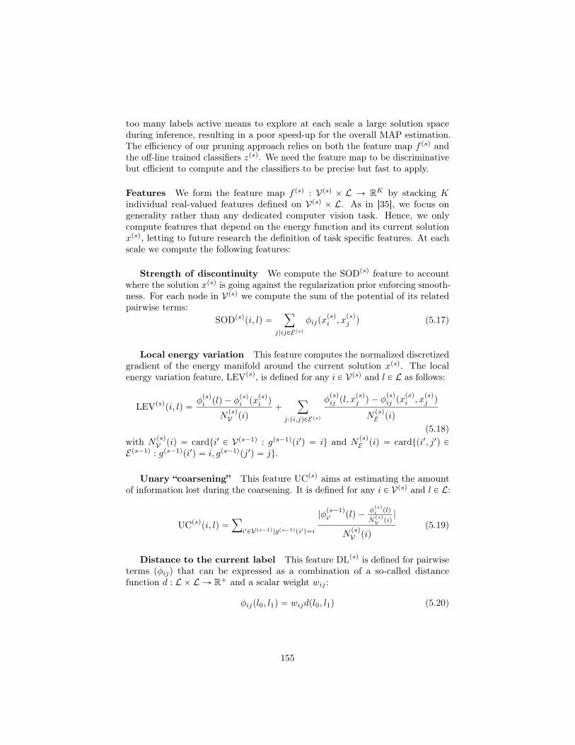
too many labels active means to explore at each scale a large solution spaceduring inference, resulting in a poor speed-up for the overall MAP estimation.The efficiency of our pruning approach relies on both the feature map f psq andthe off-line trained classifiers zpsq. We need the feature map to be discriminativebut efficient to compute and the classifiers to be precise but fast to apply.
Features We form the feature map f psq : Vpsq ˆ L Ñ RK by stacking Kindividual real-valued features defined on Vpsq ˆ L. As in [35], we focus ongenerality rather than any dedicated computer vision task. Hence, we onlycompute features that depend on the energy function and its current solutionxpsq, letting to future research the definition of task specific features. At eachscale we compute the following features:
Strength of discontinuity We compute the SODpsq feature to accountwhere the solution xpsq is going against the regularization prior enforcing smooth-ness. For each node in Vpsq we compute the sum of the potential of its relatedpairwise terms:
SODpsqpi, lq “ÿ
j|ijPEpsqφijpx
psqi , x
psqj q (5.17)
Local energy variation This feature computes the normalized discretizedgradient of the energy manifold around the current solution xpsq. The localenergy variation feature, LEVpsq, is defined for any i P Vpsq and l P L as follows:
LEVpsqpi, lq “φpsqi plq ´ φ
psqi px
psqi q
NpsqV piq
`ÿ
j:pi,jqPEpsq
φpsqij pl, x
psqj q ´ φ
psqij px
psqi , x
psqj q
NpsqE piq
(5.18)with N
psqV piq “ cardti1 P Vps´1q : gps´1qpi1q “ iu and N
psqE piq “ cardtpi1, j1q P
Eps´1q : gps´1qpi1q “ i, gps´1qpj1q “ ju.
Unary “coarsening” This feature UCpsq aims at estimating the amountof information lost during the coarsening. It is defined for any i P Vpsq and l P L:
UCpsqpi, lq “ÿ
i1PVps´1q|gps´1qpi1q“i
|φps´1qi1 plq ´
φpsqi plq
NpsqV piq
|
NpsqV piq
(5.19)
Distance to the current label This feature DLpsq is defined for pairwiseterms pφijq that can be expressed as a combination of a so-called distancefunction d : Lˆ LÑ R` and a scalar weight wij :
φijpl0, l1q “ wijdpl0, l1q (5.20)
155

It computes for each node i and each label the minimum “distance” given byd to the active label over all nodes of the k-ring of node i 1. We denote Rpsqk piqall the nodes belonging to the k-ring of node i P Vpsq . For each node i P Vpsqand label l P L, we compute:
DLpsqpi, lq “ minjPRpsqk piq
dpxpsqpjq, lq (5.21)
Feature normalization For a given computer vision task, parametersmight change from one input to the other leading to scaling factors independentlyapplied on the unary and pairwise terms. Hence, we normalize the SODpsq,LEVpsq, UCpsq and DLpsq features to make them insensitive to such scaling. Tothis en, we divide each of these feature by the average of the minimum valuesover all labels for each node.
Learning the cascade of classifiers
Defining the pruning ground truth We train the classifiers from a giventraining set of MRFs all formulating the same class of computer vision tasks,e.g., stereo-matching. For each MRF of the training set, we apply the algorithm21 without any pruning (i.e., Apsq ” 1). At the finest scale, we obtain an(approximate) MAP solution. To compute the pruning ground truth, we makeuse at each scale of the binary function XpsqMAP : Vpsq ˆLÑ t0, 1u. For the finestscale, we can simply convert the approximate MAP solution found:
p@i P V,@l P Lq, Xp0qMAPpi, lq “
#
1, if l is the MAP label of node i0, otherwise
(5.22)
To obtain the pruning ground truth at each scale s ą 0, we simply iterativelyapply the grouping functions:
p@i P Vpsq,@l P Lq, XpsqMAPpi, lq “
ł
i1PVps´1q:gpsqpi1q“i
Xps´1qMAP pi
1, lq (5.23)
whereŽ
denotes the binary OR operator.
Cascade training Since for each scale the feature map heavily depends oncurrent solution, we need to anticipate the impact of the pruning of previouscoarse scales. This is a major difference from the training method proposed in[35]. To this end we propose the following learning framework:
Classifier training At each scale we need to train a classifier zpsq from afeature map f psq and a pruning ground truth XpsqMAP. The pruning ground truthXpsqMAP defines the class c0 from c1, where c0 corresponds to the 0 values in XpsqMAP,1The set of nodes that are reachable by a path starting from i and traversing at most k
edges
156

Algorithm 20: Cascade learning of pruning classifier frameworkData: Set of training models pMmq0ďmăM , grouping functions
pgpsqm q0ďsăN , pruning ground truth pXpsqMAP,mq0ăsďN
Result: pzsq0ďsăNfor s “ rN...0s do
for m “ r0...M s doUpdate xpsqm by MAP inference:xpsqm « arg min
xmPSpMpsqm ,A
psqm q
Epxm|Mpsqm q
if s ‰ 0 thenCompute the feature MAP f
psqm from current solution xpsqm
if s ‰ 0 thenTrain pruning classifier zs from pf
psqm qm and pXpsqMAP,mqm
for m “ r0...M s doUpdate pruning matrix Apsqm pi, lq “ z
psqpostpf
psqpost,mpi, lqq
Upsample to next finest pruning matrix:Aps´1qm Ð rg
ps´1qm s´1pA
psqm q
Upsample xpsqm to initialize solution xps´1qm of next scale:
xps´1qm Ð rg
ps´1qm s´1px
psqm q
i.e., the label can be pruned, while c1 corresponds to the 1 values in XpsqMAP, i.e.,the labels that should remain active since they are part of the ground truthestimated MAP at the finest scale.
We normalize all features of f psq to the r0, 1s interval to avoid numericalinstability. We treat nodes sitting on the border of a strong discontinuityseparately from the nodes laying in smooth regions. Indeed, a discontinuity atcoarse scale is very likely to be refined during the next finest scales. Hence,there is more uncertainty on the solution in the vicinity of discontinuities thanon smooth areas. Using the SOD feature, we split the feature map f psq intoa first group f
psq0 containing only features where SODpsq ď ρs (smooth area),
and a second group fpsq1 containing only features where SODpsq ą ρ (strong
discontinuity). We also split the ground truth XpsqMAP the same way.
Since we need to compromise between good enough accuracy during trainingand fast evaluation at test time, we rely on linear classifiers for each group.To that matter, we train a standard linear C-SVM, Support Vector Machine,classifier with l2-norm regularization. We refer the reader to [37] for details aboutSVM. As we have many more samples in class c0, we randomly trim c0 suchthat its cardinal, cardpc0q, reaches a 10 to 1 ratio with respect to cardpc1q, thecardinal of c1 (cardp¨q counts the number of samples in each class). This greatlyspeeds-up the training without compromising its quality. Nevertheless, we still
157
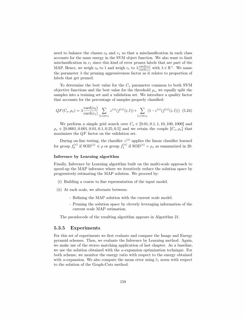
need to balance the classes c0 and c1 so that a misclassification in each classaccounts for the same energy in the SVM object function. We also want to limitmisclassification in c1 since this kind of error prunes labels that are part of theMAP. Hence, we weigh c0 to 1 and weigh c1 to λ cardpc0q
cardpc1qwith λ P R`. We name
the parameter λ the pruning aggressiveness factor as it relates to proportion oflabels that get pruned.
To determine the best value for the Cs parameter common to both SVMobjective functions and the best value for the threshold ρs, we equally split thesamples into a training set and a validation set. We introduce a quality factorthat accounts for the percentage of samples properly classified:
QF pCs, ρsq “ λcardpc0q
cardpc1q
ÿ
pi,lqPc1
zpsqpf psqpi, lqq`ÿ
pi,lqPc0
p1´zpsqpf psqpi, lqqq (5.24)
We perform a simple grid search over Cs P r0.01, 0.1, 1, 10, 100, 1000s andρs P r0.0001, 0.001, 0.01, 0.1, 0.25, 0.5s and we retain the couple rCs, ρss thatmaximizes the QF factor on the validation set.
During on-line testing, the classifier zpsq applies the linear classifier learnedfor group f psq0 if SODpsq ď ρ or group f psq1 if SODpsq ą ρs as summarized in 20.
Inference by Learning algorithm
Finally, Inference by Learning algorithm built on the multi-scale approach tospeed-up the MAP inference where we iteratively reduce the solution space byprogressively estimating the MAP solution. We proceed by:
(i) Building a coarse to fine representation of the input model.
(ii) At each scale, we alternate between:
- Refining the MAP solution with the current scale model.
- Pruning the solution space by cleverly leveraging information of thecurrent scale MAP estimation.
The pseudocode of the resulting algorithm appears in Algorithm 21.
5.3.5 ExperimentsFor this set of experiments we first evaluate and compare the Image and Energypyramid schemes. Then, we evaluate the Inference by Learning method. Again,we make use of the stereo matching application of last chapter. As a baseline,we use the solution obtained with the α-expansion optimization technique. Forboth scheme, we monitor the energy ratio with respect to the energy obtainedwith α-expansion. We also compute the mean error using `1 norm with respectto the solution of the Graph-Cuts method.
158
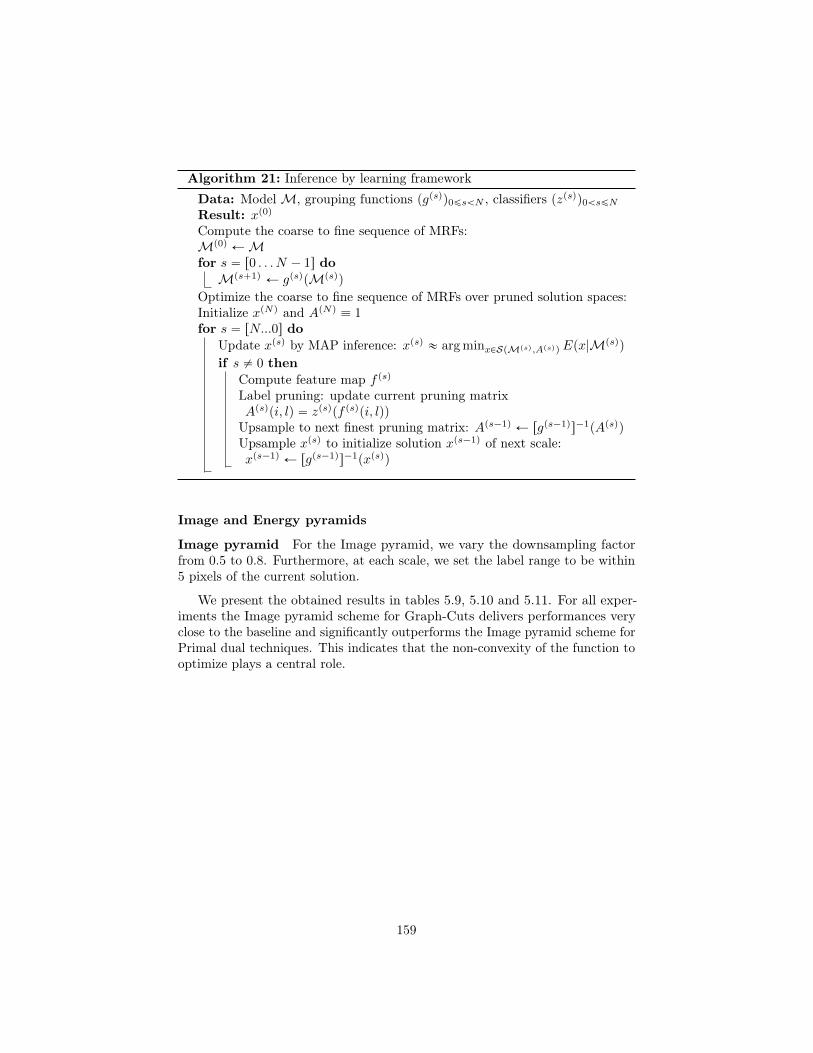
Algorithm 21: Inference by learning frameworkData: ModelM, grouping functions pgpsqq0ďsăN , classifiers pzpsqq0ăsďNResult: xp0qCompute the coarse to fine sequence of MRFs:Mp0q ÐMfor s “ r0 . . . N ´ 1s doMps`1q Ð gpsqpMpsqq
Optimize the coarse to fine sequence of MRFs over pruned solution spaces:Initialize xpNq and ApNq ” 1for s “ rN...0s do
Update xpsq by MAP inference: xpsq « arg minxPSpMpsq,ApsqqEpx|Mpsqq
if s ‰ 0 thenCompute feature map f psqLabel pruning: update current pruning matrixApsqpi, lq “ zpsqpf psqpi, lqq
Upsample to next finest pruning matrix: Aps´1q Ð rgps´1qs´1pApsqqUpsample xpsq to initialize solution xps´1q of next scale:xps´1q Ð rgps´1qs´1pxpsqq
Image and Energy pyramids
Image pyramid For the Image pyramid, we vary the downsampling factorfrom 0.5 to 0.8. Furthermore, at each scale, we set the label range to be within5 pixels of the current solution.
We present the obtained results in tables 5.9, 5.10 and 5.11. For all exper-iments the Image pyramid scheme for Graph-Cuts delivers performances veryclose to the baseline and significantly outperforms the Image pyramid scheme forPrimal dual techniques. This indicates that the non-convexity of the function tooptimize plays a central role.
159
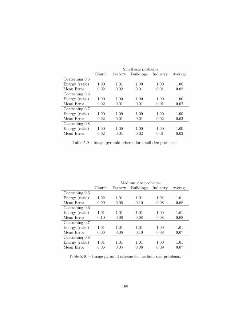
Small size problemsChurch Factory Buildings Industry Average
Coarsening 0.5Energy (ratio) 1.00 1.01 1.00 1.00 1.00Mean Error 0.02 0.02 0.01 0.01 0.02Coarsening 0.6Energy (ratio) 1.00 1.00 1.00 1.00 1.00Mean Error 0.02 0.01 0.01 0.01 0.02Coarsening 0.7Energy (ratio) 1.00 1.00 1.00 1.00 1.00Mean Error 0.02 0.01 0.01 0.02 0.02Coarsening 0.8Energy (ratio) 1.00 1.00 1.00 1.00 1.00Mean Error 0.02 0.01 0.02 0.01 0.02
Table 5.9 – Image pyramid scheme for small size problems.
Medium size problemsChurch Factory Buildings Industry Average
Coarsening 0.5Energy (ratio) 1.02 1.01 1.01 1.01 1.01Mean Error 0.09 0.06 0.10 0.08 0.08Coarsening 0.6Energy (ratio) 1.01 1.01 1.01 1.00 1.01Mean Error 0.10 0.06 0.08 0.08 0.08Coarsening 0.7Energy (ratio) 1.01 1.01 1.01 1.00 1.01Mean Error 0.06 0.06 0.10 0.08 0.07Coarsening 0.8Energy (ratio) 1.01 1.01 1.01 1.00 1.01Mean Error 0.06 0.05 0.08 0.09 0.07
Table 5.10 – Image pyramid scheme for medium size problems.
160

Large size problemsChurch Factory Buildings Industry Average
Coarsening 0.5Energy (ratio) 1.02 1.01 1.02 1.01 1.01Mean Error 0.21 0.12 0.19 0.25 0.19Coarsening 0.6Energy (ratio) 1.02 1.01 1.01 1.01 1.01Mean Error 0.25 0.11 0.16 0.20 0.18Coarsening 0.7Energy (ratio) 1.01 1.01 1.01 1.01 1.01Mean Error 0.18 0.10 0.16 0.22 0.17Coarsening 0.8Energy (ratio) 1.01 1.01 1.01 1.00 1.01Mean Error 0.17 0.10 0.16 0.19 0.16
Table 5.11 – Image pyramid scheme for large size problems.
161

Energy pyramid For the Energy pyramid, we evaluate both the node andlabel coarsening. For node coarsening, we investigate different geometric groupingfunctions gn that groups the nodes in a rk ˆ ks fashion, with k being a positiveinteger in t1, 2, 3, 4u. For the label coarsening, we set the grouping functiongl to group the labels of L by set of m labels with m being a positive integeramong t1, 2, 3, 4u. We select one every m labels to form the set of coarse labelsL1. Unselected labels are grouped with the closest selected label. If a tie appearsfor an unselected label, we arbitrarily associate it to the closest selected labelof smaller index. As for the image pyramid, at each scale, we only activate thelabels that are within a 5 label range of the current labeling solution.
Due to the number of experiments we only report the average results overthe four subset Church, Factory, Buildings and Industry.
Small size problemsLabel coarsening
Node coarsening 1 2 3 41
Energy (ratio) NA 1.01 1.00 1.00Mean Error NA 0.01 0.01 0.01
2Energy (ratio) 1.01 1.01 1.00 1.00Mean Error 0.03 0.01 0.01 0.01
3Energy (ratio) 1.01 1.01 1.00 1.00Mean Error 0.05 0.01 0.01 0.01
4Energy (ratio) 1.01 1.01 1.00 1.00Mean Error 0.05 0.01 0.01 0.01
Table 5.12 – Energy pyramid scheme for small size problems.
The 5.12, 5.13 and 5.14 summarize all the experiments. In our setting,without any label coarsening the energy scheme is only exploring the immediateneighborhood of the current solution. Hence, if the initialization is good, we getacceptable results as demonstrated by small size experiments or for experimentswith label coarsening set to 1 and node coarsening set to 2. However as weincreasing the node coarsening to 3 or 4, we deteriorate the initialization duringthe node coarsening. As a result we get poor performance since the methodmight not explore the relevant label range.
When we combine both node and label coarsening, we obtain results close tobe on par with the baseline and that significantly outperform the image pyramidscheme for both alpha-expansion and Primal-Dual optimization as pictured byfigure 5.15. We explain this improvement due to the fact that the energy pyramidscheme represents the initial energy with better precision than the image pyramidapproaches. This is illustrated by figure 5.14 where at coarse scales the solutions
162

Medium size problemsLabel coarsening
Node coarsening 1 2 3 41
Energy (ratio) NA 1.00 1.00 1.00Mean Error NA 0.04 0.04 0.03
2Energy (ratio) 1.01 1.00 1.00 1.00Mean Error 0.08 0.04 0.03 0.03
3Energy (ratio) 1.05 1.00 1.00 1.00Mean Error 0.23 0.05 0.04 0.04
4Energy (ratio) 1.13 1.00 1.00 1.00Mean Error 0.48 0.05 0.04 0.04
Table 5.13 – Energy pyramid scheme for medium size problems.
Large size problemsLabel coarsening
Node coarsening 1 2 3 41
Energy (ratio) NA 1.00 1.00 1.00Mean Error NA 0.06 0.06 0.06
2Energy (ratio) 1.02 1.00 1.00 1.00Mean Error 0.19 0.08 0.06 0.06
3Energy (ratio) 1.08 1.00 1.00 1.00Mean Error 0.51 0.10 0.06 0.06
4Energy (ratio) 1.26 1.01 1.00 1.00Mean Error 1.78 0.10 0.07 0.06
Table 5.14 – Energy pyramid scheme for large size problems.
obtained by the Energy pyramid scheme blatantly outperform the solution ofthe Image pyramid scheme.
163

Finest scale Scale 1 Scale 2
Figure 5.14 – Image coarsening results for odd rows and Energy coarseningfor even rows. The energy coarsening scheme clearly outperforms the imagecoarsening scheme for coarse scales.
164
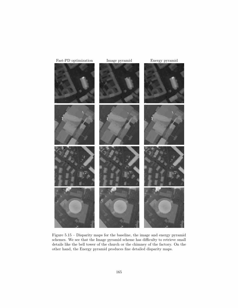
Fast-PD optimization Image pyramid Energy pyramid
Figure 5.15 – Disparity maps for the baseline, the image and energy pyramidschemes. We see that the Image pyramid scheme has difficulty to retrieve smalldetails like the bell tower of the church or the chimney of the factory. On theother hand, the Energy pyramid produces fine detailed disparity maps.
165

Inference by learning
For the evaluation of the inference by learning framework we make use of exactlythe same coarsening functions as for the energy coarsening scheme. Hence,we group the nodes in a rk ˆ ks fashion, with k being a positive integer int1, 2, 3, 4u. We also group m labels together with m being an positive integeramong t1, 2, 3, 4u.
During our experiments, we compare the baseline inference (optimizingthe input MRF with Graph-Cuts), the multi-scale inference (λ “ 0, i.e., thisframework without any pruning), and our Inference by Learning method withdifferent pruning aggressiveness factors λ that range between 0.001 and 1. Weuse 5 scales and we decrease at each scale the λ factor by an order of magnitude.
As for other experiments we use the energy ratio and the mean error to assessthe performance of this framework. We also compute the speed-up factor thatmeasure the ratio of computation time between the baseline optimization andthe current optimization strategy. To verify the expected correlation betweenthe speed-up and the number of active labels, we keep track of the Active labelratio that computes the percentage of active labels at the finest scale.
We report all results in figures 5.20, 5.21, 5.22 and 5.23. An analysis of theseresults reveals that by setting the node and label coarsening to 2 we achieve abest comprise between high quality solution and speed-up. Hence, we now focusonly on this particular set of experiments.
For all experiments illustrated in figure 5.19, λ “ 0.1 seems to be the sweetspot. This is also consistent for most of the other node and label coarseningvalues. For aggressiveness factors lower than λ “ 0.1, the inference by learningscheme computes a lower energy solution than the baseline. Hence, we get abetter solution for less computation. This happens because the approximationbounds of Fast-PD are reduced due the labels being pruned. In terms of speed,for λ “ 0.1 we get consistent and large speed-up ranging from 6 to 12. Forhigher λ, the accelerations are even better. However, the quality of the solutiondeteriorates as pictured in figure 5.18.
As for the energy pyramid scheme, the inference by learning frameworkproperly represents the energy even at coarse scales. The figure 5.17 illustratesthe behavior. We see that the disparity maps estimated at coarse scales alreadycontained the global structure. The details are then progressively resolvedthroughout the next fine scales.
As expected, the percentage of active labels strongly correlates with thespeed-up factor. In fact, the speed-up is mainly caused by having a large numberof labels being pruned. In figure 5.16, we see that a lot of labels are prunedearly on and as predicted, less pruning happens near label discontinuities. Thisjustifies the use of a dedicated linear classifier. Moreover, large homogeneouslylabeled regions are pruned earlier in the coarse to fine scale.
166

Disparity map Finest scale Scale 1 Scale 2
Figure 5.16 – Percentage of active labels per vertex (black 0%, white 100%) forInference by Learning framework for λ “ 0.1 with node and label coarseningboth set to 2. Each row is a different subset. The framework maintains moreactive labels near discontinuities than in smooth ares. Many labels are prunedat coarse scale. At the finest scale, only a few active labels remain per node.
167
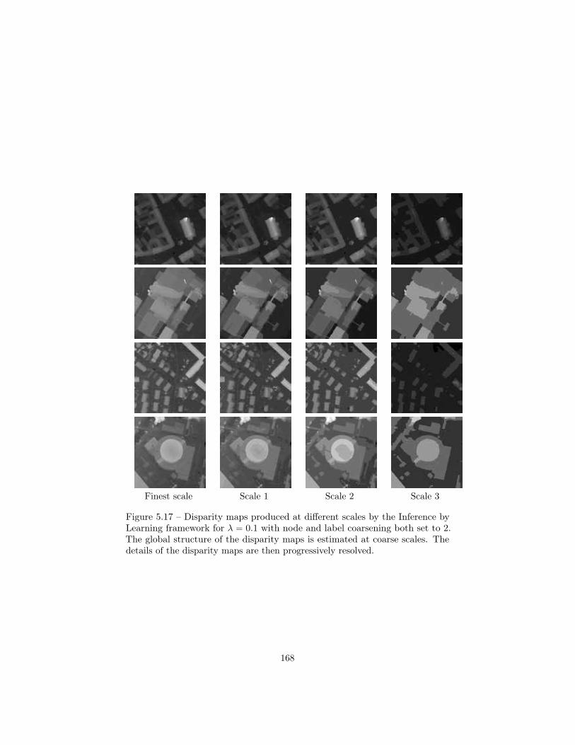
Finest scale Scale 1 Scale 2 Scale 3
Figure 5.17 – Disparity maps produced at different scales by the Inference byLearning framework for λ “ 0.1 with node and label coarsening both set to 2.The global structure of the disparity maps is estimated at coarse scales. Thedetails of the disparity maps are then progressively resolved.
168

λ “ 0.001 λ “ 0.01 λ “ 0.1 λ “ 1
Figure 5.18 – Disparity maps produced by the Inference by Learning frameworkfor different pruning factors λ with node and label coarsening both set to 2.Only the most aggressive pruning factor, λ “ 1, is unable to resolve some finedetails like the chimney of the factory subset.
169

(a) Speed-up (b) Active label ratio
(c) Energy ratio (d) Label agreement
Figure 5.19 – Performance of the Inference by Learning framework for node andlabel corsening set to 2.
170

Label coarsening1 2 3 4
Figure 5.20 – Energy ratio results for the Inference by Learning experiments.From top row to bottom row node coarsening is set to 1, 2, 3 and 4.
171
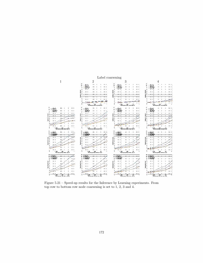
Label coarsening1 2 3 4
Figure 5.21 – Speed-up results for the Inference by Learning experiments. Fromtop row to bottom row node coarsening is set to 1, 2, 3 and 4.
172

Label coarsening1 2 3 4
Figure 5.22 – Mean Error results for the Inference by Learning experiments.From top row to bottom row node coarsening is set to 1, 2, 3 and 4.
173

Label coarsening1 2 3 4
Figure 5.23 – Active Ratio results for the Inference by Learning experiments.From top row to bottom row node coarsening is set to 1, 2, 3 and 4.
174

5.4 ConclusionThis last technical chapter introduced smoothing and coarsening schemes forboth First order Primal-Dual methods and non convex optimization techniquessuch as Fast-PD. For the latter one, we detailed a new framework, Inference byLearning, to drastically speed-up the optimization.
We now propose to apply some of the techniques presented to practicalproblems encountered in remote sensing tasks for Earth Sciences.
175

Chapter 6
Applications
6.1 Introduction and chapter organization
6.1.1 IntroductionFor this final chapter, we display some applications of the techniques presentedin chapters 3, 4 and 5. Our experiments mainly focus on remote sensing tasksperformed in geological studies.
For each task, we introduce the context and the necessary background.We model the problem as an energy optimization task and then we performexperiments to illustrate the model’s features. In any circumstances, we do notclaim to get better results than other techniques. Indeed, we keep our modelsfairly generic and we leave for future work the derivation of a finely tuned versionof our models.
6.1.2 Chapter organizationThe section 6.2 introduces the notation and terminology used throughout thechapter. We present in section 6.3 the stereo-matching task with Earth and Marsbound acquisitions. The section 6.4 proposes a study of earth crust deformationfrom LiDAR acquisition with a simulated earthquake model. In the section 6.5we apply our techniques to damage detection due to an earthquake from LiDARacquisitions of Christchurch, New-Zealand.
6.2 Notations and Preliminaries
6.2.1 ImagesWe remind some useful notation for this final chapter. An image I is a collectionof pixels taking value in R for gray images and R3 for color images. The pixelsof I are organized on a rectangular grid Ω. A row and column pri, ciq identifies
176

a unique pixel pi “ pri, ciq P Ω. To ease the notations, we access the value of apixel pi “ pri, ciq of an image I by either Ippiq or Ipri, ciq.
6.2.2 GraphA neighborhood graph G “ pV, Eq is associated to the image I. The set ofvertices V of G simply denotes the pixels of Ω. The set of edges E defines thecanonical 4-neighborhood connectivity.
6.2.3 LiDAR as elevation mapsLight Detection and Ranging, LiDAR, is a class of instrument used in remotesensing to measure distances. A LiDAR is generally composed of a laser, ascanner, and a GPS receiver. Using light pulses in a form of a laser, the LiDARmeasures the time to receive a reflection of the pulse in order to estimate a rangeof distance to an object of interest. This is illustrated by figure 6.1.
Figure 6.1 – Principle of LiDAR.
In our context LiDAR instruments are mainly used for topographic purposes[71]. They can be mounted on small aircraft during aerial surveys to estimatethe topography. However, it is also common to mount LiDAR instruments onboat to estimate the bathymetry of the seafloor or a riverbed elevation [38] and[75]. In both settings, LiDAR are precious equipments that allow scientists andmapping professionals to build precise 3D model of their environment.
The LiDAR acquisitions create a 3D point cloud such as illustrated in figure6.2. Since our acquisitions are mainly from zenith incidence with respect to theground, we can transform the 3D point cloud into an elevation image. We setthe elevation image grid to align with some portion of the ellipsoid of referenceused to represent the Earth. Each pixel represents a square surface, for instancea square meter. The intensity of each pixel defines the elevation. Popular GIS,Geographic Information System, softwares like GRASS [132] have routines toconvert a 3D point cloud to an elevation image. We note that the elevationimage representation makes it very easy to apply the techniques presented inprevious chapters.
177

Figure 6.2 – LiDAR acquisition over New Orleans, LA, USA (Courtesy of USGS).
6.2.4 Matching criterionWe also remind two useful matching criteria based respectively on the ZNCCand the census coefficient. Both criteria compute a matching likeliness scorebetween two patches P1 and P2 of the same size with spatial support P.
Zero Normalized Cross Correlation: ZNCC
The ZNNCmatching criterion derives from the Zero Normalized Cross Correlationcoefficient that computes the angles between the normalized patches P1 and P2.
ZNCCpP1, P2q “1
cardpPqÿ
iPP
pP1piq ´m1q pP2piq ´m2q
σ1σ2(6.1)
where:
• m1 and m2 are the mean values of patches P1 and P2,
• σ1 and σ2 are the standard deviations of patches P1 and P2.
The ZNCC matching criterion ρ simply computes:
ρpP1, P2q “ 1´ ZNCCpP1, P2q (6.2)
To simplify the notations, we define by
ZNCCW pIr, It, i, dq (6.3)
the ZNCC coefficient computed on patches of sizeW ˆW from image Ir centeredat pixel i and from image It centered at pixel i` d.
By construction the ZNCC coefficient and the ZNCC matching criterionare unaffected by global illumination and contrast changes. These invarianceproperties come extremely handy for image matching. We note that [172]describes an efficient implementation to compute the ZNCC coefficient in thecontext of overlapping patches.
178
Ternary Census
The Ternary Census matching criterion of [175] and relies on the Ternary Censuscode. The Ternary Census code of a patch P is defined by:
TCpP, δq “ biPP tpP picq, P piq, δq (6.4)
Where:
• b is the concatenation operator,
• ic is the central pixel of the patch P ,
• t : RˆRˆR` Ñ t´1, 0, 1u is the ternary function parametrized by δ P R`:
tpx, y, δq “
$
&
%
´1 if x ă y ´ δ1 if x ą y ` δ0 otherwise
(6.5)
The Ternary Census matching criterion ρ simply computes:
ρpP1, P2q “ ||TCpP1, δq ´ TCpP2, δq||1 (6.6)
To simply the notations, we define by
TCW,δpIr, It, i, dq (6.7)
the Ternary Census coefficient computed on patches of size W ˆW from imageIr centered at pixel i and from image It centered at pixel i` d.
As for the ZNCC matching criterion, the Census matching criterion is un-affected by global illumination change. The Census matching criterion is alsorobust to mild contrast variation.
6.3 Stereo-matchingWe briefly introduce the background of the stereo matching task. The figure6.3 illustrates the key principle of stereo-matching: the apparent motions ofan object between the two images is proportional to the object’s depth. Withadditional information about the two cameras and their positions in space, onecan recover the 3D position of each object imaged.
We explain in more detail how the problem is formulated. To this end, wefirst present the classic camera model and the epipolar geometry. Then, weformulate the stereo matching task as an optimization model which we evaluatewith a series of experiments.
179

Figure 6.3 – Stereo-matching principle, courtesy of Wikipedia.
6.3.1 Camera models and Epipolar geometryPinhole camera model
We first need to present a camera model that describes the mathematicalrelationship between 2D coordinates Q “ py1, y2q on the image plane and the 3Dcoordinates P “ px1, x2, x3q in the world. As for many modeling, we start withthe pinhole camera model [160] which assumes that the camera aperture is asimple point with no optic as illustrated by figure 6.4. Hence, this model does notintegrate neither geometrics distortions nor the discrete sampling done by theCCD sensor. However, since we process image from high quality camera we cancompensate the geometrics distortions with simple coordinate transformationsof the image coordinates. Using the notations of figure 6.4, one can easilydemonstrate:
ˆ
y1
y2
˙
“ ´f
x3
ˆ
x1
x2
˙
(6.8)
Figure 6.4 – Pinhole camera diagram
Camera parameters
To enhance the pinhole camera model, we need to introduce the intrinsic andextrinsic camera parameters.
180

Intrinsic parameters The intrinsic parameters describe features that areinternal to the camera. These features are fixed for a given camera and digital-ization setup. These parameters model:
• the focal length,
• the position of the optical center,
• the distortion introduced by the lenses,
• the size and shape of pixels.
Extrinsic parameters The extrinsic parameters define the location and ori-entation of the camera in the 3D world frame. Hence, these parameters include:
• a 3D translation to define the position,
• a 3D rotation to define the orientation.
Frame and Push-broom sensors
In our context we work with images acquired with frame and push-broom sensors.The frame sensors are the most common for aerial surveys while push-broomsensors are ubiquitous in satellite based acquisitions.
All pixels composing an image of a frame sensor are acquired at the same timeby individual CCD (charge-coupled device) or CMOS (complementary metal-oxide semiconductor) sensors. In contrast, push-broom sensors only contain asingle array of CCD or CMOS sensors. Using the motion of the satellite, onecan construct an image by stacking the series of acquisition made by the array.The figure 6.5 illustrates the two technologies.
Epipolar geometry
Epipolar geometry refers to the particular geometry of the stereo-vision task.It describes the geometric relationship between a 3D point of the world frameand its projection onto 2D images acquired by two cameras in distinct positions.Both camera are assumed to be modeled by the pinhole camera model previouslypresented. While we do not present the detailed formulation of the epipolargeometry, we illustrate with figure 6.6 its concept. We refer to the seminal bookof [76] for an extensive discussion around the epipolar geometry.
Interestingly for frame camera, in the epipolar geometry we know that a givenobject image at point XL in the left camera lies on a line in the right cameranamed the epipolar line. The position on this epipolar line is proportional to thedepth. However, for push-broom sensors the epipolar line is not straight, buthyperbola-like curve as explained in [135].
181
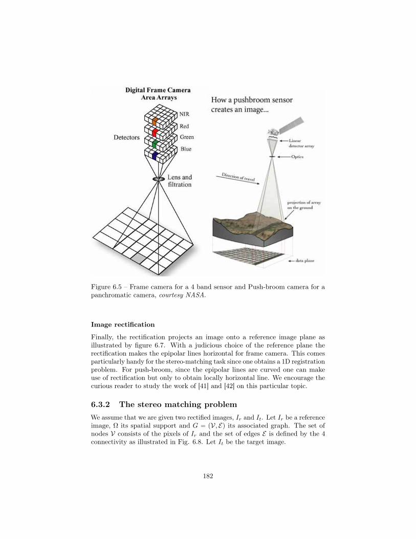
Figure 6.5 – Frame camera for a 4 band sensor and Push-broom camera for apanchromatic camera, courtesy NASA.
Image rectification
Finally, the rectification projects an image onto a reference image plane asillustrated by figure 6.7. With a judicious choice of the reference plane therectification makes the epipolar lines horizontal for frame camera. This comesparticularly handy for the stereo-matching task since one obtains a 1D registrationproblem. For push-broom, since the epipolar lines are curved one can makeuse of rectification but only to obtain locally horizontal line. We encourage thecurious reader to study the work of [41] and [42] on this particular topic.
6.3.2 The stereo matching problemWe assume that we are given two rectified images, Ir and It. Let Ir be a referenceimage, Ω its spatial support and G “ pV, Eq its associated graph. The set ofnodes V consists of the pixels of Ir and the set of edges E is defined by the 4connectivity as illustrated in Fig. 6.8. Let It be the target image.
182
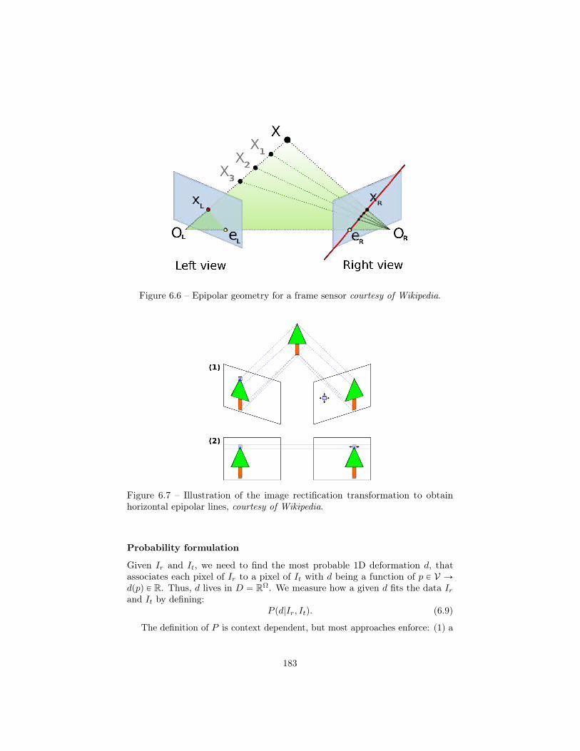
Figure 6.6 – Epipolar geometry for a frame sensor courtesy of Wikipedia.
Figure 6.7 – Illustration of the image rectification transformation to obtainhorizontal epipolar lines, courtesy of Wikipedia.
Probability formulation
Given Ir and It, we need to find the most probable 1D deformation d, thatassociates each pixel of Ir to a pixel of It with d being a function of p P V Ñdppq P R. Thus, d lives in D “ RΩ. We measure how a given d fits the data Irand It by defining:
P pd|Ir, Itq. (6.9)
The definition of P is context dependent, but most approaches enforce: (1) a
183

Figure 6.8 – Graph G “ pV, Eq of a 4 by 4 pixels image with a 4 connectivity.
notion of the similarity between Ir and It˝pid`dq (where id refers to the identityoperator) by expressing PM pd|Ir, Itq and; (2) a notion of regularity for d byexpressing PRpd|Irq. If we suppose that these two probabilities are independent,we can write:
P pd|Ir, Itq “ PM pd|Ir, ItqPRpd|Irq. (6.10)
Instead of directly working with probabilities, we prefer using the energydomain as in [83] since it is easier to define measure on images. One can simplyrelate probability density function to energy through the Gibbs measure:
P pX “ xq “1
Zexpp´Epxqq, (6.11)
with Z being a normalization factor so that the integral of the probabilityfunction equal to 1.
Energy formulation
Through Eq. 6.11, we relate E, EM , and ER to P , PM , and PR respectively,which gives the following energy:
Epdq “ÿ
pPVEM pd, pq `
ÿ
pqPEERpd, p, qq. (6.12)
We define a pixel-wise similarity measure based on the similarity function ρ.Commonly used similarity functions are L1 or L2 norms [12], Census, NormalizedCross Correlation (NCC) or Zero Normalized Cross Correlation (ZNCC) [23],and the different versions of the Mutual Information [168, 91, 79]. In any case,the matching energy of a pixel p is defined as:
EM pd, pq “ ρpIr, It ˝ pid` dqqppq. (6.13)
184

If the similarity measure is defined on a patch, we apply a rigid translationto the patch. Here, we use the ZNCC coefficient as it is robust to changes ofillumination and contrast between Ir and It that appear due to specular objectsor different acquisition times.
To enforce the regularity of d we choose to penalize the L1-norm of itsdiscretized gradient, modulated by a weight function w. For each edge pq P E :
ERpd, p, qqq “ wpp, qqdppq ´ dpqq1, (6.14)
ith :
wpp, qq “ λ1 ` λ2 exp
ˆ
´Irppq ´ Irpqq
2
σ2
˙
. (6.15)
λ1, λ2, and σ are real positive scalar parameters. The L1-norm of the gradientnaturally enforces piece-wise constant disparities. The weight function wpp, qqrelaxes the regularization on radiometric discontinuities of the reference imageas in [58, 34]. This is an effective heuristic as most of the edges of the disparitymaps are also edges of the image Ir.
6.3.3 ExperimentsWe perform experiments with images acquired by the Ultra-cam and the Hirisecameras to illustrate the different components of our model. We start bydisplaying the images of the stereo-pairs. Then, we illustrate the unary termsissued from two different the matching criteria: the ZNCC and the Censusmeasure. Finally, we study the influence of the regularization strength.
Images
Ultra-cam acquisitions The Ultra-cam cameras belong to the class of aframe sensor [109]. Hence, we can perform the calibration and rectification stepspreviously presented to end-up with a horizontal apparent motion to estimate.
From a large calibrated and rectified Ultra-cam stereo-pair we extract foursubsets: Factory, Church, Buildings and Industry. The subsets, illustrated infigure 6.9, portray urban and industrial environments. Man-made structurespresent numerous challenges for the stereo-matching task. For instance, thetall chimney of the Factory subset creates a large occlusion zone. Some areasin the Factory and Industry subsets are texture-less or repetitive, making thematching very challenging. Finally, the Church and Buildings subsets have manyfine-details due to their urban or suburban locations. This creates fine and sharpdiscontinuities in the disparity maps that are challenging to recover.
185

Factory subset Church subset
Buildings subset Industry subset
Figure 6.9 – Reference images of stereo pair subsets for the Ultra-cam experi-ments.
Hirise acquisitions The Hirise camera belongs to the class of a push-broomsensor [122]. Hence, we perform the calibration on the full image but therectification step is applied onto each of the subsets. As for the Ultra-camacquisitions we end-up with a near horizontal apparent motion to estimate.
Using two stereo-pairs from the Hirise website [134], we extract the four sub-sets pictured in figure 6.10: Valley, Dunes, Crater and Channel. Since the Hirisecamera is mounted on a satellite orbiting the planet Mars, the subsets illustratenatural scenes of dunes, channels, valleys and carters. These natural scenespresent different challenges compared to the urban environment of the UltraCamexperiments. Indeed, most areas are heavily textured and non repetitive, which
186

greatly helps the matching. However, change in disparity is less likely to followthe radiometric variation of the reference image. This hinders the a-priori priorenforced by the regularization costs. Moreover, large change of elevation can beobserved at the edges of craters, cliff, canyons and channels.
Nili Patera Ripples
Valley subset Dunes subset
Channel and in Northern Mid-Latitudes
Crater subset Channel subset
Figure 6.10 – Reference images of stereo pair subsets for the Hirise experiments.
Unary terms
In our context of stereo-matching, one can advocate that the unary terms arethe most important part of the model. Indeed, their purpose is to measure thelikelihood of one patch to match another. In a perfect world, we would liketo rely only on the matching terms to estimate the disparity. Unfortunately,texture-less patches, noise, occlusions or change in illumination all hinder the
187

reliability of the matching terms. Hence, as an illustration we display in figure6.11 and 6.12 the disparity maps obtained solely from the matching terms, i.e.we set all regularization terms to 0.
Census Zncc
Figure 6.11 – Disparity maps obtained for the Ultra-cam stereo-pairs usingexclusively the matching terms.
188

Census ZNCC
Figure 6.12 – Disparities maps obtained for the Hirise stereo-pairs using exclu-sively the matching terms.
Independently of the matching criterion, the disparity maps obtained forthe Ultra-cam images are extremely noisy and entire areas are completely miss-estimated. The ZNCC criterion seems to perform a bit better than the Census.This can be attributed to the fact that the Census is more robust than theZNCC. In our context, this extra-robustness seems to slightly deteriorate thematching performance. Interestingly, the disparity maps computed for the Hirisestereo-pairs are quite good. This is likely due to the heavily textured patchesof natural scenes. However, we still observe numerous artifacts. As for theUltra-cam results, the ZNCC outperforms the Census criterion.
Regularization weights
The regularization weights are an important part of the imposed prior onthe disparity estimation. In our model they modulate the strength of theregularization according to the radiometric discontinuity of the reference image.We illustrate in figure 6.13 the horizontal and vertical gradients of the Church
189

subset’s reference image and its derived regularization weights.
Horizontal gradients Vertical gradients
Horizontal weights Vertical weights
Figure 6.13 – Gradients and weights of the Church subset (brighter grays meanshigher values).
Impact of regularization
To study the regularization we modulate the strength of the pairwise terms by aglobal factor varying in t0.1, 0.5, 1, 2, 5u where a factor of 1 sets the regularizationof optimal hand-picked regularization parameters. This allows us to createmodels that are barely regularized (factor set to 0.1) to models that are heavilyregularized (factor set to 5). We illustrate the results in figures 6.14, 6.15, 6.16and 6.17.
190
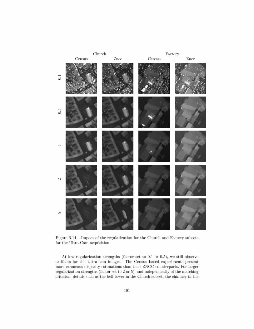
Church FactoryCensus Zncc Census Zncc
0.1
0.5
12
5
Figure 6.14 – Impact of the regularization for the Church and Factory subsetsfor the Ultra-Cam acquisition.
At low regularization strengths (factor set to 0.1 or 0.5), we still observeartifacts for the Ultra-cam images. The Census based experiments presentmore erroneous disparity estimations than their ZNCC counterparts. For largerregularization strengths (factor set to 2 or 5), and independently of the matchingcriterion, details such as the bell tower in the Church subset, the chimney in the
191
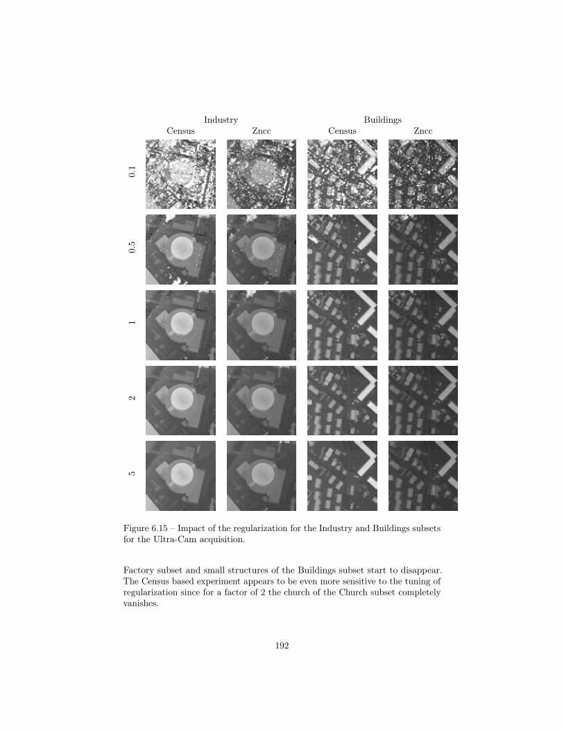
Industry BuildingsCensus Zncc Census Zncc
0.1
0.5
12
5
Figure 6.15 – Impact of the regularization for the Industry and Buildings subsetsfor the Ultra-Cam acquisition.
Factory subset and small structures of the Buildings subset start to disappear.The Census based experiment appears to be even more sensitive to the tuning ofregularization since for a factor of 2 the church of the Church subset completelyvanishes.
192
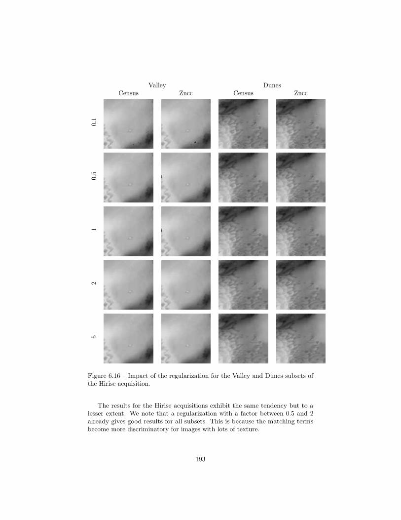
Valley DunesCensus Zncc Census Zncc
0.1
0.5
12
5
Figure 6.16 – Impact of the regularization for the Valley and Dunes subsets ofthe Hirise acquisition.
The results for the Hirise acquisitions exhibit the same tendency but to alesser extent. We note that a regularization with a factor between 0.5 and 2already gives good results for all subsets. This is because the matching termsbecome more discriminatory for images with lots of texture.
193

Subset 3 Subset 4Census Zncc Census Zncc
0.1
0.5
12
5
Figure 6.17 – Impact of the regularization for the Cater and Chanel subsets ofthe Hirise acquisition.
6.4 Simulated Earth crust deformationWe now move on to 3D registration of elevation maps. In this particular examplewe assume that an earthquake has occurred between the time of the acquisitionof two elevation maps.
194

6.4.1 ContextEarthquakes are one of the most dangerous natural hazard on Earth. Contraryto volcano, hurricanes or tornado, it is as of today quite impossible to preciselypredict when and where an earthquake will happen [60]. Earthquakes occur at afault, i.e., a boundary between two or more tectonic plates, producing seismicwaves that result from a sudden release of energy in the Earth’s lithosphere.The figure 6.18 displays the epicenter of referenced earthquakes between 1963to 1998. Earthquake are classified on a scale by their moment magnitude. TheUSGS maintains an active mapping of earthquakes thanks to an internationalnetwork of seismometer [169].
Figure 6.18 – Epicenter of earthquakes from 1963 to 1998.
The destruction and subsequent events caused by earthquakes are staggering:ground rupture and soil liquefaction, landslides and avalanches, fires, tsunamiand flood. At multiple times in the past, a single quake and its aftermath haveclaimed more than ten of thousands lives as illustrated by figure 6.19.
Geologists have historically relied on seismometers to measure the motion ofthe ground. However, in the last decades they have started to heavily rely onGPS stations. The instantaneous position of civilian GPS is fairly inaccurate,within 10 meters. Nonetheless, using temporal aggregation of a GPS signal,one can retrieve precision up to a few millimeters. Some locations like the SanAndreas fault in California, the Himalaya mountains or Japan are surveyed bynetworks of GPS stations. Unfortunately, many remote places do not benefitfrom this level of monitoring. Hence, for a large number of earthquake thescientific community does not have access to data acquired close to the epicenter.Another downside of the GPS monitoring is that even with large networks onecan only obtain local and sparse measurements.
Hence, thanks to the progress of space imaging and aerial monitoring devices,
195

Figure 6.19 – Earthquakes of magnitude 8.0 and greater since 1900. The apparent3D volumes of the bubbles are linearly proportional to their respective fatalities(Courtesy of Wikipedia).
geologists have started to take advantage of remote sensing acquisitions. In thiscontext, they seek to obtain a more global view of the ground motion inducedby an earthquake. Nevertheless, remote sensing techniques can not bring thelevel of accuracy obtained with GPS stations. Hence, it remains important toproperly fuse the different modalities of information.
In this work, we only propose to retrieve the ground motion induced by aquake using two elevation maps: one acquired before and after the quake. Tokeep this experiment simple, we make use of a crop of an elevation map of the SanAndreas fault in California, USA illustrated in figures 6.20 and 6.21. The cropserves as the pre-event elevation map. We simulate using an Okada model [137]the ground motion induced by a large earthquake. From this simulated groundmotion we transform the pre-event elevation map to a post-event elevation map.We do not claim that the position of the simulated fault nor the generatedearthquake are realistic. However, this experiment shows how to make use ofour mathematical techniques in such context.
6.4.2 ModelWe make use of notations Ipre and Ipost for the pre and post geo-registeredelevation images. Instead of directly looking for a full 3D deformation, we limit
196

Figure 6.20 – The San Andreas fault. Figure 6.21 – Simulated fault.
our model to estimate a 2D motion and we automatically infer the change ofelevation. This modeling reduces the number of unknowns and it performedbetter than others of our unreported attempts with full 3D motions. We elect touse the ZNCC matching criterion ρpq. The matching cost for pixel pri, ciq P Ωwith displacement pui, viq is defined by:
ρpri, ci, vi, uiq (6.16)
We formulate the registration problem as:
arg minppui,viqPRˆRqi
ÿ
pri,ciqPΩ
ρpri, ci, vi, uiq
`ÿ
pi,jqPEλu|ui ´ uj | ` λ
v|vi ´ vj |(6.17)
with λu and λv being real valued scalars.
We solve model 6.17 using the α-expansion technique embedded in a ImagePyramid. We elect for 4 scales with 49 labels per scale, i.e, 7 potential values foreach ui and vi.
To recover the change of elevation w, we simply compute the change ofelevation between the pre-event elevation map and the transformed post-eventelevation map with the recovered deformation pu, vq. We note that a furtherpost processing smoothing step could also be performed if necessary.
6.4.3 ExperimentsWe display in figure 6.22 the results of our method. In figure 6.23, we show aprofile for each motion direction across the fault as illustrated in figure 6.21.
197

u-component v-component w-component
Figure 6.22 – Retrieved motion.
u-component v-component w-component
Figure 6.23 – Profile of the deformation in pixel across the simulated fault.
From the three profiles, we see that our method correctly recovers theground motion for this toy example. We observe that the change of elevationw-component, is noisier. For real experiments, we would advocate to proceedwith a smoothing post-processing step. One can for instance adapt the TV-L1denoising framework to tailor an adequate smoothing algorithm.
6.5 Damage detection in New-Zealand
6.5.1 ContextFor this final experiment, we study the application of damage detection inducedby natural hazards from aerial LiDAR time series with one acquisition beforeand after the damaging event.
Natural disasters
In the context of natural disaster such as landslides, a tornadoes, hurricanes orearthquakes, a detailed cartography of the impacted area is of crucial importance.
In many cases, usual communication medium such as telephone or Internet aresometimes unavailable in some remote or less developed area or non-operationaldue damages induced by the natural disaster. Hence, gathering and centralizinginformation can be very challenging. First emergency responses face the challengeto adequately organize search and rescue operation while lacking a global view ofthe situation. Simple images from satellite and areal survey can provide crucialinformation of impacted areas.
198

Once the humanitarian situation has been resolved comes the time of re-construction. In most modern countries, habitation and buildings are insuredthrough various private or governmental based policies. Hence, one needs toprovide a detail map of which building was affected by the natural hazard. Thisinspection is generally conducted on the ground. Depending on the size of thearea impacted, this investigation can last quite a lot of time delaying familiesand business owners to obtain compensation from their insurance. Again, adetailed map of damages could fasten the economic recovery process.
Christchurch, New Zealand
Christchurch is located in the Canterbury Region in New Zealand’s South Islandas illustrated by figures 6.24 and 6.25. With a population of 389000 in 2016,Christchurch is one of the largest populated cities in New Zealand see 6.27 and6.26.
Figure 6.24 – New Zealand onthe planisphere.
Figure 6.25 – New Zealand map.
Figure 6.26 – Sattelite image ofChristchurch.
Figure 6.27 – Christchurch skyline withSouthern Alps in background.
199

On February 22, 2011 at 2:51 p.m. local time, Christchurch was struck bya 6.3 earthquake on the Richter scale [21]. This natural disaster claimed 185lives while injuring a thousand individuals. The infrastructure and buildingwere seriously damaged as illustrated by figures 6.28, 6.29, 6.30 and 6.31. Forinstance, the Canterbury Television (CTV) building nearly entirely collapsedleaving only its lift shaft standing. A series of thirty subsequent earthquakes ofsmaller magnitude, referred to as aftershocks, happened for approximatively ayear.
Figure 6.28 – Collapsed bell tower. Figure 6.29 – CTV building.
Figure 6.30 – Soil liquefaction causedby the earthquake.
Figure 6.31 – Lanslide triggered by theearthquake.
6.5.2 ModelWe propose to establish a damage map from LiDAR aerial surveys pre andpost event by using our registration technique. We first transform both LiDARacquisitions to elevation images. We geo-register both elevation images suchthat corresponding pixels of both images represent the same portion of the land.Such registration can be handled within GIS softwares for instance.
We were provided directly with elevation images of the downtown of Christchurchgridded at 1 meter. The figures 6.32 and 6.33 display these elevation images.
200

Figure 6.32 – LiDAR pre earthquake. Figure 6.33 – LiDAR post earthquake.
Brighter grays represent higher elevation (Images have been enhanced fordisplay).
To detect the damaged building, we propose to create a map that monitorsthe change of elevation between the pre and post event. If we were to dispose ofperfect elevation images then a simple difference between the pre and the postevent elevation image should create a perfect map. Unfortunately, the LiDARacquisitions, and hence the derived elevation images, suffer from noise andartifacts. For instance, LiDAR might have difficulties to resolve with accuracythe edges of tall buildings. Therefore, we propose to use a registration frameworkwith regularization to obtain the damage map.
We make use of notations Ipre and Ipost for the pre and post geo-registeredelevation images. Our goal is to find a transformation that registers Ipre to Ipost.The dominant part of the transformation belongs to the change of elevationcaused by building collapsing. The horizontal and vertical component of thetransformation attempt to account for acquisition artifacts created near buildingedges. Hence, we formulate the following optimization problem:
arg minpuiPr´1,1sqi,pviPr´1,1sqi,pwiPRqi
ÿ
pri,ciqPΩ
|Iprepri, ciq ´ pIpostpri ´ vi, ci ´ uiq ´ wiq|
`ÿ
pi,jqPEλu|ui ´ uj | ` λ
v|vi ´ vj |
`ÿ
pi,jqPEλwij |wi ´ wj |
(6.18)We set λu and λv to a small positive real value and we define for pi, jq P E :
λwij “ λw0 ` expp´λw1 ||Iprepri, ciq ´ Ipreprj , cjq||22qq (6.19)
201

with pλw0 , λw1 q P R` ˆ R`.
We make use of first order primal dual techniques embedded in image pyramidscheme to optimize equation (6.18).
6.5.3 ExperimentsAs a baseline, we propose to simply subtract the post event image to the preevent image. We display the results of the both the baseline and our approachin figures 6.34 and 6.35.
Figure 6.34 – Results from the base-line method.
Figure 6.35 – Results from our frame-work (elevation component only).
Blue color represents a negative change of elevation while the red color marks apositive change of elevation.
The result of the baseline technique in figure 6.34 highlights contour of eachbuilding, creating ghost contours. This is caused by the difficulties to resolve theedges of tall objects with aerial LiDAR acquisitions. However, our regularizedframework produces a clearer damage map free of ghost contours while preservingfine details. We note since the LiDAR acquisitions are a few months apart, bothmethods capture vegetation changes. The disappearance of tree foliage in thepost event acquisition creates a negative change of elevation. To enhance thequality of the damage map, one could classify building from vegetation by usingan additional hyper-spectral information for instance.
6.6 Chapter conclusionThis final chapter illustrated the techniques presented in chapters 3, 4 and 5with concrete applications ranging from stereo-matching to damage detection.We leave for future work the detailed study of each of these problems.
202

We strongly believe in the relevance of the presented techniques. Nevertheless,we are conscious that much work still remains to be done for achieving significantscientific contributions in tasks such as studying Earth crust deformation. How-ever, we hope to have made accessible to other communities the mathematicalconcepts and methods to tackle those challenges.
203

Chapter 7
Conclusions, limits and futurework
We conclude this thesis by summarizing each chapter and mentioning potentialfuture research avenues.
First order Primal-Dual techniques for convex optimization This chap-ters introduced the basics of convex optimization and presented in detail theFirst order Primal-Dual techniques for convex optimization. A study of the dualsolution space of TV regularized problems leads to the demonstration of varioustheorems. Using those theorems we were able to connect through their dualspace several TV regularized models.
In future work one could attempt to extend the demonstrated theorems toother classes of regularized problems. Furthermore, one could investigate todecrease the computational cost of the first order Primal-Dual techniques byrestricting the space of functions on which the convergence is ensured. Moreover,a detailed study of the implementation of such technique on GPU remains to bedone.
Maxflow and graph cuts This chapter introduced the basics of non-convexoptimization, the famous link between the maxflow and mincut problems, andpresented two graph cuts techniques, namely the α expansion and Fast-PD. Weproposed our own implementation of Fast-PD that drastically outperformed theoriginal implementation.
In future work, one could investigate to extend graph-cut techniques to higherorder terms as in [53], [85] or [92]. Furthermore, one could research on howto implement a CPU multi-threated code of Fast-PD. Moreover, efficient GPUbased implementation of maxflow-minuct and graph cuts would also be greatlywelcome by the computer vision community.
204

Coarsening schemes for optimization techniques In this chapter we stud-ied coarsening frameworks for First order Primal-Dual techniques and for thegraph cuts methods. We also introduced a new approach, the inference bylearning framework, that drastically speeds-up the optimization of graph cutsmethods.
In future work, one could research on novel ways to coarsen both nodes andlabels. One could also investigate different coarsening approaches depending onhow coarse the current scale is. Finally, a multi-grid approach could be usedinstead of the current pyramidal coarsening scheme.
Applications The final chapter of this thesis illustrated the technical methodspresented in the previous chapters. In particular, we studied the stereo-matchingproblem to estimate depth from aerial and space surveys. We also illustrated howto retrieve from LiDAR acquisitions damages induced by earthquake. Finally,we showed with a simulated earthquake the potential of our approaches to trackthe ground deformation due to geological activities.
In future work, we hope that the geologists and remote sensing practitionerswill build from our methods algorithms to extract pertinent information fromaerial and space surveys. For instance, one could attempt to monitor themotion of glaciers and dunes, to estimate the ground deformation induced byreal earthquakes, or monitor the change of volume created by landslides. Allthose measurements could help to design better physical model of those naturalphenomena.
205

Bibliography
[1] Edward H Adelson, Charles H Anderson, James R Bergen, Peter J Burt,and Joan M Ogden. Pyramid methods in image processing. RCA engineer,29(6):33–41, 1984.
[2] Andrés Almansa. Echantillonnage, interpolation et détection: applicationsen imagerie satellitaire. PhD thesis, Cachan, Ecole normale supérieure,2002.
[3] Andrés Almansa, Coloma Ballester, Vicent Caselles, and Gloria Haro. Atv based restoration model with local constraints. Journal of ScientificComputing, 34(3):209–236, 2008.
[4] Francois Ayoub, Jean-Philippe Avouac, Antoine Lucas, Sebastien Leprince,and Nathan T Bridges. Measuring mars sand flux seasonality from a timeseries of hirise images. In AGU Fall Meeting Abstracts, volume 1, page1873, 2012.
[5] Emanuel P Baltsavias. Airborne laser scanning: existing systems andfirms and other resources. ISPRS Journal of Photogrammetry and Remotesensing, 54(2):164–198, 1999.
[6] Emmanuel P Baltsavias. Airborne laser scanning: basic relations andformulas. ISPRS Journal of photogrammetry and remote sensing, 54(2):199–214, 1999.
[7] Emmanuel P Baltsavias. A comparison between photogrammetry andlaser scanning. ISPRS Journal of photogrammetry and Remote Sensing,54(2):83–94, 1999.
[8] John L Barron, David J Fleet, Steven S Beauchemin, and TA Burkitt.Performance of optical flow techniques. In Computer Vision and PatternRecognition, 1992. Proceedings CVPR’92., 1992 IEEE Computer SocietyConference on, pages 236–242. IEEE, 1992.
[9] Paul L Basgall, Fred A Kruse, and Richard C Olsen. Comparison of lidarand stereo photogrammetric point clouds for change detection. In SPIEDefense+ Security, pages 90800R–90800R. International Society for Opticsand Photonics, 2014.
206

[10] Joshua R Ben-Arie, Geoffrey J Hay, Ryan P Powers, Guillermo Castilla,and Benoît St-Onge. Development of a pit filling algorithm for lidar canopyheight models. Computers & Geosciences, 35(9):1940–1949, 2009.
[11] Robert Bindschadler. Monitoring ice sheet behavior from space. Reviewsof Geophysics, 36(1):79–104, 1998.
[12] Stan Birchfield and Carlo Tomasi. A pixel dissimilarity measure that isinsensitive to image sampling. IEEE Transactions on Pattern Analysisand Machine Intelligence, 20(4):401–406, 1998.
[13] Herman Blinchikoff and Helen Krause. Filtering in the time and frequencydomains. The Institution of Engineering and Technology, 2001.
[14] Stephen Boyd, Neal Parikh, Eric Chu, Borja Peleato, and Jonathan Eck-stein. Distributed optimization and statistical learning via the alternatingdirection method of multipliers. Found. Trends Mach. Learn., 3(1):1–122,January 2011.
[15] Stephen Boyd and Lieven Vandenberghe. Convex Optimization. CambridgeUniversity Press, New York, NY, USA, 2004.
[16] Stephen Boyd and Lieven Vandenberghe. Localization and cutting-planemethods. Stanford EE 364b lecture notes, 2007.
[17] Yuri Boykov and Vladimir Kolmogorov. An experimental comparison ofmin-cut/max-flow algorithms for energy minimization in vision. IEEEtransactions on pattern analysis and machine intelligence, 26(9):1124–1137,2004.
[18] Yuri Boykov and Olga Veksler. Graph cuts in vision and graphics: Theoriesand applications. Handbook of mathematical models in computer vision,pages 79–96, 2006.
[19] Yuri Boykov, Olga Veksler, and Ramin Zabih. Markov random fields withefficient approximations. In Computer vision and pattern recognition, 1998.Proceedings. 1998 IEEE computer society conference on, pages 648–655.IEEE, 1998.
[20] Yuri Boykov, Olga Veksler, and Ramin Zabih. Fast approximate energyminimization via graph cuts. IEEE Transactions on pattern analysis andmachine intelligence, 23(11):1222–1239, 2001.
[21] Brendon A Bradley and Misko Cubrinovski. Near-source strong groundmotions observed in the 22 february 2011 christchurch earthquake. Seis-mological Research Letters, 82(6):853–865, 2011.
[22] Kristian Bredies, Karl Kunisch, and Thomas Pock. Total generalizedvariation. SIAM J. Imag. Sci., 3(3):492–526, 2010.
207

[23] Lisa Gottesfeld Brown. A survey of image registration techniques. ACMcomputing surveys (CSUR), 24(4):325–376, 1992.
[24] Antoni Buades, Bartomeu Coll, and Jean-Michel Morel. A review of imagedenoising algorithms, with a new one. Multiscale Modeling & Simulation,4(2):490–530, 2005.
[25] Antonin Chambolle. An algorithm for total variation minimization andapplications. J. Math. Imaging Vis., 20(1-2):89–97, January 2004.
[26] Antonin Chambolle. Total variation minimization and a class of binarymrf models. In International Workshop on Energy Minimization Methodsin Computer Vision and Pattern Recognition, pages 136–152. Springer,2005.
[27] Antonin Chambolle and Thomas Pock. A first-order primal-dual algorithmfor convex problems with applications to imaging. J. Math. Imaging Vision,40(1):120–145, 2011.
[28] Tony F Chan, Selim Esedoglu, and Mila Nikolova. Algorithms for findingglobal minimizers of image segmentation and denoising models. SIAMjournal on applied mathematics, 66(5):1632–1648, 2006.
[29] Chaur-Chin Chen and Hsueh-Ting Chu. Similarity measurement betweenimages. In Computer Software and Applications Conference, 2005. COMP-SAC 2005. 29th Annual International, volume 2, pages 41–42. IEEE, 2005.
[30] Gary E Christensen and Hans J Johnson. Consistent image registration.IEEE transactions on medical imaging, 20(7):568–582, 2001.
[31] John A Christian and Scott Cryan. A survey of lidar technology and itsuse in spacecraft relative navigation. In AIAA Guidance, Navigation, andControl (GNC) Conference, page 4641, 2013.
[32] Patrick L Combettes and Jean-Christophe Pesquet. A douglas–rachfordsplitting approach to nonsmooth convex variational signal recovery. IEEEJournal of Selected Topics in Signal Processing, 1(4):564–574, 2007.
[33] Patrick L Combettes and Jean-Christophe Pesquet. Proximal splittingmethods in signal processing. In Fixed-point algorithms for inverse problemsin science and engineering, pages 185–212. Springer, 2011.
[34] B Conejo, S Leprince, F Ayoub, and Jean-Philippe Avouac. Fast globalstereo matching via energy pyramid minimization. ISPRS Annals ofthe Photogrammetry, Remote Sensing and Spatial Information Sciences,2(3):41, 2014.
[35] Bruno Conejo, Nikos Komodakis, Sebastien Leprince, and Jean PhilippeAvouac. Inference by learning: Speeding-up graphical model optimizationvia a coarse-to-fine cascade of pruning classifiers. In Advances in NeuralInformation Processing Systems, pages 2105–2113, 2014.
208
[36] Thomas H.. Cormen, Charles Eric Leiserson, Ronald L Rivest, and CliffordStein. Introduction to algorithms, volume 6. MIT press Cambridge, 2001.
[37] Corinna Cortes and Vladimir Vapnik. Support vector machine. Machinelearning, 20(3):273–297, 1995.
[38] BM Costa, TA Battista, and SJ Pittman. Comparative evaluation ofairborne lidar and ship-based multibeam sonar bathymetry and inten-sity for mapping coral reef ecosystems. Remote Sensing of Environment,113(5):1082–1100, 2009.
[39] National Research Council et al. Earth observations from space: The first50 years of scientific achievements. National Academies Press, 2008.
[40] George Dantzig. Linear programming and extensions. Princeton universitypress, 2016.
[41] Carlo de Franchis, Enric Meinhardt-Llopis, Julien Michel, J-M Morel,and Gabriele Facciolo. On stereo-rectification of pushbroom images. InImage Processing (ICIP), 2014 IEEE International Conference on, pages5447–5451. IEEE, 2014.
[42] Carlo De Franchis, Enric Meinhardt-Llopis, Julien Michel, Jean-MichelMorel, and Gabriele Facciolo. An automatic and modular stereo pipelinefor pushbroom images. ISPRS Annals of the Photogrammetry, RemoteSensing and Spatial Information Sciences, 2(3):49, 2014.
[43] Andrea Donnellan, Bernard Hallet, and Sebastien Leprince. Gazing at thesolar system: Capturing the evolution of dunes, faults, volcanoes, and icefrom space. Keck Institute journal, 2014.
[44] Stuart E Dreyfus and Averill M Law. Art and Theory of Dynamic Pro-gramming. Academic Press, Inc., 1977.
[45] Roger D Eastman, Nathan S Netanyahu, and Jacqueline Le Moigne. Surveyof image registration methods., 2011.
[46] Peter Elias, Amiel Feinstein, and Claude Shannon. A note on the maximumflow through a network. IRE Transactions on Information Theory, 2(4):117–119, 1956.
[47] Jeff Erickson, 2017.
[48] Pedro Felzenszwalb and Daniel Huttenlocher. Distance transforms ofsampled functions. Technical report, Cornell University, 2004.
[49] Pedro F Felzenszwalb and Daniel P Huttenlocher. Efficient belief propaga-tion for early vision. International journal of computer vision, 70(1):41–54,2006.
209

[50] W. Fenchel, D.W. Blackett, and Princeton University. Dept. of Mathe-matics. Logistics Research Project. Convex cones, sets, and functions.Princeton University - Lecture Notes. Princeton University, Departmentof Mathematics, 1953.
[51] Werner Fenchel. On conjugate convex functions. Canad. J. Math, 1(73-77),1949.
[52] Terrence J Finnegan. Shooting the Front: Allied Aerial Reconnaissance andPhotographic Interpretation on the Western Front–World War I. Centerfor Strategic Intelligence Research National Defense, 2006.
[53] Alexander Fix, Aritanan Gruber, Endre Boros, and Ramin Zabih. A graphcut algorithm for higher-order markov random fields. In Computer Vision(ICCV), 2011 IEEE International Conference on, pages 1020–1027. IEEE,2011.
[54] Lester R Ford and Delbert R Fulkerson. Maximal flow through a network.Canadian journal of Mathematics, 8(3):399–404, 1956.
[55] LR Ford Jr and DR Fulkerson. Maximal flow through a network. In Classicpapers in combinatorics, pages 243–248. Springer, 2009.
[56] G David Forney. The viterbi algorithm. Proceedings of the IEEE, 61(3):268–278, 1973.
[57] Jerome Friedman, Trevor Hastie, Holger Höfling, Robert Tibshirani, et al.Pathwise coordinate optimization. The Annals of Applied Statistics,1(2):302–332, 2007.
[58] Ed Gamble and Tomaso Poggio. Visual integration and detection ofdiscontinuities: The key role of intensity edges. Technical report, MAS-SACHUSETTS INST OF TECH CAMBRIDGE ARTIFICIAL INTELLI-GENCE LAB, 1987.
[59] Louis Geli, Pierre-Yves Bard, and Béatrice Jullien. The effect of topographyon earthquake ground motion: a review and new results. Bulletin of theSeismological Society of America, 78(1):42–63, 1988.
[60] Robert J Geller. Earthquake prediction: a critical review. GeophysicalJournal International, 131(3):425–450, 1997.
[61] DD Gilbertson, M Kent, and FB Pyatt. Aerial photography and satelliteimagery. In Practical Ecology for Geography and Biology, pages 176–193.Springer, 1985.
[62] Ben Glocker, Nikos Komodakis, Nikos Paragios, and Nassir Navab. Non-rigid registration using discrete mrfs: Application to thoracic ct images.In Workshop Evaluation of Methods for Pulmonary Image Registration,MICCAI 2010, 2010.
210

[63] Ben Glocker, Nikos Komodakis, Georgios Tziritas, Nassir Navab, andNikos Paragios. Dense image registration through mrfs and efficient linearprogramming. Medical image analysis, 12(6):731–741, 2008.
[64] Michel X Goemans and David P Williamson. The primal-dual method forapproximation algorithms and its application to network design problems.Approximation algorithms for NP-hard problems, pages 144–191, 1997.
[65] Tom Goldstein, Min Li, and Xiaoming Yuan. Adaptive primal-dual splittingmethods for statistical learning and image processing. In C. Cortes, N. D.Lawrence, D. D. Lee, M. Sugiyama, and R. Garnett, editors, Advancesin Neural Information Processing Systems 28, pages 2089–2097. CurranAssociates, Inc., 2015.
[66] S Gosh. History of photogrammetry. Laval University, Canada, 1981.
[67] A Ardeshir Goshtasby. Image registration: Principles, tools and methods.Springer Science & Business Media, 2012.
[68] Frédéric Guichard and François Malgouyres. Total variation based interpo-lation. In Signal Processing Conference (EUSIPCO 1998), 9th European,pages 1–4. IEEE, 1998.
[69] Ravi P Gupta. Remote sensing geology. Springer Science & Business Media,2013.
[70] Shweta Gupta et al. A review and comprehensive comparison of imagedenoising techniques. In Computing for Sustainable Global Development(INDIACom), 2014 International Conference on, pages 972–976. IEEE,2014.
[71] Roberto Gutierrez, Amy Neuenschwander, and Melba M Crawford. De-velopment of laser waveform digitization for airborne lidar topographicmapping instrumentation. In Geoscience and Remote Sensing Symposium,2005. IGARSS’05. Proceedings. 2005 IEEE International, volume 2, pages1154–1157. IEEE, 2005.
[72] Joachim Hagenauer and Peter Hoeher. A viterbi algorithm with soft-decision outputs and its applications. In Global Telecommunications Con-ference and Exhibition’Communications Technology for the 1990s andBeyond’(GLOBECOM), 1989. IEEE, pages 1680–1686. IEEE, 1989.
[73] Bertil Hallert. Photogrammetry, basic principles and general survey. TRIS,1960.
[74] TE Harris and FS Ross. Fundamentals of a method for evaluating rail netcapacities. Technical report, DTIC Document, 1955.
[75] Stefan Harsdorf, Manfred Janssen, Rainer Reuter, Stefan Toeneboen,Berhard Wachowicz, and Rainer Willkomm. Submarine lidar for seafloorinspection. Measurement Science and Technology, 10(12):1178, 1999.
211

[76] Richard Hartley and Andrew Zisserman. Multiple view geometry in com-puter vision. Cambridge university press, 2003.
[77] Javier Hervás, José I Barredo, Paul L Rosin, Alessandro Pasuto, FrancoMantovani, and Sandro Silvano. Monitoring landslides from optical re-motely sensed imagery: the case history of tessina landslide, italy. Geo-morphology, 54(1):63–75, 2003.
[78] J.B. Hiriart-Urruty and C. Lemaréchal. Fundamentals of Convex Analysis.Grundlehren Text Editions. Springer Berlin Heidelberg, 2004.
[79] Heiko Hirschmuller. Accurate and efficient stereo processing by semi-global matching and mutual information. In Computer Vision and PatternRecognition, 2005. CVPR 2005. IEEE Computer Society Conference on,volume 2, pages 807–814. IEEE, 2005.
[80] Eija Honkavaara, Roman Arbiol, Lauri Markelin, Lucas Martinez, MichaelCramer, Stéphane Bovet, Laure Chandelier, Risto Ilves, Sascha Klonus,Paul Marshal, et al. Digital airborne photogrammetry—a new tool forquantitative remote sensing?—a state-of-the-art review on radiometricaspects of digital photogrammetric images. Remote Sensing, 1(3):577–605,2009.
[81] Yue Hu and Mathews Jacob. Higher degree total variation (hdtv) regular-ization for image recovery. IEEE Trans. Image Process., 21(5):2559–2571,2012.
[82] David R Hunter and Kenneth Lange. A tutorial on mm algorithms. TheAmerican Statistician, 58(1):30–37, 2004.
[83] Laura Igual, Javier Preciozzi, Luís Garrido, Andrés Almansa, VicenteCaselles, and Bernard Rougé. Automatic low baseline stereo in urbanareas. Inverse Problems and Imaging. 2007; 1 (2), 2007.
[84] Meilano Irwan, Fumiaki Kimata, Kazuro Hirahara, Takeshi Sagiya, andAtsushi Yamagiwa. Measuring ground deformations with 1-hz gps data:the 2003 tokachi-oki earthquake (preliminary report). Earth, planets andspace, 56(3):389–393, 2004.
[85] Hiroshi Ishikawa. Higher-order gradient descent by fusion-move graph cut.In Computer Vision, 2009 IEEE 12th International Conference on, pages568–574. IEEE, 2009.
[86] Michel Jaboyedoff, Pascal Horton, Marc-Henri Derron, Céline Longchamp,and Clément Michoud. Monitoring natural hazards. In Encyclopedia ofNatural Hazards, pages 686–696. Springer, 2013.
[87] Ondřej Jamriška, Daniel Sykora, and Alexander Hornung. Grid cut code.
212

[88] Ondřej Jamriška, Daniel Sykora, and Alexander Hornung. Cache-efficientgraph cuts on structured grids. In Computer Vision and Pattern Recogni-tion (CVPR), 2012 IEEE Conference on, pages 3673–3680. IEEE, 2012.
[89] LD Jones. Monitoring landslides in hazardous terrain using terrestrial lidar:an example from montserrat. Quarterly journal of engineering geology andhydrogeology, 39(4):371–373, 2006.
[90] Joerg Kappes, Bjoern Andres, Fred Hamprecht, Christoph Schnorr, Se-bastian Nowozin, Dhruv Batra, Sungwoong Kim, Bernhard Kausler, JanLellmann, Nikos Komodakis, et al. A comparative study of modern infer-ence techniques for discrete energy minimization problems. In Proceedingsof the IEEE Conference on Computer Vision and Pattern Recognition,pages 1328–1335, 2013.
[91] Junhwan Kim et al. Visual correspondence using energy minimization andmutual information. In Computer Vision, 2003. Proceedings. Ninth IEEEInternational Conference on, pages 1033–1040. IEEE, 2003.
[92] Pushmeet Kohli, M Pawan Kumar, and Philip HS Torr. P3 & beyond:Solving energies with higher order cliques. In Computer Vision and PatternRecognition, 2007. CVPR’07. IEEE Conference on, pages 1–8. IEEE, 2007.
[93] Vladimir Kolmogorov. Convergent tree-reweighted message passing forenergy minimization. IEEE transactions on pattern analysis and machineintelligence, 28(10):1568–1583, 2006.
[94] Vladimir Kolmogorov and Yuri Boykov. Bk-maxflow code.
[95] Vladimir Kolmogorov and Ramin Zabin. What energy functions can beminimized via graph cuts? IEEE transactions on pattern analysis andmachine intelligence, 26(2):147–159, 2004.
[96] Nikos Komodakis. Fastpd mrf optimization code.
[97] Nikos Komodakis. Towards more efficient and effective lp-based algorithmsfor mrf optimization. Computer Vision–ECCV 2010, pages 520–534, 2010.
[98] Nikos Komodakis, Nikos Paragios, and Georgios Tziritas. Mrf optimizationvia dual decomposition: Message-passing revisited. In Computer Vision,2007. ICCV 2007. IEEE 11th International Conference on, pages 1–8.IEEE, 2007.
[99] Nikos Komodakis, Nikos Paragios, and Georgios Tziritas. Mrf energyminimization and beyond via dual decomposition. IEEE transactions onpattern analysis and machine intelligence, 33(3):531–552, 2011.
[100] Nikos Komodakis and Georgios Tziritas. A new framework for approximatelabeling via graph cuts. In Computer Vision, 2005. ICCV 2005. TenthIEEE International Conference on, volume 2, pages 1018–1025. IEEE,2005.
213
[101] Nikos Komodakis and Georgios Tziritas. Approximate labeling via graphcuts based on linear programming. IEEE transactions on pattern analysisand machine intelligence, 29(8):1436–1453, 2007.
[102] Nikos Komodakis, Georgios Tziritas, and Nikos Paragios. Performance vscomputational efficiency for optimizing single and dynamic mrfs: Settingthe state of the art with primal-dual strategies. Computer Vision andImage Understanding, 112(1):14–29, 2008.
[103] K Kovari et al. General report: methods of monitoring landslides. InProceedings of the Fifth International Symposium on Landslides, 10-15July 1988, Volume 3., pages 1421–1433. AA Balkema, 1990.
[104] John F Kreis, Alexander S Cochran Jr, Robert C Ehrhart, Thomas AFabyanic, Robert F Futrell, and Williamson Murray. Piercing the fog:Intelligence and army air forces operations in world war 2. Technical report,DTIC Document, 1996.
[105] Sriram Krishnan, Chaitanya Baru, and Christopher Crosby. Evaluationof mapreduce for gridding lidar data. In Cloud Computing Technologyand Science (CloudCom), 2010 IEEE Second International Conference on,pages 33–40. IEEE, 2010.
[106] NASA Landsat. Science data users handbook, 7.
[107] Donald T Lauer, Stanley A Morain, and Vincent V Salomonson. Thelandsat program: Its origins, evolution, and impacts. PhotogrammetricEngineering and Remote Sensing, 63(7):831–838, 1997.
[108] Eugene L Lawler. Combinatorial optimization: networks and matroids.Courier Corporation, 2001.
[109] F Leberl, M Gruber, M Ponticelli, S Bernoegger, and R Perko. Theultracam large format aerial digital camera system. In Proceedings ofthe American Society For Photogrammetry & Remote Sensing, pages 5–9.sl]:[sn], 2003.
[110] Claude Lemaréchal and Claudia Sagastizábal. Practical aspects of themoreau–yosida regularization: Theoretical preliminaries. SIAM J. Optim.,7(2):367–385, 1997.
[111] MJPM Lemmens. A survey on stereo matching techniques. InternationalArchives of Photogrammetry and Remote Sensing, 27(B8):11–23, 1988.
[112] Sébastien Leprince, François Ayoub, Yann Klinger, and Jean-PhilippeAvouac. Co-registration of optically sensed images and correlation (cosi-corr): An operational methodology for ground deformation measurements.In Geoscience and Remote Sensing Symposium, 2007. IGARSS 2007. IEEEInternational, pages 1943–1946. IEEE, 2007.
214

[113] John P Lewis. Fast normalized cross-correlation. In Vision interface,volume 10, pages 120–123, 1995.
[114] Jiangyu Liu and Jian Sun. Parallel graph-cuts by adaptive bottom-upmerging. In Computer Vision and Pattern Recognition (CVPR), 2010IEEE Conference on, pages 2181–2188. IEEE, 2010.
[115] Thomas Luhmann. A historical review on panorama photogrammetry.International Archives of the Photogrammetry, Remote Sensing and SpatialInformation Sciences, 34(5/W16):8, 2004.
[116] François Malgouyres. Combining total variation and wavelet packet ap-proaches for image deblurring. In Variational and Level Set Methods inComputer Vision, 2001. Proceedings. IEEE Workshop on, pages 57–64.IEEE, 2001.
[117] François Malgouyres. Mathematical analysis of a model which combinestotal variation and wavelet for image restoration. Journal of informationprocesses, 2(1):1–10, 2002.
[118] François Malgouyres. Minimizing the total variation under a general convexconstraint for image restoration. IEEE transactions on image processing,11(12):1450–1456, 2002.
[119] André FT Martins, Mário AT Figueiredo, Pedro MQ Aguiar, Noah ASmith, and Eric P Xing. Ad3: alternating directions dual decompositionfor map inference in graphical models. Journal of Machine LearningResearch, 16:495–545, 2015.
[120] David Francis Maune. Digital elevation model technologies and applications:the DEM users manual. Asprs Publications, 2007.
[121] Scott McDougall and Oldrich Hungr. Dynamic modelling of entrainment inrapid landslides. Canadian Geotechnical Journal, 42(5):1437–1448, 2005.
[122] Alfred S McEwen, Eric M Eliason, James W Bergstrom, Nathan T Bridges,Candice J Hansen, W Alan Delamere, John A Grant, Virginia C Gulick,Kenneth E Herkenhoff, Laszlo Keszthelyi, et al. Mars reconnaissanceorbiter’s high resolution imaging science experiment (hirise). Journal ofGeophysical Research: Planets, 112(E5), 2007.
[123] P Meixner and M Eckstein. Multi-temporal analysis of wwii reconnaissancephotos. ISPRS-International Archives of the Photogrammetry, RemoteSensing and Spatial Information Sciences, pages 973–978, 2016.
[124] Louis M Milne-Thomson. The calculus of finite differences. 1933.
[125] Renato DC Monteiro and Ilan Adler. Interior path following primal-dualalgorithms. part i: Linear programming. Mathematical programming,44(1):27–41, 1989.
215

[126] Jean-Jacques Moreau. Propriétés des applications “prox”. CR Acad. Sci.Paris, 256:1069–1071, 1963.
[127] Jean-Jacques Moreau. Proximité et dualité dans un espace hilbertien. Bull.Soc. Math. France, 93(2):273–299, 1965.
[128] Mukesh C Motwani, Mukesh C Gadiya, and Rakhi C Motwani. Survey ofimage denoising techniques. In Proceedings of GSPX, 2004.
[129] Kevin P Murphy, Yair Weiss, and Michael I Jordan. Loopy belief prop-agation for approximate inference: An empirical study. In Proceedingsof the Fifteenth conference on Uncertainty in artificial intelligence, pages467–475. Morgan Kaufmann Publishers Inc., 1999.
[130] George L Nemhauser and Laurence A Wolsey. Integer programming andcombinatorial optimization. Wiley, Chichester. GL Nemhauser, MWPSavelsbergh, GS Sigismondi (1992). Constraint Classification for MixedInteger Programming Formulations. COAL Bulletin, 20:8–12, 1988.
[131] Yu. Nesterov. Smooth minimization of nonsmooth functions. Math. Pro-gramming, pages 127–152, 2005.
[132] Markus Neteler and Helena Mitasova. Open source GIS: a GRASS GISapproach, volume 689. Springer Science & Business Media, 2013.
[133] Mila Nikolova. Optimization. Applications in image processing. 2016.
[134] NASA/JPL/University of Arizona. High resolution imaging science experi-ment.
[135] Jaehong Oh. Novel Approach to Epipolar Resampling of HRSI and SatelliteStereo Imagery-based Georeferencing of Aerial Images. PhD thesis, TheOhio State University, 2011.
[136] Seungmi Oh, Hyenkyun Woo, Sangwoon Yun, and Myungjoo Kang. Non-convex hybrid total variation for image denoising. J. Visual Commun.Image Represent., 24(3):332–344, 2013.
[137] Yoshimitsu Okada. Surface deformation due to shear and tensile faults ina half-space. Bulletin of the seismological society of America, 75(4):1135–1154, 1985.
[138] Francisco PM Oliveira and Joao Manuel RS Tavares. Medical imageregistration: a review. Computer methods in biomechanics and biomedicalengineering, 17(2):73–93, 2014.
[139] National Research Council (US). Committee on Earthquake Engineeringand National Research Council (US). Committee on Earthquake Engineer-ing Research. Liquefaction of soils during earthquakes, volume 1. NationalAcademies, 1985.
216
[140] Christos H Papadimitriou and Kenneth Steiglitz. Combinatorial optimiza-tion: algorithms and complexity. Courier Corporation, 1982.
[141] Neal Parikh and Stephen Boyd. Proximal algorithms. Found. TrendsOptim., 1(3):127–239, January 2014.
[142] R Gary Parker and Ronald L Rardin. Discrete optimization. Elsevier,2014.
[143] Thomas Pock and Antonin Chambolle. Diagonal preconditioning for firstorder primal-dual algorithms in convex optimization. In Computer Vision(ICCV), 2011 IEEE International Conference on, pages 1762–1769. IEEE,2011.
[144] Sorin C Popescu. Lidar remote sensing. Advances in environmental remotesensing: Sensors, algorithms, and applications, pages 57–84, 2011.
[145] R.T. Rockafellar. Convex Analysis. Princeton landmarks in mathematicsand physics. Princeton University Press, 1970.
[146] Ana-Maria Rosu, Marc Pierrot-Deseilligny, Arthur Delorme, Renaud Binet,and Yann Klinger. Measurement of ground displacement from opticalsatellite image correlation using the free open-source software micmac.ISPRS Journal of Photogrammetry and Remote Sensing, 100:48–59, 2015.
[147] Tim Roughgarden. Lecture 2: Augmenting path algorithms for maximumflow, 2016.
[148] Leonid I Rudin, Stanley Osher, and Emad Fatemi. Nonlinear total variationbased noise removal algorithms. Physica D, 60(1-4):259–268, 1992.
[149] Neus Sabater, Andrés Almansa, and Jean-Michel Morel. Meaningfulmatches in stereovision. IEEE transactions on pattern analysis and machineintelligence, 34(5):930–942, 2012.
[150] Neus Sabater, J-M Morel, and Andrés Almansa. How accurate can blockmatches be in stereo vision? SIAM Journal on Imaging Sciences, 4(1):472–500, 2011.
[151] Dirk Scherler, Sébastien Leprince, and Manfred R Strecker. Glacier-surface velocities in alpine terrain from optical satellite imagery—accuracyimprovement and quality assessment. Remote Sensing of Environment,112(10):3806–3819, 2008.
[152] Mark Schmidt and Karteek Alahari. Generalized fast approximate energyminimization via graph cuts: Alpha-expansion beta-shrink moves. arXivpreprint arXiv:1108.5710, 2011.
[153] Alexander Schrijver. Combinatorial optimization: polyhedra and efficiency,volume 24. Springer Science & Business Media, 2003.
217
[154] Arthur Schwalb. The tiros-n/noaa ag satellite series. NASA STI/ReconTechnical Report N, 79, 1978.
[155] S Silvestro, LK Fenton, DA Vaz, NT Bridges, and GG Ori. Ripplemigration and dune activity on mars: Evidence for dynamic wind processes.Geophysical Research Letters, 37(20), 2010.
[156] Aristeidis Sotiras, Christos Davatzikos, and Nikos Paragios. Deformablemedical image registration: A survey. IEEE transactions on medicalimaging, 32(7):1153–1190, 2013.
[157] Amelia Carolina Sparavigna. A study of moving sand dunes by means ofsatellite images. International Journal of Sciences, 2013.
[158] B St-Onge, C Vega, RA Fournier, and Y Hu. Mapping canopy height usinga combination of digital stereo-photogrammetry and lidar. InternationalJournal of Remote Sensing, 29(11):3343–3364, 2008.
[159] Sidney Sternberg and William G Stroud. Tiros i-meteorological satellite.(NASA Goddard Space Flight Center Technical report, 1960.
[160] Peter Sturm. Pinhole camera model. In Computer Vision, pages 610–613.Springer, 2014.
[161] Richard Szeliski, Ramin Zabih, Daniel Scharstein, Olga Veksler, VladimirKolmogorov, Aseem Agarwala, Marshall Tappen, and Carsten Rother. Acomparative study of energy minimization methods for markov randomfields with smoothness-based priors. IEEE transactions on pattern analysisand machine intelligence, 30(6):1068–1080, 2008.
[162] R. Takapoui and H. Javadi. Preconditioning via Diagonal Scaling. ArXive-prints, October 2016.
[163] Charles C Taylor. Measures of similarity between two images. LectureNotes-Monograph Series, pages 382–391, 1991.
[164] J Thurston. How does satellite imagery compare with aerial photography.The European Association of, 2010.
[165] Olga Veksler and Andrew Delong. Alpha expansion code.
[166] Tanmay Verma and Dhruv Batra. Maxflow revisited: An empirical com-parison of maxflow algorithms for dense vision problems. In BMVC, pages1–12, 2012.
[167] Robert K Vincent. Fundamentals of geological and environmental remotesensing, volume 366. Prentice Hall Upper Saddle River, NJ, 1997.
[168] Paul Viola and William M Wells. Alignment by maximization of mutualinformation. In Computer Vision, 1995. Proceedings., Fifth InternationalConference on, pages 16–23. IEEE, 1995.
218

[169] David J Wald, Bruce C Worden, Vincent Quitoriano, and Kris L Pankow.Shakemap manual: technical manual, user’s guide, and software guide.Technical report, 2005.
[170] Manuel Werlberger, Thomas Pock, and Horst Bischof. Motion estimationwith non-local total variation regularization. In Computer Vision andPattern Recognition (CVPR), 2010 IEEE Conference on, pages 2464–2471.IEEE, 2010.
[171] Jonathan S Yedidia, William T Freeman, and Yair Weiss. Generalizedbelief propagation. In Advances in neural information processing systems,pages 689–695, 2001.
[172] Jae-Chern Yoo and Tae Hee Han. Fast normalized cross-correlation. Cir-cuits, Systems, and Signal Processing, 28(6):819–843, 2009.
[173] Jing Yuan, Egil Bae, and Xue-Cheng Tai. A study on continuous max-flowand min-cut approaches. In Computer Vision and Pattern Recognition(CVPR), 2010 IEEE Conference on, pages 2217–2224. IEEE, 2010.
[174] Jing Yuan, Egil Bae, and Xue-Cheng Tai. A study on continuous max-flowand min-cut approaches. In Computer Vision and Pattern Recognition(CVPR), 2010 IEEE Conference on, pages 2217–2224. IEEE, 2010.
[175] Ramin Zabih and John Woodfill. Non-parametric local transforms forcomputing visual correspondence. In European conference on computervision, pages 151–158. Springer, 1994.
[176] Sergey Zagoruyko and Nikos Komodakis. Learning to compare imagepatches via convolutional neural networks. In Proceedings of the IEEEConference on Computer Vision and Pattern Recognition, pages 4353–4361,2015.
[177] Mingqiang Zhu and Tony Chan. An efficient primal-dual hybrid gradientalgorithm for total variation image restoration. UCLA CAM Report, 34,2008.
[178] Barbara Zitova and Jan Flusser. Image registration methods: a survey.Image and vision computing, 21(11):977–1000, 2003.
219

Résumé
Dans le context de la vision par ordinateur cette thèse étudie le problème d’ap-pariement d’images dans le cadre de la télédétection pour la géologie. Plusprécisément, nous disposons dans ce travail de deux images de la même scènegéographique, mais acquises à partir de deux points de vue différents et éven-tuellement à un autre moment. La tâche d’appariement est d’associer à chaquepixel de la première image un pixel de la seconde image.
Bien que ce problème soit relativement facile pour les êtres humains, il restedifficile à résoudre par un ordinateur. De nombreuses approches pour traitercette tâche ont été proposées. Les techniques les plus prometteuses formulentla tâche comme un problème d’optimisation numérique. Malheureusement, lenombre d’inconnues ainsi que la nature de la fonction à optimiser rendent ceproblème extrêmement difficile à résoudre. Cette thèse étudie deux approchesavec un schéma multi-échelle pour résoudre le problème numérique sous-jacent.
Abstract
This thesis studies the computer vision problem of image registration in thecontext of geological remote sensing surveys. More precisely we dispose in thiswork of two images picturing the same geographical scene but acquired from twodifferent view points and possibly at a different time. The task of registration isto associate to each pixel of the first image its counterpart in the second image.
While this problem is relatively easy for human-beings, it remains an openproblem to solve it with a computer. Numerous approaches to address thistask have been proposed. The most promising techniques formulate the taskas a numerical optimization problem. Unfortunately, the number of unknownsalong with the nature of the objective function make the optimization problemextremely difficult to solve. This thesis investigates two approaches along with acoarsening scheme to solve the underlying numerical problem.