Advanced Signal Processing Techniques Applied to Power ...

Aalborg Universitet

Advanced Signal Processing Techniques Applied to Power Systems Control andAnalysis

Bracale, Antonio; Sanjeevikumar, Padmanaban; Zbigniew, Leonowicz; Burgio, Alessandro;Sikorski, Tomasz; Janik, PrzemyslawDOI (link to publication from Publisher):10.3390/books978-3-03936-187-8

Creative Commons LicenseCC BY-NC-ND 4.0

Publication date:2020

Document VersionPublisher's PDF, also known as Version of record

Link to publication from Aalborg University

Citation for published version (APA):Bracale, A., Sanjeevikumar, P., Zbigniew, L., Burgio, A., Sikorski, T., & Janik, P. (2020). Advanced SignalProcessing Techniques Applied to Power Systems Control and Analysis. MDPI. Energieshttps://doi.org/10.3390/books978-3-03936-187-8

General rightsCopyright and moral rights for the publications made accessible in the public portal are retained by the authors and/or other copyright ownersand it is a condition of accessing publications that users recognise and abide by the legal requirements associated with these rights.

- Users may download and print one copy of any publication from the public portal for the purpose of private study or research. - You may not further distribute the material or use it for any profit-making activity or commercial gain - You may freely distribute the URL identifying the publication in the public portal -

Take down policyIf you believe that this document breaches copyright please contact us at [email protected] providing details, and we will remove access tothe work immediately and investigate your claim.

Downloaded from vbn.aau.dk on: August 26, 2022

https://doi.org/10.3390/books978-3-03936-187-8

https://vbn.aau.dk/en/publications/80e01bae-072a-40d5-a4a4-5b2bfbf25fa0

https://doi.org/10.3390/books978-3-03936-187-8

Advanced Signal Processing Techniques Applied to Power System

s Control and AnalysisZbigniew

Leonowicz, Padm

anaban Sanjeevikumar, Antonio Bracale, Alessandro Burgio, Tom

asz Sikorski and Przemyslaw

Janik

Advanced Signal Processing Techniques Applied to Power Systems Control and Analysis

Printed Edition of the Special Issue Published in Energies

www.mdpi.com/journal/energies

Zbigniew Leonowicz, Sanjeevikumar Padmanaban, Antonio Bracale, Alessandro Burgio,

Tomasz Sikorski and Przemyslaw Janik

Edited by

Advanced Signal ProcessingTechniques Applied to Power Systems Control and Analysis

Advanced Signal ProcessingTechniques Applied to Power Systems Control and Analysis

Special Issue Editors

Zbigniew Leonowicz

Sanjeevikumar Padmanaban

Antonio Bracale

Alessandro Burgio

Tomasz Sikorski

Przemyslaw Janik

MDPI • Basel • Beijing • Wuhan • Barcelona • Belgrade • Manchester • Tokyo • Cluj • Tianjin


Zbigniew Leonowicz

Wroclaw University of Science

and Technology

Poland

Sanjeevikumar Padmanaban

Aalborg University

Denmark

Antonio Bracale

University of Naples Parthenope

Italy

Alessandro Burgio

Independent Researcher

Italy

Tomasz Sikorski


and Technology

Poland

Przemyslaw Janik


and Technology

Poland

Editorial Office

MDPI

St. Alban-Anlage 66

4052 Basel, Switzerland

This is a reprint of articles from the Special Issue published online in the open access journal

Energies (ISSN 1996-1073) (available at: https://www.mdpi.com/journal/energies/special issues/

ASPTA PSCA).

For citation purposes, cite each article independently as indicated on the article page online and as

indicated below:

LastName, A.A.; LastName, B.B.; LastName, C.C. Article Title. Journal Name Year, Article Number,

Page Range.

ISBN 978-3-03936-186-1 (Hbk) ISBN 978-3-03936-187-8 (PDF)

c© 2020 by the authors. Articles in this book are Open Access and distributed under the Creative

Commons Attribution (CC BY) license, which allows users to download, copy and build upon

published articles, as long as the author and publisher are properly credited, which ensures maximum

dissemination and a wider impact of our publications.

The book as a whole is distributed by MDPI under the terms and conditions of the Creative Commons

license CC BY-NC-ND.

Contents

About the Special Issue Editors . . . . . . . . . . . . . . . . . . . . . . . . . . . . . . . . . . . . . vii

Preface to ”Advanced Signal Processing Techniques Applied to Power Systems Control and

Analysis” . . . . . . . . . . . . . . . . . . . . . . . . . . . . . . . . . . . . . . . . . . . . . . . . . . . ix

Michał Jasi nski, Tomasz Sikorski, Paweł Kostyła, Dominika Kaczorowska, Zbigniew Leonowicz, Jacek Rezmer, Jarosław Szyma nda, Przemysław Janik, Daniel Bejmert, Marek Rybia nski and Elzbieta Jasi nska

Influence of Measurement Aggregation Algorithms on Power Quality Assessment and Correlation Analysis in Electrical Power Network with PV Power PlantReprinted from: Energies 2019, 12, 3547, doi:10.3390/en12183547 . . . . . . . . . . . . . . . . . . . 1

Gopinath Subramani, Vigna K. Ramachandaramurthy, P. Sanjeevikumar, Jens Bo Holm-Nielsen, Frede Blaabjerg, Leonowicz Zbigniew and Pawel Kostyla

Techno-Economic Optimization of Grid-Connected Photovoltaic (PV) and Battery Systems Based on Maximum Demand Reduction (MDRed) Modelling in MalaysiaReprinted from: Energies 2019, 12, 3531, doi:10.3390/en12183531 . . . . . . . . . . . . . . . . . . . 19

Sivapragash C., Sanjeevikumar Padmanaban, Hossain Eklas, Jens Bo Holm-Nielsen and R. Hemalatha

Location-Based Optimized Service Selection for Data Management with Cloud Computing in Smart GridsReprinted from: Energies 2019, 12, 4517, doi:10.3390/en12234517 . . . . . . . . . . . . . . . . . . . 41

Stefano Lodetti, Jorge Bruna, Julio J. Melero and Jose F. Sanz

Wavelet Packet Decomposition for IEC Compliant Assessment of Harmonics under Stationaryand Fluctuating ConditionsReprinted from: Energies 2019, 12, 4389, doi:10.3390/en12224389 . . . . . . . . . . . . . . . . . . . 57

Asghar Sabati, Ramazan Bayindir, Sanjeevikumar Padmanaban, Eklas Hossain and Mehmet Rida Tur

Small Signal Stability with the Householder Method in Power SystemsReprinted from: Energies 2019, 12, 3412, doi:10.3390/en12183412 . . . . . . . . . . . . . . . . . . . 73

Umashankar Subramaniam, Sagar Mahajan Bhaskar, Dhafer J.Almakhles, Sanjeevikumar Padmanaban and Zbigniew Leonowicz

Investigations on EMI Mitigation Techniques: Intent to Reduce Grid-Tied PV Inverter Common Mode Current and VoltageReprinted from: Energies 2019, 12, 3395, doi:10.3390/en12173395 . . . . . . . . . . . . . . . . . . . 89

Karunakaran Venkatesan, Uma Govindarajan, Padmanathan Kasinathan, Sanjeevikumar Padmanaban, Jens Bo Holm-Nielsen and Zbigniew Leonowicz

Economic Analysis of HRES Systems with Energy Storage During Grid Interruptions and Curtailment in Tamil Nadu, India: A Hybrid RBFNOEHO TechniqueReprinted from: Energies 2019, 12, 3047, doi:10.3390/en12163047 . . . . . . . . . . . . . . . . . . . 107

Padmini Sankaramurthy, Bharatiraja Chokkalingam, Sanjeevikumar Padmanaban, Zbigniew Leonowicz and Yusuff Adedayo

Rescheduling of Generators with Pumped Hydro Storage Units to Relieve Congestion Incorporating Flower Pollination OptimizationReprinted from: Energies 2019, 12, 1477, doi:10.3390/en12081477 . . . . . . . . . . . . . . . . . . . 133

v

Ramesh Ananthavijayan, Prabhakar Karthikeyan Shanmugam, Sanjeevikumar Padmanaban, Jens Bo Holm-Nielsen, Frede Blaabjerg and Viliam Fedak Software Architectures for Smart Grid System—A Bibliographical SurveyReprinted from: Energies 2019, 12, 1183, doi:10.3390/en12061183 . . . . . . . . . . . . . . . . . . . 153

Tohid Harighi, Sanjeevikumar Padmanaban, Ramazan Bayindir, Eklas Hossain and Jens Bo Holm-Nielsen

Electric Vehicle Charge Stations Location Analysis and Determination—Ankara (Turkey) Case StudyReprinted from: Energies 2019, 12, 3472, doi:10.3390/en12183472 . . . . . . . . . . . . . . . . . . . 171

B. Kavya Santhoshi, K. Mohana Sundaram, Sanjeevikumar Padmanaban, Jens Bo Holm-Nielsen and Prabhakaran K. K.

Critical Review of PV Grid-Tied InvertersReprinted from: Energies 2019, 12, 1921, doi:10.3390/en12101921 . . . . . . . . . . . . . . . . . . . 193

Somashree Pathy, C. Subramani, R. Sridhar, T. M. Thamizh Thentral and Sanjeevikumar Padmanaban

Nature-Inspired MPPT Algorithms for Partially Shaded PV Systems: A Comparative StudyReprinted from: Energies 2019, 12, 1451, doi:10.3390/en12081451 . . . . . . . . . . . . . . . . . . . 219

vi

About the Special Issue Editors

Zbigniew Leonowicz, Professor (full), is a graduate of the Electrical Department of Wrocław

University of Technology, where he obtained his doctorate in 2001 and habilitation in 2012 before

being appointed as University Professor in 2016. In 2019, he received his Full Professor nomination

both in Poland and the Czech Republic. His main areas of scientific interest include signal analysis,

renewable energy, quality of energy, and ecology. Has has been awarded multiple times as Best

Reviewer by numerous international journals and Publons. http://weny.pwr.edu.pl/en/employees/

zbigniew-leonowicz.

Sanjeevikumar Padmanaban (Member ‘12, Senior Member ‘15, IEEE) completed his bachelor’s

degree in Electrical Engineering at the University of Madras, India, in 2002; master’s degree (Hons.)

in Electrical Engineering at Pondicherry University, India, in 2006; and Ph.D. degree in Electrical

Engineering at the University of Bologna, Italy, in 2012. He served as Associate Professor with

VIT University from 2012 to 2013. In 2013, he joined the National Institute of Technology, India,

as a Faculty Member. In 2014, he was invited as a visiting researcher at the Department of

Electrical Engineering, Qatar University, Qatar, funded by the Qatar National Research Foundation

(Government of Qatar). He continued his research activities at the Dublin Institute of Technology,

Ireland, in 2014. He was an Associate Professor with the Department of Electrical and Electronics

Engineering, University of Johannesburg, South Africa, from 2016 to 2018. Since 2018, he has

been a Faculty Member of the Department of Energy Technology, Aalborg University, Esbjerg,

Denmark. He has authored 350 plus scientific papers and has received the Best Paper cum Most

Excellence Research Paper Award from IET-SEISCON’13, IET-CEAT’16, and five best paper awards

from ETAEERE’16 and sponsored a Lecture note in Electrical Engineering, Springer book series. He is

a fellow of the Institution of Engineers, FIE, India; Institution of Telecommunication and Electronics

Engineers, FIETE, India; and Institution of Engineering and Technology, IET, UK. He serves as an

Editor/Associate Editor/Editorial Board member of numerous refereed journal, most notably, IEEE

Systems, IEEE Access, IET Power Electronics, and Journal of Power Electronics (Korea), and is the subject

editor of IET Renewable Power Generation, IET Generation, Transmission and Distribution, and FACTS

Journal, Canada.

Antonio Bracale received his degree in Telecommunication Engineering from the University of

Naples “Federico II” (Italy) in 2002 and the Ph.D. degree in electrical energy conversion from the

Second University of Naples, in 2005. Since 2008, he has been with the Department of Engineering,

University of Naples “Parthenope”, (Italy), where he is currently an associate professor. His research

interest concerns power quality, energy forecasting and power systems analysis. He is an IEEE

Senior Member.

vii

Alessandro Burgio (1973, Italy) is a consultant with over 20 years of experience in the field of

electric power systems, energy efficiency and reliability, and design and prototyping of electronic

devices for electric power measurement and conditioning. Since 2019, he has been serving with the

Italian company Evolvere SpA as designer and analyst of distributed energy storage systems in a

national energy community framework. He is also the executive director of a consortium of about

25 municipalities for the collective purchase of electricity in the deregulated Italian market.

Before assuming his current duties, Dr. Burgio has been the project leader of a National

Operating Programme Project financed by the Italian Minister of Economic Development; he also

served as research fellow and lecturer.

Dr. Burgio’s research activities have resulted in more than 60 papers, published in indexed

scientific journals and discussed at international conferences; these research activities have also

resulted in a patent of a micro cogenerator for net-zero-power dwelling based on a free-piston

Stirling engine.

Dr. Burgio is a member of various programs and scientific and technical committees of esteemed

journals and conferences. He holds a master’s degree in Management Engineering and a Ph.D. in

Computer and System Engineering from the University of Calabria, Italy.

Tomasz Sikorski (University Professor) received his Ph.D. degree in application of

time-frequency analysis in electrical power systems from Wroclaw University of Technology, Poland,

in 2005. In 2006, he was postdoctoral research in Laboratory of Brian Science in RIKEN Institute

Tokyo. During 2006–2010, he led the postdoc project founded by Polish Ministry of Higher Education

and Science dedicated to the application of novel signal processing methods in the analysis of

power quality disturbances in power systems with distributed generation. The project was realized

in cooperation with Institute of Power Systems Automation Research Center, Poland. He also

participated in a project based on agreements between the governments of Poland and Spain focused

on wind energy. He received his habilitation in 2014 and became University Professor in 2016.

He cooperates with industry and power system operators regarding the monitoring, detection,

and analysis of conducted disturbances and time-varying phenomena in power systems. He has

published more than 120 papers and holds an international patent with ABB.

Przemyslaw Janik, Ph.D., D.Sc., Associated Professor, A graduate of the Electrical Department

of the Wrocław University of Technology. In 2005 obtained the doctorate and in 2018 the habilitation

degree, in 2019 became a university professor. Area of scientific interest: signal analysis, neural

networks, renewable energy, power quality.

viii

Preface to ”Advanced Signal Processing Techniques

Applied to Power Systems Control and Analysis”

This monograph showcases the results of the latest research aimed at facilitating the

development of modern electric power systems, grids and devices, smart grids, and protection

devices, as well as for developing tools for more accurate and efficient power system analysis.

Conventional signal processing is not more effective for extracting all of the relevant information from

distorted signals through filtering, estimation, and detection in order to facilitate decision-making

and to control actions. Machine learning algorithms, optimization techniques, and efficient numerical

algorithms, distributed signal processing, and statistical signal detection and estimation may help

in solving contemporary challenges in modern power systems. The increased use of digital

information and control technology can improve the grid’s reliability, security, and efficiency;

dynamic optimization of grid operations; demand response; incorporation of demand-side resources

and integration of energy-efficient resources; distribution automation; and integration of smart

appliances and consumer devices. Signal processing offers the tools needed to convert measurement

data to information and to transform information into actionable intelligence.

Zbigniew Leonowicz, Sanjeevikumar Padmanaban, Antonio Bracale, Alessandro Burgio,

Tomasz Sikorski, Przemyslaw Janik


ix

energies

Article

Influence of Measurement Aggregation Algorithms onPower Quality Assessment and Correlation Analysisin Electrical Power Network with PV Power Plant

Michał Jasinski 1,*, Tomasz Sikorski 1,*, Paweł Kostyła 1, Dominika Kaczorowska 1,

Zbigniew Leonowicz 1, Jacek Rezmer 1, Jarosław Szymanda 1, Przemysław Janik 2,

Daniel Bejmert 2, Marek Rybianski 3 and Elzbieta Jasinska 4

1 Department of Electrical Engineering Fundamentals, Faculty of Electrical Engineering, Wroclaw Universityof Science and Technology, 50-370 Wrocław, Poland; [email protected] (P.K.);[email protected] (D.K.); [email protected] (Z.L.);[email protected] (J.R.); [email protected] (J.S.)

2 TAURON Ekoenergia Ltd., 58-500 Jelenia Góra, Poland; [email protected] (P.J.);[email protected] (D.B.)

3 Center of Energy Technology, 58-100 Swidnica, Poland; [email protected] Association of Polish Power Engineers—Branch in Lubin, 59-300 Lubin, Poland; [email protected]* Correspondence: [email protected] (M.J.); [email protected] (T.S.)

Received: 21 August 2019; Accepted: 10 September 2019; Published: 16 September 2019

Abstract: Recently a number of changes were introduced in amendment to standard EN 50160 relatedto power quality (PQ) including 1 min aggregation intervals and the obligation to consider 100% ofmeasured data taken for the assessment of voltage variation in a low voltage (LV) supply terminal.Classical power quality assessment can be extended using a correlation analysis so that relationsbetween power quality parameters and external indices such as weather conditions or power demandcan be revealed. This paper presents the results of a comparative investigation of the application of 1and 10 min aggregation times in power quality assessment as well as in the correlation analysis ofpower quality parameters and weather conditions and the energy production of a 100 kW photovoltaic(PV) power plant connected to a LV network. The influence of the 1 min aggregation time on the resultof the PQ assessment as well as the correlation matrix in comparison with the 10 min aggregationalgorithm is presented and discussed.

Keywords: power quality; voltage variations; PV system; aggregation times; correlation analysis

1. Introduction

The most often used standards related to power quality (PQ) are EN 50160:2010 [1] with furtheramendment EN 50160:2015 [2] as well as IEC 61000-4-30 [3] and IEEE 1159 [4]. The classical methodof assessing power quality is based on choosing a representative period of time, normally 1 week,which should represent normal operating conditions of the observed electrical power network (EPN).The parameters which are taken into consideration in PQ assessment are as follows: frequency variation(f ), voltage variation (U), flicker represented by long-term flicker severity (Plt) and short-term flickerseverity (Pst), asymmetry (ku2), total harmonic distortion in voltage (THDu), content of harmonicfrom 2nd to 50th. In the methodology of power quality assessment, the measurement time intervaland aggregation time interval have to be distinguished. The basic measurement time interval for theparameter magnitudes (supply voltage, harmonics, interharmonics and unbalance) is a 10-cycle timeinterval for a 50 Hz power system or a 12-cycle time interval for a 60 Hz power system. Then, themeasurement time intervals are aggregated over a 150/180-cycle interval (150 cycles for 50 Hz nominalor 180 cycles for 60 Hz nominal), 10 min interval and 2 h interval.

Energies 2019, 12, 3547; doi:10.3390/en12183547 www.mdpi.com/journal/energies1

Energies 2019, 12, 3547

The review of present literature indicates that there is some discussion related to the assessment ofpower quality in terms of the influence of the aggregation time interval on the effect of the assessment.This issue has a significant meaning in terms of the assessment of power quality at the point of thecommon coupling (PCC) of the distributed generation (DG), especially when the observed DG ischaracterized by high variations of the energy production. Common examples are PV installationswith their inherent relation of generated energy with cloud effect. The discussed aspect has alreadybeen reflected in the amendment to standard EN 50160:2015 where a 1 min aggregation interval issuggested for the assessment of voltage variation in low voltage (LV) power systems. Selected issuesrelated to aggregation interval influence can be found in the below works:

• Article [5] looks at the time varying nature of the PQ distortion level caused by different workingconditions of the load demand as well as energy production delivered to the mining electricalpower network by distributed generation.

• Article [6] presents and discusses the behavior of the voltage in the Algerian Low-Voltagedistribution network and the influence of the PV generation. The assessment is based on PQanalysis according to EN 50160 and IEC 61000-2-2 standards. The standard EN 50160:2011was used.

• Paper [7] presents a photovoltaic (PV) system with an uninterruptible power supply (UPS),equipped with energy storage (25 kWh) and a system for monitoring and management of energyflow. It contains the analysis of energy quality measurements carried out at a point where the PVsystem is connected to the power grid. The assessment is based on PQ analysis according to EN50160 and country regulation—Instructions for Distribution Network Traffic and Exploitationapplicable since 1 January, 2014, TAURON Dystrybucja S.A. The standard EN 50160:2011 was used.

• Article [8] describes possible adverse effects of the source on the power network parameters whilemeeting the conditions contained in the applicable standards and regulations. The presenteddocuments are EN 50160:2011, VDE-AR-N-4105, EN 61000-2-2, Polish Regulation of the Ministerof Economy of 2007-05-01, Polish Instructions of traffic and operation in distribution networks(network code).

• Article [9] contains the investigation of the effects of a high-power installed photovoltaic on a ruralLV grid. Additionally, the paper presents the comparison of different measures from a technicalperspective. The article analysis is based on EN 50160:2011.

• Article [10] describes a study of the rapid voltage change. It is realized by modelling the movingcloud shadow and compares the hosting capacity (HC) from the perspective of both dynamic andstatic characteristics. The article indicates the requirements for a static characteristic based on10 min on the basis of EN 50160:2011.

• Article [11] presents a model of a selected part of a distribution network. The model was createdin Matlab/Simulink, based on real data, and the impact of PV power plants on voltage amplitudein accordance with EN 50160:2011. The measurement data are based on 1 week in summer.

• Article [12] deals with impact of two PV plants with equal characteristics. The first is stronglyconnected (urban area) and second one is weakly connected (rural area) to the distribution grid atthe PCC. The PQ demands are based on EN 50160:2011.

• Paper [13] contains research on the impact of the aggregation interval (1 min, 10 min, 30 min),aggregation method (mean, max) and assessment quantiles (95%, 99%) on voltage qualityparameters. The considered parameters are voltage magnitude, selected harmonics, total harmonicdistortion index and unbalance. The research is based on a database of measurements performedin public low voltage grids. The article conclusion indicates that a higher aggregation intervalusually results in a less dynamic time series with a smaller variation range, however for theinvestigated measurement data no significant influence of the calculation parameters on the resultscould be identified. Some negligible maximum absolute deviation has been observed for differentaggregation intervals. Similar analysis of the aggregation impact is presented in paper [14] and the

2

Energies 2019, 12, 3547

obtained results are similar. However, both papers have recommended a further verification of theresults for grids with a significantly different structure. This recommendation was a motivationfor the presented paper. That is why this paper is focused on the investigation of the possibleimpact of the aggregation interval on power quality assessment in a particular case of the point ofcommon coupling of a photovoltaic plant when the variability of the parameters is more expected.

The presented state of the art supports the need for further verification of the influence of theaggregation interval on power quality assessment for power grids with different structures. Nowadaysthe widely discussed issue is the integration of distributed energy resources with a power system andits impact on power quality. One of the main contributions of this work compared to previous researchdedicated to the investigation of the influence of the aggregation interval on power quality assessmentis to expand research into a real measurement case of a 100 kW photovoltaic plant directly connectedto a low voltage power network. The investigated case is interesting due to the variability of powerquality parameters associated with variable nature of energy production affected by weather conditions.Additionally, this work explores an additional aspect of the possible impact of the aggregation intervalwhich is its influence on the correlation analysis between weather conditions and power qualityparameters. The presented results highlight some differences between the correlation coefficientobtained using 10 min and 1 min aggregation intervals.

Taking into consideration the effects of the quoted discussion, the aim of this paper is to presenta comparative investigation of the application of 1 and 10 min aggregation times in power qualityassessment. The selected times are based on the demands of PQ assessment in accordance withthe amendment to the standard EN 50160 where both 1 min and 10 min aggregation intervals areconsidered [1,2]. The observed object is the 100 kW PV power plant connected directly to LV powernetwork. Additionally, the paper extends the discussion of using different aggregation intervals in thecontext of correlation analysis of the PQ parameters and weather conditions. The obtained resultshighlight the impact of PV energy production on PQ level at the PCC when different aggregation timesare used.

2. Comparative Study of Recent Developments in Power Quality Requirements

The permissible levels of power quality parameters used for the assessment of public distributionnetworks is based on standard EN 50160. This standard was changed significantly in 2015.The comparison of demand levels for standard EN 50160:2010 [1] and standard EN 50160:2015 [2] wereinvolved in Table 1.

Studying contents of Table 1 it can be noticed that the most significant difference is the extendedrequirement for the time period when the parameters should preserve the permissible levels.The acceptance level for parameters are similar for both [1] and [2] but the time to maintain theparameter at a given level is required at 100% of the observations in [2] while the previous version ofthe standard [1] generally uses 95% for the time of observation. This indicates that the trend is towardcontinuous maintenance of power quality parameters (f, U, Plt, ku2, THDu, harmonic 2nd to 50th) forthe acceptance level.

A significant change is noted for frequency. For the systems with a synchronous connection, therequirements for the 50 Hz systems is setup to 50 Hz ± 0.1 Hz for 100% of the time. The acceptancelevel corresponding to 100% of measurement data was restricted from 47 Hz to 49.9 Hz. The frequencyis a grid parameter and local changes generally have no significant influence on frequency but theformulated requirement might be a very restrictive demand for distribution system operators.

The next difference between the documents is the mentioned aggregation time for voltagevariations. In [1], the 10 min aggregation was used. In [2], the 1 min aggregation is proposed for a LVpower network. The reduction of aggregation time as well as the demand for 100% of the data to be inthe permissible range creates a serious question for the sensitivity of the assessment when a singleaggregated 1 min value can cause a negative assessment of voltage variation.

3

Energies 2019, 12, 3547

The next difference is the introduction of the requirement for short-term flicker severity which uses10 min aggregation interval. Until 2015, long-term flicker severity was used, where 2 h aggregation isapplied. It creates the next question about the sensitivity of the assessment when rapid changes ofpower demand or power generation might be considered.

Standard [2] introduced the requirement level for harmonic from 26th to 50th. Additionally, themean value of THDu measured data was defined. It indicates that when the THDu level is high (higherthan 5%) for a long period of time it may lead to a negative assessment [15]

Table 1. Comparison of permissible levels of power quality parameters in EN 50160:2010 [1] and EN50160:2015 [2] for a 50 Hz system.

Parameter Symbol ResolutionAcceptance Level

Standard EN 50160:2010 [1] Standard EN 50160:2015 [2]

Frequency variation f 10 s49.5 to 50.5 Hz for 99.5% of

measurement data set, 49.9 to 50.1 Hz for 100% ofmeasurement data set47 to 52 Hz for 100% of

measurement data set

Voltage variation U 10 min90 to 110% Uref for 95% of

measurement data set, Not defined85 to 110% Uref for 100% of

measurement data set

1 min Not defined 90 to 110% Uref for 100% ofmeasurement data set

FlickerPst 10 min Not defined 1.2 for 95% of measurement

data set

Plt 2 h 1 for 95% of measurement data set 1 for 100% of measurementdata set

Asymmetry ku2 10 min2% for 95% of measurement

data set, 2% for 100% of measurementdata set3% in special localization

Total harmonicdistortion in voltage THDu 10 min 8% for 95% of measurement

data set

8% for 100% of measurement dataset,

Mean value from all period oftime lower than 5%

Harmonic h2–h50 h2–h50 10 min

for 95% of measurement data set: for 100% measurement data set:6.0% for h5; 6.0% for h5;

5.0% for h3, h7; 5.0% for h3, h7;3.5% for h11; 3.5% for h11;3.0% for h13; 3.0% for h13;

2.0% for h2, h17; 2.0% for h2, h17;1.5% for h9, h19, h23, h25; 1.5% for h9, h19, h23, h25;

1.0% for h4, 1.0% for h4, h29, h31, h35, h37,h41, h43, h47, h49;

0.5% for h6, h8, h10, h12, h14, h15,h16, h18, h20, h21, h22, h24.

0.5% for h6, h8, h10, h12, h14, h15,h16, h18, h20, h21, h22, h24, h26,h27, h28, h30, h32, h33, h34, h36,h38, h39, h40, h42, h44, h45, h46,

h48, h50.

3. Description of Investigated PV Power Plant

The investigated photovoltaic power plant (PVPP) consists of numerous of small photovoltaicsystems. The range of installed power of the PV systems are: 3 kWp, 5 kWp, 17 kWp, 25 kWp, 30 kWpwith a total power of 132.37 kWp, however referring to an agreement with the local distribution systemoperator, the generated power is limited to 100 kW. Thus, technically one of the 30 kWp system worksin the regulatory mode in order to keep maximum of generated power to 100 kW. The diagram withthe assignment of specific PV technologies and range of installed power is shown in Figure 1. PVmodules are made on the basis of different technologies which have been marked in in Figure 1 withgiven colors:

• First generation—silicon cells, from crystalline silicon:

4

Energies 2019, 12, 3547

� Monocrystalline (sc-Si) (yellow),� Multicrystalline (mc-Si) (orange),

• Second generation—thin-film cells:

� Cadmium telluride cells (CdTe) (pink),� Burns from CuInGaSe2 copper-indium selenide (Copper-Indium-Gallium-Diselenide

—CIGS) (green).

Figure 1. The diagram of investigated photovoltaic power plant with the assignment of rated powerand photovoltaic (PV) technologies related to particular PV systems. Note: sc-Si—monocrystalline,mc-Si—multicrystalline, CdTe—Cadmium telluride cells, CIGS—Copper-Indium-Gallium-Diselenide,CC—connector cable, MSS—main switching station, MS—measuring system, PVSS—photovoltaicswitching station.

The PV power plant (PVPP) is located in the south-western part of Poland. The angle of the PVpanel position is β = 31◦.

The database of measurements consists of electric and non-electrical quantities associated withindividual PV installations. The elements of non-electrical quantities are irradiance, temperature of thepanels and wind. Electrical quantities come from the particular PV inverters on the AC and DC sides.Additionally, power quality parameters are measured at the point of common coupling of the PV powerplant, noted as MS (measuring systems). The energy production is also measured by energy meters.

Additionally, the weather data are collected by a separate weather station including:

• Air pressure, AtmP• Ambient temperature, Ta

5

Energies 2019, 12, 3547

• Relative humidity, RH• Wind speed, WS• Global horizontal irradiance, Gh• Diffuse horizontal irradiance, Gd

In order to investigate the influence of the aggregation time interval, PQ parameters and weathercondition measurements were conducted from selected period of 12 July, 2018 to 18 July, 2018.This period of observation can be treated as a representative week of measurement data consistingof high and low irradiance levels and different weather conditions. Methods of the measurementand aggregation times were conducted in accordance with class A of standard [3]. The PQ recorderwas set up so that the 1 min and 10 min aggregations were collected simultaneously. In order todemonstrate the PV power plant behavior in the selected period of observation in Figure 2, the activepower generation in the week for both 1 min and 10 min aggregation is shown. Negative active powerduring the night is caused by the energy consumption of the plant, mainly related to supplying thedatabase server and cooling the technical container. The application of a 1 min aggregation interval incomparison to a 10 min interval allows the real changeability or power generation to be expressedbetter, especially in view of extremum values caused by the cloud effect.

Figure 2. Active power generation of observed PV power plant during selected week using 1 min and10 min aggregation intervals.

To demonstrate the variation of the weather conditions, the changes of ambient temperature,global horizontal irradiance and diffuse horizontal irradiance is presented in Figure 3 using a10 min aggregation interval and in Figure 4 using a 1 min aggregation interval. Comparison of theapplication of 1 min and 10 min of data indicates the higher changeability and extremum values ofobserved measurements.

6

Energies 2019, 12, 3547

Ta

Gh,

Gd

Gh - global horizontal irradiance intensityGd - diffuse horizontal irradiance intensityTa - ambient temperature

Figure 3. Weather conditions during the selected week of observation using a 10 minaggregation interval.

Ta

Gh,

Gd

Gh - global horizontal irradiance intensityGd - diffuse horizontal irradiance intensityTa - ambient temperature

Figure 4. Weather conditions during the selected week of observation using a 1 min aggregation interval.

7

Energies 2019, 12, 3547

4. Results of the PQ Assessment and Correlation Analysis for Different AggregationTime Intervals

4.1. General Comparison of the PQ Assessment Results Using Requirements of EN 50160:2010 and EN50160:2015

The results of the PQ assessment for both EN 50160:2010 [1] and EN 50160:2015 [2] are presented inTable 2. The analysis indicates that PQ assessment in accordance with [1,2] gives different results of theassessment. The differences appear mainly when the assessment considers 100% of the measurementdata set.

Table 2. Comparison of general results of the power quality assessment obtained using 50160:2010 [1]and 50160:2015 [2].

Parameter EN 50160:2010 [1] EN 50160:2015 [2] Comments

f Maximum frequency value 50.103 Hz

U -

Pst - Single values exceeded but for lessthan 95% of the time

Plt -

ku2 -

THDu -

h2-h14 -

h15 h15 maximum value for L3 is 0.51 %

h16-h25 -

h26-h50 - -

4.2. Voltage Variation Analysis Using 1 Min and 10 Min Aggregation Intervals

The standard EN 50160:2015 [2] has introduced the analysis of voltage variation in 1 minaggregation time. Previously, referring to EN 50160:2010 [1], the analysis was based on a 10 minaggregation interval. Table 3 presents the obtained values of minimal, mean, maximal, variance,standard deviation and median values of voltage variations aggregated in 1 min and 10 min. The analysisindicates that:

• the mean value is the same for 1 min and 10 min aggregation intervals;• extreme values are higher for the 1 min aggregation interval;• variation and standard deviation are higher for the 1 min aggregation interval;• the median value is very similar for both the 1 min and 10 min aggregation intervals.

Using 1 min or 10 min aggregation intervals has preserved the general character of the investigatedconnection point. For example, using 1 min and 10 min aggregations indicate some asymmetry in thevoltage in the connection point of the observed PV power plant. The differences between values ofvoltage in particular phases are the effect of the structure of the investigated PV power plant. The PVpower plant consists of a number of one-phase PV installations which are connected to differentphases and can bring some differences in voltages in particular phases. Generally, it can be concludedthat application of a 1 min aggregation interval in comparison to a 10 min interval introduces betterobservability of variations of voltage that exhibits itself by the higher level of extreme values andstandard deviation. Table 3 shows that the voltage variation parameters including minimal andmaximal values or standard deviations better express the variability of the observed parameters when1 min aggregation is used. Generally, it can be concluded that the application of a 1 min aggregation

8

Energies 2019, 12, 3547

interval in comparison to 10 min introduces better observability of variations of voltage that exhibitsitself by a higher level of extreme values and standard deviation.

Table 3. Comparison of voltage variation parameters of 1 min and 10 min aggregation intervals.

Voltage Variations Parameters1 Min Aggregation 10 Min Aggregation

L1 L2 L3 L1 L2 L3

Mean value 240.12 238.83 239.63 240.12 238.83 239.63Minimal value 232.83 230.01 231.38 234.00 230.81 232.73Maximal value 248.44 249.90 248.30 246.10 246.53 247.31

Variation 5.81 8.98 8.10 5.54 8.58 7.67Standard deviation 2.41 3.00 2.85 2.35 2.93 2.77

Median value 239.86 238.88 239.60 239.85 238.85 239.61

In order to highlight the impact of the aggregation interval on the assessment of PQ parameters atthe point of the connection of the PV power plant, Figure 5 presents the analysis of voltage variations inclassic term (10 min), short term (1 min) and very short term (200 ms extreme minimum and maximumvalues of each 10 min aggregated data) for two opposite weather conditions:

• high level of irradiance (12 July, 2018 12:00) Gh = 759 W/m2

• low level of irradiance (17 July, 2018 12:00) Gh = 172 W/m2

Figure 5. Observability of voltage variations of the selected phase for different aggregation intervals atdifferent solar irradiance levels.

9

Energies 2019, 12, 3547

The results are presented for one representative phase. In order to minimalize the impact ofthe network operating condition, the comparison was performed for similar working conditions i.e.,working day and working hour (12:00), but the selected days represent different conditions of solarirradiance. Using both 10 min and 1 min aggregation intervals, an expected relationship between solarirradiance and the voltage is represented. The high solar irradiance level directly indicates the higherlevel of active power generation that naturally increases voltage in the connection point. However,using 1 min aggregation data additional observations and conclusions can be done. From having 1 mindata it can be seen that the envelope of voltage variation is wider for the higher irradiance level than forthe smaller solar irradiance It can be stated that using a 1 min aggregation interval the cloud effect onvoltage variation is better represented than when a 10 min aggregation is applied. It can be concludedgenerally that a shorter aggregation interval allows the variable nature of observed parameter to beexpressed better. Instead of one mean 10 min value, a time series of 1 min values is considered.

4.3. Correlation Analysis Using 1 Min and 10 Min Aggregation Intervals

The next issue concerns the possible impact of the aggregation interval that can be considered interms of the effect on the result of the correlation analysis of selected power quality parameters andweather condition. The correlation was calculated for 1 min and 10 min aggregation time respectively.Correlation analysis was performed using the Statistica software. A correlation matrix function wasused, which is based on determining the linear correlation of the straight line (r-Pearson). It definesthe degree of proportional relations of the values of two variables. Correlation analysis was performedbetween pairs of parameters representing power quality, weather condition, level of active powerproduction. No preliminary data standardization was performed. Correlation levels were determinedon the basis of the rxy correlation coefficient defined as [16]:

rxy =

∑Ni=1(xi − x)(yi − y)∑N

i=1(xi − x)2 ∑Ni=1(yi − y)2 , (1)

The interpretation of the correlation level based on the determined rxy coefficient is presented inTable 4.

Table 4. Correlation level description [17].

Positive Correlation Negative Correlation Correlation Level Description

rxy = 0 rxy = 0 No correlation0 < rxy ≤0.1 −0.1 ≤ rxy < 0 Slight correlation

0.1 < rxy ≤0.4 −0.4 ≤ rxy < −0.1 Poor correlation0.4 < rxy ≤0.7 −0.7 ≤ rxy < −0.4 Noticeable correlation0.7 < rxy ≤0.9 −0.9 ≤ rxy < −0.7 High correlation

0.9 < rxy rxy < −0.9 Strong correlation

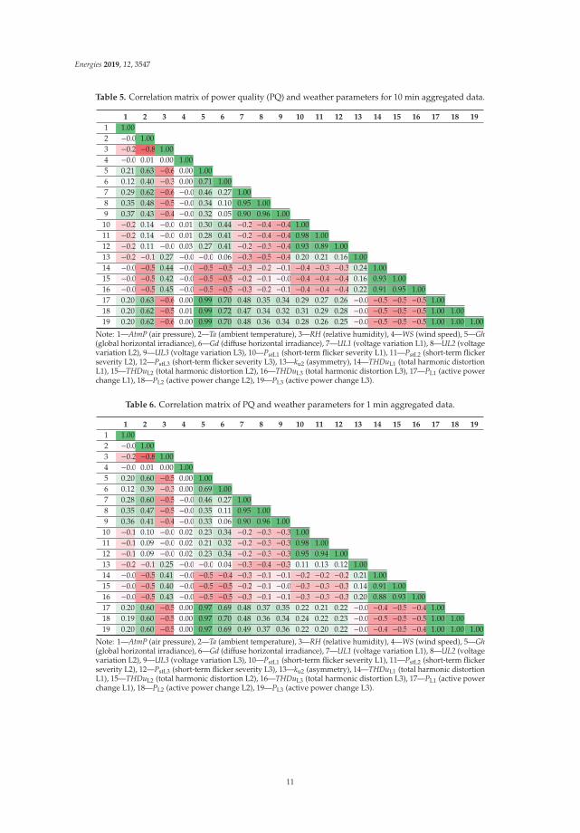
The prepared matrix of correlation is an extended matrix which consists of PQ parameters andweather condition measurements together so that the analysis of the correlation coefficient can beperformed simultaneously between particular power quality themselves, for example between voltagelevel and harmonic contents, as well as between power quality parameters and weather condition, forexample between horizontal irradiance and voltage level. The results of the correlation coefficientsusing 10 min aggregated data is presented in Table 5. Comparative results obtained 1 min aggregateddata is collected in Table 6. Additionally, the correlation diagrams of all pairs of parameters is shownin Figure 6 for the 10 min data and in Figure 7 for the 1 min data.

10

Energies 2019, 12, 3547

Table 5. Correlation matrix of power quality (PQ) and weather parameters for 10 min aggregated data.

1 2 3 4 5 6 7 8 9 10 11 12 13 14 15 16 17 18 19

1 1.002 −0.011.003 −0.26−0.851.004 −0.010.01 0.00 1.005 0.21 0.63 −0.610.00 1.006 0.12 0.40 −0.340.00 0.71 1.007 0.29 0.62 −0.60−0.010.46 0.27 1.008 0.35 0.48 −0.53−0.020.34 0.10 0.95 1.009 0.37 0.43 −0.48−0.020.32 0.05 0.90 0.96 1.00

10 −0.230.14 −0.030.01 0.30 0.44 −0.25−0.41−0.471.0011 −0.240.14 −0.030.01 0.28 0.41 −0.26−0.41−0.470.98 1.0012 −0.200.11 −0.020.03 0.27 0.41 −0.23−0.37−0.440.93 0.89 1.0013 −0.24−0.150.27 −0.02−0.060.06 −0.39−0.50−0.450.20 0.21 0.16 1.0014 −0.01−0.550.44 −0.02−0.54−0.52−0.35−0.22−0.13−0.40−0.39−0.370.24 1.0015 −0.06−0.520.42 −0.03−0.58−0.59−0.29−0.13−0.06−0.49−0.48−0.460.16 0.93 1.0016 −0.05−0.530.45 −0.01−0.54−0.57−0.37−0.21−0.12−0.44−0.43−0.410.22 0.91 0.95 1.0017 0.20 0.63 −0.600.00 0.99 0.70 0.48 0.35 0.34 0.29 0.27 0.26 −0.04−0.53−0.56−0.521.0018 0.20 0.62 −0.590.01 0.99 0.72 0.47 0.34 0.32 0.31 0.29 0.28 −0.05−0.56−0.59−0.551.00 1.0019 0.20 0.62 −0.600.00 0.99 0.70 0.48 0.36 0.34 0.28 0.26 0.25 −0.04−0.53−0.56−0.521.00 1.00 1.00

Note: 1—AtmP (air pressure), 2—Ta (ambient temperature), 3—RH (relative humidity), 4—WS (wind speed), 5—Gh(global horizontal irradiance), 6—Gd (diffuse horizontal irradiance), 7—UL1 (voltage variation L1), 8—UL2 (voltagevariation L2), 9—UL3 (voltage variation L3), 10—PstL1 (short-term flicker severity L1), 11—PstL2 (short-term flickerseverity L2), 12—PstL3 (short-term flicker severity L3), 13—ku2 (asymmetry), 14—THDuL1 (total harmonic distortionL1), 15—THDuL2 (total harmonic distortion L2), 16—THDuL3 (total harmonic distortion L3), 17—PL1 (active powerchange L1), 18—PL2 (active power change L2), 19—PL3 (active power change L3).

Table 6. Correlation matrix of PQ and weather parameters for 1 min aggregated data.

1 2 3 4 5 6 7 8 9 10 11 12 13 14 15 16 17 18 19

1 1.002 −0.011.003 −0.26−0.851.004 −0.010.01 0.00 1.005 0.20 0.60 −0.590.00 1.006 0.12 0.39 −0.340.00 0.69 1.007 0.28 0.60 −0.58−0.010.46 0.27 1.008 0.35 0.47 −0.51−0.020.35 0.11 0.95 1.009 0.36 0.41 −0.47−0.020.33 0.06 0.90 0.96 1.00

10 −0.170.10 −0.030.02 0.23 0.34 −0.20−0.31−0.341.0011 −0.180.09 −0.010.02 0.21 0.32 −0.21−0.32−0.360.98 1.0012 −0.170.09 −0.020.02 0.23 0.34 −0.20−0.31−0.350.95 0.94 1.0013 −0.22−0.140.25 −0.01−0.050.04 −0.32−0.44−0.380.11 0.13 0.12 1.0014 −0.02−0.520.41 −0.02−0.50−0.48−0.31−0.19−0.11−0.29−0.28−0.290.21 1.0015 −0.06−0.500.40 −0.02−0.54−0.56−0.27−0.11−0.05−0.35−0.34−0.350.14 0.91 1.0016 −0.05−0.520.43 −0.01−0.50−0.55−0.35−0.19−0.11−0.32−0.31−0.330.20 0.88 0.93 1.0017 0.20 0.60 −0.580.00 0.97 0.69 0.48 0.37 0.35 0.22 0.21 0.22 −0.04−0.49−0.53−0.491.0018 0.19 0.60 −0.570.00 0.97 0.70 0.48 0.36 0.34 0.24 0.22 0.23 −0.04−0.51−0.56−0.521.00 1.0019 0.20 0.60 −0.580.00 0.97 0.69 0.49 0.37 0.36 0.22 0.20 0.22 −0.04−0.49−0.52−0.491.00 1.00 1.00


11

Energies 2019, 12, 3547

Figure 6. Correlation diagrams for all pairs of parameters (PQ and weather) when 10 min aggregationinterval is used. Note: 1—AtmP (air pressure), 2—Ta (ambient temperature), 3—RH (relative humidity),4—WS (wind speed), 5—Gh (global horizontal irradiance), 6—Gd (diffuse horizontal irradiance),7—UL1 (voltage variation L1), 8—UL2 (voltage variation L2), 9—UL3 (voltage variation L3), 10—PstL1

(short-term flicker severity L1), 11—PstL2 (short-term flicker severity L2), 12—PstL3 (short-term flickerseverity L3), 13—ku2 (asymmetry), 14—THDuL1 (total harmonic distortion L1), 15—THDuL2 (totalharmonic distortion L2), 16—THDuL3 (total harmonic distortion L3), 17—PL1 (active power change L1),18—PL2 (active power change L2), 19—PL3 (active power change L3).

12

Energies 2019, 12, 3547

Figure 7. Correlation diagrams for all pairs of parameters (PQ and weather) when 1 min aggregationinterval is used. Note: 1—AtmP (air pressure), 2—Ta (ambient temperature), 3—RH (relative humidity),4—WS (wind speed), 5—Gh (global horizontal irradiance), 6—Gd (diffuse horizontal irradiance),7—UL1 (voltage variation L1), 8—UL2 (voltage variation L2), 9—UL3 (voltage variation L3), 10—PstL1

(short-term flicker severity L1), 11—PstL2 (short-term flicker severity L2), 12—PstL3 (short-term flickerseverity L3), 13—ku2 (asymmetry), 14—THDuL1 (total harmonic distortion L1), 15—THDuL2 (totalharmonic distortion L2), 16—THDuL3 (total harmonic distortion L3), 17—PL1 (active power change L1),18—PL2 (active power change L2), 19—PL3 (active power change L3).

The analysis of the correlation matrix of PQ parameters and weather conditions using a 10 minaggregation interval, presented in Table 4 and Figure 6, indicates that there is:

• strong correlation between global horizontal irradiance intensity (Gh) and active power (P) withan extremal value equal to 0.99;

• high correlation between intensity of the diffuse horizontal irradiance component (Gd) and activepower (P) with an extremal value equal to 0.72;

• noticeable correlation between ambient temperature (Ta) and voltage variation (U) with qnextremal value equal to 0.62, total harmonic distortion in voltage (THDu) with an extremal valueequal to −0.55 and active power (P) with an extremal value equal to 0.63;

• noticeable correlation between relative humidity (RH) and voltage variation (U) with an extremalvalue equal to −0.60, total harmonic distortion in voltage (THDu) with an extremal value equal to0.45, active power (P) with an extremal value equal to −0.60;

13

Energies 2019, 12, 3547

• noticeable correlation between global horizontal irradiance intensity (Gh) and total harmonicdistortion in voltage (THDu) with an extremal value equal to −0.58;

• noticeable correlation between intensity of the diffuse horizontal irradiance component (Gd) andshort-term flicker severity (Pst) with an extremal value equal to 0.44;

• strong correlation between the line-to-line values of three-phase parameters (U, Pst, THDu, P)with a minimal value equal to 0.90;

• noticeable correlation between L1 voltage variations (U) and L1, L2, L3 active power (P) with anextremal value equal to 0.48;

• noticeable correlation between L2 and L3 voltages variations (U) and L2 and L3 short-term flickerseverities (Pst) with an extremal value equal to −0.47;

• noticeable correlation between short-term flicker severities (Pst) and total harmonic distortion involtage (THDu) with an extremal value equal to −0.49;

• noticeable correlation between total harmonic distortion in voltage (THDu) and active power (P)with an extremal value equal to −0.59;

• other correlations are too low to be noticeable.

Using both 10 min and 1 min aggregation intervals, an expected relationship between solarirradiance and the active power production as well as voltage level is represented by the high level ofcorrelation coefficients. The higher solar irradiance level, the higher level of active power generationis observed that naturally has an influence on voltage level in the connection point. The correlationanalysis is sensitive enough to show small differences between phases which can be explained by thestructure of the investigated PV power plant. The PV power plant consists of many small individualPV installations including one-phase installations thus the active power or voltage level may differslightly in particular phases. It has resulted in a correlation coefficient related to the phases.

Analyzing the correlation matrix of PQ parameters and weather conditions for the 1 minaggregation interval, presented in Table 6 and Figure 7, confirms generally the same correlation resultsas for the 10 min interval. However, in order to highlight the impact of the aggregation interval onthe results of the correlation analysis, a separate matrix of differences was prepared and presentedin Table 7. The matrix consists of differences calculated between the absolute value of adequatecorrelation coefficients obtained using 10 min and 1 min aggregation intervals. A positive valueof the difference denotes that the correlation coefficient calculated using the 10 min aggregation ishigher than that calculated using the 1 min aggregation. The obtained result of the investigateddifferences indicates that the correlation results using 10 min and 1 min aggregation are characterizedby comparative level of correlation coefficient for all measured parameters. The comparative meansthat the maximal difference is slight and less than 0.1. The exception of this result is the correlationbetween flicker severity (Pst) and voltage level (U) and total harmonic distortion in voltage (THDu).For these parameters, the maximal value of difference is 0.15. Generally, it can be concluded that usinga 10 min aggregation interval in comparison to a 1 min aggregation results in a slightly higher levelof correlation coefficients. The sign of the coefficients remains the same. In other words, it can beconcluded generally that the application of different aggregation time intervals does not change thedirection of the correlation but has an influence on the absolute value of the correlation coefficient.Shorter aggregation time intervals assure sharper observability of the process but exhibit a higher levelof standard deviation and wider envelope of parameter variation. Compared to the 1 min time series,the 10 min data are more “monotonous” than the 1 min data due to the averaging process over the10 min interval. Thus, the correlation analysis performed using 10 min data, which are more smoothed,results in higher values of correlation coefficient.

14

Energies 2019, 12, 3547

Table 7. Matrix of differences between correlation coefficients obtained using 1 and 10 minaggregation intervals.

1 2 3 4 5 6 7 8 9 10 11 12 13 14 15 16 17 18 19

1 0.00

2 0.00 0.00

3 0.00 0.00 0.00

4 0.00 0.00 0.00 0.00

5 0.01 0.02 0.02 0.00 0.00

6 0.00 0.00 0.00 0.00 0.02 0.00

7 0.01 0.02 0.02 0.00 0.00 0.00 0.00

8 0.01 0.01 0.01 0.00 −0.010.00 0.00 0.00

9 0.01 0.01 0.02 0.00 −0.01−0.010.00 0.01 0.00

10 0.06 0.04 0.01 0.00 0.07 0.10 0.05 0.10 0.12 0.0011 0.06 0.05 0.02 0.00 0.07 0.09 0.04 0.09 0.12 0.00 0.0012 0.03 0.02 0.00 0.01 0.04 0.07 0.03 0.06 0.08 −0.02−0.050.0013 0.03 0.01 0.02 0.01 0.00 0.02 0.06 0.06 0.07 0.09 0.08 0.04 0.0014 0.00 0.03 0.02 0.00 0.05 0.03 0.04 0.03 0.02 0.11 0.12 0.09 0.03 0.0015 0.00 0.02 0.01 0.01 0.04 0.03 0.02 0.02 0.01 0.15 0.15 0.11 0.02 0.02 0.0016 0.00 0.01 0.01 0.00 0.04 0.02 0.02 0.01 0.01 0.12 0.12 0.08 0.02 0.03 0.02 0.0017 0.01 0.02 0.02 0.00 0.02 0.02 −0.01−0.01−0.020.06 0.06 0.04 0.01 0.04 0.03 0.03 0.0018 0.01 0.02 0.02 0.00 0.02 0.02 −0.01−0.02−0.020.07 0.07 0.05 0.01 0.04 0.04 0.03 0.00 0.0019 0.01 0.02 0.02 0.00 0.02 0.02 −0.01−0.01−0.020.06 0.06 0.04 0.01 0.04 0.03 0.03 0.00 0.00 0.00


5. Discussions

The investigations presented in this paper correspond to the recent amendment to the PQ standardEN 50160:2015 [2] in comparison to the previous version EN 50160:2010 [1]. The main issues in relationto the development of the mentioned standard are the influence of the requirement for the assessed PQparameters to preserve the limits 100% of the observed time in comparison to the previous requirementof 95% of the time of observation, as well as influence of the suggestion to use a 1 min aggregationtime interval in the case of a LV power system in comparison to the classical 10 min aggregation.Additionally, the issue of the aggregation interval is extended in the paper for the analysis of theinfluence of the aggregation interval on correlation analysis between PQ parameters and weatherconditions. The formulated problems can have a meaning in analysis of the integration of distributedenergy resources with a power system in the light of increasing requirements for power qualityparameters and increasing concentration of distributed generation in power systems.

In order to highlight mentioned issues, the results of the investigation of a real measurement of a100 kW photovoltaic power plant directly connected to a LV power system is presented. In relationto the requirement for the assessed PQ parameters to preserve the limits 100% of the observed time,it can be concluded that such requirement can be hard to obtain in selected cases. For example, theinvestigated 15th harmonic in voltage in the PCC of the investigated 100 kW PV power plant doesnot preserve the requirement for 100% of the observed time, but has a positive assessment for therequirement of 95% of the observed time. It should be emphasized that the flagging concept wasimplemented, and the investigated measurement data are free of events which might have affectedthe assessment by extremal values. A similar conclusion can be formulated in the case of a variationin frequency demand. A more restricted limit for the permissible level of frequency variation anddemand for 100% of the observed time causes the assessment to be negative when the requirements

15

Energies 2019, 12, 3547

related to the amendment to the standard EN 50160:2015 [2] is applied, but would be positive accordingto requirements of the previous version EN 50160:2010 [1].

Novel power quality analysis is not only concentrated on PQ parameters but also finds a relationbetween external components and their impact on power quality. In the case of integration of distributedgeneration with a power system, a prominent example is the influence of weather conditions on powerquality. A tool used for the assessment can be a correlation analysis. Thus, an additional aim ofthe paper is to investigate the influence of the aggregation time interval on the correlation analysis.Generally, it can be concluded that the obtained result of the investigated differences indicates that thecorrelation analysis using 10 min and 1 min aggregation intervals are characterized by comparativelevel of correlation coefficient. The application of different aggregation time intervals does not changethe direction of the correlation but has an influence on the absolute value of the correlation coefficient.The 10 min data are more smoothed than the 1 min time series due to the averaging process over the10 min and correlation coefficients obtained using 10 min aggregation are slightly higher. Only in caseof flicker severity, expressed by parameter Pst, which is sensitive even for single voltage fluctuations, isthe difference of the correlation coefficient noticeable.

The obtained results indicate the need for further investigation of the sensitivity of the assessmentwhen new requirements for power quality limits are created or a shorter aggregation time interval isconsidered. The advantage of the application of a shorter aggregation time interval is the enhancementof the observability of the investigated objects. However, it has an impact on extended requirementsfor the measurement devices and increases the time and computational power required for analysisdue to the extended size of the power quality database.

6. Conclusions

The presented results indicate that general outcomes of the analysis for both 1 min and 10 minaggregation are similar. However where the requirements for the parameters are forced to be fulfilledduring 100% of the observation time, the 1 min aggregation makes the observability of the object morerestricted. This allows us to formulate general conclusion that the results of power quality assessmentusing the 1 min aggregation can be dependent on cooperation of the observed object with the powersystems, the used regulation and integration systems, as well as the condition of the power systemat the connection point. Furthermore, the obtained results show some potential in using variationsof observed power quality parameters in the development of power quality analysis when a 1 minaggregation is used. It was shown that the voltage variation parameters including minimal andmaximal values or standard deviations better express the variability of the observed parameters when1 min aggregation is used. It was also shown that the assessment of power quality parameters at theconnection point of a PV power plant, when the cloud effect or variable operating condition of thelow voltage network are considered, is characterized by slightly higher values in the variation of theobserved power quality parameters when a 1 min aggregation interval is applied than in case of 10 minaggregation. This allows us to conclude that using 1 min aggregation increases the sensitivity of powerquality assessment that might be desirable in future when power grids with a high concentration ofdistributed energy resources, microgrids or grids working in the islanding condition are considered.

Author Contributions: Conceptualization, M.J. and T.S.; methodology, M.J., T.S. and P.K.; software, J.S., M.J. andT.S.; validation, T.S., J.R. and Z.L.; formal analysis, M.J. and T.S.; investigation, M.J., T.S. and P.K.; resources,M.J., T.S., P.K., P.J., D.B., M.R., J.S.; writing—M.J. and T.S.; writing—review and editing, M.J., T.S., E.J., D.K.;visualization, M.J., E.J.; supervision, T.S.; project administration, T.S.; funding acquisition, M.J. and T.S.

Funding: This research was funded by Polish Ministry of Science and Higher Education under the grants foryoung researchers 049M/0004/19 as well as under the project “Developing a platform for aggregating generationand regulatory potential of dispersed renewable energy sources, power retention devices and selected categoriesof controllable load” supported by European Union Operational Program Smart Growth 2014-2020, Priority AxisI: Supporting R&D carried out by enterprises, Measure 1.2: Sectoral R&D Programs, POIR.01.02.00-00-0221/16,performed by TAURON Ekoenergia Ltd. under Polish Sectoral Program PBSE coordinated by The National Centreof Research and Development in Poland.

16

Energies 2019, 12, 3547

Acknowledgments: This work uses weather condition data provided by the Center of Energy Technology inSwidnica, Poland.

Conflicts of Interest: The authors declare no conflict of interest.

Abbreviations

AC alternative currentAtmP air pressureCC connector cableCdTe Cadmium telluride cellsCIGS Copper-Indium-Gallium-DiselenideDC direct currentEN European Standardf frequency variationGd intensity of the scattered radiation componentGh total horizontal radiation intensityHC host capacityIEC International Electrotechnical CommissionIEEE Institute of Electrical and Electronics Engineersku2 asymmetrymc-Si multicrystallineMS measuring systemMSS main switching stationP active power changePlt long-term flicker severityPst short-term flicker severityPVFS PV Solar FarmPVSS photovoltaic switching stationRES renewable energy sourcesRH relative humiditysc-Si monocrystallineTa ambient temperatureTHD total harmonic distortionU voltage variationVDE Verband der Elektrotechnik, Elektronik und InformationstechnikWS wind speed

References

1. EN 50160: Voltage Characteristics of Electricity Supplied by Public Distribution Network; PKN: Warszawa,Polska, 2010.

2. EN 50160: Voltage Characteristics of Electricity Supplied by Public Distribution Network; PKN: Warszawa,Polska, 2015.

3. IEC 61000 4–30 Electromagnetic Compatibility (EMC)—Part 4–30: Testing and Measurement Techniques—PowerQuality Measurement Methods; PKN: Warszawa, Polska, 2015.

4. IEEE. Monitoring and Definition of Electric Power Quality; IEEE: Piscataway Township, NJ, USA, 2009.5. Jasinski, M.; Sikorski, T.; Borkowski, K. Clustering as a tool to support the assessment of power quality in

electrical power networks with distributed generation in the mining industry. Electr. Power Syst. Res. 2019,166, 52–60. [CrossRef]

6. Bouchakour, S.; Arab, A.H.; Abdeladim, K.; Amrouche, S.O.; Semaoui, S.; Taghezouit, B.; Boulahchiche, S.;Razagui, A. Investigation of the voltage quality at PCC of grid connected PV system. Energy Procedia 2017,141, 66–70. [CrossRef]

7. Gała, M.; Jaderko, A. Assessment of the impact of photovoltaic system on the power quality in the distributionnetwork. Prz. Elektrotech. 2018, 94, 162–165. [CrossRef]

17

Energies 2019, 12, 3547

8. Grycan, W.; Brusilowicz, B.; Kupaj, M. Photovoltaic farm impact on parameters of power quality and thecurrent legislation. Sol. Energy 2018, 165, 189–198. [CrossRef]

9. Bogenrieder, J.; Glass, O.; Luchscheider, P.; Stegner, C.; Weller, J. Technical comparison of measures forvoltage regulation in low-Voltage grids. In Proceedings of the 24th International Conference on ElectricityDistribution, Glasgow, UK, 12–15 June 2017; pp. 1–5.

10. Divshali, P.H.; Soder, L. Improving PV hosting capacity of distribution grids considering dynamic voltagecharacteristic. In Proceedings of the Power Systems Computation Conference (PSCC), Dublin, Ireland,11–15 June 2018.

11. Vojtek, M.; Kolcun, M.; Špes, M. Utilization of energy storages in low voltage grids with high penetration ofphotovoltaics—Addressing voltage issues. In Proceedings of the 2018 19th International Scientific Conferenceon Electric Power Engineering (EPE), Brno, Czech Republic, 16–18 May 2018.

12. Ramljak, I.; Ramljak, I. PV plant connection in urban and rural LV grid: Comparison of voltage qualityresults. In Advanced Technologies, Systems, and Applications III; Springer: Berlin, Germany, 2018; pp. 271–278.

13. Meyer, J.; Domagk, M.; Darda, T.; Eberl, G. Influence of aggregation intervals on power quality assessmentaccording to EN 50160. In Proceedings of the 22nd International Conference and Exhibition on ElectricityDistribution (CIRED 2013), Institution of Engineering and Technology, Stockholm, Sweden, 10–13 June 2013;p. 1174.

14. Elphick, S.; Gosbell, V.; Perera, S. The effect of data aggregation interval on voltage results. In Proceedings ofthe 2007 Australasian Universities Power Engineering Conference, Perth, Australia, 9–12 December 2007;pp. 1–7.

15. Jasinski, M.; Rezmer, J.; Sikorski, T.; Szymanda, J. Integration Monitoring of On-Grid Photovoltaic System:Case Study. Period. Polytech. Electr. Eng. Comput. Sci. 2019, 63, 99–105. [CrossRef]

16. Statsoft Polska StatSoft Electronic Statistic Textbook. Available online: http://www.statsoft.pl/textbook/stathome.html (accessed on 15 February 2019).

17. Sikorski, T. Monitoring i Ocena Jakosci Energii w Sieciach Elektroenergetycznych z Udziałem Generacji Rozproszonej;Oficyna Wydawnicza Politechniki Wrocławskiej: Wroclaw, Poland, 2013. (In Polish)

© 2019 by the authors. Licensee MDPI, Basel, Switzerland. This article is an open accessarticle distributed under the terms and conditions of the Creative Commons Attribution(CC BY) license (http://creativecommons.org/licenses/by/4.0/).

18

energies

Article

Techno-Economic Optimization of Grid-ConnectedPhotovoltaic (PV) and Battery Systems Based onMaximum Demand Reduction (MDRed) Modellingin Malaysia

Gopinath Subramani 1, Vigna K. Ramachandaramurthy 2,*, P. Sanjeevikumar 3,

Jens Bo Holm-Nielsen 3, Frede Blaabjerg 4, Leonowicz Zbigniew 5 and Pawel Kostyla 5

1 Centre of Advanced Electrical and Electronic Systems (CAEES), Faculty of Engineering & the BuiltEnvironment, Segi University, Kota Damansara, Petaling Jaya 47810, Malaysia; [email protected]

2 Institute of Power Engineering, Department of Electrical Power Engineering, College of Engineering,Universiti Tenaga Nasional, Kajang 43000, Malaysia

3 Center for Bioenergy and Green Engineering, Department of Energy Technology, Aalborg University,6700 Esbjerg, Denmark; [email protected] (P.S.); [email protected] (J.B.H.-N.)

4 Center of Reliable Power Electronics (CORPE), Department of Energy Technology, Aalborg University,9220 Esbjerg, Denmark; [email protected]

5 Faculty of Electrical Engineering, Wroclaw University of Science and Technology, Wyb. Wyspianskiego 27,50370 Wroclaw, Poland; [email protected] (L.Z.); [email protected] (P.K.)

* Correspondence: [email protected]

Received: 11 July 2019; Accepted: 9 September 2019; Published: 13 September 2019

Abstract: Under the present electricity tariff structure in Malaysia, electricity billing on a monthlybasis for commercial and industrial consumers includes the net consumption charges together withmaximum demand (MD) charges. The use of batteries in combination with photovoltaic (PV) systemsis projected to become a viable solution for energy management, in terms of peak load shaving. Basedon the latest studies, maximum demand (MD) reduction can be accomplished via a solar PV-batterysystem based on a few measures such as load pattern, techno-economic traits, and electricity scheme.Based on these measures, the Maximum Demand Reduction (MDRed) Model is developed as anoptimization tool for the solar PV-battery system. This paper shows that energy savings on netconsumption and maximum demand can be maximized via optimal sizing of the solar PV-batterysystem using the MATLAB genetic algorithm (GA) tool. GA optimization results revealed thatthe optimal sizing of solar PV-battery system gives monthly energy savings of up to 20% of netconsumption via solar PV self-consumption, 3% of maximum demand (MD) via MD shaving and 2%of surplus power supplied to grid via net energy metering (NEM) in regards to Malaysian electricitytariff scheme and cost of the overall system.

Keywords: maximum demand (MD); solar PV; battery energy storage system (BESS); net energymetering (NEM); maximum demand reduction (MDRed) model

1. Introduction

The release of greenhouse gases, especially CO2, by utilities using coal and gas reduces the ozonelayer and creates more pollution. Energy demand in developing countries is projected to rise about65% by 2040, reflecting the growing prosperity and the accelerating economies. The global energydemand will increase by about 35% due to the world’s population growth [1]. The high penetrationlevel of solar photovoltaic (PV) in the utility sector decreases the greenhouse gases emissions andpromotes the use of renewable energy compared to conventional energy resources. Solar PV systemsare able to deliver an alternative solution to reduce the peaking load throughout the day.


Energies 2019, 12, 3531

However, the intermittent supply of solar PV system during bad weather condition reduces theability to supply power during peak hours [2]. Solar PV system in combination with energy storage isexpected to be the optimum solution to accommodate the peak load.

In the modern era, energy storage technology has been widely applied for peak load reduction.Energy storage devices such as batteries, thermal storage, and supercapacitors offer similar functionalityto peaking power plants. Nevertheless, each of these technologies has economic and technical barriersto be solved [3]. Sustainable Energy Development Authority (SEDA) Malaysia has promoted cleanenergy use by authorizing the implementation of renewable energy tariff mechanisms under theRenewable Energy Act 2011. In November 2016, the Net Energy Metering (NEM) scheme wasimplemented to encourage the use of renewable energy (RE), especially solar PV in the grid. NEMpermits the self-consumption of generated power by the RE while exporting the surplus power to theutilities at a fixed rate. Under the NEM scheme, the surplus generation rate has been set at MYR 0.31(USD 0.07)/kWh and MYR 0.238 (USD 0.05)/kWh for low voltage and medium voltage interconnectionfacilities, respectively [4].

Nevertheless, the low energy rate will reduce the excess energy profit compared to the currentTime-of-Use (ToU) pricing scheme of Malaysian electricity tariff [5]. This has driven the focus onoptimization of the solar PV-battery system to capitalize on the energy-saving profits associated withthe electricity price variances between ToU and NEM scheme. Under the ToU scheme, maximumdemand (MD) is measured by recording the peak load over the timeframe of successive 30 min intervalsfrom 8.00 a.m. until 10.00 p.m. every day in a month. Table 1 displays the Malaysian electricity tariffrate for different categories of utility customers. As per Table 1, for industrial and commercial sectors,electricity tariff scheme is effective from 1st January 2014 and supersedes the previous tariff schedulewhich was effective from 1st June 2011 according to Tenaga Nasional Berhad (TNB), the Malaysianelectricity company and only electric utility company in Peninsular Malaysia. Based on the Malaysianelectricity scheme under TNB, commercial and industrial sectors are categorized based on differenttariff rates. C1 and E1 customers incur flat rate charges for MD and net consumption. For C2 and E2categories, net consumption will be charged based on peak and off-peak periods together with MDcharges. The peak period timeframe is from 8.00 a.m. until 10.00 p.m. and the off-peak period is from10.00 p.m. until 8.00 a.m., respectively [6]. For these reasons, the commercial and industrial customersare encouraged to manage their load consumption according to their respective electricity tariff schemeby focusing on peak and off-peak period rates. Implementation of renewable energy (RE) projects isexpected to reduce the maximum demand and will contribute significantly to the overall generationmix in Malaysia.

Table 1. Malaysia electricity tariff categories (Medium Voltage level).

Tariff Unit C1 a C2 b E1 c E2 d

Peak RM (USD)/kWh 0.0 0.365 (0.08) 0.0 0.365 (0.08)Off-peak RM (USD)/kWh 0.0 0.224 (0.05) 0.0 0.219 (0.05)

Net consumption RM (USD)/kWh 0.365 (0.08) 0.0 0.337 (0.08) 0.0Maximum Demand (MD) RM (USD)/kW 30.3 (6.82) 45.1 (10.2) 29.6 (6.7) 37.0 (8.3)

C1 a represents the commercial sector (general) [6]. C2 b represents the commercial sector (peak and off-peak) [6].E1 c represents the industrial sector (general) [6]. E2 d represents the industrial sector (peak and off-peak) [6].

Adding solar photovoltaic generation to commercial or industrial loads reduces utility energy(kWh) charges, but often has little effect on maximum demand (kW) charges. As per Figure 1, peakdemands or maximum demand often occur early in the morning during the beginning of office hourswhen the solar PV generation is slowly increased. Commercial customers with PV generation mayhave the same high peak (kW) demand but with a lower average (kW) demand. Since they have ahigher maximum demand, they will generally benefit more from maximum demand reduction using abattery energy storage system. Peak shaving or maximum demand reduction is the process of reducingthe amount of energy purchased from the utility sector during peak hours. A couple of the options

20

Energies 2019, 12, 3531

include reducing consumption by turning off non-essential equipment during peak hours. Apart fromthat, installing solar PV-battery systems that can assist with reducing maximum demand, since muchof the peak demand occurs during times when this system would be effective.

However, variation in solar irradiance pattern especially during peak hours may lead to a minimalreduction of MD since electricity billing for MD charges are captured on any day with peaking loadthroughout the month. Therefore, a new approach called Maximum Demand Reduction (MDRed)scheme has been developed to optimally size the solar PV-battery system with respect to Time-of-Use(ToU) pricing scheme of Malaysian electricity tariff and cost of the overall system corresponding toReturn on Investment (ROI). Apart from that, this approach will solve the challenges faced due tointermittency of solar PV generation for reliable operation of maximum demand reduction duringpeak hours with the support of battery energy storage system.

2. Concept of Maximum Demand Reduction (MDRed) Model

Recently, a lot of studies and models have been developed using solar PV-battery systems. Braamet al. [7] have developed a novel forecast-based control system for photovoltaic-battery systems.It estimates the photovoltaic excess power and develops a charging plan for the battery to store theenergy from the photovoltaic peak-production. Wang et al. [8] have developed a state-space basedmodel for BESS and implement a modest yet effective method for peak load reduction by consideringdevice limitations. Pimm et al. [9] have developed a demand model to produce high-resolutiondomestic load profiles to determine how much peak shaving could be achieved with battery storage.An efficient technique of finding the prospective peak shaving using electricity storage is developed forthis purpose. It shows that adequate levels of storage capacity can provide significant peak demandreductions if properly coordinated. Ru et al. [10] have studied the minimization of the cost associatedwith purchasing from (or selling back to) the utility grid and the battery capacity loss while at the sametime sustaining the load and decreasing the peak demand purchased from the grid.

Apart from that, Linssen et al. [11] have developed the Battery-Photovoltaic-Simulation (BaPSi)model to conduct techno-economic analyses of PV-battery systems. The model reflects the variationin the environment to determine the solar PV sizing and battery storage capacity. For each system,the mixture of the total costs of electric supply as well as associated technical and economic outputparameters are calculated. Kleissl et al. [12] have developed an operational battery dispatch controlsystem using linear programming for a solar PV-battery storage system that practices load and solarprediction to alleviate peak load. Moghim et al. [13] developed the battery energy storage system (BESS)control algorithm to concurrently overcome the outage issue and shave the peak demand consideringthe BESS sizing and degradation, microgrid system cost reduction, as well as microgrid scheduling.Liu et al. [14] studied the energy management with battery energy storage system (BESS) optimisationby bearing in mind the cost of distributed generations, cost of battery system, and bi-directional energytrading. Dongol et al. [15] developed the Model Predictive Control (MPC) scheme that could be appliedto an existing grid linked household with PV-battery system such that the use of battery is maximizedand at the same time, peaks in PV power and load demand are reduced.

Optimal sizing of the solar PV-battery system needs to be based on the effectiveness ofself-consumption and MD reduction with respect to return on investment. As stated by Subramani,et al. [16], based on Figures 1 and 2, the optimal solar PV-battery sizing depends on important elementssuch as load pattern, techno-economic traits, and electricity billing scheme to meet high maximumdemand reduction. In regard to load profile, the load consumption data of one (1) or two (2) years willbe adequate to show the load steadiness mainly on MD level and load consumption pattern duringthe peak period. Since the MD charges are very high, the energy savings through optimal sizing ofthe PV and battery system will be able to maximize the electricity bill savings mainly due to peakload reduction for commercial and industrial customers. Battery efficiency in terms of the state ofcharge (SOC) and depth of discharge (DOD) together with solar irradiance and PV inverter efficiencywill be key for optimal sizing. The total cost of the solar PV-battery system will be very critical in

21

Energies 2019, 12, 3531

response to the total energy savings, to have a good return on investment to undertake the project.As the core battery technology matures and unit pricing declines, bi-directional battery convertersproviding both battery charging (AC to DC) and battery inverting (DC to AC) will emerge as a rapidlygrowing new market for power converters. The Maximum Demand Reduction (MDRed) model isproposed and developed as an optimization tool for the solar PV-battery system. It focuses on peakload shaving and maximization of self-consumption via PV generation and battery system with respectto MD limits. The MDRed model consist of a solar PV array, PV inverter, lithium-ion battery andbi-directional converter. The MDRed model is developed by considering the technical and economicperspective. Firstly, a technical model is formulated which focuses on the battery storage and solarPV capacity to reduce the net load consumption and maximize the MD shaving for a given loadpattern. Secondly, the economic model focuses on the cost associated with the system componentscompared with the energy savings through net consumption and maximum demand to cater forthe highest Return on Investment. A flowchart describing the proposed MDRed model is shown inFigure 2. The required input parameters for MDRed model calculation include the consumer loaddata, solar PV-battery system specification data, and general economic parameters. In MDRed Model,the electricity supply chain is based on the energy balance between the supply and the demand sidewith respect to MD limitations.

Figure 1. Peak or maximum demand shaving concept using solar PV-battery system [13].

22

Energies 2019, 12, 3531

Figure 2. Maximum demand reduction (MDRed) modeling approach.

3. MATLAB Genetic Algorithm (GA) for MDRed Optimization Model

Based on Table 2, optimization techniques such as Genetic Algorithm (GA), Harmony Search (HS),Particle Swarm Optimization (PSO) and Hybrid Optimization are the most prominent algorithms tosize the solar PV-battery system.

Table 2. Comparison of optimization techniques.

Technique Highlights Strength Weakness Ref.

Genetic Algorithm(GA)

Mimics processes ofnatural evolution, likeinheritance, mutation,

selection, and crossover

Can solve problems withmultiple solutions; easilytransferable to existingsimulations and models

Convergence speed isslower than other

stochastic algorithms[17,18]

Particle swarmoptimization (PSO)

Mimics bird and fishmovement behavior

The speed of their searching isfast; calculation in PSO is simplein comparison to other methods

Cannot work out theproblems of

non-coordinate system[17,18]

Bee-inspiredalgorithms

Based on the intelligent foraging behavior of honey

bee

The algorithm has local searchand global search ability;

implemented with severaloptimization problems; easy to

use

Random initialization;algorithm has several

parameters[19]

Harmony search Based on improvisationprocess of jazz musicians

Can handle discrete variables aswell as continuous variables;

ability to perform a global andlocal search

Complex solving process [20]

Biogeography-basedoptimization (BBO)

Behavior studies of speciesin nature

Fast computation time; goodconvergence accuracy

Poor in exploiting thesolutions; no provision forselecting the best members

of each generation

[21]

Hybridoptimization

technique

Developed by using two ormore algorithms

Better accuracy in results; takesless computational time(in some

cases)

Increased complexity;difficult to code [22]

23

Energies 2019, 12, 3531

Also, these techniques can deal with the random probability distribution or generate a pattern ofrenewable energy sources [23]. In this paper, the GA programming is developed for the optimizationof optimal solar PV-battery sizing in regard to peak load shaving. GA has several advantages suchas problem-solving with numerous solutions, easy to understand and can directly be transferred toexisting simulations and models [24]. Therefore, several modeling equations and approaches fordesigning a solar PV-battery system via GA have been developed to ensure the optimum sizing of theoverall system.

The proposed MDRed model using GA coding was developed to solve the optimal capacity ofsolar PV and battery system to maximize the energy savings via self-consumption and MD shavings.Input data includes hourly solar irradiation in Watts-peak (Wp) and multiple patterns of monthly loadpower consumption in kilowatts (kW). Besides that, battery charging and discharging shall be operatedbased on Time of Use (ToU) under Malaysian electricity tariff for commercial and industrial sector.MDRed modelling scheme is made of mathematical formulation which includes the electricity tariffmodel, solar PV model and battery energy storage system model. Apart from that, the economicalmodel mainly focuses on cost of the solar PV and battery system and Return on Investment (ROI).

3.1. Financial Model

3.1.1. Electricity TariffModel

Most electricity tariff categories for commercial and industrial sectors are designed to encouragecustomers to control their electricity demand at daytime peaks since MD charges are very high. Referringto Table 1, the electricity tariffmodel is specified in Table 3 for net consumption and maximum demandcalculation according to electricity tariff categories on commercial and industrial sectors.

Table 3. Tariff rates under Malaysian utility billing scheme.

Tariff Unit Category Total Bill

Net consumption, Pload_net MYR/kWh, Uload_net C1 & E1 CnetMaximum Demand, PMD MYR/kW, UMD C1, C2, E1 & E2 CMD

The total electricity bill (Cbill) for commercial and industrial customers as calculated as follows [6]:

CMD_kW = EMD_kW * PMD (1)

Cnet_kWh = Eload_net * Pload_net (2)

Cbill =

∫Pload_net * Eload_net +

∫PMD * EMD (3)

where the combination of maximum demand bill (CMD_kW) in Equation (1) and net consumption bill(Cnet_kWh) in Equation (2) will be added on a monthly basis. Equations (1)–(3) are formulated based onthe Malaysian electricity tariff category for the commercial and industrial sector. Based on Table 4 andFigure 3, a Malaysian higher learning institution’s load profile under C1 electricity tariff is chosen forthe case study. Since the case studies is focusing on solar PV-battery sizing based on maximum demand(MD) reduction approach, the concept can be explained using one (1) type of load profile from anycommercial or industrial sector. In this paper, C1 category load profile for four (4) consecutive monthsfrom January 2017 until April 2017 is used for validation studies. Based on energy data evaluation,highest load or maximum demand is recorded at 1300 kW during beginning of academic calendar forthe higher learning institution. Therefore, four (4) months of load profile data is sufficient to cater foroptimal sizing of solar PV and battery system based on the Malaysian electricity tariff.

24

Energies 2019, 12, 3531

Figure 3. Energy consumption for C1 category commercial sector.

The MD is recorded between 1200 kW and 1300 kW during peak hours in between 8.30 a.m. and10.30 a.m. Figure 3 shows the monthly net consumption and maximum demand recorded in electricitybilling of the commercial building. Table 4 shows the maximum demand recorded throughout themonths during peak hours only. It can be observed that the highest MD occurs in the month of February2017 at 1300 kW. Besides that, the highest load has been consumed in between 8.30 a.m. and 10.00 a.m.for first four months in the year 2017. These data will be used in a MATLAB (2016a, The Mathworks,Natick, MA, USA) GA optimization algorithm for solar PV and battery sizing. The weather conditionin Malaysia is suitable for solar PV generation. Based on Figure 4, the weather condition is almostpredictable with intermittent sunlight from 8.30 a.m. until 5.30 p.m. The peak PV generation isnormally achieved at 1000 W/m2 and with solar PV module temperature and ambient temperaturereaching 50 ◦C and 33 ◦C, respectively.

Figure 4. Actual solar irradiance measurement data at Nilai, Negeri Sembilan, Malaysia.

Table 4. Maximum demand captured during peak hours.

Month-Year Time Load (kW) Total Cost (MYR)

Jan-17 9:30:00 1260 38,178.00Feb-17 9:00:00 1300 39,390.00Mar-17 10:00:00 1220 36,966.00Apr-17 8:30:00 1290 39,087.00

25

Energies 2019, 12, 3531

3.1.2. Solar PV Model

The difficulty of calculating the energy generated by a solar PV has been extensively studiedin the technical literature. The calculation of solar PV power of a grid-connected solar PV system isclassified under two categories which is indirect method and direct method. As the operation andthe performance of a PV focuses mainly on its maximum power, the indirect method describing thePV module’s maximum power output behaviors are more theoretical for solar PV system valuation.Indirect method directly calculates the maximum power without calculating first the I-V curve of thesolar PV array [25]. This simplified indirect method provides the modelled power to be used in MDRedmodelling. Based on Rus-Casa et al., indirect method directly provides power from atmosphericparameters and information provided by the manufacturers in the datasheets. PV modelled powerin per-unit conversion is based on PV module temperature and solar irradiance level at StandardTesting Condition (STC). The formula for PV modelled power in per-unit convention, Pmod is given asfollows [25]:

Pmod = PPV_kwp* (G/GSTC) [1 − γ * (TC − TSTC)] (4)

where Gs (t) is the measured solar irradiance (hourly) and PPV_kwp is the rated PV power at StandardTesting Condition (STC). GSTC and TSTC is the solar irradiance (1000 W/m2) and PV module temperature(25 degC) at Standard Testing Conditions (STC), respectively. Besides that, γ is the temperaturecorrection based on measured polycrystalline silicon PV module temperatures with a power decreasein between 0.30%/◦C and 0.5%/◦C.

The measured module temperature, TC is set at 50 ◦C at solar irradiance of 3.5 up to 4 h perday averagely based on Malaysian climate. Solar irradiance measurement was taken at Nilai, NegeriSembilan, Malaysia using a CMP3 pyranometer (KIPP & ZONEN, Delft, The Netherlands). Apartfrom the measured solar irradiance, the actual generated power will be obtained with respect to solarirradiance and PV module temperature. The cost of the solar PV system and batteries are the importantparameters for optimal sizing of the solar PV-battery system. Table 5 shows the historical prices of thesolar PV-inverter system from the year 2010–2016 in Peninsular Malaysia [26]. The PPV_rated can becalculated as follows:

PPV_rated = PPV_kWp/ηinv (5)

where PPV_rated is the rated dc output power of the proposed PV array in kWp and ηinv is the conversionefficiency from dc to ac according to inverter efficiency. Nowadays, the PV inverters can operate at90% of conversion efficiency.

Table 5. National trends in PV-inverter system prices.

Year 2010 a 2011 a 2012 a 2013 a 2014 a 2015 a 2016 a 2017

Price (MYR)/kWp 19,120 11,000 9000 7500 8500 7500 7300 -a Data is collected from [5].

3.1.3. Battery Energy Storage System (BESS) Model

The battery energy storage system (BESS) comprises batteries, control and power conditioningsystem (C-PCS). Typically, batteries will absorb power from the grid during the off-peak hours anddischarge power during peak demand. Currently, significant research and development in batterytechnology are being carried out. Tesla (Arizona, AZ, USA) has designed and commercialized thePowerwall 2, the second iteration of its home battery system. Tesla Powerwall 2 costs MYR24,200(USD5500) and delivers 14 kWh of capacity [27].

As the core battery technology matures and the unit pricing decays, bi-directional convertersproviding both battery charging (AC to DC) and battery inverting (DC to AC) will grow due to thenew market for power converters. Various technologies for BESS are available, namely lead acid(LA), vanadium redox flow (VRB), zinc–bromine flow (ZnBr), polysulfide bromide battery (PSB),

26

Energies 2019, 12, 3531

nickel–cadmium battery (NiCd), sodium sulfur and lithium-ion (Li-ion) battery [28]. Four batterytechnologies are chosen for the investigation of BESS systems such as LA, VRB, ZnBr, and Li-ion.The key parameters for these batteries are tabulated in Table 6.

Table 6. Key parameters of batteries.

TechnologyDOD a Round Trip b Cycle Life c Cost of Energy b (RM/kWh)

(%) Efficiency (%) Low High Low High

LA 50 85 500 2800 185 1147VRB 100 85 12,000 13,342 648 3700ZnBr 100 75 1500 2000 740 2220Li-ion 85 90 1000 10,000 2220 9250

a Data is collected from [29]; b Data is collected from [30]; c Data is collected from [31].

The batteries are rated in terms of their energy and power capacities. Some of the other essentialfeatures of a battery are its efficiency, life span, operating temperature, depth of discharge (DOD),self-discharge and energy density. In most cases, lithium-ion batteries and lead-acid batteries are thebest choices for peak shaving techniques, although other battery types can be more affordable [32].While lead-acid batteries have a relatively short lifespan and lower DOD than other battery types,they are also one of the least expensive options in the energy storage sector. Lithium-ion batteries arelighter and better than lead-acid batteries [33]. They also have higher DOD and longer lifespan whencompared to lead-acid batteries. Since the battery is also operated on DC, an AC-to-DC converteris necessary for charging the battery and a DC-to-AC converter is necessary during dischargingthe battery. For simplicity, we assumed that both converters have the identical constant conversionefficiency satisfying:

Pconv(t) =

⎧⎪⎪⎨⎪⎪⎩ ηBPB(t), if PB(t) < 0PB(t)ηB

otherwise(6)

Note that, ηB is the round trip efficiency of the battery converters. In other words, Pconv is thepower exchanged with the AC bus when the converters and the battery are treated as a single entity.Similarly, we can derive:

P(t) =

⎧⎪⎪⎨⎪⎪⎩Pconv(t)

ηBif Pconv(t) < 0

ηBPconv(t) otherwise(7)

Apart from that, the rated capacity of the battery, PBat is calculated by considering the optimalsize of the battery, Ebat as follows:

Pbat(kWh) = Ebat(kWh) ∗ ηbat

DOD(8)

The battery Depth of Discharge (DOD) has a significant impact on a battery’s life cycle. Thebattery life cycle is inversely proportional to the DOD. The DOD of a battery defines the fraction of thepower that can be withdrawn from the battery. For instance, if a battery system is 100% fully charged,it means the DOD of this battery is 0% and vice +Generally, battery state of charge (SOC) provides theratio of the amount of energy presently stored in the battery to the nominal rated capacity.

3.2. Economical Model

The cost of optimal PV array, CPV_inv can be calculated as follows:

CPV_inv = UPV * PPV_rated (9)

where UPV_kWp is the unit cost of PV array per kWp. Apart from that, reducing the cost of PV invertersystem will lead to lower miscellaneous costs such as operation and maintenance costs and replacement

27

Energies 2019, 12, 3531

costs. The overall cost of the solar PV system is the combination of both costs of power conversionunits and cost of inverter. In this paper, the overall solar PV system cost, Ctotal_PV_inv is evaluated byreferring to a specific planning period and is given by:

Ctotal_PV_inv (MYR) = CPV + CO&M_PV + CRC_PV (10)

The cost of batteries, CBat is calculated as follows:

Cbat (MYR) = Ubat (MYR/kWh) * Pbat (kWh) (11)

where UBat is the unit cost of the batteries in kWh, PBat is the rated capacity of the batteries. The cost ofpower conversion units, Cconv is as follows:

Cconv (MYR) = Uconv (MYR/kWh) × Pconv (kW) (12)

where UConv is the unit cost of the power conversion units in kW and Pconv is the power rating of theconverter. The overall cost of the BESS is the combination of both costs of power conversion unitsand cost of batteries. In this paper, the total overall BESS cost, Ctotal_BESS is evaluated by referring to aspecific planning period and is given by:

CBESS = Cbat + Cconv (13)

Ctotal_BESS (MYR) = CBESS + Co&m_BESS + Crep_BESS + Cdisp_bat + CLS_bat (14)

where CBESS is the capital cost, Co&m_BESS is the operation and maintenance cost, Crep_BESS is thereplacement cost, Cdisp_bat is the disposal cost related to the potential cost achievable from recyclingold batteries and lifespan cost (CLS_bat) of all the main components including its system. However,this is not added in MDRed modeling since the cost of the BESS is very high and will lead to longerROI. Cost of energy savings on net consumption and MD are according to Malaysian electricity tariffallocated for each category of commercial and industrial customers. For commercial consumers withtariff rates of C1 category, the annual savings, Syr_shave can be calculated as follows:

Pshave_MD = [max (∑

Pload_net) (15)

Syr_shave = (∑

Pload_shave * Eload_net) + (Pshave_MD * EMD) + (∑

PPV_suplus * E_surplus) * 12 (16)

Under the NEM scheme, the rate of surplus generation, E_surplus has been formulated at MYR0.238 (USD 0.05)/kWh for medium voltage interconnection. Apart from that, overall loan payment isimportant to include all the incurred cost such as operation and maintenance cost (CO&M), replacementcost (CRC) and lifespan cost (CLS) of all the main components including its system. This is appliedto PV-inverter and BESS components which includes the batteries and converter unit. Therefore, theoverall cost of the system comprises of:

Cfull_loan = (Ctotal_PV + Ctotal_BESS) * interest rate (%) (17)

The energy flow schedule of solar PV-battery system integration has been included to lower thedaily operating cost mainly on the MD reduction at the specific limit. For GA optimization, 7% ofinterest rate for total load payment has been included.

4. Modeling of System Reliability

Several approaches have been used to achieve the optimal configuration of solar PV-batterysystems from the technical and economical perspective. In this paper, the technical algorithm forthe optimal sizing is developed according to the concept of MDRed model to evaluate the reliability

28

Energies 2019, 12, 3531

of solar PV-battery system. The GA model attains the optimal size in terms of various degrees ofreliability. A binary coded GA was introduced to solve the optimal capacity of solar PV and battery.Input data includes hourly data per year, solar irradiation by indirect power calculation, load powerconsumption and timeframe of battery DOD and SOC with respect to peak hours and off-peak hour’stariff charges. The flowchart of the GA process applied to PV-battery sizing problem with respect toMDRed modelling is illustrated in Figure 5. One of the key parameters that represent the battery sizingis the capacity of battery charging, Pbat_chg and battery discharging, Pbat_dischg. Based on Figure 5 andTable 7, the amount of maximum demand reduction (MDRed) is based on battery discharging capacity(Pbat_dischg) to maintain the maximum demand limit (PMD_limit), in the presence and/or absence ofgenerated PV power (PPV) during peak hours from 8.00 a.m. and 10.00 p.m. Battery charging capacity(Pbat_chg) will be in operation during off-peak hours in between 10.00 p.m. and 8.00 a.m. As perFigure 7, the battery energy management system works to monitor the net load continuously in thepresence of solar PV and will immediately activate the battery operation to discharge if the new netload exceeds the MD limit. Besides that, the battery discharging will not take place if the new net loadis below the MD limit. Besides that, as per Figure 7, the Battery Energy management system scenariosfor MDRed modeling approach is based on any scenarios (efficient, intermittent or zero solar PV).Therefore, the proposed optimization method will deliver the optimal operation condition or optimalsizing of solar PV-battery in real time scenario.

Figure 5. Flowchart of MDRed model for optimal sizing simulation using Genetic Algorithm.

29

Energies 2019, 12, 3531

Table 7. Battery Energy management system for MDRed modeling approach.

Scenario

Concept ControlAlgorithm

Peak Hours[8.00 a.m.–10.00 p.m.]

Off Peak Hours[10.00 p.m.–8.00 a.m. ]

Actual load below the MDlimit

Pload_actual < PMD_limit

Solar PV Efficient

BatteryPPV_surplus = Pload_actual-PPV

when PPV > Polad_actual[Battery will not operate]

[Battery will notchange since 0% DOD]

Fully charged DOD: 0%

Actual load above the MDlimit

Pload_actual > PMD_limit

Solar PV Intermittent or Zero

BatteryPload_net = [Pload_Actual +

Pbat_chg] – [PPV + Pbat_discha][Battery will discharge]

[Battery will change toachieve 0% DOD]

Fully charged DOD: >50%

As per Equation (18), the generated PV power, PPV will be supplied for self-consumption toreduce the actual load, Pload_actual. Therefore, new net load, Pload_net will be obtained. However, thebattery will not discharge if the Pload_net is below PMD_limit. Due to the intermittent solar irradianceduring bad weather condition, the optimal battery sizing can be calculated using Equations (19) and(20) to cater for the MD limit. If the Pload_net is above PMD_limit, the battery will discharge (Pbat_dischg) tomaintain the required MD limit. During off-peak hours, the batteries will be charged (Pbat_chg) duringoff-peak hours until minimum DOD is reached. Therefore, new net load, Pload_net can be calculated as:

[Condition #1: PMD_limit < Pload_net with solar PV]:- Condition #1: PMD_limit < Pload_net with solar PV

∫Pload_net =

∫Pload_actual −

∫PPV (18)

[Condition #2: PMD_limit > Pload_net with solar PV]:-

Pload_net = [Pload_actual + Pbat_chg] − [PPV + Pbat_dischg] (19)

[Condition #3: PMD_limit > Pload_net without solar PV]:-

Pload_net = [Pload_actual + Pbat_chg] − [Pbat_dischg] (20)

The total load net consumption reduction will be based on sum of the new net load mainly due togenerated PV power. Therefore, total load shaving (Pload_shave) can be calculated as:∑

Pload_shave =∑

Pload_actual −∑

PPV (21)

MD reduction shaving varies according to system performance which mainly relies on total generatedPV power and battery capacity. The excess PV power, PPV_suplus will be achieved when generatedPV power is more than actual load and it can be calculated as: [Condition #4: PPV > Pload_actual withsolar PV]:

PPV_suplus =∑

[PPV − Pload_actual] (22)

The basic Return on Investment (ROI) is calculated based on payment of loan in regard to interestrate using total profit achieved using solar PV-battery system. The ROI can be calculated as:

ROI (in years) = Cload_payment/Syr_shave (23)

30

Energies 2019, 12, 3531

5. System Optimization

As per Table 8, the system parameters used for GA optimization covers the technical andeconomical data of PV, inverter, converter and battery energy storage system. In this paper, the GAoptimization gives an optimal sizing of solar PV and battery system without considering the lifespancost of battery since replacement of battery will be neglected after completion of life span period.

Table 8. Detail of the components.

Component Unit PV-Inverter Battery Converter

Cost of the system

MYR (USD)/kWp 7000 (1600)

MYR (USD)/kWh 2200 (500)

MYR (USD)/kW 1100 (250)

Lifespan Years 21 12

Efficiency % 90 95 90

DOD % 85

O&M cost 5% of CPV_INV 10% of CBESS

RC cost 5% of CPV_INV 10% of CBESS

Interest Rate % 7 7 7

5.1. Problem Formulation

The aim of this study is to attain an optimal sizing of a solar PV-battery system, which should beproperly designed in terms of technical, economic and reliability measures subject to physical andoperational constraints/strategies. The objective function of the optimization is to achieve the optimalsizing with respect to highest energy savings on maximum demand and net consumption.

5.1.1. System Constraints

In this study, battery charging and discharging mechanism and the distribution lines are ideal.Besides that, the inverter efficiency, battery efficiency and manufacturers’ round-trip efficiency isconstant regardless of the operation period. Since the battery cost is very high, the life span cost or totalcost of the new battery system will be set to zero after achieving the life span of the battery operation.For any period, t, the total power supply from the solar PV-battery system must supply the totaldemand with a certain reliability criterion. This relation can be represented by Equation (24) as follows:

PPV + PBat ≤ Pload_actual (24)

This minimizes the excess power supply to the grid since the self-consumption of PV power orexisting net consumption rate [MYR 0.365 (USD 0.08)/kWh] will be higher than net metering rate [MYR0.238 (USD 0.05)/kWh].

5.1.2. Bounds of Design Variables

The proposed solar PV-battery system optimization parameters including the solar PV capacity,PPV_kWp and maximum demand limit, PMD_limit should be within a certain range:

Load profile (Min) < PPV_kWp < Load profile (Max) (25)

Load profile (Ave) < PMD_limit < Load profile (Max) (26)

The bounds of the design variable on PV and MD limit sizing is to maximize the self-consumptioninstead of surplus to the grid.

31

Energies 2019, 12, 3531

5.2. Validation of Numerical Results

Experimental data on PV model using indirect method is verified using a 50 kWp PV system.The experimental data and figure are shown in Figure 6 and Table 9 respectively. Based on the results,based on the indirect method of Equation (4), at 1000 W/m2 of measured solar irradiance, a 50 kWpsolar PV system only delivers up to 35 kW of actual PV power and 38 kW of PV modelled power.

0.05.0

10.015.020.025.030.035.040.045.0

00:00 MYT 07:00 MYT 13:00 MYT 19:00 MYT 23:00 MYT

kWp

Pmod (kW)(AC) PPV_50kWp

Figure 6. Modelled PV power (Indirect method).

Table 9. PV model validation data with 50 kWp PV system.

Pmod = PPV_Kwp* (Gs/GSTC) [1 − γ * (TC − TSTC)]PPV_rated =

PPV_kWp/ηinv

50 kWp PVSystem (Actual)

Time (Hr)Gs

(W/m2)GSTC

(W/m2)γ Tc

(DegC)TSTC

(DegC)

Pmod

(In PerUnit)

Pmod

(kW)(DC)

PV ModelledPower,

Actual PVGenerated Power

Pmod (KW)(DC) PPV_Actual_AC

00:00 MYT 0 1000 0.005 0.0 0.0 0.00 0.0 0.0 0.001:00 MYT 0 1000 0.005 0.0 0.0 0.00 0.0 0.0 0.002:00 MYT 0 1000 0.005 0.0 0.0 0.00 0.0 0.0 0.003:00 MYT 0 1000 0.005 0.0 0.0 0.00 0.0 0.0 0.004:00 MYT 0 1000 0.005 0.0 0.0 0.00 0.0 0.0 0.005:00 MYT 0 1000 0.005 0.0 0.0 0.00 0.0 0.0 0.006:00 MYT 0 1000 0.005 35.0 25.0 0.00 0.0 0.0 0.007:00 MYT 0 1000 0.005 38.0 25.0 0.00 0.00 0.0 0.008:00 MYT 42 1000 0.005 40.0 25.0 0.04 1.94 1.7 1.009:00 MYT 227 1000 0.005 45.0 25.0 0.20 10.22 9.2 7.510:00 MYT 690 1000 0.005 45.0 25.0 0.62 31.05 27.9 23.011:00 MYT 736 1000 0.005 55.0 25.0 0.63 31.28 28.2 27.012:00 MYT 872 1000 0.005 60.0 25.0 0.72 35.97 32.4 31.513:00 MYT 1027 1000 0.005 60.0 25.0 0.85 42.36 38.1 35.814:00 MYT 755 1000 0.005 60.0 25.0 0.62 31.14 28.0 30.515:00 MYT 393 1000 0.005 60.0 25.0 0.32 16.21 14.6 16.716:00 MYT 204 1000 0.005 55.0 25.0 0.17 8.67 7.8 9.917:00 MYT 141 1000 0.005 50.0 25.0 0.12 6.17 5.6 6.618:00 MYT 19 1000 0.005 45.0 25.0 0.02 0.86 0.8 0.719:00 MYT 18 1000 0.005 40.0 25.0 0.02 0.83 0.7 0.620:00 MYT 0 1000 0.005 0.0 0.0 0.00 0.0 0.0 0.021:00 MYT 0 1000 0.005 0.0 0.0 0.00 0.0 0.0 0.022:00 MYT 0 1000 0.005 0.0 0.0 0.00 0.0 0.0 0.023:00 MYT 0 1000 0.005 0.0 0.0 0.00 0.0 0.0 0.0

For this paper, load profile with actual MD load of 1050 kW has been used. Apart from that,two different phenomena of solar irradiance pattern with perfect data is used for solar PV-batterysystem integration to verify the MDRed scheme. For validation purposes, an MD limit of 750 kW anda PV-inverter rating of 1200 kWp are used to formulate the required battery capacity together with thefinancial data. Validation data is important to verify that the solar PV-battery system works accordingto MDRed scheme. In this paper, the MDRed control algorithm is based on a few conditions to achievethe new MD limit of 750 kW as shown in Table 10 and Figure 7.

32

Energies 2019, 12, 3531

Table 10. MDRed model validation data with solar PV-battery system.

PMD_Limit = 750 kWMDRed scheme During Perfect Weather Condition (Sunny

Day)

Time (Hr)Load Profile PPV = 1200 kWp

(Based onEquation (4))

Battery Capacity, Pbat_kWh

= 48 kWhNew Net Load

ControlAlgorithm

Pload_Actual, kW Pbat_DOD Pbat_SOC Pload_net (kW)

00:00 MYT 390 0 0 −11 401

Condition #201:00 MYT 360 0 0 −11 37102:00 MYT 360 0 0 −11 37103:00 MYT 340 0 0 −11 351

04:00 MYT 320 0 0 0 320No

operation05:00 MYT 320 0 0 0 32006:00 MYT 310 0 0 0 31007:00 MYT 310 0 0 0 310

08:00 MYT 520 46.6 0 0 473 Condition #109:00 MYT 1050 252.0 48 0 750 Condition #2

10:00 MYT 1020 724.5 0 0 296Condition #111:00 MYT 990 772.8 0 0 217

12:00 MYT 900 915.6 0 0 −16Condition #413:00 MYT 940 1078.4 0 0 −138


16:00 MYT 970 214.2 6 0 750 Condition #2


19:00 MYT 580 0 0 0 580MD

monitoring20:00 MYT 620 0 0 0 62021:00 MYT 540 0 0 0 54022:00 MYT 510 0 0 510

23:00 MYT 500 0 0 −11 511 Condition #2

Figure 7. MDRed model validation graph (for Table 10 data.)

Apart from that, the MDRed model shows the control algorithm battery management system tocater for MD reduction with the support of solar PV power at preset MD limit. However, the ratedsizing of solar PV-battery system is higher than the formulated optimal values since the calculation ofrated values are based on Equations (5) and (8). The total savings is the combination of net consumptionsavings at rate of MYR 0.365/kWh, surplus power supplied to the grid at rate of MYR 0.238/kWh andmaximum demand savings at rate of MYR 30.3/kW. Based on assumption, the annual total savings iscalculated for 12 months period. Besides that, the cost of the solar PV-battery system will increasedrastically due to additional cost of O&M and replacement apart from the interest rate of 7% incurredto the total cost of the system.

33

Energies 2019, 12, 3531

Control algorithm of MDRed modeling scheme falls under any of the conditions applied onTable 11 where battery management system works based on maximum demand to maintain the MDlimit setting of 750 kW. However, battery discharging mode will take place in between 8.00 a.m. until10.00 p.m. and battery charging mode in between 10.01 p.m. until 7.59 a.m. everyday with respect tothe MD limit of different load profiles.

Table 11. Summary of validation data at 750 kW MD limit setting.

Control Algorithm StatusPV

StatusNumerical Formula

Condition #1 PMD_limit < Pload_net Yes∫

Pload_net =∫

Pload_actual −∫

PPVCondition #2 PMD_limit > Pload_net Yes Pload_net = [Pload_actual + Pbat_chg] − [PPV + Pbat_dischg]Condition #3 PMD_limit > Pload_net No Pload_net = [Pload_actual + Pbat_chg] − [Pbat_dischg]Condition #4 PPV > Pload_actual Yes PPV_suplus = PPV − Pload_actual

6. Optimization Results

Based on Figure 8, on average 25% of total energy savings can be achieved on a monthly basiswhich can be used to calculate the Return on Investment (ROI). GA optimization results on MDRedmodelling revealed that optimal sizing of solar PV-battery system contributed to energy bill savingsup to 20% of net consumption via solar PV self-consumption, 3% of maximum demand (MD) viaMD shaving and 2% of surplus power supplied to grid via net energy metering (NEM) in regards toMalaysian electricity tariff scheme and cost of overall system.

Figure 8. Percentage of energy savings based on load profile.

GA optimization results from 10 population sizes and via 300 iterations are shown in Figure 9.In this paper, GA optimization studies is based on 21-years of load pattern assumption to cater foroptimal sizing of solar PV-battery system. Since all actual MDs are captured during peak hoursbetween 8.30 a.m. and 10.00 a.m., it does not show huge differences in solar PV-battery optimal sizing.Therefore, the total energy savings achieved in the range of 23% to 26% with the use of solar PV-batterysystem. However, the differences in optimal sizing are influenced by the load margin in betweenmaximum demand and average load consumed during peak hours throughout the month.

34

Energies 2019, 12, 3531

Figure 9. GA optimization results of difference load profiles: (a) Jan-17 [Actual MD: 1260 kW], (b) Feb-17[Actual MD: 1300 kW], (c) Mar-17 [Actual MD: 1220 kW] and (d) Apr-17 [Actual MD: 1290 kW].

The surplus energy savings under Net Energy Metering (NEM) achieved at minimal level dueto low NEM billing rate compared to net consumption rate. The commercial sector may experience

35

Energies 2019, 12, 3531

fluctuating load pattern with different ranges of maximum demand. Therefore, the optimal solarPV-battery sizing at various load pattern falls in between 870 kWp and 970 kWp of solar PV and230 kWh up to 330 kWh of total battery capacity. In addition, the new MD limit has been achieved inthe range 1025 kW and 1098 kW of MD reduction using solar PV-battery system.

Load profile of the system influence the MDRed modelling optimal sizing on the solar PV-batterysystem using a GA algorithm. The load profile of the system influences the MDRed modelling optimalsizing on the solar PV-battery system using the GA algorithm. Based on Table 12, the month of March2017 is proven to give the best optimal sizing for solar PV-battery system with highest percentage oftotal energy savings. This is due to the load profile changes especially the load margin in betweenmaximum and average loading for every month. Based on Figure 10, load margin and maximumdemand of March 2017 is lowest compared to other months which gives the significant impact on MDshaving compared to net consumption savings. Therefore, the acceptable sizing of solar PV and batterycapacity will be 986 kWp and 330 kWh respectively. This will be the best choice to allow the MDRedmodel to work efficiently at any load pattern to achieve high MD load reduction with yearly energysavings up to MYR 600,000.

Table 12. GA optimization results for different load profiles.

Load ProfileEnergySavings

Percentage of TotalEnergy Savings

Optimal SizingMD Limit

PV Battery

(Actual MD) (MYR) (%) (kWp) (kWh) (kW)

Jan-17 [1260 kW] 42,534.14 23.7 869 228 1062

Feb-17 [1300 kW] 46,661.90 25.4 970 225 1098

Mar-17 [1220 kW] 47,021.84 26.5 986 330 1025

Apr-17 [1290 kW] 46,850.45 25.4 980 232.3 1093

Figure 10. Comparison data analysis of load profile.

7. Conclusions

The proposed MDRed modeling scheme works as an optimization model which focuses onmaximum demand (MD) shaving. This reduces the maximum demand and net consumption costswhen using solar PV generation and battery systems. GA optimization results on MDRed modellingreveal that optimal sizing of the solar PV-battery system contributed to energy bill savings up to 20%of net consumption via solar PV self-consumption, 3% of maximum demand (MD) via MD shavingand 2% of surplus power supplied to grid via net energy metering (NEM) in regards to the Malaysianelectricity tariff scheme and cost of the overall system. In addition, the optimal battery sizing will be

36

Energies 2019, 12, 3531

based on the amount of MD savings annually with respect to the cost of the battery system includingthe bi-directional converters. If the load demand is reduced as a result of effective energy managementsystems in place or low production in the factory or buildings, re-optimization may be useful toincrease or maintain the current solar PV-battery size to maximize the net consumption and MDsavings. In future, with higher demand for energy storage system and reduction in battery prices willlead to the realization of a higher rate of maximum demand shaving for commercial and industrialsector via MDRed modeling.

Author Contributions: Conceptualization, G.S. and P.S.; Methodology, V.K.R.; Validation, all co-authors; FormalAnalysis, J.B.H.-N.; Investigation, P.S.; Writing-Original Draft Preparation, G.S., V.K.R. and P.S.; Writing-Review &Editing, P.S., P.K., and L.Z.; Supervision, P.S., L.Z. and P.K.; Funding Acquisition, L.Z. and P.K. All co-authorscontributed substantially to the work.

Funding: This research received partial funding from EEEIC International, Poland.

Acknowledgments: The authors acknowledge the financial assistance from the Ministry of Higher Education(MOHE), Malaysia for the support to embark on renewable energy research.


Nomenclature

MDRed Maximum demand reductionPV PhotovoltaicBESS Battery energy storage systemDOD Depth of Discharge (%)SOC State of Charge (%)MD Maximum demandPload_net Net consumption (kW)PMD Maximum demand (kW)ROI Return on Investment (%)Pconv Power rating of the converter (kW)PBat Rated capacity of the battery (kWh)Ebat Optimal size of the battery (kWh)UPV Unit cost of PV array (MYR/kWp)Ctotal_PV Cumulative cost of PV system (MYR)CO&M_PV O&M cost of PV system (MYR)CRC_PV Replacement cost of PV system (MYR)CBat Cumulative cost of batteries (MYR)UBat Unit cost of the batteries (MYR/kWh)CLS_bat Cost of battery lifespan (MYR)UConv Unit cost of the converter (kW)Pshave_MD Maximum demand shaving load (kW)Syr_shave Total energy savings annually (MYR)Pload_shave Total net consumption savings load (kWh)PPV_STC Rated PV power at Standard Testing Condition (kWp)Cbill Cumulative amount of net consumption and MD (MYR)Cnet_kWh Cumulative amount of net consumption (MYR)CMD_kW Cumulative amount of Maximum demand (MYR)CPV_inv Cumulative cost of optimal PV array (MYR)C_BESS Cumulative cost of BESS and converter MYR)Cfull_loan Cumulative cost of overall PV-battery system (MYR)Uload_net Unit price of net consumption (RM/kWh)UMD Unit price of maximum demand (RM/kWEload_net Total net consumption recorded (kWh)EMD Total maximum demand recorded (kW)PPV_rated Rated dc output power of PV array (kWp)

37

Energies 2019, 12, 3531

PPV_kWp DC output power of PV array (kWp)ηinv Conversion efficiency of inverter (%)ηB Round trip efficiency of the converter (%)PMD_limit Maximum demand limit (kW)Pload_actual Actual consumed load (kWh)Pbat_chg Battery charging load (kWh)Pbat_dischg Battery discharging load (kWh)PPV Solar PV generation load (kWh)Pmod Solar PV modelled power (per unit)Ctotal_BESS Capital cost of overall BESS (MYR)Co&m_BESS O&M cost of BESS (MYR)Crep_BESS Replacement cost of BESS (MYR)Cdisp_bat Disposal cost of BESS (MYR)PPV_suplus Surplus PV power (kWh) (kWh)E_surplus Unit price of surplus PV (MYR/kWh)Gs (t) Measured solar irradiance (W/m2)γ PV module temperature correction (%/◦C)

References

1. ExxonMobil Energy. Outlook for Energy: A View to 2040; ExxonMobil Energy: Irving, TX, USA, 2013.2. Wu, H.; Wang, S.; Zhao, B.; Zhu, C. Energy management and control strategy of a grid-connected PV/battery

system. Int. Trans. Electr. Energy Syst. 2015, 25, 1590–1602. [CrossRef]3. Castillo, A.; Gayme, D.F. Grid-scale energy storage applications in renewable energy integration: A survey.

Energy Conversat. Manag. 2014, 87, 885–894. [CrossRef]4. Coordinated Low Emissions Assistance Network. Review of Networks and Platforms for Low Emission and

Climate Compatible Development Planning; Coordinated Low Emissions Assistance Network: Witzwort,Germany, 2011.

5. The Sustainable Energy Development Authority of Malaysia. Available online: http://www.seda.gov.my/(accessed on 21 September 2014).

6. TNB. Electricity Tariff Schedule; Tenaga Nasional Berhad: Kuala Lumpur, Malaysia, 2014.7. Braam, F.; Hollinger, R.; Engesser, L.M.; Müller, S.; Kohrs, R.; Wittwer, C. Peak shaving with

photovoltaic-battery systems. In Proceedings of the Innovative Smart Grid Technologies ConferenceEurope, Istanbul, Turkey, 12–15 October 2014; pp. 1–5.

8. Wang, B.; Zarghami, M.; Vaziri, M. Energy management and peak-shaving in grid-connected photovoltaicsystems integrated with battery storage. In Proceedings of the North American Power Symposium, Denver,CO, USA, 18–20 September 2016; pp. 1–5.

9. Pimm, J.A.; Cockerill, T.T.; Taylor, P.G. The potential for peak shaving on low voltage distribution networksusing electricity storage. J. Energy Storage 2018, 16, 231–242. [CrossRef]

10. Ru, Y.; Kleissl, J.; Martinez, S. Storage size determination for grid-connected photovoltaic systems. IEEE Trans.Sustain. Energy 2013, 4, 68–81. [CrossRef]

11. Linssen, J.; Stenzel, P.; Fleer, J. Techno-economic analysis of photovoltaic battery systems and the influence ofdifferent consumer load profiles. Appl. Energy 2017, 185, 2019–2025. [CrossRef]

12. Hanna, R.; Kleissl, J.; Nottrott, A.; Ferry, M. Energy dispatch schedule optimization for demand chargereduction using a photovoltaic-battery storage system with solar forecasting. Sol. Energy 2014, 103, 269–287.[CrossRef]

13. Moghimi, M.; Garmabdari, R.; Stegen, S.; Lu, J. Battery energy storage cost and capacity optimization foruniversity research center. In Proceedings of the IEEE/IAS 54th Industrial and Commercial Power SystemsTechnical Conference (I&CPS), Niagara Falls, ON, Canada, 7–10 May 2018.

14. Liu, X.; Gao, B.; Zhu, Z.; Tang, Y. Non-cooperative and cooperative optimisation of battery energy storagesystem for energy management in multi-microgrid. IET Gener. Transm. Distrib. 2018, 12, 2369–2377.[CrossRef]

38

Energies 2019, 12, 3531

15. Dongol, D.; Feldmann, T.; Schmidt, M.; Bollin, E. A model predictive control based peak shaving applicationof battery for a household with photovoltaic system in a rural distribution grid. Sustain. Energy Grids Netw.2018, 16, 1–13. [CrossRef]

16. Subramani, G.; Ramachandaramurthy, V.K.; Padmanaban, S.; Mihet-Popa, L.; Blaabjerg, F.; Guerrero, J.M.Grid-Tied Photovoltaic and Battery Storage Systems with Malaysian Electricity Tariff—A Review onMaximum Demand Shaving. Energies 2017, 10, 1884. [CrossRef]

17. Chauhan, A.; Saini, R.P. A review of an integrated renewable energy system-based power generation forstand-alone applications: Configurations, storage options, sizing methodologies and control. Renew. Sustain.Energy Rev. 2014, 38, 99–120. [CrossRef]

18. Bilal, B.O.; Sambou, V.; Kebe, C.M.F.; Ndiaye, P.A.; Ndongo, M. Methodology to Size an Optimal Stand-AlonePV/wind/diesel/battery System Minimizing the Levelized Cost of Energy and the CO2 Emissions. EnergyProcedia 2012, 14, 1636–1647. [CrossRef]

19. Tudu, B.; Majumder, S.; Mandal, K.K.; Chakraborty, N. Optimal unit sizing of stand-alone renewable hybridenergy system using bees algorithm. In Proceedings of the Energy, Automation, and Signal (ICEAS),Bhubaneswar, India, 28–30 December 2011.

20. Maleki, A.; Askarzadeh, A. Optimal sizing of a PV/wind/diesel system with battery storage for electrificationto an off-grid remote region: A case study of Rafsanjan, Iran. Sustain. Energy Technol. Assess. 2014, 7, 147–153.[CrossRef]

21. Maleki, A.; Ameri, M.; Keynia, F. Scrutiny of multifarious particle swarm optimization for finding the optimalsize of a PV/wind/battery hybrid system. Renew. Energy 2015, 80, 552–563. [CrossRef]

22. Gupta, R.A.; Kumar, R.; Bansal, A.K. BBO-based small autonomous hybrid power system optimizationincorporating wind speed and solar radiation forecasting. Renew. Sustain. Energy Rev. 2015, 41, 1366–1375.[CrossRef]

23. Alsayed, M.; Cacciato, M.; Scarcella, G.; Scelba, G. Design of hybrid power generation systems based onmulti-criteria decision analysis. Sol. Energy 2014, 105, 548–560. [CrossRef]

24. Lara-Fanego, V.; Ruiz-Arias, J.A.; Pozo-Vazquez, D.; Santos-Alamillos, F.J.; Tovar-Pescador, J. Evaluation ofthe WRF model solar irradiance forecasts in Andalusia (southern Spain). Sol. Energy 2012, 86, 2200–2217.[CrossRef]

25. Rus-Casas, C.; Aguilar, J.D.; Rodrigo, P.; Almonacid, F.; Perez-Higueras, P.J. Classification of methods forannual energy harvesting calculations of photovoltaic generators. Energy Convers. Manag. 2014, 78, 527–536.[CrossRef]

26. Ghazali, A.; Salleh, E.; Haw, L.C.; Sohif, M.; Sopian, K.B. Feasibility of vertical photovoltaic system on ahigh-rise building in Malaysia: Performance evaluation. Int. J. Low Carbon Technol. 2017, 12, 1–9. [CrossRef]

27. Divya, K.C.; Østergaard, J. Battery energy storage technology for power systems—An overview. Electr. PowerSyst. Res. 2009, 79, 511–520. [CrossRef]

28. Bulman, P. Tesla’s Powerwall battery production requires ‘super-charged’ supply chain. Renew. Energy Focus2015, 16, 126–127. [CrossRef]

29. Akhil, A.A.; Huff, G.; Currier, A.B.; Kaun, B.C.; Rastler, D.M.; Chen, S.B.; Cotter, A.L.; Bradshaw, D.T.;Gauntlett, W.D. DOE/EPRI Electricity Storage Handbook in Collaboration with NRECA; Sandia National Lab.:Albuquerque, NM, USA, 2015.

30. Poullikkas, A. A comparative overview of large-scale battery systems for electricity storage. Renew. Sustain.Energy Rev. 2013, 27, 778–788. [CrossRef]

31. Luo, X.; Wang, J.; Dooner, M.; Clarke, J. Overview of current development in electrical energy storagetechnologies and the application potential in power system operation. Appl. Energy 2015, 137, 511–536.[CrossRef]

32. Arul, P.G.; Ramachandaramurthy, V.K.; Rajkumar, R.K. Control strategies for a hybrid renewable energysystem: A review. Renew. Sustain. Energy Rev. 2015, 42, 597–608. [CrossRef]

33. Aneke, M.; Wang, M. Energy storage technologies and real-life applications—A state of the art review.Appl. Energy 2016, 179, 350–377. [CrossRef]


39

energies

Article

Location-Based Optimized Service Selection for DataManagement with Cloud Computing in Smart Grids

Sivapragash C. 1,*, Sanjeevikumar Padmanaban 2,*, Hossain Eklas 3, Jens Bo Holm-Nielsen 2 and

R. Hemalatha 4

1 Department of Electrical and Electronics Engineering, Swarnandhra College of Engineering and Technology,Narasapuram 534275, India

2 Center for Bioenergy and Green Engineering, Department of Energy Technology, Aalborg University,6700 Esbjerg, Denmark; [email protected]

3 Oregon Renewable Energy Center (OREC), Department of Electrical Engineering and Renewable Energy,Oregon Institute of Technology, Klamath Falls, OR 97601, USA; [email protected]

4 Department of Electrical and Electronics Engineering, Anna University, Chennai 600025, India;[email protected]

* Correspondence: [email protected] (S.C.); [email protected] (S.P.); Tel.: +45-71-682-084 (S.P.)

Received: 21 September 2019; Accepted: 21 November 2019; Published: 27 November 2019

Abstract: To maximize the utilization, reliability and availability of power resources, some distributionstrategy has to be implemented, which is possible nowadays with the support of modern informationtechnologies (IT). To further develop power utilization, the customer should be aware of efficientpower utilization, and the problem of customer management has to be resolved, where paymentof electric bills could be through online solutions. A customer-aware power regulatory model isproposed that provides awareness to the consumer regarding the usage of electrical energy, in asecure and reliable solution that combines the features of electrical engineering with cloud computingto ensure better performance in notifying issues, which is done based on location and enhancesthe operation of smart grids. Instant electric meters are equipped with remote gadgets whichcommunicate with a central cloud administration to produce electric bills for the client. The modelprovides mindfulness by showing history/notifications and suggestions for energy utilization throughthe smart meters. The user is provided with security keys to view the reading values and pay bills.To make the solution more accessible, the electronic data will be maintained on various serversat different locations of the cloud. Subsequently, there will be a service provider who managesservice requests. A hardwired electric meter transmits the electric readings, which in turn access theparticular service to make an entry for the particular connection on the cloud. The usage data willalso be maintained at different locations in the cloud, which are accessible to different levels of userswith appropriate security measures. The user accessibility is controlled by a Third Party Auditor(TPA) that computes the trustworthiness of users using a trust management scheme. This article alsoproposes a hash function, which computes and verifies the signature of the keys submitted by theusers and also has a higher completeness ratio, which reaches 0.93, than typical methods. This isnoteworthy, and the investigation results prove the system’s proficiency in providing assured service.

Keywords: cloud services; trust management; secure computing; smart meter; LBSS; user-awarepower regulatory model

1. Introduction

The Smart Grid (SG), is an enhancement of the 21st-century electrical grid, which is treated as asystem that uses two-way communication. It includes information technologies (IT) and computationalintelligence in an integrated way to address electricity generation, its transmission, and distribution to


Energies 2019, 12, 4517

achieve an electric system that is clean, secure, reliable, efficient, and sustainable. The evolution of SGsrelies heavily on the utilization and integration of modern IT for the development of new applicationsand services that can leverage the technological upgrades that are enabled by the advanced informationsystem. This allows electric grid systems to work in smarter ways. However, an overwhelming amountof heterogeneous information is generated in the SG, mainly due to widely deployed monitoring,metering, measurement and control devices. This calls for a dominant and cost-effective informationmanagement paradigm for data processing, analysis, and storage.

Our problem analysis is based on the situation in the regional state of Tamilnadu (India), whereelectric bills have to be produced for service payment, and the billing requires human intervention.In smart grids, the grid resource plays a significant role without the assistance of humans for suchoperations. The smart meters present in the SGs record the current energy utilization of users.Additionally, a remote gadget connected to the smart meter can send readings to a remote sink point ata specific time. The remote sink point is the cloud service, which gets the electronic reading from thegadget and creates a record in a database. Therefore, this paper suggests that the IT industry should beinvolved to assist in the information management of the SG. More specifically, the paper explores howcloud computing (CC), a next-generation computing paradigm, can serve the information managementneeds in the SG. The concept of CC is based on large data centers with massive computation andstorage capacities operated by cloud providers, which deliver computing as a service. Shared resources,software, information, and storage are provided, with computers and other devices as a utility overa network. This SG information management paradigm, in which the management is (partially)accomplished via CC, is called Cloud Service (CS)-based SG Information Management [1].

Generally, the usage of electricity is measured by a human meter reader and later fed into thesystem manually. There can be errors during the reading process or when feeding the readings into thesystem, which makes the whole system error-prone. A cloud platform is one where there are multiplelayers and services at different layers, which can be broken up into three primary services:

(1) Software-as-a-Service (SaaS): A service provider delivers software and applications through theinternet. Users subscribe to the software and access it via the web or vendor APIs.

(2) Infrastructure-as-a-Service (IaaS): A vendor provides clients with pay-as-you-go access to storage,networking, servers and other computing resources in the cloud.

(3) Platform-as-a-Service (PaaS): A service provider offers access to a cloud-based environmentin which users can build and deliver applications. The provider supplies theunderlying infrastructure.

These three services make up what Rackspace calls the Cloud Computing Stack, with SaaS ontop, PaaS in the middle, and IaaS on the bottom. To access the service at different layers, variousrestrictions can be enforced by the service provider [1]. The cloud consists of service providers whoprovide services in different forms like infrastructure services, platform services, and software services.Each kind of service belongs to a layer of the cloud. This paper focuses on two different layers, namelysoftware and databases. The cloud services are a set of software interfaces through which legitimateusers can access the cloud resource. The cloud is a loosely coupled environment where the cloudsystem does not know anything about the user and cannot trust the user easily. On a cloud platform,the data can be stored in any of the cloud servers and can be accessed through a set of available services.

The users of the cloud have been allowed to access the service, according to their trust level.Only a registered user is permitted to access the services and data. The trust in different users ismanaged and verified using a Third Party Auditor (TPA) who maintains the details of users and theiraccess permissions. Only if the TPA has verified the identity of a user successfully, he can access theservice or data from the cloud [2]. The TPA, using various approaches, performs the authentication orverification of the users of the cloud. Each method has its demerits and deficiencies. Any securityprotocol faces different network threats. However, the authentication algorithm should be morerigid and less time-complex one. The popular key-based approaches have the problem of the higher

42

Energies 2019, 12, 4517

computational complexity of keys and their higher verification time. This encourages the invention ofrigid verification algorithms.

In this paper, to ensure the regular provision of power, a user-aware power regulation method isproposed, which is updated regarding the usage of current meter readings via smart meters. The entireelectrical data is updated to the cloud. Depending on the power usage of a user, the proposed powerregulatory model provides directions to the user to cut/reduce their power consumption. However, nosuch service or idea is provided in the existing literature. Additionally, the authors use a location-basedservice selection scheme to reduce the time complexity. The main novelty of the proposed methodinvolves finding the users who use auditing service and have been cleared by the auditing service andthen the way performs service selection, which is explained in detail in Section 3.

2. Background Survey

There exist a variety of methods for the development of cloud services and smart meters; thispaper discusses a few of them that apply to our problem statement. In [3], smart meter analytics wereexamined from a software performance perspective and a performance benchmark design inclusive ofa typical smart meter analytics tasks. This system uses both an offline model for feature extraction andonline anomaly detection. Due to privacy issues, an algorithm is presented to generate large realisticdatasets from a small set of real data.

In [4], a thorough analysis of 100 anonymized 5-min commercial building meter data sets wasused to explore time series of electricity consumption using a simple forecast model. This methodimproves energy management with the support of grid control and provides a model for detectingany anomalies.

In [5], a novel design of a smart metering system was developed as a graphical user interface(GUI)-based NTL detection platform. A 3-tier model of a detection algorithm is proposed to combinethree mechanisms that complement each other for enhanced performance. The triangulation techniquefacilitates validation of detection results through cross verification of the three sources of measurementdata. Furthermore, the system also supports better flexibility with built-in or externally developed AImethods and a user-friendly GUI-based platform to monitor and analyze the NTL status of the powergrid in real-time for revenue recovery.

In [6], a smart metering technique with different technologies to capture the data from smartmeters is presented. In [7] the user privacy is maintained using the tools from information theory anda hidden Markov model for the measurements. It further addresses the issues due to the trade-offbetween privacy and utility. In [8], open-source tools are used to measure the smart meter data anddata storage, and an analytics ecosystem based on publicly available test data set is studied.

There exist a variety of methods for the development of cloud services and smart meters; thepaper discusses a few of them here that relate to our problem statement. Reference [9], using atabu search algorithm, presented an efficient search algorithm to identify the locations of data andsoftware components in data clouds. The main goal of this approach is to minimize the cost incurred inoperations and emissions, modelled using mixed-integer programming. The proposed model is solvedwith the search algorithm discussed earlier. Virtual data center embedding (VDCE) across distributedinfrastructures (DI) was introduced to make the infrastructure user-friendly and increase the revenueof providers. Reference [10], performs an analysis of different VM-based cloud environments likeEucalyptus, Open Nebula, and Nimbus. All those platforms have been evaluated with High-LevelPetri Nets (HLPN).

In [11], a formal analysis, modelling, and verification of three open-source state-of-the-artVM-based cloud platforms—Eucalyptus, Open Nebula, and Nimbus—is provided. HLPN are used tomodel, analyze the structural and behavioral properties of the systems. Moreover, to verify the models,they have used the Satisfiability Modulo Theories Library (SMTL) and Z3 Solver.

In this article, we modelled about 100 VM to verify the correctness and feasibility of proposedoriginal models. The results reveal that the models function correctly. Moreover, the increase in the

43

Energies 2019, 12, 4517

number of VMs does not affect the working of the models, which indicates the practicability of themodels in a highly scalable and flexible environment.

Reference [12] analyzes the robustness of advanced DCNs. First, the authors present multi-layeredgraph modelling of various DCNs, and they study the traditional robustness metrics consideringdifferent failure scenarios to perform a comparative analysis. Finally, they describe the inadequacyof the conventional network robustness metrics to appropriately evaluate the DCN robustness andpropose new procedures to quantify DCN robustness. Currently, there is no detailed study availablecentering on DCN robustness.

Reference [13], designs a protocol to enable secure, robust, cheating-resistant, and efficientoutsourcing of MIC to a malicious cloud in this paper. The main idea to protect the privacy is byemploying some transformations on the original matrix to get an encrypted matrix, which is sent tothe cloud; and then transforming the result returned from the cloud to get the correct inversion ofthe original matrix. Next, a randomized Monte Carlo verification algorithm with one-sided erroris employed to successful handle result verification. Further, in this paper, the superiority of thisnovel technique in designing inexpensive result verification algorithm for secure outsourcing and welldemonstrated. They analytically show that the proposed protocol simultaneously fulfils the goals ofcorrectness, security, robust cheating- resistance, and high-efficiency. Extensive theoretical analysisand experimental evaluations also show its high-efficiency and immediate practicability.

In [14] Cloud Capacity Manager (CCM), a prototype system and its methods for dynamicallymultiplexing the computing capacity of virtualized data centers at scales of thousands of machines,for diverse workloads with variable demands are presented. Extending prior studies primarilyconcerned with accurate capacity allocation and ensuring acceptable application performance. CCMalso sheds light on the tradeoffs due to two unavoidable issues in large scale commodity data centers:(i) maintaining low operational overhead given the variable cost of performing management operationsnecessary to allocate resources, and (ii) coping with the increased incidences of these operations’ failures.

Reference [15] adopts the intuitive idea of High-QoS First-Replication (HQFR) to perform datareplication. However, this greedy algorithm cannot minimize the data replication cost and the numberof QoS-violated data replicas. To achieve these two minimum objectives, the algorithm transforms theQADR problem into the well-known minimum-cost maximum-flow (MCMF) problem. By applyingthe existing MCMF algorithm to solve the QADR problem, the second algorithm can produce theoptimal solution to the QADR problem in polynomial time. Still, it takes more computational timethan the first algorithm.

Reference [16], utilizes Voronoi partitions to determine which data center requests should berouted based on the relative priorities of the cloud operator. In [17], the ability to forecast electricitydemand, respond to peak load events, and improve sustainable use of energy by consumers, are madepossible by energy informatics. Information and software system techniques for a smarter powergrid include pattern mining and machine learning over complex events and integrated semanticinformation, distributed stream processing for low latency response, cloud platforms for scalableoperations and privacy policies to mitigate information leakage in an information-rich environment.Reference [18], proposes a new prototype system, in which the cloud-computing system is combinedwith a so-called Trusted Platform Support Service (TSS) based on a Trusted Platform Module. In thisdesign, better effects can be obtained in authentication, role-based access and data protection in a cloudcomputing environment.

Reference [19] presents a pruning algorithm in which a threshold parameter is used to control thetradeoff between computation time and solution accuracy qualitatively. The algorithm is iterative withdecoupled state values in each iteration, and the paper parallelizes the state estimations to reduce theoverall computation time. They illustrate the proposal with examples where the pruning algorithmreduces the computation time significantly without losing much precision in-game solutions, and thatparallelization further reduces the computation time.

44

Energies 2019, 12, 4517

An interdisciplinary MIT study [20] focused on integrating and evaluating existing knowledgerather than performing original research and analysis. Besides, this study’s predecessors focusedon implications of national policies limiting carbon emissions, while do not make any assumptionsregarding future carbon policy initiatives. Instead, they mainly consider the impact of a set of ongoingtrends and existing policies. Reference [21] identifies and reviews several low-cost technology productsthat enable various load control functions and in an innovative prepaid power meter that will have thecapacity to direct cash exchanges through remote intervention is built, keeping in mind the end goal isto empower the client to energize his record from home. The user interface comprises an LCD, whichshows the power used and a measure of the bill to be paid, and will sound an alert when the balancegoes beneath a specific sum utilizing GSM. Prepaid meters are now present in the market and usedwidely in a few African and European nations. Additionally, this will help service organizations instaying aware of power thievery.

The review concludes that interval metering is not necessary to carry out load control functions.Available technology can remotely switch loads without requiring a connection to a meter. Whileone-way communication is essential to carry out remote switching of loads, two-way communicationis not necessary to carry out remote switching of loads. Metering, in some form, is required for thesettlement of the financial transactions associated with load control programs.

Reference [22] examined uncertainty in demand response baseline models and variability inautomated responses to dynamic pricing. It defined several demand response (DR) parameters, whichcharacterize changes in electricity use on DR days, and then presented a method for computing theerror associated with DR parameter estimates. In addition to analyzing the magnitude of DR parametererrors, in this article, the authors develop a metric to determine how much observed DR parametervariability is attributable to real event-to-event variability versus only baseline model error. Using datafrom 38 C&I facilities that participated in an automated DR program in California, it was found thatDR parameter errors are significant. For most facilities, observed DR parameter variability is morelikely explained by baseline model errors, not real DR parameter variability; however, and severalfacilities do exhibit real DR parameter variability.

Reference [23] proposes a mathematical model for the dynamic evolution where in particularsupply, demand, and clearing prices under a class of real-time pricing mechanisms are characterizedby passing on the real-time wholesale prices to the end consumers. The effects that such mechanismscould have on the stability and efficiency of the entire system are investigated, and several stabilitycriteria are discussed. It is shown that relaying the real-time wholesale electricity prices to the endconsumers creates a closed-loop feedback system, which could be unstable or lack robustness, leadingto extreme price volatility. Finally, a result is presented, which characterizes the efficiency lossesincurred when, to achieve stability, the wholesale prices are adjusted by a static pricing function beforethey are passed on to the retail consumers.

Fault current coefficient and time delay assignment for a microgrid protection system with acentral protection unit was discussed in [24], which utilizes relays of type-distributed generatorsproviding more protection between generators. This approach performs critical parameter assignmentslike fault current coefficient and relay hierarchy. This method overcomes the difficulty of the manualtask of distributed generation (DG) and protection units.

Reference [25] proposed an approach for distributed network reinforcement using a timesegmentation algorithm, which reduces the computation overhead. Discrete particle swarmoptimization is used to overcome the problem of nonlinear and discrete optimization.

Reference [26] was focused on load models of appliances. The loads for different appliancesare generated using the profiles maintained and validated with actual distribution circuits. Thenon-demand sensitive load models are used to reduce the consumption of different consumer ports,introduced the improvement of such load models at the machine level, and incorporated traditionalcontrollable burdens, i.e., space cooling/space warming, water heater, garment dryer and electricvehicles. Approval of the machine level load models’ is done by contrasting the models’ output and

45

Energies 2019, 12, 4517

the actual power utilization information for the related apparatus. The machine-level load models’ arecombined to create stack profiles for a dispersion circuit, which are approved against the load profilesof a real distribution circuit. The DR-touchy load models are utilized to examine changes in powerutilization at both the household and the distribution levels, given an arrangement of client practicesand additional actions by a utility.

In [27], an approach for real-time voltage-stability margin control via reactive power reservesensitivities is proposed. In detail, a man-in-loop control method is used to boost reactive powerreserves (RPRs) while maintaining a minimum amount of voltage stability margin bus voltage limits.The objective is to determine the most effective control actions to reestablish critical RPRs acrossthe system. Initially, the concept of reactive power reserve sensitivity concerning control actions isintroduced. In the sequel, a control approach based on convex quadratic optimization is used to findthe minimal amount of control necessary to increase RPRs above their pre-specified (offline) levels.Voltage stability margin constraints are incorporated using a linear approximation of critical RPRs.

Reference [28], discussed an evaluation method for renewable DG in distributed networks. Thisapproach allocates DGs to maximize the usage of connections to the local distribution company andcustomers. Reference [29] presents the algorithms and associated analysis, but guidelines, rules, andimplementation considerations are also discussed, especially for the more complicated situationswhere mathematical analysis is difficult. In general, it is challenging to codify and taxonomize thescheduling knowledge because there are many performance metrics, task characteristics, and systemconfigurations. Also, adding to the complexity is the fact that a variety of algorithms are designed fordifferent combinations of these considerations. In spite of the recent advances, there are still gaps inthe solution space, and there is a need to integrate the available solutions.

Security-aware scheduling strategy for real-time applications on clusters (SAREC) [30], proposesa security-aware scheduling strategy, or which integrates security requirements into scheduling forreal-time applications by employing our security overhead model.

Scheduling real-time data-intensive applications (SARDIG) is a security-attentive dynamicreal-time scheduling algorithm architecture and a dynamic grid scheduling algorithm for providingsecurity for real-time data-intensive applications [31]. It proposes a grid architecture, which describesthe scheduling framework of real-time data-intensive applications. Also, the authors introduced amathematical model for providing security of the real-time data-intensive applications and a securitygain function to quantitatively measure the security enhancement for applications running in thegrid sites. They have also proved that the SARDIG algorithm always provides optimum security forreal-time data-intensive applications.

It could be concluded that the system has a problem of service selection in all the above approacheswhen there is the considerable number of customers from different locations, so a new location-basedservice and selection approaches are proposed in this paper. In the following Section 3, the proposedlocation-based service selection approach is discussed, while Section 4 discusses the results achievedby the proposed method.

3. User-Aware Power Regulatory System with a Location-Based Service Selection Scheme

The proposed user-aware power regulatory scheme gets updates about the power usage of usersthrough smart meters. The smart meters update the power usage details to the cloud service. Basedon the power usage details, the power regulatory model provides inputs to the users to control thepower usage of the connection. The selection of a location-based service selection scheme to provideadditional comprehensive and consistent services has to be done in a more tactical approach where thetime complexity should be reduced. The method audits the identity of the user using the auditingservice, and if the user has cleared the auditing service, then the way performs service selection. Theentire process is split into several stages, namely Location-Based Service Selection, Hash Function forKey Generation, Signature Verification, Trust Management, and Profile-Based Access Restriction. Inthis section, we will explain each of the functional stages in detail. Figure 1 presents the architecture of

46

Energies 2019, 12, 4517

the proposed user aware power regulatory model with a location-based service selection framework,and it shows the various stages of the proposed model.

Figure 1. The architecture of the LBSS Model.

3.1. User-Aware Power Regulatory Model

The smart meter accesses the cloud service intermittently to send power use details, prior monthuse, cost, every month’s average units, number of units utilized at peak times, number of units usedduring off peak-times and their relative offered price. Additionally, the shutdown date and complaintsregistered, number of aggregate units, number of units utilized at peak time, number of units usedduring the off-peak times and their relative offered cost are included, and user notifications are shownon a smart meter display. The power regulatory model controls the flow of electric supply to theuser connection. At intermittent periods, the model produces electric bills and regulates the powersupply. At whatever point the instalment for the electrical supply not been paid, the substation sends acontrol message to the smart meter to detach the electric supply. When the user pays his bills again,then the substation sends the turn-on message to the meter, which provides the power back. Thepower regulatory model utilizes the ZigBee convention to the correspondence between the smart meterand substation.

47

Energies 2019, 12, 4517

Algorithm 1: User-Aware Power Regulatory System

Input: User Usage DetailsOutput: Power to be regulated.Start

Initialize the value of time slot Ti.Tv = value of time slot Ti.For each Time window TiRead Current usage units Cu.Compute Number of units at peak time NPTu.Compute Number of units at Off-Peak Time NOPTu.Compute the cost of power usage CPU.Compute Previous month usage Pmu.Compute Previous month cost Pmc.Compute Number of units on previous month Npm.Compute No of units on peak time Nupt.Compute No of units on off-peak time Nuopt.Identify complaints registered Compl.Compute shutdown date Sd.Access Cloud Service Cs.Cloud-Update-Service (Cu, NPTu, NOPTu, CPU,PMU, Pmc, Npm, Nupt, Nuopt, Compl).Display details to the smart meter.End

If payment date AliveElseAccess Payment-Detail Service.If true thenReset Payment date.ElseDisconnect the power supply.End

End

Stop.

48

Energies 2019, 12, 4517

Algorithm 1, above generates user awareness. It accesses the cloud service to update the cloud, sothe smart meter can also show the recently registered estimations of energy utilization to the user. Themodel controls the power supply by checking the instalment status by accessing the cloud service. Inlight of the state of the instalment, the power status controls the electric supply through the smart meter.

3.2. Location-Based Service Selection

The user electronics readings are maintained at different locations of the county on differentservers. Each geographic region reading is stored on separate servers located in different geographicregions. The user can view generated bills and make payment of bills through the cloud services.Upon creating a request, the cloud platform selects the respective service, according to the locationof data or the server where the data is stored. To provide a more complete, and reliable service, theselection is made in a more strategic way where the time complexity should be minimized. The rangeof services is based on the location of the data, and then the user communicates with the selectedservice. The cloud management console makes the selection, and once the service is selected, then theuser request is transferred to the service chosen (see Algorithm 2).

Algorithm 2: Location-Based Service Selection

LBSS(UserId Uid, UserLocation Uloc)Output: Selected cloud service CS.Step1: Read user-id Uid.Step2: Read user location Uloc.Step3: Read service details SD, service History Sh.Step4: Select available services according to the location Uloc.

Ss =∫ N

i=1 Mx(sh) × (Sd(Uloc))N = number of available services.Mx =Minimum frequency of serviceSh = service historyStep5: Return SS.

3.3. Hash Function for Key Generation

The cloud user is assigned a secure key using which the user is identified and authenticated. Thegeneration of the secret key is a dynamic process which is initiated for each reading, and the key isdestroyed when the user completes the task. The key generation mechanism uses a hash functionwhere the parameter of the hashing function also is changed when the existing or other users enter thesystem the next time. The selection of parameters and functions will also be adjusted according to theregion of the user to provide more security and to avoid guessing attacks (see Algorithm 3).

49

Energies 2019, 12, 4517

Algorithm 3: Hashing Function for Key Generation

Intake: Locations loc, Schemes S.Outcome: Secret key SecK.Read location details LD from the database.Compute Nl = Number of locations from Ld.Nl = sizeof(LD).Generate Random Number Rn.Rn = f (x) =

∫∅(1, S).

Selected Scheme SeS = S(Rn).If (SeS %2) = 0 thenGenerate Secret Key SecK.

Initialize SecK =∫ 8

i=1 SecK(i) = 0).// initialize the key to the size of 8 bit and set all bit to 0.//Set the bit 1,2 = for region 1,2,3//Set the bit 3,4 = for scheme 1-Feb no, 2-ams no, 3-Mona//Set bit 5 and 6 = for the value -//Set the bit 7,8 with meter noUser region ur = select the region of the user.Select a random number for the addressing scheme RanS.If(RanS = 1)Ms = Select a Fibonacci number within ur.Ms = f (x) =

∫®∩ (

∑Fibanacci ∈ (1, UR))

Else if (RanS = 2)Ms = select a amstrong number within ur.Ms = f (x) =

∫®∩ (

∑Amstrong ∈ (1, UR))

ElseMs = select a manorama number within ur.Ms = f (x) =

∫®∩ (

∑Manorama ∈ (1, UR))

End

Construct sk = {Ur,RanS,NS,Mr}.ElseCreate a Secret Key SecK.

Initialize SecK =∫ 16

i=1 SecK(i) = 0).// initialize the key to the size of 16 bit and set all bit to 0.//Set the bit 1 to,4 = for region 1,2,3//Set the bit 5 to 8 = for scheme 1-Feb no, 2-ams no, 3-Mona//Set bit 9 to12 = for the value -//Set the bit 13 to 16 with meter noUser region ur = select the region of the user.Select a random number for the addressing scheme RanS.If(RanS = 1)Ms = Select a Fibonacci number within ur.Ms = f (x) =

∫®∩ (

∑Fibanacci ∈ (1, UR))

Else if (RanS = 2)Ms = select a amstrong number within ur.Ms = f (x) =

∫®∩ (

∑Amstrong ∈ (1, UR))

ElseMs = select a manorama number within ur.Ms = f (x) =

∫®∩ (

∑Manorama ∈ (1, UR))

End

Construct SecK = {Ur,RanS,NS,Mr}.End

Return SecK.

50

Energies 2019, 12, 4517

3.4. Signature Verification

In this stage, the user key has been verified. The verification process is performed by extractingthe bit level information of the received key. If the key size is 16 bits, then a 16 bits keying mechanismis used; otherwise, an 8 bits keying mechanism is used (see Algorithm 4).

Algorithm 4: Signature Verification

Intake: SecK.Outcome: True/FalseRead Given Secret Key SecK.Read Key Set KeyS from Key Base Kb.Identify Key Size of SecK.Ks =

∑Bits ∈ SecK

If Ks = 8 thenSplit SecK by the 2-bit key base.Ur = SecK(1,2).Scheme SN = SecK(3,4).Number Mn = SecK(5,6).Meter No Mr = SecK(7,8).ElseSplit SecK into 4 bit Key Base.Ur = SecK(1,2,3,4).Scheme ScN = SecK(5,6,7,8).Number Mn = SecK(9,10,11,12).Meter No Mr = SecK(13,14,15,16).End

If(ScN = 1)Ms = Select a Fibonacci number within ur.Ms =

∫ Ur1 Feb(1, Ur)

Else if (ScN = 2)Ms = select an amstrong number within ur.

Ms =∫ Ur

1 Ams(1, Ur)ElseMs = select a manorama number within ur.Ms =

∫ Ur1 Man(1, Ur)

End

If Ms =Mn and Mr ∈ Db thenReturn True.ElseReturn False.

End

3.5. Trust Management

Trust management is the critical process in service selection because the user is allowed to accessingthe service only if he passes the trust evaluation. The trust management is categorized based on thetype of users. By identifying the user type from the request, the identity of generic users is verifiedbased on the crucial secret mechanism. For the internal registered users, the primary public/privatecritical method is used. Any user is allowed to access the service based on the trust verification result.

3.6. Profile-Based Access Restriction

The cloud platform is comprised of different users and has to be restricted to minimize access bydifferent users. For example, the internal user needs to view the readings of various users and needs to

51

Energies 2019, 12, 4517

generate reports on them, and so on. The internal users must be able to access the data more frequently,whereas the external users do not. The external user needs one-time access or access for a short time topay the bills so that the proposed work restricts the access based on the roles. It provides role-basedaccess restriction to offer more security to the cloud platform and thus, outsiders cannot make floodingattacks on the proposed system.

4. Results and Discussion

The proposed SG is entirely simulated using the CloudSim platform, and the coding is writtenusing 32 bit Java language for Windows 7 or 8. The processor used is a Core i5 with 8 GB RAM forhigher computational operation. The application server used is Tomcat 5.0.6. The proposed user-aware Power Regulatory Model with Location-Based Service Selection approach, is implemented andevaluated for its efficiency. The technique has been assessed utilizing different setups with a vastnumber of service points and numbers of users. The strategy has been tried with varying situationsof re-enactment for various periods. Table 1 lists the details of the simulation parameters utilized toassess the execution of the proposed technique. Figure 2 shows a preview of the smart meter intendedfor the proposed system. Figure 3 is a preview of the user interface utilized by the power station staffto refresh the unit costs for an assortment of associations. Table 2 shows the completeness ratio of threedifferent algorithms, and it shows that the proposed method has a higher completeness measure valuethat indicates its efficiency in providing guaranteed service.

Table 1. Simulation Parameters.

Parameter Value

Laxity Time 100–500 sNetwork Bandwidth 10 Mbps

Number of Cloud Servers 32Number of cloud services 2

Number of service providers 2Number of Users 1 million

Number of Insiders 10,000

Figure 2. Snapshot of the smart meter display.

52

Energies 2019, 12, 4517

Figure 3. Snapshot of the power station interface.

Table 2. Comparative of completeness ratio results.

Completeness Ratio

Laxity (S) EDF SAREG SARDIG Location-Based

100 0.79 0.82 0.83 0.89200 0.80 0.81 0.85 0.90300 0.83 0.85 0.87 0.91400 0.84 0.86 0.89 0.92500 0.85 0.87 0.91 0.93

The proposed solution has been implemented is Hadoop, which is a cloud computing platformintegrated with the proposed solution to evaluate the proposed methodology. Three different cloudsare created, with each one is running at various locations and on three service providers, which arerunning at N locations. The proposed solution is hardwired with the electric meter, and wirelesscommunication is enabled to access the cloud service. Another web interface is specially designedfor users to use and complete the payment procedures. To evaluate the performance of the proposedsolution, Availability Ratio, Completeness Ratio, Security Value, Overall Performance Ratio, measureswere the metrics examined. Availability is the ratio of total requests submitted and total requestshandled. Completeness is the ratio between total submitted requests and the number of requestsprocessed successfully. The security level is measured by total requests generated and completed.Overall performance is the ratio of the total number of requests submitted and the number of jobscompleted in a particular time-frame.

The performance of the proposed method is compared with three well-known schedulingmethods of the grid environment, namely Earlier Deadline First (EDF) [29] algorithms, Security-Awarescheduling strategy for Real-time applications on Clusters (SAREC) [30] and the Security of Real-TimeData-Intensive Applications on Grids (SARDIG) [31]. Table 2 shows the simulation results of thecompleteness ratio for the four algorithms. The completeness ratio is computed using different deadlinebases or latency time (from 100 to 500 s). The proposed algorithm shows a better completeness ratiothan the other algorithms as the deadline base or latency increases. Table 2 shows that the proposed

53

Energies 2019, 12, 4517

method has a higher ratio, which raised from 0.85 to 0.93, which demonstrates its efficiency in providingguaranteed service.

Table 3 shows the service availability ratio of four different algorithms, and it shows that theproposed method provides more service availability than other methods. Table 4 shows the simulationresults of the security value for the four algorithms. The security value is computed using the totalnumber of requests submitted and several requests fulfilled per number of users present in the network.

Table 3. Shows the comparison results of serviceability.

Availability Ratio %

No. of Users EDF SAREG SARDIG Location-Based

1 million 72 82 89 98.72 million 69 79 85 97.63 million 67 75 81 96.65 million 63 72 77 95.810 million 59 69 72 95.1

Table 4. Shows the comparison results of the security level.

Security Level Value

No. of Users EDF SAREG SARDIG Location-Based

1million 0.89 0.92 0.95 0.992 million 0.83 0.85 0.90 0.963 million 0.77 0.79 0.86 0.934 million 0.61 0.72 0.82 0.915 million 0.55 0.65 0.77 0.89

Figure 4 shows the time complexity of different methods to access the service where the serviceand data are available at various locations of the region. The time complexity is Φ (N × M), whereN—is the number of locations where the service is available, and M—is the number of service providersavailable. The overall time complexity is computed as follows:

Time complexity Tc = N × Log (M)

Figure 4. The time complexity of different approaches.

Figure 4 shows that the proposed method produces more efficient results compared to theother algorithms.

54

Energies 2019, 12, 4517

5. Conclusions

In this paper, we have proposed a user-aware power regulatory model with a location-basedservice selection approach for smart grids. The model provides functionality for smart meters toupdate the user details to the cloud as well be displayed on a smart meter display. Depending onthe recommendations from the smart meter display, the users can change their usage patterns. Asper the design, the proposed model manages the power supply to all its connecting units and alocation-based service selection for secure and reliable access for the cloud services in a smart grid.It maintains a list of trustworthy users with different authentication mechanisms. For a registeredinternal user, it provides role-based access and user access restriction is provided based on theirfrequency of access. A malicious intruder or an unauthorized user is restricted from accessing thesystem through various hash-based signature verification mechanisms that ensure that the cloud issecure. Further, the access session duration is limited to prevent the system from being affected byflooding attacks. The experimental results show that the proposed model obtains higher performancein terms of high throughput and quality of assurance than other existing methods. The next stepto introduce a secure and trusted solution is the requirement that needs to be focused on and to beaddressed by the cloud-computing infrastructure.

Author Contributions: All authors have involved in this research activities for the final presentation of the workas a comprehensive research current article.

Funding: No source of funding for this research activities.


References

1. Sivapragash, C.; Thilaga, S.R.; Kumar, S.S. Advance Cloud Computing in Smart Power Grid. In Proceedingsof the IET Chennai 3rd International on Sustainable Energy and Intelligent Systems (SEISCON 2012),Tiruchengode, India, 27–29 December 2012; pp. 356–361.

2. Rathi, A.; Parmar, N. Secure Cloud Data Computing with Third Party Auditor Control. In Proceedings ofthe 3rd International Conference on Frontiers of Intelligent Computing: Theory and Applications (FICTA),Bubaneswar, Odisha, India, 14–15 November 2014; pp. 145–152.

3. Liu, X.; Golab, L.; Golab, W.; Ilyas, I.F.; Jin, S. Smart meter data analytics: Systems, algorithms, andbenchmarking. ACM Trans. Database Syst. 2017, 42, 2. [CrossRef]

4. Mohammad, R. AMI Smart Meter Big Data Analytics for Time Series of Electricity Consumption.In Proceedings of the 2018 17th IEEE International Conference on Trust, Security and Privacy inComputing and Communications/12th IEEE International Conference on Big Data Science and Engineering(TrustCom/BigDataSE), New York, NY, USA, 1–3 August 2018; pp. 1771–1776.

5. Kee, K.K.; Shahab, S.M.F.; Loh, C.J. Design and development of an innovative smart metering system withGUI-based NTL detection platform. In Proceedings of the 4th IET International Conference on Clean Energyand Technology Conference, Kuala Lumpur, Malaysia, 14–15 November 2016.

6. Alahakoon, D.; Yu, X. Advanced analytics for harnessing the power of smart meter big data. In Proceedings ofthe 2013 IEEE International Workshop on Intelligent Energy Systems (IWIES), Vienna, Austria, 14 November2013; pp. 40–45.

7. Sankar, L.; Rajagopalan, S.R.; Mohajer, S. Smart meter privacy: A theoretical framework. IEEE Trans. SmartGrid 2013, 4, 837–846. [CrossRef]

8. Prasad, S.; Avinash, S.B. Smart meter data analytics using OpenTSDB and Hadoop. In Proceedings of the2013 IEEE on Innovative Smart Grid Technologies-Asia (ISGT Asia), Bangalore, India, 10–13 November 2013;pp. 1–6.

9. Larumbe, F.; Sanso, B. A Tabu Search Algorithm for the Location of Data Centers and Software Componentsin Green Cloud Computing Networks. IEEE Trans. Cloud Comput. 2013, 1, 22–35. [CrossRef]

10. Amokrane, A.; Zhani, M.F.; Langar, R.; Boutaba, R.; Pujolle, G. Greenhead: Virtual Data Center Embeddingacross Distributed Infrastructures. IEEE Trans. Cloud Comput. 2013, 1, 36–49. [CrossRef]

55

Energies 2019, 12, 4517

11. Malik, S.U.; Khan, S.U.; Srinivasan, S.K. Modeling and Analysis of State-of-the-art VM-based CloudManagement Platforms. IEEE Trans. Cloud Comput. 2013, 1, 1. [CrossRef]

12. Bilal, K.; Manzano, M.; Khan, S.U.; Calle, E.; Li, K.; Zomaya, A.Y. On the Characterization of the StructuralRobustness of Data Center Networks. IEEE Trans. Cloud Comput. 2013, 1, 1. [CrossRef]

13. Lei, X.; Liao, X.; Huang, T.; Li, H.; Hu, C. Outsourcing Large Matrix Inversion Computation to A PublicCloud. IEEE Trans. Cloud Comput. 2013, 1, 1. [CrossRef]

14. Kesavan, M. Practical Compute Capacity Management for Virtualized Data Centers. IEEE Trans. CloudComput. 2013, 1, 1. [CrossRef]

15. Lin, J.W.; Chen, C.H.; Chang, J.M. QoS-Aware Data Replication for Data-Intensive Applications in CloudComputing Systems. IEEE Trans. Cloud Comput. 2013, 1, 1. [CrossRef]

16. Doyle, J. Stratus: Load Balancing the Cloud for Carbon Emissions Control. IEEE Trans. Cloud Comput. 2013,1, 1. [CrossRef]

17. Simmhan, Y.; Aman, S.; Cao, B.; Giakkoupis, M.; Kumbhare, A.; Zhou, Q.; Paul, D.; Fern, C.; Sharma, A.;Prasanna, V.K. An Informatics Approach to Demand Response Optimization in Smart Grids; Report; ComputerScience Department, University of California: Los Angeles, CA, USA, 2013.

18. Zen, Z.D. Cloud computing based on trusted computing platform. In Proceedings of the InternationalConference on Intelligent Computation Technology and Automation, Changsha, China, 11–12 May 2010.

19. Ma, C.Y.T. Scalable Solutions of Markov Games for Smart-Grid Infrastructure Protection. IEEE Trans. SmartGrid 2013, 4, 47–55. [CrossRef]

20. Kassakian, J.G.; Schmalensee, R.; Desgroseilliers, G.; Heidel, T.D.; Afridi, K.; Farid, A.M.; Grochow, J.M.;Hogan, W.W.; Jacoby, H.D.; Kirtley, J.L.; et al. The Future of the Electric Grid: An Interdisciplinary MIT Study;Massachusetts Institute of Technology: Cambridge, MA, USA, 2011.

21. Crossley, D. The Role of Advanced Metering and Load Control in Supporting Electricity Networks; Tech. Rep. No 5Task XV, International Energy Agency Demand Side Management Programme; Energy Futures AustraliaPTY LTD: Brisbane, Australia, 2008.

22. Mathieu, J.L.; Callaway, D.S.; Kiliccote, S. Examining uncertainty in demand response baseline models andvariability in automated responses to dynamic pricing. In Proceedings of the 50th IEEE Conference onDecision and Control (CDC), Orlando, FL, USA, 12–15 December 2011; pp. 4332–4339.

23. Roozbehani, M.; Dahleh, M.; Mitter, S. On the stability of wholesale electricity markets under real-timepricing. In Proceedings of the 49th IEEE Conference on Decision and Control (CDC), Atlanta, GA, USA,15–17 December 2010; pp. 1911–1918.

24. Ustun, T.S. Fault current coefficient and time delay assignment for micro grid protection system with centralprotection unit. IEEE Trans. Power Syst. 2013, 28, 598–606. [CrossRef]

25. Ziari, S. Optimal distribution network reinforcement considering load growth, line loss, and reliability. IEEETrans. Power Syst. 2013, 28, 587–597. [CrossRef]

26. Shao, S.H. Development of physical-based demand response-enabled residential load models. IEEE Trans.Power Syst. 2013, 28, 607–614. [CrossRef]

27. Lianordi, B. An approach for real time voltage stability margin control via reactive power reserve sensitivities.IEEE Trans. Power Syst. 2013, 28, 615–625. [CrossRef]

28. Shaaban, M.F. DG allocation for benefit maximization in distribution networks. IEEE Trans. Power Syst. 2013,28, 639–649. [CrossRef]

29. Stankovic, J.A.; Spuri, M.; Ramamritham, K.; Buttazzo, G.C. Deadline Scheduling for Real-Time Systems: EDFand Related Algorithms; Kluwer: Dordrecht, The Netherlands, 1998.

30. Xie, T.; Qin, X.; Sung, A. SAREC: A security-aware scheduling strategy for real-time applications on clusters.In Proceedings of the 34th International Conference on Parallel Processing, Oslo, Norway, 14–17 June 2005.

31. Islam, M.R.; Hasan, M.T.; Ashaduzzaman, G.M. An architecture and a dynamic scheduling algorithm ofgrid for providing security for real-time data-intensive applications. Int. J. Netw. Manag. 2011, 21, 402–413.[CrossRef]


56

energies

Article

Wavelet Packet Decomposition for IEC CompliantAssessment of Harmonics under Stationary andFluctuating Conditions

Stefano Lodetti, Jorge Bruna, Julio J. Melero * and José F. Sanz

Instituto Universitario de Investigación CIRCE (Fundación CIRCE—Universidad de Zaragoza),C/Mariano Esquillor 15, 50018 Zaragoza, Spain; [email protected] (S.L.); [email protected] (J.B.);[email protected] (J.F.S.)* Correspondence: [email protected]; Tel.: +349-7676-2402

Received: 10 October 2019; Accepted: 15 November 2019; Published: 19 November 2019

Abstract: This paper presents the validation and characterization of a wavelet based decompositionmethod for the assessment of harmonic distortion in power systems, under stationary andnon-stationary conditions. It uses Wavelet Packet Decomposition with Butterworth Infinite ImpulseResponse filters and a decomposition structure, which allows the measurement of both odd andeven harmonics, up to the 63rd order, fully compliant with the requirements of the IEC 61000-4-7standard. The method is shown to fulfil the IEC accuracy requirements for stationary harmonics,obtaining the same accuracy even under fluctuating conditions. Then, it is validated using simulatedsignals with real harmonic content. The proposed method is proven to be fully equivalent to Fourieranalysis under stationary conditions, being often more accurate. Under non-stationary conditions,instead, it provides significantly higher accuracy, while the IEC strategy produces large errors. Lastly,the method is tested with real current and voltage signals, measured in conditions of high harmonicdistortion. The proposed strategy provides a method with superior performance for fluctuatingharmonics, but at the same time IEC compliant under stationary conditions.

Keywords: harmonic analysis; power quality; wavelet transform; wavelet packet;measurement techniques

1. Introduction

The fast evolution of electrical and electronic technologies is generating an exponential growth inthe use of non-linear loads, such as switch-mode power supplies, electronic lighting ballasts [1], andother harmonic sources whose penetration can be expected to increase substantially in the future [2].Harmonic distortions coming from new-generation sources and loads are generally larger and lessregular than those due to traditional sources and loads, making power and energy more difficult tomeasure [3,4]. International standards have been developed to define acceptable limits and suitablemeasurements techniques for power systems’ harmonics, e.g., [5,6]. Fourier spectral analysis is themost widely used approach for the evaluation of the harmonic content in power systems, due toits excellent accuracy under stationary conditions. This choice is reflected in the IEC 61000-4-7 [5]standard, which defines harmonics measurements and instrumentation requirements. This standardproposes the use of the Fast Fourier Transform (FFT), a fast and efficient algorithm for performingthe Discrete Fourier Transform (DFT). Although the DFT is valid under general conditions, it iswell known that limitations arise when it is applied to non-stationary signals, which is the normalsituation in modern power systems. When fluctuating harmonics are analyzed with a DFT, the energycontained in the harmonics is distributed across the spectrum, affecting the accuracy [7]. For thisreason, the IEC 61000-4-7 standard proposes a grouping strategy in order to improve the accuracy in


Energies 2019, 12, 4389

non-stationary conditions and, at the same time, explicitly mentions the possibility to employ moreadvanced processing tools. During the last few years, alternatives to DFT have been proposed in theliterature. A common workaround is to use the Short Time Fourier Transform (STFT), which assumesthe signal to be piecewise stationary, but other methods have been suggested as well [8]. Amongthem, there is Wavelet Transform (WT), typically in the form of Discrete Wavelet Transform (DWT).The main advantage of DWT is that, while DFT requires a stationary, perfectly periodic sinusoidalsignal to work properly, this is not a requirement for DWT. This signal processing tool has a widerange of applications, including power systems, where it proved to be extremely useful in signaldenoising, short time predictions, fault detection, and energy management [9–14], as well as forPower Quality [15–19]. From WT, Wavelet Packet Decomposition (WPD) was derived, generalizingthe link between wavelets and Multiresolution Analysis (MRA). Thanks to the uniform frequencybands that can be obtained with WPD, its application in Power Quality has been proposed for powercalculation [20,21] and harmonic measurements [22–24]. However, the WPD harmonic analysesproposed in the literature do not look complete from the point of view of compliance with internationalstandards and capabilities under stationary conditions, as will be discussed in Section 2.

To complete the current scenario, this paper presents a WPD method for a full harmonic analysis,in contrast with the valuable, but partial work developed in recent years, e.g., [22–25]. The proposedmethod takes advantage of the superior performance of WPD with fluctuating harmonics with respectto Fourier analysis. On the other hand, it is for the first time compliant with the IEC 61000-4-7standard. This result, never achieved before, is possible thanks to the accurate selection of the filteringimplementation and to the uniform frequency bandwidth division of WPD, as studied by the authorsin [26]. To assess the method’s implementation and validate its superior performance within theIEC standard requirements, several voltage signals with known harmonic content, both in stationaryand fluctuating conditions, were tested. The accurate assessment of individual harmonic values wasthe main focus of the proposed method, and therefore, they were the objective of the validation.Other indices, like for instance Total Harmonic Distortion (THD), were not considered since theyare the result of a further processing stage that can be performed in the same way as for FFT, asexplained in Section 2.2. In Section 4.4, a comparison of the computational effort is provided, andfinally, in Section 5, the method is tested with real voltage and current signals measured in a highharmonic distortion environment.

2. The Proposed WPD Method

2.1. Wavelet Transforms in Power Systems

WT is a mathematical transform that provides a representation of a function by a series oforthonormal functions, generated by scaling and translating a wavelet. It is particularly powerful inthe measurement of the time-frequency variations of spectral components, but not suitable for powerharmonics analysis because of the non-uniform frequency bands obtained. WPD is an extension of WTwhere the frequency axis is divided into equally wide intervals, instead of the traditional division indyadic intervals, whose sizes have an exponential growth [27]. The advantage is that, with an accurateselection of the sampling frequency and the decomposition structure, it can lead to uniform frequencybands of the desired size and can therefore be employed for harmonics analysis. Previous works onWPD based algorithms for harmonics analysis can be found in the literature, but up to this moment, noIEC compliant approach, with complete harmonic analysis, has been proposed. Hamid et al. presentedin [21] a WPD method for Root Mean Squared (RMS) and power measurements, from which harmonicdistortion can be obtained. However, with this approach, only odd harmonics can be evaluated, andthe wide frequency bands that can be obtained are not compliant with IEC standards. Eren et al.proposed a decomposition scheme in [22], but again, only bands centered in odd harmonics were takeninto account. Moreover, results were shown only up to the seventh order. A more refined strategy wasproposed by Diego and Barros in [24], where the 50 Hz wide frequency bands were compatible with

58

Energies 2019, 12, 4389

IEC 61000-4-7 [5], but the decomposition was performed only up to the 15th order, far from compliancewith the IEC standards.

Additionally, a major drawback of WPD based algorithms is their difficulty to compete with FFTin terms of computational speed. The FFT algorithm is the result of many years of developments andadvances of Fourier analysis, while newly proposed methods (such as WPD) are not yet optimizedfor high performances. However, this gap is reducing, thanks to the constant increase in availablecomputational power and the possibility of hardware implementation. In [23], it was shown that WPDcan be efficiently implemented and be employed online for harmonics analysis. However, although thework showed the feasibility of online measurements, the same limitations on the results were found,i.e., the evaluation of only odd harmonics, limited total bandwidth (only up to 15th order), and toowide frequency bands (even harmonics contributions were included in the odd ones).

WPD algorithms continue to be interesting for power system researchers, as suggested by recentworks [20,23], but in order to move forward and make WPD a feasible and better alternative to DFT,a complete algorithm for harmonic assessment must be designed. Modern power systems, with theincreasing presence of non-linear loads, require a method compatible with the IEC standards, able tomeasure not only odd harmonics, but also even harmonics, and up to the highest possible order.

2.2. Characteristics of the Proposed Method

The past limitations of WPD arose from the difficulty of adjusting the algorithm to the constraintsgiven in the IEC 61000-4-7 standard, which is not trivial. Among these constraints, there are: a fixedrectangular sampling window of 10 cycles of the fundamental (200 ms at 50 Hz), frequency bandsof 50 Hz centered in integer multiples of the fundamental (both even and odd), a bandwidth up tothe 50th harmonic order (2500 Hz), and mainly, the fulfillment of the accuracy requirements for thestationary case. Therefore, the implementation of an IEC compliant algorithm is not just an extensionof previous studies, since it requires overcoming the previous limitations and keeping the accuracywithin the prescribed limits.

In this paper, it is shown that this can be achieved by an accurate study of the WPDimplementation. The novel algorithm hereafter presented is the continuation of the work performedby the authors in [26], where a detailed study was conducted to define a methodology for theselection of the most suitable filter and convolution technique for WPD applied to power systems’harmonics. The methodology proposed in [26] is here employed to develop and characterize acomplete measurement method. In order to obtain the IEC frequency bands, up to at least the 50thorder, a sampling rate of 6400 Hz is necessary, and seven levels of decomposition must be implemented.These necessary features set high requirements on the frequency selectivity of the decomposition filters.The work performed in [26] showed that a maximally-flat Butterworth Infinite Impulse Response (IIR)filter of order 29 was the most suitable choice, and for this reason, it was employed in this paperas the mother wavelet. Its superior behavior in frequency selectivity, number of coefficients, andspectral leakage under realistic conditions, compared with traditional mother wavelet functions(e.g., db20, db10, Vaidyanathan, etc.) provides the high level of accuracy required to comply with theIEC standards in both stationary and non-stationary conditions. It must be noted that, although IIRfilters have a non-linear phase, it does not represent a problem because the purpose of the method isto extract the RMS content of each frequency band, and the convolution technique presented in [26]allows preserving this information even with non-linear phase filtering.

In the following, the filtering procedure at each node of the decomposition tree is explained:the input signal f is recursively convolved by a pair of Quadrature Mirror Filters (QMFs), high passand low pass filters (h(n) and g(n), respectively), and then, the filtered signals are downsampled bya factor of two, taking into account that the employed filters are half band filters (see Equations (1)and (2)). Thus, the high pass and low pass QMFs used were obtained from the corresponding IIRButterworth filter of order 29, as discussed before. This WPD scheme was designed and implementedusing MATLAB, allowing the authors to speed up the validation and testing procedure under realistic

59

Energies 2019, 12, 4389

input conditions, i.e., with the evaluation of real voltage waveforms. The following equations describethe basic filtering stage of the WPD method, in which the wavelet coefficients at level l, node i, areobtained from the convolution of the input signal at the previous level with the filters’ coefficients andsubsequent downsampling.

D2il (k) = ∑

ng(n)Di

l−1(2k − n) (1)

D2i+1l (k) = ∑

nh(n)Di

l−1(2k − n) (2)

where i = 0, 1, . . . , 2(l − 1)− 1, and h(n) and g(n) are the high pass and low pass filter coefficients,respectively. In this regard, Figure 1 shows the decomposition tree scheme employed.

Input signal

h(n) D11

2 ↓

g(n) D01

2 ↓

h(n) D32

2 ↓

g(n) D22

2 ↓

h(n) D12

2 ↓

g(n) D02

2 ↓

h(n) D73

2 ↓

g(n) D63

2 ↓

h(n) D53

2 ↓

g(n) D43

2 ↓

h(n) D33

2 ↓

g(n) D23

2 ↓

h(n) D13

2 ↓

g(n) D03

2 ↓

D12710

D12610

D12510

D12410

D310

D210

D110

D010

Lev. 0 Lev. 1 Lev. 2 Lev. 3 ... Lev. 7

Figure 1. Wavelet Packet Decomposition (WPD) filtering and decimation scheme.

Table 1 summarizes the characteristics of the decomposition structure at each node, includinginformation about the number of nodes per level, samples per node, effective time resolution, andbandwidth for every node at each level.

Table 1. Decomposition tree summary.

Level Number Number of Nodes Samples/Node Δt (ms) Bw/Node (Hz)

1 2 640 0.312 16002 4 320 0.625 8003 8 160 1.250 4004 16 80 2.500 2005 32 40 5.000 1006 64 20 10.000 507 128 10 20.000 257* 128/2 = 64 10 + 10 = 20 N/A 25 + 25 = 50

It is possible to observe that nodes at the seventh decomposition level have a bandwidth of25 Hz. The required 50 Hz bands were obtained by a two-nodal-grouping (7*, last level in Table 1).Aggregated RMS harmonic values are derived from individual node content as follows [15]:

60

Energies 2019, 12, 4389

xrms(j, p + q) =

√√√√∑k (dp

j,k)2+ ∑k (d

qj,k)

2

N(3)

where p and q are the two grouped nodes, N the total number of data, k the index counter, and j thelevel at which the RMS calculation is performed. In order to obtain the correct IEC bands, the groupingmust satisfy: q = p + 1, p = 2, 4, 6, ... (the first node is discarded).

Thanks to this two-nodal-grouping, each band corresponded exactly to an IEC harmonic group,and therefore, any further processing stage, e.g., THD calculation or time aggregation according to IEC61000-4-30, is perfectly possible. The algorithm was indeed designed to represent an alternative to FFTfor power quality analyzers, assuming sampled values as input and producing compliant individualharmonic values as output. As a result, the method did not have any additional requirements thanthose of FFT.

3. Compliance with IEC Accuracy Requirements

This section presents a test of accuracy, showing that the proposed method fulfills the IECprecision requirements for the stationary case and overperforms the IEC standard method for thenon-stationary case.

IEC 61000-4-7 prescribes, for Class I accuracy, a maximum error of 5% in the evaluation ofharmonic components, in case of single frequency and steady-state signals. In order to test thecompliance of the proposed method, fifty steady-state signals ui(t), of single harmonic frequencyranging from harmonic order one to 50, were generated with a MATLAB script and subsequentlyanalyzed using both the IEC method and the proposed WPD method. The input signals have thefollowing expression:

ui(t) = 100√

2 sin (i 2π f0t) (4)

where i is the ith test containing the ith pure tone, f0 is the power frequency (50 Hz), and t is the time.The top graph in Figure 2 shows the errors obtained with the proposed method for each ith

harmonic order, with respect to the expected values, which in this case was always 100. It can be seenthat the errors were well below the limit for Class I instruments for every harmonic order. The slightlyhigher errors for order 31st and 33rd were due to an intrinsic characteristic of WPD, which affected thecentral decomposition bands, as explained in [26]. This, however, did not compromise the accuracy,and compliance with IEC 61000-4-7 was proven.

The same test was repeated for non-stationary single frequency signals. To obtain non-stationarysignals, the fluctuation pattern proposed in IEC 61000-4-7 Annex C.3 was employed, i.e., a reduction ofthe RMS of the signal from 100% to 20% at t = 85 ms in a 200 ms window. Since FFT is not suitable formeasuring fluctuating harmonics, the standard proposes a grouping strategy, where the FFT bins aresummed into harmonic groups to reduce the uncertainty. However, no accuracy limits are prescribedfor this scenario. The bottom graph in Figure 2 shows the errors obtained in the case of fluctuatingsignals using the conventional FFT, the grouped IEC strategy, and the proposed WPD method. It canbe seen that the conventional FFT produced errors of the order of 20%, while the IEC grouping strategyallowed a reduction of the error below the 5% limit. In this case, the proposed WPD method furtherreduced the error, for every order but 31 and 33, never exceeding the IEC stationary-state limits.The proposed method was therefore equally valid as the grouped FFT for single frequency signals,both stationary and fluctuating, and significantly superior to standard FFT, as expected.

61

Energies 2019, 12, 4389

Figure 2. Top: errors of the proposed method with steady-state single frequency signals. Bottom:comparison of the error produced by the conventional FFT, the grouped IEC, and the WPD methods incase of single frequency signals, under fluctuating conditions (as explained in the text). The grey linesshow the limits provided by IEC 61000-4-7 for stationary conditions.

4. Validation of the Method

The validation of the method required a more complex harmonic content than single frequencysignals. Moreover, in order to be able to assess the accuracy of the method and compare it with theaccuracy of Fourier analysis, the true harmonic content of the signals needed to be known a priori,i.e., synthetic signals must be employed. For this reason, realistic signals were generated, starting fromthe National Physics Laboratory (NPL) Power Quality Waveform Library [28], a public repositoryof waveforms with known harmonic content, representative of voltage signals found in the grid orused for calibration of equipment. This approach allowed obtaining waveforms whose true harmoniccontent was known and, at the same time, was realistic harmonic content.

4.1. Test Waveforms

The 13 employed waveforms are presented in Table 2. It was decided to employ all the waveformsof the NPL library coming from direct measurements in the grid (11), together with two syntheticwaveforms, to further test the method. The synthetic waveforms were a square wave, allowing testingharmonic contents up to the 49th order, and a waveform whose harmonic content was created usingIEC 61000-3-2:2000 limits for harmonic voltage emissions [28]. In each case, the power frequency was50 Hz, so the duration of the test waveform was 200 ms, as prescribed in IEC 61000-4-7, while the RMSamplitude of the fundamental components was 230 V. Table 2 also shows the THD factors calculatedfrom the nominal harmonic content values reported in [28]. For the study of the non-stationary case,the following modulation patterns were applied to the test waveforms:

• Constant modulation: instantaneous reduction of the amplitude from 100% to 20%, 85 ms afterthe beginning of the signal. This is the modulation proposed in IEC 61000-4-7.

• Linear modulation: amplitude linearly reduced from 100% to 75% in the last 115 ms of the signal.This modulation represents a motor start.

• Rectangular modulation: flicker-type modulation of 5% amplitude and 8.8 Hz modulation frequency.

The last two modulations were considered to provide a more reliable validation, since they couldbe realistically found in the grid, in the case of the connection of large loads or in the case of flicker [29].More information about the modulation patterns is given in Section 4.3.

62

Energies 2019, 12, 4389

Table 2. Validation test waveforms, taken from [28], showing the total number of harmonic componentsincluded n, the most intense harmonic order H, and the calculated THD.

ID Description n H THD (%)

1 IEC 61000-3-2 voltage limits for the power amplifier 38 3 1.262 Voltage waveform for an accounting operation building 4 5 2.803 Voltage waveform for an apartment building 6 5 1.954 Voltage waveform for a commercial and residential load 3 5 2.445 Voltage waveform of fluorescent lights with electronic ballast 5 5 3.746 Voltage waveform of fluorescent lights with magnetic ballast 3 5 2.697 Voltage waveform for an industrial and residential load 3 5 3.008 Possible limits of voltage harmonics of a single phase feeder 49 3 6.729 Voltage waveform for a machining plant 4 5 2.0010 Voltage waveform for a residential load 3 5 2.5511 Square wave 24 3 47.3012 Voltage waveform for a supermarket 4 5 2.4213 Voltage waveform for a welded pipes plant 4 5 2.40

4.2. Validation for Stationary Conditions

In this section, an extensive analysis is presented for the case of Waveform 1, in steady stateconditions. Figure 3 shows the obtained results for Waveform 1, along with the calculated errors.

Figure 3. Analysis of the IEC 61000-3-2 limits waveform under stationary conditions. The comparisonis made between the IEC, the grouped IEC, and the proposed WPD methods. The upper graph showsthe spectrum of the RMS content of each IEC frequency band for the three methods, compared to thereal content. The middle graph shows the errors for each frequency band. The difference between theerrors is shown in the bottom graph.

The harmonic content was significantly more complex than single frequency signals, and itis possible to see that the results of the FFT slightly deviated from the expected values. The samehappened with the grouped FFT and the proposed WPD method. In all of the cases, however, the errorswere very low, always lower than 0.2%. Depending on the harmonic order and on the frequencycontent, the WPD errors were higher or lower than FFT. The bottom graph of Figure 3 shows a plot ofthe difference between the error of the WPD results and the error of the results of the grouped FFT(which resulted in being more accurate than standard FFT). This value indicated how worse WPD

63

Energies 2019, 12, 4389

was performing with respect to the grouped FFT. Negative values mean that WPD was performingbetter. It is possible to see from Figure 3 that the error of the proposed WPD method was always lowerthan the IEC method, except for the orders four and 39 where, however, the difference was negligible(less than 0.005%). In any case, all the errors presented were extremely low, and all the methods wereperfectly suitable for stationary harmonics.

The other 12 waveforms were assayed with the same methodology, and a summary of the obtainedresults is presented. Figure 4 shows that, among all the assayed waveforms, the maximum differencebetween the errors of the two methods was less than 0.35%, which represented the worst case. Thismeans that in the case of stationary signals, the presented method was almost never worse than theFFT or the grouped FFT, and when it was, the deviation was negligible.

Figure 4. Maximum positive difference between the error of the WPD and grouped IEC methods.

4.3. Validation for Non-Stationary Conditions

In this section, the performance of the proposed method in the case of non-stationary realisticwaveforms is assessed. The results were compared to the strategy proposed by IEC 61000-4-7,i.e., grouped FFT. Among the scenarios discussed so far, this was the most relevant one, since it wasthe closest to reality, where voltage and current waveforms are often, if not always, non-stationary. Asstated in Section 4.1, three different fluctuation patterns were applied to the 13 waveforms previouslyidentified. In this regard, Figure 5 illustrates the three types of modulations that were used.

Figure 5. Schematic illustration of the employed modulation patterns. From left to right: constantmodulation, linear modulation, and flicker-type modulation.

Figure 6 shows the results obtained for Waveform 1 with constant modulation. It can be easilyseen how the proposed WPD method was significantly more accurate than the grouped FFT, whichproduced large errors. When the measured RMS content was less than 1%, the percentage of error was

64

Energies 2019, 12, 4389

calculated with respect to the nominal voltage, according to the IEC 61000-4-7 standard [5]. The resultsof the conventional FFT produced even larger errors and, for the sake of clarity, are not presented.Depending on the harmonic order, the deviation of the proposed WPD method from the real contentof the signal could vary, but it was always more accurate than the grouped IEC method. This isconfirmed by the bottom graph of Figure 6, which shows the difference between the errors madeby the two methods. As can be seen, all the values were negative, meaning that WPD always gavemore accurate results than grouped FFT, and in some cases with a large difference. It can also beseen that, in both methods, the largest errors were usually produced when no harmonic content wasexpected. In this case, the appearance of non-zero values was due to the so-called energy leakage, i.e.,part of the harmonic content of nearby bands leaked to a band where no content should be present.This affected both methods, but it was evident that WPD was significantly superior in dealing withthis issue, providing a far better overall accuracy.

Figure 6. Analysis of the IEC 61000-3-2 limits waveform under non-stationary conditions (constantmodulation). The upper graph shows the spectrum of the RMS content of each IEC frequency band forthe three methods, compared to the real content. The middle graph shows the errors for each frequencyband. The difference between the errors is shown in the bottom graph.

The other 12 waveforms were assayed with the same methodology, and a summary of the obtainedresults is presented. In this case, to quantify and compare the overall accuracy of the two methods,the Root Mean Squared Error (RMSE) can be employed:

RMSE =

√∑N

h=1 ε2h

N(5)

where εh is the error produced for order h, and N is the total number of bands, 50 in this case.This quantity is typically used in statistics to measure how well a distribution fits experimental data.However, in this case, it was used to aggregate the errors of each tested method over all harmonicorders into a single measure and have an estimation of the overall accuracy. The higher the RMSE,the lower the overall accuracy. Figure 7 shows the RMSE obtained with both methods, for all theconsidered waveforms (see Table 2). The constant modulation was employed (the same proposed byIEC 61000-4-7 for fluctuating harmonics). In order to better appreciate the large differences, results areplotted in logarithmic scale. The significantly lower RMSE for the proposed WPD method means a

65

Energies 2019, 12, 4389

higher overall accuracy of the proposed method. Figures 8 and 9 present the same analysis, but usingthe linear modulation and the flicker-type modulation, respectively.

Figure 7. RMSE for each assessed waveform under fluctuating conditions, for grouped IEC and WPD,in the case of constant modulation.

Figure 8. RMSE for each assessed waveform under fluctuating conditions, for grouped IEC and WPD,in the case of linear modulation (motor-start type).

Figure 9. RMSE for each assessed waveform under fluctuating conditions, for grouped IEC and WPD,in the case of flicker-type rectangular modulation.

66

Energies 2019, 12, 4389

It can be seen that the overall accuracy of the WPD method was always significantly superiorto the grouped FFT, for all the tested waveforms and types of modulations. The only case wherethe overall accuracy of WPD was comparable with the grouped FFT was the case of Waveform 11(square wave) with the linear modulation. However, even in this extremely non-realistic case, WPDshowed a better performance. Table A1, reported in Appendix A, provides a summary of the maximumerrors obtained in the calculation of individual harmonic components, for all the assayed waveforms,in the four validation scenarios (stationary and fluctuating). It can be seen that the maximum errornever exceeded 1%, with the maximum obtained error being 0.678%. Although this was far from beinga mathematical formulation of the error, it could be considered as an indication of the accuracy of theproposed method.

4.4. Computational Effort

A drawback of the proposed WPD method could be the high number of operations that must beperformed. At each level of decomposition, the number of filtering operation increased exponentially,although the decimation allowed reducing the number of samples that were convolved with the filtercoefficients. In order to characterize the computational effort required, a comparison was performedby analyzing the same waveform, under the same conditions, with both methods. Although it did notrepresent an exhaustive study of the computational complexity, a comparison of the time required bythe two methods on the same computer, for the same signal, and under the same operating conditionscan be considered as an indication of the relationship between the computational effort of the twomethods. The same analysis was repeated 1000 times for each of the 13 waveforms described inSection 4.1, and later, the 13,000 results were averaged. The results, obtained on a 3.00 GHz Intel Corei5-7400 CPU with 16 MB RAM computer, are reported in Table 3.

Table 3. Comparison of the average computational time for both methods on the same computer.

Computational Time (FFT) (s) Computational Time (WPD) (s) Ratio WPD/FFT

3.6 × 10−4 5.2 × 10−2 148

As can be seen, the time required by the proposed WPD algorithm resulted in being, on average,148-times higher than FFT. However, it can be seen that, at least on the testing machine, the methodhad the capability of being performed online, since the time required for the calculation was less thanthe duration of the analyzed signal, i.e., 10 cycles of the power frequency (approximately 200 ms).A possible strategy to reduce the computation time is to implement the proposed method on an FieldProgrammable Gate Array (FPGA) since the structure, based on the iterative application of the samefilter, is particularly suitable for hardware implementation and the time reduction could be significant,as demonstrated by recent works [23,30].

5. Analysis of Real Signals

The newly proposed method, after being validated, was employed to analyze real waveforms.In order to obtain real waveforms, measurements were taken at the point of connection of an ActiveFront End (AFD) device. It as a three leg 50 kW converter, with a 20 kHz switching frequency. Currentand voltage waveforms were acquired using a NI PXIe-6124 module (installed on an NI PXIe-1071chassis), equipped with a Pico TA044 70 MHz 7000 V differential voltage probe and a TektronixTCP2020 50 MHz 20 A AC/DC current probe. The assayed AFD was designed to obtain low powerlosses, high efficiency (>96%), and most importantly, to produce low harmonic distortion. At nominalpower, the THD was less than 0.6%. Therefore, in order to obtain signals with higher harmonic content,the harmonic distortion was enhanced by operating the device at 5% of its nominal power. In thisway, the fundamental current was greatly reduced, while the harmonic components were only slightlyreduced, increasing the current THD up to 50%.

67

Energies 2019, 12, 4389

The top graphs of Figure 10a,b show the acquired voltage and current waveforms, respectively,with a total duration of 10 cycles of the fundamental (approximately 0.2 s), according to theIEC 61000-4-7 standard. It must be noted that in these cases, the error could not be calculated sincethe real energy content of each harmonic group was not known a priori. For this reason, the bottomplots of Figure 10a,b show the absolute difference between the RMS values obtained with the twomethods, for each harmonic group, and not the error. Hence, it is not possible to know which methodperformed better, but only how different the results could be from each other. The voltage waveformin Figure 10a offers the possibility to analyze a mostly stationary signal. It can be observed that,in this case, the results obtained with the proposed WPD method were very similar to those obtainedwith the IEC method, and the differences between RMS values were close to zero for all harmonicorders. On the other hand, the current waveform in Figure 10b has a visible fluctuating character,offering the possibility to test the proposed WPD method with a real non-stationary signal. In thiscase, the differences between the two methods were higher, up to almost 1%. These results confirmedthe conclusions of Section 4, i.e., that the WPD method was equally valid as the IEC Fourier strategyfor analyzing stationary signals, but that differences arise under fluctuating conditions, where FFT isknown to be inaccurate.

(a) (b)

Figure 10. Analysis of real waveforms with a stationary (a) and non-stationary (b) character. The topgraphs show the waveforms in the time domain, the middle graphs the harmonic content, and thebottom graphs the absolute difference between the proposed method and the IEC strategy.

6. Conclusions

This paper presented the validation and characterization of a wavelet based method for theaccurate assessment of harmonic content in power systems under stationary and non-stationaryconditions, using a WPD algorithm. Although other methods have been proposed in the last fewyears, some of them even using wavelets, Fourier analysis is still the preferred choice for power qualityanalyzers and the recommended approach according to IEC standards. It is however evident thatFourier analysis is inadequate for assessing harmonic content under non-stationary conditions, which isthe most common situation in power systems. Even IEC 61000-4-7 recognizes this limitation, proposinga grouping strategy for adapting FFT to fluctuating harmonics. The IEC grouping strategy, however,can produce large errors in the case of fluctuating signals, as shown in this paper. The proposedmethod was therefore compared not only to standard FFT, but also to the IEC grouped FFT method,showing its superior performance with respect to both. After verifying compliance with the IECprecision requirements and validating the method using simulated waveforms with real harmonic

68

Energies 2019, 12, 4389

content, the method was employed to measure real voltage and current signals. This produced resultssimilar to those obtained in the validation. The reliability of the method was clearly proven, and itsperformance was superior under fluctuating conditions. On the one hand, researchers are more andmore transitioning to more reliable tools, while on the other hand, no methods have been shown tobe able to comply with IEC standards and at the same time be precise enough to measure fluctuatingharmonics. This paper intended to fill the gap between the research community and the applicationin the field, illustrating and validating a method whose performance was largely superior to thegrouped FFT in assessing fluctuating harmonics. Moreover, the proposed method was shown toperform better than grouped FFT even under stationary conditions, and in the few cases when it didnot perform better, the error was always within the IEC accuracy limits for steady-state signals. Lastly,the proposed frequency bands, time window, and bandwidth were, for the first time, compliant withthe IEC 61000-4-7 and IEC 61000-4-30 requirements. This was achieved by an accurate selection of thedecomposition tree and filter characteristics. The features of the proposed method made it suitable forimplementation in Class I Power Quality analyzers, allowing a highly accurate estimation of harmoniccontent in power systems, both in stationary and non-stationary conditions.

Author Contributions: Conceptualization, J.J.M. and J.B.; methodology, J.B. and S.L.; validation, J.B., S.L.,and J.J.M.; formal analysis, S.L.; investigation, J.B. and S.L; data curation, J.B. and S.L.; writing, original draftpreparation, J.B. and S.L.; writing, review and editing, J.J.M. and J.F.S.; supervision, J.J.M. and J.F.S.

Funding: This paper has received funding from the European Union’s Horizon 2020 research and innovationprogram under Marie Sklodowska-Curie Grant Agreement No. 676042.


Appendix A

Table A1 shows the maximum error εmax obtained with the proposed WPD method in each of the13 tests described in Sections 4.2 and 4.3, reporting the harmonic order that registered the maximumerror. For each test type (modulation), the maximum error obtained among all waveforms is identifiedin bold. The maximum error overall is marked with a star (∗).

Table A1. Maximum errors obtained for each validation assay.

Stationary Constant Linear Rectangular

ID εmax (%) Order εmax (%) Order εmax (%) Order εmax (%) Order

1 0.048 2 0.079 1 0.041 2 0.048 22 0.416 5 0.504 5 0.281 3 0.486 53 0.416 5 0.514 5 0.271 5 0.479 54 0.374 5 0.458 5 0.232 5 0.428 55 0.322 4 0.372 5 0.285 4 0.327 46 0.319 5 0.390 5 0.184 4 0.341 57 0.348 5 0.428 5 0.213 4 0.394 58 0.589 7 0.625 7 0.446 7 0.678 * 59 0.363 5 0.443 5 0.221 5 0.406 510 0.366 5 0.449 5 0.225 5 0.418 511 0.566 7 0.667 5 0.437 2 0.671 512 0.401 5 0.488 5 0.258 5 0.462 513 0.397 5 0.484 5 0.254 5 0.476 5

69

Energies 2019, 12, 4389

References

1. Kalair, A.; Abas, N.; Kalair, A.R.; Saleem, Z.; Khan, N. Review of harmonic analysis, modeling and mitigationtechniques. Renew. Sustain. Energy Rev. 2017, 78, 1152–1187. [CrossRef]

2. Sharma, H.; Rylander, M.; Dorr, D. Grid impacts due to increased penetration of newer harmonic sources.IEEE Trans. Ind. Appl. 2016, 52, 99–104. [CrossRef]

3. Liang, X. Emerging Power Quality Challenges Due to Integration of Renewable Energy Sources. IEEE Trans.Ind. Appl. 2017, 53, 855–866. [CrossRef]

4. Moeed Amjad, A.; Salam, Z. A review of soft computing methods for harmonics elimination PWM forinverters in renewable energy conversion systems. Renew. Sustain. Energy Rev. 2014, 33, 141–153. [CrossRef]

5. Electromagnetic Compatibility (EMC)—Part 4-7: Testing and Measurement Techniques—General Guideon Harmonics and Interharmonics Measurements and Instrumentation, for Power Supply Systems andEquipment Connected Thereto. IEC 61000-4-7:2002+AMD1:2008.

6. IEEE Recommended Practices and Requirements for Harmonic Control in Electrical Power Systems. In IEEEStd. 519-2014; IEEE, 2014.

7. Clarkson, P.; Wright, P.S. A wavelet based method of measuring fluctuating harmonics for determiningthe filter time constant of IEC standard harmonic analyzers. IEEE Trans. Instrum. Meas. 2005, 54, 488–491.[CrossRef]

8. Jain, S.K.; Singh, S.N. Harmonics estimation in emerging power system: Key issues and challenges.Electr. Power Syst. Res. 2011, 81, 1754–1766. [CrossRef]

9. Mostarac, P.; Malaric, R.; Mostarac, K.; Jurcevic, M. Noise reduction of power quality measurements withtime-frequency depth analysis. Energies 2019, 12, 1052. [CrossRef]

10. Wang, C.; Yang, R.; Yu, Q. Wavelet transform based energy management strategies for plug-in hybrid electricvehicles considering temperature uncertainty. Appl. Energy 2019, 256, 113928. [CrossRef]

11. Telesca, L.; Guignard, F.; Helbig, N.; Kanevski, M. Wavelet Scale Variance Analysis of Wind Extremes inMountainous Terrains. Energies 2019, 12, 3048. [CrossRef]

12. Zhu, H.; Li, X.; Sun, Q.; Nie, L.; Yao, J.; Zhao, G. A power prediction method for photovoltaic power plantbased on wavelet decomposition and artificial neural networks. Energies 2016, 9, 11. [CrossRef]

13. Avdakovic, S.; Lukac, A.; Nuhanovic, A.; Music, M. Wind speed data analysis using wavelet transform.World Acad. Sci. Eng. Technol. 2011, 51, 829–833.

14. Karmacharya, I.M.; Gokaraju, R. Fault Location in Ungrounded Photovoltaic System Using Wavelets andANN. IEEE Trans. Power Deliv. 2018, 33, 549–559. [CrossRef]

15. Yoon, W.K.; Devaney, M.J. Reactive power measurement using the wavelet transform. IEEE Trans.Instrum. Meas. 2000, 49, 246–252. [CrossRef]

16. Morsi, W.G.; El-Hawary, M.E. On the application of wavelet transform for symmetrical componentscomputations in the presence of stationary and non-stationary power quality disturbances. Electr. PowerSyst. Res. 2011, 81, 1373–1380. [CrossRef]

17. Deokar, S.A.; Waghmare, L.M. Integrated DWT-FFT approach for detection and classification of powerquality disturbances. Int. J. Electr. Power Energy Syst. 2014, 61, 594–605. [CrossRef]

18. De Apráiz, M.; Barros, J.; Diego, R.I. A real-time method for time-frequency detection of transientdisturbances in voltage supply systems. Electr. Power Syst. Res. 2014, 108, 103–112. [CrossRef]

19. Latran, M.B.; Teke, A. A novel wavelet transform based voltage sag/swell detection algorithm. Int. J. Electr.Power Energy Syst. 2015, 71, 131–139. [CrossRef]

20. Alves, D.K.; Costa, F.B.; de Araujo Ribeiro, R.L.; de Sousa Neto, C.M.; de Oliveira, T. Power MeasurementUsing the Maximal Overlap Discrete Wavelet Transform. IEEE Trans. Ind. Electron. 2017, 64, 3177–3187.[CrossRef]

21. Hamid, E.Y.; Yokoyama, N.; Kawasaki, Z.I. Rms and Power Measurements: A Wavelet Packet TransformApproach. IEEJ Trans. Power Energy 2002, 122, 599–606. [CrossRef]

22. Eren, L.; Unal, M.; Devaney, M.J. Harmonic Analysis Via Wavelet Packet Decomposition Using SpecialElliptic Half-Band Filters. IEEE Trans. Instrum. Meas. 2007, 56, 2289–2293. [CrossRef]

23. Tiwari, V.K.; Umarikar, A.C.; Jain, T. Fast Amplitude Estimation of Harmonics Using Undecimated WaveletPacket Transform and Its Hardware Implementation. IEEE Trans. Instrum. Meas. 2017, 1–13. [CrossRef]

70

Energies 2019, 12, 4389

24. Diego, R.I.; Barros, J. Global Method for Time-Frequency Analysis of Harmonic Distortion in Power SystemsUsing the Wavelet Packet Transform. Electr. Power Syst. Res. 2009, 79, 1226–1239. [CrossRef]

25. Barros, J.; Diego, R.I. Analysis of Harmonics in Power Systems Using the Wavelet Packet Transform.IEEE Trans. Instrum. Meas. 2008, 57, 63–69. [CrossRef]

26. Bruna, J.; Melero, J.J. Selection of the Most Suitable Decomposition Filter for the Measurement of FluctuatingHarmonics. IEEE Trans. Instrum. Meas. 2016, 65, 2587–2594. [CrossRef]

27. Mallat, S.G. A Wavelet Tour of Signal Processing, 2nd ed.; Academic Press: Cambridge, MA, USA, 1999.28. NPL. Power Quality Waveform Library. Available online: http://resource.npl.co.uk/waveform/

(accessed on 30 October 2019).29. Brekke, K.; Seljeseth, H.; Mogstad, O. Rapid Voltage Changes—Definition and Minimum Requirements.

In Proceedings of the 20th International Conference on Electricity Distribution (CIRED), Prague,Czech Republic, 8–11 June 2009. [CrossRef]

30. Tiwari, V.K.; Jain, S.K. Hardware Implementation of Polyphase-Decomposition-Based Wavelet Filters forPower System Harmonics Estimation. IEEE Trans. Instrum. Meas. 2016, 65, 1585–1595. [CrossRef]


71

energies

Article

Small Signal Stability with the Householder Methodin Power Systems

Asghar Sabati 1,*, Ramazan Bayindir 2, Sanjeevikumar Padmanaban 3,*, Eklas Hossain 4 and

Mehmet Rida Tur 5

1 Energy R&D Center, EUROPOWER, PC 06980 Ankara, Turkey2 Department of Electrical & Electronics Engineering, Gazi University, PC 06500 Ankara, Turkey3 Department of Energy Technology, Aalborg University, 6700 Esbjerg, Denmark4 Oregon Renewable Energy Center (OREC), Department of Electrical Engineering and Renewable Energy,

Oregon Tech, Klamath Falls, OR 97601, USA5 Department of Electrical & Energy Engineering, Batman University, PC 72500 TBMYO, Batman, Turkey* Correspondence: [email protected] (A.S.); [email protected] (S.P.)

Received: 1 August 2019; Accepted: 30 August 2019; Published: 4 September 2019

Abstract: Voltage collapse in power systems is still considered the greatest threat, especially for thetransmission system. This is directly related to the quality of the power, which is characterized bythe loss of a stable operating point and the deterioration of voltage levels in the electrical center ofthe region exposed to voltage collapse. Numerous solution methods have been investigated for thisundesirable degradation. This paper focuses on the steady state/dynamic stability subcategory andtechniques that can be used to analyze and control the dynamic stability of a power system, especiallyfollowing a minor disturbance. In particular, the failure of one generator among the network with alarge number of synchronous generators will affect other synchronous generators. This will become amajor problem and it will be difficult to find or resolve the fault in the network due to there being toomany variables, consequently affecting the stability of the entire system. Since the solution of largematrices can be completed more easily in this complex system using the Householder method, whichis a small signal stability analysis method that is suggested in the thesis, the detection of error andtroubleshooting can be performed in a shorter period of time. In this paper, examples of differentrotor angle deviations of synchronous generators were made by simulating rotor angle stabilitydeviations up to five degrees, allowing the system to operate stably, and concluding that the systemremains constant.

Keywords: rotor angle; small signal stability; householder algorithm; power systems

1. Introduction

Developing technology, ever-growing urbanization and environmental conditions have forcedenergy systems to work close to the stability limit. This has increased the importance given to thesubject of voltage stability and it has become much more important. The stability of a power system isthe ability to keep the amplitudes of continuous or transient load bus bars within certain limits. Inaddition, voltage stability is the ability of these power systems to return to their former stable statewhen confronted with a disturbing effect and to retain the voltage in all bus bars within a certain level.One of the criteria for qualifying a system as a stable system is if the power given to a bus bar increasesnumerically, the amplitude of the voltage in that bus bar increases and this process proceeds similarlyfor all other bus bars in the system. If the reactive power given to that bus bar is increased in anyof the bus bars in the system, and the voltage amplitude does not increase, it can then be said thatthere is voltage instability in this system [1]. Also, if the V-Q sensitivity for each bus bar is directlyproportional or positive, the system is stable in terms of voltage. Thus, if the V-Q sensitivity is negative


Energies 2019, 12, 3412

for at least one bus bar, the system voltage is unstable. Failure of power systems to reach a voltagestability state is referred to as a “voltage failure”, which occurs in the event of overload, failure, orinsufficient reactive power. In recent years, the voltage stability problem called voltage collapse hasbeen experienced quite a lot. This has led to an increase in voltage stability studies [2,3]. In somestudies, solutions are made by providing a methodology aimed at maintaining frequency stability bytaking into account the latency associated with the frequency measurement process, while acquiringvirtually equal inertia limitations from virtual operational generators [4]. Voltage stability and voltageinstability are described depending on the size of static faults that may occur [5]. The oscillations inpower systems raise voltage-related problems along with a small signal stability problem, which is oneof the most important factors that limit power transmission capacity and jeopardize safe operation [6,7].Analytical solutions and mathematical models were used to analyze the effect of stochastic continuousdisturbances on the power system small signal stability [8,9].

This study aims to estimate the modal characteristics of the system including modal frequency,damping and shape. Most of the signal processing algorithms described in this section are the basisof developing several software tools. The majority of these tools are used to perform an engineeringanalysis on the grid in an offline or post-degradation environment [10]. Online real-time softwaretools and applications have recently been developed [11] and will continue to be the focus of researchfor the power system community. Voltage stability is sometimes referred to as load balancing [12].The terms voltage instability and voltage collapse are often used interchangeably. Voltage instabilityis a dynamic process involving voltage dynamics, as opposed to rotor angle (synchronous) stability.Voltage collapse is defined as a process in which voltage instability in a significant portion of thesystem leads to a very low voltage profile. The voltage instability limit is not directly connected to themaximum power transmission limit of the grid [5,11,12]. Generally, local modes are in the range of 1–2Hz, while in-field modes can range from 0.2 to 1.0 Hz [13]. Typically, in-field modes cause a little moretrouble. Consistent with the dynamic system of a power system, it can be linearized at an operatingpoint of the power system [10,11]. The proposed method offers an advantage for the difficulty ofstability analysis of nonlinear systems. In addition, it is impossible to practically analyze very largepowerful complex systems. The systems examined in this article are not actually of a linear nature.Since the deviations occurring at the equilibrium are small (small signal), they can be approximated tothe linear system. Therefore, instead of analyzing the nonlinear system, we can analyze the systemapproximated to being linear, which is easier.

Stability in a power system means that the system normally has the desired parameters. In otherwords, it can be defined as the ability of the system to return to its nominal state in a short period incase of a failure. In some studies, a small signal and a large signal stability analysis were performedusing the Lyapunov linearization method. A combined stability criterion was then proposed to predictsmall and large signal stability problems [14–16]. In a power system, when the system is in a stablestate, there is equilibrium between the incoming mechanical momentum and the outgoing electricalmomentum. This equilibrium causes the velocity to remain constant. When short-circuit faults arealso included, the equilibrium may be explained in terms of static stability. If an error occurs betweenpower systems, the balance between the incoming mechanical momentum and the outgoing electricalmomentum is relatively eliminated. According to the law of motion of rotating objects, the synchronousmachine rotor will have a positive or negative speed, so it will rotate at high or low speed compared toother generators. This uncoordinated rotation will alter the stability of the system by changing therotor angle. Furthermore, this problem is solved by using an approach based on the largest Lyapunovbase for online transient rotor angle stability assessment using data from large area measurementsystems only [17,18].

Thanks to the studies conducted on maintaining small signal stability, a few advantages in largepower systems will be addressed. One of the benefits of small signal stability is that each synchronousgenerator present in the system can be linearized around the operating point. However, differentialequations need to be solved systematically in transient stability, where the differential equations that

74

Energies 2019, 12, 3412

dominate the pre-fault system, the during-fault power system, and the equations that dominate thepost-fault system must be solved. Furthermore, if the protection relays do not work in the systemduring this time, the system will lose its synchronized state. It is not possible to find differentialequations, even when solved in a systematic manner, that determine the cleaning time and securityindex in the relays after the fault. In order to find the critical time, the system needs to be simulatedseveral times in all error-occurring situations, which will result in a great loss of time, and the fact thatthe system inspects its behavior for errors will reduce the time to intervene and cause even more timeloss. However, the time spent in inspection of small signal stability is between 10 and 20 s. In the caseof small signal stability, the stability of the system can be determined very easily through the masterdata, and only the positive or negative data will be sufficient to examine the stability of the system,without the need to inspect the data even after the calculations.

This article provides an overview of the challenges applied to the prediction of time-synchronizeddata of more successful analysis techniques of electromechanical mode. The theoretical basis,applications and performance characteristics of these methods are explained. When inter-zonemodes are studied in a power system, several generators fluctuate in the opposite direction comparedto other generators due to other failures. This is caused by a connection of two groups of generators overa weak line. The frequency of these fluctuations is between 0.2 and 1 Hz. Regional and comprehensivemodes are today’s most modern modes and are studied in stability studies of power systems. Asmodern power systems are directly connected to each other, the connection lines are often outdatedand due to their high costs, the renewal of the lines is avoided. Despite the construction of newpower plants, inter-regional fluctuations often occur because these power plants are connected topower systems through weak lines. Many PSS studies today are focused on power systems. The PSSsystem should not use local signals. However, it can use signals from other regions as input signals.In this case, too, a delay may occur when the signal is sent from other regions, which may impairthe small signal stability. When there are multiple synchronous machines, the variable parameterswill increase, and the mathematical analysis of the system will become more difficult. It is verydifficult to find the determinant of a large matrix. Therefore, the straightforward method can only bediscussed theoretically, but it does not have much use in practice. In the determination of the mainquantities by means of numerical methods such as the square method, inverse square method and theArnold method, the largest main amount is obtained in terms of absolute magnitude. Consequently,different measures should be taken to find other main quantities. For this reason, the method of similartransformations is one of the practical methods. In the Gionesis Rotation method, which is based onorthogonal similarities, only one element in the given matrix is reset at each stage after transformation.Because of repeated transformations, the given matrix is orthogonally homologized to an upper triangleor Hasenberg Matrix. Thus, the given matrix can be decomposed as QR (Q, an orthogonal matrix;R, an upper triangular matrix). The main advantage of the Householder method presented in thisarticle is that each column of the given matrix is transformed into the column of an upper-triangularmatrix at each transformation stage. This method is important when compared particularly to theGionesis method because, in the Gionesis method, for the transformation of an (n × n) matrix to anupper-triangular matrix, a conversion (matrix multiplication) operation must be performed n (n – 1/2)times. However, the conversion operation must be performed, at most, n times in the Householdermethod. In numerical terms of the data, the number of computational operations is important, becauserounded errors can accumulate due to the large number of operations and ultimately have an impacton the result. In particular, when the actual specific quantities are close to zero, these rounded errorsmay not be able to determine the sign of that main quantity. Therefore, the method presented is ofgreat importance—both in terms of the number of computational operations and in terms of obtainingall the main quantities—and has undeniable superiority over similar methods.

75

Energies 2019, 12, 3412

2. Materials and Methods

2.1. Mathematical Model of Small Signal Problems

Synchronizing and Damping Momentums: When a short circuit occurs, the momentum of asynchronous machine is divided into two components. In order for a power system to exist, bothcomponents must be present. The lack of synchronizing momentums in a power system leads toinstability that is dependent on the rotor angle and is not of the fluctuation type. The lack of dampingmomentums causes fluctuation instability. If one generator runs temporarily faster than the other does,the angular position of the rotor will increase in connection to that of the slow machine. The resultingangular difference transfers a portion of the load from the slow machine to the fast machine basedon the theoretically known power angle relationship. This tends to reduce the speed difference andtherefore the angular aperture. Further angular aperture may lead to a decrease in power transfer,leading to greater instability [19].

ΔTe = TsΔδ+ TDΔω (1)

TsΔδ: Synchronous momentum;Ts: Coefficient of synchronous momentum;TDΔω: Damping momentum (has the same phase as Δω);TD: Coefficient of damping momentum.

This involves the protection of predetermined bus voltages by a power system to reach a stablestate after a fault or short circuit occurs [20]. Therefore, the main reason for the instability in voltage isthat the power system fails to provide reactive power. In other words, because the reactive poweris directly proportional to the voltage, the electric power system has not been able to provide thereactive power required in its network well [1,21]. If for some reason (such as the input or output ofa large production unit) the voltage drops in a part of the network and other generators or systemsthat compensate for the reaction power return to the current system, the voltage returns to its normalstate [22]. Otherwise, the voltage drop will reach an unacceptable value and cause a power failure inanother part of the power system network, which is called a voltage collapse [3,23,24].

2.2. Definition of the Single Machine Infinite Bus (SMBI)

The infinite bus is a source of voltage with constant voltage and frequency. Due to the infinite bus,the generator dynamics will not change EB voltage and frequency. In terms of small signal stability,both space- and block-type display methods are used to represent the small signal. In topics related tostability, the classical model is used to model the generator [25]. In this model shown as Figure 1, thegenerator is modeled as a voltage source connected to the reactance; however, all resistances in thegenerator or synchronous machine are ignored.

Figure 1. Classic model diagram in a Single Machine Infinite Bus (SMIB) system.

Calculation of complex and active forces in the network using flow equations:

XT = X′d + XE (2)

76

Energies 2019, 12, 3412

It =E′�0 − EB∠−δ

JXT=

E′ − EB

δ︷��︸︸��︷(Cosδ− JSinδ)

JXT(3)

‘p’ is the power of air distance. p does not indicate the voltage of the terminal generator. However,since the stator resistance is ignored while the generator model is conventionally shown, P is alsoshown as the power of the terminal generator so that other analyzes can be performed.

S = P + JQ = E′It (4)

S =E′EB

XTSinδ+ J

E′(E′ − EBCosδ)XT

(5)

Another important point is that the air distance momentum is equal to the air distance power.The air distance momentum is as in Equation (6).

Te = P =E′EB

XTSinδ (6)

One of the most important equations related to rotor angle stability is the air distance momentumequation, and the other is the fluctuation equation (motion equation) [26].

2.2.1. Linearization Model of Equations in Small Signal Stability (Sinδ, Cosδ)

In order to achieve small signal stability, the air distance momentum must be converted to alinear equation around the working point δ = δ0. To achieve this goal, first the sine in the air distanceequation is linearized, so that the entire air distance equation can then be linearized [27]. Sinδ, Cosδlinearization around δ = δ0 equilibrium: a small deviation indicated by Δδ can be linearized as in thefollowing equations:

Δδ = δ− δ_0 ⇒ δ = Δδ+ δ_0 (7)

δ0 = rotor angle at equilibriumBased on Sinδ, Cosδ equations and trigonometric relations:

Cosδ = Cos(δ0 + Δδ) = Cosδ0 ·CosΔδ− Sinδ0 · SinΔδ (8)

Sinδ = Sin(δ0 + Δδ) = Sinδ0 ·CosΔδ+ Cosδ0 · SinΔδ (9)

The most important result obtained from the above equations is Δ δ = 1.

{Cos(δ0 + Δδ) = Cosδ0 + Δδ · Sinδ0

Cos(δ0 + Δδ) −Cosδ0 = Δδ · Sinδ0

Sin(δ0 + Δδ) − Sinδ0 = Δδ ·Cosδ0

(10)

Considering the above equations, when Te becomes linear at the working point δ = δ0, it becomesas follows in Equation (11).

Te =∂Te

∂δΔδ =

EE′BXT

Cosδ0(Δδ) (11)

{ dΔωrdt = 1

2H (Tm − Te −KDΔωr)dδdt = ω0Δωr

(12)

⇒{ dΔωr

dt = 12H (Tm −KsΔδ−KDΔωr)

dδdt = ω0Δωr

(13)

Tm: Mechanical momentum;Ks: Synchronous momentum coefficient.

77

Energies 2019, 12, 3412

Ks =

[E′EB

XT

]Cosδ0Te = P =

E′EB

XTSinδ (14)

Small signal stability can be analyzed by obtaining the master data. The representation of thelinearized equation in the space matrix is as in Equation (15).

Ks: Synchronous momentum coefficient;KD = Stabilizer momentum coefficient (stabilizer);

•X = AX + BU⎡⎢⎢⎢⎢⎢⎣ Δ

•ωr

Δ•δ

⎤⎥⎥⎥⎥⎥⎦ =[ −KD

2H − Ks2H

ω0 0

]︸��︷︷��︸

A

[ΔωrΔδ

]+

[ 12H0

]︸�︷︷�︸

B

ΔTm (15)

H = Coefficient of inertia.

Equations belonging to the system are determined by considering the input and output of thesystem; then the system’s main data is found using these equations and the system’s small signalstability can be examined [28].

Δδ =ω0

S

[ 12HS

(−KsΔδ−KDΔωr + ΔTm)]

(16)

Δδ = ω0S

[1

2HS

(−KsΔδ−KDS Δδ

ω0+ ΔTm

)](17)

S2(Δδ) +kD2H

S(Δδ) +ks2H

ω0(Δδ) =ω0

2HΔTm (18)

Δδ

ΔTm=

w02H

S2 + kD2H S + ks·ω0

2H

(19)

At this stage, in order to find the main data, the Equation (20) must be equal to zero [29].

S2 +kD2H

S +ks ·ω0

2H= 0 (20)

The general representation of second-order equations will be as in Equation (21): ζ = Stability ratio

S2 + 2ξωnS +ω2n = 0 (21)

The equations belonging to ωn ve ζ can also be found using the equations in Equations (20)and (21):

ωn =

√ks

ω0

2H

( rads

)(22)

ξ =12

kD2Hωn

=12

kD√ks2Hω0

(23)

a. As Ks increases; the natural frequency increases, the stability rate decreases.b. The stability ratio increases as kD increases.c. As H increases, both the ωn rate and the stability rate ζ decrease [30].

2.2.2. Control of Dynamic Systems

In a dynamic system, xi variables of the system affect each other. Each variable of the systemis a function in terms of time. The aim of the analysis of dynamic systems is to examine the future

78

Energies 2019, 12, 3412

behavior of the system. These behaviors include the determination of critical points and limit circles,examination of system stability, chelation, and chaos control.

If there is no change in rotor angle and speed, i.e., Δω (0) =Δ (0) = 0, and no change in mechanicalmomentum, the system will remain stable as per ΔTm (t) =0. For example, ΔTmt = 0, Δω0 = 0, Δδ0 =5o ≈ 0.0875 Rad; in this case, KD = 10, KS = 0.757, H = 3.5, ω0 = 377.0δ⎡⎢⎢⎢⎢⎣ Δ

.ω

Δ.δ

⎤⎥⎥⎥⎥⎦ =

[ −107

−0.7577

377.0 0

][Δω

Δδ

]+

[ 170

]0

=

[ −107

−0.7577

377.0 0

][Δω

Δδ

]

det([ −10

7 − λ −0.7577

377.0 0− λ

])= 0

{λ1 = −0.7143+6.3450i;λ2 = −0.7143− 6.3450i;

The real portions of both quantities are negative, so the system is stable shown as Figure 2.

Figure 2. Diagram of the simulation of the rotor angle and speed changes up to 10 s.

If the damper coefficient becomes 0 (KD = 0) in the above example, the response and master dataof the system will be as follows in Figure 3.

{λ1 = −0.7143+6.3450i;λ2 = −0.7143− 6.3450i;

79

Energies 2019, 12, 3412

Figure 3. Response diagram of the system fluctuating between stability and instability.

The real part of both master data is equal to zero. Therefore, the system does not go towards zero(stability) or infinity (instability). Instead, it continues its own fluctuation state. In another case shownas Figure 4, if the damping coefficient always changes as KD = −10, the master data and the responsediagram of the system change as follows:

λ1= 0.7143+6.3450iλ2= 0.7143− 6.3450i

Figure 4. The system response in which there is a linear relationship between instability and time.

80

Energies 2019, 12, 3412

The response of the system, as can be seen, is positive for both quantities. Therefore, the systemis unstable, as the diagram shows, and the fluctuation ranges of the system increase as time goes on.When the excitation system is taken into account, the matrix of the system is per Equation (24).

⎡⎢⎢⎢⎢⎢⎢⎢⎢⎢⎢⎢⎢⎢⎣Δ

.ω

Δ.δ

Δ.ψfd

Δ.v1

⎤⎥⎥⎥⎥⎥⎥⎥⎥⎥⎥⎥⎥⎥⎦ =⎡⎢⎢⎢⎢⎢⎢⎢⎢⎢⎢⎢⎢⎣

a11 a12 a13 0a21 0 0 00 a32 a33 a34

0 a42 a43 a44

⎤⎥⎥⎥⎥⎥⎥⎥⎥⎥⎥⎥⎥⎦

⎡⎢⎢⎢⎢⎢⎢⎢⎢⎢⎢⎢⎢⎣Δω

Δδ

ΔψfdΔv1

⎤⎥⎥⎥⎥⎥⎥⎥⎥⎥⎥⎥⎥⎦+⎡⎢⎢⎢⎢⎢⎢⎢⎢⎢⎢⎢⎢⎣

b1

000

⎤⎥⎥⎥⎥⎥⎥⎥⎥⎥⎥⎥⎥⎦ΔTm (24)

The dynamics of a synchronous generator with PSS will be as in Equation (25) below.

(25)

11 12 13

21

fd 32 33 34 fd

1 42 43 44 1

2 51 52 53 55 2

s 61 62 63 65 66 s

Δω a a a 0 0 0 ΔωΔδ a 0 0 0 0 0 ΔδΔψ 0 a a a 0 0 Δψ

=Δv 0 a a a 0 0 ΔvΔv a a a 0 a 0 ΔvΔv a a a 0 a a Δv

2.2.3. Multi-Machine Synchronous Systems

As mentioned in the previous sections, the master data of the mode matrix plays an importantrole in system stability. The real parts of these quantities show exponential changes and the spacematrix parts show fluctuation changes in sine. If the real part is negative, the exponential part of theresponse will tend towards zero. As a result, the fluctuating part will also be influenced by this andtend towards zero [31].

ea+ib = eaeib = ea(Cos(b) + iSin(b)) (26)

However, if some of the master data contains non-negative real parts, the responses will nottend to zero over time. However, it either will tend towards infinity with growing fluctuations (if themaster data is positive) or will continue with the previous fluctuation (if the master data is negative).Thus, even a small amount of chaos will be enough to disrupt the balance of the system. As it canbe understood from these explanations, it is sufficient to know the position of the master data on thecomplex surface in the analysis of linear systems, but it is also sufficient to know the sign in the realpart of the master data. In the following sections, methods of finding master data in large systems willbe examined. If the dynamic system of each machine is as shown in Equation (27) below [32].

.x = Ax (27)

A =

⎡⎢⎢⎢⎢⎢⎢⎢⎢⎢⎢⎢⎢⎢⎢⎢⎢⎢⎢⎢⎢⎢⎢⎣

a11 a12 a13 0 0 0a21 0 0 0 0 00 a32 a33 a34 0 00 a42 a43 a44 0 0

a51 a52 a53 0 a55 0a61 a62 a63 0 a65 a66

⎤⎥⎥⎥⎥⎥⎥⎥⎥⎥⎥⎥⎥⎥⎥⎥⎥⎥⎥⎥⎥⎥⎥⎦, x =

⎡⎢⎢⎢⎢⎢⎢⎢⎢⎢⎢⎢⎢⎢⎢⎢⎢⎢⎢⎢⎢⎢⎢⎣

Δω

Δδ

ΔψfdΔv1

Δv2

Δvs

⎤⎥⎥⎥⎥⎥⎥⎥⎥⎥⎥⎥⎥⎥⎥⎥⎥⎥⎥⎥⎥⎥⎥⎦(28)

Δ.x =

{AD+BD(Y + YN)

−1CD

}Δx (29)

A ={AD+BD(Y + YN)

−1CD

}(30)

81

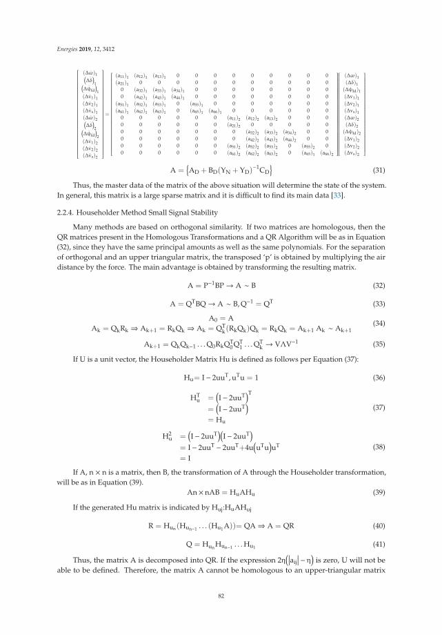
Energies 2019, 12, 3412

⎡⎢⎢⎢⎢⎢⎢⎢⎢⎢⎢⎢⎢⎢⎢⎢⎢⎢⎢⎢⎢⎢⎢⎢⎢⎢⎢⎢⎢⎢⎢⎢⎢⎢⎢⎢⎢⎢⎢⎢⎢⎢⎢⎢⎢⎢⎢⎢⎢⎢⎢⎢⎢⎢⎢⎢⎢⎣

(Δ.ω)1(

Δ.δ)1(

Δ.ψfd

)1

(Δ.v1)1

(Δ.v2)1

(Δ.vs)1

(Δ.ω)2(

Δ.δ)2(

Δ.ψfd

)2

(Δ.v1)2

(Δ.v2)2

(Δ.vs)2

⎤⎥⎥⎥⎥⎥⎥⎥⎥⎥⎥⎥⎥⎥⎥⎥⎥⎥⎥⎥⎥⎥⎥⎥⎥⎥⎥⎥⎥⎥⎥⎥⎥⎥⎥⎥⎥⎥⎥⎥⎥⎥⎥⎥⎥⎥⎥⎥⎥⎥⎥⎥⎥⎥⎥⎥⎥⎦

=

⎡⎢⎢⎢⎢⎢⎢⎢⎢⎢⎢⎢⎢⎢⎢⎢⎢⎢⎢⎢⎢⎢⎢⎢⎢⎢⎢⎢⎢⎢⎢⎢⎢⎢⎢⎢⎢⎢⎢⎢⎢⎢⎢⎢⎢⎢⎢⎢⎢⎢⎢⎢⎢⎣

(a11)1 (a12)1 (a13)1 0 0 0 0 0 0 0 0 0(a21)1 0 0 0 0 0 0 0 0 0 0 0

0 (a32)1 (a33)1 (a34)1 0 0 0 0 0 0 0 00 (a42)1 (a43)1 (a44)1 0 0 0 0 0 0 0 0

(a51)1 (a52)1 (a53)1 0 (a55)1 0 0 0 0 0 0 0(a61)1 (a62)1 (a63)1 0 (a65)1 (a66)1 0 0 0 0 0 0

0 0 0 0 0 0 (a11)2 (a12)2 (a13)2 0 0 00 0 0 0 0 0 (a21)2 0 0 0 0 00 0 0 0 0 0 0 (a32)2 (a33)2 (a34)2 0 00 0 0 0 0 0 0 (a42)2 (a43)2 (a44)2 0 00 0 0 0 0 0 (a51)2 (a52)2 (a53)2 0 (a55)2 00 0 0 0 0 0 (a61)2 (a62)2 (a63)2 0 (a65)1 (a66)2

⎤⎥⎥⎥⎥⎥⎥⎥⎥⎥⎥⎥⎥⎥⎥⎥⎥⎥⎥⎥⎥⎥⎥⎥⎥⎥⎥⎥⎥⎥⎥⎥⎥⎥⎥⎥⎥⎥⎥⎥⎥⎥⎥⎥⎥⎥⎥⎥⎥⎥⎥⎥⎥⎦

⎡⎢⎢⎢⎢⎢⎢⎢⎢⎢⎢⎢⎢⎢⎢⎢⎢⎢⎢⎢⎢⎢⎢⎢⎢⎢⎢⎢⎢⎢⎢⎢⎢⎢⎢⎢⎢⎢⎢⎢⎢⎢⎢⎢⎢⎢⎢⎢⎢⎢⎢⎢⎢⎣

(Δω)1(Δδ)1(Δψfd)1(Δv1)1(Δv2)1(Δvs)1(Δω)2(Δδ)2(Δψfd)2(Δv1)2(Δv2)2(Δvs)2

⎤⎥⎥⎥⎥⎥⎥⎥⎥⎥⎥⎥⎥⎥⎥⎥⎥⎥⎥⎥⎥⎥⎥⎥⎥⎥⎥⎥⎥⎥⎥⎥⎥⎥⎥⎥⎥⎥⎥⎥⎥⎥⎥⎥⎥⎥⎥⎥⎥⎥⎥⎥⎥⎦

A ={AD + BD(YN + YD)

−1CD

}(31)

Thus, the master data of the matrix of the above situation will determine the state of the system.In general, this matrix is a large sparse matrix and it is difficult to find its main data [33].

2.2.4. Householder Method Small Signal Stability

Many methods are based on orthogonal similarity. If two matrices are homologous, then theQR matrices present in the Homologous Transformations and a QR Algorithm will be as in Equation(32), since they have the same principal amounts as well as the same polynomials. For the separationof orthogonal and an upper triangular matrix, the transposed ‘p’ is obtained by multiplying the airdistance by the force. The main advantage is obtained by transforming the resulting matrix.

A = P−1BP → A ∼ B (32)

A = QTBQ → A ∼ B, Q−1 = QT (33)

A0 = AAk = QkRk ⇒ Ak+1 = RkQk ⇒ Ak = QT

k(RkQk)Qk = RkQk = Ak+1 Ak ∼ Ak+1(34)

Ak+1 = QkQk−1 . . .Q0RkQT0 QT

1 . . .QTk → VΛV−1 (35)

If U is a unit vector, the Householder Matrix Hu is defined as follows per Equation (37):

Hu= I− 2uuT, uTu = 1 (36)

HTu =

(I− 2uuT

)T

=(I− 2uuT

)= Hu

(37)

H2u =

(I− 2uuT

)(I− 2uuT

)= I− 2uuT − 2uuT+4u

(uTu

)uT

= I(38)

If A, n × n is a matrix, then B, the transformation of A through the Householder transformation,will be as in Equation (39).

An× nAB = HuAHu (39)

If the generated Hu matrix is indicated by Huj:HuAHuj

R = Hun(Hun−1 . . . (Hu1A))= QA ⇒ A = QR (40)

Q = Hun Hun−1 . . .Hu1 (41)

Thus, the matrix A is decomposed into QR. If the expression 2η(∣∣∣aij

∣∣∣− η)

is zero, U will not beable to be defined. Therefore, the matrix A cannot be homologous to an upper-triangular matrix

82

Energies 2019, 12, 3412

orthogonally by the QR algorithm. In this case, the matrix in discussion can be orthogonally madehomologous to the previous Hessenberg Matrix. As a result, instead of the master data of matrix A,the master data of the Hessenberg Matrix is found. There are two famous assumptions on this topic.

3. Results

Considering a 20 bus bar grid model where current is injected by four generators, the Ad matrixhaving the damping coefficient difference will be a 24 × 24 cross-block matrix, as shown in Figure 5.

Figure 5. 20-bus bar power system.

It is possible to find the master data of the system matrix via the following program. In addition,the system’s response to any change in parameters can be plotted and the output current of allgenerators can be monitored after each failure. In addition, the range of change of parameters can bedetermined upon system stability and the most appropriate mode can be selected shown as Table 1.The objective is to estimate (Δδ)1= 5o, (Δδ)3= 3o, (Δδ)2 = (Δδ)4= 0 and 5◦, 3◦ deviations in the firstand third synchronous generators, respectively. The location of the 24th master data on a complexsurface is shown in Figure 6.

The real part of the master data is completely negative, so the system is stable, and each minorfault returns to a stable state after a short time. The following Figure 7 shows how the conditionvariables of each generator, variation diagrams and other variables are changed by the deviation of therotor angle by 5 degrees in the first generator and by 3 degrees in the third generator.

In general, the total active electrical power supplied by the generators should always be equal tothe active power consumed by the loads, which also includes the losses in the system. A failure in thesystem can disrupt this balance, causing the rotors of the generators to accelerate or decelerate. If onegenerator temporarily runs faster than the other does, the angular position of the rotor will increase inconnection to that of the slower machine shown as Figure 8. Δω Variation diagram of four generatorswhen (Δδ)1= 5o, (Δδ)3= 3o, (Δδ)2 = (Δδ)4= 0.

83

Energies 2019, 12, 3412

Table 1. The data of special matrix values.

No. Real Part Imaginary Part

Landa1 −39.0967416 +0.000000000000000iLanda2 −1.00550148 +6.607284341444071iLanda3 −1.00550148 −6.607284341444071iLanda4 −0.738513482 +0.000000000000000iLanda5 −19.79697098 +12.822376834424755iLanda6 −19.79697098 −12.822376834424755iLanda7 −39.0967416 +0.000000000000000iLanda8 −1.00550148 +6.607284341444071iLanda9 −1.00550148 −6.607284341444071i

Landa10 −0.738513482 +0.000000000000000iLanda11 −19.79697098 +12.822376834424755iLanda12 −19.79697098 −12.822376834424755iLanda13 −39.0967416 +0.000000000000000iLanda14 −1.00550148 +6.607284341444071iLanda15 −1.00550148 −6.607284341444071iLanda16 −0.738513482 +0.000000000000000iLanda17 −19.79697098 +12.822376834424755iLanda18 −19.79697098 −12.822376834424755iLanda19 −39.0967416 +0.000000000000000iLanda20 −1.00550148 +6.607284341444071iLanda21 −1.00550148 −6.607284341444071iLanda22 −0.738513482 +0.000000000000000iLanda23 −19.79697098 +12.822376834424755iLanda24 −19.79697098 −12.822376834424755i

Figure 6. Location of the 24th master data on a complex surface.

84

Energies 2019, 12, 3412

Figure 7. Shows the damping momentum Δω stability diagram of the generators in the power system.

Figure 8. Δv2 Variations diagram of generators in a power system.

As can be seen in Δvs variation diagram of four generators when (Δω)1= 5o, (Δω)3= 3o,(Δω)2 = (Δω)4= 0, the system has remained stable as the real part of the master data is negative.The minimum changes of rotor angle Δδ and speed of some generators Δω did not affect the stabilityof the system and the system regained its stability after these minimum failures.

Evaluation of the Proposed Solution Method

The analysis of linear systems is much simpler than that of nonlinear systems. As can be seen inthis article, the position of the matrix state on the complex surface for the main quantities was foundbecause of the analysis of linear systems. Furthermore, the sign of the real portions of the matrix stateof the main quantities (positive or negative) showed the stability of the system. If these real parts

85

Energies 2019, 12, 3412

are negative, the system is stable and small deviations will not disrupt this stability, but after a shorttime, the system will regain its equilibrium. Any changes in the parameters of the generator andnetwork will affect the elements of the matrix state; therefore, the location of the main quantities on thecomplex surface will vary, because of which the stability of the system will be affected. In this thesis,we attempted to examine how changes in the damping coefficient affect the main quantities of the statematrix, and the diagrams of the changes in the real parts of each main quantity were drawn against thechanges in the [−200,200] range of the damping coefficient (KD). The system is unstable in KDs wherethe real part of at least one main quantity is negative. Therefore, the above diagrams show the effectof the damping coefficient on system stability. In addition, these diagrams can be drawn based onchanges of other parameters and system stability can be examined. As a result, the stability of largesystems in the small signal depends only on finding the main quantities of a very large matrix. In fact,finding the main quantities is possible by finding the roots of a polynomial equation derived from thedeterminant, det(A-λI). In other words, only n-1 steps are necessary for the conversion of the givenmatrix to an upper-triangular matrix. In the first stage, the elements below the element (1,1) are reset;in the second stage, the ones under element (2, 2) are reset; and in the final stage, only the ones underelement (n, n − 1) are reset.

4. Conclusions

This article demonstrates the formation of voltage stability in a system using conventional andsmall signal stability methods used to differentiate voltage stability. According to the literature, thenon-linear system of the Household Method has been found to provide a linearization around theworking point provided that the signal that changes the working point is small. Thus, it has beenproved that easier linear systems can be analyzed instead of analysis of demanding nonlinear systems.However, it is not easy to obtain the Lyapunov Function to study the stability of a fixed point. This isbecause there is no general method for finding this function. The complex ambiance will be comparedto non-linear functions with thousands of variables by using the concepts of coordinate functions.It has been shown that it is almost impossible to examine ultra-large systems with hundreds andthousands of variables without linearizing them. The only practical way of examining large systems issmall signal analysis, since it can be linearized. The stability analysis of these systems is related tofinding the master data of the mode matrix. Whether the real parts of these values are negative orpositive determines whether the system is stable. Although it is highly challenging to find the masterdata of such a large matrix, it can be facilitated by making it linear so that the application capability ofcomputer simulation can be improved.

The methods of finding the master data of large matrices are generally designed on homologoustransformations (especially Householder transformations), because the successive transformations ofthe householder will result in many zeros in the columns of the matrix. The QR decomposition is madewith the matrix obtained through the multiplication of the orthogonal matrix by the upper triangularmatrix. The matrix obtained using the QR algorithm is then multiplied by the upper-triangular matrix(if this matrix does not exist, by the upper Hessenberg Matrix) and made homologous. Homologoustransformations and degrees of the master data are retained so that, since the master data of thetriangular matrix, the elements on the diagonal, the master data of the resulting matrix emerges fromthe triangular matrix. The QR algorithm can also generate the master data matrix (Modal Matrix). Itis also designed to find the zero of functions in some other algorithms. These methods consider aparticular polynomial as a function and try to find the zeros of the function by methods such as theNewton–Raphson Method. Other methods that are better suited than the Newton–Raphson Methodare also used in finding the zero of different functions. Another method to find the master data is touse random algorithms. To achieve this goal, finding zeros is considered as minimizing, and thenusing complementary algorithms, such as genetic algorithms, solutions are provided for these issues.As a result, the most efficient method of finding main data in order to perform small signal stabilityanalysis in large power systems is the Householder Method.

86

Energies 2019, 12, 3412

Author Contributions: Conceptualization, A.S. and M.R.T.; Methodology, A.S.; Software, E.H.; Validation, R.B.,S.P. and A.S; Formal Analysis, M.R.T.; Investigation, A.S.; Resources, A.S.; Data Curation, M.R.T and E.H.;Writing-Original Draft Preparation, M.R.T.; Writing-Review & Editing, M.R.T.; Visualization, R.B.; Supervision,R.B and S.P.

Funding: This research received no external funding.

Conflicts of Interest: The authors declare no conflict of interest

References

1. Pierre, D.A.; Trudnowski, D.J.; Hauer, J.F. Identifying reduced-order models for large nonlinear systems witharbitrary initial conditions and multiple outputs using Prony signal analysis. In Proceedings of the 1990American Control Conference, San Diego, CA, USA, 23–25 May 1990; Volume 1, pp. 149–154.

2. Thompson, S.C.; Ahmed, A.U.; Proakis, J.G.; Zeidler, J.R.; Geile, M.J. Constant Envelope OFDM Abbrev.IEEE MILCOM. Military Commun. Conf. 2008, 56, 1300–1312.

3. Lindell, G.; Sundberg, C.E.W. An Upper Bound under bir error probability of combine convolution codingand continuous phase modulation. IEEE Trans. Inform. Theory 1988, 1, 1263–1269. [CrossRef]

4. Khan, S.; Bletterie, B.; Anta, A.; Gawlik, W. On Small Signal Frequency Stability under Virtual Inertia and theRole of PLLs. Energies 2018, 11, 2372. [CrossRef]

5. Taylor, C.W. Power Systems Voltage Stability; Electric Power Research Institute, McGraw Hill: New York, NY,USA, 1994.

6. Rajaraman, R.; Dobson, I.; Sarlashkar, J.V. Analytical modeling of thyristor-controlled series capacitors forSSR studies. IEEE Trans. Power Syst. 1996, 11, 15–32.

7. Martins, N. Retuning Stabilizers for the North-South Brazilian Interconnection. In Proceedings of the 1999IEEE Power Engineering Society Summer Meeting, Edmonton, AB, Canada, 18–22 July 1999; Volume 1,pp. 58–67.

8. Lui, W. Research on a Small Signal Stability Region Boundary Model of the Interconnected Power Systemwith Large-Scale Wind Power. Energies 2015, 8, 2312–2336. [CrossRef]

9. Xu, Y. Stochastic Small Signal Stability of a Power System with Uncertainties. Energies 2018, 11, 2980.[CrossRef]

10. Parashar, M.; Mo, J. Real Time Dynamics Monitoring System (RTDMSTM): Phasor applications for the controlroom. In Proceedings of the 42nd Annual Hawaii International Conference on System Sciences (HICSS-42),Big Island, HI, USA, 5–8 January 2009; Volume 1, pp. 5–8.

11. Abe, S.; Isono, A. Determination of power system voltage stabilitiy. Electr. Engeland Jpn. 1983, 103, 3–13.12. Hauer, J.F. Application of Prony analysis to the determination of modal content and equivalent models for

measured power system response. IEEE Trans. Power Syst. 1991, 6, 1062–1068. [CrossRef]13. Bourgin, F.; Testud, G.; Heilbronn, B.; Verseille, J. Present Practics and Trends on the French Power System to

Prevent Voltage Collapse. IEEE Trans 1993, 8, 3–13.14. Willems, J.L. Stability Theory of Dynamical Systems; Wiley Interscience Division: London/Nelson, UK, 1970.15. Chi-Tsong, T.C. Linear Systems Theory and Design; Academic Press: New York, NY, USA; London, UK, 1984.16. Che, Y.; Xu, J.; Shi, K.; Liu, H.; Chen, W.; Yu, D. Stability Analysis of Aircraft Power Systems Based on a

Unified Large Signal Model. Energies 2017, 10, 1739. [CrossRef]17. Dher, D.K.; Doolla, S.; Bandyopadhyay, S. Electrical Power and Energy Systems Effect of placement of droop

based generators in distribution network on small signal stability margin and network loss. Int. J. Electr.Power Energy Syst. 2017, 88, 108–118. [CrossRef]

18. Haung, D.; Chen, Q.; Ma, S.; Zhang, Y.; Chen, S. Wide-Area Measurement—Based Model-Free Approach forOnline Power System Transient Stability Assessment. Energies 2018, 11, 958. [CrossRef]

19. Berrou, C.; Glavieux, A.; Thitimajshima, P. Near Shannon-Limit error correcting coding and decoding: Turbocodes. Proc. ICC93 1993, 3, 1064–1070.

20. Bezerra, H.L.; Martins, N. Eigenvalue methods for calculating dominant poles of a transfer function andtheir applications in small-signal stability. Appl. Math. Comput. 2019, 347, 113–121. [CrossRef]

21. Anderson, J.B.; Aulin, T. Digital Phase Modulation; Electronics & Electrical Engineering, Applications ofCommunications Theory; Springer Science & Business Media: New York, NY, USA, 1986.

87

Energies 2019, 12, 3412

22. Khodadad, A.; Divshali, P.H.; Nazari, M.H.; Hosseinian, S.H. Small-signal stability improvement of anislanded micro grid with electronically-interfaced distributed energy resources in the presence of parametricuncertainties. Electr. Power Syst. Res. 2018, 160, 151–162. [CrossRef]

23. Bourgin, F.; Testud, G.; Heilbronn, B.; Verseille, J. Present practices and trends on the French power system toprevent voltage collapse. IEEE Trans. PWRS 1993, 8, 3–13. [CrossRef]

24. Hill, D.J. Nonlinear dynamic load models with recovery for voltage studies. IEEE Trans. PWRS 1993, 8, 1.[CrossRef]

25. IEEE Special Stability Control Working Group. Static VAR Compensator Models for Power Flow andDaynamic Performance Simulation. IEEE Trans. PWRS 1994, 9, 1.

26. Robak, S.; Gryszpanowicz, K. Rotor angle small signal stability assessment in transmission network expansionplanning. Electr. Power Syst. Res. 2015, 128, 144–150. [CrossRef]

27. IEEE Task Force. Proposed Terms and Defin. for Power System Stability. IEEE Trans. 1982, 7, 1894–1898.28. Lu, X.; Xiang, W.; Lin, W.; Wen, J. Small-signal modeling of MMC based DC grid and analysis of the impact

of DC reactors on the small-signal stability. Electr. Power Energy Syst. 2018, 101, 25–37. [CrossRef]29. Xie, R.; Kamwa, D.; Rimorov, D.; Moeini, A. Fundamental study of common mode small-signal frequency

oscillations in power systems. Electr. Power Energy Syst. 2019, 106, 201–209. [CrossRef]30. Weiyu, W. Virtual Synchronous Generator Strategy for VSC-MTDC and the Probabilistic Small Signal

Analysis. IFAC-Pap. Line 2017, 50, 5424–5429. [CrossRef]31. Sadhana, G.S. Small Signal Stability Analysis of Grid Connected Renewable Energy Resources with the Effect

of Uncertain Wind Power Penetration. Energy Procedia 2017, 117, 769–776. [CrossRef]32. Guo, C.; Zheng, A.; Yin, Z.; Zhao, C. Small-signal stability of hybrid multi-terminal HVDC system. Electr.

Power Energy Syst. 2019, 109, 434–443. [CrossRef]33. Yang, W.; Norrlund, P.; Chung, C.Y.; Yang, J.; Ludin, U. Eigen-analysis of hydraulic-mechanical-electrical

coupling mechanism for small signal stability of hydropower plant. Renew. Energy 2018, 115, 1014–1025.[CrossRef]


88

energies

Article

Investigations on EMI Mitigation Techniques:Intent to Reduce Grid-Tied PV Inverter CommonMode Current and Voltage

Umashankar Subramaniam 1,*, Sagar Mahajan Bhaskar 1, Dhafer J.Almakhles 1,

Sanjeevikumar Padmanaban 2 and Zbigniew Leonowicz 3

1 Renewable Energy Lab, Department of Communications and Networks, College of Engineering,Prince Sultan University (PSU), Riyadh 66833, Saudi Arabia

2 Department of Energy Technology, Aalborg University, 6700 Esbjerg, Denmark3 Faculty of Electrical Engineering, Wroclaw University of Science and Technology, Wyb. Wyspianskiego 27,

50370 Wroclaw, Poland* Correspondence: [email protected] or [email protected]; Tel.: +966-11-494-8059

Received: 1 August 2019; Accepted: 29 August 2019; Published: 3 September 2019

Abstract: Power inverters produce common mode voltage (CMV) and common mode current (CMC)which cause high-frequency electromagnetic interference (EMI) noise, leakage currents in electricaldrives application and grid-connected systems, which consequently drops the efficiency of the systemconsiderably. This CMV can be mitigated by designing suitable EMI filters and/or investigating theeffects of different modulation strategies. In this paper, the effect of various modulation techniquesover CMV and CMC are investigated for two-level and three-level inverters. It is observed thatthe modified third harmonic injection method reduced the CMV and CMC in the system by 60%.This modified pulse width modulation (PWM) technique is employed along with EMI chokes whichresults in reduced distortion of the system.

Keywords: common mode current; common mode voltage; modulation techniques; electromagneticinterference; mitigation; grid connected inverters

1. Introduction

The PV-grid connected power inverter is a necessary part of the PV to electrical energy conversionsystem [1]. The quality of the voltage depends upon three phenomenons of voltage harmonics, voltagedips or swells and flicker [2]. In the present day, the intense use of electrical loads driven by powerelectronics (e.g., personal computers) has led to a severe increase of current harmonics drawn from thedistribution system. These current harmonics, due to the impedance of the network, induce voltageharmonics into the utility. Voltage dips originate from fault currents in the electrical system or inrushcurrents of electrical motors and transformers [3]. The common mode circuit is formed in betweenPhoto Voltaiacs (PVs) and the grid, as well as ground due to parasitic capacitance and deficienciesin galvanic isolation between the grid and PVs [1,4]. Electromagnetic interference (EMI) is the mainsource of unexpected transition at the output port of variable frequency drive (VFD). The fall time andrise time of semiconductor devices (employed in the converter section of VFD) are used to determinevoltage transition times. These voltage transition times are around 100ns which is very fast. As a result,high dv/dt occurs. In the stray line to ground cables and capacitor, the magnitude of common modenoise current is higher if dv/dt is higher [4]. These noise currents affect the control signals and are themain source of EMI.

The instability and disturbances occur at the supply side due to the utilization of a highernumber of power devices and components for energy conversion [5]. Mainly, non-linear devices are


Energies 2019, 12, 3395

responsible for this instability and disturbances. Due to this, harmonics are introduced in the powersystem. These harmonics causes EMI-related problems, overheating in the equipment, and damage thedevices, etc. Inverter common mode voltage (CMV) and its leakage current are the primary concernsof radiated EMI. Noise with high-frequency components is emitted in the form of electromagneticenergy and may interfere with other components and equipment at the common coupling point [6].To minimize common currents, commonly used methods are [1] improved power inverter structureswith common mode current (CMC) suppression capabilities and advanced pulse width modulation(PWM) schemes [7], and (2) the addition of EMI filters [8] and bridge inverter topology basedon DC and AC bypass [9]. It is also notable that the circuitry with fast switching semiconductorsproduces a very high amount di/dt and dv/dt and which is one of the reasons for the cause of EMI [10].Decoupling effect-based configurations with constant CMV [11] and transformerless power converterconfigurations [12] are proposed to suppress CMC. The CM loop impedance can be increased inorder to suppress current in CM loop effectively. In [13], the mid-point of DC and AC side voltagenodes are connected to the proposed new CM internal loop scheme in order to suppress CMC. In [14],a novel modulation scheme is presented to control inverter power switches in order to reduce CMC.In [15], a CM internal loop is formed by employing the RC branch in between the negative bus of DCand output terminals. However, detailed analysis of the CMC and its effect on CMC high-frequencycomponents are not presented. In [16], a new scheme based on a dual CM internal loop for a PVgrid-connected transformer-less system is proposed to suppress CMC high-frequency components.In [17] characteristics and analysis of the CMV based on the simplified modelling of a cascadedH-bridge power transformer and PWM strategy are presented under the fault grid condition andbalanced condition. In [18], in order to reduce CM leakage current, a new hybrid modulation strategyis suggested. The suggested method is efficient and has reactive power provision with low distortionin the current. Filters at the input/output terminal are employed to suppress this unwanted emissionor electromagnetic interference (EMI) [19,20]. Generally, filters are employed at the connector ofpower supply in order to restrict disturbance signals [21,22]. Generally, classical filters are designedby utilizing passive components, i.e., inductor and capacitor values to attenuate high-frequencyvoltage and current components [23,24]. However, the performance of the filter is dependent onthe value of L and C and has limited achievable insertion loss that should be improved to meet thenecessary condition. Moreover, passive filters are bulky, costly, and their volume mainly depends onthe inductor size which is approximately directly proportional to the required attenuation. Moreover,there is always uncertainty in parasitic components. In order to reduce CMV and current effect,active [25] and passive filters [26] are suggested. However, these filters increase the size, cost ofthe system, and control of the equipment. As a result, it is good to advance control strategies inorder to reduce the CMV’s effect. In order to eliminate or reduce CMV, numerous control schemesare proposed based on the modulation strategy, such as the Sine PWM for three-level neutral pointclamped (NPC) inverter [27], PWM based on non-nearest vectors, Space Vector PWM for high-levelinverters [28,29], etc. In [30], a detailed comparison of SPWM and SVPWM techniques are presentedfor the three-phase inverter. Nevertheless, similar PWM schemes presented in [31,32] are restricted to3–5 levels inverters. Synchronous reference frame and feedforward reference frame-based dynamicvoltage restorer comparative study are presented in [33]. In [34], a new SVPWM scheme is presentedwith advanced features, such as the proposed scheme, which is suitable for inverters with any numberof levels, zero CMVs can be achieved at any modulation index, the simple realization of CMV vectors,fast control scheme, etc. In [35], a new methodology called the spread spectrum (SS) technique ispresented in order to reduce EMI of power converters over a wide range of frequency. However,this SS technique is competent to reduce EMI levels around 5–10 dB [36]. Based on the output voltagewaveform and its alignment, another technique is suggested in [37,38]. However, this methodologyhas a specific application. In [39], a new technique based on software is presented to reduce EMI.The methodology is suitable for single- and three-phase power inverters. In [40], analysis on the CMEMI and methodology to mitigate EMI in power inverters is discussed by using a delay compensation

90

Energies 2019, 12, 3395

technique. In order to mitigate EMI, numerous passive filter methods are proposed based on thephases of the noise signal. In [41], a common mode-coupled inductor is designed in order to mitigatecommon mode noise. Nevertheless, differential mode noise is not able to be reduced by using thistechnique. Hence, later, a new method based on an integrated choke is presented in order to reducedifferential, as well as common mode, noise at the same time [42].

In [43], a new method based on the parasitic component’s determination is presented in order topredict EMI noise. In [44,45], computer-based three-dimensional modelling is presented for the noisecurrent prediction by determining the value of parasitic components. A novel EMI filter is discussedwith sufficient attenuation with a limited LC value in order to CM EMI [46]. Nevertheless, filters areadditional components and increase the volume and cost of the system. Moreover, the implementationof the effective filter is important and the effort for the mitigation of EMI without knowing thesystem may degrade the performance and require additional cost. To reduce CM voltage, a newimpedance balancing method is presented instead of impedance mismatching [47]. The three-phasephase-lock-loop for a distorted utility is discussed in [48]. In [49], controllable devices are used andactive filters are presented to suppress CMC generated by the CMV method, called the active noisecancellation scheme, in order to mitigate the noise signal [50]. In [51], a new wavelet transform-basedtechnique to mitigate EMI noise in power converter is presented with a frequency band of 3–30 MHz.

In this paper, EMI mitigation techniques are investigated with the aim to reduce CMV and CMC ina PV-grid tied power inverter. The effect of modulation techniques over CMV and CMC are investigatedfor two-level and three-level inverters to observe the mitigation of EMI. The modified third harmonicinjection method reduced the CMV and CMC by 60% in the system. In order to reduce distortion andto improve the overall efficiency of the system, the modified PWM technique is employed along withEMI chokes.

The article is organized in the seven sections, discussing explicitly the important aspects forinvestigations and design of EMI filters for the mitigation of CMC and CMV in grid-tied invertersystem. In Section 2, the modulation techniques for high power two-level and three-level inverters,are discussed in brief. Section 3 explains the concept of CMV of the inverters and design of filters orEMI chokes. Section 3 also deals with the comparative study of space vector-based and sine-basedpulse width modulation (SVPWM and SPWM) techniques. A modified PWM strategy is discussed inSection 4. The results obtained through simulation and experimental works are presented in Section 5.Finally, the conclusion is given in Section 6.

2. Modulation Techniques for High-Power Inverters

Space vector-based and sine wave-based PWM techniques are the common techniques usedto generate pulses for the switches of the inverter [29,30]. In the SPWM technique, high-frequencytriangular carrier waves (typically several kHz) are compared with the modulating signal (50 Hz or60 Hz) to generate pulses for a three-phase inverter. In the SVPWM technique, instead of modulatingsignals, a rotating vector reference is used to generate pulses of the inverter [29,30]. The prime objectiveof this control and pulse generation scheme is to generate a sinusoidal AC output whose magnitude islimited. The PWM switching scheme not only helps to achieve reduced Total Harmonic Distortion(THD), better harmonic spectrum, and maximum utilization of DC bus but also provides a solution toreduce EMI, switching loss. Figure 1 depicts the power circuitry of three-phase two-level inverter andneutral point clamped (NPC) three-level inverters [21] and its PWM strategies shown in Figures 2–5.

91

Energies 2019, 12, 3395

(a) (b)

Figure 1. Power circuitries of (a) three-phase two-level inverter, and (b) neutral point clamped (NPC)three-level inverter.

(a)

(b)

Figure 2. Reference generation through Min–Max modulation strategy (a) associate waveform,and (b) mathematical model.

The Min–Max modulation strategy is supposed to be equivalent to the space vector modulationstrategy. Thus, using this approach, the modulation index can be extended up to 1.15. Figure 2a,bexplains the associated waveforms and mathematical model of the reference waveform generationtechnique through Min–Max modulation strategy, respectively [48]:

o f f set in (V) = −[

max(VA, VB, VC) + min(VA, VB, VC)

2

](1)

92

Energies 2019, 12, 3395

where: ⎧⎪⎪⎪⎪⎨⎪⎪⎪⎪⎩VA = Vm cos(ωt)VB = Vm cos

(ωt− 2π

3

)VC = Vm cos

(ωt + 2π

3

) (2)

Vre f = VA + VB + VC + o f f set (3)

The reference modulating signals are mathematically defined as follows:

⎧⎪⎪⎪⎪⎨⎪⎪⎪⎪⎩VAm = Vm cos(ωt) + o f f setVBm = Vm cos

(ωt− 2π

3

)+ o f f set

VCm = Vm cos(ωt + 2π

3

)+ o f f set

(4)

(a) (b)

Figure 3. Modulating signal of third harmonic injection control technique (a) modulating signal,and (b) mathematical model.

In the third harmonic injection method [52,53], the third harmonic is injected in a modulationscheme to improve the gain of the pulse width modulator in the inverter. Figure 3a,b shows the thirdharmonic injection modulating signal control reference waveform and mathematical model, respectively.

The reference modulating signals are mathematically defined as follows:

⎧⎪⎪⎪⎪⎨⎪⎪⎪⎪⎩VAm = Vm cos(ωt) + Vm3 cos(3ωt)VBm = Vm cos

(ωt− 2π

3

)+ Vm3 cos(3ωt)

VCm = Vm cos(ωt + 2π

3

)+ Vm3 cos(3ωt)

(5)

In this technique, approximately 17% of third harmonics components are added in the referencewaveform of classical SPWM [29,30,34]. The reference waveform of the method third harmonicsinjection can be also expressed as follows:

f (ωt) = (1.15Ma × sin(ωt) + 0.19Ma × sin(ωt)), 0 ≤ ωt ≤ 2π (6)

where Ma is the modulation index ratio.

3. Common Mode Voltage

The inverter common mode voltage is calculated by averaging the output voltage (VA, VB, and VC)of each leg as follows [38]:

VCM =VA + VB + VC

3(7)

For the three-phase two-level inverter, the achievable phase output voltage levels could be –VDC/2or +VDC/2 where VDC is input voltage. If the voltage at the DC link is zero then only the commonmode voltage is zero. For the three-level inverter, the achievable phase output voltage levels could be

93

Energies 2019, 12, 3395

positive, negative, and neutral point voltage. Tables 1 and 2 tabulated the output vectors and possiblecommon mode voltages for two-level and three-level inverters, respectively.

Table 1. Output vectors and common-mode voltages for two-level inverter.

Output Vector (VA, VB, VC) CMV (VCM)

(+ + +) (1/2) × VDC(+ + −), (+ − +), (− + +) (1/6) × VDC(+ − −), (− + −), (− − +) –(1/6) × VDC(− − −) –(1/2) × VDC(+ + +) (1/2) × VDC(+ + −), (+ − +), (− + +) (1/6) × VDC

Table 2. Output vectors and common-mode voltages for three-level NPC inverter.

Output Vector (VA, VB, VC) CMV (VCM)

(+ + +) (1/2) × VDC(+ + 0), (+ 0 +),(0 + +) (1/3) × VDC(+ + −), (+ − +), (− + +), (+ 0 0), (0 + 0), (0 0 +) (1/6) × VDC(+ - 0), (+ 0 −), (− + 0), (0 + −), (− + 0), (0 − +), (0 0 0) 0(+ − −), (− + −), (− − +), (− 0 0), (0 − 0), (0 0 −) –(1/6) × VDC(− − 0), (− 0 −), (0 − −) –(1/3) × VDC(− − −) –(1/2) × VDC

3.1. Filtering of Common Mode Voltage

The appropriate designed filter circuitry is needed to reduce the common mode voltage.The complete three-phase to grid (AC–DC–AC) system with the connection of a passive filter isshown in Figure 4. The DC link with voltage VD is created between the AC–DC and DC–AC converterand passive filters are added at the input and output side. The filter consists of damping resistance,Y-connected capacitor and common mode chokes. In the given system, a damping resistor RCM2is connected between grid and neutral point capacitor. Additionally, two chokes, LCM1 and LCM2,and three Y-connected capacitors, CCM2, are connected for filter purposes [12–14]. RCM1 and CCM1 areconnected between the grid and negative terminal of the DC link. The range of the resonant frequencyfor the common mode circuitry is about 1.5 kHz [7] and is calculated as follows:

fo = 1/(2π

√LCM ×CCM

)(8)

where LCM and CCM are the equivalent inductance and capacitance values. The practical limitation ofthe real-time application needs to be considered while designing the capacitors. The capacitor sizeshould be small for the designed frequency in order to reduce the bulkiness of the hardware unit.

94

Energies 2019, 12, 3395

Figure 4. Complete three-phase to grid (AC–DC–AC) system with the connection of a passive filter.

3.2. Comparison of SPWM and Space Vector PWM Techniques for a Two-Level Inverter at a HigherSwitching Frequency

The simple open-loop analysis is carried out for a two-level inverter for current and voltagedistortions both with and without a filter. For the analysis, the modulation index is maintained at0.8 and taken over a range of frequencies between 1 kHz and 150 kHz and the obtained results aretabulated in Table 3. After comparing SPWM and SVPWM results, it is known that SVPWM providessuperior results for two-level inverter system. For reduction in CMV, the SVPWM technique providesthe best results; however, due to tedious calculations, the requirement of high-end processors andcomplex hardware implementation, space vector modulation can be replaced with the carrier-basedmodulation strategy which will give the same results as that of the space vector modulation technique.If the reduction in the CMC can be achieved by using such a modulation strategy, the size of thecommon mode choke can be reduced.

Table 3. THD comparison of SPWM and SVPWMM techniques.

SwitchingTechnique

SwitchingFrequency

Without Filter (THD%) With Filter (THD%)

Line Current (A) Line Voltage (V) Line Current (A) Line Voltage (V)

SPWM

1 kHz 64.81 138.2 2.53 6.8810 kHz 24.9 88.46 1.04 4.1650 kHz 24.27 67.92 1.03 4.12100 kHz 24.27 67.92 1.03 4.12120 kHz 31.39 106.82 3.86 5.63150 kHz 43.95 301.92 7.42 7.89

SVPWM

1 kHz 4.82 52.84 0.14 0.6610 kHz 3.15 43.89 0.11 0.4250 kHz 3.15 43.89 0.11 0.43100 kHz 8.74 31.84 0.36 1.47150 kHz 5.75 56.33 0.45 1.03

4. Modified PWM Schemes

Among discussed PWM schemes, SVPWM provides quality results [30]. Nevertheless, due tosome inherent disadvantages, the space vector modulation strategy is ruled out from the agenda. Thus.the next challenge was to obtain similar results, which were given by the space vector modulation,in carrier-based modulation as well. The modified carrier phase shift scheme is developed based onthe concept of phase disposition PWM scheme. It is given that the input voltage is balanced and thepossible two conditions are:

• One input phase voltage is negative and two input phase voltage is positive.• One input phase voltage is positive and two input phase voltage is positive.

95

Energies 2019, 12, 3395

VA + VB + VC = 1 (9)

It is considered that 0 < VA, 0 > VB, and 0 > VC and CMV are caused with the peak value to reacha higher voltage level than 1/6 × VDC. The carrier signals and output voltage reference relation for theswitching 0–1–1 is as follows:

(a) (b)

Figure 5. Waveform associated with PWM strategies (a) PDPWM method, max amplitude of theaddition of the carrier waves is 2, (b) modified PWM method, max. amplitude of the addition of thecarrier waves is around 1.5.

As phase disposition PWM (PDPWM) is used, at any point of time:

f or the state ‘0− 1− 1′{

VCarrierA −VCarrierB = 13×VCarrierA − 2 > 0

(10)

Hence, to avoid this state,3×VCarrierA − 2 < 0, this condition is to be satisfied. This is done by usingthree carrier waves, which are 120◦ apart from each other. Figure 5 shows the waveform associatedwith PWM strategies. Figure 5a depicts the associated waveform of the PDPWM method where themax amplitude of the addition of the carrier waves is 2 (see amplitude in (3) in Figure 5a). Figure 5bdepicts the associated waveform of the modified PWM method where the max amplitude of theaddition of the carrier waves is around 1.5 (see amplitude in (4) in Figure 5b).

5. Simulation and Experimental Results

The simulation results are presented for the complete AC–DC–AC system. The circuit-level modelwas developed using the Simulink platform. The closed-loop analysis of both two-level and three-levelinverters is carried out. The specifications of the system parameters are given in Appendix A.

5.1. Closed-Loop Analysis of the Two-Level Inverter

The model of the system is done in various stages. Figure 6 shows the complete closed-loopAC–DC–AC system Simulink model with the two-level inverter. The first section includes the dioderectifier model to obtain a constant DC voltage. Then the DC link capacitor was designed so as toprovide a constant DC input voltage to the three-phase two-level inverter circuit which is modelledusing Insulated Gate Bipolar Transistor (IGBTs) and SVPWM techniques were implemented for firingthe inverter circuit.

The analysis of CMV and CMC for the given system is done without filter implementation and theachieved results are depicted in Figure 7a–d. The Fast Fourier Transform(FFT) analysis of the CMV andCMC waveform (150 kHz component) are done without filter, and it is observed that THD of the CMV

96

Energies 2019, 12, 3395

and CMC is 38.01% and 3152.31%, respectively. The analysis of the common mode voltage and currentfor the given system are done with a filter implementation and the achieved results are depicted inFigure 7e–h. The FFT analysis of the CMV and CMC waveform (150 kHz component) are done witha filter and it is observed that the THD of the CMV and CMC is 73.39% and 2213.58%, respectively.

Figure 6. Complete closed-loop AC–DC–AC system Simulink model with the two-level inverter.

(a) (b)

(c) (d)

Figure 7. Cont.

97

Energies 2019, 12, 3395

(e) (f)

(g) (h)

Figure 7. Simulation results: (a) CMV without filter; (b) CMC without filter; (c) without filter, commonmode voltage FFT analysis; (d) without filter, common mode current FFT analysis; (e) CMV with filter;(f) CMC with filter; (g) with filter, common mode voltage FFT analysis; (h) with filter, common modecurrent FFT analysis.

From the investigation, the objective of reducing the CMC and CMV of the two-level inverter isachieved. From the analysis made, it can be concluded that when the two-level inverter is operatingat a frequency above 10 kHz, the EMI increases drastically. Additionally, the CMV and CMC of thesystem cannot be reduced effectively by changing the reference, instead the size of the EMI filters haveto be larger. Therefore, we need to consider the three-level inverter analysis.

5.2. Closed-Loop Analysis of the Three-Level Inverter

Based on the earlier explanation, the Simulink model of the three-level NPC system is designed inMATLAB. Figure 8 shows the Simulink model of the designed three-level NPC system.

5.2.1. Existing PWM Method

Using Min–Max and the third harmonic injection method, the common mode current and voltageare investigated for the three-level NPC inverter. Figure 9a–d depicts the waveforms of CMC usingexisting Min–Max method, CMV using existing Min–Max method, CMC using the existing thirdharmonic injection methods, and CMV using the existing third harmonic injection method, respectively.

98

Energies 2019, 12, 3395

Figure 8. Matlab/Simulation model of the three-phase three-level NPC inverter.

(a) (b)

(c) (d)

Figure 9. Simulation results: (a) CMC using existing Min–Max method; (b) CMV using existingMin–Max method; (c) CMC using the existing third-harmonic injection method; (d) CMV using theexisting third-harmonic injection method.

The fast Fourier transform (FFT) is conducted for Min–Max and third harmonic injection PWMtechniques and it is observed that common mode voltage THD is 14.74% for Min–Max strategy and11.60% for the third harmonic injection method. In the existing PWM method, the magnitude of thecommon mode current (rms value) is 1.191 A using the Min–Max and 1.199 A in the case of the thirdharmonic injection method. This can be reduced further by using Modified PWM Technique.

99

Energies 2019, 12, 3395

5.2.2. Modified PWM Method

The simulation results for the modified Min–Max method and third harmonic injection methodsas applied in the three-level NPC inverter. Figure 10a–d obtained waveform of CMC using modifiedMin–Max method, waveform CMV using modified Min–Max method, waveform of CMC usingmodified third harmonic injection methods, and waveform of CMV using modified third harmonicinjection methods, respectively. Figure 10e,f show the FFT analysis of CMV and CMC with filter,respectively. It is observed that the THD of the CMV and CMC are 12.95% and 5.91%, respectively.Before modifying the PWM scheme, the common mode voltage and current of the inverter areexperimentally investigated and shown in Figure 11a. Without modification, the RMS values of thecommon mode current and common mode voltage are 1.95 A and 4.73 V, respectively.

(a) (b)

(c) (d)

(e) (f)

Figure 10. Simulation results: (a) CMC using the modified Min–Max method; (b) CMV using themodified Min–Max method; (c) CMC using the modified third-harmonic injection method; (d) CMVusing the modified third-harmonic injection method; (e) with filter, common mode voltage FFT analysis;(f) with filter, common mode current FFT analysis.

100

Energies 2019, 12, 3395

(a)

(b)

Figure 11. Experimental results: common mode current and common mode voltage, (a) beforemodifying the PWM strategy, and (b) after modifying the PWM strategy.

After modifying the PWM scheme, the common mode voltage and current of the inverter areexperimentally investigated and shown in Figure 11b. After modification, the RMS values of thecommon mode current and common mode voltage are 452.6 mA and 5.16 V, respectively. In Table 4,the observed results are tabulated and it is clear that, after modifying the PWM method, the commonmode current is reduced significantly with a small increment in the common mode voltage.

101

Energies 2019, 12, 3395

Table 4. Experimental results.

Experimental Test CMV (V) CMC (A)

Before applying modified PWM 4.73 V 1.95 AAfter applying Modified PWM 5.16 V 452.6 mA

In Table 5, a comparison of PWM strategies for reduction in CMC, CMV, and voltage THD of thethree-level inverter is tabulated based on the obtained results. The simulated results show that whenthe modified PWM method is implemented there is a considerable reduction in CMC. The voltage THDof the system is also observed to be reduced considerably. This satisfies the objective of optimizing thePWM technique to reduce the CMV and current in grid-tied inverters. From the above comparison, it isclear that the modified third harmonic injection approach shows a significant amount of reduction in theCMV and CMC. EMI mitigation techniques are investigated with the aim to reduce the CM voltage andcurrent in PV grid-tied power inverters. The common mode undesirable effects for grid-tied invertersystems has been discussed and compared for different PWM schemes. Two small passive filters areconnected between the rectifier input and grid neutral point, and in between the grid and output portof the inverter and tested for a three-phase two-level inverter using a passive cancellation method.

Table 5. Comparison of PWM strategies for reduction in the CMC, CMV, and voltage THD of thethree-level inverter.

Modulation Technique CMV (V) CMC (A) Voltage THD (%)

Existing PWM Strategy

Min–Max 34.7 1.863 14.27Third Harmonic Injection 34.7 1.863 11.5

Modified PWM Strategy

Modified Min–Max 43.31 0.74 12.95Modified Third Harmonic Injection 34.84 0.74 5.77

6. Conclusions

In order to reduce distortion in the system, the modified PWM technique is employed along withEMI chokes. Various PWM strategies are analyzed to reduce the CMV and CMC, and a modifiedPWM approach is presented for a three-phase three-level inverter. The modified third harmonicinjection method reduced the CMC by 60% in the system with a tradeoff to CMV. Simulation andexperimental results are provided which show good agreement with each other and validate that thecontrol strategies with different PWM techniques are valuable, optimize the output parameters, and areeffective in preventing common mode undesirable effects along with and without filters. Hence, it iseconomic to use modified techniques so that the filter size can be reduced and the final product will belightweight with a reduced cost compared with conventional strategies and existing PWM techniques.

Author Contributions: All authors were involved in developing the concept to make the article an error-freetechnical outcome for the set investigation work


Acknowledgments: The authors would like to express their sincere gratitude to the Renewable Energy Lab,College of Engineering, Prince Sultan University, Riyadh, Saudi Arabia for giving the opportunity to execute theproject in this area.


102

Energies 2019, 12, 3395

Nomenclature

CM Common modeCMC Common mode currentCMV Common mode voltageDC Direct currentAC Alternating currentEMI Electromagnetic interferencePWM Pulse width modulationPV PhotovoltaicVFD Variable frequency drivedv/dt Change in voltagedi/dt Change in currentLC Product of inductance and capacitanceSPWM Sinewave pulse width modulationNPC Neutral point clampedSVPWM Space vector pulse width modulationPDPWM Phase disposition PWMSS Spread spectrumVA, VB, VC AC voltage of each legVRef Voltage of reference modulating signalVAm, VBm, VCm Voltage of reference modulating signal for each legVm Peak value of output voltageVm3 Peak value of third harmonic of output voltagef(wt) Function of reference waveform of the method third harmonics injectionVdc DC input voltageRCM1, RCM2 Damping resistorLCM1, LCM2 ChokesCCM1, CCM2 CapacitorLCM, CCM Common mode equivalent inductance and capacitorfo Common mode resonant frequency

Appendix A

Table A1. Specifications of the system parameters.

Name of the Component Rating

DC link voltage 560 VDC link capacitor 2200 μFFilter inductance 450 mHFilter capacitance 11.6 μF

Rated phase voltage 230 VFrequency 50 Hz

Grid Parameters

Grid voltage and frequency 230 V, 50 HzCarrier frequency 20 kHz

References

1. Kerekes, T.; Teodorescu, R.; Liserre, M. Common mode voltage in case of transformerless PV invertersconnected to the grid. In Proceedings of the IEEE International Symposium on Industrial Electronics,Cambridge, UK, 30 June–2 July 2008; pp. 2390–2395.

2. Esmaeli, A.; Tavassoli, F. A novel passive filter to reduce PWM inverters adverse effects in electrical machinesystem. World App. Sci. J. 2011, 13, 2536–2544.

103

Energies 2019, 12, 3395

3. Elnady, A.; Salama, M.M.A. Unified approach for mitigating voltage sag and voltage flicker using theDSTATCOM. In Proceedings of the IEEE Power Engineering. Society General Meeting, Denver, CO, USA,6–10 June 2004; p. 645.

4. Yao, Z.; Xiao, L. Control of single-phase grid-connected inverters with nonlinear loads. IEEE Trans. Ind. Electron.2011, 60, 1384–1389. [CrossRef]

5. Prasad, K.N.V.; Kumar, G.R.; Kumar, Y.S.A.; Narayana, G.S. In Proceedings of the IEEE InternationalConference on Computer Communication and Informatics, Coimbatore, India, 4–6 January 2013; pp. 1–6.

6. Khan, S.A.; Guo, Y.; Zhu, J. A high efficiency transformerless PV grid-connected inverter with leakage currentsuppression. In Proceedings of the 9th International Conference on Electrical and Computer Engineering,Dhaka, Bangladesh, 20–22 December 2016; pp. 190–193.

7. Grishanov, E.V.; Brovanov, S.V. Aspects of common-mode leakage current suppression in single-phasePV-generation systems. In Proceedings of the 18th International Conference of Young Specialists onMicro/Nanotechnologies and Electron Devices, Erlagol, Russia, 29 June–3 July 2017; pp. 541–546.

8. Zhu, H.; Liu, D.; Chen, H.; Chen, G. An improved foster model of common-mode inductor and its applicationin EMI filter design. In Proceedings of the IEEE International Symposium on Electromagnetic Compatibilityand Asia-Pacific Symposium on Electromagnetic Compatibility, Singapore, 14–18 May 2018; 461–465.

9. Zhang, L.; Sun, K.; Xing, Y.; Xing, M. H6 transformerless full-bridge PV grid-tied inverters. IEEE Trans.Power Electron. 2013, 29, 1229–1238. [CrossRef]

10. Aggeler, D.; Canales, F.; Biela, J.; Kolar, J.W. Dv/Dt-control methods for the SiC JFET/Si MOSFET cascode.IEEE Trans. Power Electron. 2013, 28, 4074–4082. [CrossRef]

11. Kakosimos, P.; Sarigiannidis, A.; Beniakar, M.; Kladas, A. Investigation of transformerless topologies forrenewable energy applications eliminating leakage currents. In Proceedings of the MedPower 2014, Athens,Greece, 2–5 November 2014; pp. 1–5.

12. Araujo, S.V.; Zacharias, P.; Mallwitz, R. Highly efficient single-phase transformerless inverters forgrid-connected photovoltaic systems. IEEE Trans. Ind. Electron. 2010, 57, 3118–3128. [CrossRef]

13. Figueredo, R.S.; Carvalho, K.C.M.; Ama, N.R.N.; Matakas, L. Leakage current minimization techniques forsingle-phase transformerless grid-connected PV inverters–An overview. In Proceedings of the BrazilianPower Electronics Conference, Gramado, Brazil, 27–31 October 2013; pp. 517–524.

14. Zografos, D.; Koutroulis, E.; Yang, Y.; Blaabjerg, F. Minimization of leakage ground current in transformerlesssingle-phase full-bridge photovoltaic inverters. In Proceedings of the 17th European Conference on PowerElectronics and Applications, Geneva, Switzerland, 8–10 September 2015; pp. 1–10.

15. Yang, B.; Li, W.; Gu, Y.; Cui, W.; He, X. Improved transformerless inverter with common-mode leakagecurrent elimination for a photovoltaic grid-connected power system. IEEE Trans. Power Electron. 2012,27, 752–762. [CrossRef]

16. Liu, D.; Zhu, H.; Zhao, R. Novel common-mode current suppression method in transformerless PVgrid-connected system. Appl. Sci. 2018, 8, 2072. [CrossRef]

17. Yang, Y.; Mao, C.; Wang, D.; Tian, J.; Yang, M. Modeling and analysis of the common mode voltage ina cascaded H-bridge electronic power transformer. Energies 2017, 10, 1357. [CrossRef]

18. Yang, T.; Hao, X.; He, R.; Wei, Z.; Huang, T.; Zhang, Y. Hybrid modulation strategy to eliminate currentdistortion for PV GRID-tied H6 inverter. Appl. Sci. 2018, 8, 2578. [CrossRef]

19. Swain, S.D.; Ray, P.K.; Mohanty, K.B. Improvement of power quality using a robust hybrid series activepower filter. IEEE Trans. Power Electron. 2017, 32, 3490–3498. [CrossRef]

20. Hashempour, M.M.; Savaghebi, M.; Vasquez, J.C.; Guerrero, J.M. A control architecture to coordinatedistributed generators and active power filters coexisting in a microgrid. IEEE Trans. Smart Grid 2016,7, 2325–2336. [CrossRef]

21. Singh, B.; Jain, C.; Goel, S.; Gogia, R.; Subramaniam, U. A sustainable solar photovoltaic energy systeminterfaced with grid-tied voltage source converter for power quality improvement. Electr. Power Compon. Syst.2016, 45, 171–183. [CrossRef]

22. Wong, M.C.; Dai, N.Y.; Lam, C.S. Parallel Power Electronics Filters in Three-Phase Four-Wire Systems: Principle,Control and Design; Springer: Berlin, Germany, 2016; pp. 59–165.

23. Sarajian, S. Design and control of grid interfaced voltage source inverter with output LCL Filter. Int. J.Electron. Commun. Electr. Eng. 2014, 4, 26–40.

104

Energies 2019, 12, 3395

24. Nazeri, A.A. Comparison of different filter types for grid connected inverter. In Proceedings of the 29thPIERS Proceedings, Marrakesh, Marocco, 20–23 March 2011.

25. Boonpirom, N. The EMI improvement on active filter using common-mode noise circuits balanced method.In Proceedings of the 18th International Conference on Electrical Machines and Systems, Pattaya, Thailand,25–28 October 2015; pp. 1325–1328.

26. Chen, X.; Xu, D.; Liu, F.; Zhang, J. A novel inverter-output passive filter for reducing both differential- andcommon-mode dv/dt at the motor terminals in PWM drive systems. IEEE Trans. Ind. Electron. 2007, 54, 419–426.[CrossRef]

27. Kim, H.; Lee, H.; Sul, S. A new PWM strategy for common-mode voltage reduction in neutral point clampedinverter-fed AC motor drives. IEEE Trans. Ind. Appl. 2001, 37, 1840–1845.

28. Gupta, A.K.; Khambadkone, A.M. A space vector modulation scheme to reduce common mode voltage forcascaded multilevel inverters. IEEE Trans. Power Electron. 2007, 22, 1672–1681. [CrossRef]

29. Babu, B.C. Control of Voltage Source Inverters Using PWM/SVPWM for Adjustable Speed Drive Applications.Ph.D. Thesis, Department of Electrical Engineering, National Institute of Technology Rourkela, Rourkel,India, May 2009.

30. Kumar, K.V.; Michael, P.A.; John, J.P.; Kumar, D.S.S. Simulation and comparison of SPWM and SVPWMcontrol for three phase inverter. ARPN J. Eng. Appl. Sci. 2010, 5, 61–74.

31. Mehrasa, M.; Pouresmaeil, E.; Zabihi, S.; Trujillo Caballero, J.C.; Catalão, J.P.S. A novel modulationfunction-based control of modular multilevel converters for high voltage direct current transmission systems.Energies 2016, 9, 867. [CrossRef]

32. Moranchel, M.; Huerta, F.; Sanz, I.; Bueno, E.; Rodríguez, F.J. A comparison of modulation techniques formodular multilevel converters. Energies 2016, 9, 1091. [CrossRef]

33. Jerin, A.R.A.; Palanisamy, K.; Umashankar, S.; Sanjeevikumar, P. Comparative analysis of feed-forward andsynchronous reference frame control-based dynamic voltage restorer. Adv. Power Syst. Energy Manag. 2018,411–420. [CrossRef]

34. Tang, X.; Lai, C.; Liu, Z.; Zhang, M. A SVPWM to eliminate common-mode voltage for multilevel inverters.Energies 2017, 10, 715. [CrossRef]

35. Pareschi, F.; Rovatti, R.; Setti, G. EMI reduction via spread spectrum in DC/DC converters: State of the art,optimization, and tradeoffs. IEEE Access 2015, 3, 2857–2874. [CrossRef]

36. Park, H.; Kim, M.; Jung, J. Spread spectrum technique to reduce EMI emission for an LLC resonant converterusing a hybrid modulation method. IEEE Trans. Power Electron. 2018, 33, 3717–3721. [CrossRef]

37. Kato, T.; Inoue, K.; Akimasa, K. EMI reduction method for a Single-Phase PWM inverter by suppressingcommon-mode currents with complementary switching. In Proceedings of the IEEE 5th International PowerElectron and Motion Control Conference, Shanghai, China, 14–16 August 2006; pp. 1–5.

38. Morris, C.T.; Han, D.; Sarlioglu, B. Reduction of common mode voltage and conducted EMI throughthree-phase inverter topology. IEEE Trans. Power Electron. 2017, 32, 1720–1724. [CrossRef]

39. Perotti, M.; Fiori, F. Software based control of the EMI generated in BLDC motor drives. In Proceedingsof the International Symposium on Electromagnetic Compatibility-EMC EUROPE, Wroclaw, Poland,5–9 September 2016; pp. 417–421.

40. Perotti, M.; Fiori, F. Investigating the EMI mitigation in power inverters using delay compensation. IEEE Trans.Power Electron. 2019, 34, 4270–4278. [CrossRef]

41. Hedayati, M.H.; Acharya, A.B.; John, V. Common-mode filter design for PWM Rectifier-based motor drives.IEEE Trans. Power Electron. 2013, 28, 5364–5371. [CrossRef]

42. Ali, M.; Labouré, E.; Costa, F.; Revol, B. Design of a hybrid integrated EMC Filter for a DC–DC powerconverter. IEEE Trans. Power Electron 2012, 27, 4380–4390. [CrossRef]

43. Yücel, A.C.; Bagcı, H.; Michielssen, E. An adaptive multi-element probabilistic collocation method forstatistical EMC/EMI characterization. IEEE Trans. Electromagn. Comp. 2013, 55, 1154–1168. [CrossRef]

44. Yazdani, M.R.; Farzanehfard, H. Conducted electromagnetic interference analysis and mitigation usingzero-current transition soft switching and spread spectrum techniques. IET Power Electron. 2012, 5, 1034–1041.[CrossRef]

45. Kovacevic, I.F.; Friedli, T.; Muesing, A.M.; Kolar, J.W. 3-D electromagnetic modeling of EMI input filters.IEEE Trans. Ind. Electron. 2014, 61, 231–242. [CrossRef]

105

Energies 2019, 12, 3395

46. Son, Y.C.; Sul, S. A new active common-mode EMI filter for PWM inverter. IEEE Trans. Power Electron. 2003,18, 1309–1314. [CrossRef]

47. Xing, L.; Sun, J. Conducted common-mode EMI reduction by impedance balancing. IEEE Trans. Power Electron.2012, 27, 1084–1089. [CrossRef]

48. Salamah, A.M.; Finney, S.J.; Williams, B.W. Three-phase phase-lock loop for distorted utilities. IET Electric.Power Appl. 2007, 1, 937–945. [CrossRef]

49. Morris, C.T.; Han, D.; Sarlioglu, B. Comparison and evaluation of common mode EMI filter topologies forGaN-based motor drive systems. In Proceedings of the IEEE Applied Power Electronics Conference andExposition, Long Beach, CA, USA, 20–24 March 2016; pp. 2950–2956.

50. Ogasawara, S.; Ayano, H.; Akagi, H. An active circuit for cancellation of common-mode voltage generatedby a PWM inverter. IEEE Trans. Power Electron. 1998, 13, 835–841. [CrossRef]

51. Alam, A.; Mukul, M.K.; Thakura, P. Wavelet transform-based EMI noise mitigation in power convertertopologies. IEEE Trans. Electromagn. Compat. 2016, 58, 1662–1673. [CrossRef]

52. Tamasas, M.E.; Saleh, M.; Shaker, M.; Hammoda, A. Comparison of different third harmonic injected PWMstrategies for 5-level diode clamped inverter. In Proceedings of the IEEE Power and Energy Conference atIllinois, Champaign, IL, USA, 23–24 February 2017; pp. 1–6.

53. Colak, I.; Bayindir, R.; Kabalci, E. A modified harmonic mitigation analysis using Third Harmonic InjectionPWM in a multilevel inverter control. In Proceedings of the 14th International Power Electronics and MotionControl Conference, Ohrid, Macedonia, 6–8 September 2010; pp. 215–220.


106

energies

Article

Economic Analysis of HRES Systems with EnergyStorage During Grid Interruptions and Curtailment inTamil Nadu, India: A Hybrid RBFNOEHO Technique

Karunakaran Venkatesan 1,*, Uma Govindarajan 1, Padmanathan Kasinathan 2,

Sanjeevikumar Padmanaban 3,*, Jens Bo Holm-Nielsen 3 and Zbigniew Leonowicz 4

1 Department of Electrical and Electronics Engineering, College of Engineering, Anna University,Chennai 600025, Tamil Nadu, India

2 Department of Electrical and Electronics Engineering, Agni College of Technology, Thalambur, Chennai,Tamil Nadu 600130, India

3 Center for Bioenergy and Green Engineering, Department of Energy Technology, Aalborg University,6700 Esbjerg, Denmark

4 Faculty of Electrical Engineering, Wroclaw University of Science and Technology, Wyb. Wyspianskiego 27,50370 Wroclaw, Poland

* Correspondence: [email protected] (K.V.); [email protected] (S.P.)

Received: 30 June 2019; Accepted: 2 August 2019; Published: 7 August 2019

Abstract: This work presents an economic analysis of a hybrid renewable energy source (HRES)integrated with an energy storage system (ESS) using batteries with a new proposed strategy. Here,the HRES system comprises wind turbines (WT) and a photovoltaic (PV) system. The hybridWT, PV and energy storage system with battery offer several benefits, in particular, high windgeneration utilization rate, and optimal generation for meeting supply-demand gaps. The realrecorded data of various parameters of a 22 KV hybrid ‘Regen’ feeder of 110/22 KV Vagarai Substationof TANTRANSCO in Palani of Tamilnadu in India was gathered, studied for the entire year of 2018,and utilized in this paper. The proposed strategy is the hybridization of two algorithms called RadialBasis Function Neural Network (RBFNN) and Oppositional Elephant Herding Optimization (OEHO)named the RBFNOEHO technique. With the help of RBFNN, the continuous load demand requiredfor the HRES and be tracked. OEHO is used to optimize a perfect combination of HRES with thepredicted load demand. The aim of the proposed hybrid RBFNOEHO is to study the cost comparisonof the HRES system with the existing conventional base method, energy storage method (ESS) withbatteries and with HOMER. The proposed Hybrid RBFNOEHO technique is evaluated by comparingit with the other techniques; it is found that the proposed method yields a more optimal solution thanthe other techniques.

Keywords: energy storage system (ESS); hybrid renewable energy sources (HRES); grid; demand;load; RBFNOEHO technique

1. Introduction

In the present scenario, the energy demand is managed with both renewable and non-renewablesources in most of the countries around the world. More quantum generation of green energy thanfossil fuels is the need of the hour due to both the cost factor as well as the mitigation of globalwarming. At the same time, the optimum production of green energy even during interruptionsis a challenging task. Hence, a study of the economic analysis on this subject is more important.The Sun is the prime source of all energies and power. Heat and light, being the primary forms ofsolar energy are transformed and absorbed by the environment in various ways for sustainability;this has been reviewed in [1–4]. A review on the relationships between energy transformation from


Energies 2019, 12, 3047

renewable energy sources such as wind and solar with climate change mitigation has been presentedin [5]. This, in turn, helps to mitigate greenhouse gas emissions and reduce global warming as hasbeen explained in [6], along with the anticipated patterns of future energy use. A review on the scopeof CO2 mitigation through various renewable energy gadgets has been presented [7]. In general,wind energy is caused by airflow and solar energy is caused by irradiation. Hence, the amount ofharvestable renewable energy predicted for a particular time span might not be accurate. In addition,renewable energy sources are intermittent, fluctuating and non-continuous. Many unsatisfactoryissues due to implementation of renewable electricity systems alone have been addressed in detail [8].Voltage, frequency, and waveform are the three important affecting factors of the ‘power quality’ of thedistribution network, due to the synchronization of the generation from renewable energy sourcesinto the power grid [9]. It has been reported that this could also affect the scheduling scheme, in turn,hence further affecting the normal operation of the distribution network. The grid synchronizationof the power is discussed in detail by [10,11]. Energy storage technologies using batteries in hybridwind power operations is analyzed in [12,13]. The characteristics and a comparison of energy storagesystems have been reviewed in [14]. The need for energy storage in active distribution networks inspite of the uncertainty of wind power distributed generation is discussed in [15].

In this context, the study of the integration of hybrid renewable energy systems with the powergrid is essential. The main essence of the energy storage is nothing but the properties of its ‘spacetransfer energy’ for stable operation of the power grid and thereby to improve the power quality.In [16], an OPF control of HRES with energy storage was discussed, and the achievement of a betterdynamic response due to energy storage has been proved.

In recent years, a number of nature-inspired metaheuristic evolutionary algorithms have beenstudied in depth and are being applied to solve different types of optimization problems. Examples ofsuch algorithms are the Genetic Algorithm (GA) [17–19], Biogeography-based Optimization (BBO) [20],Particle Swarm Optimization (PSO) [21,22], Artificial Bee Colony (ABC) [23], Different Evolution(DE) [24], Bacterial Foraging Optimization (BFO) [25], Ant Colony Optimization (ACO) [26], CuckooSearch (CS) [27], Honey Bee Mating Optimization (HBMO) [28], BAT Algorithm [29], etc. These differenttypes of algorithms are often being used to solve the various engineering problems that arise in differentfields. Numerous research works are available in the literature for optimum power flow managementusing solar energy and wind energy transformation applying different techniques in different parts ofthe world. The steps taken by the Korea Electric Power Corporation (KEPCO) to develop a RenewableEnergy Map (REM) in South Korea have been reviewed in [30]. In addition, they have explainedthe steps taken for optimal location identification for a renewable complex without violating anyreliability standards.

An effective assessment approach to non-renewable energy sources has been developed in Taiwan;the country is dependent on the importation of energy, with more than 99% coming from foreigncountries, as discussed in [31]. In [32], the many problems and challenges faced by China’s windpower industry are reviewed in detail. A comprehensive assessment was presented to discuss China’swind power industry, power demand, cost and distribution of wind power. In [33] it was reported thatthe wind power access to power grids could have a great influence on the power stability and powerquality of the distribution network of Henan Province in China.

In [34], the availability of the abundant solar radiation and the challenges for utilizing it forsolar irrigation in Bangaladesh has been reviewed. In [35] the availability of RES and the presenttechnologies practiced in Bangladesh have been briefed with conclusions for the implementation ofsystematic changes from conventional to the non-conventional (renewable) methods to obtain benefitsfor the whole nation.

This work focuses on an economic analysis to integrate an energy storage system (ESS) usingbatteries along with different hybrid renewable energy source (HRES) devices using the proposedstrategy. Here, the HRES system comprises wind turbines (WT) and a photovoltaic (PV) system.The proposed strategy is the hybridization of two algorithms called Radial Basis Function Neural

108

Energies 2019, 12, 3047

network (RBFNN) explained by [36] and Oppositional Elephant Herding Optimization (OEHO)described by [37], together named the RBFNOEHO technique.

Reference [38] has proposed an optimal energy management for a grid-connected PV-WT, MT andESS hybrid energy system utilizing the ANFMDS approach and Homer. The technique has analyzedvarious load demands of the microgrid.

In the proposed study, a detailed analysis based on real data is discussed to insist on the needfor an energy storage system to avoid the wastage of the production and utilization of green energy.Beneficially and economically; in particular, generation during various types of ‘grid interruption’ andutilization during the ‘peak’ hours and ‘maintenance periods’ of the solar and wind electric generatorsare studied. The research work is a comparative economic analysis of HRES without using energystorage and battery storage during grid interruption and curtailment. Curtailment has been a majorconcern for RES. Curtailment can be defined as a reduction in the output of a generator from whatit could otherwise produce given the available resources (e.g., wind or sunlight), typically on aninvoluntary basis. Curtailment occurs when a transmission system operator issues an instruction tolimit the energy output of a specific or a group of RES generators. There is lot of evidence for theincidence of curtailment across many states in India. Curtailment is heavily influenced by local factors,such as the status of the grid infrastructure near an RE generation site and resource variability at thosesites. There is considerable variation in the quantum of curtailment across months, states, and evendistricts in a state, so there is a need to solve the issue during grid interruptions and curtailment usingHRES combined with the optimal storage system.

In this paper, an existing Hybrid Renewable Energy Source (HRES) comprising a wind powergeneration and solar power generation system in a single 22 KV feeder at Vagarai located in thePalani Division in the Dindigul Circle of TANGEDCO in Tamil Nadu, India has been chosen forstudy. This dissertation focuses on an economic analysis to integrate the hybrid renewable energysources (HRES) with an energy storage system (ESS) using batteries in the proposed strategy. Here, theHRES system comprises wind turbines (WT) and a photovoltaic (PV) system. The proposed strategyis the hybridization of two algorithms called Radial Basis Function Neural Network (RBFNN) andOppositional Elephant Herding Optimization (OEHO) named the RBFNOEHO technique. The rest ofthe paper is organized as follows: Section 2 describes the topography of Tamil Nadu state. Section 3contains a description of the chosen area. Section 4 describes the objective function formulation.Section 5 portrays the system configuration of HRES system. Section 6 postulates the economic analysisof battery storage system for HRES system using the proposed hybrid strategy. Section 7 defines thereal data and simulation results and a discussion. Section 8 concludes the manuscript.

2. Topography of the State of Tamil Nadu

In general, in India, the Sun is visible on sunny days at 6.00 a.m. in the morning and disappears at6.00 p.m. The solar insulation varies with seasons. However, in general, the peak of the irradiationduring sunny days occurs between 7.30 a.m. and 4.00 p.m. The energy demand can be fulfilled bysolar energy only during daytime hours. On the other hand, wind energy is available in the southwestmonsoon months of May through September in the peninsula and Tamil Nadu. The rest of the monthsthere will be poor generation from wind due to lull periods or shorter generation periods. The energybalance for the entire day and night and throughout the year by the hybrid system alone is very difficultand it is not at all possible. The coordinates of the location of Thoppampatti village and Vagarai villagein Palani, India are 10.5844◦ N, 77.5727◦ E. The average and maximum wind speed and wind gust overthe years in Palani, India as described in [39] are shown in Figure 1.

109

Energies 2019, 12, 3047

Figure 1. The average and maximum wind speed and wind gust over the years in Palani, India.

The average sun hours and sun days over the years in Palani, India is shown in Figure 2,as described in [39].

Figure 2. The average sun hours and sun days over the years in Palani, India.

3. Description of the Chosen Area

An existing hybrid system with both solar and wind generation combined and formed as22 KV feeders and fed into 110/22 KV Vagarai Substation, in the Palani Division in the DindigulCircle of TANGEDCO in the State of Tamil Nadu of India has been chosen for our study purposes.The presentation of the real data and analysis in this section will give the real picture of the presentscenario and the need for energy storage for economical and beneficial usage of the green energy to meetthe entire “Demand” requirement with the limited utilization of conventional energy. The switchyardarrangement of the 22 KV hybrid feeders in the 110/22 KV Vagarai SS is shown in Figure 3.

110

Energies 2019, 12, 3047

Figure 3. Switchyard arrangement of the 22 KV hybrid feeder in the 110/22 KV Vagarai SS.

4. Objective Function Formulation

The existing 22 KV Vagarai feeder consists of one standalone 1.5 MW wind turbine (W1), and one1.5 MW wind turbine (W2-PV) combined in a hybrid configuration with a 0.300 MW solar PV systemand one standalone 2.8 MW wind turbine (W3). The cost of the entire system and the initial erectionand commission cost is fixed. The objective function, which has to be minimized, can be expressedas follows:

Min (AC) = NPVCPV + NWTCWT + PESSCESS −Cgs + Cgp (1)

where, AC is the annualized cost of the system. The annualized total costs of PV, WT and ESS arerepresented as CPV, CWT and CESS. The total price ($/year) of electricity purchased from the gridannually is denoted as Cgp and the total price of electricity sold to the grid ($/year) annually is Cgs.The annualized cost of each component comprises several parts, that is, annualized capital cost, andannualized operational and annualized replacement cost.

The entire hybrid system comprises several components and the cost of the replacement ofcomponents during normal wear and tear and major breakdown is the running cost for operationsand maintenance. The salary ofthe operational crew and miscellaneous costs like taxes on land andmaintenance of the control room building is also included in the running cost. It also includes thecost ofpurchasing power for the operation of the wind turbines, when synchronized withthe grid.The system with the lowest cost would be classified as possessing the optimal strategy; it shouldovercome the constraints and one should measure the ‘per unit’ cost by dividing the total cost and thegeneration units in KWHr. In the proposed study, the production of power is the total supply of powerto the grid at the instance of generation and the stored energyfed back, generated during predictableinterruption periods. Hence when measuring per unit cost by dividing the total cost and the generationunits in KWHr, it will be less when compared to the cost of the system without energy storage:

Max(Gen) = EW1 + EW2−PV + EW3 − EImport−W1 − EImport−W2−PV − EImport−W3 (2)

Min(Cost) = CW1 + CW2−PV + CW3 −CImport−W1 −CImport−W2−PV −CImport−W3 (3)

Here, the export of energy from the wind turbine (W1) is denoted as EW1, the export of energyfrom wind turbine (W2) plus solar Photo Voltaic (PV) is denoted as (EW2-PV) and the export of energy

111

Energies 2019, 12, 3047

from the wind turbine (W3) is denoted as EW3. CW1 is the cost of the sale of power to grid due to thestandalone 1.5 MW wind turbine. CW2PV is the cost of the sale of power to the grid due to the hybrid1.5 MW wind turbine combined with the 0.300 MW solar PV systems and CW3 is the cost of the sale ofpower to the grid due to the standalone 2.8 MW wind turbine.

By substituting the real data of the energy supplied to the grid through the 22 KV hybrid feeder ofthe 110 KV Vagarai SS, into the expressions of (2) and (3), will become:

Max(Gen) = 3016380 + 3362200 + 6570120− 10800− 12420− 11960 = 12913520 KWHr (4)

Min(Cost) = 144786.24 + 161385.60 + 354786.48− 518.40− 596.16− 645.84 = 659198 $ (5)

In the existing grid-connected hybrid system, without any energy storage, the cost per unit soldwithout any storage for the year 2018 in the 22 KV hybrid feeder, considering all interruption periodsis:

Cactual = Min (Cost)/Max (Gen) (6)

By substituting the real data of the net energy sold and the net cost towards supply of energy in(6), one gets the following expression:

Cactual = 659198/12913520 = 0.05104 = 0.051 $ (7)

Hence, the annual average net cost of the energy sold to grid during the year 2018 without anystorage system during the interruptions is worked out to be $0.051.

In the first operational segment, the entire load of the 110 KV Vagarai SS is fully served by theconnected hybrid feeder, which consists of three WTz and a 0.300 KW solarPV unit:

PW1(t) + PW2−PV(t) + PW3(t) = PLoad (8)

In the second operational segment, the entire load is fully served by the connected hybrid feeder,which consists of three WTsz and the 0.300 KW solar PV system, when they are equal and higher thanthe load demand:

PW1(t) + PW2−PV(t) + PW3(t) > PLoad or PW1(t) + PW2−PV(t) + PW3(t) ≥ PLoad (9)

The remaining power would be sent to the grid.In the third operational segment, the load can be partly served by the connected hybrid feeder,

which consists of three WTs and a 0.300 KW solar PV system, is less than the load demand:

PW1(t) + PW2−PV(t) + PW3(t) < PLoad (10)

5. System Configuration of the HRES System

In this section, the system configuration of the HRES system is explained. The PV panel isconnected with a rectifier to deliver alternating current. The proposed combination of the WT-PVsystem will act as a power injection system to the power grid and does not have the features neededto apply any sort of power quality control on the generated power. The output power of the WT isdirectly delivered by means of the AC grid to the distribution side. The output power produced bythe solar panels is fed into the grid through the DC-AC converter. A bidirectional charge controllercarries out the functions of charging and discharging the battery and thus performing both the AC-DCconversion and voltage boosting. The non-continuous availability of the renewable sources wouldhinder a system not equipped for gathering the power dispatch standards of the load dispatch centers.Likewise, during periods of high wind, the wind turbines are forced to shut down to safeguard theequipment. Coordinating the battery with the renewable energy source devices will enable to store theexcess energy and it could be used beneficially during peak power demand periods, thus improving

112

Energies 2019, 12, 3047

the system reliability. It additionally enables the storage of energy duringperiods when low demandexists, so that it can be better utilized during the peak load periods. The system configuration of theHRES system in the proposed strategy is shown in Figure 4.

Figure 4. System configuration of the HRES system.

Photovoltaic systems and wind turbines are non-dispatchable resources. The battery systemis anenergy storage device. In the proposed approach, in the light of the annualized capital andreplacement cost the objective functions are resolved. Along these lines, the optimal operation isaccomplished when the objective of maximized revenues and minimized usage of HRES is fulfilled.

6. Economic Analysis of Battery Storage System for HRES System Using Hybrid Strategy

In this section, the proposed strategy for the economic analysis of battery storage system for theHRES systemis described. The proposed strategy is the incorporation of Radial Basis Function NeuralNetwork (RBFNN) and Oppositional Elephant Herding Optimization (OEHO) named RBFNOEHO.RBFNN can be regarded as a feed-forward network composed with three layers of neurons [36].The EHO algorithm is developed from the natural behavior of elephant herding [37]. Figure 5 portraysthe procedure of economic analysis of the proposed system.

113

Energies 2019, 12, 3047

Figure 5. Process of economic analysis of the proposed system.

In order to accelerate the convergence rate and performance, the EHO is enhanced with theconcept of oppositional-based learning (OBL). With the help of RBFNN, the required load demandfor the HRES system is continuously tracked. With the consideration of the predicted load demand,OEHO is optimized for the HRES perfect combination. The involvement of the annualized capitalcost and replacement cost of the HRES system is the main objective of the proposed methodology.The constraint is the renewable energy sources accessibility, power demand and storage elements stateof charge. The systematic process of RBFNN and OEHO are discussedin the following section.

6.1. Prediction of Load Demand Using RBFNN

RBFNN is an artificial neural network. In the field of mathematical modelling, the proposedartificial neural network uses radial basis functions as activation functions. The first layer is called theinput layer. It consists of the source nodes for the input data. The second layer is the single hiddenlayer in the network. It is made up of the radial basis functions. The nonlinear transformation isapplied by these functions from the input layer into the hidden layer. The third layer is called theoutput layer. The output layer of the network is a linear combination of radial basis functions of theinputs and neuron parameters.

Here, the RBFNN is trained by the target power demand with the appropriate input time intervalsof the day. To establish the proposed approach, the selection of the input variables to each node in thefirst layer and the output is computed using the Gaussian membership function.

Based on these corresponding inputs and the output values the RBFNN is trained. The structureand the training process of the ANFIS are describedas follows:

Step 1: The Input Vector. In the input layer of the network, the input vector a is applied. In theproposed approach, the time interval T is the input of the network, load demand are the output of thenetwork. Then the equation for the input vector is given by:

a =[a1 a2 · · · ap

]T(11)

Here, a represents the input vector of the RBFNN.Step 2: The RBF Neurons. From the training set, each RBF neuron stores a ‘prototype’ vector, which

is one of the vectors. Each RBF neuron compares the input vector to its prototype, and outputs a valuebetween 0 and 1 which is a measure of similarity. Output of the RBF neuron will be 1 if the input isequal to the prototype. The value of the neuron’s response is called its ‘activation’ value. The prototypevector is called neuron’s ‘centre’.

114

Energies 2019, 12, 3047

Step 3: The Output Nodes. The output of the network consists of set of nodes; each output nodecomputes a score sort for the associated category. Typically, by assigning the input to the categorywith the highest score a classification decision is made. From every RBF neuron, a score is computedby taking a weighted sum of the activation values. With each of the RBF neurons, an output nodeassociates a weight value by weighted sum and before adding it to the total response, it multipliesthe neuron’s activation by this weight. Every output node has its own set of weights for a differentcategory because each output node is computing the score. Output node give positive weight to theRBF neurons and negative weight is shared to the others.

Step 4: RBF Neuron Activation Function. In between the input and its prototype vector, each RBFneuron computes a measure of the similarity. Input vectors are similar to the prototype, which returnsa result closer to 1. There are different possible choices of similarity functions based on Gaussian.The equation for the Gaussian with a one-dimensional input is postulated as follows:

f (a) =1

α√

2πe−

(a−β)22α2 (12)

Here, input can be represented as a, mean as β, standard deviation can be represented as α. TheRBF neuron activation function is slightly different, and is typically written as:

ψ(a) = e−η‖a−β‖2 (13)

Here, β is the mean of the distribution in the Gaussian distribution. After completing the algorithm,the RBFNN generates the load demand. Then the predicted values are used as the input of OEHO toget the optimal energy management outputs for the HRES system.

6.2. Minimization of Total Cost Using OEHO

An efficient OEHO approach is presented for the optimal energy management in the connectedHRES system. EHO algorithm is developed from the natural behavior of elephant herding. An elephantgroup is composed of a number of clans headed by a matriarch. A clan consists of females and theircalves. It is seen that the preference of the females is to always live with family members; whereas, thepreference of males is to live a nomadic and solitary life. The improved version of the elephant herdingoptimization to solve the optimal energy management in the HRES system is achieved by introducingoppositional-based learning (OBL). In general, the initial population for all the evolutionary algorithmsis generated randomly and gradually until they reached the destination of the ‘optimal solution’ inthe subsequent iterations and stopped at the pre-defined condition. The convergence times of thealgorithms are linked to the distances of these initial guesses from the optimal solution. The speed ofthe convergence and the time taken depend upon the selection of the initial solution. If it is, closer to theoptimal solution, then it converges as quickly as possible; otherwise, its speed would be comparativelyless and it takes a longer time to converge. The Oppositional-based Learning (OBL) is consideredas one of the most efficient concepts. It can be used to improve the initial solution by evaluatingboth the current candidate solution and its opposite solution simultaneously; and by choosing themore fitted one as the initial solution. OEHO is used to establish the exact schedule of the HREScombinations as per the power variations in both source and load side of the grid. Two definitions areused in the OBL-based proposed system, opposite number and opposite point. The two stages utilizedhere areOpposition-based Population Initialization (OBPI) and Opposition-based Generation Jumping(OBGJ). The terms are described as follows:

Definition 1. Opposite number: Let the real number be S. The opposite number of s(s∗) is described as follows:

s∗ = a + b− s (14)

115

Energies 2019, 12, 3047

Likewise, in Definition 2 this definition can be extended to higher dimensions, which are stated as follows.

Definition 2. Opposite point: In d-dimensional search space the equation is equated to be S = s1, s2, s3, . . . , sD,where s1, s2, s3, . . . , sD ∈ Real, real number is represented as Real, si ∈ [ai, bi] ∀i ∈ {1, 2, . . . , d}. The oppositepoint OS =

(s∗1, s∗2, s∗3, . . . , s∗D

)is completely defined by its components:

OS = ai + bi − si (15)

In the accompanying section, the steps of the OEHO algorithm are explained as follows:Step 1: Opposition Based Initial Population. Opposition based initialize the population of the HRES

sources such as WT, PV are taken as the input.Step 2: Random Generation. The elephant herd population is randomly generated by using the load

demand matrix d:

d =

⎡⎢⎢⎢⎢⎢⎢⎢⎢⎢⎢⎢⎢⎢⎢⎣r11 r12 . . . r1nr21 r22 . . . r2n...

......

...rn1 rn2 . . . rnn

⎤⎥⎥⎥⎥⎥⎥⎥⎥⎥⎥⎥⎥⎥⎥⎦(16)

Here, load demand can be specified as d, random solutions can be expressed as r.Step 3: Fitness Evaluation. The fitness function is evaluated by minimizing the error value and the

equation is expressed in the following equation,

obj = Min (Cost) (17)

After the fitness function, the clan updating operator and separating operator is evaluated andthe equations are explained in the Step 4 and Step 5.

Step 4: Clan Updating Operator. Being the leaders of the elephant group, the matriarchs areinfluenced by all the members of a particular clan in each generation; the next position of the member’sj-th elephant of the clan is calculated as follows:

fnew,ci, j = fci, j + ϕ×(

fbest,ci − fci, j)× r (18)

Here, the clan is represented as ci, the fittest elephant of the clan as fbest,ci , and the new updatedposition of the j-th elephant in the clan can be expressed as fnew,ci, j. The next updated position of thefittest elephant is expressed as:

fnew,ci, j = γ× fcenter,ci (19)

fcenter,ci =1

mci

×j=1∑mci

fci d (20)

Here, the number of elephants of each clan can be represented as mci , 1 ≤ d ≤ D is the d-thdimension and D is specified as a total dimension.

Step 5: Separating Operator. The worst elephant of each clan updates its position in each generationand the equation can be expressed as follows:

fworst,ci = fmin + ( fmax − fmin) × random (21)

Here, the worst elephant of the clan of elephant group can be indicated as fworst,ci , maximum andminimum value of the search space can be represented as fmax and fmin, random ∈ [0, 1] follows theuniform distribution.

Step 6: Opposition Based Generation Jumping. To hop to another candidate solution the completelyevolutionary process can be constrained in the event that we apply a comparable approach to the

116

Energies 2019, 12, 3047

current population, which is more reasonable than the current one. The new population is createdand opposite population is determined in the wake of following the EHO operator, dependent on ajumping rate and it is a random number from (0, 1). The fittest NF individuals are chosen from thiscorrelation. To compute the opposite points search space is diminished in every generation:

OSi, j = mingenj + maxgen

j − Si, j (22)

Here, i = 1,2, . . . ., NF; j = 1,2, . . . , n,[mingen

j + maxgenj

]is the current interval in the population

which is becoming increasingly smaller than the corresponding initial range pj, qj, JR as the jumpingrate. The process of position updating is continued, until the stop condition is met.

The flowchart of the proposed technique is depicted in Figure 6.

Figure 6. Flowchart of the proposed technique.

117

Energies 2019, 12, 3047

7. Results and Discussion

In this section, the economic analysis of the HRES system without and with energy storage isconsidered. The proposed technique is implemented in the MATLAB/Simulink platform. In orderto meet the load demand of the system, PV, WT and battery have been utilized. HOMER is a freesoftware application developed by the National Renewable Energy Laboratory in the United States.This software application is used to design and evaluate technically and financially the options for theoff-grid and on-grid power systems for remote, stand-alone and distributed generation applications. Itallows considering a large number of technological options to account for energy resource availabilityand other variables.

Here, two case studies are considered and discussed as follows:

Case Study A: Cost worked out for the interruption period without using energy storage.Case Study B: Cost worked out using proposed technique for the interruption period with

energy storage.

7.1. Case Study A

The existing 22 kV Vagarai feeder consists of one standalone 1.5 MW wind turbine (W1), one 1.5MW wind turbine (W2-PV) combined in a hybrid system with a 0.300 MW solar PV system and onestandalone 2.8 MW wind turbine (W3). In this case, study A, the cost analysis for the interruption periodwithout using energy storage has been analyzed. Here, there is no generation during load curtailmentand interruption periods of the system due to non-availability of battery storage. The results ofcase study A mainly show the impacts of higher load curtailment i.e., fault trip, main supply failure,shutdowns, etc. Table 1 lists the amount of energy really sold to the TANTRANSCO grid in KWHr andthe actual cost of the electricity ($/month).

Table 1. Quantum of energy really sold to the TANTRANSCO grid in KWHr during the year 2018 andthe realization of actual cost of electricity ($/month).

Month EW1 $-CW1 EW2 PV $-CW2 PV EW3 $-CW3Export inKWHr

Total Cost ($)

January 2018 30,740 1476 152,380 7314 103,680 4977 286,800 13,766February 2018 129,800 6230 154,180 7401 282,280 13,549 566,260 27,180March 2018 26,400 1267 28,780 1381 50,480 2423 105,660 5072April 2018 102,040 4898 113,080 5428 205,920 9884 421,040 20,210May 2018 243,300 11,678 278,160 13,352 512,240 24,588 1,033,700 49,618June 2018 605,760 29,076 592,980 28,463 1,490,320 71,535 2,689,060 129,075July 2018 768,120 36,870 867,960 41,662 1,734,640 83,263 3,370,720 161,795August 2018 676,560 32,475 686,100 32,933 1,341,680 64,401 2,704,340 129,808September 2018 185,460 8902 188,400 9043 359,920 17,276 733,780 35,221October 2018 53,240 2556 64,820 3111 100,240 4812 218,300 10,478November 2018 77,260 3708 92,480 4439 151,800 7286 321,540 15,434December 2018 117,700 5650 142,880 6858 236,920 11,372 497,500 23,880

The quantum of the energy really purchased from the TANTRANSCO grid in KWHr and theactual cost paid for the electricity ($/month) is derived in Table 2. The MATLAB/Simulation proves thegeneration cost is optimum after consideringthe sale of excess stored power. The total price ($/month)of electricity sold to grid monthly is denoted as IImport−month.

The export of energy from the wind turbine (W1) is denoted as EW1, the export of energy fromwind turbine (W2) plus solar Photo Voltaic (PV) is denoted as (EW2-PV) and the export of energy fromthe wind turbine (W3) is denoted as EW3 (per unit of power purchased from TANTRANSCO in INR is3.30 [$ 0.48] for the W1 and W2 plus PV solar hybrid system and INR 3.70 for W3 [1 INR = $0.015].CW1 is the cost of the sale of power to grid due to the standalone 1.5 MW wind turbine. CW2 is thecost of the sale of power to the grid due to the hybrid 1.5 MW wind turbine combined with the 0.300MW solar PV systems and CW3 is the cost of the sale of power to the grid due to the standalone 2.8MW wind turbine. The import of energy from the wind turbine (W1) is denoted as IW1, The export of

118

Energies 2019, 12, 3047

energy from the wind turbine (W2) plus solar PV systemis denoted as IW2 PV and the export of energyfrom the wind turbine (W3) is denoted as IW3 and per unit of power purchased from TANTRANSCOin INR is 3.30 [$0.48] for W1 and W2 plus solar PV hybrid system; and INR 3.70 is for W3 [1 INR =$0.015]. Similarly, the import of energy for the wind turbine (W1) is denote as IW1, the import of energyfor the wind turbine (W2) plus solar PV systemis denoted as IW2 PV and the import of energy for thewind turbine (W3) is denoted as IW3. Here, the export of energy from wind turbine (W1) is denotedas EW1 in column (2); export of energy from wind turbine (W2) plus solar PV is denoted as EW2 PVin column (3); and export of energy from wind turbine (W3) is denoted as EW3.The amountof energyreally purchased by the grid through 22 kV feeders in the 110/22 kV Vagarai SS is tabulated in Table 2.

Table 2. Quantum of energy really purchased by the TANTRANSCO grid in KWHr and actual costpaid towards the electricity ($/month).

Month IW1 $-CW1 IW2 PV $-CW2 PV IW3 $-CW3Import(KWHr)

Total Cost ($)

January 2018 780 25.16 1040 49.92 720 38.88 2540 126.24February 2018 640 22.86 860 41.28 960 51.84 2460 123.84March 2018 460 14.84 540 25.92 560 30.24 1560 78.24April 2018 1540 51.33 1560 74.88 1760 95.04 4860 243.84May 2018 1540 49.68 920 44.16 1240 66.96 3700 185.04June 2018 480 16.00 180 8.64 200 10.80 860 42.48July 2018 580 18.71 300 14.40 280 15.12 1160 57.36August 2018 120 3.87 40 1.92 80 4.32 240 12.00September 2018 860 28.67 1560 74.88 1400 75.60 3820 191.76October 2018 1240 40.00 2120 101.76 1920 103.68 5280 264.96November 2018 1140 38.00 1780 85.44 1400 75.60 4320 215.76December 2018 1420 45.81 1520 72.96 1440 77.76 4380 218.88

The actual current flown at 01.00 hon 19 July 2018 in all segments like 22 kV side, LV 1, LV2, Bus 1and Bus 2; 110 kV side, GC and 110 kV Udumalpet/Renganathapuram in the switch yard is shown inFigure 7.

Figure 7. Actual flowchart of both the 110 kV and 22 kV sides @ 01.00 hour on 19 July 2018 in the110 kV SS.

The hourly readings of the five 22 kV feeders in the 110/22 kV Vagarai substation and the L.V 1and L.V 2 of the power transformers1 and 2 on 19 July 2018 are tabulated in Tables 3 and 4.

The 22 kV Bus 2 is connected with three 22 kV feeders, namely (1) Hybrid Generation Regenfeeder, (2) Agen Vijay feeder and (3) Appanuthu feeder; whereas the 22 kV Bus 1 is connected with two22 kV feeders, namely (4) VepanValasu feeder and (5) Mill feeder in the 110/22 kV Vagarai substation.

119

Energies 2019, 12, 3047

Table 3. Readings of all the 22 kV feeders including the hybrid generation regen feeder in the 110/22kV Vagarai SS on 19 July 2018.

Date Hybrid 22 Industrial Rural Rural Industrial

19 July 2018 Regen Feeder Agen Vijay Appanuthu VepanValasu Mill

TimeCurrent

(A)MW A MW A MW A MW A MW

1.00 a.m. −160 −5.5 30 1.0 30 1.0 65 2.2 10 0.32.00 a.m. −155 −5.3 30 1.0 30 1.0 65 2.2 10 0.33.00 a.m. −160 −5.5 30 1.0 25 0.9 70 2.4 10 0.34.00 a.m. −160 −5.5 25 0.9 25 0.9 70 2.4 10 0.35.00 a.m. −160 −5.5 30 1.0 30 1.0 70 2.4 10 0.36.00 a.m. −160 −5.5 30 1.0 35 1.2 80 2.7 10 0.37.00 a.m. −150 −5.1 30 1.0 35 1.2 100 3.4 50 1.78.00 a.m. −160 −5.5 30 1.0 40 1.4 110 3.8 55 1.99.00 a.m. −150 −5.1 25 0.9 35 1.2 100 3.4 65 2.210.00 a.m. −165 −5.7 25 0.9 30 1.0 95 3.3 65 2.211.00 a.m. −140 −4.8 25 0.9 25 0.9 85 2.9 65 2.2

12.00 Noon −135 −4.6 30 1.0 30 1.0 75 2.6 65 2.201.00 p.m. −130 −4.5 30 1.0 25 0.9 80 2.7 60 2.102.00 p.m. −130 −4.5 30 1.0 30 1.0 80 2.7 60 2.103.00 p.m. −125 −4.3 30 1.0 30 1.0 80 2.7 55 1.904.00 p.m. −125 −4.3 35 1.2 30 1.0 85 2.9 60 2.105.00 p.m. −160 −5.5 30 1.0 30 1.0 85 2.9 60 2.106.00 p.m. −170 −5.8 30 1.0 35 1.2 90 3.1 60 2.107.00 p.m. −120 −4.1 30 1.0 35 1.2 75 2.6 60 2.108.00 p.m. −165 −5.7 30 1.0 35 1.2 75 2.6 60 2.109.00 p.m. −140 −4.8 30 1.0 30 1.0 80 2.7 55 1.910.00 p.m. −130 −4.5 30 1.0 30 1.0 75 2.6 55 1.911.00 p.m. −130 −4.5 30 1.0 30 1.0 75 2.6 55 1.9

12.00 Night −150 −5.1 30 1.0 30 1.0 70 2.4 55 1.9←——————22 kV Bus-2——————→ ←——————-22 kV Bus-1——————-→

Table 4. Readings of the 22 kV regen feeder, LV1 and LV2 of power transformers 1 and 2, respectivelyin the 110/22 kV Vagarai SS on 19 July 2018.

Date Hybrid Power Tr. 2 Power Tr. l

19 July 2018 Regen Feeder L.V 2 L.V 1

Time Current (A) MW A MW A MW

1.00 a.m. −160 −5.5 −100 −3.42 75 2.57

2.00 a.m. −155 −5.3 −95 −3.25 75 2.57

3.00 a.m. −160 −5.5 −105 −3.60 80 2.74

4.00 a.m. −160 −5.5 −110 −3.77 80 2.74

5.00 a.m. −160 −5.5 −100 −3.42 80 2.74

6.00 a.m. −160 −5.5 −95 −3.25 90 3.08

7.00 a.m. −150 −5.1 −85 −2.91 150 5.14

8.00 a.m. −160 −5.5 −90 −3.08 165 5.65

9.00 a.m. −150 −5.1 −90 −3.08 165 5.65

10.00 a.m. −165 −5.7 −110 −3.77 160 5.48

11.00 a.m. −140 −4.8 −90 −3.08 150 5.14

12.00 Noon −135 −4.6 −75 −2.57 140 4.79

01.00 p.m. −130 −4.5 140 4.79 140 4.79

02.00 p.m. −130 −4.5 140 4.79 140 4.79

03.00 p.m. −125 −4.3 135 4.62 135 4.62

04.00 p.m. −125 −4.3 145 4.97 145 4.97

05.00 p.m. −160 −5.5 145 4.97 145 4.97

06.00 p.m. −170 −5.8 150 5.14 150 5.14

07.00 p.m. −120 −4.1 135 4.62 135 4.62

08.00 p.m. −165 −5.7 100 3.42 135 4.62

09.00 p.m. −140 −4.8 135 4.62 135 4.62

10.00 p.m. −130 −4.5 130 4.45 130 4.62

11.00 p.m. −130 −4.5 130 4.45 130 4.62

12.00 Night −150 −5.1 135 4.62 135 4.62←———22 kV Bus-2 ———-→ ←——-22 kV Bus-1——-→

120

Energies 2019, 12, 3047

From Figure 7 and Table 3, it is seen that the required load was only 60 Amps (30 Amps each forthe 22 kV Appanuthu and Agen Vijay feeders) on 22 kV Bus 2 and 75 Amps (10 Amps for 22 kV Millfeeder and 65 Amps for the 22 kV VepanValasu feeder).As the Bus coupler switch No. 12 was keptin an open condition, at 01.00 hon 19 July 2018, the power for an amount of 2.57 MW (75 Amps) outof 5.5 MW (160 Amps) from the hybrid feeder was stepped up to 110 kV by the power transformer(Pr. Tr)-2. And stepped down to 22 kV voltage level by power transformer (Pr. Tr)-1, (or, say fromLV-2-Pr.Tr.2–Pr.Tr.1-LV-1) from the balance power of the 22 kV regen feeder, which is kept at 22 kV Bus-2.

Anamount of current of 100 Amps at the 22 kV side got transformed through the power transformer,as 20 Amps at the 110 kV side; and only an amount of 15 Amps at 110 kV equivalent to 5 Amps for the22 kV side required for Bus 1. The balance amountof 5 Amps would flow to the 110 kV GC and finallybe exported through 110 kV Udumalpet/Ranganathapuram feeders. Or, one can say that the requiredload demand for the 22 kV Veppen Valasu and 22 kV turbinefeeders was only 75 Amps @ 01.00 h, andthe balance 25 Amps was fed into the power transformer 1 and stepped up to110 kV.

The actual current flown on all the 22 kV feeders in the 22 kV side in both the 22 kV Bus 1 and Bus2 are given in Table 4 and Figure 7. At 01.00 h, the demand of the 22 kV Agen Vijay and Appanuthufeeders was 30 Amps each, whereas the hybrid generation of the regen feeder was 160 Amps.

Similarly, duringeach hour of 19 July 2018, the actual incoming generation from the hybrid regenfeeder and the load demand of the remainingfour22 kV feeders and power flow to/from the 110 kV GCare recorded and charted in Table 3.

The time vs. current (in Amps) graph is given in Figure 8. From the graph, it is understood thatthe wind generation alone on the 22 kV hybrid feeder balanced the entire load of four 22 kV feeders.The unutilized amount of energy had been exported through the 110 kV Udumalpet/Ranganathapuramfeeders from 01.00 a.m. to 06.00 a.m. on 19 July 2018.

Figure 8. Time vs. current graph showing the actual current flowed with respect to hours of the day oneach of the 22 kV feeders and LV1, LV2 and GC of the 110 Vagarai substation on 19 July 2018.

As the load increased during the day hours and as the hybrid generation could not cater to theload, 110 kV GC imported power through the 110 kV Udumalpet/Ranganathapuram feeders from 7.00a.m. onwards. If the 22 kV regen feeder is kept connected only with the solar generation, then there

121

Energies 2019, 12, 3047

would not be any green energy from the wind and it would not fulfil the requirement at least up tosome early hours of the day. In addition, if an energy storage system were implemented in the HRES,it would be more economical and beneficial and facilitate the generation of green energy even duringpredictable interruptions and curtailment periods also using the interconnectivity of the same grid.

The following Table 5 is a summary of various interruptions occurred in the 110 kV Vagarai SSduring the year of 2018.

Table 5. Summary of all interruptions like fault trip, 110 kV main supply failure, load shedding, lineclear, hand trip, break down and shut down in 110 kV Vagarai SS during the year of 2018.

Sl. No Description No. of TrippingDuration of

Interruptions

Group 1:

a Fault Trip 37 05 H 16 Minb Load Shedding 1 00 H 10 Minc Hand Trip 10 13 H 05 Mind Main 110 kV Supply failure 45 09 H 26 Min

Group 2:

e Total Shut down 9 65 H 35 Minf Line Clear 4 09 H 40 Ming Break Down of other feeders 11 109 H 15 Min

Total 117 212 H 27 Min

From the table, it is understood that seven various types of generation interruption have occurredfora total of 212 hours and 27 min during the year 2018. The different types of interruptions are describedas fault trip, (b) load shedding, (c) hand trip, (d) main 110 kV supply failure, (e) total shut down (f) lineclear and (g) breakdown of other feeders and equipment. Asummary of all month wiseinterruptionsduring the year of 2018 in the 110/22 kV Vagarai SS is presented in Table 6. All the interruptions can begrouped into two segments, some interruptions were predictable, and others were not predictable.

Table 6. Summary showing all interruptions month wise during the year of 2018.

Total Interruption

Month Hours Min Month Hours Min

January 2018 0 0.00 July 2018 14 11.00February 2018 7 46.00 August 2018 81 9.00March 2018 0 20.00 September 2018 55 17.00April 2018 1 41.00 October 2018 10 40.00May 2018 8 15.00 November 2018 14 46.00June 2018 11 6.00 December 2018 7 16.00Total 208 H plus 267 min = 208 + 4 H 27 Min, or say, 212 H 27 Min.

7.1.1. Interruptions That Would Not Be Predictable and Can Occur Suddenly

Interruptions like (a) fault trip, (b) load shedding (c) hand trip and (d) main 110 kV supply failureare categorized in this group. These interruptions could not be predicted. However, if a proper energystorage system is available; the energy can be stored by diverting the output through the breaker to theenergy storage system. The number of occurrences of said unpredictable interruptions was 93 in theyear 2018 but the total duration of the interruptions is only 27 h and 57 min, as given in Table 7.

122

Energies 2019, 12, 3047

Table 7. Summary of unpredictable interruptions during the year 2018 in the 110 kV Vagarai SS.

Sl. No Description No. of Tripping Duration of Interruptions

a Fault Trip 37 05 h 16 minb Load Shedding 1 00 h 10 minc Hand Trip 10 13 h 05 mind Main 110 kV Supply failure 45 09 h 26 min

Total 93 27 h 57 min

7.1.2. Interruptions That Are Predictable and Carried Out with Prior Intimation

Interruptions like (e) total shut down, (f) line clear and (g) proposed break down (BD) of otherfeeders and equipment are categorized in this group. The occurrence of the predictable interruptionsduring the year 2018, in the 110/22 kV Vagarai SS was 24 in number, but the duration was 184 h 30 min,as tabulated in Table 8.

Table 8. Summary of predictable interruptions during the year 2018 in the 110 kV Vagarai SS.

Sl. No Description No. of Tripping Duration of Interruptions

e Total Shutdown 9 65 h 35 minf Line Clear 4 09 h 40 ming Breakdown of other feeders 11 109 h 15 min

Total 24 184 h 30 min

These interruptions are normally taken intentionally for maintenance of equipment in the yard ofthe substation, it can be predictable, and in fact, the details of the interruptions would be conveyedover phone before being carried out. The duration of the interruptions isvery largeand the green powerfrom the renewable energy sources can be stored; if a proper energy system is incorporated. As there isan alternative supply available for running the wind turbines, it can be possible to harness the greenenergy and store it in the energy storage system to be sold to the grid in the future.

7.2. Case Study B

In the case study B, the cost analysis for the interruption period using the proposed techniquewith energy storage has been analyzed. Here, the loss of the production of the green energy duringgrid interruptions and wind curtailment of the system are minimized because of the presence of batterystorage using the proposed technique. Consequently, the proposed system gives lower cost with anoptimal solution. The power flow in the HRES system using battery storage is analyzed forone dayand one year. The variation of load per day and for a year is depicted in Figure 9.

Figure 9. Demand versus time profile of the proposed technique for (a) one day (b) one year.

123

Energies 2019, 12, 3047

Figure 9a the depicts how with the proposed technique the load demand is calculated duringthe time period of 24 h and Figure 9b illustrates the monthly load demand of the proposed technique.From Figure 9a, it is observed that the maximum hourly load demand of 5.9 MW is reached in the timeintervals of 5 to 10 h. Likewise from Figure 9b, the maximum monthly load demand 1.39 × 104 KW isreached during the time period of 10 to 12 h.

The graphs of irradiance and wind speed for a 24 h. period are plotted in Figure 10. From Figure 10a,it is observed that the irradiance of the system is a maximum of 1000 W/m2 during the time-period of10 to 15 h. The maximum wind speed 12 m/s is predicted at the time moment of 5 to 15 h. in Figure 10b.

Figure 10. Analysis of (a) Irradiance (b) Wind Speed for one day.

Figure 11 shows the comparison analysis of power generated using energy storage, HOMER andthe proposed technique for one day. Figure 11a depicts the graph of power versus time using theenergy storage system. It is observed from Figure 11a, that by using the energy storage the maximumpower 0.049 MW is generated in a period of 2 to 7 h. Figure 11b depicts the power generated usingHOMER. By utilizing HOMER, the maximum power 0.047 MW is produced during the time intervalof 20 to 25 h. Figure 11c shows the power generated using proposed technique. The maximum powergenerated using proposed technique is 0.05 MW at the time duration of 3 to 5 h.

Figure 12 shows the comparison analysis of power generated using energy storage, HOMER andproposed technique for one year. Figure 12a depicts agraph of power versus time using energy storagesystem. It is observed from the Figure 12a, which by using the energy storage the maximum power 1MW is generated at the time period of 2 to 7 h. Figure 12b depicts the power generated using HOMER.By utilizing HOMER, the maximum power 1.3 MW is produced during the time interval of 2 to 4 h.

124

Energies 2019, 12, 3047

Fig

ure

11

.C

ompa

riso

nan

alys

isof

the

pow

erge

nera

ted

usin

g(a

)Wit

hES

S(b

)HO

MER

(c)P

ropo

sed

tech

niqu

efo

ron

eda

y.

125

Energies 2019, 12, 3047

Fig

ure

12

.C

ompa

riso

nan

alys

isof

pow

erge

nera

ted

usin

g(a

)Wit

hES

S(b

)HO

MER

(c)P

ropo

sed

tech

niqu

efo

ron

eye

ar.

126

Energies 2019, 12, 3047

Figure 13 shows the individual generated power analysis using ESS, Without ESS, HOMER andProposed for one day. Figure 13a shows the individual generated power using ESS. Figure 13a analyzesthe PV, WT1, WT2 and WT3 generated power during the time period of 24 h. As seen from Figure 13a,the power generated by PV, WT1, WT2 and WT3 reaches the peak of 5.7 MW during the time instantof 5 to 10 h. Figure 13b shows the individual generated power without considering the ESS. FromFigure 13b, it is observed that the power generated is in the maximum range of 5.75 MW at the timeinterval of 5 to 10 h. Figure 13c explains the individual generated power using HOMER. It is observedfrom the figure that the power generation is maximum 5.8 MW at the time duration of 5 to 10 h.Figure 13d delineates the individual generated power using the proposed technique. From Figure 13d,it is seen that the maximum power 5.9 MW is generated during the time interval of 5 to 10 h.

Figure 13. Individual Power analysis (a) With ESS (b) Without ESS (c) HOMER (d) Proposed techniquefor one day.

Figure 14 shows the individual generated power analysis using ESS, without ESS, HOMERand the proposed technique for one year. Figure 14a shows the individual generated power usingESS. Figure 14a analyzes the PV, WT1, WT2 and WT3 generated power during the time period of24 h. As seen from Figure 14a, the power generated by PV, WT1, WT2 and WT3 reaches a peak of160 MW during the time period of 6 to 8 h. Figure 14b shows the individual generated power withoutconsidering the BESS. From Figure 14b, it is observed that the power generated is in the maximumrange of 155 MW during the time interval of 6 to 8 h. Figure 14c explains the individual generatedpower using HOMER. It is observed from the figure that the power generation is maximum 160 at thetime periodof 6 to 8 h. Figure 14d delineates the individual generated power using proposed technique.From the Figure 14d, the maximum power 170 MW is generated during the time interval from 6 to 8 h.

127

Energies 2019, 12, 3047

Figure 14. Individual power analysis: (a) With ESS (b) Without ESS (c) HOMER (d) Proposed techniquefor one year.

Figure 15 shows the investigation of fitness graph for one day. It depicts the fitness comparisonfor one day. As seen from the figure, the base method solution converges after an iteration count of32. The HOMER fitness solution converges at the 38th iteration and the proposed technique gives thesolution faster than the other techniques.

Figure 15. Investigation of Fitness comparison for one day.

Figure 16 shows the investigation of cost for one day and one year. Figure 16a depicts the graphof cost versus time. The cost of the proposed technique is more optimal for one day than the othertechniques such as without ESS, Base and HOMER. Figure 16b depicts the graph of cost versus time.The cost of the proposed technique is more optimal for one year than the other techniques such aswithout ESS, Base and HOMER.

128

Energies 2019, 12, 3047

Figure 16. Investigation of cost for (a) One day (b) One year.

Figure 17 shows the investigation of fitness graph for one year.

Figure 17. Investigation of Fitness comparison for one year.

As seen from the Figure 17, the base method solution converges after 49 iterations. The HOMERfitness solution converges at the 41st iteration and the proposed technique gives the solution fasterthan the other techniques.

8. Conclusions

The present study has been carried out for the optimization of hybrid renewable energy systems(HRES), where WT and PV function as generation systems and battery banks for storage as well as abackup system usingthe RBFNOEHO technique. Here, an existing hybrid system with both solar andwind generation combined and formed as 22 kV feeder and fed into the 110/22 kV Vagarai substationin the Palani Division in the Dindigul Circle of TANGEDCO in the State of Tamil Nadu of Indiahasbeen chosen for study purposes. The economic analysis of battery storage for the HRES system usingthe proposed hybrid technique is discussed. By utilizing the proposed hybrid technique, the loaddemand is predicted and the total cost of the system is minimized. Here, two case studies are analyzed.First, the cost is worked out for interruption periods without using energy storage and in the second,the cost is worked out using the proposed technique for the interruption periods with energy storage.According to the results, it is concluded that the hybrid systems including WT and PV with batterybackup are less costly compared to the other systems.

Author Contributions: All authors contributed equally to the research activity to present as full article.

129

Energies 2019, 12, 3047

Funding: This research was funded in part by EEEIC International, Poland.


Abbreviations

HRES Hybrid Renewable Energy Sources.RBFN Radial Basis Function Neural NetworkOEHO Oppositional Elephant Herding OptimizationRBFNOEHO Radial Basis Function Neural Network and Oppositional Elephant Herding OptimizationOBL Oppositional based LearningOBGJ Oppositional based Generation JumpingRBF Neuron Radial Basis Function NeuronWT Wind TurbineCT Current transformerSS Sub StationHOMER Hybrid Optimization of Multiple Energy ResourcesTANGEDCO TamilNadu Generation and Distribution Corporation Ltd.TANTRANSCO TamilNadu Transmission Corporation Ltd.TNEB Ltd. Tamilnadu Electricity Board Ltd.KEPCO Korea Electric Power Corporation.ESS Energy Storage SystemANFIS Adoptive Network based Fuzzy Inference system

References

1. Dincer, I. Renewable energy and sustainable development: A crucial review. Renew. Sustain. Energy Rev.2000, 4, 157–175. [CrossRef]

2. Padmanathan, K.; Govindarajan, U.; Ramachandaramurthy, V.K.; Rajagopalan, A.; Pachaivannan, N.;Sowmmiya, U.; Padmanaban, S.; Holm-Nielsen, J.B.; Xavier, S.; Periasamy, S.K. A Sociocultural Study onSolar Photovoltaic Energy System in India: Stratification and Policy Implication. J. Clean. Prod. 2019, 216,461–481. [CrossRef]

3. Padmanathan, K.; Govindarajan, U.; Ramachandaramurthy, V.K.; Sudar Oli Selvi, T. Multiple CriteriaDecision Making (MCDM) Based Economic Analysis of Solar PV System with Respect to PerformanceInvestigation for Indian Market. Sustainability 2017, 9, 820. [CrossRef]

4. Padmanathan, K.; Uma, G.; Ramachandaramurthy, V.K.; Sudar Oli Selvi, T.; Baskaran, J. Integrating solarphotovoltaic energy conversion systems into industrial and commercial electrical energy utilization—Asurvey. J. Ind. Inf. Integr. 2018, 10, 39–54.

5. Owusu, P.; Asumadu-Sarkodie, S. A review of renewable energy sources, sustainability issues and climatechange mitigation. Cogent Eng. 2016, 3, 1167990. [CrossRef]

6. Omer, A. Energy, environment and sustainable development. Renew. Sustain. Energy Rev. 2008, 12, 2265–2300.[CrossRef]

7. Panwar, N.; Kaushik, S.; Kothari, S. Role of renewable energy sources in environmental protection: A review.Renew. Sustain. Energy Rev. 2011, 15, 1513–1524. [CrossRef]

8. Heard, B.; Brook, B.; Wigley, T.; Bradshaw, C. Burden of proof: A comprehensive review of the feasibility of100% renewable-electricity systems. Renew. Sustain. Energy Rev. 2017, 76, 1122–1133. [CrossRef]

9. Liang, X. Emerging Power Quality Challenges Due to Integration of Renewable Energy Sources. IEEE Trans.Ind. Appl. 2017, 53, 855–866. [CrossRef]

10. Blaabjerg, F.; Teodorescu, R.; Liserre, M.; Timbus, A. Overview of Control and Grid Synchronization forDistributed Power Generation Systems. IEEE Trans. Ind. Electron. 2006, 53, 1398–1409. [CrossRef]

11. Divya, K.; Ostergaard, J. Battery energy storage technology for power systems—An overview. Electr. PowerSyst. Res. 2009, 79, 511–520. [CrossRef]

12. Zhao, H.; Wu, Q.; Hu, S.; Xu, H.; Rasmussen, C. Review of energy storage system for wind power integrationsupport. Appl. Energy 2015, 137, 545–553. [CrossRef]

130

Energies 2019, 12, 3047

13. Choi, J.; Heo, S.; Kim, M. Hybrid operation strategy of wind energy storage system for power grid frequencyregulation. IET Gener. Transm. Distrib. 2016, 10, 736–749. [CrossRef]

14. Ibrahim, H.; Ilinca, A.; Perron, J. Energy storage systems—Characteristics and comparisons. Renew. Sustain.Energy Rev. 2008, 12, 1221–1250. [CrossRef]

15. Sedghi, M.; Ahmadian, A.; Aliakbar-Golkar, M. Optimal Storage Planning in Active Distribution NetworkConsidering Uncertainty of Wind Power Distributed Generation. IEEE Trans. Power Syst. 2016, 31, 304–316.[CrossRef]

16. Karunakaran, V.; Uma, G. Optimal Power Flow control of Hybrid renewable energy system with energystorage: A WOANN strategy. J. Renew. Sustain. Energy 2019, 11, 015501. [CrossRef]

17. Yin, P.Y. A fast scheme for multilevel thresholding using genetic algorithms. Signal Process. 1999, 72, 85–95.[CrossRef]

18. Hammouche, K.; Diaf, M.; Siarry, P. A multilevel automatic thresholding method based on a genetic algorithmfor fast image segmentation. Comput. Vis. Image Underst. 2008, 109, 163–175. [CrossRef]

19. Zhang, J.; Li, H.; Tang, Z.; Lu, Q.; Zheng, X.; Zhou, J. An improved quantum inspired genetic algorithm forimage multilevel thresolding segmentations. Math. Probl. Eng. 2014, 112, 1–12. [CrossRef]

20. Simon, D. Biogeography based optimization. IEEE Trans. Evol. Comput. 2008, 12, 702–713. [CrossRef]21. Yin, P.Y. Multilevel minimum cross entropy threshold selection based on Particle swarm Optimization

Algorithm. Appl. Math. Comput. 2007, 184, 503–513.22. Kennady, J.; Eberhart, R.C. Particle swarm Optimization. In Proceedings of the IEEE International Conference

of Neural Network, Perth, Australia, 27 November–1 December 1995; Volume 4, pp. 1942–1948.23. Akay, B. A study on Particle swarm Optimization and artificial bee colony algorithms for multilevel

thresholding. Appl. Soft Comput. 2013, 13, 3066–3091. [CrossRef]24. Gandomi, A.H.; yang, X.S.; Talatahari, S.; Deb, S. Coupled eagle strategy and differential evaluation for

unconstrained global optimization. Comput. Math. Appl. 2012, 63, 191–200. [CrossRef]25. Sathya, P.D.; Kayalvizhi, R. Optimum multilevel image thresholding based on Tsallis entropy method with

bacterial foraging algorithm. Int. J. Comput. Sci. 2010, 7, 336–343.26. Tao, W.; Jin, H.; Liu, L. Object segmentation using ant colony optimization algorithm and fuzzy entropy.

Pattern Recognit. Lett. 2007, 28, 788–796. [CrossRef]27. Agarwal, S.; Panda, R.; Bhuyan, S.; Panigrahi, B.K. Tsallis entropy based optimal multilevel thresholding

using Cuckoo Search algorithm. Swarm Evol. Comput. 2013, 11, 16–30. [CrossRef]28. Horng, M.H. Multilevel minimum cross entropy thresehold selection based on the honey bee mating

optimization. Expert Syst. Appl. 2010, 37, 4580–4592. [CrossRef]29. Yang, X.S. A new metaheuristic bat-inspired algorithm. In Nature Inspired Cooperative Strategies for Optimization;

Springer: Berlin, Germany, 2010; Volume 284, pp. 65–74.30. Kim, S.; Lee, H.; Kim, H.; Jang, D.H.; Kim, H.J.; Hur, J.; Cho, Y.S.; Hur, K. Improvement in policy and

proactive interconnection procedure for renewable energy expansion in South Korea. J. Renew. Sustain.Energy Rev. 2018, 98, 150–162. [CrossRef]

31. Chen, F.; Lu, S.M.; Tseng, K.T.; Lee, S.C.; Wang, E. Assessment of renewable energy reserves in Taiwan.Renew. Sustain. Energy Rev. 2010, 14, 2511–2528. [CrossRef]

32. Dai, J.; Yang, X.; Wen, L. Development of wind power industry in China: A comprehensive assessment.Renew. Sustain. Energy Rev. 2018, 97, 156–164. [CrossRef]

33. Liu, Y.; Zhang, J. Research on the effects of wind power grid to the distribution network of Henan province.AIP Conf. Proc. 2018, 1955, 030005. [CrossRef]

34. Islam, M.R.; Sarker, P.C.; Ghosh, S.K. Prospect and advancement of solar irrigation in Bangladesh: A review.Renew. Sustain. Energy Rev. 2017, 77, 406–422. [CrossRef]

35. Islam, M.R.; Islam, M.R.; Beg, M.R. Renewable energy sources and technologies practice in Bangladesh.Renew. Sustain. Energy Rev. 2008, 12, 299–343. [CrossRef]

36. Pham, B.; Shirzadi, A.; Tien Bui, D.; Prakash, I.; Dholakia, M. A hybrid machine learning ensemble approachbased on a Radial Basis Function neural network and Rotation Forest for landslide susceptibility modeling:A case study in the Himalayan area, India. Int. J. Sediment Res. 2018, 33, 157–170. [CrossRef]

37. Chakraborty, F.; Roy, P.; Nandi, D. Oppositional elephant herding optimization with dynamic Cauchymutation for multilevel image thresholding. Evol. Intell. 2019, 1–23. [CrossRef]

131

Energies 2019, 12, 3047

38. Murugaperumal, K.; Raj, P.A. Energy storage based MG connected system for optimal management ofenergy: An ANFMDA technique. Int. J. Hydrog. Energy 2019, 44, 7996–8010. [CrossRef]

39. World weather Home Page. Available online: https://www.worldweatheronline.com/lang/en-in/palani-weather-averages/tamil-nadu/in.aspx (accessed on 26 July 2019).


132

energies

Article

Rescheduling of Generators with Pumped HydroStorage Units to Relieve Congestion IncorporatingFlower Pollination Optimization

Padmini Sankaramurthy 1, Bharatiraja Chokkalingam 1,2,*, Sanjeevikumar Padmanaban 3,*,

Zbigniew Leonowicz 4 and Yusuff Adedayo 2

1 Department of Electrical and Electronics Engineering, SRM Institute of Science and Technology,Chennai 603 203, India; [email protected]

2 Department of Electrical Engineering, University of South Africa, Florida Park, Roodepoort 1709,South Africa, [email protected]

3 Department of Energy Technology, Aalborg University, 6700 Esbjerg, Denmark4 Faculty of Electrical Engineering, Wroclaw University of Science and Technology, Wyb. Wyspianskiego 27,

50370 Wroclaw, Poland; [email protected]* Correspondence: [email protected] (B.C.); [email protected] (S.P.)

Received: 3 March 2019; Accepted: 4 April 2019; Published: 18 April 2019

Abstract: In this paper, a Flower Pollination Algorithm (FPA) has been proposed for relievingcongestion in the deregulated power electricity industry. Congestion in the power market is one thecontemplative challenges to be overcome in the era of deregulation. The primary cause of congestionis due to the loss of the transmission line, an increase in load, or loss of generator(s). Hence, managingcongestion is one of the issues which have to be tackled in the present scenario. There are severaltechniques to relieve congestion. It is quite well-known that the thermal limits of transmission linesin a power system are fixed. One of the methods to abate congestion is to reschedule the real powerof the generators. The purpose of the present work is to benefit the Independent System Operator(ISO) in reliving congestion. (1) In order to meet this objective effectively, a FPA algorithm hasbeen proposed for relieving congestion and is simulated on a modified IEEE 30-bus system initially.(2) Congestion cost, compared with and without the application of FPA, is computed. (3) To validateits effectiveness, the obtained results are compared with recent power system optimization algorithmspresent in the literature. (4) Further, the work has been extended with the incorporation of a PumpedHydro Storage Unit (PHSU). Here an economic analysis of congestion cost reduction employing FPAbefore and after the incorporation of PHSU is investigated applying FPA. In comparison with otherevolutionary algorithms, the uniqueness of generating a new population is attained in FPA by the levyflight procedure. It is one of the latest evolved algorithms and is suited for different power systemproblem due to fewer clear-cut tuning parameters in contrast with other algorithms. (5) Furthermore,the effects of other network parameters, including system losses and voltage, has been computed.The result obtained is tested in terms of congestion mitigation with and without the incorporation ofPHSU, in terms of novel objective improvement, and with and without applying recently evolvingFPA for the above application. Thus the objective-wise and algorithmic-wise innovative concept hasbeen presented. This proves effectiveness of the algorithm in terms of minimized cost convergenceand other parameter including system losses and voltage before and after the incorporation of PHSUas compared with other recent trendsetting reported optimization techniques.

Keywords: congestion management; power flow; generator rescheduling; Flower PollinationAlgorithm (FPA); Pumped Hydro Storage Unit (PHSU)


Energies 2019, 12, 1477

1. Introduction

The integration of utilities being vertical, the task of separating the cost incurred in generation,transmission and distribution is quite difficult. Thus, the utilities put an average tariff on to theircustomer which relies on the aggregated fixed price for a specific period. Some of the external agenciesfix the price which focuses more on consideration rather than economics. Occurrence of Congestionat a location in power transmission system will not be able to suit all the proposed bi/multilateralexchanges. It is due to the inability to incorporate the Existing Transmission Commitments (ETC),due to the infringement of operating constraints. A glimpse of a detailed survey related to managingthe congestion issues occurring worldwide has been schemed in [1]. The authors have explained thetechniques for consolidating deregulated market arrangements for the better utilizations of the powerresources thereby providing solution to the issues [2]. A model with the inclusion of system stabilitycriterion has been accounted for so as to relieve congestion [3]. A methodology for the embodiment ofthe reactive power services and real power loss while overseeing congestion has been considered [4].The authors have examined the effects of FACTS arrangement for pacifying this problem [5]. The impactof congestion on the power system, and the financial signs of dispensing the associated cost venturehave been discussed in [6]. The authors have proposed congestion management based zones/cluster;wherein the zones are being decided by the congestion distribution factors [7,8]. A combinationof pool and bilateral trading has been considered for managing the congestion in a market basedenvironment [9]. The author has assessed a detailed review on managing the congestion in differentscenario of the market under privatization structure [10,11]. This paper ranks the management ofcongestion activities and its trappings on socio-economic impacts has been addressed in a divergentprivate mob. An analytical model based optimal technology comprising elements such as transformertaps and optimal switching has been incorporated for eliminating congestion [12]. A secure pathof managing congestion with the due consideration of stability has been urged in [13,14]. Here theoptimization problem has been effectively handled incorporated with penalty constraints [15,16].

Managing the congestion can be eased with different algorithm such as Simulated Annealing(SA), Random Search Method (RSM) and Particle Swarm Optimization (PSO) and tested on modifiedIEEE 30 bus system and IEEE 57 bus system. Further this issue has been dealt with the embodiment ofnonconventional wind energy system [17]. This paper addresses the combined operation of energyutilization from hydro and wind is utilized for devising the mathematical model for bidding ina day-ahead energy market [18]. Adjusting the real power output of generators in order to meetthe power demand is a real time challenge in the present scenario in the power grid. PHSU hascommercially proven to meet the changes in power demand owing to its capability to start/stop quicklyin accordance to change in load. The authors have presented the erection and devising of PHSU toserve peak demand. Further an insight analysis has been carried out on electricity pricing and itsassociated guidelines adopted [19]. This paper renders a wide vision into the recent developmentof PHSU in relation to its participation in deregulated energy market [20]. Further it addresses theflexibility of PHSU aiding in shift of generation thereby avoiding congestion and manages reliablesupply of power in the grid. A formative structure has been incorporated with combined operation ofhydro and PHSU for apprehending the volatility in pricing for in order to improvise the payoff fromthe generators [21]. Implementation of PSHU along with thermal plants enabled a steady decreasein emission [22,23]. This paper interprets the saving in cost yielded by optimal use of PHSU whenoperated during peak demand and thermal usage during off-peak demand [24]. The superiority ofPHSU elevated the efficiency in energy transaction [25–27]. FPA and its variants have been developedin recent years which are found to yield better efficient outputs in applications for optimizationdesigning due to its single probability switching parameter [28]. It associates the non-linearity Levyflight mechanism which proves to be effectively suited for multi-objective for enhancing the algorithmicperformance of exploring the distant pollinator thereby globally exploring and locally exploiting by theconsistency of flowers chosen [29,30]. FPA has been tested on IEEE 30 bus system with three differentobjective functions incorporating economic load dispatch and result obtained is compared with other

134

Energies 2019, 12, 1477

optimization techniques proving for its robustness over other existing algorithms [31]. SymbioticOrganisms Search algorithm [32], Ant lion algorithm [33], Gravitational Search Algorithm [34], TeachingLearning Based Optimization (TLBO) [35] are few of the latest algorithms have been found proposedfor extenuating congestion. Switching the transmission lines in optimal sequence is one of the noveltechnologies to subdue congestion [36]. A novel distribution Algorithm has been proposed usingnash equilibrium for effective cost reduction due to wheeling [37]. The technological advancementsemploying Power Electronic circuitry for Hydro Energy Electric Systems contributes widely in termsof economical payment and space reduction [38]. The reliability of the PHSU is effectively eased withthe incorporation of Doubly-Fed Induction Motor [39]. The future prospects of adventing compressedair storage embedded with PHSU has been discussed. This could increase the performance utilizationof energy. This proves to be a viable solution for the power industry in the future [40].

The major contributions of the paper are as follows. The main idea is to propose a methodologyfor managing the problem of congestion with cost reduction by rescheduling the generators activepower. To achieve this task, FPA Algorithm is presented here. The stimulus of the present effort is tobenefit the ISO in reliving the congestion. Here, modified IEEE 30 bus system is used as the test case.Initially an outage is created to cause the Congestion which results in power flow violation in certaintransmission lines and the Congestion cost has been computed. Then the novel FPA is schemed asan efficient optimizing tool for rescheduling cost minimization as well as reduces the system losses.Further the rescheduling Congestion cost is compared with and without the application of FPA iscomputed. The effectiveness of the proposed Algorithm is proven in terms of minimized Congestioncost. To validate its effectiveness, the obtained results are compared with other optimization algorithmsalready reported in literature. Thereafter to replenish the varying load demand nature, a PHSU unit hasbeen incorporated in it. The efficacy of FPA algorithm incorporating with PHSU is then investigated interms of congestion cost minimization.

The paper is methodized as follows: Section 2 deals with the frame work criterion of managingcongestion by rescheduling of generator’s active power with the inclusion of PHSU in terms ofcongestion cost and loss minimization. Section 3 accomplishesFPA as an efficient optimizing tool forcongestion cost minimization as well as reduces the system losses. Section 4 discusses the power flowviolation due to congestion and the application of suitable methodology namely FPA. The efficacyof FPA in benefitting the Independent System Operator (ISO) in reliving the congestion is presentedhere. Here, modified IEEE 30 bus system is used as the test case. There after it is validated with otheroptimization techniques. Section 5 presents the significance of PHSU incorporated in the test system inaiding further reduction in congestion cost, losses and voltage profile improvement embodying BSFand GSF. Furthermore an economic analysis of congestion cost reduction using FPA before and afterthe incorporation of PHSU is investigated.

2. Problem Formulation

The main objective that is been focused is to reduce the congestion cost of the system takeninto consideration.

MinimizeNk∑

k=1

Cnk

(ΔPn

k

)ΔPn

k (1)

where,

Cnk : Rescheduling cost of power by generators as per increase and decrease price bids at interval n.

ΔPnk : Incremental change in active power adjustment of the generator at interval n.

Pmink & Pmax

k : Minimum and maximum limits of generation.

135

Energies 2019, 12, 1477

Subject to constraints mentioned below.

Pgj − Pdj =n∑

k=1

∣∣∣Vj ||Vk||Yjk∣∣∣ cos

(δi − δk − θ jk

)(2)

Qgj −Qdj =n∑

k=1

∣∣∣Vj ||Vk||Yjk∣∣∣ cos

(δ j − δk − θ jk

)j = 1, 2, . . . , n (3)

Pmingk ≤ Pgk ≤ Pmax

gk (4)

Qmingk ≤ Qgk ≤ Qmax

gk k = 1, 2, . . . , Ng (5)

As the pumped storage units are connected on to the bus to reduce the congestion cost of thesystem, the additional constraints considered are as follows

en = einitial n = 0, en = efinal n = 24 (6)

en+1 = en + t (ηPs Pnps −

PnHsηHs

) (7)

PminPs ≤ Pn

Ps ≤ PmaxPs (8)

PminHs ≤ Pn

Hs ≤ PmaxHs (9)

el ≤ en ≤ eu (10)

2.1. Bus Sensitivity Factor

The bus sensitivity factor (BSF) is expressed as the ratio of incremental real power change flowingin bus ‘i’ connected between buses ‘j’ and ‘k’ to the incremental change in mth power of the bus asgiven below. BSF provides the optimal location for the placement of PHSU based on highest negativesensitive indexes.

BSFim =

ΔPjk

ΔPm(11)

where, BSFim indicates the quantum of real power change in real power flows in a transmission line in

accordance to real power injection at bus m.BSF can be derived from Equation (2) as illustrated below.

ΔPjk =∂Pjk

∂δ jΔδ j +

∂Pjk

∂δkΔδk +

∂Pjk

∂VjΔVj +

∂Pjk

∂VkΔVK (12)

ΔPjk = ajkΔδ j + bjkΔδk + cjkΔVj + djkΔVk (13)

ΔPjk = ajk Δδ j + bjkΔδk + cjk ΔVj + djk ΔVk (14)

where,ajk = VjVkYjk sin

(θ jk + δk − δ j

)(15)

bjk = −VjVkYjk sin(θ jk + δk − δ j

)(16)

cjk = −VkYjk cos(θ jk + δk − δ j

)− 2VkYjk cosθ jk (17)

djk = VjYjk cos(θ jk + δk − δ j

)(18)

136

Energies 2019, 12, 1477

The Jacobian Matrix using Newton–Raphson (NR) method is given in Equation (19).

(ΔPΔQ

)= [J]

(ΔδΔV

)=

(J11 J12

J21 J22

)(ΔδΔV

)(19)

where,Δδ = [J11]

−1 [Δ P] = [M][Δ P] (20)

Δδ j =n∑

l=1

mjlΔPl j = 1, 2, . . . . . . . . . ., n, j � s (21)

ThusBSFi

m = ajkmjl + bjkmjl (22)

2.2. Generator Sensitivity Factor

The generator sensitivity factor (GSF) is expressed as the ratio of incremental change in real powerflowing in bus ‘i’ connected between buses ‘j’ and ‘k’ to the incremental change in the active powersupply of the generator as shown below. Generators are rescheduled based on highest negative indexes.

GSFgn =ΔPjk

ΔPgn(23)

Congestion management is formulated using the Newton–Raphson power flow method.Congestion results in the power flow violation in certain transmission lines and the congestion costhave been computed. Then the novel FPA is schemed as an efficient optimizing tool for reschedulingcost minimization as well as reducing the system losses. Further the rescheduling congestion cost iscompared with and without the application of FPA is computed. The effectiveness of the proposedAlgorithm is proven in terms of minimized congestion cost and its validation is presented in Figure 1.The efficacy of FPA algorithm incorporating with PHSU is then investigated in terms of congestion costminimization, as shown in Figure 2. The impetus to carry out this work relies on a novel methodologyfor figuring out complexity that arises in managing the congestion. Despite the fact the problem ofmanaging congestion has been endorsed in the literature for decades, at most gets committed onmeta-heuristic and artificial intelligence approaches. Iteration number and population size are thetypical monitoring criterion shared among these different methodologies. Distinct from these generalmonitoring criterions, some techniques incorporates algorithmic based specific tuning criterion likemutation rate and cross-over rate in the Genetic Algorithm (GA). Lack of proper tuning of algorithmicparameters can lead to local minima and increases time of computation for convergence. ParticleSwarm Optimization (PSO) handles inertial weight adjustments. Although Simulated Annealing(SA) can solve optimization problems of complicated nature, the drawback is the inability to obtainthe best solution without integrating another technique in it. Further, Harmony Search Algorithm(HSA) embodies the heed on memory rate and adjustments in pitch weight. Thus the fulfillmentof the final solution is attained by the legitimate control of this algorithmic based specific tuningcriterion. Commemorating these concepts, the proposed paper employs the implementation of FPAAlgorithm. This relies on the mechanism of levy flight using a common probability switching parameterthus eliminating the need of algorithmic based specific tuning criterion and makes it effective foroptimization problems.

137

Energies 2019, 12, 1477

Figure 1. Congestion cost minimization using Flower Pollination Algorithm (FPA) and its validationwith other optimization techniques (Part I).

Figure 2. Congestion cost minimization using FPA incorporating Pumped Hydro Storage Unit (PHSU)and its validation (Part II).

3. Flower Pollination Technique

Flower pollination is a process adopted by flowers and plants to reproduce. It is classified intobiotic and abiotic. Biotic pollination is done by living organisms whereas nonliving accounts forabiotic pollination. The other way of classifying pollination is self and cross. Self-pollination meansfertilization of the same plant and cross-fertilization happens for different plants. The long distanceprocess is called global pollination, and implantation, happening over short distance, is called localpollination. Flower constancy also provides an assurance of nectar for the pollinators with minimumeffort of learning, exploration and exploitation. The global pollination is carried out by the equation

am+1i = am

i + L(am

i − c∗)

(24)

where,

L � λΓ(λ)sin(πλ2 )

π∗ 1

s1+λ(25)

ami ith pollen at mth iteration

L—Levy weight-based size of each step (s; s > 0).

138

Energies 2019, 12, 1477

c∗—Best current solution at current iteration.Γ(λ)Gamma distribution function

The pollination occurring locally is carried out by the following equation

am+1i = am

i + ∈ (amo − am

q ) (26)

ami ith pollen at mth iterations

∈—takes a value of [0,1]am

o and amq —pollen from different flowers from same plant.

Biotic, also called cross-pollinators, follows movement of step flight, which aids in attaining. A setof N flower population is generated with random solutions. Global pollination follows the rule ofbiotic and cross-pollination; the reproduction probability depends on flower constancy.

The two indispensable concepts of FPA are local and global pollination steps. Pollinatorscarry the pollens of the flower to far reaching places due to its custom manner. This helps in theexploration of the larger search space. Here the general tuning parameter of levy flight mechanism,which essentially incorporates the various distant step sizes carried out by the pollinator. Usuallythe nearby flower is pollinated by the pollens of the local adjacent flowers rather than the far-offflowers. Thus, the general probability tuning parameter using levy fight mechanism switches effectivelybetween global pollination and local pollination ensures the effective exploration and exploitation ofthe learning with minimum learning effect.

A simple numerical example is illustrated here for the implementation of FPA, as given below.Consider a simple objective function f (z) = z2

1 + z22 subject to zg,i = (0.3,0.3). The fitness value

obtained is f(zg,i

)= 0.18. Equation (26) is then applied and zg+1,i = (0.3, 0.3) and then updated to

(0.1,1) for illustration. Then the newly updated. zg+1,i = (0.1, 0.3). As a result, the new fitness valuesolution f

(zg+1,i

)= 0.04. Here f

(zg+1,i

)< f

(zg,i

). This infers that the old fitness value solution can be

replaced by the currently obtained fitness value. For example, if the newly updated. zg+1,i = (0.9, 0.3),this results in the new fitness solution f

(zg+1,i

)= 0.9. Here f

(zg+1,i

)> f

(zg,i

). This clearly indicates

there is no progress to advance zg,i . Thus, this value should be discarded and proceeded for theupdating the next fitness value as indicated in pseudocode.

4. Algorithmic Steps in FPA

The sequential steps carried out in pseudocode of the flower pollination algorithm are presentedas follows. The minimization objective function:

min f (x), x = (x1, x2, . . . .., xl) (27)

• Initially generate t population of flowers randomly• Fitness solution c* is then obtained from t population generated.• While (m <maxgen)

for i = 1:tif r and < p,

� A step vector has been drawn with levy’s distribution� And carry out Global population given by Equation (24)

• elseUniform distribution in between the range 0 to 1 is then drawn for ∈.

• Pollination is then carried out with local population with the random r and s variables by• Equation (26).

end if

139

Energies 2019, 12, 1477

� New solutions are then calculated

• If current solution obtained is better, replace the old solution by the current solution.end for

• Best current solution c∗ is then updated• end while

Managing the congestion is coded using the Flower Pollination Algorithm. The process of carryingthe pollens of the flower to far reaching places assures the fittest population for survival in the searchspace. The efficacy of FPA is implemented in terms of congestion cost minimization as shown inFigure 3. The parameters of FPA are λ, s, and size of population and iteration number. The criteria foroptimal tuning obtained using FPA are λ = 1.6, s = 1, and size of population is 6 has been carried outfor 25 iterations. Here the expedition between the global and local search using levy flight mechanismensures the optimal output. Further FPA relieves congestion by suitable rescheduling of the realpower of the generators. To validate its effectiveness, the obtained results are compared with otheroptimization algorithms already reported in literature.

Figure 3. Implementation of FPA for congestion management.

5. Results and Discussions

The proposed method is schemed considering IEEE modified 30-bus system, which consists of sixgenerator buses and 24 load buses. The slack node has been assigned as bus number 1. The numberingof buses has been done in a way that the generator buses are numbered first followed by load bus.Figure 4 depicts the single line diagram of the modified IEEE 30-bus system considered here.

140

Energies 2019, 12, 1477

Figure 4. Single line diagram of modified IEEE 30-bus system.

Contingency analysis was conducted under the base load condition to identify the harmfulcontingencies. Here the outage of line 1–2 with normal loading is considered and has been illustratedout in Figure 5. It is ascertained from Figure 5. The actual power flow violation rises to 1.14%, 2.13%,and 1% in the lines connected between 1 and 3, 2 and 6, and 4 and 6, respectively. The system has beensimulated with a line outage so as to create the contingency and results of line flow and its violationsare reported in Table 1. Here, from Table 1 we can observe that there are three lines those are violatingtheir limit that is line number 1, 5, and 6 which have 130 MW, 65 MW, and 90 MW of line flow limit,respectively. The power flows on the three violated lines are nearly 148 MW, 138 MW, and 90 MW.Even though the line 6 is violating by a small amount that is nearly equal to 0.59 MW, it has also beentaken into consideration in the calculation. Congestion due to outage of line 1–2 and its effect onnetwork framework parameters has been tabulated in Table 2. Here, due to congestion the percentageof overload on the congested line is reflected. The most overloaded line among the three lines that hasto get congestion due to the line outage of lines 1–2 is the line connecting between buses 2 and 6.

The amount of power violated by each of the congested line is also shown in Figure 6. The line 2–6has violated the limits the most that is nearly 73 MVA of power. The total amount of power violateddue to the outage is 92.292 MVA. This power violation has to be now rescheduled through other lines soas to get rid of the congestion that has appeared. It is highlighted from Figure 7 the increase in overloadamounts to 13.89%, 113.29%, and 0.65% in the lines connected between 1–3, 2–6, and 4–6, respectively.This violation is one of the issues critically faced by ISO. To achieve this task, the novel FPA is schemedas an efficient optimizing tool for congestion cost minimization as well as reduces the system losses.The stimulus of the present effort is to benefit the ISO in reliving the congestion. The reschedulingline flow is compared with and without the application of FPA is computed. The Flower PollinationAlgorithm is used here as an optimization tool and it can be seen that the result obtained in Table 3reflects its validity. The line which were violating the their line flow limits are now under the limits oftheir flow after the rescheduling of the generators is done by utilizing the FPA as shown in Figure 8.

141

Energies 2019, 12, 1477

Figure 5. Effect of MVA violations due to an outage.

Table 1. Line flows in test case.

Line No. MVAFlow Rating

(MVA)Violation

(MVA)Line No. MVA

Flow Rating(MVA)

Violation(MVA)

1 148 130 −18.0636 21 17.3 65 47.7182 19 65 46.0397 22 8.34 16 7.661813 45.9 130 84.1025 23 19.9 32 12.05164 5.51 130 124.486 24 8.84 32 23.15845 139 65 −73.6385 25 1.85 32 30.14696 90.6 90 −0.590291 26 6.77 32 25.22757 37.7 70 32.2841 27 6.12 32 25.87658 34.1 130 95.9333 28 5.18 32 26.81779 51.3 65 13.7257 29 3.49 16 12.505910 24.5 65 40.5254 30 7.06 16 8.936311 13.8 65 51.1833 31 2.85 16 13.148912 12 65 53.0422 32 6.05 32 25.952313 16.5 65 48.482 33 2.86 16 13.140914 4.45 65 60.5462 34 1.35 16 14.647315 17.9 65 47.0647 35 4.27 65 60.733716 30.8 35 4.1557 36 5.26 16 10.736517 9.52 32 22.4836 37 6.42 16 9.5808618 7.51 32 24.4883 38 7.29 16 8.7057419 18.3 32 13.6829 39 19 32 28.244820 8.66 32 23.3388 40 3.76 32 12.9574

Table 2. Impact on network framework parameters due to outage of lines 1–2.

Type ofContingencies

CongestedLines

Line LimitsMVA

Actual PowerFlow (MVA)

Amount PowerViolation (MVA)

Total PowerViolation (MVA)

Overload %

Outage of line1–2

1–3 130 148.06 18.06

92.2913.89

2–6 65 138.63 73.63 113.29

4–6 90 90.590 0.59 0.65

142

Energies 2019, 12, 1477

Figure 6. Power violation between lines due to line outage between lines 1–2.

Figure 7. Effect of overload due to an outage.

Table 3. Comparison of congested line flow.

Congested Line Limit (MVA) Before Applying FPA (MVA) After Applying FPA (MVA)

1–3 130 148.0636 63.51462–6 65 138.6385 60.61784–6 90 90.5903 43.2578

Table 4 indicates the economic cost analysis of cost before rescheduling is 941.208 $/hr, while afterrescheduling it reduces to 460.616 $/hr. Here the expedition between the global and local search usinglevy flight mechanism ensures the optimal output. This validates the effectiveness of the algorithm.Further the changes in active power rescheduling have been graphically depicted in Figure 9.

Table 4. Rescheduling of generators in the modified IEEE 30-bus system.

Generator No.Before

Rescheduling (MW)After Rescheduling

(MW)Increment

in Generation (ΔPgi)

1 138.590 65.694 −72.8962 57.560 75.640 18.0803 24.560 47.457 22.8974 35.000 33.183 −1.8175 17.910 28.547 10.6376 16.930 37.965 21.035

Total cost ($/hr) 941.208 460.616

143

Energies 2019, 12, 1477

Figure 8. Mitigation of congestion employing Flower Pollination Algorithm.

Figure 9. Comparison of power rescheduling in the modified IEEE 30-bus system employing FPA.

The results gained from the implementation of FPA for alleviation of congestion are tabulated inTable 5. With the results obtained in [16], the effectiveness of the proposed algorithm is illustratedwith the reduction in congestion cost of 1.60%, 1.55%, 1.17%, and 1.07% as compared with otheroptimization algorithms like Simulated Annealing (SA), Random Search Method (RSM), ParticleSwarm Optimization (PSO), and Teaching Learning-Based Optimization (TLBO). The best effectivefinal solution is attained due to the legitimate control of the algorithmic based specific tuning criterion.Figure 10 infers that Flower Pollination Algorithm (FPA) yields the minimum congestion of 460.616 $/hras compared with the results obtained with other optimization techniques. Figure 11 validates theeffectiveness of the algorithm in terms of its convergence in seven iterations as compared with 25iterations in SA and RM, while 50 iterations are required in PSO to obtain solution consistency. Table 6provides the parametric settings of the proposed FPA with other optimization techniques.

144

Energies 2019, 12, 1477

Table 5. Validation of proposed FPA with other optimization techniques.

Parameters SA [16] RSM [16] PSO [16] TLBO [26] Proposed FPA

Total congestion cost ($/hr) 719.86 716.25 538.95 494.66 460.62

Figure 10. Effectiveness of proposed FPA with other optimization techniques.

Figure 11. Convergence curve for managing congestion using FPA’.

Table 6. Parametric settings proposed FPA with other optimization techniques.

SA [16] RSM [16] PSO [16] TLBO [26] FPA

Start Set Temperature= 900 ◦C; End SetTemperature = 900 ◦C;

No. of swarms = 20 No. of learners = 6 No. of flowers = 6

No. of iter. = 1000 No. of iter. = 1000 No. of iter. = 300 No. of iter. = 30 No. of iter. = 25

C1 = 2; C2 = 2;ωmin = 0.4; ωmax =0.9

Λ = 1.6; Υ = 0.12;p = 0.80

6. Congestion Management with PHSU

In this proposed work, to replenish the varying load demand nature, a PHSU unit has beenincorporated with the test system. PHSU is operated in generator mode when there is power inadequacywhile operated in pumping mode where there is power sufficiency. Thus PHSU helps in minimize thecost of congestion while maintaining the voltage figuration, The test case considering the modifiedIEEE 30 bus system has been simulated with a line outage 1–2 so as to create the contingency andresults in violations of power flow between lines 1–3, 2–6, and 4–6, respectively. Considering this

145

Energies 2019, 12, 1477

outage, BSF are then computed for different load buses. The bus with the highest negative index ischosen to be the optimal location for PHSU placement. Here, it is evident from Table 7 that the ideallocation for PHSU placement is obtained at bus 4. This is pictorially depicted in Figure 12 The feasiblelocation of PSHU placement is attained assuming sufficient availability of water resource and reservoirarea. GSF is then calculated for rescheduling active power of generators. Thus the placement of PHSUat bus 4 yields the minimized congestion cost of 361.450 $/hr as compared to bus 16 with 756.03 $/hrhigher cost of congestion. This infers the efficiency of FPA in terms of congestion cost reduction. Activepowers of the generators are then rescheduled through the computed GSF as inferred from Table 8Generators with the highest negative sensitivities are opted for participation in rescheduling Table 9.

Table 7. Sensitivity factor without PHSU.

LoadBus No.

2 3 4 5 7 8 16 20 23

BSF −0.0179 0.0315 −0.192 0.0107 0.0315 0.1532 0.0016 0.0804 0.0413

Figure 12. FPA-based suitable choice of PHSU for managing congestion.

Table 8. Sensitivity factor without PHSU.

Generators G1 G2 G3 G4 G5 G6

GSF −0.5563 −0.4217 −0.5326 −0.4862 −0.4326 −0.511

Table 9. Rescheduling with PHSU.

Generator No.Before Rescheduling

(MW)After Rescheduling

(MW)Increment

in Generation (ΔPgi)

1 138.590 52.346 −86.2442 57.560 62.549 4.9893 24.560 39.820 15.2604 35.000 27.729 −7.2715 17.910 24.183 6.2736 16.930 31.856 14.926

146

Energies 2019, 12, 1477

Figure 12 interprets the incremental changes in value of rescheduling of real powers of thegenerators with the incorporation of PSHU. This facilitates meeting the objective of yielding minimumcost of congestion. The results gained from the implementation of FPA for alleviation of congestioninfluencing other network criterion is tabulated in Table 10. This investigates the effective minimizationof power losses and security enhancement after employing EPA. The total loss in the system was8.177 MW, which was also reduced to 5.217 MW after conducting congestion management, and furtherreduced to 4.208 MW after the incorporation of PHSU. Further the considerable improvement involtage portrait is also tabulated.

Table 10. Influence of FPA on other network criterion in the test case.

Other Network CriteriaRescheduling without

Applying FPAReschedulingApplying FPA

Rescheduling ApplyingFPA Incorporating PHSU

Power loss (MW) 8.177 5.217 4.208Voltage (p.u) 0.930 0.939 0.947

The PHSU is placed at load bus number 4 which is selected based on the most sensitive bussensitivity factor. The PHSU is connected to the bus 16 and the results are tabulated. The generation costis 736.426 $/hr and the congestion cost incurred to the consumer is 361.450 $/hr after the implementationof the pumped storage hydro unit at bus 4, as pictorially depicted in Figure 13. Table 11 infers thealleviation of congestion after the incorporation of PHSU employing FPA.

Figure 13. FPA-based cost comparison in placement of PHSU for managing congestion.

Table 11. FPA-based MVA line flow with and without PHSU.

Congested LineLimit

(MVA)Before Applying

FPA (MVA)After Applying

FPA (MVA)After Applying FPA

Incorporating PHSU (MVA)

1–3 130 148.0636 63.5146 61.90522–6 65 138.6385 60.6178 58.85224–6 90 90.5903 43.2578 43.1241

147

Energies 2019, 12, 1477

From Table 12, it is inferred that the rescheduling cost using FPA is considerable reduced by 1.27%with the PHSU placement. Furthermore, the superiority of the FPA is shown in terms of congestioncost reduction of 2.04% after the application of FPA algorithm employing PHSU placement as depictedpictorially in Figure 14. Thus the effectiveness of the FPA algorithm is proven in terms of minimizedcongestion cost and other parameters that influence the network framework criterion.

Table 12. Cost comparison with and without PHSU employing with and without FPA.

ParameterRescheduling Applying FPAwithout Incorporating PHSU

Rescheduling Applying FPAIncorporating PHSU

Congestion cost($/hr) 460.616 361.450

Figure 14. FPA-based cost comparison with and without placement of PHSU for managing congestion.

7. Conclusions

To relieve the congestion and recognize the congestion management’s importance in the powersystem, an attempt using FPA has been carried out in this paper. Generator rescheduling is used in thiswork for congestion management with that to reduce the transmission congestion cost. Here a studyhas been carried out to solve the congestion problem by generator rescheduling with the help of flowerpollination algorithm aimed at reducing transmission congestion cost. Then the algorithm is comparedwith the other optimization techniques taking the same constraints and outage. The efficacy of FPA inbenefitting the ISO in reliving the congestion in terms of minimized congestion cost. It is marked thatthere is a considerable amount of decrease in congestion cost by the incorporation of pumped storageunit and is validated effectively by Flower Pollination Optimization. Furthermore, the effects of othernetwork parameters like system losses and voltage has been computed. The result obtained proveseffectiveness of the algorithm in terms of minimized cost convergence as compared with other recenttrendsetting reported optimization techniques.

Author Contributions: All authors were involved in developing the concept, simulation, and validation andmaking the article an error-free technical outcome for the set investigation work.

Acknowledgments: The would authors like to acknowledge the Department of Energy Technology, AalborgUniversity, Esbjerg, Denmark for supporting this research activity for the insight technical guidance and providingtechnical information for this project.

Conflicts of Interest: The authors declare no conflicts of interest.

148

Energies 2019, 12, 1477

List of Symbols and Abbreviations

en Reservoir pumped storage energy level at interval nefinal Reservoir final limitηPs Pumping operation efficiencyηHs Generation operation efficiencyPn

Ps Pumped storage power generation at interval nPn

Hs Pumped storage power consumption at interval nPmin

Ps Minimum limit of power consumptionPmax

Ps Maximum limit of power consumptionPmin

Hs Minimum limit of power generationPmax

Hs Maximum limit of power generationel Reservoir lower limiteu Reservoir upper limitFPA Flower Pollination AlgorithmGA Genetic AlgorithmSA Simulated AnnealingRSM Random Search MethodHAS Harmony Search AlgorithmPSO Particle Swarm OptimizationTLBO Teaching Learning-based OptimizationUC Unit CommitmentEDRP Emergency Demand Response Program

References

1. Kumar, S.; Srivastava, C.; Singh, S.N. Congestion management in Competitive Power Market A BibliographicalSurvey. Electr. Power Syst. Res. 2005, 76, 153–164. [CrossRef]

2. Christie, R.D.; Wollenberg, B.; Wangensteen, I. Transmission management in the Deregulated Environment.Proc. IEEE Trans. Power Syst. 2000, 88, 170–195. [CrossRef]

3. Ma, J.; Song, Y.H.; Lu, Q.; Mei, S. Market-Based Dynamic Congestion Management. IEEE Power Eng. Rev.2002, 22, 54–56.

4. Jian, F.; Lamont, J.W. A Combined Framework for Service Identification and Congestion Management.IEEE Trans. Power Syst. 2001, 16, 56–61. [CrossRef]

5. Huang, G.M.; Yan, P. TCSC and SVC as Re-Dispatch Tools for Congestion Management and TTC Improvement.Proc. IEEE Power Eng. Soc. Winter Meet. 2002, 1, 660–665.

6. Rau, N.S. Transmission Loss and Congestion Cost Allocation—An Approach Based on Responsibility.IEEE Trans. Power Syst. 2003, 18, 346–352. [CrossRef]

7. Yu, N.; Ilic, M. Congestion clusters based markets for transmission management. In Proceedings of the IEEEPower Engineering Society, 1999 Winter Meeting, New York, NY, USA, 31 January–4 February 1999.

8. Fang, R.S.; David, A.K. Transmission Congestion Management in an Electricity Market. IEEE Trans. Power Syst.1999, 14, 877–883. [CrossRef]

9. Doll, M.; Verstege, J.F. Congestion Management in a Deregulated Environment using Corrective Measures.Proc. IEEE Power Eng. Soc. Winter Meet. 2001, 2, 393–398.

10. Masoud, E.; Ali, S.H.; Nima, A. Congestion management enhancing transient stability of power systems.Int. J. Appl. Energy 2010, 87, 971–981.

11. Yesuratnam, G.; Thukaram, D. Congestion management in open access based on relative electrical distancesusing voltage stability criteria. Electr. Power Syst. Res. 2007, 77, 1608–1618. [CrossRef]

12. Attaviriyanupap, P.; Kita, H.; Hasegawa, J. A hybrid LR-EP forsolving new profit based UC problem undercompetitive environment. IEEE Trans. Power Syst. 2003, 18, 229–237. [CrossRef]

13. Padmini, S.; Jegatheesan, R. A new model for Short-term Hydrothermal Scheduling of a GENCO in thecompetitive electricity market. Indian J. Sci. Technol. 2016, 46, 1–6. [CrossRef]

149

Energies 2019, 12, 1477

14. Padmini, S.; Srikanth, K. Optimal bidding strategy for Hydrothermal scheduling in a Deregulated EnergyMarkets. Int. J. Control Theory Appl. 2016, 16, 7783–7788.

15. Jacob Raglend, I.; Raghuveer, C.; Rakesh Avinash, G.; Padhy, N.P.; Kothari, D.P. Solution to profit based unitcommitment problem using Particle Swarm Optimization. Appl. Soft Comput. 2011, 10, 1247–1256. [CrossRef]

16. Balaraman, S.; Kamaraj, N. Transmission congestion management using particle swarm optimization.J. Electr. Syst. 2011, 7, 54–70.

17. Zeng, M.; Feng, J.; Xue, S.; Wang, Z.; Zhu, X.; Wang, Y. Development of China’s pumped storage plant andrelated policy analysis. Energy Policy 2013, 61, 104–113.

18. Deb, R. Operating hydroelectric plants and pumped storage units in a competitive environment. Electr. J.2000, 13, 24–32. [CrossRef]

19. Crampes, C.; Moreaux, M. Pumped Storage and Cost saving. Energy Econ. 2010, 32, 325–333. [CrossRef]20. Yang, X.S. Flower pollination algorithm for global optimization: Unconventional Computation and Natural

Computation. Lect. Notes Comput. Sci. 2013, 7445, 240–249.21. Yang, X.S.; Karamanoglu, M.; He, X.S. Multi-objective flower algorithm for optimization. Procedia Comput. Sci.

2013, 18, 861–868. [CrossRef]22. Yang, X.S.; Karamanaglu, X.S.; He, X.S. Flower Pollination algorithm—A Novel approach for Multiobjective

Optimization. Eng. Optim. 2014, 46, 1222–1237. [CrossRef]23. Verma, S.; Saha, S.; Mukherjee, V. A novel symbiotic organisms search algorithm for congestion management

in deregulated environment. J. Exp. Theor. Artif. Intell. 2015, 29, 59–79. [CrossRef]24. Verma, S.; Mukherjee, V. Optimal real power scheduling of generators for congestion management using a

novel ant-lion algorithm. IET Gener. Transm. Distrib. 2016, 10, 2548–2561. [CrossRef]25. Paul, K.; Kumar, N.; Agrawal, S. Optimal rescheduling of real power to mitigate congestion with incorporation

of wind farm using gravitational search algorithm in deregulated environment. Int. J. Renew. Energy Res.2017, 7, 1731–1740.

26. Verma, S.; Mukherjee, V. Optimal rescheduling of generators for congestion management using a novelteaching learning based optimization Algorithm. J. Electr. Syst. Inf. Technol. 2017, 889–907. [CrossRef]

27. Salkuti, S.R. Congestion management using optimal transmission switching. IEEE Syst. J. 2018, 12, 3555–3564.[CrossRef]

28. Gao, B.; Ma, T.T.; Tang, Y. Power transmission scheduling for generators in a deregulated environment basedon a game-theoretic approach. Energies 2015, 8, 13879–13893. [CrossRef]

29. Singh, R.R.; Chelliah, T.R.; Agarwal, P. Power Electronics in Hydro Electric Energy Systems—A Review.Renew. Sustain. Energy Rev. 2014, 32, 944–959. [CrossRef]

30. Joseph, A.; Chelliah, T.R.; Lee, S.S.; Lee, K.B. Reliability of Variable Speed Pumped Storage Plant. Electronics2018, 7, 265. [CrossRef]

31. Andebili, M.R.; Shen, H. Energy management of end users modeling their reaction from a GENCO’s point ofview. In Proceedings of the International Conference on Computing, Networking and Communications,Santa Clara, CA, USA, 26–29 January 2017; pp. 571–581.

32. Zhao, Z.; Zu, L. Impacts of high penetration wind generation and demand response on LMP’s in a day-aheadmarket. IEEE Trans. Smart Grid 2014, 5, 220–229. [CrossRef]

33. Albadi, M.H.; El-Saadany, E.F. Demand response in electricity markets: An overview. In Proceedings of thePower Engineering Society General Meeting, Tampa, FL, USA, 24–28 June 2007; pp. 1–5.

34. Strbac, G. Demand side management: Benefits and challenges. Energy Policy 2008, 36, 4419–4426. [CrossRef]35. Yousefia, A.; Nguyena, T.T.; Zareipourb, H.; Malikb, O.P. Congestion management using demand response

and FACTS devices. Int. J. Electr. Power Energy Syst. 2012, 37, 78–85. [CrossRef]36. Rahmani-Andebili, M.; Abdollahi, A.; Moghaddam, M.P. An investigation of implementing emergency

demand response programs in unit commitment problem. In Proceedings of the IEEE PES’GM, San Diego,CA, USA, 24–29 July 2011.

37. Rahmani-Andebili, M. Investigating effects of responsive loads models on unit commitment collaboratedwith demand side resources. IET Gener. Transm. Distrib. 2013, 7, 420–430. [CrossRef]

38. Rahmani-andebili, M. Risk—Cost based generation scheduling smartly mixed with reliability driven andmarket driven demand response measures. Int. Trans. Electr. Energy Syst. 2015, 25, 994–1007. [CrossRef]

150

Energies 2019, 12, 1477

39. Rahmani-andebili, M. Nonlinear demand response programs for residential customers with non-linearbehavioral models. Energy Build. 2016, 119, 352–362. [CrossRef]

40. Yao, E.; Wang, H.; Liu, L.; Xi, G.A. Novel Constant Pressure Pumped Hydro combined with Compressed AirEnergy storage systems. Energies 2015, 8, 154–171. [CrossRef]


151

energies

Article

Software Architectures for Smart GridSystem—A Bibliographical Survey

Ramesh Ananthavijayan 1,2, Prabhakar Karthikeyan Shanmugam 2,*,

Sanjeevikumar Padmanaban 3,*, Jens Bo Holm-Nielsen 3, Frede Blaabjerg 4 and Viliam Fedak 5

1 Power Steering Systems, Robert BOSCH Engineering & Solutions, Coimbatore 641035, Tamilnadu, India;[email protected]

2 School of Electrical Engineering, VIT University, Vellore 632014, Tamilnadu, India3 Center for Bioenergy and Green Engineering, Department of Energy Technology, Aalborg University,

6700 Esberg, Denmark; [email protected] Center of Reliable Power Electronics (CORPE), Department of Energy Technology, Aalborg University,

9220 Aalborg, Denmark; [email protected] Department of Electrical Engineering and Mechatronics, FEI TU of Košice, Letná 9, 04200 Košice, Slovakia;

[email protected]* Correspondence: [email protected] (P.K.S.); [email protected] (S.P.); Tel.: +45-716-820-84

Received: 3 January 2019; Accepted: 6 March 2019; Published: 26 March 2019

Abstract: Smart grid software interconnects multiple Engineering disciplines (power systems,communication, software and hardware technology, instrumentation, big data, etc.). The softwarearchitecture is an evolving concept in smart grid systems, in which system architecture development isa challenging process. The architecture has to realize the complex legacy power grid systems and copewith current Information and Communication Technologies (ICT). The distributed generation ina smart grid environment expects the software architecture to be distributed and to enable localcontrol. Smart grid architecture should also be modular, flexible, and adaptable to technologyupgrades. In this paper, the authors have made a comprehensive review of architectures for smartgrids. An in depth analysis of layered and agent-based architectures based on the National Instituteof Standards and Technology (NIST) conceptual model is presented. Also presented is a set of smartgrid Reference Architectures dealing with cross domain technology.

Keywords: Advanced Metering Infrastructure (AMI); Distributed Energy Resources (DER);Distribution Management System (DMS); Graph Reduction in Parallel (GRIP); Intelligent ElectronicDevice (IED); Intelligent Platform Management Interface (IPMI); Service Oriented Architecture (SOA);Ultra Large-Scale System (ULSS)

1. Introduction

The Smart Grid combines electricity and IT infrastructure to integrate and interconnect allusers (producers, operators, marketers, consumers, etc.) in order to efficiently balance demandand supply over an increasingly complex network. The smart grid software architecture is visualizedas interconnecting sub-systems like Generation, Transmission, Distribution, and Utilization (GTDU).ISO/IEC/IEEE 42010 defines a software architecture as “a fundamental concept or properties ofa system embodied in its elements, relationships, and in the principles of its design and evolution”.A software reference architecture is a generic architecture for a class of information systems that isused as a foundation for the design of concrete architectures from this class [1]. Smart grid is viewedas a software intensive system in which majority of devices and components contain electronicsand software. Smart grid software architecture is characterized as a large scale, multi-disciplinary,highly interconnected, data driven system. Research in smart grids has seen a flurry of proposals


Energies 2019, 12, 1183

and experiments to explore software architecture techniques. Cloud interface with grid sub-systemsis another important theme in smart grid research articles. The architectural standards (NationalInstitute of Standards and Technology (NIST), International Electrotechnical Commission (IEC))define the guiding principles to the evolving smart grid software structure. In this paper, we attemptedto group and investigate the research articles based on structure of software architecture for smartgrid applications.

Motivation

Application of software engineering methods in power grid domain is a multi-disciplinary,research-intensive topic. Design and development of software architecture for smart grids requiresdetailed research across multi domains. The software components are arranged in different layers tomeet the intended objectives of smart grids. The literature survey on smart grid software architectureis aimed with the following objectives:

� Analysis of Standards� Software layers definition and purpose� Interface mechanisms amongst layers� Data transmission mechanisms.

An electric grid is an interconnected grid of networks composed of several hardware and softwarecomponents to distribute electricity from generation utilities to end-users [2]. The Software Systemruns on the embedded electronics in the power grid, residing at the various substations that are part ofthe smart grid. The ability of the electronics to communicate with each other and use feedback makesthe power grid a smart grid. The communication channel between substations in its present form iswired, and the use of cloud interface and wireless enables smart grid.

The architecture of the electronics and the firmware configures, monitors, maintains, and controlsenergy equipment on the electric power grid. The core fundamentals of smart grid architecture pertainto reliability and definitive control (as per standards) over the power grid equipment, and focus onthe security aspects as well. Smart grid architecture physically integrates the electronics and softwaresystems of the grid together. A range of communication frameworks provide a wide flexibility fornetworking. The scenario is each sub-system operates with their own technique, and also agreeupon a common data format for overall communication. Also, this architecture is to be capable ofaccommodating future communication techniques.

The rest of the paper is organized as follows. Smart grid software architecture conceptsand requirements are addressed in Section 2. NIST and Joint Working Group’s definition of architecturallayers are briefly discussed in Section 2.1. Smart grid architectural view and requirements are addressed inSections 2.2 and 2.3. Section 3 depicts the summary of the literature survey. A detailed report referencearchitecture is presented in Section 3.1. A detailed review of layered architecture is analyzed in Section 3.2,whereas Section 3.3 investigates agent-based architectural details with relevant research papers. Section 4outlines the conclusions and the authors’ ongoing research work in smart grid software.

2. Smart Grid Software Architecture

A distributed software system is defined as a set of processing elements running at different locationsinterconnected by a communication system. The processing elements are relatively independent softwarecomponents that run on different hardware nodes and communicate to each other so that the designrequirements are met. The grid architecture is significantly influenced by the physical location of powerplants. Conventional power grids depend on larger, individual and remotely-located generating stations,whereas the modern smart grids depend on many Distributed Energy Resources (DER) with a relativelysmaller generating capacity. Seamless integration of DERs and energy storage devices are necessaryfor their effective utilization and storage [3]. Producer and consumer active participation in buyingand selling actions are to be integrated in the architecture.

154

Energies 2019, 12, 1183

Conventional systems are characterized by high voltage, and renewable energy sources areknown for medium and low voltage generators. DERs should provide the flexibility and controllabilityrequired to support secure system operations. Each DER operates with its own local control units,and they must interface coherently to realize the smart grid architecture. This results in a paradigm shiftof architectural design from traditional control philosophy of distributed control. DER componentsenable the fast realization of many functions for a stable grid operation [4].

The huge volume of data exchange in smart grids means the monitoring and control operations aremore complex. This grid architecture is comparable with software architecture for automotive systems.The vehicle architecture has various sub components, such as engine management, chassis control,and steering. An integrated complete vehicle system is designed to meet the mobility requirement withfocus from individual sub-systems. All the participating units shall adhere to the common architecturalrules. This analogy is extended to smart grid systems.

2.1. Initiatives towards Standard Architecture

NIST [5] lays down standards for smart grid devices and protocol development. The NISTarchitectural framework is addressed below:

• Common understanding of smart grid elements and their relationships• Traceability between the functions and the goals of the smart grid• High-level and strategic views of the envisioned systems• Integration of systems across domains, companies, and businesses• Guide various architectures.

The report of the Joint Working Group (JWG) for standards for smart grids has outlined [6]the smart grid software architecture concepts, as defined in Table 1:

Table 1. Architecture layers as per Joint Working Group (JWG) standard.

Conceptual Architecture High-Level Presentation of the Major Stakeholders and Their Interactions

Functional ArchitectureArrangement of functions and their sub-functions and interfacesand the conditions for control or data flow

Communication Architecture Description of functional architecture focusing on connectivity

Information Security Architecture Detailed description and guidelines of information security

Information ArchitectureRepresentation of entities including their properties, relationships,and the operations that can be performed on them

The smart grid architecture has new challenges in not only balancing the volatile, largelydistributed, small-volume energy production and consumption, but also in shifting of centralizedoverall control infrastructure to more localized and decentralized approaches [7]. The systemrepresentation captures central architectural concepts and their interaction. Smart gird architectureenables a unified and unambiguous representation of all connected sub system components [8].Describing architecture with necessary flow diagrams and symbols is another challenging task.Many architectural documentations differ in their level of detail, completeness, and preciseness.The architectural documentation guidelines are well defined to balance with detailed descriptionsand high-level explanations. [9]. The software architectural concepts can be adapted to the ULS smartgrid systems [10,11].

Smart gird architecture bridges traditional power system automation (such as SCADA systems)with DERs and cloud systems. Standards like NIST and JWG-SG 2011 are laying down the architecturalprinciples towards software layer arrangement and grid sub-system interfaces. These standards aim tocatalyze innovations, to highlight best practices, and to open global markets for Smart Grid devicesand systems [5,12]. However, these architectural view points and their level of granularity need to becarefully analyzed in power engineering with information technology.

155

Energies 2019, 12, 1183

2.2. Smart Grid Architecture—An Embedded Software View

Smart grid architecture is visualized with electronics and software elements, as represented inFigure 1. The smart grid features are realized by software algorithms that interface with grid sensorsand actuators. The device drivers enabled with an operating system ensures the real time controland operation of the smart gird system. These components are placed in three prominent layers ofdistributed software architecture:

Physical (device) layer: This base layer consists of the modules with direct access tothe microcontroller and peripherals. All device drivers and sensor interfaces are implemented inthe base layer.

Communication (service) layer: Connects to various layers with an agreed information exchangeprotocol and realizes the functionality to abstract details from modules which are architecturallyplaced beneath them. The communication protocol interface, Operating systems (OS) interface,and device independent services are the key modules. In a smart grid environment, the energysuppliers and customers are located distributively, the communication network will assume a hybridstructure with core networks and many edge networks that connect all the suppliers and customers [13].

Application layer: Implements the actual software functionality that consists of sub-layers likecomponent layer, service layer, etc. Smart grid specific features, such as load forecast and demandmanagement, are realized in the application layer.

The abstraction components ensure the required separation of connected layers, while allowingthe data communication. The RTE ensures communication between the individual softwarecomponents, and with the help of the operating system, handles execution of the software components.In a typical scenario with huge wind flow availability the static loads (such as EVs Battery) are informed.All the relevant operations with relevant sub-systems are synchronized with RTE systems.

This architecture helps to perform the effective and intelligent distribution of energy to endusers. It also helps to integrate renewable energy sources and their generation and distribution.Furthermore, it helps to have communication between the consumers and utility control centerthrough the desired network. This will lead to electricity services becoming more reliable, efficient,cost-effective, self-repairing, self-optimizing, and environmentally conscious. There are two majorobjectives for having smart grid architecture: (i) to ensure reliability and availability of the grid,continuous and autonomous monitoring, measurement, and control of the grid; and (ii) managementof energy utilization and distribution to ensure balanced demand and supply. To achieve this objective,a detailed analysis of smart grid requirements for optimized performance of networked sensorsand software system is undertaken, which is discussed in the following section.

156

Energies 2019, 12, 1183

Fig

ure

1.

Smar

tgri

dA

rchi

tect

ural

view

.

157

Energies 2019, 12, 1183

2.3. Smart Grid Requirements

Smart grid software is characterized by highly interconnected, multi layered, enormous computations,and huge data traffic and security issues [14]. DERs in GTDU sub-systems and active stakeholderparticipation in grid operations enable intelligent features like load control, demand response, etc.The functional features are realized with the algorithms and interfaces, as defined in the requirements.Deriving smart grid requirements is the first step towards realizing its architecture [12,14–16]. Smart gridsoftware architecture is designed to realize the requirements broadly listed in Table 2.

Table 2. Smart grid functional requirements.

Generation Transmission Distribution Utilization Operations Cloud Interface

Load controland dispatch

Monitoringand control Demand response Enable active customer

participationConfigurationmanagement

Forecast (weather,generation, demand)

Load shaping MaintainingPower quality

Peak clippingand load shaping Variable pricing schemes Device and asset

management Market services

Generationcontrol

and scheduling

Fault tolerantand Recoverymechanism

Fault handingand self-healing Learning user profile Enable new products

and servicesGeographic information

system

Equipmentmaintenance FACTS control

Outage managementand power theft

management

Consumer energyservices

Firmware management,time Synchronization

Protection against cyberattack

3. Literature Survey

Smart grid architecture is an interdisciplinary system interface with a range of conventionaltechnologies incorporating modern technological advancements. Smart grid architecture can bedescribed based on factors such as representation, communication flow, and range of service. Based onthe analysis of many research papers, the architecture is studied based on the below categories:

� Reference architectures—systematic experiments� Layered architectures� Agent-based architectures.

3.1. Reference Architecture

Smart grid software architecture is being explored by numerous researchers, service providers,and electricity producers. These works are aimed towards all stakeholders to accelerate smart gridcomponent development and comply with uniform protocols. A reference model is a set of viewsand descriptions that provides the basis for discussing the characteristics, uses, behavior, interfaces,requirements, and standards of the smart grid [5]. Reference architecture provides a technologystrategy that will holistically leverage standards-based solutions to realize these benefits consistentlyacross multiple stakeholders [17–19]. Table 3 summarizes the various standard architectures found inthe literature.

FREEDM architecture [24,25,28] facilitate seamless integration of distributed renewable powergeneration and storage resources and describes three states of operation, namely user level, solid statetransformer level, and system level. FREEDM is an appropriate architecture if all of the hardwarenodes and communication protocols are homogeneous, whereas CosGRID [18] architecture aimsat smart grids based on different hardware platforms and protocols. CoSGRID architecture providesa generic platform suitable to develop improved electric power management services and applicationsfor any environment and provide core smart grid control mechanisms. ScorePlus architecture [21]combines the merits from both hardware and software platforms to examine the performance of SmartGrid applications under realistic communication and computation constraints.

158

Energies 2019, 12, 1183

Table 3. Reference Architecture.

Reference Nr. Name of Architecture Salient Features Demonstration

[5] NIST framework

• Customer• Markets• Service provider• Operations• Bulk Generation

NIST established a robust smart gridinteroperability panel to developadditional standards

[11] IEC 61499-based

• Load Balancing algorithm• Intelligent fault

management algorithms

Embedded controller (ARM basedTS-7800 and verified usingco-simulation approach

[18] DIP (Duke Energy)• Enhanced security• Near real-time resiliency

Compatible with the OSI model and all7 layers are mapped.

[20] Controlling the Smart Grid(CoSGrid)

• Object-oriented• Distributed• Communication middleware

Embedded Metering Device,Information Model, set of core services

[21] ScorePlus

• Scalable• Flexible• Capable of remote access to

configure physical devices

Five solar generators, 5 storage devices,15 demanders (Loads), 5 topologyswitches, and 1 interface device

[22] BEMOSSS platform

• Open source operating system• Improve sensing and control

of equipment• Reduce energy consumption

Enable developers with different skillsets to work on a different layer

[23]GridOPTICS (Grid Operationand Planning TechnologyIntegrated Capabilities Suite)

• Efficient solution for integratingthe various projects

• Event driven

Demonstrate advanced smart gridoperational capabilities like datamanagement, operations and planning

[24–26]FREEDM (Future RenewableElectric Energy Deliveryand Management)

• Energy Internet• Enabling bidirectional flow

of electricity

Plug-and-play interface (e.g., RJ45Ethernet interface)Open-standard operating system(e.g., TCP/IP and HTML).

[27]NASPInet (North AmericanSynchro-PhasorInitiative Network)

• PhasorMeasurement Unit-centred

• Reliability coordinators

Impact analysis of the implementationof Quality of Service (Qu’s),cyber security, and networkmanagement service

GridOPTICS architecture [23] is layered architecture that addresses the data encapsulationand dependencies between layers. This promotes a clear separation of concerns and makes it possibleto independently develop capabilities within each layer while ensuring data driven mechanisms.Smart grid architecture based on IEC 61499 and IEC 61850 has been experimented in previousstudies [29,30]. IEC 61850 decomposes power substations, including functions for monitoring, control,protection and primary devices, down to objects, thus obtaining an object-oriented representation ofthe power system.

Duke Energy platform [18] implements an electric grid with “distributed intelligence”that significantly increases the operational efficiencies of the electric power system. It uses OSI modeland Internet Protocol Suite as a reference to abstract and differentiate the connectivity and computingrequirements. This architecture provides routing, bridging, and gateway capabilities to the IP basednetworks. NASPInet [27] architecture reflects the hierarchy among power grid operators, monitors,and regulators in order to provide a realistic deployment path.

Building Energy Management Open Source Software (BEMOSS) [22] is an open source operatingsystem that is expected to improve sensing and control of equipment to reduce energy consumption.

159

Energies 2019, 12, 1183

This focusses on user management in addition to the operating system and connectivity [31].BEMOSS is an open source architecture, which enables developers with different skillsets to work ondifferent layers, thus enabling rapid deployment.

3.2. Layered Architecture in Smart Grid Software

The software architecture is a very high-level design of large software systems and the overallstructure of a system with a set of defined rules. NIST recommended a conceptual model [5] for smartgrid architecture, which is considered as reference architecture, including five domains pertaining tothree areas: Smart Grid Service and Applications, Communication, and Physical Equipment.

1. Grid domain (generation, distribution, and transmission)2. Smart metering (AMI)3. Customer domain (smart appliances, electric vehicles, premises networks)4. Communication network.

The NIST architecture model is represented in Figure 2, interconnecting the domains and serviceareas. NIST model enables the smart grid architecture to be flexible, uniform, and technology-neutral.This explains the simplified domain model in ICT perspective and the mapped domain model onthe NIST smart grid interoperability framework. It is meant to foster understanding of smart gridoperational intricacies and describes the data flow techniques amongst the participants.

Service provider domain (markets, operators, service providers).

Figure 2. NIST reference model for smart grid architecture [32].

The NIST conceptual model revolves around the communication network and the informationexchange within grid domains. The interoperability of the domain is represented with numbers(Port 1 to 5) in Figure 2. The insight of different architecture layers (in literature survey) is describedunder each communication port.

Communication Port 1: Describes information exchange between grid domain and communicationnetwork. This includes exchange of control signals between devices in grid domain and the serviceprovider domain.

The data and control signal interactions are enabled with the physical layer [33], which consistsof thousands of data points. IEDs have real-time capabilities for capturing and processing massiveamounts of information of large-scale smart grids. This type of layer brings a component that translates

160

Energies 2019, 12, 1183

the different communication protocols and data models to the common communication technologyand information model. The GTDU layer [3] implements key grid functionalities, such as distributedV-AR (Volt Ampere Reactive) compensation schemes, estimating generation schedules, and regulatingpower consumption.

In Gridstat architecture [34], data plane components [35] are designed to transmit the datafrom each source to many potential destinations, as directed by management-plane components.MultiFLEX architecture [36] implements the interoperability across heterogeneous devices usingmiddleware technologies.

System Control Layer [36] represents the coordinated control required to meet the functionaland performance-system-level objectives, such as coordinated volt-var regulation, loss minimization,economic and secure operation, system restoration, etc. The system control layer continuously monitorsthe system devices and keeps track of the system state by using applications such as state estimators.The sensor and actuator layer [37] ensure the local data processing amongst grid components.

Pérez et al. applied autonomic computing techniques towards a reference architecture for microgrids [14]. The autonomous behavior helps real time capabilities to acquire, distribute, process, analyze,connect, and disconnect distributed resources. This model implements the grid controller and the realtime scenarios of all participating elements

Communication Port 2: Enables metering information exchange between the smart meteringdomain and communication network, which is a vital element in smart grid architecture.It also warrants the exchange of metering information and interactions through operatorsand service providers.

Smart meter communication is achieved by the storage layer [34] that collects the data from metersand devices in gird. The component layer [33] analyses data and behavior and provides intelligenceto the power network. The data acquisition, processing, and analysis operations are performed onthe information received from IED. The connectivity layer [22] takes care of the communication betweenthe operating system and the framework layer and all physical hardware devices. This encompassesdifferent communication technologies, data exchange protocols, and device functionalities.

The Meter Data Interface Layer [38] integrates smart meter architecture with DistributionManagement Systems (DMS). A novel AMI communication architecture [39] is described with a LocalMetering Concentrator layer. Such an architecture ensures command data processing and dataacquisition. Meter Data Interface layers [38–40] perform: (i) pushing of AMI meter data to DMS;(ii) polling of DMS meter data from the AMI; and (iii) pushing of DMS control commands toAMI [41,42].

Communication Port 3: Enables the interactions between operators and service providers inthe service provider domain and devices in the customer domain. The interface between the smartgrid and the customer domain is of special importance as the most visible and user-focused interactiveelement. Electricity usage is measured, recorded, and communicated through this port.

The service layer [7] consists of those services that are provided to the stakeholders of each ofthe systems that constitute the large-scale smart grid. The customer services, such as stake on pricingand control of equipment, are implemented under customer-level control mechanisms [3]. The emeryutilization is optimized by the information available, such as peak load, climate conditions, and powerconsumption. The local control layer [3] is used to implement the consumer level control functionalitiesand demand optimization.

The market layer [36] utilizes all the system control information and uses advanced economicand financial applications, such as reserve co-optimization, risk management, load and priceforecasting, and architecture to reduce distribution losses [43] and is designed to coordinate betweenmarket dynamics and regional load despatch center.

Communication Port 4: Enables information exchange between the service provider domainand communication network domain. It enables communication between services and applications inthe service provider domain to actors in other domains.

161

Energies 2019, 12, 1183

The service provider communication is enabled in M2M layer [44]. It increases the scalabilitybecause it removes the interdependencies between producer and consumer related to the information,allowing the development of services completely independent from the systems and deployed devices.Orchestration layer [33] represents those services that are implemented by the composition of simpleservices that are required by service providers.

The market (business) layer deals with the process of control decisions for the available resources,incorporating economic objectives [36,45]. This layer enables the service providers to participate in gridlevel transactions. The service provider domain operations, such as retail energy options, billing, etc.,are described with utility provider and third-party provider services [46]. The protocol vulnerabilityrisks for substation and transmission asset mitigation assessments are also addressed.

Communication Port 5: Enables the communication between smart metering and the customerdomain. The coordination layer [3] defines the information exchanged between the GTDU layerand smart meter to control and optimize functionality implementation. The security layer [36,47]enables secure and trusted communication to control whether a device or service can be trustedor not. The mechanism triggers mutual authentication by providing the means to create a publickey infrastructure.

In the MDI layer [38], translation means converting the AMI data to the DMS data when meter datafrom the AMI is delivered to the DMS, and vice versa. Service-oriented middleware [36] architecture isdesigned to support different kinds of smart meters and distributed power consumption information.Additionally, this architecture provides transparent interpretation of application and end users bycontrolling information exchange flow.

Comparative Study on Different Architectural Layers

Table 4 summarizes the comparison of layered architecture available in various literature.Analysis of various architectural features and key attributes are presented.

Table 4. Comparison of layered architectures.

Reference Year Layer Details Salient Features

[3] 2013

• Local control layer• Utilization layer• Distribution layer• Transmission layer• Generation layer• Cooperation layer• Global optimizer layer• Coordination layer

• It is an eight-layer architecture• Control and optimization functionality• Transform to smart grid in control perspective• Auto reconfiguration• Load balancing• Fault-detection approach

[14] 2014

• Resource layer• Autonomic Managers layer• Autonomic

Orchestrating layer

• Real time capabilities• Define a pattern of usage• Autonomous behaviour• Interoperability of the different devices• Self-balancing of demand/supply energy• Control the power flow of cells

[22] 2014

• User interface• Application

and data management• Operating system

and framework• Connectivity

• BEMOSS Architecture• Open Source protocol• Scalability, robustness• Plug and play, interoperability• Cost-effective• Local and remote monitoring• Advanced Control andd monitoring• User interaction• Ease of deployment

162

Energies 2019, 12, 1183

Table 4. Cont.

Reference Year Layer Details Salient Features

[33] 2015

• Physical layer• Communication layer• Component layer• Service layer• Orchestration layer

• Suitable for Large-Scale Smart Grids• Multi-tiered architecture based on

the Event-Driven Oriented architecture• Loosely coupled• Flexibility in reconfiguration of architecture• Tolerant to change and flexibility to expand

[36] 2011

• Device layer• Local control layer• Device control layer• Market layer

• Prosumer driven, service-oriented architecture• Mechanism to realize the economic, reliability,

and sustainability of the grid• Interoperability and scalability• Web services-based• Service provider participation

[36] 2015

• Integration• M2M• Storage• Application• Security

• Enable Secure communication• Approach to integrate smart meters• Improved Demand Response• Energy optimization during ON peak duration• Data accumulation on short term energy

demand profile and the consumer behaviours

[38] 2010 • Meter Data Interface layer

• Focus on AMI adaptation and DistributedManagement Systems

• High performance data exchange• Flexibility and scalability• Loosely-coupled event infrastructure• Extensibility

[43] 2009

• Data Applicationand integration

• Communication• Control and sensor layer

• Interfaces with WAMS• Distribution automation• Automation and reliability• Interoperability, flexibility, scalability• Decrease in transformer failure rates• Cost reduction for energy utilization• Revenue enhancement• Identification of poor management of

distribution networks

[48] 2013

• User Port• Control Port• Transmission Port

• Service oriented architecture• Access control and Power allocation• Flexibility in scheduling• Quality of service• Dynamic information exchange infrastructure• Security and consumer satisfaction

[49] 2015

• Control level• Supervisory level• Area Level• Operational

management level• Intra communication level

• Layered based on responsibilities• Process control• Process optimization• Automation• Global database management• Reduced transmission delay (latency)• Secure data transmission• Interoperability

[50] 2016

• Electric layer• Cognitive layer• Communication layer

• Standard framework based on IEEE-1516.2010• Reliable and robustness• Proper bandwidth utilization

163

Energies 2019, 12, 1183

3.3. Agent Based Architecture for Smart Grids

Service Oriented Architecture (SOA) and Multi Agents (MAS) architecture are promisingtechniques for realizing smart grid systems. In both cases, smart grid components, such as DistributedGenerators (DGs), intelligent switches, smart transformers, sensors, electric appliances, or electricvehicles, can be monitored and controlled by an autonomous software component, being eitheran agent in the MAS sense or a service in the SOA sense [51]. An intelligent agent processes severalcharacteristics: reactivity (ability to learn the environment and act), proactiveness (self-initiative tomeet expected goals), and social ability (negotiating and cooperating with other agents).

3.3.1. Description of Agents

Agents are autonomous systems which can operate in a fully-decentralized manner, i.e., it doesnot depend on a central (master) element. An agent can represent a group of appliances or bigger gridelements, such as a cluster of households. The utilities can retrieve data collected by the agents and usethis information to control the power supply and decide which power sources to use. MAS-basedsoftware architecture for micro grids has been experimented in previous studies [35–49,51–53].Agent-based software architectures are a potential technique in smart grids, hence plenty of researcharticles exist in this domain.

Existing distribution systems operate as a Master–Slave concept, responding to the centralcommand with no possibility of dynamic reconfiguration. They do not support interoperability,and utilities often are locked into solutions from a single vendor. Multi agents’ application in gridenvironments enables the local devices to be more self-operable and support decentralized monitoringand controlling operations. Data services, functional logic services, and business logic services aredescribed in smart grid architectures. An intelligent agent consists of four components:

� Input interface� Output interface� Decision making system� Communication system.

3.3.2. Agent Based Architecture in Literature

Multi Agent Systems are “autonomous decision makers that communicate their preferences,negotiate sub-goals, and coordinate their intentions in order to achieve the individual or systemgoals” [54,55]. They are suitable for smart grid architectures as they are intelligent and autonomous,exhibit distributed control, act flexibly to the changes in environment, and cooperate with each othertowards a common goal.

Malik et al. analyzed various aspects of agent usage in a smart grid environment [3]. This paperevaluates the agent’s application in smart grid functional areas, namely control, fault management,self-healing properties, energy balance management, and distribution side management. Zhabelova et al.investigated various aspects of distributed architectures for smart grid applications and uniquecontributions within this domain [29,54,56,57]. These works practically implement agent-based solutionsfor smart grids and facility migration of smart grid technology to the next level of research.

The limitations of current distribution systems are addressed with agent-based techniques [29].The proposed integration of the two international standards IEC 61499 and IEC 61850 has enableddevelopment of a prototype of the automation architecture, where the intelligence resides at the devicelevel [56,58,59].

An agent-based architecture is proposed for fault location, isolation, and supply restoration (FLISR)applications [15,57]. A hybrid approach combining both the advantages of reactive and deliberativearchitecture approaches is implemented. This paper deals with two reactive behaviors, five plans,the intention stack, and the interpreter. The design process is methodological and agents are reproducible.

164

Energies 2019, 12, 1183

An actual fault condition in a substation environment is considered and the mechanism of agent reactionsis tested.

The concept of a JIAC (Java Intelligent Agent Component) framework is integrated witha service-oriented paradigm [2]. The framework provides the agent-platform, comprising agentnodes, is physically distributed, and it enables runtime environments for JIAC agents. These aredemonstrated in two projects: The Intelligente L¨osungen zum Schutz vor Kaskadeneffekten invoneinander abh¨angigen kritischen Infrastrukturen (ILIas) project, and Gesteuertes Laden V2.0.

Agent-based design in smart grid applications requires a modular software architecture [60].This work attempts to implement different aspects of communication agents, namely communicationperspective, access to services, and handling subscriptions. Agents can have the following attributes:name, parent, child, and unique ID. Protocol adapters are proposed to bridge between agentsand appliances.

The Multi Agent Architecture for smart grids is explored in a previous study [61]. This paperdefines different roles in the smart grid as producer, storage, consumer, prosumer, and distribution.It takes JADE as a base framework to implement the proposed architecture. The salient features of thisresearch are time dependent monitoring and computation support for internal and external physicalmodels, flexibility in computation, and it eases the integration of distributed control algorithms.

4. Future Work and Conclusions

4.1. Smart Grid Architecture Proposal Based on Data Exchange

Smart grid architecture is a complex, data intensive, and safety-critical system. The data collectionand exchange among consumers, DERs, distribution, and cloud systems decides the basic structureof smart grid architecture. A typical smart grid system is similar to a datacenter system, in thatthe devices sit is a remote location and require a means for a supervisor or administrator to accessthe system remotely. Remote access is meant to happen over a secure connection and will alsoneed reliable data transfer, a light, and fast protocol definition, which is one of the focus areas ofthis document. The bit-level protocol definition ensures fast, reliable, and secure communication ina smart grid environment [62]. Cloud integration techniques also enable leverage of many technologies(automotive, home automation) into the smart grid domain.

4.2. Conclusions

This review paper is a comprehensive analysis of various aspects of smart grid softwarearchitecture. It requires multi-disciplinary research, which involves power system, communication,and information technology. Even though various researchers follow a different naming conventionfor their layered architecture, a commonality exists in the functionality. A synergy in the functionalityof the layers is also observed in many research papers. Agent technology directly enables all requiredfeatures in a smart grid due to their autonomous nature. Self-centric (not Master–Slave) agents aredirectly suitable for the distributed smart grid software architecture. Most of the research work focuseson building a standard software architecture based on smart grid elements. The experimental methodsand interfacing technologies are also analyzed with software architectures available in the literature.Some architectures, such as ScorePlus and GridOptics, are reconfigurable and implemented inhardware. BEMOSS is an open source software architecture for building energy management.FREEDM, known as Energy Internet, implements various smart grid elements and features.Basic research, architectural proposals, application of adjacent technologies, all demonstrationwith pilot projects shall all lead to smarter (i.e., intelligent, automated, decentralized, self-healing,adaptable, dynamic) intelligent power grids.

165

Energies 2019, 12, 1183

Author Contributions: All authors contributed equally to the final dissemination of the research investigationas a full article.

Funding: The authors would like to acknowledge the funds received from the VIT University, Vellore, India.The project VEGA 1/0187/18 for its support (VEGA is Slovak Research and Development Agency with the seat inBratislava). The project title is Development of Optimal Electromechanical Systems with High Dynamics.

Acknowledgments: The authors would like to acknowledge the technical assistance received from the Centerfor Bioenergy and Green Engineering, Center for Reliable Power Electronics (CORPE), Department of EnergyTechnology, Aalborg University, Denmark for making this technical survey a full article.


Nomenclature

AMI Advanced Metering InfrastructureARM Advanced RISC MachineBEMOSS Building Energy Management Open Source SoftwareCoSGrid Controlling the Smart GridDER Distributed Energy ResourcesDIP Distributed Intelligence PlatformDMS Distributed Management SystemEV Electrical VehicleFREEDM Future Renewable Electric Energy Delivery and ManagementFLISR Fault, Location, Isolation and Supply RestorationGridOPTICS Grid Operation and Planning Technology Integrated Capabilities SuiteGTDU Generation Transmission Distribution UtilizationGRIP Graph Reduction In ParallelHTML Hyper Text Markup LanguageIEC International Electrotechnical CommissionIED Intelligent Electronic DevicesIEEE Institute of Electrical and Electronics EngineersJADE JAVA Agent DEvelopment FrameworkNIST National Institute of Standards and TechnologyM2M Machine to MachineNASPInet North American Synchro-Phasor Initiative NetworkRTE Real Time EnvironmentOSI Open System InterconnectionRISC Reduced Instruction Set ComputerSOA Service Oriented ArchitectureQoS Quality of ServiceTCP Transmission Control ProtocolULS Ultra Large ScaleWAMS Wide Area Management System

References

1. Angelov, S.; Grefen, P.; Greefhorst, D. A classification of software reference architectures: Analyzing theirsuccess and effectiveness. In Proceedings of the Joint Working IEEE/IFIP Conference on SoftwareArchitecture, Cambridge, UK, 14–17 September 2009; pp. 141–150.

2. Yilmaz, C.; Albayrak, S.; Lützenberger, M. Smart grid architectures and the multi-agent system paradigm.Energy 2014, 90–95.

3. Srinivasan, S.; Kotta, U.; Ramaswamy, S. A layered architecture for control functionality implementationin smart grids. In Proceedings of the 2013 10th IEEE International Conference on Networking,Sensing and Control (ICNSC), Evry, France, 10–12 April 2013.

4. Andrén, F.P.; Strasser, T.; Langthaler, O.; Veichtlbauer, A.; Kasberger, C.; Felbauer, G. Open and interoperableICT solution for integrating distributed energy resources into smart grids. In Proceedings of the 2016 IEEE

166

Energies 2019, 12, 1183

21st International Conference on Emerging Technologies and Factory Automation (ETFA), Berlin, Germany,6–9 September 2016.

5. NIST Framework and Roadmap for Smart Grid Interoperability Standards, Release 2.0. Available online: https://www.nist.gov/sites/default/files/documents/public_affairs/releases/smartgrid_interoperability_final.pdf (accessed on15 February 2019).

6. Final Report of the CEN/CENELEC/ETSI Joint Working Group on Standards for Smart Grids.Available online: https://www.etsi.org/images/files/Report_CENCLCETSI_Standards_Smart_Grids.pdf(accessed on 15 February 2019).

7. Koß, D.; Bytschkow, D.; Gupta, P.K.; Schätz, B.; Sellmayr, F.; Bauereiß, S. Establishing a smart gridnode architecture and demonstrator in an office environment using the soa approach. In Proceedings ofthe 2012 International Workshop on Software Engineering for the Smart Grid (SE4SG), Zurich, Switzerland,3 June 2012; pp. 8–14.

8. Vukmirovic, S.; Erdeljan, A.; Kulic, F.; Lukovic, S. Software architecture for smart metering systems withvirtual power plant. In Proceedings of the MELECON 2010—2010 15th IEEE Mediterranean ElectrotechnicalConference, Valletta, Malta, 26–28 April 2010.

9. Hackenberg, G.; Irlbeck, M.; Koutsoumpas, V.; Bytschkow, D. Applying formal software engineeringtechniques to smart grids. In Proceedings of the 2012 International Workshop on Software Engineering forthe Smart Grid (SE4SG), Zurich, Switzerland, 3 June 2012; pp. 50–56.

10. Rad, B.R.; Aliee, F.S. Computational Grid as an Appropriate Infrastructure for Ultra Large Scale SoftwareIntensive Systems. In Proceedings of the 2010 International Conference on Complex, Intelligent and SoftwareIntensive Systems (CISIS), Krakow, Poland, 15–18 February 2010; pp. 469–474.

11. Anvaari, M.; Cruzes, D.S.; Conradi, R. Smart Grid software applications as an ultra-large-scale system:Challenges for evolution. In Proceedings of the 2012 IEEE PES Innovative Smart Grid Technologies (ISGT),Washington, DC, USA, 16–20 January 2012; pp. 1–6.

12. Worighi, I.; Maach, A.; Hafid, A. Smart grid architecture and impact analysis of a residential microgrid.In Proceedings of the 2016 4th IEEE International Colloquium on Information Science and Technology (CiSt),Tangier, Morocco, 24–26 October 2016; pp. 854–859.

13. Ananthavijayan, R.; Karthikeyan, S.P.; Raglend, I.J.; Edward, J.B.; Kumar, K.S. Requirement frameworkof smart grid software architecture. In Proceedings of the 2017 International Conference on High VoltageEngineering and Power Systems (ICHVEPS), Sanur, Indonesia, 2–5 October 2017.

14. Pérez, J.; Diaz, J.; Vidal, C.; Rodriguez, D.; Fernández, D. Self-Balancing Distributed Energy in Power Grids:An Architecture Based on Autonomic Computing. In Proceedings of the 2014 47th Hawaii InternationalConference on System Sciences (HICSS), Waikoloa, HI, USA, 6–9 January 2014.

15. Strasser, T.; Andrén, F.; Kathan, J.; Cecati, C.; Buccella, C.; Siano, P.; Leitao, P.; Zhabelova, G.; Vyatkin, V.;Vrba, P.; et al. A review of architectures and concepts for intelligence in future electric energy systems.IEEE Trans. Ind. Electron. 2015, 62, 2424–2438. [CrossRef]

16. López, G.; Moreno, J.I.; Sánchez, E.; Martínez, C.; Martín, F. Noise Sources, Effects and Countermeasuresin Narrowband Power-Line Communications Networks: A Practical Approach. Energies 2017, 10, 1238.[CrossRef]

17. Wu, F.F.; Varaiya, P.P.; Hui, R.S. Smart grids with intelligent periphery: An architecture for the energyinternet. Engineering 2015, 1, 436–446. [CrossRef]

18. Laval, S.; Godwin, B. Distributed Intelligence Platform (DIP) Reference Architecture Volume 1: Vision Overview;Duke Energy Duke Energy Corporation: Charlotte, NC, USA, 2015; pp. 1–31.

19. Bachmann, F.; Bass, L.; Carriere, J.; Clements, P.; Garlan, D.; Ivers, J.; Nord, R.; Little, R. Software ArchitectureDocumentation in Practice: Documenting Architectural Layers. March 2000. Available online: http://citeseerx.ist.psu.edu/viewdoc/download?doi=10.1.1.465.4046&rep=rep1&type=pdf (accessed on 15 February 2019).

20. Villa, D.; Martin, C.; Villanueva, F.J.; Moya, F.; López, J.C. A dynamically reconfigurable architecture forsmart grids. IEEE Trans. Consum. Electron. 2011, 57, 411–419. [CrossRef]

21. Tan, S.; Song, W.Z.; Yothment, S.; Yang, J.; Tong, L. ScorePlus: An integrated scalable cyber-physicalexperiment environment for Smart Grid. In Proceedings of the 2015 12th Annual IEEE InternationalConference on Sensing, Communication, and Networking (SECON), Seattle, WA, USA, 22–25 June 2015;pp. 381–389.

167

Energies 2019, 12, 1183

22. Khamphanchai, W.; Saha, A.; Rathinavel, K.; Kuzlu, M.; Pipattanasomporn, M.; Rahman, S.; Akyol, B.; Haack, J.Conceptual architecture of building energy management open source software (BEMOSS). In Proceedings ofthe IEEE PES Innovative Smart Grid Technologies, Europe (ISGT-Europe), Istanbul, Turkey, 12–15 October 2014;pp. 1–6.

23. Gorton, I.; Liu, Y.; Yin, J. Grid OPTICS (TM): A design for plug-and-play smart grid software architecture.In Proceedings of the 2012 First International Workshop on Software Engineering for the Smart Grid(SE- SmartGrids), Zurich, Switzerland, 3 June 2012; pp. 38–41.

24. Karady, G.G.; Huang, A.Q.; Baran, M. FREEDM system: An electronic smart distribution grid for the Future.In Proceedings of the Transmission and Distribution Conference and Exposition (T&D), 2012 IEEE PES,Orlando, FL, USA, 7–10 May 2012; pp. 1–6.

25. Huang, A.Q.; Crow, M.L.; Heydt, G.T.; Zheng, J.P.; Dale, S.J. The future renewable electric energy deliveryand management (FREEDM) system: The energy internet. Proc. IEEE 2011, 99, 133–148. [CrossRef]

26. Bertocco, M.; Tramarin, F. A system architecture for distributed monitoring and control in a Smart Microgrid.In Proceedings of the 2012 IEEE Workshop on Environmental Energy and Structural Monitoring Systems(EESMS), Perugia, Italy, 28 September 2012; pp. 24–31.

27. Bobba, R.; Heine, E.; Khurana, H.; Yardley, T. Exploring a tiered architecture for NASPInet. In Proceedings ofthe Innovative Smart Grid Technologies (ISGT), Gothenburg, Sweden, 19–21 January 2010; pp. 1–8.

28. Patil, S.; Vyatkin, V.; McMillin, B. Implementation of FREEDM Smart Grid distributed load balancingusing IEC 61499 function blocks. In Proceedings of the IECON 2013—39th Annual Conference of the IEEEIndustrial Electronics Society, Vienna, Austria, 10–13 November 2013; pp. 8154–8159.

29. Zhabelova, G.; Vyatkin, V. Multiagent smart grid automation architecture based on IEC 61850/61499intelligent logical nodes. IEEE Trans. Ind. Electron. 2012, 59, 2351–2361. [CrossRef]

30. Architecture view. Available online: http://smartgridstandardsmap.com/ (accessed on 15 February 2019).31. Alagoz, B.B.; Kaygusuz, A.; Karabiber, A. A user-mode distributed energy management architecture for

smart grid applications. Energy 2012, 44, 167–177. [CrossRef]32. Miguel, M.L.F.; Jamhour, E.; Pellenz, M.E.; Penna, M.C. A Power Planning Algorithm Based on RPL for AMI

Wireless Sensor Networks. Sensors 2017, 17, 679. [CrossRef]33. Pérez, J.; Díaz, J.; Garbajosa, J.; Yagüe, A.; Gonzalez, E.; Lopez-Perea, M. Towards a reference architecture

for large-scale smart grids system of systems. In Proceedings of the 2015 IEEE/ACM 3rd InternationalWorkshop on Software Engineering for Systems-of-Systems, Florence, Italy, 17 May 2015.

34. Gjermundrod, H.; Bakken, D.E.; Hauser, C.H.; Bose, A. GridStat: A flexible QoS-managed data disseminationframework for the power grid. IEEE Trans. Power Deliv. 2009, 24, 136–143. [CrossRef]

35. Pipattanasomporn, M.; Feroze, H.; Rahman, S. Multi-agent systems in a distributed smart grid:Design and implementation. In Proceedings of the 2009 IEEE/PES Power Systems Conference and Exposition,Seattle, WA, USA, 15–18 March 2009.

36. Grijalva, S.; Tariq, M.U. Prosumer-based smart grid architecture enables a flat, sustainable electricity industry.In Proceedings of the Innovative Smart Grid Technologies (ISGT), 2011 IEEE PES, Anaheim, CA, USA,17–19 January 2011.

37. Batista, N.C.; Melício, R.; Mendes, V.M.F. Layered Smart Grid architecture approach and field tests by ZigBeetechnology. Energy Convers. Manag. 2014, 88, 49–59. [CrossRef]

38. Li, Z.; Wang, Z.; Tournier, J.C.; Peterson, W.; Li, W.; Wang, Y. A Unified Solution for Advanced MeteringInfrastructure Integration with a Distribution Management System. In Proceedings of the 2010 First IEEEInternational Conference on Smart Grid Communications (SmartGridComm), Gaithersburg, MD, USA,4–6 October 2010.

39. Petruševski, I.; Rakic, A.; Popovic, I. Layered AMI architecture for various grid topologiesand communication technologies. Telfor J. 2016, 8, 38–43. [CrossRef]

40. Kim, J.; Filali, F.; Ko, Y.-B. Trends and Potentials of the Smart Grid Infrastructure: From ICT Sub-System toSDN-Enabled Smart Grid Architecture. Appl. Sci. 2015, 5, 706–727. [CrossRef]

41. Parvez, I.; Sarwat, A.I.; Wei, L.; Sundararajan, A. Securing Metering Infrastructure of Smart Grid: A MachineLearning and Localization Based Key Management Approach. Energies 2016, 9, 691. [CrossRef]

42. Park, S.-W.; Son, S.-Y. Cost Analysis for a Hybrid Advanced Metering Infrastructure in Korea. Energies 2017,10, 1308. [CrossRef]

168

Energies 2019, 12, 1183

43. Balijepalli, V.M.; Khaparde, S.A.; Gupta, R.P. Towards Indian smart grids. Available online: http://www.desismartgrid.com/wp-content/uploads/2012/07/Towards-Indian-Smart-Grids-.pdf (accessed on 15 February 2019).

44. Patti, E.; Pons, E.; Martellacci, D.; Castagnetti, F.B.; Acquaviva, A.; Macii, E. multiflex: Flexible multi-utility,multi-service smart metering architecture for energy vectors with active prosumers. In Proceedingsof the 2015 International Conference on Smart Cities and Green ICT Systems (SMARTGREENS),Lisbon, Portugal, 20–22 May 2015.

45. Trefke, J.; Dänekas, C.; Rohjans, S.; Vázquez, J.M. Adaptive architecture development for Smart Gridsbased on integrated building blocks. In Proceedings of the 2012 3rd IEEE PES International Conferenceand Exhibition on Innovative Smart Grid Technologies (ISGT Europe), Berlin, Germany, 14–17 October 2012.

46. Program on Technology Innovation Common Needed Attribute of Architecture for an Integrated Grid.2016. Available online: http://integratedgrid.com/wp-content/uploads/2016/09/000000003002009240.pdf(accessed on 15 February 2019).

47. Jararweh, Y.; Al-Ayyoub, M.; Bousselham, A.; Benkhelifa, E. Software Defined based smart grid architecture.In Proceedings of the 2015 IEEE/ACS 12th International Conference of Computer Systems and Applications(AICCSA), Marrakech, Morocco, 17–20 November 2015.

48. Zhou, L.; Rodrigues, J.J. Service-oriented middleware for smart grid: Principle, infrastructure, and application.IEEE Commun. Mag. 2013, 51, 84–89. [CrossRef]

49. Kumar, Y.P.; Bhimasingu, R. Key Aspects of Smart Grid Design for Distribution System Automation:Architecture and Responsibilities. Procedia Technol. 2015, 21, 352–359. [CrossRef]

50. Albagli, A.N.; Falcão, D.M.; de Rezende, J.F. Smart grid framework co-simulation using HLA architecture.Electr. Power Syst. Res. 2016, 130, 22–33. [CrossRef]

51. Vrba, P.; Marík, V.; Siano, P.; Leitão, P.; Zhabelova, G.; Vyatkin, V.; Strasser, T. A review of agent and service-orientedconcepts applied to intelligent energy systems. IEEE Trans. Ind. Inform. 2014, 10, 1890–1903. [CrossRef]

52. Xu, Z.; Yang, P.; Zhang, Y.; Zeng, Z.; Zheng, C.; Peng, J. Control devices development of multi-microgridsbased on hierarchical structure. IET Gener. Transm. Distrib. 2016, 10, 4249–4256. [CrossRef]

53. Sharifi, L.; Freitag, F.; Veiga, L. ARTA: An economic middleware to exchange pervasive energy and computingresources. In Proceedings of the 2016 IEEE International Conference on Smart Grid Communications(Smart Grid Comm), Sydney, NSW, Australia, 6–9 November 2016.

54. Zhabelova, G. Software Architecture and Design Methodology for Distributed Agent-Based Automation ofSMART Grid. September 2013. Available online: https://researchspace.auckland.ac.nz/bitstream/handle/2292/21409/whole.pdf?sequence=2 (accessed on 15 February 2019).

55. Considine, T.; Cox, W.; Cazalet, E.G. Understanding Microgrids as the essential smart energyarchitecture. 2014. Available online: http://coxsoftwarearchitects.com/Resources/Grid-Interop2012/Understanding_Microgrids_as_the_Essential_Architecture_of_Smart_Energy_20121201_Paper.pdf(accessed on 15 February 2019).

56. Zhabelova, G.; Patil, S.; Yang, C.W.; Vyatkin, V. Smart Grid applications with IEC 61499 referencearchitecture. In Proceedings of the 2013 11th IEEE International Conference on Industrial Informatics(INDIN), Bochum, Germany, 29–31 July 2013; pp. 458–463.

57. Zhabelova, G.; Vyatkin, V.; Dubinin, V.N. Toward Industrially Usable Agent Technology for Smart GridAutomation. IEEE Trans. Ind. Electron. 2015, 62, 2629–2641. [CrossRef]

58. Schmutzler, J.; Gröning, S.; Wietfeld, C. Management of distributed energy resources in IEC 61850 usingweb services on devices. In Proceedings of the 2011 IEEE International Conference on Smart GridCommunications (Smart Grid Comm), Brussels, Belgium, 17–20 October 2011; pp. 315–320.

59. Bredillet, P.; Lambert, E.; Schultz, E. CIM, 61850, COSEM standards used in a model driven integrationapproach to build the smart grid service oriented architecture. In Proceedings of the 2010 First IEEEInternational Conference on Smart Grid Communications (SmartGridComm), Gaithersburg, MD, USA,4–6 October 2010; pp. 467–471.

60. Adolf, D. Agent Based Architecture for Smart Grids. Available online: http://citeseerx.ist.psu.edu/viewdoc/download?doi=10.1.1.703.5131&rep=rep1&type=pdf (accessed on 15 February 2019).

169

Energies 2019, 12, 1183

61. Ductor, S.; Gil-Quijano, J.J.; Stefanovitch, N.; Mele, P.R. GRENAD, A modular and generic Smart-Gridframework. In Proceedings of the 2015 Federated Conference on Computer Science and Information Systems(FedCSIS), Lodz, Poland, 13–16 September 2015; pp. 1781–1792.

62. Wang, W.; Xu, Y.; Khanna, M. A survey on the communication architectures in smart grid. Comput. Netw.2011, 55, 3604–3629. [CrossRef]


170

energies

Review

Electric Vehicle Charge Stations Location Analysisand Determination—Ankara (Turkey) Case Study

Tohid Harighi 1,2, Sanjeevikumar Padmanaban 3,*, Ramazan Bayindir 2,*, Eklas Hossain 4 and

Jens Bo Holm-Nielsen 3

1 Graduate School of Natural and Applied Sciences, Gazi University, 06500 Ankara, Turkey2 Department of Electrical and Electronics Engineering, Faculty of Technology, Gazi University,

06500 Ankara, Turkey3 Center for Bioenergy and Green Engineering, Department of Energy Technology, Aalborg University,

6700 Esbjerg, Denmark4 Oregon Renewable Energy Center (OREC), Department of Electrical Engineering & Renewable Energy,

Oregon Tech, Klamath Falls, OR 97601, USA* Correspondence: [email protected] (S.P.); [email protected] (R.B.); Tel.: +45-2097-5179(S.P.)

Received: 4 July 2019; Accepted: 2 September 2019; Published: 9 September 2019

Abstract: Locating electric vehicle charge stations has always been an important problem for electricdistributers. Many basic and complex solutions have been provided by algorithms and methodsto solve this problem in real and assumed grids. However, the data, which has been used in thosealgorithms, are not consistent with the diversity of locations, thus, do not meet the expected results.Grid locations are the most important aspects of this issue in the eyes of designers, investors, and thegeneral public. Locating charge stations must be determined by plans which have influenced majorityin the society. In some countries, power quality has been increased by storages, which are used invehicle-to-grid (V2G) and similar operations. In this paper, all of the variables for locating chargingstations are explained according to Ankara metropolitan. During the implemented analysis andliterature reviews, an algorithm, based on location and grid priorities and infrastructures, are 154 kVand 33 kV, have been designed. Genetic algorithms have been used to demonstrate this method eventhough other algorithms can also be adopted to meet the priority.

Keywords: electric vehicles; charging station; transformer; Energy PLAN; grid; renewable energy

1. Introduction

Charging stations or other types of energy storages need organization when they are used forspecial targets. Considering the grid’s situation, an organized program should cover the supply anddemand needs of the grid. Supply needs, such as low loss operation without side effects, and demandneeds, such as abundance in the charge station, low cost, and increased power quality, are requiredto be fulfilled. All of these needs and similar problems, issues or remodeling methods have createda basis to providing organization for electric vehicles (EV) charge stations. Factors, such as societal,populace, grid infrastructure, and renewable conditions [1], critical power range, and financial analysisof a location, play important roles in determining the grid condition. However, supply/demand powerand coordination, and the estimation of equipment is the telling factor, which needs focus to meet theincessant load demand.

The estimation of power, especially on the demand side of the grid, is very difficult [2]. Increasing ordecreasing the rate of grid power does not go on determined patents, such as battery open circuit voltageestimation by Extended Kalman Filter (EKF) or similar estimation operations [3]. Supply/demand andcoordinating for EVs charge station estimations have a lot in common, so they can contribute to anincrease in power quality in the grid, directly when the grid infrastructure is ready. The benefits of


Energies 2019, 12, 3472

this work are not limited to some factors, such as the decrease in green-house gas (GHG) emissions.Fuel transmission between oil refineries to gas stations consume electric power, especially in gas stationswhere compressed natural gas (CNG) stations use electric convertors. At present, too many researchersare trying to create and optimize algorithms to harvest fine results, but the methods and algorithmsshould be fed by trustworthy numerical data. In addition, the experiments are to be simulated usingsimulation software, such as MATLAB. In one Finnish study, to meet Finland’s target of 100% renewableenergy usage by 2050’s (funded and presented by Ministry of Economy and Employment), the researchon Energy PLAN (created by Aalborg University) modelling has focused on energy potential andgeneration from a perspective of economy, the rate of fuel usage, and CO2 emission according todecrease in GHG emission policy [4]. The result of this investigation shows that the energy future,based on 100% renewable energy, is entirely possible. In another study focused on Delhi, India’s energysector, the Japanese Society for the Promotion of Science (JSPS) investigated the future of energy andits optimization methods in Delhi. Their study found that integrated-systematic modelling shouldbe used for energy flow in urban energy systems. They have used an optimal energy scenario andfound an energy gap between supply and demand. This research paid attention to government energypolicy in improving the demand side of their energy sector [5]. However, government policy and socialbehavior strongly influence the GHG emission in the transportation sector, in many countries, suchas Austria [5]. The emission of CO2 is one of the primary problems in China and the CO2 conditionwill be in 2030 with the use of control or uncontrolled EVs, V2G and similar transportation systems.Studies have shown that the application of these transportation systems provide advantages, suchas decreasing peak load, which is used for EV charging; generating power from renewable energysources (RES); and reducing energy generation and EV charging costs [6]. Some of the literaturehas focused on the distance of charge stations with respect to the most capable grids. A Taiwanesestudy looked into helping customers receive better service from the grid by creating charge stations atreasonable distances in Taiwan [7]. Therefore, it is possible to determine probable locations for EVcharging stations, based on the grid and transportation technology of the time, rather than based onany specific algorithm.

Several algorithm-based research are still used in smart grid and V2G operations for specialconditions or purposes which are explained below. One study focused on uncertain situations withrespect to V2G operation pricing, using the robust game-theory to treat uncertain issues. This algorithmwas named ENTRUST (Energy Trading under Uncertainty in Smart Grid Systems) [8]. This studyachieved reliability and cost efficiency in terms of energy management. Another grid lead systemis known as multi-agent energy management. In this system, all elements of demand side of thegrid (home, building, industries, and vehicles) are connected. It can improve autonomy, connectivity,diversity, and appearance of the systems in the grid. Another study in Great Britain (GB) [9],created a dynamic virtual energy storage systems (VESS) to solve the dynamic frequency response.This model uses V2G and similar technology storages to notify grid whenever it needs emergencyenergy or whenever the rhythm of the energy flow has been disturbed. This model considered theresponse capacity of an EVs cluster. Researchers have furthermore developed some algorithms forEV charge stations, including the flow refueling location model (FRLM) [10] maximum coveringlocation problem (MCLP) [11], nonlinear auto-regressive (NAR) [12], Genetic Algorithm (GA) [13],Genetic Algorithm-particle swarm optimization (GA-PSO) [14], and Genetic Algorithm-binary particleswarm optimization (GA-BPSO) [15].

Each research has coordinated points by special parameters, which is the dominant factor insupporting the system objectives. Previously described models, scenarios, and algorithms are thekey to managing the grid and to increasing responsibility for EVs, charge stations and interconnectedstorage. The coordination of EV charging stations at first sight needs these methods to solve somepre-requisites. This paper considers Ankara’s metropolitan electric infrastructure and the conditionsdependent on Ankara’s electricity infrastructure to determine potential locations for the chargingstations. In Ankara’s case, the grid has not been updated to be smart enough to include online sensors,

172

Energies 2019, 12, 3472

which may be used in determined algorithms. This study attempts to determine the location byspecifications of the grid infrastructure, categorizing the capacity of transformers and their otherparameters. A method, based on the Genetic Algorithm is designed to verify the probability of alocation meeting the requirement is shown.

The rest of the paper is organized as follows. Section 2 discusses the case study, particularlyconsidering four locations in Ankara. Section 3 takes grids in Ankara in consideration to nominatethem as the station location. Section 4 brings transformers into inspection by delineating severalparameters to select transformers capable of matching the EV application. Section 5 presents thecorresponding transformer indices and parameters to aid the selection process. Considering thisframework, the layout of the estimation algorithm with respect to the Genetic Algorithm is explainedin Section 6. Finally, conclusions are drawn in Section 7.

2. Case Study

In this paper, four transformer centers have been considered at the start/end points, which aresupplied by A point and finally used by D point. Each point has been analyzed by their maintenancehistory and current peak load point. Transformer maintenance history and current peak load pointcan illustrate most of their qualities. This research attempts to create a defined glance to recognizepoints, which are necessary for determining the location of EV charging stations, that can help tobuild a connection with the grid plan. In the next sections, the proposed solution for determining thecoordination of EV charging stations will be elaborated with examples. Ankara metropolitan electricitygrid is one of the real cases to study, indicating important parameters, when the grid should be readyto supply electric vehicle and storages.

As demonstrated in the literature, the categories of charging stations distance can change qualityof power, service, cost and EVs technology acceptance ratio between members of society. The rangeof charging stations were determined by various items, such as the grid infrastructure and existingEVs going around. Additionally if the grid does not use charging stations, some locations should bedetermined by other specifications. These can be different in each grid and depends on the grid’scondition. According to the previously mentioned information and Ankara metropolitan electricityinfrastructure, the distance of grid terminals and power capacity are critical points in the coordinationof electric vehicle charge station topic. A city’s transportation routes are different from the route ofthe power transmission grid and each location has specific power capacity details. In the first step,designers must select locations like points or places, which have the lowest distance to electricityterminals and are suitable for transportation systems. The goal is to measure energy, and responsibilityfor supply and demand. For example, two different points in Ankara have been assessed - the A and Btransformer centers. Both of them are on main and crowded streets, but the A transformer center’scondition makes it more operational than the B transformer center. This is, because the A transformercenter is close to downtown where the main transportation terminals, such as buses and trains arelocalized. Whereas 1~2 km from downtown, metro, terminals and location of transformer A and Bhave many free spaces, parking, schools, hospitals and ministries. It seems that in this area, a largeamount of vehicles are stationary and this can be potentially beneficial. In contrast, the B transformercenter does not have those options, and because of this, the B transformer center loses its priority tobuild a charging station. Figure 1 has given the locations of both transformer centers and a map ofAnkara for clarity.

Location EV charge station points should be categorized by reasonable distances such as 30, 35,40, 45, and 50 km, depending on area and infrastructure condition. In the mentioned case, the gridconditions were analyzed, based on the transformer status, even though there was no pre-definedstorage center or organized charge station. This indicates that transformer specifications could provideprospective information to evaluate the likelihood of charging stations.

173

Energies 2019, 12, 3472

Figure 1. Map of Ankara, and area maps of the A and the B Transformer Centers [16].

3. Grid Conditions in Ankara

One of the important factors in grid stability is its dependency on the grid size and infrastructurerevises, but efficiency and responsibility are negotiable. The electricity grid of the provinces of Ankara,Bartın, Çankırı, Karabük, Kastamonu, Kırıkkale, and Zonguldak are controlled by the ENERJISACompany (Hanımeli Avenue No:1 Sıhhiye/ANKARA) [17]. At first, the stability of grid should beexamined with respect to power and size. This area has special specifics, which help to stabilize thegrid. As the area is located in the middle of Turkey and neighbors the five other grid control areas,Ankara can receive energy from five different electricity areas, which means that this area has enoughreserve power from the Turkish National Grid. This area is formed from provinces, which have anenergy generation rate more than their consumption rate. Some information about those provinces areshown in Table 1.

Table 1. Some energy consume and generate details of province which are under the control of ankaraprovince [18].

Power Plants QuantityAnnual Consumed

Energy Rate in TurkeyAnnual Energy

Generation in Turkey

Ankara 69 3.64% ~9.299 GWhKırıkkale 9 3.44% ~8.797 GWhZonguldak 7 4.10% ~13.332 GWhKastamonu 10 0.07% ~188 GWhÇankırı 3 0.01% ~14 GWhKarabük 7 0.22% ~575 GWhBartın 3 0.02% ~56 GWh

The grid has been shown to be stable at high penetration rate. The energy terminals are in specialplaces, where they can provide high performance in particular aspects such as energy responsibility.However, they cannot exceed an appropriate amount, which are key points in the energy transfer

174

Energies 2019, 12, 3472

between grids and storage, thus, both of their accessibilities observe different purposes. Figure 2illustrates this point clearly. Generally, bi-directional energy transfer has been operated betweenmedium voltage and low voltage range. Bi-directional operation procedures develop in parallel withgrid infrastructure and customers.

Figure 2. Energy injection side and areas can be operational by storages.

4. Transformer Selection

Transformers are the last operational part of the grid, which directly influence the quality of thegrid and charge stations. Generally, all ranges of grid transformers are influenced by storages, such ascharging stations or grid independent storages. Low- and mid-range transformers in the grid receivehigh impact from power electronic equipment, but they need support from high voltage transformers.Some transformer parameters depend on their own operational period, which cannot be determined inroutine ways. The capacity of distribution in transformers has the potential to determine the necessaryvariables in the grid, related to financial problems, aging, health, and their priorities. Hence in thisalgorithm, the capacity and related problems have a higher priority. Low capacity or overload is thefirst step in system failure. Overload in electric equipment, like transformers, cause severe faults in thegrid. In the second step, it causes a nonlinear increase in the transformers’ temperature [19]. One of theregular solutions to solve these problems is by decreasing or changing the load pattern according todifferent grid specifications [20]. Transformers should be sorted according to their capacity. The flowchart of sorting is shown in Figure 3.

The purpose is to determine high priority transformers in the grid. By changing the timeslotin the Grid Valley filling technology [21], grid demand level, load factor, and transformer aginghave been changed at a reasonable scales. It can reduce load about 4~5 GW in a scenario andambient transformers temperature 1.06~1.64% instead 52~100% in 50 kVA transformers and 200 ◦Ctemperature rate. Consequently, transformer aging is influenced with these statistics, where it haschanged 17~18 factors, instead of 17~96. Another study has illustrated that EVs generate overload andshape impulses. Such grid problems have been solved through timetable changes and transformerhierarchy, as shown by MATLAB V9.5 software [22,23]. The solving method can change in eachlocation, depending on related problem conditions, therefore, there (There will be various conditions athand). The smart grid transmission and distribution costs are very important and have been influentialin the other side of the grid. The function of transmission and distribution costs has been given in

175

Energies 2019, 12, 3472

Equation (1) [24]. Equation (1) has illustrated the importance of grid infrastructure and equipment costswhen they have met low/over load. In this equation transformers and lines are the main factors [24].

Min z =∑

(i,j)∈Lineai,j

(Xi,j

)+

∑(i,j)∈OverLine

bi,j(Xi,j

)+∑

m∈Over Equipcm(Xm) +

∑n∈OutLoad

dn(Xn)+∑n∈OutLoad

en(Xn) +∑

m∈Ment Equipfm(Xm)+∑

k∈Power Equipgk(Xk) +

∑m∈Fail Equip

hm(Xm)

(1)

Figure 3. Electric vehicle (EV) charge stations coordination algorithm.

The above equation shows that transmission and distribution costs create a large part of the grid’smaintenance cost. The next equations have illustrated aging and the loss of life rate of the transformer for

176

Energies 2019, 12, 3472

an average penetration rate of EV [25,26], which completely depends on the transformers’ temperature.Through various investigations, EV fast charge stations or similar loads were found to generatean impulse load signal type, consequently, it hides hot-spot temperature points in the transformer,which sensors cannot detect.

V = e15000

110+273 − 15000θh+273 (2)

L =

∫ t2

t1

Vdt Or L ≈N∑

n=1

Vn × tn (3)

DTR_PHEV_X = A× e(B×Tx_Tr) (4)

VTR_PHEV_X =DTR_PHEV_WITHOUT

DTR_PHEV_X(5)

VTR_PHEV_LOW = A× Tx_Tr + B (6)

VTR_PHEV_X = A× e(B×Tx_Tr) + C× e(D×Tx_Tr) (7)

Figure 4 clearly shows the temperature influence on the loss of life (LOL) rate on transformers,which can be proved by Equations from (2) to (7) [25]. The transformers’ overall condition is importantwhen transformer temperature exceeds 110 ◦C, so the LOL rate starts increasing.

Figure 4. LOL and θh in different time [25].

One of the most effective ways to solve this type of problem is to monitor transformer temperatures,which are controlled at SCADA or matched on relay settings [25]. Indisputably, sometimes by assigningmore EVs in each grid, some transformers might get overloaded, consequently leading towards faultsor interruptions in the grid. The solution to capacity problems depends on the grid communicationinfrastructure and the grid creation hierarchy. The flow chart of the grid communication infrastructureand the grid creation hierarchy is also represented in Figure 3.

According to the grid condition, there are many factors in the flowchart that can be calculatedaltogether. For Ankara, we do not have a smart transformer with online monitoring, therefore, wemust use tools based on summary data. Table 2 shows information that owner C and D have a highpriority to create a charge station on their locations. For example, the data of a grid with air qualitysensor results are provided below.

177

Energies 2019, 12, 3472

Table 2. A grid transformers’ center and their environmental condition.

Transformer Center Load

A 649 MW

Transformer Center Load Usage Percentage OwnerAir Quality

PM10 SO2

Transformer No.A1 33.5 62 A - -A2 58.5 54 A

B Total: 238

Transformer No.

B1 44 60 B

31 7B2 60 55 BB3 69 65 BB4 65 74 B

C Total: 210

Transformer No.

C1 48 66 C52 15C2 32 60 C

C3 45 61 C79 15C4 18 58 C

C5 52 72 C14 8C6 15 48 D

D Total: 109

Transformer No.D1 37

83D

41 10D2 7 (15 kV) 55 DD3 65 61 C

In localizing EV charge stations, the regional condition and some of their priorities were moreimportant than the grid infrastructure on their locations. Therefore, they should develop their ownlocation grid infrastructure. In most of the locations parking and public areas provide benefits from thefinancial and technical side, to create a battery bank and base for an EV charging station. In addition,all of them are explained in the “Selection of High Efficiency and Operational Locations” section ofthis paper. In this case, the transformers are not smart and the operations group cannot monitorthe transformers status, so they do maintenance operations using technical data and by estimation.The transformers are replaced every 30 years and they reach 55~70% capacity during load peak times.These provide some information about the grid, such as transformers work condition. The ANSI/IEEEC57.96-1989 standards [27] recommend transformers be replaced every 20 years, if they have beenrun under ideal maintenance conditions. The transformers’ life expectancy may be calculated by theirinsulation life equation, as illustrated below:

loge li f e (t) = Ae +Be

T(8)

log10 li f e (t) = A10 +B10

T. (9)

Based on Equations (8) and (9), Figures 5 and 6 illustrates the time expectancy curve, used inEquations (8) and (9). It shows that transforms, which age more than 20 years, have been in the bestmaintenance condition.

Figures 5 and 6 and the related Equations (Equation number 8 and 9) have shown that thetransformers have been maintained and are in good condition (the grid has passed “CalculateTransformers Health by Load Summery, Age,” term).

178

Energies 2019, 12, 3472

Figure 5. Life hours and hottest spot temperature ◦C in transformers by LOG10.

Figure 6. Life hours and hottest spot temperature ◦C in transformers by LOG10.

179

Energies 2019, 12, 3472

5. Assessment of Infrastructure

As a crucial step for assessing the infrastructure, transformers’ heal index should be assessedaccurately by some standards and scoring system. Technical condition and their standards shouldcover their general status [28]. The technical and operational conditions are mentioned below:

• Technical conditions:

1. Transformer Parallelism Index2. Transformer Reserve Index3. Transformer Rated Power

• Operational conditions:

1. Main Health Index (HIm)2. Insulating Paper Health Index (HIiso)3. DGA Health Index (HICH)4. Oil Health Index (HIoil)

In this section of the paper, mentioned index is explained briefly.

5.1. Technical Conditions

5.1.1. Transformer Parallelism Index

If transformers are under load and analysis, the Transformer Parallelism Index is determined andshows when it pairs with another transformer, and which part of the grid demand is suitable for thisparallelism. This value can change from 0, where parallel transformers cannot work in parallel, or whenthey are not able to take charge of the connected equipment under the load, to 1, where transformerscan respond to the demand. The interval 0 to 1 has illustrated a percentage value in the transformerunder the load that can response the maximum load power. This index is accepted from 120% to 140%in Brazil in accordance with the ONS NT 038/2014 standard [29] and is illustrated in Figure 7.

Figure 7. Acceptable Over Load by ONS NT 038/2014.

The Transformer Parallelism Index value is illustrated in Equations (10)–(14);

⎧⎪⎪⎪⎪⎪⎨⎪⎪⎪⎪⎪⎩1

TRPNyTRPNx

>fL

Lmax− fLTRPNy(Lmax− fL)

TRPNy· fL ;TRPNyTRPNx

≤ fLLmax− fL

∧ 0 < fL ≤ Lmax

0 fL > Lmax ∧ fL = 0

(10)

180

Energies 2019, 12, 3472

TRPNy =∑

TRP− TRPNx (11)

fL ≥ 0 (12)

TRPNy ≥ 0 , ∀ y ∈ N (13)

TRPNx ≥ 0 , ∀ x ∈ N (14)

5.1.2. Transformer Reserve Index

The Transformer Reserve Index is an index of transformers that can increase safety and reliability.It is a very important index in identifying whether power equipment can respond to normal failure andrandom interruption. However, charging stations, specifically fast charging stations, where productionincrease appears to produce impulse signals in their connected transformers and responses fromtransformers must be received. An example of this condition from real data has been explained in astudy from São Miguel Island. Figure 8 has illustrated this fact in a curve by time and daily load [19].

Figure 8. Transformer inputs in a fast and slow charge system by daily load versus time.

This problem can be partially solved by reserve index. To solve the mentioned issue,except transformer reserve, charging stations storage reserve is more sensible. Hence both of thereserves should increase logically.

5.1.3. Transformer Rated Power

The capacity of transformers is one of the important factors in receiving positive feedback fromboth the supply and demand side of the grid. The temperature in all aspects of the transformersdepends on transformer rating. It must be stable in the operational area. As seen in the correlationbetween the life hour and temperature of transformer in Figure 5, transformer temperature can be adeterminant in controlling the transformer conditions.

5.2. Operational Conditions

5.2.1. Transformer’s Main Health Index (HIm)

The transformer main health index has always been a useful factor in the transformer operationalperiod. This index has been sensitive to temperature fluctuations, which changes in various ratiosin the transformer life, so it depends on system summary. Transformers Main Health Index (HIm) is

181

Energies 2019, 12, 3472

determined by the initial main health index reference point, which is named: HI0. HIm is defined byEquations (15) and (16) mentioned below:

HIm = HI0 × eβ×(T2−T1) (15)

β =ln 6.5− ln 0.5

T2 − T1. (16)

5.2.2. Transformers’ Insulating Paper Health Index (HIiso)

Insulation paper in each transformer directly determines the efficiency and life of a transformer.The transformer condition can be illustrated by identifying this index. Transformers Insulating PaperHealth Index (HIiso) can be recognized by analyzing some gases, such as carbon monoxide and carbondioxide, in the transformer which is damaged due to overheating over its lifetime. The TransformersInsulating Paper Health Index (HIiso) is presented in Equation (17):

HIiso = ω1HIC,O ×ω2HI f ur (17)

HI f ur = 3.344×(C f ur

)0.413. (18)

From [30], where C f ur is content of furfural to determine, HI f ur is the index of it, from [28] C f ur = 5means that the transformer is deteriorated and it can break down, in this condition HI f ur = 6.5. On theother hand C f ur = 0.01 when it is newer and HI f ur = 0.5. HIC,O is defined by carbon monoxide andcarbon dioxide gases analysis.

5.2.3. Transformer’s Dissolved Gas Analysis (DGA) Health Index (HICH)

The Transformer’s DGA health index (HICH) is one of the important and regular tests to determinea power transformer’s health. In this health index, the values of hydrogen (H2), methane (CH4), ethane(C2H6), ethylene (C2H4), acetylene (C2H2), carbon monoxide (CO), and carbon dioxide (CO2) areanalyzed in the transformer to estimate the power transformer’s material condition, and consequently,the transformer’s physical condition can be elaborated. The DGA health index (HICH) is illustrated inEquation (19):

HICH =5∑

i=1

ωi·FC,H(i) (19)

where, FC,H is the quantity of transformer ageing, hydrocarbon gas factor function, and ω is the weightof presented gases.

5.2.4. Transformer’s Oil Health Index (HIoil)

The Transformer’s Oil Health index can have some errors, such as acid value, high fluctuationof voltage, micro water, and dielectric losses. Also, these factors are the result of the transformer’scooling system and the transformer topology, which is met in transformer oil. This index calculation isgiven in Equation (20):

HIoil =4∑

i=1

ωiFoil(i) (20)

where, Foil is the oil factor function, determined the hydrocarbon gas factor function and ω is theweight of presented gases.

182

Energies 2019, 12, 3472

6. Results

In this section, we show that there are many factors which influence the distribution of chargestations. Air quality, transformer conditions, change infrastructure location, and local condition haveillustrated that there are very important factors to feed the algorithms mentioned in the Introductionsection of the paper. For example, the Gaussian distribution method in Equation (15) can give differentresults, depending on three factors, rather than two factors. Indeed, the factors change the distributionsystem variance and reference of their changes:

f (x) =1√2πσ

e− 12 (

x−μσ )

2 − ∞ < x < +∞. (21)

In addition, it is one of the distribution systems between different types. Today, most of thedistribution systems work by multi-functional operations, based on the same system. The GeneticAlgorithm is the most used algorithms for the same goal. However, they can work by different variablesand functions. The control of each algorithm has its own special strategy and their responsibilityefficiency depends on valid operational information from the location. Figure 9 has illustrated ahierarchy of input data for algorithms. In addition, operations in each algorithm will change if otherpriorities are used in their hierarchy.

Figure 9. Hierarchy of algorithm input data.

In this case, the result of the “Estimation Algorithm” block depends on Turkish energy policywhich involves long-term planning. According to the data mentioned in Table 1, two and locationinformation, the GA is a reasonable method in creating a charging station point. Therefore, there aremany drivers, reasons, and information, which can change algorithm targets. The information, which isissued by first data can be changed or improved by the GA algorithm. Figure 10 has mentioned analgorithm that was designed by the hierarchy presented in Figure 9. The algorithm has analyzedand sorted pure data to import on the main estimation algorithm. Firstly, the algorithm achieveslocation information, however, one of the algorithm targets is the charging station determinationnear the transportation road to reduce equipment faults during energy transmission. In the nextstep, the algorithm has been redeterminated in each fail loop or unsuccessful operation. In addition,the algorithm sorts each charging stations in some distance, which depends on grid and customers’needs. In the second step, the condition of the grid infrastructure has played a big role on algorithmoutput. In first technical command, it selects transformers, which have the highest reservoir capacity,so the transformers can absorb and transfer grid energy, and lacking in quality. The transformer

183

Energies 2019, 12, 3472

should be selected by the highest criteria so that the charging stations, especially fast charging stations,behave differently than transformers’ norm. In the second step, which contains the analysis of technicalcondition, the determination of the points have been issued by their previous technical conditions.Transformers’ conditions can be calculated by temperature or maintenance information.

According to above-mentioned operations, three points (B, D and C) have been determined to bethe locations for building EV fast charging stations in Ankara. There are sufficient reasons to selectthe mentioned transformer centers, by the time they have some difference between mentioned points.Some local infrastructure and transformer responsibility factors have different factors which can besolved by some location problem using GA.

Figure 10. Flow chart of Genetic Algorithm (GA) estimation method.

Using the above-mentioned factors, the designers should give some scores to parameters, in orderto determine factors’ priorities, then, their data might be ready to input on estimating algorithms.For example, in GA it can be solved by the Genetic Algorithm shown in Figure 10.

According to the above flowchart, the algorithm can adapt in most of the estimating algorithms.For three areas, marked B, C, and D, several sets of locations and electric infrastructure have beenarranged as chromosome structures, shown in Table 3. Six chromosome sets are based on the flowchartin Figure 10. The locations are sorted based on distance (a gene), local infrastructure (b gene),parking (c gene), and electric infrastructure (d gene). The generations are derived according to

184

Energies 2019, 12, 3472

low loads, ageing, and transformer capacity transformer index of the mentioned areas respectively.A maximum of 30 locations have been considered to satisfy the objective function mentioned as:

Fobj = a + 2b + 3c + 4d− 30. (22)

Table 3. Chromosome structure for aforementioned locations with their corresponding areas (termedas B, C, and D).

a b c d

Gen_1 Gen_2 Gen_3 Gen_4

⇐ Chromosome Length ⇒Area B

Location 27 24 27 12

ElectricInfrastructure 9 6 15 9

Area C

Location 6 24 9 27


Area D

Location 27 15 6 27


Six chromosome have been created by location and infrastructure genes. The calculation ofdetermination of the fittest chromosomes have been illustrated in Table 4.

Table 4. Determination of fitness function and probability for the first generator.

i Chromosome i[a;b;c;d] F_obj[i] Fitness[i]= 1Fobj[i]+1 P[i]= Fitness[i]

Total_FitnessCumulative

Probability, C[i]

1 [27; 24; 27; 12]((27 + (2*24) +(3*27) + (4*12)− 30)) = 174

0.005714285 0.131445255 0.131445255

2 [09; 06; 15; 09]((9 + (2*6) +

(3*15) + (4*9) −30)) = 072

0.013698630 0.315108524 0.446553779

3 [06; 24; 09; 27]((6 + (2*24) +

(3*9) + (4*27) −30)) = 159

0.006250000 0.143768265 0.590322044

4 [18; 24; 24; 21]((18 + (2*24) +(3*24) + (4*21)− 30)) = 192

0.005181347 0.119186123 0.709508167

5 [27; 15; 06; 27]((27 + (2*15) +

(3*6) + (4*27) −30)) = 153

0.006493506 0.149369615 0.85887778

6 [15; 21; 21; 18]((15 + (2*21) +(3*21) + (4*18)− 30)) = 162

0.006134969 0.141122216 0.999999998 ≈ 1.0

Total_Fitness =0.043472737

185

Energies 2019, 12, 3472

If the random values ranging from 0–1 are initiated and if C[1] < R[1] < C[2], then chromosome [2]can be set as the new population for the next generation.

R = [0.37, 0.08, 0.971, 0.829, 0.735, 0.359]

By those random patterns, new chromosomes have listed in below:

Chromosomes 2: [09; 06; 15; 09] as New Chromosome 1






Considering a crossover-rate of 25%, if the corresponding value of R[k] is less than the rate, thechromosome will be considered as the parent chromosome. For an array of random number:

R = [0.518, 0.224, 0.108, 0.383, 0.071, 0.481]

By the new randomization and chromosomes, the parents can be presented as below:

Chromosome 2: [27; 24; 27; 12]

Chromosome 3: [15; 21; 21; 18]

Chromosome 5: [27; 15; 06; 27]

By the random numbers that have given in crossover section, new set of crossovers will be:

Chromosome [2] × chromosome [3]



Chromosome 2: Chromosome 2 × Chromosome 3 = [27; 24; 27; 12] × [15; 21; 21; 18] = [27; 24; 21; 18]

Chromosome 3: Chromosome 3 × Chromosome 5 = [15; 21; 21; 18] × [27; 15; 06; 27] = [15; 21; 06; 27]

Chromosome 5: Chromosome 5 × Chromosome 2 = [27; 15; 06; 27] x [27; 24; 27; 12] = [27; 15; 27; 12]

New chromosomes after the crossover process have been illustrated below:

Chromosome [1]: [09; 06; 15; 09]

Chromosome [2]: [27; 24; 21; 18]

Chromosome [3]: [15; 21; 06; 27]

Chromosome [4]: [27; 15; 06; 27]

Chromosome [5]: [27; 15; 27; 12]

Chromosome [6]: [09; 06; 15; 09]

186

Energies 2019, 12, 3472

For a mutation rate of 10%, as there are 24 genes in total, the number of mutation will be0.1 × 24 = 2.4, which can be equated to 2. Thus, the mutated genes are marked in bold.

Chromosome [1]: [09; 06; 15; 09]

Chromosome [2]: [27; 24; 21; 18]

Chromosome [3]: [15; 21; 06; 27]

Chromosome [4]: [27; 15; 06; 27]

Chromosome [5]: [27; 15; 27; 12]

Chromosome [6]: [09; 06; 15; 09]

The mutated genes must be replaced by random numbers from 0–30 to obtain the new set ofchromosomes to proceed for iterating in the next generation. If the numbers be 10, 15, 20 and 25respectively, the new chromosomes will be:

Chromosome [1]: [09; 10; 15; 09]

Chromosome [2]: [27; 24; 21; 18]

Chromosome [3]: [15; 21; 15; 27]

Chromosome [4]: [27; 15; 20; 27]

Chromosome [5]: [27; 15; 27; 12]

Chromosome [6]: [09; 25; 15; 09]

This is the chromosomes of generation one of the algorithm. The process will be iterated until thevalue of a, b, c, and d meets the optimum value to satisfy the equation. After iterating for 5 generations,the evolution fitness chart will be as represented in Figure 11:

Figure 11. Evolution fitness curve showing gradual increase in fitness value corresponding to the generation.

The algorithm considered three areas, and after selecting several locations according to theaforementioned parameters (Figure 9), sorted the data into four segments. However, by creating sixchromosomes, the algorithms mentioned in Figure 10 were followed to obtain the first generation ofthe chromosome. The aim was to attain the best value for the variables in the objective function, so thatthe optimum location for the charging station can be determined. Fitness value for each corresponding

187

Energies 2019, 12, 3472

generation is calculated, and as it can be seen, fitness increased with each generation, indicating thesuccess of the algorithm. The higher the value of fitness, the better the algorithm. Thus, after severaliterations, the optimal locations in these areas were determined in Ankara metropolitan, as the locationsillustrated in Figure 12.

Figure 12. Selected points in Ankara (By Bing map).

188

Energies 2019, 12, 3472

7. Conclusions

In this research, an algorithm has been provided, which explains the hierarchy of the waythe locations of EV charging stations should be determined by experimental exemplification fromsome literatures and the Ankara case study. The algorithm has been made up of three sections:Finding a location by specifications of the grid infrastructure, categorizing the capacity of transformers,and transformer analysis. It has been created especially for grid designers who have recently started todetermine the points for charging stations in cities. In the Ankara case study, considerations for stabilityof the grid has been eliminated from the algorithm, because the grid can be considered to be stable forhaving adequate reserved power from neighboring control areas. The novelty of this research is theassertion that some limited parameters can show grid equipment conditions in the past to solve gridproblems. Finally, this research has built a congruency and connection between the algorithm theories,programming languages, and practical strategy for the grid. The research has indicated that thetransformers’ condition, electric infrastructure, budget, and various other aspects, which are influencedby energy consumption, are important factors in approaching this issue. Furthermore, this researchhas shown that the maintenance history of the grid equipment and infrastructure are the key pointsin determining the locations of electric vehicles charge stations. The optimum locations have beendetermined using a Genetic Algorithm, which has been mathematically interpreted and analyzed. EVsand storage are garnering interests to the People’s Republic of China, Europe, Japan, the United Statesof America, and recently, it has caught India’s attention for the purpose of decreasing GHG emission assoon as possible. Science and technology is improving every second. This algorithm can be a steppingstone in the field of technology, which is used for autonomous systems on storages supplied by thegrid or DC link.

Author Contributions: All authors contributed equally to the research activities and for its final presentation as afull manuscript.

Funding: No source of funding was attained for this research activity.

Acknowledgments: The authors would like to acknowledge the support and technical expertise received fromthe center for Bioenergy and Green Engineering, Department of Energy Technology, Aalborg University, Esbjerg,Denmark, which made this publication possible.


Abbreviations

Description

z The objective function of transmission and distribution costXi, j The transmission power flow from substationsXm The electric power flow in apparatus mXn The outage power of load nai, j The cost of the transmission and distribution loss during normal operationbi, j The cost of the transmission and distribution loss during overload operationcm The damage caused by a shortened service life due to overload operationdn The customer’s outage costen The supplier’s outage costfm The maintenance costgm The fuel cost of power apparatushm The repair cost of failed apparatusLine The sets of transmission linesOverLine The sets of overload linesOutLoad The sets of outage loadsMentEquip The set of apparatus in the transmission and distribution systemFailedEquip The set of failed apparatus in the transmission and distribution system

189

Energies 2019, 12, 3472

PowerEquip The set of power generation apparatusV Relative aging rateθh Hot-spot temperatureL Total aging over the time period consideredVn Relative aging rate during an interval nN Total number of intervals during the time period considered.DTR_PHEV_X Oil temperature at the bottom of the winding.

ATop-oil temperature derived as the average of the tank outlet oil temperature and thetank oil pocket temperature.

BMixed oil temperature in the tank at the top of the winding (often assumed to be thesame temperature as A).

Tx_Tr Initial load rate without PHEV.C Temperature of the average oil in the tank (Page)D Oil temperature at the bottom of the winding.∑

TRP Sum of the nominal powers of the transformers in parallel.TRPNx Rated power of the transformer under analysis.TRPNy The nominal power of the transformers in parallel with the transformer being analyzedfL Charge factor of the set of power transformersLmax Maximum load allowed.N Total number of power transformers in parallela Transformation ratioVp Primary voltage;VS Secondary voltageHIm Transformer’s Main Health IndexHI0 Transformer’s Main Health Index reference pointT1, T2 Temperatures at point 1 and 2 respectivelyHIiso Transformer’s Insulating Paper Health Indexβ Coefficient of age of the equipmentC f ur Content of furfuralHI f ur Index of the content of furfuralHIC,O Index from carbon monoxide and carbon dioxide gas analysisFC,H Hydrocarbon gas factor functionHICH Dissolved Gas Analysis health indexω Weight of gasFoil Oil factor functionHoil Transformer’s Oil Health IndexEKF Extended Kalman FilterCNG Compressed Natural Gas

References

1. Harighi, T.; Bayindir, R.; Padmanaban, S.; Mihet-Popa, L.; Hossain, E. An Overview of Energy Scenarios,Storage Systems and the Infrastructure for Vehicle-to-Grid Technology. Energies 2018, 11, 2174. [CrossRef]

2. Harighi, T.; Bayindir, R. Load Estimation Use in Electric Vehicle Charge Station Coordination in DifferentNode and Definite Area. In Proceedings of the 2018 International Conference on Smart Grid (icSmartGrid),Nagasaki, Japan, 4–6 December 2018.

3. Wang, Q.; Wang, J.; Zhao, P.; Kang, J.; Yana, F.; Dua, C. Correlation between the model accuracy andmodel-based SOC estimation. Electrochim. Acta 2017, 228, 146–159. [CrossRef]

4. Østergaard, P.A. Reviewing EnergyPLAN simulations and performance indicator applications inEnergyPLAN simulations. Appl. Energy 2015, 154, 921–933. [CrossRef]

5. Farzaneh, H.; Doll, C.N.; Oliveira, J.A.P.D. An integrated supply-demand model for the optimization ofenergy flow in the urban system. J. Clean. Prod. 2016, 114, 269–285. [CrossRef]

6. Li, Y.; Davis, C.; Lukszo, Z.; Weijnen, M. Electric vehicle charging in China’s power system: Energy, economicand environmental trade-offs and policy implications. Appl. Energy 2016, 173, 535–554. [CrossRef]

190

Energies 2019, 12, 3472

7. Wang, Y.W.; Lin, C.C.; Lee, T.J. Electric vehicle tour planning. Trans. Res. Part D 2018, 63, 121–136. [CrossRef]8. Misra, S.; Bera, S.; Ojha, T.; Mouftah, H.; Anpalagan, A. ENTRUST: Energy trading under uncertainty in

smart grid systems. Comput. Netw. 2016, 110, 232–242. [CrossRef]9. Meng, J.; Mu, Y.; Jia, H.; Wu, J.; Yu, X.; Qu, B. Dynamic frequency response from electric vehicles considering

travelling behavior in the Great Britain power system. Appl. Energy 2016, 162, 966–979. [CrossRef]10. He, Y.; Kockelman, K.M.; Perrine, K.A. Optimal locations of U.S. fast charging stations for long-distance trip

completion by battery electric vehicles. J. Clean. Prod. 2019, 214, 452–461. [CrossRef]11. Zarandi, M.F.; Davari, S.; Sisakht, S.H. The large scale maximal covering location problem. Sci. Iran.

2011, 18, 1564–1570. [CrossRef]12. Heydarian-Forushani, E.; Golshan, M.; Shafie-khah, M. Flexible interaction of plug-in electric vehicle parking

lots for efficient wind integration. Appl. Energy 2016, 179, 338–349. [CrossRef]13. Zhou, B.; Yao, F.; Littler, T.; Zhang, H. An electric vehicle dispatch module for demand-side energy

participation. Appl. Energy 2016, 177, 464–474. [CrossRef]14. Mozafar, M.R.; Moradi, M.H.; Amini, M.H. A Simultaneous Approach for Optimal Allocation of Renewable

Energy Sources and Charging Stations based on Improved GA-PSO Algorithm. Sustain. Cities Soc.2017, 32, 627–637. [CrossRef]

15. Hu, D.; Zhang, J.; Zhang, Q. Optimization design of electric vehicle charging stations based on the forecastingdata with service balance consideration. Appl. Soft Comput. J. 2019, 75, 215–226. [CrossRef]

16. Bing Map. Available online: https://www.bing.com/maps (accessed on 8 April 2019).17. EnerjiSA. Baskent Elektrik Dagıtım, A.S. Available online: https://www.enerjisa.com.tr/en/about-enerjisa/

our-operations/distribution/baskent-edas (accessed on 5 September 2019).18. Yılmaz, A. Enerji Atlası. Available online: https://www.enerjiatlasi.com/sehir/ankara/ (accessed on 8 April 2019).19. Godina, R.; Rodrigues, E.; Paterakis, N.; Erdinc, O.; Catalão, J. Innovative impact assessment of electric vehicles

charging loads on distribution transformers using real data. Energy Convers. Manag. 2016, 120, 206–216. [CrossRef]20. Clairand, J.M.; Rodríguez-García, J.; Álvarez-Bel, C. Smart Charging for Electric Vehicle Aggregators

considering Users Preferences. IEEE Trans. J. 2018, 6, 54624–54635. [CrossRef]21. Munoz, E.R.; Razeghi, G.; Zhang, L.; Jabbari, F. Electric vehicle charging algorithms for coordination of the

grid and distribution transformer levels. Energy 2016, 113, 930–942. [CrossRef]22. Zou, S.; Hiskens, I.; Ma, Z. Consensus-based coordination of electric vehicle charging considering transformer

hierarchy. Control Eng. Pract. 2018, 80, 138–145. [CrossRef]23. Shokrzadeh, S.; Ribberink, H.; Rishmawi, I.; Entchev, E. A simplified control algorithm for utilities to

utilize plug-in electric vehicles to reduce distribution transformer overloading. Energy 2017, 133, 1121–1131.[CrossRef]

24. Hanai, M.; Kojima, H.; Hayakawa, N.; Shinoda, K.; Okubo, H. Integration of Asset Management and SmartGrid with Intelligent Grid Management System. IEEE Trans. Dielectr. Electr. Insul. 2013, 20, 2195–2202.[CrossRef]

25. Godina, R.; Rodrigues, E.; Shafie-khah, M.; Matias, J.; Catalão, J. Overloading Analysis of an Industrial ClientDistribution Transformer in a Portuguese Island. In 2016 IEEE International Energy Conference (ENERGYCON);IEEE: Leuven, Belgium, 2016.

26. Turker, H.; Bacha, S.; Chatroux, D.; Hably, A. Low-Voltage Transformer Loss-of-Life Assessments for a HighPenetration of Plug-In Hybrid Electric Vehicles (PHEVs). IEEE Trans. Power Deliv. 2012, 27, 1323–1331.[CrossRef]

27. Linsley, K.; White, C.H. IEEE Guide for Loading Dry-Type Distribution and Power Transformers; IEEE: New York,NY, USA, 1989.

28. Schmitz, W.I.; Feil, D.L.P.; Canha, L.N.; Abaide, A.R.; Marchesan, T.B.; Carraro, R. Operational vulnerabilityindicator for prioritization and replacement of power transformers in substation. Electr. Power Energy Syst.2018, 102, 60–70. [CrossRef]

191

Energies 2019, 12, 3472

29. Standard, B. NT ONS 038 2014—Transformadores—Ensaios e Elevação de Temperatura em Sobrecarga; OperadorNacional do Sistema Elétrico: Rio de Janeiro, Brazil, 2014.

30. En-Wen, L.; Bin, S. Transformer health status evaluation model based on multi-feature factors. In 2014International Conference on Power System Technology; IEEE: Chengdu, China, 2014.


192

energies

Review

Critical Review of PV Grid-Tied Inverters

B. Kavya Santhoshi 1, K. Mohana Sundaram 1,*, Sanjeevikumar Padmanaban 2,

Jens Bo Holm-Nielsen 2 and Prabhakaran K. K. 3

1 Department of Electrical and Electronics, Vel Tech Multi Tech, Chennai 600062, Tamil Nadu, India;[email protected]

2 Center for Bioenergy and Green Engineering, Aalborg University, 6700 Esbjerg, Denmark;[email protected] (S.P.); [email protected] (J.B.H.-N.)

3 Center for System Design, National Institute of Technology Karnataka, Surathkal 575025, India;[email protected]

* Correspondence: [email protected]; Tel.: +91-960-004-7399

Received: 12 March 2019; Accepted: 15 May 2019; Published: 20 May 2019

Abstract: Solar Photovoltaic (PV) systems have been in use predominantly since the last decade.Inverter fed PV grid topologies are being used prominently to meet power requirements and toinsert renewable forms of energy into power grids. At present, coping with growing electricitydemands is a major challenge. This paper presents a detailed review of topological advancements inPV-Grid Tied Inverters along with the advantages, disadvantages and main features of each. Thedifferent types of inverters used in the literature in this context are presented. Reactive power is oneof the ancillary services provided by PV. It is recommended that reactive power from the inverterto grid be injected for reactive power compensation in localized networks. This practice is beingimplemented in many countries, and researchers have been trying to find an optimal way of injectingreactive power into grids considering grid codes and requirements. Keeping in mind the importanceof grid codes and standards, a review of grid integration, the popular configurations available inliterature, Synchronization methods and standards is presented, citing the key features of each kind.For successful integration with a grid, coordination between the support devices used for reactivepower compensation and their optimal reactive power capacity is important for stability in gridpower. Hence, the most important and recommended intelligent algorithms for the optimization andproper coordination are peer reviewed and presented. Thus, an overview of Solar PV energy-fedinverters connected to the grid is presented in this paper, which can serve as a guide for researchersand policymakers.

Keywords: ancillary services; grid; inverter; PV; reactive power; solar; Quasi-Z source inverter(QZSI); Y source inverter (YSI)

1. Introduction

Grid-tied photovoltaic systems are power-generating systems that are connected with grids. SolarPV energy that is generated must be processed with the help of a grid-connected inverter before puttingit to use. This inverter is present between the solar PV arrangement and the utility grid; it could be asingle unit or a collection of small inverters attached to the individual PV units. Due to the loweredcost of power electronic devices and advancements in renewable energy technology, there is significantencouragement for the power industry to utilize PV solar energy and to attach it to a medium or lowvoltage distribution grid. The renewable electrical energy market has experienced an extraordinaryincrease in scope in recent years. Its main catalyst in 2016 was solar photovoltaics, whichare boostingthe capacity of renewables all over the world. Due to reductions in costs, solar and wind energy areplaying an increasingly important role and are proving to be competitive with fossil fuels in many


Energies 2019, 12, 1921

countries. Two-thirds of overall electricity additions in 2016 were from renewable sources of energy [1].According to the International Energy Agency, solar is leading in additions compared to wind andhydropower. The statistics of net additions and retirements in electricity capacity are shown in Figure 1.

Figure 1. Net additions and retirements of Electricity capacity in 2016. Reproduced from [1],International Energy Agency: 2017.

From [2], it is noted that Solar PV has dominated all other forms of electricity production. Itscapacity comprises almost 600 Giga Watt (GW) more than all other forms of energy combined. Thus,with this increasing trend in use of Solar PVs, it becomes even more important to study the obstaclesfaced in extracting energy from solar PV systems and then exporting it or integrating it with the grid.The primary factors to be borne in mind while integrating PV solar energy with the grid are:

1. Reducing the cost during power conversion stage2. Improving the reliability of the converter in use3. Reducing the harmonics in the output current obtained4. Reducing the number of switches/components used in grid integration5. Ensuring continuity in supply by providing back up power for PVs.6. Controlling the real and reactive power7. Maintaining a constant direct current (DC) link voltage via a suitable control scheme8. Detecting the maximum power point of PV panel using Maximum Power Point Tracking

(MPPT) techniques.

Henceforth, a detailed review is done, keeping in mind the current trend and effectiveness ofenergy produced, and the simplicity of its integration with the grid. This paper is organized as follows:

Section 2: Ancillary services in electric marketSection 3: PV-grid inverters—A summary of different topologiesSection 4: A Review on Intelligent Algorithms and Optimization TechniquesSection 5: Conclusion & future scopeSection 6: References

194

Energies 2019, 12, 1921

2. Ancillary Services in Electric Market

2.1. Definitions of Ancillary Service

In this section, a brief introduction to ancillary services has been given with standard definitionsfrom the literature. An insight to Reactive Power (Q) being an ancillary service is provided. In order tounderstand the concept of ancillary services, a few definitions from the literature have been listed here.

* As per International Electro technical Commission (IEC) 60050-617, ancillary services are “servicesnecessary for the operation of an electric power system provided by the system operator and/orby power system users” [3].

* According to the Union of Electric Industry EURELECTRIC: “Ancillary Services are those servicesprovided by generation, transmission and control equipment which are necessary to support thetransmission of electric power from producer to purchaser. These services are required to ensurethat the System Operator meets its responsibilities in relation to the safe, secure and reliableoperation of the interconnected power system. The services include both mandatory services andservices subject to competition” [3].

* Federal Energy Regulatory Commission (FERC) defined ancillary services as those “necessaryto support the transmission of electric power from seller to purchaser given the obligations ofcontrol areas and transmitting utilities within those control areas to maintain reliable operationsof the interconnected transmission system” [4].

2.2. Popular Ancillary Services in Electric Power Market

Figure 2 shows some popular ancillary services in electric power market. They are:

1. Q Management: Q Management is a service that is unbundled to both suppliers and consumers.A system operator can control this service but the control is limited to local control area. Qmanagement is the same ancillary service as voltage control. Voltage control is done to balancevoltages in accordance with the prescribed limits during different time slots of power transmission.Q injection and absorption leads to system stability and yields protection against unforeseenevents that may cause voltage breakdown. Hence, reactive-power must be made available tomeet the expected demand and serve as a reserve margin during emergencies.

2. Real power (P) loss replacement: P loss is the variation in P generated and delivered. Dueto resistance in each active and passive element in the transmission line, loss is unavoidable.International Organization for Standardization (ISO) should generate power online in order tocope up with P losses although suppliers also make up for the losses.

3. Supplemental operating reserve: Supplemental-operating reserve includes generating units,which must supply power within ten minutes and must be completely available withinthirty minutes.

4. Reliability reserve: Reliability reserve includes generating units and spinning reserves, whichmust be made available completely within ten minutes.

5. Operating reserve: Operating reserve ancillary service is used to balance the power generation tothe load because of unexpected outages.

6. Load following: Load-following ancillary service includes two functions performed by thecontrol area (interconnection frequency maintenance and load balance) and two more functionsperformed by customer (monitoring fluctuations in load and keeping in track of long-termchanges). Thus, there are four different components in load following ancillary service.

7. Scheduling and dispatch: Scheduling is a separate ancillary service and not connected to dispatch,but they are lumped together since they are less expensive and coordinated by ISO. Scheduling isto anticipate load requirement and assign generating units accordingly. Dispatch is the actualcontrol of generation units and transmission units, which are available in order to satisfy the loaddemand. Scheduling, as well as dispatch, are quite inexpensive.

195

Energies 2019, 12, 1921

Figure 2. Popular ancillary services in electric power market suggested by FERC.

2.3. Additional Services in Electric Power Market

Figure 3 shows additional services in electric power market suggested by FERC. They are:

1. Black start capability: Under certain conditions in which the system collapses, drawing powerfrom the grid becomes an impossible event. Thus, some special generating units called black startunits are used to restart devoid of taking power from grid.

2. Time correction: Generally, most of the electrical clocks work by means of counting the cycles inthe frequency of power. Although this frequency is kept constant, there will be an error of 0.01 Hz.If time correction were not done, there would be an error of roughly 10 s a day considering50 Hz cycle.

3. Standby Service: Standby service serves as a generating capacity, which is kept at reserve tosupply energy when emergencies occur. Standby capacity is used in circumstances in which acustomer’s power is interrupted due to an outage or when the generating unit is under scheduledmaintenance or when a customer’s power demand exceeds the actual contracted one.

4. Planning Reserve: It serves as a planned generating unit based on customer requirement. Hence,it is a customized one and cannot be the same for all customers.

5. Redispatch: Due to transmission losses and constraints, least cost power dispatch is not possible.This is known as congestion. In order to avoid congestion, redispatch is done to adjust the powerthat is input to the transmission line. This method is applied within control areas.

6. Transmission Services:

• Transmission system monitoring and control• Transmission reserves• Repair and maintenance of the transmission network• Metering, billing and communications.

7. Power Quality: Power quality means provision of uninterrupted power which is purely sinusoidalto customers

8. Planning, Engineering & Accounting Services:

a. Planning services:

196

Energies 2019, 12, 1921

• Load forecasting• Scheduling• Coordination of the maintenance of generating units• Coordination of power transmission maintenance and power outages.

b. Engineering services:

• Black-start studies• Load-flow analysis• Planning for bulk-power system expansion.

c. Accounting services:

• Scheduling• Billing• Contract administration• Reporting to several regulatory bodies.

Figure 3. Additional services in electric power market suggested by FERC.

2.4. Q Injection to Grid

One of the primary ancillary services that is necessary for a power system operator is Q injection togrid [5]. In Figure 4, the red curve indicates the capability of the PV inverter to provide Q. Furthermore,based on the voltage at point of common coupling (PCC), freedom of having higher current distortion ispermissible. Several countries have added Reactive power injection to grid into the countries’ standardgrid code (GC) requirements. In general, if a country follows standard GC, power generation by PVs isrequired to cease immediately when there is a fault occurring in the grid. However, because of highlevel of penetration of PVs into grid, a sudden and quick power interruption due to a fault in the gridwould cause severe problems. For to this reason, many countries like Spain, Italy, Germany and Japanhave modified their GCs [6–9].

197

Energies 2019, 12, 1921

Figure 4. PV inverter reactive power capability based on current limits.

There are numerous services that can be extracted with the use of PVs. Figure 5 shows some ofthe important ancillary services involving solar PVs. It can be noted that ancillary services provided byPV systems open an important pathway in electric power market and Q injection to grid has been areaof research for the last three decades [10–22].

Figure 5. Services provided by PV systems.

Solar-PV panels do not possess Q, since they provide electric power by using PV effect. The powerconversion from DC of solar panels to AC injected to grid takes place due to inverter circuitry. Thisinverter has the capability of providing Q support in fault/normal conditions. Inverters could providevarious other ancillary services. Some of these such as lowvoltage ride-through (LVRT) and MPPThave become necessary. Although, Q support has not been made mandatory for grid connected PVsystems, the higher penetration levels of PVs indicate more accessibility to control of P and Q. Hence, itwould become a code included in GCs of all countries using more renewable form of power conversion.In general, for PV-grid topologies, the inverter converts the DC of PV panels to alternating current(AC) that is to be supplied to grid. Figure 6 shows a single-phase PV-grid system that can be usedfor requirements up to 7 kW. There are many types of inverters that are used in a PV-grid scenario.In the following section, a brief summary of inverter topologies for use in grid-connected systemsis provided.

198

Energies 2019, 12, 1921

Figure 6. A sketch of single-phase PV-grid system.

3. PV-Grid Inverters—A Summary of Different Topologies

Numerous works have been proposed in literature to illustrate various topologies of invertersincluding state-of-art review [23]. Traditional inverters such as voltage source inverter (VSI) and currentsource inverter (CSI) have a major drawback, i.e., voltage buck and boost actions cannot take placesimultaneously. In order that buck and boost actions take place collectively, an additional converterhas to be added in the circuitry, making the whole system more expensive. Popular impedance sourceinverters (ZSIs) have been discussed in the literature; they have the ability to overcome the majordisadvantage of involving a two-stage topology in power conversion. Both boosting and buckingactions are possible with this topology. ZSI is a combination of VSI and CSI. Boosting of voltagetakes place at the DC link with the help of a unique technique called shoot-through [24,25]. In recentyears, an interesting inverter topology namely admittance source inverter (YSI) was introduced. Thefollowing section gives an overview on different inverter topologies available in literature.

3.1. Traditional Inverters Vs Multilevel Inverters

One of the traditional configurations of inverters that is connected to power grid is VSI (shown inFigure 7). In VSIs, the output voltage is always lesser than the input voltage. VSIs have the ability tointroduce currents with low harmonics into the grid. When a CSI (shown in Figure 8) is used insteadof VSI, current injection to grid can take place without the need of an additional converter. The outputfrom a VSI and CSI comprises of two unique levels of voltage, but it suffers from higher switchinglosses. The rate of change of voltage (dv/dt) is higher for traditional two-level inverters. The frequencyof switching is also high. They are most suited for low voltage applications.

Figure 7. Voltage source inverter.

Multilevel inverters (MLIs) were introduced to overcome the drawbacks of traditional inverters.The classification of MLIs is given in Figure 9. Switching losses are a main factor of concern in two levelinverters. Using MLIs, they can be minimized.MLIs aid to reduce switching losses and harmonics.

199

Energies 2019, 12, 1921

They can be used for high voltage applications. The rate of change of voltage (dv/dt) is lesser for MLIs.The levels of voltage could be increased to greater than two. Hence, apure sinusoidal waveform isobtained as the output of the inverter. The harmonics in the output are mitigated and losses couldbe reduced largely. With the introduction of multilevel topology in CSI (shown in Figure 10), lowharmonic currents are obtained. The frequency at which the switching action takes place is reducedwith the introduction of a multilevel topology for a current source inverter. A brief comparison betweentraditional inverters and multilevel inverters is presented in Table 1. Table 2 summarizes the state ofart PV grid inverter topologies of MLIs.

Figure 8. Current source inverter.

Figure 9. Classification of multilevel inverter topologies.

Figure 10. A multilevel CSI topology.

200

Energies 2019, 12, 1921

Table 1. Traditional two-level inverters Vs MLI.

Factor under Consideration Two Level Inverter Multilevel Inverter

Switching loss High Lowdv/dt High Low

Voltage stress on switches More LessSwitching frequency High Low

Levels of voltage in output Two more than twoHarmonics More Less

Table 2. State of art PV grid inverter topologies of MLIs.

Network Structure Advantages Disadvantages

Diode-Clamped

• Control of Reactive power flowis possible.

• High efficiency.• Filters are not essential to

reduce harmonics.

• For high levels ofdiode-clamped structure,thenumber of diodes requiredis more.

• Control of Real power flow forindividual converter is tedious.

Flying Capacitors

• Extra ride through capability duringpower outage.

• It gives proper switchingcombination to balance differentvoltage levels.

• Real and reactive power flow canbe controlled

• No need of filters toreduce harmonics.

• The number of capacitorsrequired is high for high level.

• For real power transmission,losses and switching frequencyare high

Cascade MultilevelInverter With Separate

DC Sources

• Because of same structure, it allowsthe scalable, modularized circuitlayout and packaging.

• Less number of components isneeded for getting same number ofvoltage level.

• No need of extra diodesand capacitors.

• Separate DC sources arerequired for the realpower conversion.

3.2. Concept of Z Source and Its Application in Solar Industry

Even though multilevel inverters have shown better performance than traditional inverters, theystill have drawbacks. The number of switches is quite high in an MLI. Although the switches requiredneed smaller rating, the number of required switches is high, thus making the circuit complex and costly.Thus, ZSIs with several advantages over the aforementioned inverters were introduced. Figure 11shows a voltage fed ZSI.

A ZSI is a combination of inductors and capacitors. A ZSI would operate as a VSI or CSI dependingon the application. The output voltage ranges from zero to infinity. Many researchers have adaptedimpedance source topologies and many advances in the topologies have been listed in literature likeYSIs and their advancements [26,27] and ZSIs and their advancements [28–65]. Figure 12a–c give anoverall classification of topologies of impedance source networks. A summary of these topologies, aspresented in different literature works, is presented in the following section.

201

Energies 2019, 12, 1921

Figure 11. A voltage fed ZSI.

Solar modules are widely preferred in both residential and commercial applications. PV cells areconnected in parallel and series in order to form one module. Many such modules in combinationis a panel. To develop economical and efficient PV systems, MPPT algorithms are used. Generally,the inverter portion of the PV-inverter-grid structure comprises of a boost circuit and a filter. MPPTalgorithms may or may not be used depending upon the application. In PV systems, in order to obtaindc-ac conversion, ZSI is an intelligent choice [66]. ZSIs can boost the voltage levels with a very compactstructure. For a 10 kilowatt (kW) PV system, 20 kW inverter is required with a traditional inverter butby using ZSIs, a 10 kW inverter is enough for a 10 kW PV system with same kilo volt-ampere (KVA)maintained. Traditional inverters pose challenges in their control and modulation mmechanisms.These issues are eradicated using ZSIs.

The boost factor for a simple boost control method can be obtained from Equations (1)and (2)where M is the modulation index, and B is the Boost factor, T is the total time-period, which is onecomplete cycle. T0 is the time-period for which the output waveform is obtained.

B = 1/(2M− 1) (1)

1−M = T0/T (2)

(a)

Z SO

URCE

TO

POLO

GY

TRANSFORMERLESS

WITH TRANSFORMER/ COUPLED INDUCTOR

Figure 12. Cont.

202

Energies 2019, 12, 1921

(b)

TRANSFORMERLESS TOPOLOGY

Z SOURCE

QUASI Z SOURCE

ENHANCED/ IMPROVED Z

SOURCE

SEMI Z SOURCE

SEMI QUASI Z SOURCE

EMBEDDED Z SOURCE

Z-H

Z SOURCE B4

DIODE/ CAPACITOR ASSISTED

SWITCHED CAPACITOR/ INDUCTOR

TSTS Z SOURCE

DISTRIBUTED Z SOURCE

Figure 12. Cont.

203

Energies 2019, 12, 1921

(c)

WITH TRANSFORMER/ COUPLED INDUCTOR

Y SOURCE

SOURCE

T SOURCE

TZ SOURCE

LCCT Z SOURCE

TRANS Z SOURCE

IMPROVED TRANS Z SOURCE

HF TRANSFORMER ISOLATED Z

SOURCE

Figure 12. (a) Broad classification of Z source network topologies. (b) Classificztion of Z sourcetransformerless topologies. (c) Classification of Z source topologies with transformer/coupled inductor.

Summaries of stateof the art PV-grid inverter topologies of Z source networks without transformerand with transformer/coupled inductor arepresented in Tables 3 and 4 respectively. The features ofeach structure with components used, including passive elements and semiconductor devices peerreviewed from different literature works are listed. Detailed topological figures can be obtained fromthe respective reference papers cited for each structure listed in the tables.

204

Energies 2019, 12, 1921

Ta

ble

3.

Stat

eof

artP

Vgr

idin

vert

erto

polo

gies

oftr

ansf

orm

erle

ssZ

sour

cene

twor

ks.

Ne

two

rkS

tru

ctu

reN

OS

NO

CN

OL

Fe

atu

res

Z-S

ourc

e[6

7]1

Dio

de2

2

•Th

efir

stin

trod

uced

,bas

icci

rcui

tto

over

com

eco

ncep

tual

and

theo

reti

calb

arri

ers

ofV

SIan

dC

SI.

•Th

ein

duct

orof

curr

ent-

fed

ZSI

mus

tsus

tain

high

curr

ents

.•

Man

yto

polo

gies

are

deri

ved

from

this

topo

logy

.•

Dis

cont

inuo

usin

putc

urre

ntan

dhi

gher

volt

age

stre

sson

capa

cito

rs.

Qua

siZ

-Sou

rce

[68]

1D

iode

22

•Th

eve

ryfir

stch

ange

ofZ

-sou

rce

netw

ork.

•C

onti

nuou

sin

putc

urre

nt.

•R

educ

edpa

ssiv

eco

mpo

nent

rati

ngs.

•R

educ

edco

mpo

nent

coun

t.

Impr

oved

Z-S

ourc

e[3

1,32

]1

Dio

de2

2•

Red

uced

capa

cito

rvo

ltag

est

ress

.•

Lim

itin

rush

curr

enta

tsta

rtup

.

Sem

iZ-S

ourc

e,Se

miQ

uasi

Z-s

ourc

e[3

3–35

]2S

wit

ches

22

•H

ighe

rvo

ltag

est

ress

acro

sssw

itch

esco

mpa

red

toZ

SI/q

ZSI

.•

Red

uced

coun

tofa

ctiv

eco

mpo

nent

s.•

Low

erco

st.

•El

imin

ates

leak

age

curr

ents

•M

osts

uita

ble

for

grid

-con

nect

edPV

syst

em.

Embe

dded

Z-S

ourc

e[3

6–38

,48]

1D

iode

22

•Ex

trac

tssm

ooth

curr

entf

rom

the

sour

cew

itho

utad

ding

addi

tion

alco

mpo

nent

sor

pass

ive

filte

r

Z-H

Con

vert

er[3

9]4

Swit

ches

22

•Sh

oott

hrou

ghst

ate

isno

treq

uire

dfo

rvo

ltag

ebo

osti

ng.

•D

iode

atfr

ont-

end

isel

imin

ated

.

Z-S

ourc

eB4

[43]

1D

iode

22

•R

educ

ednu

mbe

rof

acti

vese

mic

ondu

ctor

s.•

Sim

plif

yth

eco

ntro

land

gati

ngci

rcui

trie

s.

Dio

de/C

apac

itor

assi

sted

[41,

51]

3di

odes

2di

odes

3 43 3

•H

ighe

rvo

ltag

ebo

osta

ndlo

wer

volt

age

stre

ssac

ross

the

capa

cito

rco

mpa

red

toZ

SI/Q

ZSI

•N

umbe

rof

com

pone

nts

incr

ease

sba

sed

onnu

mbe

rof

stag

es

Switc

hed

capa

cito

r/in

duct

or[1

7,50

]7

diod

es2

4•

Hig

her

volt

age

boos

tcap

abili

ty.

•C

ompo

nent

coun

tinc

reas

esba

sed

onco

rres

pond

ing

size

and

cost

•Lo

wer

volt

age

stre

ssac

ross

the

capa

cito

rco

mpa

red

toZ

SI/Q

ZSI

TST

SZ

sour

ce[4

5,55

]3

swit

ches

23

•R

educ

ednu

mbe

rof

acti

vese

mic

ondu

ctor

s•

Com

mon

grou

nd.

•Lo

wer

devi

cest

ress

.•

Itha

sBu

ck-b

oost

capa

bilit

y.•

Hig

hpo

wer

dens

ity

Dis

trib

uted

Zso

urce

[60]

Dis

trib

uted

Z•

Rem

oves

disc

rete

pass

ive

and

acti

veco

mpo

nent

sfo

rZ

sour

cede

sign

.•

Elim

inat

espa

rasi

tic

effec

t.•

Hig

hfr

eque

ncy

oper

atio

nan

dbe

tter

effici

ency

205

Energies 2019, 12, 1921

Ta

ble

4.

Stat

eof

artP

Vgr

idin

vert

erto

polo

gies

ofZ

sour

cene

twor

ksw

ith

tran

sfor

mer/c

oupl

edin

duct

or.

Netw

ork

Str

uct

ure

NO

SN

OC

NO

LF

eatu

res

YSO

UR

CE

[27]

1di

ode

1In

tegr

ated

thre

ew

indi

ngs

•Be

tter

utili

zati

onof

inpu

tvol

tage

•TH

Dis

redu

ced

•Ve

rsat

ile•

Mor

ede

gree

sof

free

dom

for

choi

ceof

gain

ofco

nver

ter

•H

ighe

rvo

ltag

ebo

osta

ndhi

gher

mod

ulat

ion

inde

xco

uld

beac

hiev

ed•

Very

high

gain

coul

dbe

achi

eved

wit

hsm

alld

uty

cycl

e

ΓSO

UR

CE

[45,

53,6

5]1

diod

e2

One

indu

ctor

and

one

two-

win

ding

coup

led

indu

ctor

•H

ighe

rga

inco

uld

beac

hiev

edby

redu

cing

the

turn

sra

tio

ofth

eco

uple

din

duct

or•

Bett

ersp

ectr

alpe

rfor

man

ceat

the

inve

rter

outp

ut

TSO

UR

CE

[59,

61]

1di

ode

1In

tegr

ated

two

win

ding

s

•In

crea

sed

volt

age

gain

com

pare

dto

ZSI

and

QZ

SI.

•R

educ

edco

mpo

nent

stre

ss•

Few

erre

acti

veco

mpo

nent

sco

mpa

red

toZ

SIan

dQ

ZSI

•C

omm

ongr

ound

wit

hlo

ad

TZSO

UR

CE

[62]

1di

ode

2Tw

oin

tegr

ated

two

win

ding

s•

Prod

uces

high

ervo

ltag

ebo

ostw

ith

N

LCC

TZ

SOU

RC

E[5

4,64

]1

diod

e2

One

indu

ctor

and

one

two-

win

ding

coup

led

indu

ctor

•C

onti

nuou

sin

putc

urre

ntde

spit

elig

htlo

adco

ndit

ion

•C

apab

leof

filte

ring

high

freq

uenc

yri

pple

from

inpu

tcur

rent

TRA

NS

ZSO

UR

CE

[46,

49,5

2,58

]1

diod

e1

Inte

grat

edtw

ow

indi

ngs

•R

educ

edco

mpo

nent

stre

ss•

Incr

ease

dvo

ltag

ega

inco

mpa

red

toZ

SIan

dQ

ZSI

.•

Few

erre

acti

veco

mpo

nent

sco

mpa

red

toZ

SIan

dQ

ZSI

•C

omm

ongr

ound

wit

hlo

ad

IMPR

OV

EDTR

AN

SZ

SOU

RC

E[5

6]1

diod

e2

1in

duct

oran

d1

tran

sfor

mer

•H

ighe

rbo

ostf

acto

rco

mpa

red

toLC

CT-

ZSI

s,Q

ZSI

wit

hin

putL

Cfil

ter

and

tran

sZ

SIs

•R

eson

antc

urre

ntsu

ppre

ssio

nis

achi

eved

HF

TRA

NSF

OR

MER

ISO

LATE

DZ

SOU

RC

E[5

7]1

diod

e1

swit

ch4

Two

inte

grat

edtw

ow

indi

ngs

•In

put-

outp

utis

olat

ion

•Lo

wer

com

pone

ntst

ress

206

Energies 2019, 12, 1921

In Tables 3 and 4, the following abbreviations were used

• NOS—Number of semiconductor devices• NOC—Number of capacitors• NOL—Number of inductors

3.3. Grid Integration Configurations, Synchronization& Standards

Grid-integrated PV systems could be of various power levels and sizes. They are designed forspecific applications and needs, with a scope ranging from one PV module to over 100 MW [69]. Hence,a generic PV-inverter-grid structure, as shown in Figure 13, could vary for each plant.

Figure 13. A generic structure of a PV-inverter-grid structure (Picture courtesy of ASEA Brown Boveri).

In order to make things seem less complex, PV-grid systems are divided based on power rating into

• Small scale (a few Ws a few tens of kWs)• Medium scale (a few tens of kWs to a few hundreds of kWs) and• Large scale (a few hundredkWs to several hundreds of MWs).

Table 5 gives a summary of PV-grid-inverter configurations along with pros and cons of eachconfiguration to provide a clear-cut guidance in choosing the type of system depending uponthe requirements.

Table 5. PV grid inverter configurations—An Overview.

Comparative index Small Scale Medium Scale Large Scale

Power range <350 W <10 kW <850 kW

Configuration AC module String Central

Power semiconductordevice(PSD) MOSFET MOSFET, IGBT IGBT

Inverter efficiency Lowest High Highest

Pros• Flexible/modular• Highest MPPT efficiency• Easy installation

• Good MPPT efficiency• Reduced dc wiring• Transformerless

(most common)

• Simple structure• Highest inverter efficiency• Reliable

Cons• Higher losses• Higher cost per watt• Two stage is mandatory

• High component count• One string, one inverter

• Needs blocking diodes(for array)

• Not flexible

207

Energies 2019, 12, 1921

Figure 14. PV-Grid Synchronization methods. Reproduced from [70], 14th European Conference onPower Electronics and Applications (EPE): 2011.

Synchronization of the inverter with the grid is a major challenge in grid integration. Typically,inverters operate like current sources that inject the current in phase with grid voltage [71]. Therefore,pf needs to be maintained at unity or near to unity while the grid is connected to an inverter system.The most important thing is the synchronization of the inverter with the grid voltage. The rule ofthumb for synchronization is that the total real power of the grid must be equal to the voltage ofthe grid and current of the inverter summed. Based on the synchronization rule, the Equation (3)is derived.

P(grid) = V(grid) + I(inverter) (3)

Several methodologies can be studied from literature for synchronization of grid and PV inverter.Figure 14 gives a brief of literature works surveyed in this regard.Grid integration and the injection ofcurrent into the grid play a critical role in the operation of a grid connected PV system. Different workshave highlighted current injection into the grid in accordance with recommended standards [72–87].

Due to the increase in PV-grid applications, many standards and GCs are proposed in orderto have secure transmission of power into grid. Some of the well-known bodies that develop thestandards are Institute of Electrical and Electronic Engineers (IEEE) of USA, IEC of Switzerland andDeutsche Kommission Elektrotechnik (DKE) of Germany. A summary of these standards and GCs isgiven in Table 6.

208

Energies 2019, 12, 1921

Table 6. A Summary of International codes for PV applications.

Category Codes Area of Implication

Grid connected

IEC 61727, IEC 60364-7-712 Installations of buildings.

IEC 61683, IEC 62093, IEC62116

Utility interfaceMeasuring efficiency.

UL 1741, IEC 62446Interconnected PV inverters, systemdocumentation & commissioning testsUseful in independent power systems

EMI

EN61000European Union EMC directive for residential,private sectors, light industrial andcommercial facilities.

FCC Part 15 U.S. EMC directive for residential, commercial,light industrial, and industrial facilities

Low voltage ride through(LVRT) IEC 61727 V< 50% at 0.1s

50% ≤ V < 85% at 2.0 s

Anti-islanding

IEEE 1547/UL 1741IEC62116 Island detection

VDE 0126-1-1 Impedance measurement

Monitoring IEC 61850-7, IEC 60870,IEC 61724,

Transmission grids and systems for powerservice automationDistributed energy resources and logical nodesMeasurement, data exchange, and analysis

Off grid

IEC 62509, IEC 61194,IEC 61702 Battery charge controllers

IEEE Standard 1526,IEC/PAS 62111 Stand-alone systems

IEC 62124Rating of direct-coupled pumping systemsSpecifications for rural decentralizedelectrification.

Rural systems IEC/TS 62257

Medium-scale renewable energy andhybrid systems.Safeguard from electrical hazards.Choice to select generator sets and batteries.Micro power systems and microgrids.

4. A Summary of Intelligent Algorithms & Optimization Techniques in Grid-Tied Inverters

Due to a rapid increase in complexity, optimization has become necessary in the design of everysystem. When PVs are involved, it means that there is going to be intermittency in the output power. Inorder that the load is fed without any fluctuation, optimization techniques must be incorporated to getsmoother and better output. In order to understand modern intelligent algorithms and optimizationtechniques, one must have an understanding on the computational intelligence, which is used alongwith optimization techniques. Figure 15 lists the computational intelligence platforms that are discussedbriefly in the following section.

1. Artificial Neural Network (ANN):The ANN was originally introduced by Rosenblatt [85]; it is areplica of human brain, and is useful for forecasting the availability of renewable energy [86].

2. Fuzzy Logic (FL): FLis used in decision making. The theory behind its application pertainingto current area of study can be found in [87], and the methodology for practical application inRenewable energy systems can be inferred from [88].

3. Multiagent system (MAS): Every component in the system is represented as an agent with uniqueobjectives. A detailed review on the subject can be studied in [89].

209

Energies 2019, 12, 1921

COMPUTATIONAL INTELLIGENCE

ANN FL MAS

Figure 15. Computational intelligence techniques.

Figure 16a shows the classification of exact optimization depending on treatment of uncertainties.Figure 16b shows the classification of heuristic optimization. Table 7 lists the optimization techniquesused in transmission and distribution systems with Q as one of the control variables. Table 8 summarizesvarious Q control techniques applied to the different sets of surveyed configurations.

(a)

EXACT OPTIMIZATION

OBJECTIVES AND CONSTRAINTS TO BE KNOWN QUANTITATIVELY

DETERMINISTIC OPTIMIZATION

ALL VARIABLES IN THE SYSTEM TO BE KNOWN PERFECTLY

STOCHASTIC OPTIMIZATION

VARIABLES ARE TREATED AS

RANDOM

ROBUST OPTIMIZATION

ASSUMES PARAMETERS TO LIE WITHIN SOME BOUNDS

(b)

HEURISTIC OPTIMIZATION

POPULATION BASED

GENETIC ALGORITHM

PARTICLE SWARM

OPTIMIZATION

NON POPULATION

BASED

TABU SEARCH

SIMULATED ANNEALING

Figure 16. (a) Classification of exact optimization depending on treatment of uncertainties.(b) Classification of Heuristic optimization.

210

Energies 2019, 12, 1921

Table 7. A summary of literature works surveyed related to optimization.

Objective Function Optimization Tool Control Variables System Type

Minimize P loss [90] SO (SOCP) Q of PV, subject to stochastic P of PV Distribution

Minimize total cost of adistribution system [91] PSO Q of PV, Q of EV Distribution

Minimize P loss [92] ES Generator bus voltages, tap positions of transformer,Q of capacitor banks Transmission

Minimize P loss [93] Ant colony optimization(ACO)

Generator bus voltages, tap positions of transformer,Q of capacitor banks Transmission

Minimize P loss [94] PSOQ of PV, P and Q of Battery Energy storage system(BESS), CL,tap positions of transformer

Distribution

Table 8. A summary of control techniques surveyed.

Configuration Features/Control Scheme Employed

AC stacked PV inverter architecture [87]

• No need for communications between inverters• Combined Constant Peak Current Control and Constant Active

Power Control• Grid inductor is very small (50 micro Henry)

8 bus radial test feeder used for sensitivityanalysis [95]

• cosφ(P,U) and Q(U) methods employed• pf control in terms of injected active power and local

grid-voltage dependent reactive power is illustrated.

Distributed PV Generators [86]• Decentralized method for Q flow control is adapted• Inverter Q is produced as a function of P [Q(P)]• German GC is followed

16 bus and 81 bus distribution systems [96]

• A Q planning model is proposed• Provides extra VAR capacity• Short-term planning and decision• Uses APL and UC for control

1 main feeder and 6 laterals. 4 loads connectedto main feeder at different points. 10 loads are

derived from 6 laterals [76].

• Auto-adaptive controller is used.• During daylight, PV generates P; Q injection is reduced.• During the absence of sunlight, Q equal to rated power is

injected into the grid.• Sensitivity theory and Lyapunov theorem are used.

Cigré 32 bus system [63,78]

• GAMS/MINOS5 solver is used for solving Non-linearprogramming (NLP)

• Emphasis is laid on design of a competitive market for Qancillary service from generator.

7 level QZSI with TSC and TSR [97,98]• A unique master-slave controller is proposed• This topological advancement saves 42 percent of

inverter rating.

5. Conclusions and Future Scope

Grid-tied inverter topologies are important components for the interface between the RER andthe utility grid. Now, single-phase, transformerless configurations of range 1–10 kW are gaininginterest. When compared to transformer-based configurations, the main advantages of transformerlessconfigurations are:

• Less complexity• Lower cost• Higher efficiency• Lighter weight• Smaller volume

211

Energies 2019, 12, 1921

Thanks to the technological advancements in the area of power electronics, numeroustransformerless inverters derived from conventional H-bridge topology have been developed. Theseinverters offer high efficiency and reliability. They also have lower electromagnetic interference, sincetransformers or coupled inductors are not involved in the design. In recent times, low-efficiencyPV arrays have been widely used. In order to achieve maximal efficiency, the materials involved infabrication of PV panels need to be carefully investigated and used. In this paper, a critical review ofgrid connected PV systems was performed. The definition of ancillary services and the reactive powermarket with reactive power as an ancillary service was examined. A review of the different topologiesof inverters with special reference to state of art topologies such as y source inverter derivatives waspresented. Unique aspects of each topology in terms of structure and functional merits/demeritswere presented in detail. In the coming era, a basic understanding of power converters becomesnecessary for the successful integration of PVs with grid. Fulfilling the GC requirements also becomesa major challenge. Hence, in this paper, the synchronization between the inverter and the grid wasexamined, with the aim of outlining important concepts in grid synchronization and standards. Finally,intelligent algorithms and optimization techniques surveyed from different literature works werelisted. A summary of different works available in the literature has been presented with the aim ofproviding researchers with an overview ofgrid-connected architectures. With the advent of Perovskitematerial used in solar cells, solar technology has seen tremendous advances. Future work may focuson the manufacturing side of solar cells, since this is currently an area of great discussion.

Author Contributions: All authors contributed equally in this research activities for its final presentation as fullresearch article.



Nomenclature

Acronyms

AC Alternating currentACO Ant colony optimizationANN Artificial neural networkBESS Battery Energy storage systemCSI Current source inverterDC Direct CurrentDO Deterministic OptimizationDVR Dynamic voltagerestorerDKE Deutsche Kommission ElektrotechnikEA Evolutionary algorithmEMF Electromotive forceEMI Electromagnetic interferenceESS Energy storage systemFACTS Flexible AC transmission systemFERC Federal Energy Regulatory CommissionFL Fuzzy logicFRT Fault ride-throughGA Genetic algorithmGC Grid codeGW Giga WattHF High frequencyHVRT High voltage ride-throughIEC International Electro technical Commission

212

Energies 2019, 12, 1921

IEEE Institute of Electrical and Electronic EngineersIGBT Insulated gate bipolar transistorISO International Organization for StandardizationKVA Kilo volt ampereKw Kilo wattLCCT inductor–capacitor–capacitor–transformerLVRT Low voltage ride-throughMAS Multiagent SystemMFAPSO Multi-function agent based particle swarm optimizationMLI Multilevel inverterMOSFET Metal oxide semiconductor field effect transistorMPC Model predictive controlMPPT Maximum power point trackingNER National electricity rulesNLP Non-linear programmingNSGA Non-dominated sorting GAOLTC On-load tap changerOPF Optimal power-flowPCC Point of common couplingPEC Power electronic converterPLL Phase Locked loopPSD Power semiconductor devicePSO Particle swarm optimizationPV PhotovoltaicPWM Pulse-width modulationRO Robust OptimizationSA Simulated annealingSO Stochastic OptimizationTHD Total Harmonic DistortionTS Tabu searchTSC Thyristor switched capacitorQZSI Quasi impedance Source InverterVSI Voltage source inverterYSI Admittance source inverterZSI Impedance source inverterVariables

X Reactanceδ Angle between stator voltage and internal emfφ Angle between voltage and currentS Apparent powerP Real powerQ Reactive powerV VoltageI CurrentE Electromotive forceD Duty cycleT Time periodm Modulation indexW WattkW KilowattMW Megawatt

213

Energies 2019, 12, 1921

References

1. International Energy Agency. Renewables 2017: Analysis and Forecasts to 2022. Available online: https://www.iea.org/renewables/ (accessed on 31 October 2018).

2. International Energy Agency. Renewables 2018: Analysis and Forecasts to 2023. Available online: https://webstore.iea.org/market-report-series-renewables-2018 (accessed on 1 November 2018).

3. Pierno, A.; di Noia, L.P.; Rubino, L. Ancillary services provided by PV power plants. Leonardo Electron. J.Pract. Technol. 2016, 28, 57–76.

4. Hirst, E.; Kirby, B. Electric-Power Ancillary Services; ORNL/CON-426; Oak Ridge National Laboratory: OakRidge, TN, USA, 1996.

5. Xavier, L.S.; Cupertino, A.F.; Pereira, H.A. Ancillary services provided by photovoltaic inverters: Single andthree phase control strategies. Comput. Electr. Eng. 2018, 70, 102–121. [CrossRef]

6. Yang, Y.; Blaabjerg, F.; Wang, H. Low-voltage ride-through of single-phase transformerless photovoltaicinverters. IEEE Trans. Ind. Appl. 2014, 50, 1942–1952. [CrossRef]

7. Comitato Elettrotecnico Italiano. Reference Technical Rules for Connecting Users to the Active and Passive LVDistribution Companies of Electricity; CEI: Milan, Italy, 2011.

8. Stetz, T.; Marten, F.; Braun, M. Improved low voltage grid-integration of photovoltaic systems in Germany.IEEE Trans. Sustain. Energy 2013, 4, 534–542. [CrossRef]

9. Miyamoto, Y. Technology for high penetration residential PV systems. In Proceedings of the 5thInternational Conference on Integration of Renewable and Distributed Energy Resources, Berlin, Germany,4–6 December 2012.

10. Patel, U.N.; Patel, H.H. An Effective Power Management Strategy for Photovoltaic based DistributedGeneration. In Proceedings of the 2016 IEEE 16th International Conference on Environment and ElectricalEngineering (EEEIC), Florence, Italy, 7–10 June 2016.

11. Xiao, W.; Edwin, F.; Spagnuolo, G.; Jatskevich, J. Efficient Approaches for Modeling and SimulatingPhotovoltaic Power Systems. IEEE J. Photovolt. 2013, 3, 500–508. [CrossRef]

12. Trabelsi, M.; Abu-Rub, H.; Ge, B. 1-MW Quasi-Z-Source based Multilevel PV Energy Conversion System.In Proceedings of the 2016 IEEE International Conference on Industrial Technology (ICIT), Taipei, Taiwan,14–17 March 2016.

13. Meraj, M.; Rahman, S.; Iqbal, A.; Ben-Brahim, L.; Alammari, R.; Abu-Rub, H. A Hybrid Active and ReactivePower Control with Quasi Z-Source Inverter in Single-Phase Grid-Connected PV systems. In Proceedingsof the IECON 2016—42nd Annual Conference of the IEEE Industrial Electronics Society, Florence, Italy,23–26 October 2016.

14. Sarkar, M.N.I.; Meegahapola, L.G.; Datta, M. Reactive Power Management in Renewable Rich Power Grids:A Review of Grid-Codes, Renewable Generators, Support Devices, Control Strategies and OptimizationAlgorithms. IEEE Access 2018, 6, 41458–41489. [CrossRef]

15. Liu, L.; Li, H.; Zhao, Y.; He, X.; Shen, Z.J. 1MHz cascaded Z-source inverters for scalable grid-interactivephotovoltaic (PV) applications using GaN device. In Proceedings of the 2011 IEEE Energy ConversionCongress and Exposition, Phoenix, AZ, USA, 17–22 September 2011; pp. 2738–2745.

16. Jabr, R.A. ‘Linear decision rules for control of reactive power by distributed photovoltaic generators. IEEETrans. Power Syst. 2017, 33, 2165–2174. [CrossRef]

17. Jafarian, H.; Enslin, J.; Parkhideh, B. On Reactive Power Injection Control of Distributed Grid-tied AC-stackedPV Inverter Architecture. In Proceedings of the 2016 IEEE Energy Conversion Congress and Exposition(ECCE), Milwaukee, WI, USA, 18–22 September 2016.

18. Yang, Y.; Wang, H.; Blaabjerg, F. Reactive power injection strategies for single-phase photovoltaic systemsconsidering grid requirements. IEEE Trans. Ind. Appl. 2014, 50, 4065–4076. [CrossRef]

19. Ouldamrouche, S.; Bouchakour, S.; Arab, H.; Abdeladim, K.; Cherfa, F.; Kerkouche, K. Reactive Power issuesin Grid Connected Photovoltaic Systems. In Proceedings of the International Conference on Nuclear andRenewable Energy Resources, Antalya, Turkey, 26–29 October 2014.

20. Gandhi, O.; Rodríguez-Gallegos, C.D.; Brahmendra, N.; Bieri, M.; Reindl, T.; Srinivasan, D. Reactive PowerCost from PV Inverters Considering Inverter Lifetime Assessment. IEEE Trans. Sustain. Energy 2018, 10,738–747. [CrossRef]

214

Energies 2019, 12, 1921

21. Solanki, N.; Patel, J. Photovoltaic Solar Farms Operating in VAR Mode: A Review. J. Power Electron. PowerSyst. 2016, 6, 73–85.

22. Pvps, I. Task 14: Transition from Uni-Directional to Bi-Directional Distribution Grids; International EnergyAgency: Paris, France, 2014.

23. Gupta, A.K.; Samuel, P.; Kumar, D. A state of art review and challenges with impedance networks topologies.In Proceedings of the 2016 IEEE 7th Power India International Conference (PIICON), Bikaner, India, 25–27November 2016; pp. 1–6. [CrossRef]

24. Kavya Santhoshi, B.; Kuppusamy, M.; Sivasubramanian, M.; Akila, S. A Novel Multiport Bidirectional DualActive Bridge Dc-dc Converter for Renewable Power Generation Systems. Indian J. Sci. Technol. 2016, 9.[CrossRef]

25. Santhoshi, B.K.; Divya, S.; Kumar, M.S. Selective harmonic elimination for a PV based Quasi—Z SourceInverter for drive systems. In Proceedings of the 2014 IEEE National Conference on Emerging Trends in New& Renewable Energy Sources and Energy Management (NCET NRES EM), Chennai, India, 16–17 December2014; pp. 143–147.

26. Siwakoti, Y.P.; Blaabjerg, F.; Loh, P.C. Quasi-Y-source inverter. In Proceedings of the 2015 AustralasianUniversities Power Engineering Conference (AUPEC), Wollongong, Australia, 27–30 September 2015; pp. 1–5.[CrossRef]

27. Siwakoti, Y.P.; Loh, P.C.; Blaabjerg, F.; Town, G. Y-source impedance network. IEEE Trans. Power Electron.2014, 29, 3250–3254. [CrossRef]

28. Abdelhakim, A.; Davari, P.; Blaabjerg, F.; Mattavelli, P. Analysis and Design of the Quasi-Z-Source Inverterfor Wide Range of Operation. In Proceedings of the 2018 IEEE 19th Workshop on Control and Modeling forPower Electronics (COMPEL), Padova, Italy, 25–28 June 2018.

29. Li, Y.; Anderson, J.; Peng, F.Z.; Liu, D. Quasi Z-source inverter for photovoltaic power generation systems. InProceedings of the 2009 Twenty-Fourth Annual IEEE Applied Power Electronics Conference and Exposition,Washington, DC, USA, 15–19 February 2009; pp. 918–924.

30. Ge, B.; Abu-Rub, H.; Peng, F.Z.; Lei, Q.; de Almeida, A.T.; Ferreira, F.J.T.E.; Sun, D.; Liu, Y. An energy storedquasi-Z-source inverter for application to photovoltaic power system. IEEE Trans. Ind. Electron. 2013, 60,4468–4481. [CrossRef]

31. Tang, Y.; Xie, S.; Zhang, C. An improved Z-source inverter. IEEE Trans. Power Electron. 2011, 26, 3865–3868.[CrossRef]

32. Tang, Y.; Xie, S.; Zhang, C.; Xu, Z. Improved Z-source inverter with reduced Z-source capacitor voltage stressand soft-start capability. IEEE Trans. Power Electron. 2009, 24, 409–415. [CrossRef]

33. Cao, D.; Jiang, S.; Yu, X.; Peng, F.Z. Low cost single-phase semi-Z source inverter. In Proceedings of the 2011Twenty-Sixth Annual IEEE Applied Power Electronics Conference and Exposition (APEC), Fort Worth, TX,USA, 6–11 March 2011; pp. 429–436.

34. Cao, D.; Jiang, S.; Yu, X.; Peng, F.Z. Low-cost semi-Z-source inverter for single-phase photovoltaic systems.IEEE Trans. Power Electron. 2011, 26, 3514–3523. [CrossRef]

35. Haimovich, H.; Middleton, R.H.; de Nicolo, L. Large-signal stability conditions for semi-quasi-Z-sourceinverters: Switched and averaged models. In Proceedings of the 52nd IEEE Conference on Decision andControl, Florence, Italy, 10–13 December 2013.

36. Loh, P.C.; Gao, F.; Blaabjerg, F. Embedded EZ-source inverter. IEEE Trans. Ind. Appl. 2010, 46, 256–267.37. Gao, F.; Loh, P.C.; Li, D.; Blaabjerg, F. Asymmetrical and symmetrical embedded Z-source inverters. IET

Power Electron. 2011, 4, 181–193. [CrossRef]38. Gao, F.; Loh, P.C.; Blaabjerg, F.; Gajanayake, C.J. Operational analysis and comparative evaluation of

embedded Z-source inverters. In Proceedings of the 2008 IEEE Power Electronics Specialists Conference,Rhodes, Greece, 15–19 June 2008; pp. 2757–2763.

39. Zhang, F.; Peng, F.Z.; Qian, Z. Z-H converter. In Proceedings of the 2008 IEEE Power Electronics SpecialistsConference, Rhodes, Greece, 15–19 June 2008; pp. 1004–1007.

40. Nguyen, M.K.; Lim, Y.C.; Cho, G.B. Switched-inductor quasi-Zsource inverter. IEEE Trans. Power Electron.2011, 26, 3183–3191. [CrossRef]

41. Gajanayake, C.J.; Luo, F.L.; Gooi, H.B.; So, P.L.; Siow, L.K. Extended-boost Z-source inverters. IEEE Trans.Power Electron. 2010, 25, 2642–2652. [CrossRef]

215

Energies 2019, 12, 1921

42. Loh, P.C.; Blaabjerg, F. Magnetically coupled impedance-source inverters. IEEE Trans. Power Electron. 2013,49, 2177–2187. [CrossRef]

43. Loh, P.C.; Duan, N.; Liang, C.; Gao, F.; Blaabjerg, F. Z-source B4 inverter. In Proceedings of the 2007 IEEEPower Electronics Specialists Conference, Orlando, FL, USA, 17–21 June 2007; pp. 1363–1369.

44. Nguyen, M.K.; Lim, Y.C.; Choi, J.H. Two switched-inductor quasi- Z-source inverters. IET Power Electron.2012, 5, 1017–1025. [CrossRef]

45. Loh, P.C.; Li, D.; Blaabjerg, F. Current-type flipped-Γ-source inverters. In Proceedings of the 7th Internationalin Power Electronics and Motion Control Conference, Harbin, China, 2–5 June 2012; pp. 594–598.

46. Li, D.; Loh, P.C.; Zhu, M.; Gao, F.; Blaabjerg, F. Cascaded multicell trans-Z-source inverters. IEEE Trans.Power Electron. 2013, 28, 826–836.

47. Zhu, M.; Yu, K.; Luo, F.L. Switched inductor Z-source inverter. IEEE Trans. Power Electron. 2010, 25,2150–2158.

48. Itozakura, H.; Koizumi, H. Embedded Z-source inverter with switched inductor. In Proceedings of theIECON 2011—37th Annual Conference of the IEEE Industrial Electronics Society, Melbourne, Australia, 7–10November 2011; pp. 1342–1347.

49. Qian, W.; Peng, F.Z.; Cha, H. Trans-Z-source inverters. IEEE Trans. Power Electron. 2011, 26, 3453–3463.[CrossRef]

50. Li, D.; Loh, P.C.; Zhu, M.; Gao, F.; Blaabjerg, F. Generalized multicell switched-inductor and switched-capacitorZ-source inverters. IEEE Trans. Power Electron. 2013, 28, 837–848. [CrossRef]

51. Gajanayake, C.J.; Gooi, H.B.; Luo, F.L.; So, P.L.; Siow, L.K.; Vo, Q.N. Simple modulation and control method fornew extended boost quasi Z-source. In Proceedings of the TENCON 2009—2009 IEEE Region 10 Conference,Singapore, 23–26 January 2009; pp. 1–6.

52. Shin, D.; Cha, H.; Lee, J.P.; Yoo, D.W.; Peng, F.Z.; Kim, H.G. Parallel operation of trans-Z-source inverter. InProceedings of the 8th International Conference on Power Electronics—ECCE Asia, Jeju, Korea, 30 May–3June 2011; pp. 744–748.

53. Loh, P.C.; Li, D.; Blaabjerg, F. Γ-Z-source inverters. IEEE Trans. Power Electron. 2013, 28, 4880–4884. [CrossRef]54. Adamowicz, M.; Strzelecki, R.; Peng, F.Z.; Guzinski, J.; Rub, H.A. New type LCCT-Z-source inverters. In

Proceedings of the 2011 14th European Conference on Power Electronics and Applications, Birmingham, UK,30 August–1 September 2011; pp. 1–10.

55. Huang, L.; Zhang, M.; Hang, L.; Yao, W.; Lu, Z. A family of three switch three-state single-phase Z-sourceinverters. IEEE Trans. Power Electron. 2013, 28, 2317–2329. [CrossRef]

56. Nguyen, M.K.; Lim, Y.C.; Park, S.J. Improved trans-Z-source inverter with continuous input current andboost inversion capability. IEEE Trans. Power Electron. 2013, 28, 4500–4510. [CrossRef]

57. Jiang, S.; Cao, D.; Peng, F.Z. High frequency transformer isolated Z-source inverters. In Proceedings of the2011 Twenty-Sixth Annual IEEE Applied Power Electronics Conference and Exposition (APEC), Fort Worth,TX, USA, 6–11 March 2011; pp. 442–449.

58. Jiang, S.; Peng, F.Z. Modular single-phase trans-Z-source inverter for multi-input renewable energy system. InProceedings of the 2012 Twenty-Seventh Annual IEEE Applied Power Electronics Conference and Exposition(APEC), Orlando, FL, USA, 5–9 February 2012; pp. 2107–2114.

59. Kumar, S.P.; Shailaja, P. T-shaped Z-source inverter. Int. J. Eng. Res. Technol. 2012, 1, 1–6.60. Peng, F.Z. Z-source network for power conversion. In Proceedings of the 2008 Twenty-Third Annual IEEE

Applied Power Electronics Conference and Exposition, Austin, TX, USA, 24–28 February 2008; pp. 1258–1265.61. Strzelecki, R.; Adamowicz, M.; Strzelecka, N.; Bury, W. New type T-source inverter. In Proceedings of the

2009 Compatibility and Power Electronics, Badajoz, Spain, 20–22 May 2009; pp. 191–195.62. Nguyen, M.K.; Lim, Y.C.; Kim, Y.G. TZ-source inverters. IEEE Trans. Ind. Electron. 2013, 60, 5686–5695.

[CrossRef]63. Bhattacharya, K.; Zhong, J. Reactive power as an ancillary service. IEEE Trans. Power Syst. 2001, 16, 294–300.

[CrossRef]64. Adamowicz, M.; Strzelecki, R.; Peng, F.Z.; Guzinski, J.; Rub, H.A. High step-up continuous input current

LCCT-Z-source inverters for fuel cells. In Proceedings of the 2011 IEEE Energy Conversion Congress andExposition, Phoenix, AZ, USA, 17–22 September 2011; pp. 2276–2282.

65. Mo, W.; Loh, P.C.; Blaabjerg, F. Asymmetrical Γ-source inverters. IEEE Trans. Ind. Electron. 2014, 61, 637–647.[CrossRef]

216

Energies 2019, 12, 1921

66. Kavya Santhoshi, B.; Mohana Sundaram, K. Hybrid Converter with Simultaneous AC and DC Output forNano-Grid Applications with Residential System. J. Eng. Appl. Sci. 2018, 13, 3289–3293.

67. Peng, F.Z. Z-source inverter. IEEE Trans. Ind. Appl. 2003, 39, 504–510. [CrossRef]68. Anderson, J.; Peng, F.Z. Four quasi-Z-source inverters. In Proceedings of the 2008 IEEE Power Electronics

Specialists Conference, Rhodes, Greece, 15–19 June 2008; pp. 2743–2749.69. First Solar Sarnia PV Power Plant, Ontario, Canada. Available online: http://www.firstsolar.com/en/Projects/

Sarnia-Solar-Project (accessed on 19 December 2013).70. Boyra, M.; Thomas, J.-L. A review on synchronization methods for grid-connected three phase VSC under

unbalanced and distorted conditions. In Proceedings of the 2011-14th European Conference on PowerElectronics and Applications (EPE), Birmingham, UK, 30 August–1 September 2011; pp. 1–10.

71. Mohana Sundaram, K.; Anandhraj, P.; Vimalraj Ambeth, V. PV-Fed Eleven-Level Capacitor SwitchingMulti-Level Inverter for Grid Integration. In Advances in Smart Grid and Renewable Energy; Sen Gupta, S.,Zobaa, A., Sherpa, K., Bhoi, A., Eds.; Lecture Notes in Electrical Engineering; Springer: Singapore, 2018;Volume 435.

72. IEEE 929-2000. IEEE Recommended Practice for Utility Interface of Photovoltaic (PV) Systems; IEEE: Piscataway,NJ, USA, 2000.

73. Committee EL-042. AS 4777.2—2005. Grid Connection of Energy Systems via Inverters. Part 2: InverterRequirements; Australian Standard: Sydney, Australia, 2005.

74. Oliva, A.; Chiacchiarini, H.; Aymonino, A.; Mandolesi, P. Reduction of Total Harmonic Distortion in PowerInverters. Lat. Am. Appl. Res. 2005, 35, 89–93.

75. Çelebi, A.; Çolak, M. The effects of harmonics produced by Grid connected photovoltaic systems onelectrical networks. Available online: http://www.emo.org.tr/ekler/0172ea66506f59c_ek.pdf (accessed on25 November 2018).

76. Watson, N.R.; Miller, A. Power Quality Indices: A Review. In Proceedings of the EEA Conference &Exhibition, Wellington, Newzealand, 24–26 June 2015.

77. IEEE Standard 519-2014. IEEE Recommended Practices and Requirements for Harmonic Control in Electric PowerSystems; IEEE Power and Energy Society: Piscataway, NJ, USA, 2014.

78. Dartawan, K.; Austria, R.; Le, H.; Suehiro, M. Harmonic issues that limit solar photovoltaic generationon distribution circuits. In Proceedings of the World Renewable Energy Forum, Denver, CO, USA,13–17 May 2012.

79. Abdurrahman, A.; Zakary, A.; A shazly, A. Simulation and Implementation of Grid-connected Inverters. Int.J. Comput. Appl. 2012, 60, 41–49.

80. Romero-Caravel, E.; Spagnuolo, G.; Tranquillo, L.G.; Ramos-Puja, C.A.; Santino, T.; Xiao, W.M.Grid-Connected Photovoltaic Generation Plants: Components and Operation. IEEE Ind. Electron. Mag. 2013,7, 6–20. [CrossRef]

81. Koura, S.; Leon, J.I.; Vinnikov, D.; Tranquillo, L.G. Grid-Connected Photovoltaic Systems: An Overview ofRecent Research and Emerging PV Converter Technology. IEEE Ind. Electron. Mag. 2015, 9, 47–61. [CrossRef]

82. Cagnano, A.; Torelli, F.; Alfonzetti, F.; de Tuglie, E. Can PV plants provide a reactive power ancillary service?A treat offered by an on-line controller. Renew. Energy 2011, 36, 1047–1052. [CrossRef]

83. Sousa, J.L.; Brito, C.J.; Fernao Pires, V. Impact of Photovoltaic Systems with ancillary services in lowvoltage grids. In Proceedings of the 15th Biennial Baltic Electronics Conference (BEC2016) Tallinn, Estonia,3–5 October 2016.

84. Zhong, J.; Bhattacharya, K. Toward a Competitive Market for Reactive Power. IEEE Trans. Power Syst. 2002,17, 1206–1215. [CrossRef]

85. Rosenblatt, F. The perceptron: A probabilistic model for information storage and organization in the brain.Psychol. Rev. 1958, 65, 386–408. [CrossRef]

86. Yuce, B.; Li, H.; Rezgui, Y.; Petri, I.; Jayan, B.; Yang, C. Utilizing artificial neural network to predict energyconsumption and thermal comfort level: An indoor swimming pool case study. Energy Build. 2014, 80, 45–56.[CrossRef]

87. Kovacic, Z.; Bogdan, S. Fuzzy Controller Design: Theory and Applications, Volume 19 of Automation and ControlEngineering; CRC Press: Boca Raton, FL, USA, 2006.

88. Radhakrishnan, B.M.; Srinivasan, D. A multi-agent based distributed energy management scheme for smartgrid applications. Energy 2016, 103, 192–204. [CrossRef]

217

Energies 2019, 12, 1921

89. Khare, A.R.; Kumar, B.Y. Multiagent structures in hybrid renewable power system: A review. J. Renew.Sustain. Energy 2015, 7, 063101. [CrossRef]

90. Kekatos, V.; Wang, G.; Conejo, A.J.; Giannakis, G.B. Stochastic Reactive Power Management in MicrogridsWith Renewables. IEEE Trans. Power Syst. 2014, 30, 3386–3395. [CrossRef]

91. Gandhi, O.; Zhang, W.; Rodríguez-Gallegos, C.D.; Srinivasan, D.; Reindl, T. Continuous optimization ofreactive power from PV and EV in distribution system. In Proceedings of the 2016 IEEE Innovative SmartGrid Technologies—Asia (ISGT-Asia), Melbourne, Australia, 28 November–1 December 2016; pp. 281–287.[CrossRef]

92. Kumar, D.S.; Srinivasan, D.; Reindl, T. Optimal power scheduling of distributed resources in Smart Grid. InProceedings of the 2013 IEEE Innovative Smart Grid Technologies-Asia (ISGT Asia), Bangalore, India, 10–13November 2013; Volume 9, pp. 1–6.

93. Abbasy, A.; Hosseini, S. Ant Colony Optimization-Based Approach to Optimal Reactive Power Dispatch: AComparison of Various Ant Systems. In Proceedings of the 2007 IEEE Power Engineering Society Conferenceand Exposition in Africa—Power Africa, Johannesburg, South Africa, 16–20 July 2007; pp. 16–20.

94. Ziadi, Z.; Taira, S.; Oshiro, M.; Funabashi, T. Optimal power scheduling for smart grids consideringcontrollable loads and high penetration of photovoltaic generation. IEEE Trans. Smart Grid 2014, 5, 2350–2359.[CrossRef]

95. Demirok, E.; Gonzalez, P.C.; Frederiksen, K.H.B.; Sera, D.; Rodriguez, P.; Teodorescu, R. Local ReactivePower Control Methods for Overvoltage Prevention of Distributed Solar Inverters in Low-Voltage Grids.IEEE J. Photovolt. 2011, 1, 174–182. [CrossRef]

96. Alkaabi, S.; Zeineldin, H.; Khadkikar, V. Short-Term Reactive Power Planning to Minimize Cost of EnergyLosses Considering PV Systems. IEEE Trans. Smart Grid 2018, 10, 2923–2935.

97. Rahman, S.; Meraj, M.; Iqbal, A.; Ben-Brahim, L.; Alammari, R. Thyristor based SVC and multilevel qZSIfor Active and Reactive power management in solar PV system. In Proceedings of the 2017 11th IEEEInternational Conference on Compatibility, Power Electronics and Power Engineering (CPE-POWERENG),Cadiz, Spain, 4–6 April 2017; pp. 528–533. [CrossRef]

98. Wang, T.; O’Neill, D.; Kamath, H. Dynamic Control and Optimization of Distributed Energy Resources in aMicrogrid. IEEE Trans. Smart Grid 2015, 6, 2884–2894. [CrossRef]


218

energies

Review

Nature-Inspired MPPT Algorithms for PartiallyShaded PV Systems: A Comparative Study

Somashree Pathy 1, C. Subramani 1,*, R. Sridhar 1, T. M. Thamizh Thentral 1 and

Sanjeevikumar Padmanaban 2

1 Department of Electrical and Electronics Engineering, SRM Institute of Science and Technology, Chennai,Tamil Nadu 603203, India; [email protected] (S.P.); [email protected] (R.S.);[email protected] (T.M.T.T.)

2 Department of Energy Technology, Aalborg University, 6700 Esbjerg, Denmark; [email protected]* Correspondence: [email protected]; Tel.: +91-960-001-3988

Received: 22 January 2019; Accepted: 8 April 2019; Published: 16 April 2019

Abstract: PV generating sources are one of the most promising power generation systems in today’spower scenario. The inherent potential barrier that PV possesses with respect to irradiation andtemperature is its nonlinear power output characteristics. An intelligent power tracking scheme, e.g.,maximum power point tracking (MPPT), is mandatorily employed to increase the power delivery ofa PV system. The MPPT schemes experiences severe setbacks when the PV is even shaded partiallyas PV exhibits multiple power peaks. Therefore, the search mechanism gets deceived and getsstuck with the local maxima. Hence, a rational search mechanism should be developed, which willfind the global maxima for a partially shaded PV. The conventional techniques like fractional opencircuit voltage (FOCV), hill climbing (HC) method, perturb and observe (P&O), etc., even in theirmodified versions, are not competent enough to track the global MPP (GMPP). Nature-inspired andbio-inspired MPPT techniques have been proposed by the researchers to optimize the power output ofa PV system during partially shaded conditions (PSCs). This paper reviews, compares, and analyzesthem. This article renders firsthand information to those in the field of research, who seek interest inthe performance enhancement of PV system during inhomogeneous irradiation. Each algorithm hasits own advantages and disadvantages in terms of convergence speed, coding complexity, hardwarecompatibility, stability, etc. Overall, the authors have presented the logic of each global search MPPTalgorithms and its comparisons, and also have reviewed the performance enhancement of thesetechniques when these algorithms are hybridized.

Keywords: photovoltaic systems; MPPT technique; partial shading; global MPP (GMPP);nature-inspired algorithms

1. Introduction

The increasing load demand on one side and the depletion of fossil fuels on the other side forcesthe world to look for alternative energy resources. Also, the concern regarding pollution through thegreenhouse effect and other environmental issues associated with the conventional energy sourcesmake renewable energy resources (RES) more attractive [1]. Among various non-conventional sources,solar energy is more widely used because of the abundant availability of solar irradiation on the earth’ssurface [2]. The photovoltaic (PV) cells convert direct sunlight into electricity, but as the solar irradianceand temperature are fluctuating in nature, as a result, it reduces the PV panel efficiency. The maindrawbacks of the PV system are its highly intermittent nature, lower conversion efficiency, lower rating,high implementation cost, and maintenance issues. PV panels also get affected due to partial shadingbecause of clouds, tree branches, birds, etc. These factors make it essential to deploy a dc–dc converterwith an MPPT technique for tracking the maximum power point from the PV panel under all operating


Energies 2019, 12, 1451

conditions. The MPPT control algorithm is employed along with the dc–dc converter, where the controlalgorithm adjusts the duty cycle according to the variation in solar irradiation and temperature, whichwill boost the lower voltage output of the PV system. A PV cell has very low power rating [3–6], andthese cells can be connected in series or parallel according to the required current and voltage rating.The series and parallel combination constitute a PV module and the modules are connected togetherto form a PV array [7]. This makes power electronic interfaces indispensable in any PV system forensuring the system voltage compatible with a load or grid [8]. PV panels can be implemented as arooftop setup and it can also operate in standalone mode and grid-connected mode [9].

For a PV system, the output voltage depends on the temperature of the panel and the current valueof the irradiance level. The PV system gives the optimum output under the standard test condition(STC-irradiance = 1000 W/m2, temperature = 25 ◦C, 1.5 air mass) [3,10]. MPPT trackers embody acontrol algorithm and converter to ensure that PV panels operate at MPP to render maximum possiblepower. This tracking scheme becomes futile when PV panels are partially shaded. In the research arena,there was a paradigm shift in MPPT algorithms as a host of research articles are being published everyyear on global search algorithms [8,9]. Many studies have been done toward developing an efficientand reliable MPPT algorithm to extract the maximum operating power point from the PV panel [11–13].Both conventional and computational intelligence algorithms are used for MPPT [14,15]. Most of theconventional algorithms perform effectively under uniform solar irradiation and temperature but fail totrack the true maximum operating point during varying weather or partial shading conditions [16,17].

The efficient nature-inspired algorithms based on MPPT techniques are the particle swarmoptimization (P&O) algorithm, ant colony optimization (ACO) algorithm, artificial bee colony (ABC)algorithm, differential evolution (DE), etc. These algorithms are used for global search problems andcan operate effectively under uniform solar irradiation and temperature, as well as partial shading andrapidly changing environmental conditions. Hybridization of these algorithms also has been done forenhancing the performance and reliability of these algorithms. In Reference [18], the authors haveproposed a swarm chasing MPPT algorithm for module integrated converters and the performance isalso compared with conventional P&O method. Here, the swarm-chasing technique is found to bemore superior. Comparative study on well-entrenched global peak tracking algorithms is archived in aresearch forum [15,19]. Some researchers paid due credit to the conventional algorithms and examinedwhether the algorithms could be sustained during partial shading. In Reference [19], conventionaland computational intelligence MPPT techniques were presented, which describes the working ofeach algorithm with their merits and demerits. The quest toward proposing new algorithms has notdwindled as one can witness recent research articles on global search MPPT [8,9,13,15].

In this paper, a review has been done for five evolutionary algorithms that are reliable and morepragmatic for practical deployment. This paper has been framed in such a manner that it gives aclear understanding of PV characteristics, partial shading, and MPP search mechanisms. The paper isorganized in such a way that Section 2 presents PV modeling and PV characteristics analysis duringboth uniform irradiation condition and PSCs. Section 3 discusses the soft computing algorithmsreviewed in this paper, whereas Section 4 follows a brief discussion about the reviewed algorithms.The concluding part is given in Section 5.

2. PV Modeling and Its Characteristic Curves

Figure 1 depicts a general block diagram of a PV generating system. In the given diagram,a PV panel connected with a dc–dc converter and the duty cycle of the converter is controlled by theMPPT algorithm. The MPPT algorithm will sense the required parameters from the solar system, andaccordingly, it modifies the converter duty cycle. Hence, under all conditions, maximum output poweris obtained from the panel. Then the converter output can be directly connected to the dc load or it canalso be given to ac loads by connecting them through an inverter.

220

Energies 2019, 12, 1451

Figure 1. Diagram of PV connected to a load.

A PV module consists of many solar cells that are generally made up of silicon material. Whenthe light energy falls on the solar cell, then the electrons start to move and current flows. Solar cells areconsidered current sources. There are many types of solar cell models, among which, the single diodemodel is well established and a simple structure [10,20]. In this paper, a single diode model solar cell isshown in Figure 2. It is basically a diode connected in parallel with a current source along with oneshunt and one series resistor. In the figure, Ipv is the current generated by light, ID is the current acrossdiode, whereas Ish represents the current flowing through a shunt resistance Rsh, and I is the outputcurrent. For the mathematical modeling of the PV system, the basic equations are given below.

Figure 2. Circuit for the modelling of a single diode PV cell.

I = IPV − Io

[exp

[V + IRs

aVT

]− 1

]− V + IRs

Rsh(1)

where VT is the PV array thermal voltage = kT/q. IP represents the photocurrent, Io represents reversesaturation current, and Rs and Rsh represent the series and shunt resistance respectively, a is the diodeideality factor, q is the charge of the electron i.e., 1.6 × 10−19 C, k represents Boltzmann’s constant(1.3806503 × 10−23 J/K), and T is the temperature.

Io = Io_STC

[TSTC

T

]3exp

⎡⎢⎢⎢⎢⎣qEg

ak

[1

TSTC− 1

T

]⎤⎥⎥⎥⎥⎦ (2)

In the above equation Eg represents band gap energy of the semi-conductor material and Io_STC

denotes the nominal saturation current at STC, TSTC is the temperature under STC (25 ◦C).In simplified form, Io can be written as

Io =(Isc,STC + KIΔT)

exp[[Voc,STC + KvΔT]/aVT] − 1(3)

here Ki is the coefficient of the short circuit current, Kv is the open circuit voltage coefficient, Isc_STC isthe short circuit current under STC, Voc_STC is the open circuit voltage under STC, and ΔT = T − TSTC.

In Figure 3a,b the I–V graph and P–V graph for different irradiation levels are shown. The I–Vgraph shown in Figure 3a shows that according to the temperature and irradiance, the voltage andcurrent value also varies. Here, the current value depends on the irradiance, i.e., directly proportional,and the voltage depends on the temperature [20]. Hence, the PV operating point does not stay at themaximum operating value and it varies with the environmental conditions, which in turn, reduces the

221

Energies 2019, 12, 1451

power. Therefore, it is preferable to install more PGS than the required demand, but simultaneously,it increases the cost [21]. Therefore, the dc–dc converter with an effective MPPT technique is deployedfor the PV systems to modify the converter duty cycle according to the environmental conditions andthereby tracks the maximum power point for all operating conditions. During uniform irradiance,the P–V graph shows only one peak power point, which gives the corresponding maximum voltageand current. Hence, the conventional MPPT techniques would suffice to track the true MPP and isfound to be reliable.

Figure 3. P–V characteristics graph for different irradiation levels. (a) shows the current versusvoltage graph for different irradiation levels; (b) shows the power versus voltage graph for differentirradiation levels.

However, when some of the PV panels in an array receive non-uniform irradiation and temperature,i.e., they are shaded, then the power production of the shaded panel decreases relative to an unshadedone. The shaded panels absorb a large amount of current from the unshaded panels in order tooperate. This condition is called hot spot formation and this damages the PV panel [22,23]. To avoidthis condition, a bypass diode is connected in parallel across each panel, as shown in Figure 4a,b,which provides another way for conduction during the occurrence of partial shading [24]. As shownin Figure 4c,d, during the partial shading condition, there exist multiple peak points in the P–Vcharacteristics graph, among which only one point is the true maximum power point. These multiplepeak points are considered the local maximum power points (LMPPs), and among all the LMPPs,the true MPP is called the global maximum power point (GMPP). Most of the conventional MPPTtechniques fail to identify the GMPP among all the LMPP. For this purpose, many researchers haveproposed various stochastic, evolutionary, and swarm-based algorithms and hybridization of thesealgorithms has also been done for more reliable and effective MPP tracking.

Figure 4. Cont.

222

Energies 2019, 12, 1451

Figure 4. PV panels operation during partial shading conditions: (a) PV panels under normal operation,(b) PV panels under a shading condition, (c) I–V characteristic of PGS during partial shading, and (d)P–V characteristic of PGS during partial shading.

3. Intelligent Nature Inspired Algorithms: An Overview

The specific evolutionary algorithms discussed are

• particle swarm optimization (PSO) algorithm• differential evolution (DE) algorithm• ant colony optimization (ACO) algorithm• artificial bee colony (ABC) optimization algorithm• bacteria foraging optimization algorithm (BFOA).

The analysis of these algorithms has been done with respect to the convergence speed, execution,and reliability.

3.1. Particle Swarm Optimization (PSO)

PSO is the most widely used algorithm used for the MPPT technique. This algorithm wasdiscovered in 1995 by Ebehart and Kennedy. PSO is widely accepted by researchers due to its simpleand easy to implementation characteristics. This algorithm is motivated by the communal activityof the crowding of birds and schooling activity of fish. PSO is a global optimization algorithm thatfinds the best solution in a multi-dimensional path. Therefore, it is able to track the GMPP from alllocal MPPs even when the PV panel is under a partial shading condition or the PV panel possessesmultiple peak points. PSO uses many operating agents that share information about their respectivesearch behavior, where all agents are termed as a particle. Here, a number of particles move in thesearch space in order to get the best solution. Each particle adjusts its movement by following thebest solution and mean while searches for new solutions will be in progress [25]. The particle referredhere can be voltage or duty cycle. For finding the optimal solution, the particle must follow the bestposition of its own or the best position of its neighbor. The mathematical representation of the PSOalgorithm is given in the following equations [26,27]:

ui(k + 1) = qui(k) + c1r1(pbest,i − gi(k)

)+ c2r2

(gbest,i − gi(k)

)(4)

gi(k + 1) = gi(k) + ui(k + 1) (5)

where i = 1, 2, 3,..., N.ui—velocity of the particlegi—particle position

223

Energies 2019, 12, 1451

k—number of iterationsq—inertia weightr1,r2—random variables which are distributed uniformly between [0,1]c1,c2—cognitive and social co-efficient respectivelypbest—individual particle’s best positiongbest—best position between all the particle’s individual best positionPSO finds the global maxima voltage point according to the maximum power in the P–V graph.

For this, we need to specify PSO parameters such as power and voltage value, size of the swarm, andnumber of iterations. PSO stores the best value as pbest and continues to update until it finds the gbest

point or it satisfies the objective function [15,27,28]:

pbest,i = gi(k) (6)

f(gi(k)) > f(gi(k + 1)) (7)

where the function “f” is the PV panel operating power. During partial shading, the particles arere-initialized to find gbest and it must satisfy the below condition. A flowchart of the PSO algorithm isgiven in Figure 5. ∣∣∣∣∣∣P(gi+1) − P(gi)

P(gi)

∣∣∣∣∣∣ > ΔP (8)

Figure 5. PSO algorithm.

In Reference [24], a cost-effective PSO algorithm is presented, which uses one single pair of sensorsfor controlling multiple PV arrays. The algorithm is also compared with many conventional techniques,from which, the proposed algorithm is found to be more effective and it also tracks the MPP even

224

Energies 2019, 12, 1451

during partial shading conditions. The authors in Reference [9] have presented a PSO algorithmintegrated with an overall distribution (OD) algorithm. The OD technique is used to efficiently trackthe MPP during any shading conditions and is again integrated with PSO to improve the accuracy ofthe MPPT technique. A novel two-stage PSO MPPT is proposed in Reference [29]. Here, for partialshading conditions and to achieve improved convergence speed, a shuffled frog leaf algorithm (SFLA)with an adaptive speed factor is implemented with PSO. For partially shaded PV power systems,a modified PSO is presented in Reference [30] whose effectiveness is shown in the paper. Many studieshave been done using PSO as an MPPT technique for both uniform irradiation and partially shadedconditions. However, the standard PSO performance is enhanced and modified by using hybridizationand modification in the algorithm [25,28,31–35], which increases the system efficiency and is found tobe more reliable.

3.2. Differential Evolution (DE)

This algorithm was suggested by Price and Storn in 1995. DE is a randomly varyingpopulation-based algorithm and it finds its application in global optimization problems [36]. Thisalgorithm is well-suited for non-linear, non-differentiable, multi-dimensional problems [37]. Therefore,this algorithm can be implemented for PV panel maximum power extraction as the PV characteristicspossesses a highly non-linear graph as they are intermittent in nature [16,20]. Furthermore, evenduring partial shading conditions, it can track the global optimum power point [38,39]. In the DEalgorithm, the complexity reduces as it requires much fewer parameters (particles) to tune. This tuningof particles makes sure that in every iteration, the particles converge toward the best solution in thesearch space. DE algorithm follows various steps for optimization and those are initialization, mutation,recombination/crossover, and selection [40]. The DE algorithm flowchart is shown in Figure 6.

Figure 6. DE algorithm.

225

Energies 2019, 12, 1451

3.2.1. Initialization

DE optimizes the problem by using different formulas for creating new particles and also bymaintaining the population size at the same time. In the search space, out of the existing particlesand newly updated particles, the best fitness value particles only remain and others having the leastfitness value are replaced. In DE optimization, various control processes are carried out step by step asdiscussed below. For optimization using DE, at first, initial parameters, population, and number ofgenerations must be initialized [37,41,42].

If a function with “P” real parameters must be optimized, then the population size is taken as“N”, where the “N” value should not be less than 4.

Hence, the parameter vectors can be written as:

xi,G = [x1,i,G, x2,i,G, x3,i,G, . . . . . . , xP,i,G] (9)

In the above equation i = 1, 2, . . . , N; and G is the number of generations.During initialization process, the user sets a predefined upper and lower boundary value for

each particle:xL

j ≤ xj,i,1 ≤ xUj (10)

The initial values are chosen randomly for each particle but in uniform intervals between theupper and lower interval of the particle.

3.2.2. Mutation

Here, each individual becomes a target vector. Mutation is performed for all N particles in thesearch space and hence it expands the search space. For a particular particle xi,G, three random vectorsare taken such as xr1,G, xr2,G, andxr3,G in such a manner that all the indices i, r1, r2, and r3 are distinctfrom each other.

For finding out the donor vector (the new particle formed from the mutation process), add theweighted difference of two vectors with the third vector:

ui,G+1 = xr1,G + F(xr2,G − xr3,G) (11)

where F is the mutation factor, which lies between [0,2]; ui,G+1 is the donor vector.

3.2.3. Crossover

Here, the next generation is formed from the parent particles. Therefore, recombination isperformed between the target and mutant vector to get the next generation vector, which is a trialvector. In other words, the trial vector ui,G+1 is formed by considering the elements of the target vectorxi,G and also from the elements of the mutant vector/donor vector ui,G+1.

Crossover may be reached on the D variables when an arbitrarily chosen number between 0to 1 lies in the range of the CR value, where CR is a constant value and is used for controlling DEparameters. The condition is given as:

uj,i,G+1 =

⎧⎪⎪⎨⎪⎪⎩ uj,i,G+1 if randj,i ≤ CR and j = Irand

xj,i,G if randj,i > CR and j � Irand

(12)

wherei = 1, 2, . . . , Nj = 1, 2, . . . ., Drandj,i is any value randomly chosen within [0,1]Irand is a random integer whose value lies within (1, 2, . . . , D). This value makes sure that

ui,G+1 � xi,G.

226

Energies 2019, 12, 1451

3.2.4. Selection

In DE optimization, the population size is kept constant throughout the generation process.Therefore, a selection criterion provides the best parameter for the next generation. In this process,both parent vector/target vector and the trial vector are compared, and if the trial vector is able to givea better fitness value compared to that of the target vector, then the target vector, i.e., the parent vector,is replaced by the trial vector and the generation gets updated.

DE has its wide acceptance in global search problems. The authors in reference [38] have proposeda DE-based MPPT technique that works with the boost converter for a partially shaded PV system.In the above work, performance of DE algorithm is compared with a conventional algorithm and itsefficiency is verified. A detail survey about DE algorithm use in various fields with its advantagesand disadvantages is given in reference [43]. The fundamentals of DE, its application to variousmulti-objective optimization problems, such as constrained, uncertain optimization problems arereviewed in reference [44]. A modified DE with a mutation process being modified, i.e., insteadof choosing the parents randomly for mutation, each individual is assigned with a probability ofselection, which is inversely proportional to the distance from the mutated individual, is presented inReference [45]. This modified DE can be applied for solving various optimization problems with somesmall changes according to the requirement of the optimization problem. A modified DE algorithm forfinding the PV model parameters during varying weather conditions and partial shading is given inReference [46], and the algorithm presented here uses only the PV datasheet information. The originalDE and the modified one, and also hybridization of the DE algorithm with various computationaltechniques or with conventional methods, have been proposed by many researchers [47,48]. The DEalgorithm possesses many advantages, but PSO is superior to it in many aspects, such as less codingcomplexity and parameter tuning.

3.3. Ant Colony Optimization (ACO)

This technique was first proposed by Colorni, Dorigo, and Maniezzo [49]. This is aprobability-based algorithm used for a computational problem-solving purpose. This algorithmis inspired by real ants’ behavior for searching the shortest path from their colony to an availablefood source. The ants will follow the shortest distance between their nest and food [15]. Initially,when the ants search for food, they leave a pheromone trail for other ants to follow the same path.This pheromone trail is a chemical material to which members of the same species respond [50].The thickness of the pheromone trail increases when it is followed by more ants. These ants may alsofollow the same path while returning to their nest, thereby making the pheromone trail thicker. Hence,the same path is followed by most of the ants till they find any other shortest path by exchanginginformation about the pheromone. If the path for the food is not the shortest one, then eventually thepheromone disappears [15,27,51].

ACO in MPPT

For implementing ACO in MPPT, most of the ants’ behavior is considered. Here, ants are initializedfirst and the objective function is set by considering the irradiation and temperature exposure of eachpanel. The procedure followed in the ACO algorithm for optimization is given below [50]:

Step 1: Initialize all ants and evaluate K random solutions.Step 2: Rank solutions according to their fitness value.Step 3: Perform a new solution.Step 4: Observe the ant that has the global best position (solution).Step 5: Upgrade the pheromone trail.Step 6: Check for termination criteria.Step 7: If satisfied, then the existing solution is the global best value, else go to Step 3.Step 8: End.

227

Energies 2019, 12, 1451

For finding the pheromone concentration, the formula is given as:

Tij = ρTij(t− 1) + ΔTij (13)

In the above equationt = 1, 2, 3, . . . , TTij is the revised concentration of the pheromoneΔTij is the change in pheromone concentrationρ is the pheromone concentration rate.The main function of ACO is to track the global peak power operating point at which the PV

system operates.

Fitness function = Panel 1(V1 × (I(S1,T1))) + Panel 2(V2 × (I(S2,T2))) +Panel 3(V3 × (I(S3,T3))) + . . . + Panel N(VN × (I(SN,TN)))

(14)

where V1, S1, and T1 represent the panel 1 voltage, irradiance, and temperature, respectively, and so onfor the other panels.

In references [42,52], the authors have used an ACO algorithm to improve the PV system efficiencyfor a partial shading condition. Apart from the MPPT techniques, the ACO has wide applicationsuch as optimization in hydro-electric generation scheduling, optimal reactive power dispatch forline loss reduction, microwave corrugated filter design, etc. [53–55]. For further improving the ACOperformance, i.e., its convergence speed and ease of operation, it can also be combined with variousevolutionary and conventional algorithms. The ACO algorithm performs excellently for partiallyshaded PV modules with improved system performance [56,57]. In reference [58], an ACO-PSO-basedMPPT technique is given for a partially shaded PV system. The proposed hybrid algorithm isimplemented with an inter-leaved boost converter, which improves the output power and providesa constant voltage to the load. The authors in reference [59] have proposed a hybrid algorithm byconsidering the simplest conventional and widely used P&O (perturb and observe) with ACO. P&Ofails during partial shading and falls on local MPP, hence in the hybrid algorithm, ACO helps thealgorithm converge towards the GMPP. This hybrid algorithm improves the system performanceand reliability.

3.4. Artificial Bee Colony (ABC)

This swarm technology-based meta-heuristic algorithm is used to solve multi-dimensional andmulti-modal problems. The algorithm was proposed by Karaboga [60]. It is inspired by variousbehaviors of honeybees such as foraging, learning, memorizing, and sharing of information foroptimization [61–63]. For the ABC algorithm, food locations are considered as effective solutionsand the amount of nectar it produces defines the quality of the food source (i.e., fitness of the foodsource) [64]. Here, the bees are classified into three categories (first one is called employed bees, secondone is onlooker bees, and the third one is scout bees), and the three types of bees perform mostly threetypes of foraging behavior, which are first searching the food source, then employing the employedbees for getting the food from the food source, and lastly, discarding the food source due to its lackof nectar quality [15,27]. The employed bees search for food or find the food location. The bee thatmakes decision regarding the food source is called the onlooker bee. The food sources discovered bythe employed bees that cannot be improved are discarded, and the employed bees that found thembecome scout bees. Here, the number of bees is equal to the number of employed scout bees andonlooker bees. Flowchart of ABC algorithm is given in Figure 7.

228

Energies 2019, 12, 1451

Figure 7. ABC algorithm.

ABC as the MPPT

For analyzing the MPPT technique based on the ABC algorithm, every candidate solution isconsidered as duty cycle “d” of the dc–dc converter. Hence, here the optimization function has only oneparameter “d” to be optimized. Let us consider a D-dimensional problem having NP food sources hasto be optimized, where NP is the number of number of bees in the search space. Hence, by assumingthat each food source has one employed bee, then the ith food source location for the tth iteration isgiven by

Xti =

[xt

i1, xti2, xt

i3, . . . xtid, . . . xt

iD

]T(15)

Randomly generate the food source as:

xid = Ld + r(Ud − Ld) (16)

where Ud and Ld are upper and lower limit for the dth dimension problem, and r is a random numberwhose value is chosen between [0,1].

In the next step, the employed bees search for a new food source Vi near to Xi along with arandomly selected dimension d:

vid = xid + β(xid − xjd

)(17)

where vid is the new food source; j is a randomly chosen vector where i � j ∈ (1, 2, 3, . . .NP) and β is arandomly chosen value between [1,−1].

In the above condition, if it is found that the new food source is better than that of the old one,then the new food source gets updated, whereas the old one is discarded; else, the old food sourceremains in the next iteration [15].

229

Energies 2019, 12, 1451

Again, the available food source information is shared with onlooker bees and the food source isselected by the onlooker bees based on a probability criteria:

Pi =fitnessi∑NP

n=1 fitnessn(18)

In this step, the employed bees also get updated with the help of a greedy selection process. In thenext step, after the prescribed number of iterations or when the limit values for the new food sourcequality have not improved, then the food source gets abandoned and goes for termination. The beesassociated with the abandoned food sources become scout bees and search for new available foodsources and checks for termination criteria. If the available solutions are acceptable and maximumiterations are reached, then the process terminates; otherwise, it continues the search.

The performance analysis of the ABC algorithm is given in reference [65]. Here, the performanceof the algorithm is compared with PSO, DE, and other evolutionary algorithms for multi-modaland multi-functional problems where ABC is found to be giving better result compared to others.ABC has successfully been implemented for leaf-constrained minimum spanning problems too [66].In reference [67], the authors have done a comparative study of the ABC algorithm for a large setof numerical optimization problems and the results obtained are compared with population-basedalgorithms. It was found that the results obtained by ABC are superior, and in some cases, same as thepopulation-based algorithms where ABC has the advantage of having less control parameters thanothers. ABC-based MPPT techniques for PV system are given in Reference [68] and the results arecompared with the P&O algorithm where the ABC-based MPPT gives a better performance. Fromvarious researchers, the effectiveness of the ABC algorithm as an MPPT technique for both uniformand partial shading conditions are shown and found to be better than the existing techniques [69–71].A modified ABC algorithm (MABC) is presented in reference [72] whose performance is comparedwith the genetic algorithm (GA), PSO, and ABC, and was found to be more suitable for reducing thepower loss of PV modules during a partial shading condition.

3.5. Bacteria Foraging Optimization Algorithm (BFOA)

This is a nature-inspired algorithm that is inspired by various foraging behaviors of EscherichiaColi (E. Coli). The E. Coli bacteria present inside the intestine of humans and animals possesses variousmulti-functional foraging behaviors so as to maximize the consumption of energy per unit time for oneparticular foraging process. When the foraging process occurs due to the environmental conditions,the bacterium with a high fitness value or those that are able to withstand the environmental changescontinue to survive and the others get eliminated [73]. These bacteria follows four basic steps forgetting to a nutrient-rich location, i.e., for foraging. These four steps are chemotaxis, swarming,reproduction, and elimination-dispersal [74].

3.5.1. Chemotaxis

The E. coli bacteria moves inside the human intestine searching for a nutrient-rich location withthe help of locomotory organelles called flagella. This search of the bacteria for nutrients is calledchemotaxis. With the help of flagella, the bacterium can swim or tumble, and these are the basicfunctions performed by the bacterium during the chemotaxis process [75]. In the swimming case,the bacterium moves continuously in some direction, but in the tumble case, it changes its directionrandomly. The chemotactic method in terms of a mathematical equation is given as:

θi(j + 1, k, l) = θi(j, k, l) + C(i)Δ(i)√

ΔT(i).Δ(i)(19)

where

230

Energies 2019, 12, 1451

θi(j + 1, k, l) is the ith bacterium at jth chemotactic for kth reproductive and lth eliminationdispersal step

C(i) is the unit step size of the bacterium taken in a random directionΔ(i) represents a vector that lies in an arbitrary direction and its elements lie within [−1,1].

3.5.2. Swarming

The E. Coli and Salmonella typhimurium (S. typhimurium) bacteria show group behavior in whichstable spatiotemporal swarms are formed in a semisolid nutrient medium. The group of E. Coli bacteriasurrounded by a semisolid matrix with a single chemo-effector place themselves in the travelling ring,thereby moving up the nutrient gradient. The cells will release an attractant aspartate when it getssimulated by a high level of succinate, and with the help of this, the bacteria will form into groups andwill move as concentric patterns of swarms with a high bacterial density.

3.5.3. Reproduction

In this step, the bacteria with a lower fitness value or the non-healthy bacteria are eliminated,which covers half of the bacteria population. Then, the healthier bacteria, i.e., the bacteria with higherfitness value, will asexually split into two bacteria. In this process, reproduction occurs and thepopulation of the search space remains constant.

Jihealth =

Nc+1∑j=1

Ji(j, k, l) (20)

where Nc is the number of chemotactic steps; Jihealth is the health of the ith bacterium.

3.5.4. Elimination and Dispersal

A sudden change in the environment where the bacteria lives might occur due to various reasonsand this phenomenon is called elimination and dispersal. The bacteria may be living at a better nutrientgradient environment, but due to environmental changes, some of the bacteria may get killed ordispersed to a new location. Due to this, many bacteria are spread all over the environment from thehuman intestine to hot springs and also to the underground environment. For implementing thesephenomena of the bacteria in BFOA, some of the bacteria are randomly liquidated with a much lowerprobability, whereas the new replacements are initialized over the search space randomly. These eventshave the possibility of destroying the chemotaxis process, or they may assist the chemotaxis processbecause the dispersal of the bacterium may place it in a new good food location.

The above explained BFOA finds its application in various fields. In reference [73], a hybridleast square fuzzy-based BFOA is proposed for the harmonic estimation in power system voltage andcurrent waveforms. Due to its capability of handling non-linear optimization, the phase estimation isdone by BFOA and the linear least square method is used for amplitude estimation of the harmoniccomponent. In reference [76], the authors have analyzed the chemotaxis process of BFOA fromthe classical gradient descent point of view. In this method the convergence speed of the BFOAalgorithm has been enhanced. BFOA has also been implemented for active noise cancellation systemssuccessfully [77]. Authors in reference [78] presented a grid-tied PV system based on an active shuntpower filter (ASPF) technique. As controlling a dc-link voltage using PI controller is difficult due tothe existence of varying loads, in this paper BFOA is used to optimize the PI controller parameters.A PSO-guided BFOA algorithm is considered for PV parameter estimation in reference [79]. Here,the optimization problem is solved using PSO, BFOA, and PSO-guided BFOA in an LDK PV testmodule and it is found that the later provides best fitness value. In [80], both conventional andcomputational techniques with hybridization of the algorithms are used for maximum PV powerextraction and the performance of the algorithms is compared. Here P&O, fuzzy-based P&O, and

231

Energies 2019, 12, 1451

fuzzy P&O with parameters tuned by BPSO (i.e., BFOA-PSO) have been considered for PV systems,among which, the later BPSO tuned fuzzy P&O was found to be the best one. BFOA has been usedas an efficient parameter extraction technique for PV cells. It shows more accurate results comparedto the classical Newton–Raphson method, PSO, and enhanced simulated annealing for different PVmodules with different test conditions [81]. From the literature, it is seen that BFOA can be applied tovarious global search problems for finding out the best solution.

4. Critical Evaluation of MPPT Algorithms

While selecting an algorithm for optimization problem, various aspects need to be consideredand those are reliability, implementation cost, convergence speed, complexity of the algorithm, etc.The evolutionary algorithms play an important role while considering the partial shading conditionof PV panels. From the literature, it is seen that there are many MPPT techniques available withdifferent control techniques, and there is still a lot to explore. The deep analysis of the algorithmsgives clear knowledge about the recent advancement in the said area. It shows the various factorsaffecting achieving the optimization goal and also shows the limitations. Among the five importantMPPT algorithms discussed, here PSO is found to be the most used one. Basic PSO has a simple codingstructure and is quite effective at tracking GMPP but sometimes due to rapidly changing weatherconditions, it may reduce its convergence speed and start oscillating near the GMPP. Hence, in theliterature it is found that many researchers’ have implemented hybrid PSO or modified PSO to achievethe optimization goal. It is seen that PSO with DE, PSO with P&O, PSO with genetic algorithm, etc.,has been used, which gives a better convergence speed and less oscillation. The swarm intelligentalgorithms like ACO and ABC involve simple and cost-effective implementation, and perform betterthan the standard PSO algorithm. However, at some period of time, these fall on local maxima.The performance of those algorithms can be further improved by combining them with conventional,artificial intelligence techniques or using soft computing techniques. This will reduce the convergencetime and will track the GMPP. The DE algorithm is quite similar to the swarm intelligent algorithmsbut in some cases, it fails to track the GMPP as the parameters have no direction. Hence, it may followa wrong direction. This algorithm can be improved by hybridizing with the soft computing techniques.BFOA based on bacteria foraging behavior provides a large search space and simple calculations, andthe limitations of the algorithm can be overcome by modifying the parameter selection process or bycombining it with other optimization techniques. The advantages and disadvantages of these fivealgorithms are listed in Table 1.

In Table 2, the use of nature-inspired algorithms as MPPT techniques for various PV models areanalyzed. These techniques can be further improved by narrowing the search space, limiting thenumber of optimization parameters, and also by selecting suitable control parameters. This, in turn,can increase the speed of convergence and can also find the best fitness value. Both the conventionaland soft computing algorithms can be integrated such that the limitations of both the algorithmscan be reduced and the resulting hybrid algorithm may improve the performance of the PV system.However, this might increase the implementation cost and complexity of the system. From this reviewof the literature, it is noted that most of these algorithms are similar and vary with a narrow border.Therefore, selection of the algorithms solely depend on the researcher’s optimization criteria, whichmay be a cost function, a simple and easy to implement technique, etc. Therefore, an efficient, robust,economical, and simple algorithm has to be developed that, in turn, can increase the use of a PV systemto its optimum.

232

Energies 2019, 12, 1451

Table 1. Advantages and disadvantages of reported algorithms.

Sl. NoAlgorithm

NameAdvantage Disadvantage

1 PSO

• Fast convergence and tracks trueMPPT during partialshading conditions.

• High efficiency

• High implement cost• Complex calculation• Oscillates during rapidly

changing conditions

2 ACO

• Possesses a simple andcost-effective technique forpractical implementation

• Good convergence speed andefficient for PSC

• Optimization process is lengthyand complex calculation as moreparameters need to be optimized.

3 ABC

• It does not depend on the system’sinitial condition

• Simple structure• Easy to implement

• During some period of time it failsto track the true GMPP

4 DE

• Independent of initial parametersfor finding true GMPP

• Fast convergence• Have fewer control parameters

• The particles have no directionduring convergence

• Particles need to be modified toconverge towards the best solution

5 BFOA

• It does not get affected more by thesystem size and non-linearity

• Ability to handle moreobjective function

• Fast convergence

• After some period of time it fallson local maxima

• Complex calculation

Table 2. Comparison of various algorithms used in the literature.

Ref.No

Method UsedYear of

PublicationSystem UnderConsideration

ObservedCondition

ConverterUsed

Advantages

[25] PSO combinedwith P&O 2015 Stand alone PSC dc–dc

• Faster convergence, reducedoscillation, better performance thanstandard PSO

[31] Dormant PSOand INC 2015 Stand alone PSC dc–dc

• Improved efficiency• Reduced global search time• Output voltage fluctuation reduced

[35] PSO 2015 Grid-Tied PSC dc–dc • Increased system efficiency

[32]Enhanced

Leader PSO(EL-PSO)

2017 Stand alone PSC dc–dc • Faster than classical PSO• Performs better than PSO and P&O

[82] PSO and INC 2017 Rooftop PV PSC dc–dc • Reduced implementation cost• Improved system efficiency

[26]Combination ofHL and SAPSO

(HSAPSO)2018 Stand alone PSC dc–dc

• Reduced search area• Algorithm complexity reduced• Improved performance

[38] DE 2010 Stand alone PSC dc–dc boostconverter

• Very fast response andaccurate results

233

Energies 2019, 12, 1451

Table 2. Cont.

Ref.No

Method UsedYear of

PublicationSystem UnderConsideration

ObservedCondition

ConverterUsed

Advantages

[47] DE 2012 Stand alone PSC dc–dc boostconverter

• More accurate results• Fast convergence• Eliminates steady state oscillation

after MPP is tracked

[37]

DE withmodifiedmutationdirection

2014 Stand alone PSC dc–dc

• Performs well during varying loadand irradiation

• Improved efficiency than P&O• Easy to implement

[48] Improved DE 2018 Stand alonePSC with

varying loadcondition

dc–dc sepicconverter

• High efficiency >99%• Faster response

[59] Improved ACObased P&O 2016 Stand alone PSC dc–dc • Improved static and

dynamic convergence

[50] ACO 2016 Stand alone PSC dc–dc • Performs better thanconventional MPPT

[56] ACO 2013 Stand alone PSC dc–dc• Reduced cost• Simple structure• Finds the GMPP effectively

[57]

ACO-NewPheromone

Update Strategy(ACO-NPU)

2017 Stand alone PSC dc–dc • Reduced computation time

[69] ABC 2015 Stand alone PSC dc–dc

• Requires less control parameters• Convergence is independent of

system initial condition• Better tracking of GMPP than PSO

[70] ABC 2015 Stand alone PSC dc–dc

• Faster tracking of GMPP• Reduced output power oscillation• Energy saving improves• Increased revenue generation

[72] MABC 2015 Stand alone PSC dc–dc • Optimizes the power loss constraint• Mitigates shading effects

[78] BFOA tuned PI 2016 Grid-Tied Varying loadconditions -

• Reduced harmonics• Meets the load demand• Robust system

[80] BPSO FuzzyP&O 2017 Stand alone - dc–dc

• More effective thanconventional techniques

• Improved system performance

5. Conclusions

In this paper, five evolutionary algorithms—PSO, DE, ABC, ACO, and BFOA—were analyzed andreviewed. The discussed evolutionary algorithms are competent enough to obtain global peak powereven in rapidly varying atmospheric conditions and also during shading. The operating principle ofthe said algorithms varies along with their choice of operating parameters. The review paper alsodiscussed the use of those MPPT techniques by hybridizing them along with other MPPT techniques.This method improves the performance as compared to the standard versions. Each algorithm has itsown merits and demerits, which are discussed in the review article, which gives a brief idea regardingselecting one MPPT technique for partially shaded PVs. The practical implementation of thesealgorithms still remains quite complex due to their effectiveness, reliability, cost for implementation,

234

Energies 2019, 12, 1451

nature of coding involved, etc., in multi-objective functions. The advent of advanced processors andsimulation compatible hardware tools has made the process effective. Potential tools like hardware inloop (HIL), dSPACE, etc., facilitates the pragmatic hardware realization of a real-time scenario. Takinginto account the necessity of MPPT for partially shaded PV, there is a wide scope of research for findingnew efficient MPPT techniques. This paper has summarized five important global search algorithmsthat can kindle the interest among the researchers to either modify the five discussed algorithms orpropose a new algorithm.

Author Contributions: Investigation, writing—original draft, methodology, S.P.; project administration,supervision, writing—review and editing, C.S.; validation, R.S.; resources, T.M.T.T.; software, S.P.



References

1. Singh, B.; Shahani, D.T.; Verma, A.K. Neural network controlled grid interfaced solar photovoltaic powergeneration. IET Power Electron. 2014, 7, 614–626. [CrossRef]

2. Eltawil, M.A.; Zhao, Z. Grid-connected photovoltaic power systems: Technical and potential problems—Areview. Renew. Sustain. Energy Rev. 2010, 14, 112–129. [CrossRef]

3. Dolara, A.; Faranda, R.; Leva, S. Energy comparison of seven MPPT techniques for PV systems. J. Electromagn.Anal. Appl. 2009, 1, 152. [CrossRef]

4. Alqarni, M.; Darwish, M.K. Maximum power point tracking for photovoltaic system: modified perturb andobserve algorithm. In Proceedings of the 2012 47th International Universities Power Engineering Conference(UPEC), London, UK, 4–7 September 2012.

5. Ishaque, K.; Salam, Z.; Amjad, M.; Mekhilef, S. An improved particle swarm optimization (PSO)—BasedMPPT for PV with reduced steady-state oscillation. IEEE Trans. Power Electron. 2012, 27, 3627–3638.[CrossRef]

6. Tyagi, V.V.; Rahim, N.A.; Rahim, N.A.; Jeyraj, A.; Selvaraj, L. Progress in solar PV technology: Research andachievement. Renew. Sustain. Energy Rev. 2013, 20, 443–461. [CrossRef]

7. Kroposki, B.; Sen, P.K.; Malmedal, K. Optimum Sizing and Placement of Distributed and Renewable EnergySources in Electric Power Distribution Systems. IEEE Trans. Ind. Appl. 2013, 49, 2741–2752. [CrossRef]

8. Chao, R.M.; Ko, S.H.; Lin, H.K.; Wang, I.K. Evaluation of a Distributed Photovoltaic System in Grid-Connectedand Standalone Applications by Different MPPT Algorithms. Energies 2018, 11, 1484. [CrossRef]

9. Li, H.; Yang, D.; Su, W.; Lü, J.; Yu, X. An overall distribution particle swarm optimization MPPT algorithmfor photovoltaic system under partial shading. IEEE Trans. Ind. Electron. 2019, 66, 265–275. [CrossRef]

10. Celik, A.N.; Acikgoz, N. Modelling and experimental verification of the operating current of mono-crystallinephotovoltaic modules using four-and five-parameter models. Appl. Energy 2007, 84, 1–15. [CrossRef]

11. Esram, T.; Chapman, P.L. Comparison of photovoltaic array maximum power point tracking techniques.IEEE Trans. Energy Convers. 2007, 22, 439–449. [CrossRef]

12. Belkaid, A.; Colak, U.; Kayisli, K. A comprehensive study of different photovoltaic peak power trackingmethods. In Proceedings of the 2017 IEEE 6th International Conference on Renewable Energy Research andApplications (ICRERA), San Diego, CA, USA, 5–8 November 2017; pp. 1073–1079.

13. Priyadarshi, N.; Sharma, A.K.; Priyam, S. Practical Realization of an Improved Photovoltaic Grid Integrationwith MPPT. Int. J. Renew. Energy Res. 2017, 7, 1880–1891.

14. Remy, G.; Bethoux, O.; Marchand, C.; Dogan, H. Review of MPPT Techniques for Photovoltaic Systems; Laboratoirede Génie Electrique de Paris (LGEP)/SPEE-Labs, Université Pierre et Marie Curie P6: Paris, France, 2009.

15. Jiang, L.L.; Srivatsan, R.; Maskell, D.L. Computational intelligence techniques for maximum power pointtracking in PV systems: A review. Renew. Sustain. Energy Rev. 2018, 85, 14–45. [CrossRef]

16. Sridhar, R.; Jeevananthan, S.; Dash, S.S.; Vishnuram, P. A new maximum power tracking in PV systemduring partially shaded conditions based on shuffled frog leap algorithm. J. Exp. Theor. Artif. Intell. 2017, 29,481–493. [CrossRef]

17. Miyatake, M.; Veerachary, M.; Toriumi, F.; Fujii, N.; Ko, H. Maximum power point tracking of multiplephotovoltaic arrays: A PSO approach. IEEE Trans. Aerosp. Electron. Syst. 2011, 47, 367–380. [CrossRef]

235

Energies 2019, 12, 1451

18. Chen, L.R.; Tsai, C.H.; Lin, Y.L.; Lai, Y.S. A biological swarm chasing algorithm for tracking the PV maximumpower point. IEEE Trans. Energy Convers. 2010, 25, 484–493. [CrossRef]

19. Kamarzaman, N.A.; Tan, C.W. A comprehensive review of maximum power point tracking algorithms forphotovoltaic systems. Renew. Sustain. Energy Rev. 2014, 37, 585–598. [CrossRef]

20. Villalva, M.G.; Gazoli, J.R.; Ruppert Filho, E. Comprehensive approach to modeling and simulation ofphotovoltaic arrays. IEEE Trans. Power Electron. 2009, 24, 1198–1208. [CrossRef]

21. Onat, N. Recent developments in maximum power point tracking technologies for photovoltaic systems.Int. J. Photoenergy 2010, 2010, 245316. [CrossRef]

22. Karatepe, E.; Hiyama, T. Artificial neural network-polar coordinated fuzzy controller based maximum powerpoint tracking control under partially shaded conditions. IET Renew. Power Gener. 2009, 3, 239–253.

23. Ramaprabha, R.; Mathur, B.L. Genetic algorithm based maximum power point tracking for partially shadedsolar photovoltaic array. Int. J. Res. Rev. Inf. Sci. (IJRRIS) 2012, 2, 161–163.

24. Liu, Y.H.; Huang, S.C.; Huang, J.W.; Liang, W.C. A particle swarm optimization-based maximum power pointtracking algorithm for PV systems operating under partially shaded conditions. IEEE Trans. Energy Convers.2012, 27, 1027–1035. [CrossRef]

25. Sundareswaran, K.; Palani, S. Application of a combined particle swarm optimization and perturb andobserve method for MPPT in PV systems under partial shading conditions. Renew. Energy 2015, 75, 308–317.[CrossRef]

26. Koad, R.B.A.; Zobaa, A.F. Comparison between the Conventional Methods and PSO Based MPPT Algorithmfor Photovoltaic Systems. Int. J. Electr. Robot. Electron. Commun. Eng. 2014, 8, 673–678.

27. Li, G.; Jin, Y.; Akram, M.W.; Chen, X.; Ji, J. Application of bio-inspired algorithms in maximum power pointtracking for PV systems under partial shading conditions—A review. Renew. Sustain. Energy Rev. 2018, 81,840–873. [CrossRef]

28. Chaieb, H.; Sakly, A. A novel MPPT method for photovoltaic application under partial shaded conditions.Sol. Energy 2018, 159, 291–299. [CrossRef]

29. Mao, M.; Duan, Q.; Zhang, L.; Chen, H.; Hu, B.; Duan, P. Maximum Power Point Tracking for CascadedPV-Converter Modules Using Two-Stage Particle Swarm Optimization. Sci. Rep. 2017, 7, 9381. [CrossRef][PubMed]

30. Dileep, G.; Singh, S.N. An improved particle swarm optimization based maximum power point trackingalgorithm for PV system operating under partial shading conditions. Sol. Energy 2017, 158, 1006–1015.[CrossRef]

31. Shi, J.; Zhang, W.; Zhang, Y.; Xue, F.; Yang, T. MPPT for PV systems based on a dormant PSO algorithm.Electr. Power Syst. Res. 2015, 123, 100–107. [CrossRef]

32. Gavhane, P.S.; Krishnamurthy, S.; Dixit, R.; Ram, J.P.; Rajasekar, N. EL-PSO based MPPT for Solar PV underPartial Shaded Condition. Energy Procedia 2017, 117, 1047–1053. [CrossRef]

33. Da Silva, S.A.; Sampaio, L.P.; de Oliveira, F.M.; Durand, F.R. Feed-forward DC-bus control loop applied to asingle-phase grid-connected PV system operating with PSO-based MPPT technique and active power-lineconditioning. IET Renew. Power Gener. 2016, 11, 183–193. [CrossRef]

34. Renaudineau, H.; Donatantonio, F.; Fontchastagner, J.; Petrone, G.; Spagnuolo, G.; Martin, J.P.; Pierfederici, S.A PSO-based global MPPT technique for distributed PV power generation. IEEE Trans. Ind. Electron. 2015,62, 1047–1058. [CrossRef]

35. De Oliveira, F.M.; da Silva, S.A.; Durand, F.R.; Sampaio, L.P.; Bacon, V.D.; Campanhol, L.B. Grid-tiedphotovoltaic system based on PSO MPPT technique with active power line conditioning. IET Power Electron.2016, 9, 1180–1191. [CrossRef]

36. Storn, R.M.; Price, K.V. Differential evolution-a simple and efficient adaptive scheme for global optimizationover continuous spaces. J. Glob. Optim. 1995, 3, 1–15.

37. Tey, K.S.; Mekhilef, S.; Yang, H.T.; Chuang, M.K. A differential evolution based MPPT method for photovoltaicmodules under partial shading conditions. Int. J. Photoenergy 2014, 2014, 945906. [CrossRef]

38. Taheri, H.; Salam, Z.; Ishaque, K. A novel maximum power point tracking control of photovoltaic systemunder partial and rapidly fluctuating shadow conditions using differential evolution. In Proceedings of the2010 IEEE Symposium on Industrial Electronics & Applications (ISIEA), Penang, Malaysia, 3–5 October 2010;pp. 82–87.

236

Energies 2019, 12, 1451

39. Tajuddin, M.F.N.; Ayob, S.M.; Salam, Z.; Saad, M.S. Evolutionary based maximum power point trackingtechnique using differential evolution algorithm. Energy Build. 2013, 67, 245–252. [CrossRef]

40. Price, K.V.; Storn, R.M.; Lampinen, J.A. Differential Evolution: A Practical Approach to Global Optimization;Springer Science & Business Media: Berlin/Heidelberg, Germany, 2006.

41. Sheraz, M.; Abido, M.A. An efficient MPPT controller using differential evolution and neural network.In Proceedings of the 2012 IEEE International Conference on Power and Energy (PECon), Kota Kinabalu,Malaysia, 2–5 December 2012; pp. 378–383.

42. Kumar, N.; Hussain, I.; Singh, B.; Panigrahi, B.K. Rapid MPPT for uniformly and partial shaded PV systemby using JayaDE algorithm in highly fluctuating atmospheric conditions. IEEE Trans. Ind. Inform. 2017, 13,2406–2416. [CrossRef]

43. Neri, F.; Tirronen, V. Recent advances in differential evolution: A survey and experimental analysis.Artif. Intell. Rev. 2010, 33, 61–106. [CrossRef]

44. Das, S.; Suganthan, P.N. Differential evolution: A survey of the state-of-the-art. IEEE Trans. Evol. Comput.2011, 15, 4–31. [CrossRef]

45. Epitropakis, M.G.; Tasoulis, D.K.; Pavlidis, N.G.; Plagianakos, V.P.; Vrahatis, M.N. Enhancing differentialevolution utilizing proximity-based mutation operators. IEEE Trans. Evol. Comput. 2011, 15, 99–119.[CrossRef]

46. Ishaque, K.; Salam, Z. An improved modeling method to determine the model parameters of photovoltaic(PV) modules using differential evolution (DE). Sol. Energy 2011, 85, 2349–2359. [CrossRef]

47. Tajuddin, M.F.; Ayob, S.M.; Salam, Z. Tracking of maximum power point in partial shading condition usingdifferential evolution (DE). In Proceedings of the 2012 IEEE International Conference on Power and Energy(PECon), Kota Kinabalu, Malaysia, 2–5 December 2012; pp. 384–389.

48. Tey, K.S.; Mekhilef, S.; Seyedmahmoudian, M.; Horan, B.; Oo, A.M.T.; Stojcevski, A. Improved DifferentialEvolution-based MPPT Algorithm using SEPIC for PV Systems under Partial Shading Conditions and LoadVariation. IEEE Trans. Ind. Inform. 2018, 14, 4322–4333. [CrossRef]

49. Dorigo, M.; Maniezzo, V.; Colorni, A. Ant system: Optimization by a colony of cooperating agents. IEEE Trans.Syst. Man Cybern. Part B (Cybern.) 1996, 26, 29–41. [CrossRef]

50. Sridhar, R.; Jeevananthan, S.; Dash, S.S.; Selvan, N.T. Unified MPPT controller for partially shaded panels ina photovoltaic array. Int. J. Autom. Comput. 2014, 11, 536–542. [CrossRef]

51. Liu, L.; Dai, Y.; Gao, J. Ant colony optimization algorithm for continuous domains based on positiondistribution model of ant colony foraging. Sci. World J. 2014, 2014, 428539. [CrossRef] [PubMed]

52. Jiang, L.L.; Maskell, D.L. A uniform implementation scheme for evolutionary optimization algorithms and theexperimental implementation of an ACO based MPPT for PV systems under partial shading. In Proceedingsof the 2014 IEEE Symposium on Computational Intelligence Applications in Smart Grid (CIASG), Orlando,FL, USA, 9–12 December 2014.

53. Huang, S.-J. Enhancement of hydroelectric generation scheduling using ant colony system based optimizationapproaches. IEEE Trans. Energy Convers. 2011, 16, 296–301. [CrossRef]

54. El-Ela, A.A.; Kinawy, A.M.; El-Sehiemy, R.A.; Mouwafi, M.T. Optimal reactive power dispatch using antcolony optimization algorithm. Electr. Eng. 2011, 93, 103–116. [CrossRef]

55. Mantilla-Gaviria, I.A.; Díaz-Morcillo, A.; Balbastre-Tejedor, J.V. An ant colony optimization algorithm formicrowave corrugated filters design. J. Comput. Eng. 2013, 2013, 942126. [CrossRef]

56. Jiang, L.L.; Maskell, D.L.; Patra, J.C. A novel ant colony optimization-based maximum power point trackingfor photovoltaic systems under partially shaded conditions. Energy Build. 2013, 58, 227–236. [CrossRef]

57. Titri, S.; Larbes, C.; Toumi, K.Y.; Benatchba, K. A new MPPT controller based on the Ant colony optimizationalgorithm for Photovoltaic systems under partial shading conditions. Appl. Soft Comput. 2017, 58, 465–479.[CrossRef]

58. Nivetha, V.; Gowri, G.V. Maximum power point tracking of photovoltaic system using ant colony and particleswam optimization algorithms. In Proceedings of the 2015 2nd International Conference on Electronics andCommunication Systems (ICECS), Coimbatore, India, 26–27 February 2015; pp. 948–952.

59. Sundareswaran, K.; Vigneshkumar, V.; Sankar, P.; Simon, S.P.; Nayak, P.S.R.; Palani, S. Development of animproved P&O algorithm assisted through a colony of foraging ants for MPPT in PV system. IEEE Trans.Ind. Inform. 2016, 12, 187–200.

237

Energies 2019, 12, 1451

60. Karaboga, D. An Idea Based on Honey Bee Swarm for Numerical Optimization [Technical Report-TR06]; ErciyesUniversity, Engineering Faculty, Computer Engineering Department: Kayseri, Turkey, 2005.

61. Tereshko, V. Reaction-diffusion model of a honeybee colony’s foraging behavior. In Proceedings of the 6thInternational Conference on Parallel Problem Solving from Nature; Springer: London, UK, 2000; pp. 807–816.

62. Tereshko, V.; Lee, T. How information mapping patterns determine foraging behaviour of a honeybee colony.Open Syst. Inf. Dyn. 2002, 9, 181–193. [CrossRef]

63. Tereshko, V.; Loengarov, A. Collective decision-making in honeybee foraging dynamics. Comput. Inf. Syst. J.2005, 9, 1–7.

64. Hassan, S.; Abdelmajid, B.; Mourad, Z.; Aicha, S.; Abdenaceur, B. An Advanced MPPT Based on ArtificialBee Colony Algorithm for MPPT Photovoltaic System under Partial Shading Condition. Int. J. Power Electron.Drive Syst. 2017, 8, 647–653. [CrossRef]

65. Karaboga, D.; Basturk, B. On the performance of artificial bee colony (ABC) algorithm. Appl. Soft Comput.2008, 8, 687–697. [CrossRef]

66. Singh, A. An artificial bee colony algorithm for the leaf-constrained minimum spanning tree problem.Appl. Soft Comput. 2009, 9, 625–631. [CrossRef]

67. Karaboga, D.; Akay, B. A comparative study of artificial bee colony algorithm. Appl. Math. Comput. 2009,214, 108–132. [CrossRef]

68. Bilal, B. Implementation of artificial bee colony algorithm on maximum power point tracking for PV modules.In Proceedings of the 2013 8th International Symposium on Advanced Topics in Electrical Engineering(ATEE), Bucharest, Romania, 23–25 May 2013.

69. Benyoucef, A.S.; Chouder, A.; Kara, K.; Silvestre, S.; Ait Sahed, O. Artificial bee colony based algorithmfor maximum power point tracking (MPPT) for PV systems operating under partial shaded conditions.Appl. Soft Comput. 2015, 32, 38–48. [CrossRef]

70. Sundareswaran, K.; Sankar, P.; Nayak, P.S.; Simon, S.P.; Palani, S. Enhanced energy output from a PV systemunder partial shaded conditions through artificial bee colony. IEEE Trans. Sustain. Energy 2015, 6, 198–209.[CrossRef]

71. Sawant, P.T.; Lbhattar, P.C.; Bhattar, C.L. Enhancement of PV system based on artificial bee colony algorithmunder dynamic conditions. In Proceedings of the IEEE International Conference on Recent Trends inElectronics, Information & Communication Technology (RTEICT), Bangalore, India, 20–21 May 2016;pp. 1251–1255.

72. Fathy, A. Reliable and efficient approach for mitigating the shading effect on photovoltaic module based onModified Artificial Bee Colony algorithm. Renew. Energy 2015, 81, 78–88. [CrossRef]

73. Mishra, S. A hybrid least square-fuzzy bacterial foraging strategy for harmonic estimation. IEEE Trans.Evol. Comput. 2005, 9, 61–73. [CrossRef]

74. Passino, K.M. Biomimicry of bacterial foraging for distributed optimization and control. IEEE Control Syst.2002, 22, 52–67.

75. Biswas, A.; Dasgupta, S.; Das, S.; Abraham, A. A synergy of differential evolution and bacterial foragingoptimization for global optimization. Neural Netw. World 2007, 17, 607.

76. Dasgupta, S.; Das, S.; Abraham, A.; Biswas, A. Adaptive computational chemotaxis in bacterial foragingoptimization: An analysis. IEEE Trans. Evol. Comput. 2009, 13, 919–941. [CrossRef]

77. Gholami-Boroujeny, S.; Eshghi, M. Non-linear active noise cancellation using a bacterial foraging optimisationalgorithm. IET Signal Process. 2012, 6, 364–373. [CrossRef]

78. Kumar, A.; Gupta, N.; Gupta, V. A synchronization of PV source by using bacterial foraging optimizationbased PI controller to reduce day-time grid dependency. In Proceedings of the 2017 IEEE InternationalConference on Intelligent Techniques in Control, Optimization and Signal Processing (INCOS), Srivilliputhur,India, 23–25 March 2017.

79. Awadallah, M.A.; Venkatesh, B. Bacterial foraging algorithm guided by particle swarm optimization forparameter identification of photovoltaic modules. Can. J. Electr. Comput. Eng. 2016, 39, 150–157. [CrossRef]

80. Dabra, V.; Paliwal, K.K.; Sharma, P.; Kumar, N. Optimization of photovoltaic power system: A comparativestudy. Prot. Control Mod. Power Syst. 2017, 2, 3. [CrossRef]

238

Energies 2019, 12, 1451

81. Subudhi, B.; Pradhan, R. Bacterial Foraging Optimization Approach to Parameter Extraction of a PhotovoltaicModule. IEEE Trans. Sustain. Energy 2018, 9, 381–389. [CrossRef]

82. Liu, J.; Li, J.; Wu, J.; Zhou, W. Global MPPT algorithm with coordinated control of PSO and INC for rooftopPV array. J. Eng. 2017, 2017, 778–782. [CrossRef]


239

MDPISt. Alban-Anlage 66

4052 BaselSwitzerland

Tel. +41 61 683 77 34Fax +41 61 302 89 18

www.mdpi.com

Energies Editorial OfficeE-mail: [email protected]

www.mdpi.com/journal/energies

MDPI St. Alban-Anlage 66 4052 Basel Switzerland

Tel: +41 61 683 77 34 Fax: +41 61 302 89 18

www.mdpi.com ISBN 978-3-03936-187-8

Advanced Signal Processing Techniques Applied to Power ...

Documents

Transcript of Advanced Signal Processing Techniques Applied to Power ...