Panos Economou, Panagiotis Charalampous

P.E. Mediterranean Acoustics Research & Development

CYPRUS

13th March 2014

From Theory to Practice: Advanced calculation methods applied in outdoor

sound propagation software product

Olive Tree Lab-Terrain

INTRODUCTION

PART 1

Slide 2 of 43

• The characteristic of our époque is lack of time. It seems that today, time must have acquired its highest price ever.

• It’s only natural that acoustical software ought to offer fast calculations.

Introduction

Slide 3 of 43

• Even though efficiency is a function of time, fast calculations do not preclude high efficiency.

• Rather fast and accurate calculations determine high efficiency.

Introduction

Slide 4 of 43

PRACTICE

• So far, we were using simplified and empirical methods to apply engineering solutions.

• This does not need to be the case anymore.

THEORY

• The advent of technology and computers allows us to implement

• complicated mathematics

• in a user friendly environment

• which allows engineers to perform their tasks – accurately and

– efficiently.

Introduction

Slide 5 of 43

BASIC EQUATIONS USED IN PRACTICE VS

ADVANCED METHODS

PART 2

Slide 6 of 43

Basic Equations & Approach in Practice

Lp = Lw - AE

Lp= SPL at receiver

Lw=Source power

AE=Excess Attenuation

AE = Distance Atten. +

Air Abs. +

Ground Refl. +

Barriers +

Meteo. +

Miscellaneous

Basic Equations

Slide 7 of 43

Basic Equations

Basic Equations & Approach

• The above approach is more or less correct and clearly distinguishes the various phenomena which take place between source and receiver

• However, if we have a closer look at the various components of the equation of AE, and compare them to what theory dictates we’ll discover discrepancies.

• Due to limited time and since all of us are well acquainted with Sound Reflection at a receiver, we will examine it a bit in detail.

Slide 8 of 43

Sound Reflection

SOUND REFLECTION AT A RECEIVER PRACTICE

Standard methodologies use • Plane wave propagation and • usually sound energy summation p2

receiver = p2direct + p2

refl

In addition, based on:

• sound absorption coefficient

or at best

• surface impedance

THEORY Advanced methodologies use • Spherical wave propagation • Surface impedance and • Sound pressure addition preceiver = pdirect + prefl

They predict

• Plane wave Reflection

• Ground wave propagation and

• Surface wave propagation

Slide 9 of 43

Sound Reflection

• We all know that there is “no free lunch”, therefore,

• What are the consequences of applying approximate equations?

Slide 10 of 43

REFLECTION - SOURCE – RECEIVER CLOSE TO A SURFACE OF FINITE IMPEDANCE

Sound Reflection

Slide 11 of 43

STATISTICAL REFLECTION COEFFICIENT - Credit, “Engineering Noise Control”, By David A. Bies and Colin H. Hansen

ρ=1-α α= statistical abs. coeff. Not angle dependent

SIMPLE & MANAGABLE

STATISTICAL REFLECTION COEFFICIENT • It is a function of absorption coefficient • It is an energy based coefficient (p2) • It does not provide Interference effects due path differences • It does not provide Interference effects due the material properties of

the reflecting surface.

Slide 12 of 43

PLANE WAVE REFLECTION COEFFICIENT - Credit, “Engineering Noise Control”, By David A. Bies and Colin H. Hansen

Zm=surface impedance ρc= characteristic impedance Angle dependent

SIMPLE & MANAGABLE

PLANE WAVE REFLECTION COEFFICIENT

• Function of surface impedance and angle of incidence. • When pressures are added (not energy), they provide, interference

effects due path differences.

• Interference ignores the additional effect of phase change due to the properties of the reflecting material

• This can only be handled by the spherical wave reflection coefficient.

Slide 13 of 43

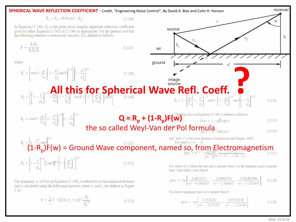
SPHERICAL WAVE REFLECTION COEFFICIENT - Credit, “Engineering Noise Control”, By David A. Bies and Colin H. Hansen

All this for Spherical Wave Refl. Coeff. ?

Q = Rp + (1-Rp)F(w) the so called Weyl-Van der Pol formula

(1-Rp)F(w) = Ground Wave component, named so, from Electromagnetism

Slide 14 of 43

Sound Reflection

REFLECTION - SOURCE – RECEIVER CLOSE TO A SURFACE OF FINITE IMPEDANCE (flow resistivity of 200 kPa s m-2)

Slide 15 of 43

STATISTICAL REFLECTION COEFFICIENT Using equivalent abs. coeff.

ρ=1-α

?

Slide 16 of 43

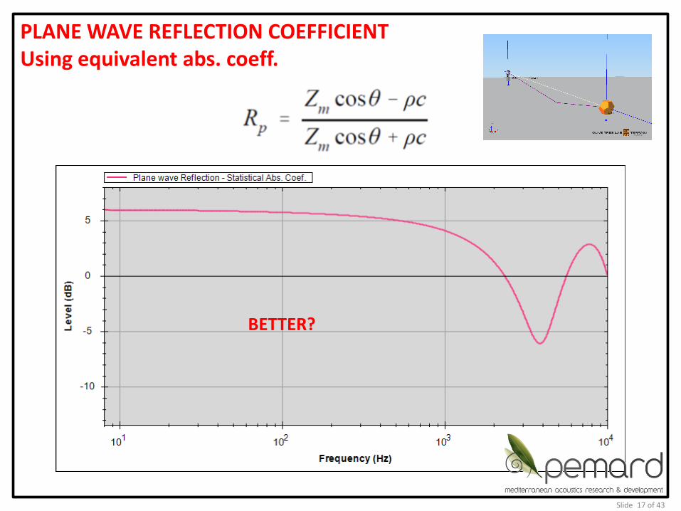
PLANE WAVE REFLECTION COEFFICIENT Using equivalent abs. coeff.

BETTER?

Slide 17 of 43

SPHERICAL WAVE REFLECTION COEFFICIENT Credit, “Engineering Noise Control”, By David A. Bies and Colin H. Hansen

YES The additional features, over and

above plane wave, are due to Ground Wave propagation

Slide 18 of 43

ALL TOGETHER FOR COMPARISON

Slide 19 of 43

SPHERICAL VS PLANE WAVE REFLECTION COEFFICIENT Harder to Softer

material (flow resistivity from 200 to 10 kPa s m-2)

Softer material

Harder material Plane wave

Spherical wave

Slide 20 of 43

REFLECTION – PREDICTING GROUND WAVE SOURCE – RECEIVER ON THE SURFACE (of finite impedance, flow resistivity of 10 kPa s m-2) NO PLANE WAVE REFLECTION IS POSSIBLE

Sound Reflection

Slide 21 of 43

SPHERICAL WAVE REFLECTION COEFFICIENT PREDICTS GROUND WAVE WHEN PLANE WAVE REFLECTION IS NOT POSSIBLE (finite impedance, flow resistivity of 10 kPa s m-2)

Slide 22 of 43

SPHERICAL WAVE REFLECTION COEFFICIENT CORRECTED FOR REFLECTING SURFACE SIZE USING FRESNEL ZONES CORRECTION

Slide 23 of 43

SPHERICAL WAVE REFLECTION COEFFICIENT CORRECTED FOR REFLECTING SURFACE SIZE USING FRESNEL ZONES CORRECTION

Infinite size Finite size

Slide 24 of 43

SPHERICAL VS PLANE WAVE REFLECTION COEFFICIENT IN TIME DOMAIN

Spherical wave, includes phase shift

due to material

Plane wave, assumes no phase shift

Slide 25 of 43

SPHERICAL WAVE CALCULATES ROOM RESONANCES

From Lam’s paper, where he proves that Spherical Reflection Coefficient matches BEM results. • estimated reflection orders 80, • our results with 23 orders (calc. time 19 hrs)

Olive Tree Lab-Terrain Calcs

Slide 26 of 43

SPHERICAL WAVE CALCULATES ROOM RESONANCES

Above at 25 Hz Left at 63 Hz

Slide 27 of 43

Olive Tree Lab – Terrain, based on the work of :

• Salomon’s ray model using analytical solutions

• Hadden & Pierce for spherical wave diffraction coefficients

• Chessel for spherical wave reflection coefficients

• Delany & Basley for finite surface impedance

• Clay on finite size reflectors with Fresnel zones

• Keller on his geometrical theory of diffraction

• Sound path explorer – an in-house model to detect and draw diffraction and reflection sound paths in a 3D environment

• Harmonoise for atmospheric turbulence

Background on OTL-Terrain

Slide 28 of 43

FROM THEORY TO PRACTICE AN EXAMPLE:

A block of flats is affected by stadium concerts and a chiller. The background noise level is determined by road traffic

between the flats and the stadium

PART 3

Slide 29 of 43

EXAMPLE: A block of flats affected by stadium concerts and a chiller

• A stadium across a block of flats and in between a main road.

• There is a chiller on the roof

• Speakers in the stadium (coherent sources)

Slide 30 of 43

A chiller on the roof

EXAMPLE: A block of flats affected by stadium concerts and a chiller

A stadium across a block of flats and in between a main road.

Speakers in the stadium (coherent sources)

Slide 31 of 43

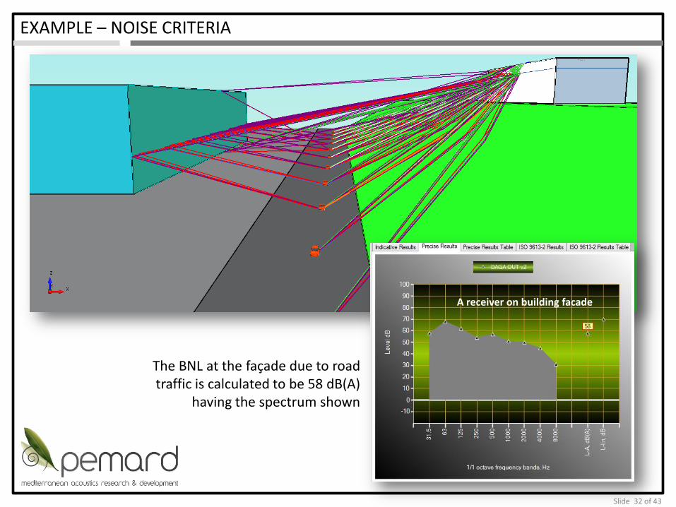
EXAMPLE – NOISE CRITERIA

The BNL at the façade due to road traffic is calculated to be 58 dB(A)

having the spectrum shown

A receiver on building facade

Slide 32 of 43

EXAMPLE – COHERENT & INCOHERENT SOURCE ADDITION

Relative Levels outside stadium during a concert.

Levels when speakers are calculated as coherent and incoherent sources.

Note: speakers are omnidirectional.

At façade

Slide 33 of 43

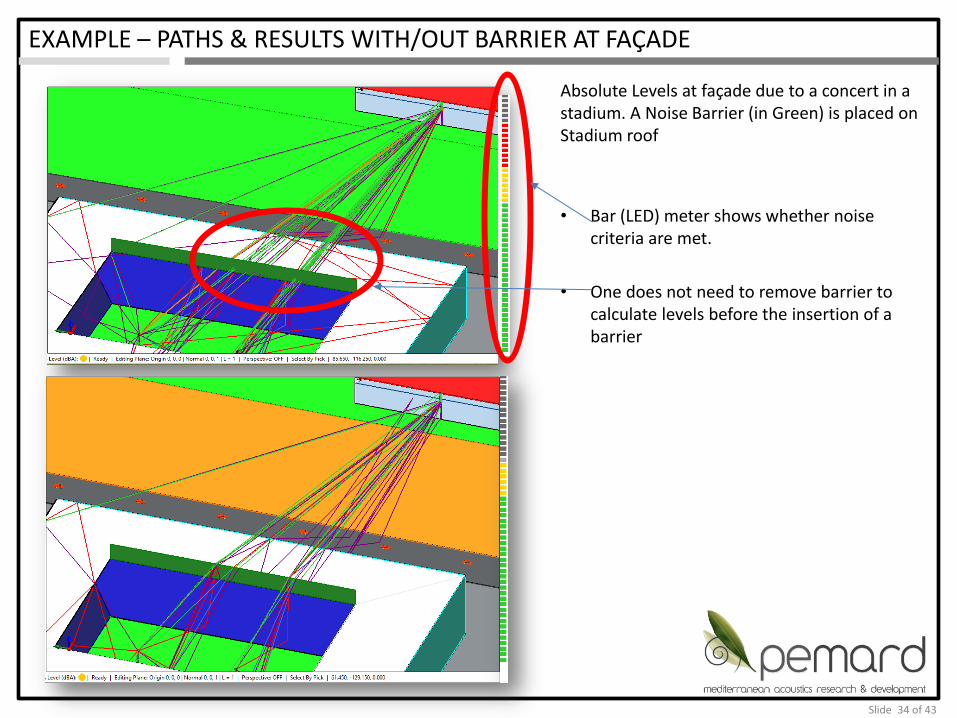
EXAMPLE – PATHS & RESULTS WITH/OUT BARRIER AT FAÇADE

Absolute Levels at façade due to a concert in a stadium. A Noise Barrier (in Green) is placed on Stadium roof

• Bar (LED) meter shows whether noise criteria are met.

• One does not need to remove barrier to calculate levels before the insertion of a barrier

Slide 34 of 43

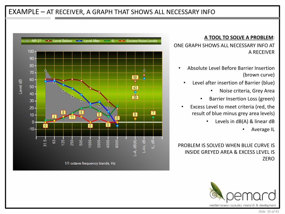
EXAMPLE – AT RECEIVER, A GRAPH THAT SHOWS ALL NECESSARY INFO

A TOOL TO SOLVE A PROBLEM:

ONE GRAPH SHOWS ALL NECESSARY INFO AT A RECEIVER

• Absolute Level Before Barrier Insertion (brown curve)

• Level after insertion of Barrier (blue)

• Noise criteria, Grey Area

• Barrier Insertion Loss (green)

• Excess Level to meet criteria (red, the result of blue minus grey area levels)

• Levels in dB(A) & linear dB

• Average IL

PROBLEM IS SOLVED WHEN BLUE CURVE IS INSIDE GREYED AREA & EXCESS LEVEL IS

ZERO

Slide 35 of 43

EXAMPLE – CHILLER, PATHS, RESULTS, CALCULATION OPTIONS

Slide 36 of 43

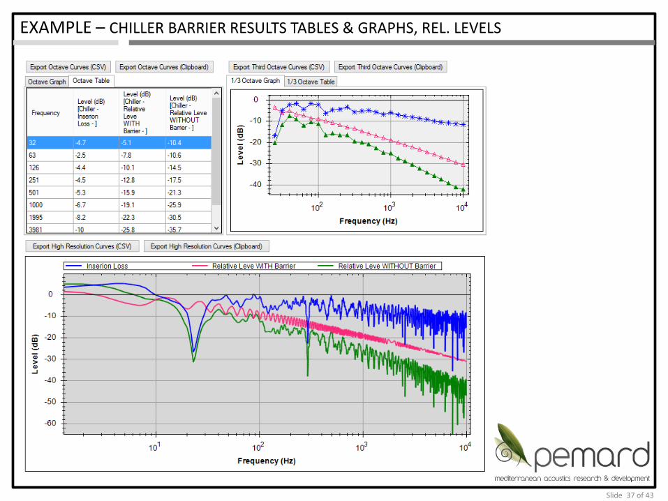
EXAMPLE – CHILLER BARRIER RESULTS TABLES & GRAPHS, REL. LEVELS

Slide 37 of 43

EXAMPLE – BARRIER IL MAPPING, BROADBAND

Mapping of Barrier IL. The effect of the stadium and barrier increase levels on the road

Slide 38 of 43

EXAMPLE – BARRIER IL MAPPING, 100Hz

Mapping of Barrier IL. The effect of the stadium and barrier increase levels on the road

Slide 39 of 43

EXAMPLE – BARRIER IL MAPPING, 10kHz

Mapping of Barrier IL. The effect of the stadium and barrier increase levels on the road

Slide 40 of 43

CONCLUSIONS

PART 4

Slide 41 of 43

CONCLUSIONS

• Nowadays technology allows the replacement of

simplified calculation methods with advanced

calculation methods.

• Advanced calculation methods offer engineers and

scientists

• Accuracy

• Simplicity

• More efficiency

Conclusions

Slide 42 of 43

I would welcome questions or comments.

Thank you for your attention.

QUESTIONS

Slide 43 of 43