Terrain Navigation for Underwater Vehicles - DIVA
270
Terrain Navigation for Underwater Vehicles Ingemar Nygren TRITA _ S3 _ SB _ 0571 ISSN 1103-8039 ISRN KTH/SB/R--05/71--SE Doctoral Thesis in Signal Processing Stockholm, Sweden 2005
-
Upload
khangminh22 -
Category
Documents
-
view
0 -
download
0
Transcript of Terrain Navigation for Underwater Vehicles - DIVA

Terrain Navigation for Underwater Vehicles
Ingemar Nygren
TRITA_S3_SB_0571ISSN 1103-8039
ISRN KTH/SB/R--05/71--SE
Doctoral Thesis in Signal ProcessingStockholm, Sweden 2005

Signal Processing GroupDepartment of Signals, Sensors and SystemsSchool of Electrical EngineeringRoyal Institute of Technology (KTH)SE-100 44 Stockholm, SwedenTel. +46 8 790 6000, Fax. +46 8 790 7260http://www.s3.kth.se
The work presented in this thesis is funded by
Swedish Defence Materiel AdministrationSE-115 88 STOCKHOLMSWEDEN
Akademisk avhandling som med tillstånd av Kungliga Tekniska Högskolanframlägges till offentlig granskning för avläggande av teknologie doktorsexa-men onsdagen den 14 december 2005 kl 13.00 i sal F3, Kungliga TekniskaHögskolan, Lindstedtsvägen 26, Stockholm.
Copyright Ingemar Nygren, 2005
Tryck: Universitetsservice US AB

In this thesis a terrain positioning method for underwater vehicles called the correlationmethod is presented. Using the method the vehicle can determine its absolute positionwith the help of a sonar and a map of the bottom topography. The thesis is focusedtowards underwater positioning but most of the material is directly applicable to flyingvehicles as well.
The positioning of surface vehicles has been revolutionized by the global positioningsystem (GPS). However, since the GPS signal does not penetrate into the sea watervolume, underwater vehicles still have to use the inertial navigation system (INS) fornavigation. Terrain positioning is therefore a serious alternative to GPS for underwatervehicles for zeroing out the INS error in military applications.
The thesis begins with a review of different estimation methods as Bayesian and extendedKalman filter methods that have been used for terrain navigation. Some other methodsthat may be used as the unscented Kalman filter or solving the Fokker-Planck equationusing finite element methods are also discussed.
The correlation method is then described and the well known problem with multipleterrain positions is discussed. It is shown that the risk of false positions decreasesexponentially with the number of measurement beams. A simple hypothesis test of falsepeaks is presented. It is also shown that the likelihood function for the position underweak assumptions converges to a Gaussian probability density function when the numberof measuring beams tends to infinity.
The Cramér-Rao lower bound on the position error covariance is determined and it isshown that the proposed method achieves this bound asymptotically. The problem withmeasurement bias causing position bias is discussed and a simple method for removing
Abstract

the measurement bias is presented.
By adjusting the footprint of the measuring sonar beams to the bottom topographya large increase in accuracy and robustness can be achieved in many bottom areas.This matter is discussed and a systematic theory about how to choose way-points isdeveloped.
Three sea-trials have been conducted to verify the characteristics of the methodand some results from the last one in October 2002 are presented. The sea-trialsverify to a very high degree the theory presented. Finally the method is brieflydiscussed under the assumption that the bottom topography can be described byan autoregressive stochastic process.
ii

Acknowledgments
First of all I want to thank Professor Björn Ottersten for letting me complete myresearch work on terrain navigation at the Signal Processing Lab at the School ofElectrical Engineering. I am also grateful to my supervisor Docent Magnus Janssonat the same department for all the effort he has put into the work of proof readingthe papers, articles and this thesis and for the discussions we have had duringmy time at the Signal Processing Lab.
This thesis had not come about without the financial support of the SwedishDefence Materiel Administration (FMV), which is gratefully acknowledged. I amespecially grateful to Cdr. Stefan Ahlberg, MSc., Swedish navy, Mr. Carl-JohanAndersson, MSc., and Mr. Filip Traugott, MSc., both at FMV, not only for thefinancial support but also for their genuine interest in underwater navigation.Thanks goes also to Capt. Håkan Larsson, Ret., former head of the TorpedoDepartment of the FMV, for the support of the idea when it first came about andto Professor Ilkka Karasalo for his participation in the reference group for theproject.
I am also grateful for valuable ideas from the submarines Cdr. Magnus Odéen andLt. Cdr. Christer Brandt in the Swedish navy. The idea of using a 3D sonar forterrain positioning came originally from Cdr. M. Odéen.
My thanks goes also to all the people that have been involved in the sea-trialsduring the years and have made them a success.


Contents1 Introduction 1
1.1 Introduction 11.2 Contributions 2
1.2.1 Published results 6
2 Terrain navigation 92.1 Terrain navigation methods in general 9
2.1.1 Introduction 92.1.2 The Bayesian approach 112.1.3 The extended Kalman filter from a Bayesian
perspective 162.1.4 TERCOM 202.1.5 The mass point filter 212.1.6 The particle filter 212.1.7 The unscented transform 252.1.8 The stochastic differential equation 26
2.2 Terrain navigation methods for underwater vehicles 302.2.1 Correlation navigation with a bathymetric sonar 31
3 The positioning method 373.1 Introduction 373.2 The positioning method 403.3 The Bayesian and the maximum likelihood method (ML) 44
3.3.1 An illustrating example 443.3.2 The linear fusing method 473.3.3 Multiple likelihood peaks 49
3.4 Concluding remarks about the basic terrain navigation method 533.5 A way of implementing the approximate method 543.6 Comparison between the single beam missile method and the

correlation method 563.7 Determining the measurement bias 613.8 Incoporation of sediment data in the correlation 63
3.8.1 Introduction 633.8.2 Incoporation of sediment data 64
3.9 Incorporation of side-scan data in the correlation 683.10 Incorporation of external sound sources in the
correlation 69
4 Characteristics of the likelihood function 734.1 Introduction 734.2 False peaks 74
4.2.1 The probability for false position 744.2.2 The amplitude of false peaks 774.2.3 False peaks, hypothesis testing 78
4.3 The shape of the likelihood function 804.3.1 The convergence of the likelihood curve 824.3.2 The convergence of the N-normalized
likelihood curve 844.3.3 The convergence of the likelihood curve
in the frequency space 844.4 The linear Kalman filter 87
4.4.1 The conditional mean 874.4.2 The linear Kalman filter 88
5 The Cramér-Rao lower bound 935.1 Introduction 935.2 The CRLB 95
5.2.1 The scalar CRLB 955.2.2 The vector CRLB 102
5.3 Additive Gaussian noise 1045.3.1 The scalar case, Gaussian noise 1045.3.2 The vector case, Gaussian noise 104
5.4 The bias expression 1065.4.1 The linear case 1065.4.2 The nonlinear case 107
5.5 Some examples of the CRLB in terrain navigation 1105.5.1 The posterior FIM 1105.5.2 Two measures of the posterior accuracy 1125.5.3 Constant measurement covariance matrix,
no measurement bias 1135.5.4 Profile matching, constant measurement covariance
matrix 1135.5.5 Regular matching, measurement bias and constant
covariance matrix 114
vi

5.5.6 CRLB in the case of uncompensated soundspeed gradients 116
6 The characteristics of the position estimate 1236.1 Introduction 1236.2 Characteristics of the positioning estimate 124
7 Optimal beam pattern and way-point selection 1377.1 Introduction 1377.2 Optimal footprint beam pattern 1377.3 How to choose way-points 143
7.3.1 An example of how to choose a way-point 147
8 Sea-trial October 2002 1538.1 Introduction 1538.2 Sonar and position error causes 153
8.2.1 Introduction 1538.2.2 Bathymetric sonars 1548.2.3 Measurement errors 158
8.3 Sea-trial October 2002, simulation 1608.3.1 Introduction 1608.3.2 Simulation of the positioning 162
8.4 Sea-trial October 2002, results 1668.4.1 Way-point 1 1668.4.2 Way-point 2 1688.4.3 Way-point 2B 1708.4.4 Way-point 3 1728.4.5 Way-point 7 174
8.5 Conclusions 176
9 The autoregressive bottom model 1779.1 Introduction 1779.2 AR bottom profiles 178
9.2.1 AR(1) bottom profile 1789.2.2 AR(2) bottom profile 1809.2.3 Determining the expected correlation function 180
9.3 The covariance matrix 1819.4 Decomposition of the covariance matrix 184
9.4.1 Choleskey decomposition of the covariance matrix 1859.5 The mean and the variance of the correlation sum 1889.6 The probability density function of the correlation sum 1919.7 The probability density function for the position 1939.8 Approximative determination of the probability density
function for the correlation sum 1979.9 The Cramér-Rao lower bound 199
vii
10 Summary 20310.1 Summary 203
10.1.1 The problem 20310.1.2 Solutions and conclusions 204
10.2 Further research 205
Appendix A 207A.1 Inertial navigation 207
A.1.1 The principle of inertial navigation (INS) 207A.1.2 The position error for INS 209
A.2 The hardware navigator 212A.2.1 The basic principle 213A.2.2 The principle of implementation 215A.2.3 The practical implementation in an FPGA 217
Appendix B 221B.1 Introduction 221B.2 Reconstruction of signals from samples 222B.3 Maximum a posterior interpolation 227B.4 The least squares autoregressive interpolation 229B.5 Interpolation in the frequency domain 235
Notational conventions 237
List of acronyms 243
Bibliography 245
viii

1
1.1 IntroductionIn this thesis a terrain positioning method for underwater vehicles called thecorrelation method is presented. Using the method the vehicle can determine itsabsolute position with the help of a sonar and a map of the bottom topography.The thesis is focused towards underwater positioning but most of the material isdirectly applicable to flying vehicles as well.
The positioning of surface vehicles has been revolutionized by the globalpositioning system (GPS). However, since the GPS signal does not penetrate intothe sea water volume, underwater vehicles still have to use the inertial navigationsystem (INS) for navigation. A great problem with inertial navigation systems isthe drift of the gyros, i.e., the position error will grow exponentially with time. Thismeans that the underwater vehicle has to break the surface regularly to zero outthe position error by reading its GPS position. This is undesired in militaryapplications since it creates a risk of being revealed and the GPS signal may notbe available or may even be jammed. Terrain positioning is therefore a serious
Chapter 1
Introduction

2 1 Introduction
alternative to GPS for zeroing out the positioning error of the INS. Certainly thesonar emits a potentially revealing signal but the short duration of the sonarpulse makes the risk of revealing very low.
During the last five years, three large sea-trials have been conducted to supportthe presented theory. The test result has been very good and this thesis canalso be seen as a presentation of the theoretical basis for the trials.
Compared to other terrain navigation methods, including the traditional methodsfor airial terrain navigation, the benefits of this method are
• Robustness• High accuracy• Minimal need of maps
In an attempt to make the thesis easy to read even for persons without immediateknowledge in estimation theory the method has been presented with numerousfigures and often with an intuitive approach but hopefully the cogency of thethesis has not suffered from this.
1.2 ContributionsOptimal methods, in a minimum mean square error (MMSE) sense, for terrainnavigation has been around for some time but as shown in this thesis theperformance can be considerably increased if the measurement of the terraintopography is made in several points simultaneously. The thesis describes theproposed method, its performance and presents briefly the result from one ofthe sea-trials that have been conducted for verification of the theoretical findings.
This thesis is organized in the following chapters besides this introductionchapter.
Chapter 2 Terrain navigation methodsIn this chapter the Bayesian approach to terrain navigation is outlined and theextended Kalman filter in a Bayesian perspective is presented. The extendedKalman filter (EKF) has been used in terrain navigation since long ago and theextended Kalman filter is here presented in a Bayesian setting.
The TERCOM terrain navigation method, which seems to be the first terrain

3
navigation method to be used, is described together with some other methods.The mass-point and particle filter, which have been used for flying vehicles withgood results, are also briefly described.
A navigation filter based on the unscented transform (UT) is briefly sketched.This is a non-optimal filtering method that seems to fit the terrain navigationproblem well even if no one yet has presented the method in a terrain navigationexample. This goes also for the next method discussed. The amazing increase incomputational power lately means that filters based on solving the Fokker-Planckequation are highly interesting and such filters may be a strong competitor to themass-point filter. A brief review of such a filter is presented. Compared to the UT-filter this is an optimal method as the mass point filter is.
Finally this chapter ends with a review of some terrain navigation methods forunderwater vehicles that have been presented at conferences and in journalpapers during the last years.
Chapter 3 The positioning methodThis chapter describes the background for the proposed terrain navigation methodas well as the benefit of using it. It also touches briefly on the problem of falsecorrelation peaks due to terrain repeatability.
The computational demand for the correlation method is substantial and animplementation method to handle this problem is presented.
The difference between measuring the terrain topography as in traditional terrainnavigation for flying vehicles and as in the proposed method is discussed andit is shown that the proposed measuring method is superior with regard toaccuracy.
A great problem in terrain navigation is position bias due to measurement biasand a simple method to eliminate it is presented.
The chapter ends with a discussion of how the position estimate can be improvedby using bottom sediment information and/or data from side-scan sonars as wellas from external sound sources.
Chapter 4 The likelihood function and the Kalman filterAn often quoted problem with the correlation methods is the problem of false
1.2 Contributions

4 1 Introduction
peaks due to terrain repeatability, i.e., positions which give high correlations butstill do not correspond to the true position. In the chapter it is shown that the riskof false peaks decreases exponentially with the number of measurement beams.A large number of measuring beams will thus eliminate the problem. A simplehypothesis test of false peaks is also presented. With the test false peaks can tosome degree be detected and a coarse “false peaks filter” can be constructed.
As described in Chapter 2 the Bayesian approach means that the prior PDF forthe vehicle position is multiplied with the likelihood function from themeasurement. This means that if the prior PDF is Gaussian and the likelihoodfunction also is Gaussian the posterior PDF will be Gaussian. In the chapter it isshown that the likelihood function converges under weak assumptions to aGaussian PDF when the number of measuring beams tends to infinity.
A consequence of this is that a linear Kalman filter can be used for fusing theposition measurement with the prior position information. This simplifies greatlythe calculation of the posterior position PDF since an analytic expression can beused instead of having to rely on numerical methods. This also means that therobustness with regards to filter divergence is greatly improved and of coursethe computational errors of the numerical methods are avoided.
Chapter 5 The Cramér-Rao lower boundIt is of course not satisfactory to simply have a position from a navigationalsystem. Information about the accuracy of the position is also needed so weknow to what degree the position figure can be trusted. However, in many casesit is not an easy task to give an exact figure of the actual accuracy for a positionestimation method and it is in this context the Cramér-Rao lower bound (CRLB)shall be seen. The CRLB gives the lowest possible position error variance, giventhe prerequisites, for the position estimate regardless of the actual estimationformula. By comparing the accuracy we achieve in simulation with the CRLB wecan judge whether the estimation method has potentially good accuracy comparedto other methods. Thus the CRLB plays an important role in judging the accuracyof the positioning method proposed in this thesis.
The chapter starts with a presentation of the original proof that H. Cramér gave ofthe CRLB theorem in 1945 which is not so often quoted nowadays. Then somespecial formulas for the terrain navigation problem are presented. As examples ofthis are cases with additional measurement noise. Another example is the CRLBdependence on the bending of the measurement beams due to uncompensated
5
temperature gradients in the sea.
Chapter 6 The characteristics of the position estimateThis chapter discusses the characteristics of the position estimate and the positionbias that may be the consequence of measurement bias, i.e., the case when themeasured depth in a position differs from the depth according to the map in thesame point due to a fix measurement error often caused by an incorrect height ofthe actual sea level.
Chapter 7 Optimal beampattern and way-point selectionBy adjusting the footprint of the measuring sonar beams to the bottomtopography a large increase in accuracy and robustness can be achieved inmany bottom areas. This matter is discussed in the first part of the chapter. Thena systematic theory about how to choose way-points in a way that minimizes theprobability of failure for the positioning is developed. The chapter ends with anexample of how to choose a way-point.
Chapter 8 Sonars and the sea-trial October 2002The chapter starts with a brief review of sonars and their measurement errors butthe main content of the chapter is a review of a sea-trial. Three sea-trials havebeen conducted to verify the characteristics of the method. Some results fromthe latest test in October 2002 are presented in the chapter. The sea-trials verifyto a very high degree the theory presented in the thesis.
Chapter 9 Terrain navigation for autoregressive bottom modelsThis chapter is freestanding from the previous chapters. It presents thecorrelation method under the assumption that the bottom topography can bedescribed by an autoregressive stochastic process.
If the bottom topography could be described in statistical terms, for example asa stationary stochastic process, qualitative and quantitative judgements couldbe drawn about the positioning accuracy and adherent matters. This would beof great advantage, but up to now the available models covering larger bottomareas are very complex and the relevance of the models might be questioned.However, it turns out that very simple autoregressive models can be of valuewhen describing local bottom characteristics. The chapter discusses and drawsconclusions from such models.
1.2 Contributions

6 1 Introduction
Appendix AThe appendix discusses very briefly the inertial navigation system (INS). Thispart may be of interest for readers unfamiliar with inertial navigation systems.The chapter also briefly reviews a master thesis about implementing the calculationof the likelihood function in a field programmable array (FPGA). This is of greatinterest if the positioning method is to be used for flying vehicles since theperformance of such an implementation makes the method also attractive in suchapplications. For flying vehicles a radar with a narrow scanning beam or a scanninglaser beam may be used.
Appendix BThe positioning method requires a considerable amount of interpolation in theunderwater map to which many well known interpolation methods can be used.However, the interpolation error will change the bottom spectrum by introducinghigh frequency components which may influence the position accuracy. Aninterpolation method that does not change the spectrum is thus of interest andthe chapter discusses such probabilistic methods after a short introduction aboutreconstruction of signals from samples of the signal. The probabilistic methodshave a remarkable performance if the bottom characteristics are stationary andknown which, however, seldom is the case.
1.2.1 Published resultsThe major results in this thesis have been published in the following papers andjournal articles.
I. Nygren, Terrängnavigering för undervattensfarkoster. Resultat avfältförsök 1998 (Terrain Navigation of Underwater Vehicles. Results from Sea-Trial 1998), Report FOA–R—99-01298-313—SE, December 1999.
I. Nygren, A Method for Terrain Positioning of an AUV, Proceedings, 12th
International Symposium UUST01, Durham, New Hampshire, USA, 2001.
I. Nygren, A Method for Terrain Navigation of an AUV, Conference proceed-ings, MTS/IEEE Oceans 2001.
I. Nygren, Recursive Terrain Navigation, Application of the CorrelatorMethod, Report FOI–R—0764—SE, Sweden, August 2002.

7
C-J. Andersson, I. Nygren, A Method for Terrain Positioning of UnderwaterVehicles, Proceedings, Undersea Defence Technology (UDT) Europe 2003.
I. Nygren, M. Jansson, Recursive Terrain Navigation with the CorrelatorMethod for High Position Accuracy, Proceedings, 13th International Sympo-sium UUST03, Durham, New Hampshire, USA, 2003.
I. Nygren, M. Jansson, Robust Terrain Navigation with the CorrelatorMethod for High Position Accuracy, Conference proceedings, MTS/IEEEOceans 2003.
I. Nygren, M. Jansson, Terrain Navigation Using the Correlator Method,Conference proceedings, IEEE Position Location And Navigation Sympo-sium, Monterey, Cal., USA, April 27-29, 2004.
I. Nygren, M. Jansson, Terrain Navigation for Underwater Vehicles Usingthe Correlation Method, IEEE Journal of Oceanic Engineering, July 2004,Vol. 29, No. 3.
J. Carlström, I. Nygren, Terrain Navigation of the Swedish AUV62F, Pro-ceedings, 14th International Symposium UUST05, Durham, New Hampshire,USA, 2005.
I. Nygren, M. Jansson, A Terrain Navigation Method for UAVs and AUVsBased on Correlation, IEEE Transactions on Aerospace and ElectronicSystems, to be published.
1.2 Contributions

8 1 Introduction

9
2.1 Terrain navigation methods in general2.1.1 IntroductionTerrain navigation has up to now mostly been used for flying vehicles and hasduring the last decennium become an accepted method to improve and aid inertialnavigation systems. The first studies and tests were done in the late fifties butmost of the development work was done during the seventies. Lately the use hasbeen substantially increased due to the increased availability of high accuracydigital terrain maps as a result of charting by satellites.
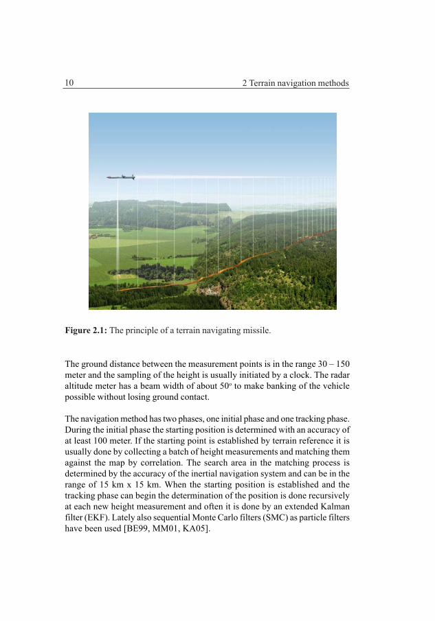
Examples of commercial terrain navigation methods within the flying communityare TERCOM [GO80], TERPROM [AR88], TERNAV [SK85, PUJP00], SITAN[HOAN85], BITAN [CYYT92], LATAN [LA88] and others. TERCOM was thefirst method to be used. The principle for all methods is to measure the terrainprofile along a flight passage as in Figure 2.1 and to compare it with a digitalmap and by that establish a position. The comparison can be done as a batchoperation as in TERCOM or as a recursive operation as in TERPROM or SITAN.
Chapter 2
Terrain navigation methods
10 2 Terrain navigation methods
The ground distance between the measurement points is in the range 30 – 150meter and the sampling of the height is usually initiated by a clock. The radaraltitude meter has a beam width of about 50o to make banking of the vehiclepossible without losing ground contact.
The navigation method has two phases, one initial phase and one tracking phase.During the initial phase the starting position is determined with an accuracy ofat least 100 meter. If the starting point is established by terrain reference it isusually done by collecting a batch of height measurements and matching themagainst the map by correlation. The search area in the matching process isdetermined by the accuracy of the inertial navigation system and can be in therange of 15 km x 15 km. When the starting position is established and thetracking phase can begin the determination of the position is done recursivelyat each new height measurement and often it is done by an extended Kalmanfilter (EKF). Lately also sequential Monte Carlo filters (SMC) as particle filtershave been used [BE99, MM01, KA05].
Figure 2.1: The principle of a terrain navigating missile.

11
For flying vehicles the vertical positions are of great interest besides thehorizontal position. For underwater vehicles the vertical position can easilyand accurately be determined by other means and the presentation will thereforebe focused on methods to determine the horizontal position. We will assumethat the movement of the vehicle in the horizontal plane is governed by thefirst of the following two equations. The height measurement is described bythe second equation.
xt+1=xt+ut+vt t=0,1,2... (2.1)
yt=h(xt)+et (2.2)
The vector xt is the position of the vehicle in the horizontal plane and thevector ut is the displacement from the earlier position and the vector vt is theuncertainty in the displacement. The displacement can be thought of as comingfrom the INS-system or by integrating the equations of the vehicle movement.The measured height yt is the height according to the map in the position xtwith the addition of a measurement error et. The error sequences vt and et areconsidered to be white with a zero mean and independent of each other.
2.1.2. The Bayesian approach to terrain navigationThe Bayesian method for recursive estimation is particularly suitable fornonlinear problems which not easily can be linearized allowing an EKF-filterto be used [BUSE71]. For applications of the Bayesian approach in terrainnavigation, see [RU85, BE99, METR02, KA05]. The Bayesian approach meansthat Bayes formula is used to incorporate the measurement data into theestimation and in most cases this also means that a numerical method has to beused to establish a position. This can be computationally demanding. Withlow order of the state vector the method is easily illustrated which can giveextra insight into the estimation problem. The idea behind the method is theconcept of a likelihood function [HAFO04]. The likelihood for the randomvariable Y to have the value y when the random variable X has the value x is inthe discrete case
( ; ) Pr{ | } for state space of L = = = ∈x y Y y X x x x (2.3)
where Pr{.} denotes the probability.
2.1 Terrain navigation methods in general
12 2 Terrain navigation methods
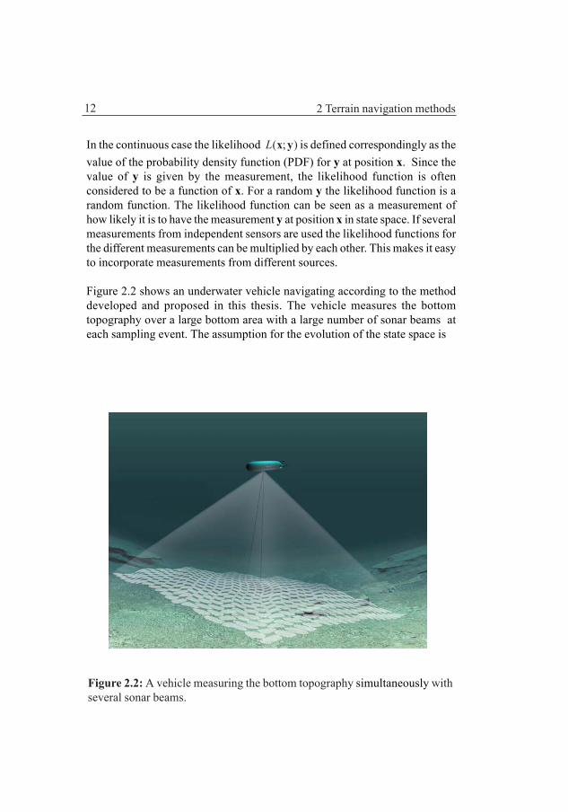
In the continuous case the likelihood ( ; )L x y is defined correspondingly as thevalue of the probability density function (PDF) for y at position x. Since thevalue of y is given by the measurement, the likelihood function is oftenconsidered to be a function of x. For a random y the likelihood function is arandom function. The likelihood function can be seen as a measurement ofhow likely it is to have the measurement y at position x in state space. If severalmeasurements from independent sensors are used the likelihood functions forthe different measurements can be multiplied by each other. This makes it easyto incorporate measurements from different sources.
Figure 2.2 shows an underwater vehicle navigating according to the methoddeveloped and proposed in this thesis. The vehicle measures the bottomtopography over a large bottom area with a large number of sonar beams ateach sampling event. The assumption for the evolution of the state space is
Figure 2.2: A vehicle measuring the bottom topography simultaneously withseveral sonar beams.
13
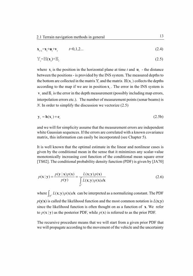
xt+1=xt+ut+vt t=0,1,2... (2.4)
Yt=H(xt)+Et (2.5)
where tx is the position in the horizontal plane at time t and tu - the distancebetween the positions - is provided by the INS system. The measured depths tothe bottom are collected in the matrixYt and the matrix ( )xH t collects the depthsaccording to the map if we are in position tx . The error in the INS system is
tv andEt is the error in the depth measurement (possibly including map errors,interpolation errors etc.). The number of measurement points (sonar beams) isN. In order to simplify the discussion we vectorize (2.5)
( )t t t= +y h x e (2.5b)
and we will for simplicity assume that the measurement errors are independentwhite Gaussian sequences. If the errors are correlated with a known covariancematrix, this information can easily be incorporated (see Chapter 5).
It is well known that the optimal estimate in the linear and nonlinear cases isgiven by the conditional mean in the sense that it minimizes any scalar-valuemonotonically increasing cost function of the conditional mean square error[TS02]. The conditional probability density function (PDF) is given by [JA70]
2
( | ) ( ) ( ; ) ( )( | )( ) ( ; ) ( )
R
p p L ppp L p d
= =∫
y x x x y xx yy x y x x
(2.6)
where2
( ; ) ( )R
L p d∫ x y x x can be interpreted as a normalizing constant. The PDF
p(y|x) is called the likelihood function and the most common notation is L(x;y)since the likelihood function is often thought on as a function of x. We referto ( | )p x y as the posterior PDF, while ( )p x is referred to as the prior PDF.
The recursive procedure means that we will start from a given prior PDF thatwe will propagate according to the movement of the vehicle and the uncertainty
2.1 Terrain navigation methods in general

14 2 Terrain navigation methods
of the movement. The movement can, for example, be determined from anINS system that has a specified uncertainty. We will denote the propagated,but not measurement updated, PDF as ( )p− x . The next step in the recursiveprocedure is to do the measurement update of ( )p− x by the multiplication of
( )p− x and ( | )L y x in order to arrive at the posterior PDF. In the followingsection we will look at this in some more details.
A. Propagation of the PDF for the vehicle positionEquation (2.4) describes how the position changes between two samplingevents. Figure 2.3 illustrates this. The left PDF (the previous posterior PDF)has a bearing upon the vehicle’s position at sampling time t and the black pileis the relative frequency of the number of realizations which have ended inpoint tx , i.e. ( | )t tp x Y . The notation ( | )tp ⋅ Y indicates that the PDF is basedon all measurements up to and including the measurement at time t. Therealizations are moved the distance tu but due to the uncertainty tv we willhave a spread in the new position. We multiply this new PDF - the small one inthe figure - by the relative frequency ( | )t tp x Y and total the contributions of
Figure 2.3: Propagation of the PDF for the vehicle position.

15
all points in the left PDF by an integral to get the position PDF at time t+1. Wecan express the propagation as
21 1( | ) ( ) ( | )
tt t t t t t t tR
p p p d+ += − −∫ vx Y x u x x Y x (2.7)
where ( )t
p ⋅v is the PDF for the error term vt. This is the Chapman-Kolmogorovsequation for the propagation of a Markov process [JA70]. See also Section2.1.8 about how to calculate the integral expression when tu is not just a simplefix translation.
B. The measurement update The measurement is made according to (2.5b). We assume the errors in thedepth measurements to be Gaussian. Therefore
11 1( ; ) exp( ( ( )) ( ( )))2(2 ) det( )
Tt t t t e t tN
e
Lπ
−= − − −x y y h x C y h xC (2.8)
where eC is the measurement error covariance matrix. The function ( ; )t tL x y isour likelihood function since, for a given position tx , it gives the likelihood ofhaving the measurement value yt. The assumption that the errors of differentbeams are uncorrelated makes the covariance matrix eC diagonal and, if the
measurement variance is the same in all beams, equal to 2eσ I . Therefore the
likelihood function will be
2,22
1
1 1( ; ) exp( ( ( )) )2(2 )
N
t t t k k tNkee
L y hσπσ =
= − −∑x y x (2.9)
where , and ( )t k k ty h x are the kth components of the vectors and ( )t ty h x , re-spectively.
The next step in the recursion is to fuse the likelihood function for themeasurement with the propagated PDF of the position. The non-normalizedposterior PDF is obtained as
2.1 Terrain navigation methods in general

16 2 Terrain navigation methods
1 1 1 1 1( | ) ( ; ) ( | )t t t t t tp L p+ + + + +x Y x y x Y∼ (2.10)
If the time between the measurements is large the variance in the propagatedPDF, ( )p− x , may increase so much that it will not noticeably improve theestimation of the position based on the likelihood function. Hence, when theprior PDF has a large variance the estimation problem becomes a maximumlikelihood (ML) estimation problem. The measurement update by Bayes formulais further discussed in Section 3.3.
Bayesian estimation [HAFO04] is used in many scientific disciplines besidesengineering. In [RO01] and [BS02] the subject is treated in a more mathematicalway. More easy to read are [TP01], [HL01], [WL90] and [AS72] and a tutorialbook is [SIL96]. A comparision between different estimatation methods fornonlinear problems can be found in [FD05].
2.1.3. The extended Kalman filter from a BayesianperspectiveIt is often advantageous to think about a filter as consisting of a propagationstage followed by a measurement update stage. In the extended Kalman filter(EKF) the nonlinear equations for movement and measurement are linearizedin order to make a linear Kalman filter feasible [TS02, KSH00]. In studying thefiltering problem from a Bayesian perspective we look at the PDFs of theinvolved stochastic variables whereby the filter procedure becomes quite natural.
The first equation (2.4) which describes the vehicle track with its stochasticfluctuations, often called the process equation, is already in a linear form. Wewill assume that the vehicle position at time t = 0 is Gaussian distributed and itwill be that also at time t = 1 provided vt is Gaussian. The mean and covarianceare calculated from the PDF given by (2.7). See also Chapter 4 for explicitexpressions.
The measurement equation (2.5b) is nonlinear and is therefore linearized aroundthe predicted position. The Taylor expansion of the terrain surface h(xt) gives
| 1 | 1 | 1 | 1 | 1 | 1ˆ ˆ ˆ ˆ( ) ( ) ( ) ( ) ( ) ...Tt t t t t t t t t t t t t t t th h − − − − − −= + − + − − +x x G x x x x H x x (2.11)
where | 1t t −G is the gradient vector and | 1t t−H is the Hessian matrix in the predicted

17
position. If we truncate the series after the second term the equation can beillustrated by the tangent plane in the predicted position. The linearizationmeans that a tangent plane to the surface is placed in the predicted position,see Figure 2.4. The likelihood function will be
222
2| 1 | 1 | 122
1 1( ; ) e xp( ( ( )) )22
1 1 ˆ ˆ e xp( ( ( ) ( )) )22
t t t tee
t t t t t t t tee
L y y h
y h
σπσ
σπσ− − −
= − − =
≈ − − − −
x x
x G x x (2.12)
In the Figures 2.4 and 2.5 the locus for the positions with the same depths asthe measurement is shown as a dashed line. The dashed line is also a symmetryline for the PDF for the measurement error et.
The PDF for the predicted position and the PDF for the measurement areillustrated in Figure 2.6 while Figure 2.7 shows the PDF after the measurementupdate. The update is made by point wise multiplications of the PDFs and willgive a Gaussian PDF if both involved PDFs are Gaussian, i.e., the errors vt andet are Gaussian distributed as well as the starting PDF.
Figure 2.4: A tangent plane isplaced in the predicted position.
Figure 2.5: The tangent plane with thelocus for all depths equal the measureddepth (the dashed line).
2.1 Terrain navigation methods in general

18 2 Terrain navigation methods
As can be seen the result will to a high degree depend on how well the predictedposition is in agreement with the true position and how well the linearizationplane describes the actual terrain around the predicted position. If the predictedposition is close to the true position a better linearization can often be obtainedby adjusting the plane to more than just one terrain point. The procedure iscalled stochastic linearization and means that the tangent plane is determinedfrom several points around the predicted position by the least squares method.Considerable improvement of the accuracy of the position by using thisprocedure is reported [YCH91].
Another step to improve the result is to adapt the following iterative procedurewhich is easy to implement. After the posterior PDF has been calculated asindicated above a new linearization is made around the obtained position and anew posterior is calculated and so on. Only a few recursive steps are most oftenneeded for obtaining a good position. The procedure is called the iterativeEKF [TS02].
An improvement in the EKF-filter can be expected if also the second orderterm is included in the Taylor expansion of the terrain topography [TS02]. Inthis case we have a second order surface passing through the predicted pointand it is likely that this surface will give a better fit than the tangent plane. Theterrain equation will in this case be
Figure 2.6: The prior PDF and thePDF for the measurement.
Figure 2.7: The posterior PDF, i.e. theprior PDF is updated by pointwisemultiplication with the measurementPDF.

19
| 1 | 1 | 1 | 1 | 1 | 1ˆ ˆ ˆ ˆ( ) ( ) ( ) ( ) ( ) ...Tt t t t t t t t t t t t t t t th h − − − − − −= + − + − − +x x G x x x x H x x (2.13)
and the likelihood function
222
| 1 | 1 | 122
2| 1 | 1 | 1
1 1 ˆ( ; ) e xp( ( ( )) )22
1 1 ˆ ˆ e xp( ( ( ) ( )22
ˆ ˆ ( ) ( )) )
t t t tee
t t t t t t t tee
Tt t t t t t t t
L y y h
y h
σπσ
σπσ− − −
− − −
= − − =
≈ − − − −
− − −
x x
x G x x
x x H x x
(2.14)
The drawback of the second order filter is besides considerably more complexcalculations that the posterior function will no more be Gaussian even if themeasurement error and the prior are Gaussian. The iterated filter is often usedbut the use of the second order filter seems to be rare.
As can be understood the EKF filter is likely to diverge if the predicted positionis bad or if the linearization does not fit the terrain well. A practical way tohandle some of the divergence problems is to have several filters running inparallel. If it can be assumed that the positions of the filters are distributed
Figure 2.8: A second order surface fitted to terrain surface at the predictedpoint by a least squares approach.
2.1 Terrain navigation methods in general
20 2 Terrain navigation methods
around the true position a better estimated position would be to take the meanof the individual filters as the predicted position and linearize around thatposition. As the new covariance the mean of the covariances of the individualfilters can be taken. Should any of the filters show divergence it will be closedand a new filter will be started up based on the estimated position and its errorcovariance.
The terrain navigation method SITAN (Sandia Inertial Terrain Aided Navigation)as it is described in [HOAN85] is almost equivalent to the described EKFmethod above even if the filter in that paper is presented by equations. In[HOAN85] parallel filter structures and stochastic linearization is also discussed.A multiple model approach is discussed in [META83]. The tracking phase ofthe TERPROM is also almost equivalent to the described EKF method.
2.1.4 TERCOMTERCOM (Terrain Contour Matching) was the first terrain navigation methodto be used. Measured height data along a straight line flight path were collectedin a vector which then was correlated with a digital map over the terrain. Therelative distance between the measurement positions was determined by theINS-system or by integrating the equations for the vehicle movement. Thismeans that the distance and orientation between the measurement footprintpoints will be afflicted with stochastic errors which will decrease the accuracyof the positioning.
When a new height measurement is available the oldest measurement is thrownaway, cf. a FIFO-register. The early days requirement for a straight line vehiclecourse, due to the computation burden in calculation the orientation of thepositions, is nowadays removed. The accuracy of the TERCOM method is inthe range 30 – 100 meter for hilly terrain [YCH91].
In the original TERCOM method the positioning was done in special navigationareas, way-points, with hilly terrain for which accurate maps were available.The vehicle moved between the way-points by help of the INS-system.
A similar correlation method is HELI/SITAN [HO90, HO91] also developedat the Sandia Laboratories.

21
2.1.5 The mass point filterThe mass point filter is a numerical method for solving the Bayesian filterproblem in an asymptotically optimal way. The state space is divided into agrid and the continuous PDF is replaced by corresponding probability massesin the grid points. A prerequisite is that the state space is of low order otherwisethe computational burden will be prohibitive since quadrature in highdimensions has to be done.
The fix grid size can cause problems in areas with high PDF gradients so it isdesirable with a small grid size to have a good agreement between the discreteand continuous PDFs. However, this can lead to increased computational burdensince a coarser grid could be sufficient in large areas of state space. A way tohandle this is to have a variable grid size determined by the gradient of thePDF but of course this will increase the complexity of the calculations. As willbe seen later the involved PDFs are not particularly suited for the numericalcalculations in the mass point filter (Figure 3.3 and Figure 3.7). The method,with some variations, is described in [BUSE71, BE99].
One of the advantages with the method is the optimality in the minimum meansquare sense but the numerical solutions lead of course to numerical errors.
2.1.6 The particle filterThe particle filter [AMGC02, BE99, GGBFJKN02, MLG99, DFG01, KA05],is also a numerical method where a large number of samples of the state vectoris generated according to its PDF. Each sample is called a particle and theprocedure means that the density of particles in a position corresponds to thevalue of the PDF at that position. The particle filter is asymptotically optimalin a minimum mean square sense.
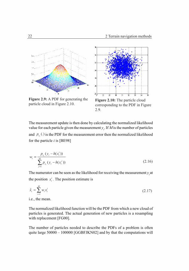
The Figure 2.9 shows a PDF and Figure 2.10 and 2.11 show the correspondingparticle cloud. The particle density in a point in Figure 2.10 corresponds to thevalue of the PDF in that point. In the simplest form of the particle filters, theBootstrap filter, the algorithm can be described as follows [BE98, FG00]. Thepropagation of the posterior PDF is done by propagation of each particleaccording to the propagation equation including the error term which shouldbe simulated with correct error PDF. Se Figure 2.11 and Figure 2.12.
2.1 Terrain navigation methods in general
22 2 Terrain navigation methods
The measurement update is then done by calculating the normalized likelihoodvalue for each particle given the measurement yt. If M is the number of particles
and (.)iep is the PDF for the measurement error then the normalized likelihood
for the particle i is [BE98]
1
( ( ))
( ( ))
i
i
ie t t
i Mj
e t tj
p y h xw
p y h x=
−=
−∑ (2.16)
The numerator can be seen as the likelihood for receiving the measurement yt atthe position i
tx . The position estimate is
1
ˆM
it i t
ix w x
=
= ∑ (2.17)
i.e., the mean.
The normalized likelihood function will be the PDF from which a new cloud ofparticles is generated. The actual generation of new particles is a resamplingwith replacement [FG00].
The number of particles needed to describe the PDFs of a problem is oftenquite large 50000 – 100000 [GGBFJKN02] and by that the computations will
Figure 2.10: The particle cloudcorresponding to the PDF in Figure2.9.
Figure 2.9: A PDF for generating theparticle cloud in Figure 2.10.

23
be demanding. A practical problem that is often encountered is that the particlestends to stick together in a single point after a number of iterations. This willhappen if the error terms are small and a fix for that problem is to add someextra noise to the real noise.
A well working resampling algorithm is thus crucial for the method to avoidparticle sticking. A practical way to circumvent the problem can be to projectthe result from the propagation phase on a known PDF family, i.e., mainly theexponential family [SY98, AS01, BR96] or another family that reasonable wellcan model the PDF described by the particle cloud. By this an analyticexpression can be found for the posterior PDF from which a new particle cloudis generated. The procedure is of course an approximation of the propagatedPDF and the performance may differ depending on the application and choiceof PDF family to project on.
Figure 2.11: Down to the left is the initial particle cloud and up to the rightare the propagated particles, see also Figure 2.12.
2.1 Terrain navigation methods in general

24 2 Terrain navigation methods
The particle filter method is asymptotically optimal but it should be noted thatmethods that interpolate in the map introduces interpolation errors. In roughhilly terrain linear interpolation, if used, can severely decrease the performanceof single beam methods.
It can often be that some parts of a system with advantage can be described bya linear Kalman filter and for other parts of a system a particle filter descriptionis of advantage. A method to implement this is a procedure called Rao-Blackwellization [DFG01].
A comparison between correlation, mass-point and particle filters is given in[MWT02, METR02].
Figure 2.12: A close up of the propagated particles showing the particles withand without noise error.
25
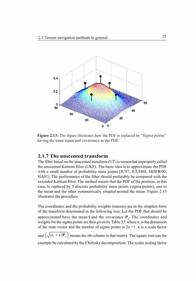
2.1.7 The unscented transformThe filter based on the unscented transform (UT) is somewhat improperly calledthe unscented Kalman filter (UKF). The basic idea is to approximate the PDFwith a small number of probability mass points [JU97, JUUH04, MDFW00,HA01]. The performance of the filter should preferably be compared with theextended Kalman filter. The method means that the PDF of the position, in thiscase, is replaced by 5 discrete probability mass points (sigma points), one inthe mean and the other symmetrically situated around the mean. Figure 2.13illustrates the procedure.
The coordinates and the probability weights (masses) are in the simplest formof the transform determined in the following way. Let the PDF that should beapproximated have the mean x and the covariance Px. The coordinates andweights for the sigma points are then given by Table 2.1 where nx is the dimensionof the state vector and the number of sigma points is 2nx+1. κ is a scale factor
and ( )( )x x in κ+ P means the ith column in that matrix. The square root can for
example be calculated by the Cholesky decomposition. The scalar scaling factor
Figure 2.13: The figure illustrates how the PDF is replaced by “Sigma points”having the same mean and covariance as the PDF.
2.1 Terrain navigation methods in general

26 2 Terrain navigation methods
κ governs the spread of the sigma points. A suitable value is often κ=2 if thePDF is Gaussian like.
Each sigma point is propagated according to the propagation equation excludingthe noise term and the mean and the covariance is calculated for the propagatedsigma points and the covariance for the noise term is added as in the linearKalman filter. The posterior PDF is then calculated by multiplying thepropagated PDF by the likelihood function. The theory of UT filters is stillunder development and more elaborate filters are around but the filter outlinedabove would probably be sufficient for terrain navigation. However, noapplication of the filter in terrain navigation is yet known.
The unscented transform can be seen as approximating the real PDF with aGaussian PDF with the same mean and covariance as the true PDF. In the casesthat the real PDF is close to Gaussian it may be an acceptable approximation.The propagated PDF will also be Gaussian and the measurement update is justmultiplying a Gaussian PDF with the likelihood function which is easily done.After normalization of the obtained posterior the mean and covariance arecalculated and a new set of sigma points is determined for propagation. Themean is taken as the position estimate.
2.1.8 The stochastic differential equationThe motion of the vehicle and the measurement update can be modeled bystochastic differential equations and by solving the equations the evolution of
Table 2.1: Coordinates and weights for the sigma points.
Coordinates Weight (Probability mass)
Central point 0 = xX /( )i xW nκ κ= +
Odd points ( )( )i x x in κ= + +x PX { }/ 2( )i xW nκ κ= +
Even points ( )( )i x x in κ= − +x PX { }/ 2( )i xW nκ κ= +
i=1,2,...,2nx

27
the position PDF in time and space can be determined and by that the positionof the vehicle. The stochastic differential equation corresponding to (2.1) is[KL01, MI00, BR96]
( ) ( , ) ( , ) td t t dt t d= +x x x βf G (2.18)where
{ }Tt tE d d dt=β β Q (2.19)
and describes the evolution of the stochastic variable x in the case of additivenoise. In the equation f(x,t) and G(x,t) are deterministic vector valued functionsand tdβ is an increment of the Brownian movement, i.e., an independentGaussian distributed increment. The differential equation describes thepropagation phase in terrain navigation quite well. The function f(x,t) modelsthe convection or transportation and the function G(x,t) models the diffusionrate. An engineering approach to stochastic differential equation methods canbe found in [MA82a, MA82b].
The weak solutions of (2.18) is the Fokker-Planck’s partial differential equation(FPE) for the PDF of the stochastic variable x [GA04, RI84]. In the twodimensional case we have
22 2,
1 , 1
( ( , )( ( ) ( ) ) )( ( , ) ( ))( , ) 12
Ti ji
i i ji i j
p tp t fp tt x x x= =
∂∂∂ = − +∂ ∂ ∂ ∂∑ ∑
x x Q xx xx G G (2.20)
where p(x,t) is the PDF for the variable x at time t. The Fokker-Planck equationis of the parabolic type and is well known in physics and is easy to solvenumerically [SM03, GOOR92, KICH91] if the dimension of the state vector islow as in our case. The earlier mentioned methods, masspoint filter, particlefilter and the unscented Kalman filter can be thought of as numerical methodsto solve the FPE. As an example of that which relates to the particle filter is the“molecular dynamics method” from the seventies. This also indicates that thementioned methods suffer from certain numerical errors due to the choosenmethod.
In terrain navigation where the displacement of the position between twosampling instances is given by the inertial navigation system the function f is aconstant independent of the position. The function G can also be consideredconstant, i.e., ( , )t =xG G . The Fokker-Planck equation can now be written as
2.1 Terrain navigation methods in general

28 2 Terrain navigation methods
22 2
,1 , 1
( , ) ( , ) 1 ( , )2i i j
i i ji i j
p t p t p tst x x x
µ= =
∂ ∂ ∂= − +∂ ∂ ∂ ∂∑ ∑x x x
(2.21)
where we also have introduced the notation
, ,( ( ) ( ) )Ti j i js = x Q xG G (2.22)
and
=µ f (2.23)
If we also adopt the notation common for partial differential equations inphysics [CO04] we can write (2.21) as
1( ) ( )2
p p pt
∂ = −∇ + ∇ ∇∂
Siµ (2.24)
where S is defined by (2.22) and • is the divergence operator and the del-operator is defined as
1 2
[ , ]x x∂ ∂∇ =
∂ ∂ (2.25)
If we now introduce the transformation
t= −y x µ (2.26)
we can write (2.24) as
1 ( )2
p pt
∂ = ∇ ∇∂
Si (2.27)
See also [ST97] which discusses transformations of different forms of the FPEto the simple basic form (2.27).
This type of partial differential equation is common in heat and diffusion problemsand can be solved readily by most PDE-solvers if the dimension of the state

29
variable is low, i.e., ≤ 3. The dominating method to solve the parabolic type ofequations seems to be the finite element method (FEM) [JO87, TH97]. Theboundary conditions for a PDF can reasonable well be approximated by the FEmethod without increasing the computational burden which is of greatadvantage. Another advantage with the FE method is that it can handle situationswhere the PDF behaves very differently in different parts of the domain[DABJ74]. The computational power of today is sufficient to solve the FPE inreal time using the FE method without problems for slowly moving vehicles assubmarines and AUVs in the two dimensional state vector case. The Figure2.14 shows the evolution of (2.27) for different times of a PDF for S=I. ThePDF at time t=0 consists of two uniform cylindrical peaks. From the figure it
Figure 2.14: The figure shows how the solution to the Fokker-Planck differen-tial equation varies with time, i.e., the propagation of a multimodal PDF withtime. The time events is in scaled time and S=I.
t=0.2 ms. t=2.0 ms.
t=20.0 ms. t=30.0 ms.
2.1 Terrain navigation methods in general
30 2 Terrain navigation methods
can be seen that the influence of the diffusion term leads to the convergencetowards a Gaussian PDF if the noise is Gaussian. The influence of the diffusionterm at different times depends of course on the magnitude of the diffusionfunction G(x,t). The graphs in Figure 2.14 are calculated by the PDE-solver in[CO04].
Equation (2.18) describes the evolution of the state vector in time and a similarequation can be formulated for the evolution of the continuous measurementvector in time. The equations fused together leads to the Kushner equation[MA82b, JA70, KU67] which gives the continuous measurement updated statevector in time. In the case of discrete measurements the measurement updatemay be done by using Bayes formula, i.e., (2.10).
2.2 Terrain navigation methods for underwatervehiclesTerrain navigation has been used for underwater vehicles to a much lesser extentthan for flying vehicles. One of the main reasons for that is certainly the lack ofreliable and accurate underwater maps of a quality which would allow themethods mentioned in Section 2.1 to be used.
The lack of maps of sufficient accuracy has lead to the development of othermethods which rely on measurements of distances to known underwater soundsources. An example of such methods is hyperbolic acoustic navigation whichrelies on acoustic sources which synchronically transmit a coded sound signalat certain points of time and the receiver measures the time difference for thearrival of the signals to the vehicle. Other systems rely on measuring bearingand distance to one ore more sound sources. Often the sound sources are oftransponder type, i.e., the sound transmission is initiated by a start pulse, “wakeup signal,” from the receiver. The accuracy is relatively high, say 10 meter, ifthe sound propagation conditions are good. In areas characterized by multipathpropagation, eg., archipelago areas, the methods will work less satisfactory.
Ground and flying vehicles use today to a high degree the global positioningsystem (GPS) to determine the position. However, the high frequency GPSsignal in the 1.5 GHz radar band does not penetrate into the sea due to the highattenuation caused by the sea water on the weak satellite signal. Thereforesystems have been developed with the GPS antenna or the whole receiver

31
contained in a buoy floating on the sea surface with a transponder system hangingbelow. The system can be deployed from air and the principle of operation isthat the transponder transmits the GPS position of the buoy on request.
However, during the last decennium some terrain navigation systems forunderwater vehicles have been developed and some of them have also beentested in the real world. Below is a review of some of them.
2.2.1 Correlation navigation with a bathymetric sonarIn [BER93] a correlation method is presented which uses a bathymetric sonarwith 60 measuring beams, a multibeam sonar. The correlation against theunderwater map gives rise to a large number of possible positions with aboutthe same correlation strength. See also Chapter 3 which shows how the numberof possible positions varies with the number of beam planes in the correlation.Therefore, the author discusses the possibility to use probabilistic dataassociation (PDA) methods [BSFO88] to handle the uncertainty of the trueposition caused by the large number of correlation peaks. He discusses mainly“nearest neighbour,” “track splitting” and “Probabilistic Data Association Filter”(PDAF).
The data association methods have been developed to discriminate target echoeson a radar screen from so called clutter which is echoes from weatherphenomena, from terrain, buildings and random measurement noise.
A prerequisite for the probabilistic data methods is that the clutter is random inboth time and space and intensity. It is doubtful if this requirement is fulfilled inthe terrain navigation case since the correlation result for repeated measurementsover the same bottom location under the same conditions will give almost thesame result in the number of correlation peaks and their locations. This isdifferent to a radar which follows the target where the target background differsall the time and the number of clutter echoes and their locations and strengthsalso varies from radar scan to radar scan.
The author of [BER93] chooses, however, not to use the PDA-methods withoutdiscussion but adapts the concept of a “validation gate,” that is an area aroundthe predicted position which a priori cover a certain percent of probability thatthe true position is within that area. A figure of 87 % is mentioned. The area isan ellipse in the case of a Gaussian prior and the actual correlation is done inthe grid points in a gridded rectangle circumscribing the ellipse.
2.2 Terrain navigation methods for underwater vehicles

32 2 Terrain navigation methods
The author also defines, without more exact discussion of its shape, a matchingstrength function which, with the notation used in this thesis is,
259
20
( )1( ) exp( )2
j jp
j j
y hf
kσ =
− = − ∑
xx (2.28)
where yj and hj(x) are the measured depth respectively the depth according tothe map for beam j in position x. The factor kj takes the different measurementaccuracies for different sonar beams into account. The standard deviation σ isassumed to be σ=1.0 which is a reasonable value. We see that this measurementstrength function differs from the usual maximum likelihood function in thatthe sum of the absolute values is squared instead of the individual terms in thesum. This will graphically show sharper correlation peaks but it does howevernot improve the position accuracy. The position error covariance at time t is
{ }ˆ ˆ( ) ( ( ) ( ))( ( ) ( ))Tt E t t t t= − −S x x x x (2.29)
and the author defines the normalized matching strength function to be the PDFfor the position error and the covariance of that PDF to be S(t). Thus the meanand covariance are calculated from the matching strength function but the posi-tion estimate is taken as the position for the maximum of the function. Thecovariance S(t) is used in the linear Kalman filter for determining the vehiclestrack. The covariance S(t) is also used to determine the validation gap.
However, it may be discussed if this is proper approximation of the positionerror covariance. The position error seems to be more a function of the localproperties of the function around the maximum peak than the properties of theother smaller matching peaks in the neighbourhood of the maximum peak.
In the abstract to the thesis [BER93] the author mentions that the navigationmethod, as it is presented, is not particularly robust. However, if the vehiclespeed is also measured and used in the Kalman filter for the vehicle position asubstantial increase in robustness and accuracy is achieved. This indicates thatthe lack of robustness and accuracy is caused by an improper prior PDF, i.e.,the validation gap is miss-placed.
Another thesis is [MA97] which is a simulation study of a single beam method
33
which to some extents is similar to the TERCOM method. See also [MAST97].However, the positions for high correlation in the validation zone are fusedtogether by the probabilistic PDAFAI approach [DOBS90]. This algorithm isa further development of the PDAF algorithm to the extent that it also takes thestrength of the correlation into account. In the correlation the mean absolutedifference (MAD) algorithm is used and the number of measurements is 50and the distance between the measurements is 5 meter which also is the gridsize of the map. The simulation study shows very small position errors. In theMAD-algorithm the sum of the absolute beam errors between the measure-ment and the map is used instead of the sum of the squares of the errors. Thismeasurement method was often used in early terrain correlation methods, forexample in TERCOM, due to the computational load in calculating the corre-lation sum. It has also the benefit not to enhance large measurement errors(outliers) as the squaring of the errors does.
In the paper [SOA99] a method is described which has its roots in the analysisof images and uses a multibeam sonar to sample depth data. From the depthdata a local map is first constructed and used for matching with the underwatermap, the reference map. The matching is done with differential map attributesand by that it is very sensitive to noise in the map and therefore both maps arecarefully filtered in order to reduce the noise. The filtering is done with ananisotropic diffusion operator, cf. diffusion in Chapter 2.1.8. The map attributesshould be invariant to rotation and translation.
The next step in the process is to determine characteristic points in the refer-ence map and the local map since those are the points that will be matchedagainst each other. Characteristic points can, for example, be borders betweendifferent terrain shapes. To each characteristic point an attribute vector, whoseelements are the attributes in that point, is attached. Examples of attributes aregradients, curvature, Laplacian and the absolute depth if this is available.
The matching is done between the characteristic points by calculating theMahalonobis distance, based on the attribute vector, between the points. Thecovariance of the attribute vector is considered known. If the distance is belowa certain threshold value the characteristic points are considered to refer to thesame points.
The matching process gives a large number of possible positions for the ve-hicle and to choose among those an extended Kalman filter is used. The state
2.2 Terrain navigation methods for underwater vehicles

34 2 Terrain navigation methods
vector in the filter consists not only of the positions but also the rotations of thecharacteristic points in the reference map. The measurement vector consists ofthe corresponding rotated and translated points in the local map.
In the paper [SCA99] another correlation method using a bathymetry sonar isdescribed but unlike the previous method no local map is constructed. Thebottom profile along a line is matched directly against the reference map. Forevery possible location, (i,j), in the map and for every beam k in the beamplane the absolute difference between the measured depth and the depth ac-cording to the map is calculated
1 1 1
( , )I J K
k ijki j k
h i j y p= = =
−∑∑∑ (2.30)
The horizontal uncertainty in the map and in the footprint of the measurementbeams is given by the factor pijk and without motivation these errors are consid-ered Gaussian. Besides this stochastic approach a Fuzzy approach is also dis-cussed.
In the paper a simulation study with a real underwater map using a Kalmanfilter is described and figures of the radial position error is given. The stochas-tic approach gives radial errors of ~110 meter and the fuzzy approach ~80meter.
The terrain navigation method described in [BMB00] consists of three parts;terrain matching, state estimator and a slant range corrector. The terrain match-ing is a maximum likelihood estimation using not only the horizontal positionsbut also the depth position. Nothing is mentioned how to calculate the positionerror covariance matrix. In the state estimator the position from the terrainmatching is fused with the position from dead reckoning of the vehicle posi-tion. The slant range corrector is a measurement of the distance and the verti-cal angle to an external sound source (transponder) with a known position. Theinformation in the along direction of the vehicle is only used. The result fromthe simulation study shows very small errors ( < 1 meter).
In [ MM01, JMHP04 ] no new methods are presented but instead interestingresults from terrain navigation as a daily method for INS aiding of the under-water vehicle Hugin which has a multibeam bathymetric sonar. They have usedthe TERCOM method with the calculation of the position error covariance asdescribed in [BER93] but also the particle filter and the mass point filter have
35
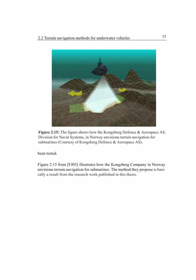
Figure 2.15: The figure shows how the Kongsberg Defence & Aerospace AS,Division for Naval Systems, in Norway envisions terrain navigation forsubmarines (Courtesy of Kongsberg Defence & Aerospace AS).
been tested.
Figure 2.15 from [FJ03] illustrates how the Kongsberg Company in Norwayenvisions terrain navigation for submarines. The method they propose is basi-cally a result from the research work published in this thesis.
2.2 Terrain navigation methods for underwater vehicles

36 2 Terrain navigation methods

37
3.1 IntroductionThe global positioning system (GPS) has implied a revolution within land, airand sea navigation during the last decades. Unfortunately this does not includenavigation of underwater vehicles as submarines or autonomous underwatervehicles since the GPS signal does not penetrate into the sea. Underwater vehicleshave therefore still to rely on dead reckoning, gyro compass or inertial navigation,see Appendix A.
Inertial navigation has the great advantage to be independent of external signalsand is by that very attractive in military applications where the threat of jammingis a great problem. However, inertial navigation has a great problem in the gyrodrift and biases in the gyros and accelerometers. Inertial navigation forsubmarines where low drift system is an absolute requirement is very costly andthe system has to be re-initiated regularly with an accurate position. This can ofcourse be done by a differential GPS position but there is always a risk of beingdetected or that the GPS signal is jammed. Terrain navigation is a possibility foran underwater vehicle to establish a position fix without breaking the sea surface.
Chapter 3
The positioning method

38 3 The positioning method
Terrain navigation and inertial navigation techniques can be said to be asuccessful couple since they are complementary with regard to the positionerrors and they both share the characteristic of being resistant to jamming.Hence they together make a system which is negligible revealing.
Terrain navigation has up to today not been used to any larger extent forunderwater vehicles but that is certainly due to lack of high quality underwatermaps. However, the GPS system together with the multibeam bathymetric sonarhas also brought a revolution into mapping of the underwater world. The costtoday to chart an underwater area is only a fraction of what it was some decadesago and the underwater maps are of a quality that was not reached before.However, the extent of the mapped areas are still very limited and will so be for along time ahead. Remember that more than 70 % of the earth surface is sea area.
Some terrain navigation attempts [NY99, BER93, JMHP04, SCA99] have howeverbeen done with multibeam sonars and methods similar to the TERCOM methodwhich was early implemented in the Tomahawk cruise missiles [MUOT82]. Oneof the problems that has to be handled if the positioning is to be successful isthe problem with multiple correlation peaks.
Figure 3.1 shows a typical matching result when a beam plane of 60 sonarbeams are matched against an underwater map of size 5 km x 5 km. The peaks inthe figure correspond to positions where the measured profile well agrees with
Figure 3.1: Correlation peaks when matching with one beam plane.

39
the map. As can be seen there are many likely positions for the vehicle.However, if the matching is done simultaneously with several beam planes asFigure 3.2 indicates the result will be very different as can be seen in Figures3.3 and 3.4. The distance between the beamplanes is 10 - 20 meters. As will beshown later the number of likely positions will decrease exponentially with thenumber of measurement beams.
Figure 3.2: The principle for assembling several beam planes from a bathymetricsonar to form a 3D measurement of the bottom topography.
3.1 Introduction
Figure 3.3: Correlation peaks whenusing two beamplanes.
Figure 3.4: Correlation peaks whenusing three beamplanes.

40 3 The positioning method
The measurement of the bottom topography, according to the proposedmethod, should be done by a true 3D sonar. In some cases the 3D picture ofthe bottom may be constructed by assembling beam planes from a bathymetricsonar. In this case, however, there will be an error in the distance between thebeam planes and the angle between the planes and the performance willtherefore be degraded. These errors will however be very small if theapproximate method is applied to a submarine. A submarine has a very largemass (~1600 ton or more) so the changes in speed or course during the samplingtime of the bottom profile will be very small if the submarine is held on a steadycourse. This has also been the experience of the sea-trials that have beenconducted with surface ships.
The problem with lack of high quality underwater maps can to some extent besolved by the same method that was used, and still is in use, in the early daysof cruise missiles. The INS is only updated in special areas called navigationcells which are chartered and have good properties for terrain navigation. Thenavigation technique is therefore especially valuable for planned vehicleoperations of considerable duration such as reconnaissance operations.
3.2 The positioning methodNavigation according to the proposed method is therefore that the vehiclemoves between so-called “navigation cells,” as shown in Figure 3.5, with thehelp of the conventional navigation system such as INS, or dead reckon/Doppler-log. When the vehicle is, according to its navigation system, withinthe navigation cell it determines its position by measuring the bottom 3Dtopography with a large number of sonar beams over a large bottom area as inFigure 3.6. The measured area typically has the size of 40 m x 40 m to 300 m x 300m depending on the actual depth. The bottom topography is then matchedwith the underwater map by comparing the measurement with the map at everypoint in the map.
The proposed navigation method has some important characteristics [NY01a,NY01b, NY02, NY99, NYJA04a, NYJA04b, NYJA04c, JCNY05]:
• Robustness with respect to the navigation filter divergence

41
Figure 3.6: The bottom topography measurement with the correlation method.The vehicles are measuring the bottom topography by several sonar beams.Likely positions are positions with the same bottom topography.
Figure 3.5: A map with indicated navigation cells.
3.2 The positioning method

42 3 The positioning method
• Low requirements on availability and quality of underwater maps• Very low risk of revealing when a 3D-sonar is used since the
duration of the sonar ping is ~1 ms.• Very high accuracy of the position• Ability to determine own bearing• High ability to determine the position in flat bottomed areas• Ability to do own mapping of the bottom topography.
Other important characteristics are:
• Very low initialization requirements• The system can be used by a stationary vehicle• Very short time for a position fix from a non-initiated system
Most of these characteristics will be shown to be true in the coming chapters.
The vehicle position is thus established by computing the correlation sum forevery point in the map and taking the position with the minimum correlationsum as the true position. The correlation sum in a map position is
2,
1
( ) ( ( ))N
t t k k tk
T y h=
= −∑x x (3.1)
That is, calculating the sum of the squared differences of the measured depth,t ky at sonar beam k with the corresponding map depth ( )k th x at beam k at
position tx . The measurement is done at time t. The number of measurementbeams is N. By letting the depth values be deviations from the respective meanvalues, the bottom profiles are compared and the influence of the actual sealevel is eliminated. However, it should be noted that the absolute depth valueoccasionally may be needed for a unique position.
We know from Chapter 2 that the PDF for the position is the result of multiplicationof the prior PDF and a likelihood function
1 1 1 1 1( | ) ( ; ) ( | )t t t t t tp L p+ + + + +x Y x y x Y∼ (3.2)
It is therefore of interest and quite illustrative to look at the shape of the likeli-hood function calculated according to (2.8) and the posterior PDF at differentnumbers of measurement beams to see the great difference between using only

43
one beam as in single beam methods, the traditional method, and using themany beam method as proposed in this thesis.
Figure 3.7 shows the non-normalized likelihood function for a measurementwith only one beam, which is the usual way that the measurement is done interrain navigation. Figure 3.8 shows the likelihood function corresponding to ameasurement with 9 x 9 beams. The size of the map is 4 x 4 km in both cases. Itcan be seen from the figures that the larger number of beams drastically reducesthe number of likely positions. It will be shown in Chapter 4 that the secondaryfalse correlation peaks are due to terrain repeatability and that they will de-crease exponentially with the number of measurement beams, i.e., the size of the
Figure 3.10: The measurementupdated prior for 9 x 9 measurementbeams.
Figure 3.9: The measurementupdated prior for one measurementbeam.
Figure 3.8: Likelihood function whenusing 9 x 9 measurement beams.
Figure 3.7: Likelihood function whenusing one measurement beam.
3.2 The positioning method

44 3 The positioning method
correlation area properly sampled. The reason for naming them to be false is thatthey disappear when N tends to infinity and there will only be one peak left, thetrue position.
3.3 The Bayesian and the maximum likelihoodmethod (ML)3.3.1 An illustrating exampleAn underwater vehicle is assumed to move from a position A to a position B bythe help of an inertial navigation system (INS). When the vehicle assumes it isin position B it measures the depth for aiding in the determination of the posi-tion. Figure 3.11 shows the bottom profile at position B.
By assuming error distributions of the position errors of the INS-system and thedepth measurement we can simulate the journey from A to B by a Monte Carloexperiment. Figures 3.12 and 3.13 show the joint PDF of position and depthmeasurement from an experiment with Gaussian error distributions. In the con-tour plot Figure 3.13 the line p(x,y=ym) represents the outcomes of the experi-ment that have the measured depth ym, i.e., p(x|y=ym)p(y=ym). The likelihoodfunction at position x is the relative frequency of the outcomes at position x thathas the measured depth ym , i.e., p(x,y=ym)/p(x).
Let us now extend the Monte Carlo experiment by also examining the positionaccuracy. The likelihood function (2.8) can also be seen as the likelihood func-tion in maximum likelihood estimation (ML). Figure 3.14 shows the outcome ofthis part of the maximum likelihood experiment. The likelihood function is calcu-
Figure 3.11: The bottom profile around position B. Alternative possiblepositions according to the measurement are indicated.

45
lated using N=51 measuring beams instead of 1 beam as in the previous experi-ment. The likelihood function will differ slightly from realization to realizationand in the figure the mean of all realizations is shown. From the figure we clearlysee that the maximum likelihood estimation gives a much better accuracy than
Figure 3.12: Illustration of the joint probability density function, centeredaround position B, of the position and the measured depth.
Figure 3.13: A contour plot of the joint density function p(x,y) of position anddepth in Figure 3.12.
3.3 The Bayesian and the maximum likelihood method (ML)

46 3 The positioning method
indicated by the mean likelihood function which is natural since the horizontalposition of each individual likelihood function varies according to the posi-tions given by the histogram. The Cramér-Rao lower bound, see Chapter 5,gives 6.29 as the lowest error variance we can achieve and we reached 6.46. Theerror distribution is asymptotically Gaussian, that is when the number of trialstends to infinity it will become Gaussian. We conclude from the figure that weare close to the asymptotic distribution.
Instead of the Bayesian estimation thinking we can perceive the situation ashaving two measurements of the position at B, one from the INS-system andone from the maximum likelihood estimation. A way of fusing the measure-ments together is to use the linear fusing method discussed in Section 3.3.2which will give a minimum variance estimate of the position.
Since the linear fusing method will give the smallest position error variance, wewill use this method in the practical estimation of the position. The involveddistributions are also close to Gaussian due to the large number of measuring
Figure 3.14: A histogram for the outcomes of the Monte Carlo positioningexperiment. The dotted curve is the mean of the likelihood functions for eachoutcome. The variance calculated from the mean likelihood function is 10.7.

47
beams we are typically using (~400).
We may interpret the situation as follows. When we are in position A all we cansay about our future position at B is contained in the joint PDF of the positionand an assumed future measurement. However, when we are in position B ourposition is no longer stochastic but deterministic but unknown by us. Even ifwe do not know the position ourself others may know it and by that it is strictlynot stochastic any more. We are thus in a position to estimate the position bylinearly fusing the positions given by the INS-system and the maximum likeli-hood estimation method.
3.3.2 The linear fusing methodLinear fusing is a way to present the Kalman equations when several sensordata are fused together into a single mesurement. The method means that a newestimate is formed by a linear combination of independent unbiased estimates.The linear fusing method is equivalent to the linear Kalman filter. In the case wehave two estimates of the position we calculate the fused estimate of 1 2ˆ ˆ and x x as[KSH00, CANY05]
1 1 2 2 1 2ˆ ˆ ˆ{ } { } { } ( )E E E= = + = +µ x A x A x A A µ (3.3)
The new estimate should be unbiased
1 1 2 2ˆ ˆ ˆ{ } { } { }E E E= +x A x A x (3.4)
which gives
1 2+ =A A I (3.5)
The covariance of the fused estimate is
1 1 2 2 1 1 2 2ˆ ˆ ˆ ˆ ˆ ˆ ˆ ˆ ˆ ˆ1 1 2 2 1 1 1 1( ) ( )T T T T= + = + − −xx x x x x x x x xP A P A A P A A P A I A P I A (3.6)
which is quadratic in A1. Completing the square gives the minimum trace ofthe covariance matrix for
3.3 The Bayesian and the maximum likelihood method (ML)

48 3 The positioning method
2 2 1 1 2 2
1ˆ ˆ ˆ ˆ ˆ ˆ1
− = + x x x x x xA P P P (3.7)
1 1 1 1 2 2
1ˆ ˆ ˆ ˆ ˆ ˆ2
− = + x x x x x xA P P P (3.8)
and the minimum covariance of the fused estimator as
1 1 2 2
1 1 1ˆ ˆ ˆ ˆ ˆ ˆ− − −= +xx x x x xP P P (3.9)
and the fused estimate as
2 2 1 1 2 2 1 1 1 1 2 2
1 1ˆ ˆ ˆ ˆ ˆ ˆ ˆ ˆ ˆ ˆ ˆ ˆ1 2ˆ ˆ ˆ
− − = + + + x x x x x x x x x x x xx P P P x P P P x (3.10)
By recursion the expressions in (3.9) and (3.10) can easily be generalized to Mmeasurements
1 1ˆ ˆ ˆ ˆ
1i i
M
i
− −
=
= ∑xx x xP P (3.11)
1ˆ ˆ ˆ ˆ
1
ˆ ˆi i
M
ii
−
=
= ∑xx x xx P P x (3.12)
Assume now, to begin with, that the frequency distributions p1 and p2 of
1 2ˆ ˆ and x x , respectively, are Gaussian with dimension n. We multiply the PDF’s
( )
( )
1 1
1 1
2 2
2 2
1 2
1ˆ ˆ1 1
ˆ ˆ
1ˆ ˆ2 2
ˆ ˆ
( ) ( ) ( )1 1 ˆ ˆ exp( ( ) ( ))
22 det( )
1 1 ˆ ˆ exp( ( ) ( ))22 det( )
Tn
Tn
p p p
π
π
−
−
=
= − − −
⋅ − − −
x x
x x
x x
x x
x x x
x x P x xP
x x P x xP
(3.13)
and it is well known [AN79, MA82a] that this function, when normalized, is aGaussian PDF with a covariance and a mean of

49
21 1
ˆ ˆ ˆ ˆ1
i i
M
i
=− −
=
= ∑xx x xP P (3.14)
21
ˆ ˆ ˆ ˆ1
ˆ ˆi i
M
ii
=−
=
= ∑xx x xx P P x (3.15)
The linear fusion can thus also be seen as a multiplication of the PDFs if theinvolved PDFs are Gaussian.
However, since no explicit expression is known for the variance of the maximumlikelihood estimate (MLE) we have to resort to the Cramér-Rao expression forthe variance. This will in many cases give an accurate approximation of thevariance of the maximum likelihood estimate since the convergence towardsthe Cramér-Rao limit is mostly quite fast [AZ96, KA93]. The matter will befurther touched on in Chapter 6 and 8 where some graphs will show the rapidconvergence in our case.
3.3.3 Multiple likelihood peaksThe difference between the Bayesian method and the linear fusing of the priorPDF and the maximum likelihood estimate is illustrated in Figure 3.15 where astep in the Bayesian recursion is illustrated. To the left in the figure is theprevious estimated PDF for the position and to the right is that PDF propa-gated and it is our estimated position PDF before our measurement of theposition. Now assume that our measurement gives a bimodal likelihood func-tion due to terrain repeatability. The right peak of the likelihood function hasthe highest amplitude and from our knowledge of the measurement error weconclude that the highest peak indicates our position with high probability.Still, after fusing the likelihood function and the prior position PDF the left peakwill give the maximum posterior position. The mean position would be betweenthe peaks but close to the left peak. The Bayesian approach will thus givedifferent positions depending on if the mean or the maximum a posterior (MAP)position is used as the estimated position. It may also give a position whichhas a low probability according to the measurement. The maximum likelihoodestimation, which is asymptotically unbiased, will choose the higher peak asthe true one and the linear fusing method will thus fuse this peak with the priorposition PDF. This estimated position will thus differ from the one estimated bythe Bayesian approach.
3.3 The Bayesian and the maximum likelihood method (ML)

50 3 The positioning method
In Chapter 4 it will be shown that not only the probability of wrong position dueto false peaks will decrease exponentially but also that the amplitudes of thefalse peaks will decrease exponentially with the number of measurement beams.
Figure 3.15: Illustration of the prior position PDF and a bi-modal likelihoodfunction.
Figure 3.16: Illustration of the posterior (measurement updated prior)position PDF .

51
Figures 3.9 and 3.10 show the non-normalized measurement-updated PDF for areal map. A comparison between figures shows that the variance is much smallerwhen correlation with many measurement beams is used.
If we look closer at the correlation peak in Figure 3.10 we will find that it isapproximately a Gaussian curve. Figure 3.17 shows the N-normalized likelihoodfunction from a positioning in a sea-trial and the Gaussian shape is clearlyvisible. The curve in Figure 3.17 is N-normalized, i.e., if the curve is self-multi-plied N times (the number of beams) we will have the true likelihood function. Itwill be shown in Chapter 4 that the likelihood function converges to a Gaussianfunction when the number of measurement beams tends to infinity. It will alsobe shown that this Gaussian curve, if normalized to have unit volume, willasymptotically coincide with the PDF of the estimation error in the maximumlikelihood estimation. That is, the unit normalized likelihood function when thenumber of measurement beams is large will also be the PDF for the positionerror.
If the time between the measurements is large the variance in the propagatedPDF, ( )p− x , may increase so much that it will not noticeably improve theestimation of the position based on the likelihood function. A typical RMS-error of the prior PDF in submarine applications may be ~3000 meter whilemaximum likelihood estimation gives an RMS-error of, say, less than a meter.
Figure 3.17: A typical N-normalized likelihood function from a sea-trial (400beams).
3.3 The Bayesian and the maximum likelihood method (ML)

52 3 The positioning method
Hence, when the prior PDF has a large variance, the estimation problem becomesa maximum likelihood estimation problem without prior PDF.
A problem both in the Bayesian method and the linear fusing method is theproblem with multiple peaks, false peaks, due to terrain repeatability since thelikelihood function (2.8) is not a one to one function, see Figure 3.11. Figure 3.18shows a terrain profile and the vehicle measures the depth y when it is in theposition x0. The PDF for the measurement error is assumed to be symmetric withcut tails. Positions outside the range of the PDF can not be explained by themeasurement error and the likelihood function for the true position which is theone marked with x0 in the figure.
Now, as can be seen from Figure 3.18 there are other positions that will give thesame depth measurement but of course the vehicle can only be at one place ata time. As common in the Bayesian method to use the mean as the probableposition may lead to an estimated position between the peaks of the posteriorPDF with no likelihood. This is not acceptable from a physical standpoint.
Therefore all likely positions according to the likelihood function have to beevaluated one by one. A technique for handling such situations is track split-ting which is frequently used in tracking of flying objects [BSFO88]. In thistechnique parallel tracks are formed and as soon as a track is found false it isterminated. However, this is not as easy as expected and does not give ananswer in real time about which peak represents the true position which may be
Figure 3.18: The figure illustrates how false likelihood peaks arise due to terrainrepeatability. True position is x0.

53
needed by the guidance system because its action may depend on the estimatedposition.
In practice the individual PDFs for the measured position candidates may not beso well separated as assumed above. However, we can draw the important con-clusion that in Bayesian terrain navigation the maximum a posteriori (MAP)position estimate is to prefer instead of the mean estimate when the posterioriPDF has multiple peaks [GDW00]. Then we note that the linear fused estimate isnot so influenced by false peaks as the Bayesian MAP position if the peaks arenot so well separated. We also note that a position variance calculation basedon the variance of the Bayesian posterior PDF is influenced by false peaks.False peaks will also give a position bias if the position is calculated as the meanof the Bayesian posterior. It is only when we have a large number of measure-ment beams that the two methods of calculation of the position and positionerror will coincide. A broad discussion about the role of the mean-measure andother measures in Bayesian inference can be found in [HAFO04]. In [CA88]multiple peaks in maximum likelihood estimation are discussed.
3.4 Concluding remarks about the basic ter-rain navigation methodDetermining the position of underwater vehicles using the proposed correlationmethod has been studied over the past years. The correlation method has provento be robust, highly precise and minimally revealing. It is also easily implementedand demands a minimum of underwater maps.
The proposed method do only terrain positioning in the navigation cells but, ofcourse, the method is also suitable for continuous navigation if the requiredmaps are available.
The terrain positioning can easily be aided by side-scan and sediments maps orby directions to external sound sources since likelihood functions fromindependent measurements are simply fused by multiplications if the processesare Markov which they often can be considered to be.
3.4 Concluding remarks about the basic terrain navigation method

54 3 The positioning method
3.5 A way of implementing the approximatemethodWhen an approximate 3D picture of the bottom is to be assembled from severalbeam planes it is also possible to correlate each beam plane against theunderwater map separately at each ping and then join them together. This willshorten the time delay for a position estimate after the last ping. Figure 3.19shows the beam footprint pattern from 5 beam planes which are moved around,as a packet, in the map to find the position where it fits the best. The best fit isconsidered to be the position where the correlation function
2
1
( , ) ( ( ) )N
i ii
T d y h d=
= − −∑x x (3.16)
has its minimum. In the expression yi is the measured depth at beam i and hi(x)is the corresponding depth according to the map in position x and d is thedifference between the actual sea level and the reference level of the map (themeasurement bias). The total number of beams is N.
Usually the correlation function (3.16) is calculated for all beam planes at oncebut the correlation function can also be written as
Figure 3.19: Beam footprint pattern from five beamplanes to be moved aroundin the map.
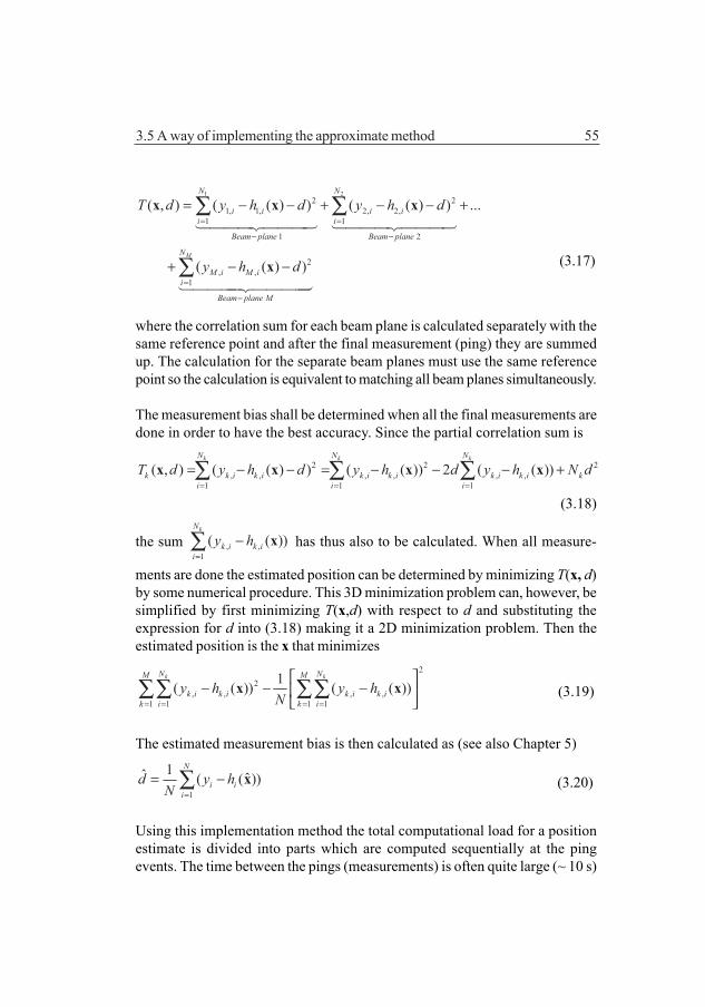
55
1 22 2
1, 1, 2, 2,1 1
1 2
2, ,
1
( , ) ( ( ) ) ( ( ) ) ...
( ( ) )M
N N
i i i ii i
Beam plane Beam plane
N
M i M ii
Beam plane M
T d y h d y h d
y h d
= =
− −
=
−
= − − + − − +
+ − −
∑ ∑
∑
x x x
x (3.17)
where the correlation sum for each beam plane is calculated separately with thesame reference point and after the final measurement (ping) they are summedup. The calculation for the separate beam planes must use the same referencepoint so the calculation is equivalent to matching all beam planes simultaneously.
The measurement bias shall be determined when all the final measurements aredone in order to have the best accuracy. Since the partial correlation sum is
2 2 2, , , , , ,
1 1 1
( , ) ( ( ) ) ( ( )) 2 ( ( ))k k kN N N
k k i k i k i k i k i k i ki i i
T d y h d y h d y h N d= = =
= − − = − − − +∑ ∑ ∑x x x x
(3.18)
the sum , ,1
( ( ))kN
k i k ii
y h=
−∑ x has thus also to be calculated. When all measure-
ments are done the estimated position can be determined by minimizing T(x, d)by some numerical procedure. This 3D minimization problem can, however, besimplified by first minimizing T(x,d) with respect to d and substituting theexpression for d into (3.18) making it a 2D minimization problem. Then theestimated position is the x that minimizes
22
, , , ,1 1 1 1
1( ( )) ( ( ))k kN NM M
k i k i k i k ik i k i
y h y hN= = = =
− − −
∑∑ ∑∑x x (3.19)
The estimated measurement bias is then calculated as (see also Chapter 5)
1
1ˆ ˆ( ( ))N
i ii
d y hN =
= −∑ x (3.20)
Using this implementation method the total computational load for a positionestimate is divided into parts which are computed sequentially at the pingevents. The time between the pings (measurements) is often quite large (~ 10 s)
3.5 A way of implementing the approximate method

56 3 The positioning method
so there will be sufficient time for the calculations even if a general computer isused for the calculation. Another advantage is that the position accuracy canbe monitored as a function of the number of measurements (pings) by calculationof the Hessian in the position of maximum of the likelihood function. This is ofinterest since assembling of beam planes for forming a 3D picture of the bottomis just an approximation. When assembling beam planes there will always be astochastic error in the distance and angle between the beam planes. The moreplanes that are added the larger will the error between the first and the lastplane be. It is thus of interest to use as few beamplanes as possible. In the sea-trial that has been conducted, with the equipment that has been used, thenumber of beam planes should not be more than 11if the distance between theplanes is 25 meter. An increase above that will in most cases not improve theposition accuracy. By studying the Hessian after each measurement it is possibleto interrupt the collection of beam planes when the increase in accuracy fallsbelow some value.
3.6 Comparison between the single beam mis-sile method and the correlation methodThe main purpose of the correlation method in recursive applications is to makea linear Kalman filter feasible, to achieve high position accuracy and robust-ness. Therefore the method, even in a recursive application with dense sam-pling, always uses a large number of measuring beams. However, even for anequal total number of measurement beams, the correlation method will alwaysgive a smaller position error compared to the traditional terrain navigation methodwith a single measuring beam. This because the distances between the foot-prints of the measurement beams are random variables in the single beam meth-ods but fix known values in the correlation method.
The implication of this can easily be illustrated in the one-dimensional case. Ifwe look at a single beam method as a batch method we collect N depth measure-ments. Then we perform a correlation against the map and we will have a situa-tion as depicted in Figure 3.20. In the correlator method we have fixed knowndistances between the nominal sampling points which are indicated by circles inthe figure. In the single beam methods we have errors in determining our posi-tion and these errors are indicated by εk. These position errors will cause errorsin the map heights determination.
A first order approximation will give us the likelihood function
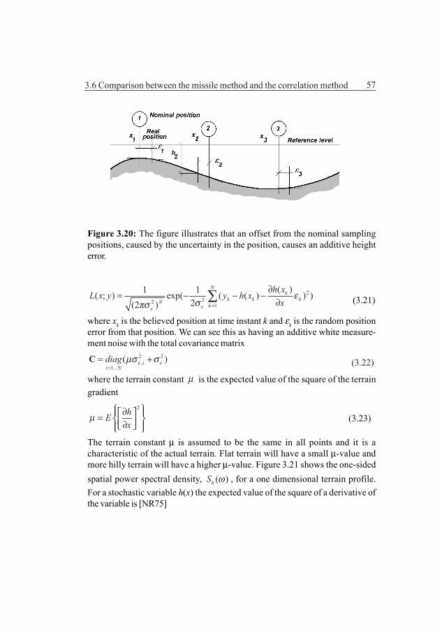
57
222
1
( )1 1( ; ) exp( ( ( ) ) )2(2 )
Nk
k k kNkee
h xL x y y h x
xε
σπσ =
∂= − − −
∂∑ (3.21)
where xk is the believed position at time instant k and εk is the random positionerror from that position. We can see this as having an additive white measure-ment noise with the total covariance matrix
2 2,
1...( )i e
i Ndiag εµσ σ=
= +C (3.22)
where the terrain constant µ is the expected value of the square of the terraingradient
2hEx
µ ∂ = ∂
(3.23)
The terrain constant µ is assumed to be the same in all points and it is acharacteristic of the actual terrain. Flat terrain will have a small µ-value andmore hilly terrain will have a higher µ-value. Figure 3.21 shows the one-sidedspatial power spectral density, ( )hS ω , for a one dimensional terrain profile.For a stochastic variable h(x) the expected value of the square of a derivative ofthe variable is [NR75]
3.6 Comparison between the missile method and the correlation method
Figure 3.20: The figure illustrates that an offset from the nominal samplingpositions, caused by the uncertainty in the position, causes an additive heighterror.

58 3 The positioning method
22
0
( ) ( )n
n
hn
hn E S dx
µ ω ω ω∞ ∂ = = ∂ ∫ (3.24)
Figure 3.21: The figure shows the spatial one-sided power spectral density fora terrain profile.
Figure 3.22: The position error variance as a function of the position error variancein sampling of the terrain topography. Synthetic AR(1) terrain with a pole in 0.98.

59
The spectrum of a terrain profile can often be assumed to have an exponentialform 0 0( ) exp( / )hS Sω ω ω= − where 0ω is a characteristic of the actual terrain.In such a case we have
30 02Sµ ω= . (3.25)
We note the heavy dependence on the high frequency content in the terrainprofile. The assumption of the same µ-value for all sampling points will give thefollowing simple expression for position the error covariance matrix in the twodimensional case
12
1 11 1 22 2 2
1 12 1 2
( )
N Ni i i
i iSingle beam e
N Ni i i
i i
h h hx x x
h h hx x x
εσ µσ
−
= =
= =
∂ ∂ ∂ ∂ ∂ ∂ = + ∂ ∂ ∂ ∂ ∂ ∂
∑ ∑
∑ ∑R
(3.26)
or2
2(1 )Single beam ETLe
εσµ
σ= +R R (3.27)
where RETL is the position error covariance for the proposed method. Chapter 5and 6 will go into the details of the expression. The orders of the two terms inthe first factor of (3.26) are about the same in flat areas so even for the samenumber of measuring beams the correlator method clearly gives smaller positionerrors. Figure 3.22 shows how the resulting position error varies with the positionerror in sampling the terrain topography. The figure shows the result from a onedimensional Monte Carlo simulation with a synthetic AR(1) terrain topography.
Figure 3.22 seems to indicate that the relation should be more quadratic insteadof linear but in (3.21) we have only included the linear term, adding another termin the Taylor expansion would add a quadratic term as well. The expression alsoexplains why the performance of the missile method in rough terrain is lowerthan expected from the terrain roughness only. The expression (3.26), given theassumptions made, is formally equivalent to the solution of the algebraic Riccatiequation for the estimation error in linear Kalman filtering.
The difference in accuracy between the two methods can also be illustrated inthe 1D-case if we make some approximations. It follows from the central limittheorem that the expected function of the likelihood function is a Gaussian
3.6 Comparison between the missile method and the correlation method

60 3 The positioning method
function. If we therefore replace the likelihood function, when we measure withonly one beam, with its expected Gaussian function and assume that the vehicleposition at the sampling event has a Gaussian error, we can directly apply theequations for the linear Kalman filter (see Chapter 4). We also assume that thelikelihood function and the position error PDF are the same at all sampling events.The starting PDF is assumed to have a variance of 2
0σ and it is assumed thatduring the propagation it will broaden to 2
0ασ where α>1. The likelihoodfunction, normalized to a PDF, is assumed to have a variance of 2
Lσ . The posteriorPDF will therefore have the following variance according to the “parallel resistorformulae” for adding variances
2 2 20
1 1 1
Lσ ασ σ= + (3.28)
If we now simplify our discussion by assuming that the propagation constantand likelihood function will be the same in all following steps we will come to thefollowing result
2 2 2 10
1 1 1 1 1 1N N NLσ α σ σ α α −
= + + + + …
(3.29)
For infinitely many steps we will have
Figure 3.23: Illustration of a recursive step under the simplified assumptionsgiven in the text.The posterior PDF and the likelihood function almost coincide.
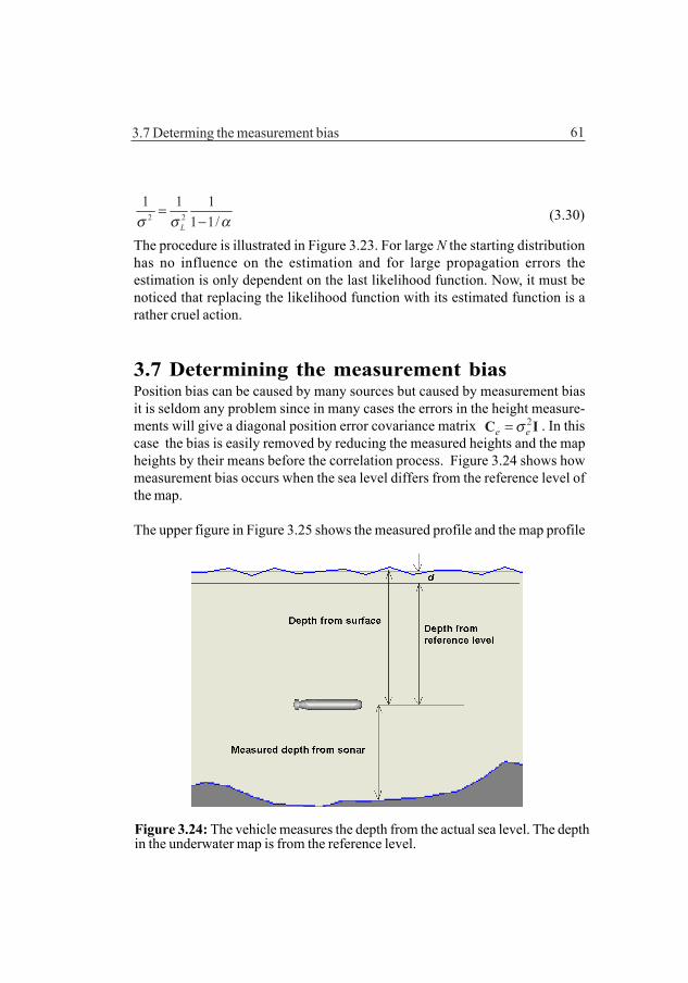
61
2 2
1 1 11 1/L ασ σ
=− (3.30)
The procedure is illustrated in Figure 3.23. For large N the starting distributionhas no influence on the estimation and for large propagation errors theestimation is only dependent on the last likelihood function. Now, it must benoticed that replacing the likelihood function with its estimated function is arather cruel action.
3.7 Determining the measurement biasPosition bias can be caused by many sources but caused by measurement biasit is seldom any problem since in many cases the errors in the height measure-ments will give a diagonal position error covariance matrix 2
e eσ=C I . In thiscase the bias is easily removed by reducing the measured heights and the mapheights by their means before the correlation process. Figure 3.24 shows howmeasurement bias occurs when the sea level differs from the reference level ofthe map.
The upper figure in Figure 3.25 shows the measured profile and the map profile
3.7 Determing the measurement bias
Figure 3.24: The vehicle measures the depth from the actual sea level. The depthin the underwater map is from the reference level.
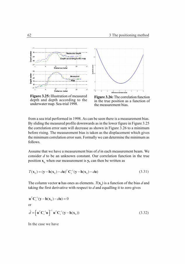
62 3 The positioning method
from a sea trial performed in 1998. As can be seen there is a measurement bias.By sliding the measured profile downwards as in the lower figure in Figure 3.25the correlation error sum will decrease as shown in Figure 3.26 to a minimumbefore rising. The measurement bias is taken as the displacement which givesthe minimum correlation error sum. Formally we can determine the minimum asfollows.
Assume that we have a measurement bias of d in each measurement beam. Weconsider d to be an unknown constant. Our correlation function in the trueposition x0, when our measurement is y, can then be written as
10 0 0( ) ( ( ) ) ( ( ) )T
eT d d−= − − − −x y h x u C y h x u (3.31)
The column vector u has ones as elements. T(x0) is a function of the bias d andtaking the first derivative with respect to d and equalling it to zero gives
10( ( ) ) 0T
e d− − − =u C y h x uor
11 10
ˆ ( ( ))T Te ed
−− − = − u C u u C y h x (3.32)
In the case we have
Figure 3.25: Illustration of measureddepth and depth according to theunderwater map. Sea-trial 1998.
Figure 3.26: The correlation functionin the true position as a function ofthe measurement bias.

63
2 2,1 ,( , , )e e e Ndiag σ σ=C
02 2 2, , ,1 1 1
1 1 1ˆ ( )N N N
i ie i e i e ii i i
d y hσ σ σ= = =
= −
∑ ∑ ∑x (3.33)
and if we have the same measurement uncertainty in all beams
0 01 1
1 1ˆ ( ) ( )N N
i ii i
d y h y hN N= =
= − = −∑ ∑ x x (3.34)
where the scalars y and h are the mean values of the elements in respectivevector. The true position may be situated between the steps in the matchingprocess and in this case the above estimation of the measurement bias will notbe correct. However, the error due to that may often be neglected.
3.8 Incorporation of sediment data in thecorrelation3.8.1 IntroductionEven if the proposed correlation method increases the navigation performancesubstantially in flat bottom areas compared to single beam methods there will ofcourse be a limit when the method no longer is sufficient for establishing aposition. One way to push this limit is to also include the sediment profile orside-scan pictures in determining the position.
Whether our estimation is to be considered as Bayesian or a linear fusingprocess it is easy to include disparate independent measurements of the stateof a Markov process since for a Markov process we have the conditional PDF
1 2 1 2( | , ,..., ) ( | ) ( | )... ( | )N Np x y y y p x y p x y p x y= (3.35)
and thus for the likelihood function
1 2 1 1 2 2( ; , ,..., ) ( ; ) ( ; )... ( ; )N NL x y y y L x y L x y L x y= (3.36)
3.8 Incorporation of sediment data in the correlation

64 3 The positioning method
Not only physical measurements but also subjective information can be usedfor formulating a likelihood function. If the measurements are not independentthat has to be taken into account.
3.8.2 Incorporation of sediment dataFlat bottom areas are often characterized by soft sediment layers and sedimentrocks (here taken together as sediment layers) on a more hilly rough crystallineunderground of primary rock or moraine ridges, or similar objects, from the lastglacial period. The ridges may have been created at the edge of the ice cap orcreated by ice river deltas. The Baltic sea, for which the navigation method has
Figure 3.28: An example of a parametric sonar manufactured by Innomar, Ger-many. Secondary frequency 4...12 kHz and penetration depth down to 50 meter.Size 250 x 350 x 80 mm.
Figure 3.27: The sediment profile along a line in the test area during the October2002 sea-trial.

65
been developed and tested in, has also during the millenniums undergone manydifferent courses of events as sea and inland sea to what it is today as abrackish sea. The size has also varied through the millenniums. During thedifferent time periods different kinds of sediments have been deposited on thebottom and by that created a profile structure which varies with the location(Figure 3.27). A general description about the sediment structures in the Swed-ish coastal waters can be found in [CKN92].
Figure 3.29: Sediment profile at way-point 2C in the October 2002 sea-trial. Notethat the vertical scale is exaggerated, see Figure 3.30.
Figure 3.30: The picture shows an area, 200 meter x 200 meter, around way-pointBP2C in the October 2002 sea-trial.
3.8 Incorporation of sediment data in the correlation
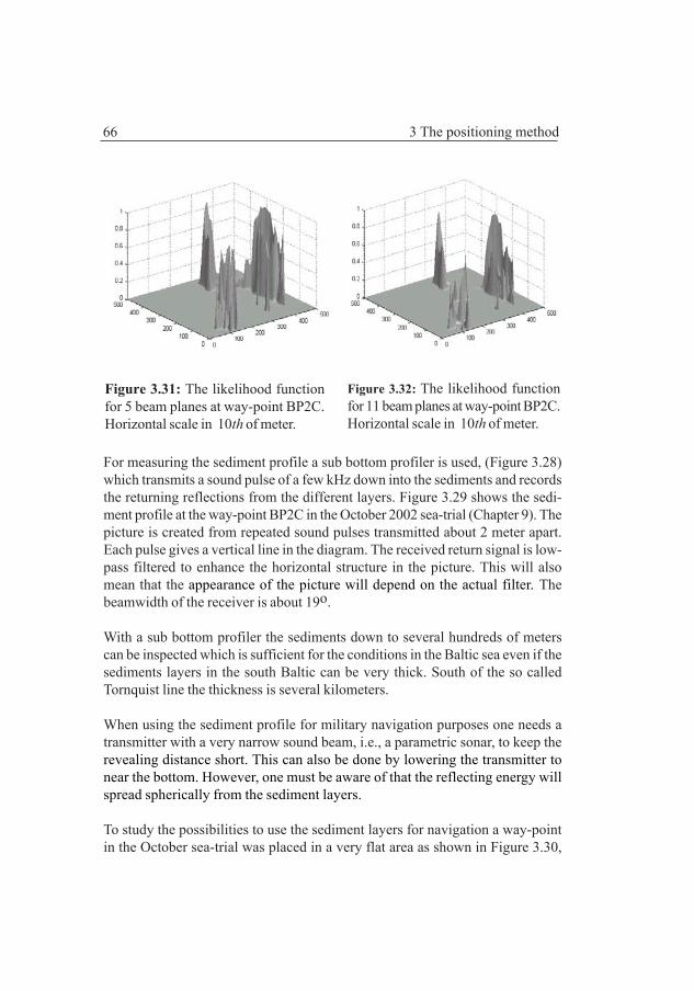
66 3 The positioning method
For measuring the sediment profile a sub bottom profiler is used, (Figure 3.28)which transmits a sound pulse of a few kHz down into the sediments and recordsthe returning reflections from the different layers. Figure 3.29 shows the sedi-ment profile at the way-point BP2C in the October 2002 sea-trial (Chapter 9). Thepicture is created from repeated sound pulses transmitted about 2 meter apart.Each pulse gives a vertical line in the diagram. The received return signal is low-pass filtered to enhance the horizontal structure in the picture. This will alsomean that the appearance of the picture will depend on the actual filter. Thebeamwidth of the receiver is about 19o.
With a sub bottom profiler the sediments down to several hundreds of meterscan be inspected which is sufficient for the conditions in the Baltic sea even if thesediments layers in the south Baltic can be very thick. South of the so calledTornquist line the thickness is several kilometers.
When using the sediment profile for military navigation purposes one needs atransmitter with a very narrow sound beam, i.e., a parametric sonar, to keep therevealing distance short. This can also be done by lowering the transmitter tonear the bottom. However, one must be aware of that the reflecting energy willspread spherically from the sediment layers.
To study the possibilities to use the sediment layers for navigation a way-pointin the October sea-trial was placed in a very flat area as shown in Figure 3.30,
Figure 3.31: The likelihood functionfor 5 beam planes at way-point BP2C.Horizontal scale in 10th of meter.
Figure 3.32: The likelihood functionfor 11 beam planes at way-point BP2C.Horizontal scale in 10th of meter.
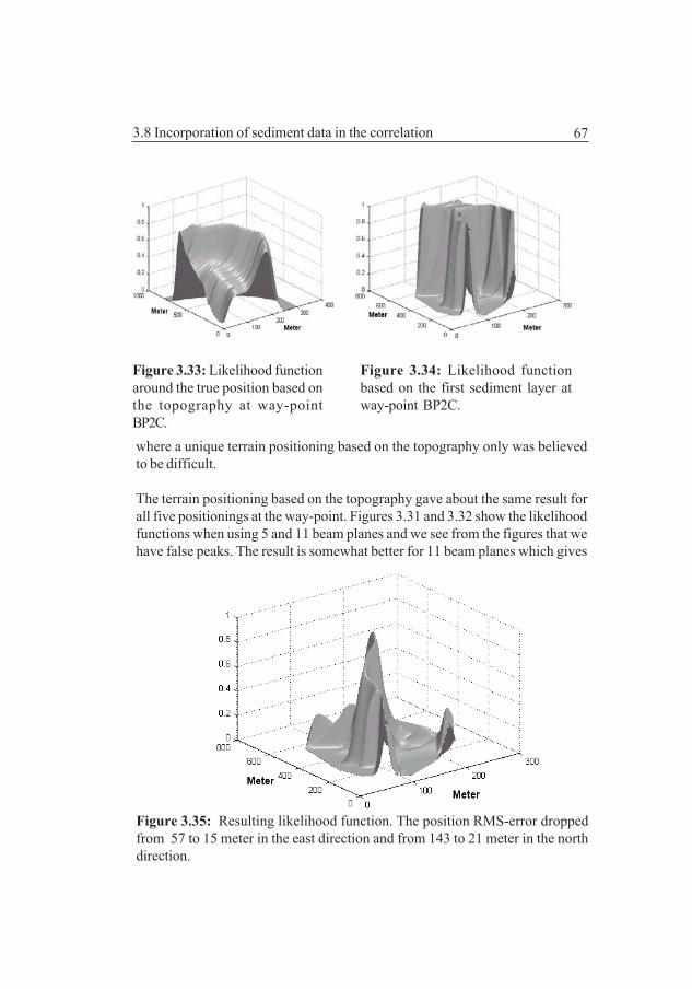
67
where a unique terrain positioning based on the topography only was believedto be difficult.
The terrain positioning based on the topography gave about the same result forall five positionings at the way-point. Figures 3.31 and 3.32 show the likelihoodfunctions when using 5 and 11 beam planes and we see from the figures that wehave false peaks. The result is somewhat better for 11 beam planes which gives
Figure 3.35: Resulting likelihood function. The position RMS-error droppedfrom 57 to 15 meter in the east direction and from 143 to 21 meter in the northdirection.
Figure 3.33: Likelihood functionaround the true position based onthe topography at way-pointBP2C.
Figure 3.34: Likelihood functionbased on the first sediment layer atway-point BP2C.
3.8 Incorporation of sediment data in the correlation
68 3 The positioning method
a correct position but a large position error. If a true 3D sonar had been used thelikelihood function would probably have been more distinct. The true peak is theone to the far right.
Suppose now that we use the distance to the first reflecting layer in Figure 3.29.We measure, in this example, with only one sub bottom profiler beam (normallyseveral sub profiler beams would be used) and we assume that we have the sameaccuracy as before, i.e., 0.5 meter RMS. The likelihood functions for the topo-graphic measurement and the sediment measurement can be seen in Figure 3.33and 3.34.
As can be seen from Figures 3.27, 3.29 and, 3.34 the sediment layer has a morebroken surface than the bottom surface. This is common in the archipelago areasof the Baltic. Multiplying the two likelihood functions will give the resultinglikelihood function (Figure 3.35). As can be seen in this case the position error isconsiderably smaller and the likelihood function more distinct.
To conclude the use of sediment data to improve the positioning. Underlyingsediment layers are naturally more broken than the current bottom surface andif used for positioning they can considerably improve the position accuracy inflat bottom areas.
The best positioning result in flat terrain areas will be achieved if a true 3D sonaris used due to the higher accuracy of the distance between the individual beamfootprints and if the 3D sonar also have a sub bottom profiler function. A para-metric sub bottom profiler will give very narrow beams at the low frequenciesused and it is ideal for military use. The sonars may transmit simultaneously butthe duration of the sub profiler pulse will be considerable longer.
3.9 Incorporation of side-scan data in thecorrelationTo improve the positioning by using side-scan pictures might not be as easy asto use sediment data. There are several reasons for that. First of all much of theinformation in a side-scan picture is from the light and shades from the heightvariations of the bottom. This information is, however, already in the usual 3Dsonar data set. This information also decreases as the bottom becomes flatter,i.e., when the extra information is most needed. Secondly, the information from

69
the bottom texture which is not in the usual 3D sonar data set varies with timeand may not be appropriate after some years. Thirdly, a side-scan picture dependsvery much on the side scan sonar attitude and distance to the bottom which willmake the matching difficult and not as easy as for the topographic heightinformation.
Figure 3.36 shows two side-scan pictures over the flat bottom area for which thesediment profile was used for the positioning. The pictures are taken only a fewhours apart. From the pictures we see that there is some texture information thatmight be used. A drawback for military use is the long time it takes to collect theside scan data and the revealing distance is also much longer than for abathymetric sonar.
3.10 Incorporation of external sound sourcesin the correlationSubmarines with their long flank arrays can determine the bearing to soundsources with high accuracy. In the case the position of the sound source isknown this information can be used to formulate a likelihood function which insome cases, i.e., in flat areas, can improve the position estimate based on terrainpositioning and the inertial navigation system.
Figure 3.36: Side-scan pictures from two passages over way-point 2C.
3.10 Incorporation of external sound sources in the correlation

70 3 The positioning method
Suppose the external sound source is at the position (xss, yss) as shown inFigures 3.37 and 3.38. While the vehicles position is at (x, y) and the measuredbearing to the sound source is θ0. If we assume that the measurement error isGaussian distributed we will have the following likelihood function
2
022
1 1( , ) exp( arctan )22
ssES
ss
x xL x yy yθθ
θσπσ
−−= − − (3.37)
Where σθ 2 is the uncertainty in the angle measurement. The Figures 3.39 , 3.40
and 3.41 show an example of a prior PDF, the likelihood function and theposterior PDF. The likelihood function calculated from the external soundsource will not be Gaussian in a Cartesian coordinate system.
The likelihood function along the arc segment with radius R, see Figure 3.38,and centered around the point (x,y) is
2
2 2( ) exp( )2ES
sL sR θσ−∆∆ ∝ − (3.38)
Where ∆s is the distance along the circular arc, i.e., ∆s= R∆θ and R and ∆θ aredefined in Figure 3.38. For large R this will approximately also be the likelihoodfunction along the tangent in the point (x,y). The improvement of the accuracyby measuring the bearing to the external sound source is determined bycalculating the Fisher information matrix
Figure 3.37: External sound sourceand own vehicle measuring thebearing to the source.
Figure 3.38: Definitions ofvariables.

71
( )22
2
[log ( ; ) ( ; ) ][log ( ; )]{ } { }
[log ( ; ) log ( ; )] { }
TP EST T
TP ESTN EST
L LLE E
L LE
θ
θ
∂∂= − = − =∂ ∂ ∂ ∂
∂ += − = +
∂ ∂
x y xx yJx x x x
x y x J Jx x
(3.39)
where subindex TP refers to terrain navigation and ES to the external soundsource. The approximation for large distances R will give the inverse information
Figure 3.39:. The prior position PDF. Figure 3.40: The likelihood functionfor the bearing measurement.
Figure 3.41: The posterior PDF for the position.
3.10 Incorporation of external sound sources in the correlation

72 3 The positioning method
matrix in the principal directions of the likelihood function for the external soundsource as
2 21 0
0ESRθσ−
= ∞ J (3.40)
By repeating the procedure recursively with the same sound source animprovement in the position estimate can be achieved. Figure 3.42 illustrates theprocedure. Up to the left in the figure is the PDF for position of the vehicle afterthe terrain measurement update in position A. Across to the right is the PDF forthe bearing measurement and the two PDFs are fused together by multiplyingthe PDFs as described earlier. This fused PDF is then propagated as describedin Chaper 2 to time t2 and is indicated to the left at position B. At time instant t2a new bearing measurement is done which is fused with the previous propagatedPDF and the resulting PDF is then propagated and so on. As understood thisscheme can be applied to aiding from several external sound sources.
In the cases the distance to the sound source is large the PDF from the bearingmeasurement can be approximated to be Gaussian and again we can use a linearKalman filter.
Figure 3.42: Recursively determining of bearing to external sound source.

73
4.1 IntroductionThe problem with false correlation peaks has already been touched on in Chapter3 where the Figures 3.7 and 3.8 show the large difference between using one ormany measurement beams. The false peaks are due to terrain repeatability and ofcourse the larger the measured bottom area is, the more unique the measuredarea will be and thereby fewer false peaks. The traditional way of selectingamong the correlation peaks is to fuse with the prior position PDF or to use avalidation gap. But even so, the false peaks may influence the estimated positionand the position error covariance if the Bayesian approach to terrain positioningis used. It is thus important to reduce the number of false peaks and we havealready seen that increasing the number of measurement beams is an effectivemethod for achieving that.
In studying the problem of how false correlation peaks depends on the numberof measuring beams two approaches are selected. In the first one we calculatehow the probability for detecting a false position due to terrain repeatabilitydepends on the number of measurement beams, i.e., the size of the correlationarea. In the second approach we study how the amplitudes of the correlation
Chapter 4
The likelihood functionand the Kalman filter

74 4 The likelihood function and the Kalman filter
peaks vary with the number of measurement beams. In both case it turns out thatthe false peaks will disappear as the number of beams increases. A method ofhow to test if a correlation peak corresponds the true position or not is alsointroduced.
Later in the chapter the shape of the likelihood function is discussed. It is shownthat if a large number of measuring beams are used the likelihood function will beclose to Gaussian, bias free, and coincide with the PDF for the position error if itis estimated by the maximum likelihood method.
Since the normalized likelihood function and the position error is Gaussian, alinear Kalman filter based on the normalized likelihood function can be used toestimate the position.
4.2 False peaks4.2.1 The probability for false positionLet us for simplicity study the problem with false positions in one dimension[NY01a, NY01b]. Assume that we have a stochastic bottom profile as inFigure 4.1. The sonar, which has N measurement beams, has measured theprofile in area 1 and it is found to be
y = h1 + e (4.1)
where e is the measurement error. Now we are comparing this measurement withthe underwater map in area 2 which has the bottom profile h2. In the following, wewill assume that the elements in the vectors 1h and h2 are correlated Gaussiansequences. Let
Figure 4.1: A bottom profile section.
75
∆h=h1- h2 (4.2)
Now we want to find the probability that the absolute value of the elements inthe vector |∆h| < εh since this means that the two bottom profiles are very closeto each other. The notation |∆h| <εh means that the absolute value of everyelement in the vector ∆h should be smaller than εh. Since we assumed 1h and h2
to be Gaussian, we have
1/ 2
1 1( ) exp( )2(2 ) det( )
TN
pπ
−∆ = − ∆ ∆h h C hC (4.3)
where C is the covariance matrix of ∆h. The simplest way to calculate theprobability that the two bottom profiles are close to each other may be to firstdecorrelate the vector ∆h by a mode decomposition of the covariance matrix
C = ULUT (4.4)
where U is the eigenvector matrix and L is the eigenvalue matrix. Making thesubstitution ∆h = Uy makes it possible to compute an upper bound of theprobability that the difference in depth profiles of the two locations is lessthan a small number.
2 2
11 1
( ) ( )
1 1exp( ) exp( )2 22 2
h
N Ni i
N ii ii ii i
P P
y ydy dy dyε ε ε
ε ε ε
ε ε
λ λπλ πλ= =− − −
∆ ≤ ≤ ∆ ≤
= − = −∏ ∏∫ ∫ ∫
h y
(4.5)
The hypercube ε encloses the hypercube hε .The covariance matrix is assumedto be positive definite, i.e., all eigenvalues λi > 0, so each factor
21 exp( ) 122
ii
ii
y dyε
ε λπλ−
− <∫ (4.6)
4.2 False peaks

76 4 The likelihood function and the Kalman filter
if ε > 0. The probability that the terrain repeats itself will thus decreaseexponentially with N.
It is easy to show that the above conclusion is valid also for non-Gaussiancorrelated sequences h since any PDF can be approximated as closely as desiredby a sum of Gaussian PDFs pm(y), [AS72, AN79]. Equation (4.5) can therefore bewritten as
1 1
( ) ( )
( ) ( )
h
M M
m mm m
P P
p y d p y dε ε ε ε
ε ε ε ε
ε ε
= =− − − −
∆ ≤ ≤ ≤
= =∑ ∑∫ ∫ ∫ ∫
h y
y y (4.7)
For every fix M the probability will exponentially approach zero when N increasesabove all bounds.
Figure 4.2 illustrates the exponential decrease in probability that the terrainrepeats itself, according to (4.5), for two synthetic bottom profiles generated by
Figure 4.2: Probability that the bottom repeats itself.

77
passing white noise through an AR(1)-filter with a pole in a = 0.96 and a = 0.99,respectively.
4.2.2 The amplitude of the false peaksIn the previous section the probability of false peaks was studied. Here insteadthe amplitudes of the false peaks are studied. Let us formulate the ratio betweenthe ordinates of the likelihood function in the false position xf and in the trueposition x0 when the measurement is taken at the true position x0, see Figure 4.3
202
0 1
20 00 02
1
2 202
1
20 02
1
2
1exp( ( ( ) ( )) )( ; ( )) 2
1( ; ( )) exp( ( ( ) ( )) )2
1 exp( ( ( ) ( )) )2
1 exp( ( ( ) ( )) 2 ( ( ) ( )))2
1 exp( (2
N
k k ff ke
N
k kke
N
k k f kkeN
k k f k k k fke
e
y x h xL x y xq
L x y x y x h x
y x h x e
h x h x e h x h x
σ
σ
σ
σ
σ
=
=
=
=
− −= =
− −
= − − −
= − − + −
→ −
∑
∑
∑
∑2
01
( ) ( )) ) N
k k fk
h x h x=
−∑
for large N. (4.8)
Now, the only way for the ratio q not to approach zero when N tends to infinity
Figure 4.3: A likelihood function with a secondary peak at position xf caused byterrain repeatability. True position at x0.
4.2 False peaks
78 4 The likelihood function and the Kalman filter
is that there is a symmetry in the terrain which extends into infinity. This is notthe case for a natural terrain and we conclude that secondary peaks will disappearas the number of beams increase.
An increase in the number of measurement beams not only decreases the numberof false likelihood positions but it also makes the peak of the likelihood functionmuch sharper that is the position accuracy increases as will be shown inChapter 5.
We conclude from the above that false positions will not be a problem if a largenumber of measuring beams is used. This has also been the experience from oursea trials. When it occasionally still happens in flat bottom areas the simplestway to eliminate the problem is to increase the size of the total sonar footprintsince the probability of a false position decays exponentially with the size ofthat area.
4.2.3 False peaks, hypothesis testingIn Chapter 3, Figure 3.15, a positioning example was shown where multiple like-lihood peaks were assumed to have occurred. Multiple likelihood peaks appearif we have too few measurement beams in relation to the height variations in theterrain. We can distinguish between two cases. The first case occurs if we areusing very few beams in a rough terrain and the second case occurs if we havemany measurement beams but the terrain is very flat. In the last case the likeli-hood function will be close to Gaussian.
Assume that we have two likelihood peaks which are close to each other inmagnitude but the one with index 1 is slightly higher than the one with index 2.Since peak no. 1 is the highest we will assume that it shows the true position.Our question is now if this is just due to the randomness of the measurementerror or is this position really the true position. The correlation function at thetrue position and at the false position is respectively
1 1 1( ) ( ) ( )T TT = − − =x y h y h e e (4.9)
and
2 2 2 1 1( ) ( ) ( ) ( ) ( )
2
T T
T T T
T = − − = − + ∆ − + ∆
= + ∆ ∆ + ∆
x y h y h y h h y h he e h h h e
(4.10)
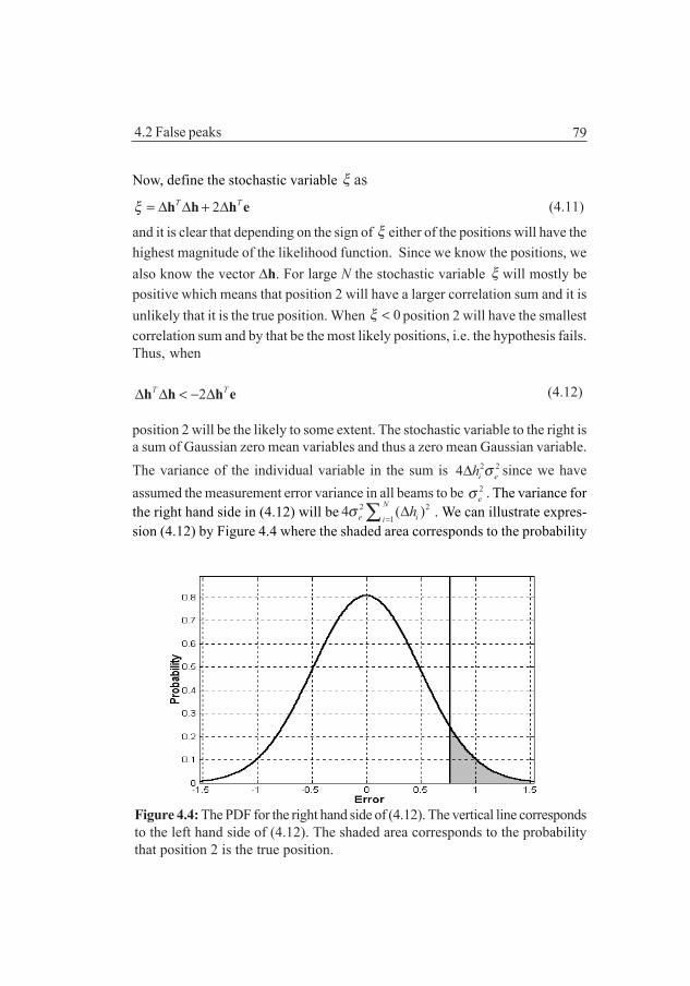
79
Now, define the stochastic variable ξ as
2T Tξ = ∆ ∆ + ∆h h h e (4.11)
and it is clear that depending on the sign of ξ either of the positions will have thehighest magnitude of the likelihood function. Since we know the positions, wealso know the vector ∆h. For large N the stochastic variable ξ will mostly bepositive which means that position 2 will have a larger correlation sum and it isunlikely that it is the true position. When 0ξ < position 2 will have the smallestcorrelation sum and by that be the most likely positions, i.e. the hypothesis fails.Thus, when
2T T∆ ∆ < − ∆h h h e (4.12)
position 2 will be the likely to some extent. The stochastic variable to the right isa sum of Gaussian zero mean variables and thus a zero mean Gaussian variable.The variance of the individual variable in the sum is 2 24 i eh σ∆ since we haveassumed the measurement error variance in all beams to be 2
eσ . The variance forthe right hand side in (4.12) will be 2 2
14 ( )N
e iihσ
=∆∑ . We can illustrate expres-
sion (4.12) by Figure 4.4 where the shaded area corresponds to the probability
4.2 False peaks
Figure 4.4: The PDF for the right hand side of (4.12). The vertical line correspondsto the left hand side of (4.12). The shaded area corresponds to the probabilitythat position 2 is the true position.

80 4 The likelihood function and the Kalman filter
that position 2 is the true position. When the difference in terrain profiles be-tween the two positions will tend to zero the probability will tend to 0.5.
The Gaussian assumption about the measurement error is very convenient touse but the real PDF for the measurement error will have the tails cut. Thatmeans that it is possible to tell if the difference between the measured profileand the map profile can be explained by the measurement error or not. If it cannot be explained the position is truly false. Since the right hand side in (4.12) isa sum of scaled stochastic variables from the same zero mean measurement errorPDF the criterion is as easy to use as in the case of the Gaussian assumption ofthe measurement error. By applying the criterion (4.12) to all points in the mapand setting the likelihood function to zero for the positions where the criterionis not fulfilled the map can in some sense be cleaned from false positions.
4.3 The shape of the likelihood functionWe have seen in the previous chapter, Figure 3.17 that the likelihood functionresembles a Gaussian curve. It is also true that the likelihood function convergesunder mild conditions towards a Gaussian curve when the number of measuringbeams increases, see for example [CA88, KH49, PE95, SESI93, VA98]. This canalso be shown plausible by a Taylor expansion of the likelihood function aroundthe point of its maximum and by assuming certain conditions for the derivativesof the likelihood function. Let us look at the one-dimensional case and let theTaylor expansion be around x = 0
22 22 4
2 21 1
1( ; ) exp( ( ) )2
N Nk k
k ke
h hL x y C x x H xx xσ = =
∂ ∂ = ⋅ − + ∂ ∂ ∑ ∑ (4.13)
where the derivatives are taken at x = 0. The function H(x ) is the remainder termand is assumed to be bounded for all x. The constant C is a normalizing constantmaking ( ; ) 1L x y dx
∞
−∞=∫ . When developing the expansion the measurement error
has been assumed to be a white sequence and the terms that tend to zero whenN increases have been set to zero. We can also write the equation as

81
2 222 2
2 21 12
1
1( ; ) exp( 1 / ( ) )2 /
N Nk k
N k kke
k
h hL x y C x x H x
xxhx
σ = =
=
∂ ∂ = ⋅ − + ∂∂ ∂ ∂
∑ ∑∑
(4.14)
For small x we can neglect the second term within the brackets in comparison to
1 assuming that 2 22
21 1
/N N
k k
k k
h hxx= =
∂ ∂ ∂∂
∑ ∑ is bounded. Left is a Gaussian curve
with the variance2
2 2
1
/N
ke
k
hx
σ σ=
∂ = ∂ ∑ (4.15)
which corresponds exactly to the variance given by the CRLB in Chapter 6. Thisis important since it means that the normalized likelihood function is the same asthe position error PDF. From Figure 4.5 which is from a sea-trial it can be seen thatthe likelihood function agrees well with a Gaussian curve. Another proof of theasymptotic convergence towards a Gaussian curve is given below.
Figure 4.5: Comparison between the likelihood function and the Gaussian PDF.Data from WP3 in the October 2002 sea-trial.
4.3 The shape of the likelihood function

82 4 The likelihood function and the Kalman filter
4.3.1 The convergence of the likelihood curveWe will assume that the terrain profile h(x) is continuous with continuoushigher derivatives. When measuring the terrain profile we will have a certainerror, e, which we will assume Gaussian distributed. The number of measure-ment beams is N. The measured profile can thus be written y(x0)=h(x0)+e, wherex0 is the true position.
The likelihood function can in the one dimensional case be written as
[ ]2
0 021
1( ; ( )) exp ( ) ( )2
N
N i iie
L x y x C y x h xσ =
= ⋅ − −
∑ (4.16)
were C is a constant. We know that 0( ; ( ))NL x y x converges to a Dirac pulse
when N→∞ but we want to show that 0( ; ( ))NL x y x also tends to a Gaussiancurve when N→∞. Besides our previous assumptions about the measurementnoise we assume that for a given fix N the likelihood function and its derivativesto be continuous so a Taylor expansion of the likelihood function around x0=0is permissible. Accordingly
22 22 40 0
0 2 21 1
220
21
( ) ( )1 1( ; ( )) exp ...42
( )1 ...( !)
N Ni i
Ni ie
kNki
ki
h x h xL x y x C x x
x x
h xx
k x
σ = =
=
∂ ∂ = ⋅ − + + ∂ ∂
∂+ + ∂
∑ ∑
∑(4.17)
or
2 22220 0
0 2 21 12 0
1
2 220 0
21 1
( ) ( )1( ; ( )) exp 1 / ...4( )2 /
( ) ( )1 /( !)
N Ni i
N N i iie
i
kN Nki i
ki i
h x h xxL x y x C xxxh x
x
h x h xx
xk x
σ = =
=
= =
∂ ∂ = ⋅ − + + ∂∂ ∂ ∂
∂ ∂ + ∂∂
∑ ∑∑
∑ ∑ 2 ...−
+
(4.18)

83
We recognize that the likelihood function LN(x;y(x0)) is not uniformly convergentand we therefore introduce the variable z through the transformation Nx zσ=where
2
2 2
1
Ni
N ei
hx
σ σ=
∂ = ∂ ∑ (4.19)
which will give us a uniformly convergent series, see Figure 4.6. The likelihoodfunction can now be written
22 22 2220 0
0 21 1
2 12 222 20 0
21 1
( ) ( )( ; ( )) exp 1 / ...
2 4
( ) ( ) / ...
( !)
N Ne i i
Ni i
kk kN N
ke i ik
i i
h x h xzL z y x C zxx
h x h xz
xk x
σ
σ
= =
−
−
= =
∂ ∂ = ⋅ − + + ∂∂
∂ ∂ + + ∂∂
∑ ∑
∑ ∑
[ ]2
exp 1 ( )2zC S N∞
= ⋅ − +
(4.20)
4.3 The shape of the likelihood function
Figure 4.6: Illustration of the difference between the likelihood function and theGaussian function.

84 4 The likelihood function and the Kalman filter
where we introduced the partial sum SM (N) of M terms as
2 12 222 20 0
22 1 1
( ) ( )( ) /
( !)
kk kM N N
ke i iM k
k i i
h x h xS N z
xk xσ
−
−
= = =
∂ ∂ = ∂∂ ∑ ∑ ∑
(4.21)
Now, since every term in the sum is strictly monotonically decreasing with Mand can be made as small as desired by choosing a sufficiently large N, thepartial sum SM(N) can be made arbitrarily small for any choice of M. This meansthat SM(N) →0 when N→¥ independent of M, [RÅWE95, p. 181], and that thelikelihood function converges to a Gaussian curve in the transformed space.Since the transformation does not affect the vertical scale, this will also be truein the non-transformed space.
4.3.2 The convergence of the N-normalized likelihoodcurveIt is often of interest to look at a likelihood expression where the exponent hasbeen normalized with the number of beams since the true likelihood function inmost cases will just be a very narrow peak when plotted due to the rapidvariance decrease with the number of beams. The N-normalized likelihoodfunction is
[ ]2
0 021
1 1( ; ( )) exp ( ) ( )2
N
NNorm i iie
L x y x y x h xNσ =
= − −
∑ (4.22)
Since the N-normalized likelihood function is just the Nth root of the truelikelihood function it will also be a Gaussian PDF if it is normalized to have thevolume one. The expected value of the exponent in (4.22) in the true position is-1/2. Often one plots the N-normalized likelihood function under the assumptionof 2 1eσ = . The N-normalized likelihood functions for different N in a certainposition will in most cases be close to each other.
4.3.3 The convergence of the likelihood curve infrequency spaceIt is also possible to come to the same conclusion as above by assuming that thebottom was created by a band limited stationary stochastic process with a cer-tain autocorrelation function. Let us look at the one-dimensional case and let us

85
assume that the bottom topography was created by a stationary stochasticprocess h(x). Our measurement of the vector h(x) is y , i.e. yt = h(xt) + et where et
is the Gaussian measurement error. The dimension of the vectors is N.
We have
2,2 2
1
2 22
( ) 1{ } { ( ( )) }2 2
1 2 2 ( )2
1 (1 ( ))2
N
t k kke e
h e he
h
T xE E y h xN N
r
r
σ σ
σ σ τσ
κ τ
=
= −
= + −
= − +
∑
(4.23)
where the bottom signal to noise ratio is 2 2/h eκ σ σ= , τ = xt - x and ( )hr ⋅ is thenormalized autocorrelation function for the bottom profile.
As an example assume that the bottom is created by a band limited stochasticprocess, see Figure 4.7. The band limited assumption is a very mild assumptionand always fulfilled for real terrains and it may therefore be proper to say that thisdiscussion is valid for any physical terrain. The autocorrelation function is
00
4( ) sin( )cos( )
2hS Br τ τ ω ττ
= (4.24)
After Taylor expansion we have the normalized autocorrelation function
222 40( ) 1 ( )
24 2hBr Oωτ τ τ
= − + +
(4.25)
4.3 The shape of the likelihood function
Figure 4.7: Power spectrum for a band-limited process.

86 4 The likelihood function and the Kalman filter
The remainder term is small in the neighbourhood of τ=0 which is the surround-ing we are interested in. Disregarding the remainder term we have
22 220
2 2
( ) 1 1{ }24 2 2 22 e BL
T x BEN
ω τκ τσ σ
= + + = +
(4.26)
where
2220
1
24 2
BL Bσ
ωκ=
+
(4.27)
A well known approximation formula which is valid with good accuracy in ourcase is
2
2 2 2
( ) ( )( ) {exp( )} exp( { }) exp( )2 2
e e BL
T x T xf x E EN N
τσ σ σ
= − ≈ − ∝ − (4.28)
In Figure 4.8 we compare this approximation with a Gaussian curve and we seethat the larger theκ -value is, the more the likelihood curve tends towards aGaussian function. In areas of interest for terrain navigation, the terrain variations
Figure 4.8: Comparison between the expected likelihood functions for astochastic band-limited bottom profile and Gaussian curves.

87
are usually much larger than the ones in Figure 4.8. We observe here that largeκ values also mean large bottom gradients. Equation (4.27) can be used as anindicator of the suitability for terrain positioning.
4.4 The linear Kalman filterThe linear Kalman filter equation can be derived in many ways; Stochasticdifferential equations as in [KL01], least squares as in [STBO97], minimummean squares as in [BRHW97], by the orthogonality principle as in [KSH00] tomention a few.
An approach that is suitable in the context of this thesis may be an approachbased on Bayes theorem [BRHW97]. Let the vehicle position and ourmeasurement be given by the equations
( 1) ( ) ( ) ( )k k k k+ = +x F x v (4.29)
( ) ( ) ( ) ( )k k k k= +y H x e (4.30)
where v(k) and e(k) are white, independent, Gaussian sequences with covari-ances Q(k) and R(k).
4.4.1. The conditional meanLet *ˆ ( ( ), ( 1),..., (0)) ( )k k= − =x g y y y g y be our estimate of the position basedon all available measurements. We can have different criteria for the optimality ofthe estimate. One criteria is the minimum mean square estimate, that is, theestimator that makes the mean square error (mse) of the estimate as small aspossible. The expression for the mse is
{ } { }{ } { } { }
* *
* * *
ˆ ˆ ˆ ˆ ˆ ˆ( ) ( ) | |
ˆ ˆ ˆ ˆ| | |
T T T T T
T T T T
E E
E E E
− − = − − + =
+ + +
x x x x y x x x x x x x x y
x x y x y x x x y x x (4.31)
since x̂ is a deterministic function of y*. Completing the square will give
4.3 The shape of the likelihood function
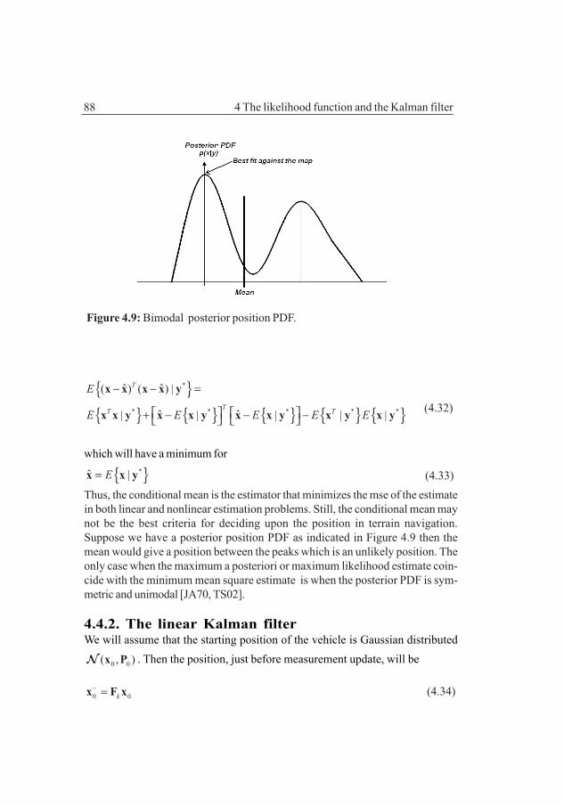
88 4 The likelihood function and the Kalman filter
{ }{ } { } { } { } { }
*
* * * * *
ˆ ˆ( ) ( ) |
ˆ ˆ| | | | |
T
TT T
E
E E E E E
− − =
+ − − −
x x x x y
x x y x x y x x y x y x y (4.32)
which will have a minimum for
{ }*ˆ |E=x x y (4.33)Thus, the conditional mean is the estimator that minimizes the mse of the estimatein both linear and nonlinear estimation problems. Still, the conditional mean maynot be the best criteria for deciding upon the position in terrain navigation.Suppose we have a posterior position PDF as indicated in Figure 4.9 then themean would give a position between the peaks which is an unlikely position. Theonly case when the maximum a posteriori or maximum likelihood estimate coin-cide with the minimum mean square estimate is when the posterior PDF is sym-metric and unimodal [JA70, TS02].
4.4.2. The linear Kalman filterWe will assume that the starting position of the vehicle is Gaussian distributed
0 0( , )x PN . Then the position, just before measurement update, will be
0 0k− =x F x (4.34)
Figure 4.9: Bimodal posterior position PDF.
89
where we have simplified the time step notification and will thus also be Gaussiandistributed. For the time step k we will have
1 ( ) ~ ( , ) ( , )Tk k k k k k k kp − −
−= +x x P F x F P F QN N (4.35)
Our measurement y is also assumed to be Gaussian distributed. From (4.30)we have for the prediction
( ) ~ ( , )Tk k k k k kp − − +y H x H P H RN (4.36)
The conditional density of yk given xk is
( | ) ( , )k k k k kp y x H x R∼ N (4.37)
Now we apply the theorem of Bayes to the Gaussian densities (4.35), (4.37)
( | ) ( )( | )( )
p ppp
= y x xx yy (4.38)
The calculation of (4.38) can be simplified by observing that if two Gaussian
PDFs, 1 1( , )µ CN and 2 2( , )µ CN are multiplied by each other the result, after
normalization is1 11 1 1 1 1 1
1 2 1 1 2 2 1 2( , )− −− − − − − − + + + C C C µ C µ C CN , i.e., the co-
variances are added together by the parallel resistor formula and the new meanis a weighted, by the covariances, sum of the individual means.
Otherwise, inserting (4.35), (4.36) and (4.37) into (4.38) will after some calcula-tions, give
( | ) ( , )p = x xx y µ CN (4.39)
where
1
1
( ) ( )
( ) ( )
T Tk k k k k k k k k k
T Tk k k k k k k k k
− − − − −
− − − − −
= + + −
= + + −xµ x P H H P H R y H x
x P H H P H R y y (4.40)
4.4 The linear Kalman filter

90 4 The likelihood function and the Kalman filter
and11 1T
k k k k
−−− − = + xC P H R H (4.41)
We can also view the mean in the measurement space
1( ) ( )T Tk k k k k k k k k k− − − − −= + + −yµ y H P H H P H R y y (4.42)
from which we clearly see that the new position is a weighted mean of thepropagated position in measurement space and the measured position. A maybesimpler approach would be to directly transform the measurement uncertaintycovariance to state space and add it to the k
−P by the parallel resistor formula.
Assume that a Gaussian stochastic vector x has the density function
1/ 2 1/ 2
1 1( ) exp( ( ) ( ))2(2 ) det( )
Txn
x
pπ
−= − − −x xx x m C x mC (4.43)
Let now a transformation be y=Ax. It is then easy to show that the new distribu-tion is also a Gaussian density whos mean and covariance are given by
=y xm Am (4.44)T=y xC AC A (4.45)
We note that Cy does not depend on x. Since the new density is Gaussian we candirectly write the PDF
1/ 2 1/ 2
1 1( ) exp( ( ) ( ))2(2 ) det( )
Tm
y
pπ
−= − − −y y yy y m C y mC (4.46)
If we now partly re-substitute x we will have
1/ 2 1/ 2
1/ 2 1/ 2
1 1( ) exp( ( ) ( ))2(2 ) det( )
1 1 exp( ( ) ( ))2(2 ) det( )
Tm
y
T Tx xm
y
pπ
π
−
−
= − − −
= − − −
x y x
y
x Ax Am C Ax AmC
x m A C A x mC
(4.47)

914.4 The linear Kalman filter
The inverted covariance expression in (4.47) does not depend on x . We note
that 1T −yA C A is similar to
1Tk k k
−H R H (4.48)
in (4.41) which represents the measurement noise and this is how the measure-ment noise maps into the state space for a given transformation Hk.

92 4 The likelihood function and the Kalman filter
93
5.1. IntroductionThe Cramér-Rao lower bound (CRLB) gives a lower limit of the accuracy thatcan be achieved in estimation of parameters and plays an important role inestablishing the accuracy of the navigation method presented in this thesis.The chapter will therefore start with a general review of the CRLB followed byan application to the terrain navigation problem.
We are using estimators to estimate the characteristics of a stochastic variableas the mean, the variance or some other quantity characterizing the variable. Wemake the estimation by taking samples of the stochastic variable and from thesamples we calculate a value of the quantity we want to estimate. In most casesthe estimator is just a formula giving us a value, an estimate, of the characteristicof the variable when we plug in the sample values.
When we take a new sample and calculate a new estimate we usually get adifferent value and by that we understand that our estimate also is a stochasticvariable. If the estimator gives a large spread in its values, when we successivelyuse it, the estimator has a large variance. Of course we want an estimator with asmall variance and a mean close to the true value so we can be sure that the
Chapter 5The Cramér-Rao lowerbound

94 5 The Cramér-Rao lower bound
estimate is close to the true value for the characteristic we are estimating. Thusthe estimate shall be unbiased and have a small variance.
The CRLB will give us some guidance in evaluating the performance of anestimator since it is the lowest variance an unbiased estimator can have if weexclude so called super-efficient estimators which are of no practical importancein our case [SO16]. If the performance of our estimator is unbiased and is closeto the CRLB our estimator is a good one, if we are far from the CRLB the estimatoris poor and we may perhaps find a better estimator. If the variance of our unbiasedestimates attains the CRLB the estimator is called efficient. An estimator isasymptotically efficient if it reaches the CRLB and is/or becomes unbiasedwhen the sample size tends to infinity. This will be the case for our estimation ofthe position from terrain matching.
If we estimate a quantity x from the set of independent samples y1,y2,…yN by theformula 1 2ˆ ˆ( , ... )Nx x y y y= repeatably based on new sample sets each time wecan arrange the estimates in a histogram as in Figure 5.1 and 5.2. We will typicallyfind that the standard deviation of the histogram will become smaller if theestimator uses a larger sample set, i.e., a larger N.
If we increase the number of estimation trials to infinity the normalized histogramwill converge to the probability density function for the estimator and the varianceof the histogram is the variance of our estimator. If our estimates have no biasand this variance equals the CRLB we know we can not find an estimator with a
Figure 5.1: Histogram for theestimator, 100 trials.
Figure 5.2: Histogram for theestimator, 100 000 trials.
95
smaller variance. If our variance is greater than the CRLB we might find, but it isnot for sure, an estimator formula which will give us an estimate with smallervariance.
There are several ways to derive the CRLB expression, [RA45, CR46, LJ99,NA69, KA93, VT68, SC91] to mention only a few places in the engineeringliterature were the derivation can be found. It is common nowadays in thederivation to assume that the estimator is unbiased since it leads to a shortderivation. This is inline with the derivation presented in [RA45]. The derivationof the CRLB which will be reviewed here follows instead the derivation in [CR46],which do not assume that the estimator is unbiased (bias will frequently occurin terrain navigation). Some comments and illustrations have been added to,hopefully, make the derivation easier to follow. The Cramér derivation alsodiscusses an interesting invariance property for transformations of the samplePDF. The review of the Cramér derivation may also be interesting from a historicalpoint of view.
5.2 The CRLB5.2.1 The scalar CRLBThe derivation starts by finding an expression of the mean square error basedon an assumed known estimator 1 2ˆ ˆ( , ,..., )Nx x y y y= of x. Our observation set
of x is 1 2, ,..., Ny y y which can be thought of as been generated by
( , )i iy f x e= (5.1)
where ie is an error with some known PDF. This means that the joint PDF
1 2( , ,..., | )Np y y y x is assumed known.
We will assume that our estimator has a bias defined by the expressionˆ{ | } ( ) ( )E x x x x b xψ = + (5.2)
There can be several reasons behind the bias b(x) but in terrain navigation sucha position bias will often occur if we have a fix depth measurement error. Due tothe bottom slope this will cause a position error that varies with the position.The mean of the estimator x̂ is by definition
5.2 The CRLB

96 5 The Cramér-Rao lower bound
ˆ
ˆ ˆ ˆ( ) ( | )x
x xp x x dxψ = ∫ (5.3)
where ˆ( | )p x x is the PDF for our estimator (cf. Figure 5.2). Since ˆ( | )p x x is aPDF we have
ˆ
ˆ ˆ( | ) 1x
p x x dx =∫ (5.4)
The left hand side of this expression is a function of our true value x. Assumingit is admissible to differentiate under the integral sign we have
ˆ
ˆ( | ) ˆ 0x
p x x dxx
∂ =∂∫ (5.5)
We now multiply both sides with the constant x and, since the integration iswith respect to x̂ , we can move x under the integral sign
ˆ
ˆ( | ) ˆ 0x
p x xx dxx
∂ =∂∫ (5.6)
Now, differentiating (5.3) with respect to x gives
ˆ
ˆ( ) ( | )ˆ ˆx
x p x xx dxx x
ψ∂ ∂=∂ ∂∫ (5.7)
If we now subtract (5.6) from (5.7) we have
ˆ
ˆ( ) ( | )ˆ ˆ( )x
x p x xx x dxx x
ψ∂ ∂= −∂ ∂∫ (5.8)
We want to use Schwartz inequality for integrals and we therefore rewrite thisexpression as
97
ˆ
ˆ( ) 1 ( | )ˆ ˆ ˆ( ) ( | )ˆ( | )x
x p x xx x p x x dxx xp x x
ψ∂ ∂= −∂ ∂∫ (5.9)
If we now take the absolute value of both sides and then apply the Schwartzinequality we have
{ }2
2 22
ˆ ˆ
ˆ( )
ˆ( ) ( | ) 1ˆ ˆ ˆ ˆ( ) ( | )ˆ( | )x x
E x x
x p x xx x p x x dx dxx x p x x
ψ
−
∂ ∂ ≤ − ∂ ∂ ∫ ∫
(5.10)
or
{ }
2
22
ˆ
( )
ˆ( )ˆ( | ) 1 ˆ
ˆ( | )x
xxE x x
p x x dxx p x x
ψ∂ ∂ − ≥
∂ ∂ ∫
(5.11)
By that we have a lower bound on the mean square error for our actual choice ofestimator.
Next we will look at a transformation invariance property of the denominator in(5.11). Let ( | )p y x be the PDF of our observation vector 1[ ,..., ]T
Ny y y= andlet us transform our observation vector by the one to one transformation
( )z z y= , ( )y f z= and ( | )p z x is the PDF of the vector 1[ ,..., ]TNz z z= .
We then have( | ) ( | ) det( )p z x p y x J= (5.12)
where det(J) is the Jacobian of the transformation ( )y f z= which does notdepend on x. We also have dz.det(J)=dy. It then follows that
2 2( | ) 1 ( | ) 1( | ) ( | )z y
p z x p y xdz dyx p z x x p y x
∂ ∂ = ∂ ∂ ∫ ∫ (5.13)
5.2 The CRLB

98 5 The Cramér-Rao lower bound
i.e., the value of the integral is independent of the transformation. This is quitenatural since a transformation means stretching or compressing the horizontalaxis and since the area below the PDF is always one, the value of the frequencyfunction has to change accordingly, i.e., the det(J) factor in numerator anddenominator cancels out. Remember now that our discussion so far deals with asupposed known estimator. The next step in the derivation is therefore to find asuitable transformation which will allow us to say that our findings also will bevalid for any estimator, especially for the one that gives the lowest variance.
An illustration of how to choose this transformation may be of value. Assumetherefore that we want to estimate the mean of a PDF and our sample size is, say,two samples, 1 2[ , ]Ty y y= , with equal means and variances for yi. We choose
our estimator to be 1 2ˆ ( ) / 2x y y= + . The contours of the PDF for the samplevector are illustrated in Figure 5.3 together with the lines Ci for y1 and y2 whichwill give the same estimate of x.
A suitable transformation is [ ]ˆ( ) ( ), ( ) Tz y x y yξ= where the dimension of the
vectorξ is N-1 and the dimension of the vector y is N . The requirement on ξ inthe transformation is that the transformation should be 1:1 and the derivatives
Figure 5.3: The contour lines for the sample PDF with shown hyper surfacesgiving the same estimate of the mean.

99
/i kz ξ∂ ∂ should exist [CR46]. The transformation means that the slanted linesCi in Figure 5.3 will then be horizontal in a graph of the transformed variable, seeFigure 5.4, and this makes it easy to split up (5.13) by Bayes theorem. We canachieve this transformation by for every point along a line iC map the PDF-
value at this point at the vertical coordinate iC and horizontal coordinate 2y inthe transformed PDF. The next step now would be to use the conditional identityp(α,β)=p(α|β)p(β). This will give us
ˆ ˆ ˆ( | ) ( , | ) ( | ) ( | , )p z x p x x p x x p x xξ ξ= = (5.14)
If we differentiate this expression we will have
ˆ ˆ( | ) ( | ) ( | , )ˆ ˆ( | , ) ( | )p z x p x x p x xp x x p x xx x x
ξξ∂ ∂ ∂= +∂ ∂ ∂ (5.15)
Substituting this into (5.13) gives
Figure 5.4: The contour lines for the transformed sample PDF in Figure 5.3.
5.2 The CRLB

100 5 The Cramér-Rao lower bound
2 2
2
2
ˆ ˆ, ,
( | ) 1 ( | ) 1( | ) ( | )
ˆ ˆ( | ) ( | , ) 1ˆ ˆ( | , ) ( | )( | )
ˆ ˆ ˆ ˆ( | ) ( | , ) ( | , ) ( | )ˆ ˆ2ˆ( | )
(
y z
z
x x
p y x p z xdy dzx p y x x p z x
p x x p x xp x x p x x dzx x p z x
p x x p x x p x x p x xdxd dxdx p x x x x
p
ξ ξ
ξξ
ξ ξξ ξ
ξ
∂ ∂ = ∂ ∂
∂ ∂ = + ∂ ∂
∂ ∂ ∂ = + ∂ ∂ ∂
∂+
∫ ∫
∫
∫ ∫2
ˆ,
ˆ ˆ| , ) ( | ) ˆˆ( | , )x
x x p x x dxdx p x xξ
ξξ
∂ ∫
(5.16)
The middle term can be written as the product of two integrals and since
ˆ( | , ) 0p x x dxξ
ξ ξ∂ =∂∫ due to ˆ( | , ) 1p x x d
ξ
ξ ξ =∫ the middle term will be zero. The
last integral will always be greater or equal to zero since the differential is insquare and the involved PDFs are always positive. We also note that the firstintegral can be written as the product of two integrals, one with the value 1. Wetherefore have
2 2
ˆ
ˆ( | ) 1 ( | ) 1 ˆˆ( | ) ( | )y x
p y x p x xdy dxx p y x x p x x
∂ ∂ ≥ ∂ ∂ ∫ ∫ (5.17)
This relates the PDF for our particular estimator with the PDF for the samplevector. We can therefore write expression (5.11) as
{ }
2
22
( )
ˆ( )( | ) 1
( | )y
xxE x x
p y x dyx p y x
ψ∂ ∂ − ≥
∂ ∂ ∫
(5.18)
which is the scalar parameter CRLB when our sample PDF is ( | )p y x and wenote that this expression does not depend on our choice of estimator. The mean

101
square error is always greater or equal to the right hand side of the expressionindependent of our choice of estimator. If we do not have bias, i.e., ( )x xψ = ,this will also be the variance of the estimator. Expression (5.18) can also bewritten
{ }
2
22
( )
ˆ( )( ( | ))
xxE x x
log p y xEx
ψ∂ ∂ − ≥
∂ ∂
(5.19)
or
{ }
2
22
2
( )
ˆ( )( ( | ))
xxE x x
log p y xEx
ψ∂ ∂ − ≥ −
∂ ∂
(5.20)
We can also derive a lower bound on the variance. If we in (5.6) multiply withˆ{ | ) ( )E x x x b x= + instead of x we will have
ˆ
ˆ( ) ( | )ˆ ˆ ˆ( { | })x
x p x xx E x x dxx x
ψ∂ ∂= −∂ ∂∫ (5.21)
instead of (5.8) and
2 22
ˆ ˆ
ˆ{ }
ˆ( ) ( | ) 1ˆ ˆ ˆ ˆ ˆ( { | }) ( | )ˆ( | )x x
Var x
x p x xx E x x p x x dx dxx x p x x
ψ ∂ ∂ ≤ − ∂ ∂ ∫ ∫
(5.22)
or
2
2
( )
ˆar{ }( ( | ))
xxV x
log p y xEx
ψ∂ ∂ ≥
∂ ∂
(5.23)
5.2 The CRLB

102 5 The Cramér-Rao lower bound
5.2.2 The vector parameter CRLBA simple approach would be to note that in the derivation of the scalar CRLBwe have not specifically used the information that the parameter was a scalar.The derivation would formally been the same if the scalar parameter x insteadhad been a parameter vector x. Therefore the CRLB for a biased estimator is
{ }12
12
( ) ( ( | )) ( )ˆ ˆ( )( )
( ) ( ( | )) ( ) =
TT
T
T
T
log pE E
log pE
−
−
∂ ∂ ∂ − − ≥ − ∂ ∂∂ ∂
∂ ∂ ∂ − + + ∂ ∂∂ ∂
ψ x y x ψ xx x x xx xx x
b x y x b xI Ix xx x
(5.24)
The inequality means that if the matrix to the left is subtracted with the matrix tothe right the resulting matrix is positive semidefinite. The quantity
2 ( ( | ))T
log pE ∂= − ∂ ∂
y xJx x (5.25)
is called the Fisher’s information matrix (FIM).
In the case we have bias the relation between the mean square error and thecovariance is
{ }ˆ ˆ ˆ{ } ( )( )
ˆ ˆ ˆ ˆ ˆ ˆ {[( { }) ( { } )][( { }) ( { } )] }ˆ { } ( ) ( )
T
T
T
Mse E
E E E E ECov
= − −
= − + − − + −= +
x x x x x
x x x x x x x xx b x b x
(5.26)
If the estimator is unbiased then the Mse and Cov are identical and we have
{ }12 ( ( | ))ˆ ˆ ˆ ˆ ˆ{ } ( { })( { })T
T
log pCov E E E E−
∂= − − ≥ − ∂ ∂
y xx x x x xx x (5.27)
Figure 5.5 illustrates the relations between the estimators.

103
If we know both the bias and the mean square error, we can calculate thecovariance from ˆ ˆ( | ) { | } ( ) ( )TMse Cov= +x x x x b x b x , in other cases we have to
resort to Monte Carlo methods to determine ˆ{ }E x and ˆ( )Cov x besides ˆ( )Mse x .Generally we have the inequality
12( ) ( ( | )) ( )ˆ ˆ{ } { }T
T
log pMse Cov E−
∂ ∂ ∂ ≥ ≥ − + + ∂ ∂∂ ∂
b x y x b xx x I Ix xx x (5.28)
The mean square error for a biased estimator in the case the CRLB is attainedis
12( ) ( ( | )) ( )ˆ{ } ( ) ( )T
TT
log pMse E−
∂ ∂ ∂ = − + + + ∂ ∂∂ ∂
b x y x b xx I I b x b xx xx x
(5.29)and the covariance
12( ) ( ( | )) ( )ˆ{ }T
T
log pCov E−
∂ ∂ ∂ = − + + ∂ ∂∂ ∂
b x y x b xx I Ix xx x (5.30)
Figure 5.5: Illustration of the PDF for a biased and an unbiased estimator.
5.2 The CRLB

104 5 The Cramér-Rao lower bound
5.3 Additive Gaussian noise5.3.1 The scalar caseIn the derivation of the scalar parameter CRLB we did not make any assumptionsabout the noise or the structure of the observations yi . Often the noise can becharacterized as additive and our observations are ( )i i iy h x e= + , i=1,2,3... N orin vector form
( )x= +y h e (5.31)
Assuming that the noise is Gaussian with zero mean with a covariance matrix C,the joint PDF of the observations is
( )1
/ 2
1 1( | ) exp( ( ( )) ( ( )))22 det( )
TNp x x x
π−= − − −y y h C y h
C (5.32)
Differentiating with respect to x and taking the expectation yields
21log ( | ) ( ) ( )Tp x x xE
x x x−
∂ ∂ ∂ = ∂ ∂ ∂
y h hC (5.33)
and, hence, according to (5.23)
2
1
( )
ˆar{ }( ) ( )T
xxV x
x xx x
−
∂ ∂ ≥
∂ ∂ ∂ ∂
ψ
h hC (5.34)
5.3.2 The vector caseAssume that the observation vector is Gaussian y~N(µµµµµ(θθθθθ),C(θθθθθ)) where themean vector is Nx1 and the covariance matrix is NxN. Both depend on the

105
unknown parameter vector θ which we want to estimate. The PDF for theobservation vector is thus
1/ 2
1 1( | ) exp ( ( )) ( )( ( ))2(2 ) det( ( ))
TN
pπ
− = − − − y θ y µ θ C θ y µ θ
C θ (5.35)
Taking the first derivative yields
1log ( | ) 1 log det[ ( )] 1 ( ( )) ( )( ( ))2 2
T
k k k
pθ θ θ
−∂ ∂ ∂ = − − − − ∂ ∂ ∂y θ C θ y µ θ C θ y µ θ
(5.36)
Now it can be shown, see for example [KA93, SC91], that the two terms in (5.36)can be written
1log det[ ( )] ( )Tr ( )
k kθ θ− ∂ ∂= ∂ ∂
C θ C θC θ (5.37)
and
1
11
( ( )) ( )( ( ))
( ) ( ) 2 ( )( ( )) ( ( )) ( ( ))
T
kT
T
k k
θ
θ θ
−
−−
∂ − −
∂∂ ∂= − − + − −
∂ ∂
y µ θ C θ y µ θ
µ θ C θC θ y µ θ y µ θ y µ θ (5.38)
where the derivatives ( )
iθ∂∂µ θ and
( )
iθ∂
∂C θ
mean the first derivative of all elements
in the vector and matrix respectively with respect to the parameter θi. The nextstep is to evaluate the elements in the Fisher matrix (5.25). After somemanipulations, see [VT02, KA93, SC91], the result is
[ ] 1 1 1,
( ) ( ) 1 ( ) ( )( ) ( ) Tr ( ) ( )2
T
i ji j i jθ θ θ θ
− − − ∂ ∂ ∂ ∂= + ∂ ∂ ∂ ∂
µ θ µ θ C θ C θJ θ C θ C θ C θ (5.39)
The scalar parameter case follows also directly from (5.39)
5.3 Additive Gaussian noise

106 5 The Cramér-Rao lower bound
21 1( ) ( ) 1 ( )( ) ( ) Tr ( )
2
T
J θ θ θθ θ θθ θ θ
− − ∂ ∂ ∂ = + ∂ ∂ ∂
µ µ CC C (5.40)
and in the case the covariance matrix does not depend on the parameter
1( ) ( )( )T
J θ θθθ θ
−∂ ∂=∂ ∂
µ µC (5.41)
5.4 The bias expressionWe have previously assumed that the bias may be expressed as
ˆ{ | } ( )E = +x x x b x , that is the expected value of the estimate of x depends in anonlinear fashion of the true value of x. In most cases the bias is introduced inthe sampling process and we will here analyze two cases more in detail. We willrestrict ourself to the case of estimating the mean.
5.4.1 The linear caseLet the stochastic variable ξ have the PDF fξ(x) with the mean x. We can constructthe following unbiased estimator of the mean based on N samples of thestochastic variable ξ
1
1ˆN
Unb ii
xN
ξ=
= ∑ (5.42)
Now, assume that our samples, due to an imperfect sampling device, instead areηi=α+β ξi and that we estimate the mean from those samples. This will give usa biased estimator
1 1 1
1 1ˆ ˆ( )N N N
Bias i i i Unbi i i
x xN N N
βη α βξ α ξ α β= = =
= = + = + = +∑ ∑ ∑ (5.43)
Thus the biased estimate of the mean is an affine transformation of the unbiasedestimate. We can determine the mean of the biased estimate
107
ˆ ˆ ˆ{ } { } { }Bias Unb UnbE x E x E x xα β α β α β= + = + = + (5.44)
This can also be written
ˆ{ } ( 1)BiasE x x xα β= + + − (5.45)
This means that the bias expression in (5.2) in the case of an affine transformationof the samples is
( ) ( 1)b x xα β= + − (5.46)
The variance of the biased estimator is (5.23) if the bound is obtained
2 2 2( )ˆ ˆ ˆ ˆ{ } (1 ) { } (1 1) { } { }Bias Unb Unb Unbb xVar x Var x Var x Var x
xβ β∂= + = + − =
∂ (5.47)
This can also be shown directly by
2ˆ ˆ ˆ{ } { } { } { }Bias Unb UnbVar x Var Var x Var xα β β= + = (5.48)
We can also study the PDF for the stochastic variable with bias. We have
1 1 1( ) { } { } ( )f x P x P x f xx xη ξ
α αη ξβ β β β β
∂ ∂= ≤ = ≤ − + = − +∂ ∂ (5.49)
That means that the PDF for the stochastic variable with bias is offset by -α/βand that the horizontal scale is changed to 1/β but the vertical scale is alsochanged the same amount so the area below the PDF remains one.
5.4.2 The nonlinear caseLet us now study a nonlinear transformation, y=g(x), of the stochastic variableξ , see Figure 5.6
( )gη ξ= (5.50)
5.4 Some transformations

108 5 The Cramér-Rao lower bound
Looking at Figure 5.6 it is obviuos that it is possible to numerically calculatethe bias as a function of the true value x if g(.) is known. From the figure we alsosee that depending on the curvature of g(.) the variance will increase ordecrease. Let us examine the situation more closely.
Assume that the true value of the parameter estimated by ξ is x=0 and thatE{ξ}=x and do a Taylor expansion of the function g(.) around that point. Weassume that the Taylor expansion is convergent, which is reasonable if boththe biased and the unbiased estimate of x exist. The estimator will be
0 11 1 0 1 1 2
0 11 2
1 1 1 1ˆ! !
1ˆ !
N N N Nk kki i
Bias i i kki i k i i k
N ki
Unb ki k
gx g g gN N k N N kx
g g x gN k
ξ ξη ξ
ξ
∞ ∞
= = = = = =∞
= =
∂= = = + +∂
= + +
∑ ∑∑ ∑ ∑∑
∑∑ (5..51)
where gk are the derivatives of g in the Taylor expension of y=g(x) at x=0 .We note here that different sequences of ξ 1,..., ξ N may result in the
Figure 5.6: Illustration of the nonlinear transformation of the stochasticvariable ξ. The PDFs in the figure refer to the estimates of the mean. True valueof the parameter estimated by ξ is x=0.

109
same ˆUnbx but different third term. After taking the expectation of both sideswe have
0 1 01 2 1 2
{ } { }1 1ˆ{ }! !
N Nk ki i
Bias k ki k i k
E EE x g g x g g gN k N k
ξ ξ∞ ∞
= = = =
= + + = +∑∑ ∑∑ (5.52)
since x=0. The last double sum is a function of the point x of the Taylor expansion,in this case x=0. An analytic expression of the expectation E{ξi
k}is easily foundfor a Gaussian distributed ξ. with zero mean
{ } 1 3 5 ( 1) { } ( 1)!! { }kE k Var k Varξ ξ ξ= ⋅ ⋅ ⋅ ⋅ ⋅ − = − (5.53)
Often only a few terms in the Taylor expansion, i.e., the inner sum is neededsince the tails of the PDF of ξ are cut due to physical reasons. This means thatthe bias expression in (5.52) can be calculated for different points x of the Taylorexpansion and the bias as a function of x
B(x)=x+b(x) (5.54)
can be calculated. A linear approximation of the bias function B(x) in a point x is
ˆ{ }BiasE x xα β= + (5.55)
We have also from (5.51)
{ }1 1 1
22
21
1 1ˆ! !
( ) (2 1)!! ( !)
N k ki
Bias k ki k k
kk
k
Var x Var g Var gN k N k
max g kN k ξ
ξ ξ
σ
∞ ∞
= = =
∞
=
= =
−≤
∑∑ ∑
∑ (5.56)
where 2ξσ is the variance of ξ.
5.4 Some transformations

110 5 The Cramér-Rao lower bound
5.5 Some examples of the CRLB in terrainnavigationThe CRLB for a position estimate is not only of interest in our Kalman filter butalso when deciding upon way-points. In the so called posterior CRLB defined in[VT68] a CRLB based on the mean of the FIM matrix which takes the informationfrom the prior position PDF into account is calculated. Since this bound giveswhat we at best can expect in accuracy at a way-point we will discuss it firstbefore developing some general expressions for the CRLB when we have aGaussian measurement noise. We will also develop an expression for the positionerror covariance when we have bending of the measurement beams due totemperature gradients in the water
In the following we are assuming that our prior position PDF has its mean in theway-point and that our estimates are the position x1 and x2 in East and Northdirections, respectively, and in some cases the measurement bias d. The numbersof parameters to estimate are thus two or three. The number of measurementbeams is N and the measurement accuracy is assumed to be known. Themeasurement noise is assumed to be additive and Gaussian.
5.5.1 The posterior FIMIn calculation of the posterior CRLB defined in [VT68] the improvement inaccuracy by the prior is taken into account in the following way. The posteriorCRLB is the inverse of the expected posterior Fisher matrix. The posterior FIM is
2 2
2 2
,
[log ( , )] [log( ( | ) ( ))]{ } { }
[log ( | )] [log( ( )] { } { }
T T
L J PT T
p p pE E
p pE E
∂ ∂= − = −∂ ∂ ∂ ∂
∂ ∂= − − = +∂ ∂ ∂ ∂
x y y x xJx x x x
y x x J Jx x x x
(5.57)
The equation (5.57) gives a “global bound” [VT02] which is independent of theactual position since the expectation in (5.57) is with respect to both x and y.
The first term can be written as

111
2 2
,
2
2
[log ( | )] [log ( | )]{ } ( , )
[log ( | )] ( | ) ( )
[log ( | )] { } ( )
L J T Tx y
T
y T
p pE p d d
p p d p d
pE p d
∂ ∂= − = −∂ ∂ ∂ ∂
∂ = − ∂ ∂ ∂= −
∂ ∂
∫∫
∫ ∫
∫
x y
x
y x y xJ x y x yx x x x
y x y x y x xx x
y x x xx x
(5.58)
Similarly, the second term in (5.57) can be expressed as
2 2
2
2
[log ( )] [log ( )]{ } ( , )
[log( ( )] =- ( ) ( | )
[log( ( )] =- ( )
P T T
T
T
p pE p d d
p p d p d
p p d
∂ ∂= − = −∂ ∂ ∂ ∂
∂ ∂ ∂
∂∂ ∂
∫∫
∫ ∫
∫
x y
x y
x
x xJ x y x yx x x x
x x x y x yx x
x x xx x
(5.59)
which is the expectation of the FIM for the prior and represents the improvementdue to the prior knowledge.
Sometimes we will be interested in the FIM for a certain position x. Therefore,omitting the expectation over x, we have
2
2 2
[log ( ; ) ( )]{ }
log ( ; ) log ( ) = { }=
y T
y L PT T
L pE
L pE
∂= −∂ ∂
∂ ∂− + +∂ ∂ ∂ ∂
x y xJx x
x y x J Jx x x x
(5.60)
The notation L(x;y) for the likelihood function has been used in (5.60). Thisbound is thus a function of the true position x.
5.5 Some terrain navigation examples
112 5 The Cramér-Rao lower bound
5.5.2 Two measures of the posterior accuracyPlanning of vehicle routes means that way-points have to be selected and it isof great interest to know what accuracy that can be expected when positioningin the way-point areas.
In many interesting cases, discussed in Chapter 6, our estimate and our trueposition will be close to each other and our accuracy will almost reach theCRLB. By calculating the expected value of the posterior CRLB, based on(5.60), we will therefore have a measure of what accuracy we can expect to beused in our Kalman filter for an actual choice of a way-point
{ } ( ) ( )P PE p= ∫x
R R x x dx (5.61)
where Rp(x) is the local posterior CRLB given by the inverse of (5.60) and theintegration is over the area where Rp(x) is defined. The CRLB based on (5.57)will give a lower bound for (5.61), cf. the relation between the harmonic and thearithmetic means.
The accuracy of the position based on the prior PDF is often much less than theaccuracy based on the terrain profile measurement which means that theimprovement by the prior can be neglected. In this case the measure will be
{ } ( ) ( )E p= ∫x
R R x x dx (5.62)
where R(x) is the usual position error covariance matrix, i.e., the CRLB based on(5.60) where the improvement by the prior has been neglected. The integrationis over the area where R(x) is defined.
The reason for introducing the measures (5.61, 5.62) instead of using theposterior CRLB based on (5.57) is the following. Firstly it mimics our actual useof the CRLB in the Kalman filter. Secondly the bottom area covered by the priorPDF may contain flat parts where the local FIM (5.60) is almost zero. However,calculating the expected value as in (5.57), the global FIM, may give an expectedvalue that indicates good navigation properties which obviously may not bethe case. In fact, most of the area can be useless for terrain navigation purposesbut the global FIM indicates otherwise.
In general we can measure our position by several means in addition to the

113
terrain positioning which is indicated in Chapter 3. Assuming that themeasurements are independent our likelihood function can be written as
1
( ; ) ( ; )M
k kk
L L=
= ∏x y x y (5.63)
and the Fisher’s information matrix is
,1
M
k L pk =
= +∑J J J (5.64)
5.5.3 Constant measurement covariance matrix, nomeasurement biasIn Chapter 5.3.2 the Fisher matrix was determined for the general case of aprocess with a Gaussian observation vector with the probability densityy~N(µµµµµ(θθθθθ),C(θθθθθ)) . Using these findings for the observation vector y=h(x)+e, i.e.,where e is Gaussian and we have no measurement bias equation (5.39) givesdirectly
[ ] 1,
( ) ( )( )T
i ji jx x
−∂ ∂=∂ ∂
h x h xJ θ C where i,j=1,2 (5.65)
If we assume the measurement beams to be independent the covariance matrixwill be diagonal. In the case the measurement accuracy is the same in all beamsequation (5.65) simplifies to
[ ] 2 2,1
( ) ( )1 ( ) ( ) 1( )T N
k ki j
ki j i je e
h hx x x xσ σ =
∂ ∂∂ ∂= =∂ ∂ ∂ ∂∑ x xh x h xJ θ (5.66)
where σe2 is the measurement error variance.
5.5.4 Profile matching, constant measurementcovariance matrixOne way to reduce the measurement bias caused by the variation of the seasurface level, variation in sound speed and instrument biases is to match themeasured bottom profile and the profile according to the map, i.e., the sonarmeasurement of the bottom is reduced by the mean of the measurement and thecorresponding map depths are reduced by their mean. These vectors are alsogiven by pre-multiplying the vectors with the absolute depth values by aprojection matrix
5.5 Some terrain navigation examples

114 5 The Cramér-Rao lower bound
, /N N N N= −Π I 1 (5.67)
where IN is the identity matrix and 1N,N is a matrix with ones as elements, both ofdimension NxN. We now want to use (5.39) directly and we therefore observethat our observation vector now is ΠΠΠΠΠy. Our data model is therefore ΠΠΠΠΠy = ΠΠΠΠΠh(x)+ εεεεε. Note that reducing the measurement by the mean introduces a correlationbetween the individual stochastic beam errors. The covariance matrix Cε=σe
2(IN-1N,N/N)= σe
2ΠΠΠΠΠ for zero mean Gaussian measurements with variance σe2. Since
the covariance matrix is singular (5.39) gives after a simple limiting calculation
[ ] [ ] [ ]2 2,
( ) ( )1 1 ( ) ( )( )T T
i ji j i je ex x x xσ σ
∂ ∂ ∂ ∂= =∂ ∂ ∂ ∂
Πh x Πh x h x h xJ x Π (5.68)
5.5.5 Regular matching, measurement bias andconstant measurement covariance matrixWe can apply (5.39) to the case when the measurement bias is explicitly modeled,i.e., y=h(x)+du+e. The stochastic measurement error is assumed to be zero meanGaussian with the covariance C and d is the bias and the vector u is a Ndimensional vector of ones. As before if x=[x1, x2, d]T
[ ] 1,
( ) ( )( )T
i ji jx x
−∂ ∂=∂ ∂
µ x µ xJ x C where i,j=1,2,.3 (5.69)
The mean of the observation vector is
( ) ( )x d= +µ x h u (5.70)
where d is the measurement bias, equal in all beams. Collect the derivatives intothe matrix
1 1
1 2
2 2
1 2
1 2
1
1[ , ]
1N N
h hx xh hx x
h hx x
∂ ∂ ∂ ∂ ∂ ∂ ∂ ∂= ∂ ∂
∂ ∂
G u (5.71)

115
then
[ ]1 1
11 1
T T T
T T T
− −−
− −
= =
G G C G G C uJ C G u
u u C G u C u (5.72)
Using the inversion formulae [LÜ96]
1 1 1 1 1 1
1 1 1 1 1
( ) ( )( ) ( )
− − − − − −
− − − − −
− − − = − − −
A B A BD C A BD C BDC D BD A BD C D CA B (5.73)
we have the block matrix11 1 1 1 1 1
1,1
11/ 2 1/ 2 1 1 1/ 2 1/ 2
( )
= ( )
T T T T
T T T
−− − − − − −
−− − − − − −
= −
−
J G C G G C u u C u u C G
G C I C u u C u u C C G (5.74)
In the case the covariance matrix is C=σe2 IN this expression transforms to
(5.68). When estimating d the inverse Fisher matrix element will be
11 1 1 1 1 1
2,2( )T T T T −− − − − − − = − J u C u u C G G C G G C u (5.75)
In the case the covariance matrix is diagonal with equal elements we have
121 1
2,2
2
1 11 2
2
1 11 1 2
2
1 12 1 2
11 ( )
1 ( ) ( ) = 1
( ) ( ) ( )
( ) ( ) ( )
T T Te
N Ne
k k
N N
k k
N N
k k
N N
h hN N x x
h h hx x x
h h hx x x
σ
σ
−− −
= =
= =
= =
= − ∂ ∂− ∂ ∂
∂ ∂ ∂ ∂ ∂ ∂ ⋅ ∂ ∂ ∂ ∂ ∂ ∂
∑ ∑
∑ ∑
∑ ∑
J u G G G G u
x x
x x x
x x x
11
1 1
1 2
( )
( )
N
k
N
k
hx
hx
−−
=
=
∂ ∂ ∂ ∂
∑
∑
x
x (5.76)
5.5 Some terrain navigation examples

116 5 The Cramér-Rao lower bound
which gives the CRLB for the variance in the estimation of d when simultaneouslyestimating the position. In the case the off diagonal elements in the matrix withinthe square brackets are zero we have
2 2
2 21 11 21
2 22,2
1 11 2
( ) ( )1 1= 1
( ) ( )
N N
k ke e
N N
k k
h hx x
N N N Nh hx x
σ σ= =−
= =
∂ ∂ ∂ ∂ − − → ∂ ∂ ∂ ∂
∑ ∑
∑ ∑
x x
Jx x (5.77)
for large N.
5.5.6 CRLB in the case of uncompensated sound speedgradientsThe measurement of depth by a sonar is in fact a measurement of the time for asound reflection of the sonar beam against the bottom. Therefore the depthvalues will depend on the actual sound speed in the water. Sound speed gradients,which are common, will bend the sonar beam and by that the sound has to travela shorter or longer path than else. The sonar software will always take the actualsound speed and speed gradients into account and try to compensate for thespeed influence but the compensation will in most cases not be fully completeand thus an additional measurement error will occur.
The influence of speed gradients on the measured depth is illustrated in Figure5.7. Assume the sonar beam has an out going angle of β relative the vertical lineand is bent along a circular line as if the speed gradient is constant. It will thenhit the bottom in point A. If the sonar does not have any compensation of thespeed gradient it will wrongly assume that the beam hits the bottom at point Bwhich corresponds to the travelling time of the sound pulse and by that we willhave an error in both the vertical and horizontal direction.
If we know the speed gradient we are able to determine the exact path for thebeam by simple means, i.e., by ray tracing programs. The radius of curvature fora sound beam is in every point determined by the speed gradient at that pointand in the case the gradient is constant the radius of curvature is constant, i.e.,the beam will follow a circular path [BU91, UR83].

117
With reference to Figure 5.7 we have
sin sin hR
α β= − (5.78)
and
arcsin(sin )hR
θ β β= − − (5.79)
and the length of the arc
l Rθ= (5.80)
The depth error is thus
1 cos ( arcsin(sin ))errR hd hh R
β β β = − − − (5.81)
and the horizontal error
5.5 Some terrain navigation examples
Figure 5.7: The sound beam is bent in the water due to temperature gradients.

118 5 The Cramér-Rao lower bound
( ) tan (cos cos )err errh h d Rβ α β= − − − (5.82)
We also have [BU91, UR83]
cos( / 2 )cR
g π β= −
− (5.83)
where c is the speed of sound and g is the vertical sound speed gradient.
A reasonable assumption about the temperature gradient in summer in theBaltic Sea is a linear varying water temperature from 14oC at the surface to 4oCat the bottom at 100 meter which gives a sound speed according to Figure 5.8.This will give a vertical sound speed gradient as in Figure 5.9. Assuming avertical speed gradient which is the mean between the gradient at the surfaceand the gradient at the bottom we can calculate the depth and horizontal erroraccording to (5.78 - 5.83) and the result is shown in Figure 5.10.
From the figure we see that the vertical error for sonar opening angles below~ 40 o is limited to ~ 1 meter for an uncompensated sonar. Today, sonars oftenhave opening angles of 130o, corresponding to 65 o in the figure. The conclusionis that if the vertical temperature gradient is known then the bending of thesound beam can be accurately compensated. This is also always done in
Figure 5.8: Sound speed as afunction of the depth at a linearvarying temperature from 14oC at thesurface to 4oC at the bottom.
Figure 5.9: Sound speed gradient asa function of the depth at a linearvarying temperature from 14oC at thesurface to 4oC at the bottom.

119
bathymetric measurements. The method used for this is a more sophisticatedversion of the theory in (5.78) - (5.83), see [BU91, UR83]. Still a certain smallremaining stochastic error remains after the compensation and this section willdeal with its effect on the lower bound off the position accuracy, i.e., the CRLB.
The vertical and horizontal errors for the different beams can be calculatedaccording to (5.78 - 5.83), see Figures 5.11 and 5.12. More interesting is however
5.5 Some terrain navigation examples
Figure 5.10: Depth and horizontal error due to uncompensated temperaturegradient.
Figure 5.11: Depth error for differentbeams.
Figure 5.12: Horizontal error fordifferent beams.

120 5 The Cramér-Rao lower bound
Figure 5.14: The derivative of thehorizontal error with respect to thespeed gradient for different beams.
the variation with the error in the sound speed gradient because that will giveus the depth error for a certain gradient error. The derivatives of the soundspeed gradient, g, can be seen in Figure 5.13 and 5.14.
As can be seen from the figures we have a strong correlation between theerrors in the beams due to uncompensated speed gradients. After adding thedepth error due to uncompensated speed gradient to previous measurementerror we have for beam no. i
, ,err i err iii i
h dhe g
x g gε
∂ ∂ ∂= + + ∆ ∂ ∂ ∂
(5.84)
where ∆g is the gradient error. The derivative ihx
∂∂ refers to the gradient of
the bottom where beam i hits the bottom.
The elements in the measurement error covariance matrix for calculating theCramér-Rao lower bound are therefore
Figure 5.13: The derivative of thedepth error with respect to the speedgradient for different beams.

121
, ,, ,2 2 2, , , ,
j err j err jerr i err iie i j i j g
h h dh dhx g x g g gεσ σ σ
∂ ∂ ∂∂ ∂ ∂= + + ∂ ∂ ∂ ∂ ∂ ∂
(5.85)
where 2, ,i jεσ is the usual white random measurement error used in previous
chapters. With reasonable assumptions about the size of the uncompensatedsound speed gradient it seems that the error due to error in measuring thesound speed gradient will cause a position error almost a magnitude greaterthan the usual sonar measurement error.
5.5 Some terrain navigation examples

122 5 The Cramér-Rao lower bound
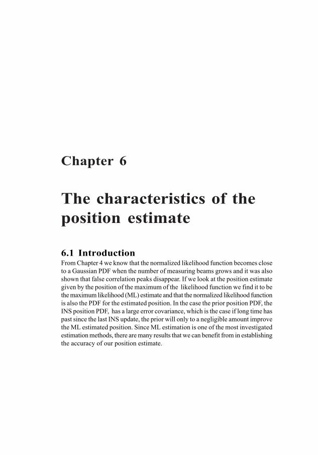
123
6.1 IntroductionFrom Chapter 4 we know that the normalized likelihood function becomes closeto a Gaussian PDF when the number of measuring beams grows and it was alsoshown that false correlation peaks disappear. If we look at the position estimategiven by the position of the maximum of the likelihood function we find it to bethe maximum likelihood (ML) estimate and that the normalized likelihood functionis also the PDF for the estimated position. In the case the prior position PDF, theINS position PDF, has a large error covariance, which is the case if long time haspast since the last INS update, the prior will only to a negligible amount improvethe ML estimated position. Since ML estimation is one of the most investigatedestimation methods, there are many results that we can benefit from in establishingthe accuracy of our position estimate.
Chapter 6
The characteristics of theposition estimate

124 6 The characteristics of the position estimate
6.2. Characteristics of the position estimateWe know from the theory of ML estimation that, under weak assumptions, theML-estimate [AOA02, KA93, VT68]
• is asymptotically unbiased• asymptotically reaches the Cramér-Rao lower
bound (CRLB)• is asymptotically Gaussian distributed
The asymptotic covariance of the ML-estimate ˆ ( )x y can therefore beexpressed as
1ˆ ˆ{( ( ) )( ( ) ) }TE −= − − =R x y x x y x J (6.1)
Where J is Fisher’s information matrix (FIM).
Let the gradient of the terrain topography in the sampling points be given by
1
1 1
1
2 2
hGx
N
N
hhx x
hhx x
∂∂ ∂ ∂∂ = = ∂∂∂ ∂ ∂
(6.2)
where x1, x2 refer to the east and north directions, respectively, then the Cramér-Rao matrix can be shown to be (see Chapter 5)
11R GC GTETL
−− = (6.3)
where C is the symmetric covariance matrix for the measurement beam errors andthe sub index ETL indicates exact terrain reference level, i.e. no measurementbias. In the case the covariance matrix is diagonal with the same error variance inall beams i.e.,
2C Ie Nσ= (6.4)
then
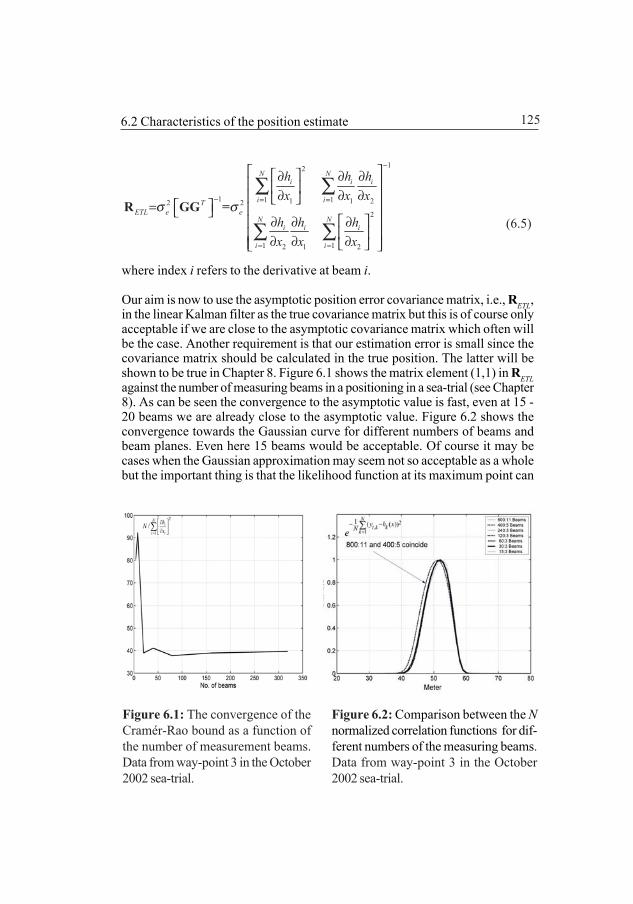
125
12
1 1 11 1 22 22
1 12 1 2
R GG =
N Ni i i
i iTETL e e
N Ni i i
i i
h h hx x x
h h hx x x
σ σ
−
− = =
= =
∂ ∂ ∂ ∂ ∂ ∂ = ∂ ∂ ∂ ∂ ∂ ∂
∑ ∑
∑ ∑ (6.5)
where index i refers to the derivative at beam i.
Our aim is now to use the asymptotic position error covariance matrix, i.e., RETL,in the linear Kalman filter as the true covariance matrix but this is of course onlyacceptable if we are close to the asymptotic covariance matrix which often willbe the case. Another requirement is that our estimation error is small since thecovariance matrix should be calculated in the true position. The latter will beshown to be true in Chapter 8. Figure 6.1 shows the matrix element (1,1) in RETLagainst the number of measuring beams in a positioning in a sea-trial (see Chapter8). As can be seen the convergence to the asymptotic value is fast, even at 15 -20 beams we are already close to the asymptotic value. Figure 6.2 shows theconvergence towards the Gaussian curve for different numbers of beams andbeam planes. Even here 15 beams would be acceptable. Of course it may becases when the Gaussian approximation may seem not so acceptable as a wholebut the important thing is that the likelihood function at its maximum point can
Figure 6.2: Comparison between the Nnormalized correlation functions for dif-ferent numbers of the measuring beams.Data from way-point 3 in the October2002 sea-trial.
Figure 6.1: The convergence of theCramér-Rao bound as a function ofthe number of measurement beams.Data from way-point 3 in the October2002 sea-trial.
6.2 Characteristics of the position estimate
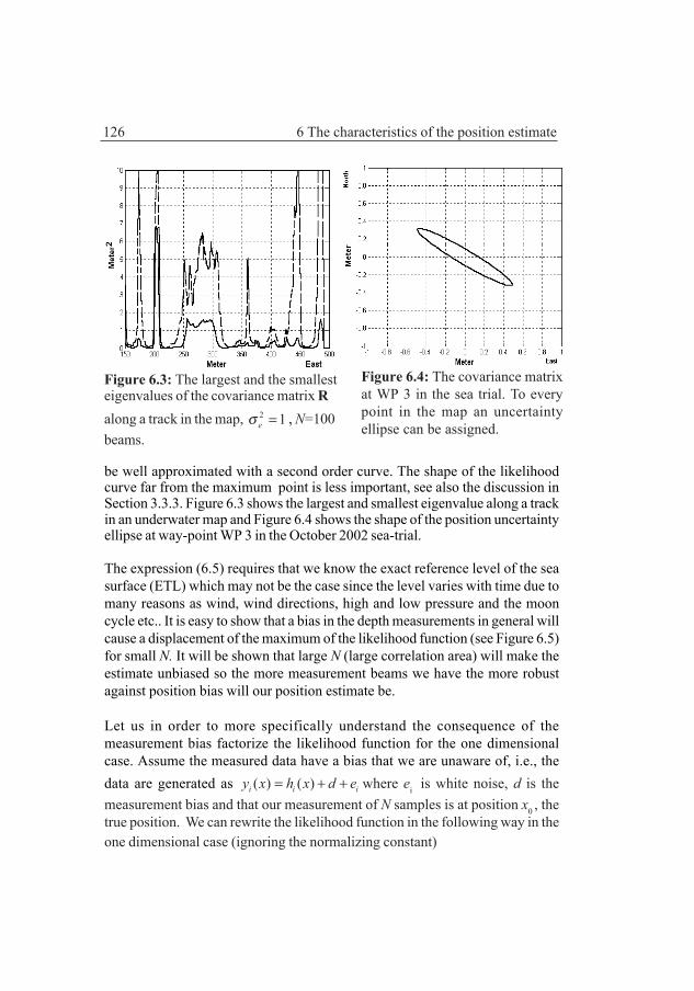
126 6 The characteristics of the position estimate
be well approximated with a second order curve. The shape of the likelihoodcurve far from the maximum point is less important, see also the discussion inSection 3.3.3. Figure 6.3 shows the largest and smallest eigenvalue along a trackin an underwater map and Figure 6.4 shows the shape of the position uncertaintyellipse at way-point WP 3 in the October 2002 sea-trial.
The expression (6.5) requires that we know the exact reference level of the seasurface (ETL) which may not be the case since the level varies with time due tomany reasons as wind, wind directions, high and low pressure and the mooncycle etc.. It is easy to show that a bias in the depth measurements in general willcause a displacement of the maximum of the likelihood function (see Figure 6.5)for small N. It will be shown that large N (large correlation area) will make theestimate unbiased so the more measurement beams we have the more robustagainst position bias will our position estimate be.
Let us in order to more specifically understand the consequence of themeasurement bias factorize the likelihood function for the one dimensionalcase. Assume the measured data have a bias that we are unaware of, i.e., thedata are generated as ( ) ( )i i iy x h x d e= + + where ei
is white noise, d is the
measurement bias and that our measurement of N samples is at position x0 , thetrue position. We can rewrite the likelihood function in the following way in theone dimensional case (ignoring the normalizing constant)
Figure 6.4: The covariance matrixat WP 3 in the sea trial. To everypoint in the map an uncertaintyellipse can be assigned.
Figure 6.3: The largest and the smallesteigenvalues of the covariance matrix Ralong a track in the map, 2 1eσ = , N=100beams.

127
20 02
1
202
1
202
1
0 0
1( ; ( ), , ) exp( (( ( ) ( ) ) )2
1 exp( ( 2 ( ( ) ( ) )))2
1 exp( ( ( ) ( ) ) )2
( ; ( ), , ) ( ; ( ), )
N
i iie
N
i iie
N
i iie
h UB
L x y x d N y x h x d d
Nd d y x h x d
y x h x d
L x y x d N L x y x N
σ
σ
σ
=
=
=
= − − − +
= − + − −
⋅ − − −
=
∑
∑
∑ (6.6)
We see that the factor LUB(x;y(x0),N) does not depend on d but is the likelihoodfunction if we had no measurement bias. The first factor can be further factorized
00 2 2
0
( ( ) / 2)( )( ; ( ), , ) exp( ) exp( )
( ; ( ), , ) ( ; ( ), , )
he e
hyhh
Nd y x dNdh xL x y x d N
L x h x d N L x y x d N
σ σ−
= ⋅ −
= (6.7)
Figure 6.5: The log likelihood function at different measurement bias in meter fora relatively flat area.The number of beams N = 100, variance in measurementnoise 0.25 m2. The figure is based on a real map.
6.2 Characteristics of the position estimate

128 6 The characteristics of the position estimate
where 0( )y x is the mean of the measurements at position x0 and ( )h x the meanof depths at position x thus indicating that the bias depends on the slope of thebottom. It is easy to determine the displacement in position caused by themeasurement bias d in an actual case given the values of d and N. We have
0 0 0 0
0
0 0
ˆ ˆ( | ( ), , ) ( ( )) ( ( )) arg max( ( | ( ), , ))
arg max( ( | ( ), , ) / ( | ( ), , ))
B UB
x
hx
b x y x d N x y x x y xL x y x d N
L x y x d N L x y x d N
= −=
− (6.8)
which is easily computed. An approximate solution can also be found, when theunbiased likelihood function can be approximated by a Gaussian curve in thefollowing way. Replace in (6.6) LUB by its Gaussian curve equivalent assumingthe maximum point is at x =x0
( )20
22 0
1
exp( )( )2 /
UBG Ni
ei
x xL
h xx
σ=
−= −
∂ ∂
∑ (6.9)
and use that
log ( ) log ( )log ( ) 0UBG hL x L xL xx x x
∂ ∂∂ = + =∂ ∂ ∂ (6.10)
at the maximum point. The result is
0
10 2
0
1
( )
( | , )( )
Ni
i
Ni
i
h xxb x d N d
h xx
=
=
∂∂=
∂ ∂
∑
∑ (6.11)
or to show the dependence of the mean bottom slope
00
( )( | , )
h xb x d N dx
∂∝
∂ (6.12)
This can be seen as an amplification factor of the measurement bias. Now, (6.7)

129
can also be written
0
202
1
2 002
1
( ; ( ), , )1 exp( ( 2 ( ( ) ( ) )))
2( )1 exp( ( 2 ( ) ))
2
hN
i iie
Ni
ie
L x y x d N
Nd d y x h x d
h xNd d x x
x
σ
σ
=
=
= − + − −
∂≈ − + −
∂
∑
∑ (6.13)
for large N and x close to x0. The width of the peak of the likelihood functionwith no measurement bias will decrease inversely with N so if we look at theneighbourhood of the peak, the first term of the exponent will dominate whichmeans that the unbiased likelihood function is multiplied by a constant, thatis, the likelihood function with measurement bias will for large N give a posi-tion estimate with no offset from the true position and a covariance as (6.5).
The bias problem can also be analyzed somewhat differently (cf. Section 5.4). Aresult from large sample theory [BS02] is that if a stochastic variable isasymptotically normal distributed 0( , )ax x R∼N , as in our case, and undergoesa one to one transformation z=B(x) then the transformed variable is alsoasymptotically normal distributed
0 00 0
( ) ( )( ( ), )
Ta ∂ ∂ = ∂ ∂
B x B xz z B x R
x x∼N (6.14)
A requirement is that the largest eigenvalue of R 0→ when the number ofsamples (beams) N → ∞ .
In the bias discussion in Section 5.4 the mean was assumed to be the positionestimate. However we can deduct a similar expression when we are assumingthe position of the maximum of the likelihood function to be the measuredposition. Let us again look at the one dimensional case and let us assume thatthe measured height in each beam can be described by
( ) ( )i i iy x h x d e= + + (6.15)
The ML position estimate is given by the solution of the equation
6.2 Characteristics of the position estimate
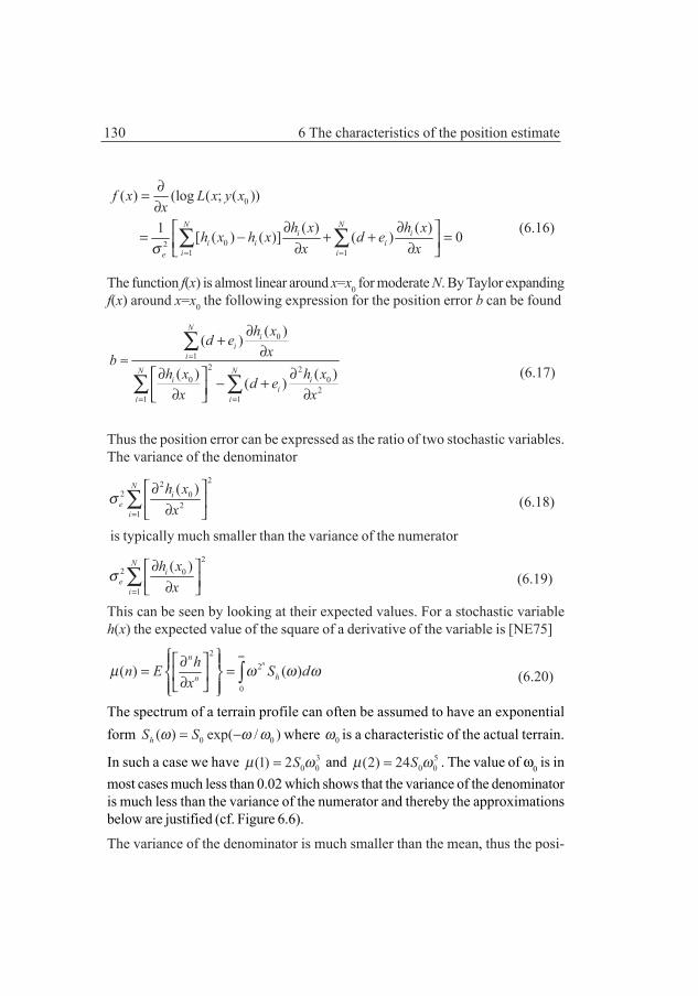
130 6 The characteristics of the position estimate
0
021 1
( ) (log ( ; ( ))
( ) ( )1 [ ( ) ( )] ( ) 0N N
i ii i i
i ie
f x L x y xx
h x h xh x h x d ex xσ = =
∂=∂
∂ ∂ = − + + = ∂ ∂ ∑ ∑ (6.16)
The function f(x) is almost linear around x=x0 for moderate N. By Taylor expandingf(x) around x=x0 the following expression for the position error b can be found
0
12 2
0 02
1 1
( )( )
( ) ( )( )
Ni
ii
N Ni i
ii i
h xd exb
h x h xd ex x
=
= =
∂+∂≈
∂ ∂ − + ∂ ∂
∑
∑ ∑ (6.17)
Thus the position error can be expressed as the ratio of two stochastic variables.The variance of the denominator
222 0
21
( )Ni
ei
h xx
σ=
∂ ∂
∑ (6.18)
is typically much smaller than the variance of the numerator2
2 0
1
( )Ni
ei
h xx
σ=
∂ ∂
∑ (6.19)
This can be seen by looking at their expected values. For a stochastic variableh(x) the expected value of the square of a derivative of the variable is [NE75]
22
0
( ) ( )n
n
hn
hn E S dx
µ ω ω ω∞ ∂ = = ∂ ∫ (6.20)
The spectrum of a terrain profile can often be assumed to have an exponentialform 0 0( ) exp( / )hS Sω ω ω= − where 0ω is a characteristic of the actual terrain.
In such a case we have 30 0(1) 2Sµ ω= and 5
0 0(2) 24Sµ ω= . The value of ω0 is inmost cases much less than 0.02 which shows that the variance of the denominatoris much less than the variance of the numerator and thereby the approximationsbelow are justified (cf. Figure 6.6).
The variance of the denominator is much smaller than the mean, thus the posi-

131
tion error will be close to Gaussian distributed. Disregarding the stochastic partof the denominator the variance will be
2
2 2220 0 0
21 1 1
222 20 0
2 21 10
1
1( )( ) ( ) ( )1 /
( ) ( ) 1 /( )
eN N Ni i i
i i i
N Ne i i
Ni ii
i
Var bh x h x h xdx x x
h x h xdx xh x
x
σ
σ
= = =
= =
=
≈∂ ∂ ∂ − ∂ ∂ ∂
∂ ∂ ≈ + ∂ ∂ ∂ ∂
∑ ∑ ∑
∑ ∑∑
(6.21)
See Figure 6.7 which compares (6.17) with a Monte Carlo simulation of the posi-tion bias.
An accurate approximation of the bias for larger N is2
0 0
1 1
( ) ( ){ }N N
i i
i i
h x h xE b b dx x= =
∂ ∂ = ≈ ∂ ∂ ∑ ∑ (6.22)
and approximately we have
Figure 6.6: The ratio between µ(1) and µ(2) as a function of the fall off constantω0.
6.2 Characteristics of the position estimate
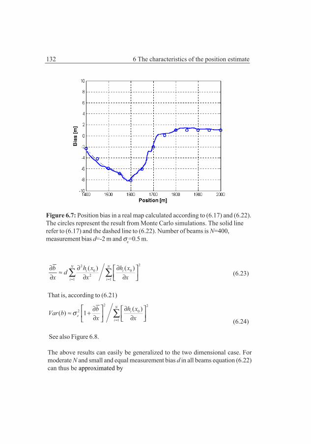
132 6 The characteristics of the position estimate
220 0
21 1
( ) ( )N Ni i
i i
h x h xb dxxx = =
∂ ∂∂ ≈ ∂∂∂ ∑ ∑ (6.23)
That is, according to (6.21)2 2
2 0
1
( )( ) 1N
ie
i
h xbVar bx x
σ=
∂∂ ≈ + ∂ ∂ ∑
(6.24)
See also Figure 6.8.
The above results can easily be generalized to the two dimensional case. Formoderate N and small and equal measurement bias d in all beams equation (6.22)can thus be approximated by
Figure 6.7: Position bias in a real map calculated according to (6.17) and (6.22).The circles represent the result from Monte Carlo simulations. The solid linerefer to (6.17) and the dashed line to (6.22). Number of beams is N=400,measurement bias d=-2 m and σe=0.5 m.
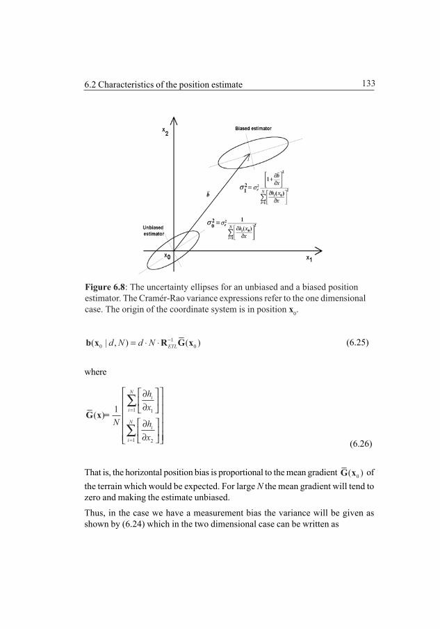
133
10 0( | , ) ( )ETLd N d N −= ⋅ ⋅b x R G x (6.25)
where
1 1
1 2
1( )
Ni
i
Ni
i
hx
N hx
=
=
∂ ∂ ∂ ∂
∑
∑G x =
(6.26)
That is, the horizontal position bias is proportional to the mean gradient 0( )G x ofthe terrain which would be expected. For large N the mean gradient will tend tozero and making the estimate unbiased.
Thus, in the case we have a measurement bias the variance will be given asshown by (6.24) which in the two dimensional case can be written as
6.2 Characteristics of the position estimate
Figure 6.8: The uncertainty ellipses for an unbiased and a biased positionestimator. The Cramér-Rao variance expressions refer to the one dimensionalcase. The origin of the coordinate system is in position x0.

134 6 The characteristics of the position estimate
0 0( ) ( )T
Bias ETL∂ ∂
≈∂ ∂
B x B xR Rx x
(6.27)
where ( ) ( )= +B x x b x .
In the estimation of the position the existence of measurement bias can of coursebe taken into account from the very beginning. This has been shown in Chapter5. Often, however, we can approximate the measurement bias to be the differencebetween the means of the measured depths and corresponding map depths aspointed out earlier. The main difference between this approximation and themore correct method (3.20) in Chapter 3 is that the first assumes that the likelihoodmaximum occur at a step point, which also should be the true position, in thematching which may not be the case. With the number of measurement beamswe are using the difference is negligible.
The reduction of the measurement and map vector with the means can bedescribed as pre-multiplying the profile vectors y(x0) and h(x) by the projectionmatrix which will subtract respective mean from the vectors. The projectionmatrix is
ΠΠΠΠΠ=IN-1N,N/N (6.28)
where IN is the identity matrix and 1N,N is a matrix with ones as elements.Straightforward calculations of the second derivative, see Chapter 5, of the loglikelihood function for this case give the CRLB matrix (cf. (6.5)).
12 TPM eσ
− = R GΠG (6.29)
When profile matching gives a unique position and we have a large number ofbeams expressions (6.5) and (6.29) will be close to each other.
In the general case when we have a measurement bias and a full measurementerror covariance matrix the CRLB for the position error is as shown in Chapter 5
11/ 2 1/ 2 1 1 1/ 2 1/ 2( )T T T −− − − − − − = − R GC I C u u C u u C C G (6.30)
where u is a column vector of N ones and C the position error covariance matrix

135
and G defined by (6.2). Since the elements in the covariance matrix of theposition error correspond to the sum of the terrain gradients in the measuringfootprint points, this also means that the method with several measuring beamscan be used in much flatter terrain areas than the measuring with only onebeam since adding of beams will compensate for the smaller terrain gradients.
The position error covariance matrix for the estimate can thus be calculated inreal time or in advance from the terrain map. We see from (6.5) that the errorcovariance is approximately inversely proportional to the number of beams. Inthe case we know the autocorrelation function for the bottom profile theestimated value of the position error covariance matrix is just a function of N.

136 6 The characteristics of the position estimate
137
7.1 IntroductionThe first part of this chapter will discuss what is called optimal footprint beampattern before turning to the problem of choosing way-points. We will restrictour discussion to rectangular beam patterns since these naturally arise frombathymetric sonars with a linear or square sensor array which is the commonarray shape. It turns out that the position accuracy could in some cases beconsiderably increased by adjusting the footprint of the beam pattern to thestructure of the bottom terrain which is a simple thing to do if a true 3D bathymet-ric sonar is used. The second part of the chapter will discuss how to choose way-points. Since it is possible to determine the position accuracy directly from theunderwater map, this information can be used in planning vehicle missions tosecure that good position fixes will be achieved.
7.2 Optimal footprint beam patternThe achievable position accuracy is given by the Cramér-Rao lower bound ex-pression (6.1). It is not obvious from (6.1) that the actual accuracy strongly
Chapter 7
Optimal beampattern andway-point selection

138 7 How to choose way-points
depends on the beam footprint array pattern in many cases. A simple examplewill show this.
Assume that we have a non-circular Gaussian hill as in Figure 7.1 and our trueposition at the sampling event is at the top of the hill. Correlation is then doneby an array of 20 x 20 beams and by an array of 10x40 beams. The same numberof beams is thus used in both cases. The contour plots for the likelihood func-tions in the two cases are shown in Figure 7.2 and 7.3. The contour of thelikelihood function will be elliptical for a square beam pattern. The semiaxis ofthe uncertainty ellipse in the center of the Gaussian hill are given by the eigen-vectors and eigenvalues of the Cramér-Rao matrix in that point. By comparingFigure 7.2 with Figure 7.3 we see a great improvement in accuracy in the worstdirection at the expense of the accuracy in the best direction.
Figure 7.4 and 7.5 show a real example from a sea-trial when the way-point issituated on the slope of an underwater ridge. In Figure 7.4 the beam array patternis 10 x 10 in a rectangular grid of 10 meter. The angle between the grid and theridge is approximately 30 degrees. In Figure 7.5 the beam pattern is 50 x 2 beamsand the pattern is rotated 30 degrees to align the long side with the ridge.
Figure 7.6 shows the magnitude of the largest semiaxis for different footprint
Figure 7.1: Flat terrain with a Gaussian hill. The true position is in the centre ofthe hill.

139
patterns, from 1x256 to 16x16, when the beampattern is rotated 360 degrees. Fora quadratic beam pattern there is only small variation in the magnitude of thelargest semiaxis but for the 2 x 128 beam pattern we have a radically smallerlargest semiaxis for a rotation angle of 150 degrees.
Figure 7.3: Uncertainty ellipse for anarray pattern of 10 x 40 beams at 80%height of the maximum of likelihoodfunction.
Figure 7.2: Uncertainty ellipse foran array pattern of 20 x 20 beams at80% height of the maximum oflikelihood function.
Nor
th
Nor
th
Figure 7.4: The likelihood functionfor a way-point situated at the slopeof a ridge.
Figure 7.5: The likelihood functionwhen the beam pattern has beenadjusted and rotated. Note thedifference in horizontal scalecompared to Figure 7.4.
EastEast
7.2 Optimal footprint beam pattern
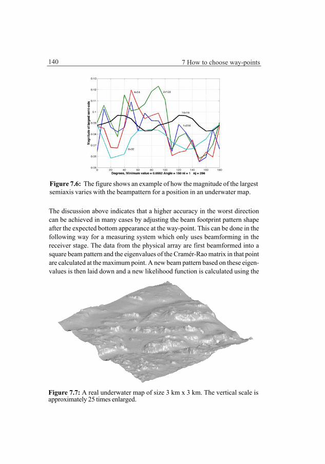
140 7 How to choose way-points
The discussion above indicates that a higher accuracy in the worst directioncan be achieved in many cases by adjusting the beam footprint pattern shapeafter the expected bottom appearance at the way-point. This can be done in thefollowing way for a measuring system which only uses beamforming in thereceiver stage. The data from the physical array are first beamformed into asquare beam pattern and the eigenvalues of the Cramér-Rao matrix in that pointare calculated at the maximum point. A new beam pattern based on these eigen-values is then laid down and a new likelihood function is calculated using the
Figure 7.7: A real underwater map of size 3 km x 3 km. The vertical scale isapproximately 25 times enlarged.
Figure 7.6: The figure shows an example of how the magnitude of the largestsemiaxis varies with the beampattern for a position in an underwater map.

141
Figure 7.8: The map shows the magnitude of the largest semiaxis for a fixedbeam footprint pattern of 16 x 16 beams for a real map.
same data. There will of course be many places where an approximation with aGaussian hill is not so good but an optimal beam footprint pattern can always befound by adjusting the side relation and the rotation of the beam footprint pattern(see Figure 7.6).
Now we will look at a real map, see Figure 7.7, to see what this will mean in reality.Figure 7.8 shows a map of the largest semiaxis for a fixed beam footprint pattern of16 x 16 beams for this map. Figure 7.9 shows the same map but now with theoptimal beampattern, i.e., the beam pattern varies from 2 x 128 to 16 x 16 and isrotated to achieve the smallest largest semiaxis of the uncertainty ellipse. As canbe seen the topography is now more chiselled and the magnitude is much lowerin many areas. Note the difference in vertical scale compared to Figure 7.8. Thefigures are based on the same number of beams. Figure 7.10 shows the percent-age of the total map area which has the largest semiaxis below a certain value. Forexample, if a magnitude of the largest semiaxis of 0.1 is acceptable then the opti-mal technique would more than double the map area where that accuracy, orbetter, could be achieved. As can be seen from the figures there is great improve-ment in certain areas and less in other areas.
7.2 Optimal footprint beam pattern
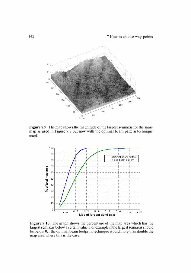
142 7 How to choose way-points
Figure 7.10: The graph shows the percentage of the map area which has thelargest semiaxis below a certain value. For example if the largest semiaxis shouldbe below 0.1 the optimal beam footprint technique would more than double themap area where this is the case.
Figure 7.9: The map shows the magnitude of the largest semiaxis for the samemap as used in Figure 7.8 but now with the optimal beam pattern techniqueused.
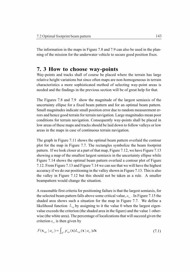
143
The information in the maps in Figure 7.8 and 7.9 can also be used in the plan-ning of the mission for the underwater vehicle to secure good position fixes.
7. 3 How to choose way-pointsWay-points and tracks shall of course be placed where the terrain has largerelative height variations but since often maps are non-homogeneous in terraincharacteristics a more sophisticated method of selecting way-point areas isneeded and the findings in the previous section will be of great help for that.
The Figures 7.8 and 7.9 show the magnitude of the largest semiaxis of theuncertainty ellipse for a fixed beam pattern and for an optimal beam pattern.Small magnitudes indicate small position error due to random measurement er-rors and hence good terrain for terrain navigation. Large magnitudes mean poorconditions for terrain navigation. Consequently way-points shall be placed inlow areas of these maps and tracks should be laid down to follow valleys or lowareas in the maps in case of continuous terrain navigation.
The graph in Figure 7.11 shows the optimal beam pattern overlaid the contourplot for the map in Figure 7.7. The rectangles symbolize the beam footprintpattern. If we look closer at a part of that map, Figure 7.12, we have Figure 7.13showing a map of the smallest largest semiaxis in the uncertainty ellipse whileFigure 7.14 shows the optimal beam pattern overlaid a contour plot of Figure7.12. From Figure 7.13 and Figure 7.14 we can see that we will have the highestaccuracy if we do our positioning in the valley shown in Figure 7.13. This is alsothe valley in Figure 7.12 but this should not be taken as a rule. A smallerbeampattern would change the situation.
A reasonable first criteria for positioning failure is that the largest semiaxis, forthe selected beam pattern falls above some critical value, cra . In Figure 7.15 theshaded area shows such a situation for the map in Figure 7.7. We define alikelihood function wpL by assigning to it the value 0 when the largest eigen-value exceeds the criterion (the shaded area in the figure) and the value 1 other-wise (the white area). The percentage of localizations that will succeed given thecriterion cra is then given by
2( | ) ( ) ( | )wp cr wp wp crRF a p L a d−= ∫x x x x (7.1)
7.2 Optimal footprint beam pattern

144 7 How to choose way-points
Figure 7.12: Part of the map shown in Figure 7.7. The vertical scale is enlargedapproximately 50 times.
Figure 7.11: Optimal beam pattern overlaid the contour plot of a map. Darkerbeam patterns are good areas for terrain positioning. Light (red) areas arebad for terrain positioning. The scale of the vertical and horizontal axis andsize of semiaxis is in 10th of meters.

145
Figure 7.14: The optimal beam patternoverlaid the contour map for Figure7.12 for determination of suitableway-points. The scale of the verticaland horizontal axis is in 10th of me-ters.
Figure 7.13: The map over the largestsemiaxis in the uncertainty ellipsewhen the optimal beampattern hasbeen used, cf. Figure 7.12. The scaleof the vertical and horizontal axis is in10th of meters.
Figure 7.15: White areas are areaswhere the largest semiaxis of theuncertainty ellipse is smaller than acertain threshold value, i.e., 0.15.
Figure 7.16: The value of the largestsemi axis for the landscape in Figure7.7. Contour lines are for 0.1, 0.15,0.20, 0.25.
7.3 How to choose way-points

146 7 How to choose way-points
Here ( )wpp− x is the INS-system’s PDF with centre in the way-point wpx , the prior
PDF.
This is illustrated in Figure 7.15 by a possible way-point in the centre of thecircle, where the size of the circle symbolizes the 1-σ INS error. Figure 7.16 showsthe largest semiaxis for the landscape in Figure 7.7. If the actual arrival at theway-point is in the shaded area then positioning is impossible, the error is toolarge. On the other hand, if it is in the white area a position fix is possible. In sucha way, for every point in the map, the percentage of success can be calculatedaccording to (7.1) , see Figures 7.17 and 7.18. The choice of cra will depend onthe accuracy needed when other sources of errors have been taken into consid-eration (see Chapter 8).
Figure 7.17: The diagram shows the probability for success for way-points inthe map in Figure 7.7.

147
Figure 7.18: Contour map of the diagram in Figure 7.17. In the dark shadedareas the probability of success in positioning is less than 25% and in the lightshaded areas the probability is almost 100 %. The step in shading is 25%. Theprior PDF from the INS is assumed to be 100 meter RMS. The scale of the verticaland horizontal axes is in 10th of meters.
7.3.1 An example of how to choose a way-pointOur goal is to decide upon a way-point in a given area for which we have anunderwater map. Our sonar equipment is a bathymetric sonar with known charac-teristics as number of beams, beam angles, measurement accuracy and so forth.We will also assume that the number of measurement beams is so large that theGaussian approximation is reasonable. The positioning result will be used forupdating an INS-system. The steps for establishing the way point will be asfollows.
The first step will be to calculate the position error covariance matrix for everypoint in the map. According to (6.1) in Chapter 6 the error covariance matrix withno beam weighting is
7.3 How to choose way-points

148 7 How to choose way-points
12
1 1 11 1 22 22
1 12 1 2
R GG =
N Ni i i
i iTETL e e
N Ni i i
i i
h h hx x x
h h hx x x
σ σ
−
− = =
= =
∂ ∂ ∂ ∂ ∂ ∂ = ∂ ∂ ∂ ∂ ∂ ∂
∑ ∑
∑ ∑ (7.2)
If we have a bathymetric sonar with only one beamplane we may have to as-semble a number of beamplanes to measure the bottom 3D topography. A goodchoice of the number of beam planes by experience may be 5 with a distancebetween the planes of 20 - 25 meter.
When calculating the uncertainty ellipse account shall preferably be given to theactual sonar and the real footprint of the sonar against the bottom, see Figures7.19 and 7.20. By that, the enlargement of the total footprint with increased depthwill automatically be taken into account. This is important since a larger footprintcoverage will mean a smaller positioning error. A way of determining the intersec-tion of the individual beams with the bottom is to first approximate the bottomwith triangles with their vertices in the grid points of the map. The intersection ofthe beams and the planes determined by the triangles is then calculated and bythat the positions of the beam footprints and the depth for the beams are known,Figure 7.21.
Figure 7.19: A typical beam plane. Figure 7.20: An assembled beampackage of five beam planes.

149
The chosen number of beam planes shall then be assembled with a fix distanceand angle between the beam planes. The beam plane assembly is then moved insteps over the map and the depth measurements are calculated from a sonarmodel which can be more or less complex, i.e., taking temperature gradients andother things into account. A more approximate solution using a beam patternwith a fixed distance between the individual beam footprints, see Figure 7.22, isoften of interest since it is much less computationally demanding and still givesa good view of the good areas for terrain navigation. When those are found thena more accurate computational method can be used. In both ways interpolationof the map depth has to be used. In relatively flat areas a linear interpolationmethod can be used but in more rough hilly terrains a more accurate methodmust be used (see Appendix B).
As an alternative to interpolation a sonar map method can be used, that is a localmap of the sonar measurement with the same grid size as the underwater map isproduced and this map is correlated with the underwater map in the gridpoints.The main complication with this method appears when the correlations shall bedone with different rotation angles of the beam pattern.
The next step in the process is to calculate, in every point of the map, the
Figure 7.21: The individual beam footprint is calculated by first finding theintersection between the bottom and the beam package of five beam planes.
7.3 How to choose way-points

150 7 How to choose way-points
eigenvalues of the position error covariances. This will give the major and minorsemiaxes of the uncertainty ellipse and the eigenvector gives the direction of thesemiaxis and by that the orientation of the likelihood function is known. In thedirection of the eigenvector corresponding to the largest eigenvalue we havethe poorest accuracy and in the direction of the eigenvector corresponding tothe smallest eigenvalue we have the best accuracy. By now a graph like Figure7.13 can be drawn for the largest eigenvalue (semiaxis for the uncertainty ellipse)and it is in the low areas the best places for way-points are.
The covariance error matrix (7.2), corresponds to the likelihood function2
,221
1 1( ; ) exp( ( ( )) )2(2 )
N
t t t k k tNkee
L y hσπσ =
= − −∑x y x (7.3)
If the more complex likelihood function with beam weighting is used11 1( ; ) exp( ( ( )) ( ( )))
2(2 ) det( )T
t t t t e t tNe
Lπ
−= − − −x y y h x C y h xC (7.4)
the corresponding error covariance matrix should be used in the calculations,see Chapter 5.
Figure 7.22: Footprint of the beam plane assembly for a flat bottom.

151
Now, for updating our IN-system with an accurate position for eliminating thedrift error we can only accept terrain positions with a largest semiaxis smallerthan a certain value so we produce a new map, the success map, of the areawhere the pixels are 1 if we meet the criteria or 0 if we fail, cf. Figure 7.15. Thisnew map will now be the basis for the calculation if we will fail or succeed inestablishing a terrain position with required accuracy. When the vehicle isapproaching the way-point it will only occasionally hit the way-point so theactual vehicle positions, when the vehicle thinks she is at the way-point, willbe spread according to the accuracy of the navigation system. Sometimes thevehicle will end up in the white areas and sometimes in the black areas.
The success rate is then calculated for every assumed way-point in the mapaccording to (7.1) which gives the probability of success when approaching away-point at position wpx . A graph of the function is shown in Figure 7.18. Thefinal step is then to select an actual point in the light shaded areas in thatfigure.
7.3 How to choose way-points

152 7 How to choose way-points

153
Chapter 8
Sonars and the sea-trialOctober 2002
8.1 IntroductionThis chapter starts with a discussion of sonars suitable for terrain navigation asan introduction to the presentation of some results from one of the sea-trialsthat have been conducted to verify the theory presented earlier in this thesis.
8.2 Sonars and position error causes8.2.1 IntroductionThe same type of sonars that are used for charting of ship routes can be used forterrain navigation. These sonars are called bathymetric sonars and have a fan-shaped beamplane with ~60 - 250 beams with beamwidths ~0.5 - 1.5 degrees.
Often such sonars work in the frequency range 100 - 200 kHz to have a reasonablerange in depth. The lower the frequency is the lower will the attenuation of thesonar pulse be and by that an increased range for the sonar.

154 8 Sonars and the Sea-trial October 2002
Large depths mean that the beam footprint will be large so a small beam angleis essential for mapping smaller objects at large depths.
There are many types of errors encountered in terrain navigation besides therandom measurement error previously discussed. To name a few of them wehave errors caused by:
- Ship movementPitch, roll and yaw and with surface ships also heave.
- The mounting of the sonarheadReflectionIncorrect assumptions about the center of vehicle movement
- Characteristics of the sonarBeamwidthNumber of beams and spacingAccuracy in depth measurementPowerAlgorithm for bottom detection
- Measurement errors caused by water characteristicsInsufficient compensation of temperature gradientsReflections of the outer beams due to stratifying layers.
- Measurement errors caused by askew reflections of sonarbeamsDue to bottom slantDue to rocksDue to objects in the water column, i.e., fish schools
8.2.2 Bathymetric sonarsFigures 8.1 and 8.2 show two types of bathymetric sonars that have been usedfor terrain navigation. Figure 8.1 shows the Reson SeaBat 9001. The cylinderon the main body is the transmitting unit consisting of a cylindrical pile ofdiscs of a piezoelectric ceramic material. To each disc a phased sonar pulse issent and by that a fan shaped beam is formed as sketched in Figure 8.3. Thephysical sound wave is transmitted from the cylindrical surfaces of the ceramicdiscs.

155
Figure 8.1: The Reson SeaBat 9001sonar used in the sea-trial 1998.
Figure 8.2: The Reson SeaBat 8101sonar used in the sea-trial 2002.
Figure 8.3: The principle to obtain a measurement beam in the Reson SeaBat9001 and 8101 sonars as cross sections between the transmitting and receivingfan shaped beams.
The half cylindrical element at the front end of the main body is the receiver.Also the reciever consists of piezoelectric ceramic elements now in the formof wedge-shaped plates. When the return pulse hits the ends of the plates anelectric signal is created. The signals from the elements are after amplificationbeamformed into 60 beams in a fan shaped plane, perpendicular to thetransmitting beam and by that the elements only catches the return pulse fromthe cross-over by the fan shaped transmitting and receiving beams. Thefrequency is 455 kHz and the beamwidth is 1.5 x 1.5 degrees with spacing 1.5degrees. The physical size of the main body is 473 x 190 x 126 mm.
8.2 Sonar and position error causes

156 8 Sonars and the Sea-trial October 2002
It is also possible to steer the transmitting fan shaped beam in an angle to avertical line as in Figure 8.4. By firing 5 succesive pings with the beam plane atan angle of, say, -45, -27, 0, 27 and 45 degrees a 3D bottom picturecorresponding to Figure 7.22 can be achieved. The time between the individualpings is as short as possible and the result is compensated for the distancetravelled between the pings. There will be an increased sensitivity foruncompensated temperature gradients in the outer beamsplanes since they arenot vertical any longer. On the other hand the error in distance and angle betweenthe beam planes will be smaller than the arrangement according to Figure 7.20.
The Reson SeaBat 8101 sonar in Figure 8.2 was used in the sea-trial describedlater in this chapter. A glimpse of the cylindrical transmitting element can befound at the left end of the body. The receiving element is the dark cylindricalstrip on the main body between the mounting details. The transmitting andreceiving beams are formed in the same manner as for the SeaBat 9001 sonar.
Figure 8.4: A sonar firing five transmit beams at different angles to the verticalline, cf. Figure 7.22.

157
The frequency is 240 kHz and there are 101 beams of width 1.5 x 1.5 degreesand with a spacing of 1.5 degrees.
Another sonar that has been used in the tests is the OmniTech EchoScope,Figure 8.5, which is a true 3D-sonar with a 40 x 40 receiver array forming4096 receiver beams of 1.5 x 1.5 degrees with a beam spacing of 1.5 degrees.The receiver array, the shaded square, is made of a piezoelectric polymer andthe three transmitters are made up of ceramics. The cylindrical element aboveand the two elements below the receiver array are the transmitters. The sonarcan transmit three different CW frequencies and the curvature of the transmittingelement determines the beam width of the transmitting pulse. Figure 8.6 showsa bottom picture taken by this sonar. Figure 8.7 shows the footprint of thebeams. The ideal terrain navigation sonar is a true 3D sonar, due to the fixeddistance between the beams, with a few hundred beams and a short singletransmitting pulse if covertness is required.
Figure 8.5: The OmniTech, EchoScope sonar is a true 3D sonar with a 40 x 40receiving array of a piezielectric polymer, PVDF. The different transmitters havedifferent frequencies, 150, 300 and 600 kHz. The curvature of the transmittersforms the transmitting beam shape. The sonar was used in the sea-trial 2000.
8.2 Sonar and position error causes

158 8 Sonars and the Sea-trial October 2002
Figure 8.6: A bottom picture fromthe EchoScope sonar.
Figure 8.7: The footprints fromthe measurement beams for theEchoScope sonar.
8.2.3 Measurement errorsWhen measuring the terrain profile consideration has to be taken to severaltypes of measurement errors with varying degree of seriousness.
Errors due to the ship movementThe usual mounting of the sonarhead is flush to the ship body. To be able tocompensate for the ship movement an inertial measurement unit (IMU) ismounted as close as possible to the sonar head. However it will not be possibleto completely compensate for the ship movement and thus some errors willremain.
An earlier study by a sonar manufacturer gave the following measurementerror for a case with a 50 meter depth and a total sonar opening beam angle of90 degrees, 60 beams with beamwidth 1.5 degrees.
Accurate sensorsuiteUncompensated pitch and roll 0.05 degrees.Uncompensated heave 0.05 meter.Depth error in individual beams at 95% confidence interval 0.25 meter.

159
Typical sensorsuiteUncompensated pitch and roll 0.1 degrees.Uncompensated heave 0.05 meter .Depth error in individual beams at 95% confidence interval 0.33 meter.
The sonar mountingThe transmitter of the sonar sound pulse is often of the omni directional typewhich means that reflections from the vehicle body my appear.
The characteristics of the sonarThe depth resolution of the sonar depends on its bandwidth and pulse shapeand is in most cases of secondary importance (<0.05 m) for the depth error.The beamwidth can, however, in certain cases be of importance. Bathymetrysonars often have a beamwidth of 1.5 x 1.5 degrees which means that thefootprint of the beam is approximately 1.3 x 1.3 meter at 50 meter depth. Sincethe sonar in most cases will take the smallest depth within the footprint as thedepth, an error may result at high slant angles, especially at larger depths.
However, the greatest error will in most cases be caused by different detectionsof the bottom line. Depending on the sonar frequency the sonar beam willpenetrate differently into the bottom sediment. The depth of the soft sedimentlayer can be several meters. A low frequency sonar will penetrate deep into thebottom sediment while a high frequency sonar will penetrate only a little.Sometimes, when using profile matching, this will not change the bottom profilein other cases, i.e., large stone blocks in the sediment, the profile will change.
The upper part of the bottom sediments will have a very high content of waterwhich is successively decreased with increasing depth. This will cause the returnecho to be diffuse and depending on the bottom detection algorithm differentsonars will give different depth measures. This can be a problem for the beamsat high angle of incidence since they travel long into the sediments. The harderthe bottom is the less is the problem.
Sound bending due to temperature gradients and stratifying layersThe depth shown by the sonar is calculated from the travelling time of thesound pulse. This means that if the path of the beam is longer due to the beambending a larger depth than the real depth is shown. If the temperature gradientis known the sonar software will compensate for this. However, in shallow
8.2 Sonar and position error causes

160 8 Sonars and the Sea-trial October 2002
water the temperature gradient will also depend on the horizontal position.One reason for that is underwater currents.
In order to minimize the problem with beam bending the sonar beams shall beas perpendicular to the bottom as possible and the weighting of the outer beamsshall be less than the central beams in the matching process.
Measurement error due to slant reflections, fishes and similar thingsFrequently depth errors will occur due to non-reflecting beams. That meansthat the side lobes of the beam will catch a return pulse from some other directionthan expected and show a wrong depth. Especially the outer beams are exposedto this at high bottom slant angles.
Fish and objects in the water column may give large depth errors but thoseerrors are often easy to correct by removing the depth values without changingthe others by filtering. The traditional way when charting is to remove thesetypes of errors manually by an operator.
The accuracy of the mapThe underwater maps produced by the Maritime authority is produced formerchant shipping and this may influence the use of them for terrain navigation.Sea bottom areas are most often charted by low frequency sonars. Depths givenare conservative i.e., the actual depth may be larger.
The official depth accuracy given is not better than 1.5 meter. In reality it mightbe better. The horizontal position error of the depth given is in the range of 1meter.
8.3 Sea-trial October 2002, Simulation8.3.1 IntroductionTo verify the characteristics of the proposed navigation method three largesea-trials have been conducted with similar results. Some of the results fromthe last sea-trial in October 2002 will be presented here. The sea-trial wasconducted in the way that a track of 65 km around an island was divided by anumber of way-points as shown in Figure 8.8. At every way-point it was testedif it was possible to get a position with the suggested navigation method. Theway-points were selected from the underwater map by the eye to have good

161
Figure 8.9: Lowering the sonar through the moon-pool. In the middle of thepicture is the IMU for measuring the sonar attitude.
Figure 8.8: The 65 km long test track with the way-points marked.
8.3 Sea-trial October 2002, Simulation
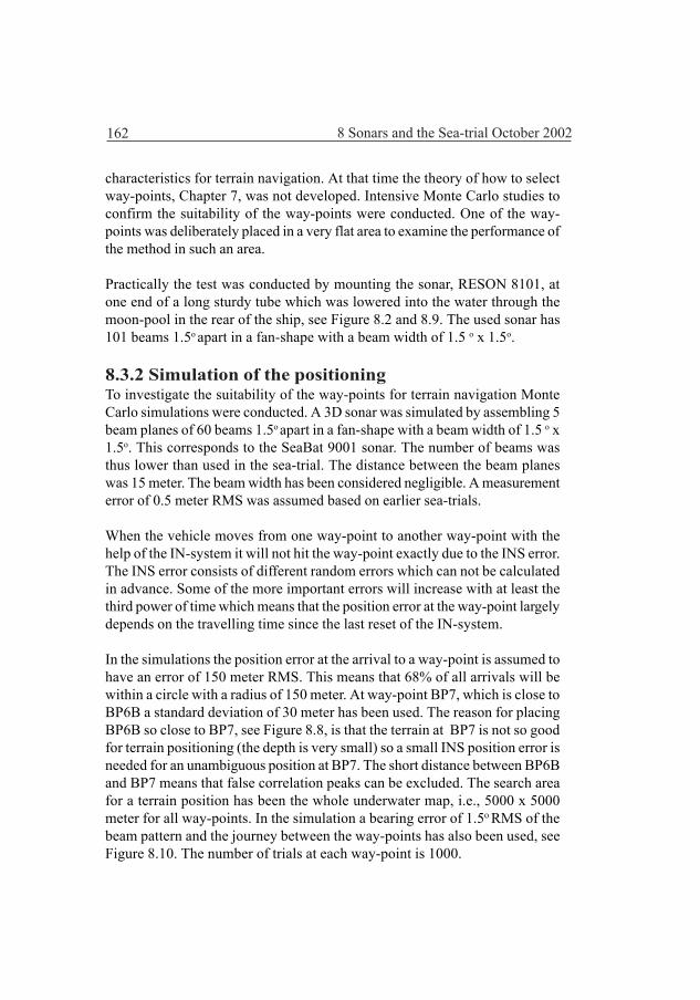
162 8 Sonars and the Sea-trial October 2002
characteristics for terrain navigation. At that time the theory of how to selectway-points, Chapter 7, was not developed. Intensive Monte Carlo studies toconfirm the suitability of the way-points were conducted. One of the way-points was deliberately placed in a very flat area to examine the performance ofthe method in such an area.
Practically the test was conducted by mounting the sonar, RESON 8101, atone end of a long sturdy tube which was lowered into the water through themoon-pool in the rear of the ship, see Figure 8.2 and 8.9. The used sonar has101 beams 1.5o apart in a fan-shape with a beam width of 1.5 o x 1.5o.
8.3.2 Simulation of the positioningTo investigate the suitability of the way-points for terrain navigation MonteCarlo simulations were conducted. A 3D sonar was simulated by assembling 5beam planes of 60 beams 1.5o apart in a fan-shape with a beam width of 1.5 o x1.5o. This corresponds to the SeaBat 9001 sonar. The number of beams wasthus lower than used in the sea-trial. The distance between the beam planeswas 15 meter. The beam width has been considered negligible. A measurementerror of 0.5 meter RMS was assumed based on earlier sea-trials.
When the vehicle moves from one way-point to another way-point with thehelp of the IN-system it will not hit the way-point exactly due to the INS error.The INS error consists of different random errors which can not be calculatedin advance. Some of the more important errors will increase with at least thethird power of time which means that the position error at the way-point largelydepends on the travelling time since the last reset of the IN-system.
In the simulations the position error at the arrival to a way-point is assumed tohave an error of 150 meter RMS. This means that 68% of all arrivals will bewithin a circle with a radius of 150 meter. At way-point BP7, which is close toBP6B a standard deviation of 30 meter has been used. The reason for placingBP6B so close to BP7, see Figure 8.8, is that the terrain at BP7 is not so goodfor terrain positioning (the depth is very small) so a small INS position error isneeded for an unambiguous position at BP7. The short distance between BP6Band BP7 means that false correlation peaks can be excluded. The search areafor a terrain position has been the whole underwater map, i.e., 5000 x 5000meter for all way-points. In the simulation a bearing error of 1.5ο RMS of thebeam pattern and the journey between the way-points has also been used, seeFigure 8.10. The number of trials at each way-point is 1000.

163
An example of simulation result at way-point BP3The depth at way-point BP3 is 38 meter. The Figure 8.10 shows the spread inposition at arrival at the way-point and Figure 8.11 shows the inverse of thecorrelation sum T(x) , see Chapter 3. From Figure 8.11 it can be seen thatthere are no false peaks of importance.
Figur 8.12: Position error in thex-direction at BP3.
Figur 8.13: Position error in they-direction at BP3.
Figure 8.11: The correlation result atway-point BP3.
Figure 8.10: The spread in po-sition at arrival at way-pointBP3.
8.3 Sea-trial October 2002, Simulation

164 8 Sonars and the Sea-trial October 2002
The result from the simulation is that at this way-point of all 1000 trials only 33trials gave a position with larger error than 3σ = 450 meter. This may beconsidered as a large number but is probably explained by the simulated randombearing error and if so does not depend on the terrain positioning. If we areconsidering these to be outliers the distribution of the position error is as inFigure 8.12 and 8.13.
From the histograms we see that they remind of Gaussian distributions. InChapter 4 it was shown that for large number of measurement beams the positionerror distribution will approximately be Gaussian.
The step in the matching procedure was 1 meter. The mean of the position errorwas 0.7 meter and the standard deviation was RMS 0.45 meter. Note that thereal world position error also include errors due to other reasons than thecorrelation and that these will add to the correlation error given here.
Other simulation results
Way-point BP1The depth at way-point BP1 is 58 meter. The mean of the position error was0.61 meter and the standard deviation was RMS 0.36 meter.
Way-point BP2The depth at way-point BP2 is 39 meter. The mean of the position error was0.56 meter and the standard deviation was RMS 0.33 meter In this case 20positions outside the 3σ−limit were obtained.
Way-point BP4The depth at way-point BP4 is 31 meter. The mean of the position error was0.51 meter and the standard deviation was RMS 0.29 meter. In this case 20positions outside the 3σ−limit were obtained, see Figure 8.14 and 8.15.
Way-point BP5The depth at way-point BP5 is 101 meter. The mean of the position error was0.60 meter and the standard deviation was RMS 0.38 meter, no positions outsidethe 3σ−limit were obtained, see Figure 8.16 and 8.17.

165
Figure 8.16: The correlationpeak for way-point BP5, 5 beamplanes. Map area 2 x 2 km.
Figure 8.17: Radial positionerror at way-point BP5.
Figure 8.14: The correlation peakfor way-point BP4, 5 beam planes.Map area 2 x 2 km.
Figure 8.15: Radial positionerror at way-point BP4.
8.3 Sea-trial October 2002, Results
Way-point BP5BThe depth at way-point BP5B is 59 meter. The mean of the position errorwas 0.49 meter and the standard deviation was RMS 0.28 meter, 5 positionsoutside the 3σ−limit were obtained.

166 8 Sonars and the Sea-trial October 2002
Way-point BP6BThe depth at way-point BP6B is 39 meter. The mean of the position error was0.54 meter and the standard deviation was RMS 0.31 meter, 8 positions outsidethe 3σ−limit were obtained.
Way-point BP7The depth at way-point BP7 is 10 meter. The mean of the position error was1.0 meter and the standard deviation was RMS 0.7 meter, 145 positions outsidethe 3σ−limit were obtained.
8.4 Sea-trial October 2002, resultsDue to bad weather conditions the way-points 4, 5, 5B and 6B could not beapproached. A reasonable assumption based on the simulations is that thepositioning result at these way-points would have been as good as at the otherway-points. The depth at these way-points would have given a large bottomcoverage for the sonar and the terrain has also large variations at the way-points. Below are some brief correlation results from the other way-points. Inthe tables the notation 5/75 means 5 beamplanes 75 pings apart. Length andwidth refer to the correlation area and outliers are removed.The positionreference is a DGPS measure with a believed accuracy of 3 meter RMS.
8.4.1 Way-point 1
Figure 8.18. Likelihood function.Map area 5 km by 5 km, 5 beamplanes. Map area 5 x 5 km. BP1
Figure 8.19: The N-normalizedlikelihood function. Horizontalscale in meter. BP1.

167
Figure 8.20: Positions at the way-point BP1. The cross marks the way-point.
8.4 Sea-trial October 2002, Results
Table 8.1. Position error at way-point BP1
Ping No./Dist. depth x error y error length width No. beam planes m m m m m
1730 5/75 -16.0 0.1 3.8 106 821150 5/75 -19.0 -2.0 6.2 160 93550 5/75 -16.0 -0.3 3.3 153 84
1100 5/75 -19.0 -2.4 4.0 141 921700 5/75 -16.0 -0.1 4.7 110 751080 5/75 -19.0 -1.4 7.3 170 89
600 5/75 -15.9 -0.3 3.4 106 591350 5/75 -18.8 -3.1 -0.7 119 921280 5/75 -15.9 -0.2 5.3 163 84
820 5/75 -18.8 4.6 31.7 164 91
Radial position error 4.7 m with respect to origo.Radial position error2.0 m with respect to the mean error.
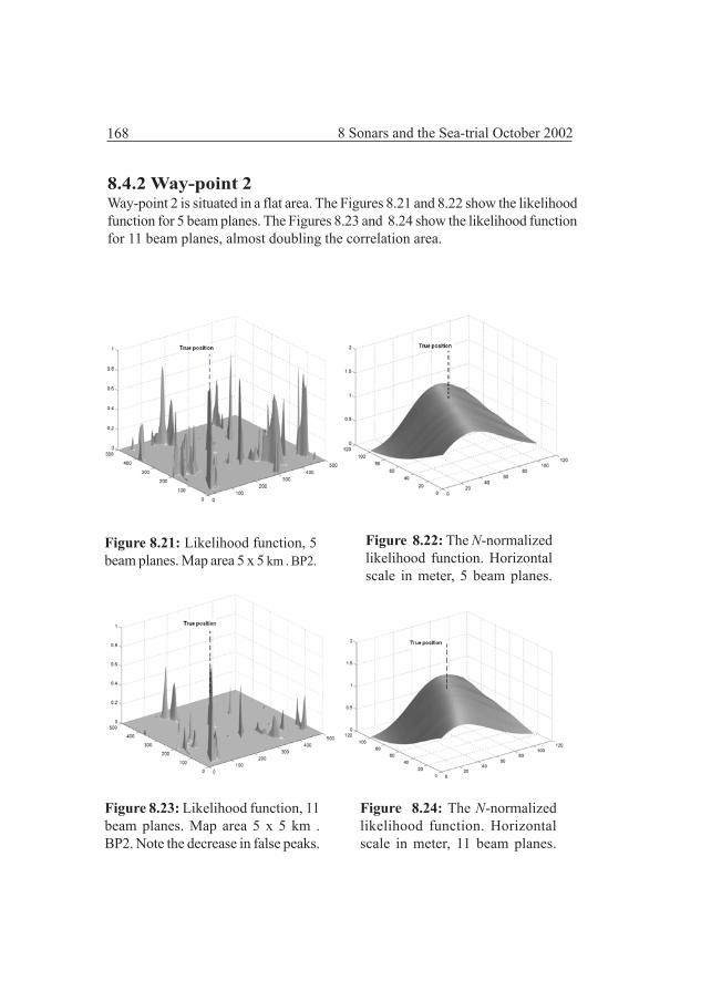
168 8 Sonars and the Sea-trial October 2002
8.4.2 Way-point 2Way-point 2 is situated in a flat area. The Figures 8.21 and 8.22 show the likelihoodfunction for 5 beam planes. The Figures 8.23 and 8.24 show the likelihood functionfor 11 beam planes, almost doubling the correlation area.
Figure 8.22: The N-normalizedlikelihood function. Horizontalscale in meter, 5 beam planes.
Figure 8.21: Likelihood function, 5beam planes. Map area 5 x 5 km . BP2.
Figure 8.23: Likelihood function, 11beam planes. Map area 5 x 5 km .BP2. Note the decrease in false peaks.
Figure 8.24: The N-normalizedlikelihood function. Horizontalscale in meter, 11 beam planes.
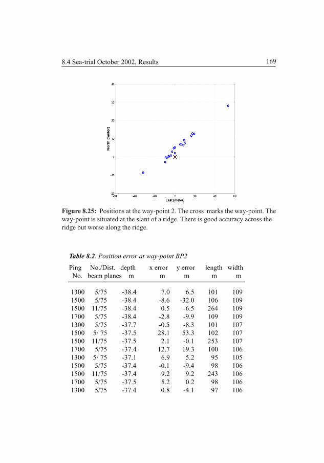
169
Table 8.2. Position error at way-point BP2
Ping No./Dist. depth x error y error length width No. beam planes m m m m m
1300 5/75 -38.4 7.0 6.5 101 109 1500 5/75 -38.4 -8.6 -32.0 106 109 1500 11/75 -38.4 0.5 -6.5 264 109 1700 5/75 -38.4 -2.8 -9.9 109 109 1300 5/75 -37.7 -0.5 -8.3 101 107 1500 5/ 75 -37.5 28.1 53.3 102 107 1500 11/75 -37.5 2.1 -0.1 253 107 1700 5/75 -37.4 12.7 19.3 100 106 1300 5/ 75 -37.1 6.9 5.2 95 105 1500 5/75 -37.4 -0.1 -9.4 98 106 1500 11/75 -37.4 9.2 9.2 243 106 1700 5/75 -37.5 5.2 0.2 98 106 1300 5/75 -37.4 0.8 -4.1 97 106
Figure 8.25: Positions at the way-point 2. The cross marks the way-point. Theway-point is situated at the slant of a ridge. There is good accuracy across theridge but worse along the ridge.
8.4 Sea-trial October 2002, Results

170 8 Sonars and the Sea-trial October 2002
Figure 8.27: The N-normalizedlikelihood function. Horizontal scalein meter, 5 beam planes. BP2B.
Figure 8.26: Likelihood function, 5beam planes. Map area 5 x 5 km.BP2B.
8.4.3 Way-point 2B
Table 8.2. Cont. Position error at way-point BP2
Ping No./Dist. depth x error y error length width No. beam planes m m m m m
1500 5/75 -37.4 0.3 -6.2 105 106 1500 11/75 -37.4 6.5 8.4 260 106 1700 5/75 -37.4 7.5 9.7 111 106 1300 5/75 -37.2 11.7 16.4 109 106 1500 11/75 -37.6 12.9 17.5 270 107 1700 5/75 -37.7 4.8 -1.3 109 107
Radial position error 10.0 m with respect to origo. Radial position error9.2 m with respect to the mean error.

171
Figure 8.28: Positions at the way-point 2B. The cross marks the way-point.
8.4 Sea-trial October 2002, Results
Table 8.3. Position error at way-point BP2B
Ping No./Dist. depth x error y error length width No. beam planes m m m m m
1300 5/ 75 -30.3 3.7 2.2 0 0 1300 5/75 -26.5 3.7 -2.0 0 0 1500 11/75 -26.5 0.3 1.4 0 0 1700 5/ 75 -27.6 -2.6 1.7 0 0 1300 5/ 75 -26.1 201.0 442.5 0 0 1500 5/75 -28.9 2.9 6.3 0 0 1500 11/75 -28.9 2.1 1.5 0 0 1700 5/ 75 -30.8 2.6 3.2 0 0 1300 5/ 75 -29.9 4.6 5.0 0 0 1500 5/ 75 -25.9 3.4 4.9 0 0 1500 11/75 -25.9 1.7 2.7 0 0 1700 5/ 75 -27.7 -5.4 4.9 0 0 1300 5/75 -30.4 1.6 3.3 0 0 1500 5/75 -32.4 0.5 2.4 0 0 1500 11/75 -32.4 -1.4 2.3 0 0 1700 5/75 -33.6 -2.6 5.0 0 0

172 8 Sonars and the Sea-trial October 2002
Table 8.3. Cont. Position error at way-point BP2B
Ping No./Dist. depth x error y error length width No. beam planes m m m m m
1300 5/75 -28.5 4.5 2.3 131 85 1500 5/75 -26.0 330.9 -69.0 120 78 1500 11/75 -26.0 -1.7 -0.4 313 78 1700 5/75 -27.6 -9.0 -0.6 121 83
Note: Missing length and width data are marked with 0.
8.4.4 Way-point 3
Figure 8.29: BP3, likelihoodfunction, 5 beam planes. Map area5 x 5 km.
Figure 8.30: BP3, the N-normalizedlikelihood function. Horizontal scalein meter, 5 beam planes.

1738.4 Sea-trial October 2002, Results
Table 8.4. Position error at BP3
Ping No./Dist. depth x error y errror length width No. beam planes m m m m m
1300 5/75 -26.7 2.1 -6.4 121 100 1500 5/75 -32.6 5.1 -5.8 117 100 1500 11/75 -32.6 4.0 -3.8 296 100 1700 5/75 -34.1 3.7 -4.9 116 104 1300 5/75 -24.4 2.3 -2.1 125 80 1500 5/75 -28.0 2.6 0.7 121 99 1500 11/75 -28.0 1.9 -0.7 306 99 1700 5/75 -36.5 3.3 0.7 120 105 1300 5/75 -24.1 4.4 -3.7 121 82 1500 5/75 -32.3 3.3 -4.0 119 104 1500 11/75 -32.3 3.1 -3.9 303 104 1700 5/75 -31.6 5.7 -6.0 123 98 1300 5/75 -26.0 1.8 -1.6 116 85 1500 5/75 -28.6 2.5 -2.8 117 94 1500 11/75 -28.6 2.6 -3.8 295 94 1700 5/75 -34.5 3.3 -1.7 121 102 1300 5/75 -25.7 2.5 -3.2 126 87
Figure 8.31: Positions at the way-point 3. The cross marks the way-point.

174 8 Sonars and the Sea-trial October 2002
Figure 8.33: BP7, the N-normalized likelihood function.Horizontal scale in meter, 5 beamplanes.
Figure 8.32: BP7, likelihood function,5 beam planes. Map area 5 x 5 km.
8.4.5 Way-point 7
Table 8.4. Cont. Position error at BP3
Ping No./Dist. depth x error y error length width No. beam planes m m m m m
1500 5/75 -32.3 3.6 -5.3 125 103 1500 11/75 -32.3 3.7 -4.2 315 103 1700 5/75 -33.6 6.0 -5.0 126 100
Radial position error 5.0 m with respect to origo. Radial position error2.0 m with respect to the mean.

175
Table 8.5. Position error at way-point BP7
Ping No./Dist. depth x error y error length width No. beam planes m m m m m
304 5/75 -41.4 0.4 -1.6 195 166500 5/75 -20.6 1.9 -2.0 215 105500 11/75 -20.6 3.1 -0.8 512 105600 5/75 -30.9 1.0 -1.1 216 144200 5/75 -33.8 3.9 0.5 247 172300 5/75 -36.1 0.7 -0.9 238 172400 5/75 -21.6 3.4 -1.7 245 75200 5/75 -36.1 1.1 0.7 318 229300 5/75 -22.1 1.2 -3.7 314 88500 5/75 -32.3 1.4 -0.8 299 201200 5/75 -47.2 1.8 0.2 253 243300 5/75 -33.8 0.1 0.5 255 217600 5/75 -22.6 1.7 -1.7 255 100300 5/75 -21.1 2.2 -0.4 261 129400 5/75 -36.6 -0.3 -0.2 267 176500 5/75 -32.6 2.3 -0.6 275 216
Radial position error 2.2 m with respect to origo. Radial position error1.3 m with respect to the mean.
Figure 8.34: Positions at the way-point 7. The cross marks the way-point.
8.4 Sea-trial October 2002, Results

176 8 Sonars and the Sea-trial October 2002
8.5 Conclusions
The horizontal position error in the simulation was less than 1 meter RMS whilethe corresponding error in the sea-trial was a few meters. This might be seen asa large deviation but since the DGPS device only had an accuracy of about 3meter RMS we could not expect an error smaller than that.
Compared to other terrain navigation methods a radial position error of 3 meteris extremely good (note that this figure includes the DGPS error) since the positionerror for the methods mentioned in Chapter 2 is in the range of 30 meter.
We see from the figures showing the estimated positions at the way-points thatthere is a position bias. Possible reasons for this bias have been carefully studiedand it is believed that it is caused by bias in the map and/or bias in the DGPSposition due to multipath in the satellite signal [PE04].
The method also shows very good performance in very flat areas as shown inway-point 2 which is considered by the eye to be completely flat. The importanceof a large correlation area is also shown for that way-point.
It is also shown that for manned underwater vehicles the quality of the positioning,which is extremely important, could easily be determined by looking at thelikelihood function. However the “variance” of the likelihood function may notalways be a good measurement of the quality of the positioning due to terrainrepeatability. It may be better to always use the Hessian of the log likelihoodfunction at its maximum point.
A likelihood function as in Figure 8.21 shows that the positioning needsimprovement either by increasing the correlation area or adding some externalmeasurements as mentioned in Chapter 3. Is the likelihood function as in Figure8.18, 8.26, 8.29, 8.32 it is almost sure that the achieved position is the correctposition, this can be confirmed by the hypothesis testing method described inSection 4.2.3.
The Gaussian shape of the likelihood function when a large number ofmeasurement beams are used is demonstrated for several way-points.

177
9.1 IntroductionWith the uprising of the computer game industry a great number of syntheticterrain models have become available, some are very advanced and some arevery simple. Also within the military sector, simulation of war theatres hasbecome common which has lead to the development of advanced terrain models.For terrain navigation, simple synthetic terrain models have been used for a longtime to evaluate performance of navigation methods [BAAB84] with varyingdegree of success.
If in the same way the bottom topography could be described in statisticalterms, e.g., as a stationary stochastic process, qualitative and quantitativejudgements could be drawn about the positioning accuracy and adherentmatters directly from the model. This would be of great advantage, but up tonow the relevance of the models, covering large areas, for that purpose mightbe questioned. However, it seems at least possible that local models can be ofvalue.
Chapter 9
Terrain navigation forautoregressive bottommodels

178 9 The autoregressive bottom model
One of the simplest models one can think of is to generate a random matrix (inimage theory called random field), symbolizing the terrain, and make 2D-filteringto give the landscape the requested correlation between locations [JA89].However, a simple 1D terrain model obtained by filtering white noise through afirst order filter may often be sufficient, that is an autoregressive process offirst order, AR(1), [BRDA91,TS02].
This chapter will therefore study the terrain navigation problem when the bottomprofile can be approximated by a low order autoregressive process. A higherorder process model will adjust better to the real world but that also meansmore parameters to be identified. The chapter is to a high degree freestandingfrom the previous chapters.
9.2 AR-bottom profilesIn this section the AR-assumption will be studied in some more details for theone dimensional bottom model.
9.2.1 AR(1) bottom profileFigure 9.1 shows a bottom profile along a 5 km straight line in an underwatermap from the Stockholm archipelago and Figure 9.2 shows the autocorrelation
Figure 9.1: A typical zero meanbottom profile.
Figure 9.2: An adjusted AR(1) pro-cess to the autocorrelation curve forthe bottom in Figure 9.1
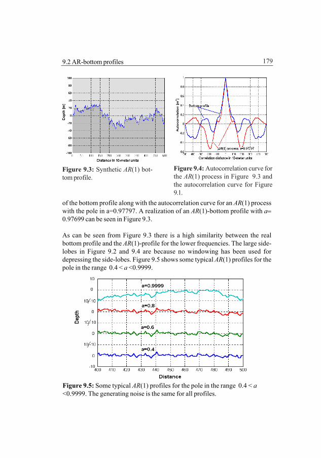
179
of the bottom profile along with the autocorrelation curve for an AR(1) processwith the pole in a=0.97797. A realization of an AR(1)-bottom profile with a=0.97699 can be seen in Figure 9.3.
As can be seen from Figure 9.3 there is a high similarity between the realbottom profile and the AR(1)-profile for the lower frequencies. The large side-lobes in Figure 9.2 and 9.4 are because no windowing has been used fordepressing the side-lobes. Figure 9.5 shows some typical AR(1) profiles for thepole in the range 0.4 < a <0.9999.
Figure 9.3: Synthetic AR(1) bot-tom profile.
Figure 9.4: Autocorrelation curve forthe AR(1) process in Figure 9.3 andthe autocorrelation curve for Figure9.1.
Figure 9.5: Some typical AR(1) profiles for the pole in the range 0.4 < a<0.9999. The generating noise is the same for all profiles.
9.2 AR-bottom profiles

180 9 The autoregressive bottom model
9.2.2 AR(2) bottom profileFigure 9.6 shows an AR(1) bottom and the same bottom profile filtered througha first order filter for removing high frequencies and by that receiving a more realbottom like profile. Filtering an AR(1) process with an AR(1) filter gives an AR(2)process. It is natural that an AR(2)- process will better describe the real bottomsince it has more parameters. Another advantage relative the first order processis that the autocorrelation function for a continuos stochastic process can bedifferentiated in all points.
9.2.3 Determining the expected correlation functionIn order to determine an estimate of the position we will later in this chaptercalculate the correlation function
[ ] [ ]( ) ( ) ( )TT x x x= − −y h y h (9.1)
where y is the measured bottom profile and h(x) is the profile according to theunderwater map in position x. Let x be the true position which we measure andcompare it with the bottom profile at the distance k from x. The measured profileis y=h(x)+e where e is the measurement error.
Figure 9.6: A filtered AR(1) process for removing high frequencies.
181
We would like to investigate if the correlation function (9.1) may be expressed instatistical terms of the bottom profile. Therefore we will determine the expectedvalue of T(x+k) where k is the sampel index corresponding to some samplingdistance. To simplify the analysis we will assume that x is a scalar and thestochastic process h(x) is stationary and uncorrelated with e. The length of thevectors y and e is N. We also assume that the elements in e are white Gaussiannoise. We have
1 12 2
0 0
12 2
0( )
2 2
{ ( )} { ( ( )) } { ( ( ) ( )) }
2 2 { ( ) ( )}
(2 ) 2 ( )h
N N
i j j j j kj j
N
h j j k ej
r k
h e h
E T x k E y h x k E h x e h x
N E h x h x N
N Nr k
σ σ
σ σ
− −
+= =
−
+=
+ = − + = + −
= − +
= + −
∑ ∑
∑ (9.2)
where we have introduced 1
2 2
0
1 { ( ( )) }N
h jj
E h xN
σ−
=
= ∑ and 1
2 2
0
1 { }N
e jj
E eN
σ−
=
= ∑ .
We can thus through the autocorrelation function, rh(k), get an understandingof the shape of the correlation function T(x).
9.3 The covariance matrixIn the previous section we found an expression for the expected value of thecorrelation function. We are equally interested in finding an expression for thecovariance of the difference between the bottom profile at two different locations.Assume therefore that the bottom profile, h, is generated by a stochastic AR(1)-process achieved by filtering a white Gaussian noise sequence ν(k), which is
20(0, )σN , through the first order filter
1
1( )1
H zaz−=
−where we will assume
that the pole is in the range 0 < a < 1.
In Figure 9.7 two positions along the bottom profile have been marked , Area 1with bottom profile h1 and Area 2 with bottom profile h2. The vectors h1 and h2are sections of the bottom profile, h. The dimension of h1 and h2 is N.
9.2 AR-bottom profiles

182 9 The autoregressive bottom model
Let the position h1 correspond to the profile measured by the sonar while positionh2 is a position situated k units from position h1, which we match the sonarmeasurement with. The elements of the vector h1 are the depth values from theunderwater map. The elements in the vectors h1 and h2 are 2
1(0, )arσN where2 2 2
1 0 (1 )ar aσ σ= − . The autocorrelation function for the process that generates
h is 21{ ( ) ( )} k
i i k arE h x h x aσ −+ = if k is the distance between the elements of h.
We will to begin with assume that the bottom profile is measured without errors.The correlation means that we compare the bottom profiles at Area 1 and Area 2by forming the difference between the profiles. Thus, we have the difference∆hi=h2,i-h1,i=hk0+k+i-hk0+i where index i refers to to the ith element in h1 and h2 andindex k0 refers to the starting point of the vector h1.
For an element in the vector ∆h=h2-h1 we have( ) 0iE h∆ = (9.3)
[ ]22
2 2 2 21, 2, 1, 2, 1, 2, 1
( ) ( ) ( )
(( ) ) ( ) ( ) 2 ( ) 2 (1 )i i i
ki i i i i i ar
Var h E h E h
E h h E h E h E h h aσ
∆ = ∆ − ∆
= − = + − = −
(9.4)The elements in the vector ∆h are thus 2(0, )σN where
22 2 0
1 2
22 (1 ) (1 )
1k k
ar a aa
σσ σ= − = −−
, they are also correlated with each other. If
Figure 9.7: Synthetic bottom profile which is assumed to be generated by anAR(1) process.

183
the distance between the positions i and j is m then we have the followingexpression for the covariance
{ }1, 2, 1, 2,
1, 1, 2, 2, 1, 2, 2, 1,
( ) ( ) ( )( )
( ) ( ) ( ) ( )i j i i j j
i j i j i j i j
m E h h E h h h h
E h h E h h E h h E h h
ρ = ∆ ∆ = − −
= + − − (9.5)
We arrive at the following expression for the elements in the covariance for anAR(1)-process with the pole in a and where m is the distance between elementsin the ∆h vector and k is the displacement between h1 and h2
( ) 21( ) 2 , 1, m k m k m
arm a a a m N kρ σ+ −= − − ≤ − ∀ (9.6)By that the covariance matrix for the bottom profile difference in the case of nomeasurement error is determined. The Figures 9.8 och 9.9 show ρ(m) as a functionof k at two different values of the pole a.
We note also that the covariance matrix is given directly by the expression
2 1 2 1
2 1 1 2
{ } {( )( ) }
2 {( } { }
T T
T T
E E
E E∆ = ∆ ∆ = − −
= − −h
h
C h h h h h hC h h h h (9.7)
where Ch=E{h1h1T}=E{h2h2
T}which for large displacements k simplifies to
Figure 9.8: The elements in thecovariance matrix for a=0.90.
Figure 9.9: The elements in thecovariance matrix for a=0.96.
9.3 The covariance matrix

184 9 The autoregressive bottom model
2∆ =h hC C (9.8)
since for large k h1 and h2 will be uncorrelated.
9.4 Decomposition of the covariance matrixThe measured bottom profile at the true position, x, can be written as y=h1+ewhere e is the white measurement noise and the correlation sum is
21
1
( ) ( ) ( )N
T Ti
iT x e
=
= − − = = ∑1y h y h e e (9.9)
which will be 2Nχ -distributed if ei is Gaussian (0,1)N .
At the position h2 we have a similar but not equal bottom profile h2=h1+∆h,where ∆h is Gaussian and correlated as described before. The correlation sumwill be
2 2( ) ( ) ( ) 2T T T T T TT x k+ = − − = − ∆ + ∆ ∆ → + ∆ ∆y h y h e e e h h h e e h h (9.10)
for large N and
2 2{ } {( ) ( )} { } { }T T TE T E E E= − − = + ∆ ∆y h y h e e h h (9.11)
The last term in (9.10) can be seen to have a kind of a 2Nχ looking distribution
by first decorrelating the stochastic variables ∆hi in the ∆h vector by a Choleskydecomposition , C∆h=LDLT, or a modal decomposition of the covariance matrix,C∆h=UΛUT. The difference being that the modal decomposition conserves thescale of the axes during the rotation of the axes which the Cholesky decompositiondoes not. The modal decomposition of the correlation matrix has been discussedin Chapter 4 and we will here discuss only the Cholesky decomposition.
The vectors h1 and h2 are zero mean Gaussian stochastic variables and ∆h=h2-h1 is the difference between the two profiles. The probability density functionfor ∆h is

185
( ) 1/ 2
1 1exp( )2(2 ) det( )
TNp
π ∆
−
∆
∆h
hh = - ∆h C ∆h
C (9.12)
where C∆h is the covariance matrix for ∆h. The Figures 9.10 and 9.11 illustratethe probability density function for the case N=2.
In the Figure 9.11 the area where ≤∆h ε is marked. The volume below theprobability density function in the shaded area corresponds to the probability
that ≤∆h ε , i.e., the absolute value of the depth difference in each sonarbeam does not exceed ε=[ε1,...εN]T.
9.4.1 Cholesky decomposition of the covariancematrixCholesky decomposition and inversion of the covariance matrix , C∆h=LDLT ,give
1 1 1 1 1( )T T T T− − − − −∆∆ ∆ = ∆ ∆ =hh C h h L D L h y D y (9.13)
where 1−= ∆y L h .
Figure 9.10: The probabilitydensity function when N=2.
Figure 9.11: Contour lines for thePDF in Figure 9.10.
9.4 Decomposition of the covariance matrix

186 9 The autoregressive bottom model
We also have that ,1
det( )N
i ii
d∆=
= ∏hC , i.e., the product of the diagonal elements
in D since the L matrix is a lower triangular matrix with 1 as diagonal elements.
If we call the diagonal elements of D for 2,i i id σ= and the elements in the vector
y for yi then we can write
( ) 22/ 2 2 2
11
2212 2/ 2 2 211
1 1 1exp( )2(2 )
1 exp( ) exp( )2 2(2 )
N
iNiiN
NN
NN
p y
yy
σπ σ σ
σ σπ σ σ
=
∆ −
−−=
∑h =…
……
(9.14)
or as a product of probability density functions
( )2
222
1; exp( )22
iii
yp y σσπσ
−= (9.15)
By that we also have conducted a rotation and scale change of the coordinatesystem. Therefore we also have to change the integration area when solving
the integral for the probability for a position in error, Pr( )ε∆ ≤h . The
variance iσ depends on k but for large k values, see Figure 9.12, all diagonalvalues, except the first, are approximately the same. We can thereforeapproximately write
( ) 2 21 2
2
( ; ) ( ; )N
i
p p y p yσ σ=
∆ ∏h (9.16)
with equality for large k and where
( )2
21 22
11
1; exp( )22
yp y σσπσ
−= (9.17)
and

187
( )2
22 22
22
1; exp( )22
yp y σσπσ
−= (9.18)
The probability that the difference between two bottom profiles is less than ε isthen approximately
1
1
2 21 1 2
2
Pr( ) ( ; ) ( ; )i
i
N
i
p y dy p y dyεε
ε ε
ε σ σ=− −
∆ ≤ = ⋅∏∫ ∫h (9.19)
A similar expression was derived in Chapter 4. The original integration limits willchange with the transformation. For large N the integrand in the second productfactor will tend to zero since the value of the integral is <1. The size of theelements in the diagonal matrix can be seen in Figure 9.12. For large k values
21iid a= − when i>1 which follows from (9.8). We can see that the curves for k= 50 and k = 100 have a similar shape as the curve for k=500. For k = 500 anda=0.99 we have 60,60 0.020032d = compared to 2(1 ) 0.0199a− = .
Figure 9.12: The diagonal elements, 2iσ , for the Cholesky decomposition of
the covariance matrix.
9.4 Decomposition of the covariance matrix
188 9 The autoregressive bottom model
9.5 The mean and variance of the correlationsumLet the mode decomposition of the correlation matrix C=E{(y-h(x))(y-h(x))T}=VΛΛΛΛΛVT then the correlation sum can be written as [CT92, KA93]
2
1
( ) ( ( )) ( ( )) ( ( )) ( ( ))
( ( ( ))) ( ( ( ))) ( )
T T T
NT T T
i ii
T x x x x x
x x z xα=
= − − = − −
= − − = ∑y h y h y h VV y h
V y h V y h (9.20)
where zi (x) is (0,1)N and2 2
, i h i eα σ σ∆= + (9.21)
where 2eσ is the measurement noise variance and 2
, ,h i h iσ λ∆ ∆= is an eigenvalue of
C∆h, see Section 9.3. The stochastic variable T(x) thus has a 2Nχ looking
distribution. The Figures 9.13 - 9.16 show some of the largest eigenvalues forN=20, 120 and a=0.96, 0.99 for different displacements k.
The distribution also has the following characteristics [NY01a]
2 2e
TEN
σ σ∆ = + h (9.22)
where 2 2,
1
1 N
iiN
σ σ∆ ∆=
= ∑h h and
2
2
2FTVar
N N =
C (9.23)
where FC is the Frobenius norm of the covariance matrix. In the case the
bottom profile is an AR(1) process and the displacement k is large
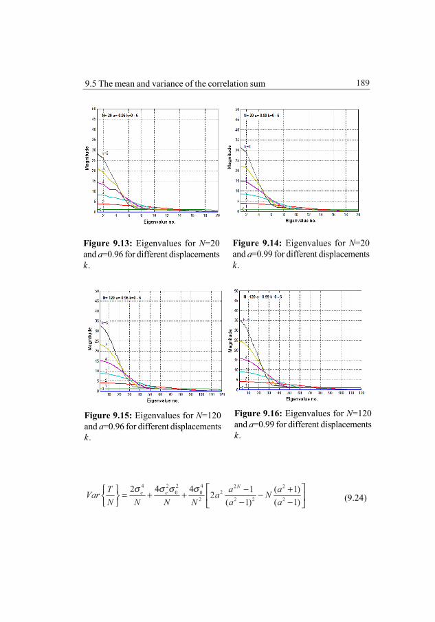
189
4 2 2 4 2 220 0
2 2 2 2
2 4 4 1 ( 1)2( 1) ( 1)
Ne eT a aVar a N
N N N N a aσ σ σ σ − + = + + − − −
(9.24)
Figure 9.16: Eigenvalues for N=120and a=0.99 for different displacementsk.
Figure 9.13: Eigenvalues for N=20and a=0.96 for different displacementsk.
Figure 9.14: Eigenvalues for N=20and a=0.99 for different displacementsk.
Figure 9.15: Eigenvalues for N=120and a=0.96 for different displacementsk.
9.5 The mean and variance of the correlation sum

190 9 The autoregressive bottom model
Figure 9.17: The variance of the correlation sum as a function of the number ofmeasurement beams, N, at two different pole placements.
Figure 9.18: The expected valueof T(x)/N at a=0.96 for differentdisplacements k.
Figure 9.19: The expected valueof T(x)/N at a=0.99 for differentdisplacements k.

191
where a is the pole in the AR(1) expression for the bottom profile, see Section9.3. Figure 9.17 shows the variance for two different pole placements as afunction of the number of beams. Figures 9.18 – 9.21 show how the expectedvalue of the correlation sum and variance differ with the distance k betweenh1and h2 .
9.6 The probability density function of thecorrelation sumA simple way to determine the probability density function is to use generating
functions. The characteristic equation for a 21χ distributed stochastic variable
is 21
11 2 jχφ
ω=
−and therefore the characteristic equation for T(x) will be
[NKB94, KA93]
1
1( )1 2
N
Tii j
φ ωα ω=
=−∏ (9.25)
Figure 9.20: The variance of T(x)/Nat a=0.96 for different displacementsk.
Figure 9.21: The variance of T(x)/Nat a=0.99 for different displacementsk.
9.5 The mean and variance of the correlation sum

192 9 The autoregressive bottom model
The inverse Fourier transform is
1
1 0( ) 21 2
0 0
Nj t
T ii
de tp t j
t
ω ωπα ω
∞−
=−∞
⋅ ⋅ ≥ = −
<
∏∫ (9.26)
For every displacement k between the bottom profile and the measured profilewe will have different covariance matrices where the elements ρ(m) are calculatedaccording to (9.6). The eigenvalues of the covariance matrix will differ, as can be
Figure 9.22: The probability densityfunction for T(x)/N while N=20, a=0.96for different displacements k.
Figure 9.23: The probability densityfunction for T(x)/N while N =20, a=0.99for different displacements k.
Figure 9.24: The probability densityfunction for T(x)/N while N =120,a=0.96 for different displacements k.
Figure 9.25: The probability densityfunction for T(x)/N while N =120,a=0.99 for different displacements k.

193
seen in Figures 9.13 – 9.16, depending on the displacement k and therefore wewill have different probability density functions for the correlation sum T(x+k).
The position estimate is determined from the position with smallest value ofthe correlation sum. The Figures 9.22 - 9.25 show, from a Monte Carlo trial, theprobability density function for different k values but also the density functionfor the smallest correlation sum among all k values (the density functions areoverlapping). As can be seen from the figures the density function for thesmallest correlation sum is almost identical with the density function for k=0.This can especially be seen in Figures 9.24 and 9.25 where the overlap of thedensity functions between k=0 and k=1 is very small.
From the figures we see that a smaller value of a, i.e., a more hillier terrain, givesa better distinction between the density functions for the correlation sum andby that the risk of larger errors in the position decreases. We also see that alarger number of measurement beams has the same effect. We also note thewell known fact that the 2
Nχ distribution asymptotically becomes normal whenN increases. Since the variance also decreases as 1/N, the likelihood functionbecomes close to normal which already has been proved in Chapter 4.
9.7 The probability density function for thepositionIf the joint probability density functions are known for M differentdisplacements between h1 and h2 the density function for the smallest correlationsum within this truncated PDF can be determined.
First, in order to have an analytic expression, we calculate the probability thata displacement of k will give the smallest correlation sum. We will have
| | 1.. 1, 1..
1 1 1 10
Pr( )
( ,..., )i i
k i k i i M
M i i M iT T
T T
p T T dT dT dT dT dT
= = − +
∞ ∞ ∞
− +
≤
= ∫ ∫ ∫… … … (9.27)
where 1( )Mp T T… is the joint probability density.
9.6 The probability density function of the correlation sum

194 9 The autoregressive bottom model
To be able to determine the joint distribution we must know the correlationbetween the stochastic variables described by the particular density functionsfor different k, cf. Figures 9.22 – 9.25 and Figures 9.26 – 9.29 .
From the Figures 9.22 – 9.25 we can draw the conclusion that the smallest valueof the correlation sum almost solely depends on the density function for k=0and k=1. The correlation for the corresponding stochastic variables is shown inthe Figures 9.26 – 9.29. From these figures we see that the major axes of thePDFs for k>1 are approximately oriented in the same direction. That means thata simultaneous diagonalization procedure may be applied [CT92] and thus makingthe correlation sums independent of each other. However, the most importantdistributions for determining the minimum of the correlation sum are those fork=0 and k=1 and we may only take those into consideration. The jointdistribution of k=0 and k=1 are originally not truly independent because theyhave the same measurement noise but can, without approximation, bedecorrelated by a simultaneous mode decomposition. A hillier terrain will makethe stochastic variables T(x) and T(x+1) less dependent of each other. In thecase we can consider the correlation sums independent after a simultaneousdiagonalization procedure, exact or approximate, the integral (9.27) can bedecomposed as
1 1 1
1.. 1, 1..
0
1 1 1
Pr( )
{ { { {
{ ( ) } } } }
i i i
i i i i
M
M
k i k i i M
T T T TT T T T
T M M i i iT
T T
p p p p
p T dT dT dT dT dT
− +
= = − +
∞ ∞ ∞ ∞ ∞
−
∞
+ −
≤ =
= ⋅ ⋅ ⋅ ⋅ ⋅∫ ∫ ∫ ∫ ∫
∫
… …
… … (9.28)
The probability density functions for the distribution p(T(x), T(x+1)) and thenumber of trials which will give no position error, T(x)<T(x+1), corresponds tothe volume below the joint distribution above the 45 line, see Figures 9.30 and
9.31. The volume below the 45 line gives a position error corresponding to onegrid distance.
If the stochastic variables T(x) and T(x+1) were independent and the cumulativefrequency distribution is denoted by F(.) then the cumulative frequency
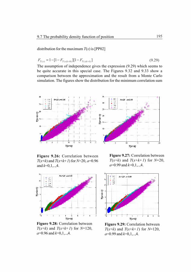
195
distribution for the maximum T(x) is [PP02]
( ) ( | 0) ( | 1)1 [1 ][1 ]T x T x k T x kF F F= == − − − (9.29)The assumption of independence gives the expression (9.29) which seems tobe quite accurate in this special case. The Figures 9.32 and 9.33 show acomparison between the approximation and the result from a Monte Carlosimulation. The figures show the distribution for the minimum correlation sum
Figure 9.26: Correlation betweenT(x+k) and T(x+k+1) for N=20, a=0.96and k=0,1,..,4.
Figure 9.27: Correlation betweenT(x+k) and T(x+k+1) for N=20,a=0.99 and k=0,1,..,4.
Figure 9.28: Correlation betweenT(x+k) and T(x+k+1) for N=120,a=0.96 and k=0,1,..,4.
Figure 9.29: Correlation betweenT(x+k) and T(x+k+1) for N=120,a=0.99 and k=0,1,..,4.
9.7 The probability density function of position

196 9 The autoregressive bottom model
if the stochastic variables T(x) and T(x+1) is dependent or assumedindependent As can be seen the difference is very small.
Figure 9.30: Correlation betweenT(x), T(x+1) for N=120, a=0.96.
Figure 9.31: Correlation betweenT(x), T(x+5) for N=120, a=0.96.
Figure 9.32: The probability densityfunction for T(x)/N for dependent andindependent variables. N=20, a=0.99.
Figure 9.32: The probability densityfunction for T(x)/N for dependent andindependent variables. N=120, a=0.96.

197
9.8 Approximate determination of theprobability density function for thecorrelation sumTo determine the probability density function for T(x) according to (9.26), i.e.,
1
1 0( ) 21 2
0 0
Nj t
T ii
de tp t j
t
ω ωπα ω
∞−
=−∞
⋅ ⋅ ≥ = −
<
∏∫ (9.30)
demands a large computational work since it has to be determined numericallyand an approximation is therefore of interest. From the Figures 9.22 – 9.25 we
see the typical 2χ shape. Let us therefore assume, as an approximation, that
this is the case and let us determine the 2χ distribution which has the same
mean and variance as pT(.), which we already know from (9.22) and (9.23).
( )T TrEN N
=
C (9.31)
2
2
2FTVar
N N =
C (9.32)
For a 2vχ distributed stochastic variable, ξ , we have
( )( ) 2
EVar
ξ υξ υ=
= (9.33)
where ν is the degree of freedom in the distribution. This will give the densityfunction for T(x) approximately the same density as the stochastic variable
2( ) MT x βχ∼ where [BSFO88]
9.8 Approximate determination of the probability density function

198 9 The autoregressive bottom model
2
2
2
( )( )
F
F
TrTrM
β =
=
CCC
C (9.34)
Figures 9.33 and 9.34 show the approximated probability density functionscompared to those determined by Monte Carlo techniques and as can be seenthere is a good agreement between the above approximation and the true PDFs.
The density function for k=0 is a true 2χ density function and does not have tobe approximated.
Figure 9.33: Approximative PDFcompared to Monte Carlo simulatedPDF for T(x)/N, N=20, a=0.99. Theapproximative PDF is slightly belowthe Monte Carlo PDF.
Figure 9.34: Approximative PDFcompared to Monte Carlo simulatedPDF for T(x)/N, N=120, a=0.99. Theapproximative PDF is slightly belowthe Monte Carlo PDF.

199
9.9 Cramér-Rao Lower BoundThe Cramér-Rao lower bound has already been discussed in Chapter 5. Thepresentation here will therefore be focused on the AR-assumption of the bottomtopography.
Let the scalar parameter x denote our unknown position and y(x) ourmeasurement of the bottom profile and let the depth profile according to themap be denoted by h(x). Then the estimate of the position has the bound on thevariance
11 22 2
2
log ( | ) log ( | )ˆ ˆ( ) {[ ( ) ] } { } { }p x p xVar x E x x E Ex x
−− ∂ ∂ = − ≥ = − ∂ ∂
y yy
(9.35)
if the position estimate is unbiased. The probability density function p(y|x) isthe density function for the observation vector in the true position x.
For the one dimensional case, in the case we have a Gaussian measurementerror, this will give us
22 2
1
log ( | ) 1 1 ( )( ( ( )) )2 2
N
k kke e
p x T xy h xx x xσ σ=
∂ ∂ ∂= − − = −∂ ∂ ∂∑y
(9.36)
which gives after the expectation has been taken
122
1
ˆ( )N
ie
i
hVar xx
σ−
=
∂ = ∂ ∑ (9.37)
since for a Gaussian measurement error the position error variance will attainthe CRLB when N tends to infinity, see also Chapter 5. Figure 9.35 shows howthe CRLB for an AR(1) - process varies with the number of measurement points.The graph is determined by Monte-Carlo simulations. In general the CRLB isgiven by the inverse of the Fisher matrix J calculated in the true position xwhich in this case is a scalar
9.9 Cramér-Rao lower bound

200 9 The autoregressive bottom model
2
2 2
1 ( )2 e
T xJ Exσ
∂= ∂ (9.38)
We can estimate the derivatives in (9.37) and (9.38) under the assumption of anAR(1)-process. Let h denote the map depth and rewrite the state equation inthe following way
1 1 1 1i i i i i i ih ah h h ahν ν− − − −= + = − + + + (9.39)
or 1 1( 1)i i i ih h a h ν− −− = − + which will give
2 2 2 2 21 1 1{[ ] } [( 1) ] ( 1) { }i i i i iE h h E a h a E h νν σ− − −− = − + = − + (9.40)
For a stationary process we have 2 2 21{ } { }i i hE h E h σ−= = (9.41)
Further the state equation gives
2 2 2 2h ha νσ σ σ= + (9.42)
Figure 9.35: CRLB as a function of the number of measurement points N.

201
or
2 2 2(1 ) haνσ σ= − (9.43)
Thus,
2 2 2 2 2 21{[ ] } ( 1) (1 ) 2(1 )i i h h hE h h a a aσ σ σ−− = − + − = − (9.44)
or alternatively2
21
2{[ ] }
1i iE h haνσ
−− =+ (9.45)
22
2 2 21
2 2
2 21
1 ( ) 1 ( )[ ]2
2 21 =1 (1 )
N
ie e
N
ie e
T x h xJ E Exx
Na aν ν
σ σ
σ σσ σ
=
=
∂ ∂ = = ∂∂
=+ +
∑
∑ (9.46)
where we have substituted the terrain height derivative with the discretederivative (9.45). The sampling interval is thus one grid distance.
For an AR(1) generated bottom profile with the pole a near 1 the variance forthe position estimate will be
2 2
2 2
(1 )ˆ( )2e ea
Var xN Nν ν
σ σσ σ+
= ≈ (9.47)
An alternative expression is given if we substitute the terrain height derivativewith the discrete derivative (9.44)
2
2ˆ( )
2 (1 )e
h
Var xN a
σσ
=− (9.48)
where 2 2
1
1 ( )N
h ii
h hN
σ=
≈ −∑ can be estimated directly from the map. For a specific
value of the variance the 2eσ must be known or estimated by some other
9.9 Cramér-Rao lower bound

202 9 The autoregressive bottom model
means. This means that not only the roughness, 2 2h eσ σ but also the pole
placement a affects the position accuracy.
The estimation of the bottom height variance can also be made from simplifiedspectral assumptions of the bottom profile since the autocorrelation or spectraldensity function can be seen as a measure how fast the terrain profile changes.We have as before (Chapter 6.2)
2{ } ( )hE h S dω ω∞
−∞= ∫ (9.49)
see also Chapter 4.3.3 and Chapter 9.2.

203
10.1 Summary10.1.1 The problemIn the thesis a method for determining the position of underwater vehicles hasbeen presented which to a large extent solves the difficult problem of aiding theinertial navigation system without breaking the surface for obtaining positionfixes from GPS or radio navigation systems.
Terrain navigation systems with single beam methods for aiding the inertialnavigation systems in flying vehicles have been around since the fifties. Alsowithin the underwater community the single beam methods have been testedsince long ago but the result has been discouraging independently of whatestimation method has been used. The method has consequently not had anypractical use in the past. The main reasons may be lack of underwater maps ofsufficient accuracy and lack of robustness. The methods have also required theunderwater terrain to have large height variations. By nature the underwater
Chapter 10
Summary

204 10 Summary
terrain has smaller height variations than land terrain since the height variationsin the sea have been smoothed during the milleniums due to sediment deposits.Other possible reasons may be that the methods require accurate startingpositions to work. For submarines it is also important that the positions mustbe determined even if the submarine does not move in the water volume. Frequentpinging with the sonar is also not acceptable since it will reveal the presence ofthe submarine.
The aiding problem is also more difficult for underwater vehicles for the followingreason. The estimated position is a fused position from the inertial navigationsystem and the terrain positioning system. The accuracy is thus dependent onthe accuracy of the inertial navigation system. Now, the position error of theinertial navigation increases with the third power of the time [LA92] due to biaserror in accelerometers and gyros. That means that the error from the inertialnavigation system, for a given distance, will be much greater for the slow speedunderwater vehicles compared to the fast moving flying vehicles. The priorposition PDF for an underwater vehicle will thus have considerable greatervariance than for a flying vehicle even if they use the same inertial system.
10.1.2 Solutions and conclusionsThe presented positioning method has been tested in three larger sea-trials andhas shown to be very accurate and robust with regards to different types ofmeasurement errors and map errors. The robustness is a very importantcharacteristics because even if a method sometimes works excellent it is uselessif you do not know when this is the case. Occasional measurement errors due toobjects in the water volume or due to interpolation errors of the depth or due tounmapped boulders should not cause the navigation system to loose itsposition.
The presented method does not need to know the starting position with anygreater accuracy. It also works in very flat areas which means that the methodcan be used in much larger areas than the single beam methods. The methodworks equally well for moving or not moving vehicles and it uses only a veryshort sonar ping for determining the position which means that the risk ofrevealing is low. The method also lowers the requirement on the inertialnavigation system compared to single beam methods for a specified requiredaccuracy.

205
The drawback of the method is that it requires a true 3D sonar if all goodcharacteristics should be fully achieved. However, this is a disadvantage whichis quickly disappearing with all the new 3D-sonars that are introduced into themarket with steady decreasing prices.
10.2 Further researchThe main drawbacks of terrain navigation for underwater vehicles are lack ofunderwater maps and flat bottom areas. The lack of bottom terrain maps can betaken care of by further charting but doing something about the flat bottomareas seems in most cases impossible. The terrain navigation method examinedin this thesis extends the use of terrain navigation in flat bottom areasconsiderably but still there is a lower limit of the needed bottom roughness toobtain a unique position. However, the needed roughness is always in relationto the measurement error so by decreasing the measurement error the areauseful for positioning may be increased. A prerequisite is, of course, that theunderwater map has sufficient accuracy so the map is not setting the bound forthe positioning accuracy.
It has been the experience during the sea-trials that the largest measurementerror in many cases is due to incomplete compensation of the sound speedgradient in the water although the sonar manufacturers procedures forcompensation have been used. A future research area could therefore be to lookinto the possibilities to adaptively adjust the compensation of the speedgradients after each terrain profile measurement. Such a method would alsomake the cumbersome sonar calibration procedure easier.
Other sonar measurement methods, i.e., interferometric measurement methodsinstead of beam forming methods are another area for future research.
The sonars that have been used in the sea-trials mentioned in the thesis all havebeen “off the shelf type” sonars from the manufacturers and they have allworked well. However, it seems likely that implementing the measurement conceptshown in Chapter 8, Figure 8.4, in a standard bathymetric sonar could give ahighly cost effective navigation sonar with high performance. The researchfield would here be to find suitable signal forms for such a sonar.
10.1 Solutions and conclusions

206 10 Summary
The terrain navigation method in the thesis has not been tested for flyingvehicles but it seems likely that it would solve two difficult problems that areencountered in current methods. The first problem is the establishing of theterrain profile in forest areas where the radar measures the distance to the treetops instead of measuring the distance to the true ground. Using narrow radarbeams for the terrain measurement would mean that some beams always willreach the true ground and by that the true terrain profile can be established. Thesecond problem, in single beam methods, is the estimation of the measurementbias. This is today mostly estimated as if it was a constant measurement errorbut in reality it can rapidly change from one measurement to another. The first ofthese problems may be an area for further research while the second is solved inthe thesis.

207
A.1 Inertial navigation
When the vehicle is moving from navigation cell A to cell B, see Figure 3.5, it isvital that the vehicle ends up beeing in cell B so it can do the correlation with theunderwater map and determine its position otherwise it will lose its position.The question is thus, how large does the navigation cell B have to be? Toanswer this question a brief review of the principles for inertial navigation willbe given.
A.1.1 The principle of an inertial navigation systemA gyroscope, or gyro for short, is a device that keeps its orientation relative thefar stars if it is whithout losses. They can thus be used as pointers of the axis ofa coordinate system. A triad of gyros and accelerometers as in Figure A.1, cantherefore, if attached to a vehicle, measure the displacement of a vehicle byintegrating the accelerations twice in the directions pointed out by the gyros.
There are basically two types of inertial navigation systems. In the first and theoriginal system, the platform system, the sensor triad is mounted on a platform
Appendix AInertial navigation systemsand the hardware navigator

208 Appendix A
which is hold free of rotation relative the far stars by the output from the gyros.This type of system is still the most accurate system but it is costly and requiresrelative large mounting space in the vehicle.
In the strapdown IN system, which is becoming more and more used, the gyrosand the accelerometers, the sensor triad, are rigidly mounted directly on thevehicle and by that the triad measures the accelaration and rotation of thevehicle in vehicle coordinates which then have to be transformed to a moresuitable coordinate system. By the increasing computational capacity ofcomputers the strapdown system has becoming more and more accurate andhas gained acceptance. Compared to a platform system the gyros have to measurethe vehicle rotation and not just keep the platform non-rotating so a higherrequirements is placed on the gyros. An advantage of the strapdown system,besides its lower requirement of space, is that it is more mechanically robustthan a platform system.
Now, gyros have losses which means that they will slowly drift away from theinitial directions. They also have bias, i.e., an output signal in spite of no rotation.They also have scale errors. Accelerometers have bias errors and scale errors.Besides these types of errors, there are the random ”white” type errors in theoutput signals. The result of all this is that the position given by an IN systemwill have an error which is increasing exponentially with time so the system hasto be frequently reset by known position fixes.
The most cumbersome type of errors are the bias errors because they varyslowly with time. This type of errors is also called ”day-to-day” errors. Theanalysis in the next paragraph does only consider this type of error because
Figure A.1: The basic principle of an inertial navigation system. The accelerationsin the directions pointed out by the gyros are integrated twice.

209
they determine the time for resetting of the IN-system. When analyzing thesystem performance the bias errors are considered being random zero meanstochastic variables with a given variance.
There are many different principles for designing gyros. The first ones werebased on a mechanically rotating mass. Today resonant laser ring gyros (RLG)and fiber optic gyros (FOG) are frequently used in high performance systems.Both types rely on the Sagnac effect. A 1 Nautical Mile/hour system is typicallybased on laser ring gyros. Accelerometers are based on measuring the force ona small mass, directly or indirectly as measuring the frequency change ofvibrations due to that force. A review of different components in IN-systemscan be found in [LA92].
A.1.2 The position error for the INSThe accuracy of IN-systems has to a great extent been treated in the literature.The study below is in large part taken from [TIWE97] but could also be found in[BRW97], see also [MIMI93, BI99, JE01]. One assumption for the simplifiedtreatment is that the vehicle is moving in a small area, say 50 x 50 km with lowspeed which will be the case for underwater vehicles.
The errors in an IN-system can roughly be categorized in bias error, randomwalk errors and other errors. The bias errors, are stochastic errors that are leftafter the best nulling of the errors. The random walk errors are random errorsthat vary more often and are easier to remove using the vehicle dynamics(Kalman filtering).
The bias errors and the errors from initializing and setting of the IN-system willdetermine the size of the positioning area over which the likelihood functionshould be calculated.
We will in order to simplify the analysis assume that the vehicle has a northernheading and a speed of 5 knots. The position errors in the northern and easterndirections can be assumed to be independent of each other. A model for studyingthe influence of gyro and accelerometer bias can be formulated, see Figure A.2.The model will be the same for both platform and strapped down systems. Themodel is valid for movements within a limited area, for example, betweennavigation cells.
A.1 Inertial navigation

210 Appendix A
Figure A.2: Simulink model for the Northern channel for studying the influenceof gyro and accelerometer bias. The Eastern channel has a similar model.
The navigation principle is that the accelerometers in the IN-system are integratedtwice in the directions pointed out by the gyros. It is customary to look att theerrors instead of the positions and the Simulink schematic refers to the errors.
In Figure A.2 dBaN means the accelerometer bias in the northern direction anddBgE and dBgD means the gyrobias in the eastern and in the down directionand L is the latitude. The performance of the IN-system is highly dependent onthe size of the bias in the accelerometers and in the gyros. The differentialequation for the model in Figure A.2 can be solved and we will have the followinganalytical expression for the 1 σ-limit of the position error [JE01]
2 2
sin( ) 1 cos( )( ) (1 ) G S S
ASS S
gB t t te t B
tω ω
ωω ω−
= − + (A1)
where BG and BA are the RMS-values for the gyro and accelerometer bias, g isthe earth acceleration and ωS is the Schuler frequency with a period time of84.4 minutes.
If BG and BA refere to independent stochastic variables with variances2
GBσ and 2ABσ , respectively, the standard deviation will be

211
2 22 2
2 2
sin( ) 1 cos( )( ) (1 )
G A
S SB B
SS S
t tgttt
ω ωσ σ σ
ωω ω −
= − + (A2)
Figure A.3: Total position error for a submarine IN-system due to accelerometer-och gyrobias according to the model in Figure A.2.
A.1 Inertial navigation
Figure A.4: Total position error for a good IN-system due to accelerometer-och gyrobias according to the model in Figure A.2.

212 Appendix A
For a vehicle with submarine performance we will have a considerably smallererror than for a good ordinary IN-system in the first place due to a lower gyrobias. Figures A.3 och A.4 show typical position errors for a good ordinarysystem, a so called 1 Nautical mile /h system and a good submarine system.
A.2 The hardware navigatorThe advantages with the correlation method is won at the expense of thecomputing time due to the larger number of measurement beams. Figure A.5shows how the computing time for the likelihood function depends on thenumber of measurement beams for one grid point. The number given in thediagram should be multiplied with the total number of gridpoints. Here, thecorrelation is assumed to be done with a local map with the same grid so nointerpolation between grid points is assumed.
The time for computing the likelihood function for 9 x 9 = 81 beams will be about40 times longer than that using only one beam. That means computing times inthe range of 4 s for a map with 501 x 501grid points which also means that thevehicle travelling with 4 knots will have a position answer not until the vehiclehas travelled ~100 meter from the actual position. If, in addition, the bearing is
Figure A.5: The time for computing a likelihood value in state space fordifferent numbers of measurement beams.

213
to be determined by doing several positionings with a rotated map it will befurther delayed. If interpolation is needed the computing time will beconsiderably longer.
However, it turns out that the calculation of the quadratic sum is easilymechanized so the complete correlation of a whole map can be done in a fewhundreds of a second or less with modern computer technology.
A.2.1 The basic principleA way of reducing the computing time is to implement the correlation algorithmin a FPGA (Field Programmable Gate Array) and two ways of doing that isdescribed here.
Figure A.6 shows a part of a 5 x 5 km underwater map with a local sonar mapinserted. The sonar map contains gridded depth data from the sonar. In thefigure the sonar map has only 3 x 3 nodes usally it is much larger. The sonarmap is moved in steps of one node distance horizontally and vertically until acomparison has been made with all nodes in the map. A sonar map is thuscreated at each sonar ping and correlated against the larger underwater mapto determine the coordinates for the best fit.
A.2 The hardware navigator
Figure A.6: Map grid with a local sonar map inserted. The arrows indicate themovement of the sonarmap.

214 Appendix A
For each node in the larger map, which can be reached by the sonarmap’sreference point, we calculate
, ,( , ) sonar map
( , ) tm smi r j s i r j s
r sV i j d d+ + + +
∈
= −∑ (A.3)
where d is the mean compensated depth value in the node. Thus, V(i,j) is thesum of the absolute differences of the mean compensated depth values in theterrain map (tm) and the sonar map (sm) and (i,j) are the coordinates of thereference point.
The reason for looking at the absolute values (MAD - Mean Absolute Distance)is that this algorithm is easier to implement in the FPGA chip than the square ofthe depth errors. The reason for looking at the differences from the mean depthis due to the problem of establishing a common reference altitude for the terrainmap and the sonarmap, see Chapter 3.
Figure A.7: One principle for a correlator.

215
In normal cases the terrain map will have 501 x 501 nodes and the sonarmap 10x 10 nodes. The distance between the nodes is 10 meters.
A.2.2 The principle of implementationOne principle for a correlator is shown in Figure A.7. The correlator consists oftwo lines of shift registers, one is for the terrain map data and the other is for thesonarmap data. The number of shift registers in the lines is 100 if the size of thesonar map is 10 x 10 nodes. The length of the shift registers is 16 bits.
Mean value compensated gridded depth data from the sonar are shifted in fromthe left in the lower line and will be fixed there during the whole correlationprocess. The modified map memory has mean value compensated depth dataorganized so that the correct data will always be shifted out at each clock pulse.
It turns out that in different proposals the memory access time will always bethe bottleneck. A recursive solution where some of the shift registers are replacedby a recursive adding loop, Figure A.8, can therefore be used without hamperingthe performance of the correlator. Such a solution will greatly reduce the numberof gates needed in the implementation.
Figure A.8: Recursive addition instead of shift registers.
A.2 The hardware navigator

216 Appendix A
Figure A.9: Block schematic of the implemented terrain correlator. From[ANTR02].
Figure A.10: Photo of the completed prototype correlator. Natural size.

217
A2.3 The practical impementation in an FPGAA hardware correlator has been implemented as a master thesis work accordingto the principle with recursive addition [ANTR02], see also [TALL03]. A blockschematic of the solution can be seen in Figure A.9 and the completed correlatorin Figure A.10.
The terrain navigator in Figure A.11 is built around the hardware correlator inFigure A.10. The input to the navigator is, besides maps, the current position andits error and the measured terrain topography. Compared to the INS system biaserror the position error from the terrain correlation is small. The main reason forthe input of the current position error is therefore to restrict the search area in thecorrelation process in order to minimize the probability of false positions. Thesearch area is typically a rectangle circumscribing the 3-σ uncertainty ellipse.Output from the navigator is besides the position the calculated position errorvariance. Output from the navigator can also be bearing, bearing error, speed andspeed error. However, since these quantities often easily can be obtained fromother sources this is assumed in the following discussion.
Figure A.12 shows a simplified schematic of the north channel for an INS-systemshowing the position error due to biases in the accelerometers and down andeast gyros [TIWE97, MIMI93, BI99, JE01]. The figure shows symbolically threepossible circle marked points of integration. Integrating at point A, feed-forward
Figure A.11: Schematic of the terrain navigator.
A.2 The hardware navigator
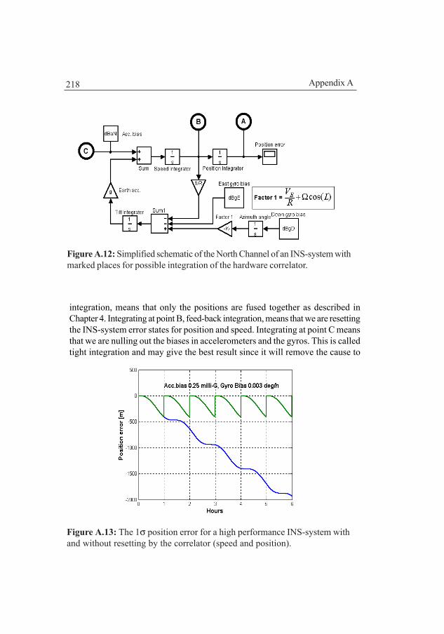
218 Appendix A
integration, means that only the positions are fused together as described inChapter 4. Integrating at point B, feed-back integration, means that we are resettingthe INS-system error states for position and speed. Integrating at point C meansthat we are nulling out the biases in accelerometers and the gyros. This is calledtight integration and may give the best result since it will remove the cause to
Figure A.12: Simplified schematic of the North Channel of an INS-system withmarked places for possible integration of the hardware correlator.
Figure A.13: The 1σ position error for a high performance INS-system withand without resetting by the correlator (speed and position).

219
the INS-drift. What we actually do is estimating the bias components in theKalman filter and then subtract them from the inputs of the accelerometers andgyros.
Figure A.13 shows the result from a simulation of the INS-position error accordingto the schematic in Figure A.12. As expected the resetting gives an upper boundon the INS position error. The INS-error after nulling the bias-errors is extremelysensitive to the quality in the estimate of the bias term so it should not beperformed before the Kalman filter has been settled. The integration of thenavigator output resembles to a high degree the integration of a GPS-system toan INS-system and has been exhaustively studied in the literature.
The conclusion of this section is that it in most cases will be sufficient with asimple feedback of position/speed, i.e., the alternatives A and B.
A.2 The hardware navigator

220 Appendix A
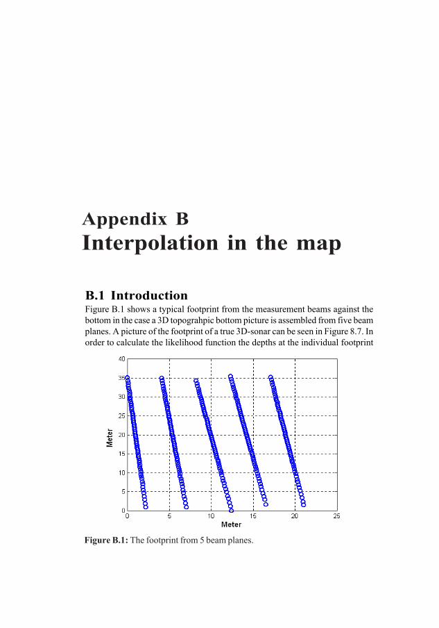
221
B.1 IntroductionFigure B.1 shows a typical footprint from the measurement beams against thebottom in the case a 3D topograhpic bottom picture is assembled from five beamplanes. A picture of the footprint of a true 3D-sonar can be seen in Figure 8.7. Inorder to calculate the likelihood function the depths at the individual footprint
Appendix BInterpolation in the map
Figure B.1: The footprint from 5 beam planes.

222 Appendix B
points have to be determined. This can be done by signal reconstruction, if thebottom profile has been properly sampled, or by interpolation.
B.2 Reconstruction of signals from samplesWe will restrict the discussion here to one dimensional signals. A discussion ofsampling and reconstruction of multidimensional signals can be found in [BP71].It is well known that when sampling a signal the sampling frequency has to bemore than twice the highest frequency in the signal if the signal is to be uniquelyrecovered from the samples [HN28]. This is easy to understand if it is observedthat a finite time signal can be uniquely represented by a Fourier series. To beable to uniquely reconstruct the highest frequency in the Fourier series thedistance between the samples must be less than half the period time of thissignal component, Figure B.2.
If the signal contains frequencies higher than half the sampling frequency thesampled signal spectra will wrongly have increased amplitudes for frequenciesless than half the sampling frequency. This because the high frequencycomponents will mistakenly be assumed to belong to the lower frequencycomponents. This phenomenon is called signal aliasing. To avoid signal aliasingdue to high frequency noise the signal is often low pass filtered to remove allfrequencies above half the sampling frequency. This makes it possible to uniquelyreconstruct the filtered signal but of course not the original signal.
Figure B.2: If the spatial sampling distance Ts is less than half the period of thesinusoid it can be uniquely reconstructed.

223
It is easy to formally analyze the aliasing phenomena if the sampled signal canbe assumed to be the product of the continuous signal and an periodic impulse-train, the sampling function [OW97, SH90, PK92]. Let the continuous signal beh(x) and the sampled signal hs(x) then
( ) ( ) ( )sh x h x f x= (B.1)
if f(x) is the impulse train
( ) ( )sn
f x x nTδ∞
=−∞
= −∑ (B.2)
where δ(.) is the Dirac function and Ts the sampling interval and it has beenobserved that the integral of the Dirac functions represents the actual signalvalues at the sampling event.
Since multiplication in the time domain is equivalent to convolution in thefrequency domain the spectrum of the sampled signal will be [OW97, SH90]
1( ) ( )hs h sns
S S nT
ω ω ω∞
=−∞
= −∑ (B.3)
where Sh is the spectrum for the continuous signal, the continuous bottomprofile, and ωs =2π/Ts is the sampling frequency. The spectrum for the sampled
B.2 Maximum a posterior interpolation
Figure B.3: The power spectrum for the sampled signal hs(x) of a band limitedcontinous signal h(x).
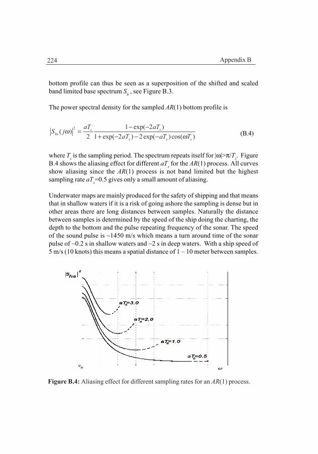
224 Appendix B
bottom profile can thus be seen as a superposition of the shifted and scaledband limited base spectrum Sh , see Figure B.3.
The power spectral density for the sampled AR(1) bottom profile is
2 1 exp( 2 )( )
2 1 exp( 2 ) 2exp( ) cos( )s s
hss s s
aT aTS j
aT aT Tω
ω− −
=+ − − − (B.4)
where Ts is the sampling period. The spectrum repeats itself for |ω|>π/Ts. FigureB.4 shows the aliasing effect for different aTs for the AR(1) process. All curvesshow aliasing since the AR(1) process is not band limited but the highestsampling rate aTs=0.5 gives only a small amount of aliasing.
Underwater maps are mainly produced for the safety of shipping and that meansthat in shallow waters if it is a risk of going ashore the sampling is dense but inother areas there are long distances between samples. Naturally the distancebetween samples is determined by the speed of the ship doing the charting, thedepth to the bottom and the pulse repeating frequency of the sonar. The speedof the sound pulse is ~1450 m/s which means a turn around time of the sonarpulse of ~0.2 s in shallow waters and ~2 s in deep waters. With a ship speed of5 m/s (10 knots) this means a spatial distance of 1 – 10 meter between samples.
Figure B.4: Aliasing effect for different sampling rates for an AR(1) process.

225
In the case of a multibeam sonar this will be the distance between beam planes.Usually a multibeam sonar has a spacing of 1.5o between beams which meansthat the distance between the samples along the beamplane will be 4 – 40 meterin the center.
From the discussion above it is clear that the spectrum of an underwater mapalways will have some aliasing. It is also clear that the degree of aliasing willvary between bottom areas depending on how dense the sampling once wasdone. The consequence of this is that the bottom profile can not be reconstructedfrom the samples using the reconstruction formula
sin( ( ))2( ) ( )( )
2
ss
ssn
s
x nTh x h nT
x nT
ω
ω
∞
=−∞
−=
−∑ (B.5)
That is, we will never know the exact shape of the bottom profile between thesample points. To reconstruct a signal from its samples, where it is theoreticallypossible, we have to sum the slowly converging infinite series (B.5) whichmeans in practice that we have to truncate it after a fairly high number of terms.It is, however, interesting to note that (B.5) can be thought of as an expansionof the bottom profile as
( ) ( )n nn
h x c xφ∞
=−∞
= ∑ (B.6)
where cn in this special case is the sampled bottom depth and φn is the sincfunction. A deeper analysis [OJ72] shows that there are many other choices offunction classes and coefficients possible for a true reconstruction. This,together with the discussion above, has lead to the use of interpolation insteadof reconstruction to determine the depth values between the depth samples.The following chapters will discuss some interpolation methods that preservethe spectrum of the bottom.
The underwater map often has a grid size of 10 meter but it can also be 5 or 1meter so it will be necessary to interpolate in the map to determine the actualdepth values at the footprint points. Deterministic methods as Lagrange, Hermi-tes or spline interpolation [BJ74, MU99], well known since long ago, can be usedbut depending on the bottom topography the result may differ and perhaps notbe satisfactory. In certain areas one method will work well but in other areas notso well. However, the difference is often not so large that it will be crucial for the
B.2 Maximum a posterior interpolation
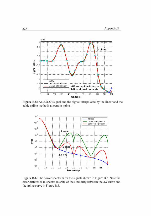
226 Appendix B
Figure B.5: An AR(20) signal and the signal interpolated by the linear and thecubic spline methods at certain points.
Figure B.6: The power spectrum for the signals shown in Figure B.5. Note theclear difference in spectra in spite of the similarity between the AR curve andthe spline curve in Figure B.5.

227
result when using many measurement beams.
A consequence of the deterministic methods is that they change the statisticalproperties of the bottom topography, especially they change the power spectrumat higher frequencies which will impact the position accuracy. Figure B.5 showsan AR(20) signal, a linearly interpolated signal and cubic spline interpolatedsignal. The corresponding power spectra can be seen in Figure B.6 and as canbe seen there is a difference at higher frequencies.
Now, the expected value of the square of the gradients, which determines theexpected value of the accuracy that can be calculated from (see Chapter 6)
22
0
( ) ( )n
n
hn
hn E S dx
µ ω ω ω∞ ∂ = = ∂ ∫ (B.7)
when n=1. This will thus give us the Fischer matrix (FIM), i.e., what we canexpect it to be in the terrain considered. We use the Fischer matrix to calculatethe position error covariance matrix. Therefore it would be desirable to have aninterpolation method that does not change the statistical properties of the bot-tom topography, i.e., the power spectra. In the following three sections differentprobabilistic approaches will be introductorily discussed.
B.3 Maximum a posteriori interpolationLet us look at a case with a band of missing samples since it clearly demonstratesthe power of the method. The interpolation case for a finer grid followsimmediately. Assume the length of the signal is N and that a band of M samplesis missing, Figure B.7. We arrange the signal vector in known and unknownvalues as follows
1 1
2 2
00
0
Kn Kn
Un Un
Kn Kn
Kn Un
= = +
= +
x x
x x xx x
Kx Ux (B.8)
where the matrices K and U only rearrange the signal values.
B.2 Maximum a posterior interpolation

228 Appendix B
The probability density function for the signal can be written as
( , ) ( | ) ( )Kn Un Un Kn Knp p p=x xx x x x x (B.9)
or
( | ) ( ) / ( )Un Kn Kn Un Knp p p= = +x x xx x x Kx Ux x (B.10)
where ( )p ⋅x is assumed to be known and ( )Knpx x is a constant. We now searchfor the xUnthat maximizes the PDF
ˆ arg max ( )Un
MAPUn Kn Unp= = +x
xx x Kx Ux (B.11)
In the case we have a Gaussian signal with known covariance matrix ΣΣΣΣΣxx
1/ 2 1/ 2
1 1( ) exp( )2(2 ) det( )
TNp
π−= − Σ
Σx xxxx
x x x (B.12)
Our estimate of the missing samples is
Figure B.7: A signal with a band of missing samples, the shadedarea.
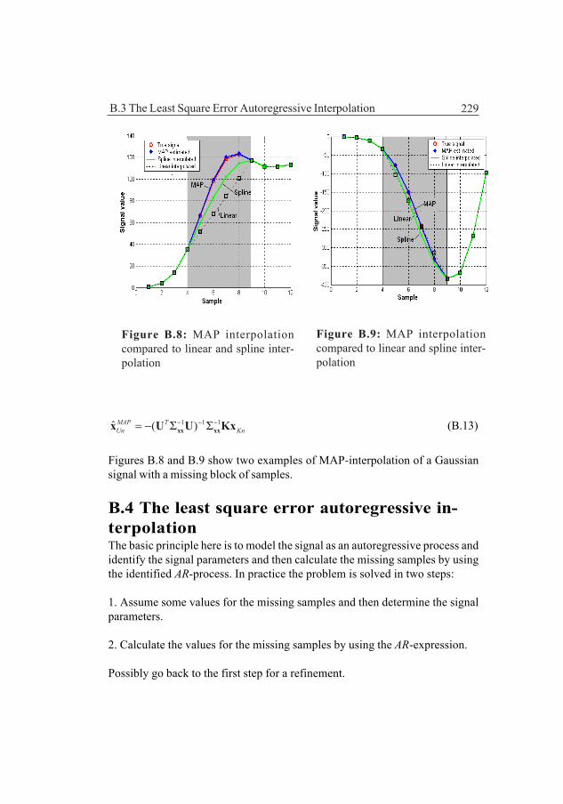
229B.3 The Least Square Error Autoregressive Interpolation
Figure B.8: MAP interpolationcompared to linear and spline inter-polation
Figure B.9: MAP interpolationcompared to linear and spline inter-polation
1 1 1ˆ ( )MAP TUn Kn
− − −= − Σ Σxx xxx U U Kx (B.13)
Figures B.8 and B.9 show two examples of MAP-interpolation of a Gaussiansignal with a missing block of samples.
B.4 The least square error autoregressive in-terpolationThe basic principle here is to model the signal as an autoregressive process andidentify the signal parameters and then calculate the missing samples by usingthe identified AR-process. In practice the problem is solved in two steps:
1. Assume some values for the missing samples and then determine the signalparameters.
2. Calculate the values for the missing samples by using the AR-expression.
Possibly go back to the first step for a refinement.

230 Appendix B
Figure B.10: The system of equations for the AR-function.
()
()
(1)
(1)
(1)
(1)
()
()
(1)
(1)
(2)
(2)
(2)
(2)
(1)
(1)
()
()
(1)
(
(1)
Un
Un Un
eP
xP
eP
xP
ek
xk
ek
xk
ek
xk
ek
xk
ek
MP
xk
MP
ek
MP
xk
MP
ek
MP
xk
MP
ek
MP
xk
M
eN
++
−−
++
++
=
++
−+
+−
++
−+
+−
++
++
++
++
+
−
(1)
(2)
(0)
()
(1)
(1)
(2)
(3)
(1)
(1)
(2)
()
()
(1)
(1)
(1)
()
(2)
(3)
(
1)
(1)
Un
UnUn
xP
xP
xx
Px
Px
xk
xk
xk
Px
kx
kx
kP
xk
xk
xk
Px
kx
kx
kP
xk
MP
xk
MP
P
xN
−−
−
−
−−
−
−
−−
−−
+
+
−+
−
++
−+
+−
+
−
1 2 3
4)(
2)(
2)(
3)(
1)(
1)(
2)(
)(
)(
1)(
1)
(2)
(3)
(1)
UnP
Un
a a a
xk
Ma
xk
MP
xk
MP
xk
Mx
kM
Px
kM
Px
kM
xk
MP
xk
MP
xk
M
xN
xN
xN
P
+−
+
+−
++
−+
−
+
+−
++
−+
++
++
−+
+
−
−−
−
(B.14)
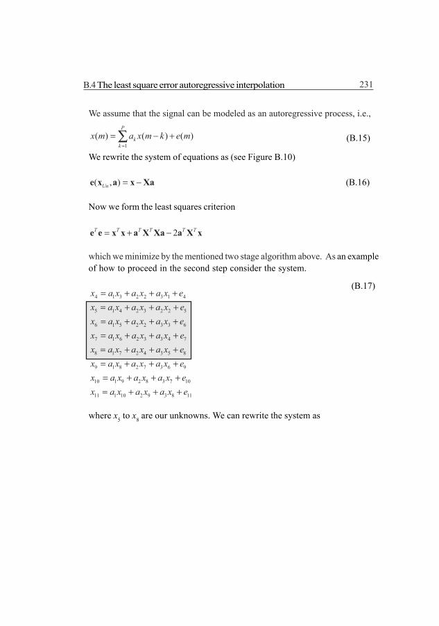
231B.4 The least square error autoregressive interpolation
We assume that the signal can be modeled as an autoregressive process, i.e.,
1
( ) ( ) ( )P
kk
x m a x m k e m=
= − +∑ (B.15)
We rewrite the system of equations as (see Figure B.10)
( , )Un = −e x a x Xa (B.16)
Now we form the least squares criterion
2T T T T T T= + −e e x x a X Xa a X x
which we minimize by the mentioned two stage algorithm above. As an exampleof how to proceed in the second step consider the system.
4 1 3 2 2 3 1 4
5 1 4 2 3 2 2 5
6 1 5 2 2 3 3 6
7 1 6 2 3 3 4 7
8 1 7 2 4 3 5 8
9 1 8 2 7 3 6 9
10 1 9 2 8 3 7 10
11 1 10 2 9 3 8 11
x a x a x a x ex a x a x a x ex a x a x a x ex a x a x a x ex a x a x a x ex a x a x a x ex a x a x a x ex a x a x a x e
= + + += + + += + + += + + += + + += + + += + + += + + +
(B.17)
where x5 to x8 are our unknowns. We can rewrite the system as

232 Appendix B
5 3 2
16 35
2 176
3 2 187
3 2 198
3 210 1Unknown
311 2 1
1 0 0 0 0 01 0 0 0 0 0
1 0 0 0 0 00 0 0 0 0
0 0 0 0 00 0 0 0 00 0 0 0 0
e a aae a
xa ae
xa a ae
xa a ae
xa ae a
ae a a
− − − − − − = − − − + − − − − − − − − −
A
3
4
5
6
Known
xxxx
B
(B.18)
This can be written as
Un Kn= +e Αx Bx (B.19)and
Figure B.11: An AR(4) signal and the interpolated signal with the least squareserror autoregressive interpolation.

233
( )T T
( )
=x 2 x
TTUn Kn Un Kn
T T T TUn Un Kn Un Kn Kn
= + + =
+ +
e e Αx Bx Αx Bx
A Ax x B Ax B Bx (B.20)
Taking the derivative gives
2 2T
T TUn Kn
Un
∂ = +∂e e A Ax A Bxx (B.21)
and setting it to zero gives1
ˆ T TUn Kn
− = − x A A A Bx (B.22)
That is ,we have minimized the prediction error [KSH00, KA93].
As an example an AR(4) process was generated and a block of samples wasconsidered unknown, Figure B.11. In the first step the signal parameters wereestimated disregarding the unknown samples [LJ91, LJ99, SÖST89], see Figure
Figure B.12: The true and the estimated parameters of the AR(4) signal.
B.4 The least square error autoregressive interpolation

234 Appendix B
Figure B.13: A bottom profile signal with a missing block of samples. Thewindow function is faintly outlined.
Figure B.14: The output of the Specgram function in Matlab SignalProcessing Toolbox.

235
Figure B.15: Some of the frequency lines constituting the specgram in FigureB.14.
B.12. In the second step the estimated parameters were used to calculate theunknown samples.
B.5 Interpolation in the frequency domainA third method for interpolation is to interpolate in the frequency domain. Asbefore, the method will be illustrated in the case of a missing block of samples,Figure B.13.
The short time Fourier transform decomposes the signal in time and frequency.It is
21
1
( , ) ( ) ( ( ) )ikN j
N
iX k m w i x m N D i e
π− −
=
= − +∑ (B.23)
where N is block length, D = block overlap, k=frequency, m= block number,w(i)=window. The transform can be calculated by Matlab’s Specgram function
B.4 The least square error autoregressive interpolation
236 Appendix B
[KSL93], see Figure B.14. The different frequency signals shown in Figure B.15can be the interpolated by any of the previously mentioned methods and themissing samples in the time domain are recovered by the inverse transform.
B.6 SummaryThis introductory study of the probabilistic interpolation methods shows, insome cases, excellent performance of the methods compared to the deterministicmethods, see Figure B.8. The probabilistic methods would be the given choiceif the signal characteristics of the bottom profile would be known at theinterpolation point. This is, however, seldom the case. Instead thecharacteristics have to be estimated from a few bottom depth samples whichwill degrade the performance considerably. Therefore, in many cases, we willhave to resort to the deterministic methods which we by experience know willhave sufficient performance.

237
SymbolsThroughout the thesis uppercase boldface letters denote matrices, lowercasebold letters denote column vectors and italics denote scalars.
Notational distinctions between the symbol for a stochastic variable and itsoutcome is only done if the meaning is not clear from the context. If a notationaldistinction is necessary Greek letters and uppercase letters are used to denotethe stochastic variable.
f∼ Notation for distributed as f.
a f∼ Notation for asymptotically distributed as f.
x̂ The ˆ notation means estimated value or estimatordepending on context.
2( , )µ σN The Gaussian probability density function with the mean µand variance σ2. The standard deviation σ>0.
N(µµµµµ,C) The vector Gaussian probability density function with themean µµµµµ and covariance C>0, i.e., positive definite.
Notational Conventions

238 Notational Conventions
arg max ( )fθ
θ Denotes the value of θθθθθ that maximizes f(θθθθθ).
,t tx A Short for ( )tx or ( )tA , ie., the vector x or matrix A is afunction of time.
tY Alternative notation for matrices.
1N,N Short for a matrix of dimension NxN whos elements areones.
IN,N The identity matrix of dimension NxN which has ones inthe diagonal and zeros elsewhere.
Π The projection matrix /N N N= −Π I 1 . The projection
matrix is idempotent, ie., ⋅ =Π Π Π .
,T Tx A Superindex T denotes transpose.
1−A The inverse of the square matrix A.
det(A) The determinant of the square matrix A.
Tr(A) The trace of the square matrix A.
h(x) A scalar valued function of the vector x.
h(x) A vector valued function of the vector x.
p(x) The probability density function.
f(x) Alternative notation for the probability density function.
p-(x) The prior probability density function beforemeasurement update.
( | )p x y The conditional density function given the event y.
( ; )L x y The likelihood function as a function of x given theevent y.
Pr{}⋅ Probability
{}E ⋅ Expectation.

239
f∂∂x A column vector whos elements are the partial derivatives
of the scalar function f(x) with respect to the elements inthe vector x. The vector is also called the gradient vectorof f(x).
Tf∂
∂xA row vector whos elements are the derivatives of the
scalar function f with respect to the elements in the vector
x, i.e. T
Tf f∂ ∂ = ∂∂ xx
.
xff ∂∇ =
∂x A notation of the gradient often used in physics and
considered to be a row vector.
f∆x The Laplacian, a scalar function which is the sum ofthe second partial derivatives of the elements in the
vector x of dimension m, 2
21
m
ii
fx=
∂∂∑ .
2f f f∆ = ∇ ∇ = ∇x x x x .
2
Tf∂
∂ ∂x xThe Hessian matrix which has the elements
2
i j
fx x∂
∂ ∂ where
i is the row index and j the column index.
T∂
∂y
xThe Jacobian matrix which has the elements
i
j
yx
∂∂
where i is the row index and j the column index. The

240 Notational Conventions
matrixTT
T∂ ∂ = ∂ ∂ y yx x
is called the vector gradient
matrix and has the elementsj
i
yx
∂∂ .
∂∂yx The gradient matrix. The gradient matrix is the transpose
of the Jacobian matrix. Also denoted T∂
∂yx in the
litterature.
T∂
∂y
x The Jacobian or Jacobian determinant. T
T∂ ∂=
∂∂y y
xx .
The Jacobian is the determinant of the Jacobian
matrix, i.e., det( T∂
∂y
x).
kx∂∂
AA matrix with the elements
ij
k
ax
∂∂ where aij is an
element of the matrix A and i is the row index and j isthe column index.
( )
ix∂
∂y x
A column vector whos elements are the derivatives
of the components of the vector y with respect to
xi, i.e., the j:th component is ( )j
i
yx
∂∂
x.

241
( )
ix∂
∂C x
A matrix whos elements are the derivatives of the
elements in the matrix C, i.e.,
[ ] ,
,
( )( ) r s
i ir sx x
∂ ∂ = ∂ ∂
C xC x.

242 Notational Conventions

243
Below is a list of acronyms that appear in the thesis.
2D Two dimensional3D Three dimensionalAR AutoregressiveBITAN Beijing University of Aeronatics and Astronautics inertial
terrain-aided navigationCOV CovarianceCRLB Cramér-Rao lower boundCW Continuous waveformEKF Extended Kalman filterFE Finite elementFEM Finite element methodFP Fokker-PlanckFPE Fokker-Planck partial differential equationFIFO First in, first outFIM Fisher information matrixFOG Fiber optic gyroFPGA Field programmable gate arrayGaussian Normally distributedGPS Global positioning systemIMU Inertial measurement unit
List of acronyms
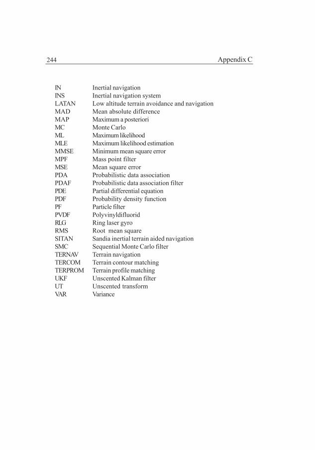
244 Appendix C
IN Inertial navigationINS Inertial navigation systemLATAN Low altitude terrain avoidance and navigationMAD Mean absolute differenceMAP Maximum a posterioriMC Monte CarloML Maximum likelihoodMLE Maximum likelihood estimationMMSE Minimum mean square errorMPF Mass point filterMSE Mean square errorPDA Probabilistic data associationPDAF Probabilistic data association filterPDE Partial differential equationPDF Probability density functionPF Particle filterPVDF PolyvinyldifluoridRLG Ring laser gyroRMS Root mean squareSITAN Sandia inertial terrain aided navigationSMC Sequential Monte Carlo filterTERNAV Terrain navigationTERCOM Terrain contour matchingTERPROM Terrain profile matchingUKF Unscented Kalman filterUT Unscented transformVAR Variance

245
[AMGC02] S. Arulampalam, S. Maskell, N. Gordon, T. Clapp, A Tutorial onParticle Filters for On-line Non-linear/Non-GaussianBayesian Tracking, IEEE Transactions on Signal Processing,Vol. 50, No. 2, February 2002.
[AN00] C-J. Andersson,“Navigation System for an AutonomousUnderwater Vehicle”, Master thesis in Automatic Control,Royal Institute of Technology, Stockholm, Sweden 2000.
[AN79] B. D. O. Anderson, J. B. Moore, Optimal Filtering,Prentice-Hall, Inc., USA, 1979.
[ANIN03] C.-J. Andersson, I. Nygren, A Method for Terrain Positioningof Underwater Vehicles, Proc. Undersea Defence Technology Europe (UDT), 2003.
[ANTR02] K. Andersson, F. Traugott, Implementation of a terraincorrelator for an underwater vehicle in an FPGA”, Masterthesis, Department of Electronics. Mälardalens University,Västerås, Sweden, 2002.
Bibliography

246
[AOA02] A. Stuart, J. K. Ord, S Arnold, Classical Inference & the LinearModel, Kendall´s Advanced Theory of Statistics, Arnold,London, UK, 2002.
[AR88] A. J. Robins, Recent developments in the ”TERPROM”Integrated Navigation System, Proceedings of the 44thAnnual Meeting, Annapolis, Maryland. June 1988.
[AS01] B. Azimi-Sadjadi, Approximate Nonlinear Filtering withApplications to Navigation, Ph.D. Thesis, Institute forSystem Research, University of Maryland, USA, 2001.
[AS72] D.L. Alspach and H.W. Sorenson. Nonlinear Bayesianestimation using Gaussian sum approximation, IEEETransactions on Automatic Control, 17:439-448, 1972.
[AZ96] A. Azzalini, Statistical Inference, Based on thelikelihood, Chapman & Hall, Monographs on Statisticsand Applied Probability, 1996.
[BA85] C. A. Baird, Designs Techniques for Improved Map-AidedNavigation, Proceedings of the IEEE National Aerospace andElectronic Conference, Naecon, 1985.
[BAAB84] C. A. Baird, M. R. Abramson, A Comparison of Several DigitalMap-Aided Navigation Techniques, Proceedings of the 1984IEEE Position, Location And Navigation Symposium(PLANS’84), San Diego, CA, 1984.
[BE01] N. Bergman, Posterior Cramér-Rao bounds forsequential estimation, in Sequential Monte CarloMethods in Practice, A. Doucet. H. deFreitas, N. Gordon,Eds. New York Springer-Verlag, 2001.
[BE98] N. Bergman, Deterministic and Stochastic BayesianMethods in Terrain Navigation, In Proc. 37th IEEEConference on Decision and Control 1998.
[BE99] N. Bergman, Recursive Bayesian Estimation: Navigation

247
and Tracking Applications, Dissertation 579, LinköpingsUniv., Linköping, Sweden, 1999.
[BER93] O. Bergem, Bathymetric Navigation of AutonomousUnderwater Vehicles Using a Multibeam Sonar and aKalman Filter with Relative Measurement CovarianceMatrices, Dr. Scient thesis, University of Trondheim, Norway, 1993.
[BI99] D. J. Biezad, Integrated Navigation and GuidanceSystems, AIAA Education Series, USA, 1999.
[BJ74] Å. Björck, Numerical Methods, Prentice-Hall Series inAutomatic Computation, Prentice-Hall Inc. 1974.
[BMB00] R. Beckman, A. Martinez, B. Bourgeois, AUV positioningusing bathymetry matching, Conference proceedings,MTS/IEEE Oceans 2000, 11-14 Sept. 2000.
[BP71] J. S. Bendat, A. G.. Piersol, Random Data: Analysis andMeasurement Procedures, Wiley-Interscience, John Wiley& Sons, New York, 1971.
[BR86] R. N. Bracewell, The Fourier Transform and ItsApplications. Second edition, revised, MacGraw-Hill,1986, Ltd., 2002.
[BR96] D. Brigo, Filtering by Projection on the Manifold ofExponential Densities, Dr thesis, Vrije University,Amsterdam, Holland, 1996.
[BRDA91] P. J. Brockwell, R. A. Davis, Time Series: Theory andMethods, 2nd Ed. Springer-Verlag, New York, 1991.
[BRHW97] R. G. Brown, P. Y. C. Hwang, Introduction to RandomSignals and Applied Kalman Filtering, John Wiley &Sons 1997.

248
[BRK01] Y. Bar-Shalom, X. Rong Li, T. Kirubarajan, Estimationwith Applications to Tracking and Navigation, WileyInterscience Publication, USA, 2001.
[BS02] J. M. Bernardo, A. F. M. Smith, Bayesian Theory, WileySeries in Probability and Statistics, Wiley Series inProbability and Statistics, John Wiley & Sons, New York,2000.
[BSFO88] Y. Bar-Shalom, T. E. Fortman, Tracking and DataAssociation, Mathematics in Science and Engineering,VOL. 179, Academic Press, Inc., 1988.
[BU91] W. S. Burdic, Underwater Acoustic System Analysis, 2ndEd. Prentice-Hall, 1991.
[BUSE71] R.S. Bucy and K.D. Senne, Digital synthesis of nonlinearfilters. Automatica, 7:287-298, 1971.
[CA88] P. E. Caines, Linear Stochastic Systems, Wiley Series inProbability and Mathematical Statistics, John Wiley & Sons,New York, 1988.
[CANY05] J. Carlström, I. Nygren, Terrain Navigation of the SwedishAUV62F, Proceedings, 14th International SymposiumUUST05, Durham, New Hampshire, USA, 2005.
[CKN92] I. Cato, B. Kjellin, K. Nordberg, Havets bottnar ochsediment, (The bottoms and the sediments of the sea),Sveriges Nationalatlas, Hav och kust. TemaredaktörBjörn Sjöberg, SNA Förlag, Kulturgeografiskainstitutionen, Stockholms universitet, Stockholm, 1992.
[CO04] Comsol AB, Partial Differential Equation Toolbox forUse with Matlab, The Math Works Inc. USA, 2004.
[CR46] H. Cramér, Mathematical Methods of Statistics, PrincetonUniversity Press, USA, 1946.

249
[CT92] C. H. Therrien, Discrete Random Signals and StatisticalSignal Processing, Prentice Hall, Signal ProcessingSeries, Englewood Cliffs, New Jersey, USA.
[CYY92] Z. Chen, P. J. Yu, H. Yang, BUAA inertial terrain-aidednavigation (BITAN) algorithm, Proceedings of the 18thICAS Congress, Beijing, China, Sept. 20-25, 1992.
[DABJ74] G. Dahlquist, Å. Björck, Numerical Methods, PrenticeHall, Inc., Englewood Cliffs, N.J. USA, 1974.
[DFG01] A. Doucet. H. deFreitas, N. Gordon, Eds., SequentialMonte Carlo Methods in Practice, New York Springer-Verlag, 2001.
[DOBS90] D. Lerro, Y. Bar-Shalom, Automated Tracking withTarget Amplitude Information, Proc. of the 1990 AmericanControl Conference, San Diego, CA. USA, 1990.
[EN01] P. Engman, Felfortplantning i ekolodsystem,(Error Propagation in Bathymetric Systems), Thesis FHSHNU 2001 (in Swedish), Försvarshögskolan, Stockholm,Sweden, 2001.
[FD05] T. S. Ferguson, A Course in Large Sample Theory,Chapman & Hall, 1996.
[FE96] F. Daum, Nonlinear Filters: Beyond the Kalman Filter,IEEE Aerospace and Electronic Systems Magazine,August 2005, Volume 20, No. 8. Part 2.
[FG00] F. Gustafsson, Adaptive Filtering and ChangeDetection, John Wiley & Sons, Ltd. UK, 2000.
[FJ03] H. Fjaereide, Navigation Aided by Terrain Correlationfor Submarines, Proc. Undersea Defence TechnologyEurope (UDT), 2003.

250
[FK88] F. Knabe, Untersuchung zum TERCOMNavigationsverfaren anhand von Flugversuchen uberden Testgebieten Deister und Harz, DeutschenForschungs- und Versuchsanstalt fur Luft- undRaumfahrt. 1988.
[FO97] J. R. Fountain, Digital Terrain System, IEE AirborneNavigation System Workshop, UK, 1997.
[GA04] C. W. Gardiner, Handbook of Stochastic Methods, 3rdEdition, Springer-Verlag Berlin, Heidelberg, New York,2004.
[GDW00] S. Godsill, A. Doucet, M. West, Maximum a posteriorisequence estimation using Monte Carlo particle filters,Ann. Inst. Stat. Math., Cambridge, UK, Vol. 52, No.1, 2001.
[GGBFJKN02] F. Gustafsson, F. Gunnarsson, N. Bergman, U. Forssell, J.
Jansson, R. Karlsson, P.-J. Nordlund, Particle Filters forPositioning, Navigation, and Tracking, IEEETransactions on Signal Processing, Vol. 50, No. 2,February 2002.
[GO80] J. Golden, Terrain contour matching (TERCOM): Acruise missile guidance aid, SPIE Vol. 238 ImageProcessing for Missile Guidance, 1980.
[GOOR92] G. H.Golub, J. M. Ortega, Scientific Computing andDifferential Equations, Academic Press Inc., 1992.
[GRAN01] M. S. Grewal, A. P. Andrews, Kalman Filtering: Theoryand Practice, Wiley-Interscience Publication, USA, 2001.
[GWA01] M. S. Grewal, L. R. Weill, A. P. Andrews, GlobalPositioning Systems, Inertial Navigation andIntegration, John Wiley & Sons, Inc., 2001.

251
[HA01] S. Haykin, Kalman Filtering and Neural Networks, JohnWiley & Sons, Inc. New York, USA, 2001.
[HAFO04] A. O’Hagan, J. Forster, Bayesian Inference, Kendall´sAdvanced Theory of Statistics, Arnold, London, UK,2004.
[HL01] Edited by D. L. Hall, J. Llinas, Handbook of MultisensorData Fusion, CRC Press, 2001.
[HN28] H. Nyquist, Certain Topics in Telegraph TransmissionTheory, AIEE Transactions, 1928, p.617, USA.
[HO90] J. A. Hollowell, Heli/SITAN: A Terrain ReferencedNavigation Algorithm for Helicopters, Proc. of the IEEE1990 PLANS - Position, Location, And NavigationSymposium, 1990, Las Vegas, NV, USA.
[HO91] J. Hollowell, Terrain Referenced Navigation for CruiseMissiles, The 1991 Cruise Missiles TechnologySymposium (CMTS-91), Laurel, MD, USA, 1991.
[HOAN85] L. D. Hostetler, R. D. Andreas, Nonlinear Kalman Filte-ring Techniques for Terrain-Aided Navigation, in H.W.Sorensen, editor, Kalman filtering: Theory andApplication, IEEE Press 1985.
[JA70] A. Jazwinski. Stochastic Process and Filtering Theory,volume 64 of Mathematics in Science and Engineering,Academic Press, New York, 1970.
[JA89] A. K. Jain, Fundamentals of Digital Image Processing,Prentice-Hall International Editions, 1989.
[JE01] C. Jekeli, Inertial Navigation Systems with GeodeticApplications, Walter de Gruyter Gmb H & Co. Berlin,Germany, 2001.

252
[JMHP04] B. Jalving, M. Mandt, O. K. Hagen, F. Pöhner, TerrainReferenced Navigation of AUVs and Submarines UsingMultibeam Echo Sounders, Proc. Undersea DefenceTechnology Europe (UDT), 2004.
[JO87] C. Johnson, Numerical solution of partial differentialequations by the finite element method, Studentlitteratur,Lund, Sweden ,1987.
[JTH90] N. Johnson, W. Tang, G. Howell, Terrain AidedNavigation Using Maximum A Posteriori Estimation,Proceedings of the 1990 IEEE Position, Location AndNavigation Symposium (PLANS’90) Las Vegas, Nevada,USA, March 1990.
[JU97] S. J. Julier, Process Models for the Navigation of High-Speed Land Vehicles, Ph.D. Thesis, Dept. of EngineeringScience, University of Oxford, UK 1977.
[JUUH04] S. J. Julier, J. K. Uhlmann, Unscented Filtering andNonlinear Estimation, Proceedings of the IEEE, Vol. 92,NO. 3, March 2004.
[KA05] R. Karlsson, Particle Filtering for Positioning andTracking Applications, Dissertation 924, LinköpingsUniv., Linköping, Sweden, 2005.
[KA93] S. M. Kay, Fundamentals of Statistical Signal Proces-sing, Estimation Theory, Prentice Hall, 1993.
[KH49] A. I. Khinchin, Mathematical Foundations of StatisticalMechanics, Dover Publications, Inc., New York, 1949.
[KICH91] D. Kincaid, W. Cheney, Numerical Analysis, Brooks/ColePublishing Company, Pacific Grove, Cal., USA, 1991.
[KL01] F. Klebaner, Introduction to Stochastic Calculus with

253
Applications, Imperial College Press, London, 2001.
[KSH00] T. Kailath, A. H. Sayed, D. Hassibi, Linear Estimation,Prentice Hall Inc., New Jersey, USA, 2000.
[KSL93] T. P. Krauss, L. Shure, J. N. Little, Signal ProcessingToolbox for use with Matlab, The Math Works Inc. USA,1993.
[KU67] H. J. Kushner, Nonlinear Filtering: The Exact DynamicalEquations Satisfied by the Conditional Mode, IEEETransactions on Automatic Control, VOL. AC-12, No. 3.June 1967.
[LA88] H.-D. Larche, LATAN, a Modern Terrain Following andFlight Control System, Messerschmitt-Boelkow-Blohm(MBB) GMBH, Ottobrunn, Germany 1988.
[LA92] Anthony Lawrence, Modern Inertial Technology,Navigation, Guidance, and Control, Second edition,Springer-Verlag, New York 1992.
[LJ91] L. Ljung, System identification Toolbox for Use withMatlab, The Math Works Inc. USA, 1991.
[LJ99] L. Ljung, System Identification. Thery for the User,Second Ed., Prentice Hall Inc., New Jersey, USA, 1999.
[LÜ96] H. Lütkepohl, Handbook of Matrices, John Wiley & SonsLtd., UK, 1996.
[MA82a] P. S. Maybeck, Stochastic models, estimation andcontrol, Vol. 1, Academic Press Inc., New York, USA,1982.
[MA82b] P. S. Maybeck, Stochastic models, estimation andcontrol, Vol. 2, Academic Press Inc., New York, USA,1982.

254
[MA97] D.E. di Massa, Terrain-relative navigation forautonomous underwater vehicles, Ph.D. Thesis MIT/WoodsHole Oceanographic Institution, 1997,USA, 1997.
[MAST97] D.E. di Massa, W. K. Stewart, Jr., Terrain-relative naviga-tion for autonomous underwater vehicles, Conferenceproceedings,MTS/IEEE Oceans 1997, 6-9 Oct. 1997.
[META83] G. L. Mealy, W. Tang, Application of Multiple ModelEsimation to a Recursive Terrain Height CorrelationSystem, IEEE Transactions on Automatic Control, VOL.AC-28, March 1983.
[METR02] J. Metzger, G. F. Trommer, Studies on Four TerrainReferenced Navigation Techniques, Symposium GyroTechnology 2002, Stuttgart, Germany, 2002.
[MDFW00] R. van der Merwe, A. Doucet, N. de Freitas, E. Wan, TheUnscented Particle Filter, Technical Report CUED/F-INFENG/TR 380, Cambridge University Eng. Dept. 2000.
[MI00] T. Mikosch, Elementary Stochastic Calculus withFinance in View, World Scientific Publishing Co. Pty.Ltd., Singapore, 2000.
[MIMI93] G. Minkler and J. Minkler, Theory and Application ofKalman Filtering, Magellan Book Company, 1993.
[MLG99] N. Bergman, L. Ljung, F. Gustafsson, Terrain navigationusing Bayesian statistics, in Proc. IEEE Int. ControlMagazine, Vol. 19, no. 3, pp. 33-40, 1999
[MM01] M. Mandt, Terrengreferert posisjonering forundervannsfarkoster, FFI/Rapport-2001/05900, NO-2027Kjeller, Norway, 2001.
[MU99] M. Unser, Splines, A Perfect Fit for Signal and ImageProcessing, IEEE Signal Processing Magazine, November,1999.
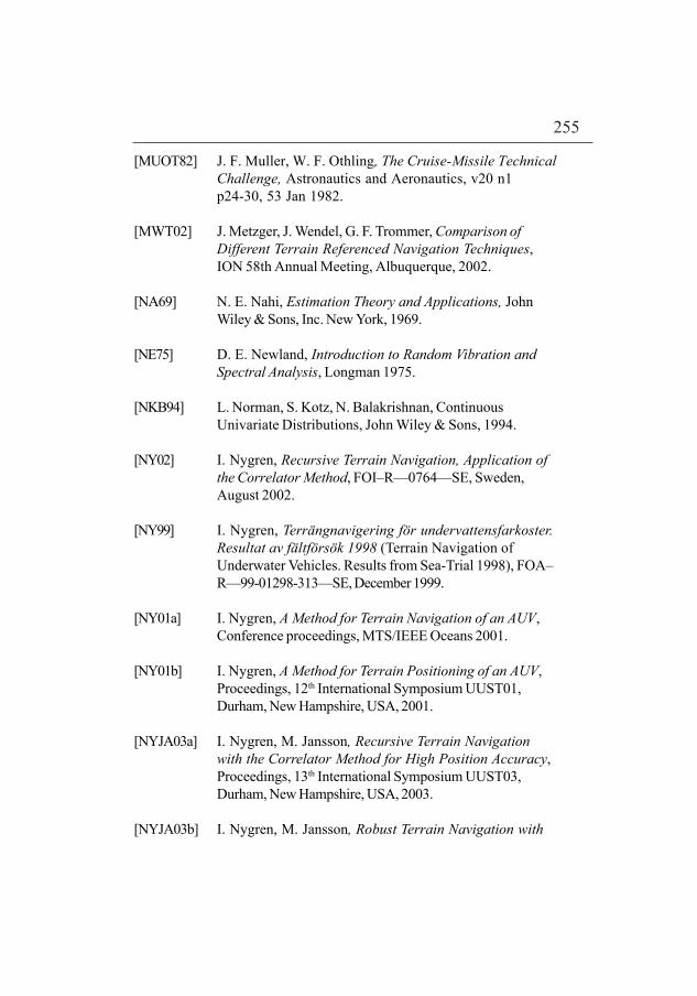
255
[MUOT82] J. F. Muller, W. F. Othling, The Cruise-Missile TechnicalChallenge, Astronautics and Aeronautics, v20 n1p24-30, 53 Jan 1982.
[MWT02] J. Metzger, J. Wendel, G. F. Trommer, Comparison ofDifferent Terrain Referenced Navigation Techniques,ION 58th Annual Meeting, Albuquerque, 2002.
[NA69] N. E. Nahi, Estimation Theory and Applications, JohnWiley & Sons, Inc. New York, 1969.
[NE75] D. E. Newland, Introduction to Random Vibration andSpectral Analysis, Longman 1975.
[NKB94] L. Norman, S. Kotz, N. Balakrishnan, ContinuousUnivariate Distributions, John Wiley & Sons, 1994.
[NY02] I. Nygren, Recursive Terrain Navigation, Application ofthe Correlator Method, FOI–R—0764—SE, Sweden,August 2002.
[NY99] I. Nygren, Terrängnavigering för undervattensfarkoster.Resultat av fältförsök 1998 (Terrain Navigation ofUnderwater Vehicles. Results from Sea-Trial 1998), FOA–R—99-01298-313—SE, December 1999.
[NY01a] I. Nygren, A Method for Terrain Navigation of an AUV,Conference proceedings, MTS/IEEE Oceans 2001.
[NY01b] I. Nygren, A Method for Terrain Positioning of an AUV,Proceedings, 12th International Symposium UUST01,Durham, New Hampshire, USA, 2001.
[NYJA03a] I. Nygren, M. Jansson, Recursive Terrain Navigationwith the Correlator Method for High Position Accuracy,Proceedings, 13th International Symposium UUST03,Durham, New Hampshire, USA, 2003.
[NYJA03b] I. Nygren, M. Jansson, Robust Terrain Navigation with

256
the Correlator Method for High Position Accuracy,Conference proceedings, MTS/IEEE Oceans 2003.
[NYJA04a] I. Nygren, M. Jansson, Terrain Navigation Using theCorrelator Method, Conference proceedings, 2004 IEEEPosition Location And Navigation Symposium, April 27-29 Monterey, Cal., USA.
[NYJA04b] I. Nygren, M. Jansson, Terrain Navigation forUnderwater Vehicles Using the Correlation Method,IEEE Journal of Oceanic Engineering, Vol. 29, No. 3. July2004.
[NYJA04c] I. Nygren, M. Jansson, A Terrain Navigation Method forUAVs and AUVs Based on Correlation, IEEE Transactionson Aerospace and Electronic Systems, to be published.
[OJ72] A. V. Oppenheim, D. H. Johnson, Discrete Representationof Signals, Proc. IEEE, Vol. 60, No. 6. June 1972.
[OW97] A. V. Oppenheim, A. S. Willsky, Signals & Systems, PrenticeHall, Signal Processing Series, 1997, USA.
[PE04] M. Pikander, P. Eskelinen, Differential GPS DynamicLocation Experiment at Sea, IEEE Aerospace &Electronic Systems Magazine, March 2004, USA.
[PE95] V. V. Petrov, Limit Theorems of Probability Theory,Sequences of Independent Random Variables, OxfordStudies in Probability 4, Claredon Press, Oxford, Uk, 1995.
[PK92] P. Kraniauskas, Transforms in Signals and Systems,Addison-Wesley Publishers Ltd. Wokingham, England,1992.
[PP02] A. Papoulis, S. Unniksishna Pillai, Probability, RandomVariables and Stochastic Processes, MacGraw-Hill, NewYork, NY, USA, 2002.
[PUJP00] P. Pucar, J. Palmqvist, Saab NINS/NILS an automatic

257
landing system for Gripen, Conf. Proceedings of the 2000IEEE Position, Location And Navigation Symposium (PLANS’00), 1200.
[RA45] C. R. Rao, Information and the Accuracy Attainable inthe Estimation of Statistical Parameters, Bulletin of theCalcutta Mathematical Society, Vol 37, 1945.
[RI84] H. Risken, The Fokker Planck Equation, Springer-VerlagBerlin, Heidelberg, New York, 1984.
[RO01] C. P. Robert, The Bayesian Choice, 2nd edition, SpringerTexts in Statistics, Springer Verlag, 2001.
[RU85] A. R. Runnals, A Bayesian Approach to Terrain ContourNavigation, AGARD Unclassified paper No. 43,Guidance and Control Panel, 40th Symposium, May1985.
[RÅWE95] L. Råde, B. Westergren, Mathematical Handbook forScience and Engineering, Studentlitteratur, Sweden,1995.
[SC91] L. L. Scharf, Statistical Signal Processing, Detection,Estimation, and Time Series Analysis, Addison-WesleyPublishing Co. New York, USA, 1991
[SCA99] O. Strauss, F. Comby, M. J. Aldon, “Multibeam sonar imagematching for terrain-based underwater navigation”,Conference proceedings, MTS/IEEE Oceans 1999, Ridingthe Crest into the 21st Century, 13-16 Sept. 1999.
[SESI93] P. K. Sen, J. M. Singer, Large Sample Methods inStatistics, An Introduction with Applications, Chapman& Hall, UK, 1993.

258
[SEV00] T. A. Severini, Likelihood Methods in Statistics, OxfordStatistical science series, 22. Oxford University press, UK,2000.
[SH90] S. D. Stearns, D. R. Hush, Digital Signal Analysis,Prentice Hall, 1990.
[SIL96] D.S. Silvia, Data Analyses, A Bayesian Tutorial, OxfordScience Publications, Claredon Press, Oxford, UK, 1996.
[SK85] E. Skarman, Flight test with a terrain aided navigationsystem, Proceedings of the 5th International Conference,Remotely piloted vehicles, Bristol, England, 1985,
[SM03] G. D. Smith, Numerical Solution of Partial DifferentialEquations, Finite Difference Methods, Third Edition,Clarendon Press, Oxford, UK, 2003.
[SO96] S. P. Stoica, B. Ottersten, The evil of super-efficiency,Signal Processing, Vol. 55, Issue 1 November 1996,Elsevier North-Holland Inc., Amsterdam, TheNetherlands.
[SOA99] M. Sistiaga, J. Opderbecke, M. J. Aldon, Depth imagematching for underwater vehicle navigation, Conferenceproceedings, In international Conference on Image Analy-sis and Processing, 1999, 27-29 Sept. 1999.
[SÖST89] T. Söderström, P. Stoica, System Identification, Prentice-Hall, 1989.
[ST97] V. Stohny, Symmetry Properties and Exact Solutions ofthe Fokker-Planck Equation, Nonlinear MathematicalPhysics, 1997, V.4. N 1-2, pp.132-136, Kiev PolytechnicalInstitute, Kiev, Ukraina.
[STBO97] G. Strang, K. Borre, Linear Algebra, Geodesy, and GPS,Wellesley-Cambridge Press, USA, 1997.

259
[SY98] H. Stark, Y. Yang, Vector Space Projections, John Wiley& Sons, Inc. USA, 1998.
[TALL03] F. Traugott, K. Andersson, A. Löfgren, L. Lindh,Successful Prototyping of a Real-Time Hardware BasedTerrain Navigation Correlator Algorithm, ConferenceProceedings, DSD2003 Euromicro Symposium On DigitalSystem Design, Architectures, Methods and Tools,Turkey, Antalya, september 2003.
[TH97] V. Thomée, Galerkin Finite Element Methods forParabolic Problems, Springer-Verlag, Berlin, Heidelberg,New York, 1997.
[TIWE97] D. H. Titterton, J. L.Weston, Strapdown inertialnavigation technology, IEE Radar, Sonar, Navigation andAvionic series 5, Peter Peregrinus Ltd. London UK, 1997
[TS02] T. Söderström, Discrete-time Stochastic Systems,Springer-Verlag, London Ltd., UK, 2002.
[UR83] R. J. Uric, Principles of underwater sound, 3rd Ed,McGraw-Hill Book Company, 1983.
[VA96] S. V. Vaseghi, Advanced Signal Processing and DigitalNoise Reduction, Wiley-Teubner, 1996.
[VA98] A. W. van der Vart, Asymptotic Statistics, CambridgeSeries in Statistical and Probabilistic Mathematics,Cambridge University Press, 1998.
[VT02] H. L. Van Trees, Optimum Array Processing, Estimationand Modulation Theory, Wiley-Interscience Publication,New York, USA, 2002.
[VT68] H. L. Van Trees, Detection, Estimation and ModulationTheory. Wiley, New York,1968.

260
[WL90] E. Waltz and J. Llinas, Multisensor data fusion, ArtechHouse, Boston, 1990.
[YP01] Yudi Patwitan, In All Likelihood: Statistical Modellingand Inference Using Likelihood, Oxford SciencePublications, Clarendon Press. Oxford, UK, 2001.
[YCH91] P. Yu, Z. Chen, J. Hung, Performance evaluation of sixterrain stochastic linearization techniques for TAN. IEEEAerospace and Electronics Conference 1991.