Integrated Planning and Control ofLarge Tracked Vehicles in Open Terrain

Xiuyi Fan1, Surya Singh2, Florian Oppolzer3

Eric Nettleton2, Ross Hennessy2, Alexander Lowe2, and Hugh Durrant-Whyte2

1Department of Computing, Imperial College London, United Kingdom2Australian Centre for Field Robotics, University of Sydney, Australia

3Technology and Innovation, Rio Tinto, Australiax.fan09@imperial.ac.uk, florian.oppolzer@riotinto.com, {spns, e.nettleton, r.hennessy, a.lowe, hugh}@acfr.usyd.edu.au

Abstract— Trajectory generation and control of large equip-ment in open field environments involves systematically androbustly operating in uncertain and dynamic terrain. Thispaper presents an integrated motion planning and controlsystem for tracked vehicles. Flexible path-end adjustments andadaptive look-ahead are introduced to a state lattice planningapproach with waypoint control. For a given processing horizon,this increases search coverage and reduces planning error.

This tramming approach has been successfully fielded on a98-ton autonomous blast hole drill rig used in iron ore mining inWestern Australia. The system has undergone extensive testingand is now integrated into a production environment. This workis a key element in a larger program aimed at developing afully autonomous, remotely operated mine.

I. INTRODUCTION

Due to the remoteness and potential hazards in mining,automation is desirable to achieve higher efficiency andsafety [1]. One of the vehicles central to open-pit miningoperations is a surface drilling rig (Fig. 1). This large trackedvehicle drills holes into the ground that are subsequentlyfilled with explosive and blasted. The fragmented rock isthen extracted. Drill motions are not arbitrary. Hole locationsare carefully planned in regular patterns according to theunderlying geology. Thus, there is an underlying structurein the form of preferred maneuvers, such as straight-linetramming, row shifting, or three-point turning.

Fig. 1. The autonomous blast hole drill rig at rest on a drill bench of anopen-pit mine (the 4x4 truck illustrates the large scale).

Drill rig automation can be divided into three modules:tramming, levelling, drilling. This paper focuses on tram-ming, i.e., the processes of travelling between locations.A multi-goal planning and control problem, tramming canbe separated into three main tasks: 1) determining theappropriate location sequence given a pattern; 2) calculatingtrajectories between initial and final pairs of drill locations;and 3) driving the drill to follow these trajectories.

In the fielded implementation, ordering is specified a pri-ori or can be determined by approximate methods (detailedin related work [2]). The paths are formulated using statelattices; and control is performed via a feed-forward, pure-pursuit law. State lattices are a path set approach and operatesin a discrete-space, discrete-time manner with reachable setsof control sequences tessellated through space at set timeintervals [3]. By reducing the problem from a continuum ofmotions to a search through a discrete lattice, this providesrapid computation and assures traversability. However, itis only complete up to the sampled control resolution. Incomparison to probabilistically complete sampling methods(e.g., RRTs), it provides fixed-time operation, efficiency forlow dimensional problems, and a direct means for exploitingthe structure through preferred maneuvers.

The operating environment adds complications that pre-clude direct application. The vibration resulting from thedrill’s suspension compliance, large forces, friction, and in-ertia make control difficult. In particular, for greater satellitevisibility in deep pits, the GPS antennas rest atop the drillmast. The consequence of which is that locomotive impulseslead to mast sway of ∼ 30 cm, which without control causespositioning errors. Computation is limited because of theharshness of the environment. Finally, actions from a set arebetter since the drill may be operated in a supervisory mode.

The paper introduces an adaptive look-ahead and a flexiblepath-end adjustment modification scheme. This providesefficient planning with sufficient operating coverage to yieldtraversable, controllable, and obstacle-robust paths. Trackingachieves positioning accuracy in the presence of sensoruncertainly on par or better than manual operation. Thispaper starts with the software architecture and then detailsthe modified state lattices planner. Later sections introduceperformance metrics and detail field operation.

II. ARCHITECTURE OVERVIEW

Considerable research in the tracked vehicle domain hasbeen focused on model-based operations with explicit kine-matic and terrain models, particularly in regards to track-ground interaction [4]. Approaches range from identificationof track slippage without previous knowledge of soil char-acteristics [5] to straight line motion control that regulatesas error the mechanical asymmetries of the tracks [6]. Thishas been extended to kinetic approaches that calculate therequired track forces to follow a path at given speeds [7].In the mining vehicle context, a tracked vehicle controllerinspired by wheeled robots is introduced and simulated in[8]. Whereas in [9], two separate controllers are shown torealize controlled translational and angular velocities.

As the overarching goals of the autonomous trammingsystem are to safely and robustly navigate the drill throughdrill-hole patterns, it is desirable to perform navigationwithout previous knowledge of soil characteristics and toavoid obstacles. This entails a number of sub-requirements inaddition to the determination of steering commands. Chieflythe autonomous tramming system needs: (1) to determinea traversable path that covers all holes in a pattern whilemaintaining tight spatial constraints; and (2) to follow theplanned path precisely and stop at holes accurately. Thesetasks may be intuitive to an experienced operator, but itsprincipled determination is non-trivial.

User InterfaceOperation Planner

Drill Hole Sequencer

Path Planner

Drill Pattern

Tramming Controller

Actuator Controller

Rate Controller

Waypoint Controller

Drive-by-wire Vehicle Interface

Vehicle

Sensors

Actuators

Perception

World State

Vehicle State

Fig. 2. Overview of the drill system architecture. The dashed line indicatesplanning and control subsystems

Figure 2 gives a simplified view of the system architecture.The entire system can be viewed as a loop of messages. Theoperation planner receives drill-hole patterns and user inputs,which are various parameter settings, and generates vehiclepath plans. The two sub-components of the operation plannerare the drill-hole sequencer and path planner. The drill-hole

sequencer (detailed in [2]) is responsible for generating thedrilling order for all holes in a pattern, whereas the pathplanner is responsible for computing traversable paths thatconnect all holes. Path plans are then fed to the trammingcontroller module, which is responsible for executing a plan.The outputs of the tramming controller, which are actuatorcontrol commands, are sent to a drive-by-wire hardwareinterface and then subsequently executed by the hardwareactuators. At the same time, the vehicle constantly collectsinformation about its environment and internal states, andprocesses and sends this information to both of the trammingcontroller and the user interface. This information is utilizedby the tramming controller to control the drill and the humanuser to monitor the drill progress.

III. STATE LATTICE PATH PLANNER

A state lattice path planning approach [3] is adopted asthe environment has not overly cluttered and the systemhas three degrees of freedom. A search graph is composedof vehicle configuration as nodes and primitive trajectories(formed from forward integrating discrete sets of vehiclecommands) as links (see Table I and Fig. 3). Minimal(not necessarily optimal) paths are found by searching thegraph. Furthermore, since the machine is non-holonomic,the heuristic function (for A* search) is nontrivial. Aninterpolation table approach [10] is adopted based on non-holonomic distance metrics [11].

TABLE IEND NODES OF THE TEN PRIMITIVE TRAJECTORIES.

Node Northing Easting Heading1 6 0 02 -6 0 03 8 3.5 04 8 -3.5 05 -8 3.5 06 -8 -3.5 07 3.5 8 π/28 3.5 -8 −π/29 -3.5 8 −π/2

10 -3.5 -8 π/2

Performance is improved by defining the primitive trajec-tories based on a functional study of tramming trajectoriesin production operation. In contrast to standard implemen-tations, in which the primitive trajectories are defined bydiscretizing the reachable configurations based on the vehiclekinematics, this approach is able to exploits histories fromboth expert drivers and previous autonomous operations.

This results in a set of trajectories that is a subset of allreachable configurations, as unlike wheeled vehicles, whichhave their maneuverability limited by vehicle dynamics, thedominant factor for drill trajectory regulation comes fromterrain constraints and drill operation procedures.

In addition to defining primitive trajectories accordingto drill operations, we employ a more flexible approachfor trajectory generation. One inherited limitation of thestandard state lattices approach is the dilemma of the searchbranching factor and the coverage of the search space. Oncethe vehicle configuration discritisation is involved, there is

−10 −5 0 5 10−8

−6

−4

−2

0

2

4

6

8

(m)

(m)

(a) Ten primitive trajectories (zero roundsof node expansion)

−20 −10 0 10 20−20

−15

−10

−5

0

5

10

15

20

(m)

(m)

(b) Trajectories after one round of nodeexpansion

−30 −20 −10 0 10 20 30−25

−20

−15

−10

−5

0

5

10

15

20

25

(m)

(m)

(c) Trajectories after two rounds of nodeexpansion

Fig. 3. The ten primitive trajectories and their first and second expansions

a compromise between the number of primitive trajectoriesand the coverage of the vehicle configuration space, i.e., thefewer primitive trajectories, the faster the search. However,there are more unreachable configurations in such a system.To ensure sufficient coverage, more primitive trajectories arerequired. This results in a higher computational burden toevaluate all possible path compositions.

The core innovation of our approach is centered at theflexibility we introduce at the primitive trajectory generation.We generate ten primitive trajectories represented using cubicBezier splines. However, instead of generating primitive tra-jectory compositions until the path is found, we first generate

a cubic spline path from the current search node to the finaldestination. In the case of an invalid path, the current searchnode is expanded with the ten pre-defined primitive splines.This strategy ensures that there is no vehicle configurationerror incurred at the path planning stage due to the searchspace discritisation. Given a set of primitive trajectories thatis complete enough, this strategy also fills all holes createdby the discritisation.

Given the relatively short path lengths, the final vehicleconfiguration can be reached within three or four levels ofnode expansion. There is no need to design a sophisticatedheuristic function to guide the search. Instead, breadth-firstsearch is used. The algorithm stops when a set of paths isfound or it reaches a node expansion threshold. We thenevaluate all resulting paths based on criteria such as the pathlength and the amount of turning. The path ranks at the topin such evaluation is returned.

Further, the implementation composes trajectories of botha cubic Bezier spline and a straight line segment (see Fig. 4)The purpose of the straight segment ending is to ease thetrajectory tracking problem for the vehicle controller. This isalso in a framework that is similar to and compatible withoptimal steering methods [12].

−10 −5 0 5 10 (m)−8

−6

−4

−2

0

2

4

6

8 (m)

Fig. 4. Ten primitive trajectories with straight-line segment ending

Since trajectories are generated using splines, they arerepresented by discritised points. It is very convenient tocompute the amount of heading change between two adjacentpoints. Since there is a direct mapping between the headingchange and the turning radius, we use this measure toevaluate the amount of turning for each trajectory, insteadof the curvature.

IV. TRAMMING CONTROLLER

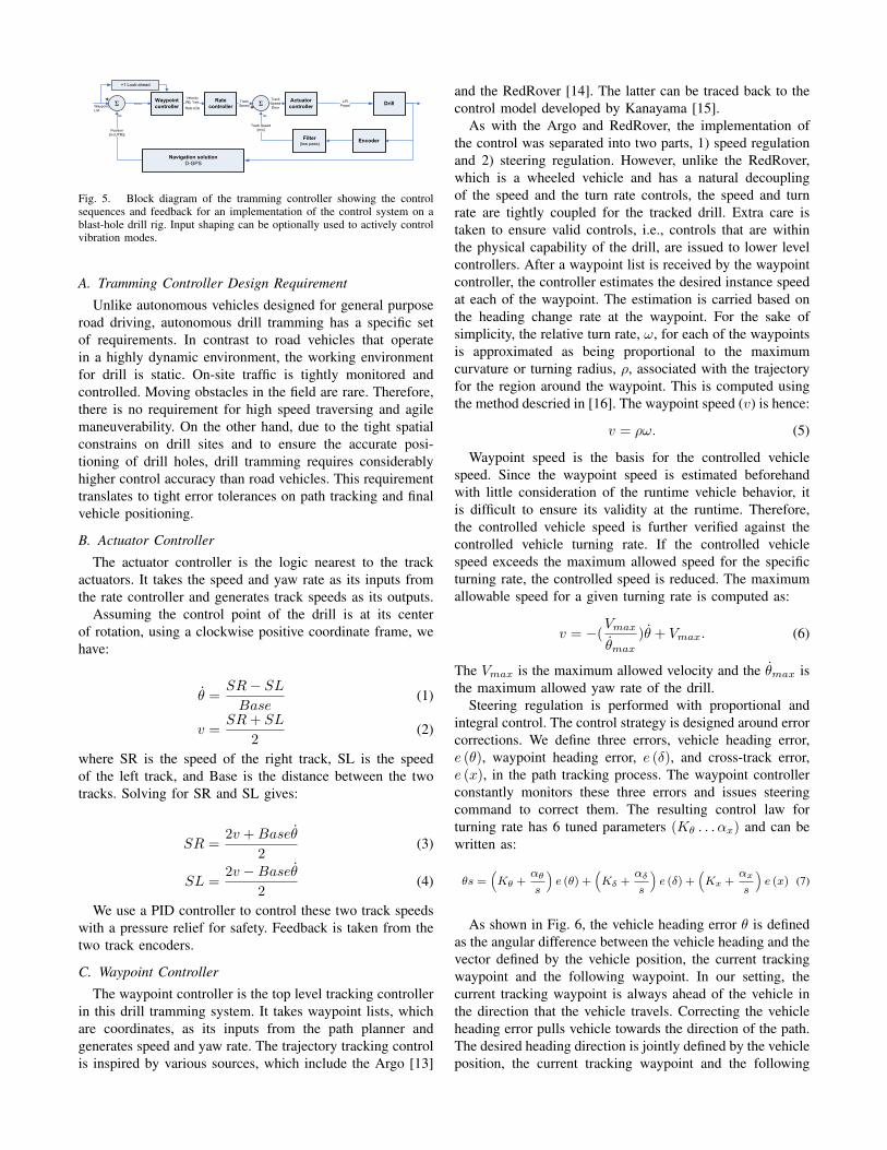
The tramming controller is composed of three sub-controllers in a hierarchical manner (see also Fig. 5). Itis designed such that the actuator controller regulates thespeed of the two tracks; the rate controller regulates thevehicle velocity and the turn rate; and the waypoint controllermaintains the tracking of planned trajectories. Due to the skidsteering nature of the drill, velocity and yaw rate are chosenas the two main control parameters because they directlyrelate to the drills tramming commands.

Ratecontroller

Actuatorcontroller

Waypoint controller

Position[m (UTM)]

errorVelocity(V), Yaw

Rate (ω)

TrackSpeed

Navigation solutionD-GPS

Filter(low pass)

TrackSpeedError

Track Speed[m/s]

DrillΣ+–

Σ+

–

+1 Look-ahead

L/R Propel

Encoder

WaypointList

Fig. 5. Block diagram of the tramming controller showing the controlsequences and feedback for an implementation of the control system on ablast-hole drill rig. Input shaping can be optionally used to actively controlvibration modes.

A. Tramming Controller Design Requirement

Unlike autonomous vehicles designed for general purposeroad driving, autonomous drill tramming has a specific setof requirements. In contrast to road vehicles that operatein a highly dynamic environment, the working environmentfor drill is static. On-site traffic is tightly monitored andcontrolled. Moving obstacles in the field are rare. Therefore,there is no requirement for high speed traversing and agilemaneuverability. On the other hand, due to the tight spatialconstrains on drill sites and to ensure the accurate posi-tioning of drill holes, drill tramming requires considerablyhigher control accuracy than road vehicles. This requirementtranslates to tight error tolerances on path tracking and finalvehicle positioning.

B. Actuator Controller

The actuator controller is the logic nearest to the trackactuators. It takes the speed and yaw rate as its inputs fromthe rate controller and generates track speeds as its outputs.

Assuming the control point of the drill is at its centerof rotation, using a clockwise positive coordinate frame, wehave:

θ =SR− SLBase

(1)

v =SR+ SL

2(2)

where SR is the speed of the right track, SL is the speedof the left track, and Base is the distance between the twotracks. Solving for SR and SL gives:

SR =2v +Baseθ

2(3)

SL =2v −Baseθ

2(4)

We use a PID controller to control these two track speedswith a pressure relief for safety. Feedback is taken from thetwo track encoders.

C. Waypoint Controller

The waypoint controller is the top level tracking controllerin this drill tramming system. It takes waypoint lists, whichare coordinates, as its inputs from the path planner andgenerates speed and yaw rate. The trajectory tracking controlis inspired by various sources, which include the Argo [13]

and the RedRover [14]. The latter can be traced back to thecontrol model developed by Kanayama [15].

As with the Argo and RedRover, the implementation ofthe control was separated into two parts, 1) speed regulationand 2) steering regulation. However, unlike the RedRover,which is a wheeled vehicle and has a natural decouplingof the speed and the turn rate controls, the speed and turnrate are tightly coupled for the tracked drill. Extra care istaken to ensure valid controls, i.e., controls that are withinthe physical capability of the drill, are issued to lower levelcontrollers. After a waypoint list is received by the waypointcontroller, the controller estimates the desired instance speedat each of the waypoint. The estimation is carried based onthe heading change rate at the waypoint. For the sake ofsimplicity, the relative turn rate, ω, for each of the waypointsis approximated as being proportional to the maximumcurvature or turning radius, ρ, associated with the trajectoryfor the region around the waypoint. This is computed usingthe method descried in [16]. The waypoint speed (v) is hence:

v = ρω. (5)

Waypoint speed is the basis for the controlled vehiclespeed. Since the waypoint speed is estimated beforehandwith little consideration of the runtime vehicle behavior, itis difficult to ensure its validity at the runtime. Therefore,the controlled vehicle speed is further verified against thecontrolled vehicle turning rate. If the controlled vehiclespeed exceeds the maximum allowed speed for the specificturning rate, the controlled speed is reduced. The maximumallowable speed for a given turning rate is computed as:

v = −(Vmax

θmax)θ + Vmax. (6)

The Vmax is the maximum allowed velocity and the θmax isthe maximum allowed yaw rate of the drill.

Steering regulation is performed with proportional andintegral control. The control strategy is designed around errorcorrections. We define three errors, vehicle heading error,e (θ), waypoint heading error, e (δ), and cross-track error,e (x), in the path tracking process. The waypoint controllerconstantly monitors these three errors and issues steeringcommand to correct them. The resulting control law forturning rate has 6 tuned parameters (Kθ . . . αx) and can bewritten as:

θs =(Kθ +

αθ

s

)e (θ) +

(Kδ +

αδ

s

)e (δ) +

(Kx +

αx

s

)e (x) (7)

As shown in Fig. 6, the vehicle heading error θ is definedas the angular difference between the vehicle heading and thevector defined by the vehicle position, the current trackingwaypoint and the following waypoint. In our setting, thecurrent tracking waypoint is always ahead of the vehicle inthe direction that the vehicle travels. Correcting the vehicleheading error pulls vehicle towards the direction of the path.The desired heading direction is jointly defined by the vehicleposition, the current tracking waypoint and the following

Velocity (v0)

x

Interpolated Path

pi

pfp0

Velocity (v0)

Fig. 6. Vehicle waypoint path following error types. The controller com-pensates position and orientation between an initial point (p0), intermediatepoint (pi) and final point (pf ) by factoring cross-track error (x) to thecurrent smooth interpolated path (dashed line), and orientation differencesbetween the current and forward waypoints (angles θ and δ).

waypoint. In this setting, the desired heading direction is aweighted average between the vector defined by the vehicleposition and the current tracking waypoint and the vectordefined by the vehicle position and the following trackingwaypoint. It can be described as:

θ =d

Dθ1 +

D − dD

θ2. (8)

D is the distance between the current tracking point andthe previous waypoint. d is the distance between the currentvehicle position and the previous waypoint. θ1 is the anglebetween the vehicle heading and the vector defined by thefollowing waypoint and the vehicle position. θ2 is the anglebetween the vehicle heading and the vector defined by thecurrent tracking waypoint and the vehicle position. Thistechnique provides one step look-ahead for the waypointtracking. It also removes abrupt changes in the error mea-surement during the transition of the tracking waypoint.

The waypoint heading error is defined as the angulardifference between the vehicle heading and the desiredheading at the tracking waypoint. The desired heading ata waypoint is then defined as the vector that connects thewaypoint and its successive waypoint.

The cross-track error is defined as the distance betweenthe vehicle position and the planned path. Even thoughpaths are represented as waypoint lists, it is problematicto define the cross-track error as the distance between thevehicle position and the tracking waypoint. As this inevitablyintroduces sudden changes in the error reading while thevehicle transits from one tracking waypoint to another andbrings disturbances to the control. We solve this problem byfurther interpolating the planned path with high order splinesand then take fine discritisation in the interpolation. We thenmeasure the cross-track error as the distance between thevehicle position and the nearest point from the fine-grainedpath interpolation. This gives accurate reading in the cross-track error and avoids all abrupt changes in error reading dueto transition of the tracking waypoint.

V. EXPERIMENT SETUP AND PERFORMANCE MEASURE

The tramming method is currently deployed at an iron-oremine on an autonomous blast-hole drill rig. It has been used

in autonomous production operations over a variety of benchtypes (e.g., Fig. 7). The performance of the control methodis shown in path following and drill positioning experimentsas measured using the on-board D-GPS position when themachine came to a rest, as compared to desired points asplanned and surveyed in advance by mine staff.

0 10 20 30 400

5

10

15

20

25

30

35

40

45

East (m)

No

rth

(m

)

Fig. 7. A sample drill hole pattern (note the regular ordering)

A. Vehicle Configuration

The blast-hole drill rig weighs 98-ton and is 13 m by 5.8m and has a 17 m tall mast. Navigation is preformed by aTopcon D-GPS suspended on the mast and two generic trackencoders. It is suspended on two large tracks and turns byskid-steering. The system has high actuator authority beingdriven by hydraulics (500 psi) and powered by a 1000 HPdiesel motor.

B. Path following

The path planner generates paths that connect drill holesin a pattern. The machine then trams along this path. Motionis constrained by two competing objectives. First, it isdesirable to drive as quickly as possible to meet productionrequirements. However, it is important that the drill doesnot deviate significantly from the prescribed path given thepresence of obstacles and crests. As shown in the Fig. 8 fortramming both a straight and curved path.

C. Drill Mast Positioning

Drill mast positioning is one of the most importantcriterion of drill operation performance. The feed-forwardcontroller is able to partially compensate for the suspensioncompliance and the resulting mast sway. Tests with D-GPSpositioning have errors <15 cm on average and maximumerrors of < 30cm (see Fig. 9). This is particularly notablesince this is less than the system’s positioning variance(recall the GPS antenna is on top of the swaying mast), thusconfirming the utility of a feed-forward approach.

D. Path Planner Performance

The two properties of the path planner we focused ourexperiments on are: 1) the coverage of all possible trajecto-ries, and 2) the number of node-explorations before a path is

−2 0 2 4 6 8 10−1

0

1

2

3

4

5

6

7

8

9

East (m)

No

rth

(m

)

Tramming TrajectoryPlanned Waypoints

(a) Turning around a bend

−15 −10 −5 0 5 10 150

5

10

15

20

25

30

East (m)

No

rth

(m

)

Tramming TrajectoryPlanned Waypoints

(b) Straight line following

Fig. 8. Path following examples: In (a) some turning is involved as the drill moves around a bend in a row-shifting maneuver that is used frequently inproduction. Note the mast vibration is evident by the circular ‘wiggle’ present. In (b) a 30 m long straight line trajectory is shown with minimal deviation.These two figures demonstrate the accurate path following performance.

−0.3 −0.2 −0.1 0 0.1 0.2 0.3−0.3

−0.2

−0.1

0

0.1

0.2

East (m)

No

rth

(m

)

Fig. 9. Drill mast positioning with <15 cm average error.

found. The first property represents the completeness of thealgorithm, and the second property represents the efficiencyof the algorithm.

The Monte Carlo method is used to determine the pathcoverage. The vehicle starts at (0,0), with heading θstart = 0.Fig. 10 shows the reachable region in the (-8:8, -8:8) msquare with the final heading θend = 4 ∗ π/5 and θend =π after one depth of search node expansion (with 20,000points are generated in each case). The allowed minimumturning radius for each trajectory is 2 m, the same as theminimum turning radius of the primitive trajectories. Fig. 12shows the relation between the coverage and the headingdifference between the starting position and the final position.In this graph, it can be seen that the unreachable area growsrapidly as the heading difference approaches π. Fig. 11 showsthe reachable region in the (-8:8, -8:8) square with the finalheading θend = π after two depth of search node expansion.It can be seen that there is a 100% coverage in this setting.

To test the search efficiency, we expand the end point areato (-20:20, -20:20). 20,000 points are randomly generated inthis area as destination points with random heading range

(a) Typical case: Final Heading θend = 4 ∗ π/5

(b) Extreme case: Final heading of θend = π

Fig. 10. Search coverage for the extended state lattice method (compareto Fig. 3). The starting heading is θstart = 0. Shaded areas are reachablein the 8 m by 8 m square (from a starting point of (0,0) after one depthof search node expansion. The later case requires a larger turn and henceshows less coverage.

from −π to π. The starting point is (0,0) and the startingheading θ is 0. Fig. 13 shows the histogram of the numberof nodes examined before a path is found. Combined withthe search coverage results presented above, we conclude oursimple breadth-first search is capable of producing desirableresults for our application.

Fig. 11. Search coverage (ref Fig. 10 for a final heading of θend = πafter two search node expansions

1.8 2 2.2 2.4 2.6 2.8 3 3.20.2

0.3

0.4

0.5

0.6

0.7

0.8

0.9

1

The Difference Between the Starting Heading and the Final HeadingThe

Per

cent

age

of E

ndin

g P

oint

Cov

erag

e in

the

(−8:

8, −

8:8)

Squ

are

Fig. 12. The search coverage as a functions of total heading variation

0 10 20 30 40 500

2000

4000

6000

8000

10000

12000

14000

Node Visited

Sea

rche

s

Fig. 13. The histogram of the number of nodes examined for each search.This shows path planning efficiency as most cases did not require extensivesearching.

VI. CONCLUSION AND FUTURE WORK

A software architecture, a control mechanism and a pathplanner for an autonomous tracked vehicle are presented.Coverage is important in open environments as there areno roads to follow. The extended state lattice method usesoperational data to achieve rapid coverage of the state-space. The tramming controller utilizes a modified waypointfollowing path tracking technique specialized for high-inertiaof the vehicle. The method is implemented as a set ofmodules and deployed on a 98-ton autonomous blast-holedrill rig in production mining environments.Experimentalresults include complete autonomous operation in productiondrill hole patterns. We demonstrated the designed controlleris capable of satisfying the two major requirements inmining production in real-time: maintaining good overallpath tracking performance and realizing accurate drill holepositioning. Field tests indicate that both the average cross-track errors and average positioning errors are <0.15 meters.

Future developments include further system refinement to

improve operating efficiency.

VII. ACKNOWLEDGEMENTS

This work is supported by the Rio Tinto Centre for MineAutomation and the ARC Centre of Excellence programfunded by the Australian Research Council (ARC) andthe New South Wales State Government. The authors alsoacknowledge the support of Charles McHugh of Rio Tinto.

REFERENCES

[1] H. L. Hartman, SME Mining Engineering Handbook. SME, 1992.[2] P. Elinas, “Multigoal planning for an autonomous blasthole drill,” in

19th International Conference on Automated Planning and Scheduling,Sept. 2009, pp. 342–345.

[3] T. Howard and A. Kelly, “Optimal rough terrain trajectory genera-tion for wheeled mobile robots,” International Journal of RoboticsResearch, vol. 26, no. 2, pp. 141–166, Feb 2007.

[4] J. L. Martınez, A. Mandow, J. Morales, S. Pedraza, and A. Garcıa-Cerezo, “Approximating kinematics for tracked mobile robots,” Int. J.Rob. Res., vol. 24, no. 10, pp. 867–878, 2005.

[5] A. T. Le, D. Rye, and H. Durrant-Whyte, “Estimation of track-soil in-teractions for autonomous tracked vehicles,” Robotics and Automation,1997. Proceedings., 1997 IEEE International Conference on, vol. 2,pp. 1388–1393 vol.2, Apr 1997.

[6] Z. Fan, J. Borenstein, D. Wehe, and Y. Koren, “Experimental evalua-tion of an encoder trailer for dead-reckoning in tracked mobile robots,”in Proceeding of the IEEE International Symposium on IntelligentControl, Monterey, CA, 1995, pp. 571–576.

[7] Z. Shiller, W. Serate, and M. Hua, “Trajectory planning of trackedvehicles,” Robotics and Automation, 1993. Proceedings., 1993 IEEEInternational Conference on, pp. 796–801 vol.3, May 1993.

[8] M. Ahmadi, V. Polotski, and R. Hurteau, “Path tracking control oftracked vehicles,” in Proceedings of the International Conference onRobotics and Automation (ICRA 2000), vol. 3, 2000, pp. 2938–2943vol.3.

[9] G. Wang, S. H. Wang, and C. W. Chen, “Design of turning control fora tracked vehicle,” IEEE Control Systems Magazine, vol. 10, no. 3,1990.

[10] R. A. Knepper and A. Kelly, “High performance state lattice planningusing heuristic look-up tables,” in 2006 IEEE/RSJ International Con-ference on Intelligent Robots and Systems, October 2006, pp. 3375 –3380.

[11] P. Giordano, M. Vendittelli, J.-P. Laumond, and P. Soueres, “Nonholo-nomic distance to polygonal obstacles for a car-like robot of polygonalshape,” IEEE Transactions on Robotics, vol. 22, no. 5, pp. 1040–1047,oct 2006.

[12] T. Fraichard and J.-M. Ahuactzin, “Smooth path planning for cars,”in Proceedings of the International Conference on Robotics andAutomation (ICRA), vol. 4, 2001, pp. 3722–3727.

[13] Q. P. Ha, T. H. Tran, S. Scheding, G. Dissanayake, and H. F.Durrant-Whyte, “Control issues of an autonomous vehicle,” in 22ndInternational Symposium on Automation and Robotics in ConstructionISARC, Ferrara, Italy, September 2005.

[14] T. Henderson, M. Minor, S. Drake, A. Hetrick, J. Quist, J. Roberts,H. Sani, R. Bandaru, M. Rasmussen, A. Collins, Y. Sun, Suraj,X. Fan, E. S. Louis, S. Mikuriya, and K. Dean, “Robust AutonomousVehicles,” July 2007, dARPA Urban Challenge Technical Paper.

[15] Y. Kanayama, Y. Kimura, F. Miyazaki, and T. Noguchi, “A stabletracking control method for an autonomous robot,” in ProceedingsIEEE International Conference on Robotics and Automation, vol. 1,1990, pp. 384–389.

[16] R. M. Haralick and L. G. Shapiro, Computer and Robot Vision (VolumeII). Prentice Hall, June 2002.