Timetabling optimization of a mixed double- and single-tracked railway network

Applied Mathematical Modelling 35 (2011) 859–878

Contents lists available at ScienceDirect

Applied Mathematical Modelling

journal homepage: www.elsevier .com/locate /apm

Timetabling optimization of a mixed double- and single-trackedrailway network

Enrique Castillo a,b,*, Inmaculada Gallego b, José María Ureña b, José María Coronado b

a Department of Applied Mathematics and Computational Sciences, University of Cantabria, 39005 Santander, Spainb Department of Civil Engineering, University of Castilla-La Mancha, 13071 Ciudad Real, Spain

a r t i c l e i n f o a b s t r a c t

Article history:Received 9 April 2009Received in revised form 11 July 2010Accepted 16 July 2010Available online 29 July 2010

Keywords:Train timetablingBisection methodGlobal optimumObjective function upper bound

0307-904X/$ - see front matter � 2010 Elsevier Incdoi:10.1016/j.apm.2010.07.041

* Corresponding author at: Department of Applied942201722; fax: +34 942201703.

E-mail address: [email protected] (E. Castillo).

The paper deals with the timetabling problem of a mixed multiple- and single-trackedrailway network. Out of all the solutions minimizing the maximum relative travel time,the one minimizing the sum of the relative travel times is selected. User preferences aretaken into account in the optimization problems, that is, the desired departure times oftravellers are used instead of artificially planned departure times. To find the global opti-mum of the optimization problem, an algorithm based on the bisection rule is used toprovide sharp upper bounds of the objective function together with one trick that allowsus to drastically reduce the number of binary variables to be evaluated by consideringonly those which really matter. These two strategies together permit the memoryrequirements and the computation time to be reduced, the latter exponentially withthe number of trains (several orders of magnitude for existing networks), when com-pared with other methods. Several examples of applications are presented to illustratethe possibilities and excellences of the proposed method. The model is applied to thecase of the existing Madrid–Sevilla high-speed line (double track), together with severalextensions to Toledo, Valencia, Albacete, and Málaga, which are contemplated in thefuture plans of the high-speed train Spanish network. The results show that the compu-tation time is reduced drastically, and that in some corridors single-tracked lines wouldsuffice instead of double-tracked lines.

� 2010 Elsevier Inc. All rights reserved.

1. Introduction and motivation

The optimization of the railway lines capacity is playing an important role in railway management (including timet-abling, re-scheduling and traffic control). In this context, research is needed to design a tool able to optimize the capacityof the whole railway network, taking into consideration type of track (single or double), speed, time constraints, stationlocation, safety, etc. Caprara et al. [1] discuss railway optimization problems in general and provide a state-of-the-art re-view, showing how they are related and even suggesting a unified treatment of them. In particular, they treat the trainschedule problem, which is one of the most interesting problems in transportation planning and operation of railwaysystems.

Although, at a first glance, railway traffic timetabling and real-time control (and re-scheduling when perturbations occur)could appear to be very similar problems, sharing common mathematical tools and models, there is a significant difference

. All rights reserved.

Mathematics and Computational Sciences, University of Cantabria, 39005 Santander, Spain. Tel.: +34

http://dx.doi.org/10.1016/j.apm.2010.07.041

mailto:[email protected]

http://dx.doi.org/10.1016/j.apm.2010.07.041

http://www.sciencedirect.com/science/journal/0307904X

http://www.elsevier.com/locate/apm

860 E. Castillo et al. / Applied Mathematical Modelling 35 (2011) 859–878

between them. Timetable optimization (see [2–6]) consists of planning departures and arrivals of trains from and at stationsso that user requirements are satisfied, travel times are minimized and conflicts between different trains are adequatelysolved. This is a theoretical design, but the real situation must contemplate several possible perturbations that change thissituation. When these perturbations occur, re-scheduling and traffic control problems have to be dealt with (see, for exam-ple, [7–12] or [13]).

When a timetabling problem is modelled, the level of detail may not need to be as precise. So, there is more room forchange since the prerequisites are not as fixed as in real-time (when some trains are already standing on certain tracks, sometracks or platforms are not available, etc.). Although the timetabling problem is the main focus of this paper, some of ourproposals can also be useful for re-scheduling problems, because the important associated reduction in computation timeallows rapid decisions to be made.

Railway network management is a challenging problem that cannot be conceived of without the help of a computer (see[14]). Some authors, such as Sahin [7] or Ghoseiri et al. [15], classify railway traffic management and control techniques inthree major groups: those based on simulation, those using mathematical programming, and those based on expert systems.However, in some cases several combinations of them are used (see [16]). The first mathematical programming methodologyapplied to train management optimization problems is due to Amit and Goldfarb [17]. Before the eighties, optimization andsimulation were the most commonly used methods (see [18–22]). However, due to computational complexities, the optimi-zation models used were far from realistic. At the end of the eighties development of artificial intelligence took place in manyareas of knowledge including transportation (see [23–26,8,27,28]). Since then, the impressive increase of computer powerhas led to a great resurgence of optimization methods.

The formulation and solution of railway optimization problems is complicated because continuous and binary variablesneed to be combined, leading to complex mixed integer (MIP) linear and sometimes non-linear programming problems (see[29–31,9,2,32,3,10,12,4,33,6,34]), requiring a huge amount of computational resources. Cordeau et al. [5] offer an exhaustiveanalysis of existing optimization methods.

Most optimization models of train scheduling have a single-objective formulation. However, the nature of this prob-lem is inherently multi-objective (see for example [35,15,36]). So, when working with train scheduling optimizationproblems it is important to make an adequate selection of the objective function, which can refer to user wishes,as in Törnquist and Persson [13], operator interests, or to a combination of both, as in Ghoseiri et al. [15], and includesconcepts such as travel times as in Zhou and Zhong [36], train delays (average or maximum) or delay costs as in Shain[7], Törnquist and Persson [13], Törnquist [37] and D’Ariano et al. [38], fuel consumption as in Ghoseiri et al. [15], oroperating policies.

Several train scheduling problems are known to be NP–hard [39] or [40], and optimal solutions are unattainable in reallarge-scale and complex cases. The presence of binary or integer variables leads to branch and bound or related techniqueswhich are time and memory consuming (see, for example, [41] or [38]). One frustrating aspect of the branch and bound tech-nique for solving MIP problems is that the solution process can continue long after the best solution has been found. A prob-lem with only 30 binary variables could produce a tree with one billion nodes. If no other stopping criteria have been set, theprocess might continue ad infinitum until the search is complete or computer’s memory is exhausted. So, any technique toreduce the number of binary variables or the search space can lead to a large reduction in computational time. In fact, intraffic control problems, some of these techniques are needed. Some examples of applications using several sophisticatedsearch procedures are: backtracking search [42], look-ahead search [7], and other algorithms [4,43]. These techniques canbe classified in two groups:

1. Those looking for approximate solutions. To reduce the computational overburden some strategies and heuristic approachesaim at obtaining suboptimal solutions (see, for example, [44]). Dorfman and Medanic [45] presents a local feedback-basedtravel advance strategy using a discrete event model of train advances along lines of the railway, which allows handlesome schedule perturbations. The model proposed by Dorfman and Medanic offers the advantage of formulating the dis-patching rules adopted in practice while coping deadlock avoidance problems.Using these techniques, the optimal solution of the initial problem is not obtained, but merely an approximation. If thisapproximation is good enough, the method is useful and can be applied. This is the case of Törnquist and Persson [13]who use some strategies to reduce the search space based on allowing a limited number h of order swaps for specific seg-ments. This means that swaps are allowed for some trains. Törnquist [37] extends this strategy to secondarily disturbedtrains.

2. Those looking for the exact solution. The existing solution algorithms of problems formulated as large and complex math-ematical mixed integer problems, such as those in railway networks, require a huge amount of computation time andmemory space to find their optimal solutions. This is in part due to the presence of a huge number of binary variableswhich are not actually needed, but are difficult to identify. The elimination of binary variables, using some strategies,can substantially reduce the search space and thus the computation time and memory resources. Some examples of inter-esting techniques in this group allowing for this reduction are those of Zhou and Zhong [6] who provided some sophis-ticated methods to guarantee global optimality, and those of D’Ariano et al. [38,11,12], who proposed a branch and boundalgorithm that considered implication rules that permit the computation to be speeded up.Unfortunately, some of these techniques are not sufficient to deal with real size problems in a reasonable time. This iswhy in this paper we introduce some new strategies that seem to be more efficient. The two main ideas consist of (a)

E. Castillo et al. / Applied Mathematical Modelling 35 (2011) 859–878 861

incorporating adequate upper bounds for the objective function, and (b) removing constraints that are inactive, togetherwith the associated unnecessary binary variables.1

The most common and effective way of handling a railway system is by means of a double or multiple-tracked lines. How-ever, when resources are limited, it is necessary to use less effective single-tracked lines, which are difficult to deal with andsubject to a higher risk. In some countries, such as Spain for example, high-speed double track train lines are plannedthroughout the country, no matter how great the demand for double-tracked lines is. We suggest and demonstrate that sin-gle-tracked bidirectional lines can be a reasonable solution when the demand is below a given level, as is the case in someregions.

In this paper we propose an optimization method to solve the train scheduling problem for a double and single-trackedbidirectional railway network, similar to that presented by Zhou and Zhong [6] and Törnquist and Persson [13] in the senseof trying to reduce the complexity of the problem, but our method leads to the exact solution of the full model, i.e., not theone of a relaxed problem, as other authors do. Of course, with slight modifications, the proposed method is also valid fortraffic re-scheduling. In addition, some techniques to speed up the solution of the optimization problem are proposed, whichproduce a reduction in computation time that can be several orders of magnitude when compared with other existingmethods.

The paper is organized as follows. In Section 2 the proposed model is presented. In Section 3 an algorithm to obtain theglobal optima of the proposed optimization problem is given. In Section 4 some examples of applications are used to illus-trate the power of the methods. Finally, in Section 5 some conclusions are given.

2. The proposed model

In this section, we introduce our model, comment on its main contributions, give the notation and discuss some tech-niques to reduce the complexity of the resulting mixed integer programming problem (MILP).

2.1. Motivation and contributions of the paper

We formulate a model that is an extension of the Zhou and Zhong [6] model to a mixed double- and single-tracked net-work, and which, apart from reducing complexity and calculation time, combines a series of features, some already existingand some new. These features are as follows:

1. We use departure times and speeds as decision variables (note that some authors, for example, [6], use fixed departureand running times).

2. To reduce the number of segments, and thus, the complexity of the problem, we take into consideration trains sharing thesame segment and travelling in the same direction. Though this has been done before by e.g. Carey [2], the incidence ofthis formulation in the practical performance of the model has not been sufficiently emphasized. Several trains can sharethe same segment if they travel in the same direction (albeit separated by a sufficient headway interval). The main idea isthat trains circulating in the same direction can, for timetabling purposes, share segments, and then it is not necessary tosubdivide the shared segment into subsegments, that is, reducing the total number of segments without decreasing thenetwork capacity but reducing the computation time. This is not true however for train operation, where care must betaken to guarantee that consecutive trains run sufficiently far apart from each other (the blocking system takes care ofthat). However we must provide sufficient headway values for this to be possible.

3. We optimize desired travel times instead of actual travel times, as was done by Vansteenwegen and Van Oudheusden[46]. One thing is the user desired departure times (for example, some users can have some constraints due to connectingproblems with other trains, buses, metro lines, etc., or to not flexible working hours, so that they would like the departuretimes to minimize not only the waiting times at the departure stations, that is, before starting the trip, but the waitingtimes at the arrival stations (for example, waiting for a meeting or a class to start)). For a user it is not relevant to use avery fast train if the time schedule is inconvenient, because the time saved in the train is wasted after or before the trip.So, our objective function takes this into account, so that the actual departure times try to get closer to the user desiresand not to the convenience of the operator company. A survey can be used to know user preferences for departure times.In other words, we consider the user desired departure time r‘i of train i as a lower bound for departure instead of theplanned departure time ri fixed by the railway company. A minimax approach, in which the maximum relative travel timefor a train is minimized, is the option used in this paper.

4. We consider single- and/or double-tracked segments between two consecutive stations, as do other researchers.5. We propose a new optimization problem. For all the solutions minimizing the maximum relative travel time for single

trains, the one where the sum of relative travel times is minimized is selected.

1 The real reason for the improvement is that, by dropping the constraints many of the binary integer variables no longer exist in the model, which greatlyreduces the complexity of the problem.


6. We present an application capable of analyzing railway networks in different scenarios defined by parameters, such astype of track (single or double), maximum segment speed, departure times bounds, etc., discussing the convenience ofsingle- or double-tracked segments.

7. We present two examples of the Spanish high-speed railway system to illustrate the proposed methods. The existingMadrid–Sevilla and Madrid–Toledo corridors are extended to include the new Madrid–Málaga and Madrid–Valenciaand Albacete corridors (in planning stage).

The proposed model is based on the important reference model of Zhou and Zhong [6], which is for analyzing single-tracked railway lines, and Törnquist and Persson [13], which includes multiple-tracked lines. Though these are very com-plete and powerful models, they have some problems when dealing with very large networks.

Though there are several reasonable choices for the objective function to be minimized, such as the total travel time of alltrains, as proposed by Zhou and Zhong [6], or the total delay, as proposed by Törnquist and Persson [13], this paper dealswith relative travel times, that is, the ratios of the travel time, considered as the difference between the arrival time andthe desired departure time, to the minimum possible actual travel time, measured as the difference between the arrivaland the departure times. A relative travel time of value 1 refers to the minimum possible travel time, that is, if the train de-parts at the desired time, uses the minimum desired dwell times at stations, and travels at maximum operational speed.However, this cannot be expected in normal situations, but only in extreme cases. An upper bound for the relative travel timearound the value 1.2, which means a 20% increase with respect to minimum time, is used in this paper, as a bound for a tol-erable performance.

For convenience and in order not to confuse the reader with different notations, the notation of Zhou and Zhong [6] andthe techniques for dealing with double tracks from Törnquist and Persson [13] have been used.

In our model the optimal departure and running time are found dynamically by the optimization solver, subject tothe required service and operational constraints at the timetabling stage. Operational maximum speed bounds for thecalculations are fixed, but it is viable for these limits to be exceeded in a small percentage (10–15%), mainly to takecare of special perturbations and supply the timetabling with some flexibility. So, when maximum speeds are men-tioned, operational speeds are being referred to. This allows for some flexibility (6–9 min per hour to deal with per-turbations) and increases the robustness of the resulting solutions, especially when they correspond to close tosaturation networks.

However, the main original contributions of this paper consist of the following strategies for efficient solution of the MIPproblem:

1. Use of sharp upper bounds of the objective function based on the bisection method. First, it must be said that for the timet-abling problem described in this paper, it is very easy to give a good (small) upper bound of the objective function, basedon its physical meaning. In fact a value of 1.4 for the maximum relative travel times is a convenient value for usual net-works, and this value can go to 1.6 or more for congested networks. The simple use of this bound reduces the search spaceconsiderably. If the upper bound for the objective function is too low, we get unfeasibility, while if it is too high, we getfeasibility (perhaps with a high computational time). To obtain sharper bounds, a bisection method is proposed. The ideaconsists of determining where the global optimum is, which is the limit between feasibility and unfeasibility of the prob-lem. This limit can be obtained without actually going through all branches of the search space in the bisection trials up toproven optimality, which is time consuming. Thus, the bisection method leads to one of these two possibilities (feasibilityor unfeasibility), until a sufficient precision is obtained, and this occurs in around 12 iterations (for a relative gap smallerthan 0.05%). Since the required computation times for the feasible and unfeasible steps of the bisection method are dif-ferent, this allows the bisection method to be optimized further.More precisely, since in these steps, we need only to know if the problem is feasible or not for the given upper bound ofthe objective function, it is not necessary to solve the problem, but only determine its feasibility, which is much faster. Forthe reader to see the effect of the bisection method, we indicate that in one of our examples, the first optimization of theMIP, when extended to proven optimality, required 1002 sec, while the mean time required by one of the bisection stepswith the corresponding upper bounds was 2.89 sec for unfeasibility, and 12 sec for feasibility. This means that the wholebisection cycle is only a very small fraction of the initial time required to solve the optimization problem for the first time.Note that an adequate upper objective function bound can imply a reduction of computation time of several orders ofmagnitude (especially for a large number of trains and complicated networks). So, knowledge of sharp upper boundsis crucial. As will be seen, this method guarantees the optimal solution to be obtained in a reasonable time for problemswith the size of our examples, and an important reduction when compared with other methods used in railway networkanalysis.

2. Reducing the number of binary variables by ignoring those associated with inactive constraints. This method, based onconsidering a minimum set of required binary variables, including those which really matter, is proposed to dras-tically reduce the number of binary variables usually employed. In order to give an idea of the order of magnitudeof the savings produced by our method, in one network with 150 trains, the initial number of 73,000 binary vari-ables can be reduced to 16,000. This implies a substantial reduction in memory requirements, which is veryimportant.


2.2. Notation

To facilitate readers’ understanding of the proposed model, the notations used in the following model are shown in Tables1 and 2. For the sake of clarity, we have separated the subscripts and parameters from the decision variables used in themathematical formulation of the model, and presented in the tables, respectively.

2.3. Formulation of the proposed model

For mathematical convenience, the minimax timetable design bounded problem (MMBP) can be stated as2

2 Not3 Thi

Minimizes;e;r;p;x

Z ¼ eþ wXi2I

1t0

i

ei;rimi� si;ri1

� �" #ð1Þ

subject to constraints (2)–(20) below, where w is a very small number (say w = 1/3000), e is the maximum relative train tra-vel time, t0

i is the reference time for train i, that is, the free running time of train i, including station dwells, which is calcu-lated using the upper bound calculation speeds and minimum desired station dwell times, and the meaning of the variabless, e, r, p, x is to be explained. Note that the sum in brackets in (1) is the sum of actual relative travel times. Note that theobjective function is of a global nature in the sense that intermediate stations do not contribute to the objective function(as other authors do), i.e., we are concerned about optimizing the total travel times. This is reasonable for the Spanish net-work because the end stations are the most important ones and involve a very high percentage of all passengers.

The objective function (1) allows us to obtain out of all the solutions with minimum maximum relative travel time theone that has a minimum sum of relative travel times.

The e value, which is the maximum relative travel time with respect to the reference time3 t0i for each train, guarantees

that there is no great difference in travel times for all trains in terms of relative travel times; that is, trains with very differentabsolute travel times can be dealt with together. Note that using absolute travel times would have a negative effect on trainstravelling shorter distances.

The minimax criteria is preferable to the minimization of total travel times, because the latter allows the good perfor-mance of some trains to be compensated with the not so good performance of others, while the minimax criterion attemptsto avoid this discrimination. In addition, though the minimax criterion implies originally a non-linear and non-differentiableproblem, it can be stated as a linear program.

The constraints of our problem are:

2.3.1. Departure time constraints (DTC)

si;ri;1¼ ri; 8i 2 I; ð2Þ

r‘i 6 ri 6 rui ; 8i 2 I; ð3Þ

where sij is the entering time for train i at segment j, rik is the segment number of the kth segment on the route of train i; r‘i

and rui are the lower and upper bounds, respectively, of the departure time from the station of origin for train i.

DTC force the entry time into the first segment of each train route to be its actual departure time, which are not neces-sarily fixed but lower and upper bounded by r‘i and ru

i , respectively. This includes the case of fixed departure times ðr‘i ¼ rui Þ,

as a particular case. These lower and upper bounds must be determined by the timetable designer taking into account theuser preferences and the train operator company.

2.3.2. Running time constraints (RTC)

ei;ri;k¼ si;ri;k

þ pi;ri;k; k 6 mi; 8i 2 I; ð4Þ

p‘i;ri;k6 pi;ri;k 6 pu

i;ri;k; k 6 mi; 8i 2 I; ð5Þ

where eij is the leaving time from segment j of train i, pij the actual running time at segment j for train i, which is determinedtaking into account the train and segment characteristics, mi is the total number of segments on the route of train i; p‘ij and pu

ij

are the lower and upper bounds, respectively, of the travel time for train i at segment j.RTC give the segment exit times as the sum of the entry times plus the actual segment running times, which are lower and

upper bounded (constraint (5)). This is equivalent to limiting the segment speeds. Upper bounds are used in our computa-tions for operating speeds, which do not necessarily coincide with actual maximum speeds. By adjusting these margins, weallow some flexibility when dealing with perturbations.

e that minimizing e, that is, the maximum relative travel time, we are indirectly improving the capacity of the network.s will become apparent when discussing the MMC (14) constraint.

Table 1Subscripts and parameters used in the mathematical formulation of the model.

Symbol Definition

d‘ij Minimum required station dwell time before train i entering segment j

duij Maximum required station dwell time before train i entering segment j

hi1 ;i2 ;j Minimum headway between entrance of two consecutive trains i1 and i2 at segment j

h0j

Minimum safety headway

i Train indexI Set of all trainsj Segment indexk Route segment indexmi Total number of segments on route of train in Node indexp‘ij;p

uij

Lower and upper bounds, respectively, of running time for train i at segment j

r‘i Desired departure time of train i from its first station

r‘i ; rui

Lower and upper bounds, respectively, of departure time from the station

of origin for train iroutei,k List of segments included in route of train i (positive values if inbound,

negative otherwise)s�ij Lower bound of arrival time of train i at segment j

S Set of all segmentst Track number in segmentt0

iReference time for train i, that is, free running time of train i,

including station dwellst0 Maximum allowed computation time per trial.tlim The threshold time above which it is assumed that two trains

cannot coincide in a common segment(tmin, tmax) The time interval when trains circulate (excluding maintenance periods)tik Initially scheduled time for train i to pass through the center of segment ku Station indexvij Takes value 1, �1 or 0 if train i travels segment j in the inbound,

outbound or no travel, respectively, in segment jgi1 ;i2 ;j Takes value 1 if routes of trains i1 and i2 contain segment j , and 0, otherwiseqi1 ;i2 ;j Takes value 1 if trains i1 and i2 are candidates to use segment j in close timesZ Objective function valuebi,k Downstream node number of segment k in route of train ielo Lower bound of relative travel timeeup Upper bound of relative travel timee0 Maximum allowed relative travel time for a single trainci Priority of train irik Segment number of the kth segment in route of train i (is equal to jroutei,kj)w A very small number (for example, 0.001)nopposite Test value for trains circulating in opposite directionnsame Test value for trains circulating in the same directionn Correction value for tlim


2.3.3. Minimum and maximum dwell time constraints (MMDTC)

u ‘
ei;ri;k�1þ di;bði;kÞ P si;ri;k
P ei;ri;k�1þ di;bði;kÞ; 1 < k 6 mi 8i 2 I; ð6Þ

where d‘ij and duij are the minimum and maximum, respectively, required station dwell times before train i enters segment j,

and bik is the downstream station number of segment k in route of train i.Constraint MMDTC bound from above and from below, the dwell time of trains at stations. Note that an upper bound is

given for limited maximum dwell time, otherwise it can be set to infinity.

2.3.4. Headway constraints at track segments (HCTS)The HCTS in this case can be implemented using the binary variables xi1 ;i2 ;j2 and yi1 ;i2 ;j, where xi1 ;i2 ;j is a binary variable that

takes value 1 if train i1 is scheduled to enter segment j before train i2, and 0 otherwise, and yi1 ;i2 ;j is a binary variable that takesvalue 1 if train i1 is scheduled to enter segment j after train i2, and 0 otherwise.

We consider two cases:

1. Opposite direction trains:

si2 ;j P ei1 ;j þ h0j xi1 ;i2 ;j �Mð1� xi1 ;i2 ;jÞ; ð7Þ

si1 ;j P ei2 ;j þ h0j yi1 ;i2 ;j �Mð1� yi1 ;i2 ;jÞ; ð8Þ

8i1 < i2 2 I; v i1 ;j � v i2 ;j < 0; qi1 ;i2 ;j¼ 1;

Table 2Decision variables used in the mathematical formulation of the model.

Symbol Definition

eij Leaving time for train i from segment jpi,j Actual running time for train i at segment jqi1 ;j;t A binary variable, which takes value 1 if train i1 uses track t in segment jri Actual departure time of train i from its first stationsij Entering time for train i at segment jxi1 ;i2 ;j A binary variable, which takes value 1 if train i1 is scheduled to enter

segment j before train i2yi1 ;i2 ;j A binary variable, which takes value 1 if train i1 is scheduled

after train i2 in segment je Relative travel timek Dual variable associated with an equality constraintl Dual variable associated with an inequality constraint


where qi1 ;i2 ;jis an auxiliary parameter, which is initially defined as qi1 ;i2 ;j

¼ 1 and later will be defined differently, to reducethe unnecessary use of binary variables, hi1 ;i2 ;j is the minimum headway between arrival and departure times of two consec-utive trains at segment j; S is the set of all segments, and vij takes value 1, �1 or 0 if train i travels segment j in the inbound,outbound or no travel, respectively, in segment j. Note however, that vij are not variables, but parameters, so they do notincrease the complexity of the optimization problem. The reason to include 0 is to avoid segments with unassigned v values.Constraints (7) and (8) force a train to enter a segment at least a minimum headway time after the previous train has aban-doned the segment if they circulate in opposite directions, and controls only when the trains enter and leave a segment, butnot what happens inside the segment. Thus, a blocking system must take care of this. However from the time schedulingpoint of view, constraints (7) and (8) suffice.2. Same direction trains:

si2 ;j P si1 ;j þ hi1 ;i2 ;jxi1 ;i2 ;j �Mð1� xi1 ;i2 ;jÞ; ð9Þsi1 ;j P si2 ;j þ hi1 ;i2 ;jyi1 ;i2 ;j �Mð1� yi1 ;i2 ;jÞ; ð10Þei2 ;j P ei1 ;j þ h0

j xi1 ;i2 ;j �Mð1� xi1 ;i2 ;jÞ; ð11Þ

ei1 ;j P ei2 ;j þ h0j yi1 ;i2 ;j �Mð1� yi1 ;i2 ;jÞ; ð12Þ

8i1 < i2 2 I; v i1 ;j � v i2 ;j > 0; qi1 ;i2 ;j¼ 1;

where M is a large enough constant.

Following Carey and Crawford [47], for trains running in the same direction, we have chosen

hi1 ;i2 ;j ¼ h0j þmaxð0;pi1 j � pi2 jÞ; ð13Þ

where h0j is the minimum safety headway needed to keep two trains running at the same speed apart at segment j.

The qi1 ;i2 ;jparameters, which are precisely defined in Section 2.4, define the saving strategy to reduce the number of bin-

ary variables involved, but without reducing the natural restrictions of the problem. The qi1 ;i2 ;jtakes value 1 if trains i1 and i2

are candidates to use segment j in close times because only in that case they compete for a track in a segment. Using ourapproach, the problem becomes solvable in many cases in which the computer program explodes due to size limitations,though there is always a limit. To define the proximity of conflicting trains to a segment, we calculate the theoretical min-imal arrival times tik of trains at each segment, and check that these times for the two conflicting trains are closer than a fixedthreshold time tlim. The initial value of tlim is obtained by common sense and mainly by experience, with an adequate safetyfactor to guarantee that it is sufficiently large, but not too large. Since tlim means the difference between the actual and opti-mum running times of the trains interfering, and we are designing a reasonable timetabling, these differences cannot be verylarge in order to be admissible. So, one initial guess of tlim can be based on this idea. This does not mean that the problemneeds to be solved many times to get a reasonable value of tlim. However, once the model has been tested with differentassumptions, it can then be further fine-tuned. When the optimal solution is found, the assumed value of tlim must be testedin order to guarantee that it does not lead to a relaxed optimization problem. The tlim value is selected depending on thesegment lengths and speeds, and depends on the saturation of the traffic in a specific segment.

Constraints (7)–(12) force segment entry and exit times of consecutive trains travelling in the same direction to be at leastseparated by hi1 ;i2 ;j. This is valid only for timetabling purposes, but the practical implementation requires to control this sep-aration between consecutive trains.

The use of variables xi1 ;i2 ;j and yi1 ;i2 ;j together with the constraints, allow three possible cases:

1. xi1 ;i2 ;j ¼ 1 and yi1 ;i2 ;j ¼ 0: This means that train i1 enters segment j before train i2.2. xi1 ;i2 ;j ¼ 0 and yi1 ;i2 ;j ¼ 1: This means that train i1 enters segment j after train i2.


3. xi1 ;i2 ;j ¼ 0 and yi1 ;i2 ;j ¼ 0: This means that neither train i1 nor train i2 enters segment j before the other train (this can bebecause one or both trains do not use segment j).

2.3.5. Minimax contraints (MMC)

‘� � 0
ei;mi
� ri =ti 6 cie; 8i 2 I; ð14Þ

where 0 6 ci 6 1 is a real value, which measures the priority of train i (the smallest the value of ci, the largest the priority).Note that r‘i is used instead of ri, because preferred departure times, and not actual departure times, have been used.

MMC guarantee that the objective function value e is the maximum relative train travel time. The reason for using relativetravel times instead of absolute travel times is to avoid degradation of travel times (too high) for short distance trains.

2.3.6. Maintenance period constraints (MPC)

si;ri;1P tmin; 8i 2 I; ð15Þ

ei;ri;mi6 tmax; 8i 2 I; ð16Þ

where (tmin, tmax) is the time interval when trains are allowed to run (it excludes maintenance periods).MPC limit the operating time of the network to the period (tmin, tmax), to allow some free time for maintenance operations

on the railway network.When double track exists the binary variable qi1 ;j;t

is used with the constraints:

2.3.7. Track use (DT1)X
t
qi1 ;j;t ¼ 1; 8i1 2 I; j 2 S: ð17Þ

Constraint DT1 means that train i1 uses only one track of segment j.

2.3.8. Train interaction (DT2)

qi1 ;j;t þ qi2 ;j;t � 1 6 xi1 ;i2 ;j þ yi1 ;i2 ;j; 8i1 < i2; i1; i2 2 I; 8j; t; ð18Þ

where t is the track number (1 or 2), qi1 ;j;t ¼ 1 if train i uses track t of segment j, and 0, otherwise. Constraint DT2 means thatif trains i1 and i2 use track t of segment j, at least one of the variables xi1 ;i2 ;j or yi1 ;i2 ;j must be 1. Note that given a double tracksegment two trains i1 and i2 running in the same direction can use the two tracks in parallel in the same segment j, becausethis is possible for xi1 ;i2 ;j ¼ 0 and yi1 ;i2 ;j ¼ 0 (see constraints (9)–(12)), because this solution satisfies (19) and (18) becauseqi1 ;j;t þ qi2 ;j;t 6 1.

2.3.9. Exclusion condition (DT3)

xi1 ;i2 ;j þ yi1 ;i2 ;j 6 1; 8i1 < i2 2 I; 8j: ð19Þ

Constraint DT3 means that variables xi1 ;i2 ;j and yi1 ;i2 ;j cannot simultaneously be one.Since we need cases in which xi1 ;i2 ;j ¼ yi1 ;i2 ;j ¼ 0, constraint (19) cannot be written = 1 instead of < = 1, because we do not

know ‘‘a priori” which train uses which track. It is the program who assigns only one track (constraint DT1 forces each trainto use one and only one track) to each train by means of the binary variable qi1 ;j;t (the variable qi1 ;j;t ¼ 1 if train i1 uses track tin segment j) depending on the other trains.

Given a double track segment j two trains i1 and i2 running in the same direction can use the two tracks in parallel in thesame segment j, and this occurs when xi1 ;i2 ;j ¼ 0 and yi1 ;i2 ;j ¼ 0, because this solution satisfies (18) due to the fact that in thiscase, according to (17), qi1 ;j;t þ qi2 ;j;t ¼ 1 for t = 1, 2 (they use different tracks).

2.3.10. Objective function bound (OFB)

0
e 6 e : l0; ð20Þ
where e0 is the maximum allowed relative travel time for a single train.Constraint OFB is used only to look for a global optimum in the iterative process to be described in Section 3, and is crucial

in reducing the computation time.The MMBP problem with w = 0 (the pure minimax problem) has many solutions, all of them with the same maximum

relative train travel times. Thus, one of them can be chosen using other optimization criteria. In this paper we minimizethe sum of relative travel times.

As indicated by Törnquist and Persson [13], the stated problem is a MILP and can require a great deal of computationaleffort to use many binary variables which are not of interest. In fact it becomes necessary to add some strategies to reducethe number of binary variables: for example, free allocation of tracks within segments while keeping the initial sequence of


trains on the segments, or ignoring the initial sequence if the trains are re-scheduled to use different tracks. These strategiesspeed up or make the solution of the problem possible, but the price paid is that we obtain a solution that normally is not theoptimal solution of the initial problem. Actually, these strategies could even be insufficient to make the problem solvable infixed time, especially when this time is small. For example, Törnquist and Persson [13] have experienced re-scheduling prob-lems at time horizons of 90 min, after 2.5 h of calculation, even using the proposed strategies. Nevertheless, by using themost advanced method/formulation called Strategy 3, or its sequel HOAT presented in Törnquist [37], the method is success-ful for fairly large instances.

Another approach which seems successful is the one by D’Ariano et al. [38,11,12]. They develop a branch and bound algo-rithm which includes two dynamic and two static implication rules which allow the search space to be reduced and speed upcomputations. The computational experience of this method to the Dutch railway network indicates that the results arepromising. The method permits obtaining the global optimum, and also an approximation.

One of the main reasons for these problems is the use of a very large number of segments, when they are not reallyneeded for timetabling purposes. In this paper, we show how this can be improved by two means: (a) reducing the numberof segments by permitting two trains to share the same segment if they run in the same direction (note that this does notmean a relaxation of the initial problem, but rather a reduction in the number of required segments which are needed tokeep trains in the same direction sufficiently separate), and (b) using a much smaller number of binary variables by usingthem only when they are really needed.

Once the binary variables are fixed, a sensitivity analysis, which is out of the scope of this paper, can be easily done usingthe techniques in Castillo et al. [48,49,34,50,53], because the problem (1)–(20) is a linear problem.

2.4. Reducing the complexity of the MILP

In this section our proposal to limit the number of binary variables is explained. The main idea consists of discussing thetrack conflict only for trains which run in close times, and ignoring those running in fairly separate times. This solution issimilar to that of Törnquist and Persson [13] in the sense that it tries to reduce the complexity, but ours lead to the exactsolution of the full model (not to the solution of a relaxed model). In other words, we first solve a relaxed optimization prob-lem, i.e., the problem with a reduced number of constraints (interactions of trains not running at close times are removed),and then we check that the resulting optimal solution satisfies the remaining constraints. This is equivalent to proving thatthe optimal solution of the full problem is the same as that of the relaxed one. To this end, we define

qi1 ;i2 ;j¼

1 if � p‘i2 j � hi1 ;i2 ;j � tlim 6 s�i2 j � s�i1j 6 p‘i1 j þ hi1 ;i2 ;j þ tlim and gi1 ;i2 ;j¼ 1;

0 otherwise

(ð21Þ

where tlim is the threshold time above which it is assumed that two trains do not coincide in a common segment, that is,qi1 ;i2 ;j

takes value 1 if trains i1 and i2 are candidates to use segment j in close (this proximity is defined by means of tlim) times,that is, routes of trains i1 and i2 contain segment j, and s�ij are the minimum arrival times of train i at segment j, that is,

s�ij ¼

r‘i if jroutei;1j ¼ j;

r‘i þPk�1

k1¼1p‘iri;k1

þ d‘ibi;k1þ1

� �if jroutei;kj ¼ j and routei;k > 0;

r‘i þPk�1

k1¼1p‘iri;k1

þ d‘ibi;k1

� �if jroutei;kj ¼ j and routei;k < 0;

8>>>>>><>>>>>>:

ð22Þ

which are calculated using the minimum possible times for trains i1 and i2 to reach the beginning of segment j in theirrespective routes. In addition, to control whether or not trains i1 and i2 share segment j, we define

gi1 ;i2 ;j¼

1 if 9k1 and k2 such that ri1 ;k1¼ j and ri2 ;k2

¼ j;

0 otherwise:

�ð23Þ

The selection of the value of tlim is critical, because a small value will produce an important saving in computation time, but ifthis value is too small it will lead to an erroneous design (not taking into account all train interactions). However, it is very easyto check ‘‘a posteriori” if the selected value of tlim was adequate, and repeat the process if not. This check can be carried out byverifying that the relaxed constraints are inactive for the resulting solution, that is, if constraints (7)–(12) with qi1 ;i2 ;j

¼ 0 areinactive. If this is not so, let nopposite and nsame be the corresponding maximum constraint violations of (7)–(12), respectively.Then, n = min(0,nopposite,nsame) gives a hint on how the tlim must be modified to get a valid design (satisfying constraints (7)–(12)).

It is convenient to clarify that, even though the proposed model treats departure times of trains as decision variables asopposed to fixed values, the departure times are restricted to be within a given range between by constraint (3). Note thatthe width of this range affects the efficiency of the heuristic because the determination rule used to drop constraints dependson the lower bound of the departure times (earliest allowed departure time) only. If the departure time is allowed a widerange, and if the parameter tlim is not large (for the purpose of higher efficiency), the optimal solution might ‘‘sneak” thedeparture times for some of the trains far enough from the lower bound (i.e., delay the departure of the trains), such thatthe headways between some trains are not appropriately regulated by constraints (because they can be dropped in the firsthand). This possibility might be a problem for crowded railways. However, the widths used for the departure times are very


small in practice (some minutes) because normally trains are exchangeable (the users are not concerned about the train buton its time schedule and speed) and then we have not this problem, even though this small freedom leads to importantimprovements in efficiency (optimal value of the objective function) when compared with fixed departure times. So, in gen-eral we have not this problem.

3. Proposed algorithm for solving the optimization problem

In this section the proposed bisection algorithm is explained in detail.

Algorithm 1. Minimizing relative maximum travel times

INPUT. The input includes railway data: line data (segments), track numbers by segment, train speeds, dwell stationbounds, departure times bounds, h0

j headway values, train routes, lower emin (this value can be emin = 1) andupper emax bounds for the objective function, a relative gap gaprel providing the criterion for a feasible solutionto be acceptable, the maximum number of iterations itermax (say itermax = 12), a maximum computation time t0

per trial, and a tolerance e1 for the relative travel time.OUTPUT. The optimal value of the objective function of problem MMBP, together with the associated values of variables e,

s, r, p, x and y.

Step 0: Initialization. Let elo = emin, eup = emax, e0 = (elo + eup)/2, and iter = 1.Step 1: Start of main loop. While iter < itermax and eup � elo > e1 repeat Steps 2 to 3.Step 2: Solving the MMBP. Try to solve the optimization problem MMBP in (1)–(20) for a limited cpu time t0, and if possible

obtain the optimal or the feasible solution e*. The following four possibilities can take place after this trial:1. Solution e* is found with the desired precision (gaprel value) in a time smaller than t0.

In this case, stop the process, return the solution and the optimal value of the objective function e*.2. A feasible solution e* is found and t0 is exceeded.

Then, let eup = min(e0,e*), e0 = (elo + eup)/2, and continue with Step 3. Passing through this step guarantees theexistence of a global solution within the given bounds elo and eup.

3. A feasible solution is not found and t0 is exceeded.In this case, let e0 ¼ elo þ e0

� �=2, and continue with Step 3.

4. A feasible solution e* is not found and t0 is not reached.Then, let elo = e0, e0 = (elo + eup)/2, and continue with Step 3.

Step 3: End of main loop. Let iter = iter + 1 and continue with Step 1.Step 4: Final trial. Let e0 = eup and try to solve the optimization problem MMBP in (1)–(20) for a longer time (say t0 = 30t0). In

this case, only the first three options above are possible. The first gives the optimal solution, the second provides anapproximate solution, the validity of which can be tested by the required tolerance. In the third case, the t0 value wasnot sufficient and needs to be increased and this step repeated, or rather, continued until a valid solution is found.

It is necessary to clarify Step 2, which is motivated by the unfortunate fact that many MIP solvers are unable to providethe global optimum in a reasonable time, as we have frequently experienced, but they always provide an approximation ifthe problem is feasible. Since we are looking for the global minimum of problem (1)–(20), we use the actual feasible solutione* as an upper bound of the global minimum and try to get a feasible solution below e0; if this problem is unfeasible, theglobal optimum is above e0; otherwise, the global optimum is below e0. However, note that this statement is true onlyfor the objective function, but not for the variables due to the nature of integer programs. So, using the same method weproceed by bisection until we are as close to the global optimum as desired. In the limit, e0 becomes the global optimum.

Since the solutions of the bisection method always range between non-feasibility and a feasible solution and the rangewidth of possible values converges to zero, if the used algorithm provides feasibility and non-feasibility correctly, the limitsolution must be the global solution. If the maximum relative travel time is 1.5, since the minimum possible is 1, the asso-ciated error for 12 iterations is 1/213 = 0.00012, which is very small, and it can be said that the global solution of the problemhas been obtained.

4. Examples of application

In this section some examples taken from the high-speed Spanish railway network are used to illustrate the proposedmethods. The modelled lines are the existing lines and those in project.

4.1. The Spanish high-speed network

Before describing the problems to be solved, some details about the high-speed Spanish railway network are in order. InSpain, there exists an overall, non-biased party that administrates the network and traffic. In theory, different (competing)


railway operators can supply and execute the railway transport services, but in practice there is a monopoly, and for the timebeing only one company handles the transport services for passengers, while several operators compete for freight trains.

In the Spanish lines considered, the problem of connections is not a special problem because lines are not saturated, trainsrun 99% on time, and passengers are returned the ticket cost if a delay of 5 min or more takes place. So, in Spain the inde-pendence of trains can be considered as an assumption close to the real situation. In addition, the trains are symmetric (theyhave traction elements at both ends).

The actual Madrid–Sevilla corridor is a double-tracked line with segments separated by stations, where a mean of 34 dailylong distance trains run from Madrid to Sevilla or vice versa, combined with 30 daily regional trains running the Madrid–Puertollano route or vice versa. Though initially two different high-speed trains (AVE and Talgo) were considered, the actualtendency (at present only two daily Talgo trains circulate between Madrid and Sevilla) is to use trains circulating at the samespeed to improve the network easiness of management.

The network used in this study consists of the existing high-speed double-tracked Madrid–Sevilla line, together with anew Madrid–Valencia corridor and the branches: La Sagra–Toledo, Motilla–Albacete and Córdoba–Málaga, as depicted inFig. 1, where the segment numbers are shown.

Table 3 shows the segment numbers, associated end stations, their locations PK (in Km from Madrid station), and themaximum segment operation speeds (in Km/hour).

Table 4 shows the reference times t0i and the train types, defined by their terminal stations, where the letters A, L, M, P, S,

T and V refer to Albacete, Málaga, Madrid, Puertollano, Sevilla, Toledo and Valencia, respectively. These reference times arethe minimum possible travel times (maximum operational speed) including the minimum required dwell times. They are,therefore, minimum operational travel times.

For the numerical example, we have assumed headways as in (13) with h0j ¼ 2 min, dwell times di‘ = 4 min and �diu ¼ 1,

that is, there is no upper bound for the dwell time at stations. The only exception is La Sagra, which corresponds to a junctionpoint, and then the dwell time is null. In our model La Sagra is a connection that has 4 incoming/outgoing lines. It is con-sidered as a virtual station with zero dwell time. However, the headway and track control of the model (q variables to bedefined) are sufficient to deal with this case without problems.

Fig. 1. Network being considered in the illustrative example.

Table 3Locations of stations in the cases considered and the corresponding speeds.

Segment Station name PK Maximum speed (Km/hour)

1 La Sagra 50.0 2302 Ciudad Real 170.7 2153 Puertollano 209.7 2004 Córdoba 343.5 2305 Sevilla 470.5 2306 Toledo 70.0 2307 Tarancón 101.1 2308 Cuenca 177.6 2009 Motilla 241.7 230

10 Albacete 304.5 23011 Valencia 378.7 23012 Antequera 457.5 23013 Málaga 513.5 230

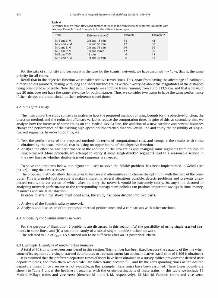
Table 4Reference relative travel times and number of trains in the corresponding segments (columns withheadings Example 1 and Example 2) for the different train types.

Train Reference time t0i

Example 1 Example 2

M-S and S-M 2 h and 18 min 18 42M-V and V-M 1 h and 55 min 12 32M-L and L-M 2 h and 33 min 16 36M-P and P-M 1 h and 2 min 12 30M-T and T-M 18 min 6 18M-A and A-M 1 h and 35 min 6 12


For the sake of simplicity and because it is the case for the Spanish network, we have assumed ci = 1; "i, that is, the samepriority for all trains.

Recall that in the objective function we consider relative travel times. This, apart from having the advantage of leading todimensionless numbers, dealing with long and short distance trains without worrying about the magnitudes of the distancesbeing considered is possible. Note that in our example we combine trains running from 70 to 513.5 Km, and that a delay, ofsay 20 min, does not have the same relevance for both distances. Thus, we consider two trains to have the same performanceif their delays are proportional to their reference travel times.

4.2. Aims of this study

The main aim of the study consists in analyzing how the proposed methods of using bounds for the objective function, thebisection method, and the reduction of binary variables reduce the computation time. In spite of this, as secondary aim, weanalyze how the increase of some trains on the Madrid–Sevilla line, the addition of a new corridor and several brancheschange the performance of the existing high-speed double-tracked Madrid–Sevilla line and study the possibility of single-tracked segments. In order to do this, we:

1. Test the performance of the proposed methods in terms of computational cost, and compare the results with thoseobtained by the usual method, that is, using no upper bound of the objective function.

2. Analyze the effect on line performance of the addition of the new trains and changing some segments from double- tosingle-tracked. More precisely, we attempt to verify if some single-tracked segments lead to a reasonable service inthe new lines or whether double-tracked segments are needed.

To solve the problems below, the algorithm, used to solve the MMBP problem, has been implemented in GAMS (see[51,52]) using the CPLEX solver.

The proposed methods allow the designer to test several alternatives and choose the optimum, with the help of the com-puter. This is a useful tool because it makes simulating several situations possible, detects problems and prevents unex-pected errors, the correction of which after building the network would be extremely costly. So, any time devoted toanalyzing network performance or the corresponding management policies can produce important savings in time, money,resources and social satisfaction.

In order to attain the above mentioned aims, the study has been divided into two parts:

1. Analysis of the Spanish railway network.2. Analysis and discussion of the proposed method performance and a comparison with other methods.

4.3. Analysis of the Spanish railway network

For the purpose of illustration 2 problems are discussed in this section: (a) the possibility of using single-tracked seg-ments in some lines, and (b) a saturation study of a mixed single- double-tracked network.

The selected value of tlim = 1.5 h turned out to be sufficient after an ‘‘a posteriori” check.

4.3.1. Example 1: analysis of single-tracked branchesA total of 70 trains have been considered in this section. This number has been fixed because the capacity of the line when

some of its segments are single-tracked deteriorates to a certain extent (an optimal relative travel time of 1.305 is obtained).It is assumed that the preferred departure times of users have been obtained in a survey, which provides the desired user

departure times, and from them we can calculate when trains become full, and fix the corresponding times as the desireddeparture times. Since a survey is not available, in this example, these times have been assumed. These lower bounds areshown in Table 5 under the heading r‘i , together with the origin-destinations of these trains. In this table we include 16Madrid–Málaga trains and vice versa (denoted M-L and L-M, respectively), 12 Madrid–Valencia trains and vice versa

Table 5Lower bounds r‘i and actual departure ri (in hours:minutes format) together with origins, destinations and relative times (RT) of all scheduled trains in theillustrative example of 70 trains and all single-tracked segments with the exception of Madrid–Sevilla (double-tracked).

i r‘i ri O-D RT i r‘i ri O-D RT i r‘i ri O-D RT

1 7.15 7.15 M-S 1.000 25 22.15 22.21 M-S 1.060 49 18.25 19.07 M-S 1.3052 7.15 7.18 S-M 1.025 26 22.15 22.15 S-M 1.029 50 18.25 18.25 S-M 1.0003 21.50 22.09 M-L 1.230 27 7.25 7.25 M-P 1.000 51 9.25 9.25 M-P 1.0004 21.50 21.58 L-M 1.055 28 7.25 7.25 P-M 1.000 52 9.25 9.25 P-M 1.0005 14.45 14.54 M-V 1.081 29 21.20 21.53 M-V 1.288 53 20.30 21.03 M-V 1.2916 14.45 14.55 V-M 1.084 30 21.20 21.45 V-M 1.257 54 20.30 20.30 V-M 1.2587 7.30 7.30 M-P 1.000 31 8.50 9.27 M-L 1.241 55 11.25 11.25 M-T 1.0008 7.30 7.49 P-M 1.305 32 8.50 9.37 L-M 1.305 56 11.25 11.25 T-M 1.0009 21.40 22.07 M-S 1.298 33 20.20 20.45 M-S 1.184 57 17.45 18.24 M-S 1.282

10 21.40 22.13 S-M 1.267 34 20.20 20.24 S-M 1.076 58 17.45 17.45 S-M 1.00011 20.00 20.00 M-L 1.000 35 15.55 15.55 M-T 1.000 59 12.55 13.19 M-L 1.15912 20.00 20.11 L-M 1.112 36 15.55 15.55 T-M 1.000 60 12.55 12.55 L-M 1.00013 7.10 7.10 M-A 1.000 37 9.22 9.39 M-P 1.270 61 19.20 19.24 M-V 1.24414 7.10 7.28 A-M 1.185 38 9.22 9.22 P-M 1.000 62 19.20 19.20 V-M 1.00015 22.00 22.00 M-T 1.000 39 20.55 21.07 M-L 1.081 63 16.20 16.20 M-P 1.00016 22.00 22.06 T-M 1.305 40 20.55 20.55 L-M 1.305 64 16.20 16.26 P-M 1.09117 7.00 7.12 M-S 1.087 41 15.30 15.45 M-S 1.110 65 11.45 12.17 M-S 1.22818 7.00 7.03 S-M 1.025 42 15.30 15.30 S-M 1.000 66 11.45 12.11 S-M 1.18519 21.30 21.30 M-P 1.000 43 10.05 10.21 M-V 1.136 67 17.00 17.00 M-A 1.00020 21.30 21.45 P-M 1.233 44 10.05 10.17 V-M 1.105 68 17.00 17.16 A-M 1.16821 14.05 14.05 M-L 1.000 45 20.00 20.13 M-A 1.140 69 10.20 10.39 M-L 1.21222 14.05 14.14 L-M 1.061 46 20.00 20.29 A-M 1.305 70 10.20 10.20 L-M 1.00023 7.45 8.06 M-V 1.181 47 9.35 10.04 M-L 1.18724 7.45 8.06 V-M 1.185 48 9.35 9.41 L-M 1.038


(M-V and V-M), and similarly, 18 Madrid–Sevilla (M-S and S-M), 6 Madrid–Toledo (M-T and T-M), 12 Madrid–Puertollano(M-P and P-M), and 6 Madrid–Albacete (M-A and A-M) trains.

The segments are assumed to be single-tracked, with the exception of the double-tracked Madrid–Sevilla line. The algo-rithm is used to solve the timetabling problem and the results appear in Table 5, which shows the actual departure and theuser preference relative travel times for all trains, under the headings ri and RT, respectively. The optimal relative travel timeis 1.305, which implies a somewhat saturated network (the departure times in boldface are those which are different fromthe desired ones).

To illustrate, Fig. 2 shows the resulting timetable for the case of single-tracked segments on all the new lines, i.e., keepingonly double-tracked segments for the Madrid–Sevilla line, where the railway network resulting timetable and the train

Fig. 2. Resulting time table for the case of 70 trains and all single-tracked segments with the exception of Madrid–Sevilla (double-tracked).

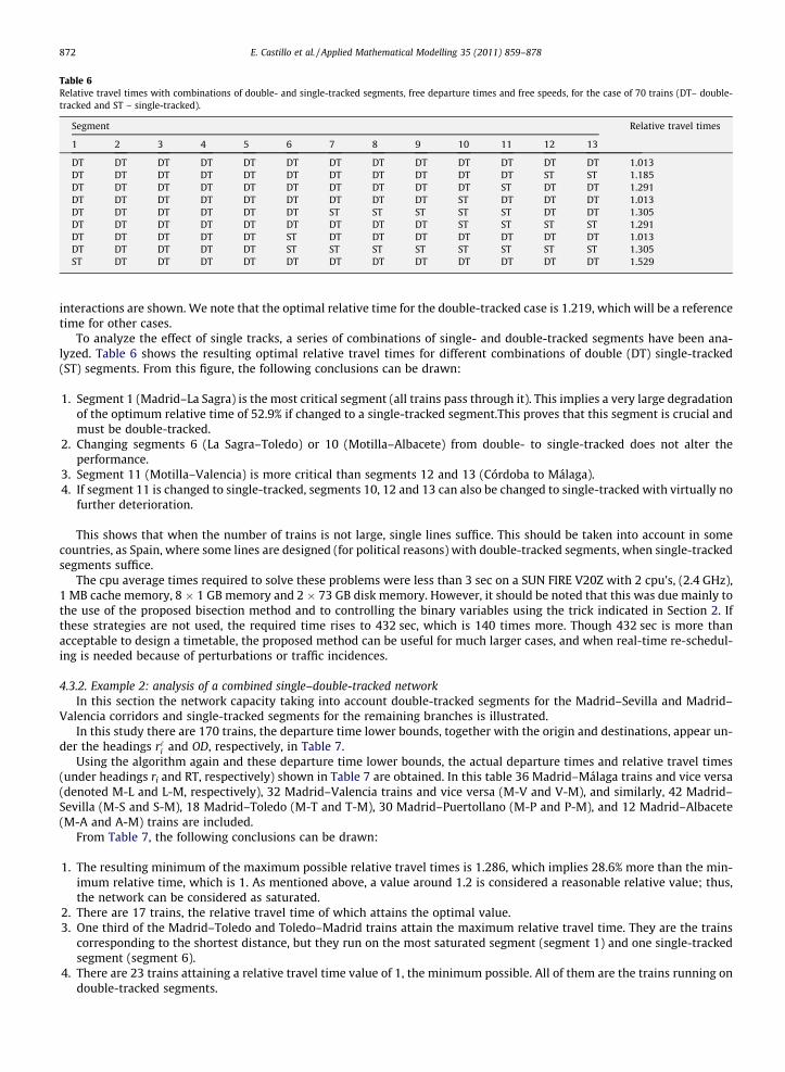
Table 6Relative travel times with combinations of double- and single-tracked segments, free departure times and free speeds, for the case of 70 trains (DT– double-tracked and ST – single-tracked).

Segment Relative travel times

1 2 3 4 5 6 7 8 9 10 11 12 13

DT DT DT DT DT DT DT DT DT DT DT DT DT 1.013DT DT DT DT DT DT DT DT DT DT DT ST ST 1.185DT DT DT DT DT DT DT DT DT DT ST DT DT 1.291DT DT DT DT DT DT DT DT DT ST DT DT DT 1.013DT DT DT DT DT DT ST ST ST ST ST DT DT 1.305DT DT DT DT DT DT DT DT DT ST ST ST ST 1.291DT DT DT DT DT ST DT DT DT DT DT DT DT 1.013DT DT DT DT DT ST ST ST ST ST ST ST ST 1.305ST DT DT DT DT DT DT DT DT DT DT DT DT 1.529


interactions are shown. We note that the optimal relative time for the double-tracked case is 1.219, which will be a referencetime for other cases.

To analyze the effect of single tracks, a series of combinations of single- and double-tracked segments have been ana-lyzed. Table 6 shows the resulting optimal relative travel times for different combinations of double (DT) single-tracked(ST) segments. From this figure, the following conclusions can be drawn:

1. Segment 1 (Madrid–La Sagra) is the most critical segment (all trains pass through it). This implies a very large degradationof the optimum relative time of 52.9% if changed to a single-tracked segment.This proves that this segment is crucial andmust be double-tracked.

2. Changing segments 6 (La Sagra–Toledo) or 10 (Motilla–Albacete) from double- to single-tracked does not alter theperformance.

3. Segment 11 (Motilla–Valencia) is more critical than segments 12 and 13 (Córdoba to Málaga).4. If segment 11 is changed to single-tracked, segments 10, 12 and 13 can also be changed to single-tracked with virtually no

further deterioration.

This shows that when the number of trains is not large, single lines suffice. This should be taken into account in somecountries, as Spain, where some lines are designed (for political reasons) with double-tracked segments, when single-trackedsegments suffice.

The cpu average times required to solve these problems were less than 3 sec on a SUN FIRE V20Z with 2 cpu’s, (2.4 GHz),1 MB cache memory, 8 � 1 GB memory and 2 � 73 GB disk memory. However, it should be noted that this was due mainly tothe use of the proposed bisection method and to controlling the binary variables using the trick indicated in Section 2. Ifthese strategies are not used, the required time rises to 432 sec, which is 140 times more. Though 432 sec is more thanacceptable to design a timetable, the proposed method can be useful for much larger cases, and when real-time re-schedul-ing is needed because of perturbations or traffic incidences.

4.3.2. Example 2: analysis of a combined single–double-tracked networkIn this section the network capacity taking into account double-tracked segments for the Madrid–Sevilla and Madrid–

Valencia corridors and single-tracked segments for the remaining branches is illustrated.In this study there are 170 trains, the departure time lower bounds, together with the origin and destinations, appear un-

der the headings r‘i and OD, respectively, in Table 7.Using the algorithm again and these departure time lower bounds, the actual departure times and relative travel times

(under headings ri and RT, respectively) shown in Table 7 are obtained. In this table 36 Madrid–Málaga trains and vice versa(denoted M-L and L-M, respectively), 32 Madrid–Valencia trains and vice versa (M-V and V-M), and similarly, 42 Madrid–Sevilla (M-S and S-M), 18 Madrid–Toledo (M-T and T-M), 30 Madrid–Puertollano (M-P and P-M), and 12 Madrid–Albacete(M-A and A-M) trains are included.

From Table 7, the following conclusions can be drawn:

1. The resulting minimum of the maximum possible relative travel times is 1.286, which implies 28.6% more than the min-imum relative time, which is 1. As mentioned above, a value around 1.2 is considered a reasonable relative value; thus,the network can be considered as saturated.

2. There are 17 trains, the relative travel time of which attains the optimal value.3. One third of the Madrid–Toledo and Toledo–Madrid trains attain the maximum relative travel time. They are the trains

corresponding to the shortest distance, but they run on the most saturated segment (segment 1) and one single-trackedsegment (segment 6).

4. There are 23 trains attaining a relative travel time value of 1, the minimum possible. All of them are the trains running ondouble-tracked segments.

Table 7Lower bounds r‘i and actual departure times ri (in hours:minutes format) together with origins, destinations and relative times (RT) of all scheduled trains in theillustrative example of 170 trains and all single-tracked segments with the exception of Madrid–Sevilla and Madrid–Valencia corridors (double-tracked). Themean RT is 1.138 and the maximum RT is 1.286.

i r‘i ri O-D RT i r‘i ri O-D RT i r‘i ri O-D RT

1 7.15 7.15 M-S 1.000 58 17.45 17.52 S-M 1.051 115 8.00 8.00 M-A 1.0002 7.15 7.52 S-M 1.270 59 12.55 13.36 M-A 1.272 116 8.00 8.44 A-M 1.2853 21.50 22.09 M-A 1.128 60 12.55 13.31 A-M 1.250 117 20.15 20.18 M-T 1.1904 21.50 22.21 A-M 1.201 61 19.20 19.22 M-V 1.175 118 20.15 20.20 T-M 1.2865 14.45 14.54 M-V 1.079 62 19.20 19.28 V-M 1.069 119 17.30 17.57 M-V 1.2356 14.45 14.51 V-M 1.052 63 16.20 16.32 M-P 1.192 120 17.30 17.58 V-M 1.2397 7.30 7.44 M-P 1.231 64 16.20 16.23 P-M 1.042 121 12.20 12.33 M-S 1.1548 7.30 7.45 P-M 1.238 65 11.45 11.55 M-S 1.138 122 12.20 12.24 S-M 1.0289 21.40 21.40 M-S 1.000 66 11.45 11.49 S-M 1.088 123 8.35 8.49 M-P 1.229

10 21.40 21.59 S-M 1.138 67 17.00 17.23 M-A 1.243 124 8.35 8.53 P-M 1.28611 20.00 20.08 M-A 1.146 68 17.00 17.17 A-M 1.240 125 10.45 11.21 M-A 1.28512 20.00 20.44 A-M 1.285 69 10.20 10.20 M-A 1.000 126 10.45 11.06 A-M 1.16213 7.10 7.37 M-A 1.286 70 10.20 11.02 A-M 1.286 127 12.00 12.00 M-T 1.00014 7.10 7.17 A-M 1.076 71 18.00 18.01 M-V 1.010 128 12.00 12.05 T-M 1.28615 22.00 22.00 M-T 1.000 72 18.00 18.11 V-M 1.096 129 19.45 20.20 M-S 1.25616 22.00 22.00 T-M 1.000 73 13.25 13.34 M-S 1.093 130 19.45 19.52 S-M 1.05017 7.00 7.10 M-S 1.071 74 13.25 13.40 S-M 1.107 131 13.20 13.32 M-P 1.28618 7.00 7.20 S-M 1.146 75 19.10 19.10 M-P 1.000 132 13.20 13.38 P-M 1.28619 21.30 21.38 M-P 1.128 76 19.10 19.10 P-M 1.001 133 14.10 14.21 M-A 1.14420 21.30 21.30 P-M 1.000 77 8.20 8.25 M-T 1.286 134 14.10 14.15 A-M 1.03021 14.05 14.23 M-A 1.163 78 8.20 8.20 T-M 1.000 135 20.40 21.06 M-A 1.27022 14.05 14.32 A-M 1.174 79 11.00 11.31 M-A 1.200 136 20.40 20.50 A-M 1.10323 7.45 8.10 M-V 1.218 80 11.00 11.04 A-M 1.052 137 9.10 9.11 M-S 1.05524 7.45 8.18 V-M 1.284 81 21.00 21.08 M-S 1.241 138 9.10 9.10 S-M 1.00025 22.15 22.42 M-S 1.192 82 21.00 21.29 S-M 1.236 139 22.45 23.05 M-V 1.17026 22.15 22.34 S-M 1.182 83 18.45 19.03 M-V 1.204 140 22.45 22.45 V-M 1.00027 7.25 7.42 M-P 1.279 84 18.45 19.18 V-M 1.286 141 9.20 9.35 M-P 1.24328 7.25 7.43 P-M 1.286 85 19.05 19.12 M-P 1.112 142 9.20 9.24 P-M 1.06429 21.20 21.38 M-V 1.156 86 19.05 19.06 P-M 1.017 143 13.45 14.28 M-A 1.28030 21.20 21.40 V-M 1.170 87 6.30 6.43 M-A 1.127 144 13.45 14.11 A-M 1.16731 8.50 9.05 M-A 1.101 88 6.30 6.43 A-M 1.085 145 11.20 11.53 M-S 1.24132 8.50 8.50 A-M 1.000 89 11.10 11.23 M-S 1.164 146 11.20 11.54 S-M 1.28333 20.20 20.43 M-S 1.238 90 11.10 11.25 S-M 1.124 147 9.45 9.45 M-T 1.00034 20.20 20.57 S-M 1.267 91 16.30 16.30 M-T 1.000 148 9.45 9.45 T-M 1.00035 15.55 16.00 M-T 1.286 92 16.30 16.32 T-M 1.115 149 13.30 13.46 M-V 1.17036 15.55 16.00 T-M 1.286 93 20.10 20.34 M-V 1.209 150 13.30 13.45 V-M 1.12937 9.22 9.24 M-P 1.030 94 20.10 20.42 V-M 1.279 151 16.00 16.24 M-A 1.15838 9.22 9.22 P-M 1.000 95 6.45 6.45 M-A 1.017 152 16.00 16.29 A-M 1.18739 20.55 21.31 M-A 1.237 96 6.45 6.48 A-M 1.021 153 17.50 17.57 M-S 1.08040 20.55 21.15 A-M 1.133 97 22.30 22.34 M-S 1.032 154 17.50 17.50 S-M 1.04341 15.30 15.30 M-S 1.000 98 22.30 22.32 S-M 1.059 155 10.25 10.25 M-P 1.00042 15.30 15.37 S-M 1.048 99 9.00 9.09 M-P 1.137 156 10.25 10.43 P-M 1.28643 10.05 10.38 M-V 1.286 100 9.00 9.13 P-M 1.203 157 16.45 16.57 M-A 1.12444 10.05 10.36 V-M 1.269 101 19.30 19.36 M-V 1.106 158 16.45 16.49 A-M 1.04445 20.00 20.16 M-A 1.245 102 19.30 19.30 V-M 1.000 159 18.35 19.06 M-V 1.27346 20.00 20.00 A-M 1.000 103 8.25 9.03 M-A 1.250 160 18.35 18.41 V-M 1.05347 9.35 10.18 M-A 1.280 104 8.25 8.46 A-M 1.135 161 11.35 11.35 M-A 1.00048 9.35 9.58 A-M 1.161 105 10.00 10.16 M-S 1.116 162 11.35 12.18 A-M 1.28349 18.25 19.04 M-S 1.285 106 10.00 10.11 S-M 1.079 163 17.15 17.27 M-S 1.10650 18.25 18.57 S-M 1.230 107 15.10 15.10 M-A 1.002 164 17.15 17.22 S-M 1.11751 9.25 9.33 M-P 1.195 108 15.10 15.24 A-M 1.147 165 12.10 12.28 M-P 1.28652 9.25 9.26 P-M 1.016 109 21.10 21.27 M-P 1.278 166 12.10 12.28 P-M 1.28653 20.30 20.36 M-V 1.053 110 21.10 21.10 P-M 1.000 167 15.20 15.25 M-T 1.28654 20.30 20.44 V-M 1.123 111 13.15 13.48 M-V 1.283 168 15.20 15.20 T-M 1.00055 11.25 11.29 M-T 1.206 112 13.15 13.27 V-M 1.103 169 18.05 18.15 M-V 1.08356 11.25 11.30 T-M 1.286 113 18.15 18.46 M-S 1.222 170 18.05 18.09 V-M 1.03557 17.45 17.59 M-S 1.131 114 18.15 18.53 S-M 1.273


5. The maximum difference between desired and actual departure times is 44 min, corresponding to trains 12 and 116Albacete–Madrid. Nevertheless, this has an associated relative travel time of 1.285 < 1.286, which implies that the userdesires are not adequately satisfied (saturated network).

6. In the column under heading ri the departure times in boldface are those which are different from the desired ones. Sincethere are 143 trains out of a total of 170 that suffer delays with respect to their optimal travel times, this implies acrowded network.

7. The hourly frequencies of trains oscillate between 3 and 8 trains per hour, for valley and rush times.

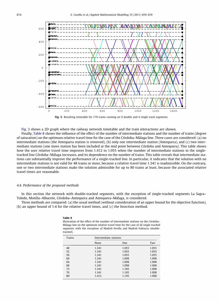
Fig. 3. Resulting timetable for 170 trains running on 9 double and 4 single track segments.


Fig. 3 shows a 2D graph where the railway network timetable and the train interactions are shown.Finally, Table 8 shows the influence of the effect of the number of intermediate stations and the number of trains (degree

of saturation) on the optimum relative travel time for the case of the Córdoba–Málaga line. Three cases are considered: (a) nointermediate stations (the Antequera station is removed), (b) only one intermediate station (Antequera), and (c) two inter-mediate stations (one more station has been included at the mid point between Córdoba and Antequera). This table showshow the user relative travel time improves from 1.412 to 1.055 when the number of intermediate stations in the single-tracked line Córdoba–Málaga increases, and its dependence on the number of trains. This table reveals that intermediate sta-tions can substantially improve the performance of a single-tracked line. In particular, it indicates that the solution with nointermediate stations is not valid for 48 trains or more, because a relative travel time 1.341 is inadmissible. On the contrary,one or two intermediate stations make the solution admissible for up to 80 trains at least, because the associated relativetravel times are reasonable.

4.4. Performance of the proposed methods

In this section the network with double-tracked segments, with the exception of single-tracked segments La Sagra–Toledo, Motilla–Albacete, Córdoba–Antequera and Antequera–Málaga, is considered.

Three methods are compared: (a) the usual method (without consideration of an upper bound for the objective function),(b) an upper bound of 1.4 for the relative travel times, and (c) the bisection method.

Table 8Illustration of the effect of the number of intermediate stations on the Córdoba–Málaga line on the optimum relative travel time for the case of all single-trackedsegments with the exception of Madrid–Sevilla and Madrid–Valencia (double-tracked).

Trains Intermediate stations

None One Two

48 1.341 1.055 1.05552 1.341 1.055 1.05556 1.341 1.055 1.05560 1.341 1.098 1.09864 1.341 1.098 1.09868 1.341 1.098 1.09872 1.341 1.185 1.09876 1.341 1.185 1.09880 1.412 1.195 1.098


Different subsets with an increasing number of trains, ranging from 10 to 170 (with a step of 4 trains), are considered. Thesubsets correspond to those in Table 7, all of them starting from the first train. For example, when 30 trains are considered,the first 30 trains are included in the subset.

Table 9 shows relevant information about the performance of these methods for different levels of saturation (from 10 to170 trains) and reveals the incredible reduction of cpu time obtained when the last two proposed methods are used. Col-umns 2 to 4 show the cpu times (in seconds) for three different strategies: (a) without supplying a bound for the objectivefunction (this is the strategy normally used), (b) using a bound for the relative travel time of 1.4, and (c) using the bisectionmethod. Columns 5 to 7 show the total number of binary variables (x and y), the resulting reduced number of binary vari-ables using the proposed strategy with tlim = 1.5 h, and the number of continuous variables (e and s). Column 8 provides theoptimal maximum desired relative travel times (the solution of the minimax problem MMBP). Finally, columns 9 and 10 givethe mean values (based on all trains) of the actual and desired relative travel times, based on the actual and desired depar-ture times, respectively. From this table, the following can be concluded:

1. The required cpu time increases exponentially with the number of trains.2. Use of an upper bound for the objective function substantially (several orders of magnitude) reduces the computation

time needed to solve the problem.3. Using the bisection method produces an additional reduction of the computation time (several orders of magnitude), with

respect to the one associated with the previous upper bound of 1.4.

Table 9Some computation time and needed resources corresponding to different degrees of saturation for the case of 9 double and 4 single track segments.

1 2 3 4 5 6 7 8 9 10Trains Cpu time (seconds) Max Bin Bin Cont Max RT Mean RT Mean RT1

No bound eup = 1.4 Bisection

10 0.03 0.04 0.03 256 90 97 1.000 1.000 1.00014 0.08 0.06 0.05 494 174 141 1.055 1.000 1.01618 0.16 0.12 0.11 756 266 169 1.055 1.000 1.02022 0.32 0.18 0.15 1206 356 205 1.055 1.000 1.02426 1.05 0.32 0.25 1666 518 245 1.055 1.000 1.02230 2.08 0.37 0.32 2130 658 277 1.055 1.000 1.01534 4.59 0.55 0.42 2936 880 321 1.055 1.000 1.02238 5.65 0.67 0.53 3426 984 341 1.055 1.001 1.02042 22.85 1.78 0.69 4448 1238 385 1.055 1.001 1.01746 34.78 1.25 0.88 5060 1344 425 1.055 1.001 1.01850 54.08 1.52 0.88 6266 1530 469 1.055 1.001 1.01954 74.10 2.85 1.11 7138 1788 501 1.055 1.002 1.01958 169.33 2.12 1.36 8056 1902 529 1.055 1.001 1.02462 75.53 2.55 1.44 9270 2112 573 1.098 1.001 1.04266 236.01 3.50 1.55 10630 2266 605 1.098 1.000 1.05170 418.38 7.64 2.93 11988 2496 649 1.185 1.002 1.07674 431.88 8.60 4.04 13416 2768 689 1.185 1.003 1.07978 1946.06 8.51 3.55 14434 2962 709 1.185 1.000 1.07282 1877.38 29.87 4.27 16408 3436 753 1.195 1.006 1.08986 >3000 29.10 4.75 17816 3796 785 1.195 1.006 1.09090 2820.7 61.09 13.76 20006 4166 829 1.195 1.004 1.08194 >3000 75.12 22.76 21108 4478 857 1.195 1.002 1.08798 >3000 136.11 15.57 23482 4914 901 1.195 1.011 1.095

102 >3000 215.21 30.92 25162 5448 933 1.195 1.004 1.087106 >3000 1595.0 37.75 27752 6106 977 1.212 1.009 1.102110 >3000 1884.7 16.41 29520 6468 1009 1.212 1.012 1.092114 >3000 >3000 61.51 31740 6842 1049 1.212 1.006 1.088118 >3000 >3000 99.06 33716 7392 1081 1.286 1.012 1.128122 >3000 >3000 27.61 36088 7866 1121 1.286 1.012 1.135126 >3000 >3000 210.54 38794 8544 1157 1.286 1.016 1.133130 >3000 >3000 216.27 40896 9044 1185 1.286 1.009 1.138134 >3000 >3000 202.04 43794 9478 1221 1.286 1.013 1.140138 >3000 >3000 203.30 46406 10212 1261 1.286 1.014 1.132142 >3000 >3000 196.55 48758 10702 1293 1.286 1.009 1.125146 >3000 >3000 856.88 52332 11410 1337 1.286 1.012 1.138150 >3000 >3000 2575.84 54114 11756 1365 1.286 1.013 1.137154 >3000 >3000 2529.98 57872 12326 1409 1.286 1.011 1.135158 >3000 >3000 2784.05 60424 12930 1441 1.286 1.013 1.138162 >3000 >3000 2552.60 63694 13784 1485 1.286 1.012 1.140166 >3000 >3000 2747.95 67158 14470 1517 1.286 1.020 1.142170 >3000 >3000 2658.53 69196 15006 1545 1.286 1.008 1.138


4. The proposed technique for reducing the number of binary variables reduces them by factors which increase with thenumber of trains and can reach a factor of 5. This reduction is important more from the point of view of memory require-ments than from that of cpu requirements. In particular, several tests revealed that the bisection method strategy hidesthe effect of the variable reduction technique in terms of cpu time. Note that the upper bounds of the relative travel timesused in the bisection method, also exclude interactions of trains circulating further apart, and then they produce the sameeffect as the tlim parameter in terms of cpu, but have no effect in terms of memory requirements.

5. The optimal relative travel times increase with the number of trains by steps, but stay constant for several train incre-ments, until a new increase occurs (see Table 9 column 8).

6. The mean of the actual relative travel times remains in reasonable values (smaller than a 10% increase) for less than 170trains.

4.5. Drawbacks of the proposed methods and suggested future work

Though the methods developed in this paper provide a substantial reduction in the time for timetabling computation, ashas been stated in this paper, the proposed methodology does have some drawbacks because the model does not considercapacity limit of stations, no detailed analysis of the timetabling robustness has been considered, and no application to real-time control has been made. In addition, though not necessary, the blocking system could be designed at the timetablingstage, because it supplies very important information for train operation and required infrastructure. Finally, for highly con-gested or very large networks, solving optimization problems takes a very long time. So, further research is still needed todeal with large networks, mainly in real-time control.

Consequently, some recommended future work should take the following directions:

1. Development of new branch and bound methods specialized in determining feasibility or non-feasibility, which couldlead to an important improvement of the methods proposed in this paper. Though the proposed methods in this papersubstantially improve the computation time, when saturation exists or the associated problems are very large, the com-putation time can be very high. So, further improvements need to be investigated if real-time control is desired.

2. Extension of the proposed method to the control and/or re-scheduling in real-time problems. The good performance ofthe method in terms of memory and computation time requirements indicates that this extension could be useful andeffective.

3. Design of the blocking system together with the timetable.4. Inclusion of the available rolling stock in the optimization program.

5. Conclusions

The following conclusions can be drawn from this paper.

1. An optimization program together with an algorithm to solve the railway timetabling optimization problem has beenproposed. The program is based on minimizing the maximum user preference relative travel times and selecting the solu-tion with minimum total sum of actual relative travel times. The test results reported in this paper indicate that theycould well be useful for timetabling design, where the degree of saturation corresponding to different numbers of trainscan be measured by the resulting optimal values of the relative travel times (relative travel times close to 1, and above 1.2or 1.3 indicate a very low and a high degree of saturation, respectively). The examples dealt with in this paper are largeenough (in fact, they are real cases) and the computation time small enough to show the practical applicability of theproposed methodology to real cases.

2. Use of an upper bound for the objective function substantially reduces the computation time. This reduction is exponen-tial with the number of trains, and for usual size railway networks, as the one in the examples, can be several orders ofmagnitude. Fixing this upper bound is specially easy for the selected objective function based on relative travel times. Infact, the lower bound is 1, and an upper bound of 1.5 should be sufficient for most existing networks in operation includ-ing highly saturated networks. Note that a value of 1.5 means a travel time 50% higher than desired.

3. The proposed bisection method, which tries to obtain sharp upper bounds for the objective function in an efficient way,allows us an extra exponential reduction of computation time on top of the previous one. For example, with only 70 trainsand a time horizon of 1440 min (one day), this time became 140 times lower. The proposed bisection method, which per-mits the global solution to be obtained in 12 iterations, does not require the optimal solution but knowledge about thefeasibility of the problem with the actual upper bound. Only in the last step, when the upper bound is very close to theoptimal value, does this problem need to be solved to proven solution or until a given gap is obtained.

4. The proposed strategy to reduce the number of binary variables, by excluding a large proportion of them, has shown to bevery effective in reducing the memory requirements of the problem, which can be as important as the reduction in thecpu time. This strategy also reduces the associated computation time, but this contribution can be hidden by the bisectionmethod. So, an adequate selection of the tlim value is important in order to reduce the complexity of the problem and not


so important to reduce cpu time if combined with the bisection method. Some formulas have been given to test that theselected value of tlim is valid, and they provide an interesting hint about how much to modify it if unfeasibility occurs inthe test.

5. The proposed method allows us analyzing the performance of real railway networks (effect of saturation and number ofintermediate stations) under different assumptions as it has been demonstrated with the Spanish network. Again, wehave quantified the effect of saturation.

6. The project of double-tracked lines must be justified in some regions with reduced traffic, because single-tracked linescould provide sufficient capacity for these regions, due to the very limited present and expected future traffic level.

Acknowledgements

The authors are indebted to the Spanish Ministry of Science and Technology (Project BIA2005-07802-C02-01), to theSpanish Ministry of Education, Culture and Sports for partial support of this work. We also wish to thank Prof. Antonio Con-ejo for providing us with computer time to solve the optimization problems with GAMS. Finally, we wish to thank theauthors of all the cited papers, in special to Zhou and Zhong and Törnquist and Persson, who motivated our work in this area.

References

[1] A. Caprara, L. Kroon, M. Monaci, M. Peeters, P. Toth, Passenger railway optimization, in: C. Barnhart, G. Laporte (Eds.), Handbooks in OperationsResearch and Management Science, vol. 14, 2006, pp. 129–187.

[2] M. Carey, A model and strategy for train pathing with choice of lines, platforms and routes, Transp. Res. Part B 28 (5) (1994) 333–353.[3] M. Carey, D. Lockwood, A model, algorithms and strategy for train pathing, J. Oper. Res. Soc. 46 (8) (1995) 988–1005.[4] A. Higgins, E. Kozan, L. Ferreira, Optimal scheduling of trains on a single line track, Transp. Res. Part B 30 (2) (1996) 147–161.[5] J.F. Cordeau, P. Toth, D. Vigo, A survey of optimization models for train routing and scheduling, Transp. Sci. 32 (4) (1998) 380–404.[6] X. Zhou, M. Zhong, Single-track train timetabling with guaranteed optimality: branch-and-bound algorithms with enhanced lower bounds, Transp. Res.

B 41 (3) (2007) 320–341.[7] I. Sahin, Railway traffic control and train scheduling based on inter-train conflict management, Transp. Res. Part B 33 (7) (1999) 511–534.[8] L-M. Jia, X-D. Zhang, Distributed intelligent railway traffic control based on fuzzy decision making, Fuzzy Sets Syst. 62 (3) (1993) 255–265.[9] D.R. Kraay, P.T. Harker, Real-time scheduling of freight railroads, Transp. Res. Part B 29 (3) (1995) 213–229.

[10] A. D’Ariano, M. Pranzo, A real time train dispatching system based on blocking time theory, in: Proceedings of the Eighth TRAIL Eighth Annual Congress2004, A World of Transport, Infrastructure and Logistics, Delft, DUP Science, 2004, pp.129–152.

[11] A. D’Ariano, M. Pranzo, I.A. Hansen, Conflict resolution and train speed coordination for solving real-time timetable perturbations, IEEE Trans.Intell.Transp. Syst. 8 (2) (2007).

[12] A. D’Ariano, D. Pacciarelli, P. Pranzo, R. Hemelrijk, Evaluating the performance of railway dynamic traffic management, in: Proceedings of the 11thWorld Conference on Transport Research, Berkeley, University of California, USA, 2007, pp. 1–12.

[13] J. Törnquist, J.A. Persson, N-tracked railway traffic re-scheduling during disturbances, Transp. Res. B 41 (3) (2007) 342–362.[14] E.R. Petersen, A.J. Taylor, C.D. Martland, An introduction to computer aided train dispatching, J. Adv. Transp. 20 (1986) 63–72.[15] K. Ghoseiri, F. Szidarovszky, M.J. Asgharpour, A multi-objective train scheduling model and solution, Transp. Res. Part B 38 (10) (2004) 927–952.[16] P. Hellström, Analysis and Evaluation of Systems and Algorithms for Computer-aided Train Dispatching, Licentiate Thesis, Uppsala University, Sweden,

1998.[17] I. Amit, D. Goldfarb, The timetable problem for railways, Dev. Oper. Res. 2 (1971) 379–387.[18] A. Assad, Models for rail transportation, Transp. Res. Part A 14 (3) (1980) 205–220.[19] A.E. Haghani, Rail freight transportation: a review of recent optimization models for train routing and empty car distribution, J. Adv. Transp. 21 (1987)

147–172.[20] O. Frank, Two-way traffic on a single line of railway, Oper. Res. 14 (1965) 801–811.[21] D.A. Rudd, A.J. Storry, Single track railway simulation, new models and old, Rail Int. (1976) 335–342.[22] E.R. Petersen, A.J. Taylor, A structured model for rail line simulation and optimization, Transp. Sci. 16 (2) (1982) 192–206.[23] Y. Iida, Timetable preparation by A.I. approach, in: Proceeding of European Simulation Multiconference, Nice, France, 1988, pp. 163–168.[24] K. Komaya, T. Fukuda, ESTRAC-III: An expert system for train track control in disturbed situations, in: J.P. Perrin (Ed.), IFAC Control, Computers,

Communications in Transportation, IFAC/IFIP/IFORS Symposium, Paris, France, 19–21 September, 1989, Published for the International Federation ofAutomatic Control by Pergamon Press, Paris, France, 1989, pp. 147–153.

[25] K. Komaya, T. Fukuda, A knowledge-based approach for railway scheduling, in: Proceedings of the Seventh IEEE Conference on Artificial Intelligence forApplications, IEEE Computer Society Press, 1991, pp. 404–411.

[26] K. Komaya, An integrated framework of simulation and scheduling in railway systems, in: T.K.S. Murthy, J. Allan, R.J. Hill, G. Sciutto, S. Sone (Eds.),Computers in Railways III, Management, vol. 1, Computational Mechanics Publications, Southampton, Boston, 1992, pp. 611–622.

[27] H. Schaefer, S. Pferdmenges, An expert system for real-time train dispatching, in: Computers in Railways (COMPRAIL) IV, Vol 2 Railway Operations,1994, pp. 27–34.

[28] P. Vieira, L.E. Neto, E. Bessa, F. Gomide, Railway dispatch and control, in: Proceedings for NAFIPS – The 18th International Conference of the NorthAmerican Fuzzy Information Processing Society, 1999, pp. 134–138.

[29] B. Szpigel, Optimal train scheduling on a single track railway, in: Operations Research’72, North-Holland, Amsterdam, Netherlands, 1973, pp. 343–352.[30] D. Jovanovic, P.T. Harker, Tactical scheduling of rail operations: The SCAN I system, Transp. Sci. 25 (1) (1991) 46–64.[31] D. Kraay, P.T. Harker, B. Chen, Optimal pacing of trains in freight railroads: model formulation and solution, Oper. Res. 39 (1991) 82–99.[32] M. Carey, Extending a train pathing model from one-way to two-way track, Transp. Res. Part B 28 (5) (1994) 395–400.[33] U. Brannlund, P.O. Lindberg, A. Nou, J.E. Nilsson, Railway timetabling using Lagrangian relaxation, Transp. Sci. 32 (4) (1998) 358–369.[34] E. Castillo, I. Gallego, J.M. Ureña, J.M. Coronado, Timetabling optimization of a single railways track line with sensitivity analysis, TOP 17 (2) (2009)

256–287.[35] S. Mackenzie, Train timetabling on complex networks, in: Proceedings from the Conference on Railway Engineering (CORE2000), Adelaide, Australia,

2000.[36] X. Zhou, M. Zhong, Bi-criteria train scheduling for high-speed passenger railroad planning applications, Eur. J. Oper. Res. 167 (3) (2005) 752–771.[37] J. Törnquist, Railway traffic disturbance management, Transp. Res. Part A: Policy Pract. 41 (3) (2007) 249–266.[38] A. D’Ariano, D. Pacciarelli, M. Pranzo, A branch and bound algorithm for scheduling trains in a railway network, Eur. J. Oper. Res. 183 (2) (2007) 643–

657.[39] X. Cai, C.J. Goh, A.I. Mees, Greedy heuristics for rapid scheduling of trains on a single track, IIE Trans. 30 (5) (1998) 481–493.


[40] A. Caprara, M. Fischetti, P. Toth, Modeling and solving the train timetabling problem, Oper. Res. 50 (5) (2002) 851–861.[41] H.H. Greenberg, A branch-and-bound solution to the general scheduling problem, Oper. Res. 16 (2) (1968) 352–361.[42] B. Adenso-Diaz, M.O. González, P. González-Torre, On-line timetable re-scheduling in regional train services, Transp. Res. Part B 33 (6) (1999) 387–398.[43] A. Higgins, E. Kozan, Modeling train delays in urban networks, Transp. Sci. 32 (4) (1998) 346–357.[44] L. Zhou, S. Hu, J. Ma, Y. Yue, Network hierarchy parallel algorithm of automatic train scheduling, in: Proceedings of the Conference on Traffic and

Transportation Studies, ICTTS, 1998, pp. 358–368.[45] M.J. Dorfman, J. Medanic, Scheduling trains on a railway network using a discrete event model of railway traffic, Transp. Res. Part B 38 (1) (2004) 81–

98.[46] P. Vansteenwegen, D. Van Oudheusden, Decreasing the passenger waiting time for an intercity rail network, Transp. Res. Part B 41 (4) (2007) 478–492.[47] M. Carey, I. Crawford, Scheduling trains on a network of busy complex stations, Transp. Res. Part B 41 (1) (2007) 159–178.[48] E. Castillo, A.S. Hadi, A. Conejo, A. Fernández-Canteli, A General Method for local sensitivity analysis with application to regression models and other

optimization problems, Technometrics 46 (2004) 430–444.[49] E. Castillo, A.J. Conejo, R. Mı´ nguez, C. Castillo, A closed formula for local sensitivity analysis in mathematical programming, Eng. Optim. 38 (1) (2006)

93–112.[50] E. Castillo, A.J. Conejo, C. Castillo, R. Mínguez, Closed formulas in local sensitivity analysis for some classes of linear and non-linear problems, TOP 15

(2) (2007) 355–371.[51] E. Castillo, A.J. Conejo, P. Pedregal, R. García, N. Alguacil, Building and Solving Mathematical Programming Models in Engineering and Science, Pure and

Applied Mathematics, Wiley, New York, 2001.[52] A. Conejo, E. Castillo, R. Mínguez, R. García-Bertrand, Decomposition Techniques in Mathematical Programming, Engineering and Science Applications,

Springer, Berlin, Heildelberg, 2006.[53] E. Castillo, A. Conejo, C. Castillo, R. Mínguez, D.A. Ortigosa, Perturbation approach to sensitivity analysis in nonlinear programming, Journal of

Optimization Theory and Applications 128 (1) (2006) 49–74.

Timetabling optimization of a mixed double- and single-tracked railway network

Documents

Transcript of Timetabling optimization of a mixed double- and single-tracked railway network