EEG Signal Processing

University of Malaya

Lab Report

Signal processing

Electroencephalogram (EEG)

Student Name:

Harmony Tan Shi Le

Matrix No. :

KED130002

Lecturer:

Dr. Wissam A. Jassim

Technician:

Pn. Fairus HanumMohammad

Group 1 Lab Members:

Muhammad Hazim Bin KamaruzamanNursyahirah Binti Ahmad Shukri

Siti Ashida Binti Asri

April 15, 2015

LAB 2 REPORT — HARMONY TAN SHI LE (KED130002) 1

EEG Signal ProcessingHarmony Tan Shi Le

Abstract—In our previous semester, we investigated the concept

and procedure of performing surface EEG with wet electrodes. In

this experiment, we explore two methods of extracting different

EEG rhythms from EEG signals using MATLAB, and compare

the energy levels of alpha and beta waves present during eyes-

closed and eyes-open resting conditions from six channels.

I. INTRODUCTION

Electroencephalography (EEG) is the measurement andrecording of electrical activity from the brain, or ’brain waves’in layman terms. In this experiment, we use surface EEG (non-invasive) to record the signals from six locations on the scalp(Fp1, Fp2, C3, C4, O1, O2) using wet electrodes (Ag/AgCl)based on the International 10-20 system shown in Fig. 1.Different regions of the brain (e.g. frontal lobe, occipital lobe,parietal lobe) control and process different bodily processes,voluntary and involuntary. Therefore, by placing the EEGsensors on positions on the scalp covering different regionsof the brain, the observed signals should present certaindifferences, reflecting the activities being processed by thoseregions. In fact, this is the basic concept behind the use ofEEG to diagnose and monitor certain medical conditions suchas epilepsy, sleeping disorders (e.g. insomnia), or other brain-related illnesses like brain tumours.

EEG waveforms are classified according to their frequency,amplitude, and shape. The conventional categorisation definesfive primary types of EEG wave rhythm, shown in Fig. 2, andsummarised in Table I (E & da Silva F., 1993; Carr, 2001).Alpha waves (also known as Berger’s wave) were the firsttypes of ’brain waves’ discovered, introduced in 1924 by HansBerger, the inventor of the EEG (Millet, 2002). Alpha wavesoriginate from the thalamus, which is located close to thecentre of the brain, between the cerebral cortex and midbrain,as can be seen in Fig. 3. It filters and relays incoming sensoryand motor information from the spinal cord and cranial nervesto the cerebral cortex, while regulating states of consciousness,sleep, and alertness (Sherman, 2006; Marieb & Hoehn, 2013;Steriade & Llinas, 1988). Hence, alpha rhythm increasessignificantly during relaxed but wakeful states characterisedby tranquil effortless alertness (Biocybernaut, 2011), i.e. whena person is fully conscious but inactive (with the eyes closed).On the other hand, beta rhythm is prominent during normalwaking consciousness, i.e when a person’s eyes are openwhile not doing anything requiring intense concentration.Considering these two types of wave rhythms, we should beable to see a change in alpha and beta rhythm with a simpleeyes-closed-eyes-open test, as is conducted in this experiment.

However, whether the subject is sleeping, closing his/hereyes, or doing a cross-word puzzle, raw EEG signals obtained

Department of Biomedical Engineering, University of Malaya, 50603 KualaLumpur, Malaysia. e-mail: [email protected].

(a) Left side view

(b) Superior view

Fig. 1. International 10-20 system, adopted from (“10/20 System Positioning”,n.d.).

from subjects are not composed of solely alpha or beta waves,but rather a combination of all of the wave types listedin Table I. If we intend to analyse specific types of waverhythm such as alpha or beta waves, the EEG signals collectedneed to be filtered or otherwise similarly processed to extractthese individual ’components’ first, before further analysescan be performed. Two popular methods are available to us;by digital filtering, or by Wavelet transform, both of whichcan be achieved through MATLAB, which is a high-levelprogramming language and interactive environment especiallydesigned for technical computations such as data analysis(MathWorks, n.d.), perfect for our purposes.


TABLE ICATEGORISATION OF EEG WAVE RHYTHM ACCORDING TO f AND Vpp

Type of rhythm Frequency band, Peak-to-peak amplitude, Brain state / activityf (Hz) Vpp (µV )

Delta (�) 0.5� 4 < 100 Sleep, dreamingTheta (✓) 4� 8 < 100 DrowsinessAlpha (↵) 8� 13 < 10 Reflective, restfulBeta (�) 13� 30 < 20 Busy, active mind, (high state of wake-

fulness)Gamma (�) 30� 100 < 2 Problem-solving, concentration (Atten-

tion or sensory stimulation)

(a) Delta waves (b) Theta waves

(c) Alpha waves (d) Beta waves

(e) Gamma waves

Fig. 2. Five primary types of EEG waveforms.

Fig. 3. Location of the thalamus in the brain.

II. MATERIALS & METHODS

A. Apparatus & Materials

⇧ Computer system attached to EEG equipment with cor-responding software

⇧ Ag/AgCl electrodes⇧ Nuprep skin preparation gel⇧ Ten20 EEG paste⇧ Medical tape⇧ Skin pencil⇧ Measurement tape

B. Methods

1) A subject is chosen from the group members and re-quired to fill in a consent form prior to performing theexperiment. The subject must not have any additional hairproducts in his/her hair, and must not have consumed anybrain stimulants such as coffee.

2) Wet (Ag-AgCl) electrodes are placed at six locations onthe scalp of the subject (Fp1, Fp2, C3, C4, O1, O2) as

determined by the International 10-20 System (Fig. 1),using Nuprep to reduce skin impedance prior to attach-ment, and Ten20 EEG paste to improve conductivity anddetection of biosignals by the electrodes. The referenceelectrode is placed at the centre of the forehead (Fpz),while the ground electrode is placed at left mastoid (M1).

3) The inter-electrode impedance (between electrode andscalp) detected at each electrode is measured by theEEG program, and the standard impedance level is setto 10 k⌦. If the impedance is greater than the standard,the electrode location as shown in the positioning systemappears red. The electrode is adjusted until the electrodelocation appears green (indicating that the inter-electrodeimpedance is below the standard impedance level).

4) The subject is requested to sit comfortably while minimis-ing movements as much as possible. The EEG is recordedfor 2 minutes with eyes-closed, followed by 2 minuteswith eyes-open, and 10 sets of 5 seconds eyes-closed and5 seconds eyes-open. Hence, the total recording time isapproximately 340 s.

5) With a sampling frequency of 256 Hz, six EEG record-ings are obtained and exported in ASCII format as plaintext (.txt).

6) After preprocessing (smoothen and remove DC offset),the five primary types of EEG waveforms (delta, theta,alpha, beta, and gamma) are extracted from each channelthrough digital filtering and Wavelet transform (WT).These signals are plotted in the time domain (ampli-tude against time) and as spectrograms (time againstfrequency).

7) The energy levels for every second of the alpha andbeta waves from each channel are calculated, from whichthe mean and standard deviation corresponding to eyes-closed and eyes-open resting conditions are compared.

III. RESULTS

A male subject of age 21 was chosen for this study fortwo main reasons; he did not consume any stimulants suchas coffee prior to conducting the experiment, and he hadthe shortest hair among the group members, which madethe process of attaching the electrodes and achieve an inter-electrode impedance of less than 10 k⌦ easier, compared toselecting a person with longer hair.

The six original (raw) EEG signals for the entire recordingduration are plotted using MATLAB and displayed in Fig. 4.


50 100 150 200 250 300 350

uV

-400-200

0200

C3

50 100 150 200 250 300 350

uV

-400-200

0200

C4

50 100 150 200 250 300 350

uV

-400

0

400

O1

50 100 150 200 250 300 350

uV

-500

0

500

O2

50 100 150 200 250 300 350

uV

-400

-200

0

Fp1

Time, in seconds

50 100 150 200 250 300 350

uV

-200

0

Fp2

Fig. 4. Original EEG signals.

If we designate the first 2 minutes of eyes-closed as ActivityNo. 1, Activity No. 2 as the 2 minutes of eyes-open, andActivity No. 3 as the 10 repetitions of 5-second-interval eyes-closed and eyes-open, we can observe that the morphology ofthe EEG signals display three distinct patterns that coincidewith each of these activities respectively. There is an obviouschange in shape of the EEG waveforms at a point around120 s, indicating the switch from eyes-closed (Activity No.1) to eyes-open (Activity No. 2). The EEG waveform appearsto increase in both amplitude and frequency when the eyesare closed (shown in the central portion of the signal). In thelater one-third of the signal waveform corresponding to theActivity No. 3, the pattern is again different from both previoussegments. Based on this observation, we can rationalise theexistence of different brain waves corresponding to differentbrain activities. All five primary types of EEG rhythms arepresent in each channel, but the ’dominant’ rhythm changesdepending on the activity and the brain region responsiblefor that activity, thus altering the overall shape of the signal.Note that the noticeable sharp spike at around 160 s can beattributed to noise from muscle movement when the subjectshifted weight within his chair after sitting still for more than2 minutes.

A. Preprocessing

Using MATLAB, the signals are run through a 5th-order(one-dimensional) median filter to smoothen the signal andreduce noise. Removal of DC components (e.g. DC offsetcaused by reaction between electrode material and skin prepgel or EEG paste) is achieved by subtracting the mean (av-erage) of the signal from the signal (Dunn, 2014). Although

170 170.1 170.2 170.3 170.4 170.5 170.6 170.7 170.8 170.9 171

uV

-40-20

020

C3

170 170.1 170.2 170.3 170.4 170.5 170.6 170.7 170.8 170.9 171

uV

-30-20-10

0

C4

170 170.1 170.2 170.3 170.4 170.5 170.6 170.7 170.8 170.9 171

uV

-60-40-20

0

O1

170 170.1 170.2 170.3 170.4 170.5 170.6 170.7 170.8 170.9 171

uV

-40-20

0O2

170 170.1 170.2 170.3 170.4 170.5 170.6 170.7 170.8 170.9 171

uV

-50

-40

-30

Fp1

Time, in seconds

170 170.1 170.2 170.3 170.4 170.5 170.6 170.7 170.8 170.9 171

uV

-40

-20

Fp2

Original signal

Preprocessed signal

Fig. 5. Comparing EEG signals before and after preprocessing, with amplitudescale in µV .

preprocessing is a form of filtering, we will refer to thesesignals as preprocessed signals instead of filtered signals, toavoid confusion with the signals processed through digitalfiltering.

The preprocessed signals from each channel are superim-posed onto the the same plot with the original signals, andshown in Fig. 5. The difference between the original signalsand the preprocessed signals appears little noticeable at firstwhen the plots are viewed for the entire time domain. Bylooking at the plots in closer magnification, as shown in Fig. 5,the preprocessed signals do in fact have smoother shapes thanthe original signals, and there is significant amplitude change(relative to the natural amplitude of biological signals i.e.within the µV range). Preprocessing is an important primarystep prior to proceeding with signal processing because thelaboratory setting in which the experiment was conducted wasnot isolated from many common sources of noise, for exampleelectronic equipment such as computers, and environmentalsources such as lighting and AC power lines (Repovs, 2010).

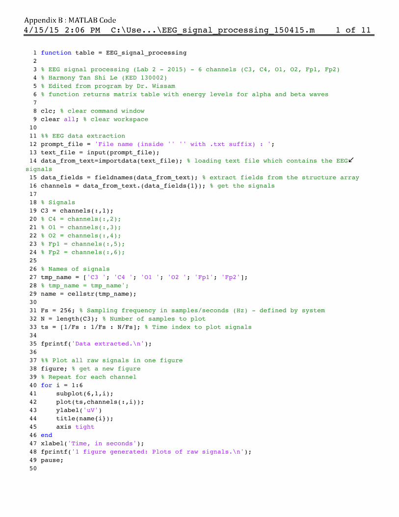
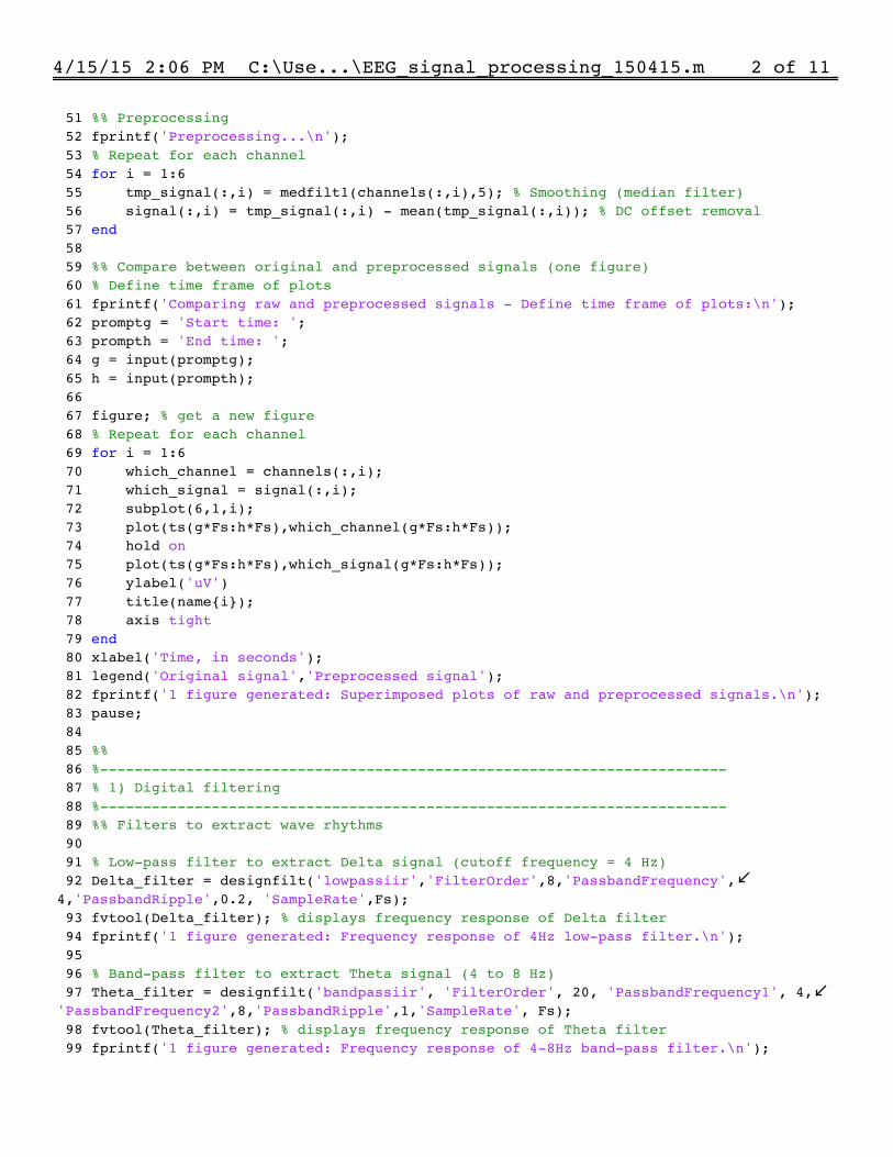
Two popular methods by which the five primary brain wavescan be extracted from the EEG signals in MATLAB are digitalfiltering and Wavelet transform. The MATLAB codes used toprocess the signals are attached in the Appendix B.

B. Extraction of different wave rhythms by digital filtering

Applying low-pass and band-pass IIR (infinite impulseresponse) filters according to the frequency bands for each


100 101 102 103 104 105 106 107 108 109 110

uV

-40-20

020

C3

100 101 102 103 104 105 106 107 108 109 110

uV

-20

0

20

Delta

100 101 102 103 104 105 106 107 108 109 110

uV

-5

0

5

Theta

100 101 102 103 104 105 106 107 108 109 110

uV

-505

Alpha

100 101 102 103 104 105 106 107 108 109 110

uV

-5

0

5Beta

Time, in seconds

100 101 102 103 104 105 106 107 108 109 110

uV

-1012

Gamma

(a) Digitally filtered C3

100 101 102 103 104 105 106 107 108 109 110

uV

-40-20

020

C3

100 101 102 103 104 105 106 107 108 109 110

uV

-20

0

20

Delta

100 101 102 103 104 105 106 107 108 109 110

uV

-10

0

10

Theta

100 101 102 103 104 105 106 107 108 109 110

uV

-10

0

10Alpha

100 101 102 103 104 105 106 107 108 109 110

uV

-5

0

5Beta

Time, in seconds

100 101 102 103 104 105 106 107 108 109 110

uV

-2

0

2

Gamma

(b) Wavelet transformed C3

Fig. 6. Time domain plots spanning 10 s from two different signal processing methods.

category of wave rhythm will individually extract the corre-sponding waveforms. The frequency responses for each filter,illustrating the variation of gain of the signal with respectto frequency, are shown in the Appendix A. Based on thesefigures, we know that the filters behave as desired, althoughthey are non-ideal. This is why a 4 Hz low-pass filter wasused to extract delta waves instead of a 0.5�4 Hz band-passfilter.

The delta, theta, alpha, beta and gamma waves extractedfrom each channel are represented in two ways, as time domainplots spanning 10 s and as spectrograms. The time domaingraphs describe the change in amplitude of the signal withrespect to time, while the spectrograms illustrate the variationin frequency of the signal with respect to time. The plots forC3 are shown in Fig. 6(a) and 7.

The time domain plots of the extracted rhythms from digitalfiltering have similar shapes with the general form of eachwave type introduced in Section I. The spectrograms for eachEEG rhythm show that the filters were effective in singlingout only the desired frequency bands, further corroboratingthat digital filters are a reliable technique of differentiatingEEG rhythms by frequency bands. However, as higher rangesof frequencies are filtered; we can see that filtered signals are’cleaner’ i.e. less undesired frequencies found.

C. Extraction of different wave rhythms by Wavelet transform

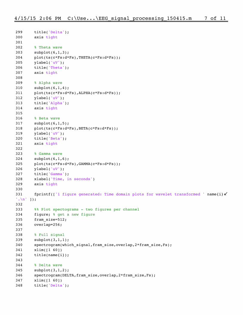
Daubechies-8 (db8) wavelet is used as the mother wavelet(Tsai, 2002), and a 5-level wavelet decomposition is performedto extract the five different wave rhythms. The delta, theta,alpha, beta and gamma waves extracted from each channel arerepresented as 10 s time domain plots and as spectrograms.

The plots for C3 are shown in Fig. 6(b) and 8. While the timedomain plots match the expected shapes and frequency foreach EEG rhythm, the spectrograms show that there are stillother frequencies besides the desired range present within eachextracted signal. In fact, in comparison with the spectrogramsfrom the digitally filtered signals, the Wavelet transform isless effective in rejecting frequencies outside the desired rangefor each type of rhythm. Between the time domain plots fordigital filters and Wavelet transform, the differences betweenthe processed signals become more apparent as the frequencyof the waveform increases.

D. Energy level

Physics tells us that work W is energy. Hence, if power Pis the time rate of work performed, then the integral of powerover time is the quantity of energy used for that work. Recallthe formula for instantaneous power is P = V I . Using Ohm’slaw, if we normalise the instantaneous power by assumingthat the resistance is R = 1 ⌦ (Valenti, 2005), this allows usto define power as either P = V 2 or P = I2. Thereforethe power of a signal f(t) is the square of that functionf2(t), where f(t) represents either voltage V or current I .By mathematics, we know that f2(t) = |f(t)|2, so it is notnecessary for us to derive function f to represent our EEGsignals; the amplitude of the signal at each point in timeis adequate to calculate the energy of the signal. Similarly,integration is simply the total area below a graph, or in ourcontext, the sum of all the elements in the data series.

Although we deduced the formula for signal energy levelbased on principle from Ohm’s law and the power law, this isactually the first part of Parseval’s theorem, which states that


Fig. 7. Spectrograms from digitally filtered C3 signal.

the energy carried by a signal f(t) is the integral of the squareof f(t) in the time domain (Eq. 1) (Sadiku & Alexander,2009).

W =

Z 1

�1f2(t) dt (1)

The rest of Parseval’s theorem is designed for calculatingthe energy of a signal in the frequency domain (Eq. 3) byapplying Fourier transform, which transforms a function in thetime domain into the frequency domain using integration (Eq.2). However, we already have the signals in the time domain,

Fig. 8. Spectrograms from Wavelet transformed C3 signal.

hence the first part of Parseval’s theorem will suffice for ourneeds.

F (!) =

Z 1

�1f(t)e�j!t dt (2)

W =1

2⇡

Z 1

�1|F (!)|2 d! (3)

Two plots for energy level against time for digitally filteredalpha and beta rhythms are shown in Fig. 9 and 10; Fp1 hasthe lowest energy levels while C3 has the highest energy levelsamong the six channels. The mean and standard deviations forthese two rhythms during 2-min eyes-closed (Activity No. 1)


and eyes-open (Activity No. 2) are calculated and presentedin Table II, with the values rounded to the nearest wholenumber. Based on these values, four clustered bar graphs areplotted in Excel for clearer comparison between alpha andbeta wave energy levels, as shown in Fig. 11, and 12. Alpharhythm has greater energy levels than beta rhythm during eyes-closed in all channels, while for eyes-open, the beta rhythmonly has higher energy levels for channels C3, C4, Fp1, andFp2. Unexpectedly, alpha rhythm still has higher energy levelsduring eyes-open for channels O1 and O2.

50 100 150 200 250 300 350

uV

×104

1

2

3

Alpha

50 100 150 200 250 300 350

uV

×105

0.5

1

1.5

2

Beta

Fig. 9. Energy level graph in time domain for C3.

50 100 150 200 250 300 350

uV

200

400

600

Alpha

50 100 150 200 250 300 350

uV

500

1000

1500

Beta

Fig. 10. Energy level graph in time domain for Fp1.

IV. DISCUSSION

Digital filters extract delta, theta, alpha, beta, and gammawaves by suppressing frequencies outside of their respectivefrequency ranges, hence selectively filtering out the appro-priate frequency bands much like how one would sieve outtea leaves with a tea strainer. On the other hand, Wavelettransform takes a signal and transforms it into a wavelet. Bydefinition, a wavelet is a mathematical function that representsthe signal in both time and frequency domains, and can beexpressed as an infinite sum of simpler functions or signals.The wavelet can then be divided (i.e. decomposed) into a

TABLE IIMEAN AND STANDARD DEVIATION FOR ALPHA AND BETA RHYTHMS

DURING 2-MIN EYES-CLOSED AND 2-MIN EYES-OPEN.

Channel EEG Eyes closed (2min) Eyes open (2min)rhythm Mean (µ) Std (�) Mean (µ) Std (�)

C3 Alpha 2443 1968 2955 2199Beta 1157 1209 6216 9564

C4 Alpha 1873 1509 3210 4958Beta 1156 1465 10734 19646

O1 Alpha 8827 9280 6129 6013Beta 2314 643 3373 1087

O2 Alpha 10249 11060 6382 6608Beta 1754 618 2874 1265

Fp1 Alpha 120 56 233 145Beta 134 42 434 257

Fp2 Alpha 144 68 250 112Beta 180 60 471 278

(a) Means (µ) of energy levels during 2-min eyes-closed.

(b) Standard deviations (�) of energy levels during 2-min eyes-closed.

Fig. 11. Bar graphs comparing energy levels for alpha and beta rhythmsduring eyes-closed.

number of components, with variable scales and frequencyranges, by using a basic set of functions known as themother wavelet, which is chosen for having the most accurateresemblance to the analysed signal (Kaushik & Sinha, 2012).In other words, Wavelet transform scales and translates asignal (Wolfram, n.d.) through dilation and translation of ananalysis function acting as a template for the generation ofthe decomposed wavelets (Sheng, 2000). However, this meansthat Wavelet transform is actually a form of advanced-level


(a) Means (µ) of energy levels during 2-min eyes-open.

(b) Standard deviation (�) of energy levels during 2-min eyes-open.

Fig. 12. Bar graphs comparing energy levels for alpha and beta rhythmsduring eyes-open.

approximation. This explains the differences in time domainplots and spectrograms from digital filter analysis and Wavelettransform analysis. To further corroborate our observations inSection III-C, the wave rhythms extracted from C3 by digitalfiltering and Wavelet transform are compared on the same timedomain plot in Fig. 13. Indeed, there are significant differencesbetween the filtered waves and the decomposed waves.

Due to the nature of Wavelet transform that uses the samemathematical constants throughout the analysis and is ableto be applied in frequency ranges beyond the scope of somedigital filters, many accept Wavelet transform as a bettermethod of EEG rhythm extraction compared to digital filtering(Xie, Pei, Jia, Chen, & Qiao, 2009). However, based on thespectrograms shown in Fig. 8, Wavelet transform appears tobe less effective in processing signals into pure extracts ofEEG rhythms, compared to digital filtering. Consequently, weused the alpha and beta signals processed by digital filtering,instead of Wavelet transform, in our analysis of the energylevels during eyes-closed and eyes-open.

As mentioned in Section I where we introduced the fiveprimary EEG rhythms, we expect alpha rhythm to increaseduring eyes-closed and decrease during eyes-open; in otherwords, beta rhythm should be higher than alpha rhythm duringeyes-open. However, channels O1-ref and O2-ref contradictthis hypothesis. This phenomenon is related to the location ofO1 and O2 i.e. the occipital lobe of the brain. While alpha

100 101 102 103 104 105 106 107 108 109 110

Delta

-20

0

20

C3

100 101 102 103 104 105 106 107 108 109 110

Theta

-10

0

10

100 101 102 103 104 105 106 107 108 109 110

Alp

ha

-10

0

10

100 101 102 103 104 105 106 107 108 109 110

Beta

-5

0

5

Time, in seconds

100 101 102 103 104 105 106 107 108 109 110

Gam

ma

-2

0

2

Digital filter

Wavelet Transform

Fig. 13. Comparing extracted signals from digital filtering and Wavelettransform, with amplitude scale in µV .

rhythm has thalamic origins (Domino et al., 2009), researchshows that alpha activity is highly centred in the occipitalregion; in fact, alpha rhythm is also commonly referred to asdominant occipital rhythm (Prinz & Vitiello, 1989). This isbecause alpha rhythm is found to be greatest (i.e. has highestamplitude) in the occipital region among all the brain regions.Indeed, this is quite apparent in Fig. 11 and 12. The occipitallobe is responsible for processing visual information; and sincealpha activity is tied to close-eyed wakeful relaxation, it makessense that alpha rhythm would be strongest in the visual cortex,which is situated in the occipital lobe. As a matter of fact,alpha waves were originally thought to indicate the occurrenceof idle activity in the visual cortex (Valipour, Shaligram,& Kulkarni, 2013). This explains why alpha rhythm is stillpredominant to beta rhythm in the occipital position.

Therefore, we were mistaken to assume that beta activitywould lead alpha activity in all channels during eyes closed.The important relation between these EEG rhythms and eyes-closed or eyes-open is that alpha rhythm becomes strongerduring eyes-closed and weaker during eyes-open, while betarhythm becomes stronger during eyes-open and weaker duringeyes-closed. This is proven by the increase in energy levels foralpha waves during eyes-closed compared to eyes-open, andthe increase in energy levels for beta waves during eyes-opencompared to eyes-closed.

V. CONCLUSION

EEG waves can be broken down into different waverhythms, each with different frequency bands and amplitude


ranges. The five primary EEG rhythms are delta (�), theta (✓),alpha (↵), beta (�), and gamma (�) waves.

EEG signals require preprocessing to remove noise and DCcomponents. EEG signal processing can be carried out througha number of techniques; two common methods include digitalfilters and Wavelet transform. While both have their merits, inthis case, digital filters perform better than Wavelet transformbecause the processed signals obtained through digital filtershave ’clearer’ spectrograms compared to those from Wavelettransform (i.e. the frequencies present within each signal haveless contamination with frequencies outside the desired rangefor that rhythm). Wavelet transform, while currently beyondthe scope of our understanding at the present moment, isan advanced form of approximation for extracting individualwave ’components’ i.e. different EEG rhythms from EEGsignals. Digital filters are a more direct approach to extractingEEG rhythms, although frequencies outside the desired rangeshould still be expected to pass through due to the practical,non-ideal nature of the filters. Therefore, the processed signalsfrom Wavelet transform and digital filtering should not beexpected to be identical; in fact, they produce quite differentresults, while still fulfilling the criteria for each class of EEGrhythm.

MATLAB is a highly useful and powerful mathematical andcomputational tool in digital signal processing. It is necessaryfor all interested in the signal processing field to be familiarwith the MATLAB language and environment.

In order to comprehensively analyse the change in alphaand beta activity during eyes-closed and eyes-open, the energylevels can be derived, from which the mean and standarddeviation are reliable statistical variables for both qualitativelyand quantitatively evaluating the relationship between visualactivity and EEG rhythms. However, it is not our intention toquantify the difference in energy levels, especially because thetrends in alpha and beta rhythm with respect to eyes-closed andeyes-open are remarkably obvious when plotted appropriately.Alpha activity increases during eyes-closed and decreasesduring eyes-open, while beta activity increases during eyes-open and decreases during eyes-closed. The occipital regionexhibits the highest power, and thus the greatest energy, inalpha waves; i.e. alpha rhythm is the dominant occipitalrhythm.

ACKNOWLEDGMENT

This template is based on IEEE journal format. Specialthanks to the lab lecturer, Dr. Wissam, the technician, Pn.Fairus Hanum, and Dr. Ng Siew Cheok.

REFERENCES

10/20 system positioning [Computer softwaremanual]. (n.d.). Retrieved from http://www.trans-cranial.com/local/manuals/10_20_pos_man_v1_0_pdf.pdf

Biocybernaut. (2011). Alpha brain waves. 4431Spellman Place, Victoria, British Columnbia V9C4C5, CANADA. Retrieved from http://www.biocybernaut.com/alpha-brain-waves/

Carr, J. J. (2001). Introduction to biomedical equipmenttechnology. In (4th ed., p. 372-382). Prentice Hall.

Domino, E. F., Ni, L., Thompson, M., Zhang, H., Shikata,H., Fukai, H., . . . Ohya, I. (2009, December). To-bacco smoking produces widespread dominant brainwave alpha frequency increases. International Jour-

nal of Psychophysiology, 74(3), 192-198. Re-trieved from http://www.ncbi.nlm.nih.gov/pubmed/19765621 doi: 10.1016/j.ijpsycho.2009.08.011

Dunn, P. (2014). Measurement and data analysis forengineering and science, third edition. In (p. 267-269). CRC Press. Retrieved from https://books.google.com.my/books?id=o23OBQAAQBAJ

E, N., & da Silva F., L. (1993). Electroencephalography: Basic

principles, clinical applications, and related fields. (5thed.). Williams & Wilkins.

Kaushik, G., & Sinha, H. (2012, September). Biomedicalsignal analysis through wavelets: A review.International Journal of Advanced Research in

Computer Science and Software Engineering

(IJARCSSE), 2(9), 422-428. Retrieved fromhttp://www.ijarcsse.com/docs/papers/9_September2012/Volume_2_issue_9/V2I900232A.pdf (ISSN 2277 128X)

Marieb, E. N., & Hoehn, K. (2013). Human anatomy andphysiology. In (p. 441-442). Pearson Education, Inc.

MathWorks. (n.d.). Matlab. Retrieved from http://www.mathworks.com/products/matlab/

Millet, D. (2002). The origins of eeg. In Seventh annual

meeting of the international society for the history of

the neurosciences (ishn). Retrieved from http://www.bri.ucla.edu/nha/ishn/ab24-2002.htm

Prinz, P. N., & Vitiello, M. V. (1989, November).Dominant occipital (alpha) rhythm frequency in earlystage alzheimer’s disease and depression. Electroen-

cephalography and Clinical Neurophysiology, 73(5),427-432. Retrieved from http://www.ncbi.nlm.nih.gov/pubmed/2479521

Repovs, G. (2010, August). Dealing with noise in eeg record-ing and data analysis. Informatica Medica Slovenica,15(1), 18-25. Retrieved from http://ims.mf.uni-lj.si/archive/15(1)/21.pdf

Sadiku, M. N. O., & Alexander, C. K. (2009). Fundamentalsof electric circuits. In (4th ed., p. 832-833). McGraw-Hill. (ISBN 9780073529554)

Sheng, Y. (2000). The transforms and applications handbook:Second edition. In A. D. Poularikas (Ed.), (chap. 10.Wavelet Transform). CRC Press LLC.

Sherman, S. M. (2006). Thalamus. Scholarpedia, 1(9), 1583.Steriade, M., & Llinas, R. R. (1988). The functional states

of the thalamus and the associated neuronal interplay.Physiological Reviews, 68(3), 649–742.

Tsai, S.-J. S. (2002). Power transformer partial discharge

(pd) acoustic signal detection using fiber sensors

and wavelet analysis, modeling, and simulation.

Retrieved from http://scholar.lib.vt.edu/theses/available/etd-12062002-152858/


unrestricted/Chapter4.pdf (Master’s Thesisfor Master of Science)

Valenti, M. C. (2005). The signals & systems workbook.

Retrieved from http://www.csee.wvu.edu/

˜natalias/ee329/workbook%202005.pdf(A companion workbook to EE 329 Signals & SystemsII, developed at West Virginia University)

Valipour, S., Shaligram, A. D., & Kulkarni, G. R.(2013, December). Spectral analysis of eeg sig-nal for detection of alpha rhythm with open andclosed eyes. International Journal of Engineering

and Innovative Technology (IJEIT), 3(6), 1-4. Re-trieved from http://www.ijeit.com/Vol%203/Issue%206/IJEIT1412201312_22.pdf (ISSN2277-3754)

Wolfram. (n.d.). Wavelet analysis. Retrievedfrom https://reference.wolfram.com/language/guide/Wavelets.html

Xie, T., Pei, J., Jia, C., Chen, S., & Qiao, D. (2009, August).Comparison of digital filter and wavelet transform forextracting electroencephalogram rhythm. Journal of

Biomedical Engineering, 26(4), 743-747.

1

Frequency (Hz)

0 20 40 60 80 100 120

Magnitu

de (

dB

)

-400

-350

-300

-250

-200

-150

-100

-50

0

Magnitude Response (dB)

4

4Hz low-pass filter

to extract delta rhythm

Frequency (Hz)

0 20 40 60 80 100 120

Magnitu

de (

dB

)

-500

-400

-300

-200

-100

0


84

4-8Hz band-pass filter

to extract theta rhythm

Frequency (Hz)

0 20 40 60 80 100 120

Magnitu

de (

dB

)

-500

-400

-300

-200

-100

0


138


to extract alpha rhythm

Frequency (Hz)

0 20 40 60 80 100 120

Magnitu

de (

dB

)

-400

-350

-300

-250

-200

-150

-100

-50

0


13 30


to extract beta rhythm

Frequency (Hz)

0 20 40 60 80 100 120

Magnitu

de (

dB

)

-200

-150

-100

-50

0


30


to extract gamma rhythm

Turing

Appendix A : Frequency responses for digital filters (generated using MATLAB)

Turing

4/15/15 2:06 PM C:\Use...\EEG_signal_processing_150415.m 1 of 11

1 function table = EEG_signal_processing 2 3 % EEG signal processing (Lab 2 - 2015) - 6 channels (C3, C4, O1, O2, Fp1, Fp2) 4 % Harmony Tan Shi Le (KED 130002) 5 % Edited from program by Dr. Wissam 6 % function returns matrix table with energy levels for alpha and beta waves 7 8 clc; % clear command window 9 clear all; % clear workspace 10 11 %% EEG data extraction 12 prompt_file = 'File name (inside '' '' with .txt suffix) : '; 13 text_file = input(prompt_file); 14 data_from_text=importdata(text_file); % loading text file which contains the EEG signals 15 data_fields = fieldnames(data_from_text); % extract fields from the structure array 16 channels = data_from_text.(data_fields{1}); % get the signals 17 18 % Signals 19 C3 = channels(:,1); 20 % C4 = channels(:,2); 21 % O1 = channels(:,3); 22 % O2 = channels(:,4); 23 % Fp1 = channels(:,5); 24 % Fp2 = channels(:,6); 25 26 % Names of signals 27 tmp_name = ['C3 '; 'C4 '; 'O1 '; 'O2 '; 'Fp1'; 'Fp2']; 28 % tmp_name = tmp_name'; 29 name = cellstr(tmp_name); 30 31 Fs = 256; % Sampling frequency in samples/seconds (Hz) - defined by system 32 N = length(C3); % Number of samples to plot 33 ts = [1/Fs : 1/Fs : N/Fs]; % Time index to plot signals 34 35 fprintf('Data extracted.\n'); 36 37 %% Plot all raw signals in one figure 38 figure; % get a new figure 39 % Repeat for each channel 40 for i = 1:6 41 subplot(6,1,i); 42 plot(ts,channels(:,i)); 43 ylabel('uV') 44 title(name{i}); 45 axis tight 46 end 47 xlabel('Time, in seconds'); 48 fprintf('1 figure generated: Plots of raw signals.\n'); 49 pause; 50

Turing

Appendix B : MATLAB Code


51 %% Preprocessing 52 fprintf('Preprocessing...\n'); 53 % Repeat for each channel 54 for i = 1:6 55 tmp_signal(:,i) = medfilt1(channels(:,i),5); % Smoothing (median filter) 56 signal(:,i) = tmp_signal(:,i) - mean(tmp_signal(:,i)); % DC offset removal 57 end 58 59 %% Compare between original and preprocessed signals (one figure) 60 % Define time frame of plots 61 fprintf('Comparing raw and preprocessed signals - Define time frame of plots:\n'); 62 promptg = 'Start time: '; 63 prompth = 'End time: '; 64 g = input(promptg); 65 h = input(prompth); 66 67 figure; % get a new figure 68 % Repeat for each channel 69 for i = 1:6 70 which_channel = channels(:,i); 71 which_signal = signal(:,i); 72 subplot(6,1,i); 73 plot(ts(g*Fs:h*Fs),which_channel(g*Fs:h*Fs)); 74 hold on 75 plot(ts(g*Fs:h*Fs),which_signal(g*Fs:h*Fs)); 76 ylabel('uV') 77 title(name{i}); 78 axis tight 79 end 80 xlabel('Time, in seconds'); 81 legend('Original signal','Preprocessed signal'); 82 fprintf('1 figure generated: Superimposed plots of raw and preprocessed signals.\n'); 83 pause; 84 85 %% 86 %------------------------------------------------------------------------- 87 % 1) Digital filtering 88 %------------------------------------------------------------------------- 89 %% Filters to extract wave rhythms 90 91 % Low-pass filter to extract Delta signal (cutoff frequency = 4 Hz) 92 Delta_filter = designfilt('lowpassiir','FilterOrder',8,'PassbandFrequency',4,'PassbandRipple',0.2, 'SampleRate',Fs); 93 fvtool(Delta_filter); % displays frequency response of Delta filter 94 fprintf('1 figure generated: Frequency response of 4Hz low-pass filter.\n'); 95 96 % Band-pass filter to extract Theta signal (4 to 8 Hz) 97 Theta_filter = designfilt('bandpassiir', 'FilterOrder', 20, 'PassbandFrequency1', 4, 'PassbandFrequency2',8,'PassbandRipple',1,'SampleRate', Fs); 98 fvtool(Theta_filter); % displays frequency response of Theta filter 99 fprintf('1 figure generated: Frequency response of 4-8Hz band-pass filter.\n');


100 101 % Band-pass filter to extract Alpha signal (8 to 13 Hz)102 Alpha_filter = designfilt('bandpassiir', 'FilterOrder', 20, 'PassbandFrequency1', 8, 'PassbandFrequency2',13,'PassbandRipple',1,'SampleRate', Fs);103 fvtool(Alpha_filter); % displays frequency response of Alpha filter104 fprintf('1 figure generated: Frequency response of 8-13Hz band-pass filter.\n');105 106 % Band-pass filter to extract Beta signal (13 to 30 Hz)107 Beta_filter = designfilt('bandpassiir', 'FilterOrder', 20, 'PassbandFrequency1', 13, 'PassbandFrequency2',30,'PassbandRipple',1,'SampleRate', Fs);108 fvtool(Beta_filter); % displays frequency response of Beta filter109 fprintf('1 figure generated: Frequency response of 13-30Hz band-pass filter.\n');110 111 % Band-pass filter to extract Gamma signal (30 to 100 Hz)112 Gamma_filter = designfilt('bandpassiir', 'FilterOrder', 20, 'PassbandFrequency1', 30, 'PassbandFrequency2',100,'PassbandRipple',1,'SampleRate', Fs);113 fvtool(Gamma_filter); % displays frequency response of Gamma filter114 fprintf('1 figure generated: Frequency response of 30-100Hz band-pass filter.\n');115 116 pause;117 118 %% Signal processing119 120 % Define time frame of plots121 fprintf('Digital filtering (DF) - Define time frame of plots:\n');122 prompta = 'Start time: ';123 promptb = 'End time: ';124 a = input(prompta);125 b = input(promptb);126 127 % Apply filters to each channel128 for i = 1:6129 delta(:,i) = filter(Delta_filter,signal(:,i));130 theta(:,i) = filter(Theta_filter,signal(:,i));131 alpha(:,i) = filter(Alpha_filter,signal(:,i));132 beta(:,i) = filter(Beta_filter,signal(:,i));133 gamma(:,i) = filter(Gamma_filter,signal(:,i));134 end135 136 % Repeat for each channel137 for i = 1:6138 % Identify channel139 which_signal = signal(:,i);140 which_delta = delta(:,i); 141 which_theta = theta(:,i);142 which_alpha = alpha(:,i);143 which_beta = beta(:,i);144 which_gamma = gamma(:,i);145 146 %% Plot time domain of signals - one figure per channel147 figure; % get a new figure


148 149 % Full signal150 subplot(6,1,1);151 plot(ts(a*Fs:b*Fs),which_signal(a*Fs:b*Fs));152 ylabel('uV')153 title(name{i});154 axis tight155 156 % Delta wave157 subplot(6,1,2);158 plot(ts(a*Fs:b*Fs),which_delta(a*Fs:b*Fs));159 ylabel('uV')160 title('Delta');161 axis tight162 163 % Theta wave164 subplot(6,1,3);165 plot(ts(a*Fs:b*Fs),which_theta(a*Fs:b*Fs));166 ylabel('uV')167 title('Theta');168 axis tight169 170 % Alpha wave171 subplot(6,1,4);172 plot(ts(a*Fs:b*Fs),which_alpha(a*Fs:b*Fs));173 ylabel('uV')174 title('Alpha');175 axis tight176 177 % Beta wave178 subplot(6,1,5);179 plot(ts(a*Fs:b*Fs),which_beta(a*Fs:b*Fs));180 ylabel('uV')181 title('Beta');182 axis tight183 184 % Gamma wave185 subplot(6,1,6);186 plot(ts(a*Fs:b*Fs),which_gamma(a*Fs:b*Fs));187 xlabel('Time, in seconds')188 ylabel('uV')189 title('Gamma');190 axis tight191 192 fprintf(['1 figure generated: Time domain plots for digitally filtered ' name{i} '.\n' ]);193 194 %% Plot spectograms - 2 figures per channel195 figure; % get a new figure196 fram_size=512;197 overlap=256;


198 199 % Full signal200 subplot(3,1,1);201 spectrogram(signal(:,i),fram_size,overlap,2*fram_size,Fs);202 xlim([1 60])203 title(name{i});204 205 % Delta wave206 subplot(3,1,2);207 spectrogram(which_delta,fram_size,overlap,2*fram_size,Fs);208 xlim([1 60])209 title('Delta');210 211 % Theta wave212 subplot(3,1,3);213 spectrogram(which_theta,fram_size,overlap,2*fram_size,Fs);214 xlim([1 60])215 title('Theta');216 217 figure; % get a new figure218 fram_size=512;219 overlap=256;220 221 % Alpha wave222 subplot(3,1,1);223 spectrogram(which_alpha,fram_size,overlap,2*fram_size,Fs);224 xlim([1 60])225 title('Alpha');226 227 % Beta wave228 subplot(3,1,2);229 spectrogram(which_beta,fram_size,overlap,2*fram_size,Fs);230 xlim([1 60])231 title('Beta');232 233 % Gamma wave234 subplot(3,1,3);235 spectrogram(which_gamma,fram_size,overlap,2*fram_size,Fs);236 xlim([1 60])237 title('Gamma');238 239 fprintf(['2 figures generated: Spectograms for digitally filtered ' name{i} '.\n' ]);240 pause;241 end242 243 %%244 %-------------------------------------------------------------------------245 % 2) Wavelet Transform (WT)246 %-------------------------------------------------------------------------247 function wavelet_transform


248 % Define the wavelet's name and the level for decomposition249 waveletName='db8';250 level=5;251 252 % Multilevel 1-D wavelet decomposition253 [C,L]=wavedec(which_signal,level,waveletName);254 255 % 1-D detail coefficients for ch0256 cD1 = detcoef(C,L,1);257 cD2 = detcoef(C,L,2); %GAMMA258 cD3 = detcoef(C,L,3); %BETA259 cD4 = detcoef(C,L,4); %ALPHA260 cD5 = detcoef(C,L,5); %THETA261 cA5 = appcoef(C,L,waveletName,5); %DELTA262 263 % Reconstruct single branch from 1-D wavelet coefficients264 D1 = wrcoef('d',C,L,waveletName,1);265 GAMMA = wrcoef('d',C,L,waveletName,2); %GAMMA266 BETA = wrcoef('d',C,L,waveletName,3); %BETA267 ALPHA = wrcoef('d',C,L,waveletName,4); %ALPHA268 THETA = wrcoef('d',C,L,waveletName,5); %THETA269 DELTA = wrcoef('a',C,L,waveletName,5); %DELTA270 end271 272 % Define time frame of plots273 fprintf('Wavelet Transform (WT) - Define time frame of plots:\n');274 promptc = 'Start time: ';275 promptd = 'End time: ';276 c = input(promptc);277 d = input(promptd);278 279 % Repeat for each channel280 for i = 1:6281 which_signal = signal(:,i); % identify channel for analysis282 283 wavelet_transform % apply WT to current channel284 285 %% Plot time domain of signals - one figure per channel286 figure; % get a new figure287 288 % Full signal289 subplot(6,1,1);290 plot(ts(c*Fs:d*Fs),which_signal(c*Fs:d*Fs));291 ylabel('uV');292 title(name{i});293 axis tight294 295 % Delta wave296 subplot(6,1,2);297 plot(ts(c*Fs:d*Fs),DELTA(c*Fs:d*Fs));298 ylabel('uV');


299 title('Delta');300 axis tight301 302 % Theta wave303 subplot(6,1,3);304 plot(ts(c*Fs:d*Fs),THETA(c*Fs:d*Fs));305 ylabel('uV');306 title('Theta');307 axis tight308 309 % Alpha wave310 subplot(6,1,4);311 plot(ts(c*Fs:d*Fs),ALPHA(c*Fs:d*Fs));312 ylabel('uV');313 title('Alpha');314 axis tight315 316 % Beta wave317 subplot(6,1,5);318 plot(ts(c*Fs:d*Fs),BETA(c*Fs:d*Fs));319 ylabel('uV');320 title('Beta');321 axis tight322 323 % Gamma wave324 subplot(6,1,6);325 plot(ts(c*Fs:d*Fs),GAMMA(c*Fs:d*Fs));326 ylabel('uV');327 title('Gamma');328 xlabel('Time, in seconds')329 axis tight330 331 fprintf(['1 figure generated: Time domain plots for wavelet transformed ' name{i} '.\n' ]);332 333 %% Plot spectograms - two figures per channel334 figure; % get a new figure335 fram_size=512;336 overlap=256;337 338 % Full signal339 subplot(3,1,1);340 spectrogram(which_signal,fram_size,overlap,2*fram_size,Fs);341 xlim([1 60])342 title(name{i});343 344 % Delta wave345 subplot(3,1,2);346 spectrogram(DELTA,fram_size,overlap,2*fram_size,Fs);347 xlim([1 60])348 title('Delta');


349 350 % Theta wave351 subplot(3,1,3);352 spectrogram(THETA,fram_size,overlap,2*fram_size,Fs);353 xlim([1 60])354 title('Theta');355 356 figure; % get a new figure357 fram_size=512;358 overlap=256;359 360 % Alpha wave361 subplot(3,1,1);362 spectrogram(ALPHA,fram_size,overlap,2*fram_size,Fs);363 xlim([1 60])364 title('Alpha');365 366 % Beta wave367 subplot(3,1,2);368 spectrogram(BETA,fram_size,overlap,2*fram_size,Fs);369 xlim([1 60])370 title('Beta');371 372 % Gamma wave373 subplot(3,1,3);374 spectrogram(GAMMA,fram_size,overlap,2*fram_size,Fs);375 xlim([1 60])376 title('Gamma');377 378 fprintf(['2 figures generated: Spectograms for wavelet transformed ' name{i} '.\n' ]);379 pause;380 end381 382 %% Compare between digital filter and Wavelet Transform (one figure)383 384 % Define time frame of plots385 fprintf('Compare DF with WT - Define time frame of plots:\n');386 prompte = 'Start time: ';387 promptf = 'End time: ';388 e = input(prompte);389 f = input(promptf);390 391 for i = 1:6 392 % Identify channel393 which_signal = signal(:,i);394 395 % Digital filtered signals396 which_delta = delta(:,i); 397 which_theta = theta(:,i);398 which_alpha = alpha(:,i);


399 which_beta = beta(:,i);400 which_gamma = gamma(:,i);401 402 % Apply WT to current channel403 wavelet_transform404 405 figure; % get a new figure406 407 % Delta wave408 subplot(5,1,1);409 plot(ts(e*Fs:f*Fs),which_delta(e*Fs:f*Fs)); % digital filter410 hold on411 plot(ts(e*Fs:f*Fs),DELTA(e*Fs:f*Fs)); % wavelet transform412 ylabel('Delta');413 title(name{i});414 axis tight415 416 % Theta wave417 subplot(5,1,2);418 plot(ts(e*Fs:f*Fs),which_theta(e*Fs:f*Fs));419 hold on420 plot(ts(e*Fs:f*Fs),THETA(e*Fs:f*Fs));421 ylabel('Theta');422 axis tight423 424 % Alpha wave425 subplot(5,1,3);426 plot(ts(e*Fs:f*Fs),which_alpha(e*Fs:f*Fs));427 hold on428 plot(ts(e*Fs:f*Fs),ALPHA(e*Fs:f*Fs));429 ylabel('Alpha');430 axis tight431 432 % Beta wave433 subplot(5,1,4);434 plot(ts(e*Fs:f*Fs),which_beta(e*Fs:f*Fs));435 hold on436 plot(ts(e*Fs:f*Fs),BETA(e*Fs:f*Fs));437 ylabel('Beta');438 axis tight439 440 % Gamma wave441 subplot(5,1,5);442 plot(ts(e*Fs:f*Fs),which_gamma(e*Fs:f*Fs));443 hold on444 plot(ts(e*Fs:f*Fs),GAMMA(e*Fs:f*Fs));445 xlabel('Time, in seconds')446 ylabel('Gamma');447 axis tight448 legend('Digital filter','Wavelet Transform');449


450 fprintf(['1 figure generated: Time domain comparison plot for ' name{i} '.\n']);451 pause;452 end453 454 %% Energy level of signal for alpha and beta rhythms455 % Using digitally filtered signals456 fprintf('Calculating energy level for DF alpha and beta rhythms...');457 458 % Repeat for each channel459 for i = 1:6460 % Identify channel461 which_alpha = alpha(:,i);462 which_beta = beta(:,i);463 464 % Square functions to get power of signal465 p_alpha = which_alpha.^2;466 p_beta = which_beta.^2;467 468 % Sum power over time (1 second) to get energy of signal per second469 n = N/Fs;470 Ts = (1:n);471 w_alpha = sum(reshape(p_alpha,Fs,n));472 w_beta = sum(reshape(p_beta,Fs,n));473 474 %% Plot energy spectrum for each channel (one figure per channel)475 figure; % get a new figure476 477 % Alpha wave478 subplot(2,1,1);479 plot(Ts,w_alpha);480 ylabel('uV')481 title('Alpha');482 axis tight483 484 % Beta wave485 subplot(2,1,2);486 plot(Ts,w_beta);487 ylabel('uV')488 title('Beta');489 axis tight490 491 fprintf(['1 figure generated: Energy level plots in time domain for ' name{i} '.\n']);492 493 %% Calculate mean and standard deviation of energy levels494 495 % Eyes closed between 0s - 120s496 M_closed_alpha = mean(w_alpha(1:120)); % mean for alpha497 S_closed_alpha = std(w_alpha(1:120)); % standard deviation for alpha498 M_closed_beta = mean(w_beta(1:120)); % mean for beta499 S_closed_beta = std(w_beta(1:120)); % standard deviation for beta


500 501 % Eyes open between 120s - 240s502 M_open_alpha = mean(w_alpha(120:240));503 S_open_alpha = std(w_alpha(120:140));504 M_open_beta = mean(w_beta(120:240));505 S_open_beta = std(w_beta(120:140));506 507 % Save values into 4-by-12 matrix508 % Each channel has two columns509 % First column of each channel for alpha510 table(:,i+i-1) = [511 M_closed_alpha;512 S_closed_alpha;513 M_open_alpha;514 S_open_alpha;515 ];516 % Second column of each channel for beta517 table(:,i+i) = [518 M_closed_beta;519 S_closed_beta;520 M_open_beta;521 S_open_beta;522 ];523 524 pause;525 end526 527 fprintf('Mean and standard deviation of energy levels for alpha and beta rhythms for eyes-closed and eyes-open - saved as matrix ans');528 529 end530

EEG Signal Processing

Documents

Transcript of EEG Signal Processing