Fitness landscapes in orchids: Parametric and non-parametric approaches.

LANKESTERIANA 11(3): 355—362. 2011.

FITNESS LANDSCAPES IN ORCHIDS: PARAMETRIC AND NON-PARAMETRICAPPROACHES

Raymond L. TRembLay1,2,3

1 Department of Biology, 100 carr. 908, University of Puerto Rico – Humacao Campus, Humacao, PR 00792, U.S.A.;

2 Department of Biology, P. O. Box 23360, San Juan, Puerto Rico,00931-3360, U.S.A.; 3 Crest-Catec, Center for Applied Tropical Ecology and Conservation,

P. O. Box 23341, University of Puerto Rico, Río Piedras, PR 00931-3341, U.S.A.

absTRacT. Natural selection and genetic drift are the two processes that can lead to cladogenesis. Without a doubt the great diversity and floral adaptation to specific pollinators are likely consequences of natural selection. Detecting natural selection in the wild requires measuring fitness advantage for specific characters. However, few published orchid studies demonstrate that floral characters are influenced by natural selection. If selection is temporal or weak, then this may explain why we rarely find selection on floral characters. Alternatively, selection on a character may not follow commonly used mathematical models that are based on linear, disruptive, and stabilizing selection and serve as null models. Moreover, fitness advantages are usually tested on general models, which assume that the parameters are normally distributed. If we forego the idea that selection followsspecific mathematical models and Gaussian distribution and that all types of selection landscapes and other types of distributions (binomial, Poisson) are possible, we may discover evidence that the process of selection does play a role in explaining the great diversity of orchids. Here I show and compare the use of traditional and non-parametric approaches for measuring selection of floral characters. I hypothesize that many characters are likely to be influenced by selection but, using traditional approaches, will fail to observe selection on the measured characters, whereas non-parametric approaches may be more useful as a tool to detect selection differences among characters.

Resumen. La selección natural y la deriva genética son dos procesos que pueden conducir a la cladogénesis. Sin duda, la gran diversidad y adaptación floral a polinizadores específicos es sorprendente y es una consecuencia de la selección natural. La observación de la selección natural en el medio ambiente silvestre requiere el medir la ventaja de su idoneidad para ciertos caracteres específicos; sin embargo, hay pocos trabajos científicos publicados que apoyan la idea de que los caracteres están bajo la influencia de la selección de caracteres florales en las orquídeas. Una de las razones que podría explicar porqué raramente identificamos la selección en caracteres florales es que la selección puede ser temporal. Una hipótesis alternativa es que la selección de caracteres podría no seguir los modelos básicos que se basan en selección linear, disruptiva, y estabilizadora. Estas ventajas de idoneidad son usualmente puestas a prueba con modelos generales que asumen que los parámetros están distribuidos en forma normal. Si nos olvidamos de la idea de que la selección sigue tal tipo de distribución Gaussiana y que todos los tipos de panoramas de selección son posibles, podríamos descubrir evidencia de que el proceso de selección si tiene un rol en la explicación de la gran variedad de orquídeas. Aquí demuestro y comparo el uso del enfoque tradicional y no-paramétrico para medir la selección de caracteres florales con ejemplos de Tolumnia variegata, Lepanthes rupestris, y Caladenia valida.

Key WoRds: orchid flowers, natural selection, fitness advantage, mathematical models

Evolution is a consequence of random (genetic drift) or non-random processes (natural selection). Natural selection requires the presence of variation, heritability of the variation, and fitness differences among individuals in a panmictic population (Endler,

1986). When we discuss fitness in an evolutionary context we are referring to the ability of an individual to leave viable offspring. However, in most cases the ability to measure the number of such offspring in the next generation is often limited because of the difficulty

LANKESTERIANA 11(3), December 2011. © Universidad de Costa Rica, 2011.

356 LANKESTERIANA

in monitoring individuals throughout their lifespan. For example, to evaluate the true lifetime fitness of an orchid would require monitoring orchid seeds, which cannot be seen or followed in the wild (in most cases) or assigned to specific parents in a population unless genetic markers are used. Consequently, fitness is measured through surrogate indices, such as number of flowers, number of pollen (pollinaria) removed and deposited on the stigma, number of fruits, number of seeds, length of the life span, etc. It is assumed that the number of flowers and pollinaria removed or deposited will be positively correlated with number of fruits. The number of these fruits, in turn, is likely positively correlated with the number of seeds produced and ultimately the number of viable offspring sired. In the same way, it is assumed that life span is positively correlated with lifetime reproductive success and that longerlived individuals will produce more offspring. These surrogate variables of fitness have been shown to be correlated with evolutionary fitness. Traditionally the models of natural selection that have been described follow a linear (positive or negative) or quadratic relationship (stabilizing and disruptive selection) between the character of interest and the fitness index (Box 1: Kingsolver et al., 2001). These relationships are used as null models for testing if a fitness advantage among morphologically different individuals is present. Such models are based on the idea that natural selection follows mathematical equations. Consequently, they require assumptions on how natural selection functions, the most serious of which is that phenotypic and natural selection follow pre-established mathematical equations. In a simple example, let us assume that plants with larger inflorescences have higher fitness (fruit set). A model of selection built from a linear equation would predict that selection should result in larger and larger inflorescences. However, biological limitations are likely to be present; perhaps large inflorescences do not attract more pollinators than intermediate inflorescences so that an asymptote should be reached. The advantage for large inflorescences may be tempered if high production of flowers and fruits results in high energetic costs that negatively affect the likelihood of future mating events.

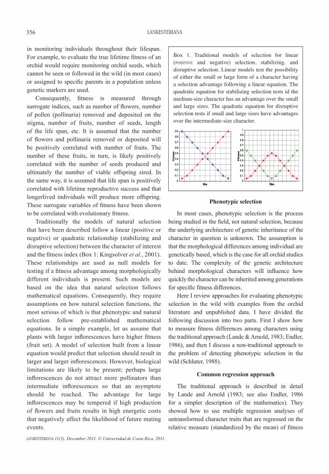
Box 1. Traditional models of selection for linear (positive and negative) selection, stabilizing, and disruptive selection. Linear models test the possibility of either the small or large form of a character having a selection advantage following a linear equation. The quadratic equation for stabilizing selection tests id the medium-size character has an advantage over the small and large sizes. The quadratic equation for disruptive selection tests if small and large sizes have advantages over the intermediate-size character.

Phenotypic selection

In most cases, phenotypic selection is the process being studied in the field, not natural selection, because the underlying architecture of genetic inheritance of the character in question is unknown. The assumption is that the morphological differences among individual are genetically based, which is the case for all orchid studies to date. The complexity of the genetic architecture behind morphological characters will influence how quickly the character can be inherited among generations for specific fitness differences. Here I review approaches for evaluating phenotypic selection in the wild with examples from the orchid literature and unpublished data. I have divided the following discussion into two parts. First I show how to measure fitness differences among characters using the traditional approach (Lande & Arnold, 1983; Endler, 1986), and then I discuss a non-traditional approach to the problem of detecting phenotypic selection in the wild (Schluter, 1988).

Common regression approach

The traditional approach is described in detail by Lande and Arnold (1983; see also Endler, 1986 for a simpler description of the mathematics). They showed how to use multiple regression analyses of untransformed character traits that are regressed on the relative measure (standardized by the mean) of fitness


TRembLay — Fitness landscapes in orchids 357

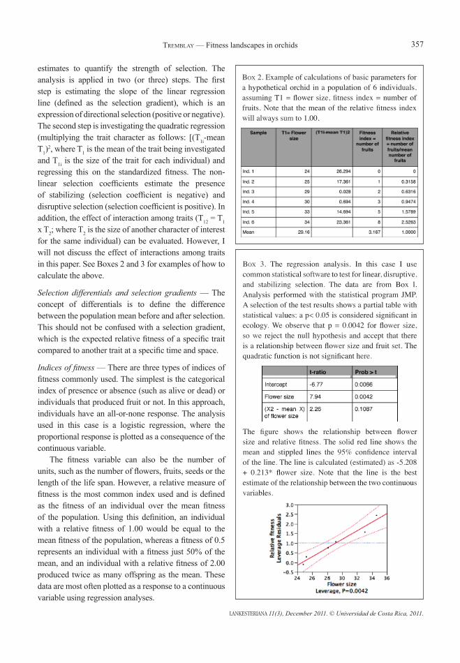
Box 2. Example of calculations of basic parameters for a hypothetical orchid in a population of 6 individuals, assuming T1 = flower size, fitness index = number of fruits. Note that the mean of the relative fitness index will always sum to 1.00.

estimates to quantify the strength of selection. The analysis is applied in two (or three) steps. The first step is estimating the slope of the linear regression line (defined as the selection gradient), which is an expression of directional selection (positive or negative). The second step is investigating the quadratic regression (multiplying the trait character as follows: [(T1i-mean T1)

2, where T1 is the mean of the trait being investigated and T1i is the size of the trait for each individual) and regressing this on the standardized fitness. The non-linear selection coefficients estimate the presence of stabilizing (selection coefficient is negative) and disruptive selection (selection coefficient is positive). In addition, the effect of interaction among traits (T12 = T1 x T2; where T2 is the size of another character of interest for the same individual) can be evaluated. However, I will not discuss the effect of interactions among traits in this paper. See Boxes 2 and 3 for examples of how to calculate the above.

Selection differentials and selection gradients — The concept of differentials is to define the difference between the population mean before and after selection. This should not be confused with a selection gradient, which is the expected relative fitness of a specific trait compared to another trait at a specific time and space.

Indices of fitness — There are three types of indices of fitness commonly used. The simplest is the categorical index of presence or absence (such as alive or dead) or individuals that produced fruit or not. In this approach, individuals have an all-or-none response. The analysis used in this case is a logistic regression, where the proportional response is plotted as a consequence of the continuous variable. The fitness variable can also be the number of units, such as the number of flowers, fruits, seeds or the length of the life span. However, a relative measure of fitness is the most common index used and is defined as the fitness of an individual over the mean fitness of the population. Using this definition, an individual with a relative fitness of 1.00 would be equal to the mean fitness of the population, whereas a fitness of 0.5 represents an individual with a fitness just 50% of the mean, and an individual with a relative fitness of 2.00 produced twice as many offspring as the mean. These data are most often plotted as a response to a continuous variable using regression analyses.

Box 3. The regression analysis. In this case I use common statistical software to test for linear, disruptive, and stabilizing selection. The data are from Box l. Analysis performed with the statistical program JMP. A selection of the test results shows a partial table with statistical values; a p< 0.05 is considered significant in ecology. We observe that p = 0.0042 for flower size, so we reject the null hypothesis and accept that there is a relationship between flower size and fruit set. The quadratic function is not significant here.

The figure shows the relationship between flower size and relative fitness. The solid red line shows the mean and stippled lines the 95% confidence interval of the line. The line is calculated (estimated) as -5.208 + 0.213* flower size. Note that the line is the best estimate of the relationship between the two continuous variables.


358 LANKESTERIANA

Assumptions of the regression analysis — Regression analysis has a number of assumptions. For example, the traditional linear model assumes five conditions: 1) for every size of some character (x-axis) there is a population of response that follows a normal distribution; 2) across the size variable (x-axis) the variance is equal, so that there is homogeneity of variance for each x; 3) the mean of y values falls in a straight line with all the other means of y values; 4) when the data are collected, individuals are selected at random; and 5) there is no error in the measurement of x. These are the conditions for testing if there is a linear relationship among two variables. If the quadratic function is the null hypothesis, then the relationship must fit that equation (Zar, 1999).

Non-parametric approach

The limitation to the parametric approach is that fitness advantage may not fit the null mathematical equations. In other words, the fitness landscape may be some other function that does not follow a linear or quadratic equation. An alternative approach is to eval uate the best possible fit of the data to equations using a cubic spline approach and allow the data to inform us of the best-fit line. The objective is to construct models of relationship of the explanatory variable that best describes the response variable. Using this approach we do not assume that relationship between x and y follows a specific mathematical equation (linear, quadratic, etc). This method, which has been applied to evolutionary models by Schluter (1988), Schluter and Nychka (1994), and Tremblay et al. (2010), is a two-step process and can be applied using Windows software GLMS, developed by Schluter and Nychka (1994) and found on Schluter’s website (http://www.zoology.ubc.ca/~schluter/software.html). The first steps are to determine the best level of complexity of the equation. A large range of possible lambda and two indices of the fit of the complexity of equation are used, OCR and GVC scores (Schluter, 1988). One chooses the lowest value and applies this value for determining the relationship between the explanatory variable (phenotype) and fitness response (e.g. fruit set). The mathematics behind the application of the cubic spline is complex and not the goal of this paper. Those interested should search the references cited above as well as cubic spline on the Internet for an

introduction to the concept. The process of performing the analysis is presented in Boxes 4-7.

Caveats of the cubic spline approach — The down side of this non-parametric approach using cubic spline for determining the best line is that we do not have a null model for how to test the observed data. An additional limitation is that environmental effects can result in biases due to environmental covariances between traits and fitness (Rauscher, 1992), although this is applicable to both methods. The challenge is detecting when a specific factor of the environment influences not only the phenotype but also the fitness of that phenotype. For example, let us consider a hypothetical epiphytic orchid. When the orchid is growing in a section of a tree where the substrate is decomposing, nutrient availability is likely to be greater. So plants may produce more flowers or larger flowers, which increases fruit or seed production if fitness is influenced by number of flowers or size. In this scenario there

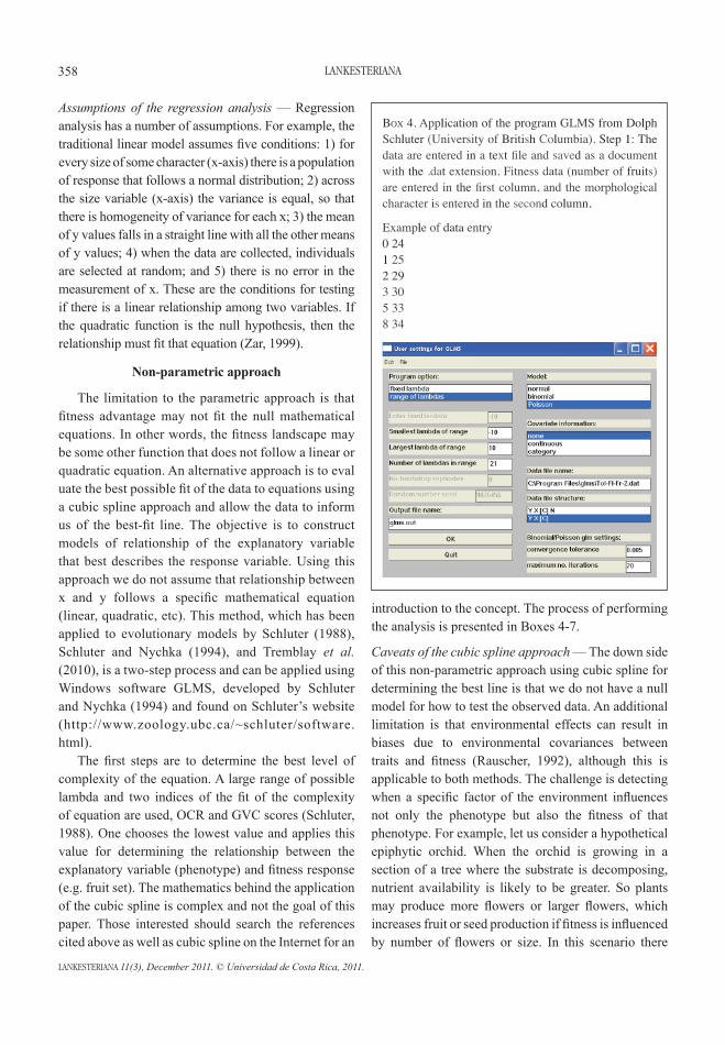
Box 4. Application of the program GLMS from Dolph Schluter (University of British Columbia). Step 1: The data are entered in a text file and saved as a document with the .dat extension. Fitness data (number of fruits) are entered in the first column, and the morphological character is entered in the second column.

Example of data entry0 241 252 293 305 338 34



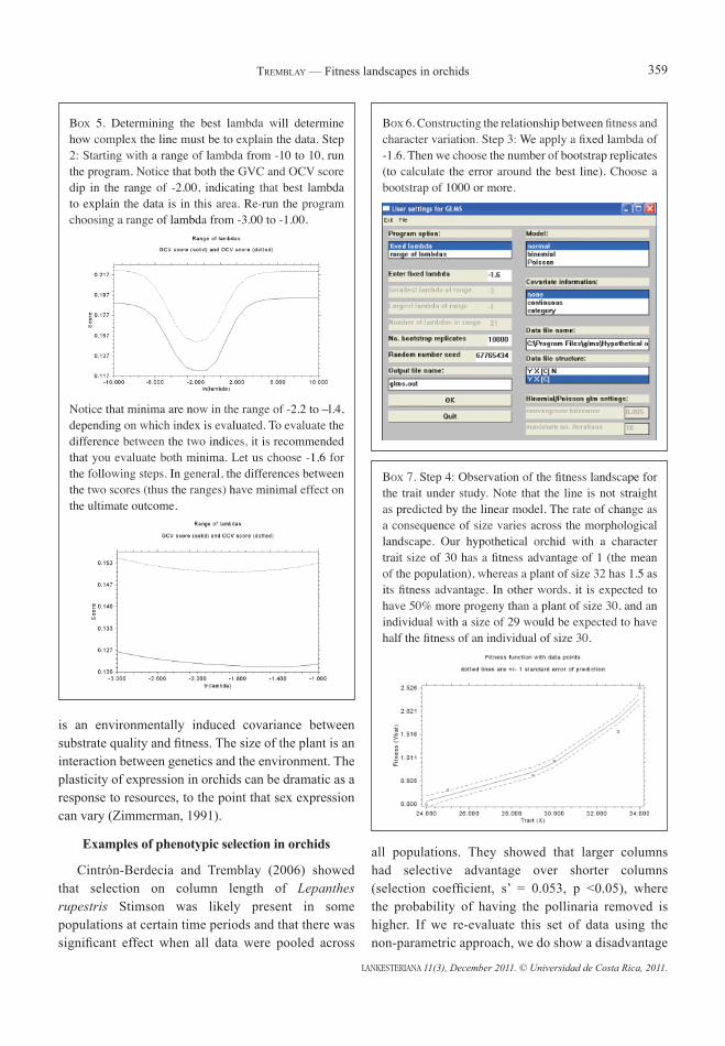
Box 5. Determining the best lambda will determine how complex the line must be to explain the data. Step 2: Starting with a range of lambda from -10 to 10, run the program. Notice that both the GVC and OCV score dip in the range of -2.00, indicating that best lambda to explain the data is in this area. Re-run the program choosing a range of lambda from -3.00 to -1.00.

Notice that minima are now in the range of -2.2 to –l.4, depending on which index is evaluated. To evaluate the difference between the two indices, it is recommended that you evaluate both minima. Let us choose -1.6 for the following steps. In general, the differences between the two scores (thus the ranges) have minimal effect on the ultimate outcome.

is an environmentally induced covariance between substrate quality and fitness. The size of the plant is an interaction between genetics and the environment. The plasticity of expression in orchids can be dramatic as a response to resources, to the point that sex expression can vary (Zimmerman, 1991).

Examples of phenotypic selection in orchids

Cintrón-Berdecia and Tremblay (2006) showed that selection on column length of Lepanthes rupestris Stimson was likely present in some populations at certain time periods and that there was significant effect when all data were pooled across

Box 6. Constructing the relationship between fitness and character variation. Step 3: We apply a fixed lambda of -1.6. Then we choose the number of bootstrap replicates (to calculate the error around the best line). Choose a bootstrap of 1000 or more.

Box 7. Step 4: Observation of the fitness landscape for the trait under study. Note that the line is not straight as predicted by the linear model. The rate of change as a consequence of size varies across the morphological landscape. Our hypothetical orchid with a character trait size of 30 has a fitness advantage of 1 (the mean of the population), whereas a plant of size 32 has 1.5 as its fitness advantage. In other words, it is expected to have 50% more progeny than a plant of size 30, and an individual with a size of 29 would be expected to have half the fitness of an individual of size 30.

all populations. They showed that larger columns had selective advantage over shorter columns (selection coefficient, s’ = 0.053, p <0.05), where the probability of having the pollinaria removed is higher. If we re-evaluate this set of data using the non-parametric approach, we do show a disadvantage


360 LANKESTERIANA

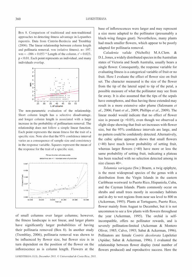
of small columns over larger columns; however, the fitness landscape is not linear, and larger plants have significantly larger probabilities of having their pollinaria removed (Box 8). In another study (Tremblay, 2006), pollinaria removal was shown to be influenced by flower size, but flower size is in turn dependent on the position of the flower on the inflorescence as is column length. Flowers at the

base of inflorescences were larger and may represent a size more adapted to the pollinator (presumably a black-wing fungus gnat). Nevertheless, many plants had much smaller flowers, which appear to be poorly adapted for pollinaria removal. Caladenia valida (Nicholls) M.A.Clem. & D.L.Jones, a widely distributed species in the Australian states of Victoria and South Australia, usually bears a single flower. Consequently, the response variable for evaluating fitness is a categorical variable of fruit or no fruit. Here I evaluate the effect of flower size on fruit set. The character measured is the size of the flower from the tip of the lateral sepal to tip of the petal, a possible measure of what the pollinator may see from far away. It is also assumed that the tips of the sepals have osmophores, and thus having these extended may result in a more extensive odor plume (Salzmann et al., 2006; Faast et al., 2009; Phillips et al., 2009). The linear model would indicate that no effect of flower size is present (p >0.05), even though we observed a slight slope showing that fruit set increases with flower size, but the 95% confidence intervals are large, and no pattern could be confidently detected. Alternatively, the cubic spline approach shows that small flowers (<40) have much lower probability of setting fruit, whereas larger flowers (>40) have more or less the same probability of setting fruit, indicating a plateau has been reached with no selection detected among in size classes 40+. Tolumnia variegata (Sw.) Braem, a twig epiphyte, is the most widespread species of the genus with a distribution from the Virgin Islands in the eastern Caribbean westward to Puerto Rico, Hispaniola, Cuba, and the Cayman Islands. Plants commonly occur on shrubs and small trees mostly in secondary habitats and in dry to wet regions from near sea level to 800 m (Ackerman, 1995). Plants at Tortuguero, Puerto Rico, flower mainly from August to December, but it is not uncommon to see a few plants with flowers throughoutthe year (Ackerman, 1995). The orchid is self-incompatible, offers no pollinator rewards, and is severely pollination-limited (Ackerman & Montero Oliver, 1985; Calvo, 1993; Sabat & Ackerman, 1996). Pollinators are female Centris decolorata Lepeletier (Apidae; Sabat & Ackerman, 1996). I evaluated the relationship between flower display (total number of flowers produced) and reproductive success. Here the

Box 8. Comparison of traditional and non-traditional approaches to detecting fitness advantage in Lepanthes rupestris. Data from Cintrón-Berdecia and Tremblay (2006). The linear relationship between column length and pollinaria removal, wm (relative fitness). n= 197, wm = -.086 + 0.053 * Length of the column, r2 = 0.023, p < 0.01. Each point represents an individual, and many individuals overlap.

The non-parametric evaluation of the relationship. Short column length has a selective disadvantage, and longer column length is associated with a large increase in the probability of pollinarium removal. The relationship does not follow a simple linear function. Each point represents the mean fitness for the trait of a specific size. Note also that the 95% confidence interval varies as a consequence of sample size and consistency in the response variable. Squares represent the mean of the response for the trait of a specific size.



fitness variable is a Poisson distribution, but because not all individuals had the same number of flowers, I used the relative fitness index (as explained above). It has been shown previously that larger display size can result in higher fruit set in this orchid (Sabat & Ackerman, 1996) and other orchids (Huda & Wilcock, 2008). The parametric and non-parametric analysis had similar results (Box 10). The error around the line is smaller for the cubic spline analysis, and the relationship is not linear (although not far from it). In general, the results from these two analyses are similar

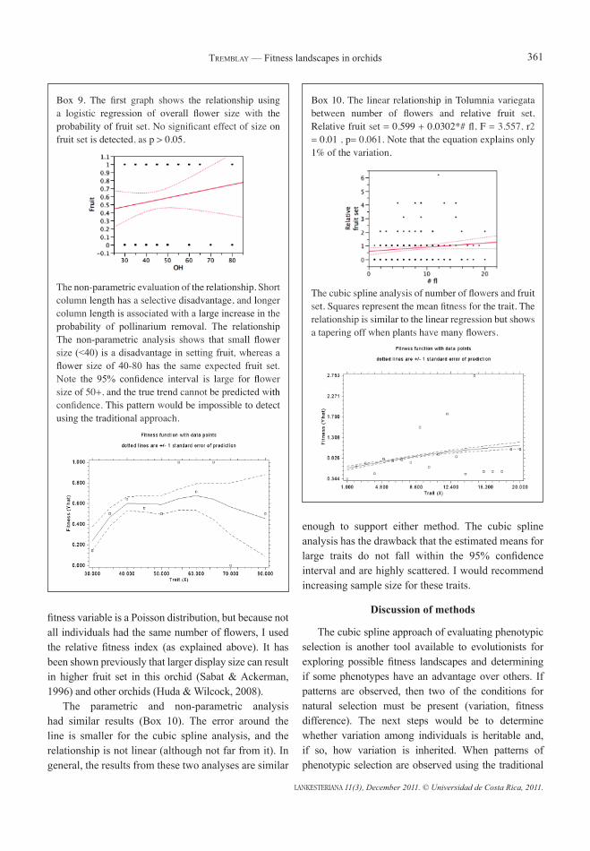
Box 9. The first graph shows the relationship using a logistic regression of overall flower size with the probability of fruit set. No significant effect of size on fruit set is detected, as p > 0.05.

The non-parametric evaluation of the relationship. Short column length has a selective disadvantage, and longer column length is associated with a large increase in the probability of pollinarium removal. The relationship The non-parametric analysis shows that small flower size (<40) is a disadvantage in setting fruit, whereas a flower size of 40-80 has the same expected fruit set. Note the 95% confidence interval is large for flower size of 50+, and the true trend cannot be predicted with confidence. This pattern would be impossible to detect using the traditional approach.

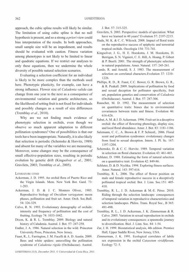
Box 10. The linear relationship in Tolumnia variegata between number of flowers and relative fruit set. Relative fruit set = 0.599 + 0.0302*# fl, F = 3.557, r2 = 0.01 , p= 0.061. Note that the equation explains only 1% of the variation.

The cubic spline analysis of number of flowers and fruit set. Squares represent the mean fitness for the trait. The relationship is similar to the linear regression but shows a tapering off when plants have many flowers.

enough to support either method. The cubic spline analysis has the drawback that the estimated means forlarge traits do not fall within the 95% confidence interval and are highly scattered. I would recommend increasing sample size for these traits.

Discussion of methods

The cubic spline approach of evaluating phenotypic selection is another tool available to evolutionists for exploring possible fitness landscapes and determining if some phenotypes have an advantage over others. If patterns are observed, then two of the conditions for natural selection must be present (variation, fitness difference). The next steps would be to determine whether variation among individuals is heritable and, if so, how variation is inherited. When patterns of phenotypic selection are observed using the traditional


362 LANKESTERIANA

approach, the cubic spline results will likely be similar. The limitation of using cubic spline is that no null hypothesis is present, and so a strong a priori view could bias interpretation of the results. In both approaches, small sample size will be an impediment, and results should be evaluated with caution. Fitness variation among phenotypes is not likely to be limited to linear and quadratic equations. If we restrict our analyses to only these equations, then we undermine the whole diversity of possible natural selection scenarios. Evaluating a selection coefficient for an individual is likely to be more complex than the methods used here. Phenotypic plasticity, for example, can have a strong influence. Flower size of Caladenia valida can change from one year to the next as a consequence of environmental variation and genetic architecture, so the likelihood of setting fruit is not fixed for individuals and possibly changes as a result of size differences (Tremblay et al., 2010). Why are we not finding much evidence of phenotypic selection in orchids, even though we observe so much apparent adaptation to different pollination syndromes? One of possibilities is that our tools have been inappropriate. Naturally, it is also likely that selection is periodic (Schemske & Horvitz, 1989) and absent for many of the variables we are measuring. Moreover, some changes may be the consequence of small effective-population sizes, resulting in periodic evolution by genetic drift (Kingsolver et al., 2001; Gravilets, 2003; Tremblay et al., 2005).

LiTeRaTuRe ciTed

Ackerman, J. D. 1995. An orchid flora of Puerto Rico and the Virgin Islands. Mem. New York Bot. Gard. 73: 1-203.

Ackerman, J. D. & J. C. Montero Oliver,. 1985. Reproductive biology of Oncidium variegatum: moon phases, pollination and fruit set. Amer. Orch. Soc.Bull. 54: 326-329.

Calvo, R. N. 1993. Evolutionary demography of orchids: intensity and frequency of pollination and the cost of fruiting. Ecology 74: 1033-1042.

Dixon, K. & R. L. Tremblay. 2009. Biology and natural history of Caladenia. Austral. J. Bot. 57: 247-258.

Endler, J. A. 1986. Natural selection in the wild. Princeton University Press, Princeton, New Jersey.

Faast, R., L. Farrington, J. M. Facelli & A. D. Austin. 2009. Bees and white spiders: unravelling the pollination syndrome of Caladenia rigida (Orchidaceae). Austral.

J. Bot. 57: 315-325.Gravilets, S. 2003. Perspective: models of speciation: What

have we learned in 40 years? Evolution 57: 2197-2215.Huda, M. K. & C. C. Wilcock. 2008. Impact of floral traits

on the reproductive success of epiphytic and terrestrial tropical orchids. Oecologia 154: 731-741.

Kingsolver, J. G., H. E. Hoeskstra, J. M. Hoeskstra, D. Berrigan, S. N. Vignieri, C. E. Hill, A. Hoang, P. Gibert & P. Beerli. 2001. The strength of phenotypic selection in natural populations. Amer. Natural. 157: 245-261.

Lande, R. and Arnold, S. J. 1983. The measurement of selection on correlated characters.Evolution 37: 1210–1226.

Phillips, R. D., R. Faast, C.C. Bower, G. R. Brown, G. R., & R. Peakall. 2009. Implications of pollination by food and sexual deception for pollinator specificity, fruit set, population genetics and conservation of Caladenia (Orchidaceae). Austral. J. Bot. 57: 287-306.

Rauscher, M. D. 1992. The measurement of selection on quantitative traits: biases due to environmental covariances between traits and fitness. Evolution 46: 616-626.

Sabat, A. M. & J. D. Ackerman. 1996. Fruit set in a deceptive orchid: the effect of flowering phenology, display size, and local floral abundance. Amer. J. Bot. 83: 1181-1186.

Salzmann, C. C., A. Brown & F. P. Schiestl,. 2006. Floral scent and pollination syndromes: evolutionary changes from food to sexual deception. Intern. J. Pl. Sc. 167: 1197-1204.

Schemske, D. & C. C. Horvitz. 1989. Temporal variation in selection on floral character. Evolution 43: 461-465.

Schluter, D. 1988. Estimating the form of natural selection on a quantitative trait. Evolution 42: 849-86.

Schluter, D. & D. Nychka. 1994. Exploring fitness surfaces. Amer. Natural. 143: 597-616.

Tremblay, R. L. 2006. The effect of flower position on male and female reproductive success in a deceptively pollinated tropical orchid. Bot. J. Linn. Soc.151: 405-410.

Tremblay, R. L., J. D. Ackerman & M.-E. Pérez. 2010. Riding through the selection landscape: consequences of temporal variation in reproductive characteristics and selection landscapes. Philos. Trans. Royal Soc., B 365: 491-498.

Tremblay, R. L., J. D. Ackerman, J. K. Zimmerman & R. Calvo. 2005. Variation in sexual reproduction in orchids and its evolutionary consequences: a spasmodic journey to diversification. Biol. J. Linn. Soc. 84: 1-54.

Zar, J. H. 1999. Biostatistical analysis, 4th edition. Prentice Hall, Upper Saddle River, New Jersey, USA.

Zimmerman, J. K. 1991. Ecological correlates of labile sex expression in the orchid Catasetum viridiflavum. Ecology 72: 5.

Fitness landscapes in orchids: Parametric and non-parametric approaches.

Documents

Transcript of Fitness landscapes in orchids: Parametric and non-parametric approaches.