SYSTEMATICS OF AFRICAN VANILLA ORCHIDS

LINKING MORPHOLOGICAL CLASSIFICATION AND DNA-BASED PHYLOGENY

SARA VAN DE KERKE

MSC THESIS - 2014

i

Sara van de Kerke

Registration number: 881211 428110

Email: sara.vandekerke@wur.nl

MSc thesis Biodiversity and Evolution - BIS-80430

Supervisors:

Jan Wieringa, Freek Bakker & Theo Damen - Biosystematics Group Wageningen University

Barbara Gravendeel – Naturalis Biodiversity Center

ii

PREFACE In this MSc Thesis, I looked into a small part of one of the genera from this large and intriguing orchid family:

Vanilla. I applied both a ‘classical morphological’ as well as a DNA-based approach. These are quite different

approaches and thus different research methods were needed. Therefore, both fields will be discussed

separately with their own introduction, material and methods, results and discussion sections. Of course, I will

also link both fields in a final discussion and conclusion.

Since this was quite a large project with many different aspects that did not always work out the way it was

first anticipated, I chose to include all these aspects in this thesis. The thesis is thus outlined in chronological

order including discussions about failed research methods and not built up in a strict scientific form.

Of course, I have had a lot of help during this project. First and foremost, I want to thank my supervisors Freek

T. Bakker, Jan Wieringa, Theo Damen and Barbara Gravendeel for their guidance and constant support during

this long-term project.

I especially want to thank Aline Nieman, Bertha Koopmanschap and Natasha Schidlo for all their help and

advice in the lab; Kris van ‘t Klooster for his help on using Matlab; Marc Pignal and Ranee Prakash for their help

in the herbaria of the Muséum National d’Histoire Naturelle in Paris and the Natural History Museum in London;

the Alberta Mennega Stichting for making it possible for me to visit these herbaria; and of course all staff and

students of the Wageningen Herbarium and the Biosystematics group!

iii

SUMMARY The goal of this MSc thesis is to link the classical morphological field of taxonomy to modern development of

DNA based taxonomy for two small groups of Continental African Vanilla orchids: the imperialis and africana

groups.

The taxonomy of species within the genus Vanilla, which is estimated to comprise 107 species, has long been

an issue. Only in 2010, Soto Arenas and Cribb proposed a new classification describing two subgenera; the

Vanilla and Xanata.

Vanilla has been used by humans for a long time. First by the Totonics from Southeastern Mexico and later by

the Europeans after the Spanish colonisation.

All around the world, Vanilla species grow in the Pan-tropical region around the equator. Researchers do not

agree how this distribution came about. Some state it is a result of radiation over Gondwanaland when it was

not yet broken-up, other say long distance dispersal of seeds by for example bats could be an option.

Vanilla morphology is quite complicated with important characteristics found in the flower and leafs. The first

part of this research concentrates on the classical morphological analysis of a number of these characteristics

in the two groups of species. Principal Component Analysis (PCA) is used to search for trends. In the imperialis

group, a number of recently newly described species are brought back to their original state. In the africana

group, no final conclusions regarding the possible eight species can be drawn.

While the main part of morphological research on Vanilla dates back to the end of the nineteenth century, the

DNA based research is only around fifteen years old. Here, I try to update the most recent cpDNA based

phylogeny of Bouetard et al. (2010) in two ways. First using Ancient DNA methods developed in Leiden and

second by using the more standard molecular systematic approached. The former method is used to

incorporated species missing from the original phylogeny using material obtained from herbarium samples of

the relevant species. For two of those, this method has been successful. The latter approach is used to

incorporate sequences obtained from unidentified silica gel preserved fresh cuttings into the phylogeny. This

has been successful for the africana and imperialis groups.

The flowers of Orchidaceae are important in species identification and are considered to be under selective

pollinator pressure. No research has been done into the pollination of the species researched here, but using

research in closely related species and genera some comments are given about this subject.

In the phylogeny of Bouetard et al. (2010), next to the rbcL region I used, also psaB, psbB and psbC have been

used. These additional regions may be sequenced in future research using the material that is now available. In

addition, the 5.8S nuclear ITS region might be interesting to research for the African species since a phylogeny

is available comprising all American species.

iv

TABLE OF CONTENTS

1. Introduction ........................................................................................................................................................ 1

1.1 Orchidaceae ................................................................................................................................................... 1

1.2 The genus Vanilla ........................................................................................................................................... 2

1.2.1 Vanilla taxonomy ............................................................................................................................... 2

1.2.2 Ethnobotanic history ......................................................................................................................... 3

1.2.3 Vanilla biogeographic distribution .................................................................................................... 4

2. Research questions & hypotheses ...................................................................................................................... 5

2.1 Morphological classification .......................................................................................................................... 5

2.2 DNA-based phylogenetic inference ............................................................................................................... 7

3. Species Concepts ................................................................................................................................................. 9

4. Morphological classification .............................................................................................................................. 12

4.1 Introduction ................................................................................................................................................. 12

4.2 Material and Methods ................................................................................................................................. 14

4.2.1 Morphology ........................................................................................................................................... 14

4.2.2 Statistical Analysis ................................................................................................................................. 16

4.3 Results .......................................................................................................................................................... 18

4.3.1 Morphology ........................................................................................................................................... 18

4.3.2 Statistical Analysis ................................................................................................................................. 24

4.4 Discussion and Conclusion ........................................................................................................................... 26

4.4.1 Imperialis group..................................................................................................................................... 26

4.4.2 Africana group ....................................................................................................................................... 27

4.4.3 General comments ................................................................................................................................ 29

5. DNA-based phylogenetic inference................................................................................................................... 31

5.1 Introduction ................................................................................................................................................. 31

5.2 Material and Methods ................................................................................................................................. 33

5.2.1 Historic DNA methods ........................................................................................................................... 33

5.2.2 Regular DNA methods ........................................................................................................................... 35

5.2.3 General phylogenetic analysis ............................................................................................................... 38

5.3 Results .......................................................................................................................................................... 39

5.4 Discussion and Conclusion ........................................................................................................................... 42

6. Pollination biology in Vanilla ............................................................................................................................. 44

7. Linking morphology and DNA ............................................................................................................................ 46

References ............................................................................................................................................................ 47

Appendix ............................................................................................................................................................... 52

1. Herbaria accessions ................................................................................................................................. 52

v

2. R Script Principal Component Analysis for the africana group ................................................................ 60

3. Herbarium specimens per morphological group ..................................................................................... 61

4. Summary and print PCA in R ................................................................................................................... 62

Imperialis group ............................................................................................................................................. 62

Africana with fans ........................................................................................................................................... 63

Africana without fans ..................................................................................................................................... 64

Africana without fans average ....................................................................................................................... 65

5. aDNA silica extraction protocol ............................................................................................................... 66

6. aDNA CTAB extraction protocol .............................................................................................................. 67

7. CTAB DNA Isolation Protocol for Pelargonium ........................................................................................ 69

8. Promega Wizard Protocol for DNA Clean – Up System using a Vacuum Manifold ................................. 72

9. Promega Wizard Genomic DNA Purification Kit, protocol for ‘Isolating Genomic DNA from Plant Tissue

73

10. PCR Protocol Biosystematics Group ........................................................................................................ 74

11. GeneJET PCR Purification Kit ................................................................................................................... 76

12. Genbank accession .................................................................................................................................. 77

13. Phylogenies of rbcL region for various combinations of sequences ....................................................... 79

phylogenetic tree of basis alignment ............................................................................................................. 79

phylogenetic tree of basis alignment plus DNA sequences obtained with historical DNA methods ............. 81

phylogenetic tree of basis alignment plus sequences obtained with regular extraction methods (both

primers) .......................................................................................................................................................... 83

1

1. INTRODUCTION

1.1 ORCHIDACEAE

From as early as the seventeenth century, orchids were considered to form a family or order (Jarvis & Cribb,

2009; Tournefort, 1694). In his Éléments de Botanique (1694), Tournefort was one of the first to give a

description of this family and in the first edition of the Genera Plantarum (1737), Linnaeus recognised eight

different orchid genera containing 113 different species and varieties (Jarvis & Cribb, 2009). The then relative

low number of described Asian and American orchids was a result of the Euro-centric origin of botany (Jarvis &

Cribb, 2009). Now, the Orchidaceae are considered to comprise 925 genera containing about 27,135 orchid

species (“The Plant List”, 2010). Orchidaceae are widely distributed around the world with multiple genera and

species in almost every part in the world except for large parts of the arctic regions.

Being one of the largest families in the angiosperms (Dressler & Dodson, 1960; Heywood, 1993) and one of the

most complex flowering plant families (Cameron, 2004), there has been a lot of speculation about the age of

this family. Since the fossil record of Orchidaceae is low, it has for a long time been difficult to accurately date

the family. Early researchers stated that the family was of a recent age because of the complicated floral

morphology and specialized pollination process. On the other hand, the fact that orchids are found all around

the world would suggest to other researchers an ancient origin in times of the Gondwana supercontinent

(Ramírez, Gravendeel, Singer, Marshall, & Pierce, 2007). In this continental-drift hypothesis, describing the

radiation of the family around the world as a result of the break-up of Gondwanaland, it is suggested that the

family is as old as 188–455 My. Other hypotheses estimate the crown radiation of the family to be between

68–104 Mya (Bouetard et al., 2010). However, with the help of a newly found fossil it has revealed that the

origin of the family probably lies between 76-84 Mya (Ramírez et al., 2007).

It has been difficult to form a satisfactory classification for this family because the flower, one of the most

important characteristics used to identify species morphologically, is thought to be under selective pollinator

pressure and is thus subjected to much morphological change (Bouetard et al., 2010; Cameron, 2004).

Nevertheless, over the years many, both classical (Dressler & Dodson, 1960; van der Pijl & Dodson, 1966) as

well as DNA based (Cameron, 2004; Cameron et al., 1999; Freudenstein et al., 2004) revisions, monographs and

articles about Orchidaceae taxonomy have been published. Still, orchid taxonomy remains complicated and

subjected to constant improvement.

2

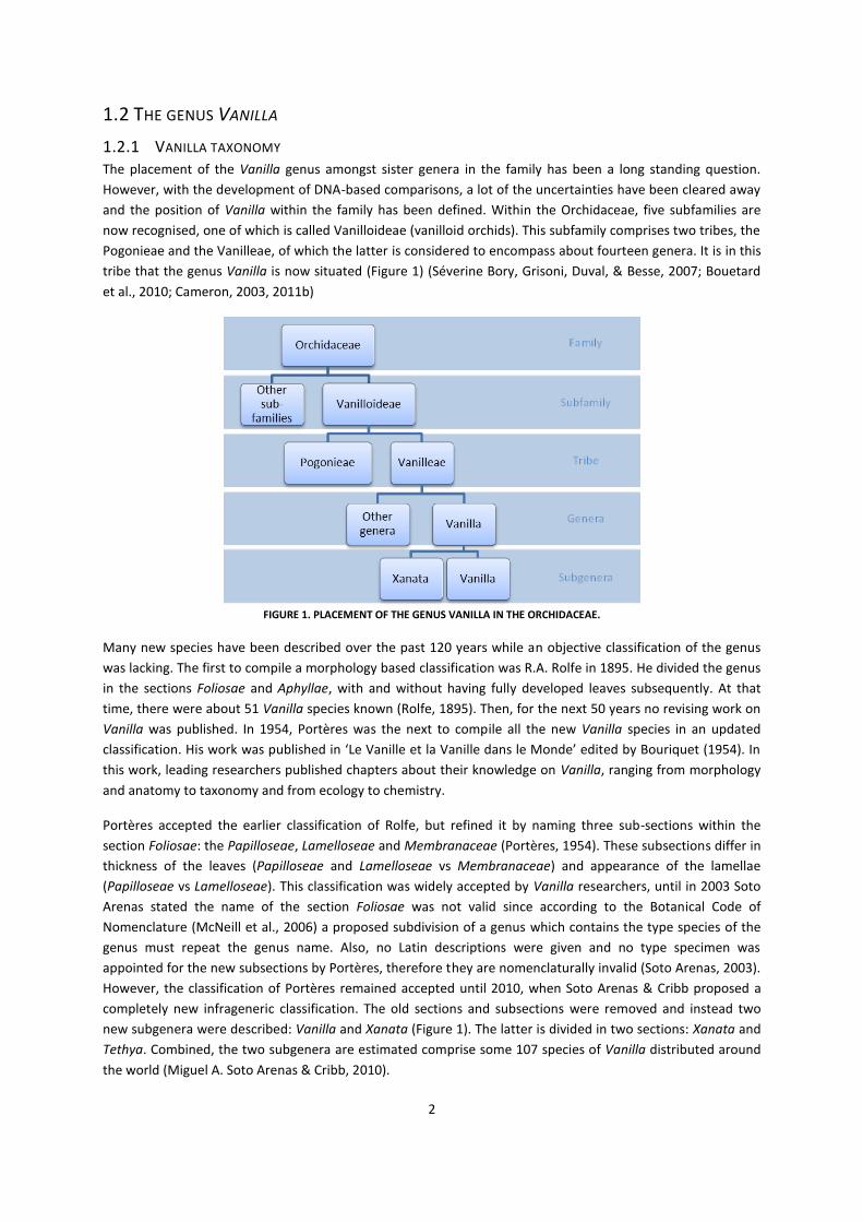
1.2 THE GENUS VANILLA

1.2.1 VANILLA TAXONOMY The placement of the Vanilla genus amongst sister genera in the family has been a long standing question.

However, with the development of DNA-based comparisons, a lot of the uncertainties have been cleared away

and the position of Vanilla within the family has been defined. Within the Orchidaceae, five subfamilies are

now recognised, one of which is called Vanilloideae (vanilloid orchids). This subfamily comprises two tribes, the

Pogonieae and the Vanilleae, of which the latter is considered to encompass about fourteen genera. It is in this

tribe that the genus Vanilla is now situated (Figure 1) (Séverine Bory, Grisoni, Duval, & Besse, 2007; Bouetard

et al., 2010; Cameron, 2003, 2011b)

FIGURE 1. PLACEMENT OF THE GENUS VANILLA IN THE ORCHIDACEAE.

Many new species have been described over the past 120 years while an objective classification of the genus

was lacking. The first to compile a morphology based classification was R.A. Rolfe in 1895. He divided the genus

in the sections Foliosae and Aphyllae, with and without having fully developed leaves subsequently. At that

time, there were about 51 Vanilla species known (Rolfe, 1895). Then, for the next 50 years no revising work on

Vanilla was published. In 1954, Portères was the next to compile all the new Vanilla species in an updated

classification. His work was published in ‘Le Vanille et la Vanille dans le Monde’ edited by Bouriquet (1954). In

this work, leading researchers published chapters about their knowledge on Vanilla, ranging from morphology

and anatomy to taxonomy and from ecology to chemistry.

Portères accepted the earlier classification of Rolfe, but refined it by naming three sub-sections within the

section Foliosae: the Papilloseae, Lamelloseae and Membranaceae (Portères, 1954). These subsections differ in

thickness of the leaves (Papilloseae and Lamelloseae vs Membranaceae) and appearance of the lamellae

(Papilloseae vs Lamelloseae). This classification was widely accepted by Vanilla researchers, until in 2003 Soto

Arenas stated the name of the section Foliosae was not valid since according to the Botanical Code of

Nomenclature (McNeill et al., 2006) a proposed subdivision of a genus which contains the type species of the

genus must repeat the genus name. Also, no Latin descriptions were given and no type specimen was

appointed for the new subsections by Portères, therefore they are nomenclaturally invalid (Soto Arenas, 2003).

However, the classification of Portères remained accepted until 2010, when Soto Arenas & Cribb proposed a

completely new infrageneric classification. The old sections and subsections were removed and instead two

new subgenera were described: Vanilla and Xanata (Figure 1). The latter is divided in two sections: Xanata and

Tethya. Combined, the two subgenera are estimated comprise some 107 species of Vanilla distributed around

the world (Miguel A. Soto Arenas & Cribb, 2010).

3

1.2.2 ETHNOBOTANIC HISTORY

The history of the use and cultivation of Vanilla by humans is a long one. There are multiple legends about the

origin of Vanilla known from the Totonics, indigenous to the southeast Mexican region Papantla, the modern

Vera Cruz (Cameron, 2011a; Correll, 1953; Ecott, 2004; Pesach Lubinsky, Romero-gonz, Heredia, & Zabel, 2011).

According to one of these legends, the Vanilla orchid arose from the spilled blood of a beautiful Totonic

prinsess (Cameron, 2011a; Ecott, 2004).

The Totonics are said to be the first people to have used Vanilla in everyday life. Not as a flavouring as we know

it now, but to perfume their houses (Ecott, 2004). When the Totonics were suppressed by the Aztecs, vanilla

was used to pay tribute to the Aztec emperors. From archaeological remains it is known that the Aztec elite

used to drink xocoatl, a thick chocolate drink flavoured with honey, peppers, maize and vanilla. Supposedly,

Hernando Cortés was the first white man to taste vanilla flavoured chocolate when meeting the Aztec emperor

Montezuma in 1519 (Correll, 1953; Ecott, 2004; Pesach Lubinsky, Bory, Hernández, Kim, & Gómez-Pompa,

2008). The Spanish were impressed with the regenerating ability of the potent drink, saying that ‘a cup of this

precious drink enables a man to walk for a whole day without food’ (Ecott, 2004). After they were finally able

to unravel the mystery of the origin of vanilla, the Aztecs were guarding their secret jealously, the import of

vanilla from Mexico to Spain was started.

For many years the Spanish had the monopoly on the vanilla trade, since the plant would not produce fruits

when it was first cultivated in the 1730’s and pods were thus only produced in the Spanish colonies. There was,

however, a lot of interest from both England and France to break the Spanish monopoly (Cameron, 2011a). The

problem was that when the Vanilla species most suitable for cultivation, the original Mexican V. planifolia, was

imported to Réunion and Madagascar for cultivation, the climate was right but there was no natural pollinator.

Eventually, the French discovered that the fruits would set when the flowers were pollinated by hand and the

Spanish monopoly was broken (Cameron, 2011a; Ecott, 2004). This was a time consuming and non-effective

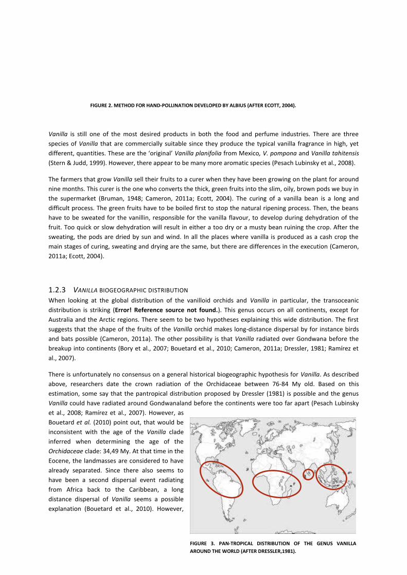
method. It was not until the early nineteenth century that the slave Edmond Albius discovered a relative easy

way to fertilize Vanilla flowers (

Figure 2). Although he was never really rewarded for his discovery, Albius’s method is now widely used in

Vanilla cultivation and nowadays, all the fruits imported from Madagascar and Réunion have been fertilized in

this way (Cameron, 2011a; Ecott, 2004).

The rostellum is lifted clear of

the stigma

The anther and stigma are pressed together

After pollination, the pollen mass adheres

to the stigma

anther

pollen mass

rostellum stigma

4

Vanilla is still one of the most desired products in both the food and perfume industries. There are three

species of Vanilla that are commercially suitable since they produce the typical vanilla fragrance in high, yet

different, quantities. These are the ‘original’ Vanilla planifolia from Mexico, V. pompona and Vanilla tahitensis

(Stern & Judd, 1999). However, there appear to be many more aromatic species (Pesach Lubinsky et al., 2008).

The farmers that grow Vanilla sell their fruits to a curer when they have been growing on the plant for around

nine months. This curer is the one who converts the thick, green fruits into the slim, oily, brown pods we buy in

the supermarket (Bruman, 1948; Cameron, 2011a; Ecott, 2004). The curing of a vanilla bean is a long and

difficult process. The green fruits have to be boiled first to stop the natural ripening process. Then, the beans

have to be sweated for the vanillin, responsible for the vanilla flavour, to develop during dehydration of the

fruit. Too quick or slow dehydration will result in either a too dry or a musty bean ruining the crop. After the

sweating, the pods are dried by sun and wind. In all the places where vanilla is produced as a cash crop the

main stages of curing, sweating and drying are the same, but there are differences in the execution (Cameron,

2011a; Ecott, 2004).

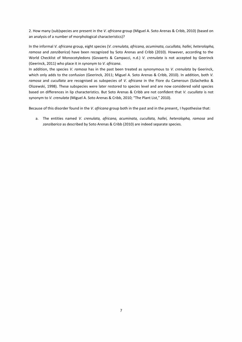
1.2.3 VANILLA BIOGEOGRAPHIC DISTRIBUTION When looking at the global distribution of the vanilloid orchids and Vanilla in particular, the transoceanic

distribution is striking (Error! Reference source not found.). This genus occurs on all continents, except for

Australia and the Arctic regions. There seem to be two hypotheses explaining this wide distribution. The first

suggests that the shape of the fruits of the Vanilla orchid makes long-distance dispersal by for instance birds

and bats possible (Cameron, 2011a). The other possibility is that Vanilla radiated over Gondwana before the

breakup into continents (Bory et al., 2007; Bouetard et al., 2010; Cameron, 2011a; Dressler, 1981; Ramírez et

al., 2007).

There is unfortunately no consensus on a general historical biogeographic hypothesis for Vanilla. As described

above, researchers date the crown radiation of the Orchidaceae between 76-84 My old. Based on this

estimation, some say that the pantropical distribution proposed by Dressler (1981) is possible and the genus

Vanilla could have radiated around Gondwanaland before the continents were too far apart (Pesach Lubinsky

et al., 2008; Ramírez et al., 2007). However, as

Bouetard et al. (2010) point out, that would be

inconsistent with the age of the Vanilla clade

inferred when determining the age of the

Orchidaceae clade: 34,49 My. At that time in the

Eocene, the landmasses are considered to have

already separated. Since there also seems to

have been a second dispersal event radiating

from Africa back to the Caribbean, a long

distance dispersal of Vanilla seems a possible

explanation (Bouetard et al., 2010). However,

FIGURE 3. PAN-TROPICAL DISTRIBUTION OF THE GENUS VANILLA

AROUND THE WORLD (AFTER DRESSLER,1981).

FIGURE 2. METHOD FOR HAND-POLLINATION DEVELOPED BY ALBIUS (AFTER ECOTT, 2004).

5

the radiation back to the Caribbean as described by Bouetard et al. (2010), is not certain, since the

phylogenetic inference doesn’t include possible sister species of the species that dispersed back from Africa.

6

2. RESEARCH QUESTIONS & HYPOTHESES Historically, Vanilla taxonomy was always based on morphological characteristics. Even now, when molecular

systematics and phylogenetic analysis is so far developed, no complete consensus classification of the Vanilla

orchids has been formed linking these two taxonomical fields.

The aim of this study was to link these two because they are both important in modern taxonomy. Since the

subjects are different, the research questions are divided over the two fields to give them both the attention

they deserve. An introduction into the fields and accessory literature whereupon I based these questions and

hypotheses is provided in the following chapters. In Chapter 6 I will discuss the pollination biology of Vanilla

and in Chapter 7, I bring these fields together in a final discussion.

2.1 MORPHOLOGICAL CLASSIFICATION

1. Is the species named V. ochyrae Szlach&Olsz. (1998) in fact V. imperialis Kraenzl.?

Recently, T.H.J. Damen from Naturalis Biodiversity Center found that there is some inconsistency in the

description of V. imperialis. Although all the authors refer to the work of Rolfe being the first to provide an

infrageneric classification of the Vanilla genus, none of them take into account the typification of V. imperialis

Kraenzl. by Kraenzlin (Kraenzlin, 1896). The type specimen (Zenker & Staudt. 626) appears to be lost when the

Berlin Herbarium was destroyed during bombing of the city in 1943, but in the publication a clear drawing of V.

imperialis was provided. Also, the German text accompanying the Latin description clearly states that ‘die Lippe

selbst ist nur vorn frei und bildet dort eine queroblonge Platte’ meaning that the lip (of the flower) itself is only

free at the front and forms there a square-like plate. In the later monograph of Portères (1954) the description

of V. imperialis seems to be comparable with the one of Kraenzlin, especially since he used the drawings from

Kraenzlin in his own description. However, in the Flore du Cameroun of Szlachetko & Olszewski (Szlachetko &

Olszewski, 1998), the description and drawing of V. imperialis do not agree with those of Kraenzlin (1896) but

the drawing of the newly named V. ochyrae Slzach&Olsz. is similar to the one of Kraenzlin and at first sight no

clear difference can be found. Also, in the revision of Soto Arenas & Cribb (2010), the only difference between

V. imperialis and ochyrae is the shape of the plate of the lip, having either a triangular or an elliptic to semi-

circular apex. Clearly, there is a problem with the descriptions of these species.

Considering the discrepancy in the descriptions of V. imperialis arisen through the years I hypothesise that:

a. V. imperialis described by Kraenzlin (1896) was mixed up by Szlachetko and Olszewski with another

Vanilla species and the new name V. ochyrae Szlach&Olsz. was given to the original V. imperialis

Kraenzl.

b. V. imperialis sensu Szlachetko & Olszewski (1998) is conspecific with the type of V. lujae De Wild.

7

2. How many (sub)species are present in the V. africana group (Miguel A. Soto Arenas & Cribb, 2010) (based on

an analysis of a number of morphological characteristics)?

In the informal V. africana group, eight species (V. crenulata, africana, acuminata, cucullata, hallei, heterolopha,

ramosa and zanzibarica) have been recognized by Soto Arenas and Cribb (2010). However, according to the

World Checklist of Monocotyledons (Govaerts & Campacci, n.d.) V. crenulata is not accepted by Geerinck

(Geerinck, 2011) who place it in synonym to V. africana.

In addition, the species V. ramosa has in the past been treated as synonymous to V. crenulata by Geerinck,

which only adds to the confusion (Geerinck, 2011; Miguel A. Soto Arenas & Cribb, 2010). In addition, both V.

ramosa and cucullata are recognised as subspecies of V. africana in the Flore du Cameroun (Szlachetko &

Olszewski, 1998). These subspecies were later restored to species level and are now considered valid species

based on differences in lip characteristics. But Soto Arenas & Cribb are not confident that V. cucullata is not

synonym to V. crenulata (Miguel A. Soto Arenas & Cribb, 2010; “The Plant List,” 2010).

Because of this disorder found in the V. africana group both in the past and in the present, I hypothesise that:

a. The entities named V. crenulata, africana, acuminata, cucullata, hallei, heterolopha, ramosa and

zanzibarica as described by Soto Arenas & Cribb (2010) are indeed separate species.

8

2.2 DNA-BASED PHYLOGENETIC INFERENCE

3. Can (part of) the phylogenetic hypothesis of Bouetard et al. (2010) be complemented and optimised with

additional Vanilla species, especially those from the V. imperialis & africana groups as described by Soto Arenas

& Cribb (2010)?

When comparing the phylogenetic tree based on cpDNA of Bouetard et al. (2010) to the infrageneric

classification of Soto Arenas & Cribb (2010) it can clearly be seen that the informal groups of the classification

are comparable to the clades formed in that phylogeny (Figure 4). The V. africana and imperialis groups, which

are of interest in the previous research questions, are arranged along the phylogenetic tree and are well

supported by the Bayesian node support probabilities. The species of the other informal groups can also be

arranged along the phylogenetic tree and form clear uniform groups.

The phylogenetic tree of Bouetard et al. (2010),

however, is far from complete. Many species are

missing from the sampling, especially in the Old World

& Caribbean clade. Of most informal groups only a few

representatives are included while the remaining

species are missing (e.g. V. acuminate, cucullata, hallei,

heterolopha, ramosa, zanzibarica, grandifolia and

ochyrae), and two informal groups (V. francoisii and

chalotii) are completely missing from the phylogenetic

tree. In addition, many sequences used in the analysis

seem not yet to have been properly identified to species

level since for many lineages only the accession

numbers in GenBank are provided. Also, it is interesting

that the two sequences of V. africana that were used in

the analysis do not group together but group in two

unrelated positions, with one of the two more closely

linked to V. crenulata than to its sister sequence. Last,

the line colonizing the Caribbean is quite intriguing since

it appears to be originated from an African line that is

separate from the other African lines and there is no

taxonomic identification available for this particular

sequenced African accession.

Therefore, I proposed to complement and optimise the

phylogenetic tree of Bouetard et al. (2010) using

sequences of the additional African Vanilla species as

described in the classification of Soto Arenas & Cribb

(2010).

Based on the problems with the phylogenetic

hypothesis as described above, this phylogeny can be

complemented by adding additional species from the

already analysed clades and implementing lacking

clades. The associated hypotheses are:

17

14

20

18

10 19

FIGURE 4 PHYLOGENETIC TREE OF BOUETARD ET AL. (2010) WITH

THE INFORMAL GROUP NUMBERS OF SOTO ARENAS & CRIBB

(2010)(10: V. ALBIDA GROUP, 14: V. IMPERIALIS GROUP, 17: V.

AFRICANA GROUP, 18: V. BARBELLATA GROUP, 19: V. APHYLLA

GROUP, 20: V. PHALEANOPSIS GROUP). COLOUR INDICATES

GEOGRAPHICAL REGION: ASIA (YELLOW), CARIBBEAN (RED),

CONTINENTAL AFRICA (BLUE) AND MADAGASCAR (GREEN) (AFTER

BOUETARD ET AL. (2010).

9

a. The V. chalotii group will cluster in an intermediate clade between African and Caribbean species.

b. The V. francoisii group will be closely related to the V. madagascariensis group, since both are Indian

Ocean based groups.

c. The informal V. imperialis and africana groups are monophyletic groups.

10

3. SPECIES CONCEPTS Before diving into the actual research and forming conclusions whether entities are species or not, I think it is

important to take a closer look into the question ‘What is a species’. Unfortunately, for many researchers this is

one of the most difficult questions one can be asked. The concept ‘species’ is one of the most fundamental

concepts in biology, but (as is often said) there are as many opinions about what a species is as there are

biologists. For every field in biology, a different set of aspects that together make up the concept species is

relevant. This is why it so hard to form a general consensus, since the interests are often quite contradictory.

In a lot of the formulated concepts, all kind of processes as evolution, speciation and mutation are taken into

consideration. But is that necessary? Does it matter to make all these processes, difficult in itself, part of your

species concept?

The question is then whether it is your goal to form a definition of a species in the light of these evolutionary

processes, or is it your goal to distinguish and describe entities we assign the rank of species? I think there is

quite a difference in these mind sets and that doesn’t help. Some researchers are only interested in accurately

describing species as groups we can find in nature. Their goal is to describe on what morphological grounds one

group is different from another. Solely based on what they see in the present state of the plants. That is quite a

difference from other researchers who are not interested in describing a particular species on its looks, but are

interested in for example differences in behaviour and use species in their research (Hausdorf, 2011).

But is not the goal of a general used species concept also to describe what Wilkins calls logical species, so

including evolutionary processes, and not ‘just’ to define biological species ‘which are diagnosed by

morphological characteristics’?

Ultimately, every researcher has to formulate his or her own species concept. At the moment, around 26

heavily discussed species concepts are in circulation and everybody chooses certain parts of them that they can

use to form their own working concept (Frankham et al., 2012; Wilkins, 2003).

Personally, I find the species concept quite a difficult problem. I have never given much thought about the

species concept question before. I find it thus difficult, with my lack of knowledge of the plant phylum, to form

a solid species concept. How can one base an underpinned opinion about such an important concept on so

little knowledge? Also, there are numerous examples of researchers changing their opinion on the species

concept as their years in research advance and their personal experience increases.

Before I started this thesis, I was quite happy with the old fashioned taxonomic practise to differentiate species

based on a number of correlated morphological characteristics the individuals within the species have in

common but clearly separate them from other individuals. This method is based on the Morphological species

concept that states that a population should be morphologically distinct from another population to make

them separate species. Usually, a number of three or more distinct characteristics is found sufficient to make

this separation. Subspecies or varieties can be recognised in much the same way. When less than three

correlated morphological characteristics can be found to separate the one entity from another but there is a

clear separation in geographical or ecological sense, they may be called subspecies. If no such additional

separation can be found but the morphology still implies a difference, the term variety is used (Sosef, personal

communication). It is quite practical to define a species in this way when performing morphological work. But

the number three is quite arbitrary. And in the USA the rules for subspecies and variety used to be the other

way around. And as Wilkins writes: ‘... living species were always understood to include or require a generative

power rather than morphological similarity or identity, which was always held to be a way of identifying them

at best.’

The outlines of this morphological practise are thus no longer enough for me. In the end, a good species

concept should define the underlying processes, but should also be fit to use in real life.

11

As I said earlier, there are about 26 species concepts. But it is difficult to adopt an already existing species

concept when every concept has its pitfalls, is vague or not complete. From my gut feeling, I would say that the

Biological species concept (‘Species are reproductively isolated units in that, by definition, only conspecific

matings yield fertile offspring’, Zachos & Lovari, 2013) makes sense. If two entities can form fertile offspring,

how can they be so different that they can be called separate species? But in plants, it is known that

fertilisation can occur even over genus boarders (Wilkins, 2003; Zachos & Lovari, 2013). Also in my clade,

species are found to hybridise. Either by accident (V. claviculata x barbellata, Nielsen, 2000), or because they

are made to (V. tahitensis, P. Lubinsky et al., 2008).

In the genetic sense, I can relate to the concept of Templeton: A species is ‘[t]he most inclusive group of

organisms having the potential for genetic and/or demographic exchangeability (Wilkins, 2003). However, as

Wilkins points out, this is more of a way to describe the underlying speciation processes and not useful for

identifying species (Wilkins, 2009).

Also, when one is taking the genetics into consideration, should you not also take in the evolutionary time

process? Here, the characterisation by E.O. Wiley ‘A species is a single lineage of ancestral descendant

populations of organisms which maintains its identity from other such lineages and which has its own

evolutionary tendencies and historical fate’ makes sense. In this light, some people say that once a species has

evolved, it remains stable (Wilkins, 2009). But is this the case? When you perform a lab experiment with a

bacterial strain of some species and you let it evolve under a certain set of environmental conditions, did you

then create a new species? Or is it still the same, but adapted to the new environment?

And again where do you draw the line? Any new species descends from another already existing species. So all

organisms that form the new species are descendants from multiple organisms from the mother species. In the

light of this concept there thus should only be one species, the one all life originated from.

With the Phylogenetic species concept we seem to circle back to the concept we started with. In this concept,

species are defined by their autapomorphies, their derived characteristics. Species have their own set of

autapomorphies that makes them unlike other species in the same genus, but they share the same

synapomorphies. These are unique on the higher taxonomic genus level. In its original form the Phylogenetic

species concepts states that ‘A species is the smallest diagnosable cluster of individual organisms within which

there is a parental pattern of ancestry and descent (Wilkins, 2009; Zachos & Lovari, 2013).

In some versions, the aspect of monophyly is added (a monophyletic group being an ancestral species and all

its descendants). If species ought to be monophyletic, they can be defined by their apomorphies, their derived

characteristics. However, under this assumption, a parent species gives rise to two daughter species and then

ceases to exist. I don’t necessarily think that to be the case. It could be that a group of individuals of a species

splits of and evolved to become a species different from the one they originally were. But that doesn’t mean

the old species is gone per se.

Again, I can find myself in this concept. It seems quite logical and usable in practise. You can statistically test

whether there is overlap in morphology or something else and when there isn’t, you have more than one

species. But as Zachos & Lovari, (2013) point out, ‘biological reality has been sacrificed on the altar of

testability’. Because where do you draw the line? Any two individuals may look the same, but with molecular

techniques every individual is different based on the mutations that may have occurred. ‘... every and any

population of every and any species will contain dozens or hundreds of diagnosable units or, under the

diagnosability PSC logic: species...’(Zachos & Lovari, 2013). Under the same argument, the monophyly part also

doesn’t hold up (Zachos & Lovari, 2013).

In my musings, I found all of these aspects to be important enough to be part of my species concept. So a

species should be reproductively isolated (while allowing for hybridisation), has the potential to exchange its

genes with other organisms in its group, has an ancestral component and is defined by a set of exclusive

autapomorphies.

12

Still, this only gives a general outline of what a species should represent. I yet have to come to a hands on

definition that I can easily use in my day to day research.

13

4. MORPHOLOGICAL CLASSIFICATION In this chapter, I address the first two research questions:

1. Is the species named V. ochyrae Szlach&Olsz. (1998) in fact V. imperialis Kraenzl.?

2. How many (sub)species are present in the V. africana group (Miguel A. Soto Arenas & Cribb, 2010)

Therefore, I first give an introduction into the morphology of Vanilla.

4.1 INTRODUCTION

The Vanilloideae is the only subfamily in the Orchidaceae that contains genera with climbing plants and their

habit is completely adjusted to this lifestyle. When recently germinated, the plants are terrestrial and grow on

the forest floor. In this stage, the roots penetrate the soil layer and take in the nutrients. When developing, the

plant starts to climb into a tree and aerial roots are formed at each leave-node. At this stage, the plant has

become a vine. When the basal part that connects the plant to the soil dies off, the plant has become an

epiphyte. The roots are used to stabilize the stem on the tree trunk and take up nutrients from fallen leaves

lying on the trunk and water from the humid air and rolling down the tree when it has been raining. Over the

years, the vine grows up the trunk into the canopy where it can flower (Cameron, 2011a; Fouché & Jouve, 1999;

M. A. Soto Arenas & Cameron, 2003). It is difficult to determine whether the Vanilla’s are truly terrestrial or epiphytic because of their changing

lifestyle. Therefore, they are often said to be hemi-epiphytic, being a bit of both (Cameron, 2011a).

From the start of Vanilla classification, flower characteristics have always been important for the identification

of the different species. These flowers grow in such a way that the chance of fertilization when visited by a

pollinator is fairly large. This is important, since the flowers open early in the morning just before dawn and

wither before noon. The chance of a pollinator being present at just the right time, and carrying suitable pollen,

is therefore only small. To increase the reproductive chances, Vanilla vines are able to produce quite large

quantities of flowers that do not flower all at the same time (Cameron, 2011a; Ecott, 2004; Fouché & Jouve,

1999).

To facilitate the visitation of a pollinator, the flower is twisted 180° and the labellum forms a landing platform

for the pollinator. Also, the labellum is fused with the other petals and forms a tube. The bee or other

pollinator is drawn to the flower by the promise of nectar. It lands on the labellum and enters the tube easily.

However, when it tries to leave the tube, it is hindered by a callus consisting of hairs or scales. These features

lay flat when the pollinator enters the flower but stand up when it tries to leave, thus preventing an easy

retreat. The pollinator has to wiggle backwards and climb over the callus. In doing so, it has to lift its abdomen

and then touches the anther holding the pollen. Since the pollen is nicely packaged together in a clump, it sticks

together and to the abdomen of the pollinator. When visiting the next flower, the pollen is delivered to the

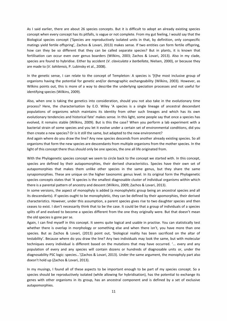
stigma when the pollinator enters the flower (Cameron, 2011a; Ecott, 2004)11) (Figure 5).

Since the anther and stigma are fused together and form the column, there is a fair change of self-fertilization.

To prevent this, a little flap called the rostellum has developed to separate the two. It is this flap that has to be

circumvented when pollinating the flowers by hand (Severine Bory et al., 2008; Cameron, 2011a) (Figure 2 and

5).

14

The leaves of the Vanilla vines are also of importance when identifying the species. Some species clearly have

only rather thin, membrane like leaves or seem to lack them completely. When plants do have leaves, they can

differ greatly in shape, size and colour. Even in one plant, the leaf morphology cannot be said to be constant.

The only species clearly distinct from all the other Vanilla’s is Vanilla grandifolia, which is the only one with

strikingly round leaves compared to the usual elliptic shape (Cameron, 2011a; Stern & Judd, 1999).

FIGURE 5. FLOWER CHARACTERISTICS (WIKIPEDIA, N.D.).

15

4.2 MATERIAL AND METHODS

4.2.1 MORPHOLOGY Extensive morphological analyses had to be performed to gather the data needed to answer the first two

research questions.

The first step in this process was to request herbarium specimens of V. ochyrae, imperialis, polylepis,

grandifolia, crenulata, africana, acuminata, cucullata, hallei, heterolopha, ramosa and zanzibarica on loan from

the herbaria of Kew Royal Botanical Gardens (K), Paris (P), Brussels (BR) and the British Museum (BM), New

York (NY) and Madrid (MA).

V. ochyrae, V. lujae and imperialis needed to be compared to answer the first research question. Together with

V. polylepis and grandifolia, they form a monophyletic group in the phylogenetic tree of Bouetard et al. (2010)

and one informal group in the revision of Soto Arenas & Cribb (2010). The same is the case with the other

species that together form the africana group.

Because it is desirable to study as many specimens of these species as possible in this kind of research, I visited

Kew Royal Botanical Gardens, the National History Museum in London and the Muséum National d’Histoire

Naturelle in Paris. There, I selected suitable specimens for the loan while I measured the other specimens on

site. Appendix 1 gives an overview of all available specimens.

All measurements were performed on boiled flowers with a ruler. Measurements were entered in an Excel

database for further use in the statistical analyses (4.2.2 Statistical Analysis). All specimens were photographed

for future use as elaborate and detailed as possible. Good flower specimens were kept on alcohol during the

research period.

In addition, all data available from the labels on the specimens was entered in the Brahms database. The Meise

herbarium of Brussels sent over their databases, which were incorporated in the Brahms database. Then, Theo

Damen searched appropriate coordinates for all mentioned locations. Using Arcview I then made appropriate

distribution maps of all relevant records.

4.2.1.1 IMPERIALIS GROUP

In the case of the imperialis/ochyrae combination, I took a close look into the shape of the floral lip since it is a

characteristic that clearly distinguishes V. imperialis from V. ochyrae as described in the Flore du Cameroun

(Szlachetko & Olszewski, 1998). The first (sensu Szlachetko & Olszewski) having a pointed lip apex and the latter

having a more quadrangular shaped lip apex. However, when looking at the drawing available from the original

protologue of V. imperialis by Kraenzlin, it became clear that the flower there also has a quadrangular shaped

lip apex. This is comparable to the shape of the lip of V. ochyrae of Szlachetko & Olszewski (1998) and not to

the drawing there available of V. imperialis, which is much more pointed. Therefore, I looked into the

possibility of a gradient in lip pointedness within the imperialis/ochyrae combination.

I calculated this pointiness by measuring the angle between the central line along the lip and the farthest point

of the lip (Figure 6). Both sides of the lip where measured in this way when possible.

I also looked into other characteristics that might be used to distinguish the two species other than lip apex

shape. I looked into the way the rest of the flower is attached to the column and measured the length and

width of the lip and the column. In addition, I looked at the hairs on the lip, since in the literature this is used to

help distinguish the species from one another. I also looked at non-floral characteristics as the bracts (their

shape and how they are attached to the inflorescence) and the leaves.

Next to this morphological study, I also studied the available literature that is mentioned above in more detail.

16

4.2.1.2 AFRICANA GROUP

In the case of the africana group, the group of species that is part of the second research question, I looked at

another set of characteristics since the flowers are quite different. Beforehand I performed no literature

research into the characteristics distinguishing the entities in this group. In this way, I could remain objective

about which characters were to be measured since I did not know which were supposed to be of interest for

each species.

To ensure this objectivity, I started with sorting all the available specimens by collector and number instead of

identification. This helped with spotting the differences among the overall specimens and the flowers.

Then I looked at the flowers under a binocular and took photographs of everything I thought could be

interesting or relevant. The photographs were not only to keep record of interesting characteristics, but also

for use in the program tpsDig2 (Rohlf, 2010). This morphometric program can automatically calculate distances

from a set combination of points that together define the characteristics studied in an organism, in this case

the flower. First I converted the JPG-files of the pictures to .TPS-files, the extension used by tpsDig2, with the

utility program tpsUtil (Rohlf, n.d.). Then the files could be loaded in tpsDig2. After a trial run however, I found

this method was not suitable for this type of flowers (see ‘Discussion and Conclusion’ section in this chapter for

further explanation). Therefore further measurements were taken by hand.

Error! Reference source not found.shows all the measurements I performed on the flowers of this group. To

begin with, I measured the entire length of the column and lip (distance between points 1-2 and 3-2). Then, I

measured the length of the lip that was visible (not hidden behind the side of the flower tube, points 1-4) and

the length from the lip apex till the fans (points 1-5). I also measured the angle between the column and lip

(angle at point 2) and the angle of the two curves in the column (points 6 and 7). When present, I also

measured the length and height of the augmentation on the lip. Also, I counted the number of fans on the

callus when possible.

FIGURE 6. MEASUREMENTS ON V. IMPERIALIS. LEFT: MEASUREMENTS TAKEN FOR POSSIBLE LIP GRADIENT. RIGHT:

ADDITIONAL MEASUREMENTS.

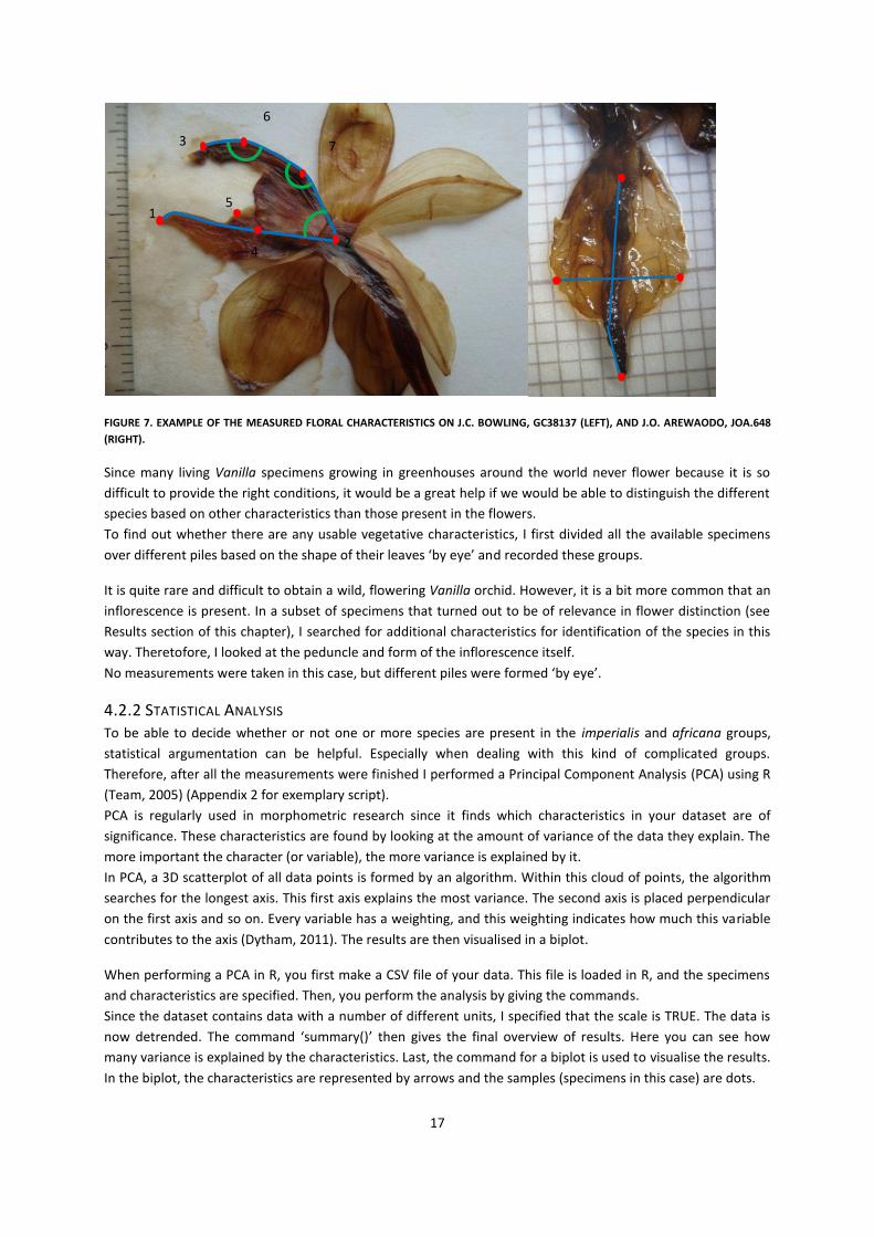
17

FIGURE 7. EXAMPLE OF THE MEASURED FLORAL CHARACTERISTICS ON J.C. BOWLING, GC38137 (LEFT), AND J.O. AREWAODO, JOA.648

(RIGHT).

Since many living Vanilla specimens growing in greenhouses around the world never flower because it is so

difficult to provide the right conditions, it would be a great help if we would be able to distinguish the different

species based on other characteristics than those present in the flowers.

To find out whether there are any usable vegetative characteristics, I first divided all the available specimens

over different piles based on the shape of their leaves ‘by eye’ and recorded these groups.

It is quite rare and difficult to obtain a wild, flowering Vanilla orchid. However, it is a bit more common that an

inflorescence is present. In a subset of specimens that turned out to be of relevance in flower distinction (see

Results section of this chapter), I searched for additional characteristics for identification of the species in this

way. Theretofore, I looked at the peduncle and form of the inflorescence itself.

No measurements were taken in this case, but different piles were formed ‘by eye’.

4.2.2 STATISTICAL ANALYSIS To be able to decide whether or not one or more species are present in the imperialis and africana groups,

statistical argumentation can be helpful. Especially when dealing with this kind of complicated groups.

Therefore, after all the measurements were finished I performed a Principal Component Analysis (PCA) using R

(Team, 2005) (Appendix 2 for exemplary script).

PCA is regularly used in morphometric research since it finds which characteristics in your dataset are of

significance. These characteristics are found by looking at the amount of variance of the data they explain. The

more important the character (or variable), the more variance is explained by it.

In PCA, a 3D scatterplot of all data points is formed by an algorithm. Within this cloud of points, the algorithm

searches for the longest axis. This first axis explains the most variance. The second axis is placed perpendicular

on the first axis and so on. Every variable has a weighting, and this weighting indicates how much this variable

contributes to the axis (Dytham, 2011). The results are then visualised in a biplot.

When performing a PCA in R, you first make a CSV file of your data. This file is loaded in R, and the specimens

and characteristics are specified. Then, you perform the analysis by giving the commands.

Since the dataset contains data with a number of different units, I specified that the scale is TRUE. The data is

now detrended. The command ‘summary()’ then gives the final overview of results. Here you can see how

many variance is explained by the characteristics. Last, the command for a biplot is used to visualise the results.

In the biplot, the characteristics are represented by arrows and the samples (specimens in this case) are dots.

1

2

3

4

5

6

7

18

To optimally perform the statistical analysis, I divided the data that I collected in the Excel file over two

separate databases (one for the imperialis group and one for the africana group). This is because of the way R

(the analysing program I used) deals with missing values in the test I performed. R namely either deletes the

entire sample row with the missing value, or the missing measurement is replaced for a substitute value.

Therefore, it was unfortunately not possible to analyse these two groups together.

In addition, it turned out that all measurements of one of the groups I formed using morphological methods

(see previous paragraph) were excluded from the analysis. A discussion on this subject can be found in the

Discussion and Conclusion of this chapter.

19

4.3 RESULTS

4.3.1 MORPHOLOGY

4.3.1.1 IMPERIALIS GROUP

To answer the first research question I mainly performed a literature study. In addition, I looked into a number

of characteristics to see whether there is a difference between what now is called V. imperialis, ochyrea and

lujae or not.

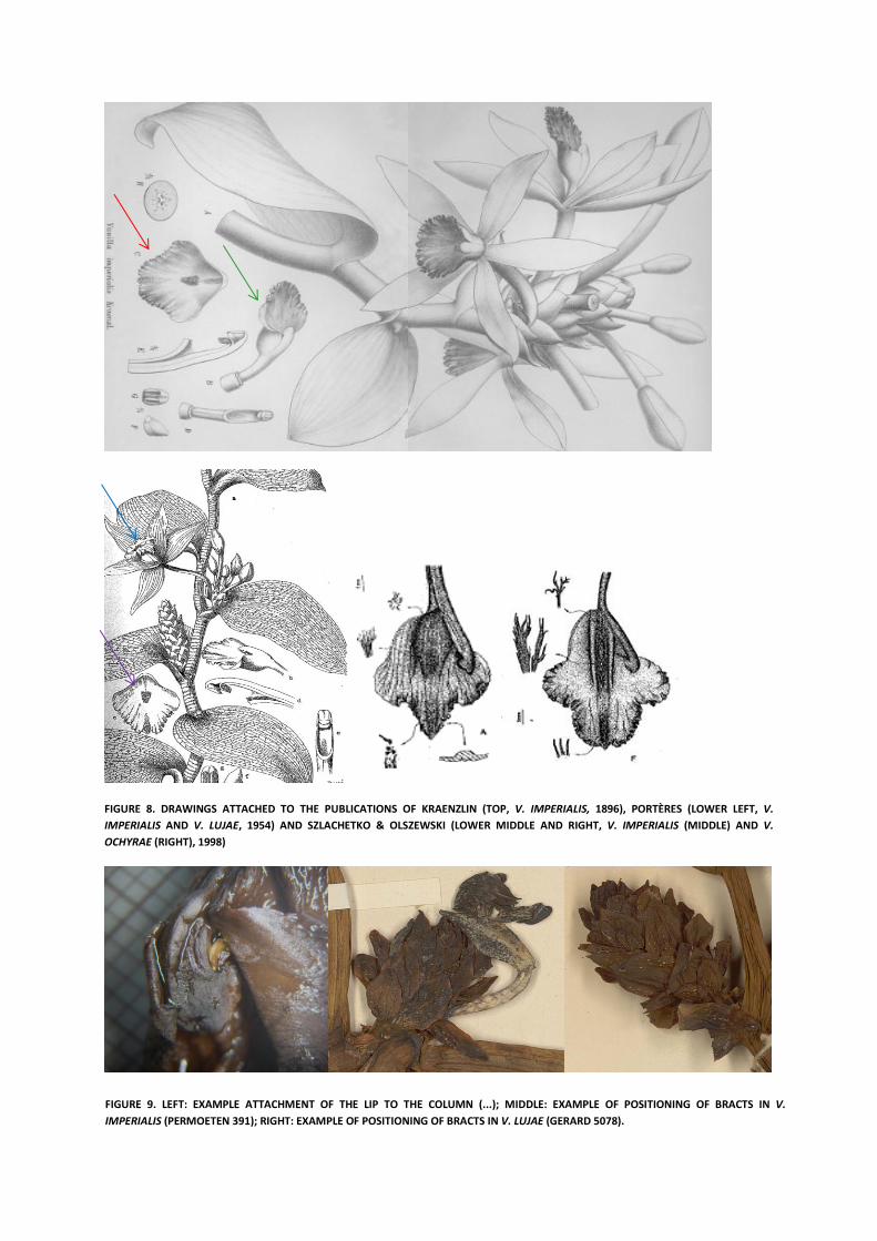
There are four publications that describe V. imperialis, ochyrea and lujae. The first is the typefication of V.

imperialis by Kraenzlin in 1896 (Kraenzlin, 1896). In the drawings accompanying the text describing the

morphology (Figure 8, top picture), it can clearly be seen that the plate of the lip is trilobal and quadrangular

when loosened from the column (red arrow in the picture). In natural position, the plate of the lip is not folded

and forms a quadrangular plate (green arrow in the picture). Also, the bracts are positioned rather densely on

the inflorescence and multiple flowers are opened at the same time.

In the publication of Portères (1954), the species imperialis and lujae are still described as separate species

based on differences in the shape of the lip. In the drawing that visualises these species (Figure 8, lower left

picture), the two of them are pictured together. The top flower (indicated as V. lujae, blue arrow) has a pointed

lip and the other flower (indicated as V. imperialis, purple arrow) does not.

In the Flore du Cameroun by Szlachetko & Olszewski (1998), V. imperialis is depicted by the drawing as shown

in the lower middle picture of Figure 8. In this picture, it can be seen that they interpret imperialis to have a

pointed lip.

The lower right picture of Figure 8 shows a drawing of the new species V. ochyrae. It is described in this

publication as being distinctly trilobal.

Last there is the original publication of V. lujae by De Wildeman in 1904, published in the 10th

edition of the

Bulletin de la Société Belge d’études coloniales, of which Marc Sosef was able to provide me with a copy.

Unfortunately, no (clear) picture is available in this article, but a number of characters are listed that separate V.

lujae from both V. planifolia and V. imperialis.

In the morphological part of the research I looked at a number of characteristics as described in the Materials

and Methods of this chapter. A number of these characteristics is solely used in the statistical analysis which

will be discussed later in this paragraph. These are characters as length, width and angle of the lip.

The other characteristics I only looked at to detect whether they are suitable to divide the available flowers

over groups ‘by eye’. One of these is the attachment of the flower to the column. In some flowers, it seemed

that the side flaps of the lip were attached to a large part of the column. Only the tip of the column is still

shown (Figure 9, left picture). In other flowers, this was not the case and a much larger portion of the column

was free.

I also looked at the shape and positioning of the bracts on the inflorescence of V. imperialis, V lujae and V.

ochyrae because they are described to be different (middle and left picture of Figure 9). Indeed differences can

be found and the specimens were divided over two piles by eye. In the one pile, the bracts are positioned really

quite dense on the inflorescence. In the other specimens, the positioning of bracts is less dense. Also, in the

latter the bract appear to be smaller.

20

FIGURE 8. DRAWINGS ATTACHED TO THE PUBLICATIONS OF KRAENZLIN (TOP, V. IMPERIALIS, 1896), PORTÈRES (LOWER LEFT, V.

IMPERIALIS AND V. LUJAE, 1954) AND SZLACHETKO & OLSZEWSKI (LOWER MIDDLE AND RIGHT, V. IMPERIALIS (MIDDLE) AND V.

OCHYRAE (RIGHT), 1998)

FIGURE 9. LEFT: EXAMPLE ATTACHMENT OF THE LIP TO THE COLUMN (...); MIDDLE: EXAMPLE OF POSITIONING OF BRACTS IN V.

IMPERIALIS (PERMOETEN 391); RIGHT: EXAMPLE OF POSITIONING OF BRACTS IN V. LUJAE (GERARD 5078).

21

FIGURE 10. DISTRIBUTION MAP OF THE IMPERIALIS GROUP. COLOUR INDICATES SPECIES: V. GRANDIFOLIA (GREEN), V. IMPERIALIS BY

SZLACHETKO & OLSZEWSKI (BLUE), V. OCHYRAE BY SZLACHETKO & OLSZEWSKI (RED) AND V. POLYLEPIS (PURPLE).

Theo Damen entered all data from the labels of all available specimens in the Brahms database and found

coordinates for them.

As can be seen in Figure 10, V. imperialis sensu Szlachetko & Olszewski has quite a wide distribution ranging

from Sierra Leone all the way south to Angola and as far to the east as Uganda. V. grandifolia is distributed

from Sao Tomé to the Democratic Republic of the Congo. V. ochyrae by Szlachetko & Olszewski is here found in

only one location in the middle of Cameroon. Also V. polylepis can be found on the African continent in

Democratic Republic of the Congo and Ivory Coast.

4.3.1.2 AFRICANA GROUP

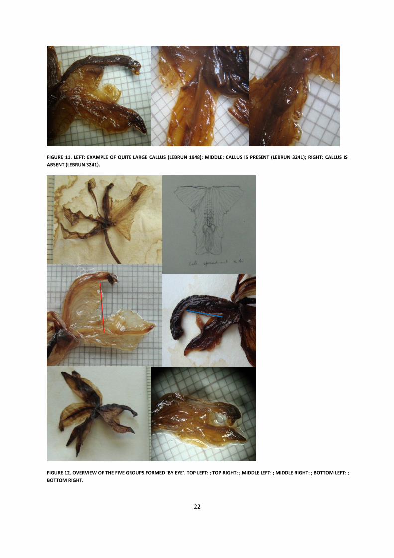
The first characteristic that I found was whether or not a callus is present at the rear of the lip (left picture of

Figure 11). This callus is an augmentation on the back of the lip behind the fans and appears to differ in size.

The presence of the callus seems to be arbitrary since of two flowers from the same collection, on only one a

callus was present (collection Lebrun 3241).

After looking at many flowers, I was able to form five morphological groups by eye from the flowers I kept on

alcohol (Figure 12, Appendix 3). What distinguishes the first group from the others (top left and top right

picture in the figure), is the strong broadening of the lip positioned closely towards the apex. A broadening is

present in some of the other groups, in which case it is positioned more to the middle of the lip. In addition,

the broadening present in this first group appears to be more of a continuation of the width of the lip towards

the apex, resulting in a quite rectangular lip form.

Comparatively, the second morphological group has a more ovate lip shape as can be seen from above in the

middle left picture.

The third group has a lip that is similar to that of the second group, but the side of the flower is quite different.

The tissue at the side of the lip that connects the lip with the column is quite straight in the second group. It

starts quite close toward the end of the column and goes down ending just before the fan like callus in the

middle of the lip (red line in picture). In the third group however, this slip is much more withdrawn towards the

base of the flower at the lip (blue line of middle right picture in the figure).

The fourth group is also quite similar to the second group, but a difference can be found in the shape of the lip.

In these flowers, the lip is much straighter and not as ovate as that of the second group (lower left picture). For

the rest, the flowers in this group are rather similar.

In the fifth group the lip is also quite narrow and the lateral lobes are also withdrawn just like in the third group.

In addition, the angle between the column and the lip is much smaller than in the other cases (lower right

picture).

22

FIGURE 11. LEFT: EXAMPLE OF QUITE LARGE CALLUS (LEBRUN 1948); MIDDLE: CALLUS IS PRESENT (LEBRUN 3241); RIGHT: CALLUS IS

ABSENT (LEBRUN 3241).

FIGURE 12. OVERVIEW OF THE FIVE GROUPS FORMED ‘BY EYE’. TOP LEFT: ; TOP RIGHT: ; MIDDLE LEFT: ; MIDDLE RIGHT: ; BOTTOM LEFT: ;

BOTTOM RIGHT.

23

I also looked into the morphology of the leaves of both the imperialis and the africana group. As described, I

divided all the herbarium specimens present by eye over different piles. I ended up with 23 different piles. In

Figure 3 I present a selection of these groups. As can be seen in the figure, there are quite a lot of different leaf

shapes. Some are almost round, others more oval and some are lanceolate. Within these shape outlines, there

is also variation in size. For example, the top left an middle left picture are both lanceolate, but the leaves in

the top left picture are twice as large as the leaves in the middle left picture.

Also, there is quite some variation in leaf shape in what previous researchers determined to be of the same

species. For example, the middle right and lower left picture (J.J. Bos 5992 and Barker 1265) are both

determined to be V. crenulata.

FIGURE 13. OVERVIEW OF THE DIFFERENCES IS LEAF SHAPE. TOP LEFT: LEEUWENBERG 5465; TOP RIGHT: LOUIS 3599: MIDDLE

LEFT: VERMOESEN 1869; MIDDLE RIGHT: J.J. BOS 5992; BOTTOM LEFT: BARKER 1265; BOTTOM RIGHT: GERARD 5078.

24

As described earlier, I searched for some additional characteristics within the specimens of the relevant

morphological groups by eye.

While looking at the peduncle, I made only one pile. There is thus no variation within this character.

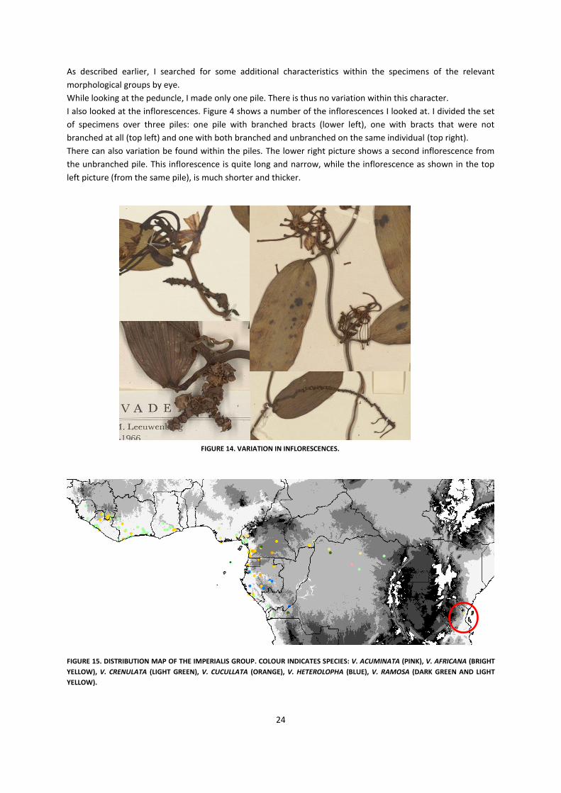
I also looked at the inflorescences. Figure 4 shows a number of the inflorescences I looked at. I divided the set

of specimens over three piles: one pile with branched bracts (lower left), one with bracts that were not

branched at all (top left) and one with both branched and unbranched on the same individual (top right).

There can also variation be found within the piles. The lower right picture shows a second inflorescence from

the unbranched pile. This inflorescence is quite long and narrow, while the inflorescence as shown in the top

left picture (from the same pile), is much shorter and thicker.

FIGURE 15. DISTRIBUTION MAP OF THE IMPERIALIS GROUP. COLOUR INDICATES SPECIES: V. ACUMINATA (PINK), V. AFRICANA (BRIGHT

YELLOW), V. CRENULATA (LIGHT GREEN), V. CUCULLATA (ORANGE), V. HETEROLOPHA (BLUE), V. RAMOSA (DARK GREEN AND LIGHT

YELLOW).

FIGURE 14. VARIATION IN INFLORESCENCES.

25

Figure 15 shows the distribution of the species present in the africana group. As can be seen in the figure, all

species quite cluster together around the same region. Their distributions overlap with a few outlyers, ranging

from Liberia east and into the Democratic Republic of the Congo. V. crenulata and africana have quite a wide

distribution, spanning the entire area. Quite a large gap seems to appear in the distribution of V. ramosa: it

occurs inland on the west side of Cameroon, but is also found along the coast of Tanzania. V. heterolopha is

mainly clustered around Gabon and Congo.

4.3.2 STATISTICAL ANALYSIS Here, I will present the results of the statistical analysis. First those for the imperialis group, then for the

africana group.

Appendix 4 shows the results of the PCA done on the imperialis dataset. As can be seen in the table, 75.91% of

the total variance is explained by PC1 and PC2. The first axis is represented by the characteristic ‘angle_left’

(angle of the left side of the lip with midline) with a value of -0.4382548. However, the weightings of the

characteristics ‘total_length’ (length of the entire flower) (-0.4329647) and ‘column_length’ (length of only the

column) (-0.4362589) are quite similar. So a combination of these three works well to explain the first axis. The

second axis is most explained by the character ‘column_width’ (width of the column) which has a weight of -

0.5652310. These results are also shown in the top left biplot of Figure 16.

As can be seen from the figure, the characteristics ‘angle_left’ and ‘angle_right’ (angle of the right side of the

lip with midline) seem to cluster together with m_length. Also lip_lenght (length of the lip, from apex until end

of the column) and total_lenght cluster together.

For the africana group, I performed a number of PCAs that differ in the composition of characteristics and how

the dataset was assembled. Biplots of these three PCAs are also shown in Figure 16 (top right, bottom left and

bottom right).

The first PCA comprises a selection of characteristics that combined covered the data in the best way and also

includes a number important characteristics that were indicated as important beforehand (for explanation and

discussion of this problem, see ‘Discussion and Conclusion’ section section of this chapter). These

characteristics and the results of the PCA are listed in Appendix 4. As can be seen in the table, 57.01% of the

variance is explained by the first two axes. Adding the third axis increases the amount of explained data to

70.99%. The first axis is represented by the character LCT (total length of the column) with a weight of

0.4808846. The character A2 (second angle within the column) with the weight 0.55104330 seems to represent

the second axis. Last, the third axis is represented by the character A3 (angle between the lip and column) with

a weight of -0.59612249.

The second PCA comprises almost the same combination of characteristics, but I left out the obscure character

‘fans’. This resulted in the biplot shown at the bottom left in Figure 16 and the results are shown in Appendix

9.10.3. With the first two axes, 62.72% of the data is explained. The first axis is again represented by the

character LCT with a weight of 0.4780531. The character A1 (first angle within the column) here explains the

second axis with a weight of 0.56216422.

Adding the third axis increases the percent of explained data to 74.60% and the character that explains it is

again A3 with a weight of 0.68577778.

I performed the third PCA on a dataset with the same characteristics as the second PCA, but here the number

and composition of specimens differed from the second PCA (see ‘Discussion and Conclusion section of this

chapter for explanation). Of this PCA, the results are shown in Appendix 9.10.4 and the lower right biplot of

Figure 15. In this PCA, the first two axis explain 63.84% of the data. Again the first axis is explained by the

character LCT with the weight of 0.4769624. The character A3 explains the second axis with a weight of -

0.54151089.

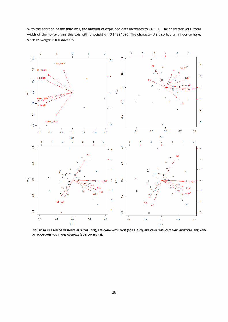
26

With the addition of the third axis, the amount of explained data increases to 74.53%. The character WLT (total

width of the lip) explains this axis with a weight of -0.64984080. The character A3 also has an influence here,

since its weight is 0.63869005.

FIGURE 16. PCA BIPLOT OF IMPERIALIS (TOP LEFT), AFRICANA WITH FANS (TOP RIGHT), AFRICANA WITHOUT FANS (BOTTOM LEFT) AND

AFRICANA WITHOUT FANS AVERAGE (BOTTOM RIGHT).

27

4.4 DISCUSSION AND CONCLUSION

Here, I will discuss the results as presented in the previous paragraph per research question. At the end, a

number of additional matters will be discussed.

4.4.1 IMPERIALIS GROUP The first research question addresses the issue with the confusion between species in the imperialis group. The

first hypothesis is that Szlachetko and Olszewski wrongly described the new species ochyrae while this species

was already described as imperialis by Kraenzlin in 1896 (Kraenzlin, 1896). Based on the literature research I

performed and the drawings available of the interpretation of the species by the different researchers, I can

say this indeed is the case. The description of what Szlachetko and Olszewski call V. ochyrae and what is

described earlier by Kraenzlin and Portères as V. imperialis is so similar, I state they are one and the same

species and the first hypothesis of this question is thus accepted.

Then there is the question which species is then mixed up with what Szlachetko and Olszewski call V. imperialis?

Because there has to be a species they exchanged for their version of imperialis. This is sought-after in the

second hypothesis where I hypothesised that the species described by Szlachetko and Olszewski as imperialis is

in fact a previously described species called V. lujae.

Evidence for this can be found in the publication of Portères of 1954 and the description and typefication of V.

imperialis by Kraenzlin (1896). Portères describes both imperialis and lujae and states that the difference

between them is whether the lip is tri-lobed or not. According to Portères, being tri-lobed results in a lip plate

that is quadrangular (as in imperialis) while not having a tri-lobular lip results in a pointy lip (like lujae). The

drawings that accompany his publication can be found in Figure 8.

Striking about this drawing is that it is so similar to the one of the original imperialis publication by Kraenzlin.

Compare the flower pointed out by the purple arrow in the publication of Portères with the red one in the

Kraenzlin publication and spot the differences.

In contrast to the species addressed by Kraenzlin and Portères, Szlachetko and Olszewski describe imperialis as

having a pointed lip and being not tri-lobed. Thus based on this literature, I conclude that indeed the species

that is called V. imperialis by Szlachetko and Olszewski (1998) is in fact V. lujae as described by Portères (1954).

In this confusion, there are thus only two species at play. One called V. lujae that was made to disappear into

synonymy and confused with V. imperialis by Szlachetko and Olszewski. And the real V. imperialis that was

thought to be a new species called V. ochyrae because its name had wrongly been labelled at the description of

another species.

In addition to this literature study, I performed morphological research to form my own opinion about these

species as described above. In the end, this thus resulted in a not intended research whether the real V.

imperialis is actually the same as the real V. lujae. Unfortunately in this group, only a small amount of

specimens made it to the statistical analysis (top left biplot of Figure 16 in this chapter). How this could be

possible is discussed below in more detail under ‘General comments’, but the same principles apply here.

Briefly: it was not possible to measure all characteristics for all specimens and as a result a large number of

accessions is excluded from analysis.

As can be seen in the biplot, this PCA does not give any information since there are only six specimens left in

the analysis. In total, I studied 28 flowers of almost 70 specimens. It is thus quite disappointing that only these

six have made it to the final analysis. No conclusions can be based on an analysis of so few measurements.

However, while studying these flowers I did get the chance to investigate the most important difference

between these species: whether the lip is quadrangular or pointy. I indeed can make a clear separation

between individuals with flowers that are pointy and those that have a quadrangular lip shape. And there is no

overlap between these groups. Sometimes this is quite hard to see because the sides of the lip are rolled-up or

torn. But with some patience in the preparation of the flowers you can indeed determine whether the lip is

actually quadrangular.

28

I also looked at a number of vegetative characteristics as explained earlier in this chapter. There turned out to

be a difference between the bracts of imperialis and lujae. Those of imperialis are rather tightly packed

together on the inflorescence (Figure 9). The bracts of lujae are not that close together. In both cases, the

bracts are quite large compared to those of the africana group.

With these differences, I find no reason to go against the findings of previous researchers and conclude

imperialis and lujae indeed are different species.

4.4.2 AFRICANA GROUP The second research question asks ‘How many (sub)species are present in the V. africana group’ as described

by Soto Arenas and Cribb (2010). The hypothesis states that all the eight species that have been described

indeed are species.

In the morphological part of the Results, I explained that I found five distinct groups of flowers on alcohol.

These groups are quite easy to separate from each other based on a few, always present, characteristics.

Appendix 3 shows an overview of the flowers (numbered with collector name and number and group number)

for each of these five groups. As can be seen from the table, flowers that I placed in different groups based on

their appearance have the same collector-number combination. For example, I placed flowers belonging to the

collection Lebrun 2493 in groups 2 and 3, flowers belonging to the collection Bos 4195 ended up in groups 2

and 4 and those of the collection Leeuwenberg 3054 in groups 3 and 5. So multiple flowers from one individual

plant can be placed in different groups based on their morphology. The only exception is morphological group

number 1, which is the only group that has no overlap with the others. Based on this result, I can say there are

only two entities in the africana complex. One entity that comprises morphological group number 1 (V.

heterolopha), and the other entity comprises morphological group number 2,3,4 and 5.

This conclusion can unfortunately not be directly backed up by the results of the statistical analysis. The PCA of

Figure 15 shows a nice scattered cloud of flowers, indicating the flowers cannot be separated based on the

measured characteristics.

Not all flowers that are placed in a morphological group are taken into the analysis because some of them were

damaged. When a flower is damaged, some characteristics might not be measured. This results in a gap in the

database: a missing value. R performs PCA in such a way that it does not allow for empty fields in the datasheet

(missing values). Therefore, all rows in the database that contain missing values are omitted from the analysis.

As a result, the data file that comprised measurements for 130 different flowers ranging all five morphological

groups, was reduced to a file with zero flowers because for each of the flowers a value is missing over the

whole range of characteristics. In order to keep as many flowers in the analysis, I first removed a number of

characteristics which contained too much missing values. Of the original nineteen characteristics, in the end I

only used nine.

The result that there are no separate groups found in the PCA does not necessarily mean there are no such

groups. I started without any knowledge of the morphology of the flowers I was about to research. This is a

good way to remain objective and to prevent a possible bias towards certain characteristics you try to find

because they are described in the literature. On the other hand, you end up with characteristics that may seem

of some importance, but turn out to be not that interesting. In my case, I ended up with nineteen

characteristics I thought could be of interest (including the usual length and width measurements). I used none

of these to form the five morphological groups. The one characteristic I used to separate morphological group

1 from morphological groups 2, 3, 4 and 5 by eye I did not think of to measure at the time I started. There are

thus no measurements of this particular character and it is also not included in the PCA. This is quite a pity. In

the future, I will adopt the method that is more commonly used in taxonomy: start by reading the existing

literature, looking at the plants and research their described and newly found differences ‘by eye’. If there are

characteristics that divide the plants over different piles, measure those characteristics. In this way, you

29

actually measure characteristics that are important in the description of the entities. Of course, you could

perform additional measurements on the more general characteristics as certain length and width

measurements. But these should be taken alongside a set of forethought characteristics.

For quite a number of specimens, I was able to measure more than one flower from the same plant. This could

give a possible bias in the statistical analysis, since flowers growing on the same plant have the same influence

from environmental conditions (as the weather and soil composition) and genetics. The easiest solution to

prevent any possible bias is to take average values for those specimens of which multiple flowers were

measured. But then, a lot of variation could possibly be removed. The second possibility is not to perform PCA,

but use an alternative correlation test called Canonical Variance Analysis or Canonical Component Analysis

(Dytham, 2011). This test works in much the same way as regular PCA, but instead of taking all the accessions

(or rows) separately, you can assign them to groups. These groups are then tested in the normal PCA way, This

is a good way to for example compare between populations while keeping the variation within every

population.

To decide which of the above named alternatives would be would be best for my data, I performed a

preliminary PCA on my already dressed-down dataset. I then checked which of the specimens were not taken

in the analysis and removed them from the data file. For the remaining specimens I checked whether they

possibly belonged to the same collection. This turned out to be the case in only four out of 60 accessions. So of

two specimens, two flowers each were measured. When I checked the measurements, I did not find a large

variation between the flowers for the specimens. Therefore, I took their averages and repeated the PCA. As can

be seen in Appendix 4., the percentage of variation explained increases with just over 1%. There is thus not a

lot of difference when you take the average values in the few cases there is overlap in specimens. This in

combination with the fact that CCA is normally used to compare not such a large amount of groups with so

little measurements, led me to the conclusion that averaging the values can be allowed in this case.

In addition, neither in the morphological groups or the statistical analysis all entities named in the hypothesis

are taken into account. In the morphological groups, only specimens identified as V. crenulata, ramosa,

cucullata, acuminata, heterolopha and africana are included. Since there are only one or two specimens of the

other entities (V. hallei and zanzibarica) available, I found it not possible to properly incorporate them.

Why not all species are included in the statistical research is, as in the imperialis group, a result of the analytical

program R and will be discussed below.

All in all, I find I cannot form any solid conclusion based on the present information and thus neither accept nor

reject the hypothesis.

However, from the ‘gut feeling’ I got from looking at these flowers for four months, I can say that the only

entity that is easily recognised in this group is V. heterolopha. The flowers of this species are clearly

distinguishable from the others, because of the broad shape of the lip.

There indeed are differences to be found between individual flowers of the other entities, but as described

above, in the statistical analysis I did not find any characteristics separating the specimens in clear groups.

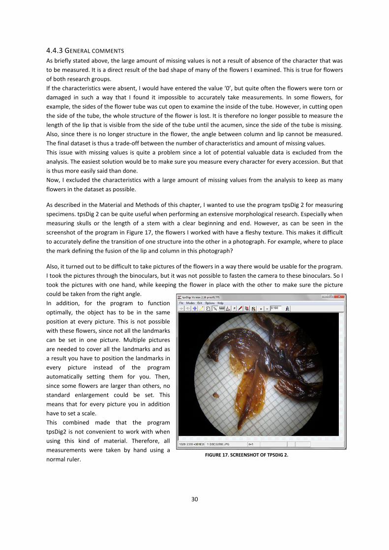
30

4.4.3 GENERAL COMMENTS

As briefly stated above, the large amount of missing values is not a result of absence of the character that was

to be measured. It is a direct result of the bad shape of many of the flowers I examined. This is true for flowers

of both research groups.

If the characteristics were absent, I would have entered the value ‘0’, but quite often the flowers were torn or

damaged in such a way that I found it impossible to accurately take measurements. In some flowers, for

example, the sides of the flower tube was cut open to examine the inside of the tube. However, in cutting open

the side of the tube, the whole structure of the flower is lost. It is therefore no longer possible to measure the

length of the lip that is visible from the side of the tube until the acumen, since the side of the tube is missing.

Also, since there is no longer structure in the flower, the angle between column and lip cannot be measured.

The final dataset is thus a trade-off between the number of characteristics and amount of missing values.

This issue with missing values is quite a problem since a lot of potential valuable data is excluded from the

analysis. The easiest solution would be to make sure you measure every character for every accession. But that

is thus more easily said than done.

Now, I excluded the characteristics with a large amount of missing values from the analysis to keep as many

flowers in the dataset as possible.

As described in the Material and Methods of this chapter, I wanted to use the program tpsDig 2 for measuring

specimens. tpsDig 2 can be quite useful when performing an extensive morphological research. Especially when

measuring skulls or the length of a stem with a clear beginning and end. However, as can be seen in the

screenshot of the program in Figure 17, the flowers I worked with have a fleshy texture. This makes it difficult

to accurately define the transition of one structure into the other in a photograph. For example, where to place

the mark defining the fusion of the lip and column in this photograph?

Also, it turned out to be difficult to take pictures of the flowers in a way there would be usable for the program.

I took the pictures through the binoculars, but it was not possible to fasten the camera to these binoculars. So I

took the pictures with one hand, while keeping the flower in place with the other to make sure the picture

could be taken from the right angle.

In addition, for the program to function

optimally, the object has to be in the same

position at every picture. This is not possible

with these flowers, since not all the landmarks

can be set in one picture. Multiple pictures

are needed to cover all the landmarks and as

a result you have to position the landmarks in

every picture instead of the program

automatically setting them for you. Then,

since some flowers are larger than others, no

standard enlargement could be set. This

means that for every picture you in addition

have to set a scale.

This combined made that the program

tpsDig2 is not convenient to work with when

using this kind of material. Therefore, all

measurements were taken by hand using a

normal ruler.

FIGURE 17. SCREENSHOT OF TPSDIG 2.

31

As described in the Materials and Methods of this chapter, it could be quite handy to be able to distinguish

between species based on vegetative characteristics. In addition to the method I have now used (dividing the

specimens by eye), I had planned to also form a statistical basis for this. To this end, I have scanned all

specimens using the scanner from the digitalisation project of Naturalis Biodiversity Center. Using these scans

in the Herbarium Leaf Finder program (Corney, Clark, Tang, & Wilkin, 2012) for Matlab, the length, width and

other characteristics of every leaf can be measured more easily than when done by hand.

Due to licensing issues I was not able to perform these analyses myself. Fortunately, Kris van ‘t Klooster of the

Cell Biology department of Wageningen UR was willing to assist. After some start-up problems, the program

did work and a number of scans were successfully analysed. However, because the scans are of such high

quality, the analysis takes quite a lot of time. Therefore, we now only performed a preliminary study on three

scans to explore the program. With the limited amount of results we now generated, the HLF program indeed

seems quite promising for future research. A large amount of data can be generated quite easily when using

this program. You only need to make sure there is a picture of a good exemplary leaf available since the

program uses it to find the leaves on the herbarium sheets by matching the general outline of the example to

structures on the sheet. When the sheets are analysed and candidate leafs are selected from them, the

program presents them and all you have to do is select the ones that you are interested in. Then, Matlab

automatically measures the characteristics and you can export the results to an Excel file.

With this program, not only leaf characteristics as length and width can more easily be measured, but there are

also options to explore for example the length of the acumen and the shape of the leaf can be described by

algorithms. Also, the program can use algorithms to describe whether a leaf is crenature or not and how much

so.

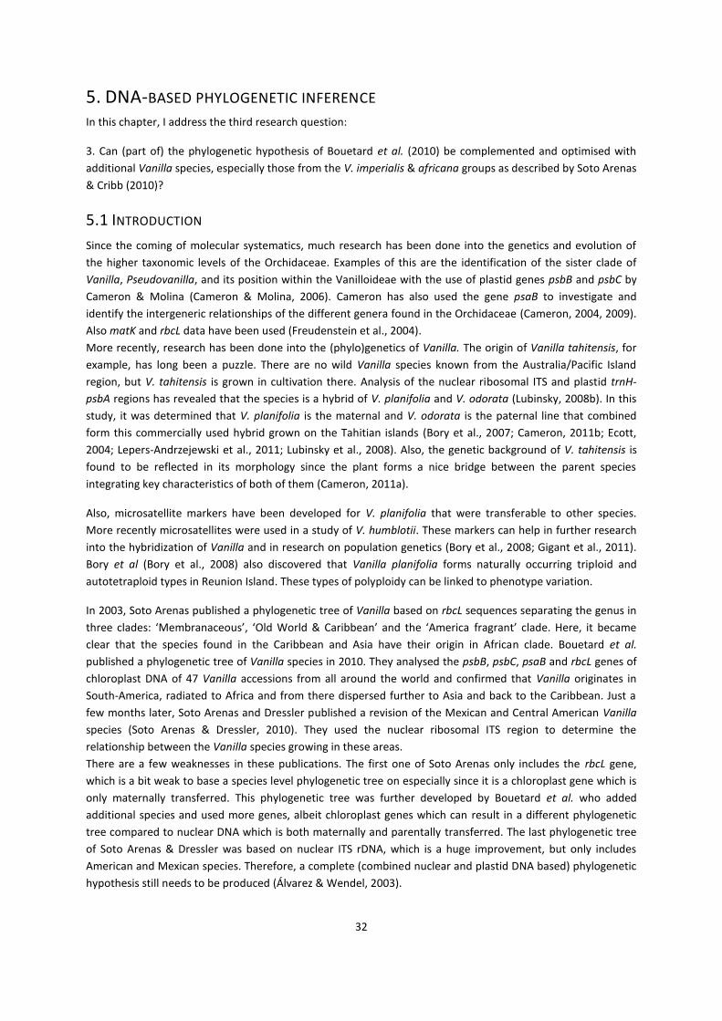
32

5. DNA-BASED PHYLOGENETIC INFERENCE In this chapter, I address the third research question:

3. Can (part of) the phylogenetic hypothesis of Bouetard et al. (2010) be complemented and optimised with

additional Vanilla species, especially those from the V. imperialis & africana groups as described by Soto Arenas

& Cribb (2010)?

5.1 INTRODUCTION

Since the coming of molecular systematics, much research has been done into the genetics and evolution of

the higher taxonomic levels of the Orchidaceae. Examples of this are the identification of the sister clade of

Vanilla, Pseudovanilla, and its position within the Vanilloideae with the use of plastid genes psbB and psbC by

Cameron & Molina (Cameron & Molina, 2006). Cameron has also used the gene psaB to investigate and

identify the intergeneric relationships of the different genera found in the Orchidaceae (Cameron, 2004, 2009).

Also matK and rbcL data have been used (Freudenstein et al., 2004). More recently, research has been done into the (phylo)genetics of Vanilla. The origin of Vanilla tahitensis, for

example, has long been a puzzle. There are no wild Vanilla species known from the Australia/Pacific Island

region, but V. tahitensis is grown in cultivation there. Analysis of the nuclear ribosomal ITS and plastid trnH-

psbA regions has revealed that the species is a hybrid of V. planifolia and V. odorata (Lubinsky, 2008b). In this

study, it was determined that V. planifolia is the maternal and V. odorata is the paternal line that combined

form this commercially used hybrid grown on the Tahitian islands (Bory et al., 2007; Cameron, 2011b; Ecott,

2004; Lepers-Andrzejewski et al., 2011; Lubinsky et al., 2008). Also, the genetic background of V. tahitensis is

found to be reflected in its morphology since the plant forms a nice bridge between the parent species

integrating key characteristics of both of them (Cameron, 2011a).

Also, microsatellite markers have been developed for V. planifolia that were transferable to other species.

More recently microsatellites were used in a study of V. humblotii. These markers can help in further research

into the hybridization of Vanilla and in research on population genetics (Bory et al., 2008; Gigant et al., 2011).

Bory et al (Bory et al., 2008) also discovered that Vanilla planifolia forms naturally occurring triploid and

autotetraploid types in Reunion Island. These types of polyploidy can be linked to phenotype variation.

In 2003, Soto Arenas published a phylogenetic tree of Vanilla based on rbcL sequences separating the genus in

three clades: ‘Membranaceous’, ‘Old World & Caribbean’ and the ‘America fragrant’ clade. Here, it became

clear that the species found in the Caribbean and Asia have their origin in African clade. Bouetard et al.

published a phylogenetic tree of Vanilla species in 2010. They analysed the psbB, psbC, psaB and rbcL genes of

chloroplast DNA of 47 Vanilla accessions from all around the world and confirmed that Vanilla originates in

South-America, radiated to Africa and from there dispersed further to Asia and back to the Caribbean. Just a

few months later, Soto Arenas and Dressler published a revision of the Mexican and Central American Vanilla

species (Soto Arenas & Dressler, 2010). They used the nuclear ribosomal ITS region to determine the

relationship between the Vanilla species growing in these areas. There are a few weaknesses in these publications. The first one of Soto Arenas only includes the rbcL gene,

which is a bit weak to base a species level phylogenetic tree on especially since it is a chloroplast gene which is

only maternally transferred. This phylogenetic tree was further developed by Bouetard et al. who added

additional species and used more genes, albeit chloroplast genes which can result in a different phylogenetic

tree compared to nuclear DNA which is both maternally and parentally transferred. The last phylogenetic tree

of Soto Arenas & Dressler was based on nuclear ITS rDNA, which is a huge improvement, but only includes

American and Mexican species. Therefore, a complete (combined nuclear and plastid DNA based) phylogenetic

hypothesis still needs to be produced (Álvarez & Wendel, 2003).

33

Of course, that is quite an undertaking for a MSc thesis. Therefore, we set the more modest goal to try to

optimise the phylogenetic tree of Bouetard et al (2010) (being the third research question of this project). I

attempted to do this in two ways. Since a number of important species is missing from the phylogenetic tree, I

tried to implement these specific species in the phylogenetic analysis using historical DNA obtained from

herbarium samples.

While working on this project, we decided to start a second project alongside it. Initially, we wanted to use the

material of Bouetard et al (2010) to extract and sequence the 5.8S rDNA gene on the nuclear ribosomal ITS

region to link the phylogenetic tree of Soto Arenas and Dressler (2010) with the one of Bouetard et al (2010).

Unfortunately, I could not acquire the necessary material. Therefore, we decided to gather as much silica dried

material as possible and use the same primers as Bouetard et al (2010) used for extraction and DNA sequencing.

In this way I can still expand the Bouetard et al phylogenetic tree and also explore the possibilities of a standard

barcode for certain species.

This genetic part of the research is thus again divided in two sets: one historic DNA and one ‘regular’ DNA

research line. But they are still interwoven and complement each other. Therefore, I will discuss them in the

same chapter alongside one another.

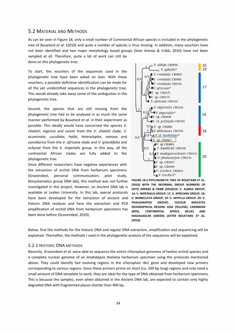
34

FIGURE 18.5 PHYLOGENETIC TREE OF BOUETARD ET AL.

(2010) WITH THE INFORMAL GROUP NUMBERS OF

SOTO ARENAS & CRIBB (2010)(10: V. ALBIDA GROUP,

14: V. IMPERIALIS GROUP, 17: V. AFRICANA GROUP, 18:

V. BARBELLATA GROUP, 19: V. APHYLLA GROUP, 20: V.

PHALEANOPSIS GROUP). COLOUR INDICATES

GEOGRAPHICAL REGION: ASIA (YELLOW), CARIBBEAN

(RED), CONTINENTAL AFRICA (BLUE) AND

MADAGASCAR (GREEN) (AFTER BOUETARD ET AL.

(2010).

5.2 MATERIAL AND METHODS

As can be seen in Figure 18, only a small number of Continental African species is included in the phylogenetic

tree of Bouetard et al. (2010) and quite a number of species is thus missing. In addition, many vouchers have

not been identified and two major morphology based groups (Soto Arenas & Cribb, 2010) have not been

sampled at all. Therefore, quite a lot of work can still be

done on this phylogenetic tree.

To start, the vouchers of the sequences used in the

phylogenetic tree have been asked on loan. With these

vouchers, a possible definitive identification can be made for

all the yet unidentified sequences in the phylogenetic tree.

This would already take away some of the ambiguities in the

phylogenetic tree.

Second, the species that are still missing from the

phylogenetic tree had to be analysed in as much the same

manner performed by Bouetard et al. in their experiment as

possible. This ideally would have concerned the species V.

chalotii, nigerica and seretii from the V. chalotii clade, V.

acuminata, cucullata, hallei, heterolopha, ramosa and

zanzibarica from the V. africana clade and V. grandifolia and

ochyrae from the V. imperialis group. In this way, all the

continental African clades are fully added to the

phylogenetic tree. Since different researchers have negative experiences with

the extraction of orchid DNA from herbarium specimens

(Gravendeel, personal communication; pilot study,

Biosystematics group DNA lab), this method was not further

investigated in this project. However, an Ancient DNA lab is

available at Leiden University. In this lab, special protocols

have been developed for the extraction of ancient and

historic DNA residues and here the extraction and PCR

amplification of orchid DNA from herbarium specimens has

been done before (Gravendeel, 2010).

Below, first the methods for the historic DNA and regular DNA extraction, amplification and sequencing will be

explained. Thereafter, the methods I used in the phylogenetic analysis of the sequences will be explained.

5.2.1 HISTORIC DNA METHODS Recently, Gravendeel et al. were able to sequence the entire chloroplast genomes of twelve orchid species and

a complete nuclear genome of an Arabidopsis thaliana herbarium specimen using the protocols mentioned

above. They could identify fast evolving regions in the chloroplast rbcL gene and developed new primers

corresponding to various regions. Since these primers prime on short (ca. 100 bp long) regions and only need a

small amount of DNA template to work, they are ideal for the type of DNA obtained from herbarium specimens.

This is because the samples, even when obtained in the Ancient DNA lab, are expected to contain only highly

degraded DNA with fragmented pieces shorter than 400 bp.

17

14

20

18

10 19

35

Together with Barbara Gravendeel I collected suitable samples of the relevant species (Table 1). For each

species we selected one herbarium specimen and hereof took a square centimetre of leaf tissue for analysis

after obtaining permission of the administering herbarium.

In the Ancient DNA lab in Leiden and under supervision of Aline Nieman, these samples were ground in a

sterilised mortar after being frozen in liquid nitrogen. Then, we extracted the DNA in two ways. One is based on

the original CTAB procedure of Doyle (Doyle, 1991) and the other is based on a silica method developed by

Hofreiter (Hofreiter et al., 2000; Hofreiter, 2001) (Appendix 5 and 6). Most important to note is that the main

difference between these extraction protocols and the use of ‘normal’ commercial kits is that soap and silica

were used to precipitate the DNA fragments rather than membranes in plastic columns (van Geel, et al., 2011;

van Geel et al., 2011).

Both extraction methods were done in duplicates and for each set an extraction blank was included. This makes

a total of 32 samples. After the extraction, I performed various PCR’s to optimise the results. I used different

combinations of additives and also two primer sets (Table 2). One (the Z1aF, 19bR combination) is the above

mentioned newly designed primer. The second (the M13F-Z1aF; M13R-19bR) is the same primer but with a

M13 bacteria tail which makes it suitable for Sanger sequencing. An overview of the various PCR’s is given in

Error! Reference source not found..

Together with Barbara Gravendeel, suitable PCR products for sequencing were selected after PCR. These

samples were prepared for sequencing by cloning of the PCR product. On eight cloned colonies PCR was

performed again and the products were run on a gel. The colonies containing the expected length of DNA were

then sequenced.

In addition, I designed an extra set of suitable rbcL primers using the design program Primer3Plus. With these

more targeted primers, Aline Nieman reran the previously described analysis.

TABLE 1. OVERVIEW OF SAMPLES USED FOR HISTORIC DNA ANALYSIS.

Extraction Nr Species Collector Number

1 V. grandifolia Léonard 1867

2 V. crenulata J.J. Bos 5537

3 V. cucullata Louis 834

4 V. africana Peguy 128

5 V. seretii Ewango 2340

6 V. heterolopha Breteler 6691

7 V.chalotii Strijk 244

TABLE 2. OVERVIEW OF THE PRIMERS USED IN THE HISTORIC DNA EXTRACTIONS.

Primer target sequence 5' - 3' reference note

Z1aF rbcL ATGTCACCACCAACAGAGACTAAAGC Hofreiter et al 2000

157 bp incl. primer

19bR rbcL CTTCTTCAGGTGGAACTCCAG Hofreiter et al 2000

157 bp incl. primer

M13F-Z1aF rbcL TGTAAAACGACGGCCAGTATGTCACCACCAACAGAGACTAAAGC

Hofreiter et al 2000

with M13 tail

M13R-19bR rbcL CAGGAAACAGCTATGACCTTCTTCAGGTGGAACTCCAG

Hofreiter et al 2000

with M13 tail

36

TABLE 3. OVERVIEW OF PERFORMED HISTORIC DNA PCRS. VOLUMES ARE IN ΜL PER SAMPLE.

5.2.2 REGULAR DNA METHODS Through Marc Pignal of the herbarium in Paris, I received some fresh cuttings of living Vanilla plants from

Cherbourgh Botanical Gardens in France (Table 4). Also, Theo Damen and Jan Wieringa collected cuttings from

wild plants in Gabon. Of these plants, there was no way I could determine which species it belongs to since the

plants were not flowering. With these samples, the phylogenetic tree could be expanded and hopefully, DNA

barcodes for a number of Vanilla species can be developed.

Starting with the analysis, I extracted the DNA from the samples based on the paper of Särkinen et al. (Särkinen,

2012) using the three methods that where most successful in their study. First, I used a version of the CTAB

protocol regularly used by the Biosystematics Chairgroup (Appendix 7). Second, I followed this CTAB protocol

until the isopropanol step and then used the Promega Wizard DNA Clean-up System Kit (Corporation, n.d.)

(Appendix 8). Last, I again followed the steps of the CTAB protocol until the samples were put in isopropanol

and then followed the protocol of the Promega Wizard Genomic DNA Purification Kit with Vacuum Manifold

(Promega Corporation, nd) (Appendix 9).

After extraction of the DNA, I performed a number of different PCR analysis for the rbcL region (Appendix 10). I

started with a regularly used set of primers. Since the rbcL region is quite a long one, it is custom to use a

number of sets of primers to cover the entire region. I performed PCR1, PCR2, PCR3 and PCR4 on extraction

samples 2, 3 and 4 both diluted and undiluted using two primer combinations. As can be seen in Table 5, I

tested various compositions of the PCR mix and a number of PCR programs which differed in annealing

temperature.

Since I did not have a positive Vanilla control, I received some extracted Arabidopsis DNA from Bertha

Koopmanschap from the Genetics laboratory of Wageningen University. With this material, I ran two gradient

PCR’s (PCR5 and PCR6) to find the right annealing temperature for the primers. PCR protocol and mixtures are

the same for these two runs, but the primers differ.

As I got no results from the previous PCRs, I used the ITS1 and ITS4 primers in PCR 7, PCR 8, PCR 9 to check

whether there was any DNA present in my extraction samples.

Since these were positive, we decided to use the same primers Bouetard et al. used in their study on my

material. The compositions of the PCR mixes can be found under PCR 10, PCR 11 and PCR 12 in the table.

The PCR mixture and protocol were thus optimised for a few samples. When this was done, all samples were

amplified using this protocol in PCR A and B.

PCR Primerset MgCl BSA DMSO

PCR 1 rbcL Za1F – M13 tail ; rbcL 19bR – M13 tail

0 0 0.5

PCR 2 rbclF 015 – MID 3; rbclR 015 – MID 3

0.5 0.25 0

PCR 3 rbcL Za1F – M13 tail ; rbcL 19bR – M13 tail

1 0.25 0.25

PCR 4 rbcL Za1F – M13 tail ; rbcL 19bR – M13 tail

0 0 0

PCR 5 rbcL Za1F; rbcL 19bR

1 0.25 0.25

PCR 6 rbcLF 015 - MID 2; rbcLR 015 - MID 2

1 0.25 0.25

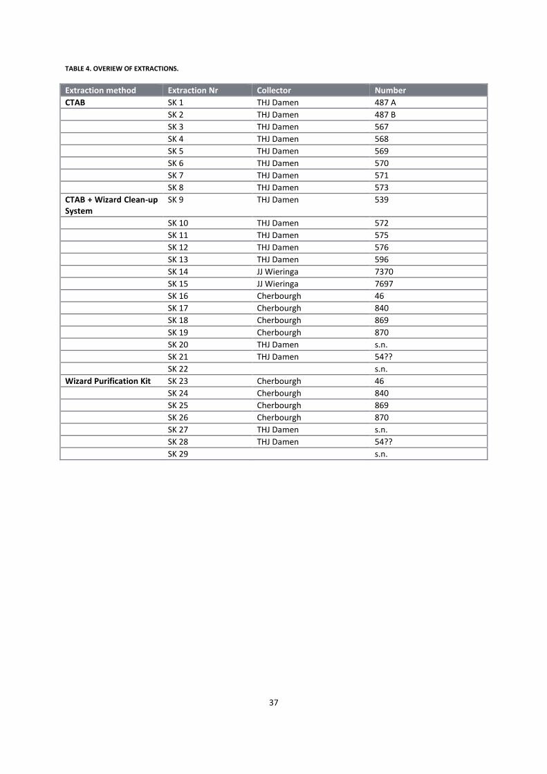
37

TABLE 4. OVERIEW OF EXTRACTIONS.

Extraction method Extraction Nr Collector Number

CTAB SK 1 THJ Damen 487 A

SK 2 THJ Damen 487 B

SK 3 THJ Damen 567

SK 4 THJ Damen 568

SK 5 THJ Damen 569

SK 6 THJ Damen 570

SK 7 THJ Damen 571

SK 8 THJ Damen 573

CTAB + Wizard Clean-up System

SK 9 THJ Damen 539

SK 10 THJ Damen 572

SK 11 THJ Damen 575

SK 12 THJ Damen 576

SK 13 THJ Damen 596

SK 14 JJ Wieringa 7370

SK 15 JJ Wieringa 7697

SK 16 Cherbourgh 46

SK 17 Cherbourgh 840

SK 18 Cherbourgh 869

SK 19 Cherbourgh 870

SK 20 THJ Damen s.n.

SK 21 THJ Damen 54??

SK 22 s.n.

Wizard Purification Kit SK 23 Cherbourgh 46

SK 24 Cherbourgh 840

SK 25 Cherbourgh 869

SK 26 Cherbourgh 870

SK 27 THJ Damen s.n.

SK 28 THJ Damen 54??

SK 29 s.n.

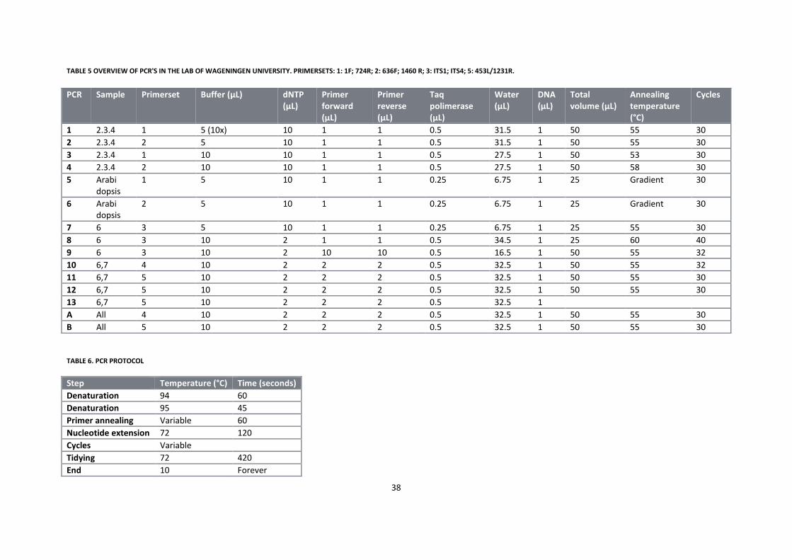
38

TABLE 5 OVERVIEW OF PCR'S IN THE LAB OF WAGENINGEN UNIVERSITY. PRIMERSETS: 1: 1F; 724R; 2: 636F; 1460 R; 3: ITS1; ITS4; 5: 453L/1231R.

TABLE 6. PCR PROTOCOL

Step Temperature (°C) Time (seconds)

Denaturation 94 60

Denaturation 95 45

Primer annealing Variable 60

Nucleotide extension 72 120

Cycles Variable

Tidying 72 420

End 10 Forever

PCR Sample Primerset Buffer (μL) dNTP (μL)

Primer forward (μL)

Primer reverse (μL)

Taq polimerase (μL)

Water (μL)

DNA (μL)

Total volume (μL)

Annealing temperature (°C)

Cycles

1 2.3.4 1 5 (10x) 10 1 1 0.5 31.5 1 50 55 30

2 2.3.4 2 5 10 1 1 0.5 31.5 1 50 55 30

3 2.3.4 1 10 10 1 1 0.5 27.5 1 50 53 30

4 2.3.4 2 10 10 1 1 0.5 27.5 1 50 58 30

5 Arabi dopsis

1 5 10 1 1 0.25 6.75 1 25 Gradient 30

6 Arabi dopsis

2 5 10 1 1 0.25 6.75 1 25 Gradient 30

7 6 3 5 10 1 1 0.25 6.75 1 25 55 30

8 6 3 10 2 1 1 0.5 34.5 1 25 60 40

9 6 3 10 2 10 10 0.5 16.5 1 50 55 32

10 6,7 4 10 2 2 2 0.5 32.5 1 50 55 32

11 6,7 5 10 2 2 2 0.5 32.5 1 50 55 30

12 6,7 5 10 2 2 2 0.5 32.5 1 50 55 30

13 6,7 5 10 2 2 2 0.5 32.5 1

A All 4 10 2 2 2 0.5 32.5 1 50 55 30

B All 5 10 2 2 2 0.5 32.5 1 50 55 30

39

After PCR amplification, I purified the PCR samples with the GeneJET PCR Purification Kit. I adjusted the

protocol slightly in order to obtain the quantity of DNA necessary for sequencing at GATC Konstanz. Instead of

solving the precipitated DNA in 50 μL of solution buffer, I used only 10 μL. Because the yield was so low, I then

let the solution buffer completely evaporate. Then, I diluted the precipitated DNA in 5μL of MQ water. To this

solution, I then added 5 μL of primer with a concentration of 5μL/μL (Appendix 11).

Hereafter, I send the PCR products to GATC Konstanz to be sequenced. We had no experience with this

sequencing company and it was the question whether the PCR products would generate a usable result.

Therefore, I first send four PCR products of the first primer pair (spanning the first region of the gene) in

combination with their forward primer to the company for testing. Little variation was found in this region, so

we decided to sequence the other region of the gene. For the second primer pair, we sequenced all 22 leaf

samples with the forward primer.

After sequencing, I checked the tracers in CodonCodeAligner (Corp., n.d.). Now and then it was necessary to

adjust the assigned nucleotides because of multiple peaks on one codon position.

5.2.3 GENERAL PHYLOGENETIC ANALYSIS I used two quite different methods to generate sequence data as are described above. However the analysis

done with these sequences are rather similar.

The sequences were added to the sequence alignment compiled by Bouetard et al. I obtained from NCBI

GenBank (Appendix 12). To this alignment, I added additional sequences of other relevant species. Examples of

this are sequences from the Apostasioideae, the basal sister family of the Vanilloideae within the Orchidaceae,

which has not been implemented yet in the phylogenetic tree to obtain a more proper rooting. Also sequences

of the Magnoliids were included since this clade is the basal sister of the Asparagales, to which the Orchidaceae

belongs.

I assembled these sequences in Mesquite (Maddison & Maddison, n.d.) and aligned them by hand. Then, I

assessed phylogenetic relationships between the sequences using RAxML-HPC2 on XSEDE via the CIPRES

Science Gateway (Miller, Pfeiffer, & Schwartz, 2010).

Since I have such different types of data, I made a number of alignments consisting of different combinations of

data. First, I made a basis alignment with all the data from Genbank (consisting mainly of the Bouetard

accessions). Second, I made a historic DNA alignment, consisting of the basis alignment plus the historic DNA

sequence data. Third, a regular DNA alignment, with the basis alignment extended with the sequence data

obtained using the regular DNA extraction methods. Last, I implemented all available sequences in one

overarching fourth alignment.

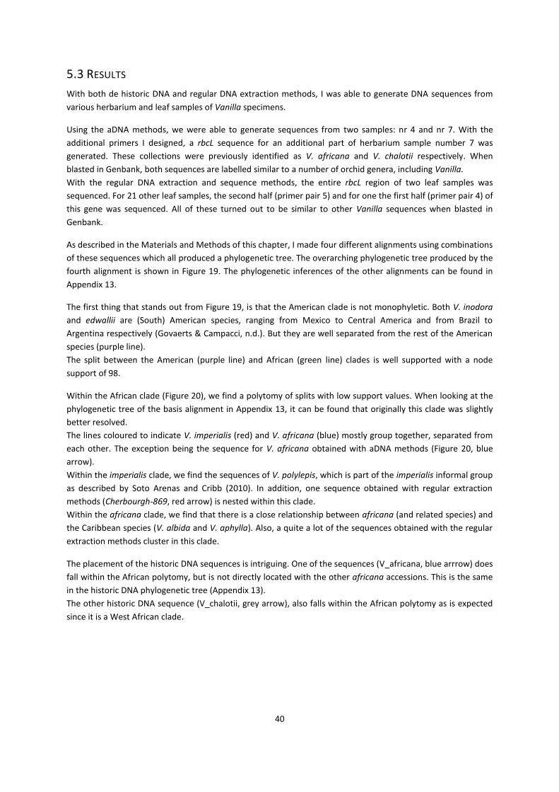
40

5.3 RESULTS

With both de historic DNA and regular DNA extraction methods, I was able to generate DNA sequences from

various herbarium and leaf samples of Vanilla specimens.

Using the aDNA methods, we were able to generate sequences from two samples: nr 4 and nr 7. With the

additional primers I designed, a rbcL sequence for an additional part of herbarium sample number 7 was

generated. These collections were previously identified as V. africana and V. chalotii respectively. When

blasted in Genbank, both sequences are labelled similar to a number of orchid genera, including Vanilla.

With the regular DNA extraction and sequence methods, the entire rbcL region of two leaf samples was

sequenced. For 21 other leaf samples, the second half (primer pair 5) and for one the first half (primer pair 4) of

this gene was sequenced. All of these turned out to be similar to other Vanilla sequences when blasted in

Genbank.

As described in the Materials and Methods of this chapter, I made four different alignments using combinations

of these sequences which all produced a phylogenetic tree. The overarching phylogenetic tree produced by the

fourth alignment is shown in Figure 19. The phylogenetic inferences of the other alignments can be found in

Appendix 13.

The first thing that stands out from Figure 19, is that the American clade is not monophyletic. Both V. inodora

and edwallii are (South) American species, ranging from Mexico to Central America and from Brazil to

Argentina respectively (Govaerts & Campacci, n.d.). But they are well separated from the rest of the American

species (purple line).

The split between the American (purple line) and African (green line) clades is well supported with a node

support of 98.

Within the African clade (Figure 20), we find a polytomy of splits with low support values. When looking at the

phylogenetic tree of the basis alignment in Appendix 13, it can be found that originally this clade was slightly

better resolved.

The lines coloured to indicate V. imperialis (red) and V. africana (blue) mostly group together, separated from

each other. The exception being the sequence for V. africana obtained with aDNA methods (Figure 20, blue

arrow).

Within the imperialis clade, we find the sequences of V. polylepis, which is part of the imperialis informal group

as described by Soto Arenas and Cribb (2010). In addition, one sequence obtained with regular extraction

methods (Cherbourgh-869, red arrow) is nested within this clade.

Within the africana clade, we find that there is a close relationship between africana (and related species) and

the Caribbean species (V. albida and V. aphylla). Also, a quite a lot of the sequences obtained with the regular

extraction methods cluster in this clade.

The placement of the historic DNA sequences is intriguing. One of the sequences (V_africana, blue arrrow) does

fall within the African polytomy, but is not directly located with the other africana accessions. This is the same

in the historic DNA phylogenetic tree (Appendix 13).

The other historic DNA sequence (V_chalotii, grey arrow), also falls within the African polytomy as is expected

since it is a West African clade.

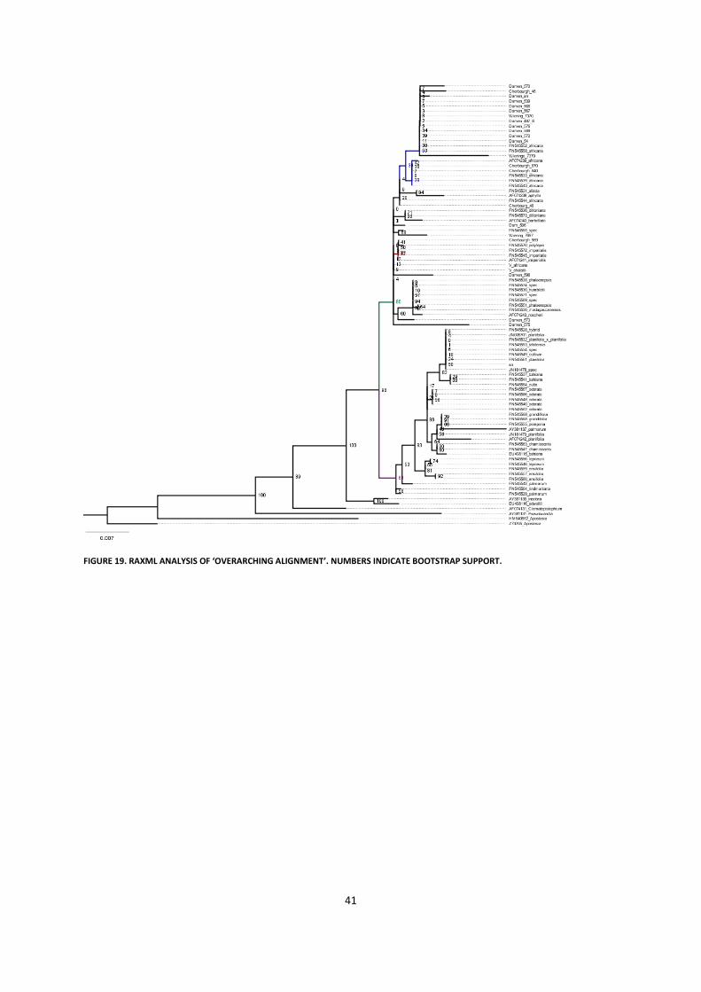
41

FIGURE 19. RAXML ANALYSIS OF ‘OVERARCHING ALIGNMENT’. NUMBERS INDICATE BOOTSTRAP SUPPORT.

42

FIGURE 20. AFRICAN CLADE OF RAXML ANALYSIS ON ‘OVERARCHING ALIGNMENT’. NUMBERS INDICATE BOOTSTRAP VALUES.

43

5.4 DISCUSSION AND CONCLUSION

The question addressed in this part of the research (Can (part of) the phylogenetic hypothesis of Bouetard et al.

(2010) be complemented and optimised with additional Vanilla species, especially those from the V. imperialis

& africana groups as described by Soto Arenas & Cribb (2010)?) is a bit arbitrary. Of course the phylogenetic

tree can be complemented and optimised. But the goal (set by the underlying hypotheses) is quite plain: rather

specific parts of the Vanilla variation are missing in this phylogenetic tree and a lot remains unclear. This has to

be cleared up.

Also, it would be very handy to have a set of model sequences that each represents a different species. In this

way, the species of not flowering Vanilla plants can be identified.

The historic DNA research was therefore set up to fill in the gaps of missing species in this phylogenetic tree.

Very specific species were attempted to be added to the phylogenetic tree of Bouetard et al. (2010). The only

way this is possible is by taking leaf samples from specimens that were identified to be those particular species

based on morphology.

We were able to successfully extract, amplify and clone five out of seven selected leaf samples using aDNA

methods, but due to DNA degradation three of these were contaminated with Solanum lycopersicon and

bacterial tissue. So only two leaf samples generated a usable sequence. However, since the target region of the

primer is only around 120 bp, this sequences were rather short. Also, they did not contain a lot of usable

information since they were placed at the beginning of the rbcL gene, even just before the majority of

sequences from GenBank started. Therefore, I designed an additional primer for a more variable part of the

rbcL gene within the Vanilla alignment. In total, three sequences for two leaf samples were obtained in this

way. One for V. africana (with the first primer) and two for V. chalotii (with both first and second primer).

To answer the first hypothesis (The V. chalotii group will cluster in an intermediate clade between African and

Caribbean species), the sequence of the herbarium specimen of V. chalotii is important. As presented in the

Results of this chapter, the hDNA sequence I obtained for V. chalotii indeed clusters within the African clade.

But unfortunately not near the africana clade and the Caribbean species V. dilloniana and V. barbellata. Based

on these results, I should thus reject this hypothesis.

However, the sequence data available for this species is still rather little, resulting in a weak node support (9)

and making the placement in the phylogenetic tree dubious. I believe no sound conclusions can be based on

these results and therefore not accept nor reject the first hypothesis. To be able to accept it, a strong

supported sequence of V. chalotii or related relevant species should cluster within the africana clade, parting it

from the Caribbean species. Now that is shown that aDNA extraction methods are possible for Vanilla, more

primers, both for other genes and other regions of the rbcL gene, can be designed and the data can help form a

better underpinned picture.

The second hypothesis states that ‘The V. francoisii group will be closely related to the V. madagascariensis

group, since both are Indian Ocean based groups’. Unfortunately, no species from the informal V. francoisii

group could be added at all to the phylogenetic tree because extraction with aDNA methods did not work in

this case. I therefore find also the second hypothesis cannot be judged.

In order to judge the third hypothesis (‘The informal V. imperialis and africana groups are monophyletic groups)

I included all relevant species that are missing from the phylogenetic tree of Bouetard et al (2010) in the

historic DNA research. Unfortunately, none of these herbarium leaf samples generated a DNA sequence. Still, in

the phylogenetic inference of the alignment shown in Appendix 13, the two groups both remain monophyletic.

Based on this, one could accept the hypothesis. However, I again feel I cannot make a proper judgement, since

the hypothesis was formulated in the spirit of the historic DNA research. Thus whether or not the informal

44

groups would remain monophyletic after incorporation of the missing species. This has not been answered

since not all species of the groups are included in the phylogenetic tree.

In addition, I would find it dangerous to make a decision based on the phylogenetic tree of Figure 19. It gives a

good indication, but overall is weakly supported and based on only one gene. Especially for the africana group,

since the historic DNA sequence for V. africana (V_africana) does not cluster with the other africana accessions.

But even more than for the V. chalotii sequence, it has to be remembered that there is really quite little

information available in this sequence.

There are a number of general differences between my phylogenetic tree and the one of Bouetard et al (2010).

In contrast to the phylogenetic tree of Bouetard et al. (2010), the American clade in the phylogenetic tree

pictured in Figure 19 is not monophyletic. The species responsible for this (V. edwallii and V. inodora) do not

occur in the phylogenetic tree of Bouetard et al.(2010). Perhaps they overlooked them when assembling their

alignment of sequences from GenBank.

Why these two species stand out so clearly is a mystery to me since I did not study their morphology in relation

to the other American based species. However, when checked in the Mesquite alignment, I found there are a

number of codons they both have in common with the species belonging to the outgroup that differ from the

Vanilla sequences.

In addition, my phylogenetic tree does not contain accessions of species from the informal Membranaceous

group. In their paper, Bouetard et al. (2010) indicate they found a sequence for V. mexicana in GenBank and

that the accession number should be listed in the attached table. But the species does not occur in the table at

all, and when searched for in GenBank, no accessions from this species could be found.

How it is possible that three out of five samples were contaminated is quite strange, since we took all

necessary precautions that are customary in an Ancient DNA lab. Every morning, all surfaces were cleaned with

a chlorine solution and all material was put in a UV chamber to destroy any stray DNA scraps. I am positive

neither Anile Nieman nor myself ate tomato during the extractions, so the contamination could not come

about that way.

As it thus turns out, sequencing orchid DNA from herbarium specimens using historic DNA methods is indeed

possible. More time then was available is only needed for the final fine tuning of the methods to have it work

on the oddities of Vanilla DNA. Then, extraction and sequencing of DNA from the particular species that are

part of one’s research should pose no great problems. Also, in the future, more herbarium specimens may be

sampled using the newly designed primer.

The second extraction path turned out to be more laborious than expected as well. It took a lot of time to

successfully amplify the leaf material that was available using PCR because of numerous difficulties in the lab. A

number of sequences are successfully added to the alignment, but due to limited time not the whole rbcL

region of all silica samples could be sequenced.

Even though a limited amount of data is thus available per sequence, all of these samples do group within the

African/Asian clade. This indicates that the region that is now sequenced indeed can be used as an indicator for

general relationships. For sterile specimens, at least their morphological group can be established.

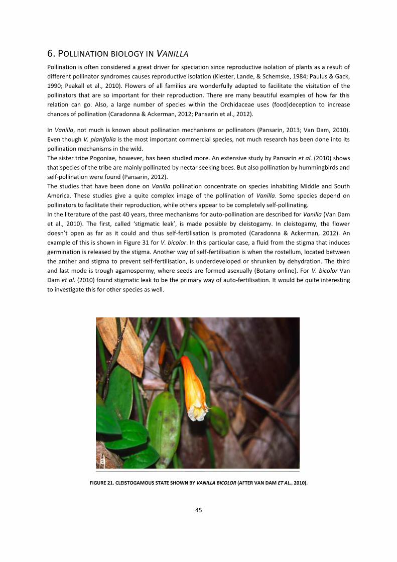
45

6. POLLINATION BIOLOGY IN VANILLA Pollination is often considered a great driver for speciation since reproductive isolation of plants as a result of

different pollinator syndromes causes reproductive isolation (Kiester, Lande, & Schemske, 1984; Paulus & Gack,

1990; Peakall et al., 2010). Flowers of all families are wonderfully adapted to facilitate the visitation of the

pollinators that are so important for their reproduction. There are many beautiful examples of how far this

relation can go. Also, a large number of species within the Orchidaceae uses (food)deception to increase

chances of pollination (Caradonna & Ackerman, 2012; Pansarin et al., 2012).

In Vanilla, not much is known about pollination mechanisms or pollinators (Pansarin, 2013; Van Dam, 2010).

Even though V. planifolia is the most important commercial species, not much research has been done into its

pollination mechanisms in the wild.

The sister tribe Pogoniae, however, has been studied more. An extensive study by Pansarin et al. (2010) shows

that species of the tribe are mainly pollinated by nectar seeking bees. But also pollination by hummingbirds and

self-pollination were found (Pansarin, 2012).

The studies that have been done on Vanilla pollination concentrate on species inhabiting Middle and South

America. These studies give a quite complex image of the pollination of Vanilla. Some species depend on

pollinators to facilitate their reproduction, while others appear to be completely self-pollinating.

In the literature of the past 40 years, three mechanisms for auto-pollination are described for Vanilla (Van Dam

et al., 2010). The first, called ‘stigmatic leak’, is made possible by cleistogamy. In cleistogamy, the flower

doesn’t open as far as it could and thus self-fertilisation is promoted (Caradonna & Ackerman, 2012). An

example of this is shown in Figure 31 for V. bicolor. In this particular case, a fluid from the stigma that induces

germination is released by the stigma. Another way of self-fertilisation is when the rostellum, located between

the anther and stigma to prevent self-fertilisation, is underdeveloped or shrunken by dehydration. The third

and last mode is trough agamospermy, where seeds are formed asexually (Botany online). For V. bicolor Van

Dam et al. (2010) found stigmatic leak to be the primary way of auto-fertilisation. It would be quite interesting

to investigate this for other species as well.

FIGURE 21. CLEISTOGAMOUS STATE SHOWN BY VANILLA BICOLOR (AFTER VAN DAM ET AL., 2010).

46

In the light of my morphological research I would have liked to be able to relate the results to possible

differences in pollination systems and pollinators. But since no pollination related research has been done into

the wild species of Continental Africa, it will be a lot of guesswork. However, although pollinator species are

not known, I can make some general comments on the pollination of both the imperialis as the africana group.

The flowers of the imperialis group show general resemblances with those of V. bicolor and V. planifolia. Both

have the same tube shape formed by the fusion of sepals/petals, lip and column as the flowers of the imperialis

group. Therefore, one might argue that there could be a resemblance in pollination. Perhaps not in pollinators,

since imperialis occurs solely in Continental Africa and V. bicolor and its relatives only reside in America. But

perhaps then in the way pollination occurs. Unfortunately, this also remains speculation since the species with

flowers that resemble those of imperialis show great variety in their pollination mechanisms. As described

above, some are quite unsuccessfully pollinated by a range of pollinators. Others are quite successful self-

pollinators, but differ in the way they self-pollinate. Of the above described methods, the second doesn’t seem

likely, because I did not encounter any flowers with a shrivelled rostellum. I also did not come upon any flowers

that were more closed than others, but this is hard to determine since I boiled the flowers and then prepared

them. Also the flowers still attached to the plant on the herbarium sheet have lost their original form due to

the drying process. Both the stigmatic leak and agamospermy methods I thus did not see, but it is possible

imperialis is fertilised by one of them.

For the flowers of the africana group, I find it rather difficult to make any comments on pollination. I suspect

some insect species are involved in the pollination rather than pollination occurring through self-pollination.

This because the flowers are much more open in their morphology. The sepals and petals, lip and column are

still fused to form a tube, but this tube is much smaller than the one formed by imperialis relative to the size of

the flowers. Also, in a number of cases the tube itself is quite open at the sides (Figure 22). This makes self-

pollination by ‘stigmatic leak’ quite difficult. Also, I again did not find any examples of shrivelled rostella.

Therefore, of the pollination of africana as a group I cannot say anything with certainty.

Within the africana group, I can say that probably there are

differences in pollinators. The first morphological group

described in Chapter 4 has a distinctly different lip shape

compared to the other groups. The lip is the landing platform

for a pollinator, so a difference in shape strongly indicates a

difference in pollinator. The lip of V. heterolopha is that much

broader and larger, and the flower as a whole is much opener

that it indicates a larger pollinator than is suitable for africana.

Within the species africana, the diversity in flower morphology

is so great that I cannot image the whole species is pollinated by

just one and the same pollinator

FIGURE 22. EXAMPLE OF FLOWER WITH OPEN

SIDES IN THE AFRICANA GROUP.

47

7. LINKING MORPHOLOGY AND DNA The aim of this study was to link the fields of morphological and phylogenetic taxonomic research. It was

already a precarious project to begin with, and unfortunately this ultimate goal is not met. Because of

difficulties resulting in unfinished research in both the morphological as the phylogenetic fields, I cannot make

the final step to link them. This does not mean that the project failed. Both fields are updated and a foundation

for future research is laid.

Especially with the DNA based phylogenetic research, there were some unexpected issues. Beforehand, we

already knew the historic DNA track would be difficult. But because of the experience with other orchid

material in the lab, there was reasonable hope this kind of analysis would work on Vanilla as well. This indeed

was the case, but as indicated in the Conclusion and Discussion of the corresponding chapter, the methods

have to be adjusted a bit to the material under research.

For further development of the still remaining problem on the phylogenetic tree filled with gaps from Bouetard

et al. (2010), my original back-up plan would still be a good option for future research. In this plan, the

phylogenies of Bouetard et al. (2010, based on the chloroplast gene regions rbcL, psaB, psbB and psbC) would

be linked to the 5.8S rDNA nuclear ribosomal ITS phylogenetic tree of Soto Arenas & Dressler (2010). They

formed a phylogenetic tree solely based on this region for Mexican and Caribbean species. With the use of the

combined samples of Bouetard et al and Soto Arenas & Dressler, a phylogenetic tree can then be made based

on these five gene regions. This phylogenetic tree would then be well supported because it is based on both

nuclear and chloroplast DNA. Also species from Asia can then be taken into the analysis to form a complete

picture of the variation within the genus.

Possible hypotheses for this research would be:

A. When the nrDNA phylogenetic tree of Soto Arenas & Dressler (2010) is complemented with African

samples, it will resemble the cpDNA phylogenetic tree of Bouetard et al. (2010).

B. The African V. africana and imperialis groups will cluster near V. barbellata from the Caribbean.

Much the same procedure would have to be followed as was done in this research. Leaf samples of all involved

species would have to be gathered for extraction, PCR amplification and sequencing. This would be quite a

challenge.

It would be important to obtain samples from V. barbellata since it is the only relevant species linking the two

already existing phylogenies.

In the future, another option for further research would be to investigate the actual pollination process of

Vanilla species. From a commercial point of view, it might be interesting to look into the pollination of V.

planifolia since hand pollination, as is common practise in Vanilla production at the moment, is quite labour-

intensive. All plants are thus effectively fertilised with their own pollen. Genetic diversity is thus more and

more limited, leaving only those plants that produce the most Vanilla pods.

Also, since the shape of the lip seems to be quite a fascinating character dividing V. heterolopha and the rest of

the africana group, it would be interesting to investigate whether this could be pollinator driven speciation.

This would pose quite some problems. Finding the species at the flowering time is in itself quite a challenge as

the inflorescences are mainly situated in the canopy of the forest. When successful, a possible pollinator would

somehow have to be recorded.

Basically, a whole lot of opportunities are still to be explored!

48

REFERENCES

Álvarez, I., & Wendel, J. F. (2003). Ribosomal ITS sequences and plant phylogenetic inference. Molecular

Phylogenetics and Evolution, 29(3), 417–434.

Bory, S., Catrice, O., Brown, S., Leitch, I. J., Gigant, R., Chiroleu, F., … Besse, P. (2008). Natural polyploidy in

Vanilla planifolia (Orchidaceae). Genome, 51(10), 816–26. doi:10.1139/G08-068

Bory, S., Da Silva, D., Risterucci, a.-M., Grisoni, M., Besse, P., & Duval, M.-F. (2008). Development of

microsatellite markers in cultivated vanilla: Polymorphism and transferability to other vanilla species.

Scientia Horticulturae, 115(4), 420–425. doi:10.1016/j.scienta.2007.10.020

Bory, S., Grisoni, M., Duval, M.-F., & Besse, P. (2007). Biodiversity and preservation of vanilla: present state of

knowledge. Genetic Resources and Crop Evolution, 55(4), 551–571. doi:10.1007/s10722-007-9260-3

Bory, S., Lubinsky, P., Risterucci, A.-M., Noyer, J.-L., Grisoni, M., Duval, M.-F., & Besse, P. (2008). Patterns of

introduction and diversification of Vanilla planifolia (Orchidaceae) in Reunion Island (Indian Ocean).

American Journal of Botany, 95(7), 805–15. doi:10.3732/ajb.2007332

Bouetard, A., Lefeuvre, P., Gigant, R., Bory, S., Pignal, M., Besse, P., & Grisoni, M. (2010). Evidence of

transoceanic dispersion of the genus Vanilla based on plastid DNA phylogenetic analysis. Molecular

Phylogenetics and Evolution, 55(2), 621–30. doi:10.1016/j.ympev.2010.01.021

Bruman, H. (1948). The Culture History of Mexican Vanilla. The Hispanic American Historical Review, 28(3),

360–376.

Cameron, K. M. (2003). Vanilloideae. In A. M. Pridgeon, P. J. Cribb, M. W. Chase, & F. N. Rasmussen (Eds.),

Genera Orchidacearum: Orchidoideae (pp. 281–285). Oxford University Press, Oncorporated.

Cameron, K. M. (2004). Utility of plastid psaB gene sequences for investigating intrafamilial relationships within

Orchidaceae. Molecular Phylogenetics and Evolution, 31(3), 1157–80. doi:10.1016/j.ympev.2003.10.010

Cameron, K. M. (2009). On the value of nuclear and mitochondrial gene sequences for reconstructing the

phylogeny of vanilloid orchids (Vanilloideae, Orchidaceae). Annals of Botany, 104(3), 377–85.

doi:10.1093/aob/mcp024

Cameron, K. M. (2011a). Vanilla orchids: natural history and cultivation. Timber Press, Inc.

Cameron, K. M. (2011b). Vanilla Phylogeny and Classification. In D. Havkin-Frenkel & F. C. Belanger (Eds.),

Handbook of Vanilla Science and Technology (pp. 243–255).

Cameron, K. M., & Carmen Molina, M. (2006). Photosystem II gene sequences of psbB and psbC clarify the

phylogenetic position of Vanilla (Vanilloideae, Orchidaceae). Cladistics, 22(3), 239–248.

doi:10.1111/j.1096-0031.2006.00102.x

Cameron, K. M., Chase, M. W., Whitten, W. M., Kores, P. J., Jarrell, D. C., Albert, V. A., … Goldman, D. H. (1999).

A Phylogenetic Analysis of the Orchidaceae: Evidence from rbcL Nucleotide Sequences. American Journal

of Botany, 86(2), 208–224.

49

Caradonna, P. J., & Ackerman, J. D. (2012). Reproductive assurance for a rewardless epiphytic orchid in Puerto

Rico: Pleurothallis ruscifolia (Orchidaceae, Pleurothallidinae). Caribbean Journal of Science, 46(2), 249–

257.

Corney, D. P. A., Clark, J. Y., Tang, H. L., & Wilkin, P. (2012). Automatic extraction of leaf characters from

herbarium specimens. Taxon, 61(1), 231–244.

Corp., C. (n.d.). CodonCode Aligner. Dedham, MA, USA.

Corporation, P. (n.d.). Wizard DNA Clean-Up System.

Correll, D. S. (1953). Vanilla: Its Botany, History, Cultivation and Economic Import. Economic Botany, 7(4), 291–

358.

Doyle, J. J. (1991). DNA protocols for plants. Molecular Techniques in Taxonomy, 283–293.

Dressler, R. L. (1981). The Orchids, Natural history and Classification. Harvard University Press.

Dressler, R. L., & Dodson, C. H. (1960). Classification and Phylogeny in the Orchidaceae. Annals of the Missouri

Botanical Garden, 47(1), 25–68.

Dytham, C. (2011). Choosing and using statistics: a biologist’s guide. John Wiley & Sons.

Ecott, T. (2004). Vanilla, travels in search of the luscious substance. Penguin Books, England.

Fouché, J. G., & Jouve, L. (1999). Vanilla planifolia: history, botany and culture in Reunion island. Agronomie,

19(8), 689–703. doi:10.1051/agro:19990804

Frankham, R., Ballou, J. D., Dudash, M. R., Eldridge, M. D. B., Fenster, C. B., Lacy, R. C., … Ryder, O. a. (2012).

Implications of different species concepts for conserving biodiversity. Biological Conservation, 153, 25–31.

doi:10.1016/j.biocon.2012.04.034

Freudenstein, J. V., van den Berg, C., Goldman, D. H., Kores, P. J., Molvray, M., & Chase, M. W. (2004). An

Expanded Plastid DNA Phylogeny of Orchidaceae and Analysis of Jackknife Branch Support Strategy.

American Journal of Botany, 91(1), 149–157.

Geerinck, D. (2011). Catalogue raisonné des Orchidaceae du Congo-Kinshasa, distribuées par districts

phytogéographiques. Taxonomia, 32, 2–37.

Gigant, R., Brugel, a., Bruyn, a., Risterucci, a. M., Guiot, V., Viscardi, G., … Besse, P. (2011). Nineteen

polymorphic microsatellite markers from two African Vanilla species: across-species transferability and

diversity in a wild population of V. humblotii from Mayotte. Conservation Genetics Resources, 4(1), 121–

125. doi:10.1007/s12686-011-9489-1

Govaerts, R., & Campacci, M. A. (n.d.). World Checklist of Orchidaceae. Retrieved from

http://www.kew.org/wcsp/monocots/.

Gravendeel, B., Harle, N., Bekker, S., Hoebe, N., & Fay, F. M. (2010). Vrouwenschoentje in het Limburgse

heuvelland: te mooi om waar te zijn? Natuurhistorisch Maandblad, 99(11).

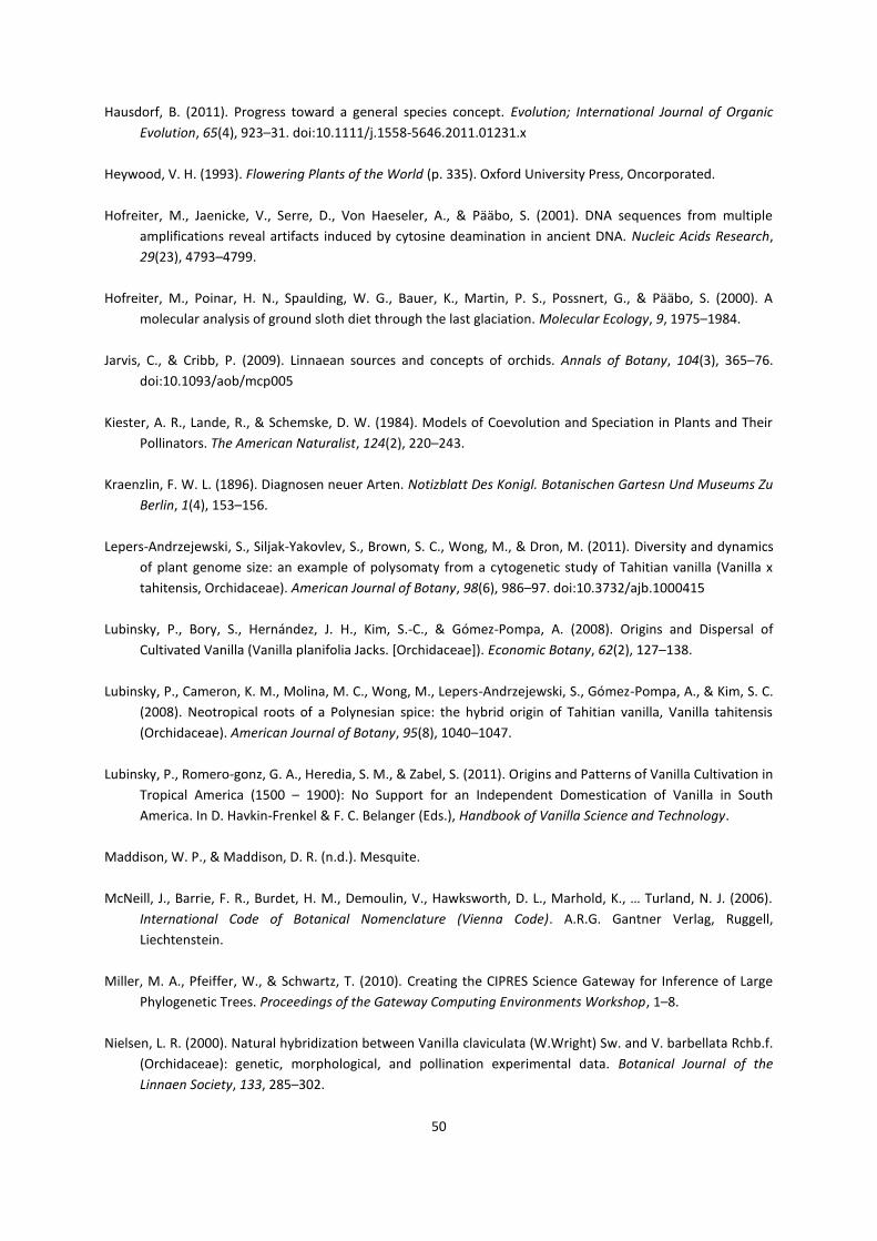
50

Hausdorf, B. (2011). Progress toward a general species concept. Evolution; International Journal of Organic

Evolution, 65(4), 923–31. doi:10.1111/j.1558-5646.2011.01231.x

Heywood, V. H. (1993). Flowering Plants of the World (p. 335). Oxford University Press, Oncorporated.

Hofreiter, M., Jaenicke, V., Serre, D., Von Haeseler, A., & Pääbo, S. (2001). DNA sequences from multiple

amplifications reveal artifacts induced by cytosine deamination in ancient DNA. Nucleic Acids Research,

29(23), 4793–4799.

Hofreiter, M., Poinar, H. N., Spaulding, W. G., Bauer, K., Martin, P. S., Possnert, G., & Pääbo, S. (2000). A

molecular analysis of ground sloth diet through the last glaciation. Molecular Ecology, 9, 1975–1984.

Jarvis, C., & Cribb, P. (2009). Linnaean sources and concepts of orchids. Annals of Botany, 104(3), 365–76.

doi:10.1093/aob/mcp005

Kiester, A. R., Lande, R., & Schemske, D. W. (1984). Models of Coevolution and Speciation in Plants and Their

Pollinators. The American Naturalist, 124(2), 220–243.

Kraenzlin, F. W. L. (1896). Diagnosen neuer Arten. Notizblatt Des Konigl. Botanischen Gartesn Und Museums Zu

Berlin, 1(4), 153–156.

Lepers-Andrzejewski, S., Siljak-Yakovlev, S., Brown, S. C., Wong, M., & Dron, M. (2011). Diversity and dynamics

of plant genome size: an example of polysomaty from a cytogenetic study of Tahitian vanilla (Vanilla x

tahitensis, Orchidaceae). American Journal of Botany, 98(6), 986–97. doi:10.3732/ajb.1000415

Lubinsky, P., Bory, S., Hernández, J. H., Kim, S.-C., & Gómez-Pompa, A. (2008). Origins and Dispersal of

Cultivated Vanilla (Vanilla planifolia Jacks. [Orchidaceae]). Economic Botany, 62(2), 127–138.

Lubinsky, P., Cameron, K. M., Molina, M. C., Wong, M., Lepers-Andrzejewski, S., Gómez-Pompa, A., & Kim, S. C.

(2008). Neotropical roots of a Polynesian spice: the hybrid origin of Tahitian vanilla, Vanilla tahitensis

(Orchidaceae). American Journal of Botany, 95(8), 1040–1047.

Lubinsky, P., Romero-gonz, G. A., Heredia, S. M., & Zabel, S. (2011). Origins and Patterns of Vanilla Cultivation in

Tropical America (1500 – 1900): No Support for an Independent Domestication of Vanilla in South

America. In D. Havkin-Frenkel & F. C. Belanger (Eds.), Handbook of Vanilla Science and Technology.

Maddison, W. P., & Maddison, D. R. (n.d.). Mesquite.

McNeill, J., Barrie, F. R., Burdet, H. M., Demoulin, V., Hawksworth, D. L., Marhold, K., … Turland, N. J. (2006).

International Code of Botanical Nomenclature (Vienna Code). A.R.G. Gantner Verlag, Ruggell,

Liechtenstein.

Miller, M. A., Pfeiffer, W., & Schwartz, T. (2010). Creating the CIPRES Science Gateway for Inference of Large

Phylogenetic Trees. Proceedings of the Gateway Computing Environments Workshop, 1–8.

Nielsen, L. R. (2000). Natural hybridization between Vanilla claviculata (W.Wright) Sw. and V. barbellata Rchb.f.

(Orchidaceae): genetic, morphological, and pollination experimental data. Botanical Journal of the

Linnaen Society, 133, 285–302.

51

Pansarin, E. R., Aguiar, J. M. R. B. V., & Pansarin, L. M. (2013). Floral biology and histochemical analysis of

Vanilla edwallii Hoehne (Orchidaceae: Vanilloideae): an orchid pollinated by Epicharis (Apidae: Centridini).

Plant Species Biology, n/a–n/a. doi:10.1111/1442-1984.12014

Pansarin, E. R., Salatino, A., Pansarin, L. M., & Sazima, M. (2012). Pollination systems in Pogonieae (Orchidaceae:

Vanilloideae): A hypothesis of evolution among reward and rewardless flowers. Flora - Morphology,

Distribution, Functional Ecology of Plants, 207(12), 849–861. doi:10.1016/j.flora.2012.09.011

Paulus, H. F., & Gack, C. (1990). POLLINATORS AS PREPOLLINATING ISOLATION FACTORS: EVOLUTION AND

SPECIATION IN OPHRYS (ORCFFLDACEAE). Israel Journal of Botany, 39(1-2), 43–79.

Peakall, R., Ebert, D., Poldy, J., Barrow, R. A., Francke, W., Bower, C. C., & Schiestl, F. P. (2010). Pollinator

specificity, floral odour chemistry and the phylogeny of Australian sexually deceptive Chiloglottis orchids:

implications for pollinator‐driven speciation. New Phytologist, 188(2), 437–450.

Portères, R. (1954). Le Genre Vanilla et ses espèces. In G. Bouriget (Ed.), Le Vanillier et la Vanille dans le Monde

(pp. 94–290). Paul Lechavalier, Paris.

Ramírez, S. R., Gravendeel, B., Singer, R. B., Marshall, C. R., & Pierce, N. E. (2007). Dating the origin of the

Orchidaceae from a fossil orchid with its pollinator. Nature, 448(7157), 1042–5. doi:10.1038/nature06039

Rohlf, F. J. (n.d.). tpsUtil, file utility program. version 1.26. Department of Ecology and Evolution, State

University of New York at Stony Brook.

Rohlf, F. J. (2010). TPSDig2 Version 2.16. Department of Ecology and Evolution, Stony Brook University, NY, USA.

Retrieved from http://life.bio.sunysb.edu/morph/

Rolfe, R. A. (1895). A revision of the genus Vanilla.pdf, 439–478.

Särkinen, T., Staats, M., Richardson, J. E., Cowan, R. S., & Bakker, F. T. (2012). How to open the treasure chest?

Optimising DNA extraction from herbarium specimens. PloS One, 7(8), e43808.

doi:10.1371/journal.pone.0043808

Soto Arenas, M. A., & Cameron, K. M. (2003). Vanilla. In Genera Orchidacearum: Orchidoideae 3 (pp. 321–334).

Soto Arenas, M. A., & Cribb, P. (2010). A new infrageneric classification and synopsis of the genus Vanilla Plum.

ex Mill. (Orchidaceae: Vanillinae). Lankesteriana, 9(3), 355–398.

Soto Arenas, M. A., & Dressler, R. L. (2010). A Revision of the Mexican and Central American Species of Vanilla

Plumier ex Miller with a Characterization of their ITS Region of the Nuclear Ribosomal DNA.

Lankesteriana, 9(3), 285–354.

Stern, W. L., & Judd, W. S. (1999). Comparative vegetative anatomy and systematics of Vanilla (Orchidaceae).

Botanical Journal of the Linnaen Society, 131, 353–382.

Szlachetko, D. L., & Olszewski, T. S. (1998). Flore du Cameroun.

Team, R. C. (2005). R: A language and environment for statistical computing. R foundation for Statistical

Computing.

52

The Plant List. (2010).

Tournefort, J. P. (1694). Elements de Botanique. Paris: Imprimerie Royale.

Van Dam, A. R., Householder, J. E., & Lubinsky, P. (2010). Vanilla bicolor Lindl.(Orchidaceae) from the Peruvian

Amazon: auto-fertilization in Vanilla and notes on floral phenology. Genet Resour Crop Evol, 57, 473–480.

Van der Pijl, L., & Dodson, C. H. (1966). Orchid flowers: their pollination and evolution.

Van Geel, B., Fisher, D. C., Rountrey, A. N., van Arkel, J., Duivenvoorden, J. F., Nieman, A. M., … Gravendeel, B.

(2011). Palaeo-environmental and dietary analysis of intestinal contents of a mammoth calf (Yamal

Peninsula, northwest Siberia). Quaternary Science Reviews, 30(27-28), 3935–3946.

doi:10.1016/j.quascirev.2011.10.009

Van Geel, B., Guthrie, R. D., Altmann, J. G., Broekens, P., Bull, I. D., Gill, F. L., … Gravendeel, B. (2011).

Mycological evidence of coprophagy from the feces of an Alaskan Late Glacial mammoth. Quaternary

Science Reviews, 30(17-18), 2289–2303. doi:10.1016/j.quascirev.2010.03.008

Wikipedia. (n.d.). Floral Characteristics. Retrieved from

http://en.wikipedia.org/wiki/Vanilla#mediaviewer/File:VanillaFlowerLongitudinalSection-en.png

Wilkins, J. S. (2003). How to be a chaste species pluralist-realist: the origins of species modes and the

synapomorphic species concept. Biology and Philosophy, 18, 621–638.

Wilkins, J. S. (2009). Species: a history of the idea. Univ of California Press.

Zachos, F. E., & Lovari, S. (2013). Taxonomic inflation and the poverty of the Phylogenetic Species Concept – a

reply to Gippoliti and Groves. Hystrix, 1–3. doi:10.4404/hystrix-24.1-8849

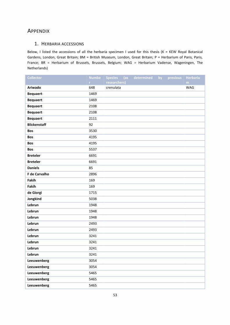
53

APPENDIX

1. HERBARIA ACCESSIONS

Below, I listed the accessions of all the herbaria specimen I used for this thesis (K = KEW Royal Botanical

Gardens, London, Great Britain; BM = British Museum, London, Great Britain; P = Herbarium of Paris, Paris,

France; BR = Herbarium of Brussels, Brussels, Belgium; WAG = Herbarium Vadense, Wageningen, The

Netherlands)

Collector Number

Species (as determined by previous researchers)

Herbarium

Ariwado 648 crenulata WAG

Bequaert 1469

Bequaert 1469

Bequaert 2108

Bequaert 2108

Bequaert 2111

Blickenstaff 92

Bos 3530

Bos 4195

Bos 4195

Bos 5537

Breteler 6691

Breteler 6691

Daniels 85

F de Carvalho 2896

Fakih 169

Fakih 169

de Giorgi 1715

Jongkind 5038

Lebrun 1948

Lebrun 1948

Lebrun 1948

Lebrun 2493

Lebrun 2493

Lebrun 3241

Lebrun 3241

Lebrun 3241

Lebrun 3241

Leeuwenberg 3054

Leeuwenberg 3054

Leeuwenberg 5465

Leeuwenberg 5465

Leeuwenberg 5465

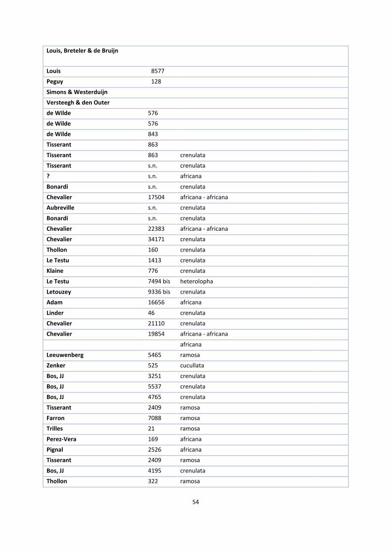
54

Louis, Breteler & de Bruijn

Louis 8577

Peguy 128

Simons & Westerduijn

Versteegh & den Outer

de Wilde 576

de Wilde 576

de Wilde 843

Tisserant 863

Tisserant 863 crenulata

Tisserant s.n. crenulata

? s.n. africana

Bonardi s.n. crenulata

Chevalier 17504 africana - africana

Aubreville s.n. crenulata

Bonardi s.n. crenulata

Chevalier 22383 africana - africana

Chevalier 34171 crenulata

Thollon 160 crenulata

Le Testu 1413 crenulata

Klaine 776 crenulata

Le Testu 7494 bis heterolopha

Letouzey 9336 bis crenulata

Adam 16656 africana

Linder 46 crenulata

Chevalier 21110 crenulata

Chevalier 19854 africana - africana

africana

Leeuwenberg 5465 ramosa

Zenker 525 cucullata

Bos, JJ 3251 crenulata

Bos, JJ 5537 crenulata

Bos, JJ 4765 crenulata

Tisserant 2409 ramosa

Farron 7088 ramosa

Trilles 21 ramosa

Perez-Vera 169 africana

Pignal 2526 africana

Tisserant 2409 ramosa

Bos, JJ 4195 crenulata

Thollon 322 ramosa

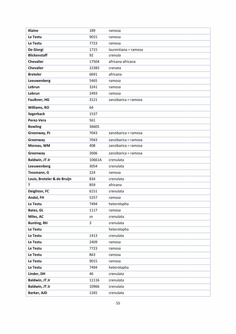
55

Klaine 189 ramosa

Le Testu 9015 ramosa

Le Testu 7723 ramosa

De Giorgi 1715 laurentiana = ramosa

Blickenstaff 92 crenula

Chevalier 17504 africana africana

Chevalier 22383 crenata

Breteler 6691 africana

Leeuwenberg 5465 ramosa

Lebrun 3241 ramosa

Lebrun 2493 ramosa

Faulkner, HG 3121 zanzibarica = ramosa

Williams, RO 64

Segerback 1537

Perez-Vera 561

Bowling 36605

Greenway, PJ 7043 zanzibarica = ramosa

Greenway 7043 zanzibarica = ramosa

Moreau, WM 408 zanzibarica = ramosa

Greenway 2606 zanzibarica = ramosa

Baldwin, JT Jr 10661A crenulata

Leeuwenberg 3054 crenulata

Tessmann, G 224 ramosa

Louis, Breteler & de Bruijn 834 crenulata

? 859 africana

Deighton, FC 6151 crenulata

Andol, FH 5257 ramosa

Le Testu 7494 heterolopha

Bates, GL 1117 ramosa

Miles, AC sn crenulata

Bunting, RH 3 crenulata

Le Testu heterolopha

Le Testu 1413 crenulata

Le Testu 2409 ramosa

Le Testu 7723 ramosa

Le Testu 863 ramosa

Le Testu 9015 ramosa

Le Testu 7494 heterolopha

Linder, DH 46 crenulata

Baldwin, JT Jr 11116 crenulata

Baldwin, JT Jr 10966 crenulata

Barker, AJD 1265 crenulata

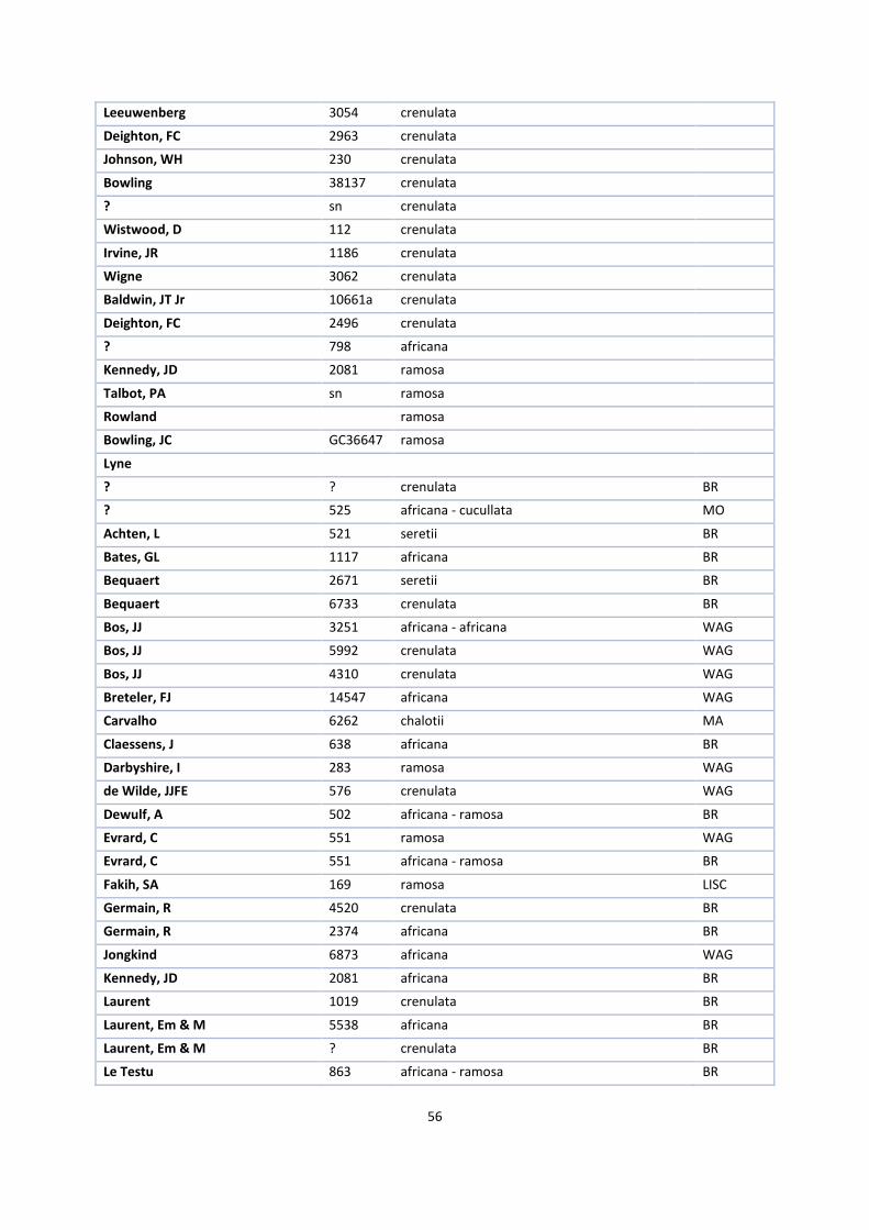
56

Leeuwenberg 3054 crenulata

Deighton, FC 2963 crenulata

Johnson, WH 230 crenulata

Bowling 38137 crenulata

? sn crenulata

Wistwood, D 112 crenulata

Irvine, JR 1186 crenulata

Wigne 3062 crenulata

Baldwin, JT Jr 10661a crenulata

Deighton, FC 2496 crenulata

? 798 africana

Kennedy, JD 2081 ramosa

Talbot, PA sn ramosa

Rowland ramosa

Bowling, JC GC36647 ramosa

Lyne

? ? crenulata BR

? 525 africana - cucullata MO

Achten, L 521 seretii BR

Bates, GL 1117 africana BR

Bequaert 2671 seretii BR

Bequaert 6733 crenulata BR

Bos, JJ 3251 africana - africana WAG

Bos, JJ 5992 crenulata WAG

Bos, JJ 4310 crenulata WAG

Breteler, FJ 14547 africana WAG

Carvalho 6262 chalotii MA

Claessens, J 638 africana BR

Darbyshire, I 283 ramosa WAG

de Wilde, JJFE 576 crenulata WAG

Dewulf, A 502 africana - ramosa BR

Evrard, C 551 ramosa WAG

Evrard, C 551 africana - ramosa BR

Fakih, SA 169 ramosa LISC

Germain, R 4520 crenulata BR

Germain, R 2374 africana BR

Jongkind 6873 africana WAG

Kennedy, JD 2081 africana BR

Laurent 1019 crenulata BR

Laurent, Em & M 5538 africana BR

Laurent, Em & M ? crenulata BR

Le Testu 863 africana - ramosa BR

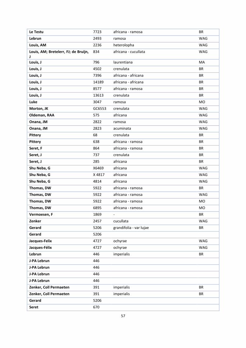
57

Le Testu 7723 africana - ramosa BR

Lebrun 2493 ramosa WAG

Louis, AM 2236 heterolopha WAG

Louis, AM; Bretelerr, FJ; de Bruijn, J

834 africana - cucullata WAG

Louis, J 796 laurentiana MA

Louis, J 4502 crenulata BR

Louis, J 7396 africana - africana BR

Louis, J 14189 africana - africana BR

Louis, J 8577 africana - ramosa BR

Louis, J 13613 crenulata BR

Luke 3047 ramosa MO

Morton, JK GC6553 crenulata WAG

Oldeman, RAA 575 africana WAG

Onana, JM 2822 ramosa WAG

Onana, JM 2823 acuminata WAG

Pittery 68 crenulata BR

Pittery 638 africana - ramosa BR

Seret, F 864 africana - ramosa BR

Seret, J 737 crenulata BR

Seret, J 285 africana BR

Shu Neba, G X6469 africana WAG

Shu Neba, G X 4817 africana WAG

Shu Neba, G 4814 africana WAG

Thomas, DW 5922 africana - ramosa BR

Thomas, DW 5922 africana - ramosa WAG

Thomas, DW 5922 africana - ramosa MO

Thomas, DW 6895 africana - ramosa MO

Vermoesen, F 1869 - BR

Zenker 2457 cucullata WAG

Gerard 5206 grandifolia - var lujae BR

Gerard 5206

Jacques-Felix 4727 ochyrae WAG

Jacques-Félix 4727 ochyrae WAG

Lebrun 446 imperialis BR

J-PA Lebrun 446

J-PA Lebrun 446

J-PA Lebrun 446

J-PA Lebrun 446

Zenker, Coll Permaeten 391 imperialis BR

Zenker, Coll Permaeten 391 imperialis BR

Gerard 5206

Seret 670

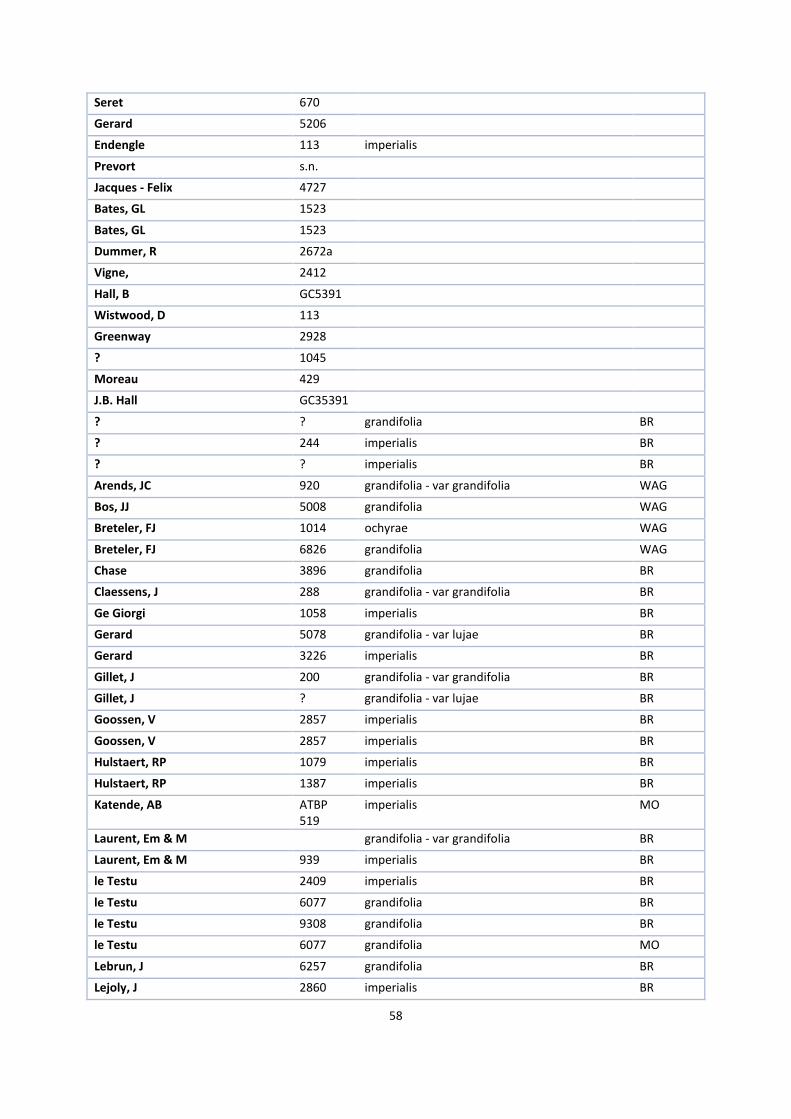
58

Seret 670

Gerard 5206

Endengle 113 imperialis

Prevort s.n.

Jacques - Felix 4727

Bates, GL 1523

Bates, GL 1523

Dummer, R 2672a

Vigne, 2412

Hall, B GC5391

Wistwood, D 113

Greenway 2928

? 1045

Moreau 429

J.B. Hall GC35391

? ? grandifolia BR

? 244 imperialis BR

? ? imperialis BR

Arends, JC 920 grandifolia - var grandifolia WAG

Bos, JJ 5008 grandifolia WAG

Breteler, FJ 1014 ochyrae WAG

Breteler, FJ 6826 grandifolia WAG

Chase 3896 grandifolia BR

Claessens, J 288 grandifolia - var grandifolia BR

Ge Giorgi 1058 imperialis BR

Gerard 5078 grandifolia - var lujae BR

Gerard 3226 imperialis BR

Gillet, J 200 grandifolia - var grandifolia BR

Gillet, J ? grandifolia - var lujae BR

Goossen, V 2857 imperialis BR

Goossen, V 2857 imperialis BR

Hulstaert, RP 1079 imperialis BR

Hulstaert, RP 1387 imperialis BR

Katende, AB ATBP 519

imperialis MO

Laurent, Em & M grandifolia - var grandifolia BR

Laurent, Em & M 939 imperialis BR

le Testu 2409 imperialis BR

le Testu 6077 grandifolia BR

le Testu 9308 grandifolia BR

le Testu 6077 grandifolia MO

Lebrun, J 6257 grandifolia BR

Lejoly, J 2860 imperialis BR

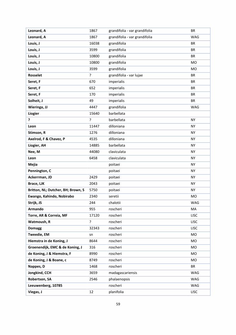
59

Leonard, A 1867 grandifolia - var grandifolia BR

Leonard, A 1867 grandifolia - var grandifolia WAG

Louis, J 16038 grandifolia BR

Louis, J 3599 grandifolia BR

Louis, J 10800 grandifolia BR

Louis, J 10800 grandifolia MO

Louis, J 3599 grandifolia MO

Rosselet ? grandifolia - var lujae BR

Seret, F 670 imperialis BR

Seret, F 652 imperialis BR

Seret, F 170 imperialis BR

Solheit, J 49 imperialis BR

Wieringa, JJ 4447 grandifolia WAG

Liogier 15640 barbellata

? ? barbellata NY

Leon 11447 dilloniana NY

Stimson, R 1276 dilloniana NY

Axelrod, F & Chavez, P 4535 dilloniana NY

Liogier, AH 14885 barbellata NY

Nee, M 44080 claviculata NY

Leon 6458 claviculata NY

Mejia poitaei NY

Pennington, C poitaei NY

Ackerrman, JD 2429 poitaei NY

Brace, LJK 2043 poitaei NY

Britton, NL; Dutcher, BH; Brown, S 5750 poitaei NY

Ewango, Kahindo, Nobirabo 2340 seretii MO

Strijk, JS 244 chalotii WAG

Armando 955 roscheri MA

Torre, AR & Correia, MF 17120 roscheri LISC

Watmoush, R ? roscheri LISC

Domagg 32343 roscheri LISC

Tweedie, EM sn roscheri MO

Hiemstra in de Koning, J 8644 roscheri MO

Groenendijk, EMC & de Koning, J 316 roscheri MO

de Koning, J & Hiemstra, F 8990 roscheri MO

de Koning, J & Boane, c 8749 roscheri MO

Nappes, D 1468 roscheri BR

Jongkind, CCH 3659 madagascariensis WAG

Robertson, SA 2546 phalaenopsis WAG

Leeuwenberg, 10785 roscheri WAG

Viegas, J 12 planifolia LISC

60

van der Meer, J 100 planifolia WAG

? 298 planifolia WAG

? ? planifolia WAG

Bos 1515 planifolia WAG

Lebrun 1459 bampsiana WAG

? 297 planifolia WAG

Mestdagh ? spec. BR

? 1001 spec. MA

? G22 spec. MA

? 148 spec. MA

Barros Machado, A 178 spec. LISC

Leeuwenberg, AJM 5465 spec. LISC

Chase, NC 33396 spec. LISC

Viegas, J 4544 spec. LISC

Santo, E 4544 spec. LISC

Seret, F 39 spec. BR

Seret, F 39 spec. BR

Seret, F 651 spec. BR

Wagemans, J 1599 spec. BR

Wagemans, J 1600 spec. BR

? ? spec. BR

? ? spec. BR

Gillet, J ? spec. BR

Gille, P spec. BR

Gille, P 245 spec. BR

Vermoesen, F ? spec. BR

Wellens, F 476 spec. BR

Leeuwenberg, AJM 5465 spec. BR

Harris, DJ; Michael, J 51 spec. MO

van Valkenburg, JLCH 2861 spec. MO

van de Laan 1356 spec. WAG

Laan 1001 spec. WAG

61

2. R SCRIPT PRINCIPAL COMPONENT ANALYSIS FOR THE AFRICANA GROUP

PCA2 <- read.table("H:\\Afstudeervak 1\\Data\\africanagemiddeld.csv",header=TRUE,sep=",")

PCA2 [,-c(1)]-> africanapcadata

rownames(africanapcadata) <-

c("1","2","3","4","5","6","7","8","9","10","11","12","13","14","15","16","17","18","19","20","21","22","23","24

","25","26","27","28","29","30","31","32","33","34","35","36","37","38","39","40","41","42","43","44","45","4

6","47","48","49","50","51","52","53","54","55","56","57","58","59","60")

africanapca <- prcomp(na.omit(africanapcadata),scale=TRUE)

summary(africanapca)

biplot(africanapca,cex=c(0.7,1.1))

print(prcomp(na.omit(africanapcadata),scale=TRUE))

62

3. HERBARIUM SPECIMENS PER MORPHOLOGICAL GROUP

Group Collector Number Herbarium Flower number

1 Breteler 6691 WAG 14

Breteler 6691 WAG 15

2 De Giorgi 1715 WAG 20

Ariwaodo 648 WAG 2

Lebrun 2493 BR 26

Bos 4195 WAG 11

Bequaert 1469 4

Lebrun 1948 BR 24

Lebrun 3241 WAG 29

Lebrun 3241 WAG 30

Bequaert 2108 BR 7

Bos 3530 WAG 10

3 Ariwaodo 648 WAG 3

Lebrun 3241 BR 27

Lebrun 1948 BR 23

Leeuwenberg 3054 WAG 32

Lebrun 2493 WAG 25

Simons&W 338 WAG 39

De Wilde 576 WAG 41

Leeuwenberg 5465 MO 33

4 F. de Carvalho 2896 MA 17

Bequaert 2108 6

Jongkind 5038 WAG 21

Bos 4195 WAG 12

5 Leeuwenberg 3054 WAG 31

Fakih 169 MO 19

Bequaert 1469 BR 5

Leeuwenberg 5465 WAG 35

Leeuwenberg 5465 WAG 34

Versteegh & den Ouden

227 WAG 40

63

4. SUMMARY AND PRINT PCA IN R

IMPERIALIS GROUP

PC1 PC2 PC3 PC4 PC5 PC6

Standard deviation

1.9080 1.2936 1.0799 0.71114 0.11946 3.637e-16

Proportion of Variance

0.5201 0.2391 0.1666 0.07225 0.00204 0.000e+00

Cumulative Proportion

0.5201 0.7591 0.9257 0.99796 1.00000 1.000e+00

PC1 PC2 PC3 PC4 PC5 PC6

total_length -0.4329647 0.2824929

-0.39427196 -0.07181637 0.0977742 -0.63075342

colum_length -0.4362589 -0.2533108 -0.40413598 0.07247727

-0.6822856

0.33350882

colum_width -0.2750196 -0.5652310 -0.08482407 0.59509925

0.4232408

-0.14673254

lip_length -0.4057760 0.4329275

-0.24440075 -0.17159219 0.4112158 0.40027698

lip_width -0.1533585 0.5567876 0.36039618 0.69373443 -0.2297592 0.03679212

angle_left -0.4382548 -0.1608629 0.45537991

-0.17087932 0.2485816 0.37783257

angle_rigth -0.4078526 -0.1150207 0.52634648

-0.30908778 -0.2492252 -0.40627426

64

AFRICANA WITH FANS

PC1 PC2 PC3 PC4 PC5 PC6 PC7 PC8 PC9

Standard deviation

1.8781 1.2665 1.1215 0.86956 0.75222 0.7016 0.68667 0.44680 0.35444

Proportion of Variance

0.3919 0.1782 0.1398 0.08402 0.06287 0.0547 0.05239 0.02218 0.01396

Cumulative Proportion

0.3919 0.5701 0.7099 0.79390 0.85677 0.9115 0.96386 0.98604 1.00000

PC1 PC2 PC3 PC4 PC5 PC6 PC7 PC8 PC9

LCT

0.4808846

-0.02550818

-0.18908627

0.2019406

-0.06544758

-0.039870114

0.09356362

0.45218533

-0.68736232

LC 0.4016701

0.07250411

-0.26809257

0.1720680

0.01513575

-0.750354630

-0.08338800

-0.34520261

0.20626119

LLV

0.3766434

-0.06639792

-0.34359370

0.2839644

-0.41740510

0.539404927

-0.22093251

-0.08633509

0.36549836

WLT

0.2985377

0.49153989

0.17208246

-0.4793817

-0.14997465

-0.093780509

-0.10417105

0.50289980

0.33881790

DAF

0.3761927

0.24343362

-0.17178700

-0.3836815

0.41745687

0.336138133

0.36901877

-0.43350889

-0.10551287

A3 -0.2779275

0.19026382

-0.59612249

0.2315367

0.49411748

0.022872942

0.08438742

0.39987737

0.25668327

A1 0.3023858

-0.39920102

0.38204255

0.2473096

0.19261212

-0.005960322

0.54840684

0.21950720

0.39498660

A2 -0.2147366

0.55104330

0.02521214

0.3168026

-0.44142387

-0.030149490

0.58306019

-0.11104125

-0.03444683

F 0.1418183

0.43543303

0.46177787

0.5067774

0.38521595

0.145496775

-0.37499890

-0.08749973

-0.04881058

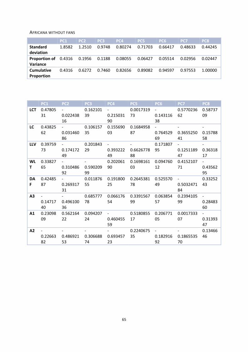
65

AFRICANA WITHOUT FANS

PC1 PC2 PC3 PC4 PC5 PC6 PC7 PC8

Standard deviation

1.8582 1.2510 0.9748 0.80274 0.71703 0.66417 0.48633 0.44245

Proportion of Variance

0.4316 0.1956 0.1188 0.08055 0.06427 0.05514 0.02956 0.02447

Cumulative Proportion

0.4316 0.6272 0.7460 0.82656 0.89082 0.94597

0.97553

1.00000

PC1 PC2 PC3 PC4 PC5 PC6 PC7 PC8

LCT 0.4780531

-0.02243816

0.16210139

-0.21503190

0.001731973

-0.14311638

0.577023662

0.5873709

LC 0.4382562

-0.03146086

0.10615735

0.15569003

0.168495887

-0.76452969

-0.365525041

-0.1578858

LLV 0.3975973

-0.17417249

0.20184329

-0.39322249

-0.662677888

0.17180795

-0.125118947

-0.3631817

WLT

0.3382765

-0.31048692

-0.59020999

0.20206190

0.169816103

0.09476012

0.415210771

-0.4356295

DAF

0.4248587

-0.26931731

0.01187655

0.19180025

0.264538178

0.52557049

-0.503247184

0.3325243

A3 -0.1471740

-0.49610036

0.68577778

0.06617654

0.339156799

0.06385457

0.239410599

-0.2848360

A1 0.2309809

0.56216422

0.09420724

-0.46045559

0.518085517

0.20677105

0.001733307

-0.3139347

A2 -0.2266382

-0.48692153

-0.30668874

-0.69345723

0.224067535

-0.18291692

-0.186553570

0.1346646

66

AFRICANA WITHOUT FANS AVERAGE

PC1 PC2 PC3 PC4 PC5 PC6 PC7 PC8

Standard deviation

1.8584 1.2859 0.9249 0.79779 0.7217 0.66507 0.49092 0.44336

Proportion of Variance

0.4317 0.2067 0.1069 0.07956 0.0651 0.05529 0.03013 0.02457

Cumulative Proportion

0.4317 0.6384 0.7453 0.82491 0.8900 0.94530 0.97543 1.00000

PC1 PC2 PC3 PC4 PC5 PC6 PC7 PC8

LCT 0.4769624

-0.02488676

0.22648833

-0.1633945

0.01898707

-0.12461394

0.52108640

-0.6375520

LC 0.4384353

-0.03923488

0.09985763

0.1731619

0.10505737

-0.77097501

-0.35705763

0.1826166

LLV 0.3978388

-0.16951475

0.20037446

-0.3964175

-0.65909153

0.19614455

-0.05532260

0.3738414

WLT

0.3351084

-0.30100818

-0.64984080

0.1121419

0.19666293

0.05481118

0.43935347

0.3570931

DAF

0.4226523

-0.27204085

-0.03782435

0.1835013

0.24340420

0.51451597

-0.55597435

-0.2813816

A3 -0.1325767

-0.54151089

0.63869005

0.1738452

0.31843374

0.07628548

0.23914998

0.2943297

A1 0.2375694

0.52956699

0.16791991

-0.4385330

0.55545395

0.17775217

0.01106613

0.3199436

A2 -0.2388664

-0.48043588

-0.19681398

-0.7192972

0.21528991

-0.21552252

-0.19612266

-0.1572776

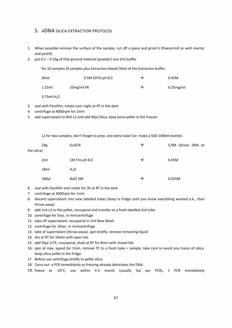
67

5. ADNA SILICA EXTRACTION PROTOCOL

1. When possible remove the surface of the sample, cut off a piece and grind it (freezermill or with mortar

and pestill)

2. put 0.1 – 0.25g of that ground material (powder) into 2ml buffer

for 10 samples (9 samples plus Extraction-blank) 50ml of the Extraction buffer:

45ml 0.5M EDTA pH 8.0 0.45M

1.25ml 10mg/ml PK 0.25mg/ml

3.75ml H2O

3. seal with Parafilm, rotate over night at RT in the dark

4. centrifuge at 4000rpm for 2min

5. add supernatant to 8ml L2 and add 40µl Silica, keep bone pellet in the freezer

L2 for two samples, don’t forget to prep. one extra tube! (or: make a 500-1000ml bottle):

24g GuSCN 5.0M (drives DNA to

the silica)

2ml 1M Tris pH 8.0 0.05M

18ml H2O

180µl NaCl 5M 0.025M

6. seal with Parafilm and rotate for 3h at RT in the dark

7. centrifuge at 4000rpm for 1min

8. discard supernatant into new labelled tubes (keep in fridge until you know everything worked o.k., then

throw away)

9. add 1ml L2 to the pellet, resuspend and transfer to a fresh labelled 2ml tube

10. centrifuge for 5sec. in minicentrifuge

11. take off supernatant, resuspend in 1ml New Wash

12. centrifuge for 10sec. in minicentrifuge

13. take of supernatant (throw away), spin briefly, remove remaining liquid

14. dry at RT for 10min with open lids

15. add 50µl 1xTE, resuspend, elute at RT for 8min with closed lids

16. spin at max. speed for 1min, remove TE to a fresh tube = sample, take care to avoid any traces of silica,

keep silica pellet in the fridge

17. Before use centrifuge briefly to pellet silica

18. Carry out a PCR immediately as freezing already detoriates the DNA.

19. freeze at -20°C, use within 4-5 month (usually 5µl per PCR), 1 PCR immediately

68

6. ADNA CTAB EXTRACTION PROTOCOL

Used chemicals

- CTAB extraction buffer

- chloroform-isoamyl alcohol (24:1)

- isopropyl alcohol (cold)

- 1x TE buffer

- RNAse

- 5M NH4 acetate

- 100% ethanol (cold)

- 76% ethanol, 10 mM NH4 acetate

Extraction procedure

Rough DNA extraction

1) Preheat a water bath at 60°C, insert a tube with sufficient CTAB extraction buffer (2 mL for each

sample) with 2% (40 μL per sample) 2-mercapto-ethanol added beforehand in the fume hood. Check

temperature with thermometer.

2) Put sample material in the mortar and add a little bit of sterile sand.

3) Carefully add liquid nitrogen, hold pestle in the nitrogen to cool, wait until part of the nitrogen has

evaporated and grind the sample material. (work with safety glasses).

4) Put the sample in a 1,5 mL tube with a cooled spatula, close the tube and put in nitrogen. Clean

grinder, pestle and spatula before grinding the next sample.

5) Carefully open the tubes and add 1 mL prepared CTAB buffer. Incubate for 1 hour at 65°C, shake every

10-15 minutes.

Removal of proteins

1) Add 450 μL chloroform-isoamyl alcohol (24:1) in fume hood, mix by inverting for 5 minutes, under

fume hood.

2) Centrifuge for 10 min. at 13200rpm.

Three phases are visible:

- Bottom- chloroform with dissolved proteins, lipids and chlorofyl.

- Middle- cell residue and dissolved green cell residue.

- Top- nucleic acids and dissolved polysacharids – water phase.

3) Carefully take 800 μL of the water phase and put in a new tube.

4) Add 450 μL chloroform-isoamyl alcohol (24:1). Mix by inverting for 5 min. under fume hood.

5) Centrifuge samples for 10 min. at 13200rpm.

6) Carefully take 550 μL of the water phase and put it in a new 2 mL tube.

DNA precipitation

1) Add 550 μL cold isopropyl alcohol. Mix by carefully inverting for 5 min. at room temperature, white

flakes should appear.

2) Centrifuge for 10 min. at 5000 rpm.

3) Drain the isopropyl alcohol. Place the tubes upside-down on a tissue to drain as much of the isopropyl

alcohol as possible. Centrifuge open tubes for 1 min. at 5000rpm.

4) Dissolve the pellets in 300 μL TE, put at 37°C for 30-60 min. Add 3 μL RNAse, put at 37°C for 60 min.

69

~Possible stop~

Keep samples in 4°C fridge overnight

Put the samples at 37°C for 30 min. before continuing the extraction

Precipitation in high salt concentration – extra purification

1) Add 300 μL 5M NH4 acetate (final concentration 2,5M).

2) Add 1500 μL of 100% cold ethanol (2,5 volumes, 2x 750 μL) .

3) Put in -20°C freezer for a minimum of 20 min.

4) Centrifuge for 10 min. at 13200 rpm at 4°C, carefully drain ethanol.

5) Wash with 500 μL 76% ethanol, 10 mM NH4 acetate, swerve carefully and centrifuge for 10 min at

13200 rpm at 4°C, and carefully drain ethanol.

6) Repeat previous step.

7) Place the tubes upside-down on a tissue to drain remaining ethanol. Centrifuge open tubes for 1 min.

at 5000rpm. Make sure all ethanol is evaporated.

8) Add 50 μL TE and put at 37°C for at least an hour to dissolve.

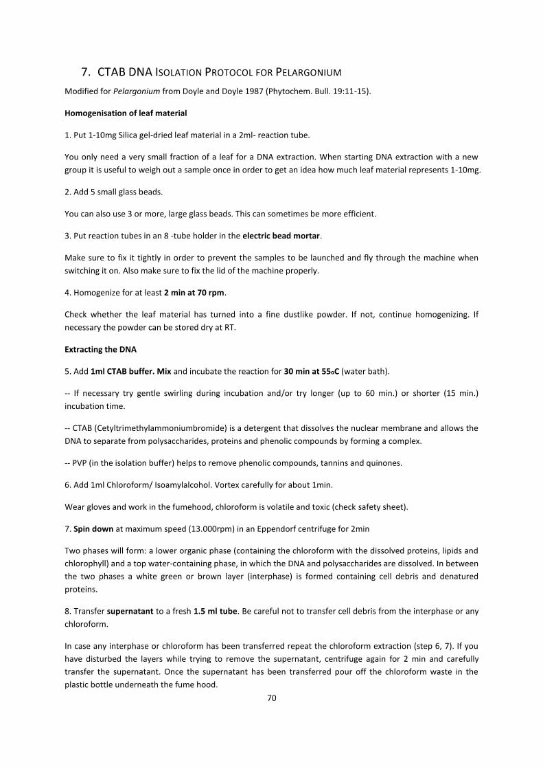
70

7. CTAB DNA ISOLATION PROTOCOL FOR PELARGONIUM

Modified for Pelargonium from Doyle and Doyle 1987 (Phytochem. Bull. 19:11-15).

Homogenisation of leaf material

1. Put 1-10mg Silica gel-dried leaf material in a 2ml- reaction tube.

You only need a very small fraction of a leaf for a DNA extraction. When starting DNA extraction with a new

group it is useful to weigh out a sample once in order to get an idea how much leaf material represents 1-10mg.

2. Add 5 small glass beads.

You can also use 3 or more, large glass beads. This can sometimes be more efficient.

3. Put reaction tubes in an 8 -tube holder in the electric bead mortar.

Make sure to fix it tightly in order to prevent the samples to be launched and fly through the machine when

switching it on. Also make sure to fix the lid of the machine properly.

4. Homogenize for at least 2 min at 70 rpm.

Check whether the leaf material has turned into a fine dustlike powder. If not, continue homogenizing. If

necessary the powder can be stored dry at RT.

Extracting the DNA

5. Add 1ml CTAB buffer. Mix and incubate the reaction for 30 min at 55oC (water bath).

-- If necessary try gentle swirling during incubation and/or try longer (up to 60 min.) or shorter (15 min.)

incubation time.

-- CTAB (Cetyltrimethylammoniumbromide) is a detergent that dissolves the nuclear membrane and allows the

DNA to separate from polysaccharides, proteins and phenolic compounds by forming a complex.

-- PVP (in the isolation buffer) helps to remove phenolic compounds, tannins and quinones.

6. Add 1ml Chloroform/ Isoamylalcohol. Vortex carefully for about 1min.

Wear gloves and work in the fumehood, chloroform is volatile and toxic (check safety sheet).

7. Spin down at maximum speed (13.000rpm) in an Eppendorf centrifuge for 2min

Two phases will form: a lower organic phase (containing the chloroform with the dissolved proteins, lipids and

chlorophyll) and a top water-containing phase, in which the DNA and polysaccharides are dissolved. In between

the two phases a white green or brown layer (interphase) is formed containing cell debris and denatured

proteins.

8. Transfer supernatant to a fresh 1.5 ml tube. Be careful not to transfer cell debris from the interphase or any

chloroform.

In case any interphase or chloroform has been transferred repeat the chloroform extraction (step 6, 7). If you

have disturbed the layers while trying to remove the supernatant, centrifuge again for 2 min and carefully

transfer the supernatant. Once the supernatant has been transferred pour off the chloroform waste in the

plastic bottle underneath the fume hood.

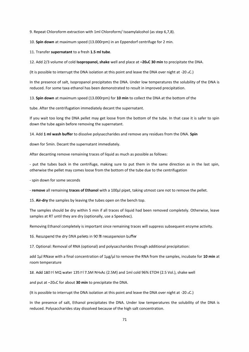
71

9. Repeat Chloroform extraction with 1ml Chloroform/ Isoamylalcohol (as step 6,7,8).

10. Spin down at maximum speed (13.000rpm) in an Eppendorf centrifuge for 2 min.

11. Transfer supernatant to a fresh 1.5 ml tube.

12. Add 2/3 volume of cold Isopropanol, shake well and place at –20oC 30 min to precipitate the DNA.

(It is possible to interrupt the DNA isolation at this point and leave the DNA over night at -20 oC.)

In the presence of salt, Isopropanol precipitates the DNA. Under low temperatures the solubility of the DNA is

reduced. For some taxa ethanol has been demonstrated to result in improved precipitation.

13. Spin down at maximum speed (13.000rpm) for 10 min to collect the DNA at the bottom of the

tube. After the centrifugation immediately decant the supernatant.

If you wait too long the DNA pellet may get loose from the bottom of the tube. In that case it is safer to spin

down the tube again before removing the supernatant.

14. Add 1 ml wash buffer to dissolve polysaccharides and remove any residues from the DNA. Spin

down for 5min. Decant the supernatant immediately.

After decanting remove remaining traces of liquid as much as possible as follows:

- put the tubes back in the centrifuge, making sure to put them in the same direction as in the last spin,

otherwise the pellet may comes loose from the bottom of the tube due to the centrifugation

- spin down for some seconds

- remove all remaining traces of Ethanol with a 100μl pipet, taking utmost care not to remove the pellet.

15. Air-dry the samples by leaving the tubes open on the bench top.

The samples should be dry within 5 min if all traces of liquid had been removed completely. Otherwise, leave

samples at RT until they are dry (optionally, use a Speedvac).

Removing Ethanol completely is important since remaining traces will suppress subsequent enzyme activity.

17. Optional: Removal of RNA (optional) and polysaccharides through additional precipitation:

add 1μl RNase with a final concentration of 1μg/μl to remove the RNA from the samples, incubate for 10 min at

room temperature

4Ac (2.5M) and 1ml cold 96% ETOH (2.5 Vol.), shake well

and put at –20oC for about 30 min to precipitate the DNA.

(It is possible to interrupt the DNA isolation at this point and leave the DNA over night at -20 oC.)

In the presence of salt, Ethanol precipitates the DNA. Under low temperatures the solubility of the DNA is

reduced. Polysaccharides stay dissolved because of the high salt concentration.

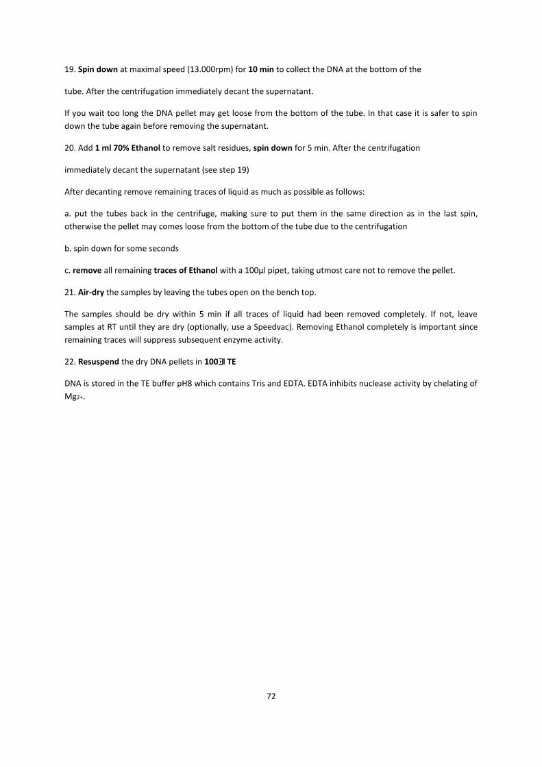
72

19. Spin down at maximal speed (13.000rpm) for 10 min to collect the DNA at the bottom of the

tube. After the centrifugation immediately decant the supernatant.

If you wait too long the DNA pellet may get loose from the bottom of the tube. In that case it is safer to spin

down the tube again before removing the supernatant.

20. Add 1 ml 70% Ethanol to remove salt residues, spin down for 5 min. After the centrifugation

immediately decant the supernatant (see step 19)

After decanting remove remaining traces of liquid as much as possible as follows:

a. put the tubes back in the centrifuge, making sure to put them in the same direction as in the last spin,

otherwise the pellet may comes loose from the bottom of the tube due to the centrifugation

b. spin down for some seconds

c. remove all remaining traces of Ethanol with a 100μl pipet, taking utmost care not to remove the pellet.

21. Air-dry the samples by leaving the tubes open on the bench top.

The samples should be dry within 5 min if all traces of liquid had been removed completely. If not, leave

samples at RT until they are dry (optionally, use a Speedvac). Removing Ethanol completely is important since

remaining traces will suppress subsequent enzyme activity.

22. Resuspend the dry DNA pellets in 100 l TE

DNA is stored in the TE buffer pH8 which contains Tris and EDTA. EDTA inhibits nuclease activity by chelating of

Mg2+.

73

8. PROMEGA WIZARD PROTOCOL FOR DNA CLEAN – UP SYSTEM USING A VACUUM

MANIFOLD

Multiple samples can be easily processed simultaneously using the Vac-Man Laboratory Vacuum Manifold. The

Wizard DNA Clean-Up System is not suitable for use with RNA because percent recoveries are less than 50%.

Notes:

1. Thoroughly mix the Wizard DNA Clean-Up Resin before removing an aliquot. If crystals or aggregates are

present, dissolve by warming the resin to 37°C for 10 minutes. The resin itself is insoluble. Cool to 25–30°C

before use.

2. The binding capacity of 1ml of resin is approximately 20μg of DNA.

Materials to Be Supplied by the User

• 80% isopropanol (2-propanol, reagent grade)

• prewarmed (65–70°C) deionized water or TE buffer

The sample volume must be between 50 and 500μl. If the sample volume is less than 50μl, bring the volume up

to at least 50μl with sterile water. If the sample volume is >500μl, split the sample into multiple purifications.

1. Use one Wizard® Minicolumn for each sample.

2. Attach the provided Syringe Barrel to the Luer-Lok extension of each Minicolumn. Insert the tip of the

Minicolumn/Syringe Barrel assembly into the vacuum manifold.

Mix the resin before use.

3. Add 1ml of Wizard DNA Clean-Up Resin to a 1.5ml microcentrifuge tube. Add the sample (50–500μl) to the

Clean-Up Resin and mix by inverting several times.

4. Pipet the resin/DNA mix into the Syringe Barrel. Apply a vacuum to draw the solution through the

Minicolumn. Break the vacuum to the Minicolumn.

5. To wash the column, add 2ml of 80% isopropanol to the Syringe Barrel, and re-apply a vacuum to draw the

solution through the Minicolumn.

6. Dry the resin by continuing to draw a vacuum for 30 seconds after the solution has been pulled through the

column. Do not dry the resin for more than 30 seconds. Remove the Syringe Barrel and transfer the

Minicolumn to a 1.5ml microcentrifuge tube. Centrifuge the Minicolumn at maximum speed (10,000 x g) in a

microcentrifuge for 2 minutes to remove any residual isopropanol.

7. Transfer the Minicolumn to a new microcentrifuge tube. Apply 50μl (see Table 1) of prewarmed (65–70°C)

water or TE buffer (10mM Tris- HCl [pH 7.6], 1mM EDTA) to the Minicolumn and wait 1 minute. (The DNA will

remain intact on the Minicolumn for up to 30 minutes.) Centrifuge the Minicolumn for 20 seconds at maximum

speed (10,000 x g) to elute the bound DNA.

Elute DNA >20kb with water or TE buffer prewarmed to 80°C.

8. Remove and discard the Minicolumn. The purified DNA may be stored in

the microcentrifuge tube at 4°C or –20°C.

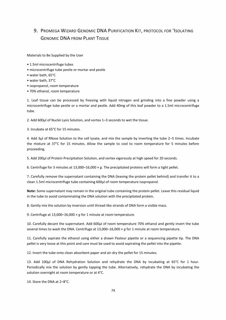
74

9. PROMEGA WIZARD GENOMIC DNA PURIFICATION KIT, PROTOCOL FOR ‘ISOLATING

GENOMIC DNA FROM PLANT TISSUE

Materials to Be Supplied by the User

• 1.5ml microcentrifuge tubes

• microcentrifuge tube pestle or mortar and pestle

• water bath, 65°C

• water bath, 37°C

• isopropanol, room temperature

• 70% ethanol, room temperature

1. Leaf tissue can be processed by freezing with liquid nitrogen and grinding into a fine powder using a

microcentrifuge tube pestle or a mortar and pestle. Add 40mg of this leaf powder to a 1.5ml microcentrifuge

tube.

2. Add 600μl of Nuclei Lysis Solution, and vortex 1–3 seconds to wet the tissue.

3. Incubate at 65°C for 15 minutes.

4. Add 3μl of RNase Solution to the cell lysate, and mix the sample by inverting the tube 2–5 times. Incubate

the mixture at 37°C for 15 minutes. Allow the sample to cool to room temperature for 5 minutes before

proceeding.

5. Add 200μl of Protein Precipitation Solution, and vortex vigorously at high speed for 20 seconds.

6. Centrifuge for 3 minutes at 13,000–16,000 × g. The precipitated proteins will form a tight pellet.

7. Carefully remove the supernatant containing the DNA (leaving the protein pellet behind) and transfer it to a

clean 1.5ml microcentrifuge tube containing 600μl of room temperature isopropanol.

Note: Some supernatant may remain in the original tube containing the protein pellet. Leave this residual liquid

in the tube to avoid contaminating the DNA solution with the precipitated protein.

8. Gently mix the solution by inversion until thread-like strands of DNA form a visible mass.

9. Centrifuge at 13,000–16,000 × g for 1 minute at room temperature.

10. Carefully decant the supernatant. Add 600μl of room temperature 70% ethanol and gently invert the tube

several times to wash the DNA. Centrifuge at 13,000–16,000 × g for 1 minute at room temperature.

11. Carefully aspirate the ethanol using either a drawn Pasteur pipette or a sequencing pipette tip. The DNA

pellet is very loose at this point and care must be used to avoid aspirating the pellet into the pipette.

12. Invert the tube onto clean absorbent paper and air-dry the pellet for 15 minutes.

13. Add 100μl of DNA Rehydration Solution and rehydrate the DNA by incubating at 65°C for 1 hour.

Periodically mix the solution by gently tapping the tube. Alternatively, rehydrate the DNA by incubating the

solution overnight at room temperature or at 4°C.

14. Store the DNA at 2–8°C.

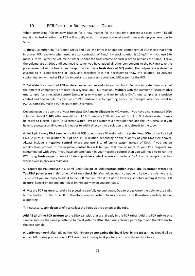
75

10. PCR PROTOCOL BIOSYSTEMATICS GROUP

When attempting PCR on new DNA or for a new marker for the first time prepare a scaled down (15 μl)

reaction to test whether the PCR will actually work. If the reaction works well then scale up your reaction to

50μl.

1. Thaw 10x buffer, dNTPs Primer, MgCl2 and BSA (the latter is an optional component of PCR mixes that often

improves PCR reactions when used at a concentration of 4mg/ml – stock solution is 10mg/ml – if you use BSA

make sure you alter the volume of water so that the final volume of each reaction remains the same). Leave

the polymerase at-20oC until you need it. When you have added all other components to the PCR mix take the

polymerase out of the freezer and keep it on ice. Use a fresh stock of MQ water. The polymerase is stored in

glycerol so it is not freezing at -20oC and therefore it is not necessary to thaw the solution. To prevent

contamination with other DNA it is important to use fresh autoclaved MQ water for the PCR.

2. Calculate the amount of PCR mixture needed and record it in your lab book. Below is indicated how much of

the different components are used for a typical 50μl PCR reaction. Multiply with the number of samples plus

one sample for a negative control (containing only water and no template DNA), one sample as a positive

control and one sample to cover loss of PCR mixture due to pipetting errors. For example: when you want to

PCR 20 samples, make a PCR mixture for 22 samples.

Depending on the quantity of your template DNA make dilutions in MQ water. If you have a concentrated DNA

solution dilute it 1:100, otherwise dilute it 1:10. To make a 1:10 dilution, add 1 μl l on 9 μl sterile water. It may

be easier to pipette 2 μl to 18 μl sterile water. First add water to a new tube than add the DNA because if you

have to pipette a small volume it is easier to add it directly into a solution that is already in the tube.

4. Put 2 μl of every DNA sample in a 0.2ml PCR tube or use a 96 well-multititre plate. Keep DNA on ice. Use 2 μl

DNA, 2 μl of a 1:10 dilution or 2 μl of a 1:100 dilution depending on the quantity of your DNA (see above).

Always include a negative control where you use 2 μl of sterile water instead of DNA. If you get an

amplification product in the negative control this will tell you that one or more of your PCR reagents are

contaminated with DNA. If you have contamination in your negative control then you will need to re-run the

PCR using fresh reagents. Also include a positive control where you include DNA from a sample that has

worked well in previous reactions

5. Prepare the PCR mixture in a 1.5ml (2ml) tube on ice: Add reaction buffer, MgCl2, dNTPs, primer, water and

Taq DNA polymerase in this order. Mark on a check list after adding each component. Leave the polymerase at

–20oC until you are ready to add it to the PCR mixture, take it out of the freezer just before adding it to the PCR

mixture, keep it on ice and put it back immediately when you are ready.

6. Mix the PCR mixture carefully by pipetting carefully up and down. Due to the glycerol the polymerase sinks

to the bottom of the tube. It is therefore very important to mix the entire PCR mixture carefully before

aliquotting.

7. If necessary, spin down briefly to collect the liquid at the bottom of the tube.

Add 48 μl of the PCR mixture to the DNA samples that are already in the PCR tubes. Add the PCR mix to one

sample and use the same pipette tip to mix it with the DNA. Then use a clean pipette tip to add the PCR mix to

the next sample.

9. Verify your work after adding the PCR mixture by comparing the liquid level in the tubes (they should all be

equal). NB: during preparation of PCR reactions it is easy to skip a tube or to add the mixture twice!

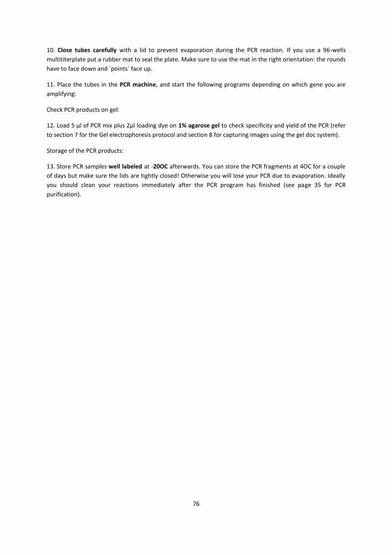
76

10. Close tubes carefully with a lid to prevent evaporation during the PCR reaction. If you use a 96-wells

multititerplate put a rubber mat to seal the plate. Make sure to use the mat in the right orientation: the rounds

have to face down and `points` face up.

11. Place the tubes in the PCR machine, and start the following programs depending on which gene you are

amplifying:

Check PCR products on gel:

12. Load 5 μl of PCR mix plus 2μl loading dye on 1% agarose gel to check specificity and yield of the PCR (refer

to section 7 for the Gel electrophoresis protocol and section 8 for capturing images using the gel doc system).

Storage of the PCR products:

13. Store PCR samples well labeled at -20OC afterwards. You can store the PCR fragments at 4OC for a couple

of days but make sure the lids are tightly closed! Otherwise you will lose your PCR due to evaporation. Ideally

you should clean your reactions immediately after the PCR program has finished (see page 35 for PCR

purification).

77

11. GENEJET PCR PURIFICATION KIT

1 Add a 1:1 volume of Binding Buffer to completed PCR mixture (e.g. for every 100 μL of reaction

mixture, add 100 μL of Binding Buffer). Mix thoroughly. Check the color of the solution. A yellow color indicates

an optimal pH for DNA binding. If the color of the solution is orange or violet, add 10 μL of 3 M sodium acetate,

pH 5.2 solution and mix. The color of the mix will become yellow.

2 for DNA ≤500 bp

Optional: if the DNA fragment is ≤500 bp, add a 1:2 volume of 100% isopropanol (e.g., 100 μL of isopropanol

should be added to 100 μL of PCR mixture combined with 100 μL of Binding Buffer). Mix thoroughly. Note. If

PCR mixture contains primer-dimers, purification without isopropanol is recommended. However, the yield of

the target DNA fragment will be lower.

3 Transfer up to 800 μL of the solution from step 1 (or optional step 2) to the GeneJET purification

column. Centrifuge for 30-60 s. Discard the flow-through. Note. If the total volume exceeds 800 μL, the solution

can be added to the column in stages. After the addition of 800 μL of solution, centrifuge the column for 30-60

s and discard flowthrough. Repeat until the entire solution has been added to the column membrane.

4 Add 700 μL of Wash Buffer (diluted with the ethanol as described on p. 3) to the GeneJET purification

column. Centrifuge for 30-60 s. Discard the flow-through and place the purification column back into the

collection tube.

5 Centrifuge the empty GeneJET purification column for an additional 1 min to completely remove any

residual wash buffer. Note. This step is essential as the presence of residual ethanol in the DNA sample may

inhibit subsequent reactions.

6 Transfer the GeneJET purification column to a clean 1.5 mL microcentrifuge tube (not included). Add

50 μL of Elution Buffer to the center of the GeneJET purification column membrane and centrifuge for 1 min.

Note For low DNA amounts the elution volumes can be reduced to increase DNA concentration. An elution

volume between 20-50 μL does not significantly reduce the DNA yield. However, elution volumes less than 10

μL are not recommended.

If DNA fragment is >10 kb, prewarm Elution Buffer to 65°C before applying to column.

If the elution volume is 10 μL and DNA amount is ≥5 μg, incubate column for 1 min at room temperature

before centrifugation.

7 Discard the GeneJET purification column and store the purified DNA at -20°C.

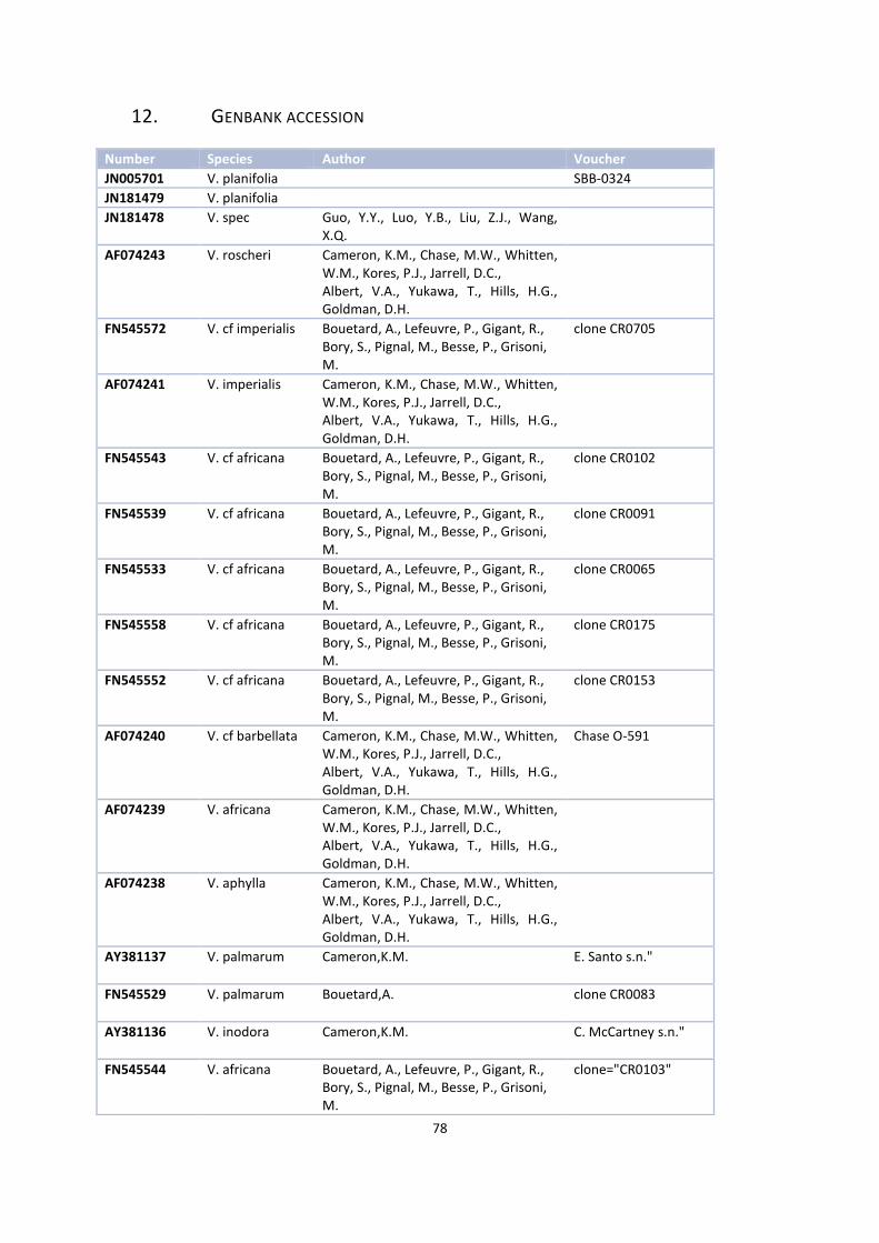
78

12. GENBANK ACCESSION

Number Species Author Voucher

JN005701 V. planifolia SBB-0324

JN181479 V. planifolia

JN181478 V. spec Guo, Y.Y., Luo, Y.B., Liu, Z.J., Wang, X.Q.

AF074243 V. roscheri Cameron, K.M., Chase, M.W., Whitten, W.M., Kores, P.J., Jarrell, D.C., Albert, V.A., Yukawa, T., Hills, H.G., Goldman, D.H.

FN545572 V. cf imperialis Bouetard, A., Lefeuvre, P., Gigant, R., Bory, S., Pignal, M., Besse, P., Grisoni, M.

clone CR0705

AF074241 V. imperialis Cameron, K.M., Chase, M.W., Whitten, W.M., Kores, P.J., Jarrell, D.C., Albert, V.A., Yukawa, T., Hills, H.G., Goldman, D.H.

FN545543 V. cf africana Bouetard, A., Lefeuvre, P., Gigant, R., Bory, S., Pignal, M., Besse, P., Grisoni, M.

clone CR0102

FN545539 V. cf africana Bouetard, A., Lefeuvre, P., Gigant, R., Bory, S., Pignal, M., Besse, P., Grisoni, M.

clone CR0091

FN545533 V. cf africana Bouetard, A., Lefeuvre, P., Gigant, R., Bory, S., Pignal, M., Besse, P., Grisoni, M.

clone CR0065

FN545558 V. cf africana Bouetard, A., Lefeuvre, P., Gigant, R., Bory, S., Pignal, M., Besse, P., Grisoni, M.

clone CR0175

FN545552 V. cf africana Bouetard, A., Lefeuvre, P., Gigant, R., Bory, S., Pignal, M., Besse, P., Grisoni, M.

clone CR0153

AF074240 V. cf barbellata Cameron, K.M., Chase, M.W., Whitten, W.M., Kores, P.J., Jarrell, D.C., Albert, V.A., Yukawa, T., Hills, H.G., Goldman, D.H.

Chase O-591

AF074239 V. africana Cameron, K.M., Chase, M.W., Whitten, W.M., Kores, P.J., Jarrell, D.C., Albert, V.A., Yukawa, T., Hills, H.G., Goldman, D.H.

AF074238 V. aphylla Cameron, K.M., Chase, M.W., Whitten, W.M., Kores, P.J., Jarrell, D.C., Albert, V.A., Yukawa, T., Hills, H.G., Goldman, D.H.

AY381137 V. palmarum Cameron,K.M.

E. Santo s.n."

FN545529 V. palmarum Bouetard,A.

clone CR0083

AY381136 V. inodora Cameron,K.M.

C. McCartney s.n."

FN545544 V. africana Bouetard, A., Lefeuvre, P., Gigant, R., Bory, S., Pignal, M., Besse, P., Grisoni, M.

clone="CR0103"

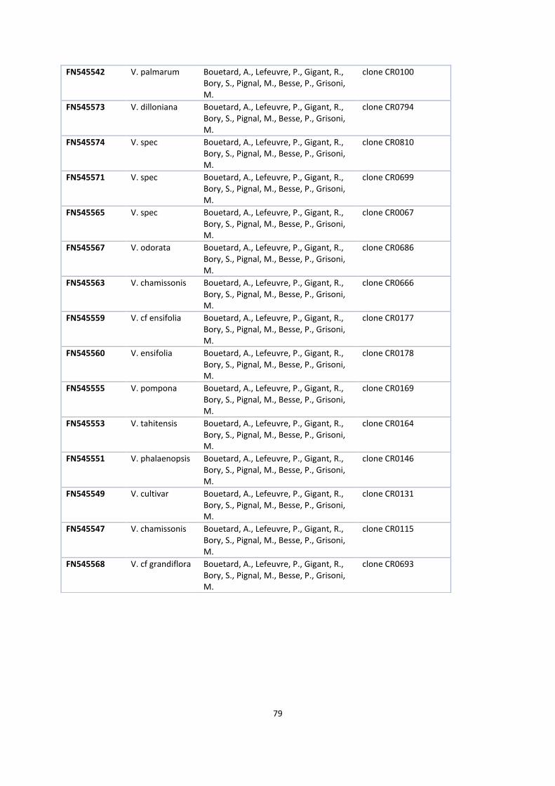
79

FN545542 V. palmarum Bouetard, A., Lefeuvre, P., Gigant, R., Bory, S., Pignal, M., Besse, P., Grisoni, M.

clone CR0100

FN545573 V. dilloniana Bouetard, A., Lefeuvre, P., Gigant, R., Bory, S., Pignal, M., Besse, P., Grisoni, M.

clone CR0794

FN545574 V. spec Bouetard, A., Lefeuvre, P., Gigant, R., Bory, S., Pignal, M., Besse, P., Grisoni, M.

clone CR0810

FN545571 V. spec Bouetard, A., Lefeuvre, P., Gigant, R., Bory, S., Pignal, M., Besse, P., Grisoni, M.

clone CR0699

FN545565 V. spec Bouetard, A., Lefeuvre, P., Gigant, R., Bory, S., Pignal, M., Besse, P., Grisoni, M.

clone CR0067

FN545567 V. odorata Bouetard, A., Lefeuvre, P., Gigant, R., Bory, S., Pignal, M., Besse, P., Grisoni, M.

clone CR0686

FN545563 V. chamissonis Bouetard, A., Lefeuvre, P., Gigant, R., Bory, S., Pignal, M., Besse, P., Grisoni, M.

clone CR0666

FN545559 V. cf ensifolia Bouetard, A., Lefeuvre, P., Gigant, R., Bory, S., Pignal, M., Besse, P., Grisoni, M.

clone CR0177

FN545560 V. ensifolia Bouetard, A., Lefeuvre, P., Gigant, R., Bory, S., Pignal, M., Besse, P., Grisoni, M.

clone CR0178

FN545555 V. pompona Bouetard, A., Lefeuvre, P., Gigant, R., Bory, S., Pignal, M., Besse, P., Grisoni, M.

clone CR0169

FN545553 V. tahitensis Bouetard, A., Lefeuvre, P., Gigant, R., Bory, S., Pignal, M., Besse, P., Grisoni, M.

clone CR0164

FN545551 V. phalaenopsis Bouetard, A., Lefeuvre, P., Gigant, R., Bory, S., Pignal, M., Besse, P., Grisoni, M.

clone CR0146

FN545549 V. cultivar Bouetard, A., Lefeuvre, P., Gigant, R., Bory, S., Pignal, M., Besse, P., Grisoni, M.

clone CR0131

FN545547 V. chamissonis Bouetard, A., Lefeuvre, P., Gigant, R., Bory, S., Pignal, M., Besse, P., Grisoni, M.

clone CR0115

FN545568 V. cf grandiflora Bouetard, A., Lefeuvre, P., Gigant, R., Bory, S., Pignal, M., Besse, P., Grisoni, M.

clone CR0693

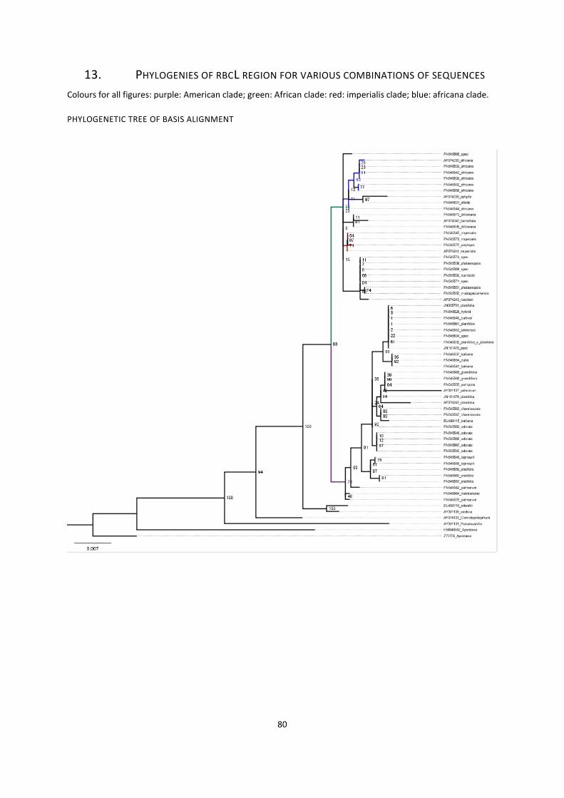
80

13. PHYLOGENIES OF RBCL REGION FOR VARIOUS COMBINATIONS OF SEQUENCES

Colours for all figures: purple: American clade; green: African clade: red: imperialis clade; blue: africana clade.

PHYLOGENETIC TREE OF BASIS ALIGNMENT

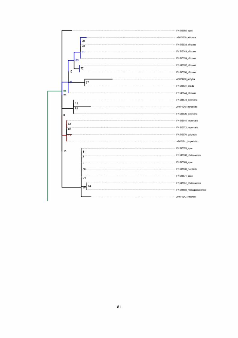
81

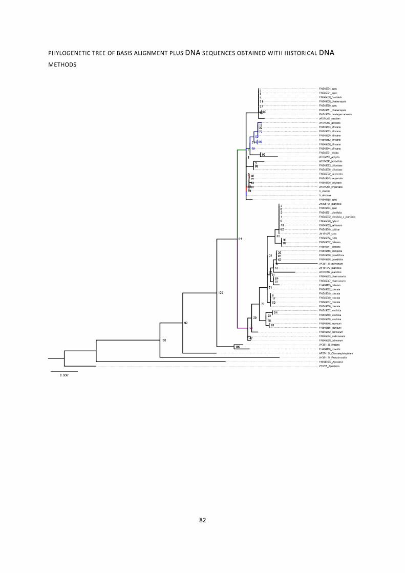
82

PHYLOGENETIC TREE OF BASIS ALIGNMENT PLUS DNA SEQUENCES OBTAINED WITH HISTORICAL DNA

METHODS

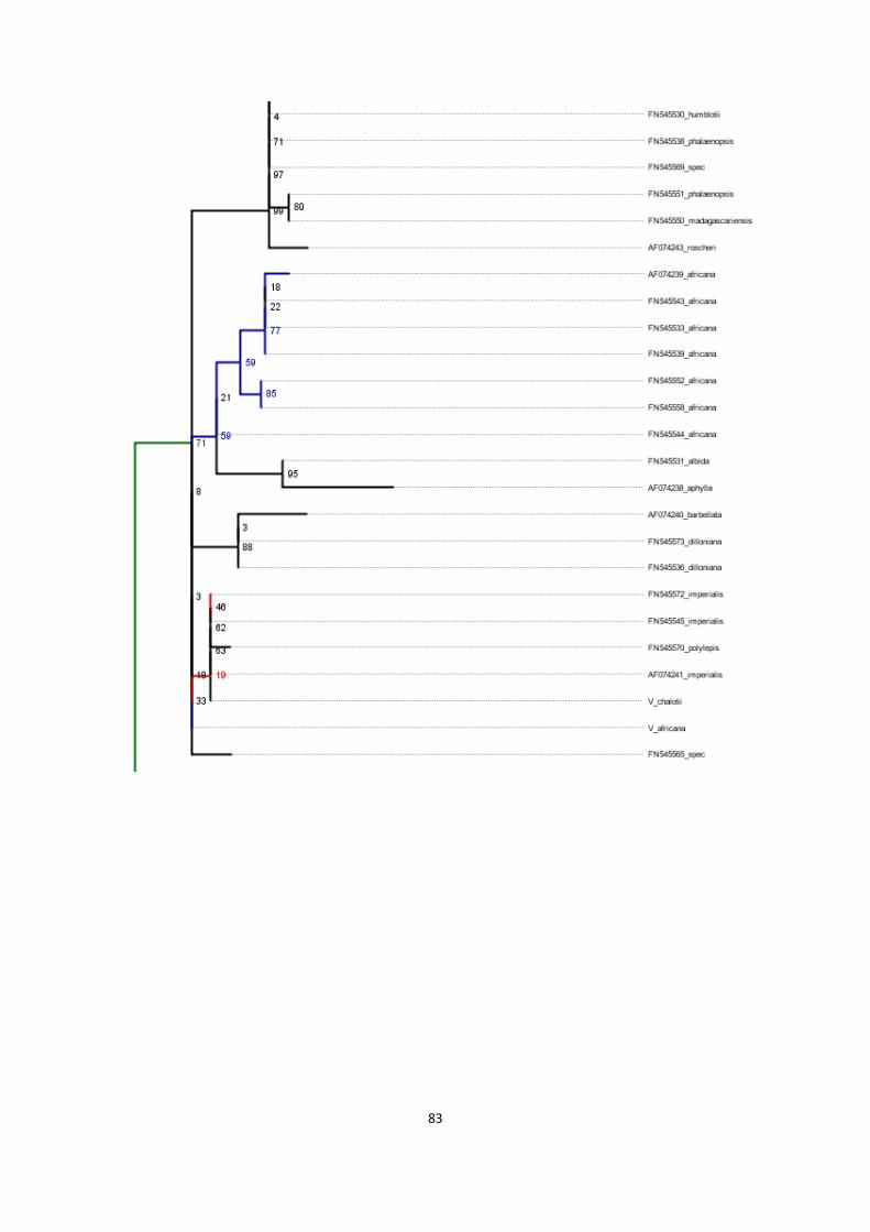
83

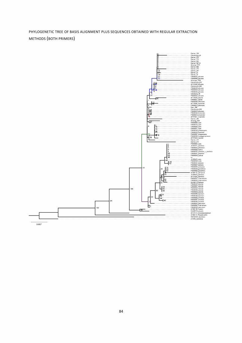
84

PHYLOGENETIC TREE OF BASIS ALIGNMENT PLUS SEQUENCES OBTAINED WITH REGULAR EXTRACTION

METHODS (BOTH PRIMERS)

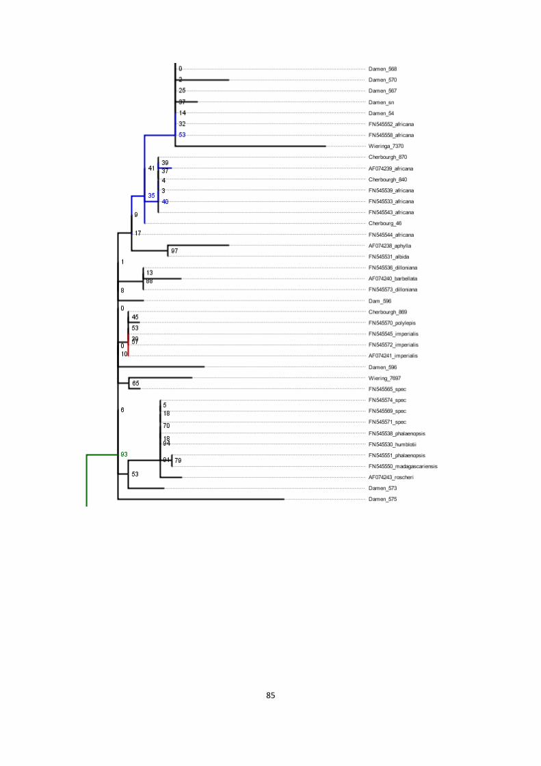
85