Parametric Contrastive Learning

Jiequan Cui 1 Zhisheng Zhong 1 Shu Liu 2 Bei Yu 1,2 Jiaya Jia 1,2

1The Chinese University of Hong Kong 2SmartMore

{jqcui, zszhong, byu, leojia}@cse.cuhk.edu.hk, {liushuhust}@gmail.com

Abstract

In this paper, we propose Parametric Contrastive Learn-ing (PaCo) to tackle long-tailed recognition. Based on the-oretical analysis, we observe supervised contrastive losstends to bias on high-frequency classes and thus increasesthe difficulty of imbalanced learning. We introduce aset of parametric class-wise learnable centers to rebal-ance from an optimization perspective. Further, we ana-lyze our PaCo loss under a balanced setting. Our anal-ysis demonstrates that PaCo can adaptively enhance theintensity of pushing samples of the same class close asmore samples are pulled together with their correspond-ing centers and benefit hard example learning. Experi-ments on long-tailed CIFAR, ImageNet, Places, and iNat-uralist 2018 manifest the new state-of-the-art for long-tailed recognition. On full ImageNet, models trainedwith PaCo loss surpass supervised contrastive learningacross various ResNet backbones, e.g., our ResNet-200achieves 81.8% top-1 accuracy. Our code is avail-able at https://github.com/dvlab-research/Parametric-Contrastive-Learning.

1. Introduction

Convolutional neural networks (CNNs) have achievedgreat success in various tasks, including image classifica-tion [22, 43], object detection [31, 34] and semantic seg-mentation [55]. Especially, with the rise of neural networksearch [60, 33, 45, 13, 4], performance of CNNs have fur-ther taken a big step. However, The huge progress highly de-pends on large-scale and high-quality datasets, such as Ima-geNet [40], MS COCO [32] and Places [59]. But when dealwith real-world applications, generally we face the long-tailed distribution problem – a few classes contain manyinstances, while most classes contain only a few instances.Learning in such an imbalanced setting is challenging as thelow-frequency classes can be easily overwhelmed by high-frequency ones. Without considering this situation, CNNswill suffer from significant performance degradation.

5 10 15 20 25 3052

54

56

58

60

Inference Time (ms)Acc

(%) PaCo

Balanced SoftmaxDecoupleRIDE

Figure 1: Comparison with state-of-the-arts on ImageNet-LT [35]. Inference time is calculated with a batch of 64 im-ages on Nvidia GeForce 2080Ti GPU. The same experimen-tal setting is adopted for comparison. ResNet-50, ResNeXt-50, and ResNeXt101 are used for Balanced Softmax [38],Decouple [28], and PaCo. For RIDE [49], various numbersof expert with RIDEResNet and RIDEResNeXt are adopted.PaCo significantly outperforms recent SOTA. Detailed num-bers for RIDE is in the supplementary file.

Contrastive learning [9, 21, 10, 19, 7] is a major re-search topic due to its success in self-supervised represen-tation learning. Khosla et al. [29] extend non-parametriccontrastive loss into non-parametric supervised contrastiveloss by leveraging label information, which trains represen-tation in the first stage and learns the linear classifier withthe fixed backbone in the second stage. Though supervisedcontrastive learning works well in a balanced setting, for im-balanced datasets, our theoretical analysis shows that high-frequency classes will have a higher lower bound of lossand contribute much higher importance than low-frequencyclasses when equipping it in training. This phenomenonleads to model bias on high-frequency classes and increasesthe difficulty of imbalance learning. As shown in Fig. 2,when the model is trained with supervised contrastive losson ImageNet-LT, the gradient norm varying from the mostfrequent class to the least one is rather steep. In particu-lar, the gradient norm dramatically decreases for the top 200most frequent classes.

Previous work [1, 25, 15, 20, 8, 41, 38, 28, 49, 14, 46,14, 57] explored to rebalance in traditional supervised cross-

200 400 600 800 1,0000.0

0.2

0.4

0.6

0.8

1.0

Sorted class index

GradientNorm

PaCoSupcon

Figure 2: Rebalance in contrastive learning. We collect theaverage L2 norm of the gradient of weights in the last classi-fier layer on ImageNet-LT. Category indices are sorted bytheir image counts. The gradient norm varying from themost frequent class to the least one is steep for supervisedcontrastive learning [29]. In particular, the gradient normdramatically decreases for the top 200 most frequent classes.Trained with PaCo, the gradient norm is better balanced.

entropy learning. In this paper, we tackle the above men-tioned imbalance issue in supervised contrastive learningand make use of contrastive learning for long-tailed recog-nition. To our knowledge, it is the first attempt of usingrebalance in contrastive learning.

To rebalance in supervised contrastive learning, we in-troduce a set of parametric class-wise learnable centers intosupervised contrastive learning. We name our algorithmParametric Contrastive Learning (PaCo) shown in Fig. 3.With such a simple and yet effective operation, we theoret-ically prove that the optimal values for the probability thattwo samples are a true positive pair (belonging to the sameclass), varying from the most frequent class to the least fre-quent class, are more balanced. Thus their lower bound ofloss values are better organized. This phenomenon meansthe model takes more care of low-frequency classes, makingthe PaCo loss benefit imbalance learning. Fig. 2 shows that,with our PaCo loss in training, gradient norm varying fromthe most frequent class to the least one are moderated bet-ter than supervised contrastive learning, which matches ouranalysis.

Further, we analyze the PaCo loss under a balanced set-ting. Our analysis demonstrates that with more samplesclustered around their corresponding centers in training, thePaCo loss increases the intensity of pushing samples of thesame class close, which benefits hard examples learning.

Finally, we conduct experiments on long-tailed versionof CIFAR [16, 5], ImageNet [35], Places [35] and iNatural-ist 2018 [48]. Experimental results show that we create anew record for long-tailed recognition. We also conduct ex-periments on full ImageNet [40] and CIFAR [30]. ResNet

models trained with PaCo also outperform the ones by su-pervised contrastive learning on such balanced datasets. Ourkey contributions are as follows.

• We identify the shortcoming of supervised contrastivelearning under an imbalanced setting – it tends to biashigh-frequency classes.

• We extend supervised contrastive loss to the PaCo loss,which is more friendly to imbalance learning, by intro-ducing a set of parametric class-wise learnable centers.

• Equipped with the PaCo loss, we create new recordacross various benchmarks for long-tailed recognition.Moreover, experimental results on full ImageNet andCIFAR validate the effectiveness of PaCo under a bal-anced setting.

2. Related Work

Re-sampling/re-weighting. The most classical way todeal with long-tailed datasets is to over-sample low-frequency class images [41, 56, 2, 3] or under-sample high-frequency class images [20, 27, 2]. However, Oversamplingcan suffer from heavy over-fitting to low-frequency classesespecially on small datasets. For under-sampling, discard-ing a large portion of high-frequency class data inevitablycauses degradation of the generalization ability of CNNs.Re-weighting [23, 24, 51, 39, 42, 26] the loss functions isan alternative way to rebalance by either enlarging weightson more challenging and sparse classes or randomly ignor-ing gradients from high-frequency classes [44]. However,with large-scale data, re-weighting makes CNNs difficult tooptimize during training [23, 24].

One/two-stage Methods. Since deferred re-weighting andre-sampling were proposed by Cao et al. [5], Kang et al. [28]and Zhou et al. [58] observed re-weighting or re-samplingstrategies could benefit classifier learning while hurting rep-resentation learning. Kang et al. [28] proposed to decom-pose representation and classifier learning. It first trains theCNNs with uniform sampling, and then fine-tune the classi-fier with class-balanced sampling while keeping parametersof representation learning fixed. Zhou et al. [58] proposedone cumulative learning strategy, with which they bridgerepresentation learning and classifier re-balancing.

The two-stage design is not for end-to-end frameworks.Tang et al. [46] analyzed the reason from the perspective ofcausal graph and concluded that the bad momentum causaleffects played a vital role. Cui et al. [14] proposed residuallearning mechanism to address this issue.

Non-parametric Contrastive Loss. Contrastive learning[9, 21, 10, 19, 7] is a framework that learns similar/dissimilar

representations from data that are organized into simi-lar/dissimilar pairs. An effective contrastive loss function,called InfoNCE [47], is

Lq,k+,{k−} = − logexp(q·k+/τ)

exp(q·k+/τ) +∑k−

exp(q·k−/τ),

(1)where q is a query representation, k+ is for the positive(similar) key sample, and {k−} denotes negative (dissimi-lar) key samples. τ is a temperature hyper-parameter. In theinstance discrimination pretext task [53] for self-supervisedlearning, a query and a key form a positive pair if they aredata-augmented versions of the same image. It forms a neg-ative pair otherwise.

Traditional cross-entropy with linear fc layer weight wand true label y among n classes is expressed as

Lcross−entropy = − logexp(q·wy)∑ni=1 exp(q·wi)

. (2)

Compared to it, InfoNCE does not get involved with para-metric learnable parameters. To distinguish our proposedparametric contrastive learning from previous ones, we treatthe InfoNCE as a non-parametric contrastive loss following[54].

Chen et al. [9] used self-supervised contrastive learn-ing SimCLR to first match the performance of a super-vised ResNet-50 with only a linear classifier trained on self-supervised representation on full ImageNet. He et al. [21]proposed MoCo and Chen et al. [10] extended MoCo toMoCo v2, with which small batch size training can alsoachieve competitive results on full ImageNet [40]. In addi-tion, many other methods [19, 7] are also proposed to furtherboost performance.

3. Parametric Contrastive Learning3.1. Supervised Contrastive Learning

Khosla et al. [29] extended the self-supervised con-trastive loss with label information into supervised con-trastive loss. Here we present it in the framework of MoCo[21, 10] as

Li=−∑

z+∈P (i)

logexp(z+ · T (xi))∑

zk∈A(i) exp(zk · T (xi)). (3)

MoCo framework [21, 10] consists of two networks with thesame structure, i.e., query network and key network. Thekey network is driven by a momentum update with the querynetwork in training. For each network, it usually containsone encoder CNN and one two-layer MLP transform.

During training, for one two-viewed image batch B =(Bv1, Bv2) and label y, Bv1 and Bv2 are fed into the query

Table 1: Top-1 accuracy (%) of supervised contrastive learn-ing on ImageNet-LT with ResNet-50. Implementation de-tails are in supplementary file. †represents model is trainedwith PaCo loss without center learning rebalance.

Method Many Medium Few All

Cross-Entropy 67.5 42.6 13.7 48.4SupCon 53.4 2.9 0 22.0PaCo (ours) † 69.6 45.8 16.0 51.0

network and key network respectively and we denote theiroutputs as Zv1 and Zv2. Especially, Zv2 is used to updatethe momentum queue.

In Eq. (3), xi is the representation for image Xi in Bv1

obtained by the encoder of query network. The transformT (·) also belongs to the query network. We write

A(i) = {zk ∈ queue ∪ Zv1 ∪ Zv2}\{zk ∈ Zv1 : k = i},P (i) = {zk ∈ A(i) : yk = yi}.

In implementation, the loss is usually scaled by1

|P (i)|and a temperature τ is applied like in Eq. (1). Different fromself-supervised contrastive loss, which treats query and keyas a positive pair if they are the data-augmented version ofthe same image, supervised contrastive loss treats them asone positive pair if they belong to the same class.

3.2. Theoretical Motivation

Analysis of Supervised Contrastive Learning. Khosla etal. [29] introduced supervised contrastive learning to en-courage more compact representation. We observe that it isnot directly applicable to long-tailed recognition. As shownin Table 1, the performance significantly decreases com-pared with traditional supervised cross-entropy. From an op-timization point of view, supervised contrastive loss concen-trates more on high-frequency classes than low-frequencyones, which is unfriendly for imbalanced learning.

Remark 1 (Optimal value for supervised contrastive learn-ing). When supervised contrastive loss converges, the opti-mal value for the probability that two samples are a true pos-

itive pair with label y is1

Ky, where, q(y) is the frequency

of class y over the whole dataset, queue is the momentumqueue in MoCo [21, 10] and Ky ≈ length(queue) · q(y).

Interpretation. As indicated by Remark 1, high-frequency classes have a higher lower bound of loss valueand contribute much more importance than low-frequencyclasses in training. Thus the training process can be domi-nated by high-frequency classes. To handle this issue, weintroduce a set of parametric class-wise learnable centersfor rebalancing in contrastive learning.

encoder momentum encoder

F(x) G(x) G(x)

parametric learnableclass centers C

similaritysimilarity

concatenation

supervised contrastive loss

queue

momentum

Figure 3: Parametric contrastive learning (PaCo). We introduce a set of para-metric class-wise learnable centers for rebalancing in contrastive learning.More analysis is in Section 3.3 for PaCo.

0 0.2 0.4 0.6 0.8 10.5

1.0

1.5

2.0

2.5

3.0

p

L(p

)

L(p) = − log(p)− 0.41 · log(1− p)

Figure 4: Curve for Lextra.

3.3. Rebalance in Contrastive Learning

As described in Fig. 3, we introduce a set of paramet-ric class-wise learnable centers C = {c1, c2, ..., cn} intothe original supervised contrastive learning, and called thisnew form Parametric Contrastive Learning (PaCo). Cor-respondingly, the loss function is changed to

Li=∑

z+∈P (i)∪{cy}

−w(z+) logexp(z+ · T (xi))∑

zk∈A(i)∪C exp(zk · T (xi)),

(4)where

w(z+)=

{α, z+∈P (i)1.0, z+∈{cy}

and

z · T (xi)={z · G(xi), z∈A(i)z · F(xi), z∈C.

Following Chen et al. [10], the transform G(·) is a two-layer MLP while F(·) is the identity mapping, i.e., F(x) =x. α is one hyper-parameter in (0,1). P (i) and A(i) arethe same with supervised contrastive learning in Eq. (3). In

implementation, the loss is scaled by1∑

z+∈P (i)∪{cy} w(z+)

and a temperature τ is applied like in Eq. (3).

Remark 2 (Optimal value for parametric contrastive learn-ing) When parametric contrastive loss converges, the op-timal value for the probability that two samples are a true

positive pair with label y isα

1 + α ·Kyand the optimal

value for the probability that a sample is closest to its cor-

responding center cy among C is1

1 + α ·Ky, where q(y)

is the frequency of class y over the whole dataset, queueis the momentum queue in MoCo [21, 10] and Ky ≈length(queue) · q(y).

Interpretation. Suppose the most frequent class yh hasKyh

≈ q(yh)·length(queue) and the least frequent class ythasKyt

≈ q(yt)·length(queue). As indicated by Remarks2 and 1, the optimal value for the probability that two sam-ples are a true positive pair varying from the most frequent

class to the least one is rebalanced from1

Kyh

−→ 1

Kyt

to

11α +Kyh

−→ 11α +Kyt

. The smaller α, the more uniform

the optimal value from the most frequent class to the leastone is, friendly to low- frequency classes learning.

However, when α decreases, the intensity of contrastamong samples will be weaker, the intensity of contrast be-tween samples and centers will be stronger. The whole lossbecomes closer to supervised cross-entropy. To make gooduse of contrastive learning and rebalance at the same time,we observe that α=0.05 is a reasonable choice.

3.4. PaCo under balanced setting

For balanced datasets, all classes have the same fre-quency, i.e., q∗=q(yi)=q(yj) and K∗=Kyi

=Kyjfor any

class yi and class yj . In this case, PaCo reduces to animproved version of multi-task with weighted sum of su-pervised cross-entropy loss and supervised contrastive loss.The connection between PaCo and multi-task is

ExpSum =∑ck∈C

exp(ck·F(xi))+∑

zk∈A(i)

exp(zk · G(xi)).

We also write the PaCo loss as

Li =∑

z+∈P (i)∪{cy}

−w(z+) logexp(z+ · T (xi))∑

zk∈A(i)∪C exp(zk · T (xi))

= − logexp(cy · F(xi))

ExpSum− α

∑z+∈P (i)

logexp(z+ · G(xi))ExpSum

= Lsup+αLsupcon−(logPsup+αK∗ logPsupcon)

= Lsup+αLsupcon−(logPsup+αK∗ log(1− Psup)) ,

where

Psup =

∑ck∈C exp(ck ·F(xi))

ExpSum;

Psupcon =

∑zk∈A(i) exp(zk · G(xi))

ExpSum.

(5)

Multi-task learning combines supervised cross-entropyloss and supervised contrastive loss with a fixed weightedscalar. When these two losses conflict, the training can suf-fer from slower or sub-optimization. Our PaCo contrarilyadjust the intensity of supervised cross-entropy loss and su-pervised contrastive loss in an adaptive way and potentiallyavoids conflict as analyzed in the following.

3.4.1 Analysis of PaCo under balanced setting

As indicated by Eq. (5), compared with multi-task, PaCo hasan additional loss item:

Lextra = − log(Psup)− αK∗ log(1− Psup). (6)

Here, we take full ImageNet as an example, i.e., q∗ =0.001, length(queue) = 8192, α = 0.05, αK∗ = 0.41.Then the function curve for Lextra is shown in Fig. 4. WithPsup increases from 0 to 1.0, the function value decreasesuntil Psup = 0.71 and then goes up, which implies Lextra

obtains the smallest loss value when Psup = 0.71. Note that,when the whole PaCo loss in Eq. (4) achieves the optimalsolution, Psup = 0.71 still establishes as demonstrated byRemark 2. With Psup increases in the training, we analyzehow does it affect the intensity of supervised contrastive lossand supervised cross-entropy loss in the following.

Adaptive weighting between Lsup and Lsupcon. Notethat the optimal value for the probability that two samplesare a true positive pair with label y is 0.035 as indicatedby Remark 2. We suppose pl, ph ∈ (0, 0.71) and pl < ph.To achieve the optimal value, when Psup=p, the supervisedcontrastive loss value Lsupcon must decrease as in Eq. (7).Here Psup increases from pl to ph, Lsupcon must decreaseto a much smaller loss value to achieve the optimal solution,which implies the need to make two different class samples

Lsupcon = −∑

z+∈P (i)

logexp(z+ · G(xi))∑

zk∈A(i) exp(zk · G(xi))

= −∑

z+∈P (i)

log

exp(z+·G(xi))ExpSum∑

zk∈A(i) exp(zk·G(xi))

ExpSum

= −K∗ log0.035

1− p.

(7)

much more discriminative, i.e., increasing inter-class mar-gins, and thus the intensity of supervised contrastive losswill enlarge.

An intuition is that as Psup increases, more samples arepulled together with their corresponding centers. Along withstronger intensity of supervised contrastive loss at that time,it is more likely to push hard examples close to those sam-ples that are already around right centers.

3.5. Center Learning Rebalance

PaCo balances the contrastive learning (for moderatingcontrast among samples). However the center learning alsoneeds to be balanced, which has been explored in [1, 25,15, 20, 8, 41, 38, 28, 49, 14, 46, 18, 57]. We incorporateBalanced Softmax [38] into the center learning. Then thePaCo loss is changed from Eq. (4) to what follows:

Li=∑

z+∈P (i)∪{cy}

−w(z+) logψ(z+, T (xi))∑

zk∈A(i)∪C ψ(zk, T (xi)),

(8)where

ψ(zk, T (xi))=

{exp(zk · G(xi)), zk∈A(i);exp(zk · F(xi)) · q(yk), zk∈C.

We emphasize that Balanced Softmax is only a practicalremedy for center learning rebalance. The theoretical analy-sis remains as a future work.

4. Experiments4.1. Ablation Study

Data augmentation strategy for PaCo. Data augmenta-tion is the key for success of contrastive learning as indi-cated by Chen et al. [9]. For PaCo, we also conduct ablationstudies for different augmentation strategies. Several obser-vations are intriguingly different from those of [37]. We ex-periment with the following ways of data augmentation.

• SimAugment: an augmentation policy [21, 10] that ap-plies random flips and color jitters followed by Gaus-sian blur.

• RandAugment [12]: A two stage augmentation pol-icy that uses random parameters in place of parameters

Table 2: Comparison with different augmentation strategiesfor PaCo on ImageNet-LT with ResNet-50.

Methods Aug. strategy Top-1 Accuracy

PaCo Strategy (1) 55.0PaCo Strategy (2) 56.5PaCo Strategy (3) 57.0

tuned by AutoAugment. The random parameters do notneed to be tuned and hence reduces the search space.

For the common random resized crop used along withthe above two strategies, work of [37] explains that the op-timal hyper-parameter for random resized crop is (0.2,1)in self-supervised contrastive learning. This setting is alsoadopted by other work of [9, 21, 10, 19, 7]. However, inthis paper, we observe severe performance degradation onImageNet-LT with ResNet-50 (55.0% vs 52.2%) for PaCowhen we change the hyper-parameter from (0.08,1) to (0.2,1). This is because PaCo involves center learning whileother self-supervised frameworks only apply non-parametriccontrastive loss as described in Section 2. Note that thesame phenomenon is also observed on traditional supervisedlearning with cross-entropy loss.

Another observation is on RandAugment [12]. The workof [50] demonstrated that directly applying strong data aug-mentation in MoCo [21, 10] does not work well. Herewe observe a similar conclusion with RandAugment [12].We experiment with 3 different augmentation strategies of(1) encoder and momentum encoder input are both withSimAugment; (2) encoder and momentum encoder input areboth with RandAugment; and (3) encoder input uses Ran-dAugment while momentum encoder input uses SimAug-ment. The experimental results are presented in Table 2.With strategy (3), PaCo achieves the best performance,showing center learning requires more aggressive data aug-mentations compared with contrastive learning among sam-ples.

4.2. Baseline implementation

Contrastive learning benefits from longer training com-pared with traditional supervised learning with cross-entropy as Chen et al. [9] concluded, which is also validatedby previous work of [9, 21, 10, 19, 7]. We run PaCo with400 epochs on CIFAR-LT, ImageNet-LT, iNaturalist 2018,full CIFAR, and full ImageNet except for Places-LT. WithPlaces-LT, we follow previous work [35, 14] by loading thepre-trained model on ImageNet and finely tune 30 epochson Places-LT. For a fair comparison on ImageNet-LT andiNaturalist 2018, we re-implement baselines with the sametraining time and RandAugment [12]. Especially, for RIDE,based on model ensemble, we compare with it under com-parable inference latency in Fig. 1.

4.3. Long-tailed Recognition

We follow the common evaluation protocol [35, 14, 28]in long-tailed recognition – that is, training models on thelong-tailed source label distribution and evaluating theirperformance on the uniform target label distribution. Weconduct experiments on long-tailed version of CIFAR-100[16, 5], Places [35], ImageNet [35] and iNaturalist 2018 [48]datasets.

CIFAR-100-LT datasets. CIFAR-100 has 60,000 images– 50,000 for training and 10,000 for validation with 100 cat-egories. For a fair comparison, we use the long-tailed ver-sion of CIFAR datasets with the same setting as those used in[6, 58, 16]. They control the degrees of data imbalance withan imbalance factor β. β= Nmax

Nminwhere Nmax and Nmin

are the numbers of training samples for the most and leastfrequent classes respectively. Following [58], we conductexperiments with imbalance factors 100, 50, and 10.

ImageNet-LT and Places-LT. ImageNet-LT and Places-LT were proposed in [35]. ImageNet-LT is a long-tailed ver-sion of ImageNet dataset [40] by sampling a subset follow-ing the Pareto distribution with power value α=6. It contains115.8K images from 1,000 categories, with class cardinalityranging from 5 to 1,280. Places-LT is a long-tailed versionof the large-scale scene classification dataset Places [59]. Itconsists of 184.5K images from 365 categories with classcardinality ranging from 5 to 4,980.

iNaturalist 2018. The iNaturalist 2018 [48] is one speciesclassification dataset, which is on a large scale and suffersfrom extremely imbalanced label distribution. It is com-posed of 437.5K images from 8,142 categories. In additionto the extreme imbalance, the iNaturalist 2018 dataset alsoconfronts the fine-grained problem [52].

Implementation details. For image classification onImageNet-LT, we used ResNet-50, ResNeXt-50-32x4d, andResNeXt-101-32x4d as our backbones for experiments. ForiNaturalist 2018, we conduct experiments with ResNet-50and ResNet-152. All models were trained using SGD opti-mizer with momentum µ = 0.9. Contrastive learning usu-ally requires long training time to converge. MoCo [21, 10],BYOL [19] and SWAV [7] train 800 epochs for model con-vergence. Supervised contrastive learning [29] trains 350epochs for feature learning and another 350 epochs for clas-sifier learning.

Following MoCo [21, 10], when we train models withPaCo, the learning rate decays by a cosine scheduler from0.02 to 0 with batch size 128 on 4 GPUs in 400 epochs.The temperature is set to 0.2. α is 0.05. For a fair com-parison, we re-implement baselines in the same setting for

Table 3: Long-tail recognition accuracy on ImageNet-LTfor different backbone architectures. † denotes models aretrained with RandAugment [12] in 400 epochs. More com-parisons with RIDE [49] are in Fig. 1.

Method ResNet-50 ResNeXt-50 ResNeXt-101

CE(baseline) 41.6 44.4 44.8Decouple-cRT 47.3 49.6 49.4Decouple-τ -norm 46.7 49.4 49.6De-confound-TDE 51.7 51.8 53.3ResLT - 52.9 54.1MiSLAS 52.7 - -

Decouple-τ -norm † 54.5 56.0 57.9Balanced Softmax † 55.0 56.2 58.0PaCo† 57.0 58.2 60.0

recent state-of-the-arts of Decouple [28], Balanced Softmax[38] and RIDE [49] as mentioned in Section 4.2.

For Places-LT, following previous setting [35, 14], wechoose ResNet-152 as the backbone network, pre-train it onthe full ImageNet-2012 dataset (provided by torchvision),and finely tune it for 30 epochs on Places-LT. Same as thaton ImageNet-LT, the learning rate decays by a cosine sched-uler from 0.02 to 0 with batch size 128. The temperature isset to 0.2. α is 0.05. For CIFAR-100-LT, we strictly followthe setting of [38] for fair comparison. A smaller tempera-ture of 0.05 and α = 0.02 are adopted for PaCo.

Comparison on ImageNet-LT. Table 3 shows extensiveexperimental results for comparison with recent SOTAmethods. We observe that Balanced Softmax [38] stillachieves comparable results with Decouple [28] acrossvarious backbones under such strong training setting onImageNet-LT, consistent with what is claimed in the originalpaper. For RIDE that is based on model ensemble, we an-alyze the real inference speed by calculating inference timewith a batch of 64 images on Nvidia GeForce 2080Ti GPU.

We observe RIDEResNet with 3 experts even hashigher inference latency than a standard ResNeXt-50-32x4d(15.3ms vs 13.1ms); RIDEResNeXt with 3 experts yieldshigher inference latency than a standard ResNeXt-101-32x4d (26ms vs 25ms). This result is in accordance withthe conclusion that network fragmentation reduces the de-gree of parallelism and thus decreases efficiency in [36, 13].For fair comparison, we do not apply knowledge distillationtricks for all these methods. As shown in Fig. 1 and Table 3,under comparable inference latency, PaCo significantly sur-passes these baselines.

Comparison on Places-LT. The experimental results onPlaces-LT are summarized in Table 4. Due to the architec-ture change of RIDE, it is not applicable to load the publicly

Table 4: Performance on Places-LT [35], starting from anImageNet pre-trained ResNet-152 provided by torchvision.†denotes the model trained with RandAugment [12].

Method Many Medium Few All

CE(baseline) 45.7 27.3 8.2 30.2OLTR 44.7 37.0 25.3 35.9Decouple-τ -norm 37.8 40.7 31.8 37.9Balanced Softmax 42.0 39.3 30.5 38.6ResLT 39.8 43.6 31.4 39.8MiSLAS 39.6 43.3 36.1 40.4RIDE (2 experts) - - - -

PaCo 37.5 47.2 33.9 41.2PaCo † 36.1 47.9 35.3 41.2

pre-trained model on full ImageNet, while PaCo is moreflexible where the network architecture is the same as thoseof [35, 14]. Under fair training setting by finely tuning 30epochs without RandAugment, PaCo surpasses SOTA Bal-anced Softmax by 2.6%. An interesting observation is thatRandAugment has little effect on the Places-LT dataset. Asimilar phenomenon can be observed on the iNaturalist 2018dataset. More evaluation numbers are in the supplementaryfile. They can be intuitively understood since RandAugmentis designed for ImageNet classification, which inspires us toexplore general augmentations across different domains.

Comparison on iNaturalist 2018. Table 5 lists experi-mental results on iNaturalist 2018. Under fair training set-ting, PaCo consistently surpasses recent SOTA methods ofDecouple, Balanced Softmax and RIDE. Our method is1.4% higher than Balanced Softmax. We also apply PaCoon large ResNet-152 architecture. And the performanceboosts to 75.3% top-1 accuracy. Note that we only transferthe hyper-parameters of PaCo on ImageNet-LT to iNatural-ist 2018 without any change. Tuning hyper-parameters forPaCo will bring further improvement.

Comparison on CIFAR-100-LT. The experimental re-sults on CIFAR-100-LT are listed in Table 6. For the CIFAR-100-LT dataset, we mainly compare with the SOTA methodBalanced Softmax [38] with the same training setting whereCutout [17] and AutoAugment [11] are used in training.As shown in Table 6, PaCo consistently outperforms Bal-anced Softmax across different imbalance factors with sucha strong setting. Specifically, PaCo surpasses Balanced Soft-max by 1.2%, 1.8% and 1.2% under imbalance factor 100,50 and 10 respectively, which testify the effectiveness of ourPaCo method.

4.4. Full ImageNet and CIFAR Recognition

As analyzed in Section 3.4, for balanced datasets, PaCoreduces to an improved version of multi-task learning, which

Table 5: Top-1 accuracy over all classes on iNaturalist 2018with ResNet-50. Knowledge distillation is not applied to allmethods for fair comparison. We compare with RIDE 1 un-der comparable inference latency. † denotes models trainedwith RandAugment [12] in 400 epochs.

Method Top-1 Accuracy

CB-Focal 61.1LDAM+DRW 68.0Decouple-τ -norm 69.3Decouple-LWS 69.5BBN 69.6ResLT 70.2MiSLAS 71.6

RIDE (2 experts) † 69.5Decouple-τ -norm † 71.5Balanced Softmax † 71.8PaCo † 73.2

Table 6: Top-1 accuracy on CIFAR-100-LT with differentimbalance factors (†: models trained in same setting).

Dataset CIFAR-100 LT

Imbalance factor 100 50 10

Focal Loss 38.4 44.3 55.8LDAM+DRW 42.0 46.6 58.7BBN 42.6 47.0 59.1Causal Norm 44.1 50.3 59.6

Balanced Softmax † 50.8 54.2 63.0PaCo † 52.0 56.0 64.2

adaptively adjusts the intensity of supervised cross-entropyloss and supervised contrastive loss. To verify the effective-ness of PaCo under this balanced setting, we conduct experi-ments on full ImageNet and full CIFAR. They are indicativeto compare PaCo with supervised contrastive learning [29].Note that, under full ImageNet and CIFAR, we remove therebalance in center learning, i.e., Balanced Softmax.

Full ImageNet. In the implementation, we transfer hyper-parameters of PaCo on ImageNet-LT to full ImageNet with-out modification. SGD optimizer with momentum µ = 0.9is used. α=0.05, temperature is 0.2 and queue size is 8,192.For multi-task training, the supervised contrastive loss is ad-ditional regularization and the loss weight is also set to 0.05.The same data augmentation strategy is applied as PaCo,which is discussed in Section 4.1.

The experimental results are summarized in Table 7.With SimAugment, our ResNet-50 model achieves 78.7%top-1 accuracy, which outperforms supervised contrastivelearning model by 0.8%. Equipped with strong augmenta-tion, i.e., RandAugment [12], the performance further im-proves to 79.3%. ResNet-101/200 trained with PaCo con-

Table 7: Top-1 accuracy on full ImageNet with ResNets.“⋆” denotes supervised contrastive learning with additionaloperation of image warping before Gaussian blur.

Method Model augmentation Top-1 Acc

Supcon ResNet-50 SimAugment ⋆ 77.9Supcon ResNet-50 RandAugment 78.4Supcon ResNet-101 StackedRandAugment 80.2

multi-task RandAugment ResNet-50 78.1

PaCo ResNet-50 SimAugment 78.7PaCo ResNet-50 RandAugment 79.3PaCo ResNet-101 StackedRandAugment 80.9PaCo ResNet-200 StackedRandAugment 81.8

Table 8: Top-1 accuracy on full CIFAR-100 (ResNet-50).

Method dataset Top-1 Accuracy

CE(baseline) CIFAR-100 77.9multi-task CIFAR-100 78.0

Supcon CIFAR-100 76.5PaCo CIFAR-100 79.1

sistently surpass supervised contrastive learning.

Full CIFAR-100. For CIFAR implementation, we followsupervised contrastive learning and train ResNet-50 withonly the SimAugment. Compared with full ImageNet, weadopt a smaller temperature of 0.07, α = 0.008 and batchsize 256 with learning rate 0.1. As shown in Table 8, onCIFAR-100, PaCo outperforms supervised contrastive learn-ing by 2.6%, which validates the advantages of PaCo. Notethat, following [13], we use a weight-decay of 5e-4.

5. ConclusionIn this paper, we have proposed Parametric Contrastive

Learning (PaCo), which contains a set of parametric class-wise learnable centers to tackle the long-tailed recognition.It is based on the theoretical analysis of supervised con-trastive learning. For balanced data, our analysis of PaCodemonstrates that it can adaptively enhance the intensityof pushing two samples of the same class close as moresamples are pulled together with their corresponding cen-ters, which can potentially benefit hard examples learning intraining.

We conduct experiments on various benchmarks ofCIFAR-LT, ImageNet-LT, Places-LT, and iNaturalist 2018.The experimental results show that we create a new state-of-the-art for long-tailed recognition. Further, experimentalresults on full ImageNet and CIFAR demonstrate that PaCoalso benefits balanced datasets.

References[1] Mateusz Buda, Atsuto Maki, and Maciej A. Mazurowski. A

systematic study of the class imbalance problem in convolu-tional neural networks. Neural Networks, 2018. 1, 5, 14

[2] Mateusz Buda, Atsuto Maki, and Maciej A Mazurowski. Asystematic study of the class imbalance problem in convolu-tional neural networks. Neural Networks, 2018. 2

[3] Jonathon Byrd and Zachary Lipton. What is the effect ofimportance weighting in deep learning? In ICML, 2019. 2

[4] Han Cai, Chuang Gan, Tianzhe Wang, Zhekai Zhang, andSong Han. Once-for-all: Train one network and specialize itfor efficient deployment. In ICLR, 2020. 1

[5] Kaidi Cao, Colin Wei, Adrien Gaidon, Nikos Arechiga,and Tengyu Ma. Learning imbalanced datasets with label-distribution-aware margin loss. In Hanna M. Wallach,Hugo Larochelle, Alina Beygelzimer, Florence d’Alche-Buc,Emily B. Fox, and Roman Garnett, editors, NeurIPS, 2019.2, 6

[6] Kaidi Cao, Colin Wei, Adrien Gaidon, Nikos Arechiga,and Tengyu Ma. Learning imbalanced datasets with label-distribution-aware margin loss. In NeurIPS, 2019. 6

[7] Mathilde Caron, Ishan Misra, Julien Mairal, Priya Goyal, Pi-otr Bojanowski, and Armand Joulin. Unsupervised learn-ing of visual features by contrasting cluster assignments.In Hugo Larochelle, Marc’Aurelio Ranzato, Raia Hadsell,Maria-Florina Balcan, and Hsuan-Tien Lin, editors, NeurIPS,2020. 1, 2, 3, 6

[8] Nitesh V. Chawla, Kevin W. Bowyer, Lawrence O. Hall, andW. Philip Kegelmeyer. SMOTE: Synthetic minority over-sampling technique. Journal of Artificial Intelligence Re-search, 2002. 1, 5, 14

[9] Ting Chen, Simon Kornblith, Mohammad Norouzi, and Ge-offrey E. Hinton. A simple framework for contrastive learn-ing of visual representations. In ICML, 2020. 1, 2, 3, 5, 6

[10] Xinlei Chen, Haoqi Fan, Ross B. Girshick, and KaimingHe. Improved baselines with momentum contrastive learn-ing. CoRR, 2020. 1, 2, 3, 4, 5, 6

[11] Ekin D. Cubuk, Barret Zoph, Dandelion Mane, Vijay Vasude-van, and Quoc V. Le. Autoaugment: Learning augmentationstrategies from data. In CVPR, 2019. 7

[12] Ekin Dogus Cubuk, Barret Zoph, Jon Shlens, and Quoc Le.Randaugment: Practical automated data augmentation witha reduced search space. In Hugo Larochelle, Marc’AurelioRanzato, Raia Hadsell, Maria-Florina Balcan, and Hsuan-Tien Lin, editors, NeurIPS, 2020. 5, 6, 7, 8

[13] Jiequan Cui, Pengguang Chen, Ruiyu Li, Shu Liu, XiaoyongShen, and Jiaya Jia. Fast and practical neural architecturesearch. In ICCV, 2019. 1, 7, 8

[14] Jiequan Cui, Shu Liu, Zhuotao Tian, Zhisheng Zhong, andJiaya Jia. Reslt: Residual learning for long-tailed recognition.CoRR, abs/2101.10633, 2021. 1, 2, 5, 6, 7, 14

[15] Yin Cui, Menglin Jia, Tsung-Yi Lin, Yang Song, and Serge J.Belongie. Class-balanced loss based on effective number ofsamples. In CVPR, 2019. 1, 5, 14

[16] Yin Cui, Menglin Jia, Tsung-Yi Lin, Yang Song, and SergeBelongie. Class-balanced loss based on effective number ofsamples. In CVPR, 2019. 2, 6, 14

[17] Terrance Devries and Graham W. Taylor. Improved regular-ization of convolutional neural networks with cutout. CoRR,abs/1708.04552, 2017. 7

[18] Rahul Duggal, Scott Freitas, Sunny Dhamnani, Duen Horng,Jimeng Sun, et al. Elf: An early-exiting framework for long-tailed classification. arXiv preprint arXiv:2006.11979, 2020.5, 14

[19] Jean-Bastien Grill, Florian Strub, Florent Altche, CorentinTallec, Pierre H. Richemond, Elena Buchatskaya, Carl Doer-sch, Bernardo Avila Pires, Zhaohan Guo, Mohammad Ghesh-laghi Azar, Bilal Piot, Koray Kavukcuoglu, Remi Munos, andMichal Valko. Bootstrap your own latent - A new approach toself-supervised learning. In Hugo Larochelle, Marc’AurelioRanzato, Raia Hadsell, Maria-Florina Balcan, and Hsuan-Tien Lin, editors, NeurIPS, 2020. 1, 2, 3, 6

[20] Haibo He and Edwardo A Garcia. Learning from imbalanceddata. IEEE TKDE, 2009. 1, 2, 5, 14

[21] Kaiming He, Haoqi Fan, Yuxin Wu, Saining Xie, and Ross B.Girshick. Momentum contrast for unsupervised visual repre-sentation learning. In CVPR, 2020. 1, 2, 3, 4, 5, 6

[22] Kaiming He, Xiangyu Zhang, Shaoqing Ren, and Jian Sun.Deep residual learning for image recognition. In CVPR, 2016.1

[23] Chen Huang, Yining Li, Chen Change Loy, and Xiaoou Tang.Learning deep representation for imbalanced classification.In CVPR, 2016. 2

[24] Chen Huang, Yining Li, Change Loy Chen, and Xiaoou Tang.Deep imbalanced learning for face recognition and attributeprediction. IEEE TPAMI, 2019. 2

[25] Chen Huang, Yining Li, Chen Change Loy, and Xiaoou Tang.Learning deep representation for imbalanced classification.In CVPR, 2016. 1, 5, 14

[26] Muhammad Abdullah Jamal, Matthew Brown, Ming-HsuanYang, Liqiang Wang, and Boqing Gong. Rethinking class-balanced methods for long-tailed visual recognition from adomain adaptation perspective. In CVPR, 2020. 2

[27] Nathalie Japkowicz and Shaju Stephen. The class imbalanceproblem: A systematic study. Intelligent Data Analysis, 2002.2

[28] Bingyi Kang, Saining Xie, Marcus Rohrbach, Zhicheng Yan,Albert Gordo, Jiashi Feng, and Yannis Kalantidis. Decou-pling representation and classifier for long-tailed recognition.In ICLR, 2020. 1, 2, 5, 6, 7, 14

[29] Prannay Khosla, Piotr Teterwak, Chen Wang, Aaron Sarna,Yonglong Tian, Phillip Isola, Aaron Maschinot, Ce Liu, andDilip Krishnan. Supervised contrastive learning. In HugoLarochelle, Marc’Aurelio Ranzato, Raia Hadsell, Maria-Florina Balcan, and Hsuan-Tien Lin, editors, NeurIPS, 2020.1, 2, 3, 6, 8

[30] Alex Krizhevsky, Geoffrey Hinton, et al. Learning multiplelayers of features from tiny images. 2009. 2

[31] Tsung-Yi Lin, Piotr Dollar, Ross B. Girshick, Kaiming He,Bharath Hariharan, and Serge J. Belongie. Feature pyramidnetworks for object detection. In CVPR, 2017. 1

[32] Tsung-Yi Lin, Michael Maire, Serge Belongie, James Hays,Pietro Perona, Deva Ramanan, Piotr Dollar, and C LawrenceZitnick. Microsoft COCO: Common objects in context. InECCV, 2014. 1

[33] Hanxiao Liu, Karen Simonyan, and Yiming Yang. DARTS:differentiable architecture search. In ICLR. OpenReview.net,2019. 1

[34] Shu Liu, Lu Qi, Haifang Qin, Jianping Shi, and Jiaya Jia. Pathaggregation network for instance segmentation. In CVPR,2018. 1

[35] Ziwei Liu, Zhongqi Miao, Xiaohang Zhan, Jiayun Wang, Bo-qing Gong, and Stella X. Yu. Large-scale long-tailed recog-nition in an open world. In CVPR, 2019. 1, 2, 6, 7

[36] Ningning Ma, Xiangyu Zhang, Hai-Tao Zheng, and Jian Sun.Shufflenet V2: practical guidelines for efficient CNN archi-tecture design. In Vittorio Ferrari, Martial Hebert, CristianSminchisescu, and Yair Weiss, editors, ECCV, 2018. 7

[37] Wanli Ouyang, Xiaogang Wang, Cong Zhang, and XiaokangYang. Factors in finetuning deep model for object detectionwith long-tail distribution. In CVPR, 2016. 5, 6

[38] Jiawei Ren, Cunjun Yu, Shunan Sheng, Xiao Ma, HaiyuZhao, Shuai Yi, and Hongsheng Li. Balanced meta-softmaxfor long-tailed visual recognition. In Hugo Larochelle,Marc’Aurelio Ranzato, Raia Hadsell, Maria-Florina Balcan,and Hsuan-Tien Lin, editors, NeurIPS, 2020. 1, 5, 7, 14

[39] Mengye Ren, Wenyuan Zeng, Bin Yang, and Raquel Urtasun.Learning to reweight examples for robust deep learning. InICML, 2018. 2

[40] Olga Russakovsky, Jia Deng, Hao Su, Jonathan Krause, San-jeev Satheesh, Sean Ma, Zhiheng Huang, Andrej Karpathy,Aditya Khosla, and Michael Bernstein. ImageNet large scalevisual recognition challenge. IJCV, 2015. 1, 2, 3, 6

[41] Li Shen, Zhouchen Lin, and Qingming Huang. Relay back-propagation for effective learning of deep convolutional neu-ral networks. In ECCV, 2016. 1, 2, 5, 14

[42] Jun Shu, Qi Xie, Lixuan Yi, Qian Zhao, Sanping Zhou, Zong-ben Xu, and Deyu Meng. Meta-weight-net: Learning an ex-plicit mapping for sample weighting. In NeurIPS, 2019. 2

[43] Karen Simonyan and Andrew Zisserman. Very deep convo-lutional networks for large-scale image recognition. In ICLR,2015. 1

[44] Jingru Tan, Changbao Wang, Buyu Li, Quanquan Li, WanliOuyang, Changqing Yin, and Junjie Yan. Equalization lossfor long-tailed object recognition. In CVPR, 2020. 2

[45] Mingxing Tan, Bo Chen, Ruoming Pang, Vijay Vasudevan,Mark Sandler, Andrew Howard, and Quoc V. Le. Mnas-net: Platform-aware neural architecture search for mobile. InCVPR, 2019. 1

[46] Kaihua Tang, Jianqiang Huang, and Hanwang Zhang. Long-tailed classification by keeping the good and removingthe bad momentum causal effect. In Hugo Larochelle,Marc’Aurelio Ranzato, Raia Hadsell, Maria-Florina Balcan,and Hsuan-Tien Lin, editors, NeurIPS, 2020. 1, 2, 5, 14

[47] Aaron van den Oord, Yazhe Li, and Oriol Vinyals. Repre-sentation learning with contrastive predictive coding. CoRR,abs/1807.03748, 2018. 3

[48] Grant Van Horn, Oisin Mac Aodha, Yang Song, Yin Cui,Chen Sun, Alex Shepard, Hartwig Adam, Pietro Perona, andSerge Belongie. The iNaturalist species classification and de-tection dataset. In CVPR, 2018. 2, 6

[49] Xudong Wang, Long Lian, Zhongqi Miao, Ziwei Liu, andStella X. Yu. Long-tailed recognition by routing diversedistribution-aware experts. CoRR, abs/2010.01809, 2020. 1,5, 7, 14

[50] Xiao Wang and Guo-Jun Qi. Contrastive learning withstronger augmentations, 2021. 6

[51] Yu-Xiong Wang, Deva Ramanan, and Martial Hebert. Learn-ing to model the tail. In NeurIPS, 2017. 2

[52] Xiu-Shen Wei, Peng Wang, Lingqiao Liu, Chunhua Shen,and Jianxin Wu. Piecewise classifier mappings: Learningfine-grained learners for novel categories with few examples.IEEE TIP, 2019. 6

[53] Zhirong Wu, Yuanjun Xiong, Stella X. Yu, and Dahua Lin.Unsupervised feature learning via non-parametric instancediscrimination. In CVPR, 2018. 3

[54] Zhirong Wu, Yuanjun Xiong, Stella X Yu, and Dahua Lin.Unsupervised feature learning via non-parametric instancediscrimination. In CVPR, 2018. 3

[55] Hengshuang Zhao, Jianping Shi, Xiaojuan Qi, XiaogangWang, and Jiaya Jia. Pyramid scene parsing network. InCVPR, 2017. 1

[56] Q Zhong, C Li, Y Zhang, H Sun, S Yang, D Xie, and S Pu.Towards good practices for recognition & detection. In CVPRworkshops, 2016. 2

[57] Zhisheng Zhong, Jiequan Cui, Shu Liu, and Jiaya Jia. Im-proving calibration for long-tailed recognition. In Pro-ceedings of the IEEE/CVF Conference on Computer Visionand Pattern Recognition (CVPR), pages 16489–16498, June2021. 1, 5

[58] Boyan Zhou, Quan Cui, Xiu-Shen Wei, and Zhao-MinChen. Bbn: Bilateral-branch network with cumulativelearning for long-tailed visual recognition. arXiv preprintarXiv:1912.02413, 2019. 2, 6

[59] Bolei Zhou, Agata Lapedriza, Aditya Khosla, Aude Oliva,and Antonio Torralba. Places: A 10 million image databasefor ccene recognition. IEEE TPAMI, 2018. 1, 6

[60] Barret Zoph, Vijay Vasudevan, Jonathon Shlens, and Quoc V.Le. Learning transferable architectures for scalable imagerecognition. In CVPR, 2018. 1

Parametric Contrastive LearningSupplementary Material

A. Proof to Remark 1For an image Xi and its label yi, the expectation number of positive pairs with respect to Xi will be:

Kyi= q(yi) ∗ (length(queue) + batchsize ∗ 2− 1) ≈ length(queue) · q(yi), (9)

q(yi) is the class frequency over the whole dataset. Here the ”≈” establishes because batchsize ≪ length(queue) intraining process. Note that we use such approximation just for simplification. Our analysis holds for the precise Kyi

. In whatfollows, we prove the optimal values for supervised contrastive loss.

Suppose training samples are i.i.d. To minimize the supervised contrastive loss for sample Xi, according to Eq. (3), werewrite:

P (i) = {z+1 , z+2 , ..., z+Kyi};

p+i =exp(z+i · T (xi))∑

zk∈A(i) exp(zk · T (xi));

p+sum = p+1 + p+2 + ...+ p+Kyi.

Then the supervised contrastive loss will be:

Li = −∑

z+∈P (i)

logexp(z+ · T (xi))∑

zk∈A(i) exp(zk · T (xi))

= −(log p+1 + log p+2 + ...+ log p+Kyi).

For obtaining its optimal solution, we define the Lagrange multiplier form of Li as:

l = −(log p+1 + log p+2 + ...+ log p+Kyi) + λ(p+1 + p+2 + ...+ p+Kyi

− p+sum), (10)

where λ is the Lagrange multiplier. The first order conditions of Eq. (10) w.r.t. λ and p+i can be written as follows:∂l

∂p+i= − 1

p+i+ λ = 0;

∂l

∂λ= p+1 + p+2 + ...+ p+Kyi

− p+sum = 0.

(11)

From Eq. (11), the optimal solution for p∗i will bep+sumKyi

. Note that p+sum ∈ [0, 1], with a specific p+sum, the minimal loss

value of Li is:

Li = −Kyi logp+sumKyi

. (12)

Thus, when p+sum = 1.0, Li achieves minimum with the optimal value p+i =1

Kyi

which is exactly the probability that

two samples of the same class are a true positive pair.

B. Proof to Remark 2For the image Xi and its label yi, Eq. (9) still establishes for our parametric contrastive loss. To minimize the parametric

contrastive loss for sample Xi, according to Eq. (4), we similarly rewrite:

P (i) = {z+1 , z+2 , ..., z+Kyi}

p+i =exp(z+i · T (xi))∑

zk∈A(i)∪C exp(zk · T (xi))

p+c =exp(cy · T (xi))∑

zk∈A(i)∪C exp(zk · T (xi))p+sum = p+1 + p+2 + ...+ p+Kyi

+ p+c .

Then the parametric contrastive loss will be:

Li =∑

z+∈P (i)∪{cy}

−w(z+) logexp(z+ · T (xi))∑

zk∈A(i)∪C exp(zk · T (xi))(13)

= −(log p+c + α · (log p+1 + log p+2 + ...+ log p+kyi

)). (14)

For obtaining its optimal solution, we define the Lagrange multiplier form of Li as:

l = −(log p+c + α · (log p+1 + log p+2 + ...+ log p+kyi

))+ λ(p+1 + p+2 + ...+ p+Kyi

+ p+c − p+sum), (15)

where λ is the Lagrange multiplier. The first order conditions of Eq. (15) w.r.t. λ, p+c and p+i can be written as follows:

∂l

∂p+i= − α

p+i+ λ = 0;

∂l

∂p+c= − 1

p+c+ λ = 0;

∂l

∂λ= p+1 + p+2 + ...+ p+Kyi

+ p+c − p+sum = 0.

(16)

From Eq. (16), the optimal solution for p+i and p+c will beαp+sum

1 + αKyi

andp+sum

1 + αKyi

respectively. Note that p+sum ∈ [0, 1],

with a specific p+sum, the minimal loss value of Li is:

Li = − logp+sum

1 + αKyi

− αKyi logαp+sum

1 + αKyi

. (17)

Thus, when p+sum = 1.0, Li achieves minimum with the optimal value p+i =α

1 + αKyi

, which is the probability that

two samples of the same class are a true positive pair, and the optimal value p+c =1

1 + αKyi

which is the probability that a

sample is closest to its corresponding center cyiamong C.

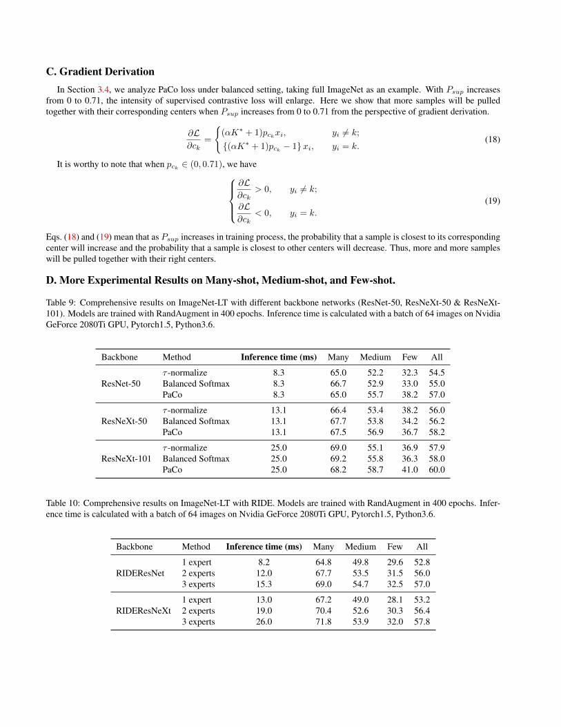
C. Gradient DerivationIn Section 3.4, we analyze PaCo loss under balanced setting, taking full ImageNet as an example. With Psup increases

from 0 to 0.71, the intensity of supervised contrastive loss will enlarge. Here we show that more samples will be pulledtogether with their corresponding centers when Psup increases from 0 to 0.71 from the perspective of gradient derivation.

∂L∂ck

=

{(αK∗ + 1)pckxi, yi = k;

{(αK∗ + 1)pck − 1}xi, yi = k.(18)

It is worthy to note that when pck ∈ (0, 0.71), we have∂L∂ck

> 0, yi = k;

∂L∂ck

< 0, yi = k.

(19)

Eqs. (18) and (19) mean that as Psup increases in training process, the probability that a sample is closest to its correspondingcenter will increase and the probability that a sample is closest to other centers will decrease. Thus, more and more sampleswill be pulled together with their right centers.

D. More Experimental Results on Many-shot, Medium-shot, and Few-shot.

Table 9: Comprehensive results on ImageNet-LT with different backbone networks (ResNet-50, ResNeXt-50 & ResNeXt-101). Models are trained with RandAugment in 400 epochs. Inference time is calculated with a batch of 64 images on NvidiaGeForce 2080Ti GPU, Pytorch1.5, Python3.6.

Backbone Method Inference time (ms) Many Medium Few All

ResNet-50τ -normalize 8.3 65.0 52.2 32.3 54.5Balanced Softmax 8.3 66.7 52.9 33.0 55.0PaCo 8.3 65.0 55.7 38.2 57.0

ResNeXt-50τ -normalize 13.1 66.4 53.4 38.2 56.0Balanced Softmax 13.1 67.7 53.8 34.2 56.2PaCo 13.1 67.5 56.9 36.7 58.2

ResNeXt-101τ -normalize 25.0 69.0 55.1 36.9 57.9Balanced Softmax 25.0 69.2 55.8 36.3 58.0PaCo 25.0 68.2 58.7 41.0 60.0

Table 10: Comprehensive results on ImageNet-LT with RIDE. Models are trained with RandAugment in 400 epochs. Infer-ence time is calculated with a batch of 64 images on Nvidia GeForce 2080Ti GPU, Pytorch1.5, Python3.6.

Backbone Method Inference time (ms) Many Medium Few All

RIDEResNet1 expert 8.2 64.8 49.8 29.6 52.82 experts 12.0 67.7 53.5 31.5 56.03 experts 15.3 69.0 54.7 32.5 57.0

RIDEResNeXt1 expert 13.0 67.2 49.0 28.1 53.22 experts 19.0 70.4 52.6 30.3 56.43 experts 26.0 71.8 53.9 32.0 57.8

Table 11: Comprehensive results on iNaturalist 2018 with ResNet-50 and ResNet-152. †represents the models are trainedwithout RandAugment. Inference time is calculated with a batch of 64 images on Nvidia GeForce 2080Ti GPU, Pytorch1.5,Python3.6.

Backbone Method Inference time (ms) Many Medium Few All

ResNet-50τ -normalize 8.3 74.1 72.1 70.4 71.5Balanced Softmax 8.3 72.3 72.6 71.7 71.8PaCo 8.3 70.3 73.2 73.6 73.2

ResNet-50 † Balanced Softmax 8.3 72.5 72.3 71.4 71.7PaCo 8.3 69.5 73.4 73.0 73.0

ResNet-152 PaCo 20.1 75.0 75.5 74.7 75.2

Table 12: Comprehensive results on iNaturalist 2018 with RIDE. Models are trained with RandAugment in 400 epochswithout knowledge distillation. Inference time is calculated with a batch of 64 images on Nvidia GeForce 2080Ti GPU,Pytorch1.5, Python3.6.

Backbone Method Inference time (ms) Many Medium Few All

RIDEResNet

1 expert 8.2 56.0 66.3 66.0 65.22 experts 12.0 62.2 70.5 70.0 69.53 experts 15.3 66.5 72.1 71.5 71.3

Table 13: Comparison with re-weighting baselines on ImageNet-LT with ResNet-50. The re-weighting strategy is applied tothe supervised contrastive loss. Models are all trained without RandAugment.

Method Top-1 Accuracy

CE 48.4multi-task (CE+Re-weighting) 49.0multi-task (CE+Blance Softmax) 48.6

PaCo 51.0

E. Implementation details for Table 1

We train models with cross-entropy, parametric contrastive loss 400 epochs without RandAugment respectively. Forsupervised contrastive loss, following the original paper, we firstly train the model 400 epochs. Then we fix the backboneand train a linear classifier 400 epochs.

F. Ablation Study

Re-weighting in contrastive learning without center learning rebalance Re-weighting is a classical method for dealingwith imbalanced data. Here we directly apply the re-weighting method of Cui et al. [16] in contrastive learning to comparewith PaCo. Moreover, Balanced softmax [38], as one state-of-the-art method for traditional cross-entropy in long-tailedrecognition, is also applied to contrastive learning rebalance. The experimental results are summarized in Table 13. It isobvious PaCo significantly surpasses the two baselines.

Rebalance in center learning PaCo balances the contrastive learning (for moderating contrast among samples). Howeverthe center learning also needs to be balanced, which has been explored in [1, 25, 15, 20, 8, 41, 38, 28, 49, 14, 46, 18].To compare with state-of-the-art methods in long-tailed recognition, we incorporate Balanced Softmax [38] into the center

Table 14: Comparison with re-weighting baselines that perform center learning rebalance on ImageNet-LT with ResNeXt-50.Models are all trained with RangAugment in 400 epochs.

Method loss weight Top-1 Accuracy

multi-task (Balanced Softmax+Re-weighting) 0.05 57.0multi-task (Balanced Softmax+Re-weighting) 0.10 57.1multi-task (Balanced Softmax+Re-weighting) 0.20 57.1multi-task (Balanced Softmax+Re-weighting) 0.30 57.0multi-task (Balanced Softmax+Re-weighting) 0.50 57.2multi-task (Balanced Softmax+Re-weighting) 0.80 57.2multi-task (Balanced Softmax+Re-weighting) 1.00 56.9

PaCo - 58.2

learning. As shown in Table 14, after rebalance in center learning, PaCo boosts performance to 58.2%, surpassing baselineswith a large margin.