On the likelihood of Condorcet’s profiles ∗

V. Merlin † M. Tataru ‡ F. Valognes §

Revised version, june 2000

Abstract

Consider a group of individuals who have to collectively choose an outcome from a

finite set of feasible alternatives. A scoring or positional rule is an aggregation procedure

where each voter awards a given number of points, wj , to the alternative she ranks in

jth position in her preference ordering; the outcome chosen is then the alternative that

receives the highest number of points. A Condorcet or majority winner is a candidate

who obtains more votes than her opponents in any pairwise comparison. Condorcet

[4] showed that all positional rules fail to satisfy the majority criterion. Furthermore,

he supplied a famous example where all the positional rules select simultaneously the

same winner while the majority rule picks another one. Let P ? be the probability of

such events in three-candidate elections. We apply the techniques of Merlin, Tataru

and Valognes [17] to evaluate P ? for a large population under the Impartial Culture

condition. With these assumptions, such a paradox occurs in 1.808 % of the cases.

1 Introduction

One of the simplest problems to state in collective decision theory is this. Consider a finite

population N = {1, 2, . . . n} together with a finite set of alternatives A = {a1, a2, . . . am}.

What method should society use in order to select an element of A? One natural method

is to base social within decision on the preferences of individual society. Typically, each∗The authors are indebted to Ashley Piggins for his careful reading.†GEMMA-CREME and CNRS, MRSH–SH230, Universite de Caen, Esplanade de la Paix, F-14032 Caen

Cedex, France.‡Northwestern University, 2033 Sheridan Road, Evanston, IL 60208-2730 USA.§Department of Economics, The University of Namur, Rempart de la Vierge 8, B-5000 Namur, Belgium.

1

individual is supposed to be rational, i.e., their preference relation is represented by a

linear order on A. This basic framework captures many collective decision problems, from

the selection of an investment project by a committee of experts, to the classical case of

political elections.

Unfortunately, there is no unproblematic method for aggregating individual preferences

in this setup. Two common principles are the ‘positional’ approach and the ‘majority’

method. Since the two-century old polemic between Borda and Condorcet, the supporters

of the positional approach and the advocates of the majority principle have continued to

provide new arguments in favor of their own views. More precisely, Borda [3] suggested that

each voter should give (m− 1) points for the candidate she prefers, (m− 2) for her second

best choice, and so on down to 1 point for the next to the last and 0 for her bottom ranked

alternative. Then, the Borda score for the alternative ak is the number of points it receives

over the whole population, and the Borda winner is the candidate whose Borda score is the

highest. In fact, the Borda count belongs to a wider class of positional rules, also called

scoring rules. A scoring rule is defined by a scoring vector w = (w1, w2, . . . wj , . . . wm),

w1 > wm, wj ≥ wj+1 ∀j = 1, . . . m − 1, where wj is the number of points an alternative

receives each time it is ranked in jth position in one individual’s preference. In this setup,

the Borda count is naturally described by the scoring vector w = (m− 1,m− 2, . . . 2, 1, 0).

The plurality rule, which selects as a winner the alternative with the highest number of first

positions, is another famous scoring rule. It is defined by the vector w = (1, 0, . . . 0). Finally,

this class of decision processes also contains one of the veto methods: the antiplurality rule,

in which each of the voters vetoes one alternative, and the candidate with the smallest

opposition wins. It is equivalent to the positional rule described by the scoring vector

w = (1, . . . 1, 0).

In his speech before the Academie Royale des Sciences in 1781, Borda proclaimed the

superiority of his method against the plurality rule. Rather than considering the candidates

all together, he proposed to compare them pairwise, and to select the one who would obtain

a majority of votes in all the comparisons. Such a candidate is now called a majority

winner or a Condorcet winner (CW). Then, he asserted that the Borda count would always

pick a Condorcet winner, whereas the plurality rule would not. Unfortunately, Borda’s

argument was wrong, and Condorcet [4] provided an example where all the scoring rules,

including the Borda count, simultaneously fail to select the majority winner. Table 1.1

2

displays this original example. Pierre � Paul � Jacques represents a preference where

Pierre is strictly preferred to Paul, and Paul to Jacques. The second column indicates the

number of individuals with such a preference.

Table 1.1

Pierre � Paul � Jacques 30

Pierre � Jacques � Paul 1

Jacques � Pierre � Paul 10

Paul � Pierre � Jacques 29

Paul � Jacques � Pierre 10

Jacques � Paul � Pierre 1

In this case, Pierre beats both Paul (41 votes against 40) and Jacques (60 against 21)

in pairwise comparisons. However, from a positional point of view, Paul (39 first positions,

31 second places) dominates both Pierre (31 first positions, 39 second places) and Jacques

(11 first positions, 11 second places). Irrespective of the scoring vector used, Paul will

be the positional winner. We call such a candidate an absolute positional winner (AW).

Throughout the rest of this paper, we shall refer to the situations in which the Condorcet

and absolute winner are different as Condorcet’s profiles.

Modern Social Choice Theory has no provided a solution to this debate. The supporters

of Condorcet principle claim that the pairwise comparison methods are more stable when

candidates are added or dropped (see, without being exhaustive, Young [27], Saari and

Merlin [20]). However, advocates of scoring rules claim that these methods offer higher

consistency when voters enter or leave the population (see Young [26], Moulin [18], Merlin

and Saari [16]).

The introduction of probability considerations brought a compromise to this debate.

Gehrlein and Fishburn [10] define the Condorcet efficiency of a scoring rule as the pro-

portion of voting situations where this positional method selects the Condorcet winner,

provided that such a candidate exists. More precisely, they consider populations where

each voter selects randomly and independently her preferences according to an uniform

probability distribution on the set of linear orderings. This assumption is called the Im-

partial Culture (IC) condition, as it does not one preference ordering over another. For

3

three-candidate elections and the family of scoring vectors w = (1, λ, 0), λ ∈ [0, 1], they

derived an exact formula giving the Condorcet efficiency for large populations as a func-

tion of λ. Under these assumptions, the Borda count maximizes the likelihood of picking

the Condorcet winner. Van Newenhizen [25] generalized this result by showing that the

Borda rule continues to maximize the Condorcet efficiency among the positional rules for

any number of alternatives and a wider class of probability models. Nevertheless, the Borda

count fails to satisfy the Condorcet criterion in almost 10% of the situations in the three-

candidate case, and computer calculations indicate that this probability rises as the number

of candidates increases (Fishburn and Gehrlein [6]).

The results are improved when we consider more homogeneous societies. A first pos-

sibility is to consider the family of Polya-Eggenberger models (see Berg [1]), where the

homogeneity of individual preferences is indexed by a contagion parameter α ≥ 0. We

recover the classical IC assumptions for α = 0, and the populations becomes more ho-

mogeneous as the parameter α increases. As one may guess, these models prove that the

Condorcet efficiency increases with α. Another possibility is to remove from consideration

some types of preferences, assuming for example single-peakedness. In the three-candidate

case, Lepelley [14, 15] found that this assumption clearly reduces the discrepancies between

the majority criterion and the positional rules. Tanguian [24] proposed recently another

probability model, assuming the existence of individual cardinal utilities and the existence

of their probability distribution. In this particular setup, the probability that the Borda

count and Condorcet principle agree converges to one, for any number of candidates as

the size of the population increases. Thus, the IC assumption should be considered as a

rather extreme case, and the values obtained in this framework could be considered as low

evaluations of the Condorcet efficiency measures.

Even if we restrict ourselves to three-candidate elections, the complexity of the compu-

tations limits the kind of probabilities we can evaluate and most of the analysis considers

the Condorcet efficiency of only one scoring rule at a time. Gehrlein [9] first managed to

obtain the joint Condorcet efficiency for the Borda count and the positional rule defined by

the scoring vector (1, λ, 0). Merlin, Tataru and Valognes [17] developed new techniques and

derived an explicit formula for the probability that all the positional rules select simulta-

neously the Condorcet winner. Gehrlein then recovered some of these results with classical

tools [8]. We provide here an analytical formula for the other case, i.e. the probability P ?

4

that all the positional rules select the same outcome, but disagree with the majority crite-

rion. Thus, this expression enables us to evaluate the occurrence of Condorcet’s profiles,

like the one displayed in Table 1.1, in a framework where this phenomenon is relatively

frequent. This completes the study of the statistical relationships between the positional

rules and the Condorcet principle in the three candidates case inaugurated twenty years

ago by Gehrlein and Fishburn. Moreover, from a technical point of view, the techniques

developed in this paper and its companion [17] potentially permit us to compute precisely

the occurences of any event for three-candidate elections and large electorates under the IC

assumption.

The rest of the paper is organized as follows. Section 2 introduces the prerequisites

of the model and the process we use to find the desired probability. The results are also

displayed and commented on in this section. The techniques we use are quite recent in

the literature on the likelihood of voting paradoxes. They have been first introduced by

Saari and Tataru [21] and developed in a couple of papers by Tataru and Merlin [23] and

Merlin, Tataru and Valognes [17]. Unlike Gehrlein and Fishburn, who base their proofs

upon previous results in statistics, we use a geometric argument involving the computation

of the volumes of spherical simplexes using Schlafli’s formula [5, 13, 22]. This technique and

the related computations are presented together in section 3.

2 The model and the result

2.1 Characterization of the voting situations

For three-candidate elections, A = {a1, a2, a3}. There exist six possible linear orderings on

A, and the different preference types are labeled in Table 2.1.

Table 2.1

1 : a1 � a2 � a3 4 : a3 � a2 � a1

2 : a1 � a3 � a2 5 : a2 � a3 � a1

3 : a3 � a1 � a2 6 : a2 � a1 � a3

Let n be the number of individuals, ni the number type i voters and call a vector n =

(n1, n2, n3, n4, n5, n6), representing the distribution of the voters on the different preferences,

a voting situation. By definition,∑6

i=1 ni = n. Without loss of generality, we use the scoring

5

vector ws = (2, s+1, 0), with s ∈ [−1, 1]. We recover the plurality method, the Borda count

and the antiplurality rule for s = −1, s = 0 and s = 1 respectively.

Saari [19] gave a necessary and sufficient condition for all positional rules to agree.

First, a constant scoring rule is defined by the scoring vector wk = (1, 1, . . . 1, 0, . . . 0),

1 ≤ k ≤ m− 1, with 1’s for the first k coordinates and 0’s for the remaining ones. Then all

the scoring methods give the same results if and only if all the constant rules agree, from

k = 1 to k = m− 1. In the three-candidate case, this condition says that the plurality and

antiplurality rule must select the same winner. Thus, we just have to consider these two

scoring rules instead of the continuum defined by the vectors ws.

According to Table 2.1, the fact that an alternative, let us say a1, has the greatest

ws-score for a given voting situation is characterized by the following two inequalities:

(1− s)n1 + 2n2 + (s + 1)n3 − (s + 1)n4 − 2n5 + (s− 1)n6 > 0 (2.1)

2n1 + (1− s)n2 + (s− 1)n3 − 2n4 − (s + 1)n5 + (s + 1)n6 > 0 (2.2)

For the plurality case, s = −1, inequalities (2.1) and (2.2) reduce to the inequalities (2.3)

and (2.4):

n1 + n2 − n5 − n6 > 0 (2.3)

n1 + n2 − n3 − n4 > 0 (2.4)

In this paper, we investigate the situations where all the scoring rules give the same result,

but fail to pick the Condorcet winner. Hence, the Condorcet winner should be a2 or a3.

The fact that a2 is a Condorcet winner is given by the inequalities (2.5) and (2.6):

−n1 − n2 − n3 + n4 + n5 + n6 > 0 (2.5)

n1 − n2 − n3 − n4 + n5 + n6 > 0 (2.6)

Thus, these six inequalities describe the following event: a1 is simultaneously the plurality

winner and the ws-winner while a2 is Condorcet winner. Let P1(s) be the probability that

the plurality rule and the ws scoring rule agree while the Condorcet principle select another

alternative. Clearly, P1(s) is six times the probability that inequalities (2.1) to (2.6) are

fulfilled. When s = −1, we recover the probability that the plurality rule fails to select the

Condorcet winner; from Gehrlein and Fishburn [10], P1(−1) = 0.22150. The value of P1(s)

is unknown for any other value of s. For s = 1, we shall obtain the probability P ?, i.e., the

likelihood of Condorcet’s profiles.

6

2.2 Probability results under IC assumption

As mentioned in the introduction, the probability of a voting paradox depends upon the

assumptions one may set about the likelihood of the different voting situations. We shall

retain throughout this paper the Impartial Culture assumption, which defines the most com-

mon model of heterogeneous populations. Thus, the probability that a voter will have the

jth preference type is 16 for three-candidate elections. In turn, p(n = (n1, n2, n3, n4, n5, n6))

follows a multinomial distribution; when the size of the population is large enough, the

central limit theorem applies and the density distribution tends toward a normal law.

Due to its complexity, the derivation of the exact formulas that gives the value of

P1(s) is postponed to section 3. The results of the computation are presented in Table

2.2. The values for P1(s) are presented in the first column. The second one displays

figures from Merlin, Tataru and Valognes [17] about P2(s), the probability that the plurality

rule and the ws scoring rule pick together the Condorcet winner. The next one gives

the values of P3(s), the probability that the plurality rule and the ws-scoring rule agree

regardless of any consideration about the majority votes. They are derived from an analytic

formula due to Gehrlein and Fishburn [12]. Finally, the last column displays the values of

P4(s) = P3(s) − P2(s) − P1(s). It gives the probability that the plurality and the ws-rule

agree when the Condorcet winner does not exist.

7

Table 2.2

s P1(s) P2(s) P3(s) P4(s)

−1 0.22150 0.69076 1.00000 0.08774

−0.8 0.18465 0.68874 0.95684 0.08345

−0.6 0.14688 0.68569 0.91031 0.07774

−0.4 0.11024 0.68075 0.86102 0.07003

−0.2 0.07779 0.67216 0.80994 0.05999

0 0.05307 0.65680 0.75834 0.05084

0.2 0.03762 0.63213 0.70759 0.03784

0.4 0.02886 0.60053 0.65900 0.02961

0.6 0.02370 0.56609 0.61359 0.02380

0.8 0.02039 0.53179 0.57205 0.01987

1 0.01808 0.49947 0.53464 0.01709

The most interesting row is the last one, which tells us the probability that all the scoring

rules agree (P3(1)) according to the state of the majority relation: the Condorcet winner

is the same outcome (P2(1)), is different (P1(1)) or does not exist (P4(1)). In particular,

P1(1) = P ?, the likelihood of Condorcet profiles, which turns out to be quite a rare event.

Table 2.3 gives the correlation matrix between the existence of an absolute winner and the

existence of a Condorcet winner.

Table 2.3

∃CW 6 ∃CW Sum

∃AW 0.51776 0.01709 0.53464

6 ∃AW 0.39450 0.07065 0.46536

Sum 0.91226 0.08874 1.00000

One should first notice that a Condorcet winner is a solution concept far more frequent

than an absolute winner. Nevertheless, we should also remark that the Condorcet principle

is not unquestioned: there exists profiles where the majority criterion is inconsistent while

the positional rules clearly pick up the same winner.

8

3 Proof

3.1 The Schlafli Method

The technique we use in order to find an exact formula for P1(s) is the same as the one de-

veloped in Merlin, Tataru and Valognes [17]. Let xk be the random variable that associates

to each voter k a vector of the form (0, 0, 0, 1, 0, 0) with probability 16 of having 1 in each

position. Then, the expectation of xk is

E(xk) = (16,16,16,16,16,16)

and the covariance matrix is a diagonal 6× 6 matrix with the common entry σ given by

σ2 = E(x2k)− E(xk)2.

Let

mT = (m1,m2, . . . m6)T =1

σ√

n

n1

...

n6

−

n6...n6

The Central Limit Theorem in R5 implies the following convergence in measure:

µ[mT]7→ 1

(√

2π)5e−|t|2

2 λ

as n →∞ where t = (t1, t2, . . . , t6) ∈ R6, |t|2 = t21+. . .+t26 and λ is Lebesgue measure on the

five-dimensional hyperplane t1+. . .+t6 = 0. Note that since mT has the measure supported

on the hyperplane m1 + . . .+m6 = 0, the limit of mT as n →∞ is also a measure supported

on t1 + . . . + t6 = 0. In order to compute P1(s), we shall evaluate the probability that a

voting situation fulfills the set of inequalities (2.1) to (2.6). By subtracting or dividing

the number of voters of each type by the same constant, the quantities change, but the

comparisons between them are unchanged, therefore, one can easily claim that nT satisfies

conditions (2.1) to (2.6) if and only if mT satisfies these inequalities. The Central Limit

Theorem yields

P(mT satisfies (2.1) to (2.6)

)7→ 1

(√

2π)5

∫C1

e−|t|2

2 dλ

9

where C1 = {t ∈ R6, t satisfies (2.1) to (2.6) and∑6

i=1(ti) = 0}. Because conditions (2.1)

to (2.6) are homogeneous, the domain C1 of the integration is a cone. Also the measure

µ ≡ 1(√

2π)5e−|t|2

2 λ

is absolutely continuous and radially symmetric. Hence computing

1(√

2π)5

∫C1

e−|t|2

2 dλ

reduces to finding the measure µ of the cone C1, when the measure is invariant to rotations.

The measure µ of such a cone is proportional to the euclidian measure of the cone, that is

the measure on the sphere.

As the cone C1 lies on the five-dimensional subspace∑6

i=1 ti = 0, its intersection with

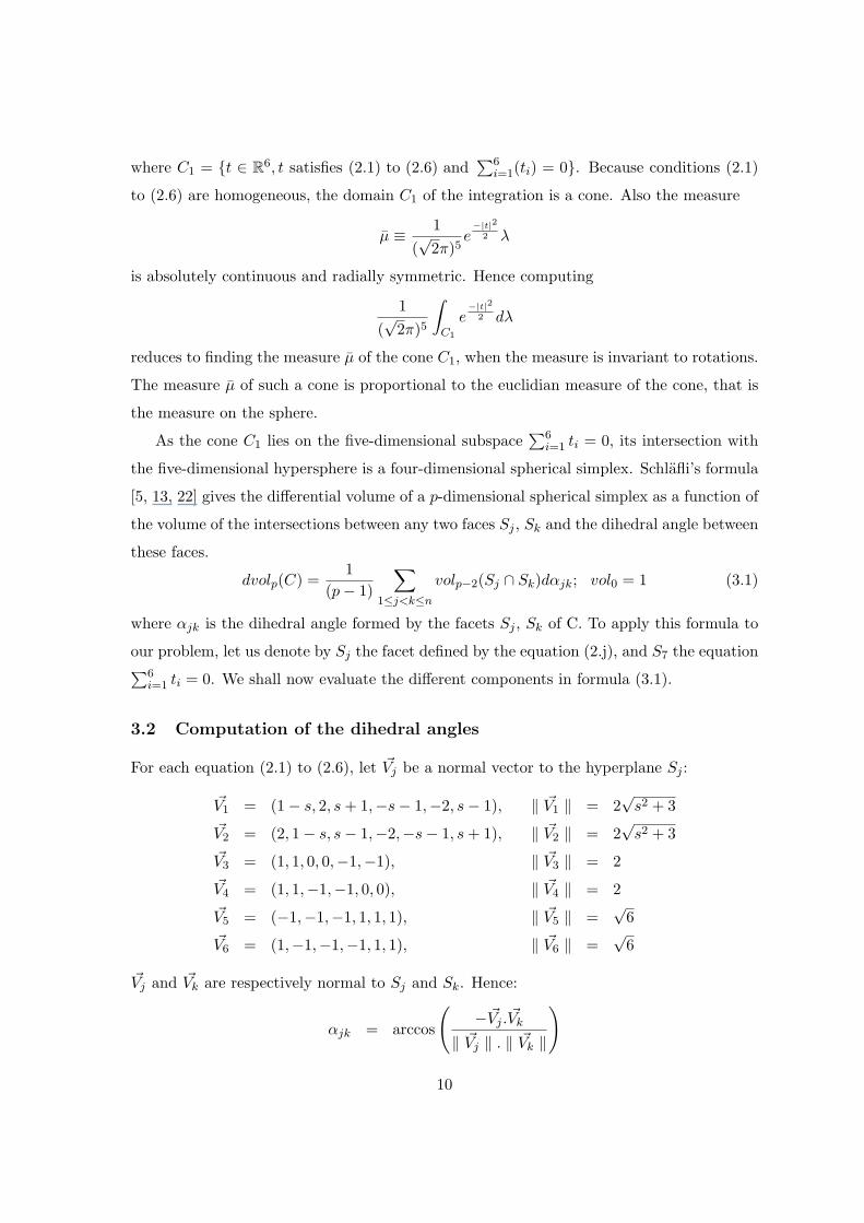
the five-dimensional hypersphere is a four-dimensional spherical simplex. Schlafli’s formula

[5, 13, 22] gives the differential volume of a p-dimensional spherical simplex as a function of

the volume of the intersections between any two faces Sj , Sk and the dihedral angle between

these faces.

dvolp(C) =1

(p− 1)

∑1≤j<k≤n

volp−2(Sj ∩ Sk)dαjk; vol0 = 1 (3.1)

where αjk is the dihedral angle formed by the facets Sj , Sk of C. To apply this formula to

our problem, let us denote by Sj the facet defined by the equation (2.j), and S7 the equation∑6i=1 ti = 0. We shall now evaluate the different components in formula (3.1).

3.2 Computation of the dihedral angles

For each equation (2.1) to (2.6), let ~Vj be a normal vector to the hyperplane Sj :

~V1 = (1− s, 2, s + 1,−s− 1,−2, s− 1), ‖ ~V1 ‖ = 2√

s2 + 3~V2 = (2, 1− s, s− 1,−2,−s− 1, s + 1), ‖ ~V2 ‖ = 2

√s2 + 3

~V3 = (1, 1, 0, 0,−1,−1), ‖ ~V3 ‖ = 2~V4 = (1, 1,−1,−1, 0, 0), ‖ ~V4 ‖ = 2~V5 = (−1,−1,−1, 1, 1, 1), ‖ ~V5 ‖ =

√6

~V6 = (1,−1,−1,−1, 1, 1), ‖ ~V6 ‖ =√

6

~Vj and ~Vk are respectively normal to Sj and Sk. Hence:

αjk = arccos

(− ~Vj . ~Vk

‖ ~Vj ‖ . ‖ ~Vk ‖

)

10

As we shall derive the dihedral angles, we are only interested in the angles which depend

on s. There are 8 of them:

α15 = arccos(

4√6(s2+3)

)α26 = arccos

(−2√

6(s2+3)

)α16 = α25 = arccos

(2√

6(s2+3)

)α13 = α24 = arccos

(s−3

2√

3+s2

)α14 = α23 = arccos

(s−3

4√

3+s2

)Hence:

dα15 = −4s(s2+3)

√6s2+18

ds

dα26 = 2s(s2+3)

√6s2+18

ds

dα16 = dα25 = −2s

(s2+3)√

6s2+18)ds

dα13 = dα24 = 3+3s2(3+s2)

√3+s2

ds

dα14 = dα23 = 3+3s4(3+s2)

√3+s2

ds

3.3 Finding the Vertices

The dihedral volumes Sj⋂

Sk are two-dimensional spherical simplexes, and we shall first

find their vertices. A direction in R5 is given by solving a system of four linear equations.

Thus, we shall find the coordinates of a vertex, P1234 for example, by solving the following

system:

S1 = 0

S2 = 0

S3 = 0

S4 = 0

S5 > 0

S6 > 0

S7 = 0

Among the 15 systems of equations, only eight of them will provide an adequate solutions.

Moreover, we shall distinguish two cases: s ≤ 0 and s ≥ 0.

11

case 1: s ≤ 0

P1256 = (0, 1 + s,−1− s, 0, 1− s, s− 1)

P1356 = (−1, 2,−1,−1, 2,−1)

P1245 = (−2s + 2, 3s− 1,−s− 1, 2s + 2,−3s− 1, s− 1)

P1246 = (2s + 2,−s− 1, 3s− 1,−2s + 2, s− 1,−3s− 1)

P2456 = (2,−1,−1, 2,−1,−1)

P1345 = (1,−1, 0, 0,−1, 1)

P1346 = (0, 0,−1, 1,−2, 2)

P3456 = (0, 0, 0, 0,−1, 1)

case 2: s ≥ 0

P1256 = (0, 1 + s,−1− s, 0, 1− s, s− 1)

P1235 = (s− 1, 2,−s− 1,−s− 1, 2, s− 1)

P1236 = (−s− 1, 2 + 2s,−3s− 1, s− 1, 2− 2s, 3s− 1)

P2356 = (−1− s, 2 + 2s,−s− 1,−s− 1, 2− s, 2s− 1)

P1456 = (2 + 2s,−s− 1,−s− 1, 2s + 2,−7s− 1, 5s− 1)

P1345 = (1,−1, 0, 0,−1, 1)

P1346 = (0, 0,−1, 1,−2, 2)

P3456 = (0, 0, 0, 0,−1, 1)

Also notice that the faces defined by the inequalities (2.2) and (2.3) do not intersect in

the first case. The same situation holds with the faces defined by the inequalities (2.2) and

(2.4) for s ≥ 0. According to each case, the spherical simplex Sj⋂

Sk could possess 3 or 4

vertices, or simply does not exist. This data is summarized in Table 3.1. Pabcd is a vertex

12

for Sj⋂

Sk if j and k appear as indices.

Table 3.1

V olumes V ertices, s ≤ 0 V ertices, s ≥ 0

S1⋂

S3 P1356, P1345, P1346 P1235, P1236, P1345, P1346

S1⋂

S4 P1245, P1246, P1345, P1346 P1456, P1345, P1346

S1⋂

S5 P1256, P1356, P1245, P1345 P1256, P1235, P1456, P1345

S1⋂

S6 P1256, P1356, P1246, P1346 P1256, P1236, P1456, P1346

S2⋂

S3 ∅ P1235, P1236, P2356, P1346

S2⋂

S4 P1245, P1246, P2456 ∅

S2⋂

S5 P1256, P1245, P2456 P1256, P1356, P2356

S2⋂

S6 P1256, P1246, P2456 P1256, P1236, P2356

3.4 Differential volumes

The differential volumes reduce to surfaces of two-dimensional simplexes on the sphere.

Thus, we can apply the Gauss-Bonnet theorem: the surface equals to the sum of the angles

on the surface minus π. We describe the details of the computations for the differential

volume S2⋂

S4 in case s ≤ 0. The other cases can be worked in a similar fashion.

Let β15, β16 and β56 be the angles on the surface of the triangle, defined by the vertices

P1245, P1246 and P2456; δ1, δ5 and δ6 are respectively the angles P1245, P1246, P1245, P2456 and

P1246, P2456. Hence:

cos(β15) =cos(δ6)− cos(δ1) cos(δ5)

sin(δ1) sin(δ5)(3.2)

cos(β16) =cos(δ5)− cos(δ1) cos(δ6)

sin(δ1) sin(δ6)(3.3)

cos(β56) =cos(δ1)− cos(δ5) cos(δ6)

sin(δ5) sin(δ6)(3.4)

In our case:

cos(δ1) =3− 5 s2

3 + 7 s2(3.5)

cos(δ5) = cos(δ6) =√

3√3 + 7 s2

(3.6)

13

Hence, by (3.2) to (3.6)

V olp−2

(S2

⋂S4

)= β15 + β16 + β56 − π (3.7)

= + arccos(57) + 2 arccos(

3√

27√

3 + s2) (3.8)

The same reasoning enables us to find exact formulas for:

• I1(s) =∑

j=1,2 k=3456 V olp−2 (Sj⋂

Sk) dαjk, s ≤ 0.

• I2(s) =∑

j=1,2 k=3456 V olp−2 (Sj⋂

Sk) dαjk, s ≥ 0.

Due to the fact that the event we analyze involves two different alternatives, there is no

symmetry among the dihedral volumes; contrary to computations in Merlin, Tataru and

Valognes [17], there is no simplification and we need to treat separately the fourteen cases.

After simplifications, formulas for I1(s) and I2(s) are given by the expressions (3.9) and

(3.10):

I1(s) = +4 s

(arccos( s√

1+4 s2)−arccos( +1+s√

13+2 s+37 s2)+arccos(

(−3+s)√

3+9 s2√(3+s2) (13+2 s+37 s2)

)−arccos(

√3+9 s2

3+13 s2+4 s4)

)(3+s2)

√2+6 s2

−2 s

(2 arccos( 2 s√

7+7 s2)−2 arccos(

2√

37 s√

3+10 s2+3 s4)−arccos(

3 (−1+s2)√(3+12 s2) (3+10 s2+3 s4)

)

)(3+s2)

√14+6 s2

+2 s

(arccos( 5 s√

7√

1+4 s2)−arccos( 7+13 s√

7√

37+26 s+37 s2)−arccos(

√3 (1−s) (3−2 s+3 s2)√

(37+26 s+37 s2) (3+10 s2+3 s4))

)(3+s2)

√14+6 s2

−

√3

(π2+arccos( 1√

7)−arccos( 3√

14)−arccos( 5

7)+2 arccos(

3√

27√

3+s2)

)3+s2

−

√3 (1+s)

(− arccos( 6 s−2 s2√

(6+2 s2) (13+2 s+37 s2))+arccos( 12+6 s+2 s2√

(6+2 s2) (37+26 s+37 s2))

)(3+s2)

√13+2 s+5 s2

−√

3 (1+s)

(arccos( 8 s√

26+4 s+74 s2)+arccos( 3+7 s√

74+52 s+74 s2)

)(3+s2)

√13+2 s+5 s2

(3.9)

14

I2(s) =4 s

(3 π2−arccos( 1+s√

13+2 s+37 s2)+arccos( −3+s−8 s2√

(1+4 s2) (13+2 s+37 s2))−arccos(

√3+9 s2

3+13 s2+4 s4)

)(3+s2)

√2+6 s2

−2 s

(arccos( 3+2 s+5 s2√

(1+s2) (37+26 s+37 s2))+arccos(

√3 (−1+s) (3−2 s+3 s2)√

(37+26 s+37 s2) (3+10 s2+3 s4))

)(3+s2)

√14+6 s2

+2 s

(− arccos( 7+13 s√

7√

37+26 s+37 s2)+arccos(

(1+s) (−3+8 s)√1+4 s2

√37+26 s+37 s2

)+arccos(3 (−1+s2)√

(3+12 s2) (3+10 s2+3 s4))

)(3+s2)

√14+6 s2

+2 s

(− arccos(

2√

37 s√

3+10 s2+3 s4)+arccos(

(−3+9 s)√

3+s2√3+9 s2

√37+2 s+13 s2

)+arccos( 3−2 s+s2√(1+s2) (37+2 s+13 s2)

)

)(3+s2)

√14+6 s2

−√

3

(− arccos( 3√

14)+arccos( −6

√5√

210+70 s2)

)3+s2

−

√3 (1+s)

(−2 π+arccos( 4

√2 s√

13+2 s+37 s2)+arccos( 13−10 s−23 s2√

(13+2 s+37 s2) (37+26 s+37 s2))+arccos( 3+7 s√

74+52 s+74 s2)

)(3+s2)

√13+2 s+5 s2

−

√3 (1+s)

(arccos(

√24+8 s2

37+2 s+13 s2)+arccos( 12+6 s+2 s2√

(6+2 s2) (37+26 s+37 s2))+arccos( −11−10 s+s2√

(37+2 s+13 s2) (37+26 s+37 s2))

)(3+s2)

√13+2 s+5 s2

(3.10)

Between -1 and 0, the differential volume is I13 as p = 4 in the Schlafli’s formula. We have

to multiply this number by 6, and to divide it by the surface of the hypersphere in R5,

ω5 = 8π2

3 . Thus, the probability that the plurality rule and the ws-rule, s ≤ 0, agree while

the Condorcet criterion selects another alternative is given by equation (3.11).

P1(s) = 0.22150 +3

4π2

∫ s

−1I1(u)du (3.11)

Recall that value 0.22150 comes from Gehrlein and Fishburn [10]. The same reasoning

applies for the case s ∈ [0, 1] and the formula of P1(s) is then given by equation (3.12).

P1(s) = P1(0) +3

4π2

∫ s

0I2(u)du (3.12)

The numerical values of the Table 2.2 are computed by performing the integration in the

above formulas.

15

References

[1] S. Berg, “Paradox of voting under an urn model: the effect of homogeneity”, Public

Choice 47, p 377-387, 1985.

[2] S. Berg and D. Lepelley, “On probability models in voting theory”, Statistica Neer-

landica 48, p 133-146, 1994.

[3] Borda, Memoire sur les Elections au Scrutin, Histoire de l’Academie Royale des Sci-

ences, Paris, 1781.

[4] Condorcet, Essai sur l’Application de l’Analyse a la Probabilite des Decisions Rendues

a la Pluralite des Voix, Paris, 1785.

[5] H. Coxeter, “The functions of Schlafli and Lobatschefsky”, Quarterly Journal of Math-

ematics 6, p 13-29, 1935.

[6] P. Fishburn and W. Gehrlein, “Majority efficiencies for simple voting procedures:

summary and interpretation”, Theory and Decision 4, p 141-153, 1982.

[7] W. Gehrlein, “Condorcet’s paradox and the Condorcet efficiency of voting rules”,

Mathematica Japonica 45, p 173-199, 1997.

[8] W. Gehrlein, “On the probability that all weighted scoring rule select the Condorcet

winner”, mimeo, University of Delaware, 1997.

[9] W. Gehrlein, “The sensitivity of weight selection on the Condorcet efficiency of

weighted scoring rules”, Social Choice and Welfare 15, p 351-358, 1998.

[10] W. Gehrlein and P. Fishburn, “Coincidence probabilities for simple majority and

positional voting rules”, Social Science Research 7, p 272-283, 1978

[11] W. Gehrlein and P. Fishburn, “Probabilities of election outcomes for large electorate”,

Journal of Economic Theory 19, p 38-49, 1978.

[12] W. Gehrlein and P. Fishburn, “Scoring rule sensitivity to weight selection”, Public

Choice 40, p 249-261, 1983.

[13] R. Kellerhals, “On the volume of hyperbolic polyhedra”, Mathematische Annalen 285,

p 541-569, 1989.

16

[14] D. Lepelley, “Condorcet efficiency of positional voting rules with single-peaked pref-

erences”, Economic Design 1, p 289-299, 1995.

[15] D. Lepelley, “Constant scoring rules, Condorcet criteria and single-peaked prefer-

ences”, Economic Theory 7, p 491-500, 1996.

[16] V. Merlin and D. Saari, “The Copeland method II: manipulations, monotonicity and

paradoxes”, Journal of Economic Theory 72, p 148-172, 1997.

[17] V. Merlin, M. Tataru and F. Valognes, “On the probability that all the rules select

the same winner”, Journal of Mathematical Economics. To appear.

[18] H. Moulin, “Condorcet’s principle implies the no show paradox”, Journal of Economic

Theory 45 p 45-53, 1988.

[19] D. Saari, “Millions of election rankings from a single profile”, Social Choice and Wel-

fare 9, p 277-306, 1992.

[20] D. Saari and V. Merlin, “The Copeland method I: relationships and the dictionary”,

Economic Theory 8, p 51-76, 1996.

[21] D. Saari and M. Tataru, “The likelihood of dubious election outcomes”, Economic

Theory. To appear.

[22] L. Schlafli, Theorie der Vielfachen Kontinuitat, Gesmmelte Mathematische Abhand-

lungen 1, Birkhauser, Basel, 1950.

[23] M. Tataru and V. Merlin, “On the relationship of the Condorcet winner and positional

voting rules”, Mathematical Social Sciences 34, pp 81-90, 1997.

[24] A. Tanguian, “Solution to Condorcet’s paradox”, paper presented at the 3rd Interna-

tional Meeting of the Society for Social Choice and Welfare, Maastricht, 1996.

[25] J. van Newenhizen, “The Borda method is the most likely to respect the Condorcet

principle”, Economic Theory 2, p 69-83, 1992.

[26] P. Young, “Social Choice Scoring Functions”, SIAM Journal of Applied Mathematics

28, p 824-838, 1975.

17

[27] P. Young, “Condorcet’s theory of voting”, American Political Science Review 82 p

1231-1244, 1988.

18