PLEASE SCROLL DOWN FOR ARTICLE

This article was downloaded by: [Feng, Yanqin]On: 4 September 2010Access details: Access Details: [subscription number 926604456]Publisher Taylor & FrancisInforma Ltd Registered in England and Wales Registered Number: 1072954 Registered office: Mortimer House, 37-41 Mortimer Street, London W1T 3JH, UK

Communications in Statistics - Theory and MethodsPublication details, including instructions for authors and subscription information:http://www.informaworld.com/smpp/title~content=t713597238

A Unified Approach to Likelihood Inference on Linear InequalityConstraints in Contingency TablesYanqin Fenga; Guoxin Zuob

a School of Mathematics and Statistics, Wuhan University, Wuhan, P.R. China b School of Mathematicsand Statistics, HuaZhong Normal University, Wuhan, P.R. China

Online publication date: 04 September 2010

To cite this Article Feng, Yanqin and Zuo, Guoxin(2010) 'A Unified Approach to Likelihood Inference on Linear InequalityConstraints in Contingency Tables', Communications in Statistics - Theory and Methods, 39: 19, 3399 — 3420To link to this Article: DOI: 10.1080/03610920903268865URL: http://dx.doi.org/10.1080/03610920903268865

Full terms and conditions of use: http://www.informaworld.com/terms-and-conditions-of-access.pdf

This article may be used for research, teaching and private study purposes. Any substantial orsystematic reproduction, re-distribution, re-selling, loan or sub-licensing, systematic supply ordistribution in any form to anyone is expressly forbidden.

The publisher does not give any warranty express or implied or make any representation that the contentswill be complete or accurate or up to date. The accuracy of any instructions, formulae and drug dosesshould be independently verified with primary sources. The publisher shall not be liable for any loss,actions, claims, proceedings, demand or costs or damages whatsoever or howsoever caused arising directlyor indirectly in connection with or arising out of the use of this material.

Communications in Statistics—Theory and Methods, 39: 3399–3420, 2010Copyright © Taylor & Francis Group, LLCISSN: 0361-0926 print/1532-415X onlineDOI: 10.1080/03610920903268865

AUnified Approach to Likelihood Inferenceon Linear Inequality Constraints

in Contingency Tables

YANQIN FENG1 AND GUOXIN ZUO2

1School of Mathematics and Statistics, Wuhan University,Wuhan, P.R. China2School of Mathematics and Statistics, HuaZhong Normal University,Wuhan, P.R. China

In contingency table analysis, a likelihood ratio test for linear inequality constraintsis discussed. The restriction condition considered in this article is much moregeneral than usual stochastic order restriction conditions. Asymptotic property oftest statistic is shown. Simulation study is conducted to compare the empirical powerand size performed via the proposed method and others. Several real data sets areused to illustrate our theoretical result. The idea used in this article can be appliedto test the problems with nonlinear inequality constraints.

Keywords Chi-bar-squared; Inequality constraint; Likelihood ratio test;Stochastic order.

Mathematics Subject Classification 62H20; 62H30.

1. Introduction

Since Lehmann (1955) introduced the concept of stochastic order among differentprobability distributions, varieties of estimation, and hypothesis test methods underorder restrictions have been discussed in statistics (Shaked and Shanthikumar, 1994;Silvapulle and Sen, 2005; and references therein).

Statistical inference under stochastic order restrictions, which commonly occursin biology, pharmacology, financial economics, etc., is widely discussed in the pastfive decades. In toxicology, dose-response study usually relies on an understandingof the causal relationships between exposure and effect. The dose-response trend,for example, a monotone increasing trend effect as dose level increasing, isusually tested. Similar order-restricted problems can be found in many other areas.Generally, let pi� i = 1� � � � � m denote the probability vector corresponding to the

Received December 13, 2008; Accepted August 18, 2009Address correspondence to Yanqin Feng, School of Mathematics and Statistics, Wuhan

University, Wuhan 430072, P.R. China; E-mail: yanqf2008@yahoo.com.cn

3399

Downloaded By: [Feng, Yanqin] At: 07:34 4 September 2010

3400 Feng and Zuo

ith population. Next, are three types of stochastic order restrictions which arecommonly seen in applications.

a. Simple order restriction. p1 ≤st · · · ≤st pm (where ‘st’ means a stochasticorder). Many researchers considered hypothesis test problem under this situation.For example, Wang (1996) proposed a likelihood ratio test method in severalpopulations. Dardanoni and Forcina (1998) discussed the likelihood inferenceproblem in a nonparametric context, Feng and Wang (2007) constructed hypothesistest statistic and gave a limit theory for this problem.

b. Simple tree order restriction. p1 ≤st pi� i = 2� � � � � m. Simple tree orderrestriction is also studied in huge number of articles. For example, for severalindependent normal populations with common variance, Cohen and Sackrowitz(2002) suggested inference procedure for testing the equality of means against thesimple tree order alternative, and for the same model, Chaudhuri and Perlman(2005) considered the biases of the maximum likelihood and Cohen–Sackrowitzestimates. Peddada et al. (2006) discussed test problem under simple tree orderrestriction in dose-response study.

c. Umbrella order restriction. p1 ≤st · · · ≤st ph ≥st · · · ≥st pm. Umbrella orderrestriction sometimes is more preferable than simple order restriction in dose-response studies (Simpson and Margolin, 1986). Two procedures for obtainingsimultaneous confidence intervals under umbrella order restriction were given byMarcus and Genizi (1994). Singh and Liu (2006) proposed a new test against anumbrella ordered alternative. Feng (2008a) gave a nonparametric test method forumbrella order constraint problems.

In real data analysis, much more order restriction may exist. For example, Feng(2008b) gave a tree order by combining the simple order and the simple tree order.Some other references are available in Silvapulle and Sen (2005)’s book. In thisarticle, we consider a likelihood inference problem under general linear inequalityrestrictions in an m× k contingency table under the product multinomial model.

Let X denote an explanatory variable with m levels, and Y an ordinalresponse variable with k levels. Let pi = �pi1� � � � � pik�

′ denote the probability vectorcorresponding to the i-th population, and �i = �pi1� � � � � pi�k−1�

′ denote the first k− 1components of pi for i = 1� � � � � m. It is obvious that the distribution of the i-thpopulation is completely determined by �i for i = 1� � � � � m. Denote �= ��′1� � � � � �

′m�

′.Let nij be the number of observations from the i-th population with the j-thoutcome, and ni =

∑kj=1 nij be the number of observations from the i-th population.

The stochastic order restriction, involved in the statistical inference problem ofinterest, is linear inequality constraints which takes form

� ∈ S = �� � A� ≥ 0�� (1.1)

where A is any full row rank constant matrix. The above three types of orderrestrictions are only particular cases to model (1.1). For example, let C be any�k− 1�-order full rank matrix, B1 = �b1ij� with b1i�i+1 = −1� b1i1 = 1 and 0 otherwise,B2 = b2ij with b2ii = 1� b2i�i+1 = −1 and 0 otherwise, and B3 = �b3ij� with b3ii = 1 if i ≤h− 1 and −1 otherwise, b3i�i+1 = −1 if i ≤ h− 1 �1 ≤ h ≤ m� and 1 otherwise, andb3ij = 0 if �i− j� > 1. If A = B1 ⊗ C, model (1.1) is the simple tree order model b.If A = B2 ⊗ C, model (1.1) is the simple order model a. If A = B3 ⊗ C, model (1.1)

Downloaded By: [Feng, Yanqin] At: 07:34 4 September 2010

Statistical Inference on Inequality Constraints 3401

is the umbrella order model c. Therefore, model (1.1) is a broader model. Teohet al. (2008) gave a very general methodology which is applicable to test a broadcollection of order restrictions (on row and columns) of a matrix, and this methodperformed very well in the estimation of unknown parameters and test procedure.Because all the test results are obtained by bootstrap method, they did not discussthe distribution theory of the test statistic.

In order to obtain the null asymptotic distribution of the likelihood ratiostatistic under model (1.1), two-stage procedure is given. In the first stage, itis shown that the restricted maximum likelihood estimators are n1/2-consistent,thus the objective function is restricted in a n−1/2-shrinking neighborhood ofthe common distribution function, and it is thought of as an empirical processindexed by distribution function. In the second stage, the process is shown toconverge in distribution to a Gaussian process, thus the desired null asymptoticdistribution by limit theory of the optimization is obtained. The main idea inderiving the asymptotic distribution could easily be applied to problems with moregeneral data type (or inequality-restricted condition, e.g., nonlinearity inequalityconstraints), including stratified data, which is commonly used to facilitate anefficient comparison of treatments in clinical trials.

In Sec. 2, the hypothesis test model is described. Likelihood ratio test statisticis constructed and the null asymptotic distribution of the test statistic is derived inSec. 3. Simulation studies is conducted to compare the performance of the proposedprocedure with some other procedures in Sec. 4. Four case studies are given toillustrate the performance of the proposed method in Sec. 5. Conclusions are givenin last section. All proofs of theoretical results are given in the Appendix.

2. Hypothesis Test Model and Test Statistic

To detect the association between the explanatory variable and the responsevariable, we consider testing H0 against H1 −H0, where

H0 � � ∈ S0 = �� � A� = 0� and H1 � � ∈ S = �� � A� ≥ 0�� (2.1)

Here, A is any full row rank constant matrix.We construct likelihood ratio test statistic for problem (2.1) by

T01 = 2{max�∈S

logL���−max�∈S0

logL���}� 2�logL���− logL����� (2.2)

where the log-likelihood for any outcome ��ni1� � � � � nik�′� i = 1� � � � � m�, omitting the

multiplicative constant, is given by

logL��� =m∑i=1

{k−1∑j=1

nij log pij +(ni −

k−1∑t=1

nit

)log

(1−

k−1∑t=1

pit

)}�

The unrestricted maximum likelihood estimate of pij is given by pij = nij/ni, andhence � = ��′1� � � � � �

′m�

′ with �i = �pi1� � � � � pi�k−1�′ for i = 1� � � � � m is the maximum

likelihood estimate of � under no restriction. Generally, there exist no closed forms

Downloaded By: [Feng, Yanqin] At: 07:34 4 September 2010

3402 Feng and Zuo

for the maximum likelihood estimates under H0 and H1, denoted as � and �, whichare the optimal solutions of the following mathematical programing problem:

min− logL��� subject to � ∈ S∗�

where S∗ takes S0 and S, respectively. A variety of constrained optimizationalgorithms in mathematical programming can be used to obtain the numericalsolution of � and �. For example, the feasible direction and the penalty functionmethod (refer to Bazaraa and Shetty, 1979) can be applied. In practice, thenumerical solution of � and � can be easily computed by some Matlab functions.

The test will reject the null hypothesis H0 in favor of the alternative hypothesisH1 for large value of the test statistic T01� that is, for a given level � the test willreject the null hypothesis H0 if T01 > C� where C satisfies

PH0�T01 > C� = � (2.3)

3. Distribution Theory of the Test Statistic

In order to find the critical value C defined in (2.3), this section gives the nullasymptotic distribution of the test statistic.

Let

gn��� =1nlogL��� =

m∑i=1

ni

n

{k−1∑j=1

pij log pij +(1−

k−1∑t=1

pit

)log

(1−

k−1∑t=1

pit

)}�

g��� = E�0

{1nlogL���

}

=m∑i=1

ni

n

{k−1∑j=1

p�0�ij log pij +

(1−

k−1∑t=1

p�0�it

)log

(1−

k−1∑t=1

pit

)}�

where n =∑mi=1 ni is the total number of observations from all the m populations,

and �0 = �p�0�11 � � � � � p

�0�1�k−1� � � � � p

�0�m1� � � � � p

�0�m�k−1�

′ denotes the unknown true value of�. The gradient vector and Hessian matrix of gn��� are given, respectively, by

gn��� =(�gn���

�p11

� � � � ��gn���

�p1�k−1

� � � � ��gn���

�pm1

� � � � ��gn���

�pm�k−1

)′�

Hn��� =�2gn���

��2=

H1n 0

� � �

0 Hmn

�

where

�gn���

�pij

= ni

n

pij

pij

−(1−

k−1∑t=1

pit

)(1−

k−1∑t=1

pit

)−1 � i = 1� � � � � m� j = 1� � � � � k− 1�

Downloaded By: [Feng, Yanqin] At: 07:34 4 September 2010

Statistical Inference on Inequality Constraints 3403

and Hin = �hi

jl��k−1�×�k−1� with

hijj = −ni

n

pij

p2ij

+(1−

k−1∑t=1

pit

)(1−

k−1∑t=1

pit

)−2 for 1 ≤ j ≤ k− 1�

and

hijl = −ni

n

(1−

k−1∑t=1

pit

)(1−

k−1∑t=1

pit

)−2

for j �= l�

The gradient vector g��� and Hessian matrix H��� of g��� can be obtained bysubstituting p

�0�ij for pij in the representations of gn��� and Hn���, respectively. It

is easily seen that Hn��� and H��� are strictly negative definite and gn��� = 0 andg��0� = 0� that is, gn��� and g��� are strictly concave functions, � and �0 maximizegn��� and g���� respectively.

The following lemmas are helpful in deriving the asymptotic nulldistribution of the test statistic T01� First of all, we introduce matrix Q =diag�r1M1� � � � � riMi� � � � � rmMm�� where ri = ni/n� Mi = �mi

jl��k−1�×�k−1� with mijj =

1/p�0�ij + 1/p�0�

ik for i = 1� � � � � m� j = 1� � � � � k− 1 and mijl = 1/p�0�

ik for j �= l�

Lemma 3.1. If �0 ∈ S� then√n��− �0� is bounded in probability, that is,

√n��− �0� = Op�1��

Lemma 3.2.√n��− �0� is bounded in probability, and for sufficiently large n� it holds

√n��− �0� =

√nQ−1gn��0�+ op�1�� (3.1)

Lemma 3.3. If �0 ∈ S0, then � converges to �0 in probability, and for sufficientlylarge n,

√n��− �0� =

√n�Q−1 −Q−1A′�AQ−1A′�−1AQ−1�gn��0�+ op�1�� (3.2)

Motivated by the results from Lemmas 3.1–3.3, we can use = √n��− �0� as

the optimization variable (see for example, Prakasa Rao, 1987; Wang, 1996). It canbe easily seen that Eq. (2.2) is equivalent to

T01 = −min�∈S

2�logL���− logL�����

Let Fn��� = 2�logL���− logL����� and substitute into the test statistic T01� weobtain that

T01 = −min ∈Sn

Gn� � = Gn� n�� (3.3)

where Gn� � = Fn�n−1/2 + �0�� Sn = � � A�n−1/2 + �0� ≥ 0� is the feasible solution

set, and n is the optimal solution. To find the the limit distribution of the test

Downloaded By: [Feng, Yanqin] At: 07:34 4 September 2010

3404 Feng and Zuo

statistic, we first give the limit form of Gn� � for any fixed in the followingtheorem, which plays an important role in obtaining the final limit distribution ofthe statistic T01.

Theorem 3.1. Gn� � converges in distribution to

G� � = �Z − �′Q�Z − �− Z′�I − BQ�′Q�I − BQ�Z� (3.4)

where B = Q−1 −Q−1A′�AQ−1A′�−1AQ−1� Z ∼ N�0� Q−1�� and I is an m�k− 1�×m�k− 1� unit matrix.

If �0 ∈ S0 = �� � A� = 0�� that is, the null hypothesis H0 is true, it can be easilyseen that

∈ S if and only if � ∈ S�

Thus, using the result of Theorem 3.1, we can formulate a limit problem of (3.4) asfollows:

T = −G� � = −min ∈S

G� �� (3.5)

where is the optimal solution. Theorem 3.1 showed that Gn� �L→ G� � for any

fixed . It is expected to show that Gn� n�L→ G� �, where is defined as

= argmin ∈S

G� �� (3.6)

and the following theorem gives the desired limit result.

Theorem 3.2. Let Z be the same as that defined in Theorem 3.1. Then, under H0� thetest statistic T01 converges in distribution to a chi-bar-squared distribution, that is,

T01L−→ T = min

�∈Rr+�X − ��′W�X − �� ∼ �2�W−1� �Rr

+�0�� (3.7)

where W = AQ−1A′� X = �AQ−1A′�−1AZ� r = rank�A�� X ∼ N�0�W−1�� and �Rr+�

0 isthe polar cone of Rr

+ = �x � x ≥ 0� x ∈ Rr��

Remark 3.1. Here, one may substitute � for the unknown parameter �0 incomputing the weights involved in the chi-bar-squared distribution. � converges to�0 in probability, then W��� also converges to W in probability. Hence, it is veryreasonable to use � for the unknown �0 of �. Later simulation studies support itsreasonability.

Our ideas could be easily applied to stratified data, which is commonly used tofacilitate an efficient comparison of treatments in clinical trials. For example, forc m× k tables, order-restricted model,

p1s ≤st · · · ≤st pms for s = 1� � � � � c

Downloaded By: [Feng, Yanqin] At: 07:34 4 September 2010

Statistical Inference on Inequality Constraints 3405

with at least one strict inequality, is interested by statistician. The reader may referto Feng and Wang (2008) and Feng (2008b) for relevant work about order-restrictedstatistical inference in stratified contingency tables.

If the inequalities in (1.1) is reversed, a similar limit theory can be obtained, withthe only difference resulting from substituting matrix −A for A. As for the two-sidedalternative case, i.e., �� � A� ≥ 0� ∪ �� � A� ≤ 0�, the p-values are computed underboth the assumption of the �A� ≥ 0� alternative, and the assumption of the order-reversing alternative. The minimum of the two p-values is then taken as the testp-value.

4. Simulation Study

We perform simulations to study the power and size of T01 when testing thehypothesis that all multinomial populations are identically distributed against thealternative that they are in simple stochastic order.

Simulation studies are conducted firstly to compare the powers of proposedmethod with some existing methods, specifically: the Anderson-Darling permutationtest TAD (refer to Pesarin, 2001), the Wilcoxon test with tie correction W (seeWilcoxon, 1945), the permutation test TF given by Giancristofaro and Bonnini(2008), the Brunner and Munzel rank test WBF

N (Brunner and Munzel, 2000), andthe method developed by Teoh et al. (2008). Since the procedures of the Wilcoxontest and the permutation test are designed for comparing two groups, similar tothat in Giancristofaro and Bonnini (2008), we also consider two-sample test model:X1 = X2 against X1 >d X2� Suppose that the 1st sample comes from the controlpopulation and the 2nd sample comes from the treatment population, three differentcases ((a), (b), (c)) are considered for the 2nd sample in Table 1.

For each independent pair of samples, we consider the same sample sizes asthose in Giancristofaro and Bonnini (2008), and we also perform 1,000 MonteCarlo simulations for each configuration to evaluate the empirical power. Underthe alternative hypothesis, for all the configurations reported in Table 1, simulationresults are listed in Table 2, and all the results, except those generated by �2 andTeoh’s method, are extracted from the Table 4 in Giancristofaro and Bonnini(2008). It is obvious that the proposed �2 test, similar to Teoh’s method, displaysthe greatest power among the configurations reported in Table 1.

The above results can be further illustrated by the Fig. 1. Comparisons of theproposed method and others are plotted. From the simulation studies, it is clear

Table 1Frequency distribution for data generation

Category

Frequency distribution(%) 1 2 3 4

1st sample 5 10 15 702nd sample (a) 5 10 55 302nd sample (b) 45 10 15 302nd sample (c) 5 30 35 30

Table 1 is same as the Table 2 in Giancristofaro and Bonnini (2008).

Downloaded By: [Feng, Yanqin] At: 07:34 4 September 2010

3406 Feng and Zuo

Table 2Empirical power

nominal TAD TF W WBFN Teoh �2

Configuration (a) 0.010 0.331 0.425 0.382 0.400 0.746 0.749n1 = 30� n2 = 30 0.050 0.624 0.687 0.642 0.649 0.888 0.904

0.100 0.731 0.787 0.729 0.730 0.936 0.942

Configuration (b) 0.010 0.845 0.740 0.786 0.800 0.982 0.773n1 = 30� n2 = 30 0.050 0.949 0.877 0.920 0.925 0.996 0.941

0.100 0.981 0.936 0.952 0.954 0.999 0.981

Configuration (c) 0.010 0.424 0.521 0.493 0.541 0.755 0.669n1 = 30� n2 = 30 0.050 0.701 0.771 0.758 0.766 0.907 0.873

0.100 0.792 0.850 0.829 0.831 0.950 0.941

that the method developed by Teoh et al. (2008) outperforms the others in mostcases considered. That is, the Teoh et al. method is superior to others for the sample(b) and sample (c), the proposed method is superior to others for the sample (a),and the proposed method and Teoh et al. method perform similarly in case (a).For the 2nd sample (b), all the procedures have great power for the reason thatthe difference between the first sample and the second sample is clear. Differentfrom Teoh’s method, the proposed method has a asymptotic theory, thus it need

Figure 1. Power comparisons of the proposed procedure with Anderson-Darlingpermutation test (©), Giancristofaro and Bonninis permutation test (�), Wilcoxon test �+�,Brunner and Munzel rank test (×), and Teoh’s test (♦). Nominal sizes are 0.01, 0.05, and0.10, respectively. Results for the proposed method are plotted on the vertical axis, andresults for other methods are plotted on the horizontal axis.

Downloaded By: [Feng, Yanqin] At: 07:34 4 September 2010

Statistical Inference on Inequality Constraints 3407

Table 3Multinomial parameters used in the simulation study for the Type 1 errors

Group 1 Group 2 Group 3

H0 2× 3 0.33 0.33 0.34 0.33 0.33 0.340.10 0.40 0.50 0.10 0.40 0.500.40 0.40 0.20 0.40 0.40 0.20

H0 2× 4 0.25 0.25 0.25 0.25 0.25 0.25 0.25 0.250.05 0.10 0.15 0.70 0.05 0.10 0.15 0.700.10 0.20 0.30 0.40 0.10 0.20 0.30 0.40 0.10 0.20 0.30 0.40

H0 3× 4 0.25 0.25 0.25 0.25 0.25 0.25 0.25 0.25 0.25 0.25 0.25 0.250.05 0.10 0.15 0.70 0.05 0.10 0.15 0.70 0.05 0.10 0.15 0.700.10 0.20 0.30 0.40 0.10 0.20 0.30 0.40 0.10 0.20 0.30 0.40

H0 3× 5 0.20 0.20 0.20 0.20 0.20 0.20 0.20 0.20 0.20 0.20 0.20 0.20 0.20 0.20 0.20

not bootstrap method to determine the p-value and is efficient in practice. Theasymptotic theory makes sure the proposed method is computationally simple forvery large sample sizes, and this is an advantage over the bootstrap method of Teohet al. Furthermore, the idea used in this article can be applied to give the limit theoryfor test problems with nonlinear inequality constraints.

Additionally, we compare the sizes of the Teoh’s method and the proposedmethod, i.e., the two methods perform the best results in the simulation ofthe empirical powers. Ordinal data are generated for a variety of parameterconfigurations listed in Table 3 with sample sizes of 10, 20, 30, and 50 subjects for

Figure 2. Size comparisons of the proposed procedure with Teoh’s test. Nominal sizes is0.05. Results for the proposed method are plotted on the vertical axis, and result for theTeoh’s method are plotted on the horizontal axis.

Downloaded By: [Feng, Yanqin] At: 07:34 4 September 2010

3408 Feng and Zuo

each independent group. Results of the simulation study are summarized graphicallyin Fig. 2 using scatter plots.

We notice that both methods, in general, approximately maintain the nominalsize of 0.05 for medium sample cases. For the small sample cases, i.e., the samplesizes of 10 and 20 cases, the Teoh’s method appears to cover the nominal size betterthan the proposed method, this is because that the proposed method generate thep-values by a asymptotic theory. But the two methods have a good consistence asthe sample size increases.

5. Case Studies

In this section, several real data sets are used to illustrate the performance of theproposed method. The alternative hypothesis model (1.1) can be utilized to testagainst different types of stochastic order. Both the following results are computedby a system of Matlab functions.

5.1. Example 5.1. Testing Against Second-Order Stochastic Order

The original data from the book by Kalbfleisch and Prentice (1980) consists of thesurvival times and several covariates for 195 patients suffering from carcinoma ofthe oropharynx, and approximately 26% of the survival times are censored. Oneof the covariates is an ordinal categorical variable with four levels, which indicatesincreasing levels of deterioration of lymph nodes in each patient, measured at timeof entry in the study. Because lymph node deterioration is an indication of theseriousness of the carcinoma, it is reasonable to expect that the four survival timedistributions would be stochastically ordered by the severity of the lymph nodedeterioration. Here we delete all censored data and regroup the data into a 4× 5table (Table 4), where population 0 indicates no evidence of lymph node metastases,and populations 1, 2 and 3 indicate the presence of sequentially more and moreserious tumors.

The test under second-order stochastic order restriction, which is definedas X ≤ico Y if E�X − x�+ ≤ E�Y − x�+� i.e.,

∫ �x�1− FX�u��du ≤ ∫ �

x�1− FY �u��du

for ∀x ∈ R, where X ≤ico Y means the mean residual life of X is smaller thanthat of Y , is constructed based on the Table 4. Similar to that in Liu andWang (2003)’s article, all the observations in a given interval are assumed to be

Table 4Observed frequencies for the oropharynx data set

Survival times

0–160 161–260 261–360 361–540 541–900ni1 ni2 ni3 ni4 ni5 ni

0 3 5 5 9 6 281 2 2 6 2 5 172 2 5 4 5 4 203 17 16 13 12 11 69

n�j 24 28 28 28 26 134

Downloaded By: [Feng, Yanqin] At: 07:34 4 September 2010

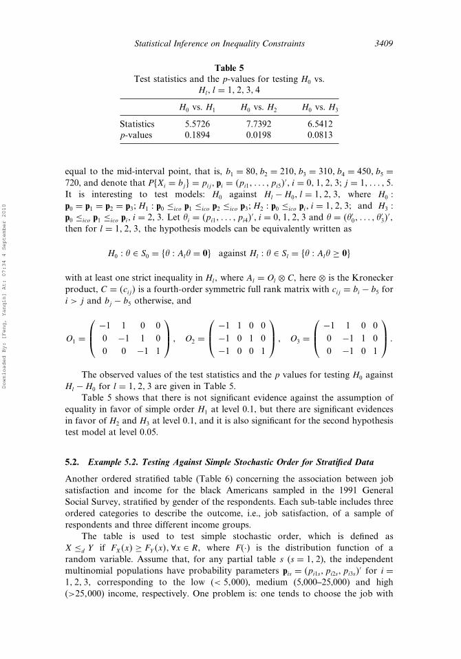
Statistical Inference on Inequality Constraints 3409

Table 5Test statistics and the p-values for testing H0 vs.

Hl� l = 1� 2� 3� 4

H0 vs. H1 H0 vs. H2 H0 vs. H3

Statistics 5.5726 7.7392 6.5412p-values 0.1894 0.0198 0.0813

equal to the mid-interval point, that is, b1 = 80� b2 = 210� b3 = 310� b4 = 450� b5 =720, and denote that P�Xi = bj� = pij� pi = �pi1� � � � � pi5�

′� i = 0� 1� 2� 3� j = 1� � � � � 5�It is interesting to test models: H0 against Hl −H0� l = 1� 2� 3� where H0 �

p0 = p1 = p2 = p3�H1 � p0 ≤ico p1 ≤ico p2 ≤ico p3�H2 � p0 ≤ico pi� i = 1� 2� 3� and H3 �

p0 ≤ico p1 ≤ico pi� i = 2� 3� Let �i = �pi1� � � � � pi4�′� i = 0� 1� 2� 3 and � = ��′0� � � � � �

′3�

′�then for l = 1� 2� 3� the hypothesis models can be equivalently written as

H0 � � ∈ S0 = �� � Al� = 0� against Hl � � ∈ Sl = �� � Al� ≥ 0�

with at least one strict inequality in Hl� where Al = Ol ⊗ C� here ⊗ is the Kroneckerproduct, C = �cij� is a fourth-order symmetric full rank matrix with cij = bi − b5 fori > j and bj − b5 otherwise, and

O1 =

−1 1 0 00 −1 1 00 0 −1 1

� O2 =

−1 1 0 0−1 0 1 0−1 0 0 1

� O3 =

−1 1 0 00 −1 1 00 −1 0 1

�

The observed values of the test statistics and the p values for testing H0 againstHl −H0 for l = 1� 2� 3 are given in Table 5.

Table 5 shows that there is not significant evidence against the assumption ofequality in favor of simple order H1 at level 0�1, but there are significant evidencesin favor of H2 and H3 at level 0�1, and it is also significant for the second hypothesistest model at level 0�05.

5.2. Example 5.2. Testing Against Simple Stochastic Order for Stratified Data

Another ordered stratified table (Table 6) concerning the association between jobsatisfaction and income for the black Americans sampled in the 1991 GeneralSocial Survey, stratified by gender of the respondents. Each sub-table includes threeordered categories to describe the outcome, i.e., job satisfaction, of a sample ofrespondents and three different income groups.

The table is used to test simple stochastic order, which is defined asX ≤d Y if FX�x� ≥ FY �x��∀x ∈ R� where F�·� is the distribution function of arandom variable. Assume that, for any partial table s (s = 1� 2), the independentmultinomial populations have probability parameters pis = �pi1s� pi2s� pi3s�

′ for i =1� 2� 3� corresponding to the low (< 5�000), medium (5,000–25,000) and high(>25�000) income, respectively. One problem is: one tends to choose the job with

Downloaded By: [Feng, Yanqin] At: 07:34 4 September 2010

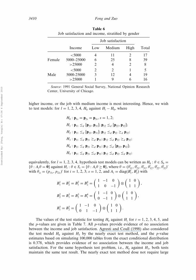
3410 Feng and Zuo

Table 6Job satisfaction and income, stratified by gender

Job satisfaction

Income Low Medium High Total

<5000 4 11 2 17Female 5000–25000 6 25 8 39

>25000 2 4 2 8

<5000 2 2 1 5Male 5000-25000 3 12 4 19

>25000 1 9 6 16

Source: 1991 General Social Survey, National Opinion ResearchCenter, University of Chicago.

higher income, or the job with medium income is most interesting. Hence, we wishto test models: for l = 1� 2� 3� 4, H0 against Hl −H0, where

H0 � p1s = p2s = p3s� s = 1� 2�

H1 � p11 ≤d �p21� p31�� p12 ≤d �p22� p32��

H2 � p11 ≤d �p21� p31�� p12 ≤d p22 ≥d p32�

H3 � p11 ≤d p21 ≥d p31� p12 ≤d p22 ≥d p32�

H4 � p11 ≤d p21 ≥d p31� p12 ≤d �p22� p32��

H5 � p11 ≤d p21 ≤d p31� p12 ≤d p22 ≤d p32�

equivalently, for l = 1� 2� 3� 4� hypothesis test models can be written as H0 � � ∈ S0 =�� � Al� = 0� against Hl � � ∈ Sl = �� � Al� ≥ 0�, where � = ��′11� �

′21� �

′31� �

′12� �

′22� �

′32�

′

with �is = �pi1s� pi2s�′ for i = 1� 2� 3� s = 1� 2� and Al = diag�Bl

1� Bl2� with

B11 = B1

2 = B21 = B4

2 =(

1 −1 01 0 −1

)⊗(

1 01 1

)�

B22 = B3

1 = B32 = B4

1 =(

1 −1 00 −1 1

)⊗(

1 01 1

)�

B51 = B5

2 =(

1 −1 00 1 −1

)⊗(

1 01 1

)�

The values of the test statistic for testing H0 against Ht for t = 1� 2� 3� 4� 5� andthe p-values are given in Table 7. All p-values provide evidence of no associationbetween the income and job satisfaction. Agresti and Coull (1998) also consideredthe test model H0 against H5 by the nearly exact test method, and the p-valueestimates based on simulating 100,000 tables from the exact conditional distributionis 0.378, which provides evidence of no association between the income and jobsatisfaction. For the same hypothesis test problem, i.e., H0 against H5, both testsmaintain the same test result. The nearly exact test method dose not require large

Downloaded By: [Feng, Yanqin] At: 07:34 4 September 2010

Statistical Inference on Inequality Constraints 3411

Table 7Test statistics for testing H0 vs. Ht t = 1� 2� 3� 4� 5 and the p values

H0 vs. H1 H0 vs. H2 H0 vs. H3 H0 vs. H4 H0 vs. H5

Statistics 5.3878 3.7660 3.3304 5.3168 4.9060p-values 0.1523 0.3225 0.4417 0.1703 0.3102

Table 8Grades in course taught by two modes of instruction

Grades

Mode of instruction A B C D F Total

Live 16 30 22 4 8 80Televised 11 19 28 8 14 80

sample theory, it is clear that our method can be used for medium sample sizes.However, our method is time saving.

5.3. Example 5.3. Comparison of p-Values of Different Statistics

Consider the following illustrative example discussed in Nair (1987). To comparethe effectiveness of two modes of instruction, live and televised, a group of studentswere randomly assigned to two groups of size. Each group was taught using one ofthe two methods of instruction, and their performances were assessed by the lettergrades for the course. The data in Table 8 give the letter grades from a coursetaught using two modes of instruction. Since there is an ordering in the grades,the inequality-restricted alternative is a reasonable way to specify that one mode ofinstruction is superior to the other, and two-sided alternative is considered as it isnot a priori obvious that televised instruction would be less effective.

The p-values, associated with the Teoh’s method, the �2-test and the test basedon the CCS-type statistic Tc given by Nair in 1987, are given in Table 9. It is clearfrom the data in Table 9, that all the methods consistently provide strong evidenceof rejection of the null hypothesis.

Table 9p-values of the different

statistics for the instructiondata in Table 5

Statistics p values

TC 0.0200�2 0.0189Teoh 0.0188

Downloaded By: [Feng, Yanqin] At: 07:34 4 September 2010

3412 Feng and Zuo

Table 10Pains scores on the third day after surgery forn1 = 14 under the treatment Y and n2 = 11

patients under the treatment N

Treatment Pain score

Y 1, 2, 1, 1, 1, 1, 1, 1, 1, 1, 2, 4, 1, 1N 3, 3, 4, 3, 1, 2, 3, 1, 1, 5, 4

5.4. Example 5.4. A Small Sample Case

In this example, we consider a data set with a small sample size (Table 10), which isadapted from Brunner and Munzel (2000), concerning the association between painscore and treatment. The pain score ranged from 1–5. Two treatments (Y and N )were randomly assigned to 25 eligible female patients where 14 patients received theactive treatment Y and 11 patients the control treatment N� and the observed painscores are listed in Table 10.

Non zero cell frequencies is necessary for our method, so we regroup the data inTable 10 in two cases. Case 1: we consider the collapsed data by collapsing the datawith Pain Score 3,4,5; Case 2: we consider the collapsed data set by collapsing thedata with Pain Score 2,3 and combining the data with Pain Score 4,5, respectively.

For the physician, it is mainly of interest to known whether the pain scoresafter the active treatment Y “trended to be lower” than after the control treatmentN� Let F1 denote the distribution of the pain scores under treatment and F2 denotethe distribution of the pain scores under treatment N� It is interest to consider thehypothesis test model:

H0 � F1 = F2 against H1 � F1 ≤d F2� (5.1)

Brunner and Munzel (2000) gave a nonparametric procedure to test problems oftwo samples. Here, we apply our method and the method developed by Brunner andMunzel (2000) to the regrouped data sets, and list the test statistics and p-values inTable 11. Both methods maintain the same results, that is, all the p-values obtainedby two tests are small enough to reject the null hypothesis and provide strong

Table 11Test statistics and p-values for model (5.1)

Data Case 1 Case 2

Statistic T01 9.9008 6.8738WBF

N 3.3518 2.7732

p-values �2-test 0.0016 0.0097WN -test 0.0022 0.0057

WBFN is defined by Brunner and Munzel (2000).

WN -test is the test based on the statistic WBFN .

Downloaded By: [Feng, Yanqin] At: 07:34 4 September 2010

Statistical Inference on Inequality Constraints 3413

evidence of a positive association, and this is consistent with the result (p-valuebased on Table 10 is 0.002) obtained by Brunner and Munzel (2000).

6. Discussion

In this article, likelihood ratio test for general order restrictions in contingency tableanalysis is discussed. The asymptotic properties of likelihood ratio test statistic isobtained. Simulation studies and real data analyses show that this test is feasibleand can be applied in the general cases. The method becomes flexible in that therestriction condition considered here is much looser than those usual stochasticorder restrictions. Although the estimations of unknown parameters � are obtainedby solving an restricted optimizing problem, the results show that problem ofcomputation time can be ignored. It is noteworthy that Teoh’s method is stronglyrecommended for small sample dose-response studies. For medium or large samplecases, test statistic resulted from asymptotic theory (3.7) can be a good alternativefor quick power and size calculations.

By the way, several interesting phenomena from our empirical results shouldbe noted. Firstly, size quickly recover the nominal size as sample size increases.Secondly, the �2 test could behave conservatively (i.e., its actual significance levelcould greatly be inferior to the pre-assigned nominal level).

In some dose-response analyses, one may wish to detect whether the dose-response relationship would present a certain nonlinearity. In these situations,nonlinear inequality constraints hypotheses/tests would be more appropriate.Although a linear inequality constraints hypothesis is assumed throughout thisarticle, theory for hypothesis with nonlinear inequality constraints can be similarlydeveloped.

Appendix

A.1. Some Results about Chi-Bar-Squared Statistic

Let Y ∼ N�0� �� be an m-dimensional normal random vector, C be a closed convexcone, then

�2 = Y ′�−1Y −min ∈C

�Y − �′�−1�Y − �

= min ∈C0

�Y − �′�−1�Y − ��

where the second equality comes from the Pythagoras’ theorem and properties ofclosed convex cones, and the set C0 is the dual cone of C which is defined by C0 =�y � �x� y� ≤ 0 for all x ∈ C�. The basic result concerning �2 is that it is a mixture ofchi-squared distributions, that is,

P��2 ≥ d� =m∑i=0

�iP��2i ≥ d��

where �2i is a chi-squared random variable with degree i of freedom, �20 ≡ 0and �i’s are non negative weights such that

∑mi=0 �i = 1� Since the distribution

of �2 is determined by the covariance matrix � and convex cone C, we write

Downloaded By: [Feng, Yanqin] At: 07:34 4 September 2010

3414 Feng and Zuo

�2 ∼ �2���C�� The result first appeared in Bartholomew (1959). His results wereextended independently to very general cases by Kudô (1963), Nüesch (1966), andPerlman (1969). Shapiro (1988) gave a presentation of the general case.

The weights �i = �i�m���C�, i = 0� 1� � � � � m� depend on � and C. Kudô (1963)proposed a formula for the weights �i�m���Rm

+�, in the case of C = Rm+ = �x � x >

0� for m ≤ 4, and the expression in a closed form of �i�m���Rm+� is available. For

m > 4, there is not a closed expression form for the weights, but reasonably accurateestimates of the weights can be obtained by Monte Carlo simulations.

A.2. Proofs

Proof of Lemma 3.1. By the central limit theorem, we obtain

gn��� = g���+ 1√n

m∑i=1

√ri

{k−1∑j=1

vij log pij + vik log�1−k−1∑t=1

pit�

}�1+ op�1��� (A.1)

where �vi1� � � � � vi�k−1�′ � vi for i = 1� � � � � m, are independent identically distributed

multivariate normal random variables with zeros mean and covariance matrix

Var�vij� = p�0�ij �1− p

�0�ij �� Cov�vij� vil� = −p

�0�ij p

�0�il � j �= l� (A.2)

here and throughout this proof, op�1� holds uniformly with respect to � in aneighborhood of �0. gn��� and g��� achieve their maxima on S at � and �0, so (A.1)implies that � is a consistent estimator of �0.

By the Taylor expansion, we have

gn���− gn��0� = gn��0�′��− �0�+

12��− �0�

′Hn��0���− �0�+ � �− �0 �2op�1��(A.3)

where gn��0� and Hn��0� can be obtained by substituting p�0�ij for pij in the

representations of gn��� and Hn���, respectively. By the weak convergence resultsmentioned above, we have

√ngn��0�

′��− �0�L−→ e′��− �0��

where e = �e11� � � � � e1�k−1� � � � � em1� � � � � em�k−1�′ with eij = √

ri�vij/p�0�ij − vim/p

�0�ik ��

For �pi1� � � � � pik� → �p�0�i1 � � � � � p

�0�ik � in probability, using the Slutsky’s theorem, then

Hn��0� → −Q in probability. Therefore, we have

12��− �0�

′Hn��0���− �0� = −12��− �0�

′Q��− �0�+ op�1�� �− �0 �2�

Substituting � for � in Eq. (A.3) and noting that � is a consistent estimator of �0and the optimal solutions of the likelihood function, then for any � > 0, there existsa constant M� > 0� and a sequence c�n → 0 (n → �), such that with probabilityp > 1− �, we have

0 < gn���− gn��0� ≤ −12��− �0�

′Q��− �0�+1√nM� � �− �0 � +c�n� �− �0 �

2�

Downloaded By: [Feng, Yanqin] At: 07:34 4 September 2010

Statistical Inference on Inequality Constraints 3415

Considering = √n��− �0�� we have

′Q /2−M� � � −c�n� �2 ≤ 0� By thepositivity definiteness of Q, it is obvious that there exists a constant C1

� > 0� suchthat � �≤ C1

�� Hence, the conclusion follows.

Proof of Lemma 3.2. Here, we omit the proof for the root-n consistency of ��and this is similar as that of Lemma 3.1. Next, we prove Eq. (3.1). By Taylor’sexpansion, we have

0 = √ngn���

= √ngn��0�+

√nHn��0���− �0�+ op�1�

√n��− �0�

= √ngn��0�+

√n�−Q+ op�1����− �0�+ op�1�

√n��− �0�

= √ngn��0�−Q

√n��− �0�+ op�1��

Equation (3.1) holds immediately.

Proof of Lemma 3.3. By using a similar method used in the proof of Lemma 3.1, itis easily shown that � converges to �0 in probability. Following, we prove Eq. (3.2).� is the optimal solution of the following problem:

min−gn��� subject to A� = 0�

By the Taylor’s theorem and the complementary condition in mathematicalprograming, � must satisfy{

Hn������− �0�+ A′� = −gn��0��

A��− �0� = 0�(A.4)

or equivalently,

(Hn���� A′

A 0

)(�− �0

�

)=(−gn��0�

0

)� (A.5)

where � is a Lagrangian multiplier, and �� = �0 + ���− �0� with 0 < � < 1 isbetween � and �0. We obtain that

(�− �0

�

)=(Hn���� A

′

A 0

)−1 (−gn��0�

0

)� (A.6)

and it holds that

√n��− �0� =

√n(Hn����

−1 −Hn����−1A′�AHn����

−1A′�−1AHn����−1)gn��0��

Since � converges to �0 in probability, �� = �0 + ���− �0�, and 0 < � < 1, usingthe Slutsky’s theorem, we have that Hn���� converges to −Q in probability. Hence,Eq. (3.2) is held immediately.

Proof of Theorem 3.1. To prove Theorem 3.1, we need the following lemma.

Downloaded By: [Feng, Yanqin] At: 07:34 4 September 2010

3416 Feng and Zuo

Lemma A.1. For sufficiently large n,

2[logLn���− logLn���

]= n��− ��′Q��− ��+ op�1�� (A.7)

Proof. Since n−1/2 logLn���L−→ N�0� Q�, and by Eqs. (A.1) and (A.2), we have

� �− � �= Op�n−1/2�� By the Taylor’s theorem

logLn��� = logLn���+n

2��− ��′

[1nHn���

]��− ��+ op�1��

Again by the Taylor’s theorem, we have

1nHn��� =

1nHn��0�+ op�1��

Noting that 1nHn��0� = −Q+ op�1�� and logLn��� = 0� hence

2�logLn���− log���� = −n��− ��′�−Q+ op�1����− ��+ op�1�

= n��− ��′Q��− ��+ op�1�� �

Now it is ready to prove Theorem 3.1. Start from the equality

Fn��� = 2�logL���− log����

= 2�log���− log����− 2�logL���− logL����

� F1 − F2�

We first prove that

F2 = −(√

n��− �0�− )′Q(√

n��− �0�− )+ op�1�� (A.8)

Since n−1/2 logL��0�L→ N�0� Q�� based on Eq. (3.1), using the weak convergence

result obtained in the proof of Lemma 3.1, we obtain√n��− �0�

L→ N�0� Q−1��Expanding logL��� at � by the Taylor’s theorem, we get

logL��� = logL���+ n

2��− ��′

(n−1Hn���

)��− ��+ op�1��

Note that

1nHn��� =

1nHn��0�+ op�1�� and

1nHn��0� = −Q+ op�1��

Thus,

F2 = 2(logL���− logL���

)= n��− ��′�−Q+ op�1����− ��+ op�1�

Downloaded By: [Feng, Yanqin] At: 07:34 4 September 2010

Statistical Inference on Inequality Constraints 3417

= −(√

n��− �0�−√n��− �0�

)′Q(√

n��− �0�−√n��− �0�

)+ op�1�

= −(√

n��− �0�− )′Q(√

n��− �0�− )+ op�1��

For the F1� combining Eqs. (3.1), (3.2), and (A.7), we obtain that

F1 = −n��− ��′Q��− ��+ op�1�

= −(√

n��− �0�−√n��− �0�

′)Q(√

n��− �0�−√n��− �0

)+ op�1�

= −(�BQ− I�

(n1/2��− �0�

))′Q(�BQ− I�

(n1/2��− �0�

))+ op�1��

where I is an m�k− 1�×m�k− 1� unit matrix. Note that√n��− �0�

L→ N�0� Q−1��By the Continuous Mapping Theorem, Eq. (3.4) holds immediately.

Proof of Theorem 3.2. To prove the result of Theorem 3.2, we need the followinglemma (refer to Feng and Wang, 2007).

Lemma A.2. The stochastic processes �Gn� � � ∈ S ∩D� converge in distribution to�G� � � ∈ S ∩D�� where D = � �� �≤ M� ∈ Rm�k−1���

Now it is ready to prove the asymptotic distribution of Theorem 3.2.Let ��S ∩D� denote the space of all continuous functions over S ∩D (of which

the elements are the sample functions of the stochastic processes �Gn� �� ∈ S ∩D�and �G� �� ∈ S ∩D�) with a metric defined by

d�h1� h2� = sup ∈S∩D

� h1� �− h2� � �� h1� h2 ∈ ��S ∩D��

Let �n and � denote the probability measures induced, respectively, by�Gn� �� ∈ S ∩D� and �G� �� ∈ S ∩D�. By Lemma A.2, we have �n ⇒ ��

Define a mapping H�·� on ��S ∩D� as follows:

H�Gn� = min ∈S∩D

Gn� �� H�G� = min ∈S∩D

G� ��

By convexity of the function G� � and the set S ∩D, we have that H�G� isunique. Hence, the Continuous Mapping Theorem (Billingsley, 1968) will lead to

H�Gn�L→H�G�.

Since is the optimal solution of (3.6) and = 0 ∈ S, we have

G� �−G�0� = �Z− �′Q�Z− �− Z′QZ = ′Q − 2 ′QZ ≤ 0�

By the positivity definiteness of Q and Z ∼ N�0� Q−1�� for all � > 0 there existsa constant C� such that � �≤ C� with probability larger than 1− �. Note thatGn� n� = H�Gn� and G� � = H�G�� for � n �≤ C� and � �≤ C�� Therefore, wehave

P�Gn� n� �= H�Gn�� < � and P�G� � �= H�G�� < ��

Downloaded By: [Feng, Yanqin] At: 07:34 4 September 2010

3418 Feng and Zuo

Since � is arbitrary and H�Gn�L→ H�G�� we obtain

Gn� n�L→ G� �� i.e., T01

L→T�

We rewrite the limit expression (3.4) as

T = −min ∈S

�Z− �′Q�Z− �+ Z′�I − BQ�′Q�I − BQ�Z

={Z′QZ−min

∈S�Z− �′Q�Z− �

}− �Z′QZ− Z′�I − BQ�′Q�I − BQ�Z�

� T1 − T2� (A.9)

where

T1 ={Z′QZ−min

∈S�Z− �′Q�Z− �

}� T2 = �Z′QZ− Z′�I − BQ�′Q�I − BQ�Z� �

It is easily seen that T1 ∼ �2�Q−1� S�� The polar cone of S is given by S0 = � � =−Q−1A′�� � ∈ Rr

+� (refer to Shapiro, 1988, p. 54). By the definition of the polar cone,it is easily to obtain that

T1 = min ∈S0

�Z− �′Q�Z− �

= min�∈Rr+

�Z+Q−1A′��′Q�Z+Q−1A′��

= min�∈Rr+

�X − ��′W�X − ��+ T3�

where W = AQ−1A′� X = �AQ−1A′�−1AZ, X ∼ N�0�W−1�� and

T3 = Z′�I −Q−1A′�AQ−1A′�−1A�′Q�I −Q−1A′�AQ−1A′�−1A�Z

= Z′�Q− A′�AQ−1A′�−1A�Z�

where I is an m�k− 1�×m�k− 1� unit matrix.Since min�∈Rr+�X − ��′W�X − �� ∼ �2�W−1� �Rr

+�0�� it is sufficient to prove T2 =

T3� Substituting B = Q−1 −Q−1A′�AQ−1A′�−1AQ−1 into T2 to obtain

T2 = �Z′QZ− Z′�I − BQ�′Q�I − BQ�Z�

= Z′QZ− Z�Q−1A′�AQ−1A′�−1A�′Q�Q−1A′�AQ−1A′�−1A�Z

= Z′QZ− Z′A′�AQ−1A′�−1AZ

= T3�

Thus, (3.7) holds immediately.

Acknowledgments

The authors wish to thank the Editor and the referee for their criticism suggestionsthat clearly improved this article.

Downloaded By: [Feng, Yanqin] At: 07:34 4 September 2010

Statistical Inference on Inequality Constraints 3419

The research is supported in part by NSFC Grant 10771163 and by NSFC#10741002.

References

Agresti, A., Coull, B. A. (1998). Order restricted inference for monotone trend alternativesin contingency tables. Comput. Statist. Data Anal. 28:139–155.

Bartholomew, H. (1959). A test of homogeneity for ordered alternative. Biometrika 46:36–48.Bazaraa, M. S., Shetty, C. M. (1979). Nonlinear Programming: Theory and Algorithms.

New York: Wiley.Billingsley, P. (1968). Convergence of Probability Measures. New York: Wiley.Brunner, E., Munzel, U. (2000). The nonparametric Behrens–Fisher problem: asymptotic

theory and a small-sample approximation. Biom J. 42:17–25.Cohen, A., Sackrowitz, H. B. (2002). Inference for the model of several treatments and a

control. J. Statist. Plann. Infer.. 107:89–101.Chaudhuri, S., Perlman, M. D. (2005). Biases of the maximum likelihood and Cohen–

Sackrowitz estimators for the tree-order model. Statist. Probab. Lett. 71:267–276.Dardanoni, V., Forcina, A. (1998). A unified approach to likelihood inference on stochastic

in a nonparametric context. J. Amer. Statist. Assoc. 93:1112–1123.Feng, Y., Wang, J. (2007). Likelihood ratio test against simple stochastic ordering among

several multinomial populations. J. Statist. Plann. Infer. 137:1362–1374.Feng, Y., Wang, J. (2008). Likelihood ratio test against stochastic order in three way

contingency tables. Commun. Statist. Theor. Meth. 37:81–96.Feng, Y. (2008a). Nonparametric statistical inference for umbrella trend alternative among

multinomial populations. Vietnam J. Math. 36:291–304.Feng, Y. (2008b). A test of conditional independence against a tree order alternative for

strtified data. Utilitas Mathematica. To appear.Giancristofaro, R. A., Bonnini, S. (2008). Moment-based multivariate permutation tests for

ordinal categorical data. J. Nonparametric Statist. 20:383–393.Kalbfleisch, J. D., Prentice, R. L. (1980). The Statistical Analysis of Failure Time Data.

New York: John Wiley & Sons.Kudô, A. (1963). A multivariate analogue of the one-sided test. Biometrika 50:403–418.Liu, X., Wang, J. (2003). Testing for increasing convex order in several populations. Ann.

Instit. Statist. Math. 1:121–136.Lehmann, E. (1955). Ordered families of distributions. Ann. Math. Stat. 26:399–419.Marcus, R., Genizi, A. (1994). Simultaneous confidence intervals for umbrella contrasts of

normal means. Comput. Statist. Data. Anal. 17:393–407.Nair, V. N. (1987). Chi-squared-type tests for ordered alternatives in contingency tables.

J. Amer. Statist. Assoc. 82:283–291.Nüesch, P. (1966). On the problem of testing location in multivariate populations for

restricted alternatives. Ann. Math. Statist. 37:113–119.Peddada, S. D., Haseman, J. K., Tan, X., Travlos, G. (2006). Tests for a simple tree

order restriction with application to dose-response studies. J. Roy. Statist. Soc. Ser. C55:493–506.

Perlman, M. D. (1969). One-sided testing problems in multivariate analysis. Ann. Math.Statist. 40:549–567.

Pesarin, P. (2001). Multivariate Permatation Test with Application to Biostatistic. Chichester:Wiley.

Prakasa Rao, B. L. S. (1987). Asymptotic Theory of Statistical Inference. New York: Wiley.Shaked, M., Shanthikumar, J. G. (1994). Stochastic Orders and Their Applications. Boston:

Academic Press, Inc.Shapiro, A. (1988). Towards a unified theory of inequality constrained testing in multivariate

analysis. Int. Statist. Rev. 56:49–62.

Downloaded By: [Feng, Yanqin] At: 07:34 4 September 2010

3420 Feng and Zuo

Silvapulle, M. J., Sen, P. K. (2005). Constrained Statist Inference: Order, Inequality, and ShapeConstraints. New York: Wiley.

Simpson, D. G., Margolin, B. H. (1986). Recursive nonparametric testing for dose-responserelationships subject to down-turns at high dose. Biometrika 73:589–596.

Singh, P., Liu, W. (2006). A test against an umbrella ordered alternative. Comput. Stat. DataAnal. 51:1957–1964.

Teoh, E., Nyska, A., Wormser, U., Peddada, S. D. (2008). Statistical inference under orderrestrictions on both rows and columns of a matrix, with an application in toxicology.Beyond parametrics in interdisciplinary research: Festschrift in honor of Professor PranabK. Sen, Inst. Math. Stat. Collect., Inst. Math. Statist., Beachwood, OH. 1:62–77.

Wang, J. (1996). Asymptotics of least squares estimators for constrained nonlinearregression. Ann. Statist. 24:1316–1326.

Wang, Y. (1996). A Likelihood ratio test against stochastic ordering in several populations.J. Amer. Statist. Assoc. 91:1676–1683.

Wilcoxon, F. (1945). Individual comparisons by ranking method. Biometrics 1:80–83.

Downloaded By: [Feng, Yanqin] At: 07:34 4 September 2010