
TOOLS: MAXIMUM LIKELIHOOD
440
T OOLS :M AXIMUM L IKELIHOOD
Transcript of TOOLS: MAXIMUM LIKELIHOOD
TOOLS: MAXIMUM LIKELIHOOD
GAUSSIAN DISTRIBUTION
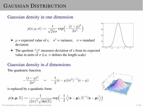
Gaussian density in one dimension
p(x; µ,�) :=1p2⇡�
exp⇣
� (x� µ)2
2�2
⌘
I µ = expected value of x, �2 = variance, � = standarddeviation
I The quotient x�µ� measures deviation of x from its expected
value in units of � (i.e. � defines the length scale)
Gaussian density in d dimensionsThe quadratric function
� (x� µ)2
2�2 = �12(x� µ)(�2)�1(x� µ)
is replaced by a quadratic form:
p(x;µµµ, ⌃) :=1
(2⇡)d2p
det(⌃)exp⇣
�12
D
(x�µµµ), ⌃�1(x�µµµ)E⌘
The Gaussian Distribution
Chris Williams, School of Informatics, University of EdinburghOverview
• Probability density functions
• Univariate Gaussian
• Multivariate Gaussian
• Mahalanobis distance
• Properties of Gaussian distributions
• Graphical Gaussian models
• Read: Tipping chs 3 and 4
Continuous distributions• Probability density function (pdf) for a continuous random variable X
P (a � X � b) =� b
ap(x)dx
thereforeP (x � X � x + �x) � p(x)�x
• Example: Gaussian distribution
p(x) =1
(2��2)1/2exp�
�(x � µ)2
2�2
�
shorthand notation X � N(µ, �2)
• Standard normal (or Gaussian) distribution Z � N(0,1)
• Normalization � ∞
−∞p(x)dx = 1
−4 −2 0 2 40
0.1
0.2
0.3
0.4
• Cumulative distribution function
�(z) = P (Z � z) =� z
−∞p(z′)dz′
• Expectation
E[g(X)] =�
g(x)p(x)dx
• mean, E[X]
• Variance E[(X � µ)2]
• For a Gaussian, mean = µ, variance = �2
• Shorthand: x � N(µ, �2)
J.P. Cunningham and P. Orbanz · Statistical Machine Learning 2 / 436
PARAMETRIC MODELS
ModelsA model P is a set of probability distributions. We index each distribution by aparameter value ✓ 2 T ; we can then write the model as
P = {P✓|✓ 2 T } .
The set T is called the parameter space of the model.
Parametric modelThe model is called parametric if the number of parameters (i.e. the dimension ofthe vector ✓) is (1) finite and (2) independent of the number of data points.Intuitively, the complexity of a parametric model does not increase with sample size.
Density representationFor parametric models, we can assume that T ⇢ Rd for some fixed dimension d. Weusually represent each P✓ be a density function p(x|✓).
J.P. Cunningham and P. Orbanz · Statistical Machine Learning 3 / 436
MAXIMUM LIKELIHOOD ESTIMATION
SettingI Given: Data x1, . . . , xn, parametric model P = {p(x|✓) | ✓ 2 T }.I Objective: Find the distribution in P which best explains the data. That means
we have to choose a "best" parameter value ✓.
Maximum Likelihood approachMaximum Likelihood assumes that the data is best explained by the distribution in Punder which it has the highest probability (or highest density value).
Hence, the maximum likelihood estimator is defined as
✓ML := arg max✓2T
p(x1, . . . , xn|✓)
the parameter which maximizes the joint density of the data.
J.P. Cunningham and P. Orbanz · Statistical Machine Learning 4 / 436
ANALYTIC MAXIMUM LIKELIHOOD
The i.i.d. assumptionThe standard assumption of ML methods is that the data is independent andidentically distributed (i.i.d.), that is, generated by independently samplingrepeatedly from the same distrubtion P.
If the density of P is p(x|✓), that means the joint density decomposes as
p(x1, . . . , xn) =nY
i=1
p(xi|✓)
Maximum Likelihood equationThe analytic criterion for a maximum likelihood estimator (under the i.i.d.assumption) is:
r✓
⇣
nY
i=1
p(xi|✓)⌘
= 0
We use the "logarithm trick" to avoid a huge product rule computation, and fornumerical stability.
J.P. Cunningham and P. Orbanz · Statistical Machine Learning 5 / 436
LOGARITHM TRICK
Recall: Logarithms turn products into sums
log⇣
Y
i
fi
⌘
=X
i
log(fi)
Logarithms and maximaThe logarithm is monotonically increasing on R+.
Consequence: Application of log does not change the location of a maximum orminimum:
maxy
log(g(y)) 6= maxy
g(y) The value changes.
arg maxy
log(g(y)) = arg maxy
g(y) The location does not change.
J.P. Cunningham and P. Orbanz · Statistical Machine Learning 6 / 436
ANALYTIC MLE
Likelihood and logarithm trick
✓ML = arg max✓
nY
i=1
p(xi|✓) = arg max✓
log⇣
nY
i=1
p(xi|✓)⌘
= arg max✓
nX
i=1
log p(xi|✓)
Analytic maximality criterion
0 =nX
i=1
r✓ log p(xi|✓) =nX
i=1
r✓p(xi|✓)p(xi|✓)
Whether or not we can solve this analytically depends on the choice of the model!
J.P. Cunningham and P. Orbanz · Statistical Machine Learning 7 / 436
EXAMPLE: GAUSSIAN MEAN MLE
Model: Multivariate GaussiansThe model P is the set of all Gaussian densities on Rd with fixed covariance matrix⌃,
P = {g( . |µ, ⌃) | µ 2 Rd} ,
where g is the Gaussian density function. The parameter space is T = Rd.
MLE equationWe have to solve the maximum equation
nX
i=1
rµ log g(xi|µ, ⌃) = 0
for µ.
J.P. Cunningham and P. Orbanz · Statistical Machine Learning 8 / 436
EXAMPLE: GAUSSIAN MEAN MLE
0 =nX
i=1
rµ log1
p
(2⇡)d|⌃| exp⇣
�12
D
(xi � µ), ⌃�1(xi � µ)E⌘
=nX
i=1
rµ
⇣
log⇣ 1p
(2⇡)d|⌃|⌘
+ log⇣
exp⇣
�12
D
(xi � µ), ⌃�1(xi � µ)E⌘
=nX
i=1
rµ
⇣
�12
D
(xi � µ), ⌃�1(xi � µ)E⌘
= �nX
i=1
⌃�1(xi � µ)
Multiplication by (�⌃) gives
0 =nX
i=1
(xi � µ) ) µ =1n
nX
i=1
xi
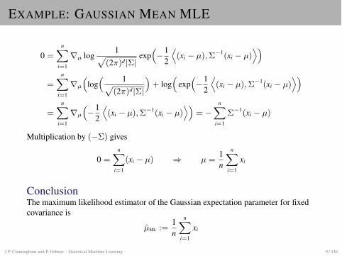
ConclusionThe maximum likelihood estimator of the Gaussian expectation parameter for fixedcovariance is
µML :=1n
nX
i=1
xi
J.P. Cunningham and P. Orbanz · Statistical Machine Learning 9 / 436
EXAMPLE: GAUSSIAN WITH UNKNOWN COVARIANCE
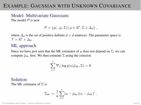
Model: Multivariate GaussiansThe model P is now
P = {g( . |µ, ⌃) | µ 2 Rd, ⌃ 2 �d} ,
where �d is the set of positive definite d ⇥ d-matrices. The parameter space isT = Rd ⇥�d.
ML approachSince we have just seen that the ML estimator of µ does not depend on ⌃, we cancompute µML first. We then estimate ⌃ using the criterion
nX
i=1
r⌃ log g(xi|µML, ⌃) = 0
SolutionThe ML estimator of ⌃ is
⌃ML :=1n
nX
i=1
(xi � µML)(xi � µML)t .
J.P. Cunningham and P. Orbanz · Statistical Machine Learning 10 / 436
CLASSIFICATION
ASSUMPTIONS AND TERMINOLOGY
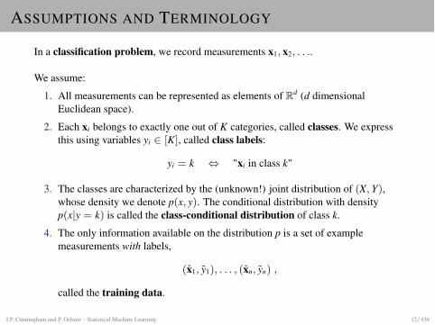
In a classification problem, we record measurements x1, x2, . . ..
We assume:
1. All measurements can be represented as elements of Rd (d dimensionalEuclidean space).
2. Each xi belongs to exactly one out of K categories, called classes. We expressthis using variables yi 2 [K], called class labels:
yi = k , "xi in class k"
3. The classes are characterized by the (unknown!) joint distribution of (X, Y),whose density we denote p(x, y). The conditional distribution with densityp(x|y = k) is called the class-conditional distribution of class k.
4. The only information available on the distribution p is a set of examplemeasurements with labels,
(x1, y1), . . . , (xn, yn) ,
called the training data.
J.P. Cunningham and P. Orbanz · Statistical Machine Learning 12 / 436
CLASSIFIERS
DefinitionA classifier is a function
f : Rd [K] ,
i.e. a function whose argument is a measurement and whose output is a class label.
Learning taskUsing the training data, we have to estimate a good classifier. This estimationprocedure is also called training.
A good classifier should generalize well to new data. Ideally, we would like it toperform with high accuracy on data sampled from p, but all we know about p is thetraining data.
Simplifying assumptionWe first develop methods for the two-class case (K=2), which is also called binaryclassification. In this case, we use the notation
y 2 {�1, +1} instead of y 2 {1, 2}
J.P. Cunningham and P. Orbanz · Statistical Machine Learning 13 / 436
SUPERVISED AND UNSUPERVISED LEARNING
Supervised vs. unsupervisedFitting a model using labeled data is called supervised learning. Fitting a modelwhen only x1, . . . , xn are available, but no labels, is called unsupervised learning.
Types of supervised learning methodsI Classification: Labels are discrete, and we estimate a classifier f : Rd [K],I Regression: Labels are real-valued (y 2 R), and we estimate a continuous
function f : Rd R. This functions is called a regressor.
J.P. Cunningham and P. Orbanz · Statistical Machine Learning 14 / 436
A VERY SIMPLE CLASSIFIER
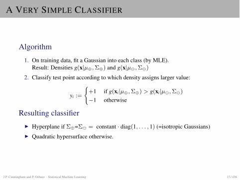
Algorithm
1. On training data, fit a Gaussian into each class (by MLE).Result: Densities g(x|µ�, ⌃�) and g(x|µ , ⌃ )
2. Classify test point according to which density assigns larger value:
yi :=
(
+1 if g(xi|µ�, ⌃�) > g(xi|µ , ⌃ )
�1 otherwise
Resulting classifierI Hyperplane if ⌃�=⌃ = constant · diag(1, . . . , 1) (=isotropic Gaussians)I Quadratic hypersurface otherwise.
J.P. Cunningham and P. Orbanz · Statistical Machine Learning 15 / 436
A VERY SIMPLE CLASSIFIER
2.6. DISCRIMINANT FUNCTIONS FOR THE NORMAL DENSITY 21
-2 2 4
0.1
0.2
0.3
0.4
P(ω1)=.5 P(ω2)=.5
p(x|ωi)
x
ω1 ω2
R1 R2
-20
2
4
-20
24
0
0.05
0.1
0.15
-20
2
4
-20
24
R1R2
P(ω2)=.5P(ω1)=.5
-2-1
0
1
2
0
1
2
-2
-1
0
1
2
-2-1
0
1
2
0
1
2
P(ω1)=.5
P(ω2)=.5
R2
R1
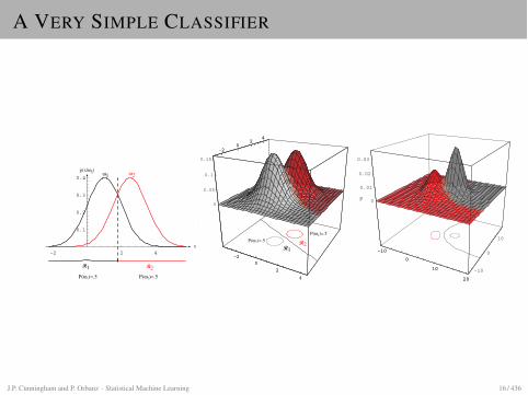
Figure 2.10: If the covariances of two distributions are equal and proportional to theidentity matrix, then the distributions are spherical in d dimensions, and the boundaryis a generalized hyperplane of d � 1 dimensions, perpendicular to the line separatingthe means. In these 1-, 2-, and 3-dimensional examples, we indicate p(x|�i) and theboundaries for the case P (�1) = P (�2). In the 3-dimensional case, the grid planeseparates R1 from R2.
wi =1
�2µi (52)
and
wi0 =�1
2�2µt
iµi + ln P (�i). (53)
We call wi0 the threshold or bias in the ith direction. threshold
biasA classifier that uses linear discriminant functions is called a linear machine. This
linearmachine
kind of classifier has many interesting theoretical properties, some of which will bediscussed in detail in Chap. ??. At this point we merely note that the decisionsurfaces for a linear machine are pieces of hyperplanes defined by the linear equationsgi(x) = gj(x) for the two categories with the highest posterior probabilities. For ourparticular case, this equation can be written as
wt(x � x0) = 0, (54)
where
w = µi � µj (55)
and
x0 =1
2(µi + µj) � �2
kµi � µjk2ln
P (�i)
P (�j)(µi � µj). (56)
This equation defines a hyperplane through the point x0 and orthogonal to thevector w. Since w = µi � µj , the hyperplane separating Ri and Rj is orthogonal tothe line linking the means. If P (�i) = P (�j), the second term on the right of Eq. 56vanishes, and thus the point x0 is halfway between the means, and the hyperplane isthe perpendicular bisector of the line between the means (Fig. 2.11). If P (�i) �= P (�j),the point x0 shifts away from the more likely mean. Note, however, that if the variance
2.6. DISCRIMINANT FUNCTIONS FOR THE NORMAL DENSITY 21
-2 2 4
0.1
0.2
0.3
0.4
P(ω1)=.5 P(ω2)=.5
p(x|ωi)
x
ω1 ω2
R1 R2
-20
2
4
-20
24
0
0.05
0.1
0.15
-20
2
4
-20
24
R1R2
P(ω2)=.5P(ω1)=.5
-2-1
0
1
2
0
1
2
-2
-1
0
1
2
-2-1
0
1
2
0
1
2
P(ω1)=.5
P(ω2)=.5
R2
R1
Figure 2.10: If the covariances of two distributions are equal and proportional to theidentity matrix, then the distributions are spherical in d dimensions, and the boundaryis a generalized hyperplane of d � 1 dimensions, perpendicular to the line separatingthe means. In these 1-, 2-, and 3-dimensional examples, we indicate p(x|�i) and theboundaries for the case P (�1) = P (�2). In the 3-dimensional case, the grid planeseparates R1 from R2.
wi =1
�2µi (52)
and
wi0 =�1
2�2µt
iµi + ln P (�i). (53)
We call wi0 the threshold or bias in the ith direction. threshold
biasA classifier that uses linear discriminant functions is called a linear machine. This
linearmachine
kind of classifier has many interesting theoretical properties, some of which will bediscussed in detail in Chap. ??. At this point we merely note that the decisionsurfaces for a linear machine are pieces of hyperplanes defined by the linear equationsgi(x) = gj(x) for the two categories with the highest posterior probabilities. For ourparticular case, this equation can be written as
wt(x � x0) = 0, (54)
where
w = µi � µj (55)
and
x0 =1
2(µi + µj) � �2
kµi � µjk2ln
P (�i)
P (�j)(µi � µj). (56)
This equation defines a hyperplane through the point x0 and orthogonal to thevector w. Since w = µi � µj , the hyperplane separating Ri and Rj is orthogonal tothe line linking the means. If P (�i) = P (�j), the second term on the right of Eq. 56vanishes, and thus the point x0 is halfway between the means, and the hyperplane isthe perpendicular bisector of the line between the means (Fig. 2.11). If P (�i) �= P (�j),the point x0 shifts away from the more likely mean. Note, however, that if the variance
26 CHAPTER 2. BAYESIAN DECISION THEORY
-100
10
20
-10
0
10
20
0
.01
.02
.03
.04
p
-100
10
20 -20
-100
1020
-10
0
10
20
0
0.005
0.01
p
-20
-100
1020
-10
0
10
20
-10
0
10
0
0.01
0.02
0.03
p
-10
0
10
20
-10
0
10
20
-10
0
10
0
0.01
0.02
0.03
0.04
0.05
p
-10
0
10
20
-100
1020
-10
0
10
20
0
0.005
0.01
P
-100
1020
0
0.005
0.01
p
-5
0
5 -5
0
5
0
0.05
0.1
0.15
p
-5
0
5
Figure 2.14: Arbitrary Gaussian distributions lead to Bayes decision boundaries thatare general hyperquadrics. Conversely, given any hyperquadratic, one can find twoGaussian distributions whose Bayes decision boundary is that hyperquadric.
J.P. Cunningham and P. Orbanz · Statistical Machine Learning 16 / 436
DISCUSSION
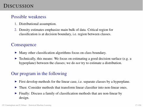
Possible weakness1. Distributional assumption.
2. Density estimates emphasize main bulk of data. Critical region forclassification is at decision boundary, i.e. region between classes.
ConsequenceI Many other classification algorithms focus on class boundary.I Technically, this means: We focus on estimating a good decision surface (e.g. a
hyperplane) between the classes; we do not try to estimate a distribution.
Our program in the followingI First develop methods for the linear case, i.e. separate classes by a hyperplane.I Then: Consider methods that transform linear classifier into non-linear ones.I Finally: Discuss a family of classification methods that are non-linear by
design.
J.P. Cunningham and P. Orbanz · Statistical Machine Learning 17 / 436
MEASURING PERFORMANCE: LOSS FUNCTIONS
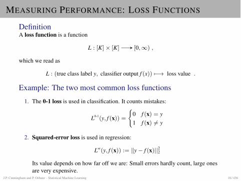
DefinitionA loss function is a function
L : [K]⇥ [K] [0,1) ,
which we read as
L : (true class label y, classifier output f (x)) 7�! loss value .
Example: The two most common loss functions
1. The 0-1 loss is used in classification. It counts mistakes:
L0-1(y, f (x)) =
(
0 f (x) = y1 f (x) 6= y
2. Squared-error loss is used in regression:
Lse(y, f (x)) := ky� f (x)||22Its value depends on how far off we are: Small errors hardly count, large onesare very expensive.
J.P. Cunningham and P. Orbanz · Statistical Machine Learning 18 / 436
RISK
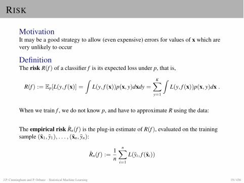
MotivationIt may be a good strategy to allow (even expensive) errors for values of x which arevery unlikely to occur
DefinitionThe risk R(f ) of a classifier f is its expected loss under p, that is,
R(f ) := Ep[L(y, f (x)] =
Z
L(y, f (x))p(x, y)dxdy =KX
y=1
Z
L(y, f (x))p(x, y)dx .
When we train f , we do not know p, and have to approximate R using the data:
The empirical risk Rn(f ) is the plug-in estimate of R(f ), evaluated on the trainingsample (x1, y1), . . . , (xn, yn):
Rn(f ) :=1n
nX
i=1
L(yi, f (xi))
J.P. Cunningham and P. Orbanz · Statistical Machine Learning 19 / 436

NAIVE BAYES CLASSIFIERS
BAYES EQUATION
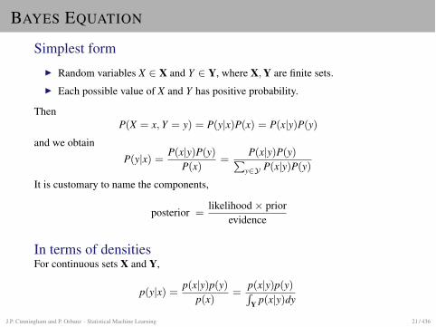
Simplest formI Random variables X 2 X and Y 2 Y, where X, Y are finite sets.I Each possible value of X and Y has positive probability.
ThenP(X = x, Y = y) = P(y|x)P(x) = P(x|y)P(y)
and we obtainP(y|x) =
P(x|y)P(y)P(x)
=P(x|y)P(y)
P
y2Y P(x|y)P(y)
It is customary to name the components,
posterior =likelihood⇥ prior
evidence
In terms of densitiesFor continuous sets X and Y,
p(y|x) =p(x|y)p(y)
p(x)=
p(x|y)p(y)R
Y p(x|y)dy
J.P. Cunningham and P. Orbanz · Statistical Machine Learning 21 / 436
BAYESIAN CLASSIFICATION
ClassificationWe define a classifier as
f (x) := arg maxy2[K]
P(y|x)
where Y = [K] and X = sample space of data variable.With the Bayes equation, we obtain
f (x) = arg maxy
P(x|y)P(y)P(x)
= arg maxy
P(x|y)P(y)
If the class-conditional distribution is continuous, we use
f (x) = arg maxy
p(x|y)P(y)
J.P. Cunningham and P. Orbanz · Statistical Machine Learning 22 / 436
BAYES-OPTIMAL CLASSIFIER
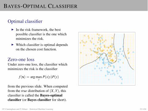
Optimal classifierI In the risk framework, the best
possible classifier is the one whichminimizes the risk.
I Which classifier is optimal dependson the chosen cost function.
Zero-one lossUnder zero-one loss, the classifier whichminimizes the risk is the classifier
f (x) = arg maxy
P(x|y)P(y)
from the previous slide. When computedfrom the true distribution of (X, Y), thisclassifier is called the Bayes-optimalclassifier (or Bayes classifier for short).
Elements of Statistical Learning (2nd Ed.) c�Hastie, Tibshirani & Friedman 2009 Chap 2
Bayes Optimal Classifier
... .. . . .. . . . .. . . . . .. . . . . . .. . . . . . . . .. . . . . . . . . .. . . . . . . . . . .. . . . . . . . . . . . . .. . . . . . . . . . . . . . .. . . . . . . . . . . . . . . . .. . . . . . . . . . . . . . . . . . . . . .. . . . . . . . . . . . . . . . . . . . . . . . . . .. . . . . . . . . . . . . . . . . . . . . . . . . . . . . .. . . . . . . . . . . . . . . . . . . . . . . . . . . . . . . . . .. . . . . . . . . . . . . . . . . . . . . . . . . . . . . . . . . . . . .. . . . . . . . . . . . . . . . . . . . . . . . . . . . . . . . . . . . . .. . . . . . . . . . . . . . . . . . . . . . . . . . . . . . . . . . . . . . . .. . . . . . . . . . . . . . . . . . . . . . . . . . . . . . . . . . . . . . . . . .. . . . . . . . . . . . . . . . . . . . . . . . . . . . . . . . . . . . . . . . . . .. . . . . . . . . . . . . . . . . . . . . . . . . . . . . . . . . . . . . . . . . . . .. . . . . . . . . . . . . . . . . . . . . . . . . . . . . . . . . . . . . . . . . . . . . .. . . . . . . . . . . . . . . . . . . . . . . . . . . . . . . . . . . . . . . . . . . . . . . .. . . . . . . . . . . . . . . . . . . . . . . . . . . . . . . . . . . . . . . . . . . . . . .. . . . . . . . . . . . . . . . . . . . . . . . . . . . . . . . . . . . . . . . . . . . . . . .. . . . . . . . . . . . . . . . . . . . . . . . . . . . . . . . . . . . . . . . . . . . . . . . .. . . . . . . . . . . . . . . . . . . . . . . . . . . . . . . . . . . . . . . . . . . . . . . . . . .. . . . . . . . . . . . . . . . . . . . . . . . . . . . . . . . . . . . . . . . . . . . . . . . . . . .. . . . . . . . . . . . . . . . . . . . . . . . . . . . . . . . . . . . . . . . . . . . . . . . . . . .. . . . . . . . . . . . . . . . . . . . . . . . . . . . . . . . . . . . . . . . . . . . . . . . . . . . . . .. . . . . . . . . . . . . . . . . . . . . . . . . . . . . . . . . . . . . . . . . . . . . . . . . . . . . .. . . . . . . . . . . . . . . . . . . . . . . . . . . . . . . . . . . . . . . . . . . . . . . . . . . . . . . . . .. . . . . . . . . . . . . . . . . . . . . . . . . . . . . . . . . . . . . . . . . . . . . . . . . . . . . . . . . .. . . . . . . . . . . . . . . . . . . . . . . . . . . . . . . . . . . . . . . . . . . . . . . . . . . . . . . . . .. . . . . . . . . . . . . . . . . . . . . . . . . . . . . . . . . . . . . . . . . . . . . . . . . . . . . . . . . .. . . . . . . . . . . . . . . . . . . . . . . . . . . . . . . . . . . . . . . . . . . . . . . . . . . . . . . . . .. . . . . . . . . . . . . . . . . . . . . . . . . . . . . . . . . . . . . . . . . . . . . . . . . . . . . . . . . .. . . . . . . . . . . . . . . . . . . . . . . . . . . . . . . . . . . . . . . . . . . . . . . . . . . . . . . . . .. . . . . . . . . . . . . . . . . . . . . . . . . . . . . . . . . . . . . . . . . . . . . . . . . . . . . . . . .. . . . . . . . . . . . . . . . . . . . . . . . . . . . . . . . . . . . . . . . . . . . . . . . . . . . . . . . .. . . . . . . . . . . . . . . . . . . . . . . . . . . . . . . . . . . . . . . . . . . . . . . . . . . . . . . . .. . . . . . . . . . . . . . . . . . . . . . . . . . . . . . . . . . . . . . . . . . . . . . . . . . . . . . . . .. . . . . . . . . . . . . . . . . . . . . . . . . . . . . . . . . . . . . . . . . . . . . . . . . . . . . . . . .. . . . . . . . . . . . . . . . . . . . . . . . . . . . . . . . . . . . . . . . . . . . . . . . . . . . . . . . .. . . . . . . . . . . . . . . . . . . . . . . . . . . . . . . . . . . . . . . . . . . . . . . . . . . . . . . . .. . . . . . . . . . . . . . . . . . . . . . . . . . . . . . . . . . . . . . . . . . . . . . . . . . . . . . . . .. . . . . . . . . . . . . . . . . . . . . . . . . . . . . . . . . . . . . . . . . . . . . . . . . . . . . . . .. . . . . . . . . . . . . . . . . . . . . . . . . . . . . . . . . . . . . . . . . . . . . . . . . . . . . . . .. . . . . . . . . . . . . . . . . . . . . . . . . . . . . . . . . . . . . . . . . . . . . . . . . . . . . . . .. . . . . . . . . . . . . . . . . . . . . . . . . . . . . . . . . . . . . . . . . . . . . . . . . . . . . . . .. . . . . . . . . . . . . . . . . . . . . . . . . . . . . . . . . . . . . . . . . . . . . . . . . . . . . . . .. . . . . . . . . . . . . . . . . . . . . . . . . . . . . . . . . . . . . . . . . . . . . . . . . . . . . . . .. . . . . . . . . . . . . . . . . . . . . . . . . . . . . . . . . . . . . . . . . . . . . . . . . . . . . . . .. . . . . . . . . . . . . . . . . . . . . . . . . . . . . . . . . . . . . . . . . . . . . . . . . . . . . . . .. . . . . . . . . . . . . . . . . . . . . . . . . . . . . . . . . . . . . . . . . . . . . . . . . . . . . . . .. . . . . . . . . . . . . . . . . . . . . . . . . . . . . . . . . . . . . . . . . . . . . . . . . . . . . . . .. . . . . . . . . . . . . . . . . . . . . . . . . . . . . . . . . . . . . . . . . . . . . . . . . . . . . . . .. . . . . . . . . . . . . . . . . . . . . . . . . . . . . . . . . . . . . . . . . . . . . . . . . . . . . . . . .. . . . . . . . . . . . . . . . . . . . . . . . . . . . . . . . . . . . . . . . . . . . . . . . . . . . . . . . .. . . . . . . . . . . . . . . . . . . . . . . . . . . . . . . . . . . . . . . . . . . . . . . . . . . . . . . . .. . . . . . . . . . . . . . . . . . . . . . . . . . . . . . . . . . . . . . . . . . . . . . . . . . . . . . . . .. . . . . . . . . . . . . . . . . . . . . . . . . . . . . . . . . . . . . . . . . . . . . . . . . . . . . . . . .. . . . . . . . . . . . . . . . . . . . . . . . . . . . . . . . . . . . . . . . . . . . . . . . . . . . . . . . .. . . . . . . . . . . . . . . . . . . . . . . . . . . . . . . . . . . . . . . . . . . . . . . . . . . . . . . . .. . . . . . . . . . . . . . . . . . . . . . . . . . . . . . . . . . . . . . . . . . . . . . . . . . . . . . . . .. . . . . . . . . . . . . . . . . . . . . . . . . . . . . . . . . . . . . . . . . . . . . . . . . . . . . . . .. . . . . . . . . . . . . . . . . . . . . . . . . . . . . . . . . . . . . . . . . . . . . . . . . . . . . . . .. . . . . . . . . . . . . . . . . . . . . . . . . . . . . . . . . . . . . . . . . . . . . . . . . . . . . . . .. . . . . . . . . . . . . . . . . . . . . . . . . . . . . . . . . . . . . . . . . . . . . . . . . . . . . . . . .. . . . . . . . . . . . . . . . . . . . . . . . . . . . . . . . . . . . . . . . . . . . . . . . . . . . . . . . .
. . . . . . . . . . . . . . . . . . . . . . . . . . . . . . . . . . . . . . . . . . . . . . . . . . . . . . . . . . . . . . . . . . . . .. . . . . . . . . . . . . . . . . . . . . . . . . . . . . . . . . . . . . . . . . . . . . . . . . . . . . . . . . . . . . . . . . . . . .. . . . . . . . . . . . . . . . . . . . . . . . . . . . . . . . . . . . . . . . . . . . . . . . . . . . . . . . . . . . . . . . . . . . .. . . . . . . . . . . . . . . . . . . . . . . . . . . . . . . . . . . . . . . . . . . . . . . . . . . . . . . . . . . . . . . . . . . . .. . . . . . . . . . . . . . . . . . . . . . . . . . . . . . . . . . . . . . . . . . . . . . . . . . . . . . . . . . . . . . . . . . . . .. . . . . . . . . . . . . . . . . . . . . . . . . . . . . . . . . . . . . . . . . . . . . . . . . . . . . . . . . . . . . . . . . . . . .. . . . . . . . . . . . . . . . . . . . . . . . . . . . . . . . . . . . . . . . . . . . . . . . . . . . . . . . . . . . . . . . . . . . .. . . . . . . . . . . . . . . . . . . . . . . . . . . . . . . . . . . . . . . . . . . . . . . . . . . . . . . . . . . . . . . . . . . . .. . . . . . . . . . . . . . . . . . . . . . . . . . . . . . . . . . . . . . . . . . . . . . . . . . . . . . . . . . . . . . . . . . . . .. . . . . . . . . . . . . . . . . . . . . . . . . . . . . . . . . . . . . . . . . . . . . . . . . . . . . . . . . . . . . . . . . . . . .. . . . . . . . . . . . . . . . . . . . . . . . . . . . . . . . . . . . . . . . . . . . . . . . . . . . . . . . . . . . . . . . . . . . .. . . . . . . . . . . . . . . . . . . . . . . . . . . . . . . . . . . . . . . . . . . . . . . . . . . . . . . . . . . . . . . . . . . . .. . . . . . . . . . . . . . . . . . . . . . . . . . . . . . . . . . . . . . . . . . . . . . . . . . . . . . . . . . . . . . . . . . . . .. . . . . . . . . . . . . . . . . . . . . . . . . . . . . . . . . . . . . . . . . . . . . . . . . . . . . . . . . . . . . . . . . . . . .. . . . . . . . . . . . . . . . . . . . . . . . . . . . . . . . . . . . . . . . . . . . . . . . . . . . . . . . . . . . . . . . . . . . .. . . . . . . . . . . . . . . . . . . . . . . . . . . . . . . . . . . . . . . . . . . . . . . . . . . . . . . . . . . . . . . . . . . . .. . . . . . . . . . . . . . . . . . . . . . . . . . . . . . . . . . . . . . . . . . . . . . . . . . . . . . . . . . . . . . . . . . . . .. . . . . . . . . . . . . . . . . . . . . . . . . . . . . . . . . . . . . . . . . . . . . . . . . . . . . . . . . . . . . . . . . . . . .. . . . . . . . . . . . . . . . . . . . . . . . . . . . . . . . . . . . . . . . . . . . . . . . . . . . . . . . . . . . . . . . . . . . .. . . . . . . . . . . . . . . . . . . . . . . . . . . . . . . . . . . . . . . . . . . . . . . . . . . . . . . . . . . . . . . . . . . . .. . . . . . . . . . . . . . . . . . . . . . . . . . . . . . . . . . . . . . . . . . . . . . . . . . . . . . . . . . . . . . . . . . . . .. . . . . . . . . . . . . . . . . . . . . . . . . . . . . . . . . . . . . . . . . . . . . . . . . . . . . . . . . . . . . . . . . . . . .. . . . . . . . . . . . . . . . . . . . . . . . . . . . . . . . . . . . . . . . . . . . . . . . . . . . . . . . . . . . . . . . . . . . .. . . . . . . . . . . . . . . . . . . . . . . . . . . . . . . . . . . . . . . . . . . . . . . . . . . . . . . . . . . . . . . . . . . . .. . . . . . . . . . . . . . . . . . . . . . . . . . . . . . . . . . . . . . . . . . . . . . . . . . . . . . . . . . . . . . . . . . . . .. . . . . . . . . . . . . . . . . . . . . . . . . . . . . . . . . . . . . . . . . . . . . . . . . . . . . . . . . . . . . . . . . . . . .. . . . . . . . . . . . . . . . . . . . . . . . . . . . . . . . . . . . . . . . . . . . . . . . . . . . . . . . . . . . . . . . . . . . .. . . . . . . . . . . . . . . . . . . . . . . . . . . . . . . . . . . . . . . . . . . . . . . . . . . . . . . . . . . . . . . . . . . .. . . . . . . . . . . . . . . . . . . . . . . . . . . . . . . . . . . . . . . . . . . . . . . . . . . . . . . . . . . . . . . . . . . .. . . . . . . . . . . . . . . . . . . . . . . . . . . . . . . . . . . . . . . . . . . . . . . . . . . . . . . . . . . . . . . . . . .. . . . . . . . . . . . . . . . . . . . . . . . . . . . . . . . . . . . . . . . . . . . . . . . . . . . . . . . . . . . . . . . .. . . . . . . . . . . . . . . . . . . . . . . . . . . . . . . . . . . . . . . . . . . . . . . . . . . . . . . . . . . . . . . .. . . . . . . . . . . . . . . . . . . . . . . . . . . . . . . . . . . . . . . . . . . . . . . . . . . . . . . . . . . . . . .. . . . . . . . . . . . . . . . . . . . . . . . . . . . . . . . . . . . . . . . . . . . . . . . . . . . . . . . . . . . . .. . . . . . . . . . . . . . . . . . . . . . . . . . . . . . . . . . . . . . . . . . . . . . . . . . . . . . . . . . . .. . . . . . . . . . . . . . . . . . . . . . . . . . . . . . . . . . . . . . . . . . . . . . . . . . . . . . . . . . .. . . . . . . . . . . . . . . . . . . . . . . . . . . . . . . . . . . . . . . . . . . . . . . . . . . . . . . . . .. . . . . . . . . . . . . . . . . . . . . . . . . . . . . . . . . . . . . . . . . . . . . . . . . . . . . . .. . . . . . . . . . . . . . . . . . . . . . . . . . . . . . . . . . . . . . . . . . . . . . . . . . . . . .. . . . . . . . . . . . . . . . . . . . . . . . . . . . . . . . . . . . . . . . . . . . . . . . . . . .. . . . . . . . . . . . . . . . . . . . . . . . . . . . . . . . . . . . . . . . . . . . . . .. . . . . . . . . . . . . . . . . . . . . . . . . . . . . . . . . . . . . . . . . .. . . . . . . . . . . . . . . . . . . . . . . . . . . . . . . . . . . . . . .. . . . . . . . . . . . . . . . . . . . . . . . . . . . . . . . . . .. . . . . . . . . . . . . . . . . . . . . . . . . . . . . . . .. . . . . . . . . . . . . . . . . . . . . . . . . . . . . . .. . . . . . . . . . . . . . . . . . . . . . . . . . . . .. . . . . . . . . . . . . . . . . . . . . . . . . . .. . . . . . . . . . . . . . . . . . . . . . . . . .. . . . . . . . . . . . . . . . . . . . . . . . .. . . . . . . . . . . . . . . . . . . . . . .. . . . . . . . . . . . . . . . . . . . .. . . . . . . . . . . . . . . . . . . . . .. . . . . . . . . . . . . . . . . . . . .. . . . . . . . . . . . . . . . . . . .. . . . . . . . . . . . . . . . . .. . . . . . . . . . . . . . . . .. . . . . . . . . . . . . . . . .. . . . . . . . . . . . . .. . . . . . . . . . . . . . .. . . . . . . . . . .. . . . . . . . . . .. . . . . . . . . . .. . . . . . . . . . .. . . . . . . . . . .. . . . . . . . . . .. . . . . . . . . . .. . . . . . . . . . . .. . . . . . . . . . . .. . . . . . . . . . . .. . . . . . . . . . . .. . . . . . . . . . . .. . . . . . . . . . . .. . . . . . . . . . . .. . . . . . . . . . . .. . . . . . . . . . . . .. . . . . . . . . . . . .. . . . . . . . . . . . .. . . . . . . . . . . . .. . . . . . . . . . . . .. . . . . . . . . . . . .. . . . . . . . . . . . .. . . . . . . . . . . . .. . . . . . . . . . . . .. . . . . . . . . . . . .. . . . . . . . . . . . .. . . . . . . . . . . .. . . . . . . . . . . .. . . . . . . . . . . .. . . . . . . . . . . .. . . . . . . . . . . .. . . . . . . . . . . .. . . . . . . . . . . .. . . . . . . . . . . .. . . . . . . . . . . . .. . . . . . . . . . . . .. . . . . . . . . . . . .. . . . . . . . . . . .. . . . . . . . . . . .
oo
ooo
o
o
o
o
o
o
o
o
oo
o
o o
oo
o
o
o
o
o
o
o
o
o
o
o
o
oo
o
o
o
o
o
o
o
o
o
o
o
o
o
o
o
o
o
o
o
o
o
o
oo
oo
o
o
o
o
o
o
o
o
o
oo o
oo
oo
o
oo
o
o
o
oo
o
o
o
o
o
o
o
o
o
o
o
o
oo
o
o
ooo
o
o
o
o
o
oo
o
o
o
o
o
o
o
oo
o
o
o
o
o
o
o
o oooo
o
ooo o
o
o
o
o
o
o
o
ooo
ooo
ooo
o
o
ooo
o
o
o
o
o
o
o
o o
o
o
o
o
o
o
oo
ooo
o
o
o
o
o
o
ooo
oo oo
o
o
o
o
o
o
o
o
o
o
FIGURE 2.5. The optimal Bayes decision boundaryfor the simulation example of Figures 2.1, 2.2 and 2.3.Since the generating density is known for each class,this boundary can be calculated exactly (Exercise 2.2).
J.P. Cunningham and P. Orbanz · Statistical Machine Learning 23 / 436
EXAMPLE: SPAM FILTERING
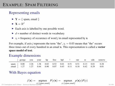
Representing emailsI Y = { spam, email }I X = Rd
I Each axis is labelled by one possible word.I d = number of distinct words in vocabularyI xj = frequency of occurence of word j in email represented by x
For example, if axis j represents the term "the", xj = 0.03 means that "the" occursthree times out of every hundred in an email x. This representation is called a vectorspace model of text.
Example dimensionsgeorge you your hp free hpl ! our re edu remove
spam 0.00 2.26 1.38 0.02 0.52 0.01 0.51 0.51 0.13 0.01 0.28email 1.27 1.27 0.44 0.90 0.07 0.43 0.11 0.18 0.42 0.29 0.01
With Bayes equation
f (x) = argmaxy2{spam,email}
P(y|x) = argmaxy2{spam,email}
p(x|y)P(y)J.P. Cunningham and P. Orbanz · Statistical Machine Learning 24 / 436
NAIVE BAYES
Simplifying assumptionThe classifier is called a naive Bayes classifier if it assumes
p(x|y) =dY
j=1
pj(xi|y) ,
i.e. if it treats the individual dimensions of x as conditionally independent given y.
In spam exampleI Corresponds to the assumption that the number of occurrences of a word carries
information about y.I Co-occurrences (how often do given combinations of words occur?) is
neglected.
J.P. Cunningham and P. Orbanz · Statistical Machine Learning 25 / 436
ESTIMATION
Class priorThe distribution P(y) is easy to estimate from training data:
P(y) =#observations in class y
#observations
Class-conditional distributionsThe class conditionals p(x|y) usually require a modeling assumption. Under a givenmodel:
I Separate the training data into classes.I Estimate p(x|y) on class y by maximum likelihood.
J.P. Cunningham and P. Orbanz · Statistical Machine Learning 26 / 436
LINEAR CLASSIFICATION
HYPERPLANES
x1
x2
H
vH
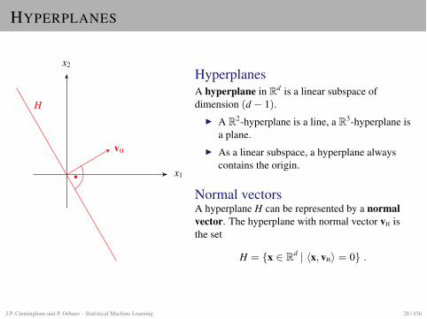
HyperplanesA hyperplane in Rd is a linear subspace ofdimension (d � 1).
I A R2-hyperplane is a line, a R3-hyperplane isa plane.
I As a linear subspace, a hyperplane alwayscontains the origin.
Normal vectorsA hyperplane H can be represented by a normalvector. The hyperplane with normal vector vH isthe set
H = {x 2 Rd | hx, vHi = 0} .
J.P. Cunningham and P. Orbanz · Statistical Machine Learning 28 / 436
WHICH SIDE OF THE PLANE ARE WE ON?
H
vH
x
cos ✓ · kxk✓
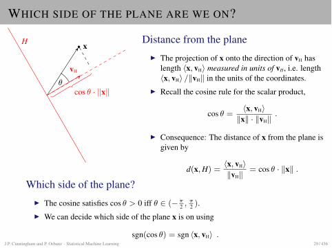
Distance from the planeI The projection of x onto the direction of vH has
length hx, vHi measured in units of vH, i.e. lengthhx, vHi /kvHk in the units of the coordinates.
I Recall the cosine rule for the scalar product,
cos ✓ =hx, vHikxk · kvHk .
I Consequence: The distance of x from the plane isgiven by
d(x, H) =hx, vHikvHk = cos ✓ · kxk .
Which side of the plane?I The cosine satisfies cos ✓ > 0 iff ✓ 2 (�⇡
2 , ⇡2 ).
I We can decide which side of the plane x is on using
sgn(cos ✓) = sgn hx, vHi .J.P. Cunningham and P. Orbanz · Statistical Machine Learning 29 / 436
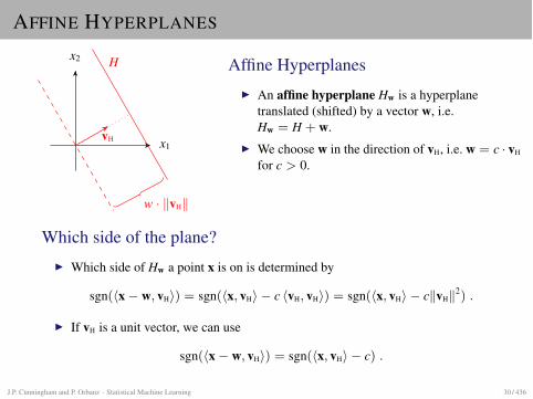
AFFINE HYPERPLANES
x1
x2 H
vH
w · kvHk
Affine HyperplanesI An affine hyperplane Hw is a hyperplane
translated (shifted) by a vector w, i.e.Hw = H + w.
I We choose w in the direction of vH, i.e. w = c · vH
for c > 0.
Which side of the plane?I Which side of Hw a point x is on is determined by
sgn(hx� w, vHi) = sgn(hx, vHi � c hvH, vHi) = sgn(hx, vHi � ckvHk2) .
I If vH is a unit vector, we can use
sgn(hx� w, vHi) = sgn(hx, vHi � c) .
J.P. Cunningham and P. Orbanz · Statistical Machine Learning 30 / 436
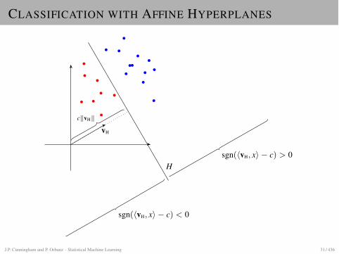
CLASSIFICATION WITH AFFINE HYPERPLANES
H
vH
sgn(hvH, xi � c) < 0
sgn(hvH, xi � c) > 0
ckvHk
J.P. Cunningham and P. Orbanz · Statistical Machine Learning 31 / 436
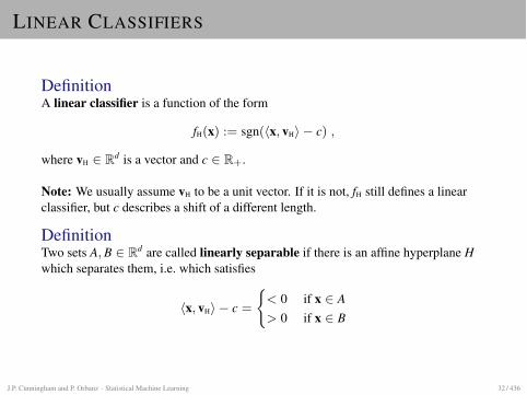
LINEAR CLASSIFIERS
DefinitionA linear classifier is a function of the form
fH(x) := sgn(hx, vHi � c) ,
where vH 2 Rd is a vector and c 2 R+.
Note: We usually assume vH to be a unit vector. If it is not, fH still defines a linearclassifier, but c describes a shift of a different length.
DefinitionTwo sets A, B 2 Rd are called linearly separable if there is an affine hyperplane Hwhich separates them, i.e. which satisfies
hx, vHi � c =
(
< 0 if x 2 A> 0 if x 2 B
J.P. Cunningham and P. Orbanz · Statistical Machine Learning 32 / 436
THE PERCEPTRON ALGORITHM
RISK MINIMIZATION
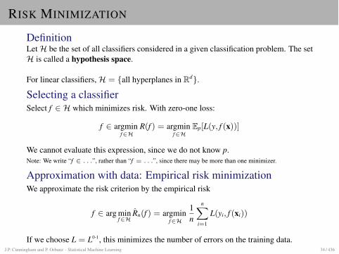
DefinitionLet H be the set of all classifiers considered in a given classification problem. The setH is called a hypothesis space.
For linear classifiers, H = {all hyperplanes in Rd}.
Selecting a classifierSelect f 2 H which minimizes risk. With zero-one loss:
f 2 argminf2H
R(f ) = argminf2H
Ep[L(y, f (x))]
We cannot evaluate this expression, since we do not know p.Note: We write “f 2 . . .”, rather than “f = . . .”, since there may be more than one minimizer.
Approximation with data: Empirical risk minimizationWe approximate the risk criterion by the empirical risk
f 2 arg minf2H
Rn(f ) = argminf2H
1n
nX
i=1
L(yi, f (xi))
If we choose L = L0-1, this minimizes the number of errors on the training data.J.P. Cunningham and P. Orbanz · Statistical Machine Learning 34 / 436
HOMOGENEOUS COORDINATES
Parameterizing the hypothesis spaceI Linear classification: Every f 2 H is of the form f (x) = sgn(hx, vHi � c).I f can be specified by specifying vH 2 Rd and c 2 R.I We collect vH and c in a single vector z := (�c, vH) 2 Rd+1.
We now have
hx, vHi � c =⌦
✓
1x
◆
, z↵
and f (x) = sgn⌦
✓
1x
◆
, z↵
The affine plane in Rd can now be interpreted as a linear plane in Rd+1. Thed + 1-dimensional coordinates in the representation are called homogeneouscoordinates.
J.P. Cunningham and P. Orbanz · Statistical Machine Learning 35 / 436
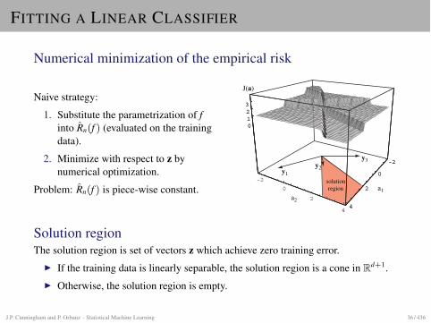
FITTING A LINEAR CLASSIFIER
Numerical minimization of the empirical risk
Naive strategy:
1. Substitute the parametrization of finto Rn(f ) (evaluated on the trainingdata).
2. Minimize with respect to z bynumerical optimization.
Problem: Rn(f ) is piece-wise constant.
16 CHAPTER 5. LINEAR DISCRIMINANT FUNCTIONS
-2
0
2
4
-2
0
2
4
0
100
-2
0
2
4
0
100
-2
0
2
4
-2
0
2
4
0
5
-2
0
2
4
0
5
-2
0
2
4
-2
0
2
4
0123
-2
0
2
4
0123
-2
0
2
4
-2
0
2
4
0
5
10
-2
0
2
4
0
5
10
y1y1
y1y1
y2y2
y2 y2
y3 y3
y3 y3
solutionregion
solutionregion
solutionregion
solutionregion
a2a2
a2a2
a1 a1
a1 a1
Jp(a)
Jq(a) Jr(a)
J(a)
Figure 5.11: Four learning criteria as a function of weights in a linear classifier. At theupper left is the total number of patterns misclassified, which is piecewise constantand hence unacceptable for gradient descent procedures. At the upper right is thePerceptron criterion (Eq. 16), which is piecewise linear and acceptable for gradientdescent. The lower left is squared error (Eq. 32), which has nice analytic propertiesand is useful even when the patterns are not linearly separable. The lower right isthe square error with margin (Eq. 33). A designer may adjust the margin b in orderto force the solution vector to lie toward the middle of the b = 0 solution region inhopes of improving generalization of the resulting classifier.
Thus, the batch Perceptron algorithm for finding a solution vector can be statedvery simply: the next weight vector is obtained by adding some multiple of the sumof the misclassified samples to the present weight vector. We use the term “batch”batch
training to refer to the fact that (in general) a large group of samples is used when com-puting each weight update. (We shall soon see alternate methods based on singlesamples.) Figure 5.12 shows how this algorithm yields a solution vector for a simpletwo-dimensional example with a(1) = 0, and �(k) = 1. We shall now show that itwill yield a solution for any linearly separable problem.
Solution regionThe solution region is set of vectors z which achieve zero training error.
I If the training data is linearly separable, the solution region is a cone in Rd+1.I Otherwise, the solution region is empty.
J.P. Cunningham and P. Orbanz · Statistical Machine Learning 36 / 436
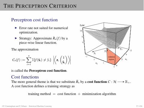
THE PERCEPTRON CRITERION
Perceptron cost functionI Error rate not suited for numerical
optimization.I Strategy: Approximate Rn(f ) by a
piece-wise linear function.
The approximation
CP(f ) :=nX
i=1
I{f (xi) 6= yi}�
�
�
�
⌧
z,✓
1xi
◆�
�
�
�
�
is called the Perceptron cost function.
16 CHAPTER 5. LINEAR DISCRIMINANT FUNCTIONS
-2
0
2
4
-2
0
2
4
0
100
-2
0
2
4
0
100
-2
0
2
4
-2
0
2
4
0
5
-2
0
2
4
0
5
-2
0
2
4
-2
0
2
4
0123
-2
0
2
4
0123
-2
0
2
4
-2
0
2
4
0
5
10
-2
0
2
4
0
5
10
y1y1
y1y1
y2y2
y2 y2
y3 y3
y3 y3
solutionregion
solutionregion
solutionregion
solutionregion
a2a2
a2a2
a1 a1
a1 a1
Jp(a)
Jq(a) Jr(a)
J(a)
Figure 5.11: Four learning criteria as a function of weights in a linear classifier. At theupper left is the total number of patterns misclassified, which is piecewise constantand hence unacceptable for gradient descent procedures. At the upper right is thePerceptron criterion (Eq. 16), which is piecewise linear and acceptable for gradientdescent. The lower left is squared error (Eq. 32), which has nice analytic propertiesand is useful even when the patterns are not linearly separable. The lower right isthe square error with margin (Eq. 33). A designer may adjust the margin b in orderto force the solution vector to lie toward the middle of the b = 0 solution region inhopes of improving generalization of the resulting classifier.
Thus, the batch Perceptron algorithm for finding a solution vector can be statedvery simply: the next weight vector is obtained by adding some multiple of the sumof the misclassified samples to the present weight vector. We use the term “batch”batch
training to refer to the fact that (in general) a large group of samples is used when com-puting each weight update. (We shall soon see alternate methods based on singlesamples.) Figure 5.12 shows how this algorithm yields a solution vector for a simpletwo-dimensional example with a(1) = 0, and �(k) = 1. We shall now show that itwill yield a solution for any linearly separable problem.
Cost functionsThe more general theme is that we substitute Rn by a cost function C : H R+.A cost function defines a training strategy as
training method = cost function + minimization algorithm
J.P. Cunningham and P. Orbanz · Statistical Machine Learning 37 / 436
PERCEPTRON ALGORITHMS
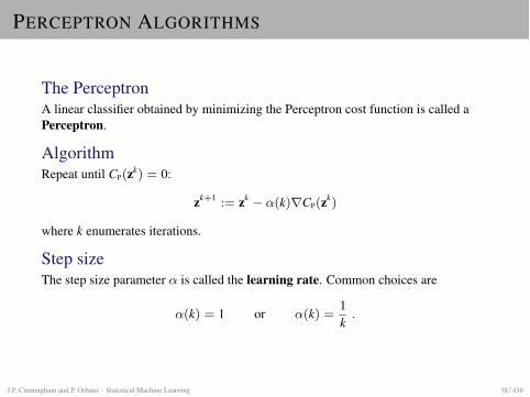
The PerceptronA linear classifier obtained by minimizing the Perceptron cost function is called aPerceptron.
AlgorithmRepeat until CP(zk) = 0:
zk+1 := zk � ↵(k)rCP(zk)
where k enumerates iterations.
Step sizeThe step size parameter ↵ is called the learning rate. Common choices are
↵(k) = 1 or ↵(k) =1k
.
J.P. Cunningham and P. Orbanz · Statistical Machine Learning 38 / 436
THE GRADIENT ALGORITHM
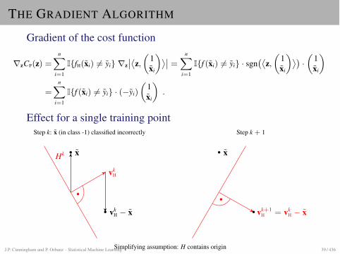
Gradient of the cost function
rzCP(z) =nX
i=1
I{fH(xi) 6= yi} rz�
�
⌦
z,✓
1xi
◆
↵
�
� =nX
i=1
I{f (xi) 6= yi} · sgn�⌦
z,✓
1xi
◆
↵� ·✓
1xi
◆
=nX
i=1
I{f (xi) 6= yi} · (�yi)
✓
1xi
◆
.
Effect for a single training pointStep k: x (in class -1) classified incorrectly
xHk
vkH
vkH � x
Step k + 1
x
vk+1H = vk
H � x
Simplifying assumption: H contains originJ.P. Cunningham and P. Orbanz · Statistical Machine Learning 39 / 436
DOES THE PERCEPTRON WORK?
The algorithm we discussed before is called the batch Perceptron. For learning rate↵ = 1, we can equivalently add data points one at a time.
Alternative AlgorithmRepeat until CP(z) = 0:
1. For all i = 1, . . . , n: zk := zk + I{fH(xi) 6= yi}(yi)
✓
1xi
◆
2. k := k + 1
This is called the fixed-increment single-sample Perceptron, and is somewhateasier to analyze than the batch Perceptron.
Theorem: Perceptron convergenceIf (and only if) the training data is linearly separable, the fixed-incrementsingle-sample Perceptron terminates after a finite number of steps with a validsolution vector z (i.e. a vector which classifies all training data points correctly).
J.P. Cunningham and P. Orbanz · Statistical Machine Learning 40 / 436

MAXIMUM MARGIN CLASSIFIERS
MAXIMUM MARGIN IDEA
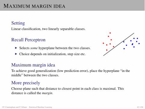
SettingLinear classification, two linearly separable classes.
Recall PerceptronI Selects some hyperplane between the two classes.I Choice depends on initialization, step size etc.
Maximum margin ideaTo achieve good generalization (low prediction error), place the hyperplane “in themiddle” between the two classes.
More preciselyChoose plane such that distance to closest point in each class is maximal. Thisdistance is called the margin.
J.P. Cunningham and P. Orbanz · Statistical Machine Learning 42 / 436
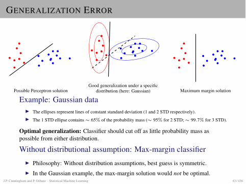
GENERALIZATION ERROR
Possible Perceptron solutionGood generalization under a specific
distribution (here: Gaussian) Maximum margin solution
Example: Gaussian dataI The ellipses represent lines of constant standard deviation (1 and 2 STD respectively).I The 1 STD ellipse contains ⇠ 65% of the probability mass (⇠ 95% for 2 STD; ⇠ 99.7% for 3 STD).
Optimal generalization: Classifier should cut off as little probability mass aspossible from either distribution.
Without distributional assumption: Max-margin classifierI Philosophy: Without distribution assumptions, best guess is symmetric.I In the Gaussian example, the max-margin solution would not be optimal.
J.P. Cunningham and P. Orbanz · Statistical Machine Learning 43 / 436
SUBSTITUTING CONVEX SETS
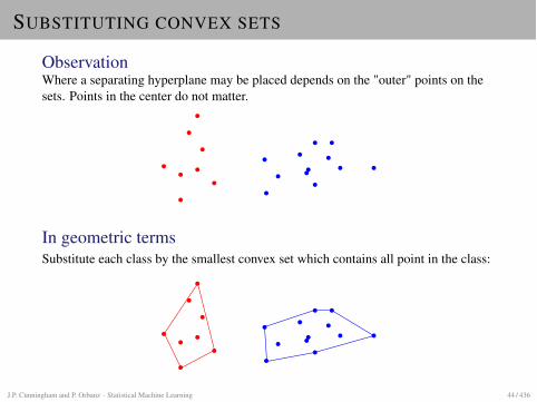
ObservationWhere a separating hyperplane may be placed depends on the "outer" points on thesets. Points in the center do not matter.
In geometric termsSubstitute each class by the smallest convex set which contains all point in the class:
J.P. Cunningham and P. Orbanz · Statistical Machine Learning 44 / 436
SUBSTITUTING CONVEX SETS
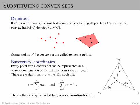
DefinitionIf C is a set of points, the smallest convex set containing all points in C is called theconvex hull of C, denoted conv(C).
Corner points of the convex set are called extreme points.
Barycentric coordinatesEvery point x in a convex set can be represented as aconvex combination of the extreme points {e1, . . . , em}.There are weights ↵1, . . . ,↵m 2 R+ such that
x =mX
i=1
↵iei andmX
i=1
↵i = 1 .
The coefficients ↵i are called barycentric coordinates of x.
e1
e2 e3
x
↵1
↵2
↵3
J.P. Cunningham and P. Orbanz · Statistical Machine Learning 45 / 436
CONVEX HULLS AND CLASSIFICATION
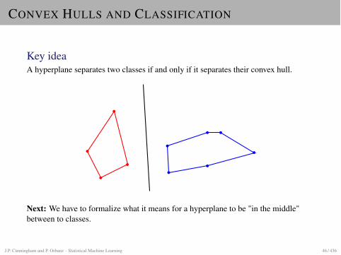
Key ideaA hyperplane separates two classes if and only if it separates their convex hull.
Next: We have to formalize what it means for a hyperplane to be "in the middle"between to classes.
J.P. Cunningham and P. Orbanz · Statistical Machine Learning 46 / 436
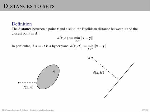
DISTANCES TO SETS
DefinitionThe distance between a point x and a set A the Euclidean distance between x and theclosest point in A:
d(x, A) := miny2Akx� yk
In particular, if A = H is a hyperplane, d(x, H) := miny2Hkx� yk.
A
d(x, A)
x
d(x, H)
J.P. Cunningham and P. Orbanz · Statistical Machine Learning 47 / 436
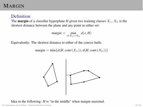
MARGIN
DefinitionThe margin of a classifier hyperplane H given two training classes X , X� is theshortest distance between the plane and any point in either set:
margin = minx2X [X�
d(x, H)
Equivalently: The shortest distance to either of the convex hulls.
margin = min{d(H, conv(X )), d(H, conv(X�))}
Idea in the following: H is "in the middle" when margin maximal.J.P. Cunningham and P. Orbanz · Statistical Machine Learning 48 / 436
LINEAR CLASSIFIER WITH MARGIN
Recall: Specifying affine planeNormal vector vH.
hvH, xi � c
(
> 0 x on positive side< 0 x on negative side
Scalar c 2 R specifies shift (plane through origin if c = 0).
Plane with marginDemand
hvH, xi � c > 1 or < �1
{�1, 1} on the right works for any margin: Size of margin determined by kvHk. Toincrease margin, scale down vH.
ClassificationConcept of margin applies only to training, not to classification. Classification worksas for any linear classifier. For a test point x:
y = sign (hvH, xi � c)
J.P. Cunningham and P. Orbanz · Statistical Machine Learning 49 / 436
SUPPORT VECTOR MACHINE
Finding the hyperplaneFor n training points (xi, yi) with labels yi 2 {�1, 1}, solve optimization problem:
minvH,c
kvHks.t. yi(hvH, xii � c) � 1 for i = 1, . . . , n
DefinitionThe classifier obtained by solving this optimization problem is called a supportvector machine.
J.P. Cunningham and P. Orbanz · Statistical Machine Learning 50 / 436
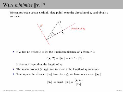
WHY minimize kvHk?We can project a vector x (think: data point) onto the direction of vH and obtain avector xv.
direction of vH
xH
xv✓
I If H has no offset (c = 0), the Euclidean distance of x from H is
d(x, H) = kxvk = cos ✓ · kxk .
It does not depend on the length of vH.I The scalar product hx, vHi does increase if the length of vH increases.I To compute the distance kxvk from hx, vHi, we have to scale out kvHk:
kxvk = cos ✓ · kxk =hx, vHikvHk
J.P. Cunningham and P. Orbanz · Statistical Machine Learning 51 / 436
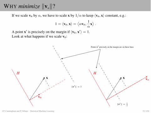
WHY minimize kvHk?If we scale vH by ↵, we have to scale x by 1/↵ to keep hvH, xi constant, e.g.:
1 = hvH, xi =⌦
↵vH,1↵
x↵
.
A point x0 is precisely on the margin if hvH, x0i = 1.Look at what happens if we scale vH:
H
vH
x
kx0k = 2
H
vHx
kx0k = 12
Points x0 precisely on the margin are on these lines
J.P. Cunningham and P. Orbanz · Statistical Machine Learning 52 / 436
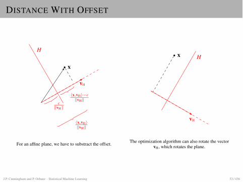
DISTANCE WITH OFFSET
H
vH
x
ckvHk
hx,vHi�ckvHk
hx,vHikvHk
x H
vH
For an affine plane, we have to substract the offset. The optimization algorithm can also rotate the vectorvH, which rotates the plane.
J.P. Cunningham and P. Orbanz · Statistical Machine Learning 53 / 436
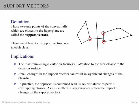
SUPPORT VECTORS
DefinitionThose extreme points of the convex hullswhich are closest to the hyperplane arecalled the support vectors.
There are at least two support vectors, onein each class.
ImplicationsI The maximum-margin criterion focuses all attention to the area closest to the
decision surface.I Small changes in the support vectors can result in significant changes of the
classifier.I In practice, the approach is combined with "slack variables" to permit
overlapping classes. As a side effect, slack variables soften the impact ofchanges in the support vectors.
J.P. Cunningham and P. Orbanz · Statistical Machine Learning 54 / 436
DUAL OPTIMIZATION PROBLEM
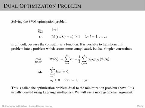
Solving the SVM opimization problem
minvH,c
kvHks.t. yi(hvH, xii � c) � 1 for i = 1, . . . , n
is difficult, because the constraint is a function. It is possible to transform thisproblem into a problem which seems more complicated, but has simpler constraints:
max↵↵↵2Rn
W(↵↵↵) :=nX
i=1
↵i � 12
nX
i,j=1
↵i↵jyiyj hxi, xji
s.t.nX
i=1
yi↵i = 0
↵i � 0 for i = 1, . . . , n
This is called the optimization problem dual to the minimization problem above. It isusually derived using Lagrange multipliers. We will use a more geometric argument.
J.P. Cunningham and P. Orbanz · Statistical Machine Learning 55 / 436
CONVEX DUALITY
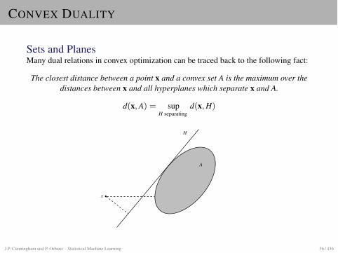
Sets and PlanesMany dual relations in convex optimization can be traced back to the following fact:
The closest distance between a point x and a convex set A is the maximum over thedistances between x and all hyperplanes which separate x and A.
d(x, A) = supH separating
d(x, H)
x
A
H
J.P. Cunningham and P. Orbanz · Statistical Machine Learning 56 / 436
DERIVING THE DUAL PROBLEM
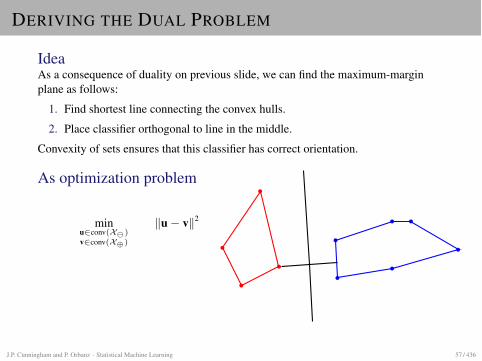
IdeaAs a consequence of duality on previous slide, we can find the maximum-marginplane as follows:
1. Find shortest line connecting the convex hulls.
2. Place classifier orthogonal to line in the middle.
Convexity of sets ensures that this classifier has correct orientation.
As optimization problem
minu2conv(X )v2conv(X�)
ku� vk2
J.P. Cunningham and P. Orbanz · Statistical Machine Learning 57 / 436
BARYCENTRIC COORDINATES
Dual optimization problem
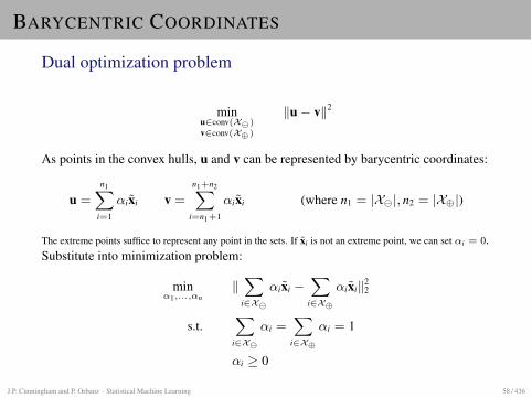
minu2conv(X )v2conv(X�)
ku� vk2
As points in the convex hulls, u and v can be represented by barycentric coordinates:
u =n1X
i=1
↵ixi v =n1+n2X
i=n1+1
↵ixi (where n1 = |X |, n2 = |X�|)
The extreme points suffice to represent any point in the sets. If xi is not an extreme point, we can set ↵i = 0.Substitute into minimization problem:
min↵1,...,↵n
kX
i2X ↵ixi �
X
i2X�↵ixik2
2
s.t.X
i2X ↵i =
X
i2X�↵i = 1
↵i � 0
J.P. Cunningham and P. Orbanz · Statistical Machine Learning 58 / 436
DUAL OPTIMIZATION PROBLEM
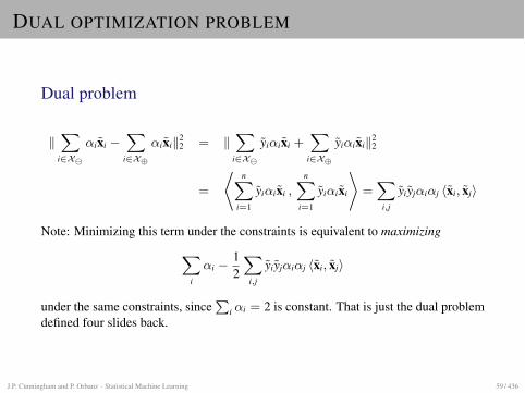
Dual problem
kX
i2X ↵ixi �
X
i2X�↵ixik2
2 = kX
i2X yi↵ixi +
X
i2X�yi↵ixik2
2
=
*
nX
i=1
yi↵ixi ,nX
i=1
yi↵ixi
+
=X
i,j
yiyj↵i↵j hxi, xji
Note: Minimizing this term under the constraints is equivalent to maximizing
X
i
↵i � 12
X
i,j
yiyj↵i↵j hxi, xji
under the same constraints, sinceP
i ↵i = 2 is constant. That is just the dual problemdefined four slides back.
J.P. Cunningham and P. Orbanz · Statistical Machine Learning 59 / 436
COMPUTING c
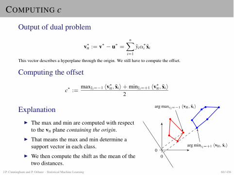
Output of dual problem
v⇤H := v⇤ � u⇤ =nX
i=1
yi↵⇤i xi
This vector describes a hyperplane through the origin. We still have to compute the offset.
Computing the offset
c⇤ :=maxyi=�1 hv⇤H, xii+ minyi=+1 hv⇤H, xii
2
ExplanationI The max and min are computed with respect
to the vH plane containing the origin.I That means the max and min determine a
support vector in each class.I We then compute the shift as the mean of the
two distances.
00
arg maxyi=�1 hvH, xii
arg minyi=+1 hvH, xii
J.P. Cunningham and P. Orbanz · Statistical Machine Learning 60 / 436
RESULTING CLASSIFICATION RULE
Output of dual optimizationI Optimal values ↵⇤i for the variables ↵i
I If xi support vector: ↵⇤i > 0, if not: ↵⇤i = 0
Note: ↵⇤i = 0 holds even if xi is an extreme point, but not a support vector.
SVM ClassifierThe classification function can be expressed in terms of the variables ↵i:
f (x) = sgn
nX
i=1
yi↵⇤i hxi, xi � c⇤
!
Intuitively: To classify a data point, it is sufficient to know which side of eachsupport vector it is on.
J.P. Cunningham and P. Orbanz · Statistical Machine Learning 61 / 436
SOFT-MARGIN CLASSIFIERS
Soft-margin classifiers are maximum-margin classifiers which permit some pointsto lie on the wrong side of the margin, or even of the hyperplane.
Motivation 1: Nonseparable dataSVMs are linear classifiers; without further modifications, they cannot be trained ona non-separable training data set.
Motivation 2: RobustnessI Recall: Location of SVM classifier depends on position of (possibly few)
support vectors.I Suppose we have two training samples (from the same joint distribution on
(X, Y)) and train an SVM on each.I If locations of support vectors vary significantly between samples, SVM
estimate of vH is “brittle” (depends too much on small variations in trainingdata). �! Bad generalization properties.
I Methods which are not susceptible to small variations in the data are oftenreferred to as robust.
J.P. Cunningham and P. Orbanz · Statistical Machine Learning 62 / 436
SLACK VARIABLES
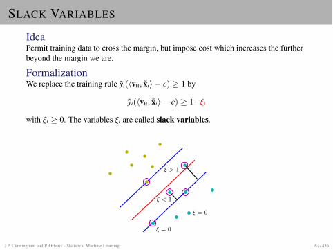
IdeaPermit training data to cross the margin, but impose cost which increases the furtherbeyond the margin we are.
FormalizationWe replace the training rule yi(hvH, xii � c) � 1 by
yi(hvH, xii � c) � 1�⇠i
with ⇠i � 0. The variables ⇠i are called slack variables.
⇠ > 1
⇠ < 1
⇠ = 0
⇠ = 0
J.P. Cunningham and P. Orbanz · Statistical Machine Learning 63 / 436
SOFT-MARGIN SVM
Soft-margin optimization problem
minvH,c,⇠
kvHk2 + �nX
i=1
⇠2i
s.t. yi(hvH, xii � c) � 1�⇠i for i = 1, . . . , n⇠i � 0, for i = 1, . . . , n
The training algorithm now has a parameter � > 0 for which we have to choose a“good” value. � is usually set by a method called cross validation (discussed later).Its value is fixed before we start the optimization.
Role of �I Specifies the "cost" of allowing a point on the wrong side.I If � is very small, many points may end up beyond the margin boundary.I For � !1, we recover the original SVM.
J.P. Cunningham and P. Orbanz · Statistical Machine Learning 64 / 436
SOFT-MARGIN SVM
Soft-margin dual problemThe slack variables vanish in the dual problem.
max↵↵↵2Rn
W(↵↵↵) :=nX
i=1
↵i � 12
nX
i,j=1
↵i↵jyiyj( hxi, xji +1�I{i = j})
s.t.nX
i=1
yi↵i = 0
↵i � 0 for i = 1, . . . , n
Soft-margin classifierThe classifier looks exactly as for the original SVM:
f (x) = sgn
nX
i=1
yi↵⇤i hxi, xi � c
!
Note: Each point on wrong side of the margin is an additional support vector(↵⇤i 6= 0), so the ratio of support vectors can be substantial when classes overlap.
J.P. Cunningham and P. Orbanz · Statistical Machine Learning 65 / 436
INFLUENCE OF MARGIN PARAMETER
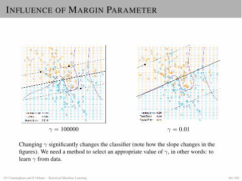
� = 100000 � = 0.01
Changing � significantly changes the classifier (note how the slope changes in thefigures). We need a method to select an appropriate value of �, in other words: tolearn � from data.
J.P. Cunningham and P. Orbanz · Statistical Machine Learning 66 / 436

TOOLS: OPTIMIZATION METHODS
OPTIMIZATION PROBLEMS
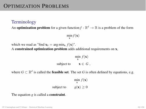
TerminologyAn optimization problem for a given function f : Rd ! R is a problem of the form
minx
f (x)
which we read as "find x0 = arg minx f (x)".A constrained optimization problem adds additional requirements on x,
minx
f (x)
subject to x 2 G ,
where G ⇢ Rd is called the feasible set. The set G is often defined by equations, e.g.
minx
f (x)
subject to g(x) � 0
The equation g is called a constraint.
J.P. Cunningham and P. Orbanz · Statistical Machine Learning 68 / 436
TYPES OF MINIMA
-3 -2 -1 1 2
-5
5
-2 2 4
-10
-5
5
10
15
20
25
global, but not local
local
global and local
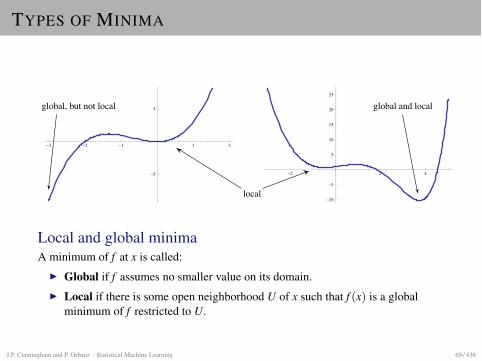
Local and global minimaA minimum of f at x is called:
I Global if f assumes no smaller value on its domain.I Local if there is some open neighborhood U of x such that f (x) is a global
minimum of f restricted to U.
J.P. Cunningham and P. Orbanz · Statistical Machine Learning 69 / 436
OPTIMA
Analytic criteria for local minimaRecall that x is a local minimum of f if
f 0(x) = 0 and f 00(x) > 0 .
In Rd,
rf (x) = 0 and Hf (x) =⇣ @f@xi@xj
(x)⌘
i,j=1,...,npositive definite.
The d ⇥ d-matrix Hf (x) is called the Hessian matrix of f at x.
Numerical methodsAll numerical minimization methods perform roughly the same steps:
I Start with some point x0.I Our goal is to find a sequence x0, . . . , xm such that f (xm) is a minimum.I At a given point xn, compute properties of f (such as f 0(xn) and f 00(xn)).I Based on these values, choose the next point xn+1.
The information f 0(xn), f 00(xn) etc is always local at xn, and we can only decidewhether a point is a local minimum, not whether it is global.
J.P. Cunningham and P. Orbanz · Statistical Machine Learning 70 / 436
CONVEX FUNCTIONS
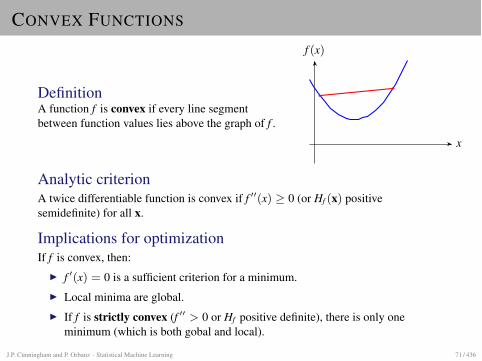
DefinitionA function f is convex if every line segmentbetween function values lies above the graph of f .
x
f (x)
Analytic criterionA twice differentiable function is convex if f 00(x) � 0 (or Hf (x) positivesemidefinite) for all x.
Implications for optimizationIf f is convex, then:
I f 0(x) = 0 is a sufficient criterion for a minimum.I Local minima are global.I If f is strictly convex (f 00 > 0 or Hf positive definite), there is only one
minimum (which is both gobal and local).
J.P. Cunningham and P. Orbanz · Statistical Machine Learning 71 / 436
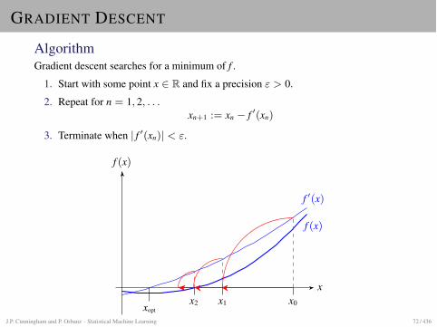
GRADIENT DESCENT
AlgorithmGradient descent searches for a minimum of f .
1. Start with some point x 2 R and fix a precision " > 0.
2. Repeat for n = 1, 2, . . .xn+1 := xn � f 0(xn)
3. Terminate when | f 0(xn)| < ".
x
f (x)
f (x)
f 0(x)
x0x1x2xopt
J.P. Cunningham and P. Orbanz · Statistical Machine Learning 72 / 436
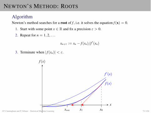
NEWTON’S METHOD: ROOTS
AlgorithmNewton’s method searches for a root of f , i.e. it solves the equation f (x) = 0.
1. Start with some point x 2 R and fix a precision " > 0.
2. Repeat for n = 1, 2, . . .
xn+1 := xn � f (xn)/f 0(xn)
3. Terminate when | f (xn)| < ".
x
f (x)
f (x)
f 0(x)
x0x1xrootJ.P. Cunningham and P. Orbanz · Statistical Machine Learning 73 / 436
BASIC APPLICATIONS
Function evaluationMost numerical evaluations of functions (
pa, sin(a), exp(a), etc) are implemented
using Newton’s method. To evaluate g at a, we have to transform x = g(a) into anequivalent equation of the form
f (x, a) = 0 .
We then fix a and solve for x using Newton’s method for roots.
Example: Square rootTo eveluate g(a) =
pa, we can solve
f (x, a) = x2 � a = 0 .
This is essentially how sqrt() is implemented in the standard C library.
J.P. Cunningham and P. Orbanz · Statistical Machine Learning 74 / 436
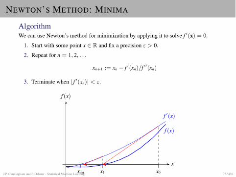
NEWTON’S METHOD: MINIMA
AlgorithmWe can use Newton’s method for minimization by applying it to solve f 0(x) = 0.
1. Start with some point x 2 R and fix a precision " > 0.
2. Repeat for n = 1, 2, . . .
xn+1 := xn � f 0(xn)/f 00(xn)
3. Terminate when | f 0(xn)| < ".
x
f (x)
f (x)
f 0(x)
x0x1xoptJ.P. Cunningham and P. Orbanz · Statistical Machine Learning 75 / 436
MULTIPLE DIMENSIONS
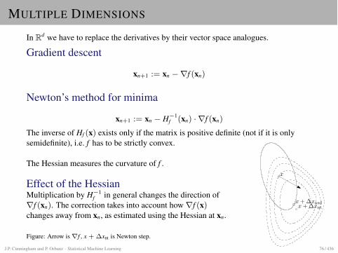
In Rd we have to replace the derivatives by their vector space analogues.
Gradient descent
xn+1 := xn �rf (xn)
Newton’s method for minima
xn+1 := xn � H�1f (xn) ·rf (xn)
The inverse of Hf (x) exists only if the matrix is positive definite (not if it is onlysemidefinite), i.e. f has to be strictly convex.
The Hessian measures the curvature of f .
Effect of the HessianMultiplication by H�1
f in general changes the direction ofrf (xn). The correction takes into account howrf (x)changes away from xn, as estimated using the Hessian at xn.
Figure: Arrow is rf , x + �xnt is Newton step.
9.5 Newton’s method 485
PSfrag replacements
x
x + �xntx + �xnsd
Figure 9.17 The dashed lines are level curves of a convex function. Theellipsoid shown (with solid line) is {x + v | vT r2f(x)v 1}. The arrowshows �rf(x), the gradient descent direction. The Newton step �xnt isthe steepest descent direction in the norm k · k�2f(x). The figure also shows�xnsd, the normalized steepest descent direction for the same norm.
Steepest descent direction in Hessian norm
The Newton step is also the steepest descent direction at x, for the quadratic normdefined by the Hessian �2f(x), i.e.,
kukr2f(x) = (uT �2f(x)u)1/2.
This gives another insight into why the Newton step should be a good searchdirection, and a very good search direction when x is near x�.
Recall from our discussion above that steepest descent, with quadratic normk · kP , converges very rapidly when the Hessian, after the associated change ofcoordinates, has small condition number. In particular, near x�, a very good choiceis P = �2f(x�). When x is near x�, we have �2f(x) � �2f(x�), which explainswhy the Newton step is a very good choice of search direction. This is illustratedin figure 9.17.
Solution of linearized optimality condition
If we linearize the optimality condition �f(x�) = 0 near x we obtain
�f(x + v) � �f(x) + �2f(x)v = 0,
which is a linear equation in v, with solution v = �xnt. So the Newton step �xnt iswhat must be added to x so that the linearized optimality condition holds. Again,this suggests that when x is near x� (so the optimality conditions almost hold),the update x + �xnt should be a very good approximation of x�.
When n = 1, i.e., f : R � R, this interpretation is particularly simple. Thesolution x� of the minimization problem is characterized by f �(x�) = 0, i.e., it is
J.P. Cunningham and P. Orbanz · Statistical Machine Learning 76 / 436
NEWTON: PROPERTIES
ConvergenceI The algorithm always converges if f 00 > 0 (or Hf positive definite).I The speed of convergence separates into two phases:
I In a (possibly small) region around the minimum, f can always beapproximated by a quadratic function.
I Once the algorithm reaches that region, the error decreases at quadraticrate. Roughly speaking, the number of correct digits in the solutiondoubles in each step.
I Before it reaches that region, the convergence rate is linear.
High dimensionsI The required number of steps hardly depends on the dimension of Rd. Even in
R10000, you can usually expect the algorithm to reach high precision in half adozen steps.
I Caveat: The individual steps can become very expensive, since we have toinvert Hf in each step, which is of size d ⇥ d.
J.P. Cunningham and P. Orbanz · Statistical Machine Learning 77 / 436
NEXT: CONSTRAINED OPTIMIZATION
So farI If f is differentiable, we can search for local minima using gradient descent.I If f is sufficiently nice (convex and twice differentiable), we know how to speed
up the search process using Newton’s method.
Constrained problemsI The numerical minimizers use the criterionrf (x) = 0 for the minimum.I In a constrained problem, the minimum is not identified by this criterion.
Next stepsWe will figure out how the constrained minimum can be identified. We have todistinguish two cases:
I Problems involving only equalities as constraints (sometimes easy).I Problems also involving inequalities (a bit more complex).
J.P. Cunningham and P. Orbanz · Statistical Machine Learning 78 / 436
OPTIMIZATION UNDER CONSTRAINTS
Objective
min f (x)
subject to g(x) = 0
IdeaI The feasible set is the set of points x which satisfy g(x) = 0,
G := {x | g(x) = 0} .
If g is reasonably smooth, G is a smooth surface in Rd.I We restrict the function f to this surface and call the restricted function fg.I The constrained optimization problem says that we are looking for the
minimum of fg.
J.P. Cunningham and P. Orbanz · Statistical Machine Learning 79 / 436
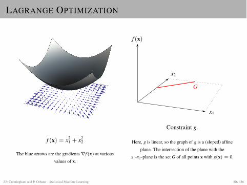
LAGRANGE OPTIMIZATION
f (x) = x21 + x2
2
The blue arrows are the gradients rf (x) at variousvalues of x.
f (x)
x2
x1
G
Constraint g.
Here, g is linear, so the graph of g is a (sloped) affineplane. The intersection of the plane with the
x1-x2-plane is the set G of all points x with g(x) = 0.
J.P. Cunningham and P. Orbanz · Statistical Machine Learning 80 / 436
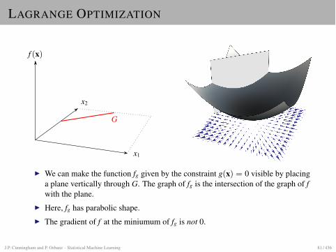
LAGRANGE OPTIMIZATION
f (x)
x2
x1
G
I We can make the function fg given by the constraint g(x) = 0 visible by placinga plane vertically through G. The graph of fg is the intersection of the graph of fwith the plane.
I Here, fg has parabolic shape.I The gradient of f at the miniumum of fg is not 0.
J.P. Cunningham and P. Orbanz · Statistical Machine Learning 81 / 436
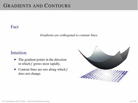
GRADIENTS AND CONTOURS
Fact
Gradients are orthogonal to contour lines.
IntuitionI The gradient points in the direction
in which f grows most rapidly.I Contour lines are sets along which f
does not change.
J.P. Cunningham and P. Orbanz · Statistical Machine Learning 82 / 436
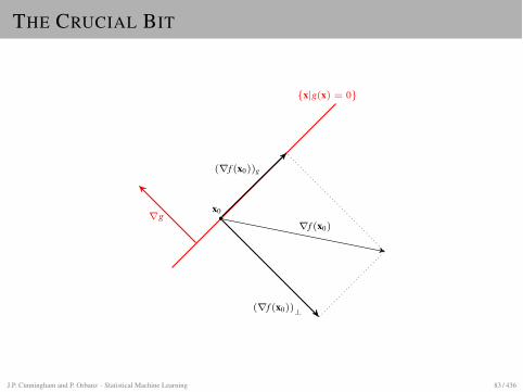
THE CRUCIAL BIT
rg
(rf (x0))g
(rf (x0))?
rf (x0)
{x|g(x) = 0}
x0
J.P. Cunningham and P. Orbanz · Statistical Machine Learning 83 / 436
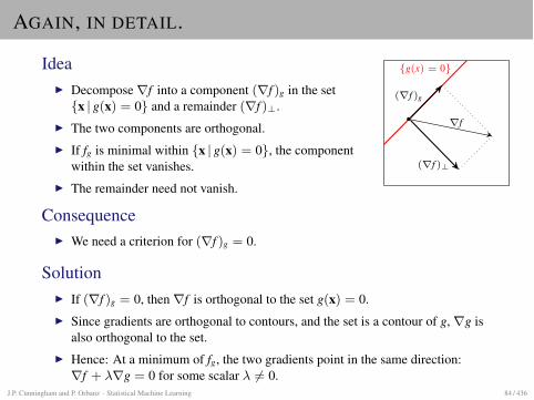
AGAIN, IN DETAIL.
IdeaI Decomposerf into a component (rf )g in the set
{x | g(x) = 0} and a remainder (rf )?.I The two components are orthogonal.I If fg is minimal within {x | g(x) = 0}, the component
within the set vanishes.I The remainder need not vanish.
(rf )g
(rf )?
rf
{g(x) = 0}
ConsequenceI We need a criterion for (rf )g = 0.
SolutionI If (rf )g = 0, thenrf is orthogonal to the set g(x) = 0.I Since gradients are orthogonal to contours, and the set is a contour of g,rg is
also orthogonal to the set.I Hence: At a minimum of fg, the two gradients point in the same direction:rf + �rg = 0 for some scalar � 6= 0.
J.P. Cunningham and P. Orbanz · Statistical Machine Learning 84 / 436
SOLUTION: CONSTRAINED OPTIMIZATION
SolutionThe constrained optimization problem
minx
f (x)
s.t. g(x) = 0
is solved by solving the equation system
rf (x) + �rg(x) = 0g(x) = 0
The vectorsrf andrg are D-dimensional, so the system contains D + 1 equationsfor the D + 1 variables x1, . . . , xD,�.
J.P. Cunningham and P. Orbanz · Statistical Machine Learning 85 / 436
INEQUALITY CONSTRAINTS
ObjectiveFor a function f and a convex function g, solve
min f (x)
subject to g(x) 0
i.e. we replace g(x) = 0 as previously by g(x) 0. This problem is called anoptimization problem with inequality constraint.
Feasible setWe again write G for the set of all points which satisfy the constraint,
G := {x | g(x) 0} .
G is often called the feasible set (the same name is used for equality constraints).
J.P. Cunningham and P. Orbanz · Statistical Machine Learning 86 / 436
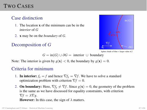
TWO CASES
Case distinction1. The location x of the minimum can be in the
interior of G
2. x may be on the boundary of G.
in(G)
@Grf
x0
lighter shade of blue = larger value of f
x1rg(x1)
Decomposition of G
G = in(G) [ @G = interior [ boundary
Note: The interior is given by g(x) < 0, the boundary by g(x) = 0.
Criteria for minimum1. In interior: fg = f and hencerfg = rf . We have to solve a standard
optimization problem with criterionrf = 0.
2. On boundary: Here,rfg 6= rf . Since g(x) = 0, the geometry of the problemis the same as we have discussed for equality constraints, with criterionrf = �rg.However: In this case, the sign of � matters.
J.P. Cunningham and P. Orbanz · Statistical Machine Learning 87 / 436
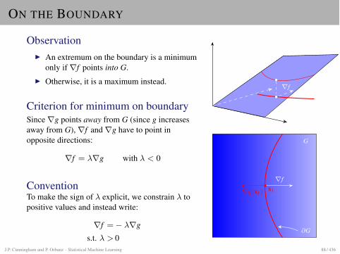
ON THE BOUNDARY
ObservationI An extremum on the boundary is a minimum
only ifrf points into G.I Otherwise, it is a maximum instead.
Criterion for minimum on boundarySincerg points away from G (since g increasesaway from G),rf andrg have to point inopposite directions:
rf = �rg with � < 0
ConventionTo make the sign of � explicit, we constrain � topositive values and instead write:
rf =� �rgs.t. � > 0
rf
G
@G
x1rg(x1)
rf
J.P. Cunningham and P. Orbanz · Statistical Machine Learning 88 / 436
COMBINING THE CASES
Combined problem
rf =� �rgs.t. g(x) 0
� = 0 if x 2 in(G)
� > 0 if x 2 @G
Can we get rid of the "if x 2 ·" distinction?Yes: Note that g(x) < 0 if x in interior and g(x) = 0 on boundary. Hence, we alwayshave either � = 0 or g(x) = 0 (and never both).
That means we can substitute
� = 0 if x 2 in(G)
� > 0 if x 2 @G
by� · g(x) = 0 and � � 0 .
J.P. Cunningham and P. Orbanz · Statistical Machine Learning 89 / 436
SOLUTION: INEQUALITY CONSTRAINTS
Combined solutionThe optimization problem with inequality constraints
min f (x)
subject to g(x) 0
can be solved by solving
rf (x) = ��rg(x)
s.t. �g(x) = 0g(x) 0� � 0
�
� system of d + 1 equations for d + 1variables x1, . . . , xD,�
These conditions are known as the Karush-Kuhn-Tucker (or KKT) conditions.
J.P. Cunningham and P. Orbanz · Statistical Machine Learning 90 / 436
REMARKS
Haven’t we made the problem more difficult?I To simplify the minimization of f for g(x) 0, we have made f more
complicated and added a variable and two constraints. Well done.I However: In the original problem, we do not know how to minimize f , since the
usual criterionrf = 0 does not work.I By adding � and additional constraints, we have reduced the problem to solving
a system of equations.
Summary: Conditions
Condition Ensures that... Purpose
rf (x) = ��rg(x) If � = 0: rf is 0 Opt. criterion inside GIf � > 0: rf is anti-parallel torg Opt. criterion on boundary
�g(x) = 0 � = 0 in interior of G Distinguish cases in(G) and @G� � 0 rf cannot flip to orientation ofrg Optimum on @G is minimum
J.P. Cunningham and P. Orbanz · Statistical Machine Learning 91 / 436
WHY SHOULD g BE CONVEX?
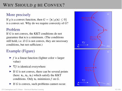
More preciselyIf g is a convex function, then G = {x | g(x) 0}is a convex set. Why do we require convexity of G?
ProblemIf G is not convex, the KKT conditions do notguarantee that x is a minimum. (The conditionsstill hold, i.e. if G is not convex, they are necessaryconditions, but not sufficient.)
Example (Figure)I f is a linear function (lighter color = larger
value)I rf is identical everywhereI If G is not convex, there can be several points
(here: x1, x2, x3) which satisfy the KKTconditions. Only x1 minimizes f on G.
I If G is convex, such problems cannot occur.
G
@Grf
x0
x1rg(x1)
x2
x3rg(x3)
G
@Grf
x0
x1rg(x1)
J.P. Cunningham and P. Orbanz · Statistical Machine Learning 92 / 436
INTERIOR POINT METHODS
Numerical methods for constrained problemsOnce we have transformed our problem using Lagrange multipliers, we still have tosolve a problem of the form
rf (x) = ��rg(x)
s.t. �g(x) = 0 and g(x) 0 and � � 0
numerically.
J.P. Cunningham and P. Orbanz · Statistical Machine Learning 93 / 436
BARRIER FUNCTIONS
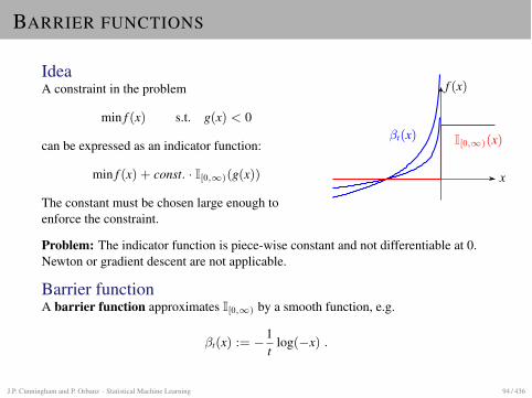
IdeaA constraint in the problem
min f (x) s.t. g(x) < 0
can be expressed as an indicator function:
min f (x) + const. · I[0,1)(g(x))
The constant must be chosen large enough toenforce the constraint.
x
f (x)
I[0,1)(x)�t(x)
Problem: The indicator function is piece-wise constant and not differentiable at 0.Newton or gradient descent are not applicable.
Barrier functionA barrier function approximates I[0,1) by a smooth function, e.g.
�t(x) := �1t
log(�x) .
J.P. Cunningham and P. Orbanz · Statistical Machine Learning 94 / 436
NEWTON FOR CONSTRAINED PROBLEMS
Interior point methodsWe can (approximately) solve
min f (x) s.t. gi(x) < 0 for i = 1, . . . , m
by solving
min f (x) +mX
i=1
�i,t(x) .
with one barrier function �i,t for each constraint gi.We do not have to adjust a multiplicative constant since �t(x)!1 as x% 0.
Constrained problems: General solution strategy
1. Convert constraints into solvable problem using Lagrange multipliers.
2. Convert constraints of transformed problem into barrier functions.
3. Apply numerical optimization (usually Newton’s method).
J.P. Cunningham and P. Orbanz · Statistical Machine Learning 95 / 436
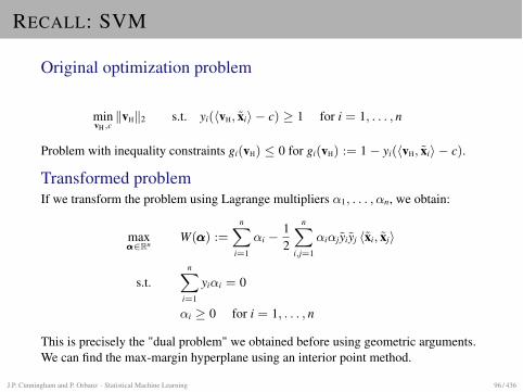
RECALL: SVM
Original optimization problem
minvH,ckvHk2 s.t. yi(hvH, xii � c) � 1 for i = 1, . . . , n
Problem with inequality constraints gi(vH) 0 for gi(vH) := 1� yi(hvH, xii � c).
Transformed problemIf we transform the problem using Lagrange multipliers ↵1, . . . ,↵n, we obtain:
max↵↵↵2Rn
W(↵↵↵) :=nX
i=1
↵i � 12
nX
i,j=1
↵i↵jyiyj hxi, xji
s.t.nX
i=1
yi↵i = 0
↵i � 0 for i = 1, . . . , n
This is precisely the "dual problem" we obtained before using geometric arguments.We can find the max-margin hyperplane using an interior point method.
J.P. Cunningham and P. Orbanz · Statistical Machine Learning 96 / 436
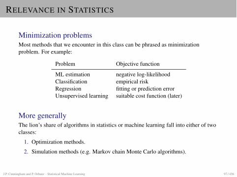
RELEVANCE IN STATISTICS
Minimization problemsMost methods that we encounter in this class can be phrased as minimizationproblem. For example:
Problem Objective function
ML estimation negative log-likelihoodClassification empirical riskRegression fitting or prediction errorUnsupervised learning suitable cost function (later)
More generallyThe lion’s share of algorithms in statistics or machine learning fall into either of twoclasses:
1. Optimization methods.
2. Simulation methods (e.g. Markov chain Monte Carlo algorithms).
J.P. Cunningham and P. Orbanz · Statistical Machine Learning 97 / 436
MULTIPLE CLASSES
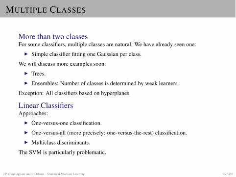
MULTIPLE CLASSES
More than two classesFor some classifiers, multiple classes are natural. We have already seen one:
I Simple classifier fitting one Gaussian per class.
We will discuss more examples soon:I Trees.I Ensembles: Number of classes is determined by weak learners.
Exception: All classifiers based on hyperplanes.
Linear ClassifiersApproaches:
I One-versus-one classification.I One-versus-all (more precisely: one-versus-the-rest) classification.I Multiclass discriminants.
The SVM is particularly problematic.
J.P. Cunningham and P. Orbanz · Statistical Machine Learning 99 / 436
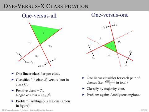
ONE-VERSUS-X CLASSIFICATION
One-versus-all
R1
R2
R3
?
C1
not C1
C2
not C2
I One linear classifier per class.I Classifies "in class k" versus "not in
class k".I Positive class = Ck.
Negative class = [j 6=kCj.I Problem: Ambiguous regions (green
in figure).
One-versus-one
R1
R2
R3
?C1
C2
C1
C3
C2
C3
I One linear classifier for each pair ofclasses (i.e. K(K�1)
2 in total).I Classify by majority vote.I Problem again: Ambiguous regions.
J.P. Cunningham and P. Orbanz · Statistical Machine Learning 100 / 436
MULTICLASS DISCRIMINANTS
Linear classifierI Recall: Decision rule is f (x) = sgn(hx, vHi � c)I Idea: Combine classifiers before computing sign. Define
gk(x) := hx, vki � ck
Multiclass linear discriminantI Use one classifier gk (as above) for each class k.I Trained e.g. as one-against-rest.I Classify according to
f (x) := arg maxk
{gk(x)}I If gk(x) is positive for several classes, a larger value of gk means that x lies
“further” into class k than into any other class j.I If gk(x) is negative for all k, the maximum means we classify x according to the
class represented by the closest hyperplane.
J.P. Cunningham and P. Orbanz · Statistical Machine Learning 101 / 436
SVMS AND MULTIPLE CLASSES
ProblemI Multiclass discriminant idea: Compare distances to hyperplanes.I Works if the orthogonal vectors vH determining the hyperplanes are normalized.I SVM: The K classifiers in the multiple discriminant approach are trained on
separate problems, so the individual lengths of vH computed by max-marginalgorithm are not comparable.
WorkaroundsI Often: One-against-all approaches.I It is possible to define a single optimization problem for all classes, but training
time scales quadratically in number of classes.
J.P. Cunningham and P. Orbanz · Statistical Machine Learning 102 / 436

KERNELS
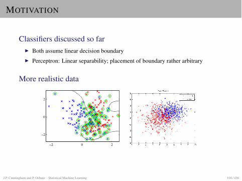
MOTIVATION
Classifiers discussed so farI Both assume linear decision boundaryI Perceptron: Linear separability; placement of boundary rather arbitrary
More realistic data
−2 0 2
−2
0
2
J.P. Cunningham and P. Orbanz · Statistical Machine Learning 104 / 436
MOTIVATION: KERNELS
IdeaI The SVM uses the scalar product hx, xii as a measure of similarity between x
and xi, and of distance to the hyperplane.I Since the scalar product is linear, the SVM is a linear method.I By using a nonlinear function instead, we can make the classifier nonlinear.
More preciselyI Scalar product can be regarded as a two-argument function
h . , . i : Rd ⇥ Rd ! R
I We will replace this function with a function k : Rd ⇥ Rd ! R and substitute
k(x, x0) for every occurrence of⌦
x, x0↵
in the SVM formulae.I Under certain conditions on k, all optimization/classification results for the
SVM still hold. Functions that satisfy these conditions are called kernelfunctions.
J.P. Cunningham and P. Orbanz · Statistical Machine Learning 105 / 436
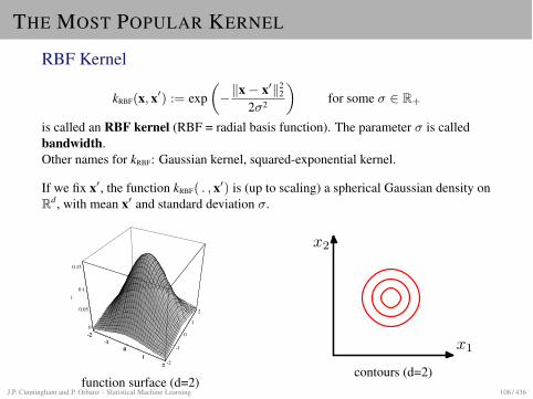
THE MOST POPULAR KERNEL
RBF Kernel
kRBF(x, x0) := exp✓
�kx� x0k22
2�2
◆
for some � 2 R+
is called an RBF kernel (RBF = radial basis function). The parameter � is calledbandwidth.Other names for kRBF: Gaussian kernel, squared-exponential kernel.
If we fix x0, the function kRBF( . , x0) is (up to scaling) a spherical Gaussian density onRd, with mean x0 and standard deviation �.
8 CHAPTER 4. NONPARAMETRIC TECHNIQUES
-2-1
0
1
2 -2
-1
0
1
2
0
0.05
0.1
0.15
-2-1
0
1
2
h = 1
δ(x)
-2-1
0
1
2 -2
-1
0
1
2
0
0.2
0.4
0.6
-2-1
0
1
2
h = .5
δ(x)
-2-1
0
1
2 -2
-1
0
1
2
0
1
2
3
4
-2-1
0
1
2
h = .2
δ(x)
Figure 4.3: Examples of two-dimensional circularly symmetric normal Parzen windows�(x/h) for three di�erent values of h. Note that because the �k(·) are normalized,di�erent vertical scales must be used to show their structure.
p(x)p(x) p(x)
Figure 4.4: Three Parzen-window density estimates based on the same set of fivesamples, using the window functions in Fig. 4.3. As before, the vertical axes havebeen scaled to show the structure of each function.
and
limn��
�2n(x) = 0. (18)
To prove convergence we must place conditions on the unknown density p(x), onthe window function �(u), and on the window width hn. In general, continuity ofp(·) at x is required, and the conditions imposed by Eqs. 12 & 13 are customarilyinvoked. With care, it can be shown that the following additional conditions assureconvergence (Problem 1):
supu
�(u) < � (19)
limkuk��
�(u)d�
i=1
ui = 0 (20)
function surface (d=2)
x1
x2
(c)contours (d=2)J.P. Cunningham and P. Orbanz · Statistical Machine Learning 106 / 436
CHOOSING A KERNEL
TheoryTo define a kernel:
I We have to define a function of two arguments and prove that it is a kernel.I This is done by checking a set of necessary and sufficient conditions known as
“Mercer’s theorem”.
PracticeThe data analyst does not define a kernel, but tries some well-known standard kernelsuntil one seems to work. Most common choices:
I The RBF kernel.I The "linear kernel" kSP(x, x0) = hx, x0i, i.e. the standard, linear SVM.
Once kernel is chosenI Classifier can be trained by solving the optimization problem using standard
software.I SVM software packages include implementations of most common kernels.
J.P. Cunningham and P. Orbanz · Statistical Machine Learning 107 / 436
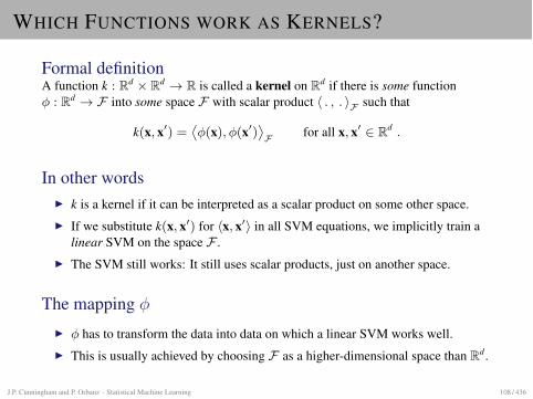
WHICH FUNCTIONS WORK AS KERNELS?
Formal definitionA function k : Rd ⇥ Rd ! R is called a kernel on Rd if there is some function� : Rd ! F into some space F with scalar product h . , . iF such that
k(x, x0) =⌦
�(x),�(x0)↵
F for all x, x0 2 Rd .
In other wordsI k is a kernel if it can be interpreted as a scalar product on some other space.I If we substitute k(x, x0) for hx, x0i in all SVM equations, we implicitly train a
linear SVM on the space F .I The SVM still works: It still uses scalar products, just on another space.
The mapping �I � has to transform the data into data on which a linear SVM works well.I This is usually achieved by choosing F as a higher-dimensional space than Rd.
J.P. Cunningham and P. Orbanz · Statistical Machine Learning 108 / 436
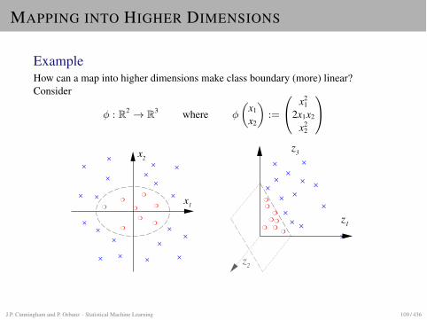
MAPPING INTO HIGHER DIMENSIONS
ExampleHow can a map into higher dimensions make class boundary (more) linear?Consider
� : R2 ! R3 where �
✓
x1
x2
◆
:=
0
@
x21
2x1x2
x22
1
A
Nonlinear Transformation in Kernel Space
�
�
�
�
�
�
�
�
�
�
�
�
�
�
�
�
�
�
��
�
�
�
�
�
�
�
�
!"
!#
��
��
�
�
�
�
�
�
�
�
�
�
�
�
�
�
�
�
�
$"
$%
�
$#
Machine Learning I : JoachimM.Buhmann 137/196
J.P. Cunningham and P. Orbanz · Statistical Machine Learning 109 / 436
MAPPING INTO HIGHER DIMENSIONS
ProblemIn previous example: We have to know what the data looks like to choose �!
SolutionI Choose high dimension h for F .I Choose components �i of �(x) = (�1(x), . . . ,�h(x)) as different nonlinear
mappings.I If two points differ in Rd, some of the nonlinear mappings will amplify
differences.
The RBF kernel is an extreme caseI The function kRBF can be shown to be a kernel, however:I F is infinite-dimensional for this kernel.
J.P. Cunningham and P. Orbanz · Statistical Machine Learning 110 / 436
DETERMINING WHETHER k IS A KERNEL
Mercer’s theoremA mathematical result called Mercer’s theorem states that, if the function k ispositive, i.e.
Z
Rd⇥Rdk(x, x0)f (x)f (x0)dxdx0 � 0
for all functions f , then it can be written as
k(x, x0) =1X
j=1
�j�j(x)�j(x0) .
The �j are functions Rd ! R and �i � 0. This means the (possibly infinite) vector�(x) = (
p�1�1(x),
p�2�2(x), . . .) is a feature map.
Kernel arithmeticVarious functions of kernels are again kernels: If k1 and k2 are kernels, then e.g.
k1 + k2 k1 · k2 const. · k1
are again kernels.
J.P. Cunningham and P. Orbanz · Statistical Machine Learning 111 / 436
THE KERNEL TRICK
Kernels in generalI Many linear machine learning and statistics algorithms can be "kernelized".I The only conditions are:
1. The algorithm uses a scalar product.2. In all relevant equations, the data (and all other elements of Rd) appear
only inside a scalar product.I This approach to making algorithms non-linear is known as the "kernel trick".
J.P. Cunningham and P. Orbanz · Statistical Machine Learning 112 / 436
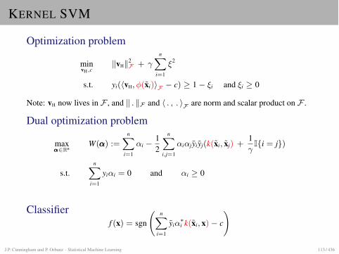
KERNEL SVM
Optimization problem
minvH,c
kvHk2F + �
nX
i=1
⇠2
s.t. yi(hvH,�(xi)iF � c) � 1� ⇠i and ⇠i � 0
Note: vH now lives in F , and k . kF and h . , . iF are norm and scalar product on F .
Dual optimization problem
max↵↵↵2Rn
W(↵↵↵) :=nX
i=1
↵i � 12
nX
i,j=1
↵i↵jyiyj(k(xi, xj) +1�I{i = j})
s.t.nX
i=1
yi↵i = 0 and ↵i � 0
Classifierf (x) = sgn
nX
i=1
yi↵⇤i k(xi, x)� c
!
J.P. Cunningham and P. Orbanz · Statistical Machine Learning 113 / 436
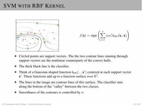
SVM WITH RBF KERNEL
f (x) = sign
nX
i=1
yi↵⇤i kRBF(xi, x)
!
I Circled points are support vectors. The the two contour lines running throughsupport vectors are the nonlinear counterparts of the convex hulls.
I The thick black line is the classifier.I Think of a Gaussian-shaped function kRBF( . , x0) centered at each support vector
x0. These functions add up to a function surface over R2.I The lines in the image are contour lines of this surface. The classifier runs
along the bottom of the "valley" between the two classes.I Smoothness of the contours is controlled by �
J.P. Cunningham and P. Orbanz · Statistical Machine Learning 114 / 436
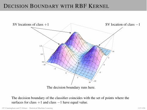
DECISION BOUNDARY WITH RBF KERNEL
-10
-5
0
5
10-10
-5
0
5
10
0.0
0.5
1.0
SV locations of class +1 SV location of class �1
The decision boundary runs here.
The decision boundary of the classifier coincides with the set of points where thesurfaces for class +1 and class �1 have equal value.
J.P. Cunningham and P. Orbanz · Statistical Machine Learning 115 / 436
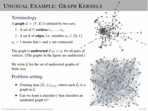
UNUSUAL EXAMPLE: GRAPH KERNELS
TerminologyA graph G = (V, E) is defined by two sets:
1. A set of V vertices v1, . . . , vm.
2. A set E of edges, i.e. variables eij 2 {0, 1}.
eij = 1 means that vi and vj are connected.
The graph is undirected if eij = eji for all pairs ofvertices. (The graphs in the figure are undirected.)
We write G for the set of undirected graphs offinite size.
Problem settingI Training data (Gi, yi)i2[n], where each Gi is a
graph in G.I Can we learn a classifier f that classifies an
unlabeled graph G?
J.P. Cunningham and P. Orbanz · Statistical Machine Learning 116 / 436
GRAPH-VALUED DATA
Example 1: Social NetworksI Each vertex vj is a user.I eij = 1 indicates that users i and j are "friends".
This data is graph-valued, but the data set typically consists of a single, very largegraph.
Example 2: BiologyThere are dozens of types of graph-valued data in biology. One example isprotein-protein interaction data:
I Each vertex vj is a protein.I eij = 1 indicates that proteins i and j interact in the given system.
(The graph on the previous slide shows such a data set.)
Graph kernels are designed for problems where we observe a set of graphs.
J.P. Cunningham and P. Orbanz · Statistical Machine Learning 117 / 436
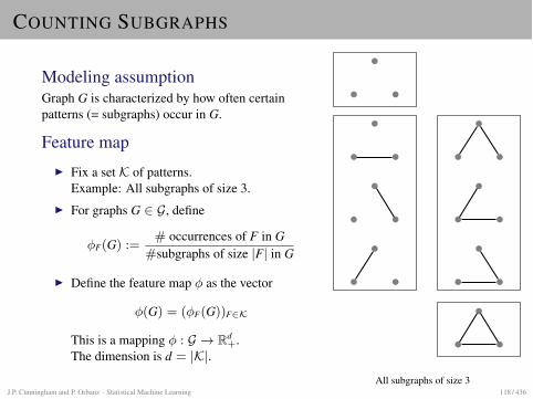
COUNTING SUBGRAPHS
Modeling assumptionGraph G is characterized by how often certainpatterns (= subgraphs) occur in G.
Feature mapI Fix a set K of patterns.
Example: All subgraphs of size 3.I For graphs G 2 G, define
�F(G) :=# occurrences of F in G
#subgraphs of size |F| in G
I Define the feature map � as the vector
�(G) = (�F(G))F2K
This is a mapping � : G ! Rd+.
The dimension is d = |K|.All subgraphs of size 3
J.P. Cunningham and P. Orbanz · Statistical Machine Learning 118 / 436
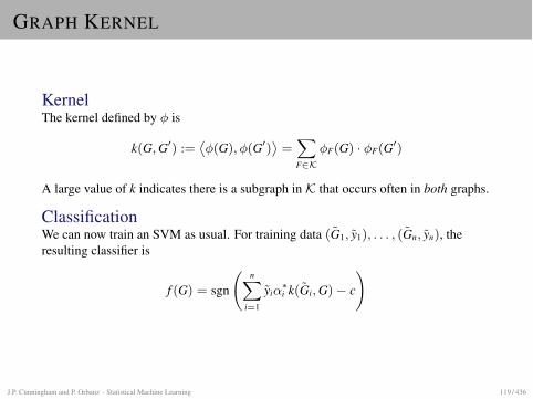
GRAPH KERNEL
KernelThe kernel defined by � is
k(G, G0) :=⌦
�(G),�(G0)↵
=X
F2K�F(G) · �F(G0)
A large value of k indicates there is a subgraph in K that occurs often in both graphs.
ClassificationWe can now train an SVM as usual. For training data (G1, y1), . . . , (Gn, yn), theresulting classifier is
f (G) = sgn
nX
i=1
yi↵⇤i k(Gi, G)� c
!
J.P. Cunningham and P. Orbanz · Statistical Machine Learning 119 / 436
REMARKS
Other graph kernelsI There are various other ways to define graph kernels. For example, k could
compare G and G0 in terms of the probability that a random walk on G and arandom walk on G0 take the same path. (Such kernels are called random walkkernels.)
I Each choice of kernel emphasizes a different property in terms of which thegraphs are compared.
More generally: Kernels for non-Euclidean dataI We have used the kernel to transform non-Euclidean data (graphs) so that it fits
into our classification framework.I There are other, similar methods, e.g. string kernels.I Note that we have not used the kernel for implicit representation, but rather
compute � explicitly.
J.P. Cunningham and P. Orbanz · Statistical Machine Learning 120 / 436
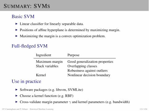
SUMMARY: SVMS
Basic SVMI Linear classifier for linearly separable data.I Positions of affine hyperplane is determined by maximizing margin.I Maximizing the margin is a convex optimization problem.
Full-fledged SVM
Ingredient Purpose
Maximum margin Good generalization propertiesSlack variables Overlapping classes
Robustness against outliersKernel Nonlinear decision boundary
Use in practiceI Software packages (e.g. libsvm, SVMLite)I Choose a kernel function (e.g. RBF)I Cross-validate margin parameter � and kernel parameters (e.g. bandwidth)
J.P. Cunningham and P. Orbanz · Statistical Machine Learning 121 / 436

MODEL SELECTION AND CROSSVALIDATION
CROSS VALIDATION
ObjectiveI Cross validation is a method which tries to select the best model from a given
set of models.I Assumption: Quality measure is predictive performance.I "Set of models" can simply mean "set of different parameter values".
TerminologyThe problem of choosing a good model is called model selection.
J.P. Cunningham and P. Orbanz · Statistical Machine Learning 123 / 436
SPECIFICALLY: SVM
Model selection problem for SVMI The SVM is a family of models indexed by the margin parameter � and the
kernel parameter(s) �.I Our goal is to find a value of (�,�) for which we can expect small
generalization error.
Naive approachI We could include (�,�) into the optimization problem, i.e. train by minimizing
over ↵ and (�,�).I This leads to a phenomenon called overfitting: The classifier adapts too closely
to specific properties of the training data, rather than the underlying distribution.
J.P. Cunningham and P. Orbanz · Statistical Machine Learning 124 / 436
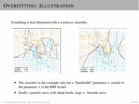
OVERFITTING: ILLUSTRATION
Overfitting is best illustrated with a nonlinear classifier.
I The classifier in this example only has a "bandwidth" parameter �, similar tothe parameter � of the RBF kernel.
I Small � permits curve with sharp bends; large �: Smooth curve.
J.P. Cunningham and P. Orbanz · Statistical Machine Learning 125 / 436
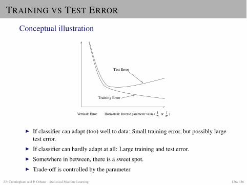
TRAINING VS TEST ERROR
Conceptual illustration
Copyright Cambridge University Press 2003. On-screen viewing permitted. Printing not permitted. http://www.cambridge.org/0521642981You can buy this book for 30 pounds or $50. See http://www.inference.phy.cam.ac.uk/mackay/itila/ for links.
44.4: Benefits of the Bayesian approach to supervised feedforward neural networks 531
(a)
(b)
(c)
(d)Model Control Parameters
Training Error
Test Error
(e)Model Control Parameters
Log Probability(Training Data | Control Parameters)
Figure 44.5. Optimization ofmodel complexity. Panels (a–c)show a radial basis function modelinterpolating a simple data setwith one input variable and oneoutput variable. As theregularization constant is variedto increase the complexity of themodel (from (a) to (c)), theinterpolant is able to fit thetraining data increasingly well,but beyond a certain point thegeneralization ability (test error)of the model deteriorates.Probability theory allows us tooptimize the control parameterswithout needing a test set.
The overfitting problem can be solved by using a Bayesian approach tocontrol model complexity.
If we give a probabilistic interpretation to the model, then we can evaluatethe evidence for alternative values of the control parameters. As was explainedin Chapter 28, over-complex models turn out to be less probable, and theevidence P (Data |Control Parameters) can be used as an objective functionfor optimization of model control parameters (figure 44.5e). The setting of �that maximizes the evidence is displayed in figure 44.5b.
Bayesian optimization of model control parameters has four important ad-vantages. (1) No ‘test set’ or ‘validation set’ is involved, so all available trainingdata can be devoted to both model fitting and model comparison. (2) Reg-ularization constants can be optimized on-line, i.e., simultaneously with theoptimization of ordinary model parameters. (3) The Bayesian objective func-tion is not noisy, in contrast to a cross-validation measure. (4) The gradient ofthe evidence with respect to the control parameters can be evaluated, makingit possible to simultaneously optimize a large number of control parameters.
Probabilistic modelling also handles uncertainty in a natural manner. Ito�ers a unique prescription, marginalization, for incorporating uncertaintyabout parameters into predictions; this procedure yields better predictions, aswe saw in Chapter 41. Figure 44.6 shows error bars on the predictions of atrained neural network.
Figure 44.6. Error bars on thepredictions of a trained regressionnetwork. The solid line gives thepredictions of the best-fitparameters of a multilayerperceptron trained on the datapoints. The error bars (dottedlines) are those produced by theuncertainty of the parameters w.Notice that the error bars becomelarger where the data are sparse.
Implementation of Bayesian inference
As was mentioned in Chapter 41, Bayesian inference for multilayer networksmay be implemented by Monte Carlo sampling, or by deterministic methodsemploying Gaussian approximations (Neal, 1996; MacKay, 1992c).
Vertical: Error Horizontal: Inverse parameter value ( 1�
or 1�
)
I If classifier can adapt (too) well to data: Small training error, but possibly largetest error.
I If classifier can hardly adapt at all: Large training and test error.I Somewhere in between, there is a sweet spot.I Trade-off is controlled by the parameter.
J.P. Cunningham and P. Orbanz · Statistical Machine Learning 126 / 436
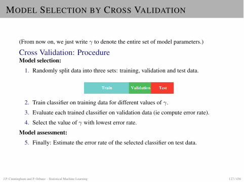
MODEL SELECTION BY CROSS VALIDATION
(From now on, we just write � to denote the entire set of model parameters.)
Cross Validation: ProcedureModel selection:
1. Randomly split data into three sets: training, validation and test data.
2. Train classifier on training data for different values of �.
3. Evaluate each trained classifier on validation data (ie compute error rate).
4. Select the value of � with lowest error rate.
Model assessment:5. Finally: Estimate the error rate of the selected classifier on test data.
J.P. Cunningham and P. Orbanz · Statistical Machine Learning 127 / 436
INTERPRETATION
MeaningI The quality measure by which we are comparing different classifiers f ( . ; �)
(for different parameter values �) is the risk
R(f ( . ; �)) = E[L(y, f (x; �))] .
I Since we do not know the true risk, we estimate it from data as R(f ( . ; �)).
Importance of model assessment stepI We always have to assume: Classifier is better adapted to any data used to
select it than to actual data distribution.I Model selection: Adapts classifier to both training and validation data.I If we estimate error rate on this data, we will in general underestimate it.
J.P. Cunningham and P. Orbanz · Statistical Machine Learning 128 / 436
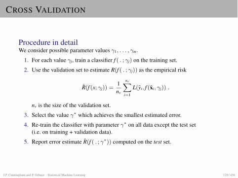
CROSS VALIDATION
Procedure in detailWe consider possible parameter values �1, . . . , �m.
1. For each value �j, train a classifier f ( . ; �j) on the training set.
2. Use the validation set to estimate R(f ( . ; �j)) as the empirical risk
R(f (x; �j)) =1nv
nvX
i=1
L(yi, f (xi, �j)) .
nv is the size of the validation set.
3. Select the value �⇤ which achieves the smallest estimated error.
4. Re-train the classifier with parameter �⇤ on all data except the test set(i.e. on training + validation data).
5. Report error estimate R(f ( . ; �⇤)) computed on the test set.
J.P. Cunningham and P. Orbanz · Statistical Machine Learning 129 / 436
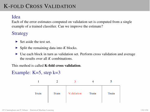
K-FOLD CROSS VALIDATION
IdeaEach of the error estimates computed on validation set is computed from a singleexample of a trained classifier. Can we improve the estimate?
StrategyI Set aside the test set.I Split the remaining data into K blocks.I Use each block in turn as validation set. Perform cross validation and average
the results over all K combinations.
This method is called K-fold cross validation.
Example: K=5, step k=3
J.P. Cunningham and P. Orbanz · Statistical Machine Learning 130 / 436
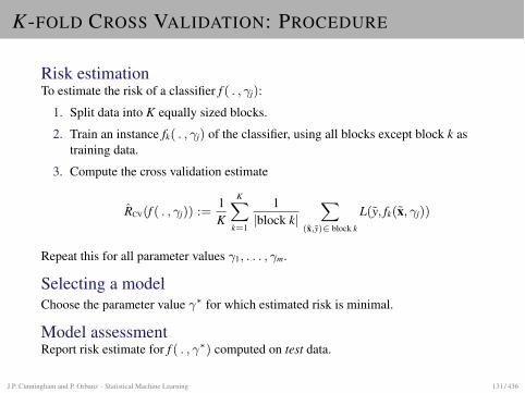
K-FOLD CROSS VALIDATION: PROCEDURE
Risk estimationTo estimate the risk of a classifier f ( . , �j):
1. Split data into K equally sized blocks.
2. Train an instance fk( . , �j) of the classifier, using all blocks except block k astraining data.
3. Compute the cross validation estimate
RCV(f ( . , �j)) :=1K
KX
k=1
1|block k|
X
(x,y)2 block k
L(y, fk(x, �j))
Repeat this for all parameter values �1, . . . , �m.
Selecting a modelChoose the parameter value �⇤ for which estimated risk is minimal.
Model assessmentReport risk estimate for f ( . , �⇤) computed on test data.
J.P. Cunningham and P. Orbanz · Statistical Machine Learning 131 / 436
HOW TO CHOOSE K?
Extremal casesI K = n, called leave one out cross validation (loocv)I K = 2
An often-cited problem with loocv is that we have to train many (= n) classifiers, butthere is also a deeper problem.
Argument 1: K should be small, e.g. K = 2I Unless we have a lot of data, variance between two distinct training sets may be
considerable.I Important concept: By removing substantial parts of the sample in turn and at
random, we can simulate this variance.I By removing a single point (loocv), we cannot make this variance visible.
J.P. Cunningham and P. Orbanz · Statistical Machine Learning 132 / 436
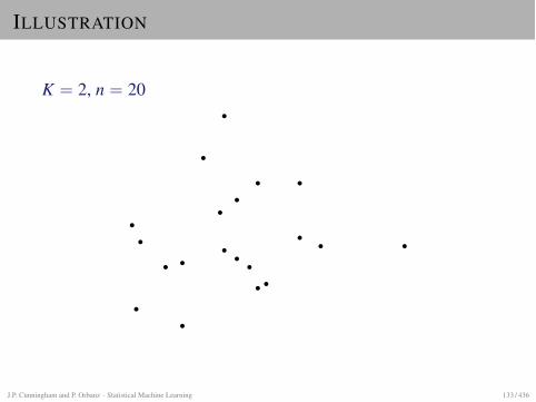
ILLUSTRATION
K = 2, n = 20
J.P. Cunningham and P. Orbanz · Statistical Machine Learning 133 / 436
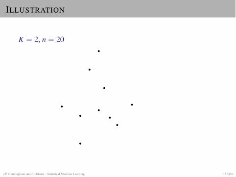
ILLUSTRATION
K = 2, n = 20
J.P. Cunningham and P. Orbanz · Statistical Machine Learning 133 / 436
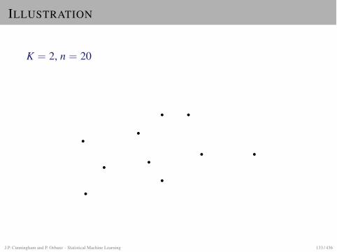
ILLUSTRATION
K = 2, n = 20
J.P. Cunningham and P. Orbanz · Statistical Machine Learning 133 / 436
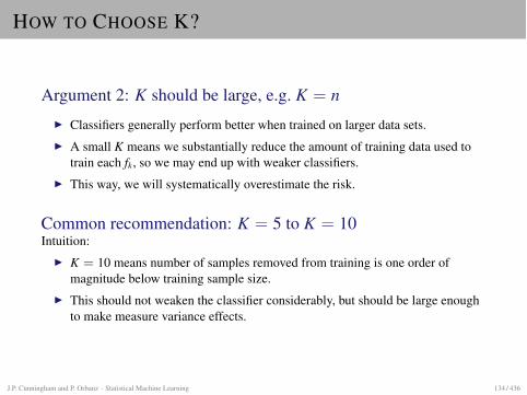
HOW TO CHOOSE K?
Argument 2: K should be large, e.g. K = nI Classifiers generally perform better when trained on larger data sets.I A small K means we substantially reduce the amount of training data used to
train each fk, so we may end up with weaker classifiers.I This way, we will systematically overestimate the risk.
Common recommendation: K = 5 to K = 10Intuition:
I K = 10 means number of samples removed from training is one order ofmagnitude below training sample size.
I This should not weaken the classifier considerably, but should be large enoughto make measure variance effects.
J.P. Cunningham and P. Orbanz · Statistical Machine Learning 134 / 436
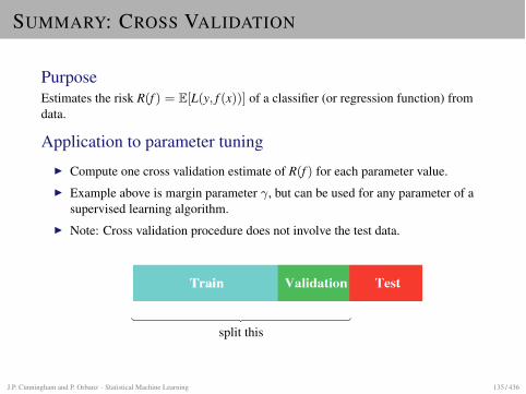
SUMMARY: CROSS VALIDATION
PurposeEstimates the risk R(f ) = E[L(y, f (x))] of a classifier (or regression function) fromdata.
Application to parameter tuningI Compute one cross validation estimate of R(f ) for each parameter value.I Example above is margin parameter �, but can be used for any parameter of a
supervised learning algorithm.I Note: Cross validation procedure does not involve the test data.
split this
J.P. Cunningham and P. Orbanz · Statistical Machine Learning 135 / 436
TREE CLASSIFIERS
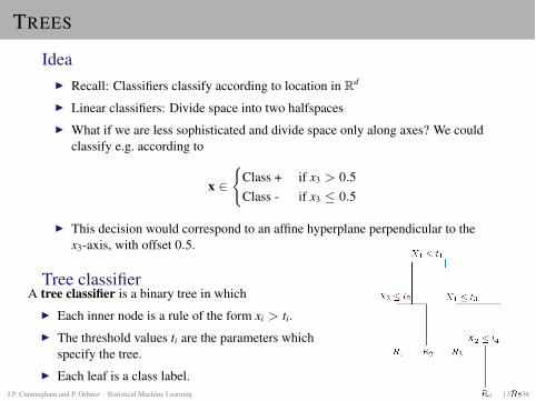
TREES
IdeaI Recall: Classifiers classify according to location in Rd
I Linear classifiers: Divide space into two halfspacesI What if we are less sophisticated and divide space only along axes? We could
classify e.g. according to
x 2(
Class + if x3 > 0.5Class - if x3 0.5
I This decision would correspond to an affine hyperplane perpendicular to thex3-axis, with offset 0.5.
Tree classifierA tree classifier is a binary tree in which
I Each inner node is a rule of the form xi > ti.I The threshold values ti are the parameters which
specify the tree.I Each leaf is a class label.
J.P. Cunningham and P. Orbanz · Statistical Machine Learning 137 / 436
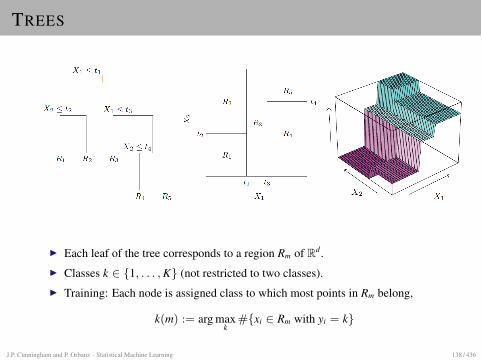
TREES
I Each leaf of the tree corresponds to a region Rm of Rd.I Classes k 2 {1, . . . , K} (not restricted to two classes).I Training: Each node is assigned class to which most points in Rm belong,
k(m) := arg maxk
#{xi 2 Rm with yi = k}
J.P. Cunningham and P. Orbanz · Statistical Machine Learning 138 / 436
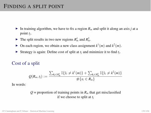
FINDING A SPLIT POINT
I In training algorithm, we have to fix a region Rm and split it along an axis j at apoint tj.
I The split results in two new regions R1m and R2
m.I On each region, we obtain a new class assignment k1(m) and k2(m).I Strategy is again: Define cost of split at tj and minimize it to find tj.
Cost of a split
Q(Rm, tj) :=
P
xi2R1mI{yi 6= k1(m)} +
P
xi2R2mI{yi 6= k2(m)}
#{xi 2 Rm}In words:
Q = proportion of training points in Rm that get misclassifiedif we choose to split at tj
J.P. Cunningham and P. Orbanz · Statistical Machine Learning 139 / 436
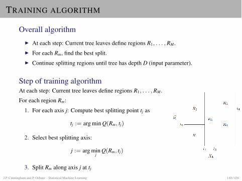
TRAINING ALGORITHM
Overall algorithmI At each step: Current tree leaves define regions R1, . . . , RM .I For each Rm, find the best split.I Continue splitting regions until tree has depth D (input parameter).
Step of training algorithmAt each step: Current tree leaves define regions R1, . . . , RM .
For each region Rm:
1. For each axis j: Compute best splitting point tj as
tj := arg min Q(Rm, tj)
2. Select best splitting axis:
j := arg minj
Q(Rm, tj)
3. Split Rm along axis j at tj
J.P. Cunningham and P. Orbanz · Statistical Machine Learning 140 / 436
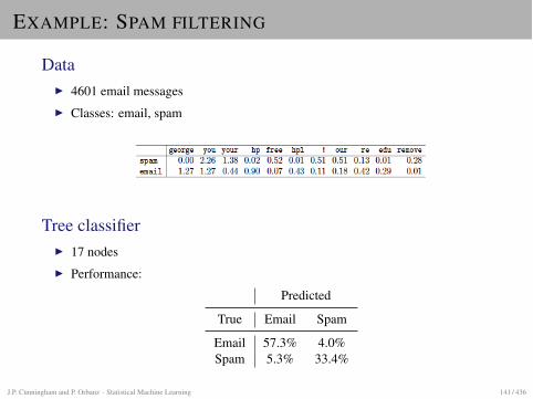
EXAMPLE: SPAM FILTERING
DataI 4601 email messagesI Classes: email, spam
Tree classifierI 17 nodesI Performance:
Predicted
True Email Spam
Email 57.3% 4.0%Spam 5.3% 33.4%
J.P. Cunningham and P. Orbanz · Statistical Machine Learning 141 / 436
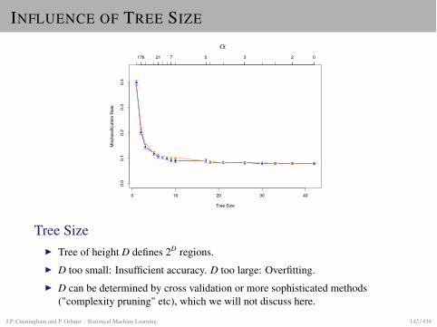
INFLUENCE OF TREE SIZEElements of Statistical Learning (2nd Ed.) c�Hastie, Tibshirani & Friedman 2009 Chap 9
0 10 20 30 40
0.0
0.1
0.2
0.3
0.4
Tree Size
Mis
clas
sific
atio
n R
ate
176 21 7 5 3 2 0
↵
FIGURE 9.4. Results for spam example. The bluecurve is the 10-fold cross-validation estimate of mis-classification rate as a function of tree size, with stan-dard error bars. The minimum occurs at a tree sizewith about 17 terminal nodes (using the “one-standard--error” rule). The orange curve is the test error, whichtracks the CV error quite closely. The cross-validationis indexed by values of ↵, shown above. The tree sizesshown below refer to |T↵|, the size of the original treeindexed by ↵.
Tree SizeI Tree of height D defines 2D regions.I D too small: Insufficient accuracy. D too large: Overfitting.I D can be determined by cross validation or more sophisticated methods
("complexity pruning" etc), which we will not discuss here.
J.P. Cunningham and P. Orbanz · Statistical Machine Learning 142 / 436
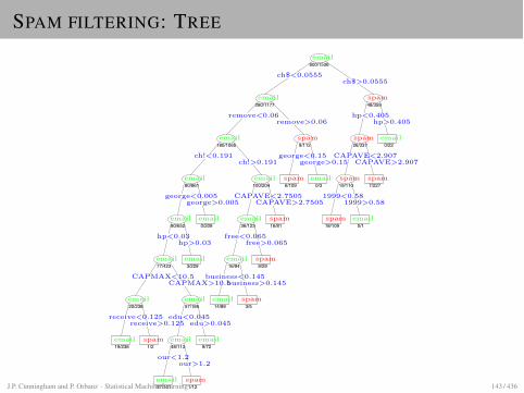
SPAM FILTERING: TREEElements of Statistical Learning (2nd Ed.) c�Hastie, Tibshirani & Friedman 2009 Chap 9
600/1536
280/1177
180/1065
80/861
80/652
77/423
20/238
19/236 1/2
57/185
48/113
37/101 1/12
9/72
3/229
0/209
100/204
36/123
16/94
14/89 3/5
9/29
16/81
9/112
6/109 0/3
48/359
26/337
19/110
18/109 0/1
7/227
0/22
spam
spam
spam
spam
spam
spam
spam
spam
spam
spam
spam
spam
ch$<0.0555
remove<0.06
ch!<0.191
george<0.005
hp<0.03
CAPMAX<10.5
receive<0.125 edu<0.045
our<1.2
CAPAVE<2.7505
free<0.065
business<0.145
george<0.15
hp<0.405
CAPAVE<2.907
1999<0.58
ch$>0.0555
remove>0.06
ch!>0.191
george>0.005
hp>0.03
CAPMAX>10.5
receive>0.125 edu>0.045
our>1.2
CAPAVE>2.7505
free>0.065
business>0.145
george>0.15
hp>0.405
CAPAVE>2.907
1999>0.58
FIGURE 9.5. The pruned tree for the spam example.The split variables are shown in blue on the branches,and the classification is shown in every node.The num-bers under the terminal nodes indicate misclassificationrates on the test data.
J.P. Cunningham and P. Orbanz · Statistical Machine Learning 143 / 436
DECISION STUMPS
I The simplest possible tree classifier is a tree of depth 1. Such a classifier iscalled a decision stump.
I A decision stump is parameterized by a pair (j, tj) of an axis j and a splittingpoint tj.
I Splits Rd into two regions.I Decision boundary is an affine hyperplane which is perpendicular to axis j and
intersects the axis at tj.I Often used in Boosting algorithms and other ensemble methods.
J.P. Cunningham and P. Orbanz · Statistical Machine Learning 144 / 436

BOOSTING
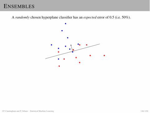
ENSEMBLES
A randomly chosen hyperplane classifier has an expected error of 0.5 (i.e. 50%).
I Many random hyperplanes combined by majority vote: Still 0.5.I A single classifier slightly better than random: 0.5 + ".I What if we use m such classifiers and take a majority vote?
J.P. Cunningham and P. Orbanz · Statistical Machine Learning 146 / 436
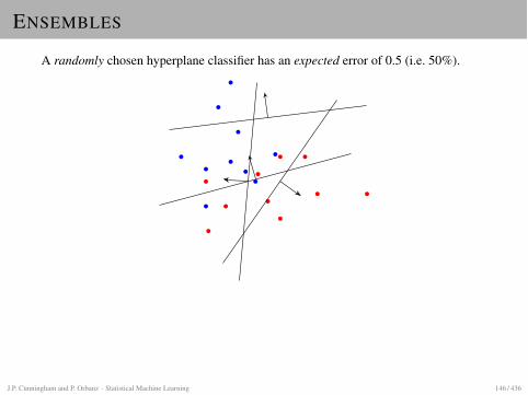
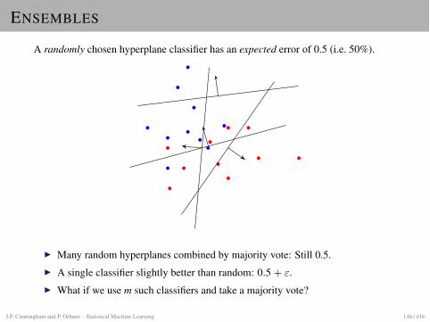
VOTING
Decision by majority voteI m individuals (or classifiers) take a vote. m is an odd number.I They decide between two choices; one is correct, one is wrong.I After everyone has voted, a decision is made by simple majority.
Note: For two-class classifiers f1, . . . , fm (with output ±1):
majority vote = sgn⇣
mX
j=1
fj
⌘
AssumptionsBefore we discuss ensembles, we try to convince ourselves that voting can bebeneficial. We make some simplifying assumptions:
I Each individual makes the right choice with probability p 2 [0, 1].I The votes are independent, i.e. stochastically independent when regarded as
random outcomes.
J.P. Cunningham and P. Orbanz · Statistical Machine Learning 147 / 436
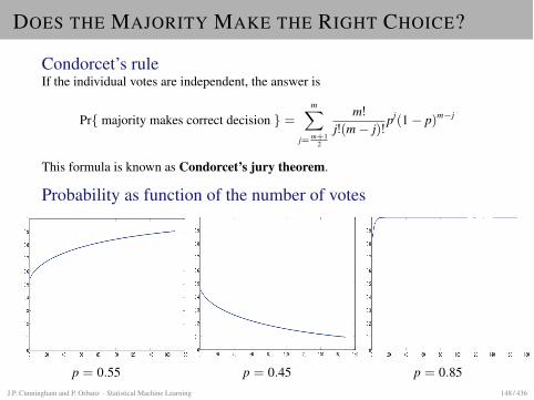
DOES THE MAJORITY MAKE THE RIGHT CHOICE?
Condorcet’s ruleIf the individual votes are independent, the answer is
Pr{ majority makes correct decision } =mX
j= m+12
m!j!(m� j)!
pj(1� p)m�j
This formula is known as Condorcet’s jury theorem.
Probability as function of the number of votes
p = 0.55 p = 0.45 p = 0.85J.P. Cunningham and P. Orbanz · Statistical Machine Learning 148 / 436
ENSEMBLE METHODS
TerminologyI An ensemble method makes a prediction by combining the predictions of
many classifiers into a single vote.I The individual classifiers are usually required to perform only slightly better
than random. For two classes, this means slightly more than 50% of the data areclassified correctly. Such a classifier is called a weak learner.
StrategyI We have seen above that if the weak learners are random and independent, the
prediction accuracy of the majority vote will increase with the number of weaklearners.
I Since the weak learners all have to be trained on the training data, producingrandom, independent weak learners is difficult.
I Different ensemble methods (e.g. Boosting, Bagging, etc) use differentstrategies to train and combine weak learners that behave relativelyindependently.
J.P. Cunningham and P. Orbanz · Statistical Machine Learning 149 / 436
METHODS WE WILL DISCUSS
BoostingI After training each weak learner, data is modified using weights.I Deterministic algorithm.
BaggingEach weak learner is trained on a random subset of the data.
Random forestsI Bagging with tree classifiers as weak learners.I Uses an additional step to remove dimensions in Rd that carry little information.
J.P. Cunningham and P. Orbanz · Statistical Machine Learning 150 / 436
BOOSTING
BoostingI Arguably the most popular (and historically the first) ensemble method.I Weak learners can be trees (decision stumps are popular), Perceptrons, etc.I Requirement: It must be possible to train the weak learner on a weighted
training set.
OverviewI Boosting adds weak learners one at a time.I A weight value is assigned to each training point.I At each step, data points which are currently classified correctly are weighted
down (i.e. the weight is smaller the more of the weak learners already trainedclassify the point correctly).
I The next weak learner is trained on the weighted data set: In the training step,the error contributions of misclassified points are multiplied by the weights ofthe points.
I Roughly speaking, each weak learner tries to get those points right which arecurrently not classified correctly.
J.P. Cunningham and P. Orbanz · Statistical Machine Learning 151 / 436
TRAINING WITH WEIGHTS
Example: Decision stumpA decision stump classifier for two classes is defined by
f ( x | j, t ) :=
(
+1 x(j) > t�1 otherwise
where j 2 {1, . . . , d} indexes an axis in Rd.
Weighted dataI Training data (x1, y1), . . . , (xn, yn).I With each data point xi we associate a weight wi � 0.
Training on weighted dataMinimize the weighted misclassifcation error:
(j⇤, t⇤) := arg minj,t
Pni=1 wiI{yi 6= f (xi|j, t)}
Pni=1 wi
J.P. Cunningham and P. Orbanz · Statistical Machine Learning 152 / 436
ADABOOST
InputI Training data (x1, y1), . . . , (xn, yn)
I Algorithm parameter: Number M of weak learners
Training algorithm
1. Initialize the observation weights wi = 1n for i = 1, 2, ..., n.
2. For m = 1 to M:
2.1 Fit a classifier gm(x) to the training data using weights wi.2.2 Compute
errm :=
Pni=1 wiI{yi 6= gm(xi)}
P
i wi
2.3 Compute ↵m = log( 1�errmerrm
)2.4 Set wi wi · exp(↵m · I(yi 6= gm(xi))) for i = 1, 2, ..., n.
3. Output
f (x) := sign
MX
m=1
↵mgm(x)
!
J.P. Cunningham and P. Orbanz · Statistical Machine Learning 153 / 436
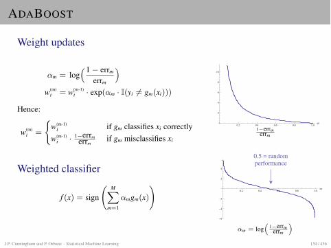
ADABOOST
Weight updates
↵m = log⇣1� errm
errm
⌘
w(m)i = w(m-1)
i · exp(↵m · I(yi 6= gm(xi)))
Hence:
w(m)i =
(
w(m-1)i if gm classifies xi correctly
w(m-1)i · 1�errm
errmif gm misclassifies xi
0.2 0.4 0.6 0.8 1.0err
2
4
6
8
10
1�errmerrm
Weighted classifier
f (x) = sign
MX
m=1
↵mgm(x)
!
0.2 0.4 0.6 0.8 1.0err
-6
-4
-2
2
4performance0.5 = random
↵m = log⇣
1�errmerrm
⌘
J.P. Cunningham and P. Orbanz · Statistical Machine Learning 154 / 436
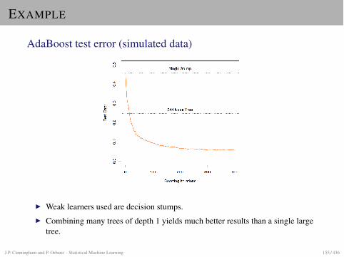
EXAMPLE
AdaBoost test error (simulated data)
I Weak learners used are decision stumps.I Combining many trees of depth 1 yields much better results than a single large
tree.
J.P. Cunningham and P. Orbanz · Statistical Machine Learning 155 / 436
BOOSTING: PROPERTIES
PropertiesI AdaBoost is one of most widely used classifiers in applications.I Decision boundary is non-linear.I Can handle multiple classes if weak learner can do so.
Test vs training errorI Most training algorithms (e.g. Perceptron) terminate when training error
reaches minimum.I AdaBoost weights keep changing even if training error is minimal.I Interestingly, the test error typically keeps decreasing even after training error
has stabilized at minimal value.I It can be shown that this behavior can be interpreted in terms of a margin:
I Adding additional classifiers slowly pushes overall f towards amaximum-margin solution.
I May not improve training error, but improves generalization properties.I This does not imply that boosting magically outperforms SVMs, only that
minimal training error does not imply an optimal solution.J.P. Cunningham and P. Orbanz · Statistical Machine Learning 156 / 436
BOOSTING AND FEATURE SELECTION
AdaBoost with Decision StumpsI Once AdaBoost has trained a classifier, the weights ↵m tell us which of the
weak learners are important (i.e. classify large subsets of the data well).I If we use Decision Stumps as weak learners, each fm corresponds to one axis.I From the weights ↵, we can read off which axis are important to separate the
classes.
TerminologyThe dimensions of Rd (= the measurements) are often called the features of the data.The process of selecting features which contain important information for theproblem is called feature selection. Thus, AdaBoost with Decision Stumps can beused to perform feature selection.
J.P. Cunningham and P. Orbanz · Statistical Machine Learning 157 / 436
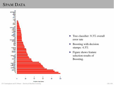
SPAM DATA
I Tree classifier: 9.3% overallerror rate
I Boosting with decisionstumps: 4.5%
I Figure shows featureselection results ofBoosting.
J.P. Cunningham and P. Orbanz · Statistical Machine Learning 158 / 436
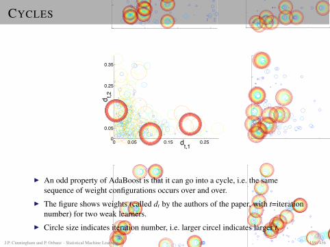
CYCLES
RUDIN, DAUBECHIES, AND SCHAPIRE
a) b)
0 0.1 0.2 0.30
0.1
0.25
0.35
dt,1
d t,2
0 0.1 0.3 0.4 0.50
0.05
0.15
0.2
0.25
dt,1
d t,2
c) d)
0 0.05 0.15 0.250
0.05
0.25
0.35
dt,1
d t,2
0 0.1 0.2 0.30
0.1
0.3
0.4
dt,1
d t,2
e) f)
0 0.1 0.35 0.450
0.1
0.4
0.5
dt,1
d t,2
0 0.05 0.15 0.20
0.05
0.15
0.2
dt,11
d t,12
Figure 6: Examples of cycles from randomly generated matricesM. An image ofM for each plotappears in Figure 7. These plots show a projection onto the first two components of Ada-Boost’s weight vector, e.g., the axes might be dt,1 vs. dt,2. Smaller circles indicate earlieriterations, and larger circles indicate later iterations. For (a), (d) and (f), 400 iterationswere plotted, and for (b) and (e), 300 iterations were plotted. Plot (c) shows 5500 itera-tions, but only every 20th iteration was plotted. This case took longer to converge, andconverged to a simple 3-cycle.
1574
I An odd property of AdaBoost is that it can go into a cycle, i.e. the samesequence of weight configurations occurs over and over.
I The figure shows weights (called dt by the authors of the paper, with t=iterationnumber) for two weak learners.
I Circle size indicates iteration number, i.e. larger circel indicates larger t.
J.P. Cunningham and P. Orbanz · Statistical Machine Learning 159 / 436
APPLICATION: FACE DETECTION
FACE DETECTION
Searching for faces in imagesTwo problems:
I Face detection Find locations of all faces in image. Two classes.I Face recognition Identify a person depicted in an image by recognizing the
face. One class per person to be identified + background class (all other people).
Face detection can be regarded as a solved problem. Face recognition is not solved.
Face detection as a classification problemI Divide image into patches.I Classify each patch as "face" or "not face"
J.P. Cunningham and P. Orbanz · Statistical Machine Learning 161 / 436
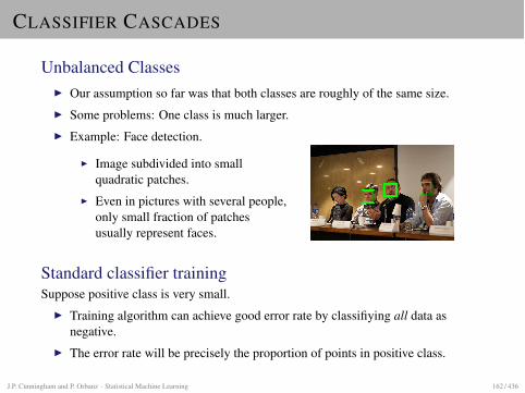
CLASSIFIER CASCADES
Unbalanced ClassesI Our assumption so far was that both classes are roughly of the same size.I Some problems: One class is much larger.I Example: Face detection.
I Image subdivided into smallquadratic patches.
I Even in pictures with several people,only small fraction of patchesusually represent faces.
Standard classifier trainingSuppose positive class is very small.
I Training algorithm can achieve good error rate by classifiying all data asnegative.
I The error rate will be precisely the proportion of points in positive class.
J.P. Cunningham and P. Orbanz · Statistical Machine Learning 162 / 436
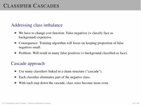
CLASSIFIER CASCADES
Addressing class imbalanceI We have to change cost function: False negatives (= classify face as
background) expensive.I Consequence: Training algorithm will focus on keeping proportion of false
negatives small.I Problem: Will result in many false positives (= background classified as face).
Cascade approachI Use many classifiers linked in a chain structure ("cascade").I Each classifier eliminates part of the negative class.I With each step down the cascade, class sizes become more even.
J.P. Cunningham and P. Orbanz · Statistical Machine Learning 163 / 436
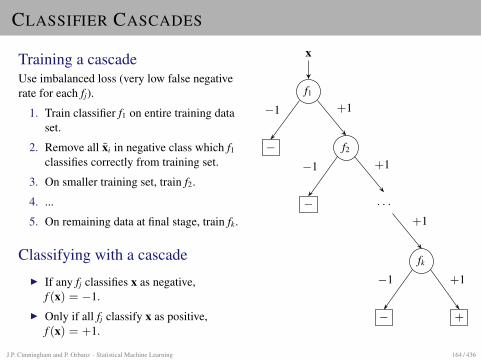
CLASSIFIER CASCADES
Training a cascadeUse imbalanced loss (very low false negativerate for each fj).
1. Train classifier f1 on entire training dataset.
2. Remove all xi in negative class which f1
classifies correctly from training set.
3. On smaller training set, train f2.
4. ...
5. On remaining data at final stage, train fk.
Classifying with a cascadeI If any fj classifies x as negative,
f (x) = �1.I Only if all fj classify x as positive,
f (x) = +1.
x
f1
f2
. . .
fk
�
�
� +
+1
+1
+1
�1
�1
�1 +1
J.P. Cunningham and P. Orbanz · Statistical Machine Learning 164 / 436
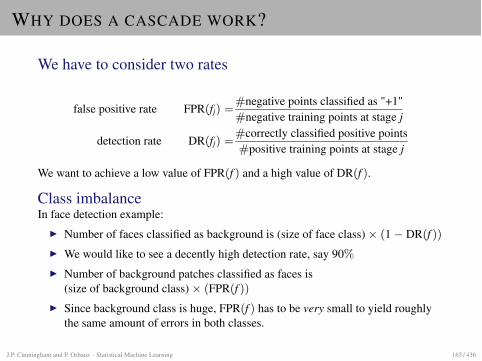
WHY DOES A CASCADE WORK?
We have to consider two rates
false positive rate FPR(fj) =#negative points classified as "+1"#negative training points at stage j
detection rate DR(fj) =#correctly classified positive points#positive training points at stage j
We want to achieve a low value of FPR(f ) and a high value of DR(f ).
Class imbalanceIn face detection example:
I Number of faces classified as background is (size of face class)⇥ (1� DR(f ))I We would like to see a decently high detection rate, say 90%
I Number of background patches classified as faces is(size of background class)⇥ (FPR(f ))
I Since background class is huge, FPR(f ) has to be very small to yield roughlythe same amount of errors in both classes.
J.P. Cunningham and P. Orbanz · Statistical Machine Learning 165 / 436
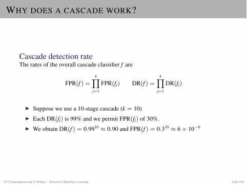
WHY DOES A CASCADE WORK?
Cascade detection rateThe rates of the overall cascade classifier f are
FPR(f ) =kY
j=1
FPR(fj) DR(f ) =kY
j=1
DR(fj)
I Suppose we use a 10-stage cascade (k = 10)I Each DR(fj) is 99% and we permit FPR(fj) of 30%.I We obtain DR(f ) = 0.9910 ⇡ 0.90 and FPR(f ) = 0.310 ⇡ 6⇥ 10�6
J.P. Cunningham and P. Orbanz · Statistical Machine Learning 166 / 436
VIOLA-JONES DETECTOR
ObjectivesI Classification step should be computationally efficient.I Expensive training affordable.
StrategyI Extract very large set of measurements (features), i.e. d in Rd large.I Use Boosting with decision stumps.I From Boosting weights, select small number of important features.I Class imbalance: Use Cascade.
Classification stepCompute only the selected features from input image.
J.P. Cunningham and P. Orbanz · Statistical Machine Learning 167 / 436
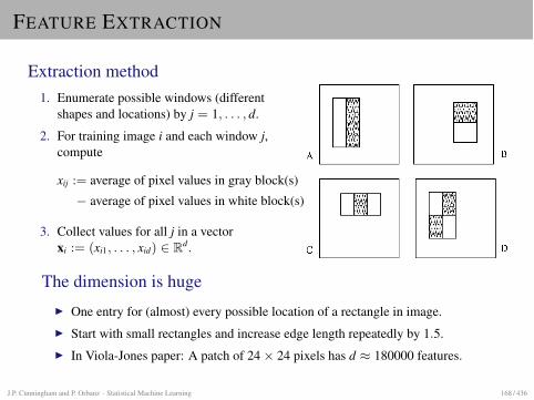
FEATURE EXTRACTION
Extraction method1. Enumerate possible windows (different
shapes and locations) by j = 1, . . . , d.
2. For training image i and each window j,compute
xij := average of pixel values in gray block(s)� average of pixel values in white block(s)
3. Collect values for all j in a vectorxi := (xi1, . . . , xid) 2 Rd.
Robust Real-Time Face Detection 139
together yield an extremely reliable and efficient facedetector. Section 5 will describe a number of experi-mental results, including a detailed description of ourexperimental methodology. Finally Section 6 containsa discussion of this system and its relationship to re-lated systems.
2. Features
Our face detection procedure classifies images basedon the value of simple features. There are many moti-vations for using features rather than the pixels directly.The most common reason is that features can act to en-code ad-hoc domain knowledge that is difficult to learnusing a finite quantity of training data. For this systemthere is also a second critical motivation for features:the feature-based system operates much faster than apixel-based system.
The simple features used are reminiscent of Haarbasis functions which have been used by Papageorgiouet al. (1998). More specifically, we use three kinds offeatures. The value of a two-rectangle feature is thedifference between the sum of the pixels within tworectangular regions. The regions have the same sizeand shape and are horizontally or vertically adjacent(see Fig. 1). A three-rectangle feature computes thesum within two outside rectangles subtracted from thesum in a center rectangle. Finally a four-rectangle fea-ture computes the difference between diagonal pairs ofrectangles.
Given that the base resolution of the detector is24 × 24, the exhaustive set of rectangle features is
Figure 1. Example rectangle features shown relative to the enclos-ing detection window. The sum of the pixels which lie within thewhite rectangles are subtracted from the sum of pixels in the greyrectangles. Two-rectangle features are shown in (A) and (B). Figure(C) shows a three-rectangle feature, and (D) a four-rectangle feature.
quite large, 160,000. Note that unlike the Haar basis,the set of rectangle features is overcomplete.3
2.1. Integral Image
Rectangle features can be computed very rapidly usingan intermediate representation for the image which wecall the integral image.4 The integral image at locationx, y contains the sum of the pixels above and to the leftof x, y, inclusive:
i i(x, y) =!
x ′≤x,y′≤y
i(x ′, y′),
where i i(x, y) is the integral image and i(x, y) is theoriginal image (see Fig. 2). Using the following pair ofrecurrences:
s(x, y) = s(x, y − 1) + i(x, y) (1)
i i(x, y) = i i(x − 1, y) + s(x, y) (2)
(where s(x, y) is the cumulative row sum, s(x, −1) =0, and i i(−1, y) = 0) the integral image can be com-puted in one pass over the original image.
Using the integral image any rectangular sum can becomputed in four array references (see Fig. 3). Clearlythe difference between two rectangular sums can becomputed in eight references. Since the two-rectanglefeatures defined above involve adjacent rectangularsums they can be computed in six array references,eight in the case of the three-rectangle features, andnine for four-rectangle features.
One alternative motivation for the integral im-age comes from the “boxlets” work of Simard et al.
Figure 2. The value of the integral image at point (x, y) is the sumof all the pixels above and to the left.
The dimension is hugeI One entry for (almost) every possible location of a rectangle in image.I Start with small rectangles and increase edge length repeatedly by 1.5.I In Viola-Jones paper: A patch of 24⇥ 24 pixels has d ⇡ 180000 features.
J.P. Cunningham and P. Orbanz · Statistical Machine Learning 168 / 436
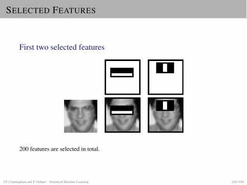
SELECTED FEATURES
First two selected features144 Viola and Jones
Figure 5. The first and second features selected by AdaBoost. Thetwo features are shown in the top row and then overlayed on a typ-ical training face in the bottom row. The first feature measures thedifference in intensity between the region of the eyes and a regionacross the upper cheeks. The feature capitalizes on the observationthat the eye region is often darker than the cheeks. The second featurecompares the intensities in the eye regions to the intensity across thebridge of the nose.
features to the classifier, directly increases computationtime.
4. The Attentional Cascade
This section describes an algorithm for constructing acascade of classifiers which achieves increased detec-tion performance while radically reducing computationtime. The key insight is that smaller, and therefore moreefficient, boosted classifiers can be constructed whichreject many of the negative sub-windows while detect-ing almost all positive instances. Simpler classifiers areused to reject the majority of sub-windows before morecomplex classifiers are called upon to achieve low falsepositive rates.
Stages in the cascade are constructed by trainingclassifiers using AdaBoost. Starting with a two-featurestrong classifier, an effective face filter can be obtainedby adjusting the strong classifier threshold to mini-mize false negatives. The initial AdaBoost threshold,12
!Tt=1 αt , is designed to yield a low error rate on the
training data. A lower threshold yields higher detec-tion rates and higher false positive rates. Based on per-formance measured using a validation training set, thetwo-feature classifier can be adjusted to detect 100% ofthe faces with a false positive rate of 50%. See Fig. 5 fora description of the two features used in this classifier.
The detection performance of the two-feature clas-sifier is far from acceptable as a face detection system.Nevertheless the classifier can significantly reduce the
number of sub-windows that need further processingwith very few operations:
1. Evaluate the rectangle features (requires between 6and 9 array references per feature).
2. Compute the weak classifier for each feature (re-quires one threshold operation per feature).
3. Combine the weak classifiers (requires one multiplyper feature, an addition, and finally a threshold).
A two feature classifier amounts to about 60 mi-croprocessor instructions. It seems hard to imaginethat any simpler filter could achieve higher rejectionrates. By comparison, scanning a simple image tem-plate would require at least 20 times as many operationsper sub-window.
The overall form of the detection process is that ofa degenerate decision tree, what we call a “cascade”(Quinlan, 1986) (see Fig. 6). A positive result fromthe first classifier triggers the evaluation of a secondclassifier which has also been adjusted to achieve veryhigh detection rates. A positive result from the secondclassifier triggers a third classifier, and so on. A negativeoutcome at any point leads to the immediate rejectionof the sub-window.
The structure of the cascade reflects the fact thatwithin any single image an overwhelming majority ofsub-windows are negative. As such, the cascade at-tempts to reject as many negatives as possible at theearliest stage possible. While a positive instance will
Figure 6. Schematic depiction of a the detection cascade. A seriesof classifiers are applied to every sub-window. The initial classifiereliminates a large number of negative examples with very little pro-cessing. Subsequent layers eliminate additional negatives but requireadditional computation. After several stages of processing the num-ber of sub-windows have been reduced radically. Further processingcan take any form such as additional stages of the cascade (as in ourdetection system) or an alternative detection system.
200 features are selected in total.
J.P. Cunningham and P. Orbanz · Statistical Machine Learning 169 / 436
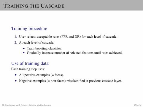
TRAINING THE CASCADE
Training procedure
1. User selects acceptable rates (FPR and DR) for each level of cascade.
2. At each level of cascade:I Train boosting classifier.I Gradually increase number of selected features until rates achieved.
Use of training dataEach training step uses:
I All positive examples (= faces).I Negative examples (= non-faces) misclassified at previous cascade layer.
J.P. Cunningham and P. Orbanz · Statistical Machine Learning 170 / 436

EXAMPLE RESULTS
152 Viola and Jones
Figure 10. Output of our face detector on a number of test images from the MIT + CMU test set.
6. Conclusions
We have presented an approach for face detectionwhich minimizes computation time while achievinghigh detection accuracy. The approach was used to con-struct a face detection system which is approximately15 times faster than any previous approach. Preliminaryexperiments, which will be described elsewhere, showthat highly efficient detectors for other objects, such aspedestrians or automobiles, can also be constructed inthis way.
This paper brings together new algorithms, represen-tations, and insights which are quite generic and maywell have broader application in computer vision andimage processing.
The first contribution is a new a technique for com-puting a rich set of image features using the integralimage. In order to achieve true scale invariance, almostall face detection systems must operate on multipleimage scales. The integral image, by eliminating theneed to compute a multi-scale image pyramid, reducesthe initial image processing required for face detection
J.P. Cunningham and P. Orbanz · Statistical Machine Learning 171 / 436
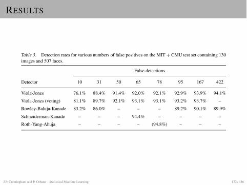
RESULTS
Robust Real-Time Face Detection 151
Table 3. Detection rates for various numbers of false positives on the MIT + CMU test set containing 130images and 507 faces.
False detections
Detector 10 31 50 65 78 95 167 422
Viola-Jones 76.1% 88.4% 91.4% 92.0% 92.1% 92.9% 93.9% 94.1%
Viola-Jones (voting) 81.1% 89.7% 92.1% 93.1% 93.1% 93.2% 93.7% –
Rowley-Baluja-Kanade 83.2% 86.0% – – – 89.2% 90.1% 89.9%
Schneiderman-Kanade – – – 94.4% – – – –
Roth-Yang-Ahuja – – – – (94.8%) – – –
regime (i.e. single point on the ROC curve). To makecomparison with our detector easier we have listed ourdetection rate for the same false positive rate reportedby the other systems. Table 3 lists the detection ratefor various numbers of false detections for our systemas well as other published systems. For the Rowley-Baluja-Kanade results (Rowley et al., 1998), a numberof different versions of their detector were tested yield-ing a number of different results. While these variousresults are not actually points on a ROC curve for aparticular detector, they do indicate a number of dif-ferent performance points that can be achieved withtheir approach. They did publish ROC curves for twoof their detectors, but these ROC curves did not rep-resent their best results. For the Roth-Yang-Ahuja de-tector (Roth et al., 2000), they reported their result onthe MIT + CMU test set minus 5 images containingline drawn faces removed. So their results are for a sub-set of the MIT + CMU test set containing 125 imageswith 483 faces. Presumably their detection rate wouldbe lower if the full test set was used. The parenthe-ses around their detection rate indicates this slightlydifferent test set. The Sung and Poggio face detec-tor (Sung and Poggio, 1998) was tested on the MITsubset of the MIT + CMU test set since the CMUportion did not exist yet. The MIT test set contains23 images with 149 faces. They achieved a detectionrate of 79.9% with 5 false positives. Our detectionrate with 5 false positives is 77.8% on the MIT testset.
Figure 10 shows the output of our face detector onsome test images from the MIT + CMU test set.
5.7.1. A Simple Voting Scheme Further ImprovesResults. The best results were obtained through thecombination of three detectors trained using differentinitial negative examples, slightly different weighting
on negative versus positive errors, and slightly differentcriteria for trading off false positives for classifier size.These three systems performed similarly on the finaltask, but in some cases errors were different. The detec-tion results from these three detectors were combinedby retaining only those detections where at least 2 outof 3 detectors agree. This improves the final detectionrate as well as eliminating more false positives. Sincedetector errors are not uncorrelated, the combinationresults in a measurable, but modest, improvement overthe best single detector.
5.7.2. Failure Modes. By observing the performanceof our face detector on a number of test images we havenoticed a few different failure modes.
The face detector was trained on frontal, uprightfaces. The faces were only very roughly aligned sothere is some variation in rotation both in plane and outof plane. Informal observation suggests that the facedetector can detect faces that are tilted up to about ±15degrees in plane and about ±45 degrees out of plane(toward a profile view). The detector becomes unreli-able with more rotation than this.
We have also noticed that harsh backlighting inwhich the faces are very dark while the backgroundis relatively light sometimes causes failures. It is in-teresting to note that using a nonlinear variance nor-malization based on robust statistics to remove out-liers improves the detection rate in this situation. Theproblem with such a normalization is the greatly in-creased computational cost within our integral imageframework.
Finally, our face detector fails on significantly oc-cluded faces. If the eyes are occluded for example, thedetector will usually fail. The mouth is not as importantand so a face with a covered mouth will usually still bedetected.
J.P. Cunningham and P. Orbanz · Statistical Machine Learning 172 / 436
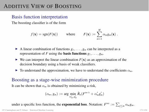
ADDITIVE VIEW OF BOOSTING
Basis function interpretationThe boosting classifier is of the form
f (x) = sgn(F(x)) where F(x) :=MX
m=1
↵mgm(x) .
I A linear combination of functions g1, . . . , gm can be interpreted as arepresentation of F using the basis functions g1, . . . , gm.
I We can interpret the linear combination F(x) as an approximation of thedecision boundary using a basis of weak classifiers.
I To understand the approximation, we have to understand the coefficients ↵m.
Boosting as a stage-wise minimization procedureIt can be shown that ↵m is obtained by minimizing a risk,
(↵m, gm) := arg min↵0m,g0m
Rn(F(m-1) + ↵0mg0m)
under a specific loss function, the exponential loss. Notation: F(m) :=P
jm ↵mgm.J.P. Cunningham and P. Orbanz · Statistical Machine Learning 173 / 436
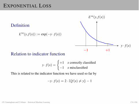
EXPONENTIAL LOSS
Definition
Lexp(y, f (x)) := exp(�y · f (x))
y · f (x)
Lexp(y, f (x))
�1 +1Relation to indicator function
y · f (x) =
(
+1 x correctly classified�1 x misclassified
This is related to the indicator function we have used so far by
�y · f (x) = 2 · I{f (x) 6= y}� 1
J.P. Cunningham and P. Orbanz · Statistical Machine Learning 174 / 436
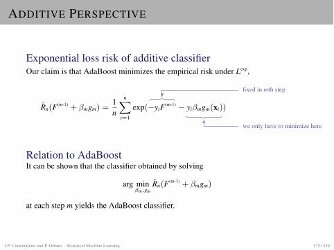
ADDITIVE PERSPECTIVE
Exponential loss risk of additive classifierOur claim is that AdaBoost minimizes the empirical risk under Lexp,
Rn(F(m-1) + �mgm) =1n
nX
i=1
exp(�yiF(m-1) � yi�mgm(xi))
fixed in mth step
we only have to minimize here
Relation to AdaBoostIt can be shown that the classifier obtained by solving
arg min�m,gm
Rn(F(m-1) + �mgm)
at each step m yields the AdaBoost classifier.
J.P. Cunningham and P. Orbanz · Statistical Machine Learning 175 / 436
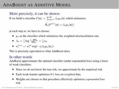
ADABOOST AS ADDITIVE MODEL
More precisely, it can be shown:If we build a classifier F(x) :=
PMm=1 �mgm(x) which minimizes
Rn(F(m-1)(x) + �mgm(x))
at each step m, we have to choose:I gm as the classifier which minimizes the weighted misclassifiation rate.I �m = 1
2 log 1�errmerrm
= 12↵m
I w(m+1)i := w(m)
i exp(�yi�mgm(xi))
This is precisely equivalent to what AdaBoost does.
In other wordsAdaBoost approximates the optimal classifier (under exponential loss) using a basisof weak classifiers.
I Since we do not know the true risk, we approximate by the empirical risk.I Each weak learner optimizes 0-1 loss on weighted data.I Weights are chosen so that procedure effectively optimizes exponential loss
risk.J.P. Cunningham and P. Orbanz · Statistical Machine Learning 176 / 436
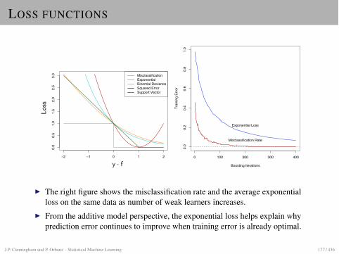
LOSS FUNCTIONSElements of Statistical Learning (2nd Ed.) c�Hastie, Tibshirani & Friedman 2009 Chap 10
−2 −1 0 1 2
0.0
0.5
1.0
1.5
2.0
2.5
3.0 Misclassification
ExponentialBinomial DevianceSquared ErrorSupport Vector
Los
s
y · f
FIGURE 10.4. Loss functions for two-class classi-fication. The response is y = ±1; the prediction isf , with class prediction sign(f). The losses are mis-classification: I(sign(f) 6= y); exponential: exp(�yf);binomial deviance: log(1 + exp(�2yf)); squared er-ror: (y � f)2; and support vector: (1 � yf)+ (see Sec-tion 12.3). Each function has been scaled so that itpasses through the point (0, 1).
Elements of Statistical Learning (2nd Ed.) c�Hastie, Tibshirani & Friedman 2009 Chap 10
0 100 200 300 400
0.0
0.2
0.4
0.6
0.8
1.0
Boosting Iterations
Trai
ning
Erro
r
Misclassification Rate
Exponential Loss
FIGURE 10.3. Simulated data, boosting with stumps:misclassification error rate on the training set, and av-erage exponential loss: (1/N)
PNi=1 exp(�yif(xi)). Af-
ter about 250 iterations, the misclassification error iszero, while the exponential loss continues to decrease.
I The right figure shows the misclassification rate and the average exponentialloss on the same data as number of weak learners increases.
I From the additive model perspective, the exponential loss helps explain whyprediction error continues to improve when training error is already optimal.
J.P. Cunningham and P. Orbanz · Statistical Machine Learning 177 / 436
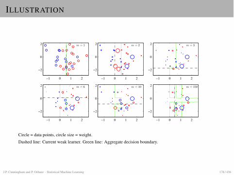
ILLUSTRATION
m = 1
−1 0 1 2
−2
0
2 m = 2
−1 0 1 2
−2
0
2 m = 3
−1 0 1 2
−2
0
2
m = 6
−1 0 1 2
−2
0
2 m = 10
−1 0 1 2
−2
0
2 m = 150
−1 0 1 2
−2
0
2
Circle = data points, circle size = weight.Dashed line: Current weak learner. Green line: Aggregate decision boundary.
J.P. Cunningham and P. Orbanz · Statistical Machine Learning 178 / 436
BAGGING AND RANDOM FORESTS
BACKGROUND: RESAMPLING TECHNIQUES
We briefly review a technique called bootstrap on which Bagging and random forests are based.
BootstrapBootstrap (or resampling) is a technique for improving the quality of estimators.
Resampling = sampling from the empirical distribution
Application to ensemble methodsI We will use resampling to generate weak learners for classification.I We discuss two classifiers which use resampling: Bagging and random forests.I Before we do so, we consider the traditional application of Bootstrap, namely
improving estimators.
J.P. Cunningham and P. Orbanz · Statistical Machine Learning 180 / 436
BOOTSTRAP: BASIC ALGORITHM
GivenI A sample x1, . . . , xn.I An estimator S for a statistic S.
Bootstrap algorithm
1. Generate B bootstrap samples B1, . . . , BB. Each bootstrap sample is obtainedby sampling n times with replacement from the sample data. (Note: Data pointscan appear multiple times in any Bb.)
2. Evaluate the estimator on each bootstrap sample:
Sb := S(Bb)
(That is: We estimate S pretending that Bb is the data.)
3. Compute the bootstrap estimate of S by averaging over all bootstrap samples:
SBS :=1B
BX
b=1
Sb
J.P. Cunningham and P. Orbanz · Statistical Machine Learning 181 / 436
EXAMPLE: VARIANCE ESTIMATION
Mean and Variance
µ :=
Z
Rdx p(x)dx �2 :=
Z
Rd(x� µ)2p(x)dx
Plug-in estimators for mean and variance
µ :=1n
nX
i=1
xi �2 :=1n
nX
i=1
(xi � µ)2
J.P. Cunningham and P. Orbanz · Statistical Machine Learning 182 / 436
BOOTSTRAP VARIANCE ESTIMATE
Bootstrap algorithm
1. For b = 1, . . . , B, generate a boostrap sample Bb. In detail:For i = 1, . . . , n:
I Sample an index j 2 {1, . . . , n}.I Set x(b)
i := xj and add it to Bb.
2. For each b, compute mean and variance estimates:
µb :=1n
nX
i=1
x(b)i �2
b :=1n
nX
i=1
(x(b)i � µb)
2
3. Compute the bootstrap estimate:
�2BS :=
1B
BX
b=1
�2b
J.P. Cunningham and P. Orbanz · Statistical Machine Learning 183 / 436
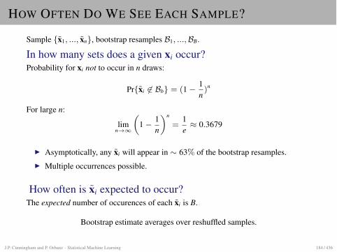
HOW OFTEN DO WE SEE EACH SAMPLE?
Sample {x1, ..., xn}, bootstrap resamples B1, ..., BB.
In how many sets does a given xi occur?Probability for xi not to occur in n draws:
Pr{xi 62 Bb} = (1� 1n)n
For large n:
limn!1
✓
1� 1n
◆n
=1e⇡ 0.3679
I Asymptotically, any xi will appear in ⇠ 63% of the bootstrap resamples.I Multiple occurrences possible.
How often is xi expected to occur?The expected number of occurences of each xi is B.
Bootstrap estimate averages over reshuffled samples.
J.P. Cunningham and P. Orbanz · Statistical Machine Learning 184 / 436
BOOTSTRAP: APPLICATIONS
Estimate variance of estimatorsI Since estimator S depends on (random) data, it is a random variable.I The more this variable scatters, the less we can trust our estimate.I If scatter is high, we can expect the values Sb to scatter as well.I In previous example, this means: Estimating the variance of the variance
estimator.
Variance reductionI Averaging over the individual bootstrap samples can reduce the variance in S.I In other words: SBS typically has lower variance than S.I This is the property we will use for classicifation in the following.
As alternative to cross validationTo estimate prediction error of classifier:
I For each b, train on Bb, estimate risk on points not in Bb.I Average risk estimates over bootstrap samples.
J.P. Cunningham and P. Orbanz · Statistical Machine Learning 185 / 436
BAGGING
IdeaI Recall Boosting: Weak learners are deterministic, but selected to exhibit high
variance.I Strategy now: Randomly distort data set by resampling.I Train weak learners on resampled training sets.I Resulting algorithm: Bagging (= Bootstrap aggregation)
J.P. Cunningham and P. Orbanz · Statistical Machine Learning 186 / 436
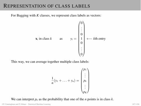
REPRESENTATION OF CLASS LABELS
For Bagging with K classes, we represent class labels as vectors:
xi in class k as yi =
0
B
B
B
B
B
B
B
B
B
B
B
@
0...010...0
1
C
C
C
C
C
C
C
C
C
C
C
A
� kth entry
This way, we can average together multiple class labels:
1n(y1 + . . . + yn) =
0
B
B
B
B
B
B
@
p1...
pk...
pK
1
C
C
C
C
C
C
A
We can interpret pk as the probability that one of the n points is in class k.J.P. Cunningham and P. Orbanz · Statistical Machine Learning 187 / 436
BAGGING: ALGORITHM
TrainingFor b = 1, . . . , B:
1. Draw a bootstrap sample Bb of size n from training data.
2. Train a classifier fb on Bb.
ClassificationI Compute
favg(x) :=1B
BX
b=1
fb(x)
This is a vector of the form favg(x) = (p1(x), . . . , pk(x)).I The Bagging classifier is given by
fBagging(x) := arg maxk
{p1(x), . . . , pk(x)} ,
i.e. we predict the class label which most weak learners have voted for.
J.P. Cunningham and P. Orbanz · Statistical Machine Learning 188 / 436
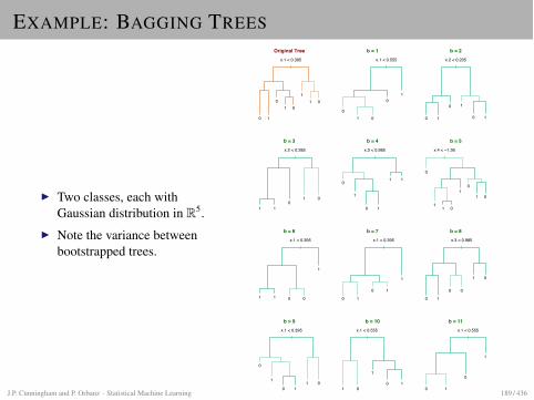
EXAMPLE: BAGGING TREES
I Two classes, each withGaussian distribution in R5.
I Note the variance betweenbootstrapped trees.
Elements of Statistical Learning (2nd Ed.) c�Hastie, Tibshirani & Friedman 2009 Chap 8
|x.1 < 0.395
0 1
01 0
11 0
Original Tree
|x.1 < 0.555
01 0
01
b = 1
|x.2 < 0.205
0 1
0 1
0 1
b = 2
|x.2 < 0.285
1 10
1 0
b = 3
|x.3 < 0.985
0
1
0 1
1 1
b = 4
|x.4 < −1.36
0
11 0
10
1 0
b = 5
|x.1 < 0.395
1 1 0 0
1
b = 6
|x.1 < 0.395
0 1
0 1
1
b = 7
|x.3 < 0.985
0 1
0 0
1 0
b = 8
|x.1 < 0.395
0
1
0 11 0
b = 9
|x.1 < 0.555
1 0
1
0 1
b = 10
|x.1 < 0.555
0 1
0
1
b = 11
FIGURE 8.9. Bagging trees on simulated dataset.Th l f l h h i i l El
J.P. Cunningham and P. Orbanz · Statistical Machine Learning 189 / 436
RANDOM FORESTS
Bagging vs. BoostingI Bagging works particularly well for trees, since trees have high variance.I Boosting typically outperforms bagging with trees.I The main culprit is usually dependence: Boosting is better at reducing
correlation between the trees than bagging is.
Random ForestsModification of bagging with trees designed to further reduce correlation.
I Tree training optimizes each split over all dimensions.I Random forests choose a different subset of dimensions at each split.I Optimal split is chosen within the subset.I The subset is chosen at random out of all dimensions {1, . . . , d}.
J.P. Cunningham and P. Orbanz · Statistical Machine Learning 190 / 436
RANDOM FORESTS: ALGORITHM
TrainingInput parameter: m (positive integer with m < d)
For b = 1, . . . , B:
1. Draw a bootstrap sample Bb of size n from training data.
2. Train a tree classifier fb on Bb, where each split is computed as follows:I Select m axes in Rd at random.I Find the best split (j⇤, t⇤) on this subset of dimensions.I Split current node along axis j⇤ at t⇤.
ClassificationExactly as for bagging: Classify by majority vote among the B trees. More precisely:
I Compute favg(x) := (p1(x), . . . , pk(x)) := 1B
PBb=1 fb(x)
I The Random Forest classification rule is
fBagging(x) := arg maxk
{p1(x), . . . , pk(x)}
J.P. Cunningham and P. Orbanz · Statistical Machine Learning 191 / 436
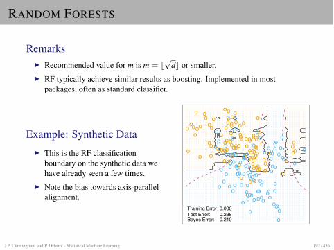
RANDOM FORESTS
RemarksI Recommended value for m is m = bpdc or smaller.I RF typically achieve similar results as boosting. Implemented in most
packages, often as standard classifier.
Example: Synthetic DataI This is the RF classification
boundary on the synthetic data wehave already seen a few times.
I Note the bias towards axis-parallelalignment.
Elements of Statistical Learning (2nd Ed.) c�Hastie, Tibshirani & Friedman 2009 Chap 15
Random Forest Classifier
oo
ooo
oo
o
o
o
o
o
o
oo
o
o o
oo
o
o
o
o
o
o
o
oo
oo
o
oo
o
o
o
o
o
o
o
o
o
o
o
o
o
o
o
o
oo
o
o
o
o
oo
o o
o
o
o
o
o
o
o
o
o
oo o
oo
oo
o
oo
o
oo
oo
o
o
o
o
o
o
o
o
o
o
o
o
oo
o
o
ooo
o
o
oo
o
oo
o
o
o
o
o
o
o
oo
o
o
o
o
o
o
o
o oooo
o
ooo o
o
o
o
o
o
o
o
ooo
ooo
oooo
o
ooo
o
o
o
o
o
o
o
o o
o
o
o
o
o
o
o oo
oo
o
o
oo
o
o
ooo o
o oo
o
o
o
o
o
o
o
o
o
o
Training Error: 0.000Test Error: 0.238Bayes Error: 0.210
3−Nearest Neighbors
oo
ooo
oo
o
o
o
o
o
o
oo
o
o o
oo
o
o
o
o
o
o
o
oo
oo
o
oo
o
o
o
o
o
o
o
o
o
o
o
o
o
o
o
o
oo
o
o
o
o
oo
o o
o
o
o
o
o
o
o
o
o
oo o
oo
oo
o
oo
o
oo
oo
o
o
o
o
o
o
o
o
o
o
o
o
oo
o
o
ooo
o
o
oo
o
oo
o
o
o
o
o
o
o
oo
o
o
o
o
o
o
o
o oooo
o
ooo o
o
o
o
o
o
o
o
ooo
ooo
oooo
o
ooo
o
o
o
o
o
o
o
o o
o
o
o
o
o
o
o oo
oo
o
o
oo
o
o
ooo o
o oo
o
o
o
o
o
o
o
o
o
o
Training Error: 0.130Test Error: 0.242Bayes Error: 0.210
FIGURE 15.11. Random forests versus 3-NN on themixture data. The axis-oriented nature of the individ-ual trees in a random forest lead to decision regionswith an axis-oriented flavor.
J.P. Cunningham and P. Orbanz · Statistical Machine Learning 192 / 436
SUMMARY: CLASSIFICATION
SUMMARY
Approaches we have discussedI Linear classifiers
I Perceptron, SVMI Nonlinear versions using kernels
I Trees (depth 1: linear and axis-parallel, depth � 2: non-linear)I Ensemble methods
What should we use?I RBF SVMs, AdaBoost and Random Forests perform well on many problems.I All have strengths and weaknesses. E.g.:
I High dimension, limited data: SVM may have the edge.I Many dimensions, but we believe only a few are important: AdaBoost
with stumps.I In general: Feature extraction (what do we measure?) is crucial.I Consider combination of different methods by voting.
J.P. Cunningham and P. Orbanz · Statistical Machine Learning 194 / 436
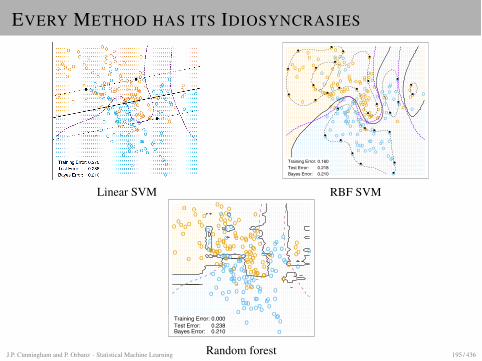
EVERY METHOD HAS ITS IDIOSYNCRASIES
Linear SVM
Elements of Statistical Learning (2nd Ed.) c�Hastie, Tibshirani & Friedman 2009 Chap 12
SVM - Degree-4 Polynomial in Feature Space
. . . . . . . . . . . . . . . . . . . . . . . . . . . . . . . . . . . . . . . . . . . . . . .. . . . . . . . . . . . . . . . . . . . . . . . . . . . . . . . . . . . . . . . . . . . .. . . . . . . . . . . . . . . . . . . . . . . . . . . . . . . . . . . . . . . . . . .. . . . . . . . . . . . . . . . . . . . . . . . . . . . . . . . . . . . . . . .. . . . . . . . . . . . . . . . . . . . . . . . . . . . . . . . . . . . .. . . . . . . . . . . . . . . . . . . . . . . . . . . . . . . . . . .. . . . . . . . . . . . . . . . . . . . . . . . . . . . . . . . .. . . . . . . . . . . . . . . . . . . . . . . . . . . . . . .. . . . . . . . . . . . . . . . . . . . . . . . . . . . . .. . . . . . . . . . . . . . . . . . . . . . . . . . . . .. . . . . . . . . . . . . . . . . . . . . . . . . . . .. . . . . . . . . . . . . . . . . . . . . . . . . . .. . . . . . . . . . . . . . . . . . . . . . . . . .. . . . . . . . . . . . . . . . . . . . . . . . .. . . . . . . . . . . . . . . . . . . . . . . . .. . . . . . . . . . . . . . . . . . . . . . . .. . . . . . . . . . . . . . . . . . . . . . .. . . . . . . . . . . . . . . . . . . . . . .. . . . . . . . . . . . . . . . . . . . . .. . . . . . . . . . . . . . . . . . . . . .. . . . . . . . . . . . . . . . . . . . .. . . . . . . . . . . . . . . . . . . . .. . . . . . . . . . . . . . . . . . . . .. . . . . . . . . . . . . . . . . . . .. . . . . . . . . . . . . . . . . . . .. . . . . . . . . . . . . . . . . . . .. . . . . . . . . . . . . . . . . . .. . . . . . . . . . . . . . . . . . .. . . . . . . . . . . . . . . . . . .. . . . . . . . . . . . . . . . . . .. . . . . . . . . . . . . . . . . .. . . . . . . . . . . . . . . . . .. . . . . . . . . . . . . . . . . .. . . . . . . . . . . . . . . . . .. . . . . . . . . . . . . . . . . .. . . . . . . . . . . . . . . . . .. . . . . . . . . . . . . . . . . .. . . . . . . . . . . . . . . . .. . . . . . . . . . . . . . . . .. . . . . . . . . . . . . . . . .. . . . . . . . . . . . . . . . . . . . .. . . . . . . . . . . . . . . . . . . . . . . .. . . . . . . . . . . . . . . . . . . . . . . . . . .. . . . . . . . . . . . . . . . . . . . . . . . . . . .. . . . . . . . . . . . . . . . . . . . . . . . . . . . .. . . . . . . . . . . . . . . . . . . . . . . . . . . . . . . .. . . . . . . . . . . . . . . . . . . . . . . . . . . . . . . . . .. . . . . . . . . . . . . . . . . . . . . . . . . . . . . . . . . . .. . . . . . . . . . . . . . . . . . . . . . . . . . . . . . . . . . . . .. . . . . . . . . . . . . . . . . . . . . . . . . . . . . . . . . . . . .. . . . . . . . . . . . . . . . . . . . . . . . . . . . . . . . . . . . . .. . . . . . . . . . . . . . . . . . . . . . . . . . . . . . . . . . . . . . . .. . . . . . . . . . . . . . . . . . . . . . . . . . . . . . . . . . . . . . . . . .. . . . . . . . . . . . . . . . . . . . . . . . . . . . . . . . . . . . . . . . . . .. . . . . . . . . . . . . . . . . . . . . . . . . . . . . . . . . . . . . . . . . . .. . . . . . . . . . . . . . . . . . . . . . . . . . . . . . . . . . . . . . . . . . . . . .. . . . . . . . . . . . . . . . . . . . . . . . . . . . . . . . . . . . . . . . . . . . . . . .. . . . . . . . . . . . . . . . . . . . . . . . . . . . . . . . . . . . . . . . . . . . . . . . . . .. . . . . . . . . . . . . . . . . . . . . . . . . . . . . . . . . . . . . . . . . . . . . . . . . . . . . . .. . . . . . . . . . . . . . . . . . . . . . . . . . . . . . . . . . . . . . . . . . . . . . . . . . . . . .. . . . . . . . . . . . . . . . . . . . . . . . . . . . . . . . . . . . . . . . . . . . . . . . . . . . . .. . . . . . . . . . . . . . . . . . . . . . . . . . . . . . . . . . . . . . . . . . . . . . . . . . . . . .. . . . . . . . . . . . . . . . . . . . . . . . . . . . . . . . . . . . . . . . . . . . . . . . . . . . . .. . . . . . . . . . . . . . . . . . . . . . . . . . . . . . . . . . . . . . . . . . . . . . . . . . . . . .. . . . . . . . . . . . . . . . . . . . . . . . . . . . . . . . . . . . . . . . . . . . . . . . . . . . . .. . . . . . . . . . . . . . . . . . . . . . . . . . . . . . . . . . . . . . . . . . . . . . . . . . . . . . .. . . . . . . . . . . . . . . . . . . . . . . . . . . . . . . . . . . . . . . . . . . . . . . . . . . . . .. . . . . . . . . . . . . . . . . . . . . . . . . . . . . . . . . . . . . . . . . . . . . . . . . . . . . .. . . . . . . . . . . . . . . . . . . . . . . . . . . . . . . . . . . . . . . . . . . . . . . . . . . . . . .. . . . . . . . . . . . . . . . . . . . . . . . . . . . . . . . . . . . . . . . . . . . . . . . . . . . . .. . . . . . . . . . . . . . . . . . . . . . . . . . . . . . . . . . . . . . . . . . . . . . . . . . . . . . .. . . . . . . . . . . . . . . . . . . . . . . . . . . . . . . . . . . . . . . . . . . . . . . . . . . . . . .. . . . . . . . . . . . . . . . . . . . . . . . . . . . . . . . . . . . . . . . . . . . . . . . . . . . . . .. . . . . . . . . . . . . . . . . . . . . . . . . . . . . . . . . . . . . . . . . . . . . . . . . . . . . . .. . . . . . . . . . . . . . . . . . . . . . . . . . . . . . . . . . . . . . . . . . . . . . . . . . . . . . .. . . . . . . . . . . . . . . . . . . . . . . . . . . . . . . . . . . . . . . . . . . . . . . . . . . . . . . .. . . . . . . . . . . . . . . . . . . . . . . . . . . . . . . . . . . . . . . . . . . . . . . . . . . . . . . .. . . . . . . . . . . . . . . . . . . . . . . . . . . . . . . . . . . . . . . . . . . . . . . . . . . . . . . . .. . . . . . . . . . . . . . . . . . . . . . . . . . . . . . . . . . . . . . . . . . . . . . . . . . . . . . . . . .. . . . . . . . . . . . . . . . . . . . . . . . . . . . . . . . . . . . . . . . . . . . . . . . . . . . . . . . . .. . . . . . . . . . . . . . . . . . . . . . . . . . . . . . . . . . . . . . . . . . . . . . . . . . . . . . . . . . .. . . . . . . . . . . . . . . . . . . . . . . . . . . . . . . . . . . . . . . . . . . . . . . . . . . . . . . . . . . .. . . . . . . . . . . . . . . . . . . . . . . . . . . . . . . . . . . . . . . . . . . . . . . . . . . . . . . . . . . . . .. . . . . . . . . . . . . . . . . . . . . . . . . . . . . . . . . . . . . . . . . . . . . . . . . . . . . . . . . . . . . . . .. . . . . . . . . . . . . . . . . . . . . . . . . . . . . . . . . . . . . . . . . . . . . . . . . . . . . . . . . . . . . . . . . . . . .. . . . . . . . . . . . . . . . . . . . . . . . . . . . . . . . . . . . . . . . . . . . . . . . . . . . . . . . . . . . . . . . . . . . .. . . . . . . . . . . . . . . . . . . . . . . . . . . . . . . . . . . . . . . . . . . . . . . . . . . . . . . . . . . . . . . . . . . . .. . . . . . . . . . . . . . . . . . . . . . . . . . . . . . . . . . . . . . . . . . . . . . . . . . . . . . . . . . . . . . . . . . . . .. . . . . . . . . . . . . . . . . . . . . . . . . . . . . . . . . . . . . . . . . . . . . . . . . . . . . . . . . . . . . . . . . . . . .. . . . . . . . . . . . . . . . . . . . . . . . . . . . . . . . . . . . . . . . . . . . . . . . . . . . . . . . . . . . . . . . . . . . .. . . . . . . . . . . . . . . . . . . . . . . . . . . . . . . . . . . . . . . . . . . . . . . . . . . . . . . . . . . . . . . . . . . . .. . . . . . . . . . . . . . . . . . . . . . . . . . . . . . . . . . . . . . . . . . . . . . . . . . . . . . . . . . . . . . . . . . . . .. . . . . . . . . . . . . . . . . . . . . . . . . . . . . . . . . . . . . . . . . . . . . . . . . . . . . . . . . . . . . . . . . . . . .. . . . . . . . . . . . . . . . . . . . . . . . . . . . . . . . . . . . . . . . . . . . . . . . . . . . . . . . . . . . . . . . . . . . .. . . . . . . . . . . . . . . . . . . . . . . . . . . . . . . . . . . . . . . . . . . . . . . . . . . . . . . . . . . . . . . . . . . . .. . . . . . . . . . . . . . . . . . . . . . . . . . . . . . . . . . . . . . . . . . . . . . . . . . . . . . . . . . . . . . . . . . . . .. . . . . . . . . . . . . . . . . . . . . . . . . . . . . . . . . . . . . . . . . . . . . . . . . . . . . . . . . . . . . . . . . . . . .. . . . . . . . . . . . . . . . . . . . . . . . . . . . . . . . . . . . . . . . . . . . . . . . . . . . . . . . . . . . . . . . . . . . .. . . . . . . . . . . . . . . . . . . . . . . . . . . . . . . . . . . . . . . . . . . . . . . . . . . . . . . . . . . . . . . . . . . . .
. . . . . . . . . . . . . . . . . . . . . .. . . . . . . . . . . . . . . . . . . . . . . .. . . . . . . . . . . . . . . . . . . . . . . . . .. . . . . . . . . . . . . . . . . . . . . . . . . . . . .. . . . . . . . . . . . . . . . . . . . . . . . . . . . . . . .. . . . . . . . . . . . . . . . . . . . . . . . . . . . . . . . . .. . . . . . . . . . . . . . . . . . . . . . . . . . . . . . . . . . . .. . . . . . . . . . . . . . . . . . . . . . . . . . . . . . . . . . . . . .. . . . . . . . . . . . . . . . . . . . . . . . . . . . . . . . . . . . . . .. . . . . . . . . . . . . . . . . . . . . . . . . . . . . . . . . . . . . . . .. . . . . . . . . . . . . . . . . . . . . . . . . . . . . . . . . . . . . . . . .. . . . . . . . . . . . . . . . . . . . . . . . . . . . . . . . . . . . . . . . . .. . . . . . . . . . . . . . . . . . . . . . . . . . . . . . . . . . . . . . . . . . .. . . . . . . . . . . . . . . . . . . . . . . . . . . . . . . . . . . . . . . . . . . .. . . . . . . . . . . . . . . . . . . . . . . . . . . . . . . . . . . . . . . . . . . .. . . . . . . . . . . . . . . . . . . . . . . . . . . . . . . . . . . . . . . . . . . . .. . . . . . . . . . . . . . . . . . . . . . . . . . . . . . . . . . . . . . . . . . . . . .. . . . . . . . . . . . . . . . . . . . . . . . . . . . . . . . . . . . . . . . . . . . . .. . . . . . . . . . . . . . . . . . . . . . . . . . . . . . . . . . . . . . . . . . . . . . .. . . . . . . . . . . . . . . . . . . . . . . . . . . . . . . . . . . . . . . . . . . . . . .. . . . . . . . . . . . . . . . . . . . . . . . . . . . . . . . . . . . . . . . . . . . . . . .. . . . . . . . . . . . . . . . . . . . . . . . . . . . . . . . . . . . . . . . . . . . . . . .. . . . . . . . . . . . . . . . . . . . . . . . . . . . . . . . . . . . . . . . . . . . . . . .. . . . . . . . . . . . . . . . . . . . . . . . . . . . . . . . . . . . . . . . . . . . . . . . .. . . . . . . . . . . . . . . . . . . . . . . . . . . . . . . . . . . . . . . . . . . . . . . . .. . . . . . . . . . . . . . . . . . . . . . . . . . . . . . . . . . . . . . . . . . . . . . . . .. . . . . . . . . . . . . . . . . . . . . . . . . . . . . . . . . . . . . . . . . . . . . . . . . .. . . . . . . . . . . . . . . . . . . . . . . . . . . . . . . . . . . . . . . . . . . . . . . . . .. . . . . . . . . . . . . . . . . . . . . . . . . . . . . . . . . . . . . . . . . . . . . . . . . .. . . . . . . . . . . . . . . . . . . . . . . . . . . . . . . . . . . . . . . . . . . . . . . . . .. . . . . . . . . . . . . . . . . . . . . . . . . . . . . . . . . . . . . . . . . . . . . . . . . . .. . . . . . . . . . . . . . . . . . . . . . . . . . . . . . . . . . . . . . . . . . . . . . . . . . .. . . . . . . . . . . . . . . . . . . . . . . . . . . . . . . . . . . . . . . . . . . . . . . . . . .. . . . . . . . . . . . . . . . . . . . . . . . . . . . . . . . . . . . . . . . . . . . . . . . . . .. . . . . . . . . . . . . . . . . . . . . . . . . . . . . . . . . . . . . . . . . . . . . . . . . . .. . . . . . . . . . . . . . . . . . . . . . . . . . . . . . . . . . . . . . . . . . . . . . . . . . .. . . . . . . . . . . . . . . . . . . . . . . . . . . . . . . . . . . . . . . . . . . . . . . . . . .. . . . . . . . . . . . . . . . . . . . . . . . . . . . . . . . . . . . . . . . . . . . . . . . . . . .. . . . . . . . . . . . . . . . . . . . . . . . . . . . . . . . . . . . . . . . . . . . . . . . . . . .. . . . . . . . . . . . . . . . . . . . . . . . . . . . . . . . . . . . . . . . . . . . . . . . . . . .. . . . . . . . . . . . . . . . . . . . . . . . . . . . . . . . . . . . . . . . . . . . . . . .. . . . . . . . . . . . . . . . . . . . . . . . . . . . . . . . . . . . . . . . . . . . .. . . . . . . . . . . . . . . . . . . . . . . . . . . . . . . . . . . . . . . . . .. . . . . . . . . . . . . . . . . . . . . . . . . . . . . . . . . . . . . . . . .. . . . . . . . . . . . . . . . . . . . . . . . . . . . . . . . . . . . . . . .. . . . . . . . . . . . . . . . . . . . . . . . . . . . . . . . . . . . .. . . . . . . . . . . . . . . . . . . . . . . . . . . . . . . . . . .. . . . . . . . . . . . . . . . . . . . . . . . . . . . . . . . . .. . . . . . . . . . . . . . . . . . . . . . . . . . . . . . . .. . . . . . . . . . . . . . . . . . . . . . . . . . . . . . . .. . . . . . . . . . . . . . . . . . . . . . . . . . . . . . .. . . . . . . . . . . . . . . . . . . . . . . . . . . . .. . . . . . . . . . . . . . . . . . . . . . . . . . .. . . . . . . . . . . . . . . . . . . . . . . . . .. . . . . . . . . . . . . . . . . . . . . . . . . .. . . . . . . . . . . . . . . . . . . . . . .. . . . . . . . . . . . . . . . . . . . .. . . . . . . . . . . . . . . . . .. . . . . . . . . . . . . .. . . . . . . . . . . . . . .. . . . . . . . . . . . . . .. . . . . . . . . . . . . . .. . . . . . . . . . . . . . .. . . . . . . . . . . . . . .. . . . . . . . . . . . . . .. . . . . . . . . . . . . .. . . . . . . . . . . . . . .. . . . . . . . . . . . . . .. . . . . . . . . . . . . .. . . . . . . . . . . . . . .. . . . . . . . . . . . . .. . . . . . . . . . . . . .. . . . . . . . . . . . . .. . . . . . . . . . . . . .. . . . . . . . . . . . . .. . . . . . . . . . . . .. . . . . . . . . . . . .. . . . . . . . . . . .. . . . . . . . . . .. . . . . . . . . . .. . . . . . . . . .. . . . . . . . .. . . . . . .. . . . .
oo
ooo
o
o
o
o
o
o
o
o
oo
o
o o
oo
o
o
o
o
o
o
o
o
o
o
o
o
oo
o
o
o
o
o
o
o
o
o
o
o
o
o
o
o
o
o
o
o
o
o
o
oo
oo
o
o
o
o
o
o
o
o
o
oo o
oo
oo
o
oo
o
o
o
oo
o
o
o
o
o
o
o
o
o
o
o
o
oo
o
o
ooo
o
o
o
o
o
oo
o
o
o
o
o
o
o
oo
o
o
o
o
o
o
o
o oooo
o
ooo o
o
o
o
o
o
o
o
ooo
ooo
ooo
o
o
ooo
o
o
o
o
o
o
o
o o
o
o
o
o
o
o
oo
ooo
o
o
o
o
o
o
ooo
oo oo
o
o
o
o
o
o
o
o
o
o
••
• • •
•
•
•• •
••
••
•
Training Error: 0.180Test Error: 0.245Bayes Error: 0.210
SVM - Radial Kernel in Feature Space
. . . . . . .. . . . . . .. . . . . .. . . . . .. . . . .. . . . .. . . .. . . .. . . .. . . .. . .. . .. . .. . .. . .. . .. . .. . .. . .. . .. . .. . . .. . . .. . . .. . . .. . . . .. . . . .. . . . . .. . . . . .. . . . . . .. . . . . . .. . . . . . . .. . . . . . . .. . . . . . . . .. . . . . . . . .. . . . . . . . . .. . . . . . . . . .. . . . . . . . . . .. . . . . . . . . . . .. . . . . . . . . . . . . . .. . . . . . . . . . . . . . . . . .. . . . . . . . . . . . . . . . . . . . .. . . . . . . . . . . . . . . . . . . . . . .. . . . . . . . . . . . . . . . . . . . . . . .. . . . . . . . . . . . . . . . . . . . . . . . . .. . . . . . . . . . . . . . . . . . . . . . . . . . . . .. . . . . . . . . . . . . . . . . . . . . . . . . . . . . . . .. . . . . . . . . . . . . . . . . . . . . . . . . . . . . . . . . .. . . . . . . . . . . . . . . . . . . . . . . . . . . . . . . . . . .. . . . . . . . . . . . . . . . . . . . . . . . . . . . . . . . . . . . .. . . . . . . . . . . . . . . . . . . . . . . . . . . . . . . . . . . . . . .. . . . . . . . . . . . . . . . . . . . . . . . . . . . . . . . . . . . . . . . .. . . . . . . . . . . . . . . . . . . . . . . . . . . . . . . . . . . . . . . . .. . . . . . . . . . . . . . . . . . . . . . . . . . . . . . . . . . . . . . . . . . . .. . . . . . . . . . . . . . . . . . . . . . . . . . . . . . . . . . . . . . . . . . . . .. . . . . . . . . . . . . . . . . . . . . . . . . . . . . . . . . . . . . . . . . . . . . .. . . . . . . . . . . . . . . . . . . . . . . . . . . . . . . . . . . . . . . . . . . . . .. . . . . . . . . . . . . . . . . . . . . . . . . . . . . . . . . . . . . . . . . . . . . . . . .. . . . . . . . . . . . . . . . . . . . . . . . . . . . . . . . . . . . . . . . . . . . . . . . . .. . . . . . . . . . . . . . . . . . . . . . . . . . . . . . . . . . . . . . . . . . . . . . . . . . . . .. . . . . . . . . . . . . . . . . . . . . . . . . . . . . . . . . . . . . . . . . . . . . . . . . . . . . . . . .. . . . . . . . . . . . . . . . . . . . . . . . . . . . . . . . . . . . . . . . . . . . . . . . . . . . . . . . .. . . . . . . . . . . . . . . . . . . . . . . . . . . . . . . . . . . . . . . . . . . . . . . . . . . . . . . . .. . . . . . . . . . . . . . . . . . . . . . . . . . . . . . . . . . . . . . . . . . . . . . . . . . . . . . . . .. . . . . . . . . . . . . . . . . . . . . . . . . . . . . . . . . . . . . . . . . . . . . . . . . . . . . . . . .. . . . . . . . . . . . . . . . . . . . . . . . . . . . . . . . . . . . . . . . . . . . . . . . . . . . . . . .. . . . . . . . . . . . . . . . . . . . . . . . . . . . . . . . . . . . . . . . . . . . . . . . . . . . . . . .. . . . . . . . . . . . . . . . . . . . . . . . . . . . . . . . . . . . . . . . . . . . . . . . . . . . . . . .. . . . . . . . . . . . . . . . . . . . . . . . . . . . . . . . . . . . . . . . . . . . . . . . . . . . . . . .. . . . . . . . . . . . . . . . . . . . . . . . . . . . . . . . . . . . . . . . . . . . . . . . . . . . . . . .. . . . . . . . . . . . . . . . . . . . . . . . . . . . . . . . . . . . . . . . . . . . . . . . . . . . . . . .. . . . . . . . . . . . . . . . . . . . . . . . . . . . . . . . . . . . . . . . . . . . . . . . . . . . . . .. . . . . . . . . . . . . . . . . . . . . . . . . . . . . . . . . . . . . . . . . . . . . . . . . . . . . . .. . . . . . . . . . . . . . . . . . . . . . . . . . . . . . . . . . . . . . . . . . . . . . . . . . . . . . .. . . . . . . . . . . . . . . . . . . . . . . . . . . . . . . . . . . . . . . . . . . . . . . . . . . . . . .. . . . . . . . . . . . . . . . . . . . . . . . . . . . . . . . . . . . . . . . . . . . . . . . . . . . . . .. . . . . . . . . . . . . . . . . . . . . . . . . . . . . . . . . . . . . . . . . . . . . . . . . . . . . . .. . . . . . . . . . . . . . . . . . . . . . . . . . . . . . . . . . . . . . . . . . . . . . . . . . . . . . . .. . . . . . . . . . . . . . . . . . . . . . . . . . . . . . . . . . . . . . . . . . . . . . . . . . . . . . . .. . . . . . . . . . . . . . . . . . . . . . . . . . . . . . . . . . . . . . . . . . . . . . . . . . . . . . .. . . . . . . . . . . . . . . . . . . . . . . . . . . . . . . . . . . . . . . . . . . . . . . . . . . . . . .. . . . . . . . . . . . . . . . . . . . . . . . . . . . . . . . . . . . . . . . . . . . . . . . . . . . . . . .. . . . . . . . . . . . . . . . . . . . . . . . . . . . . . . . . . . . . . . . . . . . . . . . . . . . . . . .. . . . . . . . . . . . . . . . . . . . . . . . . . . . . . . . . . . . . . . . . . . . . . . . . . . . . . .. . . . . . . . . . . . . . . . . . . . . . . . . . . . . . . . . . . . . . . . . . . . . . . . . . . . . . .. . . . . . . . . . . . . . . . . . . . . . . . . . . . . . . . . . . . . . . . . . . . . . . . . . . . . . . .. . . . . . . . . . . . . . . . . . . . . . . . . . . . . . . . . . . . . . . . . . . . . . . . . . . . . . . .. . . . . . . . . . . . . . . . . . . . . . . . . . . . . . . . . . . . . . . . . . . . . . . . . . . . . . .. . . . . . . . . . . . . . . . . . . . . . . . . . . . . . . . . . . . . . . . . . . . . . . . . . . . . . . .. . . . . . . . . . . . . . . . . . . . . . . . . . . . . . . . . . . . . . . . . . . . . . . . . . . . . . . .. . . . . . . . . . . . . . . . . . . . . . . . . . . . . . . . . . . . . . . . . . . . . . . . . . . . . . .. . . . . . . . . . . . . . . . . . . . . . . . . . . . . . . . . . . . . . . . . . . . . . . . . . . . . . . .. . . . . . . . . . . . . . . . . . . . . . . . . . . . . . . . . . . . . . . . . . . . . . . . . . . . . . . .. . . . . . . . . . . . . . . . . . . . . . . . . . . . . . . . . . . . . . . . . . . . . . . . . . . . . . .. . . . . . . . . . . . . . . . . . . . . . . . . . . . . . . . . . . . . . . . . . . . . . . . . . . . . . . .. . . . . . . . . . . . . . . . . . . . . . . . . . . . . . . . . . . . . . . . . . . . . . . . . . . . . . .. . . . . . . . . . . . . . . . . . . . . . . . . . . . . . . . . . . . . . . . . . . . . . . . . . . . . . .. . . . . . . . . . . . . . . . . . . . . . . . . . . . . . . . . . . . . . . . . . . . . . . . . . . . . . . .. . . . . . . . . . . . . . . . . . . . . . . . . . . . . . . . . . . . . . . . . . . . . . . . . . . . . . .
. . . . . . . . . . . . . . . . . . . . . . . . . . . . . . . . . . . . . . . . . . . . . . . . . . . . . . . . . . . . . .. . . . . . . . . . . . . . . . . . . . . . . . . . . . . . . . . . . . . . . . . . . . . . . . . . . . . . . . . . . . . .. . . . . . . . . . . . . . . . . . . . . . . . . . . . . . . . . . . . . . . . . . . . . . . . . . . . . . . . . . . . . . .. . . . . . . . . . . . . . . . . . . . . . . . . . . . . . . . . . . . . . . . . . . . . . . . . . . . . . . . . . . . . . .. . . . . . . . . . . . . . . . . . . . . . . . . . . . . . . . . . . . . . . . . . . . . . . . . . . . . . . . . . . . . . . .. . . . . . . . . . . . . . . . . . . . . . . . . . . . . . . . . . . . . . . . . . . . . . . . . . . . . . . . . . . . . . . .. . . . . . . . . . . . . . . . . . . . . . . . . . . . . . . . . . . . . . . . . . . . . . . . . . . . . . . . . . . . . . . . .. . . . . . . . . . . . . . . . . . . . . . . . . . . . . . . . . . . . . . . . . . . . . . . . . . . . . . . . . . . . . . . . .. . . . . . . . . . . . . . . . . . . . . . . . . . . . . . . . . . . . . . . . . . . . . . . . . . . . . . . . . . . . . . . . .. . . . . . . . . . . . . . . . . . . . . . . . . . . . . . . . . . . . . . . . . . . . . . . . . . . . . . . . . . . . . . . . .. . . . . . . . . . . . . . . . . . . . . . . . . . . . . . . . . . . . . . . . . . . . . . . . . . . . . . . . . . . . . . . . . .. . . . . . . . . . . . . . . . . . . . . . . . . . . . . . . . . . . . . . . . . . . . . . . . . . . . . . . . . . . . . . . . . .. . . . . . . . . . . . . . . . . . . . . . . . . . . . . . . . . . . . . . . . . . . . . . . . . . . . . . . . . . . . . . . . . .. . . . . . . . . . . . . . . . . . . . . . . . . . . . . . . . . . . . . . . . . . . . . . . . . . . . . . . . . . . . . . . . . .. . . . . . . . . . . . . . . . . . . . . . . . . . . . . . . . . . . . . . . . . . . . . . . . . . . . . . . . . . . . . . . . . .. . . . . . . . . . . . . . . . . . . . . . . . . . . . . . . . . . . . . . . . . . . . . . . . . . . . . . . . . . . . . . . . . .. . . . . . . . . . . . . . . . . . . . . . . . . . . . . . . . . . . . . . . . . . . . . . . . . . . . . . . . . . . . . . . . . .. . . . . . . . . . . . . . . . . . . . . . . . . . . . . . . . . . . . . . . . . . . . . . . . . . . . . . . . . . . . . . . . . .. . . . . . . . . . . . . . . . . . . . . . . . . . . . . . . . . . . . . . . . . . . . . . . . . . . . . . . . . . . . . . . . . .. . . . . . . . . . . . . . . . . . . . . . . . . . . . . . . . . . . . . . . . . . . . . . . . . . . . . . . . . . . . . . . . . .. . . . . . . . . . . . . . . . . . . . . . . . . . . . . . . . . . . . . . . . . . . . . . . . . . . . . . . . . . . . . . . . . .. . . . . . . . . . . . . . . . . . . . . . . . . . . . . . . . . . . . . . . . . . . . . . . . . . . . . . . . . . . . . . . . .. . . . . . . . . . . . . . . . . . . . . . . . . . . . . . . . . . . . . . . . . . . . . . . . . . . . . . . . . . . . . . . . .. . . . . . . . . . . . . . . . . . . . . . . . . . . . . . . . . . . . . . . . . . . . . . . . . . . . . . . . . . . . . . . . .. . . . . . . . . . . . . . . . . . . . . . . . . . . . . . . . . . . . . . . . . . . . . . . . . . . . . . . . . . . . . . . . .. . . . . . . . . . . . . . . . . . . . . . . . . . . . . . . . . . . . . . . . . . . . . . . . . . . . . . . . . . . . . . . .. . . . . . . . . . . . . . . . . . . . . . . . . . . . . . . . . . . . . . . . . . . . . . . . . . . . . . . . . . . . . . . .. . . . . . . . . . . . . . . . . . . . . . . . . . . . . . . . . . . . . . . . . . . . . . . . . . . . . . . . . . . . . . .. . . . . . . . . . . . . . . . . . . . . . . . . . . . . . . . . . . . . . . . . . . . . . . . . . . . . . . . . . . . . . .. . . . . . . . . . . . . . . . . . . . . . . . . . . . . . . . . . . . . . . . . . . . . . . . . . . . . . . . . . . . . .. . . . . . . . . . . . . . . . . . . . . . . . . . . . . . . . . . . . . . . . . . . . . . . . . . . . . . . . . . . . . .. . . . . . . . . . . . . . . . . . . . . . . . . . . . . . . . . . . . . . . . . . . . . . . . . . . . . . . . . . . . .. . . . . . . . . . . . . . . . . . . . . . . . . . . . . . . . . . . . . . . . . . . . . . . . . . . . . . . . . . . . .. . . . . . . . . . . . . . . . . . . . . . . . . . . . . . . . . . . . . . . . . . . . . . . . . . . . . . . . . . . .. . . . . . . . . . . . . . . . . . . . . . . . . . . . . . . . . . . . . . . . . . . . . . . . . . . . . . . . . . . .. . . . . . . . . . . . . . . . . . . . . . . . . . . . . . . . . . . . . . . . . . . . . . . . . . . . . . . . . . .. . . . . . . . . . . . . . . . . . . . . . . . . . . . . . . . . . . . . . . . . . . . . . . . . . . . . . . . . . .. . . . . . . . . . . . . . . . . . . . . . . . . . . . . . . . . . . . . . . . . . . . . . . . . . . . . . . . . .. . . . . . . . . . . . . . . . . . . . . . . . . . . . . . . . . . . . . . . . . . . . . . . . . . . . . . . . .. . . . . . . . . . . . . . . . . . . . . . . . . . . . . . . . . . . . . . . . . . . . . . . . . . . . . .. . . . . . . . . . . . . . . . . . . . . . . . . . . . . . . . . . . . . . . . . . . . . . . . . . .. . . . . . . . . . . . . . . . . . . . . . . . . . . . . . . . . . . . . . . . . . . . . . . .. . . . . . . . . . . . . . . . . . . . . . . . . . . . . . . . . . . . . . . . . . . . . .. . . . . . . . . . . . . . . . . . . . . . . . . . . . . . . . . . . . . . . . . . . . .. . . . . . . . . . . . . . . . . . . . . . . . . . . . . . . . . . . . . . . . . . .. . . . . . . . . . . . . . . . . . . . . . . . . . . . . . . . . . . . . . . .. . . . . . . . . . . . . . . . . . . . . . . . . . . . . . . . . . . . .. . . . . . . . . . . . . . . . . . . . . . . . . . . . . . . . . . .. . . . . . . . . . . . . . . . . . . . . . . . . . . . . . . . . .. . . . . . . . . . . . . . . . . . . . . . . . . . . . . . . .. . . . . . . . . . . . . . . . . . . . . . . . . . . . . .. . . . . . . . . . . . . . . . . . . . . . . . . . . .. . . . . . . . . . . . . . . . . . . . . . . . . . . .. . . . . . . . . . . . . . . . . . . . . . . . .. . . . . . . . . . . . . . . . . . . . . . . .. . . . . . . . . . . . . . . . . . . . . . .. . . . . . . . . . . . . . . . . . . . . . .. . . . . . . . . . . . . . . . . . . .. . . . . . . . . . . . . . . . . . .. . . . . . . . . . . . . . . .. . . . . . . . . . . .. . . . . . . . . . . .. . . . . . . . . . . .. . . . . . . . . . . .. . . . . . . . . . . .. . . . . . . . . . . . .. . . . . . . . . . . . .. . . . . . . . . . . . .. . . . . . . . . . . . .. . . . . . . . . . . . .. . . . . . . . . . . . .. . . . . . . . . . . . . .. . . . . . . . . . . . . .. . . . . . . . . . . . . .. . . . . . . . . . . . . .. . . . . . . . . . . . . .. . . . . . . . . . . . . .. . . . . . . . . . . . .. . . . . . . . . . . . .. . . . . . . . . . . . . .. . . . . . . . . . . . . .. . . . . . . . . . . . .. . . . . . . . . . . . .. . . . . . . . . . . . . .. . . . . . . . . . . . . .. . . . . . . . . . . . .. . . . . . . . . . . . .. . . . . . . . . . . . . .. . . . . . . . . . . . .. . . . . . . . . . . . .. . . . . . . . . . . . . .. . . . . . . . . . . . .. . . . . . . . . . . . .. . . . . . . . . . . . . .. . . . . . . . . . . . .. . . . . . . . . . . . . .. . . . . . . . . . . . . .. . . . . . . . . . . . .. . . . . . . . . . . . . .
oo
ooo
o
o
o
o
o
o
o
o
oo
o
o o
oo
o
o
o
o
o
o
o
o
o
o
o
o
oo
o
o
o
o
o
o
o
o
o
o
o
o
o
o
o
o
o
o
o
o
o
o
oo
oo
o
o
o
o
o
o
o
o
o
oo o
oo
oo
o
oo
o
o
o
oo
o
o
o
o
o
o
o
o
o
o
o
o
oo
o
o
ooo
o
o
o
o
o
oo
o
o
o
o
o
o
o
oo
o
o
o
o
o
o
o
o oooo
o
ooo o
o
o
o
o
o
o
o
ooo
ooo
ooo
o
o
ooo
o
o
o
o
o
o
o
o o
o
o
o
o
o
o
oo
ooo
o
o
o
o
o
o
ooo
oo oo
o
o
o
o
o
o
o
o
o
o•
••
•
•
••
•
•
••
•
•
••
••
•
•
••
•
••
•
•
•
••
•
•
Training Error: 0.160Test Error: 0.218Bayes Error: 0.210
FIGURE 12.3. Two nonlinear SVMs for the mix-ture data. The upper plot uses a 4th degree polynomial
RBF SVM
Elements of Statistical Learning (2nd Ed.) c�Hastie, Tibshirani & Friedman 2009 Chap 15
Random Forest Classifier
oo
ooo
oo
o
o
o
o
o
o
oo
o
o o
oo
o
o
o
o
o
o
o
oo
oo
o
oo
o
o
o
o
o
o
o
o
o
o
o
o
o
o
o
o
oo
o
o
o
o
oo
o o
o
o
o
o
o
o
o
o
o
oo o
oo
oo
o
oo
o
oo
oo
o
o
o
o
o
o
o
o
o
o
o
o
oo
o
o
ooo
o
o
oo
o
oo
o
o
o
o
o
o
o
oo
o
o
o
o
o
o
o
o oooo
o
ooo o
o
o
o
o
o
o
o
ooo
ooo
oooo
o
ooo
o
o
o
o
o
o
o
o o
o
o
o
o
o
o
o oo
oo
o
o
oo
o
o
ooo o
o oo
o
o
o
o
o
o
o
o
o
o
Training Error: 0.000Test Error: 0.238Bayes Error: 0.210
3−Nearest Neighbors
oo
ooo
oo
o
o
o
o
o
o
oo
o
o o
oo
o
o
o
o
o
o
o
oo
oo
o
oo
o
o
o
o
o
o
o
o
o
o
o
o
o
o
o
o
oo
o
o
o
o
oo
o o
o
o
o
o
o
o
o
o
o
oo o
oo
oo
o
oo
o
oo
oo
o
o
o
o
o
o
o
o
o
o
o
o
oo
o
o
ooo
o
o
oo
o
oo
o
o
o
o
o
o
o
oo
o
o
o
o
o
o
o
o oooo
o
ooo o
o
o
o
o
o
o
o
ooo
ooo
oooo
o
ooo
o
o
o
o
o
o
o
o o
o
o
o
o
o
o
o oo
oo
o
o
oo
o
o
ooo o
o oo
o
o
o
o
o
o
o
o
o
o
Training Error: 0.130Test Error: 0.242Bayes Error: 0.210
FIGURE 15.11. Random forests versus 3-NN on themixture data. The axis-oriented nature of the individ-ual trees in a random forest lead to decision regionswith an axis-oriented flavor.
Random forestJ.P. Cunningham and P. Orbanz · Statistical Machine Learning 195 / 436
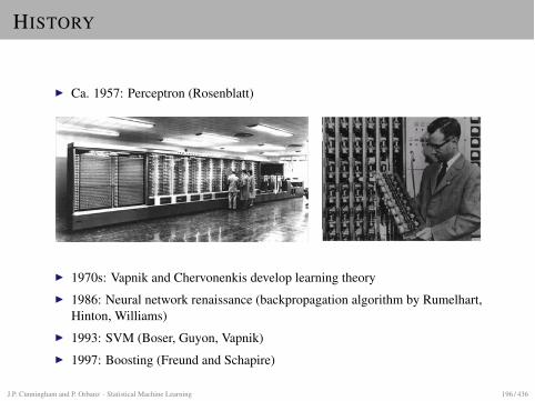
HISTORY
I Ca. 1957: Perceptron (Rosenblatt)
I 1970s: Vapnik and Chervonenkis develop learning theoryI 1986: Neural network renaissance (backpropagation algorithm by Rumelhart,
Hinton, Williams)I 1993: SVM (Boser, Guyon, Vapnik)I 1997: Boosting (Freund and Schapire)
J.P. Cunningham and P. Orbanz · Statistical Machine Learning 196 / 436
REGRESSION
REGRESSION: PROBLEM DEFINITION
DataI Measurements: x 2 Rd (also: independent variable, covariate)I Labels: y 2 R (also: dependent variable, response)
TaskFind a predictor f : Rd ! R such that (approximately) f (x) = y for data (x, y). Thepredictor is called a regression function.
Definition: Linear regressionA regression method is called linear if the predictor f is a linear function, i.e. a line ifd = 1 (more generally, an affine hyperplane).
J.P. Cunningham and P. Orbanz · Statistical Machine Learning 198 / 436
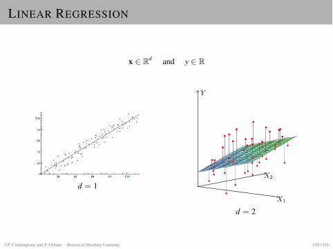
LINEAR REGRESSION
x 2 Rd and y 2 R
d = 1
Elements of Statistical Learning (2nd Ed.) c�Hastie, Tibshirani & Friedman 2009 Chap 3
•• •
••
• •••
• •••
•
•
•
••
•••
••
•
•
••
•
•• ••
•
•
••
•• •
•
•
•
•
•
•
•
•
•
•
•
•• •
•
•
•
••
•
• ••
• •
••
• •••
•
•
•
•
X1
X2
Y
FIGURE 3.1. Linear least squares fitting withX 2 IR2. We seek the linear function of X that mini-mizes the sum of squared residuals from Y .
d = 2
J.P. Cunningham and P. Orbanz · Statistical Machine Learning 199 / 436
LINEAR REGRESSION
Implications of linearityA linear function f : Rd ! R is always of the form
f (x) = �0 +dX
j=1
�jxj for �0,�1, . . . ,�d 2 R ,
where xj is the jth entry of x. Recall representation of hyperplanes in classification!
ConsequenceFinding f boils down to finding ��� 2 Rd+1.
Relation to classificationI Classification is a regression problem with {1, . . . , K} substituted for R.I Don’t get confused—the role of the hyperplane (for, say, d = 2) is different:
I Regression: Graph of regression function is hyperplane in Rd+1.I Classification: Regression function is piece-wise constant. The classifier
hyperplane lives in Rd and marks where the regression function jumps.
J.P. Cunningham and P. Orbanz · Statistical Machine Learning 200 / 436
LEAST-SQUARES REGRESSION
Squared-error lossWe use the squared-error loss function
Lse(y, f (x)) := ky� f (x)k22 .
Regression methods that determine f by minimizing Lse are called least-squaresregression methods.
Least-squares linear regressionFor training data (x1, y1), . . . , (xn, yn), we have to find the parameter vector��� 2 Rd+1 which solves
��� := arg min���
nX
i=1
Lse(yi, f (xi ;���))
where
f (x ;���) = �0 +dX
j=1
�jxj = h���, (1, x)i .
J.P. Cunningham and P. Orbanz · Statistical Machine Learning 201 / 436
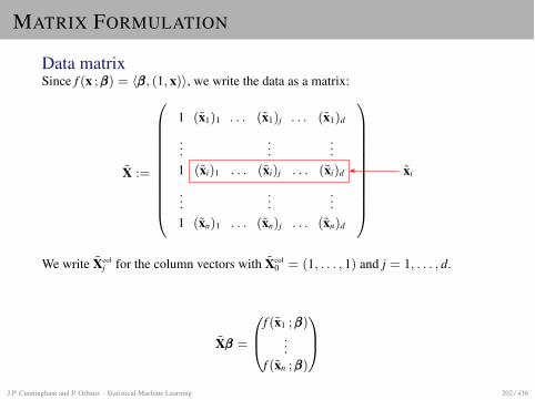
MATRIX FORMULATION
Data matrixSince f (x ;���) = h���, (1, x)i, we write the data as a matrix:
X :=
1 (x1)1 . . . (x1)j . . . (x1)d
......
...1 (xi)1 . . . (xi)j . . . (xi)d
......
...1 (xn)1 . . . (xn)j . . . (xn)d
0
B
B
B
B
B
B
B
B
B
B
B
@
1
C
C
C
C
C
C
C
C
C
C
C
A
xi
We write Xcolj for the column vectors with Xcol
0 = (1, . . . , 1) and j = 1, . . . , d.
X��� =
0
B
@
f (x1 ;���)...
f (xn ;���)
1
C
A
J.P. Cunningham and P. Orbanz · Statistical Machine Learning 202 / 436
MATRIX FORMULATION
Least-squares linear regression: Matrix formWe have to minimize
nX
i=1
Lse(yi, f (xi ;���)) =nX
i=1
(yi � f (xi ;���))2 = ky� X���k22
The solution to the linear regression problem is now ��� = arg min��� ky� X���k2.
Solving the minimization problemRecall:
I We have to solve for a zero derivative, @Lse
@��� (���) = 0.
I That means that ��� is an extremum.I To ensure that the extremum is a minimum, we have to ensure the second
derivative @2Lse
@���2 (���) is positive. For matrices: Positive definite.
J.P. Cunningham and P. Orbanz · Statistical Machine Learning 203 / 436
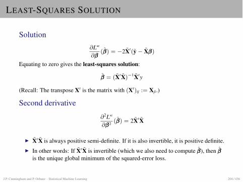
LEAST-SQUARES SOLUTION
Solution@Lse
@���(���) = �2Xt(y� X���)
Equating to zero gives the least-squares solution:
��� = (XtX)�1Xty
(Recall: The transpose Xt is the matrix with (Xt)ij := Xji.)
Second derivative
@2Lse
@���2 (���) = 2XtX
I XtX is always positive semi-definite. If it is also invertible, it is positive definite.I In other words: If XtX is invertible (which we also need to compute ���), then ���
is the unique global minimum of the squared-error loss.
J.P. Cunningham and P. Orbanz · Statistical Machine Learning 204 / 436
TOOLS: LINEAR ALGEBRABASICS
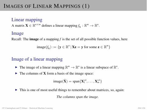
IMAGES OF LINEAR MAPPINGS (1)
Linear mappingA matrix X 2 Rn⇥m defines a linear mapping fX : Rm ! Rn.
ImageRecall: The image of a mapping f is the set of all possible function values, here
image(fX) := {y 2 Rn | Xz = y for some z 2 Rm}
Image of a linear mappingI The image of a linear mapping Rm ! Rn is a linear subspace of Rn.I The columns of X form a basis of the image space:
image(X) = span{Xcol1 , . . . , Xcol
m }
I This is one of most useful things to remember about matrices, so, again:
The columns span the image.
J.P. Cunningham and P. Orbanz · Statistical Machine Learning 206 / 436
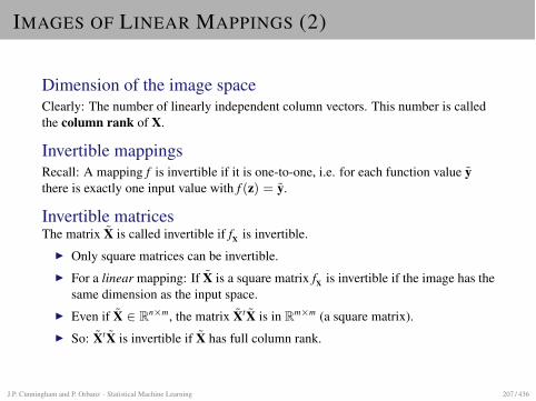
IMAGES OF LINEAR MAPPINGS (2)
Dimension of the image spaceClearly: The number of linearly independent column vectors. This number is calledthe column rank of X.
Invertible mappingsRecall: A mapping f is invertible if it is one-to-one, i.e. for each function value ythere is exactly one input value with f (z) = y.
Invertible matricesThe matrix X is called invertible if fX is invertible.
I Only square matrices can be invertible.I For a linear mapping: If X is a square matrix fX is invertible if the image has the
same dimension as the input space.I Even if X 2 Rn⇥m, the matrix XtX is in Rm⇥m (a square matrix).I So: XtX is invertible if X has full column rank.
J.P. Cunningham and P. Orbanz · Statistical Machine Learning 207 / 436
SYMMETRIC AND ORTHOGONAL MATRICES
Recall: TransposeThe transpose AT of a matrix A 2 Rm is the matrix with entries
(AT)ij := Aji
Orthogonal matricesA matrix O 2 Rm⇥m is called orthogonal
O�1 = OT
Orthogonal matrices describe two types of operations:
1. Rotations of the coordinate system.
2. Permutations of the coordinate axes.
Symmetric matricesA matrix A 2 Rm⇥m is called symmetric
A = AT
Note: Symmetric and orthogonal matrices are very different objects. Only the identity is both.J.P. Cunningham and P. Orbanz · Statistical Machine Learning 208 / 436
ORTHONORMAL BASES
Recall: ONBA basis {v1, . . . , vm} of Rm is called an orthonormal basis if
hvi, vji =
(
1 i = j0 i 6= j
In other words, the vi are pairwise orthogonal and each of length 1.
Orthogonal matricesA matrix is orthogonal precisely if its rows form an ONB. Any two ONBs can betransformed into each other by an orthogonal matrix.
J.P. Cunningham and P. Orbanz · Statistical Machine Learning 209 / 436
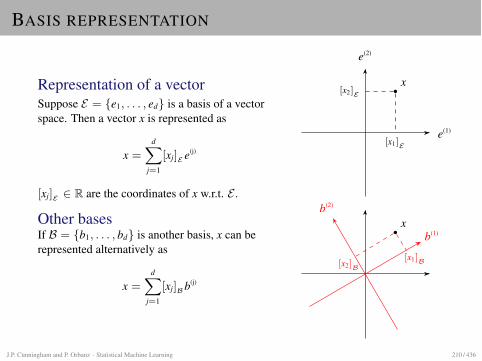
BASIS REPRESENTATION
Representation of a vectorSuppose E = {e1, . . . , ed} is a basis of a vectorspace. Then a vector x is represented as
x =dX
j=1
[xj]E e(j)
[xj]E 2 R are the coordinates of x w.r.t. E .
Other basesIf B = {b1, . . . , bd} is another basis, x can berepresented alternatively as
x =dX
j=1
[xj]B b(j)
x
e(1)
e(2)
[x2]E
[x1]E
xb(1)
b(2)
[x1]B[x2]B
J.P. Cunningham and P. Orbanz · Statistical Machine Learning 210 / 436
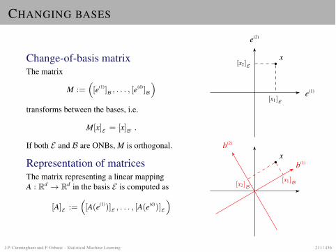
CHANGING BASES
Change-of-basis matrixThe matrix
M :=⇣
[e(1)]B , . . . , [e(d)]B
⌘
transforms between the bases, i.e.
M[x]E = [x]B .
If both E and B are ONBs, M is orthogonal.
Representation of matricesThe matrix representing a linear mappingA : Rd ! Rd in the basis E is computed as
[A]E :=⇣
[A(e(1))]E , . . . , [A(e(d))]E
⌘
x
e(1)
e(2)
[x2]E
[x1]E
xb(1)
b(2)
[x1]B[x2]B
J.P. Cunningham and P. Orbanz · Statistical Machine Learning 211 / 436
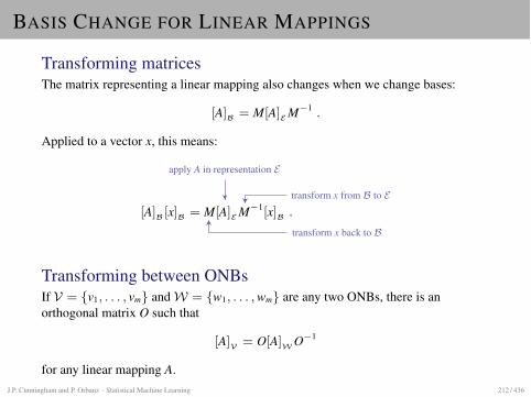
BASIS CHANGE FOR LINEAR MAPPINGS
Transforming matricesThe matrix representing a linear mapping also changes when we change bases:
[A]B = M[A]E M�1 .
Applied to a vector x, this means:
[A]B [x]B = M[A]E M�1[x]B .
transform x from B to E
apply A in representation E
transform x back to B
Transforming between ONBsIf V = {v1, . . . , vm} and W = {w1, . . . , wm} are any two ONBs, there is anorthogonal matrix O such that
[A]V = O[A]W O�1
for any linear mapping A.J.P. Cunningham and P. Orbanz · Statistical Machine Learning 212 / 436
TOOLS:EIGENVALUES AND GAUSSIAN
DISTRIBUTIONS
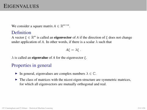
EIGENVALUES
We consider a square matrix A 2 Rm⇥m.
DefinitionA vector ⇠ 2 Rm is called an eigenvector of A if the direction of ⇠ does not changeunder application of A. In other words, if there is a scalar � such that
A⇠ = �⇠ .
� is called an eigenvalue of A for the eigenvector ⇠.
Properties in generalI In general, eigenvalues are complex numbers � 2 C.I The class of matrices with the nicest eigen-structure are symmetric matrices,
for which all eigenvectors are mutually orthogonal and real.
J.P. Cunningham and P. Orbanz · Statistical Machine Learning 214 / 436
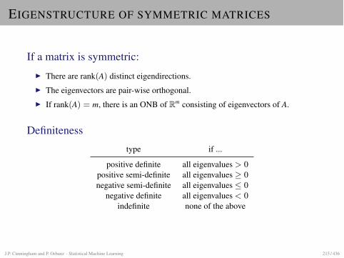
EIGENSTRUCTURE OF SYMMETRIC MATRICES
If a matrix is symmetric:I There are rank(A) distinct eigendirections.I The eigenvectors are pair-wise orthogonal.I If rank(A) = m, there is an ONB of Rm consisting of eigenvectors of A.
Definitenesstype if ...
positive definite all eigenvalues > 0positive semi-definite all eigenvalues � 0negative semi-definite all eigenvalues 0
negative definite all eigenvalues < 0indefinite none of the above
J.P. Cunningham and P. Orbanz · Statistical Machine Learning 215 / 436
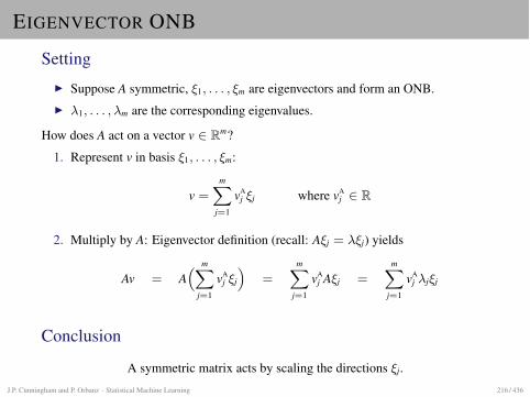
EIGENVECTOR ONB
SettingI Suppose A symmetric, ⇠1, . . . , ⇠m are eigenvectors and form an ONB.I �1, . . . ,�m are the corresponding eigenvalues.
How does A act on a vector v 2 Rm?
1. Represent v in basis ⇠1, . . . , ⇠m:
v =mX
j=1
vAj ⇠j where vA
j 2 R
2. Multiply by A: Eigenvector definition (recall: A⇠j = �⇠j) yields
Av = A⇣
mX
j=1
vAj ⇠j
⌘
=mX
j=1
vAj A⇠j =
mX
j=1
vAj �j⇠j
Conclusion
A symmetric matrix acts by scaling the directions ⇠j.J.P. Cunningham and P. Orbanz · Statistical Machine Learning 216 / 436
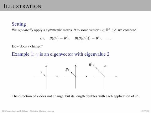
ILLUSTRATION
SettingWe repeatedly apply a symmetric matrix B to some vector v 2 Rm, i.e. we compute
Bv, B(Bv) = B2v, B(B(Bv))) = B3v, . . .
How does v change?
Example 1: v is an eigenvector with eigenvalue 2
vBv
B2v
The direction of v does not change, but its length doubles with each application of B.
J.P. Cunningham and P. Orbanz · Statistical Machine Learning 217 / 436
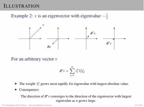
ILLUSTRATION
Example 2: v is an eigenvector with eigenvalue � 12
v
Bv
B2v
B3v
For an arbitrary vector v
Bnv =mX
j=1
vBj �
nj ⇠j
I The weight �nj grows most rapidly for eigenvalue with largest absolute value.
I Consequence:
The direction of Bnv converges to the direction of the eigenvector with largesteigenvalue as n grows large.
J.P. Cunningham and P. Orbanz · Statistical Machine Learning 218 / 436
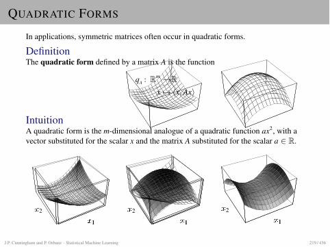
QUADRATIC FORMS
In applications, symmetric matrices often occur in quadratic forms.
DefinitionThe quadratic form defined by a matrix A is the function
qA : Rm !Rx 7! hx, Axi
IntuitionA quadratic form is the m-dimensional analogue of a quadratic function ax2, with avector substituted for the scalar x and the matrix A substituted for the scalar a 2 R.
The Quadratic Form 5
(c)
1
2
1
(d)
1
2
1
(a)
1
2
1
(b)
1
2
1
Figure 5: (a) Quadratic form for a positive-definite matrix. (b) For a negative-definite matrix. (c) For asingular (and positive-indefinite) matrix. A line that runs through the bottom of the valley is the set ofsolutions. (d) For an indefinite matrix. Because the solution is a saddle point, Steepest Descent and CGwill not work. In three dimensions or higher, a singular matrix can also have a saddle.
solution is a minimum of , so can be solved by finding an that minimizes . (If is notsymmetric, then Equation 6 hints that CG will find a solution to the system 1
2 . Note that12 is symmetric.)
Why do symmetric positive-definite matrices have this nice property? Consider the relationship betweenat some arbitrary point and at the solution point 1 . FromEquation 3 one can show (AppendixC1)
that if is symmetric (be it positive-definite or not),
12
(8)
If is positive-definite as well, then by Inequality 2, the latter term is positive for all . It follows thatis a global minimum of .
The fact that is a paraboloid is our best intuition of what it means for a matrix to be positive-definite.If is not positive-definite, there are several other possibilities. could be negative-definite — the resultof negating a positive-definite matrix (see Figure 2, but hold it upside-down). might be singular, in whichcase no solution is unique; the set of solutions is a line or hyperplane having a uniform value for . Ifis none of the above, then is a saddle point, and techniques like Steepest Descent and CG will likely fail.Figure 5 demonstrates the possibilities. The values of and determine where the minimum point of theparaboloid lies, but do not affect the paraboloid’s shape.
Why go to the trouble of converting the linear system into a tougher-looking problem? The methodsunder study — Steepest Descent and CG — were developed and are intuitively understood in terms ofminimization problems like Figure 2, not in terms of intersecting hyperplanes such as Figure 1.
J.P. Cunningham and P. Orbanz · Statistical Machine Learning 219 / 436
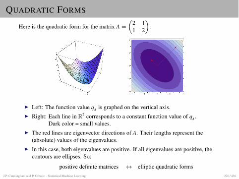
QUADRATIC FORMS
Here is the quadratic form for the matrix A =
✓
2 11 2
◆
:
I Left: The function value qA is graphed on the vertical axis.I Right: Each line in R2 corresponds to a constant function value of qA .
Dark color = small values.I The red lines are eigenvector directions of A. Their lengths represent the
(absolute) values of the eigenvalues.I In this case, both eigenvalues are positive. If all eigenvalues are positive, the
contours are ellipses. So:
positive definite matrices $ elliptic quadratic formsJ.P. Cunningham and P. Orbanz · Statistical Machine Learning 220 / 436
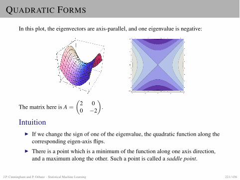
QUADRATIC FORMS
In this plot, the eigenvectors are axis-parallel, and one eigenvalue is negative:
The matrix here is A =
✓
2 00 �2
◆
.
IntuitionI If we change the sign of one of the eigenvalue, the quadratic function along the
corresponding eigen-axis flips.I There is a point which is a minimum of the function along one axis direction,
and a maximum along the other. Such a point is called a saddle point.
J.P. Cunningham and P. Orbanz · Statistical Machine Learning 221 / 436
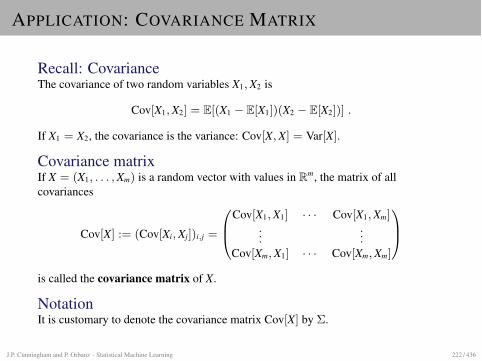
APPLICATION: COVARIANCE MATRIX
Recall: CovarianceThe covariance of two random variables X1, X2 is
Cov[X1, X2] = E[(X1 � E[X1])(X2 � E[X2])] .
If X1 = X2, the covariance is the variance: Cov[X, X] = Var[X].
Covariance matrixIf X = (X1, . . . , Xm) is a random vector with values in Rm, the matrix of allcovariances
Cov[X] := (Cov[Xi, Xj])i,j =
0
B
@
Cov[X1, X1] · · · Cov[X1, Xm]...
...Cov[Xm, X1] · · · Cov[Xm, Xm]
1
C
A
is called the covariance matrix of X.
NotationIt is customary to denote the covariance matrix Cov[X] by ⌃.
J.P. Cunningham and P. Orbanz · Statistical Machine Learning 222 / 436
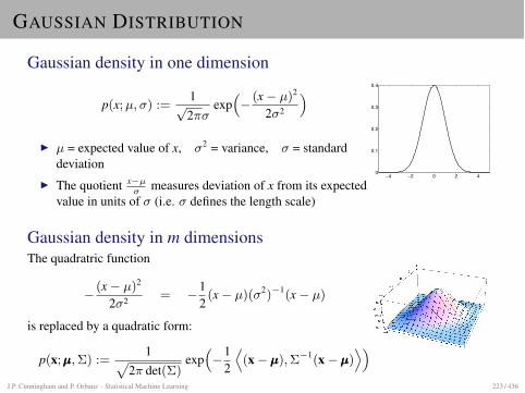
GAUSSIAN DISTRIBUTION
Gaussian density in one dimension
p(x; µ,�) :=1p2⇡�
exp⇣
� (x� µ)2
2�2
⌘
I µ = expected value of x, �2 = variance, � = standarddeviation
I The quotient x�µ� measures deviation of x from its expected
value in units of � (i.e. � defines the length scale)
Gaussian density in m dimensionsThe quadratric function
� (x� µ)2
2�2 = �12(x� µ)(�2)�1(x� µ)
is replaced by a quadratic form:
p(x;µµµ, ⌃) :=1
p
2⇡ det(⌃)exp⇣
�12
D
(x�µµµ), ⌃�1(x�µµµ)E⌘
The Gaussian Distribution
Chris Williams, School of Informatics, University of EdinburghOverview
• Probability density functions
• Univariate Gaussian
• Multivariate Gaussian
• Mahalanobis distance
• Properties of Gaussian distributions
• Graphical Gaussian models
• Read: Tipping chs 3 and 4
Continuous distributions• Probability density function (pdf) for a continuous random variable X
P (a � X � b) =� b
ap(x)dx
thereforeP (x � X � x + �x) � p(x)�x
• Example: Gaussian distribution
p(x) =1
(2��2)1/2exp�
�(x � µ)2
2�2
�
shorthand notation X � N(µ, �2)
• Standard normal (or Gaussian) distribution Z � N(0,1)
• Normalization � ∞
−∞p(x)dx = 1
−4 −2 0 2 40
0.1
0.2
0.3
0.4
• Cumulative distribution function
�(z) = P (Z � z) =� z
−∞p(z′)dz′
• Expectation
E[g(X)] =�
g(x)p(x)dx
• mean, E[X]
• Variance E[(X � µ)2]
• For a Gaussian, mean = µ, variance = �2
• Shorthand: x � N(µ, �2)
J.P. Cunningham and P. Orbanz · Statistical Machine Learning 223 / 436
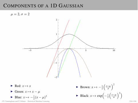
COMPONENTS OF A 1D GAUSSIAN
µ = 2, � = 2
-5 5 10
-2
-1
1
2
I Red: x 7! xI Green: x 7! x� µ
I Blue: x 7! � 12 (x� µ)2
I Brown: x 7! � 12
⇣
x�µ�
⌘2
I Black: x 7! exp⇣
� 12
⇣
x�µ�
⌘2⌘
J.P. Cunningham and P. Orbanz · Statistical Machine Learning 224 / 436
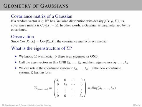
GEOMETRY OF GAUSSIANS
Covariance matrix of a GaussianIf a random vector X 2 Rm has Gaussian distribution with density p(x; µ, ⌃), itscovariance matrix is Cov[X] = ⌃. In other words, a Gaussian is parameterized by itscovariance.
ObservationSince Cov[Xi, Xj] = Cov[Xj, Xi], the covariance matrix is symmetric.
What is the eigenstructure of ⌃?I We know: ⌃ symmetric) there is an eigenvector ONBI Call the eigenvectors in this ONB ⇠1, . . . , ⇠m and their eigenvalues �1, . . . ,�m
I We can rotate the coordinate system to ⇠1, . . . , ⇠m. In the new coordinatesystem, ⌃ has the form
⌃[⇠1,...,⇠n] =
0
B
B
B
@
�1 0 · · · 00 �2 · · · 0...
.... . .
...0 0 · · · �m
1
C
C
C
A
= diag(�1, . . . ,�m)
J.P. Cunningham and P. Orbanz · Statistical Machine Learning 225 / 436
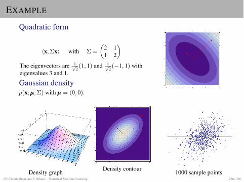
EXAMPLE
Quadratic form
hx, ⌃xi with ⌃ =
✓
2 11 2
◆
The eigenvectors are 1p2(1, 1) and 1p
2(�1, 1) with
eigenvalues 3 and 1.
Gaussian densityp(x;µµµ, ⌃) with µµµ = (0, 0).
Density graph Density contour 1000 sample pointsJ.P. Cunningham and P. Orbanz · Statistical Machine Learning 226 / 436
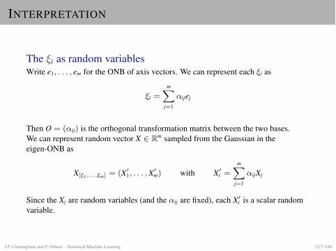
INTERPRETATION
The ⇠i as random variablesWrite e1, . . . , em for the ONB of axis vectors. We can represent each ⇠i as
⇠i =mX
j=1
↵ijej
Then O = (↵ij) is the orthogonal transformation matrix between the two bases.We can represent random vector X 2 Rm sampled from the Gaussian in theeigen-ONB as
X[⇠1,...,⇠m] = (X01, . . . , X0m) with X0i =mX
j=1
↵ijXj
Since the Xj are random variables (and the ↵ij are fixed), each X0i is a scalar randomvariable.
J.P. Cunningham and P. Orbanz · Statistical Machine Learning 227 / 436
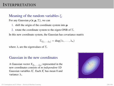
INTERPRETATION
Meaning of the random variables ⇠iFor any Gaussian p(x;µµµ, ⌃), we can
1. shift the origin of the coordinate system into µµµ
2. rotate the coordinate system to the eigen-ONB of ⌃.
In this new coordinate system, the Gaussian has covariance matrix
⌃[⇠1,...,⇠m] = diag(�1, . . . ,�m)
where �i are the eigenvalues of ⌃.
Gaussian in the new coordinates
A Gaussian vector X[⇠1,...,⇠m] represented in thenew coordinates consists of m independent 1DGaussian variables X0i . Each X0i has mean 0 andvariance �i.
J.P. Cunningham and P. Orbanz · Statistical Machine Learning 228 / 436

SHRINKAGE
ISSUES WITH LEAST SQUARES
RobustnessI Least squares works only if X has full column rank, i.e. if XtX is invertible.I If XtX almost not invertible, least squares is numerically unstable.
Statistical consequence: High variance of predictions.
Not suited for high-dimensional dataI Modern problems: Many dimensions/features/predictors (possibly thousands)I Only a few of these may be important! need some form of feature selection
I Least squares:I Treats all dimensions equallyI Relevant dimensions are averaged with irrelevant onesI Consequence: Signal loss
J.P. Cunningham and P. Orbanz · Statistical Machine Learning 230 / 436
REGULARITY OF MATRICES
RegularityA matrix which is not invertible is also called a singular matrix. A matrix which isinvertible (not singular) is called regular.
In computationsNumerically, matrices can be "almost singular". Intuition:
I A singular matrix maps an entire linear subspace into a single point.I If a matrix maps points far away from each other to points very close to each
other, it almost behaves like a singular matrix.
J.P. Cunningham and P. Orbanz · Statistical Machine Learning 231 / 436
REGULARITY OF SYMMETRIC MATRICES
Recall: A positive semi-definite matrix A is singluar, smallest EValue is 0
IllustrationIf smallest EValue �min > 0 but very small (say �min ⇡ 10�10):
I Suppose x1, x2 are two points in subspace spanned by ⇠min withkx1 � x2k ⇡ 1000.
I Image under A: kAx1 � Ax2k ⇡ 10�7
In this caseI A has an inverse, but A behaves almost like a singular matrixI The inverse A�1 can map almost identical points to points with large distance,
i.e.small change in input ! large change in output
! unstable behavior
Consequence for StatisticsIf a statistical prediction involves the inverse of an almost-singular matrix, thepredictions become unreliable (high variance).
J.P. Cunningham and P. Orbanz · Statistical Machine Learning 232 / 436
IMPLICATIONS FOR LINEAR REGRESSION
Recall: Prediction in linear regressionFor a point xnew 2 Rd, we predict the corresponding function value as
ynew =D
�, (1, x)E
= (XtX)�1Xty
Effect of unstable inversionI Suppose we choose an arbitrary training point xi and make a small change to its
response value yi.I Intuitively, that should not have a big impact on � or on prediction.I If XtX is almost singular, a small change to yi can prompt a huge change in �,
and hence in the predicted value ynew.
J.P. Cunningham and P. Orbanz · Statistical Machine Learning 233 / 436
MEASURING REGULARITY (OF SYMMETRIC MATRICES)
Symmetric matricesDenote by �max and �min the eigenvalues of A with largest/smallest absolute value. IfA is symmetric, then
A regular , |�min| > 0 .
IdeaI We can use |�min| as a measure of regularity:
larger value of �min $ "more regular" matrix A
I We need a notion of scale to determine whether |�min| is large.I The relevant scale is how A scales a vector. Maximal scaling coefficient: �max.
Regularity measure
c(A) :=|�min||�max|
The function c( . ) is called the spectral condition ("spectral" since the set ofeigenvalues is also called the "spectrum").
J.P. Cunningham and P. Orbanz · Statistical Machine Learning 234 / 436
RIDGE REGRESSION
ObjectiveRidge regression is a modification of least squares. We try to make least squaresmore robust if XtX is almost singular.
Ridge regression solutionThe ridge regression solution to a linear regression problem is defined as
���ridge
:= (XtX + �I)�1Xty
� is a tuning parameter.
J.P. Cunningham and P. Orbanz · Statistical Machine Learning 235 / 436
EXPLANATION
RecallXtX 2 R(d+1)⇥(d+1) is positive definite.
Spectral shiftSuppose ⇠1, . . . , ⇠d+1 are EVectors of XtX with EValues �1, . . . ,�d+1.Then:
(XtX + �I)⇠i = (XtX)⇠i + �I⇠i = (�i + �)⇠i
Hence: (XtX + �I) is positive definite with EValues �1 + �, . . . ,�d+1 + �.
Conclusion
XtX + �I is a regularized version of XtX.
J.P. Cunningham and P. Orbanz · Statistical Machine Learning 236 / 436
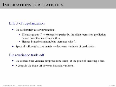
IMPLICATIONS FOR STATISTICS
Effect of regularizationI We deliberately distort prediction:
I If least squares (� = 0) predicts perfectly, the ridge regression predictionhas an error that increases with �.
I Hence: Biased estimator, bias increases with �.I Spectral shift regularizes matrix! decreases variance of predictions.
Bias-variance trade-offI We decrease the variance (improve robustness) at the price of incurring a bias.I � controls the trade-off between bias and variance.
J.P. Cunningham and P. Orbanz · Statistical Machine Learning 237 / 436
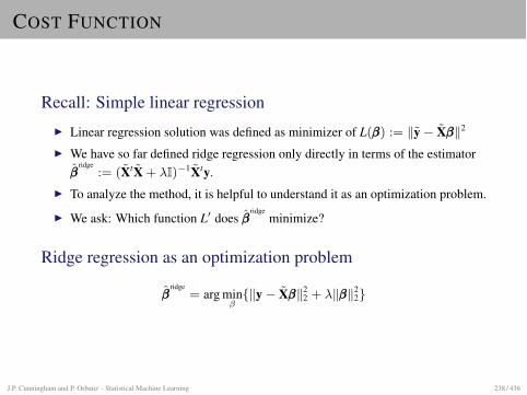
COST FUNCTION
Recall: Simple linear regressionI Linear regression solution was defined as minimizer of L(���) := ky� X���k2
I We have so far defined ridge regression only directly in terms of the estimator���
ridge:= (XtX + �I)�1Xty.
I To analyze the method, it is helpful to understand it as an optimization problem.
I We ask: Which function L0 does ���ridge
minimize?
Ridge regression as an optimization problem
���ridge
= arg min�
{ky� X���k22 + �k���k2
2}
J.P. Cunningham and P. Orbanz · Statistical Machine Learning 238 / 436
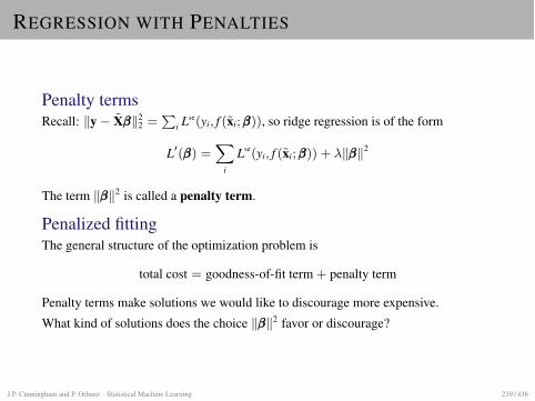
REGRESSION WITH PENALTIES
Penalty termsRecall: ky� X���k2
2 =P
i Lse(yi, f (xi;���)), so ridge regression is of the form
L0(���) =X
i
Lse(yi, f (xi;���)) + �k���k2
The term k���k2 is called a penalty term.
Penalized fittingThe general structure of the optimization problem is
total cost = goodness-of-fit term + penalty term
Penalty terms make solutions we would like to discourage more expensive.What kind of solutions does the choice k���k2 favor or discourage?
J.P. Cunningham and P. Orbanz · Statistical Machine Learning 239 / 436
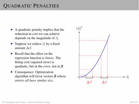
QUADRATIC PENALTIES
I A quadratic penalty implies that thereduction in cost we can achievedepends on the magnitude of �j.
I Suppose we reduce �j by a fixedamount ��.
I Recall that the effect on theregression function is linear. Thefitting cost (squared error) isquadratic, but in the error, not in ���.
I Consequence: Optimizationalgorithm will favor vectors ��� whoseentries all have similar size.
�j
|�j|2
�� ��
J.P. Cunningham and P. Orbanz · Statistical Machine Learning 240 / 436
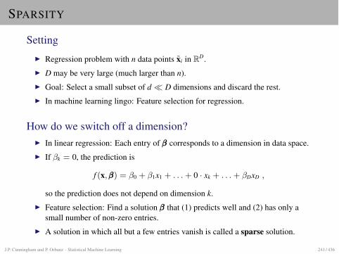
SPARSITY
SettingI Regression problem with n data points xi in RD.I D may be very large (much larger than n).I Goal: Select a small subset of d ⌧ D dimensions and discard the rest.I In machine learning lingo: Feature selection for regression.
How do we switch off a dimension?I In linear regression: Each entry of ��� corresponds to a dimension in data space.I If �k = 0, the prediction is
f (x,���) = �0 + �1x1 + . . . + 0 · xk + . . . + �DxD ,
so the prediction does not depend on dimension k.I Feature selection: Find a solution ��� that (1) predicts well and (2) has only a
small number of non-zero entries.I A solution in which all but a few entries vanish is called a sparse solution.
J.P. Cunningham and P. Orbanz · Statistical Machine Learning 241 / 436
SPARSITY AND PENALTIES
Penalization approachFind a penalty term which discourages non-sparse solutions.
Can quadratic penalty help?I Suppose �k is large, all other �j are small but non-zero.I Sparsity: Penalty should keep �k, discard others (i.e. push other �j to zero)I Quadratic penalty: Will favor entries �j which all have similar size! pushes �k towards small value.
Overall, a quadratic penalty favors many small, but non-zero values.
SolutionSparsity can be achieved using linear penalty terms.
J.P. Cunningham and P. Orbanz · Statistical Machine Learning 242 / 436
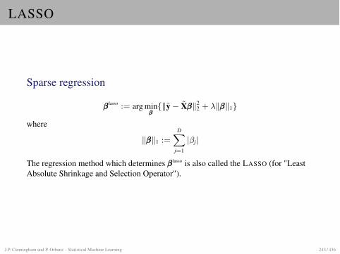
LASSO
Sparse regression
��� lasso := arg min���
{ky� X���k22 + �k���k1}
where
k���k1 :=DX
j=1
|�j|
The regression method which determines ��� lasso is also called the LASSO (for "LeastAbsolute Shrinkage and Selection Operator").
J.P. Cunningham and P. Orbanz · Statistical Machine Learning 243 / 436
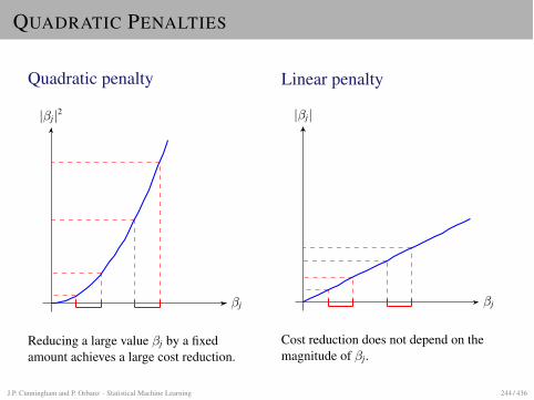
QUADRATIC PENALTIES
Quadratic penalty
�j
|�j|2
Reducing a large value �j by a fixedamount achieves a large cost reduction.
Linear penalty
�j
|�j|
Cost reduction does not depend on themagnitude of �j.
J.P. Cunningham and P. Orbanz · Statistical Machine Learning 244 / 436
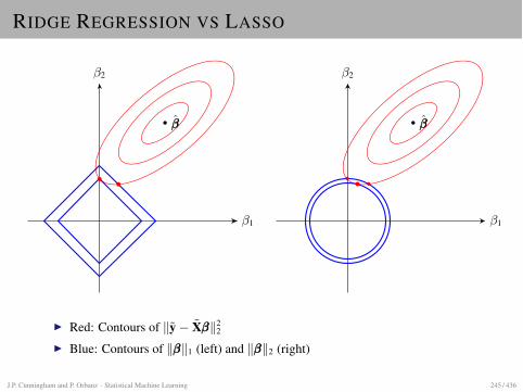
RIDGE REGRESSION VS LASSO
�1
�2
���
�1
�2
���
I Red: Contours of ky� X���k22
I Blue: Contours of k���k1 (left) and k���k2 (right)
J.P. Cunningham and P. Orbanz · Statistical Machine Learning 245 / 436
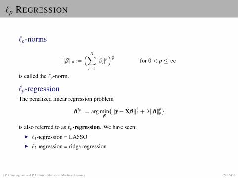
`p REGRESSION
`p-norms
k���kp :=⇣
DX
j=1
|�j|p⌘
1p for 0 < p 1
is called the `p-norm.
`p-regressionThe penalized linear regression problem
���`p := arg min���
{ky� X���k22 + �k���kp
p}
is also referred to as `p-regression. We have seen:I `1-regression = LASSOI `2-regression = ridge regression
J.P. Cunningham and P. Orbanz · Statistical Machine Learning 246 / 436

`p PENALIZATION TERMS
Elements of Statistical Learning (2nd Ed.) c�Hastie, Tibshirani & Friedman 2009 Chap 3
q = 4 q = 2 q = 1 q = 0.5 q = 0.1
FIGURE 3.12. Contours of constant value ofPj |�j |q for given values of q.
p = 4 p = 2 p = 1 p = 0.5 p = 0.1
p Behavior of k . kp
p =1 Norm measures largest absolute entry, k���k1 = maxj k�jkp > 2 Norm focusses on large entriesp = 2 Large entries are expensive; encourages similar-size entries.p = 1 Encourages sparsity.p < 1 Encourages sparsity as for p = 1 (note "pointy" behavior on the axes),
but contour set not convex.p! 0 Simply records whether an entry is non-zero, i.e. k���k0 =
P
j I{�j 6= 0}
J.P. Cunningham and P. Orbanz · Statistical Machine Learning 247 / 436
COMPUTING THE SOLUTION
Ridge regressionRecall: Solution can be computed directly as ���
ridge:= (XtX + �I)�1Xty. There is no
similar formula for the `1 case.
Solution of `1 problemBy convex optimization.
J.P. Cunningham and P. Orbanz · Statistical Machine Learning 248 / 436
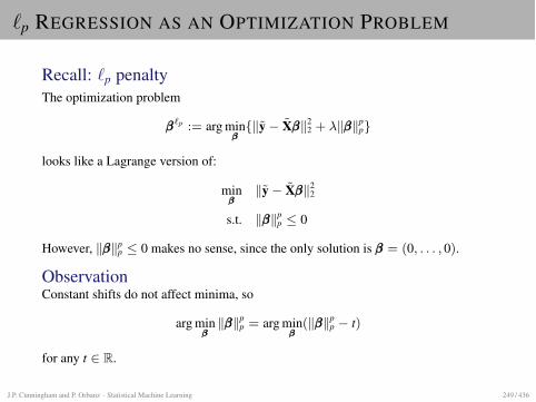
`p REGRESSION AS AN OPTIMIZATION PROBLEM
Recall: `p penaltyThe optimization problem
���`p := arg min���
{ky� X���k22 + �k���kp
p}
looks like a Lagrange version of:
min���
ky� X���k22
s.t. k���kpp 0
However, k���kpp 0 makes no sense, since the only solution is ��� = (0, . . . , 0).
ObservationConstant shifts do not affect minima, so
arg min���k���kp
p = arg min���
(k���kpp � t)
for any t 2 R.
J.P. Cunningham and P. Orbanz · Statistical Machine Learning 249 / 436
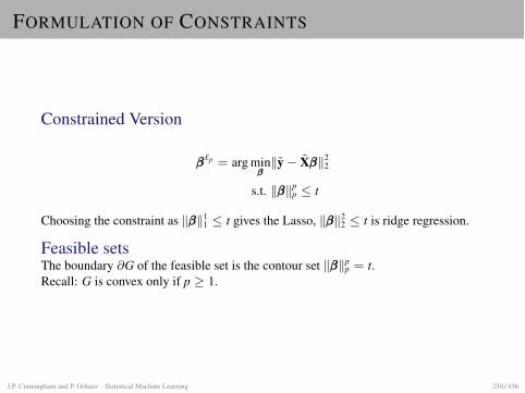
FORMULATION OF CONSTRAINTS
Constrained Version
���`p = arg min���ky� X���k2
2
s.t. k���kpp t
Choosing the constraint as k���k11 t gives the Lasso, k���k2
2 t is ridge regression.
Feasible setsThe boundary @G of the feasible set is the contour set k���kp
p = t.Recall: G is convex only if p � 1.
J.P. Cunningham and P. Orbanz · Statistical Machine Learning 250 / 436
SUMMARY: REGRESSION
Methods we have discussedI Linear regression with least squaresI Ridge regression, Lasso, and other `p penalties
Note: All of these are linear. The solutions are hyperplanes. The different methodsdiffer only in how they place the hyperplane.
Ridge regressionSuppose we obtain two training samples X1 and X2 from the same distribution.
I Ideally, the linear regression solutions on both should be (nearly) identical.I With standard linear regression, the problem may not be solvable (if XtX not
invertible).I Even if it is solvable, if the matrices XtX are close to singular (small spectral
condition c(XtX)), then the two solutions can differ significantly.I Ridge regression stabilizes the inversion of XtX. Consequences:
I Regression solutions for X1 and X2 will be almost identical if �sufficiently large.
I The price we pay is a bias that grows with �.
J.P. Cunningham and P. Orbanz · Statistical Machine Learning 251 / 436
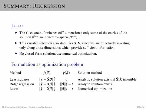
SUMMARY: REGRESSION
LassoI The `1-costraint "switches off" dimensions; only some of the entries of the
solution ��� lasso are non-zero (sparse ��� lasso).I This variable selection also stabilizes XtX, since we are effectively inverting
only along those dimensions which provide sufficient information.I No closed-form solution; use numerical optimization.
Formulation as optimization problem
Method f (���) g(���) Solution method
Least squares ky� X���k22 0 Analytic solution exists if XtX invertible
Ridge regression ky� X���k22 k���k2
2 � t Analytic solution existsLasso ky� X���k2
2 k���k1 � t Numerical optimization
J.P. Cunningham and P. Orbanz · Statistical Machine Learning 252 / 436
MODEL BIAS AND VARIANCE
OVERVIEW
I We have already encountered the fact that we can trade off model flexibilityagainst stability of estimates (e.g. shrinkage).
I To make this effect a bit more precise, we have to discuss the type of errors thatwe encounter in estimation problems.
I In this context, it is useful to interpret models as sets of probabilitydistributions.
J.P. Cunningham and P. Orbanz · Statistical Machine Learning 254 / 436
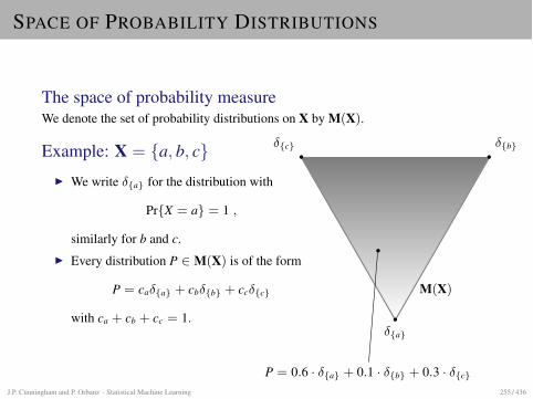
SPACE OF PROBABILITY DISTRIBUTIONS
The space of probability measureWe denote the set of probability distributions on X by M(X).
Example: X = {a, b, c}I We write �{a} for the distribution with
Pr{X = a} = 1 ,
similarly for b and c.I Every distribution P 2 M(X) is of the form
P = ca�{a} + cb�{b} + cc�{c}
with ca + cb + cc = 1.
M(X)
�{a}
�{b}�{c}
P = 0.6 · �{a} + 0.1 · �{b} + 0.3 · �{c}J.P. Cunningham and P. Orbanz · Statistical Machine Learning 255 / 436
POINT MASSES
Dirac distributionsA Dirac distribution �x is a probability distribution which concentrates all its massat a single point x. A Dirac �x is also called a point mass.
Note: This means that there is no uncertainty in a random variable X withdistribution �x: We know before we even sample that X = x with probability 1.
Working with a DiracThe defining property of a Dirac is that
Z
Xf (x)�x0(dx) = f (x0)
for every (integrable) function f .
J.P. Cunningham and P. Orbanz · Statistical Machine Learning 256 / 436
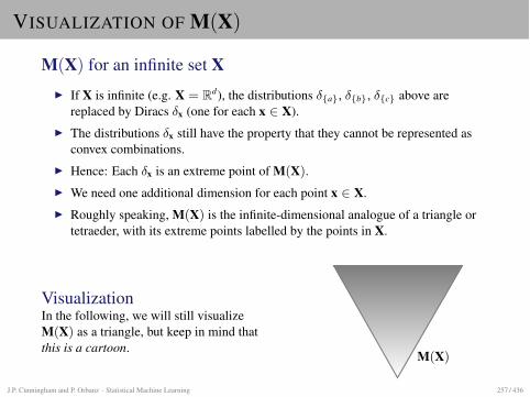
VISUALIZATION OF M(X)
M(X) for an infinite set XI If X is infinite (e.g. X = Rd), the distributions �{a}, �{b}, �{c} above are
replaced by Diracs �x (one for each x 2 X).I The distributions �x still have the property that they cannot be represented as
convex combinations.I Hence: Each �x is an extreme point of M(X).I We need one additional dimension for each point x 2 X.I Roughly speaking, M(X) is the infinite-dimensional analogue of a triangle or
tetraeder, with its extreme points labelled by the points in X.
VisualizationIn the following, we will still visualizeM(X) as a triangle, but keep in mind thatthis is a cartoon. M(X)
J.P. Cunningham and P. Orbanz · Statistical Machine Learning 257 / 436
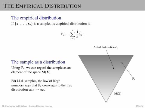
THE EMPIRICAL DISTRIBUTION
The empirical distributionIf {x1, . . . , xn} is a sample, its empirical distribution is
Fn :=nX
i=1
1n�xi .
The sample as a distributionUsing Fn, we can regard the sample as anelement of the space M(X).
For i.i.d. samples, the law of largenumbers says that Fn converges to the truedistribution as n!1.
M(X)
Actual distribution P0
Fn
J.P. Cunningham and P. Orbanz · Statistical Machine Learning 258 / 436
EXAMPLE: PLUG-IN ESTIMATORS
A simple application of the empirical distribution are plug-in estimators.
Integral statisticsMany of the most common statistics can be written in the form
S[p] =
Z
Xf (x)p(x)dx .
Examples: Expectation of p (where f (x) = x), variance of p (wheref (x) = (x� µ)2), etc.
Plug-in estimatorOne way to estimate S from a sample {x1, . . . , xn} is to "plug in" the empiricaldistribution Fn for the true distribution p:
S :=
Z
Xf (x)Fn(dx) =
1n
nX
i=1
f (xi)
This estimator is called the plug-in estimator of S.
J.P. Cunningham and P. Orbanz · Statistical Machine Learning 259 / 436
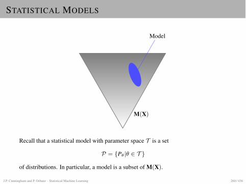
STATISTICAL MODELS
M(X)
Model
Recall that a statistical model with parameter space T is a set
P = {P✓|✓ 2 T }of distributions. In particular, a model is a subset of M(X).
J.P. Cunningham and P. Orbanz · Statistical Machine Learning 260 / 436
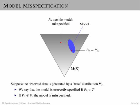
MODEL MISSPECIFICATION
M(X)
Model
P0 = P✓0
misspecifiedP0 outside model:
Suppose the observed data is generated by a "true" distribution P0.I We say that the model is correctly specified if P0 2 P .I If P0 62 P , the model is misspecified.
J.P. Cunningham and P. Orbanz · Statistical Machine Learning 261 / 436
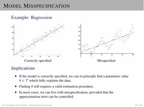
MODEL MISSPECIFICATION
Example: Regression
Correctly specified Misspecified
ImplicationsI If the model is correctly specified, we can in principle find a parameter value✓ 2 T which fully explains the data.
I Finding ✓ still requires a valid estimation procedure.I In most cases, we can live with misspecification, provided that the
approximation error can be controlled.
J.P. Cunningham and P. Orbanz · Statistical Machine Learning 262 / 436
BIAS-VARIANCE TRADE-OFF
Model complexityIf our only objective is to avoid misspecification, we should make the model (thesubset P of M(X)) as large as possible. A larger set P corresponds to a model that ismore flexible.
Bias vs. VarianceI Misspecification means that, no matter how much data we observe, our
estimated model never completely explains the data. This can be interpreted asa form of bias.
I To avoid misspecification, we can make the model more flexible.I We have already seen how estimates in more flexible models tend to vary more
between sample sets (higher variance).
Thus, we can decrease bias at the expense of increasing variance, and vice versa.This phenomenon is called the bias-variance trade-off.
J.P. Cunningham and P. Orbanz · Statistical Machine Learning 263 / 436
MEASURING MODEL COMPLEXITY
In parametric modelsI A fundamental measure of model complexity is the number of degrees of
freedom (d.o.f.).I This is roughly the dimension of the parameter space (= the number of
independent scalar paramaters), provided the parametrization is chosen suchthat the entries of the parameter vector are reasonably independent of eachother.
I For example, a Gaussian scale model on Rd (unknown mean, fixed variance)has d degrees of freedom, a Gaussian model with unknown mean and variancehas d + d(d � 1)/2.
Remark: Nonparametric modelsI In nonparametric models (= infinite-dimensional parameter space), measuring
model complexity is much harder.I Tools to solve this problem are developed in two closely related research fields
called Statistical Learning Theory (in Machine Learning) and EmpiricalProcess Theory (in Statistics).
J.P. Cunningham and P. Orbanz · Statistical Machine Learning 264 / 436
EXAMPLE: REGRESSION WITH ADDITIVE NOISE
Model
Y = f (X) + " with E["] = 0 and Var["] = �2 .
We assume that f 2 F , where F is some class of functions. Linear regression is thespecial case where F is the set of affine functions.
Bias and VariancePrediction error(x0) = E[(Y � f (x0))
2|X = x0]
= �2 + (E[ f (x0)]� f (x0))2 + E[ f (x0)� E[ f (x0)]]
2
= �2 + Bias( f (x0))2 + Var[ f (x0)]
= Irreducible error + Bias2 + Variance
This is due to Fn 6= P0.
Decreases with model flexibility.
Increases with model flexibility.
J.P. Cunningham and P. Orbanz · Statistical Machine Learning 265 / 436
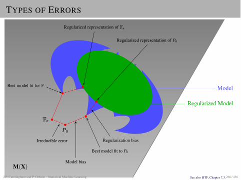
TYPES OF ERRORS
M(X)
Model
Regularized Model
P0
Fn
Model bias
Irreducible error Regularization bias
Regularized representation of Fn
Regularized representation of P0
Best model fit to P0
Best model fit for F
See also HTF, Chapter 7.3.J.P. Cunningham and P. Orbanz · Statistical Machine Learning 266 / 436
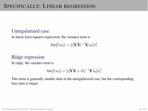
SPECIFICALLY: LINEAR REGRESSION
Unregularized caseIn linear least-squares regression, the variance term is
Var[f (x0)] = k(XtX)�1Xtx0k�2"
Ridge regressionIn ridge, the variance term is
Var[f (x0)] = k(XtX + �I)�1Xtx0k�2"
This term is generally smaller than in the unregularized case, but the correspondingbias term is larger.
J.P. Cunningham and P. Orbanz · Statistical Machine Learning 267 / 436
SUMMARY
Model complexityI Model choice has to trade off stability (low variance) vs flexibility (low bias).I It can be beneficial (in terms of prediction error) to permit a bias if this
decreases the variance.I Bias and variance terms combine to form prediction error.
How does cross validation fit in?I Cross validation estimates the prediction error.I A high variance of estimates will typically be reflected in a high variance
between estimates on different blocks.
J.P. Cunningham and P. Orbanz · Statistical Machine Learning 268 / 436
UNSUPERVISED LEARNING
UNSUPERVISED LEARNING
In shortI Label information available! supervised learning (classification, regression)I No label information available! unsupervised learning
ProblemI Try to find structure or patterns in data without knowing a correct solution.I By choosing a model, we specify what kind of patterns we are looking for.
Examples of unsupervised learning problemsI Dimension reductionI Clustering
J.P. Cunningham and P. Orbanz · Statistical Machine Learning 270 / 436
DIMENSION REDUCTION
DIMENSION REDUCTION PROBLEMS
SettingI Given: High-dimensional data x1, . . . , xn 2 RD
I Look for: Low-dimensional projection of the data such that important structurein data is preserved
More preciselyI Find suitable linear subspace V ⇢ RD with dim(V) =: d small.I Compute projection xv
j of each xj onto V
Most common cases: d 2 {2, 3} for visualization.
J.P. Cunningham and P. Orbanz · Statistical Machine Learning 272 / 436
PCA: OVERVIEW
Assumptions
1. Directions along which uncertainty in data is maximal are most interesting.
2. Uncertainty is measured by variance.
MethodI Compute empirical covariance matrix of the data.I Compute its EValues �1, . . . ,�D and EVectors ⇠1, . . . , ⇠D.I Choose the d largest EValues, say, �j1 , . . . ,�jd .I Define subspace as V := span{⇠j1 , . . . , ⇠jd }I Project data onto V: For each xi, compute xv
i :=Pd
j=1 hxi, ⇠ji ⇠j
This algorithm is called Principal Component Analysis (PCA).
J.P. Cunningham and P. Orbanz · Statistical Machine Learning 273 / 436
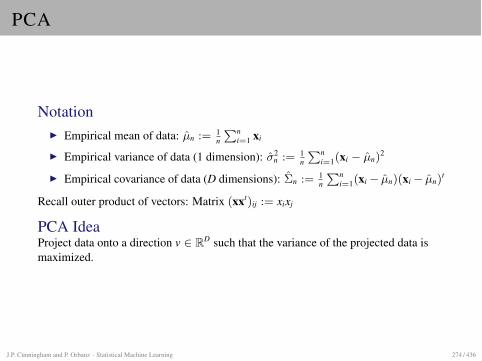
PCA
NotationI Empirical mean of data: µn := 1
n
Pni=1 xi
I Empirical variance of data (1 dimension): �2n := 1
n
Pni=1(xi � µn)
2
I Empirical covariance of data (D dimensions): ⌃n := 1n
Pni=1(xi� µn)(xi� µn)
t
Recall outer product of vectors: Matrix (xxt)ij := xixj
PCA IdeaProject data onto a direction v 2 RD such that the variance of the projected data ismaximized.
J.P. Cunningham and P. Orbanz · Statistical Machine Learning 274 / 436
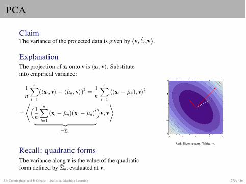
PCA
ClaimThe variance of the projected data is given by
⌦
v, ⌃nv↵
.
ExplanationThe projection of xi onto v is hxi, vi. Substituteinto empirical variance:
1n
nX
i=1
(hxi, vi � hµn, vi)2 =1n
nX
i=1
h(xi � µn), vi2
=
*
⇣1n
nX
i=1
(xi � µn)(xi � µn)t
| {z }
=⌃n
⌘
v, v
+
Recall: quadratic formsThe variance along v is the value of the quadraticform defined by ⌃n, evaluated at v.
Red: Eigenvectors. White: v.
J.P. Cunningham and P. Orbanz · Statistical Machine Learning 275 / 436
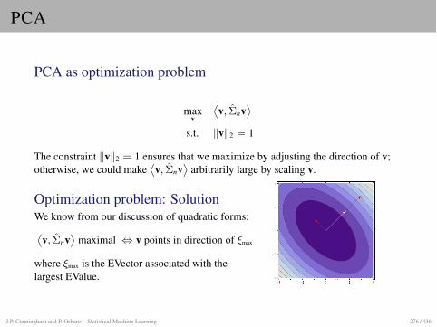
PCA
PCA as optimization problem
maxv
⌦
v, ⌃nv↵
s.t. kvk2 = 1
The constraint kvk2 = 1 ensures that we maximize by adjusting the direction of v;otherwise, we could make
⌦
v, ⌃nv↵
arbitrarily large by scaling v.
Optimization problem: SolutionWe know from our discussion of quadratic forms:⌦
v, ⌃nv↵
maximal , v points in direction of ⇠max
where ⇠max is the EVector associated with thelargest EValue.
J.P. Cunningham and P. Orbanz · Statistical Machine Learning 276 / 436
PROJECTING ONTO SEVERAL DIMENSIONS
Projecting onto 2 dimensions
1. Project onto 1 dimension.
2. Remove that dimension from data, i.e. restrict data to the space orthogonal to v.
3. Apply PCA on restricted space.
It is not hard to show that the result is the direction of the EVector associated with thesecond-largest eigenvalue.
Projecting onto d dimensionsBy iterating the procedure above, we find that the optimal projection onto ddimensions corresponds to the d largest EValues.
SummaryThe PCA algorithm (=project on the d "largest" EVectors) can be justified as theprojection which maximizes the variance of the projected data.
J.P. Cunningham and P. Orbanz · Statistical Machine Learning 277 / 436
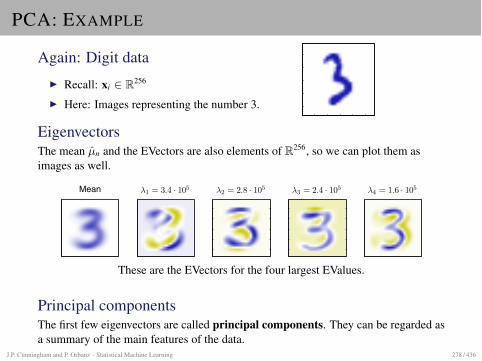
PCA: EXAMPLE
Again: Digit dataI Recall: xi 2 R256
I Here: Images representing the number 3.
Original M = 1 M = 10 M = 50 M = 250
EigenvectorsThe mean µn and the EVectors are also elements of R256, so we can plot them asimages as well.
Mean �1 = 3.4 · 105 �2 = 2.8 · 105 �3 = 2.4 · 105 �4 = 1.6 · 105
These are the EVectors for the four largest EValues.
Principal componentsThe first few eigenvectors are called principal components. They can be regarded asa summary of the main features of the data.
J.P. Cunningham and P. Orbanz · Statistical Machine Learning 278 / 436
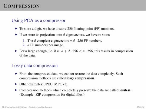
COMPRESSION
Using PCA as a compressorI To store a digit, we have to store 256 floating point (FP) numbers.I If we store its projection onto d eigenvectors, we have to store:
1. The d complete eigenvectors = d · 256 FP numbers.2. d FP numbers per image.
I For n large enough, i.e. if n · d + d · 256 < n · 256, this results in compressionof the data.
Lossy data compressionI From the compressed data, we cannot restore the data completely. Such
compression methods are called lossy compression.I Other examples: JPEG, MP3, etc.I Compression methods which completely preserve the data are called lossless.
(Example: ZIP compression for digital files.)
J.P. Cunningham and P. Orbanz · Statistical Machine Learning 279 / 436
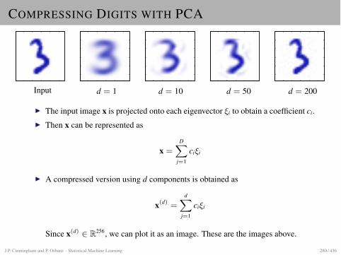
COMPRESSING DIGITS WITH PCAOriginal M = 1 M = 10 M = 50 M = 250
Input d = 1 d = 10 d = 50 d = 200
I The input image x is projected onto each eigenvector ⇠i to obtain a coefficient ci.I Then x can be represented as
x =DX
j=1
ci⇠i
I A compressed version using d components is obtained as
x(d) =dX
j=1
ci⇠i
Since x(d) 2 R256, we can plot it as an image. These are the images above.
J.P. Cunningham and P. Orbanz · Statistical Machine Learning 280 / 436
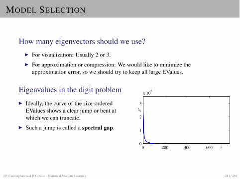
MODEL SELECTION
How many eigenvectors should we use?I For visualization: Usually 2 or 3.I For approximation or compression: We would like to minimize the
approximation error, so we should try to keep all large EValues.
Eigenvalues in the digit problemI Ideally, the curve of the size-ordered
EValues shows a clear jump or bent atwhich we can truncate.
I Such a jump is called a spectral gap.
i
�i
(a)0 200 400 600
0
1
2
3
x 105
J.P. Cunningham and P. Orbanz · Statistical Machine Learning 281 / 436
DATA CLUSTERING
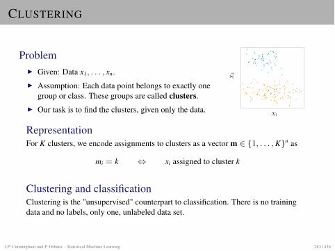
CLUSTERING
ProblemI Given: Data x1, . . . , xn.I Assumption: Each data point belongs to exactly one
group or class. These groups are called clusters.I Our task is to find the clusters, given only the data.
Elements of Statistical Learning (2nd Ed.) c�Hastie, Tibshirani & Friedman 2009 Chap 14
• • •
•
••
••
••••
•
•
• •• ••
•• • •
•
••
•
•
••
•
••
•••••
• ••
•
• •••
•
•
•
••
••
••
•••
•
••
•
•
•
•
•
•
••••
•
•
• •••
••
•• •
•• •• •
•
• •• •
••
•
• •
••
••• •
•
•• • •
•• •• ••• •
••
•••
•••
•
•• •
•
••
••
•
•
••
••
••••
• •
••• ••
X1
X2
FIGURE 14.4. Simulated data in the plane, clus-tered into three classes (represented by orange, blue andgreen) by the K-means clustering algorithm
RepresentationFor K clusters, we encode assignments to clusters as a vector m 2 {1, . . . , K}n as
mi = k , xi assigned to cluster k
Clustering and classificationClustering is the "unsupervised" counterpart to classification. There is no trainingdata and no labels, only one, unlabeled data set.
J.P. Cunningham and P. Orbanz · Statistical Machine Learning 283 / 436
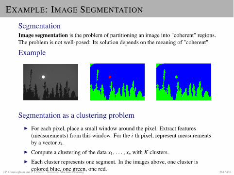
EXAMPLE: IMAGE SEGMENTATION
SegmentationImage segmentation is the problem of partitioning an image into "coherent" regions.The problem is not well-posed: Its solution depends on the meaning of "coherent".
Example
Segmentation as a clustering problemI For each pixel, place a small window around the pixel. Extract features
(measurements) from this window. For the i-th pixel, represent measurementsby a vector xi.
I Compute a clustering of the data x1, . . . , xn with K clusters.I Each cluster represents one segment. In the images above, one cluster is
colored blue, one green, one red.J.P. Cunningham and P. Orbanz · Statistical Machine Learning 284 / 436
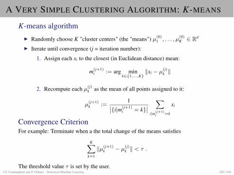
A VERY SIMPLE CLUSTERING ALGORITHM: K-MEANS
K-means algorithmI Randomly choose K "cluster centers" (the "means") µ(0)
1 , . . . , µ(0)K 2 Rd
I Iterate until convergence (j = iteration number):
1. Assign each xi to the closest (in Euclidean distance) mean:
m(j+1)i := arg min
k2{1,...,K}kxi � µ(j)
k k
2. Recompute each µ(j)k as the mean of all points assigned to it:
µ(j+1)k :=
1�
�{i|m(j+1)i = k}��
X
i|m(j+1)i =k
xi
Convergence CriterionFor example: Terminate when a the total change of the means satisfies
KX
k=1
kµ(j+1)k � µ(j)
k k < ⌧ .
The threshold value ⌧ is set by the user.J.P. Cunningham and P. Orbanz · Statistical Machine Learning 285 / 436
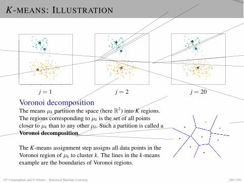
K-MEANS: ILLUSTRATIONElements of Statistical Learning (2nd Ed.) c�Hastie, Tibshirani & Friedman 2009 Chap 14
-4 -2 0 2 4 6
-20
24
6
Initial Centroids
• • •
•
••
••
••••
•
•
• •• ••
•• • •
•
••
•
•
•
••
•
••
•••••
• ••
• •••
•
•
••
• ••
•••
•
••
••
•
•
••••
•
•
• • •••
•
•• • •
• •• •
•
• •• ••
••
• •
•• ••••
••
•
••• • •
•• •• •• •• •
••• •
•••
•
•• •
••
•••
••
•••
•••
•
••
• •
••• ••
•
••
•
••
• • •
•
••
••
••••
•
•
• •• ••
•• • •
•
••
•
•
•
••
•
••
•••••
• ••
• •••
•
•
••
• ••
•••
•
••
••
•
•
••••
•
•
• • •••
•
•• • •
• •• •
•
• •• ••
••
• •
•• ••••
••
•
••• • •
•• •• •• •• •
••• •
•••
•
•• •
••
•••
••
•••
•••
•
••
• •
••• ••
•
••
•
••
Initial Partition
• • •
•
••
••
••••
•
•
• •• ••
•• • •
•
••
•
•
••
•
••
•••••
• ••
•
• •••
•
•
••
••
••
•••
•
••
•
•
•
•
•
••••
•
•
• • •••
•
•• • •
• •• •
•
• •• ••
••
• •
•• ••
••
•
••
•• •• •• •
••• •
••
••
•
•
• •• •
••
•••
••
•••
••
••
••
••
• •
••• ••
Iteration Number 2
••
•
•
••
• • •
•
••
••
••••
•
•
• •• ••
•• • •
•
••
•
•
••
•
••
•••••
• ••
•
• •••
•
•
••
•••
••
•••
•
••
•
•
•
•
•
•
••••
•
•
• • •••
•
•• • •
• •• •
•
• •• ••
••
• •
••
••• •
••• • •
•• •• ••• •• •
•••
•••
•
•• •
••
•••
••
•••
•••••
• •
••• ••
Iteration Number 20
•
••
•
••
FIGURE 14.6. Successive iterations of the K-meansclustering algorithm for the simulated data of Fig-ure 14.4.
j = 1
Elements of Statistical Learning (2nd Ed.) c�Hastie, Tibshirani & Friedman 2009 Chap 14
-4 -2 0 2 4 6
-20
24
6
Initial Centroids
• • •
•
••
••
••••
•
•
• •• ••
•• • •
•
••
•
•
•
••
•
••
•••••
• ••
• •••
•
•
••
• ••
•••
•
••
••
•
•
••••
•
•
• • •••
•
•• • •
• •• •
•
• •• ••
••
• •
•• ••••
••
•
••• • •
•• •• •• •• •
••• •
•••
•
•• •
••
•••
••
•••
•••
•
••
• •
••• ••
•
••
•
••
• • •
•
••
••
••••
•
•
• •• ••
•• • •
•
••
•
•
•
••
•
••
•••••
• ••
• •••
•
•
••
• ••
•••
•
••
••
•
•
••••
•
•
• • •••
•
•• • •
• •• •
•
• •• ••
••
• •
•• ••••
••
•
••• • •
•• •• •• •• •
••• •
•••
•
•• •
••
•••
••
•••
•••
•
••
• •
••• ••
•
••
•
••
Initial Partition
• • •
•
••
••
••••
•
•
• •• ••
•• • •
•
••
•
•
••
•
••
•••••
• ••
•
• •••
•
•
••
••
••
•••
•
••
•
•
•
•
•
••••
•
•
• • •••
•
•• • •
• •• •
•
• •• ••
••
• •
•• ••
••
•
••
•• •• •• •
••• •
••
••
•
•
• •• •
••
•••
••
•••
••
••
••
••
• •
••• ••
Iteration Number 2
••
•
•
••
• • •
•
••
••
••••
•
•
• •• ••
•• • •
•
••
•
•
••
•
••
•••••
• ••
•
• •••
•
•
••
•••
••
•••
•
••
•
•
•
•
•
•
••••
•
•
• • •••
•
•• • •
• •• •
•
• •• ••
••
• •
••
••• •
••• • •
•• •• ••• •• •
•••
•••
•
•• •
••
•••
••
•••
•••••
• •
••• ••
Iteration Number 20
•
••
•
••
FIGURE 14.6. Successive iterations of the K-meansclustering algorithm for the simulated data of Fig-ure 14.4.
j = 2
Elements of Statistical Learning (2nd Ed.) c�Hastie, Tibshirani & Friedman 2009 Chap 14
-4 -2 0 2 4 6
-20
24
6
Initial Centroids
• • •
•
••
••
••••
•
•
• •• ••
•• • •
•
••
•
•
•
••
•
••
•••••
• ••
• •••
•
•
••
• ••
•••
•
••
••
•
•
••••
•
•
• • •••
•
•• • •
• •• •
•
• •• ••
••
• •
•• ••••
••
•
••• • •
•• •• •• •• •
••• •
•••
•
•• •
••
•••
••
•••
•••
•
••
• •
••• ••
•
••
•
••
• • •
•
••
••
••••
•
•
• •• ••
•• • •
•
••
•
•
•
••
•
••
•••••
• ••
• •••
•
•
••
• ••
•••
•
••
••
•
•
••••
•
•
• • •••
•
•• • •
• •• •
•
• •• ••
••
• •
•• ••••
••
•
••• • •
•• •• •• •• •
••• •
•••
•
•• •
••
•••
••
•••
•••
•
••
• •
••• ••
•
••
•
••
Initial Partition
• • •
•
••
••
••••
•
•
• •• ••
•• • •
•
••
•
•
••
•
••
•••••
• ••
•
• •••
•
•
••
••
••
•••
•
••
•
•
•
•
•
••••
•
•
• • •••
•
•• • •
• •• •
•
• •• ••
••
• •
•• ••
••
•
••
•• •• •• •
••• •
••
••
•
•
• •• •
••
•••
••
•••
••
••
••
••
• •
••• ••
Iteration Number 2
••
•
•
••
• • •
•
••
••
••••
•
•
• •• ••
•• • •
•
••
•
•
••
•
••
•••••
• ••
•
• •••
•
•
••
•••
••
•••
•
••
•
•
•
•
•
•
••••
•
•
• • •••
•
•• • •
• •• •
•
• •• ••
••
• •
••
••• •
••• • •
•• •• ••• •• •
•••
•••
•
•• •
••
•••
••
•••
•••••
• •
••• ••
Iteration Number 20
•
••
•
••
FIGURE 14.6. Successive iterations of the K-meansclustering algorithm for the simulated data of Fig-ure 14.4.
j = 20
Voronoi decompositionThe means µk partition the space (here R2) into K regions.The regions corresponding to µk is the set of all pointscloser to µk than to any other µl. Such a partition is called aVoronoi decomposition.
The K-means assignment step assigns all data points in theVoronoi region of µk to cluster k. The lines in the k-meansexample are the boundaries of Voronoi regions.
J.P. Cunningham and P. Orbanz · Statistical Machine Learning 286 / 436
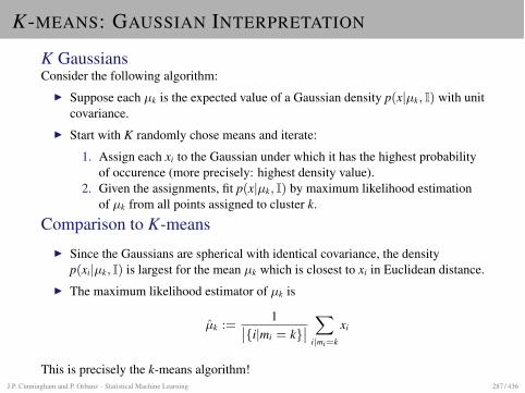
K-MEANS: GAUSSIAN INTERPRETATION
K GaussiansConsider the following algorithm:
I Suppose each µk is the expected value of a Gaussian density p(x|µk, I) with unitcovariance.
I Start with K randomly chose means and iterate:
1. Assign each xi to the Gaussian under which it has the highest probabilityof occurence (more precisely: highest density value).
2. Given the assignments, fit p(x|µk, I) by maximum likelihood estimationof µk from all points assigned to cluster k.
Comparison to K-meansI Since the Gaussians are spherical with identical covariance, the density
p(xi|µk, I) is largest for the mean µk which is closest to xi in Euclidean distance.I The maximum likelihood estimator of µk is
µk :=1
�
�{i|mi = k}��X
i|mi=k
xi
This is precisely the k-means algorithm!J.P. Cunningham and P. Orbanz · Statistical Machine Learning 287 / 436
WHAT NEXT
I We will discuss a more sophisticated version of K-means called theExpectation-Maximization (EM) algorithm.
I EM gives
1. A better statistical explanation of what is going on.2. A direct generalization to other distributions. We will consider (1)
Gaussians with general covariance structure and (2) multinomialdistributions.
J.P. Cunningham and P. Orbanz · Statistical Machine Learning 288 / 436
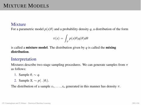
MIXTURE MODELS
MixtureFor a parametric model p(x|✓) and a probability density q, a distribution of the form
⇡(x) =
Z
Tp(x|✓)q(✓)d✓
is called a mixture model. The distribution given by q is called the mixingdistribution.
InterpretationMixtures describe two-stage sampling procedures. We can generate samples from ⇡as follows:
1. Sample ✓i ⇠ q.
2. Sample Xi ⇠ p( . |✓i).
The distribution of a sample x1, . . . , xn generated in this manner has density ⇡.
J.P. Cunningham and P. Orbanz · Statistical Machine Learning 289 / 436
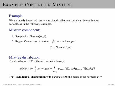
EXAMPLE: CONTINUOUS MIXTURE
ExampleWe are mostly interested discrete mixing distributions, but ✓ can be continuousvariable, as in the following example.
Mixture components
1. Sample ✓ ⇠ Gamma(↵,�).
2. Regard ✓ as an inverse variance 1�2 := ✓ and sample
X ⇠ Normal(0,�)
Mixture distributionThe distribution of X is the mixture with density
⇡(x|0, ⌫ :=↵�
, ⌧ := 2↵) =
Z
R+
pNormal(x|0, 1/✓)qGamma(✓|↵,�)d✓
This is Student’s t-distribution with parameters 0 (the mean of the normal), ⌫, ⌧ .
J.P. Cunningham and P. Orbanz · Statistical Machine Learning 290 / 436
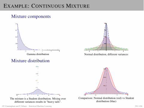
EXAMPLE: CONTINUOUS MIXTURE
Mixture components
Gamma distribution Normal distribution, different variances
Mixture distribution
The mixture is a Student distribution. Mixing overdifferent variances results in "heavy tails".
Comparison: Normal distribution (red) vs Studentdistribution (blue)
J.P. Cunningham and P. Orbanz · Statistical Machine Learning 291 / 436
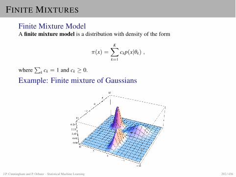
FINITE MIXTURES
Finite Mixture ModelA finite mixture model is a distribution with density of the form
⇡(x) =KX
k=1
ckp(x|✓k) ,
whereP
k ck = 1 and ck � 0.
Example: Finite mixture of Gaussians
J.P. Cunningham and P. Orbanz · Statistical Machine Learning 292 / 436
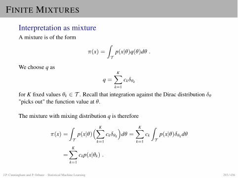
FINITE MIXTURES
Interpretation as mixtureA mixture is of the form
⇡(x) =
Z
Tp(x|✓)q(✓)d✓ .
We choose q as
q =KX
k=1
ck�✓k
for K fixed values ✓k 2 T . Recall that integration against the Dirac distribution �✓
"picks out" the function value at ✓.
The mixture with mixing distribution q is therefore
⇡(x) =
Z
Tp(x|✓)
⇣
KX
k=1
ck�✓k
⌘
d✓ =KX
k=1
ck
Z
Tp(x|✓)�✓k d✓
=KX
k=1
ckp(x|✓k) .
J.P. Cunningham and P. Orbanz · Statistical Machine Learning 293 / 436
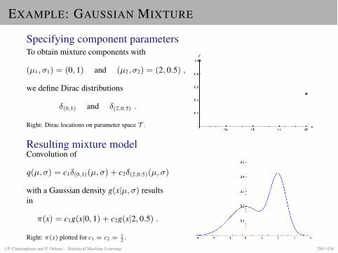
EXAMPLE: GAUSSIAN MIXTURE
Specifying component parametersTo obtain mixture components with
(µ1,�1) = (0, 1) and (µ2,�2) = (2, 0.5) ,
we define Dirac distributions
�(0,1) and �(2,0.5) .
Right: Dirac locations on parameter space T .
Resulting mixture modelConvolution of
q(µ,�) = c1�(0,1)(µ,�) + c2�(2,0.5)(µ,�)
with a Gaussian density g(x|µ,�) resultsin
⇡(x) = c1g(x|0, 1) + c2g(x|2, 0.5) .
Right: ⇡(x) plotted for c1 = c2 = 12 .
J.P. Cunningham and P. Orbanz · Statistical Machine Learning 294 / 436
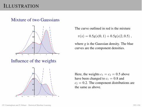
ILLUSTRATION
Mixture of two Gaussians
The curve outlined in red is the mixture
⇡(x) = 0.5g(x|0, 1) + 0.5g(x|2, 0.5) ,
where g is the Gaussian density. The bluecurves are the component densities.
Influence of the weights
Here, the weights c1 = c2 = 0.5 abovehave been changed to c1 = 0.8 andc2 = 0.2. The component distributions arethe same as above.
J.P. Cunningham and P. Orbanz · Statistical Machine Learning 295 / 436
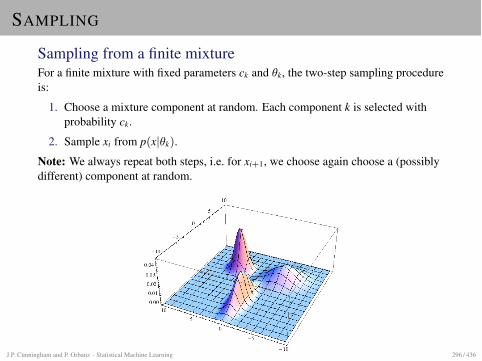
SAMPLING
Sampling from a finite mixtureFor a finite mixture with fixed parameters ck and ✓k, the two-step sampling procedureis:
1. Choose a mixture component at random. Each component k is selected withprobability ck.
2. Sample xi from p(x|✓k).
Note: We always repeat both steps, i.e. for xi+1, we choose again choose a (possiblydifferent) component at random.
J.P. Cunningham and P. Orbanz · Statistical Machine Learning 296 / 436
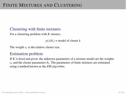
FINITE MIXTURES AND CLUSTERING
Clustering with finite mixturesFor a clustering problem with K clusters,
p(x|✓k) = model of cluster k
The weight ck is the relative cluster size.
Estimation problemIf K is fixed and given, the unknown parameters of a mixture model are the weightsck and the cluster parameters ✓k. The parameters of finite mixtures are estimatedusing a method known as the EM algorithm.
J.P. Cunningham and P. Orbanz · Statistical Machine Learning 297 / 436
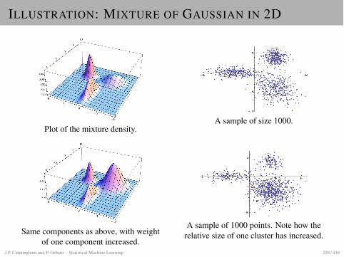
ILLUSTRATION: MIXTURE OF GAUSSIAN IN 2D
Plot of the mixture density.A sample of size 1000.
Same components as above, with weightof one component increased.
A sample of 1000 points. Note how therelative size of one cluster has increased.
J.P. Cunningham and P. Orbanz · Statistical Machine Learning 298 / 436
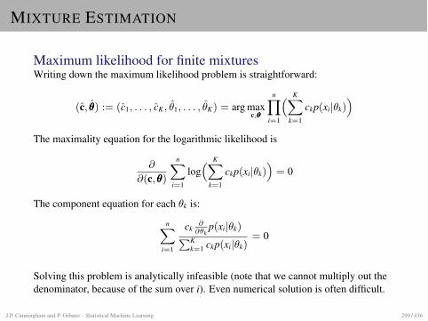
MIXTURE ESTIMATION
Maximum likelihood for finite mixturesWriting down the maximum likelihood problem is straightforward:
(c, ✓✓✓) := (c1, . . . , cK , ✓1, . . . , ✓K) = arg maxc,✓✓✓
nY
i=1
⇣
KX
k=1
ckp(xi|✓k)⌘
The maximality equation for the logarithmic likelihood is
@@(c,✓✓✓)
nX
i=1
log⇣
KX
k=1
ckp(xi|✓k)⌘
= 0
The component equation for each ✓k is:
nX
i=1
ck@
@✓kp(xi|✓k)
PKk=1 ckp(xi|✓k)
= 0
Solving this problem is analytically infeasible (note that we cannot multiply out thedenominator, because of the sum over i). Even numerical solution is often difficult.
J.P. Cunningham and P. Orbanz · Statistical Machine Learning 299 / 436
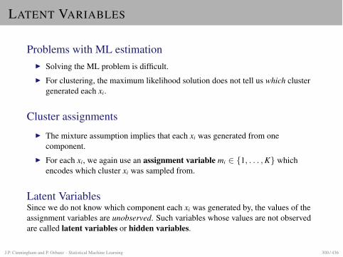
LATENT VARIABLES
Problems with ML estimationI Solving the ML problem is difficult.I For clustering, the maximum likelihood solution does not tell us which cluster
generated each xi.
Cluster assignmentsI The mixture assumption implies that each xi was generated from one
component.I For each xi, we again use an assignment variable mi 2 {1, . . . , K} which
encodes which cluster xi was sampled from.
Latent VariablesSince we do not know which component each xi was generated by, the values of theassignment variables are unobserved. Such variables whose values are not observedare called latent variables or hidden variables.
J.P. Cunningham and P. Orbanz · Statistical Machine Learning 300 / 436
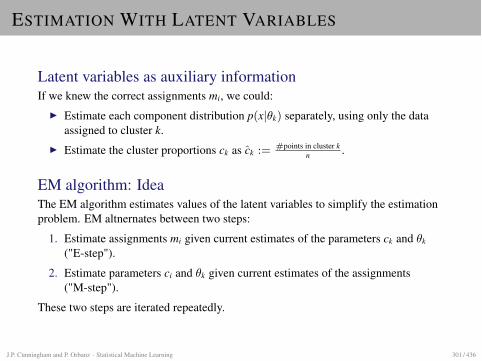
ESTIMATION WITH LATENT VARIABLES
Latent variables as auxiliary informationIf we knew the correct assignments mi, we could:
I Estimate each component distribution p(x|✓k) separately, using only the dataassigned to cluster k.
I Estimate the cluster proportions ck as ck := #points in cluster kn .
EM algorithm: IdeaThe EM algorithm estimates values of the latent variables to simplify the estimationproblem. EM altnernates between two steps:
1. Estimate assignments mi given current estimates of the parameters ck and ✓k
("E-step").
2. Estimate parameters ci and ✓k given current estimates of the assignments("M-step").
These two steps are iterated repeatedly.
J.P. Cunningham and P. Orbanz · Statistical Machine Learning 301 / 436

REPRESENTATION OF ASSIGNMENTS
We re-write the assignments as vectors of length K:
xi in cluster k as Mi :=
0
B
B
B
B
B
B
B
B
B
B
B
@
0...010...0
1
C
C
C
C
C
C
C
C
C
C
C
A
� kth entry
so Mik = 1 if xi in cluster k, and Mik = 0 otherwise.We collect the vectors into a matrix
M =
0
B
@
M11 . . . M1K...
...Mn1 . . . MnK
1
C
A
Note: Rows = observations, columns = clustersRow sums = 1, column sums = cluster sizes.
J.P. Cunningham and P. Orbanz · Statistical Machine Learning 302 / 436
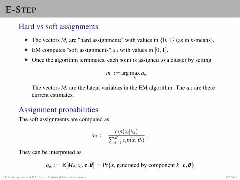
E-STEP
Hard vs soft assignmentsI The vectors Mi are "hard assignments" with values in {0, 1} (as in k-means).I EM computes "soft assignments" aik with values in [0, 1].I Once the algorithm terminates, each point is assigned to a cluster by setting
mi := arg maxk
aik
The vectors Mi are the latent variables in the EM algorithm. The aik are therecurrent estimates.
Assignment probabilitiesThe soft assignments are computed as
aik :=ckp(xi|✓k)
PKl=1 clp(xi|✓l)
.
They can be interpreted as
aik := E[Mik|xi, c,✓✓✓] = Pr{xi generated by component k | c,✓✓✓}J.P. Cunningham and P. Orbanz · Statistical Machine Learning 303 / 436
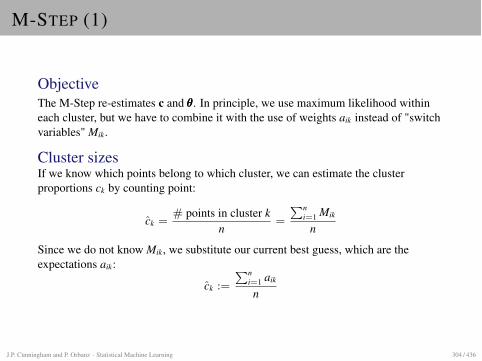
M-STEP (1)
ObjectiveThe M-Step re-estimates c and ✓✓✓. In principle, we use maximum likelihood withineach cluster, but we have to combine it with the use of weights aik instead of "switchvariables" Mik.
Cluster sizesIf we know which points belong to which cluster, we can estimate the clusterproportions ck by counting point:
ck =# points in cluster k
n=
Pni=1 Mik
n
Since we do not know Mik, we substitute our current best guess, which are theexpectations aik:
ck :=
Pni=1 aik
n
J.P. Cunningham and P. Orbanz · Statistical Machine Learning 304 / 436
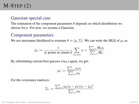
M-STEP (2)
Gaussian special caseThe estimation of the component parameters ✓ depends on which distribution wechoose for p. For now, we assume a Gaussian.
Component parametersWe use maximum likelihood to estimate ✓ = (µ, ⌃). We can write the MLE of µk as
µk :=1
# points in cluster k
X
i|xi in k
xi =
Pni=1 MikxiPn
i=1 Mik
By substituting current best guesses (=aik) again, we get:
µk :=
Pni=1 aikxiPn
i=1 aik
For the covariance matrices:
⌃k :=
Pni=1 aik(xi � µk)(xi � µk)
t
Pni=1 aik
J.P. Cunningham and P. Orbanz · Statistical Machine Learning 305 / 436
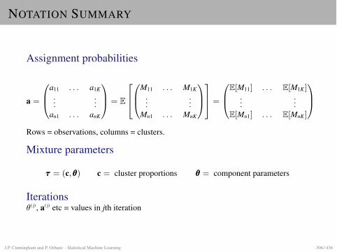
NOTATION SUMMARY
Assignment probabilities
a =
0
B
@
a11 . . . a1K...
...an1 . . . anK
1
C
A
= E
2
6
4
0
B
@
M11 . . . M1K...
...Mn1 . . . MnK
1
C
A
3
7
5
=
0
B
@
E[M11] . . . E[M1K ]...
...E[Mn1] . . . E[MnK ]
1
C
A
Rows = observations, columns = clusters.
Mixture parameters
⌧⌧⌧ = (c,✓✓✓) c = cluster proportions ✓✓✓ = component parameters
Iterations✓( j), a( j) etc = values in jth iteration
J.P. Cunningham and P. Orbanz · Statistical Machine Learning 306 / 436
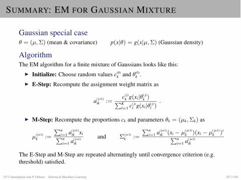
SUMMARY: EM FOR GAUSSIAN MIXTURE
Gaussian special case✓ = (µ, ⌃) (mean & covariance) p(x|✓) = g(x|µ, ⌃) (Gaussian density)
AlgorithmThe EM algorithm for a finite mixture of Gaussians looks like this:
I Initialize: Choose random values c(0)k and ✓(0)
k .I E-Step: Recompute the assignment weight matrix as
a( j+1)ik :=
c( j)k g(xi|✓( j)
k )PK
l=1 c( j)l g(xi|✓( j)
l ).
I M-Step: Recompute the proportions ck and parameters ✓k = (µk, ⌃k) as
µ( j+1)k :=
Pni=1 a( j+1)
ik xiPn
i=1 a( j+1)ik
and ⌃( j+1)k :=
Pni=1 a( j+1)
ik (xi � µ( j+1)k )(xi � µ( j+1)
k )t
Pni=1 a( j+1)
ik
The E-Step and M-Step are repeated alternatingly until convergence criterion (e.g.threshold) satisfied.
J.P. Cunningham and P. Orbanz · Statistical Machine Learning 307 / 436
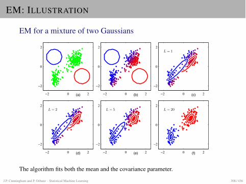
EM: ILLUSTRATION
EM for a mixture of two Gaussians
(a)−2 0 2
−2
0
2
(b)−2 0 2
−2
0
2
(c)
L = 1
−2 0 2
−2
0
2
(d)
L = 2
−2 0 2
−2
0
2
(e)
L = 5
−2 0 2
−2
0
2
(f)
L = 20
−2 0 2
−2
0
2
The algorithm fits both the mean and the covariance parameter.
J.P. Cunningham and P. Orbanz · Statistical Machine Learning 308 / 436
EM ALGORITHM: GENERAL CASE
Reminder: ObjectiveEstimate ✓ and c by (approximate) Maximum Likelihood for
⇡(x) =KX
k=1
ckp(x|✓k) =: ⇡(x|c,✓✓✓) .
The components p(x|✓k) need not be Gaussian.
J.P. Cunningham and P. Orbanz · Statistical Machine Learning 309 / 436
STEP 1 (OF 4)
Including the latent variablesRecall that we can integrate out a variable y from a joint density p(x, y):
p(x) =
Z
p(x, y)dy
We can apply this idea backwards and write the likelihood ⇡(x|c, ✓) as
⇡(x|c, ✓) =X
M
⇡(x, M|c, ✓)
Since M is discrete, the integral is a sum (over all possible assignment vectors M).
Application to the log-likelihoodnX
i=1
log⇡(xi|c, ✓) =nX
i=1
log⇣
X
Mi
⇡(x, Mi|c, ✓)⌘
J.P. Cunningham and P. Orbanz · Statistical Machine Learning 310 / 436
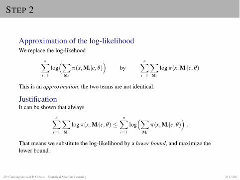
STEP 2
Approximation of the log-likelihoodWe replace the log-likehood
nX
i=1
log⇣
X
Mi
⇡(x, Mi|c, ✓)⌘
bynX
i=1
X
Mi
log⇡(x, Mi|c, ✓)
This is an approximation, the two terms are not identical.
JustificationIt can be shown that always
nX
i=1
X
Mi
log⇡(x, Mi|c, ✓) nX
i=1
log⇣
X
Mi
⇡(x, Mi|c, ✓)⌘
.
That means we substitute the log-likelihood by a lower bound, and maximize thelower bound.
J.P. Cunningham and P. Orbanz · Statistical Machine Learning 311 / 436
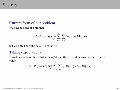
STEP 3
Current form of our problemWe have to solve the problem
(c⇤, ✓⇤) = arg maxc,✓
nX
i=1
X
Mi
log⇡(xi, Mi|c, ✓)
but we only know the data xi, not the Mi.
Taking expectationsIf we knew at least the distribution q(Mi) of Mi, we could maximize the expectedvalue:
(c⇤, ✓⇤) := arg maxc,✓
nX
i=1
X
Mi
q(Mi) log⇡(xi, Mi|c, ✓)
J.P. Cunningham and P. Orbanz · Statistical Machine Learning 312 / 436
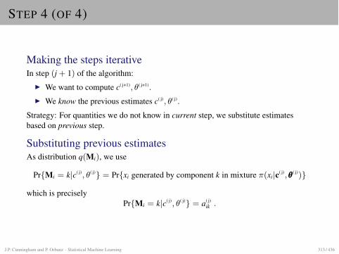
STEP 4 (OF 4)
Making the steps iterativeIn step (j + 1) of the algorithm:
I We want to compute c( j+1), ✓( j+1).I We know the previous estimates c( j), ✓( j).
Strategy: For quantities we do not know in current step, we substitute estimatesbased on previous step.
Substituting previous estimatesAs distribution q(Mi), we use
Pr{Mi = k|c( j), ✓( j)} = Pr{xi generated by component k in mixture ⇡(xi|c( j),✓✓✓( j))}which is precisely
Pr{Mi = k|c( j), ✓( j)} = a( j)ik .
J.P. Cunningham and P. Orbanz · Statistical Machine Learning 313 / 436
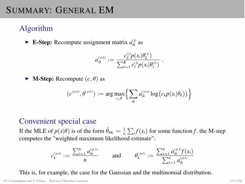
SUMMARY: GENERAL EM
AlgorithmI E-Step: Recompute assignment matrix a( j)
ik as
a( j+1)ik :=
c( j)k p(xi|✓( j)
k )PK
l=1 c( j)l p(xi|✓( j)
l ).
I M-Step: Recompute (c, ✓) as
(c( j+1), ✓( j+1)) := arg maxc,✓
n
X
ik
a( j+1)ik log
�
ckp(xi|✓k)�
o
Convenient special caseIf the MLE of p(x|✓) is of the form ✓ML = 1
n
P
i f (xi) for some function f , the M-stepcomputes the "weighted maximum likelihood estimate":
c( j+1)k :=
Pni=1 a( j+1)
ik
nand ✓( j+1)
k :=
Pni=1 a( j+1)
ik f (xi)Pn
i=1 a( j+1)ik
This is, for example, the case for the Gaussian and the multinomial distribution.J.P. Cunningham and P. Orbanz · Statistical Machine Learning 314 / 436
SUMMARY: APPROXIMATIONS
Approximations Used in EMThe derivation makes two approximations:
1. The log-likelihood is substituted by a lower bound.
2. The unknown assignments Mi are substituted by their expectations a( j)ik under the
current model.
J.P. Cunningham and P. Orbanz · Statistical Machine Learning 315 / 436
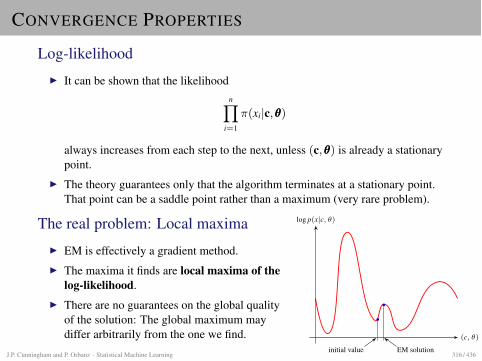
CONVERGENCE PROPERTIES
Log-likelihoodI It can be shown that the likelihood
nY
i=1
⇡(xi|c,✓✓✓)
always increases from each step to the next, unless (c,✓✓✓) is already a stationarypoint.
I The theory guarantees only that the algorithm terminates at a stationary point.That point can be a saddle point rather than a maximum (very rare problem).
The real problem: Local maximaI EM is effectively a gradient method.I The maxima it finds are local maxima of the
log-likelihood.I There are no guarantees on the global quality
of the solution: The global maximum maydiffer arbitrarily from the one we find.
initial value EM solution
log p(x|c, ✓)
(c, ✓)
J.P. Cunningham and P. Orbanz · Statistical Machine Learning 316 / 436
EM IN PRACTICE
Comparing solutionsI If (c,✓✓✓) and (c0,✓✓✓0) are two different EM solutions, we can always compute the
log-likelihoodsX
i
log⇡(xi|c,✓✓✓) andX
i
log⇡(xi|c0,✓✓✓0)
(no approximations or complications!).I The solution with the higher likelihood is better.I This is a very convenient feature of EM: Different solutions are comparable.
Random restartsIn practice, the best way to use EM is often:
I Restart EM repeatedly with randomly chosen initial values.I Compute the log-likelihoods of all solutions and compare them.I Choose the solution achieving maximal log-likelihood.
J.P. Cunningham and P. Orbanz · Statistical Machine Learning 317 / 436
EXPONENTIAL FAMILY MODELS
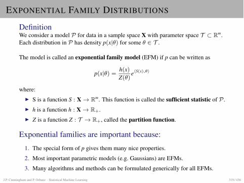
EXPONENTIAL FAMILY DISTRIBUTIONS
DefinitionWe consider a model P for data in a sample space X with parameter space T ⇢ Rm.Each distribution in P has density p(x|✓) for some ✓ 2 T .
The model is called an exponential family model (EFM) if p can be written as
p(x|✓) =h(x)Z(✓)
ehS(x),✓i
where:I S is a function S : X! Rm. This function is called the sufficient statistic of P .I h is a function h : X! R+.I Z is a function Z : T ! R+, called the partition function.
Exponential families are important because:
1. The special form of p gives them many nice properties.
2. Most important parametric models (e.g. Gaussians) are EFMs.
3. Many algorithms and methods can be formulated generically for all EFMs.
J.P. Cunningham and P. Orbanz · Statistical Machine Learning 319 / 436
ALTERNATIVE FORM
The choice of p looks perhaps less arbitrary if we write
p(x|✓) = exp⇣
hS(x), ✓i � �(x)� (✓)⌘
which is obtained by defining
�(x) := � log(h(x)) and (✓) := log(Z(✓))
A first interpretationExponential family models are models in which:
I The data and the parameter interact only through the linear term hS(x), ✓i in theexponent.
I The logarithm of p can be non-linear in both S(x) and ✓, but there is no jointnonlinear function of (S(x), ✓).
J.P. Cunningham and P. Orbanz · Statistical Machine Learning 320 / 436
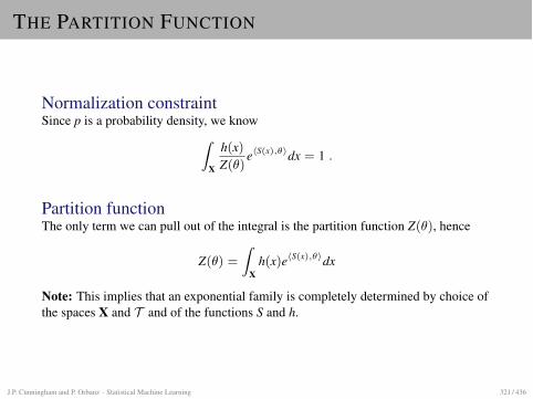
THE PARTITION FUNCTION
Normalization constraintSince p is a probability density, we know
Z
X
h(x)Z(✓)
ehS(x),✓idx = 1 .
Partition functionThe only term we can pull out of the integral is the partition function Z(✓), hence
Z(✓) =
Z
Xh(x)ehS(x),✓idx
Note: This implies that an exponential family is completely determined by choice ofthe spaces X and T and of the functions S and h.
J.P. Cunningham and P. Orbanz · Statistical Machine Learning 321 / 436
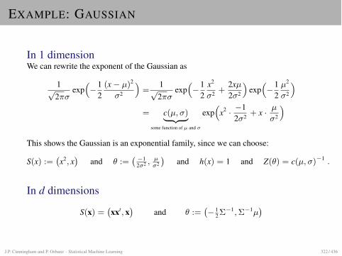
EXAMPLE: GAUSSIAN
In 1 dimensionWe can rewrite the exponent of the Gaussian as
1p2⇡�
exp⇣
�12
(x� µ)2
�2
⌘
=1p2⇡�
exp⇣
�12
x2
�2 +2xµ2�2
⌘
exp⇣
�12
µ2
�2
⌘
= c(µ,�)| {z }
some function of µ and �
exp⇣
x2 · �12�2 + x · µ
�2
⌘
This shows the Gaussian is an exponential family, since we can choose:
S(x) :=�
x2, x�
and ✓ :=� �1
2�2 , µ�2
�
and h(x) = 1 and Z(✓) = c(µ,�)�1 .
In d dimensions
S(x) =�
xxt, x�
and ✓ :=�� 1
2 ⌃�1, ⌃�1µ
�
J.P. Cunningham and P. Orbanz · Statistical Machine Learning 322 / 436
MORE EXAMPLES OF EXPONENTIAL FAMILIES
Model Sample space Sufficient statistic
Gaussian Rd S(x) = (xxt, x)Gamma R+ S(x) = (ln(x), x)Poisson N0 S(x) = xMultinomial {1, . . . , K} S(x) = xWishart Positive definite matrices (requires more details)Mallows Rankings (permutations) (requires more details)Beta [0, 1] S(x) = (ln(x), ln(1� x))Dirichlet Probability distributions on d events S(x) = (ln x1, . . . , ln xd)Bernoulli {0, 1} S(x) = x. . . . . . . . .
Roughly speakingOn every sample space, there is a "natural" statistic of interest. On a space withEuclidean distance, for example, it is natural to measure both location andcorrelation; on categories (which have no "distance" from each other), it is morenatural to measure only expected numbers of counts.On most types of sample spaces, the exponential family model with S chosen as thisnatural statistic is the prototypical distribution.
J.P. Cunningham and P. Orbanz · Statistical Machine Learning 323 / 436
MAXIMUM LIKELIHOOD FOR EFMS
Log-likelihood for n samples
lognY
i=1
p(xi|✓) =nX
i=1
⇣
log(h(xi))� log(Z(✓)) + hS(xi), ✓i⌘
MLE equation
0 =@@✓
nX
i=1
⇣
log(h(xi))� log(Z(✓)) + hS(xi), ✓i⌘
= �n@@✓
log(Z(✓)) +nX
i=1
S(xi)
Hence, the MLE is the parameter value ✓ which satisfies the equation
@@✓
log(Z(✓)) =1n
nX
i=1
S(xi)
J.P. Cunningham and P. Orbanz · Statistical Machine Learning 324 / 436
MOMENT MATCHING
Further simplificationWe know that Z(✓) =
R
h(x) exp hS(x), ✓i dx, so
@@✓
log(Z(✓)) =@@✓ Z(✓)
Z(✓)=
R
h(x) @@✓ ehS(x),✓idxZ(✓)
=
R
S(x)h(x)ehS(x),✓idxZ(✓)
= Ep(x|✓)[S(x)]
MLE equationSubstitution into the MLE equation shows that ✓ is given by
Ep(x|✓)[S(x)] =1n
nX
i=1
S(xi)
Using the empirical distribution Fn, the right-hand side can be expressed as
Ep(x|✓)[S(x)] = EFn [S(x)]
This is called a moment matching equation. Hence, MLEs of exponential familymodels can be obtained by moment matching.
J.P. Cunningham and P. Orbanz · Statistical Machine Learning 325 / 436
SUMMARY: MLE FOR EFMS
The MLEIf p(x|✓) is an exponential family model with sufficient statistic S, the maximumlikelihood estimator ✓ of ✓ given data x1, . . . , xn is given by the equation
Ep(x|✓)[S(x)] =1n
nX
i=1
S(xi)
NoteWe had already noticed that the MLE (for some parameter ⌧ ) is often of the form
⌧ =1n
nX
i=1
f (xi) .
Models are often defined so that the parameters can be interpreted as expectations ofsome useful statistic (e.g., a mean or variance). If ✓ in an exponential family ischosen as ✓ = Ep(x|✓)[S(x)], then we have indeed
✓ =1n
nX
i=1
S(xi) .
J.P. Cunningham and P. Orbanz · Statistical Machine Learning 326 / 436
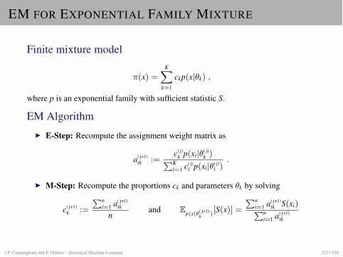
EM FOR EXPONENTIAL FAMILY MIXTURE
Finite mixture model
⇡(x) =KX
k=1
ckp(x|✓k) ,
where p is an exponential family with sufficient statistic S.
EM AlgorithmI E-Step: Recompute the assignment weight matrix as
a( j+1)ik :=
c( j)k p(xi|✓( j)
k )PK
l=1 c( j)l p(xi|✓( j)
l ).
I M-Step: Recompute the proportions ck and parameters ✓k by solving
c( j+1)k :=
Pni=1 a( j+1)
ik
nand Ep(x|✓( j+1)
k )[S(x)] =
Pni=1 a( j+1)
ik S(xi)Pn
i=1 a( j+1)ik
J.P. Cunningham and P. Orbanz · Statistical Machine Learning 327 / 436
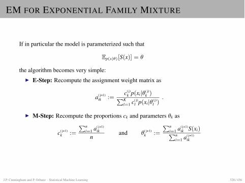
EM FOR EXPONENTIAL FAMILY MIXTURE
If in particular the model is parameterized such that
Ep(x|✓)[S(x)] = ✓
the algorithm becomes very simple:I E-Step: Recompute the assignment weight matrix as
a( j+1)ik :=
c( j)k p(xi|✓( j)
k )PK
l=1 c( j)l p(xi|✓( j)
l ).
I M-Step: Recompute the proportions ck and parameters ✓k as
c( j+1)k :=
Pni=1 a( j+1)
ik
nand ✓( j+1)
k :=
Pni=1 a( j+1)
ik S(xi)Pn
i=1 a( j+1)ik
J.P. Cunningham and P. Orbanz · Statistical Machine Learning 328 / 436

THE MULTINOMIALDISTRIBUTION
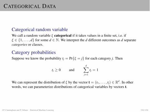
CATEGORICAL DATA
Categorical random variableWe call a random variable ⇠ categorical if it takes values in a finite set, i.e. if⇠ 2 {1, . . . , d} for some d 2 N. We interpret the d different outcomes as d separatecategories or classes.
Category probabilitiesSuppose we know the probability tj = Pr{⇠ = j} for each category j. Then
tj � 0 anddX
j=1
tj = 1
We can represent the distribution of ⇠ by the vector t = (t1, . . . , tj) 2 Rd. In otherwords, we can parameterize distributions of categorical variables by vectors t.
J.P. Cunningham and P. Orbanz · Statistical Machine Learning 330 / 436
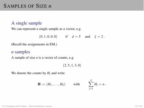
SAMPLES OF SIZE n
A single sampleWe can represent a single sample as a vector, e.g.
(0, 1, 0, 0, 0) if d = 5 and ⇠ = 2 .
(Recall the assignments in EM.)
n samplesA sample of size n is a vector of counts, e.g.
(2, 5, 1, 3, 0)
We denote the counts by Hj and write
H := (H1, . . . , Hd) withdX
j=1
Hj = n .
J.P. Cunningham and P. Orbanz · Statistical Machine Learning 331 / 436
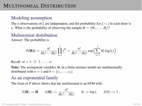
MULTINOMIAL DISTRIBUTION
Modeling assumptionThe n observations of ⇠ are independent, and the probability for ⇠ = j in each draw istj. What is the probability of observing the sample H = (H1, . . . , Hj)?
Multinomial distributionAnswer: The probability is
P(H|t) =n!
H1! · · · Hd!
dY
j=1
tHjj =
n!H1! · · · Hd!
exp⇣
dX
j=1
Hj log(tj)⌘
Recall: n! = 1 · 2 · 3 · . . . · nNote: The assingment variables Mi in a finite mixture model are multinomiallydistributed with n = 1 and ✓ = (c1, . . . , ck).
As an exponential familyThe form of P above shows that the multinomial is an EFM with
S(H) := H h(H) :=n!
H1! · · · Hd!✓j := log tj Z(✓) := 1 .
J.P. Cunningham and P. Orbanz · Statistical Machine Learning 332 / 436
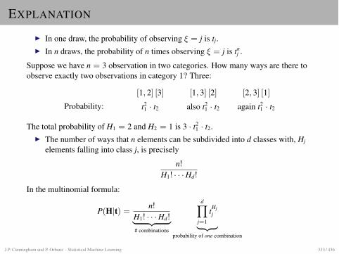
EXPLANATION
I In one draw, the probability of observing ⇠ = j is tj.I In n draws, the probability of n times observing ⇠ = j is tn
j .
Suppose we have n = 3 observation in two categories. How many ways are there toobserve exactly two observations in category 1? Three:
[1, 2] [3] [1, 3] [2] [2, 3] [1]
Probability: t21 · t2 also t2
1 · t2 again t21 · t2
The total probability of H1 = 2 and H2 = 1 is 3 · t21 · t2.
I The number of ways that n elements can be subdivided into d classes with, Hj
elements falling into class j, is precisely
n!H1! · · · Hd!
In the multinomial formula:
P(H|t) =n!
H1! · · · Hd!| {z }
# combinations
dY
j=1
tHjj
| {z }
probability of one combination
J.P. Cunningham and P. Orbanz · Statistical Machine Learning 333 / 436
PARAMETER ESTIMATION
MLEThe maximum likelihood estimator of t is
t = (t1, . . . , td) :=1n(H1, . . . , Hd) .
J.P. Cunningham and P. Orbanz · Statistical Machine Learning 334 / 436
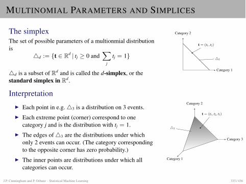
MULTINOMIAL PARAMETERS AND SIMPLICES
The simplexThe set of possible parameters of a multionmial distributionis
4d := {t 2 Rd | tj � 0 andX
j
tj = 1}
4d is a subset of Rd and is called the d-simplex, or thestandard simplex in Rd.
InterpretationI Each point in e.g.43 is a distribution on 3 events.I Each extreme point (corner) correspond to one
category j and is the distribution with tj = 1.I The edges of43 are the distributions under which
only 2 events can occur. (The category correspondingto the opposite corner has zero probability.)
I The inner points are distributions under which allcategories can occur.
Category 3
Category 2
Category 1
43
t = (t1, t2, t3)
Category 1
Category 2
42
t = (t1, t2)
J.P. Cunningham and P. Orbanz · Statistical Machine Learning 335 / 436
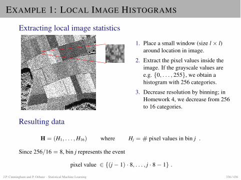
EXAMPLE 1: LOCAL IMAGE HISTOGRAMS
Extracting local image statistics
1. Place a small window (size l⇥ l)around location in image.
2. Extract the pixel values inside theimage. If the grayscale values aree.g. {0, . . . , 255}, we obtain ahistogram with 256 categories.
3. Decrease resolution by binning; inHomework 4, we decrease from 256to 16 categories.
Resulting data
H = (H1, . . . , H16) where Hj = # pixel values in bin j .
Since 256/16 = 8, bin j represents the event
pixel value 2 {(j� 1) · 8, . . . , j · 8� 1} .
J.P. Cunningham and P. Orbanz · Statistical Machine Learning 336 / 436
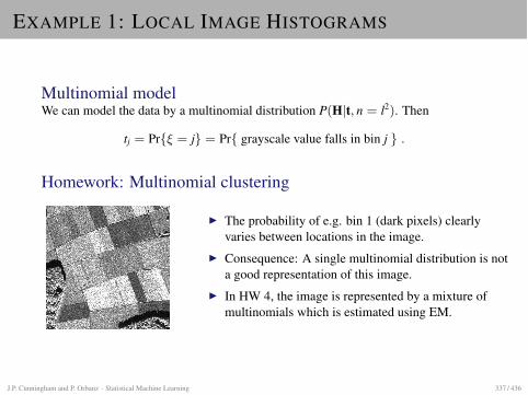
EXAMPLE 1: LOCAL IMAGE HISTOGRAMS
Multinomial modelWe can model the data by a multinomial distribution P(H|t, n = l2). Then
tj = Pr{⇠ = j} = Pr{ grayscale value falls in bin j } .
Homework: Multinomial clustering
I The probability of e.g. bin 1 (dark pixels) clearlyvaries between locations in the image.
I Consequence: A single multinomial distribution is nota good representation of this image.
I In HW 4, the image is represented by a mixture ofmultinomials which is estimated using EM.
J.P. Cunningham and P. Orbanz · Statistical Machine Learning 337 / 436
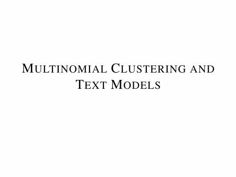
MULTINOMIAL CLUSTERING ANDTEXT MODELS

TEXT DATA
SettingData set: A huge set of text documents (e.g. all books in a library). The entire set oftexts is called a corpus.
Can we learn models from text which describe natural language?
TerminologyWe have to distinguish occurences of words in a document and distinct words in thedictionary. We refer to words regarded as entries of the dictionary as terms.
J.P. Cunningham and P. Orbanz · Statistical Machine Learning 339 / 436
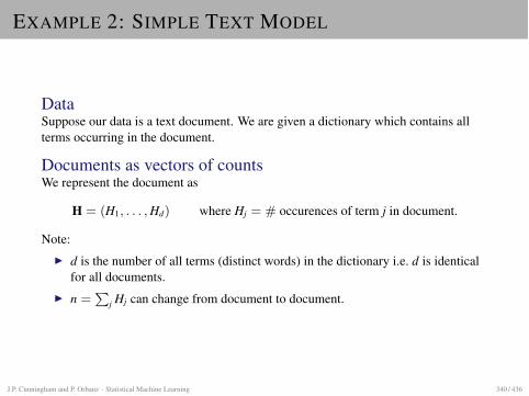
EXAMPLE 2: SIMPLE TEXT MODEL
DataSuppose our data is a text document. We are given a dictionary which contains allterms occurring in the document.
Documents as vectors of countsWe represent the document as
H = (H1, . . . , Hd) where Hj = # occurences of term j in document.
Note:I d is the number of all terms (distinct words) in the dictionary i.e. d is identical
for all documents.I n =
P
j Hj can change from document to document.
J.P. Cunningham and P. Orbanz · Statistical Machine Learning 340 / 436
EXAMPLE 2: SIMPLE TEXT MODEL
Multinomial modelTo define a simple probabilistic model of document generation, we can use amultinomial distribution P(H|t, n). That means:
I Each word in the document is sampled independently of the other words.I The probabilities of occurrence are
Pr{ word = term j } = tj .
Implicit assumptionThe assumption implicit in this model is that the probability of observing a documentis completely determined by how often each term occurs; the order of words does notmatter. This is called the bag-of-words assumption.
J.P. Cunningham and P. Orbanz · Statistical Machine Learning 341 / 436
CONTEXT
TaskCan we predict the next word in a text?
ContextIn language, the co-occurence and order of words is highly informative. Thisinformation is called the context of a word.Example: The English language has over 200,000 words.
I If we choose any word at random, there are over 200,000 possibilities.I If we want to choose the next word in
There is an airplane in the __
the number of possibilities is much smaller.
Significance for statistical methodsContext information is well-suited for machine learning: By parsing lots of text, wecan record which words occur together and which do not.
The standard models based on this idea are called n-gram models.
J.P. Cunningham and P. Orbanz · Statistical Machine Learning 342 / 436
BIGRAM MODELS
Bigram modelA bigram model represents the conditional distribution
Pr(word|previous word) =: Pr(wl|wl�1) ,
where wl is the lth word in a text.
Representation by multinomial distributionsA bigram model is a family of d multinomial distributions, one for each possibleprevious word.
EstimationFor each term k, find all terms in the corpus which are preceeded by k and recordtheir number of occurences in a vector
Hk = (Hk1, . . . , Hkd) where Hkj = number of times term j follows on term k
Then compute the maximum likelihood estimate tk from the sample Hk.Note: Both j and k run through {1, . . . , d}.
J.P. Cunningham and P. Orbanz · Statistical Machine Learning 343 / 436
N-GRAM MODELS
Multinomial representation of bigramThe distributions in the bigram model are:
Pr(word = j|previous word = k) = P(Hj = 1|tk, n = 1)
where P is the multinomial distribution. The entire bigram model is the set
{P( . |tk, n = 1) | k = 1, . . . , d}
N-gram modelsMore generally, a model conditional on the (N � 1) previous words
Pr(wl|wl�1, . . . , wl�(N�1))
is called an N-gram model (with the predicted word, there are N words in total).
UnigramsThe special case N = 1 (no context information) is the simple multinomial wordprobability model which we discussed first. This model is also called a unigrammodel.
J.P. Cunningham and P. Orbanz · Statistical Machine Learning 344 / 436
LEARNING SHAKESPEARE (1)
Unigram Model
To him swallowed confess hear both.Which. Of save on trail for are ay deviceand rote life have
Every enter now severally so, let
Hill he late speaks; or! a more to leg lessfirst you enter
Are where exeunt and sighs have riseexcellency took of.. Sleep knave we. near;vile like
Bigram Model
What means, sir. I confess she? then allsorts, he is trim, captain.
Why dost stand forth thy canopy, forsooth;he is this palpable hit the King Henry.Live king. Follow.
What we, hath got so she that I rest andsent to scold and nature bankrupt, nor thefirst gentleman?
Enter Menenius, if it so many gooddirection found’st thou art a strong uponcommand of fear not a liberal largessgiven away, Falstaff! Exeunt
From Jurafsky and Martin, "Speech and Language Processing", 2009.J.P. Cunningham and P. Orbanz · Statistical Machine Learning 345 / 436
LEARNING SHAKESPEARE (2)
Trigram Model
Sweet prince, Falstaff shall die. Harry ofMonmouth’s grave.
This shall forbid it should be branded, ifrenown made it empty.
Indeed the duke; and had a very goodfriend.
Fly, and will rid me these news of price.Therefore the sadness of parting, as theysay, ’tis done.
Quadrigram Model
King Henry. What! I will go seek thetraitor Gloucester. Exeunt some of thewatch. A great banquet serv’d in;
Will you not tell me who I am?
It cannot be but so.
Indeed the short and the long. Marry, ’tis anoble Lepidus.
From Jurafsky and Martin, "Speech and Language Processing", 2009.J.P. Cunningham and P. Orbanz · Statistical Machine Learning 346 / 436
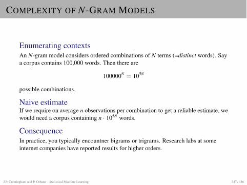
COMPLEXITY OF N-GRAM MODELS
Enumerating contextsAn N-gram model considers ordered combinations of N terms (=distinct words). Saya corpus contains 100,000 words. Then there are
100000N = 105N
possible combinations.
Naive estimateIf we require on average n observations per combination to get a reliable estimate, wewould need a corpus containing n · 105N words.
ConsequenceIn practice, you typically encountner bigrams or trigrams. Research labs at someinternet companies have reported results for higher orders.
J.P. Cunningham and P. Orbanz · Statistical Machine Learning 347 / 436
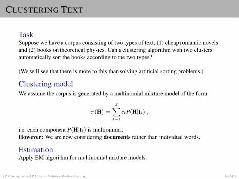
CLUSTERING TEXT
TaskSuppose we have a corpus consisting of two types of text, (1) cheap romantic novelsand (2) books on theoretical physics. Can a clustering algorithm with two clustersautomatically sort the books according to the two types?
(We will see that there is more to this than solving artificial sorting problems.)
Clustering modelWe assume the corpus is generated by a multinomial mixture model of the form
⇡(H) =KX
k=1
ckP(H|tk) ,
i.e. each component P(H|tk) is multionmial.However: We are now considering documents rather than individual words.
EstimationApply EM algorithm for multinomial mixture models.
J.P. Cunningham and P. Orbanz · Statistical Machine Learning 348 / 436
INTEPRETATION: TOPICS
Thought experimentSay we run a mixture of two multinomial distributions on the cheap romantic novelsand theoretical physics textbooks.
Outcome:I Each cluster will roughly represent one of the two topics.I The two parameter vectors t1 and t2 represent distributions of words in texts of
the respective topic.
Word distributions as topicsThis motivates the interpretation of clusters as topics.
tk = distribution of words that characterizes topic k
Language models derived from this idea are called topic models.
J.P. Cunningham and P. Orbanz · Statistical Machine Learning 349 / 436

TOOLS: INFORMATION THEORY
MEASURING INFORMATION
Information content of a random variableWe consider a random variable X with distribution P.
I P expresses what we know before we observe X.I How much information do we gain by observing X?
That is: By information content of X, we mean the difference in information betweenknowing P and knowing both P and X = x.
To reiterateFor the definition of information, it is useful to think of...
I ...the distribution P as what we expect to happen.I ...the sample outcome X = x as what actually happens.
J.P. Cunningham and P. Orbanz · Statistical Machine Learning 351 / 436
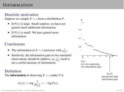
INFORMATION
Heuristic motivationSuppose we sample X = x from a distribution P.
I If P(x) is large: Small surprise; we have notgained much additional information.
I If P(x) is small: We have gained moreinformation.
ConclusionsI The information in X = x increases with 1
P(x) .I Intuitively, the information gain in two unrelated
observations should be additive, so 1P(x) itself is
not a useful measure of information.
DefinitionThe information in observing X = x under P is
JP(x) := log1
P(x)= � log P(x) .
X=1:not very surprising,low information gain
X=23:unexpected, highinformation gain
J.P. Cunningham and P. Orbanz · Statistical Machine Learning 352 / 436
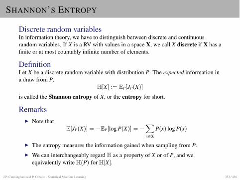
SHANNON’S ENTROPY
Discrete random variablesIn information theory, we have to distinguish between discrete and continuousrandom variables. If X is a RV with values in a space X, we call X discrete if X has afinite or at most countably infinite number of elements.
DefinitionLet X be a discrete random variable with distribution P. The expected information ina draw from P,
H[X] := EP[JP(X)]
is called the Shannon entropy of X, or the entropy for short.
RemarksI Note that
E[JP(X)] = �EP[log P(X)] = �X
x2X
P(x) log P(x)
I The entropy measures the information gained when sampling from P.I We can interchangeably regard H as a property of X or of P, and we
equivalently write H(P) for H[X].
J.P. Cunningham and P. Orbanz · Statistical Machine Learning 353 / 436
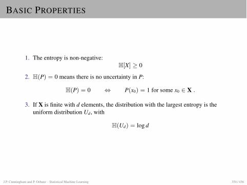
BASIC PROPERTIES
1. The entropy is non-negative:H[X] � 0
2. H(P) = 0 means there is no uncertainty in P:
H(P) = 0 , P(x0) = 1 for some x0 2 X .
3. If X is finite with d elements, the distribution with the largest entropy is theuniform distribution Ud, with
H(Ud) = log d
J.P. Cunningham and P. Orbanz · Statistical Machine Learning 354 / 436
ALTERNATIVE DERIVATION
Axiomatic descriptionSuppose we define some measure H[X] of information in X. Regardless of thedefinition, we can postulate a number of properties (axioms) that a meaningfulmeasure should satisfy.
AdditivityI If two RVs X and Y are independent, their information content should be
disjoint.I Hence, H should be additive:
X??Y ) H[X, Y] = H[X] + H[Y]
I More generally: We should be able to "remove the joint information" in X andY from Y by conditioning.
I This is what we require as our first axiom:
(Axiom I) H[X, Y] = H[X] + H[Y|X]
J.P. Cunningham and P. Orbanz · Statistical Machine Learning 355 / 436
AXIOMATIC DERIVATION
ContinuityI We can alternatively regard H[X] as a function H(P) of the distribution of X.I If we make a small change to P, then H(P) should not "jump". That is:
(Axiom II) H(P) should be continuous as a function of P.
MonotonicityI Suppose we consider in particular the uniform distribution P = Ud on d
outcomes.I If we increase d, the uncertainty in Ud increases; hence, the information gained
by sampling should be higher for d + 1 than for d:
(Axiom III) H(Ud) < H(Ud+1)
J.P. Cunningham and P. Orbanz · Statistical Machine Learning 356 / 436
AXIOMATIC DERIVATION
TheoremIf a real-valued function H on X satisfies Axioms I–III, then
H(P) = c · H(P) for all P ,
for some constant c 2 R+. (The constant is the same for all P.)
In other wordsIf any information measure satisfies our requirements, it is precisely the entropy, upto a choice of scale.
J.P. Cunningham and P. Orbanz · Statistical Machine Learning 357 / 436
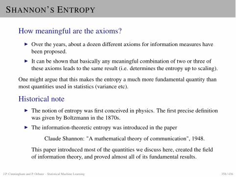
SHANNON’S ENTROPY
How meaningful are the axioms?I Over the years, about a dozen different axioms for information measures have
been proposed.I It can be shown that basically any meaningful combination of two or three of
these axioms leads to the same result (i.e. determines the entropy up to scaling).
One might argue that this makes the entropy a much more fundamental quantity thanmost quantities used in statistics (variance etc).
Historical noteI The notion of entropy was first conceived in physics. The first precise definition
was given by Boltzmann in the 1870s.I The information-theoretic entropy was introduced in the paper
Claude Shannon: "A mathematical theory of communication", 1948.
This paper introduced most of the quantities we discuss here, created the fieldof information theory, and proved almost all of its fundamental results.
J.P. Cunningham and P. Orbanz · Statistical Machine Learning 358 / 436
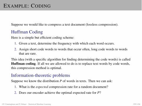
EXAMPLE: CODING
Suppose we would like to compress a text document (lossless compression).
Huffman CodingHere is a simple but efficient coding scheme:
1. Given a text, determine the frequency with which each word occurs.
2. Assign short code words to words that occur often, long code words to wordsthat are rare.
This idea (with a specific algorithm for finding determining the code words) is calledHuffman coding. If all we are allowed to do is to replace text words by code words,this compression method is optimal.
Information-theoretic problemsSuppose we know the distribution P of words in texts. Then we can ask:
1. What is the expected compression rate for a random document?
2. Does our encoder achieve the optimal expected rate for P?
J.P. Cunningham and P. Orbanz · Statistical Machine Learning 359 / 436
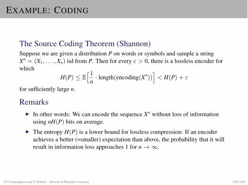
EXAMPLE: CODING
The Source Coding Theorem (Shannon)Suppose we are given a distribution P on words or symbols and sample a stringXn = (X1, . . . , Xn) iid from P. Then for every " > 0, there is a lossless encoder forwhich
H(P) Eh1
n· length(encoding(Xn))
i
< H(P) + "
for sufficiently large n.
RemarksI In other words: We can encode the sequence Xn without loss of information
using nH(P) bits on average.I The entropy H(P) is a lower bound for lossless compression: If an encoder
achieves a better (=smaller) expectation than above, the probability that it willresult in information loss approaches 1 for n!1.
J.P. Cunningham and P. Orbanz · Statistical Machine Learning 360 / 436
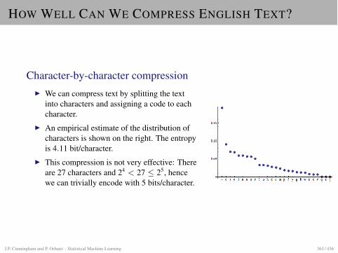
HOW WELL CAN WE COMPRESS ENGLISH TEXT?
Character-by-character compressionI We can compress text by splitting the text
into characters and assigning a code to eachcharacter.
I An empirical estimate of the distribution ofcharacters is shown on the right. The entropyis 4.11 bit/character.
I This compression is not very effective: Thereare 27 characters and 24 < 27 25, hencewe can trivially encode with 5 bits/character.
J.P. Cunningham and P. Orbanz · Statistical Machine Learning 361 / 436
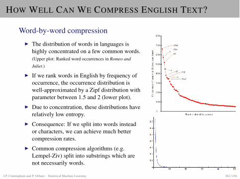
HOW WELL CAN WE COMPRESS ENGLISH TEXT?
Word-by-word compressionI The distribution of words in languages is
highly concentrated on a few common words.(Upper plot: Ranked word occurrences in Romeo and
Juliet.)
I If we rank words in English by frequency ofoccurrence, the occurrence distribution iswell-approximated by a Zipf distribution withparameter between 1.5 and 2 (lower plot).
I Due to concentration, these distributions haverelatively low entropy.
I Consequence: If we split into words insteador characters, we can achieve much bettercompression rates.
I Common compression algorithms (e.g.Lempel-Ziv) split into substrings which arenot necessarily words.
J.P. Cunningham and P. Orbanz · Statistical Machine Learning 362 / 436
KULLBACK-LEIBLER DIVERGENCE
Comparing distributionsWe can use the notion of information to compare one distribution to another.
Heuristic motivationSuppose we wish to compare two distributions P and Q on X.
I The entropy H[Q] = EQ[JQ(X)] measures how much information gain (in termsof Q) we can expect from a random sample from Q.
I Now ask instead: How much information gain in terms of Q can we expectfrom a random sample drawn from P? We compute: EP[JQ(X)].
I A measure of difference between P and Q should vanish if Q = P. SinceP = Q means EP[JQ(X)] = H(P), which is usually not 0, we have to normalizeby subtracting H(P).
DefinitionThe function
DKL(PkQ) := EP[JQ(X)]�H(P)
is called the Kullback-Leibler divergence or the relative entropy of P and Q.
J.P. Cunningham and P. Orbanz · Statistical Machine Learning 363 / 436
BASIC PROPERTIES
Equivalent forms
DKL[PkQ] = EP[JQ(X)� JP(X)] =X
x2X
P(x) logP(x)Q(x)
Positive definiteness
DKL[PkQ] � 0 and DKL[PkQ] = 0, P = Q .
The KL divergence is not a metricIntuitively, DKL can be used like a distance measure between distributions, however:
I It is not symmetric: DKL[PkQ] 6= DKL[QkP] in general.I It does not satisfy a triangle inequality.
ConvexityA very useful property of H and DKL is convexity:
I H(P) is concave as a function of P.I DKL[PkQ] is convex in the pair (P, Q).
J.P. Cunningham and P. Orbanz · Statistical Machine Learning 364 / 436
CONDITIONING
I How can we compute the entropy of Y conditional on X?I For a fixed value X = x, we can simply compute H from the conditional
probability P(Y|X = x) as
H[Y|X = x] = �X
y2X
P(y|x) log P(y|x) .
I To make the definition independent of x, we take the expectation
H[Y|X] := EP(x)[H[Y|X = x]] .
This is called the conditional entropy of Y given X.I A few lines of arithmetic show:
H[Y|X] = �X
x,y2X
P(x, y) log P(y|x)
J.P. Cunningham and P. Orbanz · Statistical Machine Learning 365 / 436
MUTUAL INFORMATION
Heuristic MotivationI Another question we can ask about a pair X, Y of random variables is: How
much information do they share?I In other words: How much does observing X tell us about Y?I If X and Y contain no shared information, they are independent, and their joint
distribution is P(x, y) = P(x)P(y).I Idea: Compare the actual joint distribution to the independent case using KL
divergence.
We first define the mutual information in a different way, but will then see that theidea above indeed applies.
DefinitionThe function
I[X, Y] := H[X]�H[X|Y] = H[Y]�H[Y|X]
is called the mutual information of X and Y .
J.P. Cunningham and P. Orbanz · Statistical Machine Learning 366 / 436
USEFUL RELATIONSHIPS
Conditioning reduces entropy
H[X, Y] = H[Y|X] + H[X]
Mutual information as a Kullback-Leibler divergence
I[X, Y] = DKL[P(x, y)kP(x)P(y)] =X
x,y
P(x, y) logP(x, y)
P(x)P(y)
Note: This compares P(x, y) to the case where X, Y are independent (which meansP(x, y) = P(x)P(y)).
Mutual information characterizes independence
I[X, Y] = 0 , X??Y
J.P. Cunningham and P. Orbanz · Statistical Machine Learning 367 / 436
THE CONTINUOUS CASE
If the sample space X is uncountable (e.g. X = R), instead of P and Q we considerdensities p and q, we have to substitute integrals for sums.
Differential entropy
H[X] := �Z
Xp(x) log p(x)dx
Since p is a density, we can have log p(x) > 0, and H[X] can be negative. Todistinguish it from the entropy, H[X] is called the differential entropy.
KL divergence and mutual informationDKL and I are defined analagously to the discrete case:
DKL(pkq) :=
Z
Xp(x) log
p(x)q(x)
dx
I[X, Y] :=
Z
Xp(x, y) log
p(x, y)p(x)p(y)
dx
J.P. Cunningham and P. Orbanz · Statistical Machine Learning 368 / 436
PROPERTIES IN THE CONTINUOUS CASE
Differential entropyI Since p is a density, we can have log p(x) > 0, and H[X] can be negative.I The term differential entropy is used to distinguish it from the entropy.
KL divergenceThe KL divergence for densities still satisfies
DKL(pkq) � 0 and DKL(pkq) = 0 , p = q .
As a consequence, the mutual information still satisfies
I[X, Y] � 0 and I[X, Y] = 0 , X??Y .
J.P. Cunningham and P. Orbanz · Statistical Machine Learning 369 / 436
KL DIVERGENCE AND MAXIMUM LIKELIHOOD
IdeaSuppose we observe data x1, . . . , xn and assume a model P = {p(x|✓)|✓ 2 T }. Wecould fit the model using the KL divergence as a cost measure:
✓ := arg min✓2T
DKL(Fn|p(x|✓))
Computation
✓ = arg min✓2T
DKL(Fn|p(x|✓)) = arg min✓2T
⇣
Z
XFn(x) log
F(x)p(x|✓)dx
⌘
= arg min✓2T
⇣
Z
XFn(x) logFn(x)dx�
Z
XFn(x) log p(x|✓)dx
⌘
= arg max✓2T
⇣
Z
XFn(x) log p(x|✓)dx
⌘
= arg max✓2T
⇣
Z
X
1n
nX
i=1
�xi(x) log p(x|✓)dx⌘
= arg max✓2T
⇣1n
nX
i=1
log p(xi|✓)⌘
= ✓MLE
Minimizing KL divergence between Fn and the model is equivalent to maximumlikelihood estimation!
J.P. Cunningham and P. Orbanz · Statistical Machine Learning 370 / 436
MAXIMUM ENTROPY METHODS
The maximum entropy principleSuppose we have to choose a model distribution from a given set P of admissibledistributions. The maximum entropy principle says: Always choose the distribution
P = arg maxQ2P
H(Q)
with the highest entropy in P . P is called the maximum entropy distribution,which is sometimes abbreviated to ‘MaxEnt distribution’.
RationaleI When choosing a model distribution, we should try to avoid illicit assumptions.I Higher entropy$ higher uncertainty$ fewer assumptions.
This idea was introduced by the physicist E. T. Jaynes, who championed it as ageneral modeling approach.
J.P. Cunningham and P. Orbanz · Statistical Machine Learning 371 / 436
MAXIMUM ENTROPY UNDER CONSTRAINTS
Maximum entropy under constraintsSuppose the set P of distributions is defined by a constraint. For example:
P = all distributions on R with variance �20 .
Example 1: Trivial constraintSuppose the only constaint is that the choice of sample space, e.g. X = [0, 1]. Thenthe maximum entropy distribution is the uniform distribution on [0, 1].
Example 2: Given varianceIf P = { distributions on R with Var[X] = �2
0}, then P is Gaussian with variance �20 .
J.P. Cunningham and P. Orbanz · Statistical Machine Learning 372 / 436
THE EXPONENTIAL FAMILY AGAIN
Expectations as constraintsSuppose X = Rd, and we formulate constraints by choosing functionsS1, . . . , Sm : X! R and positing their expected values.
That is, the constrained set is
P := {Q |EQ[S1(X)] = s1, . . . ,EQ[Sm(X)] = sm} .
Constrained optimization problem (for the discrete case)We add the constraints to the objective function H(Q) using Lagrange multipliers✓1, . . . , ✓n. We also include a normalization constraint with Lagrangre multiplier ✓0.
P = arg maxQ
H(Q)+✓0
⇣
1�X
x2X
Q(x)⌘
+✓1
⇣
s1 �X
x2X
S1(x)Q(x)⌘
+ . . . + ✓m
⇣
sm �X
x2X
Sm(x)Q(x)⌘
J.P. Cunningham and P. Orbanz · Statistical Machine Learning 373 / 436
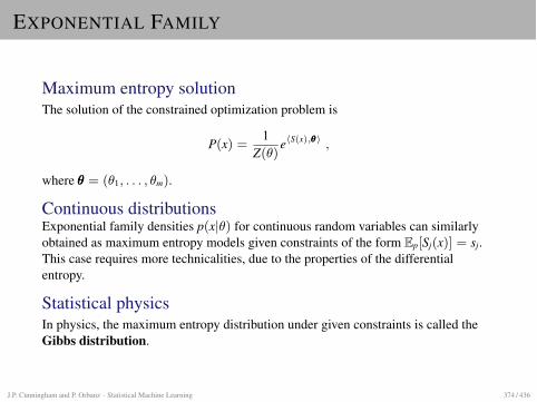
EXPONENTIAL FAMILY
Maximum entropy solutionThe solution of the constrained optimization problem is
P(x) =1
Z(✓)ehS(x),✓✓✓i ,
where ✓✓✓ = (✓1, . . . , ✓m).
Continuous distributionsExponential family densities p(x|✓) for continuous random variables can similarlyobtained as maximum entropy models given constraints of the form Ep[Sj(x)] = sj.This case requires more technicalities, due to the properties of the differentialentropy.
Statistical physicsIn physics, the maximum entropy distribution under given constraints is called theGibbs distribution.
J.P. Cunningham and P. Orbanz · Statistical Machine Learning 374 / 436
SUMMARY: INFORMATION THEORY AND STATISTICS
I Maximum likelihood minimizes DKL between empirical distribution and model.I Variance, covariance and the �2-statistic can be regarded as first-order
approximations to entropy, mutual information and KL divergence.I Various methods can be derived by substituting information-theoretic for
traditional statistical quantities.I Example: A dimension-reduction technique called independent component
analysis can be motivated as (roughly speaking) a PCA-like method whichmeasures independence in terms of mutual information rather than covariance.
J.P. Cunningham and P. Orbanz · Statistical Machine Learning 375 / 436
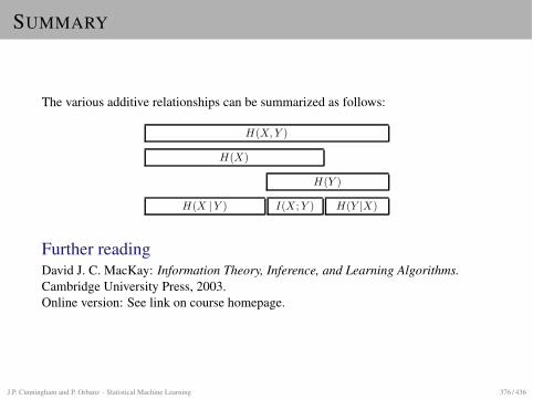
SUMMARY
The various additive relationships can be summarized as follows:
H(X, Y )
H(X)
H(Y )
I(X ; Y )H(X | Y ) H(Y |X)
Further readingDavid J. C. MacKay: Information Theory, Inference, and Learning Algorithms.Cambridge University Press, 2003.Online version: See link on course homepage.
J.P. Cunningham and P. Orbanz · Statistical Machine Learning 376 / 436

MODEL ORDER SELECTION
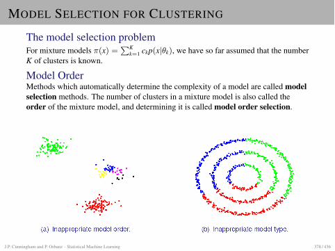
MODEL SELECTION FOR CLUSTERING
The model selection problemFor mixture models ⇡(x) =
PKk=1 ckp(x|✓k), we have so far assumed that the number
K of clusters is known.
Model OrderMethods which automatically determine the complexity of a model are called modelselection methods. The number of clusters in a mixture model is also called theorder of the mixture model, and determining it is called model order selection.
J.P. Cunningham and P. Orbanz · Statistical Machine Learning 378 / 436
MODEL SELECTION FOR CLUSTERING
NotationWe write L for the log-likelihood of a parameter under a model p(x|✓):
L(xn; ✓) := lognY
i=1
p(xi|✓)
In particular, for a mixture model:
L(xn; c,✓✓✓) := lognY
i=1
⇣
KX
k=1
ckp(xi|✓k)⌘
Number of clusters: Naive solution (wrong!)We could treat K as a parameter and use maximum likelihood, i.e. try to solve:
(K, c1, . . . , cK , ✓1, . . . , ✓K) := arg maxK,c0,✓✓✓0
L(xn; K, c0,✓✓✓0)
J.P. Cunningham and P. Orbanz · Statistical Machine Learning 379 / 436
NUMBER OF CLUSTERS
Problem with naive solution: ExampleSuppose we use a Gaussian mixture model.
I The optimization procedure can add additional components arbitrarily.I It can achieve minimal fitting error by using a separate mixture component for
each data point (ie µk = xi).I By reducing the variance of each component, it can additionally increase the
density value at µk = xi. That means we can achieve arbitrarily highlog-likelihood.
I Note that such a model (with very high, narrow component densities at the datapoints) would achieve low log-likelihood on a new sample from the samesource. In other words, it does not generalize well.
In short: The model overfits.
J.P. Cunningham and P. Orbanz · Statistical Machine Learning 380 / 436
NUMBER OF CLUSTERS
The general problemI Recall our discussion of model complexity: Models with more degrees of
freedom are more prone to overfitting.I The number of degrees of freedom is roughly the number of scalar parameters.I By increasing K, the clustering model can add more degrees of freedom.
Most common solutionsI Penalization approaches: A penalty term makes adding parameters expensive.
Similar to shrinkage in regression.I Stability: Perturb the distribution using resampling or subsampling. Idea: A
choice of K for which solutions are stable under perturbation is a goodexplanation of the data.
I Bayesian methods: Each possible value of K is assigned a probability, which iscombined with the likelihood given K to evaluate the plausibility of thesolution. Somewhat related to penalization.
J.P. Cunningham and P. Orbanz · Statistical Machine Learning 381 / 436
PENALIZATION STRATEGIES
General formPenalization approaches define a penalty function �, which is an increasing functionof the number m of model parameters.Instead of maximizing the log-likelihood, we minimize the negative log-likelihoodand add �:
(m, ✓1, . . . , ✓m) = arg minm,✓1,...,✓m
�L(xn; ✓1, . . . , ✓m) + �(m)
The most popular choicesThe penalty function
�AIC(m) := m
is called the Akaike information criterion (AIC).
�BIC(m) :=12
m log n
is called the Bayesian information criterion (BIC).
J.P. Cunningham and P. Orbanz · Statistical Machine Learning 382 / 436
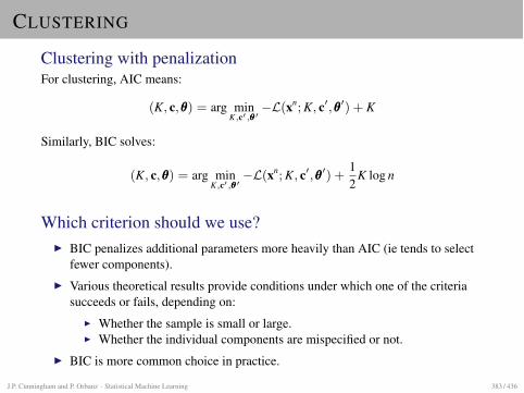
CLUSTERING
Clustering with penalizationFor clustering, AIC means:
(K, c,✓✓✓) = arg minK,c0,✓✓✓0
�L(xn; K, c0,✓✓✓0) + K
Similarly, BIC solves:
(K, c,✓✓✓) = arg minK,c0,✓✓✓0
�L(xn; K, c0,✓✓✓0) +12
K log n
Which criterion should we use?I BIC penalizes additional parameters more heavily than AIC (ie tends to select
fewer components).I Various theoretical results provide conditions under which one of the criteria
succeeds or fails, depending on:I Whether the sample is small or large.I Whether the individual components are mispecified or not.
I BIC is more common choice in practice.
J.P. Cunningham and P. Orbanz · Statistical Machine Learning 383 / 436
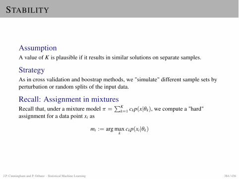
STABILITY
AssumptionA value of K is plausible if it results in similar solutions on separate samples.
StrategyAs in cross validation and boostrap methods, we "simulate" different sample sets byperturbation or random splits of the input data.
Recall: Assignment in mixturesRecall that, under a mixture model ⇡ =
PKk=1 ckp(x|✓k), we compute a "hard"
assignment for a data point xi as
mi := arg maxk
ckp(xi|✓k)
J.P. Cunningham and P. Orbanz · Statistical Machine Learning 384 / 436
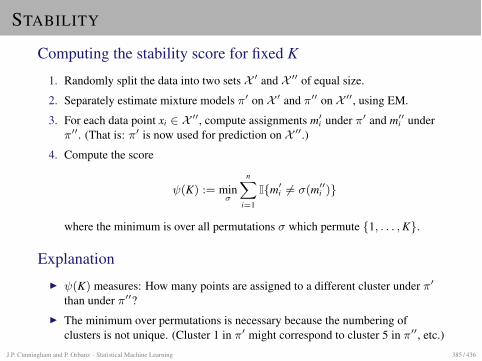
STABILITY
Computing the stability score for fixed K
1. Randomly split the data into two sets X 0 and X 00 of equal size.
2. Separately estimate mixture models ⇡0 on X 0 and ⇡00 on X 00, using EM.
3. For each data point xi 2 X 00, compute assignments m0i under ⇡0 and m00i under⇡00. (That is: ⇡0 is now used for prediction on X 00.)
4. Compute the score
(K) := min�
nX
i=1
I{m0i 6= �(m00i )}
where the minimum is over all permutations � which permute {1, . . . , K}.
ExplanationI (K) measures: How many points are assigned to a different cluster under ⇡0
than under ⇡00?I The minimum over permutations is necessary because the numbering of
clusters is not unique. (Cluster 1 in ⇡0 might correspond to cluster 5 in ⇡00, etc.)J.P. Cunningham and P. Orbanz · Statistical Machine Learning 385 / 436
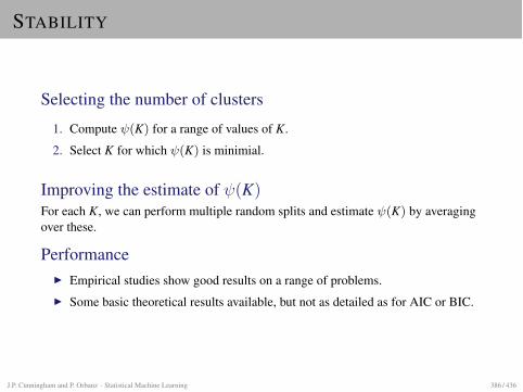
STABILITY
Selecting the number of clusters
1. Compute (K) for a range of values of K.
2. Select K for which (K) is minimial.
Improving the estimate of (K)For each K, we can perform multiple random splits and estimate (K) by averagingover these.
PerformanceI Empirical studies show good results on a range of problems.I Some basic theoretical results available, but not as detailed as for AIC or BIC.
J.P. Cunningham and P. Orbanz · Statistical Machine Learning 386 / 436
SEQUENTIAL DATA AND MARKOVMODELS
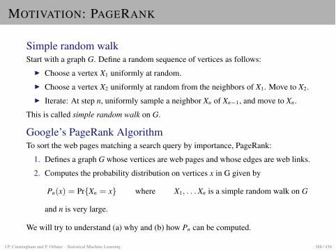
MOTIVATION: PAGERANK
Simple random walkStart with a graph G. Define a random sequence of vertices as follows:
I Choose a vertex X1 uniformly at random.I Choose a vertex X2 uniformly at random from the neighbors of X1. Move to X2.I Iterate: At step n, uniformly sample a neighbor Xn of Xn�1, and move to Xn.
This is called simple random walk on G.
Google’s PageRank AlgorithmTo sort the web pages matching a search query by importance, PageRank:
1. Defines a graph G whose vertices are web pages and whose edges are web links.
2. Computes the probability distribution on vertices x in G given by
Pn(x) = Pr{Xn = x} where X1, . . . Xn is a simple random walk on G
and n is very large.
We will try to understand (a) why and (b) how Pn can be computed.
J.P. Cunningham and P. Orbanz · Statistical Machine Learning 388 / 436
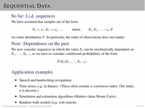
SEQUENTIAL DATA
So far: I.i.d. sequencesWe have assumed that samples are of the form
X1 = x1, X2 = x2, . . . where X1, X2, . . . ⇠iid P
for some distribution P. In particular, the order of observations does not matter.
Now: Dependence on the pastWe now consider sequences in which the value Xn can be stochastically dependent onX1, . . . , Xn�1, so we have to consider conditional probabilities of the form
P(Xn|X1, . . . , Xn�1) .
Application examplesI Speech and handwriting recognition.I Time series, e.g. in finance. (These often assume a continuous index. Our index
n is discrete.)I Simulation and estimation algorithms (Markov chain Monte Carlo).I Random walk models (e.g. web search).
J.P. Cunningham and P. Orbanz · Statistical Machine Learning 389 / 436
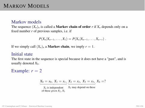
MARKOV MODELS
Markov modelsThe sequence (Xn)n is called a Markov chain of order r if Xn depends only on afixed number r of previous samples, i.e. if
P(Xn|Xn�1, . . . , X1) = P(Xn|Xn�1, . . . , Xn�r) .
If we simply call (Xn)n a Markov chain, we imply r = 1.
Initial stateThe first state in the sequence is special because it does not have a "past", and isusually denoted X0.
Example: r = 2
X0 = x0, X1 = x1, X2 = x2, X3 = x3, X4 =?
X4 is independentof these given X2, X3
X4 may depend on these
J.P. Cunningham and P. Orbanz · Statistical Machine Learning 390 / 436
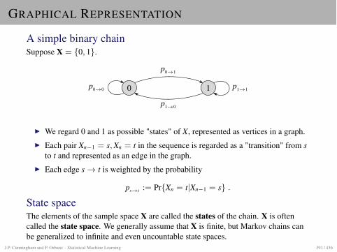
GRAPHICAL REPRESENTATION
A simple binary chainSuppose X = {0, 1}.
0 1
p0!1
p1!0
p1!1p0!0
I We regard 0 and 1 as possible "states" of X, represented as vertices in a graph.I Each pair Xn�1 = s, Xn = t in the sequence is regarded as a "transition" from s
to t and represented as an edge in the graph.I Each edge s! t is weighted by the probability
ps!t := Pr{Xn = t|Xn�1 = s} .
State spaceThe elements of the sample space X are called the states of the chain. X is oftencalled the state space. We generally assume that X is finite, but Markov chains canbe generalized to infinite and even uncountable state spaces.
J.P. Cunningham and P. Orbanz · Statistical Machine Learning 391 / 436
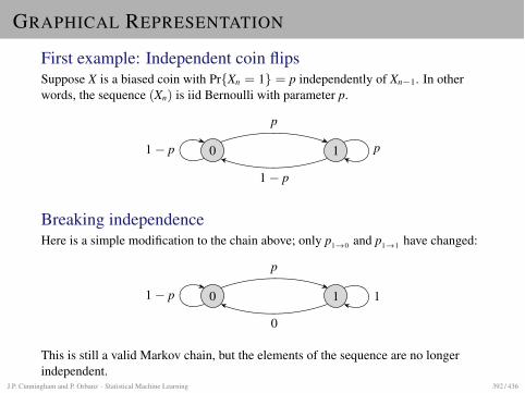
GRAPHICAL REPRESENTATION
First example: Independent coin flipsSuppose X is a biased coin with Pr{Xn = 1} = p independently of Xn�1. In otherwords, the sequence (Xn) is iid Bernoulli with parameter p.
0 1
p
1� p
p1� p
Breaking independenceHere is a simple modification to the chain above; only p1!0 and p1!1 have changed:
0 1
p
0
11� p
This is still a valid Markov chain, but the elements of the sequence are no longerindependent.
J.P. Cunningham and P. Orbanz · Statistical Machine Learning 392 / 436
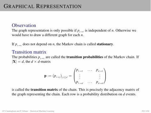
GRAPHICAL REPRESENTATION
ObservationThe graph representation is only possible if ps!t is independent of n. Otherwise wewould have to draw a different graph for each n.
If ps!t does not depend on n, the Markov chain is called stationary.
Transition matrixThe probabilities ps!t are called the transition probabilities of the Markov chain. If|X| = d, the d ⇥ d-matrix
p := (pi!j)j,id =
0
B
@
p1!1 . . . pd!1...
...p1!d . . . pd!d
1
C
A
is called the transition matrix of the chain. This is precisely the adjacency matrix ofthe graph representing the chain. Each row is a probability distribution on d events.
J.P. Cunningham and P. Orbanz · Statistical Machine Learning 393 / 436
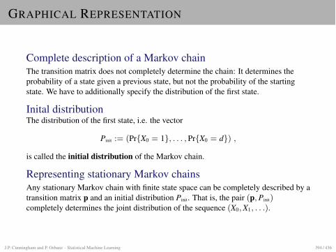
GRAPHICAL REPRESENTATION
Complete description of a Markov chainThe transition matrix does not completely determine the chain: It determines theprobability of a state given a previous state, but not the probability of the startingstate. We have to additionally specify the distribution of the first state.
Inital distributionThe distribution of the first state, i.e. the vector
Pinit := (Pr{X0 = 1}, . . . , Pr{X0 = d}) ,
is called the initial distribution of the Markov chain.
Representing stationary Markov chainsAny stationary Markov chain with finite state space can be completely described by atransition matrix p and an initial distribution Pinit. That is, the pair (p, Pinit)completely determines the joint distribution of the sequence (X0, X1, . . .).
J.P. Cunningham and P. Orbanz · Statistical Machine Learning 394 / 436
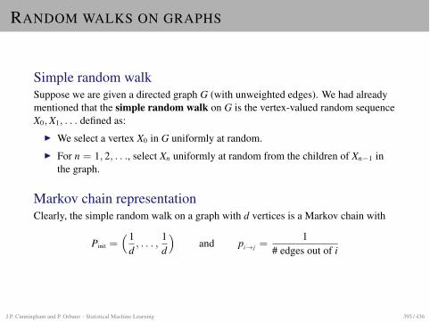
RANDOM WALKS ON GRAPHS
Simple random walkSuppose we are given a directed graph G (with unweighted edges). We had alreadymentioned that the simple random walk on G is the vertex-valued random sequenceX0, X1, . . . defined as:
I We select a vertex X0 in G uniformly at random.I For n = 1, 2, . . ., select Xn uniformly at random from the children of Xn�1 in
the graph.
Markov chain representationClearly, the simple random walk on a graph with d vertices is a Markov chain with
Pinit =⇣1
d, . . . ,
1d
⌘
and pi!j =1
# edges out of i
J.P. Cunningham and P. Orbanz · Statistical Machine Learning 395 / 436
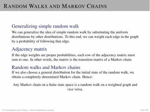
RANDOM WALKS AND MARKOV CHAINS
Generalizing simple random walkWe can generalize the idea of simple random walk by substituting the uniformdistributions by other distributions. To this end, we can weight each edge in the graphby a probability of following that edge.
Adjacency matrixIf the edge weights are proper probabilities, each row of the adjacency matrix mustsum to one. In other words, the matrix is the transition matrix of a Markov chain.
Random walks and Markov chainsIf we also choose a general distribution for the initial state of the random walk, weobtain a completely determined Markov chain. Hence:
Any Markov chain on a finite state space is a random walk on a weighted graph andvice versa.
J.P. Cunningham and P. Orbanz · Statistical Machine Learning 396 / 436
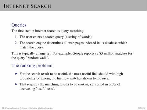
INTERNET SEARCH
QueriesThe first step in internet search is query matching:
1. The user enters a search query (a string of words).
2. The search engine determines all web pages indexed in its database whichmatch the query.
This is typically a large set. For example, Google reports ca 83 million matches forthe query "random walk".
The ranking problemI For the search result to be useful, the most useful link should with high
probability be among the first few matches shown to the user.I That requires the matching results to be ranked, i.e. sorted in order of
decreasing "usefulness".
J.P. Cunningham and P. Orbanz · Statistical Machine Learning 397 / 436
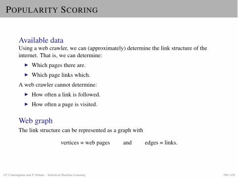
POPULARITY SCORING
Available dataUsing a web crawler, we can (approximately) determine the link structure of theinternet. That is, we can determine:
I Which pages there are.I Which page links which.
A web crawler cannot determine:I How often a link is followed.I How often a page is visited.
Web graphThe link structure can be represented as a graph with
vertices = web pages and edges = links.
J.P. Cunningham and P. Orbanz · Statistical Machine Learning 398 / 436
RANDOM WALK NETWORK MODELS
Key ideaThe popularity of a page x is proportional to the probability that a "random websurfer" ends up on page x after a n steps.
Probabilistic modelThe path of the surfer is modeled by a random walk on the web graph.
Modeling assumptionsTwo assumptions are implicit in this model:
1. Better pages are linked more often.
2. A link from a high-quality page is worth more than one from a low-qualitypage.
RemarksI We will find later that the choice of n does not matter.I To compute the popularity score, we first have to understand Markov chains a
bit better.
J.P. Cunningham and P. Orbanz · Statistical Machine Learning 399 / 436
STATE PROBABILITIES
Probability after n = 1 stepsIf we know the initial state, then
Pr{X1 = s1 | X0 = s0} = ps0!s1.
P1 describes the probability of X1 if we do not know the starting state (i.e. theprobability before we start the chain):
P1(s1) = Pr{X1 = s1} =X
s02X
Pr{X1 = s1 | X0 = s0}Pinit(s0)
=X
s02X
ps0!s1Pinit(s0) .
Matrix representationRecall that p is a d ⇥ d-matrix and Pinit a vector of length d. The equation for P1
above is a matrix-vector product, so
P1 = p · Pinit .
J.P. Cunningham and P. Orbanz · Statistical Machine Learning 400 / 436
STATE PROBABILITIES
Probability after n = 2 stepsThe same argument shows that P2 is given by
P2(s2) =X
s12X
ps1!s2P1(s1) ,
henceP2 = p · P1 = p · p · Pinit .
For arbitary n
Pn = pnPinit
J.P. Cunningham and P. Orbanz · Statistical Machine Learning 401 / 436
LIMITS AND EQUILIBRIA
Limiting distributionInstead of considering Pn for a specific, large n, we take the limit
P1 := limn!1
Pn = limn!1
pnPinit ,
provided that the limit exists.
ObservationIf the limit P1 exists, then
p · P1 = p · limn!1
pnPinit = limn!1
pnPinit = P1 ,
which motivates the next definition.
Equilibrium distributionIf p is the tansition matrix of a Markov chain, a distribution P on X which is invariantunder p in the sense that
p · P = P
is called an equilibrium distribution or invariant distribution of the Markov chain.J.P. Cunningham and P. Orbanz · Statistical Machine Learning 402 / 436
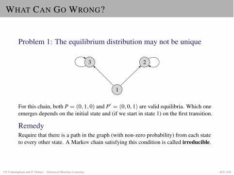
WHAT CAN GO WRONG?
Problem 1: The equilibrium distribution may not be unique
3 2
1
For this chain, both P = (0, 1, 0) and P0 = (0, 0, 1) are valid equilibria. Which oneemerges depends on the initial state and (if we start in state 1) on the first transition.
RemedyRequire that there is a path in the graph (with non-zero probability) from each stateto every other state. A Markov chain satisfying this condition is called irreducible.
J.P. Cunningham and P. Orbanz · Statistical Machine Learning 403 / 436
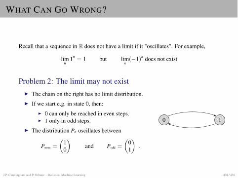
WHAT CAN GO WRONG?
Recall that a sequence in R does not have a limit if it "oscillates". For example,
limn
1n = 1 but limn
(�1)n does not exist
Problem 2: The limit may not existI The chain on the right has no limit distribution.I If we start e.g. in state 0, then:
I 0 can only be reached in even steps.I 1 only in odd steps.
I The distribution Pn oscillates between
Peven =
✓
10
◆
and Podd =
✓
01
◆
.
0 1
J.P. Cunningham and P. Orbanz · Statistical Machine Learning 404 / 436
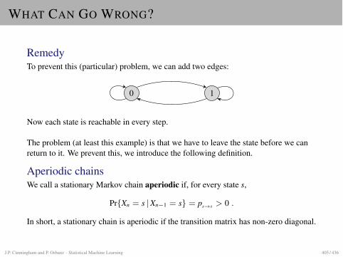
WHAT CAN GO WRONG?
RemedyTo prevent this (particular) problem, we can add two edges:
0 1
Now each state is reachable in every step.
The problem (at least this example) is that we have to leave the state before we canreturn to it. We prevent this, we introduce the following definition.
Aperiodic chainsWe call a stationary Markov chain aperiodic if, for every state s,
Pr{Xn = s | Xn�1 = s} = ps!s > 0 .
In short, a stationary chain is aperiodic if the transition matrix has non-zero diagonal.
J.P. Cunningham and P. Orbanz · Statistical Machine Learning 405 / 436
EQUILIBRIUM DISTRIBUTIONS
We have introduced two definitions which prevent two rather obvious problems. Surprisingly, thesedefinitions are all we need to guarantee limits.
TheoremSuppose a Markov chain (p, Pinit) is stationary, and for each state s 2 X:
1. There is a path (with non-zero probability) from s to every other state (i.e. thechain is irreducible).
2. ps!s > 0 (i.e. the chain is aperiodic).
Then:I The limit distribution P1 exists.I The limit distribution is also the equlibrium distribution.I The equilibrium distribution is unique.
J.P. Cunningham and P. Orbanz · Statistical Machine Learning 406 / 436
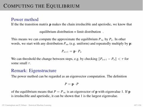
COMPUTING THE EQUILIBRIUM
Power methodIf the the transition matrix p makes the chain irreducible and aperiodic, we know that
equilibrium distribution = limit distribution .
This means we can compute the approximate the equilibrium P1 by Pn. In otherwords, we start with any distribution Pinit (e.g. uniform) and repeatedly multiply by p:
Pn+1 = p · Pn
We can threshold the change between steps, e.g. by checking kPn+1 � Pnk < ⌧ forsome small ⌧ .
Remark: EigenstructureThe power method can be regarded as an eigenvector computation. The definition
P = p · P
of the equilibrium means that P = P1 is an eigenvector of p with eigenvalue 1. If pis irreducible and aperiodic, it can be shown that 1 is the largest eigenvalue.
J.P. Cunningham and P. Orbanz · Statistical Machine Learning 407 / 436
PAGERANK
Constructing the transition matrixWe start with the web graph and construct the transition matrix of simple randomwalk, i.e.
aij :=n 1
# edges out of i if i links to j0 otherwise
A chain defined by A := (aij) will almost certainly not be irreducible (think of webpages which do not link anywhere). We therefore regularize A by defining
p := (1� ↵)A +↵d
0
B
@
1 · · · 1...
...1 · · · 1
1
C
A
for some small ↵ > 0.Clearly, this makes p both irreducible and aperiodic.
Computing the equilibriumGiven p, the equilibrium distribution is computed using the power method. Since theweb changes, the power method can be re-run every few days with the previousequilibrium as initial distribution.
J.P. Cunningham and P. Orbanz · Statistical Machine Learning 408 / 436
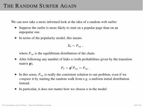
THE RANDOM SURFER AGAIN
We can now take a more informed look at the idea of a random web surfer:I Suppose the surfer is more likely to start on a popular page than on an
unpopular one.I In terms of the popularity model, this means
X0 ⇠ Pequ ,
where Pequ is the equilibrium distribution of the chain.I After following any number of links n (with probabilities given by the transition
matrix p),Pn = pnPequ = Pequ .
I In this sense, Pequ is really the consistent solution to our problem, even if wecompute it by starting the random walk from e.g. a uniform initial distributioninstead.
I In particular, it does not matter how we choose n in the model.
J.P. Cunningham and P. Orbanz · Statistical Machine Learning 409 / 436
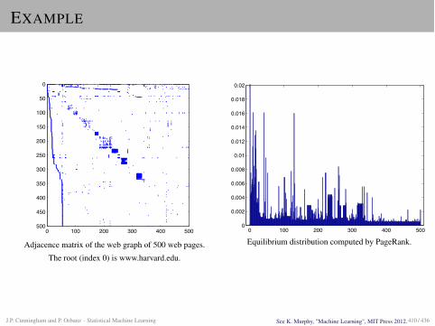
EXAMPLE
0 100 200 300 400 500
0
50
100
150
200
250
300
350
400
450
500
nz = 2636Adjacence matrix of the web graph of 500 web pages.
The root (index 0) is www.harvard.edu.
0 100 200 300 400 5000
0.002
0.004
0.006
0.008
0.01
0.012
0.014
0.016
0.018
0.02
Equilibrium distribution computed by PageRank.
See K. Murphy, "Machine Learning", MIT Press 2012.J.P. Cunningham and P. Orbanz · Statistical Machine Learning 410 / 436
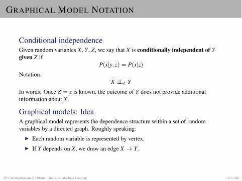
GRAPHICAL MODEL NOTATION
Conditional independenceGiven random variables X, Y , Z, we say that X is conditionally independent of Ygiven Z if
P(x|y, z) = P(x|z)Notation:
X ??Z Y
In words: Once Z = z is known, the outcome of Y does not provide additionalinformation about X.
Graphical models: IdeaA graphical model represents the dependence structure within a set of randomvariables by a directed graph. Roughly speaking:
I Each random variable is represented by vertex.I If Y depends on X, we draw an edge X ! Y .
J.P. Cunningham and P. Orbanz · Statistical Machine Learning 411 / 436
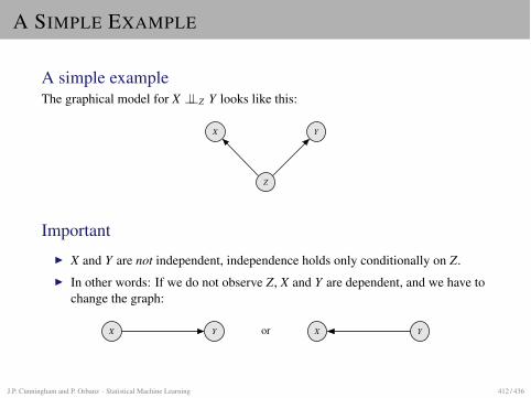
A SIMPLE EXAMPLE
A simple exampleThe graphical model for X ??Z Y looks like this:
X Y
Z
ImportantI X and Y are not independent, independence holds only conditionally on Z.I In other words: If we do not observe Z, X and Y are dependent, and we have to
change the graph:
X Y or X Y
J.P. Cunningham and P. Orbanz · Statistical Machine Learning 412 / 436
GRAPHICAL MODEL NOTATION
Factorizing a joint distributionThe joint probability of random variables X1, . . . , Xm can always be factorized as
P(x1, . . . , xm) = P(xm|x1, . . . , xm�1)P(xm�1|x1, . . . , xm�2) · · · P(x1) .
Note that we can re-arrange the variables in any order. If there are conditionalindependencies, we can remove some variables from the conditionals:
P(x1, . . . , xm) = P(xm|Xm)P(xm�1|Xm�1) · · · P(x1) ,
where Xi is the subset of X1, . . . , Xm on which Xi depends.
DefinitionLet X1, . . . , Xm be random variables. A (directed) graphical model represents afactorization of joint distribution P(x1, . . . , xm) as follows:
I Add one vertex for each variable Xi.I For each variable Xi, add and edge from each variable Xj 2 Xi to Xi.
J.P. Cunningham and P. Orbanz · Statistical Machine Learning 413 / 436
GRAPHICAL MODEL NOTATION
Lack of uniquenessThe factorization is usually not unique, since e.g.
P(x, y) = P(x|y)P(y) = P(y|x)(x) .
That means the direction of edges is not generally determined.
RemarkI If we use a graphical model to define a model or visualize a model, we decide
on the direction of the edges.I Estimating the direction of edges from data is a very difficult (and very
important) problem. This is the subject of a research field called causalinference or causality.
J.P. Cunningham and P. Orbanz · Statistical Machine Learning 414 / 436

HIDDEN MARKOV MODELS
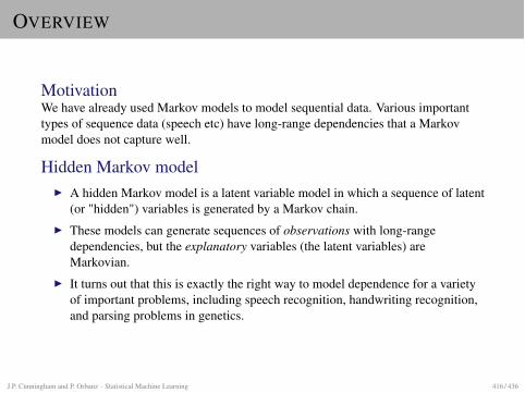
OVERVIEW
MotivationWe have already used Markov models to model sequential data. Various importanttypes of sequence data (speech etc) have long-range dependencies that a Markovmodel does not capture well.
Hidden Markov modelI A hidden Markov model is a latent variable model in which a sequence of latent
(or "hidden") variables is generated by a Markov chain.I These models can generate sequences of observations with long-range
dependencies, but the explanatory variables (the latent variables) areMarkovian.
I It turns out that this is exactly the right way to model dependence for a varietyof important problems, including speech recognition, handwriting recognition,and parsing problems in genetics.
J.P. Cunningham and P. Orbanz · Statistical Machine Learning 416 / 436
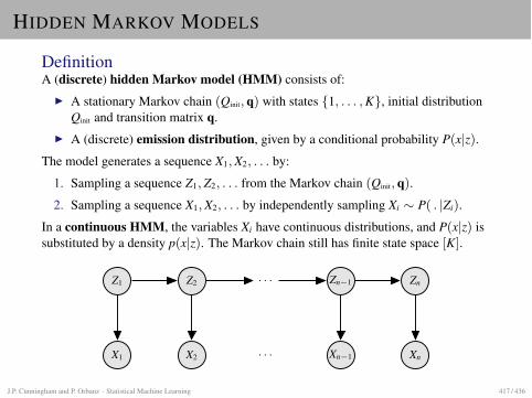
HIDDEN MARKOV MODELS
DefinitionA (discrete) hidden Markov model (HMM) consists of:
I A stationary Markov chain (Qinit, q) with states {1, . . . , K}, initial distributionQinit and transition matrix q.
I A (discrete) emission distribution, given by a conditional probability P(x|z).
The model generates a sequence X1, X2, . . . by:
1. Sampling a sequence Z1, Z2, . . . from the Markov chain (Qinit, q).
2. Sampling a sequence X1, X2, . . . by independently sampling Xi ⇠ P( . |Zi).
In a continuous HMM, the variables Xi have continuous distributions, and P(x|z) issubstituted by a density p(x|z). The Markov chain still has finite state space [K].
Z1 Z2 · · · Zn�1 Zn
X1 X2 · · · Xn�1 Xn
J.P. Cunningham and P. Orbanz · Statistical Machine Learning 417 / 436
NOTATION
We will see a lot of sequences, so we use the "programming" notation
x1:n := (x1, . . . , xn)
J.P. Cunningham and P. Orbanz · Statistical Machine Learning 418 / 436
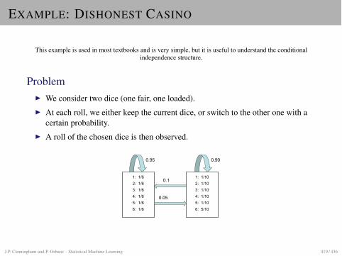
EXAMPLE: DISHONEST CASINO
This example is used in most textbooks and is very simple, but it is useful to understand the conditionalindependence structure.
ProblemI We consider two dice (one fair, one loaded).I At each roll, we either keep the current dice, or switch to the other one with a
certain probability.I A roll of the chosen dice is then observed.
������������������������������������������
������������������������������������������������
���� ����
���
����
J.P. Cunningham and P. Orbanz · Statistical Machine Learning 419 / 436
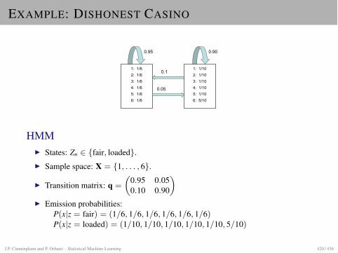
EXAMPLE: DISHONEST CASINO
������������������������������������������
������������������������������������������������
���� ����
���
����
HMMI States: Zn 2 {fair, loaded}.I Sample space: X = {1, . . . , 6}.
I Transition matrix: q =
✓
0.95 0.050.10 0.90
◆
I Emission probabilities:P(x|z = fair) = (1/6, 1/6, 1/6, 1/6, 1/6, 1/6)P(x|z = loaded) = (1/10, 1/10, 1/10, 1/10, 1/10, 5/10)
J.P. Cunningham and P. Orbanz · Statistical Machine Learning 420 / 436
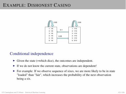
EXAMPLE: DISHONEST CASINO
������������������������������������������
������������������������������������������������
���� ����
���
����
Conditional independenceI Given the state (=which dice), the outcomes are independent.I If we do not know the current state, observations are dependent!I For example: If we observe sequence of sixes, we are more likely to be in state
"loaded" than "fair", which increases the probability of the next observationbeing a six.
J.P. Cunningham and P. Orbanz · Statistical Machine Learning 421 / 436
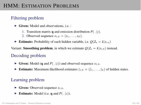
HMM: ESTIMATION PROBLEMS
Filtering problemI Given: Model and observations, i.e. :
1. Transition matrix q and emission distribution P( . |z).2. Observed sequence x1:N = (x1, . . . , xN).
I Estimate: Probability of each hidden variable, i.e. Q(Zn = k|x1:n)
Variant: Smoothing problem, in which we estimate Q(Zn = k|x1:N) instead.
Decoding problemI Given: Model (q and P( . |z)) and observed sequence x1:N .I Estimate: Maximum likelihood estimates z1:N = (z1, . . . , zN) of hidden states.
Learning problemI Given: Observed sequence x1:N .I Estimate: Model (i.e. q and P( . |z)).
J.P. Cunningham and P. Orbanz · Statistical Machine Learning 422 / 436
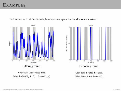
EXAMPLES
Before we look at the details, here are examples for the dishonest casino.
0 50 100 150 200 250 3000
0.5
1
roll number
p(loaded)
filtered
Filtering result.
Gray bars: Loaded dice used.Blue: Probability P(Zn = loaded|x1:N)
0 50 100 150 200 250 3000
0.5
1
roll number
MA
P s
tate
(0=
fair,1
=lo
aded)
Viterbi
Decoding result.
Gray bars: Loaded dice used.Blue: Most probable state Zn.
J.P. Cunningham and P. Orbanz · Statistical Machine Learning 423 / 436
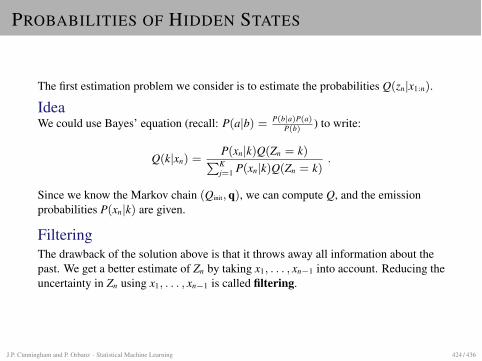
PROBABILITIES OF HIDDEN STATES
The first estimation problem we consider is to estimate the probabilities Q(zn|x1:n).
IdeaWe could use Bayes’ equation (recall: P(a|b) = P(b|a)P(a)
P(b) ) to write:
Q(k|xn) =P(xn|k)Q(Zn = k)
PKj=1 P(xn|k)Q(Zn = k)
.
Since we know the Markov chain (Qinit, q), we can compute Q, and the emissionprobabilities P(xn|k) are given.
FilteringThe drawback of the solution above is that it throws away all information about thepast. We get a better estimate of Zn by taking x1, . . . , xn�1 into account. Reducing theuncertainty in Zn using x1, . . . , xn�1 is called filtering.
J.P. Cunningham and P. Orbanz · Statistical Machine Learning 424 / 436
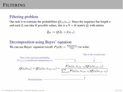
FILTERING
Filtering problemOur task is to estimate the probabilities Q(zn|x1:n). Since the sequence has length nand each Zi can take K possible values, this is a N ⇥ K-matrix Q, with entries
Qnk := Q(Zn = k|x1:n) .
Decomposition using Bayes’ equationWe can use Bayes’ equation (recall: P(a|b) = P(b|a)P(a)
P(b) ) to write:
Q(zn|x1:n) = Q(zn|xn, x1:(n�1)) =P(xn|zn, x1:(n�1))Q(zn|x1:(n�1))
PKzn=1 P(xn|zn, x1:(n�1))Q(zn|x1:(n�1))
This is the emission probabilityP(xn|zn) (conditional independence!)
This is the crucial term
Normalization
J.P. Cunningham and P. Orbanz · Statistical Machine Learning 425 / 436
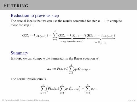
FILTERING
Reduction to previous stepThe crucial idea is that we can use the results computed for step n� 1 to computethose for step n:
Q(Zn = k|x1:(n�1)) =KX
l=1
Q(Zn = k|Zn�1 = l)| {z }
= qlk (transition matrix)
Q(Zn�1 = l|x1:(n�1))| {z }
= Q(n�1)l
SummaryIn short, we can compute the numerator in the Bayes equation as
ank := P(xn|zn)KX
l=1
qlkQ(n�1)l .
The normalization term is
KX
zn=1
⇣
P(xn|zn)KX
l=1
qlkQ(n�1)l
⌘
=KX
j=1
anj .
J.P. Cunningham and P. Orbanz · Statistical Machine Learning 426 / 436
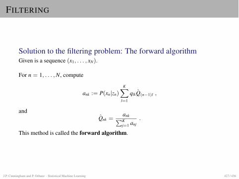
FILTERING
Solution to the filtering problem: The forward algorithmGiven is a sequence (x1, . . . , xN).
For n = 1, . . . , N, compute
ank := P(xn|zn)KX
l=1
qlkQ(n�1)l ,
andQnk =
ankPK
j=1 anj.
This method is called the forward algorithm.
J.P. Cunningham and P. Orbanz · Statistical Machine Learning 427 / 436
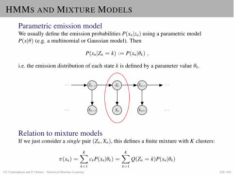
HMMS AND MIXTURE MODELS
Parametric emission modelWe usually define the emission probabilities P(xn|zn) using a parametric modelP(x|✓) (e.g. a multinomial or Gaussian model). Then
P(xn|Zn = k) := P(xn|✓k) ,
i.e. the emission distribution of each state k is defined by a parameter value ✓k.
· · · Zn�1 Zn Zn+1 · · ·
· · · Xn�1 Xn Xn+1 · · ·
Relation to mixture modelsIf we just consider a single pair (Zn, Xn), this defines a finite mixture with K clusters:
⇡(xn) =KX
k=1
ckP(xn|✓k) =KX
k=1
Q(Zn = k)P(xn|✓k)
J.P. Cunningham and P. Orbanz · Statistical Machine Learning 428 / 436
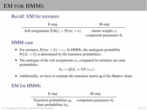
EM FOR HMMS
Recall: EM for mixturesE-step M-step
Soft assignments E[Mik] = Pr(mi = k) cluster weights ck
component parameters ✓k
HMM caseI For mixtures, Pr{mi = k} = ck. In HMMs, the analogous probability
Pr{Zn = k} is determined by the transition probabilities.I The analogue of the soft assignments aik computed for mixtures are state
probabilitiesbnk = Q(Zn = k|✓, x1:N) .
I Additionally, we have to estimate the transition matrix q of the Markov chain.
EM for HMMsE-step M-step
Transition probabilities qkj component parameters ✓k
State probabilities bnkJ.P. Cunningham and P. Orbanz · Statistical Machine Learning 429 / 436
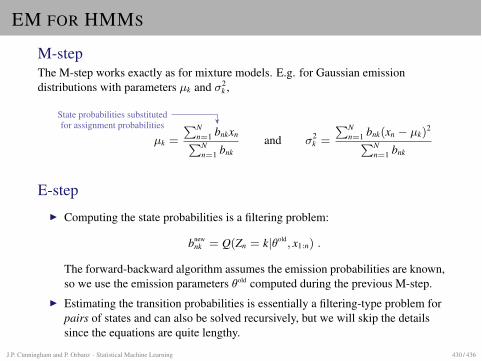
EM FOR HMMS
M-stepThe M-step works exactly as for mixture models. E.g. for Gaussian emissiondistributions with parameters µk and �2
k ,
µk =
PNn=1 bnkxnPN
n=1 bnkand �2
k =
PNn=1 bnk(xn � µk)
2
PNn=1 bnk
State probabilities substitutedfor assignment probabilities
E-stepI Computing the state probabilities is a filtering problem:
bnewnk = Q(Zn = k|✓old, x1:n) .
The forward-backward algorithm assumes the emission probabilities are known,so we use the emission parameters ✓old computed during the previous M-step.
I Estimating the transition probabilities is essentially a filtering-type problem forpairs of states and can also be solved recursively, but we will skip the detailssince the equations are quite lengthy.
J.P. Cunningham and P. Orbanz · Statistical Machine Learning 430 / 436
APPLICATION: SPEECH RECOGNITION
ProblemGiven speech in form of a sound signal, determine the words that have been spoken.
MethodI Words are broken down into small sound units (called phonemes). The states in
the HMM represent phonemes.I The incoming sound signal is transformed into a sequence of vectors (feature
extraction). Each vector xn is indexed by a time step n.I The sequence x1:N of feature vectors is the observed data in the HMM.
J.P. Cunningham and P. Orbanz · Statistical Machine Learning 431 / 436
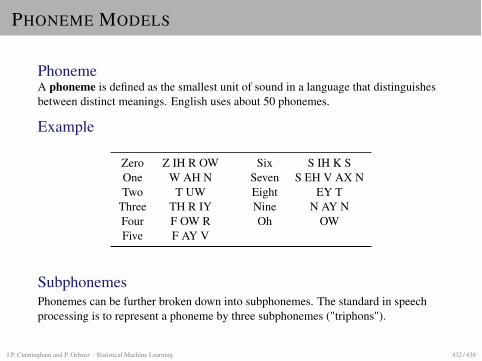
PHONEME MODELS
PhonemeA phoneme is defined as the smallest unit of sound in a language that distinguishesbetween distinct meanings. English uses about 50 phonemes.
Example
Zero Z IH R OW Six S IH K SOne W AH N Seven S EH V AX NTwo T UW Eight EY T
Three TH R IY Nine N AY NFour F OW R Oh OWFive F AY V
SubphonemesPhonemes can be further broken down into subphonemes. The standard in speechprocessing is to represent a phoneme by three subphonemes ("triphons").
J.P. Cunningham and P. Orbanz · Statistical Machine Learning 432 / 436
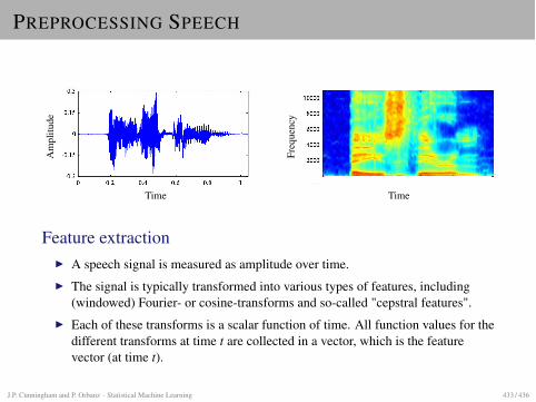
PREPROCESSING SPEECHA
mpl
itude
Time
Freq
uenc
y
Time
Feature extractionI A speech signal is measured as amplitude over time.I The signal is typically transformed into various types of features, including
(windowed) Fourier- or cosine-transforms and so-called "cepstral features".I Each of these transforms is a scalar function of time. All function values for the
different transforms at time t are collected in a vector, which is the featurevector (at time t).
J.P. Cunningham and P. Orbanz · Statistical Machine Learning 433 / 436
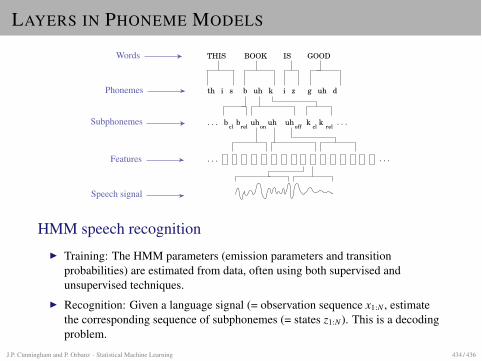
LAYERS IN PHONEME MODELS
4 WORTKETTENERKENNUNG FUR GROSSES VOKABULAR 132
4.1.2 HMMs fur Phonemstrukturen
Wörter:
Phoneme:
Subphoneme:
akustische Vektoren:
Sprachsignal:
THIS BOOK IS GOOD
th i s b uh k i z g uh d
. . . b b uh uh uh k kcl rel on off cl rel
. . .
. . .
. . .
Abbildung 4.2: Ebenen der akustischen Modellierung.
Die gesprochene Sprache kann auf jeder dieser Ebenen modelliert werden.
Spracherkennung, 12. Marz 2002 WS 01/02
Words
Phonemes
Subphonemes
Features
Speech signal
HMM speech recognitionI Training: The HMM parameters (emission parameters and transition
probabilities) are estimated from data, often using both supervised andunsupervised techniques.
I Recognition: Given a language signal (= observation sequence x1:N , estimatethe corresponding sequence of subphonemes (= states z1:N). This is a decodingproblem.
J.P. Cunningham and P. Orbanz · Statistical Machine Learning 434 / 436
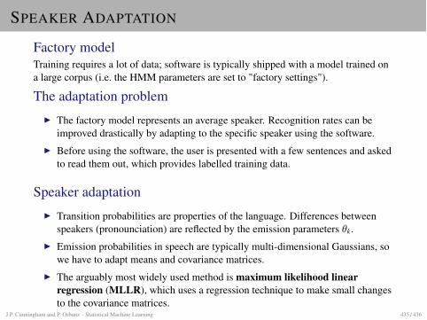
SPEAKER ADAPTATION
Factory modelTraining requires a lot of data; software is typically shipped with a model trained ona large corpus (i.e. the HMM parameters are set to "factory settings").
The adaptation problemI The factory model represents an average speaker. Recognition rates can be
improved drastically by adapting to the specific speaker using the software.I Before using the software, the user is presented with a few sentences and asked
to read them out, which provides labelled training data.
Speaker adaptationI Transition probabilities are properties of the language. Differences between
speakers (pronounciation) are reflected by the emission parameters ✓k.I Emission probabilities in speech are typically multi-dimensional Gaussians, so
we have to adapt means and covariance matrices.I The arguably most widely used method is maximum likelihood linear
regression (MLLR), which uses a regression technique to make small changesto the covariance matrices.
J.P. Cunningham and P. Orbanz · Statistical Machine Learning 435 / 436
FURTHER READING
More details on HMMsIf you feel enthusiastic, the following books provide more background:
I David Barber’s "Bayesian reasoning and machine learning" (available online;see class homepage).
I Chris Bishop’s "Pattern recognition and machine learning".I Many books on speech, e.g. Rabiner’s classic "Fundamentals of speech
recognition".
HTKIf you would like to try out speech recognition software, have a look at the HTK(HMM Toolkit) package, which is the de-facto standard in speech research. HTKimplements both HMMs for recognition and routines for feature extraction.
J.P. Cunningham and P. Orbanz · Statistical Machine Learning 436 / 436