Non-parametric maximum likelihood estimators for disease mapping

STATISTICS IN MEDICINEStatist. Med. 2000; 19:2539–2554

Non-parametric maximum likelihood estimators fordisease mapping

Annibale Biggeri1;∗;†, Marco Marchi1, Corrado Lagazio2, Marco Martuzzi3 andDankmar B�ohning4

1Department of Statistics ‘G. Parenti’; University of Florence; Italy2University of Udine; Italy3WHO ECEH; Rome; Italy

4Free University; Berlin, Germany

SUMMARY

A Non-Parametric Maximum Likelihood approach to the estimation of relative risks in the context of diseasemapping is discussed and a NPML approximation to conditional autoregressive models is proposed. NPMLestimates have been compared to other proposed solutions (Maximum Likelihood via Monte Carlo Scor-ing, Hierarchical Bayesian models) using real examples. Overall, the NPML autoregressive estimates (withweighted term) were closer to the Bayesian estimates. The exchangeable NPML model ranked immediatelyafter, even if it implied a greater shrinkage, while the truncated auto-Poisson showed inadequate for diseasemapping. The coe�cients of the autoregressive term for the di�erent mixtures have clear interpretations: inthe breast cancer example, the larger cities in the region showed high rates and very low correlation withthe neighbouring areas, while the less populated rural areas with low rates were strongly positively correlatedeach other. This pattern is expected since breast cancer is strongly correlated with parity and age at �rstbirth, and the female population of the rural areas experienced a decline in fertility much later than thoseliving in the larger cities. The leukemia example highlighted the failure of the Poisson-Gamma model andother general overdispersion tests to detect high risk areas under speci�c conditions. The NPML approachin Aitkin is very general, simple and exible. However the user should be warned against the possibility oflocal maxima and the di�culty in detecting the optimal number of components. Special software (such asCAMAN or DismapWin) had been developed and should be recommended mainly to not experienced users.Copyright ? 2000 John Wiley & Sons, Ltd.

1. INTRODUCTION

The analysis of risk pattern within a speci�ed geographical region is frequently undertaken inenvironmental epidemiology, but the maximum likelihood estimators of relative risks are quiteunstable when applied to small area data [1].

∗Correspondence to: Annibale Biggeri, Department of Statistics ‘G. Parenti’, University of Florence, Italy† E-mail: [email protected]�.it

Contract=grant sponsor: Vigoni ProgrammeContract=grant sponsor: EU BIOMED2; contract=grant number: BMH4-CT96-0633

Copyright ? 2000 John Wiley & Sons, Ltd.

2540 A. BIGGERI ET AL.

The most popular approach to overcome this problem, in current statistical and epidemiologicalliterature, consists of modelling the observed extra-Poisson variation using hierarchical Bayesianor empirical Bayes methods [2; 3].The observed disease counts Oi are assumed to follow the Poisson law with parameter �i given

by Ei�i; Ei being the expected number of cases, �i the relative risk, for area i=1 : : : n. The so-called expected number of cases is calculated as the sum over each age group of the product ofthe person-years at risk for each area times an appropriate reference rate. The observed=expectedratio is the maximum likelihood estimate and it is called standardized mortality ratio (SMR).The parameters {�i} or their convenient log-transformations are then modelled using appropriate

probability distributions, such as multivariate Gaussian, with vector mean � and variance matrix�. The matrix � is important to specify the spatially autocorrelated nature of the data, and in itssimplest form it depends on area adjacencies. More complex models describe log(�i)= �+ vi + uiwith two series of random terms for unstructured and spatially structured variation [4].The hierarchical Bayes approach requires us to specify appropriate non-informative hyperprior

distributions for � and � or its inverse, while the empirical Bayes approach uses the marginaldistribution f(O; �;�) to estimate the parameters of the prior density f(�). In both cases estimatesof the relative risks for each area are obtained as a measure of central tendency (the average, themedian or the mode) of the posterior distribution f(� |O).In the present paper we describe a non-parametric maximum likelihood approach to the esti-

mation of relative risks in the context of disease mapping. Such an approach has not receivedmuch consideration in geographical and epidemiological applications. Clayton and Kaldor [5] �rstused a discrete prior in their paper on empirical Bayes approaches to disease mapping. B�ohning[6; 7] developed a comprehensive mixture-based approach, and Schlattmann and B�ohning [8] ap-plied those ideas to disease mapping, providing also a speci�c software. Independently, Aitkin[9; 10] generalized the non-parametric maximum likelihood (NPML) approach to random e�ectsmodelling and provided simple examples on disease mapping.In the following we brie y review the NPML approach to disease mapping and propose an

NPML approximation to conditionally autoregressive models. We compare the NPML estimates tothe other proposed solutions (maximum likelihood via Monte Carlo scoring, hierarchical Bayesianmodels) using real examples. Finally, we discuss the di�erence between the NPML approach andthe algorithm in B�ohning et al. [7].

2. METHODS

2.1. The exchangeable model

Let us start with the simple model with diagonal �.In the empirical Bayes approach the marginal density f(O; �; �2I) is used as the likelihood to

estimate the prior parameters �, �2. This function is the integral of the likelihood function overf(� | �; �2)

L=∏i

∫f(Oi | �i)f(�i)d�i

Since the likelihood for the observed disease counts is Poisson, a very popular approach assumesthe conjugate gamma prior for f(�) ≈ G(�; �) leading to the negative binomial marginal density.

Copyright ? 2000 John Wiley & Sons, Ltd. Statist. Med. 2000; 19:2539–2554

NON-PARAMETRIC MAXIMUM LIKELIHOOD ESTIMATORS 2541

The principal merit of this formulation is its simplicity; it provides maximum likelihood inferenceon area heterogeneity [11] and closed formula for the estimates based on posterior distributions�i=(Oi + �)=(Ei + �) [5].There is no subject speci�c justi�cation for the choice of the gamma function. To avoid the

arbitrariness in selecting the prior density we can approximate it by assuming a discrete priordistribution with probability �k at mass points �ik ; the integrated likelihood then becomes

L =∏i

K∑kf(Oi | �ik)�k

This is a well-known solution [12; 13] in the literature on empirical Bayes estimation. Theunderlying idea is that the data contain information not only about the parameters of the priordensity but also on its form [10; 14].The �rst application to disease mapping can be found in Clayton and Kaldor [5]. Other simple

examples are provided by Aitkin [10; 15].B�ohning et al. [7] and Schlattmann and B�ohning [8] developed a similar solution based on

the estimation of the parameters of a mixture of distributions. Instead of a discrete prior with a�nite number of mass points they equivalently introduced a discrete number of distributions andestimated the probability of appartenance for each area. Schlattmann et al. extended the model toinclude covariates.

2.2. The conditionally autoregressive model

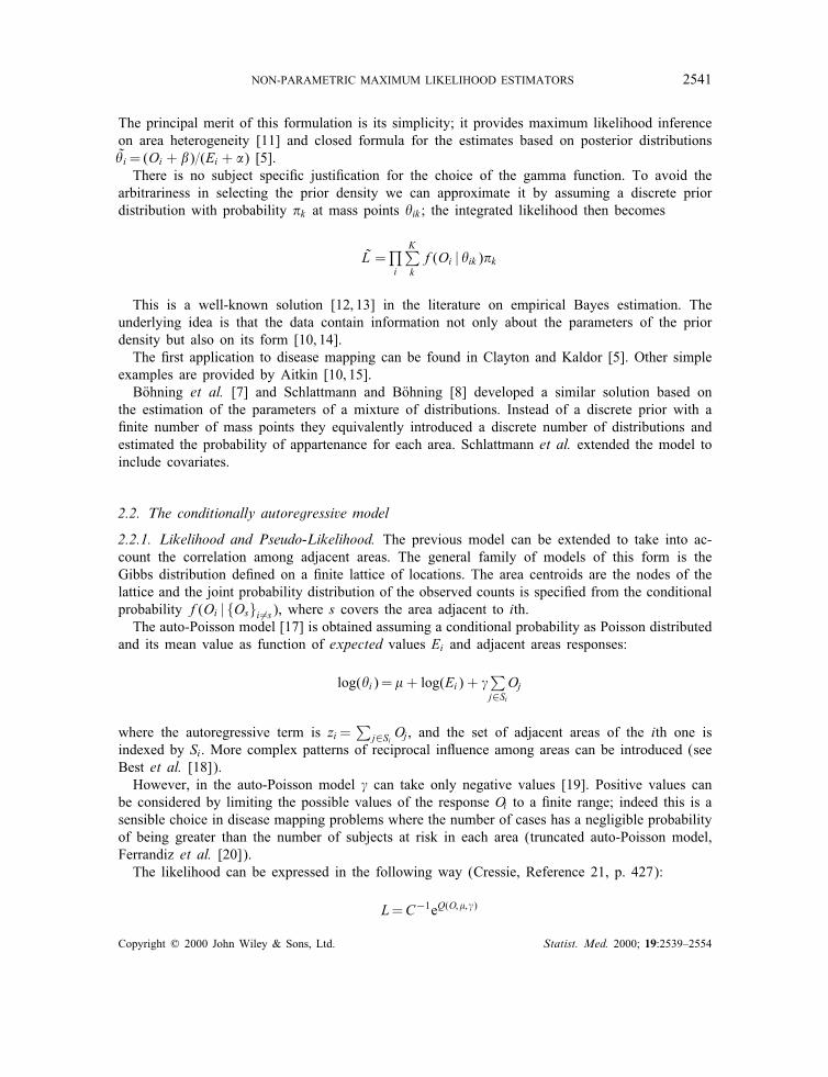
2.2.1. Likelihood and Pseudo-Likelihood. The previous model can be extended to take into ac-count the correlation among adjacent areas. The general family of models of this form is theGibbs distribution de�ned on a �nite lattice of locations. The area centroids are the nodes of thelattice and the joint probability distribution of the observed counts is speci�ed from the conditionalprobability f(Oi | {Os}i 6=s), where s covers the area adjacent to ith.The auto-Poisson model [17] is obtained assuming a conditional probability as Poisson distributed

and its mean value as function of expected values Ei and adjacent areas responses:

log(�i)= � + log(Ei) + ∑j∈SiOj

where the autoregressive term is zi=∑

j∈Si Oj, and the set of adjacent areas of the ith one isindexed by Si. More complex patterns of reciprocal in uence among areas can be introduced (seeBest et al. [18]).However, in the auto-Poisson model can take only negative values [19]. Positive values can

be considered by limiting the possible values of the response Oi to a �nite range; indeed this is asensible choice in disease mapping problems where the number of cases has a negligible probabilityof being greater than the number of subjects at risk in each area (truncated auto-Poisson model,Ferrandiz et al. [20]).The likelihood can be expressed in the following way (Cressie, Reference 21, p. 427):

L=C−1eQ(O;�; )



where

Q(O; �; )= �0∑Oi +

∑Oi log(Ei) +

∑ziOi

Since the normalizing constant is C =∑exp(Q(O; �; )) there is no closed form for the likelihood.

Assuming stochastic independence of the conditional probabilities, a pseudo-likelihood functionas an approximation to the true likelihood can be de�ned [19]. In this case zi is treated asa covariate in the augmented systematic component of a simple Poisson regression model forindependent data.A di�erent solution for the autoregressive component is more sensible. Note, �rst, that in disease

mapping applications what is actually modelled is the ratio observed=expected number of diseasecases (SMR) and, second, that the coe�cient estimate for the model with only the interceptis �= log(

∑Oi=∑Ei). The purpose of the analysis is actually to model relative risks and not

the number of cases. We propose weighting the autoregressive component zi by the sum of theexpected counts, giving zSMRi =

∑j∈Si Oj=

∑j∈Si Ej.

2.2.2. Non-parametric empirical Bayes approach to a conditional autoregressive model. Recallthe integrated likelihood considered above:

L=∏i

∫f(Oi | �i)f(�i)d�i

where �i denotes the vector of parameters of the systematic component. Assuming a discrete priordistribution with probability �k at mass points �ik we can approximate the likelihood with

L =∏i

K∑kf(Oi | �ik)�k

The di�erence with the exchangeable case consists in having speci�ed a model with randomintercept and random slope for the covariate zi, or its weighted counterpart zSMRi , which representthe autoregressive component. It is important here to specify random slope terms because thisimplies that the autocorrelation could vary among the di�erent K components.This formulation is an application of the pseudo-likelihood approach in the context of empirical

Bayesian inference (Biggeri et al. [22], Schlattmann and B�ohning, Reference [23], p. 59) andaddresses the point raised in Aitkin (Reference [10], p. 125).

2.3. Estimation

2.3.1. Non-parametric maximum likelihood. Given a �xed number K of mass points we can usethe EM algorithm to estimate

�k =n∑iwik =n

where wik =E(�ik |Oik)= �kfik(:)=∑

l �lfil(:) are obtained maximizing the likelihood of the aug-mented data set. In practice the data are replicated K times, at the start using the observed valuesarbitrarily split among the replicates.



The smoothed a posteriori relative risks {�i} are easily obtained from the �tted model, whereg() denote the inverse link function (see Aitkin [9; 10]):

�i=∑kwik(g(�ik))

This approach is presented and motivated in Aitkin [10] and has been introduced by Hinde andWood [24]. Basically the proposed algorithm is very close to the EM algorithm for latent variablemodels, and standard maximum likelihood methods are then applied to the expanded data set (fora GLIM implementation see Biggeri and Bini [25]).B�ohning et al. [7] used directional gateaux derivatives to locate the mass points and the EM

algorithm to estimate model parameters or, eventually, to re�ne them combining equal estimates(at current level of accuracy).The most important result is that the log-likelihood is a concave functional on the set of all

discrete probability distributions, but not for the set of distributions with a �xed number of Ksupport points. B�ohning [6] discusses the computational problems involved and the selection ofthe number K of mixture components. The simpler algorithm above (as in Aitkin and Francis [26])requires the number K of mixtures to be �xed in advance and may cause two distinct problems.First, local maxima of the likelihood are a possibility; second, likelihood ratio tests to select thenumber K are invalid, since the null hypothesis lies on the boundary of the alternative hypothesis.Much care is therefore required, as we illustrate in example 2.Interval estimates of the relative risks for empirical Bayes models in geographical epidemiology

are discussed by Biggeri et al. [27]; warnings on simple extension of bootstrap techniques haveto be heeded.

2.3.2. Maximum likelihood. The parameters of the truncated auto-Poisson model can be esti-mated using maximum likelihood via a Monte Carlo Markov chain procedure (see Ferrandizet al. [20], pp. 208–209).Recall the data likelihood:

L=C−1eQ(O;�; ) =C−1h(O; �)

The joint distribution of pseudo-data Y from the conditional density f∗(Oi | {Os}i 6=s), that is,the density with values of the parameter vector � �xed to some prede�ned values �∗; ∗, canbe simulated via a Monte Carlo Markov chain algorithm and then the ratio of the normalizingconstants C=C∗ can be approximated as

C=C∗ ≈ 1=mm∑j

h(Yj; �)h(Yj; �∗)

from m samples taken when the process stabilized. Estimates of the parameter vector � can thenbe obtained by Newton–Raphson using the log-likelihood ratio

l= log(L=L∗)= log h(O; �)h(O; �∗) − log(C=C

∗)

= logh(O; �)h(O; �∗) − log

(1=m

m∑j

h(Yj; �)h(Yj; �∗)

)



which leads to the following equations:

@l(�)@�

= T (O)−∑m

j Tje(�−�∗)′Tj∑m

j e(�−�∗)′Tj

@2l(�)@�2

=−∑m

j uju′je(�−�∗)′uj∑m

j e(�−�∗)′uj

where T is the vector of su�cient statistics, � is the vector of parameters to be estimated anduj =Tj − T (O).In example 1 we used maximum pseudo-likelihood estimates of the parameters in � as values

for �∗; ∗ to be used by the Gibbs sampler (as suggested by Hu�er and Wu [28]). Other authorsperformed a Monte Carlo scoring, calling the sampler at each step of the optimization procedure,in which case �∗= �k the estimates values at the last iteration of the Newton–Raphson algorithm(Younes [29]; see also Geyer and Geyer and Thompson [30; 31] for a complete presentation of thetheory). Ferrandiz et al. [32] applied this approach to the study of association between aggregateexposure data and small area mortality and provided several alternatives for the speci�cation ofthe autoregressive components.

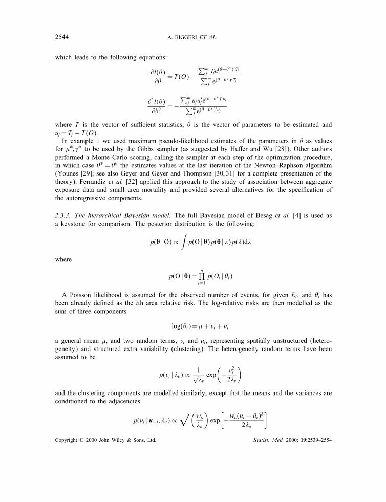
2.3.3. The hierarchical Bayesian model. The full Bayesian model of Besag et al. [4] is used asa keystone for comparison. The posterior distribution is the following:

p(X |O) ∝∫p(O | X)p(X | �)p(�)d�

where

p(O | X)=n∏i=1p(Oi | �i)

A Poisson likelihood is assumed for the observed number of events, for given Ei, and �i hasbeen already de�ned as the ith area relative risk. The log-relative risks are then modelled as thesum of three components

log(�i)= � + vi + ui

a general mean �, and two random terms, vi and ui, representing spatially unstructured (hetero-geneity) and structured extra variability (clustering). The heterogeneity random terms have beenassumed to be

p(vi | �v) ∝ 1√�vexp(− v2i2�v

)and the clustering components are modelled similarly, except that the means and the variances areconditioned to the adjacencies

p(ui | u−i ; �u) ∝√(

wi:�u

)exp[−wi:(ui − �ui)2

2�u

]Copyright ? 2000 John Wiley & Sons, Ltd. Statist. Med. 2000; 19:2539–2554


where wi: denotes the number of adjacent areas of the ith and

�ui=1wi:

∑j 6=iwijuj

Usually, an uninformative inverse gamma prior distribution for each precision parameter �−1u and�−1v is stated.The posterior distributions are approximated via Gibbs sampling [33], using the adaptive rejection

algorithm [34]. The joint posteriors are complicated but the full conditional distributions used bythe Gibbs sampler procedure have simpler forms. The full conditionals for each term vi, fori=1; : : : ; n, are

p(vi | ui; �v; Oi) ∝ exp[Oivi − Ei exp(ui + vi)− v2i

2�v

]and for each ui

p(ui | u−i ; vi; �u; Oi) ∝ exp[Oiui − Ei exp(ui + vi)− wi:(ui − �ui)2

2�u

]The full conditional for the hyperparameters are

p(�v | C)∝p(C | �v)p(�v)and

p(�u | u)∝p(u | �u)p(�u)Moreover, when inverse gamma priors are considered with parameters av and bv for �v and pa-rameters au and bu for �u, the full conditionals are still inverse gamma with parameters av + nand bv +

∑ni=1 v

2i =2 for �v and au + n=2 and bu +

∑ni=1

∑j¡i wij(ui − uj)2=2 for �u.

At each cycle of the Gibbs sampler, 2n+ 2 distributions are sampled; the two distributions forthe hyperparameters �u and �v using standard sampling routines for the inverse gamma and thedistributions for each of the terms vi and ui, for i=1; : : : ; n, using adaptive rejection sampling. Thisis because the full conditional distributions for terms u and C are not standard, but log-concave.Parameters �v and �u control the relative strength of each component of the Gaussian con-

volution; if �v=�u is large then spatially unstructured variation (heterogeneity) dominates; whensmall, spatially structured variation (clustering) dominates. It is worth mentioning that Bayesianconditioning implies that the data do in uence the relative strength of the two components.

3. APPLICATION

3.1. Example 1

Death certi�cate data for lung cancer (males and females) and female breast cancer collected inthe 341 municipalities of Emilia-Romagna Region (Italy) 1982–1988 are used as an example forthe methods proposed [35].Table I reports the summaries of the distributions of expected number of deaths obtained us-

ing indirect standardization and national reference rates. There were 341 small areas with widepopulation gradients (expected counts ranging from 0.145 to 928.688).



Table I. Descriptive statistics for the expected number of deaths for selected causes among341 municipalities of Regione Emilia-Romagna, Italy, 1982–1988. Indirect standardization

using Italian reference rates.

Mean Standard deviation Minimum Maximum

Lung cancer females 3.613 11.250 0.145 168.034Lung cancer males 22.343 63.652 0.966 928.688Breast cancer females 9.194 28.534 0.308 422.238

Table II. Descriptive statistics of di�erent relative risk estimators (see text). Death certi�catefor selected causes. Emilia-Romagna, Italy, 1982–1988.

Lung cancer females

SMR NPML NPA-1 NPA-2 Bayes

� 0.81 0.77 0.77 0.85 0.87� 0.85 0.12 0.13 0.15 0.10Median 0.67 0.74 0.75 0.85 0.85Minimum 0.00 0.57 0.41 0.54 0.66Maximum 6.94 1.78 1.82 2.06 1.60

Lung cancer males


� 0.92 0.91 0.91 0.93 0.94� 0.45 0.20 0.20 0.24 0.23Median 0.87 0.86 0.86 0.87 0.88Minimum 0.00 0.74 0.66 0.59 0.67Maximum 3.46 2.28 2.39 2.29 2.02

Breast cancer females

SMR NPML NPA-1 NPA-2 ML-AP Bayes

� 0.86 0.90 0.89 0.89 0.98 0.93� 0.56 0.07 0.10 0.14 0.04 0.07Median 0.84 0.89 0.87 0.90 0.97 0.93Minimum 0.00 0.73 0.65 0.37 0.95 0.77Maximum 3.45 1.17 1.22 1.44 1.20 1.18

Table II shows descriptive statistics for several relative risk estimators: standardized mortalityratios (SMR); non-parametric maximum likelihood (NPML); non-parametric maximum likelihoodwith an autoregressive component (non-weighted NPA-1, weighted NPA-2), and hierarchical Bayes(Besag, York and Molli�e model, Bayes). For female breast cancer only, we reported the truncatedauto-Poisson (Monte Carlo scoring, ML-AP) predicted relative risks.Table III reports the mean and standard deviation of the posterior distributions of the square

root of the hyperparameters of the Besag, York and Molli�e model. They can be interpreted as



Table III. Lung (females and males) and breast cancer deaths, 1982–1988, Emilia-RomagnaRegion, Italy. Mean and standard deviation (within brackets) of the posterior distributions of theheterogeneity and clustering hyperparameters (expressed as standard deviations of ui and vi).

HyperparameterHeterogeneity Clustering Ratio

Lung cancer female 0.2817 0.0391 7 : 1(0.0557) (0.0178)

Lung cancer male 0.0418 0.2629 1 : 6:5(0.0099) (0.0201)

Breast cancer female 0.0992 0.0989 1 : 1(0.0484) (0.0545)

standard deviations of the random terms vi and ui and their relative magnitude is informative ofthe kind of extra-Poisson variation in the map.Lung cancer risks, females, was higher in urban settings, re ecting the pattern of smoking habits

among the female population. Overall, strong heterogeneity and small clustering were evident (ratio7 : 1).Lung cancer risks, males, showed a very strong spatial clustering, with a north-east south-west

gradient (heterogeneity=clustering ratio 1 : 6:5).Breast cancer risks was higher in the mainly urban areas located along the ideal line of the

Emilia road and along the coast. A lower risk was experienced on the mountain areas locatedat the west and southern border of the region. This pattern will produce low correlation amongareas surrounding the biggest cities and higher correlation among the scarcely populated area ofthe mountain. Moreover, the great variability in population density by area produced a strongoverdispersion in the data (the heterogeneity=clustering ratio is of the order 1 : 1).The shrinkage was greater for the Bayesian estimates and lower for the autoregressive models

NP-A1 NP-A2, as expected. For breast cancer, statistics from the �tted values of the truncatedauto-Poisson model (ML-AP) are also reported; of course, these estimates showed a very smallstandard deviation compared to NPML or Bayesian estimates, which can be interpreted as weightedaverages between SMRs and model-based relative risks.In Table IV the matrix of Pearson’s and Spearman’s correlation coe�cients is shown.In all three data sets the higher correlations with the Bayes estimates were those provided

by the non-parametric maximum likelihood method with weighted autoregressive terms (NPA-2).This result is very important since a better performance would be expected of the simple non-autoregressive NPML model, which was superior only for the breast cancer example. Moreover,the not-weighted autoregressive model behaved very badly, as the truncated auto-Poisson model.In detail, for the breast cancer data set, the NPML model gave an estimated number of mass

points of three with probability 0:2250, 0:4014, 0:3736, deviance 444:76 with 337 degree of free-dom. In Table V results from the model are shown for a few areas. The �rst mass point correspondsto a high value of relative risk, while the third mass point corresponds to the lowest. The areaswith more weight than the �rst component ranked highest in risk.The NPA models also identi�ed three mass points with probability 0:2253, 0:4615, 0:3133,

deviance 435:21, 334 degree of freedom (likelihood ratio= 9:55, degree of freedom=3; p-value=0:0228) for the model with the unweighted term zi, and with probability 0:3414, 0:3571, 0:3015,



Table IV. Pearson’s (upper triangle) and Spearman’s (lower triangle) correlation coe�-cients among di�erent relative risk estimators (see text). Death certi�cate for selected causes.

Emilia-Romagna, Italy, 1982–1988.

Lung cancer females


SMR 1.00 0.38 0.42 0.55 0.71NPML 0.56 1.00 0.91 0.60 0.76NPA-1 0.60 0.79 1.00 0.66 0.79NPA-2 0.63 0.22 0.47 1.00 0.82Bayes 0.87 0.38 0.51 0.73 1.00

Lung cancer males


SMR 1.00 0.79 0.74 0.70 0.79NPML 0.95 1.00 0.98 0.81 0.83NPA-1 0.90 0.97 1.00 0.79 0.81NPA-2 0.69 0.73 0.72 1.00 0.94Bayes 0.90 0.82 0.80 0.91 1.00

Breast cancer females

SMR NPML NPA-1 NPA-2 ML-AP Bayes

SMR 1.00 0.75 0.68 0.65 0.15 0.62NPML 0.92 1.00 0.82 0.70 0.18 0.81NPA-1 0.83 0.84 1.00 0.74 0.65 0.68NPA-2 0.73 0.75 0.83 1.00 0.35 0.75ML-AP 0.15 0.09 0.49 0.42 1.00 0.16Bayes 0.67 0.73 0.66 0.77 0.12 1.00

Table V. Results for selected areas of non-parametric maximum likelihood analysis, breastcancer female, Emilia-Romagna, Italy, 1982–1988.

Mass points

Log scale 0.1606 −0:0264 −0:3488Relative risk 1.1740 0.9739 0.7055

Probability0.2250 0.4014 0.3736 RR

Area 193 0.9999 0.0006 0.0000 1.1743Area 142 0.4932 0.4235 0.0833 1.0398Area 134 0.2037 0.4444 0.3520 0.9033Area 268 0.0711 0.2723 0.6566 0.7987Area 298 0.0012 0.1131 0.8857 0.7322



deviance 432:34, 334 degree of freedom, for the model with the weighted term zSMRi . The presenceof autoregressive terms precluded simple interpretation of the mass points and the posterior areaprobabilities wik . In Table VI the coe�cient estimates and their relative standard errors are reported.We can see that the autoregressive coe�cient was negative and of the same magnitude of itsstandard error for the mass point corresponding to higher relative risk; high risk areas tended tobe uncorrelated to the neighbouring areas. The degree of autocorrelation grew as we moved to thelow risk mass points. This is coherent with previous knowledge about the pattern of breast cancerrisk in the Regione Emilia-Romagna, as explained before.Figure 1 shows the maps obtained from the di�erent models using absolute levels for grey tones

to highlight the degree of shrinkage toward the mean and the resulting high risk areas.The degree of smoothing was greater for Bayesian mapping and lesser for exchangeable non-

parametric model NPML, as expected.The non-parametric autoregressive models NPA were intermediate. The �rst model (NPA-1),

which uses the usual autoregressive unweighted term zi, regressed the small areas adjacent to thebiggest city toward the city observed=expected ratio. These areas changed their rank and they hadbeen moved in the high risk set (see the wide black area in the centre of the map, correspondingto the hinterland of the region capital Bologna).The second model (NPA-2) weighted the autoregressive component by the expected number of

deaths, that is, each area was regressed toward the observed=expected ratio of the neighbouringareas. The resulting e�ect was much more consistent with the Bayesian approach.The truncated auto-Poisson model produced a picture which underlined some inadequacies of

this approach when used for disease mapping (Figure 2); indeed, the autoregressive componenthad to be speci�ed in a more exible way than by means of only one �xed term.

3.2. Example 2

Death certi�cate data for female leukaemia collected in the surveillance high risk area of Brindisi(Puglia Region, Italy) 1990–1994 are used to illustrate the performance of di�erent algorithms fornon-parametric maximum likelihood estimates for disease mapping.The Italian Ministry of Environment de�ned a list of areas for epidemiological surveillance.

One of these areas consists of 29 municipalities surrounding the city of Brindisi. From previousknowledge and exposure data there are reasons to believe that lung cancer and non-Hodgkinlymphoma could result in high rates, but there is no expectation of high rates for leukaemia.Population size by area shows a great variability, but not spatially structured.Table VII shows the observed and expected death counts, standardized mortality ratios (SMR),

Bayes estimators, non-parametric maximum likelihood estimators with two and three components(NPML-2, NPML-3), the NPML estimators using the B�ohning algorithm (CAMAN) and the rel-ative group appartenance, the number of neighbours and their identi�ers.The usual tests for detecting extra-Poisson variation gave negative results. The Pottho�–

Whittinghill test [36] did not identify overdispersion: �=0:08274 (90 per cent CI −0:37); 0:53Z =0:3021 Monte Carlo p-value (one-sided) 0:3375. The Poisson-gamma maximum likelihoodratio test [11] did not identify overdispersion: the maximum likelihood estimate of log(�)=−13:84749 with 90 per cent CI −5859:278; 5831:583.On the contrary, the Bayesian model (Besag, York, Molli�e) did identify spatially unstructured

variability (Table VIII), but the relative risk estimates were strongly shrunk toward the null value



Figure 1. Maps of lung cancer risk in females (�rst column) and in males (second column) and breast cancer(third column). Maps are obtained using SMRs (�rst row), NPML (second row), NPA-1 (third row), NPA-2

(fourth row) and Bayesian method (�fth row). Emilia-Romagna, Italy, 1982–1988.

of 1.0. Indeed the magnitude of the standard deviation of the heterogeneity terms is very low(about half of that detected in the breast cancer data set before).The NPML identi�ed three mixture components. The results were: �rst component proba-

bility = 0:1667, relative risk = 1:514; second component probability = 0:6666, relative risk = 0:9178;third component probability = 0:1667, relative risk = 0:9138. The Poisson deviance was 32:15684,



Figure 2. Maps of predicted breast cancer risks in females using truncated auto-Poisson model,Emilia-Romagna, Italy, 1982–1988.

Table VI. Results of the �tting of the non-parametric autoregressive models. Breast cancerfemales, Emilia-Romagna, Italy, 1982–1988.

Parameter Estimate SE

Terms: 1 + K + K:Z(I)1 0.1788 0.0427K(2) −0:3032 0.0614K(3) −0:6921 0.0800K(1):Z(I) −0:0002 0.0003K(2):Z(I) 0.0006 0.0002K(3):Z(I) 0.0013 0.0003

Mixture proportions: 0.2253 0.4615 0.3133

Terms: 1 + K + K:ZSMR(I)1 −0:0799 0.1308K(2) 0.1958 0.2261K(3) −1:910 0.2717K(1):ZSMR(I) 0.2001 0.1289K(2):ZSMR(I) −0:2884 0.1955K(3):ZSMR(I) 1.7540 0.2146

Mixture proportions: 0.3414 0.3571 0.3015

and NPML deviance 32:00779 corresponding to a log-likelihood of −51:345636. Since two sup-port points were almost equal, combining them and performing a further EM step for two compo-nents gave the following results: �rst component probability = 0:2159, relative risk = 1:4572 andsecond component probability = 0:7841, relative risk = 0:8986, NPML deviance=32:026112, log-likelihood =−51:363958. This solution is very unstable and several local maxima, depending onthe initial values of the EM algorithm, were found.CAMAN (B�ohning et al. [37]) identi�ed two grid points with positive support: �rst component

probability = 0:8460, relative risk = 0:919645 and second component probability = 0:1540, relativerisk = 1:548316; log-likelihood −51:34483.



Table VII. Results for some areas ranking by di�erent relative risk estimators. Adultleukaemia, females, Brindisi area, Italy, 1990–1994.

ID O E SMR Bayes NP-3 NP-2 Caman G Neighbours

1 11 14.14 0.78 0.98 0.922 0.908 0.924 1 7:2,3,4,6,7,8,102 9 5.46 1.65 1.02 1.127 1.146 1.165 1 6:1,7,8,11,12,193 1 2.93 0.34 0.99 0.942 0.934 0.995 1 4:1,4,5,94 1 1.28 0.78 0.99 0.980 0.980 0.995 1 6:1,3,7,9,13,155 2 0.76 2.63 1.01 1.043 1.050 1.072 1 2:3,96 3 3.89 0.77 0.99 0.955 0.951 0.964 1 5:1,8,10,14,227 0 1.22 0.00 0.99 0.958 0.953 0.969 1 5:1,2,4,12,138 4 2.52 1.59 1.01 1.038 1.048 1.065 1 6:1,2,6,14,19,239 7 3.03 2.31 1.01 1.192 1.200 1.240 2 5:3,4,5,15,1610 3 2.27 1.32 1.00 1.008 1.013 1.028 1 3:1,6,2211 2 1.65 1.21 1.01 0.998 1.001 1.017 1 4:2,12,18,1912 2 1.53 1.31 1.00 1.003 1.007 1.023 1 7:2,7,11,13,17,18,2913 0 1.29 0.00 0.99 0.957 0.951 0.967 1 5:4,7,12,15,1714 3 1.12 2.68 1.00 1.074 1.083 1.109 1 5:6,8,22,23,2715 1 2.19 0.46 0.98 0.956 0.950 0.965 1 7:4,9,13,16,17,20,2516 1 2.17 0.46 0.98 0.956 0.951 0.965 1 4:9,15,20,2117 3 1.53 1.96 1.00 1.048 1.056 1.076 1 5:12,13,15,25,2918 4 1.14 3.51 1.02 1.137 1.145 1.182 1 4:11,12,19,2919 4 2.59 1.54 1.01 1.034 1.044 1.060 1 5:2,8,11,18,2320 1 2.01 0.50 0.98 0.960 0.955 0.970 1 5:15,16,24,25,2621 1 1.45 0.69 0.98 0.975 0.974 0.989 1 1:1622 5 6.71 0.74 0.99 0.937 0.929 0.942 1 4:6,10,14,2723 3 4.96 0.60 0.99 0.938 0.929 0.943 1 4:8,14,19,2724 2 2.03 0.98 0.98 0.984 0.985 0.999 1 3:20,25,2625 1 1.97 0.51 0.98 0.960 0.957 0.971 1 4:15,17,20,2426 0 0.65 0.00 0.97 0.974 0.971 0.988 1 3:20,24,2827 4 4.19 0.95 0.99 0.968 0.968 0.979 1 3:14,22,2328 2 2.18 0.92 0.97 0.978 0.979 0.992 1 1:2629 0 1.12 0.00 0.99 0.961 0.956 0.972 1 3:2,17,18

Table VIII. Results for the Bayesian model (Besag, York,Molli�e). Adult leukaemia, females, Brindisi area, Italy,1990–1994. Mean and standard deviation of the posteriordistributions of the heterogeneity and clustering hyperpa-rameters (expressed as standard deviations of ui and vi).

Terms �sd �sd

Heterogeneity 0.0454 0.0203Clustering 0.0539 0.0516

Generally speaking the non-parametric maximum likelihood estimates were consistent with someheterogeneity among areas; both agreed in assigning greater probability of being at higher risk toarea ID=9.



4. CONCLUSION

We reviewed the proposed non-parametric maximum likelihood estimators for disease mapping andpresented a simple weighted pseudo-likelihood approach to non-parametric autoregressive models.The performance of non-parametric maximum likelihood estimators were compared with those

of Bayesian hierarchical estimators using real examples.As example 1 showed, overall, the NPML autoregressive estimates (with weighted term NPA-2)

were closer to the Bayesian estimates. The three data sets were chosen to represent a variety ofreal situations: heterogeneity; clustering, and intermediate pattern of variation among areas. Theexchangeable NPML model ranked immediately after NPA-2, even if it implied a greater shrinkage.In the breast cancer example, the exchangeable NPML and the NPA-2 autoregressive estimates

(with weighted term) were closer to the Bayesian estimates, while the truncated auto-Poissonshowed inadequate for disease mapping. Actually the truncated auto-Poisson model su�ered fromassumptions about the autoregressive component; the map for the breast cancer data highlightedhow strong the areas adjacent to the larger cities were a�ected, and it is di�cult to be con�dentin such results. Similarly the NPML with the autoregressive component (NPA-1 in particular)resulted in a levelling e�ect in the neighbourhood of the larger cities. This distortion is limitedwith the NPML model with weighted autoregressive component (NPA-2). The coe�cients of theautoregressive term for the di�erent mixtures have clear interpretations; the larger cities in theregion had high rates of breast cancer and they had correlation with the neighbours very low oreven negative, while the less populated rural areas with low relative risks were strongly positivelycorrelated each other. This pattern is expected since breast cancer is strongly correlated with parityand age at �rst birth, and the female population of the rural areas experienced a decline in fertilitymuch later than those living in the larger cities. In general the exchangeable model NPML produceda less smoothed map.In the second example, the ability of NPML to detect heterogeneity of risk among areas is

highlighted. The estimate of one exceeding area was quite clear, and overall the conclusion wasclose to that reached using the more complex Bayesian analysis. It is worth noting the failure ofthe Poisson-gamma modelling and also of other general overdispersion tests. The NPML approachin Aitkin [10] is very general, simple and exible. However, the user should be warned againstthe possibility of local maxima and the di�culty in detecting the optimal number of components.Special software (such as CAMAN or DismapWin [7; 16]) has been developed and is recommendedespecially to inexperienced users.

ACKNOWLEDGEMENTS

This work has been made possible by the Vigoni Programme. One of the authors (AB) was also supportedby the European Union Biomed 2 grant BMH4-CT96-0633 and co-funded by MURST 1998.

REFERENCES

1. Lawson AB, Biggeri A, B�ohning D, Lesa�re E, Viel JF. Introduction to disease mapping. In Disease Mapping andRisk Assessment for Public Health, Lawson AB, Biggeri A, B�ohning D, Lesa�re E, Viel JF, Bertollini R (eds). Wiley:London, 1999.

2. Molli�e A. Bayesian mapping of disease. In Monte Carlo Chain Models in Practice, Gilks WR, Richardson S,Spiegelhalter DJ (eds). Chapman and Hall: London, 1996; 359–380.

3. Molli�e A. Bayesian and empirical Bayes approaches to disease mapping. In Disease Mapping and Risk Assessmentfor Public Health, Lawson A, Biggeri A, B�ohning D, Lesa�re E, Viel JF, Bertollini R (eds). Wiley: London, 1999; 15–30.



4. Besag J, York J, Molli�e A. Bayesian image restoration, with two applications in spatial statistics. Annals of the Instituteof Statistical Mathematics 1991; 43:1–59.

5. Clayton D, Kaldor J. Empirical Bayes estimates of age standardized relative risks for use in disease mapping. Biometrics1987; 43:671–681.

6. B�ohning D. Computer Assisted Analysis of Mixtures. Chapman and Hall/CRC: Boca Raton, 1999.7. B�ohning D, Schlattman P, Lindsay PG. C.A.MAN Computer assisted analysis of mixtures: statistical algorithms.Biometrics 1992; 48:283–303.

8. Schlattmann P, B�ohning D. Mixture models and disease mapping. Statistics in Medicine 1993; 12:943–950.9. Aitkin M. A general maximum likelihood analysis of overdispersion in generalized linear models. Statistics andComputing 1996; 6:251–262.

10. Aitkin, M. A general maximum likelihood analysis of variance. Biometrics 1999; 55(1):117–128.11. Martuzzi M, Hills M. Estimating the degree of heterogeneity between event rates using likelihood. American Journal

of Epidemiology 1995; 141:369–374.12. Maritz JS, Lwin T. Empirical Bayes Methods, 2nd edn. Chapman and Hall: London, 1989.13. Carlin BP, Louis TA. Bayes and Empirical Bayes Methods for Data Analysis. Chapman and Hall: New York, 1996.14. Laird NM. Nonparametric maximum likelihood estimation of a mixing distribution. Journal of the American Statistical

Association 1978; 73:805–811.15. Aitkin M. Empirical Bayes shrinkage using posterior random e�ect means from nonparametric maximum likelihood

estimation in general random e�ect models. In Statistical Modelling, Forcina A, Marchetti G, Hatzinger R, GalmacciG (eds). Graphos: Citt�a di Castello, 1996; 85–94.

16. Schlattmann P, Dietz E, B�ohning D. Covariate adjusted mixture models with the program DismapWin. Statistics inMedicine 1996; 15:919–929.

17. Besag J. Spatial interactions and the statistical analysis of lattice systems. Journal of the Royal Statistical Society;Series B 1974; 36:192–236.

18. Best NG, Arnold RA, Thomas A, Waller LA, Conlon EM. Bayesian models for spatially correlated disease and exposuredata. In Bayesian Statistics, Bernardo JM, Berger JO, Dawid AP, Smith AFM (eds). Oxford University Press: Oxford,1998.

19. Besag J. Statistical analysis of non-lattice data. Statistician 1975; 24:179–195.20. Ferrandiz J, Lopez A, Sanmartin P. Spatial regression models in epidemiological studies. In Disease Mapping and

Risk Assessment for Public Health, Lawson A, Biggeri A, B�ohning D, Lesa�re E, Viel JF, Bertollini R (eds). Wiley:London, 1999; 203–215.

21. Cressie N. Statistics for spatial data. Wiley: New York, 1991.22. Biggeri A, Marchi M, Lagazio C. Non-parametric maximum likelihood estimators useful for disease mapping.

Proceedings of the XVIII International Biometric Conference, Amsterdam, 1996; 126.23. Schlattmann P, B�ohning D. Disease mapping with hidden structures using mixture models. In Disease Mapping and

Risk Assessment for Public Health, Lawson A, Biggeri A, B�ohning D, Lesa�re E, Viel JF, Bertollini R (eds). Wiley:London, 1999; 49–62.

24. Hinde JP, Wood ATA. Binomial variance component models with a non-parametric assumption concerning randome�ects. In Longitudinal Data Analysis, Crouchley R (ed.). Avebury: Aldershot, Hants, 1987.

25. Biggeri A, Bini M. A case-study on accuracy of cytological diagnosis. In Statistical Modelling, Seeber GUH, FrancisBJ, Hatzinger R, Steckel-Berger G (eds). Springer-Verlag: New York, 1995; 27–34.

26. Aitkin M, Francis BJ. Fitting overdispersed generalized linear models by nonparametric maximum likelihood. GLIMNewsletter 1995; 25:37–45.

27. Biggeri A, Braga M, Marchi M. Empirical Bayes con�dence intervals: an application to geographical epidemiology.Journal of the Italian Statistical Society 1995; 3(2):251–268.

28. Hu�er FW, Wu H. Modelling and regression spatial binary data with application to the distribution of species. 1993Joint Statistical Meeting, San Francisco, 1993.

29. Younes L. Maximum likelihood estimation for Gibbs �elds. Proceedings AMS-IMS-SIAM, A. Possolo, 1991.30. Geyer CJ. Estimation and optimization of functions. In Monte Carlo Chain Models in Practice, Gilks WR, Richardson

S, Spiegelhalter DJ (eds). Chapman and Hall: London, 1996; 241–258.31. Geyer CJ, Thompson EA. Constrained Monte Carlo maximum likelihood for dependent data (with discussion). Journal

of the Royal Statistical Society; Series B 1992; 54:657–699.32. Ferrandiz J, Lopez A, Llopis A, Morales M, Tejerizo ML. Spatial interaction between neighbouring counties: cancer

mortality data in Valencia (Spain). Biometrics 1995; 51:665–678.33. Gelfand AE, Smith AFM. Sampling-based approaches to calculating marginal densities. Journal of the American

Statistical Association 1990; 85:398–409.34. Gilks WR, Wild P. Adaptive rejection sampling for Gibbs sampling. Applied Statistics 1992; 41: 337–348.35. Cislaghi C, Biggeri A, Braga M, Lagazio C, Marchi M. Exploratory tools for disease mapping in geographical

epidemiology. Statistics in Medicine 1995; 14(21=22):2363–2382.36. Pottho� RF, Whittinghill M. Testing for homogeneity: the Poisson distribution. Biometrika 1996; 53:183–190.37. Boehning D, Dietz E, Schlattman P. Recent developments in computer assisted analysis of mixtures. Biometrics 1998;

54:525–536.


Non-parametric maximum likelihood estimators for disease mapping

Documents

Transcript of Non-parametric maximum likelihood estimators for disease mapping