arX

iv:1

001.

2185

v1 [

stat

.ME

] 1

3 Ja

n 20

10

Improved estimators for dispersion models with

dispersion covariates

Alexandre B. Simasa,∗, Andrea V. Rochab,† and Wagner Barreto-Souzac,‡

aAssociacao Instituto Nacional de Matematica Pura e Aplicada, IMPA,

Estrada D. Castorina, 110, Jd. Botanico, 22460-320, Rio de Janeiro-RJ, Brasil

bDepartamento de Estatıstica, Universidade Federal da Paraıba,

Cidade Universitaria - Campus I, 58051-970, Joao Pessoa-PB, Brasil

cDepartamento de Estatıstica, Universidade de Sao Paulo,

Rua do Matao, 1010, 05508-090, Sao Paulo-SP, Brasil

Abstract

In this paper we discuss improved estimators for the regression and the disper-sion parameters in an extended class of dispersion models (Jørgensen, 1996). Thisclass extends the regular dispersion models by letting the dispersion parametervary throughout the observations, and contains the dispersion models as particularcase. General formulae for the second-order bias are obtained explicitly in disper-sion models with dispersion covariates, which generalize previous results by Botterand Cordeiro (1998), Cordeiro and McCullagh (1991), Cordeiro and Vasconcellos(1999), and Paula (1992). The practical use of the formulae is that we can deriveclosed-form expressions for the second-order biases of the maximum likelihood es-timators of the regression and dispersion parameters when the information matrixhas a closed-form. Various expressions for the second-order biases are given forspecial models. The formulae have advantages for numerical purposes because theyrequire only a supplementary weighted linear regression. We also compare thesebias-corrected estimators with two different estimators which are also bias-free tothe second-order that are based on bootstrap methods. These estimators are com-pared by simulation.Keywords: Dispersion models; Dispersion Covariates; Nonlinear Models; Bias Cor-rection

1 Introduction

The class of dispersion models was introduced by Jørgensen (1997a) and represents acollection of probability density functions which has as particular cases, the proper dis-

∗Corresponding author. E-mail: alesimas@impa.br†E-mail: andrea@de.ufpb.br‡E-mail: wagnerbs85@hotmail.com

1

persion models also introduced by Jørgensen (1997b), and the well-known one parameterexponential family. It is possible to introduce a regression structure, and that is whatwill be done in this work. We also allow a regression structure on the dispersion param-eter. Thus, this regression structure generalizes the exponential family nonlinear models(Cordeiro and Paula, 1989), the generalized linear models with dispersion covariates (see,for instance, Botter and Cordeiro, 1998), and the generalized linear models (McCullaghand Nelder, 1989). We will call from now on, the dispersion model together with itsregression structure simply by dispersion model. Recently, Simas et al. (2009b) studiedasymptotic tail properties of distributions in the class of dispersion models.

Few attempts have been made to develop second-order asymptotic theory for dis-persion models in order to have better likelihood inference procedures. An asymptoticformula of order n−1/2, where n is the sample size, for the skewness of the distributionof β in dispersion models was obtained by Simas et al. (2009c). Moreover, Rocha et al.(2009) obtained a matrix expression for the covariance matrix up to the second-order fordispersion models with this regression structure.

The problem of modeling variances has been largely discussed in the statistical lit-erature particularly in the econometric area (see, for instance, Harvey, 1976). Undernormal errors, Atkinson (1985) present some graphical methods to detect heteroscedas-ticity. Moving away from normal errors, Smyth (1989) describes a method which allowsmodeling the dispersion parameter in some generalized linear models.

It is known that maximum likelihood estimators (MLEs) in nonlinear regression mod-els are generally biased. These bias become problematic when the study is being done insmall samples. Bias does not pose a serious problem when the sample size n is large, sinceits order is typically O(n−1), whereas the asymptotic standard error has order O(n−1/2).Several authors have explored bias in regression models. Pike et al. (1979) investigatedthe magnitude of the bias in unconditional estimates from logistic linear models, whenthe number of strata is large. Cordeiro and McCullagh (1991) gave a general bias formu-lae in matrix notation for generalized linear models. Furthermore, Simas et al. (2009a)obtained matrix expressions for the second-order bias of the MLEs in a general betaregression model.

The method used to obtain expressions of the O(n−1) bias of the parameters of thisclass of dispersion models is the one given by Cox and Snell (1968). It is also possible toperform bias adjustment using the estimated bias from a bootstrap resampling scheme,which requires no explicit derivation of the bias function.

The chief goal of this paper is to obtain closed-form expressions for the second orderbiases of the MLEs of the parameters, of the means of the responses, and of the precisionparameters of the model. The results are used to define bias corrected estimators to orderO(n−1). We also consider bootstrap bias adjustment.

The rest of this paper unfolds as follows. In Section 2, we introduce the class ofdispersion models with dispersion covariates along with the score function and Fisher’sinformation matrix. In Section 3, we derive a matrix expression for the second order biasesof the MLEs of the parameters, and consider analytical and bootstrap bias correctionschemes. We also show how the biases of the MLEs of the parameters can be easilycomputed by means of auxiliary weighted linear regressions. In Section 4, we obtain thesecond order biases of the MLEs of the means of the responses and precision parameters ofthe model. In Section 5, we consider some special cases in detail. In Section 6, we present

2

simulation results that show that the proposed estimators have better performance insmall samples, in terms of bias, than the original MLEs. Finally, the paper is concludedin Section 7 with some final remarks. In the Appendix we give explicit expressions forthe quantities needed to calculate the O(n−1) bias of the MLEs of the parameters.

2 Dispersion models with dispersion covariates

Let the random variables Y1, . . . , Yn be independent with each Yi having a probabilitydensity function of the form

π(y;µi, φi) = exp{φt(y, µi) + a(φi, y)}, y ∈ R, (1)

where a(·, ·) and t(·, ·) are given functions, φ > 0 and µ varies in an interval of the line.Exponential dispersion models are a special case of (1), obtained by taking t(y, µ) =θy − b(θ), where µ = b′(θ). Proper dispersion models are also a special case of (1),obtained by taking a(φ, y) = d1(φ) + d2(y), where d1(·) and d2(·) are known functions.If Y is continuous, π(·) is assumed to be a density with respect to Lebesgue measure,while if Y is discrete π(·) is assumed to be a density with respect to counting measure.We call φ the precision parameter and σ2 = φ−1 the dispersion parameter. Similarly, theparameter µ may generally be interpreted as a kind of location parameter, but µ is notgenerally the expectation of the distribution.

In order to introduce a regression structure in the class of models (1), we assume that

g1(µi) = η1i = f1(xTi ; β) and g2(φi) = η2i = f2(z

Ti ; θ), i = 1, . . . , n, (2)

where xi = (xi1, . . . , xim1)T and zi = (z1i, . . . , zim2

) are m1 and m2-vectors of nonstochas-tic independent variables associated with the ith response which need not to be exclusive,β = (β1, . . . , βp)

T is a p-vector of unknown parameters, θ = (θ1, . . . , θq)T is a q-vector

of unknown parameters, g1(·) and g2(·) are strictly monotonic and twice continuouslydifferentiable and are usually referred to as link functions, f1(·; ·) and f2(·; ·) are, possiblynonlinear, twice continuously differentiable functions with respect to β and θ, respec-tively. The regression parameters β and θ are assumed to be functionally independent.The regression structures link the covariates xi and zi to the parameters of interest µi

and φi, respectively, where µi, as described above, is not necessarily the mean of Yi. Then×p matrix of derivatives of η1 with respect to β is denoted by X = X(β) = ∂η1/∂β, andthe n× q matrix of derivatives of η2 with respect to θ is denoted by Z = Z(θ) = ∂η2/∂θ,and these matrices are assumed to have ranks p and q for all β and all θ, respectively. Itis also assumed that the usual regularity conditions for maximum likelihood estimationand large sample inference hold; see Cox and Hinkley (1974, Chapter 9).

Consider a random sample y1, . . . , yn from (1). The log-likelihood function for thisclass of dispersion models with dispersion covariates has the form

ℓ(β, θ) =

n∑

i=1

{φit(yi, µi) + a(φi, yi)}, (3)

µi = g−11 (η1i), φi = g−1

2 (η2i), as defined in (2), are functions of β and θ, respectively.

3

The components of the score vector, obtained by differentiation of the log-likelihoodfunction with respect to the parameters, are given, for r = 1, . . . , p, as

Ur(β, θ) =∂ℓ(β, θ)

∂βr=

n∑

i=1

φit′(yi, µi)

dµi

dη1i

∂η1i∂βr

, r = 1, . . . , p,

where t′(yi, µi) = ∂t(yi, µi)/∂µi, and for R = 1, . . . , q

UR(β, θ) =ℓ(β, θ)

∂θR=

n∑

i=1

{t(yi, µi) + a′(φi, yi)}dφi

dη2i

∂η2i∂θR

, R = 1, . . . , q,

where a′(φi, yi) = ∂a(φi, yi)/∂φi. Further, the regularity conditions implies that

E (t′(yi, µi)) = 0 and E (t(yi, µi)) = −E (a′(φi, yi)) .

Let dri = E (∂rt(yi, µi)/∂µri ) and αri = E (∂ra(φi, yi)/∂φ

ri ), note that d1 = 0, d0 =

−α1, further, let t∗ = (t′(y1, µ1), . . . , t

′(yn, µn))T , v = t(yi, µi) + a′(φi, yi), also, define the

matrix T1 = diag(dµi/dη1i), T2 = diag(dφi/dη2i), Φ = diag(φi), with diag(µi) denotingthe n× n diagonal matrix with typical element µi, i = 1, . . . , n. Therefore, we can writethe (p+ q)× 1 dimensional score vector U(ζ) in the form (Uβ(β, θ)

T , Uθ(β, θ)T )T , with

Uβ(β, θ) = XTΦT1t∗,

Uθ(β, θ) = ZTT2v.(4)

The MLEs of β and θ are obtained as the solution of the nonlinear system U(ζ) = 0.In practice, the MLEs can be obtained through a numerical maximization of the log-likelihood function using a nonlinear optimization algorithm, e.g., BFGS. For details, seePress et al. (1992).

It is possible to obtain Fisher’s information matrix for the parameter vector ζ =(βT , θT )T as

K(ζ) =

(Kβ(ζ) 0

0 Kθ(ζ)

),

where, Kβ(ζ) = XTΦWβX , Kθ(ζ) = ZTWθZ, Wβ = diag (−d2i(dµi/dη1i)2) and Wθ =

diag (−α2i(dφi/dη2i)2). Further, note that the parameters β and θ are globally orthogonal

(Cox and Reid, 1987). Furthermore, the MLEs ζ and K(ζ) are consistent estimatorsof ζ and K(ζ), respectively, where K(ζ) is the Fisher’s information matrix evaluatedat ζ . Assuming that J(ζ) = limn→∞K(ζ)/n exists and is nonsingular, we have that√n(ζ − ζ

)d→ Np+q(0, J(ζ)

−1), where,d→ denotes convergence in distribution. Hence, if

ζr denotes the rth component of ζ , it follows that(ζ − ζ

){K(ζ)rr}−1/2 d→ N(0, 1),

where K(ζ) is the rth diagonal element of K(ζ)−1. Then, if 0 < α < 1/2, and qγrepresents the γ quantile of the N(0, 1) distribution, we have, for r = 1, . . . , p, βr ±q1−α/2

(Kβ(ζ)

rr)1/2

and θR ± q1−α/2

(Kθ(ζ)

RR)1/2

as the limits of asymptotic confidence

intervals for βr and θR, respectively, both with asymptotic coverage of 100(1 − α)%,where Kβ(ζ)

rr is the rth diagonal element of Kβ(ζ)−1 and Kθ(ζ)

RR is the Rth diagonal

element of Kθ(ζ)−1. The asymptotic variances of βr and θR are estimated by Kβ(ζ)

rr and

Kθ(ζ)RR, respectively.

4

3 Bias correction of the MLEs of β and θ

We begin by obtaining an expression for the second order biases of the MLEs of β and θin this class of dispersion models with dispersion covariates using Cox and Snell’s (1968)general formula. With this expression we will be able to obtain bias corrected estimatesof the unknown parameters.

We now introduce the following total log-likelihood derivatives in which we reservelower-case subscripts r, s, t, u, . . . to denote components of the β vector and upper-casesubscripts R, S, T, U, . . . for components of the θ vector: Ur = ∂ℓ/∂βr , UrS = ∂2ℓ/∂βrθS ,UrsT = ∂3ℓ/∂βr∂βs∂θT , and so on. The standard notation will be adopted for the mo-ments of the log-likelihood derivatives: κrs = E(Urs), κr,s = E(UrUs), κrs,T = E(UrsUT ),etc., where all κ’s to a total over sample and are, in general, of order O(n). We define the

derivatives of the moments by κ(t)rs = ∂κrs/∂βt, κ

(T )rs = ∂κrs/∂θT , etc. Not all the κ’s are

functionally independent. For example, κrs,t = κrst − κ(t)rs gives the covariance between

the first derivative of ℓ(β, θ) with respect to βt and the mixed second derivative withrespect to βr, βs. Further, let κr,s = −κrs, κR,s = −κRs, κr,S = −κrS and κR,S = −κRS

be typical elements of K(ζ)−1, the inverse of the Fisher’s information matrix, which areO(n−1).

Let B(βa) and B(θA) be the O(n−1) bias of the MLEs for the ath component of theparameter vector β and the Ath component of the parameter vector θ, respectively. Fromthe general expression for the multiparameter O(n−1) biases of the MLEs given by Coxand Snell (1968), and from the global orthogonality of the parameter (see details in theAppendix), we can write

B(βa) =∑

r,s,u

κarκsu{κ(u)rs − 1

2κrsu

}, (5)

and

B(θA) =∑

R,S,U

κARκSU{κ(U)RS − 1

2κRSU

}− 1

2

∑

R,s,u

κARκsuκRsu. (6)

These terms together with the cumulants needed to obtain them are given in the Ap-pendix. After some tedious algebra, we arrive at the following expression, in matrix form,for the second order bias of β:

B(β) = KβXTΦM1Zβ −1

2KβXTΦWβE1,

where Kβ = K−1β = (XTΦWβX)−1, 1 is an n × 1 vector of ones, Zβ is the n × 1

dimensional vector containing the diagonal elements of XTKβX , Wβ was defined in

Section 2, E = diag(tr(XiK

β)), Xi is a p× p matrix with elements ∂2η1i/∂βr∂βs, and

M1 = diag

(1

2

{(2d′2i − d3i)

(dµi

dη1i

)3

+ d2idµi

dη1i

d2µi

dη21i

}). (7)

Let ωβ = W−1β M1Zβ, thus the O(n−1) bias of β can be written as

B(β) = (XTΦWβX)−1XTΦWβ(ωβ − (1/2)E1). (8)

5

Therefore, theO(n−1) bias of β (8) is easily obtained as the vector of regression coefficientsin the formal weighted linear regression of ξβ = ωβ − (1/2)E1 on the columns of X withΦWβ as weight matrix.

The O(n−1) bias (8) is expressed as the sum of two quantities: (i) B1 =(XTΦWβX)−1XTΦWβωβ, the bias for the MLE of the parameter β on a linear dispersionregression with dispersion covariates with model matrix X and Z, and thus generalizes,for instance, the expressions obtained by Cordeiro and McCullagh (1991), and (ii) anadditional quantity B2 = −(1/2)(XTΦWβX)−1XTΦWβE1 due to the nonlinearity ofthe function f1(xi; β), and which vanishes if f1 is linear with respect to β, further, thisexpression generalizes, for instance, the expression obtained by Paula (1992).

Moving to the bias of θ, we have, after a tedious algebra on (6), the following expressionfor the O(n−1) bias of θ:

B(θ) = KθZT{M2Zθ −M3Zβ} −1

2KθZTWθF1,

where Kφ = K−1φ = (ZTWθZ)

−1, Zθ is the n × 1 dimensional vector containing the

diagonal elements of ZTKθZ, Wθ was defined in Section 2, F = diag(tr(ZiK

θ)), Zi is a

q × q matrix with elements ∂2η2i/∂θRθS,

M2 = diag

(12

{(2α′

2i − α3i)(

dφi

dη2i

)3+ α2i

dφi

dη2i

d2φi

dη22i

}),

M3 = diag

(d2i2

(dµi

dη1i

)2dφi

dη2i

).

(9)

Let now, ωθ =W−1θ {M2Zθ −M3Zβ}, then, we can express the O(n−1) bias of θ as

B(θ) = (ZTWθZ)−1ZTWθ(ωθ − (1/2)F1). (10)

Thus, analogously to the O(n−1) bias of β, the O(n−1) bias of θ can be obtainedas the vector of regression coefficients in the formal weighted linear regression of ξθ =ωθ − (1/2)F1 on the columns of Z with Wθ as weight matrix.

Again, the O(n−1) bias (10) is expressed as the sum of two quantities: (i) Q1 =(ZTWθZ)

−1ZTWθωθ, the bias of the parameter θ for a linear dispersion regression withdispersion covariates with model matrices X and Z, which generalizes the results obtainedby Botter and Cordeiro (1998), and (ii) Q2 = −(1/2)(ZTWθZ)

−1ZTWθF1 that is due tothe nonlinearity of the functions f1(xi; β) and f2(zi; θ), and which vanishes if both f1 andf2 are linear in β and θ, respectively.

Now, letB(ζ) = (B(β)T , B(θ)T )T , we can then define our first bias-corrected estimatorζ as

ζ = ζ − B(ζ),

where B(ζ) denotes the MLE of B(ζ), that is, the unknown parameters are replacedby their MLEs. Since the bias B(ζ) is of order O(n−1), it is not difficult to show that

the asymptotic normality√n(ζ − ζ

)d→ Np+q(0, J

−1(ζ)) still holds, where, as before,

we assume that J(ζ) = limn→∞K(ζ)/n exists and is nonsingular. From the asymptotic

normality of ζ, we have that ζa ± q1−α/2

{K(ζ)aa

}1/2

, for a = 1, . . . , p, p + 1, . . . , p + q.

6

The asymptotic variance of ζa is estimated by K(ζ)aa, where K(ζ)aa is the ath diagonalelement of the inverse of the Fisher’s information matrix evaluated at ζ.

The last approach we consider here, to bias-correcting MLEs of the regression parame-ters is based upon the numerical estimation of the bias through the bootstrap resamplingscheme introduced by Efron (1979). Let y = (y1, . . . , yn)

⊤ be a random sample of size n,where each element is a random draw from the random variable Y which has the distri-bution function F = F (ζ). Here, ζ is the parameter that indexes the distribution, and isviewed as a functional of F , i.e., ζ = t(F ). Finally, let ζ be an estimator of ζ based ony; we write ζ = s(y).

The application of the bootstrap method consists in obtaining, from the originalsample y, a large number of pseudo-samples y∗ = (y∗1, . . . , y

∗

n)⊤, and then extracting in-

formation from these samples to improve inference. Bootstrap methods can be classifiedinto two classes, depending on how the sampling is performed: parametric and nonpara-metric. In the parametric version, the bootstrap samples are obtained from F (ζ), whichwe shall denote as Fζ , whereas in the nonparametric version they are obtained from the

empirical distribution function F , through sampling with replacement. Note that thenonparametric bootstrap does not entail parametric assumptions.

Let BF (ζ , ζ) be the bias of the estimator ζ = s(y), that is,

BF (ζ , ζ) = EF [ζ − ζ ] = EF [s(y)]− t(F ),

where the subscript F indicates that expectation is taken with respect to F . The boot-strap estimators of the bias in the parametric and nonparametric versions are obtainedby replacing the true distribution F , which generated the original sample, with Fζ and

F , respectively, in the above expression. Therefore, the parametric and nonparametricestimates of the bias are given, respectively, by

BFζ(ζ , ζ) = EF

ζ[s(y)]− t(Fζ) and BF (ζ , ζ) = EF [s(y)]− t(F ).

If B bootstrap samples (y∗1,y∗2, . . . ,y∗B) are generated independently from the originalsample y, and the respective boostrap replications (ζ∗1, ζ∗2, . . . , ζ∗B) are calculated, whereζ∗b = s(y∗b), b = 1, 2, . . . , B, then it is possible to approximate the bootstrap expectationsEF

ζ[s(y)] and EF [s(y)] by the mean ζ∗(·) = 1

B

∑Bb=1 ζ

∗b. Therefore, the bootstrap bias

estimates based on B replications of ζ are

BFζ(ζ , ζ) = ζ∗(·) − s(y) and BF (ζ , ζ) = ζ∗(·) − s(y), (11)

for the parametric and nonparametric versions, respectively.By using the two bootstrap bias estimates presented above, we arrive at the following

two bias-corrected, to order O(n−1), estimators:

ζ1 = s(y)− BFζ(ζ , ζ) = 2ζ − ζ∗(·),

ζ2 = s(y)− BF (ζ , ζ) = 2ζ − ζ∗(·).

The corrected estimates ζ1 and ζ2 were called constant-bias-correcting (CBC) estimatesby MacKinnon and Smith (1998).

7

Since we are dealing with regression models and not with a random sample we needsome minor modifications to the algorithm given above.

For the nonparametric case, assume we want to fit a regression model with responsevariable y and predictors x1, . . . , xq1 , z1, . . . , zq2. We have a sample of n observations pTi =(yi, xi1, . . . , xiq1, zi1, . . . , ziq2), i = 1, . . . , n. Thus we use the nonparametric bootstrapmethod described above to obtain B bootstrap samples of the pTi , fit the model and savethe coefficients from each bootstrap sample. We can then obtain bias corrected estimatesfor the regression coefficients using the methods described above. This is the so-calledRandom-x resampling.

For the parametric case, assume we have the same model as for the nonparametriccase, we thus obtain the estimates µi and φi (such as in our case where the distributionis indexed by µ and φ) and using the parametric method described above, we obtainB bootstrap samples for yi from the distribution F (µi, φi), i = 1, . . . , n. We wouldthen regress each set of bootstrapped values y∗b on the covariates x1, . . . , xq1, z1, . . . , zq2to obtain bootstrap replications of the regression coefficients. We can, again, obtain biascorrected estimates for the regression coefficients using the methods described above.This method is called Fixed-x resampling.

4 Bias correction of the MLEs of µ and φ

In this Section we obtain the results that are the most valuable to the practioners, namely,the O(n−1) bias of µ and of φ, since, for practioners, the interest in a data analysis relieson sharp estimates of the responses and of the precision parameters. The fact thatthese results must be computed apart comes from the fact that if β and θ are bias-free estimators, to order O(n−1), it is not true, in general, that µi = g−1

1 (f1(xi; β)) andφi = g−1

2 (f2(zi; θ)) will also be bias-free to order O(n−1). Nevertheless, for practioners, itis even more important to correct the means of the responses and the precision parametersthan correcting the regression parameters.

We shall first obtain the O(n−1) bias of the MLEs of η1 and η2. Using (2) we find, byTaylor expansion, that to order O(n−1):

f1(xTi ; β)− f1(x

Ti ; β) = ∇β(η1i)

T (β − β) +1

2(β − β)T Xi(β − β),

and

f2(zTi ; θ)− f2(z

Ti ; θ) = ∇θ(η2i)

T (θ − θ) +1

2(θ − θ)T Zi(θ − θ),

where ∇β(η1i) is a p × 1 vector with the derivatives ∂η1i/∂βr, ∇θ(η2i) is a q × 1 vectorwith the derivatives ∂η2i/∂θR.

Thus, taking expectations on both sides of the above expression yields to this order

B(η1) = XB(β) +1

2E,

and

B(η2) = ZB(θ) +1

2F,

8

where, E and F were defined in Section 3, and we used the fact that Kβ and Kθ are theasymptotic covariance matrices of β and θ, respectively.

¿From similar calculations we obtain to order O(n−1)

B(µi) = B(η1i)dµi

dη1i+

1

2Var(η1i)

d2µi

dη21i

and

B(φi) = B(η2i)dφi

dη2i+

1

2Var(η2i)

d2µi

dη22i.

Let T1 and T2 be as in Section 2, further, let S1 = diag(d2µi/dη21i) and S2 =

diag(d2φi/dη22i). Then, we can write the above expressions in matrix notation as

B(µ) =1

2T1(2XB(β) + E) +

1

2S1Zβ (12)

and

B(φ) =1

2T2(2ZB(θ) + F ) +

1

2S2Zθ, (13)

where Zβ and Zθ were defined in Section 3, and the asymptotic covariance matrices of η1and η2 are XKβXT and ZKθZT , respectively.

If we combine (12) and (13) with (8) and (10), we will have the following explicitexpressions for the O(n−1) biases of µ and φ, respectively:

B1(µ) =1

2T1(2XK

βXTΦWβ(ωβ − (1/2)E1) + E) +1

2S1Zβ

and

B1(φ) =1

2T2(2ZK

θZTWθ(ωθ − (1/2)F1) + F ) +1

2S2Zθ.

Lastly, we can use the bootstrap-based O(n−1) biases to define, bias corrected esti-mators of µ and φ to this order. Then, let BF

ζ(β) be the vector formed by the first p

elements of the vector BFζ(ζ , ζ) defined in equation (11), BF

ζ(θ) be the vector formed

by the last q elements of the vector BFζ(ζ , ζ), and define BF (β) and BF (θ) analogously

from the vector BF (ζ , ζ) also in equation (11). Thus, we have the following alternative

expressions for the O(n−1) biases of µ and φ, respectively:

B2(µ) =1

2T1(2XBF

ζ(β) + F ) +

1

2S1Pββ and B3(µ) =

1

2T1(2XBF (β) + F ) +

1

2S1Pββ,

and

B2(φ) =1

2T2(2ZBF

ζ(θ) +G) +

1

2S2Pθθ and B3(φ) =

1

2T2(2ZBF (θ) +G) +

1

2S2Pθθ.

Therefore, we are now able to define the following second-order bias-corrected esti-mators for µ and φ:

µ = µ− B1(µ), µ1 = µ− B2(µ) and µ2 = µ− B3(µ)

andφ = φ− B1(φ), φ1 = φ− B2(φ) and φ2 = φ− B3(φ),

where, for j = 1, 2 and 3, Bj(·) denotes the MLE ofBj(·), that is, the unknown parametersare replaced by their MLEs.

9

5 Some special cases

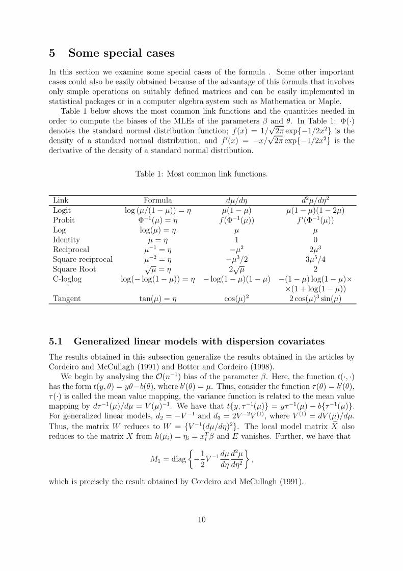
In this section we examine some special cases of the formula . Some other importantcases could also be easily obtained because of the advantage of this formula that involvesonly simple operations on suitably defined matrices and can be easily implemented instatistical packages or in a computer algebra system such as Mathematica or Maple.

Table 1 below shows the most common link functions and the quantities needed inorder to compute the biases of the MLEs of the parameters β and θ. In Table 1: Φ(·)denotes the standard normal distribution function; f(x) = 1/

√2π exp{−1/2x2} is the

density of a standard normal distribution; and f ′(x) = −x/√2π exp{−1/2x2} is the

derivative of the density of a standard normal distribution.

Table 1: Most common link functions.

Link Formula dµ/dη d2µ/dη2

Logit log (µ/(1− µ)) = η µ(1− µ) µ(1− µ)(1− 2µ)Probit Φ−1(µ) = η f(Φ−1(µ)) f ′(Φ−1(µ))Log log(µ) = η µ µIdentity µ = η 1 0Reciprocal µ−1 = η −µ2 2µ3

Square reciprocal µ−2 = η −µ3/2 3µ5/4Square Root

√µ = η 2

õ 2

C-loglog log(− log(1− µ)) = η − log(1− µ)(1− µ) −(1− µ) log(1− µ)××(1 + log(1− µ))

Tangent tan(µ) = η cos(µ)2 2 cos(µ)3 sin(µ)

5.1 Generalized linear models with dispersion covariates

The results obtained in this subsection generalize the results obtained in the articles byCordeiro and McCullagh (1991) and Botter and Cordeiro (1998).

We begin by analysing the O(n−1) bias of the parameter β. Here, the function t(·, ·)has the form t(y, θ) = yθ−b(θ), where b′(θ) = µ. Thus, consider the function τ(θ) = b′(θ),τ(·) is called the mean value mapping, the variance function is related to the mean valuemapping by dτ−1(µ)/dµ = V (µ)−1. We have that t{y, τ−1(µ)} = yτ−1(µ) − b{τ−1(µ)}.For generalized linear models, d2 = −V −1 and d3 = 2V −2V (1), where V (1) = dV (µ)/dµ.

Thus, the matrix W reduces to W = {V −1(dµ/dη)2}. The local model matrix X alsoreduces to the matrix X from h(µi) = ηi = xTi β and E vanishes. Further, we have that

M1 = diag

{−1

2V −1dµ

dη

d2µ

dη2

},

which is precisely the result obtained by Cordeiro and McCullagh (1991).

10

Table 2 shows the distributions in the exponential family, along with the quantitiesneeded to obtain the bias.

We now move to the bias for the dispersion parameter θ. So, let’s consider thetwo-parameter full exponential family distributions with canonical parameters φ and φϑ.Therefore, we have a(φ, y) = φc(y) + a1(φ) + a2(y), where c(·) is a known appropriatefunction. Then it turns out that α2 = a′′1(φ) and α3 = α′

2 = a′′′1 (φ). Then, using (9), wehave that

M2 = diag

{1

2

[a′′′1 (φ)

(dφ

dη2

)3

+ a′′1(φ)dφ

dη2

d2φ

dη22

]},

and

M3 = diag

{−1

2V −1

(dµ

dη1

)2dφ

dη2

}.

The expressions above agrees with the formula presented by Botter and Cordeiro(1998).

Table 3 presents the values of the derivatives of the function a1 for the distributionsin the exponential family. In Table 3, ψ(m)(·), m = 0, 1, . . . , is the polygamma functiondefined by ψ(m)(x) = (dm+1/dxm+1) log Γ(x), x > 0.

5.2 Exponential family nonlinear models with dispersion covari-

ates

This model generalizes the generalized linear model with dispersion covariates. RecentlySimas and Cordeiro (2009) provided ajusted Pearson residuals for exponential familynonlinear models. We only have the O(n−1) bias computed in the literature for the ex-ponential family nonlinear models with constant dispersion parameter (see Paula, 1991).The results for the exponential family nonlinear model with disperion covariates are new.

Table 2: Exponential Family

Distribution V V (1) V (2)

Normal 1 0 0Poisson µ 1 0Binomial µ(1− µ) 1− 2µ −2Gamma µ2 2µ 2Inv. Gauss. µ3 3µ2 6µ

Table 3: Exponential Family

Distribution a1(φ) a′′1(φ) a′′′1 (φ)Normal log

√φ − 1

2φ2

1φ3

Gamma φ log(φ)− log Γφ 1φ+ ψ′(φ) − 1

φ2 + ψ′′(φ)

Inv. Gauss. log√φ − 1

2φ2

1φ3

11

Let us consider the same parameterization from above, i.e., t{y, τ−1(µ)} = yτ−1(µ)−b{τ−1(µ)}, with dτ−1(µ)/dµ = V (µ)−1. Then, the matrices M1,M2 and M3 are the sameas the ones computed in the previous subsection

We now present in Table 4 the results for two distributions that belong to the classof exponential dispersion models introduced by Jørgensen (1987).

Table 4: Exponential dispersion models.

Distribution d2 d′2 d3

GHS 2(µ2+1)2

−8µ(µ2+1)3

− (2µ3+10µ)(µ2+1)3

Neg. Bin. 1µ− 1

1−µ−[

1µ2 − 1

(1−µ)2

]2

(1+µ)2− 2

µ2

Power Var. −µ−p pµ−(p+1) 2pµ−(p+1)

Exp. Var. −e−βµ βe−βµ 2βe−βµ

Among these distributions are the generalized hyperbolic secant and the negativebinomial. Our results can be applied for a very rich class of models discussed in detailin Jørgensen’s (1997b) book. He presented several exponential dispersion models in (1)including the Tweedie class of distributions with power variance function defined bytaking V (µ) = µδ and the cumulant generator function bδ(θ) for δ 6= 1, 2 by

bδ(θ) = (2− δ)−1 {(1− δ)θ}δ−2

δ−1 ,

and b1(θ) = exp(θ) and b2(θ) = − log(−θ). We recognize for δ = 0, 2 and 3, the cumu-lant generator corresponding to the normal, gamma and inverse Gaussian distributions,respectively. There exist continuous exponential dispersion models generated by extremestable distributions with support R and positive stable distributions, respectively, whenδ ≤ 0 and δ ≥ 2 and compound Poisson distributions for 1 < δ < 2. We also would liketo remark that there exists an exponential dispersion model with exponential variancefunction, V (µ) = eµ, for more details see the book of Jorgensen (1997b).

Finally, it is noteworthy that this special case has not been treated in the literatureuntil now.

5.3 Proper dispersion models with dispersion covariates

For proper dispersion models, the formula (7) have no reduction, since the only differenceof a proper dispersion model from a dispersion model is the form of the function a(·, ·)which can be decomposed into a(φ, y) = a1(φ)+a2(y). We will now give the expression forthe matricesM2 andM3. First we note that for this case α2 = a′′1(φ) and α3 = α′

2 = a′′′1 (φ).Then, using (9), we have that

M2 = diag

{1

2

[a′′′1 (φ)

(dφ

dη2

)3

+ a′′1(φ)dφ

dη2

d2φ

dη22

]},

and

M3 = diag

{−1

2V −1

(dµ

dη1

)2dφ

dη2

}.

12

Table 5: Proper Dispersion Models

Distribution d2 d′2 d3Rec. Gamma −µ−2 2µ−3 2µ−3

Log-Gamma −1 0 1Rec. Inv. Gauss. −µ−1 µ−2 0Von-Mises −r(φ) 0 0

Note that even though the form of a(φ, y) for this case is different from the form of a(φ, y)for the two-parameter full exponential family model, the expressions for M2 and M3 areequal.

But to illustrate the idea on a particular example of proper dispersion model, we willconsider the von Mises regression model. Then, we now move to von Mises regressionmodels which are quite useful for modelling circular data; see Fisher (1993) and Mardia(1972). Here,the density is given by

π(y;µ, φ) =1

2πI0(φ)exp{φ cos(y − µ)}, (14)

where, −π < y ≤ π, −π < µ ≤ π, φ > 0, and Iv denotes the modified Bessel function ofthe first kind and order v (see Abramowitz and Stegun, 1970, Eq. 9.6.1). The densityin (14) is symmetric around y = µ which is the mode and the circular mean of thedistribution. φ is a precision parameter in the sense that the larger the value of φ themore concentrated the density around µ gets. It is clear that the density (14) is a properdispersion model, since t(y, µ) = cos(y − µ) and a1(φ) = log{I0(φ)}. We now beginby investigating the skewness for the parameters β. Then, it is possible to show thatE{sin(Y − µ)} = 0 and E[{cos(Y − µ)}2] = 1 − φ−1r(φ), where r(φ) = I1(φ)/I0(φ),these results yield d2 = −r(φ), d3 = 0 and d′2 = 0. Further, we have that the matrixW = diag{(dµ/dη)2r(φ)}.

Note initially that I ′0(φ) = I1(φ) and I′

1(φ) = I0(φ)−I1(φ)/φ (Abramowitz and Stegun,1970; equations 9.6.26 and 9.6.27). Then, a′′1(φ) = r′(φ) and a′′′1 (φ) = r′′(φ), where, asabove, r(φ) = I1(φ)/I0(φ).

We have that

M1 = diag

{−r(φ)

2

dµ

dη1

d2µ

dη21

},

M2 = diag

{r′′(φ)

2

(dφ

dη2

)3

+r′(φ)

2

dφ

dη2

d2φ

dη22

},

and

M3 = diag

{−r(φ)

2

(dµ

dη1

)2dφ

dη2

}.

We provide in Tables 5 the quantities needed for several distributions in the class ofproper dispersion models.

In Table 6 we give the derivatives of the function a1 for several distributions in theclass of proper dispersion models.

13

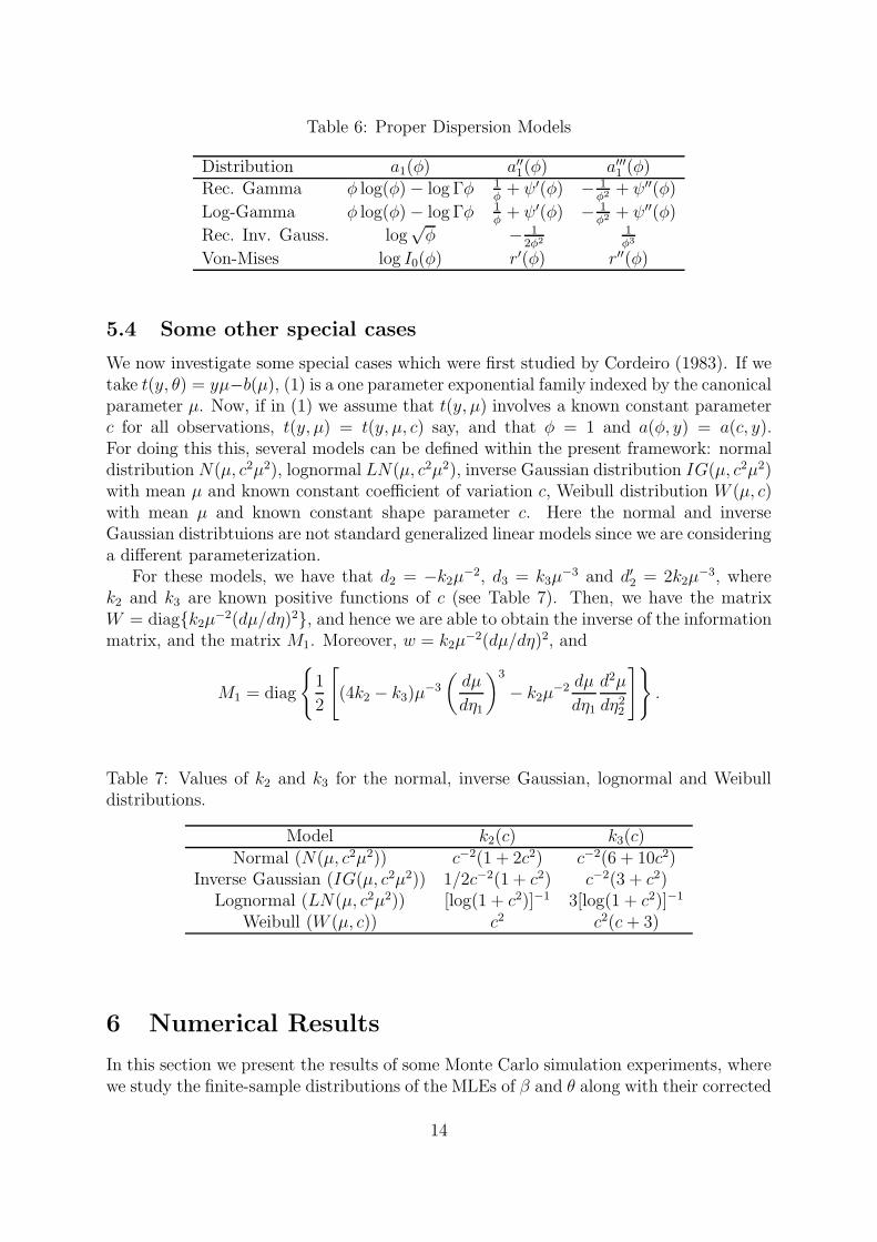
Table 6: Proper Dispersion Models

Distribution a1(φ) a′′1(φ) a′′′1 (φ)Rec. Gamma φ log(φ)− log Γφ 1

φ+ ψ′(φ) − 1

φ2 + ψ′′(φ)

Log-Gamma φ log(φ)− log Γφ 1φ+ ψ′(φ) − 1

φ2 + ψ′′(φ)

Rec. Inv. Gauss. log√φ − 1

2φ2

1φ3

Von-Mises log I0(φ) r′(φ) r′′(φ)

5.4 Some other special cases

We now investigate some special cases which were first studied by Cordeiro (1983). If wetake t(y, θ) = yµ−b(µ), (1) is a one parameter exponential family indexed by the canonicalparameter µ. Now, if in (1) we assume that t(y, µ) involves a known constant parameterc for all observations, t(y, µ) = t(y, µ, c) say, and that φ = 1 and a(φ, y) = a(c, y).For doing this this, several models can be defined within the present framework: normaldistribution N(µ, c2µ2), lognormal LN(µ, c2µ2), inverse Gaussian distribution IG(µ, c2µ2)with mean µ and known constant coefficient of variation c, Weibull distribution W (µ, c)with mean µ and known constant shape parameter c. Here the normal and inverseGaussian distribtuions are not standard generalized linear models since we are consideringa different parameterization.

For these models, we have that d2 = −k2µ−2, d3 = k3µ−3 and d′2 = 2k2µ

−3, wherek2 and k3 are known positive functions of c (see Table 7). Then, we have the matrixW = diag{k2µ−2(dµ/dη)2}, and hence we are able to obtain the inverse of the informationmatrix, and the matrix M1. Moreover, w = k2µ

−2(dµ/dη)2, and

M1 = diag

{1

2

[(4k2 − k3)µ

−3

(dµ

dη1

)3

− k2µ−2 dµ

dη1

d2µ

dη22

]}.

Table 7: Values of k2 and k3 for the normal, inverse Gaussian, lognormal and Weibulldistributions.

Model k2(c) k3(c)Normal (N(µ, c2µ2)) c−2(1 + 2c2) c−2(6 + 10c2)

Inverse Gaussian (IG(µ, c2µ2)) 1/2c−2(1 + c2) c−2(3 + c2)Lognormal (LN(µ, c2µ2)) [log(1 + c2)]−1 3[log(1 + c2)]−1

Weibull (W (µ, c)) c2 c2(c + 3)

6 Numerical Results

In this section we present the results of some Monte Carlo simulation experiments, wherewe study the finite-sample distributions of the MLEs of β and θ along with their corrected

14

versions proposed in this paper. We use a reciprocal gamma model with square root linkand a log link in a nonlinear model for the dispersion parameter

√µi = β0 + β1x1,i + xβ2

2,i,

logφi = θ0 + θ1x1,i + xθ22,i, i = 1, . . . , n,

where the true values of the parameters were taken as β0 = 1/2, β1 = 1, β2 = 2 andθ0 = 1, θ1 = 2 and θ2 = 3. Note also that here the elements of the n × 3 matrix X are:X(β)i,1 = 1; X(β)i,2 = x1,i, and X(β)i,3 = log(x2,i)x

β2

2,i. The explanatory variables x1and x2 were generated from the uniform U(0, 1) distribution for sample size n = 20, andtheir values were held constant throughout the simulations. The number of Monte Carloreplications was set at 5, 000 and all simulations were performed using the statisticalsoftware R.

In each of the 5, 000 replications, we fitted the model and computed the MLEs β,θ, its corrected versions from the corrective method (Cox and Snell, 1968), preventivemethod (Firth, 1993) and the bootstrap method both of its parametric and nonparametricversions (Efron, 1979). The number of bootstrap replications was set to 500 for bothbootstrap methods.

In order to analyze the results we computed, for each sample size and for each estima-tor, the mean of estimates, bias, variance and mean square error (MSE). Table 8 presentsimulation results.

Lastly, in each replication we estimated the confidence interval for each parameter foreach estimator, and verified if the true value of the parameter belonged to this estimatedconfidence interval. After that we obtained the average of the number of confidenceintervals that contained the true parameter. In this way we were able to check if theestimated confidence interval was close to its nominal level of confidence. The confidenceintervals were constructed following the strategies stated at the end of Section 2 and atSection 3.

Table 8 presents simulation results for sample size n = 20 with respect to the pa-rameters β and θ. We begin by looking at the estimated biases, in absolute value, ofthe estimators. Initially, we note that for all parameters the biases of the corrective es-timators were smaller than those of the original MLEs. However, for all parameters thebiases of the preventive estimators were larger than those of the original MLEs. More-over, not only the biases were larger but also the MSEs were larger as well, which showsthat the preventive method does not work well for this model. The same phenomenonoccurred in Ospina et al. (2006), which corroborates the idea that this method has someproblems in beta regression models. We now observe that the MSE of the correctiveestimators were smaller than those of the MLEs for all parameters, showing that thecorrection is effective. Moving to the bootstrap corrected-estimators, we note that theparametric bootstrap had the smallest MSE for all parameters, even though the biaseswere not the smallest. However, the MSEs were very close to the MSE of the correctivemethod, and the computation of the parametric bootstrap biases is computer intensive,whereas the corrective method is not. Lastly, we observe that for all parameters θ theMSE of the nonparametric bootstrap corrected estimators were smaller than those ofthe MLEs. Moreover, for the parameters β, the MSE of the nonparametric bootstrapcorrected estimators were very close to those of the MLEs, showing that this method is

15

satisfactory, and is very easy to implement by practitioners since no parametric assump-tions are made. Therefore, for the small sample size n = 20, we were able to concludethat the corrective method by Cox and Snell (1969) was successfully applied, as well asthe bootstrap corrections.

Table 8: Simulation results.

Parameter MLE Cox-Snell p-boot np-bootβ0 0.6356 0.5552 0.5728 0.6001Bias 0.1356 0.0552 0.0728 0.1001Variance 0.0716 0.0707 0.0683 0.0755MSE 0.0899 0.0737 0.0735 0.0855

β1 0.9383 1.0220 0.9535 1.0519Bias -0.0617 0.0220 -0.0465 0.0519Variance 0.0251 0.0224 0.0203 0.0261MSE 0.0289 0.0228 0.0224 0.0287

β2 1.8853 2.0075 1.9783 1.9099Bias -0.1147 0.0075 -0.0217 -0.0901Variance 0.0348 0.0316 0.0289 0.0331MSE 0.0479 0.0317 0.0293 0.0412

θ0 1.0531 1.0211 1.0248 1.0612Bias 0.0531 0.0211 0.0248 0.0612Variance 0.5805 0.5332 0.4669 0.4841MSE 0.5833 0.5336 0.4675 0.4878

θ1 2.1077 1.9934 1.9872 2.1067Bias 0.1077 -0.0066 -0.0128 0.1067Variance 0.3001 0.2222 0.2345 0.2300MSE 0.3117 0.2222 0.2347 0.2414

θ2 3.0464 3.0077 3.0115 3.0519Bias 0.0464 0.0077 0.0115 0.0519Variance 0.1101 0.0858 0.0686 0.0525MSE 0.1122 0.0858 0.0687 0.0551

Table 9 presents the simulation results for sample size n = 20 with respect to coverageof the interval estimates on different nominal converages 1−α = 90%, 95% and 99%. Allconfidence intervals were defined such that the probability that the true parameter valuebelongs to the interval is 1 − α, the probability that the true parameter value is smallerthan the lower limit of the interval is α/2 and the probability that the value of theparameter is greater than the upper limit of the interval is α/2 for 0 < α < 1/2.

We begin by noting that the confidence intervals induced by the Firth estimates

16

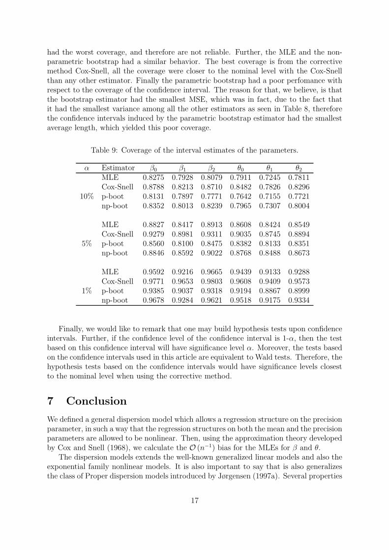
had the worst coverage, and therefore are not reliable. Further, the MLE and the non-parametric bootstrap had a similar behavior. The best coverage is from the correctivemethod Cox-Snell, all the coverage were closer to the nominal level with the Cox-Snellthan any other estimator. Finally the parametric bootstrap had a poor perfomance withrespect to the coverage of the confidence interval. The reason for that, we believe, is thatthe bootstrap estimator had the smallest MSE, which was in fact, due to the fact thatit had the smallest variance among all the other estimators as seen in Table 8, thereforethe confidence intervals induced by the parametric bootstrap estimator had the smallestaverage length, which yielded this poor coverage.

Table 9: Coverage of the interval estimates of the parameters.

α Estimator β0 β1 β2 θ0 θ1 θ2MLE 0.8275 0.7928 0.8079 0.7911 0.7245 0.7811Cox-Snell 0.8788 0.8213 0.8710 0.8482 0.7826 0.8296

10% p-boot 0.8131 0.7897 0.7771 0.7642 0.7155 0.7721np-boot 0.8352 0.8013 0.8239 0.7965 0.7307 0.8004

MLE 0.8827 0.8417 0.8913 0.8608 0.8424 0.8549Cox-Snell 0.9279 0.8981 0.9311 0.9035 0.8745 0.8894

5% p-boot 0.8560 0.8100 0.8475 0.8382 0.8133 0.8351np-boot 0.8846 0.8592 0.9022 0.8768 0.8488 0.8673

MLE 0.9592 0.9216 0.9665 0.9439 0.9133 0.9288Cox-Snell 0.9771 0.9653 0.9803 0.9608 0.9409 0.9573

1% p-boot 0.9385 0.9037 0.9318 0.9194 0.8867 0.8999np-boot 0.9678 0.9284 0.9621 0.9518 0.9175 0.9334

Finally, we would like to remark that one may build hypothesis tests upon confidenceintervals. Further, if the confidence level of the confidence interval is 1-α, then the testbased on this confidence interval will have significance level α. Moreover, the tests basedon the confidence intervals used in this article are equivalent to Wald tests. Therefore, thehypothesis tests based on the confidence intervals would have significance levels closestto the nominal level when using the corrective method.

7 Conclusion

We defined a general dispersion model which allows a regression structure on the precisionparameter, in such a way that the regression structures on both the mean and the precisionparameters are allowed to be nonlinear. Then, using the approximation theory developedby Cox and Snell (1968), we calculate the O (n−1) bias for the MLEs for β and θ.

The dispersion models extends the well-known generalized linear models and also theexponential family nonlinear models. It is also important to say that is also generalizesthe class of Proper dispersion models introduced by Jørgensen (1997a). Several properties

17

and applications of dispersion models can be found on the excellent book of Jørgensen(1997b).

Our results, thus, generalize, for instance, the formulae obtained by Cordeiro and Mc-Cullagh (1991), Paula (1992), Cordeiro and Vasconcellos (1999) and Botter and Cordeiro(1998). We then defined bias-free estimators to order O (n−1), by using the expressionsobtained through Cox and Snell’s (1968) formulae. We also considered two schemes ofbias correction based on bootstrap.

Finally, we considered a simulation study in a nonlinear reciprocal gamma model withnonlinear dispersion covariates. The simulation suggested, among other things, that bias-corrected up to the second-order estimators should be used instead of the usual MLEs.Furthermore, we were able to notice that the analytical bias-corrected estimators had thesmallest biases, whereas the bias-corrected estimators using parmetric bootstrap schemehad the smallest mean square error. Note that, even though the parametric bootstraphad the least mean square error, this fact yielded that the confidence intervals inducedby the bootstrap estimator had the poorest coverage, mainly because its small varianceproduced confidence intervals with small length. Nevertheless, the confidence intervalsobtained by the corrective method were the best in terms of coverage closer to the nominallevel.

Appendix

We give explicit expressions for the cumulants and their derivatives, both defined inSection 3. Further, we give the expressions for each quantity contained in equations (5)and (6), some of them are also deduced to help the reader who might be interested inchecking the results.

Consider initially the following notation for the derivatives, and product of the deriva-tives, of the predictor with respect to the regression parameters:

(rs)i =∂2η1i∂βr∂βs

, (RS)i =∂2η2i∂θR∂θS

, (rs, T )i =∂2η1i∂βr∂βs

∂η2i∂θT

,

and so on. Recall that

dri = E

[∂r

∂µri

t(Yi, µi)

], and αri = E

[∂r

∂φri

a(φi, Yi)

].

By using these quantities, the cumulants can be written as

κrs =

n∑

i=1

φid2i

(dµi

dη1i

)2

(r, s)i,

κrS = 0,

κRS =n∑

i=1

α2i

(dφi

dη2i

)2

(R, S)i,

18

κrsu =n∑

i=1

φi

{d3i

(dµi

dη1i

)3

+ 3d2idµi

dη1i

d2µi

dη21i

}(r, s, u)i

+

n∑

i=1

φid2i

(dµi

dη1i

)2

{(rs, u)i + (ru, s)i + (su, r)i},

κrsU =n∑

i=1

d2i

(dµi

dη1i

)2dφi

dη2i(r, s, U)i,

κrSU = 0,

κRSU =

n∑

i=1

{α3i

(dφi

dη2i

)3

+ 3α2id2φi

dη22i

dφi

dη2i

}(R, S, U)i

+n∑

i=1

α2i

(dφi

dη2i

)2

{(RS, U)i + (RU, S)i + (SU,R)i}.

Differentiating the second order cumulants with respect to the parameters, we have

κ(u)rs =n∑

i=1

φi

{d′2i

(dµi

dη1i

)3

+ 2d2idµi

dη1i

d2µi

dη21i

}(r, s, u)i

+

n∑

i=1

φid2i

(dµi

dη1i

)2

{(ru, s)i + (su, r)i},

κ(U)rs =

n∑

i=1

d2i

(dµi

dη1i

)2dφi

dη2i(r, s, U)i,

κ(u)RS = 0,

κ(U)RS =

n∑

i=1

{α′

2i

(dφi

dη2i

)3

+ 2α2idφi

dη2i

d2φi

dη22i

}(R, S, U)i

+

n∑

i=1

α2i

(dφi

η2i

)2

{(RU, S)i + (SU,R)i},

κ(u)rS = 0,

κ(U)rS = 0.

We now recall let M1, M2 and M3 be the diagonal matrices given in equations(7) and (9). Let mji be the ith diagonal element of the matrix Mj . Also, letWβ = diag (−d2i(dµi/dη1i)

2) and Wθ = diag (−α2i(dφi/dη2i)2), and wbi, and wti be the

diagonal elements of Wβ and Wθ, respectively. We then, have that the O(n−1) bias of β,

19

B(β) is

B(βa) =∑

r,s,u

κarκsu{κ(u)rs − 1

2κrsu

}=

n∑

i=1

φim1i

∑

r

κar(r)i∑

s,u

κsu(s, u)i

−n∑

i=1

1

2φiwbi

∑

r,s,u

κarκsu{(rs, u)i − (ru, s)i − (su, r)i}

=

n∑

i=1

φim1i

∑

r

κar(r)iδTi (XK

βXT )δi

−n∑

i=1

1

2φiwbi

∑

r

κar(r)i∑

s,u

κsu(su)i

= δTa∑

i=1

KβXT δiφim1iδTi (XK

βXT )δi

−δTan∑

i=1

1

2φiwbiK

βXiδiEi

= δTaKβXTΦM1Zβ −

1

2δTaK

βXTΦWβE1,

where δa is a p × 1 vector with a one in the ath position and zeros elsewhere, and thematrices E, Zβ, and K

β were defined in Section 3.Analogously, one uses the expression

B(θa) =∑

R,s,u

κaRκsu{κ(u)Rs −

1

2κRsu

}+∑

R,S,U

κaRκSU{κ(U)RS − 1

2κRSU

},

to obtain that

B(θa) = δTaKθZT{M2Zθ −M3Zβ} −

1

2δTaK

θZTWθF1,

where, in this case, a = 1, . . . , q, and the matrices Zβ, Kθ, and F were also defined in

Section 3.

References

[1] Abramowitz, W. and Stegun, I. A. (1970). Handbook of mathematical functions with

formulas, graphs and mathematical tables. Washington, National Bureau of Stan-dards. (National Bureau of Standards. Applied Mathematics Series, 55).

[2] Atkinson, A.C., (1985) . Plots, transformation and regression. Clarendon Press, Ox-ford.

[3] Botter, D. A. and Cordeiro, G. M. (1998) . Improved estimators for generalized linearmodels with dispersion covariates. J. Stat. Comp. and Simul., 62, 91-104.

[4] Cordeiro, G. M. (1985). The null expected deviance for an extended class of gener-alized linear models. Lecture Notes in Statistics, 32, 27-34.

20

[5] Cordeiro, G.M., McCullagh, P. (1991) . Bias correction in generalized linear models.J. Roy. Statist. Soc. B 53, 629-643.

[6] Cordeiro, G. M. and Vasconcellos, K. L. P. (1999) . Second-order biases of the max-imum likelihood estimates in von Mises regression models. Aust. and New Zealand

J. Stat., 41, 189-198.

[7] Cordeiro, G. M. and Paula, G. A. (1989). Improved likelihood ratio statistic forexponential family nonlinear models. Biometrika, 76, 93-100.

[8] Cox, D. R. and Hinkley, D. V. (1974) . Theoretical Statistics. Chapman & Hall,London.

[9] Cox, D. R. and N. Reid (1987). Parameter Orthogonality and Approximate Condi-tional Inference (with discussion), J. R. Stat. Soc. B, 49, 1-39.

[10] Cox, D. R. and Snell, E. (1968) . A general definition of residuals. J. Roy. Statist.Soc. B 30, 248-275.

[11] Efron, B., 1979. Bootstrap methods: another look at the jackknife. Ann. Statist. 7,1-26.

[12] Fisher, N. I. (1993). Statistical analysis of circular data. Cambridge University Press,New York.

[13] Harvey, A. C. (1976) . Estimating regression models with multiplicative heteroscedas-ticity. Econometrika, 41, 461-465.

[14] Jørgensen, B. (1987). Exponential dispersion models (with Discussion). J. Roy.

Statist. Soc., Ser. B, 49, 127-162.

[15] Jørgensen, B. (1997a). Proper dispersion models (with Discussion). Brazilian J.

Probab. Statist. 11, 89-140.

[16] Jørgensen, B. (1997b). The theory of dispersion models. Chapman & Hall.

[17] MacKinnon, J.G., Smith Jr., A.A., 1998. Approximate bias correction in economet-rics. J. Econometrics 85, 205-230.

[18] Mardia, K. V. (1972). Statistics of directional data. Academic Press, New York.

[19] McCullagh, P., Nelder, J. (1989) . Generalized linear models. second ed. Chapman& Hall, London.

[20] Paula, G. A. (1992). Bias correction for exponential family nonlinear models. J.Statist. Comput. Simul. 40, 43-54.

[21] Pike, M.C., Hill, A.P., Smith, P.G., 1980. Bias and efficiency in logistic analyses ofstratified case-controle studies. Int. J. Epidemiol. 9, 89-95.

21

[22] Press, W.H., Teukolsky, S.A., Vetterling, W.T., Flannery, B.P., 1992. Numerical

recipes in C: The art of scientific computing. second ed. Cambridge University Press,New York.

[23] Rocha, A. V., Simas, A. B. and Cordeiro, G. M. (2009). Second-order asymptoticexpressions for the covariance matrix of maximum likelihood estimators in dispersionmodels. Stat. Prob. Let. To appear.

[24] Smyth, G. K., (1989) . Generalized linear models with varying dispersion. J. Roy.Statist. Soc. B 51, 47-60.

[25] Simas, A. B., Barreto-Souza, W. and Rocha, A. V. (2009a). Improved estimators fora general class of beta regression models. Comp. Stat. Data Anal. 53, 3397-3411.

[26] Simas, A. B. and Cordeiro, G. M. (2009). Adjusted Pearson residuals in exponentialfamily nonlinear models. J. Statist. Comput. Simul. 79, 411-425.

[27] Simas, A. B., Cordeiro, G. M. and Nadarajah, S. (2009b). Asymptotic tail propertiesof the distributions in the class of dispersion models. Preprint: arXiv:0809.1840

[28] Simas, A. B., Cordeiro, G. M. and Rocha, A. V. (2009c). Skewness for Parametersin the Class of Dispersion Models. Submitted.

22