Minimum β-Divergence Estimators of Multivariate Location ...
18
International Journal of Statistical Sciences ISSN 1683-5603 Vol. 16, 2018, pp 69-86 © 2018 Dept. of Statistics, Univ. of Rajshahi, Bangladesh Minimum β-Divergence Estimators of Multivariate Location and Scatter Parameters: Some Properties and Applications Md. Nurul Haque Mollah and S. K. Bhattacharjee Department of Statistics University of Rajshahi, Rajshahi, Bangladesh Abstract The minimum β-divergence estimators of multivariate Gaussian location and scatter parameters are highly robust against outliers. Since estimating the location and scatter parameters are the cornerstone of many multivariate statistical methods, the minimum β- divergence estimators of those parameters are the important building block when developing robust multivariate techniques including robust principal component analysis, factor analysis, canonical correlation analysis, independent component analysis, multiple regression analysis, cluster analysis and discriminant analysis. It also serves as a convenient tool for detection of multivariate outliers. The minimum β-divergence estimators of multivariate Gaussian location and scatter parameters are reviewed, along with its main properties such as affine equivariance, breakdown value, and influence function. We discuss its computation and some applications in applied and methodological multivariate statistics. Keywords: Multivariate Analysis, Multivariate Normal Distribution, Minimum β- Divergence Estimators, Orthogonal Affine Equivariance and Robustness. 1. Introduction The parameter estimation of location vector and scatter matrix is the cornerstone of multivariate data analysis, as it provides necessary inputs in the subsequent inferential statistical methods [Anderson, 2003; Johnson and Wichern, 2007)]. The sample mean and the sample covariance matrix are the most common estimators of multivariate location vector and scatter matrix, respectively. In the multivariate location and scatter setting, the data are stored in an n×p data matrix X n = (x 1 , …, x n ) T with x i = (x i1 ,…, x ip ) T the i-th vector observation. Here n stands for the number of objects and p for the number of variables and the superscript T for the transpose. Then the estimators of location vector μ and the scatter matrix V are as follows
-
Upload
khangminh22 -
Category
Documents
-
view
1 -
download
0
Transcript of Minimum β-Divergence Estimators of Multivariate Location ...

International Journal of Statistical Sciences ISSN 1683-5603
Vol. 16, 2018, pp 69-86
© 2018 Dept. of Statistics, Univ. of Rajshahi, Bangladesh
Minimum β-Divergence Estimators of Multivariate
Location and Scatter Parameters: Some Properties and
Applications
Md. Nurul Haque Mollah and S. K. Bhattacharjee
Department of Statistics
University of Rajshahi, Rajshahi, Bangladesh
Abstract
The minimum β-divergence estimators of multivariate Gaussian location and scatter
parameters are highly robust against outliers. Since estimating the location and scatter
parameters are the cornerstone of many multivariate statistical methods, the minimum β-
divergence estimators of those parameters are the important building block when
developing robust multivariate techniques including robust principal component analysis,
factor analysis, canonical correlation analysis, independent component analysis, multiple
regression analysis, cluster analysis and discriminant analysis. It also serves as a
convenient tool for detection of multivariate outliers. The minimum β-divergence
estimators of multivariate Gaussian location and scatter parameters are reviewed, along
with its main properties such as affine equivariance, breakdown value, and influence
function. We discuss its computation and some applications in applied and
methodological multivariate statistics.
Keywords: Multivariate Analysis, Multivariate Normal Distribution, Minimum β-
Divergence Estimators, Orthogonal Affine Equivariance and Robustness.
1. Introduction
The parameter estimation of location vector and scatter matrix is the cornerstone
of multivariate data analysis, as it provides necessary inputs in the subsequent
inferential statistical methods [Anderson, 2003; Johnson and Wichern, 2007)].
The sample mean and the sample covariance matrix are the most common
estimators of multivariate location vector and scatter matrix, respectively. In the
multivariate location and scatter setting, the data are stored in an n×p data matrix
Xn = (x1, …, xn)T with xi = (xi1,…, xip)
T the i-th vector observation. Here n stands
for the number of objects and p for the number of variables and the superscript T
for the transpose. Then the estimators of location vector µ and the scatter matrix
V are as follows
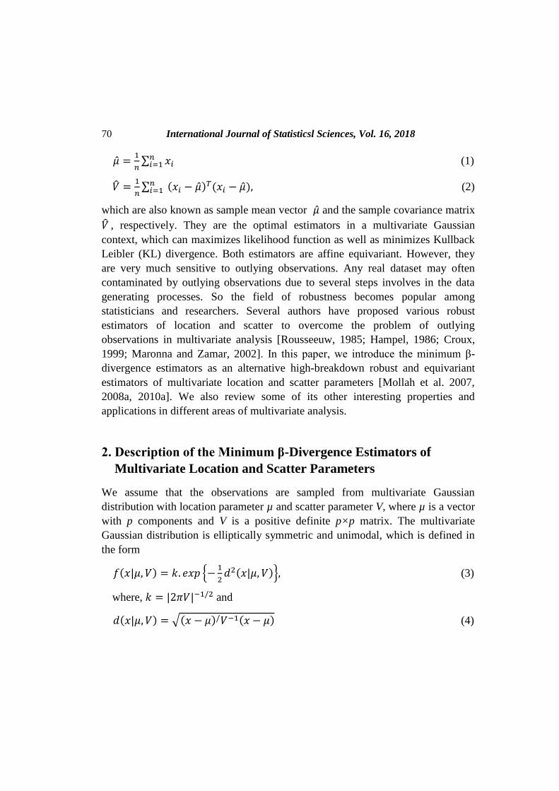
70 International Journal of Statisticsl Sciences, Vol. 16, 2018
�̂� =1
𝑛∑ 𝑥𝑖
𝑛𝑖=1 (1)
�̂� =1
𝑛∑ (𝑥𝑖 − �̂�)𝑇(𝑥𝑖 − �̂�)𝑛
𝑖=1 , (2)
which are also known as sample mean vector �̂� and the sample covariance matrix
�̂� , respectively. They are the optimal estimators in a multivariate Gaussian
context, which can maximizes likelihood function as well as minimizes Kullback
Leibler (KL) divergence. Both estimators are affine equivariant. However, they
are very much sensitive to outlying observations. Any real dataset may often
contaminated by outlying observations due to several steps involves in the data
generating processes. So the field of robustness becomes popular among
statisticians and researchers. Several authors have proposed various robust
estimators of location and scatter to overcome the problem of outlying
observations in multivariate analysis [Rousseeuw, 1985; Hampel, 1986; Croux,
1999; Maronna and Zamar, 2002]. In this paper, we introduce the minimum β-
divergence estimators as an alternative high-breakdown robust and equivariant
estimators of multivariate location and scatter parameters [Mollah et al. 2007,
2008a, 2010a]. We also review some of its other interesting properties and
applications in different areas of multivariate analysis.
2. Description of the Minimum β-Divergence Estimators of
Multivariate Location and Scatter Parameters
We assume that the observations are sampled from multivariate Gaussian
distribution with location parameter µ and scatter parameter V, where µ is a vector
with p components and V is a positive definite p×p matrix. The multivariate
Gaussian distribution is elliptically symmetric and unimodal, which is defined in
the form
𝑓(𝑥|𝜇, 𝑉) = 𝑘. 𝑒𝑥𝑝 {−1
2𝑑2(𝑥|𝜇, 𝑉)}, (3)
where, 𝑘 = |2𝜋𝑉|−1/2 and
𝑑(𝑥|𝜇, 𝑉) = √(𝑥 − 𝜇)/𝑉−1(𝑥 − 𝜇) (4)
Mollah and Bhattacharjee: Minimum β-Divergence Estimators … 71
which is known as the Mahalanobis distance between a data vector
𝑥 and its mean vector µ.
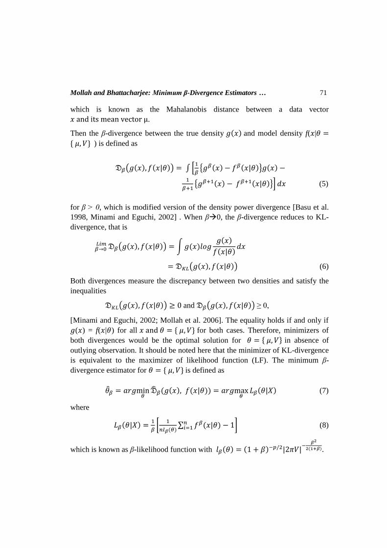
Then the β-divergence between the true density 𝑔(𝑥) and model density f(𝑥|𝜃 =
{ 𝜇, 𝑉} ) is defined as
𝔇𝛽(𝑔(𝑥), 𝑓(𝑥|𝜃)) = ∫ [1
𝛽{𝑔𝛽(𝑥) − 𝑓𝛽(𝑥|𝜃)}𝑔(𝑥) −
1
𝛽+1{𝑔𝛽+1(𝑥) − 𝑓𝛽+1(𝑥|𝜃)}] 𝑑𝑥 (5)
for β > 0, which is modified version of the density power divergence [Basu et al.
1998, Minami and Eguchi, 2002] . When β0, the β-divergence reduces to KL-
divergence, that is
𝔇𝛽(𝑔(𝑥), 𝑓(𝑥|𝜃))𝛽→0𝐿𝑖𝑚 = ∫ 𝑔(𝑥)𝑙𝑜𝑔
𝑔(𝑥)
𝑓(𝑥|𝜃)𝑑𝑥
= 𝔇𝐾𝐿(𝑔(𝑥), 𝑓(𝑥|𝜃)) (6)
Both divergences measure the discrepancy between two densities and satisfy the
inequalities
𝔇𝐾𝐿(𝑔(𝑥), 𝑓(𝑥|𝜃)) ≥ 0 and 𝔇𝛽(𝑔(𝑥), 𝑓(𝑥|𝜃)) ≥ 0,
[Minami and Eguchi, 2002; Mollah et al. 2006]. The equality holds if and only if
𝑔(𝑥) = f(𝑥|𝜃) for all 𝑥 and 𝜃 = { 𝜇, 𝑉} for both cases. Therefore, minimizers of
both divergences would be the optimal solution for 𝜃 = { 𝜇, 𝑉} in absence of
outlying observation. It should be noted here that the minimizer of KL-divergence
is equivalent to the maximizer of likelihood function (LF). The minimum β-
divergence estimator for 𝜃 = { 𝜇, 𝑉} is defined as
𝜃𝛽 = 𝑎𝑟𝑔min𝜃
�̂�𝛽(𝑔(𝑥), 𝑓(𝑥|𝜃)) = 𝑎𝑟𝑔max𝜃
𝐿𝛽(𝜃|𝑋) (7)
where
𝐿𝛽(𝜃|𝑋) =1
𝛽[
1
𝑛𝑙𝛽(𝜃)∑ 𝑓𝛽(𝑥|𝜃) − 1𝑛
𝑖=1 ] (8)
which is known as β-likelihood function with 𝑙𝛽(𝜃) = (1 + 𝛽)−𝑝/2|2𝜋𝑉|−
𝛽2
2(1+𝛽).
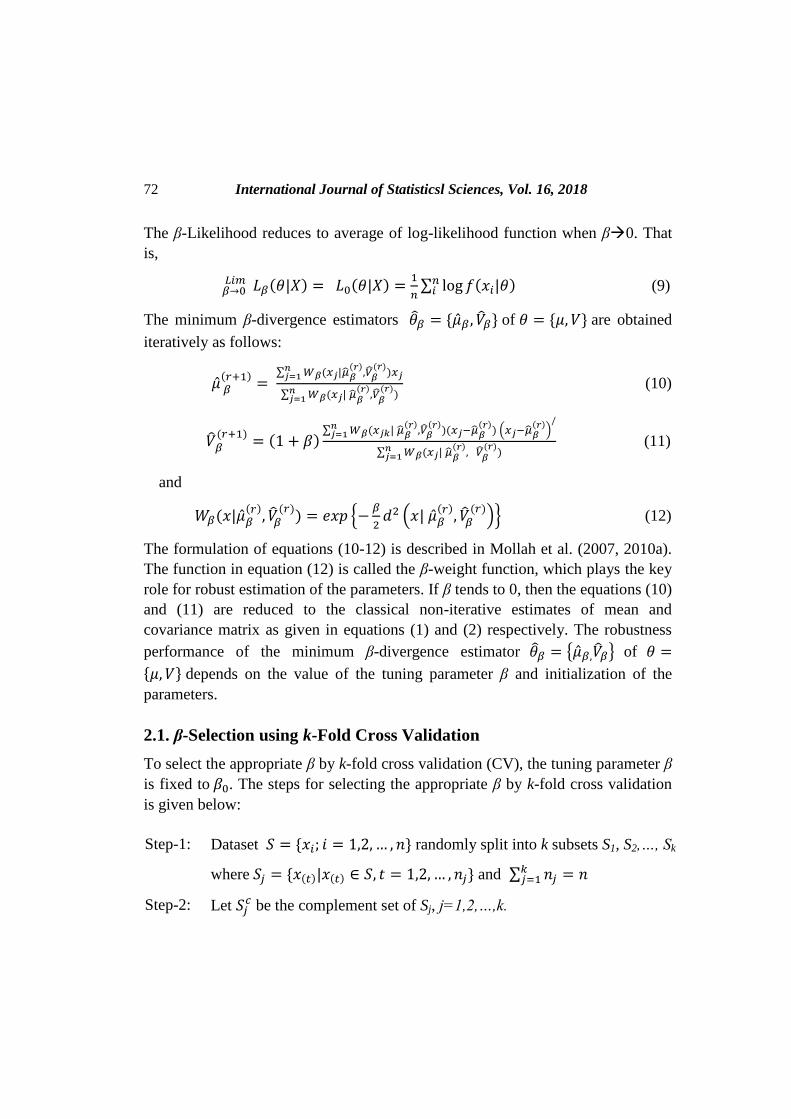
72 International Journal of Statisticsl Sciences, Vol. 16, 2018
The β-Likelihood reduces to average of log-likelihood function when β0. That
is,
𝐿𝛽(𝜃|𝑋) 𝛽→0𝐿𝑖𝑚 = 𝐿0(𝜃|𝑋) =
1
𝑛∑ log 𝑓(𝑥𝑖|𝜃)𝑛
𝑖 (9)
The minimum β-divergence estimators 𝜃𝛽 = {�̂�𝛽 , �̂�𝛽} of 𝜃 = {𝜇, 𝑉} are obtained
iteratively as follows:
�̂� 𝛽(𝑟+1)
= ∑ 𝑊𝛽(𝑥𝑗|�̂�𝛽
(𝑟),𝑉𝛽
(𝑟))𝑥𝑗
𝑛𝑗=1
∑ 𝑊𝛽(𝑥𝑗| �̂�𝛽(𝑟)
,�̂�𝛽(𝑟)
)𝑛𝑗=1
(10)
�̂� 𝛽(𝑟+1)
= (1 + 𝛽)∑ 𝑊𝛽(𝑥𝑗𝑘| �̂�𝛽
(𝑟),�̂�𝛽
(𝑟))(𝑥𝑗−�̂�𝛽
(𝑟)) (𝑥𝑗−�̂�𝛽
(𝑟))
/𝑛𝑗=1
∑ 𝑊𝛽(𝑥𝑗| �̂�𝛽(𝑟)
, �̂�𝛽(𝑟)
)𝑛𝑗=1
(11)
and
𝑊𝛽(𝑥|�̂�𝛽(𝑟)
, �̂�𝛽(𝑟)
) = 𝑒𝑥𝑝 {−𝛽
2𝑑2 (𝑥| �̂�𝛽
(𝑟), �̂�𝛽
(𝑟))} (12)
The formulation of equations (10-12) is described in Mollah et al. (2007, 2010a).
The function in equation (12) is called the β-weight function, which plays the key
role for robust estimation of the parameters. If β tends to 0, then the equations (10)
and (11) are reduced to the classical non-iterative estimates of mean and
covariance matrix as given in equations (1) and (2) respectively. The robustness
performance of the minimum β-divergence estimator 𝜃𝛽 = {�̂�𝛽,�̂�𝛽} of 𝜃 =
{𝜇, 𝑉} depends on the value of the tuning parameter β and initialization of the
parameters.
2.1. β-Selection using k-Fold Cross Validation
To select the appropriate β by k-fold cross validation (CV), the tuning parameter β
is fixed to 𝛽0. The steps for selecting the appropriate β by k-fold cross validation
is given below:
Step-1: Dataset 𝑆 = {𝑥𝑖; 𝑖 = 1,2, … , 𝑛} randomly split into k subsets S1, S2,…, Sk
where 𝑆𝑗 = {𝑥(𝑡)|𝑥(𝑡) ∈ 𝑆, 𝑡 = 1,2, … , 𝑛𝑗} and ∑ 𝑛𝑗 = 𝑛𝑘𝑗=1
Step-2: Let 𝑆𝑗𝑐 be the complement set of Sj, j=1,2,…,k.

Mollah and Bhattacharjee: Minimum β-Divergence Estimators … 73
Step-3: Estimate �̂�𝛽 and �̂�𝛽 iteratively by equations (7-8) based on dataset 𝑆𝑗𝑐
Step-4: Compute CVj(β) using the dataset 𝑆𝑗, for j=1, 2,.., k
CVj(β) =𝐿𝛽0(�̂�𝛽,�̂�𝛽| 𝑆𝑗), where
𝐿𝛽0(�̂�𝛽,�̂�𝛽| 𝑆𝑗) =
1
𝛽0[1 −
1
𝑛𝑗|�̂�𝛽|
−𝛽0
2(1+𝛽0) ∑ 𝑊𝛽0(𝑥𝑗|𝑥𝑗∈ 𝑆𝑗
�̂�𝛽,�̂�𝛽]
Step-5: Compute �̂� =
𝑎𝑟𝑔𝑚𝑖𝑛𝛽
CV(𝛽)
where CV(𝛽) = 1
𝑛∑ 𝐶𝑉𝑗(𝛽) 𝑘
𝑗=1
More discussion about 𝛽 selection also can be found in Mollah et al. (2007,
2010a).
2.2. Influence Function
The influence function for the estimator T at x under the distribution F is defined
as
𝐼𝐹(𝑥; 𝑇, 𝐹) = lim𝑡→0
𝑇[(1 − 𝑡)𝐹 + 𝑡∆𝑥] − 𝑇(𝐹)
𝑡
where ∆𝑥 is the probability measure that puts mass 1 at the point x. If the gross
error sensitivity (GES), that is, lim𝑥 |𝐼𝐹(𝑥; 𝑇, 𝐹) | is finite, then the estimator T is
said to be B-robust under the distribution F (c.f. chapter 5 of Hampel et al.
(1986)).
The robustness of the minimum β-divergence estimators were investigated by the
influence function (Mollah et el. 2007). The influence function for the location
estimator �̂�𝛽 = 𝜇𝛽(𝑋) at x under the distribution F is given by
𝐼𝐹(𝑥; 𝜇𝛽(𝑋), 𝐹) = −𝜇 +𝑊𝛽(𝑥|𝜇,𝑉)𝑥
𝐸𝑋{𝑊𝛽(𝑋|𝜇,𝑉)} (13)
The influence function for the scatter estimator �̂�𝛽 = 𝑉𝛽(𝑋) at x under the
distribution F is given by
𝐼𝐹(𝑥; 𝑉𝛽(𝑋), 𝐹) = −𝑉 +𝑊𝛽(𝑥|𝜇,𝑉)(𝑥−𝜇)(𝑥−𝜇)/
𝐸𝑋{𝑊𝛽(𝑋|𝜇,𝑉)} (14)
74 International Journal of Statisticsl Sciences, Vol. 16, 2018
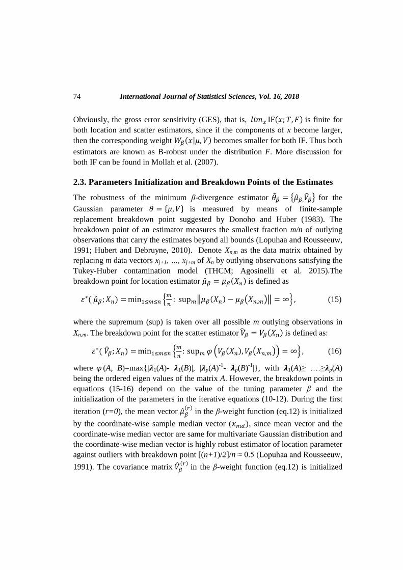
Obviously, the gross error sensitivity (GES), that is, 𝑙𝑖𝑚𝑥 IF(𝑥; 𝑇, 𝐹) is finite for
both location and scatter estimators, since if the components of x become larger,
then the corresponding weight 𝑊𝛽(𝑥|𝜇, 𝑉) becomes smaller for both IF. Thus both
estimators are known as B-robust under the distribution F. More discussion for
both IF can be found in Mollah et al. (2007).
2.3. Parameters Initialization and Breakdown Points of the Estimates
The robustness of the minimum β-divergence estimator 𝜃𝛽 = {�̂�𝛽,�̂�𝛽} for the
Gaussian parameter 𝜃 = {𝜇, 𝑉} is measured by means of finite-sample
replacement breakdown point suggested by Donoho and Huber (1983). The
breakdown point of an estimator measures the smallest fraction m/n of outlying
observations that carry the estimates beyond all bounds (Lopuhaa and Rousseeuw,
1991; Hubert and Debruyne, 2010). Denote Xn,m as the data matrix obtained by
replacing m data vectors xj+1, …, xj+m of Xn by outlying observations satisfying the
Tukey-Huber contamination model (THCM; Agosinelli et al. 2015).The
breakdown point for location estimator �̂�𝛽 = 𝜇𝛽(𝑋𝑛) is defined as
𝜀∗( �̂�𝛽; 𝑋𝑛) = min1≤𝑚≤𝑛 {𝑚
𝑛: sup𝑚‖𝜇𝛽(𝑋𝑛) − 𝜇𝛽(𝑋𝑛,𝑚)‖ = ∞} , (15)
where the supremum (sup) is taken over all possible m outlying observations in
Xn,m. The breakdown point for the scatter estimator �̂�𝛽 = 𝑉𝛽(𝑋𝑛) is defined as:
𝜀∗( �̂�𝛽; 𝑋𝑛) = min1≤𝑚≤𝑛 {𝑚
𝑛: sup𝑚 𝜑 (𝑉𝛽(𝑋𝑛), 𝑉𝛽(𝑋𝑛,𝑚)) = ∞} , (16)
where 𝜑 (A, B)=max{|𝝀1(A)- 𝝀1(B)|, |𝝀p(A)-1
- 𝝀p(B)-1
|}, with 𝝀1(A)≥ ….≥𝝀p(A)
being the ordered eigen values of the matrix A. However, the breakdown points in
equations (15-16) depend on the value of the tuning parameter β and the
initialization of the parameters in the iterative equations (10-12). During the first
iteration (r=0), the mean vector �̂�𝛽(𝑟)
in the β-weight function (eq.12) is initialized
by the coordinate-wise sample median vector (𝑥𝑚𝑑), since mean vector and the
coordinate-wise median vector are same for multivariate Gaussian distribution and
the coordinate-wise median vector is highly robust estimator of location parameter
against outliers with breakdown point [(n+1)/2]/n ≈ 0.5 (Lopuhaa and Rousseeuw,
1991). The covariance matrix �̂�𝛽(𝑟)
in the β-weight function (eq.12) is initialized
Mollah and Bhattacharjee: Minimum β-Divergence Estimators … 75
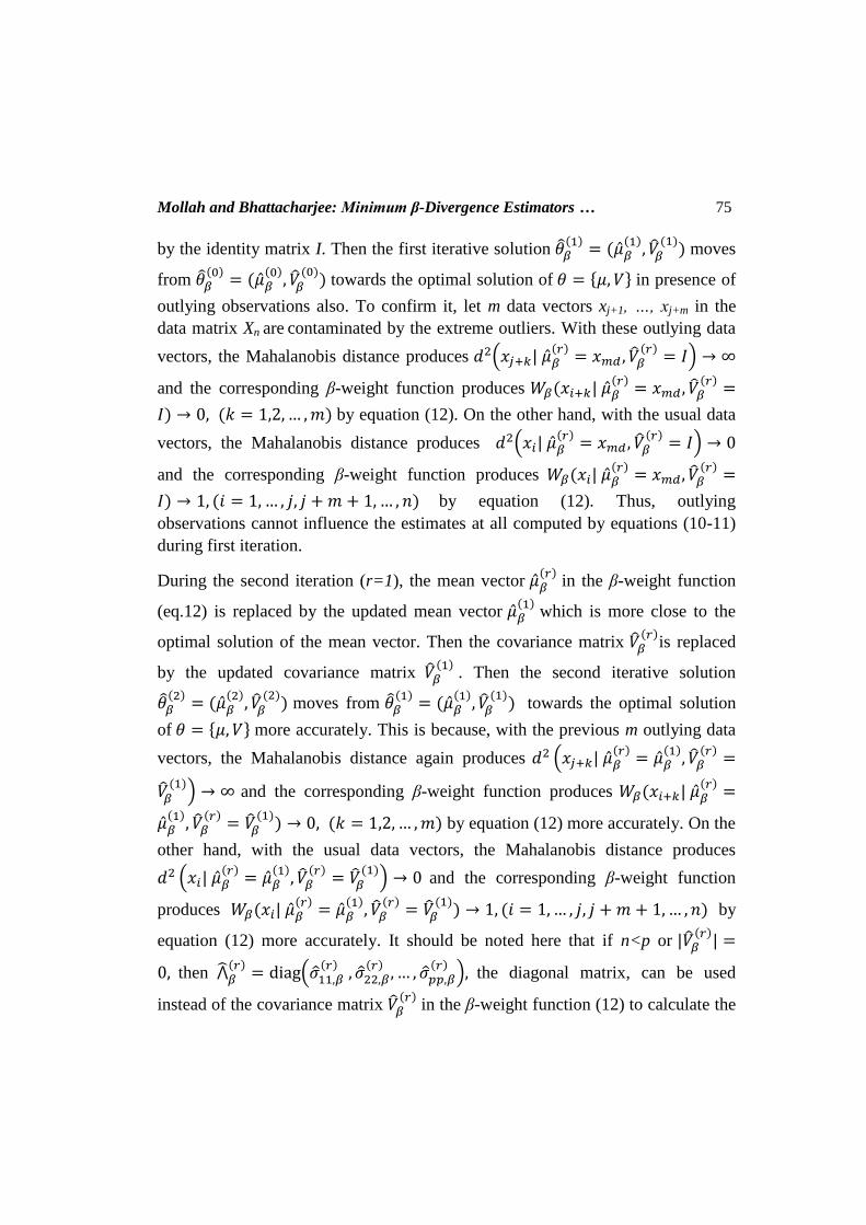
by the identity matrix I. Then the first iterative solution 𝜃𝛽(1)
= (�̂�𝛽(1)
, �̂�𝛽(1)
) moves
from 𝜃𝛽(0)
= (�̂�𝛽(0)
, �̂�𝛽(0)
) towards the optimal solution of 𝜃 = {𝜇, 𝑉} in presence of
outlying observations also. To confirm it, let m data vectors xj+1, …, xj+m in the
data matrix Xn are contaminated by the extreme outliers. With these outlying data
vectors, the Mahalanobis distance produces 𝑑2(𝑥𝑗+𝑘| �̂�𝛽(𝑟)
= 𝑥𝑚𝑑 , �̂�𝛽(𝑟)
= 𝐼) → ∞
and the corresponding β-weight function produces 𝑊𝛽(𝑥𝑖+𝑘| �̂�𝛽(𝑟)
= 𝑥𝑚𝑑 , �̂�𝛽(𝑟)
=
𝐼) → 0, (𝑘 = 1,2, … , 𝑚) by equation (12). On the other hand, with the usual data
vectors, the Mahalanobis distance produces 𝑑2(𝑥𝑖| �̂�𝛽(𝑟)
= 𝑥𝑚𝑑 , �̂�𝛽(𝑟)
= 𝐼) → 0
and the corresponding β-weight function produces 𝑊𝛽(𝑥𝑖| �̂�𝛽(𝑟)
= 𝑥𝑚𝑑 , �̂�𝛽(𝑟)
=
𝐼) → 1, (𝑖 = 1, … , 𝑗, 𝑗 + 𝑚 + 1, … , 𝑛) by equation (12). Thus, outlying
observations cannot influence the estimates at all computed by equations (10-11)
during first iteration.
During the second iteration (r=1), the mean vector �̂�𝛽(𝑟)
in the β-weight function
(eq.12) is replaced by the updated mean vector �̂�𝛽(1)
which is more close to the
optimal solution of the mean vector. Then the covariance matrix �̂�𝛽(𝑟)
is replaced
by the updated covariance matrix �̂�𝛽(1)
. Then the second iterative solution
𝜃𝛽(2)
= (�̂�𝛽(2)
, �̂�𝛽(2)
) moves from 𝜃𝛽(1)
= (�̂�𝛽(1)
, �̂�𝛽(1)
) towards the optimal solution
of 𝜃 = {𝜇, 𝑉} more accurately. This is because, with the previous m outlying data
vectors, the Mahalanobis distance again produces 𝑑2 (𝑥𝑗+𝑘| �̂�𝛽(𝑟)
= �̂�𝛽(1)
, �̂�𝛽(𝑟)
=
�̂�𝛽(1)
) → ∞ and the corresponding β-weight function produces 𝑊𝛽(𝑥𝑖+𝑘| �̂�𝛽(𝑟)
=
�̂�𝛽(1)
, �̂�𝛽(𝑟)
= �̂�𝛽(1)
) → 0, (𝑘 = 1,2, … , 𝑚) by equation (12) more accurately. On the
other hand, with the usual data vectors, the Mahalanobis distance produces
𝑑2 (𝑥𝑖| �̂�𝛽(𝑟)
= �̂�𝛽(1)
, �̂�𝛽(𝑟)
= �̂�𝛽(1)
) → 0 and the corresponding β-weight function
produces 𝑊𝛽(𝑥𝑖| �̂�𝛽(𝑟)
= �̂�𝛽(1)
, �̂�𝛽(𝑟)
= �̂�𝛽(1)
) → 1, (𝑖 = 1, … , 𝑗, 𝑗 + 𝑚 + 1, … , 𝑛) by
equation (12) more accurately. It should be noted here that if n<p or |�̂�𝛽(𝑟)
| =
0, then ⋀̂𝛽(𝑟)
= diag(�̂�11,𝛽(𝑟)
, �̂�22,𝛽(𝑟)
, … , �̂�𝑝𝑝,𝛽(𝑟)
), the diagonal matrix, can be used
instead of the covariance matrix �̂�𝛽(𝑟)
in the β-weight function (12) to calculate the
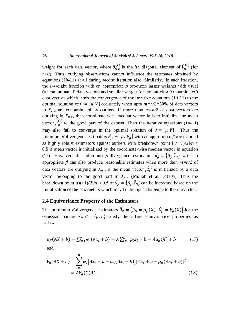
76 International Journal of Statisticsl Sciences, Vol. 16, 2018
weight for each data vector, where �̂�𝑖𝑖,𝛽(𝑟)
is the ith diagonal element of �̂�𝛽(𝑟)
(for
r>0). Thus, outlying observations cannot influence the estimates obtained by
equations (10-11) at all during second iteration also. Similarly, in each iteration,
the β-weight function with an appropriate β produces larger weights with usual
(uncontaminated) data vectors and smaller weight for the outlying (contaminated)
data vectors which leads the convergence of the iterative equations (10-11) to the
optimal solution of 𝜃 = {𝜇, 𝑉} accurately when upto m=n/2=50% of data vectors
in Xn,m are contaminated by outliers. If more than m=n/2 of data vectors are
outlying in Xn,m, then coordinate-wise median vector fails to initialize the mean
vector �̂�𝛽(𝑟)
to the good part of the dataset. Then the iterative equations (10-11)
may also fail to converge in the optimal solution of 𝜃 = {𝜇, 𝑉}. Thus the
minimum β-divergence estimators 𝜃𝛽 = {�̂�𝛽,�̂�𝛽} with an appropriate β are claimed
as highly robust estimators against outliers with breakdown point [(n+1)/2]/n ≈
0.5 if mean vector is initialized by the coordinate-wise median vector in equation
(12). However, the minimum β-divergence estimators 𝜃𝛽 = {�̂�𝛽,�̂�𝛽} with an
appropriate β can also produce reasonable estimates when more than m=n/2 of
data vectors are outlying in Xn,m if the mean vector �̂�𝛽(𝑟)
is initialized by a data
vector belonging to the good part in Xn,m (Mollah et al., 2010a). Thus the
breakdown point [(n+1)/2]/n ≈ 0.5 of 𝜃𝛽 = {�̂�𝛽,�̂�𝛽} can be increased based on the
initialization of the parameters which may be the open challenge to the researcher.
2.4 Equivariance Property of the Estimators
The minimum β-divergence estimators 𝜃𝛽 = {�̂�𝛽 = 𝜇𝛽(𝑋), �̂�𝛽 = 𝑉𝛽(𝑋)} for the
Gaussian parameters 𝜃 = {𝜇, 𝑉} satisfy the affine equivariance properties as
follows
𝜇𝛽(𝐴𝑋 + 𝑏) = ∑ 𝜑𝑖(𝐴𝑥𝑖 + 𝑏) = 𝐴 ∑ 𝜑𝑖𝑥𝑖 + 𝑏𝑛𝑖=1
𝑛𝑖=1 = 𝐴𝜇𝛽(𝑋) + 𝑏 (17)
and
𝑉𝛽(𝐴𝑋 + 𝑏) = ∑ 𝜑𝑖[𝐴𝑥𝑖 + 𝑏 − 𝜇𝛽(𝐴𝑥𝑖 + 𝑏)][𝐴𝑥𝑖 + 𝑏 − 𝜇𝛽(𝐴𝑥𝑖 + 𝑏)]/
𝑛
𝑖=1
= 𝐴𝑉𝛽(𝑋)𝐴/ (18)
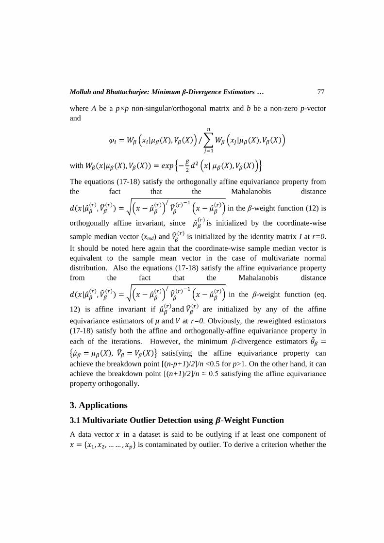
Mollah and Bhattacharjee: Minimum β-Divergence Estimators … 77
where A be a p×p non-singular/orthogonal matrix and b be a non-zero p-vector
and
𝜑𝑖 = 𝑊𝛽 (𝑥𝑖|𝜇𝛽(𝑋), 𝑉𝛽(𝑋)) / ∑ 𝑊𝛽 (𝑥𝑗|𝜇𝛽(𝑋), 𝑉𝛽(𝑋))
𝑛
𝑗=1
with 𝑊𝛽(𝑥|𝜇𝛽(𝑋), 𝑉𝛽(𝑋)) = 𝑒𝑥𝑝 {−𝛽
2𝑑2 (𝑥| 𝜇𝛽(𝑋), 𝑉𝛽(𝑋))}
The equations (17-18) satisfy the orthogonally affine equivariance property from
the fact that the Mahalanobis distance
𝑑(𝑥|�̂�𝛽(𝑟)
, �̂�𝛽(𝑟)
) = √(𝑥 − �̂�𝛽
(𝑟))
/
�̂�𝛽
(𝑟)−1(𝑥 − �̂�𝛽
(𝑟)) in the β-weight function (12) is
orthogonally affine invariant, since �̂�𝛽(𝑟)
is initialized by the coordinate-wise
sample median vector (xmd) and �̂�𝛽(𝑟)
is initialized by the identity matrix I at r=0.
It should be noted here again that the coordinate-wise sample median vector is
equivalent to the sample mean vector in the case of multivariate normal
distribution. Also the equations (17-18) satisfy the affine equivariance property
from the fact that the Mahalanobis distance
𝑑(𝑥|�̂�𝛽(𝑟)
, �̂�𝛽(𝑟)
) = √(𝑥 − �̂�𝛽
(𝑟))
/
�̂�𝛽
(𝑟)−1(𝑥 − �̂�𝛽
(𝑟)) in the β-weight function (eq.
12) is affine invariant if �̂�𝛽(𝑟)
and �̂�𝛽(𝑟)
are initialized by any of the affine
equivariance estimators of 𝜇 and 𝑉 at r=0. Obviously, the reweighted estimators
(17-18) satisfy both the affine and orthogonally-affine equivariance property in
each of the iterations. However, the minimum β-divergence estimators 𝜃𝛽 =
{�̂�𝛽 = 𝜇𝛽(𝑋), �̂�𝛽 = 𝑉𝛽(𝑋)} satisfying the affine equivariance property can
achieve the breakdown point [(n-p+1)/2]/n <0.5 for p>1. On the other hand, it can
achieve the breakdown point [(n+1)/2]/n ≈ 0.5 satisfying the affine equivariance
property orthogonally.
3. Applications
3.1 Multivariate Outlier Detection using 𝜷-Weight Function
A data vector 𝑥 in a dataset is said to be outlying if at least one component of
𝑥 = {𝑥1, 𝑥2, … … , 𝑥𝑝} is contaminated by outlier. To derive a criterion whether the
78 International Journal of Statisticsl Sciences, Vol. 16, 2018
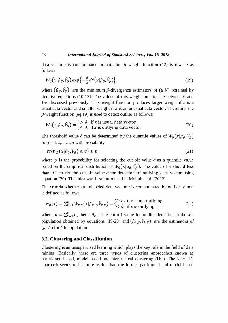
data vector 𝑥 is contaminated or not, the 𝛽-weight function (12) is rewrite as
follows
𝑊𝛽(𝑥|�̂�𝛽 , �̂�𝛽) exp {−𝛽
2𝑑2(𝑥|�̂�𝛽 , �̂�𝛽)} , (19)
where (�̂�𝛽 , �̂�𝛽) are the minimum 𝛽-divergence estimators of (𝜇, 𝑉) obtained by
iterative equations (10-12). The values of this weight function lie between 0 and
1as discussed previously. This weight function produces larger weight if 𝑥 is a
usual data vector and smaller weight if 𝑥 is an unusual data vector. Therefore, the
β-weight function (eq.19) is used to detect outlier as follows:
𝑊𝛽(𝑥|�̂�𝛽 , �̂�𝛽) = { > 𝜕, if 𝑥 is usual data vector ≤ 𝜕, if 𝑥 is outlying data vector
(20)
The threshold value 𝜕 can be determined by the quantile values of 𝑊𝛽(𝑥|�̂�𝛽 , �̂�𝛽)
for j = 1,2,……,𝑛 with probability
Pr{𝑊𝛽(𝑥|�̂�𝛽 , �̂�𝛽) ≤ 𝜕} ≤ 𝑝, (21)
where p is the probability for selecting the cut-off value 𝜕 as a quantile value
based on the empirical distribution of 𝑊𝛽(𝑥|�̂�𝛽 , �̂�𝛽). The value of p should less
than 0.1 to fix the cut-off value 𝜕 for detection of outlying data vector using
equation (20). This idea was first introduced in Mollah et al. (2012).
The criteria whether an unlabeled data vector 𝑥 is contaminated by outlier or not,
is defined as follows:
𝑤𝛽(𝑥) = ∑ 𝑊𝑘,𝛽(𝑥|�̂�𝑘,𝛽 , �̂�𝑘,𝛽)𝐾𝑘=1 = {
≥ 𝜕, if 𝑥 is not outlying< 𝜕, if 𝑥 is outlying
(22)
where, 𝜕 = ∑ 𝜕𝑘,𝐾𝑘=1 here 𝜕𝑘 is the cut-off value for outlier detection in the kth
population obtained by equations (19-20) and (�̂�𝑘,𝛽 , �̂�𝑘,𝛽) are the estimators of
(𝜇, 𝑉 ) for kth population.
3.2. Clustering and Classification
Clustering is an unsupervised learning which plays the key role in the field of data
mining. Basically, there are three types of clustering approaches known as
partitioned based, model based and hierarchical clustering (HC). The later HC
approach seems to be more useful than the former partitioned and model based

Mollah and Bhattacharjee: Minimum β-Divergence Estimators … 79
approaches, since HC does not require to knowing the number of clusters unlike
the former two approaches. It becomes popular for high-throughput high-
dimensional gene expression data analysis from the research work of Eisen et al.
(1998). The HC approaches are formulated based on the distance matrix or
dissimilarity matrix using single, complete or average linkages. The dissimilarity
matrix D is defined based on the correlation matrix R. However, the correlation
matrix R as well as the distance matrix or dissimilarity matrix D are sensitive to
outlying observations, which leads the misleading clustering results by HC. To
overcome this problem, Mollah et al. (2009) proposed β-HC by robustifying R
based on the minimum β-divergence estimator �̂�𝛽 of the covariance matrix V as
follows:
Let �̂�𝛽 = [�̂�𝑖𝑗]𝑝×𝑝
, which implies �̂�𝛽 = [�̂�𝑖𝑗]𝑝×𝑝
, the minimum β-divergence
estimator of the correlation matrix R, where �̂�𝑖𝑗 = �̂�𝑖𝑗/√�̂�𝑖𝑖�̂�𝑗𝑗 . Then the β-
dissimilarity matrix is defined as �̂�𝛽 = [�̂�𝑖𝑗]𝑝×𝑝
, where �̂�𝑖𝑗 = 1 − �̂�𝑖𝑗 ≥ 0. Then
the β-dissimilarity matrix �̂�𝛽 is used instead of traditional dissimilarity matrix D
for formulating HC algorithms from the robustness viewpoints. More discussion
about β-HC and its application for gene expression data analysis can be found in
Mollah et al. (2009). Badsha (2010) and Badsha et al. (2013) extended β-HC to β-
CHC for complementary hierarchical clustering (CHC; Nowak and Tibshirani,
2008) from the robustness viewpoints. Kabir (2018) and Kabir and Mollah (2018)
also proposed the robustification of the model based clustering using the
minimum β-divergence estimators of the mean vectors µ’s and the covariance
matrices V’s obtained by the EM algorithm.
On the other hand, classification is a supervised learning which plays the key role
in the field of machine learning for class prediction or pattern recognition. In the
literature, there are several approaches addressed for classifications (Anderson
2003; Johnson and Wichern 2007), where Gaussian Bayes classifier is one of the
most popular candidate. However, most of the existing classifiers including
Gaussian Bayes classifiers are very much sensitive to outliers. So, they can
produce misleading prediction results in presence of outliers. To overcome this
problem, Matiur (2012) and Matiur and Mollah (2018) proposed the
robustification of Gaussian Bayes Classifier based on the minimum β-divergence
estimators of the mean vectors µ’s and the covariance matrices V’s. The
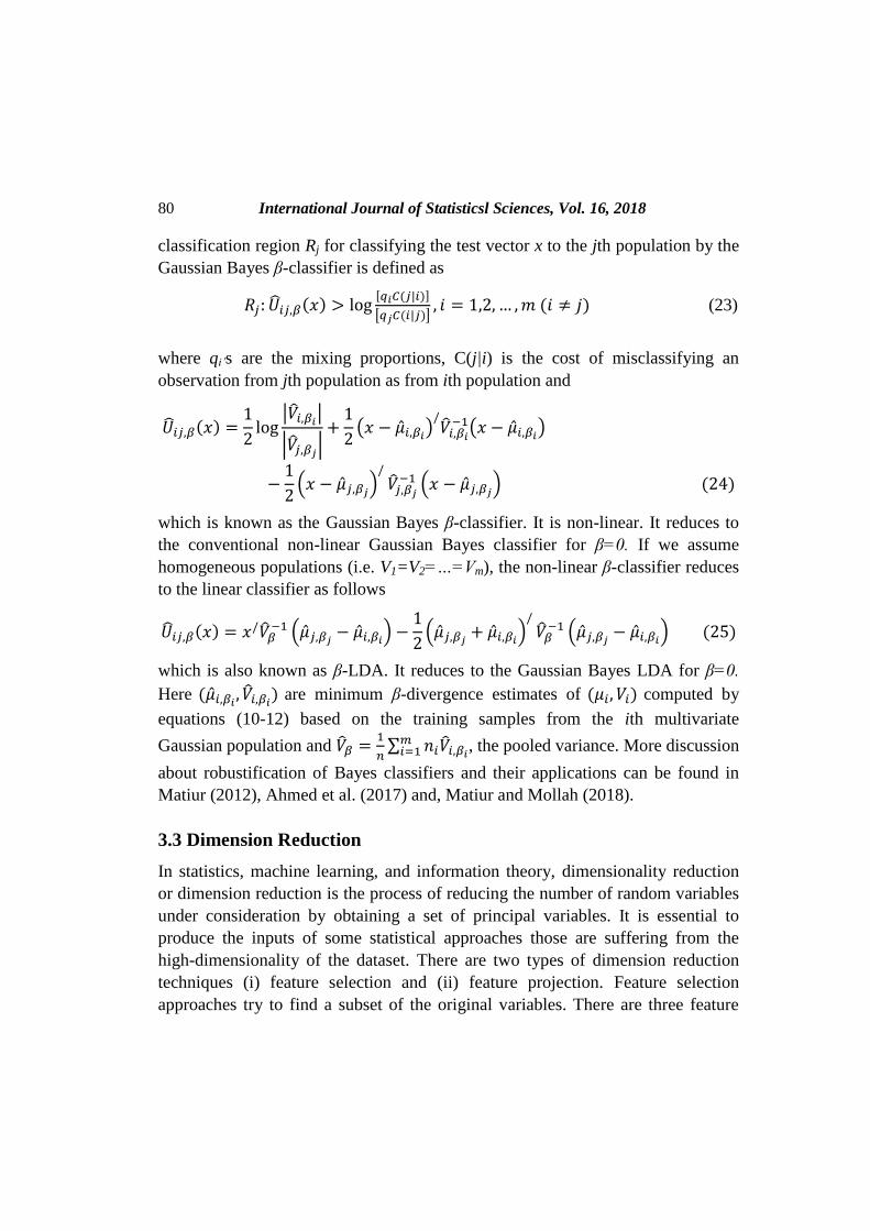
80 International Journal of Statisticsl Sciences, Vol. 16, 2018
classification region Rj for classifying the test vector x to the jth population by the
Gaussian Bayes β-classifier is defined as
𝑅𝑗: �̂�𝑖𝑗,𝛽(𝑥) > log[𝑞𝑖𝐶(𝑗|𝑖)]
[𝑞𝑗𝐶(𝑖|𝑗)], 𝑖 = 1,2, … , 𝑚 (𝑖 ≠ 𝑗) (23)
where qi’s are the mixing proportions, C(j|i) is the cost of misclassifying an
observation from jth population as from ith population and
�̂�𝑖𝑗,𝛽(𝑥) =1
2log
|�̂�𝑖,𝛽𝑖|
|�̂�𝑗,𝛽𝑗|
+1
2(𝑥 − �̂�𝑖,𝛽𝑖
)/�̂�𝑖,𝛽𝑖
−1(𝑥 − �̂�𝑖,𝛽𝑖)
−1
2(𝑥 − �̂�𝑗,𝛽𝑗
)/
�̂�𝑗,𝛽𝑗
−1 (𝑥 − �̂�𝑗,𝛽𝑗) (24)
which is known as the Gaussian Bayes β-classifier. It is non-linear. It reduces to
the conventional non-linear Gaussian Bayes classifier for β=0. If we assume
homogeneous populations (i.e. V1=V2=…=Vm), the non-linear β-classifier reduces
to the linear classifier as follows
�̂�𝑖𝑗,𝛽(𝑥) = 𝑥/�̂�𝛽−1 (�̂�𝑗,𝛽𝑗
− �̂�𝑖,𝛽𝑖) −
1
2(�̂�𝑗,𝛽𝑗
+ �̂�𝑖,𝛽𝑖)
/
�̂�𝛽−1 (�̂�𝑗,𝛽𝑗
− �̂�𝑖,𝛽𝑖) (25)
which is also known as β-LDA. It reduces to the Gaussian Bayes LDA for β=0.
Here (�̂�𝑖,𝛽𝑖, �̂�𝑖,𝛽𝑖
) are minimum β-divergence estimates of (𝜇𝑖, 𝑉𝑖) computed by
equations (10-12) based on the training samples from the ith multivariate
Gaussian population and �̂�𝛽 =1
𝑛∑ 𝑛𝑖�̂�𝑖,𝛽𝑖
𝑚𝑖=1 , the pooled variance. More discussion
about robustification of Bayes classifiers and their applications can be found in
Matiur (2012), Ahmed et al. (2017) and, Matiur and Mollah (2018).
3.3 Dimension Reduction
In statistics, machine learning, and information theory, dimensionality reduction
or dimension reduction is the process of reducing the number of random variables
under consideration by obtaining a set of principal variables. It is essential to
produce the inputs of some statistical approaches those are suffering from the
high-dimensionality of the dataset. There are two types of dimension reduction
techniques (i) feature selection and (ii) feature projection. Feature selection
approaches try to find a subset of the original variables. There are three feature

Mollah and Bhattacharjee: Minimum β-Divergence Estimators … 81
selection strategies (i) filtering strategy (ii) the wrapper strategy (e.g. search
guided by accuracy), and (iii) the embedded strategy (features are selected to add
or be removed while building the model based on the prediction errors). Feature
projection transforms the data in the high-dimensional space to a space of fewer
dimensions. Principal component analysis (PCA), factor analysis (FA) and
canonical correlation analysis (CCA) are considered as the most popular feature
projection approaches for dimension reduction. The estimation of the mean vector
µ and covariance matrix V plays the key role in each of PCA, FA and CCA.
However, traditional sample mean vector and covariance matrix (1-2) are
sensitive to outlying observations though they are affine equivariant. There are
some popular affine equivariant robust estimators like MCD and MVE for (𝜇, 𝑉),
but their robustness performance gradually decreases if the number of variables p
increases in the dataset. Mollah et al. (2010b) proposed robust PCA based on the
minimum β-divergence estimators (�̂�𝛽,�̂�𝛽) of (𝜇, 𝑉) computed by equations (10-
12) which is more robust than the other existing robust estimators in the literature
as discussed previously. In general, the β-PCA aims to extract the most
informative q-dimensional output vector 𝑦𝑗 = (𝑦𝑗1,𝑦𝑗2, … , 𝑦𝑗𝑞)/ from the input
vector 𝑥𝑗 = (𝑥𝑗1,𝑥𝑗2, … , 𝑥𝑗𝑝,)/ of dimension p ≥ q whose components are assumed
to be linearly correlated to each other. This is achieved by learning the p × q
orthogonal matrix Γ̂𝛽 = [ 𝛾1, �̂�2, … . 𝛾𝑞] which relates xj to yj by
𝑦𝑗 = Γ̂𝛽/(𝑥𝑗 − �̂�𝛽) (26)
such that components of yj are mutually uncorrelated satisfying the variance
inequality property of principal components (Higuchi and Eguchi, 2004; Mollah et
al. 2010a). The orthogonal matrix Γ̂𝛽 is determined by Γ̂𝛽 = eigen (�̂�𝛽) such that
Γ̂𝛽/�̂�𝛽Γ̂𝛽 = diag(�̂�1, �̂�2, … �̂�𝑞) satisfying the inequality �̂�1 > �̂�2 > ⋯ > �̂�𝑞 , where
�̂�𝑖 is the variance of the ith principal component (PC). Mollah et al. (2010b)
extended β-PCA for exploring the local PCA structures. Similarly, Ahsan (2012)
and Ahsan et al. (2012) robustify factor analyzers (FA) and, Singha (2013) and
Singha et al. (2014) robustify canonical correlation analyzers (CCA) based on the
minimum β-divergence estimators (�̂�𝛽,�̂�𝛽) of (𝜇, 𝑉) computed by equations (10-
12) for high-dimensional molecular OMICS data analysis from the robustness
viewpoints

82 International Journal of Statisticsl Sciences, Vol. 16, 2018
3.4 Blind Source Separation
Preprocessing of data is necessary in some adaptive independent component
analysis (ICA) algorithms for Blind Source Separation (BSS), because it reduces
the complexity of the ICA problems [Hyv¨arinen et al., 2001; Cichocki and
Amari, 2002]. For example, robust FastICA fixed-point algorithm [Hyv¨arinen et
al., 2001] is a popular algorithm for BSS, however, it produces misleading results
in presence of outliers due to the utilization of non-robust prewritten dataset. To
overcome this problem, Mollah et al. (2007) robustify the prewhitening procedure
based on the minimum β-divergence estimators (�̂�𝛽,�̂�𝛽) of (𝜇, 𝑉) computed by
equations (10-12) as follows:
Let us consider the linear ICA model for an observable random vector x of
dimension p as
x =As (27)
where A ∈ Rm×m and s is an unobservable source vector whose components are
assumed to be independent and non-Gaussian. A random vector z is said to be
whiten or sphere if E(Z)=0 and E(ZZ/)=Ip (identity matrix). In the β-prewhitening
procedure, the prewhitten data vector zj is obtained from xj by the following
equation
𝑧𝑗 = V̂𝛽−1/2
(𝑥𝑗 − �̂�𝛽) (26)
More discussion about β-prewhitening and its application to BSS can be found in
[Mollah et al. 2007, 2009, 2010c].
4. Conclusion
In this paper we have illustrated that the minimum β-divergence estimators of
multivariate Gaussian location and scatter parameters are highly robust against
outliers. We have discussed how the minimum β-divergence estimators of those
parameters playing key role when developing robust multivariate techniques
including robust principal component analysis, factor analysis, canonical
correlation analysis, independent component analysis, multiple regression
analysis, cluster analysis and discriminant analysis. It also serves as a convenient
tool for detection of multivariate outliers. The minimum β-divergence estimators
of multivariate Gaussian location and scatter parameters are reviewed, along with
Mollah and Bhattacharjee: Minimum β-Divergence Estimators … 83
its main properties such as affine equivariance, breakdown value, and influence
function. We discuss its computation and some applications in applied and
methodological multivariate statistics. Finally we have provided a detailed
reference list with applications and generalizations of the minimum β-divergence
estimators in the theoretical and applied research.
References
[1] Anderson, T. W. (2003). An Introduction to Multivariate Statistical Analysis.
Wiley Interscience.
[2] Agostinelli, C., Leung, A., Yohai, V., and Zamar, R. (2015). Robust estimation
of multivariate location and scatter in the presence of cell-wise and case-
wise contamination, TEST. 24, 441-461.
[3] Ahsan, M. A. (2012). Robustification of factor Analyzers and Its Application
for Gene Expression Data Analysis. Unpublished M.Sc. Thesis, Dept. of
Statistics, University of Rajshahi, Bangladesh.
[4] Ahsan, M. A., Rahaman, M. M., Monir, M. M., Hossain, M. R. and Mollah,
M. N. H. (2012). Robustification of Factor Analyzers and Its Application
for Microarray Gene Expression Data Analysis. Proceedings of the
International Conference on Bioinformatics, Health, Agriculture and
Environment - 2012, University of Rajshahi, Bangladesh, ISBN-978-984-
33-5876-9.
[5] Ahmed, M. S., Shahjaman, M., Rana, M. M. and Mollah, M. N. H. (2017).
Robustification of Naïve Bayes Classifier and Its Application for
Microarray Gene Expression Data Analysis. BioMed Research
International. Volume 2017, Article ID 3020627, 17 pages,
https://doi.org/10.1155/2017/3020627.
[6] Basu, A., Harris, I. R., Hjort, N. L. and Jones, M. C. (1998). Robust and
efficient estimation by minimizing a density power divergence.
Biometrika, 85, 549-559.
[7] Badsha, M. B. (2010). Robustification of Complementary Hierarchical
Clustering for Gene Expression Data Analysis. Unpublished M.Sc.
Thesis, Dept. of Statistics, University of Rajshahi, Bangladesh.
84 International Journal of Statisticsl Sciences, Vol. 16, 2018
[8] Badsha, M. B., Jahan, N., Kurata, H. and Mollah, M. N. H. (2013). Robust
Complementary Hierarchical Clustering for Gene Expression Data
Analysis by β-divergence. Journal of Bioscience and Bioengineering
(JBB), Vol-116 (3), pp. 397-407.
[9] Cichocki, A. and Amari, S. (2002). Adaptive Blind Signal and Image
Processing, Wiley, New York.
[10] Croux, C. and Haesbroeck, G. (1999). Influence function and efficiency of
the Minimum Co-variance Determinant scatter matrix estimator. Journal of
Multivariate Analysis, 71:161-190.
[11] Donoho, D. L. and Huber, P. J. (1983). The notion of breakdown point. In a
Festschrift for Ericion.
[12] Eisen, M. B., Spellman, P. T., Brown, P. O. and Botstein, D. (1998). Cluster
analysis and display of genome-wide expression patterns, Proc. Natl.
Acad. Sci. USA, 95, 14863-14868.
[13] Hampel, F.R. Ronchetti, E.M. Rousseeuw, P.J. and Stahel, W.A. (1986).
Robust Statistics: The Approach Based on Influence Functions. Wiley,
New York.
[14] Higuchi, I. and Eguchi, S. (2004). Robust principal component analysis with
adaptive selection for tuning parameters. Journal of Machine Learning
Research, 5, 453–471.
[15] Hyv¨arinen, A., Karhunen, J. and Oja, E. (2001). Independent Component
Analysis, Wiley, New York, 2001.
[16] Johnson, R. A. and Wichern, D. W. (2007). Applied multivariate statistical
analysis. Sixth edition, Prentice-Hall.
[17] Hubert, M. and Debruyne, M. (2010). Minimum Covariance Determinant.
Advanced Review. Vol.2, John Wiley & Sons. Inc.

Mollah and Bhattacharjee: Minimum β-Divergence Estimators … 85
[18] Kabir, M. H. (2018). Development of Statistical Algorithm for Data Mining
in Bioinformatics. Unpublished PhD Thesis, Dept. of Statistics, University
of Rajshahi, Bangladesh.
[19] Kabir, M. H. and Mollah, M. N. H. (2018). A Semi-Supervised Robust
Model based Clustering and Its Application for Gene Expression Data
Analysis. International Conference on New Paradigms in Statistics for
Scientific and Industrial Research, January 4-6, 2018. Kolkata, India.
[20] Lopuha, H.P. and Rousseeuw, P.J. (1991). Breakdown points of an
equivariant estimators of multivariate location and covariance matrices.
The Annals of Statistics, 19:229-248.
[21] Mollah, M. N. H., Minami, M. and Eguchi, S. (2006). Exploring Latent
Structure of Mixture ICA Models by the Minimum β-Divergence
Method. Neural Computation, Vol.18, pp.166-190.
[22] Mollah, M. N. H., Minami, M. and Eguchi, S. (2007). Robust Prewhitening
for ICA by Minimizing β-Divergence and its Application to Fast
ICA. Neural Processing Letters, Vol. 25, pp. 91-110.
[23] Mollah, M. M. H., Hossain, M. G. and Mollah, M. N. H. (2008a). Robust
Estimation for Multivariate Normal Distribution. Journal of Applied
Statistical Science (JASS), Vol. 16, pp. 377-386.
[24] Mollah, M. N. H., Mari, P., Komori, O. and Eguchi, S. (2009). Robust
Hierarchical Clustering for Gene Expression Data Analysis.
Communications of SIWN, Vol. 6, pp. 118-122.
[25] Mollah, M. N. H., Sultana, N., Minami, M. and Eguchi, S. (2010a). Robust
Extraction of Local Structures by the Minimum β-Divergence
method., Neural Network, Vol. 23, pp. 226-238.
[26] Mollah, M. M. H., Hossain, M. G. and Mollah, M. N. H. (2010b). Robust
Principal Component Analysis Based on Robust Estimation of
Multivariate Normal Distribution. International Journal of Statistical
Science (IJSS), Vol.10, pp. 19-35.
[27] Mollah, M. N. H. (2010c). Robust Image Processing by β-Prewhitening
Based FastICA algorithm. Int. Journal of Tomography and Statistics
(IJTS), Vol. 13, pp. 126-136.
[28] Mollah, M. H., Mollah, M. N. H. and Kishino, H. (2012). β-Empirical Bayes
inference and model diagnosis of microarray data . BMC Bioinformatics,
13:135.

86 International Journal of Statisticsl Sciences, Vol. 16, 2018
[29] Maronna, R.A. and Zamar, R.H. (2002). Robust estimates of location and
dispersion for high dimensional data sets. Technometrics, 44:307-317.
[30] Nowak, G. and Tibshirani, R. (2008). Complementary hierarchical clustering,
Biostatistics, 9, 467-483.
[31] Rahman, M. M. (2012). Robustification of Bayes Classifier and Its
Application for Gene Expression Data Analysis. Unpublished M.Sc.
Thesis, Dept. of Statistics, University of Rajshahi, Bangladesh.
[32] Rahman, M. M. and Mollah, M. H. (2018). Robustification of Gaussian
Bayes Classifier by the Minimum β-Divergence Method. Accepted for
publication in the Journal of Classification. Springer.
[33] Rousseeuw, P.J. (1985). Multivariate estimation with high breakdown point.
In W. Grossmann, G. Pug, I. Vincze, and W. Wertz, editors, Mathematical
Statistics and Applications, Vol. B, pages 283-297, Dordrecht, 1985.
Reidel Publishing Company.
[34] Rousseeuw, P.J. and Van Driessen, K. (1999). A fast algorithm for the
Minimum Covariance Determinant estimator. Technometrics, 41:212-223.
[35] Singha, A. C. (2013). Statistical Phylogenetic Modeling and Its Application
for DNA and Protein Sequence Analysis. Unpublished M.Sc Thesis, Dept.
of Statistics, University of Rajshahi, Bangladesh.
[36] Singha, A. C., Ahmed, M. S., Rana, M. M., Ahsan, M. A. and Mollah,
M.N.H. (2014). Robust Phylogenetic Canonical Correlation Analysis.
International Conference on Applied Statistics (ICAS), 26-28, Dec., 2014,
ISRT, University of Dhaka, Bangladesh.