Detection of Multivariate Cyclostationarity - e-Archivo
16
This is a postprint version of the following published document: D. Ramírez, P. J. Schreier, J. Vía, I. Santamaría and L. L. Scharf, "Detection of Multivariate Cyclostationarity," in IEEE Transactions on Signal Processing, vol. 63, no. 20, pp. 5395-5408, Oct.15, 2015 doi: 10.1109/TSP.2015.2450201. ©2015 IEEE. Personal use of this material is permitted. Permission from IEEE must be obtained for all other uses, in any current or future media, including reprinting/republishing this material for advertising or promotional purposes, creating new collective works, for resale or redistribution to servers or lists, or reuse of any copyrighted component of this work in other works.
-
Upload
khangminh22 -
Category
Documents
-
view
5 -
download
0
Transcript of Detection of Multivariate Cyclostationarity - e-Archivo
This is a postprint version of the following published document:
D. Ramírez, P. J. Schreier, J. Vía, I. Santamaría and L. L. Scharf, "Detection of Multivariate Cyclostationarity," in IEEE Transactions on Signal Processing, vol. 63, no. 20, pp. 5395-5408, Oct.15, 2015
doi: 10.1109/TSP.2015.2450201.
©2015 IEEE. Personal use of this material is permitted. Permission from IEEE must be obtained for all other uses, in any current or future media, including reprinting/republishing this material for advertising or promotional purposes, creating new collective works, for resale or redistribution to servers or lists, or reuse of any copyrighted component of this work in other works.

1
Detection of Multivariate CyclostationarityDavid Ramırez, Member, IEEE, Peter J. Schreier, Senior Member, IEEE, Javier Vıa, Senior Member, IEEE,
Ignacio Santamarıa, Senior Member, IEEE, and Louis L. Scharf, Life Fellow, IEEE
Abstract— This paper derives an asymptotic generalized likeli-hood ratio test (GLRT) and an asymptotic locally most powerfulinvariant test (LMPIT) for two hypothesis testing problems: 1) Isa vector-valued random process cyclostationary (CS) or is it wide-sense stationary (WSS)? 2) Is a vector-valued random processCS or is it nonstationary? Our approach uses the relationshipbetween a scalar-valued CS time series and a vector-valuedWSS time series for which the knowledge of the cycle periodis required. This relationship allows us to formulate the problemas a test for the covariance structure of the observations. Thecovariance matrix of the observations has a block-Toeplitz struc-ture for CS and WSS processes. By considering the asymptoticcase where the covariance matrix becomes block-circulant we areable to derive its maximum likelihood (ML) estimate and thus anasymptotic GLRT. Moreover, using Wijsman’s theorem, we alsoobtain an asymptotic LMPIT. These detectors may be expressedin terms of the Loeve spectrum, the cyclic spectrum, and thepower spectral density, establishing how to fuse the informationin these spectra for an asymptotic GLRT and LMPIT. Thisgoes beyond the state-of-the-art, where it is common practiceto build detectors of cyclostationarity from ad-hoc functions ofthese spectra.
Index Terms— Cyclostationarity, generalized likelihood ratiotest (GLRT), locally most powerful invariant test (LMPIT),Toeplitz matrix, Wijsman’s theorem.
I. INTRODUCTION
A zero-mean, discrete-time, complex-valued random pro-cess u[n] is said to be (second-order) cyclostationary (CS) ifits covariance function is periodic with period P [1], [2]:
ruu[n,m] = E[u[n]u∗[n−m]] = ruu[n+ P,m]
The period P is a natural number greater than 1 becauseP = 1 corresponds to a wide-sense stationary (WSS) process.CS signals model phenomena generated by periodic effectsin communications [3] (where the periodicity is induced bymodulation, sampling, and multiplexing operations), meteorol-ogy and climatology [4]–[6], oceanography [7]–[9], astronomy[10], and economics [11]–[13]. This plethora of applicationshas created significant interest in the analysis of CS signals asevidenced by the published literature [14], [15].
The detection of cyclostationarity is particularly important,for two main reasons. Firstly, if a signal is CS then this fact
D. Ramırez and P. J. Schreier are with the Department of ElectricalEngineering and Information Technology, University of Paderborn, 33098Paderborn, Germany (e-mail: {david.ramirez,peter.schreier}@sst.upb.de).
J. Vıa and I. Santamarıa are with the Department of Communica-tions Engineering, University of Cantabria, 39005 Santander, Spain (e-mail:{jvia,nacho}@gtas.dicom.unican.es).
L. L. Scharf is with the Departments of Mathematics and Statis-tics, Colorado State University, Ft. Collins, CO 80523, USA (e-mail:[email protected]).
Copyright (c) 2015 IEEE. Personal use of this material is permitted.However, permission to use this material for any other purposes must beobtained from the IEEE by sending a request to [email protected].
can usually be exploited in applications to improve detectionperformance. However, treating a signal as CS—when infact it is not—generally leads to very poor performance.Secondly, the presence or absence of CS signals can be usedto trigger other actions. This is the case in cognitive radio(CR), which is a new communications technology that hasthe potential to boost spectrum usage [16]–[18]. The mainidea behind CR is the opportunistic access of some users (so-called “cognitive” or “secondary” users) to a given frequencyband when the rightful owner of the band (the primary user)is not transmitting. Spectrum sensing (the detection of vacantchannels) is therefore a key ingredient to CR [19]. One ofthe most important properties that can be exploited to detectprimary users is the cyclostationarity of communications sig-nals, but other properties, such as temporally and/or spatiallyuncorrelated noise, can be also utilized. For these reasons,detection of cyclostationarity has received much attention inthe past [11], [20]–[23] and is now receiving a lot of renewedattention in the context of CR [24]–[31].
Detectors of cyclostationarity can roughly be classified intothe following three categories:
1) Techniques based on the Loeve (or dual-frequency) spec-trum. For a harmonizable process, the Loeve spectrum[32] is defined as the 2D-Fourier transform of thecorrelation function ruu[n,m]. The support of the Loevespectrum of a CS process is on lines parallel to thestationary manifold [33], whereas for WSS processes thesupport is only one line, the stationary manifold. Severaldetectors [11], [20], [21] have been proposed that exploitthis by comparing the values of the Loeve spectrumalong the lines that correspond to the CS componentsto the values along the line that corresponds to the WSScomponent. The critical question is what function touse for this comparison. The early works [11], [20],[21] use ad-hoc approaches, which are not grounded inestablished statistical principles. We will see later thatour approach can indeed be interpreted as comparing thestrengths of the CS and WSS components in the Loevespectrum, but in a statistically sound fashion.
2) Techniques based on testing for nonzero cyclic covari-ance function or cyclic spectrum. There are severalworks that test whether or not the estimated cycliccovariance function or cyclic spectrum are zero [22],[28], [34], [35]. This, however, raises the questions:What cycle frequencies (which harmonics) and whichlags of the covariance function (or global frequencies inthe cyclic spectrum) must be selected and how shouldthey be combined? Since our detectors admit an inter-pretation in terms of the cyclic spectrum they show how
2
to merge the information at each cycle frequency andglobal frequency.
3) Techniques based on testing for correlation between theprocess and a frequency-shifted version thereof. It wasproven in [36] that there exists correlation between theCS process u[n] and v[n] = u[n]e−j2παn, which isu[n] shifted by the cycle frequency α. This idea wasfirst used in [37] to estimate the number of CS signalsimpinging on an antenna array, by applying canonicalcorrelation analysis to the signals and their frequency-shifted versions. This has also been done in the contextof CR to detect the presence of primary users [31]. Thesetwo papers test the correlation in the temporal domain,although it is also possible to do so in the frequencydomain [23], where the frequency coherence betweenu[n] and v[n] is used as the detector statistic. However,these detectors only consider one lag or frequency andone cycle frequency, and it is not clear how to selectthese without knowledge of the true cyclic correlation. Ifwe were to consider multiple lags, it is not apparent howwe would optimally fuse the information at different lagsor frequencies and cycle frequencies.
Most of the approaches in the literature are for scalar timeseries and relatively few works have considered vector-valuedtime series [24]–[26], [28], [31], even though some of thescalar detectors could easily be extended to multivariate timeseries. All the detectors cited here consider testing cyclosta-tionarity vs. wide-sense stationarity. We are not aware of anydetectors that test cyclostationarity vs. nonstationarity.
As we have already mentioned, most detectors of cyclosta-tionarity are ad-hoc detectors, which are not derived from ac-cepted statistical principles, such as the generalized likelihoodratio test (GLRT), the uniformly most powerful invariant test(UMPIT), or the locally most powerful invariant test (LMPIT),etc. Our paper closes this gap. Our approach uses the rela-tionship between a scalar-valued CS time series and a vector-valued WSS time series [33] to formulate the problem as a testfor the covariance structure of the observations. The derivationof the GLRT is relatively straightforward, and the maindifficulty is that there is no closed-form maximum likelihood(ML) estimator of the covariance matrices because these areblock-Toeplitz. This difficulty is addressed by considering theasymptotic case where the covariance matrices become block-circulant. The derivation of the LMPIT is a bit more involved.The typical approach for deriving the LMPIT is based on themaximal invariant statistic. Then its distribution under bothhypotheses is obtained and the ratio of the distributions iscalculated. If this ratio (or a transformation thereof) does notdepend on unknown parameters it is the UMPIT. If it does,we may instead obtain the LMPIT for close hypotheses. Yetthis approach only works for a very few selected problems.Here, we instead use Wijsman’s theorem [38]–[41], whichallows us to obtain the ratio of the distributions of the maximalinvariant statistic without actually deriving the distributions oreven the maximal invariant statistic. Incidentally, both GLRTand LMPIT are functions of coherence matrices, as are thedetectors for spatial correlation in [42]–[44].
The paper is organized as follows: Section II presents the
detection problem and formulates it as a test for the covariancestructure of the observations. In Section III, we reformulatethe problem in the frequency domain. Sections IV and Vderive the GLRT and the LMPIT, respectively. An illuminatinginterpretation of the detectors in the Loeve frequency domainis presented in Section VI. Finally, Section VII numericallyevaluates the performance of our detectors.
II. PROBLEM FORMULATION
We consider the problem of testing whether a zero-meanmultivariate time series, observed by L sensors or antennas,is WSS, or CS with known cycle period P , or nonstationary(NS). That is, we are interested in the following three hypothe-ses:
H0 : u[n] is WSS,H1 : u[n] is CS with period P ,H2 : u[n] is NS,
(1)
where u[n] ∈ CL is a multivariate process of dimension L,assumed proper complex Gaussian [45]. Given NP samplesof u[n], which are collected in the vector
y =[uT [0] uT [1] · · · uT [NP − 1]
]T ∈ CLNP , (2)
the hypotheses in (1) may be formulated as
H0 : y ∼ CN (0,R0) ,H1 : y ∼ CN (0,R1) ,H2 : y ∼ CN (0,R2) ,
(3)
where Ri ∈ CLNP×LNP is the covariance matrix under theith hypothesis. Hence the hypothesis test is based on thestructure of Ri.
The NS case is the simplest because R2 does not have anyparticular structure beyond being positive definite,
R2 =
M2[0, 0] · · · M2[0,−NP + 1]...
. . ....
M2[NP − 1, NP − 1] · · · M2[NP − 1, 0]
,(4)
where M2[n,m] = E[u[n]uH [n − m]] ∈ CL×L is theNS matrix-valued covariance sequence. The structure understationarity is also easy to obtain [46], and the covariancematrix is
R0 =
M0[0] · · · M0[−NP + 1]...
. . ....
M0[NP − 1] · · · M0[0]
, (5)
where M0[m] = E[u[n]uH [n − m]] ∈ CL×L is the WSSmatrix-valued covariance sequence. It is clear that R0 is block-Toeplitz with block size L (the number of antennas or sensors).That is, the (m, l)th block is M0[m − l]. Finally, to find thestructure of R1 under cyclostationarity, we follow our previouswork [47]. We arrange u[n] in blocks of size P to obtain thetime series
x[n] =[uT [nP ] · · · uT [(n+ 1)P − 1]
]T ∈ CLP , (6)
which is WSS [33]. The vector y may therefore be rewrittenin terms of x[n] as
y =[xT [0] xT [1] · · · xT [N − 1]
]T ∈ CLNP , (7)

D. RAMIREZ, P. J. SCHREIER, J. VIA, I. SANTAMARIA AND L. L. SCHARF: DETECTION OF MULTIVARIATE CYCLOSTATIONARITY 3
which is a stack of N samples of the WSS process x[n].Hence, the covariance matrix is also block-Toeplitz, but withblock size LP :
R1 =
M1[0] · · · M1[−N + 1]...
. . ....
M1[N − 1] · · · M1[0]
, (8)
where M1[m] = E[x[n]xH [n−m]] ∈ CLP×LP is the matrix-valued WSS covariance sequence. To sum up, the covariancematrix is block-Toeplitz under H0 and H1, but only positivedefinite under H2 (see Figure 1).
One final comment is in order. Only the structure of the co-variance matrices is known under each of the three hypotheses,but the particular values, that is, the matrix-valued covariancesequences, are unknown. Thus, the only information availablea priori is the cycle period.
III. REWRITING THE HYPOTHESES: ASYMPTOTIC CASE
Since the covariance matrices are unknown, the hypothesesare composite, in which case the GLRT, the UMPIT and theLMPIT are typical approaches for binary tests [48], [49].For the GLRT we need the ML estimates of the unknownparameters, which, in our case, are the covariance matrices.As we have seen, under stationarity and cyclostationarity thesecovariance matrices are block-Toeplitz, for which there isno closed-form ML estimate [49]. Thus, we will follow anapproach similar to the one proposed in [43], [46], [47], whichenables us to derive an asymptotic GLRT.
Assume that we are given M independent and identicallydistributed (i.i.d.) realizations {yl}M−1m=0 of the vector y. Thelikelihood of these observations under Hi is
p(y0, . . . ,yM−1; Ri) =M−1∏m=0
p(ym; Ri)
=1
πLNPM det(Ri)Mexp
{−M tr
(R−1i R
)}, (9)
where the sample covariance matrix is
R =1
M
M−1∑m=0
ymyHm. (10)
Since there is no closed-form solution for ML estimatesof block-Toeplitz matrices we approximate them by block-circulant matrices. Block-Toeplitz matrices are asymptoticallyequivalent to block-circulant matrices [50], [51], and the like-lihoods converge in mean-square, as shown in the followingtheorem.
Theorem 1: As N → ∞, the log-likelihood random vari-able (RV), parameterized by a block-Toeplitz covariance ma-trix, converges in mean-square (sometimes called l.i.m.) to thelog-likelihood RV parameterized by a properly selected block-circulant covariance matrix:
limN→∞
E
[1
N2|log p (y0, . . . ,yM−1; R)
− log p (y0, . . . ,yM−1; Q)|2]
= 0,
where ym ∈ CNB , and R ∈ CNB×NB is the block-Toeplitzcovariance matrix with a generic block size B,
R =
M[0] · · · M[−N + 1]...
. . ....
M[N − 1] · · · M[0]
. (11)
The matrix-valued covariance sequence that generates R isM[m] ∈ CB×B , and Q ∈ CNB×NB is the block-circulantcovariance matrix whose (m, l)th block is M[m− l mod N ].Equivalently, the block-circulant matrix may be factored as
Q = (FN ⊗ IB) V (FN ⊗ IB)H. (12)
Here, FN is the Fourier matrix of dimension N , and V isa block-diagonal matrix, whose kth block is given by thediscrete Fourier transform (DFT) of the covariance sequence,
V(θk) =N−1∑m=0
M[m] exp {−jθkm} , (13)
with θk = 2πk/N . Thus, V(θk) is simply the cross-spectralmatrix (CSM) at frequency θk.
Proof: The proof follows from [46] with a few modifi-cations.
Corollary 1: The log-likelihood for the block-circulant co-variance matrix may be rewritten as
log p (y0, . . . ,yM−1; Q) = −NBM log π
−NM∫ 2π
0
log det V(θ)dθ
2π−NM
∫ 2π
0
tr[V−1(θ)V(θ)
] dθ2π,
(14)
where V(θ) is the sample CSM at frequency θ.Taking into account Theorem 1, the hypotheses in (3) are
asymptotically equivalent to
H0 : y ∼ CN (0,Q0) ,H1 : y ∼ CN (0,Q1) ,H2 : y ∼ CN (0,Q2) .
(15)
For nonstationary data, Q2 is positive definite without furtherstructure. For cyclostationary data, Q1 is block-circulant withblock size LP and may therefore be factored as
Q1 = (FN ⊗ ILP ) V1 (FN ⊗ ILP )H, (16)
where V1 is an unknown positive definite block-diagonalmatrix of block size LP . For stationary data, Q0 is a block-circulant covariance matrix with block size L, which may befactored as
Q0 = (FNP ⊗ IL) V0 (FNP ⊗ IL)H, (17)
where V0 is a positive definite block-diagonal matrix of blocksize L.
Let us now transform the observations as
z = (LNP,N ⊗ IL) (FNP ⊗ IL)H
y, (18)
where LNP,N is the commutation (or “stride permutation”)matrix [52], which fulfills vec(A) = LNP,Nvec(AT ), whereA is a P × N matrix. Basically, this transformation is aparticular reordering of the frequencies in the DFT of u[n].

4
(a) Stationary case (b) Cyclostationary case (c) Nonstationary case
Fig. 1: Structure of the covariance matrix for N = 3 and P = 2 under the three considered hypotheses. Each square correspondsto an L× L matrix.
We formulate the hypothesis test in terms of z instead of yand must therefore obtain the covariance matrix of z underthe three hypotheses. Under H2, the covariance matrix is
S2 = E[zzH |H2]
=(LNP,NFHNP ⊗ IL
)Q2
(FNPLTNP,N ⊗ IL
), (19)
which is another unknown positive definite matrix. Under H0,the covariance matrix of the transformed observations is
S0 =(LNP,NFHNP ⊗ IL
)Q0
(FNPLTNP,N ⊗ IL
), (20)
and, taking into account (17),
S0 = (NP )2 (LNP,N ⊗ IL) V0 (LNP,N ⊗ IL)T, (21)
where we have used (FNP ⊗ IL)H
(FNP ⊗ IL) = NP ILNP .Thus, the covariance matrix is just a scaled and permutedversion of the blocks of V0, and since V0 is unknown, S0
is also an unknown positive definite block-diagonal matrix.Under H1, the derivation is more involved and based on theCooley-Tukey theorem.
Theorem 2 (Cooley-Tukey): The Fourier matrix may be fac-tored as
FNP = (FN ⊗ IP ) TNP,P (IN ⊗ FP ) LNP,N , (22)
where TNP,P is a diagonal matrix of twiddle factors.Proof: See [53].
The covariance matrix under H1 is given by
S1 =(LNP,NFHNP ⊗ IL
)Q1
(FNPLTNP,N ⊗ IL
), (23)
and, using the factorization in (16), it becomes
S1 =(LNP,NFTNP ⊗ IL
)(FN ⊗ ILP )
×V1 (FN ⊗ ILP )H (
FNPLTNP,N ⊗ IL). (24)
WithFN ⊗ ILP = (FN ⊗ IP )⊗ IL (25)
and the associative property of the Kronecker product, weobtain(
LNP,NFHNP ⊗ IL)
(FN ⊗ ILP ) =[LNP,NFHNP (FN ⊗ IP )
]⊗ IL. (26)
Applying Theorem 2, the term inside the square bracketsbecomes
LNP,NFHNP (FN ⊗ IP ) = N (IN ⊗ FP )H
T∗NP,P , (27)
which yields
S1 = N2[(IN ⊗ FP )
HT∗NP,P
]⊗ IL
×V1 [TNP,P (IN ⊗ FP )]⊗ IL. (28)
It is clear that the Kronecker product of the matrix insidethe square brackets and the identity matrix results in a block-diagonal matrix with block size LP . Since the covariancematrix under H1 is an unknown positive definite block-diagonal matrix multiplied on the left by a block-diagonalmatrix with the same block size and on the right by theHermitian transpose of this matrix, S1 is also an unknownpositive definite block-diagonal matrix with block size LP .
Putting all the pieces together, the hypotheses are
H0 : z ∼ CN (0,S0) ,H1 : z ∼ CN (0,S1) ,H2 : z ∼ CN (0,S2) ,
(29)
where S2 is a positive definite matrix without further structure,S1 is a positive definite block-diagonal matrix with block sizeLP , and S0 is also a positive definite block-diagonal matrixbut with block size L. Hence, under all three hypotheses,the covariance matrices are block-diagonal. S2 contains justone block of size LPN × LPN . This fact will simplify thederivations of the tests. Moreover, an insightful interpretationof these covariance matrices is presented in Section VI.
IV. DERIVATION OF THE GLRT
In the previous section, we showed that the three covariancematrices are block-diagonal without further structure but dif-ferent block sizes. In this section, we derive the GLRT for thecase of two block-diagonal with arbitrary block sizes. Lateron, these block sizes are chosen as those in (29) to derive theasymptotic GLRT for the tests CS vs. WSS signals, and CS vs.NS signals. The derivation of the LMPIT follows in SectionV.

D. RAMIREZ, P. J. SCHREIER, J. VIA, I. SANTAMARIA AND L. L. SCHARF: DETECTION OF MULTIVARIATE CYCLOSTATIONARITY 5
A. GLRT for block-diagonality with different block sizes
Consider the following hypothesis test
H0 : z ∼ CN (0,D0) ,H1 : z ∼ CN (0,D1) ,
(30)
where D0 is a block-diagonal matrix with block size B0
and without further structure, i.e. D0 ∈ SB0 , and D1 is ablock-diagonal matrix with block size B1 and without furtherstructure, i.e. D1 ∈ SB1
. Of course, B1 must be a multiple ofB0 because the sizes of D1 and D0 are the same.
The generalized likelihood ratio (GLR) for the test in (30)is given by
G =
maxD0∈SB0
p (z0, . . . , zM−1; D0)
maxD1∈SB1
p (z0, . . . , zM−1; D1)(31)
where the maximization is carried out over the set of positivedefinite block-diagonal matrices, with block size B0 under H0
and block size B1 under H1. In the following theorem wepresent the solution to (31).
Theorem 3: The GLRT in (31) is
G1/M =det(diagB1
(S))
det(diagB0(S))
= det(CB1
B0), (32)
where diagBi(S), i = 0, 1, builds a block-diagonal ma-trix from the Bi × Bi blocks on the main diagonalof S by setting the off-diagonal blocks equal to zero,CB1
B0= [diagB0
(S)]−1/2 diagB1(S)[diagB0
(S)]−1/2 is a co-herence matrix, and S is the sample covariance matrix ofz0, . . . , zM−1.
Proof: Under both hypotheses, we need the ML estimateof a block-diagonal covariance matrix. The likelihood for ageneric block size B is given by
p(z0, . . . , zM−1; D) =
1
πNBM det(D)Mexp
{−M tr
(D−1S
)}. (33)
Taking into account the block-diagonal structure of D, thelikelihood becomes
p(z0, . . . , zM−1; D) =N∏k=1
1
πBM det (Dk)M
exp{−M tr
(D−1k Sk
)}, (34)
where Dk and Sk are the kth blocks of dimensions B × Bon the diagonal of D and S, respectively. Since Dk has nostructure besides being positive definite, its ML estimate isDk = Sk, which is easily proven using the derivatives in [54].Finally, the proof is concluded by building a block-diagonalmatrix with blocks Sk, with k = 1, . . . , N , which yields
D = diagB(S). (35)
Applying the ML estimator in (35) directly to the block-diagonal matrices in (30), and plugging these back into (31),the proof follows.
B. GLRT for testing cyclostationarity vs. wide-sense station-arity
The generalized likelihood ratio (GLR) for testing cyclosta-tionarity vs. wide-sense stationarity is
G0:1 =maxS0∈SL
p (z0, . . . , zM−1; S0)
maxS1∈SLP
p (z0, . . . , zM−1; S1), (36)
for which we may use the results in the previous subsection.The solution is presented in the following theorem.
Theorem 4: Asymptotically, as N → ∞, the GLR for thetest H0 vs. H1 is
G1/M0:1 =det(diagLP (S))
det(diagL(S))= det(CLP
L ) =N∏k=1
det(Ck),
(37)where CLP
L = [diagL(S)]−1/2 diagLP (S)[diagL(S)]−1/2 is acoherence matrix, and the kth LP×LP block on the diagonalof CLP
L is denoted by Ck.Proof: The proof is a direct application of the GLRT in
the previous subsection.It is clear that G0:1 is invariant to multiplications by a
nonsingular block-diagonal matrix with block size L. Thismeans the GLRT is asymptotically invariant to multiplicationsin the frequency domain, hence invariant to MIMO linearfiltering (circular convolution) of u[n]. For finite N , thisinvariance only holds approximately.
Interestingly, using the properties of the determinant, theabove GLRT may be rewritten as
log G0:1 =
∫ 2π
0
log det V1(θ)dθ
2π− P
∫ 2π
0
log det V0(θ)dθ
2π,
(38)where V1(θ) is the estimate of the CSM of the WSS vectorrepresentation x[n], given by
V1(θ) =1
M
M−1∑m=0
xm(θ)xHm(θ), (39)
where
xm(θ) =1√N
N−1∑n=0
xm[n]e−jθn. (40)
Similarly, V0(θ) is the estimate of the CSM of u[n], given by
V0(θ) =1
M
M−1∑m=0
um(θ)uHm(θ), (41)
with
um(θ) =1√NP
N−1∑n=0
um[n]e−jθn. (42)
For the scalar case, L = 1, this GLRT was derived in [47].
C. GLRT for testing Cyclostationarity vs. Nonstationarity
For the test H1 against H2, the GLR is
G1:2 =max
S1∈SLPp (z0, . . . , zM−1; S1)
maxS2∈S
p (z0, . . . , zM−1; S2), (43)

6
L =
∑Pκ,Pµ
∫DB0
det(D1)−M |det(G)2M | exp[−M tr
(D−11 PGSGHPT
)]dG
∑Pκ,Pµ
∫DB0
det(D0)−M |det(G)2M | exp[−M tr
(D−10 PGSGHPT
)]dG
, (46)
and the solution is presented next.Theorem 5: Asymptotically, as N → ∞, the GLR for the
test H2 vs. H1 is
G1/M1:2 =det(S)
det(diagLP (S))= det(CLPN
LP ), (44)
where CLPNLP = [diagLP (S)]−1/2S[diagLP (S)]−1/2 is a co-
herence matrix.Proof: The proof is a direct application of Theorem 3.
We note that while the ML estimate of S1 is an asymptoticestimate, the estimate S2 is an ML estimate for finite valuesof N , provided that M ≥ LNP . Moreover, the GLRT isinvariant to multiplications by any nonsingular block-diagonalmatrix with block size LP . Hence, the GLRT for H1 vs.H2 is asymptotically invariant to linear filtering (circularconvolution) of x[n] (rather than u[n] when testing H1 vs.H0).
Finally, it is also worth noting that this approach can be usedto show that the GLR for the test WSS vs. NS is det(CLPN
L ).However, we do not consider this test in more detail since itis outside the scope of the paper.
V. DERIVATION OF THE LMPIT
In this section, as in the previous one, we test block-diagonality with two different block sizes, but now usingthe LMPIT. To do so, we first study the invariances of thehypothesis test and use those to derive the LMPIT. We employWijsman’s theorem to avoid having to derive the maximalinvariant statistic and its distributions. For a more detailedreview of Wijsman’s theorem, see Appendix I. Then, theaforementioned LMPIT is particularized to the tests cyclosta-tionarity vs. wide-sense stationarity and cyclostationarity vs.nonstationarity.
A. LMPIT for block-diagonality with different block sizes
In this subsection we derive the LMPIT for the test in (30),and we use this LMPIT to obtain the asymptotic LMPITsfor testing cyclostationarity vs. wide-sense stationarity andcyclostationarity vs. nonstationarity. The first step is to findthe invariances of the detection problem. First, we may restrictour attention to linear operations since Gaussianity must bepreserved. We may also multiply z by any nonsingular block-diagonal matrix, with block size B0, without modifying thestructure of the hypothesis test. Moreover, we can permuteblocks of size B1 without modifying the block-diagonal struc-ture of D1, and within these B1×B1 blocks, it is also possible
to permute blocks of size B0 without modifying the block-diagonal structure of D0. Therefore, the invariance group is
G = {g : z→ g(z) = PGz,P = Pκ ⊗ (Pµ ⊗ IB0)} , (45)
where Pκ ∈ Pκ,Pµ ∈ Pµ, G ∈ DB0 , Pκ denotes the setof κ-dimensional permutation matrices and DB0 is the set ofnonsingular block-diagonal matrices with block size B0. Here,κ is the ratio between the size of the covariance matrices andB1, that is, the number of blocks of dimension B1×B1, and µis the ratio between B1 and B0, that is, the number of blocksof dimension B0 ×B0 that forms a block of size B1 ×B1.
Given this invariance group, Wijsman’s theorem [38] allowsus to write the ratio of the distributions of the maximalinvariant statistic shown in (46) at the top of this page. In (46)we sum over all possible permutations since the permutationgroup is a finite group. In its current form, L is a functionof the unknown parameters, which prevents the derivation ofthe UMPIT or LMPIT. In the following, we will simplify thisexpression to derive the LMPIT.
Lemma 1: The ratio L may be simplified to
L ∝∑Pκ,Pµ
∫DB0
β(G)e−αdG, (47)
where β(G) = |det(G)2M |e−M tr(GGH) and
α = Mκ∑k=1
µ∑l,m=1l 6=m
tr(D
(lm)k G
(m)k C
(ml)k G
(l)Hk
). (48)
Here Gk is the kth B1 × B1 block on the diagonal of G,which is also block-diagonal with B0 ×B0 blocks G
(l)k . The
coherence matrix CB1
B0is defined in the previous section, and it
is a block-diagonal matrix, with block size B1. The kth blockis denoted by1 Ck, which is itself a block matrix with B0×B0
blocks denoted by C(ml)k . Finally, Dk is the kth B1×B1 block
on the diagonal of
D = PT(diagB0
(D−11 ))−1/2
D−11
(diagB0
(D−11 ))−1/2
P,(49)
and D(lm)k denotes the (l,m)th block of Dk of size B0×B0.
Proof: See Appendix II.We may now present the LMPIT in the following theorem.
Theorem 6: The LMPIT statistic for the test in (30) is
L ∝κ∑k=1
‖Ck‖2. (50)
Proof: See Appendix III.
1Note that for the sake of notational simplicity, when there is no confussion,we drop the super-index B1 and sub-index B0.
D. RAMIREZ, P. J. SCHREIER, J. VIA, I. SANTAMARIA AND L. L. SCHARF: DETECTION OF MULTIVARIATE CYCLOSTATIONARITY 7
B. LMPIT for testing cyclostationarity vs. wide-sense station-arity
We present next the asymptotic LMPIT for testing cyclo-stationarity vs. wide-sense stationarity.
Theorem 7: Asymptotically, as N →∞, the LMPIT statis-tic for testing H0 vs. H1 is
L0:1 ∝N∑k=1
‖Ck‖2, (51)
where Ck is the kth block of CLPL , which is defined in Section
IV.Proof: Particularize the LMPIT in Theorem 6 to B1 =
LP , and B0 = L.Again, the LMPIT is invariant to MIMO linear filtering(circular convolution) of the sequence u[n], which shows thatthe detection problem does not depend on the particular cross-spectral matrix (CSM) of u[n].
The LMPIT in Theorem 7 is similar in form to the LMPITin [30] but there are differences worth mentioning. First, thederivations are different: We used the relationship between ascalar-valued CS process and a vector-valued WSS process,whereas [30] works in the frequency domain. Moreover, weconsider the general multivariate case L ≥ 1 and an arbitraryCSM under H0, whereas [30] treats the scalar case L = 1 andassumes a white process under the null hypothesis.
C. LMPIT for testing cyclostationarity vs. nonstationarity
Theorem 8: Asymptotically, as N →∞, the LMPIT statis-tic for testing cyclostationarity vs. nonstationarity is
L1:2 ∝ ‖CLPNLP ‖2. (52)
where the coherence matrix CLPNLP is defined in Section IV.
Proof: The proof is a direct application of Theorem 6.Alternatively, it may also be proven using the results in [44].
Similarly to the GLRT, the LMPIT is invariant to MIMO linearfiltering (circular convolution) of x[n], rather than u[n]. Thisinvariance allows us to whiten the cyclic CSM, which showsthat the detector cannot be a function of the cyclic CSM.
VI. INTERPRETATION OF THE DETECTORS
In this section we give an insightful interpretation of theGLRT and LMPIT in the frequency domain, for the test CS vs.WSS signals. Unfortunately, the other hypothesis test CS vs.NS signals does not easily admit an illuminating interpretation.Let us start with the covariance matrix of z, and its relationshipto the Loeve spectrum and the cyclic CSM. Recall that thetransformation
z = (FNP ⊗ IL)H
y ∈ CLNP (53)
is a column vector containing L-dimensional DFTs u(θk) ∈CL of the sequence u[n], k = 0, 1, . . . , NP − 1. Hence, itscovariance matrix contains samples of the Loeve spectrum,with the (k, l)th block of dimension L× L given by
Sk,l = E[u(θk)uH(θl)] = S(θk, θl), (54)
where S(θk, θl) ∈ CL×L is the Loeve spectrum of u[n] atfrequencies θk and θl. To study the effect of the commutationmatrix, let us rewrite the indices of the blocks of S as
k = i(k)2 N + i
(k)1 , l = i
(l)2 N + i
(l)1 , (55)
where i(k)2 , i
(l)2 = 0, . . . , P − 1, and i
(k)1 , i
(l)1 = 0, . . . , N −
1. According to [55], the commutation matrix permutes theindices as
k → k′ = i(k)1 P + i
(k)2 , (56)
l→ l′ = i(l)1 P + i
(l)2 , (57)
and the blocks of S become
Si(k)1 P+i
(k)2 ,i
(l)1 P+i
(l)2
= S(θk, θl), (58)
where
θk =2π(i(k)2 N + i
(k)1
)NP
, θl =2π(i(l)2 N + i
(l)1
)NP
. (59)
Thus, the matrix S is composed of N × N blocks of sizeP × P , where each element is a matrix of size L× L.
Now we look at the matrices DLP and DL. The former isa block-diagonal matrix with block size LP and is composedby the blocks of S that correspond to i(k)1 = i
(l)1 , i.e., S(θk, θl)
withθk − θl =
2π
P
(i(k)2 − i(l)2
).
That is, the blocks of diagLP (S) are the Loeve spectrum withthe frequencies separated by a multiple of 2π/P . On the otherhand, DL is also block-diagonal but with block size L and itcorresponds to the set of indices i(k)1 = i
(l)1 and i
(k)2 = i
(l)2 ,
which is S(θl, θl). Let us now analyze the Loeve spectrum forthese separations between the frequencies. The cyclic PSD
S(c)(θ) =∑m
R(c)[m]e−jθm (60)
with cycle frequency c and global frequency θ is the discrete-time Fourier transform of the cyclic covariance function
R(c)[m] =∑n
E[u[n]uH [n−m]]e−j2πcn/P , (61)
which in turn is the discrete Fourier series (DFS) in n ofthe periodic covariance sequence E[u[n]uH [n − m]]. ForCS processes, the Loeve spectrum and the cyclic PSD areconnected as [33]
S(θk, θl) =P−1∑c=0
S(c)(θl)δ (θk − θl − 2πc/P ) . (62)
The support of S(θk, θl) is on the lines θk−θl = 2πc/P , thatis, harmonics of the fundamental cycle frequency. Moreover,for θk − θl = 0 we have S(θl, θl) = S(0)(θl) = S(θl),which is the PSD. We conclude that DLP contains sam-ples of S(c)(θl) for c = −P + 1, . . . , P − 1 and θl =0, 2π/NP, . . . , 2π(NP − 1)/NP , and DL contains samplesof S(θl) for θl = 0, 2π/NP, . . . , 2π(NP − 1)/NP .
Taking all of the above into account, the matrix CLPL
contains blocks of the form
C(c)(θl) = S−1/2(θl)S(c)(θl)S
−1/2(θl −
2πc
P
), (63)

8
θk
θlc = 0c = 1c = 2
S(θl)
S(θl + 2π/P )S(1)(θl)
Stationary manifold
Fig. 2: Graphical representation of the coherence matrix inthe Loeve spectrum. Only the positive cycle frequencies areshown.
which will allow an insightful interpretation.2 We start byrewriting the cyclic PSD as [45]
S(c)(θ)dθ = E
[dξ(θ)dξH
(θ +
2πc
P
)], (64)
where dξ(θ) is an increment of the complex spectral processξ(θ) that generates the time series
u[n] =
∫dξ (θ) ejθn. (65)
Thus, we conclude that C(c)(θl) is the coherence matrix ofthe random vectors dξ (θl) and dξ(θl − 2πc/P ), which isillustrated in Fig. 2. For CS processes, frequencies that areseparated by a multiple of the cyclic frequency are correlated,and this coherence matrix is therefore nonzero. On the otherhand, for WSS processes, the coherence matrix is zero forc 6= 0.
The test CS vs. WSS signals is thus a test for the strengthof the cyclic components relative to the WSS component inthe estimated Loeve spectrum. The GLRT and LMPIT differin how they measure this relative strength, as they employdifferent functions of CLP
L . The LMPIT uses the Frobeniusnorm
L0:1 ∝P−1∑c=1
(P−c)N−1∑l=0
∥∥∥C(c)(θl)∥∥∥2 (66)
with
θl =2πl
NP, (67)
2Unfortunately, it does not seem possible to rewrite the matrix CLPNLP
(involved in testing CS vs. NS signals) in a similarly insightful manner.
which, asymptotically, may be written as
L0:1 ∝P−1∑c=1
∫ 2π(P−c)/P
0
∥∥∥C(c)(θ)∥∥∥2 dθ
2π. (68)
The GLRT, on the other hand, uses the determinant, which isgiven by a complicated nonlinear function of C(c)(θl).
We note that the detector in [23] uses (63) as its statistic,but considers only the scalar case L = 1. More critically, [23]uses only the fundamental cycle frequency c = 1 and only oneglobal frequency θl, instead of combining the information fromall global frequencies and all harmonics of the fundamentalcycle frequency.
VII. NUMERICAL SIMULATIONS
In this section we evaluate the performance of our detectorsusing computer simulations. We consider a cognitive radioexperiment. Our detectors can exploit the cyclostationarityinduced by the symbol rate and/or the carrier frequency pro-vided that the cycle period is known. This requires frequencysynchronization and knowledge of the symbol rate. Assumingfrequency synchronization and knowledge of the symbol rate,we may formulate the problem as
H0 : u[n] = w[n],H1 : u[n] = (H ∗ s)[n] + w[n],H2 : u[n] = (Hd ∗ s)[n] + w[n],
(69)
and w[n] ∈ CL is additive Gaussian noise, which is a WSSprocess generated by a moving average model of order 19.The signal s[n] ∈ CL is a QPSK signal with rectangularshaping and a symbol rate of Rs = 300 Kbauds. The channelH[n] ∈ CL×L is a Rayleigh channel without correlationamong antennas, it has an exponential power delay profile witha maximum delay of 24µs, and a delay spread of 6.24µs. Thechannel Hd[n] is time-varying due to the Doppler effect, whichwe generate with a normalized (to Rs) Doppler frequencyof 10−1 and a Jakes spectrum. This makes u[n] NS underH2.3 The sampling frequency is 1.2 MHz, which yields thecycle period P = 4, and the channel and noise coefficientsare Gaussian and randomly generated in each Monte Carlosimulation. One final comment is in order. In these simulationswe have considered a communications example. However,we have derived general detectors that do not exploit all theproperties present in communications signals. For instance, ourdetectors do not exploit the fact that the transmit pulse shapemight be known or that the noise might be temporally and/orspatially uncorrelated.
A. Cyclostationarity vs. wide-sense stationarity
We first compare the performance of the LMPIT and theGLRT with the detectors in [37] (see also [31]) and [28]. Thesetwo detectors require selecting which lags and/or harmonics ofthe cycle frequency to use. This is only possible if the cycliccovariance function is known, which may not be a realistic
3This is actually a generalized almost cyclostationary process [56], [57],which for our purposes may be considered as a NS process. For a moredetailed review of this kind of process, see [58].

D. RAMIREZ, P. J. SCHREIER, J. VIA, I. SANTAMARIA AND L. L. SCHARF: DETECTION OF MULTIVARIATE CYCLOSTATIONARITY 99
0 0.1 0.2 0.3 0.4 0.50.5
0.6
0.7
0.8
0.9
1
pfa
pd
LMPITGLRTDetector in [37]Detector in [28]
Fig. 3: ROC curves for the test CS vs. WSS in a scenario withL = 3, N = 256, P = 3, M = 15, and SNR = −16 dB
−20 −18 −16 −14 −12 −10
10−3
10−2
10−1
100
SNR (dB)
pm
LMPITGLRTDetector in [37]Detector in [28]
Fig. 4: Probability of missed detection vs. SNR for the testCS vs. WSS in a scenario with L = 3, N = 256, P = 3, andM = 15. The probability of false alarm is fixed at pfa = 10−3.
assumption. For a fair comparison, we decided to use lags0, 1, 2 and 3 of the cyclic covariance but only one harmonicof the cycle frequency in the detector [28]. However, for thedetector [37] we selected the lag that maximizes the cycliccovariance (although this might be unrealistic in practice)because selecting lag 0 would yield poor performance fora QPSK signal with rectangular shaping. Finally, we used aKaiser window of length 1025 to estimate the cyclic CSMrequired for the detector [28].
Figure 3 shows the receiver operating characteristic (ROC)curves for a scenario with global SNR of −16 dB, L = 3antennas, N = 256 and M = 15. Hence, the total number ofsamples at each antenna is NMP = 11520. As can be seenin the figure, the best performance is provided by the LMPIT,followed by the GLRT. Both LMPIT and GLRT outperformthe detectors [28], [37] because they exploit the information atall lags and all harmonics of the cycle frequency. On the con-trary, the detector in [37] exploits only the information at one
−10 −8 −6 −4 −2 0 2 4
10−3
10−2
10−1
100
SNR (dB)
pm
LMPITGLRTDetector in [37]Detector in [28]
Fig. 5: Probability of missed detection vs. SNR for the testCS vs. WSS in a scenario with L = 2, N = 32, P = 2, andM = 10. The probability of false alarm is fixed at pfa = 10−3.
harmonic and one lag. While the detector in [28] utilizes theinformation at multiple lags and multiple harmonics (althoughwe used only one) they have to be specified a priori. In additionto this, the detector in [28] does not take into account theinformation provided by the cyclic cross-covariance sequencesbecause it is a collaborative detector. The probability of misseddetection against the SNR for a fixed false alarm probabilitypfa = 10−3 is depicted in Figure 4, where similar conclusionscan be drawn. One would expect that for some scenarios theperformance of the LMPIT compared to the GLRT worsens.Indeed that is the case in Figure 5. In this experiment weconsidered a smaller problem in which the hypotheses arenot as close (the closeness of the hypotheses depends on thedimension of the covariance matrices, the number of samples,the SNR, . . .). Concretely, we selected L = 2 sensors, N = 32,P = 2 (the symbol rate is Rs = 600 Kbauds), and M = 10.In this scenario, the performance of the GLRT is slightly betterthan that of the LMPIT.
B. Null distribution and threshold setting
So far we have not said anything about the threshold,required to fix a probability of false alarm. It is expectedthat deriving the distributions of the statistics, required forselecting the threshold, is extremely difficult. However, in [59],[60], the authors were able to derive a stochastic representationunder the null hypothesis, which is applicable to our problem.However, here we will follow a different approach since wewant to obtain a closed-form expression for the threshold,which we could not do using the stochastic representation.First, our detectors are invariant to filtering. This means wecan obtain the thresholds using numerical simulations for awhite process under H0 and use these thresholds for anyarbitrary CSM. But since our LMPIT and GLRT are onlyasymptotically invariant to filtering, this requires some furtheranalysis. We obtained the histograms of the test statistics ofour detectors for white noise and colored noise, shown in Fig.6 for SNR = −20 dB. The remaining parameters are the same
Fig. 3: ROC curves for the test CS vs. WSS in a scenario withL = 3, N = 256, P = 3, M = 15, and SNR = −16 dB
9
0 0.1 0.2 0.3 0.4 0.50.5
0.6
0.7
0.8
0.9
1
pfa
pd
LMPITGLRTDetector in [37]Detector in [28]
Fig. 3: ROC curves for the test CS vs. WSS in a scenario withL = 3, N = 256, P = 3, M = 15, and SNR = −16 dB
−20 −18 −16 −14 −12 −10
10−3
10−2
10−1
100
SNR (dB)
pm
LMPITGLRTDetector in [37]Detector in [28]
Fig. 4: Probability of missed detection vs. SNR for the testCS vs. WSS in a scenario with L = 3, N = 256, P = 3, andM = 15. The probability of false alarm is fixed at pfa = 10−3.
assumption. For a fair comparison, we decided to use lags0, 1, 2 and 3 of the cyclic covariance but only one harmonicof the cycle frequency in the detector [28]. However, for thedetector [37] we selected the lag that maximizes the cycliccovariance (although this might be unrealistic in practice)because selecting lag 0 would yield poor performance fora QPSK signal with rectangular shaping. Finally, we used aKaiser window of length 1025 to estimate the cyclic CSMrequired for the detector [28].
Figure 3 shows the receiver operating characteristic (ROC)curves for a scenario with global SNR of −16 dB, L = 3antennas, N = 256 and M = 15. Hence, the total number ofsamples at each antenna is NMP = 11520. As can be seenin the figure, the best performance is provided by the LMPIT,followed by the GLRT. Both LMPIT and GLRT outperformthe detectors [28], [37] because they exploit the information atall lags and all harmonics of the cycle frequency. On the con-trary, the detector in [37] exploits only the information at one
−10 −8 −6 −4 −2 0 2 4
10−3
10−2
10−1
100
SNR (dB)
pm
LMPITGLRTDetector in [37]Detector in [28]
Fig. 5: Probability of missed detection vs. SNR for the testCS vs. WSS in a scenario with L = 2, N = 32, P = 2, andM = 10. The probability of false alarm is fixed at pfa = 10−3.
harmonic and one lag. While the detector in [28] utilizes theinformation at multiple lags and multiple harmonics (althoughwe used only one) they have to be specified a priori. In additionto this, the detector in [28] does not take into account theinformation provided by the cyclic cross-covariance sequencesbecause it is a collaborative detector. The probability of misseddetection against the SNR for a fixed false alarm probabilitypfa = 10−3 is depicted in Figure 4, where similar conclusionscan be drawn. One would expect that for some scenarios theperformance of the LMPIT compared to the GLRT worsens.Indeed that is the case in Figure 5. In this experiment weconsidered a smaller problem in which the hypotheses arenot as close (the closeness of the hypotheses depends on thedimension of the covariance matrices, the number of samples,the SNR, . . .). Concretely, we selected L = 2 sensors, N = 32,P = 2 (the symbol rate is Rs = 600 Kbauds), and M = 10.In this scenario, the performance of the GLRT is slightly betterthan that of the LMPIT.
B. Null distribution and threshold setting
So far we have not said anything about the threshold,required to fix a probability of false alarm. It is expectedthat deriving the distributions of the statistics, required forselecting the threshold, is extremely difficult. However, in [59],[60], the authors were able to derive a stochastic representationunder the null hypothesis, which is applicable to our problem.However, here we will follow a different approach since wewant to obtain a closed-form expression for the threshold,which we could not do using the stochastic representation.First, our detectors are invariant to filtering. This means wecan obtain the thresholds using numerical simulations for awhite process under H0 and use these thresholds for anyarbitrary CSM. But since our LMPIT and GLRT are onlyasymptotically invariant to filtering, this requires some furtheranalysis. We obtained the histograms of the test statistics ofour detectors for white noise and colored noise, shown in Fig.6 for SNR = −20 dB. The remaining parameters are the same
Fig. 4: Probability of missed detection vs. SNR for the testCS vs. WSS in a scenario with L = 3, N = 256, P = 3, andM = 15. The probability of false alarm is fixed at pfa = 10−3.
assumption. For a fair comparison, we decided to use lags0, 1, 2 and 3 of the cyclic covariance but only one harmonicof the cycle frequency in the detector [28]. However, for thedetector [37] we selected the lag that maximizes the cycliccovariance (although this might be unrealistic in practice)because selecting lag 0 would yield poor performance fora QPSK signal with rectangular shaping. Finally, we used aKaiser window of length 1025 to estimate the cyclic CSMrequired for the detector [28].
Figure 3 shows the receiver operating characteristic (ROC)curves for a scenario with global SNR of −16 dB, L = 3antennas, N = 256 and M = 15. Hence, the total number ofsamples at each antenna is NMP = 11520. As can be seenin the figure, the best performance is provided by the LMPIT,followed by the GLRT. Both LMPIT and GLRT outperformthe detectors [28], [37] because they exploit the information atall lags and all harmonics of the cycle frequency. On the con-trary, the detector in [37] exploits only the information at oneharmonic and one lag. While the detector in [28] utilizes the
9
0 0.1 0.2 0.3 0.4 0.50.5
0.6
0.7
0.8
0.9
1
pfa
pd
LMPITGLRTDetector in [37]Detector in [28]
Fig. 3: ROC curves for the test CS vs. WSS in a scenario withL = 3, N = 256, P = 3, M = 15, and SNR = −16 dB
−20 −18 −16 −14 −12 −10
10−3
10−2
10−1
100
SNR (dB)
pm
LMPITGLRTDetector in [37]Detector in [28]
Fig. 4: Probability of missed detection vs. SNR for the testCS vs. WSS in a scenario with L = 3, N = 256, P = 3, andM = 15. The probability of false alarm is fixed at pfa = 10−3.
assumption. For a fair comparison, we decided to use lags0, 1, 2 and 3 of the cyclic covariance but only one harmonicof the cycle frequency in the detector [28]. However, for thedetector [37] we selected the lag that maximizes the cycliccovariance (although this might be unrealistic in practice)because selecting lag 0 would yield poor performance fora QPSK signal with rectangular shaping. Finally, we used aKaiser window of length 1025 to estimate the cyclic CSMrequired for the detector [28].
Figure 3 shows the receiver operating characteristic (ROC)curves for a scenario with global SNR of −16 dB, L = 3antennas, N = 256 and M = 15. Hence, the total number ofsamples at each antenna is NMP = 11520. As can be seenin the figure, the best performance is provided by the LMPIT,followed by the GLRT. Both LMPIT and GLRT outperformthe detectors [28], [37] because they exploit the information atall lags and all harmonics of the cycle frequency. On the con-trary, the detector in [37] exploits only the information at one
−10 −8 −6 −4 −2 0 2 4
10−3
10−2
10−1
100
SNR (dB)
pm
LMPITGLRTDetector in [37]Detector in [28]
Fig. 5: Probability of missed detection vs. SNR for the testCS vs. WSS in a scenario with L = 2, N = 32, P = 2, andM = 10. The probability of false alarm is fixed at pfa = 10−3.
harmonic and one lag. While the detector in [28] utilizes theinformation at multiple lags and multiple harmonics (althoughwe used only one) they have to be specified a priori. In additionto this, the detector in [28] does not take into account theinformation provided by the cyclic cross-covariance sequencesbecause it is a collaborative detector. The probability of misseddetection against the SNR for a fixed false alarm probabilitypfa = 10−3 is depicted in Figure 4, where similar conclusionscan be drawn. One would expect that for some scenarios theperformance of the LMPIT compared to the GLRT worsens.Indeed that is the case in Figure 5. In this experiment weconsidered a smaller problem in which the hypotheses arenot as close (the closeness of the hypotheses depends on thedimension of the covariance matrices, the number of samples,the SNR, . . .). Concretely, we selected L = 2 sensors, N = 32,P = 2 (the symbol rate is Rs = 600 Kbauds), and M = 10.In this scenario, the performance of the GLRT is slightly betterthan that of the LMPIT.
B. Null distribution and threshold setting
So far we have not said anything about the threshold,required to fix a probability of false alarm. It is expectedthat deriving the distributions of the statistics, required forselecting the threshold, is extremely difficult. However, in [59],[60], the authors were able to derive a stochastic representationunder the null hypothesis, which is applicable to our problem.However, here we will follow a different approach since wewant to obtain a closed-form expression for the threshold,which we could not do using the stochastic representation.First, our detectors are invariant to filtering. This means wecan obtain the thresholds using numerical simulations for awhite process under H0 and use these thresholds for anyarbitrary CSM. But since our LMPIT and GLRT are onlyasymptotically invariant to filtering, this requires some furtheranalysis. We obtained the histograms of the test statistics ofour detectors for white noise and colored noise, shown in Fig.6 for SNR = −20 dB. The remaining parameters are the same
Fig. 5: Probability of missed detection vs. SNR for the testCS vs. WSS in a scenario with L = 2, N = 32, P = 2, andM = 10. The probability of false alarm is fixed at pfa = 10−3.
information at multiple lags and multiple harmonics (althoughwe used only one) they have to be specified a priori. In additionto this, the detector in [28] does not take into account theinformation provided by the cyclic cross-covariance sequencesbecause it is a collaborative detector. The probability of misseddetection against the SNR for a fixed false alarm probabilitypfa = 10−3 is depicted in Figure 4, where similar conclusionscan be drawn. One would expect that for some scenarios theperformance of the LMPIT compared to the GLRT worsens.Indeed that is the case in Figure 5. In this experiment weconsidered a smaller problem in which the hypotheses arenot as close (the closeness of the hypotheses depends on thedimension of the covariance matrices, the number of samples,the SNR, . . .). Concretely, we selected L = 2 sensors, N = 32,P = 2 (the symbol rate is Rs = 600 Kbauds), and M = 10.In this scenario, the performance of the GLRT is slightly betterthan that of the LMPIT.
B. Null distribution and threshold setting
So far we have not said anything about the threshold,required to fix a probability of false alarm. It is expectedthat deriving the distributions of the statistics, required forselecting the threshold, is extremely difficult. However, in [59],[60], the authors were able to derive a stochastic representationunder the null hypothesis, which is applicable to our problem.However, here we will follow a different approach since wewant to obtain a closed-form expression for the threshold,which we could not do using the stochastic representation.First, our detectors are invariant to filtering. This means wecan obtain the thresholds using numerical simulations for awhite process under H0 and use these thresholds for anyarbitrary CSM. But since our LMPIT and GLRT are onlyasymptotically invariant to filtering, this requires some furtheranalysis. We obtained the histograms of the test statistics ofour detectors for white noise and colored noise, shown in Fig.6 for SNR = −20 dB. The remaining parameters are the sameas in Fig. 3, unless otherwise stated. Figures 6a and 6b show
10
-200 -1800
2,000
4,000
6,000
Test statistic
Frequen
cy
(a) GLRT histogram (N = 32)
-1525 -14750
2,000
4,000
6,000
Test statistic
(b) GLRT histogram (N = 256)
605 6250
2,000
4,000
6,000
Test statistic
Frequen
cy
(c) LMPIT histogram (N = 32)
4,900 4,9500
2,000
4,000
6,000
Test statistic
(d) LMPIT histogram (N = 256)
Fig. 6: Comparison between the distributions of the statisticsunder H0 for white noise (in blue) and colored noise (in red)
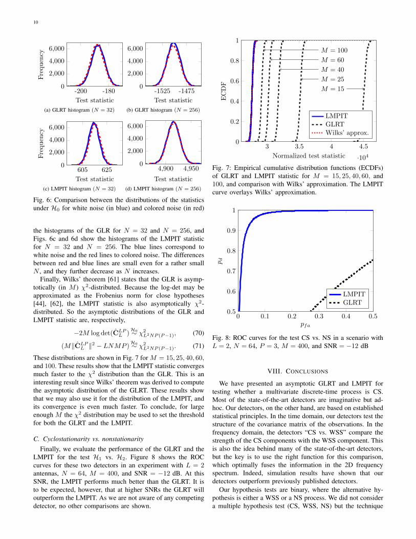
the histograms of the GLR for N = 32 and N = 256, andFigs. 6c and 6d show the histograms of the LMPIT statisticfor N = 32 and N = 256. The blue lines correspond towhite noise and the red lines to colored noise. The differencesbetween red and blue lines are small even for a rather smallN , and they further decrease as N increases.
Finally, Wilks’ theorem [61] states that the GLR is asymp-totically (in M ) χ2-distributed. Because the log-det may beapproximated as the Frobenius norm for close hypotheses[44], [62], the LMPIT statistic is also asymptotically χ2-distributed. So the asymptotic distributions of the GLR andLMPIT statistic are, respectively,
−2M log det(CLPL )
H0∼ χ2L2NP (P−1), (70)
(M‖CLPL ‖2 − LNMP )
H0∼ χ2L2NP (P−1). (71)
These distributions are shown in Fig. 7 for M = 15, 25, 40, 60,and 100. These results show that the LMPIT statistic convergesmuch faster to the χ2 distribution than the GLR. This is aninteresting result since Wilks’ theorem was derived to computethe asymptotic distribution of the GLRT. These results showthat we may also use it for the distribution of the LMPIT, andits convergence is even much faster. To conclude, for largeenough M the χ2 distribution may be used to set the thresholdfor both the GLRT and the LMPIT.
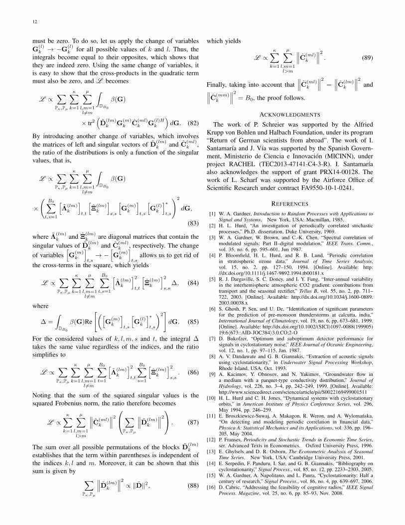
C. Cyclostationarity vs. nonstationarityFinally, we evaluate the performance of the GLRT and the
LMPIT for the test H1 vs. H2. Figure 8 shows the ROCcurves for these two detectors in an experiment with L = 2antennas, N = 64, M = 400, and SNR = −12 dB. At thisSNR, the LMPIT performs much better than the GLRT. It isto be expected, however, that at higher SNRs the GLRT willoutperform the LMPIT. As we are not aware of any competingdetector, no other comparisons are shown.
M = 100
M = 60
M = 40
M = 25
M = 15
3 3.5 4 4.5
·104
0
0.2
0.4
0.6
0.8
1
Normalized test statistic
ECDF
LMPITGLRTWilks’ approx.
Fig. 7: Empirical cumulative distribution functions (ECDFs)of GLRT and LMPIT statistic for M = 15, 25, 40, 60, and100, and comparison with Wilks’ approximation. The LMPITcurve overlays Wilks’ approximation.
0 0.1 0.2 0.3 0.4 0.50.5
0.6
0.7
0.8
0.9
1
pfa
pd
LMPITGLRT
Fig. 8: ROC curves for the test CS vs. NS in a scenario withL = 2, N = 64, P = 3, M = 400, and SNR = −12 dB
VIII. CONCLUSIONS
We have presented an asymptotic GLRT and LMPIT fortesting whether a multivariate discrete-time process is CS.Most of the state-of-the-art detectors are imaginative but ad-hoc. Our detectors, on the other hand, are based on establishedstatistical principles. In the time domain, our detectors test thestructure of the covariance matrix of the observations. In thefrequency domain, the detectors “CS vs. WSS” compare thestrength of the CS components with the WSS component. Thisis also the idea behind many of the state-of-the-art detectors,but the key is to use the right function for this comparison,which optimally fuses the information in the 2D frequencyspectrum. Indeed, simulation results have shown that ourdetectors outperform previously published detectors.
Our hypothesis tests are binary, where the alternative hy-pothesis is either a WSS or a NS process. We did not considera multiple hypothesis test (CS, WSS, NS) but the technique

D. RAMIREZ, P. J. SCHREIER, J. VIA, I. SANTAMARIA AND L. L. SCHARF: DETECTION OF MULTIVARIATE CYCLOSTATIONARITY 11
proposed in [63] could be directly applied to design a multiplehypothesis GLRT. The main idea behind the technique in [63]is that the sum of the log-GLR for testing CS vs. WSS andthe log-GLR for testing CS vs. NS signals is equal to the log-GLR for testing NS vs. WSS signals. Using this relationship itis possible to divide the space spanned by the two GLRs intothree regions, where each of these regions corresponds to aone of the hypotheses (CS, WSS, NS). Since this approach issuboptimal, applying it to design a multiple hypothesis LMPITdoes not make as much sense since the optimality of theLMPIT would be lost.
APPENDIX IWIJSMAN’S THEOREM: AN ALTERNATIVE DERIVATION
FOR THE UMPITThe derivation of the UMPIT usually requires the derivation
of the maximal invariant statistic and its distribution underboth hypotheses [49]. For many problems this is extremelydifficult or even impossible, preventing the derivation of theUMPIT. There is, however, an alternative based on Wijsman’stheorem [38], [64], [65]. This theorem states that, under somemild conditions, the ratio of the distributions of the maximalinvariant statistic may be obtained as
L =
∫G p (g(x);H1) |det (Jg)| dg∫G p (g(x);H0) |det (Jg)| dg
, (72)
where p (g(x);Hi) is the probability density function of thetransformed observations under the hypothesis Hi, G is thegroup of invariant transformations, Jg denotes the Jacobianof the transformation g(·) ∈ G and dg is an invariant groupmeasure, which we take as the usual Lebesgue measure.Even though Wijsman’s theorem is quite powerful, it has notreceived much attention in the signal processing literature,with a few notable exceptions [39], [41], [44], [66]–[70].
The main idea behind Wijsman’s theorem was first proposedby Stein [40]. However, the conditions under which (72) isvalid were studied much later by Wijsman and other authorsin [38], [64], [66], [71]–[73]. For our problem it suffices toconsider the simplest conditions. These specify that the groupof invariant transformations G must be a Lie group, a finitegroup or a composition of both, and the observations mustbelong to a linear Cartan G-space.4 Since the set of invertibleblock-diagonal matrices is a Lie group, the permutation groupis a finite group, and the observations belong to a linear CartanG-space, we may apply Wijsman’s theorem to our problem.
APPENDIX IIPROOF OF LEMMA 1
We first simplify the denominator. Ignoring the termdet(D0), which does not depend on data or the invarianttransformations, the integral in the denominator is given by∫
DB0
|det(G)2M | exp[−M tr
(D−10 PGSGHPT
)]dG.
(73)
4A linear Cartan G-space is a nonempty open subset (denoted as S) of theEuclidean space such that, for every x ∈ S, there exists a neighborhood Vfor which the closure of {g(·) ∈ G : g(V) ∩ V 6= ∅} is compact.
Taking into account the block-diagonal structure of D0 andG, with block size B0, and the fact that the permutation Pkeeps such structure, the integral may be rewritten as∫
DB0
|det(G)2M | exp[−M tr
(D−10 PG diagB0
(S)GHPT)]dG.
(74)Applying now the change of variables G →G[diagB0
(S)]−1/2, the integral becomes∫DB0
|det(G)2M | exp[−M tr
(D−10 PGGHPT
)]dG, (75)
which does not depend on the observations. Thus, the ratiodoes not depend on the denominator, which means
L ∝∑Pκ,Pµ
∫DB0
|det(G)2M |
× exp[−M tr
(D−11 PGSGHPT
)]dG, (76)
where we have also removed det(D1). It is possible to substi-tute S by diagB1
(S) in L due to the block-diagonal structureof D1 and G, with block size B1 in this case. Additionally,the change of variables G→ G[diagB0
(S)]−1/2 allows us towrite
L ∝∑Pκ,Pµ
∫DB0
|det(G)2M |
× exp[−M tr
(D−11 PGCGHPT
)]dG, (77)
For every permutation we may find a matrix G ∈ DB0, such
that the B0×B0 diagonal blocks of D−11 are IB0, which yields
L ∝∑Pκ,Pµ
∫DB0
|det(G)2M | exp[−M tr
(DGCGH
)]dG.
(78)It is clear that for any permutation in G, the matrix D is block-diagonal, which allows us to simplify the exponent as
tr(DGCGH
)=
κ∑k=1
tr(DkGkCkG
Hk
). (79)
Finally, since the diagonal blocks of both Dk and Ck are theidentity matrix, the proof follows.
APPENDIX IIIPROOF OF THEOREM 7
For close hypotheses (for instance, the CS process is almostWSS) the inverse of the whitened covariance matrix is D ≈Iκ·B1
, which implies α ≈ 0. We may therefore use a secondorder Taylor’s series to approximate e−α to obtain
L ∝∑Pκ,Pµ
∫DB0
β(G)(α2 − 2α)dG. (80)
We now prove that the linear term, given by∑Pκ,Pµ
κ∑k=1
µ∑l,m=1l 6=m
∫DB0
β(G)tr(D
(lm)k G
(m)k C
(ml)k G
(l)Hk
)dG,
(81)
12
must be zero. To do so, let us apply the change of variablesG
(l)k → −G
(l)k for all possible values of k and l. Thus, the
integrals become equal to their opposites, which shows thatthey are indeed zero. Using the same change of variables, itis easy to show that the cross-products in the quadratic termmust also be zero, and L becomes
L ∝∑Pκ,Pµ
κ∑k=1
µ∑l,m=1l 6=m
∫DB0
β(G)
× tr2(D
(lm)k G
(m)k C
(ml)k G
(l)Hk
)dG. (82)
By introducing another change of variables, which involvesthe matrices of left and singular vectors of D
(lm)k and C
(ml)k ,
the ratio of the distributions is only a function of the singularvalues, that is,
L ∝∑Pκ,Pµ
κ∑k=1
µ∑l,m=1l 6=m
∫DB0
β(G)
×(
B0∑t,s=1
[Λ
(lm)k
]t,t
[Ξ
(lm)k
]s,s
[G
(m)k
]t,s
[G
(l)k
]∗t,s
)2
dG,
(83)
where Λ(lm)k and Ξ
(lm)k are diagonal matrices that contain the
singular values of D(lm)k and C
(ml)k , respectively. The change
of variables[G
(m)k
]t,s→ −
[G
(m)k
]t,s
allows us to get rid of
the cross-terms in the square, which yields
L ∝∑Pκ,Pµ
κ∑k=1
µ∑l,m=1l 6=m
B0∑t,s=1
[Λ
(lm)k
]2t,t
[Ξ
(lm)k
]2s,s
∆, (84)
where
∆ =
∫DB0
β(G)Re
[([G
(m)k
]t,s
[G
(l)k
]∗t,s
)2]dG. (85)
For the considered values of k, l,m, s and t, the integral ∆takes the same value regardless of the indices, and the ratiosimplifies to
L ∝∑Pκ,Pµ
κ∑k=1
µ∑l,m=1l 6=m
B0∑t=1
[Λ
(lm)k
]2t,t
B0∑s=1
[Ξ
(lm)k
]2s,s. (86)
Noting that the sum of the squared singular values is thesquared Frobenius norm, the ratio therefore becomes
L ∝κ∑k=1
µ∑l,m=1l>m
∥∥∥C(ml)k
∥∥∥2∑
Pκ,Pµ
∥∥∥D(lm)k
∥∥∥2 . (87)
The sum over all possible permutations of the blocks D(lm)k
establishes that the term within parentheses is independent ofthe indices k, l and m. Moreover, it can be shown that thissum is given by ∑
Pκ,Pµ
∥∥∥D(lm)k
∥∥∥2 ∝ ‖D‖2, (88)
which yields
L ∝κ∑k=1
µ∑l,m=1l>m
∥∥∥C(ml)k
∥∥∥2 . (89)
Finally, taking into account that∥∥∥C(ml)
k
∥∥∥2 =∥∥∥C(lm)
k
∥∥∥2 and∥∥∥C(mm)k
∥∥∥2 = B0, the proof follows.
ACKNOWLEDGMENTS
The work of P. Schreier was supported by the AlfriedKrupp von Bohlen und Halbach Foundation, under its program“Return of German scientists from abroad”. The work of I.Santamarıa and J. Vıa was supported by the Spanish Govern-ment, Ministerio de Ciencia e Innovacion (MICINN), underproject RACHEL (TEC2013-47141-C4-3-R). I. Santamarıaalso acknowledges the support of grant PRX14-00128. Thework of L. Scharf was supported by the Airforce Office ofScientific Research under contract FA9550-10-1-0241.
REFERENCES
[1] W. A. Gardner, Introduction to Random Processes with Applications toSignal and Systems. New York, USA: Macmillan, 1985.
[2] H. L. Hurd, “An investigation of periodically correlated stochasticprocesses,” Ph.D. dissertation, Duke University, 1969.
[3] W. A. Gardner, W. Brown, and C.-K. Chen, “Spectral correlation ofmodulated signals: Part II–digital modulation,” IEEE Trans. Comm.,vol. 35, no. 6, pp. 595–601, Jun 1987.
[4] P. Bloomfield, H. L. Hurd, and R. B. Lund, “Periodic correlationin stratospheric ozone data,” Journal of Time Series Analysis,vol. 15, no. 2, pp. 127–150, 1994. [Online]. Available: http://dx.doi.org/10.1111/j.1467-9892.1994.tb00181.x
[5] R. J. Dargaville, S. C. Doney, and I. Y. Fung, “Inter-annual variabilityin the interhemispheric atmospheric CO2 gradient: contributions fromtransport and the seasonal rectifier,” Tellus B, vol. 55, no. 2, pp. 711–722, 2003. [Online]. Available: http://dx.doi.org/10.1034/j.1600-0889.2003.00038.x
[6] S. Ghosh, P. Sen, and U. De, “Identification of significant parametersfor the prediction of pre-monsoon thunderstorms at calcutta, india,”International Journal of Climatology, vol. 19, no. 6, pp. 673–681, 1999.[Online]. Available: http://dx.doi.org/10.1002/(SICI)1097-0088(199905)19:6〈673::AID-JOC384〉3.0.CO;2-O
[7] D. Bukofzer, “Optimum and suboptimum detector performance forsignals in cyclostationary noise,” IEEE Journal of Oceanic Engineering,vol. 12, no. 1, pp. 97–115, Jan. 1987.
[8] A. V. Dandawate and G. B. Giannakis, “Extraction of acoustic signalsusing cyclostationarity,” in Underwater Signal Processing Workshop,Rhode Island, USA, Oct. 1993.
[9] A. Kacimov, Y. Obnosov, and N. Yakimov, “Groundwater flow ina medium with a parquet-type conductivity distribution,” Journal ofHydrology, vol. 226, no. 3–4, pp. 242–249, 1999. [Online]. Available:http://www.sciencedirect.com/science/article/pii/S0022169499001511
[10] H. L. Hurd and C. H. Jones, “Dynamical systems with cyclostationaryorbits,” in American Institute of Physics Conference Series, vol. 296,May 1994, pp. 246–259.
[11] E. Broszkiewicz-Suwaj, A. Makagon, R. Weron, and A. Wylomanska,“On detecting and modeling periodic correlation in financial data,”Physica A: Statistical Mechanics and its Applications, vol. 336, pp. 196–205, May 2004.
[12] P. Franses, Periodicity and Stochastic Trends in Economic Time Series,ser. Advanced Texts in Econometrics. Oxford University Press, 1996.
[13] E. Ghylsels and D. R. Osborn, The Econometric Analysis of SeasonalTime Series. New York, USA: Cambridge University Press, 2001.
[14] E. Serpedin, F. Panduru, I. Sar, and G. B. Giannakis, “Bibliography oncyclostationarity,” Signal Process., vol. 85, no. 12, pp. 2233–2303, 2005.
[15] W. A. Gardner, A. Napolitano, and L. Paura, “Cyclostationarity: Half acentury of research,” Signal Process., vol. 86, no. 4, pp. 639–697, 2006.
[16] D. Cabric, “Addressing the feasibility of cognitive radios,” IEEE SignalProcess. Magazine, vol. 25, no. 6, pp. 85–93, Nov. 2008.
D. RAMIREZ, P. J. SCHREIER, J. VIA, I. SANTAMARIA AND L. L. SCHARF: DETECTION OF MULTIVARIATE CYCLOSTATIONARITY 13
[17] K.-C. Chen and R. Prasad, Cognitive Radio Networks. Wiley, 2009.[18] J. Mitola and G. Q. Maguire Jr., “Cognitive radio: Making software
radios more personal,” IEEE Pers. Comm., vol. 6, pp. 13–18, Aug. 1999.[19] E. Axell, G. Leus, E. Larsson, and H. Poor, “Spectrum sensing for
cognitive radio : State-of-the-art and recent advances,” IEEE SignalProcess. Mag., vol. 29, no. 3, pp. 101–116, May 2012.
[20] E. Broszkiewicz-Suwaj, “Methods for determining the presence ofperiodic correlation based on the bootstrap methodology,” WrocławUniversity of Technology, Tech. Rep. Research Report HSC/03/2, 2003.
[21] H. L. Hurd and N. L. Gerr, “Graphical methods for determining thepresence of periodic correlation,” Journal of Time Series Analysis,vol. 12, no. 4, pp. 337–350, 1991.
[22] A. V. Dandawate and G. B. Giannakis, “Statistical tests for presenceof cyclostationarity,” IEEE Trans. Signal Process., vol. 42, no. 9, pp.2355–2369, Sep. 1994.
[23] S. Enserink and D. Cochran, “On detection of cyclostationary signals,”in Proc. IEEE Int. Conf. Acoust., Speech and Signal Process. (ICASSP),Detroit, USA, May 1995, pp. 2004–2007.
[24] E. Axell and E. G. Larsson, “Multiantenna spectrum sensing of a second-order cyclostationary signal,” in IEEE Int. Work. Comp. Adv. in Multi-Sensor Adaptive Process., Dec. 2011, pp. 329–332.
[25] X. Chen, W. Xu, Z. He, and X. Tao, “Spectral correlation-basedmulti-antenna spectrum sensing technique,” in IEEE Wireless Comm.Networking Conf., Mar. 2008, pp. 735–740.
[26] G. Huang and J. K. Tugnait, “On cyclostationarity based spectrumsensing under uncertain gaussian noise,” IEEE Trans. Signal Process.,vol. 61, no. 8, pp. 2042–2054, Apr. 2013.
[27] J. Lunden, S. Kassam, and V. Koivunen, “Robust nonparametric cycliccorrelation-based spectrum sensing for cognitive radios,” IEEE Trans.Signal Process., vol. 58, no. 6, pp. 38–52, Jun. 2010.
[28] J. Lunden, V. Koivunen, A. Huttunen, and H. V. Poor, “Collaborativecyclostationary spectrum sensing for cognitive radio systems,” IEEETrans. Signal Process., vol. 57, no. 11, pp. 4182–4195, Nov. 2009.
[29] E. Rebeiz, P. Urriza, and D. Cabric, “Optimizing wideband cyclostation-ary spectrum sensing under receiver impairments,” IEEE Trans. SignalProcess., vol. 61, no. 15, pp. 3931–3943, Aug. 2013.
[30] J. Riba, J. Font-Segura, J. Villares, and G. Vazquez, “Frequency-domainGLR detection of a second-order cyclostationary signal over fadingchannels,” IEEE Trans. Signal Process., vol. 62, no. 8, pp. 1899–1912,Apr. 2014.
[31] P. Urriza, E. Rebeiz, and D. Cabric, “Multiple antenna cyclostationaryspectrum sensing based on the cyclic correlation significance test,” IEEEJournal on Selected Areas in Communications, vol. 31, no. 11, pp. 2185–2195, November 2013.
[32] M. Loeve, Probability Theory II, 4th ed. New York: Springer, 1978.[33] E. D. Gladyshev, “Periodically correlated random sequences,” Soviet
Math. Dokl., vol. 2, pp. 385–388, 1961.[34] J.-C. Shen and E. Alsusa, “Joint cycle frequencies and lags utilization in
cyclostationary feature spectrum sensing,” IEEE Trans. Signal Process.,vol. 61, no. 21, pp. 5337–5346, Nov. 2013.
[35] A. V. Vecchia and R. Ballerini, “Testing for periodic autocorrelations inseasonal time series data,” Biometrika, vol. 78, no. 1, pp. 53–63, 1991.
[36] W. Gardner, “Exploitation of spectral redundancy in cyclostationarysignals,” IEEE Signal Process. Magazine, vol. 8, no. 2, pp. 14–36, April1991.
[37] S. Schell and W. Gardner, “Detection of the number of cyclostationarysignals in unknown interference and noise,” in Asilomar Conf. onSignals, Systems and Computers, vol. 1, Nov. 1990, p. 473.
[38] R. A. Wijsman, “Cross-sections of orbits and their application todensities of maximal invariants,” in Proc. Fifth Berkeley Symp. on Math.Stat. and Prob., vol. 1, 1967, pp. 389–400.
[39] J. R. Gabriel and S. M. Kay, “Use of Wijsman’s theorem for the ratio ofmaximal invariant densities in signal detection applications,” in AsilomarConf. Signals, Systems and Computers, vol. 1, Nov. 2002, pp. 756 – 762.
[40] C. Stein, “Some problems in multivariate analysis, part 1,” Stanford Uni.Dept. Statistics, Tech. Rep., 1956.
[41] A. A. D’Amico, “IR-UWB transmitted-reference systems with partialchannel knowledge: a receiver design based on the statistical invarianceprinciple,” IEEE Trans. Signal Process., vol. 59, no. 4, pp. 1435–1448,Apr. 2011.
[42] D. Cochran, H. Gish, and D. Sinno, “A geometric approach to multiple-channel signal detection,” IEEE Trans. Signal Process., vol. 43, no. 9,pp. 2049–2057, Sep. 1995.
[43] D. Ramırez, J. Vıa, I. Santamarıa, and L. L. Scharf, “Detection ofspatially correlated Gaussian time series,” IEEE Trans. Signal Process.,vol. 58, no. 10, Oct. 2010.
[44] D. Ramırez, J. Vıa, I. Santamarıa, and L. L. Scharf, “Locally mostpowerful invariant tests for correlation and sphericity of Gaussianvectors,” IEEE Trans. Inf. Theory, vol. 59, no. 4, pp. 2128–2141, Apr.2013.
[45] P. J. Schreier and L. L. Scharf, Statistical Signal Processing of Complex-Valued Data. Cambridge University Press, 2010.
[46] D. Ramırez, G. Vazquez-Vilar, R. Lopez-Valcarce, J. Vıa, and I. San-tamarıa, “Detection of rank-P signals in cognitive radio networks withuncalibrated multiple antennas,” IEEE Trans. Signal Process., vol. 59,no. 8, pp. 3764–3774, Aug. 2011.
[47] D. Ramırez, L. L. Scharf, J. Vıa, I. Santamarıa, and P. J. Schreier, “Anasymptotic GLRT for the detection of cyclostationary signals,” in IEEEInt. Conf. on Acoustics, Speech and Signal Process., Florence, Italy, May2014.
[48] K. V. Mardia, J. T. Kent, and J. M. Bibby, Multivariate Analysis. NewYork: Academic, 1979.
[49] L. L. Scharf, Statistical Signal Processing: Detection, Estimation, andTime Series Analysis. Addison - Wesley, 1991.
[50] R. M. Gray, Toeplitz and Circulant Matrices: A Review. Foundationsand Trends in Communications and Information Theory, 2006.
[51] J. Gutierrez-Gutierrez and P. M. Crespo, “Asymptotically equivalentsequences of matrices and Hermitian block Toeplitz matrices withcontinuous symbols: Applications to MIMO systems,” IEEE Trans. Inf.Theory, vol. 54, no. 12, pp. 5671–5680, Dec. 2008.
[52] J. R. Magnus and H. Neudecker, “The commutation matrix: Someproperties and applications,” The Annals of Statistics, vol. 7, no. 2, pp.381–394, Mar. 1979.
[53] J. W. Cooley and J. W. Tukey, “An algorithm for the machine calculationof complex Fourier series,” Mathematics of Computation, vol. 19, no. 90,pp. 297–301, 1965.
[54] J. R. Magnus and H. Neudecker, Matrix Differential Calculus withApplications in Statistics and Econometrics. John Wiley & Sons, 1999.
[55] M. Puschel and J. M. F. Moura, “Algebraic signal processing theory:Cooley-Tukey type algorithms for DCTs and DSTs,” IEEE Trans. SignalProcess., vol. 56, no. 4, pp. 1502–1521, Apr. 2008.
[56] L. Izzo and A. Napolitano, “The higher order theory of general-ized almost-cyclostationary time series,” IEEE Trans. Signal Process.,vol. 46, no. 11, pp. 2975–2989, Nov. 1998.
[57] A. Napolitano, “Generalizations of cyclostationarity: A new paradigmfor signal processing for mobile communications, Radar, and Sonar,”IEEE Signal Process. Mag., vol. 30, no. 6, pp. 53–63, Nov. 2013.
[58] ——, Generalizations of Cyclostationary Signal Processing: SpectralAnalysis and Applications, ser. Wiley - IEEE. Wiley, 2012.
[59] N. Klausner, M. Azimi-Sadjadi, L. L. Scharf, and D. Cochran, “Space-time coherence and its exact null distribution,” in IEEE Int. Conf. onAcoustics, Speech and Signal Process., Vancouver, Canada, May 2013.
[60] N. Klausner, M. Azimi-Sadjadi, and L. L. Scharf, “Detection of spatiallycorrelated time series from a network of sensor arrays,” IEEE Trans.Signal Process., vol. 62, no. 6, pp. 1396–1407, Mar. 2014.
[61] S. M. Kay, Fundamentals of Statistical Signal Processing: DetectionTheory. Prentice Hall, 1998, vol. II.
[62] A. Leshem and A.-J. Van der Veen, “Multichannel detection of Gaussiansignals with uncalibrated receivers,” IEEE Signal Process. Lett., vol. 8,no. 4, pp. 120–122, Apr. 2001.
[63] J. Vıa, D. P. Palomar, and L. Vielva, “Generalized likelihood ratiosfor testing the properness of quaternion Gaussian vectors,” IEEE Trans.Signal Process., vol. 59, no. 4, pp. 1356–1370, April 2011.
[64] M. L. Eaton, Group Invariance Applications in Statistics. Inst. Math.Stat., 1989.
[65] N. C. Giri, Multivariate statistical analysis, ser. Statistics, textbooks andmonographs. Marcel Dekker, 2004.
[66] J. R. Gabriel and S. M. Kay, “On the relationship between the GLRTand UMPI tests for the detection of signals with unknown parameters,”IEEE Trans. Signal Process., vol. 53, no. 11, pp. 4194–4203, Nov. 2005.
[67] R. E. Schwartz, “Minimax CFAR detection in additive Gaussian noiseof unknown covariance,” IEEE Trans. Inf. Theory, vol. 15, no. 6, pp.722–725, Nov. 1969.
[68] J. Vıa and L. Vielva, “Locally most powerful invariant tests for theproperness of quaternion gaussian vectors,” IEEE Transactions on SignalProcessing, vol. 60, no. 3, March 2012.
[69] D. Ramırez, J. Iscar, J. Vıa, I. Santamarıa, and L. L. Scharf, “The locallymost powerful invariant test for detecting a rank-p gaussian signal inwhite noise,” in IEEE Sensor Array and Multichannel Signal Process.Work., Hoboken, NJ, USA, June 2012.
[70] D. Ramırez, J. Vıa, and I. Santamarıa, “The locally most powerfultest for multiantenna spectrum sensing with uncalibrated receivers,” in
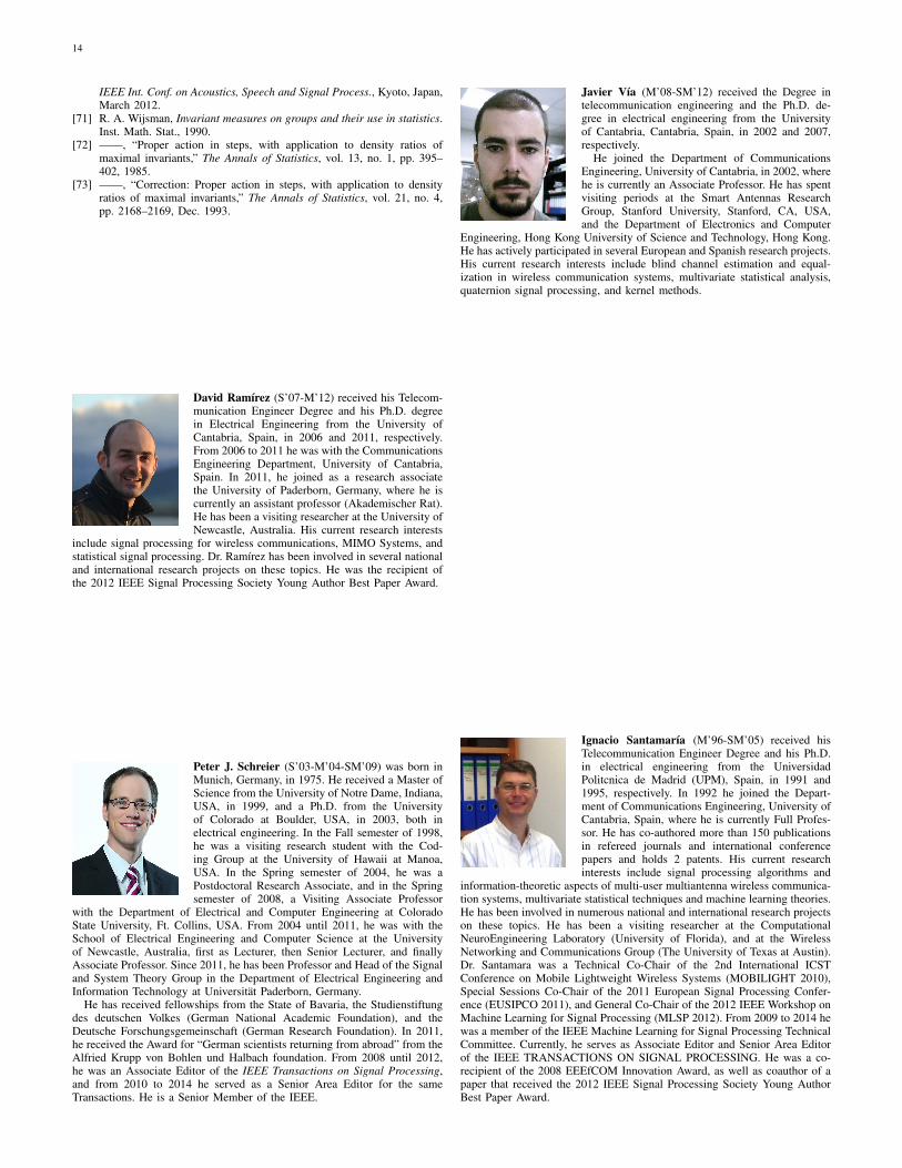
14
IEEE Int. Conf. on Acoustics, Speech and Signal Process., Kyoto, Japan,March 2012.
[71] R. A. Wijsman, Invariant measures on groups and their use in statistics.Inst. Math. Stat., 1990.
[72] ——, “Proper action in steps, with application to density ratios ofmaximal invariants,” The Annals of Statistics, vol. 13, no. 1, pp. 395–402, 1985.
[73] ——, “Correction: Proper action in steps, with application to densityratios of maximal invariants,” The Annals of Statistics, vol. 21, no. 4,pp. 2168–2169, Dec. 1993.
David Ramırez (S’07-M’12) received his Telecom-munication Engineer Degree and his Ph.D. degreein Electrical Engineering from the University ofCantabria, Spain, in 2006 and 2011, respectively.From 2006 to 2011 he was with the CommunicationsEngineering Department, University of Cantabria,Spain. In 2011, he joined as a research associatethe University of Paderborn, Germany, where he iscurrently an assistant professor (Akademischer Rat).He has been a visiting researcher at the University ofNewcastle, Australia. His current research interests
include signal processing for wireless communications, MIMO Systems, andstatistical signal processing. Dr. Ramırez has been involved in several nationaland international research projects on these topics. He was the recipient ofthe 2012 IEEE Signal Processing Society Young Author Best Paper Award.
Peter J. Schreier (S’03-M’04-SM’09) was born inMunich, Germany, in 1975. He received a Master ofScience from the University of Notre Dame, Indiana,USA, in 1999, and a Ph.D. from the Universityof Colorado at Boulder, USA, in 2003, both inelectrical engineering. In the Fall semester of 1998,he was a visiting research student with the Cod-ing Group at the University of Hawaii at Manoa,USA. In the Spring semester of 2004, he was aPostdoctoral Research Associate, and in the Springsemester of 2008, a Visiting Associate Professor
with the Department of Electrical and Computer Engineering at ColoradoState University, Ft. Collins, USA. From 2004 until 2011, he was with theSchool of Electrical Engineering and Computer Science at the Universityof Newcastle, Australia, first as Lecturer, then Senior Lecturer, and finallyAssociate Professor. Since 2011, he has been Professor and Head of the Signaland System Theory Group in the Department of Electrical Engineering andInformation Technology at Universitat Paderborn, Germany.
He has received fellowships from the State of Bavaria, the Studienstiftungdes deutschen Volkes (German National Academic Foundation), and theDeutsche Forschungsgemeinschaft (German Research Foundation). In 2011,he received the Award for “German scientists returning from abroad” from theAlfried Krupp von Bohlen und Halbach foundation. From 2008 until 2012,he was an Associate Editor of the IEEE Transactions on Signal Processing,and from 2010 to 2014 he served as a Senior Area Editor for the sameTransactions. He is a Senior Member of the IEEE.
Javier Vıa (M’08-SM’12) received the Degree intelecommunication engineering and the Ph.D. de-gree in electrical engineering from the Universityof Cantabria, Cantabria, Spain, in 2002 and 2007,respectively.
He joined the Department of CommunicationsEngineering, University of Cantabria, in 2002, wherehe is currently an Associate Professor. He has spentvisiting periods at the Smart Antennas ResearchGroup, Stanford University, Stanford, CA, USA,and the Department of Electronics and Computer
Engineering, Hong Kong University of Science and Technology, Hong Kong.He has actively participated in several European and Spanish research projects.His current research interests include blind channel estimation and equal-ization in wireless communication systems, multivariate statistical analysis,quaternion signal processing, and kernel methods.
Ignacio Santamarıa (M’96-SM’05) received hisTelecommunication Engineer Degree and his Ph.D.in electrical engineering from the UniversidadPolitcnica de Madrid (UPM), Spain, in 1991 and1995, respectively. In 1992 he joined the Depart-ment of Communications Engineering, University ofCantabria, Spain, where he is currently Full Profes-sor. He has co-authored more than 150 publicationsin refereed journals and international conferencepapers and holds 2 patents. His current researchinterests include signal processing algorithms and
information-theoretic aspects of multi-user multiantenna wireless communica-tion systems, multivariate statistical techniques and machine learning theories.He has been involved in numerous national and international research projectson these topics. He has been a visiting researcher at the ComputationalNeuroEngineering Laboratory (University of Florida), and at the WirelessNetworking and Communications Group (The University of Texas at Austin).Dr. Santamara was a Technical Co-Chair of the 2nd International ICSTConference on Mobile Lightweight Wireless Systems (MOBILIGHT 2010),Special Sessions Co-Chair of the 2011 European Signal Processing Confer-ence (EUSIPCO 2011), and General Co-Chair of the 2012 IEEE Workshop onMachine Learning for Signal Processing (MLSP 2012). From 2009 to 2014 hewas a member of the IEEE Machine Learning for Signal Processing TechnicalCommittee. Currently, he serves as Associate Editor and Senior Area Editorof the IEEE TRANSACTIONS ON SIGNAL PROCESSING. He was a co-recipient of the 2008 EEEfCOM Innovation Award, as well as coauthor of apaper that received the 2012 IEEE Signal Processing Society Young AuthorBest Paper Award.

D. RAMIREZ, P. J. SCHREIER, J. VIA, I. SANTAMARIA AND L. L. SCHARF: DETECTION OF MULTIVARIATE CYCLOSTATIONARITY 15
WANG et al.: OPTIMUM COMPRESSION OF A NOISY MEASUREMENT 1289
[9] D. Guo, S. Shamai, and S. Verdù, “Mutual information and minimummean-square error in Gaussian channels,” IEEE Trans. Inf. Theory, vol.51, no. 4, pp. 1261–1282, Apr. 2005.
[10] W. R. Carson, M. R. D. Rodrigues, M. Chen, L. Carin, and R. Calder-bank, “Communications-inspired projection design with application tocompressive sensing,” SIAM J. Imag. Sci., vol. 5, no. 4, pp. 1185–1212,2012.
[11] Z. Zhang, E. K. P. Chong, A. Pezeshki, and W. Moran, String Sub-modular Functions with Curvature Constraints [Online]. Available:arXiv:1303.3018
[12] T. M. Cover and J. A. Thomas, Elements of Information Theory, 2nded. Hoboken, NJ, USA: Wiley-Intersci., 2005.
[13] H. Hotelling, “Relations between two sets of variates,”Biometrika, vol.28, no. 3/4, pp. 321–377, Dec. 1936.
[14] F. Pukelsheim, Optimal Design of Experiments. Hoboken, NJ:Wiley-Intersci., 1993.
[15] Y. Zhu, E. Song, J. Zhou, and Z. You, “Optimal dimensionality re-duction of sensor data in multisensor estimation fusion,” IEEE Trans.Signal Process., vol. 53, no. 5, pp. 1631–1639, May 2005.
[16] A. Lozano, A. M. Tulino, and S. Verdú, “Optimum power allocationfor parallel Gaussian channels with arbitrary input distributions,” IEEETrans. Inf. Theory, vol. 52, no. 7, pp. 3033–3051, Jul. 2006.
[17] H. Witsenhausen, “A determinant maximization problem occurring inthe theory of data communication,” J. Appl. Math., vol. 29, no. 3, pp.515–522, Nov. 1975.
Yuan Wang received the B.S. (Statistics) degreefrom Special Class for Gifted Young, University ofScience and Technology of China, Hefei, in 2008.She received her Ph.D. degree in statistics fromColorado State University in 2013.She is currently a postdoctoral research fellow
with the University of Texas MD Anderson CancerCenter. Her research interests focus on informationfusion, dimension reduction, and object-orienteddata analysis including tree-structured data, imagingdata, and functional data.
HaonanWang received the Ph.D. degree in statisticsfrom the University of North Carolina at Chapel Hillin 2003.Currently, he is an Associate Professor of Statis-
tics at Colorado State University, Fort Collins. Hisresearch interests are in object oriented data analysis,statistical analysis on tree-structured objects, func-tional dynamicmodeling of neuron activities and spa-tial statistics.
Louis L. Scharf (S’67–M’69–SM’77–F’86–LF’07)received the Ph.D. degree from the University ofWashington, Seattle.From 1971 to 1982, he served as Professor of
Electrical Engineering and Statistics with ColoradoState University (CSU), Ft. Collins. From 1982 to1985, he was Professor and Chairman of Electricaland Computer Engineering, University of RhodeIsland, Kingston. From 1985 to 2000, he wasProfessor of Electrical and Computer Engineering,University of Colorado, Boulder. In January 2001,
he rejoined CSU as Professor of Electrical and Computer Engineering andStatistics. He is currently a Research Professor of Mathematics at CSU. Hehas held several visiting positions here and abroad, including the Ecole Su-perieure d’Electricite, Gif-sur-Yvette, France; Ecole Nationale Superieure desTelecommunications, Paris, France; EURECOM, Nice, France; the Universityof La Plata, La Plata, Argentina; Duke University, Durham, NC; the Universityof Wisconsin, Madison; and the University of Tromso, Tromso, Norway. Hisinterests are in statistical signal processing, as it applies to radar, sonar, andwireless communication.Prof. Scharf was Technical Program Chair for the 1980 IEEE International
Conference on Acoustics, Speech, and Signal Processing (ICASSP), Denver,CO; Tutorials Chair for ICASSP 2001, Salt Lake City, UT; and Technical Pro-gram Chair for the Asilomar Conference on Signals, Systems, and Computers2002. He is past-Chair of the Fellow Committee for the IEEE Signal ProcessingSociety. He has received numerous awards for his research contributions to sta-tistical signal processing, including a College Research Award, an IEEE Dis-tinguished Lectureship, an IEEE Third Millennium Medal, and the TechnicalAchievement and Society Awards from the IEEE Signal Processing Society.
Louis L. Scharf (S’67-M’69-SM’77-F’86-LF’07)received the Ph.D. degree from the University ofWashington, Seattle.
From 1971 to 1982, he served as Professor ofElectrical Engineering and Statistics with ColoradoState University (CSU), Ft. Collins. From 1982 to1985, he was Professor and Chairman of Electricaland Computer Engineering, University of Rhode Is-land, Kingston. From 1985 to 2000, he was Professorof Electrical and Computer Engineering, Universityof Colorado, Boulder. In January 2001, he rejoined
CSU as Professor of Electrical and Computer Engineering and Statistics. Heis currently a Research Professor of Mathematics at CSU. He has held severalvisiting positions here and abroad, including the Ecole Superieure d’electricite,Gif-sur-Yvette, France; Ecole Nationale Superieure des Telecommunications,Paris, France; EURECOM, Nice, France; the University of La Plata, LaPlata, Argentina; Duke University, Durham, NC; the University of Wisconsin,Madison; and the University of Tromsø, Tromsø, Norway. His interests are instatistical signal processing, as it applies to adaptive radar, sonar, and wirelesscommunication.
Prof. Scharf was Technical Program Chair for the 1980 IEEE InternationalConference on Acoustics, Speech, and Signal Processing (ICASSP), Denver,CO; Tutorials Chair for ICASSP 2001, Salt Lake City, UT; and Techni-cal Program Chair for the Asilomar Conference on Signals, Systems, andComputers 2002. He is past-Chair of the Fellow Committee for the IEEESignal Processing Society. He has received numerous awards for his researchcontributions to statistical signal processing, including a College ResearchAward, an IEEE Distinguished Lectureship, an IEEE Third Millennium Medal,and the Technical Achievement and Society Awards from the IEEE SignalProcessing Society.