
tesis doctoral - Archivo Digital UPM
316
U P M F I M TESIS DOCTORAL A A P G, MS D A R-P, PD M,J
-
Upload
khangminh22 -
Category
Documents
-
view
1 -
download
0
Transcript of tesis doctoral - Archivo Digital UPM

Universidad Politécnica de Madrid
Facultad Informática
Modeling and analyzing the kinetic ofconjugative plasmids
TESIS DOCTORAL
AutorAntônio Prestes García, MSc
DirectorAlfonso Rodríguez-Patón, PhD
Madrid,Junio de 2017


Dedication
Este trabalho está dedicado à minha família em geral, aos meus pais e irmãos, aos meustios e primos, tanto aos inatos como aos adquiridos. Mas em particular meu agradeci-mento à minha companheira Encarni Fernandez que estoicamente me apoiou e aguentouo meu cansaço e mau humor tudo durante os anos de elaboração dessa tese. Sem a suaajuda e a estabilidade proporcionada, jamais poderia haver aguentado tanto tempo semnenhum descanso. Aos tios Renato e Dulviaci. Ao tio Machado pelos seus churrascos napraia. Ao velho pelos verões sem fim de campeiradas na estancia e rodeios bem paradosno coxilhão do potreiro. E por último também lembrar de minha vó Dora e agradecer deforma especifica à minha mãe Carmo e à minha tia Graça, todos por terem feito verdadepara mim as palavras de Rilke que asseguram que a verdadeira pátria de todo ser humanoé a sua infância.
III


Acknowledgements
I would like to express my sincere gratitude to the professor Alfonso Rodríguez-Patón for his open mind and of his encouraging words but above all for openingthe door of his lab to me and accepting to supervise a guy who was planningto undertake his PhD in a part-time fashion using just late hours and weekends,even when the statistics says that the people who are already working for theindustry, rarely are able to complete their thesis.
We also need to thanks the Professor Fernando de la Cruz and the people ofthe Intergenomics Group which kindly provided the experimental data withoutwhich, this work would not have been possible.
I would also like to say some warm words of appreciation and recognitionfor the Professors João Baptista da Silva and Paulo Silveira Junior from themathematical and statistics department of UFPEL, who years ago gave me ascholarship for doing research and for telling me the importance of scientificresearch at all levels. I would also want to mention the Professor Frank Siewerdtfor his superb classes.
Finally, a sincere gratitude for who taught me to read, my first teacher "DonaYolanda".
V


Resumen
La conjugación bacteriana, a pesar de la gran cantidad de información disponi-ble sobre sus aspectos moleculares, todavía no dispone de una forma sistémicaestructurada que esté completamente establecida y que además pueda permi-tir una aproximación en cierto modo estándar a las tareas de construcción demodelos y su simulación computacional. Consecuentemente, ese estado de co-sas implica que el modelado de la conjugación sea normalmente complicado,repetitivo, poco fiable y extremamente difícil de ser reproducido por diferentesgrupos de investigación. Usando una metáfora computacional, se podría decirque el modelado de la conjugación bacteriana se encuentra en una etapa simi-lar a la era anterior a la programación estructurada haciendo de la comprensiónde cualquier implementación en particular, una tarea bastante complicada ade-más de impedir la comparación directa de resultados generados por distintosmodelos. Todo ello, obviamente obstaculiza bastante el avance en el aprovecha-miento de la conjugación bacteriana como una herramienta para la realizaciónde tareas computacionales a través del uso de los plásmidos como código mó-vil. Incluso una cuestión tan fundamental sobre cómo se debería representar elproceso de la conjugación en unmodelo basado en individuos, todavía necesitaser respondida. El problema empeora por el hecho de que los grupos de inves-tigación en biología sintética normalmente tiene una base formativa diversa yson interdisciplinares por su naturaleza de modo que es complicado produciruna visión homogénea sobre la cuestión debido principalmente a que investiga-dores de diferentes dominios del conocimiento emplean un vocabulario distintoy disponen de un marco mental distinto para definir el proceso bajo escrutinio.
VII

Disponer de una visión sistémica de cualquier tipo de procesos es normal-mente más que una suma simple del conocimiento acumulado sobre las partesdel mismo, cosa que en el caso particular de este trabajo se corresponde a ladescripción molecular y los aspectos relacionados con la fisiología del ciclode vida bacteriano. La acción de generar una representación abstracta para elmodelado de un sistema es lo que proporciona la visión holística de sistemapermitiendo colocar el foco en un punto concreto del sistema, pero siemprecontemplando la globalidad por lo menos de aquellos aspectos más significa-tivos. El formalismo de modelado empleado, en sí mismo, para la captura delas propiedades del sistema impone los límites de lo que puede ser estudia-do, observado y las cuestiones que se pueden responder con un determinadomodelo. Este es precisamente uno de los aspectos más interesantes del mode-lado basado en individuos que obliga a que en el modelado se tenga en cuentalos detalles internos de la entidad que está siendo representada además de lasrestricciones temporales y el orden de los eventos. Eso proporciona bastantemás información y permite conjeturar muchas más hipótesis sobre la estruc-tura interna de cada célula individual comparándolo con modelos basados enecuaciones diferenciales.
En esta tesis introducimos un modelo basado en individuos para el procesode la conjugación bacteriana que tiene como punto central el enlace que existe,de forma plausible, entre ciclo celular bacteriano y el instante temporal en el quela transferencia conjugativa es más susceptible de ocurrir. El modelo ha sidovalidado comparando los indicadores producidos como salida del modelo conlos resultados experimentales de la cinética conjugativa de diferentes tipos deplásmidos. Adicionalmente, el modelo ha sido evaluado usando la metodologíaconocida como análisis de la sensibilidad global que permite alcanzar unamejorcomprensión de la incertidumbre en los parámetros del modelo y el efecto delas formas alternativas de representar los eventos de la transferencia genéticahorizontal.
El análisis que se ha ejecutado parece soportar que se asuma que la dinámi-

ca de la conjugación está dominada por el parámetro que representa enmomen-to temporal en que el evento conjugativo tiene lugar. Esa conclusión se asientasobre dos puntos fundamentales: Uno de ellos es el hecho de que entre las tresdiferentes implementaciones realizadas, la que mejor se ajusta a los datos ex-perimentales es la que tiene en cuenta el ciclo celular. El segundo punto es elanálisis de la sensibilidad realizado, cuyos resultados apuntan a ese parámetrocomo significativo.
En el desarrollo de esta tesis hemos implementado el simulador BactoSIMusando el entorno Repast además los paquetes para GNUR, EvoPER yR/Repastpara la ejecución de los experimentos. Estosmódulos tienen un carácter generaly facilitan la realización de experimentos y análisis complejos de forma sencilla.Todo el software creado en este trabajo está disponible como software libre.Como contribución más general este trabajo puede servir a otros como guíapara la implementación de un análisis sistémico de los modelos basados enindividuos.


Abstract
The bacterial conjugation, despite of the amount ofmolecular information availa-ble about its molecular aspects, does not have yet a well-established and struc-tured systemic form which could allow a standard approach to the model buil-ding and the computational simulation task. This state of things implies thatthe modeling task are normally hard, repetitive, unreliable and extremely diffi-cult to reproduce elsewhere by other research groups. Using a computationalmetaphor, we could state that bacterial conjugation is in a pre-structured pro-graming era which makes the understanding of any particular implementation avery hard task and it also prevents the comparison of results from other models.This obviously hinders a leap forward in the use of the bacterial conjugation asa tool for doing computations with plasmid with plasmid encode mobile code.Even a very basic question, such as how should the conjugation process be re-presented in an individual-based model is still waiting for being answered. Theproblem also gets worst because the different backgrounds of synthetic biologyresearch groups, which are interdisciplinary in their very nature, making hardto produce a homogenous view about the question mainly owing to the fact thatthe people from different domains use different vocabulary and have a differentmental framework for understanding the process under study.
The systemic view for any kind of process is much more than a simple accu-mulation of knowledge about system parts, which in the particular case of con-jugation, is represented by the molecular and physiological aspects of bacteriallife cycle. The action of generating an abstract representation modeling a sys-
XI

tem is what provides an holistic systemic view allowing to put focus on a precisepoint of the system but always taking into account the totality of the significantaspects. The modeling formalism itself for capturing the system properties alsoimposes limitations on the what can be observed or studied. In other words, thefocus and the questions which can be answered are somehow dependent on thegranularity of the modeling formalism. That is one of the greatest beauties ofthe individual-based formalismwhich forces themodeler to be concerned on theinternal details of the entity being modeled as well as the time constraints andthe order of the events. These factors provide much more information and al-low to make conjectures about the internal strucure of individual bacterial cellswhen compared, for instance, to an ordinary differential equation model whichcan only expose the whole-population properies.
In this thesis, we introduce an individual-based model for the conjugationprocess using, as the central point, the plausible link between the bacterial cellcycle and the time when the conjugative event is most likely to happen. The mo-del was validated comparing the simulation outputs with the experimental datafor different types of plasmids. Additionally, the model was assessed using theglobal sensitivity analysis methodology for providing a better understandingabout the parameter uncertainty and the alternative model structures for repre-senting the horizontal genetic transfer event.
The thorough analysis seems to support the assumption that the conjugationdynamics is dominated by the parameter representing the time when the late-ral gene transfer takes place. This conclusion is settled over two fundamentalaspects. The first is related to the fact that, among the possible representati-ons with respect to the temporal aspects, the best fit to the experimental data isachieved by the logic which takes into account the cell cycle. The second pointis the sensitivity analysis which also indicates this parameter as significant.
During the development of this thesis we had implemented the individual-based mode BactoSIM using the Repast framework. We had also implementedthe GNU R packages EvoPER and R/Repast for the experimental setup and ana-

lysis. The tools developed for this work are available as opensource software.Moreover, a lateral contribution of this work is serving as a guide for other mo-delers in the systematic evaluation of their models.


Publications and Software
• Prestes García, A and Rodríguez-Patón, A — A Preliminary Assessment ofThree Strategies for the Agent-Based Modeling of Bacterial Conjugation.9th International Conference on Practical Applications of ComputationalBiology and Bioinformatics. Advances in Intelligent Systems and Compu-ting, vol. 375,Springer International Publishing, 2015.
• Prestes García, A and Rodríguez-Patón, A — BactoSim – An Individual-Based Simulation Environment for Bacterial Conjugation. 13th Internatio-nal Conference on Practical Applications of Agents and Multi-Agent Sys-tems. Springer International Publishing, 2015.
• Prestes García, A and Rodríguez-Patón, A— Sensitivity analysis of Repastcomputational ecology models with R/Repast. Ecology and Evolution, Vo-lume 6, Issue 24. John Wiley & Sons, Ltd, 2016. (JCR)
• Prestes García, A and Rodríguez-Patón, A — EvoPER – An R package forapplying evolutionary computation methods in the parameter estimationof individual-based models implemented in Repast. (2016) PeerJ Preprints4:e2279v1 https://doi.org/10.7287/peerj.preprints.2279v1.
XV

• Evolutionary Metaheuristics for Parameter Estimation of Individual-BasedModels. Submited 2017 (JCR).
• Prestes García, A and Rodríguez-Patón, A — evoper: Evolutionary Para-meter Estimation for ’Repast Simphony’ Models. https://CRAN.R-project.org/package=evoper (software).
• Prestes García, A and Rodríguez-Patón, A — rrepast: Running ’RepastSimphony’ models inside R environment. https://CRAN.R-project.org/
package=rrepast (software).
• Prestes García, A and Rodríguez-Patón, A — BactoSIM: Individual-basedsimulation of bacterial conjugation. https://goo.gl/Jo4Fzj (software).
• Prestes García, A and Rodríguez-Patón, A — T4SS Common Pool:Individual-based simulation of two plasmids sharing a common T4SS sys-tem. https://goo.gl/jbAX5w (software).

Contents
I Introduction 1
1 Introduction 31.1 Overview . . . . . . . . . . . . . . . . . . . . . . . . . . . . . . . . . . . 4
1.2 Motivation . . . . . . . . . . . . . . . . . . . . . . . . . . . . . . . . . . . 6
1.3 Objectives and Contributions . . . . . . . . . . . . . . . . . . . . . . . . 10
1.4 Document organization . . . . . . . . . . . . . . . . . . . . . . . . . . . 11
II State of the Art 13
2 Sistemic analysis of bacterial cells 152.1 Introduction . . . . . . . . . . . . . . . . . . . . . . . . . . . . . . . . . . 17
2.2 The Bacterial Cell . . . . . . . . . . . . . . . . . . . . . . . . . . . . . . 19
2.3 The Cell Envelope . . . . . . . . . . . . . . . . . . . . . . . . . . . . . . 21
2.4 Shape, Morphology and Dimensions . . . . . . . . . . . . . . . . . . . . 22
2.5 Transport systems . . . . . . . . . . . . . . . . . . . . . . . . . . . . . . 27
2.6 Secretion systems . . . . . . . . . . . . . . . . . . . . . . . . . . . . . . 29
2.7 The SOS response . . . . . . . . . . . . . . . . . . . . . . . . . . . . . . 29
2.8 Immune system . . . . . . . . . . . . . . . . . . . . . . . . . . . . . . . . 32
2.8.1 Restriction Enzymes . . . . . . . . . . . . . . . . . . . . . . . . . 32
2.8.2 The CRISPR/Cas System . . . . . . . . . . . . . . . . . . . . . . 33
2.9 The DNA Replication . . . . . . . . . . . . . . . . . . . . . . . . . . . . . 33
2.10 Energy budget . . . . . . . . . . . . . . . . . . . . . . . . . . . . . . . . 34
XVII

2.10.1 The cost of conjugation . . . . . . . . . . . . . . . . . . . . . . . 36
2.11 Plasmids and conjugation . . . . . . . . . . . . . . . . . . . . . . . . . . 37
2.12 Summary . . . . . . . . . . . . . . . . . . . . . . . . . . . . . . . . . . . 39
3 Models and Conjugation 413.1 Overview . . . . . . . . . . . . . . . . . . . . . . . . . . . . . . . . . . . 42
3.2 Whole population models of conjugation . . . . . . . . . . . . . . . . . . 42
3.3 Individual-based models of bacterial growth . . . . . . . . . . . . . . . . 45
3.4 Individual-based models of conjugation . . . . . . . . . . . . . . . . . . 49
III The Research Problem and the Methodology 53
4 The challenging of modeling the bacterial conjugation 554.1 Overview . . . . . . . . . . . . . . . . . . . . . . . . . . . . . . . . . . . 56
4.2 The research problem . . . . . . . . . . . . . . . . . . . . . . . . . . . . 57
4.3 Methodology . . . . . . . . . . . . . . . . . . . . . . . . . . . . . . . . . 59
IV The Proposed Solutions to the Research Problem 61
5 Parameter estimation 635.1 Introduction . . . . . . . . . . . . . . . . . . . . . . . . . . . . . . . . . . 64
5.2 Parameter Estimation and Optimization . . . . . . . . . . . . . . . . . . 65
5.3 Metaheuristics for Parameter Estimation . . . . . . . . . . . . . . . . . . 70
5.4 Discussion . . . . . . . . . . . . . . . . . . . . . . . . . . . . . . . . . . 85
5.4.1 Optimizing simple functions . . . . . . . . . . . . . . . . . . . . . 86
5.4.2 Tuning oscillations . . . . . . . . . . . . . . . . . . . . . . . . . . 87
5.4.3 Exploring the solution space . . . . . . . . . . . . . . . . . . . . 89
5.4.4 Comparing metaheuristics . . . . . . . . . . . . . . . . . . . . . . 93
5.4.5 Parameter estimation of individual-based models . . . . . . . . . 96
5.5 Summary . . . . . . . . . . . . . . . . . . . . . . . . . . . . . . . . . . . 107
6 Sensitivity analysis of individual-based models 1096.1 Introduction . . . . . . . . . . . . . . . . . . . . . . . . . . . . . . . . . . 111

6.1.1 Model development . . . . . . . . . . . . . . . . . . . . . . . . . 114
6.1.2 Sensitivity analysis . . . . . . . . . . . . . . . . . . . . . . . . . . 116
6.2 Overview of R/Repast package . . . . . . . . . . . . . . . . . . . . . . . 123
6.2.1 Design . . . . . . . . . . . . . . . . . . . . . . . . . . . . . . . . . 124
6.2.2 The R/Repast R API . . . . . . . . . . . . . . . . . . . . . . . . . 126
6.2.3 The objective function interface . . . . . . . . . . . . . . . . . . . 131
6.3 Examples overview . . . . . . . . . . . . . . . . . . . . . . . . . . . . . . 132
6.4 Example 1: BactoSIM . . . . . . . . . . . . . . . . . . . . . . . . . . . . 134
6.4.1 Model analysis . . . . . . . . . . . . . . . . . . . . . . . . . . . . 135
6.5 Example 2: Predator-Prey . . . . . . . . . . . . . . . . . . . . . . . . . . 136
6.5.1 Model description . . . . . . . . . . . . . . . . . . . . . . . . . . 136
6.5.2 Entities, State variables and scales . . . . . . . . . . . . . . . . . 137
6.5.3 Model analysis . . . . . . . . . . . . . . . . . . . . . . . . . . . . 139
6.6 Example 3: T4SS Common Pool . . . . . . . . . . . . . . . . . . . . . . 142
6.6.1 Model description . . . . . . . . . . . . . . . . . . . . . . . . . . 142
6.6.2 Process overview and scheduling . . . . . . . . . . . . . . . . . 143
6.6.3 Analysis of model . . . . . . . . . . . . . . . . . . . . . . . . . . 145
6.7 Summary . . . . . . . . . . . . . . . . . . . . . . . . . . . . . . . . . . . 147
7 An individual-based model of bacterial conjugation 1517.1 Introduction . . . . . . . . . . . . . . . . . . . . . . . . . . . . . . . . . . 152
7.2 High-level model description . . . . . . . . . . . . . . . . . . . . . . . . . 153
7.3 Material and methods . . . . . . . . . . . . . . . . . . . . . . . . . . . . 157
7.3.1 Purpose . . . . . . . . . . . . . . . . . . . . . . . . . . . . . . . . 157
7.3.2 State variables and scales . . . . . . . . . . . . . . . . . . . . . . 157
7.3.3 Process overview and scheduling . . . . . . . . . . . . . . . . . 158
7.3.4 Design concepts . . . . . . . . . . . . . . . . . . . . . . . . . . . 158
7.3.5 Initialization . . . . . . . . . . . . . . . . . . . . . . . . . . . . . . 161
7.3.6 Sub-models . . . . . . . . . . . . . . . . . . . . . . . . . . . . . . 163
7.4 Results and discussion . . . . . . . . . . . . . . . . . . . . . . . . . . . 170
7.5 Summary . . . . . . . . . . . . . . . . . . . . . . . . . . . . . . . . . . . 178

8 Analysis and discusion of the model output 1818.1 Overview . . . . . . . . . . . . . . . . . . . . . . . . . . . . . . . . . . . 182
8.2 Definitions . . . . . . . . . . . . . . . . . . . . . . . . . . . . . . . . . . . 183
8.3 The effect of temporal structure . . . . . . . . . . . . . . . . . . . . . . . 184
8.4 The effect of cell density on initial contact delay . . . . . . . . . . . . . . 191
8.5 Description of model analysis . . . . . . . . . . . . . . . . . . . . . . . . 194
8.6 Preliminary screening of model output . . . . . . . . . . . . . . . . . . . 196
8.7 Assessing the fitness of different models . . . . . . . . . . . . . . . . . . 208
8.8 Sensitivity analysis of Model 3 . . . . . . . . . . . . . . . . . . . . . . . 211
8.8.1 Sobol indices for a repressed plasmid . . . . . . . . . . . . . . . 213
8.8.2 Sobol indices for a de-repressed plasmid . . . . . . . . . . . . . 217
8.8.3 Sobol indices for a mobilizable plasmid . . . . . . . . . . . . . . 223
8.9 Summary . . . . . . . . . . . . . . . . . . . . . . . . . . . . . . . . . . . 238
V Conclusions and Future Research 241
9 Conclusions 243
10 Future work 247
Bibliography 251
A Scripts for model analysis 273

List of Figures
2.1 The bacterial components . . . . . . . . . . . . . . . . . . . . . . . . . . 20
2.2 Envelope volume approximation . . . . . . . . . . . . . . . . . . . . . . 24
2.3 Shape effect on growth . . . . . . . . . . . . . . . . . . . . . . . . . . . 28
2.4 Transport systems schematics . . . . . . . . . . . . . . . . . . . . . . . 29
2.5 The SOS response regulatory network . . . . . . . . . . . . . . . . . . . 31
5.1 Example values of P (µ)k for ees-1 metaheuristic . . . . . . . . . . . . . 73
5.2 Implementing a neighborhood function for PSO . . . . . . . . . . . . . . 84
5.3 Example on how to run a plain function . . . . . . . . . . . . . . . . . . . 86
5.4 Output of applying PSO to a plain function . . . . . . . . . . . . . . . . . 87
5.5 Example of tuning oscillations . . . . . . . . . . . . . . . . . . . . . . . . 89
5.6 Ouput of parameter estimation for tuning oscillations . . . . . . . . . . . 90
5.7 Tuning oscillations with four different periods . . . . . . . . . . . . . . . 91
5.8 Exploring solution space for Rosenbrock/4 . . . . . . . . . . . . . . . . . 92
5.9 Solution space for Rosenbrock/4 using ACO . . . . . . . . . . . . . . . . 100
5.10 Solution space for Rosenbrock/4 using ees-2 . . . . . . . . . . . . . . . 101
5.11 Comparing objective number function evaluations . . . . . . . . . . . . . 102
5.12 Comparing the fitness value of objective function . . . . . . . . . . . . . 103
5.13 Parameter estimation of IbM . . . . . . . . . . . . . . . . . . . . . . . . . 104
5.14 Exploring IbM solution space . . . . . . . . . . . . . . . . . . . . . . . . 105
5.15 Refining IbM solution space . . . . . . . . . . . . . . . . . . . . . . . . . 106
6.1 The iterative model development . . . . . . . . . . . . . . . . . . . . . . 114
6.2 The different types of sensitivity analysis . . . . . . . . . . . . . . . . . . 120
XXI

6.3 Wrapping an individual-based model . . . . . . . . . . . . . . . . . . . . 125
6.4 Implementing an objective function . . . . . . . . . . . . . . . . . . . . . 132
6.5 Example code for model output stability . . . . . . . . . . . . . . . . . . 136
6.6 The model output stability . . . . . . . . . . . . . . . . . . . . . . . . . . 137
6.7 Applying the Morris screening method . . . . . . . . . . . . . . . . . . . 140
6.8 The µ∗ and σ output of Morris screening method . . . . . . . . . . . . . 141
6.9 The µ and σ output of Morris screening method . . . . . . . . . . . . . . 141
6.10 The µ∗ and µ output of Morris screening method . . . . . . . . . . . . . 142
6.11 Applying the Sobol method . . . . . . . . . . . . . . . . . . . . . . . . . 145
6.12 Sobol first and total order indices for output 1 . . . . . . . . . . . . . . . 146
6.13 Sobol first and total order indices for output 2 . . . . . . . . . . . . . . . 147
6.14 Sobol first and total order indices for output 3 . . . . . . . . . . . . . . . 148
7.1 The BactoSIM Virtual Agar-Plate . . . . . . . . . . . . . . . . . . . . . . 154
7.2 Sample output for bactosim . . . . . . . . . . . . . . . . . . . . . . . . . 156
7.3 BactoSIM process scheduling . . . . . . . . . . . . . . . . . . . . . . . . 159
7.4 Comparing strategies for plasmid pAR118 . . . . . . . . . . . . . . . . . 172
7.5 Comparing strategies for plasmid pSU2007 . . . . . . . . . . . . . . . . 173
7.6 BactoSIM output (pSU2007, γ0) . . . . . . . . . . . . . . . . . . . . . . . 174
7.7 BactoSIM output (pSU2007, R0) . . . . . . . . . . . . . . . . . . . . . . 176
7.8 BactoSIM output (pSU2007, Horizontal infections) . . . . . . . . . . . . 177
8.1 Conjugation delays . . . . . . . . . . . . . . . . . . . . . . . . . . . . . . 187
8.2 Interaction graph . . . . . . . . . . . . . . . . . . . . . . . . . . . . . . . 189
8.3 Forwarding delay effect . . . . . . . . . . . . . . . . . . . . . . . . . . . 190
8.4 The effect of initial density . . . . . . . . . . . . . . . . . . . . . . . . . . 194
8.5 Initial density (N0) effect . . . . . . . . . . . . . . . . . . . . . . . . . . . 195
8.6 Case 1: The Morris metric µ for T/(T +R) output . . . . . . . . . . . . . 202
8.7 Case 1: The Morris metric µ∗ for T/(T +R) output . . . . . . . . . . . . 203
8.8 Case 2: The Morris metric µ for T/(T +R) output . . . . . . . . . . . . . 204
8.9 Case 2: The Morris metric µ∗ for T/(T +R) output . . . . . . . . . . . . 205
8.10 Case 3: The Morris metric µ for T/(T +R) output . . . . . . . . . . . . . 206
8.11 Case 3: The Morris metric µ∗ for T/(T +R) output . . . . . . . . . . . . 207
8.12 Sobol indices for T/(T +R)/pAR118(5%) . . . . . . . . . . . . . . . . . 214

8.13 Sobol indices for D doubling time/pAR118(5%) . . . . . . . . . . . . . . 215
8.14 Sobol indices for T doubling time/pAR118(5%) . . . . . . . . . . . . . . 216
8.15 Sobol indices for composite effect/pAR118(5%) . . . . . . . . . . . . . . 217
8.16 Sobol indices for T/(T +R)/pAR118(50%) . . . . . . . . . . . . . . . . 218
8.17 Sobol indices for D doubling time/pAR118(50%) . . . . . . . . . . . . . 219
8.18 Sobol indices for T doubling time/pAR118(50%) . . . . . . . . . . . . . 220
8.19 Sobol indices for composite effect/pAR118(50%) . . . . . . . . . . . . . 221
8.20 Sobol indices for T/(T +R)/pSU2007(5%) . . . . . . . . . . . . . . . . 222
8.21 Sobol indices for D doubling time/pSU2007(5%) . . . . . . . . . . . . . 223
8.22 Sobol indices for T doubling time/pSU2007(5%) . . . . . . . . . . . . . 224
8.23 Sobol indices for composite effect/pSU2007(5%) . . . . . . . . . . . . . 225
8.24 Sobol indices for T/(T +R)/pSU2007(50%) . . . . . . . . . . . . . . . . 226
8.25 Sobol indices for D doubling time/pSU2007(50%) . . . . . . . . . . . . . 227
8.26 Sobol indices for T doubling time/pSU2007(50%) . . . . . . . . . . . . . 228
8.27 Sobol indices for composite effect/pSU2007(50%) . . . . . . . . . . . . 229
8.28 Sobol indices for T/(T +R)/pR388(OriT)(5%) . . . . . . . . . . . . . . . 230
8.29 Sobol indices for D doubling time/pR388(OriT)(5%) . . . . . . . . . . . 231
8.30 Sobol indices for T doubling time/pR388(OriT)(5%) . . . . . . . . . . . . 232
8.31 Sobol indices for composite effect/pR388(OriT)(5%) . . . . . . . . . . . 233
8.32 Sobol indices for T/(T +R)/pR388(OriT)(50%) . . . . . . . . . . . . . . 234
8.33 Sobol indices for D doubling time/pR388(OriT)(50%) . . . . . . . . . . . 235
8.34 Sobol indices for T doubling time/pR388(OriT)(50%) . . . . . . . . . . . 236
8.35 Sobol indices for composite effect/pR388(OriT)(50%) . . . . . . . . . . . 237
A.1 Case 1: Script for preliminary screening of BactoSIM . . . . . . . . . . . 275
A.2 Case 2: Script for preliminary screening of BactoSIM . . . . . . . . . . . 276
A.3 Case 3: Script for preliminary screening of BactoSIM . . . . . . . . . . . 277
A.4 Model 1: Preliminary parameter estimation for BactoSIM . . . . . . . . . 278
A.5 Model 2: Preliminary parameter estimation for BactoSIM . . . . . . . . . 279
A.6 Model 3: Preliminary parameter estimation for BactoSIM . . . . . . . . . 280
A.7 Analysis of BactoSIM model cost . . . . . . . . . . . . . . . . . . . . . . 281
A.8 Initial density effect . . . . . . . . . . . . . . . . . . . . . . . . . . . . . . 282
A.9 R code for applying Sobol GSA to pAR118/5% . . . . . . . . . . . . . . 283

A.10 R code for applying Sobol GSA to pAR118/50% . . . . . . . . . . . . . . 284
A.11 R code for applying Sobol GSA to pSU2007/5% . . . . . . . . . . . . . . 285
A.12 R code for applying Sobol GSA to pSU2007/50% . . . . . . . . . . . . . 286
A.13 R code for applying Sobol GSA to pR388(OriT)/5% . . . . . . . . . . . . 287
A.14 R code for applying Sobol GSA to pR388(OriT)/50% . . . . . . . . . . . 288

List of Tables
2.1 The dimensions of different cell types . . . . . . . . . . . . . . . . . . . 18
2.2 Parameters for envelope elongation and growth . . . . . . . . . . . . . . 27
5.1 Tuning oscillations with particle swarm optimization . . . . . . . . . . . . 88
5.2 Benchmarking metaheuristics algorithms . . . . . . . . . . . . . . . . . 95
6.1 Example: Predator-pray parameters . . . . . . . . . . . . . . . . . . . . 138
6.2 Example: Common plasmid pool paramaters . . . . . . . . . . . . . . . 143
7.1 BactoSIM 1.0 initialization parameters . . . . . . . . . . . . . . . . . . . 162
7.2 Polynomial equations fitted to the experimental data . . . . . . . . . . . 163
7.3 Simulated plasmid parameters . . . . . . . . . . . . . . . . . . . . . . . 171
8.1 Additional BactoSIM input parameters . . . . . . . . . . . . . . . . . . . 196
8.2 Case 1: Morris metrics for BactoSIM . . . . . . . . . . . . . . . . . . . . 198
8.3 Case 2: Morris metrics for BactoSIM . . . . . . . . . . . . . . . . . . . . 198
8.4 Case 3: Morris metrics for BactoSIM . . . . . . . . . . . . . . . . . . . . 199
8.5 Case 1: Parameter estimation results for BactoSIM . . . . . . . . . . . . 209
8.6 Case 1: Anova of Parameter estimation results . . . . . . . . . . . . . . 210
XXV


List of Algorithms
2.1 Envelope growth and elongation . . . . . . . . . . . . . . . . . . . . . . 26
5.1 The outline of an Evolutionary Strategy . . . . . . . . . . . . . . . . . . 69
5.2 The Evoper Evolutionary Strategy-1 . . . . . . . . . . . . . . . . . . . . 75
5.3 The Evoper Evolutionary Strategy-2 . . . . . . . . . . . . . . . . . . . . 76
7.1 The logic for nutrient uptake . . . . . . . . . . . . . . . . . . . . . . . . . 164
7.2 The time-based division logic . . . . . . . . . . . . . . . . . . . . . . . . 165
7.3 The logic for conjugation strategy 1 . . . . . . . . . . . . . . . . . . . . . 166
7.4 The logic for conjugation strategy 2 . . . . . . . . . . . . . . . . . . . . . 167
7.5 The logic for conjugation strategy 3 . . . . . . . . . . . . . . . . . . . . . 167
7.6 The logic for expressing the conjugative machinery . . . . . . . . . . . . 170
XXVII


Part I
Introduction


Chapter 1Introduction
1.1 Overview . . . . . . . . . . . . . . . . . . . . . . . . . . . . . . . . . . 4
1.2 Motivation . . . . . . . . . . . . . . . . . . . . . . . . . . . . . . . . . . 6
1.3 Objectives and Contributions . . . . . . . . . . . . . . . . . . . . . . . 10
1.4 Document organization . . . . . . . . . . . . . . . . . . . . . . . . . . 11

4 Chapter 1. Introduction
1.1 Overview
The study of living systems is a history told in terms of diversity, complexity and non-linear dynamics encompassing many disjoints spatiotemporal scales. Despite of theinformal view about complexity, which usually define a complex system roughly as acollection of many simple interacting elements showing some type of emergent andcohesive global behavior, in the general case of biological systems, the system com-ponents are not but simple and even the simplest life forms shows an astonishingcomplexity in many different scales. The specific case of bacterial cells can be evenmore complex, owing to the fact that they have short generation times and the highmutation rates, making hard to define a clear separation between intracellular and evo-lutionary scales as well as favoring the existence a high level of structural diversity. Infront of the existing overwhelming structural diversity it is important to provide a highlevel functional abstraction for the cellular structures and processes in order to makethe problem treatable under a computational modeling perspective. Hence, it is im-portant to provide a comprehensive systemic and functional decomposition of a whatconstitute a bacterial cell under a computational modeler centric point of view. Thebacterial conjugative systems, despite of being quite similar, if it is considering just apurely functional high level, presents great structural differences in the underlying mo-lecular mechanisms between the two biggest bacterial classification groups defined bythe membrane structure.
The development of mathematical or computational models, despite of the appa-rent simplicity which can be gathered at a first sight, once we have crossed beyondthe surface border it is a painfully hard task, especially if we want to make modelsintended to be potentially relevant to some field or discipline and not only a mere com-putational toy. On the bottom line, we have to assume and interiorize the very basictruth about models, stated several times by George Box and Norman Draper [BD87]which fundamentally says that all models are wrong and some (very few) are useful.In addition, we also have to keep in mind that there is no unique mapping between anyreal system and the model abstraction [Min65]. Therefore, we have to be extremelycareful in dealing with models of any system but this is particularly true in the case ofIndividual-based models of microorganisms.
The Individual-based models make easy for the practitioner to capture very com-

1.1. Overview 5
plex behaviors and general ideas about the system under study without the need ofbeing constrained a priori by any kind of formalism. Therefore, any model develo-ped under these rules becomes a succession of state variables, random numbers andif/else statements linking all parts together. Of course, the first consequence of imple-menting models that way, is the complexity of the model itself which ironically in somecases emulates the complexity of the real system being modeled. Other consequenceis the tendency of modelers to think about the models as if they were real entities,which should mimic perfectly the real system, forgetting that eventually all models arewrong abstractions. Additionally, the development of these kind of models, demandsthe mechanistic knowledge of the underlying process which, in the case of biologi-cal system, are rarely thoroughly available. Although this knowledge about all cellularactivities were completely elucidated it would be computationally impractical to add somuch details to a model If we are going to simulate a large population.
It is always an interesting exercise to compare the sizes of the different cellularstructures in order to get a general picture from its relative importance. Therefore, ta-king plasmids individually each of them represents only a small fraction of total cellularDNA, ranging approximately from 1 to 200 kbp whereas the bacterial chromosome of-ten falls in the range of 1000 to 5000 kbp [Fre90]. This basically means that the bacte-rial chromosome can be one to three orders of magnitude greater than the plasmids.Even though, the real amount of plasmid DNA inside a living cell is slightly greaterthan this, owing to the effect of plasmid copy number the total qualities are small whencompared to the chromosomal DNA.
The occurrence of bacterial plasmids in natural environment is not an odd event,being the rule rather than the exception and it is not uncommon find wild-type cellsharboring up to six different identifiable plasmid types. Most of these plasmids arenormally lost within the interval of few generations [Fre90] when bacterial cells arecultured under laboratory conditions which possibly indicates that these elements arenothing but an additional metabolic load to their hosts outside of their natural ecologicalniches. Therefore, the elimination of these genetic elements in such conditions wherenutrients are readily available and the selective pressure is absent, can be attributed tothe competitive exclusion principle because uninfected cells have a slight advantageover plasmid bearing cells which, though minimal, allow plasmid free cells outcompetethe infected ones. This leads, in the course of few generations, to the dominance of

6 Chapter 1. Introduction
those cells not having the plasmid and that explanation holds for both conjugative andnon-conjugative plasmids.
Moreover, it was recently proposed that the genetic drift can be one of the mainforces behind the reduction of conjugative strength in spatially structured populations[FKJC14]. It is an interesting and unexpected result because it has always been con-sidered that population growing under these conditions had the perfect environmentfor plasmid spread but it has been shown that surface-attached colony promotes thespatial separation of donor and recipient cells which in turn decreases the changessuccessful mating events.
1.2 MotivationThe bacterial conjugation, despite of the large amount of studies available which areprimarily focused on the molecular and biological aspects, is still not completely un-derstood systemically. The main cause is the lack of an integrative framework for pro-viding a comprehensive view, qualitative explanations and quantitative predictions forthe multitude of observed global dynamics. It entails the existence of multiple confron-ted views for the aspects related to the population dynamics hindering the convergenceto global unified and homogeneous systemic view for the process. Certainly, one ofthe most illustrative example for the previous statement is the multiplicity of ways whichdistinct authors use for express the conjugation rates. There is not a single metric orstandard for describing efficiency for the conjugative process, hence whereas somestudies measure the conjugation as ratio between T/(T + R), T/R or T/D, where R,D and T express the infective state and denotes respectively the number of individualcells or concentrations of uninfected recipients, donors and transconjugants1. Othersused metrics are the minimum number of donor cells required for observing one conju-gative event for a given time lapse and the so called γend−point intended to eliminate theeffects of other factors but more focused on continuous models [SGSL90]. Anotherkey metric, for which there is also no consensus, is the cost of being infected, normallyreferred as the metabolic burden and different studies reports disparate results. Thatmakes practically impossible to conciliate these views and compare the results which
1A previously uninfected individual which becomes a proficient donor after being infected will beable to accomplish secondary transfers

1.2. Motivation 7
consequently makes extremely complicated to unveil common patterns.Fundamentally, that state of affairs implies a practical constraint for building an
operational model of bacterial conjugation which could be useful for predicting the po-pulation dynamics based on its initial conditions and on their structural properties. Thesystemic knowledge of bacterial conjugation is important for several reasons but per-haps one of the most significant is the fact that the horizontal gene transfer providedby the conjugative process associated with the selective pressure is the causing ofrapid spread and the settlement of multi-antibiotics resistance in bacterial populations,exceedingly reducing the arsenal available to fight against bacterial infections. Conse-quently, the complete knowledge of the individual intracellular aspects controlling theglobal dynamics would greatly help to understanding the singularities of conjugationwhich could lead to the generation of new strategies for talking with the bacterial in-fections. It would also be useful for harnessing the power of horizontal gene transferfor delivering information and making computations using bacterial cells.
The most prevalent condition for naturally occurring bacterial populations, is struc-tured on biofilms which, despite of having a positive cost for the individuals requiredto produce the aggregating extracellular polymeric substances, provide physical pro-tection and physiological benefits for the population as whole. It is normally discussedwhether biofilms provide the ideal cell to cell contact conditions for mating pair forma-tion which could facilitate the conjugative plasmids being spread through the bacterialcolonies. Biofilms are not a continuous in their physiological, genetic, chemical andstructural aspects. That heterogeneity is being generated as a direct consequence ofspatial structure which are intrinsic to populations on solid environments. There ex-ist divergent results about whether plasmids can fully invade or not bacterial coloniesinside biofilms. It has been proposed three simple distinctive aspects related to theplasmid spread and how they are affected by the bacterial biofilms. Thus, the effect ofbiofilm is positive for the first transfers and the initial plasmid invasion but is detrimentalfor the progress of infective wave beyond the first rounds of horizontal transfers owingto the separation between proficient plasmid bearing cells and susceptible receptors.Finally, the biofilm structure has a neutral effect on the vertical transmission, whichbasically depends on the plasmid capacity to be faithfully maintained in their hostsacross successive divisions, as well as on the metabolic cost, which is detrimental tothe host fitness in absence of positive selection for plasmid bearing traits[ST16]. It is
8 Chapter 1. Introduction
important to find and recognize regularities in the biological processes which are thekey to localize and understand the singular and anomalous behaviors which normallyleads to new discoveries.
Perhaps, one of the first approach employed for modeling the bacterial conjugationwas representing the population dynamics as system of ordinary differential equationsunder the assumption that the process follows a mass action law dynamics [LEV79].Roughly speaking, the law action assumes that conjugative encounters are comple-tely random and proportional to the concentration of donor and recipient cells. Theseassumptions only holds true for those case where cells are cultured on liquid mediumand the bacterial cells grows without spatial structure. Additionally, that approach doesnot provide any qualitative explanation about the intracellular processes governing theglobal dynamics and does not capture the individual and spatial diversity generated bythe colony structure.
The first aspect which a modeler has to face when implementing a spatially expli-cit individual-based model to represent the bacterial conjugation dynamics on struc-tured environments, either using a discrete or continuous space and a discrete timerepresentation, consists that is practically impossible to achieve a smooth and goodagreement between simulation output and the experimental data, relaying exclusivelyon the parameter describing the conjugation rate.
The population-wide or even the individual-based conjugation rates are fundamen-tally expressing how strong is the horizontal transfer process by accounting for thefrequency or for the number of horizontal infections within some population or group ofindividuals. Thus, the temporal or age related information is completely ignored. Thisis possibly a direct consequence of the beginnings of conjugation modelling, whichhas borrowed some ideas of compartmentalized epidemics for representing the dyna-mics of horizontal gene transfer. These ideas are perfectly acceptable for the prevalenthost-pathogen association, which present very different life cycles each of them. Addi-tionally, the standard epidemic models does not have to take into account the verticaltransmission component[BC93] which are important exclusively for very few pathogenssuch as T. cruzi., the causative agent of Chagas disease or the HIV, but the first hasexclusively the vertical component of transmission. Therefore, the temporal structurecan be, in most of cases, safely leaved out of the model formulation in order to avoid toincrement the complexity. Nonetheless, in the specific case of modeling the bacterial

1.2. Motivation 9
conjugation kinetics, as we will show in this work, it is necessary to take into accountnot only the frequency of events but also the time when the conjugative events aremost likely to happen in order to satisfactorily describe the complex dynamics genera-ted by the intermix of horizontal and vertical spread as well as the associated fitnesscosts.
More recently, other approaches have been explored for building computationalmodels of bacterial conjugation processes taking place in surface-attached colonies.One of these first approaches conceptualize the process as the encounter of two dif-ferent colonies of infected and uninfected cells growing and eventually meeting eachother in such way that conjugation takes place when both colonies collide [LWGP03].Subsequently, other modeling approaches, such as interacting particle systems andcellular automata have started being employed for representing the spatial structurepaving the way for more advanced methods using the agent-based modeling whichhave evolved as the main option for capturing the individual variability and providing afeature rich modeling paradigm for representing the bacterial cells with a great level ofdetail which cannot be achieved with other modeling techniques. That family of metho-dologies are normally known as individual-based modeling when the target of modelingactivity is an ecological process [GR05a] reinforcing the fact that agents are depictingindividuals from a population. The first efforts towards the spatially explicit modelingof bacterial colony growth with an individual representation of cells can be traced backto the 1998 where the BacSim [KBW98] was presented and applied for simulating thebiofilm formation. Few years later, another discrete space and time simulator was in-troduced, the INDISIM [GLV02] focused on the vegetative aspects of bacterial colonygrowth. The initial version of BacSim was further updated and improved and distribu-ted renamed as iDynoMiCS [LMM+11]. Both simulators represent bacterial cells asspherical entities and are oriented to the simulation of biofilms. Finally, in a slightlydifferent context we have the gro, which is more than an individual-based simulationtool, is a general-purpose tool with its own domain specific language for programmingmulticellular behaviors with colonies of microorganisms [JOEK12]. The gro environ-ment have been further extended by the addition of several new features, includingthe support for conjugation and an improved performance reduced the time requiredfor simulating a larger number of individual cells [GGGP+17]. The individual-basedmodeling efforts on bacterial conjugation process are scarce and perhaps one of the

10 Chapter 1. Introduction
first successful approach taking into account the spatial structure was an interactingparticle system [KLF+07] which has proven to produce much better results for spatiallystructured populations than the previous models based on differential equations.
1.3 Objectives and ContributionsThe main objective of this work is to understanding the factors, at an individual level,governing the globally observed plasmid dispersion dynamics. Taking into accountthe issues previously mentioned we had developed an individual-based model for thehorizontal gene transfer called BactoSIM which contains the essential standard set ofcellular process representing the bacterial vegetative life-cycle, as well as, the conju-gation module which have three non-overlapping alternative implementations for theplasmid transfer. We have called these alternative views, about the conjugative trans-fer, as strategies or model types. These tree strategies or model types, are defined bytwo parameters, the conjugation rate γ0 and the cell cycle. The tree model types differsexclusively in the importance of cell cycle related parameter. The model also containssome useful outputs for understanding the balance between the horizontal and verticaltransfer and the importance of each them. Therefore in this work the bacterial conju-gation is fully delimited by the conjugation rate, the cell cycle linking, the conjugationcost and the conjugative machinery expression cost.
This group of four parameters has been systematically analyzed using the refe-rence experimental data containing the population-wide conjugation rates and the va-lues of doubling times for the different cell types allowing the identification for plausibleranges of the four parameters of our model which are better explaining and reprodu-cing the experimental data dynamics. In order to undertake the model analysis we haveused two complementary approaches, one for the parameter estimation and other forthe sensitivity analysis. The parameter estimation process was carried out using evo-lutionary optimization metaheuristics and the sensitivity analysis was performed usingthe Morris screening method which allows to rank the model parameters accordingto their importance jointly with the Sobol variance decomposition method. From thebest of our knowledge no other individual-based model of bacterial conjugation eitherencloses the aspects included in our model or has been subject of a complete ana-lysis like the one presented in this work. Moreover for applying the both approaches

1.4. Document organization 11
we have implemented two R packages which are available on CRAN and distributedunder the MIT licenses scheme. These packages are the EvoPER for applying evo-lutionary metaheuristics to the parameter estimation of individual-based models andthe package R/Repast for running and analyzing individual-based model developedusing the Repast framework. This work also contains another model called T4SS com-mon pool which has been used for studding the competition of two plasmids sharing aconjugative sub-system.
We consider that the main contribution of this work for the body of knowledge re-lated to the bacterial conjugation, is bringing to the light the importance of the cyclerelated parameter which have not been previously considered in other similar models.Additionally, no other conjugation model has been so thoroughly analyzed for verifyingthe validity of its outputs. The procedures presented here, even though widely known,have not been used together for the systematic model verification and validation, hencewe believe that the work and methods described here could also serves as a guidancefor other models in the assessment of their individual-based models.
1.4 Document organizationThe current manuscript is subdivided in five parts considering the logical structureand organization of presented content. Part I is the introduction and contains thischapter which provides a general overview for this study presenting its main topics.Part II encompasses a brief exposition of the state of the question and includes twochapters. The chapter 2 gives a gentle overview exploring the general ideas about thebacterial cell under a functional and systemic perspective and the chapter 3 exposesthe basic tenets of horizontal gene transfer and the current efforts on modeling itsbasic dynamics. Subsequently, part III consists in just one chapter which intends tomake a clear statement about the problem addressed in this work exposing the generaland specific questions which this thesis tries to answer. Part IV, entitled the proposedsolutions to the research problem encompasses the chapters 5, 6, 72 and 8. All thesechapters together constitutes the material methods and the discussion of this workshowing the methodological approach and the path followed by supporting the key
2The content of the chapters 5, 6 and 7 have already been published in part or completely as separatepapers which are mentioned in the ’Publications and Software’ section.

12 Chapter 1. Introduction
points of this manuscript. The chapter 5 exposes the parameter estimation process,the chapter 6 the techniques and methods employed for sensitivity analysis and finally,the chapters 7 and 8 shows the proposed model for bacterial conjugation as well as, itssystematic analysis. The last one, part V closes this document with the conclusionsand the next steps suggested by this research work.

Part II
State of the Art


Chapter 2Sistemic analysis of
bacterial cells
2.1 Introduction . . . . . . . . . . . . . . . . . . . . . . . . . . . . . . . . . 17
2.2 The Bacterial Cell . . . . . . . . . . . . . . . . . . . . . . . . . . . . . 19
2.3 The Cell Envelope . . . . . . . . . . . . . . . . . . . . . . . . . . . . . 21
2.4 Shape, Morphology and Dimensions . . . . . . . . . . . . . . . . . . . 22
2.5 Transport systems . . . . . . . . . . . . . . . . . . . . . . . . . . . . . 27
2.6 Secretion systems . . . . . . . . . . . . . . . . . . . . . . . . . . . . . 29
2.7 The SOS response . . . . . . . . . . . . . . . . . . . . . . . . . . . . . 29
2.8 Immune system . . . . . . . . . . . . . . . . . . . . . . . . . . . . . . . 32
2.8.1 Restriction Enzymes . . . . . . . . . . . . . . . . . . . . . . . . 32
2.8.2 The CRISPR/Cas System . . . . . . . . . . . . . . . . . . . . . 33
2.9 The DNA Replication . . . . . . . . . . . . . . . . . . . . . . . . . . . . 33
2.10 Energy budget . . . . . . . . . . . . . . . . . . . . . . . . . . . . . . . 34
2.10.1 The cost of conjugation . . . . . . . . . . . . . . . . . . . . . . 36
15

2.11 Plasmids and conjugation . . . . . . . . . . . . . . . . . . . . . . . . . 37
2.12 Summary . . . . . . . . . . . . . . . . . . . . . . . . . . . . . . . . . . 39

2.1. Introduction 17
2.1 Introduction
Let us not deceive ourselves, the noble art of modeling and simulation of living thingsis awfully complex, although when the things being modeled are tiny and supposedlysimple prokaryote cells, because even the simplest form of a bacterial cell, namely theMycoplasma genitalium which barely has 525 genes enclosed in a small chromosomeof 580 kbp or being more specific 580073 bp [HCN+16], is considerably complex,just considering the genome size as the complexity metric, which can be seen as arough indicator for contextualizing the overall organism complexity. Of course, this isa very simplistic way for accounting for complexity because of even with that smallgenome the M. genitalium is coordinating a very large set of cascading biochemicalreactions, accurately-timed across cell divisions. The Table 2.1 shows the dimensionsof cell for different organisms allowing the comparison of their relative magnitudes.The individual cells are also constantly interacting in several ways with other cells ina population. Therefore, capturing every detail in a computational model for reprodu-cing the whole internal organization of bacterial cell, although computationally feasible[KSM+12] for a simulating a single cell, may not be neither desirable nor relevant in allcircumstances and must be carefully analyzed in function of the pursued objective ofthe simulation process. Thus, it is important to consider the modeling unit as well asthe complete system under study in order to decide the what details are important andwhat are not relevant for the model objective, additionally the scale factor also imposesimportant computational constraints and what could be important for single cell studiescertainly can be safely leaved out when the system being studied is a population or anecosystem. Nonetheless, regardless of these considerations, it is worth for modelersgathering a complete view of all components of the modeling target for being able oftaking a thorough and informed decision about what parts from the modeling targetshould be included in the model.

18 Chapter 2. Sistemic analysis of bacterial cells
Table 2.1: The comparative view for the dimensions of different cell typesincluding viruses and bacterial strains.
Organism Size(nm)
Genes bp Notes Reference
ColE1 plasmid 6,646 [SHPC13]λ phage 58 92 48,502 [Hat08, MPN16]T7 phage 58 55 39,936 [Hat08, MPN16]F plasmid ∼100,000 [BSP+98]M. genitalium 500 525 580,073 [HCN+16, LLS+84]E. coli 3000 ∼4300 4,639,221 [BPB+97, MPN16]E. coli 3000 5,416 5,594,477 O157:H7
strain (pato-genic)
[HMO+01, MPN16]
B. subtilis 2-5000 [SJS+11]T. namibiensis 750000 [LA15]
Understanding what constitute a bacterial cell, from a computational modeler per-spective, means initially a comprehensive functional decomposition of cell componentsas well the regulatory relationship linking together all of these elements. Therefore, re-gulatory aspects and the cell cycle coordination is also crucial for accurately represen-ting the temporal scale of interactions between cells within a population of individualbacterial cells. It is important to capture the qualitative aspects of intracellular beha-vior, mainly because the quantitative data may be misleading owing to the fact that it isnormally associated to very specific laboratorial conditions. In addition, only a minimalfraction of existing bacterial diversity is culturable, which means that we are completelyblind to a vast portion of bacterial world. Most of the available quantitative data are ta-ken from template organisms such Escherichia coli and Bacillus subtilis which are bothby far the more studied organisms and the standard references for the gram negativeand gram positive individuals respectively [JRZC14]. Once again, it is important toremark that we must be very judicious making quantitative extrapolations even for thesame organism for which quantitative data was generated because the growth dyn-amics on culture conditions are very distinct from those observed in natural habitats.

2.2. The Bacterial Cell 19
The next sections of this chapter are focused on individualizing the most importantbuilding blocks of bacterial cells which will be the basement for building bottom-upindividual-based models.
2.2 The Bacterial CellThe work of building a computational representation of a bacterial cell implies that asuitable and realistic abstraction must be provided for several the components whichare part of it. Thus, the first effort towards the modeling target is getting the big pictureof individual components in order to decide what must be included in the model asfunction of the modeling objectives. Therefore, modeling is always an activity whichnecessary loose information on many system variables which the main consequence isthat the effects of the omitted variables are normally accounted for the variables repre-sented in the model. That normally should not be a problem for extracting qualitativeideas from the model to the extent that model is structurally sound. In fact, modelingand building theories about physical entities are possible because of the Pareto princi-ple can be assumed safely for the system variables, which means that a scarce 20% ofsystem components are able to provide the explanatory power for the 80% of systemtrajectories. Bearing this in mind we can return to the functional decomposition of abacterial cell. Structurally speaking, a bacterial cell, other cell types, is a containerholding together the content of cytoplasmic matrix as well as the genetic material. Thecytoplasmic matrix is a colloidal system containing several kinds of particles, includingproteins, enzymes where, in the case of prokaryotes, all of the biochemical reactions,required for the cellular function take place.
The Figure 2.1 shows the general view of bacterial cell component tree, where canbe seen the two major entities of the system: the cellular envelope and the cytoplasm.Both structures, in turn comprise a large set of subcomponents from different functionalgroups and properties. Thus, the cell envelope comprises the cell wall, the transportsystem, the different types of secretions, including the adhesins and pili systems. Thecell wall determines the properties or cellular envelope such as the shape, morpho-logy and the dimensions as well as the physical characteristics and constraints for theprocesses associated to these elements. The cytoplasm encompasses several com-ponents enclosed in the cytoplasmic matrix and, additionally the functionalities associ-

20 Chapter 2. Sistemic analysis of bacterial cells
Bacterial Cell
Cytoplasm
DNA
Chromosome
Plasmids
SOS Response
Repair
Replicon OriC
Replication
Replicon OriV
Replication
Copy Number
EEX
Exclusion Systems
SFX
Maturation
ConjugationRepression-Derepression
RNA
Ribosomes
transfer messenger
Proteins
Enzymes Structural
Metabolites
ATP
Energy budget
Quorum Sensing Transduction Transformation
Envelope
Cell Wall Immune System
Morphology
Shape &Dimensions
FlagellumChemotaxis
Membranes
TransportSystems
Secretions Systems
Types I - VIIAdhesins
Biofilm
Endonucleases
Restriction Enzymes &Methylation
CRISPR/Cas
Figure 2.1: The schematic view of bacterial components. The figure shows asimple functional decomposition for the most important cellular sub-systems.
ated with these elements. Thus, among other constituents, the cytoplasm contains theproteins, ions, the chromosomic DNA, some variable amount of plasmid DNA, severalkinds of RNAs including the ribosomal DNA, different types of proteins including thosecatalytically active such as enzymes, the ATP and the related cellular energy budget.

2.3. The Cell Envelope 21
In addition, functionally the cytoplasm contains the modules required for the functionsrelated to the DNA replication and repair subsystems, the cellular division, the pla-smid maintenance and conjugative systems which their associated exclusion systemsand the pheromone-driven inducer which is the hallmark of gram positive conjugation.It is somewhat artificial, as any attempt to impose boundaries for classification pur-poses, but necessary for a systematic approach to the bacterial cell modelling. Forinstance, we have placed the entry exclusion systems (eex) on the cytoplasm be-cause its coded on the plasmids structural unit but they are actually active on the cellwall. Nonetheless we hope that this should not interfere with the main objective of thisoverview.
2.3 The Cell EnvelopeThe cell envelope is the membrane and its associated transmembrane structuresplaying the major structural role separating the external environment from cytoplasmand holding together the cell content as well as providing the required interactionswith the exterior through the membrane associated transport systems allowing theuptake of nutrients and the elimination of sub-products generated by the metabolicactivity[SKW10]. The structural differences in bacterial envelope has settled the ba-sis of first classification system for telling apart the bacterial cells in two large groups,namely the gram-negative and gram-positive [SHPC13], hereafter referred as G− andG+. Thus, once bacterial cells have been dyed using the Gram staining procedure,the G+ and G− will assumes a deep blue and pink color respectively. The structu-ral difference between these two groups is fundamentally that the outer membrane,which is the hallmark of G− strains, is not present on gram positive bacterial cells, inaddition the internal peptidoglycan membrane is much thicker in gram-positive bacte-rial cells[Koc90]. A notable exception for that rule can be found in those bacteria fromgenus Mycoplasma which, despite of being genetically related to gram-positive cellsdo not have the distinctive large peptidoglycan wall which instead, in their place havethe cell membrane made of sterols[Hog13]. The outer membrane structure is made oflipopolysaccharides (LPS) which is a type of glycolipid known for triggering septic re-sponse [SKW10]. The distinctive composition of bacterial envelopes of gram-negativeand gram-positive strains raise a subtle difference in the conjugative systems associ-

22 Chapter 2. Sistemic analysis of bacterial cells
ated to these two groups which in the case of G+ seems to be modulated due to theproduction and extracellular deployment of pheromone like elements by the plasmidfree cells, in the extent that these molecules are deemed to induce plasmid bearingcells to accomplish the conjugative transfer. More specifically, the pheromone-like sy-stems are comprised by hydrophobic polypeptides of approximately eight amino acidsexpressed by recipient cells whose the main identified effect is inducing the expressionof adhesins in the cell envelope and subsequent the formation cell groups facilitatingthe close contact between donor and recipient cells which is a precondition for conju-gative transfer[Sum96].
On the other hand, no evidence of a similar mechanism has been observed forgram-negative strains but the existence of exclusion systems can play a role functi-onally similar to the pheromone-induced conjugation in the sense that no conjugativetransfers are observed to an already infected individual[GBdlC08] which would consti-tute evolutionarily not justifiable energy expenditure. Therefore, from the modeler pointof view, the same modeling pattern can be safely applied for both systems, consis-ting in having for each agent and state variable for expressing the plasmid presenceand the primitive has plasmid(A,P) where A is an agent instance and P the plasmidtype. The primitive will return a Boolean true if agent A is already infected and falseotherwise.
2.4 Shape, Morphology and DimensionsThe prokaryotic cells are quite diverse in aspects related to their morphology and di-mensions, where the smallest cells, belonging to the genus mycoplasma, have sizes ofbetween 0.15 to 0.3 µm and the largest bacteria identified to the date, the Thiomarga-rita namibiensis has a diameter of approximately 750 µm, in other words, the differencebetween the smallest and the biggest one is spanning four orders of magnitude [LA15].With respect to their shape, bacterial cells can normally found in forms as rod-shaped,spherical, curved like a comma or spiraled which are respectively known as bacillus,coccus, vibrio and finally spirochaete[Hog13], additionally the helix-shaped bacteria likeHelicobacter pylori[SRP+13] must also be mentioned. The bacterial morphology andits dimensions are directly related to the habitat and the ecological niche occupied byeach strain. For instance, the helix shape of H. pylori is an adaptation which facilitates

2.4. Shape, Morphology and Dimensions 23
the cell movement and colonization of gastric mucus[SRP+13]. The different bacterialmorphologies show distinct behaviors with respect to the disposition of daughter cellsgenerated after division. For instance, the rod-shaped cells, as general rule, do notform groups and divides on the same reference plane making the colony structure anddisposition a consequence of forces generated by the cells pushing each other duringtheir growth. On the other hand, coccal forms shows the tendency of dividing along toseveral reference planes forming collective of cells which are known as diplococcus,staphylococcus, streptococcus or sarcina.
The bacterial shape represents an important adaptive aspect of bacterial cells al-lowing them to tackle with selective forces, such as the competition for nutrient accessor colonizing a wide range of habitats which may require the ability of individuals formoving toward a chemical gradient or attaching to surfaces [You07]. Despite of exis-ting diversity, the two prevalent most prevalent bacterial morphologies are the bacillusand the coccus shape. The rod-shaped morphology seems to be controlled or at leastpartially determined by the MreB protein bundle as has been proposed in a studies[BFW+09] [JSMS11] carried out with E. coli cells where the addition of A221 to thegrowth medium disrupts their he normal morphology making the cells to assume aspherical shape. Apparently, the A22 molecule depolymerizes the MreB protein. Thesame effect has also been observed [JSMS11] in another G- bacteria, the Caulobactercrescentus which is also an important model organism for bacterial cellular studies. TheMreB protein contributes to the cell wall strength and supposedly acts adding mecha-nical rigidity to the peptidoglycan mesh [JSMS11].
From the modeler perspective, it is important considering the envelope dimensions,the volume which is conditioning the cytoplasmic density for capturing realistically theaspects related to the nutrient uptake as well as the cellular elongation. The endo-cytosis rate depends on the cell wall contact surface with and extracellular elementsnutrient sources and, the total contact area in turns is function of bacterial shape. Theenvelope structure of cocci shaped bacteria can safely be approximated, for the mo-deling purposes, as a sphere which means the cellular volume is given by the simpleexpression V = 4/3πr3 and the contact surface as S = 4πr2. The bacillus, in turnrequires the summation of a cylinder and a sphere, as shown in Figure 2.2 for approx-imating the real volume of a rod-shaped cell. Thence, the surface can be calculated
1S-(3, 4-dichlorobenzyl) isothiourea

24 Chapter 2. Sistemic analysis of bacterial cells
as A = 2πr2 + 2πrh + 4πr2 and volume using the simple expression in the Equation(2.1),
V = πr2h+4
3πr3, (2.1)
the terms r and h denotes the radius and the cylinder height as usual.
lww
hl
Figure 2.2: The bacterial envelope volume approximation. The shape on the rightis the approximation with cylinder plus a sphere, for the volume of a bacillus cells.The shape on the left side represents the coccus morphology which is an specialcase where l = w.
That simplistic theoretical approximation can be contrasted to the results obtainedfrom experimental studies using image analysis techniques to densiometric and trans-mission electron microscopy data [LKKP98] which provides an estimator for the cellularvolume of a Escherichia coli strain given by the Equation (2.2),
V = [(w2π
4(l − w)] + (π
w3
6) (2.2)
where w denotes the width or diameter and l is the length of rod-shaped cell inits longitudinal axis. It is interesting to note that formula can also applicable to cocci-shaped cells when the values of l = w making the term (l − w) equal to zero. Thesame principle can also be applied to the estimation of surface area which is given bythe expression A = πw(l − w) + πw2. Another remarkable aspect of cell envelope,is that despite of size and volume variations along the cell cycle, the cytoplasm den-sity ρ is kept practically constant from the cell birth to time of division [CCS01]. Themain consequence of conserved densities, assuming a computational model evolving

2.4. Shape, Morphology and Dimensions 25
in discrete time steps, is basically that ρt ≡ ρt+1 ≡ . . . ρn, being n the total number ofsimulation steps. Therefore, when the model incorporates the state variables descri-bing the cell mass m and the cellular volume v the constraint shown in the Equation(2.3),
mt
vt' mt+1
vt+1
(2.3)
which can be rewritten, arranging the terms, as vt+1 ' (mt+1vt)/mt. Thus, theupdate scheme for the state variables must enforce that the constraint hold for keepingthe simulated cellular dynamics consistent with the real cellular behavior during thegrowth which also delimits the nutrient uptake process. The same modelling patterncan be applied for updating the cell length state variable, which is depicted in theEquation (2.4),
f(mt,mt+1, lengtht) = lt+1 =wt+1
3mt+1 − wt3mt+1 + 3wt
2ltmt+1
3mtwt+12
, (2.4)
which links the new cell length lt+1 on the next simulation time step with the increaseon the cell mass ∆m. The terms mt and mt+1 are respectively the current value of cellmass state variable and the updated value for the next iteration. The increment onthe cell mass is the outcome of the uptake process. Finally, the terms wt and wt+1
represent the cell width which can be considered constant for rod shaped cells alongtheir cell cycle. The factors governing the size and shape diversity for bacterial cellsare not completely understood [You04] and it is normally assumed a bias towardssmall dimensions mainly owing to the biophysical constraints related to the surface
to volume ratio required to keep the cellular biochemical machinery running [You07].By using these very simple math tools, a modeling pattern for envelope growth andelongation can be defined as shown on Figure 2.1, serving as a reusable componentfor individual-based models which requires the representation of elongation dynamics.The pattern can also provide answers for questions like why rod-shaped bacteria canbe bigger than spherical ones or how individual bacterial cells grows.
The application of envelope growth and elongation modeling pattern requires theexperimental elucidation for the parameters defined the cell envelope, namely the cy-

26 Chapter 2. Sistemic analysis of bacterial cells
Algorithm 2.1 The Envelope Elongation and Growth Modeling Pattern. The al-gorithm updates the agent state variable mass mt for each simulated time step fromt = 1 . . . steps ensuring that cell density ρ is conserved constant during the simulatedtime. For each time step, the mass m is incremented by the nutrient uptake U propor-tionally to the conversion factor C. The uptake is proportional to the envelope surfaceAt which in turn, depends on the elongation function f(mt,mt+1, lengtht), constitutinga positive feedback loop.
1 t← 12 mt ← ρ ∗ V (length0)3
4 while t < s t ep s5 mt+1 ← mt + U(At)× C6 lengtht+1 ← f(mt,mt+1, lengtht)7 At+1 ← f(lengtht+1)8 t← t+ 19 end
toplasm density ρ, the cell mass, the cellular volume and the length and width of cellcapsule which is a rather complicated task even for the Escherichia coli by far the moststudied, cultured and the reference prokaryote organism. The amount of studies me-asuring these essential cell data are rather scarce as can be seen on able 2.2 whichsummarize the reference values for envelope parameters. The values provided shouldbe taken with caution because there is a great variability in cell parameters which arelargely due to the varying growth conditions but in any case, the upper and lower bondscan be an acceptable reference for modeling purposes.

2.5. Transport systems 27
Table 2.2: The parameters for the envelope elongation and growth modelingpattern.
Parameter Value Unit Notes Reference
mass 665 femtograms The total mass of Escherichia coliO157:H7 strain.
[AIC08]
mass 83-1.172 femtograms The value refers to the dry mass
of an E. coli DSM 613.[LKKP98]
mass 3-1.177 femtograms Samples from natural populationtaken from two lakes in Austria.
[LKKP98]
mass ≈1000 femtograms Not from experimental data, it isjust an approximate.
[PKTG12]
ρ 1.1 g cm−3 Secondary reference. [LKKP98]
The Figure 2.3 shows a simple simulation of the bacterial envelope parameters forspherical and for rod-shaped cells. As can be observed, the rod-shaped cells presenta significant advantage over the spherical ones as they can grow keeping a quasi-linear surface-to-volume ratio and consequently maintaining the required uptake rate.The underlying assumption is that the during their growth the bacterial cells maintaina practically constant density which in turn require a constantly increment in the up-take rate for spherical cells which cannot be achieve as the surface to volume ratioquickly decreases making inviable that these type of cells shows large sizes. On theother hand, rod-shaped cells can maintain linear growth regime and do not have thatrestrictions.
2.5 Transport systemsThe term transport systems, in the context of bacterial physiology and the envelopestudy, stands for those mechanisms which are used for carrying nutrient particles fromthe substrates available on environment surrounding the bacterial cell to the interiorof cell where it will serve as raw materials for the catabolic and anabolic reactionsrequired for all cellular activities and housekeeping. From the modeler perspective,

28 Chapter 2. Sistemic analysis of bacterial cells
Figure 2.3: The effect of bacterial cell shape on the envelope-related parameters.
the transport systems and their characteristics can be important for being consideredin the model implementations of the bacterial nutrient uptake system when a moreaccurate dynamic of bacterial growth is required. The overall bacterial growth regimeessentially depends on the concentration of nutrients outside of cell as well as on theefficiency of mechanisms available for transferring these nutrients from the outside tothe cytoplasm overcoming a concentration gradient which implies that the associatedprocesses required the allocation of resources in the form of energy expenditure. Thus,the global rate of growth of bacterial cell is functionally dependent on the uptake ratewhich, in turn depends on the available transport mechanisms. The nutrient uptake isin some extent conditioned by the structural properties of cellular envelope despite ofthe fact that the transport system is situated in the cytoplasmic membrane which in turnis surrounded by the cell wall and the outer membrane in the case of gram negativebacteria.

2.6. Secretion systems 29
cytoplasm
cytoplasmic membrane
outer membrane
cytoplasm
G+ G-cytoplasmic membrane
cell wallcell wall
porintransportsystems
transportsystems
Figure 2.4: The transport systems.
2.6 Secretion systemsThe ability of carrying the produced proteins on the interior of cells, from the cytoplas-mic matrix to either the surrounding environment or to the interior of other cell types,including eukaryotes is a common and widespread conserved feature of many eu-bacteria and archaea[ASD06] strains which is known collectively as secretion systems.There are seven types of secretion systems identified and described each of themserving for an specific purpose for transporting a determinate kind of product[GM16].
The secretion systems, specifically the T4SS is of central importance for conjuga-tive systems found on gram negative bacteria. The most well characterized system isfound on the plasmids of incompatibility group F (incF), represented typically the de-rivatives of F factor of E. coli. The genes of transfer region of the F plasmid , knownas tra is considered as subset of T4SS family and contains eight out of ten of its coregenes[LKGF03a].
2.7 The SOS responseThe practical totality of living cells, as well as viruses, are provided, by the evolutionaryforces, with several mechanisms for tackling with the task of ensuring that their chromo-some is faithfully replicated and segregated to the daughter cells across generations.The bacterial chromosomal DNA content can suffer some kind of damage triggered bymany environmental factors, such as ionizing radiation, UV light, chemicals and so onwhich due to the short generation times can quickly become catastrophic for a popula-

30 Chapter 2. Sistemic analysis of bacterial cells
tion as the sequences are replicated much faster than in other types of cells. Therefore,bacterial cells can adopt distinct strategies for correcting the damaged DNA sequen-ces. The E. coli has many different mechanisms [SHPC13] implementing pathways forrecovering distinct types of DNA damage, namely the Methyl-directed mismatched
repair, the Very short repair, the guanine oxidations (GO), the Alkyl, the Nucleo-
tide excision, the Base excision, the Photoreactivation, the Recombination repair
and finally the SOS response subsystem.Among all of these previously mentioned repairing systems, the SOS response
should be take into account explicitly or implicitly for the purposes of modeling theconjugative horizontal gene transfer process. During the conjugation process, as sin-gle strand of the plasmid DNA is transferred from the donor to the recipient cell whichinduces the activation of the SOS response system [BBM10]. The level of complexityof SOS response is high and the complete system includes a minimum of 25 genes.The overall target of SOS response is to overcome the effects generated by the forma-tion of pyrimidine dimers due to the cell exposition to ultraviolet light or to the ionizingradiation breaking apart the phosphodiester bonds. Both situations prevent the com-pletion of the transcription and the replication processes which are recovered by theSOS system [Pie04] with the side effects is the introduction of replication mistakes onthe new synthetized DNA strand.
It is interesting to note that between the different corrective actions implementedby SOS response system for recovering damaged DNA is the blocking of the divisionprocess in order to avoid that the daughter cells being produced without faithfully in-heriting a copy of parent chromosome. The complete bacterial cytokinesis, that is tosay, the septum formation, the fission and the ultimate cell division depends on severalgene products but certainly the main role is occupied by the filamentation temperature-sensitive protein Z the FtsZ protein for short [dB16]. This protein in conjunction with theFtsA are the main elements of the Z-ring essential for cytokinesis [Du 13] in such ex-tent that inferring with the FtsZ protein leads to the disruption of bacterial cell division.
The Figure 2.5 shows an overview about how the SOS response stops the normalsequence required for cell division. The subsystem is triggered by the accumulationof single stranded DNA (ssDNA) beyond the normal levels which cause the activationof RecA protein as the single ssDNA is the substrate for its polymerization [Fre90][Pie04] [SHPC13]. Subsequently, the RecA/ssDNA leads to the cleavage of the LexA

2.7. The SOS response 31
Figure 2.5: The schematics view of SOS response regulatory network.
repressor which is negatively regulating the expression of the sulA gene. The proteinSulA suppresses the division by bind the FtsZ protein, hence preventing the Z-ring
formation delaying the division until the damaged DNA or ssDNA returns the referencevalues.
During the conjugation, the plasmids are transferred as ssDNA which implies theactivation of the receptor cell SOS system and consequently making these cells to havea cell cycle comparatively larger than the other transconjugant cells which have alreadyadded the complementary strand and circularized the plasmids. This affect the globaldynamics as a poor fitness values for the transconjugant cells which limits in someextend the plasmid spread[Sum96]. Some plasmids, such as the R64drd, RIP113 andthe R100-1, have evolved for circumvent this limitation and have a mechanism coddedby the plasmidic SOS inhibition, the psiB gene which interferes with the host SOS

32 Chapter 2. Sistemic analysis of bacterial cells
system, although not all plasmids, which contains this gene, are unable to express itwith the required levels for being effective[BBM10].
2.8 Immune systemThe bacterial immune system, despite of the structural differences, has the virtually thesame functional role as the immune system found in the higher animals but obviouslyhas a much simpler implementation. These functions are basically the ability of recog-nizing what constitute self and the non-self elements and, once identified the foreignelement, to attack and destroy them [GH06]. The vicissitudes of bacterial way of lifeexpose them to many different threats which could disrupt or be detrimental for cellularactivities. In their natural environment, bacteria are subject to the attack of phages aswell as being infected by plasmids, even though the last one pose a potential adap-tive selective advantage when the bacterial cells are exposed to antibiotics, most ofthe times are just a metabolic load. Additionally, any type of foreign DNA could bepotentially disruptive for the legitimate cell metabolic activities. For tacking with thesethreats the bacterial cells have evolved some not so rudimentary immune defenses[SHPC13].
2.8.1 Restriction EnzymesThe first mechanism identified in bacterial cells for protecting them against the foreignDNA was the restriction-modification system. It was discovered as consequence of thedetection that the λ phage was 10,000-fold less efficient infecting the of it E. coli K-12strain than the B strain [Fre90]. It is interesting to note that not all bacterial strains areequipped with this immune system. The functional description of this system is verystraightforward, that consists in a enzyme, known as restriction endonuclease whichis able of cutting an specific sequence of DNA but at the same time modifying therecognition sequence of the bacterial DNA by the addition of a methyl group to a cy-tosine or adenine which effectively blocks the action of the restriction enzyme. Withthis simple approach, the foreign DNA is cleaved and subsequently degraded [Fre90].Nowadays, approximately 4000 restriction endonucleases have been identified and cata-logued [RVPM15] each of them being able to recognized and cleave a specific DNA se-

2.9. The DNA Replication 33
quence. There are basically three different implementations of restriction-modificationsystems which differs amongst other things in the ATP requirements, the dimension ofthe recognition sites and on how the double stranded DNA is cut [Pie04].
2.8.2 The CRISPR/Cas SystemWhereas the previous restriction-modification system is a sort of statically defined im-mune system, the CRISPR/Cas2 system is a true adaptive immune system being ableto emulate, in some extent, the acquired immunity with is the hallmark of the immunesystem of high organism. Additionally, it is inherited and transmitted across succes-sive generations. The acronym CRISPR stands for clustered regularly interspaced shortpalindromic repeats which is a clear description of its structure. The CRISPR sys-tem is present in approximately 90% of archaea and 40% of bacteria[HB10]. Structu-rally speaking, the CRISPR consists in many direct repeats, which are normally non-contiguous separated by what is termed as spacers. The spacers are high variable se-quences because they are taken form the invading DNA sequences of plasmids andphages. Usually, both components have a length of few base pairs, being the repeatswithin a range of 23-47 base pairs and the spacers a size of 21 to 72 base pairs[HB10].The CRISPR associated proteins (Cas) encloses functionalities such as nucleases,polymerases and helicases.
2.9 The DNA ReplicationThe interdivision time is not homogeneous and can show much variability betweenindividuals of the same bacterial strain. While in the E. coli B/r strain the bacterial cellstend to divide practically in the same period, other strains such as K12 and B presents ahigh individual variability having a coefficient of variation ranging from 10-20% [Fre90].
Based mostly on gram-negative bacterium E. Coli studies, it has been assumedthat the growth dependent accumulation of DnaA protein instantiates the chromosomereplication. It has been observed in Bacillus subtilis that the initiation time of chromo-some replication is unaltered in cells that are approximately 30% small than wild-type,
2The term Cas stands for CRISPR associated protein which are together the ground of prokaryoticacquired immunity

34 Chapter 2. Sistemic analysis of bacterial cells
contradicting the idea of growth dependence. It also has been found that changes inDNA replication affects the cell size in both types of bacteria. In the Escherichia coli
cells the absolute amount of DnaA which progressively accumulates along the cell cy-cle seems to be the trigger of DNA replication instead of its cytoplasmic concentration.
2.10 Energy budgetIt is difficult to find a single and conclusive view about the real metabolic burden im-posed by any plasmid to their hosts. While some authors consider the cost as beingas low as 1% others are showing figures as high as 30% of penalization. The rea-son for these discrepancies certainly lies on the fact that it is not being measured thesame thing and failing to taking into account the distinct phases of plasmid infectionlife-cycle. Additionally, most measurements of host fitness are taken for the wholepopulation level leading the wrong estimation of individual-level values.
A much better approach would be to understand the metabolic cost as a functionof some structural property of the plasmid-host association and generate a simpletheoretical framework which could be proved or refuted by the observations and not theopposite. Making the assumptions of a simple linear relationship between replicativeenergy budget and DNA stretch size and also considering that bacterial cell is in asteady state, being the only energetic expenditure for the plasmid the required forreplicating it, the metabolic cost can be expressed as C = L(P )/L(C), where C isthe metabolic cost expressed as the ratio between the plasmid and the chromosomesize. Therefore, the cells infected may have their cycles increased by that estimatedcost. For instance, a rough estimate for the minimal metabolic cost required for themaintenance of an F plasmid in an E. coli cell can be calculated simply on the basisof plasmid size. The size of E. coli chromosome is approximately 4500 kb long andthe average size of F plasmid is close to the 95 kb [Pie12] [Fre90] which give us acost C = 95/4500 0.02 or what is the same thing, the cell cycle of infected cells wouldbe possibly a 2% larger than the plasmid free cells. Of course, this is an illustrativesimplification indeed, actually the things are slightly more complex but even so it is areasonable approximation for one type of cost imposed by a plasmid.
Naturally, the previous explanation is a simplistic approximation to just one facet ofthe problem of determining the plasmid cost. Recently, a more systematic classification

2.10. Energy budget 35
of the root causes of metabolic burden imposed by harboring non-essential foreignDNA, which can be assigned to six cost groups taking into account the underlyingmechanism responsible for the fitness reduction [BSK+13]. These mechanisms arefundamentally those derived from Energetic cost, the changes in phenotypic traits, thecrosstalk in regulatory networks, the cytotoxicity, the sequestration of cellular resourcesand finally other system-level effects.
The energetic cost of foreign DNA refers to the fact that the plasmids, as autono-mous replicons, need to drain some part of the basal energy budget of host cell fortheir housekeeping activities, such as recircularization, replication and copy numbermaintenance as well as for the expression of plasmid genes. The energy required forplasmid maintenance is not generally to high[HB12][LM15] and the most significantpart of energy budget can be clearly attributed to the gene expression, especially tothose related to the transmembrane proteins required for the conjugative machinery.
Another cause of fitness reduction can be assigned to the disruptive changes in the
phenotypic traits which can occur when the foreign DNA is incorporated by recombi-nation to the main chromosome which can somewhat produce the modification of theexpression of one or more genes responsible for important phenotypic traits. Everybacterial cell during have complex regulatory networks controlling and coordinating allcellular processes and these regulatory networks can be altered by the products offoreign DNA regulatory system which is known as crosstalk in regulatory networks.The sequestration of cellular resources stands for the plasmids interference on cellu-lar machinery by using actively the ribosome resources for their required genes. Theinterference arises when chromosome and plasmid genes are requiring a ribosomeactive site for being translated which increases the host cell cycle. It has been pointedout that plasmid foreign DNA is more susceptible to failures in folding process of itsprotein products. In high concentrations, misfolded proteins show an elevated cyto-
toxicity effect which may interfere with cellular processes. Finally, it is also mentionedin [BSK+13] the system-level effects are those related to complex systemic interactionswhich are triggered downstream of a primary change.

36 Chapter 2. Sistemic analysis of bacterial cells
2.10.1 The cost of conjugation
The global effect of conjugation and the plasmid infection on their hosts is an incrementin the duration of cellular cycle meaning an overall reduction in the nominal growth rate.This is known generically as the plasmid metabolic burden or the plasmid penalization.The knowledge about the process is scarce as well as de common values for thismetabolic penalty which range from values little as one percent up to more than 30%of increment in the doubling time of infected cells[dCRC+12]. These figures are takenfrom population wide measurements and it is surely hard to use it for individual-basedmodels. There is also no suitable explanatory theory for explaining the effect of plasmidinfection on their hosts and the experimental studies fail to provide useful data forconstructing a bottom-up theory of conjugation cost.
In order to circumvent that limitation, we propose a simple mechanistic approach forunderstanding the cost of plasmid infection. Thus the metabolic burden of conjugativeprocess expressed as a cost function is summarized the Equation (2.5)
φ = Pr + Pcn + Pgenes (2.5)
where r is the plasmid replication cost, c the cost of maintenance of plasmid copynumber and g the cost of genes which are being expressed by the plasmid duringthe cell life cycle. The energy driven cellular process are carried out hydrolyzing ATPmolecules which could be seen as the currency for our cost system. The numberof ATP required for the most of plasmid processes can be determined based on theplasmid structural properties. Hence, on average approximately 12 ATP are requiredfor replicating every base pair [Voe] [Str], of course it is a rough approximation andthe actual value depends on the kind of nucleotide is being replicated. The overallfitness reduction should not be confused with the metabolic penalization because it isconsequence of multiple processes interfering with the normal cell functions, such asthe SOS response as we have seen previously. Therefore, the two concepts shouldbe reverently treated as separated entities from the modeler perspective.

2.11. Plasmids and conjugation 37
2.11 Plasmids and conjugation
The Domain Bacteria encompass one of most successful, diverse and abundant formof life on earth. Part of this diversity is certainly a direct consequence of factors such asa succinct genome, short generation times, modulated mutation rates which are com-plemented by the existence of a feature rich supra-individual gene pool which is readilyavailable for individuals in a population through different mechanisms. One of thesemechanisms is the bacterial conjugation which is basically a form of horizontal genetransfer where cluster of genes is transferred from cell to cell within populations. Theplasmids, which are the fundamental unit of horizontal gene transfer, are circular dou-ble stranded DNA and they are also autonomous replicons replicating independentlyof bacterial chromosome and having their own life-cycle.
Plasmids can also cross the domain boundaries and infect eukaryotic cells, ascan be observed in genus Agrobacterium, responsible for causing plant diseases.That is the case of A. rhizogenes and A. tumefaciens and their associated plasmidswhich are termed Ri and Ti standing respectively for root inducer and tumor inducerplasmids. These plasmids are responsible for hairy root and crown gall plant diseasesrespectively[DVS83][Far93]. On the other hand, the genus Rhizobium and its associ-ated plasmids induce the nodule formation on plant roots acting as symbionts in theatmospheric nitrogen fixation process[CHGS17]. These plasmids can also be harnes-sed for the insertion of T-DNA in plants to create transgenic cultivars. The bacterialgene pool is also used for genetic engineered plant cultivar creation such as herbicideresistant transgenic plants[Nes15]. That is the case of aroA gene coding the AprA en-zymes which makes the plant show tolerance to glyphosate[RBH+83][HGB+02]. Lastbut not least important, plasmids are deemed to be the main cause of spreading themulti-drug resistance associated with bacterial populations exposed to the antibioticselective pressure. In fact, this severely limits the arsenal of drugs available to fightagainst bacterial infections.
Conjugative plasmids are beginning to be seen as a viable tool as the wiring proto-col for population wide computations, as the basic bricks for bacterial nano-networksand for more complex applications in synthetic biology but despite of the high rele-vance, there are either no dependable technique readily available yet, which havebeen thoroughly tested and systematically validated against the experimental data or

38 Chapter 2. Sistemic analysis of bacterial cells
simply an accepted standard to model the plasmid spread dynamics using single cellresolution. There is also more open question than answers on many points of thelateral gene transfer process with some opposing views about some specific aspects.
The conjugation is a form of horizontal gene transfer where conjugative plasmidsare transferred from cell to cell in a bacterial colony. Conjugative plasmids are dou-ble stranded DNA which replicate independently from bacterial main chromosome,containing also the required genes to express the conjugative machinery, includingthe conjugative pili, making possible the ssDNA transfer across cellular envelopes.Despite of the greatest focus on plasmid as a tool for synthetic biology and the wealthof molecular studies available little is known about the inner systemic structure of theconjugative process itself and how rules for modeling can be defined on a structurallyrealistic basis.
The bacterial conjugation is a natural process where bacterial cells interchangecircular DNA fragments known as plasmids. Conjugative plasmids are the vehiclesof antibiotic resistance spreading in hospitals, and additionally may carry other geneswhich are responsible for bacterial virulence and pathogenicity [NHS09]. Therefore,it is worth to understand how they are propagated and that is the key point whereindividual-based models come to help to shed light over the inner intricacies of theprocess. The most common strategy for modeling conjugation was some variation ofdifferential equations with mass action kinetics using whole population data for modelcalibration. But one of the main drawbacks of this approach is that it is a failure ta-king into account local variations and assume well-mixed environments which clearlyare not realistic assumptions. In order to produce a more structurally realistic repre-sentation for conjugation, a spatially explicit individual-based model is required whereagents have their own individual internal state and interact only with their closest neig-hbors being the changes in spatial position of agents exclusively consequence of theshoving relaxation due to the colony growth process.
Plasmids are mobile genetic elements, ubiquitous to the vast majority of prokaryo-tes, which can be seen, in some extent, as bacterial symbionts in all those cases whenthey confer some competitive advantage to their host or simply as plain parasitic DNAentities, using the cellular machinery only to their own persistence without providingany fitness improvement. Thereby, in the absence of any selective sweep favoring in-fected cells, plasmids are kept stably in bacterial populations but, normally, without a

2.12. Summary 39
complete dominance. As general rule, on liquid medium, the frequency of conjugativeevents is low, chiefly owing to the random distribution of donor and recipient cells andto the difficulties to make stable mate aggregates. On the other hand, in structured co-lonies such as agar plates or biofilms, these aforementioned constraints do not exist,but nonetheless plasmids are also not able to completely infect the whole colony ascould be intuitively expected.
The causes of such behavior are not clear but it seems proper to think that thereshould is some kind of feedback balancing loop, besides of the intrinsic delays, limitingthe total amount of conjugative events. Some of the aspects having a net effect de-creasing the frequency of conjugative events are the surface and the entry exclusionsystems which avoids the same plasmid being transferred many times to an alreadyinfected cell [TN05]. Another factor limiting plasmid spread is the segregative loss, butusually it is considered to be a very low value affecting primarily small plasmids withhigh copy number, thus the probability of some plasmid being lost is inversely proporti-onal to their copy number. Larger plasmids have a low copy number and present moresophisticated schemes to ensure their stability, such as the active partitioning, the post-segregational cell killing and the multimer resolution systems, being very unlike that acell does not receive their plasmid copy [SBH+05].
Plasmid infection rates are also affected by the alternation periods of transitoryderepression and repression cycles. Transitory repression is deemed to last a fewgenerations facilitating the plasmid maintenance. But even plasmids having the pilussynthesis constitutively derepressed, which represents the optimal conditions to un-dertake successful conjugative events in spatially structured colonies, are unable tocompletely infect if nutrients are not replenished [FZKT08]. This seems to indicate acommon mechanism, whose function is preserved in the different systems, which re-presents a barrier to plasmid invasion. This barrier appears to be indirectly related tothe availability of nutrients that in turn controls the growth process.
2.12 SummaryIn this chapter, we have provided a very brief overview about the main functional as-pects of bacterial cells in order to make minimally intelligible the modeling approachesused subsequently in this work for creating the agent-based computational represen-

40 Chapter 2. Sistemic analysis of bacterial cells
tation of a bacterial cell. The topics enclosed in this chapter, such as the physiologyand the biophysical aspects of bacterial life are by far too vast for being fully discus-sed, nonetheless it should be enough to getting a broad picture for remaining of thismanuscript.

Chapter 3Models and Conjugation
3.1 Overview . . . . . . . . . . . . . . . . . . . . . . . . . . . . . . . . . . 42
3.2 Whole population models of conjugation . . . . . . . . . . . . . . . . . 42
3.3 Individual-based models of bacterial growth . . . . . . . . . . . . . . . 45
3.4 Individual-based models of conjugation . . . . . . . . . . . . . . . . . 49

42 Chapter 3. Models and Conjugation
3.1 OverviewThe objective of this chapter is to provide a brief overview about the existing efforts formodeling the kinetics of plasmid spread in order to contextualize the contribution of thiswork. Despite of the great importance of bacterial conjugation as the main vector ofthe generalized spread of multidrug resistance, the number of studies addressing thesystemic aspects of that form of lateral genetic transfer are rather scarce. Certainly, itis a consequence of the relative youth of the field which dates back to the middle ofthe forties with the studies about genetic recombination in E. coli [LT46] being the termplasmid coined later [Led52] [Sum96].
3.2 Whole population models of conjugationChronologically, the first attempt to explain the kinetics of conjugative plasmid usingmathematical model based on ordinary differentia equations was a study about whythis types of mobile genetic elements are able persist over the time in bacterial popu-lations [SL77]. Subsequently, the same authors of the previous study have proposedthe classical work on the field where the dynamics of bacterial conjugation is assumedto follow a mass action model [LEV79] which is shown in the Equation (3.1).
dnr
dt= ψnr − γ(nd + nt)nr
dnd
dt= ψnd (3.1)
dnt
dt= ψnt + γ(nd + nt)nr
where nr, nd and nt1 are respectively the population density in cells/ml of plasmid
free, donors and transconjugant cells. The parameters ψ represents the rate of growthand γ the conjugation rate. The model has been used later for study the range of
1The notation employed originally in the paper was n, n+ and n∗ for plasmid free, donors andtransconjugants but we have substituted in this work for making it consistent with the current termino-logy used here for population categories R, D and T.

3.2. Whole population models of conjugation 43
conditions which allows the permanence of plasmids in bacterial populations. Theunderlying assumption was that plasmids are detrimental for the fitness of their hostsand that the plasmids are susceptible for being eliminated by vegetative segregationacross successive divisions [BLL00].
It can be easily observed, taking into account the structure of the system of ODEshown Equation (3.1), that the model is using the same growth rate for all types ofindividuals and the underlying assumption is that the rates of change in the populationdepends on the totality of individuals, as can be seen in the term γ(nd + nt)nr whichbasically states that rate of transconjugant cells are increasing is a function of tota-lity of donors, transconjugants and recipient bacterial cells represented by the statevariables nd, nt and nr. This obviously is ignoring any type population structure andpatchiness assuming a completely homogenous colony in a constant mixing, an as-sumption which clearly does not hold. Additionally, this kind of modelling approachoffers no mechanistic or qualitative explanation about what is going on in the low levelbacterial colony structure.
This basic seminal model was further extended in several ways, one of themby considering the nutrient consumption required for producing a new bacterial cell[SGSL90], the differentiate growth rates for each of the sub-population types, as wellas the cost imposed by the plasmid bearing as the net reduction of infected cell growthrate [BLL00]. The ODE term added to system for capturing the substrate dependency[SGSL90] is dC/dt = −ψ(C)(R+D+T )e where e represents the amount of substratewhich is needed by generating a new bacterial cell in micrograms (µg). The growthrates and the conjugation rate are made dependent of substrate uptake using a Monodfunction as can be seen in Equation (3.2) for both terms.
ψ(C) = ψmaxC
K + C(3.2)
γ(C) = γmaxC
K + C
where ψmax and γmax are the maximum values of growth rate and conjugation raterespectively and the term K represents the Monod half-saturation constant in µg ml−1.
Including in the model differentiate growth rate for the distinct population states

44 Chapter 3. Models and Conjugation
allowed the evolutionary ecology study of the conditions required for the plasmid per-sistence at evolutionary time keeping only a parasitic relationship with bacterial hosts,concluding that in the absence of beneficial traits, plasmids should be eliminated frombacterial populations. Interestingly, that kind of conclusions drawn from the modelresults could be seen as consistent with the competitive exclusion principle [Har60][BTH06] but are consequence of failing to take into account the spatial structure ofthe bacterial colony which gradually imposes spatial separations between the plasmidbearing and plasmid free cells leading to the formation of demes. Actually, a muchmore plausible explanation is that in structured populations, the plasmid bearing cellsand plasmid free cells become physically separated and consequently not competewith each other which could in some extent explain the parasitic persistence.
One of the main drawback of whole-populations models is that they offer very few in-formation about the underlying process. Taking this into account, another extension ofthe previous basic model has been proposed for including more structural informationinto the model, separating the functional elements of conjugative process[ZKaTK10],such as the attachment of to two cells in the mating pair formation, the DNA transferand finally, the detachment of cells. The environmental aspects are also contemplatedby including in the model the effects of mixing intensity. All of these processes havebeen considered in the model by the addition of new terms to the ODE system as canbe seen in the Equation (3.3).
dR/dt = ψR(C)(R +M1 +M2) + k−(M1 +M2)− k+R(T +D)
dT/dt = ψT (C)(T +M1 +M4 + 2M3) + k−(M1 +M4 + 2M3)− k+RT
dD/dt = ψD(C)(D +M2 +M4) + k−(M2 +M4)− k+RD
dC/dt = e[ψR(C)X1 + ψT (C)X2 + ψD(C)X3]
dM1/dt = k+RT − k−M1 − γ0T (C)M1 (3.3)
dM2/dt = k+RD − k−M2 − γ0D(C)M2
dM3/dt = γ0T (C)M1 − k−M3
dM4/dt = γ0D(C)M2 − k−M4

3.3. Individual-based models of bacterial growth 45
where the terms M1, M2, M3 and M4 represents respectively the densities of at-tached pairs of (T,R), (D,R), (T, T ) and (D,T ), it is worth to note that in the originalformulation these terms have a different representation, MTR, MDR, MTT and MDT
. Also, the terms X1, X2 and X3 are simply a shortened form of (R + M1 + M2),(T + M1 + M4 + 2M3) and (D + M2 + M4) respectively2. The other components ofdifferential equation system have the same meaning already discussed previously.
The parameters k− and k+ are the detachment and the attachment rates respecti-vely which are both affected by the intensity of mixing, these parameters could beseen as similar to the bulk conjugation rates[ZKaTK10] calculated using the end-pointmethod[SGSL90]. The detachment rate is directly proportional to the mixing and theattachment rate is favored by lower mixing speeds, becoming stable as the mixingintensity increases. It is interesting to note, that this work has used for fitting the mo-del parameters, only one experimental variable, namely the shaking speed of culturewhich affects the attachment and the detachment rates. The remaining model pa-rameters were kept fixed with the same values for the growth rates and the intrinsicconjugation rates of recipient, donors and transconjugant cells, respectively ψ = 1.7
and γ0 = 15 for the simulated plasmids F, pB10 and R1. The value of 15 for the in-trinsic conjugations rates is attributed to the average time of 4 minutes required forconjugative transfer. The work does not indicate that any kind of systematic parameterestimation methodology have been applied.
3.3 Individual-based models of bacterial growth
In the previous section, we have discussed the continuous approaches for modelingthe bacterial conjugation and here we will provide a general overview about the cur-rently available efforts for the agent-based discretized representation of lateral genetransfer process. Owing to the fact that the bacterial conjugation is not occurring isola-ted from other cellular activities, it is necessary to take into account at least a minimalset of cellular sub-process for making the conjugation dynamics consistent with thecolony growth kinetics. For that reason, we will also review some foundational andrepresentative agent-based works for simulation bacterial colonies.
2We had rewritten some terms of the original equation for making it short

46 Chapter 3. Models and Conjugation
Chronologically, the first spatially individual-based model of bacterial colony gro-wth incorporating a detailed and fine-grained quantitative representation of intracel-lular processes was BacSim [KBW98]. Previously, a lattice-based model has beenproposed for exploring the cooperative and chemotactic aspects of bacterial colonydevelopment[BJST+94] but the modeling unit was what the authors termed walkers,technically a mesoscopic entity representing an aggregate, not an individual bacteriumalthough conceptually these entities resemble some points of bacterial metabolism andnutrient uptake. The spatial patterns generated model have been comparted to expe-rimentally tuned cultures using different ranges of nutrient availability and substrateconsistency which limits the chemotactic random walks showing a good agreement.
Returning to the BacSim model, it is worth to noting that the model has fundamen-tally all components for describing the most significant aspects of bacterial life cyclewhich have been conserved in most of its descent models. The model uses 2D con-tinuous representation and considers bacterial cells as spherical entities which incor-porates the following cellular sub-process: the substrate uptake, the cellular house-keeping represented by the metabolism and maintenance, the cellular division and thestarvation and eventual cell death when the current cellular volume is less than theminimum nominal value[KBW98]. Additionally, the model also includes processes re-presenting the diffusion of nutrient substrate and the colony expansion by relaxing theforces generated due to the cellular overlapping.
The model requires the input of eight different parameters for the set of equationswhich updates the state of agents. These parameters are (1) the maximum growth
rate µmax (min−1); (2) the Monod half-saturation constant (Ks) (fg fl−1); (3) theapparent yield (Ymax) at µmax (dry mass/glucose) being both terms in femtograms; (4)the apparent maintenance rate m at µ = 0 expressed in units of glucose/(dry mass ×min), again glucose and dry mass in femtograms; (5) the median cell volume (Vu) atµ = 0 expressed in femtoliters; (6) the time for replication + cell division in minutes;(g) the minimal cell size in femtoliters; (7) the cell density in femtograms/femtoliters;and finally (8) the glucose substrate diffusion coefficient in µm2 min−1. The modelupdates the internal state variables of its agents by solving a set simple differentialequations using the previous parameters.
The previous model, in its ensuing version (BacSim version 2), have been ex-tended for adding the required support simulating the development of bacterial
3.3. Individual-based models of bacterial growth 47
biofilms[KPWvL01]. Generally the basic model structure are very similar in both ver-sions but including more parameter and state variables. Differently from its previousversion the model represents the biofilm formation in an emulated 3D geometry forpresentation purposes, even though the simulation system is still 2D. The computati-onal domain is represented by a base layer with a substratum where the cells attachand a bulk liquid separated by a boundary layer which moves up as the biofilm grows.
The previous model, in its the subsequent version (BacSim version 2), have beenextended for adding the required support simulating the development of bacterialbiofilms[KPWvL01]. In general, terms the basic model structure are very similar inboth versions but including more parameter and state variables. Differently from itsprevious version the model represents the biofilm formation in an emulated 3D ge-ometry for presentation purposes, even though the simulation system is still 2D. Thecomputational domain is represented by a base layer with a substratum where the cellsattach and a bulk liquid separated by a boundary layer which moves up as the biofilmgrows.
In the same line with the previous simulator and also including some aspectsin common with it, was introduced the Individual Discrete Simulations or simplyINDISIM[GLV02]. This model encompasses similar processes for implementing therules used in the update of the state variables. The processes are the nutrient up-take, the metabolism, the cellular viability and the cellular reproduction. But differentlyfrom BacSIM, INDISIM uses a discrete space representation, being the computationaldomain, a discrete lattice of 100× 100 and update the state variables drawing randomnumbers for the model parameters instead of solving differential equations. Differently,from BacSim which relies on Monod, INDISIM uses a simpler Blackman kinetics for cap-turing the substrate-limited growth rate µ(C). The model has the following parameters:(1) the maximum consumption (Umax); (2) the standard deviation of Umax; (3) the per-centage of available nutrient particles (k) ; (4) the metabolic efficiency (Y); (5) theenthalpy coefficient (K); (6) the residual product (E); (7) the minimum and maximumvalue of CO2 particles; (8) the average values of reproduction mass (MR); (9) the stan-dard deviation of MR and finally (10) the cellular cycle time tR.
Another existing tool is the AgentCell simulation software which has been develo-ped using the Repast framework for[NCO+13b] creating a model of the chemotaxisprocess using a 3D computational geometry[EMN+05] and trying to unravel how the

48 Chapter 3. Models and Conjugation
intracellular random noise affects the whole cell response. It is also worth to mentionthat the model is focused on simulation the chemotactic behavior of E. coli cells usingmassively parallel computers and do not have and user interface which certainly limitsits general use.
The BacSim model, have been superseded by an improved version deno-minated individual-based Dynamics of Microbial Communities Simulator or simplyiDynoMICS[LMM+11] which, according to the purpose statement, from the its ODDprotocol[GBD+10], the main objective of this software is to simulate the growth ofmicrobe populations, taking into account the competition for nutrient resources andspace, in biofilms. The standard version includes two agent types, namely the bacte-rial agents and the extracellular polymeric substances (EPS) but it is possible to addmore agent types if needed. The sub-process structure for the bacterial life cycle isquite similar to the previously described for its predecessor. One of the salient featuresof iDynoMICS is the possibility to add customized metabolic reactions to the agents,because differently from previous version it is no longer hardcoded in the model struc-ture. In the current default version, bacterial agents spherical-shaped entities but it isalso possible to use cylinders for representing the simulated cell. The standard versionhas been extended, in an alternative code branch, for supporting rod-shaped bacte-rial cells[Alv12] as well. Another interesting feature, added outside of the group whichhave developed originally the simulator, is the possibility of modeling the bacterial con-jugation process[Gar13].
Another extensible agent-based modeling for the simulation of bacterial populati-ons is the BSim software which is targeted as a synthetic biology tool[GMT+12]. Thesoftware includes a set of reusable built-in bacterial traits which can be seen as ”chas-sis” for supporting more complex functionalities. The simulation tool also includes afacility for adding to the agents simulated genetic regulatory networks based on or-dinary differential equations. It has a modular design allowing to add new types ofagents by extending the basic agent type, thus it is no limited to simulate only bacterialcells but can be used even for modeling individual molecules.
Finally, recently a very well structured and described individual-based model hasbeen proposed for simulating the effects of intercellular competition for the substrateaccess[TLNV15]. That kind of model, despite of its specificity are very useful for pro-viding a very structured approach for describing each of the bacterial sub-processes

3.4. Individual-based models of conjugation 49
which is tremendously useful for the cross validation of different model implementa-tions. The mode also includes a realistic, accurate an efficient implementation forsolving numerically the law of Fick for two-dimensional diffusion process.
3.4 Individual-based models of conjugationThe horizontal genetic transfer process, as we have already mentioned previously, isthe root cause of the rapid spread of antibiotic resistance phenotypes across bacte-rial strains and an important piece in for the action of evolutionary forces shaping thegenome of prokaryotes[HH16], especially in the case of plasmids with a high copynumber. Additionally, it is an essential tool in synthetic biology for introducing chimericor foreign DNA into different cell types for expressing gene products[Kea08][KC10].But nevertheless, the list of computational representations using individual-based ap-proaches are very short and additionally none of these models are homogenous withrespect to the structural aspects of conjugative process.
Perhaps one of the first efforts for overcoming the limitations derived from the unre-alistic assumptions of models based on ordinary differential equations was achieved bymodeling the bacterial conjugation using an asynchronous cellular automaton[KLF+07]which allowed to capture the spatial structure developed during the colony growth.The model belongs to a family of models denominated interacting particle systems[MCO05] or IPS which uses a continuous time and a discrete space representation.This model could capture one of the main constraints imposed to the plasmid transferprocess, that is to say, the infection can only take place between close neighbors andthe conjugative encounters are no longer random involving all population membersbut instead, restricted to a small number of suitable recipients on the neighborhood ofdonor cell. It was a tremendous qualitative leap for providing a more structurally con-sistent computation representation of conjugation. Additionally, the model also incor-porates the competition for nutrients and space which usually arises during the colonydevelopment. The model makes the conjugation dependent on the nutrient availabilitywhich seems to be consistent with real behavior. It is assumed a 3× 3 neighborhood(Moore neighborhood) for conjugative transfers from donors and transconjugant cellsto plasmid free recipients. This model represents the conjugative process using therates γD(C) and γT (C), respectively the conjugation rates of donors and transconju-

50 Chapter 3. Models and Conjugation
gants, both dependent on the nutrient availability. The plasmid free cells at a latticesite x are then infected with the rate shown in Equation (3.4).
γD(x,C)nD(x) + γT (x,C)nT (x) (3.4)
the terms nD(x) and nT (x) are the number of donors and transconjugant cells on theMoore neighborhood of site x and the parameter C represents the amount of nutrientavailable on the nutrient neighborhood, again a Moore neighborhood with size 7 ×7 lattice sites. The γ rates must not be misinterpreted as bulk rates, instead theserates are basically the inverse time for the occurrence of a conjugative event. Thefunctional dependency γ(x,C) between the value of conjugation rate and the nutrientconcentration is defined using the known blackman kinetics[DFW73].
Subsequently, another study carried out by the same research group, using a mix ofexperimental and mathematical modeling approach[FZKT08] has been able to identifythe most significant factors which are responsible for the extent of plasmid dissemina-tion when the initial frequency of plasmid bearing cells was very low, in the order of10−7 and additionally, no positive traits are conferred to its hosts. These factors, seemsto be the spatial structure and the nutrient availability which are shaping the epidemicpattern of plasmid spread. The model is also a stochastic cellular automaton as inthe previous one[KLF+07] but including some 3D features, allowing the presence ofseveral levels of bacterial cells on the same lattice site. The conjugation, in the sameway as in the previous model, does not depend on the internal state of bacterial cellbut instead it is a function of the number of infected cells on the sites surrounding thefocal point.
Thereafter, another study carried out by the same research group, using a mix ofexperimental and mathematical modeling approach[FZKT08] has been able to identifythe most significant factors which are responsible for the extent of plasmid dissemina-tion when the initial frequency of plasmid bearing cells was very low, in the order of10−7 and additionally, no positive traits are conferred to its hosts. These factors, seemsto be the spatial structure and the nutrient availability which are shaping the epidemicpattern of plasmid spread. The model is also a stochastic cellular automaton as in

3.4. Individual-based models of conjugation 51
the previous one[KLF+07] but including some 3D features, allowing the presence ofseveral levels of bacterial cells on the same lattice site. The conjugation, in the sameway as in the previous model, does not depend on the internal state of bacterial cellbut instead it is a function of the number of infected cells on the sites surrounding thefocal point.
The prior studies use a somewhat artificial approach for representing the conju-gative process which is modeled without considering any structural aspect about thebacterial cell for implementing the decision rule for infecting a recipient cell. Despiteof being formally consistent these types of models are unable to provide satisfactoryexplanations about what are the cellular mechanisms responsible for the observedkinetics and additionally most of the model parameters have absolutely no biologicalmeaning which seriously limits the extrapolation of model results for other plasmid-hostcombination without repeating the experimental setup and fitting the model parame-ters again. That situation has changed with the publication of a novel work descri-bing the results gathered from the in vivo direct observation of the horizontal gene-tic transfer process for the combination Pseudomonas putida host and the pWW0 TOLplasmid[SYD+11]. The results pointed out that the conjugative events are rare on theearly phases of envelope elongation in such extent that the most of conjugative eventshave been detected when the bacterial cell have achieved at least a 70% of its total gro-wth before division. Another interesting result shows that the conjugal activity requiresa tight contact between plasmid donors and recipients, so that approximately a 90%of successful transfer are likely to happen in a range from 0 to 1 µm[SYD+11]. Finally,it has also been observed that the conjugation activity is significantly impaired if thebacterial cells have the division disrupted even when nutrients are not completely de-pleted. These results have provided very important clues for subsequent models andpaved the way for a more consistent computational implementation for the plasmidtransfer.
The experimental study mentioned above inspired the development of an individual-based model for exploring the dependency between growth rate and conjugativetransfer[MLS+11]. The working hypothesis is settled over the assumption that theplasmid transfer is linked and depends on the ATP production rate which in turn hasa functional dependency from the whole cell growth rate. The model represents thisdependency making the conjugative activity associated to the pilus scan speed as fol-

52 Chapter 3. Models and Conjugation
low: vs = vmaxs f(α) where vs is the pilus scan speed and α = µobs/µmax. The model
also incorporates explicitly, as initialization parameters, the maturation time and therecovery time. The conjugative process uses a probability parameter p for decidingwhether conjugate or not when a suitable recipient is found and in the simulations car-ried out the authors used a value of p = 1 meaning that all encounters are successful.The simulation output has been systematically analyzed using the sensitivity analysismethodology and the results have shown that the most important parameters are thoserelated to the timing factors affecting, what we call in this work, the propagation or for-warding delay. Specifically, the most significant parameter was the plasmid maturationtime which effectively limits the speed of propagation wave across the bacterial colony.
One of the aspects which severely limits the comprehensive interpretation of the dif-ferent results obtained from the existing models as well as the comparison of individual-based model outputs which those produced by mean field models, is precisely the lackof a common metric for expressing the efficiency of conjugative process. The reason isthat the bulk conjugation rates taken from ordinary differential equations, that is to say,the so called γep are not directly comparable to the individual based conjugation rate γ.Bearing this in mind, it has been proposed[ZDF+12] a conversion scheme from cell-s/lattice to cells/ml and vice versa, defined as N/L2, where N is the assumed carryingcapacity of one milliliter of solute and L2 the number of lattice sites.
Recently, another individual-based approach named DISCUS[GMA15] for mo-deling the bacterial conjugation has been proposed bearing in mind the simulation ofdistributed genetic programs and its distribution as embedded as conjugative plasmids.The software has put the focus on providing and accurate physics for capturing theunderlying the colony expansion, representing it as a rigid body system. This modelimplements the conjugation rule as a discrete probability distribution, described by theauthors as C(N, p, ctime), being N the number of trials during the cell cycle, p thesuccess probability on a trial basis and ctime the interval where p = 0. This modelalso adheres to the idea that exist a positive correlation between the minimum elonga-tion and the frequency of conjugative events[SYD+11], using a parameter which theauthors termed cellinfancy which actually limits the conjugative transfer before that pe-riod. This is consistent with the results provided by a previous individual-based modelwhich explores the linking between and cell cycle and conjugative events[Pre11].

Part III
The Research Problem and theMethodology


Chapter 4The challenging of
modeling the bacterialconjugation
4.1 Overview . . . . . . . . . . . . . . . . . . . . . . . . . . . . . . . . . . 56
4.2 The research problem . . . . . . . . . . . . . . . . . . . . . . . . . . . 57
4.3 Methodology . . . . . . . . . . . . . . . . . . . . . . . . . . . . . . . . 59

56 Chapter 4. The challenging of modeling the bacterial conjugation
4.1 OverviewThe task of building individual-based models for gathering qualitative results whichcould shed light for interpreting the internal local structure responsible for the globallyobserved behavior, have a high level of complexity. This is mainly due to the fact thatthe vast majority of parameters required to model the intra-cellular behavior of bacterialcells cannot be observed directly. This is known as parameter uncertainty standingfor those parameters used in computer models for which the actual exact values areunknown and cannot be controlled [GR05a].
The most adequate way for tackling with cellular complexity is adopting a divideand conquer approach, which in that context means to provide a modular abstractionfor the bacterial cell process, constructing sub-models for every process which arecarried out by living cells and simplifying the computational representation wheneverit does not implies losing important details. As a general rule, adding many details toachieve a complete implementation would represent an extremely high computationalcost making completely impractical to simulate a representative number of individualsrequired to produce accurate results. Therefore, the right choices are required to bemade, selecting only those processes which are significant for the aspect under study.
In addition of identifying and implementing the right set processes special attentionmust be paid on their temporal scales as well as on how these processes are linkedtogether in order to capture the systemic structure. It is important to note that livingcells are a bunch of biochemical reactions occurring in parallel at distinct timescalesand failing in capture that feature will produce inconsistent global dynamics.
Thereby our model can be represented by the sum of several physiological andbiophysical sub-processes that can be readily identified at first glance as being themost representative for cell cycle. These processes are fundamentally the nutrient up-take, the metabolization of nutrient particles and its incorporation to the cell mass, thechromosome replication, the expression of a set of genes which are not part of basalmetabolic activity, including those related to the expression of conjugative apparatus,the plasmid replication and the maintenance of its copy number.
Temporal accuracy on every simulated sub-process is determinant for getting validresults in the simulated conjugation rates owing to the fact that the most importantcomponent in the plasmid spread speed are the parameters related to time and delays

4.2. The research problem 57
in the infection network.All of these sub-processes included in our model can be implemented in many dif-
ferent ways depending on the feature we are trying to capture in the simulation model.If the only objective is to get the intercellular competition for nutrient, it may be enoughto use a simple implementation making the computational representation of bacterialcells to uptake one nutrient particle every time a daughter cell is generated. That ap-proach can be found in [KLF+07] where the amount of nutrient is one per lattice cell.That implementation can be improved making more nutrient particles available. Theempirical rule for estimate the total quantity of nutrient particles is based on the to-tal time we want to simulate. Hence, if we assume saturating conditions we will useapproximately a number of particles equal to the total simulated time divided by theexpected generation time.
4.2 The research problemGenerally speaking, the problem being addressed in a first instance in this work is thedevelopment of a usable computational model for the bacterial conjugation processwhich could be safely applied for a large set of conditions. Thus, in order to ensurethe model is operational, it is necessary to achieve a good consistency level betweensimulated and the reference data, obtained from systematic laboratory experimentalsetups. Additionally, the model should be capable to facilitate the development of qua-litative explanations for the structure of the intra and inter cellular process governingthe global dynamics allowing the generalization and the subsequent application for thesimulation more complex situations for which there are no direct experimental observa-tions, such as the unculturable strains or complex microbial communities and differentplasmids and host associations. Consequently, the modeling approach will hopefullygenerate a system level knowledge about the conjugative plasmid spread relaying onthe structural characteristics which are already available for many hosts and plasmidsand inferring those which are common or can be assumed to be conserved in differentconjugative systems and bacterial strains.
More specifically, the ultimate goal is being able to produce trustworthy predicti-ons using the structural properties bacterial hosts and the associated plasmids as themodel parameters for describing quantitatively the global dynamics which is most li-

58 Chapter 4. The challenging of modeling the bacterial conjugation
kely of being generated taking into account these properties and the initial conditionseliminating the requirement of building a wet lab experimental design for having thequantitative data for every host-plasmid combination. Certainly, this is very ambitiousgoal and cannot be attacked efficiently in one step because of the elevated cellularcomplexity and the associated uncertainty. Therefore, in this work, we focus on elu-cidating two main aspect which seems to determinate the global observed behaviorand the epidemics character of conjugative process, namely the specific point in thecell cycle when the plasmid transfer is most likely to happen as well as the associatedmetabolic costs of the whole process and its subsystems. A third problem will be parti-ally outlined and is related to the linking between the plasmid structural properties andhow they are related to the previous first two key points. Briefly, the specific researchquestions which are addressed directly, laterally or simply outlined in this thesis arepresented on the box shown below.
The key research problems addressed directly or laterally in this work
Q1: When the conjugative transfer is most likely to happen during the bacterialcell cycle?Q2: Is it significant for the global plasmid spread dynamics?Q3: What biophysical factors are contributing for the conjugative dynamics?Q4: How the combination host-plasmid affects the plasmid dispersion?Q5: What are the most plausible range of values for the plasmid metabolic bur-den, including the costs related to the conjugative process and the expressionof genes which are essential for the plasmid transfer?Q6: Why there are several different metabolic costs reported for the same com-bination of conjugative system and hosts?Q7: What parts of cost component system are reduced by the coadaptation ofhost-plasmid system?Q8: How conjugative plasmids use a mixed strategy combining vertical and ho-rizontal transmission?Q9: What are the effects of spatial separation and the genetic drift in the overallconjugative efficiency?

4.3. Methodology 59
4.3 Methodology
The methodology employed for achieving the specific goals mentioned previously issettled over the development of computational models and the analysis of model out-puts, comparing them with the data obtained from cytometric experiments [dCRC+12].Fundamentally, three main complementary techniques are used together for under-standing the factors linking the local and intracellular aspects of bacterial cells withthe global dynamics measured at a whole-population level. These techniques are theindividual-based modeling [GR05a], the parameter estimation [TKG14] [BA77] [ZR06]and the sensitivity analysis of computation models [PBF+16] [STCR04] and they areused iteratively for continuously improving the quality of predictive aspects of modelimplementation. The initial model formulation uses the available knowledge on thebacterial cell structural properties for representing the single cell behavior as ensem-ble of empirically consistent set of sub-processes integrated in way that the resultingmodel is empirically consistent, honoring the parsimony principle which mandates topick just the components which are essential for representing the target of modelingprocess [PPH+12].
The research procedure encompasses the development and the evaluation of mul-tiple alternative implementations for the base model. The software required for simu-lation and analysis has been developed explicitly for this work. The bacterial colonysimulation has been primarily written in Java using the Repast agent-based modelingframework [NCO+13a] and the most of software for analyzing the model output hasbeen implemented using GNU R [R C15] [Cra07] and small parts in MATLAB. The de-velopment lifecycle begins with the implementation of a model incorporating the stan-dard set of components required for simulating a bacterial colony growth which are thenutrient uptake, its metabolization, the vegetative growth and division as well as theassociated cell pushing process allowing the colony expansion. The alternative set ofrules capturing the different empirically plausible mechanisms for the horizontal genetransfer is added on the top these sub-processes and submitted to analysis sieve.
Initially, the implementation is assessed informally, observing whether the colonygrowth shows the observed spatial patterns, including those related to the sector for-mation with subpopulations containing only a bacterial type. Subsequently, the quanti-tative growth and the conjugation rate time series are compared and contrasted against

60 Chapter 4. The challenging of modeling the bacterial conjugation
the reference data [dCRC+12] and observations [SYD+11] using and initial set of plau-sible parameters for the model. In case of model provides a good and smooth adjus-tment to the experimental data the next step is the systematic search of parameterspace and the formal verification of model behavior based on a what-if approach car-ried out using the sensitivity analysis procedure. These later steps generate moreinsights about the model structure allowing a better understanding about the parame-ters which are not obtained directly and their associated uncertainty. Additionally, thiscould lead to the improvement of the initial model structure for instance eliminatingparameters which are not representative in the total output variability.

Part IV
The Proposed Solutions to theResearch Problem


Chapter 5Parameter estimation
5.1 Introduction . . . . . . . . . . . . . . . . . . . . . . . . . . . . . . . . . 64
5.2 Parameter Estimation and Optimization . . . . . . . . . . . . . . . . . 65
5.3 Metaheuristics for Parameter Estimation . . . . . . . . . . . . . . . . . 70
5.4 Discussion . . . . . . . . . . . . . . . . . . . . . . . . . . . . . . . . . 85
5.4.1 Optimizing simple functions . . . . . . . . . . . . . . . . . . . . 86
5.4.2 Tuning oscillations . . . . . . . . . . . . . . . . . . . . . . . . . 87
5.4.3 Exploring the solution space . . . . . . . . . . . . . . . . . . . 89
5.4.4 Comparing metaheuristics . . . . . . . . . . . . . . . . . . . . . 93
5.4.5 Parameter estimation of individual-based models . . . . . . . . 96
5.5 Summary . . . . . . . . . . . . . . . . . . . . . . . . . . . . . . . . . . 107

64 Chapter 5. Parameter estimation
5.1 Introduction
Modeling and simulation is certainly a vast discipline with a broad and complex body ofknowledge having, beyond the surface, a large technical and theoretical background[Min65] [BCNN09] [ZPK00] [Boc03] which consequently, is hard to completely maste-red by modelers coming from disperse domains like biology, ecology or even computerscience. Among the existing formalisms, the agent-based or individual-based is incre-asing gradually the number of adepts in the recent years. The Individual-based mo-deling is a powerful methodology which is having more and more acceptance betweenresearchers and practitioners of distinct branches from social to biological sciences,including specifically the modeling of ecological processes and microbial consortia stu-dies. Certainly, one of the main reasons for the success of this approach is the relativesimplicity for capturing micro-level properties, stochasticity and spatially complex phe-nomena without the requirement of a high level of mathematical background [GR05b].But the counterpart of the ease for building complex and feature rich models, is thelack of a closed formal mathematical form of the model which implies that the studyof these models cannot be attacked analytically. Thereby, the only way to explore andadjust the parameters of these type of models is the brute-force approach, executingthe model many and many times and evaluating the results of each execution.
The systematic search for the best set of model parameters is a costly task for whichthere are basically two different types of approaches for exploring the solution space ofsimulation outputs. The first one is using some static sampling scheme based on thedesign of experiments (DoE), such as randomized, factorial or Latin hypercube [LH78][Loh96] [TKG14] designs which works by generating a collection of sampling points ofparameter space which are further evaluated. Alternatively, the parameter estimationcan be also stated as an instance of an optimization problem and therefore, addressedmore conveniently using the whole arsenal of metaheuristics and evolutionary strate-gies. The main difference between these two ways of tackling with the problem lieson the fact that the first one is fundamentally a static sampling technique whereas thesecond is an intrinsically dynamic form of a guided partial search over the solutionspace where the set of initial solutions are continuously improved and hopefully con-verging towards a global optimum [Wei09] [BLS13]. It turns out that comparatively, theoptimization approach may require less model evaluations to find the best, or at least

5.2. Parameter Estimation and Optimization 65
an acceptable solution for the parameter estimation problem which, in the case of mo-dels with an average complexity level, means a difference between an upper boundcomputational cost from hours to days.
The parameter estimation of individual-based models is a particularly hard instanceof an optimization problem as they are highly stochastic and the parameter space mostoften tend to show nonlinear interactions which difficult the localization of good para-meter combinations producing the minimal deviation from reference data. Differentlyfrom deterministic and closed form models, where the most significant computationalcost is due to the optimization algorithm itself, in the case of individual-based modelsthe time required for every single model execution alone is responsible for most of thecomputational time taken in the optimization process. It is important to consider thatsome metaheuristics may produce better results than others depending on the problemtype and more specially on the structure and characteristics of the model being ana-lyzed. Therefore, it is interesting before undertake a full length run to explore differentalgorithms in order to find the best suited for the problem instance.
In the next sections, we will briefly describe the scope of parameter estimation pro-blem and the usage examples of the EvoPER R package which has been developedfor facilitating the tasks of estimating the parameters of Individuals-based models. Thecurrent version of EvoPER includes implementations of Particle Swarm Optimization(PSO), Simulated annealing (SA) and Ant Colony Optimization (ACO) algorithms de-veloped exclusively for this work and adapted for their use in the parameter estimationof agent-based models. We are also introducing two simple evolutionary strategiesimplemented for exploratory analyses for the parameter space of individual-based mo-dels which can be useful for mapping the promising zones of solution space.
5.2 Parameter Estimation and OptimizationThe terms model calibration and parameter estimation, although informally are usedinterchangeably and being functionally similar are semantically distinct entities havinga different scope and objectives. Therefore, to provide a more formal definition ofthese terms let us briefly define the basic structure of a mathematical model. A mo-del is normally expressed as some form of the algebraic composition expressing therelationship between of three element types, namely the independent variables, the
66 Chapter 5. Parameter estimation
dependent or the state variables and finally the constants. For the sake of simplicity,a model expressing some linear relationship between variables is shown bellow
y = α + βx
where x and y are the independent and the state variable respectively and α and βare the model constants. More generally, the structure of and stochastic model can berepresented by the functional relation [Hae96] given by the expression shown in theEquation (5.1),
y = f(~x, ~p,~ε), (5.1)
The terms ~x, ~p and ~ε denotes respectively the vectors of independent variables, thevector of model parameters and the stochastic deviations.
The model constants are referred as the model parameters which necessarily donot have to have any correspondence to some element in the system being modeled[BA77]. The direct problem is, being known the model structure and, also knowing theindependent variables and the parameters, to estimate the value of state variable. Ofcourse, this oversimplified case is rarely seen when modeling real systems, especiallywhen dealing with biological systems. In addition, in the most cases the constants andthe independent variables are impossible to observe directly being also unknown theright model structure for representing the system under study.
Usually the only value elucidated experimentally or backed by observations of somepopulation data is the state variable; therefore, the parameters which are the structuralpart of model must be estimated having as the only reference, the measurements ofdependent variable. Hence the term calibration can be defined as the procedure towhere the values of state variable ”y” are compared to the known standard values, let’ssay ”Y ”, which in the context of biological research are those sampled from populationtrue values [ZPK00].
On the other hand, the parameter estimation is the task of estimating the values ofthe constants of a model and it can be seen somehow as an inverse problem, since weare using the reference values Y in order to determine the suitable values for the modelconstants [AFNKB09] [BA77]. The parameter estimation procedure implicitly encom-

5.2. Parameter Estimation and Optimization 67
passes the calibration process as, in order to discover the values for the constants themodel outputs must be checked to the reference values. Thus the problem can alsobe stated as an optimization problem, just because the process requires the searchfor the minimum values of some function f(yi, Yi) measuring the distance between yi
and Yi which are the simulated and the reference values respectively.The family of functions measuring how close are the simulated and the reference
values is the goodness of fit metric of a model and is known as the objective function.The objective function facilitates the determination of how well the model is able toreproduce the reference data. In other words, the objective function provides a nume-rical hint about how close are the output of the model to the reference data. For anygiven model, a family of different objective functions can be defined over the outputdata, depending on the chosen distance metric and on what is the target of parameterestimation process. More formally, the objective function can be defined as f : Rn → Rand can be further generalized for an individual-based model where, differently froma pure mathematical form, the objective function domain may assume any valid com-putational type. Thus, being S the set of valid computational model parameters, theobjective function can be rewritten as f : S→ R.
Therefore, every candidate solution x is instantiated from the solution set S beingthe best of them known as the solution or the optimal and represented as x∗. Hence,the target of optimization process is to find the solution x∗ which minimize the objectivefunction such that f(x∗) < f(X), being X the set of all candidate solutions. It is worthto mention that although uncommon, the optimization can also be defined as a maxi-mization process. Another important aspect to note is that the objective function canbe much more than a simple distance measurement, thus more complex tasks can becarried out using an algorithmic approach [Wei09]. We will illustrate that kind of appro-ach, tuning a problem solution for making model output to oscillate in a fixed period inthe example section of this work.
There are fundamentally three approaches to define the distance metrics for a mo-del [TKG14]. The first approach is based on using acceptable ranges for the modeloutputs being the most straightforward one. That approach is also known as categori-cal calibration and works defining intervals for the model output values and when theoutput falls inside the interval it is considered as having a good fit. One of the maindrawback of this approach is the fact that it is not possible to determine how close

68 Chapter 5. Parameter estimation
are the model and the reference data. The second metric relies on measuring the dif-ferences between simulated and observed values, being the least squares the mostcommonly used method for computing the quality of fit [BA77]. Finally, that last appro-ach requires the use of likelihood functions. It is hard to implement and it requires thatthe underlying distribution must be known, which usually precludes its application oncomplex non-linear computer models.
The systematic exploration of solution space which is compulsory for the calibrationprocess requires many model executions as well as many evaluations of goodness offit function over the output data to find the best estimation for the model parameters pro-vided that they minimize the discrepancies between simulated and observed values.This is a computationally expensive task, especially in the case of Individual-basedmodels, as the problem bounds increases with model complexity and the number ofinput parameters which must be tested. Roughly speaking there are basically two diffe-rent approaches for generating the sampling points required for estimating parameters.The first of them is based on the definition of sampling schemes such as Monte Carlosampling, Factorial designs or the Latin Hypercube sampling. These techniques workby generating an a priori set of samples in the search space, that is to say, a collectionof parameter combinations which are further used for running model and evaluatingthe cost function [TKG14] [Via13]. The Latin hypercube sampling is a generalizationof the Latin squares classical experimentation design randomization typically found onagricultural experimentation [LH78].
On the other hand, in the case of using optimization methods, only an initial setof points, sampled from the input space are instantiated and these solutions are up-dated dynamically searching for neighboring solutions which could approximate bettertowards to the minima. The exact implementation details, depends on the metaheuris-tic chosen for the parameter estimation process, but despite of the diversity of existingmetaheuristics practically all of them can be functionally described and completelycharacterized by combining the building blocks contained in the pseudocode shown inAlgorithm 5.1.
Despite of the multiplicity of existing metaphors inspired on a many different sour-ces, ranging from physics or the collective behavior of some eusocial insects to the mu-sical theory [Sor15], most of them are just slight variations over the basic evolutionarystrategy skeleton. As can be seen in Algorithm 5.1 the metaheuristic structure contains

5.2. Parameter Estimation and Optimization 69
Algorithm 5.1 The general outline of a metaheuristic optimization method. The pseu-docode shows the initialization step followed by the main loop where the initial solu-tion is improved and guided through the search space using the value of the fitness orthe solution cost.
1 P0 ← I n i t i a l i z e ()2 f ← Evaluate (P0 )3 while ! terminate4 P ′ ← S e l e c t i o n (P0, f )5 P ′ ← Recombination (P ′ )6 P ′ ← Mutation (P ′ )7 f ′ ← Evaluate (P ′ )8 (P0, f)← Replace (P0, f, P
′, f ′ )9 end
few operators depicted in the algorithm by the functions Selection(), Recombination(),Mutation() and Replace() the other components are the Initialization() and theEvaluate() function. The selection function is responsible for picking parents from thecurrent population which will be used later for producing the offspring in the next ge-neration. The selection process can be stochastic or using the fitness metric for se-lecting breeding individuals. The objective of recombination process is to mimic, insome extent, the genetic chromosomic recombination and mix together n, being n > 1
parent solutions for producing an offspring which will be the combination of the solu-tion structure of n parents. The mutation operator, roughly speaking, is to generatestochastically random changes in the solution structure providing the necessary va-riability for exploring the problem space. Finally, the replacement process will selectthe individuals based on their fitness values from the current solution which will beconserved in the next algorithm iteration returning a tuple (P0, f) with the individual so-lutions and its associated fitness. The accessory functions initialize and evaluate arerequired respectively for instantiating the initial solution and for evaluating the fitnessmetric for the provided solution set S. With respect to the termination condition for thealgorithm, the most commonly used approach is a combination of the convergence cri-teria and the maximum number of iterations. It is worth to say that not necessarily allthese components are required to be present on specific metaheuristics. For instance,the simulated annealing [KGV83] uses a population of size equal to one, therefore theselection and recombination process are superfluous in this metaheuristic.

70 Chapter 5. Parameter estimation
5.3 Metaheuristics for Parameter EstimationIn order to facilitate the parameter estimation task of Individual-based models we in-troduce the GNU R [R C15] package EvoPER - Evolutionary Parameter Estimationfor Repast, an open source project intended to facilitate the adoption and applica-tion of evolutionary optimization methods and algorithms to the parameter estimationof IBMs developed using the Repast Symphony framework [NCO+13a]. The Evo-PER package is released under the MIT license being the binaries available for do-wnload from CRAN (https://cran.r-project.org/web/packages/evoper/) and thecomplete source code for the project can be found on GitHub (https://github.com/antonio-pgarcia/evoper).
The package EvoPER provides implementations of most common and successfulmetaheuristics algorithms for optimization specially crafted for searching the best com-bination of input parameters for Individual-based models developed in Repast Simp-hony. Current version of EvoPER package supports the Particle Swarm Optimization(PSO) [KE95], the Simulated Annealing (SA) [KGV83] and the Ant Colony Optimiza-tion (ACO) [DBS06] algorithms for parameter estimation. We also plan to support morealgorithms in successive versions. The metaheuristic algorithms use bio-inspired, na-tural or physical system analogy having each of them subtleties making them suitablefor different types of problems. Nonetheless, despite of the differences in the chosennatural metaphor all algorithms share an important aspect which is that the searchspace is traversed downhill but allowing uphill moves to avoid to get trapped in a localoptimum far from the global one.
The basic PSO algorithm uses the idea of particles moving in a multidimensionalsearch space being the direction controlled by the velocity. The velocity has two com-ponents, one towards to the direction of best value of particle pi and other towards tothe best value found in the neighborhood of particle pi [KE95] [PKB07]. The behaviorand convergence of the algorithm is controlled by the particle population size and bythe φ1, φ2 parameters which respectively controls the particle acceleration towards thelocal and the neighbor best. The algorithm implementation and the default values forthe algorithm parameters follows the guidelines and standard values for the algorithmparameters facilitated by [Cle12] which are proved to provide the best results.
The metaheuristic known as Simulated Annealing uses the idea of a cooling

5.3. Metaheuristics for Parameter Estimation 71
scheme to control how the problem solutions are searched. The algorithm generatesan initial solution and then iterates, looking for neighbor solutions, accepting new so-lutions when they are better than the current solution or with some probability P whichis function of current temperature and the cost of solutions. Important parameters arethe initial temperature T0, the final temperature and the cooling scheme [KGV83]. Inthe implementation, available on the EvoPER package, the default function for tempe-rature update is T = αT , being α the parameter controlling how fast the temperatureis decremented. In addition, there are other methods readily available on the packagefor cooling and the users can also provide their own temperature decrement function.
The Ant Colony Optimization algorithm is settled over the computational metaphorof the stigmergy mechanism found in ant communities and used by the individualsfor coordinating their activities in the search for food. Specifically, in the case of antforaging behavior, the stigmergy is implemented by the pheromone reinforcing systemwhere the most travelled way becomes the preferred one, owing to the proportional in-crement of pheromones deposited on the environment [DG97]. The algorithm controlsthe convergence with the pheromone update and the pheromone evaporation proces-ses. The evaporation avoids the rapid convergence to a local optimum [DBS06]. Thestandard version of ACO algorithm is well suited to discrete combinatorial problemsbut its application to continuous problems require some tweaking. Thus, to cope withthese limitations an extension generalizing ACO for continuous domains and denomi-nated ACOR has been proposed [SD08]. That extension, while keeping the underlyingidea, replace the pheromone system by an equivalent structure called solution archivewhich stores the sl solutions, the results of f(sl) function evaluations and finally theweight ωl [SD08], for i = 1, . . . , k, where k is an algorithm parameter for configuringthe size solution archive. Finally, another component of the algorithm is the Gaussiankernel which is sampled for updating the solutions. The kernel contains k Gaussianfunctions, one for each row l in the solution archive.
The two metaheuristics introduced in this work, the ees1 and ees2 are simple stra-tegies for tackling with the high computational cost of executing complex individual-based models the minimal number of iterations required for ensuring the algorithmhas found an acceptable optimum value for the combination of model parameters whenthere is no information about what are their physically relevant ranges. We had deve-loped the ees1 and ees2 for analyzing the parameter space of our own individual-based

72 Chapter 5. Parameter estimation
models [PRP15b] [PRP15a] of conjugation plasmid [AF13] dynamics within bacterialcolonies. The underlying idea behind these metaheuristics is that we are interestedon keeping the track and mapping the visited search space, rather than getting a pointestimate for the best value, which may not be completely suitable for individual-basedmodels because of the high stochasticity in the model output response. The obviousalternative for facing with the variability in the model output is increasing the number ofreplications for each parameter combination, but it would increase the execution timeso much, rendering impractical the approach without parallelizing and distributing theload across several computer nodes.
The ees1 metaheuristic introduced in this work stands for EvoPER Evolutionary
Strategy 1 and it is an instance of a custom evolutionary strategy which can be des-cribed by the commonly used notation as (µ + ρwλ)-ES being µ = λ, which basicallymeans that every generation only the fittest individuals or, some suboptimal individu-als selected with a probability P taken from the parents and offspring collection, willbecome parents for the next generation. The mating selection process implemented inees1 chooses half of the existing µ parents for being used in the recombination round.
The algorithm has a parameter for parent selection which also uses the Greek lettermu but it must not be confounded with term used previously for describing the parentnumber in the evolutionary strategy descriptive notation. The parents are sorted bytheir fitness values and they are selected with an exponentially decreasing probabilityweight which is calculated using the expression P (µ)k,∀k = 1 . . . N where P (µ) isthe probability of selecting individuals with a suboptimal fitness, that is to say, whenthe values of P (µ) are small the solutions with the best fitness are string preferredand as the value P (µ) tends to 1 the selection becomes a random process where theindividuals are selected using an uniform deviate, see the Figure 5.1 for visualizinghow the parameter µ affects the probability of picking an individual having higher costvalues.
The selected parents are used for calculating the geometric average which in turnserves as the centroid measure C for the recombination process in a sense that all indi-viduals in the current solution population are recombined by calculating the arithmeticmean of the solution value and the C. For executing the recombination process two dif-ferent approaches are used, one of them is chosen with a probability P = 1/5 and otherwith 1−P . The first approach uses a weight value calculated aswk = f(xk)/
∑Nk=1 f(xk)

5.3. Metaheuristics for Parameter Estimation 73
0.00
0.25
0.50
0.75
1.00
2.5 5.0 7.5 10.0
Si
P
mu
0.1
0.2
0.3
0.4
0.5
0.6
0.7
0.8
0.9
1.0
Probability P(mu,Si)
Figure 5.1: The probability P (µ)k of selecting and individual having a suboptimalfitness value.

74 Chapter 5. Parameter estimation
for calculating the recombination component R = (xk + C) ∗w. The new value of xk isthe average (xk +R)/2. The second approach selected with probability 1−P is simplythe average of xk and C. More details on the algorithm can be seen in Algorithm 5.2.
The last component of ees1 metaheuristics is the environmental selection where thefittest individuals are selected for being part of next generation replacing the currentsolution elements. The best of all individuals from current population is always chosenfor participating as a parent in the subsequent algorithm iteration and the remainingpopulation components of suboptimal individuals can be replaced by the new indivi-duals with a worse fitness value with a probability P (S) which represents the strengthof selective pressure. Thus, the range of κ parameter may vary between 0 ≤ κ ≤ 1,being the lower bound the absence of selective preference and the upper bound themaximum selective pressure over the population. In other words, a value of κ = 0
means all elements but the best of current population are replaced by the offspringindependently of their fitness. On the other hand, a value of κ = 1 implies that onlyindividuals improving the fitness of current solution are picked up for becoming partof next generation. For other values in the κ parameter range, the selection processexecute downhill movements with a probability P (1− κ).
The second algorithm ees2 is a very simple metaheuristic which is based on gra-dually reducing the initial dimensions of search space. The algorithm works by takingsamples points of parameter space using Latin hypercube sampling scheme and al-lowing them to vary over their full range. Thus, for each iteration step, the initial setof problem solution points are further refined using the defined fitness metric as gui-dance for reducing the full span of variation of each of the analyzed input factors. Theparameters of this algorithm are the population size N , and the fraction of populationsize ρ which will be used for calculating the new ranges for model parameters. Thedefault values of these parameters are N = 100 and ρ = 0.05 but it can be tweakeddepending on the number of input parameters being estimated.
The Algorithm 5.3 shows the general outline for the algorithm. As can be seen, theinitialization section generates a sampling of problem space using Latin hypercubeusing the initial vector of input parameters ~p and the population size N . The inputparameter vector ~p contains tuples with the range of values for input factors. Onceinitialized, the fitness function is evaluated and the results are added to solution S andsorted using as sort key the fitness value. Thus, the best input parameter combinations

5.3. Metaheuristics for Parameter Estimation 75
Algorithm 5.2 . The pseudocode of evolutionary strategy 1 ees1 . The algorithmencompasses the standard components of an evolutionary strategy. First, the initialset of solutions is instantiated and evaluated. Subsequently, inside the main loop N/2individuals are selected with a probability P, for estimating the geometric mean whichwill be employed for being recombined with the current solution population using afitness weighted arithmetic mean. The next step is the mutation process, consistingin making random changes in solution components with a probability ρ from 1 to pvariables, being p the number of model parameters. Finally, if new solution improvesthe fitness, the current best solution is updated. The current best population solutionSi, for i > 1, is also updated with worst solutions with a probability κ.
1 N ← 102 µ← 0.33 ρ← 0.014 κ← 0.25 iterations← 506
7 P ← LatinHypercubeSampling (~p,N )8 f ← Evaluate (P0 )9 S ← Sort (P0, f)
10
11 while i < iterations12 # Mating s e l e c t i o n13 mates← s e l e c t N/2 Si , i f (U < P (µ, i))14
15 r ← 1/(N/2)16 G← (
∏mates)r
17
18 # Recombination19 f o r i = 1 . . . N20 w ← f(Si)/
∑S
21 i f ( U < 1/5 )22 S′i ← (Si + Si +G ∗ w)/223 e l s e24 S′i ← (Si +G)/225 end26 end27
28 # Mutation29 S′ ← f o r each (S′i)
p i f ( U < ρ ) (S′i)p + U
30
31 # S e l e c t i o n32 i f f(S′) bete r than f(S) or U < κ33 S ← S′
34 end35 end

76 Chapter 5. Parameter estimation
Algorithm 5.3 The complete pseudocode for ees2 metaheuristic. This algorithm usesthe Latin hypercube sampling together with a solution cost metric for reducing thesolution search space towards the possible solution zone.
1 ρ← 0.252 N ← 203 iterations← 304 k ← trunc(N ∗ ρ)5 r ← 0.56
7 P ← LatinHypercubeSampling (~p,N )8 f ← Evaluate (P )9 S ← Sort (P, f)
10
11 while i < iterations12 P ← S(P, f)13 ~m1 ← (min(P )×max(P ))r
14 ~m2 ← 1/2|min(P ) +max(P )|15
16 i f U < 1/517 ~pmin ← ~m1 − ~m2 − U18 ~pmax ← ~m1 + ~m2 + U19 e l s e20 ~pmin ← ~m1 − ~m2 ∗ U1...3
21 ~pmax ← ~m1 + ~m2 ∗ U1...3
22 end23
24
25 P ← LatinHypercubeSampling (~p,N )26 f ← Evaluate (P )27
28 S ← S add P, f29 S ← Sort (S )30 i← i+ 131 end
for the problem are on the initial rows of S. The solution S is a matrix with m = N
rows and n = |X| + 1, being N the parameter population size and X the set of inputparameters, hence every row of S have an instance problem input parameters and thefitness value for that parameter combination. The next section is the algorithm mainloop where the search region is updated every iteration considering the first k valuesfrom solution matrix. The number k is calculated using the parameter ρ and usuallyshould be between 5-10% of population size N . With the subset of solution matrix, the

5.3. Metaheuristics for Parameter Estimation 77
value of interval I is calculated as the arithmetic average for the minimum maximumvalues of first k elements of solution matrix S. The minimum and maximum valuesof parameter range are then calculated using the average of first k values of solutionmatrix S, the interval and a small random perturbation, then the new vector of inputparameters ~p is used for generating the new round of sampling points using the Latinhypercube. The new population is evaluated and combined with the current solution S.The new solution is sorted and a new iteration takes place using again the first k valuesfrom solution matrix. As can be observed the algorithm is pretty simple but effective formapping promising zones of solution space with a relative few number of iterations. Ithas not been extensively tested yet but when applied to standard optimization problemsproduce consistent results.
The package was designed following an object-oriented approach, being structuredaround an entry point function and a class hierarchy representing an abstraction forthe objective function to be optimized and by class encapsulating return type for theoptimization methods. The classes abstracting the objective function are the basicinput for the optimization algorithms available on the EvoPER package and can beextended for supporting other simulation platforms.
There is a parent class called ObjectiveFunction with two subclasses, namely thePlainFunction and the RepastFunction. The purpose of the first subclass is to allowthe user to run the optimization algorithms using their own mathematical functionswhich can be useful for testing purposes or for wrapping other types of simulationsubsystems. The second subclass encapsulates the Repast model calls for executingthe chosen optimization algorithm for estimating the model parameters. The entrypoint function returns an object instance of Estimates class. A brief description ofpackage with the partial structure of EvoPER classes for encapsulating the target ofparameter estimation and the main methods is given in Boxes shown below but for acomplete and updated reference please refer to the package manual.
ObjectiveFunction
The base class in hierarchy providing the skeleton for running the optimizationalgorithms.

78 Chapter 5. Parameter estimation
ObjectiveFunction,Parameter
The objective of this method is adding a parameter with range between a mini-mum and a maximum value. The parameters must coincide with those definedin the model.
ObjectiveFunction,getParameter
Returns a previously defined parameter. The companion method getParameter-
Names returns a list with the names of all user defined parameters.
ObjectiveFunction,Evaluate
The Evaluate method is responsible for wrapping the objective function evalu-ation and must be overridden by all those classes extending the parent classObjectiveFunction.
ObjectiveFunction,EvalFitness
Executes the objective function and returns the results. The user code mustprefer this method for executing the objective function.
ObjectiveFunction,RawData
Returns the complete raw output of objective function whenever it is available.
ObjectiveFunction,stats
Provides some basic statistics for the ObjectiveFunction execution.
PlainFunction
Allows the optimization of plain functions implemented in R.

5.3. Metaheuristics for Parameter Estimation 79
PlainFunction,initialize
The initialize method must be overridden in subclasses of ObjectiveFunction
and it is responsible for bootstrapping the real implementation of target function.In the case of PlainFunction it requires any user provided R function as para-meter.
PlainFunction,Evaluate
Overrides superclass method with the specific function call.
RepastFunction
Wrapper for the Repast Model objective function.
RepastFunction,initialize
This method is a wrapper initializing the Repast Model constructor. Requires themodel directory, an aggregated data source, the total simulation time and a userdefined cost function.
RepastFunction,Evaluate
Overrides superclass method with the specific function call.

80 Chapter 5. Parameter estimation
Estimates
The Estimates class serves as the standardized return type for all optimizationmethods available on the package. The initialized instance of this class storesthe values of best value ever found during the metaheuristic execution, the listof best values for every algorithm iteration and finally the complete collection ofall points which have been visited in the solution space which can be particularlyuseful for mapping the promising zones solution space.
Estimates,getBest
This method returns the best value ever found for the objective function.
Estimates,getIterationBest
Returns a list with the best values found for every iteration.
Estimates,getVisitedSpace
The method returns a collection which contains the results of all evaluations ofthe objective function.
The object-oriented approach allows the easy extension of the package for othertypes of Individual-based modeling tools or methods. As can be seen in the previ-ous boxes with the classes and methods, the only requirement to apply the methodscontained in the EvoPER package is to extend the ObjectiveFunction class and over-ride the Evaluate method to support the new parameter estimation target. One of theuseful aspects of EvoPER implementation is the possibility to specify constraints inthe search space by individually setting lower and upper bounds for every parameterbeing analyzed using the ObjectiveFunction$Parameter(name, min, max) method. Thatis an important point for limiting the parameter values only to the acceptable biologicalrange.
The workflow for carrying out the parameter estimation consists in a simple se-quence of steps. First, an object instance of any ObjectiveFunction subclasses must

5.3. Metaheuristics for Parameter Estimation 81
be created and properly initialized. As mentioned previously, currently we have twooptions available for parameter estimation: one for simple functions which could beused for testing purposes (PlainFunction) and another for estimating parameters ofRepast models (RepastFunction). Once the objective function has been initialized, therequired parameters must be provided with the appropriate lower and upper bounds.Finally, the extremize function can be applied to the previously defined function. Therequired parameters are the optimization method and the objective function instance.The function has a third optional parameter for providing the custom options for theunderlying optimization method.
The overview of the most relevant EvoPER API functions. The current a list withimplementation of metaheuristic methods for parameter estimation. The optimizationfunctions available are shown in the Boxes presented below for providing an overviewon the package contents. The EvoPER package is still in and early phase of develop-ment therefore the list could change over the time. The package manual will be themost updated source of information for the package contents.
extremize
This is the entry point function for all available parameter estimation methodsand should be preferred instead of direct call to the underlying functions. It hasthree parameters, being the first two of them required and the third optional. Thefirst parameter is a string indicating the metaheuristic algorithm, currently accep-ted values are (”pso”|”saa”|”acor”|”ees1”|”ees2”) for particle swarm, simulatedannealing, ant colony respectively, the evolutionary strategy 1 and evolutionarystrategy 2. The next version will include also genetic algorithms (GA) and TabuSearch (TS). The second is an instance of the objective function and finally, thethird one is an instance of a subclass of the Options class specific for the se-lected algorithm. If not provided the default options for the metaheuristic will beused. The extremize returns an initialized object instance of Estimates classcontaining the results for the optimization method.

82 Chapter 5. Parameter estimation
abm.acor
The abm.acor implements the Ant Colony Optimization for continuous dom-ains. The function requires an instance of a subclass of ObjectiveFunction
and an optional parameter with an instance of OptionsACOR. Currently thereare two subclasses of ObjectiveFunction, one for optimizing plain R functions(PlainFunction) and another for Repast Models (RepastFunction).
abm.pso
The function call for running the Particle Swarm Optimization method. It isnecessary to provide a subclass of the ObjectiveFunction and optionally an in-stance of OptionsACOR. If not options are given a default instance will be usedfor the maximum iterations, the swarm size, the acceleration coefficients, theinertia weight or constriction coefficient and finally the neighborhood type.
abm.saa
This is the implementation of Simulated Annealing algorithm and identically asin the previous cases the function requires an instance of the objective functionand accepts an instance of OptionsSAA. The options class have acceptabledefault values for the initial temperature, the minimum temperature, the tem-perature length, the cooling ratio, the neighborhood distance as a fraction ofparameter range and the neighborhood function.

5.3. Metaheuristics for Parameter Estimation 83
abm.ees1
The EvoPER Evolutionary Strategy 1 (ees1) is a simple evolutionary strategywhich uses the geometric mean as the focal point for constructing the recombi-nation model for the next generation of candidate solutions. The metaheuristicallows the configuration of several parameters, namely the solution size (N ), themating selection strength (µ), the mutation rate rho and the selective pressure(κ). The default values can be changed by providing an instance of options classOptionsEES1 with the desired values.
abm.ees2
That is not exactly an evolutionary strategy stricto sensu because the new gene-ration solution is not created directly from parent solution but instead, parents areused for searching the new range of solution parameter space. The algorithmis based on reducing the initial parameter space and generating new solutionswith the new ranges for each iteration. The solutions are generated using theLatin hypercube sampling scheme. The configurable parameters are basicallythe population size N , the number of algorithm iterations and the selection ratioρ which allows the specification of a fraction of N for estimating the new boun-daries. The default values for both parameters are 10 and 100 respectively. Formodifying these settings, it is necessary to provide an instance of options classOptionsEES2 with the desired values. It is intended to provide an acceptableapproximate for parameter estimation in fewer model executions.
The particle swarm optimization metaheuristic implementation requires a to-pological neighborhood function which provides the structure for the swarm parti-cles allowing the algorithm to select the best position in the solution search space.The package provides three different implementations for the neighborhood selection:pso.neighborhood.K2, pso.neighborhood.K4 and pso.neighborhood.KN. The firsttopology function returns two neighbors of solution particle xi, where the neighborsare the particles xi−1 and xi+1 using a ring topology [ZBCR13]. The second functionreturns four neighbors of particle xi using a von Neumann neighborhood function. Fi-nally, the last function returns a complete graph with the whole set of particles. The

84 Chapter 5. Parameter estimation
default implementation uses the entire population as the neighborhood. In additionto these functions, it is also possible to provide a user defined neighborhood functioncreating a non-default instance of the OptionsPSO class and passing the reference tothe alternative implementation using the method neighborhoodFunction() of Optionsclass. The neighborhood function signature is shown in Figure 5.2. The function isinvoked inside the PSO code which passes the position of current particle i and thesize of particle population n; the function must return a collection of integers with theneighbor positions, grouped with the R c() call.
1 myneighborhood<− func t ion ( i , n) 2 c ()3
Figure 5.2: The function signature for the custom particle swarm neighborhood.The function can return any number of neighbors from i to n and the returnedvalues must not be greater than n.
Most of the aspects implemented in the optimization code are standard and,perhaps the only points which are specific to the EvoPER package, are the neig-hborhood function for pso.neighborhood.K4 and saa.neighborhood. The von Neu-mann neighborhood for particle swarm optimization is generated using a topologycreated converting the linear collections of particles to a matrix using the R codem <- matrix(seq(1,N),nrow=(ceiling(sqrt(N)))) where N is the swarm size.
The case of generating the neighborhood solutions for simulated annealing hasbeen attacked using the following logic for generating new solutions: first pick randomlythe parameters to be perturbed1 and update them using two different paths selectedrandomly, preferring the second with a probability P = 0.8. The first of them is basedon drawing a number from a normal deviation given by the expression S ′ = ∆Z +
S where S ′ represents the new solution, ∆ the standard deviation calculated as therange of parameter pk multiplied by the algorithm parameter distance d = 0.5 (defaultvalue) finally, the S is the arithmetic average between the minimum and maximumallowed values of parameter pk. The second one uses the expression S ′ = S + S ∗U(−1, 1) where S ′, S, U are respectively the new neighbor solution, the current solution,
1The neighborhood functions currently implemented allows choosing from 1, 1/2 n or n, being nthe number of parameters which will be perturbed. The implementation can be easily extended foraccommodating any user defined neighborhood algorithm.
5.4. Discussion 85
a uniform random number between [−1, 1].The simulated annealing algorithm also needs a function for generating other
points in the solution space close to the actual current solution. The currently availa-ble neighborhood functions for perturbing the best solution are: saa.neighborhood1,saa.neighborhoodH and saa.neighborhoodN. The difference between these imple-mentations is basically the number of problem dimensions to be perturbed. Thus, thefirst function alters just one element of the current solution, the second changes halfof the solution elements at a time and finally the last one modifis all dimensions of asolution. The solution components to be perturbed are chosen randomly. Again, it ispossible for the package users to provide their own implementation for the neighbor-hood function.
The package provides acceptable default values for most of parameters relatedto the optimization method in use. In spite of the fact that the parameter estimationfunctions can be called directly, the users should use the function extremize(m, f, o)which is the standard entry point for the optimization methods. As has been mentionedpreviously, the function has three parameters, which are respectively the method (m),the objective function (f) and the options (o). Only the first two are required and thethird is optional. When the options parameter is not provided the default values areused. If settings different from those default values are required, the user must passan instance of the corresponding option class. For example, if more iterations arerequired for PSO method an instance of OptionsPSO must be created and the methodsetValue("iterations", value) with the appropriate value. Many other parameters can becustomized in order to fit the specific needs for the model being analyzed such as theneighborhood functions or the temperature update for the simulated annealing.
5.4 DiscussionIn this section, we will show some small and illustrative examples about how to use theEvoPER package for estimating the parameters of different kinds of models. The firstexample includes the parameter estimation required minimizing the standard functi-ons employed for testing optimization methods. The second example shows show toadjusting the output of a real individual-based model to match the experimental data.The next one is about how to tune the model output for oscillating with any specific

86 Chapter 5. Parameter estimation
user defined period. Finally, the last one gives an example on how to explore the pa-rameter solution space for getting a landscape with suitable solutions for the problembeing addressed.
5.4.1 Optimizing simple functionsIt is worth mentioning that although the package is oriented to the application of evolu-tionary optimization methods to the parameter estimation of models developed usingRepast Simphony it can also be used to minimize mathematical functions as well as,extended for other individual-based modeling frameworks. In the following exampleshown in Figure 6.5 we demonstrate the package usage applying it to the two varia-bles Rosenbrock’s function.
1 # Step 02 rm( l i s t=l s () )3 l i b r a r y ( evoper )4 s e t . seed (161803398)5
6 # Step 17 rosenbrock2<− func t ion (x1 , x2) (1 − x1) 2 + 100 * (x2 − x1^2) 2 8
9 # Step 210 o b j e c t i v e<− Pla inFunc t ion $new( rosenbrock2 )11
12 # Step 313 o b j e c t i v e $Parameter (name=" x1 " ,min=−100,max=100)14 o b j e c t i v e $Parameter (name=" x2 " ,min=−100,max=100)15
16 # Step 417 r e s u l t s<− extremize ( " pso " , o b j e c t i v e )
Figure 5.3: A simple example for minimizing the Rosenbrock’s function using theEvoPER package.
As can be seen in Figure 6.5 the step 1 shows the definition of a simple functionto be minimized; the step 2 demonstrates how to create an instance of PlainFunctionclass; in the step 3 the parameter ranges for each function’s parameter are providedand finally in the step 4 the EvoPER extremize function is used to minimize the objectivefunction. The results of running the example are shown in Figure 5.4 where we cansee the estimated parameters, the value of fitness function, the execution time and thenumber of times the function has been evaluated.
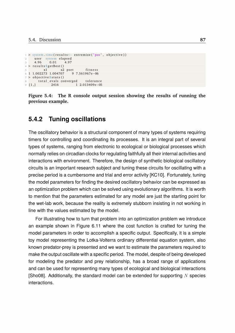
5.4. Discussion 87
1 > system . time ( r e s u l t s<− extremize ( " pso " , o b j e c t i v e ) )2 user system elapsed3 4.96 0.01 4.974 > r e s u l t s $ ge tBes t ()5 x1 x2 pse t f i t n e s s6 1 1.002273 1.004707 9 7.561967e−067 > o b j e c t i v e $ s t a t s ()8 t o t a l _ eva l s converged to l e rance9 [1 , ] 2416 1 2.013409e−05
Figure 5.4: The R console output session showing the results of running theprevious example.
5.4.2 Tuning oscillations
The oscillatory behavior is a structural component of many types of systems requiringtimers for controlling and coordinating its processes. It is an integral part of severaltypes of systems, ranging from electronic to ecological or biological processes whichnormally relies on circadian clocks for regulating faithfully all their internal activities andinteractions with environment. Therefore, the design of synthetic biological oscillatorycircuits is an important research subject and tuning these circuits for oscillating with aprecise period is a cumbersome and trial and error activity [KC10]. Fortunately, tuningthe model parameters for finding the desired oscillatory behavior can be expressed asan optimization problem which can be solved using evolutionary algorithms. It is worthto mention that the parameters estimated for any model are just the starting point forthe wet-lab work, because the reality is extremely stubborn insisting in not working inline with the values estimated by the model.
For illustrating how to turn that problem into an optimization problem we introducean example shown in Figure 6.11 where the cost function is crafted for tuning themodel parameters in order to accomplish a specific output. Specifically, it is a simpletoy model representing the Lotka-Volterra ordinary differential equation system, alsoknown predator-prey is presented and we want to estimate the parameters required tomake the output oscillate with a specific period. The model, despite of being developedfor modeling the predator and prey relationship, has a broad range of applicationsand can be used for representing many types of ecological and biological interactions[Sho08]. Additionally, the standard model can be extended for supporting N speciesinteractions.
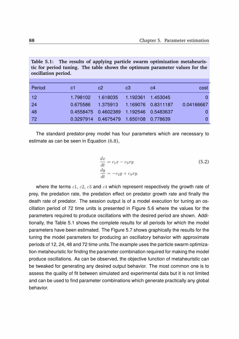
88 Chapter 5. Parameter estimation
Table 5.1: The results of applying particle swarm optimization metaheuris-tic for period tuning. The table shows the optimum parameter values for theoscillation period.
Period c1 c2 c3 c4 cost
12 1.798102 1.618035 1.192361 1.453045 024 0.675586 1.375913 1.169076 0.8311187 0.0416666748 0.4558475 0.4602389 1.192546 0.5483637 072 0.3297914 0.4675479 1.650108 0.778639 0
The standard predator-prey model has four parameters which are necessary toestimate as can be seen in Equation (6.8),
dx
dt= c1x− c3xy (5.2)
dy
dt= −c2y + c4xy.
where the terms c1, c2, c3 and c4 which represent respectively the growth rate ofprey, the predation rate, the predation effect on predator growth rate and finally thedeath rate of predator. The session output is of a model execution for tuning an os-cillation period of 72 time units is presented in Figure 5.6 where the values for theparameters required to produce oscillations with the desired period are shown. Addi-tionally, the Table 5.1 shows the complete results for all periods for which the modelparameters have been estimated. The Figure 5.7 shows graphically the results for thetuning the model parameters for producing an oscillatory behavior with approximateperiods of 12, 24, 48 and 72 time units.The example uses the particle swarm optimiza-tion metaheuristic for finding the parameter combination required for making the modelproduce oscillations. As can be observed, the objective function of metaheuristic canbe tweaked for generating any desired output behavior. The most common one is toassess the quality of fit between simulated and experimental data but it is not limitedand can be used to find parameter combinations which generate practically any globalbehavior.

5.4. Discussion 89
1 # Step 02 rm( l i s t=l s () )3 l i b r a r y ( evoper )4 s e t . seed (2718282)5
6 # Step 17 . . .8 f0 . per iodtuningpp<− func t ion (x1 , x2 , x3 , x4 , per iod ) 9 v<− predatorprey (x1 , x2 , x3 , x4 )
10 np<− naiveper iod ( i f e l s e ( v [ , " y " ] < 0 , . Machine$double . xmax , v [ , " y " ]) )11 r r e p a s t : : AoE .NRMSD(np$period , per iod )12 13 . . .14
15 # Step 216 o b j e c t i v e<−Pla inFunc t ion $new( f0 . periodtuningpp72 )17
18 # Step 319 o b j e c t i v e $Parameter (name=" x1 " ,min=0.2 ,max=2)20 o b j e c t i v e $Parameter (name=" x2 " ,min=0.2 ,max=2)21 o b j e c t i v e $Parameter (name=" x3 " ,min=0.2 ,max=2)22 o b j e c t i v e $Parameter (name=" x4 " ,min=0.2 ,max=2)23
24 # Step 425 r e s u l t s<− extremize ( " pso " , o b j e c t i v e )
Figure 5.5: Tuning the oscillation period of predator-prey model. The listinghas five sections identified by the tags Step 0 to Step 4. The first section consistsin loading the library and setting the random seed. The next section is wherethe cost function is defined, consisting in solving the initial value problem withprovided parameters and using the results of ODE for feeding the function namednaiveperiod for finding the periods in the differential equation output which islater compared with the reference period using a normalized root mean squaredeviation (AoE.NRMSD). The subsequent sections encompasses: the initializationof function to be optimized which is a wrapper for the previously defined costfunction; the definition of range of variation for the model parameters and finallythe application of the metaheuristic with the extremized function call.
5.4.3 Exploring the solution spaceThe particularities of individual-based models which make them so appealing for mo-deling populations and ecosystems, such as the structural realism, the predictive po-wer, the individual level stochasticity and the emergence of complex global dynamicsfrom the elemental interactions [GAR16] also imply that parameter estimation beco-mes a complicated matter even when using approximated techniques as those presen-ted in this work. Even simple models contain many levels of uncertainty and certainlypresenting nonlinear behavior and possibly discontinuities consequently it is very com-

90 Chapter 5. Parameter estimation
1 > system . time ( r e s u l t s<− extremize ( " pso " , f ) )2 user system elapsed3 225.89 0.01 226.164 > r e s u l t s $ ge tBes t ()5 x1 x2 x3 x4 pse t f i t n e s s6 1 0.3297914 0.4675479 1.650108 0.778639 1 07 > f $ s t a t s ()8 t o t a l _ eva l s converged to l e rance9 [1 , ] 672 1 2.013409e−05
Figure 5.6: The R console output session showing the results of running predator-prey model in Figure 6.11.
plicated, using a computationally tractable number of model executions, to make surethat the solution converges successfully to an optimum which is close to the bettersolution. Normally, modelers have not enough information about all model parametersand it is no uncommon to make assumptions or educated guesses for the acceptableranges considering the physical or biological constraints. Of course, it is not a randomchoice but it is far from being a perfect process and, despite of guessed parameterranges are hopefully within the same order of magnitude of their real values, usuallythey may diverge by a factor of two or three [MPN16] which may produce odd resultswhen adjusting several parameters.
It is worth noting that it should not be expected a perfect match between the modelpredictions and the experimental data, consequently it is very unlikely that optimizationalgorithms converge using the tolerance levels used normally for numerical optimiza-tion of plain functions. One way to tackle with this situation is defining the objectivefunction for the parameter estimation using a categorical approach with a not very strictrange of acceptance but that may lead to loosing information which may be relevantand giving the false feelling that the right parameter combination has been found. Thatis a serious issue which may render impossible to draw any conclusion from the pa-rameter estimation results. A possible alternative is not relying exclusively on the bestvalue ever found for the cost function but instead, leveraging the intermediate resultsfor analyzing the problem using it for building a landscape of solution space. The me-taheuristics described in this work have a slight modification for saving the partial bestresults for every interaction and the complete set of points visited in the problem solu-tion space which are made available as two methods of Estimates class, respectivelygetIterationBest() and getVisitedSpace(). Using these two methods the solution space

5.4. Discussion 91
0
5
10
15
20
0 25 50 75 100 125
time
valu
e
species
x
y
(a) pso, period: 12 time units
0
5
10
15
0 25 50 75 100 125
time
valu
e
species
x
y
(c) pso, period: 48 time units
0
5
10
15
0 25 50 75 100 125
time
valu
e
species
x
y
(b) pso, period: 24 time units
0.0
2.5
5.0
7.5
10.0
12.5
0 25 50 75 100 125
time
valu
e
species
x
y
(d) pso, period: 72 time units
Figure 5.7: An example of tuning the oscillation periods of predator-prey model.In this figure, we can observe how x and y species, respectively the prey and pre-dator components oscillates with different periods. The oscillations with periodsof 12, 24, 48 and 72 time units as can be seen respectively in subfigures (a), (b),(c) and (d).

92 Chapter 5. Parameter estimation
can be mapped for viewing the most promising zones. The code in Figure 5.8 showshow to generate a contour plot for the solutions space for a four variables instance ofRosenbrock function.
1 # Step 02 rm( l i s t=l s () )3 l i b r a r y ( evoper )4 s e t . seed (161803398)5
6 # Step 17 o b j e c t i v e<− Pla inFunc t ion $new( f0 . rosenbrock4 )8
9 # Step 210 o b j e c t i v e $Parameter (name=" x1 " ,min=−100,max=100)11 o b j e c t i v e $Parameter (name=" x2 " ,min=−100,max=100)12 o b j e c t i v e $Parameter (name=" x3 " ,min=−100,max=100)13 o b j e c t i v e $Parameter (name=" x4 " ,min=−100,max=100)14
15 # Step 316 r e s u l t s<− extremize ( " acor " , o b j e c t i v e )17
18 # Step 419 p1<− con tourp lo the lpe r ( v$ ge tV i s i t edSpace () [1:200 ,] , " x1 " , " x2 " , " f i t n e s s " )20 p2<− con tourp lo the lpe r ( v$ ge tV i s i t edSpace () [1:200 ,] , " x2 " , " x3 " , " f i t n e s s " )21 p3<− con tourp lo the lpe r ( v$ ge tV i s i t edSpace () [1:200 ,] , " x3 " , " x4 " , " f i t n e s s " )22 p4<− con tourp lo the lpe r ( v$ ge tV i s i t edSpace () [1:200 ,] , " x4 " , " x1 " , " f i t n e s s " )
Figure 5.8: Exploring the solution space for Rosenbrock function of four varia-bles using the Ant Colony Optimization for continuous domains (acor) algorithm.The sequence of steps is practically the same presented previously with the ex-ception of Step 4 which show the generation of four contour plots using the first200 values retuned by the getVisitedSpace() method which are sorted in ascendantorder by the fitness value.
The complete plot generated with the fourth step of command sequence providedin 5.8 is shown in Figure 5.9. These contour plots facilitate mapping and visualizingthe promising zones of solution space using the fitness of the solution generated asthe z value. The model parameters are disposed two by two making easy to find thezone where the best solution of adjacent parameters may be possibly situated. Thealgorithm employed was the Ant Colony Optimization for continuous domains whichhave not converged and the complete execution has required approximately 32K mo-del evaluations as the default options for the metaheuristic are 500 iterations using apopulation of 64 ants. The previous value is certainly not acceptable for a costly indivi-dual based model which may require from several hours to days for such high numberof evaluations. Thus, it is necessary to tune the metaheuristics for reducing the total

5.4. Discussion 93
number of iterations or alternatively using the algorithm introduced in this work ees2 formaking the initial tour to the solution landscape. The ees2 is not intended to find theminima but instead it is well suited for partitioning the problem space towards the goodsolution zones. The 5.10 shows the contour plots generated using ees2 which requiredjust 600 model evaluations for reducing the solution zone. The global minimum for theRosenbrock function of N variables is zero and is found setting all variables to 1.
The Figures 5.9 and 5.10 are demarcating the possible zones were the problemsolution can be found. In the case of Rosenbrock test function, which has been used inthese examples, the best solution is known a priori to be zero when all parameters are1. Thus, looking on the first plot, it can be easily observed that the hot zones markedwith best fitness are those corresponding the best problem solution. Nonetheless,the complete solution landscape encompasses a very wide zone when compared tothe solution estimated using the ees2 which shows a much more restricted portion ofsolution space. It is important to note that real models normally do not generate resultsso evident as those generated with test functions. Usually, the real individual-basedmodels will show discontinuities and possibly more than one zone with good fitnessvalues owing to the nonlinear or second order interaction between model parameters.
5.4.4 Comparing metaheuristicsThe task of choosing the most suitable metaheuristic for the parameter estimation pro-blem is not an easy one, mainly because the available algorithms behave differentlydepending on the problem type. It is also a consequence of intrinsic stochasticitypresent on individual-based models as well as the random nature of algorithms itself.Therefore, it is hard to provide general recipes for deciding what method is right fora particular problem instance. The algorithms enclosed in this work are tuned withthose parameters adequate for general cases but some tweaking may be required forachieving the best results. Specifically, the optimization metaheuristics can be verysensitive to the neighborhood structure and to the parameters controlling the balancebetween local search which accelerate the convergence speed and breadth of searchwhich may avoid to get stuck in local optima failing to converge to the best solution. Itmay be necessary some trial and error approach, testing different algorithms, obser-ving the convergence speed, the value of cost function and then tuning the algorithm

94 Chapter 5. Parameter estimation
parameters accordingly.
The application of optimization metaheuristics to individual-based models, as men-tioned previously, poses an additional problem because every model execution is com-putationally costly when compared to other models types and, because of that the costof the algorithm itself can be neglected. Therefore, one of the most important factorsfor selecting an algorithm is the minimal number of evaluations of objective functionswhich are needed for finding an acceptable solution satisfying the optimization target.Bearing this in mind, this section provides a systematic comparison between some ofthe metaheuristics mentioned in this work. The metaheuristics have been comparedusing the functions known as Cigar, Schaffer, Griewank and Bohachevsky [QLW+16][JY13] which are standard test functions commonly employed for benchmarking theoptimization algorithms. The benchmarks were performed using the four variablesversion of test functions and the experiments were replicated seven times using rand-omly selected initial random seeds2. The summarized numerical results obtained fromthe benchmark process are shown on Table 5.2.
2The details and the code used for the benchmark are enclosed along the package sources which areavailable on https://github.com/antonio-pgarcia/evoper

5.4. Discussion 95
Table 5.2: The output of benchmarking metaheuristics algorithms. These re-sults were produced using the function compare.algorithms1 included in packagedistribution and are the average values of seven replications with different ini-tial random seeds. The convergence values are the ratio of replications whichactually converged over the total number of performed experiments.
Function Algorithm Evaluations Convergence Fitness
Cigar saa 458.14 1.0 0.04702100pso 2621.71 1.0 0.05033806acor 2651.43 1.0 0.07268033ees1 332.86 1.0 0.06308869
Schaffer saa 649.57 1.0 0.07438586pso 6269.71 0.3 0.57479139acor 2249.14 1.0 0.08662474ees1 495.71 1.0 0.08821531
Griewank saa 501.00 1.0 0.04579390pso 4214.86 0.6 0.09860997acor 3812.57 1.0 0.07698225ees1 308.57 0.9 0.07089164
Bohachevsky saa 258.14 1.0 0.05232314pso 5053.71 0.4 0.44120018acor 1362.29 1.0 0.04323902ees1 258.57 1.0 0.06660127
The experiments were conducted setting a tolerance level of 10−1 in order to avoid atime-consuming process and for mimicking tolerance levels which may be relevant forindividual-based models which may be considered to converge with higher values thanplain mathematical functions. These values can be taken as a starting point for deci-ding what algorithm is most likely to provide acceptable results for the optima with lowernumber of model evaluations. The Figure 5.11 presents graphically the results for thebenchmark, showing the total number of model evaluations required for model conver-ging with the provided tolerance level. As can be observed, the evolutionary strategy 1(ees1) metaheuristic consistently require fewer evaluations of objective function thanthe other algorithms, excepting for the Bohachvsky function which required practically

96 Chapter 5. Parameter estimation
the same number of evaluations as the second better algorithm which is the simulatedannealing (saa). The third best algorithm is the ant colony for continuous domains(acor) followed by particle swarm optimization (pso) that curiously has not behavedas expected with the parameters tuned according to the recommended values [Cle12]and we are evaluating other combination of parameters and neighborhood functions.
The Figure 5.12 shows the value of objective function when the algorithm termina-tes wither when convergence criteria is met or when the algorithm reaches the max-imum number of configured iterations. It is important to note that the comparisonsshown here are just an initial set of hints for providing a general overview for behaviorof each of the algorithms mentioned in this work. The fact that simulated annealingalgorithm has been the best performer is the expected result because, differently fromother algorithms, it is using a population of size N = 1 which means that for each ite-ration only one individual problem solution is being evaluated. The other algorithms,by default are using values of N = 16, N = 64 and N = 10 respectively the numberof particles of particle swarm optimization, the number of ants of ant colony optimiza-tion and the solution size of evoper evolutionary strategy 1. This is one of the factorscausing the differentiate performance figures.
Consequently, the initial parameter set, defined of each algorithm, should be seenas the starting point for tuning the metaheuristics for achieving the desired results anda considerable amount of testing may be necessary for getting the best results for theparameter estimation process of a particular model instance. Additionally, some algo-rithm can be more adequate for a problem than another, therefore, checking the initialoutputs of multiple algorithms limiting the number of iterations, may be an interestingexercise for choosing the most suitable metaheuristic.
5.4.5 Parameter estimation of individual-based modelsOne of the remarkable aspects is that the syntax is simple and consistent independentof the function for which parameters are being estimated which means that the set ofAPI primitives required for applying the metaheuristics are the same independently ifthe target model is a plain mathematical function, an ODE, an individual-based modelimplemented in Repast or in any other environment for with an add-on have been im-plemented. The following example consists in the search for the best parameter com-

5.4. Discussion 97
bination which minimizes the discrepancies between the simulated values for bacterialconjugation produced using the BactoSIM simulation model [PRP15b] [PRP15a] andthe experimental values for conjugative plasmids taken experimentally [dCRC+12].The model provides several outputs but only two values will be used as reference forthe parameter estimation process: the conjugation rates and the doubling time for do-nor and transconjugant cells because experimental observations are available only forthese variables. Both model outputs conjugation rates and the doubling time are timeseries but we will just compare the first for every simulated time step and for the ge-neration time the overall average will be employed for defining the cost metric. Theconjugation rate metric used in the simulation experiments is the ration between thenumber of transconjugant cells and sum of transconjugant cells plus the uninfectedrecipients, defined as T/(T + R). For building the metrics for comparing both experi-mental and simulated time, two approaches have been explored, one using a simplemetamodeling [JDC03] [Sal08] using a linear model fit to the model output and the ob-served data and another using the dynamic time warping technique [LFLZ+15]. Thesealternative approaches are presented In Figure 6.7 where the functions my.cost1 andmy.cost2 shows respectively the implementations of cost function using a metamodeland the dynamic time warp algorithm[Gio09] for comparing experimental and simulatedconjugation rates time series. This example shows how to find the best combinationof model parameters which minimize the differences between the observed and thesimulated data for the simulated variables conjugation rate and doubling time.
The implementation of cost function shown in Step 1a creates two simple linearregression models of observed and simulated data for comparing the slope and theintercept coefficients which are serves as the distance metric for measuring how closeare both time series using root mean square deviations. The cost function also con-siders the values of doubling time for creating a composite metric. Additionally, thefunction my.cost1 uses a hybrid categorical-quantitative metric for the doubling timeoutput which is described in the Equations (5.3) and (5.4), respectively the costestimator for the doubling time of donors (D) and transconjugant (D) bacterial cells.Basically, the cost is zero if the values estimated by the model falls within a limitedrange around the average value of experimental data or the root mean square devia-

98 Chapter 5. Parameter estimation
tion (RMSD) between the simulated and observed values otherwise.
C(gD) =
0, if 42 ≤ gD ≤ 62
RMSD(gD, 52), otherwise.(5.3)
C(gT ) =
0, if 33 ≤ gT ≤ 53
RMSD(gT , 43), otherwise.(5.4)
In both cost functions my.cost1 and my.cost2, the first 60 minutes are eliminated frombeing used in the distance metric because during that time lapse the experimental datais a somewhat noise, possibly due to the lagging time or the adaptation to the culturemedium. It is also worth to mention that before undertaking a full length run, whichcertainly would last a large amount of time, would be much better start trying severalalgorithms with a limited number iterations for getting an initial map of problem solutionor using the ees2 metaheuristic which is limited to 600 evaluations of objective function.An example of an initial mapping for a real individual-based model is shown in Figure5.14. One of the things that can be perceived at a first glance is that this plot havemore diffuse borders delimiting the best zones of problem solution space than theexamples presented previously in Figures 5.9 and 5.10 where the object of study wereplain mathematical functions. That is the commonly observed pattern for real modelsowing to the stochasticity and the nonlinear iterations between the model elements.Hence, it is normally necessary to make several initial mappings of the problem forrecognizing the zones of best fitness and then making the adjustments on the initialparameter ranges for achieving best estimation results.
Returning to the Figure 5.14, despite of the lack of clearly defined limits for bestparameter combinations, it can be observed that some zones are generating bettercost values than others. Of course, the process should not be guided by just onealgorithm with a single run but a more exhaustive exploration with several runs of avai-lable algorithms, also using different sets of random seeds. But for the sake of brevityand just illustrating the process, we will extract conclusions from this single execution.Thus, the first contour plot which shows the parameters cyclePoint3 and conjugationCost
3The cycle point parameter represents the point of time, from cell birth to division when the conju-gation is most likely to happen.

5.4. Discussion 99
allows to detect interesting zones for both parameters circumscribed to those valuesbetween 25% and 75% with peaks for cyclePoint settled approximately over values of40% and 70% and the conjugationCost being close to the 50%. The plot relating theconjugationCost and the piliExpressionCost shows similar results for the first parameteras in the previous case, which have its better fitness values nearby the 50% of cellcycle, moreover the second has three promising zones at 25%, 40% and 70%. Finally,the last two plots, relating the piliExpressionCost–gamma0 and gamma0-cyclePoint arefar from being conclusive but seems to indicate better performances rounding the zoneof γ0 = 5. The next step in the analysis of parameter space may include refining so-mehow the initial assumptions about the parameter bounds, for instance, limiting theinitial range of parameter cyclePoint for the values found to contain better cost (25%-75%) and running again the exploratory analysis. Therefore, adjusting the range andrunning the simulated annealing algorithm with the maximum number of iterations limi-ted to 50, new results are obtained and presented on Figure 5.15. These exploratorysteps can be repeated a number of times before staring a complete run of metaheu-ristics.

100 Chapter 5. Parameter estimation
solution landscape for fitness ~ x1, x2
−40 0 40
−75
−50
−25
0
25
50
x1
x2
solution landscape for fitness ~ x3, x4
−50 0 50
−200
−100
0
100
x3
x4
solution landscape for fitness ~ x2, x3
−60 −30 0 30
−50
0
50
x2
x3
solution landscape for fitness ~ x4, x1
−200 −100 0 100
−40
0
40
80
x4
x1
Figure 5.9: Exploring solution landscape for visited space generated during theexecution of Ant Colony for Continuous domains (acor) algorithm. The four con-tour plots provides a panoramic view for the fitness surface of the variable pairs(x1,x2), (x2,x3), (x3,x4) and (x4,x1). The contour curves are employing a co-lor scheme, from light green to red for indicating the cost value, which meansrespectively the worst and the best fitness for the function.

5.4. Discussion 101
solution landscape for fitness ~ x1, x2
−2 −1 0 1 2
−1
0
1
x1
x2
solution landscape for fitness ~ x3, x4
−2 −1 0 1 2
−1
0
1
2
3
x3
x4
solution landscape for fitness ~ x2, x3
−1 0 1
−2
0
2
x2
x3
solution landscape for fitness ~ x4, x1
−1 0 1 2
−1
0
1
2
x4
x1
Figure 5.10: Exploring solution landscape for visited space generated during theexecution of EvoPER Evolutionary strategy 2 (ees2) algorithm. The four contour plotsprovides a panoramic view for the fitness surface of the variable pairs (x1,x2),(x2,x3), (x3,x4) and (x4,x1). The contour curves are employing a color scheme,from light green to red for indicating the cost value, which means respectivelythe worst and the best fitness for the function.

102 Chapter 5. Parameter estimation
(a) Cigar function
saa pso acor ees1
0
1000
2000
algorithm
eval
s
(c) Griewank function
saa pso acor ees1
0
1000
2000
3000
4000
algorithm
eval
s
(b) Schafer function
saa pso acor ees1
0
2000
4000
6000
algorithm
eval
s
(d) Bohachevsky function
saa pso acor ees1
0
1000
2000
3000
4000
5000
algorithm
eval
s
]
Figure 5.11: Comparing the number of objective function evaluations requiredfor each algorithm. The subplots show the average number of model evaluationswhich the metaheuristics required for reaching convergence using the benchmarkfunctions (a) Cigar, (b) Schaffer, (c) Griewank and (d) Bohachevsky. The meaningof the gray bar is that number of experiments which algorithm converge wereinferior to 60%.

5.4. Discussion 103
(a) Cigar function
saa pso acor ees1
0.00
0.02
0.04
0.06
algorithm
fitne
ss
(c) Griewank function
saa pso acor ees1
0.000
0.025
0.050
0.075
0.100
algorithm
fitne
ss
(b) Schafer function
saa pso acor ees1
0.0
0.2
0.4
0.6
algorithm
fitne
ss
(d) Bohachevsky function
saa pso acor ees1
0.0
0.1
0.2
0.3
0.4
algorithm
fitne
ss
]
Figure 5.12: Comparing the final value of objective function (fitness) for eachalgorithm. The subplots show the average fitness value for the benchmark functi-ons (a) Cigar, (b) Schaffer, (c) Griewank and (d) Bohachevsky. The meaning of thegray bar is that number of experiments which algorithm converge were inferiorto 60%.

104 Chapter 5. Parameter estimation
1 # Step 02 rm( l i s t=l s () )3 l i b r a r y ( evoper )4 s e t . seed (161803398)5
6 # Step 1a7 my. cos t1<− func t ion ( params , r e s u l t s ) 8 r e s u l t s<− r e s u l t s [ r e s u l t s $Time > 60 ,]9
10 mm1<− with ( r e s u l t s , lm(X . Simulated . ~ Time , data = r e s u l t s ) )11 mm2<− with ( r e s u l t s , lm(X . Experimental . ~ Time , data = r e s u l t s ) )12
13 r a t e<− AoE .RMSD( coef (mm1) [1] , coe f (mm2) [1]) + AoE .RMSD( coef (mm1) [2] , coef (mm2) [2])14
15 gT<− AoE .RMSD( i f e l s e (( r e s u l t s $G. T . > 41 & r e s u l t s $G. T . < 63) , 52 , r e s u l t s $G. T . ) , 52 )16 gD<− AoE .RMSD( i f e l s e (( r e s u l t s $G.D. > 32 & r e s u l t s $G.D. < 54) , 43 , r e s u l t s $G. T . ) , 43 )17
18 c r i t e r i a<− cbind ( rate , gT , gD)19 re turn ( c r i t e r i a )20 21
22 # Step 1b23 my. cos t2<− func t ion ( params , r e s u l t s ) 24 r e s u l t s<− r e s u l t s [ r e s u l t s $Time > 60 ,]25 alignment<−dtw( r e s u l t s $X . Simulated , r e s u l t s $X . Experimental , keep=TRUE)26 r a t e<− alignment$ d i s t ance27
28 . . .29
30 c r i t e r i a<− cbind ( rate , gT , gD)31 re turn ( c r i t e r i a )32 33
34 # Step 235 o b j e c t i v e<− RepastFunct ion$new( " / usr /models/BactoSim " , " ds : : Output " ,360 ,my. co s t )36
37 # Step 338 o b j e c t i v e $Parameter (name=" c y c l e P o i n t " ,min=1,max=90)39 o b j e c t i v e $Parameter (name=" con jugat ionCos t " ,min=0,max=100)40 o b j e c t i v e $Parameter (name=" p i lu sExp re s s i onCos t " ,min=0,max=100)41 o b j e c t i v e $Parameter (name="gamma0" ,min=1,max=10)42
43 # Step 444 o b j e c t i v e $ se tTo le rance (0 .1)45
46 my. opt ions<− OptionsACOR$new()47 my. opt ions $ se tVa lue ( " i t e r a t i o n s " , 30)48
49 # Step 550 r e s u l t s<− extremize ( " acor " , ob j e c t i v e , my. opt ions )
Figure 5.13: The code required running the parameter estimation for anindividual-based model using the Ant Colony Optimization algorithm. This codesnippet shows the implementation details for two alternative implementations ofcost function. As can be seen, the sequence of steps required are: Step 0 loadingthe required libraries and sets the random seed; The Step 1a and Step 1b are theimplementation of two alternative cost functions one using a metamodel fitted tothe simulated data and another the dynamic time warping distance as the costmetric; Step 2 Creates an instance of a RepastFunction class for the underlyingmodel, initializing the model directory and the total simulated time; The Step 3initialize the model parameters of interest which can be a subset of all declaredparameters; The Step 4 shows the creation of a non-default options class for set-ting the maximum number of algorithm iterations to 30; Finally, in the Step 5 theextremize function perform the optimization of cost function.

5.4. Discussion 105
fitness ~ cyclePoint, conjugationCost
0 25 50 75
0
25
50
75
100
cyclePoint
conj
ugat
ionC
ost
fitness ~ pilusExpressionCost, gamma0
0 25 50 75 100
2.5
5.0
7.5
10.0
pilusExpressionCost
gam
ma0
fitness ~ conjugationCost, pilusExpressionCost
0 25 50 75 100
0
25
50
75
100
conjugationCost
pilu
sExp
ress
ionC
ost
fitness ~ gamma0, cyclePoint
2.5 5.0 7.5 10.0
0
25
50
75
gamma0
cycl
ePoi
nt
Figure 5.14: The mapping of solution space of BactoSIM individual-based modelof bacterial conjugation dynamics. The series of four contour plot shows theeffects on the fitness value, defined by the cost function my.cost1, for the differentvalues of parameter explored by the optimization algorithm.

106 Chapter 5. Parameter estimation
fitness ~ cyclePoint, conjugationCost
20 40 60 80 100
0
25
50
75
100
cyclePoint
conj
ugat
ionC
ost
fitness ~ pilusExpressionCost, gamma0
0 40 80 120
0
4
8
12
pilusExpressionCost
gam
ma0
fitness ~ conjugationCost, pilusExpressionCost
0 25 50 75 100
0
40
80
120
conjugationCost
pilu
sExp
ress
ionC
ost
fitness ~ gamma0, cyclePoint
0 4 8 12
20
40
60
80
100
gamma0
cycl
ePoi
nt
Figure 5.15: Refining the initial mapping of solution space of BactoSIM limitingthe variation range of cyclePoint parameter based on the previous mapping results.

5.5. Summary 107
5.5 SummaryThe systematic parameter estimation should be a fundamental part of individual-basedmodeling but it is normally omitted by modelers. One of the main reasons is the re-lative complexity of available methods, the effort required for applying them and thelack of simple tools for the practitioners which usually come from different domainswith different backgrounds. Ecology has always greatly benefited from the applicationof mathematical models to the description of complex processes and iterations. Re-cently, Individual-based models are becoming a lingua franca for ecological modelingbut normally the acceptance of results produced are hindered by lack of a thoroughparameter estimation and analysis. The cause may be attributed to the deficit of expe-rience with methods and techniques required for carrying out the analysis of simulationoutput. The individual-based models are complex, stochastic and non-linear in theirnature, therefore the evaluation input parameters for making the model reproducingreliably the reference data is a hard computation task. The best available approachis to estate the parameter estimation as an instance of an optimization problem andapply the existing arsenal of optimization metaheuristics.
Beating this in mind, we have introduced in this work the partial set of featuresavailable on EvoPER package alongside with illustrative usage cases, including oneapplication to a real individual-based model with the interpretation of outputs producedand the steps necessary to the complete parameter estimation of the model. Thepackage is being developed keeping in mind the idea of minimizing the effort requiredto the application of sophisticated methods in the parameter estimation process ofIndividual-based models. This package allows the modelers to try different alternativeswithout having to code ad hoc and complex integration code to the existent packages.

108 Chapter 5. Parameter estimation

Chapter 6Sensitivity analysis of
individual-based models
6.1 Introduction . . . . . . . . . . . . . . . . . . . . . . . . . . . . . . . . . 111
6.1.1 Model development . . . . . . . . . . . . . . . . . . . . . . . . 114
6.1.2 Sensitivity analysis . . . . . . . . . . . . . . . . . . . . . . . . . 116
6.2 Overview of R/Repast package . . . . . . . . . . . . . . . . . . . . . . 123
6.2.1 Design . . . . . . . . . . . . . . . . . . . . . . . . . . . . . . . . 124
6.2.2 The R/Repast R API . . . . . . . . . . . . . . . . . . . . . . . . 126
6.2.3 The objective function interface . . . . . . . . . . . . . . . . . . 131
6.3 Examples overview . . . . . . . . . . . . . . . . . . . . . . . . . . . . . 132
6.4 Example 1: BactoSIM . . . . . . . . . . . . . . . . . . . . . . . . . . . 134
6.4.1 Model analysis . . . . . . . . . . . . . . . . . . . . . . . . . . . 135
6.5 Example 2: Predator-Prey . . . . . . . . . . . . . . . . . . . . . . . . . 136
6.5.1 Model description . . . . . . . . . . . . . . . . . . . . . . . . . 136
6.5.2 Entities, State variables and scales . . . . . . . . . . . . . . . . 137
109

6.5.3 Model analysis . . . . . . . . . . . . . . . . . . . . . . . . . . . 139
6.6 Example 3: T4SS Common Pool . . . . . . . . . . . . . . . . . . . . . 142
6.6.1 Model description . . . . . . . . . . . . . . . . . . . . . . . . . 142
6.6.2 Process overview and scheduling . . . . . . . . . . . . . . . . 143
6.6.3 Analysis of model . . . . . . . . . . . . . . . . . . . . . . . . . 145
6.7 Summary . . . . . . . . . . . . . . . . . . . . . . . . . . . . . . . . . . 147

6.1. Introduction 111
6.1 Introduction
Computational ecology is a relatively young field which relies extensively on mathemat-ical computational methods and models for studying ecological and evolutionary pro-cesses. It is based on the construction of predictive and explanatory models as well asthe quantitative description and analysis of ecological data [HCD+95] [PPH+12]. Thecontinuous growth of computational power available for and end users, the existenceof tools and the constant increment of empirical data available, makes viable for manyscientists to develop and simulate tremendously complex models from their desktops.In addition, the intrinsic characteristics of ecological processes, maxim their temporaland spatial scale [DLM00], converts the task of carrying out controlled experiments aphysical impossibility. Hence, in most cases the only feasible alternative is to simulatethe process in order to make experiments spanning the full length of ecological andevolutionary scales. The computational ecology has its roots from the successful re-sults achieved from mathematical ecology which has proven to be an essential tool forunderstanding the complexities which arise from ecological interactions.
It is a widely accepted that simple models with a small number of state variablesand parameters provide best generalizations than the complex ones [Smi74] [EGJ+13]with a clear distinction between simulation models and theories as separate entitieshandling different kind of problems. It has been recently questioned the correctnessof the idea the simple models lead to generality in ecology [EGJ+13]. We believe thatthe parsimony principle must always be taken into account when developing models,but this has a different meaning depending on the modeling formalism we are using.Simplicity does not have the same meaning when the referred modeling formalism isa deterministic ODE or when it is applied to Agent-based modeling, as long as everymodeling techniques has its own idiosyncrasy and constraints. The Agent-based mo-deling is a flexible and versatile abstraction where the whole system under study isdescribed or formalized by its component units, which facilitates a more natural des-cription of a system and the comprehension of individual properties leading to theemergent phenomena [Bon02].
The Agent-based models (AbM) are much more fine-grained than their whole-population aggregated counterpart and as consequence they tend to be more complexrequiring more equations, parameters and processes in order to represent the same

112 Chapter 6. Sensitivity analysis of individual-based models
phenomenon. That is not intrinsically a problem or a quality but simply a constraintimposed by the modeling formalism in use and it is up to the modelers to find the cor-rect tradeoff between the purpose of the model and the level of details which shouldbe part of the model structure.
The AbM have been being established progressively as a main-stream and valua-ble tool for modeling complex adaptive systems in many distinct areas of knowledge,ranging from social science, economics to any flavor of computational and systemsscience such as biology, ecology and so on [GR05b]. The reason is, amongst otherthings, the relative ease with which detailed structural information can be incorpora-ted into a model without the constraints of other methodologies [HB09]. Nonetheless,the possibility of incorporating many details comes with the cost of models with a highcomplexity level, containing many rules and parameters for which the exact valuesare, in many cases, hard or impossible to determine experimentally, that is what isknown as parameter uncertainty. When used in the context of ecological systems theAgent-based modeling is also known as Individual-based modeling (IbM) [GR05b].
The distinctive aspect defining what is an IbM is that individuals are representedby discrete entities and they also have a property or state variable which are uniquein the population being simulated [Ber02]. Hence IbM is a valuable abstraction for si-mulating populations, communities or ecosystems capturing the individual variability,randomness and their complex dynamics. It is a bottom-up approach where the sys-tem under study is modeled using mechanistic explanations on the interacting systemparts [FPL08]. Therefore, the global behavior shown by the system as a whole, is anemergent property derived from the local rules defining the individuals. That is par-ticularly useful testing different hypothesis or phenomenological explanations for theindividual processes in order to verify which of them are producing the global obser-ved behavior [Pas05]. Moreover, differently from aggregate models, it is customarythat IBM have a large number of state variables and parameters which in most ca-ses are hard or directly impossible to elucidate experimentally leading to many levelsof uncertainty in this kind of models. In order to tackle with the uncertainty and formaking robust predictions, we have to use a sound methodology for applying what-ifanalysis to check how stable are the model outputs when varying the input parameters[TKG14]. There exist a large set of mathematical tools for analyzing the model outputwhich are known generically as sensitivity analysis. Normally applying these techni-

6.1. Introduction 113
ques are cumbersome, requiring a lot of effort from modelers, hindering the throughoutanalysis of computational models.
According to [TKG14] the most of Individual-based models published tends to omitthe systematic analysis of model output, mainly because modelers normally do nothave the specific knowledge to implement the required methods. Therefore, it seemsclear, that the availability of simple and user friendly tools for experiment design andanalysis would greatly help modelers to improve the formal quality of their models.
In other scientific fields, which are strongly rooted on an extensive experimenta-lism, is practically impossible to conduct any kind of research without a well-designedexperimental setup and a further statistical analysis and hypothesis test. Perhaps thereasons are that these experimental fields already have a complete and mature toolboxfor design and evaluation of experiments [LH78] [MW95] leaving no room for devia-tion from these standards. On the other hand, in silico based experiments are still onearly stage and verification and validation procedures are not well established yet. Inaddition, the real value of a computational model depends much on the ability of otherresearchers to reproduce and enhance the results elsewhere; in other words, resultsmust be reproducible. Hence, in order to achieve reproducibility, research methodsshould be stated clearly and should preferentially being backed by standard methodsand software tools.
Bearing this in mind we introduce R/Repast a GNU R package for running Repast[NCO+13b] models from GNU R environment as well as for carrying out global sensi-tivity analysis on the model results. In the following sections we will contextualize theproblem providing a basic background for understanding what is being addressed inthis work and we will also provide a basic description about the package functionalities.Finally, we will show three worked examples on how the package can help modelersto make the conclusions drawn from model results much more robust. The first ex-ample explores the basic aspects of bacterial conjugation process. The second is anindividual-based implementation of the classic predator-prey model enclosed as partof the standard Repast Simphony distribution. Finally, the last example was developedex professo for this work and it is an instance of common pool problem in the context oftwo plasmids ”sharing” the genes required for the expression of conjugative system.

114 Chapter 6. Sensitivity analysis of individual-based models
Background
6.1.1 Model developmentModel development is an iterative and objective driven activity and the first step requi-red to develop a model is to have a clear and ideally unambiguous statement about themodel purpose. Therefore, every experimental study carried out using modeling andsimulation should follow the experimental life cycle based on the successive sequenceof four cyclic steps, starting from (a) Conjecture, which defines the model purpose andwhy the model is being developed; (b) Design phase where the model is translatedto some runnable implementation; (c) Experiment step which means the execution ofmodel following a well-established plan oriented to confirm or reject the initial conjec-ture and finally the (d) Analysis step where the data generated in the previous step isanalyzed with a sound methodology which, hopefully will generate new insights, un-cover model flaws and iteratively improve the initial conjecture and design [BD87]. Asimple graphical representation of these four iterative steps is shown in Figure 6.1.
ModelBuilding
Model Purpose
Hypothesis
Rules/
Equations
Coding
Design
Experiment
Analysis
Sen
sitivityAnalysis
Figure 6.1: The iterative model development life cycle. This figure shows the re-lationship between the modeling phases and their associated tasks when appliedto an individual-based model.
Part of design phase consist in convert the model equations and rules to a computer

6.1. Introduction 115
code implementation. Currently there are several frameworks available for developingindividual-based models. These frameworks are designed to address some specificrequirement such as usability [TW04], flexibility or scalability [NCO+13b, LCRP+05] orsupport to multiple modeling paradigm, such as AnyLogic [ESJ07]. Certainly, the mostwidespread framework in ecological modeling is NetLogo [TW04] which is consideredto provide an easier development environment based on extensions to Logo paradigmespecially suited for those which are not much familiar with modern programming lan-guages. One of the main drawbacks of NetLogo is the scalability. NetLogo tends toshow some performance issues when simulating a large number of agents. On the ot-her hand, Repast Symphony framework has a steep learning curve but provides a fastand flexible java-based environment with many interesting features for simulating largescale computational ecology models. These features include, amongst others things,the integration with Weka, exporting the model output to R environment, support forrunning distributed batch simulations and some built-in facilities for parameter swee-ping [NCO+13b]. Finally, Mason is, in some extent, very similar to Repast but lessmature than it is; It has been designed focusing on providing faster execution speeds[LCRP+05]. The only of these frameworks providing integrated sensitivity analysis ca-pabilities is AnyLogic, the other frameworks: NetLogo, Repast and Mason which areall free software do not have built in support to sensitivity analysis.
The Repast framework is widely used in many different fields for building individual-based simulation models of dynamic processes [WNF+15] [GBP+15] [TLNV15]. Inaddition, Repast also has a framework for high performance computing using the C++programing language with similar conceptual entities as those found in Repast-java.Repast also has support for running GNU R code [R C15] [Cra07] from inside the userinterface but until now it has not been feasible to run Repast models from R envi-ronment for controlling model in order to implement experimental designs, calibration,parameter estimation and sensitivity analysis, therefore hindering a throughout andcomprehensive validation of Individual-based models developed using Repast Simp-hony.
116 Chapter 6. Sensitivity analysis of individual-based models
6.1.2 Sensitivity analysis
Because of sensitivity analysis is a broad and complex subject, a throughout discus-sion would be lengthy and out of the scope of this work. Instead we will try to providea more amenable and practical approach keeping the discussion at a general level butrigorous enough to let the practitioners gain the knowledge required to understand,apply and interpret the results. For a more detailed review please refer to [STCR04][PBF+16]. It is interesting to start the discussion providing the exact meaning of somethe many expressions which are used commonly in the analysis of models. Thereare several terms used in the context of sensitivity analysis for which is important toprovide the formal meaning. For instance, the jargon of sensitivity analysis includesmodel calibration and parameter estimation which many times are used as they wereequivalent, even though they are different objectives. Other terms such as uncertaintyanalysis, omitted variable bias, objective function or cost function are also importantpart of SA lexicon.
Generally speaking, the objective of SA is to understand the effect of varying inputfactors on the model output [STCR04]. Under this very general statement we have awide range of methods and techniques which are suitable for distinct kinds of models.In order to improve this definition, it is convenient to provide a more formal definition tothe entity which is the target of SA: the model. Formally speaking, a model is a functi-onal relation between a number k of input factor, also called independent or predictorvariable and the output variable, sometimes referred as dependent or response varia-ble [BD87] as depicted by the expression η = f(x1, x2, . . . , xk), being η is the averagevalue of response variable considering any specific setting for the input factors xi. The-refore the value of a single model run is given by y = f(x1, x2, . . . , xk) + ε, where ε isdifference between the value of y and the expected value E(y) = η. The error ε isconsequence of stochasticity introduced by design in the structure of model to capturethe population variability. Finally, recognizing that most real world models usually havemore than one response variable, the structure of an individual-based model M can begeneralized for n outputs as can be seen below

6.1. Introduction 117
M =
y1 = f1(x1, x2, . . . , xk) + ε
y2 = f2(x1, x2, . . . , xk) + ε...yn = fn(x1, x2, . . . , xk) + ε
Therefore, being yi some output of model M, the model calibration process con-sists in comparing these outputs to some reference values [ZPK00] which are nor-mally, in the case of ecological or biological studies, experimental or observed data.The target of calibration process is minimizing the discrepancies between simulatedand reference values. The function used for computing how far yi output is from thereference values is known as objective function or cost function. There are manyoptions for implementing the objective function and the only requirement is that thereturn of objective function should be inversely proportional to the quality of fit, beingzero the return value for the perfect fit. Common implementations for objective functionare based on the definition of acceptable ranges, least squares or even a combinationof both. For instance, let yi be the output of some hypothetical model M, assumingthis variable represents the net reproductive rate R0. The reference values Rv for theoutput variable must fall between 0.8 and 1.2, hence any yi value within this interval isconsidered to have a perfect fit, bearing this in mind the cost function could be givenby the following expression
C(yi) =
0, if 0.8 ≤ yi ≤ 1.2
1, otherwise
That is what is known as categorical calibration criteria [TKG14]. The main draw-back of this approach is that it does not provide any information about how far is theresponse value from the reference value. A better alternative is to apply some dis-tance function d(yi, Ry) to the output and the reference values, even standalone or incombination with categorical calibration. The most commonly used metric is some ofthe multiple forms of squared deviation but any distance function can be alternativelyemployed as long as two properties hold: d(yi, Ry) = 0 if xi and Ry are equal andd(yi, Ry) > 0 when xi and Ry are not equal.
Whilst calibration is a general term, meaning fundamentally the comparison of

118 Chapter 6. Sensitivity analysis of individual-based models
some value to a reference value, the term parameter estimation has a more subtleand specific goal. The parameter estimation is normally considered an inverse pro-blem because the objective is finding the values for the model parameters providingthe best adjustment to the reference values. In other words, knowing the expectedvalues for response variable the target is estimating the suitable values for the mo-del parameters. Usually the terminology parameter refers to the constants which arepart of models with clear distinction between parameters and independent variables,[BA77], for instance in the growth differential equation shown below
dN/dt = rN
the model parameter would be only the growth rate r and the independent variable thetime, but for the purpose of this work we consider indistinctly the model constants andindependent variables as being parameters.
The two main objectives of sensitivity analysis are understanding how robust arethe model results considering the existing uncertainties and quantifying the effect ofinput factors on the variance of output [STCR04] [PBF+16] [Law05]. The intrinsic cha-racteristics of individual-based models which relies on mechanistic descriptions favorsthe production of models with many sub-processes, state variable and parameters.The design is normally based on incomplete knowledge resulting in several levels ofuncertainties in the model parameters, in the model response variables and in the mo-del structure itself. The model structure is also related to the identifiability problemwhere not all model parameters can be uniquely estimated. The sensitivity analysiscan be also used for assess the effect of model structure on the output considering thealternative model implementations as being another parameter. This can be useful foranalyzing the omitted variable bias, which basically means that some parameter ofmodel can be over or under-estimated because another important parameter was notincluded in the model structure. The sensitivity analysis can be carried out letting theparameters varying over the full range of parameter space or restricted to a small re-gion close to the average value, respectively referred as global sensitivity analysis andlocal sensitivity analysis. Sensitivity analysis can also be performed varying one fac-tor at time (OAT) leaving all others fixed or varying all factors at the same time (AAT).The application of second method is required in order to capture interaction between

6.1. Introduction 119
parameters and non-linear effects.
The central point of SA methodology is the estimation of sensitivity indices or coef-ficients. The sensitivity coefficients allow the quantitative comparison of the contribu-tions from distinct parameters to the model output. In its classical form [BA77] thesensitivity indices are defined as the first derivative with respect to some model para-meter xi. Considering the general model y = f(X), being X the parameter vector ofsize k, the sensitivity index Si is given by
Si =∂Y
∂xi
It is also important to take into account that the partial derivatives can have differentunits, hence can be necessary to scale them in order to make them comparable. Inthis approach, input factors are perturbed one-at-time, being that measure of sensitivitysuitable for local SA [PBF+16].
Several methods for estimate sensitivity indices which are adequate for global sen-sitivity analysis are available, such as meta-modeling approach [HKB06], correlationbased methods, regression based methods, Fourier Amplitude Sensitivity Test (FAST)[XG11], for a more in depth discussion please refer to [TKG14] [STCR04] [Sal08][PBF+16] [PIwcfSDV+15]. The Figure 6.2 show how are related the different met-hods for assessing the importance of input factors in simulation models, also includingscreening techniques [BK96] [AH93]. In this work we will focus on those methods ba-sed on the variance decomposition which are suitable for a wide range of situations,including those which are commonly found in individual-based models, such as non-linear mappings between input factors and outputs variables [ZR06]. In addition tofirst order effects, the variance decomposition methods, also allows the quantificationof second order effects sometimes referred as total order effects. Total order effectsindices are useful for the assessment of the interaction between factors which cannotbe expressed by a simple lineal superposition.

120 Chapter 6. Sensitivity analysis of individual-based models
SensitivityAnalysis
LocalSensitivityAnalysis
GlobalSensitivityAnalysis Regression
basedmethods
Partial RankCorrelationCoefficient
StandardizedRank
CorrelationCoefficient
Variancedecomposition
Fourrier
FANOVASobol
Screening
MorrisElementary
Effects
IteratedFractionalFactorialDesigns
SequantialBifurcation
Figure 6.2: The different types of sensitivity analysis and their associated met-hodologies and techniques.
One of main drawbacks for applying variance decomposition methods on largespatially explicit individual-based models is the requirement of very high number ofmodel evaluations in order to produce consistent results [HKRW13]. An alternative

6.1. Introduction 121
approach, in those cases where it is impractical or computationally unfeasible a fullyquantitative analysis, is the application of the Morris screening method. The Morrismethod deliver qualitative information allowing to rank the importance of input factorsrequiring less model evaluations, which in some case can one order of magnitudeinferior to the Sobol method [Sal08].
The Sobol is a method for sensitivity analysis based on the decomposition of thevariance of model output and is particularly suitable for discovering the effect of highorder interactions between input factors. The interaction means non-linearity wherethe total effect of two input factors x1 and x2 on the model output Y are not equivalentto the sum of the individual effects. The general form of sensitivity indices for Sobolmethods are shown in Equation (6.1) and Equation (6.2), respectively the first orderand total order indices.
Si =Vi
V (Y )(6.1)
ST i = 1− V (Y )− ViV (Y )
, (6.2)
where the terms Vi and V (Y ) are respectively the variance contribution attributed tothe ith parameter and the total variance. The expression V (Y )−Vi represents the totalvariance with exception of the variance which is generated by the parameter i. The totalorder index STi is the contribution of all input parameters but one, the ith parameter,and hence estimating the effect of that parameter on the variance reduction [Sal08].
The total variance V (Y ) for a model with n input parameters can be expressedas shown in Equation (6.3) as long as the orthogonality of input factors preconditionholds.
V (Y ) =∑i
Vi +∑i<j
Vij +∑i<j<k
Vijk + · · ·+ V12...n, (6.3)
being V (Y ) the total variance from model output and the components Vi, Vij and Vijkrespectively the variance contribution from the parameter i, the variance contributionform input parameters i and j and the variance contribution form input parameters i,
122 Chapter 6. Sensitivity analysis of individual-based models
j and k. Finally, the component V12...n express the interactions from all parameterspresent in the model.
The application of Sobol method, as have been mentioned, can be computatio-nally expensive and sometimes could be useful to reduce the problem dimensionalityfiltering only the most significant parameters or even simplifying the model structureconsidering only the parameters accounting for the most of the variability in the mo-del output. It can be accomplished using the Morris screening method to rank theimportance of input parameters. The Morris method is an OAT method, meaning thatit changes just one factor keeping all other input parameters fixed. The input factorsare allowed to vary in discrete levels within the relevant parameter range [Mor91]. Themethod is considered to be more effective when the number of most significant inputparameters are a small subset of model parameters [STCR04].
The original work of Morris [Mor91] define two metrics for ranking input factorswhich are depicted by µ and σ values1. Further, another metric termed µ∗ has beensuggested by [CCS07] which use absolute values in order to handle effects of distinctsigns canceling each other. These metrics for ranking input factors are calculated fromwhat has been termed elementary effects. Therefore, considering a model with k inputparameters and being X = (x1, x,2 , . . . , xk any value from the region of experimentationΩ, the elementary effects are calculated according to the Equation (6.4).
eei(X) =y(x1, . . . , xi−1, xi + ∆, xi+1, . . . , xk)− y(X)
∆(6.4)
The region of experimentation Ω is a grid defined by the number of k input factorsand by the p discrete levels for every parameter. The recommendations for the valuesof p and ∆ are respectively that the first should be an even number of levels and thesecond calculated by the expression ∆ = p/(2(p − 1)) [Mor91] [STCR04]. The valueof ∆ has important implications in the model analysis. It has been shown that in somesituations choosing an alternative value calculated as ∆ = 1/(p − 1) can detect non-monotonic behaviors that the suggested standard calculation are not able to captureotherwise [vHBC11].
The metrics of Morris method are calculated over the Fi and Gi distributions for1Not to be confused with population mean and standard deviation

6.2. Overview of R/Repast package 123
every input parameter. These distributions are generated taking random samples of X
from Ω for calculating the elementary effects and the only difference between them isthat Gi uses the absolute values of elementary effects
∣∣eei(X)∣∣ as described in [CCS07]
[Sal08]. The estimation of Morris metrics are carried out by taking r samples from Fi
and Gi distributions according to the Equations (6.5), (6.6) and (6.7).
µ =r∑
i=1
eei(X)
r(6.5)
µ∗ =r∑
i=1
∣∣eei(X)∣∣
r(6.6)
σ =
√√√√ r∑i=1
(eei(X)− µ)2
r(6.7)
These three metrics can be used to extract valuable information about the modelbehavior, in addition to ranking the input factors. For instance, a low value of µ and ahigh value of µ∗ is high, points that the input factor under scrutiny, possibly has a non-linear behavior having different signs in function of the system trajectory [STCR04]. Ahigh value of µ indicates that the input has a monotonic effect on the model output.
The sensitivity analysis methods require significant samples from input space inorder to provide reliable results. It is customary to choose between some experimentaldesign [Hic93] for generating the collection of input parameters needed by evaluatingthe model and allocating the variance contribution of every model parameter. Themost generally applied sampling schemas are based on random sampling, full factorialdesigns or Latin hypercube sampling.
6.2 Overview of R/Repast packageIn the previous sections we have seen some fundamental ideas on model building andthe role occupied by sensitivity analysis methods in the iterative modeling life-cycle.We have also introduced the basic principles of sensitivity analysis focusing on twomain techniques namely the Morris Elementary Effects Screening [Mor91] and theSobol GSA method for variance decomposition [Sal08]. Both methods have a wide

124 Chapter 6. Sensitivity analysis of individual-based models
range of applicability, making them suitable for their use in the analysis of Individual-based models. These methods require the model be evaluated many times with adifferent set of input parameters, making completely impractical undertaking a manualanalysis introducing individual parameters manually on a graphical user interface. TheRepast is an extremely flexible framework for object-oriented development of Agent-based models using Java language but it lacks from model analysis tools. On theother hand, the GNU R is a superb open source tool for data analysis with a vast andactive community developing and adding new methods to the core R system. Bearingthis in mind, we introduce our package R/Repast which bring together the best ofboth worlds. Roughly speaking, the R/Repast package have two main objectives: (a)Provide an interface for running Repast models from R and gathering the simulationdata generated and (b) Automating the application of sensitivity analysis and simplemodel calibration methods to the Repast models. The R/Repast is an open sourceproject delivered under the MIT license system. The package provides a powerfuland simple R API2 which reduces the code required for running the most commonlyused experimental methods suitable for . The software and the user manual can bedownloaded from CRAN website and the complete project source code from GitHubrepository. Both are available respectively from the following URLs:
• https://cran.r-project.org/web/packages/rrepast/
• https://github.com/antonio-pgarcia/RRepast
6.2.1 DesignThe R/Repast was intended primarily for invoking Repast Simphony models from in-side GNU R environment. Additionally, the package contains more high level and valueadded features for experimental design and experiment analysis to address the speci-fic need of individual-based models. The underlying implementation idea is to providea set of turnkey features for facilitating the task of applying the sensitivity analysis tomodels. Functionally, the package consists in four modules which interoperate toget-her for instantiate and running the Repast code inside R. All these four components
2Application Programming Interface

6.2. Overview of R/Repast package 125
are (a) the Repast Integration Broker, (b) the Repast Integration Engine, (c) The R In-tegration wrapper and finally, (c) the R API for Experiment design. An schematic viewof package architecture is shown in Figure 6.3.
R/Repast
Engine
R/Repast
Integration Broker
JVMR
R Integration
Wrapper
R/Repast
R API
Y = f(X)
User defined RepastModel
User defined R code
running Y = f(X)
Figure 6.3: The approach for wrapping an individual-based model using the R/-Repast general architecture. The scheme shows in the left box the R environmentand the associated components of R/Repast. The right box represents the RepastSimphony model running within a Java Virtual Machine as well as the R/Repastintegration broker component.
The R/Repast integration broker and the R/Repast engine are both written in javacode and are required for instantiating and loading the Repast Simphony model in ba-tch mode. The R/Repast engine contains also the required hooks for transferring themodel output data from Java to R environment. The engine can transfer data fromaggregated data set defined by the modeler on the Repast model. An aggregateddata set is a Repast Simphony entity used for collect data about the simulation modelagents which can be used for plotting or saving the model output data to a file usinga file sink. A File Sink is Repast component for saving simulation data to a file. The

126 Chapter 6. Sensitivity analysis of individual-based models
aggregated datasets use some kind of aggregate operation, such as counting, avera-ging, summing or any other used defined aggregate operation [NCO+13a], [NCO13c],[NCO+13d]. The R integration wrapper is the R code for linking together the R and Re-past subsystems. This module consist in several wrapping functions for encapsulatingthe Java code calls implemented using the rJava package [Urb16]. These functions areprefixed with the [Engine] keyword and, although exported in the R/Repast package,they are not intended for general use.
6.2.2 The R/Repast R APIThe module entitled R/Repast R API is the primary entry point for the user definedcode and relies on the subsystems mentioned previously for providing three group offunctionalities for facilitating modelers to analyze the simulation output. These groupfunctionalities are the following:
• Execution and control of Repast Simphony code.
• Basic functions for experimental design.
• High level functions for a complete experiment in one call.
The functionalities on the first group are those required for the basic interface be-tween Repast and R system, such as instantiating and running a Repast Simphonymodel, retrieving the declared model parameters, getting their default values, settingparameter values as well as running basic experimental designs and saving simulationdata. The partial list of these basic R/Repast API methods are shown in the followingboxes:
Model(d, t, o, l)
This function creates an object instance for linking the Repast model to an Robject. The required parameters are the directory where the model has beeninstalled (d), the duration of simulation in Repast ticks (t), the name of any ag-gregated dataset of model for draining data generated by the model simulation(o) and a Boolean flag (l) which tells the function to call the Load method. Thedefault value is FALSE.

6.2. Overview of R/Repast package 127
Load(m)
This function loads the Repast scenario from model’s directory. The only requi-red parameter (m) is an instance of Repast Model created with previous function.
Run(m, r, s)
The purpose of this function is to execute a single round of simulation using justone parameter set. The parameters for this function are a model instance (m),the number of repetitions (r) and a collection of random seeds (s) to be used foreach one of the repetitions. The only required parameter is the model instance,created with the Model() function. The default value for r is one.
RunExperiment(m, r, d, F)
Execute a complete experimental setup for different sets of parameters. Theparameters required are a model instance (m), the number of replications (r),the experimental design (d) and finally a user provided calibration function (F).The experimental design parameter is an R data frame containing a completeset of model’s parameter per row. The function returns a list with three dataframe elements: the paramset, the output and dataset which holds respectivelyall simulated input parameters, the result of user provide calibration function andthe complete dataset produced during the experiment execution.
GetSimulationParameters(m)
Returns the complete list of parameters declared by the model. The parame-ter (m) is an instance of Repast model generated with Model() call describedpreviously.

128 Chapter 6. Sensitivity analysis of individual-based models
SaveSimulationData(t, e)
Exports the results of Run or RunExperiment to a csv or excel files. The para-meters t and e are respectively the format of exported data (xls or csv) and theexperiment results returned by RunExperiment()
The second group of methods within R/Repast R API contain the functionalitiesrequired for setting up and applying a complete experimental design to a Repast simu-lation model. The group include functions for adding the input factors and the relevantinput range which the modeler wants to evaluate. The group also have functions for ge-nerating the experiment inputs using different sampling approaches. It is not requiredto add as input factors all declared model parameters, the modeler can just evaluatea small subset keeping the other factors fixed.
The Experimental Setup API functions. These functions are used for experimentaldesign, parameter calibration and sensitivity analysis. The functions of this group arepresented below.
AddFactor(f, l, k, b, u)
Creates the parameter collection for the experimental setup. The function re-quires the data frame (f) where parameter will be added, if this parameter isnot provided a new data frame will be created. The second parameter (l) is therandom function used internally, the default value is runif which will be the validchoice in many cases, the next parameter (k) is the name of factor, the valueprovided must match some parameter defined in the repast model. The follo-wing two parameters (b), (u) are the lower and the upper range, respectively.The function returns the updated (f) data frame with the new parameter.
AoE.RandomSampling(n, f)
Also known as Monte Carlo sampling, generate an experimental design based onmaking random samplings of parameter space. The function takes two parame-ters, the sample size (n) and the factor (f) data frame created using AddFactor().The function returns the design matrix for the provided parameters.
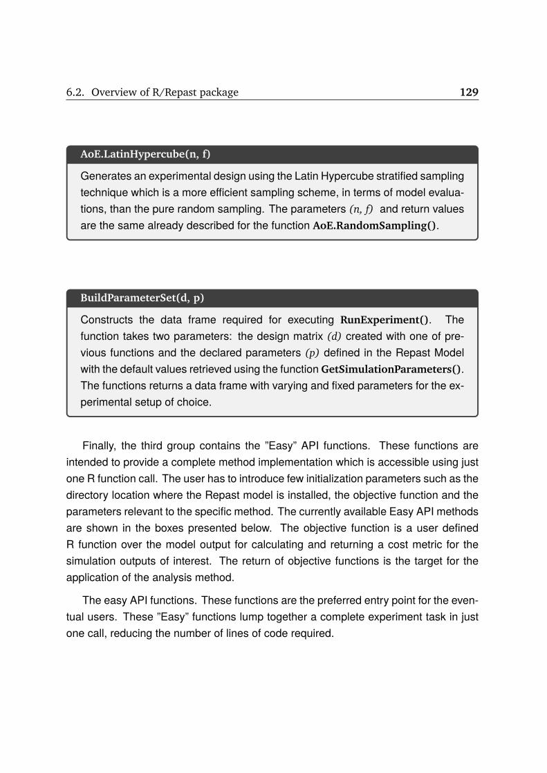
6.2. Overview of R/Repast package 129
AoE.LatinHypercube(n, f)
Generates an experimental design using the Latin Hypercube stratified samplingtechnique which is a more efficient sampling scheme, in terms of model evalua-tions, than the pure random sampling. The parameters (n, f) and return valuesare the same already described for the function AoE.RandomSampling().
BuildParameterSet(d, p)
Constructs the data frame required for executing RunExperiment(). Thefunction takes two parameters: the design matrix (d) created with one of pre-vious functions and the declared parameters (p) defined in the Repast Modelwith the default values retrieved using the function GetSimulationParameters().The functions returns a data frame with varying and fixed parameters for the ex-perimental setup of choice.
Finally, the third group contains the ”Easy” API functions. These functions areintended to provide a complete method implementation which is accessible using justone R function call. The user has to introduce few initialization parameters such as thedirectory location where the Repast model is installed, the objective function and theparameters relevant to the specific method. The currently available Easy API methodsare shown in the boxes presented below. The objective function is a user definedR function over the model output for calculating and returning a cost metric for thesimulation outputs of interest. The return of objective functions is the target for theapplication of the analysis method.
The easy API functions. These functions are the preferred entry point for the even-tual users. These ”Easy” functions lump together a complete experiment task in justone call, reducing the number of lines of code required.

130 Chapter 6. Sensitivity analysis of individual-based models
Easy.Stability(d,o,t,f,s,r,v,F)
Evaluate the behavior of model output in order to determine the minimum re-quired number of replication of the chosen experimental setup. The functionaccept the following parameters: the model installation directory (d), the aggre-gated data source defined within the Repast model (o), the simulation time inRepast ticks (t) which default value is 300 ticks, the input factors to be sampled(f) created with the previously mentioned function AddFactor(), the number ofparameter samples (s), the desired number of replications to be tried (r) beingthe default value 100, the output variables of interest which will be checked fortheir stability and convergence of the coefficient of variation (v); if this parameteris leaved empty all output variables are checked and finally the user providedcalibration function (F) for determining the best input parameter combination.
Easy.Morris(d,o,t,f,p,s,r,F)
This function performs all required tasks for carrying out the method of Morrisfor screening. The parameters are practically the same as described for theprevious function with exception of parameters (p) and (s) which are respectivelythe levels of input factors and the number of sampling points of Morris method[PIwcfSDV+15].
Easy.Sobol(d,o,t,f,n,r,F)
Encapsulate all required steps for performing sensitivity analysis using Sobolmethod. The method of Sobol is a global sensitivity analysis technique based onthe decomposition of output variance ([STCR04, PIwcfSDV+15]). The parametersemantics are the same already described: the model installation directory (d),the aggregated data source defined within the Repast model (o), the simulationtime in Repast ticks (t) , the input factors to be sampled (f), the sample size (n),the desired number of replications (r) and calibration function (F).

6.2. Overview of R/Repast package 131
Easy.Calibration(d,o,t,f,n,r,F)
This function estimates the best set of input parameters or factors, performing aset of model executions in order to sample the calibration function. The objectiveof this function is to minimize the output of calibration function provided by theuser.
Easy.Setup(d,l)
The parameters (d) and (l) are respectively the directory where repast modelis installed and the location of R/Repast deployment directory. If omitted, it as-sumes as the default value, the directory where the Repast model is installed.The function is required for automatically making the changes in the model con-figuration for adding the integration code, for deploying the Java jar files with theintegration code and for preparing the deployment directory. That directory willhold the JVM logs and the saved model output data sets.
6.2.3 The objective function interfaceThe last piece of R/Repast architecture is the definition of the objective function whichactually allows the flexible definition of the model analysis target decoupling it from theRepast dataset output. As we have mentioned previously, any model is a functionalrelationship between a vector of input parameters X and a scalar dependent variabley and expressed as y = f(X). On the other hand, usually the dataset collected fromRepast model execution will be a time series where the aggregated measure will becollected at fixed intervals. Therefore, some transformation must be applied in orderto obtain a value consistent with the functional definition. In addition, even though thevalue returned from the Repast model were a scalar one, it would add much more main-tainable and flexible a to act upon it directly from R without have to making changesin the Repast code. The objective function is also necessary for calibrating, where theoutput values are compared to some reference data or even for more complex tasks,such as tuning oscillations in the population output. It is also the place for normali-zing he model outputs. The objective function is a required parameter for all methods
132 Chapter 6. Sensitivity analysis of individual-based models
presented here.The specification of R/Repast requires the objective function having two input pa-
rameters. The first of it, which is passed for the objective function is the set of inputparameters used for executing the Repast model, the second parameter are the resultsgenerated by executing the model and corresponding to and aggregated data set inthe Repast model. The objective function must return one or more scalar values grou-ped using the cbind() [Cra07] R function. The complete function signature is shown inFigure 6.4.
1 o b j e c t i v e<− func t ion ( params , r e s u l t s ) 2 cbind ( . . . )3
Figure 6.4: The skeleton of objective function. The function has two parametersand must return a one or more scalar values.
6.3 Examples overviewIn the next sections we will provide examples on how the R/Repast can help mo-delers on the analysis of their simulation models. Three examples will be used forillustrating the application of some package’s functionalities and what kind of informa-tion these functions can offer about the simulation outputs. For clarifying what everymodel does a summary version of ODD will be given for facilitating a general ideaabout these models. The Overview, Design concepts and Detail (ODD) is a proto-col [GBB+06] [GBD+10] which has been proposed as a standard way to specify anddescribe Individual-based models. A brief description on the model structure and pa-rameters will be given in order to allow the readers to understand the kind of questionsthe model is intended to answer and how R/Repast is can be used for analyzing themodel outputs. The last section for each model under the title of Model analysis isnot part of ODD protocol but it is included to show the results of running the R/Repastmodel analysis methods.
The first model used as example here is a spatially explicit individual-based repre-sentation of bacterial conjugation using BactoSIM for simulate the plasmid spread ona surface attached bacterial colony[PRP15b]. The example will be used for showing

6.3. Examples overview 133
the application of Easy.Stability method for finding the number of replications of simu-lation experiments required for obtaining consistent outputs. The second example isa Repast implementation of the omnipresent predator-prey model describing the inte-raction between two species. This one is part of examples coming along the standardRepast distribution and will be used for showing the application of Easy.Morris function.Finally, the third example is an instance of the common pool problem in the context ofbacterial conjugation. This model was developed exclusively for this work. This modelwill be used to exemplify the use of Easy.Sobol method. The complete sources for allprojects are available respectively in the following locations:
• BactoSIM: https://github.com/antonio-pgarcia/haldane
• Predator-Prey: The sources come with the Repast distribution.
• T4SS Common Pool: https://github.com/antonio-pgarcia/PoolT4SS
For convenience, in order to facilitate the experiments shown in this paper beingreproduced elsewhere, we also provide the pre-built installers for the three projectsmentioned previously. The installers can be download from URL shown below:
• BactoSIM: http://goo.gl/YYIt1o
• Predator-Prey: http://goo.gl/cJ5z2r
• T4SS Common Pool: http://goo.gl/zq4LH0
In order to reproduce the examples that will appear in the next sections, it is re-quired a computer with a Java JVM and GNU R installed. The examples have beenproduced and tested on a windows box with java 1.8 and GNU R 3.3.1. If these pre-conditions are met, just proceed to download and install the examples and the R/-Repast package. The installation of R/Repast is carried out using the install com-mand install.packages("rrepast") on the R environment. Once the previous stepshave been completed, just copy and paste the examples shown in this paper, takingcare of changing the references to the model installation directory to the directorieswhere the models have been installed locally.

134 Chapter 6. Sensitivity analysis of individual-based models
6.4 Example 1: BactoSIM
Typically, one of the advantages of using individual-based models for biological orecological processes is the possibility of incorporating variability at an individual level.Therefore, unlike deterministic model, in order to get trustworthy results, the simulationmust be repeated a number N of times to achieve stable value on the output variance.The objective of the first example is to show the application of a simple method forfinding the minimal number of replications of a simulation model which is required forthe variance of response variables become stable, converging to a common value. Astraightforward way to determine the output stability has been suggested in [TKG14][LHM12] and consists in to compute the coefficient of variation 3 of the output of inte-rest with and increasing number of repetitions while keeping the input parameters fixed.The number of replications for which the values of coefficient of variation stop to varyare the minimum number of repetitions necessary for getting robust results. In R/Re-past we have implemented that method which is accessible through the Easy.StabilityAPI call.
For this example will be used the BactoSIM[PRP15b] model. This is an individual-based model of bacterial conjugation process. The bacterial conjugation is a form oflateral genetic transfer which occur naturally in bacterial colonies [AF13]. The conjuga-tion consists in the transference of a conjugative plasmid from a donor cell to a recipientcell. The plasmids are small circular DNA sequences which replicates independentlyfrom the main chromosome of their hosts [BLL00]. The conjugation is considered onethe causes of the rapid evolution and adaptation of bacterial colonies and the spreadof antibiotic resistance [CCD05] [SBTT08]. The BactoSIM model is currently beingused for an evaluation of the main factors governing the plasmid dispersion. A pre-liminary evaluation has shown that the point in the cell cycle are the principal factorresponsible for the global dynamics of plasmid infective dispersion[PRP15a] which isconsistent with some observations[SYD+11] taken from individual bacterial cells. Thecomplete description for the BactoSIM, including the ODD protocol can be found insection 7.2.
3Also known as relative standard deviation given by CV = σ/µ which provides a normalized versionof the standard deviation expressed relatively to the output mean

6.4. Example 1: BactoSIM 135
6.4.1 Model analysisThe objective of stability analysis is to find the minimum number of experimental setupreplications required for achieving reliable results. Thereby, the model output responseis evaluated for an increasing number of repetitions allowing the evaluation of the con-vergence for output variance of simulation outputs. The complete listing for carryingout the stability check for the BactoSIM model is shown in Figure 6.5. As can be obser-ved, the complete implementation of model analysis encompasses five steps. Thesesteps are conserved for all high level functions available in R/Repast package. Thestep 0 clean all existing R objects, loads the R/repast package and set the randomseed for the analysis. The step 1 is the definition of the objective function which canbe any user provided function following the R/Repast API specification. It is not strictlynecessary for the Easy.Stability as the coefficient of variation is calculated for the mo-del output variables. In this example the objective function is basically the comparisonof simulated data and experimental data using the normalized root mean square errorAPI call AoE.NRMSD. The step 2 is adds the model input factors for which the impor-tance on the model output will be assessed and their biologically relevant range ofvariation. It is necessary to add at least one parameter which will be varied, while allother model parameters are keep fixed using the default value or with a value previ-ously set using the R/Repast API SetSimulationParameter. The purpose of step 3 isto configure automatically the Repast model with the integration broker and for initi-alizing the integration directory. Finally, the step 4 is where the analysis method isinvoked, all analysis methods will return a list holding three objects, namely the expe-riment, the object and the charts. The experiment contains simulation parameters andresults, the object is method specific and finally the charts are pre-generated graphsfor the method results4
The method will generate automatically one chart for each model output5. One ofthe output chart of model is shown in Figure 6.6 for the variable named X.Simulated.As can be observed, the coefficient of variation of these variable decreases as thesample size increases. The variation starts to become acceptable with a sample sizeof 25 and approximately with sample size of 50 we can see that coefficient of variation
4In the currently API version there is a function for accessing the charts for the Easy.Stability method,named Easy.getChart(), please refer to the user manual for the complete syntax.
5It is possible to limit it passing to the method a subset of model outputs

136 Chapter 6. Sensitivity analysis of individual-based models
1 # Step 02 rm( l i s t=l s () )3 l i b r a r y ( r r e p a s t )4 s e t . seed (161803398)5
6 # Step 17 o b j e c t i v e<− func t ion ( params , r e s u l t s ) 8 Rate<− AoE .NRMSD( r e s u l t s $X . Simulated , r e s u l t s $X . Experimental )9 cbind ( Rate )
10 11
12 # Step 213 f<− AddFactor (name=" c y c l e P o i n t " ,min=40,max=90)14 f<− AddFactor ( f a c t o r s=f , name=" con jugat ionCos t " ,min=0,max=30)15 f<− AddFactor ( f a c t o r s=f , name=" p i lu sExpre s s i onCos t " ,min=0,max=30)16 f<− AddFactor ( f a c t o r s=f , name="gamma0" ,min=1,max=4)17
18 # Step 319 Easy . Setup ( " /models/BactoSim ( HaldaneEngine−1.0) " )20
21 # Step 422 r<− Easy . S t a b i l i t y ( " /models/BactoSim ( HaldaneEngine−1.0) " , " ds : : Output " ,300 , f ,1 ,100 , c () ,
o b j e c t i v e )
Figure 6.5: The listing for stability of model output method using theEasy.Stability function from R/Repast.
become stable. Therefore, we can feel relatively confident with or model results with anumber of replications greater than 25. Certainly, it is important to take into account thecomputation cost of our model in order to select a value for the number of repetitions.
6.5 Example 2: Predator-Prey
6.5.1 Model description
6.5.1.1 Purpose
The purpose of Predator-Prey model presented here is to provide and alternative indi-vidual based-model implementation for the classic ODE model describing the associ-ation between two species. The model will be used to show the application of Morrismethod for ranking the most important parameters.
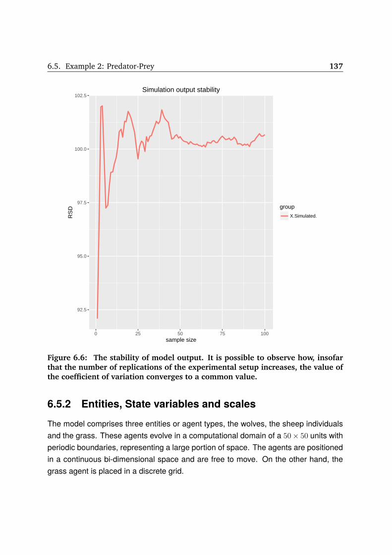
6.5. Example 2: Predator-Prey 137
92.5
95.0
97.5
100.0
102.5
0 25 50 75 100sample size
RS
D group
X.Simulated.
Simulation output stability
Figure 6.6: The stability of model output. It is possible to observe how, insofarthat the number of replications of the experimental setup increases, the value ofthe coefficient of variation converges to a common value.
6.5.2 Entities, State variables and scales
The model comprises three entities or agent types, the wolves, the sheep individualsand the grass. These agents evolve in a computational domain of a 50× 50 units withperiodic boundaries, representing a large portion of space. The agents are positionedin a continuous bi-dimensional space and are free to move. On the other hand, thegrass agent is placed in a discrete grid.

138 Chapter 6. Sensitivity analysis of individual-based models
6.5.2.1 Process overview and scheduling
The agents are defined by the execution of a set of processes depicting the agentmovement and search of food source, the consumption of food, the process incre-menting the agent reserves, the reproduction and finally the death process driven bypredation or starvation. The fundamental idea behind the model formulation is thatboth predator and prey individuals incrementing their ”energy” levels by predation orby consuming the available grass respectively. Both agent types search for their foodin the current patch where they are placed. The agents move a unit of space at timeselecting randomly the heading.
The individual-based version of this model is a spatially explicit representation andhave a few parameters more but is still very succinct. The list of model parameters areshown in Table 6.1.
Table 6.1: The input parameter collection for the Repast implementation ofPredator-Prey model.
Input parameter Description
initialnumberofwolves The initial population of predators.initialnumberofsheep The initial population of preys.wolfgainfromfood The rate of predator energy is incremented every time a
prey is consumed.wolfreproduce The reproduction rate of predator individual.sheepgainfromfood The prey rate energy increment for grazing grass.sheepreproduce The reproduction rate of prey individual.grassregrowthtime The amount of time required for grass be available again
once consumed by a prey.
The original formulation of Lotka-Volterra consists in a system of two differentialequations with four parameters, namely the predator and the prey growth rate, theeffect of predator on the prey growth and finally the effect of prey on the predatorgrowth as can be seen in Equation (6.8).

6.5. Example 2: Predator-Prey 139
dx
dt= c1x− c3xy (6.8)
dy
dt= −c2y + c4xy.
There is a conceptual correspondence between the predator c2 and prey c1 gro-wth rates with the model parameters wolfreproduce and sheepreproduce as well as withbetween the parameter wolfgainfromfood and the constant c4.
6.5.3 Model analysisThe implementation code for the Morris screening exercise is shown in Figure 6.7 and,as has been mentioned in the previous example, we have the same sequence of steps,starting with the library loading and the selection of the random seed. Subsequentlywe define the objective function, which in this case is a very simple one consisting inthe arithmetic average of the population sizes of sheep individuals and wolves. Thenext step is the selection of model input factors for the screening method and providingthe range of variation for each them. Then, the step 3 shows the call to the Easy.Setupfunction which initializes the Repast Model with the R/Repast integration code. Finally,the function Easy.Morris is called and the results stored in the variable r. The exampleuses five levels with ten sampling points for Morris method. The results consist in a Rlist holding the experiment carried out, the Morris object and a list with charts generatedby the experiment6.
The Figure 6.8 presents the µ∗ vs σ chart for both predator and prey average popu-lation sizes. At a first glance, the most important input factor for both Predator and Preypopulations is the sheepgainfromfood. The second most significant for the Predator out-put is grassregrowthtime. The other parameters are not very significant for the averageof Predator individuals. It is also interesting to note that wolfgainfromfood has veryhigh value of σ which could indicate that the parameter significance strongly dependson the values of other parameters. On the other hand, it could mean that the num-
6In order to plot the charts the user should use a R code for accessing the chat list members. Thereare three members, namely mustar, musigma and mumu. In order to get the mumu chart for the secondobjective function output we must use the R call: r$charts[2,]$mumu.

140 Chapter 6. Sensitivity analysis of individual-based models
1 # Step 02 rm( l i s t=l s () )3 l i b r a r y ( r r e p a s t )4 s e t . seed (161803398)5
6 # Step 17 o b j e c t i v e<− func t ion ( params , r e s u l t s ) 8 Predator<− mean( r e s u l t s $Wolf . Count )9 Prey<− mean( r e s u l t s $Sheep . Count )
10 cbind ( Predator , Prey )11 12
13 # Step 214 f<− AddFactor (name=" wolfreproduce " ,min=2,max=8)15 f<− AddFactor ( f a c t o r s=f , name=" wolfgainfromfood " ,min=15,max=25)16 f<− AddFactor ( f a c t o r s=f , name=" sheepreproduce " ,min=2,max=6)17 f<− AddFactor ( f a c t o r s=f , name=" sheepgainfromfood " ,min=2,max=6)18 f<− AddFactor ( f a c t o r s=f , name=" grassregrowtht ime " ,min=20,max=40)19
20 # Step 321 Easy . Setup ( " / usr /models/ PredatorPrey " )22
23 # Step 424 r<− Easy . Morr is ( " / usr /models/ PredatorPrey " , " Agent Counts " ,300 , f ,5 ,10 ,1 , o b j e c t i v e )
Figure 6.7: The listing for Morris screening method using the Easy.Morrisfunction from R/Repast.
ber of sampling points or replications should be increased. The Prey output presentsthree important parameters, which in order of importance are the sheepgainfromfood,the sheepreproduce and grassregrowthtime. These input parameters also have a high σvalues which possibly indicate some non-linear effects or that the values of these inputfactors are influencing each other. These results can be explained by the dependenceof wolf population on the availability of prey. The common observed pattern in that kindof model is the population of predators lagging in phase behind the prey population.
The chart of µ vs σ for model output is shown in Figure 6.9. It seems to providevery similar results and the only significant difference is the contribution of grassregro-wthtime. That input parameter was considered important by µ vs σ but here it has anegative value. In order to interpret this sensitivity measure, we must recall that µ∗
takes the absolute values of elementary effects. Therefore, the elementary effects ofgrassregrowthtime possibly has effect of opposite sings depending on the values of thatinput parameter.
Finally, we have the 6.10 showing the chart of µ∗ vs µ where the value of bothmeasures can be observed together allowing the appreciation of the differences of

6.5. Example 2: Predator-Prey 141
20
25
30
35
30 60 90µ*
σ
group
grassregrowthtime
sheepgainfromfood
sheepreproduce
wolfgainfromfood
wolfreproduce
criteria Predator
10
20
30
40
0 20 40 60 80µ*
σ
group
grassregrowthtime
sheepgainfromfood
sheepreproduce
wolfgainfromfood
wolfreproduce
criteria Prey
Figure 6.8: Results of Morris screening method for Predator-Prey model. Thegraph shows the µ∗ and σ sensitivity measures for Predator and Prey outputs.
20
25
30
35
−50 0 50 100µ
σ
group
grassregrowthtime
sheepgainfromfood
sheepreproduce
wolfgainfromfood
wolfreproduce
criteria Predator
10
20
30
40
0 25 50 75µ
σ
group
grassregrowthtime
sheepgainfromfood
sheepreproduce
wolfgainfromfood
wolfreproduce
criteria Prey
Figure 6.9: Results of Morris screening method for Predator-Prey model. Thegraph shows the µ and σ sensitivity measures for Predator and Prey outputs.
both, which possibly indicates that the input factors present effects with different signswhich, in other words, means non-linearity in the model behavior.

142 Chapter 6. Sensitivity analysis of individual-based models
−50
0
50
100
30 60 90µ*
µ
group
grassregrowthtime
sheepgainfromfood
sheepreproduce
wolfgainfromfood
wolfreproduce
criteria Predator
0
25
50
75
0 20 40 60 80µ*
µ
group
grassregrowthtime
sheepgainfromfood
sheepreproduce
wolfgainfromfood
wolfreproduce
criteria Prey
Figure 6.10: Results of Morris screening method for Predator-Prey model. Thegraph shows the µ∗ and µ sensitivity measures for Predator and Prey outputs.
6.6 Example 3: T4SS Common Pool
6.6.1 Model description6.6.1.1 Purpose
The objective of this model is to explore the conditions where two plasmids can coexistin a population competing for a common resource required for their horizontal transfer.The common resource is the set of genes required for conjugation because one of thetwo plasmids have lost these genes.
6.6.1.2 Entities, State variables and scales
The model uses two types of entities, namely the agents representing the bacterialcells and a ValueLayer, which is a Repast specific structure, for holding the nutrientavailable for the bacterial growth. The agents interact and grow in a computationaldomain of 100 × 100 µm squared lattice with periodic boundaries representing a totalreal surface of 0.01mm2. Despite of being a lattice the bacterial cells are positionedand allowed to move in a continuous space system. The agents are also allowed tooverlap to each other. Explicitly, the agents are defined by the five state variables: (a)

6.6. Example 3: T4SS Common Pool 143
heading, (b) mass, (c) division mass, (d) plasmid P1 infection state and (f) plasmid P1infection state. The current position of every bacterial cell in the coordinate system isavailable implicitly through a Repast API call.
6.6.2 Process overview and schedulingEvery bacterial cell in this model is abstracted as the execution of a series of successiveprocesses capturing the basic tenets of bacterial life-cycle. These processes are thenutrient uptake, the bacterial cell growth, the division and the conjugation. The inputparameters required for initialize the model are shown in Table 6.2.
Table 6.2: The input parameter collection for the conjugative plasmid commonpool model.
Input parameter Description
doublingTime The doubling time of plasmid free cellsp1P (P (γ0)) The probability of cell conjugate at least one time.p1Cost The cost imposed by the plasmid P1 including the meta-
bolic burden required to express the conjugative appara-tus.
p2Cost The metabolic cost of plasmid P2
6.6.2.1 Design concepts
Basic Principles — The plasmid dispersion rely upon an intricate balance betweenmetabolic costs associated to horizontal and vertical dispersion strategies. Theconjugative proficiency requires the expression of set of transmembrane proteinswhich are known collectively as Type IV Secretion Systems (T4SS) [LKGF03b]. Thepresence of conjugative plasmids and the expression of conjugative machinery isdetrimental for the host cell fitness [RARE+04] but there is no consensus on thevalid ranges of metabolic costs imposed by the conjugative process. Therefore, inthis model the short term dynamics of two plasmid system P1 and P2 is simulated.

144 Chapter 6. Sensitivity analysis of individual-based models
The plasmid P1 is a complete conjugative plasmid containing all genes required forhorizontal transfer and the plasmid P2 is a cheater, which having lost its conjugativegenes, depends on the T4SS system from the plasmid P1. In other words, the modelis used to assess how large should be the cost difference required for the lack ofconjugative apparatus become a true competitive advantage making P2 dominateover P1.Emergence — The colony growth pattern, the population distribution and the domi-nance of a plasmid over another on the bacterial population are global propertiesarising from local properties defining the agent behavior and the interaction con-straints.Adaptation — All agents adapt their growth rate, as well as the conjugation rates,according to the local availability of nutrient.Fitness — The bacterial cells infected by any plasmid are considered to behave lessefficiently than the plasmid free cells. The fitness of plasmid bearing cells are explicitlyspecified by the cost input parameters.Objectives — No objectives are taken into account in this model.Prediction — The model will provide predictions on the possible ranges of plasmidmetabolic cost which can favorable to the cheaters plasmid strategy.Sensing — The agents representing the virtual bacterial cells sense the environmentto the extent that the nutrient availability controls the growth and the conjugation rates.Interaction — Bacterial cells interact with their nearby individuals for nutrient access,cellular division, mate pair formation and plasmid transfer.Stochasticity — Stochasticity is introduced at an individual level for all cellular processsampling a normal deviate and fitting the value to corresponding process.Collectives — No collectives are taken into account in this model.Observation — The model provides two kind of outputs, one is numeric and containsthe total number of bacterial cells which are plasmid free or are infected by theplasmids P1, P2 or both. These outputs are generated for every time step. The modelalso has an 2D view of colony growth updated every time tick.

6.6. Example 3: T4SS Common Pool 145
6.6.3 Analysis of modelThe global sensitivity analysis using the Sobol variance decomposition method forthe T4SS Common Pool model is shown in Figure 6.11. We can observe the samesequence of steps which has been previously mentioned. The objective function isdefined for the average values of the model outputs named P1, P2 and Both. Thesevariable are respectively the bacterial population size infected by the P1 plasmid, in-fected by the cheater plasmid P2 and finally the number of individuals infected by bothplasmids. The Sobol sensitivity indices will provide the measures of the importanceof every input parameter shown in step 2 of Figure 6.11 with respect to the resultsreturned by the objective function, that is to say, the average population sizes.
1 # Step 02 rm( l i s t=l s () )3 l i b r a r y ( r r e p a s t )4 s e t . seed (161803398)5
6 # Step 17 o b j e c t i v e<− func t ion ( params , r e s u l t s ) 8 Both<− mean( r e s u l t s $Both )9 P1<− mean( r e s u l t s $P1)
10 P2<− mean( r e s u l t s $P2)11 cbind (P1 , P2 , Both )12 13
14 # Step 215 f<− AddFactor (name=" doublingTime " ,min=20,max=240)16 f<− AddFactor ( f a c t o r s=f , name=" p1P " ,min=0.1 ,max=0.8)17 f<− AddFactor ( f a c t o r s=f , name=" p1Cost " ,min=1,max=100)18 f<− AddFactor ( f a c t o r s=f , name=" p2Cost " ,min=1,max=100)19
20 # Step 321 Easy . Setup ( " / usr /models/PoolT4SS " )22
23 # Step 424 r<− Easy . Sobol ( " / usr /models/PoolT4SS " , " output " ,720 , f ,100 ,20 ,1 , o b j e c t i v e )
Figure 6.11: The listing for Sobol GSA variance decomposition method using theEasy.Sobol function from R/Repast.
The Figure 6.12 shows the first and total order indices for the model output P1.That output is the average number of bacterial cells infected just by the plasmid P1.As can be observed the most important input parameter is the bacterial cell doublingtime followed by the probability P (γ0). This is an expected result because the rulefor the conjugative transfer implemented here, have a dynamics linked to the host cell

146 Chapter 6. Sensitivity analysis of individual-based models
cycle and therefore depends on the bacterial state with respect to the total elongationand the division point[SYD+11], being consistent with other studies where the time-related parameters are the most important ones[MLS+11]. Other interesting aspectto note is the negative values of first order indices. Obviously the sensitivity indicesshould not be negative. This is consequence of a small sample size and to correctthe problem we must increase it. The other important input factors for the plasmid P1output are, in order of importance, the probability P (γ0), the cost of plasmid P2 andthe cost of plasmid P1, both with similar sensitivity indices.
0.00
0.25
0.50
0.75
1.00
doublingTime p1Cost p1P p2Costparameter
Si
Sobol indexes for P1
0.0
0.3
0.6
0.9
doublingTime p1Cost p1P p2Costparameter
ST
i
Sobol indexes for P1
Figure 6.12: Results of Sobol variance decomposition method for T4SS CommonPool model. The graph shows the first and total order indices sensitivity measuresfor bacterial population infected by plasmid P1.
The first and total order indices for the model output showing the average populationsize of plasmid P2 can be seen in Figure 6.13. It is possible to appreciate again, thatthe sensitivity indices show that the most important factor is the length of cellular cycle.The reason is simple, and can be attributed to the fact that plasmid P2 alone is onlytransferred vertically and depends on the plasmid P1 for horizontal transmission, beingboth aspects related to the cell cycle. Following in importance the doubling time wehave the cost of plasmid P1, the cost of plasmid P2 and the probability P (γ0), being thesensitivity index of P1 cost, noticeably higher than the other two indices. This couldbe attributed probably because the plasmid P2 require a significant cost difference inorder to outcompete the plasmid P1 with just the vertical transfer component.

6.7. Summary 147
0.0
0.4
0.8
doublingTime p1Cost p1P p2Costparameter
Si
Sobol indexes for P2
0.0
0.3
0.6
0.9
doublingTime p1Cost p1P p2Costparameter
ST
i
Sobol indexes for P2
Figure 6.13: Results of Sobol variance decomposition method for T4SS CommonPool model. The graph shows the first and total order indices sensitivity measuresfor bacterial population infected by plasmid P2.
Finally, in the Figure 6.14 we have the sensitivity indices for the output of modelaccounting for the average population size of bacterial cells infected by both plasmids.The importance of factors is consistent with the explanations for the previous sensitivityindices. Again, the most important model parameter is the doubling time of bacterialcell followed by the P1 and P2 cost parameters and by the probability P (γ0).
6.7 SummaryThe ecological modeling is a complex subject which can be normally perceived asbeing simpler than it actually is. Specifically, the Individual-based models are subjectto many levels of uncertainty, which means that it is hard to get completely fixed thevalues of model inputs, the model structure and the outputs. Normally there is nocomplete experimental or observational data to construct mechanistic descriptions ofindividual and therefore many assumptions and simplifications must be made in orderto implement a model. The same is truthful regarding the input values, which areparticularly critical in the case of the ecology of microorganism, as normally just veryfew input parameters are directly observed and the most of them are estimated fromwhole population experiments. Therefore, it is always important to bearing mind that

148 Chapter 6. Sensitivity analysis of individual-based models
0.00
0.25
0.50
0.75
1.00
doublingTime p1Cost p1P p2Costparameter
Si
Sobol indexes for Both
0.0
0.3
0.6
0.9
doublingTime p1Cost p1P p2Costparameter
ST
i
Sobol indexes for Both
Figure 6.14: Results of Sobol variance decomposition method for T4SS CommonPool model. The graph shows the first and total order indices sensitivity measuresfor bacterial population infected by both plasmids P1 and P2.
modeling is an iterative task which must incorporate compulsorily some what-if analysisof model outputs.
Several methods exist for assessing the uncertainty and for estimate the relativeimportance of input parameters in the model output. We have provided here and over-view on those methods which are based on the variance decomposition because theyhave a wider application scope and are specifically suitable for their use on individual-based models. These methods, although conceptually simple, are computationallyintensive and can be somewhat hard to apply because the required tools are eitherunavailable or they do not provide an easy integration pattern. Roughly speaking, thesensitivity analysis methods require the generation of large sample of the parameterspace and the model evaluation for each of them which, of course, makes the manualexecution an infeasible option.
The in silico experimentation is becoming a vital tool for understanding complexphenomena in a way that cannot be done without modeling. The effective applicationof computational ecology methods requires a high level of proficiency in many diversedomains of knowledge which sometimes are neither feasible nor practical. Therefore,it is indispensable to have a ready to use arsenal of reusable computational tools formodeling and analysis. In this work we have introduced the R/Repast package and

6.7. Summary 149
shown how it can help modelers to improve the robustness and quality of individual-based models results by using the functionalities inside the package for analyzingsystematically the model outputs. The package can save a lot of effort for modelers byproviding simple wrappers for complex methods within a simple and consistent API.We hope that these R/Repast functionalities can facilitate dramatically the systematicanalysis of Individual-based models implemented in Repast.

150 Chapter 6. Sensitivity analysis of individual-based models

Chapter 7An individual-based model
of bacterial conjugation
7.1 Introduction . . . . . . . . . . . . . . . . . . . . . . . . . . . . . . . . . 152
7.2 High-level model description . . . . . . . . . . . . . . . . . . . . . . . . 153
7.3 Material and methods . . . . . . . . . . . . . . . . . . . . . . . . . . . 157
7.3.1 Purpose . . . . . . . . . . . . . . . . . . . . . . . . . . . . . . . 157
7.3.2 State variables and scales . . . . . . . . . . . . . . . . . . . . . 157
7.3.3 Process overview and scheduling . . . . . . . . . . . . . . . . 158
7.3.4 Design concepts . . . . . . . . . . . . . . . . . . . . . . . . . . 158
7.3.5 Initialization . . . . . . . . . . . . . . . . . . . . . . . . . . . . . 161
7.3.6 Sub-models . . . . . . . . . . . . . . . . . . . . . . . . . . . . . 163
7.4 Results and discussion . . . . . . . . . . . . . . . . . . . . . . . . . . 170
7.5 Summary . . . . . . . . . . . . . . . . . . . . . . . . . . . . . . . . . . 178

152 Chapter 7. An individual-based model of bacterial conjugation
7.1 IntroductionIn this chapter we will provide a brief introduction to the BactoSIM simulation platformwhich we have used for studying the cell to cell dynamics of the horizontal genetictransfer. The main objective of the software is serving in a future as a computationalworkbench for using bacterial plasmid as a ”wiring protocol” for harnessing the powerof bacterial cell-cell communication as a tool for multicellular synthetic biology. But weclaim that for achieving such goal it is necessary first to understand better the under-lying cellular mechanism which promotes the plasmid epidemic spread in a bacterialcolony. We have tried to accomplish that goal using an integrative approach wheremolecular level and individual-based observations are incorporated, sometimes veryschematically, into the simulation model. Therefore, all relevant data about the systemunder study are part of this model as an input parameter or as the guidance and thereference for implementing the internal individual rules for updating the state variables.It is worth to mention that we have been very parsimonious for adding complexity tothe model and this representation is the result of several previous attempts.
The construction of an agent-based model uses a bottom-up approach where wespecify how agents must evolve by implementing the rules for updating their internalstate variables which additionally are also taking into account the stochasticity inherentto biological processes. The whole-population outcomes are a result of these local ru-les which generates an emergent global behavior. That kind of models is also useful forproducing new insights about the process being studied, suggesting sometimes coun-ter intuitive ideas about what local processes are responsible for some global systemcomportment. The simulation software was developed using the Repast Symphonymulti-agent simulation platform [NCO+13b].
The spatially explicit population dynamics models can be classified taking into ac-count the scheme used to describe the population size, space and time [Ber02], thusIBMs uses discrete representations for these three variables. Bearing these ideasin mind we have built a spatially explicit IBM to explore the behavior of conjugativeplasmids trying to elucidate the local parameters of conjugal activity and the effect ofgrowth in the plasmid invasion. The spatially explicit individual-based model are par-

7.2. High-level model description 153
ticularly adequate to generate bottom-up models for microbiological systems in bothnatural and laboratory conditions accounting for the spatial heterogeneity and furt-hermore allowing linking the population or system-level properties to the individualparameters helping in the realization about how such global system properties areemerging from the local and individual interaction rules[HB09].
One of the most important aspects shaping the conjugative dynamics is the timing-related factors according to the results shown in previous studies[MLS+11] where thegrowth dependence is explored as an explanatory reason for the limited invasion instructured colonies. The same idea is also proposed in works about the end-pointmethod [? ZDF+12] which supports that it is impossible to separate the effects of gro-wth and conjugation on the plasmid invasion. Finally the spatial structure itself imposesome limitations on the number of reachable neighbors to accomplish a conjugativetransfer adding a delay over the propagation front due to the recovery and maturationperiods required to forward the plasmid.
The BactoSIM code and binaries are available for download1. The simulator is apart of the European project PLASWIRES which also includes the simulator BactoSIMII[BSRP15]. BactoSIM will serve as the base for an agent-based platform for simulatingthe conjugation in spatially structured bacterial populations, which are the conditionstypically found on naturally occurring colonies such as biofilms or in agar-based labo-ratory cultures. The model provides a set of key indicators which can be visualizedin real time as the simulation evolves and saved for further analysis. The main ideabehind this simulator is to provide a simple workbench for verifying several aspects re-lated with the most suitable computational representation for the conjugative processin order to produce a simple and usable operational model.
7.2 High-level model descriptionThe simulation model is comprised by a discrete set of agents each of them represen-ting a single bacterial cell βi, i = 1 . . . N where N is the current population size at thesimulated time t. The agents interact with other agents and with the environment which
1http://goo.gl/TDGxNr

154 Chapter 7. An individual-based model of bacterial conjugation
(a) Initialization. (b) t = 600 minutes.
Figure 7.1: The BactoSIM Virtual Agar-Plate view for simulated version of R1plasmid. The color scheme used is green for R cells, red for D cells and bluefor T cells. The light-green, light-read and light-blue colors are used to representdepleted nutrient zones where cells are no longer dividing.
holds some amount of nutrient. The environment is implemented using a value layerof Repast framework [NCO+13b]. The βi agents lives and evolve in a computationaldomain represented as a 1000 × 1000 discrete2 grid, corresponding to a real surfaceof 1mm2. In approximately 20 minutes of wall clock, BactoSIM is able to simulate 600minutes of colony growth with a final population of 105 bacterial cells.
The bacterial cells evolve during the simulated time having their state variables up-dated by some processes representing the intra and intercellular behavior of everyagent βi. Hence, at a functional high level, the model have a set of processesP = (p1 . . . p5) each of them standing respectively for the Uptake, Diffusion, Division,T4SS expression (a protein needed for plasmid conjugation), Shoving relaxation andfinally the Conjugation. The execution of these processes is shuffled in order to avoidany bias and the state of agents and the value layer holding the nutrient particles areupdated asynchronously. The bacterial cells have three different states, namely R, Dand T standing respectively for plasmid free (or recipient cells), plasmid donors (cells
2Actually it is implemented as a repast multiOccupancy2D allowing cells to overlap in some extent,in the same way it really happens in a real bacterial colony
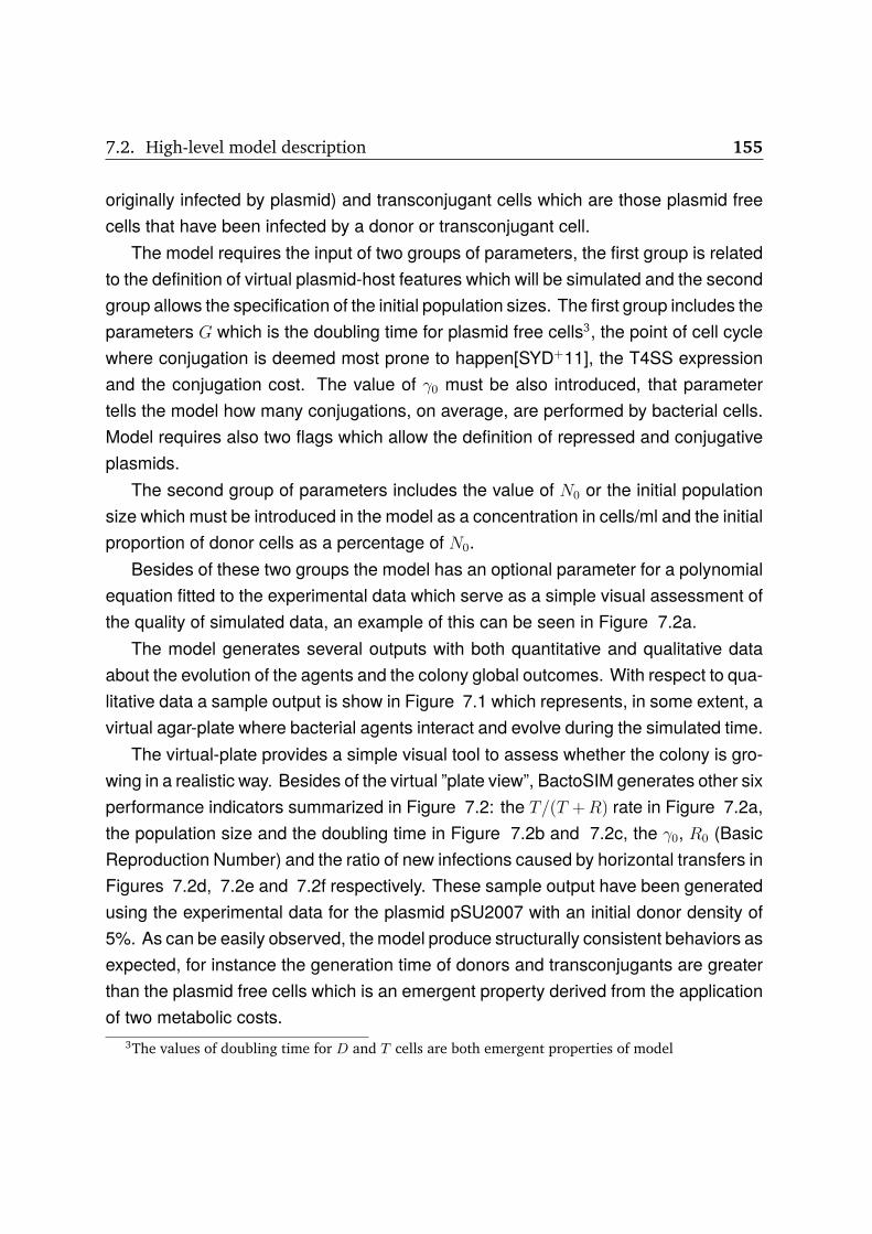
7.2. High-level model description 155
originally infected by plasmid) and transconjugant cells which are those plasmid freecells that have been infected by a donor or transconjugant cell.
The model requires the input of two groups of parameters, the first group is relatedto the definition of virtual plasmid-host features which will be simulated and the secondgroup allows the specification of the initial population sizes. The first group includes theparameters G which is the doubling time for plasmid free cells3, the point of cell cyclewhere conjugation is deemed most prone to happen[SYD+11], the T4SS expressionand the conjugation cost. The value of γ0 must be also introduced, that parametertells the model how many conjugations, on average, are performed by bacterial cells.Model requires also two flags which allow the definition of repressed and conjugativeplasmids.
The second group of parameters includes the value of N0 or the initial populationsize which must be introduced in the model as a concentration in cells/ml and the initialproportion of donor cells as a percentage of N0.
Besides of these two groups the model has an optional parameter for a polynomialequation fitted to the experimental data which serve as a simple visual assessment ofthe quality of simulated data, an example of this can be seen in Figure 7.2a.
The model generates several outputs with both quantitative and qualitative dataabout the evolution of the agents and the colony global outcomes. With respect to qua-litative data a sample output is show in Figure 7.1 which represents, in some extent, avirtual agar-plate where bacterial agents interact and evolve during the simulated time.
The virtual-plate provides a simple visual tool to assess whether the colony is gro-wing in a realistic way. Besides of the virtual ”plate view”, BactoSIM generates other sixperformance indicators summarized in Figure 7.2: the T/(T +R) rate in Figure 7.2a,the population size and the doubling time in Figure 7.2b and 7.2c, the γ0, R0 (BasicReproduction Number) and the ratio of new infections caused by horizontal transfers inFigures 7.2d, 7.2e and 7.2f respectively. These sample output have been generatedusing the experimental data for the plasmid pSU2007 with an initial donor density of5%. As can be easily observed, the model produce structurally consistent behaviors asexpected, for instance the generation time of donors and transconjugants are greaterthan the plasmid free cells which is an emergent property derived from the applicationof two metabolic costs.
3The values of doubling time for D and T cells are both emergent properties of model

156 Chapter 7. An individual-based model of bacterial conjugation
0 600
0.2
0.4
0.6
0.0
SimulatedExperimental
(a) T/(T +R)
0 600
2.5e+11
5.0e+10
1.5e+11
(b) Population
0 600
40
60
80
(c) Doubling time
0 600
1.2
1.5
1.8
(d) γ0
1.5
2.0
2.5
1.0
0 600
(e) R0
0
20
10
0 600
(f) % Horizontal
Figure 7.2: Sample of the output provided by the BactoSIM model. The subfi-gure (a) shows the conjugation rates of simulated and experimental populationsexpressed as the ratio T/(T + R). The subfigure (b) represents the populationof different cell types scaled for expressing a concentration in cells/ml. The nextsubfigure (c) provides the generation times for recipient, donor and transconju-gant cells. The figures (d) and (e) are respectively the so called intrinsic conjuga-tion rate and the basic reproductive number for donors and transconjugant cells.Finally, the subfigure (f) is the contribution of donors and transconjugants whichcan assigned to the conjugative transfer in the creation of infected individuals.The color code used here is green for plasmid free recipients (R), red for initiallyinfected donors (D) and yellow for transconjugant cells (T). The horizontal axisof all subfigures are the simulated time in minutes.

7.3. Material and methods 157
7.3 Material and methodsIn this section we present a comprehensive description of our model using the ODD(Overview, Design concepts and Detail) protocol [GBB+06, GBD+10] which is beco-ming a standard de facto for describing agent-based and individual-based models inmany domains. The model was implemented entirely in java language using RepastSimphony agent-based simulation framework [NCO+13b].
7.3.1 PurposeThe main objective4 of this model is the assessment of what strategy/model type forcapturing the structure of conjugation rule, provides the best fit to experimental dataand better captures the real structure of the process. Hence, a structurally simple mo-del has been implemented using three different approaches for describing the processof infecting a plasmid free cell. The model results have been compared to the experi-mental data obtained from wet-lab for assessing the quality of these three strategies.In further works the best strategy can be used to build models which could serve asa predictive tool for synthetic biology and to explore some aspects which are hard toobserve directly in experimental studies of plasmid spread. The key points of our mo-del lie on the idea of the existence of a local or intrinsic conjugation rate that has beentermed γ0 which stands for the number of plasmid transfer events, or conjugations ona cell life-cycle basis and that the infection wave speed depends directly from the pointalong the cell cycle when the conjugative event is triggered.
7.3.2 State variables and scalesThe model comprises two entity types, namely the bacterial individuals or agents andenvironment. The environment contains the rate limiting amount of nutrient particlesrequired for the cell metabolism and growth. All agents evolve in a computational dom-ain defined by a 1000×1000µm squared lattice divided in 106 cells of 1×1µm represen-ting a real surface of 1mm2. In this model the agents that represents the bacterial cellsare defined individually by two main state variables, namely the plasmid infection state
4The model provide several outputs allowing to evaluate also other aspects of the bacterial conjuga-tion dynamics such as the relative importance of the horizontal transfers.

158 Chapter 7. An individual-based model of bacterial conjugation
and the t0. The plasmid infection states are Q = R,D, T and the respective transitionfunction for conjugative plasmids, δ is shown in (7.1). For the oriT construction onlythe first transition rule applies since transconjugant cells are sterile. The t0 is the timeof cell birth or the time of the last cellular division, it is employed in the estimation ofagent doubling time used in the division decision rule. The T4SS pili is also taken intoaccount and the agents have a state variable representing the number of pilus alreadyexpressed and available in cell surface.
δ =
(D,R)→ (D,T )
(T,R)→ (T, T )(7.1)
Finally the environment will hold the initial nutrient concentration for every latticecell. In the model initialization, a fixed amount of substrate particles will be distributedevenly over all lattice sites.
7.3.3 Process overview and schedulingThe dynamics of bacterial conjugation is modeled as the execution of following set ofcellular processes: the cellular division, the T4SS pili expression, the shoving relaxingwhich avoid bacterial cells to overlap and allow a more realistic colony growth and theconjugation process. The state variable update is asynchronous. The order of execu-tion of this process is shuffled to avoid any bias due to a purely sequential executionof model rule base, see 7.3. The conjugation process is modeled in three differentways with respect to the time when conjugation event is most prone to happen andthe results are compared. Thus the conjugation is defined by to variables: the valueof intrinsic conjugation rate (γ0) which determines how many transfers should be per-formed by a single bacterial cell and the cell cycle point which defines the time whenthe conjugative events must occur.
7.3.4 Design conceptsBasic Principles — The model incorporate some fundamental ideas, which can be
axiomatically assumed for all biological system. Therefore, the intercellular compe-tition for nutrients and space is captured by the rules for updating the state of theindividual agents. The intracellular competition for metabolic resources sequestered

7.3. Material and methods 159
Figure 7.3: The general schematic view for the process scheduling of BactoSIM.

160 Chapter 7. An individual-based model of bacterial conjugation
by the plasmid housekeeping is also taken into account as the associated costsincorporated in the model logic. Three alternative model formulations differing in theway the conjugation rule is implemented and their results compared to the availableexperimental data. The best strategy can be used to build models which could serveas a predictive tool for synthetic biology and to explore some aspects which are hardto observe directly in experimental studies of plasmid spread. The key points of thismodel lies on the idea of the existence of a local or intrinsic conjugation rate, whichhas been termed γ0. This intrinsic rate stands for the number of plasmid transferevents, or conjugations on a cell life-cycle basis. In addition, the global infectivewave speed depends directly from the specific point in the bacterial cell cycle whenconjugative event is triggered.Emergence — We want to find out what will be the global outcome which will arise asfunction of local rules defining the evolution of the bacterial cells and the interactionwith other adjacent cells. With this objective, the model incorporates the mostsignificant aspects of the structure and possible behavior of the structure as cellularprocesses that are interrelated. Specifically the values of the generation time of donorand transconjugant cells are one emergent property depending fundamentally fromthe metabolic penalizations applied both for conjugation and for the expression ofT4SS genes.Adaptation — All agents adapt their growth according to the local availability ofnutrient and space. It is considered implicitly to the extent that plasmid free individualswill present a better adaptation in terms of growth rate than plasmid bearing cells.Furthermore in one of the model executions we explicitly impose a fitness penaltyevery time that conjugation occurs in order to compare the resulting bacterial colonystate.Prediction — The model is intended to provide prediction regarding the range ofpossible values for the number of plasmid transfer per cell cycle and the cell cyclepoint when conjugative transfer are most likely to happen.Sensing — All process defined over the agents implicitly sense the local environmentand the close neighborhood for their decisions.Interaction — Bacterial cells interact with their nearby individuals for nutrient access,cellular division, mate pair formation and plasmid transfer.Stochasticity — Stochasticity is introduced at individual level for all cellular process

7.3. Material and methods 161
sampling a normal deviate and fitting the value to corresponding process.Collectives — No collectives are taken into account in this model.Observation — All state variables will be saved at intervals of one minute of simulatedtime.
7.3.5 InitializationThe simulation model is initialized with a population of plasmid free (R) and plasmidbearing (D) cells according to input parameters. The agents are placed randomlywithin a circular surface centered over the lattice central position. The radius of circlewhere agents are placed is calculated as function of N0 in order to be consistent to thedesired initial cell density[ZDF+12]. The simulation environment is also initialized witha number of nutrient particles5 in order to support the half of the estimated number ofcellular divisions and the rationale behind it is to capture the intercellular competitionfor nutrient access.
The model input and initialization requires the parameters shown in Table 7.1.The costT4SS is the total cost of pili expression. The cost applied for a single pilusexpression is costT4SS/param(maxpili). The param(maxpili) is currently a constant,having the value of 5 for the virtual E. coli cells simulated with BatoSIM.
The cellCycle parameter, in the BactoSIM version 1.0 indicates two things: the typeof modeling rule and its parameter. A value of −1 set the model to conjugate as soonan infected cell finds a susceptible one. Setting the parameter to 0 will randomize deconjugation time between t0 and G. Finally using a value greater than zero indicatesthe specific point in the cell cycle for conjugation. In subsequent versions, a new inputparameter has been added to the BactoSIM specification for indicating the model type.Therefore, in versions greater than the 1.0 the semantics of the cyclePoint parameter,only indicates when conjugative activity is most likely to happen and the parameteronly is used when the model type is equal to 3. The model also needs an equation,fitted to the experimental data, where the dependent variable represents the conjuga-tion rate T/(T + R). Setting isConjugative flag to false creates a simulation wherethe transconjugant cells are unable to conjugate. The parameter equation is used for
5In the current version the number of nutrient particles is also an input parameter.

162 Chapter 7. An individual-based model of bacterial conjugation
assessing the quality of simulation output.
Table 7.1: The list of initialization parameters for BactoSIM 1.0 model.
Parameter Unit Description
G minutes Average doubling time for plasmid free cellscellCycle % of G The percentage of cellular cycle for conjugationcostConjugation % of G The penalization due to a conjugative eventcostT4SS % of G The Pilus expression costγ0 c/cycle Upper limit for conjugations performed by an
agentisConjugative true—false Defines a conjugative or a mobilizable plasmidisRepressed true—false The T4SS expression state for the plasmidN0 cells/ml Initial population expressed in cells/mldonorRatio % of N0 The initial density of donor cells (D)
Equation N/A An equation for experimental data
The parameter Equation previously mentioned in the Table 7.1 is basically a thirddegree polynomial equation which has been fitted to the experimental data kindly pro-vided by [dCRC+12]. This polynomial model has been generated using the standardR functions lm and poly. The reason for using an equation is due to practical reasonsfor making easier the visual assessment between the simulated and the experimentaldata, as well as, for defining the objective function required for the application of evolu-tionary methods to the model parameter estimation problem. The equations are shownin the Table 7.2 which contains the fitted models for the plasmids pAR118, pAR115,pSU2007 and pR388(OriT) for two experimental setups with varying the initial donordensities 5 and 50%. The data is representative of repressed, de-repressed and ofnon-conjugative/mobilizable plasmid.

7.3. Material and methods 163
Table 7.2: The polynomial equations fitted to the experimental data of anexperimental setup with conjugative four conjugative plasmids with differentintial densities.
Plasmid D (%) Polynomial equation
pR388(OriT) 5 y = 0.0017− 2.5e−4 × x+ 4.6e−6 × x2 − 6.8e−9 × x3
pR388(OriT) 50 y = 0.0056 + 1.9e−3 × x− 1.7e−8 × x2 − 2.0e−9 × x3
pSU2007(R388) 5 y = 0.038− 2.1e−3 × x+ 1.7e−5 × x2 − 1.9e−8 × x3
pSU2007(R388) 50 y = 0.02− 5.1e−4 × x+ 1.5e−5 × x2 − 2.3e−8 × x3
pAR115 5 y = −0.046 + 1.6e−3 × x+ 1.1e−5 × x2 − 2.0e−8 × x3
pAR115 50 y = −0.13 + 1.1e−2 × x− 3.4e−5 × x2 + 3.5e−8 × x3
pAR118(R1) 5 y = 0.012− 2.0e−4 × x+ 1.6e−6 × x2 − 2.2e−9 × x3
pAR118(R1) 50 y = 0.065− 3.5e−4 × x+ 4.1e−6 × x2 − 6.0e−9 × x3
7.3.6 Sub-modelsNutrient Diffusion — The diffusion process uses the same approach describedin[KLF+07] which is quite simple but effective capturing the essence and effects ofdiffusion process. Roughly speaking, the technique allows nutrients to be consumednot just from local lattice cell but also from its neighborhood. Thus, a size 3 Moore’sneighborhood is used (a block of 7×7 lattice cells) for nutrient uptake but always givingpriority to the locations closer to the cell. Once the corresponding nutrient uptake iscalculated, then the model logic try to retrieve such quantity from the local lattice siteif possible. If there are no nutrient particles available at the current cell site we selecta random place at a neighborhood distance equal to 1, if the nutrient concentration atthis site is greater than zero perform uptake from site otherwise remove it from list andtry again the same process at lattice distances of 2 and 3. When no nutrient particlesare found, return to some randomly selected lattice site at distance equal to one andrepeat the process until find a site with a nutrient concentration greater than zero orwhen all sites were visited. Such search is symmetric and makes nutrients closer tothe bacterial cell position, much more prone to be consumed which in some extentemulates the real flow of nutrient particles towards clusters of bacterial cells due toresource depletion in such areas[KLF+07].

164 Chapter 7. An individual-based model of bacterial conjugation
Nutrient Uptake — The uptake process always tries to consume one nutrient parti-cle, assuming a simple functional dependence between the growth rate µ and the ratelimiting substrate availability as can be seen in (7.2), that is to say when no nutrientsare available the growth rate is zero and when substrate S is greater than zero, thegrowth rate will be the maximum growth rate, as defined indirectly in the doubling time(g) parameter.
µ(S) =
S = 0, µ(S) = 0
S > 0, µ(S) = µmax
(7.2)
Algorithm 7.1 The schematic implementation representing the logic for nutrient up-take.
1 procedure uptake ()2 v ← uptake(local)3 i f v = 0 then4 v ← uptake(diffusive)5 end6 re turn v7 end
The complete nutrient uptake process is presented in 7.1 which basically showsthat the local nutrient consumption will be tried first and in the case that local sitecontains no nutrient particles the aforementioned nutrient diffusion process is used.
Cell division — For each time step of simulation process a normally distributedrandom variable Zg with a mean equal to the user provided parameter generation time(G) and standard deviation σg will be generated as shown in (7.3)
Zg = σgZ + g, (7.3)
Where Zg is a random variable sampled from a standard normal distribution, theg(R) is the average doubling time for plasmid free cells. The generated value Zg is thencompared to the actual cell time defined as ∆t = t − t0 being t the current simulationtime tick and t0 the time of last cellular division. The standard deviation is assumedfrom an coefficient of variation of 10% which is the common values for a exponentially

7.3. Material and methods 165
growth cultures.
Algorithm 7.2 The schematic implementation of time-based logic for bacterial celldivision.
1 procedure d i v i s i o n ()2 ∆t ← t− t03
4 i f Zg < ∆t then5 sites← getEmptyMooreNeighborhood(1)6 i f sites > 0 then7 i f sites > 0 then8 i f uptake() > 0 then9 t0 ← t
10 new daugther c e l l11 end12 end13 end14 end15 end
Thereby, the effective division rule can be seen in Algorithm 7.2. First the currentvalue of ∆t is compared to Zg and, if it is greater than or equal to the estimated doublingtime g for the current agent the process continues and the availability of empty sitesis checked. Subsequently the agent will try to consume one particle of nutrient, firstfrom current grid cell and, if there is no available nutrient in the local lattice site, theagent will try to consume the required nutrient particle using the diffusive process asdescribed previously. Finally, if all conditions are met, a new daughter cell with thesame conjugative state of the parent cell will be placed randomly at one of availableempty sites.
Conjugative transfer — We have modeled the conjugation process using three dif-ferent approaches which we have called strategies or model types. The distinctive pointbetween these alternative implementations is the decision criteria for the time when theconjugative event will be signaled, that is two say, when a donor or transconjugant cell,that have already found a plasmid free recipient, will try to infect this recipient. Thecomplete algorithms for the strategies 1, 2 and 3 are shown in Algorithm 7.3, 7.4 and7.5 respectively.

166 Chapter 7. An individual-based model of bacterial conjugation
Thus, the first strategy, described by the Algorithm 7.3, does not take time intoaccount and conjugation will take place simply when any recipient cell is found on thedonor neighborhood.
Algorithm 7.3 The schematic implementation representing the logic for conjugationstrategy 1.
1 procedure con juga t ionSt ra tegy1 ()2 i f S > 0 and neighbors(R) > 0 then3 i f state(γ0) < Z(param(γ0)) then4 cost← p× param(costConjugation)5 state(G)← state(G)× cost6 conjugate (random neighbor R c e l l )7 neighbor.state(repressed)← false8 state(γ0)← state(γ0) + 19 end
10 end11 end
The second strategy, shown in Algorithm 7.4, uses a random number drawn froma uniform deviate being the number in a range of 1 and the cell doubling time, thus onaverage, conjugation will must prone to happen at a 50% of cell cycle but with a highstandard deviation which is given by the expression G− 1/3.464102.
Finally, in the strategy 3, depicted in Algorithm 7.5, a more specific time selectionmechanism is used being the uniform random variable replaced by a normally distri-buted one with a small coefficient as low as a ten percent which is approximately threetimes lower than the case of strategy 2.
In all strategies the actual value of local state(γ0) is compared to a normally dis-tributed random variable Z(γ0) generated using the model parameter param(γ0) andassuming again a coefficient of variation equals to 0.1 ( Z(γ0) = 0.1γ0Z + γ0). Thestate(γ0) is just the number of conjugations which have already been performed bythe agent. All strategies also check for the nutrient availability (S) and the presenceof infectable R cells on the agent neighborhood. The parameter γ0 can be less thanthe unit and in this case it is indicating the relative frequency of agents which under-take at least a conjugation round. Thus, the parameter is used for deciding if an agent

7.3. Material and methods 167
Algorithm 7.4 The schematic implementation representing the logic for conjugationstrategy 2.
1 procedure con juga t ionSt ra tegy2 ()2 i f S > 0 and neighbors(R) > 0 then3 conjugationT ime← U(1, G)4 ∆t ← t− t05
6 i f conjugationT ime < ∆t then7 i f state(γ0) < Z(param(γ0)) then8 cost← p× param(costConjugation)9 state(G)← state(G)× cost
10 conjugate (random neighbor R c e l l )11 neighbor.state(repressed)← false12 state(γ0)← state(γ0) + 113 end14 end15 end16 end
Algorithm 7.5 The schematic implementation representing the logic for conjugationstrategy 3.
1 procedure con juga t ionSt ra tegy3 ()2 i f S > 0 and neighbors(R) > 0 then3 conjugationT imeleftarrow0.1× parameter(cellCycle)× Z + parameter(cellCycle)4 ∆t ← t− t05 i f conjugationT ime < ∆t then6 i f state(γ0) < Z(param(γ0)) then7 cost← p× param(costConjugation)8 state(G)← state(G)× cost9 conjugate (random neighbor R c e l l )
10 neighbor.state(repressed)← false11 state(γ0)← state(γ0) + 112 end13 end14 end15 end

168 Chapter 7. An individual-based model of bacterial conjugation
must conjugate, comparing a uniformly distributed random variable with the value ofγ0 divided by the agent doubling time.
Shoving relaxation — In order to capture the effect of bacterial cells pushing eachduring the colony growth and expansion we had implemented a simple version of theshoving relaxation process. We are interested mainly on emulating the net effect ofcolony expansion in the modification of the local neighborhood structure besides ofbuilding a relatively realistic colony expansion pattern. Our implementation assumesthat bacterial cells are simple circular entities with a radius r. Although we are usinga discrete grid with every agent occupying exclusively just one of the grid cells, thebacterial agents are allowed to have radius with values greater than actual grid cellwhich actually is a square of 1× 1µm.
Thus, the cell radius r is estimated using a simple linear relation between the currentcell cycle point and the cellular elongation as shown in equation (7.4).
r = s0 + (sg − s0)∆t
Zg
(7.4)
Where s0 and sg are respectively the half of minimum cell size and the cell size atdivision, which are assumed to fall between 0.5 and 3.0 µm for rod shaped cells.
The shoving vector for every bacterial cell which overlaps with a neighbor is cal-culated in the same way as described in [KBW98]. For every bacterial cell presentin the computational domain we calculate a so called shoving vector using a Moore’sneighborhood size 1, that is to say, accounting for the eight closest neighbors. Theshoving vector ~s is calculated as using the equation (7.5).
~s =n∑
i=0
kr + ri − ‖PNi‖2
ui. (7.5)
Where ~s is the shoving vector, k is a constant used to set the maximum alloweddistance or overlap between two adjacent cells, r is the radius of current bacterialagent, ri is the radius of neighbor i, PNi is the vector defined by the point centeredat current cell and their neighbor i and finally ui is the unit vector from the center ofneighbor i to the current cell. The bacterial cell position is then moved according tothe vector ~s. The rationale is to model the effect of passive movement of cells in themodification of the neighborhood structure which may facilitate plasmid donor cells to

7.3. Material and methods 169
reach more individuals susceptible to be infected.T4SS expression — This rule models the expression of conjugative pili which re-
quired for conjugative events take place. The Type IV secretion systems (T4SS) isa sort of transmembrane protein responsible, amongst other things, for the matingpair stabilization and the injection of single strand DNA into the target recipient cell.On E. coli hosts, the average number of conjugative pili over cell surface is roundingfive. The T4SS is an indispensable part of conjugative plasmid and, depending onthe plasmid type, can be found constitutively expressed or repressed. The plasmidsthat have constitutive expression are continuously keeping the level of expression con-stant and as consequence the number of pili over cell surface is also stable. On theother hand, repressed plasmids, once the negative feedback control system has beenestablished, do not enforce the expression of conjugative pili and the direct effect isthat plasmids become unable to perform conjugations. Nonetheless, bacterial cellswhich have been recently infected present what is known as transitory de-repressionallowing the transconjugant cells express the conjugative machinery and conjugate athigher frequencies.
We have implemented an straightforward and simplified version of the real processbut capturing yet the most significant aspects of the pili expression subsystem, namelythe intra and inter-cellular competition. The intra-cellular competition is modeled asa cost in the cell doubling time applied every time the cells require the expressionof conjugative apparatus. The inter-cellular competition is achieved by requiring theuptake of a nutrient particle for the expression of pili. The logic of T4SS expressionis shown in the Algorithm 7.6. Initially, in lines 1-2, we check whether plasmid isrepressed and if the current expression level is above the desired level, in both casesno further actions are taken and we simply exit the process. When the plasmid is notrepressed and the number of conjugative pili is under the average maximum numberof pili, we start the expression logic but first trying to uptake a nutrient particle, as canbe observed in line 4, in order to capture the inter-cellular competition.
The next step is to estimate the number of pili which will be generated and thisis carried out simply by sampling a random deviate with uniform distribution between1 and the parameter representing the average number of maximum number of pilipresent in cellular surface. The next step is to estimate the total cost to be appliedand this is carried out multiplying the pili number by the unity cost of pili expression

170 Chapter 7. An individual-based model of bacterial conjugation
as is shown in line 6. In the next steps the current cell generation time is increasedproportionally to the estimated cost. Finally the cell is returned to repressed state ifthe plasmid is a repressed one in line 10 and that is, transitory de-repression logic. Itmust be reminded that during conjugation we set the state(repressed) to false in thenew transconjugant cell.
Algorithm 7.6 The schematic implementation representing the logic for expressingthe conjugative machinery and applying the cost of gene expression.
1 procedure T4SS ()2 i f state(repressed) 6= True then3 i f state(pili) < param(maxpili) then4 i f uptake() > 0 then5 p← U(1, param(maxpili))6 cost← p× param(costT4SS)/param(maxpili)7 state(G)← state(G)× cost8 state(pili)← p9 i f param(repressed) = True then
10 state(repressed)← True11 end12 end13 end14 end15 end
7.4 Results and discussionUsing the model described in the previous section, we have simulated and informallyassessed two different plasmids, namely the pSU2007, which is based on the R388backbone and the pAR118 which is a R1 derivative plasmid. The first plasmid is consti-tutively expressing the conjugative T4SS apparatus whereas the second is a naturallyrepressed and new formed transconjugant cells undertake the transitory de-repressionand repression cycles. The experimental values of conjugation rates, which has beenused for assessing the model quality, serving as reference data, has been kindly pro-vided by the Intergenomic Lab[dCRC+12]. The parameters used in the simulationrounds are shown in Table 7.3. It is worth to note that these values are simple ap-proximations obtained using some assumptions about the conjugation and a trial anderror process.

7.4. Results and discussion 171
Table 7.3: The initialization parameters for conjugation experiments. Thefirst column is the name of real plasmid being simulated and the number in-side parentheses indicates what strategy is being used. The cost1 and cost2 arerespectively the cost of conjugation and the cost required to express the T4SSconjugative machinery.
Name G cellCycle cost1 cost2 γ0 N0 D (%) repressed
pSU2007(S1) 43 N/A (-1) 5 60% 3 9× 10⁹ 50% falsepSU2007(S2) 43 N/A (0) 5 60% 3 9× 10⁹ 50% falsepSU2007(S3) 43 75% 5 60% 3 9× 10⁹ 50% falseR1(S1) 43 N/A (-1) 5 40% 2 9× 10⁹ 50% trueR1(S2) 43 N/A (0) 5 40% 2 9× 10⁹ 50% trueR1(S3) 43 75% 5 40% 2 9× 10⁹ 50% true
As can be observed by the simple visual assessment of the Figure 7.4, underthe same initial conditions, the strategy 1 and the strategy 2 clearly overshoots theexperimental curve significantly, both in slope as in the final values of conjugationrates. In the case of repressed plasmid pAR118, the first two strategies do not providea good adjustment to the experimental data. On the other hand, the strategy threeseems to provide naturally a good fit to the real data, being both curves pretty closeand with similar shapes. The strategy 1 is apparently the worst for implementing thelocal conjugation rule for agent-based models.
The second strategy, although the conjugations events occur on average at a 50%of cell cycle is also very far from the experimental data. That seems to indicate thatthere are some timely mechanisms which control the plasmid infection wave in a bacte-rial colony. The exact underlying mechanism is not yet known but, it seems to existsome weak evidence on that point, that is to say, if conjugation is allowed to happentwo early in the cellular cycle the plasmid is flooded to the whole colony at a muchhigher speed that would be expected. These points are linked to the research questionsQ1 and Q2.

172 Chapter 7. An individual-based model of bacterial conjugation
0.00
0.25
0.50
0.75
0 200 400 600Time(minutes)
T/(
T+
R)
(Experimental)
(Strategy 1)
(Strategy 2)
(Strategy 3)
Conjugation Rate
Figure 7.4: The simple visual assessment of three strategies for implementingthe conjugation rule for the plasmid pAR118 (R1) with an initial donor density of50%. The black line is the reference experimental data.
Similarly, the preliminary results for the de-repressed plasmid pSU2007 shown theFigure 7.5, are telling practically the same thing as in the previous case. The both stra-tegy 1 and strategy 2 provides a very poor fitting, falling very far from the experimentalcurve. Again, the winner is the strategy 3 following the reference data very close and

7.4. Results and discussion 173
naturally.
0.00
0.25
0.50
0.75
1.00
0 200 400 600Time(minutes)
T/(
T+
R)
(Experimental)
(Strategy 1)
(Strategy 2)
(Strategy 3)
Conjugation Rate
Figure 7.5: The simple visual assessment of three strategies for implementing theconjugation rule for the plasmid pSU2007 with an initial donor density of 50%.The black line is the reference experimental data.
Returning to the Figure 7.1, we can observe how the donors, transconjugants anduninfected cells gradually, along the colony growth, become physically separated from
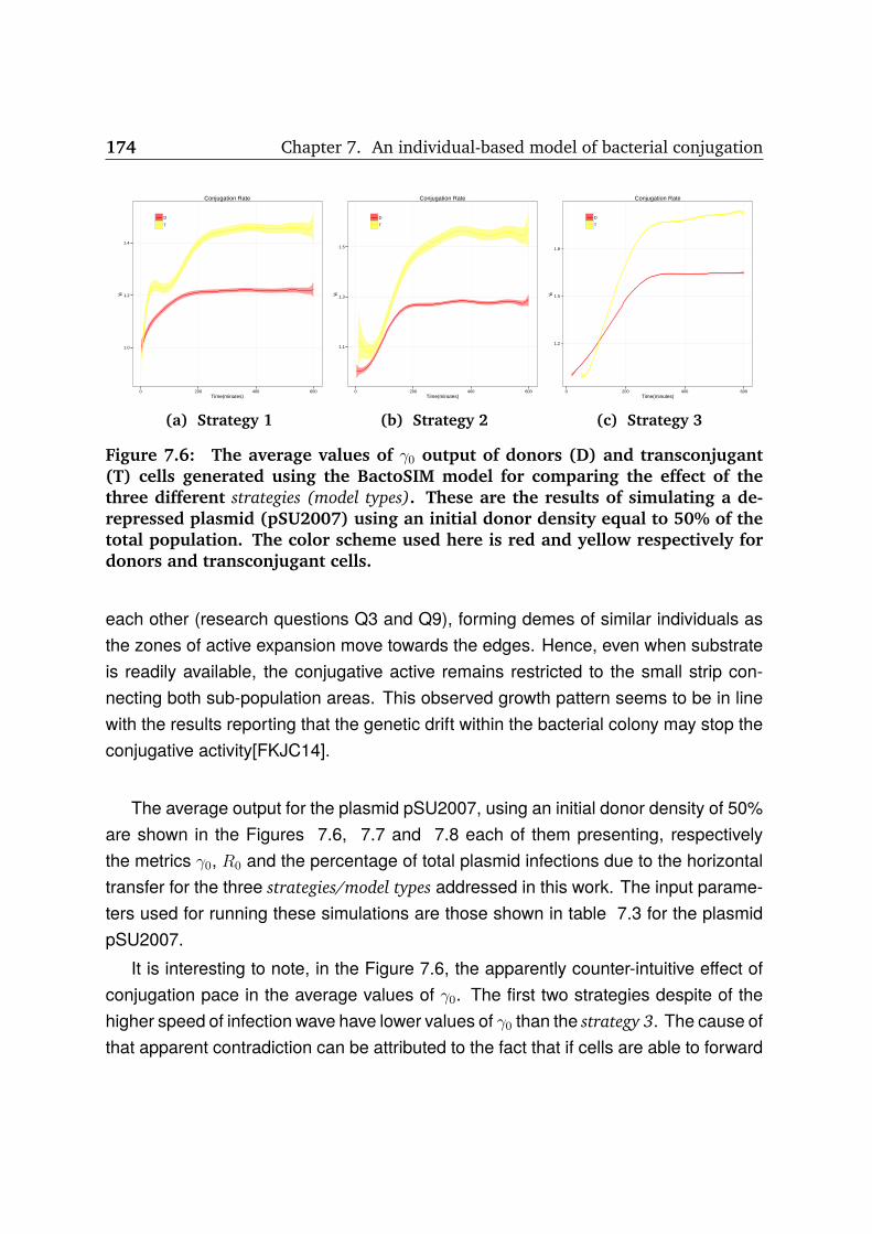
174 Chapter 7. An individual-based model of bacterial conjugation
1.0
1.2
1.4
0 200 400 600Time(minutes)
γ 0
D
T
Conjugation Rate
(a) Strategy 1
1.1
1.3
1.5
0 200 400 600Time(minutes)
γ 0
D
T
Conjugation Rate
(b) Strategy 2
1.2
1.5
1.8
0 200 400 600Time(minutes)
γ 0
D
T
Conjugation Rate
(c) Strategy 3
Figure 7.6: The average values of γ0 output of donors (D) and transconjugant(T) cells generated using the BactoSIM model for comparing the effect of thethree different strategies (model types). These are the results of simulating a de-repressed plasmid (pSU2007) using an initial donor density equal to 50% of thetotal population. The color scheme used here is red and yellow respectively fordonors and transconjugant cells.
each other (research questions Q3 and Q9), forming demes of similar individuals asthe zones of active expansion move towards the edges. Hence, even when substrateis readily available, the conjugative active remains restricted to the small strip con-necting both sub-population areas. This observed growth pattern seems to be in linewith the results reporting that the genetic drift within the bacterial colony may stop theconjugative activity[FKJC14].
The average output for the plasmid pSU2007, using an initial donor density of 50%are shown in the Figures 7.6, 7.7 and 7.8 each of them presenting, respectivelythe metrics γ0, R0 and the percentage of total plasmid infections due to the horizontaltransfer for the three strategies/model types addressed in this work. The input parame-ters used for running these simulations are those shown in table 7.3 for the plasmidpSU2007.
It is interesting to note, in the Figure 7.6, the apparently counter-intuitive effect ofconjugation pace in the average values of γ0. The first two strategies despite of thehigher speed of infection wave have lower values of γ0 than the strategy 3. The cause ofthat apparent contradiction can be attributed to the fact that if cells are able to forward

7.4. Results and discussion 175
the plasmid earlier more cells are infected and able to infect soon which implies anaverage small number of conjugations performed on a cell basis.
Interestingly, the values of γ0 estimated by all strategies are, on average, lowerthan the values provided as the model parameter (see the Table 7.3). Apparently, thisis a consequence of physical separation between infected and uninfected cells whichlimits the number of infectible neighbors (research questions Q3 and Q9). Although,some of the simulated donors or transconjugants in the whole population can reachthe upper limit, the most of individuals cannot because of other physical constraint,such as the neighborhood structure or nutrient availability.
The intrinsic conjugation rates of donor cells stabilizes sooner than the transcon-jugants which continues increasing reaching higher values of γ0. This reflectsthe fact that once the donors cells initiates the process, rapidly become surroun-ded by transconjugant ones which become the dominant factor in the infectionspeed possibly due the barrier of formed. Additionally, the transconjugant cellsare susceptible of overexpressing the conjugative genes owing to the transitory de-repression[SGSL90][RWZ12][LL86][FLdCR+14]. But even without the transitory de-repression the biophysical aspects would play an important role. In order to providea more graphical example for this situation, let us define an optimal donor which iscompletely surrounded by uninfected cells. This optimal donor is so proficient that isable to completely infect all of it plasmid free neighbors and hence all of it becometransconjugants very quickly. This leads to an apparent paradoxical situation becauseon average the transconjugant cells will have higher values of gamma0 than the optimaldonor.
The Figure 7.7 shows the metric R0 which stands for the basic reproduction numberor basic reproductive ratio for the simulated plasmid pSU2007 using an initial donordensity of 50%. This metric plays a central role in epidemiology and could be approx-imately defined as the mean number of secondary infections produced by an infectedindividual[BC93][KG00]. It serves as a reference for analyzing whether an infection willdominate of fadeout in some population. Usually, in most infections, the metric refersexclusively to the horizontal process alone, but in the case of the host-plasmid associa-

176 Chapter 7. An individual-based model of bacterial conjugation
1.0
1.5
2.0
0 200 400 600Time(minutes)
R0
D
T
Basic reproduction number
(a) Strategy 1
1.00
1.25
1.50
1.75
2.00
0 200 400 600Time(minutes)
R0
D
T
Basic reproduction number
(b) Strategy 2
1.0
1.5
2.0
2.5
0 200 400 600Time(minutes)
R0
D
T
Basic reproduction number
(c) Strategy 3
Figure 7.7: The average values of R0 output of donors (D) and transconjugant(T) cells generated using the BactoSIM model for comparing the effect of thethree different strategies (model types). These are the results of simulating a de-repressed plasmid (pSU2007) using an initial donor density equal to 50% of thetotal population. The color scheme used here is red and yellow respectively fordonors and transconjugant cells.
tion R0 is the sum of both vertical and horizontal components [LCWF05] [LNEM95]. Ascan be observed, the pattern are the same for the three strategies/model types with thevalues of R0 being greater for donors than for the transconjugants cells and increasinguntil become stable when reaching the 200 minutes of simulation.
The main idea which can be figured out from the values of R0 metric (researchquestions Q3, Q4, Q5, Q6, Q7 and Q8) shown in the Figure 7.7 is about how thedifferent epidemic strategies6 are affecting the evolution and the maintenance of theplasmid in the population. The values for the basic reproductive number of the donorsub-population clearly outcompete the transconjugants cells, showing a more effectiveplasmid persistency strategy. The focal point here is that the donor cells (D) have toinvest less metabolic resources in the horizontal transfer which could be attributed tothe plasmid-host coadaptation and possibly to the fact that the donor cells alreadyhave expressed to an stable level, most of the genes associated to the conjugation.Consequently, donor cells are able to reproduce faster than the transconjugants, whichincrements the vertical component of R0 making them more efficient. On the other
6Not to be confounded with the modeling strategies

7.4. Results and discussion 177
0
10
20
30
0 200 400 600Time(minutes)
% o
f tot
al
D
T
Cells infected horizontally (%)
(a) Strategy 1
0
10
20
30
0 200 400 600Time(minutes)
% o
f tot
al
D
T
Cells infected horizontally (%)
(b) Strategy 2
0
5
10
15
20
25
0 200 400 600Time(minutes)
% o
f tot
al
D
T
Cells infected horizontally (%)
(c) Strategy 3
Figure 7.8: The average values of horizontal spread output of donors (D) andtransconjugant (T) cells generated using the BactoSIM model for comparing theeffect of the three different strategies (model types). These are the results of si-mulating a de-repressed plasmid (pSU2007) using an initial donor density equalto 50% of the total population. The color scheme used here is red and yellowrespectively for donors and transconjugant cells.
hand, the transconjugants have to dedicate a lot of resources for becoming proficientdonors making them globally less efficient than donor cells. Hence, it can be assumedsafely that if the metabolic penalizations are separated in a system of two components,one related to the cost of conjugation C1 and another to the cost of expressing theconjugative apparatus C2, then C2 > C1.
The last metric shown in the Figure 7.8 is the relative importance which the hori-zontal component in the newly infected individuals for the three modeling strategiesanalyzed. The strategy 1 and the strategy 2 have both a similar pattern which indicatesthat the donor cells are only engaging in horizontal plasmid transmissions during thestart of the simulation process. This certainly is no realistic and is possibly a conse-quence of the donor cells are conjugating two early forcing the reachable recipientsto become quickly depleted (research questions Q1 and Q2). The strategy 3 againseems to produce results which are close to the expected behavior. As can be ob-served, the donor cells are keeping the average horizontal component under a verylow threshold, approximately a 7% of total infections are due to the conjugation. The

178 Chapter 7. An individual-based model of bacterial conjugation
remaining infections are vertically transmitted to the offspring generated by the donorcells.
On the other hand, the horizontal contribution of transconjugant cells are signifi-cantly higher with an average value of approximately 25% of newly infected cells attri-buted to the conjugative transfer. The value of this metric is incrementing linearly untilthe simulated time is equal to 400 minutes. This is basically telling us that the infectionstrategy of transconjugant cells are clearly favoring the conjugation despite of the me-tabolic effort required for expressing the conjugative machinery and for the conjugativetransfer itself. It would be much more reasonable, that donors choose that strategy asthey have an inferior overall cost. Apparently, it is an evolutionary nonsense but witha possible underneath justification which is telling us that even at a micro-scale thespatial separation may play a significant role delimiting the adaptive landscape.
7.5 SummaryIn this chapter we have introduced our modeling approach which has been calledBactoSIM. The model structure has been thoroughly described using the ODD pro-tocol and the output metrics generated by the model have been critically discussed.The model has been assessed informally and the results have allowed us to better un-derstand the individual-level components which are shaping the emergent dynamics.It is important to make clear the terms used here for making reference to the alternativeimplementations of the conjugation rule, as they will be analyzed in the next chapter.We have defined three different implementations, differing with respect to the time inthe cell cycle when the conjugative transfer takes place. These alternative implemen-tations have been called strategies. In order to select one of these strategies the modelimplementation has an input parameter denominated model type which may assumethe values 1, 2 or 3 (models M1, M2 or M3). Hence, M1 is equal to strategy 1, M2 isequal to strategy 2 and M3 is equal to strategy 3. The cyclePoint parameter is usedonly in the M3/strategy 3 and on the other strategies it has no effect as have beendescribed previously in this chapter.
Finally, it is also worth to note that the values of parameters and outputs itself arenot really important since there are a lot of uncertainty in these kind of models and allvalues should be taken as approximates. But what must be noted are the relationships

7.5. Summary 179
between them and their relative magnitudes. The parameters for which experimentaldata are available must fall in realistic ranges and in their relative magnitudes. Forinstance, it could not be stated that the costs of T4SS expression and conjugation arethose used in our simulations but it can be assumed safely that if some parameter isgreater than other in the model the same property possibly holds in the real system.

180 Chapter 7. An individual-based model of bacterial conjugation

Chapter 8Analysis and discusion of
the model output
8.1 Overview . . . . . . . . . . . . . . . . . . . . . . . . . . . . . . . . . . 182
8.2 Definitions . . . . . . . . . . . . . . . . . . . . . . . . . . . . . . . . . . 183
8.3 The effect of temporal structure . . . . . . . . . . . . . . . . . . . . . . 184
8.4 The effect of cell density on initial contact delay . . . . . . . . . . . . . 191
8.5 Description of model analysis . . . . . . . . . . . . . . . . . . . . . . . 194
8.6 Preliminary screening of model output . . . . . . . . . . . . . . . . . . 196
8.7 Assessing the fitness of different models . . . . . . . . . . . . . . . . . 208
8.8 Sensitivity analysis of Model 3 . . . . . . . . . . . . . . . . . . . . . . 211
8.8.1 Sobol indices for a repressed plasmid . . . . . . . . . . . . . . 213
8.8.2 Sobol indices for a de-repressed plasmid . . . . . . . . . . . . 217
8.8.3 Sobol indices for a mobilizable plasmid . . . . . . . . . . . . . 223
8.9 Summary . . . . . . . . . . . . . . . . . . . . . . . . . . . . . . . . . . 238

182 Chapter 8. Analysis and discusion of the model output
8.1 OverviewThe primary purpose of this thesis is to provide a robust operational model for con-jugation using an individual-based approach which can be easily adapted and useda standard modeling tool for simulating the kinetics of conjugative plasmids. In orderto accomplish that goal, we must bring to the light some hidden aspects of conjuga-tion which cannot be observed in whole population experimental setups and only canbe understood using a bottom-up modelling. That approach has an added value be-cause at the same time that we produce a more dependable model, we are generatingknowledge and trying new hypothesis about the of the local structure, as well as, theintra-intracellular and the individual-level factors responsible for the global dynamics.
That is not an easy task because it is necessary to make many assumptions andsimplifications to provide a usable abstraction for the process. It has been used in otherworks as the operational abstraction for bacterial conjugation, a set of rules relying onparameters like some arbitrary probability value, the pilus scan speed, the action radiusof conjugative pili [MLS+11] or even simply the number of infected individuals on theneighborhood [KLF+07].
As a general rule, the good initial assumptions for individual-based models arethose which are biologically consistent and could be almost axiomatically accepted.The assumptions, which fall in this category, are fundamentally that most of the pro-cesses inside of any cell are uphill which basically means that they have fight againstan energy gradient or in other words, that they have a cost. The second assumption,is that cellular processes are subjected to a precise set of timing constraints for allcellular activities and the deviation on these timers is normally disruptive for cellularactivities (temporal structure).
In order to thoroughly understand how the plasmids are distributed and evolve ina bacterial population it is necessary to separately identify the different aspects thataffect the progression of cell to cell transmission and the invasion in the whole popula-tion. The final outcome of the process leading to the partial or total infection a bacterialcolony, can be seen as a non-linear sum of a set of contributions due to vertical and ho-

8.2. Definitions 183
rizontal transfers as well as how much the metabolic burden contributes, as a negativefeedback loop, to the pace of conjugative process.
In this chapter, we will analyze the individual-based model for bacterial conjuga-tion, which has been described in the previous chapter. This model was implementedusing an ensemble of component process which has been used to evaluate the betteralternative for modeling and understand the conjugation systemically. Thereby, usingthis modular design, we have plugged different approaches (strategies/model types)for representing the conjugation with respect to the cell cycle in order to verify whatis the best approach producing a natural fit to a complete and diverse experimentaldata. These alternative modeling approaches have been informally assessed in theprevious chapter.
8.2 DefinitionsIn this section, we will provide some more stricter definitions for some terms we haveused in our conjugation model. This terms are the intrinsic conjugation rate, the cyclepoint and the degrees of freedom.
Definition of γ0
The term γ0 is the total number of conjugative transfers carried out by a sin-gle bacterial cell between the period of two successive divisions. It is a metricrepresenting partially the efficiency of an individual cell for infect its reachablesusceptible neighbors. Actually, it has two different interpretations depending onits value. The first possibility is that γ0 < 1 in this case it is as a probability ina binomial experiment, signaling the fraction of cells which could try to conju-gate. The cells which conjugate will only perform one conjugative transfer. Onthe other hand, when γ0 ≥ 1 all proficient donors could, at least theoretically,try to conjugate a number of times equal to the value of gamma0. The actualnumber of successful conjugations depends also on the availability of infectiblerecipients and on the cell cycle.

184 Chapter 8. Analysis and discusion of the model output
Definition of γ1
The term γ1 represents the fraction of bacterial cell cycle when the conjugativetransfer is most likely to happen. It must be a value from 0 to 1, being 0 the birthof a new cell and 1 the time where the divides generating a new daughter cell.
Degrees of freedom
The total degrees of freedom in the number of model parameters minus the num-ber of constraints defined over the model paramters.
8.3 The effect of temporal structure
The purpose of this section is to expose the rationale behind the idea that the conjuga-tion is most likely to happen later in the cell cycle. In order to accomplish this objectivewe have created a simple abstract representation for the process which eliminates allother factors. Take into account that wave speed of plasmid spread in a bacterial po-pulation constitutes a complex and non-linear process and, as such it is hard to graspany intuitive ideas about the main factors controlling the global behavior of the sys-tem as a whole. Hence, for understanding the spatiotemporal behavior and visualizethe processes some simplifications are required to be made. Hence we have used anetwork analogy, comparing bacterial cells to network nodes which store and forwardmessages, being the conjugative plasmids the message transmitted from cell to cell.
It is known that most cellular processes follows a tight time schedule and is naturalto think that the bacterial conjugation must be subject to the same constraints. Nonet-heless until now, no works have studied how conjugative events are distributed acrossthe cell cycle duration. With respect to time and ignoring other constraints, such as theavailability of reachable susceptible individuals, we may state the following biologicallyrelevant hypotheses:

8.3. The effect of temporal structure 185
Hypotheses
• The time of conjugative transfer event is completely independent of bacte-rial cell cycle and grown conditions being merely a function of plasmid en-dogenous factors.
• On the other hand, plasmids could behave as all other cellular processesbeing linked to the host metabolic level and growth rate.
The main implication of first hypothesis, as should became clear in the next para-graphs, is that the larger is the bacterial generation time more efficient becomes theconjugative process because the infection rate surpasses the host growth rate allowingthe complete plasmid invasion.
In the second hypothesis, the efficiency of a conjugative plasmid depends on thehost growth regime and also on the plasmid intrinsic factors. Hence the time whereconjugation will occur can be expressed as a percentage of bacterial doubling timeindicating the fact that conjugative activity depends and is coordinated by the hostdynamics.
It has already been pointed out recently[MLS+11] that time-related parameters (andconsequently the associated delays) are the most important parameters governing theglobally observed dynamics of plasmid spread in bacterial populations. The authorshave used the sensitivity analysis[MLS+11] for identifying the input factors which arecausing the variability in the model output. In this work, we are also trying to showthat the temporal structure of the process, that is to say, the elapsed interval from thetime when a cell become infected until it is able to forward the plasmid in a secondaryinfection round, is an aspect to be take into account.
The bacterial cellular dynamics controlling the growth and division process has atheoretical framework which has been pointed out as the central dogma bacterial celldivision cycle or simply of Cooper-Helmstetter model[ZWV11]. The model describesthe bacterial cell process relating a set of events such as the chromosome replicationand division to the changes in the cell mass.
According to the BactoSIM model description presented previously in Section 7.3,
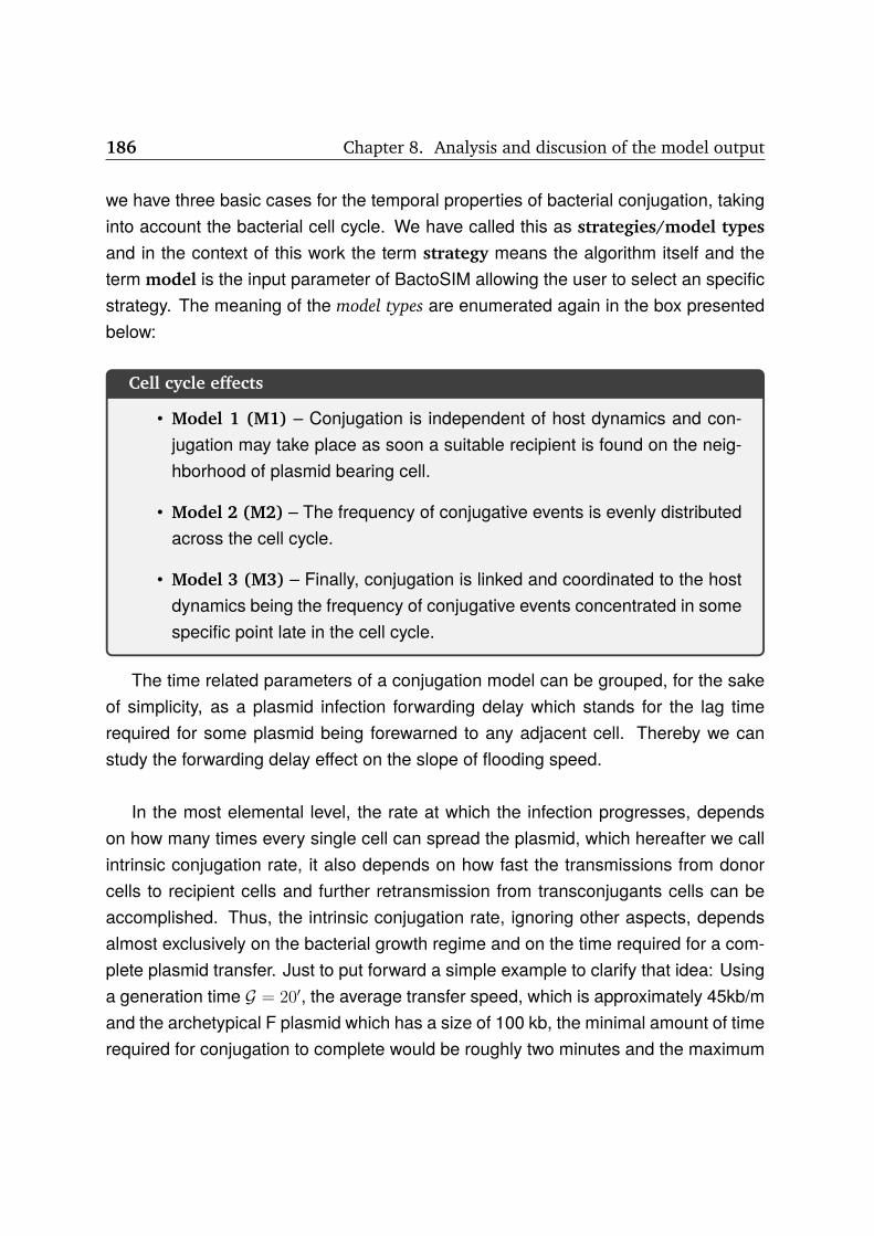
186 Chapter 8. Analysis and discusion of the model output
we have three basic cases for the temporal properties of bacterial conjugation, takinginto account the bacterial cell cycle. We have called this as strategies/model types
and in the context of this work the term strategy means the algorithm itself and theterm model is the input parameter of BactoSIM allowing the user to select an specificstrategy. The meaning of the model types are enumerated again in the box presentedbelow:
Cell cycle effects
• Model 1 (M1) – Conjugation is independent of host dynamics and con-jugation may take place as soon a suitable recipient is found on the neig-hborhood of plasmid bearing cell.
• Model 2 (M2) – The frequency of conjugative events is evenly distributedacross the cell cycle.
• Model 3 (M3) – Finally, conjugation is linked and coordinated to the hostdynamics being the frequency of conjugative events concentrated in somespecific point late in the cell cycle.
The time related parameters of a conjugation model can be grouped, for the sakeof simplicity, as a plasmid infection forwarding delay which stands for the lag timerequired for some plasmid being forewarned to any adjacent cell. Thereby we canstudy the forwarding delay effect on the slope of flooding speed.
In the most elemental level, the rate at which the infection progresses, dependson how many times every single cell can spread the plasmid, which hereafter we callintrinsic conjugation rate, it also depends on how fast the transmissions from donorcells to recipient cells and further retransmission from transconjugants cells can beaccomplished. Thus, the intrinsic conjugation rate, ignoring other aspects, dependsalmost exclusively on the bacterial growth regime and on the time required for a com-plete plasmid transfer. Just to put forward a simple example to clarify that idea: Usinga generation time G = 20′, the average transfer speed, which is approximately 45kb/mand the archetypical F plasmid which has a size of 100 kb, the minimal amount of timerequired for conjugation to complete would be roughly two minutes and the maximum

8.3. The effect of temporal structure 187
intrinsic transfer rate would be 10 conjugations per cell cycle.
Let us assume a simple and yet idealized bacterial population of N individuals witha growth rate µ = 0. The population will be sessile, which implies that the topology ofnetwork will be static and individuals cells will be distributed side by side conformingan interaction structure which could be abstracted by a linear graph as can be seen inFig. 8.1.
Bti Bri+1
Bti-1 Bri Bri+1
ti ti+1
Figure 8.1: The scheme representing the imposed delay on bacterial networks.The Br and Bt are respectively the recipient and transconjugant bacterial nodes.The figure shows the meaning of forwarding delay which is the time elapsedsince a bacteria Br
i is infected becoming a transconjugant Bti and infect the next
recipient cell Bri+1 in the linear graph shown.
Hence assuming the functional similarity between conjugation and networks a com-mon metrics can be used to analyze the process. One of these metrics is the totaldelay required for flooding all nodes in the network with some message M which inthe bacterial context is given by the Equation (8.1)
τ = N × T + (H − 1)× P + (H − 1)× T, (8.1)

188 Chapter 8. Analysis and discusion of the model output
being N the number of messages being forwarded, T the time required for trans-mitting the message, P the time needed for each node to process the message beforebeing able to forward it again and finally H stands for the number of hops in or network.Putting it in terms of bacterial conjugation we have that N represents the plasmid sizein kilobases, T the time required to move a single kilobase from a cell to another, P mayrepresent the two sources of delay which are referred as recovery and maturation timefor donors and recipient cells respectively. Finally H is the actual number of bacterialcells in the linear topology already mentioned.
The aggregated value referred globally as maturation time includes, amongst otherfactors, (a) the time required for adding the second strand to the plasmid inside thenew formed transconjugant cells, (b) the time required to express all genes coding theproteins for the trans-envelope apparatus, and (c) possibly the effect of SOS responsetriggered by entrance of single stranded DNA into the transconjugant cell[BBM10].
The Figure 8.2 shows the temporal evolution of the linear graph which denotesthe bacterial population being infected. In this graph every donor cell, depicted by Bt
i
only have a reachable neighbor which can be infected in a conjugative event. In otherwords the plasmid bearing cell Bt
i can only interact and conjugate with the bacterialagentBr
i+1. Thus, in the simplest case where the forwarding delay is fixed, the infectionspeed can be approximated by a straight line in a form of y = α + βx being α theintercept and β the slope. The value of slope for the most general case is given by theexpression shown in Equation (8.2)
β =|Bt|ti − |Bt|ti−1
∆t
,∀i > 0 (8.2)
where |Bt|ti and |Bt|ti−1 are respectively the counting of Bt cells at ti and ti−1 and∆t = ti− ti−1. The intercept α is zero since at t0 the number of |Bt| cells are also zero.The choice of |Bt| as the indicator of network flooding is just for the sake of generalitybut the same principles will also hold if instead of it the value of T/(T +R) were used.
The Equation (8.2), in the case of unitary increments in the infected nodes which isexactly what is happening in the linear graph show in Figure 8.2 , can be simplified to

8.3. The effect of temporal structure 189
t0 t1 ... tn
...
Brn
... ...
...| B
t |
Brn
Br2
Bd1 Bd1 Bd1
Btn
Bt2Bt2
t2
Br3
Bd1
Bt2
Br3 Bt3 Bt3
Brn
...
Figure 8.2: The simplified interaction graph. This figure shows from left to rightthe snapshots for the temporal evolution of the linear graph representing ourbacterial population. The cell types are Br, Bd and Bt standing respectively forrecipients, donors and transconjugants.
β = 1/∆t. Withal it is easy to realize that the slope have the following lim∆t→∞ 1/∆t = 0
lim∆t→0 1/∆t =∞ lower and upper limits.
The Figure 8.2 may seems hard to interpret at a first sight but it is really simple and
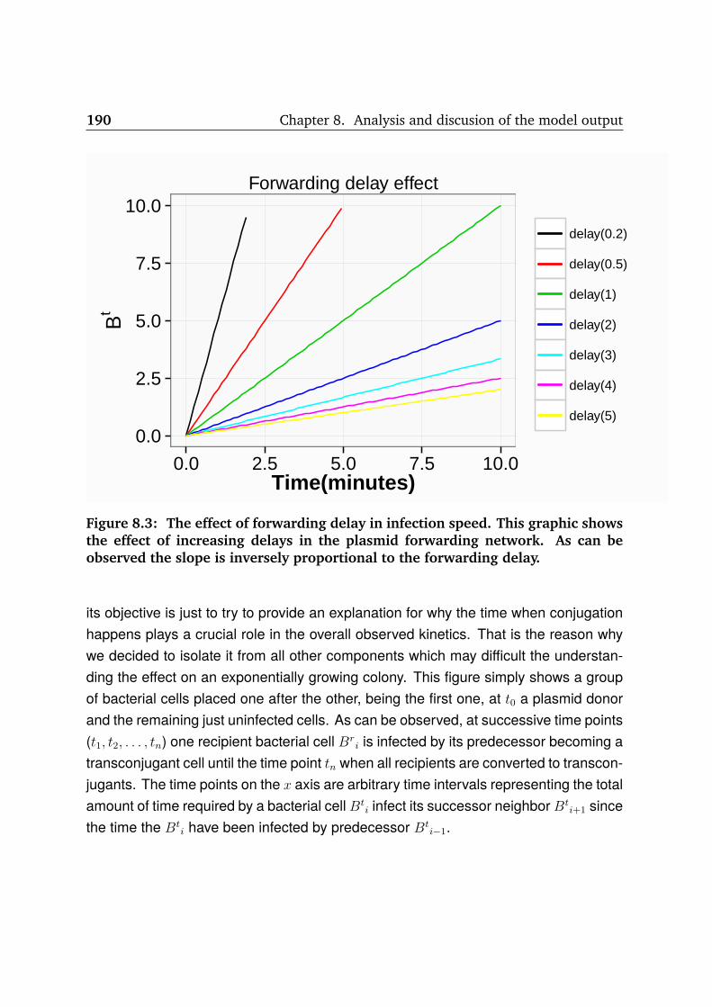
190 Chapter 8. Analysis and discusion of the model output
0.0
2.5
5.0
7.5
10.0
0.0 2.5 5.0 7.5 10.0Time(minutes)
Bt
delay(0.2)
delay(0.5)
delay(1)
delay(2)
delay(3)
delay(4)
delay(5)
Forwarding delay effect
Figure 8.3: The effect of forwarding delay in infection speed. This graphic showsthe effect of increasing delays in the plasmid forwarding network. As can beobserved the slope is inversely proportional to the forwarding delay.
its objective is just to try to provide an explanation for why the time when conjugationhappens plays a crucial role in the overall observed kinetics. That is the reason whywe decided to isolate it from all other components which may difficult the understan-ding the effect on an exponentially growing colony. This figure simply shows a groupof bacterial cells placed one after the other, being the first one, at t0 a plasmid donorand the remaining just uninfected cells. As can be observed, at successive time points(t1, t2, . . . , tn) one recipient bacterial cell Br
i is infected by its predecessor becoming atransconjugant cell until the time point tn when all recipients are converted to transcon-jugants. The time points on the x axis are arbitrary time intervals representing the totalamount of time required by a bacterial cell Bt
i infect its successor neighbor Bti+1 since
the time the Bti have been infected by predecessor Bt
i−1.

8.4. The effect of cell density on initial contact delay 191
The effects of reducing or incrementing the distance between these time pointsare shown on the Figure 8.3, where different intervals of ti+1 − ti are plotted together(ti+1− ti = 0.2, 0.5, 1.0, 2.0, 3.0, 4.0 and 5.0). As can be seen, we show the straight linesrepresenting how the distance between the time points of Figure 8.2 are affecting theslope of conjugation rate (in this case simply the number of transconjugant cells). Thisexample may be a bit naıve but capture the essential aspect of the question, that isto say, increasing the time required for accomplish a conjugation round the slope ofconjugation rate decreases. The same effect is observed in the Figures 7.4 and 7.5shown in the previous chapter for an exponentially growing colony mixed with the effectof more factors.
8.4 The effect of cell density on initial contact delayThe initial inoculum concentration and the carrying capacity of culture medium availa-ble for bacterial cells, has vital implications for elucidating accurately the conjugationrates. These parameters together may be conditioning the in-silico experimental re-sults. Both parameters are influential on the average distance between bacterial cells,which consequently affects the mating pair formation, the time required for the initialcontact and how long takes for the first conjugative event be observed. In addition,the lag period also imposes a delay for the average time required for proficient donorshave access to plasmid free cells.
A simple approximation to the problem of scaling how many bacterial cells dispo-sed over a surface are equivalent to a volumetric measurement, is to consider the totalcarrying capacity of both and determine the scale factor which is given by the expres-sion N/L2, where N is the carrying capacity of liquids and L2 the total amount of latticesites [ZDF+12]. Thus, assuming the computational domain is a grid of 1000× 1000µm
with a carrying capacity of 106 agents and that one milliliter of solution can hold approx-imately 109 bacterial cells then, the scale factor would be 109/106 = 103. That approachhas been used for scaling the results of end-point estimates [SGSL90] of 2D compu-tational models to make them comparable with those values found on liquid cultures.The values reported for the average number of cells/ml of solution present great vari-ability ranging in orders of magnitude from 107 to 109 for studies using the E. coli K-12strain MG1655 [SJPD07]. Therefore, the actual values provided in the experimental

192 Chapter 8. Analysis and discusion of the model output
setups must be taken with care as a reference for approximating the parameters of acomputational model and not as absolute values.
Nonetheless, it is important to consider carefully the initial volume inoculated onthe experimental plates alongside with the reference OD600 values reported for thelaboratory experiments being simulated. Both values are required for generating arealistic initial distribution of individuals over the computation domain. With these pa-rameters plus the surface area of the devices where the inoculum will be plated, it ispossible to generate some basic estimates for the initial average distance betweenindividuals which are responsible for the time required for the occurrence of first con-jugative event. One of the most straightforward ways of generating estimates for theaverage distance between individuals is using the relation between nearest-neighborand population density [Bla58] which is given by the Equation (8.3)
r =
√1
4m(8.3)
where r is the average distance between individuals and m the population densityexpressed as the number of individuals per surface area. The average distance willbe used in the computation model to distribute the initial population aiming to mimicthe existing real separation between bacterial cells.
The value of density m can be calculated by the expression shown in Equation(8.4)
m = OD600 ∗ I/S ∗ C ∗ 1/S (8.4)
where the term OD600 depicts the density readings in cells/ml, the next term I
is the volume of solution in µL inoculated on the experimental plates, the variable S
represents the surface of experimental plates in squared centimeters and finally C isthe conversion factor to express the value of density with the appropriated surface unit,thus for expressing m in cells/mm2 C must be equal to 10−5.
Using the data of a conjugation assay for determining the conjugation rates in solidsurfaces[dCRC+12] we can illustrate the idea presented above. This experimentalsetup uses 24-well microtiter plates which have a surface of 1.9cm2 which have beeninoculated with 15µL of a cell solution of approximately 6 × 10⁸cells/ml given by anOD600 of 0.6 units. Therefore, the value of m is calculated as shown in Equation

8.4. The effect of cell density on initial contact delay 193
(8.5)
m = 6× 10⁸cells/ml ∗ 15/1, 9 ∗ 10−5 ∗ 1/1.9 (8.5)
which give that m is approximately 25000 cells/mm2. Introducing that value inEquation (8.3) we have
r =
√1
4× 25000= 0.003mm (8.6)
converting to micrometers (0.003∗103) we have an average initial distance betweenindividuals equal to 3µm. If we increase one order of magnitude the value of initialconcentration of cells from 6×10⁸cells/ml to 6×10⁹cells/mlwe would obtain an averagedistance between individuals equal to r = 0.001 or 1µm of separation between bacterialcells.
The overall effect of using different initial densities in the separation of bacterialcells can be seen in the virtual culture plates presented in Figure 8.4. As can beobserved, the subfigures (a) to (c) shows visually the effect of decreasing the initialconcentration of bacterial cells in the increment in the average distance between in-dividuals distributed randomly over a culture plate. The Subfigures 8.4a, 8.4b, 8.4cand 8.4d are respectively the virtual plates for initial densities of 109, 108, 107 and 106.
The quantitative effects of varying the initial density of bacterial cells in the requiredtime for engaging the first conjugative contact, is shown in Figure 8.5 which containsthe simulation results of an experimental setup consisting in 301 replications keepingfixed all parameters but the initial cell density (the model parameter N0). The curvesare the average of this 30 replications for each initial density2. Additionally, the Figurealso shows the curve for the reference experimental data. As can be easily observed,the effect of initial density on the time required for making the cell-to-cell contact andconsequentially the conjugative transfer activity is quite evident. The initial densitiesof 109 and 108 implies a minimal initial distance between cells in such extent the con-jugative activity takes places almost in one generation time as can be seen in the firsttwo curves from left to right. The reference data [dCRC+12] shows conjugative activity
1The number of 30 replication has been chosen taking into account the model output stability whichhas been previously discussed in this work.
2The complete R code for this experiment is available on the Appendix A

194 Chapter 8. Analysis and discusion of the model output
(a) Initial density 5× 10⁹ (b) Initial density 5× 10⁸
(c) Initial density 5× 10⁷ (d) Initial density 5× 10⁶
Figure 8.4: Comparing the effect of initial density on the average distance bet-ween individuals in a bacterial culture.
(a conjugation rate T/(T+R) higher than 0.75) approximately from 120 minutes. Thereference data is flanked by the curves simulating the initial densities of 107 and 106 atleft and right respectively. In the last experiment, the conjugative activity is observedvery late, approximately on the 190 minutes of simulated time which is roughly morethan four generations.
8.5 Description of model analysisIn order to fully validate the structural aspects of how we have modeled the conjugationin our individual-based model BactoSIM, a throughout analysis has been carried outusing the methodological approaches previously described in this work, namely thesensitivity analysis and the parameter estimation. Therefore, three sensitivity analysisexperiments have been performed, for exploring the following base parametrization

8.5. Description of model analysis 195
0.1
0.2
0.3
0.4
100 200 300
time
T/(T
+R)
variable
simulated1
simulated2
simulated3
simulated4
experimental
initial density effect
Figure 8.5: The effect of varying the initial densities (N0) on the conjugationrates, showing how it affects the time required for the initial contact. Thesecurves represents, from left to right respectively the simulation output of usingN0 = 109 (red), N0 = 108 (olive green), N0 = 107 (green), the curve fitted to theexperimental data (magenta) and finally, the simulation output of using N0 = 106
(blue).

196 Chapter 8. Analysis and discusion of the model output
options:
• Case 1 – Study of repressed plasmids.
• Case 2 – Study of non-repressed plasmid.
• Case 3 – Study of non-conjugative mobilizable plasmids.
The objective of differentiate these three approaches is owing to the fact that themodel follow distinct trajectories for each of these initial cases and the impact of somemodel parameters on the model output variability are not the same depending on thetype of plasmid being simulated. For instance, in the Case 1 we have an additionalparameter which allow to specify the initial ratio of donors which are de-repressedand conjugative proficient and obviously it has no meaning for initially non-repressedplasmids. These updates have not been made on the model structure itself, but insteadthey are just slight superficial modifications on the required input parameters for ex-posing some previously fixed values or separating the conjugation model from the cellcycle allowing them to be evaluated using the sensitivity analysis techniques depictedon the chapter 6. Consequently, the input parameters which are assessed here are thesame already presented previously on the chapter 7 but including the new initializationoptions included in the Table 8.1.
Table 8.1: The list of BactoSIM additional model initialization parameters.
Parameter Unit Description
model N/A The model type. Accepted values are 1,2 or 3 whichare respectively the previously discussed models forconjugation.
nutrients particles The amount of nutrient particles.initialDRDratio N/A The ratio of initial donors which are derepressed.
8.6 Preliminary screening of model outputIn this section we will show the preliminary results obtained for the sensitivity analysisprocess which have been used for evaluate and understand the outputs generated by

8.6. Preliminary screening of model output 197
the BactoSIM model in order to substantiate some conclusions of this work. Thus, thefirst aspect we want to verify, is whether the modeling approach for representing theconjugation has some significant impact on the model outcome as has been visuallyevaluated in the previous chapter. Bearing this in mind, we have applied the screeningmethod of Morris for an initial approximation to the problem, evaluating the effect ofmodel choice in for the two main cases mentioned in the previous section, namelythe case 1 which represents the plasmids naturally repressed and the case 2 whichencloses those plasmids which are constitutively expressing the conjugative geneticmachinery.
The main objective of using an screening method, as have been mentioned pre-viously in the chapter 6, is to undertake an initial delimitation of the factors which areresponsible for the most of the output variance. In this specific case we want to verifywhether or not the model is an important factor. For ensuring the reproducibility ofthe results shown here, the scripts used for each of the experiments discussed in thischapter will be listed in the Appendix A.
The results shown in Table 8.2, in Table 8.3 and in Table 8.3 are the metrics µ,µ∗ and σ calculated for the elementary effects which have been estimated using themethod of Morris. These values allows to rank which factors are causing the most ofvariance for the rate (T/(T+R) output variable. The results are sorted by the µ∗ metricfrom the most to the less significant factors. As can be observed the model inputparameter has a very significant effect and is above all others remaining parametersfor the three cases of study, namely the case 1, case 2 and case 3, respectively themodel for repressed, de-repressed and mobilizable plasmids.

198 Chapter 8. Analysis and discusion of the model output
Table 8.2: The Morris metrics for the elementary effects of BactoSIM model.This table contains the results for the case 1.
Input parameter µ µ∗ σ
model -0.151139889 0.16720867 0.44574069conjugationCost 0.030000238 0.03398144 0.07126060γ0 0.020518046 0.02849222 0.06534011nutrients 0.020736414 0.02277778 0.04429573cyclePoint -0.001234407 0.01706222 0.03081159initialDRDratio 0.007167759 0.01545636 0.03506770pilusExpressionCost 0.014500096 0.01453345 0.02439932
It is interesting to recall that the model types differs fundamentally by the timingwhen conjugation is triggered and that the values for Morris metrics are very similarwhich seems to confirm, in some extent, the previous results, obtained from a simplevisual assessment, which were pointing in the same direction.
Table 8.3: The Morris metrics for the elementary effects of BactoSIM model.This table contains the results for the case 2.
Input parameter µ µ∗ σ
model 0.032421289 0.07310568 0.11969663cyclePoint 0.017944503 0.04340028 0.06430294nutrients 0.032973536 0.03821871 0.03778982initialDRDratio 0.002396539 0.03696602 0.05696925pilusExpressionCost -0.032051696 0.03267854 0.03101232conjugationCost -0.025976738 0.03093565 0.04885718γ0 0.018859565 0.02691402 0.02644715

8.6. Preliminary screening of model output 199
Table 8.4: The Morris metrics for the elementary effects of BactoSIM model.This table contains the results for the case 3.
Input parameter µ µ∗ σ
model 0.037685503 0.05526285 0.09896928cyclePoint 0.019857680 0.04926191 0.07241082initialDRDratio 0.003399129 0.03650807 0.04455440γ0 0.016580862 0.02704785 0.03759677nutrients 0.025812398 0.02581240 0.03260287conjugationCost -0.013923998 0.01916376 0.02748788pilusExpressionCost -0.018641321 0.01921991 0.02054882
Figures 8.6, 8.8 and 8.10 shows graphically the numeric results for the metric µof the screening exercise which has been previously shown in the Tables 8.2 and 8.3.Additionally, the metric µ∗ is shown in Figures 8.7, 8.9 and 8.11. Both metrics µ andµ∗ are taken from the elementary effects for model output representing the simulatedconjugation rate T/(T + R) for a repressed, de-repressed and mobilizable plasmids,the case 1, case 2 and case 3 respectively. These plots allows the easy visualizationthe effects of model choice in the variability of conjugation rate output.
The results seem to be consistent with the assumption that the approach used forrepresenting the conjugation process, is clearly responsible for the most of the mo-del output variation. In other words, the input parameter model type, which allows theselection of the conjugation strategy, is clearly and consistently ranked as the mostimportant according to the results of Morris method. It means fundamentally that tem-poral structure of the process (the time when the conjugative transfer is most likelyto happen) is responsible for the most part of the global dynamics. It is necessary tomention that the Morris method is not estimating the model parameters but just rankingthe effects of varying these parameters.
In the case of the derepressed plasmid, the other parameters in importance are thenutrient availability, the γ1 (cyclePoint) and the γ0 falling all very close in the rank butγ1 is the input parameter of this group with the greater σ which means a high effect of

200 Chapter 8. Analysis and discusion of the model output
variating the parameter input values. The mobilizable plasmid shows a similar resultswith γ1 and nutrient availability ranking high but having the first a higher value for σwhich, as we have mentioned previously indicates that the variation on the values ofthis input parameter causes a large variability in the estimated elementary effects andconsequently on the model output.
On the other hand, for the repressed plasmid, we may observe a group of threeparameters with high importance which are the frequency of initial derepressed donorratio in the population (initialDRDratio), the model type and the metabolic cost ofexpression the conjugative machinery (pilusExpressionCost). The parameter modeltype has the higher value of σ which means that the model output will be very sensibleto variations on its values. This group is followed by the conjugatioCost which alsoshows a high value of σ. It is important to mention that the differences observed forthe (pilusExpressionCost) in the metrics µ and µ∗ (see Section 6.1.2) are a possibleindication of effects of different signs which could indicate a non-monotonic3 effect onthe output. The effect of (pilusExpressionCost) possibly depends non-linearly on othermodel components, mainly those affecting the initial number of transconjugant cells,such as the initial derepressed ratio.
Finally, despite of not being a formal statistics hypothesis test, the results of Morrisscreening method can serve as reference for discarding, with relative safety that theway the conjugation rule is implemented with respect to the timing aspects, are notequal. The Morris method allows the input parameters of a model to be ranked inorder of its importance using the metric known as elementary effects. Therefore, weare not directly testing whether M1, M2 and M3 are equal or not but ranking the effectsof setting this input parameter. Indirectly, if the model type has no effect, it should havebeen ranked low, but it is not the case. Hence, we may affirm that model type (howconjugation rule is implemented) has an effect on the model output. We will extendthis observation applying a formal hypothesis test approach in the next section.
3We mean by non-monotonic effect, that the model output does not follows a linear relation with theinput parameter domain. In other words, increasing some input parameter value may cause the modeloutput to increase for a specific set of values and decrease for others. This normally indicates that modelcontains feedback loops and non-linear components.

8.6. Preliminary screening of model output 201
The hypothesis we are analyzing in this work is presented on the box below. Thenull hypothesis basically says that the model formulation (the model type is a para-meter for choosing one of the strategies presented in the previous chapter) has noeffect being all approaches equivalent. According to the model description presentedpreviously, in the M1 (strategy 1) the conjugative transfer may occur as soon a donorcell finds a suitable plasmid free recipient. In the M2 (strategy 2) the conjugation isuniformly distributed along the cell cycle and finally in the M3 (strategy 3) the conju-gation is assumed to occur in a precise point of time, specified by the parameter γ1
(cyclePoint).
Hypotheses
h0,M1 =M2 =M3
h1,M1 6=M2 6=M3

202 Chapter 8. Analysis and discusion of the model output
0.024
0.028
0.032
0.036
0.000 0.005 0.010 0.015µ
σ
group
conjugationCost
cyclePoint
gamma0
initialDRDratio
model
nutrients
pilusExpressionCost
output(rate)
Figure 8.6: Results of Morris screening method for the BactoSIM output simu-lating a repressed plasmid (case 1). This figure shows the µ sensitivity metric forBactoSIM T/(T +R) output.

8.6. Preliminary screening of model output 203
0.024
0.028
0.032
0.036
0.015 0.018 0.021 0.024
µ*
σ
group
conjugationCost
cyclePoint
gamma0
initialDRDratio
model
nutrients
pilusExpressionCost
output(rate)
Figure 8.7: Results of Morris screening method for the BactoSIM output simu-lating a repressed plasmid (case 1). This figure shows the µ∗ sensitivity metric forBactoSIM T/(T +R) output.

204 Chapter 8. Analysis and discusion of the model output
0.025
0.050
0.075
0.100
−0.02 0.00 0.02µ
σ
group
conjugationCost
cyclePoint
gamma0
initialDRDratio
model
nutrients
pilusExpressionCost
output(rate)
Figure 8.8: Results of Morris screening method for the BactoSIM output simula-ting a derepressed plasmid (case 2). This figure shows the µ sensitivity metric forBactoSIM T/(T +R) output.

8.6. Preliminary screening of model output 205
0.025
0.050
0.075
0.100
0.03 0.04 0.05 0.06 0.07
µ*
σ
group
conjugationCost
cyclePoint
gamma0
initialDRDratio
model
nutrients
pilusExpressionCost
output(rate)
Figure 8.9: Results of Morris screening method for the BactoSIM output simula-ting a derepressed plasmid (case 2). This figure shows the µ∗ sensitivity metric forBactoSIM T/(T +R) output.

206 Chapter 8. Analysis and discusion of the model output
0.02
0.04
0.06
0.08
0.10
−0.02 0.00 0.02 0.04µ
σ
group
conjugationCost
cyclePoint
gamma0
initialDRDratio
model
nutrients
pilusExpressionCost
output(rate)
Figure 8.10: Results of Morris screening method for the BactoSIM output simu-lating a mobilizable (OriT) plasmid (case 3). This figure shows the µ sensitivitymetric for BactoSIM T/(T +R) output.

8.6. Preliminary screening of model output 207
0.02
0.04
0.06
0.08
0.10
0.02 0.03 0.04 0.05
µ*
σ
group
conjugationCost
cyclePoint
gamma0
initialDRDratio
model
nutrients
pilusExpressionCost
output(rate)
Figure 8.11: Results of Morris screening method for the BactoSIM output simu-lating a mobilizable (OriT) plasmid (case 3). This figure shows the µ∗ sensitivitymetric for BactoSIM T/(T +R) output.

208 Chapter 8. Analysis and discusion of the model output
8.7 Assessing the fitness of different modelsIn the previous section we have found that the parameter model type (M1, M2 and M3)significantly affects the behavior of conjugation rate estimated by the BactoSIM model.The model type is the input parameter which allows the selection of modeling strategydefined in Sections 7.3 and 8.3 the possible values are 1, 2 and 3 respectively for M1,M2 and M3. In this section we will undertake a parameter estimation study, separatingthe analysis in three groups keeping fixed the model type for each of them in order toprovide a comprehensive view about which could be the possible best approach forrepresenting the bacterial conjugation. For undertake the parameter estimation pro-cess, we will use the EvoPER package described previously in the chapter 5. We haveused initially the simulated annealing algorithm for the parameter estimation owing tothe fact that it requires fewer model evaluations than other choices and provide goodapproximations to the model optima. The scripts for running the parameter estimationand the data analysis of this section are provided in Appendix A.
The Table 8.5 shows the fitness cost of each model type as well as the avera-ged values of the solutions found for each of the three approaches for modeling theconjugative transfer. The best values for the optimization criteria was achieved by themodel 3 followed by the model 2 and model 1. On the other hand, when considering theaverage values of cost functions the models 2 and 1 change its order but the model 3still is the best positioned. In other words, we have applied an optimization algorithmto find the best combination of parameters for the three strategies/model types whichhave been fully described in the ODD protocol of BactoSIM model presented in theSection 7.3. Roughly speaking, the process consists in keeping fixed the parameterwhich allows the selection of the model/strategy (this input parameter is called mo-
del and may have three values 1, 2 and 3) and allowing all other parameters to varyover their domains, repeating the operation for the model = 1, 2, 3. With this approachwe have found the possible best combination for each of them which shows that thestrategy/model 3 provided the minimal distance between experimental and simulateddata.
The word fitness or the expression fitness cost used in this section is unrelated to

8.7. Assessing the fitness of different models 209
the evolutive meaning of the term. Here, the term fitness basically means a functionto be optimized, which in most cases means to find the function minima. Hence, ourfitness cost function is distance measurement between the experimental data for theconjugation essays and the simulated results generated with our BactoSIM model.Therefore, in order to find the best parametrization for our model we want to minimizethe fitness function.
Table 8.5: The results for parameter estimation of BactoSIM using the simula-ted annealing metaheuristic. The table shows estimated best values satisfyingthe optimization criteria. The estimated model parameters shown in this tableare γ1, C1, C2 γ0 and ratio(drd), respectively the cell cycle point, the conjugationcost, the t4ss pilis expression cost, the intrinsic conjugation rate and the ratioof donors which are initially de-repressed.
Model fitness average γ1 C1 C2 γ0 ratio(drd)
model 1 4.551496 9.55 0.0 43.38 0.84 0.45 0.05model 2 4.489114 12.94 50.0 0.17 6.99 1.02 0.01model 3 2.618539 6.88 81.14 7.56 62.04 1.94 0.08
It is also worth to note in Table 8.5 that the parameters estimated for the models1 and 2 shown values for the metabolic cost which could be inconsistent with the ex-perimental reality. For instance, it was estimated that the conjugative cost should beapproximately 43% and 0.17% respectively for model 1 and 2. The model 1 shows avalue for the pilus expression cost inferior of the conjugation cost which does not ma-tch with the expected behavior. On the other hand the model 3 shows very consistentestimations for cell cycle and for both cost which possibly are very close to the realvalues.

210 Chapter 8. Analysis and discusion of the model output
Table 8.6: The Anova results for verifying if the values estimated by the diffe-rent models are statistically significant.
Df Sum Sq Mean Sq F value Pr(>F)
model 2 3584.41 1792.20 34.40 3.65e-14Residuals 297 15472.31 52.10
In order to verify that the null hypothesis can be reject we have applied the ANOVAtest to the estimated fitness values. The h0, as have been stated previously, is thatall alternative model formulations (model/strategy 1,2,3) are fundamentally equal andtherefore the γ1 plays no role in such extent that conjugation may take place in anypoint of bacterial cell cycle.
The results of this test is shown in table 8.6 and in addition we have also performeda non-parametric of Kruskal-Wallis for avoiding to rely on any restrictive assumptionabout the distribution of the fitness values. This test have given a p value of 2.448e-11,therefore in both case we can reject safely the null hypothesis.
It is worth noting that normally we should not rely exclusively on statistical tests forassessing the outputs of computational models. It is considered that ANOVA signifi-cance tests are not well suited for analyzing the effects alternative model formulationsor for quantifying how significant are the contribution of the input factors on the modeloutput [WRS+14] for two important reasons. First, they claim that the null hypothesisis known a priori to be false4 which violates the premise underlying the statistical testswhich dictates that the outcome for the hypothesis under study is unknown. The se-cond point is that the p-values are dependent on the number of model replication andconsequently, with a high number of simulation replicates, low p-values are achievedleading (incorrectly) to take some effect as highly significant. In any case the signifi-cant test present here are simply a comparison for the average values for the model
4We cannot completely agree with this assumptions in the case of alternative model formulations,because it is perfectly possible to build models with different implementations producing similar resultsas there is not a unique mapping between a model and the system under study.

8.8. Sensitivity analysis of Model 3 211
fitness metric and should be seen as auxiliary tool for supporting the hypothesis thatthese specific model formulations differences should be considered as relevant.
8.8 Sensitivity analysis of Model 3In this section we show and discuss the results of Sobol variance decomposition met-hod which has been used for the global sensitivity analysis of the model type 3 output.As we have previously mentioned in this work, the model/strategy type 3 consists ba-sically in one of the alternative formulations of the conjugation rule used in this studywhich takes into account the parameter γ1 (cellCycle) for linking the conjugative eventto the host cell cycle. The methodology employed for analyzing systematically the re-presentativeness of every model parameter in the total variance of the output has beenintroduced previously in the Chapter 6, Section 6.1.2, consisting in the estimation ofboth first and total order indices[STCR04][Sal08] for model output under study.
The model type 3, according to the data which has been shown in the previoussections of this chapter as well as in the previous chapter, provides the best compu-tational representation for the plasmid spread dynamics, when compared to the twoalternative representations. The objective of performing this type of analysis is to un-derstanding how the output variance should be apportioned to each model parameterin order of being able to handle consistently the uncertainty on the model inputs. Ad-ditionally, the results of this method may provide another evidence for supporting ourclaim about the importance of time-related aspects when building a discrete time con-jugation model.
We have analyzed the model contrasting its outputs to the experimental dataset(The experimental data was kindly provide by the Professor Fernando de la Cruz labo-ratory) using the time series of conjugation rate from three different plasmids, namelythe pAR118, the pSU2007 and a pR388(MOB) which are representative examples, re-spectively of a repressed system, a de-repressed one which constitutively express theconjugative machinery and finally the last plasmid is a non-conjugative construction.The pAR118 is a derivative of R1 plasmid and the last two are based on the pR388backbone. In order to undertake the sensitivity analysis, we have defined an objective

212 Chapter 8. Analysis and discusion of the model output
function for comparing the subset of model outputs for which the experimental datawere available. Specifically, these outputs are the time-series for the conjugation rateT/(T +R) and the doubling of both donors and transconjugant cells. The conjugationrate data was not used directly in the objective function, instead for simplifying the com-parison between experimental and simulated data, an simple third degree polynomialequation was fitted to the reference data which are shown in the Table 7.2 presentedpreviously in this manuscript.
Bearing in mind the reproducibility of the experimental results obtained from theapplication of Sobol method, all code required for running the same experiments areshown in the Appendix A.
It is important to remark that the results presented here are preliminary ones be-cause it is not feasible, using the computational resources of a desktop computing, toperform the required number of model execution for reaching an stable output. Accor-ding to the stability results, which have been previously shown in the Figure 6.6, wemay realize that due to the individual variability the model require a minimum numberof replications for the same parameter set in order to produce stable outputs5.
The computational cost of applying the Sobol method is N × (p+ 2) model evalua-tions, where N is the number of samples and p the number of input parameters beinganalyzed. Therefore, assuming a value of N = 1000, the number of input factors arep = 6 and the minimal number of experimental replications are r = 15 we find that weneed to execute the model at least 64K times. This is a very high number of execu-tions for a costly individual-based model which requires approximately 30 minutes forsimulating 6 hours of bacterial growth using a grid size equal to 1000µm2 hence, asthe model results are stable (data no shown) with a reduced grid dimensions, we havechosen to use a grid size of 250µm2 for practical reasons.
Even using the reduced grid size, the above number of model executions are stillprohibitive without the use of a large parallel cluster6. The complete sensitivity ana-lysis for each experimental setup would take approximately 192 hours of wall time ina hardware based on Intel(R) Core(TM) i7-2630QM processor at 2.00GHz clock with
5It is required approximately 50 replications for each set of input factors for achieving a completelysteady model output. But it can be also observed that with roughly 30 replications the model variabilitystarts to converge very significantly. Finally, with replication values greater than 15, the amplitude of theobserved oscillations can be accepted as the minimal number of replications for getting stable results.
6We are planning to reassess the model distributing the workload across several machines

8.8. Sensitivity analysis of Model 3 213
8GB being the model execution parallelized across all available cores7. Additionally,the system resources become depleted due to the lack of resources devoted to theheap space of all virtual machines running in parallel. Thereby, for performing the mo-del analysis we have had to sacrifice some precision in order to circumvent the thesepractical limitations. In the experiments shown in this chapter, we have had to reducethe number of samples, using a N = 500 with one replications of each set of inputfactors.
In some cases, this setup have produced somewhat unreliable results, possiblydue to the interactions between the model parameters and the large variability as con-sequence of the individual levels stochasticity. In these cases we have also analyzedthe sensitivity analysis outputs but noting that certainly the experiment would requiremore replications in order to provide adequate outputs. The current simulation setuprequires approximately 20 hours to complete.
8.8.1 Sobol indices for a repressed plasmidIn general the experiment for the repressed plasmid pAR118 has shown a some in-stability with respect to the input parameters producing indices with negative values,indicating that is necessary to increment the number of model samples in order toachieve a more stable results.
Figures 8.12, 8.13, 8.14 and 8.15 contains the first order indices and the totalorder indices calculated using the Sobol method of variance decomposition applied tosimulation output of the repressed plasmid pAR118 using and initial donor to recipientratio of 5% for the input factors conjugationCost, γ0 and cyclePoint. Figure 8.12shows the contribution of the input parameters on the conjugation rate expressed asthe ratio T/(T + R). The Figure 8.13 has the effect of the model input parameterson the generation time of donor cells. The Figure 8.14 shows the effect that everyinput parameter has on the generation time of transconjugant cells. Finally, the 8.15contains the effects of the model input parameters on the composite output which isthe sum of these three previous outputs.
As can be observed in the Figure 8.12, where the Sobol indices for the conjugation
7The last version of R/Repast parallelize the individual model execution using the doSNOW packagehttps://CRAN.R-project.org/package=doSNOW

214 Chapter 8. Analysis and discusion of the model output
−0.4
0.0
0.4
0.8
conjugationCost cyclePoint gamma0 initialDRDratio nutrients pilusExpressionCostparameter
Si
Sobol indexes for rate
(a) First order
0.0
0.5
1.0
1.5
conjugationCost cyclePoint gamma0 initialDRDratio nutrients pilusExpressionCostparameter
ST
i
Sobol indexes for rate
(b) Total order
Figure 8.12: Sensitivity analysis for the plasmid pAR118 using an initial donordensity of 5%. The first and total order Sobol sensitivity metrics, respectively thesubfigures (a) and (b), for the BactoSIM model parameters with respect to theconjugation rate T/(T +R) output.
rate T/(T + R) are shown, both first and the total order indices are telling us that themost important parameter is the point in the cell cycle when conjugative transfer is mostlikely to happen, followed by the γ0, the initial de-repressed donor ratio, the conjugationcost, the cost of expressing the T4SS conjugative pili and finally the nutrient availability.These results seems to be consistent which the expected model behavior and withthe logic behind the conjugative process. The first order indices Si shows a negativevalue for pili expression cost which could be possibly attributed to need of increasingthe number of samples but also due to the non-linear interactions between the modelinput factors.
The Sobol indices for the doubling time output of both donor and transconjugant

8.8. Sensitivity analysis of Model 3 215
−0.5
0.0
0.5
conjugationCost cyclePoint gamma0 initialDRDratio nutrients pilusExpressionCostparameter
Si
Sobol indexes for gD
(a) First order
0.0
0.5
1.0
1.5
conjugationCost cyclePoint gamma0 initialDRDratio nutrients pilusExpressionCostparameter
ST
i
Sobol indexes for gD
(b) Total order
Figure 8.13: Sensitivity analysis for the plasmid pAR118 using an initial donordensity of 5%. The first and total order Sobol sensitivity metrics, respectively thesubfigures (a) and (b), for the BactoSIM model parameters with respect to thegeneration time of plasmid donor cells (D) output.
cells shown in Figures 8.13 and 8.14 have some noise and requires more samples forobtaining better results. The first order indices Si of both outputs present four negativevalues therefor we avoid to draw any conclusions about it. Nonetheless, the total orderindices ST i shows for the doubling time of donors that the cost of conjugation and theexpression of conjugative apparatus are equally important which is consequence ofthe fact that donors cells also require some expression level of T4SS genes. On theother hand the most significant input factor for transconjugant cells is the cost of T4SSexpression. It is also worth to mention that the initial de-repressed donor has a highimpact on the doubling time output of both donors and transconjugants.
Finally, the overall effect on the composite output is shown in Figure 8.13 which

216 Chapter 8. Analysis and discusion of the model output
−0.5
0.0
0.5
conjugationCost cyclePoint gamma0 initialDRDratio nutrients pilusExpressionCostparameter
Si
Sobol indexes for gT
(a) First order
0.0
0.5
1.0
1.5
conjugationCost cyclePoint gamma0 initialDRDratio nutrients pilusExpressionCostparameter
ST
i
Sobol indexes for gT
(b) Total order
Figure 8.14: Sensitivity analysis for the plasmid pAR118 using an initial donordensity of 5%. The first and total order Sobol sensitivity metrics, respectively thesubfigures (a) and (b), for the BactoSIM model parameters with respect to thegeneration time of transconjugant cells (T) output.
is noise but seems to confirm the global significance for the cost of expressing theconjugative machinery, followed by the cycle point and the de-repressed donor ratio.
Figures 8.16, 8.17, 8.17 and 8.19 contains the first order indices and the totalorder indices calculated using the Sobol method of variance decomposition applied tosimulation output of the repressed plasmid pAR118 using and initial donor to recipientratio of 50%. The Figure 8.16 shows the contribution of the input parameters on theconjugation rate expressed as the ratio T/(T+R). The Figure 8.17 has the effect of themodel input parameters on the generation time of donor cells. The Figure 8.18 showsthe effect that every input parameter has on the generation time of transconjugant cells.Finally, the 8.19 contains the effects of the model input parameters on the composite

8.8. Sensitivity analysis of Model 3 217
−0.5
0.0
0.5
conjugationCost cyclePoint gamma0 initialDRDratio nutrients pilusExpressionCostparameter
Si
Sobol indexes for total
(a) First order
0.0
0.5
1.0
1.5
conjugationCost cyclePoint gamma0 initialDRDratio nutrients pilusExpressionCostparameter
ST
i
Sobol indexes for total
(b) Total order
Figure 8.15: Sensitivity analysis for the plasmid pAR118 using an initial donordensity of 5%. The first and total order Sobol sensitivity metrics, respectively thesubfigures (a) and (b), for the BactoSIM model parameters with respect to thecomposite effect output which is the sum of individual effects over T/(T + R) plusthe effects on the generation time of donors and transconjugant cells.
output which is the sum of these three previous outputs.
8.8.2 Sobol indices for a de-repressed plasmidFigures 8.20, 8.21, 8.21 and 8.23 contains the first order indices and the totalorder indices calculated using the Sobol method of variance decomposition applied tosimulation output of the repressed plasmid pSU2007 using and initial donor to recipientratio of 5%. The Figure 8.20 shows the contribution of the input parameters on theconjugation rate expressed as the ratio T/(T+R). The Figure 8.21 has the effect of themodel input parameters on the generation time of donor cells. The Figure 8.22 shows

218 Chapter 8. Analysis and discusion of the model output
−0.2
−0.1
0.0
0.1
0.2
conjugationCost cyclePoint gamma0 initialDRDratio nutrients pilusExpressionCostparameter
Si
Sobol indexes for rate
(a) First order
0.0
0.3
0.6
0.9
conjugationCost cyclePoint gamma0 initialDRDratio nutrients pilusExpressionCostparameter
ST
i
Sobol indexes for rate
(b) Total order
Figure 8.16: Sensitivity analysis for the plasmid pAR118 using an initial donordensity of 50%. The first and total order Sobol sensitivity metrics, respectivelythe subfigures (a) and (b), for the BactoSIM model parameters with respect tothe conjugation rate T/(T +R) output.
the effect that every input parameter has on the generation time of transconjugant cells.Finally, the 8.23 contains the effects of the model input parameters on the compositeoutput which is the sum of these three previous outputs.
The sensitivity analysis for the de-repressed plasmid pSU2007 with an initial do-nor density of 5% shows a strong influence of the nutrient availability which clearlydominates over the remaining input factors as can be observed for the first and totalorder indices Si and ST i shown in the Figure 8.20. The next parameters in order ofimportance are the cycle point andγ0. Finally, it can be also observed from the totalorder plot, that cost of T4SS expression followed by the conjugation costs are the lastones contributing in the total variance.

8.8. Sensitivity analysis of Model 3 219
−0.2
−0.1
0.0
0.1
0.2
conjugationCost cyclePoint gamma0 initialDRDratio nutrients pilusExpressionCostparameter
Si
Sobol indexes for gD
(a) First order
0.0
0.3
0.6
0.9
conjugationCost cyclePoint gamma0 initialDRDratio nutrients pilusExpressionCostparameter
ST
i
Sobol indexes for gD
(b) Total order
Figure 8.17: Sensitivity analysis for the plasmid pAR118 using an initial donordensity of 50%. The first and total order Sobol sensitivity metrics, respectivelythe subfigures (a) and (b), for the BactoSIM model parameters with respect tothe generation time of plasmid donor cells (D) output.
The results of the sensitivity analysis for output variable representing the doublingtime of donors cells which are presented in Figure 8.21. Both first order and totalorder indices are clearly pointing that variability of donor generation time is practicallycontrolled by the cost of expressing the conjugative pili and followed at some distanceby the conjugationCost. The other model parameters seems to present some nonli-near interaction with respect to this output. This results seems to be consistent withthe common senses that the most costly part of the donor metabolic effort is due tothe expression of conjugative apparatus.
In the case of transconjugant cells the Sobol indices shown in Figure 8.22 aresaying practically the same as in the previous case, that is to say, the generation time

220 Chapter 8. Analysis and discusion of the model output
−0.1
0.0
0.1
0.2
conjugationCost cyclePoint gamma0 initialDRDratio nutrients pilusExpressionCostparameter
Si
Sobol indexes for gT
(a) First order
0.0
0.5
1.0
conjugationCost cyclePoint gamma0 initialDRDratio nutrients pilusExpressionCostparameter
ST
i
Sobol indexes for gT
(b) Total order
Figure 8.18: Sensitivity analysis for the plasmid pAR118 using an initial donordensity of 50%. The first and total order Sobol sensitivity metrics, respectivelythe subfigures (a) and (b), for the BactoSIM model parameters with respect tothe generation time of transconjugant cells (T) output.
is strongly coupled to the metabolic effort dedicated to express the T4SS genes withthe remaining parameters showing non-additive interactions.
Finally, the composite metric shown in Figure 8.23 also indicates the greatest influ-ence of the pilusExpressionCost in the overall model behavior and the remaining inputfactors seems to interact which is somehow expected due to the coupling between theother model parameters.
Figures 8.24, 8.25, 8.25 and 8.27 contains the first order indices and the totalorder indices calculated using the Sobol method of variance decomposition applied tosimulation output of the repressed plasmid pSU2007 using and initial donor to recipientratio of 50%. The Figure 8.24 shows the contribution of the input parameters on the

8.8. Sensitivity analysis of Model 3 221
−0.2
−0.1
0.0
0.1
0.2
conjugationCost cyclePoint gamma0 initialDRDratio nutrients pilusExpressionCostparameter
Si
Sobol indexes for total
(a) First order
0.0
0.3
0.6
0.9
1.2
conjugationCost cyclePoint gamma0 initialDRDratio nutrients pilusExpressionCostparameter
ST
i
Sobol indexes for total
(b) Total order
Figure 8.19: Sensitivity analysis for the plasmid pAR118 using an initial donordensity of 50%. The first and total order Sobol sensitivity metrics, respectivelythe subfigures (a) and (b), for the BactoSIM model parameters with respect tothe composite effect output which is the sum of individual effects over T/(T + R)plus the effects on the generation time of donors and transconjugant cells.
conjugation rate expressed as the ratio T/(T+R). The Figure 8.25 has the effect of themodel input parameters on the generation time of donor cells. The Figure 8.26 showsthe effect that every input parameter has on the generation time of transconjugant cells.Finally, the 8.27 contains the effects of the model input parameters on the compositeoutput which is the sum of these three previous outputs.
Similarly as previously described in this section for the experiment with an initialdonor density of 5%, the sensitivity indices for pSU2007 using an initial concentration50% presented in Figure 8.24 shows the importance of the model parameter relatedto the availability of substrate, followed by the cyclePoint, the γ0, the expression costof T4SS genes and finally the conjugation cost itself. Both first order and total order in-

222 Chapter 8. Analysis and discusion of the model output
−0.25
0.00
0.25
0.50
conjugationCost cyclePoint gamma0 nutrients pilusExpressionCostparameter
Si
Sobol indexes for rate
(a) First order
0.0
0.2
0.4
0.6
0.8
conjugationCost cyclePoint gamma0 nutrients pilusExpressionCostparameter
ST
i
Sobol indexes for rate
(b) Total order
Figure 8.20: Sensitivity analysis for the plasmid pSU2007 using an initial donordensity of 5%. The first and total order Sobol sensitivity metrics, respectively thesubfigures (a) and (b), for the BactoSIM model parameters with respect to theconjugation rate T/(T +R) output.
dices shows practically the same thing, differing from the cases of repressed plasmidswhere it seems to be more non-linear interactions between the model parameters.
With respect to the doubling time, the Sobol indices shown in Figure 8.25 saysthat the most part of the output variability of this variable come from the cost of ex-pressing the conjugative machinery followed by the cost of conjugation but with muchless importance than the first. The remaining parameters have similar impact on theoutput.
The sensitivity analysis for the doubling time of transconjugant cells, which are pre-sented in Figure 8.26, also indicates a strong influence of the pilusExpressionConstin the variance of this model output followed by the nutrient availability. The remaining

8.8. Sensitivity analysis of Model 3 223
0.00
0.25
0.50
conjugationCost cyclePoint gamma0 nutrients pilusExpressionCostparameter
Si
Sobol indexes for gD
(a) First order
0.0
0.2
0.4
0.6
conjugationCost cyclePoint gamma0 nutrients pilusExpressionCostparameter
ST
i
Sobol indexes for gD
(b) Total order
Figure 8.21: Sensitivity analysis for the plasmid pSU2007 using an initial donordensity of 5%. The first and total order Sobol sensitivity metrics, respectively thesubfigures (a) and (b), for the BactoSIM model parameters with respect to thegeneration time of plasmid donor cells (D) output.
parameters are much less influential on the output variable.Finally, the composite output variable, shown in Figure 8.27, reproduces the pattern
observed for the doubling time of the transconjugant cells. This basically means thatthe cost of expressing the conjugative apparatus has a very strong influence on theoutput, taking into account that the output defined here is a distance metric betweenthe observed and the simulated data.
8.8.3 Sobol indices for a mobilizable plasmidThe mobilizable plasmid analyzed here in this section is a construction which uses thestructural backbone of an R388 plasmid eliminating the OriT which is added to another

224 Chapter 8. Analysis and discusion of the model output
−0.25
0.00
0.25
0.50
conjugationCost cyclePoint gamma0 nutrients pilusExpressionCostparameter
Si
Sobol indexes for gT
(a) First order
0.00
0.25
0.50
0.75
1.00
conjugationCost cyclePoint gamma0 nutrients pilusExpressionCostparameter
ST
i
Sobol indexes for gT
(b) Total order
Figure 8.22: Sensitivity analysis for the plasmid pSU2007 using an initial donordensity of 5%. The first and total order Sobol sensitivity metrics, respectively thesubfigures (a) and (b), for the BactoSIM model parameters with respect to thegeneration time of transconjugant cells (T) output.
plasmid making it mobilizable when in presence of the helper R388 plasmid which con-tains the core genes required for expressing the conjugative machinery. Being morespecific, the mobilizable element is an instance of the pGP12[SHL] plasmid contai-ning the OriT of an R388 plasmid cloned upstream of an GFP reporter protein whichis repressed in presence of R388. The helper plasmid is an R388 plasmid without afunctional OriT and therefore, the plasmid itself cannot be transferred to recipient cells.Hence, the donor cells will contain both mobilizable and helper plasmids for transfer-ring the mobilizable one but, consequently the transconjugant cells will not be able toengage in a second round of conjugative transfer [dCRC+12].
Figures 8.28, 8.29, 8.29 and 8.31 contains the first order indices and the total

8.8. Sensitivity analysis of Model 3 225
−0.25
0.00
0.25
0.50
0.75
conjugationCost cyclePoint gamma0 nutrients pilusExpressionCostparameter
Si
Sobol indexes for total
(a) First order
0.00
0.25
0.50
0.75
1.00
conjugationCost cyclePoint gamma0 nutrients pilusExpressionCostparameter
ST
i
Sobol indexes for total
(b) Total order
Figure 8.23: Sensitivity analysis for the plasmid pSU2007 using an initial donordensity of 5%. The first and total order Sobol sensitivity metrics, respectively thesubfigures (a) and (b), for the BactoSIM model parameters with respect to thecomposite effect output which is the sum of individual effects over T/(T + R) plusthe effects on the generation time of donors and transconjugant cells.
order indices calculated using the Sobol method of variance decomposition applied tosimulation output of the repressed plasmid pR388(OriT) using and initial donor to re-cipient ratio of 5%. The Figure 8.28 shows the contribution of the input parameters onthe conjugation rate expressed as the ratio T/(T +R). The Figure 8.29 has the effectof the model input parameters on the generation time of donor cells. The Figure 8.30shows the effect that every input parameter has on the generation time of transconju-gant cells. Finally, the 8.31 contains the effects of the model input parameters on thecomposite output which is the sum of these three previous outputs.
Figures 8.32, 8.33, 8.33 and 8.35 contains the first order indices and the totalorder indices calculated using the Sobol method of variance decomposition applied to

226 Chapter 8. Analysis and discusion of the model output
−0.2
0.0
0.2
0.4
conjugationCost cyclePoint gamma0 nutrients pilusExpressionCostparameter
Si
Sobol indexes for rate
(a) First order
0.0
0.2
0.4
conjugationCost cyclePoint gamma0 nutrients pilusExpressionCostparameter
ST
i
Sobol indexes for rate
(b) Total order
Figure 8.24: Sensitivity analysis for the plasmid pSU2007 using an initial donordensity of 50%. The first and total order Sobol sensitivity metrics, respectivelythe subfigures (a) and (b), for the BactoSIM model parameters with respect tothe conjugation rate T/(T +R) output.
simulation output of the repressed plasmid pR388(OriT) using and initial donor to reci-pient ratio of 50%. The Figure 8.32 shows the contribution of the input parameters onthe conjugation rate expressed as the ratio T/(T +R). The Figure 8.33 has the effectof the model input parameters on the generation time of donor cells. The Figure 8.34shows the effect that every input parameter has on the generation time of transconju-gant cells. Finally, the 8.35 contains the effects of the model input parameters on thecomposite output which is the sum of these three previous outputs.
The first order and total order Sobol indices for the conjugation rate T/(T+R) out-put obtained from the simulation of a mobilizable plasmid termed R388(OriT) at aninitial donor density of 50% presented in the Figure 8.32, shows that the input

8.8. Sensitivity analysis of Model 3 227
0.0
0.2
0.4
0.6
conjugationCost cyclePoint gamma0 nutrients pilusExpressionCostparameter
Si
Sobol indexes for gD
(a) First order
0.00
0.25
0.50
0.75
1.00
conjugationCost cyclePoint gamma0 nutrients pilusExpressionCostparameter
ST
i
Sobol indexes for gD
(b) Total order
Figure 8.25: Sensitivity analysis for the plasmid pSU2007 using an initial donordensity of 50%. The first and total order Sobol sensitivity metrics, respectivelythe subfigures (a) and (b), for the BactoSIM model parameters with respect tothe generation time of plasmid donor cells (D) output.
factor cyclePoint clearly dominates over the remaining model parameters followedby the nutrient availability, the γ0 and finally the both the conjugationCost and thepilusExpressionCost having similar importance.
The sensitivity analysis for the generation time of donor cells shown in Figure 8.33indicates that the most import parameter is the expression cost of the T4SS conjugativemachinery, which is approximately two times greater than the second in importancewhich is the cost of conjugation. The other parameters accounting for model variabilityare the cycle point, the γ0 and the nutrient availability which apparently tends to interactnon-additively as cab be seen in the discrepancies in the Si and ST i.

228 Chapter 8. Analysis and discusion of the model output
0.0
0.3
0.6
0.9
conjugationCost cyclePoint gamma0 nutrients pilusExpressionCostparameter
Si
Sobol indexes for gT
(a) First order
0.0
0.3
0.6
0.9
conjugationCost cyclePoint gamma0 nutrients pilusExpressionCostparameter
ST
i
Sobol indexes for gT
(b) Total order
Figure 8.26: Sensitivity analysis for the plasmid pSU2007 using an initial donordensity of 50%. The first and total order Sobol sensitivity metrics, respectivelythe subfigures (a) and (b), for the BactoSIM model parameters with respect tothe generation time of transconjugant cells (T) output.
Interestingly, the sensitivity indices for the transconjugant cells shown in Figure8.34 are telling us that most important input factor for the variance in this output vari-able, differently from previous cases, is the nutrient availability having the remainingparameters a similar importance. That is the correct and expected behavior becausethe transconjugant cells in this simulations are neither able to express the conjugativemachinery nor to accomplish secondary conjugation rounds. Therefore, the only li-miting and conditioning factor controlling the doubling time variance of transconjugantcells is the substrate availability.
The overall importance given by the composite output variable shown in Figure

8.8. Sensitivity analysis of Model 3 229
−0.3
0.0
0.3
0.6
conjugationCost cyclePoint gamma0 nutrients pilusExpressionCostparameter
Si
Sobol indexes for total
(a) First order
0.00
0.25
0.50
0.75
1.00
1.25
conjugationCost cyclePoint gamma0 nutrients pilusExpressionCostparameter
ST
i
Sobol indexes for total
(b) Total order
Figure 8.27: Sensitivity analysis for the plasmid pSU2007 using an initial donordensity of 50%. The first and total order Sobol sensitivity metrics, respectivelythe subfigures (a) and (b), for the BactoSIM model parameters with respect tothe composite effect output which is the sum of individual effects over T/(T + R)plus the effects on the generation time of donors and transconjugant cells.
8.35, faithfully accounts that the parameters controlling the three model outputs arein order of importance (total order), the cost of expressing the T4SS apparatus, thenutrient availability, the cost of conjugative transfer, the cycle point and finally γ0

230 Chapter 8. Analysis and discusion of the model output
−1
0
1
2
conjugationCost cyclePoint gamma0 nutrients pilusExpressionCostparameter
Si
Sobol indexes for rate
(a) First order
−1
0
1
2
conjugationCost cyclePoint gamma0 nutrients pilusExpressionCostparameter
ST
i
Sobol indexes for rate
(b) Total order
Figure 8.28: Sensitivity analysis for the plasmid pR388(OriT) using an initial do-nor density of 5%. The first and total order Sobol sensitivity metrics, respectivelythe subfigures (a) and (b), for the BactoSIM model parameters with respect tothe conjugation rate T/(T +R) output.

8.8. Sensitivity analysis of Model 3 231
−0.5
0.0
0.5
1.0
conjugationCost cyclePoint gamma0 nutrients pilusExpressionCostparameter
Si
Sobol indexes for gD
(a) First order
0.0
0.5
1.0
1.5
conjugationCost cyclePoint gamma0 nutrients pilusExpressionCostparameter
ST
i
Sobol indexes for gD
(b) Total order
Figure 8.29: Sensitivity analysis for the plasmid pR388(OriT) using an initial do-nor density of 5%. The first and total order Sobol sensitivity metrics, respectivelythe subfigures (a) and (b), for the BactoSIM model parameters with respect tothe generation time of plasmid donor cells (D) output.

232 Chapter 8. Analysis and discusion of the model output
−0.6
−0.3
0.0
0.3
0.6
conjugationCost cyclePoint gamma0 nutrients pilusExpressionCostparameter
Si
Sobol indexes for gT
(a) First order
0.0
0.5
1.0
1.5
conjugationCost cyclePoint gamma0 nutrients pilusExpressionCostparameter
ST
i
Sobol indexes for gT
(b) Total order
Figure 8.30: Sensitivity analysis for the plasmid pR388(OriT) using an initial do-nor density of 5%. The first and total order Sobol sensitivity metrics, respectivelythe subfigures (a) and (b), for the BactoSIM model parameters with respect tothe generation time of transconjugant cells (T) output.

8.8. Sensitivity analysis of Model 3 233
−1
0
1
2
conjugationCost cyclePoint gamma0 nutrients pilusExpressionCostparameter
Si
Sobol indexes for total
(a) First order
−1
0
1
2
conjugationCost cyclePoint gamma0 nutrients pilusExpressionCostparameter
ST
i
Sobol indexes for total
(b) Total order
Figure 8.31: Sensitivity analysis for the plasmid pR388(OriT) using an initial do-nor density of 5%. The first and total order Sobol sensitivity metrics, respectivelythe subfigures (a) and (b), for the BactoSIM model parameters with respect tothe composite effect output which is the sum of individual effects over T/(T + R)plus the effects on the generation time of donors and transconjugant cells.

234 Chapter 8. Analysis and discusion of the model output
0.0
0.2
0.4
conjugationCost cyclePoint gamma0 nutrients pilusExpressionCostparameter
Si
Sobol indexes for rate
(a) First order
0.0
0.1
0.2
0.3
0.4
0.5
conjugationCost cyclePoint gamma0 nutrients pilusExpressionCostparameter
ST
i
Sobol indexes for rate
(b) Total order
Figure 8.32: Sensitivity analysis for the plasmid pR388(OriT) using an initialdonor density of 50%. The first and total order Sobol sensitivity metrics, re-spectively the subfigures (a) and (b), for the BactoSIM model parameters withrespect to the conjugation rate T/(T +R) output.

8.8. Sensitivity analysis of Model 3 235
−0.25
0.00
0.25
0.50
conjugationCost cyclePoint gamma0 nutrients pilusExpressionCostparameter
Si
Sobol indexes for gD
(a) First order
0.0
0.2
0.4
0.6
0.8
conjugationCost cyclePoint gamma0 nutrients pilusExpressionCostparameter
ST
i
Sobol indexes for gD
(b) Total order
Figure 8.33: Sensitivity analysis for the plasmid pR388(OriT) using an initialdonor density of 50%. The first and total order Sobol sensitivity metrics, re-spectively the subfigures (a) and (b), for the BactoSIM model parameters withrespect to the generation time of plasmid donor cells (D) output.

236 Chapter 8. Analysis and discusion of the model output
0.0
0.2
0.4
0.6
conjugationCost cyclePoint gamma0 nutrients pilusExpressionCostparameter
Si
Sobol indexes for gT
(a) First order
0.00
0.25
0.50
0.75
conjugationCost cyclePoint gamma0 nutrients pilusExpressionCostparameter
ST
i
Sobol indexes for gT
(b) Total order
Figure 8.34: Sensitivity analysis for the plasmid pR388(OriT) using an initialdonor density of 50%. The first and total order Sobol sensitivity metrics, re-spectively the subfigures (a) and (b), for the BactoSIM model parameters withrespect to the generation time of transconjugant cells (T) output.

8.8. Sensitivity analysis of Model 3 237
0.0
0.2
0.4
conjugationCost cyclePoint gamma0 nutrients pilusExpressionCostparameter
Si
Sobol indexes for total
(a) First order
0.0
0.2
0.4
conjugationCost cyclePoint gamma0 nutrients pilusExpressionCostparameter
ST
i
Sobol indexes for total
(b) Total order
Figure 8.35: Sensitivity analysis for the plasmid pR388(OriT) using an initialdonor density of 50%. The first and total order Sobol sensitivity metrics, re-spectively the subfigures (a) and (b), for the BactoSIM model parameters withrespect to the composite effect output which is the sum of individual effects overT/(T + R) plus the effects on the generation time of donors and transconjugantcells.

238 Chapter 8. Analysis and discusion of the model output
8.9 SummaryIn this chapter we have analyzed systematically the BactoSIM model output using theparameter estimation and the sensitivity analysis tools for trying to understanding thesources of uncertainty enclosed in the model results. We have performed the prelimi-nary analysis using the Morris screening method, which provide good results and isnot too much expensive, computationally speaking. The basic objective for applyingthis technique is to check if the model parameter effectively contributes for the out-put variability and we have found that it was one of the most important parameters ofBactoSIM.
Afterwards, the next step was to order the three model types according to its contri-butions for the fitness cost, that is to say, the distance between the simulated and theobserved data. We have used an optimization metaheuristic for undertake this stepand we have found that the model type 3 provided the best fit for the experimentaldata. We have applied the ANOVA test for verifying whether the fitness outputs for thethree models were statistically distinct. Our results points that the better way to modelbacterial conjugation is making the period where a donor is able to conjugate locatedat a small window late in the bacterial cell cycle. On the average, the window wheremost conjugative events will occur is located at least 50% of bacterial generation timewith a small coefficient of variation not greater than a 10% of the average value. Withthese values the best fit to the experimental data is achieved.
Despite of the fact that the experimental values of conjugation rates T/(T +R) forthe whole population can present a broad range of variation depending on the plasmidtype or if they are repressed or depressed, the local values are consistently low. Bylocal values we mean the number of conjugative events during the interval betweentwo successive divisions, that is to say the intrinsic conjugation rate (γ0). In otherwords, the values of γ0 required for achieving a good fit to the experimental data are onaverage, equal to one event per cell cycle with an upper bound lower than two events(Tables 8.5). This seems to be consequence of spatial structure leading to physicalseparation of donors to their potential susceptible recipients but this is compensatedby the vertical transfer allowing the plasmids to become established, even though the

8.9. Summary 239
horizontal infection spread becomes slightly limited.
Additionally, the most significant contribution to the global dynamics of the model isthe total delay required to forward the plasmid, at least for derepressed and mobilizableplasmids. That is to say, the parameter γ1 (cellCycle), according to the rank of Morrisscreening method (Tables 8.2, 8.3 and 8.4) is the most significant in two cases. In thecase of repressed plasmids, such as the pAR118 used in this study, γ1 is the fifth inimportance. Furthermore, the results obtained from the Sobol method (Figures 8.20,8.24 and 8.32) has confirmed these results for the derepressed plasmid pSU2007(initial donor densities of 5% and 50%) and for the mobilizable plasmids R388(OriT)(initial donor density of 50%).
The model output for three different plasmids has been evaluated using the So-bol method, at two initial donor concentrations in order to emulate the experimen-tal setup[dCRC+12]. The global sensitivity analysis results in some of the situati-ons evaluated here were extremely clear, as in the case of de-repressed plasmidpSU2007 which show the importance of the cellCycle in the model output variability.The composite metric shows a somehow counterintuitive result about the effect of thepilusExpressionCost parameter on the generation time of both donor and transcon-jugant cells. That possible behavior has two explanations. The first explanation isrelated to the model structure which initializes the initial donor cells population withsome random ratio of them having an already stable level of T4SS expression, butpart of the initial population has to invert some metabolic effort to reach the stablelevel of expression. The second explanation has to do with the competition betweendonors and transconjugants as the transconjugant cells need to expend much moreenergy for expressing the conjugative apparatus, allowing the donor outcompete themfor space and nutrients which also explain the importance of nutrient output variable8.
Generally speaking, the sensitivity indices for the conjugation rate output are cle-arly pointing out that cyclePoint (γ1) parameter has a very significant impact on theoutput variance. In some cases, as can be observed for the de-repressed plasmid it
8The nutrient dependency is an structural part of the model and therefore it is an expected behavior.On the other hand, the cycle dependency is an emergent property.

240 Chapter 8. Analysis and discusion of the model output
was the second most important behind the nutrient input factor which could be attri-buted to a strong competition between donors and transconjugants, as well as, to thevertical transmission. The mobilizable plasmids, which are basically performing oneconjugation round, shows a canonical behavior being the cycle parameter the mostimportant. The repressed plasmid are somewhat more noise and certainly the expe-riments may require more replications, but also seems to indicate γ1 as significant forthe conjugation rate T/(T +R) output.

Part V
Conclusions and Future Research


Chapter 9Conclusions

244 Chapter 9. Conclusions
In this thesis, we have presented a study based on the computational simulationfor the bacterial conjugation kinetics in structured environments. This study uses anindividual-based modeling approach for capturing some of the fundamental structuralproperties governing the global dynamics of the plasmid spread patterns. The modelrelies on the conceptualization of the cell-cycle dependency as well as the associatedmetabolic costs and delays related to the conjugation process. In other words, themodel express the idea that horizontal gene transfer is somehow linked to the host cellcycle requiring some amount of time, relative to the interval between successive birthand divisions, for the occurrence of conjugative events. In order to carry out a conju-gative transfer, bacterial cells devote some amount of their energetic resources whichis collectively denoted as the plasmid metabolic burden encompassing the metaboliccosts and delays increasing the cell cycle length of plasmid donors. This dependencyconstitutes a feedback loop, as the conjugation depends on the cell cycle which in turn,depends on the fitness penalization derived from conjugation activity.
The former idea is conceptually simple and it could even be assumed axiomaticallyas being structurally consistent with the biological reality of the underlying system. Thecomplete process of validating this mechanistic model about how and when the con-jugation occurs, was carried out in two steps. The first step was a simple exploratoryanalysis, consisting in the visual assessment comparing the model outputs with theexperimental time series for the conjugation rates T/(T + R). The comparison wascarried out using different approaches to express the conjugation rule. The rationalebehind the methodology was to identify and build up three falsifiable hypotheses whichwere non-overlapping representations of the conjugation process. The first hypothe-sis, considered the conjugation as being completely independent of cell cycle in suchextent that the conjugative event occurred immediately when a suitable recipient isfound by any proficient donor. The second approach consisted in the assumption thatconjugative events were evenly distributed across the cell cycle and, was implemen-ted using a uniform distribution. Finally, the third one dictates that the conjugation islinked to the cycle occurring on a restrict temporal window and implemented usinga random number with normal distribution. These three rules share all the commonmodel sub-process for the vegetative cellular behavior and the colony expansion. Theinitial results obtained with the simple experimental setup have shown that the last oneprovides the most natural adjustment to the experimental data.

245
Subsequently, recognizing the need of a more formal approach for validating thesimulation outputs, the model was submitted to a more throughout assessment usingthe parameter estimation and the sensitivity analysis methodologies introduced pre-viously in this work. The first methodology consisted in expressing the discrepanciesbetween the observed and the simulated values as an optimization problem which isamenable for the application of metaheuristic-based minimization algorithms.
By recognizing the difficulties of finding an acceptable optimum in a reasonableamount of time, owing to the computational cost of simulating the minimal numberof agents for obtaining representative results, we have tried to use heuristic searchalgorithms that requires few evaluations. These algorithms have been adapted forproviding an additional output with the collection of visited points in the search space forproducing a map with the solutions with the best fitness values. These maps promotethe identifications of the real solution zones being useful for an exploratory analysisthan a single point estimate with the local optima found for the problem. The secondtechnique, the global sensitivity analysis serves for assessing quantitatively the effectsof the model inputs on the output variance constituting a fundamental piece for thewhat-if analysis allowing a broader model comprehension.
The both methodologies used together can greatly improve the level of confidenceof the conclusions and insights extracted from the model results although it is possiblya terrible error-prone and frustrating task to extract trustworthy conclusions exclusi-vely from computational simulation outputs. It is especially true when the referenceexperimental data available and used for the parameter estimation come from wholepopulation studies and the values being analyzed make reference to intracellular pro-perties which are complicated or impossible to elucidate experimentally. All the soft-ware developed in the context of this thesis for simulating the conjugation dynamics(BactoSIM) and the R packages EvoPER and R/Repast are opensource and releasedunder the MIT license.
We recognize the fact and assume that the conclusions should be taken with abso-lute care but nevertheless empathize the importance of the results and the qualitativeexplanations extracted from our computational model. The model building is viablebecause of the 80/20 Pareto principle holds for most of the physical and biological sy-stems with a limited number of system parameters explaining the most part of systemtrajectories. In the end, there is no need that model to be true, it is enough just to

246 Chapter 9. Conclusions
provide a marginal improvement about the structural parts of a system.In the specific framework of this work, we estimate that a significant advance has
been made in the local to global and in the systemic knowledge of conjugation processto the extent that some of main effects have been ranked quantitively using a soundcomputational and analytical methodology. That approach could be considered at leastas a weak evidence in the context of biological systems, allowing us to be assertive inthe importance of considering the linking between cell cycle, the intrinsic conjugationrates and metabolic costs to the global dynamics observed. These results are referringto the surface attached bacterial colonies but certainly can also be extrapolated forliquid cultures.
Admittedlly, we cannot state with a complete confidence the true values of these pa-rameters but we could be satisfied with being confident about their relative magnitudesand that at least that the simulated values are in the same order of magnitude and thatthe estimated parameters are close to their real values. Again, the size and scale areimportant physical constraints and differently from other host-parasite or host-symbiontassociations which are separated by orders of magnitude which makes the cycle de-pendence and the relative impact on the metabolic cost negligible, the case of bacterialplasmids the both magnitudes are very close and the effects on the epidemic dynamicsis a factor to be taken into account.

Chapter 10Future work

248 Chapter 10. Future work
In this work, we have outlined what we consider, based on the analysis of the modeloutputs, the most basic tenets of what conforms the kinetics of plasmid spread, namelycycle dependency and the simple metabolic cost model affecting the cell cycle. Thevalidation of these two components-model have shown an acceptable agreement withthe experimental data, both quantitatively and qualitatively. The observed global pat-tern developed during the growth of bacterial colony seems to indicate that we haveachieved a structurally sound model. Of course, it is needless to say that, as in thecase of any research work, results are far from being somehow definitive. Additionally,it is necessary to improve and extend the initial aspects presented here, relating theplasmid structural characteristics and its impact on the observed conjugation kinetics.
With respect to the experimental validation it would be very important, in order toavoid the confirmation bias, to implement an experimental design for corroborate thatthe hypothesis about the linking between conjugation and cell cycle actually holds.Therefore, it will require some laboratory work from microbiologists for designing se-veral conjugation essays for the same combination of plasmid and bacterial strain usingthe culturing medium for tuning the growth at different speeds for corroborate or refutethe null hypothesis which fundamentally states that, in average, conjugation rates aresimilar, independently of the bacterial doubling time and consequently linked to the cellcycle.
The second mentioned item, is another clear path for continuing and improving thiswork. Fundamentally, the current version of the model serves as the base for elucida-ting some intracellular aspects of plasmid-host interaction but it is no operational forpredicting what kind of behavior should be expected without first executing a completeexperimental conjugation essay. Naturally, it is not practical and an ideal model shouldbe able to provide at least some basic predictions using the data taken from the pla-smid structural aspects such as the amount of DNA, the annotated gene products insuch extent that it can be used for computing an energy budget and its interference onthe overall cellular energetic profile. This would be a really useful improvement ma-king the model suitable for prediction the conjugation dynamics even on unculturablebacterial strains or in uncontrollable natural environments.
Finally, but not least important some effort is still required on the engineering as-pects of the model software. The current versions encompass a disperse collection ofmany model implementations with slight variations for verifying some specific aspect

249
of the conjugation process. Thus, it is necessary to consolidate these versions basedon the results as well as improving some of the model sub-process. Additionally, itwould be also a significant improvement, being able to accelerate the model executionspeed in order to simulate larger populations and making a better physical dynamicsfor the aspects related to the bacterial growth sub-process dynamics.

250 Chapter 10. Future work

Bibliography
[AF13] Denis Arutyunov and Laura S. Frost, F conjugation: Back to the be-ginning, Plasmid 70 (2013), no. 1, 18–32.
[AFNKB09] Maksat Ashyraliyev, Yves Fomekong-Nanfack, Jaap A. Kaandorp,and Joke G. Blom, Systems biology: Parameter estimation for bio-chemical models, 2009, pp. 886–902.
[AH93] T.H. Andres and W.C. Hajas, Using iterated fractional factorial designto screen parameters in sensitivity analysis of a probabilistic risk as-sessment model, 1993.
[AIC08] Keith L. Aubin, Bojan Ilic, and Harold G. Craighead, Micro- andNanoelectromechanical Sensors, Handbook of Biosensors and Bio-chips, John Wiley & Sons, Ltd, Chichester, UK, mar 2008.
[Alv12] Jean Pierre Arteaga Alvarez, Enhancing idynomics framework to si-mulate rod-shape bacterial colonies growth, Master’s thesis, Facultadde informatica(UPM), 2012.
[ASD06] Sonja-Verena Albers, Zalan Szabo, and Arnold J. M. Driessen, Proteinsecretion in the Archaea: multiple paths towards a unique cell surface,Nature Reviews Microbiology 4 (2006), no. 7, 537–547.
[BA77] James Vere Beck and Kenneth J. Arnold, Parameter estimation in en-gineering and science, Wiley series in probability and mathematicalstatistics, Wiley, New York, 1977.
251

252 Bibliography
[BBM10] Zeynep Baharoglu, David Bikard, and Didier Mazel, Conjugative DNAtransfer induces the bacterial SOS response and promotes antibioticresistance development through integron activation., PLoS genetics 6(2010), no. 10, e1001165+.
[BC93] Stavros. Busenberg and Kenneth. Cooke, Vertically Transmitted Di-seases : Models and Dynamics, Springer Berlin Heidelberg, 1993.
[BCNN09] Jerry Banks, John S. Carson, Barry L. Nelson, and David M. Nicol,Discrete-Event System Simulation (5th Edition), 5 ed., Prentice Hall,July 2009.
[BD87] George Box and Norman Draper, Empirical model-building and re-sponse surfaces. Wiley series in probability and mathematical statis-tics., 1 ed., Wiley, New York, 1987.
[Ber02] Ludek Berec, Techniques of spatially explicit individual-based models:construction, simulation, and mean-field analysis, Ecological Model-ling 150 (2002), no. 1-2, 55–81.
[BFW+09] G. J. Bean, S. T. Flickinger, W. M. Westler, M. E. McCully, D. Sept,D. B. Weibel, and K. J. Amann, A22 Disrupts the Bacterial Actin Cyto-skeleton by Directly Binding and Inducing a Low-Affinity State in MreB,Biochemistry 48 (2009), no. 22, 4852–4857.
[BJST+94] Eshel Ben-Jacob, Ofer Schochet, Adam Tenenbaum, Inon Cohen,Andras Czirok, and Tamas Vicsek, Generic modelling of cooperativegrowth patterns in bacterial colonies, Nature 368 (1994), no. 6466,46–49.
[BK96] Bert Bettonvil and Jack P C Kleijnen, Searching for important fac-tors in simulation models with many factors: Sequential bifurcation,EUROPEAN JOURNAL OF OPERATIONAL RESEARCH ELSEVIEREuropean Journal of Operational Research 96 (1996), 180–194.
[Bla58] R. E. Blackith, Nearest-Neighbour Distance Measurements for the Es-timation of Animal Populations, Ecology 39 (1958), no. 1, 147.

Bibliography 253
[BLL00] Carl T. Bergstrom, Marc Lipsitch, and Bruce R. Levin, Natural Se-lection, Infectious Transfer and the Existence Conditions for BacterialPlasmids, Genetics 155 (2000), no. 4, 1505–1519.
[BLS13] Ilhem Boussaıd, Julien Lepagnot, and Patrick Siarry, A survey on op-timization metaheuristics, Information Sciences 237 (2013), 82–117.
[Boc03] Nino Boccara, Modeling Complex Systems (Graduate Texts in Con-temporary Physics), 1 ed., Springer, November 2003.
[Bon02] E. Bonabeau, Agent-based modeling: Methods and techniques forsimulating human systems, Proceedings of the National Academy ofSciences 99 (2002), no. Supplement 3, 7280–7287.
[BPB+97] F R Blattner, G Plunkett, C A Bloch, N T Perna, V Burland, M Riley,J Collado-Vides, J D Glasner, C K Rode, G F Mayhew, J Gregor, N WDavis, H A Kirkpatrick, M A Goeden, D J Rose, B Mau, and Y Shao,The complete genome sequence of Escherichia coli K-12., Science(New York, N.Y.) 277 (1997), no. 5331, 1453–62.
[BSK+13] David A. Baltrus, M. Syvanen, P.J. Keeling, J.D. Palmer,G. Schonknecht, et Al., N.A. Moran, T. Jarvik, S. Yoshida, et Al., T.J.Treangen, E.P.C. Rocha, S. Schaack, et Al., C. Park, J. Zhang, H.H.Chou, et Al., H. Engelberg-Kulka, G. Glaser, J.C. Diaz-Ricci, M.E.Hernandez, G.A. Goncalves, et Al., E. Rensburg, et Al., H. Heuer,et Al., M. Subbiah, et Al., E. Harrison, M.A. Brockhurst, M. Gaillard,et Al., T. Sato, H. Kuramitsu, C. Tagwerker, et Al., M. Itaya, et Al.,R. Sorek, et Al., C.J. Creevey, et Al., O. Cohen, et Al., C. Pal, et Al.,B. Green, et Al., L. Rabinovich, et Al., F. Hayes, A.E. Darling, et Al.,T.D. Matthews, et Al., K.A. Geiler-Samerotte, et Al., B. Jurgen, et Al.,H.P. Narra, et Al., D.A. Drummond, C.O. Wilke, M.A. Kohanski, et Al.,J.G. Bragg, A. Wagner, I. Shachrai, et Al., A. Wellner, U. Gophna,C. Pal, et Al., T. Vavouri, et Al., J.R. Yang, et Al., J.F. Gout, et Al.,J. Bonomo, R.T. Gill, Y. Chen, et Al., M. Shintani, et Al., I.J. Schalk,et Al., R.K. Azad, J.G. Lawrence, H. Akashi, T. Gojobori, R.C. Banos,

254 Bibliography
et Al., R. Raghavan, et Al., H. Gingold, Y. Pilpel, D. Agashe, et Al.,T. Tuller, et Al., O.X. Cordero, P. Hogeweg, B. Humphrey, et Al.,A. Singer, et Al., R.F. Silva, et Al., M. Miyakoshi, et Al., F.R. Slater,et Al., V. Enne, et Al., T.G. Platt, et Al., J. Grote, et Al., J.J. Grzymski,A.M. Dussaq, R.J. Woods, et Al., O. Tenaillon, et Al., J.G. Lawrence,H. Ochman, M.J. Lercher, C. Pal, D. Amoros-Moya, et Al., M-C.Lee, C.J. Marx, H-H. Chou, C.J. Marx, M. Sota, et Al., C. Dahlberg,L. Chao, P.E. Turner, et Al., L. Dethlefsen, T.M. Schmidt, M-C.Lee, C.J. Marx, D.A. Drummond, C.O. Wilke, M. Doyle, et Al., C.T.Skennerton, et Al., V. Petrova, et Al., E. Perrody, et Al., S.A. Godfrey,et Al., S.P. Otto, P. Zund, G. Lebek, G.F. Hatfull, J. Liu, et Al., P.W.Harrison, et Al., C. Smillie, et Al., D.A. Baltrus, and et Al., Exploringthe costs of horizontal gene transfer, Trends in Ecology & Evolution28 (2013), no. 8, 489–495.
[BSP+98] V Burland, Ying Shao, Nicole T. Perna, Guy Plunkett, Frederick R.Blattner, and Heidi J. Sofia, The complete DNA sequence and analysisof the large virulence plasmid of Escherichia coli O157:H7, NucleicAcids Research 26 (1998), no. 18, 4196–4204.
[BSRP15] David Benes, Petr Sosık, and Alfonso Rodrıguez-Paton, An Autono-mous In Vivo Dual Selection Protocol for Boolean Genetic Circuits,Artificial Life 21 (2015), no. 2, 247–260.
[BTH06] Michael Begon, Colin R. Townsend, and John L. Harper, Ecology :from individuals to ecosystems, Blackwell Pub, 2006.
[CCD05] Ines Chen, Peter J. Christie, and David Dubnau, The ins and outsof DNA transfer in bacteria., Science (New York, N.Y.) 310 (2005),no. 5753, 1456–1460.
[CCS01] Stephen Cooper, Cooper, and Stephen, Bacterial Reproduction andGrowth, Encyclopedia of Life Sciences, John Wiley & Sons, Ltd, Chi-chester, UK, apr 2001.

Bibliography 255
[CCS07] Francesca Campolongo, Jessica Cariboni, and Andrea Saltelli, An ef-fective screening design for sensitivity analysis of large models.
[CHGS17] Yangrong Cao, Morgan K. Halane, Walter Gassmann, and Gary Sta-cey, The Role of Plant Innate Immunity in the Legume-RhizobiumSymbiosis, Annual Review of Plant Biology 68 (2017), no. 1, annurev–arplant–042916–041030.
[Cle12] Maurice Clerc, Standard Particle Swarm Optimisation.
[Cra07] Michael J. Crawley, The R Book, 1 ed., Wiley, jun 2007.
[dB16] Piet A J de Boer, Classic Spotlight: Discovery of ftsZ., Journal ofbacteriology 198 (2016), no. 8, 1184.
[DBS06] Marco Dorigo, Mauro Birattari, and Thomas Stutzle, Ant colony opti-mization, IEEE Computational Intelligence Magazine 1 (2006), no. 4,28–39.
[dCRC+12] Irene del Campo, Raul Ruiz, Ana Cuevas, Carlos Revilla, Luis Vielva,and Fernando de la Cruz, Determination of conjugation rates on solidsurfaces, Plasmid 67 (2012), no. 2, 174–182.
[DFW73] J. N. Dabes, R. K. Finn, and C. R. Wilke, Equations of substrate-limited growth: The case for blackman kinetics, Biotechnology andBioengineering 15 (1973), no. 6, 1159–1177.
[DG97] M. Dorigo and L.M. Gambardella, Ant colony system: a cooperativelearning approach to the traveling salesman problem, IEEE Transacti-ons on Evolutionary Computation 1 (1997), no. 1, 53–66.
[DLM00] U Dieckmann, R Law, and J A J Metz, The Geometry of EcologicalInteractions, vol. 1, 2000.
[Du 13] Andrea Du Toit, Cytoskeleton: Remodelling the FtsZ network, NatureReviews Molecular Cell Biology 15 (2013), no. 1, 3–3.

256 Bibliography
[DVS83] A. Depicker, M. Van Montagu, and J. Schell, Plant Cell Transformationby Agrobacterium Plasmids, Genetic Engineering of Plants, SpringerUS, Boston, MA, 1983, pp. 143–176.
[EGJ+13] Matthew R Evans, Volker Grimm, Karin Johst, Tarja Knuuttila, et al.,Do simple models lead to generality in ecology?, Trends in ecology &evolution 28 (2013), no. 10, 578–83.
[EMN+05] T. Emonet, C. M. Macal, M. J. North, C. E. Wickersham, and P. Cluzel,AgentCell: a digital single-cell assay for bacterial chemotaxis, Bioin-formatics 21 (2005), no. 11, 2714–2721.
[ESJ07] Stefan Emrich, Sergej Suslov, and Florian Judex, Fully agent basedmodellings of epidemic spread using Anylogic, Proceeding EUROSIM2007, Ljubljana, Slovenia 2007 (2007), 1–7.
[Far93] Stephen K. Farrand, Conjugal Transfer of Agrobacterium Plasmids,Bacterial Conjugation, Springer US, Boston, MA, 1993, pp. 255–291.
[FKJC14] Peter D Freese, Kirill S Korolev, Jose I Jimenez, and Irene A Chen,Genetic drift suppresses bacterial conjugation in spatially structuredpopulations., Biophysical journal 106 (2014), no. 4, 944–54.
[FLdCR+14] Raul Fernandez-Lopez, Irene del Campo, Carlos Revilla, Ana Cue-vas, and Fernando de la Cruz, Negative Feedback and TranscriptionalOvershooting in a Regulatory Network for Horizontal Gene Transfer,PLoS Genetics 10 (2014), no. 2, e1004171.
[FPL08] Jordi Ferrer, Clara Prats, and Daniel Lopez, Individual-based model-ling: an essential tool for microbiology., Journal of biological physics34 (2008), no. 1-2, 19–37.
[Fre90] Moselio Schaechter Frederick C. Neidhardt, John L. Ingraham, Physi-ology of the Bacterial Cell: A Molecular Approach, 1 ed., Sunderland,Mass. : Sinauer Associates, Sunderland Mass., 1990.

Bibliography 257
[FZKT08] Randal E Fox, Xue Zhong, Stephen M Krone, and Eva M Top, Spatialstructure and nutrients promote invasion of IncP-1 plasmids in bacte-rial populations, The ISME Journal 2 (2008), no. 10, 1024–1039.
[Gar13] Aurora Sofıa Arroyo Garcıa, Enhancing idynomics framework witha plasmid conjugation module, Master’s thesis, Facultad de in-formatica(UPM), 2013.
[GAR16] Volker Grimm, Daniel Ayllon, and Steven F. Railsback, Next-Generation Individual-Based Models Integrate Biodiversity andEcosystems: Yes We Can, and Yes We Must, Ecosystems (2016),1–8.
[GBB+06] Volker Grimm, Uta Berger, Finn Bastiansen, Sigrunn Eliassen, Vin-cent Ginot, Jarl Giske, John Goss-Custard, Tamara Grand, Si-mone K. Heinz, Geir Huse, Andreas Huth, Jane U. Jepsen, Chris-tian Jørgensen, Wolf M. Mooij, Birgit Muller, Guy Pe’er, Cyril Piou,Steven F. Railsback, Andrew M. Robbins, Martha M. Robbins, EvaRossmanith, Nadja Ruger, Espen Strand, Sami Souissi, Richard A.Stillman, Rune Vabø, Ute Visser, and Donald L. DeAngelis, A stan-dard protocol for describing individual-based and agent-based mo-dels, Ecological Modelling 198 (2006), no. 1-2, 115–126.
[GBD+10] Volker Grimm, Uta Berger, Donald L. DeAngelis, J. Gary Polhill, JarlGiske, and Steven F. Railsback, The ODD protocol: A review and firstupdate, Ecological Modelling 221 (2010), no. 23, 2760–2768.
[GBdlC08] M. Pilar Garcillan-Barcia and Fernando de la Cruz, Why is entry exclu-sion an essential feature of conjugative plasmids?, Plasmid 60 (2008),no. 1, 1–18.
[GBP+15] Alexander Gutfraind, Basmattee Boodram, Nikhil Prachand, Atesma-chew Hailegiorgis, Harel Dahari, and Marian E. Major, Agent-BasedModel Forecasts Aging of the Population of People Who Inject Drugsin Metropolitan Chicago and Changing Prevalence of Hepatitis C In-fections, PLOS ONE 10 (2015), no. 9, e0137993.

258 Bibliography
[GGGP+17] Martın Gutierrez, Paula Gregorio-Godoy, Guillermo Perez del Pulgar,Luis E. Munoz, Sandra Saez, and Alfonso Rodrıguez-Paton, A NewImproved and Extended Version of the Multicell Bacterial Simulatorgro, ACS Synthetic Biology (2017), acssynbio.7b00003.
[GH06] Arthur C Guyton and John E Hall, Textbook of Medical Physiology,vol. 51, 2006.
[Gio09] Toni Giorgino, Computing and Visualizing Dynamic Time WarpingAlignments in R: The dtw Package, Journal Of Statistical Software31 (2009), no. 7, 1–24.
[GLV02] Marta Ginovart, Daniel Lopez, and Joaquim Valls, INDISIM, anindividual-based discrete simulation model to study bacterial cultures.,Journal of theoretical biology. 214 (2002), no. 2, 305–319.
[GM16] Erin R Green and Joan Mecsas, Bacterial Secretion Systems: AnOverview., Microbiology spectrum 4 (2016), no. 1.
[GMA15] Angel Goni-Moreno and Martyn Amos, DiSCUS: A Simulation Plat-form for Conjugation Computing, Springer, Cham, 2015, pp. 181–191.
[GMT+12] Thomas E. Gorochowski, Antoni Matyjaszkiewicz, Thomas Todd,Neeraj Oak, Kira Kowalska, Stephen Reid, Krasimira T. Tsaneva-Atanasova, Nigel J. Savery, Claire S. Grierson, and Mario di Bernardo,BSim: An Agent-Based Tool for Modeling Bacterial Populations in Sy-stems and Synthetic Biology, PLoS ONE 7 (2012), no. 8.
[GR05a] V Grimm and Sf Railsback, Individual-based Modeling and Ecology,Individual-based Modeling and Ecology (2005), 1–432.
[GR05b] Volker Grimm and Steven F. Railsback, Individual-based Modelingand Ecology: (Princeton Series in Theoretical and Computational Bi-ology), Princeton University Press, Princeton, July 2005.
[Hae96] James W. Haefner, Modeling biological systems : principles and ap-plications, Springer-Verlag, New York, 1996.

Bibliography 259
[Har60] G. Hardin, The Competitive Exclusion Principle, Science 131 (1960),no. 3409, 1292–1297.
[Hat08] Graham F Hatfull, Bacteriophage genomics., Current opinion in mi-crobiology 11 (2008), no. 5, 447–53.
[HB09] Ferdi L. Hellweger and Vanni Bucci, A bunch of tiny individuals —Individual-based modeling for microbes, Ecological Modelling 220(2009), no. 1, 8–22.
[HB10] P. Horvath and R. Barrangou, CRISPR/Cas, the Immune System ofBacteria and Archaea, Science 327 (2010), no. 5962, 167–170.
[HB12] Ellie Harrison and Michael A Brockhurst, Plasmid-mediated horizontalgene transfer is a coevolutionary process., Trends in microbiology 20(2012), no. 6, 262–7.
[HCD+95] J. Helly, T. Case, F. Davis, S. Levin, and W. Michener, The State ofComputational Ecology, San Diego, CA: San Diego Super ComputerCenter (1995).
[HCN+16] Clyde A. Hutchison, Ray-Yuan Chuang, Vladimir N. Noskov, NacyraAssad-Garcia, Thomas J. Deerinck, Mark H. Ellisman, John Gill,Krishna Kannan, Bogumil J. Karas, Li Ma, James F. Pelletier, Zhi-Qing Qi, R. Alexander Richter, Elizabeth A. Strychalski, Lijie Sun,Yo Suzuki, Billyana Tsvetanova, Kim S. Wise, Hamilton O. Smith,John I. Glass, Chuck Merryman, Daniel G. Gibson, and J. Craig Ven-ter, Design and synthesis of a minimal bacterial genome, Science 351(2016), no. 6280.
[HGB+02] Arlene R. Howe, Charles S. Gasser, Sherri M. Brown, Stephen R. Pad-gette, Jesse Hart, Gregory B. Parker, Michael E. Fromm, and Char-les L. Armstrong, Glyphosate as a selective agent for the productionof fertile transgenic maize (Zea mays L.) plants, Molecular Breeding10 (2002), no. 3, 153–164.
260 Bibliography
[HH16] James P. J. Hall and Ellie Harrison, Bacterial evolution: Resistance isa numbers game, Nature Microbiology 1 (2016), 16235.
[Hic93] Charles R. Hicks, Fundamental Concepts in the Design of Experi-ments, 4 ed., Oxford University Press, USA, March 1993.
[HKB06] Kathrin Happe, Konrad Kellermann, and Alfons Balmann, Agent-based analysis of agricultural policies: An illustration of the agricu-lutural policy simulator AgriPolis, its adaptation and behavior, Ecologyand Society 11 (2006), no. 1.
[HKRW13] J. D. Herman, J. B. Kollat, P. M. Reed, and T. Wagener, TechnicalNote: Method of Morris effectively reduces the computational de-mands of global sensitivity analysis for distributed watershed models,Hydrology and Earth System Sciences 17 (2013), no. 7, 2893–2903.
[HMO+01] T. Hayashi, Kozo Makino, Makoto Ohnishi, Ken Kurokawa, KazuoIshii, Katsushi Yokoyama, Chang-Gyun Han, Eiichi Ohtsubo, Kei-suke Nakayama, Takahiro Murata, Masashi Tanaka, Toru Tobe, Tet-suya Iida, Hideto Takami, Takeshi Honda, Chihiro Sasakawa, NaotakeOgasawara, Teruo Yasunaga, Satoru Kuhara, Tadayoshi Shiba, Ma-sahira Hattori, and Hideo Shinagawa, Complete Genome Sequenceof Enterohemorrhagic Eschelichia coli O157:H7 and Genomic Com-parison with a Laboratory Strain K-12, DNA Research 8 (2001), no. 1,11–22.
[Hog13] Stuart. Hogg, Essential microbiology, Wiley, 2013.
[JDC03] R. Jin, X. Du, and W. Chen, The use of metamodeling techniques foroptimization under uncertainty, Structural and Multidisciplinary Opti-mization 25 (2003), no. 2, 99–116.
[JOEK12] Seunghee S. Jang, Kevin T. Oishi, Robert G. Egbert, and Eric Klavins,Specification and Simulation of Synthetic Multicelled Behaviors, ACSSynthetic Biology 1 (2012), no. 8, 365–374.

Bibliography 261
[JRZC14] M. Juhas, D. R. Reuss, B. Zhu, and F. M. Commichau, Bacillus subtilisand Escherichia coli essential genes and minimal cell factories afterone decade of genome engineering, Microbiology 160 (2014), no. Pt -11, 2341–2351.
[JSMS11] Hongyuan Jiang, Fangwei Si, William Margolin, and Sean X Sun,Mechanical control of bacterial cell shape., Biophysical journal 101(2011), no. 2, 327–35.
[JY13] Momin Jamil and Xin She Yang, A literature survey of benchmarkfunctions for global optimisation problems, International Journal ofMathematical Modelling and Numerical Optimisation 4 (2013), no. 2,150.
[KBW98] Jan-Ulrich Kreft, Ginger Booth, and Julian W. T. Wimpenny, BacSim,a simulator for individual-based modelling of bacterial colony growth,Microbiology 144 (1998), no. 12, 3275–3287.
[KC10] Ahmad S. Khalil and James J. Collins, Synthetic biology: applicationscome of age, Nature Reviews Genetics 11 (2010), no. 5, 367–379.
[KE95] J Kennedy and R Eberhart, Particle swarm optimization, NeuralNetworks, 1995. Proceedings., IEEE International Conference on 4(1995), 1942–1948 vol.4.
[Kea08] Jay D. Keasling, Synthetic Biology for Synthetic Chemistry, ACS Che-mical Biology 3 (2008), no. 1, 64–76.
[KG00] Matt J Keeling and Bryan T Grenfell, Individual-based Perspectiveson R0, J. theor. Biol 203 (2000), 51–61.
[KGV83] S Kirkpatrick, C D Gelatt, and M P Vecchi, Optimization by SimulatedAnnealing, Science 220 (1983), no. 4598, pp. 671–680.
[KLF+07] Stephen M. Krone, Ruinan Lu, Randal Fox, Haruo Suzuki, and Eva M.Top, Modelling the spatial dynamics of plasmid transfer and persis-tence, Microbiology 153 (2007), no. 8, 2803–2816.

262 Bibliography
[Koc90] Arthur L Koch, Growth and Form of the Bacterial Cell Wall, AmericanScientist 78 (1990), no. 4, 327–341.
[KPWvL01] Jan-Ulrich Kreft, Cristian Picioreanu, Julian W. T. Wimpenny, andMark C. M. van Loosdrecht, Individual-based modelling of biofilms,Microbiology 147 (2001), no. 11, 2897–2912.
[KSM+12] Jonathan R. Karr, Jayodita C. Sanghvi, Derek N. Macklin, Miriam V.Gutschow, Jared M. Jacobs, Benjamin Bolival, Nacyra Assad-Garcia,John I. Glass, and Markus W. Covert, A Whole-Cell ComputationalModel Predicts Phenotype from Genotype, Cell 150 (2012), no. 2,389–401.
[LA15] Petra Anne Levin and Esther R Angert, Small but Mighty: Cell Sizeand Bacteria., Cold Spring Harbor perspectives in biology 7 (2015),no. 7, a019216.
[Law05] Averill M. Law, How to build valid and credible simulation models, Pro-ceedings of the 2005 Winter Simulation Conference (M. E. Kuhl, N. M.Steiger, F. B. Armstrong, and J. A. Joines, eds.), 2005, pp. 24–32.
[LCRP+05] Sean Luke, Claudio Cioffi-Revilla, Liviu Panait, Keith Sullivan, and Ga-briel C. Balan, MASON: A Multiagent Simulation Environment, Simu-lation 81 (2005), no. 7, 517–527.
[LCWF05] Curtis M. Lively, Keith Clay, Michael J. Wade, and Clay Fuqua, Com-petitive co-existence of vertically and horizontally transmitted parasi-tes, Evolutionary Ecology Research 7 (2005), no. 8, 1183–1190.
[Led52] J Lederberg, Cell genetics and hereditary symbiosis., Physiologicalreviews 32 (1952), no. 4, 403–430.
[LEV79] B LEVIN, The kinetics of conjugative plasmid transmission: Fit of asimple mass action model, Plasmid 2 (1979), no. 2, 247–260.
[LFLZ+15] Ju-Sung Lee, Tatiana Filatova, Arika Ligmann-Zielinska, BehroozHassani-Mahmooei, Forrest Stonedahl, Iris Lorscheid, Alexey Voinov,

Bibliography 263
J. Gary Polhill, Zhanli Sun, and Dawn C. Parker, The Complexities ofAgent-Based Modeling Output Analysis, Journal of Artificial Societiesand Social Simulation 18 (2015), no. 4, 4.
[LH78] Thomas M. (Thomas Morton) Little and Frederick Jackson Hills, Agri-cultural experimentation : design and analysis, Wiley, 1978.
[LHM12] Iris Lorscheid, Bernd-Oliver Heine, and Matthias Meyer, Opening the’black box’ of simulations: increased transparency and effective com-munication through the systematic design of experiments, Computati-onal and Mathematical Organization Theory 18 (2012), no. 1, 22–62.
[LKGF03a] T D Lawley, W A Klimke, M J Gubbins, and L S Frost, F factor conju-gation is a true type IV secretion system., FEMS microbiology letters224 (2003), no. 1, 1–15.
[LKGF03b] T. D. Lawley, W. A. Klimke, M. J. Gubbins, and L. S. Frost, F factorconjugation is a true type IV secretion system., FEMS microbiologyletters 224 (2003), no. 1, 1–15.
[LKKP98] M Loferer-Krossbacher, J Klima, and R Psenner, Determination ofbacterial cell dry mass by transmission electron microscopy and den-sitometric image analysis., Applied and environmental microbiology64 (1998), no. 2, 688–94.
[LL86] Peter D. Lundquist and Bruce R. Levin, TRANSITORY DEREPRES-SION AND THE MAINTENANCE OF CONJUGATIVE PLASMIDS,Genetics 113 (1986), no. 3, 483–497.
[LLS+84] K Lind, B O Lindhardt, H J Schutten, J Blom, and C Christiansen, Se-rological cross-reactions between Mycoplasma genitalium and Myco-plasma pneumoniae., Journal of clinical microbiology 20 (1984), no. 6,1036–43.
[LM15] Michael Lynch and Georgi K. Marinov, The bioenergetic costs of agene, Proceedings of the National Academy of Sciences 112 (2015),no. 51, 201514974.

264 Bibliography
[LMM+11] Laurent A. Lardon, Brian V. Merkey, Sonia Martins, Andreas Dotsch,Cristian Picioreanu, Jan Ulrich Kreft, and Barth F. Smets, iDynoMiCS:Next-generation individual-based modelling of biofilms, Environmen-tal Microbiology 13 (2011), no. 9, 2416–2434.
[LNEM95] M. Lipsitch, M. A. Nowak, D. Ebert, and R. M. May, The Popula-tion Dynamics of Vertically and Horizontally Transmitted Parasites,Proceedings of the Royal Society B: Biological Sciences 260 (1995),no. 1359, 321–327.
[Loh96] Wei-Liem Loh, On Latin hypercube sampling, The Annals of Statistics24 (1996), no. 5, 2058–2080.
[LT46] J Lederberg and E L Tatum, Gene recombination in Escherichia coli.,1946, p. 558.
[LWGP03] Cristina Lagido, Ian J Wilson, L.Anne Glover, and Jim I Prosser, Amodel for bacterial conjugal gene transfer on solid surfaces, FEMSMicrobiology Ecology 44 (2003), no. 1, 67–78.
[MCO05] Daniela Morale, Vincenzo Capasso, and Karl Oelschlager, An inte-racting particle system modelling aggregation behavior: from individu-als to populations, Journal of Mathematical Biology 50 (2005), no. 1,49–66.
[Min65] Marvin Minsky, Matter, Mind and Models, jan 1965, pp. 45–49.
[MLS+11] Brian V. Merkey, Laurent A. Lardon, Jose M. Seoane, Jan-Ulrich Kreft,and Barth F. Smets, Growth dependence of conjugation explains limi-ted plasmid invasion in biofilms: an individual-based modelling study,Environmental Microbiology 13 (2011), no. 9, 2435–2452.
[Mor91] Max D Morris, Factorial Sampling Plans for Preliminary ComputationalExperiments, Technometrics 33 (1991), no. 2, 161–174.
[MPN16] Ron Mil, Rob Phillips, and Orme Nigel, CELL BIOLOGY by the num-bers, Garland Science, New York, New York, USA, 2016.
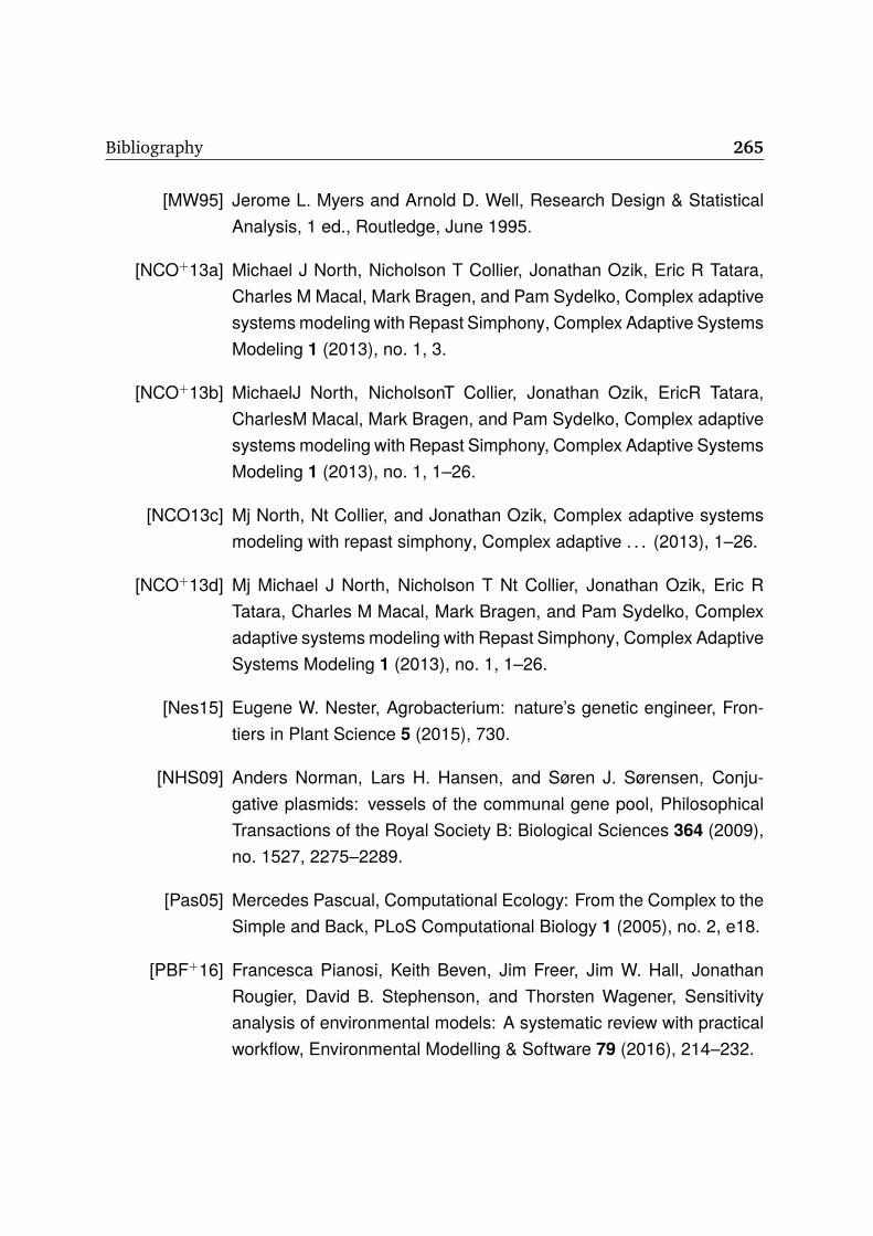
Bibliography 265
[MW95] Jerome L. Myers and Arnold D. Well, Research Design & StatisticalAnalysis, 1 ed., Routledge, June 1995.
[NCO+13a] Michael J North, Nicholson T Collier, Jonathan Ozik, Eric R Tatara,Charles M Macal, Mark Bragen, and Pam Sydelko, Complex adaptivesystems modeling with Repast Simphony, Complex Adaptive SystemsModeling 1 (2013), no. 1, 3.
[NCO+13b] MichaelJ North, NicholsonT Collier, Jonathan Ozik, EricR Tatara,CharlesM Macal, Mark Bragen, and Pam Sydelko, Complex adaptivesystems modeling with Repast Simphony, Complex Adaptive SystemsModeling 1 (2013), no. 1, 1–26.
[NCO13c] Mj North, Nt Collier, and Jonathan Ozik, Complex adaptive systemsmodeling with repast simphony, Complex adaptive . . . (2013), 1–26.
[NCO+13d] Mj Michael J North, Nicholson T Nt Collier, Jonathan Ozik, Eric RTatara, Charles M Macal, Mark Bragen, and Pam Sydelko, Complexadaptive systems modeling with Repast Simphony, Complex AdaptiveSystems Modeling 1 (2013), no. 1, 1–26.
[Nes15] Eugene W. Nester, Agrobacterium: nature’s genetic engineer, Fron-tiers in Plant Science 5 (2015), 730.
[NHS09] Anders Norman, Lars H. Hansen, and Søren J. Sørensen, Conju-gative plasmids: vessels of the communal gene pool, PhilosophicalTransactions of the Royal Society B: Biological Sciences 364 (2009),no. 1527, 2275–2289.
[Pas05] Mercedes Pascual, Computational Ecology: From the Complex to theSimple and Back, PLoS Computational Biology 1 (2005), no. 2, e18.
[PBF+16] Francesca Pianosi, Keith Beven, Jim Freer, Jim W. Hall, JonathanRougier, David B. Stephenson, and Thorsten Wagener, Sensitivityanalysis of environmental models: A systematic review with practicalworkflow, Environmental Modelling & Software 79 (2016), 214–232.

266 Bibliography
[Pie04] Benjamin Pierce, Genetics: A Conceptual Approach, 2004.
[Pie12] Benjamin A. Pierce, Genetics: A Conceptual Approach, 4th Edition,fourth edit ed., W. H. Freeman, dec 2012.
[PIwcfSDV+15] Gilles Pujol, Bertrand Iooss, Alexandre Janon with contributions fromSebastien Da Veiga, Jana Fruth, Laurent Gilquin, Joseph Guillaume,Loic Le Gratiet, Paul Lemaitre, Bernardo Ramos, and Taieb Touati,sensitivity: Sensitivity analysis, 2015, R package version 1.11.1.
[PKB07] Riccardo Poli, James; Kennedy, and Tim Blackwell, Particle swarmoptimization, Swarm Intelligence 1 (2007), no. 1, 33–57.
[PKTG12] Rob Phillips, Jane Kondev, Julie Theriot, and Hernan Garcia, PhysicalBiology of the Cell, 2 ed., Garland Science, London ; New York, NY,2012.
[PPH+12] Sergei Petrovskii, Natalia Petrovskaya, J. D. Hughes, et al., Compu-tational ecology as an emerging science., Interface focus 2 (2012),no. 2, 241–54.
[Pre11] Antonio Prestes Garcıa, A first approach to individual-based modelingof the bacterial conjugation dynamics, Master’s thesis, Facultad deinformatica(UPM), September 2011.
[PRP15a] Antonio Prestes Garcıa and Alfonso Rodrıguez-Paton, A PreliminaryAssessment of Three Strategies for the Agent-Based Modeling ofBacterial Conjugation, 9th International Conference on Practical Ap-plications of Computational Biology and Bioinformatics (Ross Over-beek, Miguel P. Rocha, Florentino Fdez-Riverola, and Juan F. De Paz,eds.), Advances in Intelligent Systems and Computing, vol. 375,Springer International Publishing, 2015, pp. 1–9.
[PRP15b] Antonio Prestes Garcıa and Alfonso Rodrıguez-Paton, BactoSim —An Individual-Based Simulation Environment for Bacterial Conjuga-tion, Springer International Publishing, 2015, pp. 275–279.

Bibliography 267
[QLW+16] B.Y. Qu, J.J. Liang, Z.Y. Wang, Q. Chen, and P.N. Suganthan, No-vel benchmark functions for continuous multimodal optimization withcomparative results, Swarm and Evolutionary Computation 26 (2016),23–34.
[R C15] R Core Team, R: A language and environment for statistical compu-ting, R Foundation for Statistical Computing, Vienna, Austria, 2015.
[RARE+04] A. Rozkov, C. A. Avignone-Rossa, P. F. Ertl, P. Jones, R. D.O’Kennedy, J. J. Smith, J. W. Dale, and M. E. Bushell, Characteri-zation of the metabolic burden on Escherichia coli DH1 cells imposedby the presence of a plasmid containing a gene therapy sequence.,Biotechnology and bioengineering 88 (2004), no. 7, 909–915.
[RBH+83] S G Rogers, L A Brand, S B Holder, E S Sharps, and M J Brackin, Am-plification of the aroA gene from Escherichia coli results in toleranceto the herbicide glyphosate., Applied and environmental microbiology46 (1983), no. 1, 37–43.
[RVPM15] R. J. Roberts, T. Vincze, J. Posfai, and D. Macelis, REBASE–a data-base for DNA restriction and modification: enzymes, genes and ge-nomes, Nucleic Acids Research 43 (2015), no. D1, D298–D299.
[RWZ12] Andreas Reisner, Heimo Wolinski, and Ellen L Zechner, In situ moni-toring of IncF plasmid transfer on semi-solid agar surfaces reveals alimited invasion of plasmids in recipient colonies., Plasmid 67 (2012),no. 2, 155–161.
[Sal08] A Saltelli, Global Sensitivity Analysis: The Primer, International Sta-tistical Review (2008), 452.
[SBH+05] Soren J. Sorensen, Mark Bailey, Lars H. Hansen, Niels Kroer, andStefan Wuertz, Studying plasmid horizontal transfer in situ: a criticalreview, Nature Reviews Microbiology 3 (2005), no. 9, 700–710.

268 Bibliography
[SBTT08] Frances R. Slater, Mark J. Bailey, Adrian J. Tett, and Sarah L. Tur-ner, Progress towards understanding the fate of plasmids in bacterialcommunities, FEMS Microbiology Ecology 66 (2008), no. 1, 3–13.
[SD08] Krzysztof Socha and Marco Dorigo, Ant colony optimization for con-tinuous domains, European Journal of Operational Research 185(2008), no. 3, 1155–1173.
[SGSL90] L. Simonsen, D. M. Gordon, F. M. Stewart, and B. R. Levin, Estimatingthe rate of plasmid transfer: an end-point method, J Gen Microbiol 136(1990), no. 11, 2319–2325.
[SHL] Davir R Setzer, Roberta M Hmiel, and Shaoyi Liao, A simple vectormodification to facilitate oligonucleotide- directed mutagenesis, Nu-cleic Acids Research 18, no. 14.
[Sho08] Ronald W. Shonkwiler, Mathematical Biology: An Introduction withMaple and Matlab, 2nd ed., Springer Publishing Company, Incorpo-rated, 2008.
[SHPC13] Larry Snyder, Tina M. Henkin, Joseph E. Peters, and Wendy Champ-ness, Molecular Genetics of Bacteria, 4th Edition, Larry Snyder, Jo-seph E. Peters, Tina M. Henkin and Wendy Champness 1 (2013),162–163, 503.
[SJPD07] Guennadi Sezonov, Daniele Joseleau-Petit, and Richard D’Ari, Es-cherichia coli physiology in Luria-Bertani broth., Journal of bacterio-logy 189 (2007), no. 23, 8746–9.
[SJS+11] Hyun-Woo Shim, Yun-Ho Jin, Seung-Deok Seo, Seung-Hun Lee, andDong-Wan Kim, Highly Reversible Lithium Storage in Bacillus subtilis-Directed Porous Co3 O4 Nanostructures, ACS Nano 5 (2011), no. 1,443–449.
[SKW10] Thomas J Silhavy, Daniel Kahne, and Suzanne Walker, The bacterialcell envelope., Cold Spring Harbor perspectives in biology 2 (2010),no. 5, a000414.
Bibliography 269
[SL77] FM Stewart and BR Levin, The Population Biology of BacterialPlasmids: A PRIORI Conditions for the Existence of ConjugationallyTransmitted Factors., Genetics 87 (1977), no. 2, 209–228.
[Smi74] John Maynard Smith, Models in ecology, revised ed ed., CambridgeUniversity Press, 1974.
[Sor15] Kenneth Sorensen, Metaheuristics-the metaphor exposed, Internatio-nal Transactions in Operational Research 22 (2015), no. 1, 3–18.
[SRP+13] Laura K. Sycuro, Chelsea S. Rule, Timothy W. Petersen, Timna J.Wyckoff, Tate Sessler, Dilip B. Nagarkar, Fakhra Khalid, Zachary Pin-cus, Jacoby Biboy, Waldemar Vollmer, and Nina R. Salama, Flowcytometry-based enrichment for cell shape mutants identifies multi-ple genes that influence<i>H</i><i>elicobacter pylori</i>morpho-logy, Molecular Microbiology 90 (2013), no. 4, 869–883.
[ST16] Thibault Stalder and Eva Top, Plasmid transfer in biofilms: a per-spective on limitations and opportunities, npj Biofilms and Microbi-omes 2 (2016), 16022.
[STCR04] A. Saltelli, Stefano Tarantola, Francesca Campolongo, and MarcoRatto, Sensitivity Analysis in Practice: A Guide to Assessing ScientificModels, 1 ed., Wiley, April 2004.
[Str] Lubert Stryer, Biochemistry, 4th ed., W.H. Freeman & Company.
[Sum96] David K. Summers, The Biology of Plasmids, Blackwell PublishingLtd., Oxford, UK, mar 1996.
[SYD+11] Jose Seoane, Tatiana Yankelevich, Arnaud Dechesne, Brian Merkey,Claus Sternberg, and Barth F. Smets, An individual-based approach toexplain plasmid invasion in bacterial populations, FEMS MicrobiologyEcology 75 (2011), no. 1, 17–27.
[TKG14] Jan C. Thiele, Winfried Kurth, and Volker Grimm, Facilitating Para-meter Estimation and Sensitivity Analysis of Agent-Based Models: A

270 Bibliography
Cookbook Using NetLogo and ’R’, Journal of Artificial Societies andSocial Simulation 17 (2014), no. 3.
[TLNV15] Ignace L.M.M. Tack, Filip Logist, Estefanıa Noriega Fernandez, andJan F.M. Van Impe, An individual-based modeling approach to simu-late the effects of cellular nutrient competition on Escherichia coli K-12MG1655 colony behavior and interactions in aerobic structured foodsystems, Food Microbiology 45 (2015), 179–188.
[TN05] Christopher M. Thomas and Kaare M. Nielsen, Mechanisms of, andBarriers to, Horizontal Gene Transfer between Bacteria, Nature Re-views Microbiology 3 (2005), no. 9, 711–721.
[TW04] Seth Tisue and Uri Wilensky, Netlogo: A simple environment for mo-deling complexity, . . . Conference on Complex Systems (2004), 1–10.
[Urb16] Simon Urbanek, rjava: Low-level r to java interface, 2016, R packageversion 0.9-8.
[vHBC11] Hans C. van Houwelingen, Hendriek C Boshuizen, and Maurizio Ca-pannesi, Sensitivity analysis of state-transition models: How to dealwith a large number of inputs, Computers in Biology and Medicine 41(2011), no. 9, 838–842.
[Via13] Felipe A C Viana, Things You Wanted to Know About the Latin Hyper-cube Design and Were Afraid to Ask, 10th World Congress on Struc-tural and Multidisciplinary Optimization (2013), 1–9.
[Voe] Donald Voet, Biochemistry, 2nd Second Edition, water damaged,highlighted, notation ed., Wiley.
[Wei09] Thomas Weise, Global optimization algorithms – theory and applica-tion, self-published, Germany, 2009.
[WNF+15] A. Watkins, J. Noble, R.J. Foster, B.J. Harmsen, and C.P. Doncaster, Aspatially explicit agent-based model of the interactions between jaguarpopulations and their habitats, Ecological Modelling 306 (2015), 268–277.

Bibliography 271
[WRS+14] J. Wilson White, Andrew Rassweiler, Jameal F. Samhouri, Adrian C.Stier, and Crow White, Ecologists should not use statistical signifi-cance tests to interpret simulation model results, Oikos 123 (2014),no. 4, 385–388.
[XG11] Chonggang Xu and George Gertner, Understanding and comparisonsof different sampling approaches for the Fourier Amplitudes Sensiti-vity Test (FAST)., Computational statistics & data analysis 55 (2011),no. 1, 184–198.
[You04] Kevin D. Young, Bacterial shape, Molecular Microbiology 49 (2004),no. 3, 571–580.
[You07] Kevin D Young, Bacterial morphology: why have different shapes?,Current opinion in microbiology 10 (2007), no. 6, 596–600.
[ZBCR13] Mauricio Zambrano-Bigiarini, Maurice Clerc, and Rodrigo Rojas,Standard Particle Swarm Optimisation 2011 at CEC-2013: A baselinefor future PSO improvements, 2013 IEEE Congress on EvolutionaryComputation, CEC 2013, 2013, pp. 2337–2344.
[ZDF+12] Xue Zhong, Jason Droesch, Randal Fox, Eva M. Top, and Stephen M.Krone, On the meaning and estimation of plasmid transfer rates forsurface-associated and well-mixed bacterial populations, Journal ofTheoretical Biology 294 (2012), 144–152.
[ZKaTK10] Xue Zhong, JarosLaw E. Kro[dot above]l, Eva M. Top, and Stephen M.Krone, Accounting for mating pair formation in plasmid population dy-namics, Journal of Theoretical Biology 262 (2010), no. 4, 711–719.
[ZPK00] Bernard P. Zeigler, Herbert Praehofer, and Tag G. Kim, Theory of Mo-deling and Simulation, Second Edition, 2 ed., Academic Press, Janu-ary 2000.
[ZR06] Y Zhang and A Rundell, Comparative study of parameter sensitivityanalyses of the TCR-activated Erk-MAPK signalling pathway., Sys-tems biology 153 (2006), no. 4, 201–11.

272 Bibliography
[ZWV11] Arieh Zaritsky, Ping Wang, and Norbert O. Vischer, Instructive si-mulation of the bacterial cell division cycle., Microbiology (Reading,England) 157 (2011), no. Pt 7, 1876–1885.

Appendix AScripts for model analysis

274 APPENDIX A. SCRIPTS FOR MODEL ANALYSIS
The objective of this Appendix is to ensure the reproducibility for the results con-tained in this work. Bearing this in mind, it is provided here all the scripts which arerequired in order to reproduce the experimental designs presented in this thesis. Thescripts were developed using the GNU R language [R C15], [Cra07], requiring for theirexecution the installation of a version of FNU R software environment for statisticalcomputing which is freely available for download. Additionally, it will be necessary toinstall the two R packages developed in the scope of this work, namely the R/Repast
and EvoPER which are both freely available from CRAN repository. Finally, it is alsonecessary to download and install the BactoSIM simulation software which is availablefor being downloaded from the following link https://goo.gl/aomr9G. It is importantto take into account that for running these scripts without modification, the BactoSIM
must be installed under the directory /usr/models/BactoSim(HaldaneEngine-1.0) other-wise it will be necessary to modify the installdir variable in all scripts.

275
1 ##================================================================================2 ## This f i l e i s par t of PhD t h e s i s e n t i t l e d3 ##4 ## " Modeling and analyz ing the k i n e t i c of con juga t i ve plasmids "5 ##6 ## (C) 2016 , 2017 Antonio P r e s t e s Garc ia <@>7 ## For l i c e n s e terms see DESCRIPTION and/ or LICENSE8 ##9 ## @fi le : case1−morris .R
10 ##11 ## This f i l e conta ins R s c r i p t apply ing the Morris sc reen ing method to the case 112 ##================================================================================13 ## I n i t i a l i z a t i o n14 rm( l i s t=l s () )15 l i b r a r y ( evoper )16 s e t . seed (2727144)17
18 i n s t a l l d i r<− " / usr /models/BactoSim ( HaldaneEngine−1.0) "19 d e f a u l t<− c ( i sCon juga t i v e=TRUE, i sRepressed=TRUE)20
21 ## Output func t ion wrapping22 my. output<− func t ion ( params , r e s u l t s ) 23 r a t e<− r e s u l t s $X . Simulated .24 c r i t e r i a<− cbind ( ra t e )25 re turn ( c r i t e r i a )26 27
28 ## Fac to r s under study29 o b j e c t i v e<− AddFactor (name=" c y c l e P o i n t " ,min=0,max=90)30 o b j e c t i v e<− AddFactor ( f a c t o r s=ob j e c t i v e , name=" con jugat ionCos t " ,min=0,max=100)31 o b j e c t i v e<− AddFactor ( f a c t o r s=ob j e c t i v e , name=" p i lu sExpre s s i onCos t " ,min=0,max=100)32 o b j e c t i v e<− AddFactor ( f a c t o r s=ob j e c t i v e , name="gamma0" ,min=0.1 ,max=10)33 o b j e c t i v e<− AddFactor ( f a c t o r s=ob j e c t i v e , name=" model " ,min=1,max=3)34 o b j e c t i v e<− AddFactor ( f a c t o r s=ob j e c t i v e , name=" n u t r i e n t s " ,min=1,max=10)35 o b j e c t i v e<− AddFactor ( f a c t o r s=ob j e c t i v e , name=" i n i t i a l D R D r a t i o " ,min=0.01 , max=1)36
37 ## Setup38 Easy . Setup ( i n s t a l l d i r )39
40 ## Ana ly s i s41 r e s u l t s<− Easy . Morr is ( i n s t a l l d i r , " ds : : Output " ,360 , ob j e c t i v e ,5 ,8 ,4 ,my. output , d e f a u l t )
Figure A.1: The script for preliminary screening of case 1 of BactoSIM outputanalysis.

276 APPENDIX A. SCRIPTS FOR MODEL ANALYSIS
1 ##================================================================================2 ## This f i l e i s par t of PhD t h e s i s e n t i t l e d3 ##4 ## " Modeling and analyz ing the k i n e t i c of con juga t i ve plasmids "5 ##6 ## (C) 2016 , 2017 Antonio P r e s t e s Garc ia <@>7 ## For l i c e n s e terms see DESCRIPTION and/ or LICENSE8 ##9 ## @fi le : case2−morris .R
10 ##11 ## This f i l e conta ins R s c r i p t apply ing the Morris sc reen ing method to the case 212 ##================================================================================13 ## I n i t i a l i z a t i o n14 rm( l i s t=l s () )15 l i b r a r y ( evoper )16 #s e t . seed (2727144)63789023117 s e t . seed (637890231)18
19 i n s t a l l d i r<− " / usr /models/BactoSim ( HaldaneEngine−1.0) "20 d e f a u l t<− c ( i sCon juga t i v e=TRUE, i sRepressed=FALSE)21
22 ## Output func t ion wrapping23 my. output<− func t ion ( params , r e s u l t s ) 24 r a t e<− r e s u l t s $X . Simulated .25 c r i t e r i a<− cbind ( ra t e )26 re turn ( c r i t e r i a )27 28
29 ## Fac to r s under study30 o b j e c t i v e<− AddFactor (name=" c y c l e P o i n t " ,min=0,max=90)31 o b j e c t i v e<− AddFactor ( f a c t o r s=ob j e c t i v e , name=" con jugat ionCos t " ,min=0,max=100)32 o b j e c t i v e<− AddFactor ( f a c t o r s=ob j e c t i v e , name=" p i lu sExpre s s i onCos t " ,min=0,max=100)33 o b j e c t i v e<− AddFactor ( f a c t o r s=ob j e c t i v e , name="gamma0" ,min=1,max=5)34 o b j e c t i v e<− AddFactor ( f a c t o r s=ob j e c t i v e , name=" model " ,min=1,max=3)35 o b j e c t i v e<− AddFactor ( f a c t o r s=ob j e c t i v e , name=" n u t r i e n t s " ,min=1,max=10)36 o b j e c t i v e<− AddFactor ( f a c t o r s=ob j e c t i v e , name=" i n i t i a l D R D r a t i o " ,min=0.01 , max=1)37
38 ## Setup39 Easy . Setup ( i n s t a l l d i r )40
41 ## Ana ly s i s42 r e s u l t s<− Easy . Morr is ( i n s t a l l d i r , " ds : : Output " ,360 , ob j e c t i v e ,5 ,4 ,2 ,my. output , d e f a u l t )
Figure A.2: The script for preliminary screening of case 2 of BactoSIM outputanalysis.

277
1 ##================================================================================2 ## This f i l e i s par t of PhD t h e s i s e n t i t l e d3 ##4 ## " Modeling and analyz ing the k i n e t i c of con juga t i ve plasmids "5 ##6 ## (C) 2016 , 2017 Antonio P r e s t e s Garc ia <@>7 ## For l i c e n s e terms see DESCRIPTION and/ or LICENSE8 ##9 ## @fi le : case3−morris .R
10 ##11 ## This f i l e conta ins R s c r i p t apply ing the Morris sc reen ing method to the case 312 ##================================================================================13 ## I n i t i a l i z a t i o n14 rm( l i s t=l s () )15 l i b r a r y ( evoper )16 s e t . seed (637890231)17
18 i n s t a l l d i r<− " / usr /models/BactoSim ( HaldaneEngine−1.0) "19 d e f a u l t<− c ( i sCon juga t i v e=FALSE , i sRepressed=FALSE)20
21 ## Output func t ion wrapping22 my. output<− func t ion ( params , r e s u l t s ) 23 r a t e<− r e s u l t s $X . Simulated .24 c r i t e r i a<− cbind ( ra t e )25 re turn ( c r i t e r i a )26 27
28 ## Fac to r s under study29 o b j e c t i v e<− AddFactor (name=" c y c l e P o i n t " ,min=0,max=90)30 o b j e c t i v e<− AddFactor ( f a c t o r s=ob j e c t i v e , name=" con jugat ionCos t " ,min=0,max=100)31 o b j e c t i v e<− AddFactor ( f a c t o r s=ob j e c t i v e , name=" p i lu sExpre s s i onCos t " ,min=0,max=100)32 o b j e c t i v e<− AddFactor ( f a c t o r s=ob j e c t i v e , name="gamma0" ,min=1,max=5)33 o b j e c t i v e<− AddFactor ( f a c t o r s=ob j e c t i v e , name=" model " ,min=1,max=3)34 o b j e c t i v e<− AddFactor ( f a c t o r s=ob j e c t i v e , name=" n u t r i e n t s " ,min=1,max=10)35 o b j e c t i v e<− AddFactor ( f a c t o r s=ob j e c t i v e , name=" i n i t i a l D R D r a t i o " ,min=0.01 , max=1)36
37 ## Setup38 Easy . Setup ( i n s t a l l d i r )39
40 ## Ana ly s i s41 r e s u l t s<− Easy . Morr is ( i n s t a l l d i r , " ds : : Output " ,360 , ob j e c t i v e ,5 ,4 ,2 ,my. output , d e f a u l t )
Figure A.3: The script for preliminary screening of case 3 of BactoSIM outputanalysis.

278 APPENDIX A. SCRIPTS FOR MODEL ANALYSIS
1 ##================================================================================2 ## This f i l e i s par t of PhD t h e s i s e n t i t l e d3 ##4 ## " Modeling and analyz ing the k i n e t i c of con juga t i ve plasmids "5 ##6 ## (C) 2016 , 2017 Antonio P r e s t e s Garc ia <@>7 ## For l i c e n s e terms see DESCRIPTION and/ or LICENSE8 ##9 ## @fi le : model1−paest−rd−50.R
10 ##11 ## This f i l e conta ins R s c r i p t f o r the parameter e s t imat ion of model 112 ##================================================================================13 ## I n i t i a l i z a t i o n14 rm( l i s t=l s () )15 l i b r a r y ( evoper )16 l i b r a r y (dtw)17 s e t . seed (637890231)18
19 i n s t a l l d i r<− " / usr /models/BactoSim ( HaldaneEngine−1.0) "20 d e f a u l t<− c ( i sCon juga t i v e=TRUE, i sRepressed=TRUE, model=1,21 exper imentalEquat ion=" y= 0.065 − 0.00035 * x + 4.1 e−06 * x 2 − 6e−09 * x 3" ,22 n u t r i e n t s =5, c y c l e P o i n t =0)23
24 ## Cost func t ion25 my. co s t<− func t ion ( params , r e s u l t s ) 26 r e s u l t s<− r e s u l t s [ r e s u l t s $Time > 30 ,]27 alignment<−dtw( r e s u l t s $X . Simulated , r e s u l t s $X . Experimental , keep=TRUE)28 r a t e<− alignment$ d i s t ance29
30 gT<− AoE .RMSD( i f e l s e (( r e s u l t s $G. T . > 47 & r e s u l t s $G. T . < 57) , 52 , r e s u l t s $G. T . ) , 52 )31 gD<− AoE .RMSD( i f e l s e (( r e s u l t s $G.D. > 38 & r e s u l t s $G.D. < 48) , 43 , r e s u l t s $G.D. ) , 43 )32
33 c r i t e r i a<− cbind ( rate , gT , gD)34 re turn ( c r i t e r i a )35 36
37
38 ## Objec t i ve func t ion39 o b j e c t i v e<− RepastFunct ion$new( i n s t a l l d i r , " ds : : Output " ,360 ,my. co s t )40
41 ## Fac to r s under study42 o b j e c t i v e $Parameter (name=" con jugat ionCos t " ,min=0,max=100)43 o b j e c t i v e $Parameter (name=" p i lu sExp re s s i onCos t " ,min=0,max=100)44 o b j e c t i v e $Parameter (name="gamma0" ,min=0.1 ,max=10)45 o b j e c t i v e $Parameter (name=" i n i t i a l D R D r a t i o " ,min=0.01 ,max=0.1)46
47 ## Se t t i ng to l e rance and d e f a u l t parameters48 o b j e c t i v e $ se tTo le rance (0 .1)49 o b j e c t i v e $ d e f a u l t s ( d e f a u l t )50
51 ## Parameter e s t imat ion method opt ions52 my. opt ions<− OptionsSAA$new()53 my. opt ions $ se tVa lue ( " i t e r a t i o n s " , 30)54
55
56 ## Optimizat ion method57 model_1<− extremize ( " saa " , ob j e c t i v e , my. opt ions )58
59 ## Save data60 saveRDS (model_ 1 , f i l e=" model_ 1 . Rda " )
Figure A.4: The script for preliminary parameter estimation of model 1 ofBactoSIM.

279
1 ##================================================================================2 ## This f i l e i s par t of PhD t h e s i s e n t i t l e d3 ##4 ## " Modeling and analyz ing the k i n e t i c of con juga t i ve plasmids "5 ##6 ## (C) 2016 , 2017 Antonio P r e s t e s Garc ia <@>7 ## For l i c e n s e terms see DESCRIPTION and/ or LICENSE8 ##9 ## @fi le : model2−paest−rd−50.R
10 ##11 ## This f i l e conta ins R s c r i p t f o r the parameter e s t imat ion of model 212 ##================================================================================13 ## I n i t i a l i z a t i o n14 rm( l i s t=l s () )15 l i b r a r y ( evoper )16 l i b r a r y (dtw)17 s e t . seed (637890231)18
19 i n s t a l l d i r<− " / usr /models/BactoSim ( HaldaneEngine−1.0) "20 d e f a u l t<− c ( i sCon juga t i v e=TRUE, i sRepressed=TRUE, model=2,21 exper imentalEquat ion=" y= 0.065 − 0.00035 * x + 4.1 e−06 * x 2 − 6e−09 * x 3" ,22 n u t r i e n t s =5, c y c l e P o i n t =50)23
24 ## Cost func t ion25 my. co s t<− func t ion ( params , r e s u l t s ) 26 r e s u l t s<− r e s u l t s [ r e s u l t s $Time > 30 ,]27 alignment<−dtw( r e s u l t s $X . Simulated , r e s u l t s $X . Experimental , keep=TRUE)28 r a t e<− alignment$ d i s t ance29
30 gT<− AoE .RMSD( i f e l s e (( r e s u l t s $G. T . > 41 & r e s u l t s $G. T . < 63) , 52 , r e s u l t s $G. T . ) , 52 )31 gD<− AoE .RMSD( i f e l s e (( r e s u l t s $G.D. > 32 & r e s u l t s $G.D. < 54) , 43 , r e s u l t s $G.D. ) , 43 )32
33 c r i t e r i a<− cbind ( rate , gT , gD)34 re turn ( c r i t e r i a )35 36
37
38 ## Objec t i ve func t ion39 o b j e c t i v e<− RepastFunct ion$new( i n s t a l l d i r , " ds : : Output " ,360 ,my. co s t )40
41 ## Fac to r s under study42 o b j e c t i v e $Parameter (name=" con jugat ionCos t " ,min=0,max=100)43 o b j e c t i v e $Parameter (name=" p i lu sExp re s s i onCos t " ,min=0,max=100)44 o b j e c t i v e $Parameter (name="gamma0" ,min=0.1 ,max=10)45 o b j e c t i v e $Parameter (name=" i n i t i a l D R D r a t i o " ,min=0.01 ,max=0.1)46
47 ## Se t t i ng to l e rance and d e f a u l t parameters48 o b j e c t i v e $ se tTo le rance (0 .1)49 o b j e c t i v e $ d e f a u l t s ( d e f a u l t )50
51 ## Parameter e s t imat ion method opt ions52 my. opt ions<− OptionsSAA$new()53 my. opt ions $ se tVa lue ( " i t e r a t i o n s " , 30)54
55
56 ## Optimizat ion method57 model_2<− extremize ( " saa " , ob j e c t i v e , my. opt ions )58
59 ## Save data60 saveRDS (model_ 2 , f i l e=" model_ 2 . Rda " )
Figure A.5: The script for preliminary parameter estimation of model 2 ofBactoSIM.

280 APPENDIX A. SCRIPTS FOR MODEL ANALYSIS
1 ##================================================================================2 ## This f i l e i s par t of PhD t h e s i s e n t i t l e d3 ##4 ## " Modeling and analyz ing the k i n e t i c of con juga t i ve plasmids "5 ##6 ## (C) 2016 , 2017 Antonio P r e s t e s Garc ia <@>7 ## For l i c e n s e terms see DESCRIPTION and/ or LICENSE8 ##9 ## @fi le : model3−paest−rd−50.R
10 ##11 ## This f i l e conta ins R s c r i p t f o r the parameter e s t imat ion of model 312 ##================================================================================13
14 ## I n i t i a l i z a t i o n15 rm( l i s t=l s () )16 l i b r a r y ( evoper )17 l i b r a r y (dtw)18 s e t . seed (637890231)19
20 i n s t a l l d i r<− " / usr /models/BactoSim ( HaldaneEngine−1.0) "21 d e f a u l t<− c ( i sCon juga t i v e=TRUE, i sRepressed=TRUE, model=3,22 exper imentalEquat ion=" y= 0.065 − 0.00035 * x + 4.1 e−06 * x 2 − 6e−09 * x 3" ,23 n u t r i e n t s =5)24
25 ## Cost func t ion26 my. co s t<− func t ion ( params , r e s u l t s ) 27 r e s u l t s<− r e s u l t s [ r e s u l t s $Time > 30 ,]28 alignment<−dtw( r e s u l t s $X . Simulated , r e s u l t s $X . Experimental , keep=TRUE)29 r a t e<− alignment$ d i s t ance30
31 gT<− AoE .RMSD( i f e l s e (( r e s u l t s $G. T . > 41 & r e s u l t s $G. T . < 63) , 52 , r e s u l t s $G. T . ) , 52 )32 gD<− AoE .RMSD( i f e l s e (( r e s u l t s $G.D. > 32 & r e s u l t s $G.D. < 54) , 43 , r e s u l t s $G.D. ) , 43 )33
34 c r i t e r i a<− cbind ( rate , gT , gD)35 re turn ( c r i t e r i a )36 37
38
39 ## Objec t i ve func t ion40 o b j e c t i v e<− RepastFunct ion$new( i n s t a l l d i r , " ds : : Output " ,360 ,my. co s t )41
42 ## Fac to r s under study43 o b j e c t i v e $Parameter (name=" c y c l e P o i n t " ,min=0,max=90)44 o b j e c t i v e $Parameter (name=" con jugat ionCos t " ,min=0,max=100)45 o b j e c t i v e $Parameter (name=" p i lu sExp re s s i onCos t " ,min=0,max=100)46 o b j e c t i v e $Parameter (name="gamma0" ,min=0.1 ,max=10)47 o b j e c t i v e $Parameter (name=" i n i t i a l D R D r a t i o " ,min=0.01 ,max=0.1)48
49 ## Se t t i ng to l e rance and d e f a u l t parameters50 o b j e c t i v e $ se tTo le rance (0 .1)51 o b j e c t i v e $ d e f a u l t s ( d e f a u l t )52
53 ## Parameter e s t imat ion method opt ions54 my. opt ions<− OptionsSAA$new()55 my. opt ions $ se tVa lue ( " i t e r a t i o n s " , 30)56
57
58 ## Optimizat ion method59 model_3<− extremize ( " saa " , ob j e c t i v e , my. opt ions )60
61 ## Save data62 saveRDS (model_ 3 , f i l e=" model_ 3 . Rda " )
Figure A.6: The script for preliminary parameter estimation of model 3 ofBactoSIM.

281
1 ##================================================================================2 ## This f i l e i s par t of PhD t h e s i s e n t i t l e d3 ##4 ## " Modeling and analyz ing the k i n e t i c of con juga t i ve plasmids "5 ##6 ## (C) 2016 , 2017 Antonio P r e s t e s Garc ia <@>7 ## For l i c e n s e terms see DESCRIPTION and/ or LICENSE8 ##9 ## @fi le : models−anova−rd−50.R
10 ##11 ## This f i l e conta ins R s c r i p t comparing the model f i t n e s s va lues12 ##================================================================================13
14 rm( l i s t=l s () )15
16 s o r t b y f i t n e s s<− func t ion ( s ) 17 s [ with ( s , order ( f i t n e s s ) ) , ]18 19
20 m1<− readRDS( f i l e=" model_ 1 . Rda " )21 m2<− readRDS( f i l e=" model_ 2 . Rda " )22 m3<− readRDS( f i l e=" model_ 3 . Rda " )23
24 m1. vs<− m1$ ge tV i s i t edSpace ()25 m2. vs<− m2$ ge tV i s i t edSpace ()26 m3. vs<− m3$ ge tV i s i t edSpace ()27
28 m1. vs0<− s o r t b y f i t n e s s (m1. vs )29 m2. vs0<− s o r t b y f i t n e s s (m2. vs )30 m3. vs0<− s o r t b y f i t n e s s (m3. vs )31
32 m1. s0<− m1. vs0 [1:100 ,]33 m2. s0<− m2. vs0 [1:100 ,]34 m3. s0<− m3. vs0 [1:100 ,]35
36 my. data<− data . frame (model = rep ( " 1 " ,100) , co s t = m1. s0$ f i t n e s s )37 my. data<− rbind (my. data , data . frame (model = rep ( " 2 " ,100) , co s t = m2. s0$ f i t n e s s ) )38 my. data<− rbind (my. data , data . frame (model = rep ( " 3 " ,100) , co s t = m3. s0$ f i t n e s s ) )39 summary( aov ( co s t ~ model , data = my. data ) )40
41 kruska l . t e s t ( co s t ~ model , data = my. data )
Figure A.7: The analysis of BactoSIM model type cost.

282 APPENDIX A. SCRIPTS FOR MODEL ANALYSIS
1 ##================================================================================2 ## This f i l e i s par t of PhD t h e s i s e n t i t l e d3 ##4 ## " Modeling and analyz ing the k i n e t i c of con juga t i ve plasmids "5 ##6 ## (C) 2016 , 2017 Antonio P r e s t e s Garc ia <@>7 ## For l i c e n s e terms see DESCRIPTION and/ or LICENSE8 ##9 ## @fi le : i n i t i a l −dens i t y .R
10 ##11 ## This f i l e conta ins R s c r i p t f o r comparing the i n i t i a l dens i t y e f f e c t12 ##================================================================================13 rm( l i s t=l s () )14
15 l i b r a r y ( reshape )16 l i b r a r y ( ggplot2 )17 l i b r a r y ( r r e p a s t )18
19 # −−−−− Adjus t data20 prepare . data<− func t ion (v , h) 21 mydata<− v [ , c ( " Time " , "X . Simulated . " , "X . Experimental . " ) ]22 names( mydata )<− c ( " time " , h , " exper imenta l " )23 mydata<− melt (mydata , id=c ( " time " ) , na . rm=TRUE)24 mydata<− c a s t (mydata , time~var i ab l e , mean)25 mydata<− melt ( data . frame ( mydata ) , id=c ( " time " ) , na . rm=TRUE)26 mydata27 28
29 # −−−−− I n i t i a l i z a t i o n parameters30 d e f a u l t<− c ( i sCon juga t i v e=TRUE, i sRepressed=TRUE, model=3, exper imentalEquat ion=" y= 0.065 −
0.00035 * x + 4.1e−06 * x 2 − 6e−09 * x 3" )31 de fau l t1<− c ( de fau l t , i n i t i a l D e n s i t y=" 5*10^9" )32 de fau l t2<− c ( de fau l t , i n i t i a l D e n s i t y=" 5*10^8" )33 de fau l t3<− c ( de fau l t , i n i t i a l D e n s i t y=" 5*10^7" )34 de fau l t4<− c ( de fau l t , i n i t i a l D e n s i t y=" 5*10^6" )35
36 # −−−−− Run model37 modeldir=" / usr /models/BactoSim ( HaldaneEngine−1.0) "38 Easy . Setup ( modeldir )39 v1<− Easy . Run( modeldir , " ds : : Output " , 360 , 30 , de fau l t1 )40 v2<− Easy . Run( modeldir , " ds : : Output " , 360 , 30 , de fau l t2 )41 v3<− Easy . Run( modeldir , " ds : : Output " , 360 , 30 , de fau l t3 )42 v4<− Easy . Run( modeldir , " ds : : Output " , 360 , 30 , de fau l t4 )43
44 # −−−−− Prepara da ta se t45 v11<− prepare . data (v1 , " s imulated1 " )46 v22<− prepare . data (v2 , " s imulated2 " )47 v33<− prepare . data (v3 , " s imulated3 " )48 v44<− prepare . data (v4 , " s imulated4 " )49
50 # −−−−− Join the four r e s u l t s51 mydata<− c ()52 mydata<− rbind (mydata , v11[v11$ v a r i a b l e != " exper imenta l " , ] )53 mydata<− rbind (mydata , v22[v22$ v a r i a b l e != " exper imenta l " , ] )54 mydata<− rbind (mydata , v33[v33$ v a r i a b l e != " exper imenta l " , ] )55 mydata<− rbind (mydata , v44[v44$ v a r i a b l e != " exper imenta l " , ] )56 mydata<− rbind (mydata , v44[v44$ v a r i a b l e == " exper imenta l " , ] )57
58 # −−−−− Fix the name of l e v e l s59 mydata$ v a r i a b l e<− f a c t o r ( mydata$ var i ab le , l e v e l s = c ( " s imulated1 " , " s imulated2 " , " s imulated3 "
, " s imulated4 " , " exper imenta l " ) )60 mydata<− mydata [mydata$time > 0 ,]61 mydata<− mydata [ ( mydata$time %% 10) == 0 ,]62 mydata<− mydata [mydata$value > 0.075 ,]63
64 # −−−−− Generate the p lo t65 p<− ggplot ( data= mydata , with (mydata , aes ( x=time , y=value , group = var i ab l e , co lour = var iab l e
, shape = v a r i a b l e ) ) )66 p<− p + labs ( y = expres s ion ( "T/ (T+R) " ) ) + theme( legend . p o s i t i o n=c (0 .2 ,0 .8 ) )67 p<− p + g g t i t l e ( " i n i t i a l dens i t y e f f e c t " ) + theme( p lo t . t i t l e = element_ t e x t ( h j u s t = 0.5) )68 p<− p + geom_ point () + geom_ l i n e ()
Figure A.8: The effect of initial cell density

283
1 ##================================================================================2 ## This f i l e i s par t of PhD t h e s i s e n t i t l e d3 ##4 ## " Modeling and analyz ing the k i n e t i c of con juga t i ve plasmids "5 ##6 ## (C) 2016 , 2017 Antonio P r e s t e s Garc ia <@>7 ## For l i c e n s e terms see DESCRIPTION and/ or LICENSE8 ##9 ## @fi le : model3−sobol−rd−50.R
10 ##11 ## This f i l e conta ins R s c r i p t f o r c a l c u l a t i n g Sobol i n d i c e s [pAR118(R1) 05%]12 ##================================================================================13
14 # Step 015 rm( l i s t=l s () )16 l i b r a r y ( r r e p a s t )17 l i b r a r y (dtw)18 s e t . seed (161803398)19
20 i n s t a l l d i r<− " / usr /models/BactoSim ( HaldaneEngine−1.5) "21 d e f a u l t<− c ( i sCon juga t i v e=TRUE, i sRepressed=TRUE, model=3,22 exper imentalEquat ion=" y= 0.012 − 2.0e−4 * x + 1.6 e−6 * x 2 − 2.2e−9 * x 3" ,23 i n i t i a l D e n s i t y=" 6*10^7" , CofV=0.01 ,24 con jugat ionCos t =30, p i l u sExpre s s i onCos t =30, gamma0=1,25 donorRatio=5, n u t r i e n t s =5)26
27 # Step 128 ## Cost func t ion29 my. o b j e c t i v e<− func t ion ( params , r e s u l t s ) 30 r e s u l t s<− r e s u l t s [ r e s u l t s $Time > 30 ,]31 s imulated<− with ( r e s u l t s , aggregate (X . Simulated . , by=l i s t (Time) , FUN=mean , na . rm=TRUE, na .
ac t i on=NULL) )32 exper imenta l<− with ( r e s u l t s , aggregate (X . Experimental . , by=l i s t (Time) , FUN=mean , na . rm=
TRUE, na . ac t i on=NULL) )33 alignment<−dtw( simulated , experimental , keep=TRUE)34
35 r a t e<− alignment$normal izedDistance36
37 gD<− hybr id . d i s t ance ( r e s u l t s $G.D. , hybr id . value (42 , 0.05) )38 gT<− hybr id . d i s t ance ( r e s u l t s $G. T . , hybr id . value (48 , 0.05) )39
40 t o t a l<− ( r a t e + gD + gT) / 341 c r i t e r i a<− cbind ( t o t a l , ra te , gD , gT)42 re turn ( c r i t e r i a )43 44
45 # Step 246 ## Fac to r s under study47 my. f a c t o r s<− AddFactor (name=" c y c l e P o i n t " ,min=1,max=90)48 my. f a c t o r s<− AddFactor ( f a c t o r s=my. f a c t o r s , name=" con jugat ionCos t " ,min=1,max=100)49 my. f a c t o r s<− AddFactor ( f a c t o r s=my. f a c t o r s , name=" p i lu sExpre s s i onCos t " ,min=1,max=100)50 my. f a c t o r s<− AddFactor ( f a c t o r s=my. f a c t o r s , name="gamma0" ,min=0.1 ,max=2)51 my. f a c t o r s<− AddFactor ( f a c t o r s=my. f a c t o r s , name=" i n i t i a l D R D r a t i o " ,min=0.01 ,max=0.1)52 my. f a c t o r s<− AddFactor ( f a c t o r s=my. f a c t o r s , name=" n u t r i e n t s " ,min=3,max=6)53
54 # Step 355 Easy . Setup ( i n s t a l l d i r )56
57 # Step 458 p a r a l l e l i z e (TRUE)59 Sys . time ()60 system . time ( r e s u l t s<− Easy . Sobol ( i n s t a l l d i r , " ds : : Output " , 360 , my. f a c t o r s , 500 , 100 , 1 , my.
ob j e c t i v e , d e f a u l t ) )61 Sys . time ()
Figure A.9: The R code for applying Sobol GSA to pAR118/5%.

284 APPENDIX A. SCRIPTS FOR MODEL ANALYSIS
1 ##================================================================================2 ## This f i l e i s par t of PhD t h e s i s e n t i t l e d3 ##4 ## " Modeling and analyz ing the k i n e t i c of con juga t i ve plasmids "5 ##6 ## (C) 2016 , 2017 Antonio P r e s t e s Garc ia <@>7 ## For l i c e n s e terms see DESCRIPTION and/ or LICENSE8 ##9 ## @fi le : model3−sobol−rd−50.R
10 ##11 ## This f i l e conta ins R s c r i p t f o r c a l c u l a t i n g Sobol i n d i c e s [pAR118(R1) 50%]12 ##================================================================================13
14 # Step 015 rm( l i s t=l s () )16 l i b r a r y ( r r e p a s t )17 l i b r a r y (dtw)18 s e t . seed (132713)19
20 i n s t a l l d i r<− " / usr /models/BactoSim ( HaldaneEngine−1.5) "21 d e f a u l t<− c ( i sCon juga t i v e=TRUE, i sRepressed=TRUE, model=3,22 exper imentalEquat ion=" y= 0.065 − 0.00035 * x + 4.1 e−06 * x 2 − 6e−09 * x 3" ,23 i n i t i a l D e n s i t y=" 6*10^7" , CofV=0.01 ,24 con jugat ionCos t =30, p i l u sExpre s s i onCos t =30, gamma0=1,25 donorRatio=50, n u t r i e n t s =5)26
27 # Step 128 ## Cost func t ion29 my. o b j e c t i v e<− func t ion ( params , r e s u l t s ) 30 r e s u l t s<− r e s u l t s [ r e s u l t s $Time > 30 ,]31 s imulated<− with ( r e s u l t s , aggregate (X . Simulated . , by=l i s t (Time) , FUN=mean , na . rm=TRUE, na .
ac t i on=NULL) )32 exper imenta l<− with ( r e s u l t s , aggregate (X . Experimental . , by=l i s t (Time) , FUN=mean , na . rm=
TRUE, na . ac t i on=NULL) )33 alignment<−dtw( simulated , experimental , keep=TRUE)34
35 r a t e<− alignment$normal izedDistance36
37 gD<− hybr id . d i s t ance ( r e s u l t s $G.D. , hybr id . value (42 , 0.05) )38 gT<− hybr id . d i s t ance ( r e s u l t s $G. T . , hybr id . value (48 , 0.05) )39
40 t o t a l<− ( r a t e + gD + gT) / 341 c r i t e r i a<− cbind ( t o t a l , ra te , gD , gT)42 re turn ( c r i t e r i a )43 44
45 # Step 246 ## Fac to r s under study47 my. f a c t o r s<− AddFactor (name=" c y c l e P o i n t " ,min=1,max=90)48 my. f a c t o r s<− AddFactor ( f a c t o r s=my. f a c t o r s , name=" con jugat ionCos t " ,min=5,max=100)49 my. f a c t o r s<− AddFactor ( f a c t o r s=my. f a c t o r s , name=" p i lu sExpre s s i onCos t " ,min=10,max=100)50 my. f a c t o r s<− AddFactor ( f a c t o r s=my. f a c t o r s , name="gamma0" ,min=0.1 ,max=1)51 my. f a c t o r s<− AddFactor ( f a c t o r s=my. f a c t o r s , name=" i n i t i a l D R D r a t i o " ,min=0.01 ,max=0.1)52 my. f a c t o r s<− AddFactor ( f a c t o r s=my. f a c t o r s , name=" n u t r i e n t s " ,min=1,max=5)53
54 # Step 355 Easy . Setup ( i n s t a l l d i r )56
57 # Step 458 p a r a l l e l i z e (TRUE)59 Sys . time ()60 system . time ( r e s u l t s<− Easy . Sobol ( i n s t a l l d i r , " ds : : Output " , 360 , my. f a c t o r s , 500 , 300 , 1 , my.
ob j e c t i v e , d e f a u l t ) )61 Sys . time ()
Figure A.10: The R code for applying Sobol GSA to pAR118/50%.

285
1 ##================================================================================2 ## This f i l e i s par t of PhD t h e s i s e n t i t l e d3 ##4 ## " Modeling and analyz ing the k i n e t i c of con juga t i ve plasmids "5 ##6 ## (C) 2016 , 2017 Antonio P r e s t e s Garc ia <@>7 ## For l i c e n s e terms see DESCRIPTION and/ or LICENSE8 ##9 ## @fi le : model3−sobol−drd−50.R
10 ##11 ## This f i l e conta ins R s c r i p t f o r c a l c u l a t i n g Sobol i n d i c e s [pSU2007(R388) 5%]12 ##================================================================================13
14 # Step 015 rm( l i s t=l s () )16 l i b r a r y ( r r e p a s t )17 l i b r a r y (dtw)18 s e t . seed (27271313)19
20 i n s t a l l d i r<− " / usr /models/BactoSim ( HaldaneEngine−1.5) "21 d e f a u l t<− c ( i sCon juga t i v e=TRUE, i sRepressed=FALSE , model=3,22 exper imentalEquat ion=" y= 0.038 − 2.1e−3 * x + 1.7 e−5 * x 2 − 1.9e−8 * x 3" ,23 i n i t i a l D e n s i t y=" 6*10^7" , CofV=0.01 ,24 con jugat ionCos t =30, p i l u sExpre s s i onCos t =30, gamma0=1,25 donorRatio=5, n u t r i e n t s =5)26
27
28 # Step 129 ## Cost func t ion30 my. o b j e c t i v e<− func t ion ( params , r e s u l t s ) 31 r e s u l t s<− r e s u l t s [ r e s u l t s $Time > 30 ,]32 s imulated<− with ( r e s u l t s , aggregate (X . Simulated . , by=l i s t (Time) , FUN=mean) )33 exper imenta l<− with ( r e s u l t s , aggregate (X . Experimental . , by=l i s t (Time) , FUN=mean , na . rm=
TRUE, na . ac t i on=NULL) )34 alignment<−dtw( simulated , experimental , keep=TRUE)35
36 r a t e<− alignment$normal izedDistance37
38 gD<− hybr id . d i s t ance ( r e s u l t s $G.D. , hybr id . value (42 , 0.05) )39 gT<− hybr id . d i s t ance ( r e s u l t s $G. T . , hybr id . value (46 , 0.05) )40
41
42 t o t a l<− ( r a t e + gD + gT) / 343 c r i t e r i a<− cbind ( t o t a l , ra te , gD , gT)44 re turn ( c r i t e r i a )45 46
47 # Step 248 ## Fac to r s under study49 my. f a c t o r s<− AddFactor (name=" c y c l e P o i n t " ,min=1,max=90)50 my. f a c t o r s<− AddFactor ( f a c t o r s=my. f a c t o r s , name=" con jugat ionCos t " ,min=1,max=100)51 my. f a c t o r s<− AddFactor ( f a c t o r s=my. f a c t o r s , name=" p i lu sExpre s s i onCos t " ,min=1,max=100)52 my. f a c t o r s<− AddFactor ( f a c t o r s=my. f a c t o r s , name="gamma0" ,min=0.1 ,max=2)53 my. f a c t o r s<− AddFactor ( f a c t o r s=my. f a c t o r s , name=" n u t r i e n t s " ,min=3,max=6)54
55
56 # Step 357 Easy . Setup ( i n s t a l l d i r )58
59 # Step 460 p a r a l l e l i z e (TRUE)61 Sys . time ()62 system . time ( r e s u l t s<− Easy . Sobol ( i n s t a l l d i r , " ds : : Output " , 360 , my. f a c t o r s , 500 , 100 , 1 , my.
ob j e c t i v e , d e f a u l t ) )63 Sys . time ()
Figure A.11: The R code for applying Sobol GSA to pPSU2007/5%.

286 APPENDIX A. SCRIPTS FOR MODEL ANALYSIS
1 ##================================================================================2 ## This f i l e i s par t of PhD t h e s i s e n t i t l e d3 ##4 ## " Modeling and analyz ing the k i n e t i c of con juga t i ve plasmids "5 ##6 ## (C) 2016 , 2017 Antonio P r e s t e s Garc ia <@>7 ## For l i c e n s e terms see DESCRIPTION and/ or LICENSE8 ##9 ## @fi le : model3−sobol−drd−50.R
10 ##11 ## This f i l e conta ins R s c r i p t f o r c a l c u l a t i n g Sobol i n d i c e s [pSU2007(R388) 50%]12 ##================================================================================13
14 # Step 015 rm( l i s t=l s () )16 l i b r a r y ( r r e p a s t )17 l i b r a r y (dtw)18 s e t . seed (2793011)19
20 i n s t a l l d i r<− " / usr /models/BactoSim ( HaldaneEngine−1.5) "21 d e f a u l t<− c ( i sCon juga t i v e=TRUE, i sRepressed=FALSE , model=3,22 exper imentalEquat ion=" y= 0.02 − 5.1e−4 * x + 1.5 e−5 * x 2 − 2.3e−8 * x 3" ,23 i n i t i a l D e n s i t y=" 6*10^7" , CofV=0.01 ,24 donorRatio=50, n u t r i e n t s =5)25
26 # Step 127 ## Cost func t ion28 my. o b j e c t i v e<− func t ion ( params , r e s u l t s ) 29 r e s u l t s<− r e s u l t s [ r e s u l t s $Time > 30 ,]30 s imulated<− with ( r e s u l t s , aggregate (X . Simulated . , by=l i s t (Time) , FUN=mean , na . rm=TRUE, na .
ac t i on=NULL) )31 exper imenta l<− with ( r e s u l t s , aggregate (X . Experimental . , by=l i s t (Time) , FUN=mean , na . rm=
TRUE, na . ac t i on=NULL) )32 alignment<−dtw( simulated , experimental , keep=TRUE)33
34 r a t e<− alignment$normal izedDistance35
36 gD<− hybr id . d i s t ance ( r e s u l t s $G.D. , hybr id . value (42 , 0.05) )37 gT<− hybr id . d i s t ance ( r e s u l t s $G. T . , hybr id . value (46 , 0.05) )38
39 t o t a l<− ( r a t e + gD + gT) / 340 c r i t e r i a<− cbind ( t o t a l , ra te , gD , gT)41 re turn ( c r i t e r i a )42 43
44 # Step 245 ## Fac to r s under study46 my. f a c t o r s<− AddFactor (name=" c y c l e P o i n t " ,min=1,max=90)47 my. f a c t o r s<− AddFactor ( f a c t o r s=my. f a c t o r s , name=" con jugat ionCos t " ,min=1,max=100)48 my. f a c t o r s<− AddFactor ( f a c t o r s=my. f a c t o r s , name=" p i lu sExpre s s i onCos t " ,min=1,max=100)49 my. f a c t o r s<− AddFactor ( f a c t o r s=my. f a c t o r s , name="gamma0" ,min=0.1 ,max=2)50 my. f a c t o r s<− AddFactor ( f a c t o r s=my. f a c t o r s , name=" n u t r i e n t s " ,min=3,max=6)51
52 # Step 353 Easy . Setup ( i n s t a l l d i r )54
55 # Step 456 p a r a l l e l i z e (TRUE)57 Sys . time ()58 system . time ( r e s u l t s<− Easy . Sobol ( i n s t a l l d i r , " ds : : Output " , 360 , ob j e c t i v e , 500 , 100 , 1 , my.
ob j e c t i v e , d e f a u l t ) )59 Sys . time ()
Figure A.12: The R code for applying Sobol GSA to pSU2007/50%.

287
1 ##================================================================================2 ## This f i l e i s par t of PhD t h e s i s e n t i t l e d3 ##4 ## " Modeling and analyz ing the k i n e t i c of con juga t i ve plasmids "5 ##6 ## (C) 2016 , 2017 Antonio P r e s t e s Garc ia <@>7 ## For l i c e n s e terms see DESCRIPTION and/ or LICENSE8 ##9 ## @fi le : model3−sobol−drd−50.R
10 ##11 ## This f i l e conta ins R s c r i p t f o r c a l c u l a t i n g Sobol i n d i c e s [pR388( OriT ) 05%]12 ##================================================================================13
14 # Step 015 rm( l i s t=l s () )16 l i b r a r y ( r r e p a s t )17 l i b r a r y (dtw)18 s e t . seed (1412593)19
20 i n s t a l l d i r<− " / usr /models/BactoSim ( HaldaneEngine−1.5) "21 d e f a u l t<− c ( i sCon juga t i v e=FALSE , i sRepressed=FALSE , model=3,22 exper imentalEquat ion=" y= 0.0017 − 2.5e−4 * x + 4.6 e−6 * x 2 − 6.8e−9 * x 3" ,23 i n i t i a l D e n s i t y=" 6*10^7" , CofV=0.01 ,24 donorRatio=5, n u t r i e n t s =5)25
26
27 # Step 128 ## Cost func t ion29 my. co s t<− func t ion ( params , r e s u l t s ) 30 r e s u l t s<− r e s u l t s [ r e s u l t s $Time > 40 ,]31 s imulated<− with ( r e s u l t s , aggregate (X . Simulated . , by=l i s t (Time) , FUN=mean) )32 exper imenta l<− with ( r e s u l t s , aggregate (X . Experimental . , by=l i s t (Time) , FUN=mean , na . rm=
TRUE, na . ac t i on=NULL) )33 alignment<−dtw( simulated , experimental , keep=TRUE)34
35 r a t e<− alignment$normal izedDistance36
37 gD<− hybr id . d i s t ance ( r e s u l t s $G.D. , hybr id . value (42 , 0.05) )38 gT<− hybr id . d i s t ance ( r e s u l t s $G. T . , hybr id . value (46 , 0.05) )39
40
41 t o t a l<− ( r a t e + gD + gT) / 342 c r i t e r i a<− cbind ( t o t a l , ra te , gD , gT)43 re turn ( c r i t e r i a )44 45
46 # Step 247 ## Fac to r s under study48 o b j e c t i v e<− AddFactor (name=" c y c l e P o i n t " ,min=1,max=90)49 o b j e c t i v e<− AddFactor ( f a c t o r s=ob j e c t i v e , name=" con jugat ionCos t " ,min=1,max=100)50 o b j e c t i v e<− AddFactor ( f a c t o r s=ob j e c t i v e , name=" p i lu sExpre s s i onCos t " ,min=1,max=100)51 o b j e c t i v e<− AddFactor ( f a c t o r s=ob j e c t i v e , name="gamma0" ,min=0.1 ,max=1)52 o b j e c t i v e<− AddFactor ( f a c t o r s=ob j e c t i v e , name=" n u t r i e n t s " ,min=1,max=5)53
54
55 # Step 356 Easy . Setup ( i n s t a l l d i r )57
58 # Step 459 p a r a l l e l i z e (TRUE)60 Sys . time ()61 system . time ( r e s u l t s<− Easy . Sobol ( i n s t a l l d i r , " ds : : Output " , 360 , ob j e c t i v e , 300 , 200 , 1 , my.
cost , d e f a u l t ) )62 Sys . time ()
Figure A.13: The R code for applying Sobol GSA to pR388(OriT)/5%.

288 APPENDIX A. SCRIPTS FOR MODEL ANALYSIS
1 ##================================================================================2 ## This f i l e i s par t of PhD t h e s i s e n t i t l e d3 ##4 ## " Modeling and analyz ing the k i n e t i c of con juga t i ve plasmids "5 ##6 ## (C) 2016 , 2017 Antonio P r e s t e s Garc ia <@>7 ## For l i c e n s e terms see DESCRIPTION and/ or LICENSE8 ##9 ## @fi le : model3−sobol−drd−50.R
10 ##11 ## This f i l e conta ins R s c r i p t f o r c a l c u l a t i n g Sobol i n d i c e s [pR388( OriT ) 50%]12 ##================================================================================13
14 # Step 015 rm( l i s t=l s () )16 l i b r a r y ( r r e p a s t )17 l i b r a r y (dtw)18 s e t . seed (161803398)19
20 i n s t a l l d i r<− " / usr /models/BactoSim ( HaldaneEngine−1.5) "21 d e f a u l t<− c ( i sCon juga t i v e=FALSE , i sRepressed=FALSE , model=3,22 exper imentalEquat ion=" y= 0.0056 + 1.9 e−3 * x − 1.7e−8 * x 2 − 2.0e−9 * x 3" ,23 i n i t i a l D e n s i t y=" 6*10^7" , CofV=0.01 ,24 donorRatio=50, n u t r i e n t s =5)25
26 # Step 127 ## Cost func t ion28 my. co s t<− func t ion ( params , r e s u l t s ) 29 r e s u l t s<− r e s u l t s [ r e s u l t s $Time > 30 ,]30 s imulated<− with ( r e s u l t s , aggregate (X . Simulated . , by=l i s t (Time) , FUN=mean) )31 exper imenta l<− with ( r e s u l t s , aggregate (X . Experimental . , by=l i s t (Time) , FUN=mean , na . rm=
TRUE, na . ac t i on=NULL) )32 alignment<−dtw( simulated , experimental , keep=TRUE)33
34 r a t e<− alignment$normal izedDistance35
36 gD<− hybr id . d i s t ance ( r e s u l t s $G.D. , hybr id . value (42 , 0.05) )37 gT<− hybr id . d i s t ance ( r e s u l t s $G. T . , hybr id . value (46 , 0.05) )38
39
40 t o t a l<− ( r a t e + gD + gT) / 341 c r i t e r i a<− cbind ( t o t a l , ra te , gD , gT)42 re turn ( c r i t e r i a )43 44
45 # Step 246 ## Fac to r s under study47 o b j e c t i v e<− AddFactor (name=" c y c l e P o i n t " ,min=1,max=90)48 o b j e c t i v e<− AddFactor ( f a c t o r s=ob j e c t i v e , name=" con jugat ionCos t " ,min=1,max=100)49 o b j e c t i v e<− AddFactor ( f a c t o r s=ob j e c t i v e , name=" p i lu sExpre s s i onCos t " ,min=1,max=100)50 o b j e c t i v e<− AddFactor ( f a c t o r s=ob j e c t i v e , name="gamma0" ,min=0.1 ,max=2)51 o b j e c t i v e<− AddFactor ( f a c t o r s=ob j e c t i v e , name=" n u t r i e n t s " ,min=3,max=6)52
53
54 # Step 355 Easy . Setup ( i n s t a l l d i r )56
57 # Step 458 p a r a l l e l i z e (TRUE)59 Sys . time ()60 system . time ( r e s u l t s<− Easy . Sobol ( i n s t a l l d i r , " ds : : Output " , 360 , my. f a c t o r s , 500 , 100 , 1 , my.
ob j e c t i v e , d e f a u l t ) )61 Sys . time ()
Figure A.14: The R code for applying Sobol GSA to pR388(OriT)/50%.