Multivariate Functional Halfspace Depth

Gerda Claeskens, Mia Hubert, Leen Slaets and Kaveh Vakili 1

October 10, 2013

A depth for multivariate functional data is defined and studied. By the multi-

variate nature and by including a weight function, it acknowledges important

characteristics of functional data, namely differences in the amount of local

amplitude, shape and phase variation. Both population and finite sample

versions are studied. The multivariate sample of curves may include warping

functions, derivatives and integrals of the original curves for a better overall

representation of the functional data via the depth. A simulation study and

data examples confirm the good performance of this depth function.

Keywords: statistical depth, functional data, time warping, multivariate

data.

1 Introduction

Nowadays, functional data are frequently observed and many statistical methods

have been developed to retrieve useful information from these data sets. Typically,

the observed data consist of a set of N curves, each measured at different time points

1Gerda Claeskens is Professor, ORSTAT, KU Leuven, Naamsestraat 69, 3000 Leuven, Belgium

(E-mail: Gerda.Claeskens@kuleuven.be. Mia Hubert is Professor, Department of Mathematics,

KU Leuven, Celestijnenlaan 200B, 3001 Leuven, Belgium (E-mail: Mia.Hubert@wis.kuleuven.be).

Leen Slaets is now Statistician at EORTC, Brussels, Belgium, part of this research was per-

formed during her doctoral studies at ORSTAT. Kaveh Vakili is a doctoral student at the De-

partment of Mathematics, KU Leuven, Celestijnenlaan 200B, 3001 Leuven, Belgium (E-mail:

Kaveh.Vakili@wis.kuleuven.be). All authors are affiliated with the Leuven Statistics Research Center

and acknowledge the support of KU Leuven grant GOA/12/14 and of the IAP Research Network

P7/06 of the Belgian Science Policy. The authors thank B. De Ketelaere for providing the data, and

the reviewers for their comments.

1

t1, . . . , tT . For an overview, see Ramsay and Silverman (2006); Ferraty and Vieu

(2006). Basic questions of interest in functional data analysis (FDA) are (i) the

estimation of the central tendency of the curves, (ii) the estimation of the variability

among the curves, (iii) the detection of outlying curves, as well as (iv) classification

and clustering of such curves.

In this paper we consider multivariate functional data. We observe for all obser-

vation units at each time point a K-dimensional vector of measurements, which arise

from an underlying set of K curves. A popular example is the bivariate gait data set,

which contains the simultaneous variation of the hip and knee angles for 39 children

at 20 equally spaced time points (Ramsay and Silverman, 2006). Berrendero et al.

(2011) have K = 3 when recording daily temperature functions at 3, 9 and 12cm

below the surface during N = 21 days. Sangalli et al. (2009) and Pigoli and Sangalli

(2012) present several multivariate functional data from medical studies. Bivariate

weather data are studied in Section 3.2.

Different types of multivariate functional data arise by computing additional

curves, starting from one observed set of univariate functional data. A well-studied

situation is the addition of the first order derivatives which provides additional in-

formation on the shape of the curves and consequently is interesting to detect curves

with an outlying shape (Cuevas et al., 2007). Note that this is different from a com-

mon practice in chemometrics, where observed spectral data are often replaced by

their first-order derivatives in order to eliminate baseline features. Also higher or-

der derivatives could be added. This has been applied in the Berkeley growth data

set (Ramsay and Silverman, 2006), which contains the heights of children and the

estimated acceleration curves that correspond to the second-order derivatives.

In this paper we introduce to the depth calculation the inclusion of other func-

tions of the original set of curves (such as warping functions, derivatives, integrals,. . . )

2

(a) (b)

0 20 40 60 80 100 120

−2.

0−

1.5

−1.

0−

0.5

0.0

0.5

Time

Acc

eler

atio

n

0 20 40 60 80 100 120

−50

−40

−30

−20

−10

0Time

Vel

ocity

Figure 1: Industrial data: (a) Acceleration and (b) velocity signals, with cross-

sectional mean curve (dashed line) and depth-based median curve (solid black line).

which allows us to obtain more powerful conclusions about the data-driven process.

Some interesting functions are obtained from a warping procedure, which often pre-

cedes the analysis of functional data. Typically some warping method (also known

as curve alignment) is applied to the observed curves as a preprocessing step, but

no further information is retained from this analysis. In Slaets et al. (2012) it is

shown how the information from the warping procedure can be incorporated into a

clustering method for functional data. In Section 4.3 we show the benefits of a multi-

variate analysis of the warped data together with the curves obtained via the warping

function.

A different augmentation of the data is presented in Section 3. It contains the

analysis of a real data set which consists of acceleration signals over time from an

industrial machine (De Ketelaere et al., 2011). Most of the observed curves, see

Figure 1(a), follow a similar nonlinear pattern, but we also notice several curves

with a deviating trend, most prominently at the final stage of the production. In

addition to these acceleration signals, we do not use their derivatives but rather the

3

integrated curves as they represent the underlying velocity, see Figure 1(b). Also

here, we observe a global structure as well as deviating signals. On both plots we

have added the cross-sectional mean curve (dashed line). Further we have plotted

our new estimator for the central tendency of the curves, shown as a solid black line.

It is already obvious that these estimates are less influenced by the outlying curves.

For the velocity curves, the effect is less pronounced as the outlying curves occur in

both directions of the central pattern.

Our approach to estimate the central tendency of multivariate functional data is

based on the concept of depth. Depth functions were initially defined for multivariate

data. They provide an ordering from the center outwards such that the most central

object gets the highest depth value and the least central objects the smallest depth.

More recently, several notions of depth have been proposed for univariate functional

data, such as the integrated depth (ID, Fraiman and Muniz, 2001), the h-mode and

random projection depth (RP, Cuevas et al., 2007), the band depth and modified band

depth (MBD, Lopez-Pintado and Romo, 2009) and the half-region depth (Lopez-

Pintado and Romo, 2011). The ID depth and MBD depth are quite similar, as

they both consider a (univariate) depth function at each time point t and define the

functional depth as the average of these depth values over all time points. Cuevas

et al. (2007) have proposed to consider the curves and their derivatives, yielding the

bivariate random projection depth (RPD). For a number of random projections, they

project both sets of curves on each direction, apply a multivariate depth function on

the bivariate sample and finally average the depth values over the random projections.

We generalize several of these ideas by constructing a depth function for K-variate

samples of curves, which we define the multivariate functional depth (MFD). Our

definition averages a multivariate depth function over the time points, but in addition

it includes a weight function. This weight function can be chosen as to account

4

for variability in amplitude, to adapt to the functional nature of the data. More

specifically we choose Tukey’s halfspace depth (Tukey, 1975) as the building block,

which leads to the multivariate functional halfspace depth (MFHD).

The population and finite-sample definition of MFD and MFHD and their main

properties are given in Section 2. We define and characterize the MFD median, as the

curve with maximal MFD. In Section 3 we illustrate using two data sets how this new

depth concept can be used to estimate the central tendency of the curves, as well as

the variability among the curves. In Section 4 we provide the results of a simulation

study in which we compare several depth functions and several augmented data sets

(such as by including derivatives and warping functions). Section 5 concludes and

gives directions for further research. All proofs are collected in the Appendix. The

supplementary material illustrates on the industrial data set the effect of adding the

velocity curves to the analysis.

2 Definition and properties of multivariate functional depth

2.1 Notation

Consider aK-variate (finiteK), real-valued stochastic process of continuous functions

Y = (Y1, . . . ,YK) with for j = 1, . . . , K, Yj : U → R : t 7→ Yj(t) continuous on a

compact interval U and denote its cumulative distribution by FY . Thus, for every

finite set of time points t1, . . . , tT ∈ U , (Y(t1), . . . ,Y(tT )) is a random variable on(R

K)T

and at each time point t ∈ U , Y(t) is a K-variate random variable with

associated cumulative distribution function (cdf) FY(t).

Real numbers, vectors, continuous functions on an interval U and vectors of func-

tions are all used in conjunction with each other. To avoid confusion, we provide an

overview of the notation that is used throughout this paper. The set of continuous

functions on U is denoted by C(U). Elements thereof and their graphs are denoted

5

by capital letters (e.g. X). For K-vectors of continuous functions in C(U)K and their

graphs, bold capital letters are used (e.g. X) or the vector notation (X1, . . . , XK)

where Xi ∈ C(U). The function value of a curve X at a time point t is denoted by

X(t) ∈ R. The vector of function values of an element X in C(U)K at a time point

t is denoted by X(t) = (X1(t), . . . , XK(t)). The empirical cumulative distribution

function based on a sample {Y 1(t), . . . ,Y N(t)} each with the same distribution as

Y(t) is denoted by FY(t),N . For vectors in RK , bold lowercase letters are used (e.g. a)

or the vector notation (a1, . . . , aK) ∈ RK . For matrices capital letters early in the

alphabet are used (e.g. A), while later letters (e.g. X) are reserved for curves. For

real numbers, lowercase letters are used (e.g. a).

2.2 Population definition

2.2.1 A general multivariate depth as building block

A depth function provides an ordering from the center outwards such that the most

central objects get the highest depth and the least central objects the smallest depth.

Let D(·;FX ) : RK → [0, 1] be a statistical depth function for the probability distri-

bution of a K-variate random vector X with cdf FX , according to Zuo and Serfling

(2000a). Associated with the depth function is the depth region Dα(FX ) at level

α > 0, defined as Dα(FX ) = {x ∈ RK : D(x;FX ) > α}.

The new definition of multivariate functional depth combines the local depths of

Y(t) at each time point t ∈ U and includes a weight function that may be specified

for different purposes.

Definition 1. Consider a K-variate stochastic process {Y(t), t ∈ U} on RK with cdf

FY that generates continuous paths in C(U)K. Let D be a statistical depth function

on RK and w a weight function that is defined on U and integrates to one. Take an

6

arbitrary X ∈ C(U)K. The multivariate functional depth (MFD) of X is defined as

MFD(X;FY) =

∫

U

D(X(t);FY(t)) · w(t) dt. (1)

This weight function may or may not depend on FY(t), t ∈ U . A first example

for the weight is a constant times an indicator for a range of interest. This allows

for example to eliminate the effect of a start-up phase in an industrial process, or

to remove imprecise measurements during certain regions which often happens for

spectral data. A second example takes the local changes in the amount of variability

in amplitude (vertical variability) into account by defining

w(t) = wα(t;FY(t)) = vol{Dα(FY(t))}/∫

U

vol{Dα(FY(u))}du, (2)

which is proportional to the volume of the depth region at time point t. This implies

that for regions where all curves nearly coincide the weight is small, heuristically,

the order of the curves does not matter much here. For regions where the amplitude

variability is large, there is a visual ordering of the curves, and the influence of those

regions on the functional depth will be large. See Section 3.1 for an illustration.

When the weight function (2) is considered, we denote the corresponding depth by

MFD(α). Note that for many cases the definition of MFD with this choice of weight

does not depend on α. In general, the value of α is irrelevant when at each time

point t the volumes of the depth regions are proportional to a fixed function of α.

In particular, for most depth functions, it holds that at unimodal elliptic symmetric

distributions, the contours of the depth regions coincide with density contours (Zuo

and Serfling, 2000b). This implies that the choice of α in MFD(α) becomes irrelevant

(at least at the population level) when the elliptic distributions remain the same for

all t up to a scale change. Also the opposite approach could be considered, in which

the weight is large in regions where all curves nearly coincide, in order to strongly

penalize outlying curves in these time intervals.

7

In Theorem 1 we show that the multivariate functional depth satisfies some key

properties, adapted to a functional data context, that were put forward by Zuo and

Serfling (2000a). All proofs are relegated to the Appendix.

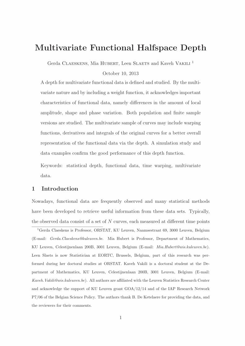
Theorem 1. Assume that the depth function D satisfies the four properties listed

in Zuo and Serfling (2000a), i.e. affine invariant, maximal at the center, monotone

relative to the deepest point and vanishing at infinity. Then MFD, as defined in

Definition 1, is a statistical depth function satisfying the following key properties:

(i) Affine invariance (invariance w.r.t. the underlying coordinate system). If the

weight function w is affine invariant, then

MFD(X;FY) = MFD(AX(ct+d) + X(ct+d);FAY(ct+d)+X(ct+d)),

with U = [l, u],AY (ct+d)+X(ct+d) the stochastic process {AY( s−dc)+X( s−d

c), s ∈ S =

[cl+ d, cu+ d]} for any constants c ∈ R0, d ∈ R, any vector of functions X ∈ C(U)K

and any matrix A ∈ RK×K with det(A) 6= 0, and X(ct+d) the curve {s, X( s−d

c)}, with

s ∈ S = [cl + d, cu+ d].

(ii) Maximality at the center. For a uniquely defined Θ ∈ C(U)K such that Θ(t) is a

symmetry point in which D is maximal at every t ∈ U , it holds that MFD(Θ;FY) =

supX∈C(U)K MFD(X;FY).

(iii) Monotonicity relative to the deepest point. Let Θ ∈ C(U)K such that Θ(t) is

a deepest point at every t ∈ U , then for any a ∈ [0, 1], MFD(X;FY) 6 MFD(Θ +

a(X −Θ);FY).

(iv) Vanishing at infinity. For 1 6 k 6 K and for a series of curves Xn,k with

limn→∞ |Xn,k(t)| = ∞ for almost all time points t in U : limn→∞ MFD(Xn,k;FY) = 0.

The affine invariance holds for all specified weight functions. When the weight is

invariant with respect to transformations t 7→ A(t)X(t) + X(t), the same holds for

MFD. In the original multivariate setting, the fourth property, ‘vanishing at infinity’,

8

requires that for a vector x ∈ RK the depth of x should converge to 0 for ‖x‖ → ∞.

When a curve behaves in accordance with the sample on the majority of the interval

and, e.g., converges to infinity near the border, one might not wish to attribute zero

depth. The vanishing at infinity property for functional depth holds as stated in (iv).

See also Lopez-Pintado and Romo (2009, p. 725- for -726) and Nieto-Reyes (2011).

Theorem 2 states the existence of a deepest MFD curve. As a result an MFD

median can be defined, see Definition 2. We use a generalized maximum theorem

(Ausubel and Deneckere, 1993) to obtain continuity related properties of the maxi-

mum depth function and of the deepest values, the arg-max correspondence (i.e. set-

valued function) Θ.

Define the function H : U × RK → [0, 1] : (t,x) 7→ D(x, FY(t)) = H(t,x). Define

γ : U → RK a correspondence that is non-empty and compact-valued. In particular

γ(t) specifies for every t the set of x ∈ RK for which we would be interested in

computing the depth. Since the process Y(t) is continuous, its range is compact, a

compact set enclosing the range of Y(t) will satisfy the purpose, it may be the same

one for all t ∈ U . Define Π : U → R : t 7→ Π(t) = (−∞,maxx∈γ(t) D(x;FY(t))].

Denote by G(t) = {(x,H(t,x));x ∈ γ(t)} the graph of H(t, ·) restricted to γ(t),

for t ∈ U , and by G(t) its closure in RK × R ∪ {−∞}. Define the correspondence

G : U → RK × R ∪ {−∞} with

G(t) = {(x, y) : there exist y′, y′′ ∈ R ∪ {−∞} such that y′′ ≤ y ≤ y′,

(x, y′) ∈ G(t) and (x, y′′) ∈ G(t)}.

Theorem 2. Assume either set of conditions (a) or (b).

(a) The function H is upper-semicontinuous, γ is an upper-hemicontinuous corre-

spondence that is non-empty and compact-valued, and Π is a lower-hemicontinuous

correspondence.

9

(b) The function H is an upper-semicontinuous function of x for every t ∈ U , γ is

a correspondence that is non-empty and compact-valued, and G is a continuous

correspondence.

Then,

(i) The maximum depth function U → [0, 1] : t 7→ maxx∈γ(t) D(x;FY(t)) is contin-

uous.

(ii) Concerning the values where maximum depth is reached,

Θ : U → RK : t 7→ arg max

x∈γ(t)D(x;FY(t))

is a non-empty, compact-valued and upper-hemicontinuous correspondence. If

Θ is single-valued, it is continuous.

(iii) Consider a curve ϑ for which at each time point t, ϑ(t) ∈ Θ(t). Then, if

t 7→ D(ϑ(t);FY(t))w(t) is measurable, il holds for all X ∈ C(U)K,

MFD(X;FY) 6

∫

U

D(ϑ(t);FY(t)) · w(t) dt.

If moreover ϑ ∈ C(U)K, then MFD(ϑ) is maximal.

(iv) Any curve ϑ ∈ C(U)K with maximal MFD should have maximal depth D at each

time point t, i.e. ϑ(t) ∈ Θ(t).

Note that if Θ is single-valued and H is continuous, the continuity of Θ follows

directly from Berge’s maximum theorem (e.g. Abalo and Kostreva, 2005, Cor. 1).

Definition 2. Assume the conditions of Theorem 2 and that Θ is single-valued. We

then define MMFD(Y) = Θ the MFD median of Y.

The MFD median is affine equivariant, following the definitions in Theorem 1(i),

i.e. MMFD(AY (ct+d) + X(ct+d)) = A MMFD(Y) + X(ct+d). This property is not

satisfied by the cross-sectional median. Moreover it does not depend on the weight

10

function. Consequently, unlike the depth values and the central regions, the MFD

median based on MFD(α) does not depend on α. Note too that the MFD median is

in general not one of the observed curves.

2.2.2 Halfspace depth as a building block

In the remainder of the paper we mainly focus on halfspace depth (Tukey, 1975). For

X a random variable on RK with cumulative distribution function FX and a vector

x ∈ RK the population halfspace depth (Tukey depth) is defined as

HD(x;FX ) = infu∈RK ,‖u‖=1

P (u′X > u′x). (3)

The resulting MFD depth is called themultivariate functional halfspace depth (MFHD).

The notation MFHD(α) is used when the weight function (2) is considered. It is well

known that the halfspace depth regions are compact convex subsets of RK (Rousseeuw

and Ruts, 1999). Theorem 2 of Mizera and Volauf (2002) then guarantees through the

upper-hemicontinuity of the depth regions and the compactness of U , together with

the closedness and boundedness of the depth regions that the weight function (2) is

well defined. For a practical choice of α, see Section 2.3.2. We also choose HD because

it satisfies the requirements of a building block for the functional depth as stated in

Theorem 1. Consequently MFHD is affine invariant, maximal at the point (curve)

of symmetry, monotone relative to the deepest point, and vanishing at infinity. An

additional advantage of HD is its robustness with respect to outliers. The influence

function of the HD of any multivariate point in RK is bounded (Romanazzi, 2001) and

the deepest point (Tukey median) has a positive breakdown value between 1/(K+1)

and 1/3 at absolutely continuous distributions (Chen and Tyler, 2002). Finally, fast

algorithms exist for the computation of HD at multivariate data, as well as for the

depth regions and for the Tukey median (see Section 2.3 for details).

Let the curve Θ be defined as in Theorem 2, i.e. Θ(t) contains the set of vectors in

11

RK with maximum value of HD(·;FY(t)). If Θ is single-valued, we call it the MFHD

median of Y , similar to Definition 2. When uniqueness of the deepest point at each

time point is not assumed, we can define MMFHD(Y) as the curve which equals at

each time point t the center of mass of Θ(t). Under the conditions of Theorem 2 we

obtain the upper-hemicontinuity of Θ. It might be possible to find conditions that

guarantee that taking the center of mass of Θ(t) is continuous as a function of t ∈ U ,

however, this would lead too far for the present purpose.

2.3 Finite sample definition

2.3.1 A general multivariate depth as a building block

In practice one does not observe curves, but rather curve evaluations at a set of time

points t1 < t2 < . . . < tT in U = [t1, tT ], not necessarily equidistant.

Definition 3. For a sample of multivariate curve observations {Y 1(tj), . . . ,Y N(tj); j =

1, . . . , T}, with at each time point t cdf FY(t),N , the sample multivariate functional

depth at X ∈ C(U)K is defined by, with t0 = t1, tT+1 = tT andWj =∫ (tj+tj+1)/2

(tj−1+tj)/2w(t)dt,

MFDN(X) =T∑

j=1

D(X(tj);FY(tj),N)Wj. (4)

Special cases. For a constant weight w(t) = w for all t ∈ U ,Wj = w·(tj+1−tj−1)/2.

For the weight in (2) and for an affine invariant depth function,

Wj = vol{Dα(FY(tj),N)}(tj+1 − tj−1)/{ T∑

j=1

vol{Dα(FY(tj),N)}(tj+1 − tj−1)}.

In the appendix we show that the finite sample MFDN can be written as a pop-

ulation MFD applied to a set of interpolating continuous K-dimensional processes

Y , see (5), for which it holds that MFDN(X) = MFD(X;FY,N). The next theorem

starts from the curves observed at a grid of time points and shows that the sample

MFD is consistent for the population MFD under some conditions, when both N and

T go to infinity.

12

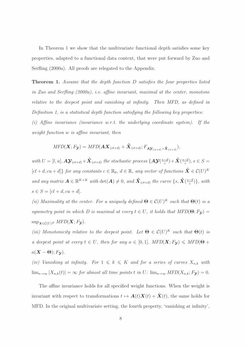
Theorem 3. (Consistency) Let Y 1, . . . ,Y N be a sample with the same distribution

as Y ∈ C(U)K with E(Y) finite. We only observe these curves at time points t1 <

. . . < tT from a design density fT with G(t) =∫ t

−∞fT (u)du such that tj = G−1( j−1

T−1)

and that U = [G−1(0), G−1(1)] is compact. We assume that fT is differentiable and

that inft∈U fT (t) > 0. It holds that

supX∈C(U)K

|MFDN(X)−MFD(X;FY)| → 0, a.s. P,

as N → ∞ and T → ∞ when the statistical depth D is such that it satisfies the

conditions of Definition 1, as well as (i) supx∈RK

∣∣D(x;FN)−D(x;F )∣∣ → 0, a.s. P ,

for FN → F as N → ∞ and (ii)∫U

∣∣∣w(t;FY(t),N)− w(t;FY(t))∣∣∣ dt → 0 as N →

∞ a.s. P . For the weight function in (2), (ii) holds when P ({x ∈ RK : D(x;F ) =

α}) = 0.

Halfspace depth satisfies condition (i) (Donoho and Gasko, 1992) and condition

(ii) for the weight (2) at absolute continuous distributions (Mizera and Volauf, 2002).

Based on MFDN we can estimate the global pattern of the observed curves by

means of the Θ(t) ∈ C(U)K which attains maximal MFDN . For a general depth

function D it might however be not straightforward to compute this median curve.

In that case one can approximate Θ(t) by the curve with maximal MFDN among

all observed curves. Apart from estimating the global pattern of the curves, we are

often interested in the variability of the curves. Our depth-based approach allows to

visualize this dispersion by means of the central regions, introduced in Lopez-Pintado

and Romo (2009). The β-central region consists of the band delimited by the [nβ]

curves with highest depth. If we draw the 25%, 50% and 75% central regions, we

obtain a representation of the data as in the enhanced functional boxplot of Sun and

Genton (2011). See Section 3 and the supplementary material for examples. Based

on these central regions, we define for each univariate set of curves their dispersion

13

curves sβ(t) as the width of the β-central region at each t. Note that the dispersion

curves are defined on each of the univariate curves, but the underlying computation

of the central regions is based on the MFDN . The t 7→ s0.5(t) dispersion curve can be

considered as a kind of functional IQR, as explained in Sun and Genton (2011). A

related concept, the scale curve, is defined in Lopez-Pintado et al. (2010). It measures

the area of the central region for β ranging from 0 to 1, and could be considered here

as well. The β-trimmed mean and the β-trimmed variance (the mean and variance of

all curves in the β-central region), see Fraiman and Muniz (2001), can be extended

in a straightforward way too.

2.3.2 Halfspace depth as a building block

As in the population case, we define the finite-sample multivariate functional halfspace

depth (MFHDN) of a curveX ∈ C(U)K as in Definition 3 withD the sample halfspace

depth based on {Y 1(t), . . . ,Y N(t)} (Tukey, 1975),

HD(X(t);FY(t),N) =1

Nmin

u∈RK ,‖u‖=1#{Y n(t), n = 1, . . . , N : u′Y n(t) > u′X(t)}.

The finite-sample Tukey median is defined as the center of gravity of the deepest

depth region. The median curve of the sample {Y 1(tj), . . . ,Y N(tj); j = 1, . . . , T} is

defined as the Tukey median at each time point.

Exact computation of the MFHDN can be done with fast algorithms for the half-

space depth up to dimension K = 4 (Bremner et al., 2008). To compute the weight

function (2), the algorithms developed in Hallin et al. (2010); Paindavaine and Siman

(2012) allow the computation of the depth contours up to dimension at least K = 5.

In this paper we used the R-packages depth and aplpack which implement fast algo-

rithms for bivariate and trivariate data (Rousseeuw and Ruts, 1996, 1998; Rousseeuw

and Struyf, 1998; Rousseeuw et al., 1999). Approximate halfspace depth in higher

dimensions can be computed by means of the random Tukey depth (Cuesta-Albertos

14

and Nieto-Reyes, 2008), but it is no longer affine invariant.

To decide upon the value of α in (2), one could consider some empirical quantile

of the HD values at each time point, and take, e.g., their minimum or average. For

example, if we set α equal to the minimal median of the HD values, the resulting

depth contours cover at least half of the data at each time point. Another possibility

is to rely on the probability coverage of the depth contours, which can be computed

exactly at some multivariate distributions. At bivariate normal data, it can be derived

that α = 1/8 gives a coverage of 48% (Rousseeuw and Ruts, 1999). For univariate

normal data, a 50% coverage is attained at α = 1/4. We have used these as default

values in our data examples and we have verified that the coverage was indeed around

50% at all time points.

3 Data examples

3.1 Industrial data

We first illustrate our new depth function MFHD(α) on an industrial data set that

produces one part during each cycle (De Ketelaere et al., 2011). The behavior of

the cycle as monitored by an accelerometer provides a fingerprint of the cycle and,

related, of the quality of the produced part. If a deviating acceleration signal occurs,

the process owner should be warned. Figure 2(a) shows the acceleration signal of

N = 224 parts measured during 120ms. Measurements are available every millisecond,

hence the time signal ranges from t1 = 1 up to tT = 120. To augment this univariate

data set, we could consider the derivatives of the curves as additional information,

but in this example, we decided to use the integrated curves instead. As the velocity

at time tj, V (tj) =∫ tj−∞

A(t)dt with A(t) the acceleration at time t, we approximated

the velocity by V (tj) ≈ V (tj−1) + {A(tj−1) +A(tj)}/2 starting with V (t1) = 0. Note

that the choice of the integration constant is not important here, due to the affine

15

(a) (b)

Time

Acc

eler

atio

n−

2.0

−1.

5−

1.0

−0.

50.

00.

5

0 20 40 60 80 100 120

Time

Vel

ocity

−50

−40

−30

−20

−10

00 20 40 60 80 100 120

Figure 2: Industrial data: all signals colored according to their bivariate MFHD(1/8)

depth.

invariance of MFHD(α). The resulting velocity curves are depicted in Figure 2(b).

Next, we performed a bivariate analysis on this data set, and computed the MFHD(α)

of all signals with α = 0.125. The resulting depth values can be visualized by means

of the so-called rainbow plot (Hyndman and Shang, 2010). It shows the curves colored

according to their MFHD value, going from dark grey for the deepest curve to light

grey for the curve with minimal depth. Such a representation of the data is in

particular useful to visualize potential outliers, as they are expected to have a lower

MFHD depth and consequently should be colored light grey. In Figure 2 we see that

the extreme outlying curves indeed are all colored light grey, which is a confirmation

that our depth measure assigns them a low depth value.

Computing the MFHD on the bivariate data (A(t), V (t)) also yields the median

curves, printed in black on Figure 1 for the acceleration and velocity curves. We see

that these median curves are not attracted by the outlying values at the end of the

cycle. Also the acceleration estimates in the valleys around time points 50 and 75 are

16

(a) (b)

0 10 20 30 40 50 60

−1.

5−

1.0

−0.

50.

00.

5

Time

Acc

eler

atio

n

0 10 20 30 40 50 60−

15−

10−

50

Time

Vel

ocity

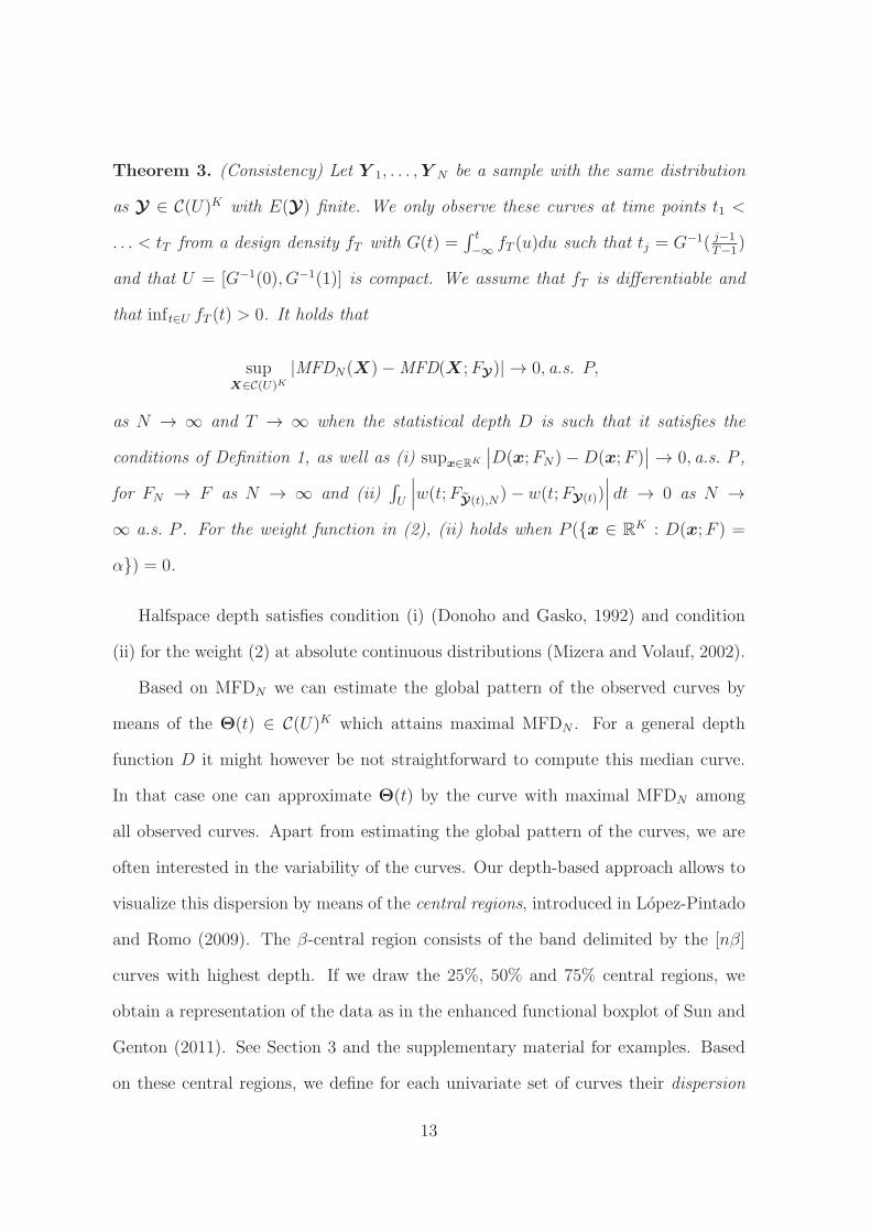
Figure 3: Industrial data: median curve (solid line), curve 7 (squares) and curve 82

(triangles).

lower than those of the mean curve, illustrating the robustness of the median curve

towards the upward contamination values in these regions.

To illustrate the effect of the weight function, we restrict the data set to the first

61 ms. We focus on curve 7 (indicated with squares in Figure 3, and curve 82 (marked

with triangles), and compute also their MFHD with a constant weight function. From

Figure 3 it is obvious that curve 7 is not at all outlying and is very close to the MFHD

median (solid line) in the second half of the time period where the amplitude is larger.

Curve 82 is behaving well in the first phase, but becomes clearly outlying afterwards.

This is well reflected in their MFHD(0.125) values, which achieve a large rank of 208

(out of 224) for curve 7 and a low rank of 34 for curve 82. When we ignore the

differences in amplitude by using a constant weight, the depth of curve 7 has only

rank 91, whereas curve 82 receives even a larger depth with rank 152. These depth

values do not well reflect the position of the curves in the sample.

In the supplementary material we show the benefit of adding the velocity curves.

17

Some curves seem to be quite central when we only consider their acceleration, but

become more outlying when adding their velocity. This not only affects the depth of

the corresponding curves, but also the central regions and the dispersion curves.

3.2 Weather data

In this section we present an example of bivariate functional data on which we illus-

trate the limited effect of outlying curves on the estimation of the MFHD median and

the central regions. Our data set contains the temperature and dewpoint tempera-

ture (in degrees Celcius) measured between January 11 and 15, 2013 at 78 weather

stations in the U.K. The raw data were downloaded from NOAA (www.noaa.gov).

As different stations have different recording times, cubic spline interpolation was

applied to obtain hourly estimates, yielding a total of 120 values, shown as the light

grey curves in Figure 4(a) and (b). The dashed curves are the cross-sectional means

which quite nicely reflect the general trend in the temperatures. On these data we ap-

plied MFHD with a constant weight function. Figures 4(c) and (d) show the resulting

MFHD median and the boundaries of the 75% central regions by dashed curves.

Next we replaced eight curves with data from eight weather stations in Central

Europe. They exhibit much lower temperatures as can be seen from the dark curves

in Figure 4(a) and (b), and they affect the cross-sectional means heavily (depicted

as solid lines). The solid lines in Figure 4(c) and (d) correspond to the MFHD

median and the 75% central regions, computed on the contaminated data set. They

are similar to the results based on the data from the U.K. only, which reflects the

robustness of MFHD.

4 Simulations

In this section we present three simulation settings each designed to illustrate a par-

ticular aspect of the behavior of MFHD. In all cases, we generate N = 50 univariate

18

(a) (b)

0 20 40 60 80 100 120

−15

−10

−5

05

10

Time

Tem

pera

ture

0 20 40 60 80 100 120

−15

−10

−5

05

Time

Dew

poin

t tem

pera

ture

(c) (d)

0 20 40 60 80 100 120

−15

−10

−5

05

10

Time

Tem

pera

ture

0 20 40 60 80 100 120

−15

−10

−5

05

Time

Dew

poin

t tem

pera

ture

Figure 4: Weather data: (a)–(b) temperature and dewpoint temperature for weather

stations in the U.K. (light grey) and Central Europe (dark) with cross-sectional means

of the U.K. data only (dashed curves) and cross-sectional means of the full data set

(solid curves) ; (c)–(d) MFHD median and central regions for the U.K. data only

(dashed curves) and the full data set (solid curves).

19

curves {Y1(t), . . . , YN(t)} from a stochastic process Y , denoted as the uncontami-

nated curves {Y (t)}N . Then we replace five curves of {Y (t)}N with curves sampled

from a contaminating stochastic process Yε, yielding a data set {Y ε1 (t), . . . , Y

εN(t)} =

{Yε(t)}N with 10% contamination. All curves are evaluated on a grid of T = 100 equi-

spaced time points t1, . . . , tT in [0, 2π]. Each experiment was replicated 100 times. In

a first set of simulations (Section 4.2) we consider the bivariate MFHD applied to the

curves and their derivatives. We compare its behavior with several univariate func-

tional depths and with the bivariate random projection depth. Next, in Section 4.3

we illustrate the advantage of using the warping functions (or a function thereof) as

additional curves. First we describe how we evaluate the performance and robustness

of the functional depths.

4.1 Evaluation criteria

ASE of the estimated central curve: the averaged squared scaled distance between

the true and the estimated central curve,

1

T

T∑

j=1

(mYε

(tj)−mY(tj)

sY(tj)

)2

,

where mY is the central curve of Y , mYεis the estimated central curve, and sY(t) is

the interquartile range of Y(t).

ASE of the estimated dispersion curve: the average squared difference between

the logarithm of the (0.5)-dispersion curves computed on the contaminated and the

uncontaminated data,

1

T

T∑

j=1

(log

(sε0.5(tj)

s0.5(tj)

))2

,

where s0.5(t) is the width of the (0.5)-central region of {Y (t)}N as defined in Sec-

tion 2.3. Analogously, sε0.5(t) is the dispersion curve computed from {Yε(t)}N .

Normalized maximum depth of outliers. To have an easily comparable criterion,

we normalize by dividing the maximum depth with the depth of the deepest curve.

20

Formally, let FDN(Yεn , FYε,N) denote the (finite-sample) functional depth of the curves

Y εn (t) from {Yε(t)}N , and denote by Ic the index set of the contaminated curves from

{Yε(t)}N . Then we consider maxn∈Ic FDN(Yεn , FYε,N)/maxn=1,...,N FD(Y ε

n , FYε,N).

4.2 Simulations with curves and their derivatives

We generate three types of univariate curves, contaminated with 10% outlying curves,

and we evaluate MFHD on the bivariate samples {(Yε(t), Y′ε (t))}N . We consider both

α = 1/4 and α = 1/8, resulting in MFHD(1/4) and MFHD(1/8). In both cases the

estimated central curve mYε(t) is the MFHD median, as in Definition 2.

We compare the behavior of MFHD on the bivariate samples, first, with three

approaches applied on the univariate curves {Yε(t)}N . (1) The cross-sectional av-

erage (CSA): mYε(t) = 1

50

∑50n=1 Y

εn (t). The corresponding depth is the univariate

Mahalanobis depth, with σYε(t) the cross-sectional standard deviation,

MD(Y εn (t)) =

{1 +

(Y εn (t)− mYε

(t)

σYε(t)

)2}−1

.

(2) The modified band depth (MBD) of Lopez-Pintado and Romo (2009). This cor-

responds with MFD(Yi,Yε) as in (4) with the simplicial depth (Liu, 1990) as depth

function D and with constant weight function w(t) = 1/T . The curve with largest

MBD is considered as mYε(t). We use the implementation provided in the R pack-

age depthtools. (3) The MFHD(α = 1/4) applied to the univariate curves {Yε(t)}N ,

which we denote by UFHD(1/4). Note that the deepest curve in this case corresponds

to the cross-sectional median.

Next, we compare with the bivariate random projection depth (RPD) of Cuevas

et al. (2007), using the default settings from the implementation in the R package

fda.usc (Febrero-Bande and Oviedo de la Fuente, 2012). Here, the curves and their

derivatives are projected on a random direction, yielding a bivariate sample on which

the (bivariate) modal depth (Cuevas et al., 2006) can be computed for all observations.

21

(a) (b) (c) (d)

0 1 2 3 4 5 6

0.0

0.1

0.2

0.3

0 1 2 3 4 5 6

02

46

8

0 1 2 3 4 5 6−0.

004

−0.

002

0.00

00.

002

0.00

4

0 1 2 3 4 5 6

−0.

6−

0.4

−0.

20.

00.

20.

40.

6

Figure 5: Simulation settings. Main curves (solid) and outliers (dashed) for the

curves (a),(b) and their derivatives (c),(d) for (a),(c) the shifted outliers; (b),(d) the

log-normal processes.

The RPD of a curve corresponds with the average modal depth over 50 random

projections. Note that this approach does not satisfy the affine invariance property

as stated in Theorem 1.

The functional derivatives are computed using B-splines using the default settings

and the algorithms from the R-package fda.usc.

4.2.1 Simulation setting I: Shifted outliers

This simulation setting illustrates the behavior of MFHD in cases where the true

curves are homoscedastic and all derivative curves follow the same process. We gen-

erated curves of the form

Y εn (t) = (1− cn){a1n sin(t) + a2n cos(t)}+ cn{a1n sin(t) + a2n cos(t) +

1

4},

where t is a grid of 100 equispaced values on [0, 2π] , cn is 1 for 10% of the curves and

0 otherwise. The random coefficients a1n and a2n follow independent uniform distri-

butions on [0, 0.05]. Figure 5(a) depicts the ‘regular’ (solid) and outlying (dashed)

curves and Figure 5(d) the corresponding derivatives.

The first panel in Figure 6 depicts, for each of the functional depth methods, the

ASE of the central curves. CSA is highly influenced by the outlying curves, and RPD

22

********* ** **

Shifted Outliers ProcessA

SE

Mea

n

********

*

*******

*

**

**A

SE

Dis

p.

CSA MBD UFHD(1/4) RPD MFHD(1/4) MFHD(1/8)

*

**********

** **O

utlie

rs D

epth

0.3

1.0

0.04

0.12

0.3

0.8

Figure 6: Setting I: shifted outliers. ASE of the estimated central curve (top), of the

0.5-dispersion curve (middle) and outlier depth (bottom).

to a lesser extend. The middle panel in Figure 6 depicts the ASE of the dispersion

curve. The effects of the outliers on the CSA estimate of dispersion s0.5(Yεn (t)) is

more muted because the outlying curves are located too far to be included in the

set of 25 curves with largest Mahalanobis depth. RPD contains some large values

too. All other methods perform well on both criteria. The third panel in Figure 6

depicts the (normalized) maximum depth of outliers. Here again, CSA assigns a high

depth to the outliers. Both univariate functional depths (MBD and UFHD) assign

higher depths to the outliers than the bivariate depth functions. The value of α for

MFHD(α) has a negligible effect on all three performance criteria.

4.2.2 Simulation setting II: Log-normal processes

Highly heteroscedastic curves are obtained by generating from a log-normal process

Yn(t) ∼ logN(µ(t),Σ(t)). Denote x = {xi}20i=1 20 equidistant points on [0, 2π].

The covariance kernel of the xi’s is given by Kxx(i, j) = exp(− (xj−xi)

2

2δ2

), with

δ = 0.25. For the time points t = {tj}100j=1 equidistant on [0, 2π], we define Ktx and

23

********* ******* ****** ********

Log−normal ProcessA

SE

Mea

n

***

*

*

* ********

*

********* ***********

***

*

*

**********

AS

E D

isp.

CSA MBD UFHD(1/4) RPD MFHD(1/4) MFHD(1/8)

*****

**

***O

utlie

rs D

epth

0.1

0.4

0.05

0.15

0.3

0.8

Figure 7: Setting II: log-normal processes. ASE of the estimated central curve (top),

of the 0.5-dispersion curve (middle) and outlier depth (bottom).

Ktt analogously. Then, the weight matrix for the mean µ is Km = Ktx(Kxx +D)−1

where D is a diagonal matrix that directs the heteroscedasticity of the final process,

D = Diagi=1,...,20{min((π − xi)2, 1)}, so that the variance of the process is mini-

mized at t = π. For the regular curves we take µ(t) = Km(a1 sin(x) + a2 cos(x)),

where a1 ∼ U(−2, 2) and a2 ∼ U(−1, 1) are randomly generated. For the outlying

curves we took µ∗(t) = Km(sin(6x) + µ(x)). The covariance matrix is given by

Σ = Ktt−Ktx(Kxx+D)−1K ′tx. For a generated sample of curves and the correspond-

ing derivatives, see Figure 5(c),(f).

This configuration was designed to penalize those estimators that do not use the

information from the derivatives of the curves to assign depths. This is particularly

visible in the third panel of Figure 7, where the CSA, MBD, UFHD and RPD are

unable to detect the outlying curves. The outliers do not affect the CSA in terms of

ASE of the central and the dispersion curves since the range of the response values

is the same for all curves. Although RPD uses the derivatives, it does not perform

24

well; RPD is not estimating the central curve well, and it does not assign low depths

to the outlying curves. MFHD retains its good behavior.

4.3 Simulation with warped curves

Warping can make outlying curves more difficult to detect by pulling them towards

the uncontaminated ones. See Figure 8 for an example where outlying curves are

initially visible but are then hidden by the warping process. Here, using a bivariate

approach can help with the ranking of the curves. For MFHD we compare two

bivariate approaches. First, we create a bivariate sample of curves by using the

warped curves together with the individual warping functions. Second, we use as

a bivariate sample of curves the warped curves together with the derivatives of the

warping functions. Adding the curves related to warping alleviates the information

loss induced by the warping procedure.

For the warping functions, our simulation design follows that used in the first

simulation setting of Arrabis-Gil and Romo (2012). The warping functions for the

good curves are generated as explained on their page 405, formula (3.7). The inverse

of

hn(t) =arctan(βn(2t− 1))

2 arctan(βn)+ 1/2, t ∈ [0, 1]

with βn equally spaced between 10 and 14 is used as warping function for the out-

liers. We use the same amplitude functions for all curves such that different warp-

ing functions correspond to original curves with different shapes and phases. To

make the results comparable with those of simulation setting I, we use Yn(t) =

a1i sin(t/(2π)) + a2i cos(t/(2π)). A sample of curves and warped curves is depicted

in Figure 8, together with the warping functions and their derivatives.

For comparison we use two versions for UFHD: only the unwarped curves, and

only the warped curves. Figure 9 contains a summary of the performance criteria.

25

(a) (b)

0.0 0.2 0.4 0.6 0.8 1.0

−0.

06−

0.04

−0.

020.

000.

020.

040.

06

0.0 0.2 0.4 0.6 0.8 1.0

−0.

06−

0.04

−0.

020.

000.

020.

040.

06(c) (d)

0.0 0.2 0.4 0.6 0.8 1.0

0.0

0.2

0.4

0.6

0.8

1.0

0.0 0.2 0.4 0.6 0.8 1.0

0.00

0.05

0.10

0.15

Figure 8: Simulation setting III. (a) Original curves, (b) warped curves, (c) warping

functions, (d) derivatives of the warping functions; outlying curves as dashed lines.

As expected, once warped, the outlying curves have no influence on the estimation of

the central (or dispersion curves) and this is visible in the first two panels of Figure 9

where UFHD has low MSE on both measures. At the same time, warping makes

the curves with different shapes similar to the other curves, causing a poor behavior

of UFHD on the warped curves in the third panel. Adding the warping functions,

or their derivatives in a bivariate analysis completely addresses the information loss

introduced by the warping procedure.

26

Estimators

*

*** *

Warped ProcessA

SE

Mea

n

*

*

*

******

AS

E D

isp.

UFHD(yraw) UFHD(ywarped) MFHD(ywarped,ht) MFHD(ywarped,ht′)

*

**

Out

liers

Dep

th

0.04

0.12

0.04

0.12

0.3

0.8

Figure 9: Setting III. ASE of the estimated central curve (top) and the 0.5-dispersion

curve (middle) and outlier depth (bottom). Using the original curves (yraw), the

warped curves (ywarped) and their warping functions (ht) with derivatives h′t.

5 Discussion

We have presented a new depth function for multivariate functional data (MFD),

defined as a weighted average of the cross-sectional multivariate depths. It assigns a

ranking to curves from the center outwards, whilst accounting for differences in am-

plitude. Shape and phase variation can be accommodated by including derivatives

and/or warping functions. Interesting theoretical properties and computational ad-

vantages are achieved when using the multivariate halfspace depth, which leads to the

MFHD depth function. The multivariate functional median curve can then be com-

puted explicitly and estimates the central behavior of the curves. MFHD also allows

to visualise and quantify the variability amongst the curves. Simulations have shown

the benefit of adding derivatives or warping information to univariate curves, and

they have illustrated the better performance of MFHD compared with the bivariate

random projection depth.

27

Depth functions are regularly used for the classification and clustering of multi-

variate data, see e.g. Ghosh and Chaudhuri (2005), Dutta and Ghosh (2011), Hubert

and Van der Veeken (2010), Jornsten (2004). This has been extended to the classifi-

cation of functional data, as in Cuevas et al. (2007), Lopez-Pintado and Romo (2006)

and Hlubinka and Nagy (2012). It will be interesting to study the use of MFHD for

the classification of multivariate curves, as well as for the classification of univariate

curves augmented with their derivatives or warping functions. Some preliminary re-

sults indicate that this will indeed be beneficial (Slaets, 2011). Combining MFDH

with the DD-plot of Li et al. (2012) is another interesting topic of further research.

We will also investigate the possible use of MFHD for online quality control.

As illustrated in the data examples and in the simulations, MFHD assigns lower

depth to curves which deviate strongly from the majority of the curves. This robust-

ness towards outliers is inherited from the halfspace depth which is applied at every

time point. It is however well known that other depth functions, such as projection

depth (Zuo, 2003) and spatial depth (Serfling, 2002), attain a higher breakdown value

and thus could lead to a more robust MFD. Alternatively one could replace the inte-

gral in (1) (or equivalently the average in (4)) by an infimum as proposed in Mosler

and Polyakova (2012). More theoretical and numerical studies are needed to compare

these different depth functions.

A Appendix – Proofs of Section 2

Proof of Theorem 1

Proof. (i) For a depth function D that is affine invariant and for weight function (2)

use that vol{Dα(Y(t))} = |det(A)| · vol(Dα{AY(t) + X(t))}, to obtain the affine

invariance for MFD. (ii) – (iv) are immediate from the assumptions on D.

28

Proof of Theorem 2

Proof. (i) and (ii) These parts of the theorem follow by application of Theorems 2

and 3 of Ausubel and Deneckere (1993). (iii) Trivial.

(iv) We prove by contradiction that a deepest curve implies deepest points at every

t ∈ U . Suppose that there exists a t1 ∈ U with D(ϑ(t1);FY(t1)) < D(Θt1 ;FY(t1))

for Θt1 ∈ Θ(t1). Since by (i) or (ii) Θ is compact-valued, there exists an open

neighborhood B of ϑ(t1), and an open neighborhood C of Θ(t1) such that B∩C = ∅.

Since ϑ is continuous, there exists a δ1 > 0 such that for |t − t1| < δ1: ϑ(t) ∈ B.

By the upper-hemicontinuity of Θ, there exists a δ2 > 0 such that for |t − t1| <

δ2: Θ(t) ⊂ C. Take δ = min{δ1, δ2}. Then, since B ∩ C = ∅, for |t − t1| < δ,

D(ϑ(t);FY(t)) < D(Θt;FY(t)) for Θt ∈ Θ(t), and thus

MFD(ϑ;FY) =

∫

U

D(ϑ(t);FY(t))w(t)dt

<

∫

|t−t1|≥δ

D(Θt;FY(t))w(t)dt+

∫

|t−t1|<δ

D(Θt;FY(t))w(t)dt

which is in contradiction with the fact that ϑ is a deepest curve.

Finite sample MFD. Calculation of (4)

In order to apply Definition 1 to the curve observations at a grid of time points,

we use linear interpolation on each interval [tj, (tj + tj+1)/2] to connect the values

(tj, Ynk(tj)) with the average of the function values at time tj in the middle of the time

interval ((tj + tj+1)/2, Yk(tj) = N−1∑N

n=1 Ynk(tj)), for j = 1, . . . , T − 1 and for each

k = 1, . . . , K. Similarly, for j = 1, . . . , T −1, on the interval [(tj+ tj+1)/2, tj+1], linear

interpolation is used to connect the values ((tj + tj+1)/2, Yk(tj)) and (tj+1, Ynk(tj+1)).

This yields a sample of continuous K-dimensional processes Yn, n = 1, . . . , N on the

29

interval [t1, tT ] of which the kth component (k = 1, . . . , K) is defined by

Yn,k(t) =

Ynk(tj)tj+tj+1−2t

tj+1−tj+ Yk(tj)

2(t−tj)

tj+1−tjfor t ∈ [tj, (tj + tj+1)/2]

−Ynk(tj+1)tj+tj+1−2t

tj+1−tj− Yk(tj)

2(t−tj+1)

tj+1−tjfor t ∈ [(tj + tj+1)/2, tj+1].

(5)

The empirical cumulative distribution function of this sample is denoted by FY,N .

Note that the definition of the K-variate processes Yn depends on both N and T .

Using the definition of MFD on population level, see (1), with the processes Yn, and

the affine invariance of D, with t0 = t1 and tT = tT+1 gives Definition 3. Indeed,

MFD(X;FY,N) =

T−1∑

j=1

{D(X(tj);FY(tj),N)

∫ (tj+tj+1)/2

tj

w(t)dt

+D(X(tj+1);FY(tj+1),N)

∫ tj+1

(tj+tj+1)/2

w(t)dt

}

= D(X(t1);FY(t1),N)

∫ (t1+t2)/2

t1

w(t)dt

+T−1∑

j=2

D(X(tj);FY(tj),N)

∫ (tj+tj+1)/2

(tj−1+tj)/2

w(t)dt

+D(X(tT );FY(tT ),N)

∫ tT

(tT−1+tT )/2

w(t)dt.

Proof of Theorem 3

Proof. On the space of curves in C(U)K we define the uniform distance ρ(X, Y ) =

supt∈U ‖X(t)−Y (t)‖, with ‖·‖ the Euclidean norm in RK . We first show that the func-

tions {Yn : U → RK : t 7→ Yn,1(t), . . . , Yn,K(t), n = 1, . . . , N} for N → ∞ and T →

∞ converge weakly to Y . Since E(Y) is finite, the law of large numbers implies that

for each t ∈ U and for k = 1, . . . , K, Yk(t) = N−1∑N

n=1 Ynk(t)→N→∞E[Yk(t)], a.s.

By the design assumption, |tj+1 − tj| = |(G−1)′(ξj)|/(T − 1) = cj/(T − 1), for a

constant cj and ξj in between tj and tj+1. For each t ∈ U there is precisely one interval

[tj, tj+1) that contains t and since the interpolating process agrees with the observed

30

curve on the time points t1, . . . , tT , it follows that for each value n = 1, . . . , N ,

0 6 ρ(Yn,Y n) 6 2 sup|s−t|6c/(T−1)

‖Y n(t)− Y n(s)‖ = 2wY n(c/(T − 1)),

with wY the modulus of continuity of Y and with c = 1/ inft∈U fT (t). Since U is

compact and each function Y n is continuous, this function is also uniformly con-

tinuous and thus wY n(c/(T − 1)) → 0 as T → ∞. Since the sample of curves is

i.i.d. and by Theorems 3.2 and 7.5 of Billingsley (1999), there is weak convergence of

the interpolating processes YN to Y as N → ∞ and T → ∞. It holds that

supX∈C(U)K

∣∣∣MFD(X;FY,N)−MFD(X;FY)

∣∣∣ 6 (6)

supX∈C(U)K

∫

U

∣∣∣D(X(t);FY(t),N)−D(X(t);FY(t))

∣∣∣ dt+∫

U

∣∣∣w(t;FY(t),N)− w(t;FY(t))∣∣∣ dt.

The convergence to zero of the first integral is obtained by rewriting the integration

over U as a sum of integrals over the domains in (5). For T ∈ [tj, (tj + tj+1))/2), e.g.,

use that∣∣∣D(X(t);F

Y(t),N)−D(X(t);FY(t))∣∣∣ ≤

∣∣∣D(X(tj);FY(t),N)−D(X(tj);FY(t))∣∣∣+

∣∣D(X(tj);FY(t))−D(X(t);FY(t))∣∣, where we used the constancy of the finite sample

depth on each such interval by definition of YN . The weak convergence of YN to Y

as N → ∞, T → ∞, together with the boundedness of the depth, the design and the

fact that the set of interval endpoints has measure zero, ends the proof.

We now prove condition (ii) for the weight in (2). Under the stated assumptions,

Theorem 4.1 of Zuo and Serfling (2000b) yields the a.s. convergence of the α-trimmed

regions Dα(FY(t),N) to Dα(FY(t)), together with a nesting property such that for

0 < ǫ < α, Dα(FY(t),N) ⊂ Dα−ǫ(FY(t)) for all t ∈ U . By the dominated convergence,

the right-hand side of (6) converges to 0 a.s. P as N, T → ∞.

References

Abalo, K. and Kostreva, M. (2005). Berge equilibrium: some recent results from

fixed-point theorems. Applied Mathematics and Computation, 169(1):624–638.

31

Arrabis-Gil, A. and Romo, J. (2012). Robust depth-based estimation in the time

warping model. Biostatistics, 13:398–414.

Ausubel, L. M. and Deneckere, R. J. (1993). A generalized theorem of the maximum.

Economic Theory, 3(1):99–107.

Berrendero, J., Justel, A., and Svarc, M. (2011). Principal components for multivari-

ate functional data. Computational Statistics & Data Analysis, 55(9):2619–2634.

Billingsley, P. (1999). Convergence of Probability Measures. John Wiley & Sons, Inc.,

second edition.

Bremner, D., Chen, D., Iacono, J., Langerman, S., and Morin, P. (2008). Output-

sensitive algorithms for Tukey depth and related problems. Statistics and Comput-

ing, 18:259–266.

Chen, Z. and Tyler, T. (2002). The influence function and maximum bias of Tukey’s

median. The Annals of Statistics, 30:1737–1759.

Cuesta-Albertos, J. and Nieto-Reyes, A. (2008). The random Tukey depth. Compu-

tational Statistics & Data Analysis, 52(11):4979–4988.

Cuevas, A., Febrero, M., and Fraiman, R. (2006). On the use of the bootstrap

for estimating functions with functional data. Computational Statistics & Data

Analysis, 51(2):1063–1074.

Cuevas, A., Febrero, M., and Fraiman, R. (2007). Robust estimation and classification

for functional data via projection-based depth notions. Computational Statistics,

22:481–496.

De Ketelaere, B., Mertens, K., Mathijs, F., Diaza, D., and De Baerdemaeker, J.

(2011). Nonstationarity in statistical process control - issues, cases, ideas. Applied

Stochastic Models in Business and Industry, 27:367–376.

Donoho, D. and Gasko, M. (1992). Breakdown properties of location estimates

based on halfspace depth and projected outlyingness. The Annals of Statistics,

20(4):1803–1827.

Dutta, S. and Ghosh, A. (2011). On robust classification using projection depth.

32

Annals of the Institute of Statistical Mathematics, 64:657–676.

Febrero-Bande, M. and Oviedo de la Fuente, M. (2012). Statistical computing in

functional data analysis: the R package fda.usc. Journal of Statistical Software,

51(4):1–28.

Ferraty, F. and Vieu, P. (2006). Nonparametric Functional Data Analysis: Theory

and Practice. Springer, New York.

Fraiman, R. and Muniz, G. (2001). Trimmed means for functional data. Test, 10:419–

440.

Ghosh, A. and Chaudhuri, P. (2005). On maximum depth and related classifiers.

Scandinavian Journal of Statistics. Theory and Applications, 32(2):327–350.

Hallin, M., Paindaveine, D., and Siman, M. (2010). Multivariate quantiles and

multiple-output regression quantiles: from L1 optimization to halfspace depth. The

Annals of Statistics, 38(2):635–669.

Hlubinka, D. and Nagy, S. (2012). Functional data depth and classification. Report.

Hubert, M. and Van der Veeken, S. (2010). Robust classification for skewed data.

Advances in Data Analysis and Classification, 4:239–254.

Hyndman, R. J. and Shang, H. L. (2010). Rainbow plots, bagplots, and boxplots for

functional data. Journal of Computational and Graphical Statistics, 19(1):29–45.

Jornsten, R. (2004). Clustering and classification based on the L1 data depth. Journal

of Multivariate Analysis, 90(1):67–89.

Li, J., Cuesta-Albertos, J., and Liu, R. (2012). DD-classifier: nonparametric classifica-

tion procedure based on DD-plot. Journal of the American Statistical Association,

107:737–753.

Liu, R. Y. (1990). On a notion of data depth based on random simplices. The Annals

of Statistics, 18(1):405–414.

Lopez-Pintado, S. and Romo, J. (2006). Depth-based classification for functional

data. In Data depth: robust multivariate analysis, computational geometry and

applications, volume 72 of DIMACS Ser. Discrete Math. Theoret. Comput. Sci.,

33

pages 103–119. Amer. Math. Soc., Providence, RI.

Lopez-Pintado, S. and Romo, J. (2009). On the concept of depth for functional data.

Journal of the Americal Statistical Association, 104:718–734.

Lopez-Pintado, S. and Romo, J. (2011). A half-region depth for functional data.

Computational Statistics & Data Analysis, 55:1679–1695.

Lopez-Pintado, S., Romo, J., and Torrente, A. (2010). Robust depth-based tools for

the analysis of gene expression data. Biostatistics, 11:254–264.

Mizera, I. and Volauf, M. (2002). Continuity of halfspace depth contours and max-

imum depth estimators: diagnostics of depth-related methods. Journal of Multi-

variate Analysis, 83(2):365–388.

Mosler, K. and Polyakova, Y. (2012). General notions of depth for functional data.

Report.

Nieto-Reyes, A. (2011). On the properties of functional depth. In Ferraty, F., editor,

Recent Advances in Functional Data Analysis and Related Topics, Contributions to

Statistics, pages 239–244. Physica-Verlag HD.

Paindavaine, D. and Siman, M. (2012). Computing multiple-output regression quan-

tile regions. Computational Statistics & Data Analysis, 56:840–853.

Pigoli, D. and Sangalli, L. (2012). Wavelets in functional data analysis: estimation

of multidimensional curves and their derivatives. Computational Statistics & Data

Analysis, 56(6):1482–1498.

Ramsay, J. and Silverman, B. (2006). Functional Data Analysis. Springer, New York,

2nd edition.

Romanazzi, M. (2001). Influence function of halfspace depth. Journal of Multivariate

Analysis, 77:138–161.

Rousseeuw, P. and Ruts, I. (1996). Bivariate location depth. Applied Statistics,

45:516–526.

Rousseeuw, P. and Ruts, I. (1998). Constructing the bivariate Tukey median. Statis-

tica Sinica, 8:827–839.

34

Rousseeuw, P. and Ruts, I. (1999). The depth function of a population distribution.

Metrika, 49:213–244.

Rousseeuw, P., Ruts, I., and Tukey, J. (1999). The bagplot: A bivariate boxplot. The

American Statistician, 53:382–387.

Rousseeuw, P. and Struyf, A. (1998). Computing location depth and regression depth

in higher dimensions. Statistics and Computing, 8:193–203.

Sangalli, L., Secchi, P., Vantini, S., and Veneziani, A. (2009). A case study in

exploratory functional data analysis: geometrical features of the internal carotid

artery. Journal of the American Statistical Association, 104(485):37–48.

Serfling, R. (2002). A depth function and a scale curve based on spatial quantiles.

In Statistical data analysis based on the L1-norm and related methods (Neuchatel,

2002), Stat. Ind. Technol., pages 25–38. Birkhauser, Basel.

Slaets, L. (2011). Analyzing phase and amplitude variation of functional data. PhD

thesis, KU Leuven.

Slaets, L., Claeskens, G., and Hubert, M. (2012). Phase and amplitude-based cluster-

ing for functional data. Computational Statistics & Data Analysis, 56:2360–2374.

Sun, Y. and Genton, M. (2011). Functional boxplots. Journal of Computational and

Graphical Statistics, 20(2):316–334.

Tukey, J. (1975). Mathematics and the picturing of data. In Proceedings of the

International Congress of Mathematicians, volume 2, pages 523–531, Vancouver.

Zuo, Y. (2003). Projection-based depth functions and associated medians. The Annals

of Statistics, 31(5):1460–1490.

Zuo, Y. and Serfling, R. (2000a). General notions of statistical depth function. The

Annals of Statistics, 28:461–482.

Zuo, Y. and Serfling, R. (2000b). Structural properties and convergence results for

contours of sample statistical depth functions. The Annals of Statistics, 28(2):483–

499.

35

Multivariate Functional Halfspace DepthSupplementary Materials

Gerda Claeskens, Mia Hubert, Leen Slaets and Kaveh Vakili

October 10, 2013

1 Univariate versus bivariate analysis of the industrial data

We illustrate on the industrial data set the benefit of adding the integrated curves

(here, the velocity curves) to the analysis. Figures 1(c) and (e) show the 25%, 50%

and 75% central regions of the acceleration and velocity curves, based on the bivariate

MFHD(1/8) depth (with the MFHD median superimposed in white). Their cross-

sectional width yields the dispersion curves in Figures 1(d) and (f). When we only

consider the acceleration data and set α = 1/4, the multivariate halfspace depth

reduces to the weighted average of the univariate halfspace depth, which we denote

by UFHD(1/4). We then obtain the UFHD median and the central regions displayed

in Figure 1(a). The UFHD median is identical to the cross-sectional median and does

not differ much from the MFHD median. We notice that the 50% and 75% central

regions of the acceleration curves are quite different between 40ms and 60ms. This

behavior is also reflected in the dispersion curves in Figure 1(a). Note that all the

dispersion curves clearly expose the heteroscedasticity of both the acceleration and

velocity signals, and they give an indication of the amount of outlying signals.

To understand the difference between the univariate and the bivariate analysis,

we first compare the univariate UFHD(1/4) and bivariate MFHD(1/8) values for all

curves, shown in Figure 2. We observe a global monotone trend showing that curves

with a low UFHD depth also have a low MFHD depth, but the relation is certainly

not strictly monotone. Changing α did not make a substantial difference in UFHD

or MFHD.

Let us focus on one specific deviating curve, with label 112, indicated by the dotted

1

(a) (b)

0 20 40 60 80 100 120

−2.

0−

1.5

−1.

0−

0.5

0.0

0.5

Time

Acc

eler

atio

n

25%50%75%

0 20 40 60 80 100 120

0.0

0.5

1.0

1.5

Time

Dis

pers

ion

Acc

eler

atio

n

0.1

0.25

0.5

0.75

0.9

(c) (d)

0 20 40 60 80 100 120

−2.

0−

1.5

−1.

0−

0.5

0.0

0.5

Time

Acc

eler

atio

n

25%50%75%

0 20 40 60 80 100 120

0.0

0.5

1.0

1.5

Time

Dis

pers

ion

Acc

eler

atio

n

0.10.250.5

0.75

0.9

(e) (f)

0 20 40 60 80 100 120

−50

−40

−30

−20

−10

0

Time

Vel

ocity

25%50%75%

0 20 40 60 80 100 120

05

1015

Time

Dis

pers

ion

Vel

ocity

0.1

0.25

0.5

0.75

0.9

Figure 1: Central regions and dispersion curves for: (a)–(b) the acceleration curves

based on UFHD(1/4), (c)–(d) the acceleration curves based on MFHD(1/8), (e)–(f)

the velocity curves based on MFHD(1/8).

2

0.1 0.2 0.3 0.4

0.00

0.05

0.10

0.15

0.20

0.25

0.30

univariate UFHD

biva

riate

MF

HD

112

Figure 2: Acceleration data: bivariate MFHD(1/8) versus univariate UFHD(1/4).

line in Figure 3, for comparison together with the deepest curve. From Figure 3(a) we

notice that it attains larger acceleration values at the peaks around 47ms and 57ms,

and one additional oscillation between 60ms and 80ms. Consequently its univariate

depth, only based on this information, is somewhat lower but it is not extremely small.

To be more precise, the univariate UFHD of curve 112 has rank 45 (out of 224). When

we include the information given by the velocity curves, we see from Figure 3(b) that

the velocity of curve 112 is outlying on almost the whole time domain. This yields

a bivariate MFHD with rank 15. As a result, the 75% central region based on the

bivariate depth does not include the curves with large peaks around 47ms and 57ms,

whereas the univariate-based central region does include them.

2 Discontinuity of the MFHD median

Theorem 2 states several conditions that are required for the MFHD median to be

continuous. The following counter example shows that only continuity of the process

Y is not sufficient.

Consider a bivariate stochastic process on U = [0, 1] which is an equal weighted

3

0 20 40 60 80 100 120

−2.

0−

1.5

−1.

0−

0.5

0.0

0.5

Time

Acc

eler

atio

n

112

0 20 40 60 80 100 120

−50

−40

−30

−20

−10

0

TimeV

eloc

ity

112

(a) (b)

Figure 3: (a) Acceleration and (b) velocity curves with one outlying curve (dotted

line) and the median curve (solid line).

mixture of three possible paths X(t),Y (t) and Z(t). The constant functions X(t)

and Y (t) are X(t) = (0, 0) and Y (t) = (0, 1), whereas Z(t) = (t− 0.5, 0). Note that

the Tukey median is unique at each time point. For t 6= 0.5 the Tukey median equals

(1/3(t− 0.5), 1/3) being the center of gravity of the triangle with coordinates (0, 0),

(0, 1) and (t− 0.5, 0). Its depth is 1/3. For t → 0.5 this median converges to (0, 1/3).

However at t = 0.5 the Tukey median is (0, 0) and has depth 2/3. The bivariate

curve with maximal HD depth, as well as the maximal depth function are thus not

continuous.

Considering the set of assumptions (a) in Theorem 2, the correspondence Π is

not lower-hemicontinuous at t = 0.5 in this case, only assuming continuity of the

processes. Indeed,

Π : [0, 1] → R : t 7→

(−∞, 1/3] for t 6= 0.5

(−∞, 2/3] for t = 0.5.

Take for example the open interval (0.5, 5/6), which has a non-empty intersection

4

with Π(0.5). For any open neighborhood of t = 0.5, for all x ∈ [0, 1] in this open

neighborhood with x 6= 0.5, it holds that Π(x) ∩ V = ∅. Analogously, for the set of

assumptions (b), it can be shown that G is not continuous in t = 0.5.

5