PENETRATION DEPTH CONTROL USING AN OPTICAL ...

MASTER THESIS

PENETRATION DEPTH CONTROL USING AN OPTICAL SPECTROSCOPIC SENSOR IN ND:YAG LASER WELDING J.K. POCORNI FACULTY OF ENGINEERING TECHNOLOGY DEPARTMENT OF MECHANICAL ENGINEERING CHAIR OF APPLIED LASER TECHNOLOGY EXAMINATION COMMITTEE Chairman : Prof.dr.ir. A.J. Huis in ’t Veld Internal member : Dr. ir. R.G.K.M. Aarts Mentor : Ir. A. R. Konuk External member : Dr. ir. ing. J.M. Jauregui-Becker

DOCUMENT NUMBER WA - 1379

2012-08-03

Light exposes the true character of everything

Paul the Apostle (~62 AD) in the Epistle to the Ephesians, God’s Word Translation

Abstract In the welding industry weld defects such as lack of penetration are considered as problematic because they decrease the strength of the weld joint. Analysis of the process light coming out of the laser material interaction is used in industry to monitor quality parameters such as the penetration depth. This monitoring signal can then be used in a feedback system to steer the weld process to a desired condition or prevent a weld defect. Part of the process light is emitted by a plasma plume which is formed above the weld pool during high power Nd:YAG laser welding. When this plume is blown away with air, cross sections have shown that the penetration depth increases. The goal of this thesis is to implement a suitable controller which maintains constant penetration, and at the same time increases the weld efficiency by blowing the laser induced plume away. For the control system the availability of a reliable sensor is essential. For this purpose the radiation from the interaction zone was measured with a spectrometer, and from this radiation a signal was calculated which monitored the penetration depth. The monitoring signal was calculated by the ratio between light intensities at two distinct wavelengths. This signal was then fed to an integral controller which adjusted the laser power such that the penetration depth could be kept constant. First, characterization experiments were carried out to identify the weld process, and based on this identified process, the controller parameter was determined. The characterization experiments were conducted to relate the monitoring signal to the laser power and penetration depth. After this relation was known, the setpoint of the feedback system was set accordingly and the performance of the designed controller was evaluated in simulations. Finally, the controller was tested experimentally with two setpoints. The obtained results have shown that the measured spectral signal successfully monitored the penetration depth but the implemented controller did not steer the process to a constant penetration. Keywords: Laser welding process control, Nd:YAG Laser, plasma emission spectroscopy

iii

Samenvatting In de lasindustrie worden lasfouten zoals geringe penetratiediepte als problematisch beschouwd omdat de sterkte van de lasverbinding verminderd. Analyse van het vrijkomend licht afkomstig van de laser materiaal interactie wordt in de industrie gebruikt om kwaliteitsparameters zoals de penetratiediepte te bewaken. Dit bewakingssignaal kan gebruikt worden in een feedback systeem om het lasproces te sturen naar een gewenste conditie of om een lasfout te voorkomen. Een deel van het vrijkomend licht wordt uitgezonden door een plasma pluim dat gevormd wordt boven het smeltbad tijdens hoog vermogen lassen met een Nd:YAG laser. Wanneer deze pluim met lucht wordt weggeblazen blijkt dat de penetratiediepte toeneemt. Het doel van deze thesis is om een geschikte regelaar te implementeren die een constante penetratiediepte onderhoudt, en tegelijkertijd de las efficiëntie verhoogt door het wegblazen van de plasma pluim. Voor het besturingsysteem is de beschikbaarheid van een betrouwbare sensor essentieel. Om dit te bereiken werd de straling afkomstig uit de laser materiaal interactie opgemeten met een spectrometer, vervolgens werd uit deze vrijkomende straling een bewakingssignaal berekend dat toezicht hield op de penetratiediepte. Het bewakingssignaal werd berekend uit de verhouding tussen de lichtintensiteiten bij twee verschillende golflengten. Dit signaal werd vervolgens doorgestuurd naar een integrerende regelaar die het laservermogen bepaalde welke nodig was om een constant penetratiediepte te behouden. Als eerste werden karakterisering experimenten uitgevoerd om het lasproces enerzijds te identificeren en om anderzijds het verband tussen het bewakingssignaal, laser vermogen en penetratiediepte vast te leggen. Op basis van de karakterisering experimenten werden de regelaar parameters ingesteld. Nadat deze relatie bekend was, werd de setpoint van het feedback systeem dienovereenkomstig ingesteld. Vervolgens werd de prestatie van de regelaar geëvalueerd in simulaties om uiteindelijk de regelaar experimenteel te testen bij twee verschillende setpoints. Uit de verkregen resultaten blijkt dat het bewakingssignaal de penetratiediepte succesvol opmeet maar de ontworpen regelaar heeft het lasproces niet kunnen sturen naar een constante penetratiediepte. Trefwoorden: Procesbesturing tijdens Laserlassen, Nd:YAG Laser, plasma emissie spectroscopie.

iv

Acknowledgment

I would like to thank dr. ir. R.G.K.M. Aarts and ir. A.R. Konuk for their daily coaching and supervision, and Prof.dr.ir. A.J. Huis in ‘t Veld for his recommendations. My special thanks also goes out to ing. Wilco Tax and ir. Frank Ploegman from the Laser Applicatie Centrum (LAC) for their practical assistance with the Laser and Wei Ya, MSc for his help in microscopy analysis.

Enschede, August 2012 Jetro K. Pocorni

Table of Contents

Abstract ............................................................................................................................................ ii

Samenvatting .................................................................................................................................. iii

Acknowledgment............................................................................................................................. iv

1 Introduction ..............................................................................................................................1

1.1 Research Objectives ............................................................................................................1

1.2 Research Approach ..............................................................................................................1

1.3 Thesis Outline ......................................................................................................................2

2 Literature Review on Process Monitoring and Control in Laser Welding ..............................3

2.1 Introduction ........................................................................................................................3

2.2 Radiation Sources ................................................................................................................3

2.2.1 Meltpool and Keyhole Radiation ..................................................................................4

2.2.2 Plasma physics .............................................................................................................5

2.3 Process Monitoring..............................................................................................................6

2.3.1 Electron Temperature and Covariance Matrix Technique .............................................6

2.3.2 Gas Shielding Detection System ...................................................................................8

2.3.3 Time and Frequency Domain Detection System ......................................................... 10

2.3.4 2D and 3D Spectral Clouds ......................................................................................... 12

2.4 Process control .................................................................................................................. 15

2.4.1 Penetration Control with Laser Power Actuation ........................................................ 15

2.4.2 Penetraton Control with Laser Power and Weld Speed Actuation .............................. 17

2.4.3 Closed Loop Control of Laser Welding using a Spectroscopic Sensor........................... 19

2.4.4 Optical Focus Control System ..................................................................................... 22

2.5 Improvement of Welding Efficiency ................................................................................... 24

2.6 Concluding Remarks .......................................................................................................... 29

2.6.1 Process monitoring .................................................................................................... 29

2.6.2 Process control .......................................................................................................... 29

2.6.3 Welding efficiency ..................................................................................................... 29

3 Experimental Setup and Procedure ........................................................................................ 31

3.1 Experimental Setup ........................................................................................................... 31

3.1.1 Laser Source and Optics ............................................................................................. 31

vi

3.1.2 Spectroscopic Optical Sensor ..................................................................................... 32

3.1.3 Data Acquisition and LabVIEW Software .................................................................... 32

3.1.4 Material Type, Sample Preparation and Welding Configuration ................................. 33

3.2 Experimental Procedure .................................................................................................... 34

3.2.1 Aligning the Focus Position ........................................................................................ 35

3.2.2 Aligning the Plume-blowing Nozzle ............................................................................ 36

3.2.3 Power Profile for Characterization Experiments ......................................................... 37

4 Sensor Signal Selection............................................................................................................ 39

4.1 Extracted Spectral Signal ................................................................................................... 39

4.2 Filtering Spectrometric Data .............................................................................................. 42

4.2.1 Introduction ............................................................................................................... 42

4.2.2 Equations for the General Savitzski-Golay Filter ......................................................... 42

4.2.3 Implementing the Savitzky-Golay Filter ...................................................................... 44

4.3 Background Ratio Signal ................................................................................................... 45

4.3.1 Explanation of Signal Behavior ................................................................................... 45

4.3.2 Change in Emissivity ................................................................................................... 48

4.3.3 Improving the Background Ratio Signal ...................................................................... 49

4.4 Peak Ratio Signal ............................................................................................................... 50


4.5 Peak and Background Ratio Signal ..................................................................................... 53


4.6 Signal Validation with Cross Sections ................................................................................. 55

4.6.1 Explanation of Penetration Depth Behavior ............................................................... 55

4.7 Concluding Remarks on the Effect of Plume-blowing on Sensor Signals.............................. 56

5 System Identification and Controller Design ......................................................................... 58

5.1 Introduction to System Identification................................................................................. 58

5.2 Identification of the Weld Process ..................................................................................... 59

5.3 Controller Design ............................................................................................................... 64

5.3.1 Control Objectives ..................................................................................................... 64

5.3.2 Discrete I Controller Derivation .................................................................................. 65

5.3.3 Performance and Robustness Parameters .................................................................. 65

5.3.4 Controller Implementation in Simulink ....................................................................... 67

5.4 Concluding Remarks on System Identification and Controller Simulations.......................... 69

vii

6 Controller Implementation ..................................................................................................... 71

6.1 Introduction ...................................................................................................................... 71

6.2 Evaluation of Characterization Experiment ........................................................................ 71

6.3 Evaluation of Controlled Experiments ................................................................................ 72

6.4 Concluding Remarks on Controlled Experiments ................................................................ 73

7 Conclusions and Recommendations ....................................................................................... 76

7.1 Conclusions ....................................................................................................................... 76

7.1.1 Conclusions on the Literature Review ........................................................................ 76

7.1.2 Conclusions on Sensor Signal Selection ...................................................................... 77

7.1.3 Conclusions on System Identification and Controller Implementation ........................ 78

7.2 Recommendations ............................................................................................................. 79

References ....................................................................................................................................... 80

Appendix 1 Penetration Depth Cross Sections ............................................................................... 83

Appendix 2 Controlled Experiment Material Specifications ......................................................... 87

1 Introduction In the Introduction the goal of the conducted research is given. The motivation for this goal and the tasks needed to achieve it are also presented.

1.1 Research Objectives By choosing the right combination of process parameters, Laser welding produces high quality welds with narrow heat affected zones (HAZ). The narrow HAZ limits thermal distortion and improves metallurgical properties. [Dulley (1999)] Also, high processing speed are attainable because in Laser welding the rate of energy input to the work piece is much greater than the conduction rate of the material. In the research conducted for this thesis, radiation from the Laser material interaction zone is measured in order to produce a spectral signal which monitors a predefined weld defect i.e. lack of penetration. Such sensor data can be used in several ways. Firstly, by acquiring a stable spectral signal from the plume radiation, the weld process is controlled in real-time to prevent the weld defect. In this thesis a spectrometer is used as a measuring device and the Laser power is used as a control actuator. Konuk et al. (2009) have used the spectrometer within the CLET project (Closed Loop control of laser welding through Electron Temperature) to find a reliable method for detection and avoidance of weld defects in Laser welding. In this thesis a new signal has been defined to detect and avoid lack of penetration. A second application of the sensor is based on the research by Oiwa et al. (2011). They used a 1070 nm fiber Laser for welding experiments and have shown that blowing the plume away with air has proven to increase the penetration depth, thus increasing the welding efficiency. The purpose of this work is to combine and go beyond earlier work done by Oiwa and Konuk in such a manner that the weld process is first monitored and then controlled in real-time while the weld efficiency is increased. The ultimate aim of this thesis is to implement a suitable controller which maintains constant penetration while the weld efficiency is increased with plume-blowing.

1.2 Research Approach In order to achieve the thesis aim, the following tasks were carried out:

- Design and realization of an experimental set-up for plume-blown and non-blown experiments.

- Conduct welding experiments to find out whether and to which extent plume-blowing increases the penetration depth with a Nd:YAG Laser source.

- Acquire the spectra of both plume–blown and non-blown experiments and derive a spectral signal for detection of lack of penetration.

- Select a sensor signal which successfully measures the increased penetration depth during plume-blowing.

- Derive a mathematical model of the weld process by identifying the process. - Design a suitable controller based on the mathematical model. - Modify the CLET LabVIEW software to implement the designed controller and test it with

plume-blown experiments. - Validate the experiments with cross sections.

2

1.3 Thesis Outline The present Chapter introduces the research carried out in this thesis. Chapter 2 gives a state-of-the-art Literature Review on monitoring and control in Laser welding and the influence of plume-blowing. Each section in Chapter 2 ends with conclusions concerning the studied literature. Chapter 3 describes the experimental set-up used for the measurements and outlines the procedure by which measurements were carried out. Chapter 4 describes the spectral signals which are used to monitor the weld process. In this chapter the ‘best’ signal for monitoring and subsequent control of the weld process is chosen. Chapter 5 describes the system identification of the weld process and shows simulation results of the designed controller. Chapter 6 deals with the implementation of the controller and its performance. The thesis ends with conclusions concerning current research and recommendations for further research.

3

2 Literature Review on Process Monitoring and Control in Laser Welding

2.1 Introduction Duley (1999) defines Laser welding as a delicate balance between heating and cooling inside a volume which overlaps two or more solids such that a liquid pool is formed and remains stable until solidification. The heating and consequent joining of the material is achieved by directing a highly concentrated beam of coherent light onto a small spot. [Shao et al. (2005)] During Laser welding, optical and acoustic emissions are produced (Figure 1). Detection of these emissions is an important step towards monitoring the Laser welding process. By recognizing certain components in the signals that are diagnostic of specific fault conditions, the welding process can be controlled in real time so that the process is optimized and weld defects are eliminated. [Duley (1999)] Figure 1 displays the emissions which can be detected with suitable sensors. The geometrical parameters of the keyhole and meltpool are measured with e.g. a CCD camera with optical filter. [Duley (1999)] Acoustic emissions are also measurable and are divided into air-borne and structure-borne. These signals are a consequence of stress waves induced by changes in the internal structure of a work piece. The air-borne emission is measured with a microphone while the structure born emissions are measured with piezoelectric transducers positioned on e.g. the work piece surface. The metal vapour, metal plasma and the meltpool emit light that can be measured with an optical device. [Shao et al. (2005)] The intensity and direction of reflected Laser light is dependent on the shape of the Laser weld interaction zone. Thus this reflected radiation contains implicit information concerning the shape and form of the weld zone. [Wiesemann (2004)] This radiation can also be measured with an optical device.

Figure 1 Signals produced during Laser welding. [Shao et al. (2005)]

The aim of this thesis is to characterize the optical spectrum with a predefined weld defect. If this is achieved with a stable signal, the Laser weld operation will be controlled in real-time to prevent further deterioration of the weld. As a control actuator, primarily the Laser power is applied. In Section 2.4 an overview of possible actuators is given. Most of the monitoring and control research described in this Chapter is carried out with photodiodes. The spectral signals obtained with photodiodes will be reconstructed with the spectrometer output.

2.2 Radiation Sources In Laser welding radiation is primarily emitted from the meltpool including keyhole, and the plasma or plume. This Master thesis primarily focuses on the radiation emission from the Laser induced plasma/plume. But radiation from the meltpool and keyhole are not intentionally omitted.

4

2.2.1 Meltpool and Keyhole Radiation During high power Laser welding, weld material evaporates and a hole is formed in the meltpool. This hole, also called keyhole, is stabilized by the pressure of a hot gas (metal plume) above it. [Steen and Mazumder (2010)] Steen and Mazumder state that the Laser induced keyhole resembles a blackbody while the plasma emits its own separate spectrum. A blackbody is an ideal matter that absorbs and emits light at all wavelengths. Blackbodies emit more energy than any other matter at a specific wavelength and temperature, and are also ideal absorbers, absorbing all incident radiation. [Siegel and Howell (2001)] Steen and Mazumder (2010) state that the keyhole behaves as an blackbody because the incoming Laser light first enters the keyhole, reflects multiple times against the keyhole wall before exiting. This causes large portion of the incoming light to be absorbed in the keyhole. Chen et al. (1992) approximate the radiant power from the meltpool with Plank’s law for spectral radiation from a blackbody

푊 ∙ 푑휆 = 푑휆 (2.1)

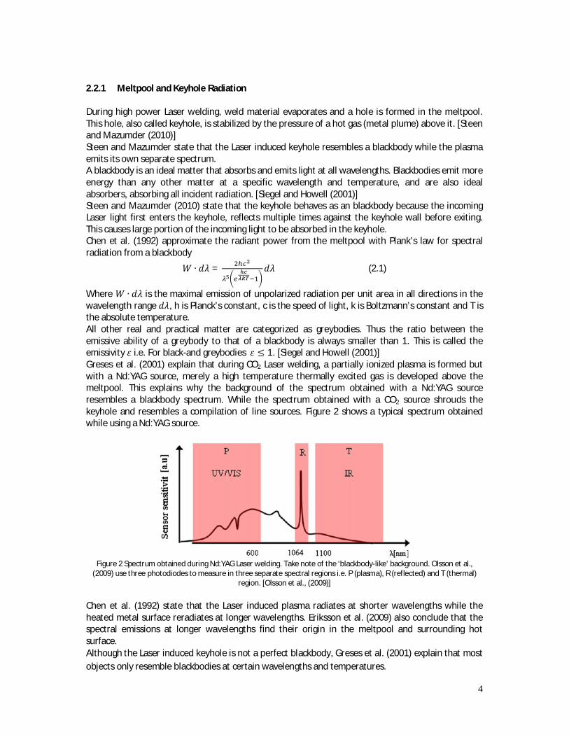
Where 푊 ∙ 푑휆 is the maximal emission of unpolarized radiation per unit area in all directions in the wavelength range 푑휆, h is Planck’s constant, c is the speed of light, k is Boltzmann’s constant and T is the absolute temperature. All other real and practical matter are categorized as greybodies. Thus the ratio between the emissive ability of a greybody to that of a blackbody is always smaller than 1. This is called the emissivity 휀 i.e. For black-and greybodies 휀 ≤ 1. [Siegel and Howell (2001)] Greses et al. (2001) explain that during CO2 Laser welding, a partially ionized plasma is formed but with a Nd:YAG source, merely a high temperature thermally excited gas is developed above the meltpool. This explains why the background of the spectrum obtained with a Nd:YAG source resembles a blackbody spectrum. While the spectrum obtained with a CO2 source shrouds the keyhole and resembles a compilation of line sources. Figure 2 shows a typical spectrum obtained while using a Nd:YAG source.

Figure 2 Spectrum obtained during Nd:YAG Laser welding. Take note of the ‘blackbody-like’ background. Olsson et al.,

(2009) use three photodiodes to measure in three separate spectral regions i.e. P (plasma), R (reflected) and T (thermal) region. [Olsson et al., (2009)]

Chen et al. (1992) state that the Laser induced plasma radiates at shorter wavelengths while the heated metal surface reradiates at longer wavelengths. Eriksson et al. (2009) also conclude that the spectral emissions at longer wavelengths find their origin in the meltpool and surrounding hot surface. Although the Laser induced keyhole is not a perfect blackbody, Greses et al. (2001) explain that most objects only resemble blackbodies at certain wavelengths and temperatures.

5

2.2.2 Plasma physics In the plume a low density of electrons is present. These electrons are generated by thermal ionization of vaporizing atoms and through thermionic emissions. Absorption of photons from the Laser beam by these electrons cause the plume to heat up. The plume is (partly) transformed into plasma if there is some kind of energy deposition into the plume which is fast compared to the expansion time of the plume. [Duley (1999)] This energy deposition is brought about by absorption of Laser beam photons by electrons. These electrons are excited to states of high kinetic energy and they are the cause of the further ionization of the plume. This transfer of energy from the Laser beam into heating of the plume is called the inverse Bremstrahlung. [Duley (1999)] The following equation gives the density of three different plasma components (i.e. electrons, ions and atoms) (Greses et al. 2001)

= ( ) exp − (2.2)

where Ne, NI, No are the density for electrons, singly ionized atoms and neutral atoms at the ground state respectively. gi, ge and go are the degeneracy factors for ions, electrons and neutral atoms. me is the electron mass, k is the Boltzmann constant, Te is the electron temperature, h is Planck’s constant and Ei is the ionisation potential for neutral atoms. Equation (2.2) is called the Saha equation and is based on the following assumptions:

- In the plume there is Local Thermal Equilibrium - The relative population of the excited states is described by the Boltzmann distribution at

temperature Te. - All components of the plasma have temperature Te.

The ratio between the electron density Ne and the total gas density N is called the level of ionization of the plasma. Since plasmas are formed only when there is vaporization of the welded material, the plasmas are used to derive information on the state of the welding process. [Duley (1999)] The emission of spectral lines coming from the plasma is one of the process signals which can be detected during Laser welding. The transition from a higher energy level m to a lower energy level n, gives the following spectral line intensity [Ancona et al. (2008) and Greses et al. 2001]

퐼 = 푁 퐴 ℎ (2.3)

where Nm is the population of the excited state, Amn is the transition probability between upper and lower energy level, c is the speed of light and 휆 is the wavelength of the observed species. Equation (2.3) is based on the assumption that the plasma is optically thin, this means that there is no self-absorption between the point of plasma radiated photon emission and the plasma surface. [Duley (1999)] Ancona et al. (2008) determine the population of states with higher energy level as follows

푁 = 푔 exp − (2.4)

where No is the population of atoms at the ground state, Z is the statistical weight at the ground state or partition function, gm is the statistical weight of the upper energy level and Em is the upper energy level. Equation (2.4) is based on the assumption of a Boltzmann equilibrium at temperature Te. If the spectral line emission of two wavelengths is considered, the electron temperature can be estimated. By combining equation (2.3) and (2.4), the ratio of intensities at 휆(1) and 휆(2) equals

6

( )( ) = ( ) ( ) ( )

( ) ( ) ( ) exp ( ) ( ) (2.5)

where 1 and 2 denote the emission lines. From (2.4) the electron temperature Te is determined

푇 = ( ) ( )( ) ( ) ( ) ( )( ) ( ) ( ) ( )

(2.6)

This electron or plasma temperature is diagnostic of specific fault conditions i.e. Konuk et al. (2009) and Ancona et al. (2008) show that there is a correlation between the electron temperature and the penetration depth. From above equations it can be concluded that the signals obtained from the plasma originate from the interaction between Laser beam and vaporized material. Thus the plasma signal is actually indirectly correlated to the welding process itself. [Duley (1999)]

2.3 Process Monitoring In process monitoring signal components that characterize ‘right’ and ‘wrong’ are extracted from the measured spectrum. These signals are based on predefined weld defects and for each weld application, the importance of a certain weld defect differs. Thus the definition of signal components that characterize ‘right’ and ‘wrong’, are application dependent. Signal extraction must be followed by some kind of signal recognition of ‘right’ and ‘wrong’. This extraction and recognition is the key to process monitoring and subsequently process control. [Duley (1999)]

2.3.1 Electron Temperature and Covariance Matrix Technique Ancona et al. (2008) extract two signals from the measured optical emission i.e. the electron temperature and correlation signal. Both signals were calculated with the optical intensity of three chemical species i.e. Mn(I), Fe(I) and Cr(I) composing the plasma plume and stainless steel alloy. Two species couples are used for the correlation analysis i.e. Cr(I)-Fe(I) and Cr(I)-Mn(I). A CO2 Laser is used to weld stainless steel during the research conducted by Ancona. A spectrometer is used that detects light from 390-580 nm with 0.3 nm resolution. The electron temperature signal Ancona uses is described by Equation (2.6) while the correlation signal is based on the Covariance Matrix Technique (CMT). In this technique the element ij of the covariance matrix is calculated as follows

퐶 =1푁

푥 (휆 )푥 (휆 )−1푁

푥 (휆 )1푁

푥 (휆 ) (2.7)

푥 (휆 ) is the optical intensity at wavelength 휆 of the kth spectrum taken by a spectrometer. N is the total amount of spectra shot. Next, the normalized covariance matrix mij is obtained such that mij lies between -1 and 1. If mij is positive, the two chemical species are formed by a known process parameter. And if mij is zero, the species couple is uncorrelated and no conclusion is drawn. If mij is negative, the species couple is anti-correlated, and they are the consequence of competing (different) processes. Figure 3 (above) displays two plots i.e. the electron temperature Te vs. the distance along the weld and the normalized correlation mij signal vs. weld distance. In the upper plot the measured electron temperature is shown with a (smooth) reference electron temperature. The reference signal is based

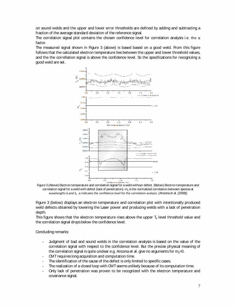
7

on sound welds and the upper and lower error thresholds are defined by adding and subtracting a fraction of the average standard deviation of the reference signal. The correlation signal plot contains the chosen confidence level for correlation analysis i.e. the α factor. The measured signal shown in Figure 3 (above) is based based on a good weld. From this figure follows that the calculated electron temperature lies between the upper and lower threshold values, and the the correllation signal is above the confidence level. So the specifications for recognizing a good weld are set.

Figure 3 (Above) Electron temperature and correlation signal for a weld without defect. (Below) Electron temperature and

correlation signal for a weld with defect (lack of penetration). mij is the normalized correlation between species at wavelengths λi and λj. α indicates the confidence level for the correlation analysis. [Ancona et al. (2008)]

Figure 3 (below) displays an electron temperature and correlation plot with intentionally produced weld defects obtained by lowering the Laser power and producing welds with a lack of penetration depth. This figure shows that the electron temperature rises above the upper Te level threshold value and the correlation signal drops below the confidence level. Concluding remarks:

- Judgment of bad and sound welds in the correlation analysis is based on the value of the correlation signal with respect to the confidence level. But the precise physical meaning of the correlation signal is quite unclear e.g. Ancona et al. give no arguments for mij=0.

- CMT requires long acquisition and computation time. - The identification of the cause of the defect is only limited to specific cases. - The realization of a closed loop with CMT seems unlikely because of its computation time. - Only lack of penetration was proven to be recognized with the electron temperature and

covariance signal.

8

2.3.2 Gas Shielding Detection System Fox et al. (2001) monitor the degradation of gas shielding by measuring radiated from the weld interaction zone. A Nd:YAG Laser was used to weld titanium and stainless steel. The emitted light from the workpiece was measured on-axis with a spectrometer that detects light from 400-850 nm with 0.5 nm resolution. A so called gas shoe was used (Figure 4) to shield the weld zone from air. The overpressure caused by the shielding gas drives away the air inside the shoe. By variation of the shielding gas flow, intentional poor gas shielding conditions were created.

Figure 4 Gas shielding arrangement. [Fox et al. (2001)]

Figure 5 shows the spectrum of poor gas shielding (upper curve) and good gas shielding (lower curve). Fox et al. (2001) describe that the presence of air inside the gas shoe has led to an increase in plume size and intensity, also the plume appeared whiter. These visual observations are accordance with the upper spectrum in Figure 5.

Figure 5 Spectrum obtained while welding stainless steel. Upper curve displays the spectrum for poor gas shielding. Lower curve displays the spectrum for good gas shielding. [Fox et al. (2001)]

Poor gas shielding conditions in Figure 5 was obtained at an argon flow rate smaller than 51 l/min. The titanium welds were severely discolored at these flow rates. Good gas shielding was obtained with a flow rate of approximately 60 l/min, resulting in clean and shiny titanium welds. The hardness of the weld was determined wihin the weld fusion zone. The hardness was found to be much higher than that of the surrounding material. Fox reports that the weld cracks if it is bent.

To investigate the spectral content of the two spectra in Figure 5, the poor gas shielding spectrum is normalized with the good gas shielding spectrum (see Figure 6). Figure 6 shows a significant peak at 426 nm.

9

Figure 6 Spectral ratio between poor gas shielding spectrum and good gas shielding spectrum. [Fox et al. (2001)]

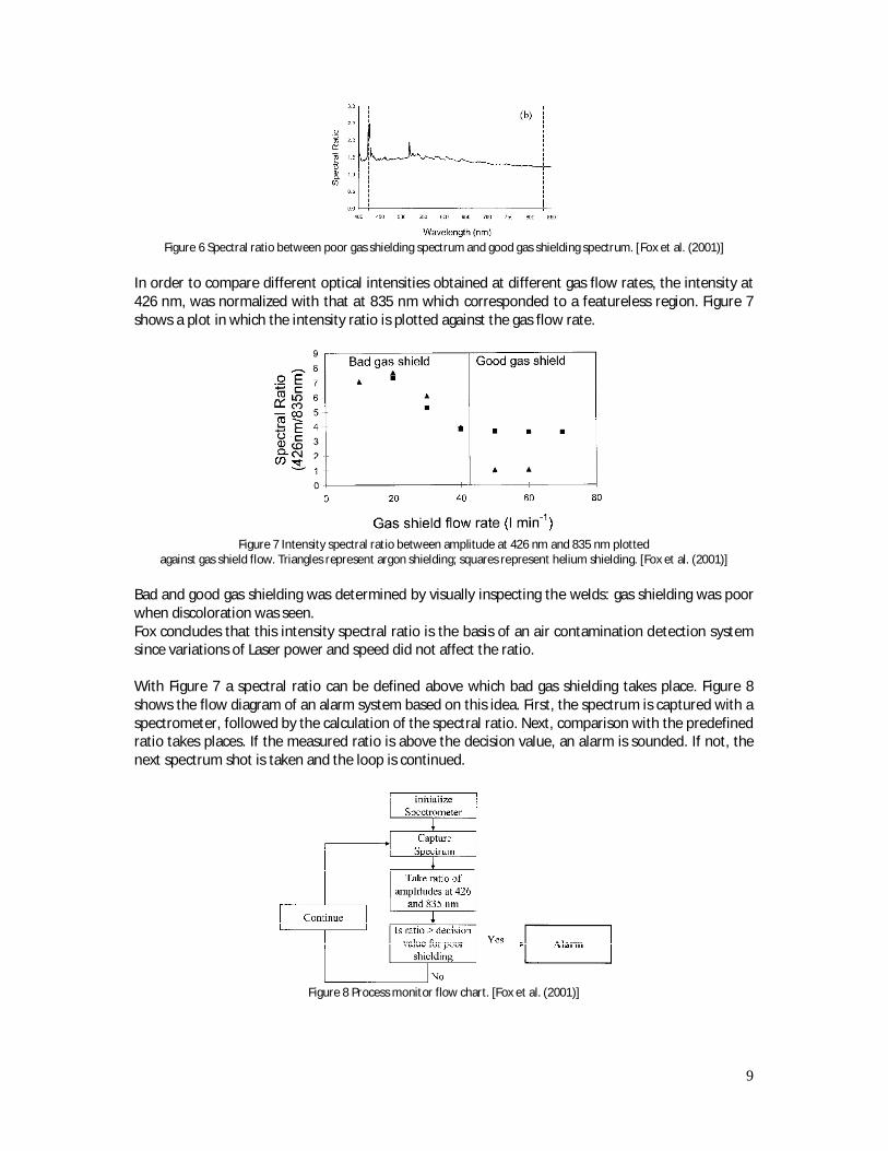
In order to compare different optical intensities obtained at different gas flow rates, the intensity at 426 nm, was normalized with that at 835 nm which corresponded to a featureless region. Figure 7 shows a plot in which the intensity ratio is plotted against the gas flow rate.

Figure 7 Intensity spectral ratio between amplitude at 426 nm and 835 nm plotted

against gas shield flow. Triangles represent argon shielding; squares represent helium shielding. [Fox et al. (2001)] Bad and good gas shielding was determined by visually inspecting the welds: gas shielding was poor when discoloration was seen. Fox concludes that this intensity spectral ratio is the basis of an air contamination detection system since variations of Laser power and speed did not affect the ratio. With Figure 7 a spectral ratio can be defined above which bad gas shielding takes place. Figure 8 shows the flow diagram of an alarm system based on this idea. First, the spectrum is captured with a spectrometer, followed by the calculation of the spectral ratio. Next, comparison with the predefined ratio takes places. If the measured ratio is above the decision value, an alarm is sounded. If not, the next spectrum shot is taken and the loop is continued.

Figure 8 Process monitor flow chart. [Fox et al. (2001)]

10

Conclusions:

- Fox et al. (2001) are unable to identify the cause of the spectral peak at 426 nm (Figure 5 and Figure 6).

- The described system can be augmented to a closed loop which adjusts the gas flow to maintain good shielding conditions.

- In Figure 7 the application of helium shielding gas does not lead to a clear drop in intensity spectral ratio when good shielding conditions are present. So a predefined decision value is not easily obtained with helium gas.

- Discolored surface appearance (e.g. oxidation) is detected with the spectral ratio signal. - Fox et al. (2001) do not clearly specify if the experiments shown in Figure 6 and Figure 7 are

based on titanium or stainless steel. - Besides visual inspection of the weld, Fox also measures the Vickers hardness of the weld

cross section to characterize between good and bad welds. - Fox does report on a relation between hardness and spectral ratio but stresses that the

hardness already increases (indicating a decrease in weld quality) before a noticeable change of the spectral ratio is seen.

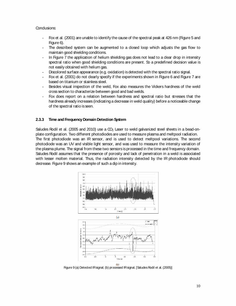
2.3.3 Time and Frequency Domain Detection System Saludes Rodil et al. (2005 and 2010) use a CO2 Laser to weld galvanized steel sheets in a bead-on-plate configuration. Two different photodiodes are used to measure plasma and meltpool radiation. The first photodiode was an IR sensor, and is used to detect meltpool variations. The second photodiode was an UV and visible light sensor, and was used to measure the intensity variation of the plasma plume. The signal from these two sensors is processed in the time and frequency domain. Saludes Rodil assumes that the presence of porosity and lack of penetration in a weld is associated with lesser molten material. Thus, the radiation intensity detected by the IR photodiode should decrease. Figure 9 shows an example of such a dip in intensity.

Figure 9 (a) Detected IR signal; (b) processed IR signal. [Saludes Rodil et al. (2005)]

11

Figure 9 (a) displays the rough data obtained with the IR sensor. This data is processed in the following fashion to obtain the curves in plot (b): First, the IR data is normalized by removing its mean and is scaled with its standard deviation. Next, an adaptive least square (LS) filter is used to obtain a polynomial fit for the measured IR data. From this polynomial fit (solid line in Figure 9 (b)), two polynomial limit curves are produced. In total, three polynomial curves are displayed in (b). The LS filter is combined with a detection system to form the so called CUSUM RLS algorithm. The detection system detects when the filtered signal goes out of the interval between polynomial limits. This time domain detection method is intended to detect ‘small’ faults such as holes. Saludes Rodil states that the algorithm is trained to respond to a limited amount of known defects by tuning the algorithm in appropriate fashion. Table 1 shows the results of the time domain detection system when applied in the automotive industry.

Table 1 Results of the time domain detection system. [Saludes Rodil et al. (2005)]

Only 55 % of the total amount of intentionally produced holes was detected while 75% of faults were detected. The settings of the CUSUM algorithm are such that the computed polynomial limits are advantageous for detection of faulty seams while specific faults, such as small holes that correspond with small signal changes, are skipped. The second detection system is based on processing both sensor signals in the frequency domain; a correlation between the power spectrum of the sensor signal and weld defects is used. [Saludes Rodil et al. (2010)] Saludes Rodil et al. conclude from their previous research that the signal energy decreases when a weld is partially penetrated. First the sensor signal is preprocessed such that the signals corresponding to the weld are isolated. Next, the signal is divided into N equally sized segments, depending on weld speed and length. A fast Fourier Transform (FFT) is done to characterize each portion of the weld with its frequency component distribution. [Saludes Rodil et al. (2010)] For each segment, the global RMS value is computed. Two frequency bands were classified for each sensor i.e. a low frequency band from 500-1500 Hz and a high frequency band from 4000-5000 Hz. The signal energy of the UV-VIS sensor is plotted in Figure 10, for the two specified bands.

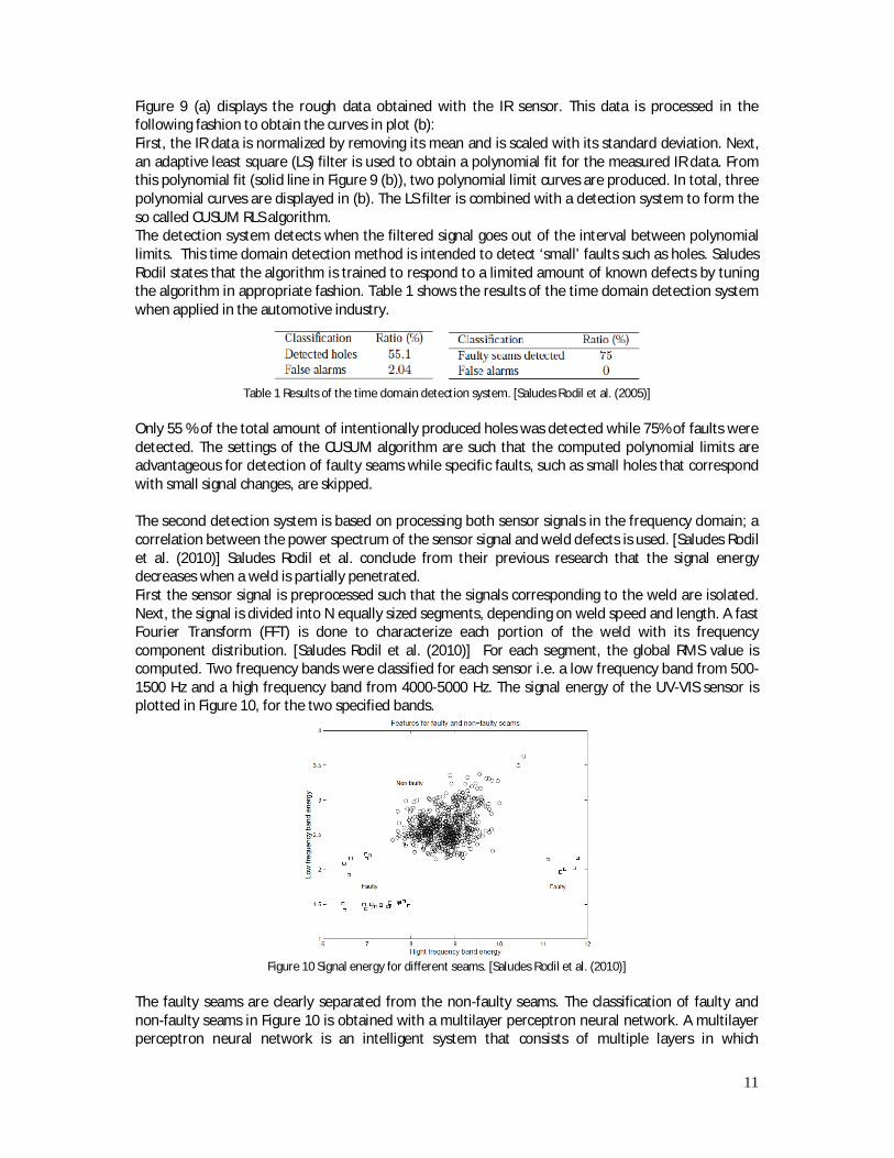
Figure 10 Signal energy for different seams. [Saludes Rodil et al. (2010)]

The faulty seams are clearly separated from the non-faulty seams. The classification of faulty and non-faulty seams in Figure 10 is obtained with a multilayer perceptron neural network. A multilayer perceptron neural network is an intelligent system that consists of multiple layers in which

12

computations are carried out. In a multilayer perceptron neural network information flows in a feedforward fashion i.e. from the input layer through hidden layers to the output. Saludes Rodil’s system processes data from the photodiodes with a neural network which is trained with faulty and non-faulty seams. The output of the neural network is displayed in Figure 11.

Figure 11 Output of neural network. [Saludes Rodil et al. (2010)]

The output varied between 1 and -1, and a decision threshold of 0 was used i.e. seams with a negative neural network output were classified as faulty and seams with positive output were non-faulty. The results of the frequency detection system are given Table 2.

Table 2 Results of frequency domain

detection system. [Saludes Rodil et al. (2010)]

Saludes Rodil states that these results are unacceptable since 6.1% of actual normal seams were discarded by the detection system as faulty (1st row of Table 2). Also, 2.9% of actual faulty seams passed as normal by the detection system. Conclusions:

- With the time domain detection system the position of the fault can be estimated. - The frequency domain detection system only distinguishes between faulty and non-faulty

seams. - The time based detection system works better when detecting faulty seams than specific

holes (see Table 1). - Although the aim of the time based system was to detect specific faults, the detection

system only managed to detect faults is general.

2.3.4 2D and 3D Spectral Clouds Olsson et al. (2011) use a Nd:YAG Laser to produce lap welds of two zinc coated steel sheets. Three sensors were used for on-axis detection of plasma, reflected and thermal radiation. Spectra of good welds and intentionally bad welds were studied. The good welds were produced by fastening the sheets such that a clear path was provided for the escape of the zinc vapour. While bad

13

welds were obtained by positioning the sheets such that there was an overlap with close contact between the sheets, preventing escape of the zinc vapour. This caused a liquid eruption or blow out. [Olsson et al. (2011)] These bad welds are referred to as blow out welds. Figure 12 displays the raw data from the sensors. The spectra in this figure displays a strong correlation between the plasma and temperature signal for both good welds as well as blow out welds. The reason for this behaviour is given further in this Section. Also, the sensor signals for the good weld is far more stable then the signals for the blow out welds. This is an expected result since the liquid eruptions cause instable emission of radiation.

Figure 12 (a) Raw data obtained with the three sensors. (b) The reflection sensor signal plotted against the thermal sensor

signal. The means have been removed from the signals. [Olsson et al. (2011)] Figure 12 (b) displays the relation between the reflected and thermal signal. The form of this 2D flat cloud shows that there is a low correlation between the reflected and thermal signal. Olsson explaines that the reflection intensity is strongly dependant on the roughness of the melt surface and

14

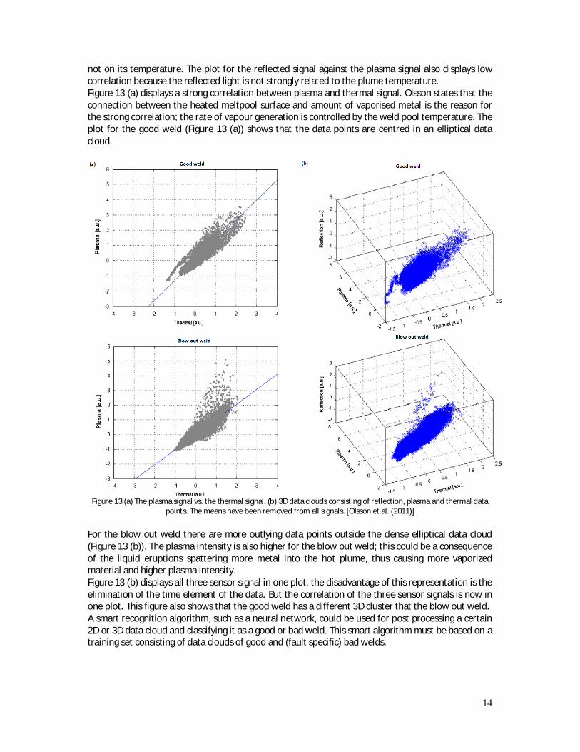
not on its temperature. The plot for the reflected signal against the plasma signal also displays low correlation because the reflected light is not strongly related to the plume temperature. Figure 13 (a) displays a strong correlation between plasma and thermal signal. Olsson states that the connection between the heated meltpool surface and amount of vaporised metal is the reason for the strong correlation; the rate of vapour generation is controlled by the weld pool temperature. The plot for the good weld (Figure 13 (a)) shows that the data points are centred in an elliptical data cloud.

Figure 13 (a) The plasma signal vs. the thermal signal. (b) 3D data clouds consisting of reflection, plasma and thermal data

points. The means have been removed from all signals. [Olsson et al. (2011)] For the blow out weld there are more outlying data points outside the dense elliptical data cloud (Figure 13 (b)). The plasma intensity is also higher for the blow out weld; this could be a consequence of the liquid eruptions spattering more metal into the hot plume, thus causing more vaporized material and higher plasma intensity. Figure 13 (b) displays all three sensor signal in one plot, the disadvantage of this representation is the elimination of the time element of the data. But the correlation of the three sensor signals is now in one plot. This figure also shows that the good weld has a different 3D cluster that the blow out weld. A smart recognition algorithm, such as a neural network, could be used for post processing a certain 2D or 3D data cloud and classifying it as a good or bad weld. This smart algorithm must be based on a training set consisting of data clouds of good and (fault specific) bad welds.

15

Conclusions: - Olsson et al. (2011) explain that raw electromagnetic data from the P-, R- and T- sensor is

insufficient for further interpretation of individual weld instability. Yet Olsson only consider blow out welds as a weld defect.

- Plasma and thermal signals show a strong correlation because the rate of vapour generation is controlled by the weld pool temperature. On the other hand, the other combinations of the three sensor signals do not show a strong correlation.

- The 2D and 3D is cloud gives new and novel information but no concrete monitoring system (let alone control system) based on this method has been found yet in literature.

2.4 Process control Monitoring systems can merely give an alarm when a quality parameter decreases but closed loop systems steer the process back on track by appropriate feedback actions such that the decrease of process quality is instantaneously compensated. [Wiesemann (2004)] Bardin et al. (2005) gives the following subdivision of actuators in the control of Laser welding processes:

- Laser power - Welding speed - Focal point position - Filler wire speed rate

Only the first three actuators will be discussed in this Section because of limitations specified in the Master thesis description.

2.4.1 Penetration Control with Laser Power Actuation Postma et al. (2002) use a Nd:YAG Laser to make bead-on-plate welds on mild steel specimens. The plume radiation was measured on-axis with a commercial monitoring system called Weldwatcher. Figure 14 shows the Weldwatcher system, Laser source and controllers. The operation of the Weldwatcher system is outlined below. Plume radiation is transmitted through the delivery fiber into the Haas 2006D Laser. In front of the Laser cavity, the process radiation is decoupled and fed through a separate fibre into a detector. The output of the detector is then filtered with an analog low pass filter of 500 Hz to filter out high frequency process dynamics. [(De Graaf et al. (2005) and Postma et al. (2002)] Argon gas shielding was applied at the top and bottom of the workpiece.

Figure 14 Experimental setup consisting of Weldwatcher system, Laser source and controllers. [Postma et al. (2002)]

16

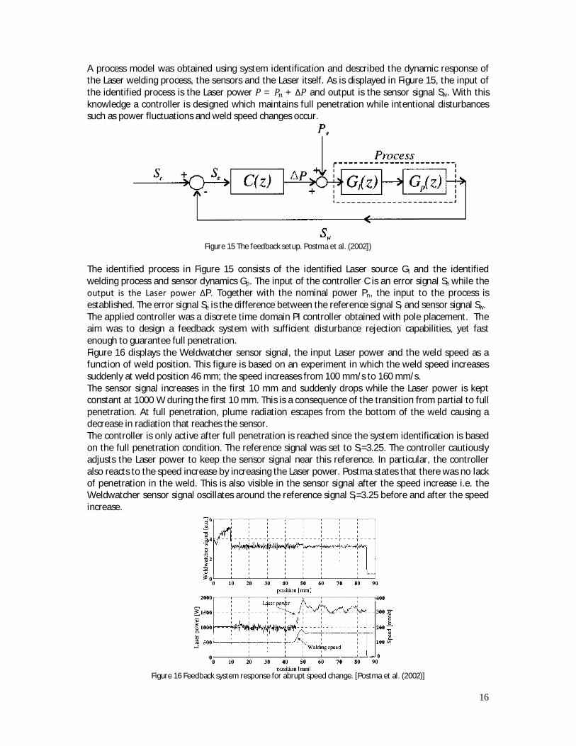
A process model was obtained using system identification and described the dynamic response of the Laser welding process, the sensors and the Laser itself. As is displayed in Figure 15, the input of the identified process is the Laser power 푃 = 푃 + Δ푃 and output is the sensor signal Sw. With this knowledge a controller is designed which maintains full penetration while intentional disturbances such as power fluctuations and weld speed changes occur.

Figure 15 The feedback setup. Postma et al. (2002])

The identified process in Figure 15 consists of the identified Laser source Gl and the identified welding process and sensor dynamics Gp. The input of the controller C is an error signal Se while the output is the Laser power ΔP. Together with the nominal power Pn, the input to the process is established. The error signal Se is the difference between the reference signal Sr and sensor signal Sw. The applied controller was a discrete time domain PI controller obtained with pole placement. The aim was to design a feedback system with sufficient disturbance rejection capabilities, yet fast enough to guarantee full penetration. Figure 16 displays the Weldwatcher sensor signal, the input Laser power and the weld speed as a function of weld position. This figure is based on an experiment in which the weld speed increases suddenly at weld position 46 mm; the speed increases from 100 mm/s to 160 mm/s. The sensor signal increases in the first 10 mm and suddenly drops while the Laser power is kept constant at 1000 W during the first 10 mm. This is a consequence of the transition from partial to full penetration. At full penetration, plume radiation escapes from the bottom of the weld causing a decrease in radiation that reaches the sensor. The controller is only active after full penetration is reached since the system identification is based on the full penetration condition. The reference signal was set to Sr=3.25. The controller cautiously adjusts the Laser power to keep the sensor signal near this reference. In particular, the controller also reacts to the speed increase by increasing the Laser power. Postma states that there was no lack of penetration in the weld. This is also visible in the sensor signal after the speed increase i.e. the Weldwatcher sensor signal oscillates around the reference signal Sr=3.25 before and after the speed increase.

Figure 16 Feedback system response for abrupt speed change. [Postma et al. (2002)]

17

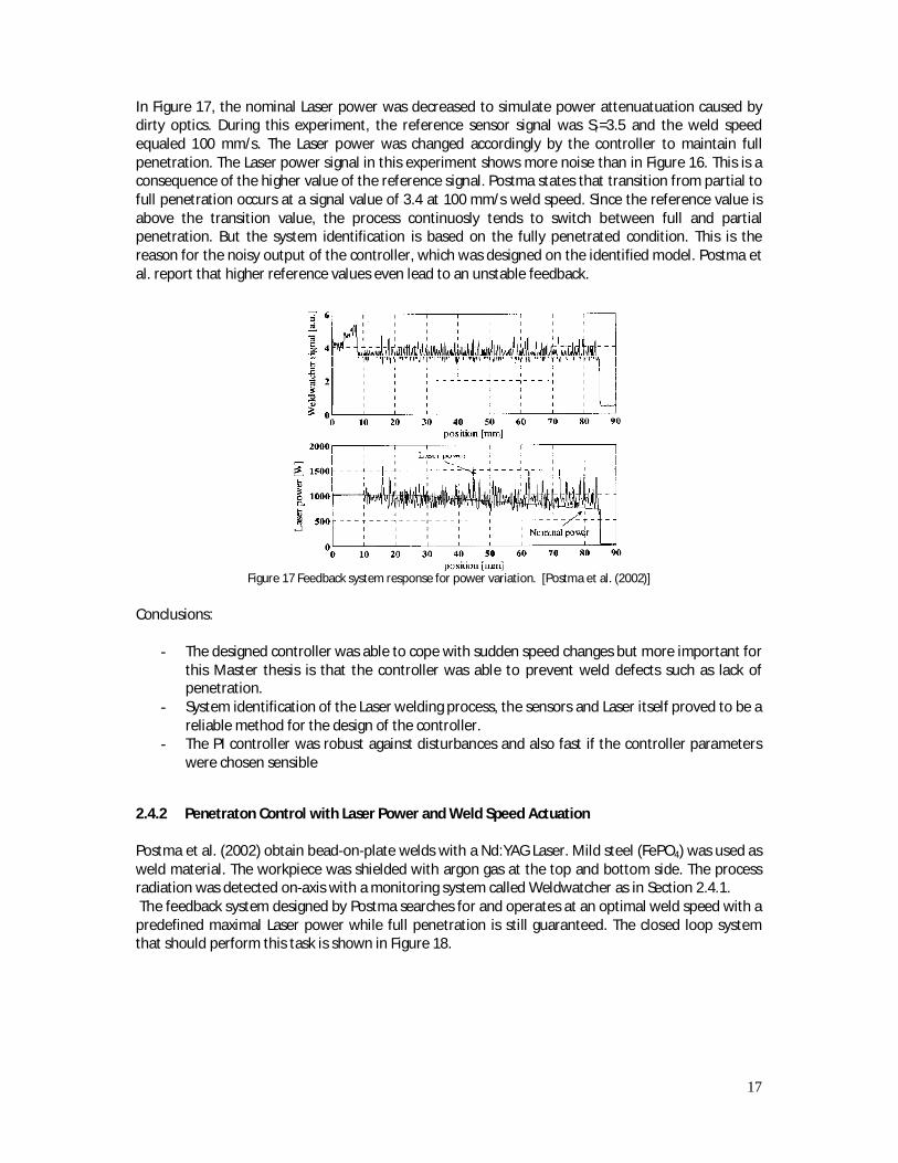
In Figure 17, the nominal Laser power was decreased to simulate power attenuatuation caused by dirty optics. During this experiment, the reference sensor signal was Sr=3.5 and the weld speed equaled 100 mm/s. The Laser power was changed accordingly by the controller to maintain full penetration. The Laser power signal in this experiment shows more noise than in Figure 16. This is a consequence of the higher value of the reference signal. Postma states that transition from partial to full penetration occurs at a signal value of 3.4 at 100 mm/s weld speed. Since the reference value is above the transition value, the process continuosly tends to switch between full and partial penetration. But the system identification is based on the fully penetrated condition. This is the reason for the noisy output of the controller, which was designed on the identified model. Postma et al. report that higher reference values even lead to an unstable feedback.

Figure 17 Feedback system response for power variation. [Postma et al. (2002)]

Conclusions:

- The designed controller was able to cope with sudden speed changes but more important for this Master thesis is that the controller was able to prevent weld defects such as lack of penetration.

- System identification of the Laser welding process, the sensors and Laser itself proved to be a reliable method for the design of the controller.

- The PI controller was robust against disturbances and also fast if the controller parameters were chosen sensible

2.4.2 Penetraton Control with Laser Power and Weld Speed Actuation Postma et al. (2002) obtain bead-on-plate welds with a Nd:YAG Laser. Mild steel (FePO4) was used as weld material. The workpiece was shielded with argon gas at the top and bottom side. The process radiation was detected on-axis with a monitoring system called Weldwatcher as in Section 2.4.1. The feedback system designed by Postma searches for and operates at an optimal weld speed with a predefined maximal Laser power while full penetration is still guaranteed. The closed loop system that should perform this task is shown in Figure 18.

18

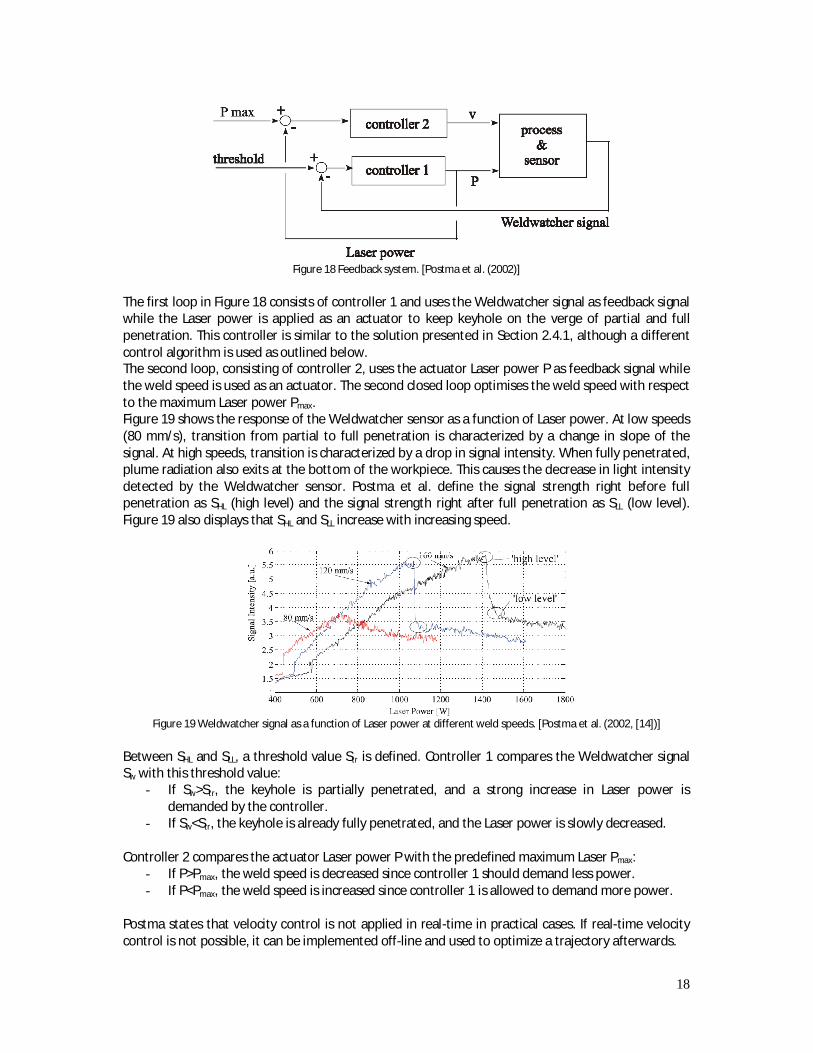
Figure 18 Feedback system. [Postma et al. (2002)]

The first loop in Figure 18 consists of controller 1 and uses the Weldwatcher signal as feedback signal while the Laser power is applied as an actuator to keep keyhole on the verge of partial and full penetration. This controller is similar to the solution presented in Section 2.4.1, although a different control algorithm is used as outlined below. The second loop, consisting of controller 2, uses the actuator Laser power P as feedback signal while the weld speed is used as an actuator. The second closed loop optimises the weld speed with respect to the maximum Laser power Pmax. Figure 19 shows the response of the Weldwatcher sensor as a function of Laser power. At low speeds (80 mm/s), transition from partial to full penetration is characterized by a change in slope of the signal. At high speeds, transition is characterized by a drop in signal intensity. When fully penetrated, plume radiation also exits at the bottom of the workpiece. This causes the decrease in light intensity detected by the Weldwatcher sensor. Postma et al. define the signal strength right before full penetration as SHL (high level) and the signal strength right after full penetration as SLL (low level). Figure 19 also displays that SHL and SLL increase with increasing speed.

Figure 19 Weldwatcher signal as a function of Laser power at different weld speeds. [Postma et al. (2002, [14])]

Between SHL and SLL, a threshold value Str is defined. Controller 1 compares the Weldwatcher signal Sw with this threshold value:

- If Sw>Str, the keyhole is partially penetrated, and a strong increase in Laser power is demanded by the controller.

- If Sw<Str, the keyhole is already fully penetrated, and the Laser power is slowly decreased.

Controller 2 compares the actuator Laser power P with the predefined maximum Laser Pmax: - If P>Pmax, the weld speed is decreased since controller 1 should demand less power. - If P<Pmax, the weld speed is increased since controller 1 is allowed to demand more power.

Postma states that velocity control is not applied in real-time in practical cases. If real-time velocity control is not possible, it can be implemented off-line and used to optimize a trajectory afterwards.

19

Figure 20 displays the responses of the closed loops during an experiment in which the initial settings were as follows: a weld speed of 150 mm/s and Laser power of 1400 W. The threshold values were set to Str=4.2 and Pmax=1800 W. For the first 10 mm, the controller was not active since the keyhole was not yet fully penetrated. After activation of the controller, the Laser power increases to its maximum value of 1800 W and an optimal weld speed of 220 mm/s was achieved. After visual inspection, Postma states that there was full penetration over the entire weld length.

Figure 20 (Top) Laser power demanded by first control loop; (Middle) Response of the second feedback loop; (Bottom)

Weldwatcher signal. [Postma et al. (2002, [14])]

The top plot in Figure 20 shows strong increase and slow decrease of the demanded Laser power. The rate of increase differed from the rate of decrease in order to keep the system from becoming unstable i.e. if the Laser power was decreased as strongly as it increased, the Weldwatcher signal value would drop considerably into the region of partial penetration (see Figure 19). But the controller would interpret this lower signal value as the keyhole being in the fully penetrated region. The controller would thus decrease the Laser power further, and become unstable. The bottom plot of Figure 20 shows the Weldwatcher signal approaching the threshold value Str as the weld progresses. The reason for this is given in Figure 19 i.e. SLL (=signal just after full penetration) increases with increasing velocity. Thus the measured sensor signal in Figure 20 will approach the fixed threshold Str as the speed increases. Conclusions:

- The control system described by Postma et al. (2002) applies Laser power and weld speed actuation to prevent an important weld defect i.e. lack of penetration.

- The control system also searches for and operates at an optimized weld speed. - Weld speed is not regulated during a trajectory in practical cases. There is still a possibility

for optimizing the weld speed off-line, and using the optimized trajectory afterwards.

2.4.3 Closed Loop Control of Laser Welding using a Spectroscopic Sensor Konuk et al. (2009) use Nd:YAG and CO2 Lasers to form overlap welds in two AISI 304 stainless steel plates. Only the results for the solid state Laser are described in this Section.

20

For the Nd:YAG experiments two sheets with thicknesses of 1 and 3 mm were placed on top of each other. A spectrometer was used with a filter with cut-off frequency of 900 nm in order to filter out the reflected Laser radiation. The top surface of the workpiece was shielded with argon gas. A PI controller was designed with the aim of achieving constant penetration depth over the entire weld length for different process conditions. The PI controller had the following form

퐶(푠) = 푘 1 + (2.8)

kp and Ti represent the proportional gain and integral time constant respectively. The block diagram of the controller and weld process is given in Figure 21.

Figure 21 Block diagram of closed loop system. [Konuk et al. (2009)]

The electron temperature Te is calculated with Equation (2.6), and the atomic Chromium Cr I 459.23 nm-495.69 nm pair of lines were selected for the calculation. A predefined reference value Te, ref was compared with the calculated electron temperature Te to produce the error ΔTe. This error is the controller input. The controller output is the Laser power demanded to form a weld penetration depth associated with Te, ref. Within the Labview software, signals received from the spectrometer were used to characterize and control the process. [Konuk et al. (2009)] The controller parameters were obtained with characterization experiments. During these experiments the weld speed was kept constant and the Laser power was varied. Figure 22 shows such a characterization experiment. The Laser power was varied to identify the characteristics of the welding process. [Konuk et al. (2009)]

Figure 22 Characterization of Nd:YAG Laser weld process. [Konuk et al. (2009)]

Figure 22 displays a V shaped Laser power profile varying between 3000 W and 1400 W; the electron temperature also had the same form. The penetration depth is depicted as vertical lines with bullets

21

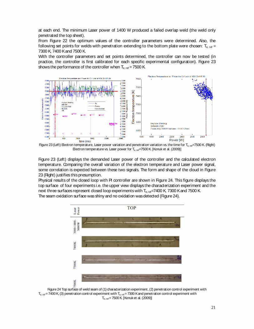
at each end. The minimum Laser power of 1400 W produced a failed overlap weld (the weld only penetrated the top sheet). From Figure 22 the optimum values of the controller parameters were determined. Also, the following set points for welds with penetration extending to the bottom plate were chosen: Te, ref = 7300 K, 7400 K and 7500 K. With the controller parameters and set points determined, the controller can now be tested (in practice, the controller is first calibrated for each specific experimental configuration). Figure 23 shows the performance of the controller when Te, ref = 7500 K.

Figure 23 (Left) Electron temperature, Laser power variation and penetration variation vs. the time for Te, ref=7500 K. (Right)

Electron temperature vs. Laser power for Te, ref=7500 K. [Konuk et al. (2009)] Figure 23 (Left) displays the demanded Laser power of the controller and the calculated electron temperature. Comparing the overall variation of the electron temperature and Laser power signal, some correlation is expected between these two signals. The form and shape of the cloud in Figure 23 (Right) justifies this presumption. Physical results of the closed loop with PI controller are shown in Figure 24. This figure displays the top surface of four experiments i.e. the upper view displays the characterization experiment and the next three surfaces represent closed loop experiments with Te, ref=7400 K, 7300 K and 7500 K. The seam oxidation surface was shiny and no oxidation was detected (Figure 24).

Figure 24 Top surface of weld seam of (1) characterization experiment, (2) penetration control experiment with

Te, ref = 7400 K, (3) penetration control experiment with Te, ref = 7300 K and penetration control experiment with Te, ref = 7500 K. [Konuk et al. (2009)]

22

Conclusions:

- There exists a correlation between the electron temperature and penetration depth (see Figure 22).

- This correlation was not just used for process monitoring but also to successfully control the penetration depth.

- The PI controller performs well, yet improvements to increase its reliability should be made. [Konuk et al. (2009)] Since the biggest challenge lies in the monitoring of the weld process, a different controller can be chosen or the current PI controller parameters should be chosen differently to improve controller reliability.

2.4.4 Optical Focus Control System Hand et al. (2000) use a Nd:YAG Laser to process mild steel by forming bead-on-plate welds. Experiments were carried out in which intentional focus errors (= distance from optimum focal position) were created. Thermal distortions of the workpiece are one of the causes of focus shift during Laser welding. Focus shifts affect the Laser power density on the workpiece, and can cause defects such as lack of penetration among others. The focus control system described by Hand et al. exploits the chromatic aberration of the collimator and focus lens in the Laser welding head such that by analysing the spectrum of process radiation, the focal error is derived. The process radiation of the Laser material interaction zone is partly collected by the collimator and focus lens, and subsequently imaged into the delivery fibre optic (Figure 25). This delivery optic transports the light into the Laser console in which it is transmitted at a dielectric turning mirror. After this mirror, the radiation is coupled into a fibre optic leading to the detection optics. These detection optics split the process radiation into the following spectral bands: the UV-visible band between 300-700 nm and the IR band between 1100-1600 nm.

Figure 25 Focus control system. [Hand et al. (2000)]

Chromatic aberration of an optic causes different wavelengths to be focussed at different positions. So chromatic aberration of the collimator and focus lens causes the two spectral bands to focus at different positions.

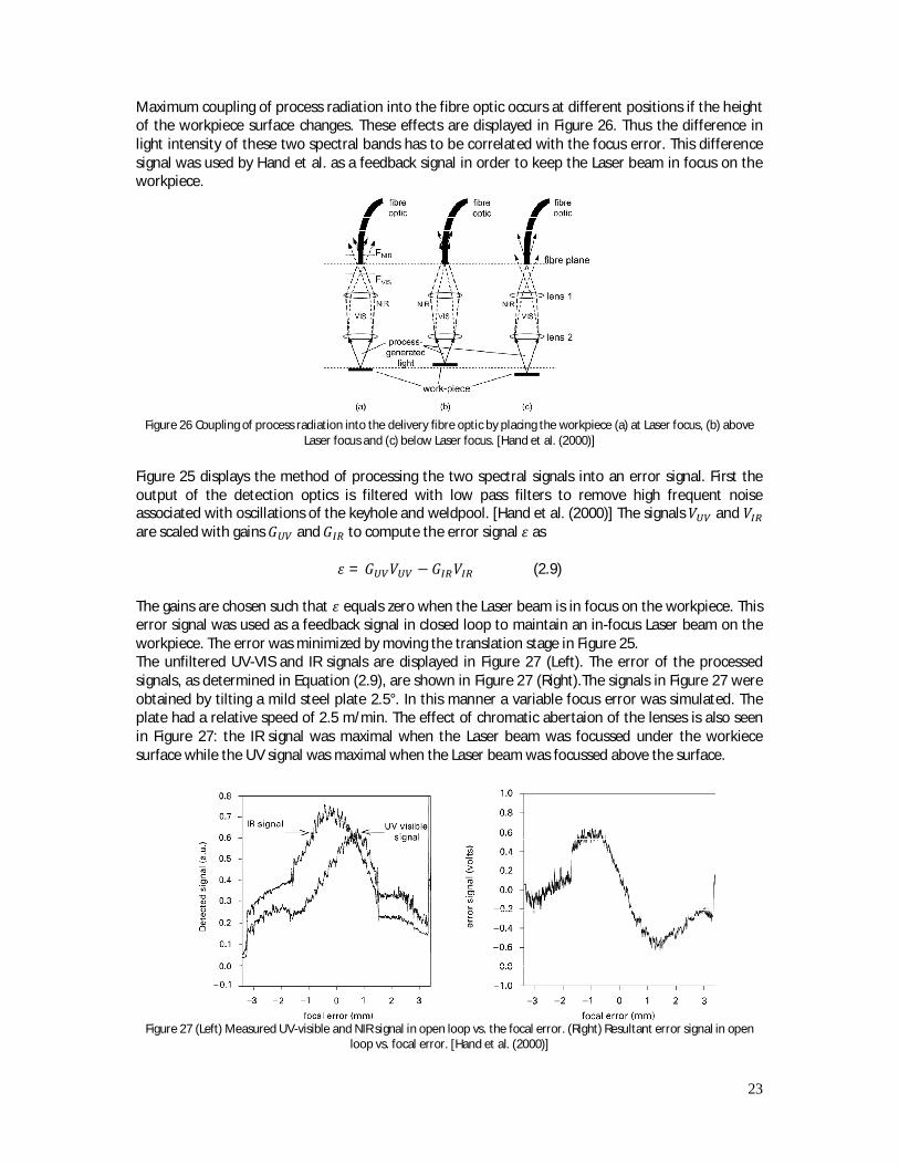
23

Maximum coupling of process radiation into the fibre optic occurs at different positions if the height of the workpiece surface changes. These effects are displayed in Figure 26. Thus the difference in light intensity of these two spectral bands has to be correlated with the focus error. This difference signal was used by Hand et al. as a feedback signal in order to keep the Laser beam in focus on the workpiece.

Figure 26 Coupling of process radiation into the delivery fibre optic by placing the workpiece (a) at Laser focus, (b) above

Laser focus and (c) below Laser focus. [Hand et al. (2000)] Figure 25 displays the method of processing the two spectral signals into an error signal. First the output of the detection optics is filtered with low pass filters to remove high frequent noise associated with oscillations of the keyhole and weldpool. [Hand et al. (2000)] The signals 푉 and 푉 are scaled with gains 퐺 and 퐺 to compute the error signal 휀 as

휀 = 퐺 푉 − 퐺 푉 (2.9)

The gains are chosen such that 휀 equals zero when the Laser beam is in focus on the workpiece. This error signal was used as a feedback signal in closed loop to maintain an in-focus Laser beam on the workpiece. The error was minimized by moving the translation stage in Figure 25. The unfiltered UV-VIS and IR signals are displayed in Figure 27 (Left). The error of the processed signals, as determined in Equation (2.9), are shown in Figure 27 (Right).The signals in Figure 27 were obtained by tilting a mild steel plate 2.5°. In this manner a variable focus error was simulated. The plate had a relative speed of 2.5 m/min. The effect of chromatic abertaion of the lenses is also seen in Figure 27: the IR signal was maximal when the Laser beam was focussed under the workiece surface while the UV signal was maximal when the Laser beam was focussed above the surface.

Figure 27 (Left) Measured UV-visible and NIR signal in open loop vs. the focal error. (Right) Resultant error signal in open

loop vs. focal error. [Hand et al. (2000)]

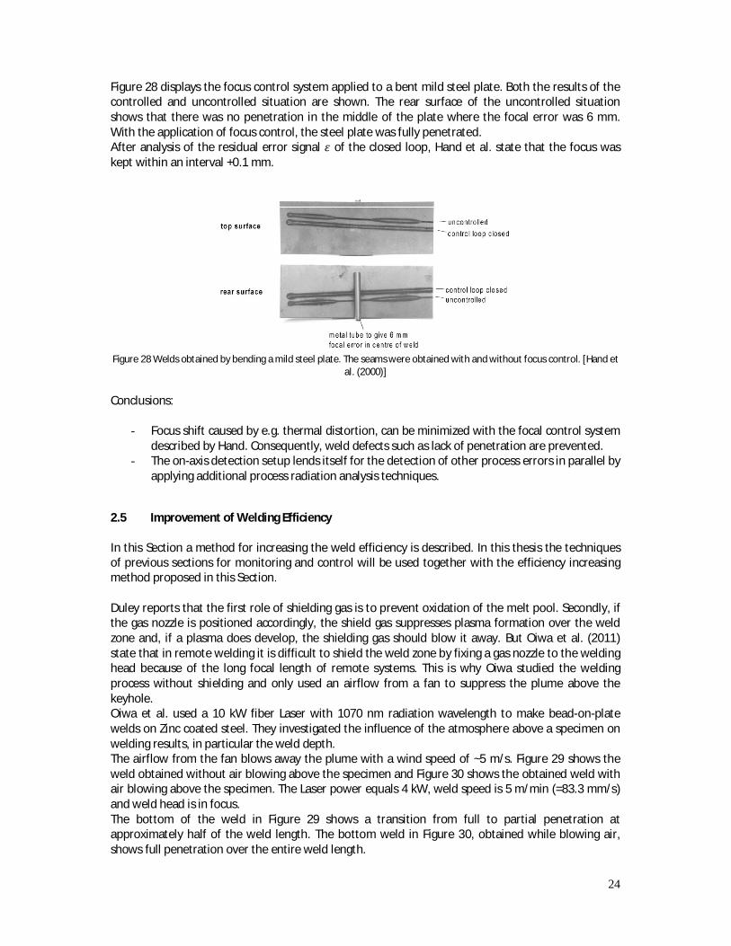
24

Figure 28 displays the focus control system applied to a bent mild steel plate. Both the results of the controlled and uncontrolled situation are shown. The rear surface of the uncontrolled situation shows that there was no penetration in the middle of the plate where the focal error was 6 mm. With the application of focus control, the steel plate was fully penetrated. After analysis of the residual error signal 휀 of the closed loop, Hand et al. state that the focus was kept within an interval +0.1 mm.

Figure 28 Welds obtained by bending a mild steel plate. The seams were obtained with and without focus control. [Hand et

al. (2000)] Conclusions:

- Focus shift caused by e.g. thermal distortion, can be minimized with the focal control system described by Hand. Consequently, weld defects such as lack of penetration are prevented.

- The on-axis detection setup lends itself for the detection of other process errors in parallel by applying additional process radiation analysis techniques.

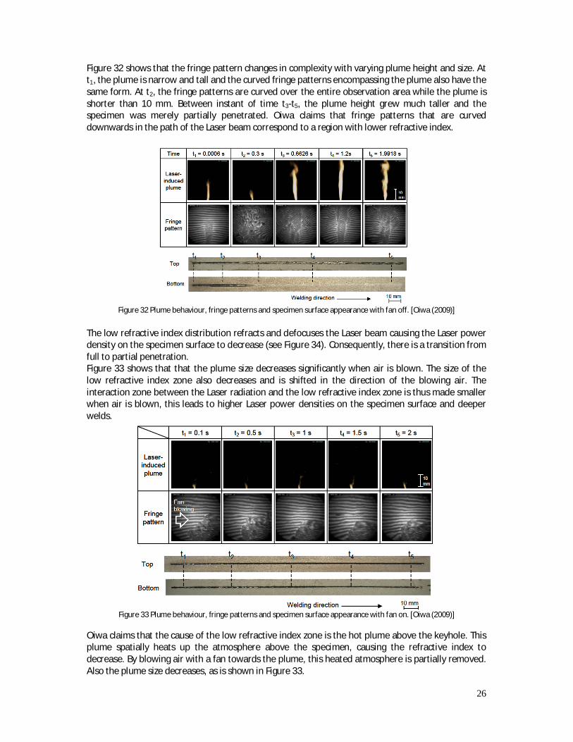
2.5 Improvement of Welding Efficiency In this Section a method for increasing the weld efficiency is described. In this thesis the techniques of previous sections for monitoring and control will be used together with the efficiency increasing method proposed in this Section. Duley reports that the first role of shielding gas is to prevent oxidation of the melt pool. Secondly, if the gas nozzle is positioned accordingly, the shield gas suppresses plasma formation over the weld zone and, if a plasma does develop, the shielding gas should blow it away. But Oiwa et al. (2011) state that in remote welding it is difficult to shield the weld zone by fixing a gas nozzle to the welding head because of the long focal length of remote systems. This is why Oiwa studied the welding process without shielding and only used an airflow from a fan to suppress the plume above the keyhole. Oiwa et al. used a 10 kW fiber Laser with 1070 nm radiation wavelength to make bead-on-plate welds on Zinc coated steel. They investigated the influence of the atmosphere above a specimen on welding results, in particular the weld depth. The airflow from the fan blows away the plume with a wind speed of ~5 m/s. Figure 29 shows the weld obtained without air blowing above the specimen and Figure 30 shows the obtained weld with air blowing above the specimen. The Laser power equals 4 kW, weld speed is 5 m/min (=83.3 mm/s) and weld head is in focus. The bottom of the weld in Figure 29 shows a transition from full to partial penetration at approximately half of the weld length. The bottom weld in Figure 30, obtained while blowing air, shows full penetration over the entire weld length.

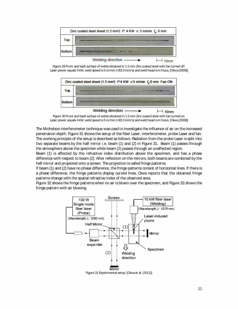
25

Figure 29 Front and back surface of welds obtained in 1.5 mm Zinc coated steel with fan turned off.

Laser power equals 4 kW, weld speed is 5 m/min (=83.3 mm/s) and weld head is in focus. [Oiwa (2009)]

Figure 30 Front and back surface of welds obtained in 1.5 mm Zinc coated steel with fan turned on.

Laser power equals 4 kW, weld speed is 5 m/min (=83.3 mm/s) and weld head is in focus. [Oiwa (2009)]

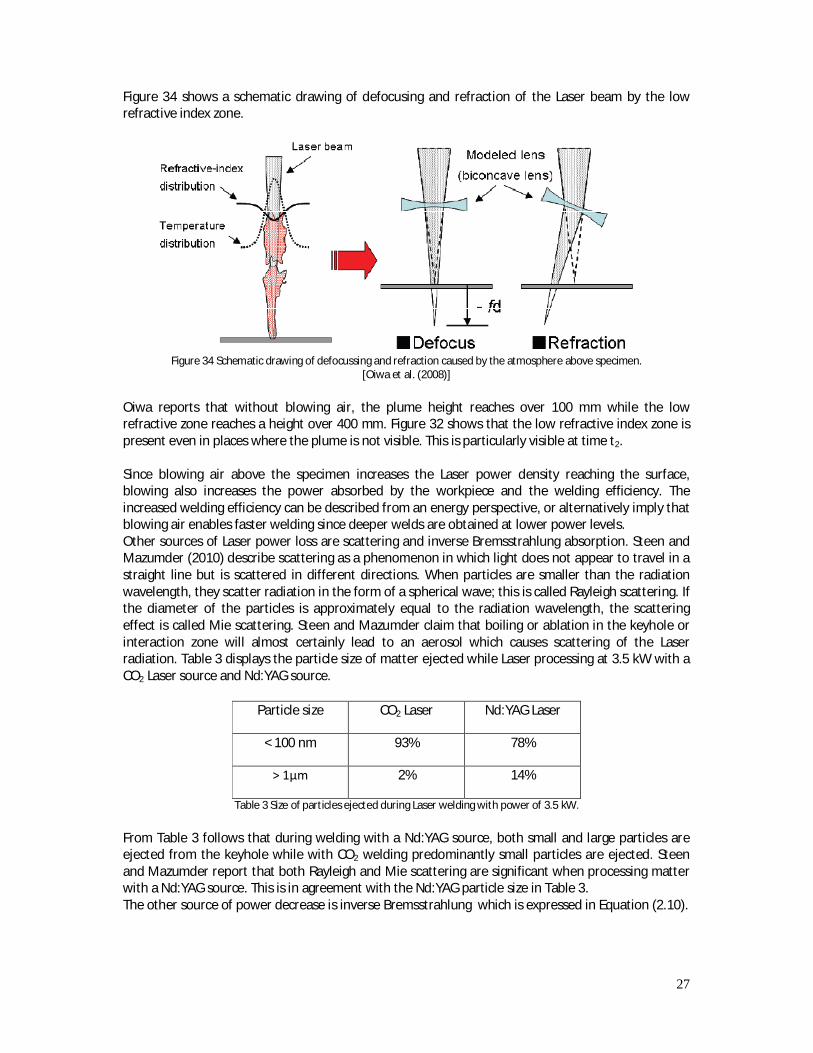
The Michelson interferometer technique was used to investigate the influence of air on the increased penetration depth. Figure 31 shows the setup of the fiber Laser, interferometer, probe Laser and fan. The working principle of the setup is described as follows. Radiation from the probe Laser is split into two separate beams by the half mirror i.e. beam (1) and (2) in Figure 31. Beam (1) passes through the atmosphere above the specimen while beam (2) passes through an unaffected region. Beam (1) is affected by the refractive index distribution above the specimen, and has a phase difference with respect to beam (2). After reflection on the mirrors, both beams are combined by the half mirror and projected onto a screen. The projection is called fringe patterns. If beam (1) and (2) have no phase difference, the fringe patterns consist of horizontal lines. If there is a phase difference, the fringe patterns display curved lines. Oiwa reports that the obtained fringe patterns change with the spatial refractive index of the observed area. Figure 32 shows the fringe patterns when no air is blown over the specimen, and Figure 33 shows the fringe pattern with air blowing.

Figure 31 Experimental setup. [Oiwa et al. (2011)]

26

Figure 32 shows that the fringe pattern changes in complexity with varying plume height and size. At t1, the plume is narrow and tall and the curved fringe patterns encompassing the plume also have the same form. At t2, the fringe patterns are curved over the entire observation area while the plume is shorter than 10 mm. Between instant of time t3-t5, the plume height grew much taller and the specimen was merely partially penetrated. Oiwa claims that fringe patterns that are curved downwards in the path of the Laser beam correspond to a region with lower refractive index.

Figure 32 Plume behaviour, fringe patterns and specimen surface appearance with fan off. [Oiwa (2009)]

The low refractive index distribution refracts and defocuses the Laser beam causing the Laser power density on the specimen surface to decrease (see Figure 34). Consequently, there is a transition from full to partial penetration. Figure 33 shows that that the plume size decreases significantly when air is blown. The size of the low refractive index zone also decreases and is shifted in the direction of the blowing air. The interaction zone between the Laser radiation and the low refractive index zone is thus made smaller when air is blown, this leads to higher Laser power densities on the specimen surface and deeper welds.

Figure 33 Plume behaviour, fringe patterns and specimen surface appearance with fan on. [Oiwa (2009)]

Oiwa claims that the cause of the low refractive index zone is the hot plume above the keyhole. This plume spatially heats up the atmosphere above the specimen, causing the refractive index to decrease. By blowing air with a fan towards the plume, this heated atmosphere is partially removed. Also the plume size decreases, as is shown in Figure 33.

27

Figure 34 shows a schematic drawing of defocusing and refraction of the Laser beam by the low refractive index zone.

Figure 34 Schematic drawing of defocussing and refraction caused by the atmosphere above specimen.

[Oiwa et al. (2008)] Oiwa reports that without blowing air, the plume height reaches over 100 mm while the low refractive zone reaches a height over 400 mm. Figure 32 shows that the low refractive index zone is present even in places where the plume is not visible. This is particularly visible at time t2. Since blowing air above the specimen increases the Laser power density reaching the surface, blowing also increases the power absorbed by the workpiece and the welding efficiency. The increased welding efficiency can be described from an energy perspective, or alternatively imply that blowing air enables faster welding since deeper welds are obtained at lower power levels. Other sources of Laser power loss are scattering and inverse Bremsstrahlung absorption. Steen and Mazumder (2010) describe scattering as a phenomenon in which light does not appear to travel in a straight line but is scattered in different directions. When particles are smaller than the radiation wavelength, they scatter radiation in the form of a spherical wave; this is called Rayleigh scattering. If the diameter of the particles is approximately equal to the radiation wavelength, the scattering effect is called Mie scattering. Steen and Mazumder claim that boiling or ablation in the keyhole or interaction zone will almost certainly lead to an aerosol which causes scattering of the Laser radiation. Table 3 displays the particle size of matter ejected while Laser processing at 3.5 kW with a CO2 Laser source and Nd:YAG source.

Particle size CO2 Laser Nd:YAG Laser

< 100 nm 93% 78%

> 1μm 2% 14%

Table 3 Size of particles ejected during Laser welding with power of 3.5 kW. From Table 3 follows that during welding with a Nd:YAG source, both small and large particles are ejected from the keyhole while with CO2 welding predominantly small particles are ejected. Steen and Mazumder report that both Rayleigh and Mie scattering are significant when processing matter with a Nd:YAG source. This is in agreement with the Nd:YAG particle size in Table 3. The other source of power decrease is inverse Bremsstrahlung which is expressed in Equation (2.10).

28

훼(푚 ) =√ ( )

( )

(2.10)

Where α is the inverse Bremsstrahlung absorption coefficient for Laser radiation, the unknown constant m=1, ne is the electron density within the plasma, ni is the density for singly ionized atoms, Z is the average ionic charge within the plasma, e is the elementary charge, g is the quantum mechanical Gaunt factor, c is the speed of light in vacuum, 휖 is the permittivity of free space, 휔 is frequency of the Laser radiation, me is the electron mass, k is the Boltzmann constant and Te is the electron temperature. Equation (2.10) is rewritten as

훼 = 퐾 with 퐾 =√ ( )

( )

and 휔 = (2.11)

Where 휆 is the Laser radiation wavelength. In order to relate the absorption coefficient in Nd:YAG and CO2 welding, K is assumed as constant. Since the radiation wavelength of Nd:YAG and CO2 sources equals 휆 = 10640 푛푚 and 휆 : =1064 푛푚, the radiation frequency are related as 휔 : = 10휔 . The absorption coefficient of both sources are then related as 훼 : = 퐾 ⇔

훼 : = 훼 . Thus the inverse Bremsstrahlung absorption for Nd:YAG sources is 100 times smaller than that of CO2 sources and is not considered as a cause of significant decrease in Laser power. So blowing above the specimen surface minimizes the effect of the low refractive index zone and blows away particles that could lead to scattering. Conclusions:

- The plume heats up the atmosphere above the specimen and consequently the refractive index of the atmosphere decreases. The Laser beam is then refracted and defocused as is shown in Figure 34.

- The refracted and defocused Laser beam causes the Laser power density on the specimen surface to decrease, leading to lower welding efficiency and e.g. to transition from full to partial penetration.

- The size of the interaction zone of the incident Laser and low refractive index zone has significant effect on the penetration depth.

- If no air is blown, the low refractive index zone is taller and broader than the plume itself. See Figure 32 at t2.

- Blowing air during Laser welding, also removes particles that cause scattering. Particle sizes are displayed in Table 3.

- The influence of the heated atmosphere only seems to be present at high Laser power since Oiwa et al. only conducted experiments at 4 kW. Pocorni (2011) also studied the influence of the atmosphere above the keyhole with varying Laser power between 1-6 kW. He found that the penetration depth only increased significantly between 4-6 kW.

29

2.6 Concluding Remarks

2.6.1 Process monitoring The covariance matrix technique (CMT) proposed by Ancona et al. (2008), the gas shielding monitoring system by Fox et al. (2001) and the frequency domain detection system by Saludes Rodil et al. (2005) are the most interesting monitoring methods, primarily because they have proven to work. Important drawbacks of CMT are the computation time and limited knowledge of the physical meaning of the covariance matrix elements mij. If the shielding gas detection system is applied in this thesis, the hardness of the weld cross section should also be measured to distinguish between good and bad welds. The 3D spectral cloud monitoring technique is quite new and has only been tested for one specific weld defect i.e. blow out welds. If the frequency domain detection system is applied in this thesis, the Nyquist-Shannon theorem states that the sampling frequency of the spectrometer should be minimally 2 ∙ 5000 Hz. The Ocean Optics HR 2000+ spectrometer has a maximal sampling rate of 1000 Hz, and cannot be used to produce signals as in Figure 10. Yet this detection system is still applicable if slow weld defects, such as improper gas shielding, are monitored.

2.6.2 Process control Actuation with Laser power and focal point position are most pragmatic options while weld speed velocity control is best suited for off-line implantation. Konuk (2009) and Postma (2002) have successfully actuated with Laser power. Konuk et al. tune their PI controller with characterization experiments while Postma et al. identify the Laser welding process, sensors and the Laser itself, and design a controller based on the identified process. In this thesis the controlled experiments will be conducted by both characterization experiments and weld process identification. The focus control system recommended by Hand et al. (2000) primarily detects focus shifts caused by e.g. thermal distortions. The direct influence of focus actuation on weld defects other than lack of penetration is not studied by Hand. But Hand does state that his control system is robust against large variations in welding conditions: for different materials, thicknesses, welding speeds and tilt angles, excellent welds are obtained with Hand’s focus control system. Ancona’s electron temperature signal and Fox’s shielding gas detection signal were used as inspiration to define new spectral signals which monitored the penetration depth.

2.6.3 Welding efficiency In this thesis blowing experiments are only conducted at high Laser power. Blowing air above a specimen is effective to the improvement of the penetration depth, but neither Oiwa (2011) nor Pocorni (2011) comment on other metallurgical effects, such as pore creation. Air blown above the specimen could also deteriorate the spectrometer signal but could also unveil other sources of radiation coming out of the keyhole. Experiments with blowing and without blowing will be conducted and the acquired spectral signals will be compared to see how and if they differ from each other. The primary goal of this thesis is to detect weld quality deterioration and control the process to prevent further deterioration. At the same time, air is blown above the specimen surface to increase

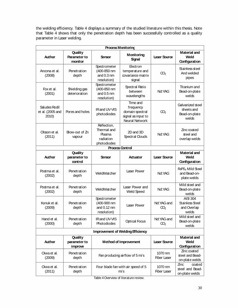
30

the welding efficiency. Table 4 displays a summary of the studied literature within this thesis. Note that Table 4 shows that only the penetration depth has been successfully controlled as a quality parameter in Laser welding.

Process Monitoring

Author Quality

Parameter to monitor

Sensor Monitoring Signal Laser Source

Material and Weld

Configuration

Ancona et al. (2008)

Penetration depth

Spectrometer (400-850 nm and 0.3 nm resolution)

Electron temperature and covariance matrix

signal

CO2 Stainless steel

And welded pipes

Fox et al. (2001)

Shielding gas deterioration


Spectral Ratio between

wavelengths Nd:YAG

Titanium and Bead-on-plate

welds

Saludes Rodil et al. (2005 and

2010) Pores and holes IR and UV-VIS

photodiodes

Time and frequency

domain spectral signal as input to Neural Network

CO2

Galvanized steel sheets and

Bead-on-plate welds

Olsson et al. (2011)

Blow-out of Zn vapour

Reflection, Thermal and

Plasma radiation

photodiodes

2D and 3D Spectral Clouds Nd:YAG

Zinc coated steel and

overlap welds

Process Control

Author Quality

parameter to control

Sensor Actuator Laser Source Material and

Weld Configuration

Postma et al. (2002)

Penetration depth WeldWatcher Laser Power

Nd:YAG FeP04 Mild Steel

and Bead-on-plate welds

Postma et al. (2002)

Penetration depth WeldWatcher Laser Power and

Weld Speed Nd:YAG Mild steel and Bead-on-plate

welds

Konuk et al. (2009)

Penetration depth


Laser Power Nd:YAG and CO2

AISI 304 Stainless Steel and Overlap

welds

Hand et al. (2000)

Penetration depth

IR and UV-VIS Photodiodes Optical Focus Nd:YAG and

CO2

Mild steel and Bead-on-plate

welds Improvement of Welding Efficiency

Author Quality

parameter to improve

Method of Improvement Laser Source Material and

Weld Configuration

Oiwa et al. (2009)

Penetration depth Fan producing airflow of 5 m/s 1070 nm

Fiber Laser

Zinc coated steel and Bead-on-plate welds

Oiwa et al. (2011)

Penetration depth

Four blade fan with air speed of 5 m/s

1070 nm Fiber Laser

Zinc coated steel and Bead-on-plate welds

Table 4 Overview of literature review.

31

3 Experimental Setup and Procedure The measurements conducted for this thesis can be divided into two parts i.e. characterization experiments for sensor signal selection in Chapter 4 and controlled experiments in Chapter 6. The experimental setup and procedure used for both of these experiments are explained in this Chapter.

3.1 Experimental Setup The experimental setup shown in Figure 35 consists of a Laser source which delivered radiation via an optical fiber to a welding head which focused the Laser beam onto the workpiece surface. The radiation coming from the Laser material interaction zone was focused into a separate optical fiber with a collimator. This optical fiber connected the collimator to a spectrometer which produced spectra that were analyzed on a Personal Computers (PC). For characterization experiments the recorded spectra were analyzed offline in order to select a suitable sensor signal. But for controlled experiments signal processing was carried out in real-time i.e. a controller computed the required Laser power signal using the spectral signal as an input. Next, the required power signal was fed back to the spectrometer which, together with a Breakout (input/output) Box, sends an analog signal to the Laser source to adjust the Laser power.

3.1.1 Laser Source and Optics A 4000 W Nd:YAG Laser source (Haas HL 4006D) with 1064 nm wavelength was used during the measurements. The focus spot diameter of the Laser beam equaled

푑 = ∙ 퐷 =

∙ 0.6 푚푚 = 0.6 푚푚 (3.1)

with df as the diameter of the focus spot, f1 and f2 the focal distances of respectively the collimator and focusing lens of the welding head and Do diameter of the optical delivery fiber. The Laser beam was continuous and was focussed onto the workpiece with a Trumpf BEO70 welding head. The welding head was robotized by a Stäubli RX 130 manipulator. All key experimental parameters are summarized in Table 6.

Figure 35 Experimental setup. Modified from Konuk (2009 and 2010).

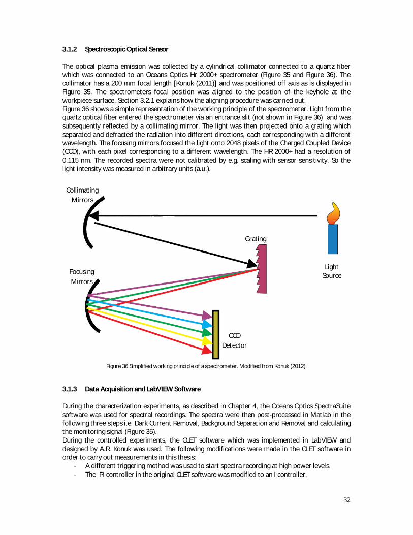
32

3.1.2 Spectroscopic Optical Sensor

The optical plasma emission was collected by a cylindrical collimator connected to a quartz fiber which was connected to an Oceans Optics Hr 2000+ spectrometer (Figure 35 and Figure 36). The collimator has a 200 mm focal length [Konuk (2011)] and was positioned off axis as is displayed in Figure 35. The spectrometers focal position was aligned to the position of the keyhole at the workpiece surface. Section 3.2.1 explains how the aligning procedure was carried out. Figure 36 shows a simple representation of the working principle of the spectrometer. Light from the quartz optical fiber entered the spectrometer via an entrance slit (not shown in Figure 36) and was subsequently reflected by a collimating mirror. The light was then projected onto a grating which separated and defracted the radiation into different directions, each corresponding with a different wavelength. The focusing mirrors focused the light onto 2048 pixels of the Charged Coupled Device (CCD), with each pixel corresponding to a different wavelength. The HR 2000+ had a resolution of 0.115 nm. The recorded spectra were not calibrated by e.g. scaling with sensor sensitivity. So the light intensity was measured in arbitrary units (a.u.).

Figure 36 Simplified working principle of a spectrometer. Modified from Konuk (2012).

3.1.3 Data Acquisition and LabVIEW Software During the characterization experiments, as described in Chapter 4, the Oceans Optics SpectraSuite software was used for spectral recordings. The spectra were then post-processed in Matlab in the following three steps i.e. Dark Current Removal, Background Separation and Removal and calculating the monitoring signal (Figure 35). During the controlled experiments, the CLET software which was implemented in LabVIEW and designed by A.R. Konuk was used. The following modifications were made in the CLET software in order to carry out measurements in this thesis:

- A different triggering method was used to start spectra recording at high power levels. - The PI controller in the original CLET software was modified to an I controller.

Collimating Mirrors

Focusing Mirrors

Grating

CCD Detector

Light Source

33

- The three above mentioned signal processing steps were introduced in the CLET software i.e. Dark Current Removal, Background Separation and Removal and calculating the monitoring signal.

Background Separation and Removal and calculation of the monitoring signal were carried out with the same algorithm as for the characterization experiments. But Dark Current Removal was carried out with a LabVIEW driver supplied by Oceans Optics. This driver corrects for dark current differently than the algorithm used in Matlab for the characterization experiments. The differences between the Dark Current Removal in Matlab and in LabVIEW will be outlined next. Dark electric current is caused by pixels comprising the Charged Coupled Device (CCD) inside the spectrometer. These dark pixels are physically coated and are not used for spectral measurements. Yet electrons escape from these pixels and cause the other pixels within the CCD detector to measure radiation even when no light is present. The characterization experiments in Chapter 4 were carried out in Ocean Optics SpectraSuite software and post-processed in Matlab. But the controlled experiments in Chapter 6 were carried out on the LabVIEW platform. It is of importance to take this into account because in LabVIEW, dark current removal is carried out by taking the average of the dark current signal and subsequently correcting the measured intensity of the other pixels with this average. OmniDriver (2009) also claims that for each change in integration time the average dark current is recalculated. Thus the dark current removal step implemented in LabVIEW computed a new average whenever the sample time changed. But in post-processing the recorded spectra in Matlab, the dark current correction was carried out with a sloping line, without averaging and without recalculating the correction factor for each change in sample time. The difference in dark current removal could cause the sensor signal level to differ for each platform. To correct for this, the characterization experiments were redone on the LabVIEW platform before conducting controlled experiments as described in Section 6.1. After the recorded spectra were processed with the three steps described earlier, the resulting monitoring signal was fed to the controller which determined the required Laser power (Figure 35). This power signal was then send back to the spectrometer and accompanying the Breakout Box which converted the digital signal from the controller to an analog signal for the Laser source. Figure 37 shows the devices used for data acquisition. The welding head is described in more detail in Figure 38.

3.1.4 Material Type, Sample Preparation and Welding Configuration

S235JR steel was used for both the characterization and controlled experiments. Unfortunately, more than two different batches were used in this thesis. For the characterization experiments needed for the selection of the sensor signal, material which was available and in stock at the time of experimenting, was used. For the controlled experiments, a newly ordered material batch was used. The assumed chemical composition of this steel for both cases is shown in Table 5. When comparing the chemical composition of the material used for the characterization experiments to the material used for the controlled experiments, it is obvious that the amount of Mn is approximately a factor 1.5 larger. The other elements, with the exception of Fe, are not of importance because their emissions were not used to define a sensor signal in Chapter 4. Unfortunately, there is no assurance that the specifications given in Table 5 correspond to the material used during the characterization experiments. Even the suppliers of the material for the controlled experiments could not guarantee that the specifications in Table 5 corresponded to the delivered steel. In Section 6.2 (Figure 67 (b)) it is pointed out that the difference in chemical compositions could be the cause of an upward shift in signal value.

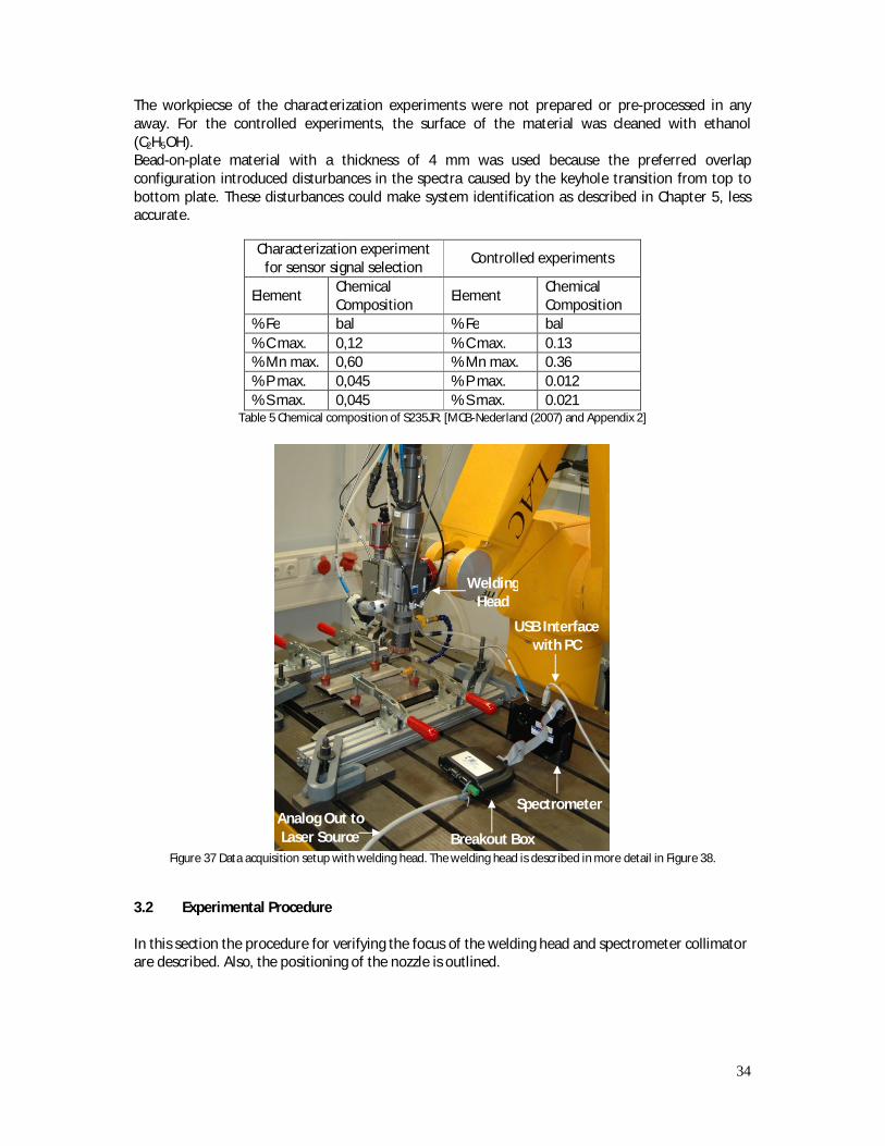
34

The workpiecse of the characterization experiments were not prepared or pre-processed in any away. For the controlled experiments, the surface of the material was cleaned with ethanol (C2H5OH). Bead-on-plate material with a thickness of 4 mm was used because the preferred overlap configuration introduced disturbances in the spectra caused by the keyhole transition from top to bottom plate. These disturbances could make system identification as described in Chapter 5, less accurate.

Characterization experiment for sensor signal selection Controlled experiments

Element Chemical Composition Element Chemical

Composition % Fe bal % Fe bal % C max. 0,12 % C max. 0.13 % Mn max. 0,60 % Mn max. 0.36 % P max. 0,045 % P max. 0.012 % S max. 0,045 % S max. 0.021

Table 5 Chemical composition of S235JR. [MCB-Nederland (2007) and Appendix 2]

Figure 37 Data acquisition setup with welding head. The welding head is described in more detail in Figure 38.

3.2 Experimental Procedure In this section the procedure for verifying the focus of the welding head and spectrometer collimator are described. Also, the positioning of the nozzle is outlined.

Welding Head

Analog Out to Laser Source

Spectrometer

USB Interface with PC

Breakout Box

35

3.2.1 Aligning the Focus Position All measurements were carried out by focusing the Laser beam on the material surface. By using a triangulation Laser, the focus position was verified for each series of experiments. The triangulation laser projects a red line onto the workpiece surface as is shown in Figure 38. Together with a camera which focusses coaxially on the keyhole position on the workpiece surface, it was checked whether the welding head was in focus on the surface. This focus verification procedure is outlined as follows. Two vertical and two horizontal lines are drawn in the camera image such that these lines form a square at their intersection points (see Figure 39). The square is positioned such that it corresponds to the position wherein the keyhole is formed in the workpiece. The position of the line from the triangulation Laser measures the distance between the welding head and workpiece surface. If the line from the triangulation laser is found in the middle of the two horizontal lines in the camera image, as is shown in Figure 39, the welding head is in focus on the workpiece surface. The focus of the collimator equals 200 mm [Konuk (2011)]. Whether the collimator was focused on the workpiece surface, was verified by connecting the collimator to a Diode Laser which projected a red spot on the workpiece surface as is seen in Figure 38. The distance between fiber-end and collimator optics was adjusted to ensure that the collimator was focused on the workpiece surface by observing the spot size. If the center of the projected spot on the workpiece surface coincided with the center of the square in the camera image, the collimator was focused on the position of the keyhole (see Figure 39). Two washers were used in front of the quartz collimator to create an entrance aperture for light to pass through. This configuration together with a small spectrometer integration time prevented radiation saturation as much as possible. Figure 40 shows the two washers which were fastened together with paper tape. The large washer has a diameter of 13.2 mm while the smaller washer has a diameter of 5.4 mm (aperture diameter).

Figure 38 Line from triangulation Laser and collimator spot on workpiece surface.

Air Nozzle Triangulation laser Housing

Collimator

Fiber-end

Camera

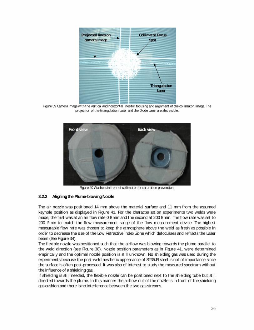
36

Figure 39 Camera image with the vertical and horizontal lines for focusing and alignment of the collimator. image. The

projection of the triangulation Laser and the Diode Laser are also visible.

Figure 40 Washers in front of collimator for saturation prevention.

3.2.2 Aligning the Plume-blowing Nozzle The air nozzle was positioned 14 mm above the material surface and 11 mm from the assumed keyhole position as displayed in Figure 41. For the characterization experiments two welds were made, the first was at an air flow rate 0 l/min and the second at 200 l/min. The flow rate was set to 200 l/min to match the flow measurement range of the flow measurement device. The highest measurable flow rate was chosen to keep the atmosphere above the weld as fresh as possible in order to decrease the size of the Low Refractive Index Zone which defocusses and refracts the Laser beam (See Figure 34). The flexible nozzle was positioned such that the airflow was blowing towards the plume parallel to the weld direction (see Figure 38). Nozzle position parameters as in Figure 41, were determined empirically and the optimal nozzle position is still unknown. No shielding gas was used during the experiments because the post-weld aesthetic appearance of S235JR steel is not of importance since the surface is often post-processed. It was also of interest to study the measured spectrum without the influence of a shielding gas. If shielding is still needed, the flexible nozzle can be positioned next to the shielding tube but still directed towards the plume. In this manner the airflow out of the nozzle is in front of the shielding gas cushion and there is no interference between the two gas streams.

Front view Back view

Projected lines on camera image

Collimator Focus Spot

Triangulation Laser

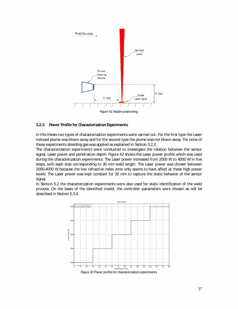
37

Figure 41 Nozzle positioning.

3.2.3 Power Profile for Characterization Experiments In this thesis two types of characterization experiments were carried out. For the first type the Laser induced plume was blown away and for the second type the plume was not blown away. For none of these experiments shielding gas was applied as explained in Section 3.2.2. The characterization experiments were conducted to investigate the relation between the sensor signal, Laser power and penetration depth. Figure 42 shows the Laser power profile which was used during the characterization experiments. The Laser power increased from 2000 W to 4000 W in five steps, with each step corresponding to 30 mm weld length. The Laser power was chosen between 2000-4000 W because the low refractive index zone only seems to have affect at these high power levels. The Laser power was kept constant for 30 mm to capture the static behavior of the sensor signal. In Section 5.2 the characterization experiments were also used for static identification of the weld process. On the basis of the identified model, the controller parameters were chosen as will be described in Section 5.3.4.

Figure 42 Power profile for characterization experiments.

0 10 20 30 40 50 60 70 80 90 100 110 120 130 140 150

2000

2500

3000

3500

4000

Power Profile

Bead Position (mm)

Lase

r Pow

er (W

)

Laser Power

38

Experimental parameters

Material and Weld Specifications Material Type S235JR

Weld Configuration Bead-on-plate Weld length 150 mm

Laser Source and Optics Laser Source Haas HL 4006D Optical Fiber Diameter 0.6 mm Robot Manipulator Stäubli RX 130

Welding Head Trumpf BEO70 head with 200 mm focus

Spot Size 0.6 mm Welding Speed 60 mm/s

Optical Measuring Device Spectrometer Hr 2000+ with Breakout Box Optical Fiber Diameter 0.4 mm

Collimator Cylindrical collimator with 200 mm focus

Argon shielding Flowrate 0 l/h

Air Flow Flowrate 0 l/min and 200 l/min

Table 6 Experimental specifications.

39

4 Sensor Signal Selection

4.1 Extracted Spectral Signal The information gained in the Literature Review (Chapter 2) provides inspiration for the extraction and definition of a new spectral signal which should monitor the penetration depth. In Section 2.3.4 Olsson et al. (2011) warn that raw spectral data measured with photodiodes is insufficient for interpretation of weld instability. They show that signals from light sensors have to be combined with each other in order to produce a reliable signal for process monitoring. So in order to produce a new spectral signal, the light intensity at a single wavelength is not enough for process monitoring. Fox (2001) on the other hand uses the spectral emission of an unidentified peak and normalizes it with the spectral emission in a peakless region (Section 2.3.2). He successfully found a signal that detects decay of gas shielding. Although the aim of this thesis is to monitor the internal behavior of the weld i.e. the penetration depth, Fox demonstrates how a simple spectral ratio can be used for process monitoring. Ancona (2008) and Konuk (2009) use two spectral peaks to produce signals which characterize lack of penetration among others (See Section 2.3.1 and Section 2.4.3). Their spectral ratio is weighted such that a physical meaning is given to the signal i.e. the electron temperature. Equation 2.6 gives the mathematical expression for the Electron Temperature. Besides the radiation from the plasma, Olsson (2011) and Saludes Rodil (2005 and 2010) observe the reflected and thermal radiation coming from the keyhole and meltpool. Observing the keyhole radiation is particularly interesting because the aim of this thesis is to monitor the keyhole penetration depth. The primary conclusion from the Literature Review is that a successful signal for characterizing the penetration depth can be obtained from the spectral ratio between two peaks, as is successfully demonstrated by the research carried out by Konuk and Ancona. Additionally, it is of peculiar interest to study the background radiation coming from the keyhole and (or) meltpool since the depth of the keyhole must be monitored. As is mentioned in the Literature Review, Fox was unable to identify the peak he uses for his monitoring system. To prevent this and to be able to explain the acquired signal unequivocally, the peaks in the spectral signal are identified with help of the NIST database in this thesis. The peak identified spectrum is shown in Figure 51 in Section 4.4. Three new signals were defined on the basis of knowledge acquired from the Literature Review i.e.:

- the Background Ratio Signal (BRS) - the Peak Ratio Signal (PRS) - the Peak and Background Ratio Signal (PBRS)

The BRS is expected to provide information on the relationship between the background radiation presumably from the keyhole and the penetration depth. The PRS should show whether the spectral ratio between emissions from atomic ions provides useful information about the penetration depth. The PBRS is a hybrid between the above mentioned signals and combines the peaks intensity and the background radiation. Besides monitoring and control of the penetration depth, the second aim of this thesis is to increase the weld efficiency with plume-blowing. As explained in Section 2.5 of the Literature Review, Oiwa (2011) explains that plume-blowing causes deeper penetration. The purpose of this work is to combine and go beyond earlier work done by Oiwa and Konuk in such a manner that the weld process is controlled in real-time and at the same time the weld efficiency is increased. The ability of the three signals to measure the penetration depth will first be tested for the non-blown situation, and secondly for the plume-blown situation. The signal(s) which measure(s) the penetration depth for both cases will subsequently be used for process control. The measured spectrum as shown in Figure 43 (a) is processed with software designed by [14] such that the background spectrum is first separated and then removed, as will be outlined next. Figure 43

40

(a)-(c) shows the processing steps starting from the measured spectrum (Figure 43 (a)), next the background spectrum (Figure 43 (b)) and lastly the spectrum with only peaks. The abbreviations P and B are used to describe the three signals, and they have the following meaning:

- P: the Peak intensity as displayed in Figure 43 (c) - B: the Background intensity as displayed in Figure 43(b)

{푥[푛]} equals the sequence of measured spectral intensities from the spectrometer and is represented by P(λn)+B(λn) in Figure 43 (a). With the Background Separation filter a new sequence {푦[푛]} was obtained which represented the background separated spectrum B(λn) in Figure 43 (b). The filter replaces each input data point with the minimum of a subset consisting of neighboring data points defined within a span. From this point on, a subset is referred to as a window. The filter output is given by

y[i] = min(푥[푖 − 푀], … , 푥[푖], … 푥[푖 +푀]) (4.1) where y[i] is the filter output for the i -th data point, M is the number of neighboring data points on either side of x[i] and the span equals 2M+1. At the beginning and end of the input dataset the window size needs to be adjusted, as will be outlined next. In the situation where there are not enough data point to the left of x[i], the window starts at the first element until the i+M -th element of x[n]. The filter then determines the minimum value of the data points within the window as follows

y[푖] = min(푥[1], … , 푥[푖], … 푥[푖 +푀]) (4.2) If there are not enough data points to the right of x[i], the window starts at the i–M -th element until the last element of x[n]. The filter then determines the minimum value of the data points within the window as follows

y[푖] = min(푥[푖 − 푀], … , 푥[푖], … 푥[푁]) (4.3) If a large window size is chosen, then a situation may occur in which there are not enough data points to the left and right of x[i]. For this situation the window starts at the first element until the last element of x[n]. The filter then determines the minimum value of the data points within the window as follows

y[푖] = min(푥[1], … , 푥[푖], … 푥[푁]) (4.4) Finally, the background spectrum is removed by subtracting the filter output y[n] from the filter input x[n] in order to obtain the background removed spectrum P(λn) in Figure 43 (c) i.e. 푃(휆 ) = 푥[푛]−푦[푛]. For this thesis the number of neighboring data points M was set to 5. The first signal, the Background Ratio Signal (BRS), was based on the ratio of the background signal (B1 and B2 in Figure 43 (b)) at two wavelengths.

Background Ratio: B1B2

(4.5)

The second signal, the Peak Ratio Signal, was determined by the ratio between the background removed spectrum (P1 and P2 in Figure 43 (c)) at two different wavelengths.

Peak Ratio Signal: P1P2

(4.6) The third signal, the Peak and Background Ratio Signal (PBRS), was determined with the ratio of the background removed spectrum (P3 in Figure 43 (c) and the background signal (B3 in Figure 43(b)) at a single wavelength. Peak and Background Ratio Signal: (4.7)

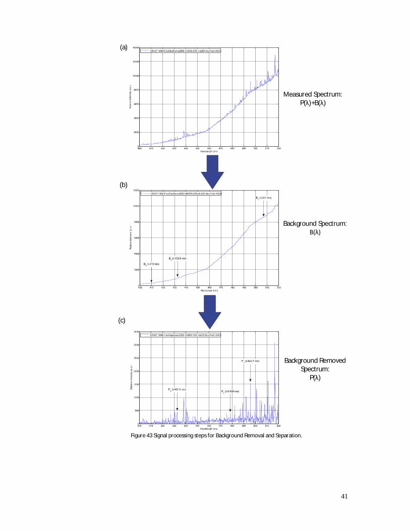
41

Figure 43 Signal processing steps for Background Removal and Separation.

(a)

(b) Breakout Box

(c)

Measured Spectrum: P(λ)+B(λ)

Background Spectrum: B(λ)

Background Removed Spectrum:

P(λ)

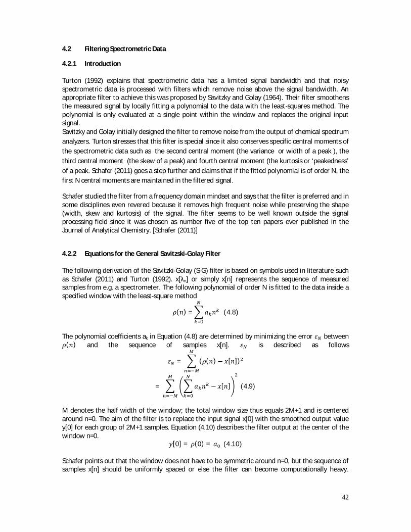
42

4.2 Filtering Spectrometric Data

4.2.1 Introduction Turton (1992) explains that spectrometric data has a limited signal bandwidth and that noisy spectrometric data is processed with filters which remove noise above the signal bandwidth. An appropriate filter to achieve this was proposed by Savitzky and Golay (1964). Their filter smoothens the measured signal by locally fitting a polynomial to the data with the least-squares method. The polynomial is only evaluated at a single point within the window and replaces the original input signal. Savitzky and Golay initially designed the filter to remove noise from the output of chemical spectrum analyzers. Turton stresses that this filter is special since it also conserves specific central moments of the spectrometric data such as the second central moment (the variance or width of a peak ), the third central moment (the skew of a peak) and fourth central moment (the kurtosis or ‘peakedness’ of a peak. Schafer (2011) goes a step further and claims that if the fitted polynomial is of order N, the first N central moments are maintained in the filtered signal.

Schafer studied the filter from a frequency domain mindset and says that the filter is preferred and in some disciplines even revered because it removes high frequent noise while preserving the shape (width, skew and kurtosis) of the signal. The filter seems to be well known outside the signal processing field since it was chosen as number five of the top ten papers ever published in the Journal of Analytical Chemistry. [Schafer (2011)]

4.2.2 Equations for the General Savitzski-Golay Filter The following derivation of the Savitzki-Golay (S-G) filter is based on symbols used in literature such as Schafer (2011) and Turton (1992). x[λn] or simply x[n] represents the sequence of measured samples from e.g. a spectrometer. The following polynomial of order N is fitted to the data inside a specified window with the least-square method

휌(푛) = 푎 푛=0

(4.8)

The polynomial coefficients ak in Equation (4.8) are determined by minimizing the error 휀 between 휌(푛) and the sequence of samples x[n]. 휀 is described as follows

휀 = (휌(푛)− 푥[푛])

= 푎 푛 − 푥[푛] (4.9)

M denotes the half width of the window; the total window size thus equals 2M+1 and is centered around n=0. The aim of the filter is to replace the input signal x[0] with the smoothed output value y[0] for each group of 2M+1 samples. Equation (4.10) describes the filter output at the center of the window n=0.

푦[0] = 휌(0) = 푎 (4.10)

Schafer points out that the window does not have to be symmetric around n=0, but the sequence of samples x[n] should be uniformly spaced or else the filter can become computationally heavy.

43

Further on in this Section it is explained how irregularly spaced data is dealt with. The output of the S-G filter is computed by a discrete convolution, as described by

푦[푛] = ℎ[푚]푥[푛 − 푚] (4.11)

Above equation shows that the filter output y[n] is a linear combination of the original signal x[n-m]. So, the output is obtained by giving the original signal x[n] different weights h[m]. Savitzky and Golay (1964) proved that fitting a polynomial to a local set of data, and evaluating it at the center of the window (n=0) is the same as the output being equal to a (fixed) linear combination of the local set of data x[n]. To find the polynomial coefficients ai, the error 휀 in Equation (4.9) is minimized as follows

휕휀휕푎

= 2푛 푎 푛 − 푥[푛] = 0 for 푖 = 0,1, …푁 (4.12)

N denotes the polynomial order, x[n] is the sequence of input samples and ak are the polynomial coefficients which are unknown. Equation (4.12) is rearranged in order to obtain the form in Equation (4.13).

푛 푎 = 푛 푥[푛] 푓표푟 푖 = 0,1, …푁 (4.13)

It is more convenient to rewrite Equation (4.13) in shorter matrix notation consisting of one matrix and two vectors. The first matrix consists of the sample numbers:

A = ൛훼 , ൟ with 훼 , = 푛 푓표푟 푛 ∈ [−푀,푀] 푎푛푑 푖 ∈ [0,푁] (4.14)

The left part of Equation (4.13) becomes

ATA = 훼 , 훼 , = 푛 (4.15)

The first vector is defined as x and consists of the discrete input signal values x = ൣ푥[−푀], … , 푥[−1],푥[0],푥[1], … , 푥[푀]൧

The second vector a consists of the unknown polynomial coefficients a = [푎 ,푎 , … ,푎 ]

Equation (4.13) is then rewritten in the following matrix notation ATAa = ATx (4.16)

The unknown polynomial coefficients equal

a=൫ATA൯-1

ATx, with H=൫ATA൯-1

AT (4.17)

where H is the pseudoinverse of the matrix A.

From Equation (4.10) follows that for each input sample x[n] only the first polynomial coefficient a0 is needed to generate a filter output y, assuming that n=0 is the center of the window 2M+1. Thus, only the first row of H is needed to obtain a0. Equation (4.18) describes the filter output y[0] and the first row of the H matrix h(0,m).

푦[0] = 푎 = ℎ( , )푥[푚] (4.18)

From Equation (4.15) and (4.17) follows that the H matrix is only dependent on the sample number n, and independent of the input samples x[n]. So, for uniformly distributed samples x[n], the H matrix is fixed, with the exception of the beginning and end of the dataset. Schafer calls this a shift invariant discrete convolution process. Figure 44 shows the polynomial fit (solid line) obtained with the least-square method. Another way of acquiring the the polynomial coefficient a0 is to to calculate

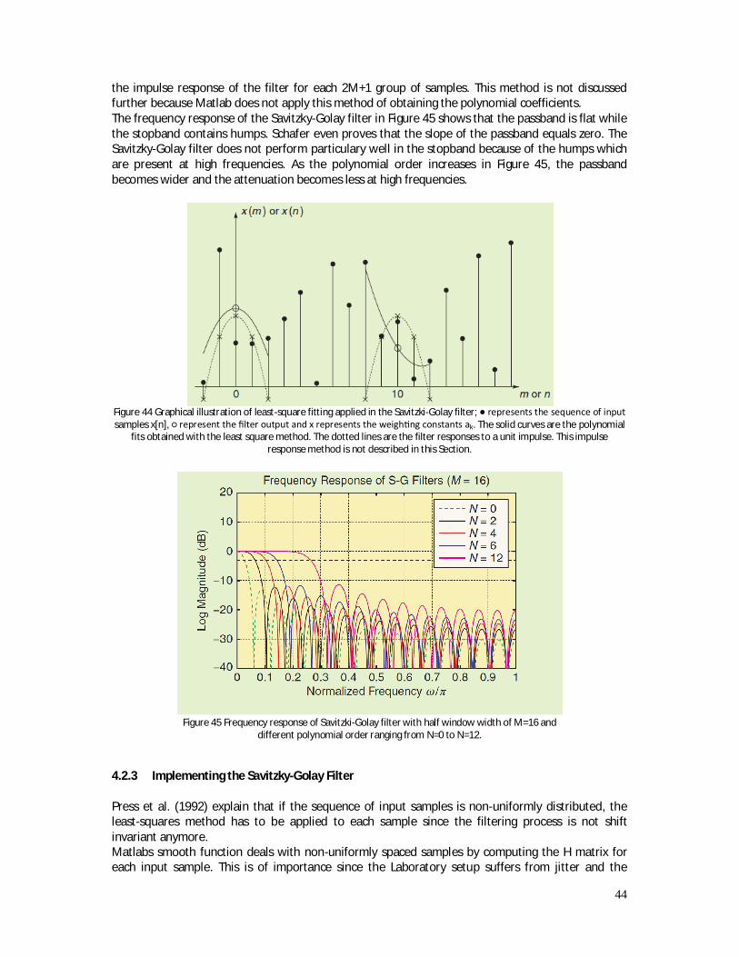
44

the impulse response of the filter for each 2M+1 group of samples. This method is not discussed further because Matlab does not apply this method of obtaining the polynomial coefficients. The frequency response of the Savitzky-Golay filter in Figure 45 shows that the passband is flat while the stopband contains humps. Schafer even proves that the slope of the passband equals zero. The Savitzky-Golay filter does not perform particulary well in the stopband because of the humps which are present at high frequencies. As the polynomial order increases in Figure 45, the passband becomes wider and the attenuation becomes less at high frequencies.

Figure 44 Graphical illustration of least-square fitting applied in the Savitzki-Golay filter; ● represents the sequence of input samples x[n], ○ represent the filter output and x represents the weigh ng constants ak. The solid curves are the polynomial

fits obtained with the least square method. The dotted lines are the filter responses to a unit impulse. This impulse response method is not described in this Section.

Figure 45 Frequency response of Savitzki-Golay filter with half window width of M=16 and

different polynomial order ranging from N=0 to N=12.

4.2.3 Implementing the Savitzky-Golay Filter Press et al. (1992) explain that if the sequence of input samples is non-uniformly distributed, the least-squares method has to be applied to each sample since the filtering process is not shift invariant anymore. Matlabs smooth function deals with non-uniformly spaced samples by computing the H matrix for each input sample. This is of importance since the Laboratory setup suffers from jitter and the

45

measured data was non-uniformly distributed. Press argues that this method is computationally heavy especially for large window sizes and large amount of input data. This is one of the reasons why the Savitzky-Golay filter was not used during real-time process control experiments in Chapter 6. Another reason is the practical inconvenience of implementing this filter into software as is described in Section 5.3.1. The window of this filter was set to 20% of the total amount of spectra shot per experiment e.g. 20% ∙ 1290 samples = 258 samples. The order of the filter was set to 4 in order to have a good approximation of the original signal. The Savitzky-Golay filter was used for process monitoring in this thesis because it was specifically designed to handle spectral signals. Yet this filter is not well known within the signal processing field as explained by Schafer (2011). By applying this filter in this thesis, it is hoped that awareness of this filter is increased within the digital signal processing field.

4.3 Background Ratio Signal

BRS (t) was determined by normalizing the background emissions B1 (t, 507 nm) with B2 (t, 410 nm). The position of the background emissions B1 and B2 are illustrated in the spectrum in Figure 43 (b). B1 was chosen specifically at 507 nm because the signal value increased with Laser power while the background emission B2 seemed unaffected by the increase in Laser power. Additionally, B1 and B2 were chosen such that they corresponded to peakless regions of the spectrum. From the Literature Review in Section 2.2.1 it was assumed that the background emission in these peakless regions was caused by keyhole radiation. The BRS is given as

BRS (t) = ( , )( , ) ·K, with K = 10 (4.19)

Since the Background Ratio Signal is a ratio of two spectral emissions presumably originating from the keyhole walls or meltpool at the surface, this signal is comparable to the method used by ratio pyrometers. These devices estimate the absolute temperature of the work piece from the spectral emissions. Figure 47 (a)-(d) shows the results for the non-blown and plume-blown experiments as described in Section 3.2.2 and 3.2.3. The upper plots (a) and (c) display the unfiltered and the filtered signal, and the lower plots (b) and (d) display solely the filtered signals for the non-blown and plume-blown case in a single plot.

4.3.1 Explanation of Signal Behavior In order to explain the signal behavior in Figure 47, the background radiance at 410 nm (B2(t)) and at 507 nm (B1(t)) are considered separately. Figure 46 shows the result when the mean of B1(t) was determined for each constant power region to obtain B (P). B (P) was also determined in the same manner from B2(t). Next, a linear curve was fitted to B (P) and to B (P). The resulting fits with their linear equation are displayed in Figure 46. The background radiance at 410 nm seems flat while the radiance at 510 nm increases with Laser power. The slope of the linear fit of B (P) equals -0.01 while that of B (P) is clearly higher i.e. 0.6. The flatness of the radiance at 410 nm is explained by the fact that at some wavelengths the background radiance is less sensitive to the increase of Laser power than others.

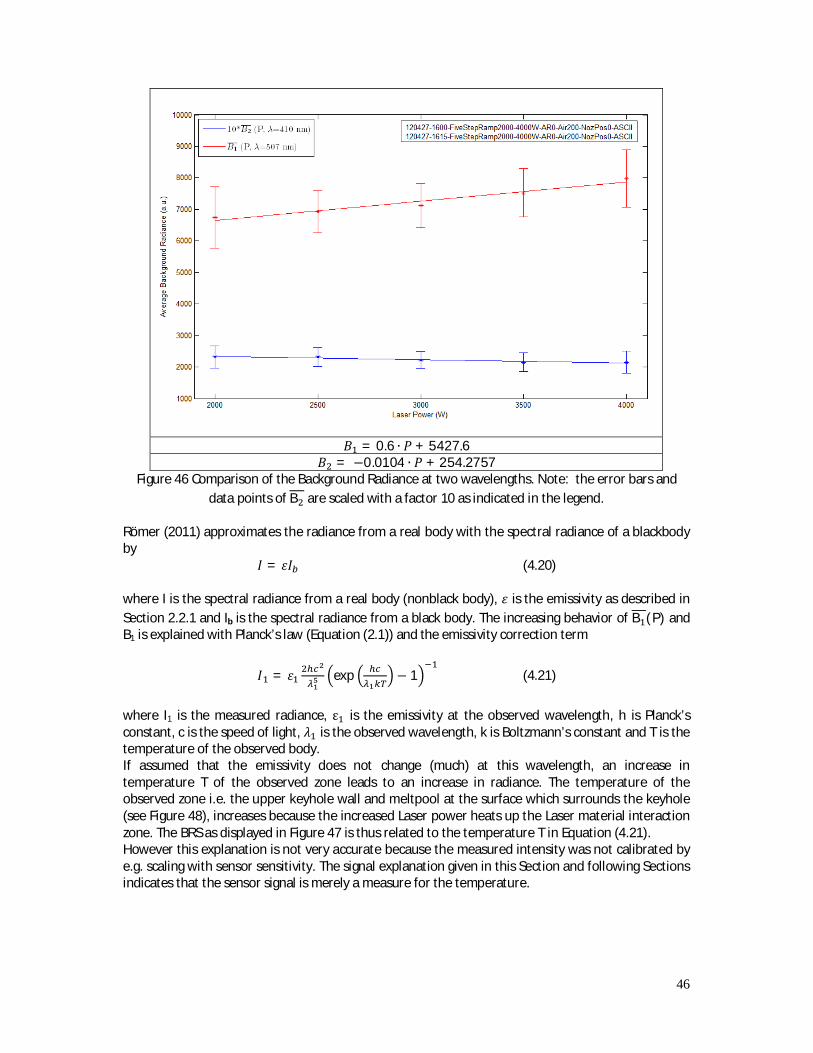
46

퐵 = 0.6 ∙ 푃 + 5427.6

퐵 = −0.0104 ∙ 푃 + 254.2757 Figure 46 Comparison of the Background Radiance at two wavelengths. Note: the error bars and

data points of B are scaled with a factor 10 as indicated in the legend. Römer (2011) approximates the radiance from a real body with the spectral radiance of a blackbody by

퐼 = 휀퐼 (4.20) where I is the spectral radiance from a real body (nonblack body), 휀 is the emissivity as described in Section 2.2.1 and Ib is the spectral radiance from a black body. The increasing behavior of B (P) and B1 is explained with Planck’s law (Equation (2.1)) and the emissivity correction term

퐼 = 휀 exp − 1 (4.21)

where I1 is the measured radiance, ε is the emissivity at the observed wavelength, h is Planck’s constant, c is the speed of light, 휆 is the observed wavelength, k is Boltzmann’s constant and T is the temperature of the observed body. If assumed that the emissivity does not change (much) at this wavelength, an increase in temperature T of the observed zone leads to an increase in radiance. The temperature of the observed zone i.e. the upper keyhole wall and meltpool at the surface which surrounds the keyhole (see Figure 48), increases because the increased Laser power heats up the Laser material interaction zone. The BRS as displayed in Figure 47 is thus related to the temperature T in Equation (4.21). However this explanation is not very accurate because the measured intensity was not calibrated by e.g. scaling with sensor sensitivity. The signal explanation given in this Section and following Sections indicates that the sensor signal is merely a measure for the temperature.

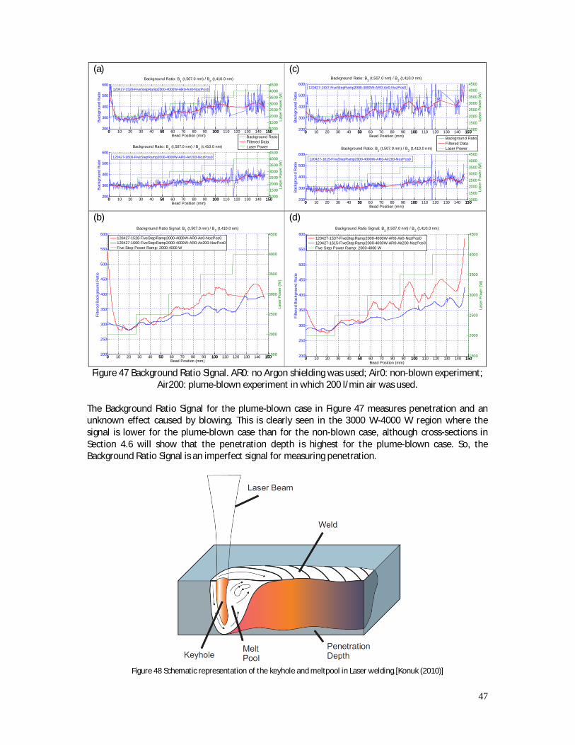
47

(a) (c)

(b)

(d)

Figure 47 Background Ratio Signal. AR0: no Argon shielding was used; Air0: non-blown experiment;

Air200: plume-blown experiment in which 200 l/min air was used. The Background Ratio Signal for the plume-blown case in Figure 47 measures penetration and an unknown effect caused by blowing. This is clearly seen in the 3000 W-4000 W region where the signal is lower for the plume-blown case than for the non-blown case, although cross-sections in Section 4.6 will show that the penetration depth is highest for the plume-blown case. So, the Background Ratio Signal is an imperfect signal for measuring penetration.

Figure 48 Schematic representation of the keyhole and meltpool in Laser welding.[Konuk (2010)]

0 10 20 30 40 50 60 70 80 90 100 110 120 130 140 150200

300

400

500

600Background Ratio: B1 (t,507.0 nm) / B2 (t,410.0 nm)

Bead Position (mm)

Bac

kgro

und

Rat

io

0 50 100 15010001500200025003000350040004500

Lase

r Pow

er (W

)

Background RatioFiltered DataLaser Power

0 10 20 30 40 50 60 70 80 90 100 110 120 130 140 150200

300

400

500


Bead Position (mm)

Bac

kgro

und

Rat

io

0 50 100 15010001500200025003000350040004500

Lase

r Pow

er (W

)

120427-1528-FiveStepRamp2000-4000W-AR0-Air0-NozPos0


0 10 20 30 40 50 60 70 80 90 100 110 120 130 140 150200

300

400

500


Bead Position (mm)

Bac

kgro

und

Rat

io

0 50 100 1501000

1500

2000

2500

30003500

40004500

Lase

r Pow

er (W

)

Background RatioFiltered DataLaser Power

0 10 20 30 40 50 60 70 80 90 100 110 120 130 140 150200

300

400

500


Bead Position (mm)

Bac

kgro

und

Rat

io

0 50 100 1501000

1500

20002500

30003500

4000

4500

Lase

r Pow

er (W

)



0 10 20 30 40 50 60 70 80 90 100 110 120 130 140 150200

250

300

350

400

450

500

550

600Background Ratio Signal: B1 (t,507.0 nm) / B2 (t,410.0 nm)

Bead Position (mm)

Filte

red

Bac

kgro

und

Rat

io

0 50 100 1501500

2000

2500

3000

3500

4000

4500

Lase

r Pow

er (W

)

120427-1528-FiveStepRamp2000-4000W-AR0-Air0-NozPos0120427-1600-FiveStepRamp2000-4000W-AR0-Air200-NozPos0Five Step Power Ramp: 2000-4000 W

0 10 20 30 40 50 60 70 80 90 100 110 120 130 140 150200

250

300

350

400

450

500

550

600Background Ratio Signal: B1 (t,507.0 nm) / B2 (t,410.0 nm)

Bead Position (mm)

Filte

red

Bac

kgro

und

Rat

io

0 50 100 1501500

2000

2500

3000

3500

4000

4500

Lase

r Pow

er (W

)


48

4.3.2 Change in Emissivity In Section 4.6 it will be shown that the penetration depth increases significantly between 3500 W- 4000 W when the Laser induced plume is blown away. To investigate the influence of plume-blowing on the spectrum, the background spectra in the 3500 W and 4000 W constant power regions were studied separately, as will be outlined next. First, the background spectrums in the constant power region of 3500 W was averaged. The resulting averaged background spectrum is denoted as B (P = 3500 W,λ) and B (P = 3500 W,λ), both of which are shown in Figure 49 (a). The background spectra were also averaged in the 4000 W constant power region as shown in Figure 49 (b). Figure 49 (a) and (b) show that the measured spectrum increases in intensity in the observed region of 400-520 nm when the plume was blown away. To study the increase in spectral intensity, the Spectral Ratio of these two averaged spectra was determined by

Spectral Ratio =( , )

( , ) (4.22)

where B (P, λ) is the averaged background spectrum for the plume-blown case at constant power level P and B (P, λ) is the averaged background spectrum for the non-blown case. The Spectral Ratio for 3500 W and 4000 W is displayed in Figure 49 (c) and (d) respectively. The Spectral Ratio shows that over the entire observed spectrum, the background radiation increases i.e. the Spectral Ratio is larger than one. This can be explained by assuming that the keyhole resembles a blackbody better when the penetration depth increases with plume-blowing. Siegel and Howell (2001) explain that blackbodies emit more energy than any other matter at a specific wavelength and temperature. The Spectral Ratio also shows that the increase in background radiation differs for each wavelength. This can be explained by the arguments of Greses et al. (2001) who explain that most objects behave as blackbodies only at certain wavelengths (and also temperatures). This explains why the spectral ratio in Figure 49 (c) and (d) has a non-zero slope. Figure 49 (c) and (d) show that the plume-blown spectra are more intense at shorter wavelengths while at longer wavelengths the spectra does not increase much. The reason for this is that the keyhole behaves more like a blackbody at short wavelengths. Thus the emissivity of the keyhole increases at short wavelengths while the emissivity at longer wavelengths does not change much. The BRS shows a strong jump at the beginning of the weld in Figure 47 (b) and (d). The following explanation is given for this strong increase in signal. In Laser welding the rate of power entering the work piece from the Laser is much greater than the conduction rate of the material. This causes the material to heat up locally around the focus. At the start of the weld, the work piece heats up very fast starting at the ambient temperature. Since the work piece temperature increases rapidly around the focus spot, the background radiance B1 will increase exponentially as is described by Equation (4.21). The BRS in Figure 47 follows the form of the background radiance B1 as is explained earlier. During the remainder of the weld, the workpiece temperature also increases with power increase but the temperature increase is not as large as at the start of the weld where the temperature increase started at ambient level.

49

3500 W Power Region 4000 W Power Region (a)

(b)

(c)

(d)

Experiment: 120427-1528-FiveStepRamp2000-4000W-AR0-Air0-NozPos0

and 120427-1600-FiveStepRamp2000-4000W-AR0-Air200-NozPos0 Figure 49 Non-blown and plume-blown spectrum.

4.3.3 Improving the Background Ratio Signal The Background Ratio Signal could be improved by calculating the ratio at a different wavelength combination. For example, the Background Ratio Signal was recalculated in a region where the Spectral Ratio in Figure 49 (d) does not change much i.e. 470-475 nm. It was assumed that in this region the emissivity stayed relatively constant. The result for the Background Ratio between 475 nm and 470 nm is given in Figure 50. The plume-blown signal is still lower than the non-blown signal although the penetration depth increases for the plume-blown case. The background Ratio Signal is thus an imperfect signal for measuring solely the penetration depth regardless of wavelength combination. Presumably this signal measures another effect of blowing i.e. the increase of the keyhole emissivity or behavior of the keyhole as a blackbody.

400 420 440 460 480 500 5200

2000

4000

6000

8000

10000

12000

14000

16000

Wavelength (nm)

Bac

kgro

und

Inte

nsity

(a.u

.)Averaged Spectra for non-blown and plume-blown case

Averaged Background Spectrum for non-blown caseAveraged Background Spectrum for plume-blown case

B2 (t,410 nm)

B1 (t,507 nm)

400 420 440 460 480 500 5200

2000

4000

6000

8000

10000

12000

14000

16000

Wavelength (nm)

Bac

kgro

und

Inte

nsity

(a.u

.)

Averaged Spectra for non-blown and plume-blown case

Averaged Background Spectrum for non-blown caseAveraged Background Spectrum for plume-blown case

B2 (t,410 nm)

B1 (t,507 nm)

400 420 440 460 480 500 5201.3

1.35

1.4

1.45

1.5

1.55

1.6

1.65

1.7

1.75

1.8

Wavelength (nm)

Spe

ctra

l Rat

io

Spectral Ratio between non-blown and plume-blown spectra

Spectral RatioLinear FitSpectral Ratio

B2 (t,410 nm)

B1 (t,507 nm)

400 420 440 460 480 500 5201.3

1.35

1.4

1.45

1.5

1.55

1.6

1.65

1.7

1.75

1.8

Wavelength (nm)

Spe

ctra

l Rat

io

Spectral Ratio between non-blown and plume-blown spectra

Spectral RatioLinear FitSpectral Ratio

B2 (t,410 nm)

B1 (t,507 nm)

50

Figure 50 BRS at different wavelengths i.e. 475 nm and 470 nm. AR0: no Argon shielding was used;

Air0: non-blown experiment; Air200: plume-blown experiment in which 200 l/min air was used.

4.4 Peak Ratio Signal Fe and Mn are the highest chemical compositions in S235JR (St37) steel as is displayed in Table 5 for characterization experiments. Because of this, the Peak Ratio Signal was determined from the ratio between an Fe (I) and Mn (I) peak. Figure 51 shows the peak identified plot of a background removed spectrum. The peak intensities P1 and P2 were taken from the background removed spectrum as displayed in Figure 43 (c). The PRS is determined as

PRS (t) = ( , . )

( , . ), with K = 10 (4.23)

P1 at 495.7 nm corresponded to a Fe (I) spectral line and P2 at 478.4 nm corresponds to a Mn (I) spectral line. These two peaks were also chosen such that they were clearly separated from each other. The Peak Ratio Signal had a low signal value and was amplified with gain K. Figure 52 shows the behavior of the Peak Ratio Signal.

Figure 51 Background Removed Spectrum with Identified Spectral Lines. Other elements were not identified for clarity reasons.

0 10 20 30 40 50 60 70 80 90 100 110 120 130 140 15011.5

11.75

12

12.25

12.5Background Ratio: B1 (t,475.0 nm) / B2 (t,470.1 nm)

Bead Position (mm)

Filte

red

Bac

kgro

und

Rat

io

0 50 100 1501500

2000

2500

3000

3500

4000

4500

Lase

r Pow

er (W

)


400 405 410 415 420 425 430 435 440 445 450 455 460 465 470 475 480 485 490 495 500 505 510 515 5200

500

1000

1500

2000

2500

3000

3500

4000

Rel

ativ

e in

tens

ity (a

.u.)

Wavelength (nm)

Measured S235JR spectrum with identified spectral linesExperiment: 120427-1600-FiveStepRamp2000-4000W-AR0-Air200-NozPos0-ASCII

400 405 410 415 420 425 430 435 440 445 450 455 460 465 470 475 480 485 490 495 500 505 510 515 5200

50

100

150

NIS

T in

tens

ity (d

B)

Measured spectrum with background removedFeMn

P3(t,432.6 nm)

P2(t,478.4 nm)

P1(t,495.7 nm)

51

4.4.1 Explanation of Signal Behavior The PRS is approximated with Equation (4.24) and Equation (4.26). Equation (4.24) describes the relation between the intensity ratio and the ratio of excited states Nm( )

Nm( ). While Equation (4.26)

describes the relation between the intensity ratio and plasma temperature Te.

= ( ) ( ) ( )( ) ( ) ( )

(4.24)

and N (x) = ( )

( ) g (x) exp − ( ) (4.25)

where I is the spectral line intensity of the observed species at wavelength λ, Nm(x) is the population of the excited state for species x, A is the transition probability between upper and lower energy level, No(x) is the total density of states for species x, Z(x) is the statistical weight of the ground state for species x, gm(x) is the statistical weight of the upper energy level for species x, Em(x) is the upper energy level for species x and Te is the electron temperature. By substituting Equation (4.25) into Equation (4.24), the relation between the intensity ratio and the electron temperature is obtained.

= ( ) ( )

( ) ( )∙ ( ) ( ) ( )

( ) ( ) ( ) exp ( ) ( ) (4.26)

If local thermal equilibrium (LTE) is assumed within the plasma plume, all components have the same temperature i.e. Te as indicated by Dulley (1999). In the following text the behavior of the PRS is explained with both the electron temperature and the population of excited states Nm. However this is not very accurate because the measured intensity was not calibrated. Dulley (1999) explains that the presence of a plasma inhibits the vaporization rate of particles from the meltpool. With a certain degree of caution the ratio ( )

( ) in Equation (4.26) is thus assumed to

remain constant. Konuk et al (2011) have proven that the electron temperature Te increases with Laser power and also penetration depth. Figure 52 shows that when the Laser power increases, the PRS also increases. This behavior of the PRS is explained with Equation (4.26) which shows that an increase in intensity ratio is a consequence of decreasing electron temperature Te. The decrease of electron temperature is quite strange since it is intuitively expected that the temperature increases with Laser power. Yet Konuk (2011) and Sibillano (2010) explain that that deep keyhole penetration causes the plume to move downwards into keyhole such that the temperature at the colder outer shell of the plume is measured. The decrease in electron temperature is substantial since the experiments in this thesis were conducted at high Laser power between 2000-4000 W which led to deep keyholes as shown by the cross-sections in Section 4.6. It must be noted that Konuk and Sibillano’s electron temperature calculation is based on spectral emissions of the same element. The PRS however is calculated by using spectral emissions from two different elements i.e. Fe (I) and Mn (I). Figure 52 also shows that the plume-blown signal is higher than the non-blown signal. The reason for this is the increased keyhole depth which leads to the collimator focusing on the outer cooler shell of the plasma, and subsequently a decrease in measured electron temperature. Another reason for the increased plume-blown signal could be that while blowing the plume away, the plasma is cooled off and the electron temperature decreases. Equation (4.26) shows that a decrease in Te leads to an increase in intensity ratio. The PRS has proven to be a successful measure for the penetration depth since the signal increases with Laser power and also with plume-blowing between 2500-4000 W. The jump in signal value at the start of the weld at 2000 W is explained in Section 6.2.

52

Besides the electron temperature, the PRS could also be a measure of the relative presence of Fe (I) and Mn (I) particles in an excited state, as is described by Equation (4.24). In explaining the behavior of the PRS, it is assumed that factors in Equation (4.26) such as the transition probability A, the statistical weights gm and Z, remain constant for a specific species at a certain wavelength. Also, the difference in upper energy level Em (2)-Em(1) is positive because Mn (I) has a higher upper energy interval than Fe (I) at their respective wavelengths. Furthermore, the plasma is assumed to consist of temperature gradients. But this is actually in contrast to that which was assumed in Section 2.2.2 and in Dulley (1999) i.e. that all components within the plasma have the same electron temperature. Yet previous research and experiments conducted in this thesis indicate the presence a temperature gradient within the plasma. The explanation of the PRS is based on the existence of a plasma but Sibillano (2010) points out that some authors doubt the existence of a plasma in Nd:YAG Laser welding altogether. As an example, Greses (2001) points out that during Nd:YAG welding there is merely a high temperature thermally excited gas present. (a)

(c)

(b)

(d)

Figure 52 Peak Ratio Signal. AR0: no Argon shielding was used; Air0: non-blown experiment; Air200:

plume-blown experiment in which 200 l/min air was used. To be certain that the difference between non-blown and plume-blown signal was not caused by an unknown effect, two of the same type of experiments are compared in Figure 53. The signals do not differ much from one another, so the difference in non-blown and plume-blown signals was caused by a known effect i.e. blowing air.

0 10 20 30 40 50 60 70 80 90 100 110 120 130 140 15020

30

40

50

60

70

80Peak Ratio Signal: P1 (t,495.7 nm) / P2 (t,478.4 nm)

Bead Position (mm)

Peak

Rat

io

0 50 100 1501000

1500

2000

2500

3000

3500

4000

Lase

r Pow

er (W

)

Peak RatioFiltered DataLaser Power

0 10 20 30 40 50 60 70 80 90 100 110 120 130 140 15020

30

40

50

60

70


Bead Position (mm)

Peak

Rat

io

0 50 100 1501000

1500

2000

2500

3000

3500

4000

Lase

r Pow

er (W

)



0 10 20 30 40 50 60 70 80 90 100 110 120 130 140 15020

30

40

50

60

70


Bead Position (mm)

Pea

k R

atio

0 50 100 1501000

1500

2000

2500

3000

3500

4000

Lase

r Pow

er (W

)

Peak RatioFiltered DataLaser Power

0 10 20 30 40 50 60 70 80 90 100 110 120 130 140 15020

30

40

50

60

70


Bead Position (mm)

Pea

k R

atio

0 50 100 1501000

1500

2000

2500

3000

3500

4000

Lase

r Pow

er (W

)



0 10 20 30 40 50 60 70 80 90 100 110 120 130 140 15020

30

40

50

60

70


Bead Position (mm)

Peak

Rat

io

0 50 100 1501000

1500

2000

2500

3000

3500

4000

Lase

r Pow

er (W

)


0 10 20 30 40 50 60 70 80 90 100 110 120 130 140 15020

30

40

50

60

70


Bead Position (mm)

Peak

Rat

io

0 50 100 1501000

1500

2000

2500

3000

3500

4000

Lase

r Pow

er (W

)


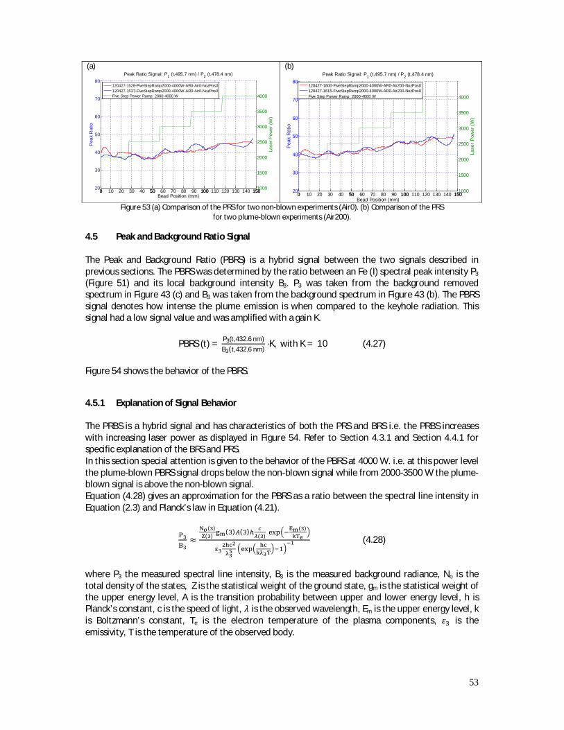
53

(a)

(b)

Figure 53 (a) Comparison of the PRS for two non-blown experiments (Air0). (b) Comparison of the PRS

for two plume-blown experiments (Air200).

4.5 Peak and Background Ratio Signal

The Peak and Background Ratio (PBRS) is a hybrid signal between the two signals described in previous sections. The PBRS was determined by the ratio between an Fe (I) spectral peak intensity P3

(Figure 51) and its local background intensity B3. P3 was taken from the background removed spectrum in Figure 43 (c) and B3 was taken from the background spectrum in Figure 43 (b). The PBRS signal denotes how intense the plume emission is when compared to the keyhole radiation. This signal had a low signal value and was amplified with a gain K.

PBRS (t) = P3(t,432.6 nm)B3(t,432.6 nm) ·K, with K = 10 (4.27)

Figure 54 shows the behavior of the PBRS.

4.5.1 Explanation of Signal Behavior The PRBS is a hybrid signal and has characteristics of both the PRS and BRS i.e. the PRBS increases with increasing laser power as displayed in Figure 54. Refer to Section 4.3.1 and Section 4.4.1 for specific explanation of the BRS and PRS. In this section special attention is given to the behavior of the PBRS at 4000 W. i.e. at this power level the plume-blown PBRS signal drops below the non-blown signal while from 2000-3500 W the plume-blown signal is above the non-blown signal. Equation (4.28) gives an approximation for the PBRS as a ratio between the spectral line intensity in Equation (2.3) and Planck’s law in Equation (4.21).

≈( )

( )( ) ( )

( ) ( )

(4.28)

where P3 the measured spectral line intensity, B3 is the measured background radiance, No is the total density of the states, Z is the statistical weight of the ground state, gm is the statistical weight of the upper energy level, A is the transition probability between upper and lower energy level, h is Planck’s constant, c is the speed of light, 휆 is the observed wavelength, Em is the upper energy level, k is Boltzmann’s constant, Te is the electron temperature of the plasma components, 휀 is the emissivity, T is the temperature of the observed body.

0 10 20 30 40 50 60 70 80 90 100 110 120 130 140 15020

30

40

50

60

70


Bead Position (mm)

Pea

k R

atio

0 50 100 1501000

1500

2000

2500

3000

3500

4000

Lase

r Pow

er (W

)


0 10 20 30 40 50 60 70 80 90 100 110 120 130 140 15020

30

40

50

60

70


Bead Position (mm)

Peak

Rat

io

0 50 100 1501000

1500

2000

2500

3000

3500

4000

Lase

r Pow

er (W

)


54

Just as with the PRS, the electron temperature decreases with increasing Laser power because the collimator observes the cooler shell of the plume. It was also assumed that when the plume was blown away, the plasma was cooled off by blowing. Subsequently causing the electron temperature Te to decrease. But with increased Laser power, the plasma descends into the keyhole, and plume-blowing plays a lesser role on cooling the plasma. Since the cooling effect of plume-blowing decreases with increasing Laser power, Te decreases less rapidly as power increases. This in turn leads to a decrease of the spectral line intensity P3 in Equation (4.28). Take note that although blowing has less effect on the plasma at deep penetration, plume-blowing still cools down the plume which ascends high and surrounds the plasma. Oiwa (2011) found that the plume height reached over 100 mm without blowing air (Section 2.5). Besides affecting the plasma temperature, increasing Laser power is assumed to lead to an increase in temperature T of the meltpool at the keyhole wall (see Figure 48). This in turn leads to an increase of the background radiation B3 in Equation (4.28). By blowing away the plume, the effective Laser power reaching the workpiece surface increases, causing the temperature of the keyhole wall to increase even more. As described earlier, the electron temperature decreases less rapidly with increasing Laser power. This causes the spectral line intensity P3 to decrease less rapid with respect to the increasing background radiation B3. So the ratio between plume and background radiation P3

B3 decreases when

plume-blowing at high Laser power of 4000 W primarily because of the difference in rate of change between the electron temperature Te and workpiece temperature T. (a)

(c)

(b)

(d)

Figure 54 Peak and Background Ratio Signal. AR0: no Argon shielding was used; Air0: non-blown

experiment; Air200: plume-blown experiment in which 200 l/min air was used.

0 10 20 30 40 50 60 70 80 90 100 110 120 130 140 1502

4

6

8

10

12Peak and Background Ratio Signal: P3 (t,432.6 nm) / B3 (t,432.6 nm)

Bead Position (mm)

Pea

k an

d B

ackg

roun

d R

atio

0 50 100 1501000150020002500300035004000

Lase

r Pow

er (W

)

Peak and BackgroundRatioFiltered DataLaser Power

0 10 20 30 40 50 60 70 80 90 100 110 120 130 140 1502

4

6

8

10


Bead Position (mm)

Peak

and

Bac

kgro

und

Rat

io

0 50 100 1501000150020002500300035004000

Lase

r Pow

er (W

)



0 10 20 30 40 50 60 70 80 90 100 110 120 130 140 1502

4

6

8

10

12Peak and Background Ratio: P3 (t,432.6 nm) / B3 (t,432.6 nm)

Bead Position (mm)

Peak

and

Bac

kgro

und

Rat

io

0 50 100 1501000150020002500300035004000

Lase

r Pow

er (W

)

Peak and BackgroundRatioFiltered DataLaser Power

0 10 20 30 40 50 60 70 80 90 100 110 120 130 140 1502

4

6

8

10

12Peak and Background Ratio: P3 (t,432.6 nm) / B3 (t,432.6 nm)

Bead Position (mm)

Pea

k an

d Ba

ckgr

ound

Rat

io

0 50 100 1501000150020002500300035004000

Lase

r Pow

er (W

)



0 10 20 30 40 50 60 70 80 90 100 110 120 130 140 1502

4

6

8

10


Bead Position (mm)

Peak

and

Bac

kgro

und

Rat

io

0 50 100 1501000

1500

2000

2500

3000

3500

4000

Lase

r Pow

er (W

)


0 10 20 30 40 50 60 70 80 90 100 110 120 130 140 1502

4

6

8

10


Bead Position (mm)

Pea

k an

d B

ackg

roun

d R

atio

0 50 100 1501000

1500

2000

2500

3000

3500

4000

Lase

r Pow

er (W

)120427-1537-FiveStepRamp2000-4000W-AR0-Air0-NozPos0120427-1615-FiveStepRamp2000-4000W-AR0-Air200-NozPos0Five Step Power Ramp: 2000-4000 W

55

The Peak and Background Ratio Signal in Figure 54 (b) and (d) also shows similar behavior to the BRS and PRS at the start of the weld i.e. the signal shows a hump at the start of the weld before settling at a lower value. This increased signal value is explained for the BRS in Section 4.3.2 and for the PRS in Section 6.2.

4.6 Signal Validation with Cross Sections Table 7 and Table 8 show the penetration depth for the non-blown and plume-blown case. As is described in the introduction, this thesis only focuses on the effect plume-blowing has on the penetration depth. Other metallurgical aspects such as e.g. hardness or porosity of the weld, are not considered. The results from these tables are averaged and plotted in Figure 55. As proven by Oiwa (2009), plume-blowing does enable deeper welds.

Laser Power

(W)

dw (mm) Experiment: 120427-1528


Average dw (mm)

2000 1.416 1.382 1.399 2500 1.841 1.797 1.819 3000 2.053 2.222 2.1375 3500 2.501 2.488 2.4945 4000 2.813 2.733 2.7730

Table 7 Penetration depths of non-blown experiments.

Laser Power

(W)



Average dw (mm)

2000 1.446 1.469 1.4575 2500 1.841 1.923 1.882 3000 2.209 2.327 2.268 3500 2.632 2.719 2.6755 4000 3.226 3.165 3.1955

Table 8 Penetration depths of plume-blown experiments.

4.6.1 Explanation of Penetration Depth Behavior

The linear fits in Figure 55 show that at low Laser power of 2000 W there is little to no difference between the non-blown and plume-blown penetration depth. This is due to the short height of the low refractive index zone at the start of the weld at low Laser power. The small size of the zone as displayed in Figure 32 at t1 does not influence the Laser beam much on its path towards the workpiece surface. As the Laser power increases, the difference in penetration depth becomes larger as shown in Figure 55. This can be explained by the increase in Laser power which leads to an increased electron temperature in the core of the plasma plume. The increased electron temperature subsequently heats up the surrounding atmosphere, causing the low refractive index zone to increase in size and height. The increased size of the zone, as shown in Figure 32, interfered with the Laser beam such that the beam was refracted and defocussed before reaching the workpiece surface. The error bars for the plume-blown experiments are relatively steady with the exception of experiments conducted at 2000 W while the error bars of the non-blown experiments vary significantly over the entire power range.

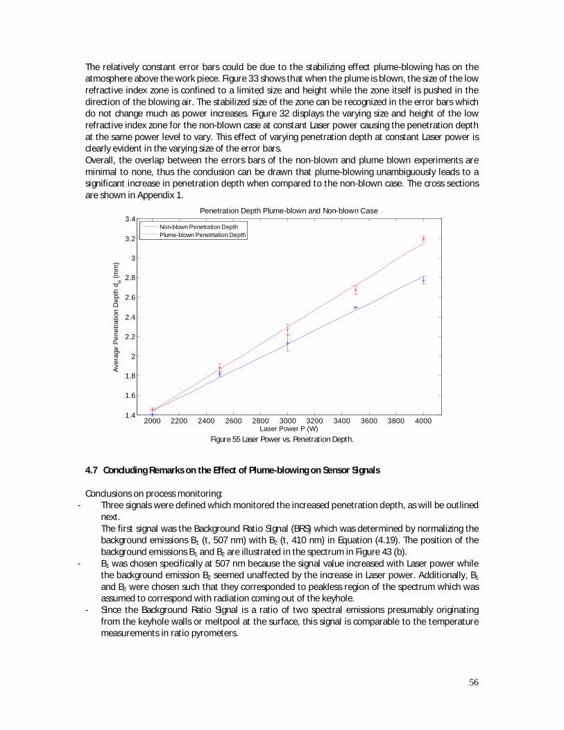
56

The relatively constant error bars could be due to the stabilizing effect plume-blowing has on the atmosphere above the work piece. Figure 33 shows that when the plume is blown, the size of the low refractive index zone is confined to a limited size and height while the zone itself is pushed in the direction of the blowing air. The stabilized size of the zone can be recognized in the error bars which do not change much as power increases. Figure 32 displays the varying size and height of the low refractive index zone for the non-blown case at constant Laser power causing the penetration depth at the same power level to vary. This effect of varying penetration depth at constant Laser power is clearly evident in the varying size of the error bars. Overall, the overlap between the errors bars of the non-blown and plume blown experiments are minimal to none, thus the conclusion can be drawn that plume-blowing unambiguously leads to a significant increase in penetration depth when compared to the non-blown case. The cross sections are shown in Appendix 1.

Figure 55 Laser Power vs. Penetration Depth.

4.7 Concluding Remarks on the Effect of Plume-blowing on Sensor Signals Conclusions on process monitoring:

- Three signals were defined which monitored the increased penetration depth, as will be outlined next. The first signal was the Background Ratio Signal (BRS) which was determined by normalizing the background emissions B1 (t, 507 nm) with B2 (t, 410 nm) in Equation (4.19). The position of the background emissions B1 and B2 are illustrated in the spectrum in Figure 43 (b).

- B1 was chosen specifically at 507 nm because the signal value increased with Laser power while the background emission B2 seemed unaffected by the increase in Laser power. Additionally, B1 and B2 were chosen such that they corresponded to peakless region of the spectrum which was assumed to correspond with radiation coming out of the keyhole.

- Since the Background Ratio Signal is a ratio of two spectral emissions presumably originating from the keyhole walls or meltpool at the surface, this signal is comparable to the temperature measurements in ratio pyrometers.

2000 2200 2400 2600 2800 3000 3200 3400 3600 3800 40001.4

1.6

1.8

2

2.2

2.4

2.6

2.8

3

3.2

3.4

Laser Power P (W)

Aver

age

Pen

etra

tion

Dep

th d

w (m

m)

Penetration Depth Plume-blown and Non-blown Case

Non-blown Penetration DepthPlume-blown Penetrtation Depth

57

- The BRS failed to measure the penetration depth in a consistent manner. Figure 47 shows that the signal increases with Laser power but the plume-blown signal does not increase above the non-blown signal as is expected from the penetration depth measurements shown Figure 55.

- Yet this signal gives insight into the keyhole behavior since it is assumed to be caused in part by keyhole radiation. Section 4.3.2 describes how this signal, in addition to the penetration depth, also measures the change in emissivity of the keyhole caused by the change in keyhole shape at high Laser power.

- The Peak Ratio Signal (PRS) was determined from the ratio between an Fe (I) and Mn (I) peak

(See Equation (4.23)). Figure 51 shows the peak identified plot of a background removed spectrum. The peak intensities P1 and P2 were taken from the background removed spectrum as is displayed in Figure 43 (c).

- The PRS is the only signal which succeeds over the entire power range from 2500 W-4000 W. This signal is explained in Section 4.4.1 by considering the decrease in observed electron temperature as the keyhole becomes deeper. Also, the cooling effect which plume-blowing has on the plasma is considered. Besides the electron temperature, the PRS could also be a measure of the relative presence of Fe (I) and Mn (I) particles in an excited state, as is described by Equation (4.24).

- The PRS is calculated by using spectral emissions from two different species while the electron temperature signal of Konuk (2011) and Sibillano (2010) is based on spectral emissions of the same species.

- Since this signal consistently succeeds in monitoring the penetration depth, it is used in the following chapters for system identification, controller design and implementation.

- The Peak and Background Ratio Signal (PBRS) is a hybrid signal between the PRS and BRS. The

PBRS was determined by the ratio between an Fe(I) spectral peak intensity P3 and its local background intensity B3 (see Equation (4.27)). P3 was taken from the background removed spectrum in Figure 43 (c) and B3 was taken from the background spectrum in Figure 43 (b). The PBRS signal denotes how intense the plume emission is when compared to the keyhole radiation. Between 3000 W-4000 W the signal fails to measure the increased penetration depth caused by plume blowing. This behavior is noticeable when the plume-blown signal drops below the non-blown signal in Figure 54 (b) and (d). In Section 4.5.1 it is explained how the difference in rate of change of the electron temperature and keyhole wall temperature caused the signal to fail at high Laser power of 4 kW.

Conclusions on weld efficiency: - The linear fits in Figure 55 show that at low Laser power of 2000 W there is little to no difference

between the non-blown and plume-blown penetration depth. This is due to the short height of the low refractive index zone at the start of the weld which does not interfere much with the Laser beam (Figure 32 at t1).

- As the Laser power increases, the difference in penetration depth becomes larger as shown in Figure 55. This can be explained by the increase in Laser power which leads to an increased electron temperature in the core of the plasma plume. The increased electron temperature subsequently heats up the surrounding atmosphere, causing the low refractive index zone to increase in size and height. The increased size of the zone, as shown in Figure 32, interfered with the Laser beam such that the beam was refracted and defocussed before reaching the workpiece surface.

- Plume-blowing has proven to decrease this low refractive index zone, and consequently increased the penetration depth with 0.4 mm at 4000 W in Figure 55.

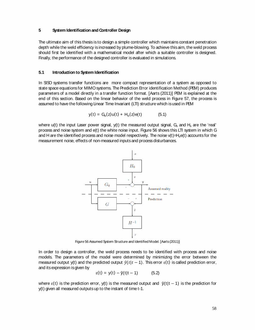
58

5 System Identification and Controller Design The ultimate aim of this thesis is to design a simple controller which maintains constant penetration depth while the weld efficiency is increased by plume-blowing. To achieve this aim, the weld process should first be identified with a mathematical model after which a suitable controller is designed. Finally, the performance of the designed controller is evaluated in simulations.

5.1 Introduction to System Identification In SISO systems transfer functions are more compact representation of a system as opposed to state space equations for MIMO systems. The Prediction Error identification Method (PEM) produces parameters of a model directly in a transfer function format. [Aarts (2011)] PEM is explained at the end of this section. Based on the linear behavior of the weld process in Figure 57, the process is assumed to have the following Linear Time Invariant (LTI) structure which is used in PEM

y(t) = G (z)u(t) + H (z)e(t) (5.1)

where u(t) the input Laser power signal, y(t) the measured output signal, Go and Ho are the ‘real’ process and noise system and e(t) the white noise input. Figure 56 shows this LTI system in which G and H are the identified process and noise model respectively. The noise v(t)=Hoe(t) accounts for the measurement noise, effects of non-measured inputs and process disturbances.

Figure 56 Assumed System Structure and Identified Model. [Aarts (2011)]

In order to design a controller, the weld process needs to be identified with process and noise models. The parameters of the model were determined by minimizing the error between the measured output y(t) and the predicted output 푦(푡|푡 − 1). This error ε(t) is called prediction error, and its expression is given by

ε(t) = y(t)− y(t|t− 1) (5.2) where ε(t) is the prediction error, y(t) is the measured output and y(t|t− 1) is the prediction for y(t) given all measured outputs up to the instant of time t-1.

59

The minimization of ε(t) was achieved by minimizing the Least Squares Criterion as expressed by the cost function VN

푉 (휃) =1푁

휀(푡,휃) (5.3)

Where N is the total number of measured samples, 휃 is the parameter set of the chosen model structure and ε(t) is the prediction error. Table 9 displays four model structures with polynomials A (z-1,θ), B (z-1,θ), C (z-1,θ), D (z-1,θ) and F (z-1,θ). The polynomials A, B, C, D and F are expressed as

퐴(푧 ,휃) = 1 + 푎 푧 +⋯+ 푎 푧 (5.4) 퐵(푧 ,휃) = 푏 + 푏 푧 +⋯+ 푏 푧 ( ) (5.4) 퐶(푧 ,휃) = 1 + 푐 푧 + ⋯+ 푐 푧 (5.4) 퐷(푧 ,휃) = 1 + 푑 푧 +⋯+ 푑 푧 (5.4) 퐹(푧 ,휃) = 1 + 푓 푧 + ⋯+ 푓 푧 (5.4)

where z is the shift operator and ai, bi, ci, di, fi are the model parameters After choosing the model structure and calculation of the Least Squares Criterion, the parameter set 휃 is obtained. This method of estimating the parameters is called the Prediction Error Method (PEM). The ARX (AutoRegressive eXogenous) structure in Table 9 has a prediction y(t|t− 1) and a prediction error ε(t) which are linear in the parameters. So linear least square techniques are applied to minimize the cost function Vn in Equation (5.3). An unique and global optimum parameter set is then quickly obtained. The other structures in Table 9 such as ARMAX (AutoRegressive Moving Average), BJ (Box-Jenkin) and OE (Output Error) have prediction errors ε(t) which are not linear in the parameters. The model parameters are then determined by minimizing Vn with non-linear optimization techniques. The BJ structure has a separate noise model while the OE model only accounts for the process structure.

Model Name Mathematical Eqauaion G(z,θ) H(z, θ)

ARX 퐴(푧 ,휃)푦(푡) = 퐵(푧 ,휃)푢(푡) + 푒(푡) 퐵(푧 ,휃)퐴(푧 ,휃)

1퐴(푧 ,휃)

ARMAX 퐴(푧 ,휃)푦(푡) = 퐵(푧 ,휃)푢(푡) + 퐶(푧 ,휃)푒(푡) 퐵(푧 ,휃)퐴(푧 ,휃)

퐶(푧 ,휃)퐴(푧 ,휃)

BJ 푦(푡) =퐵(푧 ,휃)퐹(푧 ,휃)푢

(푡) +퐶(푧 ,휃)퐷(푧 ,휃) 푒(푡)

퐵(푧 ,휃)퐹(푧 ,휃)

퐶(푧 ,휃)퐷(푧 ,휃)

OE 푦(푡) =퐵(푧 ,휃)퐹(푧 ,휃) 푢

(푡) + 푒(푡) 퐵(푧 ,휃)퐹(푧 ,휃) 1

Table 9 Overview of model structures.

5.2 Identification of the Weld Process Before a model structrure could be chosen, the linear behavior of the weld process was verified by plotting the averaged Peak Ratio Signal (PRS) against the Laser power. The Average PRS was determined by the mean of the PRS in the region corresponding to constant Laser power. Figure 57 shows the relation between the Average PRS and the Laser power. Linear behavior is clearly visible when fitting a straight line to the data. The R2 value of the fit was also nearly equal to one, indicating that the fit succesfully accounted for the variation of the data around its average. The PRS data used for this test was the same as the evaluation dataset used for identification of the weld process.

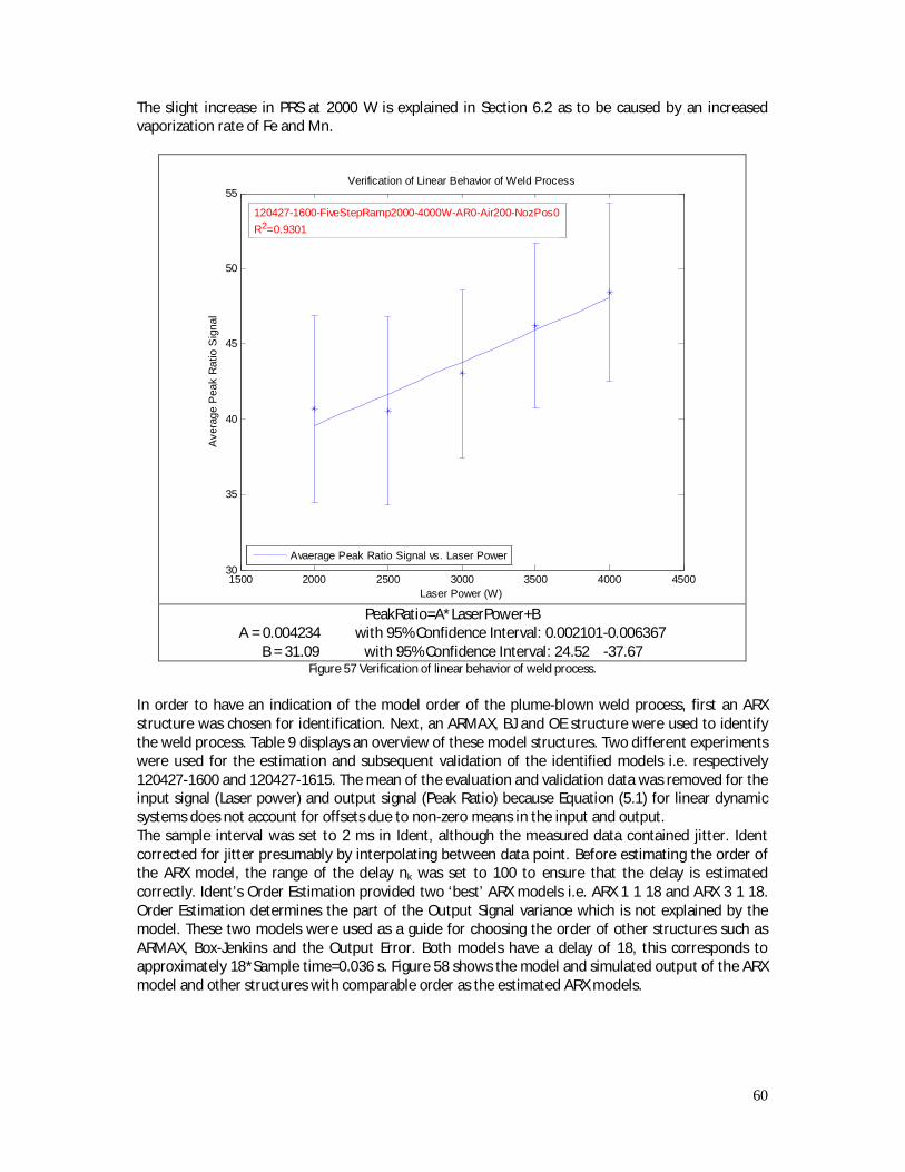
60

The slight increase in PRS at 2000 W is explained in Section 6.2 as to be caused by an increased vaporization rate of Fe and Mn.

PeakRatio=A*LaserPower+B

A = 0.004234 with 95% Confidence Interval: 0.002101-0.006367 B = 31.09 with 95% Confidence Interval: 24.52 -37.67

Figure 57 Verification of linear behavior of weld process. In order to have an indication of the model order of the plume-blown weld process, first an ARX structure was chosen for identification. Next, an ARMAX, BJ and OE structure were used to identify the weld process. Table 9 displays an overview of these model structures. Two different experiments were used for the estimation and subsequent validation of the identified models i.e. respectively 120427-1600 and 120427-1615. The mean of the evaluation and validation data was removed for the input signal (Laser power) and output signal (Peak Ratio) because Equation (5.1) for linear dynamic systems does not account for offsets due to non-zero means in the input and output. The sample interval was set to 2 ms in Ident, although the measured data contained jitter. Ident corrected for jitter presumably by interpolating between data point. Before estimating the order of the ARX model, the range of the delay nk was set to 100 to ensure that the delay is estimated correctly. Ident’s Order Estimation provided two ‘best’ ARX models i.e. ARX 1 1 18 and ARX 3 1 18. Order Estimation determines the part of the Output Signal variance which is not explained by the model. These two models were used as a guide for choosing the order of other structures such as ARMAX, Box-Jenkins and the Output Error. Both models have a delay of 18, this corresponds to approximately 18*Sample time=0.036 s. Figure 58 shows the model and simulated output of the ARX model and other structures with comparable order as the estimated ARX models.

1500 2000 2500 3000 3500 4000 450030

35

40

45

50

55

Laser Power (W)

Ave

rage

Pea

k R

atio

Sig

nal

Verification of Linear Behavior of Weld Process

Avaerage Peak Ratio Signal vs. Laser Power

120427-1600-FiveStepRamp2000-4000W-AR0-Air200-NozPos0R2=0.9301

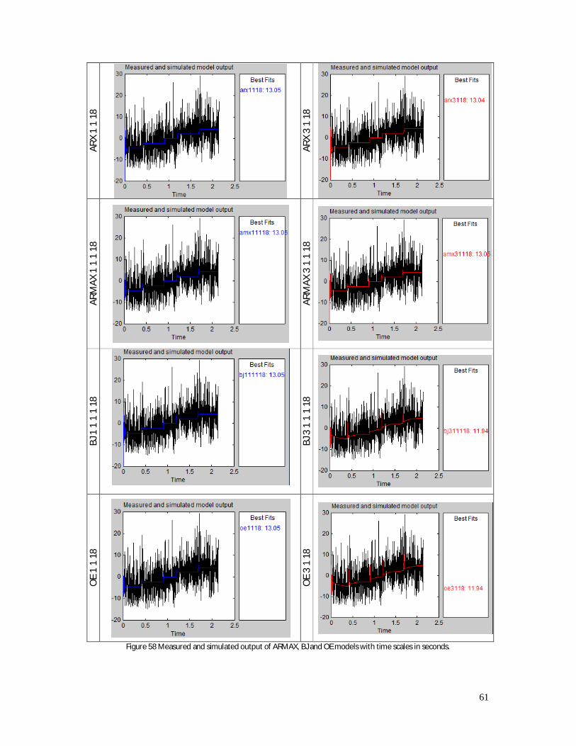
61

ARX

1 1

18

ARX

3 1

18

ARM

AX 1

1 1

18

ARM

AX 3

1 1

18

BJ 1

1 1

1 1

8

BJ 3

1 1

1 1

8

OE

1 1

18

OE

3 1

18

Figure 58 Measured and simulated output of ARMAX, BJ and OE models with time scales in seconds.

62

Although the initial states are accounted for in the ARX, ARMAX, BJ and OE models, the simulated model output shows a disturbance around t=0 s. The models also do not seem to cope very well with the 500 W power increase of the input ramp signal. Both ARX, ARMAX and the BJ 1 1 1 1 18 show a simulated output which follows the input signal in an expected manner. Both ARMAX models and the BJ 1 1 1 1 18 show some form of overshoot when the input signal rises with a step. This overshoot is an unexpected result, thus the ARX models are chosen as the best. The two ARX structures are now studied in more detail to decide the most suitable structure for the weld process. First the transfer function is verified, residual tests are conducted and then the dynamic behavior of models is studied. The transfer functions for the process models G and noise models H of the ARX models are given in Table 10.

ARX 1 1 18

퐺 = . .

(5.5)

퐻 = .

푤푖푡ℎ 푣푎푟(푒) = 35.004 (5.6)

ARX 3 1 18

퐺 = . . . .

(5.7)

퐻 = . . .

,푤푖푡ℎ 푣푎푟(푒) = 35.036 (5.8)

Table 10 Equations for the chosen ARX models. The evaluation and validation experiments were static identification methods since the input signal was a five step ramp between 2-4 kW. If a signal with zero frequency was applied as an input to the ARX 1 1 18 model the following gain factor was obtained 퐺(푧 = 1) = 0.0043. The ARX 3 1 18 also gave the same result for zero frequency signals. The ARX static gains are comparable to the slope in Figure 57, so the chosen ARX structures do model the proces well for static identification. The noise models are not studied in detail because they are only used as an additive noise term and to design a controller which should be robust against noise. When the identified models G and H in Figure 56 are equal to the real system and noise Go and Ho, 휀(푡) equals a white noise signal. Two tests were carried out to know whether the process model G and the noise model H were acceptable i.e.

- Test for both process and noise model. Is ε(t) a white noise signal: the autocorrelation of 휀(푡) should approximate a dirac delta function 훿(푡).

- Test for the process model. Is 휀(푡) a consequence of a stochastic process: the cross correlation between the prediction error 휀(푡) and the input signal u(t) should be zero.

Figure 60 shows the residual tests for the ARX models. The auto covariance and cross covariance test for both the system and noise model are within the confidence interval, so both ARX models are acceptable. The chosen model must be simple yet it should contain the dynamics of the weld process. The frequency response plots of the process and noise models of ARX 1 1 18 and ARX 3 1 18 in Figure 59 (a) and (b) do not show anything peculiar. The frequency response plots show that neither model contains information on the process dynamics, presumably, because the input ramp signal did not excite the weld process sufficiently. The frequency response does show that the ARX 3 1 18 contains more information about the weld process than ARX 1 1 18.

63

The noise response plots of both models are relatively flat e.g. the ARX 3 1 18 noise model varies between -0.3-0.4 dB≈0.97-1.05. This suggests that an OE model, preferably the OE 3 1 18, could be suitable for identification. In order to decide whether the OE model is applicable or not, the residual tests were carried out for the two OE models. The autocorrelation of residuals for the OE 3 1 18 in Figure 61 rises above the confidence interval, indicating that either the process or noise model are not acceptable. Since the cross correlation is within the confidence interval, the process model of OE 3 1 18 is acceptable. So the unit noise model does not match the ‘real’ noise that is present during the weld experiments and the OE model is discarded as a possible model. The ARX 3 1 18 is thus chosen as a suitable model for which a controller is designed.

(a) Process Models (b) Noise models

Figure 59 Bode plot of process and noise model.

ARX 1 1 18 ARX 3 1 18

Figure 60 Residual tests for the ARX models.

-48

-47.8

-47.6

-47.4

-47.2From: u1 To: y1

Mag

nitu

de (

dB)

100

101

102

103

-3600

-2880

-2160

-1440

-720

0

Pha

se (

deg)

Bode Diagram

Frequency (rad/s)

ARX 1 1 18ARX 3 1 18

-0.4

-0.2

0

0.2

0.4From: e@y1 To: y1

Mag

nitu

de (

dB)

100

101

102

103

-3

-2

-1

0

1

2

Phas

e (d

eg)

Bode Diagram

Frequency (rad/s)

ARX 1 1 18ARX 3 1 18

-20 -15 -10 -5 0 5 10 15 20-0.1

-0.05

0

0.05

0.1

Autocorrelation of residuals for output y1

-20 -15 -10 -5 0 5 10 15 20-0.2

-0.1

0

0.1

0.2

Samples

Cross corr for input u1 and output y1 resids

-20 -15 -10 -5 0 5 10 15 20-0.1

-0.05

0

0.05

0.1


-20 -15 -10 -5 0 5 10 15 20-0.2

-0.1

0

0.1

0.2

Samples


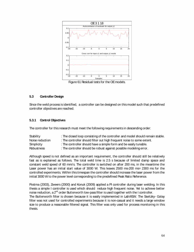
64

OE 3 1 18

Figure 61 Residual tests for the OE models.

5.3 Controller Design Since the weld process is identified, a controller can be designed on this model such that predefined controller objectives are reached.

5.3.1 Control Objectives The controller for this research must meet the following requirements in descending order: Stability : The closed loop consisting of the controller and model should remain stable. Noise reduction : The controller should filter out high frequent noise to some extent. Simplicity : The controller should have a simple form and be easily tunable. Robustness : The controller should be robust against possible modeling error. Although speed is not defined as an important requirement, the controller should still be relatively fast as is explained as follows. The total weld time is 2.5 s because of limited clamp space and constant weld speed of 60 mm/s. The controller is switched on after 200 ms, in the meantime the Laser power has an initial start value of 3000 W. This leaves 2500 ms-200 ms= 2300 ms for the controlled experiments. Within this timespan the controller should increase the laser power from the initial 3000 W to the power level corresponding to the predefined Peak Ratio Reference. Postma (2003), Zweers (2000) and Konuk (2009) applied a PI controller during laser welding. In this thesis a simple I controller is used which should reduce high frequent noise. Yet to achieve better noise reduction, a 2nd order Butterworth low-pass filter is used together with the I controller. The Butterworth filter is chosen because it is easily implemented in LabVIEW. The Savitzky- Golay filter was not used for controlled experiments because it is non-casual and it needs a large window size to produce a reasonable filtered signal. This filter was only used for process monitoring in this thesis.

-20 -15 -10 -5 0 5 10 15 20-0.1

-0.05

0

0.05

0.1


-20 -15 -10 -5 0 5 10 15 20-0.2

-0.1

0

0.1

0.2

Samples


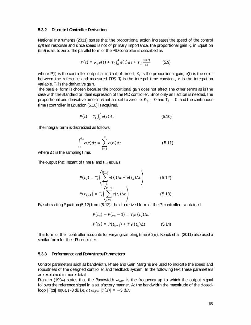
65

5.3.2 Discrete I Controller Derivation National Instruments (2011) states that the proportional action increases the speed of the control system response and since speed is not of primary importance, the proportional gain Kp in Equation (5.9) is set to zero. The parallel form of the PID controller is described as

푃(푡) = 퐾 푒(푡) + 푇 ∫ 푒(휏)푑휏 + 푇 ( ) (5.9)

where P(t) is the controller output at instant of time t, Kp is the proportional gain, e(t) is the error between the reference and measured PRS, Ti is the integral time constant, 휏 is the integration variable, Td is the derivative gain. The parallel form is chosen because the proportional gain does not affect the other terms as is the case with the standard or ideal expression of the PID controller. Since only an I action is needed, the proportional and derivative time constant are set to zero i.e. K = 0 and T = 0, and the continuous time I controller in Equation (5.10) is acquired.

푃(푡) = 푇 ∫ 푒(휏)푑휏 (5.10)

The integral term is discretized as follows

푒(휏)푑휏 = 푒(푡 )Δ푡 (5.11)

where Δ푡 is the sampling time.

The output P at instant of time tk and tk-1 equals

푃(푡 ) = 푇 푒(푡 )Δ푡 + 푒(푡 )Δ푡 (5.12)

푃(푡 ) = 푇 푒(푡 )Δ푡 (5.13)

By subtracting Equation (5.12) from (5.13), the discretized form of the PI controller is obtained

푃(푡 )− 푃(푡 − 1) = 푇 푒 (푡 )Δ푡

푃(푡 ) = 푃(푡 ) + 푇 푒 (푡 )Δ푡 (5.14) This form of the I controller accounts for varying sampling time Δ푡(푘). Konuk et al. (2011) also used a similar form for their PI controller.

5.3.3 Performance and Robustness Parameters Control parameters such as bandwidth, Phase and Gain Margins are used to indicate the speed and robustness of the designed controller and feedback system. In the following text these parameters are explained in more detail. Franklin (1994) states that the Bandwidth 휔 is the frequency up to which the output signal follows the reference signal in a satisfactory manner. At the bandwidth the magnitude of the closed-loop |T(z)| equals -3 dB i.e. 푎푡 휔 |푇(푧)| = −3 푑퐵.

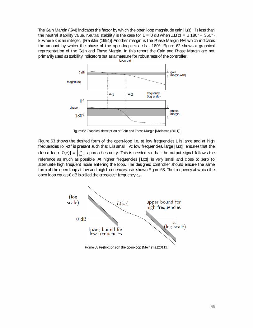
66

The Gain Margin (GM) indicates the factor by which the open loop magnitude gain |L(z)| is less than the neutral stability value. Neutral stability is the case for L = 0 dB when ∠L(z) = ±180° + 360° ∙k, where k is an integer. [Franklin (1994)] Another margin is the Phase Margin PM which indicates the amount by which the phase of the open-loop exceeds −180°. Figure 62 shows a graphical representation of the Gain and Phase Margin. In this report the Gain and Phase Margin are not primarily used as stability indicators but as a measure for robustness of the controller.

Figure 62 Graphical description of Gain and Phase Margin [Meinsma (2011)]

Figure 63 shows the desired form of the open-loop i.e. at low frequencies L is large and at high frequencies roll-off is present such that L is small. At low frequencies, large |L(z)| ensures that the closed loop |푇(푧)| = approaches unity. This is needed so that the output signal follows the reference as much as possible. At higher frequencies |L(z)| is very small and close to zero to attenuate high frequent noise entering the loop. The designed controller should ensure the same form of the open-loop at low and high frequencies as is shown Figure 63. The frequency at which the open loop equals 0 dB is called the cross over frequency 휔 .

Figure 63 Restrictions on the open-loop [Meinsma (2011)].

67

5.3.4 Controller Implementation in Simulink Since the identified model of the weld process is available, the discrete I controller can now be evaluated in simulations. By varying the integral time constant Ti, the ‘best’ controller will be chosen with the help of performance and robustness parameters described in section 5.3.3. Figure 64 shows the feedback setup in Simulink which was used for controller simulations. The feedback setup consisted of the I controller, Butterworth filter and ARX process and noise model. During the first 200 ms of the simulation, the Laser power was set constant to 3000 W. After 200 ms, a switch enabled the controller which steered the weld process to the reference PRS value. This reference was set to a signal value which corresponded to a Laser power between 3000-4000 W. Simulations were carried out between 3000 W and 4000 W because the effect of plume-blowing was best observed at high power levels, as shown in Figure 55. The chosen reference value equaled 47.

Figure 64 Feedback setup in Simulink.

As a start value, the integral time constant Ti was set to 900 s because for this specific value the controller filtered the sensor noise reasonably and caused a fast response. This can be seen from Figure 66 (d) and Table 11. The frequency responses for the open and closed loop without low-pass filter are shown in Figure 65. Figure 65 (a) shows that the cross over frequency lies at approximately 4 rad/s. Above the cross over frequency the open-loop L(z) filters high frequent noise out of the sensor signal. Figure 65 (b) shows that below the bandwidth of approximately 5 rad/s the complementary sensitivity |T(z)| equaled 0 dB allowing the sensor output to follow the reference signal. The cross over frequency and the closed loop bandwidth are measures for the speed and performance of the closed loop. Next, the speed and robustness of the feedback setup were monitored by varying Ti from ∙ 900 −2 ∙ 900 s, as displayed in Table 11. Figure 66 shows the controller and low-pass filter output for multiples of Ti=900 s. Table 11 shows the results for the bandwidth and margins for multiples of Ti. Besides the controller output, Figure 66 shows the low-pass filter output. In all situations the cut-off frequency of the Butterworth filter was set to 5*휔 to prevent the Butterworth filter interfering with the controller as is suggested by Aarts (2010).

ButterworthFilter

Controll erOff

ControllerOn

Controll erAndFil terOutputTo Workspace1 SimulatedSensorSignalTo Workspace

Scope2

47

Reference

RandomNumber

-C-PowerMean3028 W

-C-PeakRetioMean44

???Noise Model3000Ini tial

Power

???

Identifi ed Weld Process

I(z)

Discrete I Controll er

Bad Link

0

Control lerInput and Reference

ControllerAndButterworthOutput

100Controll er

Swi tch

GARX 3 1 18

HARX

3 1 18

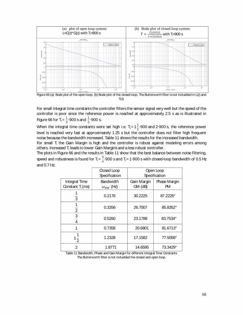
68

(a) plot of open loop system: L=C(z)*G(z) with Ti=900 s

(b) Bode plot of closed loop system: 푇 = ( ) ( )

( ) ( ) with Ti=900 s

Figure 65 (a) Bode plot of the open-loop. (b) Bode plot of the closed-loop. The Butterworth filter is not includded in L(z) and

T(z). For small integral time constants the controller filters the sensor signal very well but the speed of the controller is poor since the reference power is reached at approximately 2.5 s as is illustrated in Figure 66 for Ti=

13∙900 s and 1

2∙900 s.

When the integral time constants were set high i.e. Ti=1 12∙900 and 2∙900 s, the reference power

level is reached very fast at approximately 1.25 s but the controller does not filter high frequent noise because the bandwidth increased. Table 11 shows the results for the increased bandwidth. For small Ti the Gain Margin is high and the controller is robust against modeling errors among others. Increased Ti leads to lower Gain Margins and a less robust controller. The plots in Figure 66 and the results in Table 11 show that the best balance between noise filtering, speed and robustness is found for Ti=

34∙900 s and Ti=1∙900 s with closed-loop bandwidth of 0.5 Hz

and 0.7 Hz.

Closed Loop Specification

Open Loop Specification

Integral Time Constant Ti (ms)

Bandwidth 휔 (Hz)

Gain Margin GM (dB)

Phase Margin PM

13

0.2176 30.2225 87.2226°

12

0.3356 26.7007 85.8352°

34

0.5260 23.1788 83.7534°

1 0.7358 20.6801 81.6713°

112

1.2328 17.1582 77.5058°

2 1.8771 14.6595 73.3429° Table 11 Bandwidth, Phase and Gain Margin for different Integral Time Constants.

The Butterworth filter is not includded the closed and open loop.

-40

-20

0

20

40From: u1 To: Out(1)

Mag

nitu

de (d

B)

10-1 100 101 102 103-720

-540

-360

-180

0

Phas

e (d

eg)

Bode Diagram

Frequency (rad/sec)

Open Loop

-50

-40

-30

-20

-10

0From: u1 To: Out(1)

Mag

nitu

de (d

B)

10-1 100 101 102 103-720

-540

-360

-180

0

Phas

e (d

eg)

Bode Diagram

Frequency (rad/sec)

Closed Loop

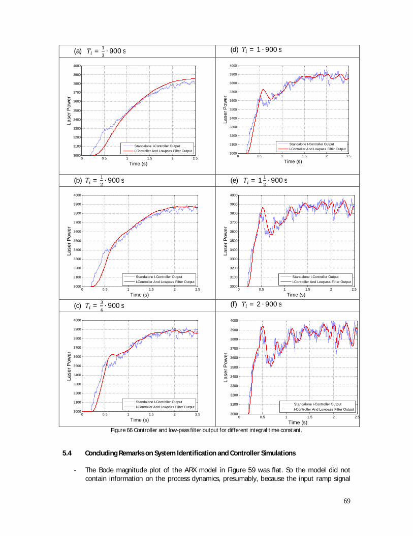
69

(a) 푇 = ∙ 900 s (d) 푇 = 1 ∙ 900 s

(b) 푇 = ∙ 900 s (e) 푇 = 1 ∙ 900 s

(c) 푇 = ∙ 900 s (f) 푇 = 2 ∙ 900 s

Figure 66 Controller and low-pass filter output for different integral time constant.

5.4 Concluding Remarks on System Identification and Controller Simulations

- The Bode magnitude plot of the ARX model in Figure 59 was flat. So the model did not contain information on the process dynamics, presumably, because the input ramp signal

0 0.5 1 1.5 2 2.53000

3100

3200

3300

3400

3500

3600

3700

3800

3900

4000

Time (s)

Lase

r Pow

er

Standalone I-Controller OutputI-Controller And Lowpass Filter Output

0 0.5 1 1.5 2 2.53000

3100

3200

3300

3400

3500

3600

3700

3800

3900

4000

Time (s)

Lase

r Pow

er


0 0.5 1 1.5 2 2.53000

3100

3200

3300

3400

3500

3600

3700

3800

3900

4000

Time (s)

Lase

r Pow

er


0 0.5 1 1.5 2 2.53000

3100

3200

3300

3400

3500

3600

3700

3800

3900

4000

Time (s)

Lase

r Pow

er


0 0.5 1 1.5 2 2.53000

3100

3200

3300

3400

3500

3600

3700

3800

3900

4000

Time (s)

Lase

r Pow

er


0 0.5 1 1.5 2 2.53000

3100

3200

3300

3400

3500

3600

3700

3800

3900

4000

Time (s)

Lase

r Pow

er


70

(Section 3.2.3) did not excite the weld process sufficiently. This will lead to differences between the real physical process and the identified model. Implementation of the controller in Chapter 6 proves that the designed controller was not robust against these differences.

- The noise model of the ARX in Figure 59 is flat and suggests that an OE structure is also a candidate for identifying the weld process but the residual tests (Figure 61) have shown that the identified noise model did not match the ‘real’ noise model. Since one of the controller objectives was noise reduction, it is of importance to have an accurate noise model which matches the noise system of the weld process to some extent.

- The ‘best’ controller for the weld process has an integral time constant Ti between ∙ 900 s and 1 ∙ 900 s.

- Controllers with lower Ti have a low bandwidth. Thus these controllers are slow but filter high frequent sensor and process noise reasonably.

- Controllers with higher Ti have an increased bandwidth. Thus they are fast and filter high frequent noise very poorly. Figure 66 shows the controller output for multiples of Ti and Table 11 shows the performance and robustness parameters of the controller.

- The standalone I controller filtered high frequent noise reasonably well and will be implemented without the Butterworth filter in Chapter 6.

- The spectrometer did not sample at a constant rate, nonetheless the identification and controller simulation were performed at a constant sample rate. This could also have lead to differences between the identified model and physical process.

71

6 Controller Implementation In Chapter 5 the identified model of the physical process was determined. Based on this model, the I controller was evaluated in simulations by varying the integral time constant. Subsequently the most suitable controller was then chosen. In this chapter the designed controller is implemented on the real physical process while the plume is blown away.

6.1 Introduction In Section 5.3.4 the most suitable controllers had an integral time constant Ti between ∙ 900− 1 ∙900 s. Before carrying out these controlled experiments, a characterization experiment as shown in Figure 68 (a) was conducted. This is done in order to find the relation between the Peak Ratio Signal (PRS) and the corresponding Laser power and penetration depth as shown in Figure 67. With this relation, appropriate PRS reference values were chosen. Figure 68 (b) and (c) display the results for two controlled experiments with PRS references of 50 and 55. The sample time during controlled experiments had a minimum of 13 ms but still varied. For the first 200 ms the Laser power was kept constant at 3000 W because the initial error was far too large for the controller to cope with. During the time window of 200 ms the keyhole was formed and the PRS enters a controllable region, thus preventing the integral windup.

6.2 Evaluation of Characterization Experiment Before the controlled experiments were conducted, a characterization experiment was carried out to set the PRS reference value. Figure 67 (b) displays the static behavior of the weld process of this characterization experiment. The static gain was determined by the slope in Figure 67 (b) and equaled 0.004 which is quite comparable to the static gain of the identified weld process in Figure 57. Yet there is an upward shift in signal value when comparing the Peak Ratio Signal of both processes. This could be caused by the difference in chemical composition of the material batches (Table 5) or by the oxidation layer at the top of the workpiece. Also, the difference in PRS signal could be caused by different dark current removal processing step in LabVIEW, as described in Section 3.1.3. The linear curve in Figure 67 (b) best fits the PRS from 2500 W-4000 W. The PRS at 2000 W is assumed to be an outlying data point, as will be explained next. At the start of the weld when the Laser beam hits the workpiece surface, the weld starts out in conduction mode. In this mode the melt pool is very small and there is a lack of efficient convective cooling. This causes the vaporization rate of elements such as Mn to increase strongly. Dulley (1999) even goes as far as to state that Mn is preferentially lost in conduction mode welding of stainless steel. If assumed that Fe also has an increased vaporization rate in conduction mode welding, the ratio of the total density of Fe and Mn, ( )

( ) in Equation (4.26), could increase. This could result in an

increased intensity ratio, in Equation (4.26). Thus the outlying PRS value at 2000 W in Figure 67 is

most likely explained by the increased vaporization rate of Fe and Mn in the conduction mode. As is the case with the signal explanation in Chapter 4, this conclusion should be interpreted with caution since the measured intensity was not calibrated.

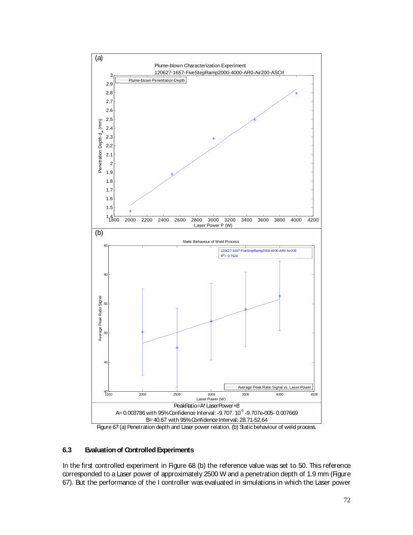
72

(a)

(b)

PeakRatio=A*LaserPower+B

A= 0.003786 with 95% Confidence Interval: -9.707. 10-5 -9.707e-005- 0.007669 B= 40.67 with 95% Confidence Interval: 28.71-52.64

Figure 67 (a) Penetration depth and Laser power relation. (b) Static behaviour of weld process.

6.3 Evaluation of Controlled Experiments In the first controlled experiment in Figure 68 (b) the reference value was set to 50. This reference corresponded to a Laser power of approximately 2500 W and a penetration depth of 1.9 mm (Figure 67). But the performance of the I controller was evaluated in simulations in which the Laser power

1800 2000 2200 2400 2600 2800 3000 3200 3400 3600 3800 4000 42001.4

1.5

1.6

1.7

1.8

1.9

2

2.1

2.2

2.3

2.4

2.5

2.6

2.7

2.8

2.9

3

Laser Power P (W)

Pene

tratio

n D

epth

dw (m

m)

Plume-blown Characterization Experiment120627-1657-FiveStepRamp2000-4000-AR0-Air200-ASCII

Plume-blown Penetrtation Depth

1500 2000 2500 3000 3500 4000 450040

45

50

55

60

65

Laser Power (W)

Ave

rage

Pea

k R

atio

Sig

nal

Static Behaviour of Weld Process

Average Peak Ratio Signal vs. Laser Power

120627-1657-FiveStepRamp2000-4000-AR0-Air200R2= 0.7624

73

was steered from 3000 W to a reference power level of 3850 W (Figure 66 in Section 5.3.4). So the reference power level for this controlled experiment was not in the power interval in which the simulations were carried out. This likely explains the strong fluctuating behavior of the power signal with large amplitude in Figure 68 (b). The penetration depth is displayed as bars with bullets on each end and also displays the strong fluctuating behavior of the Laser power. Section 1 at the start of the weld shows a depth of 2.240 mm. Next, the penetration depth decreases in Section 2 and 3 to respectively 2.140 mm and 1.856 mm. In section 4 and 5 the penetration depth increases significantly to 2.383 mm and 2.488 mm respectively. The cross sections of the penetration depth displayed in Figure 67 (a) and Figure 68 (b) and (c) are shown in Appendix 1. As described above, the choice of the Laser power reference value is likely to be the cause of the fluctuating depth. Postma et al. (2002) also encountered a similar situation. In Section 2.4.1 it is described how they designed a controller based on an identified plant which maintained full penetration. Whenever Postma set his sensor reference value close to the transition value of partial to full penetration, the amplitude of the fluctuations of the feedback and Laser power signal were larger than when the reference value was set in the full penetration region. Postma concludes that the reason for this is that his PI controller was designed for an identified model which was only valid in the fully penetrated region. Thus in choosing the reference value close to partial penetration conditions, the identified model deviated from the real physical process. The second controlled experiment in Figure 68 (c) was carried out at a reference value of 55 which corresponded to a power level of approximately 3800 W and to a penetration depth between 2.5-2.8 mm (Figure 67). This reference power level corresponded to the power interval in which controller simulations were done in Figure 66 i.e. between 3000 W-3850 W. The power signal in Figure 68 (c) shows slow fluctuations but with a lower variance than the power signal in Figure 68 (b). Section 1 at the start of the weld shows a depth of 2.271 mm. Next, the penetration depth decreased slightly to 2.227 mm in Section 2. From Section 3-5 the penetration depth increases from 2.570 mm to 2.806 mm to eventually 2.870 mm. The rate of increase of the penetration depth became smaller from section 3-5 but the depth had already surpassed the desired penetration which was between 2.5-2.8 mm. After approximately 2000 ms the required Laser power saturates because the controller tried to adjust the Laser power above the maximal power. Although the PRS reference was increased to 55, the controller was unable to maintain constant penetration. In Section 5.2 it is described that the chosen ARX 3 1 18 model did not account for the process dynamics which are known to be present in Laser welding. The difference between the identified model and real physical process is assumed to be the cause of the controller failure. Thus the controller was not robust against the differences between model and the physical process. Although the controller failed, it is still of interest to explain the behavior of the PRS in Figure 68, as will be outlined next. In Figure 33 Oiwa (2009) shows that even when the plume is blown away, the refractive index distribution changes from t1-t5. This causes the Laser beam to defocus and refract while welding and subsequently the interaction with the keyhole walls changes. This in turn causes weld pool instabilities which introduce high frequent perturbations in the measured PRS as indicated by Konuk (2011) for his electron temperature signal.

6.4 Concluding Remarks on Controlled Experiments

- The static gain for the weld process needed for sensor signal selection in Figure 57 (Section 5.2) and the static gain for the characterization experiment in Figure 67 (b) are quite comparable to each other. Yet there is an upward shift in signal value when comparing the PRS value of both processes. This is likely caused by the difference in chemical composition of the material batches, as shown in Table 5.

74

- The PRS value at 2000 W in Figure 67 (b) is assumed to be an outlying data point and is most likely explained by the increased vaporization rate of Fe and Mn in conduction mode welding at the start of the weld.

- The controlled experiments for both PRS reference values of 50 and 55 failed since the controller was unable maintain a constant penetration depth. Initially, it was assumed that the controller in Figure 68 (b) failed because the reference power was set outside of the power interval in which the simulations were conducted. Postma et al. (2002) also encountered a similar situation. Whenever they set the sensor reference value close to the transition value of partial to full penetration, the amplitude of the fluctuations of the feedback were larger than when the reference value was set in the full penetration region. Postma concludes that the reason for this is that his controller was designed for an identified model which was only valid in the fully penetrated region.

- But in the second controlled experiment in Figure 68 (c) the reference power level was set appropriately within the power interval of the simulations. The power signal in Figure 68 (c) seemed to have a lower variance than the power signal in Figure 68 (b). Yet the controller was unsuccessful in maintaining constant penetration depth.

- The difference between the identified model and real physical process is assumed to be the cause of the controller failure. The chosen identified model described Section 5.2 did not account for the process dynamics which are known to be present in Laser welding. The designed controller also proved not to be robust against the differences between model and the physical process.

- The power saturation as in Figure 68 (b) and (c) could be prevented by disabling the controller for some time, during which the Laser power is decreased back to the initial power level of 3000 W. Hereafter, the controller should be enabled again to steer the weld process to the target power level and penetration depth.

75

Figure 68 Characterization and controlled experiment with reference of 50 and 55.

0 250 500 750 1000 1250 1500 1750 2000 2250 250020

30

40

50

60

70

80

Time (ms)

Pea

k R

atio

Sig

nal

0 10 20 30 40 50 60 70 80 90 100 110 120 130 140 150

1000

1500

2000

2500

3000

3500

4000

Bead Position (mm)

Pow

er R

requ

ired

(W)

Characterization Experiment Five Step Power Ramp: 2000-4000W

120627-1657-FiveStepRamp2000-4000-AR0-Air200-ASCII

Peak Ratio SignalLaser Power

0 250 500 750 1000 1250 1500 1750 2000 2250 250020

30

40

50

60

70

80

90

100

Time (ms)

Pea

k R

atio

Sig

nal

0 10 20 30 40 50 60 70 80 90 100 110 120 130 140 150

500

1000

1500

2000

2500

3000

3500

4000

Bead Position (mm)

Pow

er R

requ

ired

(W)

Controlled Experiment with Ki=900

1206 27-1711-ControlledExperiment-PowerMin2000-Setpoint50-IntegrationTimeConstant900-Ar0-Air200-ASCIIASCII-NozPos0-ASCII

Reference=50Peak Ratio SignalLaser Power

Penetration Depth (mm)

2.240 2.1401.856

2.383 2.488

0 250 500 750 1000 1250 1500 1750 2000 2250 250020

30

40

50

60

70

80

90

100

Time (ms)

Pea

k R

atio

Sig

nal

0 10 20 30 40 50 60 70 80 90 100 110 120 130 140 150

500

1000

1500

2000

2500

3000

3500

4000

Bead Position (mm)

Pow

er R

requ

ired

(W)

Controlled Experiment with Ki=900 120627-1717-ControlledExperiment-PowerMin2000-Setpoint55-IntegrationTimeConstant900-Ar0-Air200-ASCIIASCII-NozPos0-ASCII

Reference=55Peak Ratio SignalLaser PowerPenetration Depth (mm)

2.271 2.2272.570

2.806 2.870

(a)

(b)

(c)

76

7 Conclusions and Recommendations This final Chapter summarizes the important conclusions of the Literature Review and conducted experiments. Shortcomings of the designed feedback system are also described. Furthermore, recommendations for future research are given.

7.1 Conclusions

7.1.1 Conclusions on the Literature Review Process monitoring and control in Laser welding: - In Section 2.3.4 Olson (2011) stresses that is difficult to interpret raw data from optical sensors

and to draw conclusions based on it. So the spectral data has to be processed in some way e.g. by determining the ratio of spectral intensities at two wavelengths like the PRS in Equation (4.23) or the weighted ratio of two intensities like the electron temperature signal in Equation (2.6).

- Postma (2002) describes in Section 2.4.1 that system identification of the Laser welding process, the sensors and Laser itself proved to be a reliable method for the design of a controller which should maintain full penetration.

- Konuk (2009) proves in Figure 22 (Section 2.4.3) that there exists a correlation between the electron temperature and penetration depth. This relation was not just used for process monitoring but also to successfully control the penetration depth. Konuk used a spectrometer to derive the electron temperature signal.

- In Table 4 (Section 2.6.3) a summary is given of the studied literature in this thesis. The table shows that most research in monitoring and control is focused on the penetration depth as a quality parameter. Only three authors i.e. Fox (2001), Saludes Rodil (2005) and Olsson (2011), focused their research on other quality parameters like weld discoloration, pores, holes and blow-out welds.

Improvement of weld efficiency: - In section 2.5 Oiwa (2011) states that the Laser induced plume heats up the atmosphere above

the workpiece and consequently decreases the refractive index of the atmosphere. Figure 32 shows the plume behavior and fringe patterns above the weld. Oiwa claims that fringe patterns that are curved downwards in the path of the Laser beam correspond to a region with lower refractive index.

- Within this heated atmosphere, the Laser beam is then refracted and defocused, as shown in Figure 34. The refracted and defocused Laser beam causes the Laser power density on the specimen surface to decrease, leading to lower welding efficiency and transition from full to partial penetration, as shown in Figure 32.

- When air is blown towards the plume, its size decreases significantly and a fully penetrated weld is obtained, as shown in Figure 33 (Section 2.5). The size of the low refractive index zone also decreases and is shifted in the direction of the blowing air. The interaction zone between the Laser radiation and the low refractive index zone is thus made smaller when air is blown. This leads to higher Laser power densities on the specimen surface, deeper welds and increased weld efficiency.

- Oiwa (2011) concludes that the influence of the plume on the incoming Laser beam is not limited to the plume size but to the size of the heated atmosphere which encompasses the plume. Oiwa states that the plume height reached over 100 mm while the height of the heated atmosphere equals 400 mm.

77

- The influence of the heated atmosphere only seems to be present at high Laser power since

Oiwa only conducted experiments at 4000 W. Figure 55 (Section 4.6.1) shows that plume-blowing increases the penetration depth significantly at higher laser power between 3500-4000 W.

7.1.2 Conclusions on Sensor Signal Selection Process monitoring: - Three signals were defined which monitored the increased penetration depth i.e. the

Background Ratio Signal (BRS), Peak Ratio Signal (PRS) and the Peak and Background Ratio Signal (PBRS). The PRS is the only signal which succeeds in successfully measuring the penetration depth even when the plume is blown. The other two signals i.e. BRS and the PBRS increased with increasing Laser power but the plume-blown signal did not increase above the non-blown signal as is expected from the penetration depth measurements in Figure 55 (Section 4.6.1). Important conclusions concerning the behavior of the three signals are given next.

- The BRS was determined by normalizing the background emissions B1 (t, 507 nm) with B2 (t, 410

nm) in Equation (4.19) (Section 4.3). B1 and B2 were chosen such that they corresponded to peakless region of the spectrum which was assumed to correspond to radiation coming out of the keyhole (Figure 43 in Section 4.1).

- The BRS is a ratio of two spectral emissions presumably originating from the keyhole walls or meltpool at the surface and is thus comparable to the temperature measurements in ratio pyrometers.

- The BRS failed because it measured the penetration depth and an unknown effect caused by blowing e.g. the increase of the keyhole emissivity or behavior of the keyhole as a blackbody (Section 4.3.2).

- The PRS was determined from the ratio between an Fe (I) and Mn (I) peak, as described by Equation (4.23) in Section 4.4.

- The PRS is the only signal which succeeds over the entire power range from 2500 W-4000 W even when the plume is blown away (Figure 52 (b) and (d) in Section 4.4.1). This signal is explained in Section 4.4.1 by considering the decrease in observed electron temperature as the keyhole becomes deeper. Also, the cooling effect which plume-blowing has on the plasma is described.

- The PRS is calculated by using spectral emissions from two different species while the electron temperature signal of Konuk (2011) and Sibillano (2010) is based on spectral emissions of the same species.

- Since this signal succeeds in monitoring the penetration depth, it was used for system identification in Chapter 5 and controller implementation in Chapter 6.

- The PBRS is a hybrid signal between the PRS and BRS and was determined by the ratio between an Fe(I) spectral peak intensity P3 and its local background intensity B3 (see Equation (4.27) in Section 4.5).

- The PBRS signal denotes how intense the plume emission is when compared to the keyhole radiation. Between 3000 W-4000 W the signal fails to measure the increased penetration depth caused by plume blowing. This behavior is noticeable when the plume-blown signal drops below the non-blown signal in Figure 54 (b) and (d) in Section 4.5.1. In the last named section it is explained how the difference in rate of change of the electron temperature and keyhole wall temperature caused the signal to fail at high Laser power of 4 kW.

78

- The Savitzky-Golay filter was used for process monitoring in Figure 47, Figure 52 and Figure 54 in

Chapter 4 because it was specifically designed to handle spectral signals. Yet this filter is not well known within the signal processing field as explained by Schafer (2011). By applying this filter in this thesis, it is hoped that awareness of this filter is increased within the digital signal processing field.

Weld efficiency: - The linear fits in Figure 55 (Section 4.6.1) show that at low Laser power of 2000 W there is little

to no difference between the non-blown and plume-blown penetration depth. This is due to the short height of the low refractive index zone at the start of the weld which does not interfere much with the Laser beam.

- As the Laser power increases, the difference in penetration depth becomes larger as shown in Figure 55. This can be explained by the increase in Laser power which leads to an increased electron temperature in the core of the plasma plume. The increased electron temperature subsequently heats up the surrounding atmosphere, causing the low refractive index zone to increase in size and height. The increased size of the zone, as shown in Figure 32 (Section 2.5), interfered with the Laser beam such that the beam was refracted and defocussed before reaching the workpiece surface. A schematic drawing of defocusing and refraction of the Laser beam is shown in Figure 34 (Section 2.5).

- Plume-blowing has proven to decrease this low refractive index zone, and consequently increased the penetration depth with 0.4 mm at 4000 W in Figure 55.

- Previous research conducted by Oiwa (2011) has proven that plume-blowing increases the penetration while using a 1070 nm fiber Laser. In this thesis it has been proven that the depth also increases when a 1064 nm Nd:YAG Laser is used and the plume is blown away.

7.1.3 Conclusions on System Identification and Controller Implementation System Identification and controller Design: - The chosen ARX 3 1 18 process model has a Bode magnitude plot which is relatively flat (Figure

59 in Section 5.2). So the model did not contain information on the process dynamics, presumably, because the input ramp signal did not excite the weld process sufficiently.

- By varying the integral time constant Ti in Simulink simulations, the ‘best’ controller was chosen with the help of performance and robustness parameters described in section 5.3.3. The ‘best’ controller for the weld process has an integral time constant Ti between ∙ 900 s and 1 ∙ 900 s . Figure 66 (Section 5.3.4) shows the controller output for multiples of Ti and Table 11 (Section 5.3.4) shows the performance and robustness parameters of the controller.

- Controllers with lower Ti than prescribed above have a low bandwidth and are slow but filter high frequent sensor and process noise reasonably. Controllers with higher Ti have an increased bandwidth. Thus they are fast and filter high frequent noise very poorly (See Figure 66 and Table 11).

- The spectrometer did not sample at a constant rate, nonetheless the identification and controller simulation were performed at a constant sample rate.

Controller Implementation: - The controlled experiments for both PRS reference values failed since the controller was unable

to maintain a constant penetration depth, as shown in Figure 68 (b) and (c) in Section 6.3.

79

- Initially, it was assumed that the controller in Figure 68 (b) (Section 6.3) failed because the corresponding reference power was set outside of the power interval in which the simulations in Section 5.3.4 were conducted. But in the second controlled experiment in Figure 68 (c) the reference power level was set appropriately within the power interval of the simulations. The power signal in Figure 68 (c) seemed to have a lower variance than the power signal in Figure 68 (b) but the controller was unsuccessful in maintaining a constant penetration depth.

- The difference between the identified model and real physical process is assumed to be the cause of the controller failure. The chosen identified model described Section 5.2 did not account for the process dynamics which are known to be present in Laser welding.

- The controller which was designed in Section 5.3.4 also proved not to be robust against the differences between model and the physical process.

Even if a better model was available, still it would not be advisable to use the PRS in a closed loop system. The first reason for this is that the three signal processing steps, as described in Section 3.1.3, cause the sampling interval to increase from a minimum of 5 ms [Konuk et al. (2011)], to 13 ms (Section 6.1). The increased sampling interval could also be a reason for the failure of the controlled experiments in Section 6.3. Secondly, the PRS is sensitive to small changes of the experimental setup and to different material batches of the same steel. The effect of different material batches on the sensor signal is outlined next. When comparing the PRS signal in Figure 57 (Section 5.2) to that in Figure 67 (b) (Section 6.2), there is an upward shift noticeable in signal value but the static gain for both weld processes are comparable. The upward shift is likely caused by the difference in chemical composition of the material batches, as shown in Table 5 (Section 3.1.4).

7.2 Recommendations - The input power signal for the identification of the weld process should be changed such that it

excites all dynamics which should be identified. Zweers (2000) and Postma (2002) used a Random Binary Signal (RBS) to identify the Laser and weld process.

- In future research, the varying sample rate of the spectrometer should be accounted for when identifying the weld process in Ident.

- The controlled experiments in Section 6.3 were carried out from 3000 W and upwards thus system identification of the weld process does not need to start at 2000 W as in Figure 57 (Section 5.2). If in Figure 57 the 2000 W (and even 2500 W) data point is skipped, the goodness-of-fit of the straight line will increase. The identified model would then approximate the weld process better since the controlled experiments were carried out from 3000 W and upwards.

- The monitoring signal has been smoothed with the Savitzky-Golay filter in the time domain. This filter can also be used to filter the acquired spectrum in the wavelength domain since the filter conserves specific central moments of the spectrometric data such as the second central moment (the variance or width of a peak ), the third central moment (the skew of a peak) and fourth central moment (the kurtosis or ‘peakedness’ of a peak).

- The experiments in this thesis were all conducted at constant welding speed of 60 mm/s. It would be of interest to evaluate the PRS at increased welding speed while the plume is blown away.

- The plume-blowing experiments have been conducted in an empirical manner e.g. nozzle positioning above the workpiece surface. Modeling and simulations of the temperature and refractive index distribution of the atmosphere above the keyhole could give more insight into a more effective way of plume-blowing.

80

References

[1] Aarts, R (2010), Systems and Control Engineering 1 Lecture Notes.

[2] Aarts, R (2011), System Identification and Parameter Estimation Lecture Slides .

[3] Ancona, A.; Sibillano, T. & Lugará, P. (2008), 'Optical plasma spectroscopy as a tool for monitoring Laser welding processes', Journal of Achievements in Materials and Manufacturing Engineering 31, 402-407.

[4] Bardin, F.; Cobo, A.; Lopez-Higuera, J. M.; Collin, O.; Aubry, P.; Dubois, T.; Hцgstrцm, M.;

Nylen, P.; Jonsson, P.; Jones, J. D. C. & Hand, D. P. (2005), 'Closed-loop power and focus control of Laser welding for full-penetration monitoring', Appl. Opt. 44(1), 13-21.

[5] Chen, H.; Li, L.; Brookfield, D. & Steen, W. (1993), 'Multi-frequency fibre optic sensors for in-

process Laser welding quality monitoring', NDT & E International 26(2), 67 - 73.

[6] Duley, W. (1999), Laser Welding, John Wiley and Sons, Inc.

[7] Eriksson, E. A. I.; Norman, P. & Kaplan, A. F. H. (2009), 'Basic study of photodiode signals from Laser welding emissions', 12th NOLAMP proceeding 2009.

[8] Fox, M. D. T.; Peters, C.; Blewett, I. J.; Hand, D. P. & Jones, J. D. C. (2001), 'Real-Time, Nonintrusive Oxidation Detection System for the Welding of Reactive Aerospace Materials', Appl. Opt. 40(36), 6606-6610.

[9] Franklin, G. F.; Powell, D. J. & Emami-Naeini, A. (1994), Feedback Control of Dynamic Systems, Addison-Wesley Publishing Company.

[10] God’s Word (1995), God’s Word to the Nations, Baker Publishing Group.

[11] Hand, D.; Fox, M.; Haran, F.; Peters, C.; Morgan, S.; McLean, M.; Steen, W. & Jones, J. (2000),

'Optical focus control system for Laser welding and direct casting', Optics and Lasers in Engineering 34(4-6), 415 - 427.

[12] J. Greses, P.A. Hilton, C. B. W. S. (2001), 'Spectroscopic studies of plume/plasma in different gas environments', International Congress on Application of Lasers and Electro-Optics (ICALEO) 15-18 October 2001.

[13] Kawahito, Y.; Oiwa, S.; Mizutani, M. & Katayama, S. (2011), 'Effects of Laser-Induced Plume in High-Power Fiber Laser Welding with Long-Focal-Distance Focusing Optics', Quarterly Journal of the Japan Welding Society 29, 18-23.

[14] Konuk, A. R. (2010), 'Closed Loop Control of the Laser Welding Process through the Measurement of Plasma', Indusrial Laser Event.

[15] Konuk, A. R. (2012), 'Process Control of Laser Welding using Optical Spectroscopy', Industrial

Laser Event.

[16] Konuk, A. R.; Aarts, R. & Huis in 't veld, A. J. (2009), 'Spectral analysis of the process emission during laser welding of AISI 304 stainless steel with disk and Nd:YAG laser', ICALEO 2009.

81

[17] Konuk, A. R.; Aarts, R.; Huis in ’t Veld, B..; Sibillano, T. ; Rizzi, D. & Ancona, A. (2009), 'Closed

loop control of Laser welding using an optical spectroscopic sensor for Nd:YAG and CO2 Lasers', ICALEO 2009.

[18] Konuk, A.; Aarts, R.; Huis in ‘t Veld, A. J.; Sibillano, T.; Rizzi, D. & Ancona, A. (2011), 'Process Control of Stainless Steel Laser Welding using an Optical Spectroscopic Sensor', Physics Procedia 12, Part A, 744--751.

[19] MCB-Nederland (2007), Het MCB boek, MCB Nederland BV.

[20] Meinsma, G (2011) Robust Control Slides

[21] National Instruments, PID Theory Explained (2011)

[22] OceanOptics (2009), Programming Guide', Document Number 000-20000-400-12-0609.

[23] Oiwa, S.; Katayama, S.; Mizutani, M.; Kawahito, Y.; Ishida, H. & Ozawa, N. (2008), 'Fundamental study of fiber laser remote welding', Proceedings of the Eighth International Welding Symposium, p. 36.

[24] Oiwa, S.; Kawahito, Y.; Mizutani, M. & Katayama, S. (2011), 'Effect of atmosphere above specimen on welding results during remote welding', Journal of Laser Applications 23.

[25] Olsson, R.; Eriksson, I.; Powell, J.; Langtry, A. & Kaplan, A. (2011), 'Challenges to the interpretation of the electromagnetic feedback from Laser welding', Optics and Lasers in Engineering 49(2), 188 - 194.

[26] Pocorni, J.K. (2011), ‘Influence of Airflow on Weld Depth obtained with Fiber Laser’, Internship report, University of Twente, 2011.

[27] Postma, S.; Aarts, R. G. K. M.; Meijer, J. & Jonker, J. B. (2002), 'Penetration control in Laser welding of sheet metal', Journal of Laser Applications 14(4), 210-214.

[28] Postma, S.; Aarts, R. G.; Meijer, J. & Jonker, B. (2002), 'Feedback Control for Optimal Production Speed in Laser Beam Welding of Mild Steel', ICALEO 2002.

[29] Römer, G.R.B.E. (2011) ‘Laser materials processing’. Lecture notes Master course 113740, University of Twente, Enschede, The Netherlands.

[30] Saludes Rodil, S.; Bernardez, J. M.; Arnanz, R.; Rodriguez, F.; Miguel, L. J. & Peran, J. R. (2005), 'A method for detecting defects in Laser welding for the automotive industry', Proceedings of the 16th IFAC World Congress.

[31] Saludes Rodil, S.; Gómez, R. A.; Bernárdez, J.; Rodríguez, F.; Miguel, L. J. & Perán, J. R. (2010), 'Laser welding defects detection in automotive industry based on radiation and spectroscopical measurements', The International Journal of Advanced Manufacturing Technology 49, 133-145.

[32] Shao, J. & Yan, Y. (2005), 'Review of techniques for on-line monitoring and inspection of Laser welding', Journal of Physics: Conference Series 15(1), p. 101-107.

82

[33] Sibillano, T.; Ancona, A.; Rizzi, D.; Saludes Rodil, S. S.; Nieto, J. R.; Konuk, A.; Aarts, R. & Huis in 't Veld, A.J. (2010), 'Study on the correlation between plasma electron temperature and penetration depth in laser welding processes', Physics Procedia 5, Part B(0), 429 - 436.

[34] Siegel, R. & Howell, J. R. (2001), Thermal Radiation Heat Transfer, Taylor & Francis, Inc.

[35] Steen, W. M. & Mazumder, J. (2010), Laser Material Processing, Springer London.

[36] Wiesemann, W. (2004), 'Process monitoring and closed-loop control', SpringerMaterials - The Landolt-Bцrnstein Database.

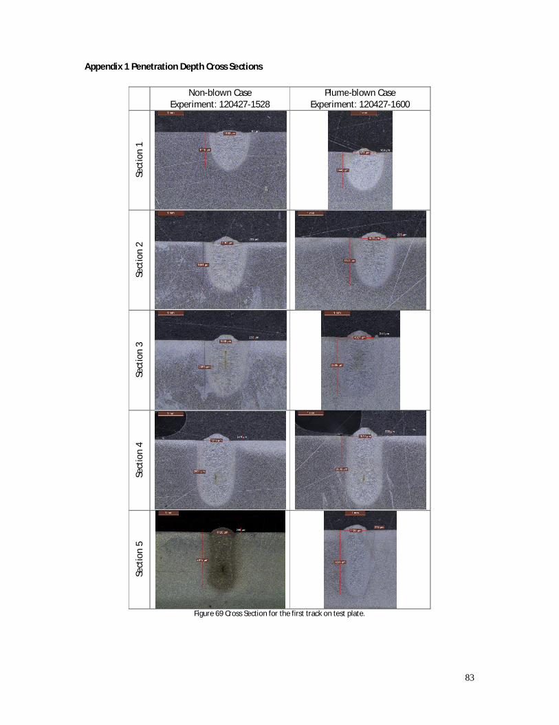
83

Appendix 1 Penetration Depth Cross Sections

Non-blown Case Experiment: 120427-1528

Plume-blown Case Experiment: 120427-1600

Sect

ion

1

Sect

ion

2

Sect

ion

3

Sect

ion

4

Sect

ion

5

Figure 69 Cross Section for the first track on test plate.

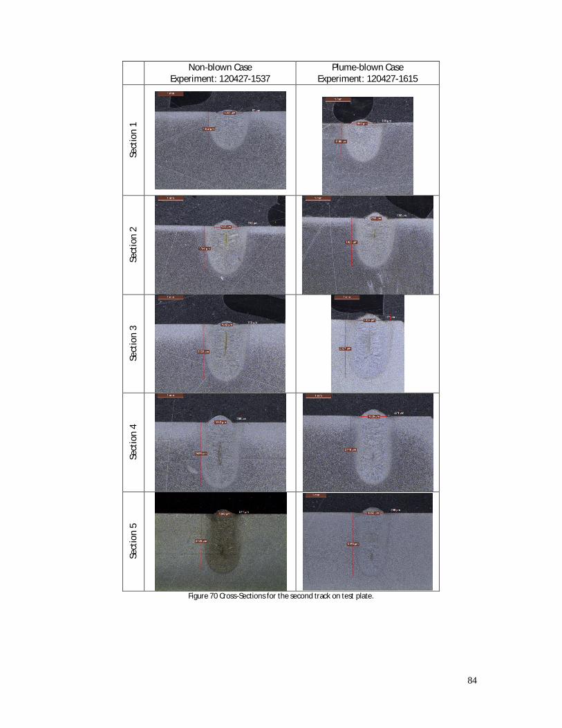
84

Non-blown Case Experiment: 120427-1537

Plume-blown Case Experiment: 120427-1615

Sect

ion

1

Sect

ion

2

Sect

ion

3

Sect

ion

4

Sect

ion

5

Figure 70 Cross-Sections for the second track on test plate.

85

Plume-blown Characterization Experiment (120627-1657)

Sect

ion

1

Sect

ion

2

Sect

ion

3

Sect

ion

4

Sect

ion

5

Figure 71 Cross sections of Plume-blown Characterization Experiment.

86

Controlled Experiment with reference: 50 (120627-1711)

Controlled Experiment with reference: 55 (120627-1717)

Sect

ion

1

Sect

ion

2

Sect

ion

3

Sect

ion

4

Sect

ion

5

Figure 72 Cross sections of Plume-blown Controlled Experiment.

87

Appendix 2 Controlled Experiment Material Specifications Below table shows the material specifications for the controlled experiments in Chapter 5.

PENETRATION DEPTH CONTROL USING AN OPTICAL ...

Documents

Transcript of PENETRATION DEPTH CONTROL USING AN OPTICAL ...