Deep Penetration Magnetoquasistatic Sensors Yanko Sheiretov
198
Deep Penetration Magnetoquasistatic Sensors by Yanko Sheiretov B.S., Massachusetts Institute of Technology (1992) M.S., Massachusetts Institute of Technology (1994) E.E., Massachusetts Institute of Technology (1998) Submitted to the Department of Electrical Engineering and Computer Science in partial fulfillment of the requirements for the degree of Doctor of Philosophy at the MASSACHUSETTS INSTITUTE OF TECHNOLOGY June 2001 c Yanko Sheiretov, 2001. All rights reserved. The author hereby grants to MIT permission to reproduce and distribute publicly paper and electronic copies of this thesis document in whole or in part. Author ................................................................................. Department of Electrical Engineering and Computer Science May 24, 2001 Certified by ............................................................................ Markus Zahn Professor of Electrical Engineering Thesis Supervisor Accepted by ............................................................................ Arthur C. Smith Chairman, Department Committee on Graduate Students
-
Upload
khangminh22 -
Category
Documents
-
view
2 -
download
0
Transcript of Deep Penetration Magnetoquasistatic Sensors Yanko Sheiretov

Deep Penetration Magnetoquasistatic Sensors
by
Yanko Sheiretov
B.S., Massachusetts Institute of Technology (1992)M.S., Massachusetts Institute of Technology (1994)E.E., Massachusetts Institute of Technology (1998)
Submitted to the Department of Electrical Engineering and Computer Sciencein partial fulfillment of the requirements for the degree of
Doctor of Philosophy
at the
MASSACHUSETTS INSTITUTE OF TECHNOLOGY
June 2001
c© Yanko Sheiretov, 2001. All rights reserved.
The author hereby grants to MIT permission to reproduce and distribute publiclypaper and electronic copies of this thesis document in whole or in part.
Author . . . . . . . . . . . . . . . . . . . . . . . . . . . . . . . . . . . . . . . . . . . . . . . . . . . . . . . . . . . . . . . . . . . . . . . . . . . . . . . . .Department of Electrical Engineering and Computer Science
May 24, 2001
Certified by . . . . . . . . . . . . . . . . . . . . . . . . . . . . . . . . . . . . . . . . . . . . . . . . . . . . . . . . . . . . . . . . . . . . . . . . . . . .Markus Zahn
Professor of Electrical EngineeringThesis Supervisor
Accepted by . . . . . . . . . . . . . . . . . . . . . . . . . . . . . . . . . . . . . . . . . . . . . . . . . . . . . . . . . . . . . . . . . . . . . . . . . . . .Arthur C. Smith
Chairman, Department Committee on Graduate Students


Deep Penetration Magnetoquasistatic Sensorsby
Yanko Sheiretov
Submitted to the Department of Electrical Engineering and Computer Scienceon May 24, 2001, in partial fulfillment of the
requirements for the degree ofDoctor of Philosophy
Abstract
This research effort extends the capabilities of existing model-based spatially periodicquasistatic-field sensors. The research developed three significant improvements in the fieldof nondestructive evaluation. The impact of each is detailed below:
1. The design of a distributed current drive magnetoresistive magnetometer that matchesthe model response sufficiently to perform air calibration and absolute property mea-surement. Replacing the secondary winding with a magnetoresistive sensor allows themagnetometer to be operated at frequencies much lower than ordinarily possible, includ-ing static (DC) operation, which enables deep penetration defect imaging. Low frequen-cies are needed for deep probing of metals, where the depth of penetration is otherwiselimited by the skin depth due to the shielding effect of induced eddy currents. The ca-pability to perform such imaging without dependence on calibration standards has bothsubstantial cost, ease of use, and technological benefits. The absolute property measure-ment capability is important because it provides a robust comparison for manufacturingquality control and monitoring of aging processes. Air calibration also alleviates thedependence on calibration standards that can be difficult to maintain.
2. The development and validation of cylindrical geometry models for inductive and ca-pacitive sensors. The development of cylindrical geometry models enable the design offamilies of circularly symmetric magnetometers and dielectrometers with the “model-based” methodology, which requires close agreement between actual sensor responseand simulated response. These kinds of sensors are needed in applications where thecomponents being tested have circular symmetry, e.g. cracks near fasteners, or if it isimportant to measure the spatial average of an anisotropic property.
3. The development of accurate and efficient two-dimensional inverse interpolation andgrid look-up techniques to determine electromagnetic and geometric properties. The abil-ity to perform accurate and efficient grid interpolation is important for all sensors thatfollow the model-based principle, but it is particularly important for the complex shapedgrids used with the magnetometers and dielectrometers in this thesis.
A prototype sensor that incorporates all new features, i.e. a circularly symmetric magne-tometer with a distributed current drive that uses a magnetoresistive secondary element, wasdesigned, built, and tested. The primary winding is designed to have no net dipole moment,which improves repeatability by reducing the influence of distant objects. It can also supportoperation at two distinct effective spatial wavelengths. A circuit is designed that places themagnetoresistive sensor in a feedback configuration with a secondary winding to provide thenecessary biasing and to ensure a linear transfer characteristic. Efficient FFT-based methodsare developed to model magnetometers with a distributed current drive for both Cartesian

and cylindrical geometry sensors. Results from measurements with a prototype circular di-electrometer that agree with the model-based analysis are also presented.
In addition to the main contributions described so far, this work also includes other re-lated enhancements to the time and space periodic-field sensor models, such as incorporatingmotion in the models to account for moving media effects. This development is importantin low frequency scanning applications. Some improvements of the existing semi-analyticalcollocation point models for the standard Cartesian magnetometers and dielectrometers arealso presented.
Thesis Supervisor: Markus ZahnTitle: Professor of Electrical Engineering

Acknowledgments
This research project was sponsored by JENTEK Sensors, Inc. I would like to thank Dr.Neil Goldfine, president of JENTEK and member of the thesis committee, for providing fi-nancial sponsorship, encouragement, many helpful suggestions, and enthusiastic support.Dr. Goldfine fosters a supportive and accommodating work environment at JENTEK, whichallowed me to take advantage of the company’s resources, and gave me freedom to direct myefforts towards areas of greatest interest to me.
Many thanks go to my thesis supervisor, Professor Markus Zahn, not only for his guidanceand critical support of my work in this thesis, but also for being a mentor for many years.I consider myself very lucky to have been able to learn from Professor Zahn for almost thir-teen years, starting from my first year at MIT. Since then I have gone to him for advice onnumerous occasions, not only for academic matters, but for personal and career choices aswell. I would also like to thank the other thesis committee members, Professors Jeffrey Lang,Terry Orlando, and Bernard Lesieutre, for their insightful comments at the defense and atour committee and individual meetings.
Darrell Schlicker provided the highest level of support throughout the entire project. Thiswas especially important in the last several months. He designed the impedance analyzerinstruments used in most experiments. I have drawn on his expertise in electronics in thedesign of the interface and support circuitry of the magnetoresistive sensor. Whenever baf-fled by a particular measurement result or a theoretical derivation, I went to Darrell for abrainstorm session. His willingness to help and generosity with which he lends his time arequalities I have rarely found in others. Many aspects of this thesis would have been muchmore difficult without his help. Thanks!
I would like to thank my other co-workers at JENTEK for their help in my work on thisproject and for making it possible to devote so much of my time to my thesis. In particular, Iwould like to thank Joni Goday for handling the financial aspects of my research, Dr. AndrewWashabaugh for our numerous discussions of the mathematical and physical models, PaulaGentile for help with graphics and literature, Dr. Vladimir Zilberstein for help with the choiceand design of the test samples, Vladimir Tsukernik for the drawing and machining of thesensors and samples, Chris Root for finding potentially useful material samples, Wayne Ryanfor help with the ferrofluid experiments, and Dr. Karen Walrath for help with the sensorprototype and for general advice. I would also like to thank my close friends Michelle McDevittand Jacqueline Aylas for manuscript review and emotional support.
Finally, I am truly grateful to my partner, Leo T. Mayer, for his love, support, and patienceover the last five years. He has helped me through many difficult times, and his unwaveringfaith in me has always been a steady source of confidence and motivation.


Contents
1 Introduction 171.1 Imposed ω-k quasistatic sensors . . . . . . . . . . . . . . . . . . . . . . . . . . . . 18
1.1.1 Meandering Wavelength Magnetometer (MWMTM) . . . . . . . . . . . . . 191.1.2 Magnetometer arrays . . . . . . . . . . . . . . . . . . . . . . . . . . . . . . 201.1.3 Interdigitated electrode dielectrometer (IDEDTM) . . . . . . . . . . . . . . 211.1.4 Multiple-Wavelength Dielectrometer . . . . . . . . . . . . . . . . . . . . . 23
1.2 Goals . . . . . . . . . . . . . . . . . . . . . . . . . . . . . . . . . . . . . . . . . . . 231.3 Motivation . . . . . . . . . . . . . . . . . . . . . . . . . . . . . . . . . . . . . . . . 24
1.3.1 Magnetoresistive sensors . . . . . . . . . . . . . . . . . . . . . . . . . . . . 251.3.2 Modeling sensors with rotational symmetry . . . . . . . . . . . . . . . . . 251.3.3 Magnetometers with distributed current drive . . . . . . . . . . . . . . . 26
1.4 Inverse estimation methods . . . . . . . . . . . . . . . . . . . . . . . . . . . . . . 271.4.1 Measurement grids . . . . . . . . . . . . . . . . . . . . . . . . . . . . . . . 271.4.2 Minimization methods . . . . . . . . . . . . . . . . . . . . . . . . . . . . . 29
1.5 Magnetic field sensing technologies . . . . . . . . . . . . . . . . . . . . . . . . . . 291.6 Summary of Chapter 1 . . . . . . . . . . . . . . . . . . . . . . . . . . . . . . . . . 32
2 Forward Models of the Spatially Periodic Sensors 332.1 Mathematical model and simulation method for the MWM . . . . . . . . . . . . 34
2.1.1 Magnetic diffusion . . . . . . . . . . . . . . . . . . . . . . . . . . . . . . . 342.1.2 Normalization . . . . . . . . . . . . . . . . . . . . . . . . . . . . . . . . . . 362.1.3 Collocation points . . . . . . . . . . . . . . . . . . . . . . . . . . . . . . . . 382.1.4 Fourier series representation . . . . . . . . . . . . . . . . . . . . . . . . . 402.1.5 Normalized surface reluctance density . . . . . . . . . . . . . . . . . . . . 412.1.6 Boundary conditions . . . . . . . . . . . . . . . . . . . . . . . . . . . . . . 432.1.7 Setting up the matrix equation . . . . . . . . . . . . . . . . . . . . . . . . 472.1.8 Terminal currents . . . . . . . . . . . . . . . . . . . . . . . . . . . . . . . . 47
2.2 Mathematical model and simulation method for the IDED . . . . . . . . . . . . 482.2.1 Laplace’s equation . . . . . . . . . . . . . . . . . . . . . . . . . . . . . . . . 492.2.2 Normalization . . . . . . . . . . . . . . . . . . . . . . . . . . . . . . . . . . 492.2.3 Collocation points . . . . . . . . . . . . . . . . . . . . . . . . . . . . . . . . 512.2.4 Fourier series representation . . . . . . . . . . . . . . . . . . . . . . . . . 512.2.5 Surface capacitance density . . . . . . . . . . . . . . . . . . . . . . . . . . 522.2.6 Boundary conditions . . . . . . . . . . . . . . . . . . . . . . . . . . . . . . 552.2.7 Setting up the matrix equation . . . . . . . . . . . . . . . . . . . . . . . . 582.2.8 Calculating transcapacitance . . . . . . . . . . . . . . . . . . . . . . . . . 58
2.3 Summary of Chapter 2 . . . . . . . . . . . . . . . . . . . . . . . . . . . . . . . . . 59
7

8 CONTENTS
3 Modeling sensors with rotational symmetry 613.1 Magnetometer . . . . . . . . . . . . . . . . . . . . . . . . . . . . . . . . . . . . . . 62
3.1.1 Use of Fourier-Bessel series . . . . . . . . . . . . . . . . . . . . . . . . . . 633.1.2 Collocation points . . . . . . . . . . . . . . . . . . . . . . . . . . . . . . . . 643.1.3 Surface reluctance density . . . . . . . . . . . . . . . . . . . . . . . . . . . 663.1.4 Boundary conditions . . . . . . . . . . . . . . . . . . . . . . . . . . . . . . 673.1.5 Matrix equation and terminal currents . . . . . . . . . . . . . . . . . . . . 68
3.2 Dielectrometer . . . . . . . . . . . . . . . . . . . . . . . . . . . . . . . . . . . . . . 693.2.1 Sensor geometry . . . . . . . . . . . . . . . . . . . . . . . . . . . . . . . . . 703.2.2 Laplace’s equation . . . . . . . . . . . . . . . . . . . . . . . . . . . . . . . . 713.2.3 Collocation points . . . . . . . . . . . . . . . . . . . . . . . . . . . . . . . . 723.2.4 Surface capacitance density and boundary conditions . . . . . . . . . . . 743.2.5 Calculating transcapacitance . . . . . . . . . . . . . . . . . . . . . . . . . 74
3.3 Experimental verification of cylindrical coordinate model . . . . . . . . . . . . . 753.4 Summary of Chapter 3 . . . . . . . . . . . . . . . . . . . . . . . . . . . . . . . . . 79
4 Distributed Current Drive Sensors 814.1 Why use a distributed current drive . . . . . . . . . . . . . . . . . . . . . . . . . 824.2 Definitions . . . . . . . . . . . . . . . . . . . . . . . . . . . . . . . . . . . . . . . . 824.3 Closed form solutions for the magnetic field . . . . . . . . . . . . . . . . . . . . . 834.4 Numerical analysis . . . . . . . . . . . . . . . . . . . . . . . . . . . . . . . . . . . 894.5 Sensor of finite width . . . . . . . . . . . . . . . . . . . . . . . . . . . . . . . . . . 904.6 Multiple homogeneous layers . . . . . . . . . . . . . . . . . . . . . . . . . . . . . 944.7 Eliminating the net dipole moment . . . . . . . . . . . . . . . . . . . . . . . . . . 964.8 Sensor with rotational symmetry . . . . . . . . . . . . . . . . . . . . . . . . . . . 100
4.8.1 Sensor description . . . . . . . . . . . . . . . . . . . . . . . . . . . . . . . . 1014.8.2 Sensor modeling . . . . . . . . . . . . . . . . . . . . . . . . . . . . . . . . . 102
4.9 Fast Hankel transform . . . . . . . . . . . . . . . . . . . . . . . . . . . . . . . . . 1034.9.1 Definition and derivation . . . . . . . . . . . . . . . . . . . . . . . . . . . . 1054.9.2 Discretization . . . . . . . . . . . . . . . . . . . . . . . . . . . . . . . . . . 1064.9.3 Application of the fast Hankel transform to the circular magnetometer . 107
4.10 Different wavelength modes with the same sensor . . . . . . . . . . . . . . . . . 1094.11 Summary of Chapter 4 . . . . . . . . . . . . . . . . . . . . . . . . . . . . . . . . . 111
5 Deep Penetration Magnetoresistive Magnetometer 1135.1 Theory of the magnetoresistive and giant magnetoresistive effects . . . . . . . . 114
5.1.1 Magnetoresistance . . . . . . . . . . . . . . . . . . . . . . . . . . . . . . . 1155.1.2 Giant magnetoresistance . . . . . . . . . . . . . . . . . . . . . . . . . . . . 117
5.2 Operation of the secondary GMR sensor assembly . . . . . . . . . . . . . . . . . 1195.2.1 GMR sensor characteristics . . . . . . . . . . . . . . . . . . . . . . . . . . 1195.2.2 Feedback loop . . . . . . . . . . . . . . . . . . . . . . . . . . . . . . . . . . 1205.2.3 Electronics . . . . . . . . . . . . . . . . . . . . . . . . . . . . . . . . . . . . 1215.2.4 DC stability . . . . . . . . . . . . . . . . . . . . . . . . . . . . . . . . . . . 1225.2.5 AC stability and loop bandwidth . . . . . . . . . . . . . . . . . . . . . . . 122
5.3 Incorporating the effects of the feedback loop into the sensor model . . . . . . . 1245.4 Conductivity / lift-off measurements at 12.6 kHz . . . . . . . . . . . . . . . . . . 1255.5 Permeability / lift-off measurements at DC . . . . . . . . . . . . . . . . . . . . . 1285.6 Thickness / lift-off measurements with a multi-layer structure . . . . . . . . . . 131

CONTENTS 9
5.7 Low frequency (100 Hz) thickness measurements . . . . . . . . . . . . . . . . . . 1335.8 Crack detection through 1/4 inch stainless steel plate . . . . . . . . . . . . . . . 1375.9 Magnetic permeability measurements of ferromagnetic fluids . . . . . . . . . . . 1425.10 Summary of Chapter 5 . . . . . . . . . . . . . . . . . . . . . . . . . . . . . . . . . 143
6 Further Extensions of the Sensor Models 1456.1 Mathematical model of the MWM sensor in the presence of convection . . . . . 145
6.1.1 Changes to the diffusion equation . . . . . . . . . . . . . . . . . . . . . . . 1456.1.2 Symmetry . . . . . . . . . . . . . . . . . . . . . . . . . . . . . . . . . . . . 1476.1.3 Collocation points . . . . . . . . . . . . . . . . . . . . . . . . . . . . . . . . 1476.1.4 Fourier series representation . . . . . . . . . . . . . . . . . . . . . . . . . 1486.1.5 Normalized surface reluctance density . . . . . . . . . . . . . . . . . . . . 1496.1.6 Boundary conditions . . . . . . . . . . . . . . . . . . . . . . . . . . . . . . 1496.1.7 Setting up the matrix equation . . . . . . . . . . . . . . . . . . . . . . . . 1506.1.8 Effect of convection on sensor response . . . . . . . . . . . . . . . . . . . . 1516.1.9 Summary . . . . . . . . . . . . . . . . . . . . . . . . . . . . . . . . . . . . . 153
6.2 Grid look-up and interpolation algorithms . . . . . . . . . . . . . . . . . . . . . . 1536.2.1 Two-dimensional inverse interpolation . . . . . . . . . . . . . . . . . . . . 1536.2.2 Search algorithm . . . . . . . . . . . . . . . . . . . . . . . . . . . . . . . . 1556.2.3 Simple inverse two-dimensional interpolation . . . . . . . . . . . . . . . . 1566.2.4 Complex inverse two-dimensional interpolation . . . . . . . . . . . . . . . 1576.2.5 Handling triangular grid cells . . . . . . . . . . . . . . . . . . . . . . . . . 1596.2.6 Comparison between the new and the old interpolation methods . . . . . 1606.2.7 Handling multi-valued grids . . . . . . . . . . . . . . . . . . . . . . . . . . 1616.2.8 Summary . . . . . . . . . . . . . . . . . . . . . . . . . . . . . . . . . . . . . 161
7 Summary and Conclusions 1637.1 Summary . . . . . . . . . . . . . . . . . . . . . . . . . . . . . . . . . . . . . . . . . 1637.2 Conclusions . . . . . . . . . . . . . . . . . . . . . . . . . . . . . . . . . . . . . . . 1657.3 Suggestions for continuing work . . . . . . . . . . . . . . . . . . . . . . . . . . . . 166
7.3.1 Scaled down GMR magnetometer . . . . . . . . . . . . . . . . . . . . . . . 1667.3.2 GMR magnetometer arrays . . . . . . . . . . . . . . . . . . . . . . . . . . 1677.3.3 Applying the cylindrical geometry collocation point method to Rosette
sensors . . . . . . . . . . . . . . . . . . . . . . . . . . . . . . . . . . . . . . 168
A Definition of Symbols, Abbreviations, and Acronyms 169
B Infinite Sums over Fourier Modes 175B.1 Overview . . . . . . . . . . . . . . . . . . . . . . . . . . . . . . . . . . . . . . . . . 175B.2 Alternative formulation . . . . . . . . . . . . . . . . . . . . . . . . . . . . . . . . 177
C Error analysis 183
D Calibration methods 187D.1 Single point air calibration . . . . . . . . . . . . . . . . . . . . . . . . . . . . . . . 188D.2 Air and shunt calibration . . . . . . . . . . . . . . . . . . . . . . . . . . . . . . . . 188D.3 Two point reference part calibration . . . . . . . . . . . . . . . . . . . . . . . . . 189D.4 Other calibration methods . . . . . . . . . . . . . . . . . . . . . . . . . . . . . . . 191

10 CONTENTS

List of Figures
1-1 Layout of a typical MWM . . . . . . . . . . . . . . . . . . . . . . . . . . . . . . . 201-2 Photograph of large MWM Array developed at JENTEK for use in metal land
mine detection . . . . . . . . . . . . . . . . . . . . . . . . . . . . . . . . . . . . . . 211-3 Two-dimensional scan image generated with the large MWM array at JENTEK 211-4 Schematic layout of an IDED . . . . . . . . . . . . . . . . . . . . . . . . . . . . . 221-5 Electric field lines for a three-wavelength dielectric sensor . . . . . . . . . . . . 231-6 Layout of a 5/2/1 mm three-wavelength dielectric sensor. . . . . . . . . . . . . . 241-7 Sensitivity comparison of magnetic sensor technologies . . . . . . . . . . . . . . 31
2-1 Definition of geometry parameters of the MWM . . . . . . . . . . . . . . . . . . 372-2 Collocation points and interval limits used in the analysis of the MWM . . . . . 402-3 Electronic interface of the IDED . . . . . . . . . . . . . . . . . . . . . . . . . . . 492-4 Piecewise-smooth collocation-point approximation for the electrostatic
potential of the IDED . . . . . . . . . . . . . . . . . . . . . . . . . . . . . . . . . . 502-5 Terminal current of an electrode in contact with a conducting dielectric medium. 532-6 Material structure with several layers of homogeneous materials . . . . . . . . 55
3-1 Basic structure of the circularly symmetric magnetometer (Rosette). . . . . . . 623-2 Definition of geometry parameters of circular dielectrometer. . . . . . . . . . . . 703-3 Normalized calculated potential at the electrode surface for the circular
dielectrometer in air . . . . . . . . . . . . . . . . . . . . . . . . . . . . . . . . . . 713-4 Positions of 16 collocation points . . . . . . . . . . . . . . . . . . . . . . . . . . . 723-5 Layout of two circular dielectric sensors with different depth of sensitivity . . . 753-6 Permittivity/lift-off measurement grid for the pair of dielectric sensors in
Figure 3-5 . . . . . . . . . . . . . . . . . . . . . . . . . . . . . . . . . . . . . . . . 773-7 Results of measurements with the circular dielectric sensors . . . . . . . . . . . 78
4-1 Comparison between distributed and concentrated current drives . . . . . . . . 824-2 Geometry and current drive of the sensor analyzed in Section 4.3 . . . . . . . . 844-3 Sine transform of the current distribution of the sensor . . . . . . . . . . . . . . 854-4 The Lorentzian function and its Fourier transform . . . . . . . . . . . . . . . . . 874-5 Magnetic field at the origin, generated by a pair of conductors positioned at a
distance d on either side. . . . . . . . . . . . . . . . . . . . . . . . . . . . . . . . . 884-6 Discretized spectrum of the current excitation shown in Figure 4-2, in a
decaying exponential envelope. . . . . . . . . . . . . . . . . . . . . . . . . . . . . 904-7 Numerically calculated magnetic field of the periodic sensor . . . . . . . . . . . 914-8 Current envelope function for a sensor of finite width and its corresponding
sine transform . . . . . . . . . . . . . . . . . . . . . . . . . . . . . . . . . . . . . . 93
11

12 LIST OF FIGURES
4-9 Sine transform of the current excitation generated by discrete current elements 944-10 Numerically calculated magnetic field of the finite-width sensor . . . . . . . . . 954-11 Material structure that consists of more than one homogeneous layer . . . . . . 964-12 Equipotential surfaces of the magnetic scalar potential for multi-pole
moments with no ϕ-dependence . . . . . . . . . . . . . . . . . . . . . . . . . . . . 994-13 Magnetic field lines for � = 3 “octupole” moment potential . . . . . . . . . . . . 1004-14 Number of winding turns for the finite sensor with no net dipole moment . . . 1004-15 Structure of the circular magnetometer with distributed current drive . . . . . 1014-16 Numerically calculated magnetic field of the circular magnetometer . . . . . . . 1044-17 Results of the application of the fast Hankel transform . . . . . . . . . . . . . . 1084-18 Magnetic field lines of the circular magnetometer, calculated with the fast
Hankel transform . . . . . . . . . . . . . . . . . . . . . . . . . . . . . . . . . . . . 1104-19 Winding pattern for the circular magnetometer that enables two different
fundamental wavelengths . . . . . . . . . . . . . . . . . . . . . . . . . . . . . . . 111
5-1 Photograph of the prototype sensor used in all experiments in Chapter 5 . . . . 1145-2 Fermi diagram of conduction states in a ferromagnetic metal . . . . . . . . . . . 1165-3 Diagram illustrating the giant magnetoresistive effect . . . . . . . . . . . . . . 1185-4 Typical GMR magnetic field sensor layout . . . . . . . . . . . . . . . . . . . . . . 1195-5 Transfer characteristic of the GMR magnetic sensor. . . . . . . . . . . . . . . . . 1205-6 Structure of the hybrid sensor feedback loop . . . . . . . . . . . . . . . . . . . . 1215-7 Feedback and interface circuit schematic . . . . . . . . . . . . . . . . . . . . . . 1235-8 Conductivity/lift-off measurement grid for circular sensor at 12.6 kHz . . . . . . 1265-9 Results of conductivity/lift-off measurements with the circular magnetometer . 1275-10 Two wavelength magnitude/magnitude permeability/lift-off grid for the
circular magnetometer with DC excitation . . . . . . . . . . . . . . . . . . . . . 1295-11 Permeability/lift-off measurement results with the circular GMR
magnetometer on magnetizable foam layer . . . . . . . . . . . . . . . . . . . . . 1305-12 Three layer structure used in thickness/lift-off measurements . . . . . . . . . . 1325-13 Thickness/lift-off measurement grid for the circular magnetometer at 12.6 kHz 1335-14 Stainless steel layer thickness measurements at five different lift-offs . . . . . . 1345-15 Low frequency (100 Hz) conductivity/thickness measurement grid and results . 1355-16 Expanded views of the upper left corner of the grid in Figure 5-15 . . . . . . . . 1365-17 A plot of the real part of complex exponential decay, characteristic of magnetic
diffusion. . . . . . . . . . . . . . . . . . . . . . . . . . . . . . . . . . . . . . . . . . 1365-18 Geometry of stainless steel plate with a slot simulating a crack. . . . . . . . . . 1375-19 Stainless steel plate configuration for three area scans . . . . . . . . . . . . . . 1385-20 Area scan of stainless steel plate with the crack at the surface . . . . . . . . . . 1395-21 Area scan of stainless steel plate with the crack 3.2 mm below the surface . . . 1405-22 Area scan of stainless steel plate with the crack 7.2 mm below the surface . . . 1405-23 Linear scan of simulated crack taken at multiple frequencies . . . . . . . . . . . 141
6-1 Locus of the transinductance of an MWM in magnitude/phase space as theconvection velocity increases. . . . . . . . . . . . . . . . . . . . . . . . . . . . . . 152
6-2 Real part of the magnetic vector potential Ay, shown for stationary andmoving media . . . . . . . . . . . . . . . . . . . . . . . . . . . . . . . . . . . . . . 152
6-3 Incorrect result of the closest grid point search algorithm . . . . . . . . . . . . . 1546-4 Schematic diagram of the two-dimensional inverse interpolation in a grid cell . 156

LIST OF FIGURES 13
6-5 Diagram of a grid cell showing the points used by the complex inversetwo-dimensional interpolation algorithm . . . . . . . . . . . . . . . . . . . . . . 157
6-6 Grid cell transformed into a parallelogram . . . . . . . . . . . . . . . . . . . . . 1586-7 Point and segment definitions for a triangular grid cell . . . . . . . . . . . . . . 1596-8 Pathological test grid and path through the grid . . . . . . . . . . . . . . . . . . 1606-9 Results with both interpolation methods for the radial property of the grid in
Figure 6-8 . . . . . . . . . . . . . . . . . . . . . . . . . . . . . . . . . . . . . . . . 1626-10 Results with both interpolation methods for the azimuthal property of the
grid in Figure 6-8 . . . . . . . . . . . . . . . . . . . . . . . . . . . . . . . . . . . . 162
B-1 Three-dimensional plot of the infinite summation function in equation (B.3). . . 176B-2 Plot of the functions f (x) and g(x) . . . . . . . . . . . . . . . . . . . . . . . . . . 177B-3 Three-dimensional plot of the infinite summation function in equation (B.4). . . 178
C-1 Comparison between simulated and measured response of the magnetometerin the conductivity/lift-off measurements . . . . . . . . . . . . . . . . . . . . . . 185

14 LIST OF FIGURES

List of Tables
1.1 Magnetoresistive sensors: advantages and application areas. . . . . . . . . . . . 30
3.1 Geometric and material parameters of the sensors in Figure 3-5. . . . . . . . . . 763.2 Results of measurements with the circular dielectric sensors, shown in
Figure 3-7 . . . . . . . . . . . . . . . . . . . . . . . . . . . . . . . . . . . . . . . . . 78
4.1 Spherical harmonic functions . . . . . . . . . . . . . . . . . . . . . . . . . . . . . 984.2 Number of winding turns for the finite sensor with no net dipole moment . . . . 994.3 Number of turns per winding wj for the circular magnetometer. . . . . . . . . . . 1024.4 Fast Hankel transform normalized parameter values. . . . . . . . . . . . . . . . 1074.5 Winding pattern for the rectangular magnetometer, enabling two different
fundamental wavelengths determined by the polarity of the connection . . . . . 1094.6 Winding pattern for the circular magnetometer, enabling two different
fundamental wavelengths, determined by the polarity of the connection. . . . . . 109
5.1 Results of conductivity/lift-off measurements with the circular magnetometer,shown in Figure 5-9 . . . . . . . . . . . . . . . . . . . . . . . . . . . . . . . . . . . 127
5.2 Conductivity of metal alloys used in experiments . . . . . . . . . . . . . . . . . . 1285.3 Experiment results of the permeability/lift-off measurements at DC, shown in
Figure 5-11 . . . . . . . . . . . . . . . . . . . . . . . . . . . . . . . . . . . . . . . . 1305.4 Stainless steel layer thickness estimation results for various lift-offs . . . . . . . 1345.5 Low frequency (100 Hz) conductivity/thickness measurement results for six
metal plates . . . . . . . . . . . . . . . . . . . . . . . . . . . . . . . . . . . . . . . 1375.6 Measured ferrofluid magnetic permeability . . . . . . . . . . . . . . . . . . . . . 143
A.1 Abbreviations and acronyms in alphabetical order. . . . . . . . . . . . . . . . . . 169A.2 Definition of symbols . . . . . . . . . . . . . . . . . . . . . . . . . . . . . . . . . . 169
C.1 Results of the conductivity/lift-off measurements of Section 5.4, including alltwenty sets, and showing percentage errors . . . . . . . . . . . . . . . . . . . . . 184
D.1 Data from Table C.1, re-calibrated using the two point reference part method . . 190
15

16 LIST OF TABLES

Chapter 1
Introduction
The goal of this research effort is to extend the capabilities of existing sensor technology basedon quasistatic magnetic and electric fields with imposed spatial periodicity. The main appli-cation area for such sensors is in nondestructive evaluation of materials, especially detectionof flaws such as cracks, voids, and inclusions in metal components. They can also be usedfor more general measurement of a material’s magnetic and dielectric properties, i.e. electricconductivity, magnetic permeability, and dielectric permittivity, which can be related to otherphysical properties of interest, such as density, thermal conductivity, chemical composition,residual mechanical stress, etc. Geometric parameters of a test structure, such as layer thick-ness and proximity, can also be measured with such sensors. An overview of existing sensortechnology is presented in Section 1.1.
The most important new idea explored in this work is the use of a giant magnetoresistivesensor in place of the secondary magnetometer winding. This makes it possible to operate themagnetometer at frequencies much lower than ordinarily possible, including DC operation,since the magnetoresistive sensors respond to the magnitude of the magnetic flux density, asopposed to the induced voltage in a secondary winding, which is proportional to the rate ofchange of the linked magnetic flux. Low frequency operation is necessary for deep probing ofmetals, where at higher frequencies the depth of penetration of the magnetic fields is limitedby the skin depth effect, caused by induced eddy currents.
Until now almost all sensors have been designed with rectangular geometry, suitable foranalysis in Cartesian coordinates. While modeling and numerical simulation of eddy currentsensors in cylindrical geometry have been done in the past, the existing semi-analytical col-location point models cannot be used to describe sensors in alternative coordinate systems.In this work the existing semi-analytical collocation point methods, used to model the mean-dering winding magnetometer and the interdigital dielectrometer, are extended to cylindricalcoordinates, making them suitable to model sensors with circular geometry. These kindsof sensors are needed in applications where parts being tested have cylindrical geometry,e.g. testing for cracks near fasteners, or when it is important to measure the average of ananisotropic property, as discussed in more detail in Chapter 3.
One of the main difficulties in developing semi-analytical models for the magnetometers isthat magnetic diffusion effects cause the winding current to be nonuniform across the windingtraces. Thus the drive current density is not known at the outset, requiring the use of colloca-tion point methods. The sensor models can be made significantly simpler and more efficientif the nonuniformity of the current distribution inside the conductors can be ignored, becausethe known excitation current density can then be broken down into its constitutive spatial
17

18 Chapter 1. Introduction
Fourier modes, and the magnetic fields can be obtained as a superposition of the solutions forall wavenumber modes.
There is a class of sensors where this assumption can be justified. There the magneticfields are shaped by a number of windings, each with a varying number of turns, that fol-low a sinusoidal envelope function in Cartesian geometry or a first order Bessel function incylindrical geometry. The physical dimensions of each winding, width and thickness, aremuch smaller than the imposed spatial wavelength, the distance between the windings in theprimary, and the distance between the secondary winding and the nearest primary windingsegment. This makes it possible to treat the windings as infinitely thin, allowing the drivencurrent density to be modeled as a series of spatial impulse functions.
Methods are developed for efficient modeling of this class of sensors. Such sensors areneeded in applications that require high depth of sensitivity, where the standard periodicsensor geometry would result in sensor footprints too large to be practical. Using a distributedcurrent drive makes it possible to have an imposed spatial period on the order of the sensorlength and width. These methods are also extended to cylindrical coordinates.
A prototype sensor incorporating all of these features, i.e. a circularly symmetric magne-tometer with a distributed current drive using a magnetoresistive secondary element, is builtand tested in a variety of representative applications, confirming the validity of the semi-analytical models, and demonstrating the new capability of low frequency operation for deeppenetration in metals.
The order in which material is presented in this thesis is chosen to avoid using a resultbefore its derivation. The existing collocation point models, with some changes and improve-ments, are described in Chapter 2. Chapter 3 develops the corresponding models in cylindri-cal geometry. The methods used to model distributed current drive sensors are presented inChapter 4, and the design and experimental results of the circularly symmetric, distributedcurrent drive, magnetoresistive sensor are presented in Chapter 5.
1.1 Imposedω-k quasistatic sensors
Almost all of the work in this research project is aimed at extending the capabilities of sensortechnology based on spatially periodic quasistatic fields. Such dielectrometer and magnetome-ter sensors have been the focus of several research projects at the Laboratory of Electromag-netic and Electronic Systems (LEES) at MIT for many years [1–11]. This section describessome of the commercially developed sensors based on this work.
The basic idea behind the imposed ω-k quasistatic sensors is that the magnetometer wind-ings or dielectrometer electrodes are laid out in a spatially periodic pattern on a substrate,making one-sided contact with the material under test. The imposed spatial period (wave-length) λ determines the rate of decay of the fields away from the sensor and is chosen toachieve the desired depth of sensitivity. The frequency of excitation does not affect this depthof sensitivity of the dielectrometer,∗ and also of the magnetometer at low frequency or withnonconducting materials. Skin depth effects on the magnetic field at high frequency in con-ductors result in a calculable decrease in magnetic field penetration depth with increasingfrequency. The periodic nature of the potentials and fields allows for the use of Fourier seriesmethods in the semi-analytical models.
∗See the foot note on page 70.

1.1. Imposed ω-k quasistatic sensors 19
The spatially periodic quasistatic sensors have several advantages over alternative sens-ing technologies:
1. Control over the depth of sensitivity allows for measuring profiles of material proper-ties by combining the results of measurements at varying depths, controlled by varyingsensor wavelength, or by varying frequency in good conductors with magnetometers.
2. The layout allows for a good match between simulated and measured sensor responsewith the simulations carried out with efficient collocation point methods, described inChapter 2. This reduces the need for elaborate calibration standards and procedures.
3. The flexible substrate makes it possible to measure on curved surfaces, with the curva-ture having no appreciable effect on sensor response.
4. The sensor geometry allows for the creation of sensor arrays, with good uniformity be-tween individual array elements. The simulation methods remain valid for arrays.
1.1.1 Meandering Wavelength Magnetometer (MWMTM)
The MWM,∗ originally called the Inter-Meander Magnetometer, was conceived at the MITLaboratory for Electromagnetic and Electronic Systems by Professor James R. Melcher asthe magnetic analogue of the interdigital electrode dielectrometer. It is suitable for measure-ments of conductivity, complex permeability, and thickness for single- and multiple-layeredmagnetic and/or conducting media. The sensor was further developed at JENTEK and hasbeen successfully applied to a variety of practical applications [12–17]:
• Early stage fatigue measurement of metallic components and fatigue testcoupons [18–23].
• Anisotropic property measurement [24], e.g. permeability, related to residual stress, orconductivity, resulting from cold working.
• Crack detection in metal components [19,22,25,26].• Coating characterization [25–28], e.g. thermal barrier coatings.• Ceramic coating thickness measurement [28].• Quality control for shotpeened and cold worked areas, independent of surface
roughness [18,26,27,29].• Weld quality [29].• Measurement of applied and residual stress in ferromagnetic materials, such as
carbon steel [30].• Surface characterization and measurement of subsurface corrosion [27,31].
The sensor geometry, with flat rectangular meandering windings, provides a number ofadvantages over conventional eddy current sensors, including the following:
• Accurate modeling of sensor response.• Ability to determine absolute properties such as electrical conductivity and magnetic
permeability.• Ability to perform one-sided magnetic anisotropy measurements.• Accurate determination of lift-off, i.e. proximity to a conductive or magnetic surface.• Ability to conform to curved surfaces, including areas of double curvature.
∗MWM is a trademark of JENTEK Sensors, Inc.

20 Chapter 1. Introduction
D
D
S1
S2
I
I
V
V
O
z
x
y
H
under testMaterial
Figure 1-1: Layout of a typical MWM. The primary winding (wider trace) is driven with acurrent ID. It generates a spatially periodic magnetic field H, shown for three meanders forz > 0. The secondary windings (narrower trace) link some of this flux, and the voltages inducedat their terminals are VS1 and VS2. The two secondary windings are usually connected in series(VS = VS1 +VS2) or in parallel (VS = VS1 = VS2). The sensor’s complex transimpedance, definedas Z21 = VS/ID, is directly linked to the properties of the material under test.
• Additional control over the depth of sensitivity through the spatial windingwavelength.
• Ability to be permanently mounted in poorly accessible locations for on-linemonitoring of damage [21].
• Ability to scan with and without direct contact with a component.
Figure 1-1 shows a schematic of the MWM. It consists of a primary winding and one ormore secondary windings laid out in a periodic pattern on an insulating flexible substrate.The imposed spatial periodicity of the current excitation results in a periodic magnetic vectorpotential. In the absence of conducting materials the vector potential and the magnetic fieldintensity satisfy Laplace’s equation and decay away from the sensor surface with a charac-teristic length proportional to the imposed spatial wavelength. In most cases, however, thematerial under study is metal, which means that the governing equation is the magnetic dif-fusion equation. The characteristic decay rate in this case is a function of both the imposedspatial wavelength and the skin depth of the material, with the shorter one dominating, ac-cording to equation (2.14).
The methods used to calculate the predicted sensor response are described in detail inChapter 2.
1.1.2 Magnetometer arrays
The possibility of two-dimensional imaging provided by magnetometer arrays is importantin military and civilian de-mining operations because the more detailed information that animage provides can be used to reduce the number of false positives caused by other buried

1.1. Imposed ω-k quasistatic sensors 21
Figure 1-2: Photograph of large (0.85× 0.50 m) MWM Array, developed at JENTEK for use inmetal land mine detection [32]. There are eight sensing elements, not visible in this photo-graph, situated in a row between the two center windings.
metal debris [32, 33]. These arrays implement the idea of using several windings to shapethe magnetic field so that the fundamental wavelength is approximately equal to the sensorwidth [34,35]. This idea is further discussed in Chapter 4.
Figure 1-2 shows a photograph of large MWM Array developed at JENTEK for use in metalland mine detection [32]. An array of secondary windings provides a one-dimensional profile ofthe material properties along the direction of the primary windings. Moving the sensor arrayin the perpendicular direction extracts a two-dimensional image of the material propertiessuch as the one shown in Figure 1-3.
1.1.3 Interdigitated electrode dielectrometer (IDEDTM)
The layout of a typical interdigitated dielectrometer is shown in Figure 1-4. A voltage VD isapplied to the driven electrode, while the sensing and guard electrodes are kept at groundpotential. A spatially periodic electric field is generated, which penetrates the material under
Ch
ann
eln
um
ber
Measurement number
Figure 1-3: Two-dimensional scan image generated with the large MWM array at JENTEK[32]. This is a contour plot of the sensor signal. Four large metal objects have been identified inthis scan. The measurement number corresponds to the x coordinate where the scan length isapproximately equal to 80′′. The channel number, identifying each array element, correspondsto the y coordinate, with scan area width of 15′′.

22 Chapter 1. Introduction
SI
Materialunder test
O
x
z
y
DV
Figure 1-4: Schematic layout of an IDED. There are two interdigitated comb electrodes.A driving voltage VD is applied to one of them, the driven electrode, while the second one,the sensing electrode, is kept at ground potential. The sensor transadmittance is defined asY21 = IS/VD, where IS is the current out of the sensing electrode. Two grounded fingers ateither side do not contribute to the signal IS in order to reduce the end effects due to thesensor’s finite length.
test. The electric field lines originate on the driven electrode and terminate on the sensingor guard electrodes. The changing surface charge on the sensing electrode is balanced by theterminal current IS. The sensor’s complex transadmittance, defined as Y21 = IS/VD, is directlylinked to the properties of the material under test. The model used to simulate the interdigitaldielectrometer is presented in Section 2.2.
The IDED∗ is suitable for measurements on insulating or slightly conducting dielectricmaterials. For reasons discussed in Section 3.2, measurements with the dielectric sensors aregenerally more difficult than the magnetic sensors, because there are often more unknown pa-rameters than degrees of freedom. Still, the interdigitated dielectrometer is in use in severalpractical applications:
• Cure monitoring of polymers, epoxy, etc. [36].• Measurement of porosity and thermal conductivity in ceramic thermal barrier
coatings [28].• Moisture measurement in transformer oil and pressboard [3,5–8,11].• Thin film characterization.
The cure monitoring application has received some attention recently [36]. During thechemical reactions of the curing process the materials exhibit significant conductivity, whichis a strong function of the curing stage and continues to decrease for a long time after thecompound has officially attained its full strength. The conductivity is due to the presence offree radicals during curing. Its value and rate of change are directly related to the curingprocess, making it possible to identify clearly the different stages of the chemical reaction.
∗IDED is a trademark of JENTEK Sensors, Inc.

1.2. Goals 23
5 mm wavelength 2 mm 1 mm
Sensorstructure
Materialunder test
d1~ λ113
d2~ λ213 d3~ λ3
13
Figure 1-5: Electric field lines for a three-wavelength dielectric sensor. The electric field linesgenerated by the sensor with the largest wavelength penetrate furthest into the material. Thedepth of sensitivity d is considered to be roughly one third of the spatial wavelength λ.
Furthermore, from the point of view of the parameter estimation methods, the presence ofconductivity adds another degree of freedom in the form of nonzero transcapacitance phaseangle. The measurement of moisture in dielectrics also takes advantage of the presence offinite conductivity in the insulation.
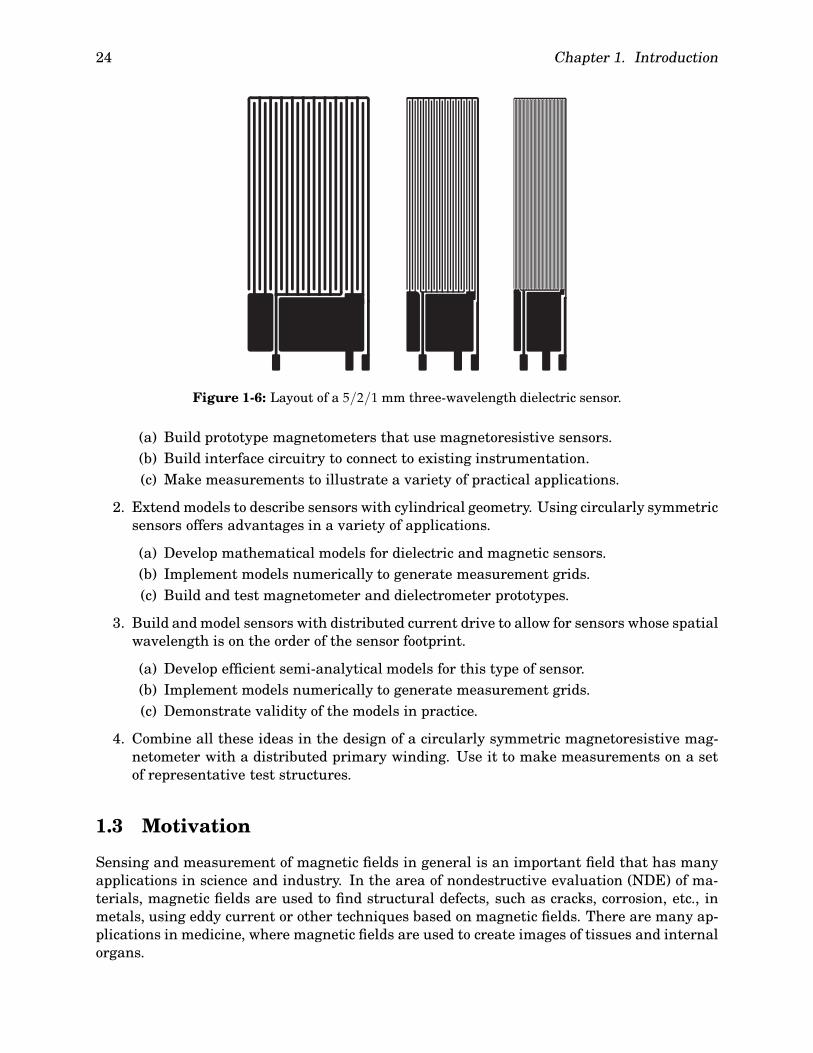
1.1.4 Multiple-Wavelength Dielectrometer
The depth of sensitivity of the sensor depends on the imposed spatial wavelength, as seen inFigure 1-5. Combining the results of sensors with different wavelengths can be used to mea-sure properties as a function of depth or to estimate more than one unknown parameter. Thisis especially useful for measurements where direct contact with the material is not possible,such as noncontact cure monitoring [36]. The lift-off, i.e. the air gap thickness, is usually notknown, especially with the material deposited on a moving web, where some vertical motion,or flutter, is inevitable. This requires the simultaneous estimation of three unknown param-eters: the permittivity and conductivity, which change with cure state, and the lift-off. Whatcomplicates matters even more is that the thickness of the film may be nonuniform, addinganother unknown to the set of properties that need to be estimated simultaneously.
In cases like this it is beneficial to combine the response of several sensors with differentspatial periods. Figure 1-6 shows the layout of a three-wavelength sensor. Although it is pos-sible, the use of multiple wavelengths in magnetometers is usually not necessary, since insideconducting materials magnetic diffusion makes it possible to change the depth of sensitivityby changing the frequency, which changes the skin depth.
Multiple-wavelength dielectrometers have also been used to monitor the diffusion of mois-ture into pressboard. The moisture content is related to the conductivity and permittivity.The use of multiple wavelength sensors makes it possible to measure the variation of theconductivity and permittivity with depth [7,8,11].
1.2 Goals
The goal of this research effort is to extend the capabilities of the existing spatially periodicquasistatic-field sensors, with a focus on the magnetometers. Stated concisely, the main goalsare:
1. Incorporate magnetoresistive technology into sensor design to allow low frequency mag-netometry measurements.
24 Chapter 1. Introduction
Figure 1-6: Layout of a 5/2/1 mm three-wavelength dielectric sensor.
(a) Build prototype magnetometers that use magnetoresistive sensors.(b) Build interface circuitry to connect to existing instrumentation.(c) Make measurements to illustrate a variety of practical applications.
2. Extend models to describe sensors with cylindrical geometry. Using circularly symmetricsensors offers advantages in a variety of applications.
(a) Develop mathematical models for dielectric and magnetic sensors.(b) Implement models numerically to generate measurement grids.(c) Build and test magnetometer and dielectrometer prototypes.
3. Build and model sensors with distributed current drive to allow for sensors whose spatialwavelength is on the order of the sensor footprint.
(a) Develop efficient semi-analytical models for this type of sensor.(b) Implement models numerically to generate measurement grids.(c) Demonstrate validity of the models in practice.
4. Combine all these ideas in the design of a circularly symmetric magnetoresistive mag-netometer with a distributed primary winding. Use it to make measurements on a setof representative test structures.
1.3 Motivation
Sensing and measurement of magnetic fields in general is an important field that has manyapplications in science and industry. In the area of nondestructive evaluation (NDE) of ma-terials, magnetic fields are used to find structural defects, such as cracks, corrosion, etc., inmetals, using eddy current or other techniques based on magnetic fields. There are many ap-plications in medicine, where magnetic fields are used to create images of tissues and internalorgans.

1.3. Motivation 25
1.3.1 Magnetoresistive sensors
The main reason to explore the use of magnetoresistive and giant magnetoresistive sensorsas an alternative to the secondary winding of the standard magnetometers is their ability tooperate at low excitation frequencies, down to DC. Operation at low frequencies is requiredwhen testing materials for deeply buried flaws, which are otherwise hidden by the skin depth,δ ∝ 1/
√ω.
Magnetizable materials can even be measured with constant magnetic fields. In the ab-sence of magnetic diffusion, the problem of calculating the magnetic field becomes analogousto the electroquasistatic sensor.
Another reason for lowering the frequency of excitation is that at high frequencies amaterial’s conductivity and magnetic permeability cannot be measured independently [1].This considerably complicates conductivity measurements of ferromagnetic materials, suchas steel, because local permeability variations pollute the conductivity measurement. Suchpermeability variations may be due, for example, to residual stresses.
There are several complications associated with the use of magnetoresistive sensors in themagnetometer design. They have a highly nonlinear transfer characteristic. The nonlinearityis in fact very extreme, since the sensors are insensitive to the polarity of the magnetic field(see Figure 5-5). For this reason they are typically biased at an appropriate operating pointby an independent constant magnetic field source, such as a permanent magnet or a solenoid.Since the magnetic field effects a resistivity change, the sensors also need electrical biasingand an appropriate bridge configuration. Many of these issues are addressed by placing thesensor in a feedback loop, as discussed in Chapter 5.
A few examples where low frequency operation, made possible by the use of magnetoresis-tive sensors, is beneficial are:
• Subsurface corrosion (airplane skins, etc.).• Flaws in magnetic media (hard drives, etc.).• Detection of deeply buried defects in metals, or features in metals positioned below a
shielding material.• Thickness measurement for metal components (0.1 – 2′′).• Stress profile measurement in steel.
1.3.2 Modeling sensors with rotational symmetry
So far all periodic field magnetometers and dielectrometers, like the MWM and the IDED,have been designed with Cartesian geometry, i.e. the magnetic or electric fields have an im-posed periodicity in the x-direction and are considered invariant in the y-direction. Designingcircularly symmetric sensors offers several advantages and may be preferred in some appli-cations:
1. They have fewer unmodeled end effects:
• The edges due to finite sensor width in the y-direction are completely eliminated,since there are no edges in the ϕ-direction in cylindrical coordinates.
• In the dielectric case the edges due to the finite length in the x-direction can beremoved far from length scales of interest in the r-direction in cylindricalcoordinates, since the models assume the electric potential to be fixed at zero by aground plane at distances from the origin greater than the end of theinter-electrode gap.

26 Chapter 1. Introduction
2. The circular geometry ensures insensitivity to anisotropic properties, by effectively tak-ing an average of the property in all directions in the x-y plane. This is useful in certainapplications, since it eliminates the need for precise sensor alignment when measuringferromagnetic materials whose magnetic permeability is anisotropic.
3. Many material defects and human-made structures have rotational symmetry, makingthem ideal candidates for testing with rotationally symmetric sensors. An example ap-plication is testing for cracks near rivets and bolts.
1.3.3 Magnetometers with distributed current drive
There are applications where the imposed spatial wavelength of the magnetic field needs tobe large for large penetration distances. An application that has such a requirement is landmine detection. In order to be sensitive to a metal object located 15 cm below the surface,the magnetometer must have a spatial wavelength of about 50 cm or more, which results ina footprint of several square meters with the standard MWM geometry shown in Figure 1-1.Since this is impractical, sensors have been developed where the magnetic field is generatedby several windings, each having a different number of turns, that follows a sinusoidal enve-lope function. The fundamental wavelength of this envelope function is several times greaterthan the winding spacing. This makes it possible to reduce the sensor footprint to be on theorder of the wavelength, or approximately 0.4 square meters. The distributed current driveconcept was developed by Dr. Neil Goldfine at JENTEK [32,34,35].
Another class of applications where a larger effective spatial wavelength is required, rela-tive to the sensor footprint, is testing for deeply buried flaws in metals. Use of low excitationfrequencies and magnetoresistive secondary elements, as discussed in Section 1.3.1, over-comes the depth limitation due to skin depth. In order to overcome the depth limitation dueto the imposed spatial wavelength, the sensor wavelength must be made several times largerthan the desired depth of sensitivity. Whereas in this application the resulting footprint of astandard magnetometer layout may not be too large from a logistical perspective, a smallerfootprint makes the flaw signature more localized and improves sensitivity, since the flawsignature is not averaged over a large area.
A further advantage of having a distributed current drive is that the effective spatialwavelength may be changed dynamically, e.g. by varying the relative phase of two or moresuperimposed windings, an idea discussed further in Section 4.10.
From a modeling perspective, an advantage of this kind of magnetic field excitation is thatthe drive current distribution is known from the beginning, since the width of the windingsis small compared to the wavelength and may be approximated as being infinitely narrow.This significantly simplifies numerical computation, since it makes it possible to apply fastdiscrete Fourier transform methods directly, as shown in Chapter 4. These efficient methodsmay also be applied to the MWM if one of the following circumstances is met:
1. Low frequency operation; the current is uniform across each winding.
2. High frequency operation; the current is concentrated at the winding edges and may berepresented by spatial impulse functions.
3. The current distribution effects are negligible or can be calibrated out, using the stan-dard calibration methods discussed in Appendix D.

1.4. Inverse estimation methods 27
1.4 Inverse estimation methods
Chapter 2 describes the forward models used to calculate the response of the MWM and IDEDfrom the sensor geometry parameters and the properties of the materials. During a mea-surement the reciprocal task needs to be accomplished, which is to obtain absolute materialproperties from the measured sensor response.
Several different methods have been used to approach this inverse problem. The methodmost commonly used in practice uses measurement grids. It is described in Section 1.4.1.An alternative approach is to use a root-finding method, which uses the forward model overmany iterations [7, 8]. There are many difficulties with this approach. The function thatrelates sensor response to material properties is nonlinear, resulting in failure of the methodif the solution is not unique or if noise in the data leads to the lack of an exact solution.Furthermore, because the method seeks an exact solution, the number of unknowns mustequal the number of degrees of freedom exactly. For example, if three unknowns are beingmeasured with an MWM at several frequencies [26], this method cannot be used, as everyfrequency produces two constraints. While it is possible to simply ignore the extra constraints,there is a much better alternative, which makes use of all data. This alternative to the root-finding methods uses a least squares minimization technique to estimate multiple unknowns,and has been successfully applied in a number of practical problems [26]. It is discussed inSection 1.4.2.
Another approach proposed recently [37], which also avoids the need for iteration, can betaken for estimating the conductivity and permittivity of a single unknown layer in a dielec-trometer measurement. In this method the inverse problem is formulated as a generalizedeigenvalue problem, where the complex unknown parameter is one of the generalized eigen-values. The multiple layers problem can be posed as a multi-variable eigenvalue problem.
1.4.1 Measurement grids
The method of parameter estimation using measurement grids was invented by Dr. NeilGoldfine [1, 38]. The standard two-dimensional measurement grid is a database of sensorresponses calculated for a range of values of two material properties. For every combinationof values of the two parameters, the magnetometer transinductance or dielectrometer trans-capacitance are computed and tabulated. The parameter estimation is then carried out byusing a two-dimensional inverse interpolation technique, to obtain the material propertiesthat correspond to the measured sensor response. It is also possible to have one-dimensionalgrids, which relate a single unknown parameter to one measured quantity. Interpolation inthis case is usually trivial.
Measurement grids may be visualized by plotting every point in magnitude/phase spaceand connecting points that correspond to a constant parameter with lines. Figure 5-8 showsa typical conductivity/lift-off grid, where the two variable material properties are the con-ductivity of an infinitely thick metallic layer and the sensor lift-off, which is the distancebetween the material and the sensor windings. The two measured variables do not have to bemagnitude and phase, although this is by far the most common situation. Figure 3-6 showsa magnitude/magnitude grid [54], combining the response of two separate dielectric sensorsto measure dielectric permittivity and lift-off independently. Similarly, Figure 5-10 shows amagnetic magnitude/magnitude grid, where the two magnitudes correspond to magnetome-ter measurements at two different spatial wavelength modes, excited within the same sensorfootprint. Other examples of two-dimensional measurement grids include the thickness/lift-

28 Chapter 1. Introduction
off magnetometer grid in Figure 5-13 and the conductivity/thickness magnetometer grid inFigure 5-15.
Visual inspection of a measurement grid can be used to assess in which region of the gridthe measurements have the highest sensitivity. In regions where the grid cells have smallareas, small changes in the instrument magnitude and phase lead to large changes in the es-timated properties, so that measurements that fall in such regions have lower accuracy thanmeasurements in the grid regions with large cell areas. Another aspect of the quality of ameasurement is its selectivity, which is a measure of how independent the two estimated pa-rameters are of each other [13]. The orthogonality of the cell edges is related to the measure-ment selectivity in that region of the grid. The sensitivity and selectivity of a measurementcan be analyzed using singular value decomposition of the Jacobian matrix [1,13].
Although grid methods have been in use for a long time now, a new implementation hasbeen developed, presented in Section 6.2, which leads to significant improvements both in theefficiency of the grid look-up and the accuracy of the results from the interpolation.
The power of parameter estimation via measurement grids stems from two importantadvantages that this method has over alternative techniques:
1. Reliability. The parameter estimation is guaranteed to succeed if the data are on thegrid, i.e. if the measurement data fall inside the range area of the grid in magni-tude/phase space. All other methods are iterative, which means that there is alwayssome danger of nonconvergence for a point that should have a solution, especially if theinitial guess is too far from the solution. Even for points off the grid, but still close to it,the estimated properties are usually reasonable, while if iterative methods fail to con-verge, the errors are typically dramatic. Reliability is a very important requirement incommercial applications, where the individual user may not have the ability to assessthe quality of the data in a way possible in a laboratory environment.
2. High speed. Although the efficiency of the forward models has been greatly improved bya judicious formulation that allows for much of the computations to be carried out onlyonce for a given sensor geometry (see Chapter 2), in general all iterative methods areorders of magnitude slower than the grid look-up method. With present day technology,typical numbers may be 5 to 10 seconds for a minimization algorithm estimation versus20 to 30 milliseconds for a grid look-up. This makes it possible to carry out parame-ter estimation in real time, which is another feature of commercial value, especially inscanning and imaging applications [23,31,32].
The main practical disadvantage of using measurement grids is that this approach on itsown cannot be used to estimate more than two unknowns.∗ It can still be possibly used asa step in some different iterative estimation algorithm. Since the properties are estimatedvia interpolation, there is always some error for points lying between the grid points. Theaccuracy can be improved by generating denser grids, but the need to store large amounts ofdata in operative memory and on disk necessarily creates an unfavorable trade-off situationbetween efficiency and accuracy. Stated another way, the cost of the estimation rises veryrapidly with improved accuracy, in contrast with iterative methods, where the opposite istypically true.
∗In theory, the grid methods may be extended to three or more dimensions, but the complexity of the grid look-up and inverse interpolation increases exponentially with the number of dimensions. Grid look-ups in more thantwo dimensions have not yet been demonstrated in practice.

1.5. Magnetic field sensing technologies 29
1.4.2 Minimization methods
The least-squares minimization parameter estimation algorithm appears to be the best choicefor estimating more than two unknowns. It operates by defining an error function based on thedifferences between measured and simulated sensor response. Using iterative applications ofthe forward model, a set of parameters are found where the error function has a minimum,establishing the set of material properties most likely to yield results matching the measureddata. If the problem is not over-determined, i.e. if the number of degrees of freedom equalsthe number of unknowns, then finding a minimum where the value of the error function iszero is equivalent to finding an exact solution.
The main advantage of this method is its universal applicability, most useful in caseswhere there are no alternative estimation methods. It is also valuable in attempting to findthe most likely material property values over a range of experimental conditions. For exam-ple, standard grid methods can be used for measuring the conductivity of a metal at severalfrequencies independently, but the least-squares minimization method can combine the datafrom all frequencies in a single estimation, thus finding the optimal solution over the en-tire frequency range. Finally, since the forward model is run with the exact set of materialproperties, the final result is typically more accurate than the grid interpolation method.
As discussed before, the reason that this method is not used universally is that it is rela-tively slow and that it is not guaranteed to find a solution, or that the solution is the correctone when it does, since the error function can have many local minima.
1.5 Magnetic field sensing technologies
One possible way of enhancing magnetometer performance is by using an alternative to re-place the secondary winding as the means of detecting the magnetic field by a different typeof magnetic sensor. This section describes in very general terms some of the existing methodsfor detecting and measuring magnetic fields, how they compare to each other, and whetherthey are suitable for this application.
The simplest magnetic sensor is a “search coil,” which is a winding typically on a circularor square frame. The voltage induced at its terminals responds to changing magnetic fluxlinked by the winding. Since it only depends on the rate of change of the linked magnetic flux,a sensor of this type is limited to higher frequencies, and when stationary is incapable of mea-suring DC fields. The magnetoresistive sensors, on the other hand, are sensitive over a widefrequency range, including zero. Along with sensors based on the Hall effect and the giantmagnetoresistive effect, these sensors are used when the application requires measurementof low-frequency magnetic fields. A review and comparison of existing magnetic field sensorsis presented in [39].
Some of the methods used for measuring magnetic fields, along with their range of sensi-tivity, are listed in Figure 1-7. Table 1.1 shows a list of the advantages of the magnetoresistivesensor and some application areas, as shown in [40].
There are many other factors, such as cost, size, ease of calibration, temperature sensi-tivity and temperature range of operation, which affect the choice of magnetic sensor for agiven application. Eddy current sensors used in nondestructive evaluation applications, forexample, are based on the search-coil sensor. Since they are sensitive to the rate of changeof magnetic flux, their use is often limited to relatively high frequencies, typically 1 kHz –10 MHz. At these frequencies, however, structural materials such as aluminum and steel

30 Chapter 1. Introduction
AdvantagesHigh sensitivity – allowing operation over relatively great distancesLow source resistance – giving low sensitivity to electrical interferenceHigh-temperature
operation– 150◦C continuous, 175◦C peak (chip alone can withstand 175◦C
continuous)Operation over a wide
frequency range– from DC up to several MHz
Metal-film technology – giving excellent long-term stabilityLow sensitivity to
mechanical stress– facilitating mounting of the sensor and allowing its use in relatively
rough environmentsSmall size – can be fabricated with micron dimensionsApplication areasTraffic control – detection of vehiclesLow-cost navigation – allowing the production of simple compass systems with an accuracy of
around 1◦, ideal for automotive applicationsLong-distance metal
detection– for the detection of, for example, military vehicles by measuring
disturbances in the earth’s magnetic fieldMotion detectors – by measuring position changes relative to the earth’s magnetic fieldCurrent detection – for example, earth leakage switchesGeneral magnetic field
measurement– from 10 A/m to 10 kA/m
Direct-currentmeasurement
– starting currents in motor vehicles
Angular or positionmeasurement
– sensing of accelerator pedal or throttle position (engine-managementsystems)
– position sensing in industrial automation systems (commercial sensorarrays that can measure positions with an accuracy of 30 m)
– force/acceleration/pressure measurement using a moving magnet, forexample: engine-intake-manifold pressure sensors, fluid-level sensors,low-cost weighing systems, geosonic (seismic) sensors, accelerometers
Mark detection andcounting
– camshaft or flywheel position sensors for engine ignition systems
– end-point sensors– wheel-speed sensors for anti-blocking systems– rpm counters (0 to 20 kHz) for engine tachometers and for electronic
synchromesh systems– flow meters– zero speed detectors — rpm control in electric motors– general instrumentation
Magnetic recording – thin-film replay heads for tape and disk systems. Swipe readers forcredit cards, bus tickets, door locks, etc.
Table 1.1: Magnetoresistive sensors: advantages and application areas.

1.5. Magnetic field sensing technologies 31
10−10 10−6 10−2 106102
Detectable Field (Gauss)Magnetic Sensor Technology
2. Flux-Gate Magnetometer3. Optically Pumped Magnetometer4. Nuclear-Precesion Magnetometer5. SQUID Magnetometer6. Hall-Effect Sensor7. Magnetoresistive Magnetometer8. Magnetodiode
Earth’s magnetic field
10. Fiber-Optic Magnetometer
1. Search-Coil Magnetometer
9. Magnetotransistor
11. Magneto-Optical Sensor
Figure 1-7: Sensitivity comparison of magnetic sensor technologies [39]. The magnetoresistivesensor includes the giant magnetoresistive sensor as well.
have skin depth on the order of tenths of a millimeter, which is a severe limitation to theability to examine materials for buried flaws. This is an example of an application where lowfrequency sensitivity, as provided by the magnetoresistive sensor, is of critical importance.
On the other hand, a search-coil based sensor that does not use a magnetizable core hasthe advantage of having a perfectly linear transfer characteristic, which is a property of thistype of sensor only. In order to approach linearity, magnetoresistive and other sensors needto be biased with a constant magnetic field, and operated within a small dynamic range.Linearity concerns for the magnetoresistive sensor are discussed in more detail in [41].
Eddy-current sensor arrays used for two-dimensional imaging have been developed andused successfully to map surface defects in a metal plate [42]. As discussed before, it is diffi-cult to measure buried metal flaws, such as cracks and voids, that lie below a layer of metalwith thickness on the order of, or greater than, the skin depth at the excitation frequency. Inorder to detect such flaws it is necessary to use lower excitation frequencies, which propor-tionally reduce the sensitivity of eddy current sensors.
To overcome this limitation, SQUID magnetometers have been used for defect mapping,with some limited success [43]. Although SQUID technology has progressed substantiallyover the last few years [44, 45], it has not yet reached the level of miniaturization and costthat are required for the development of high-density imaging arrays.
The SQUID magnetometer is another extreme example of the tradeoff between the per-formance characteristics of magnetic sensors [46]. It is sensitive to changes on the order ofa fraction of the flux quantum Φ0 = h/2e = 2.07 × 10⁻⁷G·cm2 = 2.07× 10⁻¹⁵ Wb, where h isPlanck’s constant and e is the electron charge, which makes it the most sensitive magneticsensor known. However, its response to values of enclosed flux which differ by an integralnumber of flux quanta is identical. This means that SQUIDs are incapable of measuringabsolute magnetic field intensity and that local variations of the Earth’s magnetic field andother interference must be “calibrated out”, shielded very carefully, or more than one sensormust be connected in a differential mode, before any meaningful data may be obtained from aSQUID. Furthermore, the need for operating the sensor at cryogenic temperatures makes ita costly and rather bulky device, although SQUIDs based on high-TC superconducting mate-

32 Chapter 1. Introduction
rials developed recently [44], which can operate at liquid nitrogen temperatures, have madethe SQUID magnetometer somewhat more practical.
An interesting application of the SQUID magnetometer to the detection of buried flaws ispresented in [45]. In this application the magnetic sensor is used to detect weak magneticfields generated by local current loops induced by the thermoelectric Seebeck effect whena host metal material contains an inclusion of a different metal and a thermal gradient ispresent. Magnetizable inclusions can also be detected by this method without the need for athermal gradient. In this application the ambient fields are canceled out by a second-ordergradiometer configuration that uses three SQUID heads.
Magnetoresistive and giant magnetoresistive sensors are discussed in more detail in Chap-ter 5.
1.6 Summary of Chapter 1
In this chapter the subject of nondestructive evaluation using time and space periodic-fieldquasistatic inductive and capacitive sensors has been introduced. The chapter has also intro-duced some of the fundamental concepts on which much of the rest of the thesis depends:
1. General principles of operation of the model-based quasistatic periodic-field inductiveand capacitive sensors (Section 1.1).
2. Measurement grid methods for absolute dielectric, magnetic, conduction, and geometricproperty estimation (Section 1.4).
3. Review of the state of the art technologies for sensing and measuring magnetic fields(Section 1.5).
A range of new applications that require capabilities of these sensors not available untilnow have motivated the research for improvements in the following areas:
1. Design of magnetometers with high depth of sensitivity by increasing low frequencysignal strength with the use of magnetoresistive sensors, and by exciting magnetic fieldswith high effective spatial wavelength with the help of a distributed current drive.
2. Development and validation of cylindrical geometry models for inductive and capacitivesensors.
3. Development and validation of efficient numerical techniques for modeling magnetome-ters with distributed current drive in Cartesian and cylindrical coordinates.
4. Improvement in the accuracy and efficiency of two-dimensional inverse interpolationand grid look-up techniques.
The results of the efforts in all of these areas are presented in the remaining chapters of thethesis.
Chapter 2
Forward Models of the SpatiallyPeriodic Sensors
The analytical models of the cylindrical geometry sensors, developed in Chapter 3, are struc-tured similarly to the collocation point methods in Cartesian geometry. The latter are alsooften referenced by the methods used to model the magnetometers with distributed currentdrive, presented in Chapter 4. To supply the background for these topics, it is necessary toinclude a description of the Cartesian geometry collocation point methods for both magneto-quasistatic and electroquasistatic sensors, along with all important formulas. This is done inthis chapter.
Although these methods have appeared many times in the literature [1–3, 7, 47], it hasalways been difficult to find needed details, and different sources use different conventions. Inaddition to providing a self-consistent source on which to base the material in the remainingchapters, this chapter describes some changes to the models not previously published. Whilemost of these changes are not fundamental, but aimed mainly at improving computationalefficiency and at simplifying the equations, some are quite significant. The most importantof these is perhaps the way the zero-order Fourier mode is treated for the dielectric sensors.This is discussed further in Section 2.2.
The MWM is analyzed in the magnetoquasistatic (MQS) regime, which ignores the termin Ampere’s law due to the displacement current density. Similarly, the IDED is treated inthe electroquasistatic (EQS) regime, which ignores Faraday’s law and sets the curl of the elec-tric field intensity to zero. Both cases assume that the contribution of electrodynamic (wave)effects is negligible, which is justified if the spatial period of the electromagnetic waves atthe operating frequency is much greater than the characteristic length of the structure. TheIDED and the MWM are not operated at frequencies higher than 30 MHz, so that this require-ment is typically satisfied by a margin of three orders of magnitude. The magnetoquasistaticapproximation is further discussed in Section 2.1.1.
In this chapter and for the rest of the thesis the sensors are assumed to be operated insinusoidal steady state with angular frequency ω. This means that all time dependent quan-tities can be written in the following form:
F(r, t) = �{F(r)eiωt} (2.1)
where F is a complex amplitude function only of spatial coordinates. Derivatives with re-spect to time are transformed into multiplications by iω. The hat accents will be dropped in
33

34 Chapter 2. Forward Models of the Spatially Periodic Sensors
subsequent analysis.For other notation conventions and symbol definitions, refer to Appendix A.
2.1 Mathematical model and simulation method for the MWM
This section contains the formulas used to calculate the response of the MWM, based on thephysical models. The equations are put in a form that closely parallels the steps and nameconventions used in the numerical simulation code.
This model assumes a secondary winding on either side of the primary, connected in series.All material properties are considered independent of x, y, and time. The material structureis assumed to consist of a number of homogeneous layers stacked up in the z-direction, wherethe material interfaces are planes parallel to the x-y plane.
2.1.1 Magnetic diffusion
In the magnetoquasistatic regime in the presence of conducting materials the magnetic fieldmust satisfy the magnetic diffusion equation:
∇2H− iωσµH = 0 (2.2)
which is a direct consequence of Maxwell’s equations and Ohm’s law [48–50]. For the purposeof this analysis, it is more convenient to find solutions to the magnetic vector potential A,which satisfies the following definition:
∇×A = B (2.3)
Equation (2.3) only defines the curl of the vector potential. Its divergence must also be speci-fied, if A is to be determined uniquely (within a constant of integration). The divergence canbe chosen in a particular problem to simplify the resulting equations, as will be shown laterin this section.
Using Faraday’s law ∇× E = −iωB, where the time derivative has been replaced with amultiplication by iω according to equation (2.1), and combining it with equation (2.3) yields
∇× E = −iω∇×A (2.4)
Vector fields with equal curl may differ by the gradient of a scalar field, which makes it possi-ble to express E in terms of A as
E = −iωA−∇Φ (2.5)
where Φ is the electric scalar potential. Combining Ampere’s law and Ohm’s law with theresults obtained so far yields
∇×H = J = σE = −σ(iωA+ ∇Φ
)(2.6)
which can be manipulated as follows:
∇× (∇×A)
= −σµ(iωA+∇Φ
)(2.7)
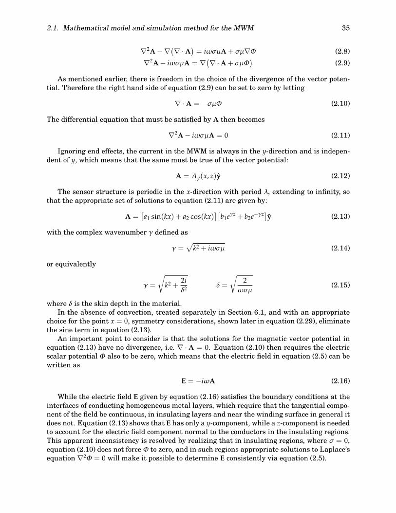
2.1. Mathematical model and simulation method for the MWM 35
∇2A−∇(∇ ·A) = iωσµA+σµ∇Φ (2.8)
∇2A− iωσµA = ∇(∇ ·A+σµΦ)
(2.9)
As mentioned earlier, there is freedom in the choice of the divergence of the vector poten-tial. Therefore the right hand side of equation (2.9) can be set to zero by letting
∇ ·A = −σµΦ (2.10)
The differential equation that must be satisfied by A then becomes
∇2A− iωσµA = 0 (2.11)
Ignoring end effects, the current in the MWM is always in the y-direction and is indepen-dent of y, which means that the same must be true of the vector potential:
A = Ay(x, z)y (2.12)
The sensor structure is periodic in the x-direction with period λ, extending to infinity, sothat the appropriate set of solutions to equation (2.11) are given by:
A =[a1 sin(kx) + a2 cos(kx)
][b1eγz + b2e−γz]y (2.13)
with the complex wavenumber γ defined as
γ =√k2 + iωσµ (2.14)
or equivalently
γ =
√k2 +
2iδ2
δ =
√2
ωσµ(2.15)
where δ is the skin depth in the material.In the absence of convection, treated separately in Section 6.1, and with an appropriate
choice for the point x = 0, symmetry considerations, shown later in equation (2.29), eliminatethe sine term in equation (2.13).
An important point to consider is that the solutions for the magnetic vector potential inequation (2.13) have no divergence, i.e. ∇ ·A = 0. Equation (2.10) then requires the electricscalar potential Φ also to be zero, which means that the electric field in equation (2.5) can bewritten as
E = −iωA (2.16)
While the electric field E given by equation (2.16) satisfies the boundary conditions at theinterfaces of conducting homogeneous metal layers, which require that the tangential compo-nent of the field be continuous, in insulating layers and near the winding surface in general itdoes not. Equation (2.13) shows that E has only a y-component, while a z-component is neededto account for the electric field component normal to the conductors in the insulating regions.This apparent inconsistency is resolved by realizing that in insulating regions, where σ = 0,equation (2.10) does not force Φ to zero, and in such regions appropriate solutions to Laplace’sequation ∇2Φ = 0 will make it possible to determine E consistently via equation (2.5).

36 Chapter 2. Forward Models of the Spatially Periodic Sensors
A conclusion that can be drawn from this discussion is that the model applies only whenthe sensor windings are surrounded by an insulating material. This is anyhow required toconstrain the winding current to remain within the windings. Although it is possible to solvefor the electric field E everywhere via Φ, it is not necessary, since the only contribution tothe magnetic field by the electric field component due to Φ comes from surface charge anddisplacement current density, which are effects ignored in the magnetoquasistatic regime.
Another assumption tacitly made in the discussion so far, and a direct consequence of theMQS approximation, is that the materials are either insulators, where σ = 0, Φ = 0, and theelectric field lines have a component normal to the conductor surfaces; or good conductors,such as metals, where σ = 0, Φ = 0, and the electric field lines are tangential to the surfaces.In the MQS regime in a current carrying wire the electric field is always tangential to thesurface. In the MWM model, the electric field is also tangential to the interface between twoconducting layers, because the winding current and the magnetic vector potential everywherehave only a y-component.
If there are materials with conductivity ranges where one of the effects does not dominatethe other, it will be necessary to consider the full set of Maxwell’s equations, including thetreatment of surface charge and displacement current density, with Φ = 0 everywhere. Thisis a much more complicated problem that does not appear to be of great practical significanceand will not be considered in this analysis.
It is important to show quantitatively under what conditions the MQS approximationis justified, in addition to the frequency restriction described earlier. This can be done bycomparing the magnetic diffusion time τm = µσ�2, where � is a characteristic length scale,such as the sensor spatial wavelength, to the charge relaxation time τe = ε/σ [50, §2.3]. Inthe MQS regime τm � τe. The conductivity at which the two time constants become equal toeach other is given by
σ =1�
√ε
µ(2.17)
which is on the order of 0.1–1 S/m for typical magnetometers. Metal conductivities are typi-cally five or more orders of magnitude greater, as shown in Table 5.2. This justifies the MQSapproximation in treating the MWM, which is used almost exclusively for measurements onmetals. The same is true for measurements on other relatively conductive nonmetallic ma-terials like graphite, whose conductivity is typically on the order of a few hundred S/m. Onthe other hand, when considering materials like salt water, for example in soil moisture andcontamination measurements, it would be necessary to include the full set of Maxwell’s equa-tions.
2.1.2 Normalization
Most of the quantities in the model are normalized appropriately so that they are all di-mensionless. This has many advantages, such as simplicity, but also saves on computation,because many variables only appear in expressions of the same form. Moreover, some pa-rameters, such as the frequency, sensor wavelength, meander length, and coil thickness, arealtogether eliminated from further computations.

2.1. Mathematical model and simulation method for the MWM 37
Primary windingSecondary windings
λ0 λ/2 3λ/4λ/4
z
x
dg gcd∆
Figure 2-1: Definition of geometry parameters of the MWM. Due to symmetry, only onequarter of a wavelength needs to be considered.
Coordinates
All spatial coordinates are normalized by the wavelength λ:
x =xλ
y =yλ
z =zλ
(2.18)
Sensor parameters
The geometrical parameters of the MWM are shown in Figure 2-1. One period of the sensor isshown in the figure. A period contains the two legs of the primary winding, carrying currentin opposite directions, and the two secondary windings. All length parameters, such as theprimary winding width c, secondary winding width d, and gap between the windings g, arenormalized by the sensor wavelength λ:
c =cλ
d =dλ
g =gλ
(2.19)
One sensor period contains two primary winding traces, four secondary winding traces, andfour gaps, which leads to the following inequalities that must be satisfied by the normalizedsensor parameters:
0 <c2; d; g <
14
0 <c2
+ d+ g <14
(2.20)
The conductivity always appears in expressions like ωσµ (e.g. equation (2.15)) that haveunits of [length−2]. The proper normalization for the winding conductivity is
σcoil = σcoil ·µ0ωλ∆ (2.21)
where one of the length parameters, ∆, is the thickness of the traces shown in Figure 2-1.The choice of normalizing parameters is motivated by the form of the boundary condition inequation (2.55), derived later. The coil thickness is assumed to be much smaller than the skindepth, ∆ � δ.
In deriving the two-port impedance matrix of the MWM, if each port is driven in turn bycurrent with unity magnitude, the terminal voltages will be equal to the two-port impedances.The currents are normalized by the driving current magnitude ID, and the voltages are nor-malized as follows:
v =v
MLµ0ωID(2.22)

38 Chapter 2. Forward Models of the Spatially Periodic Sensors
where ML is the meander length of the sensor, defined as the total length of the primarywinding.
Material parameters
Similar arguments hold for the geometric and physical properties of the material under test.Each layer’s properties are normalized as follows:
t =tλ
µ∗ =µ∗
µ0σ = σ ·µ0ωλ2 (2.23)
where t is the layer thickness, µ∗ is the complex magnetic permeability, including magneticloss, and σ is the conductivity.
Other parameters
Other parameters that are normalized include the Fourier harmonic wavenumbers
kn = kn · λ =2πnλ
· λ = 2πn (2.24)
and similarly the complex wavenumbers
γ2n = k2n + iσµ∗ (2.25)
The complex wavenumber γ appears in equation (2.13) and is defined by equation (2.14).For the rest of this chapter the bars will be dropped from the normalized variables to sim-
plify notation. All appropriate variables should be assumed to be normalized, unless explicitlystated otherwise.
2.1.3 Collocation points
The goal is to calculate the two-port matrices of impedances and admittances:[v1v2
]=[Z11 Z12Z21 Z22
] [i1i2
] [i1i2
]=[Y11 Y12Y21 Y22
] [v1v2
]Z = Y−1 (2.26)
This is accomplished by first finding the vector potential Ay at the surface as a function ofthe two terminal voltages, and then using it to find the surface current density KS, integratedacross the width of the windings to obtain the terminal currents. For this purpose Ay isrepresented as a piecewise-linear function, which connects its values at a set of collocationpoints xm with linear segments.
If the origin of the x-axis is chosen at the center of the primary winding, symmetry consid-erations constrain the vector potential in the following way (see Figure 2-1):
∂Ay
∂x
∣∣∣∣x
=∂Ay
∂x
∣∣∣∣−x (2.27a)
Ay(x) = −Ay
(x+
12
)(2.27b)

2.1. Mathematical model and simulation method for the MWM 39
The constraint on Ay that results from equation (2.27a) is
Ay(x) = Ay(−x) + AC (2.28)
where AC is an arbitrary constant of integration. Since only derivatives of the vector poten-tial are meaningful, this constant may be set to zero for convenience, letting the symmetryconstraints be written as
Ay(x) = Ay(−x) (2.29a)
Ay(x) = −Ay
(x+
12
)(2.29b)
Choosing AC = 0 also ensures that the Fourier series expansion, developed in Section 2.1.4,has no zero order term.
The symmetry properties in equation (2.29) mean that specifying Ay over one quarter ofthe period is sufficient to determine it everywhere else. The piecewise-linear representationof Ay in this interval is given by:
Ay(x) =(xm+1 − x)am + (x− xm)am+1
xm+1 − xmxm < x < xm+1 m = 0, 1, . . . , 4K − 1 (2.30)
where am are the values of Ay at the points xm. Lower case a is used because An are reservedfor the Fourier series amplitude coefficients. There are a total of 4K + 1 collocation points,K over each of the four intervals into which the quarter-period is subdivided: one-half of theprimary winding, the gap between the windings, the secondary winding, and one-half of thesecondary gap. A consequence of the constraints in equation (2.29) is that
Ay
(14
)= Ay
(−14
)= −Ay
(14
)= 0 (2.31)
This means that
a4K = Ay
(14
)= 0 (2.32)
leaving 4K independent unknowns that need to be determined.The unknowns will be found by generating 4K equations by applying boundary conditions
over 4K intervals. The collocation points themselves cannot be used to delimit these intervals,because the problem is numerically unstable in this case. To understand why this is so,consider the following: suppose that the integral over a particular interval is constrained tobe zero. This is achievable even if at the two end points the values are large, but oppositein sign. A possible solution for the entire function could be a large magnitude oscillatoryfunction. On the other hand, if the collocation point lies in the middle of the interval, thenthis constraint would force it to zero, as necessary.
The boundary conditions differ over the windings and in the gaps. As a consequence,the edges of the windings must also be integration limit points. The points that delimit theintegration intervals, x∗m, should be concentrated near the edges of the windings, because the

40 Chapter 2. Forward Models of the Spatially Periodic Sensors
✻✲
λ/4
x∗mxm
Interval limits
Collocation points
✛ ✲✛ ✲✛ ✲c/2 g d
× × × × ××××× × × × × ×××× × × ××××× × × × × ×◦ ◦ ◦ ◦ ◦◦◦◦ ◦ ◦ ◦ ◦ ◦ ◦◦◦ ◦ ◦ ◦ ◦◦◦◦ ◦ ◦ ◦ ◦ ◦ ◦
Figure 2-2: Collocation points and interval limits used in the analysis of the MWM, as definedin equations (2.33) and (2.34). The distribution shown assumes K = 7.
magnetic fields are strongest there. The following definitions are used:
x∗m =c2sin
(π
2· mK
)x∗K+m =
c2
+ g · 1− cos(πm/K)2
x∗2K+m =c2
+ g+ d · 1− cos(πm/K)2
x∗3K+m =c2
+ g+ d+(14− c
2− g− d
) [1− cos
(π
2· mK
)]
0 ≤ m ≤ K (2.33)
The collocation points xm are situated in the middle of the integration intervals, except at thetwo ends:
xm =
x∗m m = 0, 4K
x∗m+1 + x∗m2
m = 1, 2, . . . , 4K − 1(2.34)
The resulting distribution for the two sets of points is shown in Figure 2-2 for K = 7 intervalsin each of the four regions.
2.1.4 Fourier series representation
The magnetic field can be represented as a superposition of different spatial Fourier modes,because a closed form solution exists for each mode, given by equation (2.13). The magneticvector potential at z = 0 is represented as a Fourier Cosine Series:
Ay(x) =∞∑n=1n odd
An cos(knx) (2.35)
Only odd-numbered modes are necessary, because of the constraints given in equation (2.29).To obtain the Fourier coefficients An in terms of the values at the collocation points, the

2.1. Mathematical model and simulation method for the MWM 41
following integral must be solved:
An = 8∫ 1/4
0Ay(x) cos(knx) dx
= 84K−1
∑m=0
∫ xm+1
xm
(xm+1 − x)am + (x− xm)am+1
xm+1 − xmcos(knx) dx
=8k2n
4K−1
∑m=0
cos(knxm+1)− cos(knxm)xm+1 − xm
(am+1 − am
)+
8kn
4K−1
∑m=0
[am+1 sin(knxm+1) − am sin(knxm)
](2.36)
The summation in the last term of equation (2.36) cancels out on a term by term basis, withthe exception of the first and last terms:
4K−1
∑m=0
[am+1 sin(knxm+1)− am sin(knxm)
]= a4K sin(knx4K) − a0 sin(knx0) = 0 (2.37)
The two end terms are also equal to zero because x0 = 0 and a4K = 0. The remaining summa-tion in equation (2.36) may be rewritten in a more convenient form:
An =8k2n
{a01− cos(knx1)
x1
−4K−1
∑m=1
am
[cos(knxm+1) − cos(knxm)
xm+1 − xm− cos(knxm)− cos(knxm−1)
xm − xm−1
]} (2.38)
where the term multiplying a4K has been dropped because a4K = 0.
2.1.5 Normalized surface reluctance density
All information about the material that affects the sensor response can be distilled to thevalue of the surface inductance density, evaluated in the plane of the windings for each spatialmode n. It is most convenient to work with the normalized surface reluctance density, definedas
Rn(z) =1kn
· Hx,n(z)Ay,n(z)
(2.39)
The even symmetry required by equation (2.29a) eliminates the sine term in equation(2.13), so that for each spatial Fourier mode n the magnetic vector potential can be written as
Ay,n(x, z) = An(z) cos(knx) (2.40)
The tangential magnetic field intensity can be expressed in terms of the vector potential usingequation (2.3):
Hx,n(x, z) = − 1µ∗ · ∂
∂zAy,n(x, z) (2.41)

42 Chapter 2. Forward Models of the Spatially Periodic Sensors
which can be written in abbreviated form as
Hn(z) = − 1µ∗ · d
dzAn(z) (2.42)
where Hx,n(x, z) = Hn(z) cos(knx). With this notation the normalized surface reluctance den-sity can be written as
Rn(z) =1kn
· Hn(z)An(z)
(2.43)
First consider a layer that extends to infinity in the positive z-direction, with bottom in-terface at z = z0. Out of the solutions in equation (2.13), only the e−γz term remains finite atz = ∞, leading to
An(z) = An(z0)e−γn(z−z0) (2.44)
and
Hn(z) =γn
µ∗ An(z0)e−γn(z−z0) (2.45)
Consequently, at the bottom interface of an infinitely thick layer,
Rn(z0) =γn
µ∗kn(2.46)
The next step is to relate Rn at the bottom interface of a layer of thickness t to its valueat the upper interface (z = z0 + t). In regions of finite thickness it is more convenient to workwith the hyperbolic function equivalent of equation (2.13):
A =[c1 sinh(γz) + c2 cosh(γz)
]cos(kx)y (2.47)
making it possible to express the vector potential in the layer in terms of its values at the twointerfaces as
An(z) =An(z0 + t) sinhγn(z− z0) − An(z0) sinhγn(z− z0 − t)
sinhγnt(2.48)
Applying equations (2.42) and (2.43) to equation (2.48) yield the following equations for Rn(z)at the two interfaces:
Rn(z0) = − γn
µ∗kn
[An(z0 + t)An(z0)
· 1sinh(γnt)
− coth(γnt)
](2.49a)
Rn(z0 + t) = − γn
µ∗kn
[coth(γnt) − An(z0)
An(z0 + t)· 1sinh(γnt)
](2.49b)
from which the ratio An(z0 + t)/An(z0) can be eliminated to arrive at the following transfer

2.1. Mathematical model and simulation method for the MWM 43
relation:
Rn(z0) =γn
µ∗kn· µ∗knRn(z0 + t) coth(γnt) + γn
µ∗knRn(z0 + t) + γn coth(γnt)(2.50)
A more general treatment of transfer relations, including different coordinate systems, can befound in [50, §2.16].
This makes it possible to calculate Rn(z = 0) in the plane of the windings by startingwith the infinite half-space layer that is furthest from the windings, using equation (2.46),and then sequentially applying equation (2.50) across each layer until the winding surface isreached
In the winding plane the symbol Rn is redefined to stand for the difference of the value ofthe surface reluctance density above and below the windings as:
Rn ≡ Rn(z) = Rn(0+) − Rn(0−) =1kn
· Hx,n(z = 0+)− Hx,n(z = 0−)Ay,n(z = 0)
(2.51)
because only this difference appears in the equations. The jump in the tangential componentof the magnetic field in the numerator of equation (2.51) is equal to the surface current densityKS in the plane of the windings, so that:
KSn = RnknAn (2.52)
The surface reluctance density Rn is the only quantity that changes when the same MWM isused with different material structures.
2.1.6 Boundary conditions
To obtain the equations needed to solve for the values am of the vector potential Ay at thecollocation points xm, the appropriate boundary conditions are integrated over 4K intervals.The boundary condition in the two gap regions is simple: the surface current must be zero.
KS(x) = Hx(x, z = 0+) − Hx(x, z = 0−) = 0 (2.53)
Over the windings the boundary condition derives from equation (2.4), which can be trans-formed via Stokes’ Theorem into the following contour integral:∮
CE · ds = −iω
∮CA · ds (2.54)
The chosen contour goes down the length of the windings in the y-direction, following allmeanders, and then across the sensor terminals. The integral of the electric field across theterminals gives the terminal voltage v, while inside the windings the electric field can beexpressed in terms of the surface current density KS. The resulting boundary condition, inunnormalized form, is
v = iωMLA(x) + MLKS(x)∆σcoil
(2.55)

44 Chapter 2. Forward Models of the Spatially Periodic Sensors
After normalization it becomes
KS(x) + iA(x)σcoil = vσcoil (2.56)
To generate the equations, the boundary conditions given in equations (2.53) and (2.56)must be integrated over each integration interval. The following equation is used for theintegral of KS, which appears in both equation (2.53) and equation (2.56):∫ x∗m+1
x∗mKS(x) dx =
∞∑n=1n odd
Rnkn∫ x∗m+1
x∗mAn cos(knx) dx
=∞∑n=1n odd
Rn[sin
(knx∗m+1
)− sin(knx∗m
)]{a01− cos(knx1)
x1
− 8k2n
4K−1
∑j=1
aj
[cos(knxj+1)− cos(knxj)
xj+1 − xj− cos(knxj)− cos(knxj−1)
xj − xj−1
]}
=∞∑n=1n odd
Rn4K−1
∑j=0
Mnm, ja j
(2.57)
where use has been made of equation (2.38). The coefficients Mnm, j constitute the contribution
to the integral over the mth interval of the vector potential at the jth collocation point for thenth spatial Fourier mode. They can be derived from equation (2.57):
Mnm, j =
4k2n
{− 1xj+1 − xj
[sin kn
(x∗m+1 + xj+1
)+ sin kn
(x∗m+1 − xj+1
)− sin kn
(x∗m + xj+1
)− sin kn(x∗m − xj+1
)]+[
1xj+1 − xj
+1
xj − xj−1
]·[sin kn
(x∗m+1 + xj
)+ sin kn
(x∗m+1 − xj
)− sin kn
(x∗m + xj
)− sin kn(x∗m − xj
)]− 1xj − xj−1
[sin kn
(x∗m+1 + xj−1
)+ sin kn
(x∗m+1 − xj−1
)− sin kn
(x∗m + xj−1
)− sin kn(x∗m − xj−1
)]}for j > 0
(2.58a)
and
Mnm,0 =
4k2n
· 1x1
[2 sin knx∗m+1 − 2 sin knx∗m − sin kn
(x∗m+1 + x1
)− sin kn
(x∗m+1 − x1
)+ sin kn
(x∗m + x1
)+ sin kn
(x∗m − x1
)] (2.58b)
In principle, all Fourier terms up to infinity must be summed up to build the matrix ofequations. This high computational burden may be reduced by observing that for high valuesof n, Rn asymptotically converges to a constant, labeled R∞. This can be deduced by looking

2.1. Mathematical model and simulation method for the MWM 45
at equations (2.25), (2.39), and (2.46), and keeping in mind that the layers adjacent to thewindings are insulating. In fact, unless the windings are embedded in magnetizable material,then R∞ = 2, a unit from either side of the sensor. If N is such that Rn − R∞ ≈ 0 for n ≥ N,then the integral can be written as a finite summation:
∫ x∗m+1
x∗mKS(x) dx ≈
N
∑n=1n odd
(Rn − R∞
) 4K−1
∑j=0
Mnm, ja j + R∞
∞∑n=1n odd
4K−1
∑j=0
Mnm, ja j
=N
∑n=1n odd
(Rn − R∞
) 4K−1
∑j=0
Mnm, ja j + R∞
4K−1
∑j=0
M′m, ja j
(2.59)
where the coefficients M′m, j are given by:
M′m, j =
∞∑n=1n odd
Mnm, j =
1π2
{− 1xj+1 − xj
[f(x∗m+1 + xj+1
)+ f
(x∗m+1 − xj+1
)− f
(x∗m + xj+1
)− f(x∗m − xj+1
)]+[
1xj+1 − xj
+1
xj − xj−1
]·[f(x∗m+1 + xj
)+ f
(x∗m+1 − xj
)− f
(x∗m + xj
)− f(x∗m − xj
)]− 1xj − xj−1
[f(x∗m+1 + xj−1
)+ f
(x∗m+1 − xj−1
)− f
(x∗m + xj−1
)− f(x∗m − xj−1
)]}for j > 0
(2.60a)
and
M′m,0 =
∞∑n=1n odd
Mnm,0 =
1π2 ·
1x1
[2 f(x∗m+1
)− 2 f(x∗m
)− f(x∗m+1 + x1
)− f
(x∗m+1 − x1
)+ f
(x∗m + x1
)+ f
(x∗m − x1
)] (2.60b)
The function f (x) used in equation (2.60) is defined as
f( x2π
)=
∞∑n=0
sin(2n+ 1)x(2n+ 1)2
= −12
∫ x
0ln(tan
t2
)dt (2.61)
where the use of odd-numbered modes only in equation (2.60) has been made explicit. Theclosed form of the sum shown in equation (2.61) is given in [51, eq. 1.29].∗ It can also bederived via term by term integration of [52, eq. 1.442.2].
The function f (x) in equation (2.61) can be computed by performing the summation untilconvergence is reached, but it converges rather slowly. An alternative formulation, whichuses the Bernoulli numbers Bn makes the computation of the function much faster, due to the
∗There is a printing error in this reference. Equation (2.61) is the correct expression.

46 Chapter 2. Forward Models of the Spatially Periodic Sensors
factorial term in the denominator:
f( x2π
)=x2
(1+ ln
2x
)−
∞∑n=1
(−1)n+1(22n−1 − 1
)B2nx2n+1
2n(2n+ 1)!(2.62)
This expression is obtained by taking the derivative of [1, eq. A.4]. In practice, the summationnever needs more than about 25 terms. The coefficients that multiply x2n+1 under the sum-mation may all be pre-computed and stored in static memory, making the infinite summationvery fast in practice.
In [1] the formulation is in terms of the integral of f (x), which includes a numerically cal-culated constant of integration. Formulating in terms of the definitions in this section is oneof the advantages of this method compared to the one given in [1], because the computationsoften require taking small differences, and the machine precision limitation of using this con-stant is a source of error. One consequence of this error is that the precision of the simulatedresults stops improving past a certain relatively low number of collocation points.
The boundary condition in equation (2.56) also incorporates the integral of the vector po-tential. It is written as follows: ∫ x∗m+1
x∗mA(x) dx =
4K−1
∑j=0
M′′m, ja j (2.63)
Since equation (2.30) gives an explicit form for A(x) in terms of am, it is not necessary totake the route via the Fourier series representation, although it is possible. The coefficientsM′′m, j may be computed directly by substituting equation (2.30) into equation (2.63). Since the
integration intervals x∗m are interleaved with the collocation points xm, only the collocationpoint enclosed in the interval and its two neighbors affect the integral. The result is a bandmatrix:
M′′ =
M′′0,0 M′′
0,1
M′′1,0 M′′
1,1 M′′1,2 0
M′′2,1 M′′
2,2 M′′2,3
. . .
M′′3,2 M′′
3,3 M′′3,4
0 M′′4,3 M′′
4,4. . .
. . . . . . . . .
(2.64)
whose nonzero elements are
M′′m,m =
12
[x∗m+1 − xmxm+1 − xm
(2xm+1 − xm − x∗m+1
)+
x∗m − xmxm − xm−1
(x∗m + xm − 2xm−1
)]
M′′m,m+1 =
12·(x∗m+1 − xm
)2xm+1 − xm
M′′m+1,m =
12·(x∗m − xm
)2xm − xm−1
(2.65)
Note that all of these matrices, Mn, M′, and M′′, are independent of the material prop-

2.1. Mathematical model and simulation method for the MWM 47
erties, and therefore need to be computed only once for a particular sensor geometry. Thisis at least in part intentional, by choosing appropriate normalization and definition for thesurface reluctance density Rn in equation (2.39). Moreover, only N of the Mn matrices needto be pre-computed, with more of them being computed and stored on the fly as needed. Thisleads to tremendous savings in computation, especially if the forward model is a componentof an iterative method, or when measurement grids for a particular MWM are generated.
2.1.7 Setting up the matrix equation
All of the equations that result from the boundary conditions are brought together in matrixform,
Ma = b (2.66)
where a is a vector of the values am of the potential at the collocation points. The matrix M isbuilt from the pre-computed matrices using the following equations:
Mm, j =
N
∑n=1n odd
(Rn − R∞
)Mnm, j + R∞M′
m, j
{K ≤ m < 2K3K ≤ m < 4K
N
∑n=1n odd
(Rn − R∞
)Mnm, j + R∞M′
m, j + iσcoilM′′m, j
{0 ≤ m < K
2K ≤ m < 3K
(2.67)
which result directly from the boundary conditions and definitions in the previous section.Since we are looking for the full two-port admittance matrix Y, the right hand side b of
the matrix equation contains two columns, one for driving each of the two windings sepa-rately, i.e. for the first column v1 = 1 and v2 = 0, while for the second column v1 = 0 andv2 = 1. Integrating the right hand side of equation (2.56) amounts to a simple multiplicationby x∗m+1 − x∗m. Thus all components of b are zero, with the exception of:
bm,0 = σcoil(x∗m+1 − x∗m
)bm,1 =
12σcoil
(x∗m+1 − x∗m
) 0 ≤ m < K
2K ≤ m < 3K(2.68)
The factor of 1/2 comes from the fact that there are two secondary windings per primary.Solving the matrix equation yields values for am for each of the two driving conditions,
which fully determine the vector potential Ay in both cases.
2.1.8 Terminal currents
The last step is obtaining the terminal currents of the two windings for the two separatedriving voltage conditions. This can be accomplished by integrating the surface current KS
over each of the two windings. Fortunately this is very easy, because the total current ina winding is simply the sum of the integrals of KS over the intervals contained within theboundaries of the windings. If the following two-row matrix F is set up with the use of the

48 Chapter 2. Forward Models of the Spatially Periodic Sensors
pre-computed matrices:
F0, j = 2K−1
∑m=0
N
∑n=1n odd
(Rn − R∞
)Mnm, j + R∞M′
m, j
F1, j =3K−1
∑m=2K
N
∑n=1n odd
(Rn − R∞
)Mnm, j + R∞M′
m, j
(2.69)
where the factor of 2 in the first line is needed because only half of the primary winding iscontained in the quarter period, then the two-port admittance matrix can be obtained directlyby multiplying the matrix a of vector potential coefficients by the matrix F:
[Y11 Y12Y21 Y22
]=
[F
]
a
(2.70)
The impedance matrix is the inverse of the admittance matrix: Z = Y−1.
2.2 Mathematical model and simulation method for the IDED
Although the principle of duality provides many parallels between the magnetoquasistaticand electroquasistatic regimes, there is one fundamental difference: there is no equivalentto magnetic diffusion, i.e. the electrostatic potential Φ obeys Laplace’s equation. From thepoint of view of the model, this means that for each spatial mode the decay constant in thez-direction is purely real and equal to the wavenumber, i.e. it is independent of the excitationfrequency ω.
The model of the interdigital sensor is presented in [2] and [3]. In the course of a NASA andJENTEK sponsored research project at MIT in 1995–96, which used IDEDs to measure poros-ity in ceramic thermal barrier coatings [28], it became clear that the model presented in theaforementioned sources is incorrect, or at least incomplete, with significant consequences ina number of practical applications.∗ The issue is how the zero-order Fourier mode is treated,which is important in the presence of a grounded layer on the other side of the test structure.This was first discussed in a report [47] written in 1997. The model presented in this sectiondoes treat the zero-order mode correctly, which is its major contribution to previously pub-lished versions of the model. There are other changes too, primarily in the way the variousquantities are defined, similar to the MWM model of the previous section. This results in sim-pler formulas and improvements in the performance of the numerical methods. Others have
∗This analysis was done in collaboration with Dr. Philip A. von Guggenberg.

2.2. Mathematical model and simulation method for the IDED 49
Vs
Vd+
-
Back
D S
Ground
Guard
CL
Figure 2-3: Electronic interface of the IDED, designed to keep the sensing electrode virtuallygrounded.
also made improvements to the original model, such as accounting for the nonzero electrodeheight [37].
Many of the steps in this algorithm closely follow the steps in the MWM model of the previ-ous section. Consequently, only the features characteristic of the dielectrometer are discussedin detail, with only the formulas shown for steps that parallel the magnetometer method.
The structure of the IDED is shown in Figure 1-4. A cross section of half a period of thesensor is also shown in Figure 2-4. The sensing electrode is kept at ground potential via afeedback circuit, such as the one shown in Figure 2-3. The value of the electrostatic potentialis thus known at both electrodes, being equal to the driving voltage VD at the driven electrode,and zero at the sensing electrode. In the gap between the electrodes it is determined via acollocation point method, as discussed below.
2.2.1 Laplace’s equation
For the purpose of this model it is assumed that the sensor is infinite and uniform in they-direction. Due to the spatial periodicity in the x-direction, the useful set of solutions toLaplace’s equation ∇2Φ = 0 are
Φ(x, z) =[a1 sin(kx) + a2 cos(kx)
][b1ekz + b2e−kz
]+ (c1 + c2x)(d1 + d2z) (2.71)
Unlike the magnetic case, where the constant component of the vector potential is setto zero (see Section 2.1.3), the zero reference of the electric scalar potential is fixed by thepresence of grounded electrodes and cannot be set to an arbitrary value. As a consequence, atthe electrode surface the potential can have a nonzero spatially constant component, requiringthe consideration of the last term in equation (2.71).
If the x = 0 point is chosen at the middle of one of the electrodes, the sensor symmetrydictates that a1 = 0 and c2 = 0 in equation (2.71). The remaining relevant solutions are
Φ(x, z) =(b1ekz + b2e−kz
)cos(kx) + d1 + d2z (2.72)
2.2.2 Normalization
As in Section 2.1, it is convenient to keep most quantities normalized in order to simplifythe analysis and speed up computation. The spatial coordinates are normalized according toequation (2.18).
The geometrical parameters of the IDED are shown in Figure 2-4. The electrode widthsc and d, as well as all other length parameters, such as the substrate thickness h and the

50 Chapter 2. Forward Models of the Spatially Periodic Sensors
v1
v2
v3x1 x2 x3
1
Driven
c λ/2 xd
Sensing
V/VD
Figure 2-4: Piecewise-smooth collocation-point approximation to the electrostatic potential ofthe IDED. Three collocation points at x1, x2, and x3 are shown. The sensing electrode is shownwider than the driven electrode to emphasize the fact that they do not need to have the samewidth.
various layer thicknesses t, are normalized by the wavelength λ:
c =cλ
d =dλ
h =hλ
t =tλ
(2.73)
All permittivities are normalized by the permittivity of vacuum ε0:
ε∗ =ε∗
ε0εS =
εS
ε0(2.74)
where ε∗ is the complex permittivity defined by equation (2.87), and εS is the permittivity ofthe substrate.
The terminal voltages and the electrostatic potential Φ are normalized by the drivingvoltage VD, such that the potential at the driven electrode is equal to 1. The normalization ofthe sensing electrode current is
I =I
MLε0ωVD(2.75)
where ML is the meander-length of the sensor, i.e. the total length of the sensing electrodefingers, and ω is the excitation frequency. The wavenumber is normalized as
kn = kn · λ = 2πn (2.76)
For the rest of this section, the bars will be dropped from the normalized variables to sim-plify notation. All appropriate variables should be assumed to be normalized, unless explicitlystated otherwise.
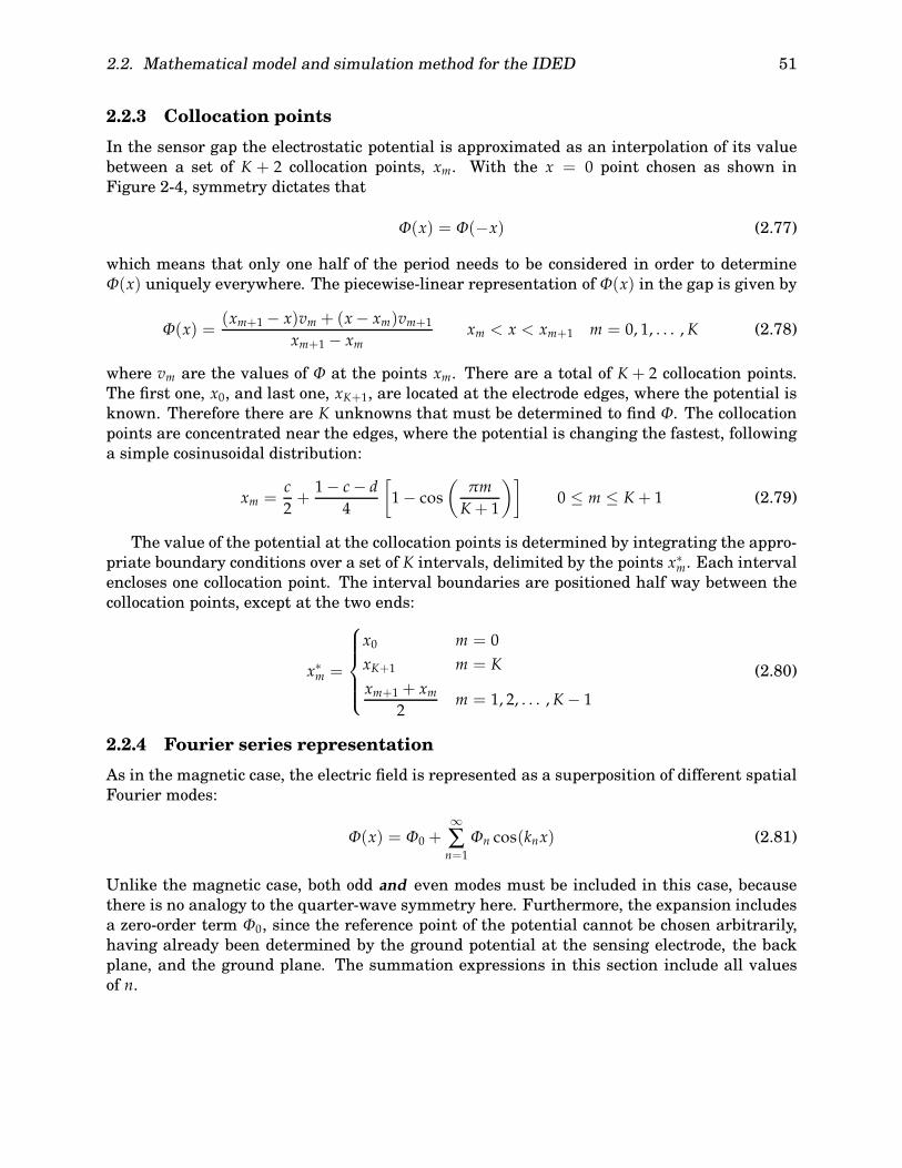
2.2. Mathematical model and simulation method for the IDED 51
2.2.3 Collocation points
In the sensor gap the electrostatic potential is approximated as an interpolation of its valuebetween a set of K + 2 collocation points, xm. With the x = 0 point chosen as shown inFigure 2-4, symmetry dictates that
Φ(x) = Φ(−x) (2.77)
which means that only one half of the period needs to be considered in order to determineΦ(x) uniquely everywhere. The piecewise-linear representation of Φ(x) in the gap is given by
Φ(x) =(xm+1 − x)vm + (x− xm)vm+1
xm+1 − xmxm < x < xm+1 m = 0, 1, . . . ,K (2.78)
where vm are the values of Φ at the points xm. There are a total of K + 2 collocation points.The first one, x0, and last one, xK+1, are located at the electrode edges, where the potential isknown. Therefore there are K unknowns that must be determined to find Φ. The collocationpoints are concentrated near the edges, where the potential is changing the fastest, followinga simple cosinusoidal distribution:
xm =c2
+1− c− d
4
[1− cos
(πmK+ 1
)]0 ≤ m ≤ K+ 1 (2.79)
The value of the potential at the collocation points is determined by integrating the appro-priate boundary conditions over a set of K intervals, delimited by the points x∗m. Each intervalencloses one collocation point. The interval boundaries are positioned half way between thecollocation points, except at the two ends:
x∗m =
x0 m = 0xK+1 m = K
xm+1 + xm2
m = 1, 2, . . . ,K− 1
(2.80)
2.2.4 Fourier series representation
As in the magnetic case, the electric field is represented as a superposition of different spatialFourier modes:
Φ(x) = Φ0 +∞∑n=1
Φn cos(knx) (2.81)
Unlike the magnetic case, both odd and even modes must be included in this case, becausethere is no analogy to the quarter-wave symmetry here. Furthermore, the expansion includesa zero-order term Φ0, since the reference point of the potential cannot be chosen arbitrarily,having already been determined by the ground potential at the sensing electrode, the backplane, and the ground plane. The summation expressions in this section include all valuesof n.

52 Chapter 2. Forward Models of the Spatially Periodic Sensors
Expressing the series coefficients Φn in terms of vm leads to the following expressions:
Φn = 4∫ 1/2
0Φ(x) cos(knx) dx
= 4∫ x0
0cos(knx) dx+ 4
K
∑m=0
∫ xm+1
xm
(xm+1 − x)vm + (x− xm)vm+1
xm+1 − xmcos(knx) dx
=4kn
sin(knx0) +4k2n
K
∑m=0
cos(knxm+1) − cos(knxm)xm+1 − xm
(vm+1 − vm
)+
4kn
K
∑m=0
[vm+1 sin(knxm+1) − vm sin(knxm)
](2.82)
The first term in equation (2.82) results from integration over the driven electrode, where thepotential is fixed at the driving voltage, whose normalized value is unity. The potential is zeroat the sensing electrode and therefore this interval is not included.
The last summation in equation (2.82) cancels out on a term-by-term basis, except for thetwo end terms multiplying v0 and vK+1. The latter is at the sensing electrode edge, where thepotential is zero, and can be ignored. The v0 term makes a contribution that exactly cancelsthe leading term in equation (2.82), since v0 = 1. Carrying out these simplifications resultsin:
Φn = − 4k2n
K
∑m=1
vm
[cos(knxm+1)− cos(knxm)
xm+1 − xm− cos(knxm) − cos(knxm−1)
xm − xm−1
]
− 4k2n
· cos(knx1) − cos(knx0)x1 − x0
(2.83)
Note than in equation (2.83) the index of the summation starts at m = 1. The first term hasbeen written out separately because v0 = 1 is known, and thus its coefficient will contributeto the right hand side of the matrix equation.
The constant term may similarly be evaluated as:
Φ0 = 2∫ 1/2
0Φ(x) dx = 2
∫ x0
0dx+ 2
K
∑m=0
∫ xm+1
xm
(xm+1 − x)vm + (x− xm)vm+1
xm+1 − xmdx
= 2x0 + 2K
∑m=0
(vmxm+1 − vm+1xm) + 2K
∑m=0
(vm+1 − vm)(xm+1 − xm)
= x0 + x1 +K
∑m=1
vm(xm+1 − xm−1)
(2.84)
2.2.5 Surface capacitance density
There are two parameters of a medium that determine the quasistatic distribution of elec-tric fields: the dielectric permittivity ε and the conductivity σ . The former determines thedisplacement current density from the electric field, while the latter relates the conductioncurrent density to the electric field. The permittivity governs energy storage (reactive power)phenomena, while the conductivity determines the power dissipation (active power). It is

2.2. Mathematical model and simulation method for the IDED 53
I
ε, σE
Figure 2-5: Terminal current of an electrode in contact with a conducting dielectric medium.
possible to combine these two effects by adding the effect of the ohmic conductivity to theimaginary (loss) component of the complex permittivity.
Consider an electrode in contact with a medium as shown in Figure 2-5. In the one-dimensional geometry in the figure, the current density and the electric field are perpendicu-lar to the electrode. Let the normal component of the electric field at the electrode surface beE. The terminal current I can be obtained by integrating the total current per unit electrodearea J that flows into the electrode. The total current density is given by
J = JC + JD = σE+ddt
(εE) (2.85)
where JC is the conduction current density and JD is the displacement current density.Under sinusoidal steady state operation equation (2.85) becomes
J = JC + JD = σE+ iωεE = iωE(ε +
σ
iω
)(2.86)
It is convenient to define the complex permittivity ε∗ of a medium as:
ε∗ = ε′ − iε′′ = ε − iσ
ω(2.87)
making it possible to rewrite equation (2.86) as
J = iωε∗E (2.88)
In analogy to the surface reluctance density defined in Section 2.1.5, in the electroqua-sistatic regime it is possible to define the complex surface capacitance density as
C∗n(z) =
1kn
· ε∗(z)Ez,n(z)
Φn(z)n > 0 (2.89a)
C∗0(z) =
ε∗(z)Ez,0(z)Φ0(z)
(2.89b)
As before, all information about the material under test is contained in the value of C∗n at
z = 0 for all spatial Fourier modes.Taking advantage of duality, it is possible to use equations (2.40) through (2.51), after

54 Chapter 2. Forward Models of the Spatially Periodic Sensors
making the following substitutions:
Φ ←→ Ay
ε∗Ez ←→ Hx
C∗n ←→ Rn
ε∗ ←→ 1µ∗
(2.90)
and letting γn → kn, since there is no diffusion term in the electroquasistatic case.At the bottom interface (z = z0) of any layer, for high mode numbers
limn→∞C∗
n(z0) = ε∗ (2.91)
and the transfer relation across a layer of thickness t and complex permittivity ε∗ is
C∗n(z0) = ε∗C∗
n(z0 + t) coth(knt) +ε∗
C∗n(z0 + t) +ε∗ coth(knt)
n > 0 (2.92)
To calculate the transfer relation for n = 0, the linear component of equation (2.72) mustbe used, leading to
Φ0(z) =(z− z0)Φ0(z0 + t) − (z− z0 − t)Φ0(z0)
t(2.93)
and
Ez,0(z) = − ddz
Φ0(z) = −Φ0(z0 + t) −Φ0(z0)t
(2.94)
At the two interfaces, C0(z) is
C0(z0) = −ε∗
t
[Φ0(z0 + t)
Φ0(z0)− 1
](2.95a)
C0(z0 + t) = −ε∗
t
[1− Φ0(z0)
Φ0(z0 + t)
](2.95b)
which can be combined to yield the following transfer relation:
C∗0(z0) =
ε∗C∗0(z0 + t)
tC∗0(z0 + t) +ε∗ (2.96)
A material structure with several homogeneous layers is shown in Figure 2-6. One notabledifference is that while in the magnetic case there always is a top layer of infinite thickness,in the electrostatic case the top layer is limited by a ground plane. This is true even if no suchelectrode is present in an experimental setup, since there are many objects in the vicinitywhich are at ground potential, which act as a ground at a certain effective distance. In fact, itis better to explicitly place a grounded metal plate behind the material under test, so that itis at a controlled distance to be used in the model. Nonetheless, it is still possible to model astructure with no ground plane by letting the thickness of the top layer approach infinity.
The surface capacitance density at the bottom interface of this ground-limited top layer

2.2. Mathematical model and simulation method for the IDED 55
t3
t2
h
t1
t4
λ
ε∗1
ε∗2
ε∗3
ε∗4
εS
Figure 2-6: Material structure with several layers of homogeneous materials
can be computed from equations (2.92) and (2.96) by taking the limit where Cn(z0 + t) → ∞,since Φn(z0 + t) = 0 at the top interface in contact with the ground plane:
C∗n(z0) = ε∗ coth(knt) n > 0 (2.97a)
C∗0(z0) =
ε∗
t(2.97b)
which approaches ε∗ for all n > 0 at sufficiently large values of the thickness t.The quantity σ∗
S is defined as the jump in the normal component of ε∗E:
σ∗S (x) = ε∗Ez(x) = ε∗(z = 0+)Ez(x, z = 0+)−ε∗(z = 0−)Ez(x, z = 0−) (2.98)
It would be equal to the surface charge density in the absence of ohmic conduction in themedium. Incorporating the conductivity as part of the complex permittivity changes ε, C,and σS to ε∗, C∗, and σ∗
S . The jump in the normal component of the total current density,conduction and displacement, is expressed in terms of σ∗
S via equation (2.88):
Jz = iωσ∗S (2.99)
Using equation (2.98), the values of the surface capacitance density above and below theelectrodes can be combined in a single quantity:
C∗n ≡ C∗
n(z) = C∗n(0
+)− C∗n(0
−) =1kn
· σ∗S n
Φn(z = 0)(2.100)
resulting in the following expression for the coefficients of the Fourier series expansion ofσ∗
S (x):
σ∗S n = C∗
nknΦn (2.101)
2.2.6 Boundary conditions
Compared to the magnetometer, formulating the boundary conditions that need to be appliedover the integration intervals around each collocation point is much simpler in the dielectriccase. This is due to the fact that in the electroquasistatic regime the metal electrodes can be

56 Chapter 2. Forward Models of the Spatially Periodic Sensors
treated as infinitely conducting, so that the potential at the electrodes is known. It needs to bedetermined only in a single region in the gap, unlike the MWM where there are four separateregions, as seen in Figure 2-1.
The relevant boundary condition between electrodes is
σ∗S (x) = 0 (2.102)
which results from equation (2.99), since there is no electrode to act as a current source orsink, and no surface conduction is considered. Surface conductivity and permittivity may bemodeled by introducing an extra layer and letting its thickness approach zero. The integralof the condition in equation (2.102) is∫ x∗m+1
x∗mσ∗
S (x) dx =∞∑n=1
∫ x∗m+1
x∗mC∗nΦnkn cos(knx) dx+
∫ x∗m+1
x∗mC∗0Φ0 dx
= −∞∑n=1
(C∗n
[sin
(knx∗m+1
)− sin(knx∗m
)]×× 4k2n
{K
∑j=1
vj
[cos(knxj+1) − cos(knxj)
xj+1 − xj− cos(knxj) − cos(knxj−1)
xj − xj−1
]
+cos(knx1)− cos(knx0)
x1 − x0
})
+ C∗0(x∗m+1 − x∗m
) [x0 + x1 +
K
∑j=1
vj(xj+1 − xj−1)
]
=∞∑n=0
C∗n
K
∑j=1
Mnm, jv j = 0
(2.103)
In matrix form this set of equations is Mv = b, where v is a vector of the unknown potentialvalues vm. The matrix M is calculated for a particular material structure as:
M =∞∑n=1
C∗nM
n + C∗0M
0 (2.104)
where the sub-matrices Mn are defined in equation (2.103). The advantage of formulating Mas a summation of sub-matrices is that they depend only on the sensor parameters, and needto be computed once when calculating the sensor response for a variety of material proper-ties and geometries. After substituting equations (2.83) and (2.84) into equation (2.103), the

2.2. Mathematical model and simulation method for the IDED 57
elements of Mn are determined to be:
Mnm, j =
2k2n
{− 1xj+1 − xj
[sin kn
(x∗m+1 + xj+1
)+ sin kn
(x∗m+1 − xj+1
)− sin kn
(x∗m + xj+1
)− sin kn(x∗m − xj+1
)]+[
1xj+1 − xj
+1
xj − xj−1
]·[sin kn
(x∗m+1 + xj
)+ sin kn
(x∗m+1 − xj
)− sin kn
(x∗m + xj
)− sin kn(x∗m − xj
)]− 1xj − xj−1
[sin kn
(x∗m+1 + xj−1
)+ sin kn
(x∗m+1 − xj−1
)− sin kn
(x∗m + xj−1
)− sin kn(x∗m − xj−1
)]}for n > 0
(2.105a)
and
M0m, j =
(x∗m+1 − x∗m
)(xj+1 − xj−1
)(2.105b)
As in the magnetic case, the surface capacitance density approaches a limit C∗∞ for largevalues of n. Using a similar definition, it is possible to separate the C∗∞ component:
∫ x∗m+1
x∗mσ∗
S (x) dx ≈N
∑n=1
(C∗n − C∗∞
) K
∑j=1
Mnm, ja j + C∗∞
∞∑n=1
K
∑j=1
Mnm, ja j
=N
∑n=1
(C∗n − C∗∞
) K
∑j=1
Mnm, ja j + C∗∞
K
∑j=1
M′m, ja j
(2.106)
where the elements of the matrix M′ are given by
M′m, j =
∞∑n=1
Mnm, j =
1π2
{− 1xj+1 − xj
[g(x∗m+1 + xj+1
)+ g
(x∗m+1 − xj+1
)− g
(x∗m + xj+1
)− g(x∗m − xj+1
)]+[
1xj+1 − xj
+1
xj − xj−1
]·[g(x∗m+1 + xj
)+ g
(x∗m+1 − xj
)− g
(x∗m + xj
)− g(x∗m − xj
)]− 1xj − xj−1
[g(x∗m+1 + xj−1
)+ g
(x∗m+1 − xj−1
)− g
(x∗m + xj−1
)− g(x∗m − xj−1
)]}
(2.107)
In the dielectric case the summation does include the even-numbered Fourier terms, so

58 Chapter 2. Forward Models of the Spatially Periodic Sensors
that the function g(x) differs from f (x) of equation (2.61). The definition of g(x) is
g( x2π
)=
∞∑n=1
sin(nx)n2
= −∫ x
0ln(2 sin
t2
)dt (2.108)
The closed form of the sum is taken from [51, eq. 1.25], or via term-by-term integration of [52,eq. 1.441.2]. As for f (x), a fast converging series expression is also possible for g(x) [3, eq. A.6]:
g( x2π
)= x
[1+ ln(x)
]− ∞∑n=1
(−1)n+1B2nx2n+1
2n(2n+ 1)!(2.109)
The function g(x) is further discussed in Appendix B.
2.2.7 Setting up the matrix equation
The set of equations generated by equation (2.103) are written in matrix form as Mv = b.The matrix M is already defined in equation (2.104). Forming the right hand side vector bin the dielectric case is quite different. In the magnetic case the constant term comes fromthe boundary conditions over the windings, which include the terminal voltages. Here, how-ever, the constant terms arise from the expressions multiplying v0 = 1, written out explicitlyoutside the sums in equation (2.103). It also has a contribution due to the n = 0 term, so that
b =∞∑n=1
C∗nbn + C∗
0b0 (2.110)
Extracting the appropriate terms from equation (2.103) gives
bnm =2k2n
· 1x1 − x0
[sin kn
(x∗m+1 − x1
)+ sin kn
(x∗m+1 + x1
)− sin kn
(x∗m − x1
)− sin kn(x∗m + x1
)− sin kn
(x∗m+1 − x0
)− sin kn(x∗m+1 + x0
)+ sin kn
(x∗m − x0
)+ sin kn
(x∗m + x0
)]for n > 0
(2.111a)
and
b0m = −(x∗m+1 − x∗m
)(x0 + x1
)(2.111b)
Solving the matrix equation results in full knowledge of the electrostatic potential Φ(x) atthe electrode surface.
2.2.8 Calculating transcapacitance
In the magnetometer case, the entire two-port impedance matrix is computed. Although fullmeasurement information is contained in the transinductance term, having all componentsis useful, because it makes it possible to include parasitic source and load impedances in themodel and account for them. In the case of the dielectrometer, the only useful component ofthe two-port matrix is the transcapacitance, because the sensing electrode voltage is alwaysat zero potential and the current into the driven electrode is generally too small for any sourceimpedance to have an appreciable effect on the measurement results.

2.3. Summary of Chapter 2 59
Obtaining the transcapacitance term is done by integrating σ∗S over the area of the virtu-
ally grounded sensing electrode. In the magnetic case this integral was already computed forthe windings, but in the dielectric case the electrode surface needs to be considered separately.Using equation (2.99), the transcapacitance is determined as follows:
CT = −∞∑n=1
∫ 1/2
xK+1
C∗nΦnkn cos(knx) dx−
∫ 1/2
xK+1
C∗0Φ0 dx
= −∞∑n=1
C∗n sin(knxK+1)
4k2n
{K
∑j=1
vj
[cos(knxj+1) − cos(knxj)
xj+1 − xj− cos(knxj) − cos(knxj−1)
xj − xj−1
]
+cos(knx1)− cos(knx0)
x1 − x0
}
− C∗0
(12− xK+1
)[x0 + x1 +
K
∑j=1
vj(xj+1 − xj−1)
](2.112)
where the sensing electrode extends from xK+1 = 1/2− d/2 to 1/2.
2.3 Summary of Chapter 2
In this chapter the semi-analytical collocation point models for the MWM and the IDED,which are the inductive and capacitive implementations of the Cartesian geometry quasistaticspatially periodic sensors, have been presented in detail. The new concepts in this formulationinclude:
1. The equations are written in a form that lends itself to efficient numerical implementa-tion.
2. The infinite series are formulated in a way that minimizes sensitivity to machine impre-cision.
3. The distributions of collocation points and integration interval limits are chosen to max-imize the numerical stability of the collocation point method.
4. The zero-order term in the dielectric case is treated appropriately, correcting errors inearlier work.
Although most of the material in this chapter has appeared in previous publications, theformulation and conventions used here have the advantages of completeness, consistency,and efficiency of the numerical implementation. These qualities make the material in thischapter a solid base for the development of the cylindrical geometry models in Chapter 3, thedistributed current drive magnetometer models in Chapter 4, and the moving media analysisin Section 6.1. Furthermore, this chapter has already become a useful reference source forusers of the MWM and IDED Cartesian geometry sensors and arrays.

60 Chapter 2. Forward Models of the Spatially Periodic Sensors

Chapter 3
Modeling sensors with rotationalsymmetry
As already briefly discussed in the introductory Section 1.3.2, there are several reasons whyit may be advantageous to design rotationally symmetric sensors. In the case of the Cartesiangeometry sensors, such as the existing MWM and IDED, it is necessary to assume that: (1) theextent of the sensor is infinite in the y-direction, and all physical quantities are independent ofy; and (2) all physical quantities are spatially periodic in the x-direction with a period equalto the spatial wavelength λ, and extend to infinity in the x-direction. Whereas the secondassumption is generally justified when guard electrodes or windings are used near the twosides, as illustrated in the IDED schematic in Figure 1-4, there is really no easy way to justifythe first one, unless impractically long sensors are designed.
The circular geometry completely eliminates the y edge effect, because the counterpartof y in cylindrical coordinates for this geometry is ϕ. The x edge effect, which correspondsto r in cylindrical coordinates, can also be minimized by making the radius R, used in themathematical model, large compared to the relevant length scales.
A further possible advantage of the rotationally symmetric sensors is their insensitivity toanisotropy of the material. Anisotropy plays a particularly important role in magnetometermeasurements, where a metal’s conductivity may be anisotropic, due to processing, such asrolling or directional solidification. Furthermore, in ferromagnetic metals the magnetic per-meability can manifest strong anisotropy due to residual or applied stress. Whereas thereare many cases when it is useful to measure this anisotropy [18, 24], at other times it maybe preferable to measure the directional average of a property. For example, when comparingtwo parts, the lack of sensitivity to direction eliminates the need for precise alignment of thesensor to the anisotropy axis.
Finally, certain structures, such as holes and fasteners, are by nature rotationally sym-metric. Cracks that originate from a hole propagate radially out, and thus a sensor with con-centric windings is ideal for this application, since it is uniformly sensitive to cracks aroundthe entire circumference of the hole. Such sensors have already been developed at JENTEK,called Rosettes [23], whose basic structure is shown in Figure 3-1. At present the measure-ment grids for these sensors are still being generated with the Cartesian coordinate methodsoutlined in Section 2.1, which can be justified only if the width of the annulus that containsthe active windings is small compared to the radius, which is not true for practical sensors.Using the method developed in this chapter will result in more accurate models for thesesensors.
61

62 Chapter 3. Modeling sensors with rotational symmetry
VS1
VS2
ID
Figure 3-1: Basic structure of the circularly symmetric magnetometer (Rosette).
This chapter presents mathematical models and numerical techniques used to calculatethe response of sensors with rotational symmetry. Both the magnetic and dielectric casesare presented in Sections 3.1 and 3.2 respectively. Section 3.3 shows experimental resultswith the dielectric sensor, which confirm the validity of the model developed in Section 3.2.Only the collocation point methods are discussed in this chapter; methods for modeling of thecircular magnetometer with distributed current drive are presented in Sections 4.8 and 4.9.
The problem is approached similarly to the Cartesian collocation point methods in Chap-ter 2. Frequent references to that chapter are made, in order to illustrate the parallels andthe differences between the two coordinate systems. Unlike Chapter 2, in this chapter no nor-malization is included in the equations.
Perhaps the most important difference is that the periodicity built into the Cartesian ge-ometry sensors, which makes it possible to use Fourier series methods efficiently, does notexist in cylindrical geometry. This is not to say that the idea of imposing a certain spatialperiodicity as a way of controlling the effective depth of sensitivity no longer holds; on thecontrary, this still is the main factor that determines the radii and spacing of the electrodesor windings. In cylindrical coordinates Fourier-Bessel Series is used instead, but the radius Rover which the Bessel Series is applied is chosen large compared to the characteristic lengthsof the sensor. As a consequence of choosing a large radius, terms of much higher order mustbe considered for the same numerical precision. This, coupled with the lack of convenientclosed form product and summation formulas for Bessel functions, makes the computationalburden much higher than the Cartesian coordinate methods.
3.1 Magnetometer
In this section the equations needed for developing the numerical method used to model thecircularly symmetric magnetometer are developed.
The magnetometer windings are formed on a planar substrate in the form of concentricannuli, as shown in Figure 3-1. It is most convenient to formulate the problem in cylindricalcoordinates, with the origin at the center of the sensor, and the z-axis perpendicular to theplane of the sensor. Because of the winding layout, the current always flows only in the ϕ-

3.1. Magnetometer 63
direction, and all physical quantities are independent of the angle coordinate ϕ. The magneticvector potential must therefore be of the following form:
A = Aϕ(r, z)ϕ (3.1)
The magnetic diffusion equation (2.11) requires that the function Aϕ(r, z) be a solution to thefollowing partial differential equation:
∂∂r
[1r· ∂
∂r(rAϕ)
]+
∂2
∂z2Aϕ − iωσµAϕ = 0 (3.2)
A useful solution to equation (3.2) is
A = J1(βr)(c1e+γz + c2e−γz
)ϕ γ =
√β2 + iωσµ (3.3)
where J1 is the Bessel function of the first kind of order one. The Bessel function of thesecond kind Y1, which also satisfies the radial part of equation (3.2), is not suitable, becauseit has a singularity at r = 0, where A must remain finite. The role of the wavenumber kin equation (2.14) is played by β in cylindrical coordinates. In terms of equation (3.3), theelectromagnetic flux density B is:
B = ∇×A =1r· ∂
∂r(rAϕ)z+
∂∂zAϕ r
= βJ0(βr)(c1e+γz + c2e−γz
)z+ γJ1(βr)
(c1e+γz − c2e−γz
)r
(3.4)
3.1.1 Use of Fourier-Bessel series
The form of equation (3.3) suggests that Aϕ, at a given value of z, may conveniently be rep-resented by a Fourier-Bessel series based on J1. A function f (r) may be represented as aninfinite summation of Bessel functions over an interval (0, R) as follows [53]:
f (r) =∞∑n=1
AnJ1(αn
Rr)
0 < r < R (3.5)
where αn are the positive real zeros of J1. The trivial zero α0 = 0 does not participate in thisseries. To find the series coefficients An, the following integral must be evaluated:
An =1Qn
∫ R
0r f (r)J1
(αn
Rr)dr (3.6)
where the coefficients Qn are given by:
Qn =∫ R
0rJ21
(αn
Rr)dr =
R2
2J22 (αn) =
R2
2J20 (αn) (3.7)
The transformation of J2 to J0 in the last equation is possible because of the following equality:
J2(x) =2xJ1(x) − J0(x) (3.8)

64 Chapter 3. Modeling sensors with rotational symmetry
which means that J2(αn) = −J0(αn), since J1(αn) = 0. Attempting to express everything interms of J0 and J1 only is motivated by the desire to maintain the analogy of the relationshipbetween these two functions to the sine/cosine pair in Cartesian coordinates. The roles of J0and J1 are reversed in the dielectric case, as seen in Section 3.2. Furthermore, restrictingthe use of Bessel functions to J0 and J1 is beneficial from the point of view of computationalefficiency.
The radius R is the outer limit of the interval over which the Bessel series expansion isapplied. It is chosen to be several times greater than the outer radius of the sensor, in order tomake the effect of any phantom magnetic fields that result from the summation of the seriesoutside of this radius negligible.
3.1.2 Collocation points
Since no specific winding layout is used in this section, Figure 3-1 being only a simple exampleof a possible layout, no explicit definition of the collocation points is given. As in Section 2.1.3,the collocation points rm should be spread out over the interval where A is to be determined,i.e. 0 ≤ r ≤ R, with higher concentration of points near the winding edges, and interleavedwith the integration limit points r∗m. The latter must include the winding edges exactly, inorder to have the same boundary conditions apply within the range of each interval. Thetotal number of collocation points used in the analysis in this section, including the first andlast points, is K + 1. Thus a total of K constraining equations are required, since the vectorpotential needs to be determined only to within an additive constant. The last collocationpoint is at rK = R. The first one does not need to be at the origin, because for r < r0 thepotential is fully determined by, and equal to, its value at r0, for reasons described below.
The next step is expressing the series coefficients of the Bessel function expansion of themagnetic vector potential in terms of its value at the collocation points, in analogy to equa-tion (2.38). The choice of interpolating function in the Cartesian case is a simple line connect-ing the two neighboring points, which leads to equation (2.30). Using this same function herewould be unsuitable, because equation (3.6) yields an integral, namely
∫xJ1(x) dx, that has no
closed form solution.∗ More generally, integrals of the form∫xp J1(x) dx cannot be solved when
p is an odd integer. Conversely, when p is an even integer, closed form solutions are possible,as in the following cases: ∫
J1(x) dx = −J0(x) (3.9a)∫x2 J1(x) dx = x2 J2(x) (3.9b)
Equation (3.9) suggests that a convenient function to be used for interpolation betweentwo consecutive collocation points is:
y = c1x+c2x
x > 0 (3.10)
Specifically, in terms of its values y1 and y2 known at two distinct points x1 and x2, with
∗At least, not a practical closed form solution. This integral may be expressed as a hypergeometric function.

3.1. Magnetometer 65
0 ≤ x1 < x2, the value of a function y(x) is given by the following formula:
y =
y2x2x x1 = 0 and y1 = 0
(y1/x2 − y2/x1) x+ (x1y2 − x2y1)/xx1/x2 − x2/x1
otherwise(3.11)
Using this interpolation function, the magnetic vector potential between two collocationpoints is given by the following expression:
Aϕ(r) =amrm
(r2m+1/r− r
)+ am+1rm+1
(r− r2m/r
)r2m+1 − r2m
rm ≤ r ≤ rm+1
m = 0, 1, . . . ,K− 1(3.12)
analogous to equation (2.30). For 0 ≤ r ≤ r0 the magnetic vector potential must be constantand equal to a0, since its partial derivative with respect to r at r = 0 must be zero, or else Bzwould be infinite there. Therefore equation (3.10) cannot be used in this interval, since bothcoefficients would have to be zero. To avoid having to carry out an integral with no closedform over this interval, which would result from constant Aϕ(r), it is best to set the constantpotential there to zero, using the degree of freedom afforded by the arbitrary constant thatcan be added to the vector potential. Thus
Aϕ(r) = a0 = 0 0 ≤ r ≤ r0 (3.13)
Letting
βn ≡ αn
R(3.14)
the series coefficients are obtained by an integral from zero to rK = R, which can be dividedup as:
An =1Qn
K−1
∑m=0
∫ rm+1
rmrAϕ(r)J1(βnr) dr (3.15)
Substituting equation (3.12) into equation (3.15) and carrying out the integration yields
AnQnβn =K−1
∑m=0
(1
r2m+1 − r2m×
×{am+1rm+1
[r2m+1 J2(βnrm+1)− r2mJ2(βnrm) + r2mJ0(βnrm+1)− r2mJ0(βnrm)
]− amrm
[r2m+1 J2(βnrm+1) − r2mJ2(βnrm) + r2m+1 J0(βnrm+1) − r2m+1 J0(βnrm)
]})(3.16)

66 Chapter 3. Modeling sensors with rotational symmetry
which, with the help of equation (3.8), is written as
AnQnβ2n = 2
K−1
∑m=0
am+1rm+1 − amrmr2m+1 − r2m
[rm+1 J1(βnrm+1) − rm J1(βnrm)
]−βn
K−1
∑m=0
[am+1rm+1 J0(βnrm+1) − amrmJ0(βnrm)
] (3.17)
The second summation in equation (3.17) cancels out on a term by term basis, with the excep-tion of the first and last terms. The other summation can be rewritten as
An = − 4α2n J20 (αn)
{aKrK
[rK−1 J1(βnrK−1)r2K − r2K−1
+βn
2J0(βnrK)
]
+K−1
∑m=1
amrm
[rm+1 J1(βnrm+1) − rm J1(βnrm)
r2m+1 − r2m− rm J1(βnrm) − rm−1 J1(βnrm−1)
r2m − r2m−1
]} (3.18)
similar to equation (2.38). Use has been made of the fact that a0 = 0 and J1(βnrK) = 0.
3.1.3 Surface reluctance density
As seen in equation (3.3), the z-dependence of the magnetic vector potential is identical to theCartesian case in equation (2.13), with β substituted for the wavenumber k in the definitionof the complex wavenumber γ. Consequently, the concept of defining the surface reluctancedensity Rn(z) and finding its value at the electrode surface for every spatial mode n via trans-fer relations across every homogeneous layer is directly applicable here. After substituting β
for k, equations (2.39), (2.46), and (2.50) through (2.52) become
Rn(z) ≡ 1βn
· Hr,n(z)Aϕ,n(z)
(3.19)
Rn(z0) =γn
µ∗βn(3.20)
Rn(z0) =γn
µ∗βn· µ∗βnRn(z0 + t) coth(γnt) + γn
µ∗βnRn(z0 + t) + γn coth(γnt)(3.21)
Rn ≡ Rn(0+)− Rn(0−) =1βn
· Hr,n(z = 0+) − Hr,n(z = 0−)Aϕ,n(z = 0)
(3.22)
KSn = RnβnAn (3.23)
At the bottom interface (z = z0) of any layer for high mode numbers
limn→∞Rn(z0) =
1µ∗ (3.24)
which means that unless embedded in a magnetizable material,
R∞ = limn→∞ Rn =
2µ0
(3.25)

3.1. Magnetometer 67
3.1.4 Boundary conditions
In the gaps between the windings the condition is that the surface current density must bezero, as in equation (2.53):
KS(r) = Hr(r, z = 0+)− Hr(r, z = 0−) = 0 (3.26)
Similarly, for a single turn winding the contour integral∮CE · ds = −iω
∮CA · ds (3.27)
results in a boundary condition of the form
v = iω(2πr)Aϕ(r) + (2πr)KS(r)∆σcoil
(3.28)
A complicating factor in equation (3.28) as compared to equation (2.55) is that equation (3.27)involves integration over ϕ, which introduces a factor of r to the integrand.
Integrating the boundary conditions given by equations (3.26) and (3.28) over an inter-val, in order to generate a constraining equation for the evaluation of the potential at thecollocation points, involves an integral of the surface current density:∫ r∗m+1
r∗mKS(r) dr =
∞∑n=1
∫ r∗m+1
r∗mRnAnβn J1(βnr) dr
= −∞∑n=1
AnRn[J0(βnr∗m+1)− J0(βnr∗m)
]=
∞∑n=1
RnK
∑j=1
Mnm, ja j
(3.29)
The coefficients Mnm, j constitute the contribution to the integral over the mth interval of the
vector potential at the jth collocation point for the nth Bessel mode. They can be obtained bysubstituting equation (3.18) into equation (3.29) yielding
Mnm, j =
4α2n J20 (αn)
[J0(βnr∗m+1) − J0(βnr∗m)
]×
× r j
[r j+1 J1(βnr j+1)− r j J1(βnr j)
r2j+1 − r2j− r j J1(βnr j)− r j−1 J1(βnr j−1)
r2j − r2j−1
]for j < K
(3.30a)
and
Mnm,K =
4α2n J20 (αn)
[J0(βnr∗m+1) − J0(βnr∗m)
]rK
[rK−1 J1(βnrK−1)r2K − r2K−1
+βn
2J0(βnrK)
](3.30b)
At this point the method diverges somewhat from the Cartesian coordinate method of Sec-tion 2.1. The difference comes from the fact that when using Bessel functions there is no anal-ogous closed form of the infinite summation used to define function f (x) in equation (2.61).Consequently, there is no benefit in isolating the R∞ component and creating a separate M′matrix. This issue is treated with more detail in Appendix B.
Before integrating the boundary condition over the windings, it is convenient to divide

68 Chapter 3. Modeling sensors with rotational symmetry
both sides of equation (3.28) by 2πr first, leading to the following expression for the integralof the left hand side: ∫ r∗m+1
r∗m
v2πr
dr =v2π
ln( r∗m+1
r∗m
)(3.31)
The right hand side of equation (3.28) contains a term with∫KS(r) dr, already handled in
equation (3.29), and an integral over Aϕ(r). The latter may be obtained by integrating equa-tion (3.12) directly, but closer scrutiny reveals that this is unnecessarily complicated. Theinterpolation function in equation (3.11) was chosen in order to make it possible to find aclosed form expression for the Bessel series coefficients. Since this function is only an ap-proximation to Aϕ(r) anyway, it is better for the purpose of this integral to assume a linearinterpolation function, similar to equation (2.30):
Aϕ(r) =am(rm+1 − r) + am+1(r− rm)
rm+1 − rm(3.32)
yielding
2∫ r∗m+1
r∗mAϕ(r) dr = am−1
(r∗m − rm)2
rm − rm−1+ am+1
(r∗m+1 − rm)2
rm+1 − rm
+ am
[r∗m − rmrm − rm−1
(r∗m + rm − 2rm−1) +r∗m+1 − rmrm+1 − rm
(2rm+1 − rm − r∗m+1)]
rm−1 < r∗m < rm < r∗m+1 < rm+1
(3.33)
If written as ∫ r∗m+1
r∗mAϕ(r) dr =
K
∑j=1
M′′m, ja j (3.34)
the matrix M′′ will have exactly the form given in equation (2.64), with nonzero elementsgiven by
M′′m,m =
12
[r∗m+1 − rmrm+1 − rm
(2rm+1 − rm − r∗m+1
)+
r∗m − rmrm − rm−1
(r∗m + rm − 2rm−1
)]
M′′m,m+1 =
12·(r∗m+1 − rm
)2rm+1 − rm
M′′m+1,m =
12·(r∗m − rm
)2rm − rm−1
(3.35)
3.1.5 Matrix equation and terminal currents
Integrating the boundary conditions over each of the intervals delimited by r∗m yields equa-tions that may be combined in matrix form to solve for the unknown am, which appear invector a in the matrix equation Ma = b. The matrix M can be built from the previously

3.2. Dielectrometer 69
defined matrices Mn and M′′ as follows:
Mm, j =
∞∑n=1
RnMnm, j rm is in a gap
1∆σcoil
∞∑n=1
RnMnm, j + iωM′′
m, j rm is in a winding(3.36)
The right hand side b is determined from equation (3.31), and its nonzero elements aregiven by:
bm,p =12π
ln( r∗m+1
r∗m
)(3.37)
if p = 0 and rm falls on the primary winding, or if p = 1 and rm falls on the secondary winding.Solving the matrix equations determines am, which in turn determine the magnetic vec-
tor potential A. The magnetic flux intensity B may now be obtained everywhere via equa-tion (3.4).
To determine the terminal currents, the surface current density KS(r) is integrated acrosseach of the two windings. This can be done by taking advantage of the established matricesby defining the two-port sensor matrix as a product of matrices
Y = Fa (3.38)
where a is the just calculated set of collocation point vector potential values. The requiredform for F is
Fp, j = ∑m
∞∑n=1
RnMnm, j (3.39)
with the understanding that the same constraints on the values of m included in the summa-tion hold as for equation (3.37) above.
This concludes the derivation of the formulas necessary to implement the collocation pointmethod of modeling a magnetometer with circular geometry.
3.2 Dielectrometer
This section presents the model of the rotationally symmetric dielectrometer. Although mostof the research in this project is focused on magnetic sensors, there are reasons why it isbeneficial to consider the electroquasistatic sensor: no one has worked on this model before,and a sensor of this geometry already exists at JENTEK, which makes it easy to test the modelexperimentally, with the results presented in Section 3.3.
Although the principle of duality provides many parallels between the magnetoquasistaticand electroquasistatic regimes, there is one fundamental difference: there is no equivalentto magnetic diffusion, i.e. the electrostatic potential Φ obeys Laplace’s equation. From thepoint of view of the model, this means that for each spatial mode the decay constant in thez-direction is purely real and equal to the wavenumber k, or β in cylindrical coordinates. It isthus independent of the excitation frequency ω.
In practical terms the lack of the equivalent of magnetic diffusion, already discussed in

70 Chapter 3. Modeling sensors with rotational symmetry
Driven GroundSensing Ground
0 ra b a1 a2
z
Figure 3-2: Definition of geometry parameters of circular dielectrometer.
Section 2.2, makes dielectric measurements much harder to perform for the following reasons:
1. In the absence of conductivity in the materials, the sensor transadmittance is purelyimaginary (capacitive), and therefore there is enough information to determine only asingle unknown quantity. Since in practice the sensor lift-off, which is the thickness ofthe air gap between the sensor electrodes and the material, is almost always unknown,due to surface roughness, sensor electrode thickness, etc., in order to measure evena single unknown material property, data from two sensors with different depths ofsensitivity must be combined. Conductivity in the material does not improve matterssignificantly either, since the extra information present in the phase signal is used upby the extra unknown property, the conductivity. It is usually not possible to assumethat this conductivity is known, because in nominally insulating materials, on whichthese dielectric measurements are performed, the conductivity is a very strong functionof temperature, relative humidity, and the presence of contaminants.
2. Since the depth of penetration is independent of frequency,∗ it is not possible to obtainextra information by operating the same sensor at two or more frequencies.
As a consequence, unless some questionable assumptions are made, two or more sensorsneed to be used simultaneously, if a meaningful measurement is to be performed.
3.2.1 Sensor geometry
A top view of the sensor considered in this section is shown in Figure 3-5. A cross sectionof the sensor is shown in Figure 3-2, which also defines the geometrical parameters. In theanalysis it is assumed that everywhere for r ≥ b the potential at z = 0 is forced to zero bythe presence of a ground plane. The sensing electrode is formed as a cut-out from this groundplane, with as small a gap as practically possible. It is kept at ground potential via a circuitlike the one shown in Figure 2-3. The other side of the sensor substrate is also kept at groundvia an electrode over the entire area of the sensor.
The value of the electrostatic potential is known for 0 ≤ r ≤ a, where it is equal to thedriving voltage, and for r ≥ b, where it is zero. In the gap, it is determined via a collocationpoint method. An example of a potential function for a sensor in air is shown in Figure 3-3.
∗This is actually strictly true only within a single homogeneous layer, which is the most important case anyway.But in a two-layer structure, a slightly conducting thin layer close to the sensor may let the electric field penetrateand reach to the next layer at high frequencies, while completely shielding the field at low frequencies. At least intheory, in such cases it is possible to obtain extra information by operating at multiple frequencies.

3.2. Dielectrometer 71
✲
✻Φ(r)
1
a b r
Figure 3-3: Normalized calculated potential at the electrode surface for the circular dielec-trometer in air. In this case a = 0.5 mm, b = 1.5 mm, and the substrate thickness ish = 0.127 mm.
3.2.2 Laplace’s equation
Due to symmetry, the potential is independent of ϕ, i.e. Φ = Φ(r, z). Laplace’s equationassumes the following form:
∇2Φ =1r
∂∂r
(r
∂∂r
Φ
)+
∂2
∂z2Φ = 0 (3.40)
The relevant solution of this differential equation is:
Φ(r, z) = J0(βr)(c1e−βz + c2e+βz
)(3.41)
since the Bessel function Y0 is infinite at r = 0. For this solution the electric field is given by:
E = −∇Φ = βJ1(βr)(c1e−βz + c2e+βz
)r+ βJ0(βr)
(c1e−βz − c2e+βz
)z (3.42)
Because of equation (3.41), the Bessel series to use in this case is based on J0:
f (x) =∞∑n=1
AnJ0(αn
Rx)
0 < x < R (3.43)
where αn here are the positive real of J0. The zeros are numbered from one, i.e. α1 = 2.405.Correspondingly, An and Qn are given by
An =1Qn
∫ R
0x f (x)J0
(αn
Rx)dx (3.44)
Qn =∫ R
0x J20
(αn
Rx)dx =
R2
2J21 (αn) (3.45)
As in the magnetometer case, the radius R is the outer limit of the interval over whichthe Bessel series expansion is applied. It is chosen to be several times greater than the outerradius of the sensor, in order to make the effect of any phantom electric fields resulting fromthe summation of the series terms outside of this radius negligible.

72 Chapter 3. Modeling sensors with rotational symmetry
✲
✻rm
a
b
m0 3 6 9 12 15
××××××××××××××××
◦ ◦ ◦ ◦ ◦ ◦ ◦◦
◦◦
◦◦
◦ ◦ ◦ ◦
Figure 3-4: Positions of 16 collocation points. The points are concentrated near the electrodeedges, where the potential is changing most rapidly. The concentration is skewed toward thedriven electrode.
3.2.3 Collocation points
In the sensor gap the electrostatic potential is approximated by an interpolation of its valuebetween a set of K+ 2 collocation points, rm. The first and last ones are at the electrode edges,and inbetween the points are concentrated near the edges, where the potential is changingthe most rapidly as shown in Figure 3-3. The collocation points are more heavily concentratednear the driven electrode, according to the following formula:
rm = a+b− a2
{1− cos
(mπ
K+ 1
)+ 0.15
[cos
(2mπ
K+ 1
)− 1
]}m = 0, 1, 2, . . . ,K+ 1 (3.46)
A bit of the second harmonic is added to the traditionally used cosinusoidal distribution, inorder to skew the points toward the driven electrode. Figure 3-4 shows the resulting positionsof the collocation points. The integration intervals, delimited by r∗m, are positioned half waybetween the collocation points, except at the two ends:
r∗m =
r0 m = 0rK+1 m = K
rm+1 + rm2
m = 1, 2, . . . ,K − 1
(3.47)
As before, a suitable interpolation function must be chosen to express Φ as a function of itsvalues at the collocation points. Integrals of the form
∫xp J0(x) dx have closed form solutions
when p is an odd number. For example:∫xJ0(x) dx = xJ1(x) (3.48a)∫x3 J0(x) dx = x3 J1(x)− 2x2 J2(x) (3.48b)

3.2. Dielectrometer 73
An appropriate interpolation function therefore is
y = c1 + c2x2 (3.49)
which results in the following interpolation function y(x) in the interval between x1 and x2:
y =y1(x22 − x2) + y2(x2 − x21)
x22 − x21(3.50)
Using equation (3.50), the Bessel series coefficients in the expansion of the potential Φ
over the period 0 ≤ r ≤ R are given by:
Φn =1Qn
[∫ a
0rJ0(βnr) dr+
K
∑m=0
∫ rm+1
rmrJ0(βnr)
vm(r2m+1 − r2) + vm+1(r2 − r2m)r2m+1 − r2m
dr
](3.51)
where the coefficients Qn are defined in equation (3.45) and βn = αn/R. The first term inequation (3.51) results from integration over the driven electrode, where the potential is forcedto the driving voltage and may be set to unity for the computation of the transcapacitance.The potential is zero for r ≥ b and therefore this interval is not included. Carrying out theintegration yields
ΦnQnβ2n = βnaJ1(βna) + 2
K
∑m=0
vm − vm+1
r2m+1 − r2m
[r2m+1 J2(βnrm+1)− r2mJ2(βnrm)
]+ βn
K
∑m=0
[vm+1rm+1 J1(βnrm+1) − vmrmJ1(βnrm)
] (3.52)
The terms in the second summation of equation (3.52) cancel out on a term by term basis,except for the two end terms multiplying v0 and vK+1. The latter is at rK+1 = b, where thepotential is zero due to the ground, and can be ignored. The first one contributes a term equalto −βnaJ1(βna), which exactly cancels the leading term in equation (3.52), since v0 = 1. Thisresults in a much simpler expression:
Φn =4
α2nJ21 (αn)
K
∑m=0
vm − vm+1
r2m+1 − r2m
[r2m+1 J2(βnrm+1)− r2mJ2(βnrm)
](3.53)
which can be rewritten as
Φn =4
α2n J21 (αn)
{r21 J2(βnr1) − r20 J2(βnr0)
r21 − r20
+K
∑m=1
vm
[r2m+1 J2(βnrm+1) − r2mJ2(βnrm)
r2m+1 − r2m− r2mJ2(βnrm) − r2m−1 J2(βnrm−1)
r2m − r2m−1
]}(3.54)
Note than in equation (3.54) the index of the summation starts at m = 1. The first term hasbeen written out separately, because v0 = 1 is known, and its coefficient will contribute to theright hand side of the matrix equation.

74 Chapter 3. Modeling sensors with rotational symmetry
3.2.4 Surface capacitance density and boundary conditions
All equations derived in Section 2.2.5 directly apply to cylindrical coordinates. The constantterm C∗
0 is not needed in this case.In cylindrical coordinates the σ∗
S (r) = 0 constraint of equation (2.103) takes the followingform: ∫ r∗m+1
r∗mσ∗
S (r)2πr dr =∞∑n=1
∫ r∗m+1
r∗mC∗nΦnβn J0(βnr)2πr dr
= 2π∞∑n=1
C∗nΦn
[r∗m+1 J1(βnr
∗m+1) − r∗mJ1(βnr∗m)
]=
∞∑n=1
C∗n
K
∑j=0
Mnm, jv j = 0
(3.55)
After substituting equation (3.54) into equation (3.55), the elements of Mn are determinedto be:
Mnm, j =
8πα2n J21 (αn)
[r∗m+1 J1(βnr
∗m+1) − r∗mJ1(βnr∗m)
]×
×[ r2j+1 J2(βnr j+1)− r2j J2(βnr j)
r2j+1 − r2j−r2j J2(βnr j) − r2j−1 J2(βnr j−1)
r2j − r2j−1
] (3.56)
Similarly, the right hand side vector b of the matrix equation is given by
b =∞∑n=1
C∗nbn (3.57)
where the elements of bn are
bnm = − 8πα2n J21 (αn)
[r∗m+1 J1(βnr
∗m+1) − r∗mJ1(βnr∗m)
] r21 J2(βnr1) − r20 J2(βnr0)r21 − r20
(3.58)
Solving the matrix equation results in full knowledge of the electrostatic potential Φ(r)at the electrode surface. Figure 3-3 shows this function for a dielectric sensor in air, usingstraight lines to interpolate between its values at the collocation points.
3.2.5 Calculating transcapacitance
In analogy to Section 2.2.8, the transcapacitance is obtained by integrating σ∗S over the elec-
trode area:
CT = −∞∑n=1
∫ a2
a1C∗nΦnβn J0(βnr)θr dr
= −θ∞∑n=1
C∗nΦn
[a2 J1(βna2)− a1 J1(βna1)
] (3.59)
where the electrode extends from a1 to a2 radially and has an arc angle of θ, which for practicalsensors must be less than 2π . In Figure 3-5 both sensors have θ = π , i.e. 180◦.
In order to express the transcapacitance CT in terms of the potential values v calculated

3.3. Experimental verification of cylindrical coordinate model 75
Driven
Sensing
Ground
Driven
Ground
Sensing
Figure 3-5: Layout of two circular dielectric sensors with different depth of sensitivity. Thedepth of sensitivity is determined by the position of the sensing electrode. Ignoring the effectof the narrow gap between the virtually grounded sensing electrode and the ground electrode,the electric field is identical for both sensors.
in the last step, equation (3.54) is substituted into equation (3.59), yielding
CT = −4θ∞∑n=1
C∗n
α2n J21 (αn)
[a2 J1(βna2) − a1 J1(βna1)
]{ r21 J2(βnr1)− r20 J2(βnr0)r21 − r20
+K
∑m=1
vm
[r2m+1 J2(βnrm+1) − r2mJ2(βnrm)
r2m+1 − r2m− r2mJ2(βnrm) − r2m−1 J2(βnrm−1)
r2m − r2m−1
]}(3.60)
The method described in this section is used to generate the measurement grid shown inthe next section.
3.3 Experimental verification of cylindrical coordinate model
This section describes an experiment designed to test the cylindrical geometry methods inthis chapter in general, and the dielectric case in particular. The experiment entails mea-surements with a pair of circular dielectrometers with different depths of sensitivity, shownin Figure 3-5.
At the frequency of operation, 15.8 kHz, all materials used in the experiment can betreated as perfect insulators, i.e. their values of the permittivity ε∗ are purely real. Thismeans that the sensor transcapacitance is also purely real, and no useful instrument phasedata are available. This frequency is chosen primarily as a matter of convenience for use withthe standard test instruments at JENTEK. There is no loss of generality by working only withreal ε, because working with complex ε∗ results in no changes to the model.
In this experiment two unknown quantities are measured simultaneously, by combiningthe magnitude of the signal from the two sensors. The two unknown quantities are the permit-tivity of a dielectric plate positioned above the sensors, and the lift-off, defined as the distancebetween the bottom surface of the plate and the sensor electrode surface. The thickness ofthe plate is known, 1.58 mm, and is included in the model used to generate the measurementgrid. The entire sensor assembly is contained in a metal chamber, whose cover acts as theground plane, positioned several centimeters above the sensor and the dielectric plate.

76 Chapter 3. Modeling sensors with rotational symmetry
Parameter Sensor 1 Sensor 2Driven electrode outer radius a 1.75 mmGround plane inner radius b 4.5 mmSensing electrode inner radius a1 4.75 mm 9.1875 mmSensing electrode outer radius a2 5.50 mm 10.625 mmSensing electrode segment angle θ 180◦Substrate thickness h 0.254 mmSubstrate relative permittivity εS 2.1
Table 3.1: Geometric and material parameters of the sensors in Figure 3-5.
The reason for choosing a dielectric sensor with a magnitude/magnitude grid∗ to test themodels is that this configuration is most sensitive to the accuracy of the model, and in partic-ular to the correct treatment of the differences between cylindrical and Cartesian geometry.To understand why this is so, consider the alternatives:
1. For a magnetic sensor the test material would have to be metal, where the conductivityis the dominant material property. Using insulating ferromagnetic materials, such asferrites, could be an alternative, but these usually have values of the magnetic perme-ability that are so high as to be essentially infinite. In other words, it is very difficultto differentiate between insulating ferrites of relative permeability of, say, 500 vs. 2000.When using metal, signal phase information has to be considered, which means thatin order to have only two degrees of freedom, a single sensor would have to be used.The reason why the dielectric magnitude/magnitude measurement is more sensitive tothe correctness of the model is that, since the only difference between the two dielec-tric magnitude signals stems from the position of the sensing electrode, this differenceis extremely sensitive to correct modeling of the sensor geometry, while both magneticmeasurement quantities would be affected similarly by an error in the model.
2. Another possibility is to use a single dielectric sensor with a material with non-negligibleconductivity. However, as with the magnetic sensor, incorrect modeling of the sensor ge-ometry would tend to affect the two measured quantities similarly, while the differencebetween two magnitude signals is based entirely on geometrical considerations.
The geometric parameters of the sensors in Figure 3-5 are listed in Table 3.1. Convertingthe raw sensor magnitude data to estimated parameter data is done with the help of a twodimensional measurement grid. Measurement grids are described in Section 1.4.1. The gridused here is shown in Figure 3-6. A way to understand of the grid qualitatively is to followtwo constant lift-off lines, for two different values of the lift-off. When the lift-off is low, theaverage slope of the line is low, because the signal of the first sensor increases much fasterthan the second one, since it is closer to the driven electrode. On the other hand, at higher lift-off values the lines become almost vertical, since the dielectric plate is too far from the firstsensor to affect its response significantly, while some of the electric field lines that terminateon the second sensor electrode still pass through the plate.
A curious aspect of the grid in Figure 3-6 is that at the highest lift-off values the sensors’magnitudes actually decrease with increasing permittivity, and as a consequence in the figurethe ε = 1 point on the grid is not at the bottom left corner. This happens because while the
∗The concept of magnitude/magnitude grids was developed by Dr. N. J. Goldfine and Dr. A. Washabaugh [54].

3.3. Experimental verification of cylindrical coordinate model 77
0 5 10 15 20 25 30 35 400.5
1
1.5
2
2.5
3
3.5
4
4.5
5
First sensor magnitude [fF]
Sec
ond
sens
or m
agni
tude
[fF
]
ε = 1
ε = 5
ε = 10
h = 0.1 mm
Increasing permittivity
Increasing lift−off
h = 0.01 mm
h = 1 mm
h = 10 mm
Figure 3-6: Permittivity/lift-off measurement grid for the pair of dielectric sensors in Fig-ure 3-5. The thickness of the dielectric plate is fixed at 1.58 mm (1/16′′). The relative permit-tivity range of the grid is from 1 to 10, and the lift-off range is 0.01 mm to 10 mm, both on alogarithmic scale.
plate is too far from the sensors for any electric field lines that terminate on the sensingelectrodes to pass through it, it can still affect the response by redirecting some of the fieldlines that would otherwise have ended on the electrodes to the grounded back plane, whichis the sensor enclosure cover in this setup. This effect would not have been modeled correctlyif the back plane had not been considered, which is how the models used to be formulatedby others [2, 3]. For further discussion on the effect of the back plane to the collocation pointmodels, refer to Section 2.2.
The measurements are made with two dielectric sheets of equal thickness, 1.58 mm, madeof different materials. The first one is made of polycarbonate (Lexan), with a dielectric con-stant of 3.2. The second one is made of material used in printed circuit boards, with a higherdielectric constant, apparently near 4.8. These two dielectric plates are suspended above thesensors with the aid of spacers at the sides, at lift-offs ranging from intimate contact, whichis a few hundredths of a millimeter due to surface roughness, to about three millimeters.
The calibration method used for this set of measurements is two-point reference calibra-tion. For a discussion of the available calibration methods and the circumstances that favorone versus the others, refer to Appendix D. One of the reference points is the air point, ε = 1.The other reference point is taken with a polycarbonate plate, whose permittivity is knownand equal to 3.2, with an empirically determined value for the reference lift-off, 0.02 mm,which accounts for surface roughness and the nonzero electrode thickness, not otherwise in-

78 Chapter 3. Modeling sensors with rotational symmetry
2 4 6 8 10 12 141
1.2
1.4
1.6
1.8
2
2.2
First sensor magnitude [fF]
Sec
ond
sens
or m
agni
tude
[fF
]
ε = 3.2ε = 4.8
0.4
mm
0.2
mm
0.1
mm
0.05 mm
2
4
5
2.5
3
1 m
m
Figure 3-7: Results of measurements with the circular dielectric sensors. Two sets of measure-ments are shown with materials of different permittivity, taken at a variety of lift-off positions.Each set follows lines of constant permittivity on the measurement grid.
Data set Permittivity Lift-off [mm] Data set Permittivity Lift-off [mm]1 3.20 0.019 11 4.76 0.0292 3.22 0.070 12 4.83 0.1003 3.18 0.135 13 4.73 0.1394 3.15 0.299 14 4.90 0.2135 3.14 0.458 15 4.84 0.3256 3.30 1.028 16 4.68 0.4977 3.46 1.528 17 4.82 0.9848 3.49 1.845 18 4.48 1.6629 3.57 1.979 19 4.53 1.86510 3.60 2.877 20 3.68 2.641
Table 3.2: Results of measurements with the circular dielectric sensors, shown in Figure 3-7.Data sets 1–10 are taken with the polycarbonate plate, with nominal permittivity of 3.2. Datasets 11–20 are taken with the printed circuit board material.

3.4. Summary of Chapter 3 79
corporated in the model.∗ For this measurement it is not practical to use one-point air calibra-tion, because with this sensor geometry the parasitic coupling to the sensing electrode leadscannot be neglected. Still, an attempt is made to remain true to the principle of model-basedsensor design, where calibration parameters have a valid physical interpretation, by keepingthe air point as one of the reference points.
The results of the measurements are listed in Table 3.2 and plotted on the measurementgrid in Figure 3-7. The two groups of ten measurement sets correspond to the two differentmaterials. It can be seen right away in the table that the task of independently measuring per-mittivity and lift-off has succeeded. The measured permittivity is decoupled from the varyinglift-off. The accuracy of the measurement decreases significantly at high lift-off values, aboveapproximately 1 mm. This is understandable, since at these separations very few of the elec-tric field lines pass through the material. This can be visualized graphically by noting thatthe high lift-off points fall on areas of the grid in Figure 3-7 where the grid lines are verydense, which means that small variations of the sensor response result in large variations ofthe estimated properties.
It can be further observed in Figure 3-7 that the two data sets follow two separate lines ofconstant permittivity, closely matching the curvature of these lines. This, more than anythingelse, validates the correctness of the model, since it is very unlikely that a correct relationshipthat is so highly nonlinear could be accidental.
3.4 Summary of Chapter 3
The semi-analytical collocation point models have been successfully applied to magnetic anddielectric sensors with cylindrical geometry in Sections 3.1 and 3.2 respectively. The depen-dence of the electromagnetic fields on the z-coordinate exactly parallels the Cartesian case,while the periodic sinusoidal dependence on the x-coordinate is transformed to Bessel func-tions of the r-coordinate in cylindrical geometry. This requires the use of Fourier-Bessel series.Although there is no periodicity in this geometry, the basic principles of the periodic sensorscan still be applied by choosing a domain for the Bessel series that is much larger than thecharacteristic sensor dimensions.
The validity of the newly developed methods has been confirmed for the capacitive sensorby an experiment, described in Section 3.3, designed to be particularly sensitive to the correcttreatment of the sensor geometry.
The new models make it possible to design new families of model-based sensors for a newrange of applications. They also provide the basis for the extension of the distributed currentdrive models, developed in Chapter 4, to cylindrical geometry, adopted for the design of theprototype giant magnetoresistive magnetometer described in Chapter 5.
∗Lesieutre et al. present a method of incorporating electrode thickness into the semi-analytical models in [37].

80 Chapter 3. Modeling sensors with rotational symmetry

Chapter 4
Distributed Current Drive Sensors
In magnetometers where the primary windings are driven in a way that excites a magneticfield with a fundamental spatial wavelength much greater than the distance between neigh-boring windings, the numerical techniques used to calculate the sensor response are funda-mentally different. If the assumption is made that the physical dimensions of the conductorsare small with respect to the other relevant length parameters, it becomes possible to analyzeeach Fourier mode independently, which significantly simplifies the computations, and elim-inates the need for iterative techniques or for solving large sets of simultaneous equations.This is a consequence of the fact that with this assumption the current excitation is indepen-dent of the resulting magnetic fields, and the constituent Fourier modes are decoupled fromeach other. It is thus possible to use fast Fourier transforms and related methods to arrive atthe magnetic field distribution. These principles are presented in more detail, and with somespecific examples, in the rest of this chapter.
Note that these methods may also be applied to the MWM in cases where it is acceptableto assume a current distribution within the windings determined a priori. Suitable candi-dates are: low frequency operation, where the current is uniform across each winding; highfrequency operation, where the current is concentrated at the winding edges and may be rep-resented by spatial impulse functions; and cases where the current distribution effects arenegligible and can be absorbed in the calibration step.
Three types of sensors are modeled in this chapter:
1. Infinite periodic sensor with a distributed current drive. The simulation results areshown in Section 4.4. This is the simplest case to consider.
2. Rectangular (Cartesian) sensor with a finite width. The finite width of the sensor mustbe included in the model. Discussed in Section 4.5.
3. Circularly symmetric sensor with a distributed current drive. The methods developedfor the other two sensors are combined with some of the ideas from Section 3.1, resultingin the model presented in Sections 4.8 and 4.9. This is the geometry of choice for thegiant magnetoresistive sensor in Chapter 5.
Fourier methods are used to compute the sensor response to a material structure thatconsists of a stack of layers with homogeneous properties. There is no property variation in adirection parallel to the plane of the sensor.
81

82 Chapter 4. Distributed Current Drive Sensors
✲
✻
x
f (x)
−L/2L/2
(a)
✲
✻
q
FS(q)
2πL · · ·
(b)
Figure 4-1: Comparison between distributed and concentrated current drives. (a) Two pos-sible current profiles exciting a fundamental spatial mode of similar wavelength. (b) Corre-sponding spatial spectra.
4.1 Why use a distributed current drive
The concept of a distributed drive was first proposed by Prof. James R. Melcher [4] and refinedby Dr. N. J. Goldfine et al. [32, 34, 35]. It is possible to excite a spatial mode of the same fun-damental wavelength by using a single current loop of similar dimensions, instead of havingseveral windings that follow a sinusoidal envelope function, which is the case considered inthis chapter. Such single-loop implementation would be much simpler than the proposed dis-tributed current drive. Figure 4-1 illustrates why the distributed drive current configurationis to be preferred, by comparing the spatial spectra of the two alternative current excitationschemes.
The applied surface current drive for both cases is shown in Figure 4-1 (a). The discrete na-ture of the sinusoidal current drive is ignored for the sake of this discussion. If the conductorspacing h is significantly smaller than the sensor width L, this simplification is justified. Thesingle loop is represented by a pair of Lorentzian pulse functions, defined by equation (4.20)with a = L/100. Figure 4-1 (b) shows the corresponding spatial spectra.
In the case of the sinusoidal drive the magnitude of the transform falls off quickly for wave-numbers greater than the dominant mode, while the spectrum of the single loop shows sub-stantial energy at wavenumbers much greater than the fundamental. In practice, this meansthat in the former case the energy is concentrated in the modes that penetrate furthest intothe material, which is the desirable characteristic of distributed current drive designs, whilein the latter case the sensitivity to material properties away from the surface is substantiallyreduced.
4.2 Definitions
The following definition for the exponential Fourier transform is used in the rest of this chap-ter:
f (x) =12π
∫ ∞
−∞F(q)eiqx dq (4.1a)
F(q) =∫ ∞
−∞f (x)e−iqx dx (4.1b)
Given these definitions, the operation of convolution, denoted by the symbol ⊗, is defined
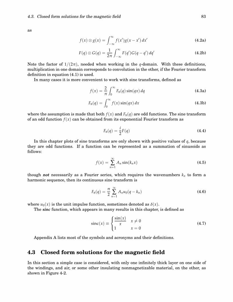
4.3. Closed form solutions for the magnetic field 83
as
f (x) ⊗ g(x) =∫ ∞
−∞f (x′)g(x− x′) dx′ (4.2a)
F(q) ⊗ G(q) =12π
∫ ∞
−∞F(q′)G(q− q′) dq′ (4.2b)
Note the factor of 1/(2π), needed when working in the q-domain. With these definitions,multiplication in one domain corresponds to convolution in the other, if the Fourier transformdefinition in equation (4.1) is used.
In many cases it is more convenient to work with sine transforms, defined as
f (x) =2π
∫ ∞
0FS(q) sin(qx) dq (4.3a)
FS(q) =∫ ∞
0f (x) sin(qx) dx (4.3b)
where the assumption is made that both f (x) and FS(q) are odd functions. The sine transformof an odd function f (x) can be obtained from its exponential Fourier transform as
FS(q) =i2F(q) (4.4)
In this chapter plots of sine transforms are only shown with positive values of q, becausethey are odd functions. If a function can be represented as a summation of sinusoids asfollows:
f (x) =∞∑n=1
An sin(knx) (4.5)
though not necessarily as a Fourier series, which requires the wavenumbers kn to form aharmonic sequence, then its continuous sine transform is
FS(q) =π
2
∞∑n=1
Anu0(q− kn) (4.6)
where u0(x) is the unit impulse function, sometimes denoted as δ(x).The sinc function, which appears in many results in this chapter, is defined as
sinc(x) ≡sin(x)x
x = 0
1 x = 0(4.7)
Appendix A lists most of the symbols and acronyms and their definitions.
4.3 Closed form solutions for the magnetic field
In this section a simple case is considered, with only one infinitely thick layer on one side ofthe windings, and air, or some other insulating nonmagnetizable material, on the other, asshown in Figure 4-2.
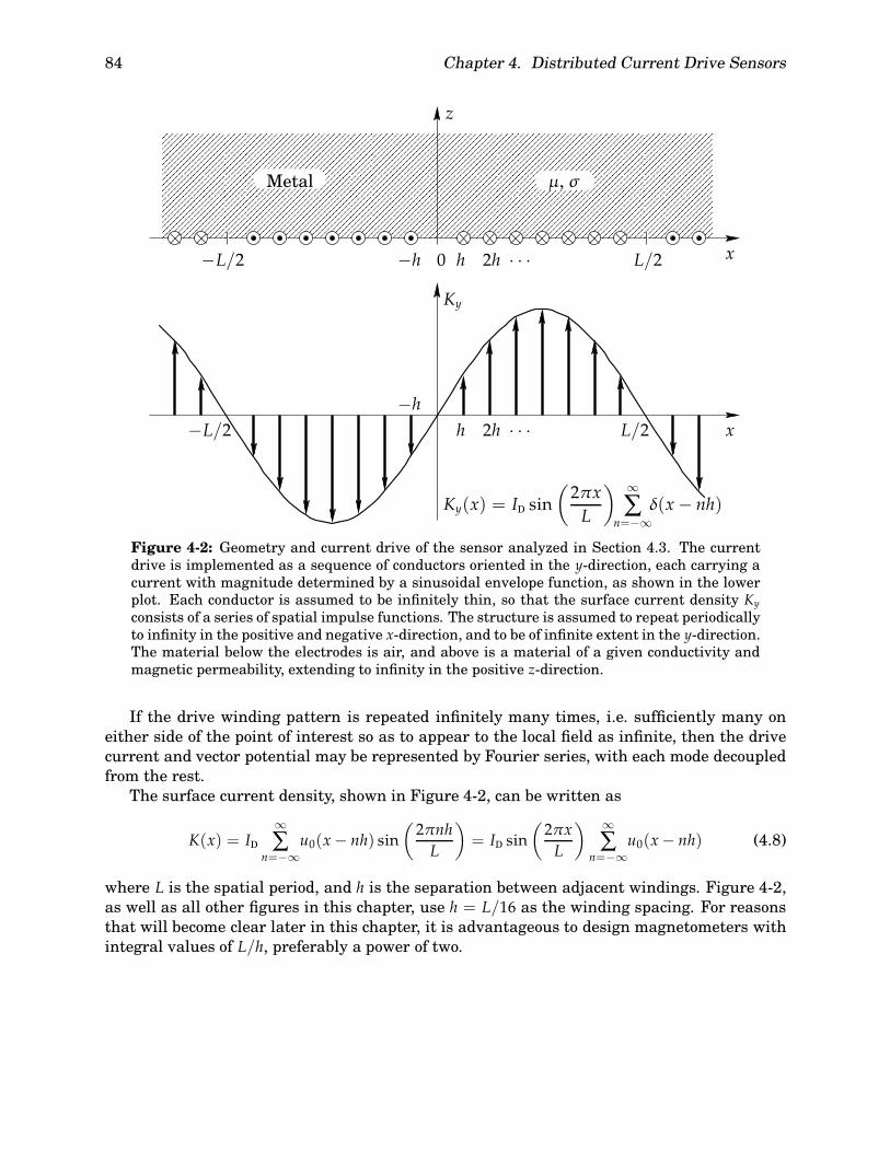
84 Chapter 4. Distributed Current Drive Sensors
��������������������������������������������������������������������������������������������������������������������������������������������
��������������������������������������������������������������������������������������������������������������������������������������������
�������������
�������������
���
���
�����
�����
�����
�����
�������
�������
�����
����� �
����
�����
���
���
���
��� �
����
�����
Ky
h 2h−h
L/2−L/2 x
−h h 2h0−L/2 L/2 x
z
Ky(x) = ID sin(2πxL
) ∞∑
n=−∞δ(x− nh)
· · ·
Metal µ, σ
· · ·
Figure 4-2: Geometry and current drive of the sensor analyzed in Section 4.3. The currentdrive is implemented as a sequence of conductors oriented in the y-direction, each carrying acurrent with magnitude determined by a sinusoidal envelope function, as shown in the lowerplot. Each conductor is assumed to be infinitely thin, so that the surface current density Kyconsists of a series of spatial impulse functions. The structure is assumed to repeat periodicallyto infinity in the positive and negative x-direction, and to be of infinite extent in the y-direction.The material below the electrodes is air, and above is a material of a given conductivity andmagnetic permeability, extending to infinity in the positive z-direction.
If the drive winding pattern is repeated infinitely many times, i.e. sufficiently many oneither side of the point of interest so as to appear to the local field as infinite, then the drivecurrent and vector potential may be represented by Fourier series, with each mode decoupledfrom the rest.
The surface current density, shown in Figure 4-2, can be written as
K(x) = ID∞∑
n=−∞u0(x− nh) sin
(2πnhL
)= ID sin
(2πxL
) ∞∑
n=−∞u0(x− nh) (4.8)
where L is the spatial period, and h is the separation between adjacent windings. Figure 4-2,as well as all other figures in this chapter, use h = L/16 as the winding spacing. For reasonsthat will become clear later in this chapter, it is advantageous to design magnetometers withintegral values of L/h, preferably a power of two.

4.3. Closed form solutions for the magnetic field 85
✲
✻,----,----,----
,----,----,----
,----,----,--------.
----.----.
----.----.----.1
L1h
+1L
2h
+1L
1h− 1L
2h− 1L
q/2π
KS(q)
Figure 4-3: Sine transform of the current distribution of the sensor, given by equation (4.10).It is plotted for positive values of q only, because all sine transforms are odd functions.
The Fourier transform of equation (4.8) is
K(q) = ID2π2i
[u0
(q− 2π
L
)− u0
(q+
2πL
)]⊗[2πh
∞∑
n=−∞u0
(q− 2πn
h
)]
=IDh· 2π2i
∞∑
n=−∞
{u0
(q− 2π
[nh
+1L
])− u0
(q− 2π
[nh− 1L
])} (4.9)
where the symbol ⊗ is used to denote convolution. The corresponding sine transform
KS(q) =IDh· π
2
∞∑
n=−∞
{u0
(q− 2π
[nh
+1L
])− u0
(q− 2π
[nh− 1L
])}(4.10)
obtained from equation (4.9) via equation (4.4), is more useful, because it represents the cur-rent distribution as a summation of impulse functions in reciprocal “sine” space, and thereforedirectly gives the coefficient of every constituent sinusoidal mode. The sine transform functionin equation (4.10) is shown in Figure 4-3.
The next step in computing the magnetic fields that result from this current excitation isto calculate the contribution of each constitutive spatial Fourier mode. Let the current densityof a mode with wavenumber q = k be
Ky(x) = K0 sin(kx) (4.11)
The solutions of the magnetic diffusion equation, given in equation (2.13), also apply inthis geometry. The solutions above and below the sensor are of the form:
Ay(x, z) =
{Aa sin(kx)e−γz z ≥ 0Ab sin(kx)ekz z ≤ 0
(4.12)
with γ defined in equation (2.14). In terms of the two unknown coefficients Aa and Ab, the

86 Chapter 4. Distributed Current Drive Sensors
magnetic field intensity is
H(x, z) =
Aa
µ0µr
[γ sin(kx)x+ k cos(kx)z
]e−γz z > 0
Ab
µ0
[−k sin(kx)x+ k cos(kx)z]ekz z < 0
(4.13)
where µr = µ/µ0 is the relative permeability of the material above the windings.The boundary conditions at the surface z = 0 require that
Hx(x, z) = Hx(x, z = 0+) − Hx(x, z = 0−) = Ky(x) (4.14a)
µrHz(x, z = 0+) = Hz(x, z = 0−) (4.14b)
The constraint in equation (4.14b) is satisfied if Aa = Ab.Substituting equations (4.11), (4.12) and (4.13) into equation (4.14) yields
Aa = Ab =µ0µrK0γ + kµr
(4.15)
resulting in
Ay(x, z) =
µ0µrK0γ + kµr
sin(kx)e−γz z ≥ 0
µ0µrK0γ + kµr
sin(kx)ekz z ≤ 0
(4.16)
The corresponding expressions for the magnetic field intensity are
H(x, z) =
K0
γ + kµr
[γ sin(kx)x+ k cos(kx)z
]e−γz z > 0
K0µr
γ + kµr
[−k sin(kx)x+ k cos(kx)z]ekz z < 0
(4.17)
In general, the summation of the above result over all spatial modes must be carried outnumerically. In some simple cases it is possible to derive an analytical expression. As anexample, consider the magnetic field at the origin (x = 0, z = 0) when the material undertest is air, i.e. µr = 1 and σ = 0, or δ = ∞. In this simplest possible case equation (4.17)degenerates to
H(x = 0, z = 0) =K02z (4.18)
which is independent of the wavenumber k. Summing over all modes that characterize thecurrent distribution in Figure 4-2 presents a problem. As can be seen in equation (4.10),the magnitude of the impulses does not decrease with increasing wavenumber. This is aconsequence of neglecting the finite width of the current elements. Attempting to combineequations (4.10) and (4.18) with the help of equation (4.6) yields a summation of the following

4.3. Closed form solutions for the magnetic field 87
✲
✻
x/a−5 0 5
.2
.4 a f (x) =1π· 1(x/a)2 + 1
✲
✻
qa−5 0 5
.5
1 F(q) = e−a|q|
Figure 4-4: The Lorentzian function, defined in equation (4.20), and its Fourier transform,defined in equation (4.21). The area under f (x) is equal to 1, so that f (x) → u0(x) when a → 0.The area under the transform is 2π f (0) = 2/a.
form:
Hz =ID2h
(1+ ∑ 1−∑ 1
)(4.19)
which does not formally converge. In order to carry out this computation it is necessaryinitially to give each current element a finite width and then take the limit of the result asthis width approaches zero. Any pulse function of area unity can be used in place of theimpulse functions in equation (4.8) for this purpose, but it is most convenient to choose onewhose Fourier transform will make the summation over modes easy to carry out. For example,a function that has a transform whose positive side is a decaying exponential works well,because the summation becomes a pair of geometric series. This function is the Lorentzian
f (x) =12π
· 2ax2 + a2
(4.20)
and it can be used in place of u0(x). It is plotted in Figure 4-4, together with its Fouriertransform
F(q) = e−a|q| (4.21)
Using equations (4.10), (4.18) and (4.21), it is now possible to write the magnetic field atthe origin (x = 0, z = 0) as
Hz =ID2h
S (4.22)

88 Chapter 4. Distributed Current Drive Sensors
−d d0
z
x
Hz =IDπdI = IDI = −ID
Figure 4-5: Magnetic field at the origin, generated by a pair of conductors positioned at adistance d on either side.
where S is the summation over the Fourier modes and is given by
S = lima→0
[e−2πa/L +
∞∑n=1
e−2πa(n/h+1/L) −∞∑n=1
e−2πa(n/h−1/L)
]
= 1+ lima′→0
[(e−a
′/L− ea′/L) ∞
∑n=1
e−na′/h
](letting a′ = 2πa)
= 1− 2 lima′→0
[sinh(a′/L)ea′/h − 1
]= 1− 2 lim
a′→0
(1/L) cosh(a′/L)(1/h)ea′/h
= 1− 2hL
(4.23)
The magnetic field intensity at the origin (x = 0, z = 0) is therefore
Hz =ID2hS =
ID2h
(1− 2h
L
)(4.24)
As a way of validating the Fourier series method used to obtain the result in equation(4.24), it is possible to calculate the magnetic field intensity for this simple case using a directmethod. The field at the origin generated by a pair of conductors positioned at x = ±d,extending to infinity in the y-direction, and each carrying current ID as shown in Figure 4-5,is given by
Hz =IDπd
(4.25)
calculated directly from Ampere’s Law. The entire sensor must therefore generate a magneticfield whose magnitude at the origin is
Hz =∞∑n=1
IDπnh
sin(2πnhL
)=
ID2h
(1− 2h
L
)(4.26)
where use has been made of the following formula [52, eq. 1.441]:
∞∑n=1
sin(nπx)n
=π
2(1− x) (4.27)
Equation (4.26) agrees with equation (4.24), which confirms that the Fourier transformmethod developed in this section give the correct result.

4.4. Numerical analysis 89
4.4 Numerical analysis
The analytical method shown above also works if the material above the sensor is magneti-zable (µr > 1), because in this case equation (4.17) still depends on k only via the sine (orcosine) term, which makes it possible to carry out the summation over modes in closed form.However, if a conducting material with finite skin depth δ is present, the calculations must becarried out numerically.
This can be done with the help of fast Fourier transform (FFT) methods. The algorithmhas the following steps:
1. Obtain the sine transform of the current excitation. For the periodic sensor this is givenby equation (4.10). For the finite width sensor this step has several substeps, as dis-cussed in Section 4.5.
2. Discretize the spectrum. A property of the FFT algorithm is that the number of samplepoints in q-space is equal to the number of points in the spatial discretization of themagnetic field in the x-direction. This consideration should determine how many samplepoints to obtain.
If the sensor wavelength L, defined in Figure 4-2, is an exact multiple of h, then allimpulse functions in Figure 4-3 fall on multiples of 2π/h in q-space. This means thatno information is lost if the discretization step is set to this value. Otherwise a muchdenser discretization would be necessary to maintain the information in the spectrum.Furthermore, since the FFT algorithm is more efficient if the number of samples isa power of two, it is preferable for L/h also to be a power of two. For the exampleconsidered in this chapter, L = 16h.
3. Apply a decaying exponential envelope to the discrete spectrum, to give the current ele-ments a finite width. The decay rate should be chosen such that most of the transitionhas happened by the end of the series of samples. If the exponent decays too fast, theninformation is unnecessarily being lost, while if the decay is too slow, the resulting fieldwill not be smooth, as a result of the sudden step in the spectrum effectively introducedat the end of the sample sequence. A plot of the resulting discretized spectrum of Fig-ure 4-3 is shown in Figure 4-6.
4. Choose a discretization step in the z-direction. This should most likely be the same asthe one in the x-direction, determined in step 2.
5. For every value of z, obtain the spectrum of the vector potential by applying equa-tion (4.16), without the sine term, to the excitation spectrum of step 3.
6. For every value of z, apply inverse FFT to obtain the vector potential as a function ofx and z. Standard FFT algorithms perform exponential, not sine, Fourier transforms.As seen in equation (4.4), the sine transform of a function FS(q), defined for q > 0, canbe calculated by taking the inverse exponential Fourier transform of the odd functionwhose positive side is FS(q), and multiplying the result by i/2. Therefore the discretesine transform can be obtained by first appending a reversed copy of the sample arrayto itself, and then applying the inverse FFT algorithm to the longer sequence.∗
∗This procedure introduces a factor of two redundancy in the numerical calculation. The easiest way to takeadvantage of it is to take the discrete Fourier transform of two functions simultaneously, e.g. for two differentvalues of z, as discussed in [81].

90 Chapter 4. Distributed Current Drive Sensors
✲
✻
−0.5
0
0.5
1KS
q
Figure 4-6: Discretized spectrum of the current excitation shown in Figure 4-2, in a decayingexponential envelope.
A contour plot of the vector potential yields the magnetic field lines, since they correspondto lines of constant vector potential. The result of applying this algorithm to the case of thesensor in air is shown in Figure 4-7 (a).
The magnetic fields that result when the material under test has a finite skin depth isshown in Figure 4-7 (b). Unlike the field of Figure 4-7 (a), in this case the temporal phaseangle of the vector potential depends on z. The figure shows the real part of the calculatedresponse.
The best way to get the actual magnetic field intensity H is to avoid calculating the vec-tor potential by carrying out the algorithm as outlined above, but with equation (4.17) usedin step 5 instead. The alternative way of calculating it from the vector potential introducesunnecessary numerical imprecision into the result, because it involves taking numeric deriva-tives.
4.5 Sensor of finite width
When the sensor is not infinitely wide, one must include the finite size as part of the analy-sis. It is no longer possible to use a quasi∗ Fourier series representation, where the spectrumconsists of a series of impulse functions, as in Figure 4-3. The full Fourier transform of themagnetic field distribution in this case is continuous. The discrete Fourier transform (DFT)methods therefore require a finer discretization of the spectrum. By virtue of the discretenessof the numerical transform methods, the functions represented by DFTs in both domains arealways periodic, but this periodicity may be ignored if the period is much larger than the in-terval of interest. The spacing between samples in reciprocal space in this case is determinedas the inverse of the minimum distance that two sensors must be physically separated in
∗The word “quasi” used here is meant to convey that the spectrum shown in Figure 4-3 does not necessarilyform a harmonic sequence, and therefore is not a Fourier Series, although it is similar to it in that it representsthe coefficients of the sinusoidal modes that constitute the original function. On the other hand, a practicalimplementation of the sensor requires that L be an exact multiple of h, which does in fact make the spectrum aFourier series, with most coefficients equal to zero.
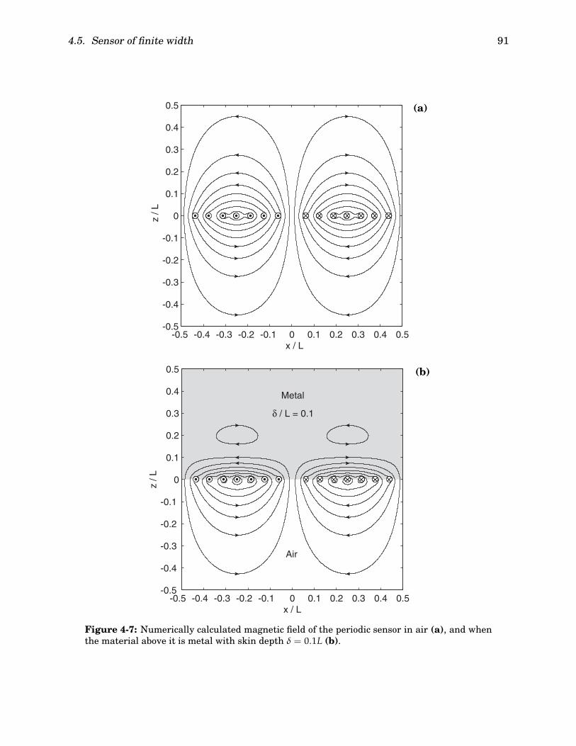
4.5. Sensor of finite width 91
-0.5 -0.4 -0.3 -0.2 -0.1 0 0.1 0.2 0.3 0.4 0.5-0.5
-0.4
-0.3
-0.2
-0.1
0
0.1
0.2
0.3
0.4
0.5
x / L
z / L
(a)
x / L
z / L
Air
Metal
δ / L = 0.1
-0.5 -0.4 -0.3 -0.2 -0.1 0 0.1 0.2 0.3 0.4 0.5-0.5
-0.4
-0.3
-0.2
-0.1
0
0.1
0.2
0.3
0.4
0.5 (b)
Figure 4-7: Numerically calculated magnetic field of the periodic sensor in air (a), and whenthe material above it is metal with skin depth δ = 0.1L (b).

92 Chapter 4. Distributed Current Drive Sensors
order to influence each other only negligibly, which is usually much greater than the spatialregion of interest. This stands in contrast to the periodic case considered in the previous sec-tion, where the sample distance in reciprocal space is the inverse of the fundamental sensorwavelength.
The numerical algorithm remains largely the same as before, with the exception of the cal-culation of the excitation spectrum, which now must consider the finite size of the sensor. Thecurrent distribution in this case can be obtained by multiplying the function in equation (4.8)by the square-pulse function
f (x) =
1 |x| <W2
0 otherwise(4.28)
where W is the width of the sensor. The Fourier transform of the square-pulse function is
F(q) =sin(qW/2)
q/2= W sinc
(qW2
)(4.29)
which must be convolved with the spectrum of equation (4.9) in order to obtain the Fouriertransform of the current excitation of the finite sensor. The resulting sine transform is:
KS(q) = IDW4h
∞∑
n=−∞
{sinc
(W2
[q− 2π
(nh
+1L
)])− sinc
(W2
[q− 2π
(nh− 1L
)])}(4.30)
In practice it is easier to carry out the discretization of the current excitation after thesine transform of the truncated sinusoid is calculated, for reasons presented in step 4 onpage 93 later in this section. The spectrum of the nondiscretized single-period surface currentdensity is obtained by taking the convolution of a sinusoid of period L and equation (4.29),and converting it to a sine transform via equation (4.4):
KS(q) =i2· ID 2π2i
[u0
(q− 2π
L
)− u0
(q+
2πL
)]⊗W sinc
(qW2
)
= IDW4
{sinc
(W2
[q− 2π
L
])− sinc
(W2
[q+
2πL
])} (4.31)
The current envelope function for the sensor of finite width, for the case when W = L,and its sine transform, given by equation (4.31), are shown in Figure 4-8 with the thick lines.It can be seen in the figure that the peak wavenumber, which is a measure of the effectivefundamental wavelength, is not 2π/L, as it would be in the case of the periodic sensor. Inorder to make this effective wavelength equal to the wavelength L of the current envelope,the width W would have to be increased to 1.210L (calculated numerically). The result wouldbe an envelope function that includes the tail of a second period on either side, as shown inFigure 4-8 with thin lines. This is undesirable, because if the sensor ends do not coincide withzeros in the current excitation, the resulting sharp transition at the ends contributes to moreenergy in the higher wavenumber modes, which have shallower penetration depths. This isclearly visible in Figure 4-8 (b). This is the reason why W = L is the optimal choice. On theother hand, extending the current excitation past the end of the period may be necessary forother reasons, as discussed in Section 4.7.

4.5. Sensor of finite width 93
✲
✻
x
f (x)
−1
1
−L/2L/2−W/2
W/2
(a)
✲
✻
q2π/L
FS(q)
−0.1
0
0.1
0.2
0.3
2 4 6 8
1✻0.837
(b)
Figure 4-8: Current envelope function for a sensor of finite width (a), and its correspondingsine transform (b). Two cases are shown, for the sensor width W equal to the wavelength L(thick lines), and forW = 1.210L, making the effective sensor wavelength equal to the sinusoidwavelength (thin lines).
When using a sensor of finite width, the first two steps in the algorithm outlined on page 89in Section 4.4 need to be replaced by the following steps:
1. Obtain the sine transform of the current envelope function, as in Figure 4-8 (b).
2. Discretize and truncate the transform. The length of the transform sample to use in thisstep is determined by the number of current segments in the sensor. For the exampleused in this chapter, where W = L = 16h, the sine transform in Figure 4-8 (b) must betruncated at q = 8(2π/L). As before, the sample density is determined by the necessaryprecision.
3. Append a reversed and negated copy of the sequence to its end, in order to make theFFT algorithm carry out the inverse sine transform.
Alternatively, the result of the first three steps may be obtained by taking the FFT ofthe current profile directly, especially in cases when a closed form of the transform of theprofile function is not available.
4. Replicate the resulting sequence a number of times. The resulting sine transform isshown in Figure 4-9. Periodicity in one domain implies discreteness in the other, andtherefore the effect of this step is to build into the data the fact that the current distri-bution is not continuous, but rather generated by discrete current segments. Replicationis a simple operation and this is why this method is preferred to discretizing the driveprofile function first and convolving with equation (4.29) later. The number of periodsis determined by the needed level of detail in close proximity to the current segments.The greater the number of periods, the narrower the implied effective width of the con-ductors. For example, four periods are used in the calculation of the field distributionsshown in Figure 4-10.
5. Proceed with steps 3–6 on page 89.
It is informative to compare the spectrum in Figure 4-9 to that in Figure 4-3. One cansee that the effect of limiting the sensor to only one wavelength is to smear out the peaksat the excitation wavenumbers, and as a consequence the magnetic field can no longer berepresented as a superposition of individual sinusoidal modes.

94 Chapter 4. Distributed Current Drive Sensors
✲
✻
q2π/h
KS(q)WID/4
−0.2
0
0.2
1 2 30.5 1.5 2.5
Figure 4-9: Sine transform of the current excitation generated by discrete current elements.It is computed by step 4 on page 93. The discrete nature of the transform is not explicitlyshown in the plot. Compare to the spectrum in Figure 4-3.
The magnetic field calculated in this way is shown in Figure 4-10, with the same materialsand current excitation as in Figure 4-7, but with no current elements for |x| > L/2 (seeFigure 4-2). By comparing these sets of figures, the observation may be made that they differlittle at the origin, where the sensing elements are positioned, but there is a substantialdifference toward the ends of the sensor.
4.6 Multiple homogeneous layers
The models developed so far in this chapter may be extended to apply to material structuresthat consist of more than one homogeneous layer. Figure 4-11 shows a diagram of such alayered material structure.
The thickness of the top layer in the figure is treated as infinite, which means that it ismany times larger than the real part of the characteristic decay rate 1/γ in that material,so that the properties at the upper surface have no effect on the sensor response. In practicethere is always a layer of air, or another nonmagnetic insulating material, between the sensorand the material. This layer, number 4 in the figure, must be included in the model, and itsthickness is known as the measurement “lift-off.”
The structure in Figure 4-11 may represent a metal coating on a metal substrate, which isa very common situation [26]. Layer number 1 represents the substrate, layer 3 is the coating,and layer 2 is used to model an inter-diffusion zone, whose properties are often quite differentfrom either the coating or the substrate.
The effect of having more than one homogeneous layer of material above the sensor en-ters the computational method only at step 5 in the method on page 89 in Section 4.4, as achange in equation (4.16), because the invariance of the material structure in the x- and y-directions is maintained. The idea is similar to the method in Section 2.1.5, with the surfacereluctance density Rn relating the magnetic vector potential to the normal component of themagnetic field intensity, as in equation (2.51). Rn is derived from the properties of the layersin Figure 4-11, using equations (2.46) and (2.50).
In terms of Rn, for every Fourier mode n equation (4.15) becomes
Aa = Ab =KnknRn
(4.32)
where Kn is the Fourier component of order n of the surface current density. This fully deter-

4.6. Multiple homogeneous layers 95
x / L
z / L
-1 -0.8 -0.6 -0.4 -0.2 0 0.2 0.4 0.6 0.8 1-0.8
-0.6
-0.4
-0.2
0
0.2
0.4
0.6
0.8 (a)
x / L
z / L
Air
Metal δ / L = 0.1
-1 -0.8 -0.6 -0.4 -0.2 0 0.2 0.4 0.6 0.8 1-0.8
-0.6
-0.4
-0.2
0
0.2
0.4(b)
Figure 4-10: Numerically calculated magnetic field of the finite-width sensor in air (a), andwhen the material above it is metal with skin depth δ = 0.1L (b).

96 Chapter 4. Distributed Current Drive Sensors
������������������������������������������������������������������������������������������������������������������������������������������������������
������������������������������������������������������������������������������������������������������������������������������������������������������
���
���
������������������������������������������������������������
������������������������������������������������������������
t1 = ∞
t2
t3
t4σ4 = 0, µ4 = µ0
sensor
σ1, µ1
σ2, µ2
σ3, µ3
Figure 4-11: Material structure that consists of more than one homogeneous layer. The top-most layer is assumed to extend to infinity. An air layer that models the sensor lift-off is in-cluded between the sensor and the material under test. The sensor windings are representedby � and ⊗.
mines the magnetic field, via equation (4.13).
4.7 Eliminating the net dipole moment
The finite width sensor, described in Section 4.5, has a net dipole moment in the sense that atdistances larger than the sensor wavelength the magnetic field approaches the form of a fieldgenerated by a magnetic dipole at the origin. It can easily be seen that the net dipole momentis not zero, because each pair of windings, comprising a current segment on either side of thecenter, together with the return current path, forms a current loop of nonzero area, and theeffective magnetic moments of all these loops point in the same direction.
Certainly, close to the sensor windings, at typical measurement distances, the magneticfield is described well by the model of the preceding sections. The reason for addressing thenet dipole moment is not to improve the results of this model.
It is important that the sensors have a winding layout which results in no net dipolemoment.∗ This is due to the following reason: At some distance away from the sensor, theassumptions of the model no longer hold. The sensor is finite in the y-direction, which cannotbe ignored at distances comparable to the sensor length. Furthermore, the discrete Fouriertransform does have an implied periodicity, determined by the reciprocal domain sample fre-quency, so that the finite width sensor model only holds at distances much smaller than thedistance between the sensor and its first phantom image. For example, the magnetic fieldlines shown in Figure 4-10 have a phantom image period sixteen times greater than the sen-sor width W.
These unmodeled effects in general do not affect the accuracy of a measurement, becauseall practical measurement procedures include a calibration step, designed to compensate forsuch imperfections of the model, which do not change with time or experimental conditions.Calibration methods are discussed in more detail in Appendix D.
The difficulty comes from the rate at which the sensor loses sensitivity with distance. Nearthe sensor surface the magnetic field decays essentially exponentially, at a rate determined
∗This issue was first discovered and addressed by Darrell E. Schlicker in connection with the standard MWM.It led to a redesign of the MWM with two separate layers for the primary and secondary windings.
4.7. Eliminating the net dipole moment 97
by its spatial wavelength and the skin depth in the medium, given in equation (2.14). Farfrom the sensor the fields fall off at a rate determined by the lowest order multi-pole momentexcited by the sensor. This should be a high order moment, since it is important for the sensorto lose sensitivity quickly with distance. Otherwise its response would be slightly affected bythe presence of magnetizable and/or conducting objects in its vicinity, even if they are muchfarther than the material under test. Whereas this effect may be small, even compared toother unmodeled effects, the problem is that it can change with time, as objects near thesensor are moved, or when the sensor is moved to inspect a new location. This means that itcannot be eliminated via calibration, ultimately leading to lack of reproducibility.
Sometimes very small changes in the material properties must be measured, e.g. conduc-tivity variations related to shotpeen intensity or cold work quality [18, 24]. In cases like thatthe accuracy of the measurement may be substantially degraded by the presence of a netdipole moment. It is desirable for the sensor to lose sensitivity far from its active region asquickly as possible. This is why the goal is to create a winding pattern with no net dipolemoment.
The analysis of the sensor in the far field, i.e. at distances much greater than the sensordimensions, is most conveniently formulated in spherical coordinates with the use of the mag-netic scalar potential. This is because at large distances all windings and conducting mediamay be represented by a singularity at the origin, since there is no interest in the magneticfield details near the sensor. This makes it possible to write the magnetic field intensity in thecurrent-free region as a gradient of a scalar potential Ψ , defined everywhere except at r = 0:
H = −∇Ψ (4.33)
The magnetic scalar potential must obey Laplace’s equation, because the divergence of themagnetic flux density is zero: ∇2Ψ = 0. In spherical coordinates it becomes
1r2
∂∂r
(r2
∂∂r
Ψ
)+
1r2 sinθ
· ∂∂θ
(sinθ
∂∂θ
Ψ
)+
1r2 sin2θ
· ∂2
∂ϕ2Ψ = 0 (4.34)
which, letting Ψ (r,θ,ϕ) = R(r)Y(θ,ϕ), separates into
ddr
(r2ddrR)− �(� + 1)R = 0 (4.35)
and
1sinθ
· ∂∂θ
(sinθ
∂∂θY)
+1
sin2θ· ∂2
∂ϕ2Y + �(� + 1)Y = 0 (4.36)
The solutions of equation (4.35) are r� and r−�−1, and the solutions to equation (4.36) are [55]:
Y�m(θ,ϕ) =
√2� + 14π
· (� −m)!(� +m)!
Pm�(cosθ
)e−imϕ m = −�, . . . , � (4.37)
where Pm� are the Associated Legendre functions. The series of functions Y�m are the sphericalharmonic functions. They are written out for the first several values of � in Table 4.1.
For magnetic fields the lowest order possible is the dipole moment, whose scalar magneticpotential decays as r−2. Figure 4-12 shows the equipotential surfaces of the scalar magnetic

98 Chapter 4. Distributed Current Drive Sensors
� = 0 Y00 =√
14π
� = 1
Y11 = −1
2
√32π
sinθ eiϕ
Y10 =
√34π
cosθ
� = 2
Y22 =14
√152π
sin2θ e2iϕ
Y21 = −12
√152π
sinθ cosθ eiϕ
Y20 =
√54π
(32cos2θ − 1
2
)
� = 3
Y33 = −14
√354π
sin3θ e3iϕ
Y32 =14
√1052π
sin2θ cosθ e2iϕ
Y31 = −14
√214π
sinθ(5 cos2θ − 1
)eiϕ
Y30 =
√74π
(52cos3θ − 3
2cosθ
)
� = 4
Y44 =316
√352π
sin4θ e4iϕ
Y43 = −34
√354π
sin3θ cosθ e3iϕ
Y42 =38
√52π
sin2θ(7 cos2θ − 1
)e2iϕ
Y41 = −34
√54π
sinθ(7 cos3θ − 3 cosθ
)eiϕ
Y40 =√
94π
(358cos4θ − 30
8cos2θ +
38
)Table 4.1: Spherical harmonic functions defined in equation (4.37).
potential for the three lowest order rotationally symmetric multipole modes. The requirementfor rotational symmetry is due to the fact that the sensor windings are confined to the x-yplane, and applies both to the rectangular sensor and to the circular sensor of Section 4.8. Ofthe spherical harmonic functions Y�m in Table 4.1, only those with m = 0 have this symmetry,i.e. are independent of ϕ. The “quadrupole” mode, � = 2, cannot be excited by these magneticsensors, since it is even with respect to z, whereas flipping the sensor upside down reversesthe current direction in all windings, changing the sense of all magnetic fields.
If the dipole moment is eliminated, the next dominant mode is the “octupole,” or � = 3moment, whose magnetic field lines are shown in Figure 4-13. The potential of this mode hasa r−4 dependence, which means that the magnetic field intensity falls off as r−5. In practicethis is fast enough that canceling out the dipole moment is all that is required to eliminateunwanted long range sensitivity.
Instead of driving each current segment of the sensor independently, it is much easier toset the correct current profile by changing the number of windings in each segment. As aconsequence, the relative values of the segment current must be ratios of integer numbers.Since the sensor length is constant, the dipole moment of each loop made up of windings atx = ± jh is proportional to the number of windings wj and to j:
p ∝ jwj (4.38)

4.7. Eliminating the net dipole moment 99
1 0.5
0-0.5
-1
1
0.5
0
-0.5
-1-1
-0.5
0
xy
z
θ
r0.5
1
1 0.5
0-0.5
-1
1
0.5
0
-0.5
-1-1
-0.5
0
0.5
1
1 0.5
0-0.5
-1
1
0.5
0
-0.5
-1-1
-0.5
0
0.5
1
Ψ = Ψ0r−2 cosθ
� = 1
Ψ = Ψ0r−3( 32 cos
2θ − 12
)� = 2
Ψ = Ψ0r−4( 52 cos
3θ − 32 cosθ
)� = 3
(a) (b) (c)
Figure 4-12: Equipotential surfaces, Ψ (r,θ,ϕ) = Ψ0, of the magnetic scalar potential for multi-pole moments with no ϕ-dependence. These three cases correspond to the spherical harmonicfunctions Y10 (a), Y20 (b), and Y30 (c) respectively. If the dipole (� = 1) moment is zero, thenthe lowest order moment remaining for the magnetometer is � = 3, since the � = 2 moment isnot allowed, due to its symmetry.
which means that in order to cancel out the net dipole moment, these individual contributionsmust sum up to zero:
N
∑j=1
jwj = 0 (4.39)
where N is the total number of current segments in one half of the sensor.To satisfy equation (4.39), the sensor must include a fraction of a wavelength past the
end of the single period, where the current flow is in the opposite direction (see Figure 4-2).Since both j and wj are integers, it is impossible to satisfy equation (4.39) exactly while atthe same time strictly following the sinusoidal envelope function. A compromise is shownin Table 4.2, which lists a winding pattern resulting in no net dipole moment. The windingturns are also plotted in Figure 4-14. The current in the last two segments deviates fromthe sinusoid. Another consideration in choosing the numbers in this table is to taper off thecurrent towards the ends of the sensor, in order to avoid rapid changes in the primary currentdistribution, which would result in more energy in higher Fourier modes. This matter waspreviously discussed in Section 4.5.
j = x/h 0 1 2 3 4 5 6 7 8 9 10 11 12Winding turns wj 0 5 9 12 13 12 9 5 0 −5 −9 −7 −4
Table 4.2: Number of winding turns wj for the finite sensor with no net dipole moment. Neg-ative number of turns means that the winding is wound in the opposite direction (clockwise).Only the windings for x ≥ 0 are given, because the sensor is symmetric.

100 Chapter 4. Distributed Current Drive Sensors
z
Figure 4-13: Magnetic field lines for � = 3 “octupole” moment potential. The central region isleft blank, because the density of lines increases very rapidly, due to the r−5 dependence of themagnetic field intensity.
4.8 Sensor with rotational symmetry
This section describes a circular magnetometer with a distributed current drive, applying theideas and methods of Chapter 3 to the sensors in this chapter.
When designing distributed current drive sensors, the reasons for preferring a circulargeometry are even more compelling. Since the sensor width is the same as, or similar to, thespatial wavelength, the edge effects due to the finite length in the y-direction are much morepronounced. Even worse, the total amount of current that flows in this return path is equalto the total of all windings, making it several times higher than the winding with the highestcurrent. To make the edge effects negligible, it would be necessary to make the sensor width inthe y-direction perhaps a factor of ten larger than its length, defeating the purpose of havinga distributed drive in the first place, which is to create a relatively large spatial wavelength
0
5
9
12 13
12
9
5
0
−5
−9 −7 −4
Figure 4-14: Number of winding turns for the finite sensor with no net dipole moment, accord-ing to Table 4.2. The sinusoidal envelope function is shown with a dashed line. The number ofturns do not fall exactly on the curve, since they need to be integers. The number of turns in thelast two windings on either side are tapered off in order to avoid rapid changes in the primarycurrent distribution, which would result in more energy in higher order Fourier modes.

4.8. Sensor with rotational symmetry 101
W
h
Figure 4-15: Structure of the circular magnetometer with distributed current drive. There isa set of concentric grooves, equally spaced h apart, to hold the primary windings. The numberof turns in each winding follows a first order Bessel function envelope, according to Table 4.3.There is no groove at r = W, since this point corresponds to a zero in the envelope function.
excitation with a small footprint. Employing a circular geometry altogether eliminates theunmodeled edge effects.
This section discusses a sensor with this geometry and the changes needed to adapt themodeling techniques developed so far in this chapter to cylindrical coordinates.
4.8.1 Sensor description
A circularly symmetric sensor with distributed primary current drive has been created. Itsstructure is shown in Figure 4-15. The sensor substrate is made of a 0.5 inch thick polypropy-lene plate with 3 mm wide concentric grooves used to hold the windings. The grooves arespaced h = 1 cm apart, machined at an angle directed radially inward to keep the windings inplace at the correct radius. The two straight radial grooves are used to hold wires connectingthe windings.
The current drive follows a Bessel function envelope, J1(α1r/W), where α1 ≈ 3.832 is thefirst zero of J1. There is no groove at r = W = 8 cm, because this point corresponds to thezero in the Bessel function. Windings are present past the first zero, in order to allow for netdipole moment cancellation, as discussed in Section 4.7. Unlike the rectangular sensor, whosewindings have a fixed length, here the dipole moment of each winding is proportional to thesquare of the radius, which changes the requirement for dipole cancellation to
N
∑j=1
j2wj = 0 (4.40)
The number of windings chosen for this sensor prototype are given in Table 4.3 and in Fig-

102 Chapter 4. Distributed Current Drive Sensors
j = r/h 1 2 3 4 5 6 7 8 9 10 11Winding turns wj 5 9 11 12 11 8 4 0 −4 −4 −3
Table 4.3: Number of turns per winding wj for the circular magnetometer.
ure 4-19.This sensor is built with a single sensing element, located in the center. Since a magne-
toresistive sensor is used, details and experimental measurement results are presented inChapter 5. This section focuses on the mathematical models of the sensor response, used togenerate appropriate measurement grids.
4.8.2 Sensor modeling
The surface current density of a sensor with N concentric windings is
KS(r) = ID J1(α1
Wr) N
∑j=1
u0(r− jh) = IDN
∑j=1
u0(r− jh)J1(α1
Wjh)
(4.41)
where h is the radial spacing of the windings, and W is the position of the first zero of thecurrent distribution. This envelope function is chosen to match the solutions of the magneticdiffusion equation in cylindrical coordinates, shown in equation (3.3). Using the definitionof the Fourier-Bessel Series from Section 3.1.1, the series coefficients of the surface currentdensity are
Kn =1Qn
∫ R
0rKS(r)J1(βnr) dr =
2IDR2 J20 (αn)
N
∑j=1
J1(α1
Wjh)J1(βn jh) jh (4.42)
where βn = αn/R, and the radius R, over which the series is defined, is chosen large comparedto W.
The counterpart of equations (4.12) and (4.13) of Section 4.3 in cylindrical coordinates are
Aϕ(r, z) =
{AaJ1(βr)e−γz z ≥ 0AbJ1(βr)eβz z ≤ 0
(4.43)
and
H(r, z) =
Aa
µ0µr
[γJ1(βr)r+ βJ0(βr)z
]e−γz z > 0
Ab
µ0
[−βJ1(βr)r+ βJ0(βr)z]eβz z < 0
(4.44)
Application of the boundary conditions then yields
Aa = Ab =µ0µr IDγ + βµr
(4.45)
exactly analogous to equation (4.15).The method of incorporating multiple layers in the model, developed in Section 4.6, is also
directly applicable in this case. Combining the results in equations (4.44), (4.32), and (4.42),

4.9. Fast Hankel transform 103
and summing over all Fourier-Bessel modes, yields the following result for the magnetic fluxdensity at the origin:
Bz(r = 0, z = 0) = ID∞∑n=1
2R2 J20 (αn)
· 1Rn
N
∑j=1
J1(α1
Wjh)J1(βn jh) jh (4.46)
So far the ideal value of the drive current density in equation (4.41) has been used. In thepractical implementation of the sensor, the shape of the current density is achieved by adjust-ing the number of turns in each segment of the winding, to approximate the ideal envelopefunction. As a consequence, the total effective current in each segment is an integral mul-tiple of the driving current. The approximation can be made arbitrarily close by increasingthe number of turns, but from a practical perspective a compromise must be made betweenthe coarseness of the quantization and the increasing inductance and parasitic capacitance ofthe primary winding, as the total number of turns increases. The winding turns in Table 4.3are the result of such a compromise. Figure 4-19 plots the actual number of turns and thecorresponding ideal envelope function for two different winding patterns.
To use the actual current density that results from the winding pattern in Table 4.3, equa-tion (4.41) must be replaced with
KS(r) = IDN
∑j=1
wju0(r− jh) (4.47)
where the value of the driving current ID is not necessarily the same. As discussed in Chap-ter 5 and Appendix D, such multiplicative factors in the magnitude of the sensor responsecan be ignored in the simulations, since they are absorbed in the sensor calibration step.Equations (4.42) and (4.46) must similarly be altered as follows:
Kn =2ID
R2 J20 (αn)
N
∑j=1
wjJ1(βn jh) jh (4.48)
Bz(r = 0, z = 0) = ID∞∑n=1
2R2 J20 (αn)
· 1Rn
N
∑j=1
wjJ1(βn jh) jh (4.49)
Equations (4.44), (4.45), and (4.48) are used to calculate the magnetic field lines of thesensor in this section for air and metal, in analogy to the results shown in Figure 4-10. Theresults are shown in Figure 4-16.
The measurement grids used in Chapter 5, shown in Figures 5-8, 5-10, 5-13, and 5-15, aregenerated using a version of this method, described in Section 5.3.
One may visually confirm that the field far from the windings in Figure 4-16 (a) has nodipole moment by comparing it to the pattern in Figure 4-13, observing that the dominantmulti-pole moment appears to be the “octupole” (� = 3) moment.
4.9 Fast Hankel transform
Methods similar to the FFT methods in Section 4.4 may be used to model sensors with rota-tional symmetry, such as the one described in Section 4.8. The magnetic vector potential inthis case is represented as a Fourier-Bessel series, applied over the interval 0 < r ≤ R, where

104 Chapter 4. Distributed Current Drive Sensors
r / W
z / W
-1.5 -1 -0.5 0 0.5 1 1.5-1
-0.5
0
0.5
1 (a)
r / W
z / W
Air
Metal
δ / W = 0.2
-1.5 -1 -0.5 0 0.5 1 1.5-1
-0.5
0
0.5
1 (b)
Figure 4-16: Numerically calculated magnetic field of the circular magnetometer in air (a),and when the material above it is metal with skin depth δ = 0.2W (b), where W is the radiuswhere the first order Bessel function has its first zero.

4.9. Fast Hankel transform 105
the radius R is chosen to be large compared to the relevant length scale.Calculating the Bessel series coefficients and then summing over the spatial modes, as
done in Section 4.8, can be a very computationally intensive task. The Cartesian geometrycase took advantage of the FFT methods, which unfortunately have no direct analog for theBessel series.
The continuous Fourier-Bessel transform is better known as the Hankel transform. Amethod of Hankel transform evaluation using FFT methods is described in [56]. There theHankel transform is carried out in two FFT steps. This section presents an implementationof this Fast Hankel Transform (FHT), as an alternative to the direct method of Section 4.8.
4.9.1 Definition and derivation
The Hankel transform can be based on Bessel functions of any order. Here the relevanttransform is based on J1. It is defined as follows:
g(u) =∫ ∞
0f (r)J1(ur)r dr (4.50)
If the following substitutions are made:
r = r0eαx (4.51)
u = u0eαy (4.52)
f (x) = r f (r) = r0eαx f(r0eαx
)(4.53)
g(y) = ug(u) = u0eαyg(u0eαy
)(4.54)
then equation (4.50) transforms to the following correlation integral:
g(y) =∫ ∞
−∞f (x)(x+ y) dx (4.55)
where the kernel (x) is defined as
(x) = αr0u0eαx (4.56)
Taking the Fourier transform, defined in equation (4.1b), of both sides of equation (4.55),the following relationship is derived:
F{g}
=∫ ∞
−∞g(y)e−iky dy =
∫ ∞
−∞f (x) dx
∫ ∞
−∞(x+ y)e−iky dy
=∫ ∞
−∞f (x)e+ikx dx
∫ ∞
−∞(y′)e−iky
′dy′ = F
{}· 2πF−1
{f} (4.57)
where the substitution y′ = y+ x was used.It is therefore possible to compute the Hankel transform by applying the Fourier transform
twice. It is important to realize that the Fourier transform of the kernel does not dependon the original function f (r), and therefore needs to be computed only once for multiple Han-kel transform evaluations. This step is also the only one which involves evaluating Besselfunctions. These features of the fast Hankel transform give it its computational advantage.
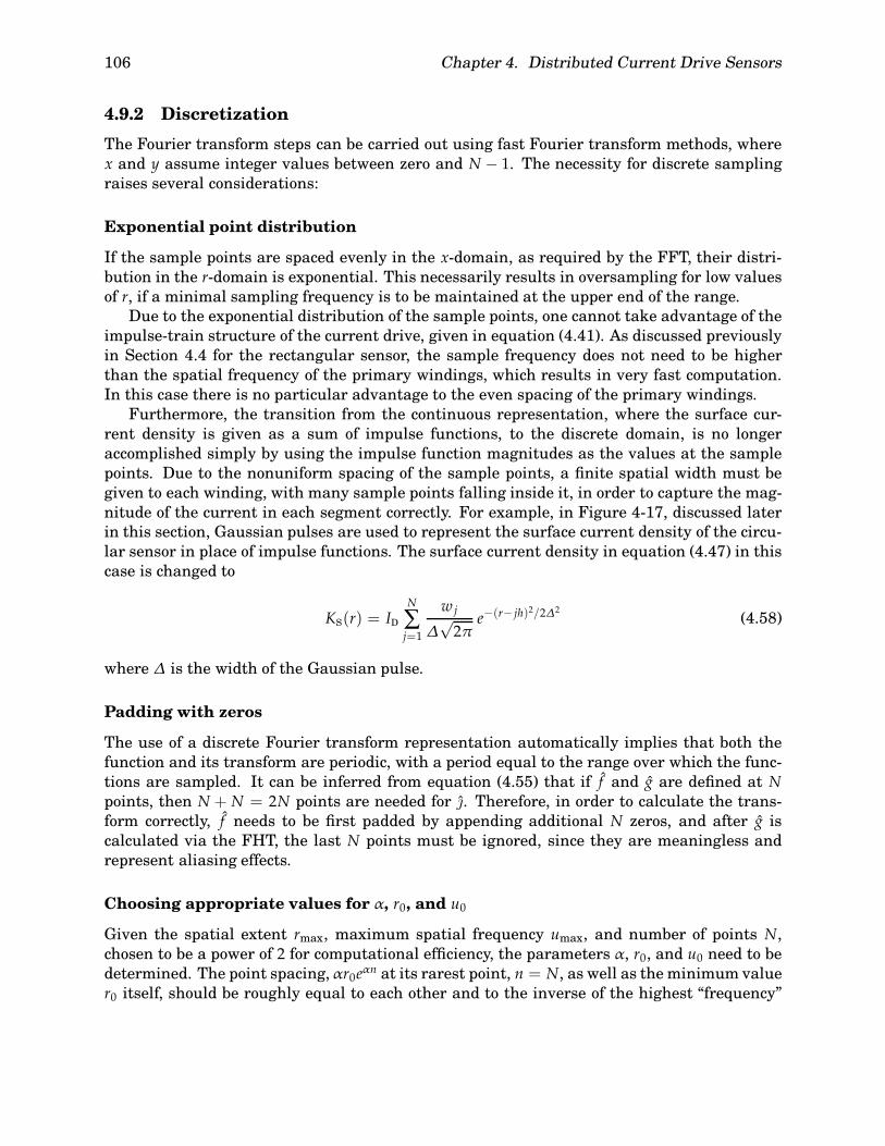
106 Chapter 4. Distributed Current Drive Sensors
4.9.2 Discretization
The Fourier transform steps can be carried out using fast Fourier transform methods, wherex and y assume integer values between zero and N − 1. The necessity for discrete samplingraises several considerations:
Exponential point distribution
If the sample points are spaced evenly in the x-domain, as required by the FFT, their distri-bution in the r-domain is exponential. This necessarily results in oversampling for low valuesof r, if a minimal sampling frequency is to be maintained at the upper end of the range.
Due to the exponential distribution of the sample points, one cannot take advantage of theimpulse-train structure of the current drive, given in equation (4.41). As discussed previouslyin Section 4.4 for the rectangular sensor, the sample frequency does not need to be higherthan the spatial frequency of the primary windings, which results in very fast computation.In this case there is no particular advantage to the even spacing of the primary windings.
Furthermore, the transition from the continuous representation, where the surface cur-rent density is given as a sum of impulse functions, to the discrete domain, is no longeraccomplished simply by using the impulse function magnitudes as the values at the samplepoints. Due to the nonuniform spacing of the sample points, a finite spatial width must begiven to each winding, with many sample points falling inside it, in order to capture the mag-nitude of the current in each segment correctly. For example, in Figure 4-17, discussed laterin this section, Gaussian pulses are used to represent the surface current density of the circu-lar sensor in place of impulse functions. The surface current density in equation (4.47) in thiscase is changed to
KS(r) = IDN
∑j=1
wj
∆√2π
e−(r− jh)2/2∆2(4.58)
where ∆ is the width of the Gaussian pulse.
Padding with zeros
The use of a discrete Fourier transform representation automatically implies that both thefunction and its transform are periodic, with a period equal to the range over which the func-tions are sampled. It can be inferred from equation (4.55) that if f and g are defined at Npoints, then N + N = 2N points are needed for . Therefore, in order to calculate the trans-form correctly, f needs to be first padded by appending additional N zeros, and after g iscalculated via the FHT, the last N points must be ignored, since they are meaningless andrepresent aliasing effects.
Choosing appropriate values for α, r0, and u0
Given the spatial extent rmax, maximum spatial frequency umax, and number of points N,chosen to be a power of 2 for computational efficiency, the parameters α, r0, and u0 need to bedetermined. The point spacing,αr0eαn at its rarest point, n = N, as well as the minimum valuer0 itself, should be roughly equal to each other and to the inverse of the highest “frequency”

4.9. Fast Hankel transform 107
Parameter Value
N 210 = 1024α 0.00515r0 0.0154rmax 3.00q0 0.946qmax 184
Table 4.4: Fast Hankel transform normalized parameter values.
value in the reciprocal domain. This results in the following equation for α:
αeαN = 1 (4.59)
This in turn determines r0 and u0:
r0 = rmaxe−αN (4.60)
u0 = umaxe−αN (4.61)
Whether or not the resulting values of r0 and u0 are small enough to be able to represent thediscretized functions with adequate accuracy depends on the original choice of N. It is alsopossible to pick r0 and u0 first, and let this determine α and N, as was done in [56].
4.9.3 Application of the fast Hankel transform to the circularmagnetometer
The first step in applying the FHT to calculate the response of the circular magnetometer isto verify that the values of the various FHT parameters are appropriate, to ensure that thetransform represents the sensor with adequate precision, while keeping the computationalburden at a minimum.
Figure 4-17 (a) is a plot of the surface current density in equation (4.58). The FHT isapplied to obtain the transform of the surface current density, with the result shown in Fig-ure 4-17 (b). The FHT parameters used are given in Table 4.4. This transform is similar instructure to the spectrum shown in Figure 4-9. Here the magnitude decreases with increas-ing q because of the nonzero width of the current pulses in the r-domain. A similar amplitudeenvelope was used in the computations in Section 4.5, although not explicitly shown in Fig-ure 4-9. In that case the exponential decay was imposed on the spectrum after it was com-puted, while here it occurs naturally, because the initial current function already includes thenonzero pulse width.
Applying the FHT for a second time to the transform restores the original function, be-cause the Hankel transform is its own inverse. The result is shown in Figure 4-17 (c). It canbe seen in the figure that the twice-transformed function f ′(r) is a very close match to f (r),with the exception of the ripples that result from the finite length of the spectrum, the ripplefrequency being dominated by the first nontrivial component past the truncated end of thespectrum, somewhere near qW = 190 in this case.
Thus the correctness of the FHT developed in this section is confirmed. This method cannow be applied to generate the same magnetic field line diagrams as Figure 4-16 in Sec-

108 Chapter 4. Distributed Current Drive Sensors
0 0.5 1 1.5 2 2.5 3−0.1
0
0.1
0.2
0.3Fast Hankel Transform
r / W
f(r)
0 20 40 60 80 100 120 140 160 180 200−5
0
5
10
15x 10
−3
qW
g(q)
0 0.5 1 1.5 2 2.5 3−0.1
0
0.1
0.2
0.3
r / W
f’(r)
(a)
(b)
(c)
Figure 4-17: Results of the application of the fast Hankel transform. The FHT parametersused are given in Table 4.4. (a) The function used to represent the surface current densityKS(r) of the primary winding. (b) The fast Hankel transform of this function. (c) The originalfunction restored with another application of the FHT. The high frequency ripples are wellunderstood, and are due to the truncation of the Hankel transform.

4.10. Different wavelength modes with the same sensor 109
A 0 14 22 21 13 3 −4 −4 0 1 −2 −7 −4B 0 −4 −4 3 13 21 22 14 0 −11 −16 −7 −4
A+ B 0 10 18 24 26 24 18 10 0 −10 −18 −14 −8A− B 0 18 26 18 0 −18 −26 −18 0 12 14 0 0
Table 4.5: Winding pattern for the rectangular magnetometer, enabling two different funda-mental wavelengths, determined by the polarity of the connection.
A 13 21 21 15 7 1 −1 0 1 −4 −3B −3 −3 1 9 15 15 9 0 −9 −4 −3
A+ B 10 18 22 24 22 16 8 0 −8 −8 −6A− B 16 24 20 6 −8 −14 −10 0 10 0 0
Table 4.6: Winding pattern for the circular magnetometer, enabling two different fundamentalwavelengths, determined by the polarity of the connection.
tion 4.8, by using the numerical techniques of Sections 4.4 and 4.5, using the FHT in place ofthe FFT. The results are shown in Figure 4-18. The two sets of figures appear identical.
4.10 Different wavelength modes with the same sensor
It is possible to change the fundamental wavelength of the current excitation without chang-ing the geometry of the sensor, by changing the current distribution in the primary windingsegments. This may be accomplished by supplying an independent current drive for each seg-ment, and changing the relative magnitudes of these drives to follow an appropriate envelopefunction with the needed spatial wavelength.
Another possibility, which avoids the need for multiple drives, is to use two or more inde-pendent winding circuits, and to switch the relative current direction between them. As anexample, consider the winding pattern in Table 4.5, meant for the rectangular sensor.
Two windings, A and B, and the number of turns each has in every winding segment, areshown in this table. As before, negative turns indicate that they are wound in the oppositedirection. When the two windings are driven with the same polarity, the resulting currentdistribution is proportional to the one in Table 4.2, exciting a mode with a fundamental wave-length equal to the length of the sensor. If, on the other hand, the two windings are drivenwith opposite polarities, the resulting excitation has a fundamental wavelength equal to one-half of the sensor length.
The depth of sensitivity of the sensor depends on the imposed spatial wavelength. There-fore, the use of more than one excitation wavelength provides some information on how thematerial properties change with depth. Furthermore, the use of more than one wavelengthwithin the same footprint has the advantage that the lift-off, defined as the distance betweensensor and material, is the same for both modes of operation. This is very useful when thereare more than two unknown parameters, and measurements under two different applied mag-netic field distributions are necessary to determine all unknowns uniquely.
A similar idea can be applied to the circular sensor, where the higher mode uses α2 ≈ 7.016in the current envelope function, so that W is the radius where it has its second zero. Thewinding pattern, including the dipole cancellation windings for both modes, is given in Ta-ble 4.6, and is plotted in Figure 4-19. This is the winding pattern actually used in the sensor

110 Chapter 4. Distributed Current Drive Sensors
r / W
z / W
-1.5 -1 -0.5 0 0.5 1 1.5-1
-0.5
0
0.5
1 (a)
r / W
z / W
Air
Metal
δ / W = 0.2
-1.5 -1 -0.5 0 0.5 1 1.5-1
-0.5
0
0.5
1 (b)
Figure 4-18: Magnetic field lines of the circular magnetometer, calculated with the fast Han-kel transform: in air (a), and when the material above it is metal with skin depth δ = 0.2W(b), where W is the radius where the first order Bessel function has its first zero.
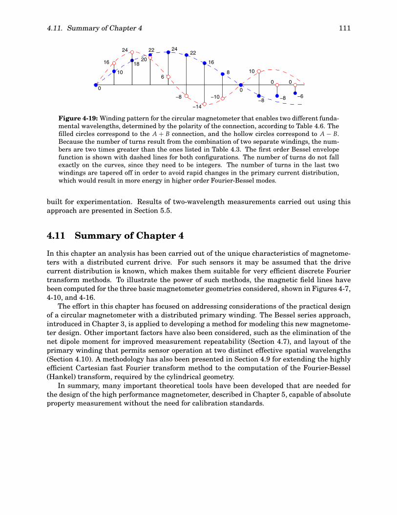
4.11. Summary of Chapter 4 111
0
10
18
22 24 22
16
8
0
−8 −8 −6
16
24
20
6
−8
−14
−10
10
0 0
Figure 4-19: Winding pattern for the circular magnetometer that enables two different funda-mental wavelengths, determined by the polarity of the connection, according to Table 4.6. Thefilled circles correspond to the A+ B connection, and the hollow circles correspond to A− B.Because the number of turns result from the combination of two separate windings, the num-bers are two times greater than the ones listed in Table 4.3. The first order Bessel envelopefunction is shown with dashed lines for both configurations. The number of turns do not fallexactly on the curves, since they need to be integers. The number of turns in the last twowindings are tapered off in order to avoid rapid changes in the primary current distribution,which would result in more energy in higher order Fourier-Bessel modes.
built for experimentation. Results of two-wavelength measurements carried out using thisapproach are presented in Section 5.5.
4.11 Summary of Chapter 4
In this chapter an analysis has been carried out of the unique characteristics of magnetome-ters with a distributed current drive. For such sensors it may be assumed that the drivecurrent distribution is known, which makes them suitable for very efficient discrete Fouriertransform methods. To illustrate the power of such methods, the magnetic field lines havebeen computed for the three basic magnetometer geometries considered, shown in Figures 4-7,4-10, and 4-16.
The effort in this chapter has focused on addressing considerations of the practical designof a circular magnetometer with a distributed primary winding. The Bessel series approach,introduced in Chapter 3, is applied to developing a method for modeling this new magnetome-ter design. Other important factors have also been considered, such as the elimination of thenet dipole moment for improved measurement repeatability (Section 4.7), and layout of theprimary winding that permits sensor operation at two distinct effective spatial wavelengths(Section 4.10). A methodology has also been presented in Section 4.9 for extending the highlyefficient Cartesian fast Fourier transform method to the computation of the Fourier-Bessel(Hankel) transform, required by the cylindrical geometry.
In summary, many important theoretical tools have been developed that are needed forthe design of the high performance magnetometer, described in Chapter 5, capable of absoluteproperty measurement without the need for calibration standards.

112 Chapter 4. Distributed Current Drive Sensors

Chapter 5
Deep Penetration MagnetoresistiveMagnetometer: Structure andMeasurement Results
This chapter describes the design of a circularly symmetric, distributed current drive magne-tometer with a secondary sensor based on the giant magnetoresistive (GMR) effect. It is animplementation of the ideas and models presented in the previous chapters.
As discussed in Chapter 1, the use of a magnetoresistive sensor allows the magnetometerto be operated at frequencies lower than currently possible with existing MWM and othereddy current sensors. Indeed, it is possible to operate this magnetometer with temporallyconstant magnetic field excitation, confirmed experimentally with measurements shown inSection 5.5. Low frequency operation is needed to increase the depth of sensitivity of themagnetometer, which is determined by the skin depth δ ∝ 1/
√ω, and by the imposed spatial
period via equation (2.14). The latter can be made large by using a distributed current drive,as discussed in Chapter 4.
The principles of operation of the magnetoresistive and giant magnetoresistive sensors aredescribed in Section 5.1.
A photograph of the prototype sensor used in the experiments in this chapter is shown inFigure 5-1. It is built according to the diagram in Figure 4-15, with W = 8 cm and h = 1 cm.There are two overlapping windings, with the number of turns in each groove determined bythe A and B rows in Table 4.6. These two windings are connected in series, and the polar-ity of the connection determines which of the two current drive patterns, given in Table 4.6and Figure 4-19, are excited. The two excitation modes have different effective fundamentalspatial wavelengths.
A secondary sensor assembly, consisting of a giant magnetoresistive sensor and a sec-ondary solenoidal coil, is positioned at the center of the magnetometer. They are connected ina feedback loop, as described in Section 5.2. A circuit board that hosts the GMR sensor bufferamplifier, not visible in the photograph, is positioned near the center below the magnetometerbase. The primary windings and the sensor assembly are connected to a circuit board thatcontains the secondary coil driver, compensation amplifier, and interface electronics. It doesnot need to be in very close proximity to the sensor. The interface circuitry is connected to theimpedance analyzer instrumentation used to measure the magnetometer’s transfer functionmagnitude and phase angle.
Section 5.2 describes the reasons for placing the GMR sensor in a feedback loop with
113

114 Chapter 5. Deep Penetration Magnetoresistive Magnetometer
Figure 5-1: Photograph of the prototype sensor used in all experiments shown in Chapter 5.The sensor base is built according to Figure 4-15, and the number of turns in each segment ofthe primary winding are specified in Table 4.6 and Figure 4-19. A secondary sensor assembly,consisting of a giant magnetoresistive sensor and a secondary solenoidal coil, connected ina feedback loop as described in Section 5.2, is positioned at the center of the magnetometer.Below the base, not visible in the photograph, is a circuit board hosting a buffer amplifier stage.The visible detached circuit board contains the secondary coil driver, compensation amplifier,and interface electronics.
a secondary driven winding. The design of the supporting electronic circuit is shown, andquestions associated with the dynamic behavior of the feedback loop are addressed. Thepresence of the secondary driven coil needs to be incorporated in the model developed inChapter 4. This expansion of the model is described in Section 5.3.
Sections 5.4 and beyond are dedicated to reporting the results of a variety of measure-ments, chosen to illustrate the useful new unique features of this magnetometer, includingultra low frequency, and DC two-wavelength measurements on magnetizable materials, eval-uation of thick metallic coatings, thickness measurement of thick metal plates, used for corro-sion mapping of metal components via measurements through the opposite surface, detectionof deeply buried flaws in metals, and measurements of the magnetic permeability of ferroflu-ids.
5.1 Theory of the magnetoresistive and giantmagnetoresistive effects
This section describes magnetoresistance, magnetoresistive anisotropy in ferromagnetic met-als, and giant magnetoresistance in metallic magnetic superlattices. This is a qualitative dis-cussion, since these are complex quantum effects, and the actual physics behind the operation

5.1. Theory of the magnetoresistive and giant magnetoresistive effects 115
of the sensors based on these phenomena does not affect the modeling of the magnetometerresponse. Furthermore, as shown in Section 5.2, the sensor is connected in a way that elimi-nates the effect of the transfer function of the magnetoresistive sensor on the magnetometerresponse.
5.1.1 Magnetoresistance
In general magnetoresistance is an effect which results when the carrier trajectories in amaterial are curved due to the Lorentz force which acts in a direction orthogonal to theirmotion. If an electron undergoes no scattering, then in the presence of a magnetic field itfollows a helical orbit with angular frequency
ωC =eBm∗ (5.1)
(the cyclotron frequency), where e is the charge of the electron, B is the magnetic flux density,and m∗ is the cyclotron effective mass. When scattering is present, the carriers experience adrag force characterized by a decay time constant τ , related to the conductivity as
σ =ne2τm∗ (5.2)
where n is the carrier density. The dimensionless product
ωCτ =Bσne
(5.3)
is a measure of how significant the magnetoresistance is under the specified conditions. Itrepresents the mean angular deflection that a carrier undergoes between collisions. If thisnumber is much less than one, then the trajectory radius is much greater than the mean freepath and consequently the resistivity is not affected. To make an observable difference, ωCτ
must be of order unity or greater [57].In practice, to meet this condition it is necessary to use very pure materials at cryogenic
temperatures, in order to make τ large, and subject the sample to an extremely strong mag-netic field, > 1T, to make ωC large.
It can be shown that the curved trajectories themselves do not necessarily lead to mag-netoresistance, so that the condition ωCτ > 1 is a necessary, but not sufficient condition formagnetoresistance. In materials with only one type of carrier that has a spherical Fermi sur-face, like the alkali metals, the diagonal elements of the resistivity tensor remain unchanged,and no magnetoresistance is observed. A the other extreme, in materials such as the noblemetals, which have highly irregular interconnected Fermi surfaces, the magnetoresistance israther strong and very much dependent on the orientation of the magnetic field with respectto the crystal lattice axes. Alternatively, materials like the semimetal bismuth, which have anequal number of electrons and holes as carriers, also exhibit high magnetoresistance [57]. Theresistivity ρ = 1/σ of the material along the magnetic field direction is unaffected, as carriersmoving in this direction experience no Lorentz force, while it is increased in the orthogonaldirection, i.e. ρ‖ < ρ⊥.

116 Chapter 5. Deep Penetration Magnetoresistive Magnetometer
���
����
�����
����
��
yyy
yyyy
yyyyy
yyyy
yy
�����������������������������������������������������������
��
����
�����
�����
�����
����
��
yy
yyyy
yyyyy
yyyyy
yyyyy
yyyy
yy
��
����
����
��
yy
yyyy
yyyy
yy EF
E
N(E) N(E)
4s 4s
3d
3d
Figure 5-2: Fermi diagram of conduction states in a ferromagnetic metal. At low temperaturesthe spin-up 3d states are almost completely filled, and due to the magnetization, the holes inthis band are not evenly distributed between the five d-orbitals. This results in anisotropyin the scattering rates of conduction electrons, leading to magnetoresistive anisotropy in suchmaterials.
Magnetoresistive anisotropy
In the following discussion it is assumed that anisotropic behavior due to crystal lattice sym-metries is negligible, which is true for amorphous or polycrystalline materials. In this casethe direction of the magnetic field determines the resistive anisotropy axis in the material.
A stronger magnetoresistive effect of a different nature, also known as magnetoresistiveanisotropy, is observed in thin films of ferromagnetic metals and alloys [58]. The trends ob-served in these materials are in some respects opposite to those described so far. In ferro-magnetic thin films the magnetoresistive effect is strongest in alloys, such as Ni-Fe, whilethe large number of crystalline defects in alloys tends to make τ shorter. Furthermore, thelower resistivity is observed in the orthogonal direction, i.e. ρ‖ > ρ⊥, also in contradiction toordinary magnetoresistance.
Clearly, a different mechanism is responsible for this effect. One theory that presents anexplanation for this behavior is given in [58]. According to this explanation, the conductivityis largely determined by s-electrons scattering into and out of d-orbitals, with the scatteringcaused by lattice vibration and lattice imperfections, much higher in alloys than in pure met-als. The current may be divided in two branches, corresponding to spin-up and spin-downelectrons. This is known as the two-current, or two-band, model, and is commonly used tomodel transport phenomena in ferromagnetic transition metals [59, 60]. Ignoring spin ex-change between the s-electrons keeps the two bands independent, and the total resistivityis
ρ =ρ↑ρ↓
ρ↑ + ρ↓(5.4)
where ρ↑ and ρ↓ are the resistivities of the spin-up and spin-down branches respectively. Atlow temperatures the 3d spin-up states are almost completely occupied, allowing only 4s to4s transitions, resulting in less scattering and lower resistivity for the spin-up band. Thiscondition is graphically illustrated in Figure 5-2.
5.1. Theory of the magnetoresistive and giant magnetoresistive effects 117
This in itself does not introduce any anisotropy. However, when the spin-orbit interactionis considered, some mixing of parallel and antiparallel states occurs, and as a consequencethere are some unoccupied parallel 3d states (holes) even at absolute zero. These holes are notequally distributed between the five d-orbitals, with a deficit of holes in orbitals perpendicularto the magnetization. The 4s to 3d transition probability is smallest if the s-electron movesperpendicular to the orbit. Thus an electron moving in the direction of magnetization has ahigher than average probability of being trapped in a 3d state, resulting in higher resistivityin this direction, i.e. ρ‖ > ρ⊥.
Results shown in [58] indicate that magnetoresistive anisotropy is strongest in Fe/Co/Nialloys with an average atomic magnetic moment of one Bohr magneton µB, independent ofthe actual alloy composition. The Bohr magneton µB = eh/(2me) is the magnetic moment ofan electron, where me is the electron rest mass, and h = h/(2π) is the normalized Planck’sconstant. This effect has yet to be explained theoretically.
One of the earlier practical magnetoresistive sensors based on this effect was proposedby R. P. Hunt in 1971 [61], and since then they have enjoyed popularity for many practicalapplications, some of which are listed in Table 1.1 [40,62–64].
5.1.2 Giant magnetoresistance
The magnetoresistive effect is generally on the order of a few percent, perhaps as much as5% at low temperature. Giant magnetoresistance refers to magnetoresistive changes of 20%or more [65], observed in certain metallic magnetic superlattices, also called magnetic mul-tilayers. It was first described in 1988 [66] and has since then been an area of very activeresearch [67–73, and many papers in 74].
The definition used in the literature for reporting the magnitude of the giant magnetore-sistive (GMR) effect is not consistent in whether the change in resistivity is referenced to itshighest value, which occurs with no external field, or its lowest value, which occurs in sat-uration. This can lead to large disparity in the reported values. One must be aware whichconvention is used when comparing the performance of different structures. The definitionused here expresses the magnitude as a percent change of the resistivity with respect to itsvalue with no external field, i.e. ∆ρ/ρmax.
Giant magnetoresistance was first observed in Fe/Cr magnetic superlattices [66], where adrop of as much as 45% of the resistivity was measured at liquid helium temperature (4.2 K).At room temperature the magnitude of the effect was reduced to about 12%. Other materialsystems have been tested since then, with the Co/Cu magnetic superlattice emerging as thesystem of choice in the development of practical sensors. It exhibits resistivity drops of up to55% at liquid helium temperature and 40% at room temperature [69].
The magnetic superlattices have alternating layers of a nonferromagnetic and ferromag-netic metal. The thickness of the nonferromagnetic layers is chosen such that in the absenceof applied external magnetic field the moments of consecutive ferromagnetic layers are ar-ranged antiparallel to each other. This antiferromagnetic coupling between these layers hasbeen ascribed to indirect exchange interactions through the nonferromagnetic layers [66]. Thepresence of an external field acts to align the moments of all ferromagnetic layers, resultingin reduction of the electric resistivity. This is schematically illustrated in Figure 5-3. Themagnetoresistance is thus defined as [61]
∆ρ
ρmax=
ρ↑↓ − ρ↑↑ρ↑↓
(5.5)

118 Chapter 5. Deep Penetration Magnetoresistive Magnetometer
lowresistivity
highresistivity
MAntiferromagnetic alignment
MFerromagnetic alignment
Ferromagnetic layer (Co)
mediumresistivity
Nonferromagnetic layer (Cu)
Figure 5-3: Diagram illustrating the giant magnetoresistive effect. GMR is the result of dif-ferences in the scattering of spin-up and spin-down electrons at the layer interfaces. In theabsence of external magnetic fields the moments of adjacent ferromagnetic layers are antipar-allel, resulting in medium resistivity for both spin bands. In the presence of an externallyapplied magnetic field the ferromagnetic layers are aligned, drastically reducing the scatter-ing of spin-up electrons, which acts to reduce the overall resistivity of the superlattice.
where ρ↑↑ and ρ↑↓ are the resistivities in the parallel and antiparallel states respectively.The physical explanation for this phenomenon, as initially suggested in [66], hinges on
the spin-dependent scattering characteristic of ferromagnetic metals. As before, the currentis divided into two branches, for spin-up electrons and spin-down electrons [59, 60]. In theantiferromagnetic state, on average both types of electrons experience the same set of scatter-ing potentials, resulting in the two branches having equal resistivity of intermediate value,2ρ↑↓ = ρ↑ = ρ↓ (see equation (5.4)). In the aligned state, the spin-up electrons are scatteredmuch less effectively, resulting in low resistivity for this current branch and an overall lowerresistivity for the entire structure, ρ↑↑ ≈ ρ↑ � ρ↓.
Several publications offer explanations and theoretical models for the difference of scat-tering for spin-up and spin-down electrons [65, 68]. Two distinct processes can lead to suchdifference. The first is spin-flip scattering. As illustrated in Figure 5-2, in ferromagneticmetals there is a difference in the number of available states at the Fermi level for spin-upand spin-down electrons. Thus an electron spin-polarized in one ferromagnetic layer may ex-perience spin reversal when it enters the next one [67]. Such scattering events are causedby spin-orbit effects, by impurities with a localized magnetic moment, or by magnons (spinwaves).
The other process leading to scattering differences between the two electron bands is spin-dependent scattering at the layer interfaces, which is the only effect considered by the Boltz-mann transport equation model in [68]. As pointed out in that publication, there would beno magnetoresistance effect for perfect interfaces, and as the surface roughness increases, sodoes the scattering. The scattering rates for the two types of electrons can differ by a factor ofsix or more [66, 68], leading to the needed difference in resistivity in the two branches of thecurrent.

5.2. Operation of the secondary GMR sensor assembly 119
Flux concentrator (2)
Magnetically shielded resistor (2)Bonding pads (4)(100µm x 100µm)
Metal interconnectsCeramic substrate(1300 µm x 400 µm)
Axis of sensitivity
Magnetically active resistor pair
Figure 5-4: Typical GMR magnetic field sensor layout [75]. Four magnetic superlattice resis-tors are formed on a common ceramic substrate and connected in a bridge configuration. Twoof the resistors are shielded from external fields. Ferromagnetic flux concentrators are used toincrease the effect of the magnetic field on the other two resistors. If a voltage is applied acrossa pair of diagonally opposed terminals, a differential voltage is developed across the other pairin the presence of magnetic field.
Due to the spin alignment in a ferromagnetic metal, the spin-up and spin-down electronshave different band structure, Fermi surface, effective mass, etc. This is why the scatteringrates for the different spin electrons can be different for the same scatterer. A. Fert and I. A.Campbell apply the two-band model to resistivity data in Ni and Fe based alloys to obtain aconsistent set of parameters for the scattering within each spin band for various impurities[59,60]. The large differences in scattering rates have been confirmed experimentally.
On the whole, the best quantitative physical model of the giant magnetoresistive effectappears to be the one developed by R. Q. Hood and L. M. Falicov [65]. One of the conclusionsdrawn in this work is that spin-flip scattering can account for no more than a few percentof magnetoresistance, and a large difference in interface scattering for the different spins isneeded to explain the observed large GMR values.
5.2 Operation of the secondary GMR sensor assembly
5.2.1 GMR sensor characteristics
A commercially available magnetic sensor, based on the giant magnetoresistive effect, is usedas the secondary element of the magnetometer. The sensor is manufactured by NonvolatileElectronics, Inc. It consists of four magnetic superlattice resistors, deposited on a commonceramic substrate, and connected in a bridge configuration, as shown in Figure 5-4 [75]. Twoof the resistors are shielded from external magnetic fields. Ferromagnetic flux concentratorsare used to increase the effect of the magnetic field on the other two resistors. If a voltage isapplied across a pair of diagonally opposed terminals, a potential difference appears betweenthe other terminal pair in the presence of an externally applied magnetic field.
Figure 5-5 is a plot of the transfer characteristic of this magnetic sensor [75]. Several

120 Chapter 5. Deep Penetration Magnetoresistive Magnetometer
0
0.05
0.1
0.15
0.2
0.25
0.3
-100 -50 0 50 100
Applied Field (Oersteds)
Ou
tpu
t V
olt
age
(V)
Figure 5-5: Transfer characteristic of the GMR magnetic sensor biased at 5 V [75]. Thiscurve illustrates some of the features of the giant magnetoresistive effect: the output voltageis independent of the field polarity, saturates at high fields, and displays some hysteresis.
features of the giant magnetoresistive effect are evident in this figure. The differential outputvoltage is independent of the polarity of the applied field, because either polarity leads to adeparture from the fully antiparallel alignment. At a certain field magnitude, about 50 Oefor this sensor, the output reaches a saturation value, corresponding to complete alignment ofthe ferromagnetic layers. Finally, the response shows some hysteresis.
The highly nonlinear nature of the transfer characteristic, especially near zero, makesit necessary to operate the sensor with a certain DC field bias, moving the operating pointto the linear region of the characteristic, at approximately 25 Oe and 0.15 V. The biasingmay be accomplished with the help of a permanent magnet, but a magnet will perturb thesurrounding magnetic flux density, more than just adding its constant field. Alternatively,the sensor may be biased with an electromagnet.
5.2.2 Feedback loop
While DC biasing addresses the nonlinearity and hysteresis problems, a severe limitation stillremains: satisfactory operation is maintained only for fields with magnitudes that are smallcompared to the DC bias field. As the field magnitude increases, the response becomes moreand more nonlinear, and for amplitudes on the order of the bias field, saturation and polarityreversal come into effect.
To address these limitations, it is beneficial to place the sensor in a feedback configurationwith a secondary winding, as shown in Figure 5-6. In this way the magnetic field at the GMRsensor remains constant during operation, eliminating the effect of the nonlinear transfercharacteristic, while maintaining sensitivity at low frequencies. The magnitude of the currentin the secondary winding is taken as the output signal, and since the relationship betweenthis current and the magnetic field for an air-core winding is perfectly linear, so is the transfercharacteristic of the entire hybrid sensor structure.
Another benefit of the feedback configuration is temperature stability. Since the measuredquantities are currents in the windings, which are directly related to the magnetic fields,

5.2. Operation of the secondary GMR sensor assembly 121
DC bias
Secondary
V in Gain
Magnetoresistive sensor
winding
Prop + IntFI
Figure 5-6: Structure of the hybrid sensor feedback loop. The secondary winding maintains aconstant magnetic field at the GMR sensor, determined by the value of the DC bias. This allowsfor high dynamic range and linearity, while retaining low frequency sensitivity. In addition togain, the forward stage of the loop includes an integral term, which ensures zero error at DC.
temperature dependence of the GMR sensor or winding resistance, etc. has no effect on themagnetometer response.
The magnetic field magnitude that this hybrid sensor can measure is limited only by themagnitude of the field that the secondary winding can produce, which can be orders of mag-nitude higher than the saturation field of the GMR sensor. There is a further advantage ofthe feedback connection: biasing the GMR sensor to the appropriate operating point is accom-plished simply by adding an appropriate DC voltage offset at the input of the gain stage. Thisis much better than the biasing methods described so far, because correct biasing is main-tained even if the position of the GMR sensor with respect to the bias source changes, whichwould not be true for biasing with a constant field source. This eliminates the need for com-plex alignment methods, since biasing at the correct level is automatic with the appropriatechoice of circuit components.
There can be situations where this kind of feedback configuration may be inappropriate.The bandwidth of the hybrid sensor is limited by the dynamics of the feedback loop, and isalways narrower than open-loop operation. Therefore, at high frequencies the sensor mayneed to be operated open-loop, although it is still possible to keep the loop closed for lowfrequencies at the same time, in order to maintain the proper DC bias. This is not a severelimitation, since this magnetometer is not designed for high frequency operation, where it maybe more appropriate to use a standard MWM, or simply the induced voltage in a secondarywinding. An additional limitation of the feedback loop configuration is that in an array setup,the feedback windings of adjacent elements will be coupled to each other, leading to inter-channel cross talk. It is in general possible to compensate for this in the models, but it isbetter to avoid such situations by appropriate shielding or by open-loop operation.
5.2.3 Electronics
A full schematic of the electronic circuit used to implement the feedback loop, biasing, andinterface is shown in Figure 5-7. The resistor bridge of the GMR sensor is shown as U1. Theoutput impedance of the sensor is relatively high, on the order of 40 k, and in order to avoidparasitic signal and noise pick-up, as well as extra phase shift due to cable capacitance, abuffer amplifier is placed in close proximity to the sensor. The entire buffer stage assembly,which also implements the sensor DC biasing scheme, is enclosed in a dashed box in thefigure. The buffering is accomplished with a high bandwidth instrumentation amplifier U2.

122 Chapter 5. Deep Penetration Magnetoresistive Magnetometer
The voltage regulator U3 is needed to ensure constant sensor voltage and field biasing. TheDC operating point is set by the voltage divider implemented with R1 and R2. This firstamplifier stage has a gain of ten.
The loop gain and compensation, described later, are implemented with the U4 amplifierstage. The secondary winding is driven by the high power video amplifier U5, connected asa unity gain follower. Since U5 is a current feedback operational amplifier, it is necessary toinclude R9, which is also used to set the bandwidth of the stage.
The current IF through the secondary feedback winding is measured as the voltage acrossa precision zero-inductance power resistor R10, connected in series. The last stage, imple-mented with U6, is used as a coaxial cable driver. It also eliminates the DC component of thesignal, and brings the output magnitude to the optimal input levels of the JENTEK impedanceanalyzer equipment. For constant field measurements, which do not require an impedanceanalyzer, the output signal is taken at test point 3.
5.2.4 DC stability
Because of the rectifying effect of the GMR sensor, the overall polarity of the feedback loopdepends on the direction of the magnetic field, which means that as the circuit is initiallypowered up, it may enter a positive feedback mode, which is unstable, and leads to the outputof U5 saturating at the positive supply voltage level, rendering the system inoperable. On theother hand, once the correct operating point is established, then the feedback is negative, andthe loop remains stable from then on, unless the magnetic field reaches such magnitude thatthe driver of the secondary winding cannot keep up, in which case the loop may again becomeunstable.
This complication is a direct consequence of the GMR sensor transfer characteristic, andcannot be avoided. It is therefore necessary to implement some external mechanism that de-tects the faulty condition and resets the loop by forcing the output to be near the operatingpoint. A much simpler remedy, used in this implementation, is to ensure that the currentthrough the secondary winding is always negative, by connecting a diode D1 in series with it.This does resolve the stability problem, and ensures that the feedback loop always recoversto the proper operating point. However, it also introduces a limitation. While the magni-tude of the measured field is unlimited in the positive direction, in the negative direction itsmagnitude may not exceed that of the bias field. Although this compromise is acceptable forthe prototype magnetometer, in a more general setting it may be necessary to incorporate anauxiliary “watch dog” circuit of the kind described above.
5.2.5 AC stability and loop bandwidth
Ignoring for the moment the U4 stage, the ideal open-loop transfer characteristic consists ofa single pole at ω = R10/L, introduced by the relationship between driver output voltageand secondary winding current IF. In the ideal case where this is the only pole, the loop isalways stable, and its bandwidth can be increased indefinitely by increasing the loop gain.In practice all operational amplifiers have a limited bandwidth, plus parasitic capacitancesalways introduce extra phase.
The approach taken here to find the optimal loop gain is to measure the open-loop transferfunction experimentally. This is done by shorting out R6 and C1, which turns U4 into a voltagefollower, applying a signal at test point 2, and measuring the relative magnitude and phaseof the voltage at test point 1. The input signal must include an appropriate DC offset, needed

5.2. Operation of the secondary GMR sensor assembly 123
C1
7
6
432
C2
R2
RR3
R9
R12
R11
R7
B
B
U2
U3
U6
U1
AA
002-
021 2
AD
815
U5
1R
1D
U4
LT13
57I F
0.10.
1
+12
V
0.1
0.1
0.1
+12
V
-12V
+
+
+12
V
Out
put
619
-12V
0.1
0.1
4.99
k
49.9
+12
V
R
R
7
6
432
9
10
11
78
21 3 4
8 5
7
AD
830
3.01
k
-12V
4
R6
5
R8
100
4.99
k45
3
453
10
13
TP
1
TP
3+
-12V
49.9
TP
2
V+
V-
1
84
5G
MR
Sen
sor 78
L05
2+
0.1
+12
V 31+
5V
Sen
sor
and
buffe
r as
sem
bly
Fee
dbac
k co
il
909
100
20
78.7
A =
1
V V
I I
R
AD
811
1N40
01
L30
Hµ
10
1010
10
0.01
5
Figure
5-7:
Fee
dbac
kan
din
terf
ace
circ
uit
sch
emat
ic.
Res
isto
rva
lues
are
inoh
ms,
and
capa
cito
rva
lues
are
inm
icro
fara
ds.
Th
eco
mpo
nen
tsen
clos
edw
ith
ada
shed
box
are
mou
nte
don
ase
para
teci
rcu
itbo
ard,
loca
ted
incl
ose
prox
imit
yto
the
GM
Rse
nso
r.

124 Chapter 5. Deep Penetration Magnetoresistive Magnetometer
for proper biasing of the GMR sensor.As expected, the phase angle reaches −45◦ at about 100 kHz, the frequency of the pole. The
phase angle reaches −90◦ at about 350 kHz, which is chosen as the loop bandwidth, allowingfor plenty of phase margin, 90◦ [76]. This is accomplished by choosing R6 so that the gain ofthe U4 amplifier stage is equal to the inverse of the open-loop magnitude at this frequency.
The presence of C1 in series with R6 is useful, though not required, because it introducesa pole at ω = 0 and a zero at ω = 1/(R6C1), near 2 kHz. As a consequence, the feedback looperror, given by the voltage at test point 1, is zero at DC, and small at low frequencies.
5.3 Incorporating the effects of the feedback loop into thesensor model
Initially the measurement grids used in the experiments in this chapter had been generatedvia equation (4.49). The results were less than satisfactory, and complex two-point reference-part calibration methods, described in Appendix D, had to be employed to bring the data nearthe correct place in the grid, and even then the results were poor for points far from the tworeference calibration points. It became apparent that there was a large unmodeled effect thathad to be taken in consideration.
This unmodeled effect is the dependence of the relationship between the feedback windingcurrent IF and the magnetic flux intensity at the origin Bz(x = 0, z = 0) on the material undertest. The previous section assumed that the output signal IF, is directly proportional to theimposed field at the origin, since the secondary winding is a solenoid tightly wound aroundthe GMR sensor. The experiments show that that this assumption is not justified.
A different way of looking at this is that while equation (4.49) gives Bz/ID, where ID is theprimary current, the impedance analyzer measures IF/ID. It is therefore necessary to developa method of calculating Bz/IF as a function of the material structure and sensor parameters.
This turns out to be a very easy task, because it can be done by applying the method ofSection 4.8 directly to the special case of a single concentric winding. Thus, if the feedbackcoil’s radius is rF, and it has wF turns, then the surface current density is
KS(r) = IFwFu0(r− rF) (5.6)
whose Fourier-Bessel series components, derived from equation (4.42), are
Kn =2IFwF
R2 J20 (αn)J1(βnrF)rF (5.7)
leading to the required relationship
Bz(r = 0, z = 0) = IFwF
∞∑n=1
2R2 J20 (αn)
· 1RnJ1(βnrF)rF (5.8)
Taking the ratio of equations (4.49) and (5.8) yields the expression of the complex transfer

5.4. Conductivity / lift-off measurements at 12.6 kHz 125
function magnitude, measured by the impedance analyzer:
IFID
=
∞∑n=1
2R2 J20 (αn)
· 1Rn
N
∑j=1
wjJ1(βn jh) jh
∞∑n=1
2R2 J20 (αn)
· 1RnwF J1(βnrF)rF
(5.9)
The measurement grids in this chapter have been generated using equation (5.9), andnormalized to the magnitude in air, so that the air point on a grid always has unity magnitudeand zero phase. For all grid plots in this chapter, the normalized magnitude is the magnitudeof the ratio IF/ID divided by the magnitude of this ratio for the magnetometer in air.
The magnitude/magnitude grid in Figure 5-10 did not acquire its characteristic spiralshape until the correction described in this section was applied to the model. The spiralcurve followed by the experimental data in Section 5.5 was what first suggested the need forthe change, and once applied, it significantly improved the results of all other measurementsas well.
5.4 Conductivity / lift-off measurements at 12.6 kHz
The first set of measurements with the GMR magnetometer consists of conductivity/lift-offmeasurements with three different materials, at a range of lift-off values. The measurementgrid used is generated via equation (5.9). It is shown in Figure 5-8. Since both the conductivityand the lift-off parameters vary over a relatively wide range, the parameter values for thisgrid are chosen on a logarithmic scale. As discussed in Section 1.4.1, the grid cell area isa measure of the sensitivity of the measurement in that region of the grid. For the grid inFigure 5-8, it should be noted that for high conductivity and lift-off values the grid cells wouldhave been even narrower, if the parameter values had been equally spaced on a linear scale.
This pair of estimated properties is chosen because it is the most common type of mea-surement made with the MWM family of magnetometers and magnetometer arrays. Themeasurements are carried out at 12.6 kHz, which is the lowest frequency supported by theJENTEK impedance analyzer instruments, in order to illustrate the low frequency capabilityof this magnetometer. A simple one-point air calibration method is used for this measure-ment and for all other measurements in this chapter. Calibration methods and their effect onmeasurement error are described in Appendix D.
The lift-off is changed by placing plastic sheet shims between the sensor and the metalplates. A set of five shims, whose thicknesses are approximately related as consecutive powersof two, makes it possible to take many data points at closely spaced values of the lift-off. Theresults are shown in Figure 5-9 and listed in Table 5.1.
The first observation to make in Figure 5-9 is that the three data sets follow lines ofconstant conductivity very closely. Since the sensitivity of the measurement decreases athigher lift-off, only the first twelve out of the twenty data sets are listed in the table. The lastcolumn in the table lists the nominal values of the lift-off, calculated by adding the thicknessesof the shims used, measured with a caliper. The estimated lift-off values are in excellentagreement with the nominal values. The conductivity data in Table 5.1 are also in goodagreement with the numbers reported in the literature [77, 78]. Table 5.2 lists typical valuesof the conductivity for the metals used in this chapter. The magnitude, nature, and source of

126 Chapter 5. Deep Penetration Magnetoresistive Magnetometer
0 0.1 0.2 0.3 0.4 0.5 0.6 0.7 0.8 0.9 1−35
−30
−25
−20
−15
−10
−5
0
Normalized magnitude
Pha
se [d
eg]
Increasinglift−off
Increasing conductivity
σ = 0.1 MS/m
h = 1 mm
h = 5 mm
10 mm
17.8 mm
σ = 1 MS/m
10 MS/m
100MS/m
Figure 5-8: Conductivity/lift-off measurement grid for circular sensor at 12.6 kHz. The twocoordinate axes are the magnitude and phase of the ratio IF/ID, normalized by its value in air.
the measurement errors are discussed in more detail in Appendix C.The lowest value of the lift-off, 3.3 mm, corresponds to carrying out the measurement with
no shim, and is equal to the effective depth of the windings below the surface. This amounthas been added to the data in the last column, after having been estimated by taking theaverage of the difference between the magnetometer estimated values and the measured shimthicknesses. This number is quite reasonable, given that the average depth of the grooves ison the order of 3 mm, and that the winding thickness, about 2 mm, is not considered by themodel.
As discussed in Appendix C, there appears to be an optimal range of the lift-off, 5–7 mm,where the estimated conductivity is most accurate. This is to be expected, since sensitivity tothe material’s conductivity is lost as it is positioned further from the sensor surface. Being tooclose to the sensor windings also reduces the accuracy, since the effects of the nonzero windingthickness become stronger in close proximity.
It may appear at first that there is too much spread in the conductivity data in Table 5.1.Given that this measurement was carried out with no calibration standards and with a singleair calibration point, the simplicity of the model used, and the fact that no empirical datahave been used to compute the grid, we consider these measurement results to be remarkablygood. It has taken years of effort to improve the MWM design to the point where with onepoint air calibration it can produce results as accurate as these.
If it is necessary to perform a very exact conductivity measurement, then a two-point ref-erence part calibration is recommended, with the properties of the two reference parts, or thesame part at two lift-off values, closely bracketing the properties of the unknown part. A com-parison of the measurement error and other performance criteria of the different calibration

5.4. Conductivity / lift-off measurements at 12.6 kHz 127
0.2 0.3 0.4 0.5 0.6 0.7 0.8
-7
-6
-5
-4
-3
-2
-1
0
Normalized magnitude
Pha
se [d
eg]
Copper 110Aluminum 6061Aluminum 2024
100 MS/m
40 MS/m
11 M
S/m
1 M
S/m3
MS/
m5 m
m
10 mm
15 mm
7.5 mm
3 mm
Figure 5-9: Results of conductivity/lift-off measurements with the circular magnetometer.Three sets of measurements are shown with metal plates of different conductivity, taken at avariety of lift-off positions. Each set follows a line of constant conductivity on the measurementgrid, which is an expanded view of the grid in Figure 5-8.
Cu 110 Al 6061 Al 2024 NominalData Cond. Lift. Cond. Lift. Cond. Lift. lift-offset [MS/m] [mm] [MS/m] [mm] [MS/m] [mm] [mm]1 59.2 3.3 29.5 3.2 18.0 3.3 3.32 59.2 4.1 28.9 4.0 17.8 4.1 4.13 58.7 4.8 28.7 4.7 17.8 4.8 4.84 58.3 5.6 28.6 5.5 17.6 5.6 5.65 57.8 6.5 28.3 6.4 17.6 6.5 6.56 57.1 7.4 28.1 7.3 17.5 7.3 7.37 55.7 8.0 27.4 7.9 17.3 8.0 8.08 56.1 8.9 27.5 8.7 17.4 8.8 8.89 54.3 9.5 26.8 9.4 17.1 9.4 9.410 55.2 10.3 27.0 10.2 17.2 10.3 10.211 53.5 10.9 26.4 10.8 17.0 10.9 10.912 53.0 11.7 26.3 11.7 16.7 11.7 11.7
Table 5.1: Results of conductivity/lift-off measurements with the circular magnetometer,shown in Figure 5-9. Only the first twelve sets of the twenty shown in the figure are listed,due to the lack of sensitivity at higher lift-off values, as illustrated by the narrowing grid cellsat the top right corner of Figure 5-9.
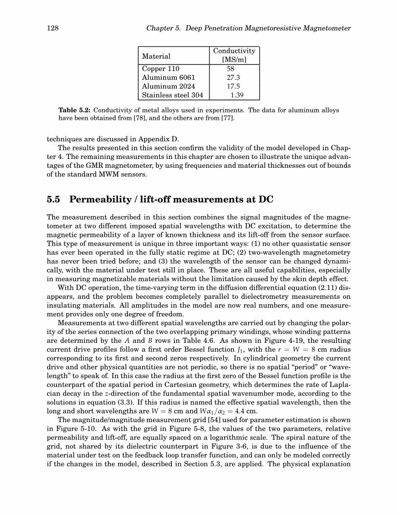
128 Chapter 5. Deep Penetration Magnetoresistive Magnetometer
ConductivityMaterial [MS/m]Copper 110 58Aluminum 6061 27.3Aluminum 2024 17.5Stainless steel 304 1.39
Table 5.2: Conductivity of metal alloys used in experiments. The data for aluminum alloyshave been obtained from [78], and the others are from [77].
techniques are discussed in Appendix D.The results presented in this section confirm the validity of the model developed in Chap-
ter 4. The remaining measurements in this chapter are chosen to illustrate the unique advan-tages of the GMR magnetometer, by using frequencies and material thicknesses out of boundsof the standard MWM sensors.
5.5 Permeability / lift-off measurements at DC
The measurement described in this section combines the signal magnitudes of the magne-tometer at two different imposed spatial wavelengths with DC excitation, to determine themagnetic permeability of a layer of known thickness and its lift-off from the sensor surface.This type of measurement is unique in three important ways: (1) no other quasistatic sensorhas ever been operated in the fully static regime at DC; (2) two-wavelength magnetometryhas never been tried before; and (3) the wavelength of the sensor can be changed dynami-cally, with the material under test still in place. These are all useful capabilities, especiallyin measuring magnetizable materials without the limitation caused by the skin depth effect.
With DC operation, the time-varying term in the diffusion differential equation (2.11) dis-appears, and the problem becomes completely parallel to dielectrometry measurements oninsulating materials. All amplitudes in the model are now real numbers, and one measure-ment provides only one degree of freedom.
Measurements at two different spatial wavelengths are carried out by changing the polar-ity of the series connection of the two overlapping primary windings, whose winding patternsare determined by the A and B rows in Table 4.6. As shown in Figure 4-19, the resultingcurrent drive profiles follow a first order Bessel function J1, with the r = W = 8 cm radiuscorresponding to its first and second zeros respectively. In cylindrical geometry the currentdrive and other physical quantities are not periodic, so there is no spatial “period” or “wave-length” to speak of. In this case the radius at the first zero of the Bessel function profile is thecounterpart of the spatial period in Cartesian geometry, which determines the rate of Lapla-cian decay in the z-direction of the fundamental spatial wavenumber mode, according to thesolutions in equation (3.3). If this radius is named the effective spatial wavelength, then thelong and short wavelengths are W = 8 cm and Wα1/α2 = 4.4 cm.
The magnitude/magnitude measurement grid [54] used for parameter estimation is shownin Figure 5-10. As with the grid in Figure 5-8, the values of the two parameters, relativepermeability and lift-off, are equally spaced on a logarithmic scale. The spiral nature of thegrid, not shared by its dielectric counterpart in Figure 3-6, is due to the influence of thematerial under test on the feedback loop transfer function, and can only be modeled correctlyif the changes in the model, described in Section 5.3, are applied. The physical explanation

5.5. Permeability / lift-off measurements at DC 129
0.96 0.98 1 1.02 1.04 1.06 1.08 1.1 1.12
0.92
0.94
0.96
0.98
1
1.02
1.04
1.06
1.08
1.1
Long
wav
elen
gth
norm
aliz
ed m
agni
tude
Short wavelength normalized magnitude
h = 1.58 mm
h = 2 mm
h = 5 mm
h = 10 mm
h = 20 mm
µ = 10 µ = 4
µ = 1
Increasinglift−off
Increasingpermea−bility
Figure 5-10: Two wavelength magnitude/magnitude permeability/lift-off grid for the circularmagnetometer with DC excitation. The short and long wavelength current drive patterns areexcited by appropriate connection of the two overlapping primary windings, and correspond toeffective spatial wavelengths of 4.4 cm and 8 cm respectively. The thickness of the magnetizablelayer is fixed at 1 mm.
of this spiral behavior is as follows: In general, as a magnetizable material is brought closerto the sensor windings, the magnitude of the signal increases, because the material tendsto concentrate the magnetic flux. However, as the lift-off is reduced even further, this fieldconcentration effect begins to affect the secondary feedback winding too, and since its radiusis much smaller than the radii of the segments of the primary winding, this effect begins todominate the overall magnetometer transfer function, bringing the magnitude back down.This effect is easy to observe in the grid in Figure 5-10.
This measurement is completely analogous to the dielectrometer measurements describedin Section 3.3. Both types of measurements use the signal magnitudes at two different spa-tial wavelengths to estimate the dielectric permittivity or magnetic permeability of a samplewith known thickness and its distance from the sensor electrodes or windings. The magneti-zable layer consists of 1 mm thick polymer that contains ferromagnetic particles suspendedin the polymer foam. The sensor lift-off is controlled with the same set of plastic shims as inSection 5.4. The results of the measurement are shown in Figure 5-11, and listed in Table 5.3.
The measurement procedure at DC presents some challenges. On the one hand, the onlyequipment necessary are a power supply and a voltmeter, making the measurement simpler.On the other hand, the accuracy of the measurement is lower than that possible with ACexcitation. When operating the sensor at a certain frequency, the magnitude of this frequencycomponent in the output signal can be measured very accurately by mixing it with a signal atthe same frequency from the same source, and passing the resulting signal through a low passfilter to obtain the DC component. The signal can be integrated over many cycles, resulting

130 Chapter 5. Deep Penetration Magnetoresistive Magnetometer
1 1.01 1.02 1.03 1.04 1.05
1
1.005
1.01
1.015
1.02
1.025
1.03
1.035
1.04
Short wavelength normalized magnitude
Long
wav
elen
gth
norm
aliz
ed m
agni
tude
5 mm
2.5 mm
20 m
m
10 m
m
2
3
4
5
Figure 5-11: Permeability/lift-off measurement results with the circular GMR magnetome-ter of 1 mm thick magnetizable foam layer. The data points follow a spiral line of constantpermeability. The grid is an expanded view of the grid in Figure 5-10.
Data Relative Lift-off Nominalset permeability [mm] Lift-off [mm]1 4.23 4.2 4.22 4.30 5.0 5.03 4.30 5.7 5.74 4.29 6.6 6.55 4.28 7.5 7.46 4.19 8.1 8.27 4.21 8.9 8.98 4.36 10.0 9.79 4.37 10.8 10.310 4.39 11.7 11.111 4.21 12.0 11.812 4.28 13.1 12.613 4.43 14.4 13.514 4.44 15.2 14.315 4.41 15.8 15.016 4.50 17.0 15.8
Table 5.3: Experiment results of the permeability/lift-off measurements at DC, shown in Fig-ure 5-11. Only the first sixteen out of the thirty-one sets shown in the figure are listed, due tothe lack of sensitivity at higher lift-off values, as illustrated by the narrowing grid cells in thelower left of Figure 5-11.

5.6. Thickness / lift-off measurements with a multi-layer structure 131
in a very accurate measurement of the transfer function at this frequency.With DC operation this frequency mixing technique is not available. Furthermore, it is
not practical to average the signal over a long time, because outside factors affecting themeasurement may change during that time. For example, the output voltage of the powersupply used to drive the primary winding may be not perfectly stable, and the primary currentis also affected by changing contact resistance in the leads and the changing resistance of theprimary winding itself, as its equilibrium temperature varies based on the thermal insulationcaused by the material under test. Finally, changes in the physical position of the sensor canalter its output due to the presence of magnetically active objects in the vicinity, and as aresult of changes of its position relative to the direction of the earth’s magnetic field.
The approach taken in this measurement to eliminate the signal noise introduced by allthese factors is to measure the sensor response in air not just once before the measurement,as is done with the other measurements in this chapter, but before every data point, withas little time in between as possible. In this way every measurement data point has its ownair calibration reference. Air calibration and other calibration techniques are described inAppendix D.
Bearing in mind that in general DC data are less accurate, the results in Table 5.3 arestill very good, even if the lift-off does not track its nominal value as well as the data inSection 5.4. The relative permeability of the polymer layer is measured to be about 4.3. As inthe conductivity/lift-off measurements of the previous section, the measurement results aremost accurate for lift-off values in the 5–7 mm range.
The data follow a constant permeability curve quite well. An interesting phenomenon thatmay be observed in Figure 5-11 is that at the highest lift-off values, there is a range wherethe magnitude of the short wavelength signal is lower than its value in air. The grid linesconfirm that this effect is physical. It is due to the fact that this far from the surface themagnetizable layer is too far to intercept any magnetic field lines going through the center,but is still close enough to attract some of the field lines away from the surface. An exact dualof this effect is observed in the dielectrometer grids in the presence of a ground plane behindthe material sample. This can be seen in Figure 3-6, where at the high lift-off with nonunityrelative permittivity the magnitudes dip slightly below the air point.
5.6 Thickness / lift-off measurements with a multi-layerstructure
Thickness/lift-off measurements most often arise in applications where it is necessary to mea-sure the thickness of a metallic coating on a metal substrate. The multi-layer structure thatneeds to be modeled has at least three layers, two metal layers and an air layer, where theconductivity and magnetic permeability of the two metal layers are known. A diagram ofthis structure is shown in Figure 5-12. Low frequency operation, made possible by the GMRmagnetometer, allows measurement of much higher coating thicknesses. The measurementsdescribed in this section illustrate this type of measurement by determining the thickness ofa stainless steel layer, backed by a copper layer. The upper limit of the thickness of a stainlesssteel layer that can be measured at 12.6 kHz is approximately 5 mm.
The measurement grid used in this application is shown in Figure 5-13. It assumes opera-tion at 12.6 kHz. The conductivities of stainless steel 304 and copper 110, used for generatingthe grid, are taken from Table 5.2. Unlike the measurement grids used in the previous two

132 Chapter 5. Deep Penetration Magnetoresistive Magnetometer
ht
copper
airstainless steel
GMR sensor and secondary windingprimary windings
Figure 5-12: Three layer structure used in thickness/lift-off measurements. The two proper-ties being estimated are the thickness t of the first metal layer and the thickness h of the airlayer, called the lift-off. The thickness of the second metal layer is considered to be infinite,since it is much greater than the skin depth in this material.
sections, the parameter values for this grid are chosen on a linear scale.The copper plate is 3.2 mm thick, but its thickness is modeled as being infinite, because
it is several times greater than the value of the skin depth δ in copper at this frequency,0.59 mm, calculated using equation (2.15). This is typical of coating characterization applica-tions, where the substrate is much thicker than the depth of sensitivity of the magnetometer.In comparison, due to its much lower conductivity, the skin depth in the stainless steel layeris 3.8 mm, several times greater than that of the copper layer, and comparable to the platethicknesses. By considering the size of the grid cells in Figure 5-13, it can be observed thatthe thickness measurement, but not the lift-off, loses sensitivity for thickness values belowabout 0.5 mm and above 5 mm. This is explained by comparing these values to the skin depthof 3.8 mm. At the lower thickness values the stainless steel layer has little influence on themagnetic fields, since its conductivity is much lower than that of the copper layer, which dom-inates the sensor response. At the high end of the thickness range the exponential decay ofthe magnetic field intensity makes the magnetometer insensitive to the position of the ma-terial interface. For these two limits the grid lines approach two constant lift-off lines of theinfinite-half-space conductivity/lift-off grid in Figure 5-8, corresponding to the conductivitiesof copper and stainless steel. This can be confirmed visually by comparing the two grids.
Optimal sensitivity, corresponding to the biggest and most orthogonal grid cells, isachieved for thicknesses on the order of 3 mm, approximately equal to (π/4)δ. This is tobe expected, as explained in the next section, and illustrated by the curve in Figure 5-17. Ifthe values of the thickness parameter in the grid extend past the (π/2)δ = 6 mm point, thegrid would develop a curl, also described in Section 5.7.
The thickness of the stainless steel layer in this set of measurements is changed by stack-ing up to four plates of various thicknesses in different combinations. As with the plasticplates used for changing the lift-off, the thicknesses of the metal sheets are chosen to allowfor a wide range of possible total thickness values. Twelve sets of data are taken at each oneof five different lift-off values. The results are shown in Figure 5-14 and listed in Table 5.4.
As in all other measurements in this chapter, the calibration of the sensor and equipmentis done with a single point in air. Therefore any deviation of the actual material conductivitiesfrom the quoted values used for the generation of the grid would lead to errors in the estimatedproperties. This is particularly true at the lower thickness values, where the grid cells are verynarrow. This explains the negative thickness values reported in the first row in Table 5.4,which lists data taken with no steel layer. Nevertheless, it can be seen in Figure 5-14 thatthese five points fall exactly on the grid edge, as they should. If an application requires betteraccuracy at such low thickness values, a two-point calibration method, including calibrationon the copper layer, would eliminate the effect of any disparity between the conductivity valueused in generating the grid and the actual conductivity of the part. Also, higher frequency

5.7. Low frequency (100 Hz) thickness measurements 133
0.1 0.2 0.3 0.4 0.5 0.6 0.7
−30
−25
−20
−15
−10
−5
0
Normalized magnitude
Pha
se [d
eg]
h = 1 mm
h = 3 mm
h = 6 mm
h = 10 mm
Increasinglift−off
t = 6 mm
t = 4 mm
t = 0
2 mmt =
Increasingthickness
Figure 5-13: Thickness/lift-off measurement grid for the circular magnetometer at 12.6 kHz.The thickness is of a stainless steel layer on an infinitely thick copper substrate.
would improve sensitivity to thinner coatings by reducing the skin depth. The choice not totake this approach here is made in order to emphasize the high level of agreement betweenthe simulated and measured results, as evidenced in the rest of the table, by avoiding the useof empirical measurements with a calibration standard.
The excellent agreement between the nominal and estimated values of the thickness andlift-off in Table 5.4 is further confirmation of the validity of the analytical model, applied to amore complex material structure that incorporates more than one conducting metal layer.
5.7 Low frequency (100 Hz) thickness measurements
This section describes another type of measurement, not possible with previous magnetome-ters, namely thickness measurement of quarter inch or thicker aluminum plates. In order tomake the skin depth large enough, the magnetometer is operated at 100 Hz, which yields askin depth of 9.5 mm for the more conducting aluminum alloy 6061 tested.
One important application of this type of measurement is in corrosion mapping, wherethe side that experiences corrosion is not accessible for direct measurement. Since the othermaterial property being measured is conductivity, an area scan of this type simultaneouslydetects cracks and other flaws in the metal, as illustrated in the next section.
The conductivity/thickness grid used in this set of measurements is shown in Figure 5-15.Unlike all other grids considered, this one does not have lift-off as one of the two estimatedparameters. The lift-off is assumed to be known and equal to 3.3 mm, the intrinsic magne-tometer value obtained from the measurements in Section 5.4. There are two reasons why

134 Chapter 5. Deep Penetration Magnetoresistive Magnetometer
0.25 0.3 0.35 0.4 0.45 0.5 0.55
-16
-14
-12
-10
-8
-6
-4
-2
Normalized magnitude
Pha
se [d
eg]
h = 3.3 mmh = 4.1 mmh = 4.8 mmh = 5.6 mmh = 6.5 mm
1 mm
4 mm
1 mm
3 mm
3 mm
4 m
m
2 mm
2 mm
5 mm
6 mm
7 mm
Figure 5-14: Stainless steel layer thickness measurements at five different lift-offs. Each dataset follows a line of constant lift-off. The data are listed in Table 5.4.
Data h = 3.3 mm h = 4.1 mm h = 4.8 mm h = 5.6 mm h = 6.5 mm Nominalset Thk. Lift. Thk. Lift. Thk. Lift. Thk. Lift. Thk. Lift. thickness1 −0.33 3.57 −0.33 4.40 −0.33 5.05 0.02 5.60 0.24 6.33 0.002 0.61 3.26 0.63 4.06 0.63 4.72 0.71 5.54 0.69 6.49 0.603 0.92 3.26 0.93 4.09 0.94 4.81 0.94 5.64 0.97 6.54 0.964 1.49 3.23 1.50 4.08 1.56 4.73 1.53 5.57 1.55 6.51 1.505 1.93 3.23 1.94 4.07 1.95 4.76 1.95 5.60 1.97 6.53 1.896 2.14 3.21 2.16 4.06 2.16 4.73 2.15 5.60 2.16 6.51 2.107 2.57 3.25 2.58 4.06 2.56 4.78 2.56 5.63 2.57 6.54 2.498 2.90 3.24 2.90 4.06 2.88 4.77 2.89 5.60 2.90 6.53 2.859 3.45 3.24 3.47 4.05 3.50 4.72 3.50 5.55 3.52 6.49 3.3910 4.13 3.22 4.12 4.04 4.13 4.75 4.13 5.55 4.10 6.50 3.9911 4.33 3.24 4.43 4.06 4.46 4.75 4.46 5.55 4.44 6.49 4.3512 5.03 3.23 5.01 4.05 5.30 4.76 5.04 5.55 5.04 6.49 4.95
Table 5.4: Stainless steel layer thickness estimation results for various lift-offs h. Each of thefive sets of twelve measurements is taken at a different value of the lift-off.

5.7. Low frequency (100 Hz) thickness measurements 135
0.4 0.5 0.6 0.7 0.8 0.9 1
−35
−30
−25
−20
−15
−10
−5
Normalized magnitude
Pha
se [d
eg]
Cu 110, 3.2 mmAl 2024, 3.2 mmAl 2024, 1.3 mmAl 6061, 6.7 mmAl 2024, 9.9 mmAl 6061, 9.8 mm
σ = 100 MS/m
σ = 10 MS/m Increasingconductivity
t =15.6mm
t =4 mm
t = 1 mm Increasingthickness
Figure 5-15: Low frequency (100 Hz) conductivity/thickness measurement grid and resultsfor six different metal plates. The data are listed in Table 5.5. The grid is built assuming aconstant lift-off of 3.3 mm.
lift-off is almost always one of the unknown properties to be estimated in magnetometer mea-surements: (1) at the lower thickness scales typical of MWM sensors dust particles and sur-face roughness make a non-negligible contribution to the lift-off; and (2) grids including lift-offhave more closely “orthogonal” cells, and thus better selectivity, as other material propertiesare less independent of each other when they enter the model. The relatively large minimumlift-off value for this sensor reduces the importance of the first consideration. The second onestill remains an issue, as can be observed in the upper right corner of Figure 5-15, where thegrid cells collapse and approach zero area, as their edges become almost parallel to each other,making it impossible to measure conductivity and thickness independently. Grid look-ups insuch an area of the grid are naturally unreliable. Nonetheless, there is a large region of thegrid where the two unknown properties are sufficiently independent of each other.
Another interesting property displayed by this grid is that near the upper left corner linesof constant conductivity form spirals, as they approach the limiting point, which correspondsto infinite thickness. As a result the grid folds in on itself, sometimes several times for alarge enough range of thicknesses. This means that for certain values of the complex sensormagnitude there can be two or more solutions, all physically valid. Expanded views of thisregion of the grid are shown in Figure 5-16.
This kind of behavior can be manifested by magnetometer grids where one of the unknownparameters is the thickness of a metal layer [13]. This is caused by the fact that in thepresence of magnetic diffusion, the exponent γ of the z-dependent term is a complex number,as shown in equation (2.14). If the decay is dominated by the skin depth, as is the case here,the real and imaginary components of γ are approximately equal. The resulting exponentialdecay is shown in Figure 5-17, which is a plot of �{e−(1+i)z/δ} = e−z/δ cos(z/δ).

136 Chapter 5. Deep Penetration Magnetoresistive Magnetometer
0.4 0.45 0.5 0.55 0.6 0.65 0.7 0.75−21.5
−21
−20.5
−20
−19.5
−19
−18.5
−18
−17.5
−17
−16.5
Normalized magnitude
Pha
se [d
eg]
(a)
0.415 0.42 0.425 0.43 0.435 0.44 0.445 0.45 0.455
−19.6
−19.4
−19.2
−19
−18.8
−18.6
−18.4
−18.2
−18
Normalized magnitude
Pha
se [d
eg]
(b)
Figure 5-16: Expanded views of the upper left corner of the grid in Figure 5-15, showing thecurl in the grid.
Due to the imaginary part of the exponent, the phase of the induced eddy currents changeswith depth, so that the effect of the missing tail of the exponent, due to the finite width of thelayer, can alternatively enhance or reduce the fields at the secondary sensor, leading to thespiral grid effect. Exactly the same phenomenon is responsible for the sign reversal of thecrack signature in Figure 5-22 in the next section, compared to the other two scans taken atshallower depths.
Since 100 Hz is outside the range of frequencies available with the JENTEK impedanceanalyzer equipment, an HP 4263A instrument is used to carry out measurements shown inFigure 5-15 and Table 5.5. This has certain disadvantages, because the JENTEK softwareenvironment provides some useful features, such as data averaging, filtering, and real timegrid look-up, unavailable here.
The data in Table 5.5 are in good agreement with the conductivity values in Table 5.2 andthe nominal thicknesses, measured with a caliper. One notable exception is the 1.3 mm thickaluminum plate. It is simply out of the range of sensitivity for this measurement. This canbe seen visually in Figure 5-15, with this point falling in a very narrow region of the grid.
✲
✻
z/δ
�{e−(1+i)z/δ}
= e−z/δ cos(z/δ)1
0.5
0π/2 π 3π/2 2π
Figure 5-17: A plot of the real part of complex exponential decay, characteristic of magneticdiffusion.

5.8. Crack detection through 1/4 inch stainless steel plate 137
Nominal Measured MeasuredData Material thickness conductivity thicknessset [mm] [MS/m] [mm]1 Cu 110 3.2 56.2 3.392 Al 2024 3.2 17.5 3.343 Al 2024 1.3 12.5 2.194 Al 6061 6.7 29.1 6.535 Al 2024 9.9 17.1 10.386 Al 6061 9.8 28.1 9.52
Table 5.5: Low frequency (100 Hz) conductivity/thickness measurement results for six metalplates.
Given how narrow the grid is at this point, and that only one point air calibration is used, itis fortunate that the point does not fall outside of the grid. Similarly, given that the Al 20243.2 mm point is also in a very narrow region, it is surprising that the values estimated forthis case are as good as they are. This loss of sensitivity for metal layers with thicknessesmuch less than the skin depth is exactly analogous to the measurement of thin coatings inSection 5.6.
5.8 Crack detection through 1/4 inch stainless steel plate
The last set of experiments with the prototype GMR sensor magnetometer illustrate its abil-ity to detect material flaws hidden behind a thick layer of metal. They are carried out byperforming area scans of a set of stainless steel plates, into one of which a one inch long slothas been milled out to simulate a crack. The geometry of the plate and slot are shown inFigure 5-18.
The grid used for this measurement is the conductivity/lift-off grid in Figure 5-8. Thecrack is not modeled explicitly, but its presence is usually manifested by a local reduction inthe value of the measured effective conductivity. In some cases, depending on its depth and
25 mm
Slot lengh
Slot width 0.4 mm
3.2 mm
thicknessPlate
12 in
12 in
Plate center
Slot
Slot depth
2.4 mm
Figure 5-18: Geometry of stainless steel plate with a slot simulating a crack.

138 Chapter 5. Deep Penetration Magnetoresistive Magnetometer
Sensor side Sensor sideSensor side
(a) (b) (c)
Figure 5-19: Stainless steel plate configuration for three area scans. The three arrangementsposition the simulated crack at the upper surface (a), 3.2 mm below the upper surface (b), and7.2 mm below the upper surface (c).
position below the surface, it may appear as a local change in the lift-off, as explained later inthis section.
The scans are carried out by attaching a linear encoder to the magnetometer base, andsliding it down the length of the plates, using a ruler as a guide. The instrument takes datacontinuously and records it together with the encoder position. The position of the ruler ischanged in small increments in the x-direction, for a total of thirty-nine linear scans, com-bined into one two-dimensional area scan. The number of points in the y-direction is typicallybetween 500 and 1000 and the data are processed in a way that averages and interpolates thepoints, giving a value for every 0.1 inch increment in the y-direction. The excitation frequencyis 12.6 kHz.
Due to the relatively large diameter of the magnetometer, ≈ 11′′, relative to the plates’dimensions, 12′′ × 12′′, the area scanned is limited to less than 6′′ × 6′′. Even so, near theedges of the scan area some of the sensor windings fall past the end of the plates. The magne-tometer always has its inner windings, contained in a circle with radius equal to W = 8 cm,corresponding to the first zero of the Bessel function current distribution, over the metalplates.
Three scans are taken, with the stainless steel plates arranged as shown in Figure 5-19.The image generated by the first scan, with the slot at the surface, is shown in Figure 5-20.The image shows the conductivity, normalized by its value far away from the crack, by assign-ing color according to the scale shown on the right side of the figure. The crack signal is verystrong, with the effective conductivity decreasing more than 3% near the crack position.
The double hump signature of the crack is characteristic of the effect cracks have on thesignal of spatially periodic magnetometers. The crack alters the magnetic fields by causingan interruption in the path of the eddy currents induced in the metal. The induced currentdensity tends to mirror the current density of the drive, and as a consequence the disruptioncaused by the crack is greatest when it is directly below the primary winding nearest to thesensing element, and is oriented perpendicular to the direction of the current. This explainsthe nature of the signature seen in Figure 5-20.
The image generated with the crack positioned 3.2 mm below the surface is shown inFigure 5-21. The change of the effective conductivity is approximately 2.5% in this case.
The most important area scan is done with the crack 7.2 mm below the surface. The imageis shown in Figure 5-22. In this case the conductivity change is less than 0.5%, which is barelygreater than the noise level with this setup. This is to be expected, since the skin depth ofthe stainless steel at the excitation frequency is 3.8 mm, calculated earlier in Section 5.6. Thequality of the image at this depth can be improved by measuring at a lower frequency, withthe skin depth becoming correspondingly larger. This experiment confirms that this type ofmagnetometer can detect deeply buried cracks by operating at sufficiently low frequency.

5.8. Crack detection through 1/4 inch stainless steel plate 139
x [in]
y [in
]
0 1 2 3 4 50
1
2
3
4
5
0.97
0.975
0.98
0.985
0.99
0.995
1
1.005
Figure 5-20: Area scan of stainless steel plate with the crack at the surface. The position ofthe crack is indicated with a white line. The color in the image represents the value of theconductivity, normalized by its average value far away from the crack, according to the scaleon the right side of the figure.
It is important to understand that the depth of sensitivity to flaws cannot be extendedindefinitely by making the frequency of excitation arbitrarily low. There are two factors thatcontribute to the eventual loss of sensitivity at lower frequencies. The first one is that sincethe flaws affect the measurement by altering the eddy current path, and are thus manifestedas a change in the effective conductivity, if the frequency is lowered to the point where theLaplacian decay term in equation (2.14) begins to dominate, the measurement loses sensitiv-ity to the presence of the flaw and to the conductivity in general. The second factor is thatas the skin depth becomes larger, in order to reach a flaw buried deeper, the flaw’s signaturebecomes more diluted by the averaging of the conductivity over a greater volume of metal.Consequently, the size of the smallest crack that can be detected increases. Nevertheless,since the GMR sensor overcomes the previously described loss of sensitivity experienced bystandard eddy current sensors at low frequencies, the depth of sensitivity is much greaterthan what can be achieved with the MWM and other magnetometers, as confirmed by thedata in this section.
An interesting feature to be observed in Figure 5-22 is that the effective conductivitychange is in the opposite direction, i.e. near the crack the measured effective conductivityis actually higher. The cause of this effect is the same as what causes the grid in Figure 5-15to curl in. As illustrated in Figure 5-17, the phase of the induced eddy currents changes withdepth. With the crack positioned 7.2 mm below the surface, which is 0.6π skin depths intothe metal, falling in the negative region in Figure 5-17, it interrupts eddy currents that areflowing in a direction opposite to the surface eddy currents, thereby increasing the magneticflux at the sensor. This reversal of the eddy current direction and associated magnetic field

140 Chapter 5. Deep Penetration Magnetoresistive Magnetometer
x [in]
y [in
]
0 1 2 3 4 50
1
2
3
4
5 0.98
0.985
0.99
0.995
1
Figure 5-21: Area scan of stainless steel plate with the crack 3.2 mm below the surface. Theposition of the crack is indicated with a white line.
x [in]
y [in
]
0 1 2 3 4 50
1
2
3
4
5
0.997
0.998
0.999
1
1.001
1.002
1.003
1.004
Figure 5-22: Area scan of stainless steel plate with the crack 7.2 mm below the surface. Theposition of the crack is indicated with a black line. Because of the change in phase of theinduced current, at this depth the polarity of the crack signature is reversed.

5.8. Crack detection through 1/4 inch stainless steel plate 141
1 1.5 2 2.5 3 3.5 4 4.5 50.98
0.985
0.99
0.995
1
1.005
y position [in]
Nor
mal
ized
con
duct
ivity
12.6 kHz15.8 kHz20.0 kHz25.1 kHz31.6 kHz39.8 kHz50.1 kHz63.1 kHz
Figure 5-23: Linear scan of simulated crack taken at multiple frequencies. The slot is 3.2 mmbelow the surface, according to Figure 5-19 (b). The motion is in the y-direction, with theslot oriented perpendicular to the scan direction at a position just before the 3 inch point.The x-position of the scan corresponds to the right end point of the slot in Figure 5-20. Theconductivity is normalized by its value far away from the slot. As the frequency of excitation isincreased, decreasing the skin depth, the polarity of the crack signature is reversed.
can also be observed in Figure 4-16 (b), where the magnetic field lines reverse direction deeperinto the metal.
An interesting consequence of this effect is that there is a characteristic depth, near π/2skin depths, where a crack causes no change in the effective conductivity. Figure 5-23 showsone of the constitutive linear scans used to generate the area scan in Figure 5-21, taken ateight different frequencies, with the slot 3.2 mm below the surface. It can be seen that at40 kHz the crack cannot be detected. At this frequency the skin depth is 2.1 mm, so that theslot extends from 1.5δ to 2.6δ in the z-direction, and it straddles the π/2 point in Figure 5-17in just the right proportion to cancel out its effect on the measured effective conductivity.As expected, at higher frequencies and corresponding lower skin depths the polarity on thesignature is reversed.
To avoid the risk of missing a flaw in this way, it is common practice to test at more thanone frequency. In addition, while the real part of the exponent may average out to zero, theimaginary component in that case does not, and consequently the crack signature is presentin a plot of the effective lift-off. This is also evident in the grid in Figure 5-15, where a constantconductivity line may change its direction along a spiral, but never crosses itself.

142 Chapter 5. Deep Penetration Magnetoresistive Magnetometer
5.9 Magnetic permeability measurements of ferromagneticfluids
The circular magnetometer is also used to measure the magnetic permeability of a set ofsamples of different ferrofluids. Ferromagnetic fluids, or ferrofluids, are highly paramagneticmaterials synthesized by introducing a colloidal suspension of permanently magnetized singledomain particles, typically magnetite, of order 10 nm diameter in a carrier fluid [79, 80] [49,§12.2.4]. A surfactant, such as oleic acid, is needed to keep the particles from agglomeratingfrom attractive magnetic and van der Waals forces, by using steric repulsion with a molecularmonolayer coating around each particle. Typical ferrofluids can thus remain gravitationallyand magnetically stable indefinitely. The particle density of a typical ferrofluid is on the orderof 1023 m−3.
Since ferrofluids are typically electrical insulators, in the absence of other materials thephase of the magnetometer transfer function is zero. The imaginary component µ′′ of thecomplex magnetic permeability µ∗ is defined by
µ∗ = µ′ − iµ′′ (5.10)
The imaginary component µ′′ reflects energy loss due to magnetization. At excitation frequen-cies of several megahertz or higher, µ′′ can become significant, in which case the magnetome-ter phase is not zero, and the information contained in it can be used to estimate its value.Typical power loss mechanisms are associated with the change in magnetization directiondue to particle rotation in the carrier liquid, called Brownian relaxation, or by rotation of themagnetization within the particle, called Neel relaxation.
Neither one of these processes can be observed with the magnetometer used in this set ofexperiments, because it is not designed to be operated at the high frequency range needed toobserve the loss spectrum of the fluids. Whatever contribution to the phase the imaginarycomponent of the permeability may have is overwhelmed by the parasitic phase shift dueto the self-capacitance of the primary winding. Consequently, at a given excitation spatialwavelength only one degree of freedom is available, making it possible to estimate only oneunknown parameter. Unlike measurements on conducting media, operation at different fre-quencies does not provide independent information, which is also the case with dielectrometermeasurements.
The type of measurement carried out with the ferromagnetic fluids estimates their mag-netic permeability, assuming that the lift-off and the thickness of the magnetic layer areknown. The thickness is calculated by dividing the measured volume of fluid by the surfacearea of the flat-bottomed glass vessel used to contain the liquid during measurement. Thelift-off is the sum of the intrinsic lift-off of the sensor and the thickness of the bottom of theglass container. It is best to measure this lift-off experimentally, using the conductivity/lift-offmethod described in Section 5.4, with several thick sheets of copper positioned at the bot-tom of the glass beaker. In this way any nonuniformity in the lift-off due to glass thicknessvariation and/or curvature is absorbed into a single average effective lift-off value.
The results of measurements with six ferrofluid samples are shown in Table 5.6. Theinner diameter of the circular beaker is 18.5 cm, corresponding to a surface area of 269 cm2.The first four tests use 50 cm3 fluid samples, yielding a layer thickness of t = 1.87 mm. Thevolume in sets 5 and 6 is increased by 50 and 100 cm3 respectively, by adding water to thewater-based fluid in set 4, yielding layer thicknesses of 3.74 mm and 5.61 mm. The measured

5.10. Summary of Chapter 5 143
Data Type of Saturation Measured relativeset ferrofluid magnetization permeability µr
Ferrofluidics Corporation Isopar-m(similar to kerosene) ferrofluids
1 Lot no. 1634 400 Gauss 1.952 NF 1848 400 Gauss 1.623 NF 1680 250 Gauss 1.26
Georgia Pacific Lignositewater-based ferromagnetic liquid
4 Concentrated 150 Gauss 1.395 Diluted with one part water 75 Gauss 1.226 Diluted with two parts water 50 Gauss 1.18
Table 5.6: Measured ferrofluid magnetic permeability. This is a single unknown measurementat 12.6 kHz. The thickness of the fluid and the lift-off are known and included in the generationof the measurement grid.
average lift-off value is h = 6.5 mm. The measurements are carried out at 12.6 kHz.For a given type and size of ferromagnetic particles, the magnetic susceptibility χm in a
ferrofluid is expected to be proportional to the density of the particles. The permeability isexpressed in terms of the susceptibility as
µ = µ0µr = µ0(1 + χm
)(5.11)
Therefore the susceptibilities of the three different concentrations of water-based ferrofluid,given as sets 4, 5, and 6 in Table 5.6, should be expected to be related in proportion as1 : 1/2 : 1/3. The actual measured susceptibility values are 0.39, 0.22, and 0.18, in the ratio1 : 0.56 : 0.46. Thus the diluted samples have susceptibilities higher than expected. This isdue to the fact that when water is added to the vessel, even after stirring, the concentration offerromagnetic particles remains higher closer to the bottom, resulting in property averagingbiased toward overestimating the permeability, since the exponential magnetic field profileplaces higher weight on the properties of material closest to the sensor.
In principle, the magnitudes of two fundamental wavelength modes can be combined to es-timate two unknown properties simultaneously, as described in Section 5.5. For the measure-ments in this section, given that both the thickness and lift-off are known and well controlled,better accuracy of the permeability measurement is achieved by limiting the estimation pro-cess to a single unknown property.
5.10 Summary of Chapter 5
This chapter has described a magnetometer that incorporates all of the new ideas in its design:a giant magnetoresistive secondary element, a distributed primary winding, and cylindricalgeometry. The correct treatment and analysis of all of these features is necessary for thesuccessful operation of the new magnetometer, along with the improvements in grid look-upmethods that are described in Section 6.2.
A solution has been found for the problems that result from the highly nonlinear andlimited response of the GMR sensor, which is to place it in a feedback loop with a secondary

144 Chapter 5. Deep Penetration Magnetoresistive Magnetometer
winding (Section 5.2). The transfer characteristics of the loop also depend on the materialunder test, and this has made it necessary to expand the distributed current drive model,developed in Chapter 4, to incorporate these effects (Section 5.3). Having addressed all ofthese issues, the magnetometer has been tested in a range of applications:
1. Conductivity/lift-off measurements on nonmagnetic metals (Section 5.4).
2. Two-wavelength permeability/lift-off measurements on magnetizable nonconductingmaterials (Section 5.5).
3. Thickness/lift-off measurements for a metal layer in a two-metal test structure (Sec-tion 5.6).
4. Thickness/conductivity measurements for thick metal plates at ultralow frequency andhigh skin depth (Section 5.7).
5. Detection of cracks buried beneath a thick layer of metal (Section 5.8).
6. Magnetic permeability measurements of ferromagnetic fluids (Section 5.9).
All of these are absolute property measurements that have been performed using a one-point air calibration method, i.e. without the use of calibration standards. The excellentagreement between the property values obtained with the magnetometer and data from othersources demonstrates the success of the most important new contribution to existing NDEtechnology, which is the ability to perform low-frequency deep-penetration absolute propertymeasurements without the need for calibration standards.

Chapter 6
Further Extensions of the SensorModels
Each of the two sections in this chapter is an extension of the semi-analytical models describedin previous chapters. Section 6.1 introduces motion to the model of the MWM sensor, whichcan be useful in scanning applications at low frequencies and high scanning speeds, if thedistance traveled by the sensor in one temporal cycle period is not negligible compared tothe effective spatial wavelength. Section 6.2 describes improvements to the grid look-up andinverse interpolation methods.
6.1 Mathematical model of the MWM sensor in the presenceof convection
In order to scan a material for flaws, a sensor array can be moved so that the one-dimensionalproperty profile, provided by the row of sensing elements, can be used to generate a two-dimensional image. Most often the time interval determined by the scanning speed and thecharacteristic length scale of the sensor is much greater than the time period of the imposedAC field, and in this case the effects of the motion become negligible.
However, as the excitation frequency is lowered, in order to overcome the depth of pene-tration limitation due to the skin depth effect, it may become important to incorporate sen-sor motion into the mathematical models. This section shows the changes to the model ofSection 2.1 that result from convection, and shows the results of simulations based on thismodified model.
6.1.1 Changes to the diffusion equation
The most convenient way of incorporating motion in magnetoquasistatic systems is to replaceE by E+ v× B [49,50], so that the current density is written as
J = σ(E+ v× B
)(6.1)
and equation (2.6) becomes
∇×H = −σ(iωA+∇Φ − v× B
)(6.2)
145
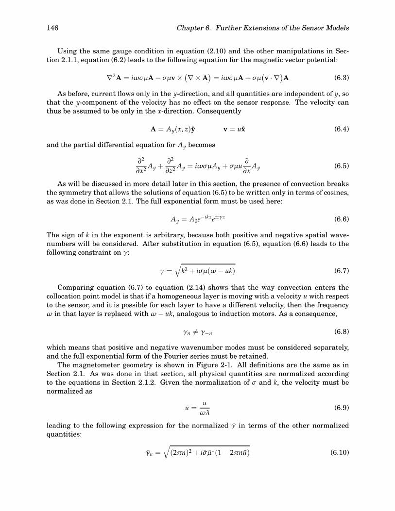
146 Chapter 6. Further Extensions of the Sensor Models
Using the same gauge condition in equation (2.10) and the other manipulations in Sec-tion 2.1.1, equation (6.2) leads to the following equation for the magnetic vector potential:
∇2A = iωσµA−σµv× (∇×A)
= iωσµA+σµ(v · ∇)
A (6.3)
As before, current flows only in the y-direction, and all quantities are independent of y, sothat the y-component of the velocity has no effect on the sensor response. The velocity canthus be assumed to be only in the x-direction. Consequently
A = Ay(x, z)y v = ux (6.4)
and the partial differential equation for Ay becomes
∂2
∂x2Ay +
∂2
∂z2Ay = iωσµAy +σµu
∂∂xAy (6.5)
As will be discussed in more detail later in this section, the presence of convection breaksthe symmetry that allows the solutions of equation (6.5) to be written only in terms of cosines,as was done in Section 2.1. The full exponential form must be used here:
Ay = A0e−ikxe±γz (6.6)
The sign of k in the exponent is arbitrary, because both positive and negative spatial wave-numbers will be considered. After substitution in equation (6.5), equation (6.6) leads to thefollowing constraint on γ:
γ =√k2 + iσµ(ω − uk) (6.7)
Comparing equation (6.7) to equation (2.14) shows that the way convection enters thecollocation point model is that if a homogeneous layer is moving with a velocity u with respectto the sensor, and it is possible for each layer to have a different velocity, then the frequencyω in that layer is replaced with ω − uk, analogous to induction motors. As a consequence,
γn = γ−n (6.8)
which means that positive and negative wavenumber modes must be considered separately,and the full exponential form of the Fourier series must be retained.
The magnetometer geometry is shown in Figure 2-1. All definitions are the same as inSection 2.1. As was done in that section, all physical quantities are normalized accordingto the equations in Section 2.1.2. Given the normalization of σ and k, the velocity must benormalized as
u =u
ωλ(6.9)
leading to the following expression for the normalized γ in terms of the other normalizedquantities:
γn =√
(2πn)2 + iσµ∗(1− 2πnu) (6.10)

6.1. Mathematical model of the MWM sensor in the presence of convection 147
6.1.2 Symmetry
The presence of convection changes the symmetry constraints of equation (2.27) to
∂Ay
∂x
∣∣∣∣x = ∂Ay
∂x
∣∣∣∣−x (6.11a)
Ay(x) = −Ay
(x+
12
)(6.11b)
Comparing equation (6.11) to equation (2.27) shows that the even symmetry with respectto x = 0 is broken, because v changes direction when reflected across the y-z plane. Thenegative symmetry of translation by 1/2 still holds because, the presence of motion does notinvalidate the fact that half a period to the right all current flows in the opposite direction,changing the sense of most other physical quantities as well.
The effect of the broken symmetry is to require the use of the full exponential Fourierseries, instead of the even cosine series. Furthermore, a full half period must be included inthe model, to determine the magnetic vector potential everywhere.
As before, only odd-numbered Fourier modes are needed, due to the translational symme-try conditions, and, as in Section 2.1, all summations over Fourier modes use only odd valuesof n.
6.1.3 Collocation points
Since the interval of interest now contains one half wavelength, the number of regions mod-eled separately increases to seven, with the addition of the return leg of the secondary wind-ing, another gap, and half of the return leg of the primary.
This number may be reduced to six by shifting the origin from the center of the primarywinding to its left edge. This change does not violate the built-in symmetry assumptions inequation (6.11), since the odd symmetry with respect to the origin is already broken.
If K collocation points are still placed in each interval, the total number becomes 6K. Thedistribution of the points is made cosinusoidal in every interval. It is still necessary for theintegration interval limits to include the winding edges, and in analogy to equation (2.33)they are defined as
x∗m = ctm
x∗K+m = c+ gtm
x∗2K+m = c+ g+ dtm
x∗3K+m = c+ g+ d+(12− c− 2d− 2g
)tm
x∗4K+m =12− g− (1− tm)d
x∗5K+m =12− (1− tm)g
0 ≤ m ≤ K (6.12)
where tm is defined as
tm =1− cos(πm/K)
2(6.13)

148 Chapter 6. Further Extensions of the Sensor Models
The geometrical parameters c, d, and g are defined in Figure 2-1, and all length parametersare normalized by the wavelength λ. As in equation (2.34), the collocation points xm aresituated in the middle of the integration intervals, except at the two ends:
xm =
x∗m m = 0, 6K
x∗m+1 + x∗m2
m = 1, 2, . . . , 6K − 1(6.14)
The collocation points span half a period, so that x6K − x0 = 1/2. Equation (6.11) requiresthat
a6K = −a0 (6.15)
where am are the values of Ay at the points xm. Equation (6.15) is the extra constraint neededto make the number of independent unknowns equal to the number of integration intervals.The corresponding constraint in Section 2.1 is equation (2.32).
6.1.4 Fourier series representation
The magnetic vector potential is represented as an exponential Fourier series:
Ay(x) =∞∑
n=−∞n odd
Ane−iknx (6.16)
Only odd-numbered modes are necessary, because of the constraint given in equation (6.11).To obtain the Fourier coefficients An in terms of the values at the collocation points, thefollowing integral must be solved:
An = 2∫ 1/2
0Ay(x)eiknxdx
= 26K−1
∑m=0
∫ xm+1
xm
(xm+1 − x)am + (x− xm)am+1
xm+1 − xmeiknxdx
=2k2n
6K−1
∑m=0
eiknxm+1 − eiknxm
xm+1 − xm
(am+1 − am
)+
2ikn
6K−1
∑m=0
[am+1eiknxm+1 − ameiknxm
](6.17)
The summation in the last term of equation (6.17) cancels out on a term by term basis,with the first and last terms also canceling each other due to the wrap-around effect:
a6Keiknx6K = −a0eikn(x0+ 12 ) = −a0eiknx0eiπn = a0eiknx0 (6.18)
where n is an odd number, and use has been made of the previously established relationshipsa0 = −a6K and x6K − x0 = 1/2. The remaining summation in equation (6.17) can be rewrittenas
An = − 2k2n
6K
∑m=1
am
[eiknxm+1 − eiknxm
xm+1 − xm− eiknxm − eiknxm−1
xm − xm−1
](6.19)

6.1. Mathematical model of the MWM sensor in the presence of convection 149
if, for convenience, an extra collocation point is defined:
x6K+1 = x1 +12
(6.20)
This works because
−a0 eiknx1 − eiknx0
x1 − x0= a6K
−eiknx6K+1 + eiknx6K
x6K+1 − x6K(6.21)
having used the same method as in equation (6.18).
6.1.5 Normalized surface reluctance density
Equations (2.39) through (2.52) apply without any changes, as long as negative values forthe mode number n are allowed, and the definition of γn used in each layer is obtained viaequation (6.7).
6.1.6 Boundary conditions
As before, the surface current must be zero in the gaps, requiring no changes to equation(2.53). Equation (2.56) also applies, but there is one complication: whereas over the primarywinding the terminal voltage is still v1, it is not known ahead of time how v2 is divided betweenthe two legs of the secondary winding, since the symmetry is broken and the voltage is notdivided equally.
If −v′ is the terminal voltage in equation (2.56) applied over the second leg of the sec-ondary winding, then for the first leg v2 − v′ must be used. The extra unknown v′ requires anadditional constraint, in order to determine the vector potential uniquely. The extra equationcomes from the restriction that the total current in both legs of the secondary winding mustbe equal in magnitude.
The integral over KS remains in a similar form:∫ x∗m+1
x∗mKS(x) dx =
∞∑
n=−∞n odd
Rnkn∫ x∗m+1
x∗mAne−iknx dx
= −∞∑
n=−∞n odd
iRn[e−iknx
∗m+1 − e−iknx
∗m
] 2k2n
6K
∑j=1
aj
[eiknx j+1 − eiknx j
x j+1 − xj− eiknx j − eiknx j−1
xj − xj−1
]
=∞∑
n=−∞n odd
Rn6K
∑j=1
Mnm, ja j
(6.22)

150 Chapter 6. Further Extensions of the Sensor Models
which leads to the following definition of Mnm, j:
Mnm, j =
2ik2n
{− 1xj+1 − xj
[eikn(xj+1−x∗m+1) − eikn(xj+1−x∗m)
]+[
1xj+1 − xj
+1
xj − xj−1
]·[eikn(xj−x
∗m+1) − eikn(xj−x
∗m)]
− 1xj − xj−1
[eikn(xj−1−x∗m+1) − eikn(xj−1−x∗m)
]} (6.23)
It is still possible to use the shortcut implemented in Section 2.1.6 via R∞ and M′m, j. If N
is large enough, so that Rn ≈ R∞ for n > N and Rn ≈ −R∞ for n < −N, then the modes withpositive and negative indices may be paired up as
∞∑n=1n odd
2ik2n
(eiknx − e−iknx
)= −4
∞∑n=1n odd
sin(knx)k2n
= − 1π2 f (x) (6.24)
where f (x) is the function defined in equation (2.61). The integral over KS(x) in equation(6.22) can then be written as:∫ x∗m+1
x∗mKS(x) dx ≈
N
∑n=−Nn odd
(Rn − R∞
) 6K
∑j=1
Mnm, ja j + R∞
6K
∑j=1
M′m, ja j (6.25)
where the coefficients M′m, j are given by:
M′m, j =
∞∑
n=−∞n odd
Mnm, j = − 1
π2
{− 1xj+1 − xj
[f(xj+1 − x∗m+1
)− f(xj+1 − x∗m
)]+[
1xj+1 − xj
+1
xj − xj−1
]·[f(xj − x∗m+1
)− f(xj − x∗m
)]− 1xj − xj−1
[f(xj−1 − x∗m+1
)− f(xj−1 − x∗m
)]}(6.26)
The computation of the integral over A(x) does not depend on the Fourier representation,which means that equations (2.63), (2.64), and (2.65) remain valid in the presence of motion.
6.1.7 Setting up the matrix equation
As explained in the previous section, there is an extra unknown, v′, and an extra equationwhich must be considered when setting up the matrix equation. If v′ is appended to the end ofthe vector a, then the matrix M in Ma = b has one extra row and one extra column, comparedto the matrices Mn, M′, and M′′, which are 6K × 6K matrices. This results in the following

6.1. Mathematical model of the MWM sensor in the presence of convection 151
definition for the elements of M:
Mm, j =
N
∑n=−∞n odd
(Rn − R∞
)Mnm, j + R∞M′
m, j
K ≤ m < 2K3K ≤ m < 4K5K ≤ m < 6K
0 ≤ j ≤ 6K
N
∑n=−∞n odd
(Rn − R∞
)Mnm, j + R∞M′
m, j + iσcoilM′′m, j
0 ≤ m < K
2K ≤ m < 3K4K ≤ m < 5K
0 ≤ j ≤ 6K
σcoil(x∗m+1 − x∗m
) {2K ≤ m < 3K4K ≤ m < 5K
j = 6K{3K−1
∑�=2K
−5K−1
∑�=4K
} N
∑n=−∞n odd
(Rn − R∞
)Mn
�, j + R∞M′�, j
m = 6K 0 ≤ j ≤ 6K
0 m = 6K j = 6K(6.27)
where the definition of the last row, m = 6K, which implements the constraint that the totalof the current in the two legs of the secondary winding must be zero, is derived from equa-tion (2.69). The following short hand notation was used in equation (6.27):{
∑1−∑2
}[ ] ≡ ∑1
[ ]−∑2
[ ](6.28)
The definition of b in equation (2.68) remains unchanged, with the addition of an extrarow of zeros at the bottom.
A minor change in equation (2.69) requires the removal of the factor of two, since the entireprimary is in the half period, and the addition of a column of zeros:
Fm, j =
K−1
∑�=0
N
∑n=−∞n odd
(Rn − R∞
)Mn
�, j + R∞M′�, j
m = 0 j < 6K
3K−1
∑�=2K
N
∑n=−∞n odd
(Rn− R∞
)Mn
�, j + R∞M′�, j
m = 1 j < 6K
0 j = 6K
(6.29)
6.1.8 Effect of convection on sensor response
The implementation of the changes to the model shown in this section makes it possible tostudy how the sensor response changes with increasing velocity. Figure 6-1 shows the trajec-tory of the sensor transinductance in magnitude/phase space, as the velocity of the materialis increased.
An interesting phenomenon to observe in Figure 6-1 is that for a certain range of valuesthe phase of the transinductance becomes positive, corresponding to impedance with a nega-tive real component. Whereas this may appear nonphysical at first, one must bear in mindthat this is a two-port transinductance of a continuum system and cannot be thought of asa single lumped component. A somewhat similar phenomenon of negative transconductanceand transcapacitance can occur in the IDED [10].

152 Chapter 6. Further Extensions of the Sensor Models
0.05 0.1 0.15 0.2 0.25 0.3 0.35 0.4−35
−30
−25
−20
−15
−10
−5
0
5
Magnitude [µH]
Pha
se [d
eg]
Parametric Plot of Sensor Response as a Function of Velocity
Velocity in km/sSensor wavelength: 2.4 mmFrequency: 1 MHzMaterial: Al, 3.8 MS/mLift−off: 40 microns
50 20
10 5 4
3
2
1 0.5
0
Figure 6-1: Locus of the transinductance of an MWM in magnitude/phase space as the con-vection velocity increases.
0 0.05 0.1 0.15 0.2 0.25 0.3 0.35 0.4 0.45 0.5−0.8
−0.6
−0.4
−0.2
0
0.2
0.4
0.6
Normalized position x
Rea
l par
t of v
ecto
r po
tent
ial A
y
Effect of convection on vector potential
u = 0u = 50 km/s
primarywinding
secondary winding
Quarter−periodsymmetry point
Figure 6-2: Real part of the magnetic vector potential Ay, shown for stationary and movingmedia. It can be seen that the odd symmetry with respect to the quarter-period point is brokenwhile the translational symmetry still holds, as implied by equation (6.11). The potentialin this figure corresponds to driving the secondary winding, which is the opposite of typicaloperation, but the effect is easier to observe in this case.

6.2. Grid look-up and interpolation algorithms 153
Figure 6-2 shows a comparison between a moving and stationary metal layer. In additionto breaking the symmetry with respect to the quarter-period point, clearly visible in the figure,the motion also acts to decrease the magnitude of the potential. The ability of the conductingmaterial to counteract the imposed magnetic field improves at higher speed, a behavior alsoobservable in Figure 6-1.
6.1.9 Summary
This section has illustrated how to incorporate material motion into the semi-analytical collo-cation point model of the magnetometers with Cartesian geometry. Although the analysis hasfocused on the MWM, the same methods are also directly applicable to modeling Cartesiangeometry magnetometers with distributed current drives, of the type described in Chapter 4.Most magnetometer arrays, used for generating two-dimensional scans of a material, for ex-ample the one shown in Figure 1-2, fall in the latter category.
Use of magnetoresistive secondary elements, as described in Chapter 5, makes it possibleto operate magnetometers and magnetometer arrays at very low excitation frequencies, andin such cases the scanning velocity may begin to have an appreciable effect on the sensorresponse, and will have to be incorporated in the simulation methods.
6.2 Grid look-up and interpolation algorithms
This section describes the most recent implementation of the two-dimensional grid look-upalgorithm. The purpose of this algorithm is to convert the value of the measured transimpe-dance of a sensor to material properties, i.e. parameter estimation, by interpolating betweenthe points of a look-up table of pre-computed sensor responses, known as a measurement grid.The concept of using measurement grids for parameter estimation is described in Section 1.4.
The type of interpolation that needs to be carried out for a grid look-up is not what is donein typical look-up table algorithms, which are forward interpolation algorithms. This is acritical distinction and deserves some more explanation. Interpolation methods of this natureare discussed in [81], though the subject of two-dimensional inverse interpolation algorithmsis not discussed at all.
6.2.1 Two-dimensional inverse interpolation
The concept of inverse interpolation is best illustrated with an example. Suppose there is afunction y(x), whose values yn are known at a set of points xn. The independent variable is x,and xn are chosen by the designer of the look-up table to span the anticipated function domain.The most common task is finding a value for y at a given value of x. This is one-dimensionalforward interpolation and is very easy to carry out, since it is known from the start which xnis closest to x, etc.
Finding a value of x that corresponds to a given value of y in the table described aboveis what is known as inverse interpolation. It is a much more difficult operation, especially ify(x) is not a monotonic function. Furthermore, the values of y may be repeated, and are notevenly spaced, unless the function is a straight line.
In two dimensions, forward interpolation entails finding the value of a function y(x1, x2)from x1 and x2 by interpolating in a two-dimensional table that lists the values of y at aset of predetermined values of the two independent variables. This can be done via bilinearinterpolation or its higher order variants. The key feature is that, as in the one-dimensional

154 Chapter 6. Further Extensions of the Sensor Models
Figure 6-3: Example of a situation where the closest grid point to a target point is not one ofthe corners of the grid cell enclosing the target point.
case, it is known from the outset which is the closest point in the table to the target point, andwhich of the table’s points to use for the interpolation. The actual interpolation is also easy,since when plotted in x1-x2 space the table forms a rectangular grid.
Two-dimensional inverse interpolation comes about when there is a table that lists thevalues of two functions, y1(x1, x2) and y2(x1, x2), at a set of predetermined values of the inde-pendent variables, which form a rectangular grid. The goal is to find the appropriate valuesfor x1 and x2 where the functions y1 and y2 attain a pair of known values. This task is ordersof magnitude more complicated. Here are some of the complications:
• Even when both target y1 and y2 fall inside the ranges of the corresponding functions,there is no guarantee that a solution exists.
• It is not known at the outset what the indices of x1 and x2 are for the point closest tothe target.
• Even if the first two difficulties are overcome, and it is established which cell in thetable should be used for interpolation, in general in y1-y2 space this cell is notrectangular, or even a parallelogram, and no standard interpolation formula can beapplied.
The grid methods implement this kind of two-dimensional inverse interpolation to convertthe sensor measurement’s magnitude and phase data to real physical quantities, such as con-ductivity and lift-off. The measurement grids are generated by applying the forward models,described in Chapters 2–4, at a set of values for the two parameters, giving the magnitude andphase at each combination. The two measurement parameters do not need to be magnitudeand phase, it is possible to have magnitude/magnitude grids for two sensors, or two spatialwavelengths inside the same sensor, for example the grids used in Section 3.3 and Section 5.5.
Previously the method of identifying the closest grid point, used to establish which cell touse in the interpolation, was to calculate the distance to each point on the grid and pick theshortest one. This is clearly very inefficient, and can also give the wrong result in some cases,as seen in Figure 6-3. The cell that contains the target point is shaded in the figure. Theclosest grid point to the target is clearly not one of its four corners.
The actual interpolation step was also deficient in many respects for nonrectangular gridcells, giving discontinuous interpolation not only at cell boundaries, but sometimes even insidethe same cell, in addition to sometimes manifesting bias toward some of the grid cells thatcannot be justified geometrically.
This section describes methods that successfully overcome all of these limitations. It isdivided into three subsections: the search algorithm, which aims to find the grid cell insidewhich the target point is located; and two interpolation methods of increasing performanceand complexity.

6.2. Grid look-up and interpolation algorithms 155
6.2.2 Search algorithm
The function of this algorithm is to locate quickly the grid cell that contains the target point.It can be roughly divided into four steps:
1. Choose a starting point. Initiating the search close to the target point can significantlyimprove the efficiency of the search. In general, this should be the cell used in the lastlook-up, because it is very likely that consecutive measurements lie close together on thegrid. In fact, in most cases the last cell used contains the current target point, so thatthis step often concludes the search. If this is the first look-up in the current session, arough interpolation is done based on the four corners of the grid to estimate the indicesof the starting point, using a method similar to the one described in Section 6.2.3.
2. Zoom out. If the target point is not inside the current cell, increase the size of the areatested to 2× 2, 4× 4, etc., until either the current grid “square” (collection of cells beingconsidered) contains the target point, or it reaches a predefined limit or the size of theentire grid.
3. Move the grid square. If the grid square currently under consideration does not containthe target point, move to the next grid square of the current size in the direction towardthe target point. Keep moving until one of the following three conditions occurs:
(a) The target point falls inside the current square.
(b) The square reaches the edge of the grid.
(c) It cannot be determined which the correct direction to move is. This last conditioncan occur in special cases near singular points, near grid folds, or if the current gridsquare is not a convex quadrangle.
4. Zoom in. If the size of the current grid square is greater than a single grid cell, reduceit by a factor of two and go back to step 3. Otherwise, end the search.
If in the end the current grid cell contains the target point, the search was successful.Otherwise, the target point is most likely off the grid.
There can be cases when the search fails even if the target point is on the grid. This canhappen if the grid is so curved that moving in a direction toward the target in the plane ofthe grid, i.e. in magnitude/phase space, moves away from the correct cell in parameter space.These cases are handled by reverting to the “brute force” method of computing the distanceto every point on the grid and finding the closest grid point to the target point. It is then usedas the starting cell for a second run through the search algorithm. If, in fact, the target pointis on the grid, this will find the correct cell with a very high likelihood. Most often, however,if the first run fails, it is because the point is off the grid, so that if used every time a point offthe grid is encountered, this second search step takes a disproportionately long time to run,which can create problems, especially when performing real-time estimation. Whether to giveup after the first try or attempt the long search method depends on the particular application.
In order to determine the direction to move in step 3 above, a formula (equation (6.31)) isapplied that calculates the area of the triangles formed by each of the four sides of the gridsquare and the target point, and the sign of the result is used to determine whether the targetpoint lies inside the square, or else in which direction the square is to be moved. For example,if the target point is to the “right” of both the “left” and “right” sides of the square, it mustbe moved one over to the right, etc. The directions here are put in quotations, because the

156 Chapter 6. Further Extensions of the Sensor Models
1
2
3
4
T
d4d1
d2d3 Q1
P2
P1Q2
Figure 6-4: Schematic diagram of the two-dimensional inverse interpolation in a grid cell.Each pair of opposing sides is associated with two values of a parameter being estimated, P orQ. d1 through d4 are the distances from the target point T to the four grid edges.
meanings of “right”, “left”, “top”, and “bottom” depend on the direction of increasing parameterindex number, and on whether the grid is “right-handed” or “left-handed”, i.e. whether theaxes in magnitude/phase space and parameter space have the same or opposite sense.
6.2.3 Simple inverse two-dimensional interpolation
This interpolation method is based on the distances between the target point and the lines ofconstant parameter, P or Q, as shown in Figure 6-4:
P =d3P1 − d1P2d3 − d1
Q =d4Q1 − d2Q2
d4 − d2(6.30)
The distances d1 through d4 are calculated by dividing the area of the triangle with verticesat the two corners and the target point by the length of the cell side, and then dividing by two.The following formula is used to find the triangle area:
Aijk = xi(yk − yj) + xj(yi − yk) + xk(yj − yi) (6.31)
The sign of Aijk can be positive or negative, depending on whether the motion is in a posi-tive (counterclockwise) or negative (clockwise) direction along the circumscribed circle whengoing from i to j to k. Therefore this formula retains directionality information, although itcalculates area. If all three points lie on a line, the result is zero.
It is important to realize that the distances d1 through d4 in equation (6.30) are signedquantities, so that when the target point lies inside the cell, d1 and d3 have opposite signs, asdo d2 and d4. The order of the area indices in equation (6.31) is important. The advantageof maintaining the polarity information is that the correct result will be obtained even if thetarget point lies outside the grid cell used for interpolation.
The problem with the “simple” method in this section is continuity across cell boundaries.The value of the parameter associated with the cell wall being crossed, e.g. P when crossingline 1–2 in Figure 6-4, is continuous, because it is equal to the value of the parameter onthat line, P1. However, the value of the other parameter, e.g. Q, when crossing line 1–2,

6.2. Grid look-up and interpolation algorithms 157
1
5
6
7
8
2
3
4
T
d4
d1
d2d3Q1
P2
P1Q2
Figure 6-5: Diagram of a grid cell showing the points used by the complex inverse two-dimensional interpolation algorithm. Points 5–8 are positioned on the grid cell edges accordingto equation (6.32). Instead of being associated with line segments, the four parameter valuesP1, Q1, P2, and Q2 are now associated with points 5–8 respectively.
in general makes a discontinuous jump as the grid cell being used for interpolation changes.This is usually a very small jump, since in most grids the edges of neighboring cells are nearlyparallel.
The practical implications of this discontinuous behaviour are most pronounced when us-ing iterative techniques, e.g. in coating characterization applications where three unknownsare measured simultaneously [26], or other multiple-unknown measurements, where it couldlead to lack of convergence. It is also possible to observe the effect when scanning along a partwith continuously varying properties using a coarser grid, where the measured property mayappear to change in steps.
6.2.4 Complex inverse two-dimensional interpolation
To solve the discontinuity problem, given a target point on a grid cell wall, both of the esti-mated parameters, P and Q, must depend only on the coordinates of the target point and thetwo end points of the edge being crossed, common to both cells. For example, when the targetpoint lies on line 1–2, both P and Q must depend only on the coordinates of points 1, 2, and T.With the simple method this is true only for P.
This is accomplished in the following way. Instead of using equation (6.30) to calculate Pand Q directly, it is used to find the coordinates of four new points, 5–8, one on each of the

158 Chapter 6. Further Extensions of the Sensor Models
5T
6
a
1–a
1–b
b
Q1
P2
P1
Q2
7
8
Figure 6-6: Grid cell transformed into a parallelogram via points 5–8. The interpolationbecomes the simple linear operation given in equation (6.33). The ratios a and b are determinedby the lengths of the sections into which the line segments 5–7 and 6–8 are divided by linesthrough the target point T and parallel to the two segments.
four sides of the cell, as shown in Figure 6-5. This is done via the following equations:
x5 =d4x2 − d2x1d4 − d2
y5 =d4y2 − d2y1d4 − d2
(6.32a)
x6 =d3x2 − d1x3d3 − d1
y6 =d3y2 − d1y3d3 − d1
(6.32b)
x7 =d4x3 − d2x4d4 − d2
y7 =d4y3 − d2y4d4 − d2
(6.32c)
x8 =d3x1 − d1x4d3 − d1
y8 =d3y1 − d1y4d3 − d1
(6.32d)
Now instead of being associated with a line segment, each of the two pairs of grid param-eters is associated with a pair of points, as shown in Figure 6-6. If, for example, the targetpoint lies on cell side 1–2, points 8 and 6 will coincide with 1 and 2 respectively, making Qdependent only on these two points, as required. If P and Q are expressed in terms of thecoefficients a and b, using
P = (1− a)P1 + aP2 Q = (1− b)Q1 + bQ2 (6.33)
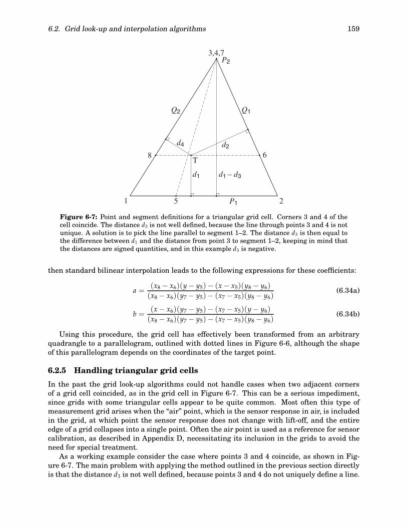
6.2. Grid look-up and interpolation algorithms 159
1 5
68
2
3,4,7
T
d4
d1
d2
d1 – d3
Q1
P2
P1
Q2
Figure 6-7: Point and segment definitions for a triangular grid cell. Corners 3 and 4 of thecell coincide. The distance d3 is not well defined, because the line through points 3 and 4 is notunique. A solution is to pick the line parallel to segment 1–2. The distance d3 is then equal tothe difference between d1 and the distance from point 3 to segment 1–2, keeping in mind thatthe distances are signed quantities, and in this example d3 is negative.
then standard bilinear interpolation leads to the following expressions for these coefficients:
a =(x8 − x6)(y− y5)− (x− x5)(y8 − y6)
(x8 − x6)(y7 − y5)− (x7 − x5)(y8 − y6)(6.34a)
b =(x− x6)(y7 − y5)− (x7 − x5)(y− y6)
(x8 − x6)(y7 − y5)− (x7 − x5)(y8 − y6)(6.34b)
Using this procedure, the grid cell has effectively been transformed from an arbitraryquadrangle to a parallelogram, outlined with dotted lines in Figure 6-6, although the shapeof this parallelogram depends on the coordinates of the target point.
6.2.5 Handling triangular grid cells
In the past the grid look-up algorithms could not handle cases when two adjacent cornersof a grid cell coincided, as in the grid cell in Figure 6-7. This can be a serious impediment,since grids with some triangular cells appear to be quite common. Most often this type ofmeasurement grid arises when the “air” point, which is the sensor response in air, is includedin the grid, at which point the sensor response does not change with lift-off, and the entireedge of a grid collapses into a single point. Often the air point is used as a reference for sensorcalibration, as described in Appendix D, necessitating its inclusion in the grids to avoid theneed for special treatment.
As a working example consider the case where points 3 and 4 coincide, as shown in Fig-ure 6-7. The main problem with applying the method outlined in the previous section directlyis that the distance d3 is not well defined, because points 3 and 4 do not uniquely define a line.

160 Chapter 6. Further Extensions of the Sensor Models
0 5 10 15 20 25−10
−5
0
5
103
1
−1
−3 30
20
10
0
Figure 6-8: Pathological test grid and path through the grid followed by the target point. Thenew algorithm makes sure that the estimated values of the two properties remain continuousat cell edge crossings inside the grid, and that proper parameter estimation is possible insidethe triangular cells near the grid singularity at (22, 0).
It is not possible simply to use the distance between the target point T and point 3, becausethe polarity information is lost in this case, among other things, and the results would be verywrong indeed, especially if the target is outside the cell, which we hope to handle with at leastsome grace. The solution is to take the direction of the line through 3 and 4 to be parallelto the line through 1 and 2. A consequence of this is that the line through 6 and 8 is alwaysparallel to 1–2 and passes through the target point T. The undefined distance d3 needs to beredefined via the segments as shown in the figure.
6.2.6 Comparison between the new and the old interpolation methods
A test grid is used to compare the performance of the two interpolation methods, shown inFigure 6-8. It is crooked by design, so that the discontinuity of the estimated properties ismore pronounced. The grid also includes three triangular grid cells. The values of the param-eters are shown with arrows in the figure. The range of the “radial,” or perhaps “horizontal,”property is from 30 to 0 and the range of the “azimuthal,” or “vertical,” property is from −3 to3. The figure also shows the continuous path followed by the target point through the grid,which would ideally result in a continuous estimate of the two properties.
The results of using the two look-up methods are shown in the plots in Figures 6-9 and6-10. A number of discontinuous steps are visible at grid line crossings with the simplemethod, while the new complex method remains continuous. As seen in the plot of the radialproperty, the complex method can also be discontinuous, but only outside the grid. Whereasan attempt has been made to treat off-grid cases reasonably, in general continuity cannot beguaranteed, because it is not possible to determine uniquely which grid cell should be used forthe interpolation. Nonetheless, one can see that as long as the target point remains near the

6.2. Grid look-up and interpolation algorithms 161
grid, the results of the complex method are still quite reasonable. It is only in the azimuthalproperty near the singular point at (22, 0) that the estimated property attains extreme values,but this is to be expected, since several segments with different parameter values merge toa single point there. Following the air point example, this is the equivalent of attempting toestimate the lift-off of a material made of air, which is clearly meaningless.
It can be seen in the plots of the estimated properties that the old method curves endprematurely. This is because the old method could not effectively handle nonstandard, e.g.triangular, grid cells, which it encounters in the process of locating the bounding grid cell.
6.2.7 Handling multi-valued grids
There are cases when a grid folds in on itself, as described and illustrated in Section 5.7. Thislook-up algorithm also attempts to handle this kind of grid, at least in the simplest caseswhen there is no more than one “fold” or “twist”. The main difficulty is that the searchingstage of the algorithm may become confused near the fold line. For example, at the fold manygrid cells are quadrangles whose opposite edges cross. It is not possible to determine whetherthe target point is to the “left” or “right” of a cell whose left and right edges intersect. In fact,it is not possible to decide whether the target point falls inside the cell at all.
The approach taken in such cases is to try four different runs of the search algorithmdescribed in Section 6.2.2, starting at the four corners of the grid. Practice has shown thatthis approach is quite effective at handling most cases, providing even for the possibility offinding two solutions in the areas where the grid surface overlaps itself. No attempt is madeto determine which one of the two solutions is to be considered the “correct” one, as suchdecisions need to be made at a higher level, using other information.
6.2.8 Summary
This section has described changes to the existing grid look-up algorithms that result in sub-stantial improvements of the efficiency and accuracy of these methods. In particular, thenumerical search algorithm that locates the grid cell that encloses the target point has beenmade very efficient and capable of handling unconventional or singular grids. The inverseinterpolation step is formulated in a way that ensures continuity of both estimated propertiesthroughout the range of the grid. In addition to better accuracy and efficiency, the new gridlook-up is much more robust in its ability to treat unusual cases, such as target points thatlie outside the grid or near grid singularities, in a reasonable way.
High performance of the grid look-up algorithm is essential for obtaining the full benefitsof the model-based sensor methodology. The algorithm enhancements described in this sectionhave already led to great improvements in the quality of data taken with the MWM, IDED,and their derivatives. Furthermore, the continuity property is very important in algorithmsthat include grid look-ups as an intermediate step in an iterative process, as is the case withseveral algorithms used to estimate more than two unknowns simultaneously. The robustnessis also very valuable in such cases.
In addition to its application in measurements with the magnetic and dielectric sensors,this method has independent value as a generic numerical tool for two-dimensional inverseinterpolation.

162 Chapter 6. Further Extensions of the Sensor Models
0 5 10 15 20 25−5
0
5
10
15
20
25
30
35Radial property
New interpolation methodOld interpolation methodGridline crossings
Slight discontinuitywhen going off grid
Figure 6-9: Results with both interpolation methods for the radial property of the grid inFigure 6-8. The values estimated with the new complex method are continuous across internalcell boundaries. The line of the simple method ends prematurely because it cannot handletriangular grid cells.
0 5 10 15 20 25−5
−4
−3
−2
−1
0
1
2
3
4
5Azimuthal property
New interpolation methodOld interpolation methodGridline crossings
Figure 6-10: Results with both interpolation methods for the azimuthal property of the grid inFigure 6-8. The values estimated with the new complex method are continuous across internalcell boundaries. The extreme values attained near the end of the path are due to the fact thatthey correspond to target points outside the grid, near a grid singularity, where grid lines withdifferent values of the azimuthal parameter converge to a single point.

Chapter 7
Summary, Conclusions, andSuggestions for Continuing Work
7.1 Summary
The main focus of the research effort has been to extend the depth of sensitivity of the periodic-field quasistatic magnetometers, in order to allow them to detect flaws, such as cracks, voids,and inclusions, buried deep in a metallic component, or hidden behind a metal layer. Thistype of measurement is difficult with the MWM and traditional eddy current magnetometers,because in the frequency range of sensitivity of these devices, the depth of penetration is lim-ited by the skin depth of the magnetic field in the metal. In order to overcome this limitation,it is necessary to make the skin depth on the order of, or larger than, the thickness of metalbetween the flaw and the sensor. This may be accomplished by lowering the frequency ofoperation, since the skin depth is related to frequency as δ ∝ 1/
√ω.
The output of traditional eddy current magnetometers is the induced voltage in a sec-ondary winding. Since it is proportional to the rate of change of the magnetic flux, the sen-sitivity of the measurement decreases with decreasing frequency, which makes such sensorsunsuitable for low frequency operation. In order to overcome this limitation, the approachtaken here is to replace the secondary winding with a giant magnetoresistive magnetic fieldsensor, which responds to the magnitude of the magnetic flux density, and consequently hasno lower bound on its frequency of operation.
A prototype magnetometer that uses this idea has been built and tested. Its deep pene-tration and low frequency operation capabilities have been used for a range of measurementapplications:
1. Conductivity/lift-off measurements on nonmagnetic metals.
2. Two-wavelength permeability/lift-off measurements on magnetizable nonconductingmaterials.
3. Thickness/lift-off measurements for a metal layer in a two-metal test structure.
4. Thickness/conductivity measurements for thick metal plates at ultralow frequency andhigh skin depth.
5. Detection of cracks buried beneath a thick layer of metal.
6. Magnetic permeability measurements of ferromagnetic fluids.
163

164 Chapter 7. Summary and Conclusions
Successful operation of the GMR-based magnetometer has required that solutions befound to a number of design problems. Magnetic sensors based on the giant magnetoresis-tive effect are passive components, with a highly nonlinear transfer characteristic and limiteddynamic range. These limitations have been overcome by appropriate biasing, and by plac-ing the sensor in a feedback loop configuration with a secondary winding that maintains themagnetic flux density at the sensor constant.
The imposed spatial wavelength of the magnetometer is the other factor, together withskin depth, that can potentially limit its depth of sensitivity. It must therefore also be longcompared to the required depth of penetration. Generating a magnetic field pattern witha long effective spatial wavelength, while avoiding the need to increase the magnetometerfootprint to impractical dimensions, is accomplished by shaping the current in each segmentof the primary winding to follow an appropriate envelope function.
An important necessary requirement for GMR magnetometer operation is the develop-ment of good mathematical and physical models, needed for the interpretation of data, andfor parameter estimation of absolute properties. Such models must address the nature of thedistributed current drive primary winding, and must be developed in cylindrical coordinates,because of the circular symmetry chosen for the sensor prototype.
Efficient simulation methods based on the fast Fourier transform have been developedfor distributed current drive magnetometers, with versions available for both Cartesian andcylindrical geometry. The validity of the simulation results has been demonstrated by show-ing the close agreement between a variety of experimental data and corresponding sensorsimulations.
In addition to the many stages of the project that have had to be completed before a GMRmagnetometer could be tested successfully, the capabilities of the spatially periodic sensorfamily have been extended in a number of other areas:
1. The existing semi-analytical collocation point methods, used to model magnetometersand dielectrometers, have been reformulated in a way that offers several advantages:
(a) The magnetometer and dielectrometer models, previously developed by differentearlier research teams, now use a formulation that maintains the direct parallelsbetween the magnetoquasistatic and electroquasistatic regimes, afforded by theprinciple of duality. Unifying the two models is beneficial in that improvementsin one can be directly incorporated in the other with little extra effort.
(b) The electroquasistatic model has corrected earlier errors by incorporating the zeroorder spatial Fourier mode properly. This makes a particularly noticeable improve-ment in cases where a ground plane is present behind the material under test.
(c) Perhaps with greatest significance, the equations are written in a way that cleanlyseparates the computation of intermediate results that depend only on the sensorgeometry, and which constitute the greatest computational burden, from those thatdepend on the material under test. In almost all practical cases, the former need tobe carried out only once per session, and as a consequence the tasks of generatingmeasurement grids for a given sensor, or running parameter estimation based on aminimization algorithm, have been rendered many times more efficient.
2. The semi-analytical collocation point methods have been extended to cylindrical geom-etry. New practical applications have required the development of analogs of the stan-dard magnetometers and dielectrometers that have rotational symmetry, suitable for

7.2. Conclusions 165
measurements on circularly symmetric components or in cases where it is important toavoid the dependence of sensitivity on orientation. These extended models have beensuccessfully applied to this new type of sensor. Experimental data have been presentedthat confirm the validity of these models by showing the close agreement between sim-ulated and measured dielectrometer behavior.
3. The highly efficient FFT methods, used to simulate sensors with distributed currentdrive, can also be applied for modeling of magnetometers that traditionally use the col-location point technique, in cases when the exact distribution of the current densityinside the windings is not important.
4. The magnetometer collocation point models have also been extended to accommodaterelative motion between the magnetometer and the material under test. This effect maybecome important in scanning applications at low frequencies, if the distance traveledby the sensor in one temporal cycle period is not negligible compared to the effectivespatial wavelength.
Several improvements to the measurement grid look-up method, which is the most com-mon approach to two-dimensional parameter estimation, have also been presented. Superiorperformance has been demonstrated in both aspects of the look-up process:
1. The numerical search algorithm has been made much more efficient and more reliable.In addition to being able to find the needed target cell quickly, the new method is also ca-pable of responding appropriately to unusual cases, which arise in the presence of topo-logical anomalies in the grid, such as folds, twists, curls, or triangular grid cells. Thiscapability has become very important recently, as new practical applications have intro-duced whole new classes of nonstandard measurement grids, like magnitude/magnitude,or higher-dimensional grids that involve three or more unknowns.
2. The inverse two-dimensional interpolation stage has been formulated in a way thatguarantees continuity in both of the estimated properties across grid cell boundaries.This avoids the problem of introducing artificial “features” to a sensitive property scan,and also improves convergence of iterative algorithms that use grid look-up as an inter-mediate step. Furthermore, compared to previous interpolation methods, on the wholethe improvement in the algorithm’s performance for grid cells whose opposite sides areappreciably nonparallel makes it possible to use coarser grids with the same level of ac-curacy, leading to further improvement in efficiency, as well as conservation of computermemory resources.
7.2 Conclusions
The combination of the various enhancements and innovations in this work has resulted in thedesign of a whole new magnetometer sensor structure, capable of absolute property measure-ment of conductivity, magnetic permeability, and layer thickness at metal depths previouslyunattainable with the periodic-field eddy current magnetometers. It has been successfullydemonstrated in the following deep-penetration measurements:
1. Detection of a crack hidden behind a 0.25′′ steel plate.
2. Thickness of aluminum plates on the order of 0.4′′.

166 Chapter 7. Summary and Conclusions
3. Thickness of a steel layer approximately 0.2′′ thick in a two-metal structure.
These thickness values are at least a factor of ten higher than the current thickness upperlimits of the MWM with the same materials, and are nowhere near the outer bound of thedepth of sensitivity of the magnetoresistive magnetometer. Rather, they are the result ofthe choice of convenient frequencies and materials used to show feasibility. The depth ofpenetration limits of this sensor design have yet to be determined, and by operating at verylow frequencies can in principle be extended to any material thickness.
Another important conclusion is that it has been possible to create a deep penetration mag-netometer that matches the models so well that it can measure absolute physical propertieswithout the need for calibration standards. The excellent results of a range of different mea-surements with the prototype magnetometer that rely only on a single calibration point in airdemonstrate that the models used to simulate the sensor response, based on Fourier-Besselanalysis and the magnetic diffusion equation, are valid and accurate.
While there are other (nonperiodic) types of eddy-current sensors that use sensing coilswith high number of turns for increased sensitivity at frequencies as low as 1 kHz, they arenot capable of air calibration, and thus always require calibration standards and empiricalcalibration curves.
In addition to validating the simulation techniques, the experiments also confirm that thecircuits that implement the feedback loop are operating correctly, and that the errors due tounmodeled parasitic effects can be neglected.
The data taken with the circular capacitive sensors in Chapter 3 demonstrate that thecylindrical geometry formulation of the collocation point methods is correct, and that this isan acceptable layout for dielectric sensors.
Altogether this thesis has demonstrated the feasibility of the new sensing technology con-cepts, and has opened up several possibilities for further improvements of existing time andspace periodic sensor technology and design of new types of magnetometers and dielectrome-ters that belong to this class of sensors.
7.3 Suggestions for continuing work
The validity of the semi-analytical models and numerical methods has been confirmed, andthe feasibility of creating a deep penetration magnetometer has been demonstrated. Now theresearch and design effort can focus on the adaptation of the principles established in theconstruction of the prototype to specific practical applications. A few of the potential areas offurther research are suggested in this section.
7.3.1 Scaled down GMR magnetometer
The dimensions of the prototype magnetometer analyzed here have been chosen to make con-struction and experimentation easier. The relatively large size has made it possible to useprepackaged off-the-shelf components, and has relaxed the requirements on the connections,circuits, windings, etc., that are needed to minimize the performance deterioration due toparasitic and unmodeled effects. It has also facilitated the implementation of the multiple-wavelength idea, which requires double the number of turns in the primary winding. One ofthe first questions that needs to be investigated is how miniaturization will affect the mag-netometer’s performance, and what new engineering challenges will arise from its smallersize.

7.3. Suggestions for continuing work 167
In general, a smaller magnetometer footprint is desirable because it increases its versa-tility in being able to inspect components with smaller dimensions. In addition, reducingthe size of the secondary winding of a magnetometer or a magnetometer array improves sen-sitivity, because the signal is less diluted by averaging over a large area. Nevertheless, theminimal size of the magnetometer footprint will be limited by the minimal spatial wavelengthrequirement, determined by the necessary depth of penetration. For example, if one is to beable to see through 1/4′′ of aluminum, the imposed spatial wavelength needs to be on theorder of an inch.
Another aspect of the practical design of a smaller version of the GMR magnetometer ismaking its base flexible, which is a property of the standard MWM. If a similar flexible circuittechnology is to be used, one must address the question of how the distributed current driveprimary winding is to be designed. Multiple turn windings are difficult to implement in aplanar two-dimensional topology, so that in this case it would possibly be more appropriate toshape the surface current density by controlling the current, not the number of turns, of eachwinding segment.
Regardless of the exact implementation details, it is almost certain that the next stage inthe process of adapting GMR magnetometer technology to practical applications is the designand implementation of a smaller, perhaps by a factor of a hundred in area, version of the GMRmagnetometer prototype.
7.3.2 GMR magnetometer arrays
The ultimate goal of the GMR magnetometer effort is to be able to design analogs of the ex-isting MWM sensor arrays to use GMR secondary elements, rather than secondary windings.In principle, this may be as simple as adapting an existing MWM array geometry by replac-ing the individual secondary elements with pre-manufactured GMR sensor chips. One of thequestions that arises is whether it will be practical in this case to maintain the feedback loopconfiguration. While offering many advantages, the feedback connection does increase thesize requirements on each array element, in addition to introducing unwanted cross-couplingbetween the individual array elements. Therefore in an array configuration the preferredmode of operation may be open-loop, in which case an alternative biasing method must bedesigned. For example, it may be possible to set the operating point by adding a DC offset tothe primary current drive. Most likely, though, this would lead to impractically large currentrequirements for the primary, so that the preferred biasing method may be to place a suitablepermanently magnetized flexible ferromagnetic polymer layer behind the sensor array. Fer-romagnetic polymers are made by a suspension of small ferromagnetic particles. A furtheradvantage of this approach is that it is relatively easy to incorporate the effect of a magneti-zable layer in the model, due to its spatial uniformity. The presence of a magnetizable layerwill concentrate the magnetic field intensity on the active side of the magnetometer array, butit has not yet been established whether this will lead to improvement or deterioration of thesensitivity to material faults.
With low frequency operation in scanning applications it may be necessary to incorporatesome of the model changes that include media motion into the methods used to simulate suchsensor arrays.
With the present homogeneous layer models, as the depth of the flaw’s position is in-creased, the relative effect a material flaw has on the effective measured conductivity of themetal is reduced in magnitude, and is spread over a wider area. Therefore, in deep penetra-tion applications it may be necessary to apply data filtering and transformations that combine

168 Chapter 7. Summary and Conclusions
the signal from many individual pixels to reconstruct the original position of the flaw.
7.3.3 Applying the cylindrical geometry collocation point method toRosette sensors
The cylindrical coordinate magnetometer method described in Chapter 3 has not yet been ap-plied to practical magnetometers, although JENTEK’s Rosette sensor arrays, which have theappropriate geometry, are already in use in a number of crack detection and fatigue monitor-ing applications. It is interesting to determine whether use of the cylindrical geometry modelwill lead to a performance improvement for these magnetometers. The validity of the dielec-tric equivalent of the model has already been confirmed by measurements with the circulardielectrometer in Chapter 3.

Appendix A
Definition of Symbols,Abbreviations, and Acronyms
Most of the mathematical symbols used in this document are shown in Table A.2. Symbolsused only locally, and not meaningful outside of the paragraph that defines them, are usuallynot listed here. Not listed are also summation indices, such as j, �, m, or n.
Bold upright Roman letters are used for vectors. Unit vectors are denoted by a hat ac-cent ‘ˆ ’ over the lowercase symbol. Subscripts in italics denote array or matrix indices andcoordinate components, while upright Roman subscripts are considered part of the symbol’sname. The coordinates used are: Cartesian (x, y, z), cylindrical (r,ϕ, z), and spherical (r,θ,ϕ).
Abbreviations and acronyms are listed in Table A.1.
Table A.1: Abbreviations and acronyms in alphabetical order.
DFT Discrete Fourier TransformEQS ElectroquasistaticFFT Fast Fourier TransformFHT Fast Hankel TransformGMR Giant MagnetoresistiveIDED∗ Interdigitated Electrode DielectrometerMQS MagnetoquasistaticMUT Material Under TestMWM∗ Meandering Winding MagnetometerNDE Non-Destructive EvaluationSQUID Superconducting Quantum Interference Device
Table A.2: Definition of symbols
Symbol (Eq.) / Fig. Page Description
¯ accent (2.18), etc. 37 Normalized quantitycontinued on next page
∗MWM and IDED are trademarks of JENTEK Sensors, Inc.
169

170 Appendix A. Definition of Symbols, Abbreviations, and Acronyms
continued from previous page
Symbol (Eq.) / Fig. Page Description
ˆ accent (2.1) 33 Complex amplitude. Also used for unitvectors and in the definition of the FHT˜ accent (2.40) 41 Implied cos(knx) factor
⊗ (4.2) 83 Convolution
f (z) Discontinuous change in f (z) across aboundary, usually at z = 0
A, Ay(x), Aϕ(r) (2.3) 34 Magnetic vector potential
An (2.35), (3.15) 40, 65 Fourier component of A
am (2.30) 39 Values of A at collocation points
a (2.66) 47 am as a vector
a 3-2 70 Driven electrode radius
a1, a2 3-2 70 Inner and outer radii of sensingelectrode
αn (3.5), (3.43) 63, 71 Zeros of J1(r) or J0(r)
B Magnetic flux density
Bn (2.61), (2.108) 45, 58 Bernoulli numbers
b 3-2 70 Inner radius of guard ring
b (2.66) 47 Right hand side vector for matrixequation
bn, b0 (2.110) 58 Fourier components of the vector b
β,βn (3.14) 65 “Wavenumber” in cylindricalcoordinates
C∗n(z) (2.89) 53 Complex surface capacitance density
C∗n,C
∗0 (2.100) 55 Jump in the surface capacitance
density across the electrode plane
C∗∞ (2.106) 57 Asymptotic limit of C∗n for high values
of n
CT (2.112), (3.59) 59, 74 Transcapacitance of dielectric sensors
c 2-1, 2-4 37, 50 Primary winding width; drivenelectrode width
χm (5.11) 143 Magnetic susceptibility χm = µr − 1
d 2-1, 2-4 37, 50 Secondary winding width; sensingelectrode width
continued on next page

171
continued from previous page
Symbol (Eq.) / Fig. Page Description
∆ 2-1 37 Winding thickness
δ (2.15) 35 Skin depth
E Electric field intensity
e Base of natural logarithms
ε (2.85) 53 Dielectric permittivity
ε0 Dielectric permittivity of vacuum
ε∗ (2.87) 53 Complex dielectric permittivity,including conduction loss
εS 2-6 55 Dielectric permittivity of sensorsubstrate
F{}Fourier transform
F (2.70), (3.38) 48, 69 Matrix used to computetransimpedance matrix from magneticvector potential
F(q) (4.1b) 82 Fourier transform function of f (x)
FS(q) (4.3b) 83 Sine transform function of f (x)
f (x) Used to denote a generic function
f (x) (2.61), (B.1), B-2 45, 175, 177 Infinite summation function for MWM
g 2-1 37 Gap between windings
g(x) (2.108), (B.2), B-2 58, 175, 177 Infinite summation function for IDED
γ,γn (2.14) 35 Magnetic diffusion complexwavenumber
H Magnetic field intensity
h 4-2, 4-15 84, 101 Spacing between windings ofdistributed current drive
h 2-6 55 Dielectrometer substrate thickness
h 5-8 126 Sensor lift-off
ID 1-1 20 Magnetometer drive current
IS 1-4 22 Dielectrometer sense current
IF (5.6) 124 Secondary feedback winding current
i Imaginary unitcontinued on next page

172 Appendix A. Definition of Symbols, Abbreviations, and Acronyms
continued from previous page
Symbol (Eq.) / Fig. Page Description
i1, i2 (2.26) 38 Two-port terminal currents
J Electric current density
J0, J1, J2 Bessel functions of the first kind
K (2.30), (2.78) 39, 51 Number of collocation points per region
KS(x),KS(r) (2.53), (3.26) 43, 67 Surface current density
KSn (2.52), (3.23) 43, 66 Fourier component of KS(x) or KS(r)
k, kn (2.24) 38 Wavenumber, kn = 2πn/λ
L 4-2 84 Period (wavelength) of current driveenvelope function
λ 2-1, 2-4 37, 50 Periodic sensor wavelength
M (2.66) 47 Matrix of collocation point constraints
Mn,M0,M′,M′′ (2.67), (2.104) 47, 56 Fourier components and othersubmatrices of M
ML Meander length, total length ofwindings/electrodes
µ Magnetic permeability
µ0 Magnetic permeability of vacuum
µr Relative magnetic permeabilityµr = µ/µ0
µ∗ Complex magnetic permeability,including magnetic, but not conduction,loss
N (2.59) 45 Upper limit of needed Fourier modes
ω Angular frequency of excitation
p (2.59) 45 Magnetic dipole moment
Φ(x),Φ(r) (2.72), (3.41) 49, 71 Electric potential
Φn (2.81), (3.51) 51, 73 Fourier components of Φ(x) or Φ(r)
Ψ (4.33) 97 Magnetic scalar potential
Qn (3.7), (3.45) 63, 71 Bessel series normalization coefficients
continued on next page

173
continued from previous page
Symbol (Eq.) / Fig. Page Description
R (3.5), (3.43), (4.42) 63, 71, 102 Bessel series expansion radius, chosenmuch greater than sensor dimensions
Rn(z) (2.39) 41 Surface reluctance density
Rn (2.51) 43 Jump in the surface reluctance densityacross the winding plane
R∞ (2.59) 45 Asymptotic limit of Rn for high valuesof n
rm (3.46) 72 Collocation points in cylindricalcoordinates
r∗m (3.47) 72 Integration interval limits in cylindricalcoordinates
rF (5.6) 124 Radius of secondary feedback coil
ρ Resistivity ρ = 1/σ
ρ‖,ρ⊥ Section 5.1.1 Directional resistivity, parallel andperpendicular to direction ofmagnetization
ρ↑,ρ↓ (5.4) 116 Ferromagnetic metal resistivities due tospin-up and spin-down electrons
ρ↑↑,ρ↑↓ (5.5) 117 Resistivity in parallel and antiparallelstates of GMR superlattice
sinc(x) (4.7) 83 sinc(x) = sin(x)/x, x = 0; sinc(0) = 1
σ Electric conductivity, J = σE
σcoil Conductivity of the MWM windings
σ∗S (x),σ∗
S (r) (2.98) 55 Jump in ε∗E across z = 0 boundary
σ∗S n (2.101) 55 Fourier components of σ∗
S (x) or σ∗S (r)
t (2-6), (4-11) 55, 96 Material layer thicknesses
θ (3.59) 74 Arc angle of the sensing electrode of thecircular dielectrometer
u (6.4) 146 x-component of the convection velocity
u0(x) Unit impulse functional
VD 1-4 22 Dielectrometer driven electrode voltage
VS,VS1,VS2 1-1 20 Magnetometer secondary windingvoltages
continued on next page

174 Appendix A. Definition of Symbols, Abbreviations, and Acronyms
continued from previous page
Symbol (Eq.) / Fig. Page Description
v (6.1) 145 Convection velocity
vm (2.78) 51 Values of the electric potential Φ at thecollocation points
v 56 vm as a vector
v1, v2 (2.26) 38 Two-port terminal voltages
v′ Section 6.1.6 Part of the secondary winding terminalvoltage, associated with one of its legs
W 4-8 93 Distributed current drivemagnetometer width
W 4-15 101 Radius where the first order Besselfunction has its first zero
wj Tbl. 4.2, 4.3 99, 102 Turns per winding for distributedcurrent drive
wF (5.6) 124 Number of turns in secondary feedbackcoil
xm (2.34), (2.79) 40, 51 Collocation points in Cartesiancoordinates
x∗m (2.33), (2.80) 40, 51 Integration interval limits in Cartesiancoordinates
Y,Y11, etc. (2.26) 38 Two-port admittance matrix and itselements
Y�m(θ,ϕ) (4.37), Tbl. 4.1 97, 98 Spherical harmonic functions
Y0,Y1 Bessel functions of the second kind
Z, Z11, etc. (2.26) 38 Two-port impedance matrix and itselements

Appendix B
Infinite Sums over Fourier Modes
This appendix discusses in some detail the properties of the infinite summation functions thatarise in the collocation point methods, discussed in Chapters 2 and 3.
As illustrated in Section 2.1, while summing over the Fourier modes, past a certain mode itis possible to carry out the summation over the remaining modes in a single operation, usingequations (2.59) and (2.60). Equation (2.61), repeated here for convenience, defines a functionf (x), which results from the evaluation of the Fourier series:
f( x2π
)=
∞∑n=0
sin(2n+ 1)x(2n+ 1)2
= −12
∫ x
0ln(tan
t2
)dt (B.1)
This function, given by the integral∫ln(tan x) dx, appears often enough in Fourier series
analyses that perhaps it deserves to be given its own name. A relative of this function alsoappears in the collocation point methods used to model the IDED in Section 2.2:
g( x2π
)=
∞∑n=1
sin(nx)n2
= −∫ x
0ln(2 sin
t2
)dt (B.2)
Several aspects of these Fourier series are discussed in this appendix. Section B.1 presentsthe infinite sums for both Cartesian and cylindrical coordinate systems, some of their prop-erties, and methods of computing them. Section B.2 presents a way of altogether eliminatingthe need for evaluating the sum in equation (B.1). No computational advantage is achievedvia this alternative method, because in the end it appears again as
∫ln(tan x) dx, but this
alternative formulation suggests a way to approach the cylindrical coordinate case, where thesum cannot be evaluated in closed form.
B.1 Overview
The values of the magnetic vector potential at the collocation points are determined by apply-ing the appropriate boundary conditions over a set of intervals, each containing one collocationpoint, as described in Section 2.1. After carrying out the integration over these intervals, the
175

176 Appendix B. Infinite Sums over Fourier Modes
0
0.1
0.2
0.3
0.4
0.5
00.1
0.20.3
0.40.5
−1
−0.5
0
0.5
1
1
∑n=1n odd
sin(knx1) cos(knx2)n2
xx1
2
Figure B-1: Three-dimensional plot of the infinite summation function in equation (B.3).
need arises to evaluate the following function:
f (x1, x2) =∞∑n=1n odd
sin(knx1) cos(knx2)n2
(B.3)
where x1 is one of the integration interval limits x∗m, and x2 is one of the collocation points xm.In fact, all such combinations need to be evaluated. The surface plot of this function is shownin Figure B-1.
Equation (B.3) can be simplified using a product formula, so that it is evaluated via twoapplications of the single variable function in equation (B.1). The surface plot is shown as acomparison to the cylindrical case, where no such product formula exists.
The function f (x) in equation (B.1) is plotted in Figure B-2. One interesting characteris-tic of this function is that its derivative at its zeros is infinite. This can be seen by takingthe derivative in its definition, which results in a sum of the form ∑(1/n). This turns out tobe of practical significance, because when used in the collocation point methods, often differ-ences of its values are taken for arguments very near zero. An attempt was made once toevaluate this function via interpolation in a look-up table, but significant errors arose no mat-ter how dense the interpolation points near zero were. Interpolation cannot handle infinitederivatives adequately, since that requires the interpolation points to be infinitely dense inthis vicinity. Consequently, it is always necessary to use the Bernoulli number series given inequation (2.62) to evaluate the function.
The function g(x), defined in equation (B.2), is also shown in Figure B-2. It includes the

B.2. Alternative formulation 177
0 0.1 0.2 0.3 0.4 0.5 0.6 0.7 0.8 0.9 1
−1
−0.5
0
0.5
1f(x)g(x)sin(2πx)
Figure B-2: Plot of the functions f (x) and g(x). A sinusoid with the same period is shown forcomparison.
even Fourier modes, manifested as a skew toward zero. Its derivative is also infinite at x = 0,but not at x = 1/2.
As seen in equations equation (3.30) and equation (3.56), analogous infinite summationseries arise in cylindrical coordinates:
f (r1, r2) =∞∑n=1
J1(αnr1)J0(αnr2)α2n J20 (αn)
αn : J1(αn) = 0 (B.4)
and
g(r1, r2) =∞∑n=1
J2(αnr1)J1(αnr2)α2n J21 (αn)
αn : J0(αn) = 0 (B.5)
A surface plot of f (r1, r2) in equation (B.4) is shown in Figure B-3. At this time there appearsto be no efficient method of calculating it, other than carrying out the summation itself upto a sufficiently high number of terms. Its derivative with respect to r1 is also infinite atr1 = r2 = 0.
The lack of an efficient method of calculating the sum in equations (B.4) and (B.5) [82] iswhat motivated the search for an alternative approach to setting up the constraining equa-tions for the collocation points, which avoids the infinite sums.
B.2 Alternative formulation
The magnetoquasistatic case is considered in this section. The infinite summation arises fromthe need to express the surface current density KS in terms of the magnetic vector potentialAy, which in turn is expressed in terms of its values am at the collocation points xm. Theboundary conditions of the surface current density, now a function of am, can be integratedover a set of intervals to create the constraints needed to solve for the unknowns am. In theFourier domain, equation (2.52), repeated here for convenience, expresses the surface current

178 Appendix B. Infinite Sums over Fourier Modes
0
0.2
0.4
0.6
0.8
1
00.2
0.40.6
0.81
−0.1
0
0.1
0.2
0.3
0.4
0.5
0.6
x2
x1
r 2r 1
1
∑n=1
J1(αnr 1)J0(αnr 2)α2n J20(αn)
Figure B-3: Three-dimensional plot of the infinite summation function in equation (B.4).
density in terms of the vector potential:
KSn = RnknAn (B.6)
As discussed in Section 2.1.6, at high values of n the surface reluctance density Rn ap-proaches a common value, R∞, which is used for all n in equation (B.6), allowing the summa-tion of all modes to be carried out in a single step.
The new idea here is to find an expression of KS(x) in terms of Ay(x) in the x-domain, fullybypassing the Fourier series operations. The question that needs to be answered is this: Ifthe sine series coefficients of a function F(x) are An, then which is the function G(x) whosesine series coefficients are knAn? In other words, given that
F(x) =∞∑n=1
An sin(knx) kn =2πnλ
(B.7)
and
G(x) =∞∑n=1
Ankn sin(knx) (B.8)
how is G(x) expressed in terms of F(x)?Multiplication by the transform variable in one domain corresponds to differentiation in

B.2. Alternative formulation 179
the other. Therefore, since
An =2λ
∫ λ/2
−λ/2F(x) sin(knx)dx (B.9)
then via integration by parts
Ankn =2λ
∫ λ/2
−λ/2F′(x) cos(knx)dx (B.10)
While differentiation does yield the necessary factor of kn, it also changes all sines to cosines,so that another operation is necessary to reach G(x), derived later in this section.
There is another way of thinking about this problem. Consider the full exponential Fourierseries:
F(x) =∞∑
n=−∞Ane−iknx kn =
2πnλ
(B.11)
In this formulation the function G(x) must be expressed as:
G(x) =∞∑
n=−∞|kn|Ane−iknx (B.12)
When considering the full exponential series, the operation in the Fourier domain that trans-forms Ay to KS is multiplication by the absolute value of kn. From a physical perspective,this comes about from the fact that the exponential component e±γz of the solutions in equa-tion (2.13) must have a negative real part for z > 0, for both positive and negative valuesof the wavenumber kn, to make sure that the field decays to zero at infinity. With negativevalues of kn the solution with the opposite sign in the exponent must be taken.∗ This isequivalent to multiplication by the sign function in reciprocal space, effectively convertingthe cosines resulting from the differentiation back to sines. Another example of the use of thefull exponential Fourier series in the collocation point model is given in Section 6.1.
For the continuous Fourier transform, multiplication by the sign function in the reciprocaldomain corresponds to convolution with its transform in the real domain. The equivalent inthe discrete series case turns out to be circular convolution with the cotangent function. Toshow this, substitute equation (B.10) in equation (B.8), having returned to the original sine
∗For the purpose of this discussion, the definition of γ, given by equation (2.14), is altered so that γ incorporatesthe sign of k, i.e. γ = sgn(k)
√k2 + iωσµ. This is unlike the convention used in Section 6.1, where the change of
sign discussed in this paragraph is implicit in the definition of γ in equation (6.7), where it has a positive real partfor both positive and negative values of k.

180 Appendix B. Infinite Sums over Fourier Modes
series form:
G(x) =∞∑n=1
sin(knx)2λ
∫ λ/2
−λ/2F′(t) cos(knt)dt =
2λ
∫ λ/2
−λ/2F′(t)dt
∞∑n=1
sin(knx) cos(knt)
=1λ
{∫ λ/2
−λ/2F′(t)dt
∞∑n=1
sin kn(x− t) +∫ λ/2
−λ/2F′(t)dt
∞∑n=1
sin kn(x+ t)}
=2λ
∫ λ/2
−λ/2F′(t)dt
∞∑n=1
sin kn(x− t)
=1λ
∫ λ/2
−λ/2F′(t) cot
π
λ(x− t) dt
(B.13)
Equation (B.13) makes it possible to get an expression of KS(x) in terms of am directly fromequation (2.30). Taking the derivative of the vector potential function
A′y(x) =
am+1 − amxm+1 − xm
xm < x < xm+1 (B.14)
and switching to normalized quantities (i.e. λ → 1), the following expression for KS(x) isobtained:
KS(x) = R∞∫ 1/2
−1/2A′y(t) cot π(x− t) dt
= R∞4K−1
∑m=1
am+1 − amxm+1 − xm
{−
∫ xm+1−1/2
xm−1/2cot π(x− t) dt−
∫ −xm−xm+1
cot π(x− t) dt
+∫ xm+1
xmcot π(x− t) dt+
∫ 1/2−xm1/2−xm+1
cot π(x− t) dt} (B.15)
where all four quarter periods are considered separately, since the cotangent function doesnot have the same symmetry. It has also been taken into consideration that A′
y(x) is odd withrespect to the x = 0 point, and even with respect to x = 1/2, which is a consequence of thesymmetry properties of Ay(x) given in equation (2.29). Carrying out the integration,
KS(x) =R∞π
4K−1
∑m=1
am+1 − amxm+1 − xm
{− ln
∣∣∣∣sin[π(x− xm) +π
2
]∣∣∣∣+ ln∣∣∣∣sin[π(x− xm+1) +
π
2
]∣∣∣∣− ln
∣∣∣∣sin[π(x+ xm+1)]∣∣∣∣+ ln
∣∣∣∣sin[π(x+ xm)]∣∣∣∣+ ln
∣∣∣∣sin[π(x− xm)]∣∣∣∣− ln
∣∣∣∣sin[π(x− xm+1)]∣∣∣∣
+ ln∣∣∣∣sin[π(x+ xm+1)− π
2
]∣∣∣∣− ln∣∣∣∣sin[π(x+ xm)− π
2
]∣∣∣∣}
(B.16)
Converting the terms containing π/2 to cosines and combining them with the corresponding

B.2. Alternative formulation 181
sine terms finally yields
KS(x) =R∞π
4K−1
∑m=1
am+1 − amxm+1 − xm
[ln∣∣tan π(x− xm)
∣∣+ ln∣∣tan π(x+ xm)
∣∣− ln
∣∣tan π(x− xm+1)∣∣− ln
∣∣tan π(x+ xm+1)∣∣] (B.17)
It can be seen in equation (B.17) that building the matrix M′ of Section 2.1.6 involvestaking the integral
∫ln(tan x) dx, which, as seen in equation (B.1), is the same as evaluat-
ing the function f (x), defined by the infinite sum. In other words, while completely avoidingthe infinite sum, no direct benefit has been achieved, except for deriving a proof for equa-tion (B.1). The indirect benefit is that an alternative approach is now available for handlingthe analogous problem in cylindrical coordinates.
Following the same steps, if the Bessel series expansion of a function F(r) is given by
F(r) =∞∑n=1
AnJ1(αn
Rr)
0 < r < R αn : J1(αn) = 0 (B.18)
then how can the function G(r), defined by
G(r) =∞∑n=1
αn
RAnJ1
(αn
Rr)
(B.19)
be expressed in terms of F(r) in the r-domain? As in the Cartesian case, differentiation withrespect to r yields the necessary factor of αn/R, but it also changes J1 to J0. Therefore it isnecessary to derive the operation that would change J0 back to J1, analogous to the circularconvolution with the cotangent in the Cartesian case.
Because of the lack of (finite) product formulas for Bessel functions [82], the last stepappears to be a very difficult task, and is still open for further study. Should this problembe solved, it would lead to tremendous improvement of the computational efficiency of thecollocation point method in cylindrical coordinates.

182 Appendix B. Infinite Sums over Fourier Modes
Appendix C
Error analysis
Although at this stage of the development of the new GMR sensor-based magnetometer tech-nology the goal is to establish the basic principles of operation and to demonstrate feasibility,it is important to consider the magnitude, nature, and source of the measurement errorsin one representative experiment. The conductivity/lift-off measurements described in Sec-tion 5.4 are a good choice, because they are the most common type of measurement madewith the MWM family of magnetometers and magnetometer arrays.
The results of the measurements in Section 5.4, previously listed in Table 5.1, are repeatedin Table C.1, for all twenty sets, accompanied by the percent deviation of the estimated prop-erties from the reference values. For the lift-off, the latter are obtained from the caliperthicknesses of the plastic shims, and are listed in the last column of the table. These nominallift-off values are listed with only one digit after the decimal point, because of local variationsof the shim thickness, and because dust and surface roughness affect the total lift-off whenseveral shims are used. The reference metal conductivities are taken from Table 5.2, and arerepeated in Table C.1 at the top of the columns for each of the three metal samples.
It may be observed in the data in Table C.1 that the lift-off errors are much smaller thanthe conductivity errors. This is a known characteristic of all model-based magnetometer mea-surements. It is due to the much higher sensitivity of the sensor response to lift-off, comparedto other properties of the test structure. The sensitivity and selectivity of a measurement toa physical property may be determined by analysis based on singular value decomposition ofthe corresponding Jacobian matrix [1,13]. The high sensitivity to lift-off is also the main rea-son why it is chosen to be one of the unknown properties in most measurement grids, becauseif a grid is built with an assumed lift-off value, there is a danger that a small difference in theactual physical lift-off, possibly due to surface roughness or dust, would lead to large errorsin the estimated properties.
Each data point in Table C.1 is the average of seven sequential measurements. The aver-aging is carried out after the grid look-up has been performed, because in this way the data arecompensated for actual lift-off differences among the seven individual measurements, whichmay be due, for example, to varying pressure applied by the operator to the material/sensorinterface. The availability of more than one measurement per data point makes it possible tocompute standard deviations, as a measure of the noise. It is unnecessary to list these stan-dard deviations for every data point in Table C.1, because there is little variation among themfor the different data points in this measurement. The averages of the standard deviations ofthe conductivity and lift-off estimates are 0.43% and 0.046% respectively.
The measurement noise, characterized by the standard deviation values listed above, is
183

184 Appendix C. Error analysis
Cu110,
σ=58
MS
/mAl6061,
σ=27.3
MS
/mAl2024,
σ=17.5
MS
/mN
omin
alD
atacon
d.%
lift-off%
cond.
%lift-off
%con
d.%
lift-off%
lift-offset
[MS
/m]
error[m
m]
error[M
S/m
]error
[mm
]error
[MS
/m]
error[m
m]
error[m
m]
159.2
+2.1
3.27+0.8
29.5+8.1
3.22−2.5
18.0+2.9
3.26−1.3
3.32
59.2+2.0
4.11+0.2
28.9+5.9
4.04−1.5
17.8+2.0
4.09−0.2
4.13
58.7+1.3
4.80+0.0
28.7+5.0
4.70−2.2
17.8+1.5
4.76−0.8
4.84
58.3+0.5
5.61+0.2
28.6+4.6
5.52−1.3
17.6+0.6
5.61+0.1
5.65
57.8−0.3
6.52+0.3
28.3+3.7
6.43−1.1
17.6+0.3
6.49−0.2
6.56
57.1−1.5
7.36+0.8
28.1+2.9
7.25−0.7
17.5+0.0
7.33+0.4
7.37
55.7−4.0
8.02+0.3
27.4+0.4
7.91−1.2
17.3−1.3
7.99−0.2
8.08
56.1−3.3
8.86+0.6
27.5+0.9
8.75−0.6
17.4−0.5
8.80+0.0
8.89
54.3−6.4
9.50+1.0
26.8−2.0
9.37−0.3
17.1−2.1
9.41+0.1
9.410
55.2−4.8
10.29+0.9
27.0−1.1
10.19−0.1
17.2−1.5
10.27+0.6
10.211
53.5−7.8
10.94+0.3
26.4−3.3
10.84−0.5
17.0−2.6
10.89−0.1
10.912
53.0−8.7
11.74+0.4
26.3−3.8
11.66−0.4
16.7−4.5
11.72+0.2
11.713
50.3−13.3
12.76+1.3
25.6−6.3
12.55−0.4
16.7−4.3
12.61+0.1
12.614
51.1−11.9
13.50+0.7
25.7−5.9
13.37−0.2
16.4−6.3
13.51+0.8
13.415
49.5−14.6
14.15+0.4
25.1−8.0
14.01−0.6
16.1−8.2
14.11+0.1
14.116
46.6−19.6
14.94+0.3
24.2−11.5
14.83−0.5
16.3−6.8
14.92+0.1
14.917
46.3−20.2
15.36−0.9
23.7−13.0
15.25−1.6
16.2−7.3
15.31−1.2
15.518
46.6−19.6
16.15−0.9
24.1−11.8
16.06−1.5
15.7−10.3
16.11−1.2
16.319
45.1−22.3
16.80−1.2
23.4−14.1
16.71−1.7
15.4−12.1
16.77−1.3
17.020
43.2−25.5
17.64−5.7
22.6−17.3
17.52−6.3
15.6−10.6
17.61−5.8
18.7Average
errormagn
i-tude,sets
1–12:3.6
0.53.5
1.01.7
0.4
TableC.1:
Resu
ltsof
the
condu
ctivity/lift-offmeasu
remen
tsof
Section
5.4,inclu
ding
alltw
enty
sets,and
show
ing
percentage
errors.T
he
lift-offdataare
referredto
the
nom
inallift-offvalu
es,listedin
the
lastcolu
mn
.T
he
condu
ctivityerrors
arecalcu
latedw
ithrespect
toth
evalu
esreported
inth
eliteratu
refor
these
alloys,listedin
the
first
line
ofthe
table.T
he
percentage
errorssh
own
inbold
typein
the
bottomlin
eare
the
averageof
the
absolute
values
ofth
eerrors
ofth
efi
rsttw
elvedata
sets.

185
0.2 0.3 0.4 0.5 0.6 0.7 0.8-8
-7
-6
-5
-4
-3
-2
-1
0
Normalized magnitude
Pha
se [d
eg]
Simulated responseSet 1
Set 20
Increasing lift-off
Cu 110
Al 606
1Al
202
4
Measured response
Figure C-1: Comparison between simulated and measured response of the magnetometer inthe conductivity/lift-off measurements. A systematic error is evident at higher lift-offs thatresults in an offset of every measurement point toward the lower left of the correspondingsimulated point. This is attributed to unmodeled changes in the primary winding current, dueto the parasitic inter-winding capacitance.
clearly not enough to account for the magnitude of the errors reported in Table C.1. The errorsdue to instrumentation noise, etc. are not directly relevant to this research effort, whose focusis on the validity of the semi-analytical models, and on the demonstration of the principleof operation. Furthermore, the deviations from the reference values in Table C.1 manifest aclear bias, which is in the same direction and increases in magnitude as the lift-off increases.They are clearly due not to noise, which would result in uncorrelated random errors, but tothe effects of unmodeled or parasitic magnetometer behavior.
To investigate the latter point further, it is useful to move from considering errors inproperty space to magnetometer magnitude/phase space. The data are shown in a magni-tude/phase plot in Figure C-1, which also shows the simulated sensor response for the threesamples, using the conductivity values from Table 5.2 and the measured lift-off values inTables 5.1 and C.1.
The data in Figure C-1 clearly demonstrate the presence of systematic error that resultsin an offset of every measurement point toward the lower left of the corresponding simulatedpoint at higher lift-offs. This error is most likely due to the parasitic self-capacitance of theprimary winding. The instrumentation only measures the primary winding current at themagnetometer terminals, which means that the effect of parasitic cable and inter-windingcapacitance is not eliminated. Although the frequency at which the data was taken, 12.6 kHz,is far below the self-resonant frequency of the primary winding, which is on the order of a

186 Appendix C. Error analysis
megahertz, the resulting negative phase shift and magnitude decrease are nonetheless non-negligible. Although this difference in measured and actual drive current is compensatedfor in the calibration step, as described in Appendix D, it is quite sensitive to the loss factorof the resonance, which changes in the presence of materials with finite conductivity, and istherefore dependent on the lift-off. As magnetometers with smaller dimensions and fewerwinding turns are designed, this source of error will be greatly diminished.
Although all errors in the figure are small, the corresponding errors of the estimated prop-erties at higher lift-offs can be large. For example, the copper conductivity for set 20 is morethan 25% off. This is due to the loss of sensitivity of the measurement as the material ismoved farther away from the magnetometer. This loss of sensitivity can be observed on thegrid in Figure 5-8, where the density of grid lines is high in the upper right corner of the grid.When the grid cells are narrow, small changes in signal magnitude or phase result in largechanges of the estimated properties.
It can also be observed in Table C.1 that the error increases somewhat at the lowest lift-offvalues, so that there is an optimal range of the lift-off, approximately 5–7 mm, where theestimated conductivity is most accurate. Being too close to the sensor windings also reducesthe accuracy, since the effects of the nonzero winding thickness become stronger as the sepa-ration between the windings and the metal samples becomes smaller and comparable to thethickness of the windings.
Although it is expected that the errors due to parasitic and unmodeled effects will becomeless significant as the magnetometer design is improved and its size is reduced, it is alsopossible to improve the accuracy of a particular measurement significantly by performing atwo-point reference calibration instead of the air calibration used in Section 5.4. In this ap-proach the calibration parameters are chosen to ensure that the measured response matchesthe simulated response at two points in magnitude/phase space that are closely spaced andpositioned on either side of the expected data point. Thus the precision of the estimated prop-erties in this range can be made arbitrarily high, at the expense of precision in other areasof the grid. The trade-offs of the different calibration methods are discussed in more detailin Appendix D, which also compares the measurement errors associated with them. The av-erage percentage error magnitudes reported in the bottom line of Table C.1 are used for aquantitative comparison between the two methods.
This appendix has described the measurement errors of the conductivity/lift-off measure-ments and has discussed the source and nature of these errors. As the new technology andnumerical techniques mature, more research will be needed to analyze the performance ofthe magnetometers and to develop sensor improvements that minimize such measurementerrors.

Appendix D
Calibration methods
In this context calibration refers to the processing step applied to raw impedance analyzerdata before they are passed through the measurement grid for parameter estimation, and tothe methods used in obtaining the parameters used in this step. The methods described inthis appendix have been developed at JENTEK Sensors, Inc., and are an integral componentof JENTEK’s copyrighted GridStationTM software environment [83].
The calibration step is in general necessary because of the presence of unmodeled parasiticeffects of a physical nature, and because the instrumentation itself can introduce magnitudeand phase errors. The raw data transformation is a very simple linear operation of the form
Z = K · Z− Zoff (D.1)
where Z is the raw complex measurement magnitude, and Z is the complex magnitude usedfor parameter estimation. The two coefficients K and Zoff are also complex numbers.
Both K and Zoff have a physical interpretation. The constant offset term Zoff representsthe parasitic coupling of the primary drive to the secondary signal, which can be due to cablecapacitance and inductive pick-up, unmodeled sensor interconnect traces, etc.
The phase angle of the complex parameter K compensates for phase offsets, usually in-troduced by the interface electronics and the impedance analyzer. For the magnetometer inChapter 5, there is another source of phase error. Due to its relatively high total numberof turns, the primary winding has a large inductance, typically on the order of 1 mH. Thisin itself is not a problem, since all measurements are referred to the current in the primary.The unknown phase offset is introduced by the self-capacitance of the winding, which can-not be eliminated from the overall sensor transfer function, because the primary current ismeasured at its terminals, while the capacitance is distributed across the windings. This in-troduces phase angle that is dependent on the frequency of excitation, on the resistance of thewinding, which can change with temperature, etc.
The absolute value of K scales the magnitude of the sensor signal to match the correspond-ing magnitude on the measurement grid. In general it is not practical to attempt to obtainthe exact magnitude in the models, for several reasons: Various stages of the equipment haveamplification that is not known with high precision. Furthermore, preamplifier gain stagesin JENTEK instruments may have variable gain, used to tune the instrument to the dynamicrange with optimal signal to noise ratio. Sometimes a new sensor is designed that has exactlythe same parameters as an existing sensor, such as wavelength, gap, etc., but which has alarger or smaller footprint. In such cases the same measurement grids may be used, with theextra scale factor absorbed in the calibration step. Finally, from a practical point of view, it is
187

188 Appendix D. Calibration methods
easier not to have to keep track of the numerous scale factors introduced at various stages ofthe measurement process.
Based on the arguments outlined so far, it is clear that the complex scale factor K is alwaysneeded. On the other hand, under ideal conditions Zoff may be taken to be zero. Use of acalibration step makes it possible to normalize all grids in Chapter 5 to the simulated sensorresponse in air, which makes grid visualization and interpretation easier.
The rest of the appendix describes specific methods for obtaining the calibration parame-ters, K and Zoff, used in a particular measurement.
D.1 Single point air calibration
This is the simplest calibration method. It involves making a measurement with the sensorin air, and taking K to be the ratio of the simulated sensor complex magnitude in air and themeasured complex magnitude. This method assumes that there is no parasitic coupling, i.e.Zoff = 0.
The advantages of this method are its simplicity and that it does not involve measurementstandards. Unlike calibration on standard parts, whose properties may not be known exactlyand may shift with aging, the electromagnetic properties of air are known and universal. Asdiscussed later in Section D.3, where the two methods are compared, an additional positiveaspect of air calibration is that it does not bias the measurement accuracy to be better for aparticular range of estimated property values.
Air calibration gives good results only if the sensors’ parasitic coupling is negligible. Forexample, it is not a good choice for the experiment in Section 3.3, because the circular di-electric sensors have non-negligible parasitic coupling of the driven electrode to the sensingelectrode traces and to the leads that connect the dielectrometer to the buffer amplifier. Onthe other hand, the success with which this method has been applied to the GMR magnetome-ter in Chapter 5 implies that the parasitic coupling in that type of magnetometer is indeednegligible.
D.2 Air and shunt calibration
In general, two data points are needed to determine both K and Zoff uniquely. This methodtakes the point of view that Zoff is a measurable physical quantity. It is obtained by shunting,or disconnecting if appropriate, the secondary sensing element while driving the primary, andmeasuring the resulting signal level. This signal is due entirely to parasitic coupling.
The value of K is then determined by an air measurement, as with the single point aircalibration method, after having subtracted the measured offset Zoff from the instrumentcomplex magnitude in air.
While this method is very useful for MWM measurements, it cannot be applied to theGMR magnetometer, since with the secondary in a feedback loop it is not possible to shuntor disconnect it in a meaningful way: disconnecting at the output of the loop would ignoreparasitic pickup by the loop components, which is most likely the dominant source, whiledisconnecting the GMR sensor itself prevents loop operation altogether.

D.3. Two point reference part calibration 189
D.3 Two point reference part calibration
The two complex calibration parameters may alternatively be obtained from measurementsat any two points on the grid, by solving the resulting system of two linear equations. Thismethod is very useful in a number of different cases.
If a property is to be measured with very high precision, and it is known ahead of timewhat its value is likely to be approximately, then by choosing two points on the grid in closeproximity to the unknown, it is possible to guarantee that this region of the grid is in verygood agreement with the standard used for the measurement. For example, this occurs insituations where the purpose of the measurement is not to obtain the absolute value of aphysical property of the material, which may be known, but to capture with high precisionlocal variations in this property. The most common example of this is in conductivity/lift-offmeasurements, where the sensor is calibrated on a sample of known conductivity, with andwithout a plastic shim.
Another situation where reference point calibration may be needed is when the value of amaterial property is built into the grid. For example, the thickness/lift-off grid in Section 5.6incorporates the conductivity of the copper and steel layers. In such cases reference calibra-tion on the actual substrate material eliminates errors that are introduced into the thicknessestimation by a difference between the actual conductivity of the copper layer and the valueassumed in the generation of the grid. Such differences may be due to variation betweendifferent parts.
There is a danger associated with the use of this method. Since it guarantees that mea-surements at the two reference points produce the prescribed parameter values, it is possibleto force a measurement to match any region of any grid. If the reference points are chosen tofall on either side of the unknown property, then with this method practically any grid willproduce results which, while being wrong, are not far out of the expected range, so that theuser is not aware that there is problem with the measurement. Similarly, this method makesit possible to “calibrate out” errors due to hardware failure, improper connection, etc., or tohide real discrepancies between simulated and measured sensor behavior.
On a more fundamental level, by treating the calibration step simply as a linear transfor-mation, with the two point reference part method the two calibration parameters are deter-mined empirically, and lose their physical meaning, which is in discord with the principle ofmodel-based sensor design. Relying on sound physical models, as opposed to empirical cali-bration, is what sets apart the spatially periodic quasistatic sensors from other eddy currentand similar technologies. Still, as discussed earlier, there are many applications where use ofthis method is beneficial.
As a way of comparing the air and reference part calibration methods, consider the datain Table D.1. The table shows the results of using two point reference calibration with themeasurements in Section 5.4. It has the same format as Table C.1. The two reference pointschosen are with Aluminum 6061, which is the intermediate conductivity material, with noshim and with a 6.1 mm shim, corresponding to data sets 1 and 9 respectively. The referenceconductivity used is 27.3 MS/m, taken from Table 5.2.
As expected, the results for Al 6061 are markedly better than those in Table C.1, withthe average errors of the first twelve sets reduced by more than a factor of three for boththe conductivity and lift-off estimates. In fact, the lift-off values for this material matchthe nominal values perfectly if listed with one digit after the decimal point. However, theimproved performance for this material comes at the expense of measurement accuracy forother materials. While the estimated conductivity for copper and Al 2024 may be only a

190 Appendix D. Calibration methods
Cu110,
σ=58
MS
/mAl6061,
σ=27.3
MS
/mAl2024,
σ=17.5
MS
/mN
omin
alD
atacon
d.%
lift-off%
cond.
%lift-off
%con
d.%
lift-off%
lift-offset
[MS
/m]
error[m
m]
error[M
S/m
]error
[mm
]error
[MS
/m]
error[m
m]
error[m
m]
152.7
−9.2
3.35+1.6
27.3+0.1
3.30+0.0
17.0−2.6
3.34+1.2
3.32
53.4−7.9
4.18+2.0
27.1−0.8
4.11+0.4
17.0−2.6
4.17+1.6
4.13
53.8−7.3
4.87+1.4
27.1−0.8
4.77−0.7
17.1−2.2
4.83+0.7
4.84
54.2−6.5
5.68+1.4
27.3−0.1
5.59−0.2
17.1−2.2
5.67+1.3
5.65
54.8−5.6
6.57+1.1
27.4+0.4
6.49−0.2
17.2−1.5
6.55+0.7
6.56
55.1−5.0
7.40+1.4
27.6+1.0
7.30+0.0
17.4−0.7
7.38+1.0
7.37
54.6−5.8
8.07+0.8
27.2−0.2
7.95−0.6
17.3−1.0
8.03+0.4
8.08
56.1−3.2
8.89+1.0
27.8+1.8
8.78−0.2
17.7+1.1
8.84+0.4
8.89
55.3−4.6
9.53+1.3
27.3+0.1
9.40+0.0
17.6+0.4
9.44+0.5
9.410
57.5−0.9
10.31+1.1
28.1+2.9
10.21+0.1
18.0+2.7
10.29+0.9
10.211
56.8−2.0
10.95+0.5
27.8+1.9
10.86−0.4
18.0+2.7
10.91+0.1
10.912
57.8−0.3
11.74+0.4
28.2+3.4
11.66−0.3
17.9+2.3
11.73+0.2
11.713
56.8−2.1
12.75+1.2
28.2+3.2
12.54−0.5
18.3+4.6
12.61+0.1
12.614
59.5+2.6
13.48+0.6
29.0+6.1
13.35−0.4
18.3+4.5
13.49+0.7
13.415
59.1+2.0
14.12+0.2
28.9+5.8
13.98−0.8
18.2+4.0
14.09−0.1
14.116
57.4−1.0
14.90+0.0
28.4+4.2
14.79−0.7
18.9+7.9
14.88−0.1
14.917
58.0+0.1
15.30−1.3
28.3+3.7
15.20−1.9
19.0+8.5
15.27−1.5
15.518
60.9+5.0
16.08−1.3
29.6+8.4
16.00−1.9
18.8+7.5
16.05−1.5
16.319
60.8+4.8
16.73−1.6
29.5+8.1
16.64−2.1
18.8+7.4
16.70−1.7
17.020
60.8+4.9
17.55−6.1
29.3+7.2
17.43−6.8
19.7+12.8
17.52−6.3
18.7Average
errormagn
i-tude,sets
1–12:4.9
1.21.1
0.31.8
0.7
TableD.1:
Data
fromT
ableC
.1,re-calibratedu
sing
the
two
point
reference
partm
ethod.
Th
etw
oreferen
cepoin
tsare
set1
and
set9
with
the
Al
6061plate,
printed
inbold
typein
the
table.A
scom
paredto
the
results
inT
ableC
.1,th
eaverage
percent
errorfor
the
reference
materialin
the
bracketedlift-offran
geis
reduced
bym
oreth
ana
factorofth
ree,wh
ileth
eerrors
forth
eoth
ertw
om
aterialsare
high
erth
anth
eerrors
ofth
em
easurem
ents
done
with
the
one
point
aircalibration
meth
od.

D.4. Other calibration methods 191
little worse in this case as compared to air calibration, a definite offset is apparent in theestimated lift-off for these materials, leading to much larger average errors. Thus the two-point reference calibration has introduced an accuracy bias towards Al 6061 samples with 3.3to 9.4 mm lift-off.
D.4 Other calibration methods
There are other methods of obtaining the two calibration parameters, usually tailored to spe-cific applications. For example, it is possible to use more than two reference points. In thiscase the system of equations for K and Zoff is over-determined, and can be solved in the leastsquares sense. In other applications these calibration methods may be combined in a multiple-step algorithm.
In all cases, the goal is to improve sensor design and models to the point where singlepoint air calibration would provide adequate performance for most applications.

192 Appendix D. Calibration methods

Bibliography
[1] N. J. Goldfine, “Uncalibrated, Absolute Property Estimation and Measurement Opti-mization for Conducting and Magnetic Media Using Imposed ω-k Magnetometry,” Sc.D.thesis, Department of Mechanical Engineering, Massachusetts Institute of Technology,September, 1990.
[2] M. C. Zaretsky, L. Mouayad, J. R. Melcher, “Continuum Properties from Interdigital Elec-trode Dielectrometry,” IEEE Transactions on Electrical Insulation, vol. 23, no. 6, pp. 897–917, December 1988.
[3] M. C. Zaretsky, “Parameter Estimation Using Microdielectrometry with Application toTransformer Monitoring,” Ph.D. thesis, Department of Electrical Engineering and Com-puter Science, Massachusetts Institute of Technology, Cambridge, MA, November 1987.
[4] J. R. Melcher, M. C. Zaretsky, “Apparatus and Methods for Measuring Permittivity inMaterials,” US patent number 4,814,690, March 21, 1989.
[5] P. Li, “Low Frequency, Millimeter Wavelength, Interdigital Dielectrometry of InsulatingMedia in a Transformer Environment,” M.S. thesis, Department of Electrical Engineer-ing and Computer Science, Massachusetts Institute of Technology, Cambridge, MA, May1987.
[6] P. A. von Guggenberg, “Applications of Interdigital Dielectrometry to Moisture and Dou-ble Layer Measurements in Transformer Insulation,” Ph.D. thesis, Department of Elec-trical Engineering and Computer Science, Massachusetts Institute of Technology, Cam-bridge, MA, June 1993.
[7] Y. Sheiretov, “Dielectrometry Measurements of Moisture Dynamics in Oil-ImpregnatedPressboard,” M.S. thesis, Department of Electrical Engineering and Computer Science,Massachusetts Institute of Technology, Cambridge, MA, May 1994.
[8] Y. Sheiretov, M. Zahn, “Dielectrometry Measurements of Moisture Dynamics in Oil-Impregnated Pressboard,” IEEE Transactions on Dielectrics and Electrical Insulation,vol. 2, pp. 329–351, June 1995.
[9] N. J. Goldfine, A. Washabaugh, J. V. Dearlove, P. A. von Guggenberg, “Imposed ω-k Mag-netometer and Dielectrometer Applications,” Review of Progress in Quantitative Nonde-structive Evaluation, vol. 12A, pp. 1115-1122, 1993.
[10] A. V. Mamishev, “Interdigital Dielectrometry Sensor Design and Parameter EstimationAlgorithms for Non-Destructive Materials Evaluation,” Ph.D. thesis, Department of Elec-trical Engineering and Computer Science, Massachusetts Institute of Technology, Cam-bridge, MA, May 1999.
193

194 BIBLIOGRAPHY
[11] Y. Du, “Measurements and Modeling of Moisture Diffusion Processes in TransformerInsulation Using Interdigital Dielectrometry Sensors,” Ph.D. thesis, Department of Elec-trical Engineering and Computer Science, Massachusetts Institute of Technology, Cam-bridge, MA, May 1999.
[12] J. R. Melcher, “Apparatus and Methods for Measuring Permeability and Conductivityin Materials Using Multiple Wavelength Interrogations,” US patent number 5,015,951,May 14, 1991.
[13] N. J. Goldfine, “Magnetometers for Improved Materials Characterization in AerospaceApplications,” Materials Evaluation, 51 (3), pp. 396, March 1993.
[14] N. J. Goldfine, J. R. Melcher, “Magnetometer Having Periodic Winding Structure andMaterial Property Estimator,” US patent number 5,453,689, September 26, 1995.
[15] N. J. Goldfine, D. Clark, H. Eckhardt, “Apparatus and Methods for Measuring BulkMaterials and Surface Condition for Flat and Curved Parts,” US patent pending, ser.no. 60/002,804.
[16] N. J. Goldfine, D. Clark, T. Lovett, “Materials Characterization Using Model-based MW-ET,” EPRI Topical Workshop: Electromagnetic NDE Applications in the Electric PowerIndustry, Charlotte, NC, 1995.
[17] N. J. Goldfine, D. E. Schlicker, W. M. Chepolis, “Robust, Absolute Property Measure-ments for Aerospace System Health Monitoring and Manufacturing Quality Control,”Proceedings of BiNDT Conference “NDT ’98,” September 1998.
[18] J. M. Fisher, N. J. Goldfine, V. Zilberstein, “Cold Work Quality Assessment and Fa-tigue Characterization Using Conformable MWMTM Eddy-Current Sensors,” 49th De-fense Working Group on NDT, Biloxi, Mississippi, November 2000.
[19] V. Zilberstein, D. E. Schlicker, K. Walrath, V. Weiss, N. J. Goldfine, “MWMTM Eddy Cur-rent Sensors for Monitoring of Crack Initiation and Growth during Fatigue Tests and inService,” International Conference of Fatigue Damage in Structural Materials III, Hyan-nis, MA, September 2000.
[20] V. Weiss, N. J. Goldfine, M. Natishan, “Early Stage Fatigue Damage Characterization inAluminum Alloys and Stainless Steels with Meandering Winding Magnetometer Tech-nology,” ASTM 30th National Symposium on Fatigue and Fracture Mechanics at Wash-ington University, St. Louis, MO, June 1998.
[21] N. J. Goldfine, D. E. Schlicker, A. Washabaugh, “Surface-Mounted Eddy-Current Sensorsfor On-Line Monitoring of Fatigue Tests and for Aircraft Health Monitoring,” SecondJoint NASA/FAA/DoD Conference on Aging Aircraft, August 1998.
[22] N. J. Goldfine, “Conformable Meandering Winding Magnetometer (MWM) for Flawand Materials Characterization in Ferrous and Nonferrous Metals,” NDE PerformanceDemonstration, Planning and Research, American Society of Mechanical Engineers, Pres-sure Vessels and Piping Division, PVP, vol. 352 1997. ASM. New York, NY, 1997.
[23] N. J. Goldfine, A. Washabaugh, V. Zilberstein, D. E. Schlicker, M. Fisher, T. Lovett, T.Yentzer, R. Pittman, “Scanning and Permanently Mounted Conformable MWM Eddy

BIBLIOGRAPHY 195
Current Arrays for Fatigue/Corrosion Imaging and Fatigue Monitoring,” USAF ASIPConference, San Antonio, TX, December 2000.
[24] T. Yentzer, V. Zilberstein, N. Goldfine, D. Schlicker, D. Clark, “Anisotropic ConductivityMeasurements for Quality Control of C-130/P-3 Propeller Blades Using MWMTM Sensorswith Grid Methods,” Fourth DoD/FAA/NASA Conference on Aging Aircraft, St. Louis,MO, May 2000.
[25] N. J. Goldfine, Y. Sheiretov, A. Washabaugh, V. Zilberstein, “Materials Characterizationand Flaw Detection for Metallic Coating Repairs,” Insight: Non-Destructive Testing andCondition Monitoring, vol. 42, no. 12, December 2000.
[26] N. J. Goldfine, D. E. Schlicker, Y. Sheiretov, A. Washabaugh, V. Zilberstein, “ConformableEddy-Current Sensors and Arrays for Fleet-Wide Gas Turbine Component Quality As-sessment,” ASME Turbo Expo Land, Sea, & Air, New Orleans, LA, 2001.
[27] V. Zilberstein, Y. Sheiretov, A. Washabaugh, Y. Chen, N. J. Goldfine, “Applications ofSpatially Periodic Field Eddy Current Sensors for Surface Layer Characterization inMetallic Alloys,” 27th Annual Review of Progress in QNDE, Iowa State University, Ames,Iowa, July 2000.
[28] N. J. Goldfine, T. Lovett, Y. Sheiretov, P. J. Zombo, “Dielectrometers and Magnetome-ters, Suitable for In-situ Inspection of Ceramic and Metallic Coated Components,” SPIEproceedings, vol. 2459, pp. 164–174, 1995.
[29] N. J. Goldfine, V. Zilberstein, “Recent Applications of Meandering Winding Magnetome-ters to Materials Characterization,” Insight: Non-Destructive Testing and ConditionMonitoring, vol. 42, no. 1, 2000.
[30] N. J. Goldfine, J. T. Lovett, Y. J. Zhao, “A New Eddy-Current Based Technology for Re-peatable Residual Stress and Age Degradation Monitoring,” ASNT International Chem-ical and Petroleum Industry Inspection Technology, IV Topical Conference, Houston, TX,June 1995.
[31] N. J. Goldfine, D. E. Schlicker, K. Walrath, A. Washabaugh, V. Zilberstein, “Applicationsof MWM-Array Eddy Current Sensors to Corrosion Mapping,” 4th International AircraftCorrosion Workshop, Naval Air Warfare Center, Patuxent River, MD, August 2000.
[32] N. J. Goldfine, A. Washabaugh, D. E. Schlicker, “High Resolution Inductive Array Imag-ing of Buried Objects,” SPIE AeroSense 2000, Orlando, FL, April 2000.
[33] N. J. Goldfine, D. E. Schlicker, A. Washabaugh, D. Clark, M. Zahn, “New QuasistaticMagnetic and Electric Field Imaging Arrays and Algorithms for Object Detection, Iden-tification, and Discrimination,” Proceedings of SPIE, the International Society for OpticalEngineers, vol. 3710, no. 1, pp. 89–100, 1999.
[34] N. J. Goldfine, D. E. Schlicker, “Magnetometer with Waveform Shaping,” US patent num-ber 6,144,206, November 2000.
[35] N. J. Goldfine, D. E. Schlicker, M. Zahn, W. D. Ryan, Y. Sheiretov, A. Washabaugh, “Mag-netometer and Dielectrometer Detection of Subsurface Objects,” US patent pending, ser.no. 09/488,241.

196 BIBLIOGRAPHY
[36] A. Washabaugh, Y. Sheiretov, D. E. Schlicker, N. J. Goldfine, “Non-Contact CapacitiveSensing Dielectrometers for Characterization of Adhesives and Epoxies,” ASNT Fall Con-ference 2000, Indianapolis, IN, November 2000.
[37] B. C. Lesieutre, A. V. Mamishev, Y. Du, E. Keskiner, M. Zahn, G. C. Verghese, “Forwardand Inverse Parameter Estimation Algorithms of Interdigital Dielectrometry Sensors,”IEEE Transactions on Dielectrics and Electrical Insulation, 2001.
[38] N. J. Goldfine, J. R. Melcher, “Apparatus and Methods for Obtaining Increased Sensitiv-ity, Selectivity, and Dynamic Range in Property Measurements Using Magnetometers,”US patent number 5,629,621, May 13, 1997.
[39] James E. Lenz, “A Review of Magnetic Sensors,” Proceedings of the IEEE, vol. 78, no. 6,June 1990.
[40] D. J. Mapps, “Magnetoresistive sensors,” Sensors and Actuators, A 59 (1997), pp. 9–19.
[41] D. J. Mapps, “Non Linear Magnetoresistance,” Nonlinear Electromagnetic Systems, IOSPress, 1996.
[42] M. Uesaka, T. Nakanishi, K. Miya, H. Komatsu, K. Aoki, K. Kasai, “Micro Eddy CurrentTesting by Micro Magnetic Sensor Array,” IEEE Transactions on Magnetics, vol. 31, no. 1,January 1995.
[43] D. J. Staton, Y. P. Ma, N. G. Sepulveda, J. P. Wikswo Jr., “High-resolution magneticmapping using a squid magnetometer array,” IEEE Transactions on Magnetics, vol. 27,no. 2, March 1991.
[44] S. S. Tinchev, J. H. Hinken, M. Stiller, A. Baranyak, D. Hartmann, “High-TC RF SQUIDmagnetometer system for high-resolution magnetic imaging,” IEEE Transactions on Ap-plied Superconductivity, vol. 3, no. 1, pt. 4, March 1993, pp. 2469–71.
[45] J. H. Hinken, Y. Tavrin, “Detection of Segregation in Aero Engine Turbine Disks withthe Thermoelectric SQUID Method,” ASNT Fall Conference and Quality Testing Show,Phoenix, Arizona, October 1999.
[46] W. G. Jenks, S. S. H. Sadeghi, J. P. Wikswo Jr., “SQUIDs for nondestructive evaluation,”Journal of Physics D: Applied Physics, vol. 30, no. 3, pp. 293–323, 7 February 1997.
[47] Y. Sheiretov, “Continuum Modeling of the Flexible Interdigitated Electroquasistatic Sen-sor: Numerical Methods for Parameter Estimation,” Technical Report, Laboratory forElectromagnetic and Electronic Systems, Massachusetts Institute of Technology, Cam-bridge, MA, November 1997.
[48] H. A. Haus, J. R. Melcher, “Electromagnetic fields and energy,” Prentice-Hall, Inc., NewJersey, 1989.
[49] H. H. Woodson, J. R. Melcher, “Electromechanical Dynamics,” John Wiley & Sons, NewYork, 1968.
[50] J. R. Melcher, “Continuum Electromechanics,” The MIT Press, Cambridge, MA, 1981.
[51] F. Oberhettinger, “Fourier Expansions, A Collection of Formulas,” Academic Press, 1973.

BIBLIOGRAPHY 197
[52] I. S. Gradshteyn, I. M. Ryzhik, “Table of Integrals, Series, and Products,” Fifth edition,Academic Press, 1994.
[53] F. B. Hildebrand, “Advanced Calculus for Applications,” 2nd Edition, Prentice-Hall, Inc.,Englewood Cliffs, NJ, 1976.
[54] N. J. Goldfine, M. Zahn, A. V. Mamishev, D. E. Schlicker, A. P. Washabaugh, “Methods forProcessing, Optimization, Calibration, and Display of Measured Dielectrometry SignalsUsing Property Estimation Grids,” US patent pending, ser. no. 09/310,507.
[55] J. D. Jackson, “Classical Electrodynamics,” Second edition, John Wiley & Sons, New York,1975.
[56] A. E. Siegman, “Quasi fast Hankel transform,” Optics Letters, vol. 1, no. 1, pp. 13–15,July 1977.
[57] A. B. Pippard, “Magnetoresistance in Metals,” Cambridge University Press, 1989.
[58] J. Smit, “Magnetoresistance of Ferromagnetic Metals and Alloys at Low Temperatures,”Physica XVI, no. 6, pp. 612, June 1951.
[59] A. Fert, I. A. Campbell, “Electrical resistivity of ferromagnetic nickel and iron basedalloys,” Journal of Physics F: Metal Physics, vol. 6, no. 5, pp. 849, 1976.
[60] I. A. Campbell, A. Fert, in “Ferromagnetic Materials,” edited by E. P. Wohlfarth (Amster-dam, Holland, 1982), vol. 3, pp. 769.
[61] R. P. Hunt, “A magnetoresistive Readout Transducer,” IEEE Transactions on Magnetics,vol. MAG-7, no. 1, March 1971
[62] D. J. Mapps, “Magnetoresistance,” Applied Magnetism, pp. 377–403, 1994.
[63] T. Kawai, T. Sagara, Y. Syonowaki, A. Tanaka, “Magnetoresistive Sensors,” IEEE Trans-lation Journal on Magnetics in Japan, vol. 8, no. 6, pp. 381, June 1993.
[64] N. Smith, F. Jeffers, J. Freeman, “A High-Sensitivity Magnetoresistive Magnetometer,”Journal of Applied Physics, 69 (8), 15 April 1991.
[65] R. Hood, L. M. Falicov, “Theory of the negative magnetoresistance in magnetic metallicmultilayers,” Materials Research Society Symposium Proceedings, vol. 313, San Fran-cisco, California, April 12–16, 1993.
[66] M. N. Baibich, J. M. Broto, A. Fert, F. Nguyen Van Dau, F. Petroff, P. Eitenne, G. Creuzet,A. Friedrich, J. Chazelas, “Giant Magnetoresistance of (001)Fe/(001)Cr Magnetic Super-lattices,” Physical Review Letters, vol. 61, no. 21, pp. 2472, November 1988.
[67] G. Binasch, P. Grunberg, F. Saurenbach, W. Zinn, “Enhanced magnetoresistance in lay-ered magnetic structures with antiferromagnetic interlayer exchange,” Physical ReviewB, vol. 39, no. 7, pp. 4828, March 1989.
[68] R. E. Camley, J. Barnas, “Theory of Giant Magnetoresistance Effects in Magnetic Lay-ered Structures with Antiferromagnetic Coupling,” Physical Review Letters, vol. 63, no. 6,pp. 664, August 1989.

198 BIBLIOGRAPHY
[69] S. S. P. Parkin, Z. G. Li, D. J. Smith, “Giant magnetoresistance in antiferromagneticCo/Cu multilayers,” Applied Physics Letters, vol. 58 (23), pp. 2720, June 1991.
[70] S. S. P. Parkin, “Oscillations in giant magnetoresistance and antiferromagnetic couplingin [Ni81Fe19/Cu]N multilayers,” Applied Physics Letters, vol. 60 (4), pp. 512, January1992.
[71] L. M. Falicov, “Metallic magnetic superlattices,” Physics Today, October 1992.
[72] S. S. P. Parkin, R. F. Marks, R. F. C. Farrow, G. R. Harp, Q. H. Lam, R. J. Savoy, “Giantmagnetoresistance and enhanced antiferromagnetic coupling in highly oriented Co/Cu(111) superlattices,” Physical Review B, vol. 46, no. 14, pp. 9262, October 1992.
[73] S.-F. Lee, W. P. Pratt Jr., Q. Yang, P. Halody, R. Loloee, P. A. Schroeder, J. Bass, “Two-channel analysis of CPP-MR data for Ag/Co and AgSn/Co multilayers,” Journal of Mag-netism and Magnetic Materials, 118, pp. L1, 1993.
[74] “Magnetic Ultrathin Films,” Materials Research Society Symposium Proceedings,vol. 313, San Francisco, California, April 12–16, 1993.
[75] “NVE Sensor Engineering and Application Notes,” revision 9/10/98, Nonvolatile Elec-tronics, Inc., Eden Prairie, MN, http://www.nve.com.
[76] J. Van de Vegte, “Feedback control systems,” Prentice-Hall, Inc., New Jersey, 1990.
[77] “CRC Handbook of Chemistry and Physics,” 76th edition, CRC Press, Inc., Boca Raton,FL, 33431, 1996.
[78] “Electrical and Magnetic Properties of Metals,” ASM Ready Reference, ASM Interna-tional, Materials Park, OH 44073, 2000, Table 2.1.
[79] R. E. Rosensweig, “Magnetic Fluids,” International Science and Technology, 55, pp. 48–66, July 1966.
[80] R. E. Rosensweig, “Ferrohydrodynamics,” Cambridge University Press, Cambridge, 1985.
[81] W. H. Press, B. P. Flannery, S. A. Teukolsky, W. T. Vetterling, “Numerical Recipes; TheArt of Scientific Computing,” 2nd Edition, Cambridge University Press, 1992.
[82] G. N. Watson, “A Treatise on the Theory of Bessel Functions,” Cambridge UniversityPress, 1966.
[83] N. J. Goldfine, D. E. Schlicker, A. Washabaugh, “Absolute Property Measurement withAir Calibration,” US patent number 6,188,218, February 13, 2001.