sensors

Article

Earthquake Probability Assessment for the IndianSubcontinent Using Deep Learning

Ratiranjan Jena 1, Biswajeet Pradhan 1,2,* , Abdullah Al-Amri 3, Chang Wook Lee 4,* andHyuck-jin Park 2

1 Center for Advanced Modeling and Geospatial Information Systems (CAMGIS), Faculty of Engineering andInformation Technology, University of Technology Sydney, Sydney 2007, Australia;Ratiranjan.Jena@uts.edu.au

2 Department of Energy and Mineral Resources Engineering, Sejong University, Choongmu-gwan, 209,Neungdong-ro Gwangin-gu, Seoul 05006, Korea; hjpark@sejong.edu kr

3 Department of Geology and Geophysics, College of Science, King Saud University, P.O. Box 2455,Riyadh 11451, Saudi Arabia; amsamri@ksu.edu.sa

4 Division of Science Education, Kangwon National University, Kangwondaehak-gil, Chuncheon-si,Gangwon-do 24341, Korea

* Correspondence: Biswajeet.Pradhan@uts.edu.au (B.P.); cwlee@kangwoon.ac.kr (C.W.L)

Received: 22 May 2020; Accepted: 1 August 2020; Published: 5 August 2020�����������������

Abstract: Earthquake prediction is a popular topic among earth scientists; however, this task ischallenging and exhibits uncertainty therefore, probability assessment is indispensable in the currentperiod. During the last decades, the volume of seismic data has increased exponentially, addingscalability issues to probability assessment models. Several machine learning methods, such as deeplearning, have been applied to large-scale images, video, and text processing; however, they havebeen rarely utilized in earthquake probability assessment. Therefore, the present research leveragedadvances in deep learning techniques to generate scalable earthquake probability mapping. To achievethis objective, this research used a convolutional neural network (CNN). Nine indicators, namely,proximity to faults, fault density, lithology with an amplification factor value, slope angle, elevation,magnitude density, epicenter density, distance from the epicenter, and peak ground acceleration (PGA)density, served as inputs. Meanwhile, 0 and 1 were used as outputs corresponding to non-earthquakeand earthquake parameters, respectively. The proposed classification model was tested at the countrylevel on datasets gathered to update the probability map for the Indian subcontinent using statisticalmeasures, such as overall accuracy (OA), F1 score, recall, and precision. The OA values of the modelbased on the training and testing datasets were 96% and 92%, respectively. The proposed model alsoachieved precision, recall, and F1 score values of 0.88, 0.99, and 0.93, respectively, for the positive(earthquake) class based on the testing dataset. The model predicted two classes and observedvery-high (712,375 km2) and high probability (591,240.5 km2) areas consisting of 19.8% and 16.43%of the abovementioned zones, respectively. Results indicated that the proposed model is superiorto the traditional methods for earthquake probability assessment in terms of accuracy. Aside fromfacilitating the prediction of the pixel values for probability assessment, the proposed model can alsohelp urban-planners and disaster managers make appropriate decisions regarding future plans andearthquake management.

Keywords: deep learning; GIS; earthquake probability; Indian subcontinent

1. Introduction

Earthquakes are devastating natural disasters that can cause mass destruction and result in theloss of properties and human lives. Therefore, earthquake prevention, prediction and probability

Sensors 2020, 20, 4369; doi:10.3390/s20164369 www.mdpi.com/journal/sensors

Sensors 2020, 20, 4369 2 of 23

monitoring are essential, along with hazard, risk and mitigation preparation. Countries, such asChina, Taiwan, Japan, USA and Chile have developed early warning techniques and are highlyadvanced in earthquake research. However, traditional approaches are not used in the recent hazardassessment or monitoring of earthquakes because these methods are unable to achieve good results [1,2].Waveform autocorrelation is a popular method for earthquake prediction from seismogram records [3];meanwhile, deep learning is the latest technique for both earthquake prediction and probabilityassessment. However, some precursors can also be used for the probability and prediction ofearthquakes. Seismological gravity monitoring was adopted in China after the occurrence of the 7.2magnitude Xingtai earthquake in 1966 [4]. A mobile gravity survey that satisfactorily recorded gravityreadings was conducted to measure gravity near the earthquake epicenter. Therefore, earthquakes canbe predicted on the basis of precursors through recent knowledge of gravity and magnetic changesin the earthquake-prone areas [5]. Some major earthquakes in the world have occurred in India,and the development in earthquake study has started early in this country [6]. Therefore, India iscurrently developing seismic codes, code-compliant, and earthquake-resistant structures, institutionaldevelopment, education, training, manpower development, and necessary research facilities [7].India had experienced a huge number of earthquakes and the updated total deaths and injuries due toearthquake events are presented in Figure 1.

Sensors 2020, 20, x FOR PEER REVIEW 2 of 24

China, Taiwan, Japan, USA and Chile have developed early warning techniques and are highly

advanced in earthquake research. However, traditional approaches are not used in the recent hazard

assessment or monitoring of earthquakes because these methods are unable to achieve good results

[1,2]. Waveform autocorrelation is a popular method for earthquake prediction from seismogram

records [3]; meanwhile, deep learning is the latest technique for both earthquake prediction and

probability assessment. However, some precursors can also be used for the probability and prediction

of earthquakes. Seismological gravity monitoring was adopted in China after the occurrence of the

7.2 magnitude Xingtai earthquake in 1966 [4]. A mobile gravity survey that satisfactorily recorded

gravity readings was conducted to measure gravity near the earthquake epicenter. Therefore,

earthquakes can be predicted on the basis of precursors through recent knowledge of gravity and

magnetic changes in the earthquake-prone areas [5]. Some major earthquakes in the world have

occurred in India, and the development in earthquake study has started early in this country [6].

Therefore, India is currently developing seismic codes, code-compliant, and earthquake-resistant

structures, institutional development, education, training, manpower development, and necessary

research facilities [7]. India had experienced a huge number of earthquakes and the updated total

deaths and injuries due to earthquake events are presented in Figure 1.

Figure 1. Statistics showing the deaths and injuries caused by earthquakes in India since 2000.

1.1. Global Earthquake Probability Assessment

Krinitzsky [8] calculated probabilistic earthquake ground motions by implementing the

Gutenberg-Richter magnitude and recurrence relationship. However, several assumptions in

probabilistic seismic hazard analysis were considered during the analysis. Therefore, though it is

needed to make some essential assumptions in probability theory, it nevertheless has limited validity

that leads to unsatisfactory results for critical structures. Hardebeck [9] mentioned that in quantitative

earthquake probability assessment, the main concepts must be incorporated such as stress triggering

and fault interaction. He introduced a novel method for translating to earthquake probability from

stress changes. The proposed method could be potentially used with fault models. He concluded that

stress change calculations would be useful for low slip-rate faults only in the long-term assessment.

Nevertheless, stress-triggering calculations are generally applied in the short-term followed by a

major earthquake. Parsons [10] pointed out that earthquake rate changes due to stress change.

However, he answered some questions such as earthquake probability changed due to stress change

and data used to generate parameters for forecasting. According to his study, a fault system with an

understandable history of earthquakes, a ratio of stress change to stressing rate should be a minimum

of 10:1 to 20:1 that can skew probabilities with >80–85% confidence level. Shapiro et al. [11]

investigated the distribution of event magnitudes and described that with constant injection pressure,

0

50000

100000

150000

200000

250000

0 5 10 15 20

Nu

mb

er o

f d

eath

s an

d i

nju

ries

Years

Current number of deaths and injuries due to earthquakes

in India

Death

Injuries

Figure 1. Statistics showing the deaths and injuries caused by earthquakes in India since 2000.

1.1. Global Earthquake Probability Assessment

Krinitzsky [8] calculated probabilistic earthquake ground motions by implementing the Gutenberg-Richter magnitude and recurrence relationship. However, several assumptions in probabilistic seismichazard analysis were considered during the analysis. Therefore, though it is needed to makesome essential assumptions in probability theory, it nevertheless has limited validity that leads tounsatisfactory results for critical structures. Hardebeck [9] mentioned that in quantitative earthquakeprobability assessment, the main concepts must be incorporated such as stress triggering and faultinteraction. He introduced a novel method for translating to earthquake probability from stresschanges. The proposed method could be potentially used with fault models. He concluded thatstress change calculations would be useful for low slip-rate faults only in the long-term assessment.Nevertheless, stress-triggering calculations are generally applied in the short-term followed by a majorearthquake. Parsons [10] pointed out that earthquake rate changes due to stress change. However,he answered some questions such as earthquake probability changed due to stress change and data used

Sensors 2020, 20, 4369 3 of 23

to generate parameters for forecasting. According to his study, a fault system with an understandablehistory of earthquakes, a ratio of stress change to stressing rate should be a minimum of 10:1 to20:1 that can skew probabilities with >80–85% confidence level. Shapiro et al. [11] investigated thedistribution of event magnitudes and described that with constant injection pressure, the probabilityof a magnitude >4 Mw could originate. They analyzed the injection time in bi-logarithmical lawwith a coefficient of proportionality. They observed that the diffusion process of pressure diffusionobeying a Gutenberg-Richter relationship in a poroelastic system with sub-critical cracks whichwere randomly distributed well explains the observations. Hagiwara [12] estimated the large-scaleearthquake probability geodetically from crustal strain in a seismic prone area. He implementedthe Weibull distribution function, generally used for research on quality control. Therefore, it wasimplemented in this study for probabilistic crustal strain treatments. Shcherbakov et al., [13] describedthat unexpected occurrence of earthquakes could trigger subsequent events that can lead up to powerfulearthquakes. They developed a methodology to compute the extreme earthquake probabilities tobe above some specific magnitudes. Authors combined the extreme value theory with the Bayesianmethod, having an assumption of the Epidemic Type Aftershock Sequence process. They applied andanalyzed the proposed methodology to the 2016 Kumamoto earthquake sequence in Japan. Their studymight help to find out the probabilities in several stages of an earthquake sequence for large events.Brinkman et al. [14] described that for mitigation purposes, there is a requirement of forecasting seismicevents. Authors in this study present a simple earthquake model to investigate if the correlationbetween small earthquakes and tidal stresses could inform about the probability of large events.The model shows that the significant correlations between periodic stresses and low magnitude eventscould lead to large earthquakes. The recent observations agreed with the obtained results. It is expectedthat important input parameters and fault-specific information in the model could provide new toolsin achieving the improved probabilities of large earthquakes. Wyss and Wiemer [15] described in theirstudy that the landers event redistributed the stress in southern California, shutting off the earthquakein some locations while leading to increasing seismicity in neighboring locations until date. In morerecent work, Jena et al. [16] developed an integrated model of artificial neural network-analyticalhierarchy process (ANN-AHP) for earthquake risk assessment and applied it to the Aceh province inIndonesia. They observed that the southwest part of the city is highly probable for earthquakes basedon the ANN technique with an accuracy of 84%.

1.2. Probabilistic Earthquake Hazard Assessment in India

Parvez and Ram [17] estimated the probability of recurrence of large events with magnitude greaterthan 7.0 based on four probabilistic models such as Gamma, Weibull, Lognormal, and Exponential in NEIndia. The parameters were estimated using the Method of Moments (MOM) and Maximum LikelihoodEstimates (MLE). The estimated cumulative probability ranges from 0.881 to 0.995 for 40 years from1964 until 1995. The conditional probability was estimated and it was expected a great earthquakewould hit NE Indian peninsula at any time in the future. Tripathi [18] conducted a probabilistic studyon the occurrence of large earthquakes (Mw ≥ 6.0 and Mw ≥ 5.0) using models such as Weibull, Gamma,and Lognormal. The 180 years of earthquake catalog having magnitudes ≥5.0 Mw used in this study.However, MLE was applied for earthquake hazard parameters. For events (Mw ≥ 5.0), the cumulativeprobability estimated as 0.8 based on Lognormal and Gamma models while it is 0.9 based on the Weibullmodel. However, for Mw ≥ 6.0, the probability is 0.8 while it is 0.9 in the next 53, 54, and 55 years basedon Weibull, Gamma, and Lognormal models, respectively. Yadav et al. [19] worked on the probabilisticrecurrence of earthquakes in Northeast India. Wei-bull, Gamm, and Lognormal models wereimplemented along with the earthquake catalog spanning the period from 1846 to 1995. The resultedcumulative probability for a large earthquake of magnitude 7.0 can be reached to 0.8 after about15–16 years and 0.9 after about 18–20 years from the time of the last earthquake (1995) in the study area.Thaker et al. [20] performed the probabilistic seismic hazard analyses in the Surat region, where fiveseismotectonic sources were considered. The results obtained from the study focus on bedrock level

Sensors 2020, 20, 4369 4 of 23

peak ground acceleration (PGA) and response spectra using the local site effects. The values of PGAand spectral acceleration observed as 0.01 s and 1.0 s whereas the calculated probability of exceedancesis 10% and 2% in 50 years. Gupta and Singh [21] examined earthquake occurrences before 30 December1984 and the earthquake on 6 August 1988. They considered seismicity examples and applied thepreparatory swarm theory of Evison [22] to develop a prognosis. Four micro-earthquake overviewswere presented from 1983 to 1986 through an impermanent five-station system in various parts ofthe Shillong Plateau and neighboring regions [23,24]. The chronological change in the miniaturizedscale of the seismicity rate was examined. Sitharam et al. [25] estimated the spatial variation of thespectral and peak horizontal acceleration (PHA) values in South India. Sitharam et al. [26] also studiedprobabilistic seismic hazard assessment in India using a topographic gradient.

In the current study, a convolutional neural network (CNN) model was developed for earthquakeprobability assessment. To date, no study has been conducted using deep learning and GIS for theearthquake probability assessment. However, this model was implemented for the Indian subcontinentfor the first time. The current study aims to update the earthquake probability map of the Indiansubcontinent. Some researchers have conducted probabilistic seismic hazard mapping in India.However, they have used traditional methods that exhibit many uncertainties. As the Earth’s internalstructure is complicated, therefore traditional models consider some assumptions such as (a) consideringsegments of a specific fault as one based on uniform seismicity, (b) local attenuation equation to calculatePGA (c) earthquakes occur randomly through time and space. However, these assumptions were notconsidered in the current study, which could lead to uncertainties on data and accuracy of results.Therefore, mapping the probability of earthquakes and updating old maps are essential. The specificobjectives of this study are as follows: (1) to develop a CNN model for prediction of earthquakeclassification and (2) to develop a probability map based on the CNN prediction of classification results.The model will enable performance accuracy evaluation and loss estimation. The proposed model wastested in India and covered nine probability factors. The estimation result was analyzed by calculatingand comparing area and length with those of published old seismic hazard maps.

2. Seismic Tectonics of the Study Area

Study Region

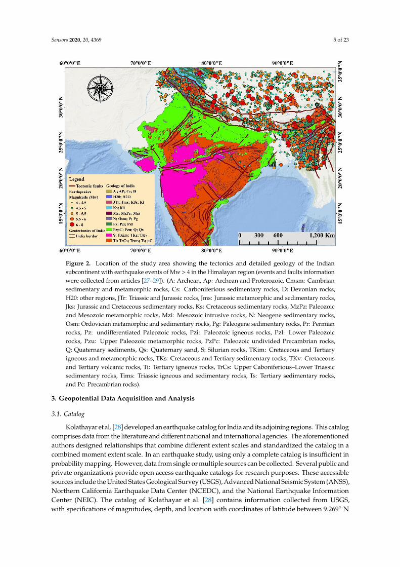
The Himalayas is located in the northern part of the Indian subcontinent, which is seismicallydynamic [26]. The study area is situated at a latitude and longitude of 20.5937◦ N and 78.9629◦ E basedon the WGS 84 geodetic coordinates system, respectively (Figure 2). This area is the seventh-largestnation by territory, the second most populated country in the world. The total population in India is1,324,171,354, and the total country area is 3,287,263 km2 [27]. The most common rock types in theHimalayan Mountains are oceanic and ophiolite rocks. In the past decade, four extraordinary seismictremors (M > 8) occurred along the Himalayas, along with countless moderate-sized quakes. Nearbyseismic systems are confined toward the western Himalayas and the Assam area. Hence, seismictremor hypocenters for the Himalayan earthquakes depend on the teleseismic areas. Nevertheless,the focal depths of these quakes can exhibit errors of up to 50 km. The distortion of the Himalayasis due to the gravitational distribution in the area. The main boundary thrust is the present activefault system of the Himalayan arc based on data recorded by teleseismic earthquakes. Medium-sizedthrust-type quakes suggest that numerous chances of great Himalayan earthquakes can occur alongthe same detachment region.

Sensors 2020, 20, 4369 5 of 23Sensors 2020, 20, x FOR PEER REVIEW 5 of 24

Figure 2. Location of the study area showing the tectonics and detailed geology of the Indian

subcontinent with earthquake events of Mw > 4 in the Himalayan region (events and faults

information were collected from articles [27–29]). (A: Archean, Ap: Archean and Proterozoic, Cmsm:

Cambrian sedimentary and metamorphic rocks, Cs: Carboniferious sedimentary rocks, D: Devonian

rocks, H20: other regions, JTr: Triassic and Jurassic rocks, Jms: Jurassic metamorphic and sedimentary

rocks, Jks: Jurassic and Cretaceous sedimentary rocks, Ks: Cretaceous sedimentary rocks, MzPz:

Paleozoic and Mesozoic metamorphic rocks, Mzi: Mesozoic intrusive rocks, N: Neogene sedimentary

rocks, Osm: Ordovician metamorphic and sedimentary rocks, Pg: Paleogene sedimentary rocks, Pr:

Permian rocks, Pz: undifferentiated Paleozoic rocks, Pzi: Paleozoic igneous rocks, Pzl: Lower

Paleozoic rocks, Pzu: Upper Paleozoic metamorphic rocks, PzPc: Paleozoic undivided Precambrian

rocks, Q: Quaternary sediments, Qs: Quaternary sand, S: Silurian rocks, TKim: Cretaceous and

Tertiary igneous and metamorphic rocks, TKs: Cretaceous and Tertiary sedimentary rocks, TKv:

Cretaceous and Tertiary volcanic rocks, Ti: Tertiary igneous rocks, TrCs: Upper Caboniferious–Lower

Triassic sedimentary rocks, Tims: Triassic igneous and sedimentary rocks, Ts: Tertiary sedimentary

rocks, and Pc: Precambrian rocks).

3. Geopotential Data Acquisition and Analysis

3.1. Catalog

Kolathayar et al. [28] developed an earthquake catalog for India and its adjoining regions. This

catalog comprises data from the literature and different national and international agencies. The

aforementioned authors designed relationships that combine different extent scales and standardized

the catalog in a combined moment extent scale. In an earthquake study, using only a complete catalog

is insufficient in probability mapping. However, data from single or multiple sources can be collected.

Several public and private organizations provide open access earthquake catalogs for research

purposes. These accessible sources include the United States Geological Survey (USGS), Advanced

National Seismic System (ANSS), Northern California Earthquake Data Center (NCEDC), and the

National Earthquake Information Center (NEIC). The catalog of Kolathayar et al. [28] contains

information collected from USGS, with specifications of magnitudes, depth, and location with

Figure 2. Location of the study area showing the tectonics and detailed geology of the Indiansubcontinent with earthquake events of Mw > 4 in the Himalayan region (events and faults informationwere collected from articles [27–29]). (A: Archean, Ap: Archean and Proterozoic, Cmsm: Cambriansedimentary and metamorphic rocks, Cs: Carboniferious sedimentary rocks, D: Devonian rocks,H20: other regions, JTr: Triassic and Jurassic rocks, Jms: Jurassic metamorphic and sedimentary rocks,Jks: Jurassic and Cretaceous sedimentary rocks, Ks: Cretaceous sedimentary rocks, MzPz: Paleozoicand Mesozoic metamorphic rocks, Mzi: Mesozoic intrusive rocks, N: Neogene sedimentary rocks,Osm: Ordovician metamorphic and sedimentary rocks, Pg: Paleogene sedimentary rocks, Pr: Permianrocks, Pz: undifferentiated Paleozoic rocks, Pzi: Paleozoic igneous rocks, Pzl: Lower Paleozoicrocks, Pzu: Upper Paleozoic metamorphic rocks, PzPc: Paleozoic undivided Precambrian rocks,Q: Quaternary sediments, Qs: Quaternary sand, S: Silurian rocks, TKim: Cretaceous and Tertiaryigneous and metamorphic rocks, TKs: Cretaceous and Tertiary sedimentary rocks, TKv: Cretaceousand Tertiary volcanic rocks, Ti: Tertiary igneous rocks, TrCs: Upper Caboniferious–Lower Triassicsedimentary rocks, Tims: Triassic igneous and sedimentary rocks, Ts: Tertiary sedimentary rocks,and Pc: Precambrian rocks).

3. Geopotential Data Acquisition and Analysis

3.1. Catalog

Kolathayar et al. [28] developed an earthquake catalog for India and its adjoining regions. This catalogcomprises data from the literature and different national and international agencies. The aforementionedauthors designed relationships that combine different extent scales and standardized the catalog in acombined moment extent scale. In an earthquake study, using only a complete catalog is insufficient inprobability mapping. However, data from single or multiple sources can be collected. Several public andprivate organizations provide open access earthquake catalogs for research purposes. These accessiblesources include the United States Geological Survey (USGS), Advanced National Seismic System (ANSS),Northern California Earthquake Data Center (NCEDC), and the National Earthquake InformationCenter (NEIC). The catalog of Kolathayar et al. [28] contains information collected from USGS,with specifications of magnitudes, depth, and location with coordinates of latitude between 9.269◦ N

Sensors 2020, 20, 4369 6 of 23

and 37.435◦N and longitude between 66.533◦ E and 97.822◦ E based on the WGS 84 geodetic coordinatesreference system. This distributed earthquake catalog and data from USGS were used to train themodel, predict classifications, and generate the probability map in the present study.

3.2. Local Sources

Local sources refer to the raw data sources in India used in this study. The Geological Survey ofIndia published the seismotectonic atlas [29], which is regarded as an authentic referral for seismicsource identification. Iyengar and Ghosh [30] conducted studies in Delhi and produced a micro-zonationmap of earthquake hazards. Nath et al. [31] performed micro-zonation in Sikkim as a case study.Boominathan et al. [32] conducted earthquake hazard mapping in Chennai using local site effects.Kanth and Iyengar [33] studied seismic hazards in Mumbai. Anbazhagan et al. [34] and Vipin et al. [35]researched seismic probability in Bangalore and South India, respectively. Detailed information aboutlineaments, faults, shear zones, and several features in India was documented by Narula et al. [29].In the present study, a detailed geological map representing earthquake hazards in India and showingfaults, thrusts, and earthquakes stronger than 4 Mw was used to generate several thematic layers andimplemented in CNN model [36,37]. This information, along with lithology information, was processedin the present study through the digitization and georeferencing of available maps using ArcGIS 10.4.and the clustered earthquake information. The final map superimposed all the information preparedin thematic layers. Table 1 summarizes the list of input paramters and their sources.

Table 1. Earthquake probability parameters and their characteristics.

Parameters Data Source Resolution Scale Description

SlopeElevation

DEM (USGS) https://earthexplorer.usgs.gov/

30 m 1:250000 Derived from raster DEM

Fault densityDistance from fault Geological map of India, GSI Derived from image

digitization in ArcGISMagnitude densityEpicenter densityDistance from epicenter

USGS earthquake catalog(https://earthquake.usgs.gov)

Derived using Joyner andBoore (1981), Campbell(1981)

PGA density USGS earthquake catalogPGA can be derived using(MMI = 1/0.3 ∗(log 10 (PGA∗980) − 0.014)

Lithology andamplification factor

Geological map of India, GSI(www.gsi.gov.in),(bhuvan.nrsc.gov.in), (USGSWorld Geologic Map)

Derived from imagedigitization in ArcGIS1. Unknown:12. Hard rock:0.553. Soft rock:0.704. Medium soil:15. Soft soil:1.30

3.3. Thematic Layers

In this study, various thematic layers (Figure A1) were produced after an extensive review of theliterature [38]. An underlying process is linked to an analytic framework to construct a map usinga geographic information system (GIS). The data used in this study does not support choroplethmaps. Cartogram and chorochromatic maps were produced using statistical software, MS Excel,and ArcGIS (http://www.pbcgis.com/normalize/). Probability assessment is challenging withoutselecting appropriate criteria on which the model fully depends upon. To achieve good accuracy inproducing a probability map, the most essential and useful steps are selecting important indicatorsand removing noise and heterogeneity from the data. In this study, freely available 30 m resolutiondigital elevation model (DEM) data was used to generate several layers. The UTM/WGS 1998reference system was used to map and produce thematic layers. The following thematic layers werederived from several sources: Euclidean distance from normal, strike-slip and thrust faults (includingmajor photo lineaments), fault density, lithology with an amplification factor value, slope angle map,elevation, magnitude density, epicenter distance, depth density, distance from the epicenter, and PGA

Sensors 2020, 20, 4369 7 of 23

density [39–42]. The layers were presented in a stretched format starting from negative values topositive values. Table 1 provides an overview of the importance of data layer preparation. These layerscan be understood by uncovering concepts, emerging patterns, themes of objectives, and insight logic.Pre-processing was performed on the basis of the literature [30]. Subsequently, all the layers wereconverted into multiple values by points using GIS tools. All the values for each pixel were producedin an Excel file. Next, some negative and illogical values were removed because they can result in noise.Post-processing was performed after the prediction task was completed for the testing dataset [38].The proposed model predicted the exact values of each pixel. The values were added to the GISdatabase, and a point-to-raster conversion tool was used to produce a raster map, which was classifiedusing the quantile classification technique.

Slope and elevation: Slope and elevation are two main factors used for earthquake potentialzoning and earthquake-induced landslide susceptibility mapping [43]. Rough slopes can be observedin the hilly areas, where fault length and size are controlled by slope inclination [44]. These factorsare quite important because hilly regions are seismically more active with complicated tectonics andstructure as compared to plane lands. Therefore, these are two major input data used in earthquakeprobability estimation.

Fault density and distance from fault: Faults are the main source of earthquakes. High faultdensity denotes the areas with complex tectonics, thus increasing the probability of earthquakes [43].The complex fault system or interconnected active faults can generate a high magnitude and numberof events [45]. Distance from fault is significant because the earthquake potential zones are close tofaults and decrease as the distance from fault increases [46]. In this study, major active faults wereincluded for thematic layer preparation.

Magnitude, PGA, epicenter density, and distance from epicenter: Likelihood of a particularmagnitude, location, depth, and PGA values depend on tectonic condition [43]. Epicenter densityindicates the clustering of events that denotes the probable locations [46]. Epicenter density analysiscould provide a way to focus on a structure’s riftogenesis study, a cluster of large earthquakes, and thelarge active fractures [43]. Such indicators are interlinked to each other because these can provideinformation on ground acceleration associated with several lithology types, maximum magnitudeareas, and low seismic zones with the increase in distance from the earthquake source zone [43].

Lithology and amplification factor: Ground shaking depends on the amplification factor and rocktypes [43]. These are two major indicators because the amplification value of different rock types variesand could create either high or low ground shaking [43,46].

4. Methodology

4.1. CNN Architecture

The architecture of CNN for earthquake prediction of classification consists of a sequential modelwith four convolutional layers, each of which is followed by a dropout and pooling layer. The detailsof the employed CNN layers are described below and presented in Figure 3:

Input layer: Each layer is characterized by a 2D vector. An input sequence of n layers can bepresented by concatenating the mathematical structure with multivalued points. The matrix X ∈ Rd×n,where X is the network input [36].

Convolutional layer: A set of m convolutional filters is attached to this layer, where h is the length.X[i:i+h] indicates the concatenation of all data Xi. to X[i+h]. Therefore, the feature Ci can be applied to afilter F using the following formula [37]:

Ci :=∑k,j

(X[i:i+h]

)k,j

.Fk,j (1)

Sensors 2020, 20, 4369 8 of 23

Sensors 2020, 20, x FOR PEER REVIEW 8 of 24

Ci: = ∑(X[i:i+h])k,jk,j

. Fk,j (1)

Figure 3. Architecture of the convolutional neural network (CNN) model for prediction of earthquake

classification.

The concatenation of all data points in a layer describes the feature vector C ∈ Rn−h+1. Therefore,

C vectors can be aggregated from all m filters into a feature map matrix C ∈ Rm(n−h+1). During the

training phase, the convolution filters within CNN are learned. A nonlinear ReLU activation function

is applied to pass the output of the convolutional layer before entering a pooling layer.

Pooling layer: The aggregation of the input vectors occurred in a pooling layer, which is the

maximum value over a set of non-overlapping intervals. The resulting pooled matrix can be

expressed as C pooled ∈ Rm×(n−h+1/s), where s is the length of each interval. However, when the

stride value st is observed in the case of overlapping intervals, the pooled matrix can be presented

as C pooled ∈ Rm×(n−h+1−s/st). The fraction result is rounded up or down, depending on the inclusion

of the boundaries.

Hidden layer: A fully connected hidden layer is located at the end of the four convolutional

layers. This layer computes the transformation ∝ (W × x + b), where the weight matrix is expressed

as W ∈ Rm×m, the bias can be estimated as b ∈ Rm, and the ReLU function is ∝. Consequently, the

output can be presented as the x ∈ Rm of this layer, which is similar to the mathematical structure of

the input data [38].

Softmax: A softmax regression layer is connected to the outputs of the previous layer x ∈ Rm,

which provides the largest probability values as ŷ ∈ [1, K] and can be expressed as:

ŷ = arg maxj P(y = j|x, w, a) (2)

= arg maxj 𝐞

𝐱𝐰𝐣+𝐚𝐣𝐭

∑ 𝐞𝐱𝐰𝐣+𝐚𝐣

𝐭𝐤𝐤=𝟏

(3)

where wj indicates the weight vector of class j, from which the dot product can be generated with

the input, and aj is the bias of class j.

Optimization: The CNN parameters are learned using the Adam optimizer. The validation and

parameters with the highest value should be computed and selected, respectively, at a fixed interval.

Loss estimation: The loss function is also called the cost function. This function measures the

compatibility among output predictions and uses ground truth labels. In this model, a sparse categorical

cross-entropy function is implemented as the loss function, which is beneficial for binary classification.

However, the mean square error of the continuous values is applied to the regression. One of the

hyperparameters is a loss function that can be determined on the basis of the given tasks.

Network parameters: The parameters learned during the training are as follows: 𝜃 =

{𝑋, 𝐹1, 𝑏1, 𝐹2, 𝑏2, 𝑊, 𝑎} (with X is the input data point matrix), where a d-dimensional vector can be

Figure 3. Architecture of the convolutional neural network (CNN) model for prediction ofearthquake classification.

The concatenation of all data points in a layer describes the feature vector C ∈ Rn−h+1. Therefore,C vectors can be aggregated from all m filters into a feature map matrix C ∈ Rm(n−h+1). During thetraining phase, the convolution filters within CNN are learned. A nonlinear ReLU activation functionis applied to pass the output of the convolutional layer before entering a pooling layer.

Pooling layer: The aggregation of the input vectors occurred in a pooling layer, which is themaximum value over a set of non-overlapping intervals. The resulting pooled matrix can be expressedas C pooled ∈ Rm×(n−h+1/s), where s is the length of each interval. However, when the stridevalue st is observed in the case of overlapping intervals, the pooled matrix can be presented asC pooled ∈ Rm×(n−h+1−s/st). The fraction result is rounded up or down, depending on the inclusion of

the boundaries.Hidden layer: A fully connected hidden layer is located at the end of the four convolutional

layers. This layer computes the transformation ∝ (W× x + b), where the weight matrix is expressed asW ∈ Rm×m, the bias can be estimated as b ∈ Rm, and the ReLU function is ∝. Consequently, the outputcan be presented as the x ∈ Rm of this layer, which is similar to the mathematical structure of theinput data [38].

Softmax: A softmax regression layer is connected to the outputs of the previous layer x ∈ Rm,which provides the largest probability values as y ∈ [1, K] and can be expressed as:

y = arg maxj P(y = j|x, w, a) (2)

= arg maxjext

wj+aj∑kk=1 e

xtwj+aj

(3)

where wj indicates the weight vector of class j, from which the dot product can be generated with theinput, and aj is the bias of class j.

Optimization: The CNN parameters are learned using the Adam optimizer. The validation andparameters with the highest value should be computed and selected, respectively, at a fixed interval.

Loss estimation: The loss function is also called the cost function. This function measuresthe compatibility among output predictions and uses ground truth labels. In this model, a sparsecategorical cross-entropy function is implemented as the loss function, which is beneficial for binaryclassification. However, the mean square error of the continuous values is applied to the regression.One of the hyperparameters is a loss function that can be determined on the basis of the given tasks.

Network parameters: The parameters learned during the training are as follows: θ =

{X, F1, b1, F2, b2, W, a} (with X is the input data point matrix), where a d-dimensional vectorcan be found in each row for a specific layer; Fi and bi are used as the convolutional layer’s filter

Sensors 2020, 20, 4369 9 of 23

weights and biases, respectively; and W and a are the weight matrices in the softmax layer for theoutput classes.

4.2. Learning the Model Parameters and Performance

The parameters of the CNN model were learned through a three-phase procedure: (1) creation ofdata point embedding; (2) distant supervised phase, wherein the parameters are tuned by training,and; (3) final supervised phase, wherein the training is performed using the supervised training data [37].In the distant supervised phase, heuristic techniques were used to reduce noise in the data points.This process can be regarded as a pretraining procedure to eliminate data noise and improve accuracy.The pretraining phase datasets do not necessarily overlap to generate the input embedding. CNN wastrained for 1 epoch on this dataset before the final supervised training of 100 epochs. The weight of thedata layers was updated in the distant and supervised training phases through backpropagation.

Accuracy is a simple measure of a classifier’s performance [36,37].

Accuracy =Number of correctly labeled samples

Number of all testing samples(4)

The F1 score is computed from the precision and recall (i.e., the harmonic mean) of each class.

F1 =

precision−1 + recall−1

2

−1

(5)

4.3. PGA, Source to Site Distance and Intensity Calculation

The earthquake catalog from USGS was used to estimate PGA based on the attenuation equationprovided by Joyner and Boore [39]. The source to site distance was calculated using the epicentraldistance provided in Equation (6). To estimate the intensity variation for the proposed study area,Equation (8) was used. Several attenuation equations have been proposed by various researchers,however, the current study applied the developed equation by Joyner and Boore [39]. Therefore,D value can be calculated using the formula written below:

D = (Eˆ2 + 7.3ˆ2) ˆ0.5 (6)

where, E = Epicentral distance; and D = source to site distance.According to Joyner and Boore [39], PGA can be calculated using the equation presented below:

PGA = 10ˆ(0.249∗M− Log(D) − 0.00255∗D− 1.02, D = (Eˆ2 + 7.3ˆ2)ˆ0.5 (7)

where, M = Earthquake magnitude, R= Radius from the epicenter to the location. There are severalother attenuation relationships which could be implemented in probabilistic hazard analysis [40–42].The most popular general equation of regression by Boore and Joyner [39] is used for regional andworldwide datasets for probabilistic analysis. Therefore, MMI (Modified Mercalli Intensity) could beestimated using the formula:

MMI = 1/0.3 ∗ (log 10 (PGA∗980) − 0.014 (8)

where, the PGA unit is G (Gal).Three main thematic layers were obtained such as MMI variation, PGA variation, and lithology

with an amplification factor map using GIS along with several other layers from the same dataset. Firstly,various attributes of earthquakes were investigated in detail as per the requirement of earthquakeprobability assessment. Secondly, PGA and MMI were calculated based on the employed attenuationlaws and implemented in GIS. PGA density map and intensity variation layers were utilized in

Sensors 2020, 20, 4369 10 of 23

earthquake probability mapping and hazard estimation. Several lithological units were extracted fromthe geological map and assigned amplification factor values to each unit to generate another thematiclayer. The detailed information regarding the implementation of the CNN model and attenuation lawsto generate the earthquake probability map was described in Section 5.

5. CNN Model Implementation for Prediction and Probability Mapping

The detailed methodological flowchart of the employed model is shown in Figure 4.The implemented supervised classifier was trained using 75% of the spectrograms (training set)on a random subset, and performance was evaluated in terms of two-class classification. The traineddataset comprised 500 samples, with 350 and 150 samples used for training and validation, respectively.Once the model achieves good accuracy, the model is considered as well-trained. The selecteddatasets (20 million points) for testing all of India depend on the training sets that were used forprobability assessment.

Sensors 2020, 20, x FOR PEER REVIEW 10 of 24

5. CNN Model Implementation for Prediction and Probability Mapping

The detailed methodological flowchart of the employed model is shown in Figure 4. The

implemented supervised classifier was trained using 75% of the spectrograms (training set) on a

random subset, and performance was evaluated in terms of two-class classification. The trained

dataset comprised 500 samples, with 350 and 150 samples used for training and validation,

respectively. Once the model achieves good accuracy, the model is considered as well-trained. The

selected datasets (20 million points) for testing all of India depend on the training sets that were used

for probability assessment.

Figure 4. Methodological flowchart of the CNN model for earthquake probability assessment.

In the first step, a comprehensive earthquake catalog was collected from USGS. Then, several

random non-earthquake points were created to train the CNN classifier using GIS. Nine different

indicators were used to extract multiple values by points and by keeping earthquake and non-

earthquake as the target (Figure 4). In the second step, A CNN model was designed for earthquake

prediction of two classes (0,1) that can continuously scan through several input indicators and

convolutional layers and classify earthquake (1) and non-earthquake (0) values. After inspecting and

discarding irrelevant data, the final dataset contained 250 earthquakes during the training period.

The Adam optimizer was utilized to optimize the model, and then batch size (100), validation split

(0.2), and verbose (1) were applied to avoid overfitting epochs (100). A total of 123,002 parameters

were collected during training, all of which were trainable. The classifier predicted the target as 0 and

1 in the training and testing datasets for 500 points, respectively. Among the 500 points, 250 points

were earthquakes and the rest were non-earthquakes. In the third step, post-processing was

conducted to convert the pixels to raster to generate the probability map.

Figure 4. Methodological flowchart of the CNN model for earthquake probability assessment.

In the first step, a comprehensive earthquake catalog was collected from USGS. Then, severalrandom non-earthquake points were created to train the CNN classifier using GIS. Nine differentindicators were used to extract multiple values by points and by keeping earthquake and non-earthquakeas the target (Figure 4). In the second step, A CNN model was designed for earthquake prediction oftwo classes (0,1) that can continuously scan through several input indicators and convolutional layersand classify earthquake (1) and non-earthquake (0) values. After inspecting and discarding irrelevant

Sensors 2020, 20, 4369 11 of 23

data, the final dataset contained 250 earthquakes during the training period. The Adam optimizer wasutilized to optimize the model, and then batch size (100), validation split (0.2), and verbose (1) wereapplied to avoid overfitting epochs (100). A total of 123,002 parameters were collected during training,all of which were trainable. The classifier predicted the target as 0 and 1 in the training and testingdatasets for 500 points, respectively. Among the 500 points, 250 points were earthquakes and the restwere non-earthquakes. In the third step, post-processing was conducted to convert the pixels to rasterto generate the probability map.

The spatial layers generated for probability mapping were elevation, slope, lithology with anamplification factor, magnitude density, PGA density, depth density, distance from epicenter, distancefrom fault, and fault density (Table 1). Training was performed by splitting the data into training (75%)and testing sets (25%), normalizing and defining the variables, constructing and optimizing the model,and compiling the results for loss estimation [38]. Highly accurate prediction values can be obtainedby applying the testing set. In this study, the number of earthquakes was determined by filtering themagnitude of quakes to higher than 4.5 within the period of 1900–2019 because low-magnitude eventscan be attributed to human activities and may not be destructive. There is no problem with the numberof indicators to be used in a deep learning model. It has the capacity to run a huge number of indicators.However, model accuracy depends on the importance and weights of the factors. Therefore, severalauthors achieved low accuracy by applying unrelated factors in previous studies [38–44]. Therefore,these studies achieved low accuracy due to data heterogeneity and unrelated factors, which wereremoved from the study, applied nine major and useful factors, and described the importance of eachfactor in Table 1. Therefore, several layers from the study were removed such as aspect, hill shade,epicenter density, etc. This model was a predictive analysis-based probability assessment, whereintwo classes were predicted. Then, the values for each pixel in the study area were predicted usingthe testing dataset. Each pixel value was converted into pixels using GIS to generate a probabilitymap. The value for the probability map varies from 0 to 1. As probability varies between 0 and 1,then earthquakes (1) and non-earthquakes (0), while the pixels are not falling within these two classes,have a value between 0 to 1. Therefore, the map presented below is an unclassified probability mapshowing earthquakes and non-earthquakes. However, this model attempts to learn the associatedgeneral characteristics of earthquake and non-earthquake parameters from the indicators. Given thatsome thematic layers were prepared through GIS digitization, irrelevant pixel values originated canaffect model performance. However, network performance can be further improved by applying allmajor indicators and noise removal techniques. Model performance was presented through graphs.Figure 5 shows the estimated loss and accuracy, and Table 2 lists the parameter details.

6. Results

6.1. CNN Classification and Bi-histogram Results

Major earthquake scenarios experienced in the past 200 years in the Indian subcontinent withmagnitudes 7.0 to 8.0 and above were also included in the current study. Bi-histogram provides arelationship between magnitude, intensity, and frequency (Figure 6). In total, 11 bins formed for boththe variables. Normal fit for both the magnitude and intensity shows the mirror reflection of eachother. However, the kernel density of both variables does not project mirror reflection. Therefore,it reflects that the frequency varies for both the variables differently. The conversion of magnitude tointensity depends on the source-site distance. If the distance is less, then intensity could be higherfor low magnitude events and extreme for high magnitude earthquakes. Similarly, if the distanceis huge, then intensity could be lower for high magnitude events and negligible for low magnitudeearthquakes. Therefore, the intensity values obtained in the current study applied to produce thematiclayers as an indicator to generate a hazard map in the future.

Sensors 2020, 20, 4369 12 of 23

Sensors 2020, 20, x FOR PEER REVIEW 12 of 24

Table 2. CNN model parameters for prediction.

Layer (Type) Output Shape Parameter

dense_1 (Dense) (None, 200) 2000

dropout_1 (None, 200) 0

dense_2 (Dense) (None, 200) 40200

dropout_2 (None, 200) 0

dense_3 (Dense) (None, 200) 40200

dropout_3 (None, 200) 0

dense_4 (Dense) (None, 200) 40200

dropout_4 (None, 200) 0

dense_4 (Dense) (None, 2) 402

Input number of units = 9

Output = 2

Hidden units = 200

Kernel regularizer = l2(0.0001)

Activation = ‘relu’

Activation = ‘softmax’

Total params: 123,002

Trainable params: 123,002

Non-trainable params: 0

Figure 5. (a) Accuracy and (b) loss estimation of the CNN model for earthquake prediction.

a)

b)

Figure 5. (a) Accuracy and (b) loss estimation of the CNN model for earthquake prediction.

Table 2. CNN model parameters for prediction.

Layer (Type) Output Shape Parameter

dense_1 (Dense) (None, 200) 2000

dropout_1 (None, 200) 0

dense_2 (Dense) (None, 200) 40,200

dropout_2 (None, 200) 0

dense_3 (Dense) (None, 200) 40,200

dropout_3 (None, 200) 0

dense_4 (Dense) (None, 200) 40,200

dropout_4 (None, 200) 0

dense_4 (Dense) (None, 2) 402

Input number of units = 9Output = 2Hidden units = 200Kernel regularizer = l2(0.0001)Activation = ‘relu’Activation = ‘softmax’Total params: 123,002Trainable params: 123,002Non-trainable params: 0

Sensors 2020, 20, 4369 13 of 23

Sensors 2020, 20, x FOR PEER REVIEW 13 of 24

6. Results

6.1. CNN Classification and Bi-histogram Results

Major earthquake scenarios experienced in the past 200 years in the Indian subcontinent with

magnitudes 7.0 to 8.0 and above were also included in the current study. Bi-histogram provides a

relationship between magnitude, intensity, and frequency (Figure 6). In total, 11 bins formed for both

the variables. Normal fit for both the magnitude and intensity shows the mirror reflection of each

other. However, the kernel density of both variables does not project mirror reflection. Therefore, it

reflects that the frequency varies for both the variables differently. The conversion of magnitude to

intensity depends on the source-site distance. If the distance is less, then intensity could be higher for

low magnitude events and extreme for high magnitude earthquakes. Similarly, if the distance is huge,

then intensity could be lower for high magnitude events and negligible for low magnitude

earthquakes. Therefore, the intensity values obtained in the current study applied to produce

thematic layers as an indicator to generate a hazard map in the future.

Figure 6. Bi-histogram of magnitude and intensity comparison using frequency that is used for

probability assessment (Mw: moment magnitude, MMI: modified Mercalli intensity scale).

The strong quakes that happened in India are the source locations that can produce future events

in accordance with active faults. Previous quakes, such as Kutch (Mw = 8.3), Assam (Mw = 8.7),

Kangra (Mw = 8.1), Bihar–Nepal (Mw = 8.3), and Assam (Mw = 8.6), are moving closer to the high

hazard zones. Training is a major component of the CNN model to achieve an accurate result.

Therefore, training and testing accuracies were calculated after the performance evaluation of the

proposed CNN framework, reaching 96% and 92%, respectively. The estimated loss from this model

was compared against the epochs. The obtained baseline error was 7.95%, and the final accuracy was

92.05%. The confusion matrix (Table 3) and the classification report (Table 4) targeting two classes

presented, respectively. The false negatives in the confusion matrix did not follow any patterns. The

result shows that the precision, recall, F1 score, and support for non-earthquake (0) and earthquake

(1) classes were 0.98, 0.85, 0.91, and 71 and 0.88, 0.99, 0.93, and 80, respectively. The micro average

and weighted average were also calculated and summarized in Table 4.

Figure 6. Bi-histogram of magnitude and intensity comparison using frequency that is used forprobability assessment (Mw: moment magnitude, MMI: modified Mercalli intensity scale).

The strong quakes that happened in India are the source locations that can produce future eventsin accordance with active faults. Previous quakes, such as Kutch (Mw = 8.3), Assam (Mw = 8.7), Kangra(Mw = 8.1), Bihar–Nepal (Mw = 8.3), and Assam (Mw = 8.6), are moving closer to the high hazard zones.Training is a major component of the CNN model to achieve an accurate result. Therefore, training andtesting accuracies were calculated after the performance evaluation of the proposed CNN framework,reaching 96% and 92%, respectively. The estimated loss from this model was compared against theepochs. The obtained baseline error was 7.95%, and the final accuracy was 92.05%. The confusionmatrix (Table 3) and the classification report (Table 4) targeting two classes presented, respectively.The false negatives in the confusion matrix did not follow any patterns. The result shows that theprecision, recall, F1 score, and support for non-earthquake (0) and earthquake (1) classes were 0.98,0.85, 0.91, and 71 and 0.88, 0.99, 0.93, and 80, respectively. The micro average and weighted averagewere also calculated and summarized in Table 4.

Table 3. Confusion matrix for the prediction model.

Predicted

Positive Negative

Actual Positive 60 11

Negative 1 79

Table 4. Performance of the developed CNN model.

ClassificationReport

Precision Recall F1 Score Support

0 0.98 0.85 0.91 71

1 0.88 0.99 0.93 80

Micro average 0.92 0.92 0.92 151

Micro average 0.93 0.92 0.92 151

Weighted average 0.93 0.92 0.92 151

Prediction accuracy: 0.920530

Sensors 2020, 20, 4369 14 of 23

The CNN model’s accuracy reached 92.05% for the testing dataset. Tables 3 and 4 present thedetails of the accuracy, error, and confusion matrices. The loss was estimated and plotted against theepochs. Loss decreases with an increase in the number of epochs. The predicted earthquakes wereclassified under the high- to very-high-hazard zones, indicating that the results are correct and useful.

6.2. Probability Mapping

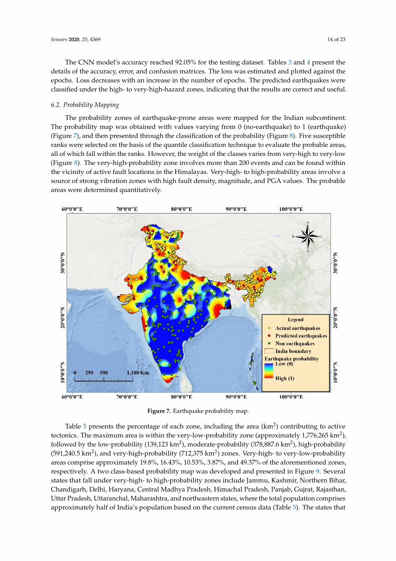
The probability zones of earthquake-prone areas were mapped for the Indian subcontinent.The probability map was obtained with values varying from 0 (no-earthquake) to 1 (earthquake)(Figure 7), and then presented through the classification of the probability (Figure 8). Five susceptibleranks were selected on the basis of the quantile classification technique to evaluate the probable areas,all of which fall within the ranks. However, the weight of the classes varies from very-high to very-low(Figure 8). The very-high-probability zone involves more than 200 events and can be found withinthe vicinity of active fault locations in the Himalayas. Very-high- to high-probability areas involve asource of strong vibration zones with high fault density, magnitude, and PGA values. The probableareas were determined quantitatively.Sensors 2020, 20, x FOR PEER REVIEW 15 of 24

Figure 7. Earthquake probability map.

Table 5 presents the percentage of each zone, including the area (km2) contributing to active

tectonics. The maximum area is within the very-low-probability zone (approximately 1,776,265 km2),

followed by the low-probability (139,123 km2), moderate-probability (378,887.6 km2), high-

probability (591,240.5 km2), and very-high-probability (712,375 km2) zones. Very-high- to very-low-

probability areas comprise approximately 19.8%, 16.43%, 10.53%, 3.87%, and 49.37% of the

aforementioned zones, respectively. A two class-based probability map was developed and

presented in Figure 9. Several states that fall under very-high- to high-probability zones include

Jammu, Kashmir, Northern Bihar, Chandigarh, Delhi, Haryana, Central Madhya Pradesh, Himachal

Pradesh, Panjab, Gujrat, Rajasthan, Uttar Pradesh, Uttaranchal, Maharashtra, and northeastern states,

where the total population comprises approximately half of India’s population based on the current

census data (Table 5). The states that fall under the moderate- to very-low-probability zones are

Tamilnadu, Kerala, Odisha, West Bengal, Chhattisgarh, Andhra Pradesh, Karnataka, the western part

of Madhya Pradesh, Eastern Rajasthan, Central Bihar, Jharkhand, and some North Indian states.

Table 5. Earthquake probable areas in km2 and percentage.

Class No. Probability Classes Shape Length (km) Area (km2) Area (%)

1 Very-high 19,788.24 712,375 19.8

2 High 22,309.64 591,240.5 16.43

3 Moderate 26,041.08 37,8887.6 10.53

4 Low 30,004.07 139,123.1 3.87

5 Very-low 25,599.15 1,776,265 49.37

Total 3,597,891 100

Figure 7. Earthquake probability map.

Table 5 presents the percentage of each zone, including the area (km2) contributing to activetectonics. The maximum area is within the very-low-probability zone (approximately 1,776,265 km2),followed by the low-probability (139,123 km2), moderate-probability (378,887.6 km2), high-probability(591,240.5 km2), and very-high-probability (712,375 km2) zones. Very-high- to very-low-probabilityareas comprise approximately 19.8%, 16.43%, 10.53%, 3.87%, and 49.37% of the aforementioned zones,respectively. A two class-based probability map was developed and presented in Figure 9. Severalstates that fall under very-high- to high-probability zones include Jammu, Kashmir, Northern Bihar,Chandigarh, Delhi, Haryana, Central Madhya Pradesh, Himachal Pradesh, Panjab, Gujrat, Rajasthan,Uttar Pradesh, Uttaranchal, Maharashtra, and northeastern states, where the total population comprisesapproximately half of India’s population based on the current census data (Table 5). The states that

Sensors 2020, 20, 4369 15 of 23

fall under the moderate- to very-low-probability zones are Tamilnadu, Kerala, Odisha, West Bengal,Chhattisgarh, Andhra Pradesh, Karnataka, the western part of Madhya Pradesh, Eastern Rajasthan,Central Bihar, Jharkhand, and some North Indian states.Sensors 2020, 20, x FOR PEER REVIEW 16 of 24

Figure 8. Classified earthquake probability map of India.

Approximately 92% of predicted earthquake classes fall within the Himalayan zones (high- to

very-high-hazard zones). These probable zones provide a holistic view, which is an integration of

several parameters without considering a particular context of the scenario. This finding explains the

severity of earthquake hazards that can originate from these regions in the future and provides an

alarming view to local and national authorities with respect to necessary preparations for the worst

situations with a gradual time course.

Figure 8. Classified earthquake probability map of India.

Table 5. Earthquake probable areas in km2 and percentage.

Class No. Probability Classes Shape Length (km) Area (km2) Area (%)

1 Very-high 19,788.24 712,375 19.82 High 22,309.64 591,240.5 16.433 Moderate 26,041.08 37,8887.6 10.534 Low 30,004.07 139,123.1 3.875 Very-low 25,599.15 1,776,265 49.37

Total 3,597,891 100

Approximately 92% of predicted earthquake classes fall within the Himalayan zones (high- tovery-high-hazard zones). These probable zones provide a holistic view, which is an integration ofseveral parameters without considering a particular context of the scenario. This finding explains theseverity of earthquake hazards that can originate from these regions in the future and provides analarming view to local and national authorities with respect to necessary preparations for the worstsituations with a gradual time course.

Sensors 2020, 20, 4369 16 of 23Sensors 2020, 20, x FOR PEER REVIEW 17 of 24

Figure 9. Two class-based scheme earthquake probability in all the states of India.

6.3. Result Validation

The validation of results was conducted using a published seismotectonic zonation map and

experts’ feedback. Sitharam et al. [26] reported the estimation of earthquake hazards at the surface

level by applying necessary amplification factors with respect to several site classes based on the VS30

values obtained from the topographic gradient. They obtained a PHA at the surface level, wherein

the return periods are 475 and 2475 years (presented in contour maps).

Vipin et al. [35] estimated a seismic hazard in South India by implementing a probabilistic

seismic hazard analysis. The seismic hazard map of India produced using GSI and the old seismic

micro-zonation map of India show that the developed probability map is accurate and can be used

in future studies on hazard and risk assessments. Five experts’ opinions were also considered to check

the quality of the generated map (Table 6). Out of the five experts, four were highly satisfied (80%)

with the obtained results and one was satisfied (20%).

Figure 9. Two class-based scheme earthquake probability in all the states of India.

6.3. Result Validation

The validation of results was conducted using a published seismotectonic zonation map andexperts’ feedback. Sitharam et al. [26] reported the estimation of earthquake hazards at the surfacelevel by applying necessary amplification factors with respect to several site classes based on the VS30

values obtained from the topographic gradient. They obtained a PHA at the surface level, wherein thereturn periods are 475 and 2475 years (presented in contour maps).

Vipin et al. [35] estimated a seismic hazard in South India by implementing a probabilisticseismic hazard analysis. The seismic hazard map of India produced using GSI and the old seismicmicro-zonation map of India show that the developed probability map is accurate and can be used infuture studies on hazard and risk assessments. Five experts’ opinions were also considered to checkthe quality of the generated map (Table 6). Out of the five experts, four were highly satisfied (80%)with the obtained results and one was satisfied (20%).

Table 6. Experts’ profile and feedback on the probability results.

Category No. ofExperts Profession Specialization Recruitment Process Validation Criteria Feedback

Researchers 5

Seismologist,geologist,hydrologist,GIS analyst,soilphysicist,geotechnicalresearcher

Researcher onnatural hazardsusing GIS andremote sensing,monitoring,mapping, GIS,artificialintelligence

• Deep learningapplication toearthquake prediction

• Geological mappingwith sensitivity

• Expert in local andregional earthquakeprobability andrisk assessment

• Dataanalysis expertise

• Published goodarticles inhigh-impact journals

• Probabilitydeterminants

• Representationof spatial maps

• Expecteduncertainties

• Map validationusing old mapsby GSI

• Results• Communica

bility• Usefulness to

landuse planning

• Benefit tolocal people

• Fourexperts arehighlysatisfied(80%)

• One expertis satisfied(20%)

Sensors 2020, 20, 4369 17 of 23

7. Discussion

The associated earthquake probability with peninsular India was evaluated using a CNN modelthat was described in the implementation section of this paper. While integrating uncertaintiesassociated with various modeling parameters, the most recent knowledge on seismic activity in theIndian subcontinent was applied to estimate probability. Uncertainties related to data that can be linkedto a catalog or existing probable factors or other parameters involved in hazard analysis. The discussionpart describes the comparison of old probabilistic results and seismic zoning maps with the obtainedearthquake probability map. Most traditional techniques are poorly designed for low-magnitudeevents and do not record seismicity [47]. The objective of the current study is to develop a probabilityassessment model for independent earthquakes based on several indicators. A deep learning techniquewas proposed to achieve robust accuracy for probability assessment. However, CNN’s learning abilitycan vary with changes in the parameters [48]. Therefore, the sensitivity of the model was analyzed byapplying changes to the convolutional layer filters and adopting various activation functions. Severalsignificant changes were observed in the model’s performance. The model that exhibited the mostsatisfactory performance was selected. To avoid over-training, dropout rates were set as 0.2 and 0.1 forthe convolutional and input layers, respectively, to facilitate the network in learning and performinga robust training process. The applied dropout rate exhibits the best trade-off between validationaccuracy and training data misfit.

Khattri et al. [49] developed the first probabilistic seismic hazard map of the Indian subcontinent.They divided the region into 24 seismic sources for hazard parameter estimation based on peakacceleration for 50 years, wherein the exceedance probability was 10%. However, the intensity valuesfor hazard estimation were not used in the present study. Instead, an earthquake probability map basedon predictive analysis was presented. Khattri et al. [49] reported that a maximum peak accelerationof 0.8 g was expected in the northeast region, and the value varied from 0.03 g to 0.04 g in thesouth, southeastern, and central parts. Similar values were observed for Northeast and Central India.On average, the PGA values of the Himalayan region varied from 0.5 to 1.01 (Figure 7). Bhatia et al. [50]developed another probabilistic seismic hazard map for India. The hazard level was estimated on thebasis of the PGA values after locating 86 potential sources based on seismicity trends and major tectonicfeatures. Joyner and Boore’s [51] attenuation equation was applied to this probabilistic assessment.Aman et al. [52] and Singh et al. [53] performed a probabilistic assessment in the Himalayan regions,and the two groups of researchers achieved similar results. Lyubushin and Parvez [54] applied a purelystatistical procedure for probability assessment. However, the present study did not focus on hazards.

The probability assessment was completed on the basis of nine factors (Table 1). Figure 8 presentsthe results of the predictive analysis-based probability assessment and the probability map. Accordingto the literature, CNN is one of the most reliable models for probability assessment; ANN provides anaccuracy of 84%. The proposed technique performs better than ANN prediction while significantlyreducing processing time and improving efficiency. In addition to event prediction, the proposedapproach provides the best estimates of probability from the events that already occurred. The plot ofthe probable classes (with area and shape length) explains the variation in the probability with respectto distance and area (Figure 10).

The objective was to produce an earthquake probability map based on experienced events. In thisstudy, the authors did not implement any technique to predict events based on magnitudes, intensity,time, or location. This study is a prediction of classification-based probability assessment; therefore,the areas close to the experienced events will be the probable areas for earthquakes. First, pixels closeto the predicted classes can be interpolated to generate a probability map. Second, the entire area canbe converted into points for testing using the same model to obtain the pixel values for each point andgenerate a probability map. Both techniques are effective; however; the second one is more accurate thanthe first one. In accordance with the old hazard map of India, the Himalayan region belongs to Zone V,which includes Gujarat State in the west, and some cities belong to Zone IV. However, in accordance withthe seismic zoning map of India (BIS, 2002), a large part of the Narmada lineament region spreads up

Sensors 2020, 20, 4369 18 of 23

to the northern part of the Godavari graben (https://law.resource.org/pub/in/bis/S03/is.1893.1.2002.pdf).Therefore, the hazard estimated in this region is higher in contrast with the Indian Standard code.The current study of probability mapping is linked to the hazard map, which is under Zone IV but withlow probability. Southern portions, including Tamil Nadu, are under passive margin and exhibit higherground motion based on the hazard map (Zone III) while presenting low probability in accordance withthe obtained map. The western portions of some states, such as Bengal and Orissa, and the westernpart of Madhya Pradesh, Chhattisgarh, Andhra Pradesh, and Karnataka are estimated as moderate tolow probability and low hazard zones on the basis of the seismic zoning map (Figure 10). Therefore,these areas are considered the stable shield of peninsular India. However, the resulting probable areasare nearly similar to other parts of the hazard map of India. The resultant earthquake probabilitymap indicates that priority should be focused on the Central Himalayas and Northwest, Northeast,and Shillong areas of the Indian subcontinent; because of the complicated tectonics and active faults inareas where no large earthquake has occurred since the 2011 Sikkim earthquake. Other priority areasexperienced mild events such as Maharashtra, Kachchh region, cratonic regions, and rift basins in Indiathat can be considered for future hazard and risk studies. A national database of active faults shouldbe created, and event prediction should be initiated using GIS [55]. The database would enhancethe geological and earthquake hazard-related issues under different tectonic settings using machinelearning techniques [56,57].

Sensors 2020, 20, x FOR PEER REVIEW 19 of 24

The probability assessment was completed on the basis of nine factors (Table 1). Figure 8

presents the results of the predictive analysis-based probability assessment and the probability map.

According to the literature, CNN is one of the most reliable models for probability assessment; ANN

provides an accuracy of 84%. The proposed technique performs better than ANN prediction while

significantly reducing processing time and improving efficiency. In addition to event prediction, the

proposed approach provides the best estimates of probability from the events that already occurred.

The plot of the probable classes (with area and shape length) explains the variation in the probability

with respect to distance and area (Figure 10).

The objective was to produce an earthquake probability map based on experienced events. In

this study, the authors did not implement any technique to predict events based on magnitudes,

intensity, time, or location. This study is a prediction of classification-based probability assessment;

therefore, the areas close to the experienced events will be the probable areas for earthquakes. First,

pixels close to the predicted classes can be interpolated to generate a probability map. Second, the

entire area can be converted into points for testing using the same model to obtain the pixel values

for each point and generate a probability map. Both techniques are effective; however; the second

one is more accurate than the first one. In accordance with the old hazard map of India, the

Himalayan region belongs to Zone V, which includes Gujarat State in the west, and some cities belong

to Zone IV. However, in accordance with the seismic zoning map of India (BIS, 2002), a large part of

the Narmada lineament region spreads up to the northern part of the Godavari graben

(https://law.resource.org/pub/in/bis/S03/is.1893.1.2002.pdf). Therefore, the hazard estimated in this

region is higher in contrast with the Indian Standard code. The current study of probability mapping

is linked to the hazard map, which is under Zone IV but with low probability. Southern portions,

including Tamil Nadu, are under passive margin and exhibit higher ground motion based on the

hazard map (Zone III) while presenting low probability in accordance with the obtained map. The

western portions of some states, such as Bengal and Orissa, and the western part of Madhya Pradesh,

Chhattisgarh, Andhra Pradesh, and Karnataka are estimated as moderate to low probability and low

hazard zones on the basis of the seismic zoning map (Figure 10). Therefore, these areas are considered

the stable shield of peninsular India. However, the resulting probable areas are nearly similar to other

parts of the hazard map of India. The resultant earthquake probability map indicates that priority

should be focused on the Central Himalayas and Northwest, Northeast, and Shillong areas of the

Indian subcontinent; because of the complicated tectonics and active faults in areas where no large

earthquake has occurred since the 2011 Sikkim earthquake. Other priority areas experienced mild

events such as Maharashtra, Kachchh region, cratonic regions, and rift basins in India that can be

considered for future hazard and risk studies. A national database of active faults should be created,

and event prediction should be initiated using GIS [55]. The database would enhance the geological

and earthquake hazard-related issues under different tectonic settings using machine learning

techniques [56,57].

Figure 10. Graphical presentation of probability among classes, area, and distance.

Very high High Moderate Low Very low

0

5,000

10,000

15,000

20,000

25,000

30,000

0

200000

400000

600000

800000

1000000

1200000

1400000

1600000

1800000

2000000

0 1 2 3 4 5 6

SH

AP

E L

EN

GT

H (

KM

)

AR

EA

(K

M2 )

Figure 10. Graphical presentation of probability among classes, area, and distance.

8. Conclusions

On the basis of the recent advances in deep learning, a CNN model was proposed to achieve arobust prediction of experienced earthquake events to address the shortcomings of existing methodsand develop a probability map for the Indian subcontinent. In the current study, the authorsattempted to estimate the probable areas (spatial) for future earthquakes. The final probability mapachieved an accuracy of 92.05%. Therefore, the proposed model is superior to traditional methods forearthquake probability assessment in terms of accuracy. From the results, very-high (712,375 km2)and high (591,240.5 km2) probability areas consist of 19.8% and 16.43% of the aforementioned zones,respectively. The limitation of this study includes the implementation of CNN, which is time- anddata-consuming, particularly the training data. This study is limited to earthquake figure probabilityassessment. The geological and deep learning constraints presented in this research are insufficient forprobability mapping. The detailed analysis of factors, including geophysical and precursor studies,could be enhanced to improve the accuracy of the probability assessment. Several assumptionswere made and model parameter modification was performed during the entire process, such as theselection of earthquakes with more than 4.5 Mw, distance criteria, including maximum magnitude

Sensors 2020, 20, 4369 19 of 23

scenarios, removal of unwanted thematic layers, and the weighting scheme within the CNN model.The earthquake probability map presented in this study is intended to highlight nine influencingparameters that can be changed further with geophysical, geomorphologic, seismic, and field data.The probability map based on CNN can be useful for earthquake hazard and risk mapping, mitigation,land use planning, and other related applications. Understanding the relative importance of theapplied factors is crucial for further studies. This study can further support hazard and mitigationstrategies and proper planning for critical facilities, including hydropower projects, dams and tunnels,nuclear power plants, and other engineering structures. Source-specific paleoseismic parameters,geodetic considerations, and geophysical parameters can depict micro-level sources in future research.Accurately dealing with associated uncertainties can be another future focus to achieve a goodassessment in the field of earthquake probability assessment. More research should be done to improvethe seismic probability mapping using state-of-the-art machine learning approaches and advancedartificial intelligence techniques.

Author Contributions: Conceptualization, R.J. and B.P.; methodology, R.J.; software, B.P.; validation, R.J.,B.P.; formal analysis, R.J.; investigation, R.J.; resources, B.P.; writing—original draft preparation, R.J. andB.P.; writing—review and editing, B.P.; A.A.-A.; C.W.L; H.-j.P.; visualization, B.P.; supervision, B.P.; projectadministration, B.P.; funding acquisition, B.P., A.A.-A., and C.W.L. All authors have read and agreed to thepublished version of the manuscript.

Funding: This research is funded by the Centre for Advanced Modelling and Geospatial Information Systems(CAMGIS), Faculty of engineering and IT, University of Technology Sydney. This research was also supported byResearchers Supporting Project number RSP-2020/14, King Saud University, Riyadh, Saudi Arabia. This work wassupported by Basic Science Research Program through the National Research Foundation of Korea (NRF) fundedby the Ministry of Education [No. 2019R1A2C1085686].

Acknowledgments: The authors are thankful to the University of Technology Sydney for providing UTSpresident’s scholarship, international research scholarship and UTS TOP UP scholarship to the first author.

Conflicts of Interest: The authors declare no conflict of interest.

Sensors 2020, 20, 4369 20 of 23

Appendix A

Sensors 2020, 20, x FOR PEER REVIEW 21 of 24

Appendix A

Figure A1. Thematic data indicators for the earthquake probability assessment. (No.: number; km:

kilometer; km2: square kilometer; °: degree; g: gal).

References

1. Allen, R. Automatic phase pickers: Their present use and future prospects. Bull. Seismol. Soc. Am. 1982, 72,

S225–S242.

2. Withers, M.; Aster, R.; Young, C.; Beiriger, J.; Harris, M.; Moore, S.; Trujillo, J., A comparison of select trigger

algorithms for automated global seismic phase and event detection. Bull. Seismol. Soc. Am. 1998, 88, 95–106.

3. Gibbons, S.J.; Ringdal, F. The detection of low magnitude seismic events using array-based waveform

correlation. Geophys. J. Int. 2006, 165, 149–166, doi:10.1111/j.1365-246x.2006.02865.x.

Figure A1. Thematic data indicators for the earthquake probability assessment. (No.: number; km:kilometer; km2: square kilometer; ◦: degree; g: gal).

References

1. Allen, R. Automatic phase pickers: Their present use and future prospects. Bull. Seismol. Soc. Am. 1982, 72,S225–S242.

2. Withers, M.; Aster, R.; Young, C.; Beiriger, J.; Harris, M.; Moore, S.; Trujillo, J. A comparison of select triggeralgorithms for automated global seismic phase and event detection. Bull. Seismol. Soc. Am. 1998, 88, 95–106.

Sensors 2020, 20, 4369 21 of 23

3. Gibbons, S.J.; Ringdal, F. The detection of low magnitude seismic events using array-based waveformcorrelation. Geophys. J. Int. 2006, 165, 149–166. [CrossRef]

4. Perol, T.; Gharbi, M.; Denolle, M. Convolutional neural network for earthquake detection and location.Sci. Adv. 2018, 4, e1700578. [CrossRef]

5. Park, S.K.; Johnston, M.J.S.; Madden, T.R.; Morgan, F.D.; Morrison, H.F. Electromagnetic precursors toearthquakes in the Ulf band: A review of observations and mechanisms. Rev. Geophys. 1993, 31, 117–132.[CrossRef]

6. Bilham, R. Earthquakes in India and the Himalaya: Tectonics, geodesy and history. Ann. Geophys. 2004, 47,839–858.

7. Matsagar, V. Special Issue: Earthquake Engineering and Structural Dynamics. J. Inst. Eng. (India): Ser. A2016, 97, 355–357. [CrossRef]

8. Krinitzsky, E.L. Earthquake probability in engineering—Part 2: Earthquake recurrence and limitations ofGutenberg-Richter b-values for the engineering of critical structures. Eng. Geol. 1993, 36, 1–52. [CrossRef]

9. Hardebeck, J.L. Stress triggering and earthquake probability estimates. J. Geophys. Res. Space Phys. 2004, 109,4. [CrossRef]

10. Parsons, T. Significance of stress transfer in time-dependent earthquake probability calculations. J. Geophys.Res. Space Phys. 2005, 110, 5. [CrossRef]

11. Shapiro, S.; Dinske, C.; Kummerow, J. Probability of a given-magnitude earthquake induced by a fluidinjection. Geophys. Res. Lett. 2007, 34, 22. [CrossRef]

12. Hagiwara, Y. Probability of earthquake occurrence as obtained from a Weibull distribution analysis of crustalstrain. Tectonophysics 1974, 23, 313–318. [CrossRef]

13. Shcherbakov, R.; Zhuang, J.; Zöller, G.; Ogata, Y. Forecasting the magnitude of the largest expected earthquake.Nat. Commun. 2019, 10, 1–11. [CrossRef] [PubMed]

14. Brinkman, B.A.W.; Leblanc, M.; Ben-Zion, Y.; Uhl, J.T.; Dahmen, K.A. Probing failure susceptibilities ofearthquake faults using small-quake tidal correlations. Nat. Commun. 2015, 6, 6157. [CrossRef]

15. Wyss, M.; Pouysségur, J. Change in the Probability for Earthquakes in Southern California Due to the LandersMagnitude 7.3 Earthquake. Science 2000, 290, 1334–1338. [CrossRef]

16. Jena, R.; Pradhan, B.; Beydoun, G.; Nizamuddin; Ardiansyah; Sofyan, H.; Affan, M. Integrated model forearthquake risk assessment using neural network and analytic hierarchy process: Aceh province, Indonesia.Geosci. Front. 2020, 11, 613–634. [CrossRef]

17. Parvez, I.A.; Ram, A. Probabilistic Assessment of Earthquake Hazards in the North-East Indian Peninsulaand Hindukush Regions. Pure Appl. Geophys. PAGEOPH 1997, 149, 731–746. [CrossRef]

18. Tripathi, J.N. Probabilistic assessment of earthquake recurrence in the January 26, 2001 earthquake region ofGujrat, India. J. Seism. 2006, 10, 119–130. [CrossRef]

19. Yadav, R.B.S.; Tripathi, J.N.; Rastogi, B.K.; Das, M.C.; Chopra, S. Probabilistic Assessment of EarthquakeRecurrence in Northeast India and Adjoining Regions. Pure Appl. Geophys. PAGEOPH 2010, 167, 1331–1342.[CrossRef]

20. Thaker, T.P.; Rathod, G.W.; Rao, K.S.; Gupta, K.K. Use of Seismotectonic Information for the SeismicHazard Analysis for Surat City, Gujarat, India: Deterministic and Probabilistic Approach. Pure Appl.Geophys. PAGEOPH 2011, 169, 37–54. [CrossRef]

21. Gupta, H.; Singh, H. Earthquake swarms precursory to moderate to great earthquakes in the northeast Indiaregion. Tectonophysics 1989, 167, 285–298. [CrossRef]

22. Evison, F.F. Fluctuations of seismicity before major earthquakes. Nature 1977, 266, 710–712. [CrossRef]23. Kayal, J.R.; Banerjee, B. Anomalous behaviour of precursor resistivity in Shillong area, NE India.

Geophys. J. Int. 1988, 94, 97–103. [CrossRef]24. Kayal, J.R. Earthquake prediction in northeast India?A review. Pure Appl. Geophys. PAGEOPH 1991, 136,

297–313. [CrossRef]25. Sitharam, T.; Vipin, K.S. Evaluation of spatial variation of peak horizontal acceleration and spectral

acceleration for south India: A probabilistic approach. Nat. Hazards 2011, 59, 639–653. [CrossRef]26. Sitharam, T.; Kolathayar, S.; James, N. Probabilistic assessment of surface level seismic hazard in India using

topographic gradient as a proxy for site condition. Geosci. Front. 2015, 6, 847–859. [CrossRef]27. Chandramouli, C.; General, R. Census of India 2011. Available online: https://censusindia.gov.in/2011-prov-

results/data_files/india/paper_contentsetc.pdf (accessed on 28 February 2020).

Sensors 2020, 20, 4369 22 of 23

28. Kolathayar, S.; Sitharam, T.G.; Vipin, K.S. Deterministic seismic hazard macrozonation of India. J. EarthSyst. Sci. 2012, 121, 1351–1364. [CrossRef]

29. India, G.S.o.; Dasgupta, S.; Narula, P.; Acharyya, S.; Banerjee, J. Seismotectonic Atlas of India and its Environs;Geological Survey of India: Kolkata, India, 2000.

30. Iyengar, R.; Ghosh, S. Microzonation of earthquake hazard in greater Delhi area. Curr. Sci. 2004, 87,1193–1202.

31. Nath, S.K.; Thingbaijam, K.K.S.; Raj, A. Earthquake hazard in Northeast India — A seismic microzonationapproach with typical case studies from Sikkim Himalaya and Guwahati city. J. Earth Syst. Sci. 2008, 117,809–831. [CrossRef]

32. Boominathan, A.; Dodagoudar, G.R.; Suganthi, A.; Maheswari, R.U. Seismic hazard assessment of Chennaicity considering local site effects. J. Earth Syst. Sci. 2008, 117, 853–863. [CrossRef]

33. Kanth, S.R.; Iyengar, R. Seismic hazard estimation for Mumbai city. Curr. Sci. 2006, 91, 1486–1494.34. Anbazhagan, P.; Vinod, J.S.; Sitharam, T. Probabilistic seismic hazard analysis for Bangalore. Nat. Hazards

2008, 48, 145–166. [CrossRef]35. Vipin, K.S.; Anbazhagan, P.; Sitharam, T. Estimation of peak ground acceleration and spectral acceleration

for South India with local site effects: Probabilistic approach. Nat. Hazards Earth Syst. Sci. 2009, 9, 865–878.[CrossRef]

36. Mitchell, T.M. Machine Learning; McGraw-hill: New York, NY, USA, 1997.37. Severyn, A.; Moschitti, A. Unitn: Training deep convolutional neural network for twitter sentiment

classification. In Proceedings of the 9th international workshop on semantic evaluation (SemEval 2015),Denver, CO, USA, 4–5 June 2015; pp. 464–469.

38. Jena, R.; Pradhan, B.; Beydoun, G. Earthquake vulnerability assessment in Northern Sumatra province byusing a multi-criteria decision-making model. Int. J. Disaster Risk Reduct. 2020, 46, 101518. [CrossRef]

39. Joyner, W.; Boore, D.M.; Porcella, R. Peak horizontal acceleration and velocity from strong motion recordsincluding records from the 1979 Imperial Valley, California, earthquake. Open-File Rep. 1981, 71, 2011–2038.[CrossRef]

40. Boore, D.M.; Joyner, W.B. The empirical prediction of ground motion. Bull. Seismol. Soc. Am. 1982, 72,S43–S60.

41. Campbell, G.S. Soil Physics with BASIC: Transport Models for Soil-Plant Systems; Elsevier: Pullman, WA,USA, 1985.

42. Fukushima, Y.; Tanaka, T. A new attenuation relation for peak horizontal acceleration of strong earthquakeground motion in Japan. Bull. Seismol. Soc. Am. 1990, 80, 757–783.

43. Jena, R.; Pradhan, B. Integrated ANN-cross-validation and AHP-TOPSIS model to improve earthquake riskassessment. Int. J. Disaster Risk Reduct. 2020, 50, 101723. [CrossRef]

44. Alizadeh, M.; Ngah, I.; Hashim, M.; Pradhan, B.; Pour, A.B. A Hybrid Analytic Network Process and ArtificialNeural Network (ANP-ANN) Model for Urban Earthquake Vulnerability Assessment. Remote Sens. 2018, 10,975. [CrossRef]

45. Bathrellos, G.; Skilodimou, D.; Chousianitis, K.; Youssef, A.; Pradhan, B. Suitability estimation for urbandevelopment using multi-hazard assessment map. Sci. Total Environ. 2017, 575, 119–134. [CrossRef]

46. Soe, M.; Ryutaro, T.; Ishiyama, D.; Takashima, I.; Charusiri, K.W.-I.P. Remote sensing and GIS based approachfor earthquake probability map: A case study of the northern Sagaing fault area, Myanmar. J. Geol. Soc. Thail.2009, 1, 29–46.

47. Yoon, C.E.; O’Reilly, O.; Bergen, K.J.; Beroza, G.C. Earthquake detection through computationally efficientsimilarity search. Sci. Adv. 2015, 1, e1501057. [CrossRef] [PubMed]

48. Wang, J.; Teng, T.-L. Artificial neural network-based seismic detector. Bull. Seismol. Soc. Am. 1995, 85,308–319.

49. Khattri, K.; Rogers, A.; Perkins, D.; Algermissen, S. A seismic hazard map of India and adjacent areas.Tectonophysics 1984, 108, 93–134. [CrossRef]

50. Bhatia, S.C.; Kumar, M.R.; Gupta, H.K. A probabilistic seismic hazard map of India and adjoining regions.Annali di Geofisica. 1999, 42, 1153–1164.

51. Joyner, W.B.; Boore, D.M. Measurement, Characterization, and Prediction of Strong Ground Motion.Available online: http://ww.daveboore.com/pubs_online/joyner_boore_park_city_1988.pdf (accessed on 26February 2020).

Sensors 2020, 20, 4369 23 of 23

52. Aman, A.; Singh, U.K.; Singh, R.P. A new empirical relation for strong seismic ground motion for theHimalayan region. Curr. Sci. 1995, 69, 772–777.

53. Singh, R.P.; Aman, A.; Prasad, Y.J.J. Attenuation relations for strong seismic ground motion in the Himalayanregion. Pure Appl. Geophys. PAGEOPH 1996, 147, 161–180. [CrossRef]

54. Lyubushin, A.; Parvez, I. Map of seismic hazard of India using Bayesian approach. Nat. Hazards 2010, 55,543–556. [CrossRef]

55. Jena, R.; Pradhan, B. A model for visual assessment of fault plane solutions and active tectonics analysisusing the global centroid moment tensor catalog. Earth Syst. Environ. 2019, 4, 197–211. [CrossRef]

56. Fanos, A.M.; Pradhan, B. A novel hybrid machine learning-based model for rockfall source identification inpresence of other landslide types using LiDAR and GIS. Earth Syst. Environ. 2019, 3, 491–506. [CrossRef]

57. Fanos, A.M.; Pradhan, B. Laser scanning systems and techniques in rockfall source identification and riskassessment: A critical review. Earth Syst. Environ. 2018, 2, 163–182. [CrossRef]

© 2020 by the authors. Licensee MDPI, Basel, Switzerland. This article is an open accessarticle distributed under the terms and conditions of the Creative Commons Attribution(CC BY) license (http://creativecommons.org/licenses/by/4.0/).