sensors

Article

Custom Scanning Hyperspectral Imaging System forBiomedical Applications: Modeling, Benchmarking,and Specifications

José A. Gutiérrez-Gutiérrez 1,2,† , Arturo Pardo 1,2,†,* , Eusebio Real 1,2 ,José M. López-Higuera 1,2,3 and Olga M. Conde 1,2,3,*

1 Photonics Engineering Group, Universidad de Cantabria, 39006 Santander, Cantabria, Spain;gutierrja@unican.es (J.A.G.-G.); eusebio.real@unican.es (E.R.); miguel.lopezhiguera@unican.es (J.M.L.-H.)

2 Instituto de Investigación Sanitaria Valdecilla (IDIVAL), 39011 Santander, Cantabria, Spain3 Biomedical Research Networking Center—Bioengineering, Biomaterials, and Nanomedicine (CIBER-BBN),

Av. Monforte de Lemos, 3-5. Pabellón 11. Planta 0 28029 Madrid, Spain* Correspondence: arturo.pardo@unican.es (A.P.); olga.conde@unican.es (O.M.C.)† These authors contributed equally to this work.

Received: 22 February 2019; Accepted: 5 April 2019; Published: 9 April 2019

Abstract: Prototyping hyperspectral imaging devices in current biomedical optics research requirestaking into consideration various issues regarding optics, imaging, and instrumentation. In summary,an ideal imaging system should only be limited by exposure time, but there will be technologicallimitations (e.g., actuator delay and backlash, network delays, or embedded CPU speed) that shouldbe considered, modeled, and optimized. This can be achieved by constructing a multiparametricmodel for the imaging system in question. The article describes a rotating-mirror scanninghyperspectral imaging device, its multiparametric model, as well as design and calibration protocolsused to achieve its optimal performance. The main objective of the manuscript is to describe the deviceand review this imaging modality, while showcasing technical caveats, models and benchmarks,in an attempt to simplify and standardize specifications, as well as to incentivize prototyping similarfuture designs.

Keywords: biomedical optical imaging; hyperspectral imaging; systems modeling; systemimplementation; system integration; benchmark testing

1. Introduction

In the past decade, the advent of embedded computing has produced a new array of imagingsystems that, while based upon mature technologies, have and will increase in complexity. Multi- andhyperspectral imaging (MSI/HSI) is an imaging modality capable of obtaining spatially resolvedspectral information of a subject of interest, and one of many areas of research that can also exploitthese new developments. This technique has been thoroughly employed in remote sensing [1],crop analysis and agricultural and soil science [2–4], as well as food quality control [5–7]. In the field ofBiomedical Optics, MSI/HSI systems are used in various diffuse optical imaging technologies, such asSpatial Frequency Domain Imaging (SFDI) [8], Single Shot Optical Properties (SSOP) [9], and correctedfluorescence imaging (qF-SSOP) [10], among others [11]. While handheld devices are becoming readilyavailable on the market [12], for more specific applications such as SFDI, SSOP or qF-SSOP, havingcontrol over the optics and mechatronics of the system (e.g., automatic gain control, exposure control,communications with additional instrumentation, non-proprietary API control, etc.) is an unavoidablerequirement. In these fields of research, then, it is common practice to design highly controllable, fullycustomizable, open-architecture systems with high spectral and spatial resolution.

Sensors 2019, 19, 1692; doi:10.3390/s19071692 www.mdpi.com/journal/sensors

Sensors 2019, 19, 1692 2 of 22

The design modalities of HSI systems are well documented [13], and the multiplicity of differentspectroscopic configurations for material classification is certainly notable, with various designcharacteristics and tradeoffs (see [14–16]), and increasing in number in recent years (e.g., [17–22]).The main characteristics of the most ubiquitous imaging systems are left in Table 1. In scanningimaging systems in particular, the spectra of a single point or line in an object plane is measured ata time, and a complete spatial image is achieved by moving either the sample, the imaging device,or components that may change the direction of acquisition (a thorough description of these devicescan be found in the literature [12,13]). To the authors’ knowledge, unfortunately, there are no reportedreviews on scanning imaging system design, modeling, and benchmarking, so relevant tradeoffs mayhave been left unexplored. Prototyping a scanning imaging system is indeed a challenging job but,as will be described in the following sections, in practice there are a few caveats and considerationswhich, once thoroughly reviewed, greatly illustrate the most relevant difficulties of HSI imagingsystem design. Encouraging the exploitation and implementation of more custom-built devices forbiomedical applications, as well as hopefully endowing some degree of standardization for futurecases, may be deemed desireable.

Table 1. Frequent far-field reflectance hyperspectral imaging systems for biomedical applications,with its properties and applications (summary from [13,23]). Most devices trade off spatial, spectralresolution, and speed, depending on the configuration.

Imaging Modality Spatial Channels/Resolution Spectral Channels/Resolution

Snapshot imaging Given by sensor resolution,∼100 × 100 px/spatial resolutiondependent on optics

Given by optics,50–100 ch./∼10 nm

Staring systems(filtering)

Given by sensor resolution, ∼Mpx 6–24 ch./∼100 nm (filter wheel)variable/∼10–40 nm (LCTF)

Whiskbroom(point-scanning)

Given by motorized platform (both xand y)

Given by detector and spectrograph,100–1000 ch./∼2–10 nm

Pushbroom(line-scanning)

Given by camera (x) and motor (y)linear resolution/∼Mpx

Given by detector and spectrograph,100–1000 ch./∼2–10 nm

Rotating mirror scanner Given by camera (x) and motor (y)angular resolution/∼Mpx

Given by detector and spectrograph,100–1000 ch./∼2–10 nm

The main objective of this article, therefore, is to propose a set of metrics that represent scanningdevices such that the key variables that define image quality become adequately established, sinceoverall system performance is not only dependent on the properties of its constituent parts, but also onhow efficiently these elements are combined together. A second objective is to describe a custom-builtHSI prototype, which presents a structure that may constitute a novel approach, and to use thesedefined benchmarks to optimize its properties and evaluate where it could be improved. The proposedwork pursues the optimization of these efficiency metrics, which could also be extrapolated to otherHSI imaging modalities, comparing each other in terms of systems efficiency, evaluating imagingartifacts and acquisition delays, or using them with already existing custom multi- and hyperspectralscientific prototypes for debugging and design optimization.

The document is structured as follows. Section 2 describes a model proposition for apushbroom/scanning system, as well as a general overview of a custom-built prototype and, finally,the proposed set of performance benchmarks for scanning devices. In Section 3, these benchmarks aretested on the prototype with a series of simple protocols. Finally, some optimization considerationsand the complete characterization of the pushbroom scanning system are discussed in the last pages ofthe article.

Sensors 2019, 19, 1692 3 of 22

2. Materials and Methods

2.1. Fundamental Parts of a Scanning Imaging System

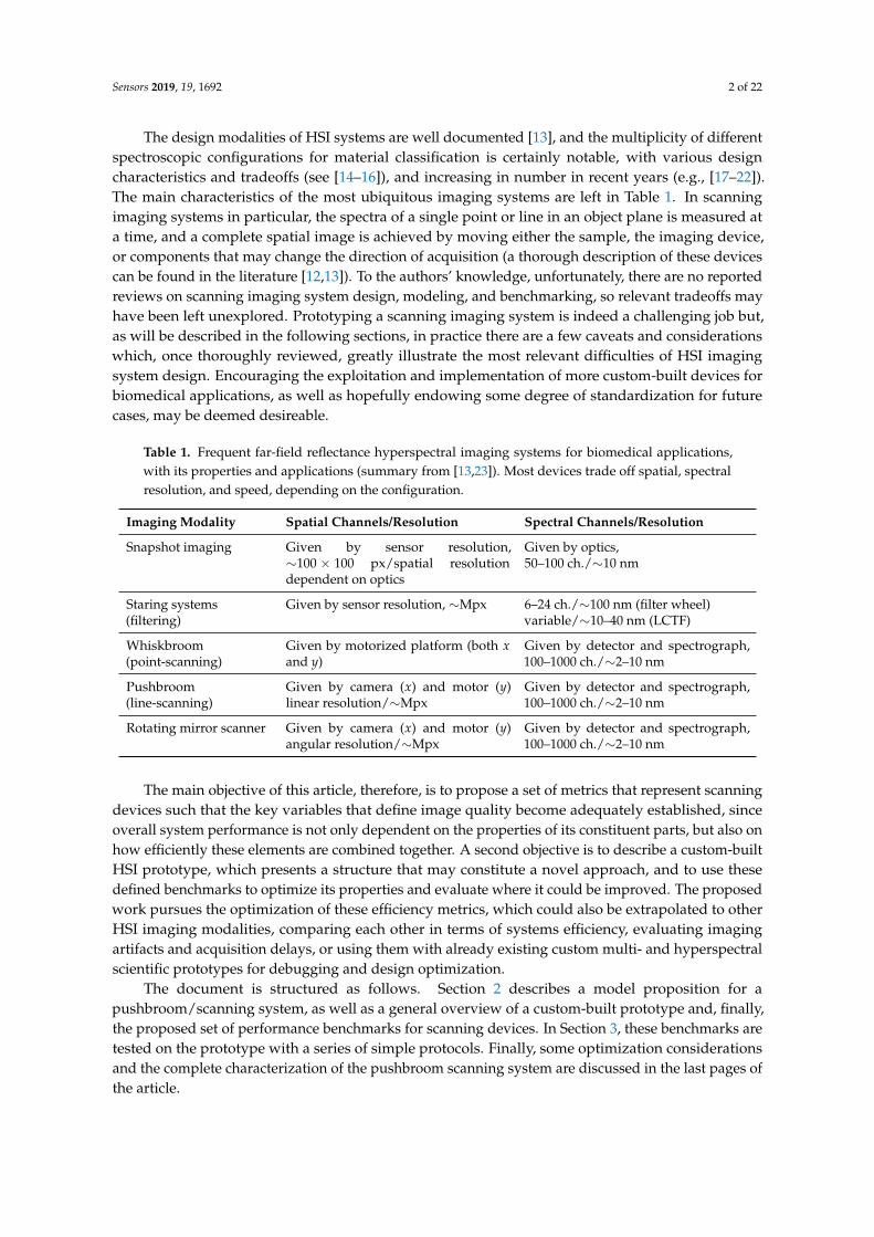
Figure 1 shows a brief summary of the components that comprise a far-field scanning imagingdevice. Consider the following list as a generic description of the main components of any scanningsystem. Their names and properties will be the starting point for the evaluation of the custom device:

1. Optical subsystem. An optical component will take a line in the field of view (FOV) and break itup into spatial and spectral information, which will be measured by a camera. There will likely befocusing optics, a spectrographic element and their corresponding couplings and interfaces. Froma systems perspective, optics will constrain our wavelength range of operation, and the spectrographand lens will limit the overall spectral resolution, i.e., the minimum spectral distance between twomonochromatic signals that can be spatially separated.

2. Imaging device. Light spatially separated by wavelength will reach a camera, which will captureincoming photons across its active pixel sensor. Different wavelengths will, then, be differentiatedby their arrival onto different pixels. Consequently, several imaging parameters will depend onsensor characteristics, namely quantum efficiency (and wavelength range of operation), exposuretime, camera gain, pixel depth and spectral resolution. While the first parameters will depend on thespecific characteristics of the camera, the latter will be also related to the spectrograph’s ability toseparate wavelengths. In the case of line-scanning hyperspectral devices, the camera will alsospecify the spatial resolution for one of the two spatial axes.

3. Actuator subsystem. The actuator subsystem will usually constitute the sole moving part of theimaging device. In pushbroom systems, for example, either the imaging device or the platformwhere the sample is placed is moved by a large actuator. In the case of rotating mirror scanners,an actuator/motor will drive a mirror fixed to an otherwise free-rotating axle. Dependingon the driving mechanism, (e.g., belts and/or gear mechanisms) there will be mechanicalimperfections—such as backlash—as well as delays due to serial communications between themain computer and the actuator controller/driver. Consequently, the main variables at play willbe the repeatability of the drive system (i.e., its ability to obtain the same image pixel-wise whenrepeating the same motion) and time delays due to serial communications. If using a steppermotor, its properties (e.g., steps per revolution, stepper resolution, and degree of microstepping)will define the actuator system and its ability to produce high-resolution images.

4. Communications and storage. Image acquisition and actuation control must be governed by amain computer, which must communicate with both camera and actuator subsystems, as wellas manage data storage and image calibration. Storage must also be sufficiently efficient sothat storing acquired spectra does not impose a significant hindrance on the overall system.We will assume that the imaging system must be able to communicate with other instrumentationand computers within a laboratory network. Camera-computer communications will impose arestriction on the total time per measurement, and therefore communication delays as well as driverand application program interface (API) delays will play a significant role in our efficiency models.

Sensors 2019, 19, 1692 4 of 22

CCD/CMOS

CAMERA

ROTATING

MIRROR TO NETWORK

CPU + CONTROL ROUTER

OBJECTIVE LENS

SPECTROGRAPH

SCANNED LINE

LINEAR RANGE (A) (B) (C)

2048

10

88

FIELD OF VIEW

(FOV)

Figure 1. A generalized description of an external rotating mirror scanning imaging system. (A) Asingle focused line within the field of view can be captured at a time; (B) each line will consist of atwo-dimensional sensor measurement, where the first axis will represent spatial dimension x, and thesecond one specifies wavelength, λ. (C) A complete hyperspectral image is obtained by moving therotating mirror and storing more images for each of the mirror’s positions (y).

2.2. Developed Rotating Mirror Scanning HSI Imaging System

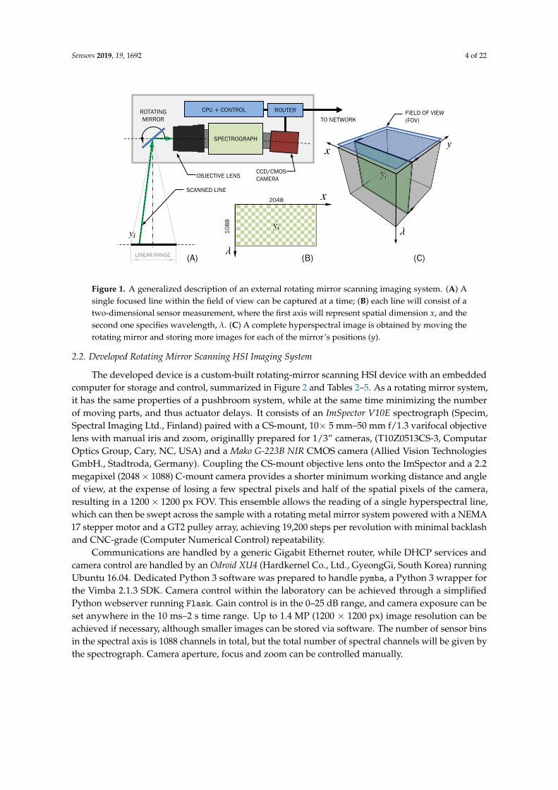
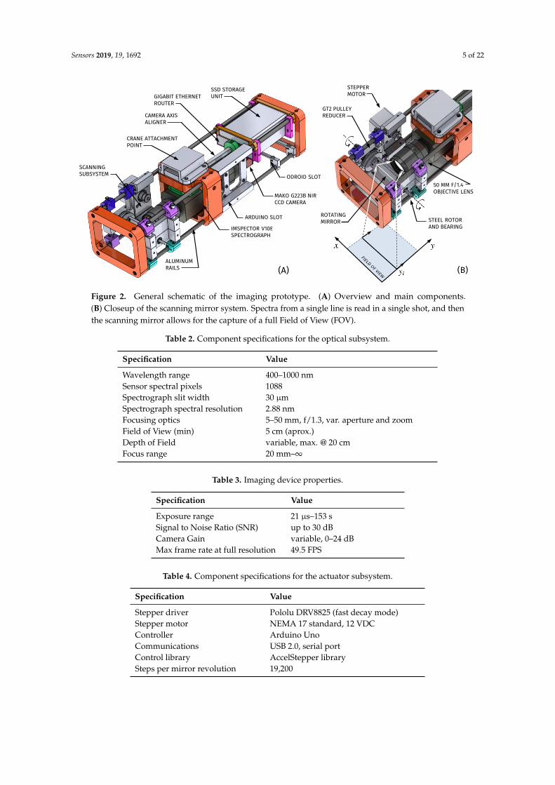
The developed device is a custom-built rotating-mirror scanning HSI device with an embeddedcomputer for storage and control, summarized in Figure 2 and Tables 2–5. As a rotating mirror system,it has the same properties of a pushbroom system, while at the same time minimizing the numberof moving parts, and thus actuator delays. It consists of an ImSpector V10E spectrograph (Specim,Spectral Imaging Ltd., Finland) paired with a CS-mount, 10× 5 mm–50 mm f/1.3 varifocal objectivelens with manual iris and zoom, originallly prepared for 1/3” cameras, (T10Z0513CS-3, ComputarOptics Group, Cary, NC, USA) and a Mako G-223B NIR CMOS camera (Allied Vision TechnologiesGmbH., Stadtroda, Germany). Coupling the CS-mount objective lens onto the ImSpector and a 2.2megapixel (2048× 1088) C-mount camera provides a shorter minimum working distance and angleof view, at the expense of losing a few spectral pixels and half of the spatial pixels of the camera,resulting in a 1200× 1200 px FOV. This ensemble allows the reading of a single hyperspectral line,which can then be swept across the sample with a rotating metal mirror system powered with a NEMA17 stepper motor and a GT2 pulley array, achieving 19,200 steps per revolution with minimal backlashand CNC-grade (Computer Numerical Control) repeatability.

Communications are handled by a generic Gigabit Ethernet router, while DHCP services andcamera control are handled by an Odroid XU4 (Hardkernel Co., Ltd., GyeongGi, South Korea) runningUbuntu 16.04. Dedicated Python 3 software was prepared to handle pymba, a Python 3 wrapper forthe Vimba 2.1.3 SDK. Camera control within the laboratory can be achieved through a simplifiedPython webserver running Flask. Gain control is in the 0–25 dB range, and camera exposure can beset anywhere in the 10 ms–2 s time range. Up to 1.4 MP (1200 × 1200 px) image resolution can beachieved if necessary, although smaller images can be stored via software. The number of sensor binsin the spectral axis is 1088 channels in total, but the total number of spectral channels will be given bythe spectrograph. Camera aperture, focus and zoom can be controlled manually.

Sensors 2019, 19, 1692 5 of 22

MAKO G223B NIR CCD CAMERA

50 MM F/1.4 OBJECTIVE LENS

ROTATING MIRROR

ALUMINUM RAILS

ARDUINO SLOT

SSD STORAGE UNIT

STEPPER MOTOR

CRANE ATTACHMENT POINT

GIGABIT ETHERNET ROUTER

CAMERA AXIS ALIGNER

GT2 PULLEY REDUCER

STEEL ROTOR AND BEARING

SCANNING SUBSYSTEM ODROID SLOT

IMSPECTOR V10E SPECTROGRAPH

(A) (B)

Figure 2. General schematic of the imaging prototype. (A) Overview and main components.(B) Closeup of the scanning mirror system. Spectra from a single line is read in a single shot, and thenthe scanning mirror allows for the capture of a full Field of View (FOV).

Table 2. Component specifications for the optical subsystem.

Specification Value

Wavelength range 400–1000 nmSensor spectral pixels 1088Spectrograph slit width 30 µmSpectrograph spectral resolution 2.88 nmFocusing optics 5–50 mm, f/1.3, var. aperture and zoomField of View (min) 5 cm (aprox.)Depth of Field variable, max. @ 20 cmFocus range 20 mm–∞

Table 3. Imaging device properties.

Specification Value

Exposure range 21 µs–153 sSignal to Noise Ratio (SNR) up to 30 dBCamera Gain variable, 0–24 dBMax frame rate at full resolution 49.5 FPS

Table 4. Component specifications for the actuator subsystem.

Specification Value

Stepper driver Pololu DRV8825 (fast decay mode)Stepper motor NEMA 17 standard, 12 VDCController Arduino UnoCommunications USB 2.0, serial portControl library AccelStepper librarySteps per mirror revolution 19,200

Sensors 2019, 19, 1692 6 of 22

Table 5. Communications, interface and storage specifications.

Specification Value

WAN Interface Gigabit EthernetAPI Protocol RESTful (HTTP)API Metalanguage JSONSSD Storage 128 GBMain computer Odroid XU4Operating system Ubuntu Mate 16.04.5 LTSControl software language Python 3.5.2Measurement file format mat or pklDisplay/touchscreen Odroid VU7Display resolution 800 × 480

2.3. Efficiency Benchmarks and Calibration Procedures

We shall obtain a set of expressions that can serve as adequate overall system performancemetrics, as well as calibration and correction protocols for spatial and spectral information. While theformer will provide insight into this particular imaging modality, the latter are standard procedure inhyperspectral imaging.

2.3.1. Lines per Second (LPS)

Analogous to frames per second (FPS) in conventional systems, it is the inverse of the total timerequired to measure a single line, namely the exposure time plus additional time delays:

LPS =1

Tline=

1Texp + Trx + Tapi + Tmcpy + Tact︸ ︷︷ ︸

Textra

+Trand. (1)

In this equation, Tline represents the total time needed for acquiring a single line, and it is constitutedby a combination of various different time delays and intervals that take place during acquisition:

• Exposure time, denoted by Texp, is the time that a sensor will spend capturing photons froma single line of the FOV (shown in Figure 1). Ideally, image acquisition should only consist ofinteger multiples of a preset exposure time, and image storage and communications should beimmediate. It will be shown that this is not the case.

• Transfer/receiving time Trx is the relationship between file size and network speed within thedevice. Transfer time over an Ethernet network will be practically constant and, thus, for a fixedimage size, transfer time between the camera and the main computer will be fixed. As a generalrule, the total transfer time will be given by

Trx =h · w · b

Rb·Ω, (2)

where h, w are the native height and width (in pixels) of the camera, b is the bit depth (either 8 or12 bits), Rb is the bitrate (in bits/s), and Ω is the overhead of the protocol. In our practical case,where Vimba uses UDP (with an overhead of 1.9%, Ω = 1.019) on a 2048× 1088 pixel camera with8 (or 12) bits per pixel connected to a Gigabit Ethernet router, we obtain 18.16 ms and 27.24 ms oftransmission time for 8- and 12-bit images, respectively. This will introduce a limitation of about55.06 and 27.04 frames per second, respectively, since the camera will be the only device sendingpackets to the main computer, and switching time will be considered negligible.

• Camera Application Program Interface (API) delays, Tapi. Any imaging sensor will be controlledby the computer via an API or driver library. Driver and API delays should be constant delays

Sensors 2019, 19, 1692 7 of 22

that an imaging device presents that can be shown to be due to runtime execution of precompiledAPI dynamic libraries.

• Memory buffer copying and transfer times Tmcpy. They represent buffer copying delays due tointernal bus limitations within the main computer, i.e., between its network interface and memory.

• Actuator/mirror movement delays Tact. These comprise delays in serial communications betweenthe main computer and the actuator subsystem, and due to stepper motor movement, which willbe negligible for high-resolution images, but noticeable in low-resolution acquisition.

• There will be additional, random delays, mostly due to Operating System (OS) interruptions.We will denote them as Trand. Unless we work with a real-time operating system, there shall berandom interruptions during acquisition, due to the OS scheduler setting the measurement APIto background due to priority issues. This phenomenon has a stochastic nature and cannot becontrolled unless a real-time operating system is used.

For our model, Textra = Trx + Tapi + Tmcpy + Tact represents all the additional delays in the systemthat are not random. This value will be estimated as a constant during nonlinear least squares fittingin the following sections.

2.3.2. System Efficiency

The efficiency of a scanning imaging device can be described as the ratio between the specifiedexposure time per sensor capture and the actual time per line:

ε =Texp

Tline=

Texp

Texp + Textra + Trand, (3)

and this measurement will always be ε ≤ 1, since

εmax = limTexp→∞

ε = 1. (4)

2.3.3. Object Plane Curvature

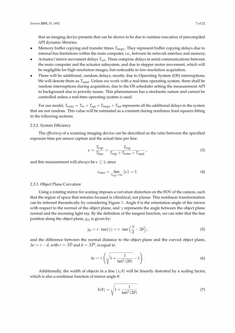
Using a rotating mirror for scaning imposes a curvature distortion on the FOV of the camera, suchthat the region of space that remains focused is cilindrical, not planar. This nonlinear transformationcan be inferred theoretically by considering Figure 3. Angle θ is the orientation angle of the mirrorwith respect to the normal of the object plane, and γ represents the angle between the object planenormal and the incoming light ray. By the definition of the tangent function, we can infer that the lineposition along the object plane, yd, is given by:

yd = r · tan(γ) = r · tan(π

2− 2θ

), (5)

and the difference between the normal distance to the object plane and the curved object plane,∆r = r− d, with r = AP and d = AP′, is equal to

∆r = r

(√1 +

1tan2 (2θ)

− 1

). (6)

Additionally, the width of objects in a line (x, θ) will be linearly distorted by a scaling factor,which is also a nonlinear function of mirror angle θ:

h(θ) =

√1 +

1tan2 (2θ)

(7)

Sensors 2019, 19, 1692 8 of 22

Therefore, every pixel in the image (x, y) will correspond to a spatial position (xd, yd), where

yd = r · tan(π

2− 2θk

), (8)

xd = x · ∆x · h(θk), (9)

θk = ∆θ · (y− yπ/4) + π/4, (10)

where ∆x is the spatial resolution of the measured line in millimeters (which will be generally afunction of lens optical angle of acceptance and r), yπ/4 corresponds to the pixel index where the raypath is fully normal to the object plane (also, where θ = π/4), and the angular resolution of the steppermotor ∆θ, in our case, will be the total number of steps per revolution times a stepping factor s:

∆θ = s2π

Nres= s

2π

19,200. (11)

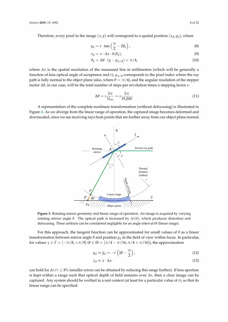
A representation of the complete nonlinear transformation (without defocusing) is illustrated inFigure 4. As we diverge from the linear range of operation, the captured image becomes deformed anddownscaled, since we are receiving rays from points that are further away from our object plane normal.

𝑦

Rotating

mirror

Inverse ray path

𝑟

𝜃

𝜃

𝑛

Δ𝑟

𝑃

𝑦𝑑 ×

𝑃′

𝐴

Normal

distance

(radius)

Object plane

Linear range

𝛾

Figure 3. Rotating mirror geometry and linear range of operation. An image is acquired by varyingrotating mirror angle θ. The optical path is increased by ∆r(θ), which produces distortion anddefocusing. These artifacts can be considered negligible for an angle interval Θ (linear range).

For this approach, the tangent function can be approximated for small values of θ as a lineartransformation between mirror angle θ and position yd in the field of view within focus. In particular,for values γ ∈ Γ = [−π/8,+π/8] (θ ∈ Θ = [π/4− π/16, π/4 + π/16]), the approximation

yd ≈ yd = −r(

2θ − π

2

), (12)

xd ≈ x · ∆x (13)

can hold for ∆r/r ≤ 8% (smaller errors can be obtained by reducing this range further). If lens apertureis kept within a range such that optical depth of field remains over ∆r, then a clear image can becaptured. Any system should be verified in a real context (at least for a particular value of r), so that itslinear range can be specified.

Sensors 2019, 19, 1692 9 of 22

0.0 64.88 129.75 194.62 259.5x [mm]

0.0

75.0

150.0

225.0

300.0

y[m

m]

Object plane

0 512 1024 1536 2048x

1600

2000

2400

2799

3199

y

Measured image

3π16

7π32

π4

9π32

5π16

θ

Figure 4. Image distortion in a scanning imaging system with a rotating mirror for a system height ofr = 225 mm. Left plot: object plane, normal to the imaging system (axes in mm). Blue dots representthe positions of a subset of captured pixels that will form a uniform pixel grid in the measured image(right plot). Aspect ratio is not preserved so that distortions can be better highlighted.

2.3.4. Microstepping Accuracy

Once the main distortions due to using a rotating mirror have been considered, there willbe additional accuracy noise caused by the remaining mechanical factors, namely backlash andmicrostepping. We will assume that any remaining errors will be coming from random sources and areGaussian-distributed, i.e., n ∼ N (0, σ2), hence simplifying the remaining uncertainties of the model.The standard deviation of these random events will be estimated by histogram approximation of aGaussian probability density function (PDF), and is expected to be negligible for high-resolution imagesand quite relevant in low-resolution acquisition, since motor inertia will correct current variations inthe windings of the stepper [24].

2.3.5. Spatial Resolution

Spatial resolution is typically estimated using a resolution test chart. The one we choose to use isa 1951 USAF Resolution Test Chart (MIL-STD-150), printed with reference lines with known lengths.Such lines provide a relationship between pixel positions and actual distances in the image plane.

2.3.6. Spectral Calibration

Wavelength separation through a spectrograph is known to be non-linear in nature. Generally,since a given spectrograph has a fixed response over time, spectral characterization only needs tobe performed once. There are two steps required in order to fully calibrate a hyperspectral system.First, the polynomic response of the spectrograph as a function of pixel position must be found.The characteristic polynomial of a spectrograph, λ = P(p), is a least-squares fit that attempts to relatea spectral wavelength λ to its pixel position p within the sensor:

λ = a0 + a1 p + a2 p2 + · · ·+ ad pd. (14)

Having a material with well-known reflectance peaks, a polynomial of degree d can be obtainedthrough least-squares regression with d or more reference peaks, λ0, . . . , λd, which can be thenidentified at specific pixel locations, p0, . . . , pd [25].

After being able to relate pixels with wavelengths, we can then establish the spectral resolution ofthe device. This was achieved via a CAL-2000 Mercury–Argon light source (Ocean Optics Mikropack,

Sensors 2019, 19, 1692 10 of 22

Ostfildern, Germany) oriented towards the rotating mirror, which shall be kept at a 45 angle. Afterbackground substraction, the spectral emission lines of both gasses should be visible. Since theirspectral emission lines are well-known, finding the smallest discernible lines will provide a lowerbound for spectral resolution.

2.3.7. Dark Image Substraction

The term hot pixels refers to the appearance of bright pixels at long exposure times due to sensorlattice damage; its correction can be achieved via dark image substraction, quite common procedure inastronomical imaging calibration [26]. Hot pixels in the sensor must be corrected by characterizingtheir behavior as a function of exposure time when they are not exposed to any light. This can beachieved by closing the aperture completely and obtaining several measurements. By obtaining thebaseline pixel values for several exposure times, hot pixel background signals can be modeled in eachpixel by

hbg,ij = aijTexp + bij, (15)

where indices i, j indicate the pixel’s position in the sensor, aij and bij are the coefficients that model thelinear behavior of the pixel as a function of exposure time Texp, and hbg,ij will be the estimated hot pixelvalue that should be subtracted to each pixel for every new measurement. This relationship should beoccasionally verified, in order to keep track of the number of damaged pixels in the sensor [27].

2.3.8. Light Source Stability and SNR

Without properly characterizing the main source of optical power, we may incur in inaccuraciesin power output and, therefore, in reflectance measurements. Ideally, for biomedical applicationsit is preferable to use stable and power-controlled devices, such as monochromatic lasers and/orsupercontinuum light sources. As a preliminary approach, it is sufficient to use a tungsten halogenlamp in the Vis–NIR range, due mainly to its thermal inertia, which provides light source stability inthe millisecond-to-second scale. We shall procure two protocols for analyzing how the signal-to-noiseratio (SNR) of the camera is a function of exposure time and light source optical power.

We will use either one or two 1-kW tungsten halogen bulbs for all measurements, dependingon the absorption of the sample. For the first experiment, we turn on the light source and take alow resolution snapshot of an illuminated white Spectralon calibration reference. This is repeatedseveral times (20 times in our case), and each snapshot is timestamped and stored. The averageSpectralon reflectance value for each timestamp will be calculated, and then plotted as a function oftime. If thermal inertia works well under standard temperature conditions, the average value of thisSpectralon reference should become constant over time.

The second experiment assumes that the received sensor counts are a function of backscatteredoptical power. Therefore, the electrical current transformed into a byte in each pixel will be consequenceof the sum of two powers:

Prx = Ps + Pn, Pn ∼ N (0, σ2), (16)

where Prx is the received optical power on that pixel, Ps is the optical power coming from the sample,and Pn is Additive White Gaussian Noise (AWGN). Under this assumption, the average SNR as afunction of wavelength and exposure time can be calculated via the following expected value ratio:

SNR(Texp; λ) = 10 log10

(Ps

Pn

)= 10 log10

(E[Prx(Texp; λ)]

E[(

Prx(Texp; λ)− E[Prx(Texp; λ))2]

), (17)

Sensors 2019, 19, 1692 11 of 22

which for the given assumption is equivalent to calculating

µ(Texp; λ) =1N

N

∑n=1

xk(Texp; λ), (18)

σ2(Texp; λ) =1N

N

∑n=1

(xk(Texp; λ)− µ(Texp; λ)

)2, (19)

SNR(Texp; λ) = 10 log10

(µ

σ2

), (20)

where here x1, . . . , xN(Texp; λ) are several pixels of a reference material measured at a given exposuretime and wavelength, µ is a maximum likelihood (ML) estimate of the average reflectance of suchmaterial, and σ2 the ML estimate of the variance of the light source. These calculations should beperformed on reference-calibrated reflectance data, so two Spectralon captures are required for eachevaluated exposure time, and square-law losses due to light source directionality can be corrected.

3. Results and Discussion

Once all constraints and properties of our model are adequately defined, we must characterize theimaging system and verify that, indeed, it behaves as described. These results have been obtained fromthe device explained in Section 2.2, and attempt to serve as an example of how to measure whether ornot each component is being exploited to its maximum potential. Here, we shall focus on the elementsof the reviewed model that have not been studied by previous work: (1) timing issues, (2) spatialdistortions, (3) microstepping noise, and (4) overall efficiency.

3.1. Timing and Delays

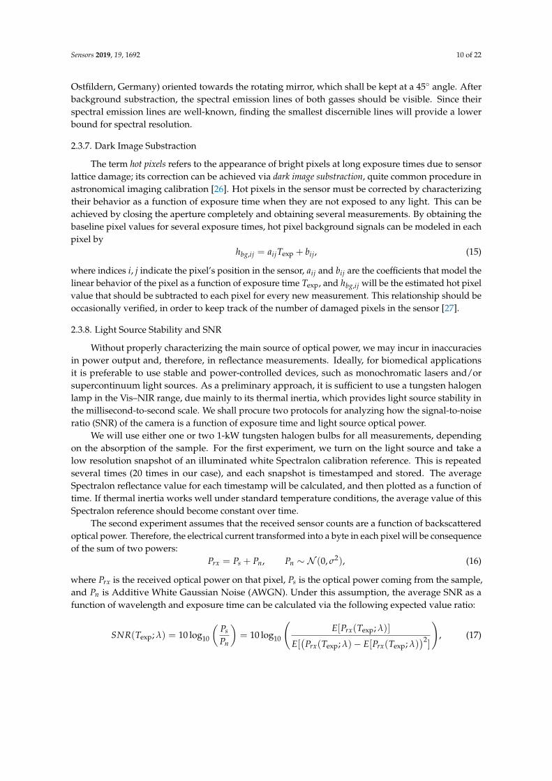
Measuring time spent in each of the modeled operations is an adequate first step in characterizingsystem efficiency. In Figure 5, the total time per line is partitioned between its essential tasks. For thisexperiment, each measured line is separated by a single motor step (i.e., the device is working at fullresolution). This was tested at 8-bit and 12-bit depth, since bit depth will influence the total time spenttransmitting data. As expected, with no other processes running in the system, transfer and buffercopying only take a small fraction of the total time, while a fixed time is spent communicating with thecamera and the rest of the time is spent acquiring light.

1.0 1.9 3.7 7.1 13.7 26.3 50.7 97.4 187.4 360.5Exposure time [ms]

0

100

200

300

400

500

600

Tot

alti

me

[ms]

Time distribution as a function of Texp [8 bits]

TexpTrx

Tapi

TmcpyTact

1.0 1.9 3.7 7.1 13.7 26.3 50.7 97.4 187.4 360.5Exposure time [ms]

0

100

200

300

400

500

600

Tot

alti

me

[ms]

Time distribution as a function of Texp [12 bits]

TexpTrx

Tapi

TmcpyTact

Figure 5. Line measurement time distribution for different exposure times, and bit depth (left andright subplots correspond to 8- and 12-bit depth, respectively). The total time spent in each line is acombination of exposure time Texp (in blue), network transmission time Trx, dynamic library time Tapi

(in green), memory buffer copying Tmcpy (in red) and actuator delays Tact (in purple).

Sensors 2019, 19, 1692 12 of 22

By obtaining the inverse of this time per line, we can represent the rate of acquired lines per secondof the scanning device. This calculation is shown in Figure 6, where the dots represent the inverse ofthe bars in Figure 5, and the continuous line is a nonlinear least squares fit to 1/(Texp + Textra), beingTextra the constant time parameter that we wish to estimate. Additionally, the ideal model, i.e., 1/Texp,is shown as a dotted black line. The different graphs represent the average lines per second whenparts of the system are disabled: the red plot represents normal acquisition, while in the case of theblue line the rotating mirror remains static (i.e., no serial commands are sent to the rotating mirroractuator) and, for the green line, only acquisition commands are being executed, and acquired imagesare discarded (not stored into memory). Driver and API delays are, in theory, constant values that canbe shown to be due to runtime execution of precompiled dynamic libraries. Nevertheless, randomvariations in timing are clearly visible after adjusting for our model, and are related to OS schdulerinterruptions and multithreading management, since acquisition, actuator control, storage and RAMmanagement are run by different processes. In order to obtain accurate, stable LPS measurements,we must use application-specific circuits, and/or real-time operating systems.

1.0 1.9 3.7 7.1 13.7 26.3 50.7 97.4 187.4 360.5Exposure time [ms]

0

10

20

30

40

50

Lin

esp

erse

cond

Lines per second vs. exposure time [8 bits]

Ideal model

Normal measurement

Actuator disabled

Acquisition only

1.0 1.9 3.7 7.1 13.7 26.3 50.7 97.4 187.4 360.5Exposure time [ms]

0

10

20

30

40

50L

ines

per

seco

nd

Lines per second vs. exposure time [12 bits]

Ideal model

Normal measurement

Actuator disabled

Acquisition only

Figure 6. Acquisition speed (in lines per second) as a function of exposure time, disabling different partsof the imaging equipment. Measurements correspond to the colored scatter plots, while a nonlinearleast-squares fit is superimposed as a continuous line plot for each scenario. As expected, disablingthe scanning system and ignoring buffer copying allows us to reach the theoretical limit of the camera(40–50 FPS).

Additionally, it must be noted how, regardless of exposure time, all measurements are limited bythe maximum FPS rate that the camera and/or network protocol can manage (49.5 FPS/LPS for 8 bits islimited by camera performance, 27 FPS/LPS for 12 bits is limited by network speed). All measurementsare bounded from above from the value given by Equation (2) due to network bandwidth, overheadsin transmission, as well as transmission delays, router switching delays, and DLL runtime delays(which cannot be optimized since the Vimba API is already compiled and no source code is available).These issues produce an additional limit, as well as random acquisition speed variability. Some clinicalapproaches, like fluorescence quantification, will require 12-bit images, while other methods couldbenefit of much faster acquisition times rather than a higher pixel resolution; these issues should beconsidered in advance depending on the application.

A similar approach can be done for the other modalities shown in Table 1, considering theirideal efficiency or throughput (Table 6). For the spatial and spectral resolution considered in Table 1,a rotating mirror scanning system would score favorably with respect to other modalities, consideringthat rotating a small mirror will take a shorter amount of time and less power consumption thandisplacing either the sample or the imaging system (i.e., as indicated in the table, Tact Tmove).

Sensors 2019, 19, 1692 13 of 22

Table 6. Ideal throughput/efficiency summary with the proposed device (other entries extractedfrom [23]). We have shown that ideal efficiencies diverge from real ones by various timing issues thatshould be overcome. These systems, then, can benefit from the evaluation approaches in this article.

Imaging Modality Ideal Acquisition Time

Snapshot imaging Texp

Staring systems (Texp + Tchange)× NfiltersWhiskbroom (point-scanning) (Texp + Tmove)× Nx × NyPushbroom (line-scanning) (Texp + Tmove)× NlinesRotating mirror scanner (Texp + Tact)× Nlines

Texp := exposure time (in s), Nfilters := number of filters, Nx , Ny := number of spatial positions in thepoint-scanner, Nlines := number of line positions in pushbroom and scanning systems, Tchange := time neededfor changing filters, Tmove := time needed for moving the imaging platform or device, Tact := scanning mirroractuator rotation time.

3.2. Image Distortions and Noise

Since focusing optics are independent from the actuator subsystem in many cases, the objectplane will inevitably suffer nonlinearities. A rotating mirror with a stepper motor will incur threetypes of measurement errors. First, the object plane will be curved, as the focusing distance will befixed for any mirror angle; this curvature effect must be limited to a linear range, and its effects mustbe quantified. Second, there will be backlash in the transmission system that connects the motor tothe mirror axle; such backlash can damage repeatability, and must be minimized. Third, and finally,there will be microstepping noise due to spurious currents in both driver and stepper rotor; those mustbe minimized by using an adequate stepper driver and microstepping factor.

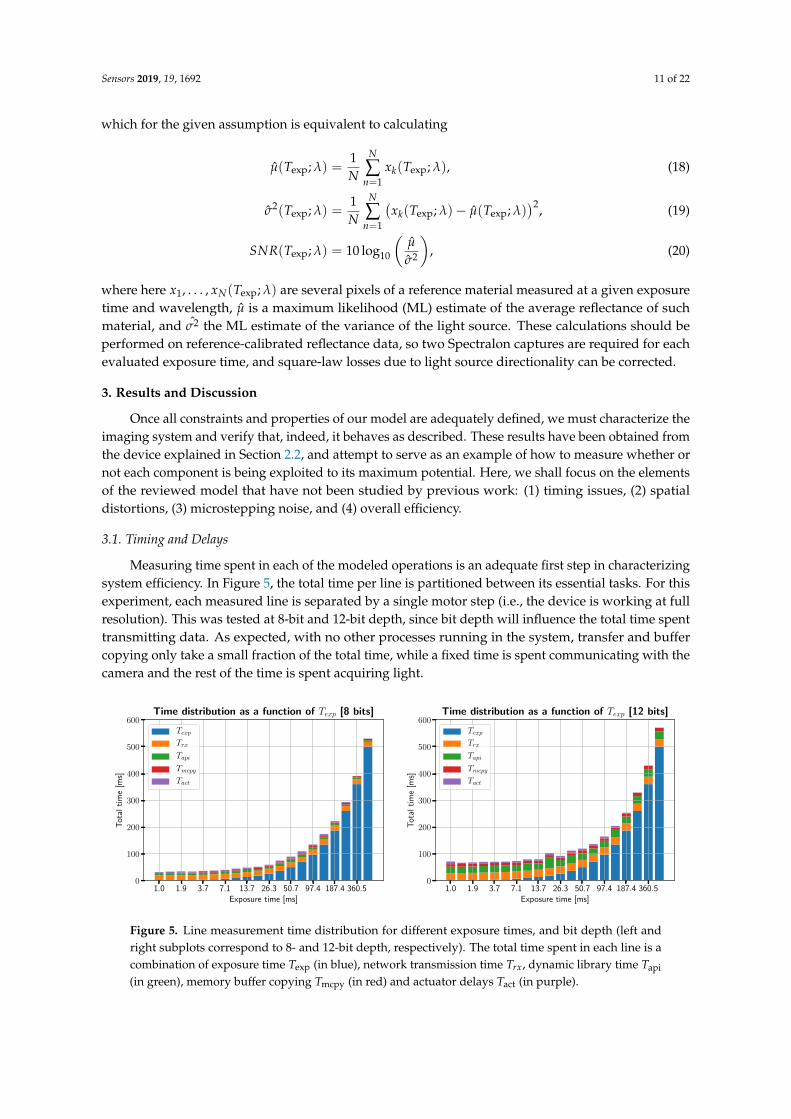
Although we can model theoretical distortion due to mirror rotation and avoid exceeding itslinear range of operation, overall distortion and noise can (and should) be characterized by imagingan Amsler grid with various lengths and forcing the rotating mirror to capture a half/quarter rotationat maximum resolution. Then, the first finite difference along the y axis can be obtained, which allowsfor edge detection in the grid. The variation in grid cell width can be approximated by the nonlinearscaling factor of Section 2.3.3, and therefore a nonlinear least-squares fit of Equation (5) can be obtained.This deterministic distortion allows for obtaining r, the total distance to our object, as well as isolatingany remaining errors coming from other sources. The result of this calculation is left in Figure 7.To obtain a successful alignment, an Amsler grid with 6× 6 mm squares was printed at maximumresolution, screwed to an optical table, where a SMS20 Heavy Duty Boom stand/crane (DiagnosticInstruments, Inc., Michigan, US) was situated holding the instrument above the grid. Then, horizontal(x-wise) alignment between grid and camera was achieved by constantly previewing the image andoverlaying a series of horizontal lines in a custom-designed graphical user interface (GUI), moving andfixing the stand until centering and alignment of the center dot of the grid was achieved at θ = π/4(or, alternatively, γ = 0). The relationship between position y and angle θ is linear within the range±π/8 ≈ ±0.3926 and distortions in the x axis can be corrected by an inverse affine transformation.

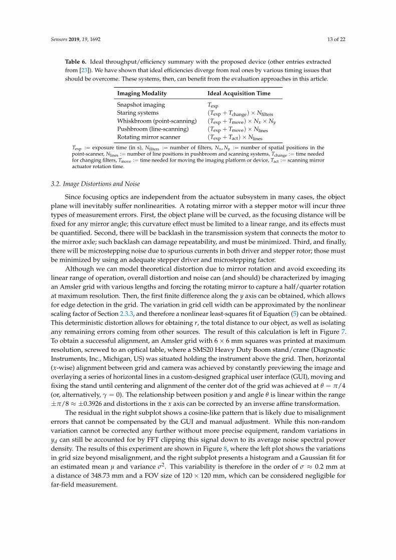
The residual in the right subplot shows a cosine-like pattern that is likely due to misalignmenterrors that cannot be compensated by the GUI and manual adjustment. While this non-randomvariation cannot be corrected any further without more precise equipment, random variations inyd can still be accounted for by FFT clipping this signal down to its average noise spectral powerdensity. The results of this experiment are shown in Figure 8, where the left plot shows the variationsin grid size beyond misalignment, and the right subplot presents a histogram and a Gaussian fit foran estimated mean µ and variance σ2. This variability is therefore in the order of σ ≈ 0.2 mm ata distance of 348.73 mm and a FOV size of 120× 120 mm, which can be considered negligible forfar-field measurement.

Sensors 2019, 19, 1692 14 of 22

500 1000 1500x [px]

0

200

400

600

800

1000

1200

y[p

x]

Original image and measurement range

Measured lines

Grid center

−1 0 1γ [rad]

−2.0

−1.5

−1.0

−0.5

0.0

0.5

1.0

1.5

2.0

y d[m

]

r = 34.8729 cm

Tangential distortion

NLS fit

Detected lines

−0.4 −0.2 0.0 0.2 0.4

−0.4

−0.2

0.0

0.2

0.4

y d[m

]

Linear range and residual error

NLS fit

Detected lines

−0.4 −0.2 0.0 0.2 0.4γ [rad]

−0.0020.0000.002

Res

.

Figure 7. Tangential image distortions due to the selected rotating mirror configuration.

−0.3 −0.2 −0.1 0.0 0.1 0.2 0.3γ [rad]

−0.00100

−0.00075

−0.00050

−0.00025

0.00000

0.00025

0.00050

0.00075

0.00100

Filt

ered

nois

e[m

]

Microstepping noise

0 500 1000 1500fN(n)

−0.00100

−0.00075

−0.00050

−0.00025

0.00000

0.00025

0.00050

0.00075

0.00100

ny

[m]

Gaussian model

Gaussian fit

Histogram

Figure 8. Image noise due to microstepping.

3.3. Spectral Calibration

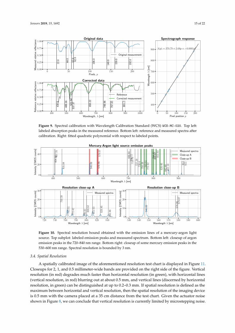
As specified in the Materials and Methods section, a Wavelength Calibration Standard platewith tabulated absorption peaks was imaged with a tungsten halogen lamp . The result of findingat least 8 tabulated peaks is displayed in Figure 9, where absorption peak distribution before andafter calibration can be seen. Spectral resolution was empirically obtained using a calibration lightsource with known proximal emission peaks within the wavelength range and peak distances withinthe range tolerated by the spectrograph. The top subfigure in Figure 10 shows such measurement,with superimposed well-known argon and mercury peak wavelengths. Lines closer than 3 nm to eachother were not discernible (e.g., 576.96 and 579.07 nm), which means that spectral resolution shall bebounded by 3 nm. This provides an upper bound on the number of spectral channels, namely 218(i.e., 5 pixels or 3 nm per channel). Taking resolution into consideration, the spectrograph responsecan be calculated, resulting in λ(p) = 370.79 + 2.68p− 0.0001p2, with p being one of the 218 channels.This fairly linear response is expected.

Sensors 2019, 19, 1692 15 of 22

0 50 100 150 200Pixels, p

0.00

0.25

0.50

0.75

1.00

Mea

sure

dre

lati

vere

flect

ance

22.0 44

.0

57.0

62.0

106.

0

140.

0

159.

0

192.

0

Original data

Original measurement

400 500 600 700 800 900 1000Wavelength, λ [nm]

0.00

0.25

0.50

0.75

1.00

Ref

eren

cere

lati

vere

flect

ance

430.

8

489.

16

521.

5453

7.37

650.

22

748.

96

797.

83

881.

23

Corrected data

Reference

Corrected measurement

0 50 100 150 200Pixel position p

400

500

600

700

800

900

Wav

elen

gthλ

[nm

]

λ(p) = 370.79 + 2.68p +−0.0001p2

Spectrograph response

Figure 9. Spectral calibration with Wavelength Calibration Standard (WCS) WCS-MC-020. Top left:labeled absorption peaks in the measured reference. Bottom left: reference and measured spectra aftercalibration. Right: fitted quadratic polynomial with respect to labeled points.

400 500 600 700 800 900Wavelength λ [nm]

0

20

40

Inte

nsit

y[C

MO

Sco

unts

]

404.

66 407

.78

435.

84

546.

08

576.

9657

9.07

696.

5470

6.72

710.

75

727.

2973

8.4

750.

3976

3.51

772.

42

794.

8280

0.62

811.

53

826.

45

842.

4685

2.14

866.

79

912.

392

2.45

Mercury-Argon light source emission peaks

Measured spectra

Close-up A

Close-up B

720 740 760 780 800 820 840Wavelength λ [nm]

0

10

20

30

Inte

nsit

y[C

MO

Sco

unts

]

750.

39

763.

51

772.

42

794.

82 800.

62

811.

53

826.

45

842.

46

Resolution close-up A

Measured spectra

530 540 550 560 570 580 590 600Wavelength λ [nm]

0

10

20

30

Inte

nsit

y[C

MO

Sco

unts

]

546.

08 576.

96 579.

07

Resolution close-up B

Measured spectra

Figure 10. Spectral resolution bound obtained with the emission lines of a mercury-argon lightsource. Top subplot: labeled emission peaks and measured spectrum. Bottom left: closeup of argonemission peaks in the 720–840 nm range. Bottom right: closeup of some mercury emission peaks in the530–600 nm range. Spectral resolution is bounded by 3 nm.

3.4. Spatial Resolution

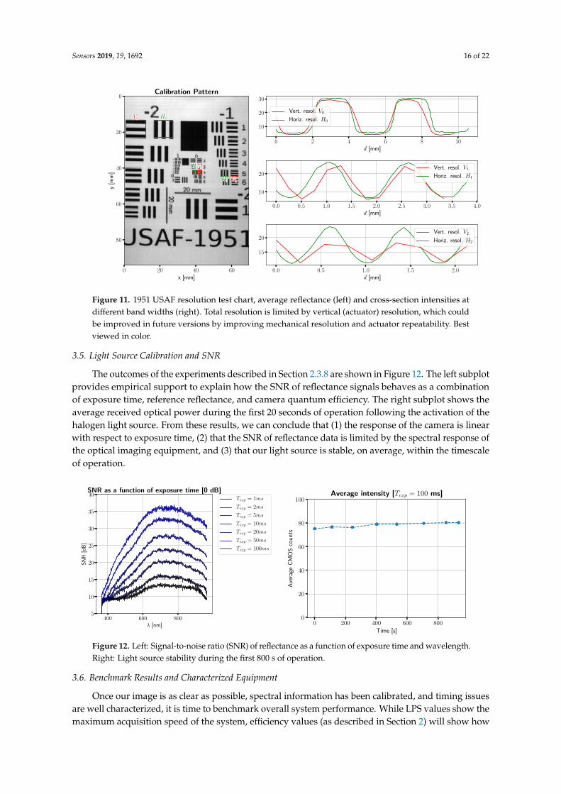
A spatially calibrated image of the aforementioned resolution test chart is displayed in Figure 11.Closeups for 2, 1, and 0.5 millimeter-wide bands are provided on the right side of the figure. Verticalresolution (in red) degrades much faster than horizontal resolution (in green), with horizontal lines(vertical resolution, in red) blurring out at about 0.5 mm, and vertical lines (discerned by horizontalresolution, in green) can be distinguished at up to 0.2–0.3 mm. If spatial resolution is defined as themaximum between horizontal and vertical resolution, then the spatial resolution of the imaging deviceis 0.5 mm with the camera placed at a 35 cm distance from the test chart. Given the actuator noiseshown in Figure 8, we can conclude that vertical resolution is currently limited by microstepping noise.

Sensors 2019, 19, 1692 16 of 22

0 20 40 60x [mm]

0

20

40

60

80

y[m

m]

Calibration Pattern

0 2 4 6 8 10d [mm]

10

20

30

Vert. resol. V0

Horiz. resol. H0

0.0 0.5 1.0 1.5 2.0 2.5 3.0 3.5 4.0d [mm]

10

20Vert. resol. V1

Horiz. resol. H1

0.0 0.5 1.0 1.5 2.0d [mm]

15

20Vert. resol. V2

Horiz. resol. H2

Figure 11. 1951 USAF resolution test chart, average reflectance (left) and cross-section intensities atdifferent band widths (right). Total resolution is limited by vertical (actuator) resolution, which couldbe improved in future versions by improving mechanical resolution and actuator repeatability. Bestviewed in color.

3.5. Light Source Calibration and SNR

The outcomes of the experiments described in Section 2.3.8 are shown in Figure 12. The left subplotprovides empirical support to explain how the SNR of reflectance signals behaves as a combinationof exposure time, reference reflectance, and camera quantum efficiency. The right subplot shows theaverage received optical power during the first 20 seconds of operation following the activation of thehalogen light source. From these results, we can conclude that (1) the response of the camera is linearwith respect to exposure time, (2) that the SNR of reflectance data is limited by the spectral response ofthe optical imaging equipment, and (3) that our light source is stable, on average, within the timescaleof operation.

400 600 800λ [nm]

5

10

15

20

25

30

35

40

SN

R[d

B]

SNR as a function of exposure time [0 dB]Texp = 1ms

Texp = 2ms

Texp = 5ms

Texp = 10ms

Texp = 20ms

Texp = 50ms

Texp = 100ms

0 200 400 600 800Time [s]

0

20

40

60

80

100

Ave

rage

CM

OS

coun

ts

Average intensity [Texp = 100 ms]

Figure 12. Left: Signal-to-noise ratio (SNR) of reflectance as a function of exposure time and wavelength.Right: Light source stability during the first 800 s of operation.

3.6. Benchmark Results and Characterized Equipment

Once our image is as clear as possible, spectral information has been calibrated, and timing issuesare well characterized, it is time to benchmark overall system performance. While LPS values show themaximum acquisition speed of the system, efficiency values (as described in Section 2) will show how

Sensors 2019, 19, 1692 17 of 22

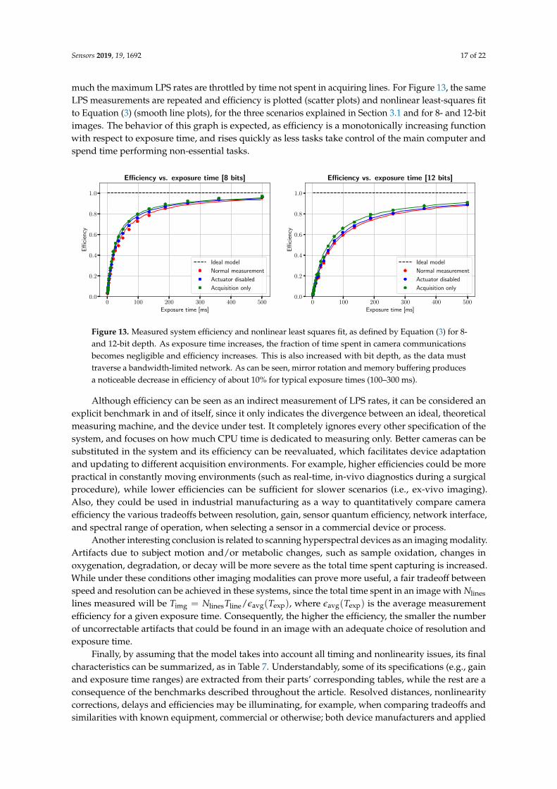
much the maximum LPS rates are throttled by time not spent in acquiring lines. For Figure 13, the sameLPS measurements are repeated and efficiency is plotted (scatter plots) and nonlinear least-squares fitto Equation (3) (smooth line plots), for the three scenarios explained in Section 3.1 and for 8- and 12-bitimages. The behavior of this graph is expected, as efficiency is a monotonically increasing functionwith respect to exposure time, and rises quickly as less tasks take control of the main computer andspend time performing non-essential tasks.

0 100 200 300 400 500Exposure time [ms]

0.0

0.2

0.4

0.6

0.8

1.0

Effi

cien

cy

Efficiency vs. exposure time [8 bits]

Ideal model

Normal measurement

Actuator disabled

Acquisition only

0 100 200 300 400 500Exposure time [ms]

0.0

0.2

0.4

0.6

0.8

1.0

Effi

cien

cy

Efficiency vs. exposure time [12 bits]

Ideal model

Normal measurement

Actuator disabled

Acquisition only

Figure 13. Measured system efficiency and nonlinear least squares fit, as defined by Equation (3) for 8-and 12-bit depth. As exposure time increases, the fraction of time spent in camera communicationsbecomes negligible and efficiency increases. This is also increased with bit depth, as the data musttraverse a bandwidth-limited network. As can be seen, mirror rotation and memory buffering producesa noticeable decrease in efficiency of about 10% for typical exposure times (100–300 ms).

Although efficiency can be seen as an indirect measurement of LPS rates, it can be considered anexplicit benchmark in and of itself, since it only indicates the divergence between an ideal, theoreticalmeasuring machine, and the device under test. It completely ignores every other specification of thesystem, and focuses on how much CPU time is dedicated to measuring only. Better cameras can besubstituted in the system and its efficiency can be reevaluated, which facilitates device adaptationand updating to different acquisition environments. For example, higher efficiencies could be morepractical in constantly moving environments (such as real-time, in-vivo diagnostics during a surgicalprocedure), while lower efficiencies can be sufficient for slower scenarios (i.e., ex-vivo imaging).Also, they could be used in industrial manufacturing as a way to quantitatively compare cameraefficiency the various tradeoffs between resolution, gain, sensor quantum efficiency, network interface,and spectral range of operation, when selecting a sensor in a commercial device or process.

Another interesting conclusion is related to scanning hyperspectral devices as an imaging modality.Artifacts due to subject motion and/or metabolic changes, such as sample oxidation, changes inoxygenation, degradation, or decay will be more severe as the total time spent capturing is increased.While under these conditions other imaging modalities can prove more useful, a fair tradeoff betweenspeed and resolution can be achieved in these systems, since the total time spent in an image with Nlineslines measured will be Timg = NlinesTline/εavg(Texp), where εavg(Texp) is the average measurementefficiency for a given exposure time. Consequently, the higher the efficiency, the smaller the numberof uncorrectable artifacts that could be found in an image with an adequate choice of resolution andexposure time.

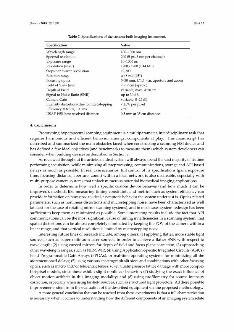
Finally, by assuming that the model takes into account all timing and nonlinearity issues, its finalcharacteristics can be summarized, as in Table 7. Understandably, some of its specifications (e.g., gainand exposure time ranges) are extracted from their parts’ corresponding tables, while the rest are aconsequence of the benchmarks described throughout the article. Resolved distances, nonlinearitycorrections, delays and efficiencies may be illuminating, for example, when comparing tradeoffs andsimilarities with known equipment, commercial or otherwise; both device manufacturers and applied

Sensors 2019, 19, 1692 18 of 22

optics scientists can compare, select, replicate and improve their systems, based on how well differentparts perform together.

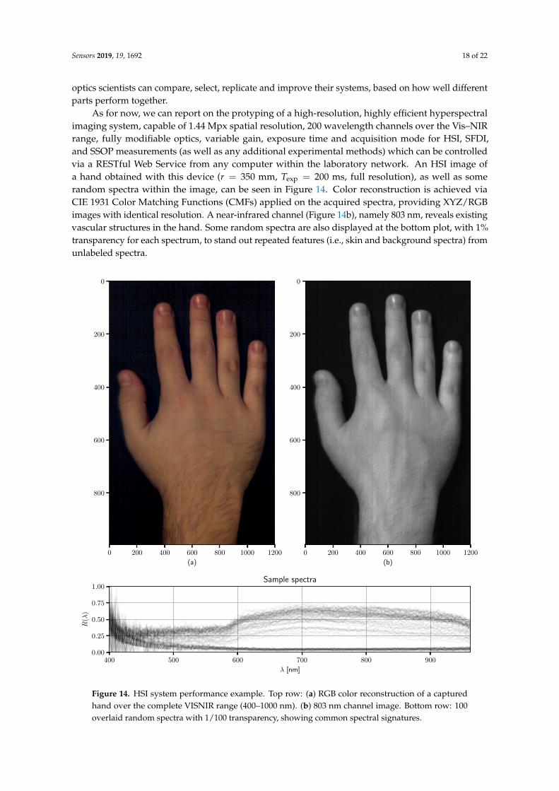
As for now, we can report on the protyping of a high-resolution, highly efficient hyperspectralimaging system, capable of 1.44 Mpx spatial resolution, 200 wavelength channels over the Vis–NIRrange, fully modifiable optics, variable gain, exposure time and acquisition mode for HSI, SFDI,and SSOP measurements (as well as any additional experimental methods) which can be controlledvia a RESTful Web Service from any computer within the laboratory network. An HSI image ofa hand obtained with this device (r = 350 mm, Texp = 200 ms, full resolution), as well as somerandom spectra within the image, can be seen in Figure 14. Color reconstruction is achieved viaCIE 1931 Color Matching Functions (CMFs) applied on the acquired spectra, providing XYZ/RGBimages with identical resolution. A near-infrared channel (Figure 14b), namely 803 nm, reveals existingvascular structures in the hand. Some random spectra are also displayed at the bottom plot, with 1%transparency for each spectrum, to stand out repeated features (i.e., skin and background spectra) fromunlabeled spectra.

0 200 400 600 800 1000 1200

(a)

0

200

400

600

800

0 200 400 600 800 1000 1200

(b)

0

200

400

600

800

400 500 600 700 800 900

λ [nm]

0.00

0.25

0.50

0.75

1.00

R(λ

)

Sample spectra

Figure 14. HSI system performance example. Top row: (a) RGB color reconstruction of a capturedhand over the complete VISNIR range (400–1000 nm). (b) 803 nm channel image. Bottom row: 100overlaid random spectra with 1/100 transparency, showing common spectral signatures.

Sensors 2019, 19, 1692 19 of 22

Table 7. Specifications of the custom-built imaging instrument.

Specification Value

Wavelength range 400–1000 nmSpectral resolution 200 (5 px, 3 nm per channel)Exposure range 10–1000 µsResolution (max.) 1200×1200 (1.44 MP)Steps per mirror revolution 19,200Rotation range π/8 rad (45)Focusing optics 5–50 mm, f/1.3, var. aperture and zoomField of View (min) 7× 7 cm (aprox.)Depth of Field variable, max. @ 20 cmSignal to Noise Ratio (SNR) up to 30 dBCamera Gain variable, 0–25 dBIntensity distortions due to microstepping <10% per pixelEfficiency @ 8 bits, 100 ms 75%USAF 1951 best resolved distance 0.5 mm at 35 cm distance

4. Conclusions

Prototyping hyperspectral scanning equipment is a multiparameter, interdisciplinary task thatrequires harmonious and efficient behavior amongst components at play. This manuscript hasdescribed and summarized the main obstacles faced when constructing a scanning HSI device andhas defined a few ideal objectives (and benchmarks to measure them) which system developers canconsider when building devices as described in Section 2.

As reviewed throughout the article, an ideal system will always spend the vast majority of its timeperforming acquisition, while minimizing all preprocessing, communications, storage and API-baseddelays as much as possible. In real case scenarios, full control of its specifications (gain, exposuretime, focusing distance, aperture, zoom) within a local network is also desireable, especially withmulti-purpose camera systems that unlock numerous potential biomedical imaging applications.

In order to determine how well a specific custom device behaves (and how much it can beimproved), methods like measuring timing constraints and metrics such as system efficiency canprovide information on how close to ideal, asymptotic behavior the system under test is. Optics-relatedparameters, such as nonlinear distortions and microstepping noise, have been characterized as well(at least for the case of rotating mirror scanning systems), and in most cases system redesign has beensufficient to keep them as minimized as possible. Some interesting results include the fact that APIcommunications can be the most significant cause of timing innefficiencies in a scanning system, thatspatial distortions can be almost completely eliminated by keeping the FOV of the camera within alinear range, and that vertical resolution is limited by microstepping noise.

Interesting future lines of research include, among others: (1) applying flatter, more stable lightsources, such as supercontinuum laser sources, in order to achieve a flatter SNR with respect towavelength; (2) using curved mirrors for depth-of-field and focus plane correction; (3) approachingother wavelength ranges, such as NIR-SWIR; (4) using Application-Specific Integrated Circuits (ASICs),Field Programmable Gate Arrays (FPGAs), or real-time operating systems for minimizing all theaforementioned delays; (5) using various spectrograph slit sizes and combinations with other focusingoptics, such as macro and/or telecentric lenses; (6) evaluating sensor lattice damage with more complexhot-pixel models, since these exhibit slight nonlinear behavior; (7) studying the exact influence ofobject motion artifacts in this imaging modality; and (8) using profilometry for source intensitycorrection, especially when using far-field sources, such as structured light projectors. All these possibleimprovements stem from the evaluation of the described equipment via the proposed methodology.

A more general conclusion that can be reached from these experiments is that a full characterizationis necessary when it comes to understanding how the different components of an imaging system relate

Sensors 2019, 19, 1692 20 of 22

to each other, so that the root causes of imperfections and/or slowdowns in image acquisition can beadequately detected, and design can be improved in further versions, especially when building andtesting devices with clinical and surgical applications, where timeliness and precision are fundamental.

Author Contributions: Conceptualization, O.M.C., E.R. and A.P.; methodology, A.P., J.A.G.-G.; software, J.A.G.-G.,A.P.; data curation, J.A.G.-G., A.P.; validation, J.A.G.-G., A.P.; formal analysis, A.P., J.A.G.-G.; investigation, A.P.,J.A.G.-G.; resources, O.M.C., J.M.L.-H.; writing—original draft preparation, A.P., J.A.G.-G.; writing—review andediting, A.P., J.A.G.-G., E.R., O.M.C., J.M.L.-H.; visualization, A.P., J.A.G.-G.; supervision, O.M.C. and J.M.L.-H.;project administration, O.M.C.; funding acquisition, O.M.C. and J.M.L.-H.

Funding: This research, as well as APC charges, was funded by: CIBER-BBN; MINECO (Ministerio de Economíay Competitividad) and Instituto de Salud Carlos III (ISCIII), grant numbers DTS15/00238, DTS17/00055,and TEC2016-76021-C2-2-R; Instituto de Investigación Sanitaria Valdecilla (IDIVAL), grant number INNVAL16/02;Ministry of Education, Culture and Sports, PhD grant number FPU16/05705.

Conflicts of Interest: The authors declare no conflict of interest.

Abbreviations

The following abbreviations are used in this manuscript:

API Application Program InterfaceCCD Charge-Coupled DeviceCMOS Complementary Metal-Oxide SemiconductorCNC Computer Numerical ControlCPU Central Processing UnitdB DecibelDC Direct CurrentDHCP Dynamic Host Configuration ProtocolFOV Field of ViewFPS Frames Per SecondGPU Graphics Processing UnitHSI Hyperspectral ImagingLAN Local Area NetworkLPS Lines Per SecondLTS Long Term SupportMSI Multispectral ImagingMP, Mpx Megapixel (106 pixels)NAT Network Address TranslationNEMA National Electrical Manufacturer AssociationqF-SSOP Corrected Fluorescence SSOP imagingSDK Software Development KitSFDI Spatial Frequency Domain ImagingSSOP Single-Shot Optical PropertiesUSB Universal Serial BusWAN Wide Area NetworkWCS Wavelength Calibration Standard

References

1. Pu, R. Hyperspectral Remote Sensing: Fundamentals and Practices, 1st ed.; CRC Press: Boca Raton, FL, USA, 2017.2. Veraverbeke, S.; Dennison, P.; Gitas, I.; Hulley, G.; Kalashnikova, O.; Katagis, T.; Kuai, L.; Meng, R.;

Roberts, D.; Stavros, N. Hyperspectral remote sensing of fire: State-of-the-Art and future perspectives.Remote Sens. Environ. 2018, 216, 105–121. [CrossRef]

Sensors 2019, 19, 1692 21 of 22

3. Vaz, A.S.; Alcaraz-Segura, D.; Campos, J.C.; Vicente, J.R.; Honrado, J.P. Managing plant invasions throughthe lens of remote sensing: A review of progress and the way forward. Sci. Total Environ. 2018, 642, 1328–1339.[CrossRef]

4. Van der Meer, F.D.; van der Werff, H.M.A.; van Ruitenbeek, F.J.A.; Heckeer, C.A.; Bakker, W.H.; Noomen,M.F.; van der Mejide, M.; Carranza, E.J.M.; de Smeth, J.B.; Woldai, T. Multi- and hyperspectral geologicremote sensing: A review. Int. J. Appl. Earth Observ. Geoinf. 2012, 14, 112–128. [CrossRef]

5. Gowen, A.A.; O’Donnell, C.P.; Cullen, P.J.; Downey, G.; Frias, J.M. Hyperspectral imaging—And emergingprocess analytical tool for food quality and safety control. Trends Food Sci. Technol. 2007, 18, 590–598.[CrossRef]

6. Wu, D.; Sun, D.W. Advanced applications of hyperspectral imaging technology for food quality and safetyanalysis and assessment: A Review—Part I: Fundamentals. Innov. Food Sci. Emerg. Technol. 2013, 19, 1–14.[CrossRef]

7. Wu, D.; Sun, D.W. Advanced applications of hyperspectral imaging technology for food quality and safetyanalysis and assessment: A Review—Part II: Applications. Innov. Food Sci. Emerg. Technol. 2013, 19, 15–28.[CrossRef]

8. Cuccia, D.J.; Bevilacqua, F.; Durkin, A.J.; Tromberg, B.J. Modulated imaging: Quantitative analysis andtomography of turbid media in the spatial-frequency domain. Opt. Lett. 2005, 30, 1354–1356. [CrossRef][PubMed]

9. Vervandier, J.; Gioux, S. Single snapshot imaging of optical properties. Biomed. Opt. Express 2013,4, 2938–2944. [CrossRef]

10. Valdes, P.A.; Angelo, J.P.; Choi, H.S.; Gioux, S. qF-SSOP: Real-Time optical property corrected fluorescenceimaging. Biomed. Opt. Express 2017, 8, 3597–3605. [CrossRef]

11. Angelo, J.P.; Chen, S.J.; Ochoa, M.; Sunar, U.; Gioux, S.; Intes, X. Review of structured light in diffuse opticalimaging. J. Biomed. Opt. 2018, 24, 071602. [CrossRef] [PubMed]

12. Behmann, J.; Acebron, K.; Emin, D.; Bennertz, S.; Matsubara, S.; Thomas, S.; Bohnenkamp, D.; Kuska, M.T.;Jussila, J.; Salo, H.; Mahlein, A.K.; Rascher, U. Specim IQ: Evaluation of a New, Miniaturized HandheldHyperspectral Camera and Its Application for Plant Phenotyping and Disease Detection. Sensors 2018,18, 441. [CrossRef]

13. Lu, G.; Fei, B. Medical hyperspectral imaging: A review. J. Biomed. Opt. 2014, 19, 010901. [CrossRef]14. Arablouei, R.; goan, E.; Gensemer, S.; Kusy, B. Fast and robust pushbroom hyperspectral imaging via

DMD-based scanning. Proc. SPIE 2016, 9948, 99480A. [CrossRef]15. Uto, K.; Seki, H.; Saito, G.; Kosugi, Y.; Komatsu, T. Development of a Low-Cost, Lightweight Hyperspectral

Imaging System Based on a Polygon Mirror and Compact Spectrometers. IEEE J. Sel. Top. Appl. Earth Observ.Remote Sens. 2016, 9. [CrossRef]

16. Livens, S.; Pauly, K.; Baeck, P.; Blommaert, J.; Nuyts, D.; Zender, J.; Delaure, B. A Spatio-Spectral Camerafor High Resolution Hyperspectral Imaging. ISPRS Int. Arch. Photogram. Remote Sens. Spat. Inf. Sci. 2017,XLII-2/W6, 223–228. [CrossRef]

17. Abdo, M.; Forster, E.; Bohnert, P.; Badilita, V.; Brunner, R.; Wallrabe, U.; Korvink, J.G. Dual-mode pushbroomhyperspectral imaging using active system components and feed-forward compensation. Rev. Sci. Instrum.2018, 89, 083113. [CrossRef]

18. Chaudhary, S.; Ninsawat, S.; Nakamura, T. Non-Destructive Trace Detection of Explosives Using PushbroomScanning Hyperspectral Imaging System. Sensors 2019, 19, 97. [CrossRef]

19. Khan, H.A.; Milhoubi, S.; Mathon, B.; Thomas, J.B.; Hardeberg, J.Y. HyTexiLa: High Resolution Visible andNear Infrared Hyperspectral Texture Images. Sensors 2018, 18, 2045. [CrossRef]

20. Su, D.; Bender, A.; Sukkarieh, S. Improved Cross-Ration Invariant-Based Intrinsic Calibration of AHyperspectral Line-Scan Camera. Sensors 2018, 18, 1885. [CrossRef]

21. Chu, B.; Zhao, Y.; He, Y. Development of Noninvasive Classification Methods for Different Roasting Degreesof Coffee Beans Using Hyperspectral Imaging. Sensors 2018, 18, 1259. [CrossRef]

22. Xiong, J.; Lin, R.; Liu, Z.; Yu, L. A Micro-Damage Detection Method of Litchi Fruit Using HyperspectralImaging Technology. Sensors 2018, 18, 700. [CrossRef]

23. Gao, L.; Smith, R.T. Optical hyperspectral imaging in microscopy and spectroscopy—A review of dataacquisition. J. Biophotonics 2015, 8, 441–456. [CrossRef]

Sensors 2019, 19, 1692 22 of 22

24. Olivka, P.; Krumnikl, M. Software Controlled High Efficient and Accurate Microstepping Unit for EmbeddedSystems. In Digital Information Processing and Communications; Snasel, V., Platos, J., El-Qawasmeh, E., Eds.;Springer: Berlin/Heidelberg, Germany, 2011; pp. 138–146. [CrossRef]

25. Mirapeix, J.; Cobo, A.; Cubillas, A.M.; Conde, O.M.; López-Higuera, J.M. In-process automatic wavelengthcalibration for CCD spectrometers. Proc. SPIE 2008, 7003, 70031T.

26. Sirianni, M.; Jee, M.J.; Benítez, N.; Blakeslee, J.P.; Martel, A.R.; Meurer, G.; Clampin, M.; Marchi, G.D.; Ford,H.C.; Gilliland, R.; Hartig, G.F.; Illingworth, G.D.; Mack, J.; McCann, W.J. The Photometric Performanceand Calibration of the Hubble Space Telescope Advance Camera for Surveys. Publ. Astron. Soc. Pac. 2005,117, 1049–1112. [CrossRef]

27. Chapman, G.H.; Thomas, R.; Thomas, R.; Koren, Z.; Koren, I. Enhanced Correction Methods for HighDensity Hot Pixel Defects in Digital Imagers. Proc. SPIE 2015, 9403, 94030T. [CrossRef]

c© 2019 by the authors. Licensee MDPI, Basel, Switzerland. This article is an open accessarticle distributed under the terms and conditions of the Creative Commons Attribution(CC BY) license (http://creativecommons.org/licenses/by/4.0/).