Deep Clustering and Deep NetworkCompression

Ali Alqahtani

Submitted to Swansea University in fulfilmentof the requirements for the Degree of Doctor of Philosophy

Department of Computer Science

Swansea University

July 1, 2021

Copyright: The author, Ali Alqahtani, 2021.

DeclarationThis work has not been previously accepted in substance for any degree and is not being con-

currently submitted in candidature for any degree.

Signed ............... ....... (candidate)

Date ............................................................

Statement 1This thesis is the result of my own investigations, except where otherwise stated. Other sources

are acknowledged by footnotes giving explicit references. A bibliography is appended.

Signed ................. .......... (candidate)

Date ............................................................

Statement 2I hereby give my consent for my thesis, if accepted, to be available for photocopying and for

inter-library loan, and for the title and summary to be made available to outside organisations.

Signed .............. .......... (candidate)

Date ............................................................

1 July 2021

1 July 2021

1 July 2021

To my parents and my wife.

I would also like to dedicate this thesis to my grandmother and grandfather, who

passed away during the final stage of my Ph.D. study.

Abstract

The use of deep learning has grown increasingly in recent years, thereby becoming a much-

discussed topic across a diverse range of fields, especially in computer vision, text mining, and

speech recognition. Deep learning methods have proven to be robust in representation learning

and attained extraordinary achievement. Their success is primarily due to the ability of deep

learning to discover and automatically learn feature representations by mapping input data into

abstract and composite representations in a latent space. Deep learning’s ability to deal with

high-level representations from data has inspired us to make use of learned representations,

aiming to enhance unsupervised clustering and evaluate the characteristic strength of internal

representations to compress and accelerate deep neural networks.

Traditional clustering algorithms attain a limited performance as the dimensionality in-

creases. Therefore, the ability to extract high-level representations provides beneficial compo-

nents that can support such clustering algorithms. In this work, we first present DeepCluster,

a clustering approach embedded in a deep convolutional auto-encoder. We introduce two clus-

tering methods, namely DCAE-Kmeans and DCAE-GMM. The DeepCluster allows for data

points to be grouped into their identical cluster, in the latent space, in a joint-cost function by

simultaneously optimizing the clustering objective and the DCAE objective, producing stable

representations, which is appropriate for the clustering process. Both qualitative and quanti-

tative evaluations of proposed methods are reported, showing the efficiency of deep clustering

on several public datasets in comparison to the previous state-of-the-art methods.

Following this, we propose a new version of the DeepCluster model to include varying

degrees of discriminative power. This introduces a mechanism which enables the imposition

of regularization techniques and the involvement of a supervision component. The key idea of

our approach is to distinguish the discriminatory power of numerous structures when searching

for a compact structure to form robust clusters. The effectiveness of injecting various levels of

discriminatory powers into the learning process is investigated alongside the exploration and

analytical study of the discriminatory power obtained through the use of two discriminative

i

attributes: data-driven discriminative attributes with the support of regularization techniques,

and supervision discriminative attributes with the support of the supervision component. An

evaluation is provided on four different datasets.

The use of neural networks in various applications is accompanied by a dramatic increase

in computational costs and memory requirements. Making use of the characteristic strength of

learned representations, we propose an iterative pruning method that simultaneously identifies

the critical neurons and prunes the model during training without involving any pre-training

or fine-tuning procedures. We introduce a majority voting technique to compare the activation

values among neurons and assign a voting score to evaluate their importance quantitatively.

This mechanism effectively reduces model complexity by eliminating the less influential neu-

rons and aims to determine a subset of the whole model that can represent the reference model

with much fewer parameters within the training process. Empirically, we demonstrate that our

pruning method is robust across various scenarios, including fully-connected networks (FCNs),

sparsely-connected networks (SCNs), and Convolutional neural networks (CNNs), using two

public datasets.

Moreover, we also propose a novel framework to measure the importance of individual

hidden units by computing a measure of relevance to identify the most critical filters and prune

them to compress and accelerate CNNs. Unlike existing methods, we introduce the use of

the activation of feature maps to detect valuable information and the essential semantic parts,

with the aim of evaluating the importance of feature maps, inspired by novel neural network

interpretability. A majority voting technique based on the degree of alignment between a se-

mantic concept and individual hidden unit representations is utilized to evaluate feature maps’

importance quantitatively. We also propose a simple yet effective method to estimate new

convolution kernels based on the remaining crucial channels to accomplish effective CNN

compression. Experimental results show the effectiveness of our filter selection criteria, which

outperforms the state-of-the-art baselines.

To conclude, we present a comprehensive, detailed review of time-series data analysis,

with emphasis on deep time-series clustering (DTSC), and a founding contribution to the area

of applying deep clustering to time-series data by presenting the first case study in the context

of movement behavior clustering utilizing the DeepCluster method. The results are promis-

ing, showing that the latent space encodes sufficient patterns to facilitate accurate clustering

of movement behaviors. Finally, we identify state-of-the-art and present an outlook on this

important field of DTSC from five important perspectives.

Acknowledgements

First of all, I would like to extend my sincerest appreciation and gratitude to my supervisor,

Prof. Xianghua Xie, for his supervision, guidance, support, and inspiration. Over the years, he

has been a constant source of advice and encouragement, for which I will always be thankful.

Without his tireless encouragement and help, this thesis would not have been possible. I would

like to thank him for the support and discussions that have assisted me in developing my

professional skills. He has all my thanks for pushing me to do my best. I am also grateful to

my second supervisor, Prof. Mark W. Jones for his help and support.

I would also like to thank all of my colleagues in the SwanseaVision Lab. Thanks espe-

cially to Dr. Essa Ehab, Dr. Jingjing Deng, Dr. Michael Edwards, Majedaldein Almahasneh,

Hanchi Ren, Hassan Eshkiki, and Michael Kenning for their helpful discussions and support

throughout my Ph.D.

I am also thankful to all of my friends, Mohammed Ali, Abdulrahim Meshari, Majed

Bin Othayman, and Khalid Alharthi for their continuous support.

Finally, I would also like to express my gratitude to my family, especially my amazing

parents, my wonderful wife (for her patience and support in helping me pursue something

that I love, despite the difficulties), my daughters (Taraf, Arob, and Hoor), my sisters, and my

brothers for their encouragement and support throughout the years; they always believed in

me and pushed me to succeed.

iii

Contents

List of Publications ix

List of Tables x

List of Figures xii

1 Introduction 1

1.1 Motivations . . . . . . . . . . . . . . . . . . . . . . . . . . . . . . . . . . . . 2

1.1.1 Deep Clustering . . . . . . . . . . . . . . . . . . . . . . . . . . . . . 3

1.1.2 Learning Discriminatory Deep Clustering Models . . . . . . . . . . . . 4

1.1.3 Deep Neural Network Compression and Acceleration . . . . . . . . . . 4

1.2 Overview . . . . . . . . . . . . . . . . . . . . . . . . . . . . . . . . . . . . . 5

1.3 Contributions . . . . . . . . . . . . . . . . . . . . . . . . . . . . . . . . . . . 6

1.4 Outline . . . . . . . . . . . . . . . . . . . . . . . . . . . . . . . . . . . . . . 9

2 Background 11

2.1 Introduction . . . . . . . . . . . . . . . . . . . . . . . . . . . . . . . . . . . . 12

2.2 Deep Learning . . . . . . . . . . . . . . . . . . . . . . . . . . . . . . . . . . 13

2.2.1 Neural Networks . . . . . . . . . . . . . . . . . . . . . . . . . . . . . 13

2.2.2 Convolutional Neural Networks . . . . . . . . . . . . . . . . . . . . . 21

2.2.3 Modern Convolutional Neural Networks . . . . . . . . . . . . . . . . . 24

2.2.4 Auto-encoders . . . . . . . . . . . . . . . . . . . . . . . . . . . . . . 28

2.2.5 Advances in Deep Learning . . . . . . . . . . . . . . . . . . . . . . . 30

2.2.6 Visualizing, Explaining and Interpreting Deep Learning . . . . . . . . 31

2.3 Clustering . . . . . . . . . . . . . . . . . . . . . . . . . . . . . . . . . . . . . 34

2.3.1 Conventional Clustering Methods . . . . . . . . . . . . . . . . . . . . 34

v

2.3.2 Deep Clustering Methods . . . . . . . . . . . . . . . . . . . . . . . . 38

2.3.3 Clustering Supervision . . . . . . . . . . . . . . . . . . . . . . . . . . 44

2.4 Deep Neural Network Compression and Acceleration . . . . . . . . . . . . . . 45

2.4.1 Pruning Methods . . . . . . . . . . . . . . . . . . . . . . . . . . . . . 47

2.4.2 Quantization Methods . . . . . . . . . . . . . . . . . . . . . . . . . . 51

2.4.3 Low-rank Factorization Methods . . . . . . . . . . . . . . . . . . . . . 52

2.5 Summary . . . . . . . . . . . . . . . . . . . . . . . . . . . . . . . . . . . . . 53

3 DeepCluster: A Deep Convolutional Auto-encoder with Embedded Clustering 55

3.1 Introduction . . . . . . . . . . . . . . . . . . . . . . . . . . . . . . . . . . . . 56

3.2 Proposed Methods . . . . . . . . . . . . . . . . . . . . . . . . . . . . . . . . 57

3.2.1 Deep Convolutional Auto-encoder (DCAE) . . . . . . . . . . . . . . . 58

3.2.2 DeepCluster: A Deep Convolutional Auto-encoder with Embedded

Clustering . . . . . . . . . . . . . . . . . . . . . . . . . . . . . . . . . 59

3.3 Experiments and Discussion . . . . . . . . . . . . . . . . . . . . . . . . . . . 62

3.3.1 Datasets . . . . . . . . . . . . . . . . . . . . . . . . . . . . . . . . . . 62

3.3.2 Network Architectures . . . . . . . . . . . . . . . . . . . . . . . . . . 63

3.3.3 Evaluation Metrics . . . . . . . . . . . . . . . . . . . . . . . . . . . . 65

3.3.4 Implementation Details . . . . . . . . . . . . . . . . . . . . . . . . . . 65

3.3.5 Baseline Methods . . . . . . . . . . . . . . . . . . . . . . . . . . . . . 66

3.3.6 Quantitative Results and Analysis . . . . . . . . . . . . . . . . . . . . 66

3.3.7 Visualization Results and Analysis . . . . . . . . . . . . . . . . . . . . 68

3.4 Summary . . . . . . . . . . . . . . . . . . . . . . . . . . . . . . . . . . . . . 73

4 Learning Discriminatory Deep Clustering Models 75

4.1 Introduction . . . . . . . . . . . . . . . . . . . . . . . . . . . . . . . . . . . . 76

4.2 Proposed Methods . . . . . . . . . . . . . . . . . . . . . . . . . . . . . . . . 78

4.2.1 DeepCluster: A DCAE with Embedded Clustering . . . . . . . . . . . 79

4.2.2 Architecture . . . . . . . . . . . . . . . . . . . . . . . . . . . . . . . . 79

4.2.3 Graph-Based Activity Regularization (GBAR) . . . . . . . . . . . . . 80

4.2.4 Data Augmentation (DA) . . . . . . . . . . . . . . . . . . . . . . . . . 81

4.2.5 Extended Output Layer and Different Levels of Supervision . . . . . . 82

4.3 Experimental Results . . . . . . . . . . . . . . . . . . . . . . . . . . . . . . . 83

4.3.1 Regularizations for DeepCluster . . . . . . . . . . . . . . . . . . . . . 84

4.3.2 Learning Discriminatory Deep Clustering Models Through Different

Levels of supervision . . . . . . . . . . . . . . . . . . . . . . . . . . . 87

4.3.3 Deep Clustering Through Various Levels of Supervision . . . . . . . . 91

4.4 Summary . . . . . . . . . . . . . . . . . . . . . . . . . . . . . . . . . . . . . 93

5 Reducing Neural Network Parameters via Neuron-based Iterative Pruning 97

5.1 Introduction . . . . . . . . . . . . . . . . . . . . . . . . . . . . . . . . . . . . 98

5.2 Proposed Method . . . . . . . . . . . . . . . . . . . . . . . . . . . . . . . . . 99

5.2.1 Importance of Individual Neurons via Majority voting (MV) . . . . . . 100

5.2.2 Pruning algorithm . . . . . . . . . . . . . . . . . . . . . . . . . . . . 101

5.3 Experiments and Discussion . . . . . . . . . . . . . . . . . . . . . . . . . . . 102

5.3.1 Measuring Neuron Importance via Ablation . . . . . . . . . . . . . . . 104

5.3.2 Pruning Redundant Neurons During Training . . . . . . . . . . . . . . 106

5.3.3 Integrating our Pruning Method to Sparsely-Connected Networks (SCNs)108

5.3.4 Extension to Convolutional Neural Networks (CNNs) . . . . . . . . . . 109

5.4 Summary . . . . . . . . . . . . . . . . . . . . . . . . . . . . . . . . . . . . . 110

6 Pruning CNN Filters via Quantifying the Importance of Deep Visual Represen-

tations 113

6.1 Introduction . . . . . . . . . . . . . . . . . . . . . . . . . . . . . . . . . . . . 114

6.2 Proposed Method . . . . . . . . . . . . . . . . . . . . . . . . . . . . . . . . . 117

6.2.1 Overview of our Pruning Methodology . . . . . . . . . . . . . . . . . 117

6.2.2 Scoring Channel Importance Method . . . . . . . . . . . . . . . . . . 118

6.2.3 Majority voting (MV) Method . . . . . . . . . . . . . . . . . . . . . . 120

6.2.4 Kernels Estimation Method . . . . . . . . . . . . . . . . . . . . . . . 122

6.3 Experiments and Discussion . . . . . . . . . . . . . . . . . . . . . . . . . . . 123

6.3.1 VGG16 on CIFAR-10 . . . . . . . . . . . . . . . . . . . . . . . . . . 129

6.3.2 ResNet-20/ResNet-32 on CIFAR-10 . . . . . . . . . . . . . . . . . . . 131

6.3.3 ResNet-20/ResNet-32 on CUB-200 . . . . . . . . . . . . . . . . . . . 132

6.3.4 ResNet-50 on ImageNet . . . . . . . . . . . . . . . . . . . . . . . . . 134

6.3.5 Feature Map Visualization . . . . . . . . . . . . . . . . . . . . . . . . 136

6.3.6 Comparison with Filter Selection Criteria . . . . . . . . . . . . . . . . 137

6.3.7 Comparison of Kernal Estimation (KE) vs. Fine-Tuning (FT) . . . . . . 142

6.4 Summary . . . . . . . . . . . . . . . . . . . . . . . . . . . . . . . . . . . . . 143

7 Deep Time-Series Clustering 145

7.1 Introduction . . . . . . . . . . . . . . . . . . . . . . . . . . . . . . . . . . . . 146

7.2 Time-series Data Type . . . . . . . . . . . . . . . . . . . . . . . . . . . . . . 147

7.2.1 Univariate . . . . . . . . . . . . . . . . . . . . . . . . . . . . . . . . . 147

7.2.2 Multivariate . . . . . . . . . . . . . . . . . . . . . . . . . . . . . . . . 147

7.2.3 Tensor Fields . . . . . . . . . . . . . . . . . . . . . . . . . . . . . . . 148

7.2.4 Multifield . . . . . . . . . . . . . . . . . . . . . . . . . . . . . . . . . 149

7.3 Conventional Time-series Analysis . . . . . . . . . . . . . . . . . . . . . . . . 149

7.3.1 Similarity Measures and Features Extraction . . . . . . . . . . . . . . 151

7.3.2 Conventional Clustering Algorithms . . . . . . . . . . . . . . . . . . . 155

7.4 DeepCluster Method Applied to Biological Time-series Data: A Case Study . . 157

7.4.1 Network Architectures for ICBD . . . . . . . . . . . . . . . . . . . . . 158

7.4.2 Imperial Cormorant Birds Dataset (ICBD) and Pre-processing . . . . . 161

7.4.3 Experiment and Discussion . . . . . . . . . . . . . . . . . . . . . . . . 163

7.5 State-of-the-art and Outlook . . . . . . . . . . . . . . . . . . . . . . . . . . . 165

7.5.1 Different Network Architectures . . . . . . . . . . . . . . . . . . . . . 165

7.5.2 Different Clustering Methods . . . . . . . . . . . . . . . . . . . . . . 168

7.5.3 Deep Learning Heuristics . . . . . . . . . . . . . . . . . . . . . . . . 169

7.5.4 DTSC Applictions . . . . . . . . . . . . . . . . . . . . . . . . . . . . 170

7.5.5 DTSC Benchmarks . . . . . . . . . . . . . . . . . . . . . . . . . . . . 171

7.6 Summary . . . . . . . . . . . . . . . . . . . . . . . . . . . . . . . . . . . . . 171

8 Conclusions and Future Work 173

8.1 Conclusions . . . . . . . . . . . . . . . . . . . . . . . . . . . . . . . . . . . . 174

8.2 Future Work . . . . . . . . . . . . . . . . . . . . . . . . . . . . . . . . . . . . 176

Bibliography 181

List of Publications

The following is a list of published papers as a result of the work in this thesis. An outline of

contributions related to the main body of the thesis work can be found in Section 1.3.

1. A. Alqahtani, X. Xie, Mark W. Jones, and E. Essa. Pruning CNN Filters via Quantifying

the Importance of Deep Visual Representations. Computer Vision and Image Under-

standing (CVIU), 2021. [1]

2. A. Alqahtani, X. Xie, E. Essa, and Mark W. Jones. Neuron-based Network Pruning

Based on Majority Voting. International Conference on Pattern Recognition (ICPR),

2020. [2]

3. M. Ali, A. Alqahtani, Mark W. Jones, and X. Xie. Clustering and classification for time

series data in visual analytics: A survey. IEEE Access, 2019. [3] (Mohammed Ali and

Ali Alqahtani contributed equally to this work).

4. A. Alqahtani, X. Xie, J. Deng, and Mark W. Jones. Learning discriminatory deep clus-

tering models. International Conference on Computer Analysis of Images and Patterns

(CAIP), 2019. [4]

5. A. Alqahtani, X. Xie, J. Deng, and Mark W. Jones. A deep convolutional auto-encoder

with embedded clustering. IEEE International Conference on Image Processing (ICIP),

2018. [5]

ix

List of Tables

2.1 Summary of Modern CNNs and their performanc. . . . . . . . . . . . . . . . . . . 46

3.1 Details of datasets used in our experiments for the DeepCluster method. . . . . . . 63

3.2 Detailed configuration of the DCAE network architecture used in the experiments. . 64

3.3 Comparison of clustering quality with the baselines on three datasets using two

evaluation metrics: accuracy (ACC) and normalized mutual information (NMI). . . 67

4.1 Detailed configuration of the DCAE network architecture used in the experiments. . 80

4.2 Details of the datasets used in our experiments for the discriminatory DeepCluster

models. . . . . . . . . . . . . . . . . . . . . . . . . . . . . . . . . . . . . . . . . 84

4.3 Comparison of clustering quality of the DeepCluster method using accuracy eval-

uation metric with and without regularizations. . . . . . . . . . . . . . . . . . . . 85

4.4 Number of samples used in the training stage and clustering accuracy. . . . . . . . 88

4.5 Comparison of clustering accuracy on four different datasets using different learn-

ing levels. . . . . . . . . . . . . . . . . . . . . . . . . . . . . . . . . . . . . . . . 90

4.6 Supervised Clustering. Clustering accuracy with GBAR regularization technique

using different weighting coefficients. . . . . . . . . . . . . . . . . . . . . . . . . 92

4.7 Semi-supervised. Clustering accuracy with GBAR regularization technique using

different weighting coefficients. . . . . . . . . . . . . . . . . . . . . . . . . . . . 93

5.1 Details of Datasets and their FC Architectures used in our experiments. . . . . . . 103

5.2 Examining neuron importance via ablation study with different selection criteria

on CIFAR10. . . . . . . . . . . . . . . . . . . . . . . . . . . . . . . . . . . . . . 106

5.3 Examining neuron importance via ablation study with different selection criteria

on MNIST. . . . . . . . . . . . . . . . . . . . . . . . . . . . . . . . . . . . . . . 106

5.4 Summarization of our experiments with fully-connected networks. . . . . . . . . . 107

x

5.5 Summarization of our experiments with sparsely-connected networks. . . . . . . . 109

6.1 VGG-16 on CIFAR-10 and three different pruned models. . . . . . . . . . . . . . 129

6.2 Performance of pruning VGG16 on CIFAR-10. . . . . . . . . . . . . . . . . . . . 130

6.3 Performance of pruning ResNet-20/32 on CIFAR-10. . . . . . . . . . . . . . . . . 132

6.4 Performance of pruning ResNet-20/32 on CUB-200. . . . . . . . . . . . . . . . . 134

6.5 Performance of pruning ResNet-50 on ImageNet. . . . . . . . . . . . . . . . . . . 135

6.6 Comparison among several state-of-the-art pruning methods on ResNet-50 and Im-

ageNet. . . . . . . . . . . . . . . . . . . . . . . . . . . . . . . . . . . . . . . . . 136

6.7 Overall results of layer-wise pruning utilizing different filter selection criteria for

VGG-16 on CIFAR-10. . . . . . . . . . . . . . . . . . . . . . . . . . . . . . . . . 141

6.8 Overall results of layer-wise pruning utilizing different filter selection criteria for

our small CNN model on CIFAR-10. . . . . . . . . . . . . . . . . . . . . . . . . . 141

6.9 Comparison of fine-tuning (FT) and kernels estimation (KE) . . . . . . . . . . . . 143

7.1 Deep Clustering Methods . . . . . . . . . . . . . . . . . . . . . . . . . . . . . . . 158

7.2 Detailed configuration of the DCAE network architecture used on time-series data. 161

7.3 Experimental results of clustering quality, reporting averaged performance across

5-fold cross-validation on three methods on the ICBD. . . . . . . . . . . . . . . . 164

7.4 Deep Time-series Clustering Methods. . . . . . . . . . . . . . . . . . . . . . . . . 169

List of Figures

2.1 Perceptron function process. . . . . . . . . . . . . . . . . . . . . . . . . . . . . . 14

2.2 An overview of the two-layer network. . . . . . . . . . . . . . . . . . . . . . . . . 15

2.3 Visualization of common activation functions used in neural networks. . . . . . . . 19

2.4 Two main layers of CNNs. . . . . . . . . . . . . . . . . . . . . . . . . . . . . . . 22

2.5 Structure of the Inception and ResNet blocks. . . . . . . . . . . . . . . . . . . . . 26

2.6 The development of CNN Architectures. . . . . . . . . . . . . . . . . . . . . . . . 27

2.7 An Auto-encoder (AE) framework. . . . . . . . . . . . . . . . . . . . . . . . . . . 29

3.1 The architecture of the DeepCluster model. . . . . . . . . . . . . . . . . . . . . . 64

3.3 Visualizations of reconstruction images (Top) and input images (Bottom) on 3

datasets using the DCAE-Kmeans proposed method. . . . . . . . . . . . . . . . . 69

3.4 Visualizing the reconstruction of clustering centres on 3 different datasets. Top:

USPS; Middle: MNIST-FASHION; Bottom: MNIST. . . . . . . . . . . . . . . . . 70

3.5 Visualizations of latent representations in a two-dimensional space with t-SNE on

MNIST. . . . . . . . . . . . . . . . . . . . . . . . . . . . . . . . . . . . . . . . . 71

3.6 Visualizations of latent representations with our clustering results in a two-

dimensional space with t-SNE through an iterative training scheme on MNIST. . . 72

4.1 The architecture of the discriminatory DeepCluster models. An extra layer is added

at the end of the network just after the reconstruction layer to inject different de-

grees of supervision. . . . . . . . . . . . . . . . . . . . . . . . . . . . . . . . . . 83

4.2 Visualizations of reconstruction images (Top) and input images (Bottom) in SVHN

dataset. . . . . . . . . . . . . . . . . . . . . . . . . . . . . . . . . . . . . . . . . 85

4.3 Visualizations of latent representation for our deep clustering method through

through different levels of supervision on the MNIST testing set. Top: True Labels.

Bottom: Our Results . . . . . . . . . . . . . . . . . . . . . . . . . . . . . . . . . 89

xii

4.4 Invariance properties of the learned representation in different layers from five

different models . . . . . . . . . . . . . . . . . . . . . . . . . . . . . . . . . . . . 91

5.1 Neuron-based pruning method. . . . . . . . . . . . . . . . . . . . . . . . . . . . . 100

5.2 Majority voting (MV) method. . . . . . . . . . . . . . . . . . . . . . . . . . . . . 102

5.3 The architecture of the CNN model. . . . . . . . . . . . . . . . . . . . . . . . . . 108

5.4 Change in accuracy during training with our pruning method for three different

models. . . . . . . . . . . . . . . . . . . . . . . . . . . . . . . . . . . . . . . . . 110

6.1 The overall pipeline of our proposed framework for pruning CNN filters via quan-

tifying the importance of deep visual representations. . . . . . . . . . . . . . . . . 118

6.2 The detailed process of our pruning procedure. . . . . . . . . . . . . . . . . . . . 119

6.3 Scoring Channel Importance Method. . . . . . . . . . . . . . . . . . . . . . . . . 121

6.4 Majority Voting (MV) method. . . . . . . . . . . . . . . . . . . . . . . . . . . . . 122

6.5 Different settings to determine the top quantile level T in Eq.(6.2) at different

layers of VGG16 on CIFAR-10. . . . . . . . . . . . . . . . . . . . . . . . . . . . 126

6.6 Different settings to determine the optimal l value in Eq.(6.3) at different layers of

VGG16 on CIFAR-10. . . . . . . . . . . . . . . . . . . . . . . . . . . . . . . . . 127

6.7 Comparison of IoU pruning selection criteria. . . . . . . . . . . . . . . . . . . . . 128

6.8 Layer-wise pruning of VGG-16 on CIFAR-10. . . . . . . . . . . . . . . . . . . . . 130

6.9 Layer-wise pruning of ResNet-20/32 on CIFAR-10. . . . . . . . . . . . . . . . . . 131

6.10 Layer-wise pruning of ResNet 20/32 on CUB-200. . . . . . . . . . . . . . . . . . 133

6.11 Different input images from the ImageNet dataset and their semantic segmentation

and visualization of feature maps binary segmentation . . . . . . . . . . . . . . . . 137

6.12 The architecture of the CNN model. . . . . . . . . . . . . . . . . . . . . . . . . . 139

6.13 Comparison of layer-wise pruning methods for VGG-16 on CIFAR-10 . . . . . . . 140

7.1 The pipeline of conventional time-series analysis. . . . . . . . . . . . . . . . . . . 151

7.2 Line chart of the raw accelerometer data (Multivariate time-series data). . . . . . . 159

7.3 The DAE network architecture for time-series data shown the number of neurons

for each fully-connected layer in both encoder and decoder parts. . . . . . . . . . . 160

7.4 The detailed process of the sliding window approach with a window size of 12 and

and a stride of 6 are adopted in both cases. . . . . . . . . . . . . . . . . . . . . . . 163

7.5 The pipelines of deep time-series clustering. . . . . . . . . . . . . . . . . . . . . . 166

Chapter 1

Introduction

Contents1.1 Motivations . . . . . . . . . . . . . . . . . . . . . . . . . . . . . . . . . . 2

1.1.1 Deep Clustering . . . . . . . . . . . . . . . . . . . . . . . . . . . 3

1.1.2 Learning Discriminatory Deep Clustering Models . . . . . . . . . 4

1.1.3 Deep Neural Network Compression and Acceleration . . . . . . . 4

1.2 Overview . . . . . . . . . . . . . . . . . . . . . . . . . . . . . . . . . . . 5

1.3 Contributions . . . . . . . . . . . . . . . . . . . . . . . . . . . . . . . . . 6

1.4 Outline . . . . . . . . . . . . . . . . . . . . . . . . . . . . . . . . . . . . 9

1

1. Introduction

1.1 Motivations

Over recent decades, machine learning has rapidly grown as a tool for analyzing and utiliz-

ing data, presenting a wide range of methodologies to extract information from observed data.

Different approaches have been developed to understand the characteristics of the data and ob-

tain meaningful statistics in order to explore the underlying processes, identify and estimate

trends, make decisions and predict the future. Driven by a justifiable belief that an improved

feature-extraction pipeline and a cleaner and bigger dataset are entirely mattered to the final

performance [6], the use of hand-crafted features to represent data structures has been replaced,

shifting the focus to representation learning and features extraction and encouraging the im-

provement of automated learning techniques which are able to optimize their feature extractors

and learn representations from observed data. Deep learning methods have proven robust in

representation learning and have grown increasingly widespread in recent years. As a result

of the greater availability of data and advanced computing power, deep learning has advanced

into wider and deeper models, driving state-of-the-art performance across various tasks, es-

pecially in computer vision (i.e., object detection [7], semantic segmentation, [8] and image

classification [9–11]). This achievement has been possible through the ability of deep learning

to discover, learn, and perform automatic representation by transforming raw data into an ab-

stract representation, which allows the system to learn the right representations from the raw

data. During the learning process, a deep learning model utilizes a hierarchical level of neural

networks and can learn feature representations at multiple abstraction levels so complicated

concepts can be developed from simpler ones.

The development of the deep learning strategy for representation learning relies heavily on

the choice of data representations (or features) and the improvement of the feature-extraction

pipeline [6]. Therefore, much of the effort in developing, exploring, or analyzing deep learning

algorithms go into the structure underlying discriminative and representative features, and the

ability to learn the identification and disentanglement of the underlying explanatory factors

hidden in the data, in order to expand the scope and ease of applicability of deep learning

models [12].

The overarching motivation of this thesis is to continue the current trend in making use of

learned representations, specifically to enhance unsupervised learning and evaluate the charac-

teristics of internal representations to compress and accelerate deep neural networks. The use

of representation learning for the clustering process will be explored, and an in-depth analysis

of strengthening the discriminative features in relation to improvements in the performance

2

1.1. Motivations

of deep clustering methods will be provided. The effectiveness of deep representations will

be investigated by measuring their importance, where a novel pruning framework is presented

based on quantifying the importance of deep visual representations of Convolutional neural

networks (CNNs).

1.1.1 Deep Clustering

Clustering is a fundamental task in a number of areas, including machine learning, computer

vision, and pattern recognition [13]. The goal of clustering is to group a set of unlabeled data

in the given feature space based on similarity measures (e.g. Euclidean distance). Although

conventional clustering methods have received significant attention [14–16], they attain limited

performance as dimensionality increases, and usually suffer from high computational complex-

ity on large-scale datasets. To overcome the weaknesses associated with high dimensionality,

many approaches corresponding to dimensionality reduction and feature transformation meth-

ods have been extensively studied, including linear mapping (i.e. principal component analysis

(PCA) [17]), non-linear mapping (i.e. kernel methods [18] and spectral methods [19]). Never-

theless, a higher-level, more complex latent structure of data still challenges the effectiveness

of existing clustering methods [20]. Due to the development of deep learning [21], deep neural

networks minimize this issue by allowing a clustering algorithm to deal with clustering-friendly

features, as working with high-level representations provides beneficial components that sup-

port the achievement of traditional algorithms to demonstrate satisfactory performance. As

there is no supervision knowledge to provide information on categorical labels, representative

features with compact clusters are more valuable. They allow a clustering algorithm to obtain

characteristic features and extract useful information for its structure. Chapter 2 introduces the

current state of deep clustering approaches and highlights the need to develop an unsupervised

deep learning method that enables on to embed a clustering approach into a deep network more

appropriate to image processing tasks. Such joint optimization often leads to a more compact

hidden feature space and minimizes the time cost needed in multi-step deep clustering meth-

ods [13]. Chapters 3, 4, and 7 are motivated by this aim to explore the utilization of deep

learning methods for the clustering process, identifying a feature representation that can com-

pute informative features, spatially localized, on the input space, and support the achievement

of deep clustering methods in the latent space. An evaluation is carried out using numerous

datasets and a case study.

3

1. Introduction

1.1.2 Learning Discriminatory Deep Clustering Models

The work on deep clustering contains novel materials and it has become crucial to explore and

extend this with further analysis. In the procedure of a deep clustering method, the discrim-

inative patterns are only discovered through certain parts or patterns in a data sample in an

unsupervised manner, with limited attention paid toward enhancing more discriminative latent

features to further support the embedded clustering. In an attempt to investigate the ways in

which to reinforce the performance of conventional clustering methods, several methods have

been developed to study semi-supervised clustering and supervised clustering approaches. De-

spite the substantial success of deep learning, there has been limited focus on deep supervised

and semi-supervised clustering models; to address this, Chapter 4 provides an analytical study

for understanding the effectiveness of differing discriminatory power, focusing on strengthen-

ing and discriminating the learned features. Such a mechanism would ensure that the learned

features derived from the encoding layer are the best discriminative attributes by reconciling

the ability of representation learning and discriminative powers imposed on the clustering layer

or injected into the body of the learning process. Evaluation is provided using four different

datasets, considering several regularization techniques, through varying degrees of supervision.

1.1.3 Deep Neural Network Compression and Acceleration

Despite the success of deep learning models, deep networks often possess a vast number of pa-

rameters, and their significant redundancy in parameterization has become a widely-recognized

property [22]. The over-parametrized and redundant nature of deep networks results in expen-

sive computational costs and high storage requirements - significant challenges which restrict

many deep network applications. Network pruning focuses on discarding the unnecessary parts

of neural networks, aiming to obtain a sub-network with fewer parameters without reducing ac-

curacy. The pruned version, a subset of the whole model, can represent the reference model at

a smaller size or with far fewer parameters. Reducing the complexity of models while main-

taining their high performance creates unprecedented opportunities for researchers to tackle

the challenges of deploying deep learning systems to a resource-limited device and increase

the applicability of deep network models to a broader range of applications. While pruning ap-

proaches have received considerable attention as a way to tackle over-parameterization and re-

dundancy, some existing methods require a particular software/hardware accelerator that is not

supported by off-the-shelf libraries. The random connectivity of non-structured sparse models

can also cause poor cache locality and jumping memory access, which significantly limits the

4

1.2. Overview

practical acceleration [23]. Moreover, most existing methods tend to focus on applying simple

pruning techniques (e.g. statistical approaches) to compress networks rather than discover-

ing informative units for effective pruning [24]. To confront these challenges, Chapter 5 and

Chapter 6 introduce pruning frameworks, where removing an unimportant part in its entirety

does not change the network structure contrary to previous methods, and any off-the-shelf deep

learning library can support the method. This procedure can also effectively reduce memory re-

quirements as model compression focuses on reducing not only model parameters but also the

intermediate activation. The ways in which to integrate the pruning procedure into the learning

process are investigated in Chapter 5 to allow the finding of a smaller architecture to the target

task at the training phase, which avoids the need for a multi-step pruning procedure. Unlike

other pruning methods, the training-based pruning method allows the input configuration to be

handled by applying a constraint function to the weights matrix during training without chang-

ing the network structure and adaptively determining hyperparameters. The proposed method

is evaluated across various scenarios, including fully-connected networks (FCNs), sparsely-

connected networks (SCNs), and CNNs using two datasets. Chapter 6 explores the concept

that not all filters deliver essential information for the final prediction of the model [25–27]

and fundamentally relies on quantifying the importance of latent representations of CNNs by

evaluating the alignment/matching between semantic concepts and individual hidden units to

score the semantics of hidden units at each intermediate convolutional layer. The core aim is

to evaluate filters’ importance, which provides meaningful insight into the characteristics of

neural networks’ internal representations, reducing the computational complexity of the con-

volutional layers. The pruning method is evaluated on large-scale datasets and well-known

CNN architectures.

1.2 Overview

In line with the rationale presented in section 1.1, this study aims to explore the use of represen-

tation learning in deep clustering and deep network compression. In previous years, common

approaches for deep clustering have focused on taking advantage of a deep neural network,

separating the learning process from the clustering task, which requires various emphases and

involves a cumbersome, time-consuming process. Chapter 3 introduces the use of DeepCluster,

an embedded clustering approach in a deep convolutional auto-encoder (DCAE) for efficient

simultaneous, end-to-end learned local features and cluster assignments. This scheme usually

leads to a more compact latent feature space and enables a faster process. Chapter 4 utilizes

5

1. Introduction

the DeepCluster to explore the use of deep clustering carried out in presence of varying de-

grees of discriminative power by evolving a mechanism to inject various levels of supervision

into the learning process or impose constraints on the clustering layer. In Chapters 5 and 6,

overparameterized networks are efficiently compressed and allow for the acquisition of a small

subset of the whole model, representing the reference model with much fewer parameters. This

work explores the use of representation learning in deep network compression, presenting two

pruning frameworks for neurons in fully-connected layers and filters in convolutional layers.

1.3 Contributions

The main contributions of this thesis are as follows:

• A deep convolutional auto-encoder with embedded clustering.

We propose DeepCluster, a clustering approach embedded into a deep convolutional

auto-encoder (DCAE) framework which can alternately learn feature representation and

cluster assignments. In contrast to conventional clustering approaches, our method

makes use of representation learning by deep neural networks, which assists in finding

compact and representative latent features for further recognition tasks. It also exploits

the strength of DCAE to learn useful properties of image data for the purpose of clus-

tering. In this work, we introduce two deep clustering methods: DCAE-Kmeans and

DCAE-GMM. An objective function that reduces the distance between learned feature

representations in a latent space and their identical centroids is applied. A mixture of

multiple Gaussian distributions in a latent space is also considered, so that all data sam-

ples are assumed to be generated from multiple Gaussian distributions. These procedures

enable the classification of a data point into its identical cluster in the latent space in a

joint-cost function by alternately optimizing the clustering objective and the DCAE ob-

jective, thereby producing stable representations appropriate for the clustering process.

The proposed method is trained in an end-to-end way using fixed settings without any

pre-training or fine-tuning procedures, enabling a faster training process. Qualitative

and quantitative evaluations of proposed methods are reported, showing the efficiency

of deep clustering on several public datasets in comparison to previous state-of-the-art

methods. This work was published in [5].

6

1.3. Contributions

• Learning discriminatory features when searching for a compact structure to form

robust clusters.

We present a new version of the DeepCluster to include varying degrees of discriminative

power. This work introduces a mechanism to allow for the imposition of regularization

techniques and the involvement of a supervision component; effectively reconciling the

extracted latent representations and the provided supervising knowledge to produce the

best discriminative attributes. The key idea of our approach is distinguishing the discrim-

inatory power of numerous structures when searching for a compact structure to form

robust clusters. The effectiveness of injecting various levels of discriminatory powers

into the learning process is investigated alongside exploration and analytical study of the

discriminatory power obtained through the use of several discriminative attributes. Two

regularization techniques are considered: one that is embedded in the clustering layer

and another that is used during the training process. We also take into account three

different learning levels: supervised, semi-supervised and unsupervised. An evaluation

is provided using four different datasets. This work was published in [4].

• An iterative pruning method to reduce network complexity.

We propose an iterative pruning method that prunes neurons based on the level of im-

portance during training, without involving pre-training or fine-tuning procedures. The

proposed method mainly targets the parameters of the fully-connected layers, does not

require special initialization, and can be supported by any off-the-shelf machine learning

library. We introduce a majority voting technique, which aims to compute a measure of

relevance that identifies the most critical neurons by assigning a voting score to evaluate

their importance and helps to effectively reduce model complexity by eliminating less

influential neurons, with the aim of determining a subset of the whole model which can

represent the reference model with fewer parameters within the training process. A com-

parative study with experimental results on public datasets is presented. An evaluation

is also provided across various scenarios, including FCNs, SCNs, and CNNs. This work

was published in [2].

• Pruning CNN filters via quantifying the importance of deep visual representations.

We propose a novel framework to measure the importance of individual hidden units by

computing a measure of relevance to identify the most critical filters and prune them to

compress and accelerate CNNs. This work is considered pioneering in that it attempts to

7

1. Introduction

use the quantifying interpretability for more robust and effective CNN pruning. Inspired

by novel neural network interpretability, we first introduce the use of the activation of

feature maps as well as the use of and essential semantic parts to detect valuable in-

formation and evaluate the importance of feature maps. A majority voting technique

based on the degree of alignment between a semantic concept and individual hidden unit

representations is proposed to quantitatively evaluate the importance of feature maps,

as well as a simple, effective method to estimate new convolution kernels based on the

remaining crucial channels to recover compromised accuracy. An evaluation is provided

using large-scale datasets and well-known CNN architectures. A comparison with other

state-of-the-art pruning methods is given. A paper [1] has been submitted and is under

review at the time of writing.

• Deep embedded clustering of time-series data for movement behavior analysis.

We present a comprehensive, detailed review of time-series data analysis, with emphasis

on deep time-series clustering (DTSC), and a case study in the context of movement be-

havior clustering utilizing the DeepCluster method. Specifically, we modified the DCAE

architectures to suit time-series data; see Chapter 7 for details. The work was done in

2017, and we believe that we were the first to approach this topic and have made found-

ing contributions to the area of deep clustering of time-series data; Chapter 7 describes

these contributions. Since 2018, several works have been carried out on DTSC. We also

review these works and identify state-of-the-art and present an outlook on this important

field of DTSC. A part of this work was published in [3].

8

1.4. Outline

1.4 Outline

The remaining chapters of this work are outlined as follows:

Chapter 2 Background:

The necessary background information surrounding neural networks and deep learning,

as well as an overview of popular methods and considerations required in deep clustering

and deep network compression and acceleration.

Chapter 3 DeepCluster: A Deep Convolutional Auto-encoder with Embedded Clustering:

Introduces clustering approaches embedded into a deep convolutional auto-encoder

(DCAE). Two joint-cost functions are introduced, where the clustering objective and

DCAE objective are alternately optimized. Experimental evaluations of the method are

presented in comparison to previous state-of-the-art methods.

Chapter 4 Learning Discriminatory Deep Clustering Models:

Explores the use of DeepCluster to study discriminative power when searching for a

compact structure to form robust clusters in a latent space in presence of regularization

techniques and supervision components. Experimental evaluations of the method are

presented and discussed.

Chapter 5 Reducing Neural Network Parameters via Neuron-based Iterative Pruning:

The proposed iterative pruning method prunes neurons to reduce network complexity,

an activation-based method which iteratively prunes neurons based on a measure of rel-

evance that identifies the most critical neurons by assigning a voting score to evaluate

their importance. Experimental evaluation and analytical discussions are provided.

Chapter 6 Pruning CNN Filters via Quantifying the Importance of Deep Visual Representa-

tions:

Introduces a novel framework to measure the importance of individual hidden units by

evaluating the degree of alignment between a semantic concept and individual hidden

unit representations. A majority voting technique is proposed to quantitatively evalu-

ate the importance of feature maps. The performance of the method is evaluated and

compared with other state-of-the-art pruning methods.

9

1. Introduction

Chapter 7 Deep Time-Series Clustering:

Presents a comprehensive, detailed review of time-series data analysis, introducing the

use of DeepCluster methodology to learn and cluster temporal features from accelerom-

eter data for the clustering of animal behaviors. An evaluation and discussion are given

on real-world data, namely, the Imperial Cormorant bird dataset (ICBD). The state-of-

the-art and an outlook of DTSC are also provided.

Chapter 8 Conclusions and Future Work:

Concluding remarks on studies presented in the previous chapters, highlighting opportu-

nities and potential future directions.

10

Chapter 2

Background

Contents2.1 Introduction . . . . . . . . . . . . . . . . . . . . . . . . . . . . . . . . . 12

2.2 Deep Learning . . . . . . . . . . . . . . . . . . . . . . . . . . . . . . . . 13

2.2.1 Neural Networks . . . . . . . . . . . . . . . . . . . . . . . . . . 13

2.2.2 Convolutional Neural Networks . . . . . . . . . . . . . . . . . . 21

2.2.3 Modern Convolutional Neural Networks . . . . . . . . . . . . . . 24

2.2.4 Auto-encoders . . . . . . . . . . . . . . . . . . . . . . . . . . . 28

2.2.5 Advances in Deep Learning . . . . . . . . . . . . . . . . . . . . 30

2.2.6 Visualizing, Explaining and Interpreting Deep Learning . . . . . . 31

2.3 Clustering . . . . . . . . . . . . . . . . . . . . . . . . . . . . . . . . . . 34

2.3.1 Conventional Clustering Methods . . . . . . . . . . . . . . . . . 34

2.3.2 Deep Clustering Methods . . . . . . . . . . . . . . . . . . . . . . 38

2.3.3 Clustering Supervision . . . . . . . . . . . . . . . . . . . . . . . 44

2.4 Deep Neural Network Compression and Acceleration . . . . . . . . . . . 45

2.4.1 Pruning Methods . . . . . . . . . . . . . . . . . . . . . . . . . . 47

2.4.2 Quantization Methods . . . . . . . . . . . . . . . . . . . . . . . 51

2.4.3 Low-rank Factorization Methods . . . . . . . . . . . . . . . . . . 52

2.5 Summary . . . . . . . . . . . . . . . . . . . . . . . . . . . . . . . . . . . 53

11

2. Background

2.1 Introduction

Over recent decades, machine learning has rapidly grown as a tool for analyzing and uti-

lizing data, presenting a wide range of methodologies to extract information from observed

data [28, 29]. Machine learning gives computers the ability to learn without explicit program-

ming [30]. Alpaydin [31] gives a concise description of machine learning, which is “optimizing

a performance criterion using example data and past experience”. Machine learning algorithms

provide a collection of automated analyses that can be much more efficient, accurate, and ob-

jective in solving different tasks. Data plays a significant role in machine learning, where

the learning algorithm is utilized to discover and learn knowledge or properties from the data

(learn from experience) without depending on a predetermined equation as a model [32]. In

supervised learning, the training set is composed of pairs of input and desired output, and the

learning aim is to generate a function that maps inputs to outputs. Each example is associated

with a label or target. In unsupervised learning, the training set is composed of unlabeled in-

puts without any assigned desired output, and the aim is to find hidden patterns or substantial

structures in data [33].

The dependence on hand-crafted features over raw data is a general phenomenon that ap-

pears as a standard procedure for most machine learning algorithms [6]. However, a careful

approach is required by domain experts in order to develop informative features and generalize

information across the distribution of observations. For instance, Histogram of Oriented Gra-

dients (HoG) [34] and Scale Invariant Feature Transform (SIFT) [35] are feature descriptors

which are generalized well to image domain problems and developed from a knowledge of

image processing principles. Feature descriptors would allow the classical machine learning

methods to deal with features instead of raw data and train to recognize patterns in a feature

space. Notwithstanding, the evolution of the deep learning strategy replaces the need for hand-

crafted feature descriptors by enabling a model to learn its extractor set from the data in a new

representation space [12]. This process is referred to as the term of “representation learning”,

which has rapidly grown in the last decade with the development of neural networks and deep

learning [21].

In recent years, deep learning has rapidly grown and begun to show its robust ability in rep-

resentation learning, achieving remarkable success in diverse applications. This achievement

has been possible through its ability to discover, learn, and perform automatic representation

by transforming raw data into an abstract representation. The process of deep learning utilizes

a hierarchical level of neural networks of different kinds, such as multilayer perceptron (MLP),

12

2.2. Deep Learning

convolutional neural networks (CNNs), and recurrent neural networks (RNNs). This hierarchi-

cal representation allows models to learn features at multiple abstraction levels, meaning that

complicated concepts can be learned from simpler ones. Neurons in earlier layers of a network

learn low-level features, while neurons in later layers learn more complex concepts [32].

This chapter presents an overview of deep learning algorithms and the relevant background

knowledge considered in this thesis. An introduction to deep neural networks is discussed in

section 2.2. First, we walk through the basic operations, learning procedure, and optimization

of deep neural networks. Then, we provide insight into CNNs, discussing the backbone of

all convolutional neural networks and the structure of modern architectures along with their

motivations, advantages, and disadvantages. Later, we provide a review of auto-encoder (AE)

and other advanced deep learning algorithms. The development of visual interpretability to

understand deep networks is also discussed. In section 2.3, an overview of conventional clus-

tering methods is presented. Following this, we provide a review of deep clustering methods,

introducing different approaches to said methods and their fundamental structure. Thereafter,

in section 2.4, we present an overview of popular methods for compressing and accelerating

deep neural networks, reviewing the recent works of related techniques used in our research.

The focus is essentially on deep clustering and deep network compression, as they form the

primary subjects of this thesis. Finally, a concluding summary is provided in section 2.5.

2.2 Deep Learning

2.2.1 Neural Networks

Inspired by neurobiology, neural networks (NNs) grew by way of artifical neurons as the pre-

cursor of perceptron from the combination of input stimuli and the activation response of in-

terconnected neurons in the human brain [36]. The algorithm for NNs is a machine learning

technique that consists of simple processing elements known as units, neurons or nodes, which

are linked together with weighted connections acquired by a process of learning from a set of

training data [37]. A perceptron, considered to be the foundation of all neural network mod-

els, is a building block in NN structure which presents a fundamental mathematical model of

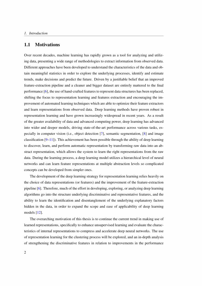
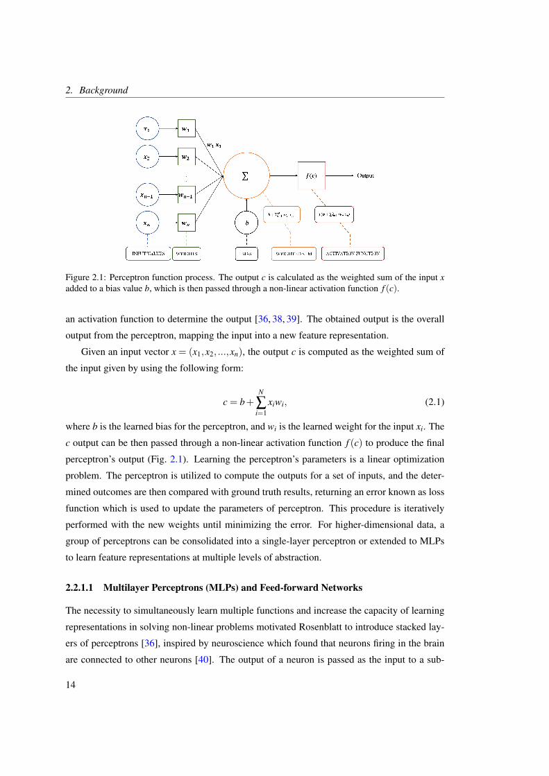
a neuron adopted in all neural network models. Fig. 2.1 shows the mathematical model of a

single neuron (perceptron), which consists of input values X , weights W and bias b, a sum-

mation operation, an activation function and an output. The perceptron was introduced as a

function which computes a weighted summation of all inputs, adds a bias and passes it through

13

2. Background

Figure 2.1: Perceptron function process. The output c is calculated as the weighted sum of the input xadded to a bias value b, which is then passed through a non-linear activation function f (c).

an activation function to determine the output [36, 38, 39]. The obtained output is the overall

output from the perceptron, mapping the input into a new feature representation.

Given an input vector x = (x1,x2, ...,xn), the output c is computed as the weighted sum of

the input given by using the following form:

c = b+N

∑i=1

xiwi, (2.1)

where b is the learned bias for the perceptron, and wi is the learned weight for the input xi. The

c output can be then passed through a non-linear activation function f (c) to produce the final

perceptron’s output (Fig. 2.1). Learning the perceptron’s parameters is a linear optimization

problem. The perceptron is utilized to compute the outputs for a set of inputs, and the deter-

mined outcomes are then compared with ground truth results, returning an error known as loss

function which is used to update the parameters of perceptron. This procedure is iteratively

performed with the new weights until minimizing the error. For higher-dimensional data, a

group of perceptrons can be consolidated into a single-layer perceptron or extended to MLPs

to learn feature representations at multiple levels of abstraction.

2.2.1.1 Multilayer Perceptrons (MLPs) and Feed-forward Networks

The necessity to simultaneously learn multiple functions and increase the capacity of learning

representations in solving non-linear problems motivated Rosenblatt to introduce stacked lay-

ers of perceptrons [36], inspired by neuroscience which found that neurons firing in the brain

are connected to other neurons [40]. The output of a neuron is passed as the input to a sub-

14

2.2. Deep Learning

Figure 2.2: An overview of the two-layer network. Each hidden layer consists of one or more per-ceptron, and each perceptron has its own trainable weights and bias as well as a non-linear activationfunction.

sequent neuron in the next layer of the network. From this notion, the architecture of MLPs

is made up of a sequential structure of multiple layers (Fig. 2.2), with each layer containing

neurons with weighted interconnections between them [41], forming a fully connected neural

network. Neurons act as switching units associated with interconnected weights, with the aim

of ideally approximating function (e.g. classifier function) by mapping the input values into a

category (a class) to learn the parameters (weights) [32]. With the notion of multiple layers of

a sequential network, Eq.(2.1) is generalized to the following form:

cl+1j = bl+1

j +N

∑i=1

xliw

li j, (2.2)

where bl+1j denotes the corresponding bias for the j-th neuron in the l +1-th layer, xi denotes

the input value of a perceptron i, and wli j is the weight that connects i-th neuron from the previ-

ous layer l with the j-th neuron in the l+1-th layer (existing layer). Like standard Eq.(2.1), the

linear transformation of the perceptron cl+1j is passed to a non-linear activation function. Each

internal layer (hidden layer) processes the input data as per the activation function and passes it

to the successive layer. This hierarchical process allows the MLP to learn better representations

of the input data at multiple levels of abstraction and via non-linear mapping [21]. Larger per-

ceptron counts in the hidden layers increase the information processing capacity and allow the

layer to better represent the input features, but struggles to enable higher-level generalization.

15

2. Background

However, using too few layers and nodes in layers can lead to underfitting the input data while

using too many layers and nodes in layers can lead to overfitting the input data [11, 42]. Un-

derfitting arises when the information processing capacity is not sufficient to detect the signals

in a complex data set, while overfitting occurs when the information processing capacity of

the neural network is far more than the amount of information contained in the training set. A

balance between the two makes architecture design (i.e. the number of perceptrons and layers,

activation functions, etc.) a sensitive task with which to achieve achieve generalization without

overfitting. The overall architecture design of a neural network model is still an open research

topic, with several research papers dedicated to investigating it [43–48].

2.2.1.2 Back-propagation and Weight Optimization

The back-propagation algorithm [49] is the core of neural network learning, where parame-

ters are learned to reach the minimum cost function value, relying on the back-propagation

of errors to optimize the parameters. The process of back-propagation refers to the method of

optimizing the parameters of MLP or feed-forward network methods in order to learn the latent

space function from the observed samples. Feeding the training data through the network, each

example is represented differently and has individual predicted output. In supervised learning,

class labels should be given, and the weights are learned by finding the best relationship be-

tween the input data and its appropriate classes. The error loss between the outputs computed

by the current model and ground truth labels given by the training dataset is computed and

back-propagated in reverse order, from the output to the input layer, based on the chain rule

from calculus to calculate the derivative with regard to the network parameters. During the

training process, weights are tweaked and changed by minimizing the loss function using an

optimization method, such as gradient descent optimization. Feeding the training data t through

the network, each example has individual predicted output vector. The objective function cal-

culates the difference between the predicted output vector αLj and the expected target value of

y j, where j corresponds to a given class. In classification tasks, a famous example of a loss

function is the cross-entropy, given by:

E =−1t ∑

x∑

jy j In α

Lj +(1− y j) In (1−α

Lj ) , (2.3)

where t is the total number of training examples, and x is a given training input. The cost

function E, between the output sample and the input, is then back-propagated through the

16

2.2. Deep Learning

network to update individual weights. The partial derivative of each neuron is computed with

respect to a given neuron’s inputs and their weights:

∆ωi j =−α∂E

∂ωi j, (2.4)

where ωi j denotes the weights between two neurons i and j, α is the learning rate used to

adjust the feature weighting. The partial derivative is then added: ωi j = ωi j +∆ωi j to update

each weight. Here, we name a particular loss function and optimizer to provide an overview

of the neural networks’ background and their working mechanisms. However, there are many

other choices for these roles in the neural networks, and selecting the right loss function and

optimizer is critical to optimize the network parameters, depending on the task at hand [50].

With deep learning toolboxes, it has become more popular to attach a method of automatic

differentiation to each function [51, 52], allowing each layer to be used as a feed-forward

operator, and the derivative with respect to the weights and biases to be obtained.

The effectiveness of the back-propagation becomes minor as the network goes deeper.

When errors are back-propagated through each layer of the network, the derivatives are ob-

tained for each neuron, and the gradients identified for use in stochastic gradient descent

updates quickly depreciate [53]. This may be due to the use of certain activation functions

(i.e. Sigmoid and Tanh) which suffer from diminishing gradient issues and cause a deriva-

tive to vanish quickly towards zero, which saturates the neurons in the layer and decreases

their gradients. The saturation of the sigmoid function and vanishing gradient problem attain

a limited optimization gain during training and affect the model’s final performance [54]. In

order to overcome back-propagation challenges and achieve more effective learning, several

approaches have been introduced. The Rectified Linear Unit (ReLU) activation has become

the most commonly used activation function, overcoming issues of all other activation func-

tions (e.g. sigmoid and Tanh), as it speeds up neural network training and presents a stable

derivative for all positive values. In practice, the use of regularization techniques (i.e. batch

normalization [55] and dropout layers [56]) has proven very effective [57,58] in improving the

generalization of deep network models.

Batch normalization [55] introduces a method to standardize the mean and variance within

a layer based on the experimental batches during training. Thus, new observations at test time

will be normalized based on the learned parameters. The batch normalization aids to stabilize

learning, avoids gradient explosion, and enables models to be more generalized. Dropout [56]

presents a method of preventing large networks from overfitting by randomly dropping a neu-

17

2. Background

ron out based on which the income or outgoing connections are removed during training. This

mechanism enables the model to be more generalized, aiming to stifle the co-adaptation of

neurons. At test time, the dropout rate is set to 1, leaving the output unchanged for all network

neurons.

As well as these, different settings of optimization algorithms and learning rate can aid

the overall generalization [6]. Optimization algorithms have received considerable attention

and several optimizers have been proposed as an extension to stochastic gradient descent [59].

Mini-batch gradient descent [60], Adagrad [61], Adadelta [62], and Adam [63] are the most

advanced optimization algorithms for neural network training. They mimic many of the desir-

able properties of the stochastic gradient descent and also consolidate parameters for learning

rate to influence the stability of the gradient steps that are made during parameter updates.

2.2.1.3 Activation Functions

The activation function is considered a mathematical gate between the input of the current neu-

ron and its output going to the next layer. It can be a simple binary step function that turns the

neuron output on and off based on a threshold, or a feature transformation that maps the origi-

nal data into latent representation spaces required for the neural network to function. A linear

activation function in a neural network model is simply a linear regression model. The role of

a neural network with a non-linear activation function is to enable networks to reproduce more

complex non-linear function spaces and solve the limitations of linear models. Several acti-

vation functions have been introduced and utilized in modern deep learning implementations,

each of which has varying degrees of impact on the model’s training and overall efficiency

when dealing with different types of data. The types of activation function discussed below

are intended to provide an overview of popular related techniques used in our research, not to

define a taxonomy of functions.

A linear activation function is another simple function where an input passes to the output

with no change (see Fig 2.3A.). The linear function is used with particular layers (i.e. the

output of the encoding layer in the model of auto-encoders latent space). However, the back-

propagation has no impact, as the derivative of this function is a constant and has no association

with the input. Regardless of how many layers in the network, if all are linear, the last layer

will be a linear function of the first.

f (x) = x. (2.5)

18

2.2. Deep Learning

A. Liner B. Binary Step C. Sigmoid

D. Tanh E. ReLU F. Leaky ReLU

Figure 2.3: Visualization of common activation functions used in neural networks.

The limitation of the ability and power of linear functions to deal with complex varying

parameters of input data raises the necessity to employ continuous activation functions in their

place.

A binary step function is the original activation of a perceptron. The perceptron is fired

and sends the same signal to the next layer if the input value satisfies a certain threshold. This

function indicates whether or not a neuron should be activated (see Fig. 2.3B.).

f (x) =

{1, if x > 0

0, otherwise. (2.6)

The binary step function works well with linear binary classification tasks where a percep-

tron would estimate a line class boundary and the output predicts whether or not the data is part

of a specific class. However, this activation function does not allow multi-value outputs and

proves to be ineffective for feature mapping between layers of MLPs. A reasonable explanation

19

2. Background

is that when data is passing between layers, thresholded outputs prevent learning of meaningful

feature representations. In addition, the derivative of step function has an undefined gradient

at zero, which means the back-propagation will fail as an optimizer and be unable to make

progress in updating the weights.

The sigmoid activation function prevents jumps in output values through mapping input

values between 0 and 1 (see Fig. 2.3C.) via the following equation:

f (x) =1

1+ e−x . (2.7)

This simple activation function is commonly used for neural networks, allowing networks

to learn and model complex data and represent complex mappings. However, it suffers from the

saturation and vanishing gradient issues [53]. When back-propagating, minimal gradients are

obtained for neurons whose outputs are close to 0 or 1, known as saturated neurons [54]. This

prevents the network from learning further or reduces the speed at which a correct prediction

is reached, which may explain the limited research of neural networks from 1990 until the rise

of the Hyperbolic Tangent (Tanh) and ReLU functions.

The Tanh function provides a zero-centred activation to solve the saturation of the sigmoid

function, making it more manageable to model inputs that have extreme positive, neutral, and

negative values (see Fig. 2.3D.).

f (x) =e2x−1e2x +1

. (2.8)

Although the Tanh function becomes the preferred choice over the sigmoid activation, it

still demonstrates the vanishing gradient problem [64]. In recent years, the ReLU activation has

proven useful in overcoming the previous activation issues, enhancing the convergence when

training a model and allowing the network to converge quickly [65]. The ReLU activation

similarly acts as a linear function with thresholding negative values to 0, allowing the provision

of constant gradients with positive inputs and zero gradients elsewhere (see Fig. 2.3E.). The

constant gradient greatly reduces the vanishing gradient problem [64], ensuring the gradient

descent algorithm does not stop learning as a result of a vanishing gradient.

f (x) = max(0,x). (2.9)

Although the standard ReLU activation has received significant attention and become a

popular activation function, it nevertheless presents issues. When inputs are negative or ap-

20

2.2. Deep Learning

proach zero, the gradient of the ReLU activation function becomes zero, driving weight op-

timization to result in dead neurons which never fire. These dead neurons do not contribute

to the final model performance, essentially rendering them trivial and non-informative to the

network. In order to prevent the dying ReLU issue, residual connections described later in

this chapter have offered a popular idea to maintain the magnitude of the gradients. Moreover,

several improvements to ReLU have been introduced to mitigate this without losing the advan-

tages of the ReLU function. Leaky Rectified Linear Unit (Leaky ReLU) is considered one of

the most popular alternatives [66], given by the following form:

f (x) =

{x, if x > 0

αx, otherwise(2.10)

Leaky ReLU allows a small positive slope in the negative area by α ∈ [0,1], instead of a

thresholded negative value to 0 (see Fig. 2.3F.). This function enables back-propagation and

solves the problem of dead neurons. Thanks to recent studies and the development of linear

unit functions, deep neural networks have advanced in various tasks, driving these activation

functions to be the standard option for the majority of neural network models [57, 67].

2.2.2 Convolutional Neural Networks

The evolution of deep learning algorithms for learning representation coincided with the emer-

gence of Convolutional Neural Networks (CNNs) [68]. CNNs are introduced as a kind of

neural network that has been developed for processing data with a grid-structured topology,

such as time-series (1-D grid) data and image data (2-D grid of pixels). In contrast to stan-

dard architectures of NNs, CNNs comprise convolutional layers for spatially-related feature

extraction, so instead of matrix multiplication, convolutional layers apply a mathematical op-

eration called convolution that slides a locally connected filter consisting of trainable weights

through parts of the input to learn localized information from different regions of the input.

This procedure efficiently reduces the number of trainable weights and allows CNNs to admit

multi-dimensional arrays of traditional data (e.g. images) as an input, instead of an arbitrary

feature vector. The convolutional part generally consists of multiple stages, and each layer

has three stages: the convolution stage (filter), the detector stage (activation) and the pooling

stage [32]. The input and output of each stage are called feature maps [69]. The convolutional

layer and the pooling layer are two new building blocks introduced with the advent of CNN

(see Fig. 2.4).

21

2. Background

A. B.

Figure 2.4: Two main layers of CNNs. A. Convolutional layer with a filter size of 3x3 and stride of 1.B. Max-pooling layer with filter size of 2×2 and a stride of 2

2.2.2.1 Convolutional layers

The robust ability in representation learning for CNNs is concentrated on convolutional layers,

where it comprises a set of learnable localized and translational filters. Each filter performs a

convolution operation across the input spatial domain, producing an output feature map that

represents the filter’s responses at every spatial position of the input (see Fig. 2.4A.). Such

filters learn multiple features in parallel for a given input and produce a single response to each

filter as an output feature map, which represent several localized features. Similar to standard

NNs, the forward and back-propagation algorithms are used to train the CNN and estimate

parameters. A gradient-based optimization method is utilized to minimize the loss function

and update each parameter of the filter weights. Stacking several building blocks, CNNs allow

models to hierarchically learn features at multiple levels of abstraction, meaning complicated

concepts can be learned from simpler ones and more generalized versions of a feature detector

of the input image. Filters in earlier layers of a network learn low-level features (e.g. edges,

curves and corners), while filters in later layers learn more complex concepts (e.g. parts and

objects) [70]. This hierarchical structure is prevalent in image-processing, which justifies why

CNNs work well for image recognition without the need to apply pre-processing techniques

such as hand-crafted features used in traditional image processing methods.

2.2.2.2 Feature Map, Padding, and Stride

A feature map is the output of a convolutional layer. When feeding data samples through the

network, each is represented differently and has individual feature maps throughout all filters.

In CNNs, the feature map of each filter refers to all calculations from all of the previous layers

that may affect the obtained output during the forward passing. Feature maps can be observed

22

2.2. Deep Learning

as the learned representations or features in the spatial dimensions. The size of feature maps is

determined by the input’s size and the convolution filter’s size and can be controlled by three

parameters: depth, stride, and padding. Depth represents the number of filters used for the

convolution operation, while stride is the number of shifted pixels based on which the filter is

slid over the input image. When the stride is 2, the amount of movement is 2 pixels at a time.

A larger value for stride can produce much smaller feature maps. Padding adds additional

filler pixels around the input image boundary to avoid losing pixels on the perimeter. Stride,

padding, and kernel size techniques can be incorporated to control the overall size (e.g. width

and height) of feature maps.

2.2.2.3 Pooling layers

A pooling layer usually follows a sequence of one or more convolutional layers as a way

to consolidate the feature representations learned in the previous layers. As pooling layers

have no trainable weights, they perform a down-sample operation to the input feature maps

through striding an aggregation function (e.g. maximum) across each receptive field in the

input feature maps. As a result, the values of the covered receptive field are reduced to a

single value in the produced feature map (see Fig. 2.4B.). Pooling layers generally apply a

simple statistic operation, taking the maximum or the average of the covered receptive fields

in order to produce its own feature map [71]. The main goal of the pooling layers is to reduce

memory usage, computational load, and the number of parameters [68], where the spatial size

of the data feature maps generated by successive convolutional layers is progressively reduced,

consequently reducing the overall size. As with convolutional layers, stride, padding, and

kernel size can modify the operation to achieve the desired output size.

2.2.2.4 Convolutional Neural Networks (LeNet)

LeCun et al.’s 1998 paper [68] was a significant breakthrough; in it, the famous CNN LeNet-5

was introduced to recognize handwritten zip code numbers. LeNet-5 is one of the first neural

networks to be successfully introduced during the developing phase of deep learning because

it can be better appropriate in image-processing tasks where it exploits the local information

through convolutional layers. Its architecture is straightforward and is composed of five layers,

three of which are convolutional layers and two of which are fully-connected (see Fig. 2.6A.).

Since then, the architectures of typical CNNs have consisted of several convolutional stages,

where each stage has a convolutional layer generally followed by an activation layer, and each

23

2. Background

stage ends with a pooling layer. Progressing through the network, the input image becomes

smaller and more abstract. At the final stage, several fully-connected layers are added, and the

final layer outputs the prediction.

2.2.3 Modern Convolutional Neural Networks

Although LeNet achieved positive results in handwritten recognition problems, the perfor-

mance and feasibility of training CNNs on larger, more realistic datasets has yet to be estab-

lished [6]. Important developments in the field of CNNs have expanded and evolved CNN

architectures to build deep networks and learn more complex functions. In 2012, AlexNet [9]

won the ImageNet Large Scale Visual Recognition Challenge, achieving state-of-the-art per-

formance on the ImageNet database [72] at its time. AlexNet is a classic CNN architecture and

is considered the first deep, large-scale network, encouraging the use of CNNs in real-world

applications. It consists of eight weighted layers, five of which are convolutional, followed

by three fully-connected layers, of which the third layer is the output layer (see Fig. 2.6B.).

ReLU was utilized as an activation function in the AlexNet rather than the sigmoid function.

AlexNet provided experimental proof that deep CNNs can achieve desirable results, but limited

attention has been paid to providing general guidance for designing a worthwhile CNN model.

The idea of using blocks when designing CNNs was first introduced by the Visual Geome-

try Group (VGG) at Oxford University. Each building block of their CNN architecture consists

of convolutional layers, ReLU activation functions, and a max-pooling layer. VGGNet [10]

is a CNN architecture for large-scale image recognition, designed for the ImageNet dataset.

VGG16, for instance, consists of sixteen layers, of which the first thirteen are convolutional

with a filter size of 3× 3 with a stride of 1 and a pooling region of 2× 2 without overlap,

reducing the size of feature maps after each block (see Fig. 2.6C.). The success of VGG lies

in the adoption of a small kernel-sized filter (i.e. 3× 3) to allow the network to extract more

complex features, overcoming the issues of applying the large kernels used in AlexNet. The

use of smaller kernels can reduce the number of training parameters and increase the depth of

the network, allowing the learning of high-level, non-linear representations.

The achievement of CNNs raised the necessity to design networks that are more powerful

and expressive rather than merely deep. Examining the design of CNN architectures evolved

from LeNet, AlexNet, and VGGNet, their focus was on designing deeper networks in order

to widen learning capacity, extract more complex features, and learn features at multiple lev-

els of abstraction. Although networks that are too deep are more likely to overfit the training

24

2.2. Deep Learning

data [11], the use of regularization techniques (i.e. dropout layers [56], and batch normal-

ization [55]) has proven very effective in improving the generalization and avoiding overfit-

ting [57, 58]. However, the issue of vanishing gradients remained an obstacle that inhibits the

development of deep neural networks.

GoogLeNet [42], also known as the Inception network, was introduced by researchers at

Google and won the ImageNet Challenge in 2014. Said researchers proposed a deeper network

with far fewer parameters, 12 times fewer than VGGNet, to improve computing resource uti-

lization. The novel element of this architecture is the introduction of inception blocks. Unlike

classical architectures, where layers are stacked on top of each other, an inception block con-

sists of several convolutional layers in four parallel paths with various kernel sizes (i.e. 1×1,

3× 3, and 5× 5), followed by concatenation to comprise the blocks output (see Fig. 2.5A.).

All four paths use suitable padding to satisfy the dimension of input and output feature maps.

The GoogleNet architecture consists of 22 layers, nine of which are inception blocks. A 3×3

pooling layer is added after every several inception blocks for downsampling, and a global

average pooling is added at the end to avoid the use of fully-connected layers (see Fig. 2.6D.).

The GoogLeNet has shown to be effective because it explores the image in a variety of filter

sizes, allowing to efficiently recognize details at different extents [6].

The Residual Neural Network (ResNet) [11] was introduced as a novel architecture with

skip connections known as residual connections, which allow the training of very deep neu-

ral networks with 50, 101, and 152 layers and solve the vanishing gradient problem. ResNet

achieved state-of-the-art performance for the ImageNet database and outperformed all prior

CNNs. The residual connections are applied to pass information across layers, creating an al-

ternative shortcut path for the gradient to pass through the residual connections (see Fig. 2.6E.).

Learning an identity function is another advantage of residual connections. ResNets have sev-

eral stages of residual blocks, each of which has two 3×3 convolutional layers with an equal

number of output channels, followed by a batch normalization layer and a ReLU activation

function. The two convolution operations are skipped by connecting the original input directly

to the output of the second convolution block before the final ReLU activation of the residual

block. Identity shortcuts are directly used when the input and output comprise the same dimen-

sions. When the feature maps are down-sampled, the shortcut performs by 1× 1 kernels (see

Fig. 2.5B.). This procedure overcomes the issue which occurs when the shortcuts go across

feature maps of two different sizes.

The development of several robust CNNs approaches and their utilization in major prob-

25

2. Background

A. Inception block.

B. ResNet block

Figure 2.5: Structure of the Inception and ResNet blocks.

lems made them the center of attention. Convolutional neural networks (CNNs) can be seen as

powerful tools that compose the backbone of most advanced computer vision systems [6]. We

have introduced popular deep models which are related to our research and commonly used

in the vision community. However, CNNs have also attained extraordinary achievement in

other recognition tasks (i.e., object detection [7,73–77] and semantic segmentation [8,78,79]),

thereby becoming an indispensable method used for a wide variety of applications.

Object detection identifies specific positions of one or multiple objects in an image. The

use of this task extends across many fields; such as self-driving technology, robots, and sys-

tems in the security field to detect targets of interest or identify their locations. Regions with

CNN features (R-CNNs) [73] is considered a pioneering work that introduced deep models to

object detection. In the R-CNN model, several proposed regions from an image are selected

by the selective search algorithm [80], and a CNN is then utilized as a feature extractor to learn

features from each proposed region. These features are then fed to a classifier, which predicts

offset values for bounding boxes of the proposed regions and their categories. Following this

work, a series of improvements to the R-CNNs have been developed. Fast R-CNN [7] per-

forms CNN forward computation using the whole image. The learned feature map allows for

26

2.2. Deep Learning

A. LeNet [68] B. AlexNet [9] C. VGGNet [10] D. GoogLeNet [42] E. ResNet [11]

Figure 2.6: The development of CNN Architectures.

the identification of the proposed regions. A Region of Interest (RoI) pooling layer is intro-

duced to extract features of the same shape from RoIs of different shapes. As a result, the

extracted features are reshaped into a fixed size and used as inputs to fully connected layers, in

order to predict the category and offset values for the proposed region’s bounding box. Faster

R-CNN [74] improved the Fast R-CNN by replacing the selective search on the feature map

with a region proposal network, reducing the number of proposed regions. The RoI pooling

layer is then utilized to reshape the predicted regions used to predict an object’s final detection.

Later, Mask R-CNN [77] was developed on top of Faster R-CNN. Here, the RoI pooling layer

is replaced with an RoI alignment layer, which employs bilinear interpolation to preserve spa-

tial information on feature maps. Along with predicting the bounding boxes and categories of

RoIs, the RoI alignment layer allows for the addition of a fully convolutional layer to localize

objects at the pixel level.

Semantic segmentation attempts to segment images into regions with different semantic

categories, predicting objects or regions label at the pixel level. Papandreou et al. [81] used

a CNN model for semantic image segmentation training under weakly supervised and semi-

27

2. Background

supervised settings using image-level labels. A fully convolutional network (FCN) [78] is

another deep semantic segmentation model that utilizes CNNs to map image pixels into pixel

categories. In contrast to CNNs, an FCN first applies convolutional layers to extract image fea-

tures, which are then transformed into several categories using the 1× 1 convolutional layer.

Each pixel’s output category is learned by transforming the feature maps to the same size as

that of the input image utilizing the deconvolution layer. The Pyramid Scene Parsing Network

(PSPNet) [79] is also a framework for semantic segmentation. The PSPNet model firstly ex-

tracts the feature map by adopting ResNet [11]. The learned features are then fed to a pyramid

pooling module to recognize patterns with different scales. They are pooled with four different

scales, each corresponding to a pyramid level, and processed by a 1× 1 convolutional layer

to reduce their dimensions. The pyramid levels’ outputs are upsampled to a standard scale

and concatenated together, processed later by a convolutional layer to generate the pixel-wise

predictions.

2.2.4 Auto-encoders

An auto-encoder (AE) is a deep unsupervised model for representation learning, consisting of

encoding and decoding parts. AEs are a specific type of neural network capable of learning

efficient representations of the input data without supervision. The data X is projected into a

set of feature spaces H using the encoding part, from which the decoding part reconstructs the

original data X (see Fig. 2.7). The training is performed in an unsupervised manner by mini-

mizing the differences between the original and reconstructed data with distance metrics. Like

standard NNs, the weights of the AE are optimized using an optimizer and back-propagation.

The most common loss function of an AE is Mean Squared Error (MSE) [82], given by the

following form:

E =1N

n

∑i=1‖ xi− xi ‖2, (2.11)

where x is a reconstructed image, and x is an original image.

In this procedure, the input is mapped into new space representations, allowing useful

features to be obtained through encoding procedures. The AE point of interest is the encoding

(middle) part, in contrast to standard NN architectures which use the final output as the point of

interest. The encoding part makes AEs robust feature detectors and useful for dimensionality

reduction. Deep auto-encoders (DAEs) and deep convolutional auto-encoders (DCAEs) are

the most common types of AE. The significant difference between DAE and DCAE is that the

28

2.2. Deep Learning

Figure 2.7: An Auto-encoder (AE) framework, where the input X is projected into a lower-dimensionalspace H and then reconstructed to an output representation X . The hidden layers will have weightsoptimized such that the output representation is as similar to the original data as possible.

former adopts fully-connected layers to globally reconstruct a signal, while the latter utilizes

local information to achieve the same objective. Moreover, DCAEs may be better suited for

image processing as they fully utilize the properties of CNNs, which are shown to outperform

all other techniques used on image data [83,84]. These properties, mainly local connection and

parameter sharing, make CNN suitable to have a property in translation latent features.

In contrast to the DAE model, which uses matrix multiplication to perform full connectivity

on the node connection, DCAE [85] uses a convolution operation to force spatial connectivity

through convolutional and deconvolutional layers. Deconvolutional layers were proposed in

conjunction with unpooling (or upsampling) layers [86] to map the activations of the encoding

layer back to pixel space. In the encoding parts, convolutional layers are used as feature ex-

tractors to learn features by mapping the data into an internal layer. A latent representation of

the nth feature map of the existing layer is given by the following form:

hn = σ(x∗W n +bn), (2.12)

where W is the filters and b is the corresponding bias of the nth feature map, σ is the activation

function (e.g. sigmoid, ReLU), and ∗ denotes the 2D convolution operation.

In contrast, the deconvolutional layers invert this process and reconstruct the latent repre-

sentation back into its original shape, thus, this process maps the obtained features into pix-

els [87] by using the following form:

y = σ(∑n∈H

hn ∗W n + c), (2.13)

29

2. Background

where H denotes the group of latent feature maps, W is the flip operation over both dimensions

of the weights, c is the corresponding bias, σ is the activation function, and ∗ denotes the

2D convolution operation. The difference between convolution operations in Eq.(2.12) and

Eq.(2.13) is that the convolutional layer performs a valid convolution which decreases the

output size of feature maps, while the deconvolution layer performs a full convolution which

increases the output size of feature maps [85, 88]. In other words, if x is an m×m image and

the filters are n× n, then the valid convolution performs (m− n+ 1)× (m− n+ 1) and full

convolution performs (m+n−1)× (m+n−1).

2.2.5 Advances in Deep Learning

Other deep unsupervised models for representation learning that leverage CNN’s power of lo-

calized feature learning have been developed. Goodfellow et al. [89] introduced Generative

Adversarial Networks (GANs), a breakthrough concept which makes use of the discrimina-

tive models to produce good generative models. GANs rely on the adversarial interactions

between generative and discriminative models [90–92]. A generative model produces sam-

ples from latent variables, while the discriminative network attempts to distinguish between

samples produced from an actual data distribution and those produced by the generator. The

discriminator and generator are optimized in an attempt to maximize the discriminator’s abil-

ity to get better at distinguishing real and fake samples, and the generator’s ability to generate

better samples to trick the discriminator.

Other advanced deep learning architectures have been developed in the context of time-

series analysis, including prediction, which aims to deduce from data collected in the past and

reveal how the data will develop in the future. Recurrent Neural Networks (RNNs) [12, 93]

and Long Short-Term Memory (LSTM) [54] are the most commonly used techniques for this

task. These methods produce a feedback loop by using a layer’s outputs as inputs to the same

layer and make use of internal memory to remember information about previous steps. In their

early development, the RNNs suffered from the exploding and vanishing gradient problem,

as they rely on the backpropagation through time when calculating the gradient. In order to

overcome the gradient challenges of standard RNN and achieve more effective learning, the

gated memory units of an LSTM are utilized as building units for RNN’s layers, where the

backpropagated error is robust to degradation. LSTMs introduce a kind of storage within

a network over time, enabling RNNs to remember inputs over a long time. Such networks

have been increasingly used with sequential data, including speech recognition and translation

30

2.2. Deep Learning

analysis [93, 94], resutling in state-of-the-art performance.

2.2.6 Visualizing, Explaining and Interpreting Deep Learning

Deep learning algorithms are often perceived as black-box models due to their ambiguity and

unclear working mechanisms [12]. Visualization techniques are developed to explore such

complex models as well as illustrate and explain their internal operation and work mecha-

nisms, as there is no clear understanding of why deep classification algorithms achieve highly

performant results. These techniques allow the community to gain general insights and ob-

tain an overview of how to control and improve such models. Efforts have been made in the

field of computer vision to clarify the learned features of deep learning models and provide a

clear understanding of the internal operation and work mechanisms of deep networks. Several

approaches have been developed to visually understand convolutional layers (i.e. code inver-

sion [70, 95, 96]) and activation maximization [97–99]), interpret deep visual representations

and quantify their interpretability [100, 101], as well as measure the influence of hidden units

on the final prediction [102–104]. Furthermore, a set of visualizations have been developed to

help machine learning experts clearly understand such deep complex models (e.g. [105, 106]).

Liu et al. [105] have recently presented an interactive visual analytics approach which allows

for the better understanding, diagnosis, and improvement of deep CNNs.

2.2.6.1 Visualizing and Understanding Deep Learning Models

Several approaches have been introduced to understand the learned feature obtained via CNNs.

Zeile et al. [70] developed a novel visualization technique that makes use of deconvolution

and unpooling layers to study and analyze the intermediate representations, allowing for the

inspection of the evolution of features during training and diagnosis of possible problems with

the model. The DeconvNet architecture aims to approximately reconstruct each layer’s input

from its output, mapping the activations of intermediate layers back to a pixel space, which

describes a filter’s response to a particular input image. They show that filters in earlier layers of

a network learn low-level features, while filters of later layers learn more complex concepts for

a given class. Mahendran et al. [96] adopted the same approach. They developed a method to

analyze the visual information in learned representations by computing an approximate inverse

of an image representation. In another approach, Erhan et al. [97] visualized the hidden layers’

features by maximizing the activation to find the optimal stimulus for each unit. Their aim

was to find qualitative explanations of high-level feature representation by simply weighing

31

2. Background

the filters at the previous layer using the connections with the largest weights. The main focus

of these methods is to understand a model’s predictions by analyzing the individual units and

seeking an explanation for specific activation.

2.2.6.2 Explaining and Interpreting Deep Learning Models

The interpretation of deep learning models is accompanied by multiple challenges due to their

size, complexity, and often ambiguous internal state; this has lead to an increasing development

of practical and robust methods to explain deep networks’ decisions [107–109]. In particular,

Layer-wise Relevance Propagation (LRP) [104] is one of the most important methods in ex-

plaining deep network decisions [110]. It computes a measure of relevance quantity and deter-

mines important pixels with high relevance R in the input through a backward procedure. LRP

calculates each neuron’s summed relevance quantity in the network to the overall classification

score, decomposing a classification decision into contributions for each neuron. This proce-

dure allows LRP to explain individual network decisions and identify the important regions

in the image for the classification decision. The principal characteristic of this method is that

during the backward pass, the network output is redistributed to all elements of the network in

a layer-by-layer fashion: at each layer, the unit that contributes the most to the next layer will

receive the most relevance from it, conserving fair relevance redistribution. Let R(l)i represent

the relevance of a neuron i in l layer and R(l+1)j denotes the relevance of a neuron j of the next

layer l +1, this is defined as:

R(l)i = ∑

jR(l+1)

j . (2.14)

To satisfy this equation, Bach et al. [104] presented the relevance propagation rule, defined

as:

R(l)i = ∑

j

zi j

∑i zi j + εR(l+1)

j , (2.15)

where zi j is the relevance quantity that presents a value to which neuron i has contributed to

make neuron j relevant, according to their contributions to the neurons in the next layer l +1.

The constant ε adds a small positive term to prevent the denominator from becoming zero.

Other propagation rules have been proposed [110] to suit other layers (i.e. pooling [111], and

LSTM blocks [112]).

Further methods interpret deep visual representations and quantify their interpretabil-

ity [101,113,114], explaining deep network decisions in terms of the learned features in latent

32

2.2. Deep Learning

space. In particular, [115] was introduced to estimate how important a concept is, providing an

internal-space explanation for every particular prediction. They used directional derivatives to

measure the degree to which a concept is essential to a classification result. Network Dissec-

tion [100] was also developed to quantify the interpretability of latent representations of CNNs

that reflect the contribution of an input to deliver essential information for the final prediction

of the model. To measure channels’ importance, the latent representations of every individual

feature map are evaluated as a solution to a binary segmentation task of the visual concept in the

input space. Determining the function of individual filters in a CNN and their ability to localize

the meaningful semantic part both aid to efficiently measure the importance of different feature

maps. After the activation matrix is calculated, the distributions of individual feature map j

are computed, based on which a top quantile value is determined over every spatial location

of the feature map. The top quantile value is used as a threshold T to produce a binary matrix

for each channel in the latent space. Here, the output feature map t(i)j xn is thresholded into a

binary segmentation M, where all regions that exceed the threshold are selected. If a channel in

hidden layers has feature maps that are smaller than the input resolution, they are scaled up to

match the input resolution using bilinear interpolation. The interpolating function assigns each

missing pixel by taking the weighted average of the nearest pixels. The importance of every

individual channel M j(t(i)j xn) is evaluated by computing intersection over union score between

their binary segmented versions against the input binary segmentation I(xn).

IoU j =

∣∣∣M j(t(i)j xn > T )∩ I(xn)

∣∣∣∣∣∣M j(t(i)j xn > T )∪ I(xn)

∣∣∣ . (2.16)

Some methods combine multiple approaches (e.g., different layers of the neural networks)

to achieve a more informative explanation of the prediction process [116, 117]. Other recent

works on interpreting GANs have been proposed [101, 118], where structured textual expla-

nations of deep learning models have been built. Bau et al. [101] has proposed to visualize

and understand GANs by identifying interpretable latent representations that match some ob-

ject concepts. They demonstrated that a subset of internal units essentially contributes to the

particular objects generating for GAN’s outputs.

Finally, the quantitative assessment of neurons’ property has been adopted to understand

neuron property and evaluate neurons’ importance. Such techniques introduce objectives to

measure the activation values of each neuron and assign to them a score. Dhamdhere et al. [102]

utilized integrated gradients by summing the gradients of the output prediction with respect to

33

2. Background

the input, in order to evaluate the importance of hidden neurons. Amjad et al. [119] also pro-

posed a method to compute internal neuron importance, utilizing information-theoretic quan-

tities (i.e. entropy and mutual information) to understand the outputs of individual neurons of

trained neural networks. Moreover, Morcos et al. [45] investigated the relationship between the

classification performance of neural networks and the output of individual neurons to estimate

class selectivity and mutual information for the activation of each neuron. In addition to this,

Na et al. [103] have recently used the highest mean activation to measure the importance of

individual units on language tasks, showing that different units are selectively responsive to

specific morphemes, words and phrases.

2.3 Clustering

2.3.1 Conventional Clustering Methods

Clustering is a machine learning technique that is widely used as an unsupervised method. A

clustering algorithm aims to define a grouped structure of similar objects in unlabeled data

based on their similar features. Consequently, data in one cluster is homogeneous with each

other and dissimilar to the data in other clusters. Features do not provide any information about

an appropriate group for its objects; they only describe each object in the dataset, assisting

clustering algorithms to learn and extract useful information for their structure. We provide a

review of popular clustering algorithms, which can be divided into four methods: partitioning

methods, hierarchical methods, model-based methods, and density-based methods.

2.3.1.1 Partitioning Methods

Partitioning methods are described as the process of partitioning unlabeled data into K groups.

Kmeans, Kmedoids (PAM), Fuzzy Cmeans, and Fuzzy Cmedoids are the most popular algo-

rithms for partitioning clustering. Kaufman et al. [120] categorized these algorithms into two

categories: crisp (hard) clustering methods (including Kmeans and Kmedoids) and fuzzy (soft)

clustering methods (including Fuzzy Cmeans and Fuzzy Cmedoids). While in hard clustering

methods, each object is assigned to only one cluster, in fuzzy clustering methods, each object

is assigned to more than one cluster with a probability. In such methods, the number of clusters

must be pre-assigned and most partitioning algorithms cannot tackle the problem of finding the

number of clusters [120].

34

2.3. Clustering

Kmeans [121] is a simple and widely used algorithm which divides a set of data into K

groups represented by their mean values. After K cluster centers (centroids) are randomly ini-

tialized, each example is assigned to the nearest cluster center. It iterates until it converges

to a locally optimal partition of the data. For each iteration, each example is assigned to the

closest cluster center, which will be recalculated based on the mean value of all examples

of that particular cluster [122]. The use of the Kmeans algorithm was preferred due to its

speed, simplicity, ease of implementation, and the possibility of assigning the desired amount

of clusters [123, 124]. Kmedoids or PAM (Partition Around Medoids) [120] is another par-

titioning algorithm in which a set of K representative samples are initially selected, before each

example in the dataset is assigned to the nearest representative sample, constructing partitioned

clusters. Although this algorithm is like the Kmeans algorithm, it can be more robust to noise

and outliers because it minimizes a sum of general pairwise dissimilarities and only differs

in its representation. Instead of implying a mean, Kmedoids clusters are represented by the

representative data sample in each cluster.

Fuzzy clustering algorithms aim to minimize an objective function that usually has numer-

ous undesirable local minima [125], allowing fuzzy partitioning instead of hard partitioning.

Thus, each sample in the dataset could be assigned to more than one cluster with a member-

ship that measures degrees of association to clusters. Although fuzzy clustering algorithms

are usually more time-consuming, they provide more detailed information concerning the data

structure [120]. Fuzzy Cmeans [126,127] is the most common fuzzy clustering algorithm and

an extended version of Kmeans. It provides both effective and significantly meaningful (fuzzy)

data partition [128]; moreover, this algorithm was later improved [128–131]. Here, a dataset

is divided into fuzzy groups that differentiate in representatives by minimizing the objective

function (within groups) of weighted coefficients (e.g. distances between objects and cluster

center), influencing the fuzziness of membership values. Fuzzy Cmedoids [132] is another

fuzzy partition algorithm which is an extended version of Kmedoids. The candidate medoids

are picked (as objective functions located in the cluster center) from the dataset to minimize all

fuzzy dissimilar objects in the cluster.

2.3.1.2 Hierarchical Methods

Hierarchical clustering defines a tree structure for unlabeled data by aggregating data samples

into a tree of clusters. This method does not assume a value of K, unlike Kmeans clustering.

There are two main kinds of hierarchical clustering methods - agglomerative (bottom-up) and

35

2. Background

divisive (top-down) [133, 134].

An agglomerative algorithm (bottom-up) considers each object as a cluster and then

progressively integrates clusters. The merging process is repeated until all items are in one

cluster or termination conditions are satisfied, such as the number of clusters being sufficient.

The divisive algorithm (top-down) starts by grouping all objects into one cluster, then divides

the cluster until each object is in a separate cluster [133, 134]. Bernard et al. [135] described

two advantages of divisive clustering for data. Firstly, the hierarchical structure allows for

multiple levels of detail with the same data elements in respective sub-trees. Secondly, the

level of detail concept can be achieved with a single calculation. However, both algorithms

predominantly suffer from an inability to perform adjustments once a combining or dividing

decision has been implemented, and they lack the ability to undo what has previously been

done [120, 122, 136, 137].

The basic hierarchical clustering algorithm starts by assigning each vector to its own clus-

ter, then computing the distances between all clusters and saving these distances into a distance

matrix. Next, it finds, through the distance matrix, the two closest clusters or objects which

will produce a cluster. It updates the distance matrix and returns to the previous step until only

one cluster remains [136]. Hierarchical algorithms usually employ a similarity or distance ma-

trix to merge or split one cluster, and this can be visualized as a dendrogram [122]. Lin et

al. [138] present Symbolic Aggregate Approximation (SAX) representation and use hierarchi-

cal clustering to evaluate their work. Hierarchical clustering methods can also be divided based

on the way that the similarity measure is calculated; examples include single-link clustering,

average-link clustering, and complete-link clustering [122]. CURE [139], BIRCH [140], and

Chameleon [141] are some examples for improving the performance of hierarchical clustering

algorithms. Hierarchical methods can produce multi-nested partitions that let different users

select diverse partitions based on the similarity level required, but suffer from computational

complexity in time and space, and clustering many objects incurs a substantial I/O cost.

2.3.1.3 Model Based Methods

Gaussian mixture modelling (GMM) [142, 143] is a model-based approach to data cluster-

ing which is described as a weighted sum of Gaussian functions. GMM involves a mixture of

multiple Gaussian functions, all of which allow for the learning of the distribution of data in a

given space. It is also considered a centroid-based clustering algorithm, which divides a set of

d-dimensional data into K groups represented by several parameters. As all data samples are

36

2.3. Clustering

assumed to be generated from a mixture of a number of Gaussian distributions with unknown

parameters, learning Gaussian distributions of such data can provide much better clustering

results than Kmeans, where a single radii attains limited results to constrain the cluster bound-

aries. The parameters of GMM give an insight into the clustering confidence. Although GMM

can be considered an extension of Kmeans, it differs in a number of ways. GMM performs

soft clustering, whereas Kmeans performs hard clustering. Moreover, instead of describing

each cluster by only its centroid, GMM represents a cluster by its centroid (mean), standard

deviation or covariance matrix for each Gaussian function, which can be conveniently com-

puted from clustered feature representations and the size of the cluster (weight), which is itself

computed by counting the amount of data belonging to each Gaussian component. GMM is a

probabilistic model because it can give probabilities of each point being in a specific cluster,

which are used to predict the clustering output.

A self-organizing map (SOM), a model-based method developed by Kohonen [144], is

a specific type of neural network (NN) used for model-based clustering. As an unsuper-

vised learning method, self-organizing neural networks rely on neurons coordinated in a low-

dimensional (often two-dimensional) structure. Those neurons are iteratively trained by the

self-organizing procedure during which the topological ordering of the weight vectors takes

place. SOM is one of the most common neural network models and is often used for data anal-

ysis. It is also described by Kohonen as an analysis and visualization tool for high-dimensional

data [145]. However, SOM can also be used for other applications such as clustering, sampling,

dimensionality reduction, vector quantization, and data mining [146,147]. The most important

feature of SOM is produced in the output layer by the neighborhood relationship [148].

Various extensions have been developed to enhance the SOM’s scope and performance,

such as adaptive subspace SOM (ASSOM) [149,150], the parameterized SOM (PSOM) [151],

visualization induced SOM (ViSOM) [152, 153], and the Self-Organizing Mixture Network

(SOMN) [154]. A SOM uses a collection of neurons usually arranged in a 2-D hexagonal

or rectangular grid to shape a discrete topological mapping of input space. At the beginning

of the training process, weights are initialized by assigning small random numbers. In this

algorithm, each training iteration has three stages. First, an input is presented every time,

and then the best matching cell, or winning neuron, is selected. After that, the weight of the

winner and its neighbors are updated. The process is repeated until the map converges and the

weights have stabilized. In the feature space, the neighboring locations are always represented

in the neighboring neurons in the network because they are updated at every step. During the

37

2. Background

mapping, the topology of the data is maintained as it was in the input space [155–157].

2.3.1.4 Density-Based Methods

In density-based clustering, the cluster continues to expand if the density of a set of points

with its neighbors is closely packed together, and that cluster is separated by subspaces where

the objects have low density. This kind of algorithm is more complex than other clustering

algorithms such as partitioning clustering [134]. As it is based on data density, density-based

clustering can distinguish noise data and does not require a prior number of clusters, which can

be more helpful for non-linear clustering. DBSCAN [158], OPTICS [159] and LOF [160] are

some of the common algorithms that work with the density-based concept.

DBSCAN (Density-Based Spatial Clustering of Applications with Noise) [158] is one of

the most highly cited density-based methods. It depends on a density-based concept of clusters

which is designed to detect clusters and noise in a set of data. For each point of a cluster, the

eps-neighborhood (eps) must have a minimum number of points (minPts). Therefore, the two

parameters, eps and minPts, must be known for each cluster or, at the very least, for one point

from the particular cluster. Every cluster contains two sets of points, the core and border points,

which are on the cluster’s border. DBSCAN is efficient for large datasets and aims to discover

clusters of arbitrary shapes, but cannot transact with clusters of various densities, which is

one of the algorithm’s main problems. In contrast, OPTICS (Ordering Points To Identify the

Clustering Structure) [159] can deal with the issue of an unknown number of clusters with

different densities [161]. Local Outlier Factor (LOF) [160] also shares certain notions with

DBSCAN and OPTICS with regard to local density estimation, and depends on distances in its

local neighborhood. Most clustering algorithms are developed to find and optimize clustering,

and usually ignore noise when the clustering result is produced, however, the LOF tries to

assign for each object a degree of being an outlier.

2.3.2 Deep Clustering Methods

Deep learning [21, 32] has forged a transformational path in machine learning algorithms ,

finding most fame in supervised learning. Many supervised models depend on a preliminary

unsupervised learning step, known as unsupervised pertaining, where the right representations

for data are learned and exploited to improve training and the performance of supervised mod-

els. The unprecedented achievement of deep learning has inspired researchers to develop deep

learning-based methods for clustering analysis. High-level representations provide beneficial

38

2.3. Clustering

components that support traditional algorithms to demonstrate satisfying performance and al-

low them to deal with latent abstract representations in a given space. Deep learning has been

exploited for the purpose of clustering, where its representational power provides latent rep-

resentations as inputs for clustering algorithms so clusters are easier to extract and clustering

quality is improved. Although some approaches apply clustering as an enabling step to enhance

their representations, most of the focus was on providing different procedures to obtain richer

deep representations, with some reference to deep clustering. However, deep representations

and clustering outputs are the results of such approaches; we therefore use the Deep Clustering

term to refer to all the methods introduced in this section.

Different approaches to deep clustering methods have been developed utilizing the power

of deep neural networks. The deep auto-encoder (DAE) and deep convolutional auto-encoder

(DCAE) have been shown to be efficient approaches that can be used to extract features and

reduce dimensionality in an unsupervised manner. These deep approaches are commonly used

models for deep clustering. In this section, we mainly focus on deep clustering methods,

where feature representations learned through deep networks are utilized for the purpose of

clustering. Deep clustering methods can be different in several key respects, including network

architectures, algorithmic structure, loss functions, and optimization.Existing works can be

classified into three categories based on their design and the overall procedural structure. In this

classification, we consider how the clustering algorithm is applied. First, some methods consist

of two main steps, where they extract latent features for given data and then perform clustering

on the learned representations. In another category, some methods use an iterative loop to

improve the procedure of the first category, although it still comprises the two salient steps. In

the last category, researchers have embedded a clustering algorithm into deep neural networks,

where feature representations and clustering assignments are simultaneously learned, applying

joint loss function.

All three classifications of deep clustering are based on core components (i.e. representa-

tion learning and clustering loss functions) that are fundamental in designing deep clustering

methods. A common factor between most of the clustering methods is that they deal with

deep learned features rather than raw data. Traditional clustering algorithms demonstrate lim-

ited performance as dimensionality increases, but deep neural networks minimize this issue

by allowing a clustering algorithm to deal with a clustering-friendly representation instead

of high-dimensional data. Dealing with high-level representations is beneficial to improv-

ing such clustering algorithms. The deep representations can be learned via linear mapping

39

2. Background

methods (e.g. Principal Component Analysis (PCA) and Non-negative Matrix Factorization

(NMF) [162–164]) or non-linear mapping methods (e.g. Spectral Clustering [19, 165, 166],

DAE [167–172], CNN [173] or DCAE [5, 174, 175]). We, here, focus on non-linear mapping

methods, where features learned through deep networks provide an abstracted latent represen-

tation which is used for clustering analysis.

2.3.2.1 Fundamental Structure for Deep Clustering

Representation Learning

An auto-encoder [176] and a Restricted Boltzmann Machine network [177] are deep unsu-

pervised models for representation learning that map inputs into new space representations,

allowing useful features to be obtained through latent, hidden layers. A deep neural network is

trained to optimize the parameters in order to learn the latent space function from the observed

samples by minimizing the loss function. In this procedure, a deep neural network can discover

better feature mappings. DAEs and DCAEs are commonly used methods for deep clustering.

They can be better suited for a clustering problem [178], which can be solved in a short time

for a small number of clusters, but might become an NP-hard problem for a large number of

clusters.

Clustering Loss Functions

A loss function allows for evaluating how well a specific algorithm models the given data,

which learns to reduce the error in predictions using an optimization function. The loss function

of mean squared error is commonly used as an auto-encoder reconstruction loss to minimize

the reconstruction error by the following optimization problem:

min1N

N

∑n=1‖ xn− xn ‖2, (2.17)

where N denotes the number of samples, x is a reconstructed image, and x is an original image.

Through this procedure, the input x is mapped into a set of feature spaces, using the encoding

part, from which the decoding part reconstructs the original data x. This procedure allows

auto-encoders to learn effective feature representations [179] or reduce the dimensionality of

high-dimensional data [180] through mapping the data into a latent layer.

Although an auto-encode provides effective representations in a new latent space, it does

not internally impose compact representation constraints using clustering. Clustering loss

40

2.3. Clustering

guides the clustering process to obtain more appropriate data partitioning. The clustering ob-

jective function [181] minimizes the distance between data samples and assigned centroids in

a given space.

min1N

N

∑n=1‖ (xn)

t − c∗n ‖2, (2.18)

where N denotes the number of samples, (xn) is the nth sample in the dataset at the tth iteration,

and c∗n is the assigned cluster center to the nth sample. At each iteration, the clustering algorithm

optimizes cluster centres c. At each iteration, each sample is assigned to the closest centroid

c∗n = argminct−1m‖ (xn)

t − ct−1m ‖2. After that, the cluster centers are updated using the sample

assignment computed in the previous iteration.

The joint deep clustering objective function is a combination of two parts: the first part

is essentially the mean squared error minimizing the reconstruction error, Eq.(2.17), while the

second part is the clustering objective function minimizing the distance between data represen-

tations in the latent space and their corresponding cluster centers, Eq.(2.18), producing a stable

representation appropriate for the clustering process [182, 183]. Similar to standard networks,

the back-propagation method computes the gradient of the errors with respect to all parameters.

minW,b

1N

N

∑n=1‖ xn− xn ‖2 + λ · 1

N

N

∑n=1‖ ht(xn)− c∗n ‖2, (2.19)

where λ is a clustering weight-parameter that controls the contribution percentage of clustering

cost function in the overall cost function, ht(∗) is the internal representation obtained by the

encoder mapping at the tth iteration, and (xn) is the nth sample in the dataset.

2.3.2.2 Subsequent Multi-step Deep Clustering Methods

These types of methods consist of two major steps which separate the clustering task from

representation learning and feature extraction. In the first step, deep neural networks have

been utilized to learn a lower-dimensional representation space and obtain useful features for

clustering; after that, a clustering algorithm is applied to cluster the derived features in the

second step.

Patel et al. [182] proposed kernel subspace clustering, which applies the procedure of learn-

ing a subspace by mapping input data into low-dimensional representations with an embedded

projection. This strategy allows for learning the projection of data by minimizing the recon-

struction error and finding the coefficients in the latent space for clustering to obtain better

performance.

41

2. Background

Huang et al. [169] made use of a DAE to support the clustering task. Their deep network

learns low-dimensional representation from raw data, seeking to obtain high-level features used

for clustering. After that, Kmeans is applied to cluster the obtained learned representation.

Their work takes advantage of a deep neural network, which is used to acquire clustering-

oriented representations by considering preserved locality and group sparsity constraints.

Tian et al. [168] also adopted the same approach. They proposed a graph clustering method

based on a deep neural network which first learns a non-linear embedding of the original graph

by a stacked auto-encoder, followed by the use of a Kmeans algorithm to perform clustering.

The stacked auto-encoder is developed by stacking multiple autoencoders to make a deep neu-

ral network. Thus, they used a DAE to map the similarity graph into a low-dimensional space.

Their study has compared auto-encoder and spectral clustering [19], and shown that the clus-

tering performance is efficiently improved by replacing the eigenvalue decomposition with a

DAE.

2.3.2.3 Closed-loop Multi-step Deep Clustering Methods

This approach consists of two salient steps, although such schemes take advantage of a deep

neural network, where the original data is mapped into a representative feature space followed

by clustering analysis, and feature space learning and the clustering process are two separate

procedures. These steps alternate in a loop where the objectives are not optimized jointly, and

they require various emphases, which can be time-consuming.

Xie et al. [171] also proposed Deep Embedded Clustering (DEC), which uses auto-

encoders as an initialization method to learn feature representations, and then perform clus-

tering in an indirect way using DNNs. Their method fundamentally relies on pre-training the

parameters of DAE, applying a loss function by optimizing a Kullback Leibler (KL) divergence

objective to enforce a self-training target distribution. To perform clustering, the optimized

DAE is pre-trained, and the learned features are fed into the Kmeans algorithm to cluster data

points into their identical centroids. This process is repeated until clusters reach high confi-

dence assignments. The clustering procedure does not directly contribute to the overall loss

function, enabling a faster process.

Lia et al. [174] utilized a DCAE to learn feature representations. Their experiment at-

tempted to train DCAE directly in an end-to-end fashion. Their method improves DEC [171]

by replacing a stacked auto-encoder with a DCAE. The model utilizes the convolutional

encoder-decoder network for fast and coarse image feature extraction. The decoder part is then

42

2.3. Clustering

neglected, and a soft Kmeans algorithm is added on top of the encoder part to form a unified

clustering model. One of the shortcomings of this approach is that local structure preservation

is ignored when optimizing the clustering task.

Guo et al. [175] also proposed a clustering method with DCAE. First, they prepared a

DCAE network with a clustering layer utilizing KL-divergence to enforce a target distribution

and then trained a DCAE model to learn feature representation. Through an iterative process,

they fed the learned features into a Kmeans algorithm to cluster data points into their identical

centroids. Similar to [171], the feature space learning and the clustering process are two sepa-

rate procedures, and their clustering procedure does not contribute to the overall loss function.

Moreover, KL-divergence may not be the most effective method for clustering, as it is not sym-

metric and hence, the distance from data point A to data point B is not the same as from B to

A [184]. This can directly influence the quality of clusters generated.

Aljalbout et al. [185] introduced another closed-loop approach whereby auto-encoder train-

ing and Kmeans clustering are performed in an iterative loop. Their deep network initially

learns representations to obtain high-level features, and the learned representations are then

fed to Kmeans clustering. Similary, Yang et al. [183] applied a multi-step procedure in a

closing-loop, applying deep convolutional networks to obtain more efficient latent representa-

tions and then applying Kmeans to perform clustering. Image clustering is conducted in the

forward pass, while representation learning is carried out in the backward pass. Their aim

was to make use of data representations to support clustering, and use the clustering results to

provide supervisory signals when learning representations.

2.3.2.4 Joint Deep Clustering Methods

Deep neural networks with embedded clustering which simultaneously allow for the extraction

of features and the clustering of assignments within the training process have been developed.

The approach is performed by simultaneously optimizing the deep network parameters and the

clustering parameters with joint loss functions in a combination of two parts: the reconstruction

error and the clustering loss function.

Pioneering research by Song et al. [167] involved developing embedded clustering in a

DAE framework. Their clustering process can be carried out simultaneously considering data

reconstructions. They prepared the DAE network to be used for clustering by utilizing an ob-

jective function that is embedded into an auto-encoder model, minimizing the reconstruction

error and clustering distances between data representations and their corresponding centroids

43

2. Background

in low-dimensional space. Their clustering algorithm depends on the constraint of the dis-

tance between data representations and their identical cluster centres. Tian et al. [186] also

proposed a method to integrate clustering methods (like Kmeans and GMM) into DAE, which

simultaneously learns feature representations and cluster assignment under the same frame-

work. However, these methods involve a cumbersome, time-consuming process in which they

pertained the parameters of DAE to fine-tune the model of DAE-based data clustering. In other

words, the optimized parameters of the DAE are copied into a new model to be used for a

clustering framework. The DAE might also not be the best choice when clustering images,

so embedding a clustering approach into a deep network that is more appropriate to image

processing tasks may present an effective solution.

2.3.3 Clustering Supervision

Providing varying degrees of supervision to clustering methods has received considerable at-

tention as a way of enhancing the performance of an unsupervised clustering task. Supervision

can be derived from supervising knowledge through labeled data (i.e. by utilizing labeled

data) or by enhancing human supervision through iterative user feedback [187–190]. Cohn et

al. [187], for instance, introduced a semi-supervised clustering method that is iteratively based

on user feedback to a clustering algorithm, which enhances human supervision to a cluster-

ing method. Here, we focus on data-driven supervision, where additional information about

targeted groups is available.

Several approaches have been developed to study semi-supervised clustering, making use

of partial supervision for the purpose of clustering guidance. The core aim is to provide an ele-

ment of supervision to the clustering process, which can guide a clustering algorithm to obtain

more enhanced discriminative groups and support its performance. The developed methods

have attempted to cluster a large amount of unlabeled data in the presence of a small amount

of supervision. Providing additional information can support the achievement of such a clus-

tering task and help obtain more appropriate data partitioning. Basu et al. [191] explored the

effect of using a small amount of labeled data to generate initial seeds for Kmeans. Moreover,

Pedrycz et al. [192] proposed a fuzzy clustering algorithm with partial supervision which aims

to take advantage of the available classification information and apply it actively as part of the

optimization procedure. Their method allows structure to be found in the presence of a small

amount of supervised data or labeled patterns. Others utilize a pairwise constrained clustering

method [193] as a semi-supervised learning procedure for clustering algorithms, a framework

44

2.4. Deep Neural Network Compression and Acceleration

which contains pairwise must-link and cannot-link constraints between points in a dataset. This

semi-supervised approach emphasizes that two data points must be part of, or not part of, the

same cluster, and has been applied to partitioning clustering methods [193,194], a hierarchical

clustering method [195], and a density-based clustering method [196].

Supervised clustering approaches represent another clustering approach that involves a su-

pervisory scheme in the clustering process, aiming to improve unsupervised clustering algo-

rithms by exploiting the supervised information [197]. Pedrycz et al. [198] introduced a fuzzy

supervised clustering algorithm that is carried out in the presence of labeled patterns. Their

aim was to form a kind of structure that reconciles the structure discovered by the clustering

mechanism and the labels of the patterns. Tagliaferri et al. [199] also employed supervised

fuzzy clustering to search for the centroids of the hidden units, while Eick et al. [200,201] pro-

posed a supervised clustering method which supposes that all obtained clusters hold ground

truth labels, aiming to identify class-uniform clusters. Later, Al-Harbi et al. [202] introduced

a supervised clustering method by modifying the Kmeans algorithm to be used as a classifier.

They substantially used the labeled data for cluster seeding. Supervision can be exploited in

pre-processing approaches for the traditional clustering context. Ismaili et al. [203] also studied

the effectiveness of using supervised pre-processing steps for standard clustering to obtain bet-

ter performance. A review paper by Amalaman et al. [204] focused on supervised taxonomy,

which leverages background information such as class labels and distance metrics in order to

enable capturing class-uniform regions in a dataset.

Although conventional semi-supervised and supervised clustering approaches have re-

ceived much attention, with the revolution of deep learning, limited attention has been paid

to semi-supervised and supervised deep clustering methods, where a clustering algorithm can

deal with more enhanced discriminative latent features supported by supervision knowledge.

The existing methods provide different ways to help clustering through levels of supervision,

but most of the focus has been on modifying clustering methods. Making use of deep learning

along with supervision can strengthen and support the learned features, and thus facilitate the

job of traditional clustering methods in demonstrating satisfying performance.

2.4 Deep Neural Network Compression and Acceleration

As a result of increasing amounts of data and advanced computing power, deep learning models

have turned into wider and deeper architectures, driving state-of-the-art performance in a wide

range of applications. Despite their great success, deep networks often possess a vast num-

45

2. Background

Table 2.1: Summary of Modern CNNs with their performance, computational and parameter complexi-ties in ImageNet database. M/B indicates million/billion (106/109), respectively.

Performance Computational complexity Parameter complexity

Year Network layers(#) Size Top-1 (%) Top-5 (%) FLOPs Conv (%) FC (%) Par.(#) Conv (%) FC (%)

2012 AlexNet [9] 8 240 megabyte 36.70 15.30 724M 91.9 8.1 61M 3.8 96.2

2014 VGGNet [10] 16 528 megabyte 23.70 6.80 15.5B 99.2 0.8 138M 10.6 89.4

2014 GoogleNet [42] 22 88 megabyte 22.10 6.30 1.6B 99.9 0.1 6.9M 85.1 14.9

2015 ResNet [11] 50 98 megabyte 20.74 5.25 3.9B 100 0 25.5M 100 0

ber of parameters, and their significant redundancy in parameterization has become a widely-

recognized property [22]. The over-parametrized and redundant nature of deep networks cause

expensive computational costs and high storage requirements, significant challenges which re-

strict many deep network applications. For example, to classify a single image, the VGG-16

model [10] requires more than 30 billion floating point operations per second (FLOPs) and

contains about 138 million parameters with more than 500MB of storage space.

Most of the computational complexity originates in the convolutional layers due to massive

multiplication and addition operations, although they contain less parameters due to parameter

sharing. The number of FLOPs is utilized as a popular metric to estimate the complexity of

CNN models. The FLOPs in convolutional layers are calculated as follows [48]:

FLOPs = 2HW(CinK2 +1)Cout , (2.20)

where H, W , Cout refers to the height, width and number of channels in the output tensor,

K is the kernel size, Cin denotes the number of input channels, and 1 is the corresponding

bias. In contrast, most of the weights parameters exist in fully-connected layers, where the

dense vector-matrix multiplications are very substantial resources. Table 2.1 represents the

complexity of several CNNs’ architectures, which consist of two parts: (1) the computational

complexity is essentially related to the convolutional layers and (2) the parameters in fully-

connected layers dominate complexity. Accordingly, reducing the computational complexity

of the convolutional layers became the focus of most model acceleration methods, while model

compression methods mainly target the parameters of the fully-connected layers.

These complexities present significant challenges and restrict many applications. For in-

stance, deploying sizeable deep learning models to a resource-limited device leads to various

constraints as on-device memory is limited [205]. Therefore, reducing computational costs

and storage requirements is critical to widen the applicability of deep learning models in a

broader range of applications (e.g. mobile devices, autonomous agents, embedded systems, and

46

2.4. Deep Neural Network Compression and Acceleration

real-time applications). Reducing the complexity of models while maintaining their powerful

performance creates unprecedented opportunities for researchers to tackle major challenges

in deploying deep learning systems to a resource-limited device. Network pruning focuses

on discarding unnecessary parts of neural networks to reduce the computational costs and

memory requirements associated with deep models. Pruning approaches have received con-

siderable attention as a way to tackle over-parameterization and redundancy. Consequently,

over-parameterized networks can be efficiently compressed and allow for the acquisition of a

small subset of the whole model, representing the reference model with fewer parameters [206].

There is no authoritative guide for choosing the best network architecture; a model may require

a certain level of redundancy during model training to guarantee excellent performance [207].

Hence, decreasing the size of a model after training can be an effective solution.

Pruning approaches were conceptualized in the early 1980s and ’90s, and can be applied

to any part of deep neural networks [208–214]. Optimal Brain Damage (OBD) by LeCun et

al. [210], and Optimal Brain Surgeon (OBS) by Hassibi et al. [211] are considered pioneering

works of network pruning, demonstrating that several unimportant weights can be removed

from a trained network with little accuracy loss. Due to expensive computation costs, these

methods are not applicable to today’s deep models. Obtaining a sub-network with fewer param-

eters without reducing accuracy is the main goal of pruning algorithms. The pruned version, a

subset of the whole model, can represent the reference model at a smaller size or with a smaller

number of parameters. Over-parameterized networks can therefore be efficiently compressed

while maintaining the property of better generalization [44].

In this section, we present an overview of popular methods and review recent works on

compressing and accelerating deep neural networks, which have received considerable atten-

tion from the deep learning community and have already achieved remarkable progress. The

recently advanced approaches for deep networks’ compression and acceleration presented here

can be classified into three categories: pruning methods, quantization methods, and low-rank

factorization methods. The types of compression methods discussed below are intended to

provide an overview of popular related techniques used in our research.

2.4.1 Pruning Methods

This section illustrates approaches that have been proposed to prune non-informative parts

from heavy, over-parameterized deep models, including weights (i.e. parameters or connec-

tions) and units (i.e. neurons or filters). The core of network pruning is eliminating unimpor-

47

2. Background

tant, redundant, or unnecessary parts according to the level of importance. Pruning methods

can be applied to pre-trained models or trained from scratch and are further categorized into

two classes according to pruning level: weights level and units level. Weight-based pruning

eliminates unnecessary, low-weight connections between layers of a neural network while unit-

based methods remove all weight connections to a specific unit, where both income or outgoing

weights are removed.

2.4.1.1 Weight-Based Methods

Several weight-based methods have been proposed to prune non-informative connections. Re-

cently, Han et al. [215] introduced a pruning method to remove connections whose absolute

values are smaller than a predefined threshold value calculated using the standard deviation

of a layer’s weights. The network is then retrained to account for the drop in accuracy. Al-

though Han’s framework received significant attention and has become a typical method of

network pruning, it focuses on the magnitude of weights, relies on iterative pruning and fine-

tuning, and requires a particular software/hardware accelerator not supported by off-the-shelf

libraries. Moreover, the reliance on a predefined threshold is not practical and too inflexible

for some applications.

Liu et al. [216] showed the possibility of overriding the retraining phase by random reini-

tialization before the retraining step, which delivers equal accuracy with comparable training

time. Furthermore, Mocanu et al. [217] replaced the fully-connected layers with sparsely-

connected layers by applying initial topology based on the Erdos–Rényi random graph. Dur-

ing training, fractions of the smallest weights are iteratively removed and replaced with the

new random weights. Applying initial topology allows for the finding of a sparse architecture

before training; however, this requires expansive training steps and obviously benefits from

iteratively random initialization.

Through an iterative pruning technique, Frankle et al. [43] found that over-parameterized

networks contain small sub-networks (winning tickets) that reach test accuracy comparable to

the original network. The obtained sparse network can be trained from scratch using the same

initialization as the original model to achieve the same level of accuracy. Their core idea was

to find a smaller architecture better suited to the target task at the training phase. In a follow-up

study, Frankle et al. [218] found that pruning networks at initialization values does not work

well with deeper architectures, and suggested setting the weights to those obtained at a given

early epoch in training. Various extensions have been developed for further improvement and to

48

2.4. Deep Neural Network Compression and Acceleration

experimentally analyze the existence of the lottery hypothesis in other types of networks [219–

222].

To overcome the weaknesses associated with unstructured pruning, strategies correspond-

ing to group-wise sparsity-based network pruning have been explored. Wen et al. [23] proposed

the Structured Sparsity Learning (SSL) method, which imposes group-wise sparsity regular-

ization on CNNs, applying the sparsity at different levels of their structure (filters, channels,

and layers) to construct compressed networks. Lebedev et al. [223] also employed group-wise

sparsity regularization to shrink individual weights toward zero so they can be effectively ig-

nored. Furthermore, Zhou et al. [224] incorporated sparsity constraints on network weights

during the training stage, aiming to build pruned DNNs. Although this proved successful in

such sparse solutions, it results in damage to the original network structure and there is still a

need to adopt special libraries or use particular sparse matrix multiplication to accelerate the

inference speed in real applications.

It can be argued that the use of weight-based methods suffers from certain limitations.

The need to remove low-weight connections means that important neurons whose activation

does not contribute enough due to low-magnitude income or outgoing connections could be

ignored. Moreover, the overall impact of weight-based pruning on network compression is

lower than neuron-based methods. Pruning a neuron eliminates entire rows or columns of the

weight matrices from both the former and later layers connected to that neuron, while weight-

based methods only prune the low-weight connections between layers. To process the resulting

sparse weight-matrices, some methods also require a particular software/hardware accelerator

that off-the-shelf libraries do not support. Despite these drawbacks, the weight-based methods

can be applied in combination with unit-based methods to add extra compression value.

2.4.1.2 Unit-based Methods (Neurons, Kernels and Filters)

Unit-based methods represent a pruning approach proposed to eliminate the least important

units. He et al. [225] developed a simple unit-based pruning strategy that involves evaluating

the importance of a neuron by summing the output weights of each one, and eliminating unim-

portant nodes based on this. They also apply neuron-based pruning utilizing the entropy of

neuron activation. Their entropy function evaluates the activation distribution of each neuron

based on a predefined threshold, which is only suitable with a sigmoid activation function.

Since this method damages the network’s accuracy, additional fine-tuning is required to obtain

satisfactory performance.

49

2. Background

Srinivas et al. [226] also introduced a unit-based pruning method by evaluating the weights

similarity of neurons in a layer. A neuron is removed when its weights are similar to that of

another in its layer. Mariet et al. [227] introduced Divnet, which selects a subset of diverse neu-

rons and merges similar neurons into one. The subset is selected based on activation patterns

by defining a probability measure over subsets of neurons. As with others, these non-structured

pruning methods require software/hardware accelerators that are unsupported by off-the-shelf

libraries and a multi-step procedure to prune neurons.

Filter-level pruning strategies have been widely studied. The aim of these strategies is to

evaluate the importance of intermediate units, where pruning is conducted according to the

lowest scores. Li et al. [228] suggested such a pruning method based on the absolute weighted

sum, and Liu et al. [229] proposed a pruning method based on the mean gradient of feature

maps in each layer, which reflects the importance of features extracted by convolutional ker-

nels. Other data-driven pruning methods have been developed to prune non-informative filters.

For instance, Polyak et al. [230] designed a statistical pruning method that removes filters

based on variance of channels by applying the feature maps activation variance to evaluate the

critical filters. Unimportant filters can also be pruned according to the level of importance.

Luo’s [231] pruning method is based on the entropy of the channels’ output to evaluate the im-

portance of their filters, and prunes the lowest output entropy, while Hu et al. [232] evaluated

the importance of filters based on the average percentage of zero activations (APoZ) in their

output feature maps.

Furthermore, Luo et al. [207] proposed the ThiNet method, which applies a greedy strategy

for channel selection. This prunes the target layer by greedily selecting the input channel with

the smallest increase in reconstruction error. The least-squares approach is applied to indicate a

subset of input channels which have the smallest impact to approximate the output feature map.

These methods tend to compress networks by simply adopting straightforward selection crite-

ria based on statistical information. However, dealing with an individual CNN filter requires

an intuitive process to determine selective and semantically meaningful criteria for filter se-

lection, where each convolution filter responds to a specific high-level concept associated with

different semantic parts. The most relevant work is a CNN pruning method inspired by neural

network interpretability. Yeom et al. [233] combined the two disconnected research lines of

interpretability and model compression by basing a pruning method on layer-wise relevance

propagation (LRP) [104], where weights or filters are pruned based on their relevance score.

It could be argued that compressing a network via a training process may provide more ef-

50

2.4. Deep Neural Network Compression and Acceleration

fective solutions. Ding et al. [234] presented an optimization method that enforces correlation

among filters to converge at the same values to create identical filters, the redundant of which

are safely eliminated during training. He et al. [235] proposed a filter pruning method which

prunes convolutional filters in the training phase. After each training epoch, the method mea-

sures the importance of filters based on L2 norm, and the least essential filters are set to zero.

He et al. [236] later iteratively measured the importance of the filter by calculating the distance

between the convolution kernel and the origin or the geometric mean based on which redundant

kernels are identified and pruned during training. Liu et al. [237] trained an auxiliary network

to predict the weights of the pruned networks and estimate the performance of the remaining

filters. Moreover, Zhonghui et al. [238] applied a training objective to compress the model as

a task of learning a scaling factor associated with each filter and estimating its importance by

evaluating the change in the loss function. AutoPruner [239] embedded the pruning phase into

an end-to-end trainable framework. After each activation, an extra layer is added to estimate

a similar scaling effect of activation, which is then binarized for pruning. A significant draw-

back of iterative pruning is the extensive computational cost, and pruning procedures based on

training iterations often change the optimization function and even introduce hyper-parameters

which make the training more challenging to converge.

2.4.2 Quantization Methods

Network quantization is a deep network compression procedure in which quantization, low

precision, or binary representations are used to reduce the number of bits when representing

each weight. Typical deep networks apply floating point (e.g. 32-bit) precision for training

and inference, which is accompanied by a dramatic increase in computational costs, memory

and storage requirements. Several works [240–242] introduced low bit-width models with a

high level of accuracy, considering both activation and weight quantization. In the parame-

ter space, Gong et al. [243], and Wu et al. [205] applied Kmeans clustering on the weight

values for quantization. As a result, the network weights are stored in a compressed format

after completing the training process, which allows them to reduce storage requirements and

computational complexity. 8-bit quantization of the parameters has been proved to achieve

significant speedup with minimal accuracy loss [244]. Suyog et al. [245] showed that truncat-

ing all parameters to 16-bits can result in a significant reduction in memory usage and floating

point operations without compromising accuracy.

Others have proposed to simultaneously prune and quantize the weights’ magnitudes of a

51

2. Background

trained neural network. Han et al. [246] iteratively eliminated the unnecessary weight connec-

tions and quantized the weights, which were then encoded to single-bit precision by applying

Huffman coding for further compression. This achieved state-of-the-art performance with no

drop in model accuracy. Soft weight-sharing [247] was also developed to combine quanti-

zation and pruning approaches in one retraining procedure. Chen et al. [248] introduced a

HashedNets model that applied a random hash function on the connection weights to force the

weights to share identical values, resulting in a reduction in the number of trainable parameters

by grouping them into hash buckets. These pruning approaches typically generate connec-

tion pruning in CNNs. In advanced cases, 1-bit quantization is used to represent each weight.

A number of binary-based methods exist to directly train networks with binary weights (i.e.,

BinaryNet [249], BinaryConnect [250], and XNORNetworks [240]), who shared the idea of

learning binary weights or activation during the training process.

The disadvantages of binary networks include significant performance drops when dealing

with larger CNNs, and they ignore the impact of binarization on accuracy loss. To overcome

this, Hou et al. [251] employed a proximal Newton algorithm with a diagonal Hessian ap-

proximation to minimize the overall loss associated with binary weights, and Lin et al. [252]

quantized the representations at each layer when computing parameter gradients, converting

multiplications into binary shifts by enforcing the values of the neurons of power-of-two inte-

gers.

2.4.3 Low-rank Factorization Methods

Low-rank approximation (factorization) is applied to determine the informative parameters,

applying matrix or tensor decomposition. A weight matrix is factorized into a product of

two smaller matrices, performing a similar function to the original weight matrix. In deep

CNNs, the greatest computational cost results from convolution operations, so compressing

the convolutional layers would improve overall speedup and compression rate. Convolutional

units can be viewed as a 4D tensor, as the fact that the 4D tensor consists of a significant

amount of redundancy drives the idea of tensor decomposition, which is an effective way to

eliminate redundancy.

Low-rank factorization has been utilized for model compression and acceleration to achieve

further speedup and obtain small CNN models. Rigamonti et al. [253] post-processed the

learned filters by employing a shared set of separable 1D filters to approximate convolutional

filters with low-rank filters, and Denton et al. [254] used low-rank approximation and cluster-

52

2.5. Summary

ing schemes to reduce the computational complexity of CNNs. Jaderberg et al. [255] suggested

using different tensor decomposition schemes, achieving double speedup for a particular con-

volutional layer with little drop in model accuracy. Low-rank factorization has also been used

to exploit low-rankness in fully-connected layers. Denil et al. [206] utilized a low-rank decom-

position of the weight matrices which learned from an auto-encoder to reduce the number of

dynamic parameters, while Sainath et al. [256] showed that low-rank factorization of the last

weighting layer significantly reduces the number of parameters. Lu et al. [257] adopted SVD

to composite the fully-connected layer, attempting to design compact multi-task deep learning

architectures. Low-rank approximation is made in a layer-by-layer fashion: at each layer, the

layer is fine-tuned based on a reconstruction objective, while keeping all other layers fixed.

Following this approach, Lebedev et al. [258] applied the non-linear least-squares algorithm,

a type of Canonical Polyadic Decomposition (CPD), to approximate the weight tensors of the

convolution kernels. Tai et al. [259] introduced a closed-form solution to obtain results of the

low-rank decomposition through training constrained CNNs from scratch. The Batch Normal-

ization layer (BN) is utilized to normalize the activations of the latent, hidden layers. This

procedure has been shown to be effective in learning the low-rank constrained networks.

Low-rank factorization approaches are computationally expensive because they involve de-

composition operations. They also cannot perform global parameter compression as low-rank

approximation is carried out layer-by-layer [24]. Undertaking sufficient retraining is the only

technique which can be used to achieve convergence when compared to the original model. De-

spite their downsides, these approaches can be integrated with conventional pruning methods

to obtain more compressed networks for further improvement.

2.5 Summary

This chapter has discussed necessary background information in preparation for introducing

the proposed methods in the following chapters. An overview of deep learning algorithms was

provided, emphasizing the fundamental operations that comprise all convolutional networks’

backbone. We have highlighted popular conventional clustering algorithms, identifying their

shortcomings as the dimensionality goes higher. This was followed by an overview of deep

clustering, where an insight was provided into the development of deep learning algorithms as

methods of representation learning used for the purpose of clustering. Moreover, we presented

an overview of deep networks compressing and accelerating. Popular methods such as pruning

methods, quantization methods, and low-rank factorization methods were described, as well as

53

2. Background

advanced related techniques used in our research.

The following chapters will employ deep learning’s ability to deal with high-level represen-

tations, making use of learned representations to enhance unsupervised learning and evaluate

the characteristic strength of internal representations to compress and accelerate deep neural

networks. Chapter 3 first presents DeepCluster, a clustering approach embedded in a deep

convolutional auto-encoder. In Chapter 4, a new version of the DeepCluster model is intro-

duced to include varying degrees of discriminative power, introducing a mechanism to allow

for the imposition of regularization techniques and the involvement of a supervision compo-

nent. Following this, the use of representation learning in deep network compression is ex-

plored, introducing two pruning frameworks in Chapters 5 and 6. Finally, Chapter 7 introduces

a founding contribution to the area of applying deep time-series clustering (DTSC), identifies

state-of-the-art, and presents an outlook of the field of DTSC from five important perspectives.

54

Chapter 3

DeepCluster: A Deep ConvolutionalAuto-encoder with EmbeddedClustering

Contents3.1 Introduction . . . . . . . . . . . . . . . . . . . . . . . . . . . . . . . . . 56

3.2 Proposed Methods . . . . . . . . . . . . . . . . . . . . . . . . . . . . . . 57

3.2.1 Deep Convolutional Auto-encoder (DCAE) . . . . . . . . . . . . 58

3.2.2 DeepCluster: A Deep Convolutional Auto-encoder with Embed-

ded Clustering . . . . . . . . . . . . . . . . . . . . . . . . . . . 59

3.3 Experiments and Discussion . . . . . . . . . . . . . . . . . . . . . . . . . 62

3.3.1 Datasets . . . . . . . . . . . . . . . . . . . . . . . . . . . . . . . 62

3.3.2 Network Architectures . . . . . . . . . . . . . . . . . . . . . . . 63

3.3.3 Evaluation Metrics . . . . . . . . . . . . . . . . . . . . . . . . . 65

3.3.4 Implementation Details . . . . . . . . . . . . . . . . . . . . . . . 65

3.3.5 Baseline Methods . . . . . . . . . . . . . . . . . . . . . . . . . . 66

3.3.6 Quantitative Results and Analysis . . . . . . . . . . . . . . . . . 66

3.3.7 Visualization Results and Analysis . . . . . . . . . . . . . . . . . 68

3.4 Summary . . . . . . . . . . . . . . . . . . . . . . . . . . . . . . . . . . . 73

55

3. DeepCluster: A Deep Convolutional Auto-encoder with Embedded Clustering

3.1 Introduction

Clustering is an unsupervised machine learning approach which aims to group a set of unla-

beled data in the given feature space based on their homogeneous patterns. Data instances in

one cluster are more homogeneous and similar to one another, while data instances that are

different or far away from each other should be in different clusters. Traditional clustering al-

gorithms attain a limited performance as the dimensionality increases. Therefore, dealing with

high-level representations provides beneficial components that can support the achievement of

such a clustering algorithm. As there is no supervision knowledge to provide information on

categorical labels, representative features with compact clusters are much more valuable. They

allow a clustering algorithm to obtain characteristic features and extract useful information for

its structure.

Deep auto-encoder (DAE) [180] and deep convolutional auto-encoder (DCAE) are unsu-

pervised models for representation learning. They map inputs into new space representations,

allowing us to obtain useful features through encoding procedures. The data is projected into

a set of feature spaces, using the encoding part, from which the decoding part reconstructs

the original data. The training is performed in an unsupervised manner by minimizing the

differences between the original data and reconstructed data with distance metrics. The major

difference between DAE and DCAE is that the former adopts fully-connected layers to globally

reconstruct a signal, while the latter utilizes local information to achieve the same objective.

DCAEs may be better suited for image processing as they fully utilize the properties of convo-

lutional neural networks (CNNs), which are shown to outperform all other techniques used on

image data [83]. These methods have been exploited for the purpose of clustering, where fea-

tures learned through deep networks (e.g. DAE [167–169,171] or DCAE [5,174,175]) provide

an abstracted latent representation which is efficiently adopted for clustering analysis.

In this chapter, we propose clustering approaches embedded into a DCAE framework,

which can learn feature representation and cluster assignment alternately. In contrast to con-

ventional clustering approaches, our method makes use of representation learning by deep

neural networks, which assists in finding compact and representative latent features for further

recognition tasks. It also exploits the strength of DCAE to learn useful properties of image

data for the purpose of clustering. We introduce two deep clustering methods: DCAE-Kmeans

and DCAE-GMM. The proposed methods embed Kmeans and GMM clustering algorithms

into a DCAE framework. Moreover, they introduce a general and flexible framework that can

integrate different deep learning frameworks and traditional clustering methods via this joint

56

3.2. Proposed Methods

optimization procedure. This procedure enables the classification of a data point into its iden-

tical cluster in the latent space, in a joint cost function by alternately optimizing the clustering

objective and the DCAE objective, thereby producing stable representations which are appro-

priate for the clustering process. Most of the existing deep clustering methods fundamentally

rely on the pre-training of parameters using different settings. However, our proposed method

is trained in an end-to-end way using fixed settings without any pre-training or fine-tuning

procedures, enabling a faster training process. Our work also differs from other approaches in

terms of cost functions, architecture, and optimization. We evaluate our proposed method on

three different image datasets: MNIST, USPS, and MNIST fashion, and compare our method

with several baselines. We show that our approach substantially outperforms others in both

reconstruction and clustering quality.

The rest of this chapter is organized as follows: in section 3.2, we present our proposed

methodology, and outline our experimental results in section 3.3, providing qualitative and

quantitative evaluations of proposed methods. Finally, concluding remarks and summary are

provided in section 3.4.

3.2 Proposed Methods

The proposed approach embeds clustering algorithms (e.g. Kmeans and GMM) into a DCAE

framework which is jointly optimized and trained in a fully unsupervised manner. The methods

alternately learn effective feature representation and cluster assignment through DCAE. We

initially give insight into the Deep Convolutional Auto-encoder (DCAE) and explain how it

works in section 3.2.1, after which we introduce our DeepCluster method, explaining how it has

been utilized for our clustering approaches in section 3.2.2. More specifically, we introduce the

DCAE-Kmeans, where a Kmeans clustering algorithm is embedded into a DCAE framework

in section 3.2.2.1. We then describe DCAE-GMM, where GMM clustering is embedded into

DCAE, in section 3.2.2.2. The DeepCluster consists of two objective functions; one minimizes

the reconstruction error, while the other minimizes the clustering objective. Both objectives are

alternately optimized. Through this procedure, the model maps a 2D input image via a series

of convolutional layers into latent representations. Then, deconvolutional layers are employed

to reconstruct the data representation into its original shape. An effective representation, via

the internal code, can be exploited to support our clustering task. The following subsections

clarify our methodology.

57

3. DeepCluster: A Deep Convolutional Auto-encoder with Embedded Clustering

3.2.1 Deep Convolutional Auto-encoder (DCAE)

In contrast to the deep auto-encoder (DAE) model, which uses fully-connected layers,

DCAE [85] uses convolutional and deconvolutional layers. The latter is more appropriate

for image-processing tasks because it takes advantage of the convolutional neural networks’

(CNN) properties [84]. These properties, mainly local connection and parameter sharing, dis-

tinguish CNN to have a property in translation latent features. In the encoding parts, con-

volutional layers are used as feature extractors to learn features by mapping the data into an

internal layer. A latent representation of the nth feature map of the existing layer is given by

the following form:

hn = σ(x∗W n +bn), (3.1)

where W is the filters and b is the corresponding bias of the nth feature map, σ is the activation

function (e.g. sigmoid, ReLU), and ∗ denotes the 2D convolution operation.

In contrast, the deconvolutional layers invert this process and reconstruct the latent repre-

sentation back into its original shape; thus, this process maps the obtained features into pix-

els [87] by using the following form:

y = σ(∑n∈H

hn ∗W n + c), (3.2)

where H denotes the group of latent feature maps, W is the flip operation over both dimensions

of the weights, c is the corresponding bias, σ is the activation function, and ∗ denotes the 2D

convolution operation. The difference between convolution operations in Eq.(3.1) and Eq.(3.2)

is that the convolutional layer performs a valid convolution, which decreases the output size

of feature maps, while the deconvolution layer performs a full convolution, which increases

the output size of feature maps [85, 88]. In other words, if x is an m×m image and the filters

are n× n, then the valid convolution performs (m− n+ 1)× (m− n+ 1) and full convolution

performs (m+n−1)× (m+n−1).

The DCAE extracts latent representations through its internal layer by minimizing the re-

construction error; the euclidean (L2) loss function is utilized in this case. Similar to standard

networks, the back-propagation method computes the gradient of the error with respect to all

parameters.

E1 =1N

N

∑n=1‖ xn− xn ‖2, (3.3)

where x is a reconstructed image, and x is an original image.

58

3.2. Proposed Methods

3.2.2 DeepCluster: A Deep Convolutional Auto-encoder with EmbeddedClustering

Taking advantage of the strength of the DCAE model described in section 3.2.1, we use it as

a training procedure for feature transformations. The goal of our clustering method is to learn

feature representation and cluster assignment alternately. Using DCAE as a feature extractor

supports the achievement of such a clustering process. This allows the clustering method to

deal with learned features instead of raw data. Here, we develop two deep clustering methods.

Although DCAE provides effective representation in a new latent space, it does not internally

impose compact representation constraints using clustering. Therefore, we introduce two ob-

jective clustering functions to the DCAE model.

3.2.2.1 Embedding Kmeans clustering into DCAE (DCAE-Kmeans)

We append an objective clustering function to the DCAE model, aiming to find the closest

cluster centre for each instance and assign it to that cluster with great confidence. The objective

clustering function minimizes the distance between data samples and assigned centroids in

latent space:

E2 = λ · 1N

N

∑n=1‖ ht(xn)− c∗n ‖2, (3.4)

where N denotes the number of samples, λ is the clustering weight-parameter that controls the

contribution percentage of clustering cost function in the overall cost function Eq.(3.5), ht(∗)is the internal representation obtained by the encoder mapping at the tth iteration, (xn) is the

nth sample in the dataset, and c∗n is the assigned cluster center to the nth sample. The overall

cost function is a combination of two parts: the first part is essentially the Euclidean (L2) loss

function minimizing reconstruction error, by Eq.(3.3), while the second part is the clustering

objective function minimizing the distance between data representation in a latent space and

their corresponding cluster centres, by Eq.(3.4).

minW,b

E1 +E2. (3.5)

At each epoch, our model optimizes two components using an optimizer and back-

propagation algorithm: (1) conventional auto-encoder parameters as well as mapping function

h, and (2) cluster centres c. At each epoch, the model optimizes the mapping function h, while

keeping the cluster centres fixed at c. Thereafter, each obtained new internal representation is

59

3. DeepCluster: A Deep Convolutional Auto-encoder with Embedded Clustering

assigned to the closest centroid; this is defined as:

c∗n = argminct−1

m

‖ ht(xn)− ct−1m ‖2, (3.6)

where ct−1m denotes the cluster centres computed at the previous epoch. After each internal

representation is assigned to the closest cluster centre, the cluster centres are updated using the

sample assignment computed in the previous epoch via the following equation:

ctm =

∑xn∈ct−1m

ht(xn)

∑ct−1m

, (3.7)

where ct−1m represents all samples that belong to the mth cluster at the previous epoch, and

∑ct−1m is the number of samples that belong to the mth cluster. The learning algorithm of

DCAE-Kmeans is given in Algorithm 1.

Algorithm 1: The Learning Algorithm of DCAE-Kmeans

1 Input: input data X, hyperparameters λ , the number of clusters K ;2 Output: well-trained DCAE, cluster centres c ;3 initialization parameters of DCAE W ;4 initialization centres c ;5 while not converged do6 perform standard training procedure ;7 update W , h ;8 assign new representations to the closest centroids Eq.(3.6) ;9 update the centroids Eq.(3.7) ;

10 end

3.2.2.2 Embedding Gaussian mixture modelling (GMM) clustering into DCAE

(DCAE-GMM)

We also embed a model-based clustering method into the DCAE. GMM is a model-based

approach to data clustering, which is described as a weighted sum of single Gaussian functions.

GMM is a probabilistic model that is described by several parameters and involves a mixture

of multiple Gaussian functions, all of which allow for the learning of the distribution of data

in the latent space. Therefore, all data samples are assumed to be generated from a mixture

of a number of Gaussian distributions with unknown parameters. GMM differs from Kmeans

in various ways. For instance, instead of describing each cluster by only its centroid, GMM,

as a probabilistic approach, represents a cluster by its centroid (mean) µ , standard deviation

60

3.2. Proposed Methods

(covariance matrix) Σ for each Gaussian function, which can be conveniently computed from

clustered feature representations, and the size of the cluster (weight) P, which is computed by

counting the amount of data belonging to each Gaussian component. GMM also performs soft

clustering, whereas Kmeans performs hard clustering.

Here, we embed a cost function to fit a GMM to the latent features of DCAE. As a clus-

tering objective function, the log posterior (likelihood) probability of the learned features is

defined as follows [186]:

E3 = λ ·N

∑n=1

ln

[K

∑k=1

πkN (ht(xn)|µk,Σk)

], (3.8)

where λ is the clustering weight parameter that controls the contribution percentage of the

clustering cost function in the overall cost function Eq.(3.9), which defines a trade-off between

the network objective and the clustering objective. N denotes the number of samples, while K

denotes the number of components (Gaussians). N (ht(xn)|µk,Σk) is a multivariate Gaussian

distribution of ht(∗), which is the internal representation obtained by the encoder mapping at

the tth iteration. µk is a mean, Σk is a covariance matrix, and πk is a mixing coefficient of the

kth component of our Gaussians.

The overall cost function is a combination of two parts: the first part is essentially the

Euclidean loss (L2) minimizing reconstruction error, by Eq.(3.3), while the second part is the

clustering objective function, by Eq.(3.8).

minW,b

E1 +E3. (3.9)

At each epoch, our model optimizes several components using an optimizer and backprop-

agation: DCAE parameters, as well as mapping function h, and GMM parameters µk, Σk, and

πk. Here, we mainly use the iterative Expectation-Maximization (EM) algorithm to estimate

GMM’s parameter so that each data point can be represented by its probability. This pro-

cess effectively allows for maximizing the log posterior probability. At each epoch, the model

optimizes the mapping function h, while keeping the GMM parameters fixed at µt−1k , Σ

t−1k ,

and πt−1k . After that, the posterior probability for each obtained new internal representation is

computed; this is defined as:

P(k|ht(xn)) =π

t−1k N (ht(xn)|µ t−1

k ,Σt−1k )

∑Kj=1 π

t−1j N (ht(xn)|µ t−1

j ,Σt−1j )

. (3.10)

The GMM parameters are then updated using the sample assignment computed in the pre-

vious epoch t−1 via the following equations:

61

3. DeepCluster: A Deep Convolutional Auto-encoder with Embedded Clustering

πtk =

1N

N

∑n=1

P(k|ht(xn)), (3.11)

where π tk is the new mixing coefficient, which is simply the normalized summation of the pos-

terior probability. The posterior probability-weighted mean µ tk and the posterior probability-

weighted covariance matrix Σtk are updated as follows:

µtk =

∑Nn=1 P(k|ht(xn))ht(xn)

∑Nn=1 P(k|ht(xn))

, (3.12)

Σtk =

∑Nn=1 P(k|ht(xn)(ht(xn)−µ t

k)(ht(xn)−µ t

k)T

∑Nn=1 P(k|ht(xn))

. (3.13)

Algorithm 2: The Learning Algorithm of DCAE-GMM

1 Input: input data X, hyperparameters λ , the number of clusters K ;2 Output: well-trained DCAE, cluster parameters: µ , Σ, π ;3 initialization parameters of DCAE W ;4 initialization parameters of GMM µ , Σ, π ;5 while not converged do6 perform standard training procedure ;7 update W , h ;8 E step. Evaluate the responsibilities using the current parameter values ;9 compute the posterior probability for each internal representation, via Eq.(3.10);

10 M step. Re-estimate the parameters using the current responsibilities ;11 update the mixing coefficient π , via Eq.(3.11) ;12 update the posterior probability-weighted mean µ via, Eq.(3.12) ;13 update the posterior probability-weighted covariance matrix Σ via, Eq.(3.13) ;14 end

3.3 Experiments and Discussion

3.3.1 Datasets

We evaluated our proposed methods on three different image datasets, including MNIST,

USPS, and MNIST-fashion, two of which are the most commonly used datasets in the area

of deep clustering. Specifications of these datasets are presented in Table 3.1.

• MNIST [83]: consists of handwritten digits [0-9] images, and each example is a 28×28

grayscale image, associated with a label from 10 classes. MNIST comprises 60,000

examples as a training set and 10,000 examples as a test set.

62

3.3. Experiments and Discussion

• USPS [260]: also consists of handwritten digits [0-9] images, and each example is a

16× 16 grayscale image, associated with a label from 10 classes. Each class has 1,100

samples, and the total number of images in this dataset is 11,000, which consists of 7,291

examples as a training set and 2,007 examples as a test set.

• MNIST-Fashion [261]: is article images. Each example is a 28× 28 grayscale image

associated with a label from 10 classes [T-shirt/top, Trouser, Pullover, Dress, Coat, San-

dal, Shirt, Sneaker, Bag, Ankle boot]. MNIST-Fashion consists of 60,000 examples as a

training set and 10,000 examples as a test set.

No modification has been applied to the input data; we have only normalized scale images

from the range of [0,255] to be in the range of [0,1] on a per-image basis by using Eq.(3.14).

The labels have only been used as ground truth to evaluate clustering results in the last stage.

x =x−min(x)

max(x)−min(x). (3.14)

Table 3.1: Details of datasets used in our experiments for the DeepCluster method.

dataset Examples Classes Image Size Channels Number of classes

MNIST 70000 10 28x28 1 10

USPS 11000 10 16x16 1 10

MNIST-Fashion 70000 10 28x28 1 10

3.3.2 Network Architectures

The detailed architecture of the DCAE model is presented in Fig. 3.1. Our contributions to

the architecture are the following: we exploit the learned features via the internal layer and

feed them to the clustering loss function, which embeds a clustering algorithm into the body

of a DCAE model, applying a joint cost function by jointly optimizing the clustering objective

and the DCAE objective. Therefore, instead of optimizing an auto-encoder to reach optimal

reconstruction, we sequentially optimize the mapping function h and cluster parameters to

obtain efficient clustering results.

The network architecture consists of three convolutional layers with different filter sizes

(e.g. 5× 5 and 4× 4) based on the datasets. There are 32 kernels in the first convolutional

layer, 64 kernels in the second convolutional layer, and 128 kernels in the third convolutional

63

3. DeepCluster: A Deep Convolutional Auto-encoder with Embedded Clustering

Figure 3.1: The architecture of the DeepCluster model.

Table 3.2: Detailed configuration of the DCAE network architecture used in the experiments.

Layer MNIST USPS MNIST Fashion

Convolutional 5×5×32 4×4×32 5×5×32

Convolutional 5×5×64 4×4×64 5×5×64

Convolutional 3×3×128 2×2×128 3×3×128

Fully-Connected 1152 512 1152

Fully-Connected 10 10 10

Fully-Connected 1152 512 1152

Deconvolutional 3×3×128 2×2×128 3×3×128

Deconvolutional 5×5×64 3×3×64 5×5×64

Deconvolutional 5×5×32 3×3×32 5×5×32

layer. This is followed by two fully-connected layers, of which the second layer has 10 neurons

as a result of the encoding part. In the decoding part, a single fully-connected layer is followed

by three deconvolutional layers. The first deconvolutional layer consists of 128 kernels, the

second consists of 64 kernels, and the third consists of 32 kernels. The detailed configuration

of the DCAE network architectures used in the experiments for the three datasets is presented

in Table 3.2. ReLU was utilized as a standard activation function, except the reconstruction

layer, Sigmoid activation function was utilized.

64

3.3. Experiments and Discussion

3.3.3 Evaluation Metrics

To justify our methods, two evaluation approaches are used to compute the cluster quality:

Accuracy (ACC) and Normalized Mutual Information (NMI), which distinguish the clustering

results generated by our DeepCluster method and the ground truth labels.

3.3.3.1 Accuracy (ACC)

Clustering accuracy is a widely used measurement to evaluate clustering results. It is computed

using obtained clustering results and ground truth labels by using the following form [262,263]:

Accuracy =∑

ni=1 δ (yi,map(ci))

n, (3.15)

where N is the number of samples, yi denotes ground truth labels, ci is obtained clusters,

δ (y,c) is a function that equals one if y = c and zero otherwise, and map(ci) is the permutation

function that maps obtained cluster labels into their corresponding ground truth labels.

3.3.3.2 Normalized Mutual Information (NMI)

The NMI is another metric used to measure clustering quality. It is defined between two random

variables as [264]:

NMI(X ;Y ) =I(X ;Y )√

H(X)H(Y ), (3.16)

where X denotes ground truth labels, Y is the obtained cluster, I(X ;Y ) is the mutual information

between X and Y , and H(X) and H(Y ) denote the utilized entropy, which normalize the value

of mutual information into [0,1] range.

3.3.4 Implementation Details

The proposed method was implemented using Keras [265] and TensorFlow [52] in Python. The

model was trained end-to-end in an unsupervised manner. There are no pre-training and fine-

tuning procedures involved. All weights were initialized using Xavier uniform initializer and

cluster centres were also initialized randomly. The Adam optimizer [63] was used, where each

batch contains 100 randomly shuffled images. We set λ , the clustering weight-parameter that

controls the loss contribution percentage of clustering error, to 0.1 throughout all experiments,

and the model converged after 500 epochs. Throughout our experiment, we used an initial

learning rate of 0.001, a momentum of 0.9, and a weight decay of 0.0005.

65

3. DeepCluster: A Deep Convolutional Auto-encoder with Embedded Clustering

3.3.5 Baseline Methods

To evaluate the cluster quality, the two evaluation metrics, accuracy (ACC) and normalized

mutual information (NMI), were computed. We demonstrate the effectiveness of our clustering

methods by comparing ours with seven baseline methods: Kmeans, GMM, DEC, AEC, DC-

Kmeans, DC-GMM, and DCEC. Kmeans and GMM are applied to the raw input data. DEC by

Xie et al. [171], AEC by Song et al., [167] and DC-Kmeans and DC-GMM by Tian et al., [186]

are clustering methods that learn feature representations utilizing a deep auto-encoder, while

DCEC, by Guo et al., [175] is a clustering method that learns feature representations utilizing

a DCAE. These methods utilize deep networks to learn abstracted latent representations that

are used for clustering analysis. The results are summarized in Table 3.3.

3.3.6 Quantitative Results and Analysis

On both ACC and NMI metrics, our proposed methods, DCAE-GMM and DCAE-Kmeans,

outperform all baseline methods by a significant margin. Table 3.3 demonstrates that DCAE-

GMM outperforms all other methods on all three datasets, where 96.78% and 92.14% were

achieved on both ACC and NMI respectively on the MNIST dataset, 86.07% and 85.18%

were achieved on both ACC and NMI respectively on the USPS dataset, and 62.95% and

72.41% were achieved on both ACC and NMI respectively on the MNIST-Fashion dataset. The

results also demonstrate that on the MNIST dataset, DCAE-Kmeans outperforms the baseline

methods by a significant margin on both ACC and NMI metrics, where 93.42% and 86.78%

were achieved on both ACC and NMI respectively. Notably, the proposed method substantially

outperforms the one in second place by 8.13% on MNIST and 4.25% on USPS on ACC, which

also uses a DCAE approach with a clustering algorithm.

Table 3.3 also experimentally analyzes the performance of a clustering algorithm in dif-

ferent spaces, i.e., the original data space and space learned via non-linear mapping with both

DAE and DCAE. The experimental results of traditional Kmeans and GMM support our hy-

pothesis that conventional clustering algorithms attain a limited performance as the dimen-

sionality increases. Deep neural networks are considered as a potential solution to overcoming

this issue by allowing a clustering algorithm to deal with a clustering-friendly representation

instead of high dimensional data. This high-level representation provides beneficial proper-

ties that can support traditional clustering algorithms in demonstrating satisfying performance.

With AE space, the clustering algorithm performs much better compared to the original space

clustering. The comparative results of DCAE-Kmeans and DCAE-GMM also demonstrate that

66

3.3. Experiments and Discussion

Table 3.3: Comparison of clustering quality with the baselines on three datasets using two evaluationmetrics: accuracy (ACC) and normalized mutual information (NMI).

MNIST USPS MNIST-FASHION

ACC MNI ACC MNI ACC MNI

Kmeans 61.63% 57.26% 61.63% 57.26% 48.30% 51.47%

GMM 62.93% 59.74% 62.93% 59.74% 51.90% 53.59%

Xie et. al [171], DEC 84.30% 83%? 76.2%? 76.7%? 51.8%? 54.6%?

Song et. al [167], AEC 76.00% 66.90% 71.50% 65.10% - -

Tian et. al [186], DC-Kmeans 80.15% 74.48% 64.42% 57.37% - -

Tian et. al [186], DC-GMM 85.55% 83.18% 64.76% 69.39% - -

Guo et. al [175], DCEC 85.29% 83.61% 79.00% 82.57% 56.60%? 61.40%?

Proposed, DCAE-Kmeans 93.42% 86.78% 83.25% 82.22% 58.20% 67.02%

Proposed, DCAE-GMM 96.78% 92.14% 86.07% 85.18% 62.95% 72.41%- The original paper did not report their accuracy on the MNIST-FASHION dataset.? The results are excerpted from [266].

the procedure of embedding clustering algorithms into DCAE leads to the formation of a kind

of structure that enhances the achievement of deep clustering methods, which significantly

improves the representation of data for clustering.

Comparing with all deep embedded clustering baselines, the experimental results in all

datasets demonstrate that methods utilizing a DCAE to learn feature representations (i.e., our

clustering methods and DCEC by Guo et al. [175]) perform much better than methods that

utilize a standard auto-encoder (DAE). DCAE mainly takes advantage of convolutional neural

networks’ (CNN) properties to preserve the local structure of the data and share parameters

which can be more appropriate for image-processing tasks. Under these advantages, the clus-

tering algorithm can perform much better, and therefore improve its accuracy.

Fig. 3.2 shows the changes of both ACC and NMI with the number of training cycles in all

experimental datasets, which indicate that clustering stably converges using an iterative training

scheme. The performance is improved after dozens of iterations, which demonstrates that the

convergence of our proposed method is fast and more stable. After a reasonable number of

epochs, both ACC and NMI become stable, and are gradually improved until they converge.

Therefore, we have reported the results after 500 iterations.

67

3. DeepCluster: A Deep Convolutional Auto-encoder with Embedded Clustering

A. MNIST B. USPS

C. MNIST Fashion

Figure 3.2: Changes in ACC and NMI of the DCAE-Kmeans proposed method over different epochsduring training on 3 datasets.

3.3.7 Visualization Results and Analysis

We consider not only quantitative analysis but also visual analysis, as it provides a practical

way in which to evaluate the effectiveness of our proposed method. The reconstruction quality

of the DCAE is essential because it is highly desirable to obtain efficient clustering results as

well as typical reconstruction quality. Obtaining identical reconstruction quality indicates that

the DCAE model efficiently learns latent representations, which are considered as representa-

tive features of the input data. We have visualized original inputs and reconstruction images

provided by our model, which allows us to visually differentiate and evaluate how well our

model reconstructs original images. Fig. 3.3 shows the quality of the reconstructed images

for random examples from 3 different datasets. Fig. 3.3 shows that our model tends to reach

optimal reconstruction, and the original data points are retrieved as flawlessly as possible.

The DCAE is trained to transform the data into latent representations and then reconstruct

68

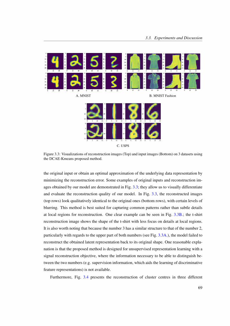
3.3. Experiments and Discussion

A. MNIST B. MNIST Fashion

C. USPS

Figure 3.3: Visualizations of reconstruction images (Top) and input images (Bottom) on 3 datasets usingthe DCAE-Kmeans proposed method.

the original input or obtain an optimal approximation of the underlying data representation by

minimizing the reconstruction error. Some examples of original inputs and reconstruction im-

ages obtained by our model are demonstrated in Fig. 3.3; they allow us to visually differentiate

and evaluate the reconstruction quality of our model. In Fig. 3.3, the reconstructed images

(top rows) look qualitatively identical to the original ones (bottom rows), with certain levels of

blurring. This method is best suited for capturing common patterns rather than subtle details

at local regions for reconstruction. One clear example can be seen in Fig. 3.3B.; the t-shirt

reconstruction image shows the shape of the t-shirt with less focus on details at local regions.

It is also worth noting that because the number 3 has a similar structure to that of the number 2,

particularly with regards to the upper part of both numbers (see Fig. 3.3A.), the model failed to

reconstruct the obtained latent representation back to its original shape. One reasonable expla-

nation is that the proposed method is designed for unsupervised representation learning with a

signal reconstruction objective, where the information necessary to be able to distinguish be-

tween the two numbers (e.g. supervision information, which aids the learning of discriminative

feature representations) is not available.

Furthermore, Fig. 3.4 presents the reconstruction of cluster centres in three different

69

3. DeepCluster: A Deep Convolutional Auto-encoder with Embedded Clustering

Figure 3.4: Visualizing the reconstruction of clustering centres on 3 different datasets. Top: USPS;Middle: MNIST-FASHION; Bottom: MNIST.

datasets for the DCAE-Kmeans method. This procedure allows for the evaluation of not only

the reconstruction quality but also the clustering quality, as the results of our clustering methods

can be visually justified and the reasons behind such results can be identified. In the MNIST

dataset, the typical reconstruction quality of cluster centres is clearly shown, allowing to vi-

sually evaluate the clustering quality. A cluster centre represents the common homogeneous

patterns in the latent space for a particular digit. Fig. 3.4 allows for the identification of where

the misclustering has occurred. For instance, with the USPS dataset, the model fails to recon-

struct the cluster centre of digit 5 and reconstruct a cluster centre similar to digit 2, indicating

that the model has an issue with the samples of digit 5 and misclassifies them as digit 2. More-

over, in the MNIST-Fashion dataset, the model shows the ability to reconstruct the majority

of the data cluster centres, however, it fails to reconstruct the cluster centre of the Coat class

and Shirt class, allowing us to justify the obtained low clustering results and help us to identify

where the clustering error has occurred.

In addition, we carried out a visual assessment where the t-Distributed Stochastic Neighbor

Embedding (t-SNE) visualization method [267] was applied to evaluate the clustering results

of the proposed methods. The t-SNE is used to visualize high-dimensional data, where it gives

each datapoint a location in a two-dimensional map. Fig. 3.5 shows a 2D projection of latent

representations obtained with the proposed methods, where the clustering results are color-

coded using ground truth labels. It shows that with joint clustering loss, the learned latent

representation space has more compact structures forming significant clusters which match

better with the true labels. This is particularly the case with joint clustering loss (Fig. 3.5C.

and Fig. 3.5D.), where the learned features have larger inter-cluster distances and tighter struc-

tures (see clusters labeled with orange, magenta, pink and dark green colors) compared to the

70

3.3. Experiments and Discussion

A. DCAE-Kmeans (True Labels) B. DCAE-GMM (True Labels)

C. DCAE-Kmeans (Our results) D. DCAE-GMM (Our results)

E. DCAE without clustering

Figure 3.5: Visualizations of latent representations in a two-dimensional space with t-SNE on MNIST.

method using no clustering constrains (Fig. 3.5E.). The learned features with no clustering con-

straint are sparse and not compacted, where lots of outliers can be recognized, and the clusters

overlap with each other. Imposing a clustering objective function aids to ensure the newly ob-

tained data representations in the internal layer are assigned to their identical cluster. Although

DCAE-Kmeans Fig. 3.5C. and DCAE-GMM Fig. 3.5D. enforce compact representation on a

71

3. DeepCluster: A Deep Convolutional Auto-encoder with Embedded Clustering

A. Epoch 0 B. Epoch 10 C. Epoch 30

D. Epoch 50 E. Epoch 100 F. Epoch 200

Figure 3.6: Visualizations of latent representations with our clustering results in a two-dimensionalspace with t-SNE through an iterative training scheme on MNIST.

hidden layer, showing that our proposed objective functions effectively enhance the clustering

process and form a kind of structure to increase data compactness, DCAE-GMM can perform

much better than DCAE-Kmeans. In the representation of digits 7, 4, and 9 (clusters labeled

with the color grey, light blue, and purple), the DCAE-Kmeans model failed to identify some

outlier samples, while DCAE-GMM classified them in a much better way, looking qualitatively

identical to the ground truth Fig. 3.5B..

Lastly, we applied t-SNE visualization to show the distribution of the latent representa-

tions in a two-dimensional space. The learned representations of the MNIST test dataset at

different epochs are shown in Fig. 3.6. The figure compares the cluster formation during dif-

ferent epochs of the learning procedure of the DCAE with embedded clustering. At the initial

epoch, no clustering structure is observed, and the learned features with DCAE are not dis-

criminative and sparse for clustering (Fig. 3.6A.). After ten epochs, some clusters are initially

composed, but the majority of them overlap one another, and clustering outliers are widely ob-

72

3.4. Summary

served (Fig. 3.6B.). For instance, the representation of digits 8, 0, and 1 (clusters labeled with

the colors lime, dark blue and orange) begin to form compact clusters, while the representation

of digits 6, 4, and 9 (clusters labeled with the colors pink, purple, and light blue) overlap one

another. This also occurred with digits 3 and 5 (clusters labeled with the colors red, and brown).

It is noteworthy that due to such smoothness the digit 4 has a similar structure to digits 6 and 9.

One reasonable explanation is that all of these digits have a similar structure and the model not

trained enough to distinguish them. However, with more training iterations, representative fea-

tures and useful information are obtained, and similar patterns of the learned representation are

locally compacted. Fig. 3.6C. shows that the representations of digits 3 and 5 are distributed

and form separate clusters. Similarly, the representations of digits 6, 4, and 9 are far away from

each other and form separate clusters. Fig. 3.6D. shows the cluster starting to form the best

partitioning of data and maximize the purity of clusters. As the learning scheme continues,

the overlapping clusters become discriminative and enforce compact representation, and the

intra-cluster variances are reduced significantly, while the inter-cluster distances are enlarged.

Furthermore, fewer cluster outliers are observed. The observation is consistent with the results

shown in Fig. 3.2.

3.4 Summary

In this chapter, we have proposed clustering approaches embedded in a DCAE. The proposed

methods alternately learn feature representation and cluster assignment through a DCAE. Both

methods consist of clustering and reconstruction objective functions. These procedures en-

able the classification of a data point into its identical cluster in the latent space in a joint-cost

function by alternately optimizing the clustering objective and the DCAE objective, thereby

producing stable representations appropriate for the clustering process. The proposed method

is trained in an end-to-end way using fixed settings without any pre-training or fine-tuning pro-

cedures, enabling a faster training process. We demonstrate the effectiveness of our clustering

methods by comparing ours with seven baseline methods on three different image datasets. The

experimental results show that DCAE-GMM substantially outperforms all other deep cluster-

ing methods. The DCAE-GMM has also performed much better than DCAE-Kmeans, as the

DCAE-Kmeans method failed to identify some outlier samples, while DCAE-GMM classified

them in a much better way, looking qualitatively identical to the ground truth with visual analy-

sis. The visual assessments demonstrate that as the learning scheme continues, the overlapping

clusters become discriminative and enforce compact representation, and the inter-cluster dis-

73

3. DeepCluster: A Deep Convolutional Auto-encoder with Embedded Clustering

tances are enlarged, which indicates that clustering stably converges using an iterative training

scheme.

The work on deep clustering contains novel materials, and it has become crucial to explore

and extend this with further analysis. The discriminative patterns of the DeepCluster are only

discovered through certain parts or objects in an image in an unsupervised manner, where the

information necessary to be able to further distinguish between clusters (e.g. supervision in-

formation which aids the learning of discriminative feature representations) is not available.

To address this, the following chapter investigates ways to reinforce the performance of deep

clustering methods and provides an analytical study for understanding the effectiveness of dif-

fering discriminatory power, focusing on strengthening and discriminating the learned features

through deep clustering methods. The discriminative feature representation is then utilized in

Chapter 5 and 6 to measure the importance of a network’s units for the purpose of network

compression. Finally, we apply what we proposed in this chapter to real-world data; a case

study in which the DeepCluster method is used to cluster animal behaviors through movement

is presented in Chapter 7.

74

Chapter 4

Learning Discriminatory DeepClustering Models

Contents4.1 Introduction . . . . . . . . . . . . . . . . . . . . . . . . . . . . . . . . . 76

4.2 Proposed Methods . . . . . . . . . . . . . . . . . . . . . . . . . . . . . . 78

4.2.1 DeepCluster: A DCAE with Embedded Clustering . . . . . . . . 79

4.2.2 Architecture . . . . . . . . . . . . . . . . . . . . . . . . . . . . . 79

4.2.3 Graph-Based Activity Regularization (GBAR) . . . . . . . . . . . 80

4.2.4 Data Augmentation (DA) . . . . . . . . . . . . . . . . . . . . . . 81

4.2.5 Extended Output Layer and Different Levels of Supervision . . . 82

4.3 Experimental Results . . . . . . . . . . . . . . . . . . . . . . . . . . . . . 83

4.3.1 Regularizations for DeepCluster . . . . . . . . . . . . . . . . . . 84

4.3.2 Learning Discriminatory Deep Clustering Models Through Dif-

ferent Levels of supervision . . . . . . . . . . . . . . . . . . . . 87

4.3.3 Deep Clustering Through Various Levels of Supervision . . . . . 91

4.4 Summary . . . . . . . . . . . . . . . . . . . . . . . . . . . . . . . . . . . 93

75

4. Learning Discriminatory Deep Clustering Models

4.1 Introduction

In recent years, different approaches to unsupervised deep clustering have been developed

utilizing deep neural networks [20]. A deep convolutional auto-encoder (DCAE) has been

exploited for clustering analysis, allowing clustering algorithms to deal with abstract latent

representations in a low-dimensional space. DCAE is a deep unsupervised model for represen-

tation learning. It maps inputs into a new latent space, allowing for the acquisition of useful

feature representations via its encoding layer. These high-level representations provide ben-

eficial properties that support traditional clustering algorithms in demonstrating a satisfying

performance.

DeepCluster [5], a DCAE with embedded clustering which is proposed in the previous

chapter, is a deep unsupervised clustering method that simultaneously captures representative

features and the relationships among images, extracts similar patterns in new space repre-

sentations, and finds ideal representative centers for distributed data. In this procedure, the

discriminative patterns are only discovered through certain parts or objects in an image in an

unsupervised manner. The goal of this method is to learn feature representations and cluster

assignments simultaneously, utilizing the strength of the DCAE to learn high-level features

in the latent space. Two objective functions were utilized: one was embedded into a DCAE

model to minimize the distance between features and their corresponding cluster centres, while

the other was used to minimize the reconstruction error of the DCAE. During optimization, all

data representations are assigned to their new identical cluster centres, after which the cluster

centres are updated iteratively, allowing the model to achieve a stable clustering performance.

The defined clustering objective, as well as the reconstruction objective, are simultaneously

utilized to update the parameters of the transforming network.

In an attempt to investigate the ways in which to reinforce the performance of conventional

clustering methods, several methods have been developed to study semi-supervised clustering

approaches [191–196], which aim to cluster a large amount of unlabeled data in the presence

of minimal supervision. Similarly, several supervised clustering methods [198–202] have been

proposed. Their core idea is to include a supervisory scheme into the clustering process, so as to

improve unsupervised clustering performance by exploiting supervised information. Conven-

tional supervised and semi-supervised clustering approaches have received a lot of attention;

however, despite the substantial success of deep learning, limited attention has been paid to

deep supervised and semi-supervised clustering methods. Therefore, providing a way to inject

varying degrees of supervision into the body of the learning process and exploring the influence

76

4.1. Introduction

of adding supervision knowledge into a deep clustering method are worthwhile endeavors in

order to distinguish the discriminative powers obtained by patterns in an unsupervised manner

or provided by supervision components. To empirically analyze the above insight, a new ver-

sion of DeepCluste is introduced to involve a supervision component and assist with forming a

kind of a structure that reconciles discriminative features discovered by the clustering process

and discriminative features provided by labeling patterns. This mechanism ensures that the

learned features derived from the encoding layer are the best discriminative attributes. In other

words, it looks to find a well-defined structure for clusters, through the encoding part of the

DCAE, in the presence of discriminative power attributes.

Furthermore, most of the previously mentioned methods focus on providing supervision

to the clustering process; however, their focus was on modifying the clustering methods by

imposing more constraints. Limited attention was paid to strengthening the discriminative fea-

tures, which would facilitate the job of traditional clustering algorithms. Therefore, taking

advantage of deep learning methods to strengthen the discriminatory power of the learned fea-

tures through the learning process is deserving of study, where the deep clustering algorithm

can be supported in demonstrating satisfying performance. Our key insight is that a DCAE

with embedded clustering can have robust discriminative power, as the learned features are

highly expressive and can be worthy injective functions. As a result, we introduce a deep clus-

tering method that is carried out in the presence of varying degrees of discriminative power. To

the best of our knowledge, our work provides the first analytical study for understanding the

effectiveness of the discriminatory power obtained by the use of two discriminative attributes:

data-driven discriminative attributes with the support of regularization techniques, and super-

vision discriminative attributes with the support of the supervision components. Although the

data augmentation technique has received considerable attention in supervised learning as a

way to tackle the generalization issue, it has been overlooked by most of the deep clustering

methods. To fill this gap, we introduce the data augmentation technique into the method of

DeepCluster and study the effectiveness of the discriminatory power obtained by data augmen-

tation patterns in deep clustering performance.

In this chapter, we focus on deep clustering methods in which varying degrees of discrim-

inative powers can be imposed on the clustering layer or injected into the body of the learning

process. We propose a new version of the DeepCluster to allow for the imposing of regulariza-

tion techniques and the involvement of a supervision component. This mechanism allows us

to experience different discriminatory powers and examine the clustering performance through

77

4. Learning Discriminatory Deep Clustering Models

different discriminative attributes. We consider two regularization techniques: one that is em-

bedded into the clustering layer, and another that is used during the training process. We also

consider three different learning levels: supervised, semi-supervised and unsupervised. We

evaluate our experimental methods on MNIST, USPS, MNIST fashion, and SVHN datasets.

Furthermore, we show the deep clustering performance at certain levels of supervision as well

as the impact of the regularization techniques.

The rest of the chapter is organized as follows: in section 4.2, we present our methodologies

and approaches. In section 4.3, we present our experimental results, and finally, concluding

remarks are given in section 4.4.

4.2 Proposed Methods

The proposed approach is a deep clustering method that is carried out in the presence of vary-

ing degrees of discriminative power. It introduces a mechanism with which various levels of

supervision are injected into the body of the learning process. This mechanism allows us to ex-

plore the impact of supervised information on the achievement of our deep clustering method.

The effectiveness of the discriminatory power that is obtained by discriminative attributes with

the support of regularization techniques is also studied. It allows us to investigate the discrim-

inative power resulting from the inclusion of regularization and data augmentation techniques

into the body of the deep clustering model.

We consider two regularization techniques and three different learning levels. A discrimi-

native representation, via the internal layer of DCAE, is exploited to support the clustering task

in the presence of varying degrees of supervision, regularization and data augmentation tech-

niques. A combination of methods is imposed on the DCAE architecture or injected into the

body of the learning process to strengthen the learned features and support the performance of

the deep clustering. Each experimental model consists of a combination of objective functions,

some of which minimize the clustering loss, the reconstruction loss, and the categorical cross-

entropy function of the provided supervision. All objectives are simultaneously optimized.

The following subsections clarify our methodology. First, we briefly review how the Deep-

Cluster works and define the necessary loss functions when introducing the proposed methods.

After that, we describe the architecture used in our methods. Then, we explain the regular-

ization and data augmentation techniques and how they are utilized to support the learning of

discriminative features. Finally, we introduce a new version of the DeepCluster, where the out-

78

4.2. Proposed Methods

put layer is extended to allow for the injection of different levels of supervision into the body

of the learning process.

4.2.1 DeepCluster: A DCAE with Embedded Clustering

In the encoding part of DCAE, convolutional layers are used as feature extractors to learn fea-

tures through mapping the data into an internal layer. Then, the deconvolutional layers are used

to reconstruct the data representation to its original shape by minimizing the reconstruction er-

ror using the Euclidean (L2) loss function.

E1 =1N

N

∑n=1‖ xn− xn ‖2, (4.1)

where x is a reconstructed image, and x is an original image.

Although DCAE learns effective representations via its encoding layer, it does not explic-

itly force representation to form compact clustering. In the previous chapter, we proposed the

DeepCluster that learns feature representations and clusters assignments simultaneously. It

embeds a clustering objective function into a DCAE framework that minimizes the distance

between data points and their assigned centers in the latent space as follows:

E2 = λ · 1N

N

∑n=1‖ ht(xn)− c∗n ‖2, (4.2)

where λ is a weight-parameter that controls the contribution percentage of a certain cost func-

tion in the overall cost function, N is the number of data examples, ht(∗) denotes the encoded

representation obtained at the tth iteration, (xn) is the nth example in the dataset x, and c∗n is the

assigned centroids to the nth example. At each iteration, the model optimizes two components

using an optimizer and backpropagation: (1) network parameters as well as a mapping function

h, and (2) cluster centers c. After each internal representation is assigned to the closest cluster

center, the cluster centers are iteratively updated.

4.2.2 Architecture

Our DCAE architecture consists of three convolutional layers. This is followed by two fully-

connected layers, of which the second layer (clustering layer) has ten neurons. These are

considered to be hidden representations learned through the training process. A single fully-

connected layer is followed by three deconvolutional layers as the decoding part, and ReLU

is utilized as the activation function. Table 4.1 shows a detailed configuration of the DCAE

79

4. Learning Discriminatory Deep Clustering Models

Table 4.1: Detailed configuration of the DCAE network architecture used in the experiments.

Layer MNIST USPS MNIST Fashion SVHN

Convolutional 5×5×32 4×4×32 5×5×32 5×5×32

Convolutional 5×5×64 4×4×64 5×5×64 5×5×64

Convolutional 3×3×128 2×2×128 3×3×128 2×2×128

Fully-Connected 1152 512 1152 2048

Fully-Connected 10 10 10 10

Fully-Connected 1152 512 1152 2048

Deconvolutional 3×3×128 2×2×128 3×3×128 2×2×128

Deconvolutional 5×5×64 3×3×64 5×5×64 5×5×64

Deconvolutional 5×5×32 3×3×32 5×5×32 5×5×32

network architecture for all experimental datasets. Our extensions to this architecture are as

follows: firstly, the learned features given by the encoding layer are optimized to form compact

and discriminative clusters using a clustering objective function, which minimizes the distance

between a feature representation and its respective centroid. Secondly, at the same time as min-

imizing the reconstruction loss, we iteratively optimize the mapping function of the encoding

part and cluster centres to obtain more effective clustering. Thirdly, we modify the architecture

to include the regularization terms; see section 4.2.3 for details. Lastly, instead of a reconstruc-

tion layer at the end of the DCAE, extra layers are added at the end of the network just after

the reconstruction layer to inject different degrees of supervision; see section 4.2.5 for details.

4.2.3 Graph-Based Activity Regularization (GBAR)

A combination of activity regularization techniques, which were recently proposed in [268],

are included in the clustering layer. This allows us to examine the achievements of the deep

clustering method with regularizer terms. The activity regularization techniques ensure each

node is specialized and enforce inputs to equally spread out over the clustering layer nodes.

We adopt these techniques in combination with our clustering loss to determine the impact of

the regularization techniques on the clustering performance

Considering B represents the outputs of the clustering layer for all m examples with n

number of output nodes, N is the symmetric matrix defined as N = BT B. In order to obtain an

identity matrix, affinity enforces the off-diagonal entries to be zeros, which ensures that a single

80

4.2. Proposed Methods

input can only have one high activation node, allowing for the specialization of the nodes. The

input must belong to one of the clusters. Otherwise, it will cause some errors in clustering.

A f f inity = α(B) =∑

ni 6= j Ni j

(n−1)∑ni= j Ni j

. (4.3)

The diagonal entries of N is a 1-D vector called v. V is a symmetric matrix that results from

the manipulation of the transpose of the diagonal entries of N by the diagonal entries, defined

as V = vT v. The term (Balance) forces inputs to equally spread out over the clustering layer

nodes, ensuring all nodes in the clustering layer are equally activated within one batch.

Balance = β (B) =∑

ni 6= j Vi j

(n−1)∑ni= j Vi j

. (4.4)

The overall cost function is a combination of loss functions and regularization terms: the

first part essentially minimizes the reconstruction objective function E1, by Eq.(4.1) , and clus-

tering objective function E2, by Eq.(4.2). The rest of the overall cost function is regularization

terms.

minW,b

E1 +E2 + cαα(B)+ cβ (1−β (B))+ cF ‖ B ‖2F , (4.5)

where α(.) and β (.) are the unsupervised regularization terms respectively defined in Eq.(4.3),

Eq.(4.4), ‖ B ‖F denotes to the Frobenius norm for B, and cα ,cβ ,cF are the regularization

weighing coefficients.

4.2.4 Data Augmentation (DA)

Data augmentation is a regularization technique widely used in supervised deep learning mod-

els to improve their generalization. Data augmentation is the process of generating transformed

versions of original images in the training dataset. Transforms include a range of operations

such as random rotation, flipping, shifting, zooming and cropping, and much more. The lo-

cal structure preservation distinguishes the convolutional neural network (CNN), so it learns

features that are invariant to their local information in the image. Data augmentation can aid

a model to learn features that are invariant to transformation and can support learning using

the transform invariant approach. Therefore, it is worthwhile to study the effectiveness of the

discriminatory power obtained by data augmentation patterns in an unsupervised clustering

method. To that end, we introduce a data augmentation technique into the DeepCluster.

81

4. Learning Discriminatory Deep Clustering Models

Given a set of training samples Xn , where n donates the number of samples. For each

example Xi, we can apply augmentation using the following form: Xi = Taugmentation(Xi). In the

DCAE, the reconstruction objective function utilized in this case is:

E1 =1N

N

∑n=1‖ xn− yn ‖2, (4.6)

where x is an augmented version of the original image x, and y is a reconstructed image of the

augmented version.

4.2.5 Extended Output Layer and Different Levels of Supervision

We utilize the network architecture, discussed in section 4.2.2. Our extension to the architec-

ture is that instead of a reconstruction layer at the end of the DCAE, an extra layer is added at

the end of the network, just after the reconstruction layer. This allows us to inject supervision

knowledge across the learning process and also examine clustering performance with different

discriminatory power provided by supervision knowledge. The new version of the DeepClus-

ter method allows us to utilize its strength to obtain discriminative and robust features from

the encoding layer. It also allows the deep clustering method to extract more discriminative

features and cluster assignments simultaneously.

We use the same architectures in the supervised and semi-supervised models, as shown on

Table 4.1. Instead of a reconstruction layer at the end of the DCAE, we flatten the output of

the reconstruction layer and feed it into a certain number of nodes in the last layer. The number

of nodes depends on the task at hand, i.e. the number of provided classes (e.g. ten nodes for

the supervised case and two nodes for the semi-supervised case). A softmax function is used

for the final prediction. The final architecture of our extended version of the DeepCluster is

presented in Fig. 4.1.

Two forms of labels are used, true labels and parent-class labels, to reflect two different

levels of supervision. True labels are provided in the supervised training process. Parent-class

labels are used in semi-supervised deep clustering, where true class labels are combined to

form parent-class labels. For example, in the clustering digit images created using the the

proposed DCAE, the parent-class labels are defined as:

ParentLabel =

0 Labels < 5

1 otherwise. (4.7)

82

4.3. Experimental Results

Figure 4.1: The architecture of the discriminatory DeepCluster models. An extra layer is added at theend of the network just after the reconstruction layer to inject different degrees of supervision.

The categorical cross-entropy function between network predictions and provided labels is

defined as:

E3 =−∑j

ti, jlog(pi, j), (4.8)

where p is prediction, t is the sample label, i indexes samples, and j indexes classes. In the

DCAE hidden layer, encoded features are used to compute clustering loss function in order to

minimize the distance between data points and their corresponding cluster centers.

The overall cost function is thus a combination of reconstruction loss E1, by Eq.(4.1),

clustering residual in latent space E2, by Eq.(4.2), and categorical cross-entropy loss E3, by

Eq.(4.8) that minimizes the classification error with any supervised or semi-supervised scheme:

minW,b

E1 +E2 +E3. (4.9)

4.3 Experimental Results

Learning discriminatory deep clustering models through adopting a variety of regularization

techniques or through injecting various levels of supervision into the learning process is a

unique mechanism. It helps to reconcile extracted latent representations effectively and pro-

vide discriminative power to produce the best discriminative attributes. The key idea of our

approach is to distinguish the discriminatory power of numerous formats (e.g. through adopt-

ing GBAR and DA techniques or through varying degrees of supervision) when searching for a

83

4. Learning Discriminatory Deep Clustering Models

Table 4.2: Details of the datasets used in our experiments for the discriminatory DeepCluster models.

Dataset Examples Classes Image Size Channels

MNIST [83] 70000 10 28x28 1

USPS [260] 11000 10 16x16 1

MNIST Fashion [261] 70000 10 28x28 1

SVHN [270] 99289 10 32x32 3

compact structure with which to form robust clusters. We first studied the achievements of our

DeepCluster method when adopting GBAR and DA techniques. After this, we analyzed the

impact of injecting different levels of supervision into a deep clustering method. Lastly, we in-

vestigated the deep clustering performance when adopting the GBAR regularization technique

with various levels of supervision.

Implementation Details

The proposed methods were implemented using Keras [265] and Theano [269] in Python and

evaluated on four different datasets; MNIST [83], USPS [260], MNIST fashion [261], and

SVHN [270] datasets. Some of these are the most commonly used datasets in previous liter-

ature published in the field of deep clustering methods. The specifications of these datasets

are presented in Table 4.2. The proposed models were trained end-to-end without involving

any pre-training or fine-tuning procedures. All weights and cluster centers were initialized ran-

domly. The Adam [63] optimizer was used, where each batch contains 100 randomly shuffled

images. We set λ , which is the clustering weight-parameter that controls the loss contribution

percentage of clustering error, to 0.1. Throughout our experiment, we used a fixed learning

rate of 0.006, a momentum of 0.9, and a weight decay of 0.0005.

4.3.1 Regularizations for DeepCluster

Here, we study the impact of embedding a variety of regularization techniques (e.g. GBAR

or DA) into a deep clustering method. This procedure allows us to analyze the discriminative

powers of the learned features by adopting GBAR or DA and examine the achievements of

our DeepCluster method. We use a DCAE model to map the data, via a series of convolu-

tional layers, into latent representation, and embed the Kmeans clustering algorithm as well

as regularization techniques into an integral deep clustering framework. This process enables

84

4.3. Experimental Results

Figure 4.2: Visualizations of reconstruction images (Top) and input images (Bottom) in SVHN dataset.

Table 4.3: Comparison of clustering quality of the DeepCluster method using accuracy evaluation metricwith and without regularizations.

Regularization MNIST USPS MNIST fashion SVHN

None 93.42% 83.25% 58.20% 17.41%

GBAR 93.37% 73.49% 57.79% 17.05%

DA 95.46% 84.81% 60.06% 22.30%

the deep clustering method to extract more enhanced discriminative features while clustering

assignments in a simultaneous manner. The deconvolutional layers are, thereafter, used to

reconstruct the data representation to its original shape.

The GBAR regularization technique, discussed in section 4.2.3, is embedded into the clus-

tering layer, which is the last layer of the encoding part of the DCAE. Said technique ensures

that each node in the clustering layer is specialized and forces inputs to spread out over the clus-

tering layer nodes equally. Considering B is the output of the clustering layer, which forms an

m×10 matrix, where m is the number of examples and 10 is the output nodes of the encoding

part, which represent the number of clusters in our experiments. N is 10×10 symmetric matrix

defined as N = BT B, which is enforced to be an identity matrix, called affinity regularization.

This term ensures a single input can have only one high-activation node, allowing specializa-

tion of such a node, while the term of balance regularization enforces inputs to equally spread

out over the clustering layer nodes, which ensure all nodes in the clustering layer are equally

activated within one batch. The DA, on the other hand, is used as a regularization to help a

model avoid the over-fitting issue and learn invariant features to support the performance of

85

4. Learning Discriminatory Deep Clustering Models

the DeepCluster method. The utilized DA comprises a suite of techniques, including various

degrees of flipping and rotation, which can enhance more discriminative power, such that better

deep clustering can be achieved using them.

To validate the effectiveness of consolidating regularization techniques, we compare the

clustering performance of our DeepCluster method with and without regularization techniques.

Table 4.3 compares the results of the unsupervised deep clustering methods using the recon-

structed loss. It shows that the adoption of the GBAR technique did not significantly affect

the result of clustering accuracy, neither did it add any discriminative ability to the deep clus-

tering method. Essentially, at the beginning of learning, the clusters have not yet formed, and

thus, activation of one node in a layer from an input does not reflect the actual situation and

thus multiple nodes should be allowed to be activated. In contrast, the adoption of the DA

technique resulted in moderate improvement in clustering accuracy. In other words, the accu-

racy of the DeepCluster method on MNIST, USPS, and MNIST Fashion increased by 2.04%,

1.56%, and 1.86% respectively, compared to the method which did not use any regularization

technique. The improvement is still observable even on the more difficult dataset SVHN. Our

unsupervised deep clustering method did not perform well for the SVHN dataset, even though

it retrieved the effective latent representation into an appropriate approximation of the original

input data Fig. 4.2. The reason is that instead of clustering the digits’ patterns, the clustering

method intends to group the data examples based on their backgrounds’ shape and color.

Table 4.3 demonstrates that the adoption of the DA can improve the clustering accuracy,

which is consistent with a recent study by [266]. Our result proves that the adoption of the

DA can moderately provide a discriminative power to the DeepCluster method. One reason-

able explanation for this minor improvement is the invariance of the learned features of the

unsupervised deep clustering method. In contrast to supervised learning, the learned features

of unsupervised learning are more invariant, and the aid of generating transformed versions of

original images can be limited to improve the clustering performance significantly. This fact

motivated us to investigate and analyze the invariance properties of the learned representation

in the latent space through different levels of supervision, see section 4.3.2 for details.

The utilization of the GBAR technique is intended to enforce the clustering process and im-

pose restrictions when clustering the feature representations of the DCAE. Our results demon-

strate that obtaining clustering-friendly latent representations through unsupervised DCAE

model, where the learned features are invariant, could be sufficient to allow our DeepCluster

method to yield a substantially better performance for both reconstruction and clustering qual-

86

4.3. Experimental Results

ity without any enforcement. Therefore, adopting a regularization technique such as GBAR

is useless in this case as it may depend on when such regularizations are imposed. Given that

a DCAE offers clustering-friendly discriminative latent representations by minimizing the re-

construction error, the learned features can be efficiently clustered without any regularization

technique. The GBAR technique [271] has shown its ability to help clustering latent represen-

tation when the hidden information is captured through the help of discriminative models (e.g.

semi-supervised process [272] or an initialized supervised pertaining process [268]). These

findings motivated us to investigate and analyze the impact of adopting GBAR into a deep

clustering method when injecting different levels of supervision, see section 4.3.3, for details.

4.3.2 Learning Discriminatory Deep Clustering Models Through DifferentLevels of supervision

Here, we extend the architecture of the DCAE and add an output layer to inject supervision

information into the body of the learning process. In the encoding part of the DCAE, an abstract

latent representation is learned in a discriminative way to capture not only the discriminative

attributes from the data, but also patterns provided by supervision components. The injection

of the supervision into a DCAE framework provides a powerful discriminative capability that

supports our deep clustering method in demonstrating satisfying performance. To thoroughly

investigate the abilities of our proposed method, we first evaluated the clustering performance

in the presence of minimal supervision. After that, we visually and empirically evaluated

the impact of supervision on the deep clustering methods. Then, we evaluated the clustering

performance with different supervision schemes. Lastly, we analyzed the invariance properties

of learned representation, given different levels of supervision.

4.3.2.1 Deep Clustering Performance with Minimal Supervision

For the MNIST dataset, the experiments were performed using four different numbers of

trained examples, i.e. 2000, 4000, 6000, 8000. In other words, we only used a limited number

of examples at the training stage to simulate data with a shortage of labeled data. We trained

our supervised model using these settings with the same number of iterations. The comparative

results are shown in Table 4.4, and support our hypothesis that a small amount of labeled data

can add enough discriminative ability to unsupervised deep clustering. Note that the results are

the accuracy of clustering, not classification using reconstructed image.

87

4. Learning Discriminatory Deep Clustering Models

Table 4.4: Number of samples used in the training stage and clustering accuracy.

Trained Examples Clustering Accuracy

2000 94.24 %

4000 96.48 %

6000 97.52 %

8000 98.06 %

4.3.2.2 Visualizing Learned Representation Through Different Levels of Supervision

In order to visualize the impact of supervision in deep clustering, the t-SNE visualization

method [267] was applied as a visual assessment to show that the addition of supervision

allows to guide the clustering task to obtain more appropriate data partitioning and present

demarcated clusters relevant to the supervised learning task. Fig. 4.3 shows the latent rep-

resentation of our proposed methods in 2D space using different levels of supervision; the

color-coding of the ground truth labels are used to visualize the clustering results. This visual-

ization shows that adding a supervision component into the deep clustering method produces

significantly more compact clusters, which have a better matching with true labels Fig. 4.3

(top row). The learned features involve a supervised process has tighter structures and larger

inter-cluster distances compared with semi-supervised and unsupervised models. Injecting su-

pervision into the learning process effectively reconciles data-driven obtained representations

and the provided supervision knowledge to form the best partitioning of data and maximize

the purity of clusters. With the semi-supervised model (Fig. 4.3E.), the clustering results show

typical compact clusters, producing much better clustering results compared with the unsuper-

vised model (Fig. 4.3, Right), where the learned features are sparse and not compact. Although

the visualization of (Fig. 4.3F.) shows compact clusters, when comparing this with (Fig. 4.3C.),

it appears the learned features via the unsupervised model do not match the true labels. That is

illustrated by the overlapping colors on (Fig. 4.3F.). Compared to (Fig. 4.3F.) which enforces

compact representation on a hidden layer, the clusters formed by normal DCAE still present

ten distinct clusters, although they have higher intra-cluster variance and lower inter-cluster

difference. Thus, by adopting semi-supervised (see Fig. 4.3E.) and supervised models (see

Fig. 4.3D.), intra-cluster variances are reduced significantly while the inter-cluster distances

are enlarged. In particular, less cluster outliers are observed in Fig. 4.3D..

88

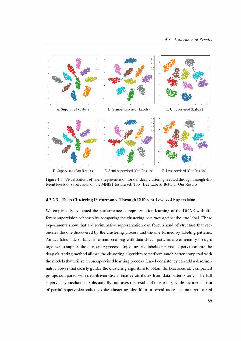
4.3. Experimental Results

A. Supervised (Labels) B. Semi-supervised (Labels) C. Unsupervised (Labels)

D. Supervised (Our Results) E. Semi-supervised (Our Results) F. Unsupervised (Our Results)

Figure 4.3: Visualizations of latent representation for our deep clustering method through through dif-ferent levels of supervision on the MNIST testing set. Top: True Labels. Bottom: Our Results

4.3.2.3 Deep Clustering Performance Through Different Levels of Supervision

We empirically evaluated the performance of representation learning of the DCAE with dif-

ferent supervision schemes by comparing the clustering accuracy against the true label. These

experiments show that a discriminative representation can form a kind of structure that rec-

onciles the one discovered by the clustering process and the one formed by labeling patterns.

An available side of label information along with data-driven patterns are efficiently brought

together to support the clustering process. Injecting true labels or partial supervision into the

deep clustering method allows the clustering algorithm to perform much better compared with

the models that utilize an unsupervised learning process. Label consistency can add a discrimi-

native power that clearly guides the clustering algorithm to obtain the best accurate compacted

groups compared with data-driven discriminative attributes from data patterns only. The full

supervisory mechanism substantially improves the results of clustering, while the mechanism

of partial supervision enhances the clustering algorithm to reveal more accurate compacted

89

4. Learning Discriminatory Deep Clustering Models

groups compared to unsupervised deep clustering methods. Table 4.5 summarizes the experi-

mental results on four different datasets including MNIST, USPS, and more challenging ones,

such as MNIST fashion and SVHN. Since the performances were evaluated on a clustering

task, the accuracy increasing with supervision knowledge can be observed in both cases. Par-

ticularly for the SVHN dataset, the accuracy is boosted by more than double when weak labels

are provided. We argue that the common structures are not well-formed without supervision,

where large appearance variance and image noise are commonly observed in the SVHN dataset.

Table 4.5: Comparison of clustering accuracy on four different datasets using different learning levels.

MNIST USPS MNIST fashion SVHN

Unsupervised 93.42% 83.25% 58.20% 17.41%

Semi-supervised 97.77% 91.92% 63.59% 43.96%

Supervised 98.82% 95.06% 88.73% 92.40%

4.3.2.4 Invariance Properties of the Learned Representation Through Different Levels

of Supervision

We analyzed the invariance properties of learned representation given different levels of su-

pervision. We trained five different models with varying degrees of supervision: supervised,

semi-supervised with three different percentages of supervision (20% (Semi-1), 30% (Semi-

2), 50% (Semi-3)), and unsupervised. We applied a range of rotation-based transformations

(rotate by 90o, 180o, 270o, flip horizontally, flip horizontally and rotate by 90o, 180o, 270o)

to each image. Moreover, we followed [273, 274] to measure the variance properties by cal-

culating the Mean Squared Error (MSE) between the features of the original images and the

transformed ones. The comparison results of invariance properties of the learned representa-

tion in four different layers are shown in Fig. 4.4. This allows for the tracking of the changes of

invariance properties through different layers, where the encoding layer (Fig. 4.4D.) is shown

to be the most robust and invariant layer. The figure also compares the invariance properties

of learned representation in five different models. Overall, the experiment empirically con-

firms that the features are more invariant when no supervision is provided. In other words, the

features learned by the unsupervised model are more invariant compared to features learned

with supervision. With the semi-supervised approach, the invariance properties of the learned

representation differ based on the provided percentages of supervision. This indicates that the

90

4.3. Experimental Results

more limited a supervision percentage is, the more invariant and stable the obtained learned

representations are. However, such invariant representations are not expressive and thus lead

to worse clustering results.

A. Conv-1 B. Conv-2

C. Conv-3 D. Encoding

Figure 4.4: Invariance properties of the learned representation in different layers from five differentmodels: supervised, semi-supervised with three different percentages of supervision (20% (Semi-1),30% (Semi-2), 50% (Semi-3)), and unsupervised. We applied a range of rotation-based transformations:rotate by 90o (1), 180o (2), 270o (3), flip horizontally (4), flip horizontally and rotate by 90o (5), 180o (6),270o (7).

4.3.3 Deep Clustering Through Various Levels of Supervision

4.3.3.1 Supervised Clustering

To thoroughly investigate the impact of injecting full supervision by providing true labels, we

performed extra experiments in four different datasets and analyzed the learned features as well

as the impact of embedding the GBAR into the clustering layer of the DCAE. We exploited

91

4. Learning Discriminatory Deep Clustering Models

the discriminative patterns provided by supervision components to improve the accuracy of our

deep clustering method and allow us to obtain the best representative cluster centres for such

data in a given space. Table 4.6 summarizes the performance of our deep clustering method

in a fully supervised manner with different settings of the embedded GBAR technique. The

results represent the accuracy of clustering. Providing true labels to the DCAE with the em-

bedded clustering method allowed the clustering algorithm to deal with more discriminative

features and perform much better compared with other models (i.e. semi-supervised and unsu-

pervised), because the labels’ consistency in the latent space can be biased and guided to obtain

more characteristic features for compacted groups of such data. In addition, adding supervi-

sion guides the clustering task towards more appropriate data partitioning, which allows for the

acquisition of the best clustering performance. Table 4.6 also demonstrates that the adoption of

the GBAR technique restrains the clustering algorithm from achieving competitive clustering

results, because the obtained latent representations are biased and guided by the provided su-

pervision, offering clustering-friendly features for such a clustering algorithm; in other words,

imposing more restrictions can be inefficient and confusing.

Table 4.6: Supervised Clustering. Clustering accuracy with GBAR regularization technique using dif-ferent weighting coefficients.

cα cβ cF MNIST USPS MNIST fashion SVHN

With Regularization 0.1 0.1 0 84.04 % 95.51 % 77.51 % 75.46 %

With Regularization 0.8 0.8 0.0003 84.78 % 94.27 % 77.41 % 74.39 %

With Regularization 0.8 0.8 0.000001 96.81 % 93.67 % 77.37 % 73.33 %

Without Regularization 0 0 0 98.82 % 95.06 % 88.73 % 92.40 %

4.3.3.2 Semi-supervised Clustering

Here, we created a semi-supervised problem for all experimental datasets by providing two

parent-class labels, of which a class label is smaller or larger than 5. This setting allowed

us to examine the achievements of our deep clustering method, analyze the learned features

with partial supervision information, and observe the impact of adopting the GBAR technique.

Although injecting partial supervision into the deep clustering method is supposed to provide

discriminative features, the results of Table 4.7 show that the clustering algorithm embedded

into a semi-supervised deep clustering method struggles to demonstrate a good clustering per-

formance. However, clustering with the adoption of the GBAR significantly improves the

92

4.4. Summary

clustering accuracy, where adding the regularization technique into the semi-supervised model

ensures that each node is specialized and enforces input features to equally spread out over

the clustering layer nodes in a discriminative manner. These constraints provide discrimina-

tive patterns to enhance the clustering algorithm in more trustworthy partitioning, reveal more

accurate compacted groups for the learned feature representations, and thus improve the per-

formance of the clustering algorithm. Therefore, utilizing a small part of supervision as well

as the GBAR in this model guides the clustering algorithm in supporting its achievement and

help to obtain more appropriate data partitioning.

Table 4.7: Semi-supervised. Clustering accuracy with GBAR regularization technique using differentweighting coefficients.

cα cβ cF MNIST USPS MNIST fashion SVHN

With Regularization 0.1 0.1 0 76.42 % 62.87 % 36.58 % 31.52 %

With Regularization 0.8 0.8 0.0003 97.77 % 91.92 % 63.59 % 43.96 %

With Regularization 0.8 0.8 0.000001 94.60 % 83.30 % 55.64 % 33.74 %

Without Regularization 0 0 0 27.53 % 28.45 % 30.98 % 26.30 %

4.4 Summary

This study has shown that a deep clustering method is capable of learning discriminative

data representations incorporated into different learning schemes, i.e. unsupervised, semi-

supervised, and supervised, with the help of two regularization techniques. This analytical

study seeks to establish an understanding of the effectiveness of the discriminatory power that

is obtained by two discriminative attributes: data-driven discriminative attributes with the sup-

port of regularization techniques, and supervision discriminative attributes with the support

of supervision knowledge. The mechanism of imposing a discriminative power on the clus-

tering layer or injecting it into the body of the learning process makes the learned features

derived from the encoding layer the best discriminative attributes, forming a kind of structure

that reconciles the one discovered by the clustering process and the one provided by labeling

patterns. During our experiments, a well-defined structure for clusters is found through the

encoding part of the DCAE, in the presence of discriminative power attributes. An available

side of background knowledge along with representative patterns in latent space can be lever-

aged to find the best partitioning of data and maximize the purity of clusters. We evaluated

our experimental methods on MNIST, USPS, MNIST fashion, and SVHN datasets, and show

93

4. Learning Discriminatory Deep Clustering Models

the clustering accuracy of our methods through supervised, semi-supervised and unsupervised

learning levels, illustrating the influence of discriminatory power on clustering performance.

We found that such supervision knowledge greatly helps to form discriminative transforma-

tions that are learned by the encoding part of the DCAE model and significantly improves

clustering performance. The results also demonstrate that even weak or partial supervision

knowledge could significantly improve the quality of deep clustering. Finally, the impact of

the regularization techniques on the achievements of clustering performance through a certain

level of supervision has been discussed.

In terms of performance, although the DeepCluster method retrieved the effective latent

representation into an appropriate approximation of the original input data, it did not perform

well with the more challenging datasets, such as the SVHN one, in which large appearance

variance and image noise are commonly observed. The reached accuracy is reasonable, as the

clustering method intends to group the data examples based on their backgrounds’ shape and

color. With supervision, the accuracy is increased by more than double when weak labels are

provided. We argue that the common structures are not well formed without supervision. Fur-

ther studies to improve the deep clustering would be beneficial, particularly on more difficult

datasets. In this study, we only provided a few limited scenarios involving the injection of

supervision; we believe that there is much more scope for the investigation and exploration of

various other scenarios for deep clustering with supervision and partial supervision, aiming to

differently simulate a shortage of labeled data.

The adoption of the GBAR regularization technique varies with regards to improving the

clustering accuracy across numerous learning schemes. It does provide benefits in improv-

ing the semi-supervised clustering accuracy, revealing more accurate compacted groups for

the learned feature representations. However, it does not significantly affect the clustering re-

sults of the unsupervised model and restrains the supervised clustering method from achieving

competitive clustering. Thus, it would be of considerable interest to further investigate the rela-

tionship between the GBAR regularization technique and invariance properties of the learned

representation through different supervision levels. Moreover, further theoretical analysis is

also required to understand how to improve clustering performance.

A key observation from work shown in this chapter and the previous chapter is that the

characteristic strength of learned representations lies in its ability to enhance and further sup-

port the embedded clustering. This observation raises the question of whether the characteristic

strength of learned representations aids in compressing and accelerating deep neural networks?

94

4.4. Summary

In Chapters 5 and 6, we explore this idea by evaluating the importance of a network’s units for

the purpose of network compression. Following this, Chapter 7 concludes by presenting a com-

prehensive review of time-series data analysis, with emphasis on deep time-series clustering

(DTSC), and a founding contribution to the area of DTSC application. The state-of-the-art and

outlook on DTSC are also provided.

95

Chapter 5

Reducing Neural Network Parametersvia Neuron-based Iterative Pruning

Contents5.1 Introduction . . . . . . . . . . . . . . . . . . . . . . . . . . . . . . . . . 98

5.2 Proposed Method . . . . . . . . . . . . . . . . . . . . . . . . . . . . . . . 99

5.2.1 Importance of Individual Neurons via Majority voting (MV) . . . 100

5.2.2 Pruning algorithm . . . . . . . . . . . . . . . . . . . . . . . . . . 101

5.3 Experiments and Discussion . . . . . . . . . . . . . . . . . . . . . . . . . 102

5.3.1 Measuring Neuron Importance via Ablation . . . . . . . . . . . . 104

5.3.2 Pruning Redundant Neurons During Training . . . . . . . . . . . 106

5.3.3 Integrating our Pruning Method to Sparsely-Connected Networks

(SCNs) . . . . . . . . . . . . . . . . . . . . . . . . . . . . . . . 108

5.3.4 Extension to Convolutional Neural Networks (CNNs) . . . . . . . 109

5.4 Summary . . . . . . . . . . . . . . . . . . . . . . . . . . . . . . . . . . . 110

97

5. Reducing Neural Network Parameters via Neuron-based Iterative Pruning

5.1 Introduction

The over-parametrized and redundant nature of deep neural networks present significant chal-

lenges for many applications. For instance, deploying sizeable deep learning models to a

resource-limited device leads to various constrains, as on-device memory is limited [205].

Moreover, training with more parameters than necessary incurs expensive computational costs

and high storage requirements. In an attempt to confront these challenges, several approaches

have been developed to visually understand the importance of intermediate neurons in neural

networks [70, 100, 101] and measure the influence of hidden units [102, 103, 119]. Although

these approaches provide different ways to measure the importance of individual hidden units

and can be utilized to determine neuron selection criteria for effective pruning, most of the

focus is on gaining a better understanding of the network’s behavior, with limited attention be-

ing paid to pruning studies. The ways in which neuron-based pruning assists in decreasing the

complexity of large scale networks are not the focus of the current research. Influential neurons

usually identify essential features or high-level concepts on a trained network. Recognizing the

importance of such neurons can help to reduce the model complexity by discarding less impor-

tant units. Reducing the complexity of models while maintaining their powerful performance

is always desirable.

Pruning approaches can be applied to any part of deep neural networks, including

weights [210, 211, 215], neurons [225, 227], filters [228], and channels [207]. Most of the

existing methods tend to focus on compressing networks rather than on discovering informa-

tive neurons for effective pruning. The fact that not all nodes deliver essential information for

the final prediction of the model motivates us to fundamentally rely on applying the impor-

tance method when pruning non-informative neurons. Moreover, model compression not only

focuses on model parameters, but also on the intermediate activation, which has rarely been

studied in previous works. Most of the existing methods also tend to compress the networks

through the following three-step procedure: training, pruning, and fine-tuning; in contrast, we

train our models from scratch without the use of any pre-training or fine-tuning. We integrate

the pruning procedure into the learning process, aiming to find a smaller, well-suited architec-

ture to the target task at the training phase. The main goal of pruning algorithms is to obtain

a subnetwork with much fewer parameters without harming accuracy. The pruned version,

a subset of the whole model, can represent the reference model at a smaller size with much

fewer parameters. Hence, overparameterized networks can be efficiently compressed while

maintaining the property of better generalization [44].

98

5.2. Proposed Method

In this research work, the focus is on a neuron-pruning approach that is carried out ac-

cording to levels of importance. We propose a majority voting technique which votes for

crucial neurons and removes redundant nodes accordingly. Our activation-based method aims

to compute a measure of relevance that identifies the most critical neurons by assigning a vot-

ing score to evaluate their importance. In order to gather conclusive evidence to evaluate the

effectiveness of our method, an experiment based on ablation analysis in trained models was

carried out. By comparing our importance method with several baselines, we show that our

method substantially outperforms others in terms of the effective measurement of neurons. We

also introduce a network-wide holistic approach to prune neurons based on our majority voting

method during training, without involving any pre-training or fine-tuning procedures. This pro-

posed framework introduces a mechanism which embeds efficient neuron measurement into the

pruning process. This mechanism helps to effectively reduce the models’ complexity by elim-

inating the less important neurons. We evaluated our pruning model on MNIST and CIFAR10

datasets, and the experimental results show that the proposed method efficiently reduces the

number of parameters without harming the accuracy.

The rest of the chapter is organized as follows. We describe our proposed methodology in

section 5.2 and present our experimental results in section 5.3. Lastly, concluding remarks are

provided in section 5.4.

5.2 Proposed Method

In this research work, we introduce a comprehensive approach to prune network’s neurons

based on our majority voting method during training, without involving any pre-training or

fine-tuning procedures. The proposed method introduces a mechanism for measuring the im-

portance of neurons and pruning them accordingly into the body of the learning phase, aiming

to obtain a subset of the whole model which represents the reference model with much fewer

parameters. In this section, we introduce our overall proposed framework, which consists of

two parts. First, the measurement of neuron importance is discussed; this includes utilizing the

majority voting approach in order to determine the importance of neurons in each layer. Then,

we introduce a network-wide holistic approach which can be used to prune network neurons

during training. The details are provided below.

99

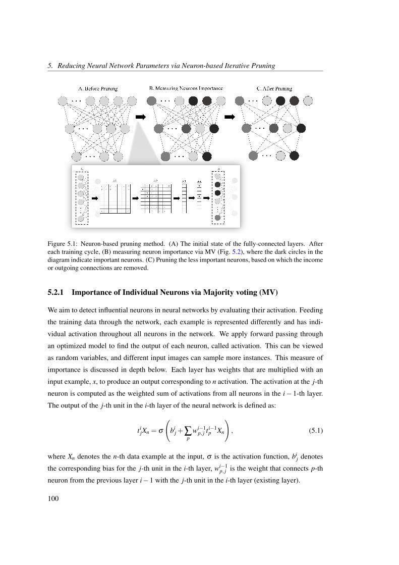
5. Reducing Neural Network Parameters via Neuron-based Iterative Pruning

Figure 5.1: Neuron-based pruning method. (A) The initial state of the fully-connected layers. Aftereach training cycle, (B) measuring neuron importance via MV (Fig. 5.2), where the dark circles in thediagram indicate important neurons. (C) Pruning the less important neurons, based on which the incomeor outgoing connections are removed.

5.2.1 Importance of Individual Neurons via Majority voting (MV)

We aim to detect influential neurons in neural networks by evaluating their activation. Feeding

the training data through the network, each example is represented differently and has indi-

vidual activation throughout all neurons in the network. We apply forward passing through

an optimized model to find the output of each neuron, called activation. This can be viewed

as random variables, and different input images can sample more instances. This measure of

importance is discussed in depth below. Each layer has weights that are multiplied with an

input example, x, to produce an output corresponding to n activation. The activation at the j-th

neuron is computed as the weighted sum of activations from all neurons in the i− 1-th layer.

The output of the j-th unit in the i-th layer of the neural network is defined as:

t ijXn = σ

(bi

j +∑p

wi−1p, j t i−1

p Xn

), (5.1)

where Xn denotes the n-th data example at the input, σ is the activation function, bij denotes

the corresponding bias for the j-th unit in the i-th layer, wi−1p, j is the weight that connects p-th

neuron from the previous layer i−1 with the j-th unit in the i-th layer (existing layer).

100

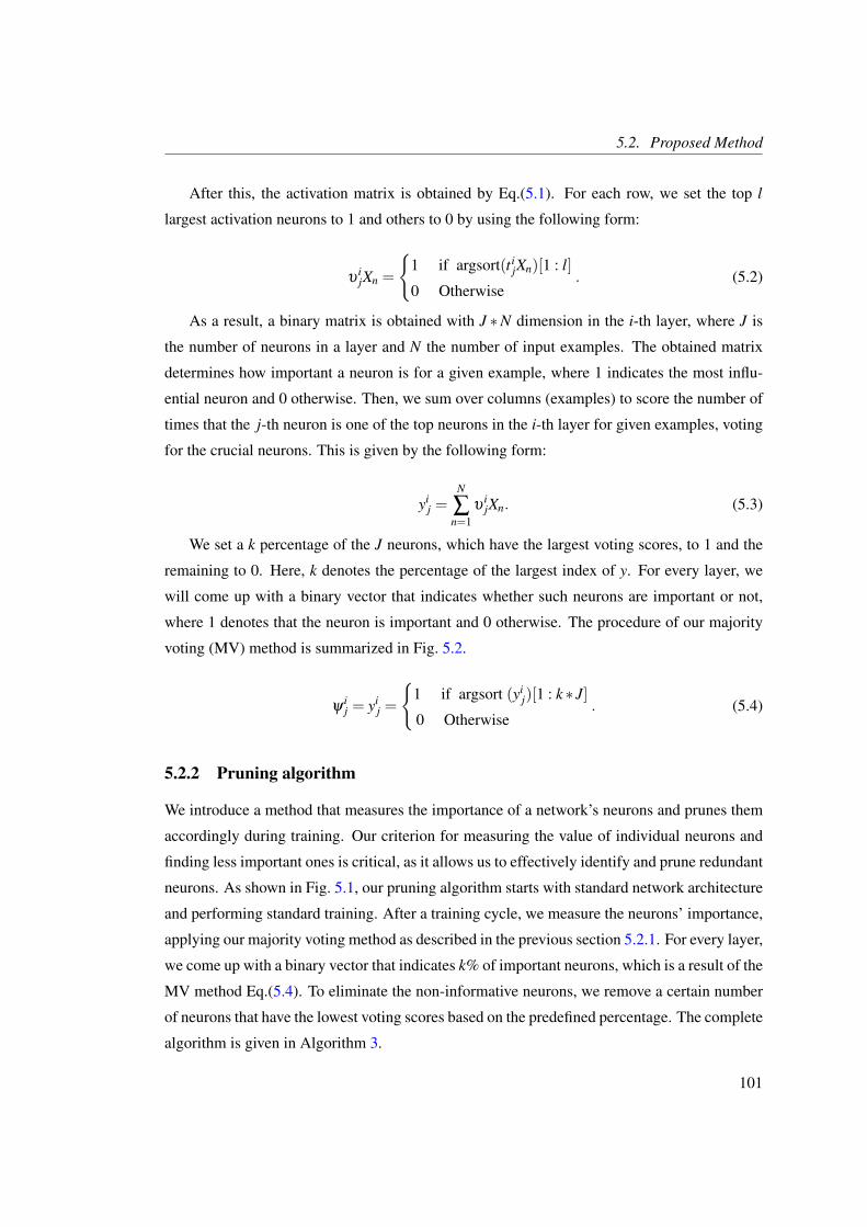
5.2. Proposed Method

After this, the activation matrix is obtained by Eq.(5.1). For each row, we set the top l

largest activation neurons to 1 and others to 0 by using the following form:

υijXn =

{1 if argsort(t i

jXn)[1 : l]

0 Otherwise. (5.2)

As a result, a binary matrix is obtained with J ∗N dimension in the i-th layer, where J is

the number of neurons in a layer and N the number of input examples. The obtained matrix

determines how important a neuron is for a given example, where 1 indicates the most influ-

ential neuron and 0 otherwise. Then, we sum over columns (examples) to score the number of

times that the j-th neuron is one of the top neurons in the i-th layer for given examples, voting

for the crucial neurons. This is given by the following form:

yij =

N

∑n=1

υijXn. (5.3)

We set a k percentage of the J neurons, which have the largest voting scores, to 1 and the

remaining to 0. Here, k denotes the percentage of the largest index of y. For every layer, we

will come up with a binary vector that indicates whether such neurons are important or not,

where 1 denotes that the neuron is important and 0 otherwise. The procedure of our majority

voting (MV) method is summarized in Fig. 5.2.

ψij = yi

j =

{1 if argsort (yi

j)[1 : k ∗ J]

0 Otherwise. (5.4)

5.2.2 Pruning algorithm

We introduce a method that measures the importance of a network’s neurons and prunes them

accordingly during training. Our criterion for measuring the value of individual neurons and

finding less important ones is critical, as it allows us to effectively identify and prune redundant

neurons. As shown in Fig. 5.1, our pruning algorithm starts with standard network architecture

and performing standard training. After a training cycle, we measure the neurons’ importance,

applying our majority voting method as described in the previous section 5.2.1. For every layer,

we come up with a binary vector that indicates k% of important neurons, which is a result of the

MV method Eq.(5.4). To eliminate the non-informative neurons, we remove a certain number

of neurons that have the lowest voting scores based on the predefined percentage. The complete

algorithm is given in Algorithm 3.

101

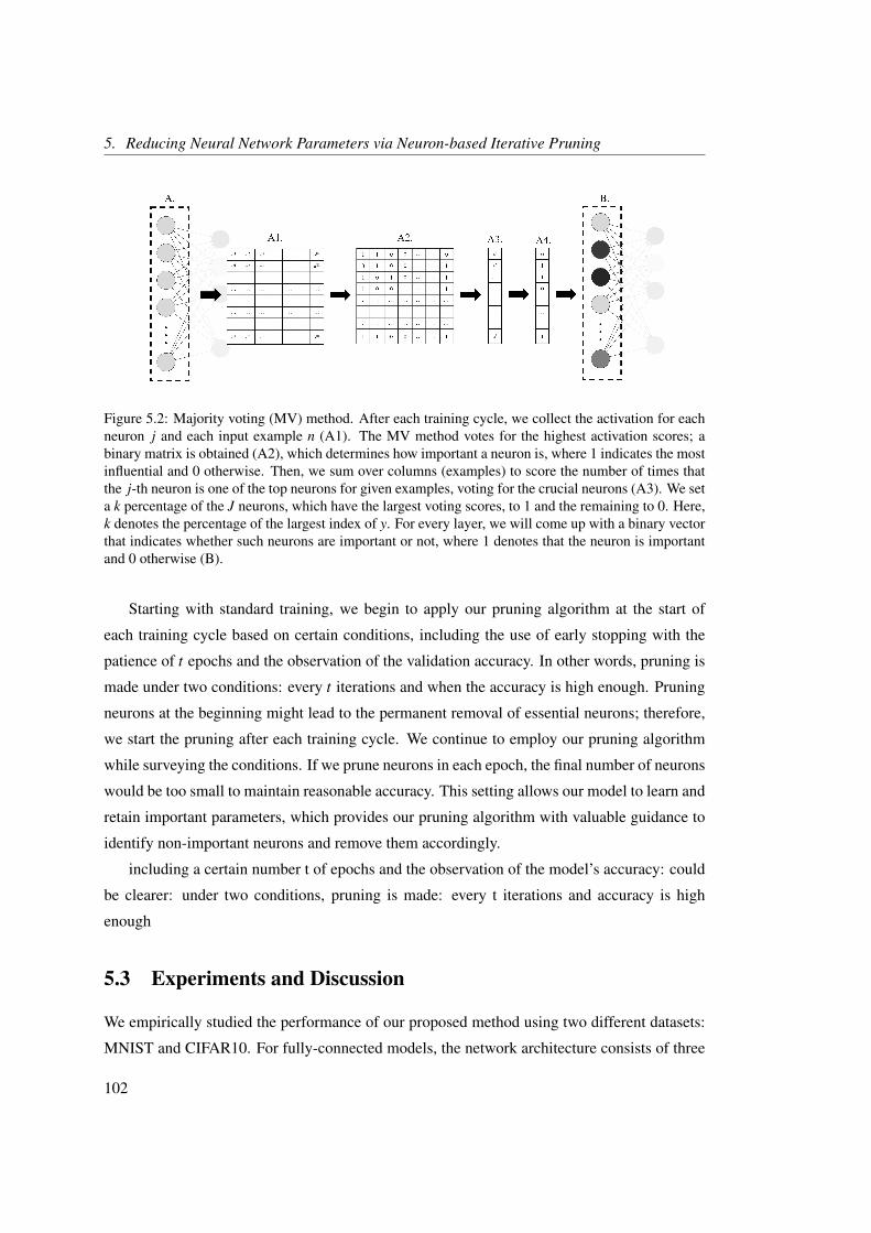
5. Reducing Neural Network Parameters via Neuron-based Iterative Pruning

Figure 5.2: Majority voting (MV) method. After each training cycle, we collect the activation for eachneuron j and each input example n (A1). The MV method votes for the highest activation scores; abinary matrix is obtained (A2), which determines how important a neuron is, where 1 indicates the mostinfluential and 0 otherwise. Then, we sum over columns (examples) to score the number of times thatthe j-th neuron is one of the top neurons for given examples, voting for the crucial neurons (A3). We seta k percentage of the J neurons, which have the largest voting scores, to 1 and the remaining to 0. Here,k denotes the percentage of the largest index of y. For every layer, we will come up with a binary vectorthat indicates whether such neurons are important or not, where 1 denotes that the neuron is importantand 0 otherwise (B).

Starting with standard training, we begin to apply our pruning algorithm at the start of

each training cycle based on certain conditions, including the use of early stopping with the

patience of t epochs and the observation of the validation accuracy. In other words, pruning is

made under two conditions: every t iterations and when the accuracy is high enough. Pruning

neurons at the beginning might lead to the permanent removal of essential neurons; therefore,

we start the pruning after each training cycle. We continue to employ our pruning algorithm

while surveying the conditions. If we prune neurons in each epoch, the final number of neurons

would be too small to maintain reasonable accuracy. This setting allows our model to learn and

retain important parameters, which provides our pruning algorithm with valuable guidance to

identify non-important neurons and remove them accordingly.

including a certain number t of epochs and the observation of the model’s accuracy: could

be clearer: under two conditions, pruning is made: every t iterations and accuracy is high

enough

5.3 Experiments and Discussion

We empirically studied the performance of our proposed method using two different datasets:

MNIST and CIFAR10. For fully-connected models, the network architecture consists of three

102

5.3. Experiments and Discussion

Algorithm 3: Pruning algorithm using Majority Voting (MV)

1 Input: training set (x, y), validation set (x, y), E, t, and k ;2 Output: pruned model;3 initialization ;4 best accuracy← 0 ;5 for e← 1 to E do6 perform standard training procedure at most t epochs until early stopping ;7 perform weights update ;8 accuracy← validation accuracy ;9 if accuracy > best accuracy then

10 best accuracy← accuracy ;11 for each layer do12 compute the activation for each neuron Eq.(5.1) ;13 vote for top l largest activations Eq.(5.2) ;14 compute how many times a neuron has been voted Eq.(5.3) ;15 vote for k% of largest voting-score neurons Eq.(5.4) ;16 remove the non-important neurons ;17 end18 end19 end

fully-connected layers, which is adopted by the base architecture proposed in [217]. Specifi-

cations of the datasets and their architecture are presented in Table 5.1. We first compared our

evaluative importance method with several baselines, using an ablation study. The experimen-

tal results on both datasets show that our method substantially outperforms the baselines. After

this, we applied the proposed method to remove redundant nodes and compress the neuron net-

work during training. Then, we integrated our neuron-pruning method with sparsely-connected

network models. The experimental results show that our method adds substantial compression

and further reduces the number of parameters, without harming the accuracy. Lastly, we em-

pirically studied our method with convolutional neural networks architecture. The details are

provided below.

Table 5.1: Details of Datasets and their FC Architectures used in our experiments.

Dataset Examples Image Size FC Architecture

MNIST 70000 28x28x1 784-1000-1000-1000-10

CIFAR10 60000 32x32x3 3072-4000-1000-4000-10

103

5. Reducing Neural Network Parameters via Neuron-based Iterative Pruning

5.3.1 Measuring Neuron Importance via Ablation

Classification performance was used in order to evaluate the impact of our majority voting

method. An ablation study, which is a commonly used technique, allows for the evaluation

of the effectiveness of measuring neuron importance quantitatively. This procedure typically

refers to the removal of some parts of the model and the study of its performance, as crucial

neurons capture meaningful information and contribute substantially to the model’s final per-

formance. We ablated unimportant neurons by forcing the activation to be zero and computed

the classification accuracy on the test set. Quantifying the effect of the ablation on the classi-

fication performance allows for an impartial evaluation in order to measure a neuron’s impor-

tance and distinguish the most important neurons in a neural network, allowing for layer-wise

and whole-network comparisons. This method not only enables the evaluation of neurons’ im-

portance, but can also detect the unimportant, redundant neurons, which can be removed while

compressing the network during training.

To evaluate the effectiveness of our proposed importance method, it was compared with

several baseline methods. These methods are briefly summarized as follows:

• Random. Neurons are randomly ablated.

• Weights sum [225, 228]. Neurons (p) with lowest absolute weights sum values are

ablated: ψp = ∑p | wp, j |.

• Activation Mean [228]. ψp =1N ∑mean(tp), where tp is the activation values for neuron

p, and N denotes the size of data.

• Activation standard deviation (SD) [228]. ψp =1N ∑std(tp).

• Activation l1-norms [228]. ψp =1N ∑‖tp‖1.

• Activation l2-norms [228]. ψp =1N ∑‖tp‖2.

All these baseline methods consider neurons with higher values as more important, which

is motivated by the intuition that unimportant activation has influential outputs to the final

prediction of a model. Following [228], we calculated neurons’ importance measure on the

activation of the neurons before batch normalization or non-linear activation.

Table 5.2 and Table 5.3 summarize the classification results on CIFAR10 and MNIST test

sets respectively. These tables provide layer-wise comparisons, where neuron importance was

104

5.3. Experiments and Discussion

evaluated using different selection criteria in a fully trained model utilizing the ablation ap-

proach. A compression ratio of 0.7 was set, where 70% of the important neurons in each

layer are preserved. The tables show layer-wise results for each layer, where we ablated layer

by layer and calculated the accuracy for each layer separately. We also examined the whole

network cumulative ablation, where the same ratio from all layers in the whole network are

ablated. For random selection criteria, the mean value of three runs are reported.

Our ablation study shows that MV achieves higher classification performance compared

with other baselines, especially in the case of the whole network cumulative ablation. In CI-

FAR, Table 5.2, MV achieves 68.28% when having a compression ratio of 0.7 for each layer

of the reference model. This shows that MV has less impact on the dropping of model accu-

racy compared with the second place method, which used activation standard deviation and

achieved 66.33%. This demonstrates the robustness of our proposed method in identifying the

most important neurons.

One interesting finding is that ablating neurons with random selection shows that the first

layer has stronger negative effects and more synergistic neurons compared with higher hidden

layers. It can also be seen that the higher hidden layers are significantly redundant and more

class-specific. This observation is consistent with a previous theoretical proposal [275]. One

reasonable explanation is that the neuron networks hierarchically learn representations. Hence,

the first layer is not relevant to a specific object. Still, it builds feature representations of all

input images that are joined to form more relevant object features in the later layers. By ablating

these fundamental features, deeper layers fail to produce class-specific features and have more

negative impacts on the overall accuracy.

Although a random selection is not robust and not applicable in practice [207], it provides

insight and demonstrates that the detection of principal neurons is a critical approach when

pruning redundant neurons. The experiment empirically confirms that our importance method

is sufficient, given that ablating neurons with low values in the layers only has the most negli-

gible impact on the overall accuracy compared with all baselines. As shown in Table 5.2 and

Table 5.3, the experimental results on both datasets show that the method substantially out-

performs the baselines. Our proposed method to measure neuron importance helps not only

to remove redundant nodes and compress the neuron network, but also to understand their

inter-relationships and how said neurons impact the model. The experiment confirms that se-

lecting the right criteria to evaluate neurons’ importance throughout all layers can guarantee a

successful pruning approach.

105

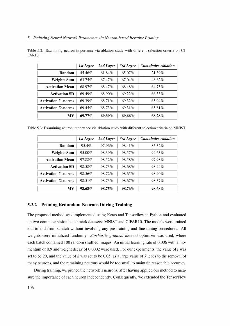
5. Reducing Neural Network Parameters via Neuron-based Iterative Pruning

Table 5.2: Examining neuron importance via ablation study with different selection criteria on CI-FAR10.

1st Layer 2nd Layer 3rd Layer Cumulative Ablation

Random 45.46% 61.84% 65.07% 21.39%

Weights Sum 63.75% 67.47% 67.04% 48.62%

Activation Mean 68.97% 68.47% 68.48% 64.75%

Activation SD 69.49% 68.90% 69.22% 66.33%

Activation l1-norms 69.39% 68.71% 69.32% 65.94%

Activation l2-norms 69.45% 68.73% 69.31% 65.81%

MV 69.77% 69.39% 69.66% 68.28%

Table 5.3: Examining neuron importance via ablation study with different selection criteria on MNIST.

1st Layer 2nd Layer 3rd Layer Cumulative Ablation

Random 95.4% 97.96% 98.41% 85.32%

Weights Sum 95.00% 98.39% 98.57% 94.63%

Activation Mean 97.88% 98.52% 98.58% 97.98%

Activation SD 98.58% 98.73% 98.68% 98.44%

Activation l1-norms 98.56% 98.72% 98.65% 98.40%

Activation l2-norms 98.51% 98.73% 98.67% 98.37%

MV 98.68% 98.75% 98.76% 98.68%

5.3.2 Pruning Redundant Neurons During Training

The proposed method was implemented using Keras and Tensorflow in Python and evaluated

on two computer vision benchmark datasets: MNIST and CIFAR10. The models were trained

end-to-end from scratch without involving any pre-training and fine-tuning procedures. All

weights were initialized randomly. Stochastic gradient descent optimizer was used, where

each batch contained 100 random shuffled images. An initial learning rate of 0.006 with a mo-

mentum of 0.9 and weight decay of 0.0002 were used. For our experiments, the value of t was

set to be 20, and the value of k was set to be 0.05, as a large value of k leads to the removal of

many neurons, and the remaining neurons would be too small to maintain reasonable accuracy.

During training, we pruned the network’s neurons, after having applied our method to mea-

sure the importance of each neuron independently. Consequently, we extended the TensorFlow

106

5.3. Experiments and Discussion

framework to prune the neurons of a network during training. TensorFlow allows us to apply

a constraint function to the weights matrix, which in turn means that constraints can be set on

network parameters during optimization. For every pruned layer, we utilized the output binary

vector, which is obtained via the importance measure method (MV) Eq.(5.4), for the constraint

function. The binary vector contributes to generating a binary mask variable which is the same

size as the layer’s weight matrix. The binary mask determines the participation of the weights

in the forward procedure. In the back-propagation, gradients pass through the binary masks,

and the masked weights in the forward-propagation are not updated in the back-propagation

phase.

Determining and eliminating the non-informative neurons results in a significant additional

increment into the body of the learning process. This approach is aimed at forming a kind of

structure that enhances the identification of non-informative neurons and removes any redun-

dant parts of the model during training. The comparative results are shown in Table 5.4, and

supports our hypothesis that significantly fewer parameters can add enough discriminative abil-

ity without harming the original accuracy of the baseline dense models. These are considered

a solution to overcoming the over-parametrized and redundant nature of deep learning models.

It can be observed that the models’ accuracy were improved after the removal of unimportant

neurons.

Table 5.4 demonstrates how the pruned versions of models outperform the original, fully-

connected models with only significantly fewer parameters. With regards to the CIFAR10

dataset, it has been shown that a significant gain can be obtained with only 20% of the weights

of the original fully-connected model. Based on CIFAR10-related literature, [276] is con-

sidered as one of the state-of-the-art, fully-connected models, which achieves a classification

accuracy of 74.1% with 31,600K parameters, while our model reached a comparable accuracy

of 74.21% with only around 4,245K parameters.

Table 5.4: Summarization of our experiments with fully-connected networks.

FC MV Pruning

Dataset Accuracy nW Accuracy nW

MNIST 98.78% 2,794K 98.88% 232K

CIFAR10 71.90% 20,328K 74.21% 4,245K

107

5. Reducing Neural Network Parameters via Neuron-based Iterative Pruning

Figure 5.3: The architecture of the CNN model.

5.3.3 Integrating our Pruning Method to Sparsely-Connected Networks (SCNs)

To thoroughly investigate the abilities of our proposed method, we also evaluated its perfor-

mance with sparsely-connected networks (SCNs). SCN by Mocanu et al. [217] is an interesting

approach that replaces fully-connected layers with sparsely-connected ones. They have intro-

duced a way to connect nodes in neural networks before training by applying an initial sparse

topology based on the Erdos–Rényi random graph and by starting training using standard op-

timization techniques. They iteratively replace the weakest connections with the new random

initialization until they reach the end of the training process and entirely remove the weakest

connections, which leads to a substantial reduction in connections and, therefore, to increased

memory and computational efficiency.

A massive number of neurons still poses a challenge, as it can lead to significant redun-

dancy. Although sparsely-connected layers remove unnecessary connections without signif-

icant performance degradation, neuron-pruning methods are much more beneficial. This is

because unimportant neurons do not contribute much to the final model performance, as shown

in the previous section, therefore, all of their income or outcome connections (weights) are

trivial and non-informative. Eliminating unimportant neurons can guarantee the removal of

extra parameters, as pruning a neuron removes entire rows or columns of the weight matrices

from the former and latter layers.

Our experiment began with a sparse topology random graph [217], after which the weakest

connections were iteratively replaced with new initialized ones in the training phase. In the

108

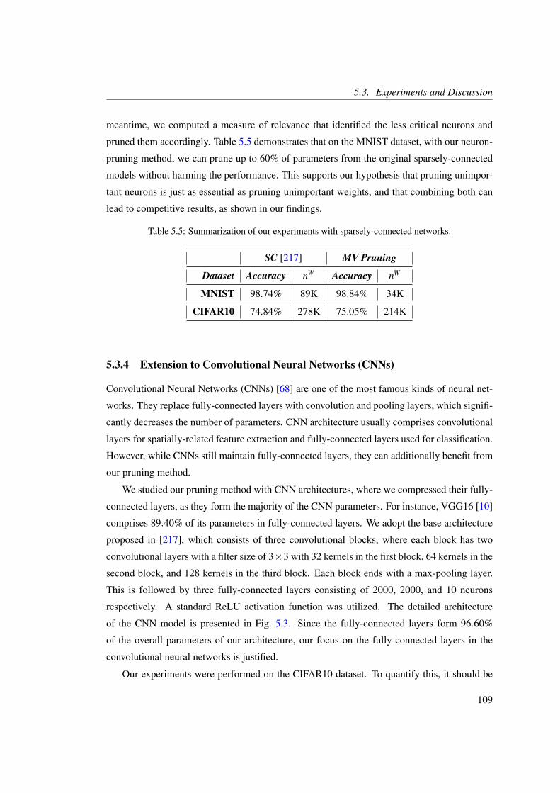
5.3. Experiments and Discussion

meantime, we computed a measure of relevance that identified the less critical neurons and

pruned them accordingly. Table 5.5 demonstrates that on the MNIST dataset, with our neuron-

pruning method, we can prune up to 60% of parameters from the original sparsely-connected

models without harming the performance. This supports our hypothesis that pruning unimpor-

tant neurons is just as essential as pruning unimportant weights, and that combining both can

lead to competitive results, as shown in our findings.

Table 5.5: Summarization of our experiments with sparsely-connected networks.

SC [217] MV Pruning

Dataset Accuracy nW Accuracy nW

MNIST 98.74% 89K 98.84% 34K

CIFAR10 74.84% 278K 75.05% 214K

5.3.4 Extension to Convolutional Neural Networks (CNNs)

Convolutional Neural Networks (CNNs) [68] are one of the most famous kinds of neural net-

works. They replace fully-connected layers with convolution and pooling layers, which signifi-

cantly decreases the number of parameters. CNN architecture usually comprises convolutional

layers for spatially-related feature extraction and fully-connected layers used for classification.

However, while CNNs still maintain fully-connected layers, they can additionally benefit from

our pruning method.

We studied our pruning method with CNN architectures, where we compressed their fully-

connected layers, as they form the majority of the CNN parameters. For instance, VGG16 [10]

comprises 89.40% of its parameters in fully-connected layers. We adopt the base architecture

proposed in [217], which consists of three convolutional blocks, where each block has two

convolutional layers with a filter size of 3×3 with 32 kernels in the first block, 64 kernels in the

second block, and 128 kernels in the third block. Each block ends with a max-pooling layer.

This is followed by three fully-connected layers consisting of 2000, 2000, and 10 neurons

respectively. A standard ReLU activation function was utilized. The detailed architecture

of the CNN model is presented in Fig. 5.3. Since the fully-connected layers form 96.60%

of the overall parameters of our architecture, our focus on the fully-connected layers in the

convolutional neural networks is justified.

Our experiments were performed on the CIFAR10 dataset. To quantify this, it should be

109

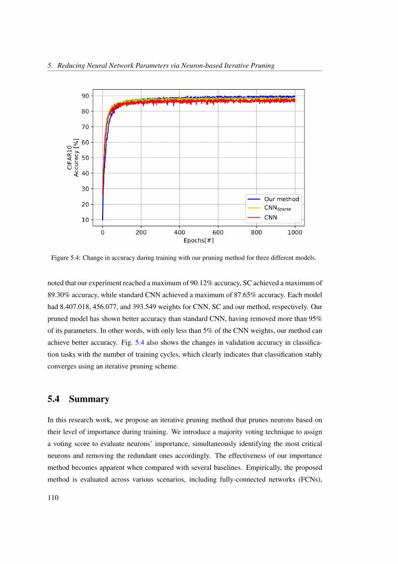
5. Reducing Neural Network Parameters via Neuron-based Iterative Pruning

Figure 5.4: Change in accuracy during training with our pruning method for three different models.

noted that our experiment reached a maximum of 90.12% accuracy, SC achieved a maximum of

89.30% accuracy, while standard CNN achieved a maximum of 87.65% accuracy. Each model

had 8.407.018, 456.077, and 393.549 weights for CNN, SC and our method, respectively. Our

pruned model has shown better accuracy than standard CNN, having removed more than 95%

of its parameters. In other words, with only less than 5% of the CNN weights, our method can

achieve better accuracy. Fig. 5.4 also shows the changes in validation accuracy in classifica-

tion tasks with the number of training cycles, which clearly indicates that classification stably

converges using an iterative pruning scheme.

5.4 Summary

In this research work, we propose an iterative pruning method that prunes neurons based on

their level of importance during training. We introduce a majority voting technique to assign

a voting score to evaluate neurons’ importance, simultaneously identifying the most critical

neurons and removing the redundant ones accordingly. The effectiveness of our importance

method becomes apparent when compared with several baselines. Empirically, the proposed

method is evaluated across various scenarios, including fully-connected networks (FCNs),

110

5.4. Summary

sparsely-connected networks (SCNs), and convolutional neural networks (CNNs) using the

MNIST and CIFAR-10 datasets. The experimental results have demonstrated the effectiveness

of our pruning method in improving accuracy after removing the unimportant neurons. The

results also demonstrate that our proposed method is applicable to weight-based pruning meth-

ods and adds extra compression. Moreover, we show that SCNs and CNNs can be pruned into

even smaller models using our proposed method with no drop in the reference model accuracy.

Our method mainly targeted the parameters of the fully-connected layers to compress deep

neural networks, as most of the weights parameters exist in fully-connected layers. However,

most of the computational complexity originates in the convolutional layers due to massive

multiplication- and addition operations, although they contain fewer parameters due to param-

eter sharing. Dealing with an individual CNNs filter requires an intuitive process to determine

selective and semantically meaningful criteria for filter selection, where each convolution fil-

ter responds to a specific high-level concept associated with different semantic parts. In the

following chapter, our core aim is to evaluate filter importance, which provides meaningful

insight into the characteristics of the internal representations of neural networks, reducing

the computational complexity of the convolutional layers in order to compress and acceler-

ate CNNs. In Chapter 7, we conclude by presenting a comprehensive, detailed review of

time-series data analysis and a founding contribution to the area of applying deep time-series

clustering (DTSC), with emphasis on identifying state-of-the-art and providing an outlook on

DTSC.

111

Chapter 6

Pruning CNN Filters via Quantifyingthe Importance of Deep VisualRepresentations

Contents6.1 Introduction . . . . . . . . . . . . . . . . . . . . . . . . . . . . . . . . . 114

6.2 Proposed Method . . . . . . . . . . . . . . . . . . . . . . . . . . . . . . . 117

6.2.1 Overview of our Pruning Methodology . . . . . . . . . . . . . . 117

6.2.2 Scoring Channel Importance Method . . . . . . . . . . . . . . . 118

6.2.3 Majority voting (MV) Method . . . . . . . . . . . . . . . . . . . 120

6.2.4 Kernels Estimation Method . . . . . . . . . . . . . . . . . . . . . 122

6.3 Experiments and Discussion . . . . . . . . . . . . . . . . . . . . . . . . . 123

6.3.1 VGG16 on CIFAR-10 . . . . . . . . . . . . . . . . . . . . . . . 129

6.3.2 ResNet-20/ResNet-32 on CIFAR-10 . . . . . . . . . . . . . . . . 131

6.3.3 ResNet-20/ResNet-32 on CUB-200 . . . . . . . . . . . . . . . . 132

6.3.4 ResNet-50 on ImageNet . . . . . . . . . . . . . . . . . . . . . . 134

6.3.5 Feature Map Visualization . . . . . . . . . . . . . . . . . . . . . 136

6.3.6 Comparison with Filter Selection Criteria . . . . . . . . . . . . . 137

6.3.7 Comparison of Kernal Estimation (KE) vs. Fine-Tuning (FT) . . . 142

6.4 Summary . . . . . . . . . . . . . . . . . . . . . . . . . . . . . . . . . . . 143

113

6. Pruning CNN Filters via Quantifying the Importance of Deep Visual Representations

6.1 Introduction

Network pruning focuses on discarding unnecessary parts of neural networks, which reduces

the massive computational costs and memory requirements associated with deep models. Prun-

ing approaches can be applied to any part of deep neural networks, including fully connected

layers [210, 211, 215, 225, 227, 233] and convolutional layers [48, 207, 228, 229, 232, 233]. The

idea of pruning was studied in the early 1990s. Optimal Brain Damage (OBD) by LeCun et

al. [210] and Optimal Brain Surgeon (OBS) by Hassibi et al. [211] are considered to be some of

the pioneering works in network pruning, demonstrating that several unimportant weights can

be eliminated from a trained network with little accuracy loss. Due to expensive computation

costs, these methods are not applicable to today’s deep models. Obtaining a subnetwork with

much fewer parameters without harming accuracy is the main goal of pruning algorithms. The

pruned version, a subset of the whole model, can represent the reference model at a smaller

size or with much fewer parameters. Thus, overparameterized networks can be efficiently

compressed while maintaining the property of better generalization [44].

Recently, Han et al. [215] introduced a simple pruning method to remove connections

based on a predefined threshold. Han’s framework relies on an iterative pruning procedure to

obtain a very sparse model. However, such a non-structured sparse model requires a particular

software/hardware accelerator which is not supported by off-the-shelf libraries. Moreover, the

reliance on a predefined threshold is less practical and proves too inflexible for some appli-

cations. The random connectivity of non-structured sparse models can also cause poor cache

locality and jumping memory access, which extremely limits the practical acceleration [23].

In an attempt to confront these challenges, we consider filter-level pruning in our proposed

method, where removing the unimportant filter in its entirety does not change the network

structure, and the method can be supported by any off-the-shelf deep learning library, allowing

for more compression and acceleration by other compression methods, such as the parameter

quantization approach [205]. This procedure can also effectively reduce the memory require-

ments, as model compression focuses on reducing not only model parameters but also the

intermediate activation; this has rarely been studied in previous works.

In contrast, filter-level pruning strategies have been widely studied in the commu-

nity [48, 207, 228, 229, 232]. The aim of these strategies is to evaluate the importance of in-

termediate units, where pruning is conducted according to the lowest scores. Li et al. [228]

put forward a pruning method based on the absolute weighted sum, where pruning is carried

out according to the lowest scores. [229] also proposed a pruning method based on the mean

114

6.1. Introduction

gradient of feature maps in each layer, which reflects the importance of features extracted by

convolutional kernels. Furthermore, Luo et al. [207] proposed the ThiNet method, which ap-

plies a greedy strategy for channel selection. They prune the target layer by greedily selecting

the input channel that has the least increase in reconstruction error. The least-squares approach

is applied to indicate a subset of input channels which have the smallest impact to approxi-

mate the output feature map. These methods tend to compress networks by simply adopting

straightforward selection criteria based on the statistical information. However, dealing with

an individual CNNs filter requires an intuitive process to determine selective and semantically

meaningful criteria for filter selection, where each convolution filter responds to a specific

high-level concept associated with different semantic parts.

The fact that not all filters deliver essential information for the final prediction of the model

motivates us to fundamentally rely on quantifying the importance of latent representations of

CNNs by evaluating the alignment/matching between semantic concepts and individual hid-

den units to score the semantics of hidden units at each intermediate convolutional layer. Our

core aim is to evaluate neuron importance, which provides meaningful insight into the char-

acteristics of the internal representations of neural networks. For the purpose of providing a

clear understanding of the internal operation and work mechanisms of deep networks, sev-

eral approaches have been developed to visually understand convolutional layers [70, 96, 98],

interpret deep visual representations and quantify their interpretability [100, 101], as well as

measure the influence of hidden units on the final prediction [102–104]. The main focus of

these methods is to understand the predictions of a model by analyzing the individual units and

seeking an explanation for specific activation. Although these methods provide an intuitive

process to determine criteria for neuron selection for effective pruning, most of the previously

mentioned methods focus on gaining a better understanding of the network’s behavior, with

limited attention being paid to pruning methods. Most relevant to our current work is a CNN

pruning method inspired by neural network interpretability. Yeom et al. [233] have proposed

such a method based on layer-wise relevance propagation (LRP) [104], where weights or filters

are pruned based on their relevance score, combining the two disconnected research lines of

interpretability and model compression.

In this chapter, we propose a novel framework to compute a measure of relevance, identify

the most critical filters and prune the unimportant filters to compress and accelerate CNNs,

with only a small drop in model accuracy. Our proposed framework focuses on filter-level

pruning based on evaluating the degree of alignment between a semantic concept and individ-

115

6. Pruning CNN Filters via Quantifying the Importance of Deep Visual Representations

ual hidden unit representations. Quantifying the interpretability of deep visual representations

of CNNs [100] determines the function of individual CNNs filters to deliver essential infor-

mation, where a filter’s feature map is more critical for the network when it represents more

information. Individual network decisions can be explained using localization maps [25–27],

identifying the important regions in the image for predicting the concept. This fact moti-

vates us to fundamentally rely on applying the feature map importance method when pruning

non-informative elements. Our work is considered a pioneering one that attempts to use the

quantification of interpretability for more robust and effective CNNs pruning. We first intro-

duce feature maps to detect valuable information and the essential semantic parts, which are

fundamental factors in the evaluation of the importance of feature maps.

We propose a more accurate importance measure, a majority voting technique, to com-

pare the degree of alignment values among filters and assign a voting score to evaluate their

importance quantitatively. This mechanism helps to effectively reduce model complexity by

eliminating the less influential filters and aims to determine a subset of the whole model that

can represent the reference model with much fewer parameters. One significant advantage of

filter-level pruning is that it does not lead to model structure damage; therefore, other pruning

methods can be efficiently adopted for further compression.

To minimize the damage of the pruning procedure, we propose a simple yet effective

method to estimate new convolution kernels based on the remaining, crucial channels. Our

fundamental insight is that we introduce an optimization problem, based on which the kernels

can be estimated depending on the remaining feature maps inputs and the output of the pruned

filter. This novel finding differentiates our kernels estimation method from a fine-tuning proce-

dure, which is the most common technique applied by most of the existing methods to recover

damaged accuracy.

In order to gather conclusive evidence to evaluate the effectiveness of our method, an ex-

periment based on ablation analysis in trained models was carried out. By comparing our

importance method with several state-of-the-art methods, we demonstrate that our approach

substantially outperforms others in terms of filters’ effective measurement, notably with larger

compression ratios. We evaluate our pruning method on CIFAR-10, CUB-200 , and ImageNet

(ILSVRC 2012) datasets and two types of network architecture: plain CNN (VGG-16 [10])

and residual CNN (ResNet-20/32/50 [11]). The experimental results show that the proposed

method efficiently achieves 50% FLOPs reduction on the VGG-16 model, with only 0.86% ac-

curacy drop. Although ResNet is more compact and has less redundancy than VGG models, it

116

6.2. Proposed Method

can still reduce 30% FLOPs, with 0.12% and 0.02% accuracy drop on ResNet-20 and ResNet-

32 respectively. For ResNet-50 on ImageNet, our proposed model is capable of reducing 30%

FLOPs with only a 0.24% reduction in the original model’s top-1 error and a 0.03% reduction

in the top-5 error.

The rest of the chapter is organized as follows. We describe our proposed methodology in

section 6.2, and present our experimental results in section 6.3. Finally, concluding remarks

are provided in section 6.4.

6.2 Proposed Method

The chapter mainly studies a filter-level pruning method to reduce model complexity and obtain

a small subset of the whole model that can represent the reference model without performance

degradation. In this section, we first present our overall pruning framework; our proposed

method consists of three major parts, the first two being scoring channel importance via quan-

tifying the importance of individual hidden representations in section 6.2.2 and assigning their

voting scores in section 6.2.3, on which we quantitatively evaluate the importance of filters in a

specific layer, eliminating the less influential filters accordingly. Then, we introduce a kernels

estimation method in section 6.2.4.

6.2.1 Overview of our Pruning Methodology

Our method prunes a pre-trained model layer-by-layer with a predefined compression rate.

Given a pre-trained CNN model, the proposed novel method is used to compute a measure of

relevance that identifies the most critical units. Based on this, the less informative channels are

pruned. Then, new convolution kernels are estimated based on the surviving channels, and a

final fine-tune for the whole network is carried out. As we mainly focus on filter-level pruning,

the pruned version of our model can be further pruned into an even smaller model by adopting

other methods. The overall pipeline of our method is presented in Fig. 6.1. Here, the proposed

method consists of four iterative steps as follows:

1. Channels Selection Criteria. In contrast to the previous methods, which benefit from the

statistical information of layer i to lead the pruning of filters in the same layer, we benefit

from the output feature maps of the previous layer i− 1 to prune filters in the existing

layer i. Based on the proposed novel method to score channels’ importance, we aim to

117

6. Pruning CNN Filters via Quantifying the Importance of Deep Visual Representations

Figure 6.1: The overall pipeline of our proposed framework. A pre-trained CNN model is prunedlayer-by-layer through iteratively applying our proposed channels selection criteria, majority voting,and kernels estimation, followed by further final fine-tuning to recover the dropped accuracy.

carefully select a set of channels in layer i−1 that are the most influential in the output

feature map of layer i, as shown in Fig. 6.2.

2. Pruning. Unimportant channels and their corresponding filters in layer i are pruned,

keeping the structure of the original network the same. This means that our pruning

method assumes that only fewer informative filters and channels can approximate an

output feature map of layer i. This procedure allows for unimportant filters to be ne-

glected without harming the structure of the original network.

3. Kernels Estimation. To minimize the damage of the pruning procedure, we introduce a

method to estimate new convolution kernels based on part of the remaining, un-pruned

channels. The target number of filters is obtained by computing a partial convolution,

which means that we only utilize the remaining channels of the output feature maps of

layer i−1 to estimate optimal kernels that approximate the output feature map of layer

i.

4. We iterate to the first step to prune the next layer.

5. In order to get a more accurate model, further final fine-tuning is carried out once all

layers have been pruned.

6.2.2 Scoring Channel Importance Method

Our aim was to identify the most influential channels on CNNs based on which the crucial

filters are detected. Measuring the importance of every individual convolutional channel al-

118

6.2. Proposed Method

Figure 6.2: Our pruning method. The initial state of a CNN feature map in a fully trained model. Greendotted boxes in the diagram indicate important channels. We identify several weak channels and theircorresponding filters (the red dotted boxes), which contribute very little to the overall performance.These channels and their associated filters can be pruned, leading to a pruned model.

lows for the determination of a subset of the channels whose patterns are the most substantial.

Inspired by neural network interpretability, we propose a novel pruning framework based on

evaluating the degree of alignment between a semantic concept and individual hidden unit rep-

resentations. Network Dissection [100] was originally developed to quantify the interpretabil-

ity of latent representations of CNNs that reflect the contribution of an input to deliver essential

information for the final prediction of the model.

Every input image x is fed through a pre-trained model by applying forward passing

through an optimized model to find the output of each feature map. Each layer has kernels

that are convolved on an input example n or a feature map of the internal layers, x, to pro-

duce an output corresponding to the n-th example. The activation at j-th feature map is then

computed, where the output of the j-th unit in the i-th layer of CNN is defined as:

t ijxn = σ

(bi

j +∑p

wip ∗ t i−1

p xn

), (6.1)

where xn denotes the n-th data example at the input, σ is the activation function (e.g. sigmoid,

ReLU), bij denotes the corresponding bias for the j-th unit in the i-th layer, wi−1

p is the weights

of the p-th kernel in the i-th layer (existing layer), t i−1p xn is the output feature maps of the

previous layer i−1 and ∗ denotes the 2D convolution operation.

To measure channels’ importance, the latent representations of every individual feature

map is evaluated as a solution to a binary segmentation task of the visual concept in the input

space. Determining the function of individual filters in a CNN and their ability to localize the

meaningful semantic part aids to efficiently measure the importance of different feature maps,

119

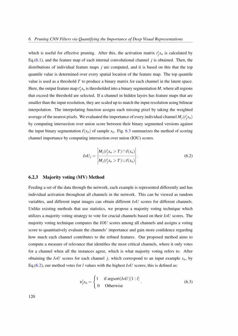
6. Pruning CNN Filters via Quantifying the Importance of Deep Visual Representations

which is useful for effective pruning. After this, the activation matrix t ijxn is calculated by

Eq.(6.1), and the feature map of each internal convolutional channel j is obtained. Then, the

distributions of individual feature maps j are computed, and it is based on this that the top

quantile value is determined over every spatial location of the feature map. The top quantile

value is used as a threshold T to produce a binary matrix for each channel in the latent space.

Here, the output feature map t ijxn is thresholded into a binary segmentation M, where all regions

that exceed the threshold are selected. If a channel in hidden layers has feature maps that are

smaller than the input resolution, they are scaled up to match the input resolution using bilinear

interpolation. The interpolating function assigns each missing pixel by taking the weighted

average of the nearest pixels. We evaluated the importance of every individual channel M j(t ijxn)

by computing intersection over union score between their binary segmented versions against

the input binary segmentation I(xn) of sample xn. Fig. 6.3 summarizes the method of scoring

channel importance by computing intersection over union (IOU) scores.

IoU j =

∣∣∣M j(t ijxn > T )∩ I(xn)

∣∣∣∣∣∣M j(t ijxn > T )∪ I(xn)

∣∣∣ . (6.2)

6.2.3 Majority voting (MV) Method

Feeding a set of the data through the network, each example is represented differently and has

individual activation throughout all channels in the network. This can be viewed as random

variables, and different input images can obtain different IoU scores for different channels.

Unlike existing methods that use statistics, we propose a majority voting technique which

utilizes a majority voting strategy to vote for crucial channels based on their IoU scores. The

majority voting technique compares the IOU scores among all channels and assigns a voting

score to quantitatively evaluate the channels’ importance and gain more confidence regarding

how much each channel contributes to the refined features. Our proposed method aims to

compute a measure of relevance that identifies the most critical channels, where it only votes

for a channel when all the instances agree, which is what majority voting refers to. After

obtaining the IoU scores for each channel j, which correspond to an input example xn, by

Eq.(6.2), our method votes for l values with the highest IoU scores; this is defined as:

υijxn =

{1 if argsort(IoU)[1 : l]

0 Otherwise. (6.3)

120

6.2. Proposed Method

Figure 6.3: Scoring Channel Importance Method. The activation matrix t ixn is obtained by Eq.(6.1). Thefeature map of each internal convolutional channel j is collected. For each channel j, we determined thetop quantile value and used it as a threshold T to produce a binary matrix for each channel M j(t i

jxn > T ).We evaluated the importance of every individual binary segmentation for each channel M j(t i

jxn > T )against the input binary segmentation I(xn) by computing intersection over union scores (this figure isbest viewed in color).

As a result, a binary matrix is obtained with J ∗N dimension in the i-th layer, where J is

the number of channels and N the number of input examples. The obtained matrix determines

how important a channel is for a given example, where 1 indicates the most influential and 0

indicates otherwise. Then, we sum over columns (examples) to score the number of times that

the j-th channel is one of the top channels for given examples, voting for the crucial channels.

This is given by the following form:

yij =

N

∑n=1

υijxn. (6.4)

ψij = yi

j =

{1 if argsort (yi

j)[1 : k ∗ J]

0 Otherwise, (6.5)

where k is the compression rate, and J are the channels. We set a k percentage of the J channels,

which have the largest voting scores, to 1 and the remaining to 0. Here, k denotes the percentage

121

6. Pruning CNN Filters via Quantifying the Importance of Deep Visual Representations

Figure 6.4: Majority voting (MV) method. After obtaining IoU scores for each channel (Fig. 6.3), wecollect the IoU for each channel j and each input example n (A1). Our method votes for l percentage ofhighest IoU scores, and as a result, a binary matrix is obtained (A2), which determines how importanta channel is for a given example, where 1 indicates the most influential and 0 indicates otherwise.Then, we sum over columns (examples) to score the number of times that the j-th channel is one ofthe top channels for given examples, voting for the crucial channels (A3). We set a k percentage ofthe J channels, which have the largest voting scores, to 1 and the remaining to 0. Here, k denotesthe percentage of the largest index of y. For every layer, we determine a binary vector that indicateswhether such channels are important or not, where 1 denotes that the channel is important and 0 denotesotherwise (B) (this figure is best viewed in color).

of the largest index of y. For every layer, we determine a binary vector that indicates whether

such channels are important or not, where 1 denotes that the channel is important and 0 denotes

otherwise. The procedure of our majority voting (MV) method is summarized in Fig. 6.4.

6.2.4 Kernels Estimation Method

A binary vector by Eq.(6.5) indicates k percent of the essential channels for every layer, based

on which the non-important channels are pruned. Here, a certain number of channels that

have the lowest voting scores are pruned. This mechanism helps to effectively reduce model

complexity by eliminating the less influential channels and aims to obtain a subset of the whole

model that can represent the reference model with much fewer parameters, whilst preserving

the reference model accuracy.

Since there is no guarantee of preserving the accuracy throughout the compression phase,

a final fine-tuning or iterative layer-wise fine-tuning are the only techniques applied by most

of the existing methods to recover damaged accuracy. A simple compression approach ben-

efits from such valuable steps, especially when the selection criteria is straightforward and

does not adequately measure the importance, due to the adoption of less efficient measurement

standards.

To minimize the damage of the pruning procedure, we propose a simple yet effective

122

6.3. Experiments and Discussion

method to estimate new convolution kernels based on the remaining unpruned channels. The

new kernels can be estimated with only a small number of examples without further train-

ing, which is significantly faster to implement. This procedure does not require a multi-step

process, in contrast to the fine-tuning procedure (e.g, building a new model, reloading the pa-

rameters of the pruned model, and freezing/unfreezing some of the layers), allowing for a fast

and efficient process.

Here, we introduce a method to estimate a new convolution kernel based on the remaining,

crucial feature map. The new convolution kernel is computed by partial convolution, which

means that we will not convolve through all channel in the input feature map, as a subset of

channels is pruned already. The target number of filters is obtained by utilizing the remain-

ing channels of the output feature maps of the previous layer to estimate optimal kernels that

approximate the output feature map of the existing layer. Therefore, we can prune the filter

channels while minimizing the pruning effect.

Using the output feature maps of the previous layer and the convolved version of it, which

is the output feature maps of the existing layer, we are able to calculate the convolution kernel.

This problem is considered a simple optimization problem in the spatial domain. Given an

objective function as follows:

12‖ h∗ x− y ‖2, (6.6)

where h is the 2D convolution kernel, y is the convolution output feature maps, x is a given

output feature maps of the previous layer and ∗ forms the 2D convolution operation. The

gradient with respect to the convolution kernel h would be:

d 12 ‖ h∗ x− y ‖2

dh=

1N

n

∑i=1

x⊗ (x∗h− y), (6.7)

where N denotes the number of samples used in our estimation method, ⊗ denotes the correla-

tion operation and ∗ denotes the convolution operation.

6.3 Experiments and Discussion

In this section, we empirically study the performance of our proposed method. Pruning chan-

nels with efficient selection criteria along with the majority voting technique indicates that

channels with larger voting scores are more important in network performance. We first

apply the proposed method to prune two types of network architectures - plain networks

123

6. Pruning CNN Filters via Quantifying the Importance of Deep Visual Representations

Algorithm 4: Channel pruning algorithm based on quantifying the importance ofdeep visual representations.

1 Input: a pre-trained Model, training set (x, y), and compression rate r ;2 Output: a pruned model ;3 for each layer do4 collect the receptive field of each feature map, Eq.(6.1) ;5 compute the IOU score for each filter, Eq.(6.2) ;6 vote for top lOU scores, Eq.(6.3) ;7 compute how many times a filter has been voted, Eq.(6.4) ;8 vote for k% of largest voting-score neurons, Eq.(6.5) ;9 prune the non-important filters ;

10 estimate new convolution kernels based on part of the remaining, un-prunedchannels, section. 6.2.4 ;

11 end12 final fine-tuning of the pruned model;

(VGG-16 [10]) and residual networks (ResNet-20/32/50 [11]) - on three different datasets:

The CIFAR-10 dataset [277], Caltech-UCSD Birds (CUB-200) dataset [278], and ImageNet

(ILSVRC 2012) dataset [279]. The experimental results show that our method adds substantial

compression and further reduces model complexity, with little reduction in model accuracy. In

this section, we also compare our selection criteria for filter-level pruning with several base-

lines, and evaluate the change in loss caused by removing a set of filters. The experimental

results show that our method substantially outperforms all other baselines. Finally, we empir-

ically verify the validity of our kernels estimation (KE) method and compare it with the stan-

dard fine-tuning (FT) procedure. The proposed method was implemented using Keras [265]

and Tensorflow [52] in Python.

Experimental Datasets

We evaluated our filter-level pruning method on three different datasets.

• CIFAR-10 [277] : is an image dataset which consists of 60,000 images. Each example is

a 32 x 32 color image, and is associated with a label from 1 of 10 different classes. Each

class contains 6,000 images. The CIFAR-10 consists of 50,000 examples as a training

set and 10,000 examples as a test set.

• CUB-200 [278] : is a bird subcategories image dataset which contains 200 species of

birds; 11,788 images are associated with a label from 1 of 200 classes, where each class

124

6.3. Experiments and Discussion

has roughly 30 training images and 30 testing images. The CUB-200 contains 5,994

examples as a training set and 5,794 examples as a test set.

• ImageNet (ILSVRC 2012) [279] : is a large-scale dataset which consists of over 14

million labeled images. Each example is associated with a label from 1 of 1,000 different

classes. The ImageNet consists of 1.28 million images as a training set and 50,000

images as validation images.

For CUB-200 and ImageNet, each image is resized to 256×256, then a 224×224 area is

randomly cropped from each resized image. The classification performance is reported on the

test set for both CIFAR-10 and CUB-200 datasets and on the standard validation set for the

ImageNet dataset.

Inputs and Feature Maps Binary Segmentation

To collect instances for channel selection, we randomly selected ten images from each class

in the training set to form our evaluation set. These selected samples were used to find the

optimal channel subset via Algorithm 4. For semantic segmentation, we used the PSPnet model

by [79] to segment the input images of CIFAR-10. For CUB-200, the segmentation masks

were provided by Ryan Farrell1. We also used the segmentation masks provided by [280] for

the ImageNet dataset. The proposed method evaluates every individual convolutional unit in

a CNN as a solution to a binary segmentation task of the visual concept in the input space

(Fig. 6.3). Feeding the selected instances through the network, each example has an individual

activation throughout all feature maps in the network. Each collected feature map is converted

into a binary matrix using the top quantile value as a threshold T . An experiment based on

different settings to determine the top quantile level T in Eq.(6.2) was carried out in order to

gather conclusive evidence to carefully choose the top quantile value when producing a binary

matrix for each channel in the given feature map. The comparative results are shown in Fig. 6.5.

As a result, the top quantile value is determined such that M j(t ijxn > T ) = 0.8 over every spatial

location of the feature map. Therefore, the output feature maps of the previous layer i−1 are

segmented into binary segmentation.

1http://www.vision.caltech.edu/visipedia/CUB-200-2011.html

125

6. Pruning CNN Filters via Quantifying the Importance of Deep Visual Representations

T

0.1 0.2 0.3 0.4 0.5 0.6 0.7 0.8 0.9

Accuracy

0.6

0.65

0.7

0.75

0.8

0.85

0.9

0.95

cov_2 cov_3 cov_4 cov_5 cov_6 cov_7 cov_8 cov_9

Figure 6.5: Different settings to determine the top quantile level T in Eq.(6.2) at different layers ofVGG16 on CIFAR-10.

Implementation Details

To measure channels’ importance, the feature maps’ binary segmentation are evaluated against

the semantic input segmentation by computing intersection over union (IoU) score. Given IoU

scores for each channel, our results show that each example has different IoU scores, as each

is represented differently and has individual activation throughout all channels in the network.

Therefore, by using a set of data samples to find the optimal channel subset, the judgment

of the selection criteria becomes more accurate. Empirical evidence comes from a compari-

son between a range of hyper-parameter settings of the l values in Eq.(6.3). Fig. 6.6 presents

valuable evidence for choosing 0.2 as an appropriate value for the parameter l. The sensitiv-

ity of pruning channels for VGG-16 on CIFAR-10 was examined with minimum MV values,

summed IoU scores, and maximum MV values. Fig. 6.7 shows the comparison of different IoU

measured criteria and a reduction in the accuracy of different convolution layers, differentiat-

ing all three methods. Our proposed method (MV) votes for the highest IoU scores, compares

these scores among all examples, and assigns a voting score to compute a measure of relevance

that identifies the most critical channels. It only votes for a channel when all instances agree.

Fig. 6.7A. shows how the minimum voting scores indicate the most crucial channels. Pruning

by smallest voting scores yields better performance than pruning by largest voting scores. As

shown in Fig. 6.7C., pruning channels with the maximum MV values causes the accuracy to

drop quickly as the pruning compression rate increases. However, from the comparison be-

126

6.3. Experiments and Discussion

L

0.1 0.2 0.3 0.4 0.5 0.6 0.7 0.8 0.9

Accuracy

0.7

0.75

0.8

0.85

0.9

0.95

cov_2 cov_3 cov_4 cov_5 cov_6 cov_7 cov_8 cov_9

Figure 6.6: Different settings to determine the optimal l value in Eq.(6.3) at different layers of VGG16on CIFAR-10.

tween pruning with minimum voting scores and the minimum IoU scores summed values, we

can see that the accuracy of a pruned network with minimum MV scores adequately evaluates

channel importance and demonstrates the best performance.

In each convolutional layer, the filter channels with the smallest voting scores are pruned;

consequently, filters and their corresponding channels on a batch normalization layer are also

eliminated. After pruning the unimportant filters, we were able to minimize the pruning im-

pact by applying our kernel estimation method. When unimportant filters are discarded, a new

model with thinner filters is created. The weights of the modified layers, as well as the non-

pruned layers, were transferred to the new model. After pruning all layers, a final fine-tuning

for the whole pruned model was performed to recover the overall dropped accuracy. During

fine-tuning, the stochastic gradient descent optimizer was used, where each batch contained 32

randomly shuffled images. A data augmentation technique was applied using simple transfor-

mations such as flipping images horizontally. The entire network was pruned layer-by-layer.

For both CIFAR-10 and CUB-200 datasets, we fine-tuned the pruned models for 40 epochs

with a constant learning rate of 10−3 with a momentum of 0.9; a weight decay of 0.0005 was

used. This was performed at the last round. For the ImageNet dataset, images were resized

to 256×256, after which we randomly cropped them to 224×224. The pruned models were

fine-tuned for only 20 epochs to reduce training time, where the learning rate changes from

10−3 to 10−5. Other parameters were kept the same.

127

6. Pruning CNN Filters via Quantifying the Importance of Deep Visual Representations

0

0.1

0.2

0.3

0.4

0.5

0.6

0.7

0.8

0.9

1

90% 80% 70% 60% 50% 40% 30% 20% 10% 0%

Top

-1 A

ccura

cy

FLOPs Percentage

Conv_2 Conv_3 Conv_4

Conv_5 Conv_6 Conv_7

Conv_8 Conv_9 Conv_10

Conv_11 Conv_12 Conv_13

A. Minimum MV values

0

0.1

0.2

0.3

0.4

0.5

0.6

0.7

0.8

0.9

1

90% 80% 70% 60% 50% 40% 30% 20% 10% 0%

Top

-1 A

ccura

cy

FLOPs Percentage

B. Minimum Summed IOU scores

0

0.1

0.2

0.3

0.4

0.5

0.6

0.7

0.8

0.9

1

90% 80% 70% 60% 50% 40% 30% 20% 10% 0%

Top

-1 A

ccura

cy

FLOPs Percentage

C. Maximum MV values

Figure 6.7: Comparison of IoU pruning selection criteria. (a) and (c) compare our MV of IoU pruningselection criteria when pruning the lowest and highest MV scores. (b) Pruning filters based on assumingIoU scores.

Compression Ratio

Deciding the number of filters which must be pruned from each layer as well as the best pruning

ratios for different layers is a very challenging task [207]. It is also challenging to determine

the layer importance due to the fact that the performance of a CNN model is susceptible to

specific layers and different layers have a different degree of filter-level redundancy. Thus,

we applied a fixed compression ratio to all layers in the pruned model for simplicity. In our

experiment, we applied three different compression ratios: pruned-70, pruned-50, and pruned-

30, where 70%, 50%, 30% of filters are preserved in each convolutional layer, respectively.

Reducing the complexity of models with larger compression ratios while maintaining their

powerful performance is always desirable, as the inference speed is highly essential for some

real-world applications. For example, the model used for self-driving vehicles must return fast

predictions for safety considerations. Thus, the FLOPs of this kind of model should be reduced

to fulfil the standard requirements.

128

6.3. Experiments and Discussion

6.3.1 VGG16 on CIFAR-10

In this section, we evaluate the performance of the proposed method on the most popular

deep convolutional network: VGG-16 [10]. VGG-16 is a CNN architecture for large-scale

image recognition proposed by Simonyan et al., which was initially designed for the ImageNet

dataset. VGG-16 was modified by Liu et al. [281] to fit the CIFAR-10 dataset, achieving

state-of-the art results. VGG16 on CIFAR-10 consists of thirteen convolutional layers with a

filter size of 3× 3 with a stride of 1, and a pooling region of 2× 2 without overlap. This is

followed by two fully-connected layers, with the last layer consisting of 10 neurons. Due to the

smaller input size, the dimensions of the fully-connected layers are shrunk, which significantly

reduces the number of parameters. Here, we adopted the model described in [281], adding a

batch normalization layer [55] as well as a dropout layer [56] after each convolutional layer.

The detailed architecture of the CNN model is presented in Table 6.1.

Table 6.1: VGG-16 on CIFAR-10 and three different pruned models. The number of remaining featuremaps and the reduced percentage of FLOPs from each pruned model are shown. VGG-16-pruned-A,VGG16-pruned-50/B and VGG-16-pruned-C are different pruned versions of the original VGG-16.

VGG-16 VGG-16-pruned-A VGG-16-pruned-50/B VGG-16-pruned-C [228]layer type wi x hi #Maps #FLOP #Params #Maps pruned% #Maps pruned% #Maps pruned%Conv 2 32*32 64 3.80E+07 3.7E+04 38 40% 32 50% 32 50%Conv 3 16*16 128 1.90E+07 7.4E+04 102 20% 64 50% 128 0%Conv 4 16*16 128 3.80E+07 1.5E+05 102 20% 64 50% 128 0%Conv 5 8*8 256 1.90E+07 2.9E+05 230 10% 128 50% 256 0%Conv 6 8*8 256 3.80E+07 5.9E+05 205 20% 128 50% 256 0%Conv 7 8*8 256 3.80E+07 5.9E+05 205 20% 128 50% 256 0%Conv 8 4*4 512 1.90E+07 1.2E+06 410 20% 256 50% 256 50%Conv 9 4*4 512 3.80E+07 2.4E+06 256 50% 256 50% 128 75%Conv 10 4*4 512 3.80E+07 2.4E+06 205 60% 256 50% 128 75%Conv 11 2*2 512 9.40E+06 2.4E+06 205 60% 256 50% 128 75%Conv 12 2*2 512 9.40E+06 2.4E+06 205 60% 256 50% 128 75%Conv 13 2*2 512 9.40E+06 2.4E+06 205 60% 256 50% 128 75%FC 1 512 2.60E+05 2.6E+05 512 0% 512 0% 512 0%FC 1 10 5.10E+03 5.1E+03 10 0% 10 0% 10 0%Total 3.13E+08 1.47E+07 43.04% 50% 53.03%

Table 6.2 shows the results of the pruned models for VGG-16 on CIFAR-10, VGG16-

pruned-70, VGG16-pruned-50, and VGG16-pruned-30, in which 70%, 50%, and 30% of filters

are preserved respectively in each convolutional layer. This also means that we assigned con-

stant compression ratios of 30%, 50%, and 70% respectively for all layers. Fig. 6.8A. shows

that the convolutional layers with 512 feature maps have less impact on the dropping of model

accuracy, as they can be pruned up to 70% without harming the original accuracy. One def-

inite explanation is that small dimensions of feature maps do not indicate meaningful spatial

features for these convolutional layers. Our kernel estimation method can recover the pruning

129

6. Pruning CNN Filters via Quantifying the Importance of Deep Visual Representations

Table 6.2: Performance of pruning VGG16 on CIFAR-10 using different pruning rates. The classifica-tion error is reported.

Model Error(%) FLOPs PrunedVGG-16 [10] 6.41 3.13E+08 -VGG-16-pruned-70 6.18 2.20E+08 30%VGG-16-pruned-A 6.37 1.37E+08 43.04%VGG-16-pruned-50/B 7.27 1.57E+08 50%VGG-16-pruned-C 7.00 1.66E+08 53.03%VGG-16-pruned-30 9.10 9.42E+07 70%VGG-16-pruned-A scratch-train 8.57 1.37E+08 43.04%VGG-16-pruned-50 scratch-train 9.79 1.57E+08 50%

0

0.1

0.2

0.3

0.4

0.5

0.6

0.7

0.8

0.9

1

90% 80% 70% 60% 50% 40% 30% 20% 10% 0%

Top

-1 A

ccura

cy

FLOPs Percentage

Conv_2 Conv_3 Conv_4

Conv_5 Conv_6 Conv_7

Conv_8 Conv_9 Conv_10

Conv_11 Conv_12 Conv_13

A. Pruning smallest value

0

0.1

0.2

0.3

0.4

0.5

0.6

0.7

0.8

0.9

1

90% 80% 70% 60% 50% 40% 30% 20% 10% 0%

Top

-1 A

ccura

cy

FLOPs Percentage

B. Prune and re-estimate new kernels

Figure 6.8: Layer-wise pruning of VGG-16 on CIFAR-10. (a) Pruning filters with the lowest MVscores and their corresponding test accuracies on CIFAR-10. (b) Prune and estimate new kernels foreach single layer of VGG-16 on CIFAR-10.

effect and help us to safely prune the majority of the filters of such layers, see Fig. 6.8B.. We

observe that the first few layers have stronger negative effects and more synergistic filters com-

pared with higher hidden layers due to hierarchically learnt representations of deep networks.

Therefore, an effective pruning method, as well as the reduction of FLOPs, mostly relies on

the layer where pruning is applied within the network.

This observation motivated us to assign different compression rates to different layers based

on our ablation study; thus, if the layer shows more sensitivity to pruning, the compression ra-

tio decreases. The network pruning ratio is 43.04% and 53.03% for VGG16-pruned-A and

VGG16-pruned-C, respectively. The detail specification of such pruned models is presented in

Table 6.1. Moreover, for both VGG16-pruned-A and VGG16-pruned-70 pruned models, we

achieved 43.04% and 30% FLOP reduction, respectively, with no drop in the original model ac-

curacy. We also trained a model from scratch with the same architecture as VGG-16-pruned-A

130

6.3. Experiments and Discussion

and VGG-16-pruned-50, which allowed us to obtain the baseline accuracies for such networks

and differentiate between training from scratch and pruning. Table 6.2 shows that VGG-16-

pruned-A scratch-train and VGG-16-pruned-50 scratch-train present considerably worse re-

sults than our pruned models. Thus, a model may need a certain level of redundancy during

model training to guarantee excellent quality performance. Hence, decreasing a model’s size

after training can be an effective solution.

6.3.2 ResNet-20/ResNet-32 on CIFAR-10

The performance of our pruning method was also evaluated on the famous CNN architecture

ResNet [11]. The ResNets for CIFAR-10 have three stages of residual blocks, where 32×32,

16×16, and 8×8 are the sizes of their corresponding output feature maps. Each stage has an

equal number of residual blocks. Identity shortcuts are directly used when the input and output

comprise the same dimensions. When a feature map’s size is down-sampled, the shortcut

performs by 1×1 kernels. This procedure overcomes the issue which occurs when the shortcuts

go across feature maps of two different sizes. As the input and output feature map sizes of this

convolutional layer are different, we skipped those layers and pruned the remaining layers at

each stage.

0

0.1

0.2

0.3

0.4

0.5

0.6

0.7

0.8

0.9

1

90% 60% 40% 20% 0%

Top

-1 A

ccura

cy

FLOPs Percentage

conv_1 conv_2

conv_3 conv_4

conv_5 conv_6

conv_7 conv_8

conv_10 conv_11

conv_12 conv_13

conv_14 conv_15

conv_17 conv_18

conv_19 conv_20

A. ResNet-20

0

0.1

0.2

0.3

0.4

0.5

0.6

0.7

0.8

0.9

1

90% 60% 40% 20% 0%

To

p-1

Acc

ura

cy

FLOPs Percentage

conv_1 conv_2 conv_3

conv_4 conv_5 conv_6

conv_7 conv_8 conv_9

conv_10 conv_11 conv_12

conv_14 conv_15 conv_16

conv_17 conv_18 conv_19

conv_20 conv_21 conv_22

conv_23 conv_25 conv_26

conv_27 conv_28 conv_29

conv_30 conv_31 conv_32

B. ResNet-32

Figure 6.9: Layer-wise pruning of ResNet-20/32 on CIFAR-10.

To investigate the abilities of our proposed method, we chose ResNet-20 and ResNet-32

to represent the ResNet family, which have the same designs, except for the number of lay-

ers and the depth of the network. In the initial experiment, we started with a trained Keras

implementation with classification errors of 8.75% and 7.51% on the test set for ResNet-20

and ResNet-32, respectively. Fig. 6.9 shows the classification accuracy of ResNet-20 (left)

and ResNet-32 (right) after pruning each layer using our proposed method. Unlike VGG-16,

131

6. Pruning CNN Filters via Quantifying the Importance of Deep Visual Representations

ResNet is more compact, and due to its reduced redundancy, pruning a large number of chan-

nels appears to be more challenging. It can be seen that some layers were more sensitive to

pruning, such as layers 11 and 22 in ResNet-32 and 14 in ResNet-20. Similar to VGG-16, we

found that deeper layers of the ResNet architecture were less sensitive to pruning than those in

the earlier layers of the network.

Table 6.3: Performance of pruning ResNet-20/32 on CIFAR-10 using different pruning rates. Theclassification error is reported.

Model Error(%) FLOPs PrunedResNet-20 [11] 8.75 8.16E+07 -ResNet-20-pruned-70 8.87 5.71E+07 30%ResNet-20-pruned-50 10.98 4.08E+07 50%ResNet-20-pruned-30 14.67 2.45E+07 70%ResNet-32 [11] 7.51 1.38E+08 -ResNet-32-pruned-70 7.53 9.68E+07 30%ResNet-32-pruned-50 10.75 6.91E+07 50%ResNet-32-pruned-30 13.73 4.15E+07 70%

Similar to VGG-16, we iteratively pruned ResNet-20/32 from the first block to the last.

In the batch normalization layer, the channels corresponding to the pruned filters were also

pruned. Within pruning iterations, we estimated new kernels using our proposed method and

then applied final fine-tuning with a fixed learning rate of 10−3, which was performed at the

last round. A horizontal flip was applied for data augmentation. We pruned both models using

three different compression rates, pruned-70, pruned-50, and pruned-30, where 70%, 50%,

30% of filters were preserved respectively in each block. Due to reduced redundancy and the

more compact nature of the ResNet architecture, pruning a large number of filters is more

challenging and affects the overall accuracy. However, we were able to prune 30% of both

models with only 0.12% accuracy decrease on ResNet-20 and 0.02% accuracy decrease on

ResNet-32. The results are presented in Table 6.3.

6.3.3 ResNet-20/ResNet-32 on CUB-200

We also evaluated the performance of the proposed method on larger data: the CUB-200 dataset

on ResNet architecture. Our focus was to reduce the number of convolutional channels in

each filer and the approximated floating-point operations (FLOPs). In the first experiment, we

began with an ImageNet pre-trained model to fine-tune the ResNet models, as fine-tuning is

a common approach adopted in many recognition tasks, and the CUB-200 examples are not

132

6.3. Experiments and Discussion

large enough to train such models from scratch; it seemed that the models overfit the training

data and had poor generalization performance. In our implementation, a horizontal flip was

applied for data augmentation. The Adam optimizer [63] was used, where each batch contains

32 randomly shuffled images. For our experiment, we started with a learning rate of 0.001, a

fixed momentum of 0.9, and a fixed weight decay of 0.0005. The learning rate was scheduled

to be reduced after every 40 epochs.

We used our proposed method to prune unimportant filters of both ResNet-20 and ResNet-

32 and convert a large model into a smaller one with a minor drop in model accuracy. Similar

to CIFAR-10, we pruned both ResNet-20 and ResNet-32 models on CUB-200 using three

different compression rates, pruned-70, pruned-50, and pruned-30, where 70%, 50%, 30% of

filters are preserved in each block respectively. The results are shown in Table 6.4. Due to

the small number of training examples, the accuracy of the pruning model ultimately could not

be improved, and the final fine-tuning attains a limited contribution to completely recovering

the accuracy of the reference model. Another issue is that the ResNet architecture has little

redundancy, so pruning a large number of filters is more challenging and affects the overall

accuracy.

0

0.1

0.2

0.3

0.4

0.5

0.6

0.7

0.8

90% 70% 50% 30% 10% 0%

Top

-1 A

ccura

cy

FLOPs Percentage

conv_1 conv_2

conv_3 conv_4

conv_5 conv_6

conv_7 conv_8

conv_10 conv_11

conv_12 conv_13

conv_14 conv_15

conv_17 conv_18

conv_19 conv_20

A. ResNet-20

0

0.1

0.2

0.3

0.4

0.5

0.6

0.7

0.8

90% 70% 50% 30% 10% 0%

Top

-1 A

ccura

cy

FLOPs Percentage

conv_1 conv_2 conv_3

conv_4 conv_5 conv_6

conv_7 conv_8 conv_9

conv_10 conv_11 conv_12

conv_14 conv_15 conv_16

conv_17 conv_18 conv_19

conv_20 conv_21 conv_22

conv_23 conv_25 conv_26

conv_27 conv_28 conv_29

conv_30 conv_31 conv_32

B. ResNet-32

Figure 6.10: Layer-wise pruning of ResNet 20/32 on CUB-200.

Fig. 6.10 shows the classification accuracy of both ResNet-20 and ResNet-32 on CUB-

200 after pruning each layer using our proposed method. Despite the compactness and reduced

redundancy of ResNet models, our pruning method was able to compute a measure of relevance

that identifies the less critical filters and prunes them accordingly, as illustrated in Fig. 6.10.

In other words, our pruning method removes the unimportant part which does not appreciably

contribute much to the final model performance. Fig. 6.10 also shows that many layers were

minimally affected by the pruning of their unnecessary parts, especially when using a low

133

6. Pruning CNN Filters via Quantifying the Importance of Deep Visual Representations

Table 6.4: Performance of pruning ResNet-20/32 on CUB-200 using different pruning rates. The clas-sification error is reported.

Model Error(%) FLOPs PrunedResNet-20 [11] 27.67 2.95E +08 -ResNet-20-pruned-70 29.69 2.07E +08 30%ResNet-20-pruned-50 32.95 1.48E +08 50%ResNet-20-pruned-30 39.99 8.86E +07 70%ResNet-32 [11] 26.68 1.82E +09 -ResNet-32-pruned-70 29.08 1.27E +09 30%ResNet-32-pruned-50 35.48 9.08E +08 50%ResNet-32-pruned-30 41.63 5.45E +08 70%

compression rate. This also explains why the overall accuracy was not recovered completely

when a small set of training examples was used for the final fine-tuning.

6.3.4 ResNet-50 on ImageNet

To thoroughly validate our proposed method, we also evaluated its performance on a large-scale

dataset: the ImageNet data [279] with ResNet-50 [11]. In the initial experiment, we started with

a pre-trained model in Keras Applications2, which achieved classification errors of 25.1% in

top-1 error and 7.9% in top-5. The classification errors are reported on the standard validation

set, using the single central crop. The resized images are center-cropped to 224×224. To prune

the ResNet-50, we followed the setting of ThiNet [207], where the first two layers of each

residual block are pruned; this leaves the output block and the projection shortcuts consistent.

The entire network was pruned from block 2a to 5c iteratively. The corresponding channels

in the batch normalization layer were also pruned. Within pruning iterations, new kernels

were estimated using the proposed method. After pruning, a final fine-tuning was performed

for 20 epochs at the last round. The model was pruned using three different compression

rates, pruned-70, pruned-50, and pruned-30, where 70%, 50%, 30% of filters were preserved

respectively in each targeted block. We were able to prune 30% of ResNet-50 with 0.24%

reduction in the original model’s top-1 error and with only a 0.03% drop in the top-5 error.

The results are presented in Table 6.5, showing that significant performance degradation arises

with an increased pruning rate. A much smaller model can be obtained at the cost of further

accuracy reduction.

2https://keras.io/api/applications/

134

6.3. Experiments and Discussion

Table 6.5: Performance of pruning ResNet-50 on ImageNet using different pruning rates. The classifi-cation errors (Top-1/5 Err.) are reported on the standard validation set, using the single central crop.

Model Top-1Err.(%)

Top-5Err.(%)

#FLOPs Pruned

ResNet-50 [11] 25.10 7.90 7.72E+09 -ResNet-50-pruned-70 25.34 7.93 4.88E+09 30%ResNet-50-pruned-50 26.41 8.17 3.41E+09 50%ResNet-50-pruned-30 30.95 10.99 2.20E+09 70%

We compared our proposed approach with other state-of-the-art pruning methods. Ta-

ble 6.6 presents the comparison results on ResNet-50 and ImageNet. For a fair comparison, all

compared methods targeted the first and second layers of each residual block and adopted the

same compression ratio of 0.7 and 0.5, where 70% and 50% of filters were preserved in each

targeted layer respectively. In the first stage, we compared our proposed approach with other

filter-level pruning methods including ThinNet [207], SSR-L2 [282], Weights Sum [228], and

APoZ [232]. These methods evaluate the importance of intermediate units and prune them

accordingly. Because the pruning pipeline of these filter-level pruning methods is the same, it

is a fair comparison, and our proposed approach has achieved better results. In top-1 error, the

proposed approach surpasses the baseline methods ThinNet, SSR-L2, Weights Sum, and APoZ

by 1.96%, 2.34%, 3% and 2.94% respectively, representing significant improvements on the

ImageNet with a compression ratio of 0.5. In top-5 error, our method also outperforms Thin-

Net, SSR-L2, Weights Sum, and APoZ by 0.94%, 1.84%, 2.15% and 2.14% respectively, with

the same compression ratio. The relationship between a semantic concept and individual hid-

den unit representations is directly considered in our proposed approach, which can adaptively

determine the function of individual CNN filters to deliver essential information and prune the

lower impact filters on the global output.

We also compared our proposed approach with three training-based pruning methods in-

cluding AutoPruner [239], C-SGD [234], and DCP [283]. The results are summarized in

Table 6.6. The pruning procedure of these methods is considered a single end-to-end train-

able system, where evaluating channels’ importance, pruning channels, and fine-tuning are

performed jointly during an iterative training procedure. Although they achieve remarkable

accuracy, their computational costs and memory requirements are increased as modern GPUs

do not benefit from sparse convolutions. Pruning procedures based on iterative training of-

ten change the optimization function and even introduce many hyper-parameters, making the

training more challenging. However, our pruned networks show a similar reduction in FLOPs

135

6. Pruning CNN Filters via Quantifying the Importance of Deep Visual Representations

with comparable accuracy. Note that we adopt the same compression ratios and target the same

layer for ResNet-50. When comparing with AutoPruner [239], our method achieves a 0.08%

increase in the top-1 error and 0.45% increase in the top-5 error with similar FLOPs. Com-

pared to the iteratively optimized pruning methods, our approach has several advantages. It is

capable of pruning any CNN using a single forward pass without the need for a training process

or back-propagation. For the forward pass, we only select a few images from each category

to form our evaluation set used to find the optimal channel subset. Consequently, the small

number of instances are used to find the optimal filter subset via Algorithm 4. After pruning all

layers, we only fine-tune the pruned models once for a reasonable number of epochs to reduce

training time.

Table 6.6: Comparison among several state-of-the-art pruning methods on ResNet-50 and ImageNet.The Acc.↓ (%) denotes the accuracy drop between the baseline model and the pruned model.

Model Top-1Acc.↓ (%)

Top-5Acc.↓ (%)

#Param. #FLOPs Pruned

C-SGD-70 [234] 0.06 0.10 16.94E+06 4.88E+09 30%C-SGD-50 [234] 0.79 0.47 12.38E+06 3.41E+09 50%DCP [283] 1.06 0.61 12.38E+06 3.41E+09 50%AutoPruner [239] 1.39 0.72 12.38E+06 3.41E+09 50%ThinNet-70 [207] 1.27 0.09 16.94E+06 4.88E+09 30%ThinNet-50 [207] 3.27 1.21 12.38E+06 3.41E+09 50%SSR-L2 [282] 3.65 2.11 12.38E+06 3.41E+09 50%Weights Sum [228] 4.31 2.42 12.38E+06 3.41E+09 50%APoZ [232] 4.25 2.41 12.38E+06 3.41E+09 50%ResNet-50-pruned-70 0.24 0.03 16.94E+06 4.88E+09 30%ResNet-50-pruned-50 1.31 0.27 12.38E+06 3.41E+09 50%

6.3.5 Feature Map Visualization

We carried out a visual assessment to provide a convincing analysis of the motivation to funda-

mentally rely on evaluating the alignment between a semantic concept and individual hidden

unit representations. Fig. 6.11 shows different examples from the ImageNet dataset with their

semantic segmentation and visualization of feature maps binary segmentation for the first layer

of the ResNet-50 first block (i.e. res2a). The channels with red borders correspond to the chan-

nels selected to be eliminated in our pruned model when the compression rate is set to 30%.

Fig. 6.11 demonstrates that the selected channels are less informative (i.e. channels with title 2,

6, 23, 31, 35 and 56) compared to other channels that highly correlated to the region of an ob-

ject class across different images. For instance, the channel’s visualization with title 62 reveals

136

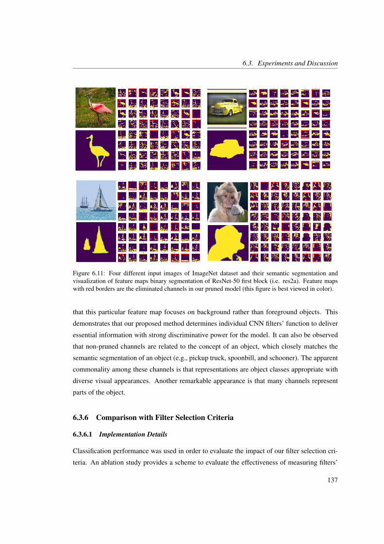
6.3. Experiments and Discussion

Figure 6.11: Four different input images of ImageNet dataset and their semantic segmentation andvisualization of feature maps binary segmentation of ResNet-50 first block (i.e. res2a). Feature mapswith red borders are the eliminated channels in our pruned model (this figure is best viewed in color).

that this particular feature map focuses on background rather than foreground objects. This

demonstrates that our proposed method determines individual CNN filters’ function to deliver

essential information with strong discriminative power for the model. It can also be observed

that non-pruned channels are related to the concept of an object, which closely matches the

semantic segmentation of an object (e.g., pickup truck, spoonbill, and schooner). The apparent

commonality among these channels is that representations are object classes appropriate with

diverse visual appearances. Another remarkable appearance is that many channels represent

parts of the object.

6.3.6 Comparison with Filter Selection Criteria

6.3.6.1 Implementation Details

Classification performance was used in order to evaluate the impact of our filter selection cri-

teria. An ablation study provides a scheme to evaluate the effectiveness of measuring filters’

137

6. Pruning CNN Filters via Quantifying the Importance of Deep Visual Representations

importance quantitatively. This procedure typically refers to the removal of some parts of the

model and the study of its performance, as crucial filters capture meaningful information and

contribute substantially to the model’s final performance. We ablated non-informative filters

by forcing their activation to be zero and computed the classification accuracy on the test set.

Quantifying the influence of the ablation on the classification performance allows for an im-

partial evaluation, in order to distinguish the essential filters in a CNNs and measure their

importance, allowing for layer-wise comparison. This method not only enables the evaluation

of filters’ importance, but can also detect the unimportant, redundant filters which can be safely

pruned.

6.3.6.2 Different Filter Selection Criteria

Several criteria to estimate the importance of a feature map or convolutional kernel in the CNNs

have been developed. To evaluate the effectiveness of our evaluation criterion, we compared

our filter selection method with several baseline methods. These can be briefly summarized as

follows:

• Random. Filters are randomly ablated.

• Weights sum [228]. Filters (i) with lowest absolute weights sum values are ablated:

ψi = ∑i | ω(i, :, :, :) |.

• Activation Mean [228]. ψi =1N ∑mean(τ(i, :, :)), where τ is the activation values for

filter i, and N denotes the size of data. The feature maps with weak patterns and their

corresponding filters and kernels are ablated.

• Mean gradient [229]. ψi =1N ∑mean(κ(i, :, :)), where κ is the calculated gradient for

each filter channel i, and N denotes the size of data.

• LRP (Layer-wise Relevance Propagation) [233]. The LRP of each channel i is calcu-

lated as its importance score ψi =1N ∑∑(LRP(i, :, :)), where N denotes the size of data;

LRP calculates the summed relevance quantity of each channel in the network to the

overall classification score, decomposing a classification decision into contributions for

each channels.

All these baseline methods consider the higher scores as more important, which is motivated

by the intuition that unimportant activation and filters have no influential outputs to the final

prediction of a model.

138

6.3. Experiments and Discussion

Figure 6.12: The architecture of the CNN model.

6.3.6.3 Overall Performance Comparison

Table 6.7 and Table 6.8 summarize the comparison results for two network architectures: our

proposed CNN architecture and VGG-16 on CIFAR-10 with different pruning criteria. Our

CNN architecture consists of three convolutional blocks, where each block has two convolu-

tional layers with a filter size of 3 x 3 with 32 kernels in the first block, 64 kernels in the

second block, and 128 kernels in the third block. Each block ends with a max-pooling layer.

This is followed by three fully-connected layers consisting of 2,000, 2,000, and 10 neurons

respectively. A standard Relu activation function was utilized. The detailed architecture of the

CNN model is presented in Fig. 6.12. Using the ablation approach, the importance of the filters

was evaluated by employing different selection criteria in a fully trained model. We compared

our method with such baselines, and the results are reported in Fig. 6.13, where different com-

pression rates are used. Table 6.7 and Table 6.8 also show different methods to measure the

importance of filters, using fixed compression ratio= 0.5, where 50% of channels are preserved

after pruning. The tables show layer-wise results for each layer, where we ablated layer-by-

layer and calculated the accuracy for each layer separately. For random selection criteria, the

mean value of three runs are reported.

Our ablation study has shown that for both architectures, MV achieves higher classifica-

tion performance when compared with other baselines. This demonstrates the robustness of our

proposed method in identifying the essential filters. With VGG16, as shown in Table 6.7, our

139

6. Pruning CNN Filters via Quantifying the Importance of Deep Visual Representations

0

0.1

0.2

0.3

0.4

0.5

0.6

0.7

0.8

0.9

1

90% 80% 70% 60% 50% 40% 30% 20% 10% 0%

Top

-1 A

ccura

cy

FLOPs Percentage

Conv_2 Conv_3 Conv_4

Conv_5 Conv_6 Conv_7

Conv_8 Conv_9 Conv_10

Conv_11 Conv_12 Conv_13

A. Proposed Method

0

0.1

0.2

0.3

0.4

0.5

0.6

0.7

0.8

0.9

1

90% 80% 70% 60% 50% 40% 30% 20% 10% 0%

Top

-1 A

ccura

cy

FLOPs Percentage

B. Random

0

0.1

0.2

0.3

0.4

0.5

0.6

0.7

0.8

0.9

1

90% 80% 70% 60% 50% 40% 30% 20% 10% 0%

Top

-1 A

ccura

cy

FLOPs Percentage

C. Mean-Mean [228]

0

0.1

0.2

0.3

0.4

0.5

0.6

0.7

0.8

0.9

1

90% 80% 70% 60% 50% 40% 30% 20% 10% 0%

Top

-1 A

ccura

cy

FLOPs Percentage

D. Weights Sum [228]

0

0.1

0.2

0.3

0.4

0.5

0.6

0.7

0.8

0.9

1

90% 80% 70% 60% 50% 40% 30% 20% 10% 0%

Top

-1 A

ccura

cy

FLOPs Percentage

E. Mean Gradient [229]

0

0.1

0.2

0.3

0.4

0.5

0.6

0.7

0.8

0.9

1

90% 80% 70% 60% 50% 40% 30% 20% 10% 0%

Top

-1 A

ccura

cy

FLOPs Percentage

F. LRP [233]

Figure 6.13: Comparison of layer-wise pruning methods for VGG-16 on CIFAR-10. The test accuracyis reported after ablating the unimportant filters with different compression ratios

pruning method achieved the best results when using a compression ratio of 0.5 for each layer

of the reference model. Fig. 6.13A. demonstrates that the performance of the pruned model

with our proposed method is relatively consistent, as model FLOPs reduce, especially when

reaching a reduction of 60%. Our method delivers the best result among all baselines. On the

other hand, it has less impact on the dropping of model accuracy while reducing FLOPs com-

pared with the LRP-based method, which is also inspired by neural network interpretability.

These results indicate an interesting potential research direction of combining the two fields of

140

6.3. Experiments and Discussion

Table 6.7: Overall results of layer-wise pruning utilizing different filter selection criteria. The testaccuracy is reported after ablating the unimportant filters. The results were conducted on an NVIDIAGeForce GTX 1080 GPU to prune the VGG-16 model on CIFAR-10 with a compression ratio of 0.5,where 50% of filters were preserved after pruning. For conv_2, the running time of identifying importantfilters is also reported (the model’s forward time is approximately 9s).

Conv_2 Conv_3 Conv_4 Conv_5 Conv_6 Conv_7 Conv_8 Conv_9 Conv_10 Conv_11 Conv_12 Conv_13Random 0.8290 (0.073ms) 0.408 0.7776 0.8592 0.8824 0.895 0.8605 0.9194 0.9307 0.931 0.932 0.9341

Weights-sum [228] 0.8630 (2.015ms) 0.5333 0.2785 0.7558 0.8681 0.7834 0.8655 0.92 0.9218 0.9321 0.934 0.9343Mean-mean [228] 0.8686 (4.5s) 0.1433 0.6995 0.795 0.8707 0.8157 0.8587 0.9198 0.9323 0.9314 0.932 0.9339

Mean Gradient [229] 0.5706 (11.1s) 0.4017 0.7448 0.7795 0.868 0.9052 0.821 0.9095 0.9313 0.9313 0.9331 0.9345LRP [233] 0.9186 (13.2s) 0.88 0.8698 0.8675 0.9067 0.9005 0.8815 0.9234 0.9316 0.9328 0.9332 0.9342

Our method 0.9199 (10.9s) 0.864 0.8784 0.8686 0.915 0.9059 0.8907 0.9286 0.932 0.9347 0.9346 0.9349

Table 6.8: Overall results of layer-wise pruning utilizing different filter selection criteria. The resultsare reported on our small CNN model on CIFAR-10 with a compression ratio of 0.5, where 50% offilters were preserved after pruning. The test accuracy is reported after ablating the unimportant filters.

Conv_2 Conv_3 Conv_4 Conv_5 Conv_6Random 0.7935 0.3556 0.6843 0.7096 0.7975

Weights-sum [228] 0.8027 0.4500 0.7091 0.6852 0.7645Mean-mean [228] 0.7790 0.3761 0.7465 0.7133 0.7855

Mean Gradient [229] 0.8471 0.2673 0.6149 0.6214 0.7437LRP [233] 0.8475 0.6122 0.7729 0.7466 0.8091

Our method (Sum-IoU) 0.8422 0.6709 0.7515 0.6988 0.8152Our method (MV) 0.8599 0.6935 0.7858 0.7201 0.8239

interpretability and model compression research.

Interestingly, ablating filters with random selection showed that the first few layers had

stronger negative effects and more synergistic filters compared with higher hidden layers. It

was also observed that the higher hidden layers were significantly redundant and more class-

specific. This observation is consistent with a previous theoretical proposal by [275]. One

reasonable explanation is that the neural networks hierarchically learn representations. Hence,

the first layers are not relevant to a specific object. Still, they build feature representations of

all input images that are joined to form more relevant object features in the later layers. By

ablating these fundamental features, deeper layers fail to produce class-specific features and

have a more negative impact on overall accuracy.

Although random selection is neither robust nor applicable in practice [207], it offers in-

sight and demonstrates that the detection of principal filters is a critical approach when pruning

redundant filters. The experiment empirically confirms that our importance method is suffi-

cient, given that ablating filters with low values in the layers had a negligible impact on the

overall accuracy compared to all baselines. As shown in Table 6.7 and Table 6.8, the exper-

imental results for both networks show that the method substantially outperformed the base-

lines. Our proposed method to measure filters’ importance helps not only to remove redundant

141

6. Pruning CNN Filters via Quantifying the Importance of Deep Visual Representations

nodes and compress the neuron network, but also to understand their inter-relationships and

how said filters impact the model. The experiment confirms that selecting the right criteria

to evaluate filters’ importance throughout all layers can guarantee a successful pruning ap-

proach. In Table 6.7, we reported the running time of different filter selection approaches. The

running speed of data-driven methods relies on model inference speed and dataset size. On

an NVIDIA GeForce GTX 1080 GPU, it takes 9.186s to apply forward passing through the

optimized VGG-16 model on CIFAR-10. Our proposed approach takes 10.9s to identify the

important filters, which is faster than some competitive methods. For ResNet-50 on ImageNet,

the time cost to estimate IoU scores and MV values is 422.3s of ResNet-50 first block (i.e.

res2a).

6.3.7 Comparison of Kernal Estimation (KE) vs. Fine-Tuning (FT)

In order to gather conclusive evidence to evaluate the effectiveness of our kernels estimation

(KE) method, an experiment based on the iterative layer-wise pruning process was carried out

using the VGG-16 model on CIFAR-10. Thus, we were able to fairly compare our KE method

with the standard fine-tuning (FT) procedure that is performed to preserve the original accu-

racy or recover the damage that might occur during the compression phase. After pruning

each layer with a fixed compression ratio of 0.5, our KE method, as well as the FT procedure,

were applied to improve the performance degradation. The experiments were performed on

the training set using three different numbers of trained examples, i.e. 200, 500, and 1,000.

We estimated new kernels and performed the fine-tuning using these settings with the same

amount of iteration. The comparative results are shown in Table 6.9, which demonstrates that

with a small number of examples, KE performed much better with less run-time requirements.

The approximate time needed to complete the process of each method is shown on the table.

The KE achieved higher classification performance, especially when the whole network was

cumulatively pruned. Our experiment has shown that both KE and FT improved the accuracy

after pruning each layer. These results demonstrate the necessity of adopting such steps to re-

cover model accuracy which has been damaged iteratively. However, even though the strategy

of iterative pruning with fine-tuning is the typical setting for CNN pruning, it incurs expensive

computational costs, significant inference time, and high storage requirements. Such an itera-

tive process requires significant inference costs, including costs related to the creation of a new

model, loading of parameters, and retraining of the whole model.

142

6.4. Summary

Table 6.9: Comparison of layer-by-layer pruning with fine-tuning (FT) and kernels estimation (KE)using the VGG-16 model on CIFAR-10 using 200, 500, and 1000 training examples. These results wereconducted on NVIDIA GeForce GTX 1080 GPU. The pruning is applied in a layer-by-layer fashionfrom the shallow layers to the deeper ones sequentially. The test accuracy is reported before and afterindependently performing fine-tuning and kernels estimation. For conv13, the running time of bothprocedures is also reported.

Conv_2 Conv_3 Conv_4 Conv_5 Conv_6 Conv_7 Conv_8 Conv_9 Conv_10 Conv_11 Conv_12 Conv_13200 samples

Before KE 0.9173 0.8536 0.8151 0.8084 0.8482 0.8219 0.7546 0.7988 0.7839 0.7769 0.8028 0.7707After KE 0.9338 0.9265 0.9195 0.8923 0.8746 0.8619 0.8151 0.8028 0.7971 0.7958 0.7954 0.7941 (5.86s)Before FT 0.9173 0.8254 0.7362 0.705 0.6991 0.671 0.5714 0.6128 0.6163 0.5881 0.6001 0.6091After FT 0.9203 0.8873 0.8499 0.7681 0.7401 0.6926 0.632 0.6317 0.6148 0.6034 0.6074 0.6044 (22.60s)

500 samplesBefore KE 0.9173 0.8498 0.8232 0.82 0.8494 0.8279 0.7699 0.8077 0.8055 0.806 0.8171 0.7979After KE 0.9332 0.9271 0.9196 0.8942 0.8771 0.8647 0.829 0.8195 0.8157 0.8161 0.8145 0.8138 (6.81s)Before FT 0.9173 0.826 0.7395 0.7143 0.7102 0.7026 0.6341 0.6759 0.6765 0.6663 0.6609 0.6751After FT 0.9239 0.8918 0.8559 0.7859 0.7647 0.7326 0.6817 0.6848 0.6808 0.6699 0.6725 0.6723 (22.74s)

1000 samplesBefore KE 0.9173 0.851 0.8165 0.8203 0.8556 0.8369 0.7935 0.8177 0.8127 0.8147 0.8238 0.809After KE 0.9331 0.9275 0.9202 0.8958 0.8811 0.8685 0.8404 0.8303 0.8247 0.8245 0.8243 0.8227 (8.81s)Before FT 0.9173 0.8325 0.7507 0.7173 0.7499 0.7247 0.6506 0.6939 0.6963 0.6858 0.6888 0.6887After FT 0.9235 0.8969 0.8622 0.8007 0.7777 0.7472 0.7011 0.709 0.6952 0.6915 0.6904 0.6948 (23.34s)

6.4 Summary

In this chapter, we have proposed a novel framework based on an effective channel-level prun-

ing method, considering the power of novel neural network interpretability in evaluating the

importance of feature maps. Based on the discriminative ability of interpretable latent repre-

sentations, a majority voting technique is proposed to compare the degree of alignment values

among filters and assign a voting score to quantitatively evaluate the importance of feature

maps. The experimental results show the effectiveness of our filter selection criteria, which

outperforms all other pruning criteria. It also allows for the identification of layers which are ro-

bust or sensitive to pruning, and this can be beneficial for further improving and understanding

the architectures. We also propose a simple yet effective method to estimate new convolution

kernels based on the remaining, crucial channels to accomplish effective CNN compression.

The experimental results on CIFAR-10, CUB-200, and ImageNet (ILSVRC 2012) datasets

demonstrate the effectiveness of our pruning framework in maintaining or even improving ac-

curacy after removing unimportant filters. Our results also display the excellent performance

of our proposed method. Moreover, our pruned model can be further pruned into even smaller

models by adopting any existing model compression method. Our potential future work is to

extend this framework and combine it with other pruning criteria to deeply explore the prob-

lem of CNN pruning from an interpretable perspective, aiming to link model compression and

interpretability research.

143

6. Pruning CNN Filters via Quantifying the Importance of Deep Visual Representations

In the following chapter, we present a comprehensive review of time-series data analysis,

introducing the use of DeepCluster methodology to learn and cluster temporal features from

accelerometer data for the clustering of animal behaviors. An evaluation and discussion are

given on real-world data. We also identify state-of-the-art and provide an outlook on the field

of deep time-series clustering.

144

Chapter 7

Deep Time-Series Clustering

Contents7.1 Introduction . . . . . . . . . . . . . . . . . . . . . . . . . . . . . . . . . 146

7.2 Time-series Data Type . . . . . . . . . . . . . . . . . . . . . . . . . . . . 147

7.2.1 Univariate . . . . . . . . . . . . . . . . . . . . . . . . . . . . . . 147

7.2.2 Multivariate . . . . . . . . . . . . . . . . . . . . . . . . . . . . . 147

7.2.3 Tensor Fields . . . . . . . . . . . . . . . . . . . . . . . . . . . . 148

7.2.4 Multifield . . . . . . . . . . . . . . . . . . . . . . . . . . . . . . 149

7.3 Conventional Time-series Analysis . . . . . . . . . . . . . . . . . . . . . 149

7.3.1 Similarity Measures and Features Extraction . . . . . . . . . . . . 151

7.3.2 Conventional Clustering Algorithms . . . . . . . . . . . . . . . . 155

7.4 DeepCluster Method Applied to Biological Time-series Data: A Case Study 157

7.4.1 Network Architectures for ICBD . . . . . . . . . . . . . . . . . . 158

7.4.2 Imperial Cormorant Birds Dataset (ICBD) and Pre-processing . . 161

7.4.3 Experiment and Discussion . . . . . . . . . . . . . . . . . . . . . 163

7.5 State-of-the-art and Outlook . . . . . . . . . . . . . . . . . . . . . . . . . 165

7.5.1 Different Network Architectures . . . . . . . . . . . . . . . . . . 165

7.5.2 Different Clustering Methods . . . . . . . . . . . . . . . . . . . . 168

7.5.3 Deep Learning Heuristics . . . . . . . . . . . . . . . . . . . . . . 169

7.5.4 DTSC Applictions . . . . . . . . . . . . . . . . . . . . . . . . . 170

7.5.5 DTSC Benchmarks . . . . . . . . . . . . . . . . . . . . . . . . . 171

7.6 Summary . . . . . . . . . . . . . . . . . . . . . . . . . . . . . . . . . . . 171

145

7. Deep Time-Series Clustering

7.1 Introduction

Recent advances in time-series clustering have shown great success in a range of fields, in-

cluding networks and systems, meteorology, social media, behavior analysis, trajectory data,

biological science, and finance. Extracting useful structures from large volumes of data re-

quires interdisciplinary research involving several domains such as statistics, machine learn-

ing, data visualization, pattern recognition, and high-performance computing [284]. Despite

the progress made in time-series data clustering, the presence of noise, high dimensionality,

and high feature correlation pose challenges in designing effective and efficient clustering

algorithms. Traditional algorithms display limited performance with the increase in data di-

mensionality. Variants of deep learning methods have shown a robust ability in representation

learning, finding the most success in supervised learning. Deep learning’s ability to deal with

high-level representations from data has inspired us to develop deep learning-based methods

for clustering analysis. We have proposed the DeepCluster, a clustering approach embedded in

a deep convolutional auto-encoder (DCAE), consisting of clustering and reconstruction objec-

tive functions. Its results on different datasets have shown the ability of deep clustering models

to substantially outperform other methods in terms of clustering quality. We published this

work in ICIP 2018 [5]. Moreover, we believe that we were the first to apply deep clustering

methods to time-series data. Specifically, we modified the DCAE architectures to suit time-

series data; see section 7.4 for details. The work was done in 2017, and therefore we believe

that we were the first to approach this topic and have made founding contributions to the area

of deep clustering of time-series data; this chapter describes these contributions. Since 2018,

several works have been reported on deep clustering of time-series data. We also review these

works in this chapter and identify state-of-the-art and present an outlook on this important field

of deep time-series clustering (DTSC).

The chapter is organised as follows. First, a detailed review of time-series data analy-

sis is provided, focusing on a general classification for time-series data. All data types, as

described in section 7.2, refer to the main definition of time-series data, and the section an-

swers questions such as how time-series data are different, along with providing examples of

this kind of data. Section 7.3 reviews the conventional time-series analysis with a discussion

about similarity measures and feature extraction, which are important for time-series data as,

usually, the quality of analysis techniques is significantly influenced by its selection. A com-

prehensive explanation for popular conventional clustering algorithms that have been used with

time-series data is then offered. In section 7.4, we apply the DeepCluster method to real-world

146

7.2. Time-series Data Type

data; namely, the Imperial Cormorant bird dataset (ICBD) from the Biosciences department at

Swansea University. Other recent works are subsequently discussed in section 7.5. The chal-

lenges of DTSC, opportunities, and future directions are also described. Finally, concluding

remarks and summary are provided in section 7.6.

7.2 Time-series Data Type

Time-series data could be an umbrella term for many different data with an associated time

component. It is defined as an ordered collection of observations or sequences of data points

made over time, usually at uniform time intervals. In order to understand the complexity of

time-series and explore the underlying processes, the processing and analysis of such data re-

quire particular supporting tasks and methods. Here, we classify time-series data into four

categories, subsumed under the concepts of univariate, multivariate, tensor fields, and multi-

fields. Hotz et al. [285] discuss the complex structure of scientific data and provide a clear

definition of a multifield. Our four types, or categories, are generalized to include many related

subtypes of time-series data in order to achieve a comprehensive classification for said data.

7.2.1 Univariate

The univariate time-series is a sequence that contains only one data value per temporal primi-

tive [69, 284]. It is a field of a single variable captured or observed through time. The temper-

ature in a city spanning a period of time is a clear example of this type of data.

7.2.2 Multivariate

Multivariate time-series is a set of time-series which have the same timestamps [69,284]. This

kind of time-series data is an array of variables or numbers at each point in time and can be

a collection of multiple univariates captured through time, such as temperature and pressure

readings, or associative multivariate, such as 3D acceleration measured from a tri-axial ac-

celerometer, where each component of the multivariate has the same units and sensor source.

As time-series data is an ordered collection of observations or a sequence of data points made

over time, this special type of multivariate time-series data is relevant in many fields includ-

ing biology, medicine, finance and animation. Multivariate time-series data have been used in

manufacturing systems and predictive maintenance [286,287]. Time-series data obtained from

gene expression measurement [288–290], for instance, can be used by biologists to understand

147

7. Deep Time-Series Clustering

the correlation between types of genes, analyze gene interactions, and compare regulatory be-

haviors for genes of interest. Medical experts also utilize time-series data from blood pressure

measurements [291] to understand and deal with cases such as monitoring illness progression,

and understanding ecological and behavioral processes related to a disease which may lead to

improved diagnoses. Furthermore, time-series data such as that obtained from sampled trans-

actions over a period of time [292–294], stock markets [124, 295], and international financial

markets [296, 297] can be used in the financial field and are usually analyzed to understand

and forecast market conditions. It is useful to find correlations between the data and test hy-

potheses about the market, as this helps in making correct decisions at the appropriate time

under changing businesses and economic circumstances. A multivariate can also present time-

series data obtained from various data sets including metadata, e.g. patient records [298, 299],

employment records [300, 301], and social networks [302].

7.2.3 Tensor Fields

These comprise an array of data arranged on a regular grid with a variable number of axes [32].

They can be described as a quantity associated with each point in space-time as it has been

extended to functions or distributions linked to points in space-time [285]. Dealing with spatio-

temporal data, this type of time-series data is generalized to include many related subtypes:

time-series of graphs and networks, time-series of spatial positions of moving objects, and

time-series of spatial configurations/distributions.

7.2.3.1 Time-series of Graph and Network

Time-series data in the form of networks consist of associated attributes such as nodes and

edges that reflect different kinds of behavior over time. Node or edge attributes of dynamic

graphs can be introduced as time-series. This kind of time-series data helps with understanding

different temporal patterns and evaluating the network dynamics in general [303–307]. As

each machine (e.g. engines or computers) typically consists of a large number of sensors

that produce massive quantities of data, time-series data can be obtained from the nodes of

such machines over a period of time, such as CPU load, memory usage, network load, and

data center chiller sensor, helping to improve the understanding of how machines are used

in practice and analyze the performance and behaviors of such systems [308–314]. Indeed,

analyzing this data can help users and experts understand and evaluate the network dynamics.

148

7.3. Conventional Time-series Analysis

7.2.3.2 Time-series of Spatial Positions of Moving Objects

Spatial positions of moving objects data with an associated time component classifies as tra-

jectory data. It presents different places over time, providing a clear idea of spatio-temporal

changes. The process and analysis of time-series data are important procedures for understand-

ing the characteristics of the data and obtaining meaningful statistics which aid the exploration

of the underlying processes, analysis, tracking, and representation of this type of data in order

to understand and recognize the mobility of a diverse array of moving objects, such as vehi-

cles [315–322], and aircrafts [317,318], which can lead to path discovery, movement analysis,

and location prediction.

7.2.3.3 Time-series of Spatial Configurations and Distributions

Being able to extract useful insights from time-series of spatial distributions and configura-

tions has become increasingly important due to significant growth in data science and rapid

advancement in many technologies. In our research, we consider discovering behavioral pat-

terns and finding interesting events that might take place in certain municipalities [323] and

public or business sectors as spatial configurations and distributions. This identification of reg-

ular configurations and distributions over time is represented by a total number of events and

behaviors extracted from a chosen spatial scale. Personal mobility behaviors and movement

patterns [324–332], behaviors of animals [333, 334], pattern changes in climate (weather) and

the ozone layer [332,335–341], and behavior capture data made through time at often uniform

time intervals [135, 342–346] can be regarded as instances of this type of data that take place

in specific spatial identification.

7.2.4 Multifield

This kind of data, defined as a set of fields, provides enough flexibility to capture most types

of compound datasets that occur in practice [285]. Combining multiple modality sensors such

as gyroscopes, magnetometers and accelerometers with other environmental sensors is an ex-

ample of this data type.

7.3 Conventional Time-series Analysis

For time-series data, the presence of noise, high dimensionality, and high feature correlation

pose challenges for designing effective and efficient clustering algorithms compared to data

149

7. Deep Time-Series Clustering

without a temporal component [284,347]. Analyzing time-series data is nontrivial and can even

vary over time due to complex interrelations between time-series variables. Xing et al. [348]

describe three significant challenges for time-series analysis. First, many methods can only

take input data as a vector of features. Unfortunately, there are no explicit features in sequence

data. Second, feature selection is not easy because the dimensionality of the feature space can

be high and computation can be costly. Third, since there are no explicit features in the raw

data, building a partitioning task is burdensome in some applications. Therefore, efficiently

handling the raw data in time-series is difficult without using similarity measures and feature

extraction to reduce dimensionality and provide representative features of such data.

Computing the similarity between two data objects is considered one of the main differ-

ences between clustering of temporal and non-temporal data [155, 349]. The unique char-

acteristics of time-series data such as noise, including outliers and shifts, and the varying

length of time-series has made similarity measures one of the main challenges for cluster-

ing of time-series data [134]. When dealing with time-series data, the greatest challenge lies

in replacing the distance/similarity measure for static data with a suitable one for time-series

data, because it may be scaled and translated differently on both the temporal and behavioral

dimensions [347, 350]. Therefore, modifying distance functions to suit the characteristics of

time-series data has become essential when developing a clustering method for time-series

data. Petitjean et al. [351] introduced a kDBA method that combines Kmeans and dynamic

time warping for better alignment. Moreover, Yang et al. [352] presented the K-Spectral Cen-

troid (K-SC) method, using an invariant similarity metric to reveal the temporal dynamics.

Lastly, Paparrizos et al. [353] developed a k-Shape method whereby the shapes of the time-

series are considered by applying cross-correlation measures. However, these methods are

usually sensitive to noise and outliers because all time points are considered [354].

Furthermore, the quality of clustering methods is significantly affected by the choice of fea-

ture extraction technique. This fact made feature extraction very essential when clustering data.

Guo et al. [355] proposed a feature-based approach to time-series clustering by applying in-

dependent component analysis to convert the raw time-series into a lower-dimensional feature

vector and then further applying kmeans clustering on the extracted features. In addition, Za-

karia et al. [356] employed u-shapelet algorithms to learn local patterns in a time-series, as they

are highly predictive when performing clustering. Other recent advances in feature extractions

have efficiently supported clustering tasks, where linear [357–360] and non-linear [361–364]

methods have been adopted to transform the original time-series data into representative fea-

150

7.3. Conventional Time-series Analysis

Figure 7.1: The pipeline of conventional time-series analysis.

tures, allowing unsupervised clustering methods to deal with beneficial features instead of raw

data.

The conventional time-series analysis pipeline consists of three different perspectives, these

being time-series data, similarity measures and feature extraction for time-series data, and time-

series clustering technique (see Fig. 7.1).

7.3.1 Similarity Measures and Features Extraction

Large time-series data require adequate pre-processing to gain an appropriate approximation

of the underlying data representation. The aim is to generate a higher-level abstraction which

represents the data while preserving the shape characteristics of the original data during di-

mensionality reduction. There are several dimensionality reduction techniques specifically

designed for time-series which exploit the frequential content of the signal and its usual sparse-

ness in the frequency space [365]. In general terms, choosing a distance measure is important

and assists in dealing with outliers, amplitude differences, and time axis distortion. Further-

more, selecting important features in the data requires sufficient communication of knowledge

from domain experts. Thus, the quality of clustering approaches is significantly affected by the

choice of similarity measures and feature extraction techniques to obtain the relevant knowl-

edge from the data. The below discussion about the types of methods is intended to provide

a review of popular similarity measures and feature extraction techniques along with works

which have been adopted in time-series data mining.

7.3.1.1 Raw Data Similarity

Most mining approaches utilize the concept of the similarity between a pair of time-series.

Similarity measures must be chosen when dealing with time-series data in order to take into

account outliers, different amplitude, and time axis distortion. When dealing with time-series

151

7. Deep Time-Series Clustering

data, efficiency and effectiveness are the main targets of representation methods and similar-

ity measures [366]. Tornai et al. [367] argue that the distance between two sequences as a

measurement plays an important role in the quality of clustering algorithms. The accuracy of

such algorithms can be significantly impacted by the choice of similarity measures. Yahyaoui

et al. [368] and Wang et al. [366] presented a comprehensive review of time-series measures,

classifying them into four major categories: lock-step measures (e.g. Euclidean distance and

Manhattan distance), elastic measures (e.g. longest common subsequence (LCS) and dynamic

time warping (DTW)), pattern-based measures (e.g. spatial assembling distance (SpADe)), and

threshold-based measures (e.g. threshold query based similarity search (TQuEST)). The types

of methods, discussed below, are intended to provide a review of popular similarity measures.

Euclidean distance (ED): is a commonly used metric for time-series. It is defined between

two time-series X and Y having length L; therefore, the Euclidean distance, between each pair

of corresponding points X and Y, is the square root of the sum of the squared differences [369].

Thus, the two time-series being compared must have the same length, and the computational

cost is linear in terms of temporal sequence length [370]. Along the horizontal axis, the dis-

tance between the two time-series is calculated by matching the corresponding points [371].

The Euclidean distance metric is very sensitive to distortion and noise [348], and is not able

to handle one of the elements being compressed or stretched [334]. This approach is there-

fore not reliable, especially when computing similarity between time-series with different time

durations [372].

Dynamic Time Warping (DTW): is another distance measure that is proposed to over-

come some Euclidean distance limitations such as non-linear distortions. In DTW, the two

time-series do not have to be the same length, and the idea is to align (warp) the series before

computing the distance [348]. However, two temporal points with completely different local

structures might be mistakenly matched by DTW. This issue can be addressed by improving the

alignment algorithm, e.g. shape dynamic time warping. It considers point-wise local structural

information [373].

Due to its quadratic time complexity, DTW does not scale well when dealing with large

datasets. Despite this, it is widely used in various applications, such as in bioinformatics, fi-

nance and medicine [374]. DTW has several local constraints, namely boundary, monotonicity

and continuity constraints [372]. Common misunderstandings about DTW include concep-

tions that it is too slow to be useful and that the warping window size does not matter much;

Wang et al. [366] and Mueen et al. [375] have attempted to correct these notion. Kotas et

152

7.3. Conventional Time-series Analysis

al. [376] have reformulated the matrix of the alignment costs, which led to a major increase in

the noise reduction capability. Other surveys review distance measures such as Euclidean Dis-

tance (ED) [377], Dynamic Time Warping (DTW) [378, 379], and distance based on Longest

Common Subsequence (LCS) [366, 380].

Correlation: is a mathematical operation widely used to describe how two or more vari-

ables fluctuate together. Different types of correlation can be found by considering the level

of measurement for each variable. Distance correlation can be used as a distance measure be-

tween two variables that are not necessarily of equal dimension. In time-series data, it is used

to detect a known waveform in random noise. Unlike DTW and LCS, correlation also offers a

linear complexity frequency space implementation in signal processing [334, 381].

Cross-correlation: is the correlation between two signals which shape a new signal, and

its peaks can indicate the similarity between the original signals; it is used as a distance met-

ric [134]. However, cross-correlation can be carried out more efficiently in the frequency

domain [381]. Autocorrelation occurs when the signal is correlated with itself, which is useful

for finding repeating patterns [334]. Cross-correlation might be a slow operation in time-series

space [334], but it corresponds to point-wise multiplication in frequency space. It is also con-

sidered the best distance measure to detect a known waveform in random noise [334]. When

processing the signal, the correlation has a linear complexity frequency space implementation

which cannot be achieved by DTW.

7.3.1.2 Features Extraction

Feature extraction is a form of dimension reduction which helps to lower the computational cost

of dealing with high-dimensional data and achieve higher accuracy of clustering [382]. Match-

ing features from time-series data should be extracted before applying learning algorithms to

the vector of extracted features. Several feature-based techniques have been proposed to repre-

sent features with low dimensionality for time-series data. Wang et al. [366] list several meth-

ods for reducing time-series dimensionality as feature extraction; including Discrete Fourier

Transform (DFT), Discrete Wavelet Transform (DWT), Discrete Cosine Transform (DCT),

Single Value Decomposition (SVD), Adaptive Piecewise Constant Approximation (APCA),

Piecewise Aggregate Approximation (PAA), Chebyshev polynomials (CHEB), and Symbolic

Aggregate approXimation (SAX).

Principal Component Analysis (PCA), as an eigenvalue method, is a technique which

transforms the original time-series data into low-dimensional features. As a feature extraction

153

7. Deep Time-Series Clustering

method, PCA is effectively applied to time-series data [383–386]. It transforms data to a new

set of variables whose elements are mutually uncorrelated, thus learning a representation of

data that has lower dimensionality than the original input. PCA is a linear dimensionality

reduction technique, and has been used as an effective dimensionality reduction method that

eliminates the least significant information in the data and preserves the most significant. [135,

294, 305, 321, 335, 338, 346, 387] use PCA to reduce high-dimensional data and analyze the

similarity of time-series data.

Multidimensional Scaling (MDS): is a very popular non-linear dimensionality reduction

technique that is useful for effectively representing high-dimensionality data in lower dimen-

sional space [289, 300, 305, 307, 308, 314, 329, 332, 335]. It struggles, however, to separate

Kmeans clusters [335]. Jeong et al. [289] use MDS to gain a better understanding of gene

interactions and regulatory behaviors. Thus, two different MDS representations are considered

with respect to time-series data. One shows local differences among genes in the same clus-

ter group, while the other shows global differences among all genes in all the clusters. It is

also used to reveal the distributions of the time-series data, helping to understand the relations

among time-series [300].

K-grams: Transforming time-series data into a set of features cannot capture the sequential

nature of series. K-gram is an example of a feature-based technique that aims to maintain the

order of elements in series using short sequence segments of k consecutive symbols [368]. K-

grams [388] represent a feature vector of symbolic sequences of K-grams in time-series data.

Given a set of K-grams, this feature vector can represent the frequency of the K-grams (i.e.

how often a K-gram appears in a sequence).

Discrete Fourier Transform (DFT): is one of the most common transformation meth-

ods [389]. It has been used to transform original time-series data into low-dimensionality

time-frequency characteristics and index them to obtain an effective similarity search [390].

DFT is used to perform dimensionality reduction and extract features into an index used for

similarity searching. This technique is continually under improvement and some of its limita-

tions have been overcome [377, 391, 392].

Discrete Wavelet Transform (DWT): has also been used as a technique to transform

original time-series and obtain low-dimensional features that efficiently represent the original

time-series data [367, 393]. Chan et al. [394] use Haar Wavelet Transform for time-series

indexing, which shows the technique’s effectiveness with regard to the decomposition and

reconstruction of time-series. With a large set of time-series data, analysis tasks face certain

154

7.3. Conventional Time-series Analysis

challenges in defining matching features; therefore, taking advantage of wavelet decomposition

to reduce the dimensionality of data is beneficial [395]. The analysis task can be accurately

performed utilizing the discrete wavelet transform technique [396].

Shapelets: Discretization is often required when applying feature-extraction techniques

in time-series data, but it can cause information loss [348]. To address this, Ye et al. [397]

introduce time-series shapelets which can be directly applied to time-series. This technique

is based on comparing the subsection of shapes (shapelets) instead of comparing the whole

time-series sequences to measure the similarity. A binary decision maker decides whether

each new sequence belongs to a class or not. The shapelet classifier has some limitations with

a multi-class problem, and to overcome this issue, Ye et al. [397] use the shapelet classifier as

a decision tree. Xing et al. [398] show that early classification can be efficiently achieved by

extracting the local shapelets features.

7.3.2 Conventional Clustering Algorithms

Clustering is widely used as an unsupervised learning method. The aim of time-series cluster-

ing is to define a grouped structure of similar objects in unlabeled data based on their similar

features. Due to the unique structure of time-series data (e.g. high dimensionality, noise,

and high feature correlation), clustering time-series differs from traditional clustering, conse-

quently, several algorithms have been improved to deal with time-series. Most works involving

the clustering of time-series can be classified into three categories [134]. The first is whole

time-series clustering, where a set of individual time-series is given and the aim is to group

similar time-series into clusters with respect to their similarity. The second is subsequence

clustering, which involves dividing the time-series data at certain intervals using a sliding win-

dow technique to perform clustering on the extracted subsequences of a time-series. The third

category is a clustering of time points based on a consolidation of their temporal proximity

and the similarity of the corresponding values. Some points might not assign to any clusters

and are deemed as noise. Chapter 2 provided a review of popular clustering algorithms (see

section 2.3.1 for detailed descriptions of these methods). The discussion about various types

of methods discussed below aims to review clustering algorithms used for time-series data.

7.3.2.1 Partitioning Methods

Partitioning methods are described as the process of partitioning unlabeled data into K groups.

Kmeans [121] , Kmedoids (PAM)) [120], Fuzzy Cmeans [126,127], and Fuzzy Cmedoids [132]

155

7. Deep Time-Series Clustering

are the most popular algorithms for partitioning clustering. Kmeans has been used to cluster

time-series data, achieving efficient clustering results due to its speed, simplicity, ease of im-

plementation, and the possibility to assign the desired amount of clusters [123, 124]. The

Kmedoids or PAM (partition around medoids) algorithm is often used alongside the DTW dis-

tance measure to cluster time-series data [399]. Andrienko et al. [320] used Kmedoids as a

clustering algorithm, which could be better suited than Kmeans, as it uses medoids instead of

means. However, it still has the same issues as Kmeans, where the number of clusters must be

known in advance. Unsupervised partitioning has been shown to be as efficient at providing

good clustering accuracy for time-series clustering. Several partitioning clustering approaches

(e.g. Kmeans [123, 355, 399, 400, 400, 401], Kmedoids [402], Fuzzy Cmeans [129, 403], and

Fuzzy Cmedoids [404]) have been used to achieve efficient clustering results for sequences of

time-series data.

7.3.2.2 Hierarchical Methods

Hierarchical clustering defines a tree structure for unlabeled data by aggregating data samples

into a tree of clusters. This method does not assume a value of K, unlike Kmeans cluster-

ing. There are two main kinds of hierarchical clustering methods - agglomerative (bottom-up)

and divisive (top-down) [133, 134]. The hierarchical method is applied to determine the or-

der of time-series data [292, 387]. Wijk et al. [405] conducted pioneering work in which they

use a bottom-up hierarchical clustering approach to identify common and uncommon subse-

quences that occur in large time-series. Battke et al. [288] overcame the issue of hierarchical

clustering speed for large time-series datasets by implementing the rapid neighbour-joining

algorithm [406].

7.3.2.3 Model Based Methods

A self-organizing map (SOM), a model-based method developed by Kohonen [144], is a spe-

cific type of neural network (NN) used for model-based clustering. SOM has been used to

analyze temporal data and is utilized for pattern discovery in temporal data [135, 288, 296,

297, 321, 330, 407]. The introduction of Recurrent SOM [408] and Recursive SOM [409] has

enhanced SOM for mapping time-series data [156]. Fuet et al. [410] use self-organizing maps

to gather similar temporal patterns into clusters. A continuous sliding window is used to seg-

ment data sequences from numerical time-series before applying the SOM algorithm. SOM

is also used in [157] to cluster time-series features. Many works on clustering have chosen

156

7.4. DeepCluster Method Applied to Biological Time-series Data: A Case Study

SOM due to its advantages with regard to certain properties such as parameter selection and

data analysis. However, one of its main disadvantages is that it does not work perfectly with

time-series of unequal length, as it is difficult to define the dimension of weight vectors [155].

7.3.2.4 Density-Based Methods

In density-based clustering, the cluster continues to expand if the density of a set of points with

its neighbors is closely packed together, and that cluster is separated by subspaces where the

objects have low density. Density-based clustering for time-series data has some advantages;

it is a fast algorithm which does not require pre-setting the number of clusters, is able to detect

arbitrarily shaped clusters as well as outliers, and uses easily comprehensible parameters such

as spatial closeness [329]. Although density-based clustering entails some complexity, many

time-series clustering algorithms have adopted this method [288, 295, 300, 308, 315, 317, 318,

320, 322, 324, 325, 328, 329, 340].

7.4 DeepCluster Method Applied to Biological Time-series Data:

A Case Study

The process of time-series clustering is accompanied by several difficulties and challenges,

such as feature representations at different time scales, and distortion by high-frequency per-

turbations and random noise in time-series data [411]. Time-series data has also shown consid-

erable diversity in relevant features and properties, dimensionality, and temporal scales [412].

To overcome these challenges, a deep learning method can be designed to disentangle the

data manifolds and allow a clustering method to deal with learned features instead of raw

data. Traditional clustering algorithms tend to attain limited performance as dimensionality in-

creases. Dealing with high-level representation provides benefits that support the achievement

of clustering tasks. Deep clustering allows a deep neural network to extract similar patterns in

lower-dimensional space and find idealistic representative centers for distributed data. Efforts

have been made in the field of computer vision in developing deep clustering methods for im-

age datasets. Deep auto-encoders (DAEs) and deep convolutional auto-encoders (DCAEs) are

unsupervised models. These models have been exploited for clustering, where features learned

through deep networks provide an abstracted latent representation used for clustering analysis.

The previous works can be categorized into four different categories, summarized in Table 7.1.

157

7. Deep Time-Series Clustering

Method Separated Clustering Embedded ClusteringDAE Tian et al. [168], Huang et al. [169] Song et al. [167], Xie et al. [171]

DCAE Li et al. [174], Guo et al. [175] Alqahtani et al. [5]

Table 7.1: Deep Clustering Methods. Separated Clustering consists of two main steps, where they ex-tract latent features for given data and then perform clustering on the learned representations. whileembedded Clustering methods have embedded a clustering algorithm into deep neural networks, wherefeature representations and clustering assignments are simultaneously learned, applying joint loss func-tion.

DeepCluster [5] is an unsupervised clustering method that simultaneously captures rep-

resentative features and the relationships among images. The goal is to learn feature repre-

sentations and cluster assignments simultaneously, employing the strength of DCAE to learn

high-level features. Two objective functions were integrated together: one minimizes the dis-

tance between features and their corresponding cluster centers, while the other minimizes the

reconstruction error of the DCAE, defined as follows:

minW,b

1N

N

∑n=1‖ xn− xn ‖2 + λ · 1

N

N

∑n=1‖ ht(xn)− c∗n ‖2, (7.1)

where N denotes the number of samples, x is a reconstructed sample, and x is an original

sample, λ controls the contribution of the clustering cost function, ht(∗) is the internal rep-

resentation obtained by the encoder mapping at the tth iteration, xn is the nth sample in the

dataset, and c∗n is the assigned cluster center to the nth sample. During optimization, all data

representations are assigned to their new identical cluster centers, after which the cluster cen-

ters are updated iteratively, allowing the model to achieve stable clustering performance. The

defined clustering objective, as well as the reconstruction objective, are simultaneously used to

update the parameters of the transforming network. DCAE might be well-suited to time-series

data because it captures the time-series’ shape and allows local shift-invariance. This section

applies what was proposed in Chapter 3 to real-world time-series data; namely, the Imperial

Cormorant bird dataset (ICBD) from the Biosciences department at Swansea University. The

experimental architectures of DAE and DCAE (Section 7.4.1) will be discussed and the Im-

perial Cormorant Birds Dataset (ICBD) described before the preparation of time-series data is

highlighted (Section 7.4.2), and our experimental results outlined (Section 7.4.3).

7.4.1 Network Architectures for ICBD

Our method is designed to cluster large time-series data using deep neural networks. In this

section, we introduce our experimental architectures of two types of neural networks: DAE

158

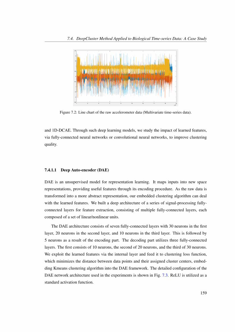
7.4. DeepCluster Method Applied to Biological Time-series Data: A Case Study

Figure 7.2: Line chart of the raw accelerometer data (Multivariate time-series data).

and 1D-DCAE. Through such deep learning models, we study the impact of learned features,

via fully-connected neural networks or convolutional neural networks, to improve clustering

quality.

7.4.1.1 Deep Auto-encoder (DAE)

DAE is an unsupervised model for representation learning. It maps inputs into new space

representations, providing useful features through its encoding procedure. As the raw data is

transformed into a more abstract representation, our embedded clustering algorithm can deal

with the learned features. We built a deep architecture of a series of signal-processing fully-

connected layers for feature extraction, consisting of multiple fully-connected layers, each

composed of a set of linear/nonlinear units.

The DAE architecture consists of seven fully-connected layers with 30 neurons in the first

layer, 20 neurons in the second layer, and 10 neurons in the third layer. This is followed by

5 neurons as a result of the encoding part. The decoding part utilizes three fully-connected

layers. The first consists of 10 neurons, the second of 20 neurons, and the third of 30 neurons.

We exploit the learned features via the internal layer and feed it to clustering loss function,

which minimizes the distance between data points and their assigned cluster centers, embed-

ding Kmeans clustering algorithm into the DAE framework. The detailed configuration of the

DAE network architecture used in the experiments is shown in Fig. 7.3. ReLU is utilized as a

standard activation function.

159

7. Deep Time-Series Clustering

Figure 7.3: The DAE network architecture for time-series data shown the number of neurons for eachfully-connected layer in both encoder and decoder parts.

7.4.1.2 1D-Convolutional Layer for Deep Convolutional Auto-encoder (1D-DCAE)

Unlike 2D grid (e.g. image data) input, convolutional layers for time-series data use a 1D grid,

so instead of holding raw 2D pixel values, the input of time-series data is multiple 1D subse-

quences. In this case, multivariate time-series [69] are separated into univariate ones so that

feature learning can be performed for each univariate series. In other words, the multivariate

time-series are considered as input that is fed into the convolutional layers, learning features

through convolution and activation layers. The 1D-convolutional layer extracts features by

applying dot products between transformed waves and a 1D learnable kernel (filter) [411],

computing the output of neurons that are connected to local temporal regions in the input. This

stage is followed by the activation layer, which is used to perform non-linearity within the

networks, allowing for the learning of more complex models [413]. After extracting feature

maps from multiple channels, they are fed into other convolutional layers and then passed as

inputs of the fully-connected layer. In the fully-connected layer, the learned feature represen-

tations are fed to the clustering loss function via the internal layer of DCAE, which embeds a

clustering algorithm into the body of a DCAE model.

The architecture of DCAE consists of three 1D-convolutional layers with filter sizes of

10× 1 with 32 kernels in the first convolutional layer, 64 kernels in the second convolutional

160

7.4. DeepCluster Method Applied to Biological Time-series Data: A Case Study

Table 7.2: Detailed configuration of the DCAE network architecture used on time-series data.

Layer Biological Dataset

Convolutional 10×1×32

Convolutional 10×1×64

Convolutional 10×1×128

Convolutional 1×3×128

Fully-connected 384

Fully-connected 5

Fully-connected 384

Deconvolutional 1×3×128

Deconvolutional 10×1×128

Deconvolutional 10×1×64

Deconvolutional 10×1×32

layer, and 128 kernels in the third convolutional layer. This is followed by two fully-connected

layers, which have 384 and 5 neurons respectively, in the encoding part. In the decoding

part, a single fully-connected layer of 384 neurons is followed by three 1D-deconvolutional

layers. The first deconvolutional layer consists of 128 kernels, the second deconvolutional

layer consists of 64 kernels, and the third deconvolutional layer consists of 32 kernels. The

detailed configuration of the DCAE network architecture used in the experiment is presented

in Table 7.2. ReLU is utilized as a standard activation function.

7.4.2 Imperial Cormorant Birds Dataset (ICBD) and Pre-processing

Animal behavior analysis has received considerable attention in this area of interest, where

’smart’ sensors (i.e. accelerometers) attached to wild animals have revolutionized biologists’

understanding of their ecology. A tri-axial accelerometer is one preferred source of quantita-

tive data to identify animal behavior through movement. Biologists widely use accelerometers

as they help them monitor and determine wild animals’ behaviors [414] in their natural en-

vironment over long periods of time. The attachment of a tri-axial accelerometer provides

analyzed data, which allows researchers to investigate an animal’s movement through iden-

tifying its posture and changes in its body velocity [334], revealing much about its behav-

ior [415]. Directly dealing with multiple sensors at high frequencies is expensive and requires

161

7. Deep Time-Series Clustering

expert knowledge [414, 416]. Previous efforts by biologists have been made to analyze raw

accelerometer data, where Overall Dynamic Body Acceleration (ODBA) [417] and Vectorial

Dynamic Body Acceleration (VeDBA) [418] have been proposed as surrogate measures for

speed. The VeDBA appears more robust than the ODBA because it provides values closer

to the true physical acceleration experienced and copes better than ODBA with variability in

substrate [418]. Therefore, we calculate the VeDBA to derive new acceleration values from

tri-axial accelerometer data using the following form:

VeDBA =√

DA2x +DA2

y +DA2z , (7.2)

where DA2x , DA2

y , and DA2z denote the dynamic acceleration values obtained by taking the

absolute values of running means of the raw acceleration values of each of the accelerometer’s

3 axes from the corresponding raw acceleration values.

The Imperial Cormorant bird dataset (ICBD) was provided by biologists from the Bio-

sciences department at Swansea University. This dataset contains more than 173K data points

associated with a label from 5 different classes (descent diving, bottom diving, ascent diving,

swimming, and flying). Fig. 7.2 presents the raw accelerometer data.

7.4.2.1 Normalization

In our case, each dimension of the time-series data is normalized using unity-based normaliza-

tion where all values are set in a range between [0,1] using the following form:

x′ =x−min(x)

max(x)−min(x)(7.3)

7.4.2.2 Sliding Window Approach

A sliding window approach was used to segment continuous time-series data into a set of

short segments. The sliding window technique convolves along the time axis based on two

parameters (i.e. window size W and stride S, which is the step size of sliding a window).

Here, the window size W is a determined sampling rate. A fixed sliding step of 30 is adopted

in our experiments, and stride S is set to 15 as recommended by the biologists. However, a

smaller value for stride can be chosen to increase the number of samples in the dataset and

would be useful to capture more local temporal patterns and avoid lost data, smoothing the

transition between time-steps. Fig. 7.4A. and Fig. 7.4 present the sliding window approaches

which were used in our experiment. The sliding window approach is applied to two different

162

7.4. DeepCluster Method Applied to Biological Time-series Data: A Case Study

categories of time-series data: univariate time-series data (Fig. 7.4A.) and multivariate time-

series data (Fig. 7.4).

A. Univariate Time-series Data B. Multivariate Time-series Data

Figure 7.4: The detailed process of the sliding window approach with a window size of 12 and and astride of 6 are adopted in both cases.

7.4.3 Experiment and Discussion

7.4.3.1 Experiments Setup

The proposed method was implemented using MatConvNet [419] in Matlab. As a result of the

complexity and variability characteristics of the ICBD dataset, obtaining reliable training data

normally requires collecting multiple annotations from different experts and then performing

cross-validation on the collected labelings. We performed 5-fold cross-validation on the pro-

vided classes, splitting them into 5 equal subsets. In each evaluation round, each model was

trained on 4 folds and tested on the 5th one. This procedure was repeated for all 5 folds. Both

sliding window approaches were applied to extract subsequences from the folds. Moreover,

the VeDBA method was applied to the raw tri-axial accelerometer data using Eq.(7.2) to obtain

univariate time-series data. Following this, the univariate time-series data was segmented to be

used as input data for the Kmeans and the DAE framework, while the multivariate time-series

data was segmented to be used as input data for the DCAE.

The model was trained end-to-end in an unsupervised manner, with no pre-training or

fine-tuning procedures involved. All weights were initialized using the Xavier method [57],

163

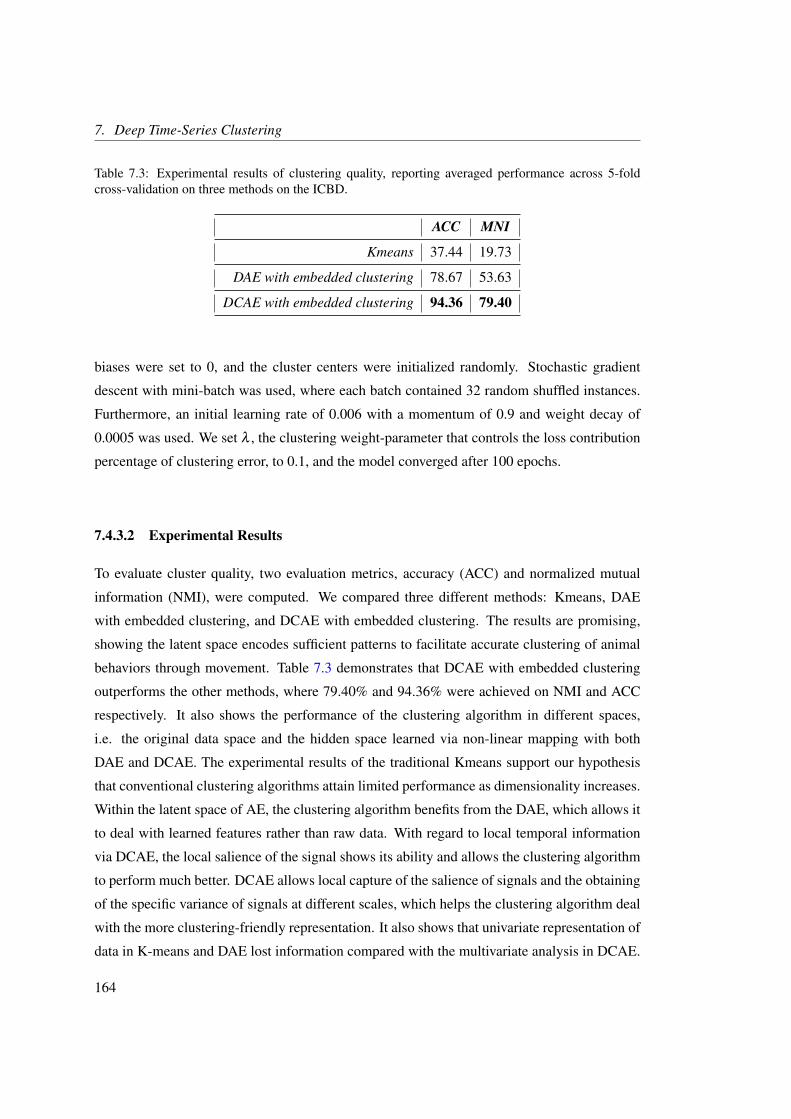
7. Deep Time-Series Clustering

Table 7.3: Experimental results of clustering quality, reporting averaged performance across 5-foldcross-validation on three methods on the ICBD.

ACC MNI

Kmeans 37.44 19.73

DAE with embedded clustering 78.67 53.63

DCAE with embedded clustering 94.36 79.40

biases were set to 0, and the cluster centers were initialized randomly. Stochastic gradient

descent with mini-batch was used, where each batch contained 32 random shuffled instances.

Furthermore, an initial learning rate of 0.006 with a momentum of 0.9 and weight decay of

0.0005 was used. We set λ , the clustering weight-parameter that controls the loss contribution

percentage of clustering error, to 0.1, and the model converged after 100 epochs.

7.4.3.2 Experimental Results

To evaluate cluster quality, two evaluation metrics, accuracy (ACC) and normalized mutual

information (NMI), were computed. We compared three different methods: Kmeans, DAE

with embedded clustering, and DCAE with embedded clustering. The results are promising,

showing the latent space encodes sufficient patterns to facilitate accurate clustering of animal

behaviors through movement. Table 7.3 demonstrates that DCAE with embedded clustering

outperforms the other methods, where 79.40% and 94.36% were achieved on NMI and ACC

respectively. It also shows the performance of the clustering algorithm in different spaces,

i.e. the original data space and the hidden space learned via non-linear mapping with both

DAE and DCAE. The experimental results of the traditional Kmeans support our hypothesis

that conventional clustering algorithms attain limited performance as dimensionality increases.

Within the latent space of AE, the clustering algorithm benefits from the DAE, which allows it

to deal with learned features rather than raw data. With regard to local temporal information

via DCAE, the local salience of the signal shows its ability and allows the clustering algorithm

to perform much better. DCAE allows local capture of the salience of signals and the obtaining

of the specific variance of signals at different scales, which helps the clustering algorithm deal

with the more clustering-friendly representation. It also shows that univariate representation of

data in K-means and DAE lost information compared with the multivariate analysis in DCAE.

164

7.5. State-of-the-art and Outlook

7.5 State-of-the-art and Outlook

Since we applied our DeepCluster method to time-series data, deep learning-based clustering

methods have become a novel trend and are increasingly adopted in time-series applications

with various designs of deep network architectures and clustering methods from several appli-

cation domains. We review these works, identifying state-of-the-art, and present an outlook on

this important field of deep time-series clustering (DTSC) from five important perspective. We

believe that the following aspects of DTSC are worthy of further investigation, and could open

up promising research directions.

7.5.1 Different Network Architectures

Since 2018, the DTSC has received particular attention with regards to different kinds of

network achitecture, such as deep auto-encoder (DAE) [420–423], deep convolutional auto-

encoder (DCAE) [424–431], and recurrent neural networks (RNNs), including RNN auto-

encoder (RNN-AE) [432–435] or seq2seq auto-encoder (S2S-AE) [436–438]. DTSC can be

considered to fall into two pipelines (see Fig. 7.5): the sequential multi-step approach or joint

approach. The sequential multi-step approach consists of two main steps (see Fig. 7.5A.); the

first step learns efficient representations of the time-series data through deep networks, while

the second step performs clustering on the learned representations. In the joint approach, learn-

ing time-series representation and the clustering process are integrated into a single network

model, allowing the extraction of latent features and cluster assignments simultaneously (see

Fig. 7.5B.).

Two significant steps separate the clustering task from representation learning and feature

extraction. Thinsungnoen et al. [420] apply a DAE to learn efficient time-series representatives,

demonstrating that time-series data of ECG signals reveals useful hidden information. The

learned ECG representations are then fed to an agglomerative hierarchical approach for the

clustering process. In the same manner, a DCAE was used to extract latent features of time-

series under the influence of temporal distortion [429], demonstrating that the learned latent

space is suitable for Kmeans clustering. The DCAE was also utilized by [430] to map the data

of the yearly load profile into a low-dimensionality representative vector. A Kmeans clustering

algorithm was then carried out based on the learned vectors. In [425], ECG records also benefit

from deep clustering, where a GMM clustering metric is optimized in the lower-dimensional

latent space of DCAE. These techniques are applied to time segments of continuous wavelet

165

7. Deep Time-Series Clustering

A. Multi-step deep time-series clustering

B. Joint deep time-series clustering

Figure 7.5: The pipelines of deep time-series clustering.

transforms of ECG signal, representing a diversity of health conditions. A 1D-convolutional

layer’s architecture was also adopted for a deep clustering method [427] to cluster the operating

conditions of a system and identify the fault signals not associated with the new conditions

clusters. In addition, Guillaume et al. [428] propose 1D-DCAE to learn the features of time-

series data, which are used as input to a Kmedoids algorithm to perform clustering.

Deep neural networks with embedded clustering have been developed, which simultane-

ously allow extracting features and clustering assignments within the training process. Inspired

by deep image clustering [171], Sai et al. [424] propose deep temporal clustering (DTC), which

uses DAE as an initialization method to learn feature representations and indirectly perform

clustering. The clustering layer is designed to optimize a Kullback Leibler (KL) divergence

objective to enforce a self-training target distribution. The encoding procedure can control the

clustering performance, since the predicted distribution is estimated based on the learned rep-

resentations which are later fed to Kmeans for clustering. The concept of deep clustering for

static image datasets was also transferred to multivariate time-series data by [426], where 1D-

DCAE was utilized to help latent space clustering. High-dimensional time-series data poses

some difficulties when looking to effectively model traffic patterns; thus, deep clustering has

been employed to jointly perform representation learning and clustering of a large unlabeled

dataset [439]. Sun et al. [421] adopted a deep embedded clustering to jointly extract new fea-

tures and form the clusters for household load in demand response application. Moreover, Lee

166

7.5. State-of-the-art and Outlook

and Schaar [434] have introduced a deep learning approach for clustering time-series data us-

ing a method which consists of several networks: an encoder, a selector, a predictor, and an

embedding dictionary. Together, these components provide the cluster assignment and the cor-

responding centroid based on a given sequence of observations through optimizing joint loss

functions. This encourages each cluster to have homogeneous future outcomes (e.g., adverse

events, the onset of comorbidities, etc.).

Recurrent Neural Network (RNN) [12, 93] and Long Short-Term Memory (LSTM) [440]

are the most commonly used techniques for time-series analysis tasks, particularly in super-

vised learning. However, RNN hasrecently been exploited for unsupervised clustering. Ienco

et al. [432] propose a multivariate time-series clustering method utilizing RNN in a method

which employs a Gated Recurrent Unit [441] to encode time-series data into a new vector em-

bedding representation, based on which a centroid-based clustering algorithm (i.e. Kmeans)

is applied on the new data representation. Like the mechanism of a traditional auto-encoder,

the RNN encoder maps inputs into a new representation space. The data is projected into a

set of feature spaces, using the encoding part, from which a recurrent decoder reconstructs

the original data. Yue et al. [433] adopted an RNN auto-encoder to jointly learn embedding

latent space behaviors. A clustering-oriented loss is directly built on the embedded features

to cluster assignments. The same architecture was adopted by Abedin et al. [436] for human

activity recognition. The encoder maps a windowed excerpt of a raw multi-channel sensory

sequence into a fixed-length representation as a holistic summary of the input. Once the DAE

is pre-trained, a parameterized clustering network is applied as an extension to the framework

to refine the latent space and guide the network towards yielding clustering-friendly represen-

tations.

The seq2seq [442] is an unsupervised encoder-decoder based model able to learn repre-

sentations from sequence data, exploiting labels to support the learning process [443]. Two

RNNs work together with a unique token, attempting to predict the next state sequence from

the previous one. The seq2seq is used by Kiros et al. [444] to learn the sentence representations

and predict the context sentences of a given sentence. Gan et al. [445] also used the seq2seq

model to predict multiple future sentences. Their experiments demonstrated the benefits of a

task-related representation, where model performance can be significantly improved by fine-

tuning with a downstream classification task. Motivated by this, Ma et al. [437] proposed deep

temporal clustering representation (DTCR), where the learned representations facilitate the

clustering task. The original time-series data is mapped through an encoder procedure into la-

167

7. Deep Time-Series Clustering

tent space representations, which are used to reconstruct the original shape with a decoder part.

At the same time, a Kmeans objective is embedded into the model, allowing latent features and

clustering assignments to be learned simultaneously.

Section 7.4 focused on DAE and DCAE and proposed a deep time-series clustering

(DTSC). We were inspired by the results of our proposed method of a deep convolutional

auto-encoder with embedded clustering applied to image datasets. Following a similar line of

thinking, researchers can further adapt the neural architecture advances in deep clustering in

the field of computer vision to satisfy time-series data. However, we argue that there is no ulti-

mate architecture to DTSC, thus, it is a strong starting point to study how various architectures

could solve a particular DTSC problem.

Most of the previously described methods rely on the capabilities of the encoder, so the fo-

cus is on the auto-encoder architectures. Deep clustering with generative adversarial networks

(GANs) [89] for time-series data is a research direction of interest. To the best of our knowl-

edge, time-series clustering tasks have not exploited the full power of GANs, even though they

have received attention in the field of computer vision and image processing. For example,

GAN has been adopted for clustering by Mukherjee et al. [446], who proposed ClusterGAN, a

GAN-based image clustering method. They recovered latent features of image data, exploiting

the unconditional GAN to effectively achieve unsupervised clustering in the latent space. The

latent variables from a mixture of encoded variables (i.e. one-hot encoded vectors) are jointly

trained with clustering-specific loss. Although ClusterGAN has achieved state-of-the-art in the

computer vision community, it is currently under-represented in DTSC works. Furthermore,

the original GAN was extended to model realistic time-series data [447], demonstrating that

time-series GAN (TSGAN) can be a better generator and produce high fidelity and diverse

synthetic time-series with low to limited training data. Benefiting from TSGAN, the utilization

of ClusterGAN could be applied to the DTSC; this could result in promising future work.

7.5.2 Different Clustering Methods

Examining the clustering methods utilized in DTSC, the papers surveyed indicate that the trend

is dominated by Kmeans as a commonly applied partitioning method of clustering [421, 423,

424, 426, 427, 429–439]. The reason for this may be due to its speed, simplicity and ease of

implementation. In [426], soft-dynamic time warping (SDTW) [448] was used as an alternative

similarity measure to Kmeans, allowing for the management of dissimilarity evaluation of two

time-series of variable length. The SDTW is a smooth formulation of DTW recently introduced

168

7.5. State-of-the-art and Outlook

Table 7.4: Deep Time-series Clustering Methods. RL Indicates Reconstruction loss

Categories DTSC Methods Year Architecture Loss Clustering Methods Data Type & Applictions

Multi-step

DAN-ECG [420] 2018 DAE RL Hierarchical ECGRLPC-DCAE [430] 2018 DCAE RL Kmeans Load Forecasting

DEC-ECG [425] 2019 DCAE RL GMM ECGCSS-DCAE [429] 2019 DCAE RL Kmeans Seismology

STTP-DC [439] 2019 CNN Multi Kmeans Traffic AnalysisAE-TSC [428] 2020 DCAE RL Kmedoids Energy (Demand Response)

CA-MTD [431] 2020 DCAE RL Kmeans Urban DetectionTCN-SDF [427] 2020 1D-DCAE RL Kmeans Operating MachineryDM-TSEC [432] 2020 RNN-AE RL Kmeans ECG

IBS-DC [435] 2020 RNN-AE RL Kmeans Animal MotionDPC-DP [434] 2020 RNN-AE Multi Kmeans Disease Progression

Joint

DTC [424] 2018 1D-DCAE RL Kmeans UCR Archive datasetsDL-CMCPT [422] 2019 DAE RL GMM Disease Progression

C-RBE [421] 2019 DAE RL Kmeans Energy (Demand Response)STC-TD [423] 2019 DAE RL Kmeans Traffic Analysis

IDTC [426] 2019 DCAE RL Kmeans Automotive DiagnosticDETECT [433] 2019 RNN-AE RL Kmeans Mobility AnalysisLR-TSC [437] 2019 S2S-AE RL Kmeans ECG

TC-TCM [438] 2020 RNN-AE,DCAE RL Kmeans Thermal Condition MonitoringDC-HA [436] 2020 RNN-AE RL Kmeans Human Activities

to overcome the computational costs of DTW [449]. Other partitioning clustering methods can

be efficiently applied to DTSC, such as Richard et al. [428] using a Kmedoids algorithm to

cluster time-series data on the latent space due to its simplicity and robustness to outliers.

Although popular conventional clustering methods (i.e. hierarchical, model-based, and

density-based clustering) have achieved efficient clustering results, they have rarely been used

as clustering methods in DTSC frameworks. Driven by the achievements of these conventional

methods, exploring the usefulness of adopting them in DTSC is a suggested path. This would

open another interesting direction for researchers, as the powerful non-linear transformation

would benefit these methods’ performance. For instance, self-organizing maps (SOM) [144]

have rarely been used as a clustering algorithm for DTSC. Embedding SOM into the latent

space would allow modeling of the latent space and joint learning of the latent representations

and code vectors of SOM.

7.5.3 Deep Learning Heuristics

As one of the concrete examples, data augmentation can help a model learn features that are

invariant to transformation and can support learning using the transform invariant approach to

facilitate the job of DTSC in producing a significant performance. We believe there is consid-

erable research potential in developing specific augmentation techniques for time-series data,

where the temporal aspect of the data can be considered. For instance, Weber et al.’s learnable

169

7. Deep Time-Series Clustering

warping functions [450] can be leveraged so the network can learn the optimal warping fea-

tures by adopting continuous affine and more complex transformations, which can improve the

performance of DTSC.

The use of time-series clustering is due to the lack of labels in such data. Supervision

knowledge dramatically assists the formation of discriminative transformations learned by the

encoding part of the DCAE, ameliorating the clustering algorithms in the latent space [4]. Even

weak or partial supervision knowledge could significantly improve the quality of DTSC. Since

semi-supervised learning has allowed us to leverage a large number of unlabeled images effi-

ciently, we assume that DTSC researchers would benefit from adopting this type of procedure

to more efficiently guide a large amount of unlabeled time-series data toward obtaining more

discriminative data partitioning.

7.5.4 DTSC Applictions

Concerning our classification of time-series data in section 7.2, DTSC is applied to different

time-series data types from various applications. Multivariate time-series data including dis-

ease progression [422, 434], ECG signals [420, 425, 432], demand response [421, 428], load

forecasting [430], pattern changes in temperature [438], and seismic signal [429], made use

of DCAE. Moreover, DTSC provided a great benefit to tensor fields’ data type, including

machines (e.g. engines), which typically consist of a large number of sensors or nodes that

produce vast amounts of data collected over a period of time [426, 427]. In time-series of spa-

tial positions of moving objects, trajectory data presents different places over time, providing

a clear idea of spatio-temporal changes. The DTSC method is applied to cluster this type of

application to understand and recognize the mobility of a range of moving objects, such as

vehicles [423, 439] and spacecrafts [424], which can lead to path discovery, movement analy-

sis, and location prediction. Discovering behavioral patterns and finding interesting events in

certain municipalities’ sectors is considered spatial configurations and distributions. This type

of application (i.e. personal mobility behaviors [436] and movement patterns [431, 433], and

behaviors of animals [435]) has also benefited from DTSC. Time-series data pose challenges

for real-world applications because of the data acquisition method and the inherent nature of

such data [412]. Based on the aforementioned architectures, methods, and applications, we

believe that it would be possible to enable more application domains to access the significant

gains of DTSC. For instance, a wide range of applications in human motion capture and action

recognition [451] can benefit from DTSC. Thus, it would be of considerable interest to explore

170

7.6. Summary

how such applications can make use of DTSC and how its abilities can be improved.

7.5.5 DTSC Benchmarks

DTSC has been applied to various applications, and we believe it will have an influence on

even more application domains in the future, in the same manner as conventional clustering

algorithms. The UCR time-series archive [452] has become the state-of-the-art repository of

time-series data and an essential resource for the time-series data mining community. The lim-

itation associated with testing time-series clustering algorithms is studied by [453], utilizing all

time-series datasets available in the UCR archive for popular conventional clustering methods

(i.e., partitional, hierarchical, and density-based, discussed in section 7.3.2). Beyond present-

ing new review papers, especially for DTSC, we believe the generalization of this time-series

clustering benchmark to include DTSC methods warrants further study. This can present a

useful reference for the research community, and dataset-level assessment metrics can be used

to validate the newly proposed methods.

7.6 Summary

As has been shown, deep clustering of time-series data comes with several challenges under

continual study. This chapter has explicitly examined automatic methods, with a focus on

time-series data and machine learning clustering techniques as part of deep time-series cluster-

ing (DTSC). A comprehensive review of time-series data analysis was provided, focusing on

time-series data and several choices of similarity measures and feature extraction, which sig-

nificantly influence the quality of analysis techniques. Time-series clustering faces obstacles

and difficulties, such as feature representations at different time scales, and the potential for

distortion by high-frequency perturbations, random noise in time-series data, and increasing

dimensionality. These challenges can make the detection of interesting patterns very difficult

for traditional clustering algorithms, but this can be overcome by the adoption of deep learning.

We explored the topic of DTSC for the first time and presented a case study. We applied what

we proposed in Chapter 3 to real-world time-series data in the form of the Imperial Cormorant

bird dataset (ICBD) from the Biosciences department at Swansea University. We subsequently

reviewed other recent state-of-the-art methods, discussed the challenges of DTSC, suggested

opportunities and potential future directions for research, and presented an outlook of the field

of DTSC from five important perspectives. Finally, as deep learning has attained extraordinary

171

7. Deep Time-Series Clustering

achievement in numerous machine learning fields, especially in computer vision, text mining,

speech recognition, and image segmentation, we believe that there is ample scope for DTSC

researchers’ exploration, as deep learning models have advanced extremely quickly. We hope

this chapter can act as a keystone for future research on DTSC.

In the following chapter, we will summarize the presented works, drawing conclusions on

the use of deep representation and its strength in deep clustering and deep network compres-

sion. We will consider the future of both fields and highlight potential research directions.

172

Chapter 8

Conclusions and Future Work

Contents8.1 Conclusions . . . . . . . . . . . . . . . . . . . . . . . . . . . . . . . . . 174

8.2 Future Work . . . . . . . . . . . . . . . . . . . . . . . . . . . . . . . . . 176

173

8. Conclusions and Future Work

8.1 Conclusions

This study explored the use of representation learning in deep clustering and deep network

compression. Learned representation has a demonstrated ability to enhance unsupervised clus-

tering and help determine substantial parts of a network when compressing and accelerating

deep networks. We initially presented DeepCluster, which embeds clustering approaches in a

deep convolutional auto-encoder (DCAE) for efficient, simultaneous, end-to-end learned local

features and cluster assignments. From this study, we identified the necessity of exploring the

use of deep clustering in the presence of varying degrees of discriminative power. We also

presented a novel framework to measure the importance of individual hidden unit representa-

tions, quantifying interpretability for more robust and effective CNN pruning, and proposed an

iterative pruning method that prunes neurons based on their level of importance during train-

ing. Lastly, we explored the use of a DeepCluster to learn and cluster temporal features from

accelerometer data for the clustering of animal behaviors, and discussed the current state of

deep time-series clustering approaches, the challenges and opportunities associated with them,

and future directions.

We introduced an unsupervised deep clustering method where a non-linear latent repre-

sentation and compact clusters are learned jointly in Chapter 3. We proposed two clustering

methods embedded in a deep convolutional auto-encoder (DCAE). DCAEs have been effec-

tive in image processing, as they fully utilize the properties of convolutional neural networks.

Our methods consist of clustering and reconstruction objective functions. All data points are

assigned to their new corresponding cluster centers during the optimization, after which clus-

tering parameters are iteratively updated to obtain a stable performance of clustering. We

demonstrated the effectiveness of our clustering methods by comparing them with seven base-

line methods on three image datasets. The experimental results showed that DCAE-GMM

substantially outperforms all other deep clustering models, and far better than DCAE-Kmeans,

as the DCAE-Kmeans model failed to identify some outliers samples, while DCAE-GMM clas-

sified them effectively, looking qualitatively identical to the ground truth with visual analysis.

The visual assessments showed that as the learning scheme continues, the overlapping clusters

become discriminative and enforce compact representation, and the inter-cluster distances are

enlarged, which indicates that clustering stably converges using an iterative training scheme.

In Chapter 4, we proposed a DCAE model capable of learning compact data representation

that can be incorporated into different learning schemes, i.e. unsupervised, semi-supervised,

supervised. Two regularization techniques were also considered: one that is embedded into the

174

8.1. Conclusions

clustering layer and another imposed into the training process. To the best of our knowledge,

our work provides the first analytical study seeking to establish an understanding of the ef-

fectiveness of the discriminatory power obtained by two discriminative attributes: data-driven

discriminative attributes with the support of regularization techniques, and supervision discrim-

inative attributes with the support of supervision knowledge. We evaluated our experimental

models on MNIST, USPS, MNIST fashion, and SVHN datasets, and showed the clustering

accuracy of our framework through supervised, semi-supervised and unsupervised learning

levels. The experimental results illustrated the influence of discriminatory power on clustering

performance, and it was found that such supervision knowledge greatly helps to form discrim-

inative transformations that are learned by the encoding part of the DCAE model, significantly

improving the performance of clustering. The results also demonstrated that even weak or

partial supervision knowledge could significantly improve the quality of deep clustering. Fi-

nally, the impact of the regularization techniques through a certain level of supervision has

been discussed, showing that GBAR efficiently benefits the performance of semi-supervised

clustering.

Chapter 5 proposed an iterative pruning method that prunes neurons based on their level of

importance during training. We introduced a majority voting technique to assign a voting score

when evaluating neurons’ importance, alternately identifying the most critical neurons and

removing redundancy accordingly. The effectiveness of our importance method becomes ap-

parent when compared with several baselines. We empirically evaluated the proposed method

across various scenarios, including fully-connected networks (FCNs), sparsely-connected net-

works (SCNs), and convolutional neural networks (CNNs) using the MNIST and CIFAR-10

datasets. The experimental results demonstrated the effectiveness of our pruning method in

maintaining or even improving accuracy after removing unimportant neurons. We illustrated

how our proposed method can reduce network parameters by up to 90% with no significant

loss in the model’s accuracy. The results also demonstrated that our proposed method is ap-

plicable to weight-based pruning methods and adds extra compression. Moreover, we showed

that sparse models can be further pruned into even smaller models with our proposed method

while preserving reference model accuracy.

Chapter 6 detailed our novel framework based on an effective channel-level pruning

method, considering the power of novel neural network interpretability in evaluating the impor-

tance of feature maps. Based on the discriminative ability interpretable latent representations,

a majority voting technique was proposed to compare the degree of alignment values among

175

8. Conclusions and Future Work

filters and assign a voting score to quantitatively evaluate the importance of feature maps. The

experimental results showed the effectiveness of our filter selection criteria, which outperforms

state-of-the-art pruning criteria and allows for the identification of layers which are robust or

sensitive to pruning. We also proposed a simple but effective method to estimate new con-

volution kernels based on the remaining crucial channels to accomplish effective CNN com-

pression. The experimental results on CIFAR-10, CUB-200, and ImageNet (ILSVRC 2012)

datasets demonstrated the effectiveness of our pruning framework in maintaining and improv-

ing accuracy after removing unimportant filters, highlighting the excellent performance of our

proposed method. We also compared our approach with other state-of-the-art pruning methods

and showed a similar reduction in FLOPs with comparable or greater accuracy. Our pruned

model can be further pruned into even smaller models by adopting any other model compres-

sion method.

Chapter 7 comprised a comprehensive review of conventional time-series data analysis,

focusing on the time-series data, several choices of similarity measures and feature extraction,

and popular conventional clustering algorithms. We then presented a founding contribution to

the area of applying deep clustering to time-series data by providing the first case study in the

context of movement behavior clustering, utilizing the DeepCluster method to cluster animal

behavior through movement. The results were promising, showing that the latent space has

encoded sufficient patterns and facilitated better clustering of movement behaviors. Subse-

quently, we reviewed other works that have been published since the publication of our work,

identifing the recent state-of-the-art and presenting an outlook on the important field of deep

time-series clustering from five important perspectives. This chapter is intended to be a key-

stone for future research on DTSC.

8.2 Future Work

Adapting deep clustering approaches, which alternately learn feature representation and cluster

assignments, to a more generalized form provides enormous scope, as embedding a clustering

approach into deep networks may benefit other application domains. By generalizing the us-

ability of the latent space, it becomes possible to enable more applications to access the signif-

icant potential gains. We believe the latent space with clustering cooperation has the potential

to be used for diverse tasks such as image generation/ synthesis. The latent space of the deep

clustering method not only captures representative features and the relationships among repet-

itive patterns, but also aids in finding interesting anomalies for a variety of applications. The

176

8.2. Future Work

number of application domains is vast and stretches to fields as diverse as biology, medicine,

finance, and animation. Research is therefore recommended to explore how such applications

are able to make use of deep clustering methods, especially with a shortage of labeled data.

The development of methodologies within the field of deep clustering is still part of a

relatively young and emerging field. Most of the proposed methods rely on the encoder’s capa-

bilities, as the clustering target distributions are estimated based on the learned representations

in the latent space. As a result, focusing on strengthening the discriminative features and im-

proving the encoder’s ability is an important direction for future work. Chapter 4 provided

an analytical study that establishes efficient discriminatory power. Similarly, it is possible to

introduce more effective regularizations or tricks through the learning process, and research

should be carried out into how such regularizations could benefit the achievement of deep clus-

tering. This procedure opens up potential research directions with regards to imposing further

constraints in the encoding part and strengthening the discriminative features learned by the

encoder for DeepCluster. Although this procedure significantly boosts clustering performance,

the more theoretical analysis also requires further study to understand how to improve clus-

tering performance further. Moreover, simultaneous optimization of the objective function for

deep clustering may present an effective solution to improve clustering results, allowing to

simultaneously optimize the parameters of the network and clustering.

The prior-known number of clusters is still an area of active study, and making use of

deep clustering will help to develop an understanding of the choice of approaches for a given

DeepCluster architecture and, thus, for designing the best deep clustering architecture. In

DeepCluster, the number of nodes in the clustering layer (encoding layer) always depends on

the task at hand, i.e. the predefined number of clustering. Although this setting was applicable

in practice, we believe more investigation is needed to gather conclusive evidence, carefully

identify the best architecture choices for DeepCluster, and explore the usage of the model to

find the number of clusters without any label information.

Although existing deep clustering methods achieved remarkable accuracy on MNIST and

USPS, which are the most commonly used datasets in deep clustering, such methods demon-

strate limited performance when dealing with more complex datasets, as their common struc-

tures are not well-formed. For instance, large appearance variance and image noise are com-

mon in a dataset like SVHN. It has been observed that the DeepCluster method grouped the

SVHN’s data samples based on the shape and color of their backgrounds. By evaluating the

importance of filters and discarding the unnecessary parts of neural networks, as discussed

177

8. Conclusions and Future Work

in Chapter 6, it would be possible to force the learned features to be more discriminative. We

have shown that identifying feature maps that focus on foreground objects rather than the back-

ground would determine individual filters to deliver essential information with strong discrim-

inative features. Thus, developing deep clustering inspired by neural network interpretability

and network compression is another potential research direction.

The effectiveness of deep representations has been shown to extend to network pruning.

Our pruning methods presented in this study make use of quantifying the importance of latent

representations. In Chapter 6, our approach compresses and accelerates CNNs for image clas-

sification tasks, including CIFAR object recognition, CUB-200 fine-grained classification, and

ImageNet large-scale object classification. Applying our pruning method to real applications

in several different computer vision tasks, including object detection, semantic segmentation,

image generation, image retrieval, and style transfer is a fertile avenue for future research, as

these visual tasks require richer knowledge and more abstract feature representation than image

classification, meaning that they may face a sharp reduction in model performance [454, 455].

Research could visually explore how such applications are capable of making use of our prun-

ing method, particularly semantic segmentation and image generation.

Our proposed CNN compression and acceleration approach mainly focuses on filter-level

pruning, where removing the unimportant filter in its entirety does not affect the network struc-

ture. This would allow for greater compression and acceleration by other compression ap-

proaches, such as the parameter quantization approach, and low-rank factorization methods.

Although these approaches are computationally expensive and cannot perform global parame-

ter compression, integrating them with ours would obtain more compressed networks for fur-

ther improvement. It would also be fruitful to explore the usage of a hybrid scheme for network

compression, where the advantages of each network compression category can be exploited to

prune models further.

There are also several challenges and extensions we perceive as useful research directions.

The first would be to extend our proposed framework and combine it with an iterative pruning

method to more deeply explore the problem and accomplish effective CNN compression and

acceleration, as pruning a network via a training process may provide more effective solutions.

Secondly, most network interpretability methods are data-driven based, so their speed effi-

ciency is a significant concern. Although pruning-based methods inspired by neural network

interpretability achieved better results, it can be time-consuming to complete their process. Al-

though a few images are selected from each category to form our evaluation set used to find the

178

8.2. Future Work

optimal channel subset, our proposed method still requires more than seven minutes to estimate

IoU scores and MV values for one block only on ResNet-50 and ImageNet. Therefore, parallel

implementation could be a promising solution, where CNN-based methods are more suitable

for efficient parallelization benefit on both CPUs and GPUs. Consideration of a set of nodes,

filters, and layers for pruning, instead of one by one in a greedy manner is also worthwhile to

study in our future work.

Overall, the potential for deep network compression is vast; the field has many open prob-

lems to understand and explore. The remarkable advancement of neural network interpretabil-

ity should encourage the development of efficient methods for network compression and ac-

celeration to facilitate the deployment of advanced deep networks.

179

Bibliography

[1] A. Alqahtani, X. Xie, M. W. Jones, and E. Essa, “Pruning cnn filters via quantifying the

importance of deep visual representations,” Computer Vision and Image Understanding,

2020, submitted.

[2] A. Alqahtani, X. Xie, E. Essa, and M. W. Jones, “Neuron-based network pruning based

on majority voting,” in Proceedings of the International Conference on Pattern Recog-

nition, 2020, pp. 3090–3097.

[3] M. Ali, A. Alqahtani, M. W. Jones, and X. Xie, “Clustering and classification for time

series data in visual analytics: A survey,” IEEE Access, vol. 7, pp. 181 314–181 338,

2019.

[4] A. Alqahtani, X. Xie, J. Deng, and M. W. Jones, “Learning discriminatory deep cluster-

ing models,” in Proceedings of the International Conference on Computer Analysis of

Images and Patterns, 2019, pp. 224–233.

[5] A. Alqahtani, X. Xie, J. Deng, and M. Jones, “A deep convolutional auto-encoder with

embedded clustering,” in Proceedings of the IEEE International Conference on Image

Processing, 2018, pp. 4058–4062.

[6] A. Zhang, Z. C. Lipton, M. Li, and A. J. Smola, Dive into Deep Learning, 2020.

[Online]. Available: https://d2l.ai

[7] R. Girshick, “Fast r-cnn,” in Proceedings of the IEEE International Conference on Com-

puter Vision, 2015, pp. 1440–1448.

[8] H. Noh, S. Hong, and B. Han, “Learning deconvolution network for semantic segmen-

tation,” in Proceedings of the IEEE Conference on Computer Vision and Pattern Recog-

nition, 2015, pp. 1520–1528.

181

Bibliography

[9] A. Krizhevsky, I. Sutskever, and G. E. Hinton, “Imagenet classification with deep con-

volutional neural networks,” in Proceedings of the Advances in Neural Information Pro-

cessing Systems, 2012, pp. 1097–1105.

[10] K. Simonyan and A. Zisserman, “Very deep convolutional networks for large-scale im-

age recognition,” in Proceedings of the International Conference on Learning Repre-

sentations, 2015.

[11] K. He, X. Zhang, S. Ren, and J. Sun, “Deep residual learning for image recognition,”

in Proceedings of the IEEE Conference on Computer Vision and Pattern Recognition,

2016, pp. 770–778.

[12] Y. Bengio, A. Courville, and P. Vincent, “Representation learning: A review and new

perspectives,” IEEE Transactions on Pattern Analysis and Machine Intelligence, vol. 35,

no. 8, pp. 1798–1828, 2013.

[13] G. C. Nutakki, B. Abdollahi, W. Sun, and O. Nasraoui, “An introduction to deep clus-

tering,” in Clustering Methods for Big Data Analytics, 2019, pp. 73–89.

[14] R. Xu and D. Wunsch, “Survey of clustering algorithms,” IEEE Transactions on Neural

Networks, vol. 16, no. 3, pp. 645–678, 2005.

[15] D. Xu and Y. Tian, “A comprehensive survey of clustering algorithms,” Annals of Data

Science, vol. 2, no. 2, pp. 165–193, 2015.

[16] P. Berkhin, “A survey of clustering data mining techniques,” in Grouping Multidimen-

sional Bata. Springer, 2006, pp. 25–71.

[17] S. Wold, K. Esbensen, and P. Geladi, “Principal component analysis,” Chemometrics

and Intelligent Laboratory Systems, vol. 2, no. 1-3, pp. 37–52, 1987.

[18] T. Hofmann, B. Schölkopf, and A. J. Smola, “Kernel methods in machine learning,” The

Annals of Statistics, pp. 1171–1220, 2008.

[19] A. Y. Ng, M. I. Jordan, and Y. Weiss, “On spectral clustering: Analysis and an al-

gorithm,” in Proceedings of the Advances in Neural Information Processing Systems,

2002, pp. 849–856.

182

Bibliography

[20] E. Min, X. Guo, Q. Liu, G. Zhang, J. Cui, and J. Long, “A survey of clustering with

deep learning: From the perspective of network architecture,” IEEE Access, vol. 6, pp.

39 501–39 514, 2018.

[21] Y. LeCun, Y. Bengio, and G. Hinton, “Deep learning,” Nature, vol. 521, no. 7553, pp.

436–444, 2015.

[22] E. L. Denton, W. Zaremba, J. Bruna, Y. LeCun, and R. Fergus, “Exploiting linear struc-

ture within convolutional networks for efficient evaluation,” in Proceedings of the Ad-

vances in Neural Information Processing Systems, 2014, pp. 1269–1277.

[23] W. Wen, C. Wu, Y. Wang, Y. Chen, and H. Li, “Learning structured sparsity in deep

neural networks,” in Proceedings of the Advances in Neural Information Processing

Systems, 2016, pp. 2074–2082.

[24] Y. Cheng, D. Wang, P. Zhou, and T. Zhang, “Model compression and acceleration for

deep neural networks: The principles, progress, and challenges,” IEEE Signal Process-

ing Magazine, vol. 35, no. 1, pp. 126–136, 2018.

[25] R. R. Selvaraju, M. Cogswell, A. Das, R. Vedantam, D. Parikh, and D. Batra, “Grad-

cam: Visual explanations from deep networks via gradient-based localization,” in Pro-

ceedings of the IEEE International Conference on Computer Vision, 2017, pp. 618–626.

[26] J.-Y. Zhu, P. Krähenbühl, E. Shechtman, and A. A. Efros, “Generative visual manipu-

lation on the natural image manifold,” in Proceedings of the European Conference on

Computer Vision, 2016, pp. 597–613.

[27] B. Zhou, Y. Sun, D. Bau, and A. Torralba, “Interpretable basis decomposition for visual

explanation,” in Proceedings of the European Conference on Computer Vision, 2018,

pp. 119–134.

[28] T. Hastie, R. Tibshirani, and J. Friedman, The elements of statistical learning: data

mining, inference, and prediction. Springer, 2009.

[29] C. M. Bishop, Pattern recognition and machine learning. Springer, 2006.

[30] V. Vo, J. Luo, and B. Vo, “Time series trend analysis based on k-means and support

vector machine,” Computing and Informatics, vol. 35, pp. 111–127, 2016.

183

Bibliography

[31] E. Alpaydin, Introduction to machine learning. MIT press, 2009.

[32] I. Goodfellow, Y. Bengio, and A. Courville, Deep Learning. MIT Press, 2016.

[Online]. Available: https://www.deeplearningbook.org

[33] O. Simeone, “A very brief introduction to machine learning with applications to commu-

nication systems,” IEEE Transactions on Cognitive Communications and Networking,

vol. 4, no. 4, pp. 648–664, 2018.

[34] N. Dalal and B. Triggs, “Histograms of oriented gradients for human detection,” in Pro-

ceedings of the IEEE Conference on Computer Vision and Pattern Recognition, 2005,

pp. 886–893.

[35] D. G. Lowe, “Object recognition from local scale-invariant features,” in Proceedings

of the IEEE Conference on Computer Vision and Pattern Recognition, 1999, pp. 1150–

1157.

[36] F. Rosenblatt, “The perceptron: a probabilistic model for information storage and orga-

nization in the brain.” Psychological Review, vol. 65, no. 6, p. 386, 1958.

[37] H. B. Demuth, M. H. Beale, O. De Jess, and M. T. Hagan, Neural network design.

Martin Hagan, 2014.

[38] W. S. McCulloch and W. Pitts, “A logical calculus of the ideas immanent in nervous

activity,” The Bulletin of Mathematical Biophysics, vol. 5, no. 4, pp. 115–133, 1943.

[39] F. Rosenblatt and S. Papert, “The perceptron,” A Perceiving and Recognizing Automa-

tion, Cornell Aeronautical Laboratory Report, pp. 85–460, 1957.

[40] P. Dole, Neuroscience. Oxford University Press, 2012.

[41] A. Nanopoulos, R. Alcock, and Y. Manolopoulos, “Feature-based classification of time-

series data,” International Journal of Computer Research, vol. 10, no. 3, pp. 49–61,

2001.

[42] C. Szegedy, W. Liu, Y. Jia, P. Sermanet, S. Reed, D. Anguelov, D. Erhan, V. Vanhoucke,

and A. Rabinovich, “Going deeper with convolutions,” in Proceedings of the IEEE Con-

ference on Computer Vision and Pattern Recognition, 2015, pp. 1–9.

184

Bibliography

[43] J. Frankle and M. Carbin, “The lottery ticket hypothesis: Finding sparse, trainable neural

networks,” in Proceedings of the International Conference on Learning Representations,

2019.

[44] S. Arora, R. Ge, B. Neyshabur, and Y. Zhang, “Stronger generalization bounds for deep

nets via a compression approach,” in Proceedings of the International Conference on

Machine Learning, 2018, pp. 254–263.

[45] A. S. Morcos, D. G. Barrett, N. C. Rabinowitz, and M. Botvinick, “On the importance

of single directions for generalization,” in Proceedings of the International Conference

on Learning Representations, 2018.

[46] K. O. Stanley and R. Miikkulainen, “Evolving neural networks through augmenting

topologies,” Evolutionary Computation, vol. 10, no. 2, pp. 99–127, 2002.

[47] K. O. Stanley, D. B. D’Ambrosio, and J. Gauci, “A hypercube-based encoding for evolv-

ing large-scale neural networks,” Artificial Life, vol. 15, no. 2, pp. 185–212, 2009.

[48] P. Molchanov, S. Tyree, T. Karras, T. Aila, and J. Kautz, “Pruning convolutional neural

networks for resource efficient inference,” in Proceedings of the International Confer-

ence on Learning Representations, 2017.

[49] D. E. Rumelhart, G. E. Hinton, and R. J. Williams, “Learning representations by back-

propagating errors,” Nature, vol. 323, no. 6088, pp. 533–536, 1986.

[50] K. Janocha and W. M. Czarnecki, “On loss functions for deep neural networks in clas-

sification,” CoRR, vol. abs/1702.05659, 2017.

[51] A. G. Baydin, B. A. Pearlmutter, A. A. Radul, and J. M. Siskind, “Automatic differen-

tiation in machine learning: a survey,” Journal of Machine Learning Research, vol. 18,

no. 1, pp. 5595–5637, 2017.

[52] M. Abadi, P. Barham, J. Chen, Z. Chen, A. Davis, J. Dean, M. Devin, S. Ghemawat,

G. Irving, M. Isard et al., “Tensorflow: A system for large-scale machine learning,” in

Proceedings of the Symposium on Operating Systems Design and Implementation, 2016,

pp. 265–283.

185

Bibliography

[53] R. Pascanu, T. Mikolov, and Y. Bengio, “On the difficulty of training recurrent neural

networks,” in Proceedings of the International Conference on Machine Learning, 2013,

pp. 1310–1318.

[54] S. Hochreiter and J. Schmidhuber, “Long short-term memory,” Neural Computation,

vol. 9, no. 8, pp. 1735–1780, 1997.

[55] S. Ioffe and C. Szegedy, “Batch normalization: Accelerating deep network training by

reducing internal covariate shift,” in Proceedings of the International Conference on

Machine Learning, 2015, pp. 448–456.

[56] N. Srivastava, G. Hinton, A. Krizhevsky, I. Sutskever, and R. Salakhutdinov, “Dropout:

a simple way to prevent neural networks from overfitting,” Journal of Machine Learning

Research, vol. 15, no. 1, pp. 1929–1958, 2014.

[57] X. Glorot and Y. Bengio, “Understanding the difficulty of training deep feedforward

neural networks,” in Proceedings of the International Conference on Artificial Intelli-

gence and Statistics, 2010, pp. 249–256.

[58] K. He, X. Zhang, S. Ren, and J. Sun, “Delving deep into rectifiers: Surpassing human-

level performance on imagenet classification,” in Proceedings of the IEEE Conference

on Computer Vision and Pattern Recognition, 2015, pp. 1026–1034.

[59] Y. Bengio, “Practical recommendations for gradient-based training of deep architec-

tures,” in Neural Networks: Tricks of the Trade. Springer, 2012, pp. 437–478.

[60] M. Li, T. Zhang, Y. Chen, and A. J. Smola, “Efficient mini-batch training for stochastic

optimization,” in Proceedings of the International Conference on Knowledge Discovery

and Data Mining, 2014, pp. 661–670.

[61] J. Duchi, E. Hazan, and Y. Singer, “Adaptive subgradient methods for online learning

and stochastic optimization.” Journal of Machine Learning Research, p. 2121–2159,

2011.

[62] M. D. Zeiler, “Adadelta: an adaptive learning rate method,” CoRR, vol. abs/1212.5701,

2012.

[63] D. P. Kingma and J. Ba, “Adam: A method for stochastic optimization,” in Proceedings

of the International Conference on Learning Representations, 2015.

186

Bibliography

[64] G. B. Goh, N. O. Hodas, and A. Vishnu, “Deep learning for computational chemistry,”

Journal of Computational Chemistry, pp. 1291–1307, 2017.

[65] V. Nair and G. E. Hinton, “Rectified linear units improve restricted Boltzmann ma-

chines,” in Proceedings of the International Conference on Machine Learning, 2010, p.

807–814.

[66] B. Xu, N. Wang, T. Chen, and M. Li, “Empirical evaluation of rectified activations in

convolutional network,” CoRR, vol. abs/1505.00853, 2015.

[67] K. Jarrett, K. Kavukcuoglu, M. Ranzato, and Y. LeCun, “What is the best multi-stage ar-

chitecture for object recognition?” in Proceedings of the IEEE International Conference

on Computer Vision, 2009, pp. 2146–2153.

[68] Y. LeCun, L. Bottou, Y. Bengio, P. Haffner et al., “Gradient-based learning applied to

document recognition,” Proceedings of the IEEE, vol. 86, no. 11, pp. 2278–2324, 1998.

[69] Y. Zheng, Q. Liu, E. Chen, Y. Ge, and J. L. Zhao, “Time series classification using

multi-channels deep convolutional neural networks,” in Proceedings of the International

Conference on Web-Age Information Management, 2014, pp. 298–310.

[70] M. D. Zeiler and R. Fergus, “Visualizing and understanding convolutional networks,” in

Proceedings of the European Conference on Computer Vision, 2014, pp. 818–833.

[71] Y.-L. Boureau, J. Ponce, and Y. LeCun, “A theoretical analysis of feature pooling in vi-

sual recognition,” in Proceedings of the International Conference on Machine Learning,

2010, pp. 111–118.

[72] J. Deng, W. Dong, R. Socher, L.-J. Li, K. Li, and L. Fei-Fei, “Imagenet: A large-

scale hierarchical image database,” in Proceedings of the IEEE Conference on Computer

Vision and Pattern Recognition, 2009, pp. 248–255.

[73] R. Girshick, J. Donahue, T. Darrell, and J. Malik, “Rich feature hierarchies for accurate

object detection and semantic segmentation,” in Proceedings of the IEEE Conference on

Computer Vision and Pattern Recognition, 2014, pp. 580–587.

[74] S. Ren, K. He, R. Girshick, and J. Sun, “Faster R-CNN: towards real-time object detec-

tion with region proposal networks,” IEEE Transactions on Pattern Analysis and Ma-

chine Intelligence, vol. 39, no. 6, pp. 1137–1149, 2016.

187

Bibliography

[75] J. Dai, Y. Li, K. He, and J. Sun, “R-FCN: Object detection via region-based fully con-

volutional networks,” in Proceedings of the Advances in Neural Information Processing

Systems, 2016, pp. 379–387.

[76] T.-Y. Lin, P. Dollar, R. Girshick, K. He, B. Hariharan, and S. Belongie, “Feature pyramid

networks for object detection,” in Proceedings of the IEEE Conference on Computer

Vision and Pattern Recognition, 2017, pp. 2117–2125.

[77] K. He, G. Gkioxari, P. Dollar, and R. Girshick, “Mask R-CNN,” in Proceedings of the

IEEE International Conference on Computer Vision, 2017, pp. 2961–2969.

[78] J. Long, E. Shelhamer, and T. Darrell, “Fully convolutional networks for semantic seg-

mentation,” in Proceedings of the IEEE International Conference on Computer Vision,

2015, pp. 3431–3440.

[79] H. Zhao, J. Shi, X. Qi, X. Wang, and J. Jia, “Pyramid scene parsing network,” in Pro-

ceedings of the IEEE Conference on Computer Vision and Pattern Recognition, 2017,

pp. 2881–2890.

[80] J. R. Uijlings, K. E. Van De Sande, T. Gevers, and A. W. Smeulders, “Selective search

for object recognition,” International Journal of Computer Vision, vol. 104, no. 2, pp.

154–171, 2013.

[81] G. Papandreou, L.-C. Chen, K. P. Murphy, and A. L. Yuille, “Weakly-and semi-

supervised learning of a deep convolutional network for semantic image segmentation,”

in Proceedings of the IEEE International Conference on Computer Vision, 2015, pp.

1742–1750.

[82] J. T. Barron, “A general and adaptive robust loss function,” in Proceedings of the IEEE

Conference on Computer Vision and Pattern Recognition, 2019, pp. 4331–4339.

[83] Y. Lecun, L. Bottou, Y. Bengio, and P. Haffner, “Gradient-based learning applied to

document recognition,” Proceedings of the IEEE, vol. 86, no. 11, pp. 2278–2324, Nov

1998.

[84] Y. Wang, Z. Xie, K. Xu, Y. Dou, and Y. Lei, “An efficient and effective convolutional

auto-encoder extreme learning machine network for 3d feature learning,” Neurocomput-

ing, vol. 174, pp. 988–998, 2016.

188

Bibliography

[85] J. Masci, U. Meier, D. Ciresan, and J. Schmidhuber, “Stacked convolutional auto-

encoders for hierarchical feature extraction,” in Proceedings of the International Con-

ference on Artificial Neural Networks, 2011, pp. 52–59.

[86] W. Shi, J. Caballero, L. Theis, F. Huszar, A. Aitken, C. Ledig, and Z. Wang, “Is the

deconvolution layer the same as a convolutional layer?” CoRR, vol. abs/1609.07009,

2016.

[87] M. D. Zeiler, G. W. Taylor, and R. Fergus, “Adaptive deconvolutional networks for mid

and high level feature learning,” in Proceedings of the IEEE International Conference

on Computer Vision, 2011, pp. 2018–2025.

[88] M. D. Zeiler, D. Krishnan, G. W. Taylor, and R. Fergus, “Deconvolutional networks,”

in Proceedings of the IEEE Conference on Computer Vision and Pattern Recognition.

IEEE, 2010, pp. 2528–2535.

[89] I. Goodfellow, J. Pouget-Abadie, M. Mirza, B. Xu, D. Warde-Farley, S. Ozair,

A. Courville, and Y. Bengio, “Generative adversarial nets,” in Proceedings of the Ad-

vances in Neural Information Processing Systems, 2014, pp. 2672–2680.

[90] A. Radford, L. Metz, and S. Chintala, “Unsupervised representation learning with deep

convolutional generative adversarial networks,” CoRR, vol. abs/1511.06434, 2015.

[91] T. Salimans, I. Goodfellow, W. Zaremba, V. Cheung, A. Radford, and X. Chen, “Im-

proved techniques for training gans,” in Proceedings of the Advances in Neural Infor-

mation Processing Systems, 2016, pp. 2234—-2242.

[92] X. Chen, Y. Duan, R. Houthooft, J. Schulman, I. Sutskever, and P. Abbeel, “Infogan:

Interpretable representation learning by information maximizing generative adversarial

nets,” in Proceedings of the Advances in Neural Information Processing Systems, 2016,

pp. 2180–2188.

[93] A. Graves, A.-r. Mohamed, and G. Hinton, “Speech recognition with deep recurrent neu-

ral networks,” in Proceedings of IEEE International Conference on Acoustics, Speech

and Signal Processing, 2013, pp. 6645–6649.

[94] Y. Wu, M. Schuster, Z. Chen, Q. V. Le, M. Norouzi, W. Macherey, M. Krikun, Y. Cao,

Q. Gao, K. Macherey et al., “Google’s neural machine translation system: Bridging the

gap between human and machine translation,” CoRR, vol. abs/1609.08144, 2016.

189

Bibliography

[95] A. Dosovitskiy and T. Brox, “Inverting visual representations with convolutional net-

works,” in Proceedings of the IEEE Conference on Computer Vision and Pattern Recog-

nition, 2016, pp. 4829–4837.

[96] A. Mahendran and A. Vedaldi, “Understanding deep image representations by inverting

them,” in Proceedings of the IEEE Conference on Computer Vision and Pattern Recog-

nition, 2015, pp. 5188–5196.

[97] D. Erhan, Y. Bengio, A. Courville, and P. Vincent, “Visualizing higher-layer features

of a deep network,” Technical report, University of Montreal, vol. 1341, no. 3,

2009. [Online]. Available: http://www.iro.umontreal.ca/~lisa/publications2/index.php/

publications/show/247

[98] K. Simonyan, A. Vedaldi, and A. Zisserman, “Deep inside convolutional networks: Vi-

sualising image classification models and saliency maps,” CoRR, vol. abs/1312.6034,

2013.

[99] J. Yosinski, J. Clune, A. Nguyen, T. Fuchs, and H. Lipson, “Understanding neural net-

works through deep visualization,” CoRR, vol. abs/1506.06579, 2015.

[100] D. Bau, B. Zhou, A. Khosla, A. Oliva, and A. Torralba, “Network dissection: Quantify-

ing interpretability of deep visual representations,” in Proceedings of the IEEE Confer-

ence on Computer Vision and Pattern Recognition, 2017, pp. 6541–6549.

[101] D. Bau, J.-Y. Zhu, H. Strobelt, B. Zhou, J. B. Tenenbaum, W. T. Freeman, and A. Tor-

ralba, “Gan dissection: Visualizing and understanding generative adversarial networks,”

in Proceedings of the International Conference on Learning Representations, 2019.

[102] K. Dhamdhere, M. Sundararajan, and Q. Yan, “How important is a neuron?” in Pro-

ceedings of the International Conference on Learning Representations, 2019.

[103] S. Na, Y. J. Choe, D.-H. Lee, and G. Kim, “Discovery of natural language concepts in

individual units of cnns,” in Proceedings of the International Conference on Learning

Representations, 2019.

[104] S. Bach, A. Binder, G. Montavon, F. Klauschen, K.-R. Muller, and W. Samek, “On

pixel-wise explanations for non-linear classifier decisions by layer-wise relevance prop-

agation,” PloS one, vol. 10, no. 7, 2015.

190

Bibliography

[105] M. Liu, J. Shi, Z. Li, C. Li, J. Zhu, and S. Liu, “Towards better analysis of deep convo-

lutional neural networks,” IEEE Transactions on Visualization and Computer Graphics,

vol. 23, no. 1, pp. 91–100, 2017.

[106] F.-Y. Tzeng and K.-L. Ma, “Opening the black box-data driven visualization of neural

networks,” in Proceedings of the IEEE Visualization, 2005, pp. 383–390.

[107] R. Guidotti, A. Monreale, S. Ruggieri, F. Turini, F. Giannotti, and D. Pedreschi, “A

survey of methods for explaining black box models,” ACM Computing Surveys (CSUR),

pp. 1–42, 2018.

[108] G. Montavon, W. Samek, and K.-R. Muller, “Methods for interpreting and understand-

ing deep neural networks,” Digital Signal Processing, vol. 73, pp. 1–15, 2018.

[109] W. Samek, G. Montavon, S. Lapuschkin, C. J. Anders, and K.-R. Muller, “Explaining

deep neural networks and beyond: A review of methods and applications,” Proceedings

of the IEEE, vol. 109, no. 3, pp. 247–278, 2021.

[110] G. Montavon, A. Binder, S. Lapuschkin, W. Samek, and K.-R. Muller, “Layer-wise

relevance propagation: an overview,” Explainable AI: Interpreting, Explaining and Vi-

sualizing Deep Learning, pp. 193–209, 2019.

[111] G. Montavon, S. Lapuschkin, A. Binder, W. Samek, and K.-R. Muller, “Explaining

nonlinear classification decisions with deep taylor decomposition,” Pattern Recognition,

vol. 65, pp. 211–222, 2017.

[112] L. Arras, J. Arjona-Medina, M. Widrich, G. Montavon, M. Gillhofer, K.-R. Muller,

S. Hochreiter, and W. Samek, “Explaining and interpreting LSTMs,” in Explainable AI:

Interpreting, Explaining and Visualizing Deep Learning, 2019, pp. 211–238.

[113] B. Zhou, D. Bau, A. Oliva, and A. Torralba, “Interpreting deep visual representations via

network dissection,” IEEE Transactions on Pattern Analysis and Machine Intelligence,

vol. 41, no. 9, pp. 2131–2145, 2018.

[114] D. Bau, J.-Y. Zhu, H. Strobelt, A. Lapedriza, B. Zhou, and A. Torralba, “Understand-

ing the role of individual units in a deep neural network,” Proceedings of the National

Academy of Sciences, vol. 117, no. 48, pp. 30 071–30 078, 2020.

191

Bibliography

[115] B. Kim, M. Wattenberg, J. Gilmer, C. Cai, J. Wexler, F. Viegas et al., “Interpretability be-

yond feature attribution: Quantitative testing with concept activation vectors (TCAV),”

in Proceedings of the International Conference on Machine Learning, 2018, pp. 2668–

2677.

[116] M. Simon, E. Rodner, T. Darrell, and J. Denzler, “The whole is more than its parts?

from explicit to implicit pose normalization,” IEEE Transactions on Pattern Analysis

and Machine Intelligence, vol. 42, no. 3, pp. 749–763, 2018.

[117] Q. Zhang, X. Wang, R. Cao, Y. N. Wu, F. Shi, and S.-C. Zhu, “Extracting an explana-

tory graph to interpret a CNN,” IEEE Transactions on Pattern Analysis and Machine

Intelligence, 2020.

[118] L. A. Hendricks, Z. Akata, M. Rohrbach, J. Donahue, B. Schiele, and T. Darrell, “Gen-

erating visual explanations,” in Proceedings of the European Conference on Computer

Vision, 2016, pp. 3–19.

[119] R. A. Amjad, K. Liu, and B. C. Geiger, “Understanding individual neuron importance

using information theory,” CoRR, vol. abs/1804.06679, 2018.

[120] L. Kaufman and P. J. Rousseeuw, Finding groups in data: an introduction to cluster

analysis. John Wiley & Sons, 2009, vol. 344.

[121] J. MacQueen et al., “Some methods for classification and analysis of multivariate ob-

servations,” in Proceedings of the Berkeley Symposium on Mathematical Statistics and

Probability, 1967, pp. 281–297.

[122] L. Rokach and O. Maimon, “Clustering methods,” in Data Mining and Knowledge Dis-

covery Handbook. Springer, 2005, pp. 321–352.

[123] C. Goutte, P. Toft, E. Rostrup, F. A. Nielsen, and L. K. Hansen, “On clustering fMRI

time series,” NeuroImage, vol. 9, no. 3, pp. 298–310, 1999.

[124] H. Ziegler, M. Jenny, T. Gruse, and D. A. Keim, “Visual market sector analysis for

financial time series data,” in Proceedings of the IEEE Symposium on Visual Analytics

Science and Technology, 2010, pp. 83–90.

[125] F. Klawonn, “Fuzzy clustering: insights and a new approach,” Mathware & Soft Com-

puting, vol. 11, 2004.

192

Bibliography

[126] J. C. Dunn, A fuzzy relative of the ISODATA process and its use in detecting compact

well-separated clusters. Taylor & Francis, 1973.

[127] J. C. Bezdek, “Pattern recognition with fuzzy objective function algorithms,” in Pro-

ceedings of the Advanced Applications in Pattern Recognition, 1981.

[128] S. Eschrich, J. Ke, L. O. Hall, and D. B. Goldgof, “Fast accurate fuzzy clustering through

data reduction,” IEEE Transactions on Fuzzy Systems, vol. 11, no. 2, pp. 262–270, 2003.

[129] C. S. Möller-Levet, F. Klawonn, K.-H. Cho, and O. Wolkenhauer, “Fuzzy clustering

of short time-series and unevenly distributed sam-pling points,” in Proceedings of the

International Symposium on Intelligent Data Analysis, 2003, pp. 330–340.

[130] J. C. Bezdek, “A convergence theorem for the fuzzy isodata clustering algorithms.” IEEE

Transactions on Pattern Analysis and Machine Intelligence, vol. 2, no. 1, pp. 1–8, 1980.

[131] R. L. Cannon, J. V. Dave, and J. C. Bezdek, “Efficient implementation of the fuzzy

c-means clustering algorithms,” IEEE Transactions on Pattern Analysis and Machine

Intelligence, no. 2, pp. 248–255, 1986.

[132] R. Krishnapuram, A. Joshi, O. Nasraoui, and L.-y. Yi, “Low-complexity fuzzy relational

clustering algorithms for web mining,” IEEE Transactions on Fuzzy Systems, vol. 9,

no. 4, pp. 595–607, 2001.

[133] S. Das, A. Abraham, and A. Konar, “Automatic clustering using an improved differential

evolution algorithm,” IEEE Transactions on Systems, Man, and Cybernetics-Part A:

Systems and Humans, vol. 38, no. 1, pp. 218–237, 2008.

[134] S. Aghabozorgi, A. S. Shirkhorshidi, and T. Y. Wah, “Time-series clustering–a decade

review,” Information Systems, vol. 53, pp. 16–38, 2015.

[135] J. Bernard, N. Wilhelm, B. Krüger, T. May, T. Schreck, and J. Kohlhammer, “Motionex-

plorer: Exploratory search in human motion capture data based on hierarchical aggrega-

tion,” IEEE Transactions on Visualization and Computer Graphics, vol. 19, no. 12, pp.

2257–2266, 2013.

[136] E. Keogh and J. Lin, “Clustering of time-series subsequences is meaningless: impli-

cations for previous and future research,” Knowledge and Information Systems, vol. 8,

no. 2, pp. 154–177, 2005.

193

Bibliography

[137] M. Halkidi, Y. Batistakis, and M. Vazirgiannis, “On clustering validation techniques,”

Journal of Intelligent Information Systems, vol. 17, no. 2-3, pp. 107–145, 2001.

[138] J. Lin, E. Keogh, S. Lonardi, and B. Chiu, “A symbolic representation of time series,

with implications for streaming algorithms,” in Proceedings of the Workshop on Re-

search Issues in Data Mining and Knowledge Discovery, 2003, pp. 2–11.

[139] S. Guha, R. Rastogi, and K. Shim, “Cure: an efficient clustering algorithm for large

databases,” in ACM Sigmod Record, 1998, pp. 73–84.

[140] T. Zhang, R. Ramakrishnan, and M. Livny, “BIRCH: an efficient data clustering method

for very large databases,” in ACM Sigmod Record, vol. 25, no. 2, 1996, pp. 103–114.

[141] S. Aghabozorgi, M. R. Saybani, and T. Y. Wah, “Incremental clustering of time-series

by fuzzy clustering,” Journal of Information Science and Engineering, vol. 28, no. 4,

pp. 671–688, 2012.

[142] K. Fukunaga and L. Hostetler, “The estimation of the gradient of a density function, with

applications in pattern recognition,” IEEE Transactions on Information Theory, vol. 21,

no. 1, pp. 32–40, 1975.

[143] D. A. Reynolds, “Gaussian mixture models.” Encyclopedia of Biometrics, vol. 741,

2009.

[144] T. Kohonen, “The self-organizing map,” Proceedings of the IEEE, vol. 78, no. 9, pp.

1464–1480, 1990.

[145] M. Shanmuganathan, “An overview of IRFS on canadian GAAP - self-organizing maps

(SOMs) MS,” in SAI Computing Conference, 2016, pp. 100–107.

[146] V. J. Lobo, “Application of self-organizing maps to the maritime environment,” in Infor-

mation Fusion and Geographic Information Systems, 2009, pp. 19–36.

[147] F. Bação, V. Lobo, and M. Painho, “The self-organizing map, the Geo-SOM, and rele-

vant variants for geosciences,” Computers & Geosciences, vol. 31, no. 2, pp. 155–163,

2005.

[148] M. Chang, H.-J. Yu, and J.-S. Heh, “Evolutionary self-organizing map,” in Proceedings

of the International Joint Conference on Neural Networks and IEEE World Congress on

Computational Intelligence, vol. 1, 1998, pp. 680–685.

194

Bibliography

[149] T. Kohonen, “The adaptive-subspace SOM (ASSOM) and its use for the implementa-

tion of invariant feature detection,” in Proceedings of the International Conference on

Artificial Neural Networks, vol. 95, 1995, pp. 3–10.

[150] T. Kohonen, “Emergence of invariant-feature detectors in the adaptive-subspace self-

organizing map,” Biological Cybernetics, vol. 75, no. 4, pp. 281–291, 1996.

[151] J. Walter and H. Ritter, “Rapid learning with parametrized self-organizing maps,” Neu-

rocomputing, vol. 12, no. 2, pp. 131–153, 1996.

[152] H. Yin, “Visualisation induced SOM (ViSOM),” in Proceedings of the Advances in Self-

Organising Maps, 2001, pp. 81–88.

[153] H. Yin, “ViSOM-a novel method for multivariate data projection and structure visual-

ization,” IEEE Transactions on Neural networks, vol. 13, no. 1, pp. 237–243, 2002.

[154] H. Yin and N. M. Allinson, “Self-organizing mixture networks for probability density

estimation,” IEEE Transactions on Neural Networks, vol. 12, no. 2, pp. 405–411, 2001.

[155] T. W. Liao, “Clustering of time series data - a survey,” Pattern Recognition, vol. 38,

no. 11, pp. 1857–1874, 2005.

[156] H. Yin, “The self-organizing maps: background, theories, extensions and applications,”

in Computational Intelligence: A Compendium. Springer, 2008, pp. 715–762.

[157] X. Wang, K. A. Smith, R. Hyndman, and D. Alahakoon, “A scalable method for

time series clustering,” Research Paper, vol. 1, 2004. [Online]. Available: https:

//citeseerx.ist.psu.edu/viewdoc/download?doi=10.1.1.155.207&rep=rep1&type=pdf

[158] M. Ester, H.-P. Kriegel, J. Sander, X. Xu et al., “A density-based algorithm for discov-

ering clusters in large spatial databases with noise.” in Proceedings of the International

Conference on Knowledge Discovery and Data Mining, vol. 96, no. 34, 1996, pp. 226–

231.

[159] M. Ankerst, M. M. Breunig, H.-P. Kriegel, and J. Sander, “OPTICS: ordering points

to identify the clustering structure,” in ACM Sigmod Record, vol. 28, no. 2, 1999, pp.

49–60.

[160] M. M. Breunig, H.-P. Kriegel, R. T. Ng, and J. Sander, “LOF: identifying density-based

local outliers,” in ACM Sigmod Record, vol. 29, no. 2, 2000, pp. 93–104.

195

Bibliography

[161] X. Yang, L. J. Latecki, and D. Pokrajac, “Outlier detection with globally optimal

exemplar-based GMM,” in Proceedings of the SIAM International Conference on Data

Mining, 2009, pp. 145–154.

[162] D. Cai, X. He, and J. Han, “Locally consistent concept factorization for document clus-

tering,” IEEE Transactions on Knowledge and Data Engineering, vol. 23, no. 6, pp.

902–913, 2010.

[163] R. Xu, “Measuring explained variation in linear mixed effects models,” Statistics in

Medicine, vol. 22, no. 22, pp. 3527–3541, 2003.

[164] D. D. Lee and H. S. Seung, “Learning the parts of objects by non-negative matrix fac-

torization,” Nature, vol. 401, no. 6755, pp. 788–791, 1999.

[165] A. Y. Yang, S. S. Sastry, A. Ganesh, and Y. Ma, “Fast 1-minimization algorithms and

an application in robust face recognition: A review,” in Proceedings of the IEEE Inter-

national Conference on Image Processing, 2010, pp. 1849–1852.

[166] U. Von Luxburg, “A tutorial on spectral clustering,” Statistics and Computing, vol. 17,

no. 4, pp. 395–416, 2007.

[167] C. Song, F. Liu, Y. Huang, L. Wang, and T. Tan, “Auto-encoder based data clustering,”

in Proceedings of the Iberoamerican Congress on Pattern Recognition. Springer, 2013,

pp. 117–124.

[168] F. Tian, B. Gao, Q. Cui, E. Chen, and T.-Y. Liu, “Learning deep representations for graph

clustering.” in Proceedings of the AAAI Conference on Artificial Intelligence, 2014, pp.

1293–1299.

[169] P. Huang, Y. Huang, W. Wang, and L. Wang, “Deep embedding network for clustering,”

in Proceedings of the International Conference on Pattern Recognition, 2014, pp. 1532–

1537.

[170] J. R. Hershey, Z. Chen, J. Le Roux, and S. Watanabe, “Deep clustering: Discriminative

embeddings for segmentation and separation,” in Proceedings of the IEEE International

Conference on Acoustics, Speech and Signal Processing, 2016, pp. 31–35.

196

Bibliography

[171] J. Xie, R. Girshick, and A. Farhadi, “Unsupervised deep embedding for clustering anal-

ysis,” in Proceedings of the International Conference on Machine Learning, 2016, pp.

478–487.

[172] B. Yang, X. Fu, N. D. Sidiropoulos, and M. Hong, “Towards k-means-friendly spaces:

Simultaneous deep learning and clustering,” in Proceedings of the International Confer-

ence on Machine Learning, 2017, pp. 3861–3870.

[173] F. Schroff, D. Kalenichenko, and J. Philbin, “Facenet: A unified embedding for face

recognition and clustering,” in Proceedings of the IEEE Conference on Computer Vision

and Pattern Recognition, 2015, pp. 815–823.

[174] F. Li, H. Qiao, B. Zhang, and X. Xi, “Discriminatively boosted image clustering with

fully convolutional auto-encoders,” Pattern Recognition, vol. 83, pp. 161–173, 2018.

[175] X. Guo, X. Liu, E. Zhu, and J. Yin, “Deep clustering with convolutional autoencoders,”

in Proceedings of the International Conference on Neural Information Processing, 2017,

pp. 373–382.

[176] P. Vincent, H. Larochelle, Y. Bengio, and P. A. Manzagol, “Extracting and compos-

ing robust features with denoising autoencoders,” in Proceedings of the International

Conference on Machine Learning, 2008, pp. 1096–1103.

[177] G. E. Hinton, “A practical guide to training restricted Boltzmann machines,” in Neural

Networks: Tricks of the Trade, 2012, pp. 599–619.

[178] P. Baldi, “Autoencoders, unsupervised learning, and deep architectures,” in Proceedings

of the ICML Workshop on Unsupervised and Transfer Learning, 2012, pp. 37–49.

[179] P. Vincent, H. Larochelle, I. Lajoie, Y. Bengio, P.-A. Manzagol, and L. Bottou, “Stacked

denoising autoencoders: Learning useful representations in a deep network with a local

denoising criterion.” Journal of machine learning research, vol. 11, no. 12, 2010.

[180] G. E. Hinton and R. R. Salakhutdinov, “Reducing the dimensionality of data with neural

networks,” Science, vol. 313, no. 5786, pp. 504–507, 2006.

[181] S. Lloyd, “Least squares quantization in PCM,” IEEE Transactions on Information The-

ory, vol. 28, no. 2, pp. 129–137, 1982.

197

Bibliography

[182] V. M. Patel, H. Van Nguyen, and R. Vidal, “Latent space sparse subspace clustering,”

in Proceedings of the IEEE International Conference on Computer Vision, 2013, pp.

225–232.

[183] J. Yang, D. Parikh, and D. Batra, “Joint unsupervised learning of deep representations

and image clusters,” in Proceedings of the IEEE Conference on Computer Vision and

Pattern Recognition, 2016, pp. 5147–5156.

[184] X. Liu and W. B. Croft, “Cluster-based retrieval using language models,” in Proceedings

of the International Conference on Research and Development in Information Retrieval,

2004, pp. 186–193.

[185] E. Aljalbout, V. Golkov, Y. Siddiqui, M. Strobel, and D. Cremers, “Clustering with deep

learning: Taxonomy and new methods,” CoRR, vol. abs/1801.07648, 2018.

[186] K. Tian, S. Zhou, and J. Guan, “Deepcluster: a general clustering framework based on

deep learning,” in Proceedings of the Joint European Conference on Machine Learning

and Knowledge Discovery in Databases, 2017, pp. 809–825.

[187] D. Cohn, R. Caruana, and A. McCallum, “Semi-supervised clustering with user feed-

back,” Constrained Clustering: Advances in Algorithms, Theory, and Applications,

vol. 4, no. 1, pp. 17–32, 2003.

[188] I. Davidson, S. Ravi, and M. Ester, “Efficient incremental constrained clustering,” in

Proceedings of the International Conference on Knowledge Discovery and Data Mining,

2007, pp. 240–249.

[189] A. Dubey, I. Bhattacharya, and S. Godbole, “A cluster-level semi-supervision model for

interactive clustering,” in Proceedings of the Joint European Conference on Machine

Learning and Knowledge Discovery in Databases, 2010, pp. 409–424.

[190] H. P. Lai, M. Visani, A. Boucher, and J.-M. Ogier, “A new interactive semi-supervised

clustering model for large image database indexing,” Pattern Recognition Letters,

vol. 37, pp. 94–106, 2014.

[191] S. Basu, A. Banerjee, and R. Mooney, “Semi-supervised clustering by seeding,” in Pro-

ceedings of the International Conference on Machine Learning, 2002, pp. 19–26.

198

Bibliography

[192] W. Pedrycz and J. Waletzky, “Fuzzy clustering with partial supervision,” IEEE Transac-

tions on Systems, Man, and Cybernetics, vol. 27, no. 5, pp. 787–795, 1997.

[193] K. Wagstaff, C. Cardie, S. Rogers, and S. Schrodl, “Constrained k-means clustering with

background knowledge,” in Proceedings of the International Conference on Machine

Learning, 2001, pp. 577–584.

[194] S. Basu, A. Banerjee, and R. J. Mooney, “Active semi-supervision for pairwise con-

strained clustering,” in Proceedings of the SIAM International Conference on Data Min-

ing, 2004, pp. 333–344.

[195] I. Davidson and S. Ravi, “Agglomerative hierarchical clustering with constraints: Theo-

retical and empirical results,” in Proceedings of the European Conference on Principles

of Data Mining and Knowledge Discovery, 2005, pp. 59–70.

[196] C. Ruiz, M. Spiliopoulou, and E. Menasalvas, “Density-based semi-supervised cluster-

ing,” Data mining and Knowledge Discovery, vol. 21, no. 3, pp. 345–370, 2010.

[197] A. Zaghian and F. Noorbehbahani, “A novel supervised cluster adjustment method us-

ing a fast exact nearest neighbor search algorithm,” Pattern Analysis and Applications,

vol. 20, no. 3, pp. 701–715, 2017.

[198] W. Pedrycz and G. Vukovich, “Fuzzy clustering with supervision,” Pattern Recognition,

vol. 37, no. 7, pp. 1339–1349, 2004.

[199] R. Tagliaferri, A. Staiano, and D. Scala, “A supervised fuzzy clustering for radial basis

function neural networks training,” in Proceedings of the Joint IFSA World Congress

and NAFIPS International Conference, vol. 3, 2001, pp. 1804–1809.

[200] C. F. Eick, N. Zeidat, and Z. Zhao, “Supervised clustering-algorithms and benefits,” in

Proceedings of the IEEE International Conference on Tools with Artificial Intelligence,

2004, pp. 774–776.

[201] C. F. Eick, B. Vaezian, D. Jiang, and J. Wang, “Discovery of interesting regions in spatial

data sets using supervised clustering,” in Proceedings of the European Conference on

Principles of Data Mining and Knowledge Discovery, 2006, pp. 127–138.

[202] S. H. Al-Harbi and V. J. Rayward-Smith, “Adapting k-means for supervised clustering,”

Applied Intelligence, vol. 24, no. 3, pp. 219–226, 2006.

199

Bibliography

[203] O. A. Ismaili, V. Lemaire, and A. Cornuejols, “Supervised pre-processings are useful

for supervised clustering,” in Analysis of Large and Complex Data, 2016, pp. 147–157.

[204] P. K. Amalaman, C. F. Eick, and C. Wang, “Supervised taxonomies, algorithms and

applications,” IEEE Transactions on Knowledge and Data Engineering, vol. 29, no. 9,

pp. 2040–2052, 2017.

[205] J. Wu, C. Leng, Y. Wang, Q. Hu, and J. Cheng, “Quantized convolutional neural net-

works for mobile devices,” in Proceedings of the IEEE Conference on Computer Vision

and Pattern Recognition, 2016, pp. 4820–4828.

[206] M. Denil, B. Shakibi, L. Dinh, M. Ranzato, and N. De Freitas, “Predicting parameters

in deep learning,” in Proceedings of the Advances in Neural Information Processing

Systems, 2013, pp. 2148–2156.

[207] J. Luo, H. Zhang, H. Zhou, C. Xie, J. Wu, and W. Lin, “ThiNet: Pruning CNN filters for

a thinner net,” IEEE Transactions on Pattern Analysis and Machine Intelligence, vol. 41,

no. 10, pp. 2525–2538, 2019.

[208] M. C. Mozer and P. Smolensky, “Skeletonization: A technique for trimming the fat

from a network via relevance assessment,” in Proceedings of the Advances in Neural

Information Processing Systems, vol. 1, 1988, pp. 107–115.

[209] R. Reed, “Pruning algorithms: A survey,” IEEE Transactions on Neural Networks,

vol. 4, no. 5, pp. 740–747, 1993.

[210] Y. LeCun, J. S. Denker, and S. A. Solla, “Optimal brain damage,” in Proceedings of the

Advances in Neural Information Processing Systems, 1990, pp. 598–605.

[211] B. Hassibi and D. G. Stork, “Second order derivatives for network pruning: Optimal

brain surgeon,” in Proceedings of the Advances in Neural Information Processing Sys-

tems, 1993, pp. 164–171.

[212] A. S. Weigend, D. E. Rumelhart, and B. A. Huberman, “Generalization by weight-

elimination applied to currency exchange rate prediction,” in Proceedings of the IEEE

International Joint Conference on Neural Networks, 1991, pp. 2374–2379.

200

Bibliography

[213] S. Hanson and L. Pratt, “Comparing biases for minimal network construction with back-

propagation,” in Proceedings of the Advances in Neural Information Processing Sys-

tems, 1988, pp. 177–185.

[214] A. S. Weigend, D. E. Rumelhart, and B. A. Huberman, “Back-propagation, weight-

elimination and time series prediction,” in Connectionist models, 1991, pp. 105–116.

[215] S. Han, J. Pool, J. Tran, and W. Dally, “Learning both weights and connections for effi-

cient neural network,” in Proceedings of the Advances in Neural Information Processing

Systems, 2015, pp. 1135–1143.

[216] Z. Liu, M. Sun, T. Zhou, G. Huang, and T. Darrell, “Rethinking the value of network

pruning,” in Proceedings of the International Conference on Learning Representations,

2019.

[217] D. C. Mocanu, E. Mocanu, P. Stone, P. H. Nguyen, M. Gibescu, and A. Liotta, “Scal-

able training of artificial neural networks with adaptive sparse connectivity inspired by

network science,” Nature communications, vol. 9, no. 1, p. 2383, 2018.

[218] J. Frankle, G. K. Dziugaite, D. M. Roy, and M. Carbin, “Stabilizing the lottery ticket

hypothesis,” CoRR, vol. abs/1903.01611, 2019.

[219] A. Morcos, H. Yu, M. Paganini, and Y. Tian, “One ticket to win them all: generaliz-

ing lottery ticket initializations across datasets and optimizers,” in Proceedings of the

Advances in Neural Information Processing Systems, 2019, pp. 4932–4942.

[220] N. Hubens, M. Mancas, M. Decombas, M. Preda, T. Zaharia, B. Gosselin, and T. Dutoit,

“An experimental study of the impact of pre-training on the pruning of a convolutional

neural network,” in Proceedings of the International Conference on Applications of In-

telligent Systems, 2020, pp. 1–6.

[221] H. Zhou, J. Lan, R. Liu, and J. Yosinski, “Deconstructing lottery tickets: Zeros, signs,

and the supermask,” in Proceedings of the Advances in Neural Information Processing

Systems, 2019, pp. 3597–3607.

[222] H. Yu, S. Edunov, Y. Tian, and A. S. Morcos, “Playing the lottery with rewards and mul-

tiple languages: lottery tickets in rl and nlp,” in International Conference on Learning

Representations, 2020.

201

Bibliography

[223] V. Lebedev and V. Lempitsky, “Fast ConvNets using group-wise brain damage,” in Pro-

ceedings of the IEEE Conference on Computer Vision and Pattern Recognition, 2016,

pp. 2554–2564.

[224] H. Zhou, J. M. Alvarez, and F. Porikli, “Less is more: Towards compact CNNs,” in

Proceedings of the European Conference on Computer Vision, 2016, pp. 662–677.

[225] T. He, Y. Fan, Y. Qian, T. Tan, and K. Yu, “Reshaping deep neural network for fast de-

coding by node-pruning,” in Proceedings of the International Conference on Acoustics,

Speech and Signal Processing, 2014, pp. 245–249.

[226] S. Srinivas and R. V. Babu, “Data-free parameter pruning for deep neural networks,” in

Proceedings of the British Machine Vision Conference, 2015, pp. 31.1–31.12.

[227] Z. Mariet and S. Sra, “Diversity networks: Neural network compression using deter-

minantal point processes,” in Proceedings of the International Conference on Learning

Representations, 2016.

[228] H. Li, A. Kadav, I. Durdanovic, H. Samet, and H. P. Graf, “Pruning filters for efficient

ConvNets,” in Proceedings of the International Conference on Learning Representa-

tions, 2017.

[229] C. Liu and H. Wu, “Channel pruning based on mean gradient for accelerating convolu-

tional neural networks,” Signal Processing, vol. 156, pp. 84–91, 2019.

[230] A. Polyak and L. Wolf, “Channel-level acceleration of deep face representations,” IEEE

Access, no. 3, pp. 2163–2175, 2015.

[231] J.-H. Luo and J. Wu, “An entropy-based pruning method for cnn compression,” CoRR,

vol. abs/1706.05791, 2017.

[232] H. Hu, R. Peng, Y.-W. Tai, and C.-K. Tang, “Network trimming: A data-driven neu-

ron pruning approach towards efficient deep architectures,” CoRR, vol. abs/1607.03250,

2016.

[233] S.-K. Yeom, P. Seegerer, S. Lapuschkin, S. Wiedemann, K.-R. Müller, and W. Samek,

“Pruning by explaining: A novel criterion for deep neural network pruning,” Pattern

Recognition, p. 107899, 2021.

202

Bibliography

[234] X. Ding, G. Ding, Y. Guo, and J. Han, “Centripetal SGD for pruning very deep convo-

lutional networks with complicated structure,” in Proceedings of the IEEE Conference

on Computer Vision and Pattern Recognition, 2019, pp. 4943–4953.

[235] Y. He, G. Kang, X. Dong, Y. Fu, and Y. Yang, “Soft filter pruning for accelerating deep

convolutional neural networks,” in Proceedings of the International Joint Conference on

Artificial Intelligence, 2018, pp. 2234–2240.

[236] Y. He, P. Liu, Z. Wang, Z. Hu, and Y. Yang, “Filter pruning via geometric median for

deep convolutional neural networks acceleration,” in Proceedings of the IEEE Confer-

ence on Computer Vision and Pattern Recognition, 2019, pp. 4340–4349.

[237] Z. Liu, H. Mu, X. Zhang, Z. Guo, X. Yang, K.-T. Cheng, and J. Sun, “Metapruning:

Meta learning for automatic neural network channel pruning,” in Proceedings of the

IEEE International Conference on Computer Vision, 2019, pp. 3296–3305.

[238] Z. You, K. Yan, J. Ye, M. Ma, and P. Wang, “Gate decorator: Global filter pruning

method for accelerating deep convolutional neural networks,” in Proceedings of the Ad-

vances in Neural Information Processing Systems, 2019, pp. 2133–2144.

[239] J.-H. Luo and J. Wu, “Autopruner: An end-to-end trainable filter pruning method for

efficient deep model inference,” Pattern Recognition, p. 107461, 2020.

[240] M. Rastegari, V. Ordonez, J. Redmon, and A. Farhadi, “XNOR-Net: Imagenet classi-

fication using binary convolutional neural networks,” in Proceedings of the European

conference on computer vision, 2016, pp. 525–542.

[241] Y. Zhao, X. Gao, D. Bates, R. Mullins, and C.-Z. Xu, “Focused quantization for sparse

CNNs,” in Proceedings of the Advances in Neural Information Processing Systems,

2019, pp. 5584–5593.

[242] A. Zhou, A. Yao, Y. Guo, L. Xu, and Y. Chen, “Incremental network quantization:

Towards lossless CNNs with low-precision weights,” CoRR, vol. abs/1702.03044, 2017.

[243] Y. Gong, L. Liu, M. Yang, and L. Bourdev, “Compressing deep convolutional networks

using vector quantization,” CoRR, vol. abs/1412.6115, 2014.

203

Bibliography

[244] V. Vanhoucke, A. Senior, and M. Z. Mao, “Improving the speed of neural networks

on cpus,” in Proceedings of the NIPS Workshop on Deep Learning and Unsupervised

Feature Learning, 2011.

[245] S. Gupta, A. Agrawal, K. Gopalakrishnan, and P. Narayanan, “Deep learning with lim-

ited numerical precision,” in Proceedings of the International Conference on Machine

Learning, 2015, pp. 1737–1746.

[246] S. Han, H. Mao, and W. J. Dally, “Deep compression: Compressing deep neural net-

works with pruning, trained quantization and Huffman coding,” in Proceedings of the

International Conference on Learning Representations, 2016.

[247] K. Ullrich, E. Meeds, and M. Welling, “Soft weight-sharing for neural network com-

pression,” in Proceedings of the International Conference on Learning Representations,

2017.

[248] W. Chen, J. Wilson, S. Tyree, K. Weinberger, and Y. Chen, “Compressing neural net-

works with the hashing trick,” in Proceedings of the International Conference on Ma-

chine Learning, 2015, pp. 2285–2294.

[249] M. Courbariaux, I. Hubara, D. Soudry, R. El-Yaniv, and Y. Bengio, “Binarized neural

networks: Training deep neural networks with weights and activations constrained to +1

or -1,” CoRR, vol. abs/1602.02830, 2016.

[250] M. Courbariaux, Y. Bengio, and J.-P. David, “Binaryconnect: Training deep neural net-

works with binary weights during propagations,” in Proceedings of the Advances in

Neural Information Processing Systems, 2015, pp. 3123–3131.

[251] L. Hou, Q. Yao, and J. T. Kwok, “Loss-aware binarization of deep networks,” in Pro-

ceedings of the International Conference on Learning Representations, 2017.

[252] Z. Lin, M. Courbariaux, R. Memisevic, and Y. Bengio, “Neural networks with few mul-

tiplications,” in Proceedings of the International Conference on Learning Representa-

tions, 2016.

[253] A. Sironi, B. Tekin, R. Rigamonti, V. Lepetit, and P. Fua, “Learning separable filters,”

in Proceedings of the IEEE Conference on Computer Vision and Pattern Recognition,

2013, pp. 2754–2761.

204

Bibliography

[254] E. L. Denton, W. Zaremba, J. Bruna, Y. LeCun, and R. Fergus, “Exploiting linear struc-

ture within convolutional networks for efficient evaluation,” in Proceedings of the Ad-

vances in Neural Information Processing Systems, 2014, pp. 1269–1277.

[255] M. Jaderberg, A. Vedaldi, and A. Zisserman, “Speeding up convolutional neural net-

works with low rank expansions,” in Proceedings of the British Machine Vision Confer-

ence, 2014.

[256] T. Sainath, B. Kingsbury, V. Sindhwani, E. Arisoy, and B. Ramabhadran, “Low-rank

matrix factorization for deep neural network training with high-dimensional output tar-

gets,” in Proceedings of the IEEE International Conference on Acoustics, Speech and

Signal Processing, 2013, pp. 6655–6659.

[257] Y. Lu, A. Kumar, S. Zhai, Y. Cheng, T. Javidi, and R. Feris, “Fully-adaptive feature shar-

ing in multi-task networks with applications in person attribute classification,” in Pro-

ceedings of the IEEE Conference on Computer Vision and Pattern Recognition, 2017,

pp. 1131–1140.

[258] V. Lebedev, Y. Ganin, M. Rakhuba, I. Oseledets, and V. Lempitsky, “Speeding-up con-

volutional neural networks using fine-tuned CP-Decomposition,” in Proceedings of the

International Conference on Learning Representations, 2015.

[259] C. Tai, T. Xiao, X. Wang, and E. Weinan, “Convolutional neural networks with low-rank

regularization,” in Proceedings of the International Conference on Learning Represen-

tations, 2016.

[260] J. J. Hull, “A database for handwritten text recognition research,” IEEE Transactions on

Pattern Analysis and Machine Intelligence, vol. 16, no. 5, pp. 550–554, 1994.

[261] H. Xiao, K. Rasul, and R. Vollgraf, “Fashion-MNIST: a novel image dataset for bench-

marking machine learning algorithms,” CoRR, vol. abs/1708.07747, 2017.

[262] M. Wu and B. Schölkopf, “A local learning approach for clustering,” in Proceedings of

the Advances in Neural Information Processing Systems, 2007, pp. 1529–1536.

[263] W. Y. Chen, Y. Song, H. Bai, C. J. Lin, and E. Y. Chang, “Parallel spectral clustering in

distributed systems,” IEEE Transactions on Pattern Analysis and Machine Intelligence,

vol. 33, no. 3, pp. 568–586, 2010.

205

Bibliography

[264] A. Strehl and J. Ghosh, “Cluster ensembles—a knowledge reuse framework for com-

bining multiple partitions,” Journal of Machine Learning Research, vol. 3, pp. 583–617,

2002.

[265] F. Chollet et al., “Keras,” 2015. [Online]. Available: https://github.com/fchollet/keras

[266] X. Guo, E. Zhu, X. Liu, and J. Yin, “Deep embedded clustering with data augmentation,”

in Proceedings of the Asian Conference on Machine Learning, 2018, pp. 550–565.

[267] L. v. d. Maaten and G. Hinton, “Visualizing data using t-SNE,” Journal of Machine

Learning Research, vol. 9, pp. 2579–2605, 2008.

[268] O. Kilinc and I. Uysal, “GAR: an efficient and scalable graph-based activity regulariza-

tion for semi-supervised learning,” Neurocomputing, vol. 296, pp. 46–54, 2018.

[269] Theano Development Team, “Theano: A Python framework for fast computation of

mathematical expressions,” CoRR, vol. abs/1605.02688, 2016.

[270] Y. Netzer, T. Wang, A. Coates, A. Bissacco, B. Wu, and A. Y. Ng, “Reading digits in nat-

ural images with unsupervised feature learning,” in Proceedings of the NIPS Workshop

on Deep Learning and Unsupervised Feature Learning, 2011.

[271] O. Kilinc and I. Uysal, “Learning latent representations in neural networks for clustering

through pseudo supervision and graph-based activity regularization,” in Proceedings of

the International Conference on Learning Representations, 2018.

[272] ——, “Auto-clustering output layer: Automatic learning of latent annotations in neural

networks,” CoRR, vol. abs/1702.08648, 2017.

[273] A. Dosovitskiy, P. Fischer, J. T. Springenberg, M. Riedmiller, and T. Brox, “Discrimina-

tive unsupervised feature learning with exemplar convolutional neural networks,” IEEE

Transactions on Pattern Analysis and Machine Intelligence, vol. 38, no. 9, pp. 1734–

1747, 2016.

[274] K. Kavukcuoglu, R. Fergus, Y. LeCun et al., “Learning invariant features through topo-

graphic filter maps,” in Proceedings of the IEEE Conference on Computer Vision and

Pattern Recognition, 2009, pp. 1605–1612.

206

Bibliography

[275] M. Raghu, B. Poole, J. Kleinberg, S. Ganguli, and J. S. Dickstein, “On the expressive

power of deep neural networks,” in Proceedings of the International Conference on

Machine Learning, 2017, pp. 2847–2854.

[276] G. Urban, K. J. Geras, S. E. Kahou, O. Aslan, S. Wang, R. Caruana, A. Mohamed,

M. Philipose, and M. Richardson, “Do deep convolutional nets really need to be deep

and convolutional?” in Proceedings of the International Conference on Learning Rep-

resentations, 2017.

[277] A. Krizhevsky and G. Hinton, “Learning multiple layers of features from tiny

images,” Technical report, University of Toronto, 2009. [Online]. Available:

https://www.cs.utoronto.ca/~kriz/learning-features-2009-TR.pdf

[278] C. Wah, S. Branson, P. Welinder, P. Perona, and S. Belongie, “The Caltech-UCSD Birds-

200-2011 Dataset,” Technical report, California Institute of Technology, 2011. [Online].

Available: http://www.vision.caltech.edu/visipedia/papers/CUB_200_2011.pdf

[279] O. Russakovsky, J. Deng, H. Su, J. Krause, S. Satheesh, S. Ma, Z. Huang, A. Karpathy,

A. Khosla, M. Bernstein et al., “Imagenet large scale visual recognition challenge,”

International Journal of Computer Vision, vol. 115, pp. 211–252, 2015.

[280] M. Guillaumin, D. Küttel, and V. Ferrari, “Imagenet auto-annotation with segmentation

propagation,” International Journal of Computer Vision, vol. 110, pp. 328–348, 2014.

[281] S. Liu and W. Deng, “Very deep convolutional neural network based image classification

using small training sample size,” in Proceedings of the IAPR Asian Conference on

Pattern Recognition, 2015, pp. 730–734.

[282] S. Lin, R. Ji, Y. Li, C. Deng, and X. Li, “Toward compact convnets via structure-sparsity

regularized filter pruning,” IEEE Transactions on Neural Networks and Learning Sys-

tems, vol. 31, no. 2, pp. 574–588, 2019.

[283] Z. Zhuang, M. Tan, B. Zhuang, J. Liu, Y. Guo, Q. Wu, J. Huang, and J. Zhu,

“Discrimination-aware channel pruning for deep neural networks,” in Proceedings of

the Advances in Neural Information Processing Systems, 2018, pp. 875–886.

[284] W. Aigner, S. Miksch, H. Schumann, and C. Tominski, Visualization of time-oriented

data. Springer Publishing Company, Incorporated, 2011.

207

Bibliography

[285] I. Hotz and R. Peikert, “Definition of a multifield,” in Scientific Visualization, 2014, pp.

105–109.

[286] E. Lughofer and M. Sayed-Mouchaweh, Predictive Maintenance in Dynamic Systems:

Advanced Methods, Decision Support Tools and Real-World Applications. Springer,

2019.

[287] E. Lughofer, A.-C. Zavoianu, R. Pollak, M. Pratama, P. Meyer-Heye, H. Zörrer,

C. Eitzinger, and T. Radauer, “Autonomous supervision and optimization of product

quality in a multi-stage manufacturing process based on self-adaptive prediction mod-

els,” Journal of Process Control, vol. 76, pp. 27–45, 2019.

[288] F. Battke, S. Symons, and K. Nieselt, “Mayday-integrative analytics for expression

data,” BMC Bioinformatics, vol. 11, no. 1, p. 121, 2010.

[289] D. H. Jeong, A. Darvish, K. Najarian, J. Yang, and W. Ribarsky, “Interactive visual

analysis of time-series microarray data,” The Visual Computer, vol. 24, no. 12, pp. 1053–

1066, 2008.

[290] A. Vogogias, J. Kennedy, and D. Archambault, “Hierarchical clustering with multiple-

height branch-cut applied to short time-series gene expression data,” in Proceedings of

the EuroVis, 2016.

[291] M. Cho, B. Kim, H.-J. Bae, and J. Seo, “Stroscope: Multi-scale visualization of irreg-

ularly measured time-series data,” IEEE Transactions on Visualization and Computer

Graphics, vol. 20, no. 5, pp. 808–821, 2014.

[292] R. Chang, M. Ghoniem, R. Kosara, W. Ribarsky, J. Yang, E. Suma, C. Ziemkiewicz,

D. Kern, and A. Sudjianto, “Wirevis: Visualization of categorical, time-varying data

from financial transactions,” in Proceedings of the IEEE Symposium on Visual Analytics

Science and Technology, 2007, pp. 155–162.

[293] C. Xie, W. Chen, X. Huang, Y. Hu, S. Barlowe, and J. Yang, “VAET: A visual ana-

lytics approach for e-transactions time-series,” IEEE Transactions on Visualization and

Computer Graphics, vol. 20, no. 12, pp. 1743–1752, 2014.

[294] C. Turkay, E. Kaya, S. Balcisoy, and H. Hauser, “Designing progressive and interactive

analytics processes for high-dimensional data analysis,” IEEE Transactions on Visual-

ization and Computer Graphics, vol. 23, no. 1, pp. 131–140, 2017.

208

Bibliography

[295] S. T. Lei and K. Zhang, “A visual analytics system for financial time-series data,” in Pro-

ceedings of the International Symposium on Visual Information Communication, 2010,

pp. 1–9.

[296] T. Schreck, J. Bernard, T. Von Landesberger, and J. Kohlhammer, “Visual cluster analy-

sis of trajectory data with interactive kohonen maps,” in Information Visualization, 2009,

pp. 14–29.

[297] T. Schreck, T. Tekušová, J. Kohlhammer, and D. Fellner, “Trajectory-based visual anal-

ysis of large financial time series data,” ACM SIGKDD Explorations Newsletter, vol. 9,

no. 2, pp. 30–37, 2007.

[298] A. Perer and J. Sun, “Matrixflow: temporal network visual analytics to track symptom

evolution during disease progression,” in Proceedings of the AMIA Annual Symposium,

vol. 2012, 2012, pp. 716–725.

[299] S. Guo, K. Xu, R. Zhao, D. Gotz, H. Zha, and N. Cao, “Eventthread: Visual summa-

rization and stage analysis of event sequence data,” IEEE Transactions on Visualization

and Computer Graphics, vol. 24, no. 1, pp. 56–65, 2018.

[300] Y. Wang, T. Wu, Z. Chen, Q. Luo, and H. Qu, “Stac: Enhancing stacked graphs for time

series analysis,” in Proceedings of the IEEE Pacific Visualization Symposium, 2016, pp.

234–238.

[301] L. Wilkinson, “Visualizing big data outliers through distributed aggregation,” IEEE

Transactions on Visualization and Computer Graphics, no. 1, pp. 1–1, 2018.

[302] A. Meidiana and S.-H. Hong, “Multistory: Visual analytics of dynamic multi-relational

networks,” in Proceedings of the IEEE Pacific Visualization Symposium, 2015, pp. 75–

79.

[303] S. Hadlak, H. Schumann, C. H. Cap, and T. Wollenberg, “Supporting the visual analysis

of dynamic networks by clustering associated temporal attributes,” IEEE Transactions

on Visualization and Computer Graphics, vol. 19, no. 12, pp. 2267–2276, 2013.

[304] M. Steiger, J. Bernard, S. Mittelstadt, H. Lucke-Tieke, D. Keim, T. May, and

J. Kohlhammer, “Visual analysis of time-series similarities for anomaly detection in

sensor networks,” Computer Graphics Forum, vol. 33, no. 3, pp. 401–410, 2014.

209

Bibliography

[305] S. van den Elzen, D. Holten, J. Blaas, and J. J. van Wijk, “Reducing snapshots to points:

A visual analytics approach to dynamic network exploration,” IEEE Transactions on

Visualization and Computer Graphics, vol. 22, no. 1, pp. 1–10, 2016.

[306] F. Zhou, W. Huang, Y. Zhao, Y. Shi, X. Liang, and X. Fan, “Entvis: A visual analytic

tool for entropy-based network traffic anomaly detection,” IEEE Computer Graphics

and Applications, vol. 35, no. 6, pp. 42–50, 2015.

[307] T. Fujiwara, J. K. Li, M. Mubarak, C. Ross, C. D. Carothers, R. B. Ross, and K.-L. Ma,

“A visual analytics system for optimizing the performance of large-scale networks in

supercomputing systems,” Visual Informatics, vol. 2, no. 1, pp. 98–110, 2018.

[308] N. Cao, C. Shi, S. Lin, J. Lu, Y.-R. Lin, and C.-Y. Lin, “Targetvue: Visual analysis

of anomalous user behaviors in online communication systems,” IEEE Transactions on

Visualization and Computer Graphics, vol. 22, no. 1, pp. 280–289, 2016.

[309] M. C. Hao, M. Marwah, H. Janetzko, D.-i. A. Keim, U. Dayal, R. Sharma, D. Patnaik,

and N. Ramakrish-nan, “Visual analysis of frequent patterns in large time series,” in

Proceedings of the IEEE Symposium on Visual Analytics Science and Technology, 2010,

pp. 227–228.

[310] C. Muelder, B. Zhu, W. Chen, H. Zhang, and K.-L. Ma, “Visual analysis of cloud com-

puting performance using behavioral lines,” IEEE Transactions on Visualization and

Computer Graphics, vol. 22, no. 6, pp. 1694–1704, 2016.

[311] G. Sharma, G. Shroff, A. Pandey, B. Singh, G. Sehgal, K. Paneri, and P. Agarwal,

“Multi-sensor visual analytics supported by machine-learning models,” in Proceedings

of the International Conference on Data Mining Workshop, 2015, pp. 668–674.

[312] L. Shi, Q. Liao, Y. He, R. Li, A. Striegel, and Z. Su, “Save: Sensor anomaly visualiza-

tion engine,” in Proceedings of the IEEE Conference on Visual Analytics Science and

Technology, 2011, pp. 201–210.

[313] C. Arbesser, F. Spechtenhauser, T. Mühlbacher, and H. Piringer, “Visplause: Visual data

quality assessment of many time series using plausibility checks,” IEEE Transactions

on Visualization and Computer Graphics, vol. 23, no. 1, pp. 641–650, 2017.

210

Bibliography

[314] Y. Chen, P. Xu, and L. Ren, “Sequence synopsis: Optimize visual summary of temporal

event data,” IEEE Transactions on Visualization and Computer Graphics, vol. 24, no. 1,

pp. 45–55, 2018.

[315] G. Andrienko, N. Andrienko, and S. Wrobel, “Visual analytics tools for analysis of

movement data,” ACM SIGKDD Explorations Newsletter, vol. 9, no. 2, pp. 38–46, 2007.

[316] G. Andrienko and N. Andrienko, “Spatio-temporal aggregation for visual analysis of

movements,” in Proceedings of the IEEE Symposium on Visual Analytics Science and

Technology, 2008, pp. 51–58.

[317] G. Andrienko, N. Andrienko, C. Hurter, S. Rinzivillo, and S. Wrobel, “From movement

tracks through events to places: Extracting and characterizing significant places from

mobility data,” in Proceedings of the IEEE Conference on Visual Analytics Science and

Technology, 2011, pp. 161–170.

[318] G. Andrienko, N. Andrienko, C. Hurter, S. Rinzivillo, and S. Wrobel, “Scalable analysis

of movement data for extracting and exploring significant places,” IEEE Transactions

on Visualization and Computer Graphics, vol. 19, no. 7, pp. 1078–1094, 2013.

[319] M. Lu, Z. Wang, and X. Yuan, “Trajrank: Exploring travel behaviour on a route by

trajectory ranking,” in Proceedings of the IEEE Pacific Visualization Symposium, 2015,

pp. 311–318.

[320] G. Andrienko, N. Andrienko, S. Rinzivillo, M. Nanni, D. Pedreschi, and F. Giannotti,

“Interactive visual clustering of large collections of trajectories,” in Proceedings of the

IEEE Symposium on Visual Analytics Science and Technology, 2009, pp. 3–10.

[321] M. Riveiro, M. Lebram, and M. Elmer, “Anomaly detection for road traffic: A visual

analytics framework,” IEEE Transactions on Intelligent Transportation Systems, vol. 18,

no. 8, pp. 2260–2270, 2017.

[322] I. Kalamaras, A. Zamichos, A. Salamanis, A. Drosou, D. D. Kehagias, G. Margari-

tis, S. Papadopoulos, and D. Tzovaras, “An interactive visual analytics platform for

smart intelligent transportation systems management,” IEEE Transactions on Intelligent

Transportation Systems, vol. 19, no. 2, pp. 487–496, 2018.

211

Bibliography

[323] G. Andrienko, N. Andrienko, M. Mladenov, M. Mock, and C. Pölitz, “Identifying place

histories from activity traces with an eye to parameter impact,” IEEE Transactions on

Visualization and Computer Graphics, vol. 18, no. 5, pp. 675–688, 2012.

[324] G. L. Andrienko, N. V. Andrienko, G. Fuchs, A.-M. O. Raimond, J. Symanzik, and

C. Ziemlicki, “Extracting semantics of individual places from movement data by analyz-

ing temporal patterns of visits.” in Proceedings of the ACM SIGSPATIAL International

Workshop on Computational Models of Place, 2013, pp. 9–15.

[325] J. Chae, G. Wang, B. Ahlbrand, M. B. Gorantla, J. Zhang, S. Chen, H. Xu, J. Zhao,

W. Hatton, A. Malik et al., “Visual analytics of heterogeneous data for criminal event

analysis vast challenge 2015: Grand challenge,” in Proceedings of the IEEE Conference

on Visual Analytics Science and Technology, 2015, pp. 149–150.

[326] J. Pu, S. Liu, P. Xu, H. Qu, and L. M. Ni, “Mviewer: mobile phone spatiotemporal data

viewer,” Frontiers of Computer Science, vol. 8, no. 2, pp. 298–315, 2014.

[327] Z. Shen and K.-L. Ma, “Mobivis: A visualization system for exploring mobile data,” in

Proceedings of the IEEE Pacific Visualization Symposium, 2008, pp. 175–182.

[328] J. Zhao, G. Wang, J. Chae, H. Xu, S. Chen, W. Hatton, S. Towers, M. B. Gorantla,

B. Ahlbrand, J. Zhang et al., “Parkanalyzer: Characterizing the movement patterns of

visitors vast 2015 mini-challenge 1,” in Proceedings of the IEEE Conference on Visual

Analytics Science and Technology, 2015, pp. 179–180.

[329] T. von Landesberger, F. Brodkorb, P. Roskosch, N. Andrienko, G. Andrienko, and

A. Kerren, “Mobilitygraphs: Visual analysis of mass mobility dynamics via spatio-

temporal graphs and clustering,” IEEE Transactions on Visualization and Computer

Graphics, vol. 22, no. 1, pp. 11–20, 2016.

[330] A. Biswas, G. Lin, X. Liu, and H.-W. Shen, “Visualization of time-varying weather en-

sembles across multiple resolutions,” IEEE Transactions on Visualization and Computer

Graphics, vol. 23, no. 1, pp. 841–850, 2017.

[331] H. Senaratne, M. Mueller, M. Behrisch, F. Lalanne, J. Bustos-Jiménez, J. Schneidewind,

D. Keim, and T. Schreck, “Urban mobility analysis with mobile network data: A visual

analytics approach,” IEEE Transactions on Intelligent Transportation Systems, vol. 19,

no. 5, pp. 1537–1546, 2018.

212

Bibliography

[332] L. Stopar, P. Skraba, M. Grobelnik, and D. Mladenic, “Streamstory: Exploring multi-

variate time series on multiple scales,” IEEE Transactions on Visualization and Com-

puter Graphics, 2018.

[333] L. Gao, H. A. Campbell, O. R. Bidder, and J. Hunter, “A web-based semantic tagging

and activity recognition system for species’ accelerometry data,” Ecological Informat-

ics, vol. 13, pp. 47–56, 2013.

[334] J. S. Walker, M. W. Jones, R. S. Laramee, O. R. Bidder, H. J. Williams, R. Scott, E. L.

Shepard, and R. P. Wilson, “Timeclassifier: a visual analytic system for the classification

of multi-dimensional time series data,” The Visual Computer, vol. 31, no. 6-8, pp. 1067–

1078, 2015.

[335] J. Bernard, N. Wilhelm, M. Scherer, T. May, and T. Schreck, “Timeseriespaths:

projection-based explorative analysis of multivariate time series data,” Journal of

WSCG, pp. 97–106, 2012.

[336] R. Kincaid and H. Lam, “Line graph explorer: scalable display of line graphs using

focus+ context,” in Proceedings of the Conference on Advanced Visual Interfaces, 2006,

pp. 404–411.

[337] J. Li, Z. Xiao, H.-Q. Zhao, Z.-P. Meng, and K. Zhang, “Visual analytics of smogs in

china,” Journal of Visualization, vol. 19, no. 3, pp. 461–474, 2016.

[338] J. Li, K. Zhang, and Z.-P. Meng, “Vismate: Interactive visual analysis of station-based

observation data on climate changes,” in Proceedings of Conference Visual Analytics

Science and Technology, 2014, pp. 133–142.

[339] S. Martin and T.-T. Quach, “Interactive visualization of multivariate time series data,” in

Proceedings of the International Conference on Augmented Cognition, 2016, pp. 322–

332.

[340] Q. Shu, H. Guo, J. Liang, L. Che, J. Liu, and X. Yuan, “Ensemblegraph: Interactive vi-

sual analysis of spatiotemporal behaviors in ensemble simulation data,” in Proceedings

of the IEEE Pacific Visualization Symposium, 2016, pp. 56–63.

[341] W. Wu, Y. Zheng, H. Qu, W. Chen, E. Gröller, and L. M. Ni, “Boundaryseer: Visual

analysis of 2d boundary changes,” in Proceedings of the IEEE Conference on Visual

Analytics Science and Technology, 2014, pp. 143–152.

213

Bibliography

[342] T. Blascheck, M. John, K. Kurzhals, S. Koch, and T. Ertl, “Va 2: A visual analytics ap-

proach for evaluating visual analytics applications,” IEEE Transactions on Visualization

and Computer Graphics, vol. 22, no. 1, pp. 61–70, 2016.

[343] O. Purwantiningsih, A. Sallaberry, S. Andary, A. Seilles, and J. Aze, “Visual analysis

of body movement in serious games for healthcare,” in Proceedings of the IEEE Pacific

Visualization Symposium, 2016, pp. 229–233.

[344] J. G. Kim, M. Snodgrass, M. Pietrowicz, and K. Karahalios, “Visual analysis of re-

lationships between behavioral and physiological sensor data,” in Proceedings of the

International Conference on Healthcare Informatics, 2015, pp. 170–179.

[345] C. Turkay, J. Parulek, N. Reuter, and H. Hauser, “Interactive visual analysis of temporal

cluster structures,” Computer Graphics Forum, vol. 30, no. 3, pp. 711–720, 2011.

[346] A. Soriano-Vargas, B. C. Vani, M. H. Shimabukuro, J. F. Monico, M. C. F. Oliveira,

and B. Hamann, “Visual analytics of time-varying multivariate ionospheric scintillation

data,” Computers & Graphics, vol. 68, pp. 96–107, 2017.

[347] G. Trajcevski, D. Gunopulos, C. C. Aggarwal, and C. Reddy, “Time-series data cluster-

ing,” in Data Clustering: Algorithms and Applications, 2013, pp. 357–375.

[348] Z. Xing, J. Pei, and E. Keogh, “A brief survey on sequence classification,” ACM

SIGKDD Explorations Newsletter, vol. 12, no. 1, pp. 40–48, 2010.

[349] B. D. Fulcher and N. S. Jones, “Highly comparative feature-based time-series classifi-

cation,” IEEE Transactions on Knowledge and Data Engineering, vol. 26, no. 12, pp.

3026–3037, 2014.

[350] M. Tucci and M. Raugi, “Analysis of spectral clustering algorithms for linear and nonlin-

ear time series,” in Proceedings of the International Conference on Intelligent Systems

Design and Applications, 2011, pp. 925–930.

[351] F. Petitjean, A. Ketterlin, and P. Gançarski, “A global averaging method for dynamic

time warping, with applications to clustering,” Pattern Recognition, vol. 44, no. 3, pp.

678–693, 2011.

214

Bibliography

[352] J. Yang and J. Leskovec, “Patterns of temporal variation in online media,” in Proceed-

ings of the ACM International Conference on Web Search and Data Mining, 2011, pp.

177–186.

[353] J. Paparrizos and L. Gravano, “k-shape: Efficient and accurate clustering of time series,”

in Proceedings of the ACM SIGMOD International Conference on Management of Data,

2015, pp. 1855–1870.

[354] L. N. Ferreira and L. Zhao, “Time series clustering via community detection in net-

works,” Information Sciences, vol. 326, pp. 227–242, 2016.

[355] C. Guo, H. Jia, and N. Zhang, “Time series clustering based on ica for stock data analy-

sis,” in Proceedings of the International Conference on Wireless Communications, Net-

working and Mobile Computing, 2008, pp. 1–4.

[356] J. Zakaria, A. Mueen, and E. Keogh, “Clustering time series using unsupervised-

shapelets,” in Proceedings of the International Conference on Data Mining, 2012, pp.

785–794.

[357] L. Shi, L. Du, and Y.-D. Shen, “Robust spectral learning for unsupervised feature se-

lection,” in Proceedings of the International Conference on Data Mining, 2014, pp.

977–982.

[358] M. Qian and C. Zhai, “Robust unsupervised feature selection,” in Proceedings of the

International Joint Conference on Artificial Intelligence, 2013, pp. 1621–1627.

[359] Z. Li, Y. Yang, J. Liu, X. Zhou, and H. Lu, “Unsupervised feature selection using non-

negative spectral analysis,” in Proceedings of the AAAI Conference on Artificial Intelli-

gence, 2012, pp. 1026–1032.

[360] Y. Yang, H. T. Shen, Z. Ma, Z. Huang, and X. Zhou, “ 2, 1-norm regularized discrimi-

native feature selection for unsupervised learning,” in Proceedings of the International

Joint Conference on Artificial Intelligence, 2011, pp. 1589 – 1594.

[361] Q. Ma, S. Li, L. Shen, J. Wang, J. Wei, Z. Yu, and G. Cottrell, “End-to-end incomplete

time-series modeling from linear memory of latent variables,” IEEE Transactions on

Cybernetics, vol. 50, pp. 4908–4920, 2020.

215

Bibliography

[362] H. Lei, Y. Xia, and X. Qin, “Estimation of semivarying coefficient time series models

with arma errors,” Annals of Statistics, vol. 44, pp. 1618–1660, 2016.

[363] Z. Cai, J. Fan, and Q. Yao, “Functional-coefficient regression models for nonlinear time

series,” Journal of the American Statistical Association, vol. 95, pp. 941 – 956, 1999.

[364] D. Tjostheim and B. Auestad, “Nonparametric identification of nonlinear time series:

Projections,” Journal of the American Statistical Association, vol. 89, pp. 1398–1409,

1994.

[365] C. O. S. Sorzano, J. Vargas, and A. P. Montano, “A survey of dimensionality reduction

techniques,” CoRR, vol. abs/1403.2877, 2014.

[366] X. Wang, A. Mueen, H. Ding, G. Trajcevski, P. Scheuermann, and E. Keogh, “Exper-

imental comparison of representation methods and distance measures for time series

data,” Data Mining and Knowledge Discovery, vol. 26, no. 2, pp. 275–309, 2013.

[367] K. Tornai, L. Kovács, A. Oláh, R. Drenyovszki, I. Pintér, D. Tisza, and J. Levendovszky,

“Classification for consumption data in smart grid based on forecasting time series,”

Electric Power Systems Research, vol. 141, pp. 191–201, 2016.

[368] H. Yahyaoui and A. Al-Mutairi, “A feature-based trust sequence classification algo-

rithm,” Information Sciences, vol. 328, pp. 455–484, 2016.

[369] L. Wei and E. Keogh, “Semi-supervised time series classification,” in Proceedings of the

International Conference on Knowledge Discovery and Data Mining, 2006, pp. 748–

753.

[370] J. Ye, C. Xiao, R. M. Esteves, and C. Rong, “Time series similarity evaluation based

on spearman’s correlation coefficients and distance measures,” in Proceedings of the

International Conference on Cloud Computing and Big Data in Asia, 2015, pp. 319–

331.

[371] P. Buono, A. Aris, C. Plaisant, A. Khella, and B. Shneiderman, “Interactive pattern

search in time series,” in Electronic Imaging, 2005, pp. 175–186.

[372] D. Yu, X. Yu, Q. Hu, J. Liu, and A. Wu, “Dynamic time warping constraint learning for

large margin nearest neighbor classification,” Information Sciences, vol. 181, no. 13, pp.

2787–2796, 2011.

216

Bibliography

[373] J. Zhao and L. Itti, “shapedtw: shape dynamic time warping,” Pattern Recognition,

vol. 74, no. C, pp. 171–184, 2018.

[374] C. A. Ratanamahatana and E. Keogh, “Making time-series classification more accurate

using learned constraints,” in Proceedings of the SIAM International Conference on

Data Mining, 2004, pp. 11–22.

[375] A. Mueen and E. Keogh, “Extracting optimal performance from dynamic time warp-

ing,” in Proceedings of the International Conference on Knowledge Discovery and Data

Mining, 2016, pp. 2129–2130.

[376] M. Kotas, J. M. Leski, and T. Moron, “Dynamic time warping based on modified align-

ment costs for evoked potentials averaging,” in Man–Machine Interactions 4, 2016, pp.

305–314.

[377] C. Faloutsos, M. Ranganathan, and Y. Manolopoulos, Fast subsequence matching in

time-series databases. ACM, 1994, vol. 23, no. 2.

[378] D. J. Berndt and J. Clifford, “Using dynamic time warping to find patterns in time se-

ries.” in Proceedings of the Workshop on Knowledge Discovery in Databases, 1994, pp.

359–370.

[379] E. Keogh and C. A. Ratanamahatana, “Exact indexing of dynamic time warping,”

Knowledge and Information Systems, vol. 7, no. 3, pp. 358–386, 2005.

[380] M. Vlachos, G. Kollios, and D. Gunopulos, “Discovering similar multidimensional tra-

jectories,” in Proceedings of the International Conference on Data Engineering, 2002,

pp. 673–684.

[381] S. Smith, Digital signal processing: a practical guide for engineers and scientists. El-

sevier, 2013.

[382] H. Kaya and S. Gündüz-Ögüdücü, “A distance based time series classification frame-

work,” Information Systems, vol. 51, pp. 27–42, 2015.

[383] K. Yang and C. Shahabi, “A pca-based similarity measure for multivariate time series,”

in Proceedings of the ACM International Workshop on Multimedia Databases, 2004, pp.

65–74.

217

Bibliography

[384] A. Singhal and D. E. Seborg, “Clustering multivariate time-series data,” Journal of

Chemometrics, vol. 19, no. 8, pp. 427–438, 2005.

[385] K. Yang and C. Shahabi, “On the stationarity of multivariate time series for correlation-

based data analysis,” in Proceedings of the International Conference on Data Mining,

2005, pp. 4–pp.

[386] R. H. Lesch, Y. Caillé, and D. Lowe, “Component analysis in financial time series,” in

Proceedings of the Conference on Computational Intelligence for Financial Engineer-

ing, 1999, pp. 183–190.

[387] T. Lin, F. Guo, Y. Wu, B. Zhu, F. Zhang, H. Qu, and W. Chen, “Tievis: Visual analytics

of evolution of interpersonal ties,” in Proceedings of the International Conference on

Technologies for E-Learning and Digital Entertainment, 2016, pp. 412–424.

[388] G. Dong and J. Pei, Sequence Data Mining. Springer, 2007, vol. 33.

[389] T.-c. Fu, “A review on time series data mining,” Engineering Applications of Artificial

Intelligence, vol. 24, no. 1, pp. 164–181, 2011.

[390] R. Agrawal, C. Faloutsos, and A. Swami, “Efficient similarity search in sequence

databases,” in Proceedings of the International Conference on Foundations of Data Or-

ganization and Algorithms, 1993, pp. 69–84.

[391] D. Rafiei and A. O. Mendelzon, “Querying time series data based on similarity,” IEEE

Transactions on Knowledge and Data Engineering, vol. 12, no. 5, pp. 675–693, 2000.

[392] G. J. Janacek, A. J. Bagnall, and M. Powell, “A likelihood ratio distance measure for the

similarity between the fourier transform of time series,” in Proceedings of the Pacific

Asia Conference on Knowledge Discovery and Data Mining, 2005, pp. 737–743.

[393] I. Popivanov and R. J. Miller, “Similarity search over time-series data using wavelets,” in

Proceedings of the International Conference on Data Engineering, 2002, pp. 212–221.

[394] K.-P. Chan and A. W.-C. Fu, “Efficient time series matching by wavelets,” in Proceed-

ings of the International Conference on Data Engineering, 1999, pp. 126–133.

[395] C. C. Aggarwal, “On effective classification of strings with wavelets,” in Proceedings

of the International Conference on Knowledge Discovery and Data Mining, 2002, pp.

163–172.

218

Bibliography

[396] D. Li, T. F. D. A. Bissyande, J. Klein, and Y. Le Traon, “Time series classification with

discrete wavelet transformed data: Insights from an empirical study,” in Proceedings

of the International Conference on Software Engineering and Knowledge Engineering,

2016, pp. 1361–1377.

[397] L. Ye and E. Keogh, “Time series shapelets: a new primitive for data mining,” in Pro-

ceedings of the International Conference on Knowledge discovery and Data Mining,

2009, pp. 947–956.

[398] Z. Xing, J. Pei, S. Y. Philip, and K. Wang, “Extracting interpretable features for early

classification on time series.” in Proceedings of the SIAM International Conference on

Data Mining, vol. 11, 2011, pp. 247–258.

[399] V. Niennattrakul and C. A. Ratanamahatana, “On clustering multimedia time series data

using k-means and dynamic time warping,” in Proceedings of the International Confer-

ence on Multimedia and Ubiquitous Engineering, 2007, pp. 733–738.

[400] W. Meesrikamolkul, V. Niennattrakul, and C. A. Ratanamahatana, “Shape-based clus-

tering for time series data,” in Proceedings of the Pacific Asia Conference on Knowledge

Discovery and Data Mining, 2012, pp. 530–541.

[401] V. Hautamaki, P. Nykanen, and P. Franti, “Time-series clustering by approximate pro-

totypes,” in Proceedings of the International Conference on Pattern Recognition, 2008,

pp. 1–4.

[402] K. Kalpakis, D. Gada, and V. Puttagunta, “Distance measures for effective clustering

of arima time-series,” in Proceedings of the International Conference on Data Mining,

2001, pp. 273–280.

[403] X. Golay, S. Kollias, G. Stoll, D.-e. Meier, A. Valavanis, and P. Boesiger, “A new

correlation-based fuzzy logic clustering algorithm for fmri,” Magnetic Resonance in

Medicine, vol. 40, no. 2, pp. 249–260, 1998.

[404] P. D’Urso, C. Cappelli, D. D. Lallo, and R. Massari, “Clustering of financial time series,”

Physica A: Statistical Mechanics and its Applications, vol. 392, no. 9, pp. 2114–2129,

2013.

219

Bibliography

[405] J. J. Van Wijk and E. R. Van Selow, “Cluster and calendar based visualization of time

series data,” in Proceedings of the IEEE Symposium on Information Visualization, 1999,

pp. 4–9.

[406] M. Simonsen, T. Mailund, and C. N. S. Pedersen, “Rapid neighbour-joining,” in Pro-

ceedings of the International Workshop on Algorithms in Bioinformatics, 2008, pp. 113–

122.

[407] D. Sacha, M. Kraus, J. Bernard, M. Behrisch, T. Schreck, Y. Asano, and D. A. Keim,

“Somflow: Guided exploratory cluster analysis with self-organizing maps and ana-

lytic provenance,” IEEE Transactions on Visualization and Computer Graphics, vol. 24,

no. 1, pp. 120–130, 2018.

[408] M. Varstal, J. D. R. Millán, and J. Heikkonen, “A recurrent self-organizing map for tem-

poral sequence processing,” in Proceedings of the International Conference on Artificial

Neural Networks, 1997, pp. 421–426.

[409] T. Voegtlin, “Recursive self-organizing maps,” Neural Networks, vol. 15, no. 8, pp. 979–

991, 2002.

[410] T.-c. Fu, F.-l. Chung, V. Ng, and R. Luk, “Pattern discovery from stock time series using

self-organizing maps,” in Proceedings of the Workshop on Temporal Data Mining, 2001,

pp. 26–29.

[411] Z. Cui, W. Chen, and Y. Chen, “Multi-scale convolutional neural networks for time

series classification,” CoRR, vol. abs/1603.06995, 2016.

[412] C. Antunes and A. Oliveira, “Temporal data mining: An overview,” in Proceedings of

the KDD Workshop on Temporal Data Mining, 2001, pp. 26–29.

[413] Y. Zheng, Q. Liu, E. Chen, Y. Ge, and J. L. Zhao, “Exploiting multi-channels deep

convolutional neural networks for multivariate time series classification,” Frontiers of

Computer Science, vol. 10, no. 1, pp. 96–112, 2016.

[414] J. S. Walker, M. W. Jones, R. S. Laramee, M. D. Holton, E. L. Shepard, H. J. Williams,

D. M. Scantlebury, J. M. Nikki, E. A. Magowan, I. E. Maguire et al., “Prying into the in-

timate secrets of animal lives; software beyond hardware for comprehensive annotation

in ‘daily diary’tags,” Movement Ecology, vol. 3, no. 1, p. 29, 2015.

220

Bibliography

[415] O. Bidder, J. Walker, M. Jones, M. Holton, P. Urge, D. Scantlebury, N. Marks,

E. Magowan, I. Maguire, and R. Wilson, “Step by step: reconstruction of terrestrial

animal movement paths by dead-reckoning,” Movement Ecology, vol. 3, no. 1, p. 23,

2015.

[416] R. P. Wilson, E. Shepard, and N. Liebsch, “Prying into the intimate details of animal

lives: use of a daily diary on animals,” Endangered Species Research, vol. 4, no. 1-2,

pp. 123–137, 2008.

[417] W. F. Fagan, M. A. Lewis, M. Auger-Méthé, T. Avgar, S. Benhamou, G. Breed,

L. LaDage, U. E. Schlägel, W.-w. Tang, Y. P. Papastamatiou et al., “Spatial memory

and animal movement,” Ecology letters, vol. 16, no. 10, pp. 1316–1329, 2013.

[418] O. R. Bidder, L. A. Qasem, and R. P. Wilson, “On higher ground: how well can dynamic

body acceleration determine speed in variable terrain?” PloS one, vol. 7, no. 11, 2012.

[419] A. Vedaldi and K. Lenc, “Matconvnet: Convolutional neural networks for matlab,” in

Proceedings of the ACM Conference on Multimedia, 2015, pp. 689–692.

[420] T. Thinsungnoen, K. Kerdprasop, and N. Kerdprasop, “Deep autoencoder networks op-

timized with genetic algorithms for efficient ecg clustering,” International Journal of

Machine Learning and Computing, vol. 8, no. 2, pp. 112–116, 2018.

[421] M. Sun, Y. Wang, F. Teng, Y. Ye, G. Strbac, and C. Kang, “Clustering-based residential

baseline estimation: A probabilistic perspective,” IEEE Transactions on Smart Grid,

vol. 10, pp. 6014–6028, 2019.

[422] J. de Jong, M. A. Emon, P. Wu, R. Karki, M. Sood, P. Godard, A. Ahmad, H. A.

Vrooman, M. Hofmann-Apitius, and H. Frohlich, “Deep learning for clustering of mul-

tivariate clinical patient trajectories with missing values,” GigaScience, vol. 8, 2019.

[423] R. Asadi and A. Regan, “Spatio-temporal clustering of traffic data with deep embed-

ded clustering,” in Proceedings of the ACM SIGSPATIAL International Workshop on

Prediction of Human Mobility, 2019, pp. 45–52.

[424] N. S. Madiraju, S. Sadat, D. Fisher, and H. Karimabadi, “Deep temporal clustering

: Fully unsupervised learning of time-domain features,” CoRR, vol. abs/1802.01059,

2018.

221

Bibliography

[425] M. P. Wachowiak, J. J. Moggridge, and R. Wachowiak-Smolikova, “Deep embedded

clustering for data-driven ecg exploration using continuous wavelet transforms,” in

Proceedings of the International Conference on Information and Digital Technologies,

2019, pp. 551–556.

[426] P. Wolf, A. Chin, and B. Baker, “Unsupervised data-driven automotive diagnostics with

improved deep temporal clustering,” in Proceedings of the Vehicular Technology Con-

ference, 2019, pp. 1–6.

[427] G. Zhang, A. R. Singer, and N. Vlahopoulos, “Temporal clustering network for self-

diagnosing faults from vibration measurements,” CoRR, vol. abs/2006.09505, 2020.

[428] G. Richard, B. Grossin, G. Germaine, G. Hebrail, and A. de Moliner, “Autoencoder-

based time series clustering with energy applications,” CoRR, vol. abs/2002.03624,

2020.

[429] S. M. Mousavi, W. Zhu, W. Ellsworth, and G. Beroza, “Unsupervised clustering of

seismic signals using deep convolutional autoencoders,” IEEE Geoscience and Remote

Sensing Letters, vol. 16, no. 11, pp. 1693–1697, 2019.

[430] S. Ryu, H. Choi, H. Lee, H. Kim, and V. S. Wong, “Residential load profile clustering via

deep convolutional autoencoder,” in Proceedings of the IEEE International Conference

on Communications, Control, and Computing Technologies for Smart Grids, 2018, pp.

1–6.

[431] C. Liu, C. Liu, F. Liu, and J. Hu, “Clustering analysis of urban fabric detection based

on mobile traffic data,” in Journal of Physics: Conference Series, vol. 1453, 2020, p.

012158.

[432] D. Ienco and R. Interdonato, “Deep multivariate time series embedding clustering via

attentive-gated autoencoder,” in Proceedings of the Pacific-Asia Conference on Knowl-

edge Discovery and Data Mining, 2020, pp. 318–329.

[433] M. Yue, Y. Li, H. Yang, R. Ahuja, Y.-Y. Chiang, and C. Shahabi, “Detect: Deep tra-

jectory clustering for mobility-behavior analysis,” in Proceedings of the International

Conference on Big Data, 2019, pp. 988–997.

222

Bibliography

[434] C. Lee and M. V. D. Schaar, “Temporal phenotyping using deep predictive clustering

of disease progression,” in Proceedings of the International Conference on Machine

learning, 2020, pp. 5767–5777.

[435] K. Luxem, F. Fuhrmann, J. Kursch, S. Remy, and P. Bauer, “Identifying behavioral

structure from deep variational embeddings of animal motion,” Preprint at bioRxiv,

2020. [Online]. Available: https://doi.org/10.1101/2020.05.14.095430

[436] A. Abedin, F. Motlagh, Q. Shi, H. Rezatofighi, and D. Ranasinghe, “Towards deep clus-

tering of human activities from wearables,” in Proceedings of the International Sympo-

sium on Wearable Computers, 2020, p. 1–6.

[437] Q. Ma, J. Zheng, S. Li, and G. Cottrell, “Learning representations for time series cluster-

ing,” in Proceedings of the Advances in Neural Information Processing Systems, 2019.

[438] N. Khan, M. Ahmed, and N. Roy, “Temporal clustering based thermal condition moni-

toring in building,” Sustainable Computing: Informatics and Systems, p. 100441, 2020.

[439] L. Han, K. Zheng, L. Zhao, X. Wang, and X. Shen, “Short-term traffic prediction based

on deepcluster in large-scale road networks,” IEEE Transactions on Vehicular Technol-

ogy, vol. 68, pp. 12 301–12 313, 2019.

[440] K. Greff, R. K. Srivastava, J. Koutnik, B. R. Steunebrink, and J. Schmidhuber, “Lstm: A

search space odyssey,” IEEE Transactions on Neural Networks and Learning Systems,

vol. 28, no. 10, pp. 2222–2232, 2016.

[441] K. Cho, B. Van Merrienboer, C. Gulcehre, D. Bahdanau, F. Bougares, H. Schwenk, and

Y. Bengio, “Learning phrase representations using rnn encoder-decoder for statistical

machine translation,” CoRR, vol. abs/1406.1078, 2014.

[442] I. Sutskever, O. Vinyals, and Q. V. Le, “Sequence to sequence learning with neural

networks,” in Proceedings of the Advances in Neural Information Processing Systems,

2014, pp. 3104–3112.

[443] L. Logeswaran and H. Lee, “An efficient framework for learning sentence represen-

tations,” in Proceedings of the International Conference on Learning Representations,

2018.

223

Bibliography

[444] R. Kiros, Y. Zhu, R. R. Salakhutdinov, R. Zemel, R. Urtasun, A. Torralba, and S. Fidler,

“Skip-thought vectors,” in Proceedings of the Advances in Neural Information Process-

ing Systems, 2015, pp. 3294–3302.

[445] Z. Gan, Y. Pu, R. Henao, C. Li, X. He, and L. Carin, “Learning generic sentence rep-

resentations using convolutional neural networks,” in Proceedings of the Conference on

Empirical Methods in Natural Language Processing, 2017, pp. 2390–2400.

[446] S. Mukherjee, H. Asnani, E. Lin, and S. Kannan, “Clustergan: Latent space clustering

in generative adversarial networks,” in Proceedings of the AAAI Conference on Artificial

Intelligence, vol. 33, 2019, pp. 4610–4617.

[447] K. E. Smith and A. O. Smith, “Conditional gan for timeseries generation,” CoRR, vol.

abs/2006.16477, 2020.

[448] M. Cuturi and M. Blondel, “Soft-dtw: a differentiable loss function for time-series,” in

Proceedings of the International Conference on Machine Learning, 2017, pp. 894–903.

[449] H. Sakoe and S. Chiba, “Dynamic programming algorithm optimization for spoken word

recognition,” IEEE Transactions on Acoustics, Speech, and Signal Processing, pp. 43–

49, 1978.

[450] R. A. S. Weber, M. Eyal, N. Skafte, O. Shriki, and O. Freifeld, “Diffeomorphic tempo-

ral alignment nets,” in Proceedings of the Advances in Neural Information Processing

Systems, 2019, pp. 6574–6585.

[451] M. Edwards, J. Deng, and X. Xie, “From pose to activity: Surveying datasets and in-

troducing converse,” Computer Vision and Image Understanding, vol. 144, pp. 73–105,

2016.

[452] H. A. Dau, A. Bagnall, K. Kamgar, C.-C. M. Yeh, Y. Zhu, S. Gharghabi, C. A.

Ratanamahatana, and E. Keogh, “The ucr time series archive,” Journal of Automatica

Sinica, vol. 6, no. 6, pp. 1293–1305, 2019.

[453] A. Javed, B. S. Lee, and D. M. Rizzo, “A benchmark study on time series clustering,”

Machine Learning with Applications, p. 100001, 2020.

[454] D. Zeng, F. Zhao, W. Shen, and S. Ge, “Compressing and accelerating neural network

for facial point localization,” Cognitive Computation, pp. 359–367, 2018.

224

Bibliography

[455] S. Ge, “Efficient deep learning in network compression and acceleration,” in Digital

Systems. IntechOpen, 2018.

225