Generalized penetration depth computation based on kinematical geometry

Computer Aided Geometric Design 26 (2009) 425–443

Contents lists available at ScienceDirect

Computer Aided Geometric Design

www.elsevier.com/locate/cagd

Generalized penetration depth computation based on kinematicalgeometry

Georg Nawratil a,∗, Helmut Pottmann a, Bahram Ravani b

a Institute of Discrete Mathematics and Geometry, Vienna University of Technology, Wiedner Hauptstrasse 8-10/104, Vienna, A-1040, Austriab Department of Mechanical and Aeronautical Engineering, University of California, Davis, CA 95616, USA

a r t i c l e i n f o a b s t r a c t

Article history:Received 6 March 2007Received in revised form 24 April 2008Accepted 1 January 2009Available online 7 January 2009

Keywords:Penetration depthGeometric optimizationGliding motionsKinematicsDistance function

The generalized penetration depth PD of two overlapping bodies X and Y is the distancebetween the given colliding position of X and the closest collision-free Euclidean copy Xε

to X according to a distance metric. We present geometric optimization algorithms forthe computation of PD with respect to an object-oriented metric S which takes the massdistribution of the moving body X into consideration. We use a kinematic mapping whichmaps rigid body displacements to points of a 6-dimensional manifold M6 in the 12-dimensional space R

12 of affine mappings equipped with S . We formulate PD as thesolution of the constrained minimization problem of finding the closest point on theboundary of the set of all points of M6 which correspond to colliding configurations.Based on the theory of gliding motions, the closest point with respect to the metric S(⇒ PDS ) can be computed with an adapted projected gradient algorithm. We also presentan algorithm for the computation of the closest point with respect to the geodesic metric Gof M6 induced by S (⇒ PDG ). Moreover we introduce two methods for the computation ofa collision-free initial guess and give a physical interpretation of PDS and PDG .

© 2009 Elsevier B.V. All rights reserved.

1. Introduction

Assume two rigid objects X and Y of R3 are interpenetrating each other. One way to characterize the extent of overlap

is the distance between the given colliding position of X and the closest collision-free pose Xε to X according to a distancemetric, where ε is a Euclidean map (rigid body motion). Such a measure is called penetration depth. If ε is restricted tothe group of spatial translations ST (3) then we speak of translational penetration depth PDt , where the distance betweenX and Xε is defined as the Euclidean distance between any corresponding point pair x and xε of X. Most of the prior workdeals with translational penetration depth computation. A detailed review of this topic is given in Zhang et al. (2006).

Zhang et al. (2006) pointed out that PDt computation is not sufficient for many applications (these include rigid bodydynamics simulation, motion planning for dexterous manipulation, workspace analysis and 6-dof haptic rendering) becauseit does not take the rotational motion into account. Therefore they introduced the nomenclature of generalized penetrationdepth PD for the case that ε is allowed to be any Euclidean displacement of SE(3).

* Corresponding author.E-mail address: [email protected] (G. Nawratil).URL: http://www.geometrie.tuwien.ac.at/nawratil (G. Nawratil).

0167-8396/$ – see front matter © 2009 Elsevier B.V. All rights reserved.doi:10.1016/j.cagd.2009.01.001

http://www.ScienceDirect.com/

http://www.elsevier.com/locate/cagd

mailto:[email protected]

http://www.geometrie.tuwien.ac.at/nawratil

http://dx.doi.org/10.1016/j.cagd.2009.01.001

426 G. Nawratil et al. / Computer Aided Geometric Design 26 (2009) 425–443

1.1. Prior work

To the best of our knowledge, the papers of Zhang et al. (2006, 2007) are the only works on PD computation. A key issuefor the definition of PD is the choice of the distance metric on SE(3), because there exists no naturally introduced metric asin the case of PDt .

Zhang et al. (2006) used a model dependent distance metric L(Xα,Xβ) for their computation of generalized penetrationdepth. This metric is defined as follows: Assume Lβ

α denotes the set of all rigid body transformations ct with t ∈ [0,1],c0(X) = Xα and c1(X) = Xβ . If Lβ

α(c(x)) is the trajectory length of a point x ∈ X under c ∈ Lβα , the distance metric of Zhang

et al. can be written as:

L(Xα,Xβ

) := min({

max({

Lβα

(c(x)

) ∣∣ x ∈ X}) ∣∣ c ∈ Lβ

α

}). (1)

The generalized penetration depth with respect to the above distance metric on SE(3) is denoted by PDL . Therefore PDL(X,Y)

equals the minimum of the longest trajectories of X under all possible rigid transformations which separate the overlappingbodies X and Y. The advantage of the used metric is that for convex objects PDL equals PDt . Therefore the PDL computationof two convex bodies can be put down to the computation of PDt , where many good algorithms are already known (e.g.Cameron (1997), Kim et al. (2002) and Van den Bergen (2001)). These algorithms compute PDt by calculating the minimumdistance from the origin to the surface of the Minkowski sum of the two convex polyhedra.

The L metric is indeed nice in theory but it is not very suitable for practical computation. Due to this fact, Zhang et al.were only able to present algorithms for the computation of the upper and lower bounds of PDL for non-convex objects.The algorithm for the lower bound of PDL is based on the convex decomposition of both input models. The maximum valueof PDt between all pairwise combinations of the resulting convex pieces of X and Y gives the lower bound of PDL . Thecomputation of the upper bound equals a variant of a 3D convex containment problem, which is solved by using linearprogramming.

Recently, Zhang et al. (2007) also presented an optimization-based algorithm for PD computation with respect to the socalled DIST-metric, which is more suitable for computation than the above mentioned one.

1.2. Overview

In Section 2 we repeat the kinematic mapping of Hofer et al. (2004), which maps rigid body displacements to points ofa 6-dimensional manifold M6 in the 12-dimensional space R

12 of affine mappings equipped with the distance metric S .In Section 3 we define the generalized penetration depth with respect to S , because it allows for a very efficient com-

putation. Therefore this metric was already successfully used for the design of rigid body motions (see e.g. Hofer (2004),Hofer and Pottmann (2004) and Hofer et al. (2004)) as well as for the definition of new performance indices for 6R robots(see Nawratil (2007)).

We formulate generalized penetration depth PD as the solution of the constrained minimization problem of findingthe closest point on the boundary of the set of all points of M6 which correspond to colliding configurations. Based onthe theory of gliding motions (repeated in Section 2), the closest point with respect to the metric S (⇒ PDS ) can becomputed with an adapted projected gradient algorithm, which is outlined in Section 3.1. The complexity analysis is donein Section 3.2.

In Section 4 we also present an algorithm for the computation of the closest point with respect to the geodesic metricG of M6 induced by S (⇒ PDG ). Moreover we introduce two methods for the computation of a collision-free initial guess(see Section 3.4) and give a physical interpretation of PDS and PDG in Sections 3.3 and 4.3, respectively.

2. Fundamentals

Consider a rigid body moving in Euclidean three-space E3. We use Cartesian coordinates and denote the coordinatevectors of points of the moving system Σ0 by x0,y0, . . . , and points of the fixed system Σ by x,y, and so on. A one-parameter motion Σ0/Σ is a smooth family of Euclidean congruence transformations depending on a parameter t whichcan be thought of as time. A point x0 of Σ0 is, at time t , mapped to the point x(t) = A(t) · x0 + a0(t) of Σ . If we do notimpose orthogonality on the matrix A, we get, for each t , an affine map.

2.1. The kinematic image space

We use a kinematic mapping (see Hofer et al. (2004)) that views affine maps as points in 12-dimensional space R12.

For that, we consider the affine map x = α(x0) = a0 + A · x0 with x0 = (x01, x0

2, x03). If we denote the three column vectors

of A as a1,a2,a3 we can rewrite x as α(x0) = a0 + x01a1 + x0

2a2 + x03a3. Now we represent the affine map α by the point

A := (a0,a1,a2,a3) in the 12-dimensional affine space R12. The image of the group of Euclidean maps under this kinematic

mapping is a 6-dimensional manifold M6.Hofer et al. (2004) introduced a meaningful metric in R

12, which is based on the following idea. We represent therigid body X by a finite number of points x0, . . . ,x0 . In our case these are the vertices of a triangular mesh X , which
1 N

G. Nawratil et al. / Computer Aided Geometric Design 26 (2009) 425–443 427

approximates the boundary surface of X. By means of this point cloud it is possible to define the distance between any twoaffine copies Xα and Xβ as follows:

S(Xα,Xβ

)2 :=N∑

i=1

∥∥α(x0

i

) − β(x0

i

)∥∥2. (2)

This object-oriented metric only depends on the barycenter bX and the covariance matrix DX with respect to bX given by:

bX := N−1N∑

i=1

x0i and DX :=

N∑i=1

(x0

i − bX) · (x0

i − bX)T

. (3)

Therefore we can replace the points x01, . . . ,x0

N by the six special points si with

si := bX +√

λi

2di, si+3 := bX −

√λi

2di, i = 1,2,3, (4)

where λi denotes an eigenvalue and di a corresponding unit eigenvector of DX . This does not change the barycenter, thecovariance matrix and the inertia tensor TX := trace(DX)I3 − DX of X.

The distance between any two points A and B of R12 is defined as the distance between the corresponding affine copies

of the moving body X, i.e.,

‖α − β‖2 = ‖A − B‖2 := S(Xα,Xβ

)2 =6∑

i=1

∥∥α(si) − β(si)∥∥2

. (5)

With D := A − B the squared distance can be rewritten as:

‖A − B‖2 = ‖D‖2 = DT · M · D =: 〈D,D〉, (6)

where M is a positive definite 12 × 12 matrix. R12 equipped with this metric is a Euclidean space E12. If we choose the

barycenter as origin in the moving system and the eigenvectors of DX as coordinate axes then the six points (4) are givenby (± f1,0,0), (0,± f2,0) and (0,0,± f3). Therefore M of (6) can be written as

M = diag(6I3,2 f 2

1 I3,2 f 22 I3,2 f 2

3 I3). (7)

In the following we consider tangent spaces of points E ∈ M6. A tangent vector TE of M6 at a point E ∈ M6 correspondsin R

3 to a velocity vector field of a Euclidean motion. If we denote the instantaneous screw associated with this velocityvector field by q = (q, q), the velocity vector of a point x ∈ R

3 equals v(x) = q + q × x. Therefore the coordinates of TE in

E12 at the point E = (e0,e1,e2,e3) ∈ M6 are given by:

TE = (q + q × e0,q × e1,q × e2,q × e3). (8)

The normalized Plücker coordinates (p, p) of the axis, the angular velocity ω, the translatory velocity ω and the pitch p ofthe instantaneous screw q can be reconstructed by

ω = ‖q‖, ω = q · q

ω, p = ω

ωand (p, p) = 1

ω(q, q − p q). (9)

We denote the 6-dimensional tangent space of E ∈ M6 by T 6E

. A basis of this tangent space is spanned by the six vectorsTi

E∈ R

12

T1E = (0,−e03, e02,0,−e13, e12,0,−e23, e22,0,−e33, e32)

T ,

T2E = (e03,0,−e01, e13,0,−e11, e23,0,−e21, e33,0,−e31)

T ,

T3E = (−e02, e01,0,−e12, e11,0,−e22, e21,0,−e32, e31,0)T ,

T4E = (1,0,0,0,0,0,0,0,0,0,0,0),

T5E = (0,1,0,0,0,0,0,0,0,0,0,0),

T6E = (0,0,1,0,0,0,0,0,0,0,0,0), (10)

with ei = (ei1, ei2, ei3)T for i = 0, . . . ,3.


2.2. Instantaneous gliding motions

We assume Xε and Y are in contact, where ε is a Euclidean map which corresponds to the point E ∈ M6. Thereforethe surface normals of both objects coincide in the contact points p1, . . . ,pn . By a well known result from kinematics (seePottmann and Wallner (2001)), the instantaneous screw q = (q, q) of the motion such that Xε glides on Y has to meet then linear gliding constraints

hi(q): ni · q + ni · q = 0 for i = 1, . . . ,n, (11)

where (ni, ni) denote the Plücker coordinates of the common normal in the contact point pi . Up to first order these are theonly conditions on a gliding surface pair, see Pottmann and Ravani (2000). These linear constraints mean nothing else thatthe n lines (ni, ni) are contained in the path normal complex of q. The velocity vector fields of all possible gliding motions

q determined by (11) correspond to the (6 − g)-dimensional tangent space T 6−gE

of E ∈ M6 with

g = rank((n1, n1), . . . , (nn, nn)

). (12)

3. PD computation with respect to the metric of the ambient space

The generalized penetration depth with respect to the metric (5) is denoted by PDS(X,Y) and defined as follows:

Definition 1. PDS(X,Y) equals S(Xid,Xϕ) divided by√

6, where ϕ is the Euclidean map causing the minimal distancebetween Xid and all Euclidean copies Xε of Xid which do not collide with Y.

PDS (X,Y) = min

({S(Xid,Xε)√

6

∣∣∣ interior(Xε

) ∩ Y = ∅ ∧ ε ∈ SE(3)

}).

It should be noted that the metric S depends on the moving body which is given by the first element in the bracket.Therefore the object-oriented metric S of PDS(X,Y) depends on X in contrary to the metric S of PDS(Y,X) which dependson the mass distribution of Y.

If ϕ is a translation, then PDS (X,Y) equals the translational penetration depth PDt due to the division by√

6. Generallywe can say that Xϕ and Y are in contact, otherwise Xϕ could be translated along the vector t(bX − ϕ(bX)) with t ∈ R

+into the position Xϕ , where the two objects are touching each other. Due to (5) the inequality S(Xid,Xϕ) > S(Xid,Xϕ) holds,which contradicts the definition of ϕ .

Zhang et al. (2006) proved that PDL(X,Y) equals PDt if both given objects X and Y are convex. This theorem does nothold for the generalized penetration depth with respect to the metric S . The following counter example illustrates this:

Counter example. Assume the moving object X is an ellipsoidal shell given by x2/a2 + y2/b2 + z2/c2 = 1. The fixed body Yis the half-space z � −b. Without loss of generality we assume c > b > 0. The upright projection of the situation is given inFig. 1. The coordinates of the points si can be computed from the well known covariance matrix

DX = diag

(a2

3,

b2

3,

c2

3

)

according to (4). If we apply a quarter rotation ρ on X about the x-axis, we get a collision-free configuration Xρ . Due tothe fact that S(Xid,Xρ) and PDt only depend on b and c, we have to choose the right values for these variables such thatS(Xid,Xρ)/

√6 < PDt = c − b holds. This inequality is fulfilled for e.g. c = 2 and b = 1.

Fig. 1. Counter example.


We can also see that PDS (X,Y) is not necessarily equal to PDS(Y,X) in this example. If Y is movable, then S(Yid,Yε) = ∞for all ε ∈ SE(3) \ ST (3) because Y is unbounded. Therefore PDS(Y,X) equals PDt(Y,X) = PDt(X,Y), which is for c = 2 andb = 1 greater than PDS(X,Y).

In the following we translate the expression for PDS(X,Y) given in Definition 1 in terms of the kinematic image space.The kinematic image of Xid is the point I = (0,0,0,1,0,0,0,1,0,0,0,1) on M6. I belongs to the set C of points E ∈ M6

which correspond to colliding configurations; i.e.

C = {E

∣∣ interior(Xε

) ∩ Y �= ∅ ∧ E ∈ M6}. (13)

The image point F of ϕ is located on the boundary ∂C of C , because ∂C corresponds to all free configurations of X and Ywith a surface to surface contact. Therefore PDS (X,Y) can also be formulated as:

PDS (X,Y) = min

({‖I − E‖√6

∣∣∣ E ∈ ∂C})

. (14)

It follows immediately that the point F is the closest normal footpoint on ∂C with respect to I. It should also be noted thatthe tangent space T 6−g

Eof ∂C at a point E ∈ ∂C is (6 − g)-dimensional with g from (12) and that T 6−g

Eis spanned by the

velocity vector fields of all possible gliding motions (see Section 2.2). On basis of these preliminary considerations we canformulate the following PDS(X,Y) algorithm for the computation of F.

3.1. Algorithm for the computation of PD with respect to the metric of the ambient space

This PDS (X,Y) algorithm is based on the projected gradient algorithm of Hofer and Pottmann (2004). This is an iterativemethod consisting of repeated application of the following three steps (see Fig. 2). When we discuss one procedure ofthe iteration, we will denote the current iterate by Ec , the next iterate by E+ and the prior one by E− . We assume thata collision-free starting configuration Xς is known. In Section 3.4 we present two methods for calculating such an initialguess.

1. If Ec ∈ ∂C we compute the gc linearly independent gliding constraints according to (11). We project I orthogonally into

the tangent space T 6−gc

Ec of all possible gliding motions, which results in the point I⊥ .If Ec /∈ ∂C we project I orthogonally into the tangent space T 6

Ec .2. Compute an appropriate stepsize s and project Es := Ec + s(I⊥ − Ec) back onto M6, which yields E⊥ .3. If E⊥ is a collision-free configuration we set E+ := E⊥ . Otherwise we reduce the stepsize s until E⊥ ∈ ∂C .

3.1.1. Preprocessing steps and preliminary considerationsWe assume that the two given objects X and Y have smooth boundary surfaces. These boundary surfaces are ap-

proximated by triangular meshes X and Y with uniformly distributed vertices x1, . . . ,xN and y1, . . . ,yM , respectively. Inpreparation for the algorithm we compute the surface normal vectors nxi in each vertex xi of X and nyi in each vertex yiof Y . It is assumed that these surface normal vectors are normalized and that they are oriented outward.

The last preparatory work which must be done is the computation of a signed distance field to the boundary surface(triangular mesh Y ) of the fixed object Y, where all points inside of Y have a negative distance. We denote the signed

Fig. 2. PDS (X,Y) algorithm.


distance of a point z ∈ R3 and the object Y by d(z,Y). Because we approximated the boundary surfaces of X and Y by

triangular meshes, we have to define when the moving mesh X and the fixed mesh Y are in contact.

Definition 2. The moving mesh X and the fixed mesh Y are in contact if

0 � min({

d(x,Y)∣∣ x ∈ X

})� w, (15)

where w ∈ R+ is an appropriate small value, called contact value.

Definition 3. The point m of X is a local minimum of the distance function d(x,Y) if

d(m,Y) � min({

d(s,Y)∣∣ s ∈ S

}), (16)

where S denotes the star neighborhood of m.

With this framework we are able to define the contact points and the contact normals of the moving mesh X and thefixed mesh Y as follows:

Definition 4. Assume the moving mesh X and the fixed mesh Y are in contact (Definition 2). If pi ∈ X is a local minimumof the distance function d(x,Y) according to Definition 3 and d(pi,Y) � w , where w is the contact value of Definition 2,then pi is defined as a contact point of the moving mesh X and the fixed mesh Y . The Plücker coordinates (ni, ni) of thecorresponding contact normal are given by:

ni := npi and ni := pi × ni (17)

where npi is the normalized surface normal vector of pi with respect to X .

3.1.2. Step 1In the very first step we check via the signed distance field if the current pose of the moving mesh X εc

and Y arein contact (⇐⇒ Ec ∈ ∂C ) with respect to the contact value wc := w− . If this is the case we compute the contact pointsp1, . . . ,pn ∈ X εc

and the contact normals (n1, n1), . . . , (ni, ni) according to Definition 4. Without loss of generality weassume d(p1,Y) � d(p2,Y) � · · · � d(pn,Y). In the following two cases we redefine the current contact value wc :

Case A gc = 6. If there exists no instantaneous gliding motion, i.e. gc of (12) is equal to 6, then we redefine the contactvalue wc such that

d(p j+ ,Y) < wc < d(p j,Y) (18)

with

d(p j+ ,Y) = max({

d(pk,Y)∣∣ d(pk,Y) < d(p j,Y) for k = 1, . . . , j − 1

})(19)

holds. Starting with j = n and iterating this procedure until a gliding motion is possible, i.e. gc � 5. The next iterate is givenby j+ .

Case B ‖Ec − E−‖ < b and gc � g− �= 0. If both conditions are fulfilled we redefine the contact value wc as in case A untilgc < g− . The inequality ‖Ec − E−‖ < b is part of the algorithm’s stopping condition, where b is a certain threshold. Due to‖Ec − E−‖ < b there was only a very small change in the last step. Therefore we give the objects Xεc

additional degrees offreedom for the current iteration step by reducing the contact value wc .

In all other cases wc remains unchanged. Without loss of generality we assume that the Plücker coordinates of the firstgc � 5 contact normals are linearly independent. If X εc

and Y are not in contact, then we set gc equal to zero.

Remark. There is one exceptional case where the iterative procedure of case A and B fails. Assume d(p1,Y) = d(p2,Y) =· · · = d(pk,Y) = 0 with k > 5 and gc = 6. Then there exists no instantaneous motion such that Xεc

glides on Y. Therefore wecannot bring Xεc

closer to Xid and so Ec is the searched footpoint F on the boundary of C . In this case the local minimizerF is a singular point of ∂C .

In the general case we project I orthogonally onto the tangent space T 6−gc

Ec . This orthogonal projection is equivalent for

searching the point X ∈ T 6−gEc such that ‖I−X‖ is minimal. Therefore we have to minimize the quadratic objective function

f (q) :6∑∥∥sεc

i + v(sεc

i

) − sidi

∥∥2with v

(sεc

i

) = q + (q × sεc

i

)(20)

i=1


under the gc linear constraint equations h(q) of (11). We get the minimizer q = (q, q) as the solution of the followingsystem of linear equations:⎛

⎜⎜⎜⎜⎜⎜⎜⎝

∑SiST

i

∑Si∑

STi 6I3

nT1 nT

1...

.

.

.

nTgc nT

gc

⎞⎟⎟⎟⎟⎟⎟⎟⎠

(qq

)=

⎛⎜⎜⎜⎜⎜⎝

∑sεc

i × sidi∑

sidi − sεc

i0...

0

⎞⎟⎟⎟⎟⎟⎠ , (21)

where I3 denotes the 3 × 3 identity matrix and Si the following 3 × 3 matrix:

Si :=⎛⎜⎝

0 −s3i s2

i

s3i 0 −s1

i

−s2i s1

i 0

⎞⎟⎠ with sεc

i = (s1

i , s2i , s3

i

)for i = 1, . . . ,6. (22)

Therefore I⊥ is given by I⊥ = Ec + T with T of (8).

3.1.3. Step 2The stepsize s for the computation of Es := Ec + s(I⊥ − Ec) = Ec + sT is chosen as follows: In the general case we take

a small stepsize s, whose validity is tested with the Armijo rule. Only if gc equals g− we apply the stepsize selection ofPottmann and Hofer (2004) (see also Hofer and Pottmann (2004)), which is based on an approximate planar developmentof a part of the footpoint cone. This can be done for the following reason:

If gc = g− = 0 we have exactly the same situation as in the cited papers and the part of the footpoint cone ΛM6

is determined by the vertex I, the footpoints Ec ∈ M6 and E− ∈ M6 and the direction T of the base curve’s tangent atthe point Ec . If gc = g− �= 0 we can think of a (6 − g)-dimensional manifold B6−g ∈ M6 which locally approximates theboundary of C such that T 6−g

Ec and T 6−gE− are the tangent spaces in Ec ∈ B6−g resp. E− ∈ B6−g with respect to B6−g . Now

the stepsize selection can be done by developing the footpoint cone ΛB6−g into the plane. The validity of the resultingstepsize must be tested with the Armijo rule, because large changes of the normal curvature of the surface M6 resp. B6−g

unbalance the supposed stepsize selection.In the next step we project Es := Ec + sT orthogonally back onto M6, which yields E⊥ . In the algorithm this is done by

using the helical motion σ which is determined by the instantaneous screw sq = (sq, sq). More precisely, for q �= 0 we get

Xε⊥by applying a motion to Xεc

which is the superposition of a rotation about the axis (p, p) through an angle of

λ = arctan(s‖q‖) ∈

]0,

π

2

[ (or for small λ just λ = s‖q‖) (23)

and a translation λ p p with p := (p1, p2, p3)T parallel to the axis. Therefore this helical motion σ can be parametrized as

σt(xεc ) = R

(xεc − p × p

) + tpp + p × p (24)

with

R =⎛⎜⎝

r20 + r2

1 − r22 − r2

3 2(r1r2 + r0r3) 2(r1r3 − r0r2)

2(r1r2 − r0r3) r20 − r2

1 + r22 − r2

3 2(r2r3 + r0r1)

2(r1r3 + r0r2) 2(r2r3 − r0r1) r20 − r2

1 − r22 + r2

3

⎞⎟⎠

and

r0 := cos

(t

2

), ri := pi sin

(t

2

)for i = 1,2,3. (25)

If we set t equal to λ the point xεcis mapped onto σλ(xεc

) = xε⊥. For the computation of the Plücker coordinates (p, p) of

the axis and the pitch p from q see (9).

In the special case of q = 0 there is no need of an orthogonal projection onto M6 because Es is already located on M6

for any stepsize s (�⇒ Es = E⊥). This is due to the fact that q is an instantaneous translation and therefore we get Xε⊥by

translating Xεcalong the vector sq.

Remark. We project Es onto M6 by using the helical motion σ associated with q instead of solving the registration prob-lem with known correspondences (see e.g. Belta and Kumar (2002) and Horn (1987)) as recommended by Botsch et al.(2006). Therefore we can give a more efficient algorithm for the reduction of the stepsize, if E⊥ corresponds to a collidingconfiguration. This algorithm is outlined in the next section.


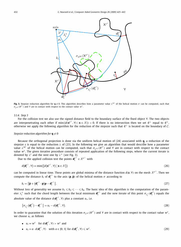
Fig. 3. Stepsize reduction algorithm for q �= 0. This algorithm describes how a parameter value λ∂C of the helical motion σ can be computed, such thatσλ∂C (Xεc

) and Y are in contact with respect to the contact value wc .

3.1.4. Step 3For the collision test we also use the signed distance field to the boundary surface of the fixed object Y. The two objects

are interpenetrating each other if min({d(xε⊥,Y) | x ∈ X }) < 0. If there is no intersection then we set E⊥ equal to E+ ,

otherwise we apply the following algorithm for the reduction of the stepsize such that E⊥ is located on the boundary of C .

Stepsize reduction algorithm for q �= 0

Because the orthogonal projection is done via the uniform helical motion of (24) associated with q, a reduction of thestepsize s is equal to the reduction λ of (23). In the following we give an algorithm that would describe how a parametervalue λ∂C of the helical motion can be computed, such that σλ∂C (Xεc

) and Y are in contact with respect to the contactvalue wc . The given iterative procedure consists of repeated application of the following steps, where the current iterate isdenoted by λc and the next one by λ+ (see Fig. 3).

Due to the applied collision test the points dε⊥i ∈ X ε⊥

with

d(dε⊥

i ,Y) = min

({d(xε⊥

,Y) ∣∣ x ∈ X

})(26)

can be computed in linear time. These points are global minima of the distance function d(z,Y) on the mesh X ε⊥. Then we

compute the distance ki of dε⊥i to the axis (p, p) of the helical motion σ according to

ki = ∥∥p + (dε⊥

i · p)p − dε⊥

i

∥∥. (27)

Without loss of generality we assume k1 � k2 � · · · � kk . The basic idea of this algorithm is the computation of the param-eter λ+

i such that the chord length between the local minimum dε⊥i and the new iterate of this point σλ+

i(dεc

i ) equals the

absolute value of the distance d(dε⊥i ,Y) plus a constant ui , i.e.∥∥σλ+

i

(dεc

i

) − dε⊥i

∥∥ = ui − d(dε⊥

i ,Y). (28)

In order to guarantee that the solution of this iteration σλ∂C (Xεc) and Y are in contact with respect to the contact value wc ,

we choose ui as follows

• ui = wc for d(dεc

i ,Y) > wc and

• ui = a · d(dεc,Y) with a ∈ ]0,1[ for d(dεc

,Y) � wc . (29)
i i


If we set λ+i = λc − μi we obtain μi by solving the following equation

p2μ2i + 2k2

i

(1 − cos(μi)

) − (ui − d

(dε⊥

i ,Y))2 = 0. (30)

Because of the validity of the trivial inequality

ui − d(dε⊥

i ,Y)� d

(dεc

i ,Y) − d

(dε⊥

i ,Y)�

∥∥dεc

i − dε⊥i

∥∥ (31)

and λc ∈ ]0,π/2[ due to (23) the last equation has a unique solution for μi within the interval ]0, λc]. If we assume ui = cfor all i = 1, . . . ,k then from (30) follows immediately μ1 � μ2 � · · · � μk . In order to reduce computational costs wesuppose to solve (30) only for i = 1 if there is more than one global minimum. It should be noted that in the border casek1 = 0 Eq. (30) can be solved explicitly for μ1 which yields

μ1 =∣∣∣∣ u1 − d

(dε⊥

1 ,Y)

p

∣∣∣∣. (32)

Now we set λ+ = λc − μ1 and run again the collision test for σλ+ (Xεc) and Y. If there is no interpenetration, then the

meshes must be in contact due to the construction of the stepsize reduction algorithm. Otherwise we iterate the procedure.

Remark. Instead of using the stepsize reduction algorithm one can also apply methods for continuous collision detectionunder screwing motions like the one proposed by Kim and Rossignac (2003). It should be noted that such methods are timeconsuming tasks, because the exact collision time (stepsize) is computed by testing all vertex/face and edge/edge collisioncases which cannot be excluded by a series of rejection tests.

In contrast to the cited method the proposed one is based on an iterative algorithm using the signed distance field ofthe fixed object. For the computation of the generalized penetration depth it is advantageous to use such a distance fieldbecause it only must be computed once. Moreover we are not interested in the exact collision time but only in a stepsizesuch that the surfaces are in contact with respect to the contact value w .

Stepsize reduction algorithm for q = 0

Due to the equation Xεs = Xεc + τ q0 where q0 denotes the normalized translation vector and τ := s‖q‖, a reduction ofthe stepsize s corresponds to a reduction of τ . We give again an iterative procedure, where the current iterate is denotedby τ c and the next one by τ+ . As in the case q �= 0 we compute the global minima dε⊥

i , . . . ,dε⊥k according to (26). Without

loss of generality we assume d(dεc

1 ,Y) � d(dεc

2 ,Y) � · · · � d(dεc

k ,Y). Now we reduce τ c by νi ∈ R+ given by

νi := ui − d(dε⊥

k ,Y)

(33)

with ui of (29). Because of ν1 � ν2 � · · · � νk we set τ+ := τ c −ν1 and run again the collision test. If there is no intersection,then the meshes must be in contact due to the applied stepsize reduction algorithm. Otherwise we iterate the procedure.

If ‖E+ −Ec‖ < b and if the current contact value wc also falls below a certain threshold v , then the PDS(X,Y) algorithmis stopped.

Remark. The presented algorithm can easily be adapted for the computation of the translational penetration depth. Weonly have to solve the system of linear equations given in (21) under the side condition that q = o. Furthermore we have toconsider that there exists no translational gliding motion if gc is greater than 2 which affects the conditions in case A andcase B of step 1.

3.2. Computational complexity

As preprocessing step we have to compute the distance field of Y. This can for example be done with the fast sweepingalgorithm of Zhao (2005) which is of complexity O (N), where N denotes the number of grid points.

The collision test is based on this distance field. There are different possibilities to compute d(x,Y) from the distancesof the neighboring grid points of x, but it can be done with a computational complexity depending linearly on the numberNx of vertices of X . If these distances are known, the computation of the minimal value dmin = min(d(x,Y)|x ∈ X ), whichalready indicates the collision, is of complexity O (Nx). Moreover the point which causes this minimal value is also used forthe stepsize reduction algorithm and so we need no further computation for this part.

It can also be seen immediately from dmin whether the non-penetrating objects are in contact with respect to the contactvalue w . If 0 � dmin � w holds we must check if there are also other contact points. Now the time complexity for computingthe local minima depends linearly on the number of points x ∈ X with d(x,Y) � w . Computing this set of points is againof complexity O (Nx).


3.3. Physical interpretation of PDS

In the following we present a physical interpretation of PDS(X,Y). Assume the pose Xϕ which cause PDS(X,Y) is known.This pose corresponds to the local minimizer F ∈ ∂C with F = (f0, f1, f2, f3). It is well known that the eigenvector of F =(f1, f2, f3) with respect to the eigenvalue 1 equals the direction of the rotation axis a (unit vector) and that the rotationangle ρ is given by 2 cosρ = trace(F) − 1. Under this considerations PDS (X,Y) can be rewritten as follows:

PDS (X,Y)2 = ‖E − I‖2

6= ‖f0‖2 + dT · TX · d

6(34)

with

dT = (±√2 f11 − 2 cosρ,±√

2 f22 − 2 cosρ,±√2 f33 − 2 cosρ

), (35)

where TX denotes the inertia tensor of the moving body X. Two of the eight possibilities of d are linearly dependent withthe direction a of the rotation axis.1 Due to the well known formula of the total kinetic energy K

K = mv2

2+ Tω2

2, (36)

where m denotes the mass of the body, v the body’s velocity, T the body’s moment of inertia and ω the body’s angularvelocity, we can interpret PDS(X,Y) as follows:

Theorem 1. PDS (X,Y) equals√

K where K is the total kinetic energy of S induced by the instantaneous screw q = (ωa, f0) with

ω = √2(1 − cosρ) = √

3 − trace(F). (37)

S denotes an ellipsoidal shell of mass 2, whose vertices are identical with the six special points si (i = 1, . . . ,6) of the moving body Xgiven in (4).

The angular velocity ω of (37) is the chord length approximation of the arc length of ρ and not ρ itself. This is due tothe used metric S of the ambient space. Therefore PDS (X,Y) equals the square root of the minimal needed kinetic energyof S such that Sid moves affinely into the pose Sϕ within one time unit. It should be noted that this ellipsoidal shell S wasalso used to define a new performance index for 6R robots (see Nawratil (2007)).

3.4. Algorithm for the computation of a collision-free starting configuration

In the following we present two methods for calculating an initial guess.

3.4.1. Method 1We replace the moving body X by the smallest ellipsoidal shell E that encloses X. E should be centered at the barycenter

bX and its axis lengths ratio should equal a1 : a2 : a3 = f1 : f2 : f3. Because E encloses X, E and Y are interpenetrating eachother. Now we want to compute the closest collision-free pose Eς to E according to the distance metric (2) where ς is asuperposition of a rotation ρi ∈ I and a translation t ∈ R

3. I denotes the icosahedral group of rotations which contains 60elements. This group serve us as a fair discretization of SO(3).

The map ς can be computed as follows: If Eρi is a collision-free configuration we are done. Otherwise we have tocompute the shortest translation vector ti which separates Eρi and Y. This can easily done as follows: We apply to Eρi andY the affine mapping αi which maps Eρi onto a sphere of radius a1. Assume Ai denotes the matrix of this linear mappingαi . Then the offset mesh O Y αi of distance a1 from Y αi is given by:

O Y αi :={

zi := Ai · yi + A−Ti · nyi

‖A−Ti · nyi ‖

a1

∣∣∣yi ∈ Y}. (38)

If Y is not convex we have to trim O Y αi which yields the trimmed offset mesh T Y αi with

T Y αi := {zi

∣∣ zi ∈ O Y αi ∧ d(zi,Yαi

)� a1

}, (39)

where the distance function d(zi,Yαi ) can, for example, be computed by the Approximate Nearest Neighbors (ANN) algo-rithm. Now we apply to T Y αi the mapping α−1

i which yields the point cloud T Y . Trivially the position vector of thatpoint of T Y which is closest to the origin is the searched translation vector ti . Now ς equals those of the 60 mappings ςiwhich causes the minimal distance S(Xid,Xςi ). Because E encloses X we can be sure that the starting configuration Xς iscollision-free.

1 Due to the symmetry of the inertia ellipsoid there exist eight possibilities for choosing d.


Remark. One must not stick to the icosahedral group but could also take a refined discretization of SO(3). Subdivisionschemes for a fair discretization of the spherical motion group are given in Nawratil and Pottmann (2008).

The limitations of this conservative method are illustrated in Fig. 6 of Section 5. Moreover it should be noted that thismethod works in all cases in contrast to the second method, presented next.

3.4.2. Method 2The key idea of this more sophisticated method for generating an initial guess is that we compute corresponding point

pairs {xi, ci} where ci is the closest point (footpoint) of Y with respect to xi ∈ X (see Fig. 4). Based on the resulting knowncorrespondence it is possible to formulate the following algorithm which tries to minimize the extent of overlap in eachiteration step:

1. We choose a chord length cl > 0.2. Compute the screw qmax which maximizes the objective function

ζ(q):N∑

i=1

w(xi)v(xi) · nci with d(xi,Y) � cl (40)

and

w(xi) = d(xi,Y) + cl

min(d(x,Y)|x ∈ X ) − cl∈ [0,1] (41)

under the side condition

ν(q):∑∥∥v(si)

∥∥2 = 1. (42)

Hence, we maximize nothing else than the weighted sum of the components of the velocity vectors v(xi) in directionof the surface normal vector nci in ci of Y . Moreover it should be noted that the weighting function w(xi) preferringpoints with a deeper penetration, depends linearly on the distance d(xi,Y). The side condition normalizes the screwaccording to the metric of the ambient space.As ν(q) is a quadratic form and ζ(q) a linear equation in the unknowns of the screw, we get qmax by solving a systemof linear equations.

Remark. In the unlucky case that xi is located on the cut locus of the fixed object, we get several footpoints c ji with

j > 1. For those points we replace v(xi) · nci of the objective function by the mean value∑

j v(xi) · nc j

i/ j.

3. Compute the helical motion σ associated with qmax and displace the object X such that max(‖σ(xi) − xi‖) = cl. Notethat max(‖σ(xi)−xi‖) = ‖σ(xmax)−xmax‖ holds where xmax is the point of X which has the biggest distance kmax fromthe helical axis or axis of rotation, respectively. Then the corresponding stepsize can be computed as in Section 3.1.4 forthe point xmax. If qmax is a translation the stepsize s can be computed from cl = s‖qmax‖.We end up with the new iterate X+ .

It should be noted that the above given stepsize selection guarantees that points xi ∈ X which have no influence on theobjective function due to d(xi,Y) > cl do not penetrate the fixed object in the next iterate. The reason for the restriction ofthe objective function to this set of points is the following:

In most practical cases, the extent of penetration is small, and therefore the set of non-penetrating points far away fromthe fixed object would affect the objective function too much despite of the natural weighting function w(xi). Thereforethe input data reduction as well as the weighting function w(xi) improves the quality of the screw qmax which can beevaluated by the function

κ(q): ζ(q)/

N∑i=1

w(xi)∥∥v(xi)

∥∥ ∈ [0,1] with d(xi,Y) � cl. (43)

A value of 1 indicates a velocity field q which exactly fits our requirements.We suggest to set the only free parameter cl equal to w −min(d(x,Y)|x ∈ X ) where w is the contact value of Definition 2

(see Fig. 4). Additionally we set cl = b if cl exceeds a predefined upper bound b. This choice ensures that the obtained initialguess and the fixed object are in contact with respect to the contract value w , if the algorithm yields a solution. In Section 5we give examples which show that this algorithm works very well for most practical cases where the extent of penetrationis small.


Fig. 4. Method 2 for the computation of a collision-free starting configuration: We compute for each point xi ∈ X with d(xi ,Y) � cl the correspondingclosest point (footpoint) ci ∈ Y . Moreover the selection of the chord length cl as w − min(d(x,Y)|x ∈ X ) is illustrated.

4. PD computation with respect to the geodesic metric of M6

In this section we want to compute the footpoint G on ∂C with respect to the geodesic metric of M6 which is definedas follows:

Definition 5. The geodesic distance G(Xα,Xβ) = ‖A − B‖G between two points A and B on M6 is defined as the length ofthe shortest (geodesic) path g ∈ M6 with respect to the metric from the ambient space (5) connecting A and B.

The following results about geodesics on M6 are known: Pottmann et al. (2004) proved that motions ct which join twogiven positions Xα resp. Xβ and arise from minimization of the functional

E1 =1∫

0

‖ct‖2 dt with c0 = Xα and c1 = Xβ (44)

correspond to geodesics g on M6, parametrized by a constant multiple of arc length. The meaning of minimizing E1 isthat the total first energy of the feature point trajectories is minimized. Moreover they proved, that the trajectory of thebarycenter under the geodesic motion is a straight line traced with constant speed. These motions are well-known inmechanics as free motions of a body (see Arnol’d (1989)).

We can define the generalized penetration depth with respect to the geodesic metric of M6 analogously to (14) as:

PDG(X,Y) = min

({‖I − E‖G√6

∣∣∣E ∈ ∂C})

. (45)

It should be noted that PDG(X,Y) is not necessarily equal to PDt if both given objects X and Y are convex, because thecounter example also holds for the geodesic metric. This can easily be verified by taking into account that the geodesicmotion between X and Xρ is the rotation about the x-axis (see Arnol’d (1989)). It follows immediately that PDG(Y,X) isgreater than PDG(X,Y) in the given example, which shows that PDG(Y,X) and PDG(X,Y) are not equal in the general case.Trivially PDG(X,Y) � PDS (X,Y) where the equality only holds if the Euclidean map ϕ which causes PDS (X,Y) is a puretranslation. In the following we want to give an algorithm for the computation of the closest point G on ∂C with respect tothe geodesic metric of Definition 5.

4.1. Preliminary considerations

It is well known that the computation of geodesics requires discretization. The unknown curve g ∈ M6 must pass throughthe only fixed point I ∈ M6 and a point EN on the boundary of C due to (45). The curve g itself is represented by a pointsequence I,E1,E2, . . . ,EN which contains the points EN and I (see Fig. 5).

We can view the point sequence E1, . . . ,EN on M6 as a point P ∈ Φ in R12N , where Φ denotes the set of all points, such

that each single Ei ’s are contained in M6. Therefore the dimension of Φ is equal to 6N . Due to the fact that the tangentspace T 6

Eiof M6 for each point Ei of P is spanned by the six vectors T1

i , . . . ,T6i of (10), the tangent space in P of Φ is

given by the 6N vectors

B j := (0, . . . ,0,T

j,0, . . . ,0

)with i = 1, . . . , N and j = 1, . . . ,6. (46)
i i


In order to simplify the computation we apply to M6 a translation δ such that δ(I) equals the origin O = (0, . . . ,0). If wedenote the translated points δ(Ei) by Ki ∈ δ(M6), the point sequence K1, . . . ,KN can be seen as a point K := Δ(P) ∈ Δ(Φ)

where Δ is a translation along the vector −I := −(I, . . . ,I). It should be noted that due to the applied translation δ thetangent spaces of Ei and Ki on M6 resp. δ(M6) are spanned by the same basis vectors and therefore they are parallel.

If we use the difference of successive points as a discrete first derivative and replace integration by summation, thefunctional E1 converts into

E1 = ‖K1‖2 +N−1∑i=1

‖Ki − Ki+1‖2. (47)

Because E1 of (47) is a quadratic function it can be written as

E1 : R12N �→ R, E1(K) = K · Q · K + 2lT · K + c, (48)

where Q is a symmetric positive definite matrix. Now we want to minimize E1 under the constraint that K lies in thesurface Δ(Φ) ∈ R

12N . The geometric approach to this minimization problem views the matrix Q as the matrix of the innerproduct 〈K,K〉 := KT · Q · K, of a Euclidean metric in R

12N . Generally E1 assumes its minimum in the point −Q−1 · l. In ourcase this point is identical with the origin O = (O, . . . ,O) because E1(O) = 0. As a consequence l = o and c = 0, thus E1 isequal to the length of the vector K; i.e.

E1(K) = KT · Q · K = ‖K‖2Q with Q =

⎛⎜⎜⎜⎜⎝

2M −M−M 2M −M

. . .. . .

. . .

−M 2M −M−M M

⎞⎟⎟⎟⎟⎠ (49)

and M of (7). O is the solution of our minimization problem because this point belongs to Δ(Φ). But we have an addi-tional constraint namely that the point KN is located on the translated boundary δ(∂C). Therefore we have to computethe closest point Δ(F) of Δ(Γ ) to O with respect to the metric defined by Q, where Γ denotes the set of all pointsP = (E1, . . . ,EN) ∈ Φ with EN ∈ ∂C . Consequently, the point F ∈ Γ is the solution of our optimization problem, which canbe computed with the following projected gradient algorithm.

4.2. Algorithm for the computation of PD with respect to the geodesic metric of M6

The given PDG(X,Y) algorithm is again based on the work done by Hofer and Pottmann (2004). When we discuss oneprocedure of the iteration, we will denote the current iterate by Pc = (Ec

1, . . . ,EcN), the next iterate by P+ = (E+

1 , . . . ,E+N )

and the prior one by P− . We assume that the initial guess is a discretized geodesic connecting I and the footpoint F,computed with the PDS (X,Y) algorithm of the last section. The computation of this initial guess can be done with thealgorithm given in the above cited paper.

1. If EcN ∈ ∂C we compute the gc linearly independent gliding constraints according to (11). Otherwise gc = 0. Then

we compute the tangent space T6N−gc

Pc of Φ at the current iterate Pc and project the point O orthogonally into the

translated tangent space T6N−gc

Kc of Δ(Φ) at the point Δ(Pc) = Kc , which results in O⊥ .

Fig. 5. PDG (X,Y) algorithm.


2. Compute an appropriate stepsize s and project EsN of Ps := Pc + s(O⊥ − Kc) onto M6, which yields the point E⊥

N .3. If E⊥

N corresponds to a colliding configuration we reduce s until both surfaces are in contact. Then we project the pointsEs

1, . . . ,EsN−1 onto M6 which yields our new iterate P+ .

4.2.1. Step 1First of all we want to give an elementary view of this step: We displace each point Ec

i of the polygon Pc in the tangentspace Ti of M6, such that the generated polygon Es

1 = Ec1 + T1, . . . ,E

sN = Ec

N + TN with Ti of (8) minimizes the objective

function E1 under the gc constraints that XεcN glides instantaneously on Y (see Fig. 5).

We compute the gc gliding constrains according to (11) with respect to the contact value wc := w− . We redefine wc inthe same two cases as in the PDS(X,Y) algorithm, where we replace ‖Ec − E−‖ by ‖Ec

N − E−N ‖. Further we compute the

matrix Q of (48) and the basis vectors {B11, . . . ,B6

1, . . . ,B1N , . . . ,B6

N } of Φ ’s tangent space at the current iterate Pc , which aregiven by (46). Because these vectors also span the tangent space of Δ(Φ) at the point Kc , we can compute the Gramianmatrix GKc := (〈Bi

j,Blk〉Q). Then O⊥ equals Kc + T with

T :=N∑

i=1

3∑j=1

q ji B j

i + q ji B j+3

i , (50)

where Q := (q1, q1, . . . ,qN , qN )T is the solution of the following systems of linear equations:

(GK c

N

)· Q =

(ro

)with N :=

⎛⎜⎜⎝

0 . . . 0 nT1 nT

1

0 . . . 0...

.

.

.

0 . . . 0 nTgc nT

gc

⎞⎟⎟⎠ , (51)

where r := (r11, . . . , r6

1, . . . , r1N , . . . , r6

N )T is given by r ji := (〈Kc,B j

i 〉Q).

4.2.2. Step 2The stepsize s for the computation of Ps := Pc + s(O⊥ − Kc) = Pc + sT is chosen as in the PDS (X,Y) algorithm. In the

general case we take a small stepsize s, whose validity is tested with the Armijo rule. Only if gc equals g− we apply thestepsize selection of Pottmann and Hofer (2004) (see also Hofer and Pottmann (2004)).

If gc = g− = 0 the part of the footpoint cone ΛΦ is determined by the vertex I, the footpoints Pc ∈ Φ and P− ∈ Φ

and the direction T of the tangent of the base curve in Pc . If gc = g− �= 0 we can think again of a (6N − g)-dimensionalmanifold Ψ ∈ Φ which locally approximate Γ such that T 6N−g

Pc and T 6N−gP− are the tangent spaces in Pc ∈ Ψ resp. P− ∈ Ψ

with respect to Ψ . Now the stepsize selection can be done by developing the footpoint cone ΛΨ into the plane. The validityof the resulting stepsize must again be tested with the Armijo rule.

In the next step we project EsN orthogonally onto M6. This is done as in the PDS (X,Y) algorithm by using the helical

motion σ determined by the instantaneous screw sqN = (sqN , sqN ).

4.2.3. Step 3If Xε⊥

N and Y are colliding then we reduce the stepsize s with the stepsize reduction algorithm, which yields E+N . In

the next step we project the remaining points Es1, . . . ,E

sN−1 orthogonally onto M6 by solving the registration problem with

known correspondences. This is a known algebraic problem of degree four, which was explicitly solved by Horn (1987) usingunit quaternions. For further details see e.g. Belta and Kumar (2002). We denote the resulting points by E⊥

1 , . . . ,E⊥N−1.

We can improve our iterate by taking into account that the trajectory of the barycenter under a geodesic motion hasto be a straight line. In the general case the barycenters ε⊥

1 (bX), . . . , ε⊥N−1(bX) are not located on the line spanned by bX

and ε+N (bX) due to the two different kinds of used back projections onto M6. Therefore we translate each point E⊥

i fori = 1, . . . , N − 1 within the surface M6 by Hi := (hi,o,o,o) such that the approximated first energy

E1 = ∥∥I − E⊥1 − H1

∥∥2 +N−2∑i=1

∥∥E⊥i + Hi − E⊥

i+1 − Hi+1∥∥2 + ∥∥E⊥

N−1 + HN−1 − E+N

∥∥2

is minimized. This quadratic function in 3(N − 1) unknowns can be rewritten as

E1(H) = HT · W · H + kT · H + c, (52)

with H := (h1, . . . ,hN−1). Because W is a symmetric positive definite matrix the unique global minimizer equals −W−1 · k.By setting E

+i := E⊥

i + Hi for i = 1, . . . , N − 1 we get the new iterate P+ := (E+1 , . . . ,E+

N ).If ‖E+

N −EcN‖ < b and if the current contact value wc also falls below a certain threshold v , then the PDG(X,Y) algorithm

is stopped.


4.3. Physical interpretation of PDG

The pose Xγ which cause PDG(X,Y) corresponds to the local minimizer G = (g0,g1,g2,g3) ∈ ∂C . Due to considerationsof Section 3.3 and the well known result (see Arnol’d (1989)), that geodesic motions are motions of a free rigid bodyunder its own inertia outside of any force field (⇒ kinetic energy is conserved), we can give the following interpretation ofPDG(X,Y):

Theorem 2. PDG(X,Y) equals√

K where K is the minimal needed total kinetic energy of S such that the rigid body Sid moves underits own inertia into the pose Sγ within one time unit. S denotes the ellipsoidal shell of Theorem 1.

Remark. Assume that G = (g1,g2,g3) describes a rotation about one of the axis of the inertia ellipsoid of S through theangle ρ . Now the superposition of this uniform rotation and the uniform translation g0 is a geodesic motion. In such casesthe only difference between PDS(X,Y) and PDG(X,Y) is that the angular velocity ω of (37) (chord length approximation ofρ) is replaced by the arc length of ρ .

5. Examples

The numerical experiments have been performed with Matlab implementations on a AMD 64 Athlon Processor with 1GB RAM. The main focus in implementing our algorithms was on the demonstration of the functionality and not on theimprovement of the computation time. We are aware of the fact that our prototype implementations are not optimized andthat there is a very large potential for speedup, especially in performing the collision test. Moreover some routines can beimproved by additional preprocessing steps.

Xid denotes the given interpenetrating configuration and Xςi the collision-free initial guess, which was computed by

method i (i = 1,2) of Section 3.4. As the result of the PDS (X,Y) algorithm we obtain the pose Xϕ which corresponds to thelocal minimizer F ∈ ∂C . With the adapted version of this algorithm, we computed the pose Xτ which causes PDt . As theresult of the PDG(X,Y) algorithm we obtain the pose Xγ which corresponds to the local minimizer G ∈ ∂C .

Here for simplicity and comparability of the results the PDG(X,Y) algorithm was always performed with 10 intermediatepositions. Clearly, an increase of these positions improves the accuracy at the cost of computation time. As the computationof the geodesic distance on M6 can be decomposed into a translational and a rotational part (see Hofer and Pottmann(2004)) a more sophisticated choice of the number of intermediate positions should be based on the spherical distance ofXid and Xϕ .

The cup examples

This example can also be found in the paper of Zhang et al. (2006), where the boundary surfaces of the fixed object (cup)Y and the moving body (spoon) X were approximated by triangular meshes Y resp. X with about 4200 resp. 170 vertices.

Fig. 6. Cup: Ex. 1.

Table 1

Distance Initial guess Calls Total time (tt) Collision test Fig.

PDt 1 Xς1 43 4.1719 sec 87% of tt 6(a)

PDS 0.8277 Xς1 43 4.4375 sec 96% of tt 6(a)

PDG 0.8301 Xς1 60 5.8430 sec 90% of tt 6(a)

PDS 0.6339 Xς 53 5.2031 sec 81% of tt 6(b)PDG 0.6359 Xς 57 6.0781 sec 79% of tt 6(b)


Fig. 7. Cup: Ex. 2.

Fig. 8. Cup: Ex. 3.

Table 2


PDS 0.8070 · PDt Xς1 55 5.1250 sec 88% of tt 7

PDG 0.8071 · PDt Xς1 63 6.4219 sec 85% of tt 7

PDS 0.8276 · PDt Xς1 38 5.0313 sec 88% of tt 8

PDG 0.8285 · PDt Xς1 46 6.1250 sec 79% of tt 8

We increased the number of vertices of the triangular meshes Y resp. X to 12 500 resp. 1500 in order to improve therepresentation of the objects and therefore the accuracy of our results. Computing the collision-free starting configurationX

ς1 lasts about 2.1 sec, where performing 60 times the ANN-algorithm requires about 87% of the total cputime.

Example 1. The starting configuration Xς1 as well as the solutions Xϕ and Xτ of the PDS (X,Y) algorithm resp. of the

adapted one are displayed in Fig. 6(a). We also tested our PDG(X,Y) algorithm for the same starting configuration Xς1

but its solution Xγ is too close to Xϕ that one can see a difference. These two minimization problems seem to have thesame local minimizer. The performance of these three algorithms is shown in Table 1.

The obtained solutions are only local minima because running the PDS(X,Y) algorithm resp. PDG(X,Y) algorithm start-ing with the pose Xς illustrated in Fig. 6(b) yields another solution Xϕ resp. Xγ , which is closer to Xid as Xϕ resp. Xγ

(see Table 1). The starting configuration Xς could not be obtained by method 1 of Section 3.4 because the ellipsoid E,which encloses X is to big for the hole of the handle. This example points out the limitations of the presented algorithm.The PDG(X,Y) algorithm with respect to the starting configuration Xς has again a nearly identical solution to Xϕ . Theperformance of the PDG(X,Y) resp. PDS(X,Y) algorithm with respect to Xς is also shown in Table 1.

Examples 2 and 3. In Examples 2 and 3 illustrated in Fig. 7 and Fig. 8, respectively, we run the PDS (X,Y) algorithm andthe PDG(X,Y) algorithm with respect to the starting configuration X

ς1 . As in example 1 the obtained poses Xϕ and Xγ are

too close to see a difference. The performance of the algorithms is shown in Table 2, where the values for PDS (X,Y) andPDG(X,Y) are given with respect to PDt . The pose Xτ which causes PDt is illustrated in Fig. 7(b) and Fig. 8(b), respectively.


Fig. 9. The gap example.

Table 3


PDS 1 Xς1 58 17.9375 sec 80% of tt 10(a)

PDS 1.5396 Xς1 71 16.6406 sec 79% of tt 10(b)

PDS 1.1079 Xς1 79 21.5313 sec 84% of tt 11(a)

PDS 1.6650 Xς1 49 12.4219 sec 72% of tt 11(b)

Table 4

Calls Total time (tt) Collision test S(Xϕ,Xς2 ) Fig.

Xς2 10 1.5156 sec 63% of tt 0.10 · S(Xϕ,X

ς1 ) 10(a)

Xς2 12 1.6094 sec 63% of tt 0.39 · S(Xϕ,X

ς1 ) 10(b)

Xς2 9 1.6093 sec 67% of tt 0.07 · S(Xϕ,X

ς1 ) 11(a)

Xς2 13 1.7813 sec 59% of tt 0.58 · S(Xϕ,X

ς1 ) 11(b)

The gap example

We constructed this example in order to illustrate the slight difference between the poses Xϕ and Xγ . The fixed object Yconsists of two disjoint half-spaces and the moving object X looks like the character ‘X’. Due to the fact that the boundarysurface ∂Y of Y are two planes we can be sure that our algorithms do not only reach local minima but global ones. Moreoverit should be said that the Euclidean maps ϕ and γ are pure rotations. The angle enclosed by these two spherical motions isonly about 0.64◦ . The corresponding poses Xϕ and Xγ as well as ∂Y and the 10 intermediate positions for the computationof PDG(X,Y) are displayed in Fig. 9.

The cross examples

The triangular meshes Y and X of the half torus and cross, respectively, consists of 7000 and 11 000 vertices. Thecomputation of the collision-free initial guess X

ς1 lasts about 5.1 sec, where performing 60 times the ANN-algorithm requires

about 94% of the total cputime. In the following four examples we tested the PDS(X,Y) algorithm (see Table 3) startingwith X

ς1 .

Moreover we tested the second method of Section 3.4 for computing an initial guess. We run the corresponding Xς2

algorithm for b = −min(d(x,Y)|x ∈ X id)/5. The performance of this algorithm is shown in Table 4 and Fig. 12, respectively.The given examples demonstrate that the proposed algorithm works very well for examples, where the extent of overlap issmall.

If we run the PDG(X,Y) algorithm with the initial guess Xϕ we cannot achieve a significant improvement of the geodesicdistance because the algorithm stops after a few iteration steps. The resulting local minimum is again too close to Xϕ that


Fig. 10. Cross: (a) Ex. 1 (b) Ex. 2. Illustration of Xid (red), Xς1 (green), X

ς2 (yellow) and Xϕ (blue). (For interpretation of the references to colour in these

figures, the reader is referred to the web version of this article.)

Fig. 11. Cross: (a) Ex. 3 (b) Ex. 4. Illustration of Xid (red), Xς1 (green), X

ς2 (yellow) and Xϕ (blue). (For interpretation of the references to colour in these

figures, the reader is referred to the web version of this article.)

Fig. 12. Performance of the Xς2 algorithm: (a) The extent of overlap measured by −min(d(x,Y)|x ∈ X ) for each iteration step. (b) Evaluation of the screw

qmax by the function κ(q) of (43).

a graphical representation would make sense. It seems that in the general case these minima Xϕ and Xγ are much closerto each other than in the synthetically generated example illustrated in Fig. 9.

6. Conclusion and future work

In this paper we defined the generalized penetration depth PD of two colliding rigid bodies X and Y with respect to theobject-oriented metric S introduced by Hofer et al. (2004) which takes the mass distribution of the moving body X intoconsideration. We used a kinematic mapping which maps rigid body displacements to points of a 6-dimensional manifold


M6 in the 12-dimensional space of affine mappings. This space equipped with the above mentioned metric is a Euclideanspace. We formulated PD as the solution of the constrained minimization problem of finding the closest footpoint on theboundary of the set of all points of M6 which correspond to colliding configurations. Based on the theory of gliding motions,the closest footpoint with respect to the metric S (⇒ PDS ) can be computed with an adapted projected gradient algorithm.The outlined PDS algorithm can easily be modified for the computation of the translational penetration depth as well. Wealso presented a geometric optimization algorithm which computes the closest footpoint with respect to the geodesic metricG of M6 induced by the metric of the ambient space (⇒ PDG ). Moreover we introduced two algorithms for the computationof a collision-free initial guess and gave a physical interpretation of PDS and PDG . We also tested the functionality of thepresented geometric optimization algorithms based on prototype implementations and gave several examples.

A drawback of our approach is that our algorithms can only compute local minima, and thus they depend on the choiceof the initial guess. Therefore we are working on a global approach by calculating a distance field on M6 based on a fairdiscretization of SO(3). Subdivision schemes for generating such fair discretizations of the spherical motion group werealready presented (see Nawratil and Pottmann (2008)).

Acknowledgements

This research was carried out as part of the project S9206-N12 which was supported by the Austrian Science Fund (FWF).The authors would like to thank Michael Hofer for providing us some of his Matlab implementations, as well as LiangjunZhang for placing the dataset of the cup and spoon example at our disposal.

The authors would also like to thank the reviewers for their useful comments and suggestions.

References

Arnol’d, V.I., 1989. Mathematical Methods of Classical Mechanics, 2nd ed. Springer, New York.Belta, C., Kumar, V., 2002. An SVD-projection method for interpolation on SE(3). IEEE Trans. Robotics Automation 18 (3), 334–345.Botsch, M., Pauly, M., Gross, M., Kobbelt, L., 2006. PriMo: Coupled prisms for intuitive surface modeling. In: Polthier, K., Sheffer, A. (Eds.), Eurographics

Symposium on Geometry Processing, pp. 11–20.Cameron, S., 1997. Enhancing GJK: Computing minimum and penetration distance between convex polyhedra. In: Proc. of IEEE International Conference on

Robotics and Automation, pp. 3112–3117.Hofer, M., 2004. Variational motion design in the presence of obstacles. Ph.D. Dissertation, Vienna University of Technology.Hofer, M., Pottmann, H., 2004. Energy-minimizing splines in manifolds. In: Proceedings of ACM SIGGRAPH 2004. Trans. Graph. 23 (3), 284–293.Hofer, M., Pottmann, H., Ravani, B., 2004. From curve design algorithms to the design of rigid body motions. Visual Comput. 20 (5), 279–297.Horn, B.K.P., 1987. Closed form solution of absolute orientation using unit quaternions. J. Optical Soc. A 4, 629–642.Kim, B., Rossignac, J., 2003. Collision Prediction for Polyhedra under Screw Motions. In: Proc. of ACM Symposium on Solid Modeling and Applications, pp.

4–10.Kim, Y., Lin, M., Manocha, D., 2002. Deep: Dual-space expansion for estimating penetration depth between convex polytopes. In: Proc. of IEEE International

Conference on Robotics and Automation, pp. 921–926.Nawratil, G., 2007. New performance indices for 6R robots. Mech. Mach. Theory 42 (11), 1499–1511.Nawratil, G., Pottmann, H., 2008. Subdivision schemes for the fair discretization of the spherical motion group. J. Comp. Appl. Math. 222 (2), 574–591.Pottmann, H., Hofer, M., 2004. Algorithms for constrained minimization of quadratic functions – geometry and convergence analysis. Technical Report 121,

Geometry Preprint Series, Vienna Univ. of Technology.Pottmann, H., Hofer, M., Ravani, B., 2004. Variational motion design. In: Lenarcic, J., Galletti, C. (Eds.), On Advances in Robot Kinematics, pp. 361–370.Pottmann, H., Ravani, B., 2000. Singularities of motions constrained by contacting surfaces. Mech. Mach. Theory 35 (7), 963–984.Pottmann, H., Wallner, J., 2001. Computational Line Geometry. Springer-Verlag.Van den Bergen, G., 2001. Proximity queries and penetration depth computation on 3D game objects. In: Proc. Game Developers Conference, pp. 821–837.Zhang, L., Kim, Y.J., Varadhan, G., Manocha, D., 2006. Generalized penetration depth computation. In: Symposium on Solid and Physical Modeling, pp.

173–184.Zhang, L., Kim, Y.J., Manocha, D., 2007. A fast and practical algorithm for generalized penetration depth computation. In: Proc. of Robotics: Science and

Systems Conference (RSS07), 2007.Zhao, H.K., 2005. Fast sweeping method for eikonal equations. Math. Comp. 74, 603–627.

Generalized penetration depth computation based on kinematical geometry

Documents

Transcript of Generalized penetration depth computation based on kinematical geometry