SCALE MODEL PENETRATION EXPERIMENTS - DTIC

SCALE MODEL PENETRATION EXPERIMENTS: FINITE-THICKNESS STEEL TARGETS

Prepared by

Scott A. Mullin v

Charles E. Anderson, Jr. Andrew J. Piekutowski

Kevin L. Poormoh Neil W. Blaylock Bruce L. Morris

SwRI Report 3593/003

Prepared Under Contract DE-AC04-90Ä158770

DAAL3-91-C-0021

Prepared for

U.S. Army Research Office Advanced Research Projects Agency

CM

May 1995

SOUTHWEST RESEARCH INSTITUTE SAN ANTONIO DETROIT

HOUSTON WASHINGTON, DC

REPORT DOCUMENTATION PAGE Form Approved OMB No. 0704-0188

Public reporting burden for this collection of Wormatlon Is estimated to average i hour per response, Including me tune lor reviewing instructions, searching existing data sources, garnering ana maintaining the data needed, and completing and reviewing the collection of information. Send comments regarding this burden estimate or any other aspect of this collection of Information, including suggestions for reducing this burden, to Washington Headquarters Services, Directorate for Information Operations and Reports, 1215 Jefferson Davis Highway, Suite 1204, Arlington, VA 22202-4302, and to the Office of Management and Budget, Paperwork Reduction Project (0704-0188), Washington, DC 20503.

1. AGENCY USE ONLY (Leave blank) 2. REPORT DATE May 1995

3. REPORT TYPE AND DATES COVERED Technical Report

4. TITLE AND SUBTITLE Scale Model Penetration Experiments: Finite-Thickness Steel Targets

6. AUTHOR(S)

Scott A. Mullin, Charles E. Anderson, Jr., Andrew J. Piekutowski, Kevin L. Poormon, Neil W. Blaylock, Bruce L. Morris

&fiftL6$~V-C'O0ll

7. PERFORMING ORGANIZATION NAME(S) AND ADDRESS(ES)

Southwest Research Institute Materials and Structures Division 6220 Culebra Road P.O. Drawer 28510 San Antonio, TX 78228-0510

9. SPONSORING / MONITORING AGENCY NAME(S) AND ADDRESS(ES)

U.S. Army Research Office P.O. Box 12211 Research Triangle Park, NC 27709-2211

5. FUNDING NUMBERS

8. PERFORMING ORGANIZATION REPORT NUMBER

SwRI 3593/003

10. SPONSORING /MONrrORING AGENCY REPORT NUMBER

f\U «394V7.-S-AI5

11. SUPPLEMENTARY NOTES

The view, opinions and/or findings contained in this report are those of the author(s) and should not be construed as an official Department of the Army position, policy, or decision, unless so designated by other documentation.

12a. DISTRIBUTION / AVAILABILITY STATEMENT

Approved for public release; distribution unlimited.

12b. DISTRIBUTION CODE

13. ABSTRACT (Maximum 200 words)

A kinetic energy penetration scaling study has been performed with L/D 20 projectiles into homogeneous RHA-like targets at two impact velocities: 1.5 km/sand 2.2 km/s. The experiments were performed at three scales: nominally 1/3,1/6, and 1/12. The report documents the similituide analysis, discusses issues in scaling using replica models, and the experiments. The report concludes with a discussion of a possible cause of the observed distortions in perfect scaling.

DTIG ©UALT?7 INSPECTED 3

14. SUBJECT TERMS

penetration mechanics, scale modeling, scale model, ballistic performance, scaling, damage, pi terms

17. SECURITY CLASSIFICATION OF REPORT

UNCLASSIFIED

18. SECURITY CLASSIFICATION OF THIS PAGE

UNCLASSIFIED

19. SECURITY CLASSIFICATION OFABSTRACT

UNCLASSIFIED

15. NUMBER OF PAGES

64 16. PRICE CODE

20. LIMITATION OF ABSTRACT

UL

NSN 7540-01-280-5500 Standard Form 298 (Rev. 2-89) Prescribed by ANSI Std. 239-18 298-102

IAT Form 13a 3/93

Table of Contents

Page

List of Figures iii

List of Tables v

Notation vii

1.0 INTRODUCTION 1

2.0 SIMILITUDE ANALYSIS 3

2.1 Model Parameters 3

2.2 Pi Terms 9

2.3 Similarity and Geometric Scale Factor 10

3.0 SCALING ISSUES IN THE USE OF REPLICA MODELS 13

4.0 SELECTION OF SCALE SIZES 17

4.1 Introduction 17

4.2 The Prototype Projectile 17

4.3 Scale Model Projectiles 17

4.4 Final Selection of Scale Sizes 18

5.0 FINITE-THICKNESS TARGET TEST MATRTX 23

5.1 Target Size and Test Matrix Overview 23

5.2 Statistical Test Plan 27

6.0 EXPERIMENTAL DATA 31

7.0 DATA ANALYSIS 37

7.1 Measurement Uncertainty 37

7.2 Penetration Depth 37

7.3 Projectile Residual Length and Velocity 38 —/-

7.4 Hole Diameter, Crater Height, and Bulge Height 38 ^

By Distribution/^^,

Availability Cbd^s

Table of Contents (Cont'd)

Page

8.0 ANALYSIS OF SCALING EFFECTS 41

8.1 Analysis Procedure 41

8.2 Normalized Crater Diameter 44

8.3 Normalized Front Face Crater Height 47

8.4 Normalized Bulge Height 54

8.5 Normalized Penetration Depth 54

8.6 Normalized Residual Projectile Length and Velocity 54

9.0 DISCUSSION AND CONCLUSIONS 57

10.0 ACKNOWLEDGMENTS 61

11.0 REFERENCES 63

-n-

List of Figures

Page

Figure 1. Economy of Testing versus Scale Size 2

Figure 2. Schematic for Model Analysis 3

Figure 3. Impact Model Parameters: Projectile 5

Figure 4. Impact Model Parameters: Target 7

Figure 5. Impact Model Parameters: Responses 8

Figure 6. Buckingham Pi Theorem 11

Figure 7. Replica Model Law Issue: Strain Rate Effects 14 (a) Armor Steel (b) Tungsten Alloy

Figure 8. (a) Schematic and Dimensions for Scale Model Projectile Design 19 (b) Photo of the Projectiles in Their Sabots 20 (c) Photo of Sabot Section, Showing Projectiles and Threading 20

Figure 9. Residual Rod Velocity V/V0 Versus Effective Plate Thickness T/(LcosQ), Ref. [9] 24

Figure 10. Photographs of the 1/3.15,1/6.30, and 1/12.60-Scale Projectiles and Targets (a) Comparison of the Three Scale Sizes, 0°-Obliquiry Test 25 (b) Comparison of the Three Scale Sizes, 60°-Obliquity Test 25 (c) Comparison of the Three Target Thickness Categories (NUT, IB, WB)

for a 1/6.30-Scale, 0°-Obliquity Test 26 (d) Comparison of the Three Target Thickness Categories (NUT, IB, WB)

for a 1/6.30-Scale, 60°-Obliquity Test 26

Figure 11. Test Layout for the Experiments (a) 0° Obliquity (b) 60° Obliquity 34

Figure 12. Schematic of Post-Test Target Measurements (a) 0° Obliquity (b) 60° Obliquity 35

Figure 13. Examples of Target Damage (a) 0° Obliquity (b) 60° Obliquity 36

Figure 14. Example of Residual Projectile X-ray Image After Target Perforation 39 (a) Test 4-1458: 1/6.30-Scale Test: V= 1.51 km/s, Vr= 1.07 km/s,

Lr/L = 0.24 (b) Test 4-1389: 1/12.60-Scale Test: V= 2.21 km/s, Vr = 1.99 km/s,

Lr/L = 0.20

Figure 15. Example of Analysis Procedure 42 (a) Curve Fit to Composite Data (b) Curve Fits to Each Scale Size

-in-

List of Figures (Cont'd)

Page

Figure 16. Nondimensional Minimum Hole Diameter as a Function of Impact Velocity 45 (a) 0° Obliquity (b) 60° Obliquity

Figure 17. Nondimensional Minimum Hole Diameter as a Function of Total Yaw 46 (a) 1.5 km/s, 0° Obliquity (b) 22. km/s, 0° Obliquity (c) 1.5 km/s, 60° Obliquity (d) 2.2 km/s, 60° Obliquity

Figure 18. Nondimensional Maximum Hole Diameter as a Function of Impact Velocity 48 (a) 0° Obliquity (b) 60° Obliquity

Figure 19. Nondimensional Maximum Hole Diameter as a Function of Total Yaw 49 (a) 1.5 km/s, 0° Obliquity (b) 2.2 km/s, 0° Obliquity (c) 1.5 km/s, 60° Obliquity (d) 2.2 km/s, 60° Obliquity

Figure 20. Normalized Minimum Hole Diameter 50

Figure 21. Normalized Maximum Hole Diameter 50 (a) 0° Obliquity (b) 60° Obliquity

Figure 22. Nondimensional Crater Height as a Function of Impact Velocity 51

Figure 23. Nondimensional Crater Height as a Function of Total Yaw 52 (a) 1.5 km/s, 0° Obliquity (b) 2.2 km/s, 0° Obliquity (c) 1.5 km/s, 60° ObUquity (d) 2.2 km/s, 60° Obliquity

Figure 24. Normalized Crater Height 53

-IV-

List of Tables

Page

Table 1. Projectile Parameters 5

Table 2a. Target Parameters for a Semi-Infinite Target 6

Table 2b. Target Parameters for a Finite-Thickness Target 6

Table 3a. Response Parameters for a Semi-Infinite Target 7

Table 3b. Response Parameters for a Finite-Thickness Target 8

Table 4a. Pi Terms for a Semi-Infinite Target 9

Table 4b. Pi Terms for a Finite-Thickness Target 10

Table 5. Replica Model Law Based on Pi Terms of Table 4 12

Table 6. Masses and Dimensions of Geometrically-Scaled Projectiles (JJD = 20) 18

Table 7. Rod Masses 21

Table 8. Finite Thickness Target Test Matrix 23

Table 9. A 2232 Mixed Factorial Experimental Plan 27

Table 10. A 1/2-Fraction of a 2232 Mixed Factorial Experimental Plan 28

Table 11. Experiment Combinations Tested Twice 29

Table 12. Complete Test Sequence For Finite Thickness Targets 29

Table 13. Scale Modeling Experimental Data: 0°-Obliquity Tests 32

Table 14. Scale Modeling Experimental Data: 60°-Obliquity Tests 33

Table 15. Uncertainty Values for the Ballistic Response Measurements 37

Table 16. Comparison of Nondimensional Response Values 43

NOTATION

B height of back surface bulge c specific heat C height of front surface crater lip D projectile diameter H hole diameter in target

"■max maximum entrance hole diameter ■fl minimum entrance hole diameter k thermal conductivity K damage parameter Kt target fracture toughness L projectile length Lr projectile residual length Mr projectile residual mass N rate of void growth

N0 material constant

P penetration depth

Ps tensile stress in solid

°«Ä0 threshold stress for nucleating voids

Pthl threshold stress for void growth

Pt material constant t time T target thickness u projectile tail velocity V impact velocity vr projectile residual velocity vs projectile striking (impact) velocity K void volume v void volume at beginning of a time step a thermal diffusivity (a = k/pc)

AV„ change in void volume due to void nucleation

AcF uncertainty in analysis methodology

An measurement uncertainty

Ar total uncertainty

8 effective plastic strain

£ strain rate

n material viscosity

Y impact inclination (yaw)

X scale size

p density

C flow stress

-Vll-

c0 threshold stress

T time 9 target inclination 0 temperature £ material constant for spallation subscripts p projectile t target

-vin-

1.0 INTRODUCTION

A kinetic energy penetration scaling study has been performed with monolithic penetrators and homogeneous metallic targets at two impact velocities: 1.5 km/s and 2.2 km/s. The first is representative of current large caliber weapon systems and the second might be representative of a future weapon system. This study was performed to evaluate the ability of subscale experiments to replicate larger scale target-penetrator response.

The primary reason for performing model experiments is financial. Scaled experiments generally can be performed at a fraction of the cost of a full-scale experiment. Additionally, the turn around time between successive tests is generally less for subscale tests (which also affects labor costs since more tests can be performed in a fixed time period). Figure 1 represents a schematic of the costs to perform a typical armor test. Of course, these estimates depend on target arrangement and instrumentation requirements for each test. Nevertheless, the solid curve depicts a reasonable estimate for the labor costs associated with the conduct of one test. The costs are estimated from industrial, fully-loaded (salary, fringe, and overhead) labor rates in 1990 dollars. The primary difference in costs as size increases is the time for set-up for each test; also, for full scale tests, more manpower support may be required.

Material rates are normalized to 1.0 for the 1/4-scale test, and two "growth" curves are indicated: 1) the costs are directly proportional to the geometric dimensions of the target, and 2) the costs increase by the square of the material size, as might be appropriate for some advanced materials. Note that the material costs are on a logarithmic scale, i.e., material costs can quickly dominate the expense of performing an experiment. Figure 1 demonstrates the economy of testing at small scale.

Most scaling studies have shown good correlation, but some studies have indicated a response at small scale that is contrary to results at full scale. Certainly a major concern is that an extremely effective armor designed and tested at small scale might be ineffective at full scale; folklore exists, but is not often documented, concerning such studies. Thus, there exists a high level of skepticism in the technical and user community concerning the validity of scale model experiments, to the point of the insistence of full-scale verification tests for modern targets. This results in high development costs.

A variety of reasons may exist for the lack of correlation between subscale and full scale tests. These reasons could include improper scale modeling analysis, lack of understanding or neglect of important parameters, failure to properly construct the models, failure to test under the proper ("scaled") conditions, lack of attention to material selection, differences in failure modes, and changes in a physical mechanism with scale size. One or more of these items, acting alone or in concert, could result in dissimilar responses between the model and prototype.

10000

1000

- 100

10

CO o Ü

a S

I 1 o C

J1 1/4 1/2 3/4

Scale Size

Figure 1. Economy of Testing versus Scale Size

The objective of this project was to investigate and determine the validity of using scale-model experiments to quantify long-rod projectile effectiveness against metallic1 targets at impact velocities ranging from 1.5 to 2.2 km/s. Limitations and restrictions in scaling were critically examined. A series of experiments were conducted at several different scale sizes, and the experimental data were examined to separate experimental repeatability (i.e., inherent experimental scatter) and statistically significant differences in the responses of interest.

The data permit a quantitative assessment of ballistic responses as a function of scale size. Some statistically significant differences in various measures of penetration performance were observed between scale sizes; the physical reasons for the "breakdown" of the scaling laws are postulated. These are discussed in some detail in Section 9.0.

1 An investigation of the scaling of penetration into ceramic targets, similar to the work presented herein, is the subject of Ref. [1].

-2-

2.0 SIMILITUDE ANALYSIS

In the paragraphs below, a similitude analysis is presented that is applicable to semi-infinite and finite-thickness metallic armor penetration by long-rod projectiles. Parameters are included to account for projectile and target geometries, material densities, constitutive properties, thermal effects, and impact velocity. Bulk melting is assumed to be insignificant because analysis indicates that no large scale melting takes place when a tungsten projectile impacts a steel target at velocities up to 3 km/s; however, thermal softening—the result of plastic work—is important.

Response terms are included in the model analysis. These responses include penetration depths, residual penetrator characteristics after perforation of the armor, and hole sizes or other damage descriptors for the target plates. Additionally, terms that aid in the analysis of the modeling results, such as the scaled time, are included.

2.1 Model Parameters

The analysis begins with the selection of the important specific terms for each problem. Figure 2 serves to depict an idealized impact condition. A single finite-thickness target is shown in Fig. 2; for cases of a semi-infinite target, the thickness of the plate will be substantially greater. The initial impact conditions are the impact velocity and obliquity. After perforation of the target plate, the remnant projectile has some residual mass and velocity. On the other hand, if the armor is sufficiently thick, the target is not perforated, and a measure of ballistic performance is the depth of penetration.

L J

Figure 2. Schematic for Model Analysis

-3-

Table 1 lists the projectile parameters. Typical units are shown for each parameter, along with the fundamental units of mass (M), length (L), temperature (©), and time (x). Some of these parameters are also shown on Fig. 3, which depicts the geometry. The projectile is considered to be a uniform material, constant diameter long rod with a hemispherical nose. The geometrical terms necessary to describe it are the diameter and the length. The density and impact velocity describe the inertial properties. The constitutive behavior is characterized by the strength and the failure strain of the projectile material. These terms will be described in more detail when the Pi terms are formed. The thermal diffusivity is the ratio of the thermal conductivity to the heat capacity per unit volume, and thus characterizes the heat flow and heat retention of a material. The subscript "p" in Table 1 refers to the projectile.

Tables 2a and 2b list the parameters for each of the target types considered here: semi-infinite and finite-thickness. Figure 4 depicts a finite-thickness target, showing the geometrical parameters. For a semi-infinite target, geometric descriptions of the target are not required ("semi-infinite" implies that the target is sufficiently thick so that the penetration event is not influenced by the presence of free surfaces); the plate thickness is required for a finite-thickness target. It should be noted that the target plates are assumed to be flat, of uniform thickness throughout, and homogeneous. The constitutive parameters for the target plates are the same as for the projectile, with the exception of the addition of the fracture toughness for the finite-thickness targets. The fracture toughness was included as a descriptor that might account for failure characteristics of the rear of the target during perforation. The subscript "t" in the tables refers to the target.

-4-

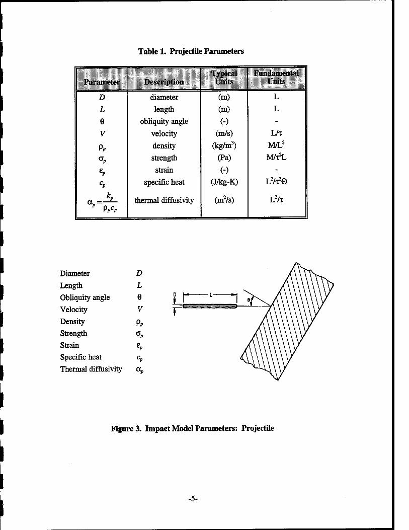
Table 1. Projectile Parameters

Parameter Description Typical Units

Fundamental Units

D diameter (m) L

L length (m) L

e obliquity angle (-) -

V velocity (m/s) L/T

yp density (kg/m3) M/L3

°P strength (Pa) M/^L

% strain (-) -

CP specific heat (J/kg-K) LWe

Yp^p

thermal difrusivity (m2/s) L2/T

Diameter D

Length L Obliquity angle e Velocity V Density pp Strength % Strain *p

Specific heat CP

Thermal difrusivity °v

Figure 3. Impact Model Parameters: Projectile

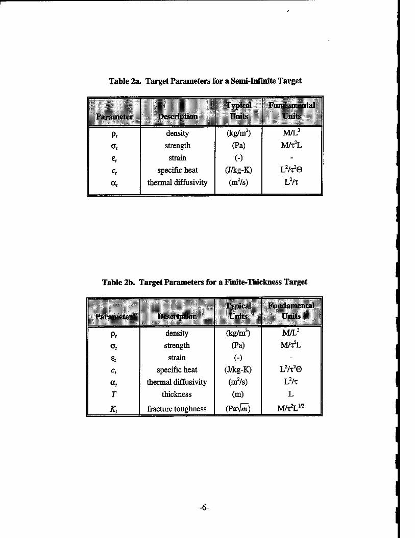
Table 2a. Target Parameters for a Semi-Infinite Target

Typical Fundamental Parameter Description Units Units

Pt density (kg/m3) M/L3

<*t strength (Pa) Wc*L

e* strain (-) -

ct specific heat (J/kg-K) lirt® a, thermal diffusivity (m2/s) L2/T

Table 2b. Target Parameters for a Finite-Thickness Target

Typical Fundamental Parameter Description Units Units

P, density (kg/m3) M/L3

<*t strength (Pa) M/i*L

e, strain (-) -

ct specific heat (J/kg-K) L2/!2©

a, thermal diffusivity (m2/s) L2/x

T thickness (m) L

Kt fracture toughness (PaVm) M/TV72

-6-

Thickness T

Density 9t

Strength <*t

Strain £*

Specific heat ct

Thermal diffusivity a,

Fracture toughness Kt

Figure 4. Impact Model Parameters: Target

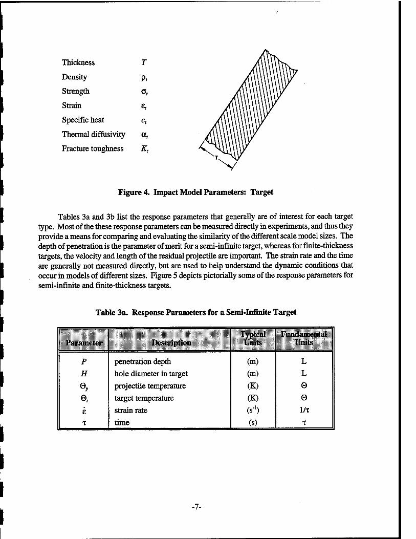
Tables 3a and 3b list the response parameters that generally are of interest for each target type. Most of the these response parameters can be measured directly in experiments, and thus they provide a means for comparing and evaluating the similarity of the different scale model sizes. The depth of penetration is the parameter of merit for a semi-infinite target, whereas for finite-thickness targets, the velocity and length of the residual projectile are important. The strain rate and the time are generally not measured directly, but are used to help understand the dynamic conditions that occur in models of different sizes. Figure 5 depicts pictorially some of the response parameters for semi-infinite and finite-thickness targets.

Table 3a. Response Parameters for a Semi-Infinite Target

Parameter Description Tvpical Units

Fundamental Units

P penetration depth (m) L

H hole diameter in target (m) L

®P projectile temperature (K) 0

et target temperature (K) 0

e strain rate (s-1) 1/T

T time (s) 1

-7-

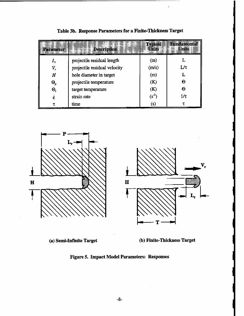
Table 3b. Response Parameters for a Finite-Thickness Target

Parameter Description Typical Units

Fundamental Units

Lr projectile residual length (m) L

Vr projectile residual velocity (m/s) L/T

H hole diameter in target (m) L

®P projectile temperature (K) 0

0, target temperature (K) 0

£ strain rate (s-1) 1/T

1 time (s) 1

(a) Semi-Infinite Target (b) Finite-Thickness Target

Figure 5. Impact Model Parameters: Responses

-8-

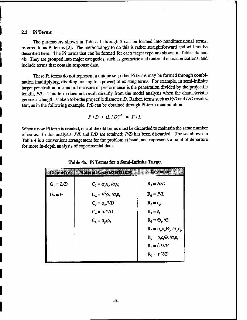
2.2 Pi Terms

The parameters shown in Tables 1 through 3 can be formed into nondimensional terms, referred to as Pi terms [2]. The methodology to do this is rather straightforward and will not be described here. The Pi terms that can be formed for each target type are shown in Tables 4a and 4b. They are grouped into major categories, such as geometric and material characterizations, and include terms that contain response data.

These Pi terms do not represent a unique set; other Pi terms may be formed through combi- nation (multiplying, dividing, raising to a power) of existing terms. For example, in semi-infinite target penetration, a standard measure of performance is the penetration divided by the projectile length, P/L. This term does not result directly from the model analysis when the characteristic geometric length is taken to be the projectile diameter, D. Rather, terms such as P/D and L/D results. But, as in the following example, P/L can be obtained through Pi-term manipulation:

PID • (L/D)-1 = PIL

When a new Pi term is created, one of the old terms must be discarded to maintain the same number of terms. In this analysis, P/L and L/D are retained; P/D has been discarded. The set shown in Table 4 is a convenient arrangement for the problem at hand, and represents a point of departure for more in-depth analysis of experimental data.

Table 4a. Pi Terms for a Semi-Infinite Target

Geometric Material Characterization Response

GX = UD Q = 0^/0,6, RX = H/D

G2 = 6 C2 = V2p;,/CTrer R2 = P/L

Q = ap/VD R3 = ep

C4 = a,/VD R4 = et

Q = pp/p, 1*5 = ©,/©,

R6=PpCp@p/cpep

R7 = p,c,0,/<?,£,

R8 = eZW

Rg = XV/D

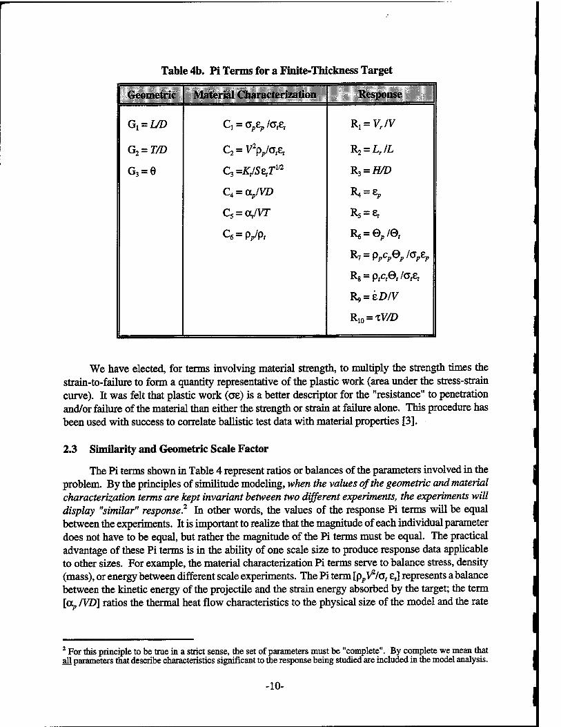
Table 4b. Pi Terms for a Finite-Thickness Target

Geometric Material Characterization Response

G^L/D Q = GpzplGtzt R^Vr/V

G2=T/D C2=V2pp/GtEt R2 = Lr/L

G3 = 6 C3 =Kt/SetTm R3 = H/D

C4 = ap/VD R4 = £p

C5 = a,IVT R5 = et

Q-Pp/p» Rs = 0p/0,

R7=ppcpep/cpep

Ri=ptCt@t/Gt£t

R9 = eD/V

R10 = xV/D

We have elected, for terms involving material strength, to multiply the strength times the strain-to-failure to form a quantity representative of the plastic work (area under the stress-strain curve). It was felt that plastic work (ae) is a better descriptor for the "resistance" to penetration and/or failure of the material than either the strength or strain at failure alone. This procedure has been used with success to correlate ballistic test data with material properties [3].

2.3 Similarity and Geometric Scale Factor

The Pi terms shown in Table 4 represent ratios or balances of the parameters involved in the problem. By the principles of similitude modeling, when the values of the geometric and material characterization terms are kept invariant between two different experiments, the experiments will display "similar" response? In other words, the values of the response Pi terms will be equal between the experiments. It is important to realize that the magnitude of each individual parameter does not have to be equal, but rather the magnitude of the Pi terms must be equal. The practical advantage of these Pi terms is in the ability of one scale size to produce response data applicable to other sizes. For example, the material characterization Pi terms serve to balance stress, density (mass), or energy between different scale experiments. The Pi term [ppV

2/G, ej represents a balance

between the kinetic energy of the projectile and the strain energy absorbed by the target; the term [CLp /VD] ratios the thermal heat flow characteristics to the physical size of the model and the rate

2 For this principle to be true in a strict sense, the set of parameters must be "complete". By complete we mean that all parameters that describe characteristics significant to the response being studied are included in the model analysis.

-10-

of penetration (through the impact velocity); the term [pp /pj serves as a measure of the density (inertia) mismatch between the target and the projectile. The pi term [ppcp®p/apEp] is a ratio of internal (thermal) energy per unit volume to plastic work. Plastic work increases the bulk temperature of the material, which can lead to thermal softening, as will be shown in Section 3.0.

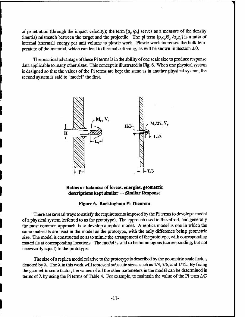
The practical advantage of these Pi terms is in the ability of one scale size to produce response data applicable to many other sizes. This concept is illustrated in Fig. 6. When one physical system is designed so that the values of the Pi terms are kept the same as in another physical system, the second system is said to "model" the first.

1

Mr,Vr

11/3 LJaf

M^J '3fn~V3

kT/3

Ratios or balances of forces, energies, geometric descriptions kept similar => Similar Response

Figure 6. Buckingham Pi Theorem

There are several ways to satisfy the requirements imposed by the Pi terms to develop a model of a physical system (referred to as the prototype). The approach used in this effort, and generally the most common approach, is to develop a replica model. A replica model is one in which the same materials are used in the model as the prototype, with the only difference being geometric size. The model is constructed so as to mimic the arrangement of the prototype, with corresponding materials at corresponding locations. The model is said to be homologous (corresponding, but not necessarily equal) to the prototype.

The size of a replica model relative to the prototype is described by the geometric scale factor, denoted by X,. The X in this work will represent subscale sizes, such as 1/3,1/6, and 1/12. By fixing the geometric scale factor, the values of all the other parameters in the model can be determined in terms of A. by using the Pi terms of Table 4. For example, to maintain the value of the Pi term L/D

-11-

equal in a model and prototype, both the length (L) and the diameter (£>) of the model have to be sized such that they are X times the prototype values. This will be true of all linear geometric quantities in the model. The Pi term [pp V2/at £,] is used to determine the appropriate impact velocity for the subscale model experiment. Since we are assuming a replica model, both pp and Gt £, are equal in model and prototype.3 Thus, keeping [ppV

2/at et] invariant will require the same impact velocity in the model as for the prototype. The procedure to determine the model law is illustrated below for these two examples, one for geometry and the other for the impact velocity:

Geometry Velocity

L-Model — ^Prototype (PP). V'Uodel vKptprototype

^Model * *&Prototype «VA*« = «*A> Prototype

-1 XL* 'Prototype

XDt Prototype \ U ) Prototype

S.V2- l/2n [V(pp/o,e,rL, = MpMen

v = v 'Model 'Prototype

Prototype

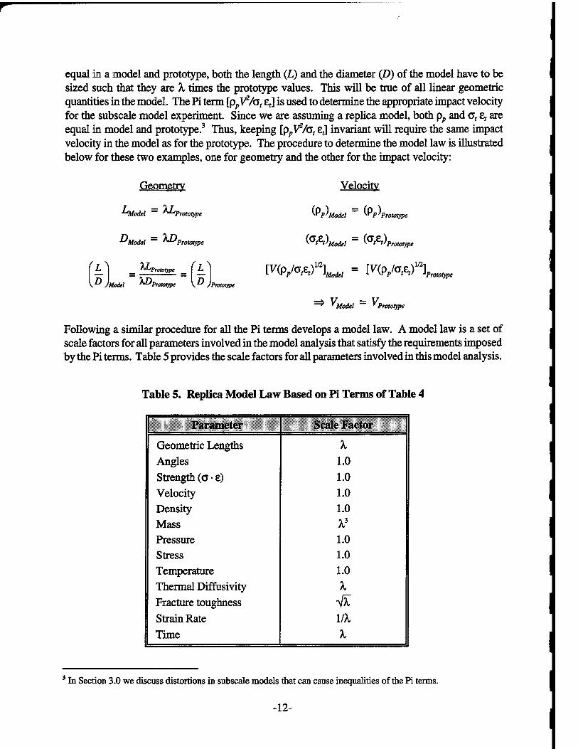
Following a similar procedure for all the Pi terms develops a model law. A model law is a set of scale factors for all parameters involved in the model analysis that satisfy the requirements imposed by the Pi terms. Table 5 provides the scale factors for all parameters involved in this model analysis.

Table 5. Replica Model Law Based on Pi Terms of Table 4

Parameter Scale Factor

Geometric Lengths X Angles 1.0 Strength (a • e) 1.0 Velocity 1.0 Density 1.0 Mass X3

Pressure 1.0 Stress 1.0 Temperature 1.0 Thermal Diffusivity X Fracture toughness Jx Strain Rate 1/X Time X

3 In Section 3.0 we discuss distortions in subscale models that can cause inequalities of the Pi terms.

-12-

3.0 SCALING ISSUES IN THE USE OF REPLICA MODELS

The assumption of a replica model, and the model law presented in Table 5, contains some inherent issues that may lead to distortions in the ability of subscale models to reproduce full-scale results. For the model to reproduce the prototype response, all Pi terms must remain invariant. Practical considerations sometimes make this very difficult to do. In certain cases, the model law results in conflicting requirements on the Pi terms, thereby making it impossible to keep all Pi terms invariant simultaneously. Then the question becomes: How much distortion results between the responses of the prototype and model because of Pi term(s) not being invariant? Several issues are discussed below.

The assumption of a replica model requires that the subscale models have the same material density and strength as the prototype. This is not difficult to do for density, but matching the strength is more subtle for two reasons. The first of these is the fact that manufacturing processes can lead to different strengths for different thicknesses of plates of the same material. Generally, thinner plates are stronger due to increased amounts of cold working, or other manufacturing processes. A similar condition may occur for the projectiles. This discrepancy can be overcome through careful selection and manufacturing of the projectile and target pieces. For example, all target plates can be cut from the same stock items, with care taken to insure that the target center-line corresponds for all tests.

The second issue related to strength involves the effects of strain rate. The model law in Table 5 indicates that the strain rate in a subscale model will be higher than that in a larger prototype:

^■Model = A> ^Prototype

For A, = 1/10, then the following relationship exists between the strain rates for the model and prototype:

^■Model = *V£Prototype

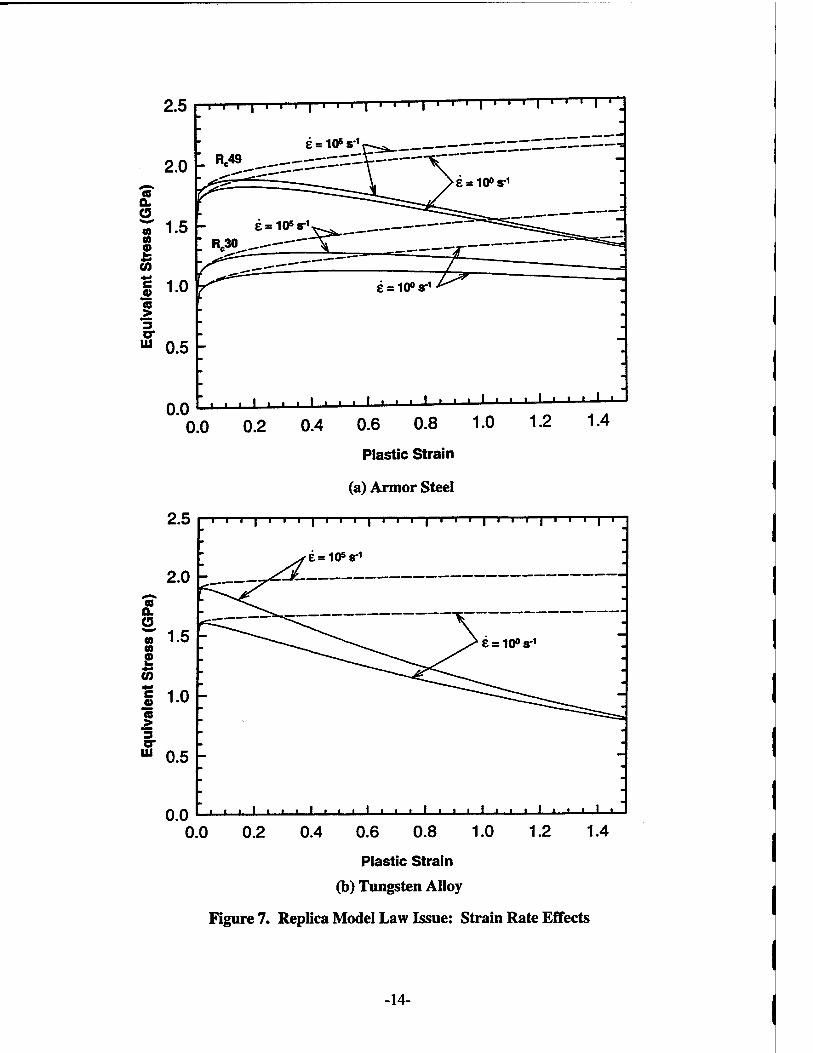
It is well-known that some materials exhibit increased strength as strain rate increases. The equivalent stress versus equivalent plastic strain responses are shown in Fig. 7a for two armor steels, and Fig. 7b for a tungsten alloy, at two different strain rates (10° and 105 s"1). The dashed lines represent the response when thermal softening is neglected; the solid lines represent the full constitutive response. These stress-strain curves were generated using the Johnson-Cook constitutive model [4-5]. For the adiabatic (solid) curves in these figures, it was assumed that 100% of the plastic work goes into heating, i.e., thermal softening. The steel with a hardness R,49 is a high-hard armor steel; the R..30 steel is for 4340 steel, which is often used as a surrogate material for rolled homogeneous armor (RHA).

■13-

2.5

2.0 co a. o

I I I I I I I I I 1 I I I I ' ' ■ I ' ' ' I ' ' ' I ''.

esKFs-1

R,49

^

1.5 - e = io*s-' g ; Re30 -.^--—\

C/J

| 1.0 > "5 & 0.5

0.0

e = 10° s-1

, , | ... i ■■•'■• ■ » , i l i i i I i

0.0 0.2 0.4 0.6 0.8 1.0 1.2 1.4

Plastic Strain

(a) Armor Steel

2.5 I—r—T—i—|—i—i—i—|—i i i |—r—T—i—i—i—i—i—|—i—i—I—]—i—i—r

esKPs-1

* 0.5

0.0 J I L I I I I I ■ I ■ I ■ ■ t t I I I I l__l l_J I I—I—I—1_

0.0 0.2 0.4 0.6 0.8 1.0 1.2 1.4

Plastic Strain

(b) Tungsten Alloy

Figure 7. Replica Model Law Issue: Strain Rate Effects

-14-

Due to strain-rate hardening, scale targets and projectiles that deform at a higher strain rate will exhibit greater resistance to plastic flow than the larger prototype. This effect is difficult to overcome. It might be possible to do careful metallurgy to obtain model materials that behave the same as the prototype materials at their corresponding rates of strain, but this undoubtedly would be difficult and expensive. But, it is also possible that the difference in material strengths due to strain-rate effects between model and prototype will result in a small or negligible difference in observed response. Such a conclusion was reached in the study of Ref. [6].

Another issue related to strain rate is the possible existence of two deformation flow regions with different scales in the penetration zone. One of these regions would act "globally" and follow the model law prediction of higher strain rates. The other would be a "local" region and only affected by the projectile velocity. Since the impact velocity is the same for all scale sizes in a replica model, the "local" region would move at the same strain rate, regardless of scale size. Intuition might argue for the existence of a "local" strain rate; that is, there would be a region where the dynamics is independent of the geometric scale sizes because the "natural" scale may be, for example, the grain size of the material. Thus, if target deformation and failure were taking place in the "local" region, then there would be no difference in different scale sizes. Numerical simulations conducted to quantify the magnitude of strain-rate effect show only the "global" response [6]. All locations in the scale target moved at strain rates higher than the prototype target, the difference being exactly the inverse of the scale factor as indicted in Table 5. The reason for this behavior is that homologous locations in a scale model are closer together, by a factor of A,, than they are in the prototype, yet the impact velocity is the same. The strain or relative deformation in the subscale target is the same as in the full scale target, but it occurs in a shorter time (since all the geometric dimensions are reduced by a factor X), thereby forcing the increase in the strain rate.

There are situations where physical response depends upon the absolute magnitude of a metric (e.g., time, physical size, etc). For example, adiabatic shear bands have a characteristic size on the order of 50 microns, which is independent of the size of a test specimen. Thus, once failure is initiated, damage would evolve at micromechanically-controlled rates (e.g., absolute time), independent of scale size. More in-depth discussions on failure are provided in Ref. [6], and at the end of this report.

Two other material property issues which result from the model law in Table 5 are the scaling of fracture toughness and thermal diffusivity. The replica model law states that these properties have to be different in the model than prototype, which is essentially impossible to do when the materials are the same in both cases. As a result, these parameters will be distorted in the model. The model law requires fracture toughness in the subscale model to be less than that in the prototype by the square root of the geometric scale factor (see Table 5). This requirement dictates, for example, that a 1/4-scale model should have one-half the fracture toughness of the full-scale prototype. Since this will not be the case, the model may be too tough, i.e., have a higher resistance to fracture than in full scale.

The thermal diffusivity of the subscale model should also be smaller than the prototype by the geometric scale factor (Table 5). As in the previous example, a 1/4-scale model should ideally have one-quarter the thermal diffusivity, implying a lower rate of heat flow through the material.

-15-

Since the model material will have the same thermal diffusivity, heat conduction at homologous locations will be "faster" in the model, thereby potentially distorting thermal effects. However, for the time scales of a penetration event, heat conduction is negligible; that is, the penetration event is essentially adiabatic. Therefore, since the time domain for penetration has a very short duration, nonscaling of thermal diffusivity should lead to negligible distortions in the ballistic response between scale sizes.

In general, it is reasonable to state that if the response is weakly dependent on some parameter, then a distortion in the associated Pi terms will not appreciably affect the response. Conversely, if the target and projectile response is strongly dependent upon a parameter which cannot remain invariant, then similarity between scale sizes will be violated to some degree. The question then becomes: what is the magnitude of the distortion?

In the paragraphs above, we have identified four distortions in a replica model: strain-rate hardening, failure, fracture toughness, and thermal conduction. The work in Ref. [6] demonstrated that strain-rate hardening, for typical armor steels and tungsten alloys, is approximately a 5% effect over a scale factor of 10. Therefore, for relatively small changes in scale, e.g., three to five, differences in strain-rate hardening with changes in scale has almost a negligible effect in similitude response. The nonscaling of thermal diffusivity is also considered to have negligible influence on measured responses since penetration processes are essentially adiabatic over the time scales of interest. Nonscaling of fracture toughness and failure, however, remain as material-related issues that could affect similar responses in model and prototype.

-16-

4.0 SELECTION OF SCALE SIZES

4.1 Introduction

Several criteria were used to establish the scale sizes for the experimental phase of the program. These criteria will be discussed briefly. Impact velocities of interest ranged from 1.0 to greater than 2.0 km/s. Available launchers included 30- and 50-mm powder gun systems and 50/20-mm and 75/30-mm two-stage light-gas gun systems. Too large of a scale size would preclude high impact velocities; too small of a scale size would result in sabot separation problems.

It was also desired that the range in scale sizes investigated be as large as possible. For example, 1/4 and 1/5 scale only differ by a factor of 1/20. Further, the range in scale sizes should also be comparable to the difference in full scale and the largest of the subscales selected, e.g., if 1/4 scale was selected as the largest of the subscale experiments, then a difference of 4 exists between the 1/4 scale and full scale. Thus, the subscale tests, to run over the same scale factor of 4, would require a 1/16-scale test series.

Finally, costs in fabricating targets can be minimized by the judicious selection of scale sizes to match "stock" thicknesses of plates.

4.2 The Prototype Projectile

The baseline (prototype) projectile was selected to be representative of current kinetic energy, tank-fired projectiles. The full-scale projectile was defined as a homogeneous, hemispherical-nosed, long rod made of a tungsten alloy. The full-scale prototype projectile is defined as having a diameter of 25.4 mm, with a length-to-diameter ratio (UD) of 20.

4.3 Scale Model Projectiles

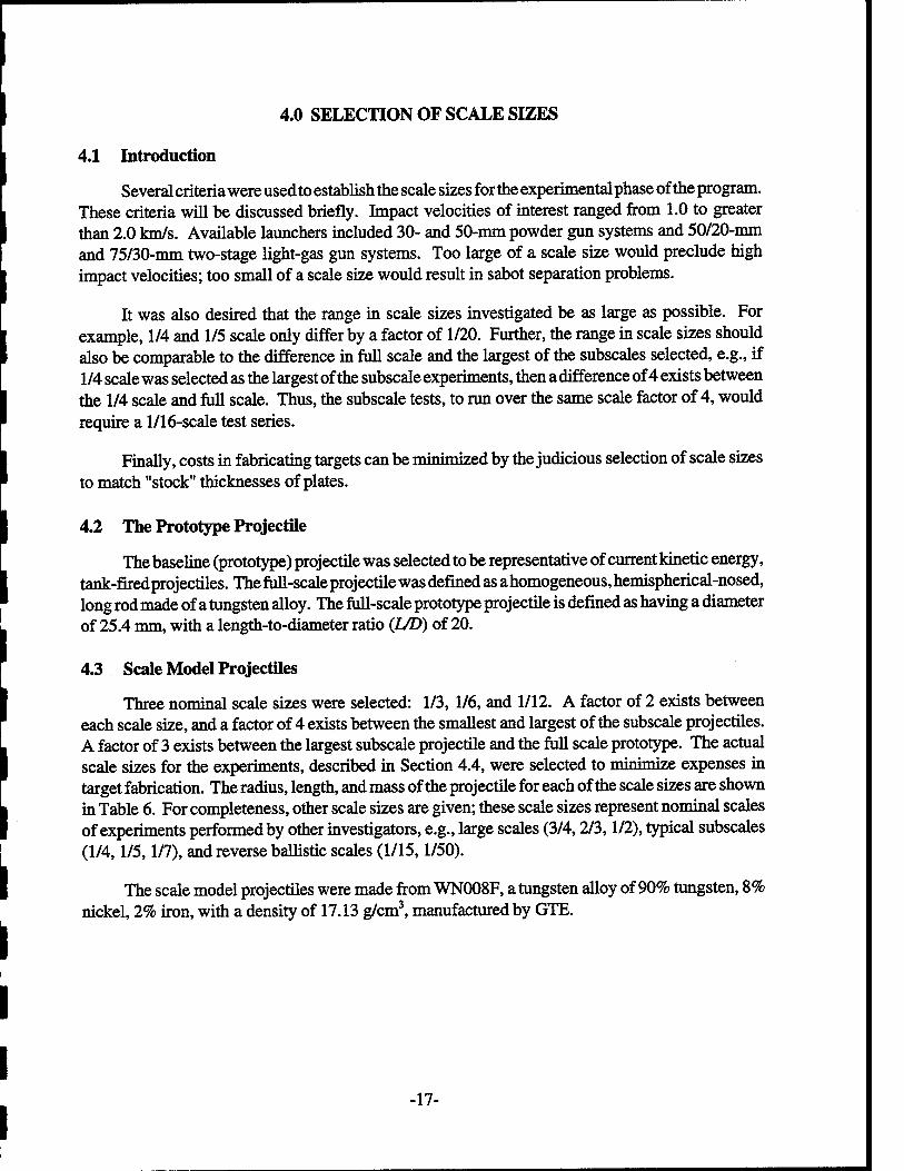
Three nominal scale sizes were selected: 1/3, 1/6, and 1/12. A factor of 2 exists between each scale size, and a factor of 4 exists between the smallest and largest of the subscale projectiles. A factor of 3 exists between the largest subscale projectile and the full scale prototype. The actual scale sizes for the experiments, described in Section 4.4, were selected to minimize expenses in target fabrication. The radius, length, and mass of the projectile for each of the scale sizes are shown in Table 6. For completeness, other scale sizes are given; these scale sizes represent nominal scales of experiments performed by other investigators, e.g., large scales (3/4,2/3,1/2), typical subscales (1/4,1/5,1/7), and reverse ballistic scales (1/15,1/50).

The scale model projectiles were made from WN008F, a tungsten alloy of 90% tungsten, 8% nickel, 2% iron, with a density of 17.13 g/cm3, manufactured by GTE.

-17-

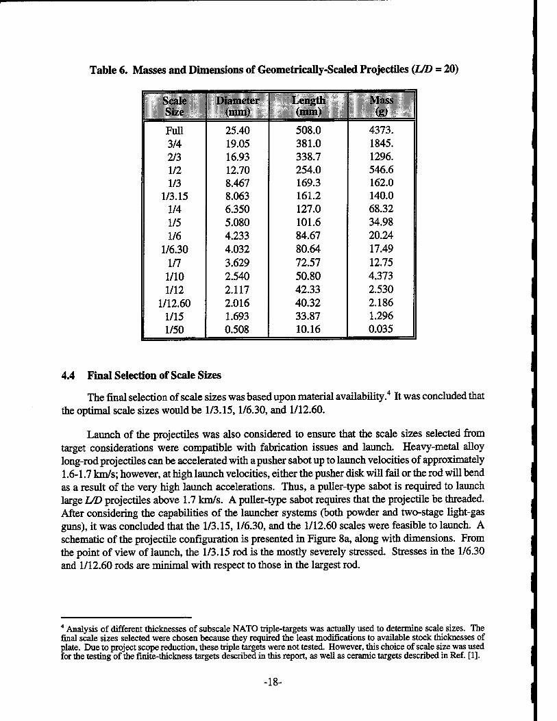
Table 6. Masses and Dimensions of Geometrically-Scaled Projectiles (L/D = 20)

Scale Diameter Length Mass Size (mm) (mm) <g>

Full 25.40 508.0 4373. 3/4 19.05 381.0 1845. 2/3 16.93 338.7 1296. 1/2 12.70 254.0 546.6 1/3 8.467 169.3 162.0

1/3.15 8.063 161.2 140.0 1/4 6.350 127.0 68.32 1/5 5.080 101.6 34.98 1/6 4.233 84.67 20.24

1/6.30 4.032 80.64 17.49 1/7 3.629 72.57 12.75

1/10 2.540 50.80 4.373 1/12 2.117 42.33 2.530

1/12.60 2.016 40.32 2.186 1/15 1.693 33.87 1.296 1/50 0.508 10.16 0.035

4.4 Final Selection of Scale Sizes

The final selection of scale sizes was based upon material availability.4 It was concluded that the optimal scale sizes would be 1/3.15,1/6.30, and 1/12.60.

Launch of the projectiles was also considered to ensure that the scale sizes selected from target considerations were compatible with fabrication issues and launch. Heavy-metal alloy long-rod projectiles can be accelerated with a pusher sabot up to launch velocities of approximately 1.6-1.7 km/s; however, at high launch velocities, either the pusher disk will fail or the rod will bend as a result of the very high launch accelerations. Thus, a puller-type sabot is required to launch large L/D projectiles above 1.7 km/s. A puller-type sabot requires that the projectile be threaded. After considering the capabilities of the launcher systems (both powder and two-stage light-gas guns), it was concluded that the 1/3.15,1/6.30, and the 1/12.60 scales were feasible to launch. A schematic of the projectile configuration is presented in Figure 8a, along with dimensions. From the point of view of launch, the 1/3.15 rod is the mostly severely stressed. Stresses in the 1/6.30 and 1/12.60 rods are minimal with respect to those in the largest rod.

4 Analysis of different thicknesses of subscale NATO triple-targets was actually used to determine scale sizes. The final scale sizes selected were chosen because they required the least modifications to available stock thicknesses of plate. Due to project scope reduction, these triple targets were not tested. However, this choice of scale size was used for the testing of the finite-thickness targets described in this report, as well as ceramic targets described in Ref. [1].

-18-

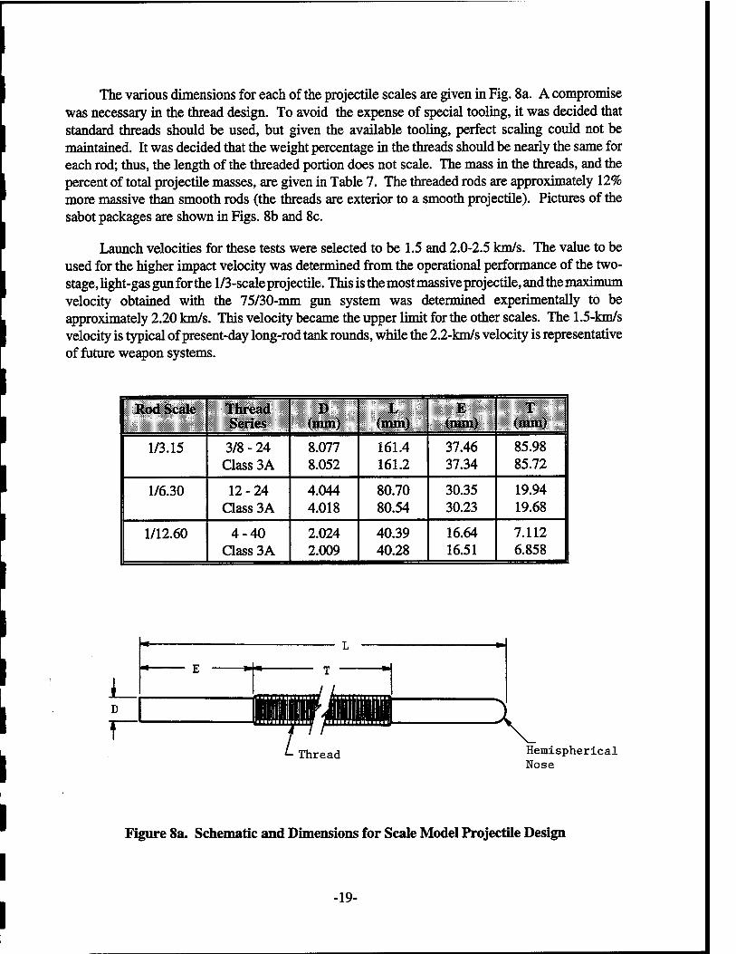
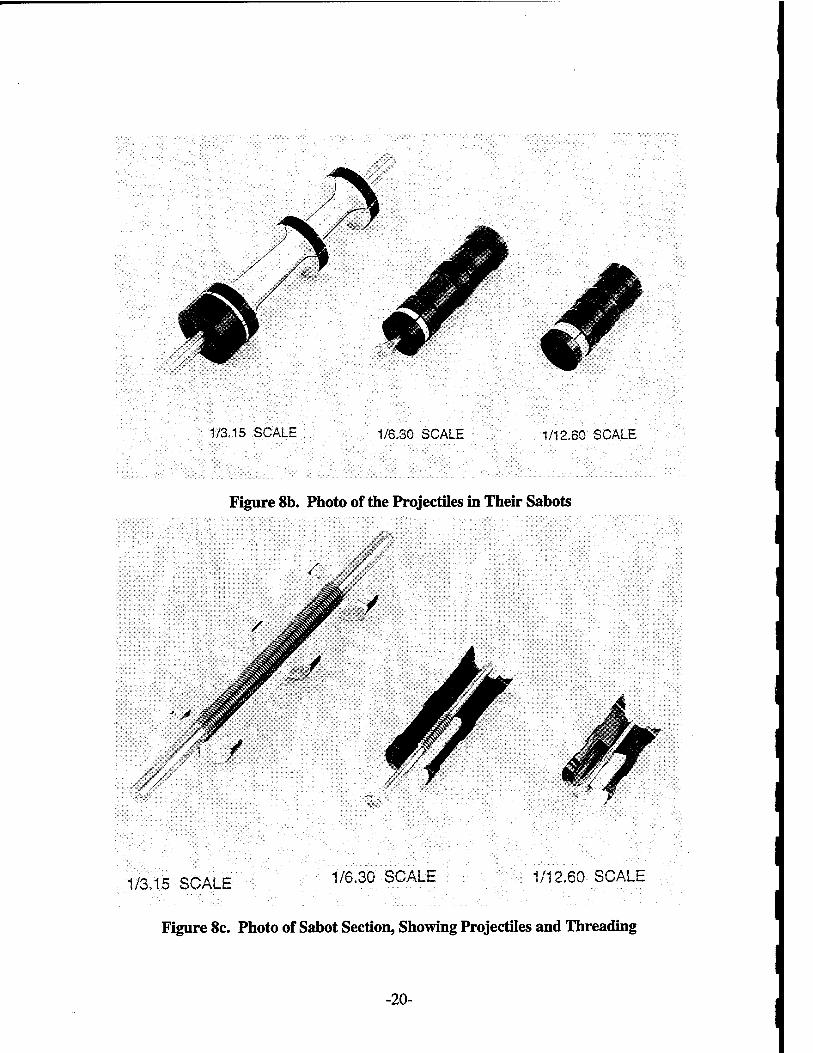
The various dimensions for each of the projectile scales are given in Fig. 8a. A compromise was necessary in the thread design. To avoid the expense of special tooling, it was decided that standard threads should be used, but given the available tooling, perfect scaling could not be maintained. It was decided that the weight percentage in the threads should be nearly the same for each rod; thus, the length of the threaded portion does not scale. The mass in the threads, and the percent of total projectile masses, are given in Table 7. The threaded rods are approximately 12% more massive than smooth rods (the threads are exterior to a smooth projectile). Pictures of the sabot packages are shown in Figs. 8b and 8c.

Launch velocities for these tests were selected to be 1.5 and 2.0-2.5 km/s. The value to be used for the higher impact velocity was determined from the operational performance of the two- stage, light-gas gun for the 1/3-scale projectile. This is the most massive projectile, and the maximum velocity obtained with the 75/30-mm gun system was determined experimentally to be approximately 2.20 km/s. This velocity became the upper limit for the other scales. The 1.5-km/s velocity is typical of present-day long-rod tank rounds, while the 2.2-km/s velocity is representative of future weapon systems.

Rod Scale Thread Series

D (mm)

L (mm)

E (mm)

T (mm)

1/3.15 3/8 - 24 Class 3A

8.077 8.052

161.4 161.2

37.46 37.34

85.98 85.72

1/6.30 12-24 Class 3A

4.044 4.018

80.70 80.54

30.35 30.23

19.94 19.68

1/12.60 4-40 Class 3A

2.024 2.009

40.39 40.28

16.64 16.51

7.112 6.858

Thread Hemispherical Nose

Figure 8a. Schematic and Dimensions for Scale Model Projectile Design

-19-

1/3.15 SCALE 1/6.30 SCALE 1/12.60 SCALE

Figure 8b. Photo of the Projectiles in Their Sabots

1/3.15 SCALE 1/6.30 SCALE 1/12.60 SCALE

Figure 8c. Photo of Sabot Section, Showing Projectiles and Threading

-20-

Table 7. Rod Masses

Rod Scale Plain Rod Mass(g)

Thread Mass(g)

Total Rod Mass(g)

Thread Per- cent of Total

1/3.15 1/6.30 1/12.60

140.0 17.49 2.186

18.686 2.330 0.2470

158.7 19.82 2.433

11.77 11.76 10.15

-21-

5.0 FINITE-THICKNESS TARGET TEST MATRIX

5.1 Target Size and Test Matrix Overview

The single-plate finite-thickness targets were sized so that tests would be conducted near the ballistic limit thickness (NUT), below the limit thickness (WB), and somewhere in between (IB). In this manner, comparisons would be conducted over a wide range of terminal ballistic conditions. Additionally, one set of tests was conducted at normal obliquity, while the other was at 60-degrees obliquity. The test matrix for these tests is shown in Table 8. The plates were fabricated from 4340 steel with a Rockwell C hardness of R<27±2, a surrogate material for RHA.

Table 8. Finite-Thickness Target Test Matrix

Velocity Target Target Thick Test No.* M> (km/s) Scale Obliquity Type (cm)

FT-l 20 1.50 1/3.15 0° NLT 14.52

FT-2 20 1.50 1/6.30 0° NLT 7.37

FT-3 20 1.50 1/12.60 0° NLT 3.62

FT-4 20 1.50 1/3.15 60° NLT 7.26

FT-5 20 1.50 1/6.30 60° NLT 3.68

FT-6 20 1.50 1/12.60 60° NLT 1.81

FT-7 20 2.25 1/3.15 0° NLT 24.32

FT-8 20 2.25 1/6.30 0° NLT 12.35

FT-9 20 2.25 1/12.60 0° NLT 6.07

FT-10 20 2.25 iai5 60° NLT 12.16

FT-11 20 2.25 1/6.30 60° NLT 6.18

FT-12 20 2.25 1/12.60 60° NLT 3.04

FT-13-»FT-24 20 1.50/2.25 1/3.15^1/12.60 0° 60° 0° 60°

WB 10.16,5.16,2.53 5.08,2.58,1.26 22.25,11.30,5.55 11.12,5.65,2.78

FT-25-»FT-36 20 1.50/2.25 1/3.15->1/12.60 0° 60° 0° 60°

IB 13.4,6.8,3.34 6.70,3.40, 1.67 2.34,11.88,5.84 11.70,5.94,2.92

-

"NOTE: 18 repeat tests to be distributed within this test matrix.

The thicknesses for the target plates were determined through analysis with the Täte model [7-8]. The thicknesses for the NLT tests were chosen by determining the depth of penetration into a semi-infinite target, and adding one to two projectile diameters. The resulting thickness should just be perforated by the projectile. The thicknesses for the WB tests were chosen by selecting that

-23-

thickness which would allow the projectile to have a residual velocity of about 85 to 90 percent of the impact velocity. Analysis indicates that the residual velocity of the projectile drops off very rapidly as the target thickness approaches the limit thickness (for example, see Fig. 9). Thicknesses for the IB tests were based upon the thickness which would provide a residual velocity of about 66% the impact velocity. The thicknesses for the tests conducted at 60° obliquity were determined by maintaining the line-of-sight thickness equal to the thickness of the normal obliquity tests.

Leos 6

Figure 9. Residual Rod Velocity Vr IV0 versus Effective Plate Thickness TI(LcosQ\ Ref. [9]

A total of 36 tests are shown on Table 8. An additional 18 tests were dedicated to the test program to provide an indication of data scatter. Figure 10 shows the three scale sizes of targets; the projectiles are also shown in the figure. Figure 10a depicts the three scale sizes for 0° obliquity, and Fig. 10b shows the comparable targets for the 60°-obliquity experiments. The three different thicknesses, at the same scale, are shown in Figs. 10c and lOd.

-24-

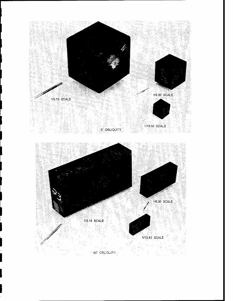
1/3.15 SCALE

.S* 1/6.30 SCALE

0' OBLIQUITY 1/12.60 SCALE

1/3.15 SCALE

1/6.30 SCALE

/

1/12.60 SCALE

60* OBLIQUITY

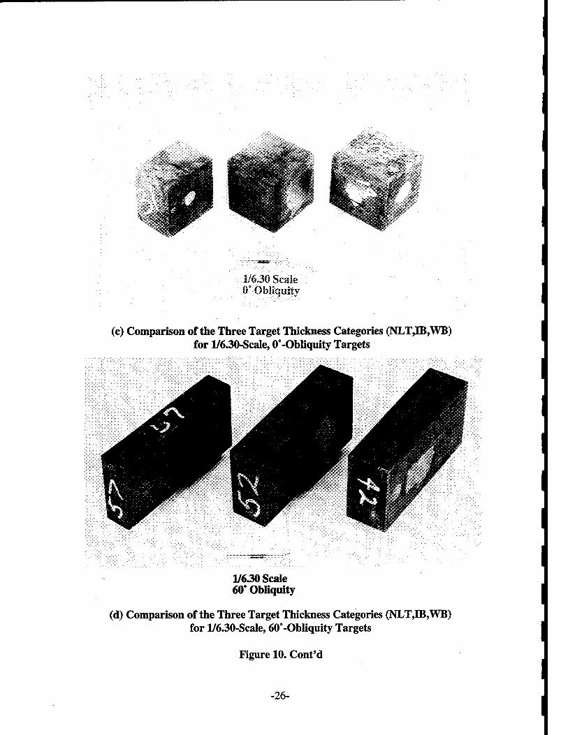
1/6.30 Scale 0° Obliquity

(c) Comparison of the Three Target Thickness Categories (NLT,IB,WB) for 1/6.30-Scale, 0°-Obliquity Targets

1/630 Scale 60° Obliquity

(d) Comparison of the Three Target Thickness Categories (NLT,IB,WB) for 1/6.30-Scale, 60°-Obliquity Targets

Figure 10. Cont'd

-26-

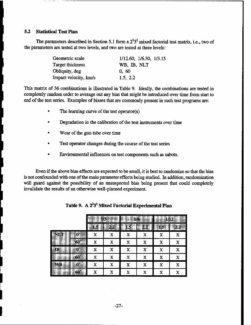
5.2 Statistical Test Plan

The parameters described in Section 5.1 form a 2232 mixed factorial test matrix, i.e., two of the parameters are tested at two levels, and two are tested at three levels:

Geometric scale Target thickness Obliquity, deg Impact velocity, km/s

1/12.60, 1/6.30, 1/3.15 WB, IB, NLT 0, 60 1.5, 2.2

This matrix of 36 combinations is illustrated in Table 9. Ideally, the combinations are tested in completely random order to average out any bias that might be introduced over time from start to end of the test series. Examples of biases that are commonly present in such test programs are:

The learning curve of the test operator(s)

Degradation in the calibration of the test instruments over time

Wear of the gun tube over time

Test operator changes during the course of the test series

Environmental influences on test components such as sabots.

Even if the above bias effects are expected to be small, it is best to randomize so that the bias is not confounded with one of the main parameter effects being studied. In addition, randomization will guard against the possibility of an unsuspected bias being present that could completely invalidate the results of an otherwise well-planned experiment.

Table 9. A 2232 Mixed Factorial Experimental Plan

1/3 1/6 1/12

L5 2.2 1.« 22, 1.5 2.2

NLT 0' X X X X X X

6ir X X X X X X

IB oc X X X X X X

60 X X X X X X

WB 0" X X X X X X

60' X X X X X X

-27-

In the test program, we had one restriction on complete randomization. In order to achieve the velocity levels desired, the 1/3-scale projectiles had to be fired from a different gun than the 1/6 and 1/12-scale projectiles. For logistical reasons, it was not desirable to randomly switch back and forth between the two guns. Consequently, the gun type was treated as a two-level blocking factor in the test plan. Within each block (gun type), the tests were conducted in random order.

There is always some random experimental variation present in a test program. The goal is to control as much as possible the factors that contribute to this random variability in test results. In order to form statistically significant conclusions about how the main parameters of interest influence the test results, these main factors must produce variations in the results that are much larger than the variations produced by random chance. If the opposite is true (i.e., random variations are not kept small), then these random test-to-test differences will mask the main factor effects that are of real interest.

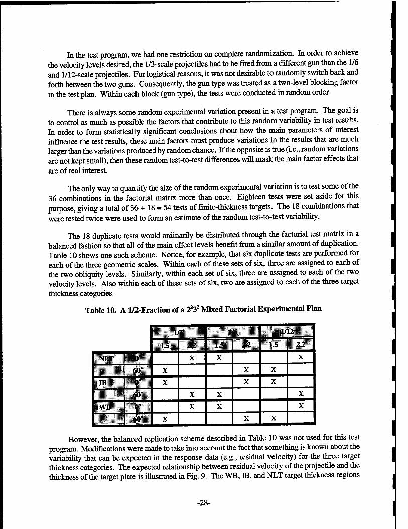
The only way to quantify the size of the random experimental variation is to test some of the 36 combinations in the factorial matrix more than once. Eighteen tests were set aside for this purpose, giving a total of 36+18 = 54 tests of finite-thickness targets. The 18 combinations that were tested twice were used to form an estimate of the random test-to-test variability.

The 18 duplicate tests would ordinarily be distributed through the factorial test matrix in a balanced fashion so that all of the main effect levels benefit from a similar amount of duplication. Table 10 shows one such scheme. Notice, for example, that six duplicate tests are performed for each of the three geometric scales. Within each of these sets of six, three are assigned to each of the two obliquity levels. Similarly, within each set of six, three are assigned to each of the two velocity levels. Also within each of these sets of six, two are assigned to each of the three target thickness categories.

Table 10. A 1/2-Fraction of a 2232 Mixed Factorial Experimental Plan

1/3 1/6 1/12

1.5 &2 1.5 2.2 1.5 2.2

NLT 0* X X X

60 X X X

IB 0l X X X

60" X X X

WB Ö* X X X

60 X X X

However, the balanced replication scheme described in Table 10 was not used for this test program. Modifications were made to take into account the fact that something is known about the variability that can be expected in the response data (e.g., residual velocity) for the three target thickness categories. The expected relationship between residual velocity of the projectile and the thickness of the target plate is illustrated in Fig. 9. The WB, IB, and NLT target thickness regions

-28-

are marked on the figure. Note the steepness of the curve in the NLT and IB regions compared to the WB region. This sensitivity indicates that residual velocity measurements will have much more scatter in the NLT region than in the WB region. Consequently, it is desirable to do more replication of the NLT conditions than of the WB conditions. Table 11 shows the replication pattern that was used for this test program. Most of the parameters are still balanced. However, 10 of the NLT conditions will be repeated, compared to six IB and two WB combinations. The complete sequence of 54 tests is summarized in Table 12. The order of testing within the four sets of experiments has been randomly established.

Table 11. Experiment Combinations Tested Twice

W 1/6 1/12

1.5 2.2 1.5 2.2 L5 2.2

NLT 0" X X X X X

60' X X X X X

IB 0 X X X

60° X X X

WB 0' X

60' X

Table 12. Complete Test Sequence for Finite-Thickness Targets

1/3 1/6 1/12

1.5 22 1.5 2.2 1.5 22

NLT 0' 31,37 2,9 15,23 39,54 51 14,19

60 5,7 36,38 45,48 16,22 17,28 50

IB 0J 6,10 32 44 11,27 20,26 43

60 35 3,8 13,24 41 49 21,25

WB V 34 1 29 52 47,53 30

60s 4 33 40 18 12 42,46

-29-

6.0 EXPERIMENTAL DATA

The projectiles were launched using a two-stage light-gas gun. The two smaller projectiles were launched from a 50/20-mm system, and a 75/30-mm system was used for the larger projectile. Velocities were determined using a laser "break" beam system. Projectile yaw and pitch were obtained by orthogonal flash X-rays prior to impact. Table 13 provides the test number, scale size, normalized target thickness (T/L), and total projectile inclination at impact for the thirty-one 0°-obliquity tests conducted. Table 14 shows similar data for the thirty-one 60°-obliquity shots. Figure 11 shows the test layout for the normal and oblique shots and defines the nomenclature for the pitch and yaw in Table 14. Note that the 60°-obliquity angle is measured in the yaw plane. Two pairs of orthogonal X-ray heads were used to determine the residual velocity and residual length of the projectile if it perforated the target; these values are also listed in Tables 13 and 14.

The tests displayed in Tables 13 and 14 were conducted in the randomized sequence described in Section 5. The only deviation from the test matrix occurred when a test firing was unacceptable due to a launch system malfunction, such as a rod broken during launch, or very high yaw. In such cases, the test was repeated. Therefore, Tables 13 and 14 display more tests than would be derived from Table 12 since we have elected to report all the data.

Target responses were measured so that comparisons could be made at the different scales. Post-test measurements include crater height, entrance hole diameter, and the extent of bulging on the back side of the target (if any). The depth of penetration was measured for targets not perforated. Figure 12 provides a schematic of various items measured along with the nomenclature. Figure 12a depicts the nomenclature for a 0° target that was not perforated, andFig. 12b shows the nomenclature for a 60° target that was perforated. The response data, in nondimensional form, are summarized in Tables 13 and 14.

Figure 13 shows photographs of target damage incurred during testing. Figure 13a shows three comparable 0°-obliquity tests (the 1/6.30-scale target has been sliced for X-ray imaging). Figure 13b shows comparable 60°-obliquity tests, where the 1/6.30 and 1/3.15-scale targets have been cut for X-ray imaging.

Most of the 1/12.6-scale tests and some of the 1/6.30-scale tests were plagued with excessive yaw. This was largely attributed to the mass of the projectile with respect to the sabot mass since any asymmetry in the opening of the sabot would be sufficient to perturb the flight of the projectile. Although projectile yaw confounds data analysis, we have attempted to account explicitly for yaw in the data analysis.

-31-

5 J

rtONrtr* „ new — <r>~-"~* * ©es cs es es es es es' r4 cs

t-oo© © CS CS CS es es cs' cs

NOrtON© «OWN es es es es'

t> cscs ONCS ON t-; 00 00 00 00 00

ON t~-ON VO 00 ON 00 VI 00 t-^ ON t-;

rtrteSNO </">"> 00 t~;

J MrtOiC, „ rtNOrt v> trt r-* * es cs c- CS <r> eS vi NN'pi

rt en ONCS ON1* ON es es es" es es'

C-; p vies 4 CS encs'

ON cs f-rt cs v> p oq oq en oq cs en 1-" 1-5 4 rt c-i

oq \q * es i p en -- es' en

rt NO en oo es ON es p es es es es

I

8 en n^- en oo i-i i-i !-* ON ^d; ON en ^ * ON ON ©

en ON es ON o\ ON ON 00 dodo

eS 00 <n © </">ON •* t-; rt O rt i—'

•*Ooo g vt 00 00 f- i "> t> odd 9°'

»- i* p~ t- r> rt v6 r- ON i r» ^ööö d

es oo ■<* oo r-oor- t> öööö

ooooooooo o t> r-

©■* ©*o O i-i

>rt rt en O 00 Tf CS

i—11—11—i

en <* o © S > <•* o ° o rtesvn o

O ** f "* I rt odd o

es-* NOrt t>NO o«n d des'es

s o 0 o

1 Q

s ONNOenNOP-rtOt-NO i-«vqN«*^^NN

engest: »-OE Ort- -H & O 5<0 °"

en ©t> cs — «n \o\D i r> r> odd do

t~-oes vo t> rt NONO NO i >n öööö d OO &> o*

5 | id +++++++++ + + +* + <N + 2 ++++++ ++++++

C3N es i i O i-i

d©

c

> ̂ ^

+++++++++ + + +* + ON + 2 o &

++++++ ++++++ en oo

■ i — m d©

I 03 "S Ik. 5» f Is r-ooof-

rl;<r> r-;eS 4cS Cn'rt

rt ON© w o f-w"> ON NO rt*

w-» ©cs r-o © •* p"rt ■* ON p 4 rt rt en d rt

en esoN NO "> rt t~- # # ^* NO rt o en

ON t- es © NO es © ON es4es'd

• •* * » O OM^ (S OO 0\

es" es ci es es es' es" cs' cs'

f-O ONt-

es cs' es es

00 rt OON rt CM eS rt es' CM cs' es

t> ONI— eno o ■* rt ift rt ir> iri

ON O ON rt o 00 *"t "2 4 "5"} *"""■

en •* oo oo 4 4rt-*

1? en P 4 rt

O0 '^

2 § ON £ d t* d g^

NO g; © c,

^J ^ ,_ ,_ rt i—1 rt i—IHrt £}vgvojn rt2iS22 2 ^^ enjn en £J £J NO en en en

•~^rt rt rt rt 22i$£2

^ ©

SONO\0NONONSCSON

_LT,T''T'rT,'T,_Loöoö

c^rt p~ cs tiHNm

i-i mirivo NO NO 00 r-

l—1 l—( l-H O 1 1 1 1

■* ■* is- oo

<§©•£- en en C-^-' 00 ON SS oooo^S

44--

^-\ ^-^ ^-N O ^ ^-V rt in en ,2:2 t> >n rt es ZT™ en ^^^_,^^en,^n,^^

l?elei^S| 222ggS ---oboo00

cf^fell p~rtesgmT^ f~ oo NO >fi ?-. ?£ enen-<tggS

rtrtrtOOoooo

t> en ON rt

oo >n t- 00 NO r» oo r- rt rt en © T—1 1—t »—* O

1 1 I 1 rt rt rt oo

CO

Ä o X o a <-• .a "o CL CA S? « M 53 2 co e &> S 2

+ *

1 00

s o P3

X) ° c *J « o ^

fl ü o

XS X

* * I

-32-

I s o I o © vo

I 1

I DO

.a 'S

I a* es u

0)

■a

I

tfl

H

11 Hi

5:

SI

II ill

m

P~ C» 0\ — — •* r-; p-; co m m vi es' cö es es es es'

co£J*- — ■>* vo in m. a\ r- •$■ cs in ^ »ri vö vo vo

O VO vo CJvvO f» oq in oq p ON CO N ^f -' fi «" N

— CO oom o ■* o •"* <^ ""> "t ö dodo

es ^ CS <-< es es ^ ©• ^ _;«»j

++++++

++++++

.Zi t- t^invO

'Sf^deö

ts titstSÄts

£8 cs' ON

in in>n © t» r-^cs p rtvöd'-'

Q..S Cu O. O. O. g-p s s s g

si m in in < r~ c»cs (

ic 2'-* "-i Ö rö

c- cs •* in vo r-

is es es cs" es es"

S 5.

2 VO VO >o CO jT)

-5 co co

^44

o© co oo oo oo 288 ■ i i tOOM

t- o\ r» vo t» — es r-; co r-; es r-; m ■* es cs CM es es' es es

inpiMVjovtt; 00 Ov ON •—CS CJN © in oo m vo r~ m vo

in vo co o o\ •<* vp ON •* co vq oq cs © ** es' es es »-« es" cö

esin in oov© O "! f^ "! o ") *

>-<cs © <-< —<

oo vo 1 p" So 11

+ + I+ + CO

O.Q. co to

+ + ?+ + ü a. co

O.O. oo co

in in in o\ ■* in in — o\es m — com m r* es in in d es

SS AS ssss-et: "SoOOmO es — vo in es ©es

a. 3

o «no in es in

in" m es —' rf d d

eeee a. B "O "O "O T3 Ö "O

es es <

co ON *■* *■■* o\ oo in es i-; es »-< I-« I-; -H es es es es es es es

3 /—^ a

£2 2 £3 se se n S2

S° cn o o\ vo vo r~ E:OOOV>QVOPQ J2 enen Tt Tt p p J. jL W T* oo ob

vo oq vo t-; >n es es es es es

Ov vo rt 3- es es i-i <no 0\ t~ vo vo vo" vo

s t-H oo m 00 i-i Tt ov cn

es es es es en

NmvovO"* m >-< oo <n oo d —' O es' —'

oo o in1*- <tj «novoo H H o o o &o<

es + + + * —. o

+ + +*

•* 00 00 0\ 0\ f-; cn ^; t~: vq vo >n >n" es es

SSSSÄ tJ ti *r> © moo es p es>n>n •* es es es es

e e es a. *0 T3 "O "O S

«88^8 >n >n" >ri -< —

r- — Ovoot-

es es es es es

« Sj^vocn

Q «s t- pv f: « vor- ^S^^8 J--*.

vo <-» r~ i— ■«}■ o es. p p p -1 es es' es' es es es es

00 « —IT-. VO ■* f~; •* Tl; O) vn —_ Tj-' >n ui \ri >n rS

lOHOVlOVO es p 00 C-; f"; —. es' es -H es -- vd

t- mON ON 00 O o rt"« f~- "* —' d d d d

■^■oowoonin t- eri vo vo r- vo öööööö

++++++

++++++

^ H.H. 9 ^ ^ es eö es es' -H 'H

ttssssttsse es >n f-o © © es' -J © es —i i-i

eeeeea "O "O "O 10 "O s ©>n©©©© »ihqifloq © es es' © TJ TJ

0^ 00 *-< ON ON t—• ■<}• -<t <n ■<*■<* ■<*

s Ö eS 5

fertig ig £2 £2

r-»oo »i es

■*■*•*■*'

—— ©© <np es es es es' es' es

enen >nen ©in oqo\ «n'in in'oN

©©■* — er, es enoq es es en-H

oo oo r** oo m ^H in-t d ——'©

oo o\ <e ON mvo Sm ©d ö©

+ +4+ +

+ ++H-

oovo esi-i

in'^H es ©

titstiss t-t~ m«n es' ©' ~ ©

e e B B *0 "O "O *o mm o© r~f~mm •*©—'©

m oo T-c ej\ •*■* m-*

5 &

£jvovorn

t-CSON VO 00 t> nno >H »-1 ©

■* "<t TT 00

SS© cN) es es

VO 00 0\ -^es>-^ m xrt'ri

VOONt- ^CS'-H'

men oo m co es

tststs « a o u. ö. o.

— es es ©d©

r- — es Tt t-oo ©d©

— © ©r-«n

©—'

©Oo

o.a. s s

oo© mm © —

ON — OV cnmm

es©5-

VO 00! vo m; co^t

■*Tts

8 Ä o ■SS

«I S 2

+ *

o V V

«s o

II

A3 OO

■c II ti 8 iS

■8 St! ii o B

9 «t o. o.

B w II OO Q. 9 S a.

-33-

Velocity

Vector

Projectile

Yaw (left)

Target -

Top View

• Projectile

Velocity _

Vector T Yaw (right)

Top View

Velocity Vector

Velocity Vectpr

Side View

(a) 0° Obliquity

Side View

(b) 60° Obliquity

Figure 11. Test Layout for the Experiments

-34-

Bulge HeigMB

(a) 0° Obliquity

KMK

* c^ «to H.

t

Crater Height C

Bulge Height B

(b) 60° ObHquity

Figure 12. Schematic of Post-Test Target Measurements

-35-

r:? #~.+,3(>s

Total Yaw = 2.69° Total Yaw = Total Yaw = 0.90°

(a) 0° Obliquity

^^•iP n^

Total Yaw = 2.30*

I '6 4-M64

Toto! Yaw = 2.14" •i 3 3 GOTO

Total Yaw = 1.41'

(b) 60° Obliquity

Figure 13. Examples of Target Damage

-36-

7.0 DATA ANALYSIS

The targets were "tougher" to penetrate than originally expected. The targets were designed using experimental data for L/D = 10 projectiles. It has been shown that there exists a significant L/D effect even for projectiles with aspect ratios greater than 10 [10-12]. Penetration performance, as measured by P/L, in the ordnance velocity range is degraded approximately 14% as the projectile L/D increases from 10 to 20. For constant T/L, this translates into a higher impact velocity for perforation since the larger L/D projectiles are less efficient in penetration. As a result, the NLT-type targets acted like they were semi-infinite, and we had only five perforations of the IB-type targets. This response is reflected in Tables 13 and 14, which show only a few target perforations.

7.1 Measurement Uncertainty

Each of the experimental variables contain some uncertainty in their respective measurements. It was anticipated that scale size effects would be relatively small, and a question to be addressed is whether any differences between the three scale sizes would be larger than the uncertainty and scatter of the individual measurements. Table 15 lists the uncertainties in measured parameters based upon known accuracies of the measurement devices; repeat measurements, where appropriate, of the same quantity at different times; and variations, where applicable, between minimum and maximum values. The variation in some of the parameters is larger than the precision of the measurements, which for post-test measurements was approximately 0.02 mm. The residual velocity measurements have a larger uncertainty than the impact velocity measurements only because the residual projectile sometimes tumbled, making it more difficult to determine the exact location of the reference point. As described in the following sections, measurement accuracy was sufficient to observe differences in scale in the experiments.

Table 15. Uncertainty Values for the Ballistic Response Measurements (refer to Figure 12)

Quantity (km/s)

Yaw (Deg) (km/s) (mm)

P 1 B (mm) | (mm)

C i H (mm) 1 (mm)

Uncertainty 0.01 0.25 0.025 0.5 0.5 | 0.1 0.1 | 0.25

7.2 Penetration Depth

Penetration depth was measured in those targets that were not perforated. Since projectile erosion debris usually clogged the penetration channel, it was not possible to measure the actual depth of penetration directly without cutting the targets. Targets were sliced, leaving an undisturbed region approximately 6-cm thick surrounding the impact site. These sectioned targets were sub- sequently X-rayed and the X-ray shadowgraphs developed. The differences between the residual projectile and penetration channel were clearly distinguishable on the X-ray image. The depth of penetration was measured from the X-ray shadowgraph of each target.

-37-

73 Projectile Residual Length and Velocity

For those targets that were perforated, the residual rod was usually visible in the flash X-ray images taken behind the target. X-ray shadowgraphs were taken at two times after perforation so that a residual velocity could be determined. The length of the rod after perforation was also measured from these X-ray images. Figure 14 shows a typical X-ray image of the residual rod and target debris on the exit side of a target. Figure 14a shows the image from Test 4-1458,1/6.30-scale test that impacted at 1.51 km/s. The residual velocity is 1.07 km/s; the residual projectile has approximately 25% ofits initial length. Figure 14b shows the image from Test 4-1389,1/12.60-scale test that impacted at 2.21 km/s. The residual velocity is 1.99 km/s, and Lr/L is 0.20.

7.4 Hole Diameter, Crater Height, and Bulge Height

Entrance hole diameter, crater height on the target entrance side, and bulge height on the target exit side, were measured with vernier calipers. The crater height and bulge height listed in Tables 13 and 14 are the maximum values measured. For 0°-obliquity targets, the entrance holes for the very low yawed impacts were essentially circular in shape. An average of a number of measurements was used to determine the hole diameter given in Table 13. For cases where the projectile had significant inclination angle at impact, the entrance hole was elliptical. For these tests, both a minimum and maximum hole diameters were measured; see the top view of Fig. 12a. Both diameters are listed in Table 13.

For the 60°-obliquity targets, the entrance holes are elliptical due to the impact geometry, Fig. 12b. For these targets, both the minimum and maximum hole diameters were measured, and are given in Table 14.

-38-

(a) Test 4-1458: 1/6.30-ScaIe Test: V = 1.51 km/s, Vr = 1.07 km/s, Lr/L = 0.24

T4-1389

(b) Test 4-1389: 1/12.60-Scale Test: V = 2.21 km/s, Fr = 1.99 km/s, Lr /L = 0.20

Figure 14. Example of Residual Projectile X-ray Image After Target Perforation

-39-

8.0 ANALYSIS OF SCALING EFFECTS

8.1 Analysis Procedure

The analysis of the experimental data seeks to determine whether there is a systematic difference in response, beyond that attributable to measurement uncertainty and experimental variability, as a function of scale size. It is possible that scale size effects may be apparent in some response measurements but not others.

A factor that complicated the scaling analysis was impact inclination (total yaw) of the rod at impact. As might be expected, tests with considerable impact inclination display different results than otherwise identical tests with low yaw. For cases where sufficient low inclination data exist, comparisons between tests of different scale size could be made directly. However, in order to make comparisons between the three scale sizes, it generally was necessary to account for the yaw effect before these comparisons could be made. Statistical curve fitting techniques were primarily used to accomplish this. We use Fig. 15 to demonstrate the procedures. In this figure, CID is plotted versus total yaw for the 60°-obliquity, nominally 2.2-km/s tests. It can be seen that the normalized crater height tends to increase as total yaw increases. The technique we employed to account for (orfactor out) the yaw effect was to curve fit the existing data trends to estimate what the parameter value would have been at the ideal conditions of no yaw.

Statistical analysis of the response data indicated that parabolic curves provided the best analytical correlation with the experimental data. The curve fits were assumed to have the form y = a + cf where y represents the response variable and y is the yaw. This form was adopted, as contrasted to y = a + by+ cf, so that dy/dy -* 0 as the yaw approaches zero. In general, the curve fits primarily used the 1/6.30 and 1/12.60-scale data because the of the larger total yaw with these data. The solid curve in Fig. 15arepresents the "composite data" curve fit. Once a curve fit equation was obtained, parabolic curves using this same coefficient for c were fit to the data of each scale size separately to determine the zero-yaw intercept. These "separate" curve fits are shown in Fig. 15b. In the example shown, the zero-yaw value for CID for 1/12.60 scale is 1.97; for 1/6.30 scale it is 2.26; for 1/3.15 scale it is 2.55. In most all cases, this technique for accounting for yaw provided a parameter value that was very close in magnitude to the average obtained from the low (less than 4°) total yaw data points.

The aforementioned technique was used to correct for yaw for most of the H^ ID, H,^ ID, and CID response data. Some of the response data appeared to be relatively independent of yaw (up to some specific value); for these cases, average values for the responses were calculated from the data with total yaw less than 4°. Insufficient data existed to use the curve fit technique with BID, Lr ID, and Vr IV. For these data responses, representative average values were calculated from data points of less than 4° total yaw.

Table 16 presents a summary of the "zero yaw" scaled response data for each scale size, obliquity, and nominal impact velocity, indicating differences seen as a function of scale size. It was assumed that #min ID, H^ ID, and CID do not depend upon target thickness so all target types

-41-

Q

IM . ■ ■ I i i i I i i i I i i 1 [III ■ynr 1 1 | I 1

6.0 - 60 Deg, 2.2 km/s

-

5.0 .

4.0 ■ .

3.0 •

_

A _•. *" , A

- 2.0 . * A 1/12 Scale

1.0 ■ 1/6 Scale — • 1/3 Scale .

0.0 ± _L J__L J—I I ■ ■ ' I ' J 0.0 2.0 4.0 6.0 8.0 10.0 12.0 14.0

Total Yaw (Degrees)

(a) Curve Fit to Composite Data

Q

7.0

6.0

5.0

4.0

3.0

2.0

1.0 h

r1—'—'—i—'—'—'—r-1—r"'—r

1 60 Deg, 2.2 km/s

0.0

T—r T—r T—i—r

J L ±

1/12 Scale 1/6 Scale 1/3 Scale

J—I I I I I I I I L ± J I L

0.0 2.0 4.0 6.0 8.0 10.0 12.0

Total Yaw (Degrees)

(b) Curve Fits to Each Scale Size

Figure 15. Example of Analysis Procedure

14.0

-42-

./•—s

. tj *e 5 O 4> S

1 e. O.C £ (S rf co

p ■* S PI « © © © ©

wo oo co vo ON © WO CM ON CO WO ON co wo PI r-l

IIP 2* « (N _l

odd —i o o odd

O O y-~. © © h

6- S.& & iSi X -H +1 -H +1 +1 -H +1 +l +l 1

CO 00 o * I * ffl & ^B HI OW» «moo r- vo wo (O » w «1 CÄ

P* 0 wo ■* •* VO t-; « ON Oj wo 1- f pi it

s pi pi pi w-i wo vd «' pi pi d o

111 p vo « 2

1 2 2s *3 >

sso» /^N

IISI ts , «B g ■ wm 8. 1 8.6

3 ills til

111 O O «-1 ■* WO —< «S CO CO

O »IN PI -H

s «J ci « n «pj; ymt ^

1 *3 « — o « « © o o o «„£ © S'oa

© jg odd odd odd ©

Ü1 3 -H +1 +1 -H -H -H +1 +1 -H O O O i-l ^ t! ^ 12 &S

■H o< s -H ' 4>

3 i!!I ÜI vp wo Pi

SON CO o wo CO OJ CO

wo ■>* CO ON ON «

© ON

CO w

o pi pi pi pi pi pi do« © ©

S. & p

« PI vo 2 pj « p; B « « l-H O tt

es a o

"a 1

£> ti ts ts S

1 ■* ^ CO t* PI «

2S8 O WO CS o WO M «j u a> & PI VO CO t- r- t-

I co r» ^ « © ©

W0 O) <— o o o 3 p) «

© © ,-N © © h ■H+IÖ vo •* e- CO vo

O4 Cu Q* <*s qlS^ 1-H —* © © s ^

1 ijl^gSijs Ö Ö Ö odd d © © d © © © pa d d © p tip 3 -H -H -H -H -H -H -H -H +1 +l +I-H-HÄ +1 -H ■H S

CM © ipi O

o •* p) PI NO«

r-l vq ON vo — wo ON vq oo wo ■* ON £-- i— Pi PJ

P4 v^- 00

s o 1! 3 ci N pi wo wo \d « pi pi d d © odd © © ©

.3 £> u es p

V0 ■* ON 2 wo vo VO E © © © O 1 if»!

>■

sag« sip: U

•

1331

o wo o

W0 PI

ÖS ©0-0-0 Ä: d © © ^"v M

A 1 IÜ ■* •* ON PI VO WO

■* VO ■* CO P) CO

—1 r~ co !Q £3 £3 +l ■H-HS

PJ oo *=- i§^ r-

es e *3 «■* © o »-M 1-N l-H o o o t-M o P --> H HI psf odd odd odd "* ■* PI dd m d O CQ

lasl +1 -H -H -H -H +1 -H -H +1 d © © O N N ^ vo vo vo eg © © © o

° -H +1 S ° -H +• ? ÜI Tf P) ON

in oo t^ ON vo wo CO 00 rt

ON VO CO vo r- f- W0 PJ

P) 1— © ©

ON PI •—' o «

CO 00 •—/ wo

o © © © © © © d © © o -H -H 5 wo © Z 1

iSSei © ©

\oom * O Kl vo O wo VO © wo VD © wo vo © wo vo © wo pi <*! ~. pi ^ 1 pi <*} ~ <s CO i-i pi w. ^ PI <*1 rt. P5 «*! 1-H

« vo co >—I VO CO i—i vo co 1-H vd co' JM VO JO « ^ CO « vo £0 -^ *; ^ ■-Si ■-*. lUt l-H FH »-H i-*i—i^* 1—< 1-H 1—i i-H r—< *-H T-^ 1—1 1—< « l-H TH

,3 sifli! it»

9 a 9

J 3 § s^ ^ ^

111 o e$ ^ 4" ^

-43-

(NUT, IB, WB) are considered together. For data parameters where target thickness affects the results, such as BID or PIL, the target thickness is indicated. Each data item is discussed in the following sections. In general, we first show the measured responses as a function of impact velocity. Then the response is plotted as a function of impact inclination (total yaw) for each impact condition (velocity and obliquity) and examined for scale effects at "zero" yaw.

Uncertainty has to be accounted for when comparing each scale size. Uncertainty arises from measurement inaccuracy, from the stochastic nature of penetration mechanics, and from the techniques used to estimate "zero yaw" values from the data set. To account for uncertainty introduced by our analysis techniques and the stochastic processes, we have compared the values obtained from the curve fit technique, Table 16, with the average value of the data derived from tests with less than 4° total yaw. This difference we term Acp. A separate measure of uncertainty comes from the measurement inaccuracy, A^ in Table 15. The total uncertainty AT is then calculated from:

Aj = V^CF + An-

The total uncertainties are provided in Table 16 for the H^ ID, H^ ID, and CID data. For BID, Lr IL, and Vr IV, only measurement errors are reflected in the uncertainties due to lack of data for curve fits.

If a scale size effect is to be statistically significant, the value for the given scale size, including uncertainty bounds, must not overlap another scale size. This point is demonstrated in subsequent sections.

8.2 Normalized Crater Diameter

Minimum and maximum entrance hole (crater) diameters were measured for each target. It is assumed, for these target response parameters, that the values can be combined from all scaled target thicknesses (NLT, IB, WB) since these responses are frontal features not affected by target thickness (for thick targets). The data in Tables 13 and 14 confirm this assumption by showing similar values for each scaled target thickness.

Minimum Hole Diameter. Nondimensional minimum hole diameter, H^ ID, is plotted versus impact velocity in Figs. 16a and 16b for the two target obliquities. The data fall into two clusters, one around 1.5 km/s, and the other at approximately 2.2 km/s, the two nominal impact velocities used for the test series. Hole diameter is observed to increase, as expected, with impact velocity. The spread in data grouped at a nominal impact velocity is due primarily to yaw, discussed below.

A,*, ID is plotted as a function of total yaw in Fig. 17, along with the curve fits for each scale size. Examining Fig. 17, it is observed that there is arelatively weak dependence of nondimensional minimum entrance hole diameter upon total yaw. The data (and curve fits) plotted in these graphs give some appearance of a difference as a function of scale size. For example, the zero yaw intercept in Fig. 17b shows a larger value for the 1/3.15-scale size, compared to both the 1/12.60 and 1/6.30- scale sizes. A similar trend is seen in Fig. 17c. In both of these figures, the 1/12.60 and 1/6.30- scale size data are nearly equal. Figure 17a also indicates a difference between 1/3.15 and 1/12.60

-44-

2.5

2.0 -

e E

1.5 -

1.0

1 r i i | i i i i | —r- —i—i—i— - ▲ -

-

•

%£ AM

A M

-

- JB -

1 ▲ ▲ ^

■ ■

A 1/12 Scale . m 1/6 Scale -

ii i i 1 i i i i . .1..

• 1/3 Scale - ■ ■ I i

1.0 1.5 2.0

Impact Velocity (km/s)

(a) 0° Obliquity

2.5

HM 1 1 i 1 1 1 1 1 i i 1 T 1 1 1

■ -

3.0

2.0 /*.

▲

li. ■ -

A 1/12 Scale

i i ■ ilii i i i

■ •

1/6 Scale 1/3 Scale -

1 n 1 i i ■ i

1.0 1.5 2.0


2.5

(b) 60° Obliquity

Figure 16. Nondimensional Minimum Hole Diameter as a Function of Impact Velocity

-45-

2.5 I i i i i i i i i i i i i i i i i i i i i i i i i i i i i i i i i i i i

2.0

1.5 -

1.0

A 1/12 Scale ■ 1/6 Scale * 1/3 Scale

■ In i i i i l i i i i i i i i i I • ■ ■ ■ I ■ ■ ■ ■ I ■ ■ ■ ■ * ■ ■ ■ ■ I ■ ■ ■ ■

3.0 I i i i i | i i i i | i i i i | i i i i | i i i i | i i i i | i

0.0 1.0 2.0 3.0 4.0 5.0 6.0 7.0 8.0

Total Yaw (Degrees)

2.0—

1.5 -

1.0

A 1/12 Scale ■ 1/6 Scale

• 1/3 Scale

I i i i i I i i i i I i i i i 1 i i i i I ■■''■'

0.0 2.0 4.0 6.0 8.0 10.0 12.0 14.0

Total Yaw (Degrees)

(a) US km/s, 0° Obliquity (b) 2.2 km/s,0° Obliquity

3.0

25

i 2.0 E

X

15 -

1.0

I I I I I I I I I I I I I I I I I I I I I I I I I I I I

a..as,1BBMjj»*«#='-,*JP"

A 1/12 Scale ■ 1/6 Scale • 1/3 Scale

I ■ i i ■ I ■ t i i ■ ■ . i ■ ■ i

_i i i i I i i i i I i i i i I i i i i I i i i i I i i i i I ■ i i i.

0.0 1.0 2.0 3.0 4.0 5.0 6.0

Total Yaw (Degrees)

2.0

15

1.0

*■ 1/12 Scale ■ 1/6 Scale • 1/3 Scale

■ '■■•■'•• ' 0.0 2.0 4.0 6.0 8.0 10.0 12.0 14.0

Total Yaw (Degrees)

(c) 1.5 km/s, 60° Obliquity (d) 2.2 km/s, 60° Obliquity

Figure 17. Nondimensional Minimum Hole Diameter as a Function of Total Yaw

-46-

scale, but in this case the 1/6.30 scale size value is slightly largerthan the 1/3.15 scale size. Figure 17d goes against the trend of the other parts of Fig. 17, and indicates very little scale size effects.

Maximum Hole Diameter. Normalized maximum hole diameter, Emax ID, is shown in Fig. 18 as a function of impact velocity. These data display different trends thanÄ^ ID data. Plate obliquity had only a minor influence on H^ ID. At 1.5 km/s, H^ ID went from ~ 1.8 for the 0° obliquity target to ~ 2.1 for the 60° obliquity target. A similar observation holds for 2.2 km/s. These observations are contrasted with Hmax ID, which changed by a factor of 2 to 3 as the target obliquity changed from 0° to 60°, Figs. 18a and 18b. But similar to H^ ID, there is a systematic increase in ffM ID with impact velocity.

The "vertical" spread in the data at a nominal impact velocity (1.5 km/s or 2.2 km/s) is primarily due to impact yaw, although there appears to be some scale dependency. Figure 19 shows the strong effect of yaw upon the maximum normalized entrance hole diameter, which is expected. Figures 19a, 19c, and 19d show a scale size effect: the "zero yaw" 1/3.15-scale data are larger than the values for 1/6.30 and 1/12.60-scale size. These graphs indicate that the values from the smaller two scale sizes are fairly close in magnitude, except for 19c, which shows a value for the 1/6.30-scale size slightly larger than the 1/12.60 scale size value; there is a slight indication of this same conclusion in Fig. 19d. Figure 19b does not show any appreciable difference between 1/3.15 and 1/12.60-scale sizes, but indicates a lower 1/6.30 value.

Summary. The data, including the uncertainty bounds, from Table 16 are plotted in Figs. 20 and 21. The previous discussions indicated the potential for a scale size effect. Looking at Fig. 20 for the H„j„ ID data, it can be seen that for the 60°-obliquity impact data, a clear scale size distinction cannot be made. The error bars overlap for all scale sizes. For the 0°-obliquity impact data, the 1/3.15-scale normalized hole diameter appear to be slightly larger than those of the 1/12.60 scale (there is no overlap in the error bars). However, for the 1.5-km/s impact speed, the 1/6.30 and 1/3.15 scales are seen to be equivalent; for 2.2 km/s, the 1/12.60 and 1/6.30 scales are seen to be equivalent within the given uncertainties. Therefore, although there is the hint of a scale size effect at 0° obliquity, it is concluded that scale size effects are not clearly demonstrated by H^ ID data.

The Hmax ID data for 0°-obliquity impacts, Fig. 21, displays similar trends as the H^ ID data, that is, no clear scale size effect is demonstrated. The H,^ ID, 60°-obliquity data, however, does demonstrate a distinct difference between the 1/3.15 and 1/12.60-scale sizes: the 1/3.15 value is significantly larger. The 1/6.30-scale data lay in between the 1/3.15 and 1/12.60-scale data, although they are not significantly different from the 1/12.60-scale data. These data do appear to demonstrate that a scale size effect is present for the Hmax ID, 60°-obliquity data.

8.3 Normalized Front Face Crater Height

A single maximum crater height was also obtained from each target. Nondimensional crater heights, C/D, on the front face of the target are plotted versus impact velocity in Fig. 22 for the two target obliquities. It is noted the pusher plate hit the target front face in some of the experiments, thereby preventing accurate measurements of the crater height (Tables 13 and 14). The C/D has a dependency on both the impact velocity (Fig. 22) and target obliquity (Fig. 23). Thus, the spread in the two groupings of data at 2.2 km/s in Fig. 22a are a consequence of impact yaw. Examining

-47-

6.0

5.0 -

4.0 -

E X 3.0

2.0 -

1.0

—i—r—r —|—1—1—1—|—1—1—1—|—1— • i i i i i ■,-.-r '1 ' ' -r—

. ▲ 1/12 Scale A . - ■ 1/6 Scale - — • 1/3 Scale — - ▲ •

. • . ■~

▲ —

- ■ -

— A* m — ■ • ▲ •

- Ar ■ ▲

-

& ■

▲ .

—1 1—L _] i—i i 1 i i i L_J i i 1 i i i 1 i i . i . , _L_

1.0 1.2 1.4 1.6 1.8 2.0 2.2 2.4


(a) 0° Obliquity

12.0

11.0

10.0

9.0

8.0

S 7.0 I 6.0

1 5.0 4.0

- i—rr | i i i | i i i | i i i | ■ i i 1 i i i I i

■ i—r-

. - — • "*■

— ▲ ^

— —

^m • £ _

-

-*.

■Jji. -

— - A ■

1/12 Scale 1/6 Scale

■

• 1/3 Scale ■ i i i i i i i i i i—. ' ' I i i i I i ■ i 1 i i _i_J 1.0

1.0 1.2 1.4 1.6 1.8 2.0 2.2 2.4


(b) 60° Obliquity

Figure 18. Nondimensional Maximum Hole Diameter as a Function of Impact Velocity

-48-

6.0

5.0

4.0

I 3.0 -

2.0 -

1.0

—i—i i i i—i—i—r-i—|—rmi—i—i—|—i i i i ' yy // . // // _ /y

■

• /s /s : /U "~ / s

/.s LS^-S .

• ^*y — ^s^s

^•^ ^ " —t—C^ A 1/12 Scale

A

■ 1/6 Scale 1/3 Scale -

i 1.1 J_A_.I_X, ,„ L_l 1 1 1 1 1_ 1 1 1 1 1 i . . .

0.0 2.0 4.0 6.0

Total Yaw (Degrees)

8.0 10.0 2.0 4.0 6.0 8.0 10.0

Total Yaw (Degrees)

12.0 14.0

(a) 1.5 km/s, 0° Obliquity (b) 2.2 km/s, 0° OMiquity

12.0 11.0

10.0 9.0 8.0 7.0 6.0 5.0

4.0

3.0

2.0

1.0 0.

1 1 1 1 I 1 1 1 I I 1 I 1 1 I I 1 1 I [ 1 1 1 1 I 1 1 1 1

•

•

-

Ezzic-V:zzB:™-z-: A

- |- A «

- - ■ 1/6 Scale

i i i i 1 i i i i 1 i i i i 1 i ■ ■ > I ■ " ill i i- i—i "

_ Q

1.0 2.0 3.0 4.0

Total Yaw (Degrees)

5.0 6.0

2.0 l- 1.0 I I t I I J—1 I I L_i J_ _l I

0.0 2.0 4.0 6.0 8.0 10.0

Total Yaw (Degrees)

12.0 14.0

(c) L5 km/s, 60° Obliquity (d) 2.2 km/s, 60° Obliquity

Figure 19. Nondimensional Maximum Hole Diameter as a Function of Total Yaw

-49-

3.0

2.5

I 2.0

1.5 -

1.0

ill 1/12.60 Uli 1/6.30 I I 1/3.15

0° 1.5km/s

ffi

60° 1.5km/s

0° 2.2 km/s

60° 2.2 km/s

Figure 20. Normalized Minimum Hole Diameter

Q 5.0 '-

I 4.0 -

60° 2.2 km/s

Figure 21. Normalized Maximum Hole Diameter

-50-

2.0 —i—T"T—|—r i i | i i i | i T—1—|—1—T-T , 1 1 1 | 1 1 1

•

1.5

- ■

▲ -

8 1.0 O

• •HA :

0.5

% -

* 1/12 Scale - ■ 1/6 Scale

" . . , I . ■ ■ > ■ ■ ■ 1 i i i 1 i I I • 1/3 Scale

n n 1 ■■■iiit \

1.0 1.2 1.4 1.6 1.8 2.0 2.2 2.4


(a) 0° Obliquity

Q

7.0

6.0

5.0

4.0

3.0

2.0

1.0

0.0

I i i i I i i i | T—i—r i I i i

~* 1/12 Scale ■ 1/6 Scale • 1/3 Scale

%. '&

■ i ■ i ■ t i it i

1.0 1.2 1.4

i i i ■ i i i ■ i j i i i I i

1.6 1.8 2.0 2.2


2.4

(b) 60° Obliquity

Figure 22. Nondimensional Crater Height as a Function of Impact Velocity

-51-

0.5 -

0.0

I i i i i [ i i i i I i i i i I i i i i I i i i i I i i i i

A 1/12 Scale ■ 1/6 Scale • 1/3 Scale

' ' ' ' ' ' ■■■■!■■■ ■ I i t i t

_ I I I | I I I | I

0.0 1.0 2.0 3.0 4.0 5.0 6.0 7.0

Total Yaw (Degrees)

1.0

0.5

0.0

i i i i i i i i I i i i I i i i .

A 1/12 Scale ■ 1« Scale • 1/3 Scale

i i i I i i _L JU

0.0 2.0 4.0 6.0 8.0 10.0 12.0 14.0

Total Yaw (Degrees)

(a) 1.5 km/s, 0° Obliquity (b) 2.2 km/s, 0° Obliquity

8

IM 7~'—'—"" T- l—i—i—|—'—i—i—|—i- ,-r ' ■■ ■'-:

6.0 '- • •j

5.0 ■f

4.0 -m

3.0 ■ ■ j

?n " *

■ m

A A •* ■

A j 1/12 Scale ■

10 ■ 1/6 Scale J

' .1....I .1... , 1 t 1 t 1 1 t •

1/3 Scale ■

nn 1 1 1 1 1 ■ I i ■ ■ - 0.0 1.0 2.0 3.0 4.0

Total Yaw (Degrees)

7.0

6.0

5.0

4.0

3.0

2.0

1.0

0.0 5.0 6.0 0.0 2.0

i i i |—1—>—r—|—i—r—i | i—i—i

• 7 ^____—arr^

111111111 ■ i

"A r-^j^-""/:"i' -

-_ ■ 1/6 scale

■ 11111 ■ 111111111 I , , , i . . . I . . ■

4.0 6.0 8.0 10.0

Total Yaw (Degrees)

12.0 14.0

(c) 1.5 km/s, 60° Obliquity (d) 2.2 km/s, 60° Obliquity

Figure 23. Nondimeusional Crater Height as a Function of Total Yaw

-52-

all four figures in Fig. 23, it appears that the CID data are relatively independent of yaw up to approximately 5°, after which an effect of impact yaw is observed.

The 0°-obliquity data on Figs. 23a and 23b do not indicate a scale size effect greater than the measurement uncertainties, Table 16. However, the graphs for the 60°-obliquity data, Figs. 23c and 23d, do show a scale effect that is greater than the measurement uncertainties, with the 1/3.15-scale data the largest, the 1/6.30-scale data smaller, and the 1/12.60-scale data the smallest. Figure 23b indicates that the 1/3.15-scale data are also the largest, but the 1/6.30 and 1/12.60-scale data are nearly equal.

Summary. The "zero yaw" CID data, with the associated uncertainties (Table 16), are plotted in Fig. 24. No scale size effect is observed for the 0°-obliquity, 1.5-km/s impact data. The 0°-obliquity, 2.2-km/s impact data provide some indication of a scale size effect because the 1/3.15-scale data are significantly larger than the 1/12.60 and 1/6.30 data values. However, the values for the 1/12.60 and 1/6.30 scale sizes are nearly equal, which casts some doubt about the validity of a scale size effect for all the C/D, 0°-obliquity impacts. The 60°-obliquity impact data do demonstrate a scale size effect that is larger than the uncertainties. For both the 1.5 and 2.2-km/s impact values, the 1/3.15-scale size value is significantly larger than the 1/6.30, which in turn, are significantly larger than the 1/12.60-scale size values.

O

3.0

2.5

2.0

1.5

1.0

0.5

0.0

^M 1/12.60 1 1/6.30 I I 1/3.15

60° 1.5 km/s

60° 2.2 km/s

Figure 24. Normalize Crater Height

-53-

8.4 Normalized Bulge Height

Graphical displays of the data are not shown for BID, PIL, Vr IV, and LrIL because of the small quantity of data; however, limited comparisons can be made by examining the data in Table 16. The nondimensional bulge height data, BID, shown in Table 16, are those data of low yaw (total yaw less than 4°) where comparisons could be made. The target thickness is important in BID comparisons; the target type (NLT or IB) is also shown on Table 16. It was expected that the 1/3.15-scale size would show larger relative bulges, in accordance with the trends observed with the other data parameters, and in particular, the observations of tests with ceramic laminate targets [1]. However, within the measurement uncertainties, no clear, systematic scale effect is seen for either the 0°-obliquity data or the 60°-obliquity data. The 1/3.15-scale BID value is larger than either the 1/6.30 or 1/12.60-scale values at both the 1.5 and 2.2-km/s impact velocities for the 60°-obliquity data; however, it is smaller for the 0°-obliquity data. We note that very small changes in impact velocity can make fairly large differences in the measured response near breakout.

8.5 Normalized Penetration Depth

The PIL data in Table 16 contain some evidence of scale size effects, although it certainly is not unambiguous. The uncertainty in deteraiining the depth of penetration is 0.5 mm, independent of scale size; but the relative uncertainties in normalized depth of penetration are 0.003,0.006, and 0.012 for the 1/3.15,1/6.30, and the 1/12.60 scales respectively. At 1.5 km/s, there is a clear trend of deeper normalized penetration as the scale size increases for the NLT targets. On the other hand, for the IB and WB target thicknesses, no systematic scale size effect is observed for the 1.5-km/s impact cases. At 2.2 km/s, a scale effect trend is not apparent for the NLT target, and data are insufficient to draw conclusions for the other target types.

For the cases where targets were perforated, comparisons are made using residual velocity and residual length data. However, comparisons can also be made within a target group that have some targets perforated and some targets not perforated. Consistently, for the small data set that is here, larger scale targets appear to be more easily perforated at both impact velocities (the WB, 0°-obliquity target at 1.5 km/s; and the IB, 60°-obliquity target at 2.2 km/s).

In summary, excessive impact yaw has prevented many comparisons of PIL that otherwise could have been made. The limited data set represented in Table 16 suggests that the 1/3.15-scale targets are slightly easier to penetrate than the smaller scale sizes.

8.6 Normalized Residual Projectile Length and Velocity

Table 16 lists selected projectile residual length and velocity data that can be compared due to similar relative target thickness. These data are for total yaw less than 4.3°. The target thickness categories (WB or IB) are indicated on Table 16. The entry shown as "spray" indicates that no residual projectile was evident in the fragmented debris behind the target. Comparisons are somewhat limited since few of the targets were perforated.

-54-

The residual velocity and length data seem to show a scale size effect for the 1.5-km/s nominal impact velocity, but none for the 2.2-km/s nominal velocity. That is, the 1/3.15-scale size is generally larger in Vr IVand Lr IL than either the 1/6.30 or 1/12.6-scale size for 1.5-km/s impact velocity. For the 0°-obliquity tests, the 1/3.15-scale size is also larger than the 1/6.30-scale size; this trend is not strongly visible for the 60°-obliquity data. At 2.2-km/s, all data are the same, or else there are too few data from which to draw conclusions.

Although the comparisons are rather limited, these data tend to indicate that the 1/12.6-scale targets are harder to perforate than 1/3.15 and 1/6.30-scale at 1.5-km/s. This trend is not observed at 2.2 km/s.

-55-

9.0 DISCUSSION AND CONCLUSIONS

This work has demonstrated that for certain ballistic response measures, such as maximum entrance hole size and crater height for the 60°-obliquity targets, a quantifiable difference in response attributable to scale size exists; this difference is larger than that due to experimental uncertainty. For these parameters, sufficient data exist to make definitive comparisons since all the target thickness categories (NUT, WB, IB) could be examined together. The lack of comparable data prevented firm qualification of a scale size effect for quantities such as bulge height, and projectile residual velocity and length. It is noted, in general, for the impact conditions and types of targets and projectiles tested herein, the scale size effect appears to be more pronounced at the lower impact speed of 1.5 km/s, and at 60°-obliquity as opposed to 0°-obliquity.

What is the explanation for the scale size effect? One possible source of the scale size effect is the distortion inherent in the subscale models due to nonscaling of the fracture toughness. The use of replica models (made of the same material) led to an unavoidable distortion of the Pi terms that account for this parameter. Assuming that the failure of material in the target (and projectile) during the penetration process is dependent upon the fracture toughness, a difference in ballistic response measurements can be expected. As discussed in Section 3.0, the distortions involved in scaling fracture toughness would lead to the conclusion that smaller scale sizes would be more resistant to failure than larger scale sizes, a trend in agreement with the experimental data for hole size and crater height.

Fracture toughness is associated with fracture initiation and crack propagation, aspects of damage or failure. Another possibility for nonscaling is the difference in absolute time available for damage or failure to evolve. In these scale model experiments, time scales as A,, which means that events happen faster in the subscale models. For example, the penetration takes 1/12 the time for the 1/12 geometric scale target, when compared to a full scale experiment (therefore, a 1/3.15-scale experiment takes four times longer than a 1/12.60-scale experiment). Failure of the target depends upon the stress state and the accumulation of damage, which is a function of time. For example, the Tuler-Butcher model for spall failure [13] was developed to account for the observed dependence of spall failure on stress pulse duration. Failure is assumed to occur instan- taneously when a critical value of the damage parameter K is reached:

K = (\o-a0f dt Jo

(1)

where c is the tensile stress pulse of arbitrary shape, and a0 is a threshold stress level below which no significant damage will occur regardless of stress duration. The material constant £ is used to fit experimental data. Later models also account for strength degradation due to partial damage, e.g., the Cochran-Banner model [14].

Equation (1) was formulated specifically to model spallation numerically. The above argument concerning the effects of scale size and damage is strengthened further by examining nucleation and growth damage models. In particular, it is instructive to examine the work of Curran, et al. [15], since their work was largely motivated by a desire to develop computational damage models

-57-

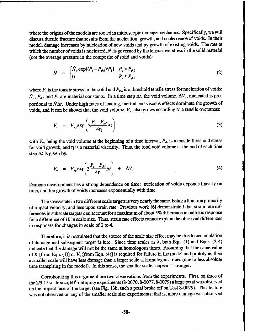
where the origins of the models are rooted in microscopic damage mechanics. Specifically, we will discuss ductile fracture that results from the nucleation, growth, and coalescence of voids. In their model, damage increases by nucleation of new voids and by growth of existing voids. The rate at which the number of voids is nucleated, N, is governed by the tensile overstress in the solid material (not the average pressure in the composite of solid and voids):

[0 PSZP,HO

where Ps is the tensile stress in the solid and Pm is a threshold tensile stress for nucleation of voids; fie, Pm and Pj are material constants. In a time step At, the void volume, AV„, nucleated is proportional to NAt. Under high rates of loading, inertial and viscous effects dominate the growth of voids, and it can be shown that the void volume, Vv, also grows according to a tensile overstress:

Vv = Vvoexp ( P -P } s rW-ht

4T| (3)

V *"l J

with Vvo being the void volume at the beginning of a time interval, PM is a tensile threshold stress for void growth, and t| is a material viscosity. Thus, the total void volume at the end of each time step At is given by:

Vv = VTOexp 3^-^Af + AV» <4>

Damage development has a strong dependence on time: nucleation of voids depends linearly on time, and the growth of voids increases exponentially with time.

The stress state in two different scale targets is very nearly the same, being a function primarily of impact velocity, and less upon strain rate. Previous work [6] demonstrated that strain rate differences in subscale targets can account for a maximum of about 5% difference in ballistic response for a difference of 10 in scale size. Thus, strain rate effects cannot explain the observed differences in responses for changes in scale of 2 to 4.

Therefore, it is postulated that the source of the scale size effect may be due to accumulation of damage and subsequent target failure. Since time scales as X, both Eqn. (1) and Eqns. (2-4) indicate that the damage will not be the same at homologous times. Assuming that the same value of K [from Eqn. (1)] or Vy [from Eqn. (4)] is required for failure in the model and prototype, then a smaller scale will have less damage than a larger scale at homologous times (due to less absolute time transpiring in the model). In this sense, the smaller scale "appears" stronger.

Corroborating this argument are two observations from the experiments. First, on three of the 1/3.15 scale size, 60°-obliquity experiments (8-0070,8-0077,8-0079) a large petal was observed on the impact face of the target (see Fig. 13b, such a petal broke off on Test 8-0079). This feature was not observed on any of the smaller scale size experiments; that is, more damage was observed

-58-

on the larger target. Second, for the experiments reported here, the scale size effect is only seen in the "larger values" of the data sets. For example, a scale size effect is seen in CID for the 60°-obliquity tests, where values are ~ 2 to 2.8, while the 0o-obliquity CID values are all less than 1. Similarly, scale size effects are seen in the larger H^ ID values at 60° obliquity (~ 5 to 7), and not in the rest of the Hmax ID and H^ ID data set, where all values are approximately 2.5 or less. This suggests that scale size effects are observed in those features that require more time to deform plastically to their larger sizes.

There is a caveat to the above argument, however. If the stress is far above damage thresholds, the damage rate is quickly saturated, and a time-evolution model can be replaced by a much more simplistic "sudden damage" criterion. An appropriate critical level can then be estimated from known material properties, e.g., total equivalent plastic strain at failure. Reference [16] discusses computational failure models, and provides an example that demonstrates that computational results are insensitive to the details of failure when a projectile overmatches a target. If a maximum stress, equivalent plastic strain, or plastic work is a suitable failure criterion, then there will be no differences in failure between the model and prototype (per the model law of Table 5), except for slight differences in the stress resulting from strain rate. This saturation of damage possibly explains the observed differences between the results at 1.5 km/s and 2.2 km/s. The overstress would be considerably larger at 2.2 km/s, and therefore damage would saturate much quicker.

If differences in damage evolution are to be a plausible explanation of the scaling effect, it must be demonstrated that the characteristic failure times are approximately the same as the loading times. We offer the following example. It is observed experimentally that the spall strength of metals, e.g., Armco iron and 6061-T6 aluminum, decreases by a factor of two as the pulse width changes from 0.05-0.10 |is, which implies that a characteristic damage time for spallation (a wave propagation phenomenon) is on the order of several tenths of a microsecond [17]. The failure mode of the targets in the present work is not spallation, but order-of-magnitude estimates can be made of the failure time for the experiments reported here. It might be expected, for ballistic experiments where the operative mechanism is large-field plastic flow, that characteristic damage times might be an order of magnitude longer than for spallation, i.e., on the order of a few microseconds. An estimate of the loading time is obtained from nominal steady-state penetration. For the order-of- magnitude estimates here, the erosion rate of the projectile is approximately one-half the impact velocity, e.g., 1.0 km/s. Since the projectile opens a cavity approximately 2.0 projectile diameters, a characteristic loading time is estimated to be on the order of 4 to 16 |is as the scale factor changes from 1/12 to 1/3. Clearly, these order-of-magnitude estimates are heuristic, but it appears plausible that characteristic loading and failure times are similar.

One might ask the question why scale size effects were not clearly observed in features such as penetration depth, bulge height, and residual projectile velocity and length, "long term" features which, according to the above theory, should demonstrate a scale size effect. These data do indicate that the 1/12.60-scale targets were harder to penetrate than the comparable 1/3.15-scale targets. However, the relatively small quantity of low yaw data seem to have precluded the clear quantification of a scale size effect. We attempted to "correct" the P/L data set to account for total yaw greater than 4°, but were not able to derive a data set that clearly indicated a scale size effect. It is likely that our correction methodology introduced as much or more uncertainty as any difference

-59-

attributable to scale size effects. We believe that a larger experimental database would allow for quantification of the penetration/perforation scale size effect. The experimental work in Refs. [1] and [18] clearly demonstrate a scale effect for the ballistic limit velocity. Magness and Leonard [18] also showed a scale size effect for P/L.

The work here is suggestive of a scale size effect, but is not as definitive as one might like for some measures of ballistic performance. But this work, in conjunction with the studies of Ref. [ 1 ] and that of Magness and Leonard [18], support the existence of a scale effect in ballistic experiments, and that this effect is most pronounced near a threshold condition, such as a ballistic limit condition. A number of questions are unresolved at this point. For example, is there some scale at which the scale effect saturates, i.e., further increases in scale size will not change the experimental findings? What is the dependence of the scale effect on impact velocity? (A velocity dependence has been suggested in the findings in this study.) Is there a dependence on normalized target thickness, i.e., do thicker targets demonstrate a larger scale effect than thinner targets? If failure is a contributing cause to the scale effect, how much of the scale effect is attributed to the projectile versus the target, and are there different domains of influence, e.g., penetration versus breakout? The resolution of the questions are worthy of further study.

-60-

10.0 ACKNOWLEDGMENTS

The authors would like to acknowledge the support and encouragement of Dr. Thomas Kiehne, formerly of the Defense Advanced Research Projects Agency, and now at the Institute for Advanced Technology, Mr. Billy Hogan of Los Alamos National Laboratory, and Mr. Rene Larriva of Interferometrics, Inc. This work was performed under contract DE-AC04-90AL58770, adminis- tered out of the Department of Energy, Albuquerque Office, and then transferred to the U.S. Army Research Office, Contract DAAL03-91-C-0021. The contract was funded by the Defense Advanced Projects Research Agency.

-61-

11.0 REFERENCES

1. Charles E. Anderson, Jr., Scott A. Mullin, Andrew J. Piekutowski, Neil W. Blaylock, Kevin L. Poormon, "Scale Model Experiments with Ceramic Laminate Targets", Int. J. Impact Engng, 16(6), in publication (1995).

2. W. E. Baker, P. S. Westing, and F. T. Dodge, Similarity Methods in Engineering Dynamics: Theory and Practice of Scale Modeling, Southwest Research Institute, San Antonio, TX (1981).

3. Walt Gray, Scott A. Mullin, Herve Couque, Neil Blaylock, "Heavy Metal Fragment Effects with Light Armor," prepared by Southwest Research Institute for U.S. Air Force AFATL, Eglin AFB, FL, Project 06-2494, AFATL-TR-90-91, September 1990.

4. G. R. Johnson and W. H. Cook, "Fracture Characteristics of Three Metals Subjected to Various Strains, Strain Rates, Temperature and Pressures," Engng. Fract. Mech., 21(1), 31-48 (1985).

5. G. R. Johnson and T. J. Holmquist, "Test Data and Computational Strength and Fracture Model Constants for 23 Materials Subjected to Large Strains, High Strain Rates, and High Temperatures," Report LA-11463-MS, Los Alamos National Laboratory, Los Alamos, NM (1989).

6. Charles E. Anderson, Jr., Scott A. Mullin, Chris J. Kuhlman, "Strain-Rate Effects in Replica Scale Model Penetration Experiments," Int. J. Impact Engng., 13(1), 35-52 (1993).

7. A. Täte, "A Theory for the Deceleration of Long Rods after Impact," /. Phys. Mechs. Solids, 15,389-399 (1967).

8. A. Täte, "Further Results in the Theory of Long-Rod Penetration," /. Phys. Mech. Solids, 17, 141-150 (1969).

9. V. Hohler and A. J. Stilp, "Long-Rod Penetration Mechanics", in High Velocity Impact Dynamics (J. A. Zukas, editor), John Wiley & Sons, Inc., New York (1990).

10. Y. Partom and D. Yaziv, "Penetration of L/D = 10 and 20 Tungsten Alloy Projectiles into RHA," High Pressure Science and Technology—1993, (S. C. Schmidt, J. W. Shaner, G. A. Samara, and M. Ross, Eds.), pp. 1801-1804, AIP Press, Woodbury, NY (1994).

11. A. Rosenberg and E. Dekel, "The Relation Between the Penetration Capability of Long Rods and their Length to Diameter Ratio," Int. J. Impact Engng., 15(2), 125-129 (1994).

12. C. E. Anderson, Jr., J. D. Walker, S. J. Bless, and Y. Partom, "On the UD Effect for Long-Rod Penetration," Int. J. Impact Engng., 18(1), in publication (1996).

13. F. R. Tuler and B. M. Butcher, "A Criterion for the Time Dependence of Dynamic Fracture," Int. J. Fract. Mech., 4(4), 431-437 (1968).

14. S. Cochran and D. Banner, "Spall Studies in Uranium," /. Appl. Phys., 48(7), 2729-2737 (1977).

-63-

15. D. R. Curran, L. Seaman, and D. A. Shockey, "Dynamic Failure of Solids," Physics Reports (Review Section of Physics Letters), 147(5&6), 253-388 (1987).

16. C. E. Anderson, Jr. and S. R. Bodner, "Ballistic Impact: The Status of Analytical and Numerical Modeling," Int. J. Impact Engng., 7(1), 9-35 (1988).

17. L. Davison and R. A. Graham, "Shock Compression of Solids," Physics Reports (Review Section of Physics Letters), 55(4), 255-379, (1979).

18. L. Magness, Jr. and W. Leonard, "Scaling Issues for Kinetic Energy Penetrators," Proc. 14th Int. Symp. on Ballistics, Vol. 2,281-289, Quebec City, 26-29 September (1993).

-64-

SCALE MODEL PENETRATION EXPERIMENTS - DTIC

Documents

Transcript of SCALE MODEL PENETRATION EXPERIMENTS - DTIC