Convenient estimators for the panel probit model

Journal of Econometrics 87 (1998) 329—371

Convenient estimators for the panel probit model

Irene Bertschek!, Michael Lechner",*! Institut de Statistique, Universite& Catholique de Louvain, Voie du Roman Pays 20,

B-1348 Louvain-la-Neuve, Belgium" Fakulta( t fu( r Volkswirtschaftslehre, Universita% t St. Gallen, Dufourstr. 50,

CH-9000 St. Gallen, Switzerland

Received 1 October 1995; received in revised form 1 November 1997

Abstract

The paper shows that several estimators for the panel probit model suggested in theliterature belong to a common class of GMM estimators. They are relatively easy tocompute because they are based on conditional moment restrictions involving univariatemoments of the binary dependent variable only. Applying nonparametric methods wediscuss an estimator that is optimal in this class. A Monte Carlo study shows thata particular variant of this estimator has good small sample properties and that theefficiency loss compared to maximum likelihood is small. An application to theproduct innovation decisions of German firms reveals the expected efficiency gains.( 1998 Elsevier Science S.A. All rights reserved.

JEL classification: C14; C23; C25

Keywords: Panel probit model; GMM; Conditional moment restrictions; k-nearestneighbor estimation

1. Introduction

The probit model is a popular model in applied microeconometric work. Incross-section analysis, when the error terms of the observations are assumed tobe identically and independently distributed (i.i.d.), maximum-likelihood (ML) istypically the chosen estimation method. It is easy and fast to compute andasymptotically efficient. However, using ML on panel data is burdensome unless

*Corresponding author. E-mail: [email protected]

0304-4076/98/$— see front matter ( 1998 Elsevier Science S.A. All rights reserved.PII S 0 3 0 4 - 4 0 7 6 ( 9 8 ) 0 0 0 0 8 - 6

one adopts the unattractive assumption of i.i.d. error terms, which rules out anypersistent or idiosyncratic components in the errors of the same unit (firm,individual) over time.1 As a consequence, the joint ¹-variate probability distri-bution over time needs to be specified. In cases when no analytical expressionsexist for the individual likelihood contributions — such as for probit and tobitmodels — numerical evaluations of cumulative distribution functions could bea problem. In addition, there may be a possibly large number of nuisanceparameters resulting from the intertemporal error covariance matrix.

Several solutions to that problem are discussed in the literature: one group ofmethods focuses on approximating the integrals by simulation. Although sub-stantial progress has been achieved recently — see for example the survey byHajivassiliou and Ruud (1994) — these methods are still computationally expen-sive. At least for a large number of time periods, they require a specification ofthe error process with a limited number of covariance parameters. Anothergroup of estimators restricts the error terms to have a random effects specifica-tion whereby the computation of the ML estimator is considerably simplified(see for instance Butler and Moffitt, 1982). This can be generalized by introduc-ing one-factor or multi-factor schemes to allow for a more flexible error struc-ture as proposed for example by Heckman (1981). However, this generalizationcomes at the cost of having to estimate more parameters of the covariancematrix, and — in the case of multi-factor schemes — increases the dimension ofintegration. Finally, a third group of estimators is based on the generalizedmethod of moments (GMM) using moment restrictions that do not dependon parameters of the intertemporal error covariance matrix (Avery et al., 1983).An evaluation of the joint ¹-variate cumulative distribution function is notnecessary.

The main focus of the paper is on this third group of estimators. We show thatseveral often-used and conveniently computable estimators, such as pooledprobit, Chamberlain’s (1980, 1984) sequential estimator or several variants ofother suggested GMM estimators belong to a class of GMM estimators usingthe same conditional moment restrictions. An asymptotic efficiency ranking ofthese and other related GMM estimators is established. Applying the asymp-totic efficiency results for intrumental variable estimation of nonlinear modelsestablished by Newey (1990) and Chamberlain (1987), we discuss several feasibleestimators that are asymptotically efficient in that class of GMM estimators.Although the estimators use nonparameteric estimation to obtain the asymp-totically efficient instruments, they retain the basic simplicity, feasibility androbustness to arbitrary error structures that are the great advantages of thepreviously discussed GMM estimators. An extensive Monte Carlo study shows

1We consider the case of a large number of independent units (N) observed for a finite number ofperiods (¹).

330 I. Bertschek, M. Lechner / Journal of Econometrics 87 (1998) 329–371

that a particular variant has good small sample properties. Furthermore,the efficiency loss compared to full information maximum likelihood appearsto be rather small. Finally, various estimators are applied to an exampletaken from industrial economics. Firms’ product innovative activity isanalysed using a panel data set that contains 1270 firms of the Germanmanufacturing industry observed over five periods (years). The suggested es-timator performs well in practice, and the efficiency gains compared to the otherestimators turn out to be important for the economic interpretation of theestimation results.

The following section motivates the econometric discussion by introducing anempirical example. Furthermore, it establishes the necessary notation and thestatistical assumptions underlying the analysis. Section 3 briefly discusses re-stricted and unrestricted maximum likelihood estimation and points out someof the problems that could appear in the context considered here. The first partof Section 4 gives a compact summary of the theory of GMM estimation withconditional moment restrictions. An asymptotic efficiency ranking of severalestimators using this framework is established in the second part. The third partdiscusses the implementation of an estimator that exploits the information ofthese conditional moment restrictions optimally. The Monte Carlo results arepresented in Section 5. In particular, the data generating processes are describedin Section 5.1. Section 5.2 discusses the implementation of the various es-timators. Their asymptotic distributions are compared in Section 5.3. Finally,Section 5.4 addresses the finite sample properties. The application is given inSection 6. Section 7 concludes. Appendix A gives a useful lemma concerning theasymptotic equivalence of several types of GMM estimators. Appendix B con-tains additional Monte Carlo results and Appendix C gives more details on thedata used for the application.

2. Empirical example, notation and basic assumptions

An empirical example for our discussion of panel probit models is the analysisof firms’ innovative activity as a response to imports and foreign direct invest-ment (FDI) as considered in Bertschek (1995). The main hypothesis put forwardin that paper is that imports and inward FDI have positive effects on theinnovative activity of domestic firms. The intuition for this effect is that importsand FDI represent a competitive threat to domestic firms. Competition on thedomestic market is enhanced and the profitability of the domestic firms might bereduced. As a consequence, these firms have to produce more efficiently. Increas-ing the innovative activity is one possibility to react to this competitive threatand to maintain the market position.

The dependent variable available in the data takes the value one if a productinnovation has been realized within the last year and the value zero otherwise.

I. Bertschek, M. Lechner / Journal of Econometrics 87 (1998) 329–371 331

The binary character of this variable leads us to formulate the model in terms ofa latent variable y*

tithat represents for instance the firms’ unobservable expendi-

tures for innovation. y*ti

is linearly related to the explanatory variables xti. The

vector b0 contains K deterministic coefficients. uti

is a scalar error term control-ling effects that are not captured by the regressors:

y*ti"x

tib0#u

ti. (1)

The observation rule is:

yti"1(y*

ti'0), i"1,2, N, t"1,2,¹, (2)

where the indicator function 1( ) ) equals one if the expression in brackets is trueand zero otherwise. For each individual i we collect ¹ observations such thatyi"(y

1i,2,y

Ti)@ is a ¹]1 vector and x

i"(x@

1i,2,x@

Ti)@ represents a ¹]K

matrix of regressors.The following standard assumptions are made: We observe N independent

random draws (yi, x

i)"z

iin the joint distribution of the random variables

(½,X)"Z. Thus, zihas dimension ¹](K#1). In the data set, z

iis observed for

N"1270 firms from 1984 to 1988 (¹"5). This is compatible with the assump-tion of fixed ¹ and increasing N forming the basis of the following asymptoticarguments.

The error terms ui"(u

1i,2,u

Ti)@ are assumed to be jointly normally distrib-

uted with mean zero and covariance matrix R and to be independent of theexplanatory variables which implies the strict exogeneity of the latter. They areuncorrelated over firms but may be correlated over time for the same firm. Onemain-diagonal element of R has to be set to unity because indentification of b0 isonly up to scale.2 The off-diagonal elements of R are not of interest in theempirical study and therefore, they are considered as nuisance parameters.

3. Maximum likelihood estimation

The typical approach for estimating probit models in applied microeconomet-ric work based on single cross-sections is maximum likelihood (cf. Maddala,

2 In order to simplify the exposition we normalize all variances (p11"p

tt"p

TT"1, for all t).

However, the basic structure of the results remains unchanged if the following reparameterization ismade: h"(h@

1, h@

2)@, h

1"b/p

1, h

2"(h

22,2,h

2T)@, h

2t"p

1/p

tand o

ts"p

ts/(p

spt) where p

tsdenotes

Eºtº

sand p

t"Jp

tt. h is then used in place of b in Sections 4 and 5. The exact results using this

extensive notation are contained in a previous version of this paper that is available on request fromthe authors.


1983, for many examples). Due to the availability of fast and accurate methodsto evaluate the univariate normal cumulative distribution function (c.d.f.) — forwhich no analytical formula is available — and due to the global concavity of thelog likelihood function, this is a useful approach implemented in many softwarepackages. However, in the case of panel data there are several issues that makeML estimation less attractive: first of all, the likelihood function depends on¹(¹!1)/2 unknown off-diagonal elements of R that have to be estimated.Secondly and probably even more important in practice, the computation timeof the ¹-variate c.d.f. instead of the univariate c.d.f. is prohibitively high for¹'4 or 5 even on very powerful computers (cf. Hajivassiliou and Ruud, 1994).Finally, the possible lack of global concavity may represent a problem as well.

While the last issue is widely ignored, many papers appeared recently in theliterature suggesting that the dimensionality problem with respect to integrationcan be overcome by using suitable simulation methods to approximate themultidimensional integral. For details on these issues the reader is referred to theexcellent survey by Hajivassiliou and Ruud (1994). However, although estimatesbased on simulation methods are easier to compute than exact ML, there aredrawbacks with this approach as well: firstly, a sufficiently accurate estima-tion of the multivariate probabilities may still be computationally expensive.Secondly, R is typically restricted by assuming parametric error processes,mostly AR or MA processes, sometimes combined with random effects specifica-tions. Due to these restrictions the number of parameters is considerablyreduced and simulation estimation becomes feasible.

Some restrictions also drastically reduce the dimension of integration. Themost widely used restriction is the assumption that the error terms are equicor-related over time, i.e. the error terms can be decomposed into two mutuallyindependent components: a time constant random effect c

iand a remainder term

eti

(assumed to be independent over time) such that uti"dc

i#e

ti. d is a positive

constant to be estimated and ciand e

tifollow a standard normal distribution.3 In

this case the log likelihood function is given by:

¸(y,x;b, d)"1

N

N+i/1

ln

`=

P~=

T<t/1

MU(xtib#dc)yti

][1!U(xtib#dc](1~yti)N/(c) dc, (3)

U( ) ) and /( ) ) denote the cumulative distribution function and the probabilitydistribution function (p.d.f.) of the univariate standard normal distribution,respectively. Butler and Moffitt (1982) suggest an efficient method to evaluate

3For notational convenience we change the normalization of ptt

in this case, by setting p2et"1.


the integral numerically by Hermite integration (e.g. Stroud and Secrest, 1966,p. 22). The estimator is then given by:

AbKN

dKNB"argmax

b,d

1

N

N+i/1

lnV+v/1

T<t/1

MU(xtib#dc

v)yti

][1!U(xtib#dc

v)](1~yti)Nw

v, (4)

where cvand w

vare the respective evaluation points and weights. Their values

have been tabulated by various authors, e.g. Abramowitz and Stegun (1966, p.924) and Stroud and Secrest (1966, Table 5).

A comparison of restricted ‘exact’ and simulated ML for this error decompo-sition can be found in Guilkey and Murphy (1993). The error structure can bemade more flexible by allowing d to vary over time and by the possibleintroduction of more than one factor (cf. Heckman, 1981). However, this willagain increase the number of parameters to be estimated and the dimension ofintegration.

Using the framework of generalized method of moments (GMM) estimationAvery et al. (1983) show that ML estimation under the even more restrictiveassumption of independent errors over time leads to consistent estimates for b0.4The ‘pooled’ pseudo-log likelihood function is given by:

bKN"argmax

b

1

N

N+i/1

T+t/1

ytiln U(x

tib)#(1!y

ti) ln[1!U(x

tib)]. (5)

The advantage of the pooled estimator is its simplicity, global concavity andlack of nuisance parameters. However, the disadvantage is its inefficiency andthat the estimated asymptotic standard errors assuming the pseudo-log likeli-hood function to be the true log likelihood are inconsistent, if the errors are infact correlated over time. The following section will show that with GMMestimation the advantages of the pooled probit can be retained and that thedisadvantages can be overcome.

4. GMM estimation

The following subsection introduces the GMM framework based on condi-tional moment restriction. It summarizes some of the results of Chamberlain(1987) and Newey (1990, 1993) and adapts them to the panel probit model.

4See also Robinson (1982) for the more general proof that the probit-ML assuming independenterrors represents a consistent estimator even when the true errors are not independent.


Section 4.2 shows how this framework can be used to obtain an efficiencyranking of several panel probit estimators that have been suggested in theliterature. Finally, the estimation of the asymptotically optimal instruments isdiscussed.

4.1. Conditional moment restrictions and asymptotic efficiency

The model presented in Section 2 implies the following moment conditions:

E[M(Z;b0)DX]"0,

M(Z;b)"[m1(Z

1;b),2, m

t(Z

t;b),2, m

T(Z

T;b)]@,

mt(Z

t;b)"½

t!U(x

tib). (6)

The use of these conditional moments for estimation has the advantage thattheir evaluation does not require multidimensional integration and that they donot depend on the ¹(¹!1)/2 off-diagonal elements of R.

Given these conditional moment restrictions GMM can be used forestimation (Hansen, 1982). The following exposition borrows from the ex-cellent survey by Newey (1993), who summarizes the results for such GMMestimators.

Based on Eq. (6) the unconditional moment restrictions to be used for theestimation are obtained by observing that M(Z;b0) will be uncorrelated with allfunctions of X. Hence

EA(X)M(Z;b0)"0. (7)

A(X) is a p]¹ ‘instrument matrix’. An estimate bKN

of b0 is obtained by settinga quadratic form of the sample analogues

gN(b)"

1

N

N+i/1

A(xi)M(z

i;b) (8)

close to zero such that

bKN"argmin

bgN(b)@Pg

N(b). (9)

Under suitable regularity conditions on gN

and with the positive semi-definite

matrix P,bKN

is JN-consistent and asymptotically normal:

JN(bKN!b0)

$P N(0,K), (10)


where

K:"(G@PG)~1G@P»PG(G@PG)~1 (K]K),

G:"ECA(X)LM(Z;b0)

Lb@ D"EA(X)D(X)(p]K),

»:"E[A(X)M(Z;b0)M(Z;b0)@A(X)@]

"E[A(X)X(X)A(X)@] (p]p),

D(X)"ELM(Z;b0)

Lb@DX

(¹]K),

X(X)"EM(Z;b0)M(Z;b0)@DX (¹]¹). (11)

A consistent estimate of the covariance matrix K can be obtained by replacingexpectations by sample means and b0 by bK

N. The tools to minimize the asymp-

totic variance of this estimator are the optimal choice of the instruments A(X)and of the weighting matrix P. As shown by Hansen (1982) in a more generalsetting, the optimal choice of P is »~1 or any consistent estimator of it.Chamberlain (1987) and Newey (1990) derived the optimal instrument matrixA*:

A*(X)"CD(X)@X(X)~1, (12)

where C is any nonsingular K]K matrix. The column-dimension of A* equalsK, so the choice of P is irrelevant. To obtain a feasible estimator, D(X) and X(X)may be substituted by consistent estimates without affecting the asymptoticdistribution of bK

N. For the GMM estimator using the optimal instruments, the

covariance matrix simplifies to

K*"ME[D(X)@X(X)~1D(X)]N~1. (13)

For the probit model and observation ‘i’, D(xi) with typical row d

ti, and X(x

i)

with typical element utsi

, have the following form:

dti"!/(x

tib)x

ti. (14)

For notational convenience let Uti:"U(x

tib0) and U(2)

tsi:"U(2)(x

tib0, x

sib0, o0

ts).

U(2)( ) ) denotes the cumulative distribution function of the bivariate standard-ized normal distribution with correlation coefficient o0

ts. Hence, we obtain

utsi"[E(½

t!U

ti)(½

s!U

si)DX"x

i]"G

Uti(1!U

ti) if t"s,

U(2)tsi!U

tiU

siif tOs.

(15)


Note that utsi

(xi) has the same sign as o

tsand that u

tsi"0 if o

ts"0. The

estimation of the optimal GMM-estimator is still difficult, because it depends onthe unknown correlation coefficients of R through the terms U(2)

tsiin Eq. (15).

A possible solution would be to replace these unknown coefficients by consistentestimates obtained from (¹!1)¹/2 separate bivariate probits. But this iscumbersome for large ¹.5

To circumvent these problems, Newey (1990, 1993) suggests the use of non-parametric methods, such as nearest neighbor estimation and series approxima-tions to obtain consistent estimates of X(x

i). He derives the conditions necessary

for these methods to result in consistent and asymptotically efficient estimates ofb (Newey, 1993, Theorems 1 and 2). We will come back to this issue inSection 4.3.

Before doing so, we will discuss the asymptotic properties of various othersub-optimal GMM estimators suggested in the literature. They should beconsidered as competitors to the asymptotically optimal GMM estimator be-cause of their computational simplicity, and because some of them requireweaker conditions with respect to the exogeneity of the regressors. Note that theconditioning in the ¹-dimensional moment function given in Eq. (6) is onX"(X

1,2, X

T). This is the so-called strict exogeneity restriction. The results

with respect to consistency and asymptotic efficiency put forward in Section 4do require this assumption to hold. A weaker assumption would be to requireonly E[m

t(Z

t; b0)DX

t]"0 (weak exogeneity).6 The consequence is that only

functions of Xtare valid instruments for the t’th-element of M. Inspecting the

form of the instrument matrix A(X) suggested in this section, it can be seen thatonly the pooled probit and the sequential estimator are not affected by thisweakening of the exogeneity assumption. This might be an important considera-tion in practice, since in particular the ‘optimal’ instrument matrix given inEq. (12) is no longer valid if errors are correlated over time.

4.2. Efficiency ranking of several estimators

All GMM estimators to be discussed in the following are consistent regardlessof the true covariance matrix of the error terms, but differ in their asymptoticvariance. We use the GMM framework to readily obtain asymptotic efficiencycomparisons.

5An alternative would be to set up another GMM estimator based on ¹(¹!1)/2 momentconditions like y

tiysi!U(2)

tsiwith unknown b0 replaced by a consistent estimate bK

N. In this case these

moment conditions would suffice to estimate the unknown correlations.

6Note that when X contains lagged dependent variables this condition holds only when errors areassumed to be independent over time.


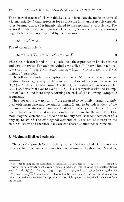
Avery et al. (1983) observe that the scores of the pooled ML estimator implymoment conditions that can be used for GMM estimation. Using the lemma inAppendix A leads to an asymptotically equivalent GMM estimator of thefollowing form:

gPP1N

(z;b)"1

N

N+i/1

APP1i

(xi)M(z

i;b) (K]1), (16)

APP1i

(xi)"D@

i(x

i)[XPP

i(x

i)]~1,

XPPi

(xi)"A

U(x1ib0)[1!U(x

1ib0)] 0 0

0 } 0

0 0 U(xTi

b0)[1!U(xTi

b0)]B(¹]¹).

Since there are no overidentifying restrictions, the choice of the weighting matrixP does not matter. It is clear from the structure of XPP

ithat the efficiency loss of

the pooled probit estimator is due to the ignorance of possible nonzero off-diagonal elements in X. In order to compare the pooled ML estimator withother GMM estimators, it is useful to rewrite this estimator in an equivalentrepresentation:

gPP2N

(z;b)"1

N

N+i/1

APP2i

(xi)M(z

i;b) (¹K]1), (17)

APP2i

(xi)"A

~((x1ib0)U(x1ib0)*1~U(x1ib0)+

x@1i

0 0

0 } 0

0 0 ~((xTib0)U(xTib0)*1~U(xTib0)+

x@TiB (¹K]¹).

(18)

Note that by stacking the moment conditions there are overidentifying restric-tions and the particular choice of the weighting matrix P matters. We see thatpooled probit is equivalent to a GMM estimator with an inefficient weightingmatrix PPP2:

PPP2"RR@, R"AIKF

IKB (¹K]K), I

K"A

1 0 0

0 } 0

0 0 1B (K]K).

Therefore using the optimal PPP2* instead of PPP2 leads to an asymptoticallymore efficient estimator:

PPP2*"EAPP2(X)M(Z;b0)M(Z;b0)@APP2(X)@

"EAPP2(X)X(X)APP2(X)@. (19)


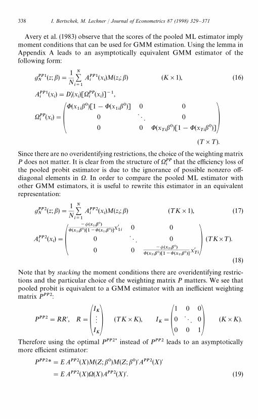
However, as Breitung and Lechner (1997) show in a Monte Carlo study, theestimator based on PPP2* may actually perform worse than pooled probit insmall and medium sized samples. Other estimators suggested by Avery et al.(1983) are in the same spirit, i.e. the efficiency gains depend on an expansion ofthe instrument set together with the use of the optimal weighting matrix. Hence,they share the same problem, namely that a large number of observations isneeded to get a sufficiently accurate estimate of this high-dimensional matrix.

Another popular and convenient estimator is the sequential estimator sugges-ted by Chamberlain (1980, 1984). The idea is as follows: In a first step a probit isestimated for each cross-section. After computing the joint covariance matrix ofall first step estimates, a minimum distance procedure is used to impose thecoefficient restrictions due to the panel structure to obtain more efficientestimates. Using the scores of the probit for each period and employing similarreformulations as for the pooled probit the first step of this estimator can beexpressed in our framework:

gSN(z;b

1,2,b

T)"

1

N

N+i/1

DSi(x

i)@(XP

i)~1M(z

i;b

1,2,b

T)

"

1

N

N+i/1

APP2i

(xi)M(z

i; b

1,2,b

T), (20)

DSi"A

!/(x1ib0)x

1i0 0

0 } 0

0 0 !/(xTi

b0)xTiB (¹]K¹).

Breitung and Lechner (1997) show that when the minimum distance step isbased on the optimal weighting matrix, this estimator is asymptotically moreefficient than pooled ML, because it is equivalent to the GMM estimator ofEq. (17) using the optimal weighting matrix PPP2*.

Since Monte Carlo evidence suggests that increasing efficiency by increasingthe number of instruments may lead to small sample problems, we now turn toa different way of increasing efficiency compared to pooled ML that avoids thisdilemma.

The idea is to use the moment function given in Eq. (8) together with theoptimal instruments (Eq. (12)) leading to an estimator without overidentifyingrestrictions, so that a high-dimensional weighting matrix does not need to beestimated. The problem is then to find a consistent estimator of X(X). Oneapproach is to assume an error distribution that is plausible in many cases andleads to an X(X) that is easy to compute. When this assumption is wrong, thenthe estimator is not efficient but still consistent. In this vein is a suggestion byBreitung and Lechner (1997). They assume a random effects (equicorrelation)


structure with a ‘small’ variance of the random effect (p2c). A Taylor expansion of

the moment condition (conditional on c) around p2c, leads to an approximation

of X(X), denoted by XSS(X), that should be particularly good when the true errorstructure is small random effects:

There is only one unknown parameter, pct, in addition to b0, and it can be

estimated for example by OLS with the following regressions:

(yti!UI

ti)(y

si!UI

si)"p2

c/I

ti/Isi#error, t, s"1,2,¹; tOs, (21)

where I denotes quantities evaluated with a consistent JN-normal first stepestimate bI

Nof b0. This estimator (GMM-SS) is easy and fast to compute.

However, the dependence of the potential efficiency gains on the validity of therather restrictive assumption about the true error covariance is not very satisfac-tory. Therefore, the next subsection discusses a simple nonparametric estimateof the optimal instruments.

4.3. Nonparametric estimation of X(xi)

In the following we focus on the k-nearest neighbor (k-NN) approach toestimate X(x

i), because of its simplicity. k-NN averages locally over functions of

the data of those observations belonging to the k-nearest neighbors. Underregularity conditions (Newey, 1993), this gives consistent estimates of X(x

i)

evaluated at bIN

and denoted by XI (xi) for each observation ‘i’ without the need

for estimating ots. Thus, an element of X(x

i) is estimated by

uJtsi

(xi)"

N+j/1

¼tsij

mt(z

tj; bI

N)m

s(z

sj; bI

N), (22)

where ¼tsij

represents a weight function.In order to determine the neighbors of observation ‘i’ it is necessary to define

a distance or similarity measure. Since the elements of the diagonal ofX(x

i) (u

tsi, t"s) depend only on the individual indices of one time period (x

tib),

we face a simple one-dimensional estimation problem. The off-diagonal


elements, utsi

, tOs, depend on the linear indices of two time periods,W

tsij"[(x

ti!x

tj)b, (x

si!x

sj)b].7

Hence, the distance used to define the neighbors should refer to those two.Here, another possibility is considered: The distance between observations ‘i’and ‘j’ refers to the indices of all periods W

ij"[(x

1i!x

1j)b,2, (x

Ti!x

Tj)b].

Thus, the distance is defined either by mtsij

"Wtsij

Cxbts

W@tsij

in case of estimatingeach single element of X(x

i) individually or by m

ij"W

ijCxbW@

ijwhen all elements

of X(xi) are estimated jointly (¼

tsij"¼

ijfor all t, s). If not indicated otherwise,

the weighting matrices Cxb and Cxbts

, respectively, are set to unity in the MonteCarlo study. However, different choices of positive definite matrices can be usedas well, such as the inverse of the covariance matrix of the linear indices (S~1

xb ) oronly the main diagonal of S~1

xb .As a consequence, the nonparametric estimators can either be constructed

according to Eq. (22) which estimates every single element of X(xi) individually

(indiv) or alternatively, by estimating all elements of X(xi) jointly ( joint). The joint

estimator is given by

XI +(xi)"

N+j/1

¼ijM(z

j;bI

N)M(z

j;bI

N)@. (23)

The second procedure is much faster to compute, because the observationshave to be sorted only once for the estimation of all elements of X(x

i). Therefore,

the larger ¹ the faster is joint relative to indiv.A weight function assigns positive weights to those observations belonging to

the k nearest neighbors (k)N), but zero weights to all other observations andthe observation i itself. The weights sum to unity. Stone (1977, p. 600) suggestsseveral weight functions that fulfil the necessary regularity conditions. Supposethat the observations are ordered according to their distance to observation ‘i’,where ‘j"1’ denotes observation ‘i’ itself. The uniform weight function (uniform)is then given by:

¼tsij

"G1/k, 2)j)k,

0, j"1, j'k.(24)

A smoother version is for example the quadratic (quadr) weight function:

¼tsij

"G[k2!( j!1)2]/[k(k#1)(4k!1)/6], 2)j)k,

0 j"1, j'k.(25)

It remains to choose the smoothing parameter k. In our Monte Carlo studywe follow Newey (1993) in applying cross-validation for a data-driven choice

7Note that the dimension is lower than for the measure suggested by Newey (1993) who uses thesingle elements of x

ti(xk

ti) instead of x

tib to define similarity for more general models.


of k. He shows that cross-validation can be based on the difference betweenestimated and true moment functions:

N+i/1

MAI *(xi)!A*(x

i)NM(Z;b0)/JN. (26)

Suppose that AI *(xi) denotes a consistent estimate of A*(x

i) evaluated at bI

N.

Then the resulting cross-validation function to be minimized is as follows(Newey, 1993, p. 433):

CK »(k)"trCQN+i/1

RI (xi)XI (x

i)RI (x

i)@D, (27)

RI (xi)"MAI *(x

i)[M(z

i,bI

N)M(z

i, bI

N)@!XI (x

i)]NXI (x

i)~1.

Q is a positive definite matrix. In the following Monte Carlo study and theapplication we choose Q"+N

i/1D(x

i)D(x

i)@ according to Newey (1993).

Another possibility for nonparametric estimation of X(xi) is to use

kernel regression (Carroll, 1982; Hardle, 1990, for example). However, twodrawbacks of kernel regression in our context are the increased complexityof the estimation and the problem of random denominators which mightproduce erratic behavior (see Robinson, 1987). This problem could be solved bytrimming, but this leads to a loss of efficiency by reducing the number ofobservations.

5. Monte Carlo study

The following subsection describes the data generating processes (DGPs)used. Following this, we discuss the implementation of the various esti-mators. We compare the standard errors of their asymptotic distributionsin Section 5.3. Finally, their finite sample properties are addressed inSection 5.4.8

5.1. Data generating processes

The data generating processes (DGP) considered crudely mimic situationscommon in applied microeconometric work, e.g. regressors and error terms are

8 In order to save space we did not include all simulation results in the following tables. Theexcluded results are available on request from the authors.


both correlated over time, and dummy explanatory variables are part of theregressors. All DGPs can be summarized in the following equations:

yti"1(bC#bDxD

ti#bNxN

ti#u

ti'0),

xDti"1(xJ D

ti'0), P(xJ D

ti'0)"0.5,

xNti"cxxN

t~1,i#ctt#xJ U

ti, xJ U

ti&uniform(!1, 1),

uti"dc

i#e

ti, c

i&N(0, 1),

eti"ae

t~1,i#peJ

ti, eJ

ti&N(0, 1),

or

uti"0.5(eJ

ti#eJ

t~1,i),

i"1,2,N, t"1,2,¹.

(bC, bD, bN, cx, ct,d, a, p) are fixed coefficients. Initial values for the dynamic pro-cesses are discussed below. All random numbers are drawn independently overtime and individuals.9 The first regressor is an indicator variable that is uncor-related over time, whereas the second regressor is a smooth variable withbounded support. The dependence on lagged values and on a time trend inducesa correlation over time. This type of regressor is suggested by Nerlove (1971).The error terms may exhibit correlations over time due to an individual specificeffect as well as a first-order autoregression or a moving average process. Todiminish the impact of initial conditions, the dynamic processes start at t"!10 with xN

t~11,i"e

t~11,i"0. ¹ is set to 5 and 10, and N to 100, 400 and 1600

in order to study the behavior in fairly small and large samples. Since all

estimators are JN-consistent, the standard errors for the larger sample sizeshould be approximately half the size for the next smaller sample. In addition togenerating these finite samples, we use these DGPs to derive the asymptoticcovariance matrices of the estimators as described below.

Tables 1 and 2 contain some statistics for the DGPs used in the estimations aswell as the chosen coefficient values. All DGPs have the common feature thatthe unconditional mean of the dependent indicator variable is close to 0.5 inorder to obtain maximum variance and thus to contain maximum informationabout the underlying latent variable. For ease of presentation letkti"bC#xD

tibD#xN

tibN. Table 1 gives some summary statistics for the part of

the DGP related to the regressors. The coefficients cx and ct are used to generatedifferent correlation patterns of k

tiover time. Here, we focus only on a ‘medium’

9We used the random number generators RNDN and RNDU implemented in GAUSS 3.1 andGAUSS 3.2.


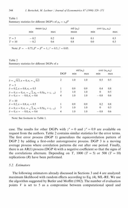
Table 1Summary statistics for different DGP’s of k

ti"x

tib0

mean (kti) std (k

ti) corr (k

ti,k

si)

min max mean min max

¹"5 !0.2 0.2 0.8 0.1 0.3¹"10 !0.2 0.6 0.8 0.0 0.3

Note: bc"!0.75, b0"bN"1, cx"0.5, ct"0.05.

Table 2Summary statistics for different DGPs of u

std (uti) corr (u

ti,u

si)

DGP min max min max

d"J0.5, a"0,pt"J0.5 2 1.0 1.0 0.5 0.5

¹"5d"0.2, a"0.8,p

t"0.5 1 0.9 0.9 0.4 0.8

d"0, a"0,pt"J2, u

ti"0.5(e

ti#e

t~1i) 3 1.0 1.0 0 0.5

d"0, a"!0.8,pt"0.6 4 1.0 1.0 !0.8 0.6

¹"10d"0.2, a"0.8,p

t"0.5 1 0.9 0.9 0.2 0.8

d"0, a"0,pt"J2, u

ti"0.5(e

ti#e

t~1i) 3 1.0 1.0 0 0.5

d"0, a"!0.8,pt"0.6 4 1.0 1.0 !0.8 0.6

Note: See footnote to Table 1.

case. The results for other DGPs with cx"0 and cx"0.9 are available onrequest from the authors. Table 2 contains similar statistics for the error terms.The first error process (DGP 1) generalizes the equicorrelation pattern ofDGP 2 by adding a first-order autoregressive process. DGP 3 is a movingaverage process where correlation patterns die out after one period. Finally,there is an AR(1) process (DGP 4) with a negative coefficient so that the signs ofthe correlations alternate. Depending on ¹, 1000 (¹"5) or 500 (¹"10)replications (R) have been performed.

5.2. Estimators

The following estimators already discussed in Sections 3 and 4 are analyzed:maximum likelihood with random effects according to Eq. (4), ML-RE. We usethe algorithm suggested by Butler and Moffitt (1982). The number of evaluationpoints » is set to 5 as a compromise between computational speed and


numerical accuracy (see Guilkey and Murphy, 1993, for more Monte Carloresults). When the assumed error structure is the true one this estimator isconsistent and asymptotically efficient for (b, d). In the Monte Carlo study thestandard errors are computed in the ‘robust’ way suggested by White (1982).Furthermore, there are the pooled estimator and the sequential estimator aspresented in Eqs. (5) and (20), respectively. The latter uses the optimal weightingmatrix, given by the inverse of the joint covariance matrix of the first stepestimates, to obtain the final estimates in the second step.

The estimator based on the instruments A*(xi) and computed under the

assumption of random effects with a small variance (small sigma) of the randomeffect relative to the total error variance (GMM—SS, cf. Eq. (21)), dominated theother GMM estimators (for details see Breitung and Lechner, 1997). Hence, wereport only results for this ‘best’ estimator to see whether it can be improved bythe use of nonparametric methods. GMM—SS and all nonparametric estimatorsdepend on a preliminary consistent estimate bI

N. In the Monte Carlo study this is

always the pooled probit estimate.Several different variants of nonparametric estimators are considered. Instead

of using the conditional moments given in Eq. (6) and denoted by NP, one couldalso use the following scaled moments (WNP):

mWt(Z

t; b)"

mt(Z

t; b)

JE[mt(Z

t;b)2DX]

(28)

E[mWt

(Zt; b0)DX"x

i]"

E [mt(Z

t; b0)DX"x

i]

JUti(1!U

ti)

"0.

The conditional variance of the moments given by Eq. (6) is heteroscedasticacross individuals, because it depends on explanatory variables, whereas theversion given by Eq. (28) leads to the following conditional covariance of themoments:

utsi"[E(mW

tmW{

s)DX"x

i]"G

1 if t"s,U(2)

tsi~UtiU

siJ(ti(1~U

ti)Usi(1~Usi)

if tOs.(29)

The latter is homoscedastic on the main diagonal and this could lead to smallsample improvements. The matrix D( ) ) has to be changed accordingly. We alsoconsider versions of NP and WNP for which only the off-diagonal elements ofX(x

i) are estimated nonparametrically, and the main diagonal elements are set

either to unity (WNP) or to Uti(1!U

ti) (NP). However, this leads to numerical

problems in some cases of NP, because some eigenvalues of XI (xi) are very small

or even negative.For the cross-validation a grid with eight values of k equally spaced in the

interval N0.67, N0.97 is chosen. When the estimate of X(xi) is not positive


definite, the smoothing parameter k is increased according to this grid of k’suntil a positive definite estimate of X(x

i) is obtained. If the use of the largest

possible k still does not produce a positive definite estimate, the values of themain diagonal are doubled until the matrix becomes positive definite. The lattercorrection is also applied to the versions of NP and WNP which only estimatethe off-diagonal elements of X(x

i). We also analysed the case k"N, however,

the results turned out to be worse than those for the above-mentioned k’ssmaller than N (results available on request).

Finally, we computed a conditional moment estimator based on the truevalues of X(x

i) and D(x

i) which are known in a Monte Carlo study. This

estimator (infeasible GMM-IV) is generally infeasible and is used only asa benchmark for what could be achieved with an estimator optimal in that classand free of any variability coming from a first step estimation.

5.3. Asymptotic comparisons

Before comparing the finite sample performance of the various estimators, weaddress the issue on how informative the particular moments are asymp-totically. This will give us an indication about the efficiency gains that might beachievable in finite samples under these DGPs.10

Since the analytical computation of the asymptotic covariances proved in-tractable, we employed the following simulation strategy. For the GMM es-timators (including the pooled probit), Eq. (11) is the appropriate varianceformula. Using the information about the DGP we computed D(X),A(X), X(X)analytically. Then, we drew 50.000 (¹"5) or 25.000 (¹"10) realizations fromthe distribution of X. The unconditional expectations appearing in Eq. (11) (andalso in Eq. (13)) are estimated by averaging the respective quantities using thislarge number of independent draws.

For the ML-RE obtaining analytical expressions for the information matrixproved intractable as well. Therefore, we drew realizations from the jointdistribution of ½ and X to simulate the asymptotic covariance matrix. Toaccount for possible additional simulation variance introduced by drawing alsothe binary indicator ½, the number of draws are doubled to 100,000 and 50,000,respectively. Additionally, to reduce the influence of having to approximate theintegral appearing in Eq. (3), we increased the number of evaluation points to136 (taken from Stroud and Secrest, 1966, pp. 250—252).11 For the ML-RE two

10We thank an Associate Editor of this journal for proposing this comparison to us.

11However, there is virtually no difference for the asymptotic standard deviation when 20 pointsare used instead. Similarly, the results based on using either the OPG, the Hessian, or White-versionof the covariance matrix for these simulations are virtually identical.


other issues arise: first, it is only for the case of (pure) random effects (DGP 2)that it is clearly consistent. Hence, we do not give asymptotic standard errors forthe other DGPs. Second, there are two versions of this estimator that areinteresting as a benchmark for the GMM estimators. One treats the standarddeviation of the random effect (d) as a known quantity. The other (feasible)ML-RE that has to be used in practice is the one that treats d as an additionalcoefficient to be estimated (it attains the Cramer—Rao bound for (b@, d)@).

Table 3 contains the results of these computations.12 The overall efficiencyranking is as expected from the theoretical results presented in the previoussection. Comparing the pooled estimator, that has the largest variance of theestimators presented, to the sequential estimator, we find that the efficiency gainsfrom using the latter one are tiny. GMM-SS is always more efficient thansequential, however — as expected — the efficiency gains depend very much on theparticular DGP. This feature is not true for the Optimal GMM-IV. OptimalGMM-IV denotes the limit for all the various versions of GMM estimators thatare asymptotically efficient, such as the Infeasible GMM-IV, and the variousversions of WNPs and NPs. To see the magnitude of the efficiency gains, it isuseful to ask how many additional observations would be necessary so thatinference, for example, with the pooled probit is as efficient as with an OptimalGMM-IV. For bN and ¹"5, a pooled probit analysis based on about 30%(DGP 1), 17% (DGP 2), 13% (DGP 3) or 32% (DGP 4) more observationswould be as precise as an analysis based on an Optimal GMM-IV. Theseefficiency gains rise for ¹"10, but the magnitude of the rise depends on theDGPs. The corresponding numbers are 32% (DGP 1), 21% (DGP 2), 15%(DGP 3), and 34% (DGP 4). It appears that such efficiency gains are well worthpursuing by using an asymptotically Optimal GMM-IV. Before we analyzewhether these gains materialize in finite samples, a comparison of the GMMswith the ML-RE is informative. For bN we find an efficiency loss of the OptimalGMM-IV of about 4% for ¹"5 and about 11% for ¹"10 compared to theinfeasible ML-RE. However, when making the more relevant comparison to thefeasible ML-RE, we find only a small efficiency loss of 1.3% and 1.6%, respec-tively.

5.4. Finite sample results

Table 4 describes the measures for the accuracy of the estimates used in thissection. They are the root mean square error and the bias of the estimatedasymptotic standard errors of the coefficient estimates. bK

rdenotes the estimate of

12Since in binary choice models identification is only up to scale, the ratio of estimatedcoefficients is also of interest.


Table 3Asymptotic standard errors (]10)

¹"5 ¹"10

bc bD bN bD/bN bc bD bN bD/bN

DGP 1 AR(1)(a"0.8) and random effects (d"0.2)

Pooled 13.40 13.74 14.69 13.75 11.21 10.08 10.92 9.86Sequential 13.36 13.65 14.68 13.70 11.13 10.02 10.91 9.83GMM-SS 12.94 12.35 13.31 11.57 10.87 9.30 10.07 8.61Optimal GMM-IV 12.72 12.00 12.88 10.94 10.57 8.76 9.51 7.67

DGP 2 Random Effects

ML-RE-known d 11.34 10.49 12.04 13.56 9.75 7.01 8.52 9.16ML-RE-unknown d 11.44 10.69 12.23 13.56 9.99 7.54 8.93 9.16Pooled 11.89 11.90 13.31 15.38 10.43 8.63 9.90 10.83Sequential 11.88 11.37 13.31 15.34 10.41 8.50 9.90 10.72GMM-SS 11.57 10.86 12.36 13.75 10.07 7.65 9.05 9.26Optimal GMM-IV 11.53 10.80 12.31 13.68 10.04 7.60 9.00 9.19

DGP 3 MA(1)


DGP 4 AR(1)(a"!0.8,d"0)


Note: Asymptotic standard errors of JN[( Yb/pu)N!(b0/p0

u)]. Asymptotic variance of

JN(bKD/bK

N!b0

D/b0

N) and for the rescaled MLEs JN[bK MLE

N/J(dK MLE

N)2#1!(b0/p0

u)] are computed

by the delta method.

the true value b0 in replication ‘r’, and asstd (bKr) denotes the estimated asymp-

totic standard error in replication ‘r’. Since there may be concerns that theexpectation and the variance of the estimates may not exist in finite samples forall estimators used, we also consider the median absolute error. Additionally,Table 11 presents the upper and lower bounds as well as the width of the central95% quantile of estimates based on the Monte Carlo simulations and on theasymptotic normal approximation using the average of the estimated asymp-totic covariance matrices of the coefficients. For the sake of brevity, the statisticsrelated to the constant term are omitted.


Table 4Measures of accuracy used in the Monte Carlo study

Root mean square error ]10 C100

R

R+r/1

(bKr!b0)2D

1@2]10

Median of absolute error ]10 medianrDbK

r!b0D]10

Bias of asymptotic standard error in %100

R

R+r/1

as std(bKr)!std err(bK )

std err(bK )

Note: bKrand asstd(bK

r) denote the coefficient estimate and the estimated asymptotic standard error

obtained in replication r. std(bK ) denotes the empirical standard error of the estimated coefficients inthe Monte Carlo study. All results are scaled to estimate (b0/p0

u). This scaling already applies to all

estimators except the MLE. The MLE is appropriately rescaled [bK MLEN

/J(dK MLEN

)2#1]. The estimatedasymptotic variances for the MLE presented in the following tables are approximated by dividingthe estimated asymptotic variances by (dK MLE

N)2#1.

For the DGP with an AR(1) process combined with random effects (Tables 5and 11), several GMM-estimators with nonparametric estimation of thecovariance matrix are computed for N"100, 400.13 The results do not revealmuch difference within the groups of estimators NP and WNP. However, thereare substantial differences between these groups (although not reported in thetables, all estimates are almost unbiased). The estimators with scaled moments(WNP) have lower root mean squared errors (RMSE) and median absoluteerror (MAE). WNP is sometimes observed with a somewhat larger bias of theasymptotic standard errors. Increasing the sample size N, the performance of theestimators is generally improving, becoming closer to that of the asymptoticallyoptimal GMM-estimates given by the benchmark of the infeasible GMM-IV.Increasing the time-dimension ¹ generally improves the results with respect tothe RMSE, the MAE, and the bias of asymptotic standard errors. A notableexception on the latter criterion is WNP-indiv-quadr.

Compared to choosing between NP and WNP the ranking according to thechoice of the weight function for the k-NN approach, uniform or quadratic, isinconclusive with the exception of WNP-indiv-quadr. The results for the tri-angular weights are omitted from the tables since they turned out to be nearlyindistinguishable from those for quadratic weights. Furthermore, it does notseem to matter if the distance is measured individually or jointly over the indicesxtib, although the results of the latter are more stable in the small sample.

13The same range of estimators has been computed for the case of independent errors. Since theobtained results are qualitatively the same as for the AR(1) process they are omitted from the tables.The results are available from the authors on request.


Table 5Simulation results for AR(1) (a"0.8) and random effects (d"0.2) (DGP 1)

root MSE]10 median absoluteerror]10

bias of as.std. err. in %

bD bN bD/bN bD bN bD/bN bD bN

N"100 ¹"5, 1000 replications

Infeasible GMM-IV 1.18 1.30 1.17 0.78 0.89 0.77 2.7 !0.8ML-RE 1.26 1.34 1.19 0.81 0.96 0.79 !4.6 !3.7Pooled 1.41 1.49 1.51 0.95 1.00 0.99 !3.1 !2.0Sequential 1.51 1.63 1.66 1.03 1.16 1.04 !17.6 !15.1GMM-SS 1.21 1.35 1.24 0.80 0.95 0.80 2.2 !1.4NP-joint-uniform 1.44 1.48 1.24 0.89 1.05 0.82 !2.1 !0.5NP-indiv-uniform 1.44 1.48 1.24 0.90 1.02 0.84 !2.5 !1.0NP-joint-quadr. 1.44 1.47 1.24 0.90 1.04 0.83 !1.8 0.4NP-indiv-quadr. 1.41 1.47 1.23 0.90 1.04 0.83 !1.1 !0.7NP-joint-unif.- S~1

xb 1.43 1.47 1.24 0.91 1.02 0.81 !1.5 0.2WNP-joint-uniform 1.31 1.42 1.24 0.87 0.97 0.83 !2.2 !3.1WNP-indiv-uniform 1.38 1.47 1.34 0.88 0.98 0.87 !4.6 !3.7WNP-joint-quadr. 1.30 1.42 1.24 0.86 0.96 0.82 !1.2 !2.6WNP-indiv-quadr. 1.32 1.48 1.29 0.88 1.02 0.82 !1.0 !4.1WNP-joint-unif.- S~1

xb 1.30 1.41 1.24 0.87 0.99 0.83 !1.5 !2.5WNP-joint-unif.-no d. 1.29 1.37 1.21 0.86 0.86 0.78 !0.4 1.7


Infeasible GMM-IV 0.61 0.66 0.56 0.41 0.45 0.38 !0.2 !1.3ML-RE 0.61 0.64 0.56 0.40 0.44 0.39 4.0 2.2Pooled 0.70 0.73 0.69 0.47 0.51 0.47 !1.3 0.9Sequential 0.72 0.75 0.70 0.47 0.51 0.47 !6.5 !3.0GMM-SS 0.63 0.67 0.60 0.42 0.47 0.39 !2.6 !0.3NP-joint-uniform 0.67 0.71 0.58 0.44 0.46 0.38 2.0 1.2NP-indiv-uniform 0.66 0.71 0.58 0.44 0.46 0.39 2.4 0.9NP-joint-quadr. 0.67 0.71 0.58 0.44 0.49 0.39 1.2 0.4NP-indiv-quadr. 0.66 0.70 0.58 0.43 0.45 0.38 2.6 1.0NP-joint-unif.- S~1

xb 0.67 0.71 0.59 0.44 0.50 0.39 !0.7 !0.5WNP-joint-uniform 0.61 0.68 0.58 0.41 0.46 0.38 2.2 !0.2WNP-indiv-uniform 0.62 0.68 0.58 0.41 0.45 0.39 2.2 !0.1WNP-joint-quadr. 0.61 0.68 0.58 0.41 0.46 0.38 2.3 0.0WNP-indiv-quadr. 0.71 0.72 0.65 0.41 0.45 0.38 !10.7 !5.2WNP-joint-unif.- S~1

xb 0.61 0.67 0.58 0.41 0.45 0.38 2.2 0.1WNP-joint-unif.-no d. 0.60 0.68 0.59 0.41 0.46 0.39 2.9 !1.1

N"1600! ¹"5, 1000 replications

Infeasible GMM-IV 0.30 0.33 0.27 0.20 0.22 0.19 2.2 !0.6Pooled 0.34 0.37 0.34 0.23 0.26 0.23 2.0 1.0Sequential 0.35 0.39 0.35 0.22 0.25 0.23 1.3 !3.2GMM-SS 0.31 0.34 0.29 0.21 0.22 0.19 1.8 0.3WNP-joint-uniform 0.31 0.34 0.28 0.20 0.23 0.18 1.3 2.0

Table 5 to be continued


Table 5 (Continued)




N"100!," ¹"10, 500 replications

Infeasible GMM-IV 0.90 0.94 0.77 0.61 0.61 0.53 !3.2 0.5Pooled 1.05 1.12 1.02 0.73 0.74 0.67 !5.2 !2.6Sequential 1.24 1.33 1.27 0.87 0.93 0.81 !32.4 !27.7GMM-SS 0.97 0.98 0.88 0.66 0.67 0.60 !5.5 1.1NP-joint-uniform 1.05 1.09 0.87 0.70 0.76 0.61 !2.8 0.6NP-indiv-uniform 1.07 1.10 0.87 0.73 0.74 0.58 !2.5 1.3NP-joint-quadr. 1.05 1.11 0.87 0.74 0.74 0.62 0.3 1.4NP-indiv-quadr. 1.09 1.12 0.86 0.72 0.74 0.58 !2.8 0.6NP-joint-unif.- S~1

xb 1.04 1.09 0.87 0.67 0.74 0.60 0.2 2.2WNP-joint-uniform 0.99 1.06 0.86 0.68 0.75 0.59 !2.1 0.7WNP-joint-quadr. 1.00 1.08 0.87 0.70 0.75 0.60 !2.5 !1.9WNP-indiv-quadr. 1.05 1.39 2.93 0.75 0.79 0.64 !2.5 !18.1WNP-joint-unif.- S~1

xb 0.98 1.06 0.86 0.66 0.73 0.58 !1.6 !1.0WNP-joint-unif.-no d. 1.00 1.17 1.00 0.64 0.84 0.66 2.3 !3.0


Infeasible GMM-IV 0.44 0.49 0.39 0.30 0.33 0.25 0.2 !3.9Pooled 0.53 0.56 0.51 0.34 0.38 0.35 !3.7 !1.1Sequential 0.56 0.60 0.54 0.37 0.39 0.37 !12.0 !9.1GMM-SS 0.47 0.52 0.43 0.32 0.34 0.29 !0.2 !3.1NP-joint-uniform 0.51 0.55 0.43 0.34 0.33 0.30 !2.3 !2.1NP-indiv-uniform 0.51 0.54 0.42 0.34 0.34 0.30 !1.8 !1.8NP-joint-quadr. 0.51 0.55 0.43 0.36 0.34 0.30 !1.7 !2.0NP-indiv-quadr. 0.50 0.53 0.42 0.33 0.33 0.30 !1.4 !1.3NP-joint-unif.- S~1

xb 0.51 0.55 0.42 0.34 0.33 0.30 !2.3 !2.1WNP-joint-uniform 0.46 0.50 0.41 0.30 0.32 0.29 1.3 0.1WNP-indiv-uniform 0.46 0.51 0.41 0.30 0.32 0.30 1.7 0.2WNP-joint-quadr. 0.46 0.50 0.41 0.30 0.33 0.29 2.0 0.4WNP-indiv-quadr. 0.46 0.50 0.42 0.31 0.33 0.31 1.4 0.7WNP-joint-unif.- S~1

xb 0.46 0.50 0.41 0.31 0.32 0.30 1.1 0.0WNP-joint-unif.-no d. 0.45 0.51 0.42 0.31 0.32 0.29 1.4 !0.5


Infeasible GMM-IV 0.24 0.25 0.19 0.16 0.15 0.12 !4.2 1.5Pooled 0.28 0.29 0.25 0.18 0.18 0.18 !2.3 !1.0Sequential 0.29 0.30 0.25 0.17 0.19 0.17 !3.7 !2.1GMM-SS 0.25 0.27 0.22 0.16 0.17 0.14 !4.0 !0.4WNP-joint-uniform 0.25 0.28 0.20 0.17 0.18 0.14 !5.5 !9.5

!ML-RE not available, because variance of random effect (d2) approached zero."WNP-indiv-uniform not available, because of singular weighting matrix.


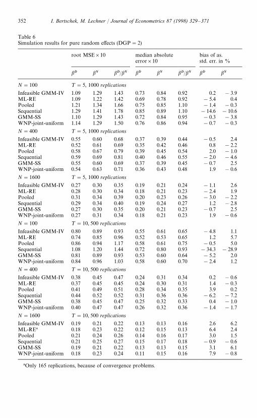
Table 6Simulation results for pure random effects (DGP"2)





Infeasible GMM-IV 1.09 1.29 1.43 0.73 0.84 0.92 0.2 !3.9ML-RE 1.09 1.22 1.42 0.69 0.78 0.92 !5.4 0.4Pooled 1.21 1.34 1.66 0.75 0.85 1.10 !1.4 !0.3Sequential 1.29 1.41 1.78 0.85 0.89 1.10 !14.6 !10.6GMM-SS 1.10 1.29 1.43 0.72 0.84 0.95 !0.3 !3.8WNP-joint-uniform 1.14 1.29 1.50 0.76 0.86 0.94 !0.7 !0.3


Infeasible GMM-IV 0.55 0.60 0.68 0.37 0.39 0.44 !0.5 2.4ML-RE 0.52 0.61 0.69 0.35 0.42 0.46 0.8 !2.2Pooled 0.58 0.67 0.79 0.39 0.45 0.54 2.0 !1.0Sequential 0.59 0.69 0.81 0.40 0.46 0.55 !2.0 !4.6GMM-SS 0.55 0.60 0.69 0.37 0.39 0.45 !0.7 2.5WNP-joint-uniform 0.54 0.63 0.71 0.36 0.43 0.48 1.9 !0.6


Infeasible GMM-IV 0.27 0.30 0.35 0.19 0.21 0.24 !1.1 2.6ML-RE 0.28 0.30 0.34 0.18 0.21 0.23 !2.4 1.9Pooled 0.31 0.34 0.39 0.20 0.23 0.26 !3.0 !2.2Sequential 0.29 0.34 0.40 0.19 0.24 0.27 1.2 !2.8GMM-SS 0.27 0.30 0.35 0.20 0.21 0.23 !0.7 2.5WNP-joint-uniform 0.27 0.31 0.34 0.18 0.21 0.23 1.9 !0.6


Infeasible GMM-IV 0.80 0.89 0.93 0.55 0.61 0.65 !4.8 1.1ML-RE 0.74 0.85 0.96 0.52 0.53 0.65 1.2 5.7Pooled 0.86 0.94 1.17 0.58 0.61 0.75 !0.5 5.0Sequential 1.08 1.20 1.44 0.72 0.80 0.93 !34.3 !28.9GMM-SS 0.81 0.89 0.93 0.53 0.60 0.64 !5.2 2.0WNP-joint-uniform 0.84 0.96 1.03 0.58 0.60 0.70 !2.4 1.2


Infeasible GMM-IV 0.38 0.45 0.47 0.24 0.31 0.34 0.2 !0.6ML-RE 0.37 0.45 0.45 0.24 0.30 0.31 1.4 !0.3Pooled 0.41 0.49 0.51 0.28 0.34 0.35 3.9 0.2Sequential 0.44 0.52 0.52 0.31 0.36 0.36 !6.2 !7.2GMM-SS 0.38 0.45 0.47 0.25 0.32 0.33 0.4 !1.0WNP-joint-uniform 0.40 0.47 0.47 0.26 0.32 0.36 !1.4 !1.7


Infeasible GMM-IV 0.19 0.21 0.22 0.13 0.13 0.16 2.6 6.2ML-RE! 0.18 0.23 0.22 0.12 0.15 0.13 6.4 2.4Pooled 0.21 0.24 0.26 0.14 0.16 0.17 3.0 1.5Sequential 0.21 0.25 0.27 0.15 0.17 0.18 !0.9 !0.6GMM-SS 0.19 0.21 0.22 0.13 0.13 0.15 3.1 6.1WNP-joint-uniform 0.18 0.23 0.24 0.11 0.15 0.16 7.9 !0.8

!Only 165 replications, because of convergence problems.


Table 7Simulation results for MA(1)(DGP"3)





Infeasible GMM-IV 1.12 1.23 1.52 0.75 0.84 0.96 !2.2 0.8Pooled 1.18 1.33 1.57 0.76 0.88 1.00 !2.5 !1.2Sequential 1.22 1.38 1.70 0.76 0.96 1.11 !13.6 !10.1GMM-SS 1.16 1.29 1.65 0.79 0.88 0.98 !2.8 0.4WNP-joint-uniform 1.18 1.34 1.57 0.78 0.91 1.00 !5.1 1.6


Infeasible GMM-IV 0.53 0.61 0.70 0.34 0.41 0.48 1.9 !0.1ML-RE 0.56 0.61 0.77 0.37 0.39 0.48 !1.2 3.7Pooled 0.57 0.63 0.79 0.39 0.42 0.51 !1.2 4.1Sequential 0.59 0.63 0.80 0.40 0.41 0.51 !5.2 1.9GMM-SS 0.55 0.65 0.76 0.36 0.45 0.50 2.3 !0.6WNP-joint-uniform 0.55 0.60 0.73 0.37 0.40 0.48 !0.3 4.4


Infeasible GMM-IV 0.26 0.31 0.35 0.18 0.20 0.23 4.2 0.4ML-RE 0.28 0.32 0.37 0.19 0.21 0.23 !2.5 !2.2Pooled 0.29 0.33 0.38 0.20 0.22 0.25 !0.7 !0.1Sequential 0.28 0.33 0.38 0.20 0.22 0.25 !0.9 !1.5GMM-SS 0.27 0.31 0.37 0.19 0.21 0.25 3.7 2.3WNP-joint-uniform 0.28 0.31 0.36 0.20 0.21 0.23 !2.4 !1.7


Infeasible GMM-IV 0.75 0.91 1.02 0.53 0.60 0.68 0.6 !3.2Pooled 0.75 0.93 1.10 0.49 0.61 0.69 4.6 !0.2Sequential 0.92 1.12 1.37 0.56 0.74 0.85 !27.8 !27.5GMM-SS 0.79 0.96 1.09 0.53 0.63 0.74 !0.7 !2.3WNP-joint-uniform 0.77 0.96 1.07 0.52 0.65 0.67 6.1 !2.1


Infeasible GMM-IV 0.36 0.43 0.52 0.24 0.28 0.35 5.0 0.9Pooled 0.42 0.47 0.55 0.28 0.30 0.36 !5.6 1.1Sequential 0.43 0.48 0.56 0.30 0.28 0.36 !11.6 !6.0GMM-SS 0.38 0.46 0.57 0.26 0.31 0.39 2.3 0.7WNP-joint-uniform 0.39 0.42 0.48 0.27 0.28 0.34 0.1 6.6


Infeasible GMM-IV 0.18 0.22 0.24 0.12 0.14 0.16 2.7 !1.5Pooled 0.20 0.24 0.27 0.14 0.16 0.17 0.2 !1.2Sequential 0.20 0.24 0.27 0.13 0.16 0.17 !2.1 !3.3GMM-SS 0.20 0.24 0.26 0.13 0.16 0.17 0.7 !3.9WNP-joint-uniform 0.19 0.22 0.25 0.13 0.15 0.16 !0.2 0.1

!ML-RE not available, because variance of random effect (d2) approached zero.


Table 8Simulation results for AR(1)(a"!0.8,d"0)(DGP4)

root MSE]10 median absolute error]10 bias of as.std. err. in %



Infeasible GMM-IV 1.02 1.22 1.22 0.72 0.83 0.78 !4.6 !3.0Pooled 1.06 1.38 1.49 0.68 0.92 0.90 !1.1 !1.4Sequential 1.12 1.45 1.58 0.77 0.98 0.98 !12.1 !10.6GMM-SS 1.14 1.39 1.52 0.76 0.88 0.93 !8.0 !4.5WNP-joint-uniform 1.05 1.25 1.27 0.71 0.82 0.85 !2.5 !0.2


Infeasible GMM-IV 0.48 0.57 0.58 0.32 0.39 0.39 1.0 3.9Pooled 0.53 0.70 0.72 0.36 0.46 0.48 !2.2 !2.5Sequential 0.54 0.71 0.73 0.36 0.47 0.50 !4.1 !5.2GMM-SS 0.52 0.64 0.69 0.34 0.45 0.46 1.0 3.8WNP-joint-uniform 0.51 0.62 0.61 0.36 0.40 0.40 !1.6 !1.2


Infeasible GMM-IV 0.24 0.30 0.29 0.16 0.19 0.19 !0.1 !0.8Pooled 0.26 0.34 0.35 0.17 0.22 0.24 0.2 0.2Sequential 0.26 0.35 0.35 0.18 0.22 0.24 !1.6 !0.8GMM-SS 0.26 0.34 0.35 0.17 0.23 0.23 !0.3 !1.8WNP-joint-uniform 0.25 0.31 0.30 0.17 0.21 0.19 2.0 !1.1


Infeasible GMM-IV 0.70 0.85 0.80 0.47 0.54 0.57 0.2 0.4Pooled 0.77 1.02 0.97 0.52 0.73 0.64 !4.2 !2.0Sequential 0.92 1.21 1.16 0.60 0.84 0.86 !31.6 !29.2GMM-SS 0.75 0.97 0.96 0.50 0.65 0.65 !0.2 1.5WNP-joint-uniform 0.75 0.95 0.93 0.53 0.69 0.65 !0.9 !1.1


Infeasible GMM-IV 0.34 0.43 0.40 0.23 0.26 0.26 3.4 0.2Pooled 0.39 0.50 0.47 0.27 0.36 0.29 !5.2 0.7Sequential 0.40 0.51 0.48 0.27 0.34 0.30 !11.0 !4.8GMM-SS 0.36 0.49 0.50 0.24 0.30 0.35 2.7 1.0WNP-joint-uniform 0.39 0.45 0.42 0.24 0.27 0.29 !6.4 0.2


Infeasible GMM-IV 0.18 0.22 0.20 0.12 0.14 0.13 !3.1 !2.8Pooled 0.20 0.26 0.24 0.14 0.17 0.16 !5.5 !3.0Sequential 0.20 0.26 0.24 0.14 0.17 0.16 !7.5 !4.8GMM-SS 0.19 0.25 0.24 0.14 0.17 0.16 !2.4 !2.1WNP-joint-uniform 0.18 0.22 0.22 0.12 0.14 0.14 1.3 2.2

!ML-RE not available, because variance of random effect (d2) approached zero.


For each replication of the Monte Carlo study the smoothing parameter k ischosen via cross-validation. The distributions of the choice of k are depicted inTables 12—15. For DGP 1 there is a tendency to choose a relatively large k (seeTable 12). This tendency is slightly stronger for the joint than for the individualmeasure of distance. The same is true when increasing the time periods from 5 to10. Both cases represent an increase in the dimension of the nonparametricestimation. WNP has an even stronger tendency to choose a large k than NP.An intuitive explanation is that the diagonal elements of the covariance matrixfor WNP are estimated without bias, because they do not vary across ‘i’. Withincreasing k the variance of the estimation is reduced. If these elements havestrong weights in the cross-validation, the effect of decreasing the variance bylarge k might dominate the bias-variance trade-off important for the off-diag-onal elements, and hence, a large (or the largest) k minimizes the cross-validationfunction. However, replacing alternatively the diagonal elements of thecovariance matrix by their parametrically estimated values and using only theoff-diagonal elements for the cross-validation (WNP-joint-uniform-no.d.) doesnot seem to matter for N"400. For N"100 the results are mixed: for ¹"5 itis the best for all criteria, but for ¹"10 several WNP-estimators performbetter. Introducing the covariance matrix of the linear indices S~1

xb as the weightmatrix for measuring the distance does not seem to bring clear-cut efficiencygains. This is supported by the results for independent errors.14 Since there doesnot appear to be any significant difference between using S~1

xb or its maindiagonal, the latter is omitted from the tables.

Comparing the results of Table 5 and Table 11 we find that there are nosubstantial qualitative differences. Furthermore, the confidence bounds aresymmetric around the true value, which implies that, at least for its tail, there isno concern about a severely asymmetric distribution.

Given these results, we choose within the class of WNP estimators theestimator with uniform weights and joint distance measure (WNP-joint-uni-form) as the preferred version, because it has the simplest form of weights, itseems to be more robust with respect to the asymptotic standard errors than forinstance the WNP-indiv-quadr, and saves computation time compared to anestimator with an individual distance measure.

Turning now to the fully parametric estimators, the following results areobtained: for the DGPs that have several forms of correlation of the error terms,ML-RE and GMM-SS show best results with respect to the RMSE and MAE.For the (nonreported) case of independent errors the small sigma method isalready in small samples as good as pooled probit, although the latter is themaximum likelihood estimator for this DGP. The calculation of ML-RE is time

14The results are available on request from the authors.


consuming compared to the other methods, and often convergence cannot bereached, especially for ¹"10.

Chamberlain’s sequential estimator produces quite large RMSE and MAEcompared to the other parametric methods for the sample size of N"100.Although it improves with increasing N, it performs still worse than ML-RE andGMM-SS. A striking feature is the large bias of the asymptotic standard errorsfor N"100, which is even larger for ¹"10 than for ¹"5. Thus, sequentialneeds quite a large sample size N in order to obtain good results. The relativelybad performance of sequential is also illustrated in Figs. 1 and 2 where kernelplots of the distribution of the various estimators based on DGP 1 are de-picted.15 Compared to the other estimators the distribution of sequential turnsout to be flatter and right-skewed, even stronger for ¹"10 than for ¹"5.Note that the asymptotic efficiency gains for this estimator compared to pooled,for example, depend on the accurate estimation of the covariance matrix in thefirst step estimates, which then has to be inverted. In our Monte Carlo examplethis matrix has the dimension 15 for ¹"5 and 30 for ¹"10. However, theasymptotic standard errors ignore the fact that this inverse may exhibit con-siderable variability in small samples.

Comparing now GMM-SS and WNP-joint-uniform, one observes that forthe DGPs presented in Tables 5 and 6 (and also for independent errors)GMM-SS is better than WNP-joint-uniform for N"100. For N"400 andN"1600 the differences in RMSE and bias of asymptotic standard errorsare very small and the ranking is inconclusive. The latter result is sup-ported by the corresponding kernel plots in Figs. 1 and 2 except for N"100and ¹"5 where the distribution of GMM-SS is left-skewed compared tothat of WNP-joint-uniform with a flat region at the top of the distribution.For the other cases the distributions of the two estimators are very close to eachother.

When considering covariance structures that are very different from a randomeffects structure implying equicorrelated errors, as presented by the MA(1)process or the AR(1) process with alternating signs of the correlation over time(Tables 7 and 8), WNP-joint-uniform is clearly superior to GMM-SS (as it isasymptotically, see Table 3).

Thus, since in real-world applications the true DGP is unknown, WNP-joint-uniform with nonparametric estimation of the covariance matrix can berecommended for applications.

15We present kernel plots for bN, but only for DGP 1 and N"100, 400. For N"1600, thesample distributions are very close to the asymptotic ones. The results for the other coefficients aswell as for the other DGPs are qualitatively the same as for DGP 1.


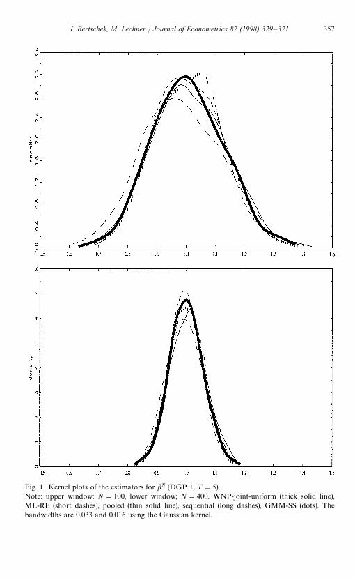
Fig. 1. Kernel plots of the estimators for bN (DGP 1, ¹"5).Note: upper window: N"100, lower window; N"400. WNP-joint-uniform (thick solid line),ML-RE (short dashes), pooled (thin solid line), sequential (long dashes), GMM-SS (dots). Thebandwidths are 0.033 and 0.016 using the Gaussian kernel.


Fig. 2. Kernel plots of the estimators for bN (DGP 1, ¹"10).Note: upper window: N"100, lower window; N"400. WNP-joint-uniform (thick solid line),pooled (thin solid line), sequential (long dashes), GMM-SS (dots). The bandwidths are 0.029 and0.014 using the Gaussian kernel.


6. Application

According to the empirical example that motivated our discussion the mainhypothesis to be tested is that imports and foreign direct investment (FDI) havepositive effects on the innovative activity of domestic firms. The firm-level datahave been collected by the Ifo-Institute, Munich (‘Ifo-Konjunkturtest’) andhave been merged with official statistics from the German Statistical Year-books. The binary dependent variable indicates whether a firm reports havingrealized a product innovation within the last year or not. The independentvariables refer to the market structure, in particular the market size of theindustry ln (sales), the shares of imports and FDI in the supply on the domesticmarket (import share and FDI-share), the productivity as a measure of thecompetitiveness of the industry as well as two variables indicating whethera firm belongs to the raw materials or to the investment goods industry. More-over, including the relative firm size allows to take account of the innovation— firm size relation often discussed in the literature. Hence, all variables withexception of the firm size are measured at the industry level (for descriptivestatistics see Appendix C).

The estimators applied to the example include the one used in Bertschek(1995), (sequential), the simplest one (pooled), the maximum likelihood estimatorunder the assumption of random effects with five evaluation points as used inthe Monte Carlo study (ML-RE 5) and with 10 evaluation points (ML-RE 10),the best parametric GMM estimator (GMM-SS) and finally, the simplest(WNP-joint-uniform) of the estimators with weighted nonparametric estimationof the covariance. Furthermore, we compute two versions of the asymptotict-values for the pooled estimator. The first (denoted by t-val) ignore the possiblecorrelations over time. They are the same that would be obtained by usinga standard software package for cross-section probit estimation. The second arecomputed using the correct GMM-formula as given in Eq. (16). The latter arecomparable to the covariance matrices used in the Monte Carlo study.

The estimation results are presented in Tables 9 and 10. Let us start bycomparing the outcomes implied by the two different ways to compute thecovariance matrices of pooled: not surprisingly, the t-values ignoring the inter-temporal correlations are generally larger than the t-values taking account ofthese correlations.

The results of the various parametric estimators are quite similar and lead tothe same conclusions (first part of Table 9). Both import share and FDI-sharehave positive and significant effects on product innovative activity. The firm sizevariable has a positive and significant impact (except for sequential) — a resultthat supports the Schumpeterian hypothesis that large firms are more innova-tive than small firms. The productivity coefficient is insignificant in most estima-tions. The estimates for ML-RE 5 and ML-RE 10 are very close to each otherexcept of the productivity that is significant only for ML-RE 10. Increasing the


Tab

le9

Inno

vation

prob

it:Est

imat

edco

effici

ents

and

t-va

lues

Poole

dM

L-R

E5

ML-R

E10

GM

M-S

SSe

quen

tial

Var

iable

coef

t-va

lt-va

lco

eft-va

lco

eft-va

lco

eft-va

lco

eft-va

l

Inte

rcep

t!

1.96

8.2

5.2

!2.

914.

6!

2.84

5.0

!1.

794.

8!

1.80

5.1

ln(sal

es)

0.18

7.2

4.8

0.25

4.1

0.25

4.6

0.16

4.4

0.15

4.4

Rel

.firm

size

1.07

5.2

3.5

1.56

2.5

1.52

3.9

0.88

3.5

0.26

1.4

Impo

rtsh

are

1.13

7.4

4.6

1.77

4.8

1.78

4.8

1.17

4.9

1.27

5.4

FD

I-sh

are

2.85

6.1

4.2

3.77

3.7

3.65

3.8

2.54

3.9

2.52

3.9

Pro

duc

tivi

ty!

2.34

2.1

1.8

!2.

211.

5!

2.30

2.0

!1.

501.

8!

0.43

0.4

Raw

mat

eria

ls!

0.28

2.9

2.1

!0.

482.

6!

0.48

2.7

!0.

332.

8!

0.28

2.3

Inve

stm

ent

0.19

4.7

3.0

0.33

3.5

0.33

3.4

0.21

3.3

0.21

3.3

¼N

P-joi

nt-u

nifo

rm

k"20

k"50

k"10

0k"

263

k"88

0k"

1270

Var

iable

coef

t-va

lco

eft-va

lco

eft-va

lco

eft-va

lco

eft-va

lco

eft-va

l

Inte

rcep

t!

3.82

0.5

!1.

704.

4!

1.81

4.8

!1.

744.

7!

1.74

4.8

!1.

794.

9ln

(sal

es)

0.44

0.7

0.16

4.4

0.16

4.6

0.15

4.4

0.15

4.5

0.16

4.6

Rel

.firm

size

0.00

50.

030.

914.

20.

974.

81.

004.

90.

954.

70.

984.

8Im

port

shar

e!

3.12

0.7

1.02

4.1

1.10

4.4

1.13

4.7

1.14

4.8

1.15

4.8

FD

I-sh

are

14.0

92.

92.

644.

22.

594.

42.

564.

32.

594.

42.

574.

4Pro

duc

tivi

ty!

7.32

5.2

!2.

482.

6!

1.76

2.0

!1.

892.

2!

1.91

2.3

!1.

922.

3R

awm

ater

ials

0.50

0.4

!0.

191.

5!

0.27

2.2

!0.

282.

4!

0.28

2.4

!0.

292.

5In

vest

men

t0.

100.

20.

223.

40.

243.

70.

223.

40.

213.

40.

213.

3

CV

-val

ue

99]

107

21.0

017

.36

15.5

114

.80

15.1

2

Note

:Dep

ende

ntva

riab

le:p

rodu

ctin

nov

atio

n,N"

1270

,¹"

5.t-

val:

t-va

lues

ofp

oole

dpro

bitas

sum

ing

indep

enden

ter

rors

over

tim

e.B

old

lett

ersif

t-va

lues

are

larg

erth

an1.

96.


number of evaluation points to 20 produces almost the same results as for 10evaluation points. Hence, they are omitted from the table.

Turning now to the results of WNP-joint-uniform (second part of Table 9)one can find that the estimates as well as the t-values are quite robust fork"100, 263, 880, 1270. For k"263 the cross-validation function (Fig. 3) hasa local minimum whereas its global minimum is reached for k"880. For allthese k’s the productivity coefficient is negative and significant. In contrast to theresults of the sequential estimator the firm size always keeps its positiveand significant coefficient. For k"20 and k"50 the dummy for theraw materials industry has an insignificant coefficient. In the first case allcoefficients and t-values differ considerably from those of the other k’s. However,the value of the cross-validation function indicates that k"20 is far from beingoptimal.

A look at the estimated standard errors (Table 10) reveals again that pooledwhen ignoring possible correlations of the error over time generally leads to

Fig. 3. Cross-validation function for innovation probit estimated with WNP-joint-uniform.


Tab

le10

Inno

vation

pro

bit:Est

imat

edst

anda

rder

rors

WN

P-joi

nt-uni

form

with

Var

iable

Poole

dSS

seq.

k"20

k"50

k"10

0k"

263

k"88

0k"

1270

Inte

rcep

t0.

210.

380.

370.

357.

300.

380.

370.

370.

370.

37In

(sal

es)

0.02

50.

037

0.03

50.

034

0.61

0.03

60.

035

0.03

40.

034

0.03

4Firm

size

0.21

0.31

0.25

0.19

0.16

0.22

0.20

0.20

0.20

0.20

Imp.sh

are

0.15

0.24

0.24

0.24

4.63

0.25

0.25

0.24

0.24

0.24

FD

I-sh

are

0.47

0.68

0.65

0.64

4.94

0.63

0.59

0.60

0.59

0.59

Pro

duc

t1.

101.

320.

841.

051.

390.

960.

870.

840.

820.

83R

awm

at.

0.09

70.

130.

120.

121.

340.

120.

120.

120.

120.

12In

vest

.0.

040

0.06

30.

063

0.06

20.

630.

065

0.06

40.

063

0.06

30.

063

Note

:See

Tab

le9.

ML

-RE

uses

diffe

rent

erro

rva

rian

ceno

rmal

izat

ion.

The

refo

re,it

isom

mitte

dfrom

the

tabl

e.


downward biased standard errors and thus to upward biased t-values. Thestandard errors of GMM-SS and sequential are in general lower than those ofpooled. The standard errors of WNP-joint-uniform differ only slightly overk"100 to k"1270. The large values for k"20 accompanied by a very largevalue for the cross-validation function confirm the inaccuracy of the estimatesfor this size of undersmoothing. For k"880 the standard errors are the smallestfor all variables.

Hence, WNP-joint-uniform clearly dominates the other estimators with re-spect to its efficiency for most coefficients. There are efficiency gains comparedto pooled probit, GMM-SS and sequential concerning the variables firm size andproductivity. The standard errors for the FDI-share coefficient decrease com-pared to pooled and GMM-SS. These results are in particular important withrespect to the variable productivity. While its coefficient is negative and insigni-ficant for all parametric estimators (except ML-RE 10), it now turns out to besignificant allowing to draw more reliable conclusions. Firms belonging to moreproductive industries put less effort in product innovative activity. At firstglance, this result seems surprising since one expects that higher productivityimplies more innovative activity. However, a closer look at the data reveals thatindustries with extremely high levels of labor productivity are those of the rawmaterials industry. These industries produce with a high capital intensity. Sinceraw materials such as nonferrous metals or paper generally cannot be changedmuch — as compared to consumer goods, for example — by innovations thenegative sign of the productivity coefficient seems plausible.

The estimations have been performed on a personal computer with a Pentium100MHz processor. The computation times are: 30 s for pooled probit, 10minfor GMM-SS and for WNP-joint-uniform and 15min for ML-RE 10. TheGAUSS-program is available on request from the authors.

7. Conclusions

The paper shows that often-used and conveniently computable estimators,such as pooled probit, Chamberlain’s (1980, 1984) sequential estimators orseveral variants of GMM estimators, belong to a class of GMM estimatorsusing the same conditional moment restrictions. An asymptotic efficiencyranking of these and other related estimators is established. Additionally, usingnonparametric methods a feasible estimator that is asymptotically efficient inthat class but retains most of the simplicity of the other class members issuggested. This estimator — fast to compute and efficient — represents anattractive alternative to simulation or restricted ML methods. The MonteCarlo study shows that this estimator has good small sample propertiesand only a tiny efficiency loss compared to ML occurs. Finally, when analyzingthe determinants of product innovation of 1270 German firms, the suggested


nonparametric estimators perform very well in practice. The efficiency gains,compared to the other estimators, turn out to be important for the economicinterpretation of the estimation results.

Our aim of future research should be to analyze if the same results can beobtained for other nonlinear models such as tobit. Another topic of interestmight be the comparison of other nonparametric methods with the k-nearestneighbor approach within this context as well as to consider other approachesfor choosing the smoothing parameter.

Acknowledgements

We gratefully acknowledge financial support by the ‘Human Capital andMobility’ programme, ERBCHBICT 941032 (first author) and by the DeutscheForschungsgemeinschaft (DFG) (second author). Parts of the paper were writ-ten when the first author was visiting Humboldt University, Berlin, and thesecond author was at the Center for European Studies, Harvard University.Therefore, we thank the SFB373 and the CES, respectively, for financial sup-port. Thanks also to Franiois Laisney, Richard Blundell, Jorg Breitung, GaryChamberlain, Bruno Crepon, Wolfgang Hardle, Guido Imbens, Sigbert Klinke,Byeong Park, Gerd Ronning, Klaus Winckler and the participants of econo-metric seminars at Harvard, Konstanz, Mannheim, Tilburg and HumboldtUniversity, Berlin, as well as an Associate Editor and a referee of this journal forhelpful comments and suggestions on a previous draft of the paper.

Appendix A. Lemma

The following lemma shows a useful invariance property of GMM estimatorsbased on conditional moments. It shows that we can consider functions ofX alone either as part of the instrument matrix A or as part of the conditionalmoment function M without changing the asymptotic distribution of the es-timator.

¸emma A.1 (Asymptotic Invariance). ¸et H be a square matrix of full rank and letbIN

denote a consistent and square root normal estimator of b. Define a newestimator bK `

Nbased on minimizing the following modified conditional moments and

modified instrument. All quantities are defined as in Section 4.1, but those relatedto bK `

Nare marked with a ‘#’.

A`(xi)"A(x

i; bI

N)[H(x

i; bI

N)]~1,JN(bI

N!b0)PN(0,C).

M`(zi; b)"H(x

i;b)M(z

i;b)


E[M`(Z; b0) DX"xi]"H(x

i;b0)E[M(Z;b0) D X"x

i]"0

g`N(z;b) :"

1

N

N+i/1

A`(xi)M`(z

i; b),

bK `N"argmin

bg`N(z; b)@Pg`

N(z;b),

JN(bK `N!b0)PN(0,K`),

K`"(G`@PG`)~1G`@P»`PG`(G`@PG`)~1,

G`"ECA`LM`

Lb@(Z;b0)D,

»`"E(A`M`M`@A`@).

Now compare this estimator to the one consisting of instruments A andmoments M with covariance matrix K. The claim is that K"K` so that theestimators are asymptotically identical.

Proof. The proof proceeds in two steps. First, note that the respective weightingmatrices are identical:

»`"EMA[H(X;b0)]~1H(X;b0)M(Z;b0)M@H@H~1@A@N"».

Second, the expected values of the derivatives of the moments are the same.

G`"EGA(X)[H(X;b0)]~1L(HM)

Lb@(Z;b0)H"EGAEC

L(M)

Lb@DX"x

iDH"G.

The last equality can be verified by considering a typical element of

ECAhqtLm

tLb

k

#mt

LhqtLb

kBDX"x

iD"EAhqtLm

tLb

k

DX"xiB#E(m

tDX"x

i)LhqtLb

k

"EAhqtLm

tLb

k

DX"xiB

"hqtEALm

tLb

k

DX"xiB,

ECL(HM)

Lb@DX"x

iD"HECLM

Lb@DX"x

iDNG*"GN"*"". Q.E.D.


Table 11Simulation results for AR(1) (a"0.8) and random effects (d"0.2) (DGP 1): upper and lower boundsand width of 95% confidence intervals!

Monte Carlo Asymptotic - W

bD2.5 bD97.5 ¼ bN2.5 bN97.5 ¼ bD bN


Infeasible GMM-IV !0.18 0.22 0.40 !0.21 0.23 0.43 0.40 0.43ML-RE !0.20 0.22 0.42 !0.22 0.23 0.45 0.41 0.43Pooled !0.21 0.25 0.46 !0.24 0.24 0.48 0.45 0.49Sequential !0.24 0.24 0.49 !0.27 0.24 0.52 0.41 0.45GMM-SS !0.17 0.23 0.40 !0.21 0.23 0.44 0.41 0.44NP-joint-uniform !0.23 0.26 0.49 !0.22 0.26 0.48 0.47 0.49NP-indiv-uniform !0.22 0.26 0.49 !0.23 0.26 0.49 0.47 0.49NP-joint-quadr. !0.23 0.26 0.48 !0.23 0.25 0.48 0.47 0.49NP-indiv-quadr. !0.22 0.26 0.48 !0.24 0.26 0.49 0.47 0.49NP-joint-unif. S~1

xb !0.22 0.25 0.47 !0.23 0.26 0.49 0.47 0.49WNP-joint-uniform !0.20 0.23 0.43 !0.23 0.24 0.46 0.43 0.46WNP-indiv-uniform !0.22 0.25 0.46 !0.23 0.25 0.48 0.44 0.47WNP-joint-quadr. !0.21 0.23 0.43 !0.23 0.24 0.46 0.43 0.46WNP-indiv-quadr. !0.21 0.24 0.45 !0.24 0.25 0.49 0.44 0.47WNP-joint-unif. S~1

xb !0.20 0.23 0.43 !0.22 0.23 0.45 0.43 0.46WNP-joint-unif.-no.d. !0.20 0.23 0.43 !0.22 0.24 0.46 0.43 0.46


Infeasible GMM-IV !0.11 0.10 0.21 !0.11 0.10 0.21 0.20 0.21ML-RE !0.11 0.09 0.20 !0.11 0.10 0.21 0.21 0.21Pooled !0.12 0.11 0.23 !0.12 0.13 0.25 0.23 0.24Sequential !0.13 0.11 0.23 !0.13 0.12 0.24 0.22 0.24GMM-SS !0.11 0.11 0.21 !0.11 0.10 0.21 0.21 0.22NP-joint-uniform !0.11 0.11 0.23 !0.12 0.11 0.24 0.23 0.24NP-indiv-uniform !0.11 0.11 0.22 !0.12 0.11 0.24 0.22 0.24NP-joint-quadr. !0.11 0.11 0.23 !0.12 0.11 0.24 0.22 0.24NP-indiv-quadr. !0.11 0.11 0.23 !0.12 0.11 0.24 0.22 0.24NP-joint-unif. S~1




Infeasible GMM-IV !0.05 0.05 0.10 !0.06 0.05 0.11 0.10 0.11Pooled !0.06 0.05 0.11 !0.07 0.05 0.12 0.11 0.12Sequential !0.06 0.06 0.12 !0.07 0.05 0.12 0.11 0.12GMM-SS !0.05 0.05 0.10 !0.06 0.05 0.11 0.10 0.11WNP-joint-uniform !0.06 0.05 0.10 !0.06 0.05 0.11 0.10 0.11

Table 11 to be continued.


Table 11 (Continued)

Monte Carlo Asymptotic - W

bD2.5 bD97.5 ¼ bN2.5 bN97.5 ¼ bD bN


Infeasible GMM-IV !0.13 0.16 0.29 !0.17 0.15 0.31 0.29 0.31Pooled !0.16 0.19 0.35 !0.18 0.20 0.38 0.33 0.36GMM-SS !0.15 0.16 0.30 !0.17 0.15 0.32 0.31 0.33NP-joint-uniform !0.17 0.18 0.35 !0.17 0.18 0.35 0.35 0.37NP-indiv-uniform !0.16 0.20 0.36 !0.17 0.19 0.36 0.35 0.37NP-joint-quadr. !0.17 0.17 0.34 !0.17 0.19 0.37 0.35 0.38NP-indiv-quadr. !0.17 0.19 0.37 !0.18 0.20 0.38 0.35 0.38NP-joint-unif. S~1

xb !0.17 0.18 0.34 !0.18 0.19 0.37 0.35 0.37WNP-joint-uniform !0.17 0.16 0.32 !0.18 0.18 0.36 0.32 0.35WNP-joint-quadr. !0.17 0.16 0.33 !0.18 0.19 0.36 0.32 0.35WNP-indiv-quadr. !0.17 0.18 0.35 !0.19 0.20 0.39 0.34 0.38WNP-joint-unif. S~1



Infeasible GMM-IV !0.07 0.07 0.14 !0.08 0.08 0.17 0.15 0.16Pooled !0.09 0.08 0.17 !0.10 0.09 0.19 0.18 0.17Sequential !0.11 0.08 0.18 !0.11 0.09 0.20 0.16 0.17GMM-SS !0.08 0.08 0.15 !0.09 0.09 0.18 0.15 0.17NP-joint-uniform !0.09 0.08 0.16 !0.09 0.09 0.18 0.17 0.18NP-indiv-uniform !0.09 0.07 0.16 !0.09 0.09 0.18 0.16 0.18NP-joint-quadr. !0.09 0.07 0.16 !0.09 0.09 0.18 0.17 0.18NP-indiv-quadr. !0.08 0.07 0.16 !0.09 0.08 0.17 0.16 0.18NP-joint-unif. S~1




Infeasible GMM-IV !0.04 0.03 0.076 !0.05 0.03 0.079 0.073 0.079Pooled !0.04 0.04 0.084 !0.05 0.04 0.089 0.084 0.091Sequential !0.04 0.04 0.087 !0.06 0.03 0.089 0.082 0.090GMM-SS !0.04 0.04 0.083 !0.05 0.04 0.086 0.077 0.084NP-joint-uniform !0.04 0.03 0.081 !0.05 0.04 0.091 0.075 0.082

Note: True value of coefficient subtracted.


Tab

le12

Sim

ulat

ion

resu

lts

for

AR

(a"

0.8)

and

rand

omeff

ects

(d"

0.2)

(DG

P1)

:distr

ibut

ion

ofnum

ber

ofnei

ghbou

rs(k

)

¹"

5,10

00re

plic

atio

ns¹"

10,5

00re

plic

atio

ns

N"

100

3140

4958

6776

8531

4049

5867

7685

NP

-joi

nt-uni

form

0.1

2.6

7.0

13.3

22.3

54.7

4.8

95.2

NP

-ind

iv-u

nifo

rm7.

438

.639

.914

.10.

23.

244

.851

.8N

P-joi

nt-qua

dr.

0.1

0.7

2.3

4.7

92.2

100

NP

-ind

iv-q

uad

r.12

.088

.010

0N

P-join

t-unif.

-S~

1xb

0.9

2.4

6.0

10.9

17.0

62.8

0.4

3.8

95.8

WN

P-joi

nt-uni

form

0.4

1.4

3.5

13.2

81.5

0.4

0.8

5.8

93.0

WN

P-ind

iv-u

nifo

rm0.

32.

316

.081

.4W

NP-joi

nt-qua

dr.

0.1

0.8

99.1

0.2

99.8

WN

P-ind

iv-q

uad

r.0.

699

.410

0W

NP

-joi

nt-uni

f.-S~

1xb

0.2

0.4

2.1

5.1

9.6

82.6

0.2

0.2

5.8

93.8

WN

P-joi

nt-uni

f.-no

d.

0.5*

1.2

1.6

1.0

2.7

5.1

87.4

1.8*

*2.

04.

23.

61.

62.

682

.8N"

400

9513

517

521

525

529

533

595

135

175

215

255

295

335

NP

-join

t-unifo

rm2.

327

.434

.820

.010

.03.

81.

72.

216

.133

.632

.415

.4N

P-ind

iv-u

nifo

rm2.

681

.515

.952

.048

.0N

P-joi

nt-qua

dr.

3.2

27.5

32.7

21.1

10.3

5.2

0.2

5.4

24.8

69.6

NP

-ind

iv-q

uad

r.43

.356

.71.

698

.4N

P-join

t-unif.

-S~

1xb

11.3

42.6

26.9

10.0

4.5

1.7

3.0

1.4

15.0

26.4

27.2

30.0

WN

P-joi

nt-uni

form

0.1

0.4

0.3

0.6

1.1

6.5

91.0

0.2

0.2

0.8

5.4

93.4

WN

P-ind

iv-u

nifo

rm0.

20.

51.

69.

388

.40.

20.

24.

495

.2W

NP-joi

nt-qua

dr.

0.3

0.3

0.1

0.2

0.3

98.8

0.2

99.8

WN

P-ind

iv-q

uad

r.0.

10.

20.

998

.80.

299

.8W

NP

-joi

nt-uni

f.-S~

1xb

0.2

0.4

0.5

1.0

1.8

7.6

88.5

0.2

0.4

0.6

4.6

94.2

WN

P-joi

nt-uni

f.-no

d.

0.3

0.5

0.3

0.5

1.7

5.2

91.5

0.4

1.4

1.6

0.6

0.8

4.2

91.0

N"

1600

303

466

629

792

955

1118

1281

303

466

629

792

955

1118

1281

WN

P-joi

nt-uni

form

0.3

0.4

0.2

0.1

0.1

1.1

97.9

0.2

0.4

0.4

0.8

2.4

95.8

*0.5

%fo

rk"

28;

**1.

4%fo

rk"

28.See

also

note

bel

owTab

le5.


Tab

le13

Sim

ulat

ion

resu

lts

for

pur

era

ndom

effec

ts(a"

0,d"

J0.

5)(D

GP

2):distr

ibution

ofnum

ber

ofnei

ghbour

s(k

)

¹"

5,10

00re

plic

atio

ns¹"

10,5

00re

plic

atio

ns

N"

100

3140

4958

6776

8531

4049

5867

7685

WN

P-joi

nt-uni

form

0.1

0.6

3.7

13.6

82.0

3.6

96.4

N"

400

9513

517

521

525

529

533

595

135

175

215

255

295

335

WN

P-joi

nt-uni

form

0.1

1.2

3.2

9.1

86.4

1.8

4.6

93.6

N"

1600

303

466

629

792

955

1118

1281

303

466

629

792

955

1118

1281

WN

P-joi

nt-uni

form

0.2

0.8

0.6

1.5

2.3

3.8

90.8

0.2

0.6

2.2

3.0

7.4

86.6

Tab

le14

Sim

ulat

ion

resu

lts

for

MA

(1)(D

GP

3):distr

ibution

ofnum

ber

ofnei

ghbou

rs(k

)

¹"

5,10

00re

plic

atio

ns¹"

10,5

00re

plic

atio

ns

N"

100

3140

4958

6776

8531

4049

5867

7685

WN

P-joi

nt-uni

form

0.1

0.9

4.3

15.9

78.8

0.2

0.4

2.6

96.8

N"

400

9513

517

521

525

529

533

595

135

175

215

255

295

335

WN

P-joi

nt-uni

form

0.3

0.7

3.3

10.4

85.3

0.4

3.4

96.2

N"

1600

303

466

629

792

955

1118

1281

303

466

629

792

955

1118

1281

WN

P-joi

nt-uni

form

0.1

0.5

1.6

5.4

92.4

0.6

3.2

96.2

Tab

le15

Sim

ulat

ion

resu

lts

for

AR

(1)(a"

!0.

8,d"

0)(D

GP

4):distr

ibut

ion

ofnum

ber

ofnei

ghbou

rs(k

)

¹"

5,10

00re

plic

atio

ns¹"

10,5

00re

plic

atio

ns

N"

100

3140

4958

6776

8531

4049

5867

7685

WN

P-joi

nt-uni

form

0.1

0.9

4.2

94.8

0.2

2.0

97.8

N"

400

9513

517

521

525

529

533

595

135

175

215

255

295

335

WN

P-joi

nt-uni

form

0.1

0.1

0.1

0.1

0.1

0.3

99.1

0.4

1.4

98.2

N"

1600

303

466

629

792

955

1118

1281

303

466

629

792

955

1118

1281

WN

P-joi

nt-uni

form

0.5

2.0

0.1

97.4

0.8

0.4

0.4

98.4


Appendix B. Additional Monte Carlo results

In Table 11 the bounds (b2.5,b97.5) and the widths (¼) of the 95% confidenceintervals for one of the data generating processes (DGP 1, Table 5) are given.Results under the heading ‘Monte Carlo’ are computed using the Monte Carlodistributions of the estimates, whereas the heading ‘Asymptotic-¼’ refers to thewidths computed using normality and the estimated asymptotic covariancematrices. The latter widths are averaged over the sample (Tables 11—15).

Appendix C. Descriptive statistics

Table 16Descriptive statistics for variables used in application

mean std.

In (sales) In of industry sales in DM 10.54 1.0Rel. firm size Ratio of employment in business unit to

employment in industry (*30)0.074 0.29

Import share Ratio of industry imports to (industrysales # imports)

0.25 0.12

FDJ-share Ratio of industry foreign direct investmentto (industry sales # imports)

0.046 0.047

Productivity Ratio of industry value added to industryemployment

0.090 0.033

Raw materials " 1 if firm in sector ‘raw materials’ 0.087Investment " 1 if firm in sector ‘investment goods’ 0.50Dependent variable " 1 if product innovation realized 0.60

Observations: 1270 business units of German firms observed from1984 to 1988

1270

References

Abramowitz, M., Stegun, I.A., 1966. Handbook of Mathematical Functions with Formulas, Graphsand Mathematical Tables. Dover Publications, New York.

Avery, R., Hansen, L., Hotz, V., (1983) Multiperiod probit models and orthogonality conditionestimation. International Economic Review 24, 21—35.

Bertschek, I., 1995. Product and process innovation as a response to increasing imports and foreigndirect investment. Journal of Industrial Economics 43 (4), 341—357.

Breitung, J., Lechner, M., 1997. Estimation de modeles non lineaires sur donnees de panel par lamethode des moments generalises, Economie et Prevision, forthcoming. (The English version isavailable as SFB-discussion paper 67, Humboldt-University, Berlin, 1995).

Butler, I., Moffitt, R., 1982. A computationally efficient quadrature procedure for the one-factormultinomial probit model. Econometrica 50, 761—764.


Carroll, R.J., 1982. Adapting for heteroscedasticity in linear models. The Annals of Statistics 10,1224—1233.

Chamberlain, G., 1980. Analysis of covariance with qualitative data. Review of Economic Studies 47,225—238.

Chamberlain, G., 1984. Panel data. In: Griliches, Z., Intrilligator, M. (Eds.), Handbook of Econo-metrics, vol. 2, chap. 22. Elsevier, New York.

Chamberlain, G., 1987. Asymptotic efficiency in estimation with conditional moment restrictions.Journal of Econometrics 34, 305—334.

Guilkey, D., Murphy, J., 1993. Estimation and testing in the random effects probit model. Journal ofEconometrics 59, 301—317.

Hajivassiliou, V.A., Ruud, P.A., 1994. Classical estimation methods for LDV models using simula-tion. In: Engle, R.F., McFadden, D.L. (Eds.), Handbook of Econometrics, vol. 4, chap 40.Elsevier, New York.

Hansen, L., 1982. Large sample properties of generalized methods of moments estimators. Econo-metrica 50, 1029—1055.

Hardle, W., 1990. Applied Nonparametric Regression, Econometric Society Monographs vol. 19.Cambridge University Press, Cambridge.

Heckman, J., 1981. Statistical models for discrete panel data. In: Manski, C., McFadden, D. (Eds.),Structural Analysis of Discrete Data. MIT Press, Cambridge.

Maddala, G.S., 1983. Limited-dependent and qualitative variables in econometrics. EconometricSociety Monographs, vol. 3. Cambridge University Press, Cambridge.

Nerlove, M., 1971. Further evidence on the estimation of dynamic economic relations from a timeseries of cross sections. Econometrica 39, 359—383.

Newey, W.K., 1990. Efficient instrumental variables estimation of nonlinear models. Econometrica59, 809—837.

Newey, W.K, 1993. Efficient estimation of models with conditional moment restrictions. In: Mad-dala, G., Rao, C., Vinod, H. (Eds.), Handbook of Statistics, vol. 11, chap. 16. North-Holland,Amsterdam.

Robinson, P.M., 1982. On the asymptotic properties of estimators of models containing limiteddependent variables. Econometrica 50, 27—41.

Robinson, P.M., 1987. Asymptotically efficient estimation in the presence of heteroscedasticity ofunknown form. Econometrica 55, 875—891.

Stone, C.J., 1997. Consistent nonparametric regression. The Annals of Statistics 5, 595—645.Stroud, A., Secrest, D., 1966. Gaussian Quadrature Formulas, Prentice-Hall, Englewood Cliffs.White, H., 1982. Maximum likelihood estimation of misspecified models. Econometrica 50, 1—25.


Convenient estimators for the panel probit model

Documents

Transcript of Convenient estimators for the panel probit model