Using composite estimators to improve both domain and total area estimation

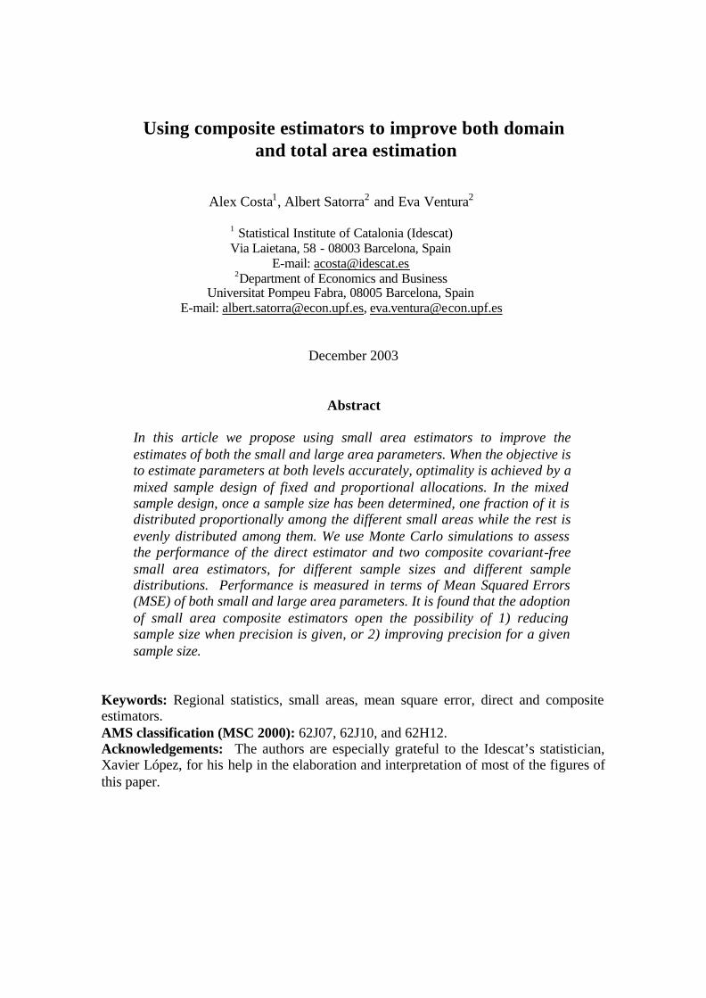
Using composite estimators to improve both domain and total area estimation

Alex Costa1, Albert Satorra2 and Eva Ventura2

1 Statistical Institute of Catalonia (Idescat) Via Laietana, 58 - 08003 Barcelona, Spain

E-mail: [email protected] 2Department of Economics and Business

Universitat Pompeu Fabra, 08005 Barcelona, Spain E-mail: [email protected], [email protected]

December 2003

Abstract

In this article we propose using small area estimators to improve the estimates of both the small and large area parameters. When the objective is to estimate parameters at both levels accurately, optimality is achieved by a mixed sample design of fixed and proportional allocations. In the mixed sample design, once a sample size has been determined, one fraction of it is distributed proportionally among the different small areas while the rest is evenly distributed among them. We use Monte Carlo simulations to assess the performance of the direct estimator and two composite covariant-free small area estimators, for different sample sizes and different sample distributions. Performance is measured in terms of Mean Squared Errors (MSE) of both small and large area parameters. It is found that the adoption of small area composite estimators open the possibility of 1) reducing sample size when precision is given, or 2) improving precision for a given sample size.

Keywords: Regional statistics, small areas, mean square error, direct and composite estimators. AMS classification (MSC 2000): 62J07, 62J10, and 62H12. Acknowledgements: The authors are especially grateful to the Idescat’s statistician, Xavier López, for his help in the elaboration and interpretation of most of the figures of this paper.

2

1 Introduction This study stems from the need to answer a very practical issue. The Institut d’Estadística de Catalunya (IDESCAT) had to develop an Industrial Production Index (IPI) for the Catalan autonomous community. The Instituto Español de Estadística (INE) did not produce any regional IPI for Spain, just a national one. The IDESCAT did not count with a budget that could support a Catalan monthly survey. Instead of tha t, the IDESCAT estimated a Catalan general IPI using the Spanish IPI of 150 industrial branches, weighted according to their relative importance in Catalonia. This Catalan IPI was a synthetic estimator and was accepted very well by the analysts of the Catalan economy. Actually, the statisticians of the IDESCAT had performed a test prior to publishing the new index. They knew that the Instituto Vasco de Estadística (Eustat) conducted their own regional survey in the Basque Country and published a Basque IPI. The IDESCAT created a synthetic index for the Basque Country, using the same methodology applied to the Catalan index. This index was compared to the Eustat’s IPI and the results of such comparison were successful. Both the level value of the synthetic IPI and its rate of variation were very useful in order to follow the Basque economic situation (see Costa and Galter 1994). Based on those results the IDESCAT produced a synthetic IPI for Catalonia. This index was so successful that, just a few months la ter, the INE decided to apply the same methodology to obtain a distinct IPI for each of the seventeen Spanish autonomous communities. However, the method used by the IDESCAT was by no means a standard one in the Spanish official statistics. The synthetic IPI was criticized within some fields, even when it worked well in Catalonia. Some studies (see Clar, Ramon and Surinach 2000) showed that the synthetic IPI works well in those regions that possess a significant and quite diversified industry, such as Catalonia. But it does not work well in the rest of the Spanish regions. This observation encouraged the IDESCAT to investigate the theoretical basis of its synthetic IPI framing it into the context of the small area estimation methodology. A joint research project with statisticians of the Universitat Pompeu Fabra was started. There is a varied methodology on small area estimation. The reader can consult Platek, Rao, Särndal and Singh (1987), Isaki (1990), Ghosh and Rao (1994), and Singh, Gambino and Mantel (1994) to gain an overview of them. Some of the methods use auxiliary information from related variables in the estimation of area level parameters. Here we concentrate on what we call covariate–free methods, which use sample information solely from the variables whose area parameters are being estimated. These covariate- free methods include direct and indirect estimators and their combinations. Traditional direct estimators use only data from the small area being examined. Usually they are unbiased, but their exhibit a high degree of variation. Indirect, composite and model-based estimators are more precise since they also use observations from related or neighboring areas. Indirect estimators are obtained through unbiased large area estimators. Based on them, it is possible to derive estimators for smaller areas under the assumption that they exhibit the same structure (with regard to the phenomenon being studied) as the initial large area. If this condition is not met, biased estimators could result. Covariate- free composite estimators are linear combinations of direct and indirect estimators. More information on small area

3

estimation can be obtained from Cressie (1995), Datta et al. (1999), Farrell, MacGibbon and Tomberlin (1997), Longford (2001), Pfeffermann and Barnard (1991), Raghunathan (1993), Singh, Mantel and Thomas (1994), Singh, Stukel and Pfeffermann (1998), and Thomas, Longford and Rolph (1994). In Spain, recent work of Morales, Molina and Santamaría (2003) deals with small area estimation with auxiliary variables and complex sample designs. The research program on small area estimation carried out jointly by IDESCAT and researchers of the Universitat Pompeu Fabra is characterized by its focus on covariate-free models. We believe that an estimator that is based on using auxiliary information from other variables at hand is, in some respect, subjective. We think that the covariate-free small area estimators are the only ones that are readily usable in the present stage of our official statistics framework. In a first article, Costa, Satorra and Ventura (2002) worked with a survey that included direct regional estimations of the Spanish work force. They studied three small area estimators: a synthetic one, a direct one and a composite one. The study concluded that the composite estimator and the synthetic estimator were almost the same in Catalonia, due to the fact that this region’s economy is very large relative to the whole Spanish economy, and the bias of the synthetic estimator was found to be very small for Catalonia. In a second study, Costa, Satorra and Ventura (2003) used Monte Carlo methods (with both an empirical1 and a theoretical population) to compare the performance of several small area estimators: one direct, one synthetic, and three composite estimators. The difference between those three composite estimators lies in the way the relative weights of the direct and synthetic estimators are calculated. One of the composite estimators used theoretical weights (that is we assume that bias and variances are known). The other two use estimated weights and differ depending on whether we assume homogeneous or heterogeneous biases and variances across the small areas. We compared the mean and median of the MSE of the estimators across small areas. We concluded that, given the usual sample sizes used in official statistics, the best possible estimator was the composite estimator based on the assumption of heterogeneity of biases and variances. Often the statistician is interested on the estimation of both small and large area parameters. In this case, classical estimation methods use sample designs that vary according to the assignment of sample size to the small areas. The following sample designs are considered: a) a proportional design, in which the sample size of each area is proportional to the size of the area in the population; b) uniform design, in which all the areas share the same sample size, irregardless of the population size of the area and, c) the mixed design, that uses a weighted combination of strategies a) and b). Clearly, design a) will be optimal when we focus on estimating accurately the large area parameter; while design b) will be chosen when we want to obtain accurate estimates of the small area parameters. In the present paper we show that small area estimation, in combination with a mixed design achieves optimality when we need accurate estimates of both level parameters. 1 The empirical population is the Labour Force Census of Enterprises affiliated with the Social Security system in Catalonia. The small areas are the forty-one Catalan counties.

4

In this case, the adoption of small area composite estimators opens the possibility of either reducing sample size, when precision is given; or, improving precision, when sample size is fixed. 2 Small area estimation without covariates Suppose that a large area (population) is divided into 1,2, ,j J= … small area domains. Let N be the size of the population, and N1, N2,… , NJ be the sizes of the J small areas. Let X be a one-dimensional variable that varies on each individual, 1, , jk N= … , in each

small area, 1,2, ,j J= … , with values denoted as kjx . Suppose we are interested in estimating the mean (or the total) of X for each of the J domains, as well as the mean (total) over all the population. Let jθ be the mean of X in the domain j , and *θ be the mean of X in the population. The variance of X restricted to area j is denoted as

2jσ .

Assume we have a direct estimator ˆ

jθ of the mean of X in each domain, such that

( )2ˆ ,j j j jN nθ θ σ∼ , 1,2, ,j J= … , as well as an estimator *̂θ for the large area mean,

with ( )2* * *ˆ ,Nθ θ σ∼ . Furthermore, assume a distribution for the mean of area j,

( )2* ,j jN bθ θ∼ where 2

jb is a variance parameter that (possibly) varies with j.

Typically, in practice, the design of the survey attends only to the objective of ensuring precision when estimating the parameters at the population parameters, large area level. That is, typically, *̂θ is unbiased for *θ and 2

*σ is very small. Often, however, the sample survey has the secondary use of providing information for parameters at the small area level. A typical problem for this secondary use of the survey is that the sample size of each small area domain is too small, may even be null, to drawn accurate inferences for the mean of the small area on the basis of the direct estimate ˆ

jθ . That is,

even though ˆjθ is an unbiased estimate for jθ , its variance 2

jσ is too large to provide an accurate estimation of the small area level parameter. In this context it is advisable to use composite estimators. These estimators combine the direct estimator and a synthetic (indirect) estimator in a linear fashion. It is well known that the best linear composite estimator of jθ (in the sense of minimizing the MSE) is

( )*̂ˆ1j j j jθ π θ π θ= + −% (1)

with

5

( )

2

2 2 2* * 2

j j jj

j j j j

n

n

σ γπ

θ θ σ σ γ

−=

− + + − (2)

where jγ denotes the covariance between the direct estimator and *̂θ . For simplicity,

assume that the covariance 0jγ = and 2*σ is negligible. The value of jπ that

minimizes the MSE is

( )

2

2 2

j jj

j j j

n

b n

σπ

σ=

+ (3)

where ( )22*j jb θ θ= − .

In practice, the values of the variance 2

jσ and squared bias 2jb are unknown (they are

population-based parameters), and therefore they must be estimated if we wish to approach the optimal value of jπ in (3). There are several procedures for estimating these population parameters, all of which lead to different small area estimators. In the present study we use two estimators, which we call the “classic composite” and the “alternative composite”. These estimators are further investigated in Costa, Satorra and Ventura (2003).

1. Classic composite estimator. The classic composite estimator assumes that the small areas share the same within-area variance (of the baseline data) and a common estimate for the squared bias. Specifically, we assume ( )2ˆ , , 1,2, ,j j jN n j Jθ θ σ =∼ … , and ( )2

* ,j N bθ θ∼ .

Here we use a weighted mean of the sample variances from each area as an estimate of the baseline data variance. Thus we define the pooled within -variance

( )( )

2

12

1

J

j jj

n ss

n J=

−=

−

∑, (4)

where n is the size of the entire sample, jn is the sample size of the small area and 2js is the sample variance of the baseline data of the small area j . If we assume that 2 2jσ σ= for all of j , the estimator of 2

jσ is 2s .

For the squared bias ( )2

* jθ θ− , we define the common estimator

( )22

*1

1 ˆ ˆJ

jj

bJ

θ θ=

= −∑ , (5)

i.e., the mean squared difference of the direct and indirect estimators.

Thus, the estimator of jπ is:

6

2

2 2

/ˆ

/j

jc

j

s n

s n bπ =

+, (6)

and the composite estimator with weights estimated using the sample data is ( )*̂

ˆˆ ˆ1c c cj j j jθ π θ π θ= + −% (7)

2. Alternative composite estimator An alternative for the above classic composite estimator is based on direct estimators of each area’s variance and bias. In this way the estimator of jπ is:

( )

2

2

*

/ˆ

ˆ ˆj

j ja

j

s nπ

θ θ=

− (8)

Note that ( )2

*ˆ ˆ

jθ θ− is biased for 2*( )jθ θ− , but is unbiased for 2 2

j j jn bσ + , as

( ) ( )( ) ( ) ( ) ( )

2 2

* *

2 2

* *

2 2

ˆ ˆ ˆ ˆ

ˆ ˆ ˆ ˆ2

j j j j

j j j j j j

j j j

E E

E E E

n b

θ θ θ θ θ θ

θ θ θ θ θ θ θ θ

σ

− = − + − =

= − + − + − − =

= +

which leads to the alternative composite estimator

( )*̂ˆˆ ˆ1a a a

j j j jθ π θ π θ= + −% (9)

If necessary, the weight ˆ ajπ is truncated to one.

3 Survey design with small areas The behavior of the direct estimators depends on the size of the sample and the survey design strategy. Here, we examine the behavior of the direct estimators and the two composite estimators under different survey designs. Assume we want to extract a sample of size n of the whole population. A purely proportional survey design distributes the sample units across the small areas in a way such that

1

J

jj

n n=

=∑ (10)

and

7

1,2. ,j jn Nj J

n N= = … (11)

where jn is the size of the sample belonging to area j . A purely fixed survey design assigns the same sample size to each small area. Therefore

1

for 1,2, , and n

j jj

nn j J n n

J =

= = =∑… (12)

A mixed survey design distributes a fraction of the whole sample in a proportional way among the different areas, with the rest of the sample distributed evenly among the areas. Let k be the fraction of the sample to be assigned to the proportional design. Then

( )1

1 for 1,2, , and J

jj j

j

N nn k n k j J n n

N J =

= + − = =∑… (13)

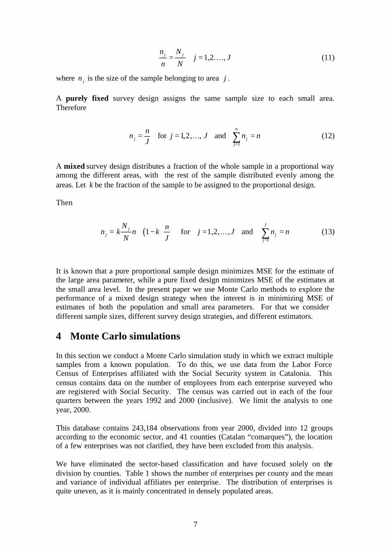
It is known that a pure proportional sample design minimizes MSE for the estimate of the large area parameter, while a pure fixed design minimizes MSE of the estimates at the small area level. In the present paper we use Monte Carlo methods to explore the performance of a mixed design strategy when the interest is in minimizing MSE of estimates of both the population and small area parameters. For that we consider different sample sizes, different survey design strategies, and different estimators. 4 Monte Carlo simulations In this section we conduct a Monte Carlo simulation study in which we extract multiple samples from a known population. To do this, we use data from the Labor Force Census of Enterprises affiliated with the Social Security system in Catalonia. This census contains data on the number of employees from each enterprise surveyed who are registered with Social Security. The census was carried out in each of the four quarters between the years 1992 and 2000 (inclusive). We limit the analysis to one year, 2000. This database contains 243,184 observations from year 2000, divided into 12 groups according to the economic sector, and 41 counties (Catalan “comarques”), the location of a few enterprises was not clarified, they have been excluded from this analysis. We have eliminated the sector-based classification and have focused solely on the division by counties. Table 1 shows the number of enterprises per county and the mean and variance of individual affiliates per enterprise. The distribution of enterprises is quite uneven, as it is mainly concentrated in densely populated areas.

8

Table 1: Population Parameters

We will consider four sample sizes and five alternative survey design strategies. The smallest sample size will be 2,050 observations. We then repeatedly double that size and consider 4,100, 8,200 and 16,400 observations. For each one of the four sample sizes we consider a purely proportional sample ( 1k = ), a 75%, 50% and 25% mixed sample design ( 0.75k = , 0.5k = and 0.25k = respectively), and a purely fixed sample design ( 0k = ).

Populationsize

Alt Camp 1282 8,73ª 0,09 3250,37 Alt Empordà 4712 5,28 14,11 294,27 Alt Penedès 3052 8,91 0,02 1686,24 Alt Urgell 745 4,71 18,7 158,25 Alta Ribagorça 140 4,59 19,73 205,38 Anoia 3264 7,86 1,37 801,64 Bages 5698 8,24 0,63 1356,9 Baix camp 5530 6,47 6,59 479,54 Baix Ebre 2237 6,31 7,41 534,4 Baix Empordà 4634 5,44 12,92 425,17 Baix Llobregat 20541 9,73 0,48 1642,46 Baix Penedès 2197 5,26 14,23 171,82 Barcelonès 88331 10,63 2,55 10314,88 Berguedà 1397 5,44 12,9 196,15 Cerdanya 788 3,71 28,34 71,93 Conca de Barberà 611 8,29 0,56 1388,95 Garraf 3466 6,28 7,62 685,91 Garrigues 516 5,24 14,42 96,89 Garrotxa 1909 7,51 2,33 419,72 Gironès 6369 9,82 0,62 2037,47 Maresme 11718 6,46 6,64 605,07 Montsià 1918 5,61 11,73 246 Noguera 1128 5,12 15,3 93,29 Osona 5494 7,09 3,77 774,65 Pallars Jussà 410 4,37 21,76 130,37 Pallars Sobirà 272 4,06 24,76 55,46 Pla d'Urgell 1106 6,59 5,95 271,85 Pla de l'Estany 1160 6,07 8,79 143,37 Priorat 254 4,11 24,26 180,17 Ribera d'Ebre 620 5,71 11,07 418,72 Ripollès 959 7,87 1,35 875,92 Segarra 594 10,87 3,35 8171,41 Segrià 7096 7,74 1,69 714,23 Selva 4586 7,11 3,7 610,2 Solsonès 508 5,58 11,93 157,58 Tarragonès 7440 9,42 0,15 1675,66 Terra Alta 297 4,25 22,87 40,28 Urgell 1178 6,28 7,59 312,25 Val d'Aran 503 5,28 14,08 270,11 Vallès Occidental 26683 10,34 1,71 3026,89 Vallès Oriental 11795 8,45 0,34 832,68

The mean of the affiliates for the whole Catalonia is 9.04

jθ ( )2

*jθ θ− 2( )j xσ

9

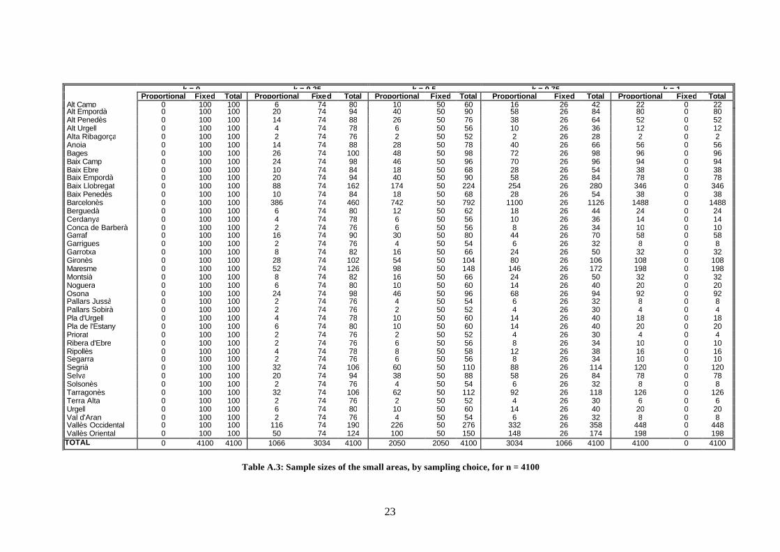
Table A.3 in the appendix shows the small area sample sizes in each of those 4 by 5 = 20 scenarios and sample size 4,100. Due to the small population size in some of the counties (especially for the proportional design), we used sampling with replacement. The number of Monte Carlo replications is 1,000. The simulation exercises let us obtain small area direct, classic composite and alternative composite estimators for each of the 41 counties as well as for the whole Catalonia.

5 Direct vs. Composite Estimators: MSE performance functions.

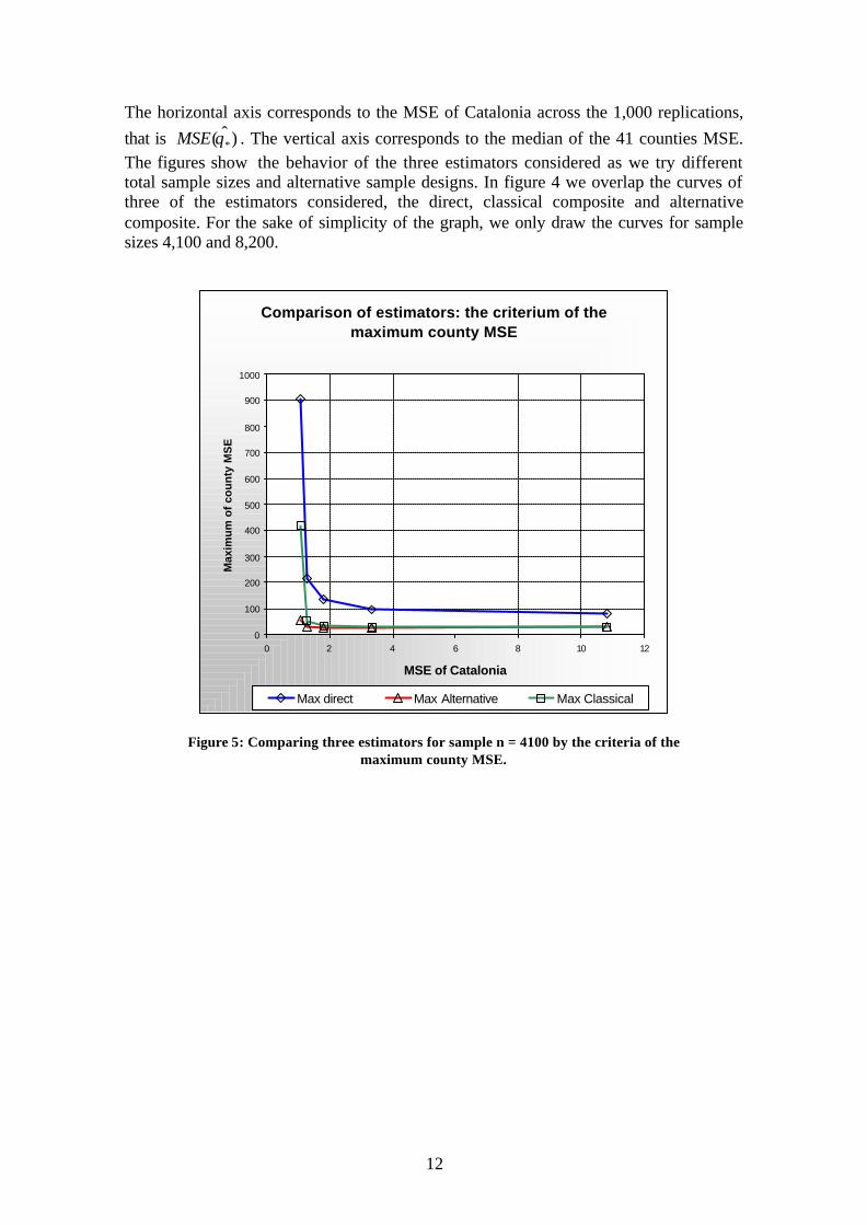
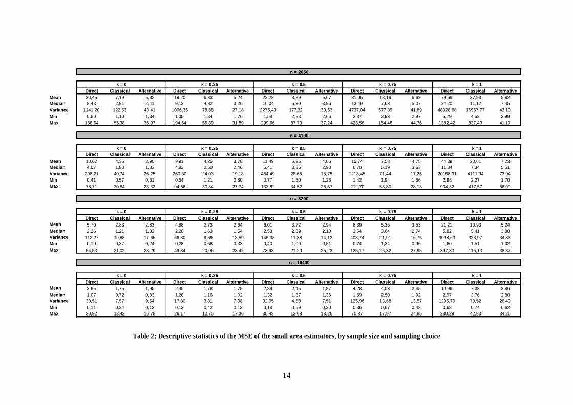
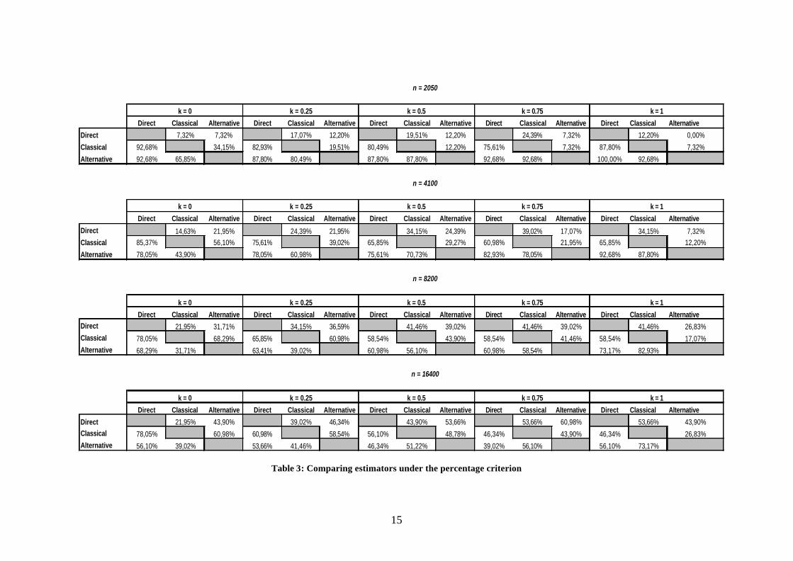
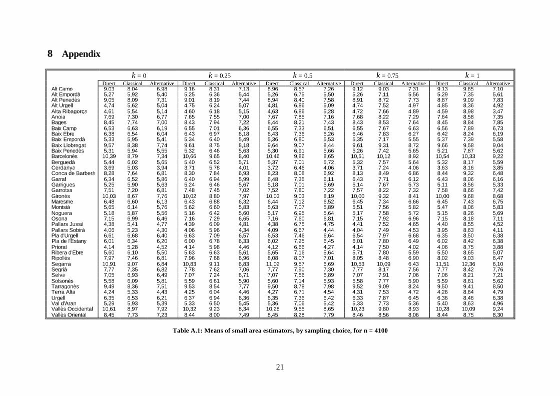
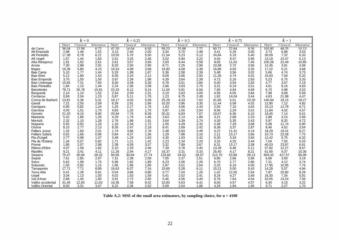
We have computed the MSE of the different small area estimators. Table 2 shows a summary of descriptive statistics. The mean, median, va riance, minimum and maximum values of the MSE of the small area estimators across the 1,000 replications are presented. Table A.1 in the appendix shows the mean value of the small area estimators in the simulations that we have performed, for a sample size of 4,100. Table A.2 in the appendix offers the MSE values for each small area in our simulations, also for a sample size of 4,1002. Also in this section, Table 3 offers a different way to evaluate the relative performance of the three alternative estimators considered. In that table we calculate the percentage of counties for which the MSE of a particular estimator (in the leftmost column) is lower than the MSE of a different estimator (in the top row). There are several useful criteria to evaluate the performance of the small area estimations. In a previous study (see Costa, Satorra and Ventura 2003) we have observed that the distribution of the MSE across the Catalan counties is asymmetric. It also exhibits extreme values and it is very disperse. This is the reason why we used the median, in addition to the mean, as the median has the advantage of not being affected by the presence of extreme values. On the other hand, sometimes we are interested on putting a limit to how bad any individual small area estimation can be. If this is the case we might be looking at the maximum MSE of the counties. To keep things simple and easy to read, we have chosen to present our graphical results using the median evaluation criterion. However, Tables 2 and 3, as well as Figures 5 and 6 in this section, show some numerical results using other evaluation criteria. Those criteria are the average of the MSE of the counties, the maximum and minimum values of the MSE of the counties, and the percentage of counties for which a particular type of estimator performs better than the rest of the estimators considered. Figures 1 to 6 visually summarize the results.

2 We have chosen to show just this case, in order to illustrate the way the results are obtained. The interested reader can obtain upon request the exact small area MSE of all the cases studied.

10

Direct Estimator

0

5

10

15

20

25

30

0 5 10 15 20 25

MSE of Catalonia

Med

ian

of c

ou

nty

MS

E

n = 2050 n = 4100 n = 8200 n = 16400

k = 0.75

k = 0

k = 1

k = 0.25k = 0.5

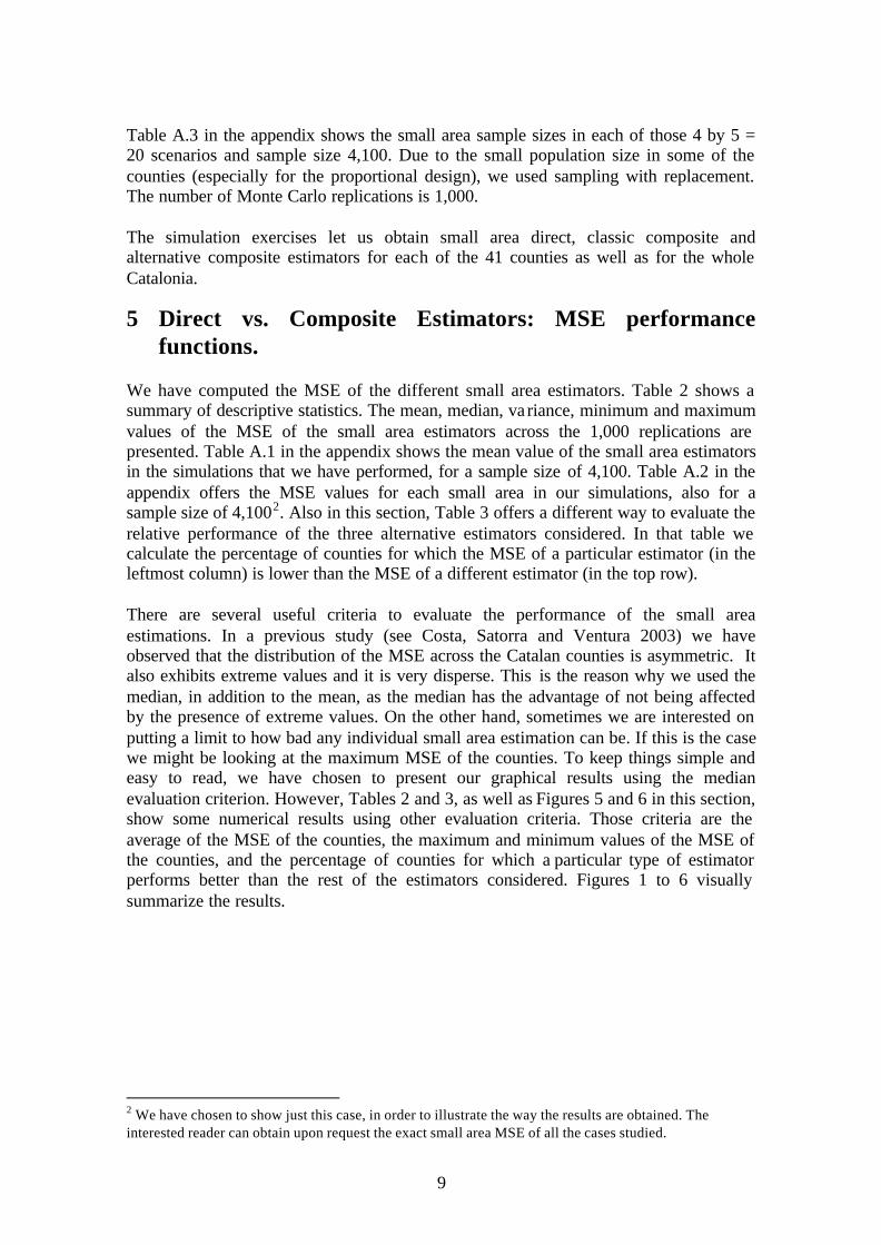
Figure 1: MSE of Direct estimator by sample size and sample design

Classical Composite Estimator

0

2

4

6

8

10

12

0 5 10 15 20 25

MSE of Catalonia

Med

ian

of c

ount

y M

SE

n = 2050 n = 4100 n = 8200 n = 16400

k = 1

k = 0.75

k = 0.5k = 0.25

k = 0

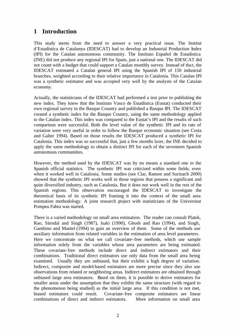
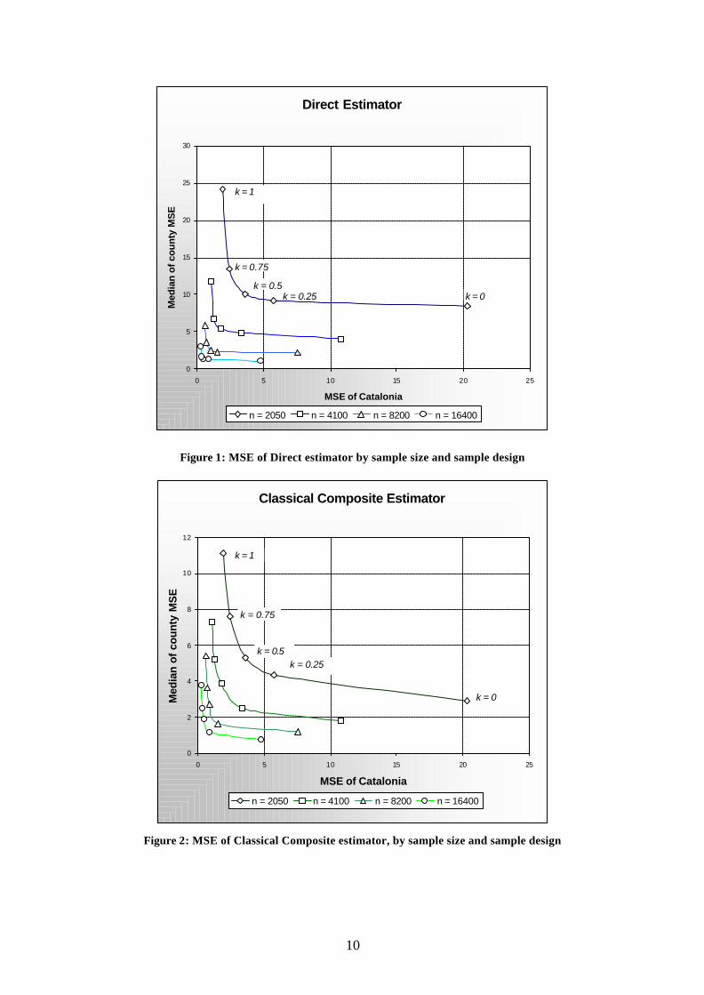
Figure 2: MSE of Classical Composite estimator, by sample size and sample design

11

Alternative Composite Estimator

0

1

2

3

4

5

6

7

8

0 5 10 15 20 25

MSE of Catalonia

Med

ian

of c

ou

nty

MS

E

n = 2050 n = 4100 n = 8200 n = 16400

k = 1

k = 0.75

k = 0.5

k = 0.25

k = 0

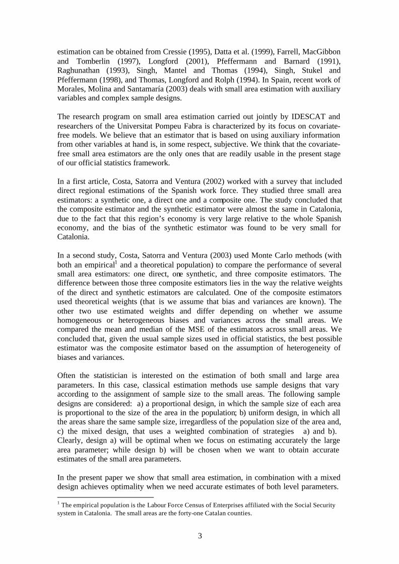
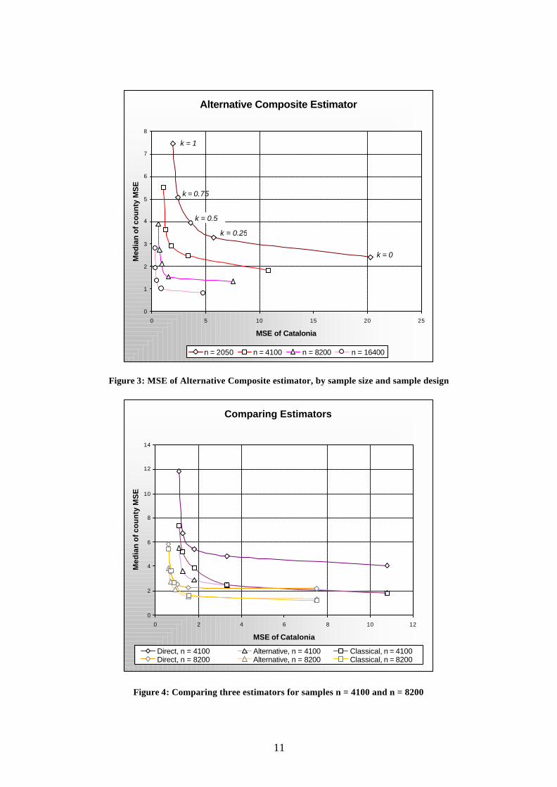
Figure 3: MSE of Alternative Composite estimator, by sample size and sample design

Comparing Estimators

0

2

4

6

8

10

12

14

0 2 4 6 8 10 12

MSE of Catalonia

Med

ian

of c

ou

nty

MS

E

Direct, n = 4100 Alternative, n = 4100 Classical, n = 4100Direct, n = 8200 Alternative, n = 8200 Classical, n = 8200

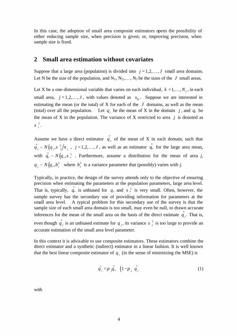
Figure 4: Comparing three estimators for samples n = 4100 and n = 8200

12

The horizontal axis corresponds to the MSE of Catalonia across the 1,000 replications, that is *̂( )MSE θ . The vertical axis corresponds to the median of the 41 counties MSE. The figures show the behavior of the three estimators considered as we try different total sample sizes and alternative sample designs. In figure 4 we overlap the curves of three of the estimators considered, the direct, classical composite and alternative composite. For the sake of simplicity of the graph, we only draw the curves for sample sizes 4,100 and 8,200.

Comparison of estimators: the criterium of the maximum county MSE

0

100

200

300

400

500

600

700

800

900

1000

0 2 4 6 8 10 12

MSE of Catalonia

Max

imu

m o

f co

un

ty M

SE

Max direct Max Alternative Max Classical

Figure 5: Comparing three estimators for sample n = 4100 by the criteria of the

maximum county MSE.

13

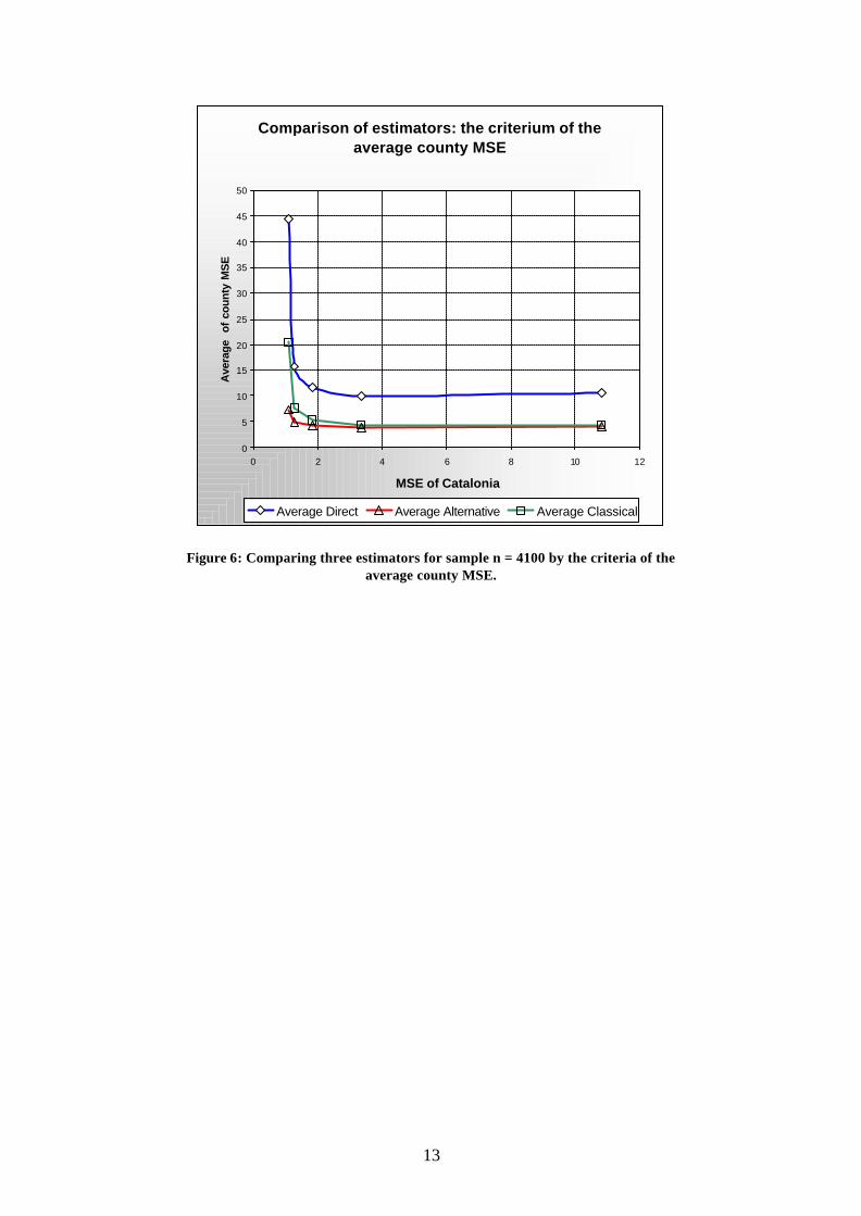
Comparison of estimators: the criterium of the average county MSE

0

5

10

15

20

25

30

35

40

45

50

0 2 4 6 8 10 12

MSE of Catalonia

Ave

rage

of

cou

nty

MS

E

Average Direct Average Alternative Average Classical

Figure 6: Comparing three estimators for sample n = 4100 by the criteria of the

average county MSE.

14

Direct Classical Alternative Direct Classical Alternative Direct Classical Alternative Direct Classical Alternative Direct Classical AlternativeMean 20,45 7,19 5,32 19,20 6,83 5,24 23,22 8,89 5,67 31,05 13,19 6,62 79,69 37,93 8,82Median 8,43 2,91 2,41 9,12 4,32 3,26 10,04 5,30 3,96 13,49 7,63 5,07 24,20 11,12 7,45Variance 1141,20 122,53 43,41 1006,35 78,88 27,18 2275,40 177,32 30,53 4737,04 577,39 41,89 48928,68 16967,77 43,10Min 0,80 1,10 1,34 1,05 1,84 1,76 1,58 2,83 2,66 2,87 3,93 2,97 5,79 4,53 2,99Max 158,64 55,38 36,97 194,64 56,89 31,89 299,66 87,70 37,24 423,58 154,48 44,76 1382,42 837,40 41,17




n = 16400

k = 0 k = 0.25 k = 0.5 k = 0.75 k = 1

n = 8200

k = 0 k = 0.25 k = 0.5 k = 0.75 k = 1

n = 4100

k = 0 k = 0.25 k = 0.5 k = 0.75 k = 1

k = 0.5 k = 0.75 k = 1

n = 2050

k = 0 k = 0.25

Table 2: Descriptive statistics of the MSE of the small area estimators, by sample size and sampling choice

15

Direct Classical Alternative Direct Classical Alternative Direct Classical Alternative Direct Classical Alternative Direct Classical Alternative

Direct 7,32% 7,32% 17,07% 12,20% 19,51% 12,20% 24,39% 7,32% 12,20% 0,00%

Classical 92,68% 34,15% 82,93% 19,51% 80,49% 12,20% 75,61% 7,32% 87,80% 7,32%

Alternative 92,68% 65,85% 87,80% 80,49% 87,80% 87,80% 92,68% 92,68% 100,00% 92,68%


Direct 14,63% 21,95% 24,39% 21,95% 34,15% 24,39% 39,02% 17,07% 34,15% 7,32%Classical 85,37% 56,10% 75,61% 39,02% 65,85% 29,27% 60,98% 21,95% 65,85% 12,20%

Alternative 78,05% 43,90% 78,05% 60,98% 75,61% 70,73% 82,93% 78,05% 92,68% 87,80%

Direct Classical Alternative Direct Classical Alternative Direct Classical Alternative Direct Classical Alternative Direct Classical AlternativeDirect 21,95% 31,71% 34,15% 36,59% 41,46% 39,02% 41,46% 39,02% 41,46% 26,83%Classical 78,05% 68,29% 65,85% 60,98% 58,54% 43,90% 58,54% 41,46% 58,54% 17,07%Alternative 68,29% 31,71% 63,41% 39,02% 60,98% 56,10% 60,98% 58,54% 73,17% 82,93%


Direct 21,95% 43,90% 39,02% 46,34% 43,90% 53,66% 53,66% 60,98% 53,66% 43,90%Classical 78,05% 60,98% 60,98% 58,54% 56,10% 48,78% 46,34% 43,90% 46,34% 26,83%Alternative 56,10% 39,02% 53,66% 41,46% 46,34% 51,22% 39,02% 56,10% 56,10% 73,17%

n = 16400

k = 0 k = 0.25 k = 0.5 k = 0.75 k = 1

n = 8200

k = 0 k = 0.25 k = 0.5 k = 0.75 k = 1

n = 4100

k = 0 k = 0.25 k = 0.5 k = 0.75 k = 1

n = 2050

k = 0 k = 0.25 k = 0.5 k = 0.75 k = 1

Table 3: Comparing estimators under the percentage criterion

16

We observe the following results, some of which are corroboration of what was to be expected form a priory grounds:

• As expected, the MSE for Catalonia is smaller when 1k = and larger when 0k = . Contrarily, the median county MSE is smaller when 0k = and larger

when 1k = . This result is valid for the three estimators considered: direct, classic composite and alternative composite. It also holds when we consider the average county MSE instead of the median county MSE, although the differences between small and large area MSE are magnified.

• Both the MSE for Catalonia and the median county MSE diminish as the total

sample size increases, independently of which estimator we are considering. The same result holds when we consider other statistics such as the average county MSE, or the maximum values of MSE. See figures 5 and 6.

• Figure 4 shows how, on average, the alternative composite estimator is best in

the sense of providing the lower MSE of Catalonia and median county MSE for any sample size and any sample design. There are some not very noticeable exceptions when the total sample sizes are large and we use a fixed sample survey design. In this figure we report only sample sizes n = 4100 and n = 8200, just to make the figure more readable.

• When we look at Table 3 we conclude that the two composite estimators are

almost always better than the direct estimator. There are some exceptions when the total sample size is large. We also observe that the direct estimator improves its behavior as the total sample size increases, independently of the survey design.

• Also in Table 3 we observe that the alternative composite estimator is better

than the classical one except in the case in which we consider k = 0 or k = 0.25 (non proportional survey designs) and the sample size increases.

• If the statistician wants to achieve a particular combination of a small MSE for

the large area jointly with small median or average small area MSE, a mixed sampling strategy survey might be a good choice. The desired combination will depend on the preferences of the statistician. This observation suggests that we could borrow some elements from the economic theory of consumption in order to explain the statistician decision-making process. In any case, it is certainly clear that the use of composite estimators offers very interesting improving opportunities for both small area estimation and sample design. This can be observed in Figure 4 and it is discussed in the next section.

17

6 Discussion: improving survey design through small area estimation

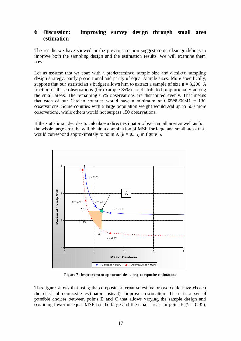
The results we have showed in the previous section suggest some clear guidelines to improve both the sampling design and the estimation results. We will examine them now. Let us assume that we start with a predetermined sample size and a mixed sampling design strategy, partly proportional and partly of equal sample sizes. More specifically, suppose that our statistician’s budget allows him to extract a sample of size n = 8,200. A fraction of these observations (for example 35%) are distributed proportionally among the small areas. The remaining 65% observations are distributed evenly. That means that each of our Catalan counties would have a minimum of 0.65*8200/41 = 130 observations. Some counties with a large population weight would add up to 500 more observations, while others would not surpass 150 observations. If the statistic ian decides to calculate a direct estimator of each small area as well as for the whole large area, he will obtain a combination of MSE for large and small areas that would correspond approximately to point A (k = 0.35) in figure 5.

1

2

3

4

0 1 2 3 4

MSE of Catalonia

Med

ian

of c

ou

nty

MS

E

Direct, n = 8200 Alternative, n = 8200

C

B

A

k = 0.75

k = 0.5

k = 0.25

k = 0.25

k = 0.5

k = 0.75

1

2

3

4

0 1 2 3 4

MSE of Catalonia

Med

ian

of c

ou

nty

MS

E

Direct, n = 8200 Alternative, n = 8200

C

B

A

k = 0.75

k = 0.5

k = 0.25

k = 0.25

k = 0.5

k = 0.75

Figure 7: Improvement opportunities using composite estimators

This figure shows that using the composite alternative estimator (we could have chosen the classical composite estimator instead), improves estimation. There is a set of possible choices between points B and C that allows varying the sample design and obtaining lower or equal MSE for the large and the small areas. In point B (k = 0.35),

18

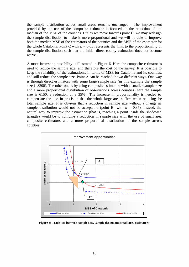
the sample distribution across small areas remains unchanged. The improvement provided by the use of the composite estimator is focused on the reduction of the median of the MSE of the counties. But as we move towards point C, we may redesign the sample distribution to make it more proportional and we will be able to improve both the median MSE of the estimators of the counties and the MSE of the estimator for the whole Catalonia. Point C with k = 0.65 represents the limit to the proportionality of the sample distribution such that the initial direct county estimation does not become worse. A more interesting possibility is illustrated in Figure 6. Here the composite estimator is used to reduce the sample size, and therefore the cost of the survey. It is possible to keep the reliability of the estimations, in terms of MSE for Catalonia and its counties, and still reduce the sample size. Point A can be reached in two different ways. One way is through direct estimators with some large sample size (in this example the sample size is 8200). The other one is by using composite estimators with a smaller sample size and a more proportional distribution of observations across counties (here the sample size is 6150, a reduction of a 25%). The increase in proportionality is needed to compensate the loss in precision that the whole large area suffers when reducing the total sample size. It is obvious that a reduction in sample size without a change in sample distribution would not be acceptable (point B’ with k = 0.35). Instead, the natural way to improve the estimation (that is, reaching a point inside the shadowed triangle) would be to combine a reduction in sample size with the use of small area composite estimators and a more proportional distribution of the sample across counties.

Improvement opportunities

1

2

3

4

0 1 2 3 4

MSE of Catalonia

Med

ian

of c

ou

nty

MS

E

Direct, n = 8200 Alternative, n = 8200 Alternative n=6150

A

B’

k = 0.75

k = 0.25

k = 0.50

Improvement opportunities

1

2

3

4

0 1 2 3 4

MSE of Catalonia

Med

ian

of c

ou

nty

MS

E

Direct, n = 8200 Alternative, n = 8200 Alternative n=6150

A

B’

k = 0.75

k = 0.25

k = 0.50

Figure 8: Trade -off between sample size, sample design and small area estimators

19

7 References CLAR, M., RAMOS, and J. SURIÑACH (2000). Avantatges i inconvenients de la metodologia del INE per elaborar indicadors de la producció industrial per a les regions espanyoles, Qüestiió, Vol 24, Núm 1, p.151-186. COSTA, A. and J. GALTER (1994). L’IPPI, un indicador molt valuós per mesurar l’activitat industrial catalana, Revista d’Indústria, Núm 3, Generalitat de Catalunya, p.6-15. COSTA, A., SATORRA, A. and E. VENTURA (2002). Estimadores compuestos en estadística regional: Aplicación para la tasa de variación de la ocupación en la industria, Qüestiió, vol. 26, Núm. 1-2, p. 213-243. COSTA, A., SATORRA, A. and E. VENTURA (2003). An empirical evaluation of small area estimators, SORT (Statistics and Operations Research Transactions), vol. 27, 1, p. 113-135. CRESSIE, N. (1995). Bayesian Smoothing of Rates in Small Geographic Areas. Journal of Regional Science. Vol. 35 (4), p 659-73. DATTA, G. S., et al. (1999). Hierarchical Bayes Estimation of Unemployment Rates for the States of the U.S. Journal of the American Statistical Association. Vol.94 (448). p 1074-82. FARRELL, P. J, MACGIBBON, B., and TOMBERLIN,T. J. (1997). Empirical Bayes Small-Area Estimation Using Logistic Regression Models and Summary Statistics. Journal of Business & Economic Statistics. Vol. 15 (1), p 101-8. GHOSH, M. and RAO, J.N.K. (1994). Small Area Estimation: An Appraisal. Statistical Science, vol. 9, no. 1, Statistics Canada, p. 55-93. ISAKI, C. T. (1990). Small-Area Estimation of Economic Statistics. Journal of Business & Economic Statistics. Vol. 8 (4).p 435-41. LONGFORD, N.T. (2001). Synthetic Estimators With Moderating Influence: the Carry-Over in Cross-Over Trials Revisited, Statistics in Medicine, 20, p. 3189-3203. MORALES, D., MOLINA, I. and SANTAMARÍA, L. (2003). “Modelos estándard para estimaciones en áreas pequeñas. Extensión a diseños complejos”. Proceedings of the XXVII Congreso Nacional de Estadística e Investigación Operativa (Lleida, Abril de 2003) PFEFFERMANN, D., and BARNARD, C. H. (1991). ''Some New Estimators for Small-Area Means with Application to the Assessment of Farmland Values'', Journal of Business & Economic Statistics. Vol. 9 (1), p. 73-84. PLATEK, R., RAO, J.N.K., SÄRNDAL, C.E. and SINGH, M.P. Eds.(1987). Small Area Statistics: An International Symposium; New York; John Wiley and Sons.

20

RAGHUNATHAN, T E. (1993). ''A Quasi-empirical Bayes Method for Small Area Estimation'', Journal of the American Statistical Association. Vol.88 (424), p. 1444-48. SINGH, M.P., GAMBINO, J. and MANTEL, H.J. (1994). ''Issues and Strategies for Small Area Data'', Survey Methodology, vol. 20, no. 1, Statistics Canada, 3-22. SINGH, A.C., MANTEL, H.J. y THOMAS, B.W. (1994). ''Time Series EBLUPs for Small Areas Using Survey Data'', Survey Methodology, vol. 20, no. 1, Statistics Canada, 33-43. SINGH, A.C., STUKEL, D.M. and PFEFFERMANN, D. (1998). ''Bayesian versus frequentist measures of error in small area estimation'', Journal of the Royal Statistical Society, b, no. 60, p. 377-396. THOMAS, N., LONGFORD, N.T. and ROLPH, J.E. (1994). ''Empirical Bayes Methods for Estimating Hospital-Specific Mortality Rates'', Statistics in Medicine.

21

8 Appendix k = 0 k = 0.25 k = 0.5 k = 0.75 k = 1

Direct Classical Alternative Direct Classical Alternative Direct Classical Alternative Direct Classical Alternative Direct Classical Alternative Alt Camp 9,03 8,04 6,98 9,16 8,31 7,13 8,96 8,57 7,26 9,12 9,03 7,31 9,13 9,65 7,10 Alt Empordà 5,27 5,92 5,40 5,25 6,36 5,44 5,26 6,75 5,50 5,26 7,11 5,56 5,29 7,35 5,61 Alt Penedès 9,05 8,09 7,31 9,01 8,19 7,44 8,94 8,40 7,58 8,91 8,72 7,73 8,87 9,09 7,83 Alt Urgell 4,74 5,62 5,04 4,75 6,24 5,07 4,81 6,86 5,09 4,74 7,52 4,97 4,85 8,36 4,92 Alta Ribagorça 4,61 5,54 5,14 4,60 6,18 5,15 4,63 6,86 5,28 4,72 7,66 4,89 4,59 8,98 3,47 Anoia 7,69 7,30 6,77 7,65 7,55 7,00 7,67 7,85 7,16 7,68 8,22 7,29 7,64 8,58 7,35 Bages 8,45 7,74 7,00 8,43 7,94 7,22 8,44 8,21 7,43 8,43 8,53 7,64 8,45 8,84 7,85 Baix Camp 6,53 6,63 6,19 6,55 7,01 6,36 6,55 7,33 6,51 6,55 7,67 6,63 6,56 7,89 6,73 Baix Ebre 6,38 6,54 6,04 6,43 6,97 6,18 6,43 7,36 6,26 6,46 7,83 6,27 6,42 8,24 6,19 Baix Empordà 5,33 5,95 5,41 5,34 6,40 5,49 5,36 6,80 5,53 5,35 7,17 5,55 5,37 7,39 5,58 Baix Llobregat 9,57 8,38 7,74 9,61 8,75 8,18 9,64 9,07 8,44 9,61 9,31 8,72 9,66 9,58 9,04 Baix Penedès 5,31 5,94 5,55 5,32 6,46 5,63 5,30 6,91 5,66 5,26 7,42 5,65 5,21 7,87 5,62 Barcelonès 10,39 8,79 7,34 10,66 9,65 8,40 10,46 9,86 8,65 10,51 10,12 8,92 10,54 10,33 9,22 Berguedà 5,44 6,02 5,65 5,40 6,52 5,71 5,37 7,01 5,72 5,32 7,57 5,64 5,32 8,17 5,59 Cerdanya 3,69 5,03 3,94 3,71 5,78 4,01 3,72 6,46 4,06 3,71 7,24 4,06 3,63 8,16 3,85 Conca de Barberà 8,28 7,64 6,81 8,30 7,84 6,93 8,23 8,08 6,92 8,13 8,49 6,86 8,44 9,32 6,48 Garraf 6,34 6,52 5,86 6,40 6,94 5,99 6,48 7,35 6,11 6,43 7,71 6,12 6,43 8,06 6,16 Garrigues 5,25 5,90 5,63 5,24 6,46 5,67 5,18 7,01 5,69 5,14 7,67 5,73 5,11 8,56 5,33 Garrotxa 7,51 7,20 6,81 7,48 7,45 7,02 7,52 7,80 7,22 7,57 8,22 7,32 7,58 8,66 7,42 Gironès 10,03 8,67 7,76 10,02 8,80 7,97 10,03 9,03 8,19 10,00 9,32 8,41 10,00 9,68 8,68 Maresme 6,48 6,60 6,13 6,43 6,88 6,32 6,44 7,12 6,52 6,45 7,34 6,66 6,45 7,43 6,75 Montsià 5,65 6,14 5,76 5,62 6,60 5,83 5,63 7,07 5,89 5,51 7,56 5,82 5,47 8,06 5,83 Noguera 5,18 5,87 5,56 5,16 6,42 5,60 5,17 6,95 5,64 5,17 7,58 5,72 5,15 8,26 5,69 Osona 7,15 6,99 6,46 7,16 7,29 6,65 7,16 7,60 6,81 7,15 7,92 6,96 7,15 8,18 7,11 Pallars Jussà 4,38 5,41 4,77 4,39 6,09 4,81 4,38 6,75 4,75 4,41 7,52 4,65 4,40 8,55 4,52 Pallars Sobirà 4,06 5,23 4,30 4,06 5,96 4,34 4,09 6,67 4,44 4,04 7,49 4,53 3,95 8,63 4,11 Pla d'Urgell 6,61 6,68 6,40 6,63 7,09 6,57 6,53 7,46 6,64 6,54 7,97 6,68 6,35 8,50 6,38 Pla de l'Estany 6,01 6,34 6,20 6,00 6,78 6,33 6,02 7,25 6,45 6,01 7,80 6,49 6,02 8,42 6,38 Priorat 4,14 5,28 4,52 4,14 5,98 4,46 4,12 6,66 4,27 4,14 7,50 4,02 4,06 8,75 3,88 Ribera d'Ebre 5,60 6,10 5,50 5,63 6,63 5,61 5,65 7,16 5,64 5,71 7,80 5,59 5,50 8,65 5,07 Ripollès 7,97 7,46 6,81 7,96 7,68 6,96 8,08 8,07 7,01 8,05 8,48 6,90 8,02 9,03 6,47 Segarra 10,91 9,07 6,84 10,83 9,11 6,83 11,02 9,57 6,69 10,53 10,09 6,43 11,51 12,36 6,10 Segrià 7,77 7,35 6,82 7,78 7,62 7,06 7,77 7,90 7,30 7,77 8,17 7,56 7,77 8,42 7,76 Selva 7,05 6,93 6,49 7,07 7,24 6,71 7,07 7,56 6,89 7,07 7,91 7,06 7,06 8,21 7,21 Solsonès 5,58 6,09 5,81 5,59 6,61 5,90 5,60 7,14 5,93 5,58 7,77 5,90 5,59 8,61 5,62 Tarragonès 9,49 8,36 7,51 9,53 8,54 7,77 9,50 8,78 7,98 9,52 9,09 8,24 9,50 9,41 8,50 Terra Alta 4,24 5,33 4,43 4,25 6,04 4,46 4,27 6,71 4,54 4,31 7,53 4,72 4,26 8,64 4,79 Urgell 6,35 6,53 6,21 6,37 6,94 6,36 6,35 7,36 6,42 6,33 7,87 6,45 6,36 8,46 6,38 Val d'Aran 5,29 5,93 5,39 5,33 6,50 5,45 5,36 7,06 5,42 5,33 7,73 5,36 5,40 8,63 4,96 Vallès Occidental 10,61 8,97 7,92 10,32 9,23 8,34 10,28 9,55 8,65 10,23 9,80 8,93 10,28 10,09 9,24 Vallès Oriental 8,45 7,73 7,23 8,44 8,00 7,49 8,45 8,28 7,79 8,46 8,56 8,06 8,44 8,75 8,30

Table A.1: Means of small area estimators, by sampling choice, for n = 4100

22

k = 0 k = 0.25 k = 0.5 k = 0.75 k = 1 Direct Classical Alternative Direct Classical Alternative Direct Classical Alternative Direct Classical Alternative Direct Classical Alternative

Alt Camp 36,04 12,58 6,72 47,20 14,04 6,50 59,23 15,98 7,77 90,71 22,64 9,26 163,90 48,25 10,13 Alt Empordà 2,98 1,46 1,52 3,13 2,40 2,00 3,34 3,70 2,48 3,41 5,26 3,00 3,73 6,88 3,53 Alt Penedès 17,38 6,78 6,21 19,55 5,70 5,50 21,54 5,23 5,12 24,84 5,19 5,40 30,09 7,32 6,33 Alt Urgell 1,57 1,44 1,83 2,01 3,25 2,46 3,02 5,84 3,22 4,54 9,47 3,90 13,19 15,47 6,13 Alta Ribagorça 1,91 1,62 2,61 2,61 3,57 3,56 3,93 6,44 5,58 8,05 11,02 7,45 100,28 22,49 10,85 Anoia 7,30 2,88 2,91 8,20 2,50 2,90 8,71 2,25 2,90 10,58 2,72 3,56 12,45 3,91 4,58 Bages 16,36 5,80 4,23 16,53 4,99 3,68 16,83 4,58 3,38 16,86 4,93 3,35 17,22 6,21 3,68 Baix Camp 5,10 1,77 1,44 5,33 1,99 1,87 5,36 2,58 2,39 5,48 3,56 3,02 5,66 4,74 3,73 Baix Ebre 5,12 1,80 1,53 6,55 2,24 2,12 8,09 3,06 2,93 11,30 4,74 4,01 15,93 7,09 5,32 Baix Empordà 3,70 1,55 1,50 3,97 2,39 1,98 4,39 3,64 2,39 4,72 5,16 2,83 5,23 6,75 3,33 Baix Llobregat 15,65 7,31 7,83 9,30 4,58 5,30 6,78 3,51 3,84 5,40 3,04 2,83 4,77 3,07 2,19 Baix Penedès 1,84 1,15 1,44 2,24 2,36 2,08 2,66 3,93 2,75 3,31 6,19 3,51 4,61 9,16 4,63 Barcelonès 78,71 26,78 15,81 22,33 8,12 9,15 11,55 5,81 6,56 7,95 4,94 4,69 6,70 4,98 3,53 Berguedà 2,10 1,10 1,52 2,54 2,09 2,31 3,19 3,63 3,05 4,56 6,05 3,84 7,98 9,68 5,59 Cerdanya 0,69 2,04 1,23 0,87 5,11 1,76 1,23 8,75 2,49 1,92 14,04 3,44 4,63 21,98 4,47 Conca de Barberà 13,81 5,36 5,31 18,17 4,55 5,58 25,29 4,33 7,02 41,65 5,51 10,20 140,94 18,15 18,27 Garraf 7,21 2,55 2,09 8,39 2,91 2,66 10,20 3,86 3,35 11,44 5,08 4,02 12,80 7,12 4,82 Garrigues 0,95 0,82 1,24 1,25 2,17 1,76 1,63 4,06 2,43 2,50 7,15 3,63 10,13 12,78 6,71 Garrotxa 4,03 1,51 1,70 4,83 1,32 1,75 5,87 1,50 2,04 8,56 2,29 3,01 11,84 4,02 4,57 Gironès 21,20 9,15 9,90 20,94 7,76 8,39 20,31 6,83 7,07 19,67 6,36 6,10 19,45 7,14 5,51 Maresme 5,42 1,86 1,26 4,29 1,79 1,46 3,63 2,14 1,86 3,21 2,68 2,23 2,88 3,15 2,69 Montsià 2,32 1,10 1,28 2,76 1,98 1,91 3,64 3,39 2,74 4,30 5,35 3,43 5,97 8,20 4,72 Noguera 0,92 0,92 1,20 1,16 2,34 1,72 1,55 4,29 2,32 2,48 7,29 3,68 5,08 11,74 5,90 Osona 8,10 2,77 2,13 8,35 2,47 2,18 8,41 2,69 2,42 8,38 3,37 2,87 8,46 4,52 3,54 Pallars Jussà 1,32 1,60 2,01 1,74 3,86 2,78 2,48 6,83 3,49 4,22 11,41 4,14 18,29 19,41 8,27 Pallars Sobirà 0,62 1,66 0,96 0,84 4,37 1,36 1,29 7,88 2,16 2,11 13,17 3,66 10,73 22,58 7,75 Pla d'Urgell 2,77 0,98 1,07 3,48 1,29 1,63 4,30 1,93 2,42 6,30 3,34 3,60 12,42 5,75 6,32 Pla de l'Estany 1,34 0,57 0,82 1,71 1,21 1,42 2,23 2,34 2,20 3,33 4,25 3,44 7,04 7,50 5,53 Priorat 1,85 2,07 2,98 2,38 4,59 3,57 3,32 7,89 3,67 6,31 13,17 3,38 40,03 23,87 6,61 Ribera d'Ebre 4,07 1,58 1,82 5,10 2,33 2,46 7,39 3,78 3,45 13,28 6,46 5,11 37,82 12,27 8,67 Ripollès 9,21 3,41 4,11 11,26 2,94 4,17 16,37 3,31 5,33 26,40 4,17 8,21 61,90 9,37 15,36 Segarra 75,47 30,84 28,32 94,56 30,84 27,74 133,82 34,52 26,57 212,70 53,80 28,13 904,32 417,57 56,99 Segrià 7,61 2,85 2,97 7,31 2,38 2,59 7,05 2,37 2,51 6,80 2,66 2,66 6,66 3,59 3,19 Selva 5,62 1,99 1,75 5,96 1,82 1,89 6,23 2,06 2,26 6,70 2,77 2,86 7,31 4,12 3,74 Solsonès 1,50 0,82 1,15 1,96 1,86 1,80 2,87 3,51 2,64 5,25 6,19 4,00 17,95 10,95 7,76 Tarragonès 17,71 7,71 8,89 16,63 6,07 7,16 15,69 5,28 6,11 15,21 5,00 5,43 14,28 5,57 4,94 Terra Alta 0,41 1,39 0,61 0,54 3,86 0,80 0,77 7,04 1,26 1,42 12,05 2,54 7,87 20,80 8,29 Urgell 3,04 1,13 1,00 4,02 1,63 1,59 5,41 2,52 2,41 8,24 4,27 3,49 16,30 7,34 5,91 Val d'Aran 2,89 1,45 1,80 3,91 2,72 2,60 5,46 4,56 3,40 8,78 7,64 4,54 33,05 13,24 7,56 Vallès occidental 31,45 12,93 11,63 16,36 7,58 8,42 10,83 5,63 6,41 8,00 4,57 4,57 6,40 4,19 3,22 Vallès Oriental 8,00 3,31 3,47 6,22 2,36 2,52 5,09 2,04 1,86 4,29 1,94 1,56 3,71 2,27 1,70

Table A.2: MSE of the small area estimators, by sampling choice, for n = 4100

23

Table A.3: Sample sizes of the small areas, by sampling choice, for n = 4100

k = 0 k = 0.25 k = 0.5 k = 0.75 k = 1 Proportional Fixed Total Proportional Fixed Total Proportional Fixed Total Proportional Fixed Total Proportional Fixed Total Alt Camp 0 100 100 6 74 80 10 50 60 16 26 42 22 0 22 Alt Empordà 0 100 100 20 74 94 40 50 90 58 26 84 80 0 80 Alt Penedès 0 100 100 14 74 88 26 50 76 38 26 64 52 0 52 Alt Urgell 0 100 100 4 74 78 6 50 56 10 26 36 12 0 12 Alta Ribagorça 0 100 100 2 74 76 2 50 52 2 26 28 2 0 2 Anoia 0 100 100 14 74 88 28 50 78 40 26 66 56 0 56 Bages 0 100 100 26 74 100 48 50 98 72 26 98 96 0 96 Baix Camp 0 100 100 24 74 98 46 50 96 70 26 96 94 0 94 Baix Ebre 0 100 100 10 74 84 18 50 68 28 26 54 38 0 38 Baix Empordà 0 100 100 20 74 94 40 50 90 58 26 84 78 0 78 Baix Llobregat 0 100 100 88 74 162 174 50 224 254 26 280 346 0 346 Baix Penedès 0 100 100 10 74 84 18 50 68 28 26 54 38 0 38 Barcelonès 0 100 100 386 74 460 742 50 792 1100 26 1126 1488 0 1488 Berguedà 0 100 100 6 74 80 12 50 62 18 26 44 24 0 24 Cerdanya 0 100 100 4 74 78 6 50 56 10 26 36 14 0 14 Conca de Barberà 0 100 100 2 74 76 6 50 56 8 26 34 10 0 10 Garraf 0 100 100 16 74 90 30 50 80 44 26 70 58 0 58 Garrigues 0 100 100 2 74 76 4 50 54 6 26 32 8 0 8 Garrotxa 0 100 100 8 74 82 16 50 66 24 26 50 32 0 32 Gironès 0 100 100 28 74 102 54 50 104 80 26 106 108 0 108 Maresme 0 100 100 52 74 126 98 50 148 146 26 172 198 0 198 Montsià 0 100 100 8 74 82 16 50 66 24 26 50 32 0 32 Noguera 0 100 100 6 74 80 10 50 60 14 26 40 20 0 20 Osona 0 100 100 24 74 98 46 50 96 68 26 94 92 0 92 Pallars Jussà 0 100 100 2 74 76 4 50 54 6 26 32 8 0 8 Pallars Sobirà 0 100 100 2 74 76 2 50 52 4 26 30 4 0 4 Pla d'Urgell 0 100 100 4 74 78 10 50 60 14 26 40 18 0 18 Pla de l'Estany 0 100 100 6 74 80 10 50 60 14 26 40 20 0 20 Priorat 0 100 100 2 74 76 2 50 52 4 26 30 4 0 4 Ribera d'Ebre 0 100 100 2 74 76 6 50 56 8 26 34 10 0 10 Ripollès 0 100 100 4 74 78 8 50 58 12 26 38 16 0 16 Segarra 0 100 100 2 74 76 6 50 56 8 26 34 10 0 10 Segrià 0 100 100 32 74 106 60 50 110 88 26 114 120 0 120 Selva 0 100 100 20 74 94 38 50 88 58 26 84 78 0 78 Solsonès 0 100 100 2 74 76 4 50 54 6 26 32 8 0 8 Tarragonès 0 100 100 32 74 106 62 50 112 92 26 118 126 0 126 Terra Alta 0 100 100 2 74 76 2 50 52 4 26 30 6 0 6 Urgell 0 100 100 6 74 80 10 50 60 14 26 40 20 0 20 Val d'Aran 0 100 100 2 74 76 4 50 54 6 26 32 8 0 8 Vallès Occidental 0 100 100 116 74 190 226 50 276 332 26 358 448 0 448 Vallès Oriental 0 100 100 50 74 124 100 50 150 148 26 174 198 0 198 TOTAL 0 4100 4100 1066 3034 4100 2050 2050 4100 3034 1066 4100 4100 0 4100

Using composite estimators to improve both domain and total area estimation

Documents

Transcript of Using composite estimators to improve both domain and total area estimation