A&A 644, A78 (2020)https://doi.org/10.1051/0004-6361/202038718c© ESO 2020

Astronomy&Astrophysics

Comparing different mass estimators for a large subsample of thePlanck -ESZ clusters

L. Lovisari1,2, S. Ettori1,3, M. Sereno1,3, G. Schellenberger2, W. R. Forman2, F. Andrade-Santos2, and C. Jones2

1 INAF – Osservatorio di Astrofisica e Scienza dello Spazio di Bologna, Via Piero Gobetti 93/3, 40129 Bologna, Italiae-mail: lorenzo.lovisari@inaf.it

2 Center for Astrophysics Harvard & Smithsonian, 60 Garden Street, Cambridge, MA 02138, USA3 INFN, Sezione di Bologna, Viale Berti Pichat 6/2, 40127 Bologna, Italia

Received 22 June 2020 / Accepted 6 October 2020

ABSTRACT

Context. Total mass is arguably the most fundamental property for cosmological studies with galaxy clusters. The individual clustermasses can be obtained with different methods, each with its own biases and limitations. Systematic differences in mass measurementscan strongly impact the determination of the hydrostatic bias and of the mass-observable relations, key requirements of many clusterabundance studies.Aims. We investigate the present differences in the mass estimates obtained through independent X-ray, weak-lensing, and dynamicalstudies using a large subsample of the Planck-ESZ clusters. We also discuss the implications for mass bias analyses.Methods. After assessing the systematic differences in the X-ray-derived masses reported by distinct groups, we examine the massestimates obtained with independent methods and quantify the differences as the mean ratio 1-b = MHE/MWL,dyn, where HE refersto hydrostatic masses obtained from X-ray observations, WL refers to the results of weak-lensing measurements, and dyn refers tothe mass estimates either from velocity dispersion or from the caustic technique. So defined, the 1-b parameter includes all possibleastrophysical, observational, and methodological biases in one single value.Results. Recent X-ray masses reported by independent groups show average differences smaller than ∼10%, posing a strong limit onthe systematics that can be ascribed to the differences in the X-ray analysis when studying the hydrostatic bias. The mean ratio betweenour X-ray masses and the weak-lensing masses in the LC2-single catalog is 1-b = 0.74 ± 0.06, which corresponds to a mass bias of26±6%, a value insufficient to reconcile the Planck cluster abundance and cosmic microwave background results. However, the meanmass ratios inferred from the WL masses of different projects vary by a large amount, with APEX-SZ showing a bias consistent withzero (1-b = 1.02 ± 0.12), LoCuSS and CCCP/MENeaCS showing a significant difference (1-b = 0.76 ± 0.09 and 1-b = 0.77 ± 0.10,respectively), and WtG pointing to the largest deviation (1-b = 0.61 ± 0.12), which would substantially reduce the tension betweenthe Planck results. Because of small differences between our M − YX relation and the one used by the Planck collaboration, our X-raymasses are on average 7% lower (4% at the same physical radius) than the Planck masses and can further reduce the required bias.At odds with the WL results, the dynamical mass measurements show better agreement with the X-ray hydrostatic masses, althoughthere are significant differences when relaxed or disturbed clusters are used. However, the comparison is currently limited by the smallsample sizes.Conclisions. The systematic differences between total masses obtained with recent independent X-ray analyses are smaller than thosefound in previous studies. This shifts the focus to WL and dynamical studies for a better convergence of the level of mass bias.However, the ratios obtained using different mass estimators suggest that there are still systematics that are not accounted for in all thetechniques used to recover cluster masses. This prevents the determination of firm constraints on the level of hydrostatic mass bias ingalaxy clusters.

Key words. X-rays: galaxies: clusters – galaxies: clusters: general – galaxies: clusters: intracluster medium –gravitational lensing: weak

1. Introduction

Galaxy cluster abundances provide sensitive constraints on thecosmological parameters that govern the expansion history of theUniverse (e.g., Vikhlinin et al. 2009; Allen et al. 2011; Kravtsov& Borgani 2012). Typical galaxy cluster number count experi-ments infer total masses from a mass-observable scaling relation,which in turn requires calibration of the mass-proxy bias andscatter (e.g., see Planck Collaboration XXIV 2016; Hilton et al.2018; Bocquet et al. 2019, for Sunyaev-Zel’dovich-based exper-iments). Thus, to use clusters for cosmological studies, accuratetotal masses for large samples of clusters with well-understoodselection criteria are required.

One surprising result from the Planck collaboration isthat the σ8 and ΩM derived from Sunyaev-Zel’dovich (SZ,Sunyaev & Zeldovich 1972) cluster counts are inconsistent with

the values derived from the Planck cosmic microwave background(CMB) cosmology (see Planck Collaboration XXIV 2016). Thetension would be removed if clusters were 60–85% more mas-sive than estimates based on scaling relations. Although a red-shift dependence could alleviate the tension (Sereno & Ettori2017), this level of bias is much larger than expected from numer-ical simulations which suggest that X-ray-derived masses, basedon hydrostatic equilibrium, are biased low by up to 30% (e.g.,Piffaretti & Valdarnini 2008; Meneghetti et al. 2010; Rasia et al.2012, 2014; Biffi et al. 2016; Ansarifard et al. 2020; Barneset al. 2020). This level of bias is also not fully supportedby observations, although different studies find quite differentresults hampered by the different mass and redshift ranges andrelated selection effects explored in each analysis, as well as thefact that analyses are performed with different methodologies.For instance, assuming that weak-lensing (WL) reconstruction

Article published by EDP Sciences A78, page 1 of 12

A&A 644, A78 (2020)

provides unbiased measurements of the true mass, von derLinden et al. (2014), with a sample of N = 22 clusters withmass and redshift ranges of M = [0 − 30] × 1014 M and z =[0.15 − 0.7], found a bias 1-b = M/Mtrue = 0.69 ± 0.07, whichis consistent at the 1σ level with the bias required by Planck.Penna-Lima et al. (2017) (N = 21,M = [3 − 11] × 1014 M andz = [0.19 − 0.89]) found a similar result (i.e., 1-b = 0.73 ± 0.10).Herbonnet et al. (2020) (N = 100,M = [0.5 − 20] × 1014 Mand z = [0.05 − 0.55]) and Medezinski et al. (2018) (N =5,M = [2 − 30] × 1014 M and z = [0.06 − 0.33]) found asmaller bias (0.84±0.04 and 0.80±0.14, respectively), while theresults of Ettori et al. (2019) (N = 13,M = [2 − 9] × 1014 Mand z = [0.05 − 0.09]), Smith et al. (2016) (N = 50,M =[2 − 15] × 1014 M and z = [0.15 − 0.3]), and Israel et al.(2014) (N = 8,M = [1 − 5] × 1014 M and z = [0.4 − 0.8])point to a bias of only a few percent. Many other studies haveinvestigated this subject and found a mass bias in the above-mentioned range (e.g., see Zhang et al. 2010; Mahdavi et al.2013; Gruen et al. 2014; Hoekstra et al. 2015; Applegate et al.2016; Miyatake et al. 2019). Thus, while assessing the level ofmass bias in galaxy clusters is a fundamental step for their appli-cation to precision cosmology, the magnitude of the bias is still anopen issue.

Under the assumption of hydrostatic equilibrium, the massesfor individual clusters of galaxies can be derived from the dis-tribution of their X-ray emitting gas. However, for most ofthe clusters, the hydrostatic equilibrium assumption is proba-bly invalid, at least mildly, making hydrostatic mass determi-nations more prone to biases. The more disturbed the cluster is,the more underestimated the X-ray cluster mass is expected tobe. In fact, the major source of bias is associated with bulk gasmotions which act as additional pressure support against grav-ity (e.g., Rasia et al. 2006, 2012; Piffaretti & Valdarnini 2008;Lau et al. 2009; Biffi et al. 2016; Vazza et al. 2018). On top ofthat, the presence of temperature inhomogeneites and/or multi-phase gas can bias the estimate from X-ray instruments becauseof the higher weight of the colder gas components (e.g., seeMazzotta et al. 2004). Also, the bias is found to be higher in theoutskirts because of the increasing contribution of gas motionsand temperature inhomogeneities (e.g., Rasia et al. 2012).

At the moment, WL is considered the most reliable methodto determine accurate masses because it measures the total massdirectly, without relying on baryonic tracers. Hence, the lens-ing signal does not require any assumption about the dynam-ical state of the gravitating mass of the cluster. Motivated bythe results of numerical simulations (e.g., Becker & Kravtsov2011; Oguri & Hamana 2011; Rasia et al. 2012) that show thatthe average WL masses are biased low by less than 10%, manycluster mass studies used WL measurements to constrain clustermasses. Nonetheless, individual systems can suffer significantbiases depending on the observer’s viewing angle with respectto the cluster mass distribution and the presence of substructures(see, e.g., Meneghetti et al. 2010; Sereno et al. 2018, and Prattet al. 2019 for more details). Moreover, the triaxial distributionof mass introduces a scatter of up to 30% in lensing masses forindividual clusters. This quite large scatter implies that samplesof a few dozens of clusters are required to constrain the normal-ization of scaling relations to better than 10% (e.g., Becker &Kravtsov 2011).

Techniques based on galaxy dynamics, such as the caus-tic technique (e.g., Diaferio & Geller 1997; Diaferio 1999) andmethods using either the Jeans equation or the virial theorem(e.g., Biviano et al. 2013; Amodeo et al. 2017), can also be usedto estimate total masses, although these methods are impeded

by the expensive observational requirements to obtain spectro-scopic measurements of galaxies velocities. Similar to WL esti-mates, the total masses obtained with the caustic technique donot rely on the hypothesis of dynamical equilibrium which isinstead required by the Jeans and virial estimators. In the lit-erature, there are fewer caustic studies than those using WLmeasurements to compare hydrostatic and dynamical masses forrelatively large samples. Maughan et al. (2016) found a smallor zero value of the hydrostatic bias if the caustic masses areassumed to be equivalent to the true mass, and Rines et al.(2016) found a similar result comparing SZ mass estimates (cal-ibrated with hydrostatic X-ray masses) with the caustic masses.On the contrary, Foëx et al. (2017) found that the dynamicalmasses are on average larger than the hydrostatic values with theratio between the Jeans, virial theorem, and caustic estimators,with respect to the hydrostatic mass, being 1-b = 1.22 ± 0.18,1-b = 1.51 ± 0.26, and 1-b = 1.32 ± 0.18, respectively.

Each of the above-mentioned approaches requires varioushypotheses and suffers from different systematics (see, e.g., thereview by Pratt et al. 2019 and references therein). Thus, aninter-comparison of the different results can provide useful infor-mation to better understand their respective systematics. In thispaper, we examine the differences in such measurements for alarge sample of Planck-selected clusters analyzed in X-rays inLovisari et al. (2017, hereafter L17) and Lovisari et al. (2020,hereafter L20). The comparison will also shed light on the mag-nitude of the hydrostatic equilibrium mass bias, and whether thevalue 1-b = 0.58 ± 0.04, required to reconcile the Planck CMBwith number counts (Planck Collaboration XXIV 2016, see alsoSalvati et al. 2019), is consistent with a significant underestimateof the X-ray-derived masses. In fact, the Planck team estimatedcluster masses using the SZ signal YSZ

1 calibrated against hydro-static masses. Therefore, a significant bias would help to recon-cile the Planck results.

The paper is organized as follows. In Sect. 2, we introduceour sample and describe the data analysis. In Sect. 3, we presentour results, and, in Sect. 4, we discuss our findings. A summaryis provided in Sect. 5. In Appendix A we compare the biasescomputed with different estimators, and in Appendix B we showthe comparison between the X-ray masses derived in differentstudies.

Throughout this paper, we assume a flat ΛCDM cosmologywith Ωm = 0.3 and H0 = 70 km s−1 Mpc−1. Uncertainties are atthe 68% confidence level. Log is always base 10.

2. Data and analysis

2.1. Sample

The Planck Early Sunyaev-Zel’dovich (ESZ, PlanckCollaboration VIII 2011) sample consists of 188 massiveclusters, which were selected by imposing a signal-to-noise ratiothreshold of 6 and a Galactic cut |b| > 14 on the catalogof SZ detections from the first ten months of the Planck sur-vey. Although SZ-selected samples suffer from Malmquist biasand are not fully mass-selected, they are considered represen-tative of the underlying cluster population. In fact, simulationshave shown that SZ quantities do not strongly depend on thedynamical state of the clusters (e.g., Motl et al. 2005), withonly a modest effect due to mergers (e.g., Battaglia et al. 2012).

1 The YSZ parameter corresponds to the Compton y-profile integratedwithin a sphere of radius R500, the radius within which the mean over-density of a cluster is 500 times the critical density of the Universe atthe cluster redshift.

A78, page 2 of 12

L. Lovisari et al.: Comparing different mass estimators for the ESZ sample

0.25 0.50 0.75 1.00 1.25 1.50log M

1014M

0

10

20

30

40

50

N

0.1 0.2 0.3 0.4 0.5redshift

0

10

20

30

40

50

N

ESZ (183 * )L20 (120)this work (62)

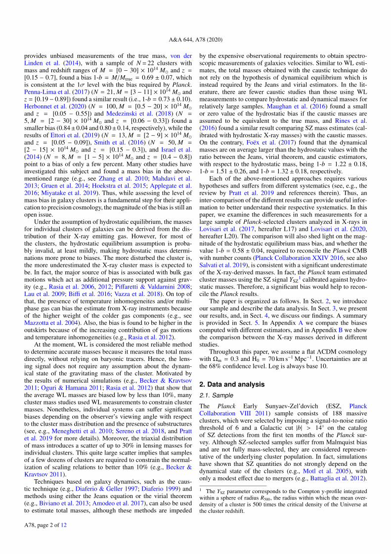
Fig. 1. Distribution of the cluster masses (left panel) and redshifts (rightpanel) for the ESZ clusters (dashed green), the L20 sample (solid blue),and the clusters with weak-leansing masses (filled red). Numbers in thelegend represent the sample size.

This is supported observationally by the tight correlationbetween SZ signal and mass (e.g., Planck Collaboration XI2011). Moreover, the morphology of the source has little impacton the detection procedure in the Planck survey, as shown viaMonteCarlo simulations (Planck Collaboration XXVII 2016).

L17 and L20 analyzed the XMM-Newton data to determinethe morphological and global cluster properties for a representa-tive subsample of 120 ESZ clusters, selected to ensure that R500is completely covered by XMM-Newton observations (either sin-gle or multiple pointings). A single pipeline was used in the anal-ysis allowing a uniform processing of the data, eliminating onesource of uncertainties in the comparison with the masses esti-mated from other methods.

For all these 120 clusters, we know the dynamical state andboth X-ray and SZ masses (from L20 and Planck CollaborationXXVII 2016, respectively). Instead of the SZ masses estimatedin Planck Collaboration VIII (2011), we preferred to use themore recent and more accurate PSZ2 masses reported in PlanckCollaboration XXVII (2016) obtained from the 29 month fullPlanck mission data. We note that five ESZ clusters are notincluded in the PSZ2 catalog because they fall into the PSZ2point source mask, but only three of these overlap with oursubsample of 120 clusters. For these clusters we use the PSZ1masses.

For WL masses, we used the compilation obtained in theCoMaLit framework (see, e.g., Sereno & Ettori 2015). The Lit-erature Catalogs of Weak Lensing Clusters (LC2, Sereno 2015)is publicly available2. LC2-single (v. 3.9) is a meta-catalogwith 806 unique entries. When multiple analyses per cluster areavailable, preference is given to studies exploiting the deeperobservations and multiband optical coverage for optimal galaxybackground selection. There are 62 clusters in common with thesample analyzed in L20. The distribution of mass and redshiftfor these clusters with respect to the ESZ and L20 samples isshown in Fig. 1.

Given the relatively large sample, we also investigatedwhether or not the X-ray/SZ masses of disturbed clusters aresignificantly more biased than the masses derived for relaxedclusters. The dynamical state of each cluster was determined byusing two morphological parameters: one sensitive to the core-properties (i.e., surface brightness concentration) and one sen-sitive to the large-scale inhomogeneities (i.e., centroid-shift). InL20 (see also Rasia et al. 2013), these two parameters have beencombined to define a new general parameter M (hereafter Mpar),which allows us to use a single value to rank the clusters fromthe most relaxed to the most disturbed in the sample of interest.In the following, we refer to relaxed and disturbed cluster whenMpar is greater than and smaller than zero, respectively. This

2 http://pico.oabo.inaf.it/~sereno/CoMaLit/LC2/

classification provides a simple way to divide a sample betweenthe most relaxed and most disturbed clusters but does not neces-sarily provide an absolute reference.

2.2. Estimation of the hydrostatic bias

We estimated the mass ratio by fitting the data with LIRA whichallows normalization, slope, and scatters (and relative uncertain-ties) to be fitted simultaneously3. In particular, for each subsam-ple of WL (or dynamical) masses we linearly fit our data as

log(

MHE

6 × 1014 M

)= α + β log

(Mtrue

6 × 1014 M

)± σHE|true, (1)

log (Mtrue) = log (MWL) ± σWL|true

where α quantifies the mass ratio (i.e., 1-b = MHE/MWL = 10α),β is fixed to 1 (unless otherwise specified), and the MHE and MWLmasses are evaluated at their respective R500 (unless otherwisestated). Mtrue represents the unbiased cluster mass. The intrinsicscatters σHE|true and σWL|true are assumed to be uncorrelated. Asdescribed in Sereno (2016), for each set of parameters, the linearregression is performed calling the function lira, whose outputare Markov chains produced with a Gibbs sampler. The medianvalues of α, σHE|true, σWL|true and their 1σ uncertainties are takenfrom the distribution of 80 000 Markov chains. For comparison,in Appendix A we provide also the bias estimated by computingthe geometric mean and the median.

2.3. X-ray total masses

Under the assumption of spherical symmetry, one can solve thehydrostatic equilibrium equation and recover the total mass withonly two ingredients: gas density and temperature profiles. Forthe ESZ sample, the gas density profiles were recovered fromthe best-fit parameters of a double β-model, while, for the tem-perature profiles, we used the 3D model by Vikhlinin et al.(2006) projected along the line of sight to fit the observed datapoints following the implementation presented in Schellenberger& Reiprich (2017a).

In L20, the X-ray total cluster masses have beenobtained by assuming a Navarro-Frenk-White (NFW, Navarroet al. 1996, 1997) model for the mass profile with the relationfrom Bhattacharya et al. (2013) between the Dark Matter con-centration and radius as a prior. However, we also estimated themasses by directly solving the equation of hydrostatic equilib-rium without any prior on the form of the gravitational poten-tial. Following the nomenclature by Ettori et al. (2013) (see alsoPratt et al. 2019), we refer to these masses as backward (hereafterMHE) and forward (hereafter Mfor), respectively, each measuredat their R500.

There is a good correlation between MHE and Mfor (seeFig. 2), with a one-to-one relation and small intrinsic scatterwith respect to the fitted relation (i.e., 4 ± 1%). However, theMfor masses are on average ∼9% lower than MHE masses, almostindependently of the dynamical state of the clusters. Instead, themass difference slightly decreases as a function of the X-ray dataquality. For instance, clusters for which the last temperature binis at a radius <0.6R500, within 0.6–0.8R500, or >0.8R500 havean average offset of 13%, 9%, and 7%, respectively. Thus, thesmaller the extrapolation required, the better the two estimates

3 LIRA (LInear Regression in Astronomy) is based on a Bayesianmethod (see Sereno 2016 for more details) and is available fromthe R archive network at https://cran.r-project.org/web/packages/lira/index.html.

A78, page 3 of 12

A&A 644, A78 (2020)

1014 1015Mfor (M )

1014

1015

MHE

(M)

=1.00±0.03=1.03±0.06=0.99±0.04

equalityAll (120)R (60)D (60)

Fig. 2. Comparison between the total masses obtained with a forwardapproach (Mfor) and a backward approach (MHE). Relaxed (R) and dis-turbed (D) clusters are displayed as blue squares and red triangles,respectively. Numbers in the legend represent the sample size. The βvalues represent the fitted slope for disturbed (red), relaxed (blue), andall (black) clusters, respectively.

agree. Low redshift clusters (i.e., z < 0.2) show a marginallysmaller offset (7% on average) than high redshift (i.e., z > 0.2)clusters (11%). This is mainly due to higher quality data of thelow redshift clusters that allow measurements of the temperatureto a larger fraction of R500.

Previous studies showed that X-ray masses obtained withdifferent analyses can be quite discordant. Indeed, this is asource of noise in the calculation of the level of hydrostaticbias. Since most of our clusters have been previously studiedby other authors, here we provide a comparison of the mass esti-mates, evaluated at their respective R500 and in Appendix B weshow the plot comparing the L20 total masses with those fromliterature.

There are 48 clusters that overlap with the sample used bythe Planck Collaboration XI (2011) to investigate the relationbetween the integrated Compton parameter and several X-ray-derived properties. On average, our masses are 4 ± 2% lowerthan their masses estimated using the M−YX relation4 by Arnaudet al. (2010). There is a mild, not statistically significant, depen-dence on the dynamical state: for the relaxed clusters, our massestimates are in agreement (i.e., offset of 2 ± 2%) with PlanckCollaboration XI (2011), while for disturbed clusters the aver-age offset is slightly larger (i.e., offset of 7 ± 3%).

There are 18 clusters in common with Martino et al. (2014),who analyzed 50 clusters from the LoCuSS (Local Cluster Sub-structure Survey, e.g., Zhang et al. 2008) sample. Of these 18clusters, Martino et al. (2014) provide 17 (14) total massesobtained with Chandra (XMM-Newton) data. The mass profilesin Martino et al. (2014) were derived with a forward approachusing a powerlaw model for the temperature profile and the para-metric form by Vikhlinin et al. (2006) for the gas density profile.On average, our masses are 7 ± 10% (10 ± 8%) lower than whatthey reported.

4 The YX = Mgas × kT parameter measures the total gas energy contentand is the X-ray counterpart of the Sunyaev-Zel’dovich signal YSZ.

1014 1015MSZ (M )

1014

1015

MHE

(M)

=1.09±0.09=1.10±0.13=1.09±0.09

equalityAll (117)R (57)D (60)

Fig. 3. MHE − MSZ relation for the ESZ clusters investigated in L20.Relaxed (i.e., Mpar > 0) and disturbed (i.e., Mpar < 0) clusters are shownin blue squares and red triangles, respectively. The dark shaded arearepresent the 1σ statistical error for the full sample.

There are 12 clusters in common with Schellenberger &Reiprich (2017a) who analyzed the HIFLUGCS (HIghest X-rayFLUx Galaxy Cluster Sample, Reiprich & Böhringer 2002) sam-ple with Chandra data. The mass profiles were derived with aforward approach using a double β-model for the density profileand several parametric forms which approximate a powerlaw inthe outer regions, for the temperature profiles. Our total massesare, on average, 9 ± 11% lower.

There are 6 clusters in common with the CLASH (Clus-ter Lensing And Supernova survey with Hubble, Postman et al.2012) sample. The masses were obtained with a backwardapproach assuming an NFW form for the mass profile and atriple β-model for the density profiles. Our total masses are onaverage ∼5% lower than the masses estimated by Donahue et al.(2014) with Chandra data and the difference reduces to ∼2%when compared to the masses obtained with XMM-Newton data.

Finally, there are 5 clusters in common with XCOP (XMMCluster Outskirts Project, Eckert et al. 2017). The total massesderived in L20 are on average 11% lower than the massesestimated with the backward method and an NFW model asreported by Ettori et al. (2019). For two clusters (i.e., A3266 andZwCl1215.1+0400) our total masses are ∼30% lower than theXCOP estimate, but are in agreement with the Planck masses.Of the XCOP clusters, these two are the ones that deviate moresignificantly with respect to the Planck estimates.

2.4. MHE −MSZ

The thermal SZ effect directly measures the line-of-sight pres-sure, and thus, in the adiabatic scenario, the thermal energy con-tent of the cluster gas, which is strongly correlated with thetotal mass. However, the SZ-derived masses largely rely on priorinformation on the calibration of the integrated SZ Comptoniza-tion (i.e., YSZ) with cluster masses from X-ray and/or WL anal-yses. The Planck masses have been determined using the X-rayhydrostatic masses to calibrate the YX − YSZ relation. Therefore,the comparison MHE and MSZ indirectly provides the compar-ison between our ESZ masses (i.e., MHE) and the hydrostaticmasses used by Planck.

A78, page 4 of 12

L. Lovisari et al.: Comparing different mass estimators for the ESZ sample

Table 1. Summary of the 1-b = MHE/MSZ, estimated at R500.

All

Sample N MSZ z 1-b σSZ σHE

L20 All 117 6.59 0.19 0.93± 0.02 5± 3 16± 2L20 R 57 6.68 0.20 0.96± 0.03 7± 4 16± 3L20 D 60 6.51 0.19 0.90± 0.03 6± 4 15± 3LC2-single 60 7.56 0.22 0.93± 0.02 5± 3 17± 3CCCP/MENeaCS 25 7.65 0.18 0.94± 0.04 11± 6 14± 6APEX-SZ 19 8.76 0.28 0.95± 0.04 4± 3 15± 3LoCuSS 18 7.78 0.22 0.88± 0.04 6± 4 13± 4WtG 17 8.27 0.29 0.92± 0.04 5± 3 13± 4

Notes. For each subsample we provide the number of clusters, themedian SZ masses (i.e., MSZ), and the median redshift (i.e., z). Theintrinsic scatters are given in percent.

In Fig. 3 we show the comparison between the X-ray (i.e.,MHE) and PSZ2 masses (i.e., MSZ). The SZ masses are, on aver-age, 7% higher than the X-ray masses (see Table 1). When wecompute the X-ray masses at R500 determined by Planck, the dif-ference decreases to ∼4%. When left free to vary, the slope of theMHE − MSZ relation is found to be only slightly steeper than theequality line (i.e., β = 1.09 ± 0.09) indicating a not significantmass dependence. There is no variation in slope when the sampleis split based on the dynamical state of the clusters (see blue andred lines in Fig. 3). Even when selecting the most relaxed (top30%) and most disturbed clusters in our sample, we do not findany significant dependence. However, there is a mild effect onthe normalization with relaxed clusters more in agreement withthe Planck masses than the disturbed clusters.

When splitting the sample in 3 redshift bins (i.e., z < 0.15,0.15 < z < 0.25, z > 0.25), we found the MHE/MSZ ratio tobe 0.96± 0.04, 0.90± 0.03, and 0.96± 0.04, respectively. Thus,there are no indication of a dependence on redshift, as also con-firmed by the Spearman rank test (i.e., r = 0.06 and p = 0.53).We also subdivided each redshift bin based on cluster mass butwe did not find any trend.

We also investigated if any of the WL subsamples show asignificantly different MHE/MSZ ratio. The LoCuSS subsampleshows the lowest value (i.e., 1-b = 0.88± 0.04) but it is still con-sistent within 1σ with the results from the other subsamples.

3. Results

Cluster masses can be directly estimated through X-ray obser-vations, gravitational weak-lensing, and dynamical analysis ofcluster galaxies, or alternatively using a mass proxy, such asthe SZ flux which relies on prior information on the SZ-masscalibration obtained from X-ray or WL masses. Although eachmethod requires some assumptions and is limited by differ-ent systematics, WL and caustic technique do not require theassumption of hydrostatic equilibrium, and numerical studiessuggest that they can provide cluster mass estimates with littlebias. In the following we compare our ESZ masses (i.e., MHE)with the ones from other mass estimators.

3.1. X-ray versus weak-lensing masses

In this section, we compare X-ray and WL masses estimatedwithin R500 which is one of the most common overdensities usedfor cosmological studies. In Fig. 4 we show the MHE−MWL rela-tion, while in Table 2, we provide the values 1-b computed forall the investigated subsamples.

1014 1015MWL (M )

1014

1015

MHE

(M)

equality1-b=0.74CCCP/MENeaCSAPEX-SZLoCuSSWtGother

Fig. 4. Comparison between X-ray and WL masses from LC2-single.Red circles, brown diamonds, green triangles, and blue squares repre-sent the masses obtained by Herbonnet et al. (2020), Klein et al. (2019),Okabe & Smith (2016), and Applegate et al. (2014), respectively. Themagenta line represents the average MHE/MWL ratio.

When the LC2-single catalog is used, we find that the aver-age ratio between HE and WL masses is 1-b = 0.74± 0.06. Thisnumber is almost independent of the dynamical state: relaxedand disturbed clusters have mass ratios of 1-b = 0.75± 0.08 and1-b = 0.73± 0.12, respectively. By splitting the sample in threeredshift bins, we find no dependence of the mass ratio on red-shift (i.e., 1-b = 0.72± 0.09 for z < 0.17, 1-b = 0.75± 0.12 for0.17 < z < 0.29, and 1-b = 0.76± 0.12 for z > 0.29). Instead, wefind indication for a dependence on the total mass with smaller1-b values for high mass clusters and a better agreement forlow mass systems. In detail, for MWL ≤ 6.5 × 1014 M wefound 1-b = 1.15± 0.11, for 6.5 × 1014 M < MWL ≤ 1015 Mwe found 1-b = 0.73± 0.11, and for MWL > 1015 M we found1-b = 0.62± 0.08. This is also confirmed by the Spearman testwhich gives a significant anti-correlation (i.e., r = −0.67, p <0.01).

Also for WL there are significant differences between massesreported by distinct groups (e.g., see also Umetsu et al. 2014;Sereno & Ettori 2015). Here we provide a comparison betweenour masses, MHE, and those estimated by different WL projects.

There are 27 clusters in common with the sample analyzedby Herbonnet et al. (2020, hereafter H20) who determined themasses for 48 clusters in the Multi Epoch Nearby Cluster Sur-vey (MENeaCS), and 52 clusters from the Canadian ClusterComparison Project (CCCP). We find MHE/MWL = 0.77± 0.10.Among the common clusters, there are 17 relaxed clusters(i.e., Mpar > 0) for which we obtain MHE/MWL = 0.83± 0.12and 10 disturbed clusters (i.e., Mpar <0) for which we obtainMHE/MWL = 0.73± 0.21. Given the large uncertainties, thetendency of a better agreement for relaxed clusters is onlymarginal. The correlation between bias and dynamical state mea-sured by Mpar is also not supported by the Spearman test (i.e.,r = −0.05, p = 0.81).

There are 19 clusters in common with Klein et al. (2019,hereafter K19) who presented the WL analysis for clusters fromthe APEX-SZ survey (see also Nagarajan et al. 2019). Our HEmasses are in agreement (i.e., MHE/MWL = 1.02± 0.12) with theWL masses by K19.

A78, page 5 of 12

A&A 644, A78 (2020)

Table 2. Summary of the 1-b = MHE/MWL values, estimated at R500.

AllSample N MWL z 1-b σWL σHE

LC2-single 62 8.37 0.21 0.74± 0.06 27± 8 30± 6CCCP/MENeaCS 27 7.40 0.18 0.77± 0.10 10± 9 40± 8APEX-SZ 19 8.51 0.28 1.02± 0.12 37± 10 28± 10LoCuSS 18 8.24 0.22 0.76± 0.09 23± 9 24± 8WtG 17 11.73 0.29 0.61± 0.12 31± 15 26± 11

RelaxedSample N MWL z 1-b σWL σHE

LC2-single 34 8.65 0.21 0.75± 0.08 27± 9 18± 8CCCP/MENeaCS 17 7.10 0.17 0.83± 0.12 21± 13 25± 10APEX-SZ 11 8.75 0.27 0.90± 0.17 42± 14 27± 13LoCuSS 14 9.42 0.22 0.74± 0.10 20± 10 26± 8WtG 10 11.46 0.23 0.71± 0.17 22± 18 32± 14

DisturbedSample N MWL z 1-b σWL σHE

LC2-single 28 8.09 0.29 0.73± 0.12 31± 14 45± 10CCCP/MENeaCS 10 8.35 0.19 0.73± 0.21 10± 13 61± 17APEX-SZ 8 7.57 0.30 1.19± 0.15 14± 15 15± 14LoCuSS 4 5.89 0.24 0.93± 0.29 9± 20 22± 29WtG 7 15.20 0.41 0.48± 0.18 16± 17 18± 16

Notes. The data for the CCCP/MENeaCS, APEX-SZ, LoCuSS, andWtG samples have been taken from H20, K19, O16, and A14, respec-tively. For each subsample we provide the number of clusters, themedian WL mass (i.e., MWL), and the median redshift (i.e., z). Massesare in units of 1014 M. The intrinsic scatters are given in percent.

There are 18 clusters in common with Okabe & Smith (2016,hereafter O16), who analyzed the LoCuSS clusters. The aver-age mass ratio is 1-b = 0.76± 0.09. It is worth mentioning thatLoCuSS shows the larger deviation in MHE/MSZ (i.e., 12% ± 4offset, see Sect. 2.4).

Finally, there are 17 clusters in common with Weighing theGiants (WtG), the sample analyzed by Applegate et al. (2014,hereafter A14) who reported WL masses for 51 massive clus-ters. We find MHE/MWL = 0.61± 0.12, a much larger discrep-ancy than the one observed with respect to the other samples.There is a clear correlation between the dynamical state (i.e.,Mpar) and MHE/MWL (i.e., Spearman r = 0.52, p = 0.03). Infact, when splitting the sample in relaxed and disturbed clusters,we find MHE/MWL = 0.71± 0.17 and MHE/MWL = 0.48± 0.18,respectively.

The intrinsic scatter σWL of the different samples varies from∼10% for CCCP/MENeaCS to ∼35% for APEX-SZ clusters.Also for WtG the scatter is >30% but is probably boosted bythe clear dependence of the mass ratio on the dynamical state. Infact, both subsamples of relaxed and disturbed clusters show asmaller scatter (i.e., 15–20%), although with large uncertainties.The scatters σWL and σHE are often at the same level. An excep-tion is CCCP/MENeaCS which show a significantly larger σHEfor the disturbed systems.

3.2. X-ray versus caustic masses

An alternative technique to estimate cluster masses is throughthe caustic method, that makes use of galaxy dynamics. Thecaustic, a trumpet-shaped region in the diagram of line-of-sightvelocity versus projected distance, defines which galaxies lieinside and outside a cluster assuming that a system cannot have avelocity larger than the escape velocity. Caustic-derived masses

Table 3. Summary of the mass ratio between X-ray and dynamical clus-ter masses.

AllSample N Mdyn z 1-b σdyn σHE

HeCS-omnibus 25 7.10 0.16 1.30± 0.14 76± 11 8± 8HeCS-omnibus (N > 135) 12 9.31 0.18 1.03± 0.10 26± 11 13± 10HeCS-omnibus (N < 135) 13 5.80 0.14 1.72± 0.27 103± 20 18± 12HeCS-omnibus (N > 100) 18 7.36 0.18 1.04± 0.11 26± 12 14± 11HeCS-omnibus (N < 100) 7 2.74 0.14 2.34± 1.48 121± 41 19± 15HIFLUGCS 12 4.89 0.08 0.95± 0.17 49± 18 14± 14

Relaxed

Sample N Mdyn z 1-b σdyn σHE

HeCS-omnibus 14 7.46 0.19 1.37± 0.21 99± 19 8± 9HIFLUGCS 7 3.77 0.09 1.28± 0.23 37± 23 23± 15

Disturbed

Sample N Mdyn z 1-b σdyn σHE

HeCS-omnibus 11 7.10 0.11 1.17± 0.16 41± 15 25± 14HIFLUGCS 5 9.15 0.07 0.69± 0.23 12± 19 22± 25

Notes. The comparison is done at R200 for the HeCS-omnibus causticmasses by Sohn et al. (2020) and at R500 for the HIFLUGCS massesestimate from the velocity dispersion by Zhang et al. (2017). Massesare in units of 1014 M. The intrinsic scatters are given in percent.

(i.e., Mc) are insensitive to the physical processes that mightcause hydrostatic biases and are subject to different systematicuncertainties than lensing masses.

One of the advantages of the caustic approach is that it doesnot rely on the hypothesis of dynamical equilibrium. The draw-back is that a reliable measurement of the underlying dark mat-ter distribution requires a large number of member galaxies (e.g.,Serra & Diaferio 2013).

There are 25 clusters in common with Sohn et al. (2020)who obtained the caustic masses at R200 for the HeCS-omnibuscluster sample (see also Maughan et al. 2016). For a compar-ison with their masses, we computed the M200 masses for theL20 sample. We found that the caustic masses are, on average,smaller than the X-ray-derived masses with no indication fora relation with the dynamical state of the clusters (see Table3 and Fig. 5). However, we note that the clusters showing thelargest difference between X-ray and caustic masses tend to have asmall N200, which is the number of spectroscopic members withinR200. For instance, when we split the sample based on N200, wefind MHE/Mc = 1.04± 0.11 for clusters with N200 > 135 andMHE/Mc = 1.72± 0.27 for clusters with N200 < 135. This isalso supported by the good anti-correlation between MHE/Mc andN200 (i.e., Spearman r = −0.54, p < 0.01). Also, the scatter sig-nificantly decreases when clusters with few member galaxies areremoved, and becomes comparable with the one observed for WLsamples. The low bias and relatively small scatter σdyn is foundalso with different cuts on N200 and start to show significant devi-ations when clusters with N200 < 100 are included in the fit.

3.3. X-ray versus virial masses

As an alternative to the caustic method, one can derive dynam-ical masses using the virial theorem (i.e., Mv hereafter). Thismethod is based on the hypothesis of dynamical equilibrium,spherical symmetry, and on the additional assumptions that allthe galaxies have the same mass and their spatial and velocity

A78, page 6 of 12

L. Lovisari et al.: Comparing different mass estimators for the ESZ sample

1014 1015Mc (M )

1014

1015

MHE

(M)

equality1-b=1.301-b (N200 > 100)=1.04RD

Fig. 5. Comparison between X-ray and caustic masses for the 25clusters in common with Sohn et al. (2020). Relaxed (R) and dis-turbed (D) clusters are plotted with blue and red circles, respectively.Filled and empty circles represent the clusters with N200 > 100 andN200 < 100, respectively. The dotted magenta line represents the aver-age MHE/Mc ratio. The dashed green line represents the average MHE/Mcratio obtained after removing the clusters with less than 100 galaxieswithin R200.

distribution follow those of dark matter particles. Despite theseapproximations, the virial theorem has proven to be a good esti-mator even for a small number of cluster galaxies (e.g., seeBiviano et al. 2006 and Munari et al. 2013).

Zhang et al. (2017) obtained the dynamical masses for theHIFLUGCS sample based on the velocity dispersion of themember galaxies. For the 12 clusters in common with the sam-ple in L20, we find reasonably good agreement with a mass ratioconsistent with zero (i.e., 1-b = 0.95± 0.18). However, relaxedand disturbed objects clearly populate different regions of theMHE − Mv plane (see Fig. 6) although larger samples are clearlyneeded to obtain firmer conclusions. When the HE masses arecomputed at R500 provided by Zhang et al. (2017), we obtain amass ratio of 0.97± 0.10 and a significant reduction of the scatter(i.e., σdyn=18± 12% and σHE=8± 7%).

4. Discussion

4.1. X-ray hydrostatic masses

Rozo et al. (2014) and Sereno & Ettori (2015) reported that theX-ray properties estimated by competing groups can show largediscrepancies. They found that total masses can differ by a fac-tor of two even for relaxed clusters. The major sources of thediscrepancies have been ascribed to differences in the data anal-ysis, to cross-calibration problems between instruments, and todifferent techniques to recover the mass.

As seen in Sect. 2.3 the total masses obtained in L20 aresystematically lower than the masses published by other authors(at least for the ones discussed in this paper). However, while thediscrepancy can be up to 30% for individual clusters, the averagedifference in sample pairs is only a few percent with respect tothe values by Donahue et al. (2014) and Planck CollaborationXI (2011) and ∼10% with respect to Ettori et al. (2019), Martinoet al. (2014), and Schellenberger & Reiprich (2017a).

1014 1015Mv (M )

1014

1015

MHE

(M)

equality1-b=0.95RD

Fig. 6. Comparison between X-ray and virial masses for the 12HIFLUGCS clusters in common with Zhang et al. (2017). Relaxed(R) and disturbed (D) clusters are plotted with blue and red circles,respectively. The dotted magenta line represents the average MHE/Mvratio.

In Sect. 2.3 we showed that part of these differences is indeedassociated with the mass reconstruction methodology. Tradition-ally, as discussed in Ettori et al. (2013) and Pratt et al. (2019),two main approaches have been used to determine the massprofile. In one case, a parametric mass model (e.g., NFW) isassumed, while in the second, two functional forms are fitted tothe density and temperature profiles and propagated through theHE equation to derive the mass profile. In this paper, we refer tothe masses estimated with the first and second methods as MHEand Mfor, respectively. Our results show that the Mfor massesare, on average, 9% smaller than the MHE masses. One of thereasons is a poor radial sampling (i.e., few temperature measure-ments) of some clusters for which the model extrapolation candiverge (see, e.g., Bartalucci et al. 2018 for a more extended dis-cussion). In fact, when we compare the 25 clusters with at leastten temperature bins, the average difference between the MHEand Mfor masses is less than 1%. When the X-ray data allow onlya few temperature measurements, the assumption of the NFWprofile, which is a physically motivated model and is found toprovide a good fit for massive clusters, can be used to obtainmass estimates without introducing strong systematics if thetemperature profile is measured at least out to 0.5R500, as shownby Schellenberger & Reiprich (2017b). Our results are also inagreement with Ettori et al. (2019) and Bartalucci et al. (2018),who analyzed samples of 13 and 5 clusters with high X-ray qual-ity data and found that different mass estimation methods yieldreasonably consistent results.

Another cause for the lower masses in L20 is the use ofthe total (i.e., neutral and molecular) column density, whichhas a significant impact on the measured temperatures in theregions with high molecular contributions. The inclusion of themolecular component allows a better fit to the X-ray data (seeLovisari & Reiprich 2019 for more details) and, for very hightotal column densities (i.e., NH > 1021 cm−2), can lead to esti-mated temperatures (and therefore total masses) that are 10–15%lower than when only the neutral component is used. However,for most clusters the effect is limited to a few percent.

A78, page 7 of 12

A&A 644, A78 (2020)

LC2 -s

ingl

e

CCCP

/MEn

eacs

APEX

-SZ

LOCU

SS

WtG

HeCS

-om

nibu

s

HIFL

UGCS

0.2

0.4

0.6

0.8

1.0

1.2

1.4

1.6

1-b

0.74 0.77 1.02 0.76 0.61 1.30 0.95

Planck All R D

Fig. 7. Hydrostatic mass bias for each of the subsamples investigated inthis paper. Filled color bars represent the mass bias estimated using WLmasses, while horizontal and diagonal hatches show the estimates usingmasses from caustics and velocity dispersion, respectively. In magentawe show the bias obtained with caustics after removing the clusters withfew member galaxies. The bar lengths enclose the 1σ estimates andthe central values are also reported on the top of the panel. The grayline represents the bias necessary to reconcile Planck number countsand CMB. The green shaded region indicates the area defined as ± 20%centered on 1-b = 0.

Table 4. Summary of the MHE/MWL ratio estimated at R = 1 Mpc.

AllSample N MWL z 1-b σWL σHE

LC2-single All 62 8.37 0.21 0.83± 0.04 21± 4 22± 5LC2-single R 34 8.65 0.21 0.84± 0.05 20± 6 14± 6LC2-single D 28 8.09 0.29 0.83± 0.08 23± 10 30± 7

Notes. Masses are in units of 1014 M. The intrinsic scatters are givenin percent.

4.2. MHE −MSZ and MSZ −MWL

The PSZ2 masses were estimated from the M − YSZ relationcalibrated using the M − YX relation by Arnaud et al. (2010),which links the hydrostatic mass to the YX parameter, the X-rayequivalent of the integrated Compton parameter YSZ. Consider-ing uncertainties and scatter, the M − YX relation for the ESZsample obtained in L20 is in good agreement with the oneby Arnaud et al. (2010), in particular in the low mass regime.However, in the high mass regime, the difference is about 5–6%.Therefore, the difference of 4% that we observe at the sameradius (i.e., R500 from Planck) can be easily explained by thesmall offset in the M − YX relation.

We found a mild mass-dependent trend between X-rayand Planck SZ masses as previously obtained by other stud-ies. Schellenberger & Reiprich (2017a) suggest that this effectis caused by the Planck selection function and the intrinsic scat-ter of the hydrostatic mass estimates. However, since the Planckmasses are obtained using the M −YX relation, it is also possiblethat there is a mass dependent effect introduced by the calibra-tion of the scaling relations.

The agreement between the X-ray and SZ masses is betterfor relaxed clusters (4± 3%) than disturbed clusters (11± 3%).Since the relation used to estimate the Planck masses is the same,and there is no significant difference in the M − YX for relaxedand disturbed systems (e.g., see L20), the larger MHE/MSZ ratiofor disturbed systems may indicate that the SZ signal is some-how impacted (i.e., overestimated). For instance, due to the largePlanck beam, the integrated SZ signal may include unidenti-fied substructures along the line of sight, which instead couldbe masked in the X-ray analysis. Projection effects are also asource of intrinsic scatter (e.g., Krause et al. 2012), and indeedwe note that the scatter in the low mass regime is higher than theone for massive clusters (10% versus 4%).

Sereno et al. (2017), for a subsample of 35 PSZ2 clusters,found that the Planck masses are biased low with respect to WLmasses by 27± 11(stat)± 8(sys)%. Instead, the bias obtainedwith the heterogeneous LC2 catalog is ∼13% (see Sereno et al.2015). For the 62 ESZ clusters in common with LC2, we esti-mate a mass ratio of 1-b = 0.80± 0.06 (corresponding to a biasof b = 20± 6%), essentially in agreement with previous findings.Due to the large uncertainties, it is hard to say if there is any trendwith the dynamical state, although, based on the average values,disturbed clusters show a slightly better agreement between theSZ and WL masses (i.e., 1-b = 0.78 and 1-b = 0.83 for disturbedand relaxed clusters, respectively). This is in agreement with theabove-mentioned suggestion of an overestimated SZ signal fordisturbed clusters. However, another possibility is that the WLmasses are on average slightly underestimated.

4.3. MHE and MWL comparison

We compared our estimates of the hydrostatic mass with con-straints obtained with WL analysis from different groups (seeSect. 3.1). The mass ratio obtained with the LC2 compilation is1-b = 0.74± 0.06 (see Table 2 and Fig. 7). This is consistent withpredictions from hydrodynamical simulations (e.g., Rasia et al.2012; Biffi et al. 2016). Moreover, as discussed by Sereno &Ettori (2015), given the relation between mass and overdensity-radius, mass differences are inflated when computed at R500.Therefore, we also compare the masses obtained within a phys-ical aperture of 1 Mpc (see Table 4), keeping in mind that thisaperture refers to a physically different region in clusters withdifferent mass. The average difference decreases by ∼9% withalso a substantial reduction of the intrinsic scatter.

The large differences between the total masses in L20 andthe LC2 sample is partially driven by the larger mass ratio (seeTable 2 and Fig. 7) observed with WtG (masses from A14) andCLASH (masses from Umetsu et al. 2016) programs, whoseresults agree. In fact, of the 62 matched clusters, 18 of thematched clusters are included either in WtG or CLASH.

The mass ratio observed, when considering the WL massesfrom A14, is 1-b = 0.61± 0.12, which corresponds to a bias of39± 12%. This is consistent with the value required to recon-cile Planck cluster number counts and Planck primary CMBmesurements. Our result is in agreement with the finding byvon der Linden et al. (2014) who found an overall mass ratio ofMPlanck/MWtG = 0.69± 0.07. Also, although the uncertainties arelarge, this is the only sample for which the hydrostatic bias fordisturbed systems is significantly higher than the bias obtainedfor relaxed systems, which is what would be expected if the WLmasses are indeed unbiased and the hydrostatic bias is larger fordynamical active clusters.

The other samples show a higher mass ratio (correspond-ing to a lower hydrostatic bias, i.e., 20–30%) and a less clear

A78, page 8 of 12

L. Lovisari et al.: Comparing different mass estimators for the ESZ sample

dependence on the dynamical state. The results from K19 showan anti-correlation even though not statistically significant. Since,relaxed clusters are expected to have a smaller mass bias than dis-turbed objects (e.g., Biffi et al. 2016), the lack of correlation ofthe mass ratios with the dynamical state may suggest that somesystematics in the WL analyses are still not accounted for. Forinstance, it is worth noting that WL masses can be significantlyunderestimated because of massive sub-clumps (Meneghetti et al.2010) or uncorrelated large-scale matter projections along theline of sight (Becker & Kravtsov 2011). For instance, the lensingmasses are typically overestimated when the cluster is elongatedalong the line of sight, and underestimated when it is elongatedon the plane of the sky. If we focus on the more relaxed clusters,we find that the mass ratios, derived from the different subsam-ples, tend to agree better, and correspond to biases on the order of5–20%. Instead, when disturbed clusters are considered, the massratios vary a lot from sample to sample. One of the reasons is thateach of the lensing subsamples contains only a small fraction ofdisturbed clusters (e.g., only four in O16). This makes possiblefor the lensing bias of individual systems to not be fully averagedout. We also stress that, although the subdivision between relaxedand disturbed clusters using Mpar, is only relative, SZ surveys arethought to be very close to being mass selected, and therefore theMpar distribution is probably indicative of the cluster populationin the Universe.

We investigated any dependence of the mass ratio on clus-ter mass and redshift (see Sect. 3.1). We do not find any redshiftdependence of the mass ratio but our clusters span a relativelysmall range of redshifts and we cannot place conclusive con-straints. Instead, we find a moderate mass dependence, with themost massive clusters showing a larger bias in agreement withthe finding by von der Linden et al. (2014) and Eckert et al.(2019), while Sereno et al. (2015) and Sereno & Ettori (2017)found the bias to be redshift rather than mass dependent. Naively,one would expect the more massive objects to be on averagemore disturbed than the least massive clusters, and therefore witha large bias. However, in L17, we did not find any correlationbetween the different morphological parameters (i.e., a measureof the dynamical state) and the total mass (see also Böhringeret al. 2010). This is confirmed by the Spearman rank test for thefull L20 sample (r = 0.02, p = 0.80) and for the subsample of62 clusters with WL masses (r = −0.09, p = 0.46).

4.4. MHE and Mc comparison

In addition to the widely used WL technique to constrain thehydrostatic mass bias, we also compared the X-ray masses withcaustic masses. The comparison with caustic masses determinedat R200 by Sohn et al. (2020) required a significant extrapola-tion of the X-ray data, so our finding should be treated with cau-tion. We find that the caustic masses are significantly lower thanthe X-ray masses in agreement with the finding by Ettori et al.(2019), Maughan et al. (2016), and Sereno et al. (2015). How-ever, Serra & Diaferio (2013) found that only with a large num-ber of spectroscopic members can the velocity field be properlysampled and return a correct mass. In particular, they showedthat for N = 50 the mass estimate is biased low by ∼20%, whilefor N = 200 the bias is consistent with zero. After removingthe clusters with fewer member galaxies, the agreement betweenX-ray and caustic measurements is good. Moreover, there is noindication of any dependence of the mass ratio on the dynamicalstate of the clusters, supporting the finding by Maughan et al.(2016). This, together with the overall trend observed with thecomparison to WL masses, suggests that there are still unknown

systematics that introduce significant scatter in the relations thatprevent a complete and proper estimate of the hydrostatic mass.

Previous comparisons of caustic masses with X-ray massesby Maughan et al. (2016) and with Planck masses (calibratedwith hydrostatic X-ray masses) by Rines et al. (2016) also showlittle or no bias. Instead, Ettori et al. (2019) found that the causticmasses of 6 X-COP clusters, that are nearby massive objects forwhich the determinations of caustics might be more problematic,are significantly underestimated with respect to the hydrostaticmasses. However, given the large scatter observed in the MHE −

Mc relation, a comparison with a much larger sample is requiredto obtain more conclusive results.

4.5. MHE and Mv comparison

The velocity dispersion of member galaxies provides anotherway to estimate cluster masses under the hydrostatic equilibriumassumption. We find agreement when the L20 X-ray masses arecompared to the masses estimated based on the velocity disper-sion. In fact, for the 12 clusters in common with Zhang et al.(2017) we find 1-b = 0.95± 0.17 in agreement with the findingby Ettori et al. (2019). On the contrary, Amodeo et al. (2017)reported a bias of 1-b = 0.64± 0.11 for a sample of 17 Planck clus-ters. However, it is still debated whether the velocity dispersionof the galaxies is a good tracer for the velocity dispersion of thedark matter particles. In fact, differences like the so-called veloc-ity bias, have been reported to be at the± 10% level (e.g., Munariet al. 2013; Armitage et al. 2018), and could partially explain thedifferent hydrostatic bias derived in different studies. Although,there is no general agreement on the magnitude or even the signof the velocity bias, Rines et al. (2016), using a sample of 123clusters, found that the Planck masses are not significantly biasedcompared to dynamical mass estimates unless, there is a signif-icant velocity bias. We also note that our results show a signif-icant difference between the mass ratio determined for relaxedand disturbed clusters. Although the number of objects in eachsubsample is small, this systematic difference suggests that thehydrostatic equilibrium assumption does affect quite differentlythe MHE and Mv masses, and therefore that some systematics arenot accounted for in at least one of the two methods.

The dynamical masses have large scatter (see Table 3) whichprevents robust determination with small samples. However, thescatter for the caustic is significantly reduced when clusters witha limited number of member galaxies are excluded from thesample.

5. Summary and conclusion

We have compared the masses obtained with X-ray, WL, anddynamical analyses of a Planck-selected sample of clusters. Ourmain findings are the following:

– X-ray hydrostatic mass estimates with a forward approach(Mfor) and a backward approach (MHE) yield consistentresults, as long as only the clusters with sufficiently largenumber of temperature measurements in the radial range ofinterest are considered. Otherwise, Mfor tend to be underes-timated with respect to MHE.

– The X-ray masses reported by competing groups and inves-tigated in this paper show discrepancies lower than 10% onaverage, although tensions up to 30% can be still presentin single objects, as consequence of systematic differences(mainly) in the spectroscopic analysis (see also Sereno &Ettori 2015).

– The X-ray masses are smaller than the Planck SZmasses, which are derived iteratively from scaling relations

A78, page 9 of 12

A&A 644, A78 (2020)

calibrated using masses not corrected for the hydrostaticbias. However, the difference most probably arises from asmall offset between the M − YX relation determined for theESZ sample and the one used to calibrate the Planck M−YSZrelation. Interestingly, we find that the difference is higher forthe disturbed systems which could be an indication that theSZ signal is overestimated for these systems.

– Based on the compilation of WL masses from differentworks, the estimated MHE/MWL mass ratio is 1-b ∼ 0.7−0.8.This corresponds to an hydrostatic bias of 20–30%, which issmaller than that required to resolve the discrepancy betweenPlanck cluster number counts and primary CMB. However,the bias derived with different subsamples gives significantlydifferent results, for example, the comparison with 17 WtGclusters yields a mass bias of ∼40% (which would substan-tially reduce the tension) while, for example, the comparisonwith 19 APEX-SZ clusters points to a zero bias. Therefore,because of the intrinsic uncertainties in the WL calibrationswe cannot provide a final conclusion.

– Unlike the WL masses, the dynamical masses, either fromcaustic or velocity dispersion, favor a scenario where X-rayhydrostatic masses have little or no bias requiring a differentexplanation to solve the tension between SZ cluster countsand primary CMB. However, the dynamical masses show alarge scatter and are affected by some systematics (e.g., thevelocity bias) which are source of uncertainty in our finalresult.

– We do not observe a significant dependence of the massratio 1-b with the dynamical state of the clusters. The onlysubsamples showing a clear trend are WtG (WL masses)and HIFLUGCS (dynamical masses), while for the othersthe effect is small or shows an opposite behavior. This sug-gests that there are systematics not accounted for in the dif-ferent analyses. However, since most of the subsamples ofdynamically disturbed objects have fewer than 10 clusters,the dependence on the dynamical state needs to be confirmedwith larger samples.

Acknowledgements. The authors thank the anonymous referee for useful com-ments and suggestions that helped improve and clarify the presentation of thiswork. L.L, S.E, and M.S. acknowledge financial contribution from the contractsASI-INAF Athena 2015-046-R.0, ASI-INAF Athena 2019-27-HH.0, “Attivitàdi Studio per la comunità scientifica di Astrofisica delle Alte Energie e FisicaAstroparticellare” (Accordo Attuativo ASI-INAF n. 2017-14-H.0), and fromINAF “Call per interventi aggiuntivi a sostegno della ricerca di main stream diINAF”. G.S. acknowledges support from Chandra grant GO5-16126X. W.R.F.and C.J. acknowledge support from the Smithsonian Institution and the ChandraHigh Resolution Camera Project through NASA contract NAS8-03060. F.A-S.acknowledges support from Chandra grant GO3-14131X.

ReferencesAllen, S. W., Evrard, A. E., & Mantz, A. B. 2011, ARA&A, 49, 409Amodeo, S., Mei, S., Stanford, S. A., et al. 2017, ApJ, 844, 101Ansarifard, S., Rasia, E., Biffi, V., et al. 2020, A&A, 634, A113Applegate, D. E., von der Linden, A., Kelly, P. L., et al. 2014, MNRAS, 439, 48Applegate, D. E., Mantz, A., Allen, S. W., et al. 2016, MNRAS, 457, 1522Armitage, T. J., Barnes, D. J., Kay, S. T., et al. 2018, MNRAS, 474, 3746Arnaud, M., Pratt, G. W., Piffaretti, R., et al. 2010, A&A, 517, A92Barnes, D. J., Vogelsberger, M., Pearce, F. A., et al. 2020, MNRAS, in press,

[arXiv:2001.11508]Bartalucci, I., Arnaud, M., Pratt, G. W., & Le Brun, A. M. C. 2018, A&A, 617,

A64Battaglia, N., Bond, J. R., Pfrommer, C., & Sievers, J. L. 2012, ApJ, 758, 74Becker, M. R., & Kravtsov, A. V. 2011, ApJ, 740, 25Bhattacharya, S., Habib, S., Heitmann, K., & Vikhlinin, A. 2013, ApJ, 766, 32Biffi, V., Borgani, S., Murante, G., et al. 2016, ApJ, 827, 112Biviano, A., Murante, G., Borgani, S., et al. 2006, A&A, 456, 23Biviano, A., Rosati, P., Balestra, I., et al. 2013, A&A, 558, A1Bocquet, S., Dietrich, J. P., Schrabback, T., et al. 2019, ApJ, 878, 55

Böhringer, H., Pratt, G. W., Arnaud, M., et al. 2010, A&A, 514, A32Diaferio, A. 1999, MNRAS, 309, 610Diaferio, A., & Geller, M. J. 1997, ApJ, 481, 633Donahue, M., Voit, G. M., Mahdavi, A., et al. 2014, ApJ, 794, 136Donahue, M., Ettori, S., Rasia, E., et al. 2016, ApJ, 819, 36Eckert, D., Ettori, S., Pointecouteau, E., et al. 2017, Astron. Nachr., 338, 293Eckert, D., Ghirardini, V., Ettori, S., et al. 2019, A&A, 621, A40Ettori, S., Donnarumma, A., Pointecouteau, E., et al. 2013, Space Sci. Rev., 177,

119Ettori, S., Ghirardini, V., Eckert, D., et al. 2019, A&A, 621, A39Foëx, G., Böhringer, H., & Chon, G. 2017, A&A, 606, A122Gruen, D., Seitz, S., Brimioulle, F., et al. 2014, MNRAS, 442, 1507Herbonnet, R., Sifón, C., Hoekstra, H., et al. 2020, MNRAS, 497, 4684Hilton, M., Hasselfield, M., Sifón, C., et al. 2018, ApJS, 235, 20Hoekstra, H., Herbonnet, R., Muzzin, A., et al. 2015, MNRAS, 449, 685Israel, H., Reiprich, T. H., Erben, T., et al. 2014, A&A, 564, A129Klein, M., Israel, H., Nagarajan, A., et al. 2019, MNRAS, 488, 1704Krause, E., Pierpaoli, E., Dolag, K., & Borgani, S. 2012, MNRAS, 419, 1766Kravtsov, A. V., & Borgani, S. 2012, ARA&A, 50, 353Lau, E. T., Kravtsov, A. V., & Nagai, D. 2009, ApJ, 705, 1129Lovisari, L., & Reiprich, T. H. 2019, MNRAS, 483, 540Lovisari, L., Forman, W. R., Jones, C., et al. 2017, ApJ, 846, 51Lovisari, L., Schellenberger, G., Sereno, M., et al. 2020, ApJ, 892, 102Mahdavi, A., Hoekstra, H., Babul, A., et al. 2013, ApJ, 767, 116Martino, R., Mazzotta, P., Bourdin, H., et al. 2014, MNRAS, 443, 2342Maughan, B. J., Giles, P. A., Rines, K. J., et al. 2016, MNRAS, 461, 4182Mazzotta, P., Rasia, E., Moscardini, L., & Tormen, G. 2004, MNRAS, 354, 10Medezinski, E., Battaglia, N., Umetsu, K., et al. 2018, PASJ, 70, S28Meneghetti, M., Rasia, E., Merten, J., et al. 2010, A&A, 514, A93Miyatake, H., Battaglia, N., Hilton, M., et al. 2019, ApJ, 875, 63Motl, P. M., Hallman, E. J., Burns, J. O., & Norman, M. L. 2005, ApJ, 623, L63Munari, E., Biviano, A., Borgani, S., Murante, G., & Fabjan, D. 2013, MNRAS,

430, 2638Nagarajan, A., Pacaud, F., Sommer, M., et al. 2019, MNRAS, 488, 1728Navarro, J. F., Frenk, C. S., & White, S. D. M. 1996, ApJ, 462, 563Navarro, J. F., Frenk, C. S., & White, S. D. M. 1997, ApJ, 490, 493Oguri, M., & Hamana, T. 2011, MNRAS, 414, 1851Okabe, N., & Smith, G. P. 2016, MNRAS, 461, 3794Penna-Lima, M., Bartlett, J. G., Rozo, E., et al. 2017, A&A, 604, A89Piffaretti, R., & Valdarnini, R. 2008, A&A, 491, 71Planck Collaboration VIII. 2011, A&A, 536, A8Planck Collaboration XI. 2011, A&A, 536, A11Planck Collaboration XXVII. 2016, A&A, 594, A27Planck Collaboration XXIV. 2016, A&A, 594, A24Postman, M., Coe, D., Benítez, N., et al. 2012, ApJS, 199, 25Pratt, G. W., Arnaud, M., Biviano, A., et al. 2019, Space Sci. Rev., 215, 25Rasia, E., Ettori, S., Moscardini, L., et al. 2006, MNRAS, 369, 2013Rasia, E., Meneghetti, M., Martino, R., et al. 2012, New J. Phys., 14, 055018Rasia, E., Meneghetti, M., & Ettori, S. 2013, Astron. Rev., 8, 40Rasia, E., Lau, E. T., Borgani, S., et al. 2014, ApJ, 791, 96Reiprich, T. H., & Böhringer, H. 2002, ApJ, 567, 716Rines, K. J., Geller, M. J., Diaferio, A., & Hwang, H. S. 2016, ApJ, 819, 63Rozo, E., Rykoff, E. S., Bartlett, J. G., & Evrard, A. 2014, MNRAS, 438, 49Salvati, L., Douspis, M., Ritz, A., Aghanim, N., & Babul, A. 2019, A&A, 626,

A27Schellenberger, G., & Reiprich, T. H. 2017a, MNRAS, 469, 3738Schellenberger, G., & Reiprich, T. H. 2017b, MNRAS, 471, 1370Sereno, M. 2015, MNRAS, 450, 3665Sereno, M. 2016, MNRAS, 455, 2149Sereno, M., & Ettori, S. 2015, MNRAS, 450, 3633Sereno, M., & Ettori, S. 2017, MNRAS, 468, 3322Sereno, M., Ettori, S., & Moscardini, L. 2015, MNRAS, 450, 3649Sereno, M., Covone, G., Izzo, L., et al. 2017, MNRAS, 472, 1946Sereno, M., Umetsu, K., Ettori, S., et al. 2018, ApJ, 860, L4Serra, A. L., & Diaferio, A. 2013, ApJ, 768, 116Smith, G. P., Mazzotta, P., Okabe, N., et al. 2016, MNRAS, 456, L74Sohn, J., Geller, M. J., Diaferio, A., & Rines, K. J. 2020, ApJ, 891, 129Sunyaev, R. A., & Zeldovich, Y. B. 1972, Comm. Astrophys. Space Phys., 4, 173Umetsu, K., Medezinski, E., Nonino, M., et al. 2014, ApJ, 795, 163Umetsu, K., Zitrin, A., Gruen, D., et al. 2016, ApJ, 821, 116Umetsu, K., Sereno, M., Lieu, M., et al. 2020, ApJ, 890, 148Vazza, F., Angelinelli, M., Jones, T. W., et al. 2018, MNRAS, 481, 120Vikhlinin, A., Kravtsov, A., Forman, W., et al. 2006, ApJ, 640, 691Vikhlinin, A., Kravtsov, A. V., Burenin, R. A., et al. 2009, ApJ, 692, 1060von der Linden, A., Mantz, A., Allen, S. W., et al. 2014, MNRAS, 443, 1973Zhang, Y.-Y., Finoguenov, A., Böhringer, H., et al. 2008, A&A, 482, 451Zhang, Y.-Y., Okabe, N., Finoguenov, A., et al. 2010, ApJ, 711, 1033Zhang, Y.-Y., Reiprich, T. H., Schneider, P., et al. 2017, A&A, 599, A138

A78, page 10 of 12

L. Lovisari et al.: Comparing different mass estimators for the ESZ sample

Appendix A: Mass ratio with different estimators

In addition to the estimates from LIRA, we also quantifythe mass ratios by computing the geometric mean5 (hereaftergmean) which provides, similarly to the median (also quoted inthe table for an easier comparison with literature), an estimate ofthe typical mass ratio in the sample of interest (see e.g., Donahueet al. 2016; Okabe & Smith 2016; Umetsu et al. 2020). Errors inthe estimates are computed via bootstrap resampling. The resultsare shown in Table A.1.

Overall, the three different estimators show the same trendwhen comparing the results for different samples. However, thebias obtained with LIRA are on average larger than what pro-vided by gmean and median. This suggests that some of theobjects with the largest bias have also very small statistical

uncertainties, and therefore have a larger weight in the fit withLIRA. To test that, we performed the fit with LIRA assum-ing that each cluster have the same average error (equal to themedian error of the sample). The results are in very good agree-ment with the estimate from gmean which provides a good mea-sure of the typical bias in the subsample of interest. Of course, asmall statistical error is often a sign of a better data quality andshould indeed be accounted for during the fit. Nonetheless, if anyof the measurements is systematically biased, then small statis-tical uncertainties associated with it can have significant impacton the interpretation of the results. This is particularly true whenusing data from different studies because as argued by Rozo et al.(2014), the errors quoted in different papers account for differentsources of statistical and systematic uncertainties and they areunable to account for the variance seen in sample pairs.

Table A.1. Summary of the bias between cluster masses estimated at R500 for X-ray, SZ, and WL, estimated with gmean, meadian and LIRA.

AllSample MHE/MWL MHE/MSZ

N MWL z gmean median LIRA N MSZ z gmean median LIRA

LC2-single 62 8.37 0.21 0.82+0.05−0.05 0.86+0.02

−0.05 0.75+0.06−0.06 60 7.56 0.22 0.93+0.02

−0.02 0.94+0.01−0.03 0.93+0.02

−0.02

CCCP/MENeaCS 27 7.40 0.18 0.85+0.09−0.07 0.82+0.22

−0.15 0.77+0.10−0.10 25 7.65 0.18 0.93+0.03

−0.03 0.90+0.02−0.02 0.94+0.04

−0.04APEX-SZ 19 8.51 0.28 1.08+0.10

−0.10 1.20+0.02−0.22 1.02+0.12

−0.12 19 8.76 0.28 0.95+0.03−0.03 0.95+0.01

−0.01 0.95+0.04−0.04

LoCuSS 18 8.24 0.22 0.80+0.06−0.06 0.79+0.25

−0.11 0.76+0.09−0.09 18 7.78 0.22 0.87+0.03

−0.03 0.88+0.01−0.04 0.88+0.04

−0.04WtG 17 11.73 0.29 0.66+0.08

−0.07 0.65+0.14−0.16 0.62+0.12

−0.12 17 8.27 0.29 0.91+0.03−0.03 0.89+0.04

−0.01 0.92+0.04−0.04

Relaxed

Sample MHE/MWL MHE/MSZ

N MWL z gmean median LIRA N MSZ z gmean median LIRALC2-single 34 8.65 0.21 0.84+0.06

−0.06 0.87+0.11−0.05 0.75+0.08

−0.08 32 7.45 0.21 0.96+0.03−0.03 0.94+0.03

−0.03 0.96+0.03−0.03

CCCP/MENeaCS 17 7.10 0.17 0.92+0.09−0.09 1.05+0.02

−0.22 0.83+0.12−0.12 15 7.78 0.18 0.96+0.05

−0.04 0.90+0.02−0.02 0.96+0.05

−0.05APEX-SZ 11 8.75 0.27 0.96+0.11

−0.11 1.03+0.17−0.19 0.90+0.17

−0.17 11 8.13 0.27 0.93+0.05−0.05 0.94+0.01

−0.05 0.93+0.07−0.07

LoCuSS 14 9.42 0.22 0.77+0.07−0.07 0.68+0.22

−0.03 0.74+0.09−0.09 14 7.96 0.22 0.89+0.04

−0.04 0.89+0.02−0.04 0.89+0.05

−0.05WtG 10 11.46 0.23 0.80+0.12

−0.11 0.95+0.07−0.29 0.71+0.17

−0.17 10 8.13 0.23 0.94+0.05−0.04 0.90+0.05

−0.02 0.94+0.06−0.06

Disturbed

Sample MHE/MWL MHE/MSZ

N MWL z gmean median LIRA N MSZ z gmean median LIRALC2-single 28 8.09 0.29 0.80+0.09

−0.07 0.81+0.06−0.20 0.74+0.11

−0.11 28 7.86 0.29 0.89+0.03−0.03 0.95+0.02

−0.06 0.89+0.03−0.03

CCCP/MENeaCS 10 8.35 0.19 0.74+0.15−0.11 0.63+0.10

−0.05 0.71+0.23−0.23 10 7.12 0.19 0.89+0.05

−0.05 0.91+0.06−0.06 0.96+0.05

−0.05APEX-SZ 8 7.57 0.30 1.27+0.17

−0.15 1.27+0.30−0.22 1.19+0.15

−0.15 8 9.40 0.30 0.98+0.05−0.05 1.00+0.05

−0.05 0.98+0.06−0.06

LoCuSS 4 5.89 0.24 0.93+0.14−0.13 1.05+0.06

−0.23 0.93+0.39−0.39 4 6.89 0.24 0.82+0.05

−0.05 0.82+0.10−0.09 0.82+0.16

−0.16WtG 7 15.20 0.41 0.51+0.07

−0.06 0.50+0.01−0.01 0.48+0.19

−0.19 7 8.27 0.41 0.86+0.05−0.05 0.88+0.05

−0.12 0.89+0.08−0.08

Notes. The uncertainties for gmean and median have been computed from bootstrapping. Masses are in units of 1014 M.

5 Opposite to the arithmetic means, the geometric mean is symmetricwith respect to an exchange of the numerator and denominator (i.e.,〈X/Y〉 = 〈Y/X〉−1).

A78, page 11 of 12

A&A 644, A78 (2020)

Appendix B: Comparing the X-ray masses fromdifferent studies

In Sect. 2.3 we discussed the differences between pairs oftotal X-ray mass measurements performed by different groups(i.e., L20, Planck Collaboration XI 2011, Martino et al. 2014,Donahue et al. 2016, Schellenberger & Reiprich 2017a, andEttori et al. 2019). In Fig. B.1 we show the comparison betweenthese total masses to better visualize the level of systematic dif-ferences between different studies. We note that, apart from theHIFLUGCS and a few CLASH clusters, all the plotted masseshave been obtained using XMM-Newton data. Therefore, thedifferences cannot be attributed to cross-calibration differencebetween X-ray detectors, but instead to differences in the dataanalysis and/or to the methodology used to derive the mass (butsee the discussion in Sect. 4 for the latter point).

1014 1015ML20 (M )

1014

1015

Mlit

erat

ure (

M)

equalityPC11LOCUSSHIFLUGCSCLASHXCOP

Fig. B.1. X-ray masses obtained in L20 compared with the massesreported in literature. Red circles, green diamonds, magenta hexagons,blue squares, and black triangles represent the comparison with thevalues by Planck Collaboration XI (2011), Martino et al. (2014),Schellenberger & Reiprich (2017a), Donahue et al. (2014), and Ettoriet al. (2019), respectively. Fill and empty symbols represent the liter-ature masses obtained with XMM-Newton and Chandra, respectively.

A78, page 12 of 12