1

Extreme Value Index Estimators and Smoothing Alternatives: Review and Simulation Comparison

Zoi Tsourti and Ioannis Panaretos Department of Statistics, Athens University Of Economics and Business

76 Patision Str, 10434, Athens, GREECE

Abstract

Extreme-value theory and corresponding analysis is an issue extensively applied in many

different fields. The central point of this theory is the estimation of a parameter γ, known

as extreme-value index. In this paper we review several extreme-value index estimators,

ranging from the oldest ones to the most recent developments. Moreover, some

smoothing and robustifying procedures of these estimators are presented. A simulation

study is conducted in order to compare the behaviour of the estimators and their

smoothed alternatives. Maybe, the most prominent result of this study is that no

uniformly best estimator exist and that the behaviour of estimators depends on the value

of the parameter γ itself.

Keywords : extreme value index; semi-parametric estimation; smoothing modification.

1 Introduction Extreme value theory is an issue of major importance in many fields of application where

extreme values may appear and have detrimental effects. Such fields range from

hydrology (Smith (1989), Davison and Smith (1990), Coles and Tawn (1996), Barão and

Tawn (1999)) to insurance (Beirlant et al. (1994), Mikosch (1997), McNeil (1997),

Rootzen and Tajvidi (1997)) and finance (Danielsson and de Vries (1997), McNeil (1998

and 1999), Embrechts et al. (1998, 1999), Embrechts (1999)). Actually, extreme value

theory is a blend of a variety of applications and sophisticated mathematical results on

point processes and regular varying functions.

The cornerstone of extreme value theory is Fisher-Tippet's theorem for limit laws for

maxima (Fisher and Tippet, 1928). According to this, if the maximum value of a

distribution function (d.f.) tends (in distribution) to a non-degenerate d.f. then this

limiting d.f. can only be the Generalized Extreme Value (GEV) distribution:

2

H x H xx

θ γ µ σ

γ

γµ

σ( ) ( ) exp; ,

/

= = − +−

−

11

,

where 1 0+−

>γµ

σx , and θ γ µ σ= ∈ℜ × ℜ × ℜ +( , , ) .

A comprehensive sketch of the proof can be found in Embrechts et al. (1997).

The random variable (r.v.) X (the d.f. F of X, or the distribution of X) is said to belong to

the maximum domain of attraction of the extreme value distribution Hγ if there exist

constants cn > 0, dn∈ℜ such that ( )c M d Hn n nd− − →1

γ holds. We write X∈MDA(Hγ)

(or F∈MDA(Hγ)).

In this paper we deal with the estimation of the parameter (extreme-value index) γ. In

section 2 a general theoretical background is provided, in section 3 several existing

estimators for γ are presented, while in section 4 some smoothing methods on specific

estimators are given and extended to other estimators, too. A simulation comparison of

the presented extreme-value index estimators along with their smoothing alternatives is

analytically described in section 5. Finally, concluding remarks are found in section 6.

2 Modelling Approaches A starting point for modelling the extremes of a process is based on distributional models

derived from asymptotic theory. The parametric approach to modelling extremes is

based on the assumption that the data in hand (X1, X2, ..., Xn) form an i.i.d. sample from

an exact GEV d.f. In this case, standard statistical methodology from parametric

estimation theory can be utilised in order to derive estimates of the parameters θ . In

practice, this approach is adopted whenever our dataset is consisted of maxima of

independent samples (e.g. in hydrology we have disjoint time periods). This method is

often called method of block maxima. Such techniques are discussed in DuMouchel

(1983), Hosking (1985), Hosking et al. (1985), Smith (1985), Scarf (1992), Embrechts et

al. (1997) and Coles and Dixon (1999). However, this approach may seem restrictive and

not very realistic since the grouping of data into epochs is sometimes rather arbitrary,

while by using only the block maxima, we may loose important information (some blocks

may contain several among the largest observations, while other blocks may contain

3

none). Moreover, in the case that we have few data, block maxima cannot be actually

implemented.

In this paper we deal with another widely used approach, the so-called ‘Maximum

Domain of Attraction Approach’ (Embrechts et al., 1997), or Non-Parametric. In the

present context we prefer the term ‘semi-parametric’ since this term reflects the fact that

we make only partly assumptions about the unknown d.f. F.

So, essentially, we are interested in the distribution of the maximum (or minimum) value.

Here is the point where extreme-value theory gets involved. According to the Fisher-

Tippet theorem, the limiting d.f. of the (normalized) maximum value (if it exists) is the

GEV d.f. Hθ = Hγ µ σ; , . So, without making any assumptions about the unknown d.f. F

(apart from some continuity conditions which ensure the existence of the limiting d.f.),

extreme-value theory provides us with a fairly sufficient tool for describing the behaviour

of extremes of the distribution that the data in hand stem from. The only issue that

remains to be resolved is the estimation of the parameters of the GEV d.f. θ γ µ σ= ( , , ) .

Of these parameters, the shape parameter γ (also called tail index or extreme-value index)

is the one that attracts most of the attention, since this is the parameter that determines, in

general terms, the behaviour of extremes.

According to extreme-value theory these are the parameters of the GEV d.f. that the

maximum value follows asymptotically. Of course, in reality, we only have a finite

sample and, in any case, we cannot use only the largest observation for inference. So, the

procedure followed in practice is that we assume that the asymptotic approximation is

achieved for the largest k observations (where k is large but not as large as the sample

size n), which we subsequently use for the estimation of the parameters. However, the

choice of k is not an easy task. On the contrary, it is a very controversial issue. Many

authors have suggested alternative methods for choosing k, but no method has been

universally accepted.

4

3 Semi-Parametric Extreme-Value Index Estimators In this section, we give the most prominent answers to the issue of parameter estimation.

We mainly concentrate to the estimation of the shape parameter γ due to its (already

stressed) importance. The setting on which we are working is :

Suppose that we have a sample of i.i.d r.v.’s X1, X2, ..., Xn (where X1:n ≥ X2:n ≥ ... ≥ Xn:n

are the corresponding descending order statistics) from an unknown continuous d.f. F.

According to extreme-value theory, the normalized maximum of such a sample follows

asymptotically a GEV d.f. Hγ µ σ; , , i.e. ( )F MDA H∈ γ µ σ; , .

In the remaining of this section, we give the most prominent answers to the above

question of estimation of extreme-value index γ. Of course, it would be unrealistic to

claim that we can cover the whole literature on these issues, since the literature is indeed

vast. We describe the most known suggestions, ranging from the first contributions, of

1975, in the area to very recent modifications and new developments.

3.1 Pickands Estimator The Pickands estimator (Pickands, 1975), is the first suggested estimator for the

parameter γ ∈ℜ of GEV d.f and is given by the formula

lnln ( / ): ( / ):

( / ): :

γ Pk n k n

k n k n

X XX X

=−

−

12

4 2

2

.

The original justification of Pickands estimator was based on adopting a percentile

estimation method for the differences among the upper-order statistics. A more formal

justification is provided by Embrechts et al. (1997).

A particular characteristic of Pickands estimator is the fact that the largest observation is

not explicitly used in the estimation. One can argue that this makes sense since the largest

observation may add too much uncertainty.

The properties of Pickands estimator were mainly explored by Dekkers and de Haan

(1989). They proved, under certain conditions, weak and strong consistency, as well as

asymptotic normality. Consistency depends only on the behaviour of k, while asymptotic

normality requires more delicate conditions (2nd order conditions) on the underlying d.f.

F, which are difficult to verify in practice. Still, Dekkers and de Haan (1989) have shown

5

that these conditions hold for various known and widely-used d.f.’s (normal, gamma,

GEV, exponential, uniform, Cauchy).

3.2 Hill Estimator The most popular tail index estimator is the Hill estimator, (Hill, 1975), which, though, is

restricted to the Fréchet case γ > 0 . The the Hill estimator is provided by the formula

ln ln: :γ H i ni

k

k nkX X= −

=+∑1

11 .

The original derivation of the Hill estimator relied on the notion of conditional maximum

likelihood estimation method.

The statistical behaviour and properties of the Hill estimator have been studied by many

authors separately, and under diverse conditions. Weak and strong consistency as well as

asymptotic normality of the Hill estimator hold under the assumption of i.i.d. data

(Embrechts et al., 1997). Similar (or slightly modified) results have been derived for data

with several types of dependence or some other specific structures (see for example

Hsing, 1991 as well as Resnick and Stărică, 1995, 1996 and 1998).

Note that, the conditions on k and d.f. F that ensure the consistency and asymptotic

normality of the Hill estimator are the same as those imposed for Pickands estimator.

Such conditions have been discussed by many authors, such as Davis and Resnick

(1984), Haeusler and Teugels (1985), de Haan and Resnick (1998).

Though the Hill estimator has the apparent disadvantage that is restricted to the case γ>0,

it has been widely used in practice and extensively studied by statisticians. Its popularity

is partly due to its simplicity and partly due to the fact that in most of the cases where

extreme-value analysis is called for, we have long-tailed d.f.’s (i.e. γ>0).

3.3 Adapted Hill Estimator The popularity of the Hill estimator generated a tempting problem to try to extend the

Hill estimator (with its simplicity and good properties) to the general case γ ∈ ℜ. Such an

attempt, led Beirlant et al. (1996) to the so-called adapted the Hill estimator, which is

applicable for any γ in the range of real numbers :

ln( ) ln( )γ adH ii

k

kkU U= −

=+∑1

11 , where U X

iX Xi i n j n

j

i

i n= −

+

=+∑( ): : ( ):ln ln1

11

1 .

6

3.4 Moment Estimator Another estimator that can be considered as an adaptation of the Hill estimator, in order

to obtain consistency for all γ ∈ ℜ, has been proposed by Dekkers et al. (1989). This is

the moment estimator, given by

( )γ M M

MM

= + − −

−

11

2

2

1

1 12

1 , where ( )∑ −≡=

+k

i

jnknij XX

kM

1:)1(: lnln1

, j=1, 2.

Weak and strong consistency, as well as asymptotic normality of the moment estimator

have been proven by its creators Dekkers et al. (1989).

3.5 QQ – Estimator One of the approaches concerning Ηill’s derivation is the ‘QQ-plot’ approach (Beirlant et

al., 1996). According to this, the Hill estimator is approximately the slope of the line

fitted to the upper tail of Pareto QQ plot. A more precise estimator, under this approach,

has been suggested by Kratz and Resnick (1996), who derived the following estimator of

γ:

ln ln ln

ln ln

: :

γ qq

j nj

k

i ni

k

i

k

i

k

ik

X k X

k ik

ik

=+

−

+

−+

==

= =

∑∑

∑ ∑

1

1 1

11

2

1 1

2 .

The authors proved weak consistency and asymptotic normality of qq-estimator (under

conditions similar to the ones imposed for the Hill estimator). However, the asymptotic

variance of qq-estimator is twice the asymptotic variance of the Hill estimator, while

similar conclusions are drawn from simulations of small samples. On the other hand, one

of the advantages of qq-estimator over the Hill estimator is that the residuals (of the

Pareto plot) contain information which potentially can be utilised to confront the bias in

the estimates when the approximation is not exactly valid.

3.6 Moments Ratio Estimator Concentrating on cases where γ > 0 , the main disadvantage of the Hill estimator is that it

can be severely biased, depending on the 2nd order behaviour of the underlying d.f. F.

Based on an asymptotic 2nd order expansion of the d.f. F, from which one gets the bias of

the Hill estimator, Danielsson et al. (1996) proposed the moments ratio estimator :

7

γ MRMM

= ⋅12

2

1

.

They proved that γ MR has lower asymptotic square bias than the Hill estimator (when

evaluated at the same threshold, i.e. for the same k), though the convergence rates are the

same.

3.7 Peng's and W estimators An estimator related to the moment estimator γ M is Peng’s estimator, suggested by

Deheuvels et al. (1997):

( )γ L

MM

MM

= + − −

−

2

1

12

2

1

21 1

21 .

This estimator has been designed to somewhat reduce the bias of the moment estimator.

Another related estimator suggested by the same authors is the W estimator

( )γ W

LL

= − −

−

1 12

1 12

2

1

, where ( )Lk

X Xj i n k nj

i

k

≡ − +=∑1

11

: ( ): , j=1, 2.

As Deheuvels et al. (1997) mentioned, γ L is consistent for any γ ∈ℜ (under the usual

conditions), while γ W is consistent only for γ < 1 2/ . Moreover, under appropriate

conditions on F and k n( ) , γ L is asymptotically normal. Normality holds for γ W only for

γ < 1 4/ .

3.8 Use of Mean Excess Plot A graphical tool for assessing the behaviour of a d.f. F is the mean excess function

(MEF). The limit behaviour of MEF of a distribution gives important information on the

tail of that distribution function (Beirlant et al., 1995). MEF’s and the corresponding

mean excess plots (MEP’s) are widely used in the first exploratory step of extreme-value

analysis, while they also play an important role in the more systematic steps of tail index

and large quantiles estimation. MEF is essentially the expected value of excesses over a

threshold value u. The formal definition of MEF (Beirlant et al., 1996) is as follows:

Let X be a positive r.v. X with d.f. F and with finite first moment. Then MEF of X is

8

( )e u E X u X uF u

F y dyu

xF

( )( )

( )= − > = ∫1 , for all u>0.

The corresponding MEP is the plot of points { }u e u, ( ), for all u > 0 .

The empirical counterpart of MEF based on sample ( )X X X n1 2, ,..., , is

( ) ( ) ( )

( ) ( )( )

,

,

e uX u X

X

i u ii

n

u ii

n=− ∞

=

∞=

∑

∑

1

1

1

1

, where 1( , ) ( )u x∞ =1 if x>u, 0 otherwise.

Usually, the MEP is evaluated at the points. In that case, MEF takes the form

( ) ( )E e Xk

X Xk k n i ni

k

k n= = −+=

+∑( ): : :11

11 , k=1,..., n.

If X MDA H∈ ( )γ , γ>0, then it s easy to show that

( ) ( )e u E X u X uXln ln ln ln= − > → γ , as u → ∞ .

Intuitively, this suggests that if the MEF of the logarithmic-transformed data is ultimately

constant, then X MDA H∈ ( )γ , γ>0 and the values of MEF converge to the true value γ.

Replacing u, in the above relation, by a high quantile Q kn

1−

, or empirically by

X(k+1):n, we find that the estimator e XX k nln ( ):( )+1 will be a consistent estimator of γ in case

X MDA H∈ ( )γ , γ>0. This holds when k n/ → 0 as n → ∞ . Notice that the empirical

counterpart of e XX k nln ( ):( )+1 is the well-known the Hill estimator.

3.9 Comparison of Estimators The aforementioned estimators share some common desirable properties, such as weak

consistency and asymptotic normality (though these properties may hold under slightly

different, unverifiable in any case, conditions). On the other hand, simulation studies or

applications on real data can end up in large differences among these estimators. In any

case, there is no ‘uniformly best’ estimator. Of course, Hill, Pickands and Moment

estimators are the most popular ones. This could be partly due to the fact that they are the

oldest ones. The rest estimators have been introduced later. Actually, most of these have

been introduced as alternatives to Hill, Pickands or Moment estimator and some of them

9

have been proven to be superior in some cases only. In the literature, there are several

comparison studies of extreme-value index estimators (either theoretically or via Monte-

Carlo methods), such as Deheuvels et al. (1997) and Rosen and Weissman (1996). Still,

these studies are confined to a small number of estimators.

4 Smoothing and Robustifying Procedures for Semi-Parametric Extreme-Value Index Estimators

4.1 Introduction In the previous section, we presented a series of (semi-parametric) estimators for the

extreme value index γ. Still, one of the most serious objections one could raise against

these methods is their sensitivity towards the choice of k (number of upper order statistics

used in the estimation). The well-known phenomenon of bias-variance trade off turns out

to be unresolved, and choosing k seems to be more of an art than a science.

Some refinements of these estimators have been proposed, in an effort to produce

unbiased estimators even when a large number of upper order statistics is used in the

estimation (see, for example, Peng, 1998, or Drees, 1996). From another standpoint,

adaptive methods for choosing k were proposed for special classes of distributions (see

Beirlant et al., 1996 and references in Resnick and Stărică, 1997). Still, no hard and fast

rule seems to exist. Another common unfortunate feature of semi-parametric estimators

of γ is that the optimal choice of k depends mainly on 2nd order assumptions of the

underlying d.f. F, which are not verifiable in practice. Accordingly, it is not an

exaggeration to say that choosing is the Achilles heel of semi-parametric estimation

methods for extreme-value index γ. In this paper we present a different approach towards

this issue. We go back to elementary notions of extreme-value theory, and statistical

analysis in general, and try to explore methods to render (at least partially) this problem.

The procedures we use are i) smoothing techniques and ii) robustifying techniques.

4.2 Smoothing Extreme-Value Index Estimators The essence of semi-parametric estimators of extreme-value index γ, is that we use

information of only the most extreme observations in order to make inference about the

behaviour of the maximum of a d.f. An exploratory way to subjectively choose the

10

number k is based on the plot of the estimator ( )γ k versus k. A stable region of the plot

indicates a valid value for the estimator. The search for a stable region in the plot is a

standard but problematic and ill-defined practice. The need for a stable region results

from adapting theoretical limit theorems which are proved subject to the conditions

k n( ) → ∞ and k n n( ) / → 0 .

But, since extreme events by definition are rare, there is only little data (few

observations) that can be utilised and this inevitably involves an added large statistical

uncertainty. Thus, sparseness of large observations and the unexpectedly large

differences between them, lead to a high volatility of the part of the plot that we are

interested in and makes the choice of k very difficult. That is, the practical use of the

estimator on real data is hampered by the high volatility of the plot and bias problems and

it is often the case that volatility of the plot prevents a clear choice of k. A possible

solution would be to smooth ‘somehow’ the estimates with respect to the choice of k (i.e.

make it more insensitive to the choice of k), leading to a more stable plot and a more

reliable estimate of γ. Such a method was proposed by Resnick and Stărică (1997, 1999)

for smoothing Hill and Moment estimators, respectively.

4.2.1 Smoothing Hill Estimator

Resnick and Stărică (1997) proposed a simple averaging technique that reduces the

volatility of the Hill-plot. The smoothing procedure consists of averaging the Hill

estimator values corresponding to different values of order statistics p. The formula of the

proposed averaged-Hill estimator is :

av kk ku

pH Hp ku

k

( )[ ]

( )[ ]

γ γ=− = +

∑11

,

where u<1, and [x] denotes the smallest integer greater than or equal to x.

The authors proved that through averaging (using the above formula), the variance of the

Hill estimator can be considerably reduced and the volatility of the plot tamed. The

smoothed graph has a narrower range over its stable regime, with less sensitivity to the

value of k. This fact diminishes the importance of selecting the optimal k. The smoothing

techniques make no (additional) unrealistic or uncheckable assumptions and are always

11

available to complement the Hill plot. Obviously, when considerable bias is present, the

averaging technique offers no improvement.

Resnick and Stărică (1997) derived the adequacy (consistency and asymptotic normality)

of the averaged-Hill estimator, as well as its improvement over the Hill estimator (smaller

asymptotic variance). Since the asymptotic variance is a decreasing function of u, one

would like to choose u as big as possible to ensure the maximum decrease of the

variance. However, the choice of u is limited by the sample size. Due to the averaging,

the larger the u, the fewer the points one gets on the plot of averaged Hill. Therefore, an

equilibrium should be reached between variance reduction and a comfortable number of

points on the plot. This is a problem similar to the variance-bias trade-off encountered in

the simple extreme-value index estimators.

4.2.2 Smoothing Moment Estimator

Resnick and Stărică (1999) also applied their idea of smoothing to the more general

moment estimator γ M , essentially generalizing their reasoning of smoothing the Hill

estimator.

The proposed smoothing technique consists of averaging the moment estimator values

corresponding to different numbers of order statistics p. The formula of the proposed

averaged-moment estimator, for given 0 1< <u , is :

[ ]av k

k kupM M

p ku

k

( )[ ]

( )γ γ=− = +

∑11

.

In practice, the authors suggest to take u=0.3 or u=0.5 depending on the sample size (the

smaller the sample size the larger u should be).

In this case the consequent reduction in asymptotic variance is not so profound. The

authors actually showed that through averaging (using the above formula), the variance

of the moment estimator can be considerably reduced only in the case γ < 0 . In the case

γ > 0 the simple moment estimator turns out to be superior that the averaged-moment

estimator. For γ ≈ 0 the two moment estimators (simple and averaged) are almost

equivalent. These conclusions hold asymptotically, and have been verified via a graphical

comparison, since the analytic formulas of variances are rather complicated to be

12

compared directly. Full treatment of this issue and proofs of the propositions can be

found in Resnick and Stărică (1999).

4.3 Robust Estimators Based on Excess Plots As we have previously mentioned the MEP constitutes a starting point for the estimation

of extreme-value index. However, though theoretically the values of MEF consistently

estimate parameter γ, in practice strong random fluctuations of the empirical MEF and

the corresponding MEP are observed, especially in the right part of the plot (i.e. for large

values of u), since there we have fewer data. But this exactly is the part of plot that

mostly concerns us, that is the part that theoretically informs us about the tail behaviour

of the underlying d.f. Consequently, the calculation of the ‘ultimate’ value of MEF can

be largely influenced by only a few extreme outliers, which may not even be

representative of the general ‘trend’. It is striking the result of Drees and Reiss (1996)

that the empirical MEF is an inaccurate estimate of the Pareto MEF, and that the shape of

the empirical curve heavily depends on the maximum of the sample.

In an attempt to make the procedure more robust, that is less sensitive to the strong

random fluctuations of the empirical MEF at the end of the range, the following

adaptations of MEF have been considered (Beirlant et al., 1996):

• Generalized Median Excess Function M k X Xppk n k n

( )([ ] ): ( ):( ) = −+ +1 1

(for p=0.5 we get the simple median excess function).

• Trimmed Mean Excess Function T kk pk

X Xpj n

j pk

k

k n( )

:[ ]

( ):( )[ ]

=−

−= +

+∑11

1 .

The general motivations and procedures explained for the MEF and its contribution to the

estimation of γ hold here as well. Thus, alternative estimators for γ>0 are :

• ( )ln( / )ln ln. ([ ] ): ( ):γ gen med pk n k np

X X= −+ +1

1 1 1

which for p=0.5 gives ( )ln( )ln ln([ / ] ): ( ):γ med k n k nX X= −+ +

12 2 1 1

(the consistency of this estimator is proven by Beirlant et al., 1996).

• [ ]

ln ln:[ ]

( ):γ trim j nj pk

k

k nk pkX X=

−−

= ++∑1

11

13

The performance of both of these families of alternative estimators is going to be

explored (via simulation) in the next section.

5 Simulation Comparison of Extreme-Value Index Estimators

5.1 Details of Simulation Study In this section, we try to investigate and compare, via Monte Carlo methods, the

performance of the extreme-value index estimators introduced, as well as the

performance of the modifications suggested previously. Apart from the standard form of

estimators, we apply to all of them the averaging procedure presented in section 4.

Resnick and Stărică (1997, 1999) suggested (and proved the adequacy and good

properties of) this procedure only in the context of Hill and moment estimator. We apply

the procedure to other extreme-value index estimators, so as to empirically evaluate its

effect on these estimators. In addition, apart from these mean-averaged estimators, we

apply analogously a median-averaging procedure to our estimators. Moreover, for γ > 0 ,

we also examine estimators based on median excess plot as well as on trimmed mean

excess plot. The following table 1 contains all the estimators that are included in the

present simulation study. These estimators are compared with respect to the distributions

of table 2.

Table 1. Estimators included in the simulation study

Estimators Formula

Standard Estimators

Pickands estimator (for γ∈ℜ) ln

ln : :

: :

γ PM n M n

M n M n

X XX X

=−−

12

2

2 4

Hill estimator (for γ>0) ln ln: :γ H i ni

k

k nkX X= −

=+∑1

11

Adapted the Hill estimator (for γ∈ℜ) ln( ) ln( )γ adH ii

k

kkUH UH= −

=+∑1

11

Moment estimator (for γ∈ℜ) ( )

γ M MMM

= + − −

−

11

2

2

1

1 12

1

14

Moment-Ratio estimator (for γ>0) γ MRMM

= ⋅12

2

1

QQ estimator (for γ>0)

ln ln ln

ln ln

: :

γ qq

j nj

k

i ni

k

i

k

i

k

ik

X k X

k ik

ik

=+

−

+

−+

==

= =

∑∑

∑ ∑

1

1 1

11

2

1 1

2

Peng’s estimator (for γ∈ℜ) ( )

γ LMM

MM

= + − −

−

2

1

12

2

1

21 1

21

W estimator (for γ<1/2) ( )

γ W

LL

= − −

−

1 12

1 12

2

1

Mean-Averaged Estimators (u=0.5)

Averaged X estimator (X stands for all the standard estimators) av k

k kupX X

p ks

k

( )[ ]

( )[ ]

γ γ=− = +

∑11

Median-Averaged Estimators (u=0.5)

Median-Averaged X estimator (X stands for all the standard estimators)

{ }med av k med p p ku kX X. ( ) ( ), [ ] ,...,γ γ= = + 1

Estimators based on Excess Plot

Estimator based on Median Excess Plot (for γ>0) ( )ln( )

ln ln([ / ] ): ( ):γ med k n k nX X= −+ +12 2 1 1

Estimators based on Trimmed Mean Excess Plot (for γ>0) p=0.01, 0.05, 0.10 [ ]

ln ln:[ ]

( ):γ trim j nj pk

k

k nk pkX X=

−−

= ++∑1

11

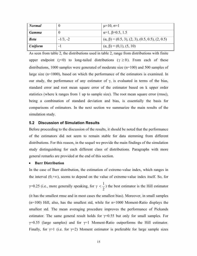
Table 2. Distributions used in the simulation study

Name Extreme-value index γ Other parameters

Burr 0.25, 0.55, 1, 2 (τ, λ) = (0.25, 1), (0.55, 1), (0.5, 2), (1, 0.5)

Fréchet 0.25, 0.55, 1, 2 -

Log-gamma 0.25, 0.55, 1, 2 α=1, λ = 4, 1/0.55, 1, 0.5

Log-logistic 0.25, 0.55, 1, 2 -

Pareto 0.25, 0.55, 1, 2 -

Weibull 0 λ=1, τ=0.5, 1.5

Exponential 0 -

Log-normal 0 µ=100, σ=1

15

Normal 0 µ=10, σ=1

Gamma 0 α=1, β=0.5, 1.5

Beta -1/3, -2 (α, β) = (0.5, 3), (2, 3), (0.5, 0.5), (2, 0.5)

Uniform -1 (α, β) = (0,1), (5, 10)

As seen from table 2, the distributions used in table 2, range from distributions with finite

upper endpoint (γ<0) to long-tailed distributions (γ ≥ 0). From each of these

distributions, 1000 samples were generated of moderate size (n=100) and 500 samples of

large size (n=1000), based on which the performance of the estimators is examined. In

our study, the performance of any estimator of γ, is evaluated in terms of the bias,

standard error and root mean square error of the estimator based on k upper order

statistics (where k ranges from 1 up to sample size). The root mean square error (rmse),

being a combination of standard deviation and bias, is essentially the basis for

comparisons of estimators. In the next section we summarize the main results of the

simulation study.

5.2 Discussion of Simulation Results Before proceeding to the discussion of the results, it should be noted that the performance

of the estimators did not seem to remain stable for data stemming from different

distributions. For this reason, in the sequel we provide the main findings of the simulation

study distinguishing for each different class of distributions. Paragraphs with more

general remarks are provided at the end of this section.

• Burr Distribution

In the case of Burr distribution, the estimation of extreme-value index, which ranges in

the interval (0,+∞), seems to depend on the value of extreme-value index itself. So, for

γ=0.25 (i.e., more generally speaking, for γ <12

) the best estimator is the Hill estimator

(it has the smallest rmse and in most cases the smallest bias). Moreover, in small samples

(n=100) Hill, also, has the smallest std, while for n=1000 Moment-Ratio displays the

smallest std. The mean averaging procedure improves the performance of Pickands

estimator. The same general result holds for γ=0.55 but only for small samples. For

γ=0.55 (large samples) and for γ=1 Moment-Ratio outperforms the Hill estimator.

Finally, for γ>1 (i.e. for γ=2) Moment estimator is preferable for large sample sizes

16

(n=1000), while W is best when it comes to small sample sizes. As long as trimming

effect is concerned, no clear effect exists.

• Fréchet Distribution

For samples of small size (n=100), the Hill estimator, in general, displays the best

performance. For Fréchet data with γ up to 1, the Hill estimator has the smallest rmse

and, most of the times, the smallest bias and std. However, when γ exceeds 1 (in our case

for γ=2) the variability of Hill is much increased and W stands out as the best estimator.

When we are dealing with large simulated data-sets (n=1000), though the performance of

Hill remains in the same level, Moment-Ratio estimator improves greatly (its bias and,

consequently, its rmse is reduced significantly) and turns out to be the best estimator.

Again this holds for values of γ smaller than or equal to 1, since for γ=2, Moment

estimator has the smallest rmse. As long as the averaging procedures are concerned, the

only improvement is observed in the case of mean-averaged Pickands estimator.

• Log-Gamma Distribution

For large sample sizes (n=1000) and γ up to 1, the best estimator is, undeniably, the

Moment-Ratio estimator. It has the smallest bias, std, as well as rmse. However, when γ

exceeds 1, the behaviour of Moment-Ratio deteriorates (mainly due to the large increase

of std) and though, still, Moment-Ratio has the smallest bias, it is Moment the estimator

with the smallest rmse. A point that is worthy to be pointed out here is that while the

behaviour of most estimators deteriorates as γ exceeds 1, the performance of W estimator

is improved. Actually, now, W has the smallest std. The situation is quite different when

we are dealing with small samples (n=100). In those cases, it is the Hill the best estimator

(smallest bias, std, rmse). Of course the behaviour of Moment-Ratio is not disappointing

since it is the second best estimator (not differing much from the Hill). The only case

where Hill is surpassed by another estimator is for γ=2 and for small k (k=12, 20), when

W estimator displays the smallest std and rmse. No satisfactory improvement can be

attributed to the averaging procedures.

• Log-Logistic Distribution

When we are dealing with large samples the situation is quite clear. The best estimator is

the Moment-Ratio estimator, since it always has the smallest rmse (in many cases it also

has minimum bias or std). However, the evaluation of estimators gets more complicated

17

for small sample sizes (n=100). Generally speaking, we could say that among all

estimators the estimator based on 10% trimmed mean excess plot is the best estimator

(smallest rmse). If we confine our comparison among the standard estimators, then Hill

and Moment-Ratio estimators are the most preferable. For γ<1 and for small and

moderate choice of k (k=12, 20) it is the Hill which has the smallest rmse (while the

second smallest rmse is achieved by the Moment-Ratio), while when a larger portion of

data is used in the estimation (k=40) the Moment-Ratio stands out as the best estimator

(followed by the Hill). Irrespectively of the choice of k, in the case of γ>1, the best

estimator is W.

• Pareto Distribution

As was the case for distributions previously discussed, the Moment-Ratio estimator tends

to be, in general, preferable. For large samples and γ up to 1, Moment-Ratio has the

smallest rmse and the smallest bias (for γ smaller than 1 it also has the smallest std).

However, when γ exceeds 1, Moment estimator “outguns” Moment-Ratio. Even then,

Moment-Ratio has the smallest bias, while W has the smallest std. Again, for small

samples the situation is somewhat different. For γ up to 1, Hill is the best estimator

(smallest rmse, bias and, usually, smallest std). But for γ=2 and for k small (k=12, 20) its

variability is much increased while the behaviour of W is improved leading to a

minimum rmse attributed to W. It is useful to add that Moment-Ratio is the second best

estimator here.

• Weibull Distribution

Weibull d.f. belongs to the maximum domain of attraction of Gumbel d.f., i.e. the

extreme value index equals zero. That means that not all of the estimators under

examination should actually be applied to that type of data. Indeed, according to

theoretical results, Hill, Moment-Ratio and QQ estimators are not consistent for γ ≤ 0 .

However, in the context of our simulation study we applied all estimators even in cases

that they are not applicable (for comparison reasons). The simulation results here do not

suggest that any single estimator is uniformly best. So, for large samples and τ=0.5 Peng

is the best estimator, while for τ=1.5 the result depends on the number of upper order

statistics used (k). For large k, again Peng is the best estimator. However for smaller k

(k=12, 20) QQ and Moment estimators display better performances (though even then the

18

performance of Peng is not bad). The situation is somehow similar for small samples

(n=100). That is, for τ=0.5 Peng is preferable but for τ=1.5, it is outperformed by

Moment and Moment-Ratio estimators.

• Exponential Distribution

For large sample sizes (n=1000) Moment estimator has the best performance (for all

choices of k). Apart from having the smallest rmse, it also exhibits minimum bias. As

long as standard error is concerned, Moment-Ratio has the smallest values (though

Moment-Ratio is theoretically applicable only for γ > 0 ). The mean averaging procedure

improves the performance of Pickands estimator (though it still remains inferior to other

estimators). Estimators based on trimmed mean excess plots have a better performance

than simple the Hill estimator (the larger the proportion of trimming the better the

performance of the estimator, while the median excess estimator is worse than Hill.

For small samples (n=100) Moment estimators perform better only when a large portion

of the sample is used in the estimation (k=40). Even then when we are dealing with

averaged estimators, Pickands outperforms the Moment. When a smaller k is used in the

estimation of extreme-value index (k=12 or 20) Moment-Ratio performs better (in terms

of rmse) and has the smallest std, while Pickands has the smallest bias.

Generally speaking, for estimating the extreme-value index in the case of exponential

d.f.s Moment estimator is most preferable for large samples, while for small samples we

should opt for mean-averaged Pickands estimators.

• Log-Normal Distributions

For large samples the situation is quite clear, since Peng is the best estimator for all

choices of k. However, things are not so simple for n=100. In that case, the choice of best

estimator seems to depend on the choice of k. So, for large k, Peng is the best estimator,

while for small k Moment and Moment-Ratio outperform it.

• Normal Distribution

In the case of normally distributed data the zero extreme-value index seems to be better

estimated by the Moment-Ratio estimators. This holds for all choices of k, for small and

for large sample sizes. The only problem seems to be the fact that Moment-Ratio

estimator is not theoretically applicable when extreme-value index equals zero. Other

estimators with satisfactory behaviour are Hill and Q-Q estimators (both of which are,

19

again, not applicable for zero extreme-value index). As long as averaging procedures are

concerned, we should note that mean averaging greatly improves the performance of the

standard Pickands estimator. However, mean averaged Pickands estimator is not one of

the best estimators.

• Gamma Distribution

Here, for the first time the mean averaging procedure provides rather promising results.

Though there is not a uniformly best estimator (for all choices of k and sample size n),

the mean averaged Pickands estimator displays the most satisfactory behaviour (in most

cases it has the smallest rmse). It is really impressive its improvement over the simple,

standard Pickands estimator. Other estimators with acceptable performance are Peng's,

Moment, Moment-Ratio and the Hill estimator.

• Beta Distribution

Beta distribution belongs to the maximum domain of attraction of Weibull d.f, since it

has finite upper end-point. That means that the extreme-value index that we are trying to

estimate is negative and, as previously mentioned, not all estimators are applicable here.

When we are dealing with large samples the situation is quite clear. Moment estimator is

uniformly the best estimator (with the smallest rmse). Also, Peng's performance is almost

as good as Moment's. Moreover, here it is evident the beneficial effect of the averaging

procedures (the mean as well as the median averaging). Mean averaging procedure

substantially improves the performance of Pickands estimator, while both averaging

procedures improve the performance of Moment and Peng's estimator. So, in most cases

it is the mean averaged Moment estimator that has the smallest rmse among all tested

estimators. These results hold for different choices of k and parameters α,β of the beta

distribution (i.e. for different values of the extreme-value index). However, this is not so

when it comes to small sample sizes. Actually, for small sample sizes (n=100 in our case)

the situation is much more complicated. The performance of the estimators depends not

only on the value of k but also on the value of the extreme-value index γ itself. So, for

values of γ close to 0 (-1/3 in particular) mean averaged Pickands estimator seems to be

the best choice, while among the standard estimators Moment-Ratio and Moment are

more preferable. As the value of γ draws away from zero (γ=-2) the performance of all

estimators deteriorates (the values of rmse's are evidently larger). The behaviour of

20

Moment, Moment-Ratio and Peng's estimator is very disappointing. Pickands is the best

estimator among standard estimators. Moreover, the effect of averaging procedures is

much less significant. Anyhow, it is the median averaged Pickands and Moment

estimators that exhibit the smallest rmse.

• Uniform Distribution

Uniform distribution is also bounded to the right and its tails are characterized by

extreme-value index equal to -1. The situation here is somewhat similar to the case of

Beta distribution. More specifically, for large sample sizes (n=1000) Moment estimator is

the most preferable estimator, followed by Peng's. Averaging procedures (mean and

median) improve their performances, while mean averaging also improves the

performance of Pickands estimator. Here it is the median averaging procedure that

provides better results than the mean averaging. These results hold for small samples of

uniformly distributed data. The only difference in this case is that for small k (k=12)

standard estimators display very large rmse's and the 'good' estimators previously

mentioned are outperformed by estimators such as Hill and Moment-Ratio.

5.3 General Comments Though differences exist between different distribution, some common underlying

behaviour of estimators, if we discern them according to the corresponding value of γ.

More particularly:

• For γ>0

For large sample sizes Moment-Ratio seems to be the most preferable estimator. It is

usually the best estimator, in terms of minimum rmse. Even in cases that other estimators

outperform it, it is one of the bests, while in no case does it display very unsatisfactory

performance. It is interesting to note that the W estimator tends to be appropriate for

distributions with extreme-value index γ larger than 1, though for smaller values of γ its

performance can be very unsatisfactory. So, it may be risky to use this estimator, since in

real-life applications, the value of γ is unknown. For small samples (in our case n=100),

the Hill estimator turns out to be the best choice, while Moment-Ratio and Moment

estimators can also be regarded as safe options. Among averaging procedures, only the

mean averaging of Pickands estimator is effective. However, the improvement is not

large enough to out-beat the other standard estimators. On the other hand, the trimming

21

procedure concerning the Hill estimator slightly improves the performance of Hill. This

result combined with the fact that standard the Hill estimator is, in some cases, the best

estimator lead to even better results. Still further exploration on this issue is required.

• For γ=0

The maximum domain of attraction of Gumbel distribution contains a wide range of

distributions differing a lot. Consequently, there is not a uniformly superior estimator.

However, by examining more carefully the above results one could deduce that Peng's is

the most preferable estimator of the extreme-value index. Moment and (surprisingly)

Moment-Ratio also display an adequate behaviour. The usefulness of averaging

procedures in these cases should also be stressed out. These procedures have an obvious

profitable impact on Pickands estimator, so that mean-averaged Pickands estimator can

also be regarded as an adequate estimator of zero γ.

• For γ<0

This class contains upper-bounded distributions. Though the shape of distributions differs

a lot from the distributions with γ=0, the behaviour of extreme-value index estimators in

these two classes of d.f.'s displays great analogies. Here, Moment and Peng's estimators

are undeniably the most preferable estimators and the beneficial effect of both mean and

median averaging procedures is even more evident. Moreover, as we deviate from zero

(and positive) values of γ, the inadequacy of estimators such as Hill, Moment-Ratio and

so on, is more clear.

6 Discussion The comparison (via simulation) of semi-parametric estimation methods for the

extreme-value index and some robustifying alternatives has been the central issue of this

paper. The simulation study conducted led to some very interesting results. The first is

that, as one could naturally expect, the performance of estimators on a specific data-set

depends on the distribution of the data. So, there is not a uniformly best estimator.

Nevertheless, by looking more carefully at the results, some general conclusions may be

reached. More specifically, in cases of long-tailed data (with an infinite upper end-point)

Moment and Moment-Ratio estimators seem to estimate more satisfactorily the non-

negative extreme-value index γ. However, when it comes to upper-bounded distributions

22

(characterized by a negative value of γ) Peng's and Moment estimators are more

preferable. As far as the impact of smoothing (averaging) procedures is concerned, we

deduce that it is effective (improving the performance of standard estimators) in cases

where the true value of extreme-value index is non-positive. Particularly, mean-averaging

procedures improve greatly the performance of Pickands estimator (in case of zero γ),

while median-averaging of Moment and Peng's also leads to improved estimators (for γ

negative).

The dependence of estimators' performance on the distribution of data in hand can be

alternatively seen as dependence on the true value of the index itself. So, before

proceeding to the use of any estimation formula it would be useful if we could get an idea

about the range of values where the true γ lies in. This can be achieved graphically via

QQ and mean excess plots. Alternatively, there exist statistical tests which tests such

hypothesis. See, for example, Hosking (1984), Hasofer and Wang (1992), Alves and

Gomes (1996) and Marohn (1998).

Moreover, it should be pointed out that among the averaged estimators used in the

simulation study only the mean-averaged Hill and Moment estimators have been

theoretically explored by Resnick and Stărică (1997, 1999). As we have seen, the median

averaging procedure has also displayed some interesting effectiveness, implying that it

may be worthy to be also studied theoretically (with special emphasis on Moment and

Peng's estimators). The same holds for the mean-averaged Pickands estimator.

7 References Alves, M.I.F. and Gomes, M.I. (1996). Statistical Choice of Extreme Value Domains of

Attraction – A Comparative Analysis. Communication in Statistics (A) – Theory and Methods 25 (4), 789-811.

Barão, M.I. and Tawn, J.A. (1999). Extremal Analysis of Short Series with Outliers: Sea-Levels and Athletic Records. Applied Statistics 48 (4), 469-487.

Beirlant, J., Broniatowski, M., Teugels, J.L. and Vynckier, P. (1995). The Mean Residual Life Function at Great Age: Applications to Tail Estimation. Journal of Statistical Planning and Inference 45, 21-48.

Beirlant, J., Teugels, J.L. and Vynckier, P. (1994). Extremes in Non-Life Insurance. Extremal Value Theory and Applications, ed. Galambos, J., Lenchner, J. and Simiu, E., Dordrecht, Kluwer, 489-510.

23

Beirlant, J., Teugels, J.L. and Vynckier, P. (1996). Practical Analysis of Extreme Values. Leuven University Press, Leuven.

Coles, S.G. and Dixon, M.J. (1999). Likelihood-Based Inference for Extreme Value Models. Extremes 2 (1), 5-23.

Coles, S.G. and Tawn, J.A. (1996). Modelling Extremes of the Areal Rainfall Process. Journal of the Royal Statistical Society B 58(2), 329-347.

Danielsson, J. and de Vries, C.G. (1997). Beyond the Sample: Extreme Quantile and Probability Estimation. Preprint, Erasmus University, Rotterdam.

Danielsson, J., Jansen, D.W. and deVries, C.G. (1996). The Method of Moment Ratio Estimator for the Tail Shape Distribution. Communication in Statistics (A) – Theory and Methods 25 (4), 711-720.

Davis, R. and Resnick, S. (1984). Tail Estimates Motivated by Extreme Value Theory. The Annals of Statistics 12 (4), 1467-1487.

Davison, A.C. and Smith, R.L. (1990). Models for Exceedances over High Thresholds. Journal of the Royal Statistical Society B 52 (3), 393-442.

Deheuvels, P., de Haan, L., Peng, L. and Pereira, T.T. (1997). NEPTUNE T400:EUR-09, Comparison of Extreme Value Index Estimators.

Dekkers, A.L.M. and de Haan, L. (1989). On the Estimation of the Extreme-Value Index and Large Quantile Estimation. The Annals of Statistics 17 (4), 1795 - 1832.

Dekkers, A.L.M., Einmahl, J.H.J. and de Haan, L. (1989). A Moment Estimator for the Index of an Extreme-Value Distribution. The Annals of Statistics 17 (4), 1833-1855.

Drees, H. (1996). Refined Pickands Estimators with Bias Correction. Communication in Statistics (A) – Theory and Methods 25 (4), 837-851.

Drees, H. and Reiss, R.D. (1996). Residual Life Functionals at Great Age. Communication in Statistics (A) – Theory and Methods 25 (4), 823-835.

DuMouchel, W.H. (1983). Estimating the Stable Index α in Order to Measure Tail Thickness: a Critique. The Annals of Statistics 11, 1019-1031.

Embrechts, P. (1999). Extreme Value Theory in Finance and Insurance. Preprint, ETH. Embrechts, P., Klüppelberg, C. and Mikosch, T. (1997). Modelling Extremal Events

for Insurance and Finance. Springer, Berlin. Embrechts, P., Resnick, S. and Samorodnitsky, G. (1998). Living on the Edge. RISK

Magazine 11 (1), 96-100. Embrechts, P., Resnick, S. and Samorodnitsky, G. (1999). Extreme Value Theory as a

Risk Management Tool. North American Actuarial Journal 26, 30-41. Fisher, R.A. and Tippet, L.H.C. (1928). Limiting Forms of the Frequency Distribution

of the Largest or Smallest Member of a Sample. Proc. Cambridge Phil. Soc., 24 (2), 163-190. (in Embrechts et al. 1997)

Haan, L. de and Resnick, S. (1998). On Asymptotic Normality of the Hill Estimator. Stochastic Models 14, 849-867.

Haeusler, E. and Teugels, J.L. (1985). On Asymptotic Normality of Hill’s Estimator for the Exponent of Regular Variation. The Annals of Statistics 13 (2), 743-756.

Hasofer, A.M. and Wang, Z. (1992). A Test for Extreme Value Domain of Attraction. Journal of the American Statistical Association 87, 171-177.

Hill, B.M. (1975). A Simple General Approach to Inference about the Tail of a Distribution. The Annals of Statistics 3 (5), 1163-1174.

24

Hosking, J.R.M. (1984). Testing Whether the Shape Parameter Is Zero in the Generalized Extreme-Value Distribution. Biometrika 71(2), 367-374.

Hosking, J.R.M. (1985). Maximum-Likelihood Estimation of the Parameter of the Generalized Extreme-Value Distribution. Applied Statistics 34, 301-310.

Hosking, J.R.M., Wallis, J.R. and Wood, E.F. (1985). Estimation of the Generalized Extreme-Value Distribution by the Method of Probability-Weighted Moments. Technometrics 27 (3), 251-261.

Hsing, T. (1991). On Tail Index Estimation Using Dependent Data. Annals of Statistics, 19 (3), 1547-1569.

Kratz, M. and Resnick, S.I. (1996). The QQ Estimator and Heavy Tails. Communication in Statistics – Stochastic Models 12 (4), 699-724.

Marohn, F. (1998). Testing the Gumbel Hypothesis via the Pot-Method. Extremes 1(2), 191-213.

McNeil, A.J. (1997). Estimating the Tails of Loss Severity Distributions Using Extreme Value Theory. ASTIN Bulletin 27, 117-137.

McNeil, A.J. (1998). On Extremes and Crashes. A short-non-tecnhical article. RISK, January 1998, 99.

McNeil, A.J. (1999). Extreme Value Theory for Risk Managers. Internal Modelling and CAD II published by RISK Books, 93-113.

Mikosch, T. (1997). Heavy-Tailed Modelling in Insurance. Communication in Statistics – Stochastic Models 13 (4), 799-815.

Peng, L. (1998). Asymptotically Unbiased Estimators for the Extreme-Value Index. Statistics and Probability Letters 38, 107-115.

Pickands, J. (1975). Statistical Inference Using Extreme order statistics. The Annals of Statistics 3 (1), 119-131.

Resnick, S. and Stărică, C. (1995). Consistency of Hill’s Estimator for Dependent Data. Journal of Applied Probability 32, 139-167.

Resnick, S. and Stărică, C. (1996). Asymptotic Behaviour of Hill’s Estimator for Autoregresive Data. Preprint, Cornell University. (Available as TR1165.ps.Z at http://www.orie.cornell.edu/trlist/trlist.html.)

Resnick, S. and Stărică, C. (1997). Smoothing the Hill Estimator. Advances in Applied Probability 29, 271-293.

Resnick, S. and Stărică, C. (1998). Tail Index Estimation for Dependent Data. Annals of Applied Probability 8 (4), 1156-1183.

Resnick, S. and Stărică, C. (1999). Smoothing the Moment Estimator of the Extreme Value Parameter. Extremes 1(3), 263-293.

Rootzén, H. and Tajvidi, N. (1997). Extreme Value Statistics and Wind Storm Losses: A Case Study. Scandinavian Actuarial Journal, 70-94.

Rosen, O. and Weissman, I. (1996). Comparison of Estimation Methods in Extreme Value Theory. Communication in Statistics – Theory and Methods 25 (4), 759-773.

Scarf, P.A. (1992). Estimation for a Four Parameter Generalized Extreme Value Distribution. Communication in Statistics – Theory and Method 21 (8), 2185-2201.

Smith, R.L. (1985). Maximum-Likelihood Estimation in a Class of Non-Regular Cases. Biometrika 72, 67-90.

25

Smith, R.L. (1989). Extreme Value Analysis of Environmental Time Series: An Application to Trend Detection in Ground-Level Ozone. Statistical Science, 4 (4), 367-393.