LINEAR PROGRAMMING-BASED ESTIMATORS IN NONNEGATIVEAUTOREGRESSION

DANIEL PREVE†

AUGUST 11, 2015

Abstract. This note studies robust estimation of the autoregressive (AR) parameter in a nonlin-ear, nonnegative AR model driven by nonnegative errors. It is shown that a linear programmingestimator (LPE), considered by Nielsen and Shephard (2003) among others, remains consistentunder severe model misspecification. Consequently, the LPE can be used to test for, and seeksources of, misspecification when a pure autoregression cannot satisfactorily describe the datagenerating process, and to isolate certain trend, seasonal or cyclical components. Simple andquite general conditions under which the LPE is strongly consistent in the presence of seri-ally dependent, non-identically distributed or otherwise misspecified errors are given, and abrief review of the literature on LP-based estimators in nonnegative autoregression is presented.Finite-sample properties of the LPE are investigated in an extensive simulation study coveringa wide range of model misspecifications. A small scale empirical study, employing a volatilityproxy to model and forecast latent daily return volatility of three major stock market indexes,illustrates the potential usefulness of the LPE.

JEL classification. C13, C14, C22, C51, C58.Key words and phrases. Robust estimation, linear programming estimator, strong convergence, nonlinear nonnega-tive autoregression, dependent non-identically distributed errors, heavy-tailed errors.† City University of Hong Kong. Address correspondence to Daniel Preve, Department of Economics and Fi-nance, City University of Hong Kong, 83 Tat Chee Avenue, Kowloon, Hong Kong; e-mail: pdapreve@cityu.edu.hk.The author thanks Jun Yu, Marcelo C. Medeiros, Bent Nielsen, Rickard Sandberg, Kevin Sheppard and Peter C. B.Phillips for helpful comments on an early version of this note, and conference participants at the 6th Annual SoFiEConference (2013, Singapore), the 2014 Asian Meeting of the Econometric Society (Taipei), the 1st Conference onRecent Developments in Financial Econometrics and Applications (2014, Geelong), and seminar participants atSingapore Management University and National University of Singapore for their comments and suggestions.Comments and suggestions from two anonymous referees are also gratefully acknowledged. The author is re-sponsible for any remaining errors. The work described in this note was substantially supported by a grant fromthe Research Grants Council of the Hong Kong Special Administrative Region, China (project no. CityU198813).Partial research support from the Jan Wallander and Tom Hedelius Research Foundation (grant P 2006-0166:1)and the Sim Kee Boon Institute for Financial Economics, and the Institute’s Centre for Financial Econometrics, atSingapore Management University is also gratefully acknowledged.

1

2

1. Introduction

In the last decades, nonlinear and nonstationary time series analysis have gained much at-tention. This attention is mainly motivated by evidence that many real life time series arenon-Gaussian with a structure that evolves over time. For example, many economic time se-ries are known to show nonlinear features such as cycles, asymmetries, time irreversibility,jumps, thresholds, heteroskedasticity and combinations thereof. This note considers robustestimation in a (potentially) misspecified nonlinear, nonnegative autoregressive model, thatmay be a useful tool for describing the behaviour of a broad class of nonnegative time series.

For nonlinear time series models it is common to assume that the errors are i.i.d. withzero-mean and finite variance. Recently, however, there has been considerable interest in non-negative models. See, e.g., Abraham and Balakrishna (1999), Engle (2002), Tsai and Chan(2006), Lanne (2006) and Shephard and Sheppard (2010). The motivation to consider suchmodels comes from the need to account for the nonnegative nature of certain time series. Ex-amples from finance include variables such as absolute or squared returns, bid-ask spreads,trade volumes, trade durations, and standard volatility proxies such as realized variance, real-ized bipower variation (Barndorff-Nielsen and Shephard, 2004) or realized kernel (Barndorff-Nielsen et al., 2008).1 This note considers a nonlinear, nonnegative autoregressive modeldriven by nonnegative errors. More specifically, it considers robust estimation of the AR pa-rameter β in the autoregression

yt = β f (yt−1, . . . , yt−s) + ut, (1)

with nonnegative (possibly) misspecified errors ut. Potential distributions for ut include log-normal, gamma, uniform, Weibull, inverse Gaussian, Pareto and mixtures of them. In someapplications, robust estimation of the AR parameter is of interest in its own right. One ex-ample is point forecasting, as described in Preve et al. (2015). Another is seeking sources ofmodel misspecification. In recognition of this fact, this note focuses explicitly on the robustestimation of β in (1). If the function f is known, a natural estimator for β given the sampley1, . . . , yn of size n and the nonnegativity of the errors is

βn = min{

ys+1

f (ys, . . . , y1), . . . ,

yn

f (yn−1, . . . , yn−s)

}. (2)

This estimator has been used to estimate β in certain restricted first-order autoregressive,AR(1), models (e.g. Andel, 1989b; Datta and McCormick, 1995; Nielsen and Shephard, 2003).An early reference of the autoregression in (1) is Bell and Smith (1986), who considers thelinear AR(1) specification f (yt−1, . . . , yt−s) = yt−1 to model water pollution and the accom-panying estimator in (2) for estimation.2 The estimator in (2) can, under some additionalconditions, be viewed as the solution to the linear programming problem of maximizing theobjective function g(β) = β subject to the n− s linear constraints yt − β f (yt−1, . . . , yt−s) ≥ 0(cf. Feigin and Resnick, 1994). Because of this, we will refer to it as a LP-based estimator orLPE. As it happens, (2) is also the (on y1, . . . , ys) conditional maximum likelihood estimator(MLE) for β when the errors are exponentially distributed (cf. Andel, 1989a). What is inter-esting, however, is that βn is a strongly consistent estimator of β for a wide range of errordistributions, thus the LPE is also a quasi-MLE (QMLE).

In all of the above references the errors are assumed to be i.i.d.. To the authors knowledge,there has so far been no attempt to investigate the statistical properties of LP-based estimators

1Another example is temperature, which can be used for pricing weather derivatives (e.g. Campbell and Diebold,2005; Alexandridis and Zapranis, 2013).2Bell and Smith (1986) refer to the LPE as a ‘quick and dirty’ nonparametric point estimator.

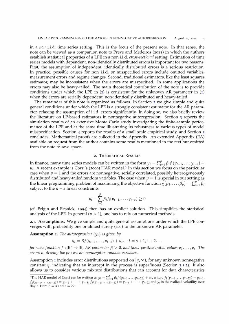
LINEAR PROGRAMMING-BASED ESTIMATORS IN NONNEGATIVE AUTOREGRESSION August 11, 2015 3

in a non i.i.d. time series setting. This is the focus of the present note. In that sense, thenote can be viewed as a companion note to Preve and Medeiros (2011) in which the authorsestablish statistical properties of a LPE in a non i.i.d. cross-sectional setting. Estimation of timeseries models with dependent, non-identically distributed errors is important for two reasons:First, the assumption of independent, identically distributed errors is a serious restriction.In practice, possible causes for non i.i.d. or misspecified errors include omitted variables,measurement errors and regime changes. Second, traditional estimators, like the least squaresestimator, may be inconsistent when the errors are misspecified. In some applications theerrors may also be heavy-tailed. The main theoretical contribution of the note is to provideconditions under which the LPE in (2) is consistent for the unknown AR parameter in (1)when the errors are serially dependent, non-identically distributed and heavy-tailed.

The remainder of this note is organized as follows. In Section 2 we give simple and quitegeneral conditions under which the LPE is a strongly consistent estimator for the AR param-eter, relaxing the assumption of i.i.d. errors significantly. In doing so, we also briefly reviewthe literature on LP-based estimators in nonnegative autoregression. Section 3 reports thesimulation results of an extensive Monte Carlo study investigating the finite-sample perfor-mance of the LPE and at the same time illustrating its robustness to various types of modelmisspecification. Section 4 reports the results of a small scale empirical study, and Section 5

concludes. Mathematical proofs are collected in the Appendix. An extended Appendix (EA)available on request from the author contains some results mentioned in the text but omittedfrom the note to save space.

2. Theoretical Results

In finance, many time series models can be written in the form yt = ∑pi=1 βi fi(yt−1, . . . , yt−s) +

ut. A recent example is Corsi’s (2009) HAR model.3 In this section we focus on the particularcase when p = 1 and the errors are nonnegative, serially correlated, possibly heterogeneouslydistributed and heavy-tailed random variables. The case when p = 1 is special in our setting asthe linear programming problem of maximizing the objective function g(β1, . . . , βp) = ∑

pi=1 βi

subject to the n− s linear constraints

yt −p

∑i=1

βi fi(yt−1, . . . , yt−s) ≥ 0

(cf. Feigin and Resnick, 1994) then has an explicit solution. This simplifies the statisticalanalysis of the LPE. In general (p > 1), one has to rely on numerical methods.

2.1. Assumptions. We give simple and quite general assumptions under which the LPE con-verges with probability one or almost surely (a.s.) to the unknown AR parameter.

Assumption 1. The autoregression {yt} is given by

yt = β f (yt−1, . . . , yt−s) + ut, t = s + 1, s + 2, . . .

for some function f : Rs → R, AR parameter β > 0, and (a.s.) positive initial values y1, . . . , ys. Theerrors ut driving the process are nonnegative random variables.

Assumption 1 includes error distributions supported on [η, ∞), for any unknown nonnegativeconstant η, indicating that an intercept in the process is superfluous (Section 3.1.2). It alsoallows us to consider various mixture distributions that can account for data characteristics3The HAR model of Corsi can be written as yt = ∑3

i=1 βi fi(yt−1, . . . , yt−22) + ut, where f1(yt−1, . . . , yt−22) = yt−1,f2(yt−1, . . . , yt−22) = yt−2 + · · ·+ yt−5, f3(yt−1, . . . , yt−22) = yt−6 + · · ·+ yt−22 and yt is the realized volatility overday t. Here p = 3 and s = 22.

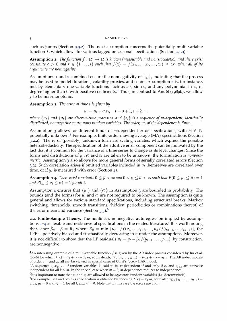
4 DANIEL PREVE

such as jumps (Section 3.3.2). The next assumption concerns the potentially multi-variablefunction f , which allows for various lagged or seasonal specifications (Section 3.1.3).

Assumption 2. The function f : Rs → R is known (measurable and nonstochastic), and there existconstants c > 0 and r ∈ {1, . . . , s} such that f (x) = f (x1, . . . , xr, . . . , xs) ≥ cxr when all of itsarguments are nonnegative.

Assumptions 1 and 2 combined ensure the nonnegativity of {yt}, indicating that the processmay be used to model durations, volatility proxies, and so on. Assumption 2 is, for instance,met by elementary one-variable functions such as exs , sinh xs and any polynomial in xs ofdegree higher than 0 with positive coefficients.4 Thus, in contrast to Andel (1989b), we allowf to be non-monotonic.

Assumption 3. The error at time t is given by

ut = µt + σtεt, t = s + 1, s + 2, . . .

where {µt} and {σt} are discrete-time processes, and {εt} is a sequence of m-dependent, identicallydistributed, nonnegative continuous random variables. The order, m, of the dependence is finite.

Assumption 3 allows for different kinds of m-dependent error specifications, with m ∈ N

potentially unknown.5 For example, finite-order moving average (MA) specifications (Section3.2.2). The σt of (possibly) unknown form are scaling variates, which express the possibleheteroskedasticity. The specification of the additive error component can be motivated by thefact that it is common for the variance of a time series to change as its level changes. Since theforms and distributions of µt, σt and εt are taken to be unknown, the formulation is nonpara-metric. Assumption 3 also allows for more general forms of serially correlated errors (Section3.2). Such correlation arises if omitted variables included in ut themselves are correlated overtime, or if yt is measured with error (Section 4).

Assumption 4. There exist constants 0 ≤ µ < ∞ and 0 < σ ≤ σ < ∞ such that P(0 ≤ µt ≤ µ) = 1and P(σ ≤ σt ≤ σ) = 1 for all t.

Assumption 4 ensures that {µt} and {σt} in Assumption 3 are bounded in probability. Thebounds (and the forms) for µt and σt are not required to be known. The assumption is quitegeneral and allows for various standard specifications, including structural breaks, Markovswitching, thresholds, smooth transitions, ‘hidden’ periodicities or combinations thereof, ofthe error mean and variance (Section 3.3).6

2.2. Finite-Sample Theory. The nonlinear, nonnegative autoregression implied by assump-tions 1–4 is flexible and nests several specifications in the related literature.7 It is worth notingthat, since βn − β = Rn where Rn = min {us+1/ f (ys, . . . , y1), . . . , un/ f (yn−1, . . . , yn−s)}, theLPE is positively biased and stochastically decreasing in n under the assumptions. Moreover,it is not difficult to show that the LP residuals ut = yt − βn f (yt−1, . . . , yt−s), by construction,are nonnegative.

4An interesting example of a multi-variable function f is given by the AR index process considered by Im et al.(2006) for which f (x) = x1 + · · ·+ xs or, equivalently, f (yt−1, . . . , yt−s) = yt−1 + · · ·+ yt−s. The AR index modelsof order 1, 5 and 22 all can be viewed as special cases of Corsi’s (2009) HAR model.5A sequence ε1, ε2, . . . of random variables is said to be m-dependent if and only if εt and εt+k are pairwiseindependent for all k > m. In the special case when m = 0, m-dependence reduces to independence.6It is important to note that µt and σt are allowed to be degenerate random variables (i.e. deterministic).7For example, Bell and Smith’s specification is obtained by choosing f (x) = x1 or, equivalently, f (yt−1, . . . , yt−s) =yt−1, µt = 0 and σt = 1 for all t, and m = 0. Note that in this case the errors are i.i.d..

LINEAR PROGRAMMING-BASED ESTIMATORS IN NONNEGATIVE AUTOREGRESSION August 11, 2015 5

2.3. Asymptotic Theory.

2.3.1. Convergence. Previous works focusing explicitly on the strong convergence of LP-basedestimators in nonnegative autoregressions include Andel (1989a), Andel (1989b) and An (1992).These LPEs are interesting as they can yield much more accurate estimates than traditionalmethods, such as conditional least squares (LS). See, e.g., Datta et al. (1998) and Nielsen andShephard (2003). Like the LSE for β, the LPE is distribution-free in the sense that its consis-tency does not rely on a particular distributional assumption for the errors. However, the LPEis sometimes superior to the LSE. For example, its rate of convergence can be faster than

√n

even when β < 1.8 For instance, in the linear AR(1) with exponential errors the (supercon-sistent) LPE converges to β at the rate of n. For another example, in contrast to the LSE, theconsistency conditions of the LPE do not involve the existence of any higher order moments.

The following theorem is the main theoretical contribution of the note. It provides condi-tions under which the LPE is strongly consistent for the unknown AR parameter.

Theorem 1. Suppose that assumptions 1–4 hold. Then the LPE or QMLE in (2) is strongly consistentfor β in (1), i.e. βn converges to β a.s. as n tends to infinity, if either (i) P(c1 < εt < c2) < 1 for all0 < c1 < c2 < ∞ and µt = 0 for all t, or (ii) P(εt < c3) < 1 for all 0 < c3 < ∞.

In other words, the LPE remains a consistent estimator for β if the i.i.d. error assumption issignificantly relaxed. The convergence is almost surely (and, hence, also in probability). Notethat the additional condition of Theorem 1 is satisfied for any distribution with unboundednonnegative support (sufficient, but not necessary), and that the consistency conditions of theLPE do not involve the existence of any moments.9 Hence, heavy-tailed error distributions arealso included (Section 3.1.2).

2.3.2. Distribution. As aforementioned, the purpose of this note is not to derive the distribu-tion of the LPE in our (quite general) setting, but rather to highlight some of its robustnessproperties. Nevertheless, for completeness, we here mention some related distributional re-sults. For the case with i.i.d. nonnegative errors several results are available: Davis and Mc-Cormick (1989) derive the limiting distribution of the LPE in a stationary AR(1) and Nielsenand Shephard (2003) derive the exact (finite-sample) distribution of the LPE in a AR(1) withexponential errors. Feigin and Resnick (1994) derive limiting distributions of LPEs in a sta-tionary AR(p). Datta et al. (1998) establish the limiting distribution of a LPE in an extendednonlinear autoregression. The limited success of LPEs in applied work can be partially ex-plained by the fact that their asymptotic distributions depend on the (in most cases) unknowndistribution of the errors. To overcome this problem, Datta and McCormick (1995) and Feiginand Resnick (1997) consider bootstrap inference for linear autoregressions via LPEs. Some ro-bustness properties and exact distributional results of the LPE in a cross-sectional setting wererecently derived by Preve and Medeiros (2011).

8This occurs, under some additional conditions, when the exponent of regular variation of the error distributionat 0 or ∞ is less than 2 (Davis and McCormick, 1989; Feigin and Resnick, 1992). The rate of convergence for theLSE is faster than

√n only when β ≥ 1 (Phillips, 1987).

9As an extreme example, consider estimating 0 < β < 1 in the linear specification yt = βyt−1 + ut with indepen-dent, nonnegative stable errors ut ∼ S(a, b, c, d; 1), where the index of stability a < 1, the skewness parameterb = 1 and the location parameter d ≥ 0 (cf. Lemma 1.10 in Nolan, 2015). In this case yt also follows a stabledistribution with index of stability a and, hence, no finite first moment for a suitable choice of y1 (cf. the MonteCarlo experiment with Levy distributed errors in Section 3.1.2).

6 DANIEL PREVE

3. Simulation Results

In this section we report simulation results concerning the estimation of the AR parameter βin the nonnegative autoregression yt = β f (yt−1, . . . , yt−s) + ut, ut = µt + σtεt, considered insections 1–2. The purpose of the simulations is to see how the LPE and a benchmark estimatorperform under controlled circumstances when the data generating process is known.

For ease of exposition, we let f (yt−1, . . . , yt−s) = yt−s and s = 1, 4.10 Thus, in the simulationsthe data generating process (DGP) is

yt = βyt−s + ut, with ut = µt + σtεt, t = s + 1, s + 2, . . . (3)

and the LPE is

βLP = min{

ys+1

y1, . . . ,

yn

yn−s

}= β + min

{us+1

y1, . . . ,

un

yn−s

}. (4)

In this case, whenever the errors ut are believed to be serially uncorrelated and to satisfy theusual moment conditions, a natural benchmark for the LPE of β is the corresponding ordinaryleast squares estimator, βLS, which also is a distribution-free estimator. If {yt} is generated by(3) and {ut} is a sequence of random variables with common finite mean, the LSE for β givena sample y1, . . . , yn of size n > s is

βLS =∑n

t=s+1(yt − y+)(yt−s − y−)∑n

t=s+1(yt−s − y−)2 = β +∑n

t=s+1(ut − u+)(yt−s − y−)∑n

t=s+1(yt−s − y−)2 , (5)

where

y+ =1

n− s

n

∑t=s+1

yt, and y− =1

n− s

n

∑t=s+1

yt−s.

By the second equality in (5) it is clear that the LSE, like the LPE, can be decomposed into twoparts: the true (unknown) value β and a stochastic remainder term, indicating that βLS maybe asymptotically biased. For instance, if the errors ut are serially correlated.

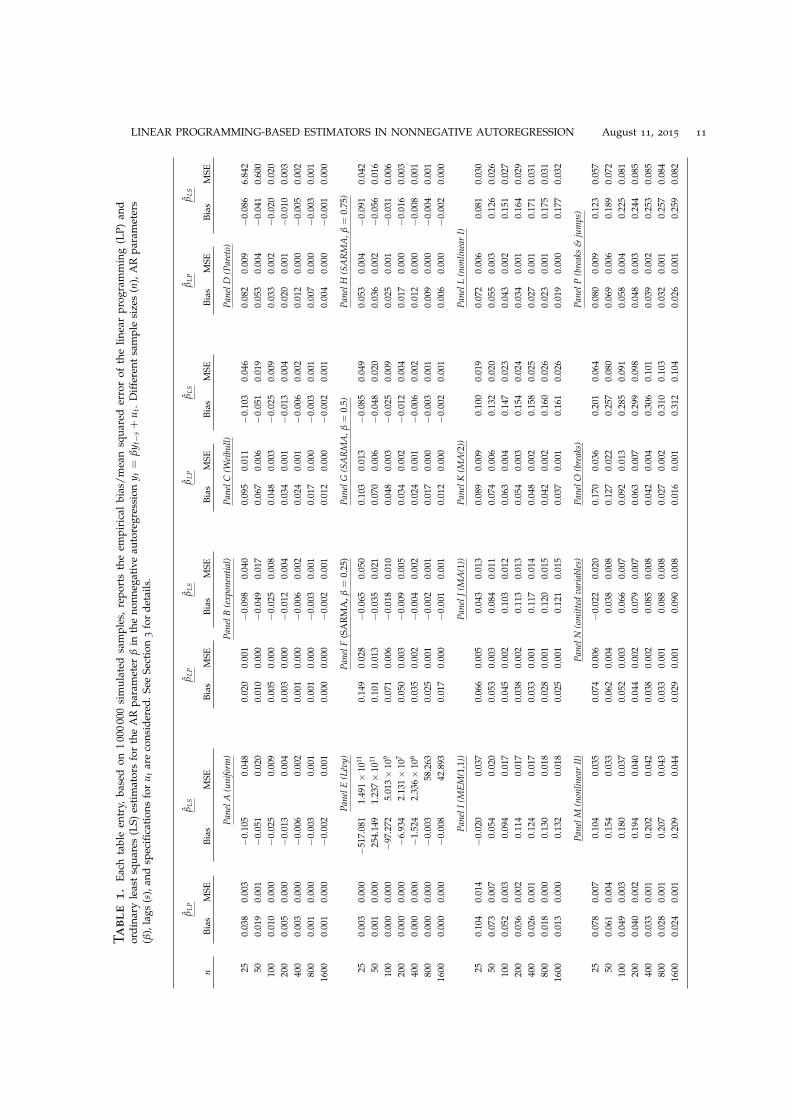
Table 1 shows simulation results for various specifications of µt, σt and εt in (3). The as-sumptions of Theorem 1 are satisfied for all of these specifications, hence, the LPE (but notnecessarily the LSE) is consistent for β. Our simulations try to answer two questions: First,how well does the LPE perform when the estimated model is misspecified? Second, how welldoes a traditional estimator, the LSE, perform by comparison? We report the empirical biasand mean squared error (MSE) of the LPE and LSE based on 1 000 000 simulated samples fordifferent sample sizes n. Each table entry is rounded to three decimal places. All the reportedexperiments share a common initial state of the generator for pseudo-random number gen-eration, use initial values y1 = ∑100 000

i=0 βiu1−is as an approximation of ∑∞i=0 βiu1−is, and were

carried out using Matlab. The initial values µs+1 and σs+1 for the experiments in sections3.2.1, 3.2.4 and 3.3.1.–3.3.2 were obtained similarly.11

3.1. I.I.D. Errors. Panels A–H of Table 1 report simulation results when the errors ut in (3) areindependent, identically distributed. In all eight experiments, the bias and MSE of the LPEis quite reasonable. The LSE also performs reasonably well, but often has a larger bias and amuch larger MSE.

10Sample paths of some of the processes considered in this study and additional supporting simulation resultscan be found in Section 2 of the EA.11Matlab code for the Monte Carlo experiments of this section is available through the authors webpage athttp://www.researchgate.net\profile\Daniel Preve.

LINEAR PROGRAMMING-BASED ESTIMATORS IN NONNEGATIVE AUTOREGRESSION August 11, 2015 7

3.1.1. Light-Tailed Errors. The LPE can be comparatively accurate also when there is no modelmisspecification (i.e. when model and DGP coincide). To illustrate this, we first consider threedifferent light-tailed distributions for the errors. Panels A–C report simulation results whenyt = 0.5yt−1 + ut and the ut are i.i.d. uniform, exponential, and Weibull.12 In all experimentsthe estimated model is an AR(1). In the first experiment (Panel A) the error at time t has astandard uniform distribution. Here the distribution of yt conditional on yt−1 is also uniform.In the second experiment (Panel B) the errors are standard exponential, and in the third (PanelC) Weibull distributed with scale parameter 1 and shape parameter 2. The simulation resultsshow that the accuracy of the LPE can be quite remarkable. For example, when n = 25 andthe errors are exponentially distributed the results are close to those expected by the limittheory. The magnitudes of the bias and MSE of the LSE on the other hand are nearly 5 and 40

times as large, respectively.

3.1.2. Heavy-Tailed Errors. Panels D–E report simulation results when yt = 0.5yt−1 + ut andthe ut are i.i.d. Pareto and Levy, respectively.13 In both experiments the estimated model is anAR(1). In the first experiment (Panel D) the error is Pareto distributed with scale parameter1 and shape parameter 1.25 and, hence, with support [1, ∞). The Pareto distribution is oneof the simplest distributions with heavy-tails. Here the errors have finite mean, 5, but infinitevariance. In the second experiment (Panel E) the error is Levy distributed with locationparameter 0 and scale parameter 1.14 The Levy distribution is a member of the class of stabledistributions, that allow for asymmetry and heavy-tails. Here the errors have infinite mean(but finite median) and variance. AR(MA) processes with infinite variance have been used byFama (1965) and others to model stock market prices. See also Ling (2005), Andrews et al.(2009), and Andrews and Davis (2013). The simulation results show that LPE performs well,particularly in small samples. The bias and MSE of the LSE on the other hand can be severeeven in moderate samples, as illustrated in Panel E.

3.1.3. Seasonal Autoregression. Panels F–H report simulation results when yt = βyt−4 + ut, theAR parameter β = 0.25, 0.5, 0.75, the errors ut are i.i.d. Weibull with scale parameter 1 andshape parameter 2, and the (correctly specified) estimated model is a SARMA(0,0)×(1,0)4.15

These three experiments illustrate that the bias and MSE of the LPE for a fixed n, viewed asa function of β, is stochastically decreasing in the AR parameter. It can be shown that thisproperty holds under fairly general conditions on f in Assumption 2.16

3.2. Serially Correlated Errors. Panels I–N of Table 1 report simulation results when yt =βyt−1 + ut, and the ut are serially correlated. In all six experiments the estimated model is anAR(1). To investigate the sensitivity of the LPE to serially correlated errors, we consider fourdifferent specifications for ut: a multiplicative specification belonging to the MEM family of

12Nonnegative first-order autoregressions with uniformly distributed errors have been considered by Nouali andFellag (2005) and Bell and Smith (1986), and with exponential errors by Nielsen and Shephard (2003), amongothers. Exponential and Weibull errors are popular in the autoregressive conditional duration (ACD) literatureinitiated by Engle and Russell (1998).13Pareto and Levy pseudo-random numbers were generated using the inversion method and via Problem 1.17 inNolan (2015), respectively.14Cf. Corollary 1 in the EA.15More generally, it is not difficult to show that (Proposition 3 in the EA) the LPE in (4) can consistently estimatethe AR parameter of a nonnegative covariance stationary SARMA(0,q)×(1,Q)4 process under the assumptions ofTheorem 1.16See Proposition 4 in the EA.

8 DANIEL PREVE

Engle (2002), a MA specification, a nonlinear specification, and an omitted variables specifica-tion. In all experiments the bias and MSE of the LPE vanishes rather quickly. In contrast, thebias of the LSE does not vanish and its MSE is quite substantial even for large samples.17

3.2.1. MEM Errors. First we consider the multiplicative error specification

ut = σtεt

σt = α0 +q

∑i=1

αiut−i +p

∑j=1

β jσt−j, t = 0,±1,±2, . . .

with i.i.d. εt, that is, a MEM(p,q). Here µt in Assumption 3 is zero for all t and m is also zero.This specification has the same structure as the ACD model of Engle and Russell (1998) fortrade durations. Panel I reports simulation results for the case p = q = 1. The DGP is

yt = 0.5yt−1 + σtεt, σt = α0 + α1σt−1εt−1 + β1σt−1,

with independent identically beta distributed εt (beta distributed with both shape parametersequal to 2 and, hence, with about 0.5 symmetric common density), and α1 = 0.2, β1 = 0.75,α0 = 1− α1 − β1. For these values of α1, β1 and α0 the autocorrelation function of {ut} decaysslowly (cf. Bauwens and Giot, 2000, p. 124). It can be shown that Assumption 4 is satisfied forthis case with µ = 0, σ = 0.2 and σ = 1.

3.2.2. MA Errors. Next we consider the linear m-dependent error specification

ut = εt = εt +q

∑i=1

ψiεt−i, t = 0,±1,±2, . . .

with i.i.d. εt, that is, a MA(q). Here µt = 0, σt = 1 and m = q. Panels J–K report simulationresults for this case, which may be considered as a basic omitted variables specification, withq = 1, 2.18 The DGPs for panels J and K are

yt = 0.75yt−1 + εt+0.75εt−1, and yt = 0.75yt−1 + εt+0.75εt−1 + 0.5εt−2,

respectively, where the εt are i.i.d. inverse Gaussian with mean and variance both equal to 1.The inverse Gaussian distribution (Seshadri, 1993) has previously been considered by Abra-ham and Balakrishna (1999) for the error term in a nonnegative first-order autoregression.Although the LPE is strongly consistent in this case whenever q is finite, extended simulationsnot reported in the note indicate that its convergence can be slow for large values of q.

3.2.3. Nonlinear Specification. The third specification we consider is a nonlinear m-dependenterror specification

ut = εt = εt +m

∑i=1

ψiεtεt−i,

with i.i.d. εt. Panels L–M report simulation results for this case, with m = 1, 2. The DGPs forpanels L and M are

yt = 0.5yt−1 + εt+0.75εtεt−1, and yt = 0.5yt−1 + εt+0.75εtεt−1 + 0.5εtεt−2,

respecively, where the εt are i.i.d. inverse Gaussian with mean and variance both equal to 1.

17Recall that the variance of an estimator is equal to the difference of its MSE and its squared bias.18For example, finite sums of finite-order MA processes driven by i.i.d. disturbances are m-dependent.

LINEAR PROGRAMMING-BASED ESTIMATORS IN NONNEGATIVE AUTOREGRESSION August 11, 2015 9

3.2.4. Omitted Variables. Last we consider the linear error specification

ut = µt + εt

µt =p

∑i=1

αiµt−i + εt, t = 0,±1,±2, . . .

with i.i.d. εt. Here the pth-order AR specification for µt may be considered to represent oneor more omitted variables, σt = 1, and m = 0. Panel N reports simulation results for the casep = 1. The DGP is

yt = 0.75yt−1+µt + εt, µt = 0.25µt−1 + εt,

with standard exponential εt (mean and variance both equal to 1) and i.i.d. on (0, 25) uniformεt, mutually independent of the εt. It is not difficult to show that Assumption 4 is satisfied forthis case with µ = 100/3 and σ = σ = 1.

3.3. Structural Breaks. Finally we investigate the sensitivity of the LPE to an unknown num-ber of unknown breaks in the mean. This is of interest as such structural breaks are wellknown to be able to reproduce the slow decay frequently observed in the sample autocorrela-tions of financial variables such as volatility proxies and absolute stock returns. The simulationresults are reported in Panels O–P of Table 1. In both experiments the estimated model is anAR(1). Once again the bias and MSE of the LPE vanishes rather quickly, whereas the bias ofthe LSE does not vanish and its MSE is quite substantial even for large samples.

3.3.1. Random Breakdates. An autoregression with b ≥ 1 structural breaks in the sample andbreakdates n1 < · · · < nb can be specified using

µt =b−1

∑i=1

αi1{ni<t≤ni+1} + αb1{t>nb},

where 1{·} is the indicator function. Panel O reports simulation results for a nonnegativeautoregression with b = 2 structural breaks in the sample and random breakdates n1 < n2.The DGP is

yt = 0.5yt−1 + α11{n1<t≤n2} + α21{t>n2} + εt,

with α1 = 2.3543, α2 = α1/2, and i.i.d. truncated normal εt (normal distribution with mean2.3263 and variance 1, truncated at zero).19 The random breakdate n1 has a discrete uniformdistribution on {1, . . . , n− 2}, and the on n1 conditional distribution of n2 is discrete uniformon {n1 + 1, . . . , n− 1}.20

3.3.2. Random Breakdates & Occasional Jumps. Alternatively, we can specify an autoregressionwith b structural breaks using

σt = 1{t≤n1} +b−1

∑i=1

αi1{ni<t≤ni+1} + αb1{t>nb},

and multiplicative errors ut = σtεt. We can further allow for jumps by letting the i.i.d. εt havea k-component mixture distribution, with each component representing a different jump size

19Here µt = α11{n1<t≤n2} + α21{t>n2}, σt = 1 and m = 0. Other types of breaks are considered in the EA.20Note that the results for different sample sizes are not directly comparable for this (and the following) experi-ment, as the supports for the breakdate variables involve n.

10 DANIEL PREVE

(e.g. small, medium, large). Panel P report simulation results for a nonnegative autoregressionwith b = 5 structural breaks in the sample and random breakdates n1 < · · · < n5. The DGP is

yt = βyt−1 +

(1{t≤n1} +

4

∑i=1

αi1{ni<t≤ni+1} + α51{t>n5}

)εt,

with i.i.d. εt having a 2-component lognormal mixture distribution. Once more, the condi-tional distribution of the breakdate ni is discrete uniform. For this experiment, the parametersof the DGP were calibrated using the S&P 500 realized kernel data considered in Section 4.Figures 1b and 1c show that this fairly simple process is able to reproduce some of the featuresof the S&P 500 data.

4. Empirical Results

This section reports the results of a small scale empirical study employing the LPE. The pur-pose of the study is twofold: First, it illustrates how the robustness of the LPE can be capi-talized on to estimate and forecast a simple semiparametric model in an environment wheretraditional estimators, like the LSE, are likely to be inconsistent. The model combines a para-metric component, taking into account the most recent observation, with a nonparametriccomponent - forecasted by a moving median similar to the moving averages frequently usedin technical analysis, taking into account possible omitted variables, measurement errors andstructural breaks. Second, it also illustrates that volatility proxy forecasts of a parsimonious(single parameter) model estimated by the LPE can be at least as accurate as those of a ratherinvolved (multiple parameter) ARFIMA benchmark model. The ARFIMA is probably themost commonly used model for forecasting volatility proxies. See, for example, Andersen etal. (2003), Koopman et al. (2005), Lanne (2006), Corsi (2009) and the references therein.

We use a volatility proxy to model and forecast latent daily return volatility of three majorstock market indexes. The Standard & Poor’s 500 (S&P 500), the NASDAQ-100, and the DowJones Industrial Average (DJIA). We employ the LPE as the observable process is nonnega-tive, persistent and likely to be nonlinear (changes in index components) with measurementerrors.21 Also, the LPE of β avoids the need for estimating potential additional parameters,which may prove useful. Two models are considered: a simple nonnegative, semiparametric,autoregressive (NNAR) model and a parametric benchmark model.

Following Andersen et al. (2003), we use a fractionally-integrated long-memory Gaussianautoregression of order five (corresponding to five days or one trading week) for the dailylogarithmic volatility proxy as our benchmark model. We use the realized kernel (RK) ofBarndorff-Nielsen et al. (2008) as a volatility proxy for latent volatility. This proxy is knownto be robust to certain types of market microstructure noise. Daily RK data over the period3 January 2000 through 3 June 2014 for the three assets was obtained from the Oxford-ManInstitute’s Realized Library v0.2 (Heber et al., 2009). Figure 1a shows the S&P 500 data, whichwill be used for illustration in the remainder of this section.

We estimate the ARFIMA(5,d,0) for log-RK using the Ox language of Doornik (2009) andcompute bias corrected forecasts for raw RK, due to the data transformation (Granger and

21If the observable process {yt} is a noisy proxy for an underlying latent process {xt} then measurement errorswill influence the dynamics of {yt} and may conceal the persistence of {xt}. In this case the robustness propertiesof the LPE can be useful. Consider Example 1 in Hansen and Lunde (2014) for illustration: With a slightlydifferent notation, the latent variable is xt = βxt−1 + (1 − β)δ + vt and the observable noisy, possibly biased,proxy is yt = xt + ξ + wt. Thus yt = βyt−1 + ut, where ut = (1− β)(δ + ξ) + vt + wt − βwt−1. Here the LPEconsistently estimates β, the persistence parameter, under suitable conditions for the supports of the independentzero-mean disturbances vt and wt (ensuring that {xt} and {yt} both are nonnegative processes) when 0 < β < 1and the bias ξ is positive. The LSE of β, however, is inconsistent (Hansen and Lunde, 2014).

LINEAR PROGRAMMING-BASED ESTIMATORS IN NONNEGATIVE AUTOREGRESSION August 11, 2015 11

Table

1.

Each

tabl

een

try,

base

don

100

000

0si

mul

ated

sam

ples

,re

port

sth

eem

piri

cal

bias

/mea

nsq

uare

der

ror

ofth

elin

ear

prog

ram

min

g(L

P)an

dor

dina

ryle

ast

squa

res

(LS)

esti

mat

ors

for

the

AR

para

met

erβ

inth

eno

nneg

ativ

eau

tore

gres

sion

y t=

βy t−

s+

u t.

Diff

eren

tsa

mpl

esi

zes

(n),

AR

para

met

ers

(β),

lags

(s),

and

spec

ifica

tion

sfo

ru t

are

cons

ider

ed.S

eeSe

ctio

n3

for

deta

ils.

βLP

βLS

βLP

βLS

βLP

βLS

βLP

βLS

nBi

asM

SEBi

asM

SEBi

asM

SEBi

asM

SEBi

asM

SEBi

asM

SEBi

asM

SEBi

asM

SE

Pane

lA(u

nifo

rm)

Pane

lB(e

xpon

entia

l)Pa

nelC

(Wei

bull)

Pane

lD(P

aret

o)

250.

038

0.00

3−

0.10

50.

048

0.02

00.

001

−0.

098

0.04

00.

095

0.01

1−

0.10

30.

046

0.08

20.

009

−0.

086

6.84

250

0.01

90.

001

−0.

051

0.02

00.

010

0.00

0−

0.04

90.

017

0.06

70.

006

−0.

051

0.01

90.

053

0.00

4−

0.04

10.

600

100

0.01

00.

000

−0.

025

0.00

90.

005

0.00

0−

0.02

50.

008

0.04

80.

003

−0.

025

0.00

90.

033

0.00

2−

0.02

00.

020

200

0.00

50.

000

−0.

013

0.00

40.

003

0.00

0−

0.01

20.

004

0.03

40.

001

−0.

013

0.00

40.

020

0.00

1−

0.01

00.

003

400

0.00

30.

000

−0.

006

0.00

20.

001

0.00

0−

0.00

60.

002

0.02

40.

001

−0.

006

0.00

20.

012

0.00

0−

0.00

50.

002

800

0.00

10.

000

−0.

003

0.00

10.

001

0.00

0−

0.00

30.

001

0.01

70.

000

−0.

003

0.00

10.

007

0.00

0−

0.00

30.

001

1600

0.00

10.

000

−0.

002

0.00

10.

000

0.00

0−

0.00

20.

001

0.01

20.

000

−0.

002

0.00

10.

004

0.00

0−

0.00

10.

000

Pane

lE(L

evy)

Pane

lF(S

AR

MA

,β=

0.25

)Pa

nelG

(SA

RM

A,β

=0.

5)Pa

nelH

(SA

RM

A,β

=0.

75)

250.

003

0.00

0−

517.

081

1.49

1×

1011

0.14

90.

028

−0.

065

0.05

00.

103

0.01

3−

0.08

50.

049

0.05

30.

004

−0.

091

0.04

250

0.00

10.

000

254.

149

1.23

7×

1011

0.10

10.

013

−0.

035

0.02

10.

070

0.00

6−

0.04

80.

020

0.03

60.

002

−0.

056

0.01

610

00.

000

0.00

0−

97.2

725.

013×

109

0.07

10.

006

−0.

018

0.01

00.

048

0.00

3−

0.02

50.

009

0.02

50.

001

−0.

031

0.00

620

00.

000

0.00

0−

6.93

42.

131×

107

0.05

00.

003

−0.

009

0.00

50.

034

0.00

2−

0.01

20.

004

0.01

70.

000

−0.

016

0.00

340

00.

000

0.00

0−

1.52

42.

336×

106

0.03

50.

002

−0.

004

0.00

20.

024

0.00

1−

0.00

60.

002

0.01

20.

000

−0.

008

0.00

180

00.

000

0.00

0−

0.00

358

.263

0.02

50.

001

−0.

002

0.00

10.

017

0.00

0−

0.00

30.

001

0.00

90.

000

−0.

004

0.00

116

000.

000

0.00

0−

0.00

842

.893

0.01

70.

000

−0.

001

0.00

10.

012

0.00

0−

0.00

20.

001

0.00

60.

000

−0.

002

0.00

0

Pane

lI(M

EM(1

,1))

Pane

lJ(M

A(1

))Pa

nelK

(MA

(2))

Pane

lL(n

onlin

ear

I)

250.

104

0.01

4−

0.02

00.

037

0.06

60.

005

0.04

30.

013

0.08

90.

009

0.10

00.

019

0.07

20.

006

0.08

10.

030

500.

073

0.00

70.

054

0.02

00.

053

0.00

30.

084

0.01

10.

074

0.00

60.

132

0.02

00.

055

0.00

30.

126

0.02

610

00.

052

0.00

30.

094

0.01

70.

045

0.00

20.

103

0.01

20.

063

0.00

40.

147

0.02

30.

043

0.00

20.

151

0.02

720

00.

036

0.00

20.

114

0.01

70.

038

0.00

20.

113

0.01

30.

054

0.00

30.

154

0.02

40.

034

0.00

10.

164

0.02

940

00.

026

0.00

10.

124

0.01

70.

033

0.00

10.

117

0.01

40.

048

0.00

20.

158

0.02

50.

027

0.00

10.

171

0.03

180

00.

018

0.00

00.

130

0.01

80.

028

0.00

10.

120

0.01

50.

042

0.00

20.

160

0.02

60.

023

0.00

10.

175

0.03

116

000.

013

0.00

00.

132

0.01

80.

025

0.00

10.

121

0.01

50.

037

0.00

10.

161

0.02

60.

019

0.00

00.

177

0.03

2

Pane

lM(n

onlin

ear

II)

Pane

lN(o

mitt

edva

riab

les)

Pane

lO(b

reak

s)Pa

nelP

(bre

aks

&ju

mps

)

250.

078

0.00

70.

104

0.03

50.

074

0.00

6−

0.02

20.

020

0.17

00.

036

0.20

10.

064

0.08

00.

009

0.12

30.

057

500.

061

0.00

40.

154

0.03

30.

062

0.00

40.

038

0.00

80.

127

0.02

20.

257

0.08

00.

069

0.00

60.

189

0.07

210

00.

049

0.00

30.

180

0.03

70.

052

0.00

30.

066

0.00

70.

092

0.01

30.

285

0.09

10.

058

0.00

40.

225

0.08

120

00.

040

0.00

20.

194

0.04

00.

044

0.00

20.

079

0.00

70.

063

0.00

70.

299

0.09

80.

048

0.00

30.

244

0.08

540

00.

033

0.00

10.

202

0.04

20.

038

0.00

20.

085

0.00

80.

042

0.00

40.

306

0.10

10.

039

0.00

20.

253

0.08

580

00.

028

0.00

10.

207

0.04

30.

033

0.00

10.

088

0.00

80.

027

0.00

20.

310

0.10

30.

032

0.00

10.

257

0.08

416

000.

024

0.00

10.

209

0.04

40.

029

0.00

10.

090

0.00

80.

016

0.00

10.

312

0.10

40.

026

0.00

10.

259

0.08

2

12 DANIEL PREVE

1500

10001500

20002500

30003500

0

0.002

0.004

0.006

0.008

0.01

RK

t

−14

−12

−10

−8 −6 −4

log−RK

(a)

Daily

S&P

50

0realized

kernel(R

K,

solidline)

andlogarithm

icrealized

kernel(log-RK

,dashedline).

1500

10001500

20002500

30003500

0

0.002

0.004

0.006

0.008

0.01

t

0 1 2 3 4 5

σt

(b)

Sample

pathof

anonnegative

autoregression(solid

line),with

parameters

calibratedto

theS&

P5

00

RK

data,andits

structuralbreaks(dashed

line).

00.2

0.40.6

0.81

1.2x 10

−3

0

2000

4000

6000

8000

(c)

Kernel

densityestim

ate(solid

line)and

fittedtw

ocom

ponent,lognormal

mixture

density(dashed

line)for

theLPE

residualsof

theinitialsam

pleused

inthe

S&P

50

0R

Kforecasting

exercise.

020

4060

80100

120140

160180

200−0.2 0

0.2

0.4

0.6

0.8

LagSample Autocorrelation

(d)

Sample

autocorrelationsfor

theS&

P5

00

RK

datain

Figure1a

(dashedline)

andthe

associatedsim

ulateddata

inFigure

1b(solid

line).

Fig

ur

e1.

Results

forthe

dailyS&

P5

00

realizedkerneldata.

LINEAR PROGRAMMING-BASED ESTIMATORS IN NONNEGATIVE AUTOREGRESSION August 11, 2015 13

Newbold, 1986, p. 311). We fit the NNAR model yt = βyt−1 + ut using the LPE and calculatethe, by construction, nonnegative LP residuals

ut = yt − βLPyt−1.

Ideally, we want to allow for an unknown number of unknown breaks in the mean as suchstructural breaks are able to reproduce the slow decay observed in the sample autocorrelationsof volatility proxies (cf. Section 3.3). Due to the robustness of the LPE, simple semiparametricforecasts in the presence of breaks can be obtained by applying a one-sided moving average, ormoving median, to the LP residuals. Motivated by the five trading days ARFIMA specification,and the several large observations in the sample, as a simple one-day-ahead semiparametricforecast we take

yn+1|n = βLPyn + un,where un is the sample median of the last five LP residuals.

For the S&P 500 data, we use the period Jan 3, 2000–Dec 31, 2003 (985 observations) toinitialize the forecasts, and the remaining 2612 observations to compare the forecasts. We usethe recursive scheme, where the size of the sample used for parameter estimation grows as wemake forecasts for successive observations.

Table 2. Forecasting performance (one-day-ahead forecasts).

S&P 500 NASDAQ-100 DJIA

Model MSE QLIKE MSE QLIKE MSE QLIKE

Log-ARFIMA(5,d,0) 4.573× 10−8 −8.676 1.863× 10−8 −8.699 4.483× 10−8 −8.671

NNAR 4.434× 10−8 −8.639 1.853× 10−8 −8.676 4.548× 10−8 −8.627

We consider MSE and QLIKE as these loss functions are known to be robust to the use ofnoisy volatility proxies (Patton and Sheppard, 2009; Patton, 2011). The results for the threeassets are shown in Table 2. One might, of course, also wonder if the observed differencesunder MSE and QLIKE in Table 2 are statistically significant or not. One way to address thisquestion is to employ the Diebold and Mariano (1995, DM) test for equal predictive accuracy.For the S&P 500 data, the DM t-statistics under MSE and QLIKE loss are −0.009 and 0.148,respectively, indicating that the two models have equal predictive accuracy.22 The results forNASDAQ-100 and DJIA are similar.23

5. Conclusions and Future Work

The focus in this note is on robust estimation of the AR parameter in a nonlinear, nonnegativeAR model driven by nonnegative errors using a LPE or QMLE. In the previous literature theerrors are assumed to be i.i.d.. Many times this assumption may be considered too restric-tive and one would like to relax it. In this note, we relax the i.i.d. assumption significantly

22We could, of course, also fit one or more parametric models to the LP residuals. For example the MEM modelconsidered in Section 3, or a nonnegative MA model (Feigin et al., 1996). For the case with three or more forecastingmodels a multivariate version of the DM test can be used (Mariano and Preve, 2012). Here we restrict ourselves totwo models for simplicity.23Specifically, the DM t-statistics under MSE and QLIKE loss are −0.002 and 0.129 for NASDAQ-100, and 0.010and 0.133 for DJIA. We emphasize that the purpose of the study is not to advocate the superiority of the NNARmodel, but rather to illustrate that its forecasting performance, presumably due to the robustness of the LPE, canmatch that of a commonly used benchmark model.

14 DANIEL PREVE

by allowing for serially correlated, heterogeneously distributed, heavy-tailed errors and givesimple conditions under which the LPE is strongly consistent for these types of model mis-specifications. In doing so, we also briefly review the literature on LP-based estimators innonnegative autoregression. Because of its robustness properties, the LPE can be used to seeksources of misspecification in the errors of the estimated model and to isolate certain trend,seasonal or cyclical components. In addition, the observed difference between the LPE anda traditional estimator, like the LSE, can form the basis of a test for model misspecification.Our simulation results show that the LPE can have very reasonable finite-sample properties,and that it can be a strong alternative to the LSE when a purely autoregressive process cannotsatisfactorily describe the data generating process. Extended simulations not reported in thenote indicate that the LPE works best when the probability that εt in Assumption 3 is nearzero (cf. the first condition of Theorem 1), or is relatively large (cf. the second condition ofTheorem 1), is not close to zero. Our empirical study used a nonnegative semiparametric au-toregressive model, estimated by the LPE, to successfully forecast latent daily return volatilityof three major stock market indexes.

Some extensions may also be possible. First, a natural question is whether the establishedrobustness generalizes to the LP estimators for extended nonnegative autoregressions de-scribed in Feigin and Resnick (1994) and Datta et al. (1998). Second, it would be interesting tosee if the results of the note generalize to the multivariate setting described in Andel (1992).These extensions will be explored in later studies.

APPENDIX

The following lemmas are applied in the proof of Theorem 1.

Lemma 1. Under assumptions 1–2, Rnp→ 0⇒ βn

a.s.−→ β.

Proof. We will use that βn converges almost surely to β if and only if for every ε > 0,limn→∞ P(|βk − β| < ε; k ≥ n) = 1 (Lemma 1 in Ferguson, 1996). Let ε > 0 be arbitrary.Then,

P(|βk − β| < ε; k ≥ n) = P(|Rk| < ε; k ≥ n) = P(|Rn| < ε)→ 1 as n→ ∞.

The last equality follows since the sequence {Rk} of nonnegative random variables is stochas-tically decreasing, and the limit since Rn

p→ 0 by assumption. �

Lemma 2. Under assumptions 1–2,

ylr+s ≥ (cβ)lys +l−1

∑j=0

(cβ)ju(l−j)r+s

for l = 1, 2, . . . (a.s.).

Proof. We proceed with a proof by induction. By Assumption 1, with t = r + s,

yr+s = β f (yr+s−1, . . . , yr) + ur+s. (6)

By Assumption 2, with x1 = y(r+s)−1, . . . , xr = y(r+s)−r, . . . , xs = y(r+s)−s,

f (yr+s−1, . . . , ys, . . . , yr) ≥ cys. (7)

Equations (6) and (7) together imply that

yr+s ≥ cβys + ur+s.

LINEAR PROGRAMMING-BASED ESTIMATORS IN NONNEGATIVE AUTOREGRESSION August 11, 2015 15

Hence the assertion is true for l = 1. Suppose it is true for some positive integer k. Then, fork + 1

y(k+1)r+s = β f (y(k+1)r+s−1, . . . , ykr+s, . . . , y(k+1)r) + u(k+1)r+s ≥ cβykr+s + u(k+1)r+s

≥ (cβ)k+1ys +k

∑j=0

(cβ)ju(k+1−j)r+s,

where the last inequality follows by the induction assumption. �

Lemma 3. Let v and w be i.i.d. nonnegative continuous random variables. Then the following twostatements are equivalent:

(i) P(v > εw) = 1 for some ε > 0,(ii) there exist c1 and c2, 0 < c1 < c2 < ∞, such that P(c1 < v < c2) = 1.

Proof. See p. 2291 in Bell and Smith (1986). �

Lemma 4. Let v and w be i.i.d. nonnegative continuous random variables, and let κ > 0. Then thefollowing two statements are equivalent:

(i) P(κ + v > εw) = 1 for some ε > 0,(ii) there exists c3, 0 < c3 < ∞, such that P(v < c3) = 1.

Proof. If (i) holds, a geometric argument shows that

0 = P(w ≥ κ+vε ) ≥ P(κ + v ≤ δ, w > δ

ε )

for any δ > 0. By independence it follows that

P(κ + v ≤ δ)P(w > δε ) = 0. (8)

Clearly there exists some δ0 > 0 such that P(κ + v ≤ δ0) > 0. By (8) we then must have

P(w > δ0ε ) = 0.

Since v and w are identically distributed we can take c3 = δ0/ε. Conversely, if (ii) holdsP(εw < εc3) = 1 for all ε > 0. At the same time P(κ + v > κ) = 1. Hence, P(κ + v > εw) = 1for all 0 < ε < κ/c3. �

Proof of Theorem 1. In view of Lemma 1 it is sufficient to show that Rnp→ 0 as the sample

size n tends to infinity. Let ε > 0 be given. By a series of inequalities, we will establish anupper bound for P(|Rn| > ε) and then show that this bound tends to zero as n→ ∞. For easeof exposition, let k = 2(m + 1)r where m is as in Assumption 3. We begin by noting that forn ≥ k(s + 1) + r + s

P(|Rn| > ε) = P(Rn > ε) = P(ut > ε f (yt−1, . . . , yt−s); t = s + 1, . . . , n)

≤ P(uki+r+s > ε f (yki+r+s−1, . . . , yki+r); i = s + 1, . . . , N),

where N is the integer part of (n− r− s)/k. Here the first equality follows as Rn is nonnegativea.s. under assumptions 1–2. Apparently, s + 1 ≤ N < n and tends to infinity as n → ∞. Letl = ki/r. By Assumption 2 and Lemma 2, respectively,

f (ylr+r+s−1, . . . , ylr+s, . . . , ylr+r) ≥ cylr+s

≥ cl+1βlys +l−1

∑j=0

cj+1βju(l−j)r+s

≥ cj+1βju(l−j)r+s,

16 DANIEL PREVE

for each j ∈ {0, . . . , l − 1}. Hence, for j = m it is readily verified that

P(|Rn| > ε) ≤ P(uki+r+s > εcm+1βmuki−mr+s; i = s + 1, . . . , N).

By assumptions 3 and 4, respectively,

P(|Rn| > ε) ≤ P(uki+r+s > εcm+1βmuki−mr+s; i = s + 1, . . . , N)

= P(µki+r+s + σki+r+sεki+r+s > εcm+1βmµki−mr+s + εcm+1βmσki−mr+sεki−mr+s; i = s + 1, . . . , N)

≤ P(µki+r+s + σki+r+sεki+r+s > εcm+1βmσki−mr+sεki−mr+s; i = s + 1, . . . , N)

≤ P(µ + σki+r+sεki+r+s > εcm+1βmσki−mr+sεki−mr+s; i = s + 1, . . . , N).

Moreover, by assumption 4,

P(|Rn| > ε) ≤ P(µ + σki+r+sεki+r+s > εcm+1βmσki−mr+sεki−mr+s; i = s + 1, . . . , N)

= P(µ/σki+r+s + εki+r+s > εcm+1βm(σki−mr+s/σki+r+s)εki−mr+s; i = s + 1, . . . , N)

≤ P(κ + εki+r+s > εεki−mr+s; i = s + 1, . . . , N),

where κ = µ/σ and ε = εcm+1βm(σ/σ). We first consider case (i) of the theorem. Since µt = 0for all t we can take µ = 0, which gives κ = 0 and

P(|Rn| > ε) ≤ P(εki+r+s > εεki−mr+s; i = s + 1, . . . , N).

Since the sequence εs+1, . . . , εn of errors is m-dependent, εt and εt+k are pairwise independentfor all k > m. Let ξi = εki+r+s/εki−mr+s. Then ξs+1, . . . , ξN is a sequence of i.i.d. randomvariables, for which the numerator and denominator of each ξi are pairwise independent, andhence

P(|Rn| > ε) ≤ P(ξs+1 > ε)× · · · × P(ξN > ε) = P(εk(s+1)+r+s > εεk(s+1)−mr+s)N−s.

In view of Lemma 3 and the limiting behavior of N this implies that P(|Rn| > ε) → 0 asn → ∞. Since ε > 0 was arbitrary, Rn converges in probability to zero. Similarly, for case (ii)where κ > 0 we have that

P(|Rn| > ε) ≤ P(κ + εk(s+1)+r+s > εεk(s+1)−mr+s)N−s.

In view of Lemma 4 this also implies that Rn converges in probability to zero. �

References

Abraham, B. & N. Balakrishna (1999) Inverse Gaussian autoregressive models. Journal of Time Series Analysis 6,605–618.

Andersen, T.G., T. Bollerslev, F.X. Diebold & P. Labys (2003) Modeling and forecasting realized volatility. Econo-metrica 71, 579–625.

Andrews, B., M. Calder & R.A. Davis (2009) Maximum likelihood estimation for α-stable autoregressive processes.The Annals of Statistics 37, 1946–1982.

Andrews, B. & R.A. Davis (2013) Model identification for infinite variance autoregressive processes. Journal ofEconometrics 172, 222–234.

Alexandridis, A.K. & A.D. Zapranis (2013) Weather derivatives: modeling and pricing weather-related risk. Springer,New York.

An, H.Z. (1992) Non-negative autoregressive models. Journal of Time Series Analysis 13, 283–295.Andel, J. (1989a) Non-negative autoregressive processes. Journal of Time Series Analysis 10, 1–12.Andel, J. (1989b) Nonlinear nonnegative AR(1) processes. Communications in Statistics - Theory and Methods 18,

4029–4037.

LINEAR PROGRAMMING-BASED ESTIMATORS IN NONNEGATIVE AUTOREGRESSION August 11, 2015 17

Andel, J. (1992) Nonnegative multivariate AR(1) processes. Kybernetika 28, 213–226.Barndorff-Nielsen, O.E. & N. Shephard (2004) Power and bipower variation with stochastic volatility and jumps.

Journal of Financial Econometrics 2, 1–37.Barndorff-Nielsen, O.E., P.R. Hansen, A. Lunde & N. Shephard (2008) Designing realized kernels to measure ex

post variation of equity prices in the presence of noise. Econometrica 76, 1481–1536.Bauwens, L. & P. Giot (2000) The logarithmic ACD model: an application to the bid-ask quote process of three

NYSE stocks. Annales d’Economie et de Statistique 60, 117–149.Bell, C.B. & E.P. Smith (1986) Inference for non-negative autoregressive schemes. Communications in Statistics -

Theory and Methods 15, 2267–2293.Campbell, S.D. & F.X. Diebold (2005) Weather forecasting for weather derivatives. Journal of the American Statistical

Association 100, 6–16.Corsi, F. (2009) A simple approximate long-memory model of realized volatility. Journal of Financial Econometrics 7,

174–196.Datta, S. & W.P. McCormick (1995) Bootstrap inference for a first-order autoregression with positive innovations.

Journal of the American Statistical Association 90, 1289–1300.Datta, S., G. Mathew, & W.P. McCormick (1998) Nonlinear autoregression with positive innovations. Australian &

New Zealand Journal of Statistics 40, 229–239.Davis, R.A. & W.P. McCormick (1989) Estimation for first-order autoregressive processes with positive or bounded

innovations. Stochastic Processes and their Applications 31, 237–250.Diebold, F.X. & R.S. Mariano (1995) Comparing predictive accuracy. Journal of Business & Economic Statistics 13,

134–145.Doornik, J.A. (2009) An Object-Oriented Matrix Programming Language Ox 6. Timberlake Consultants Press, London.Engle, R.F. & J.R. Russell (1998) Autoregressive conditional duration: a new model for irregularly spaced transac-

tion data. Econometrica 66, 1127–1162.Engle, R.F. (2002) New frontiers for ARCH models. Journal of Applied Econometrics 17, 425–446.Fama, E.F. (1965) The behavior of stock-market prices. The Journal of Business 38, 34–105.Feigin, P.D., M.F. Kratz, & S.I. Resnick (1996) Parameter estimation for moving averages with positive innovations.

The Annals of Applied Probability 6, 1157–1190.Feigin, P.D. & S.I. Resnick (1992) Estimation for autoregressive processes with positive innovations. Communications

in Statistics - Stochastic Models 8, 479–498.Feigin, P.D. & S.I. Resnick (1994) Limit distributions for linear programming time series estimators. Stochastic

Processes and their Applications 51, 135–165.Feigin, P.D. & S.I. Resnick (1997) Linear programming estimators and bootstrapping for heavy tailed phenomena.

Advances in Applied Probability 29, 759–805.Ferguson, T. (1996) A Course in Large Sample Theory. Chapman & Hall, London.Granger, C.W.J. & P. Newbold (1986) Forecasting Economic Time Series (2nd ed.). Academic Press, Orlando Florida.Hansen, P.R. & A. Lunde (2014) Estimating the persistence and the autocorrelation function of a time series that is

measured with error. Econometric Theory 30, 60–93.Heber, G., A. Lunde, N. Shephard, & K. Sheppard (2009) “Oxford-Man Institute’s Realized Library v0.2”, Oxford-

Man Institute, University of Oxford.Im, E.I., D.L. Hammes, & D.T. Wills (2006) Stationarity condition for AR index process. Econometric Theory 22,

164–168.Koopman, S.J., B. Jungbacker, & E. Hol (2005) Forecasting daily variability of the S&P 100 stock index using

historical, realised and implied volatility measurements. Journal of Empirical Finance 12, 445–475.Lanne, M. (2006) A mixture multiplicative error model for realized volatility. Journal of Financial Econometrics 4,

594–616.

18 DANIEL PREVE

Ling, S. (2005) Self-weighted absolute deviation estimation for infinite variance autoregressive models. Journal ofthe Royal Statistical Society: Series B (Statistical Methodology) 67, 381–393.

Mariano, R.S. & D. Preve (2012) Statistical tests for multiple forecast comparison. Journal of Econometrics 169, 123–130.

Nielsen, B. & N. Shephard (2003) Likelihood analysis of a first-order autoregressive model with exponential inno-vations. Journal of Time Series Analysis 24, 337–344.

Nolan, J.P. (2015) Stable Distributions - Models for Heavy Tailed Data. Birkhauser, Boston. In progress, Chapter 1

online at academic2.american.edu/∼jpnolan.Nouali, K. & H. Fellag (2005) Testing of the first-order autoregressive model with uniform innovations under

contamination. Journal of Mathematical Sciences 131, 5657–5663.Patton, A.J. (2011) Volatility forecast comparison using imperfect volatility proxies. Journal of Econometrics 160,

246–256.Patton, A.J. & K. Sheppard (2009) Evaluating volatility and correlation forecasts, in T.G. Andersen, R.A. Davis, J.P.

Kreiß and T. Mikosch (Eds.), Handbook of Financial Time Series. Springer, Berlin Heidelberg.Phillips, P.C.B. (1987) Time series regression with a unit root. Econometrica 55, 277–301.Preve, D., A. Eriksson, & J. Yu (2015) Forecasting realized volatility using a nonnegative semiparametric model.

Working Paper.Preve, D. & M.C. Medeiros (2011) Linear programming-based estimators in simple linear regression. Journal of

Econometrics 165, 128–136.Seshadri, V. (1993) The Inverse Gaussian Distribution - A Case Study in Exponential Families. Clarendon Press, Oxford.Shephard, N. & K. Sheppard (2010) Realising the future: forecasting with high-frequency-based volatility (HEAVY)

models. Journal of Applied Econometrics 25, 197–231.Tsai, H. & K.S. Chan (2006) A note on non-negative ARMA processes. Journal of Time Series Analysis 28, 350–360.