arX

iv:0

710.

0386

v1 [

cs.N

I] 1

Oct

200

71

Comparing Maintenance Strategies for OverlaysSupriya Krishnamurthy1,3, Sameh El-Ansary1, Erik Aurell1,2 and Seif Haridi1,3

1 Swedish Institute of Computer Science (SICS), Sweden2 Department of Computational Biology, KTH-Royal Instituteof Technology, Sweden

3 IMIT, KTH-Royal Institute of Technology, Sweden{supriya,sameh,eaurell,seif}@sics.se

Abstract— In this paper, we present an analytical tool forunderstanding the performance of structured overlay networksunder churn based on the master-equation approach of physics.We motivate and derive an equation for the average number ofhops taken by lookups during churn, for the Chord network.We analyse this equation in detail to understand the behaviourwith and without churn. We then use this understanding topredict how lookups will scale for varying peer population aswell as varying the sizes of the routing tables. We then considera change in the maintenance algorithm of the overlay, fromperiodic stabilisation to a reactive one which corrects fingers onlywhen a change is detected. We generalise our earlier analysis tounderstand how the reactive strategy compares with the periodicone.

I. I NTRODUCTION

A crucial part of assessing the performance of a structuredP2P system (aka DHT) is evaluating how it copes with churn.Extensive simulation is currently the prevalent tool for gainingsuch knowledge. Examples include the work of Liet al. [10],Rhea et al. [12], and Rowstronet al. [5]. There has alsobeen some theoretical analyses done, albeit less frequently. Forinstance, Liben-Nowellet al. [11] prove a lower bound on themaintenance rate required for a network to remain connectedin the face of a given churn rate. Aspneset al. [4] give upperand lower bounds on the number of messages needed to locatea node/data item in a DHT in the presence of node or linkfailures. The value of theoretical studies of this nature isthatthey provide insights neutral to the details of any particularDHT.

We have chosen to adopt a slightly different approach totheoretical work on DHTs. We concentrate not on establishingbounds, but rather on a more precise prediction of the relevantquantities in such dynamically evolving systems. Our approachis based mainly on the Master-Equation approach used in theanalysis of physical systems. We have previously introducedour approach in in [7], [8] where we presented a detailed anal-ysis of the Chord system [13]. In this paper, we show that theapproach is applicable to other systems as well. We do this bycomparing the periodic stabilization maintenance technique ofChord with the correction-on-change maintenance techniqueof DKS [3].

Due to space limitations, we assume reader familiarity withChord and DKS, including such terminology as successors,finger starts and finger nodesetc.

This work is funded by the 6th FP EVERGROW project.

The rest of the paper is organised as follows. In SectionII, we introduce the Master-Equation approach. In Section III,we mention some related work. In section IV we begin bybriefly reviewing some of our previously published results onpredicting the performance of the Chord network as a functionof the failed pointers in the system in the case that the nodesuse a periodic maintenance scheme. We then show some newresults on how this complicated equation can be simplified toget quick predictions for varying number of peers and varyingnumber of links per node. We relegate some of the details ofthis analysis to Appendix VII. In section V, we explain howto use the Master-Equation approach to analyse the reactivemaintenance strategy of interest and present our results onhowthis strategy compares with the periodic case analysed earlier.We summarise our results in Section VI.

II. T HE MASTER-EQUATION APPROACH FOR

STRUCTURED OVERLAYS

In a complicated system like a P2P network, in which thereare many participants, and in which there are many inter-leaved processes happening in time, predicting the state ofthe network (or of any quantity of interest) can at best bedone by specifying the probability distribution function (PDF)of the quantity in the steady state (when the system, thoughchanging continually in time, is stationary on average). Forexample, one quantity of interest for us when analysing sucha network, is the fraction of failed links between nodes, in thesteady state. This quantity does not take some deterministicvalue in the steady state. Instead it is specified by a PDF,which can then be used to determine the average value. Theproblem is thus to calculate the PDF (and then to understandhow it affects the performance of the network, as explainedbelow).

In general this is not an easy task, since the probabilityis affected by a number of inter-leaved processes in anytime-varying system. In [7], [8], we demonstrated how wecould analyse a P2P network like Chord [13], using a Master-Equation based approach. This approach is generally used inphysics to understand a system evolving in time, by means ofequations specifying the time-evolution of the probabilities offinding the system in a specific state. These equations requireas an input, the rates of various processes affecting the stateof the system. For example, in a peer-to-peer network, theseprocesses could be the join and failure rates of the membernodes, the rate at which each node performs maintenance as

2

well as the rate at which lookups are done in the network(the latter rate is relevant only if the lookups affect the stateof the network in some way). Given these rates, the equationfor the time-evolution of the probability of the quantity ofinterest can be written by keeping track of how these ratesaffect this quantity (such as the number of failed pointers inthe system) in an infinitesimal interval of time, when only alimited number of processes (typically one) can be expectedto occur simultaneously.

With this approach, we were able to quantify very accuratelythe probabilities of any connection in the network (eitherfingers or successors) having failed. We then demonstratedhow we could use this information to predict the performanceof the network—the number of hopsincludingtime outs whicha lookup takes on average — as a function of the rates (ofjoin, failure and stabilization) of all the processes happeningin the network, as well as of all the parameters specifying thenetwork (such as how many pointers a node has on average).The analysis was done for a specific maintenance strategy,called periodic maintenance (or eager maintenance)

In this paper, we generalise our approach so as to be ableto compare networks using different maintenance strategies.In particular, we compare our earlier results for periodicmaintenance with a reactive maintenance strategy proposedin [6]. Combining this with some of our previous results, weare also, as a by product, able to compare the performanceof networks specified by different numbers of peers, differentnumber of pointers per node and/or different maintenancestrategies. As we show below, which system is better dependsboth on the value of the parameters as well as the level ofchurn. The approach we propose is thus a useful tool forthe quantitative and fair comparison of networks specified bydifferent parameters and using different algorithms.

III. R ELATED WORK

In [2], an analysis, very similar in spirit to the one donein this paper, is carried out in the context of P-Grid [1].An equation is written for system performance in the stateof dynamic equilibrium for various maintenance strategies.However for each maintenance strategy, the analysis has tobe entirely redone. In contrast, a master equation descriptionprovides a foundation for the theoretical analysis of overlays,which does not have to be entirely rebuilt each time any givenalgorithm is changed. As we show in this paper, we can carryover a lot of our earlier analysis, when the maintenance schemeis changed from a periodic to a reactive one. In addition, themaster equation description can be made arbitrarily precise toinclude non-linear effects as well. And as we show, non lineareffects are important when churn is high.

IV. T HE LOOKUP EQUATION FOR CHORD

We quantify the performance of the network, by the numberof hops required on average from the originator of the queryto the node with the answer. This is just the total number ofnodes contacted per query (or equivalently, the total numberof pointers used per query)including the total number offailed pointers used en route. This latter quantity (which arises

because of the churn in the network) is the reason that thehop count per query increases with high dynamism and ishence an important quantity to understand. In the case of theperiodic maintenance scheme, this quantity is a function of(1 − β)r wherer is the ratio of the stabilisation rate to thejoin (or failure) rate and1 − β is the fraction of times anode stabilises its finger, when performing maintenance, asmentioned in Section I. We demonstrate how this quantitycan be calculated in Section V, in the context of the reactivemaintenance policy, which is a simple generalisation of howit is calculated earlier in [7], [8], for the periodic maintenancescheme. In this section, we briefly review our earlier resultson how the performance of the network (as exemplified bythe average hopcount per query), can be determined once thefraction of failed pointers is known.

The key to predicting the performance of the network is towrite a recursive equation for the expected costCt(r, β) (alsodenotedCt) for a given node to reach some target,t keysaway from it. (For example,C1 is the cost of looking up theadjacent key which is1 key away).

The Lookup Equation for the expected cost of reaching ageneral distancet is then derived by following closely theChord protocol which is a greedy strategy designed to reducethe distance to the query at every step without overshootingthetarget . A lookup fort thus proceeds by first finding the closestpreceding finger. The node that this finger points to is thenasked to continue the query, if it is alive. If this node is dead,the originator of the query uses the next closest precedingfinger and the query proceeds in this manner.

For the purposes of the analysis, it is easier to think in termsof the closest precedingstart. Let us hence defineξ to be thestart of the finger (say thekth) that most closely precedest.Henceξ = 2k−1 + n and t = ξ + m, i.e. there arem keysbetween the sought targett and the start of the most closelypreceding finger. With that, we can write a recursion relationfor Cξ+m as follows:

Cξ+m = Cξ [1 − a(m)]

+ (1 − fk)a(m)

[

1 +

m−1∑

i=0

bc(i, m)Cm−i

]

+ fka(m)

[

1 +k−1∑

i=1

hk(i)

ξ/2i−1

∑

l=0

bc(l, ξ/2i)(1 + (i − 1) + Cξi−l+m) + O(hk(k))

]

(1)

whereξi ≡∑

m=1,i ξ/2m andhk(i) is the probability thata node is forced to use itsk − ith finger owing to the deathof its kth finger.

The probabilitiesa, bc can be derived from the internodeinterval distribution [7], [8] which is just the distribution ofdistances between adjacent nodes. Given a ring ofK keysand N nodes (on average), where nodes can join and leaveindependently, the probability that two adjacent nodes areadistancex apart on the ring is simplyP (x) = ρx−1(1 − ρ)whereρ = K−N

K. Using this distribution, its easy to estimate

3

the probability that there is definitely atleast one node in aninterval of lengthx. This is: a(x) ≡ 1 − ρx. The probabilitythat thefirst node encountered from any key is at a distancei from that key is thenbi ≡ ρi(1 − ρ). Hence the conditionalprobability that the first node from a given key is at a distance igiventhat there is atleast one node in the interval isbc(i, x) ≡b(i)/a(x).

The probabilityhk(i) is easy to compute given the proba-bility a as well as the probabilitiesfk’s of thekth finger beingdead.

hk(i) =a(ξ/2i)(1 − fk−i)

×Πs=1,i−1(1 − a(ξ/2s) + a(ξ/2s)fk−s), i < k

hk(k) =Πs=1,k−1(1 − a(ξ/2s) + a(ξ/2s)fk−s)

(2)

Eqn.2 accounts for all the reasons that a node may have touse itsk−ith finger instead of itskth finger. This could happenbecause the intervening fingers were either dead or not distinct(fingersk andk−1 are not distinct if they have the same entryin the finger table. Though thestarts of the two fingers aredifferent, if there is no node in the interval between thestarts,the entry in the finger table will be the same). The probabilitieshk(i) satisfy the constraint

∑ki=1 hk(i) = 1. hk(k), is the

probability that a node cannot use any earlier entry in its fingertable,in which case it has to fall back on its successor listinstead. We indicate this case by the last term in Eq. 1 whichis O(hk(k)). In practise, the probability for this is extremelysmall except for targets very close ton. Hence this does notsignificantly affect the value of general lookups and we ignoreit for the moment.

The cost for general lookups is

L(r, β) =ΣK−1

i=1 Ci(r, β)

K

The lookup equation is solved recursively numerically, usingthe expressions fora, bc, hk(i) and C1. In Fig. 1, we haveplotted the theoretical prediction of Equation 1 versus whatwe get from simulating Chord. Here we have usedN ∼ 1000andK = 220. As can be seen the the theoretical results matchthe simulation results very well.

In Fig. 2 we also show the theoretical predictions for somelarger values ofN .

On general grounds, it is easy to argue from the structureof Equation 1, that the dependence of the average lookupon churn comes entirely from the presence of the termsfk.Sincefk ∼ f is independent ofk for large fingers, we canapproximate the average lookup length by the functional formL(r, β) = A + Bf + Cf2 + · · · . The coefficientsA, B, C etccan be recursively computed by solving the lookup equation tothe required order inf . They depend only onN the number ofnodes,1−ρ the density of peers andb the base or equivalentlythe size of the finger table of each node. The advantage ofwriting the lookup length this way is that churn-specific detailssuch as how new joinees construct a finger table or howexactly stabilizations are done in the system, can be isolatedin the expression forf . If we were to change our stabilizationstrategy, as we will demonstrate below, we could immediately

6

6.4

6.8

7.2

7.6

8

8.4

8.8

9.2

9.6

10

10.4

10.8

11.2

0 200 400 600 800 1000 1200 1400 1600

Lo

ok

up

lat

ency

(h

op

s+ti

meo

uts

) L

((1

-β)r

)

Rate of Stabilisation of Fingers/Rate of failure (1-β)r

L((1-β)r) SimulationL((1-β)r) Theory

Fig. 1

THEORY AND SIMULATION FOR L(r, β)

5

6

7

8

9

10

11

12

13

14

15

16

0 200 400 600 800 1000 1200 1400 1600

L((

1-β

)r)

fro

m t

he

Lo

ok

up

Eq

uat

ion

(1-β)r

N=1000N=2000N=4000N=8000

N=160007.846+7.846*(f+3*f

2)

7.346+7.346*(f+3*f2)

6.846+6.846*(f+3*f2)

6.346+6.346*(f+3*f2)

5.846+5.846*(f+3*f2)

Fig. 2

LOOKUP COST, THEORETICAL CURVE, FOR

N = 1000, 2000, 4000, 8000, 160000 PEERS. THE RATIONALE FOR THE

FITS IS EXPLAINED LATER IN THE TEXT.

estimate the lookup length by plugging in the new expressionfor f in the above relation.

Another advantage of having a simple expression such asthe above, is that if we can estimateA, B, C · · · accurately,we can make use of the expression forL to estimate the churn(or the value ofr) in the system, hence using a local measureto estimate a global quantity. The logic in doing so is theinverse of the reasoning we have used so far. So far, we haveused the churn as the input for findingfk and henceL. Butwe can also reverse the logic and try and estimate churn, ifwe know the value of the average lookup lengthL. If L hasthe above simple expression, then givenA and B to O(f),we havef = L−A

B . From the expression forf (see section Vfor how to evaluatef ), we can now get the value ofr. Henceany peer can make an estimate of the churn that the system isfacing if it knows how long its lookups are taking on average,and if it has an estimate ofN .

To getA, we need to consider Eqn 1 with no churn (allfk ’sset to zero). In Appendix VII, we study the lookup equation 1in some detail to understand the behaviour without churn and

4

obtain the value ofA for any baseb. This is useful on severalcounts. First, the value ofA is needed to predict the lookupcosts as explained above. Secondly, ifb changes ( a systemof baseb has a finger table of sizeM = (b − 1)logb(K)),all else remaining the same, the only major change in thelookup cost is due to the change inA. So estimatingAprecisely has the benefit that we can predict the lookup costfor any baseb. Thirdly, the analysis confirms that Equation1 does indeed reproduce well known results for the lookuphop count in Chord, such as for example, that the averagelookup cost is0.5 ∗ log(N) without churn [13]. Infact asdemonstrated in Appendix VII, for anyN , the average lookupcost as predicted by Eq. 1 is indeed0.5 ∗ log(N) plus someρ-dependent corrections which though small are accuratelypredicted.

A simple estimate forB andC can be made in the followingmanner. Let every finger be dead with some finite probabilityf . Each lookup encounters on averageA fingers, whereA isthe average lookup lengthwithoutchurn. Each of these fingerscould be alive (in which case it contributes a cost of1), deadwith a probabilityf in which case it contributes a cost of2 ifthe next finger chosen is alive (with probability1− f ) and soon. Its trivial to verify that this estimates the look-up cost tobe A(1 + f + f2 + · · · ). Comparing with our expression forL, this gives an estimate ofB = A, C = A, · · · .

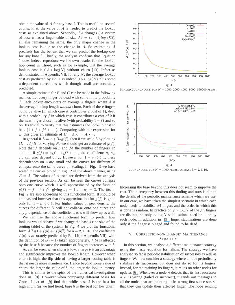
In general ifL = A+B∗g(f), then if we scaleL by plotting(L−A)/B for varyingN , we should get an estimate ofg(f).Note thatf depends onρ andM the number of fingers. Inaddition if g(f) = a1f + a2f

2 + · · · , the coefficientsa1,a2,etc can also depend onρ. However for1 − ρ << 1, thesedependences onρ are small and the curves for differentNcollapse onto the same curve on scaling. In Fig. 3 we havescaled the curves ploted in Fig. 2 in the above manner, usingB = A. The values ofA used are derived from the analysisof the previous section. As can be seen the curves collapseonto one curve which is well approximated by the functiong(f) = f + 3 ∗ f2, giving a1 = 1 and a2 = 3. The fits inFig 2 are also according to this functional form. It should beemphasized however that this approximation forg(f) is goodonly for 1 − ρ << 1. For higher values of peer density, thecurves for differentN will not collapse onto one curve andanyρ-dependence of the coefficientsai’s will show up as well.

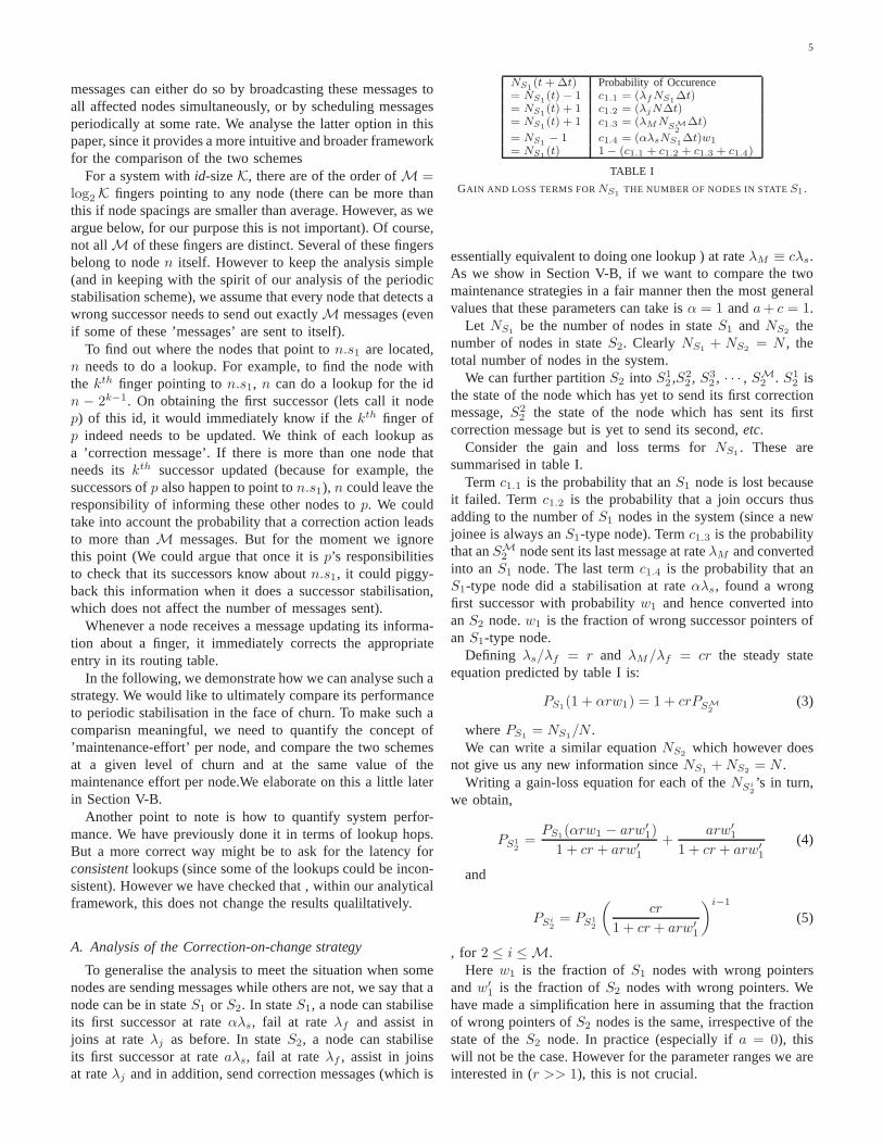
We can use the above functional form to predict howlookups would behave if we change the baseb (the size of therouting table) of the system. In Fig 4 we plot the functionalform A(b)(1+ f(b)+3f(b)2) for b = 2, 4, 16. The coefficientA(b) is accurately predicted by Eq. 11(in Appendix VII), withthe definition ofξ(i + 1) taken appropriately.f(b) is affectedby the baseb because the number of fingers increases withb.

As can be seen, when churn is low, a largeb is an advantageand significantly improves the lookup length. However whenchurn is high, the flip side of having a larger routing table isthat it needs more maintenance. Hence beyond some value ofchurn, the larger the value ofb, the larger the lookup latency.

This is similar to the spirit of the numerical investigationsdone in [9]. However when comparing different bases forChord, Li et al [9] find that while base2 is the best forhigh churn (as we find here), base8 is the best for low churn.

0

0.1

0.2

0.3

0.4

0.5

0.6

0.7

0.8

0.9

1

0 100 200 300 400 500 600 700 800 900 1000

(L((

1-β

)r)

-A )

/A

(1-β)r

N=1000N=2000N=4000N=8000

N=16000f(x)+3*f(x)

2

Fig. 3

SCALED LOOKUP COST, FORN = 1000, 2000, 4000, 8000, 160000 PEERS.

4

6

8

10

12

14

16

100 200 300 400 500 600 700 800 900 1000

L((

1-β

)r)=

A(b

)(1

+f+

3f2

) fo

r b

ase

b=

2,4

,16

(1-β)r

A(b)=5.846,b=2A(b)= 4.8832, b=4

A(b)= 3.6855, b=16

Fig. 4

LOOKUP COST, FORN = 1000 PEERS FOR BASEb = 2, 4, 16.

Increasing the base beyond this does not seem to improve thecost. The discrepancy between this finding and ours is due tothe details of the periodic maintenance scheme which we use.In our case, we have taken the simplest scenario in which eachnode needs to stabiliseM fingers and the order in which thisis done is random. In practice only∼ log N of theM fingersare distinct, so only∼ log N stabilisations need be done byeach node. In addition, in [9], finger stabilisations are doneonly if the finger is pinged and found to be dead.

V. ’C ORRECTION-ON-CHANGE’ M AINTENANCE

STRATEGY

In this section, we analyse a different maintenance strategyusing the master-equation formalism. The strategy we haveanalysed so far is periodic stabilisation of successors as well asfingers. We now consider a strategy where a node periodicallystabilises its successors but does not do so for its fingers.Instead, for maintaining its fingers, it relies on other nodes forupdates [6]. Whenever a noden detects that its first successorn.s1 is wrong (failed or incorrect), it sends out messages toall the nodes that are pointing to its wrong first successor, sothat they can update their affected finger. The node sending

5

messages can either do so by broadcasting these messages toall affected nodes simultaneously, or by scheduling messagesperiodically at some rate. We analyse the latter option in thispaper, since it provides a more intuitive and broader frameworkfor the comparison of the two schemes

For a system withid-sizeK, there are of the order ofM =log2 K fingers pointing to any node (there can be more thanthis if node spacings are smaller than average. However, as weargue below, for our purpose this is not important). Of course,not allM of these fingers are distinct. Several of these fingersbelong to noden itself. However to keep the analysis simple(and in keeping with the spirit of our analysis of the periodicstabilisation scheme), we assume that every node that detects awrong successor needs to send out exactlyM messages (evenif some of these ’messages’ are sent to itself).

To find out where the nodes that point ton.s1 are located,n needs to do a lookup. For example, to find the node withthe kth finger pointing ton.s1, n can do a lookup for the idn − 2k−1. On obtaining the first successor (lets call it nodep) of this id, it would immediately know if thekth finger ofp indeed needs to be updated. We think of each lookup asa ’correction message’. If there is more than one node thatneeds itskth successor updated (because for example, thesuccessors ofp also happen to point ton.s1), n could leave theresponsibility of informing these other nodes top. We couldtake into account the probability that a correction action leadsto more thanM messages. But for the moment we ignorethis point (We could argue that once it isp’s responsibilitiesto check that its successors know aboutn.s1, it could piggy-back this information when it does a successor stabilisation,which does not affect the number of messages sent).

Whenever a node receives a message updating its informa-tion about a finger, it immediately corrects the appropriateentry in its routing table.

In the following, we demonstrate how we can analyse such astrategy. We would like to ultimately compare its performanceto periodic stabilisation in the face of churn. To make such acomparisn meaningful, we need to quantify the concept of’maintenance-effort’ per node, and compare the two schemesat a given level of churn and at the same value of themaintenance effort per node.We elaborate on this a little laterin Section V-B.

Another point to note is how to quantify system perfor-mance. We have previously done it in terms of lookup hops.But a more correct way might be to ask for the latency forconsistentlookups (since some of the lookups could be incon-sistent). However we have checked that , within our analyticalframework, this does not change the results qualiltatively.

A. Analysis of the Correction-on-change strategy

To generalise the analysis to meet the situation when somenodes are sending messages while others are not, we say that anode can be in stateS1 or S2. In stateS1, a node can stabiliseits first successor at rateαλs, fail at rate λf and assist injoins at rateλj as before. In stateS2, a node can stabiliseits first successor at rateaλs, fail at rateλf , assist in joinsat rateλj and in addition, send correction messages (which is

NS1(t + ∆t) Probability of Occurence

= NS1(t) − 1 c1.1 = (λf NS1

∆t)= NS1

(t) + 1 c1.2 = (λjN∆t)= NS1

(t) + 1 c1.3 = (λM NSM2

∆t)

= NS1− 1 c1.4 = (αλsNS1

∆t)w1

= NS1(t) 1 − (c1.1 + c1.2 + c1.3 + c1.4)

TABLE I

GAIN AND LOSS TERMS FORNS1THE NUMBER OF NODES IN STATES1 .

essentially equivalent to doing one lookup ) at rateλM ≡ cλs.As we show in Section V-B, if we want to compare the twomaintenance strategies in a fair manner then the most generalvalues that these parameters can take isα = 1 anda + c = 1.

Let NS1be the number of nodes in stateS1 and NS2

thenumber of nodes in stateS2. Clearly NS1

+ NS2= N , the

total number of nodes in the system.We can further partitionS2 into S1

2 ,S22 , S3

2 , · · · , SM2 . S1

2 isthe state of the node which has yet to send its first correctionmessage,S2

2 the state of the node which has sent its firstcorrection message but is yet to send its second,etc.

Consider the gain and loss terms forNS1. These are

summarised in table I.Term c1.1 is the probability that anS1 node is lost because

it failed. Term c1.2 is the probability that a join occurs thusadding to the number ofS1 nodes in the system (since a newjoinee is always anS1-type node). Termc1.3 is the probabilitythat anSM

2 node sent its last message at rateλM and convertedinto anS1 node. The last termc1.4 is the probability that anS1-type node did a stabilisation at rateαλs, found a wrongfirst successor with probabilityw1 and hence converted intoanS2 node.w1 is the fraction of wrong successor pointers ofan S1-type node.

Defining λs/λf = r and λM/λf = cr the steady stateequation predicted by table I is:

PS1(1 + αrw1) = 1 + crPSM

2

(3)

wherePS1= NS1

/N .We can write a similar equationNS2

which however doesnot give us any new information sinceNS1

+ NS2= N .

Writing a gain-loss equation for each of theNSi2

’s in turn,we obtain,

PS1

2

=PS1

(αrw1 − arw′1)

1 + cr + arw′1

+arw′

1

1 + cr + arw′1

(4)

and

PSi2

= PS1

2

(

cr

1 + cr + arw′1

)i−1

(5)

, for 2 ≤ i ≤ M.Here w1 is the fraction ofS1 nodes with wrong pointers

and w′1 is the fraction ofS2 nodes with wrong pointers. We

have made a simplification here in assuming that the fractionof wrong pointers ofS2 nodes is the same, irrespective of thestate of theS2 node. In practice (especially ifa = 0), thiswill not be the case. However for the parameter ranges we areinterested in (r >> 1), this is not crucial.

6

TABLE II

GAIN AND LOSS TERMS FORWT : THE TOTAL NUMBER OF WRONG FIRST

SUCCESSOR POINTERS IN THE SYSTEM.

Change inWT Probability of OccurrenceWT (t + ∆t) = WT (t) + 1 c2.1 = (λjN∆t)(1 − w)WT (t + ∆t) = W1(t) + 1 c2.2 = (λf N∆t)(1 − w)2

WT (t + ∆t) = W1(t) − 1 c2.3 = (λf N∆t)W1(t + ∆t) = W1(t) − 1 c2.4 = (αλs∆t)NS1

w1 + (aλs∆t)NS2w′

1

W1(t + ∆t) = W1(t) 1 − (c2.1 + c2.2 + c2.3 + c2.4)

TABLE III

GAIN AND LOSS TERMS FORW ′1: THE NUMBER OF WRONG FIRST

SUCCESSOR POINTERS OFS2-TYPE NODES.

Change inW1 Probability of OccurrenceW ′

1(t + ∆t) = W ′

1(t) + 1 c2.1 = (λjNS2

∆t)(1 − w′1).

W ′1(t + ∆t) = W ′

1(t) + 1 c2.2 = λf NS2

(1 − w′1)2PS2

+(1 − w1)(1 − w′1)PS1

)∆t

W ′1(t + ∆t) = W ′

1(t) − 1 c2.3 = λf NS2

(w′1

2PS2

+ w1w′1PS1

)∆tW ′

1(t + ∆t) = W ′

1(t) − 1 c2.4 = aλsNS2

w′1∆t

W ′1(t + ∆t) = W ′

1(t) − 1 c2.5 = λM NM

S2w′

1∆t

W1(t + ∆t) = W1(t) 1 − (c2.1 + c2.2 + c2.3 + c2.4 + c2.5)

Clearly∑M

1 PSi2

= PS2. A quantity of interest in our

analysis is

PSM2

/PS2= 1 −

(1 − gM−11 )

1 − gM1(6)

whereg1 = cr(1+cr+arw′

1) .

To solve forPS1etc, we need to solve forw1 andw′

1.However, consider first the equation forWT – the total

number of wrong successor pointers in the system (irrespectiveof whether the pointer belongs to anS1 or anS2 type node.The gain and loss terms forWT are shown in table II.w = WT /N is the fraction of wrong succesor pointers inthe system.

This gives the following equation

(3 + αr)w1PS1+ (3 + ar)w′

1PS2= 2 (7)

The gain and loss termsW ′1. – the number ofS2 nodes with

wrong successor pointers – are written in much the same wayexcept for a few small changes. Table III details the changesthat occur inW ′

1. in time ∆t.The terms here are much the same as derived earlier except

that we now have to keep track of whether the node that isfailing (in terms c2.2 and c2.3) is a S1 or an S2-type node.In addition termc2.5 is the probability that anSM

2 -type nodehas a wrong successor pointer, but sends a message and henceturns into anS1 node with a wrong pointer.

Table III gives us the following equation forw′1 in the steady

state

2 = w′1

(

3 + ar + crPSM

2

PS2

)

+ (w1 − w′1)PS1

(8)

We can write a similar equation forw1 which howeverdoes not contain any new information sincew1 andw′

1 satisfyequation 7.

So in effect we have three equations, Eqn. 3, Eq. 7 and8 for three unknownsPS1

, w1 and w′1. In practice this set

TABLE IV

THE RELEVANT GAIN AND LOSS TERMS FORFk , THE NUMBER OF NODES

WHOSEkth FINGERS ARE POINTING TO A FAILED NODE FORk > 1.

Fk(t + ∆t) Probability of Occurence= Fk(t) + 1 c3.1 = (λjN∆t)

Pki=1

pjoin (i, k)fi

= Fk(t) − 1 c3.2 = fkP

k fk(λM NS2

(1 − w′1)A(w1, w′

1)∆t)

= Fk(t) + 1 c3.3 = (1 − fk)2[1 − p1(k)](λf N∆t)= Fk(t) + 2 c3.4 = (1 − fk)2(p1(k) − p2(k))(λf N∆t)= Fk(t) + 3 c3.5 = (1 − fk)2(p2(k) − p3(k))(λf N∆t)= Fk(t) 1 − (c3.1 + c3.2 + c3.3 + c3.4 + c3.5)

of equations is very hard to solve exactly because of theappearance of terms such asgM1 in Eq. 6.

In the following we will solve the set of equation toO(1/r)by expanding Eq. 6 to first order inw′

1. In this case,

PSM2

/PS2=

1

M−

(

M− 1

2M

)

1 + arw′1

cr(9)

We can now solve the set of three coupled equations toget a quartic equation forw′

1 as a function ofa, α,M andr. Only one of the roots of the quartic equation is a truesolution satisfying all the conditions above. The details of thecalculations though straight forward are tedious and not shownhere.

To calculate the cost of lookups, we still need to calculatethe probability that a finger is dead. The loss and gain termsfor this calculation are almost exactly the same as carried outearlier, in [7], [8] (except for termc3.2) and are shown in tableIV.

The term c3.2 is the probability that a message is sent(λMNS2

) times the probability that akth pointer gets thismessage (with probabilityfk/

∑

fk since only nodes withwrong pointers get the messages), times the probability thatthe message is not outdated (1−w′

1), times the probability thatthe predecessor of the node which has to receive the messagehas a correct successor pointer. This last quantity is denotedby A(w1, w

′1) = 1− (w1PS1

+ w′1PS2

), since the predecessorcould have been anS1 or anS2 type node.

An estimate for∑

fk is simply∼ MNS2/N . Substituting

this in termc3.2, this term becomes= λMN∆t(fk/M)(1 −w′

1)A(w1, w′1)

Solving for fk in the steady state, and substituting forw′1,

we get fk as a function of the parameters. As mentionedearlier a quick and precise estimate of the lookup length isthen obtained by takingL = A(1 + f + 3f2).

B. Comparison of Correction-on-change and Periodic Stabil-isation

In order to compare how the two strategies perform underchurn, we need to make sure that we are comparing lookuplatencies for the same number of total maintenance messagessent.

Let us assume that the maximum rate for sending messagesper node isC. In the case of periodic stabilisation, this impliesthat the rate of doing successor stabilisationsλs1

and fingerstabilisationsλs2

must in total not exceeedC. This impliesthat λs1

/C + λs2/C ≤ 1. If we assume that all nodes always

7

5

10

15

20

25

30

200 400 600 800 1000 1200 1400 1600 1800 2000

Look

up C

ost

r

periodic stabilisationreactive stabilisation (a=0,c=1)

Fig. 5

COMPARISON OF THELOOKUP COST FOR THE TWO MAINTENANCE

STRATEGIES, FORN = 1000.

send messages up to their maximum capacity, then clearlyλs1

/C + λs2/C = 1. Suppose we definer ≡ C/λj andr1 ≡

λs1/λj , r2 ≡ λs2

/λj . Then for a given value ofr, r1+r2 = r.Hence if finger stabilisations are done at rate(1 − β)r, thesuccessor stabilisations need to be done at rateβr, where theparameterβ can be varied from0 to 1.

In the case of correction-on-change, we need to impose thesame maximum rateC no matter which state the nodes arein. In this case, letλS1

be the rate of successor stabilisationin stateS1, λS2

the rate of successor stabilisation in stateS2

andλS3be the rate of sending messages in stateS2. Clearly

λS1= C and λS2

+ λS3= C. Defining r as before, we get

λs1/λj = r andλs2

/λj +λs3/λj = r. Hence comparing with

our parametersα = 1 anda + c = 1.In Fig. 5, we have plotted the functionL = A(1+f +3f2)

with the value of the lookup length without churnA = 5.846for N = 1000 nodes, fora = 0 (andc = 1) and forβ = 0.4.f is calculated separately for the two maintenance techniques.

As can be seen, correction-on-change is better than periodicstabilisation when churn is low but not when churn is high. Oncomparing lookup lengths for several differenta, it becomesevident (see yFig. 6) thata ∼ 0.2 is the optimum value forthe correction-on-change strategy.

So interestingly, for nodes in stateS2, it is not the beststrategy to increasec as much as possible. Its a better strategyto spend some of the bandwidth on maintaining a correctsuccessor.

VI. SUMMARY

In summary, we have demonstrated the usefulness of themaster-equation approach for understanding churn in overlaynetworks. Our analysis can take into account most details ofthe algorithms used by these networks, to provide predictionsfor how the performance depends on the parameters. There areseveral directions in which we can extend the present analysis.One of the more important ones is to model congestion on thelinks. This could affect the performance of the two comparedmaintenance strategies differently. The periodic case maynot

10

100 1000

Lo

ok

up

len

gth

r

a=0,c=1a=0.1,c=0.9a=0.2,c=0.8a=0.3,c=0.7a=0.4,c=0.6a=0.5,c=0.5a=0.6,c=0.4

Fig. 6

COMPARISON OF THELOOKUP COST FOR DIFFERENT VALUES OF THE

PARAMETERa, AS EXPLAINED IN THE TEXT.

be as affected as much as the reactive case, which could sufferfrom congestion collapse.

AcknowledgmentsWe would like to thank Ali Ghodsi forseveral very useful discussions.

REFERENCES

[1] Karl Aberer, P-Grid: A self-organizing access structure for p2p infor-mation systems, InProceedings of the Sixth International Conference onCooperative Information Systems (CoopIS 2001) (Trento, Italy), 2001.

[2] Karl Aberer, Anwitaman Datta, and Manfred Hauswirth,Efficient, self-contained handling of identity in peer-to-peer systems, IEEE Transac-tions on Knowledge and Data Engineering16 (2004), no. 7, 858–869.

[3] Luc Onana Alima, Sameh El-Ansary, Per Brand, and Seif Haridi,DKS(N; k; f): A Family of Low Communication, Scalable and Fault-Tolerant Infrastructures for P2P Applications, The 3rd InternationalWorkshop On Global and Peer-To-Peer Computing on Large ScaleDistributed Systems (CCGRID 2003) (Tokyo, Japan), May 2003.

[4] James Aspnes, Zoe Diamadi, and Gauri Shah,Fault-tolerant routing inpeer-to-peer systems, Proceedings of the twenty-first annual symposiumon Principles of distributed computing, ACM Press, 2002, pp. 223–232.

[5] Miguel Castro, Manuel Costa, and Antony Rowstron,Performance anddependability of structured peer-to-peer overlays, Proceedings of the2004 International Conference on Dependable Systems and Networks(DSN’04), IEEE Computer Society, 2004.

[6] Ali Ghodsi, Luc Onana Alima, and Seif Haridi,Low- bandwdithtopology maintenance for robustness in structured overlaynetworks,38th International HICSS Conference, Springer-Verlag, 2005.

[7] Supriya Krishnamurthy, Sameh El-Ansary, Erik Aurell, and Seif Haridi,A statistical theory of chord under churn, The 4th International Work-shop on Peer-to-Peer Systems (IPTPS’05) (Ithaca, New York), February2005.

[8] , An analytical study of a strutured overlay in the presence ofdynamic embership, IEEE Joint Transaction on Networking (2007).

[9] Jinyang Li, Jeremy Stribling, Thomer M. Gil, Robert Morris, andFrans Kaashoek,Comparing the performance of distributed hash tablesunder churn, The 3rd International Workshop on Peer-to-Peer Systems(IPTPS’02) (San Diego, CA), Feb 2004.

[10] Jinyang Li, Jeremy Stribling, Robert Morris, M. Frans Kaashoek, andThomer M. Gil, A performance vs. cost framework for evaluating dhtdesign tradeoffs under churn, Proceedings of the 24th Infocom (Miami,FL), March 2005.

[11] David Liben-Nowell, Hari Balakrishnan, and David Karger, Analysisof the evolution of peer-to-peer systems, ACM Conf. on Principles ofDistributed Computing (PODC) (Monterey, CA), July 2002.

[12] Sean Rhea, Dennis Geels, Timothy Roscoe, and John Kubiatowicz,Handling churn in a DHT, Proceedings of the 2004 USENIX AnnualTechnical Conference(USENIX ’04) (Boston, Massachusetts, USA),June 2004.

8

5.2

5.4

5.6

5.8

6

6.2

6.4

6.6

6.8

7

0.1 0.2 0.3 0.4 0.5 0.6 0.7 0.8 0.9 1

Look

up c

ost (

in h

ops)

1- ρ=N/K

L (without churn) - SimulationL (wihtout churn) - Theory

0.5 * log2(N)

Fig. 7

THEORY AND SIMULATION FOR THE LOOKUP COST WITHOUT CHURN FOR

A KEY SPACE OF SIZEK = 214 FOR VARYING N . PLOTTED AS REFERENCE

IS THE CURVE0.5 log2(N). NOTE THAT ON THE Y AXIS WE HAVE

ACTUALLY PLOTTED L − 1 FOR CONVENIENCE.

[13] Ion Stoica, Robert Morris, David Liben-Nowell, David Karger, M. FransKaashoek, Frank Dabek, and Hari Balakrishnan,Chord: A scalable peer-to-peer lookup service for internet applications, IEEE Transactions onNetworking 11 (2003).

VII. A PPENDIX

Equation 1 with the churn-dependent terms set to zerobecomes:

Cξ+m = Cξ [1 − a(m)] + a(m) +

m−1∑

i=0

b(i)Cm−i (10)

After some rewriting of this, it is easily seen that the costfor any key i + 1 can be written as the following recursionrelation:

Ci+1 = ρCi + (1 − ρ) + (1 − ρ)Ci+1−ξ(i+1) (11)

Here we have used the definition ofa and b from theinternode-interval distribution and the notationξ(i + 1) refersto the start of the finger most closely precedingi + 1. Forinstance, fori + 1 = 4, ξ(i + 1) = 2 and for i + 1 = 11,ξ(i + 1) = 8 etc.

We are interested in solving the recursion relation andcomputingL = 1

K

∑K−1i=1 Ci. To do this, we decompose this

sum into the following partial sums:

s0 = C1 = 1

s1 = C2

s2 = C3 + C4

s3 = C5 + C6 + C7 + C8

. . .

sM = C2M−1+1 + . . . + CK−1

(12)

1

2

3

4

5

6

7

8

9

10

0 200000 400000 600000 800000 1e+006

Look

up c

ost (

in h

ops)

Distance i (in keys)

CiL = <Ci>

Fig. 8

THE AVERAGE COSTCi (THE NUMBER HOPS FOR LOOKING UP AN ITEMi

KEYS AWAY ) IN A NETWORK OFN = 1000 NODES ANDK = 220 KEYS

WITHOUT CHURN OBTAINED FROM THE RECURRENCE RELATION(11).

THE AVERAGE LOOKUP LENGTHL IS ALSO PLOTTED AS A REFERENCE.

Substituting the expressions for theC ’s in the above, we find:

s0 = 1

s1 =ρ

1 − ρ[C1 − C2] + 1 + s0

s2 =ρ

1 − ρ[C2 − C4] + 2 + [s0 + s1]

. . .

si =ρ

1 − ρ[C2i−1 − C2i ] + 2i−1 +

j−1∑

j=0

sj

(13)

By substituting serially the expressions forsj (where0 ≤ j ≤i − 1), the expression forsi (for i ≥ 2) becomes:

si =ρ

1 − ρ[2i−2C1 − C2i −

i−2∑

j=1

si−2−jC2j ]

+ 2i + (i − 1)2i−2

(14)

HenceM∑

i=0

si = −ρ + [2M+1 − 1] + M2M−1 − [2M − 1]

+ρ

1 − ρ

[

(2M−1 − 1)C1 −

M−1∑

i=2

C2i − CK−1

− (2M−2 − 1)C2 − (2M−3 − 1)C4 − . . .

]

(15)

ThereforeM∑

i=0

si = −ρ + 2M + M2M−1

+ρ

1 − ρ

[

(2M−1 − 1)C1 −

M−1∑

i=2

C2i − CK−1

−

M−2∑

j=2

(2M−j − 1)C2j−1

]

(16)

9

The equation for the average lookup length without churn isthus,

L =

∑

s

K

= −ρ

K+ 1 +

1

2M

+ρ

1 − ρ

[

2M−1 − 1

KC1 −

1

K

M−1∑

i=2

C2i −1

KCK−1

−

M−2∑

j=2

2M−j − 1

KC2j−1

]

(17)

If we can take the limitK → ∞, we can throw away someof the terms.

limK→∞

L = 1 +1

2M

+ρ

1 − ρ

[

C1

2−

1

K

M−1∑

i=1

C2i +C2

K−

1

KCK−1

−

M−2∑

j=2

2M−j

KC2j−1 +

M−2∑

j=2

C2j−1

K

]

≈1 +1

2M +

ρ

1 − ρ

[

C1

2−

C2

4−

C4

8. . . −

C2M−3

2M−2

]

(18)

SinceC1 = 1, we can write

L = 1 +1

2M−

ρ

2(1 − ρ)

[

C2 − 1

2+

C4 − 1

4+ . . .

+C2M−3 − 1

2M−3

] (19)

From the recursion relation for theCi’s, it is easy to see that

(Ci − 1) = (1 − ρ)g(1)i (ρ) + (1 − ρ)2g

(2)i (ρ) + . . . (20)

where thegi’s are functions only ofρ.Hence if (1 − ρ) is small (N

K→ 0), we need only compute

theCi’s to first order in (1− ρ) to get the leading order effectand second order in (1 − ρ) to get the correction etc.

Hence in general the, the expression forL is:

L = 1 +1

2M−

ρ

2

[

e1(ρ) + (1 − ρ)e2(ρ) + (1 − ρ)2e3(ρ) . . .

]

(21)

Wheree1(ρ) =∑M−3

i=1 g(1)2i (ρ) etc.

We evaluate this expression numerically by solving recur-sion relation (11) and compare it with simulations done at zerochurn. As can be seen the prediction of the equation is veryaccurate (Figure 7).

Let us now computee1(ρ) to see what the leading ordereffect is. We now need to solve recursion relation (11) onlyto order1 − ρ, which gives:

C2 − 1 = (1 − ρ)

C4 − 1 = (1 − ρ)[

1 + ρ + ρ2]

C8 − 1 = (1 − ρ)[

1 + ρ + ρ2 + · · · + ρ6]

. . .

Ci − 1 = (1 − ρ)[

1 + ρ + ρ2 + · · · + ρi−2]

(22)

Therefore,

L = 1 +1

2M +

ρ

2

[

1

2+

1 + ρ + ρ2

4+ . . .

]

(23)

Consider the expression inside the brackets. We are computingthis in the approximationN

K= ǫ → 0, i.e.ρ = 1− ǫ, therefore

ρx = (1 − ǫ)x ≈ e−ǫx. If x > 1ǫ , thenρx → 0, therefore if

x > K

N , thenρx → 0. Hence, the terms inside the bracketsbecome:

T∑

j=1

2j − 1

2j+ (2T − 1)

M−3∑

j=T+1

1

2j (24)

WhereT ≡ ln2 K− ln2 N and we have putρx ≈ 1 for x < K

Nandρ → 0 for x > K

N . This is clearly an overestimation andso we expect the result to over estimate the exact expression21.

Expression 24 becomes:

T −

[

1 − (1

2)M−3

]

+

[

1 − (1

2)M−3−T

]

≈ T

Therefore:

L = 1 +1

2ln2 K −

1

2[ln2 K− ln2 N ]

≈ 1 +1

2ln2 N

(25)

Which is the known result for the average lookup length ofChord.

Another important parameter in the performance of DHTsin general is the base. By increasing the base, the number offingers per node increases which leads to a shorter lookup pathlength. The effect of varying the base has been studied in [3],[10]. So far, we have considered in this analysis base-2 Chord.We can likewise carry out this analysis for any base.

In general, we have base-b with (b − 1)logb(K) fingers pernode. Consider as an exampleb = 4. Here we can define thethe partial sums again in the following manner:

∆0 = s0 = C1 = 1

∆1 = s1 + s2 + s3

∆2 = s4 + s5 + s6

. . .

(26)

wheres1 = C2 = ρC1 + (1 − ρ) + (1 − ρ)C1

s2 = C3 = ρC2 + (1 − ρ) + (1 − ρ)C1

s3 = C4 = ρC3 + (1 − ρ) + (1 − ρ)C1

s4 = C5 + C6 + C7 + C8

s5 = C9 + C10 + C11 + C12

s6 = C13 + C14 + C15 + C16

. . .

(27)

Therefore∆0 = C1

∆1 = ρ [∆1 + C1 − C4] + 3(1 − ρ) + 3(1 − ρ) [∆0]

∆2 = ρ [∆2 + C4 − C16] + 12(1 − ρ) + 3(1 − ρ) [∆0 + ∆1]

. . .(28)

10

In general for a baseb, defineB ≡ b− 1 andbM = K. Thenwe have:

∆j =ρ

1 − ρ[Cbj−1 − Cbj ]

+B(B + 1)j−1 + B [∆0 + ∆1 + · · · + ∆j−1](29)

Following much the same procedure as before, we find

L =1

K

M∑

j=0

∆j

≈1 +B

B + 1M−

B

B + 1

ρ

1 − ρ

[

Cb − 1

B + 1+

Cb2 − 1

(B + 1)2+ . . .

]

(30)

for K → ∞ as the analogue of (19). Again we can simplifyand slightly overestimate the sum by assuming thatρx ≈ 0for x > K

N andρx ≈ 1 for x < K

N . Then we get:

L ≈ 1 +b − 1

b

ln2 N

ln2 b(31)

This is the analogue of Eq. 25 for any baseb.