Nonparametric Stein-type Shrinkage Covariance Matrix Estimators in

High-Dimensional Settings

Anestis TouloumisCancer Research UK Cambridge Institute

University of CambridgeCambridge CB2 0RE, U.K.

Anestis.Touloumis@cruk.cam.ac.uk

Abstract

Estimating a covariance matrix is an important task in applications where the number of vari-ables is larger than the number of observations. In the literature, shrinkage approaches for estimat-ing a high-dimensional covariance matrix are employed to circumvent the limitations of the samplecovariance matrix. A new family of nonparametric Stein-type shrinkage covariance estimators isproposed whose members are written as a convex linear combination of the sample covariance ma-trix and of a predefined invertible target matrix. Under the Frobenius norm criterion, the optimalshrinkage intensity that defines the best convex linear combination depends on the unobserved co-variance matrix and it must be estimated from the data. A simple but effective estimation processthat produces nonparametric and consistent estimators of the optimal shrinkage intensity for threepopular target matrices is introduced. In simulations, the proposed Stein-type shrinkage covari-ance matrix estimator based on a scaled identity matrix appeared to be up to 80% more efficientthan existing ones in extreme high-dimensional settings. A colon cancer dataset was analyzed todemonstrate the utility of the proposed estimators. A rule of thumb for adhoc selection among thethree commonly used target matrices is recommended.

Keywords— Covariance matrix, High-dimensional settings, Nonparametric estimation, Shrinkageestimation

1 Introduction

The problem of estimating large covariance matrices arises frequently in modern applications, such as ingenomics, cancer research, clinical trials, signal processing, financial mathematics, pattern recognitionand computational convex geometry. Formally, the goal is to estimate the covariance matrix Σ basedon a sample of N independent and identically distributed (i.i.d) p-variate random vectors X1, . . . ,XN

with mean vector µ in the “small N , large p” paradigm, that is when N is a lot smaller compared top. It is a well-known fact that the sample covariance matrix

S =1

N − 1

N∑i=1

(Xi − X)(Xi − X)T ,

where X =∑N

i=1 Xi/N is the sample mean vector, is not performing satisfactory in high-dimensionalsettings. For example, S is singular even when Σ is a strictly positive definite matrix. Recentresearch in estimating high-dimensional covariance matrices includes banding, tapering, penalizationand shrinkage methods. We focus on the Steinian shrinkage method (Stein, 1956) as adopted byLedoit and Wolf (2004) because it leads to covariance matrix estimators that are: (i) non-singular(ii) well-conditioned, (iii) invariant to permutations of the order of the p variables, (iv) consistent todepartures from a multivariate normal model, (v) not necessarily sparse, (vi) expressed in closed formand (vii) computationally cheap regardless of p.

Ledoit and Wolf (2004) proposed a Stein-type covariance matrix estimator for Σ based on

S? = (1− λ)S + λνIp, (1)

1

arX

iv:1

410.

4726

v2 [

stat

.ME

] 3

Nov

201

4

where Ip is the p × p identity matrix, and where λ and ν minimize the risk function E[||S? −Σ||2F

],

that is

λ =E[||S−Σ||2F

]E[||S− νIp||2F

]and

ν =tr(Σ)

p.

The optimal shrinkage intensity parameter λ in (1) suggests how much we must shrink the eigenvaluesof the sample covariance matrix S towards the eigenvalues of the target matrix νIp. For example, λ = 0implies no contribution of νIp to S?, while λ = 1 implies no contribution of S to S?. Intermediate valuesfor λ reveal the simultaneous contribution of S and νIp to S?. Despite the attractive interpretation, S?

is not a covariance matrix estimator because ν and λ depend on the unobservable covariance matrix Σ.For this reason, Ledoit and Wolf (2004) proposed to plug-in nonparametric N -consistent estimators forν and λ in (1) and use the resulting matrix as a shrinkage covariance matrix estimator for Σ. Althoughν seems to be adequately estimated by ν = tr(S)/p, we noticed via simulations that the estimatorof λ proposed by Ledoit and Wolf (2004) was biased in extreme high-dimensional settings and whenΣ = Ip. This is counter-intuitive because λ = 1 and the plug-in estimator of S? is expected to beas close as possible to the target matrix νIp. In addition, this observation underlines the importanceof choosing a target matrix that approximates well the true underlying dependence structure. Tothis direction, Fisher and Sun (2011) proposed Stein-type shrinkage covariance matrix estimators foralternative target matrices. However, they are no longer nonparametric as their construction wasbased on a multivariate normal model assumption.

Motivated by the above, we improve estimation of the optimal shrinkage intensity by providinga consistent estimator of λ in high-dimensional settings. To construct the estimator of λ we followthree simple steps: (i) expand the expectations in the numerator and denominator of λ assuming amultivariate normal model, (ii) prove that this ratio, say λ?, is asymptotically equivalent to λ, and(iii) replace each unknown parameter in λ? with unbiased and consistent estimators constructed usingU -statistics. The last step is essential in our proposal so as to ensure consistent and nonparametricestimation of λ. Further, we relax the normality assumption in Fisher and Sun (2011) for targetmatrices other than νIp in (1) and we illustrate how to estimate consistently the corresponding optimalshrinkage intensities in high-dimensional settings. In other words, we propose a new nonparametricfamily of Stein-type shrinkage estimators suitable for high-dimensional settings that preserve theattractive properties mentioned in the first paragraph and can accommodate arbitrary target matrices.

The rest of this paper is organized as follows. In Section 2, we present the working framework thatallows us to manage the high-dimensional setting. Section 3 contains the main results where we deriveconsistent and nonparametric estimators for the optimal shrinkage intensity of three different targetmatrices. We evaluate the performance of the proposed covariance matrix estimators via simulationsin Section 4. In Section 5, we illustrate the use of the proposed estimators in a colon cancer studyand we recommend a rule of thumb for selecting the target matrix. In Section 6, we summarize ourfindings and discuss future research. The technical details can be found in the appendix. Throughoutthe paper, we use ||A||2F = tr(ATA)/p to denote the scaled Frobenius norm of A, tr(A) to denote thetrace of the matrix A, DA to denote the diagonal matrix with elements the diagonal elements of A,and A ◦B to denote the Hadamard product of the matrices A and B, i.e., the matrix whose (a, b)-thelement is the product of the corresponding elements of A and B. In the above, it is implicit that Aand B are p× p matrices.

2 Framework for High-Dimensional Settings

Let X1, . . . ,XN be a sample of i.i.d. p-variate random vectors from the nonparametric model

Xi = Σ1/2Zi + µ, (2)

where µ = E[Xi] is the p-variate mean vector, Σ = cov[Xi] = Σ1/2Σ1/2 is the p×p covariance matrix,and Z1, . . . ,ZN is a collection of i.i.d. p-variate random vectors. Instead of distributional assumptions,

2

moments restrictions are imposed on the random variables in Zi. In particular, let Zia be the a-thrandom variable in Zi and suppose that E[Zia] = 0, E[Z2

ia] = 1, E[Z4ia] = 3 + B with −2 ≤ B < ∞

and for any nonnegative integers l1, . . . , l4 such that∑4

ν=1 lν ≤ 4

E[Z l1ia1Zl2ia2Z l3ia3Z

l4ia4

] = E[Z l1ia1 ]E[Z l2ia2 ]E[Z l2ia3 ]E[Z l4ia4 ], (3)

where the indexes a1, . . . , a4 are distinct. The nonparametric model (2) includes the p-variate normaldistribution Np(µ,Σ) as a special case obtained if Zia are i.i.d. N(0, 1) random variables. Since B = 0under a multivariate normal model, B can be interpreted as a measure of departure of the fourthmoment of Zia to that of a N(0, 1) random variable. The assumption of common fourth momentsis made for notational ease and the results of this paper remain valid even if E[Z4

ia] = 3 + Ba forfinite Ba (a = 1, . . . , p). Model (2) assumes that Xi is a linear combination of Zi, a random vectorthat contains standardized white noise variables. Unlike the usual definition of white noise, model (2)makes no distributional assumptions for Zi and it allows dependence patterns given that the pseudo-independence condition (3) holds. Therefore, the working framework can cover situations in which thewhite noise mechanism does not produce independent and/or identically distributed random variables.

To handle the high-dimensional setting, we restrict the dimension of Σ by assuming that

as N →∞, p = p(N)→∞, tr(Σ4)

tr2(Σ2)→ t1 and

tr(Σ2)

tr2(Σ)→ t2, (4)

with 0 ≤ t2 ≤ t1 ≤ 1. This flexible assumption does not specify the limiting behavior of p withrespect to N , thus including the case where p/N is bounded (Ledoit and Wolf, 2004). At the sametime, it does not seriously restrict the class of covariance matrices for Σ that satisfy assumption (4).For example, members of this class are covariance matrices whose eigenvalues are bounded awayfrom 0 and ∞ (Chen et al., 2010), banded first-order auto-regressive covariance matrices such thatΣ = {σaσbρ|a−b|I(|a − b| ≤ k)}1≤a,b≤p with −1 ≤ ρ ≤ 1, σa and σb bounded positive constants and1 ≤ k ≤ p (Chen et al., 2010), covariance matrices that have a few divergent eigenvalues as long as theydiverge slowly (Chen and Qin, 2010), and covariance matrices with a compound symmetry correlationpattern, that is Σ = {σaσbρ}1≤a,b≤p. Model (2) and assumption (4) constitute an attractive workingframework to handle the ‘small N , large p’ paradigm. A similar but stricter working framework wasconsidered by Chen et al. (2010) in the context of hypothesis testing for Σ. By contrast, we avoidmaking assumptions about moments of fifth or higher order and we allow more options for Σ.

3 Main Results

Under the nonparametric model (2), the expectations in the numerator and denominator of the optimalshrinkage intensity λ in (1) can be explicitly calculated to obtain that

λ =E[||S−Σ||2F

]E[||S− νI||2F

] =tr(Σ2) + tr2(Σ) +Btr(D2

Σ)

Ntr(Σ2) + p−N+1p tr2(Σ) +Btr(D2

Σ).

Since tr(D2A) = tr(A ◦A) ≤ tr(A2) ≤ tr2(A) for any positive definite matrix A, the contribution of

Btr(D2Σ) to λ under assumption (4) is negligible when compared to that of tr(Σ2) or tr2(Σ). Ignore

Btr(D2Σ) in λ and define

λ? =tr(Σ2) + tr2(Σ)

Ntr(Σ2) + p−N+1p tr2(Σ)

.

3

This is the optimal shrinkage intensity of the multivariate normal model or, more generally, λ = λ?

when B = 0 in the nonparametric model (2). Under assumption (4), it follows that

|λ− λ?| =(N − 1)

(tr(Σ2)− 1

ptr2(Σ))

N(

tr(Σ2)− 1ptr2(Σ)

)+ p+1

p tr2(Σ)

×|B|tr(D2

Σ)

N(

tr(Σ2)− 1ptr2(Σ)

)+ p+1

p tr2(Σ) +Btr(D2Σ)

≤|B| tr(D

2Σ)

tr2(Σ)

N(tr(Σ2)tr2(Σ)

− 1p

)+ p+1

p +Btr(D2

Σ)

tr2(Σ)

→ 0,

where |k| denotes the absolute value of the real number k. Therefore, the optimal shrinkage intensityobtained under normality is asymptotically equivalent to the optimal shrinkage intensity with respectto model (2) as long as the trace ratios restrictions in (4) hold. This means that it suffices to constructa nonparametric and consistent estimator of λ∗ to estimate λ. To accomplish this, replace the unknownparameters tr(Σ) and tr(Σ2) in λ? with the unbiased estimators

Y1N = U1N − U4N =1

N

N∑i=1

XTi Xi −

1

PN2

∗∑i 6=j

XTj Xi

and

Y2N = U2N − 2U5N + U6N

=1

PN2

∗∑i 6=j

(XTi Xj)

2 − 21

PN3

∗∑i 6=j 6=k

XTi XjX

Ti Xk +

1

PN4

∗∑i 6=j 6=k 6=l

XiXTj XkX

Tl

respectively, where P st = s!/(s− t)! and∑∗ denotes summation over mutually distinct indices. Note

that U1N and U2N are the unbiased estimators of tr(Σ) and tr(Σ2) respectively, when the data arecentered around the mean vector (i.e., µ = 0), while the remaining terms (U4,U5 and U6) are U -statistics of second, third and fourth order that ensure the unbiasedness of Y1N and Y2N when µ 6= 0.In B, we argue that Y1N and Y2N are ratio-consistent estimators to tr(Σ) and tr(Σ2) respectively.Here, it should be noted a statistic θ is called a ratio-consistent estimator to θ if θ/θ converges inprobability to one. Therefore, it follows from the continuous mapping theorem that

λ =Y2N + Y 2

1N

NY2N + p−N+1p Y 2

1N

is a consistent estimator of λ. The proposed Stein-type shrinkage estimator for Σ,

S? = (1− λ)S + λνIp,

is obtained by plugging-in ν = Y1N/p and λ in (1).

3.1 Alternative target matrices

Next, we consider target matrices other than νIp in (1). This extension is motivated by situations

where λ → 1 and νIp is not a good approximation of Σ. In this case, S? remains a well-defined andnon-singular covariance matrix estimator but it fails to reflect the underlying dependence structure.

Let T be a well-conditioned and non-singular target matrix, and define the matrix

S?T = (1− λT )S + λTT. (5)

4

Simple algebraic manipulation shows that the optimal shrinkage intensity

λT =E[||S−Σ||2F

]+ E [tr{(S−Σ)(Σ−T)}] /pE[||S−T||2F

] (6)

minimizes the expected risk function E[||S∗T − Σ||2F ]. A closed form solution for λT can be derivedby calculating the expectations in (6) with respect to model (2). The key idea of our proposal is tosimplify the estimation process for λT by identifying terms in the numerator and denominator of λTthat can be safely ignored under assumption (4). One approach is to examine whether the optimalshrinkage intensity under the multivariate normal model assumption is asymptotically equivalent toλT . Whenever this is the case, we can set B = 0 in λT and replace the remaining parameters withunbiased and ratio-consistent estimators to obtain λT . The proposed Stein-type shrinkage covariancematrix estimator is

S?T = (1− λT )S + λTT.

Note that if we set T = νIp then λT = λ and thus S?T = S?. We provide the estimator of λT for twotarget matrices: i) the identity matrix T = Ip, and ii) the diagonal matrix T = DS whose diagonalelements are the sample variances. To guarantee the consistency of λT , we suppose that t1 = t2 = 0in (4). This assumption does not heavily affects the class of Σ under consideration. In fact, all thedependence patterns mentioned in Section 2 satisfy this stronger version of assumption (4) except thecompound symmetry correlation matrix. We believe that this is a small price to pay if we are willingto increase the range of the target matrices in (1).

First, when T = Ip in (5) the optimal shrinkage intensity in (6) becomes

λI =tr(Σ2) + tr2(Σ) +Btr(D2

Σ)

tr(Σ2) + tr2(Σ) + (N − 1)tr [(Σ− Ip)2] +Btr(D2Σ).

As before, we can ignore the terms Btr(D2Σ) in λI and prove that

λI =Y2N + Y 2

1N

NY2N + Y 21N − (N − 1)(2Y1N − p)

is a consistent estimator of λI .When T = DS, we can use the results in A and prove that the optimal shrinkage intensity in (6)

is

λD =E[||S−Σ||2F

]+ E [tr{(S−Σ)(Σ−DS)}] /pE[||S−DS||2F

]=

(E[tr(S2)]− tr(Σ2)

)+ (E[tr(ΣDS)]− E[tr(SDS)])

E[tr(S2)]− E[tr(D2S)]

=

tr(Σ2) + tr2(Σ)− 2tr(D2Σ) +B

[tr(D2

Σ)−∑p

a=1

∑pb=1

(Σ1/2ab

)4]Ntr(Σ2) + tr2(Σ)− (N + 1)tr(D2

Σ) +B

[tr(D2

Σ)−∑p

a=1

∑pb=1

(Σ1/2ab

)4] ,

where Σ1/2ab denotes the (a, b)-th element of Σ1/2. It can be shown thatB

[tr(D2

Σ)−∑p

a=1

∑pb=1

(Σ1/2ab

)4]has negligible contribution to λD and that

Y3N = U3N − 2U7N + U8N

=1

PN2

∗∑i 6=j

tr(XiXTi ◦XjX

Tj )− 2

1

PN3

∗∑i 6=j 6=k

tr(XiXTi ◦XjX

Tk ) +

1

PN4

∗∑i 6=j 6=k 6=l

tr(XiXTj ◦XkX

Tl )

is an unbiased and ratio-consistent estimator to tr(D2Σ). The construction of Y3N is closely related to

that of Y1N and Y2N . To see this, note that Y3N is a linear combination of three U -statistics, U3N ,

5

the unbiased estimator of tr(D2Σ) when µ = 0, and U7N and U8N , which make the bias of Y3N zero

when µ 6= 0. Hence, a consistent estimator of λD is

λD =Y2N + Y 2

1N − 2Y3NNY2N + Y 2

1N − (N + 1)Y3N.

3.2 Remarks

There is no need to account for the mean vector when the random vectors are centered. In this case,the proposed shrinkage covariance matrix estimators can be obtained by replacing N−1 with N in theformula for λ, λI or λD, the sample covariance matrix S with

∑pi=1 XiX

Ti /N and the statistics Y1N ,

Y2N and Y3N with U1N , U2N and U3N respectively. The last modification is due to the fact that U1N ,U2N and U3N are unbiased and ratio-consistent estimators to the targeted parameters when µ = 0.

Fisher and Sun (2011) derived Stein-type shrinkage covariance matrix estimators for the three tar-get matrices considered herein under a multivariate normal model. We emphasize that our estimatorsdiffer in three important aspects. First, the consistency of the proposed estimators for the optimalshrinkage intensities λ, λI or λD is not sensitive to departures of the normality assumption. Second,tr(Σ2) and tr(DΣ) are estimated using U -statistics and are not based on the sample covariance matrixS as in Fisher and Sun (2011). Consequently, we avoid terms such as (XT

i Xi)2 or X4

ia, which allowsus to control their asymptotic variance. Third, the class of covariance matrices under considerationin Fisher and Sun (2011) is different. They require the first four arithmetic means of the eigenvaluesof Σ to converge while we place trace ratios restrictions on Σ.

3.3 Software implementation

The R (R Core Team, 2014) language package Shrinkcovmat implements the proposed Stein-typeshrinkage covariance estimators and it is available at http://cran.r-project.org/web/packages/ShrinkCovMat.The core functions shinkcovmat.equal, shinkcovmat.identity and shinkcovmat.unequal provide the pro-posed shrinkage covariance matrix estimators when T = νIp, T = Ip and T = DS respectively. Thestatistics Y1N , Y2N and Y3N are calculated using the computationally efficient formulas given in C.To modify the shrinkage estimators when µ = 0, one should set the argument centered=TRUE in thecore functions.

4 Simulations

We carried out a simulation study to investigate the performance of the proposed Stein-type covariancematrix estimators. The p-variate random vectors X1,. . .,XN were generated according to model (2),where we employed the following three distributional scenarios regarding Z1, . . . ,ZN :

1. A normality scenario, in which Ziai.i.d∼ N(0, 1).

2. A gamma scenario, in which Zia = (Z∗ia − 8)/4, Z∗iai.i.d∼ Gamma(4, 0.5) and thus B = 12.

3. A mixture of Scenarios 1 and 2, in which the first p/2 elements of Zi are distributed accordingto Scenario 1 and the remaining elements according to Scenario 2.

Scenarios 2 and 3 were used to empirically verify the nonparametric nature of the proposed method-ology. To mimic high-dimensional settings, we let N range from 10 to 100 with increments of 10 andwe let p = 100, 500, 1000, 1500 and 2500. The proposed family of covariance estimators was evaluatedusing S?, the proposed shrinkage covariance matrix estimator when T = νIp, which was then com-

pared to S?LW and S?FS , the corresponding shrinkage covariance matrix estimator proposed by Ledoitand Wolf (2004) and Fisher and Sun (2011) respectively. As in Ledoit and Wolf (2004), we assumedthat µ = 0 and we made the necessary adjustments to S? and S?FS . Since S?FS was constructed undera multivariate normal model assumption, its performance was evaluated only in sampling schemesthat involved Scenario 1. We excluded the shrinkage estimator of Schafer and Strimmer (2005) in

6

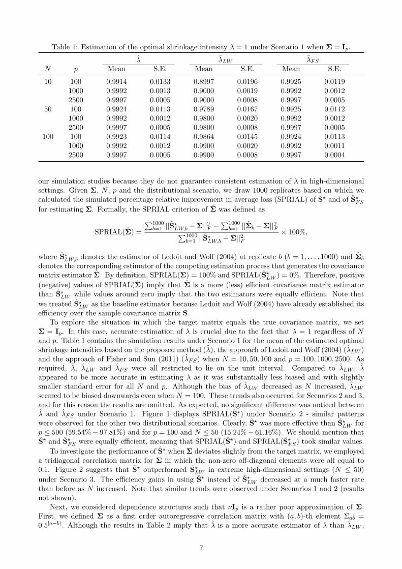
Table 1: Estimation of the optimal shrinkage intensity λ = 1 under Scenario 1 when Σ = Ip.

λ λLW λFSN p Mean S.E. Mean S.E. Mean S.E.

10 100 0.9914 0.0133 0.8997 0.0196 0.9925 0.01191000 0.9992 0.0013 0.9000 0.0019 0.9992 0.00122500 0.9997 0.0005 0.9000 0.0008 0.9997 0.0005

50 100 0.9924 0.0113 0.9789 0.0167 0.9925 0.01121000 0.9992 0.0012 0.9800 0.0020 0.9992 0.00122500 0.9997 0.0005 0.9800 0.0008 0.9997 0.0005

100 100 0.9923 0.0114 0.9864 0.0145 0.9924 0.01131000 0.9992 0.0012 0.9900 0.0020 0.9992 0.00112500 0.9997 0.0005 0.9900 0.0008 0.9997 0.0004

our simulation studies because they do not guarantee consistent estimation of λ in high-dimensionalsettings. Given Σ, N , p and the distributional scenario, we draw 1000 replicates based on which wecalculated the simulated percentage relative improvement in average loss (SPRIAL) of S? and of S?FSfor estimating Σ. Formally, the SPRIAL criterion of Σ was defined as

SPRIAL(Σ) =

∑1000b=1 ||S?LW,b −Σ||2F −

∑1000b=1 ||Σb −Σ||2F∑1000

b=1 ||S?LW,b −Σ||2F× 100%,

where S?LW,b denotes the estimator of Ledoit and Wolf (2004) at replicate b (b = 1, . . . , 1000) and Σb

denotes the corresponding estimator of the competing estimation process that generates the covariancematrix estimator Σ. By definition, SPRIAL(Σ) = 100% and SPRIAL(S?LW ) = 0%. Therefore, positive

(negative) values of SPRIAL(Σ) imply that Σ is a more (less) efficient covariance matrix estimatorthan S?LW while values around zero imply that the two estimators were equally efficient. Note that

we treated S?LW as the baseline estimator because Ledoit and Wolf (2004) have already established itsefficiency over the sample covariance matrix S.

To explore the situation in which the target matrix equals the true covariance matrix, we setΣ = Ip. In this case, accurate estimation of λ is crucial due to the fact that λ = 1 regardless of Nand p. Table 1 contains the simulation results under Scenario 1 for the mean of the estimated optimalshrinkage intensities based on the proposed method (λ), the approach of Ledoit and Wolf (2004) (λLW )and the approach of Fisher and Sun (2011) (λFS) when N = 10, 50, 100 and p = 100, 1000, 2500. Asrequired, λ, λLW and λFS were all restricted to lie on the unit interval. Compared to λLW , λappeared to be more accurate in estimating λ as it was substantially less biased and with slightlysmaller standard error for all N and p. Although the bias of λLW decreased as N increased, λLWseemed to be biased downwards even when N = 100. These trends also occurred for Scenarios 2 and 3,and for this reason the results are omitted. As expected, no significant difference was noticed betweenλ and λFS under Scenario 1. Figure 1 displays SPRIAL(S?) under Scenario 2 - similar patternswere observed for the other two distributional scenarios. Clearly, S? was more effective than S?LW forp ≤ 500 (59.54%− 97.81%) and for p = 100 and N ≤ 50 (15.24%− 61.16%). We should mention thatS? and S?FS were equally efficient, meaning that SPRIAL(S?) and SPRIAL(S?FS) took similar values.

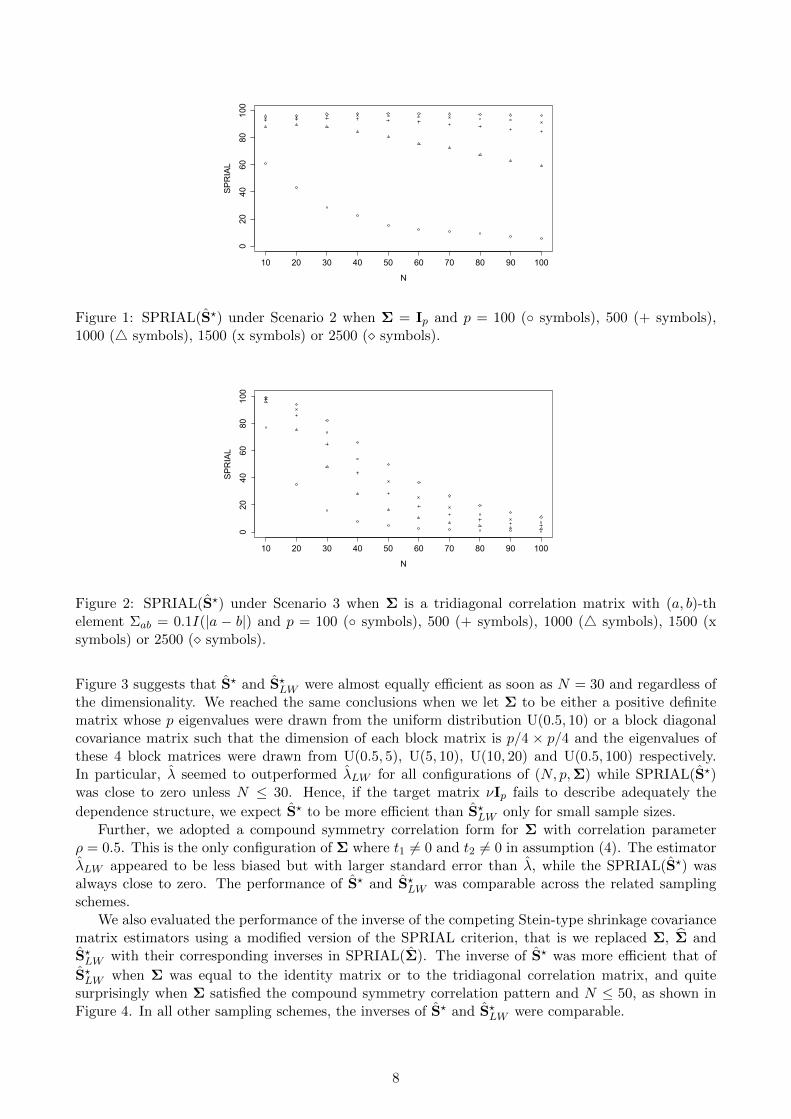
To investigate the performance of S? when Σ deviates slightly from the target matrix, we employeda tridiagonal correlation matrix for Σ in which the non-zero off-diagonal elements were all equal to0.1. Figure 2 suggests that S? outperformed S?LW in extreme high-dimensional settings (N ≤ 50)

under Scenario 3. The efficiency gains in using S? instead of S?LW decreased at a much faster ratethan before as N increased. Note that similar trends were observed under Scenarios 1 and 2 (resultsnot shown).

Next, we considered dependence structures such that νIp is a rather poor approximation of Σ.First, we defined Σ as a first order autoregressive correlation matrix with (a, b)-th element Σab =0.5|a−b|. Although the results in Table 2 imply that λ is a more accurate estimator of λ than λLW ,

7

20 40 60 80 100

020

4060

80100

N

SPRIAL

10 30 50 70 90

Figure 1: SPRIAL(S?) under Scenario 2 when Σ = Ip and p = 100 (◦ symbols), 500 (+ symbols),1000 (4 symbols), 1500 (x symbols) or 2500 (� symbols).

20 40 60 80 100

020

4060

80100

N

SPRIAL

10 30 50 70 90

Figure 2: SPRIAL(S?) under Scenario 3 when Σ is a tridiagonal correlation matrix with (a, b)-thelement Σab = 0.1I(|a − b|) and p = 100 (◦ symbols), 500 (+ symbols), 1000 (4 symbols), 1500 (xsymbols) or 2500 (� symbols).

Figure 3 suggests that S? and S?LW were almost equally efficient as soon as N = 30 and regardless ofthe dimensionality. We reached the same conclusions when we let Σ to be either a positive definitematrix whose p eigenvalues were drawn from the uniform distribution U(0.5, 10) or a block diagonalcovariance matrix such that the dimension of each block matrix is p/4 × p/4 and the eigenvalues ofthese 4 block matrices were drawn from U(0.5, 5), U(5, 10), U(10, 20) and U(0.5, 100) respectively.In particular, λ seemed to outperformed λLW for all configurations of (N, p,Σ) while SPRIAL(S?)was close to zero unless N ≤ 30. Hence, if the target matrix νIp fails to describe adequately the

dependence structure, we expect S? to be more efficient than S?LW only for small sample sizes.Further, we adopted a compound symmetry correlation form for Σ with correlation parameter

ρ = 0.5. This is the only configuration of Σ where t1 6= 0 and t2 6= 0 in assumption (4). The estimatorλLW appeared to be less biased but with larger standard error than λ, while the SPRIAL(S?) wasalways close to zero. The performance of S? and S?LW was comparable across the related samplingschemes.

We also evaluated the performance of the inverse of the competing Stein-type shrinkage covariancematrix estimators using a modified version of the SPRIAL criterion, that is we replaced Σ, Σ andS?LW with their corresponding inverses in SPRIAL(Σ). The inverse of S? was more efficient that of

S?LW when Σ was equal to the identity matrix or to the tridiagonal correlation matrix, and quitesurprisingly when Σ satisfied the compound symmetry correlation pattern and N ≤ 50, as shown inFigure 4. In all other sampling schemes, the inverses of S? and S?LW were comparable.

8

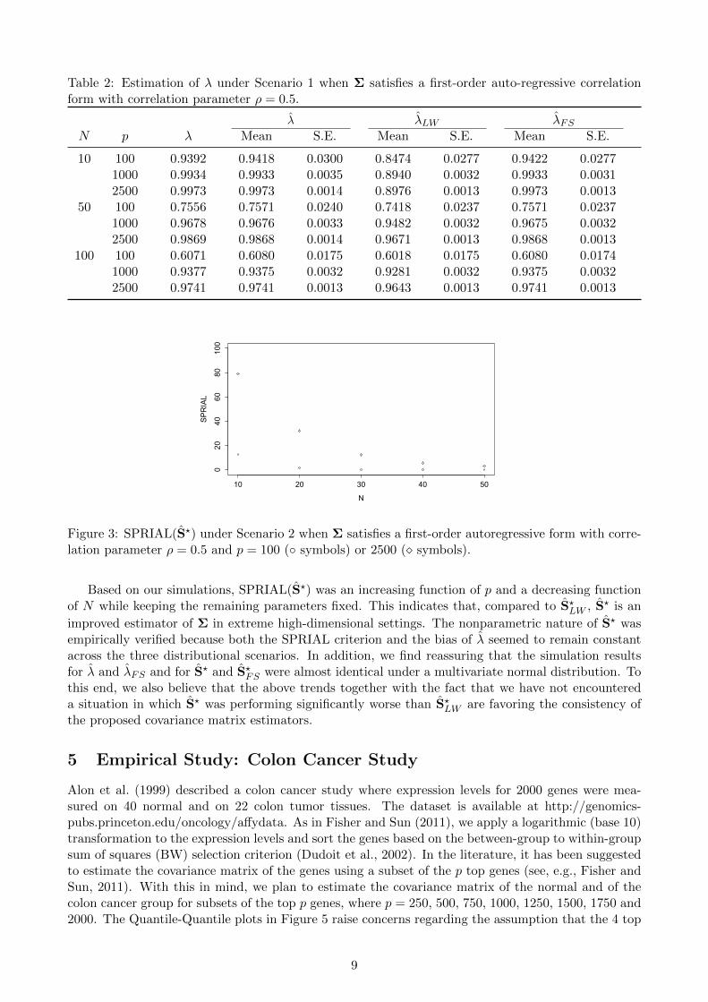
Table 2: Estimation of λ under Scenario 1 when Σ satisfies a first-order auto-regressive correlationform with correlation parameter ρ = 0.5.

λ λLW λFSN p λ Mean S.E. Mean S.E. Mean S.E.

10 100 0.9392 0.9418 0.0300 0.8474 0.0277 0.9422 0.02771000 0.9934 0.9933 0.0035 0.8940 0.0032 0.9933 0.00312500 0.9973 0.9973 0.0014 0.8976 0.0013 0.9973 0.0013

50 100 0.7556 0.7571 0.0240 0.7418 0.0237 0.7571 0.02371000 0.9678 0.9676 0.0033 0.9482 0.0032 0.9675 0.00322500 0.9869 0.9868 0.0014 0.9671 0.0013 0.9868 0.0013

100 100 0.6071 0.6080 0.0175 0.6018 0.0175 0.6080 0.01741000 0.9377 0.9375 0.0032 0.9281 0.0032 0.9375 0.00322500 0.9741 0.9741 0.0013 0.9643 0.0013 0.9741 0.0013

10 20 30 40 50

020

4060

80100

N

SPRIAL

Figure 3: SPRIAL(S?) under Scenario 2 when Σ satisfies a first-order autoregressive form with corre-lation parameter ρ = 0.5 and p = 100 (◦ symbols) or 2500 (� symbols).

Based on our simulations, SPRIAL(S?) was an increasing function of p and a decreasing functionof N while keeping the remaining parameters fixed. This indicates that, compared to S?LW , S? is an

improved estimator of Σ in extreme high-dimensional settings. The nonparametric nature of S? wasempirically verified because both the SPRIAL criterion and the bias of λ seemed to remain constantacross the three distributional scenarios. In addition, we find reassuring that the simulation resultsfor λ and λFS and for S? and S?FS were almost identical under a multivariate normal distribution. Tothis end, we also believe that the above trends together with the fact that we have not encountereda situation in which S? was performing significantly worse than S?LW are favoring the consistency ofthe proposed covariance matrix estimators.

5 Empirical Study: Colon Cancer Study

Alon et al. (1999) described a colon cancer study where expression levels for 2000 genes were mea-sured on 40 normal and on 22 colon tumor tissues. The dataset is available at http://genomics-pubs.princeton.edu/oncology/affydata. As in Fisher and Sun (2011), we apply a logarithmic (base 10)transformation to the expression levels and sort the genes based on the between-group to within-groupsum of squares (BW) selection criterion (Dudoit et al., 2002). In the literature, it has been suggestedto estimate the covariance matrix of the genes using a subset of the p top genes (see, e.g., Fisher andSun, 2011). With this in mind, we plan to estimate the covariance matrix of the normal and of thecolon cancer group for subsets of the top p genes, where p = 250, 500, 750, 1000, 1250, 1500, 1750 and2000. The Quantile-Quantile plots in Figure 5 raise concerns regarding the assumption that the 4 top

9

020

4060

80100

N

SPRIAL

10 20 30 40 50

Figure 4: SPRIAL criterion for the inverse of S? under Scenario 3 when Σ satisfies a compoundsymmetry correlation matrix and p = 100 (◦ symbols) or 2500 (� symbols).

−2 0 1 2

1.8

2.2

2.6

3.0

−2 0 1 2

2.0

2.4

2.8

3.2

−2 0 1 2

2.0

2.5

3.0

−2 0 1 2

1.4

1.8

2.2

2.6

−2 −1 0 1 2

2.2

2.6

3.0

−2 −1 0 1 2

2.5

3.0

3.5

−2 −1 0 1 2

1.0

1.5

2.0

2.5

−2 −1 0 1 2

1.0

1.4

1.8

Figure 5: Quantile-Quantile plots for the expression levels of the 4 top genes according to the BWselection criterion. The top panel corresponds to the normal group and the bottom panel to the coloncancer group.

genes are marginally normally distributed. Since similar patterns occur for the remaining genes, weconclude that a multivariate normal model is not likely to hold and nonparametric covariance matrixestimation is required. For this purpose, we calculate S?, S?I and S?D for both groups and for all valuesof p.

The optimal shrinkage intensity λT in (5) is informative for the suitability of the selected targetmatrix T because it reveals its contribution to S?T . If λ, λI and λD differ significantly, then itis meaningful to choose the target matrix with the largest estimated optimal shrinkage intensity.Otherwise, the selection of the target matrix can be based on ν and r, the range of the p samplevariances. In particular, we suggest to employ Ip when ν is close to 1.00, DS when r is large (saymore than one unit so as to account for the sampling variability), and νIp when neither of these seemsplausible. Table 3 displays the estimated optimal shrinkage intensities for the proposed family ofshrinkage covariance estimators, ν and r in both groups. The estimates of λ and λD are very similarin both groups for all subsets of genes and larger than those of λI . This suggests that DS and νIp arebetter options than Ip as a target matrix. Since r appears to be relatively small and constant acrossthe top p genes in both groups, it seems sensible to set T = νIp for all p. Therefore, we recommend

using S? to estimate the covariance matrix of the genes in the normal and in the colon cancer groupand regardless of p.

10

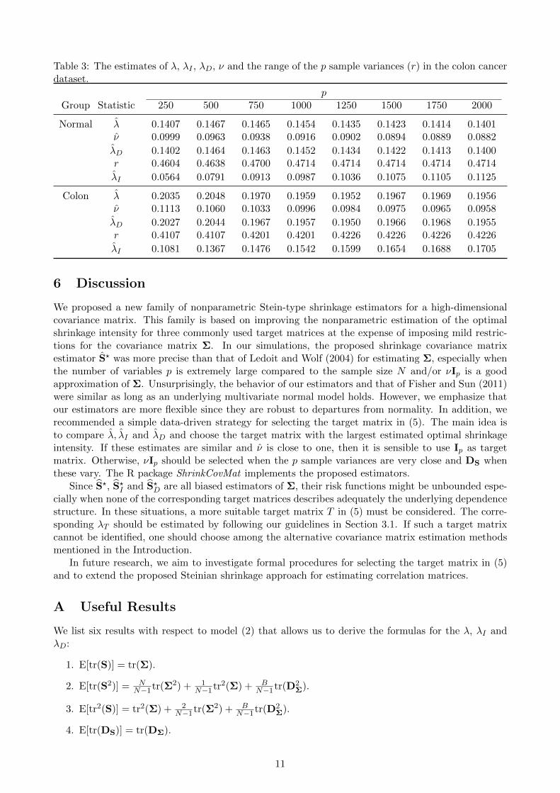
Table 3: The estimates of λ, λI , λD, ν and the range of the p sample variances (r) in the colon cancerdataset.

pGroup Statistic 250 500 750 1000 1250 1500 1750 2000

Normal λ 0.1407 0.1467 0.1465 0.1454 0.1435 0.1423 0.1414 0.1401ν 0.0999 0.0963 0.0938 0.0916 0.0902 0.0894 0.0889 0.0882

λD 0.1402 0.1464 0.1463 0.1452 0.1434 0.1422 0.1413 0.1400r 0.4604 0.4638 0.4700 0.4714 0.4714 0.4714 0.4714 0.4714

λI 0.0564 0.0791 0.0913 0.0987 0.1036 0.1075 0.1105 0.1125

Colon λ 0.2035 0.2048 0.1970 0.1959 0.1952 0.1967 0.1969 0.1956ν 0.1113 0.1060 0.1033 0.0996 0.0984 0.0975 0.0965 0.0958

λD 0.2027 0.2044 0.1967 0.1957 0.1950 0.1966 0.1968 0.1955r 0.4107 0.4107 0.4201 0.4201 0.4226 0.4226 0.4226 0.4226

λI 0.1081 0.1367 0.1476 0.1542 0.1599 0.1654 0.1688 0.1705

6 Discussion

We proposed a new family of nonparametric Stein-type shrinkage estimators for a high-dimensionalcovariance matrix. This family is based on improving the nonparametric estimation of the optimalshrinkage intensity for three commonly used target matrices at the expense of imposing mild restric-tions for the covariance matrix Σ. In our simulations, the proposed shrinkage covariance matrixestimator S? was more precise than that of Ledoit and Wolf (2004) for estimating Σ, especially whenthe number of variables p is extremely large compared to the sample size N and/or νIp is a goodapproximation of Σ. Unsurprisingly, the behavior of our estimators and that of Fisher and Sun (2011)were similar as long as an underlying multivariate normal model holds. However, we emphasize thatour estimators are more flexible since they are robust to departures from normality. In addition, werecommended a simple data-driven strategy for selecting the target matrix in (5). The main idea isto compare λ, λI and λD and choose the target matrix with the largest estimated optimal shrinkageintensity. If these estimates are similar and ν is close to one, then it is sensible to use Ip as targetmatrix. Otherwise, νIp should be selected when the p sample variances are very close and DS whenthese vary. The R package ShrinkCovMat implements the proposed estimators.

Since S?, S?I and S?D are all biased estimators of Σ, their risk functions might be unbounded espe-cially when none of the corresponding target matrices describes adequately the underlying dependencestructure. In these situations, a more suitable target matrix T in (5) must be considered. The corre-sponding λT should be estimated by following our guidelines in Section 3.1. If such a target matrixcannot be identified, one should choose among the alternative covariance matrix estimation methodsmentioned in the Introduction.

In future research, we aim to investigate formal procedures for selecting the target matrix in (5)and to extend the proposed Steinian shrinkage approach for estimating correlation matrices.

A Useful Results

We list six results with respect to model (2) that allows us to derive the formulas for the λ, λI andλD:

1. E[tr(S)] = tr(Σ).

2. E[tr(S2)] = NN−1tr(Σ2) + 1

N−1tr2(Σ) + BN−1tr(D2

Σ).

3. E[tr2(S)] = tr2(Σ) + 2N−1tr(Σ2) + B

N−1tr(D2Σ).

4. E[tr(DS)] = tr(DΣ).

11

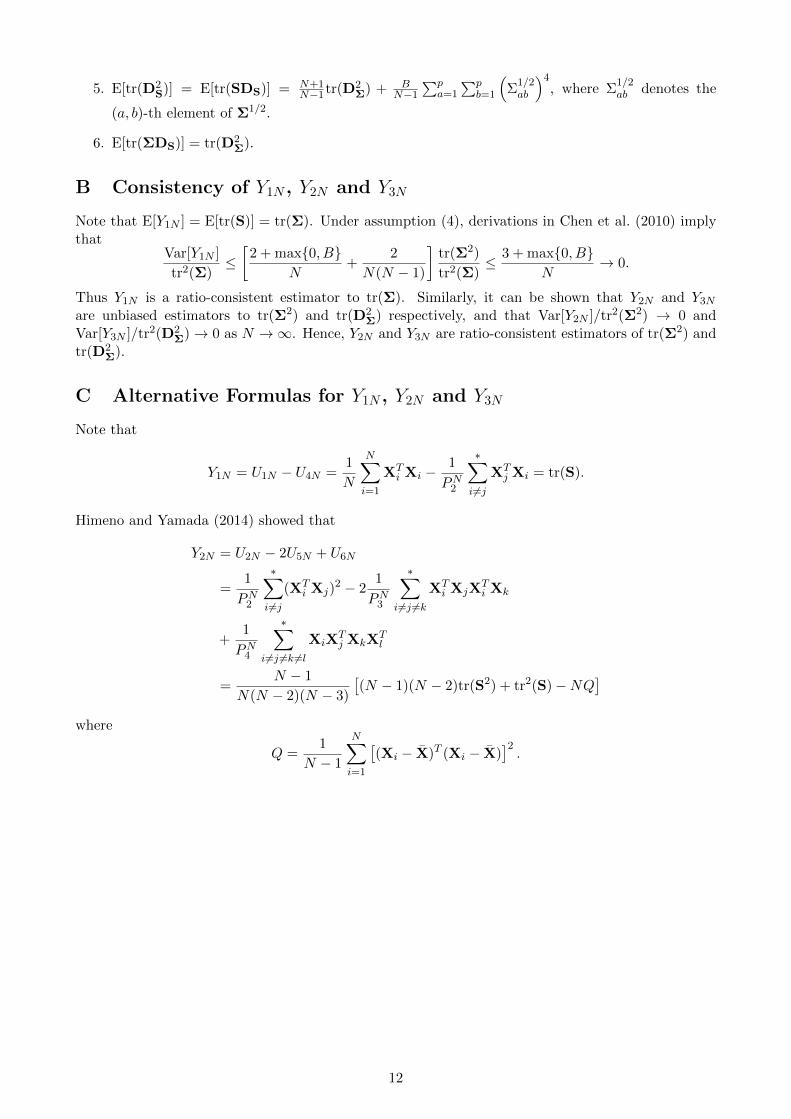
5. E[tr(D2S)] = E[tr(SDS)] = N+1

N−1tr(D2Σ) + B

N−1∑p

a=1

∑pb=1

(Σ1/2ab

)4, where Σ

1/2ab denotes the

(a, b)-th element of Σ1/2.

6. E[tr(ΣDS)] = tr(D2Σ).

B Consistency of Y1N , Y2N and Y3N

Note that E[Y1N ] = E[tr(S)] = tr(Σ). Under assumption (4), derivations in Chen et al. (2010) implythat

Var[Y1N ]

tr2(Σ)≤[

2 + max{0, B}N

+2

N(N − 1)

]tr(Σ2)

tr2(Σ)≤ 3 + max{0, B}

N→ 0.

Thus Y1N is a ratio-consistent estimator to tr(Σ). Similarly, it can be shown that Y2N and Y3Nare unbiased estimators to tr(Σ2) and tr(D2

Σ) respectively, and that Var[Y2N ]/tr2(Σ2) → 0 andVar[Y3N ]/tr2(D2

Σ)→ 0 as N →∞. Hence, Y2N and Y3N are ratio-consistent estimators of tr(Σ2) andtr(D2

Σ).

C Alternative Formulas for Y1N , Y2N and Y3N

Note that

Y1N = U1N − U4N =1

N

N∑i=1

XTi Xi −

1

PN2

∗∑i 6=j

XTj Xi = tr(S).

Himeno and Yamada (2014) showed that

Y2N = U2N − 2U5N + U6N

=1

PN2

∗∑i 6=j

(XTi Xj)

2 − 21

PN3

∗∑i 6=j 6=k

XTi XjX

Ti Xk

+1

PN4

∗∑i 6=j 6=k 6=l

XiXTj XkX

Tl

=N − 1

N(N − 2)(N − 3)

[(N − 1)(N − 2)tr(S2) + tr2(S)−NQ

]where

Q =1

N − 1

N∑i=1

[(Xi − X)T (Xi − X)

]2.

12

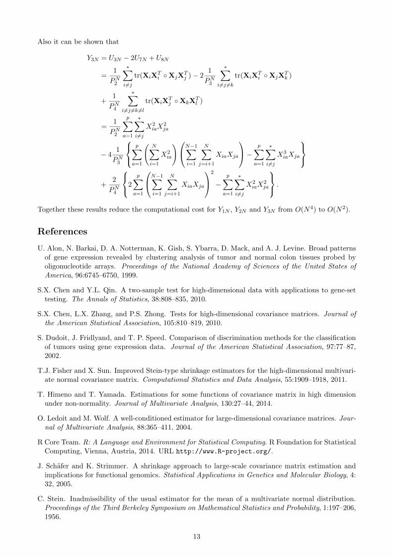
Also it can be shown that

Y3N = U3N − 2U7N + U8N

=1

PN2

∗∑i 6=j

tr(XiXTi ◦XjX

Tj )− 2

1

PN3

∗∑i 6=j 6=k

tr(XiXTi ◦XjX

Tk )

+1

PN4

∗∑i 6=j 6=k 6=l

tr(XiXTj ◦XkX

Tl )

=1

PN2

p∑a=1

∗∑i 6=j

X2iaX

2ja

− 41

PN3

p∑a=1

(N∑i=1

X2ia

)N−1∑i=1

N∑j=i+1

XiaXja

− p∑a=1

∗∑i 6=j

X3iaXja

+

2

PN4

2

p∑a=1

N−1∑i=1

N∑j=i+1

XiaXja

2

−p∑a=1

∗∑i 6=j

X2iaX

2ja

.

Together these results reduce the computational cost for Y1N , Y2N and Y3N from O(N4) to O(N2).

References

U. Alon, N. Barkai, D. A. Notterman, K. Gish, S. Ybarra, D. Mack, and A. J. Levine. Broad patternsof gene expression revealed by clustering analysis of tumor and normal colon tissues probed byoligonucleotide arrays. Proceedings of the National Academy of Sciences of the United States ofAmerica, 96:6745–6750, 1999.

S.X. Chen and Y.L. Qin. A two-sample test for high-dimensional data with applications to gene-settesting. The Annals of Statistics, 38:808–835, 2010.

S.X. Chen, L.X. Zhang, and P.S. Zhong. Tests for high-dimensional covariance matrices. Journal ofthe American Statistical Association, 105:810–819, 2010.

S. Dudoit, J. Fridlyand, and T. P. Speed. Comparison of discrimination methods for the classificationof tumors using gene expression data. Journal of the American Statistical Association, 97:77–87,2002.

T.J. Fisher and X. Sun. Improved Stein-type shrinkage estimators for the high-dimensional multivari-ate normal covariance matrix. Computational Statistics and Data Analysis, 55:1909–1918, 2011.

T. Himeno and T. Yamada. Estimations for some functions of covariance matrix in high dimensionunder non-normality. Journal of Multivariate Analysis, 130:27–44, 2014.

O. Ledoit and M. Wolf. A well-conditioned estimator for large-dimensional covariance matrices. Jour-nal of Multivariate Analysis, 88:365–411, 2004.

R Core Team. R: A Language and Environment for Statistical Computing. R Foundation for StatisticalComputing, Vienna, Austria, 2014. URL http://www.R-project.org/.

J. Schafer and K. Strimmer. A shrinkage approach to large-scale covariance matrix estimation andimplications for functional genomics. Statistical Applications in Genetics and Molecular Biology, 4:32, 2005.

C. Stein. Inadmissibility of the usual estimator for the mean of a multivariate normal distribution.Proceedings of the Third Berkeley Symposium on Mathematical Statistics and Probability, 1:197–206,1956.

13