Hierarchical Shrinkage in Time-Varying Parameter Models

STRATHCLYDE

DISCUSSION PAPERS IN ECONOMICS

DEPARTMENT OF ECONOMICS UNIVERSITY OF STRATHCLYDE

GLASGOW

HIERARCHICAL SHRINKAGE IN TIME-VARYING

PARAMETER MODELS

BY

MIGUEL BELMONTE, GARY KOOP AND

DIMITRIS KOROBILIS

NO. 11-37

Hierarchical Shrinkage in Time-Varying Parameter

Models

Miguel A. G. Belmonte

University of Strathclyde

Gary Koop

University of Strathclyde

Dimitris Korobilis

Université Catholique de Louvain

June 22, 2011

Abstract

In this paper, we forecast EU-area inflation with many predictors using time-varying

parameter models. The facts that time-varying parameter models are parameter-rich

and the time span of our data is relatively short motivate a desire for shrinkage. In con-

stant coefficient regression models, the Bayesian Lasso is gaining increasing popularity

as an effective tool for achieving such shrinkage. In this paper, we develop econometric

methods for using the Bayesian Lasso with time-varying parameter models. Our ap-

proach allows for the coefficient on each predictor to be: i) time varying, ii) constant

over time or iii) shrunk to zero. The econometric methodology decides automatically

which category each coefficient belongs in. Our empirical results indicate the benefits

of such an approach.

Keywords: Forecasting; hierarchical prior; time-varying parameters; Bayesian Lasso

JEL Classification: C11, C52, E37, E47

1

1 Introduction

The goal of this paper is to forecast EU area inflation using many predictors. Our appli-

cation (and many similar applications in macroeconomics) has several characteristics that

require the development of statistical methods that depart from standard regression-based

methods. To explain these departures and motivate our statistical methods, we begin with a

generalized Phillips curve specification where inflation, πt, depends on lags of inflation and

other predictors (xt). In this case, the generalized Phillips curve suitable for forecasting h

periods ahead (using the direct method of forecasting) is:

πt+h = α+

p−1∑

j=0

ϕjπt−j + γxt + εt+h. (1)

On its own, such a model may be inappropriate for a couple of reasons. First of all the

number of parameters to estimate may be large relative to the number of observations in

the data set. That is, xt may contain many predictors. In macroeconomic forecasting, we

typically having hundreds of variables to choose from. For instance, De Mol, Giannone

and Reichlin (2008) forecast with a regression involving over 100 variables. Banbura, Gi-

annone and Reichlin (2010) forecast using a vector autoregression (VAR) with over 100

variables. Estimation of such models, where the number of parameters is large relative

to the number of observations, can lead to imprecise estimation and over-fitting (i.e. the

model can fit the noise in the data, rather than finding the pattern useful for forecasting).

Both of these can lead to poor forecast performance. This has led many papers (including

De Mol, Giannone and Reichlin 2008, and Banbura, Giannone and Reichlin 2010) to use

Bayesian methods which use shrinkage to reduce over-fitting problems and improve fore-

cast performance. Closely related to the idea of shrinkage is the idea of variable selection

(which can be thought of as shrinking the coefficient on a predictor to zero). The challenge

faced by the researcher is often that there are many potential predictors, most are likely to

be unimportant but the researcher does not know, a priori, which ones are unimportant.

Sequential hypothesis testing procedures run into serious pre-testing problems, which has

2

led researchers to adopt various variable selection measures (see, e.g., George and McCul-

loch 1997 or Chipman, George and McCulloch, 2001). In the present paper, we draw on

one promising approach to shrinkage and variable selection, the Lasso1 (Park and Casella,

2008).

A second drawback of (1) is that it assumes parameters are constant over time. There is

a plethora of evidence of structural breaks and other kinds of parameter change in macro-

economic variables (see, among many others, Stock and Watson, 1996, Cogley and Sargent,

2001, 2005, Primiceri 2005, Sims and Zha, 2006, and D’Agostino, Gambetti and Giannone,

2009). The negative consequences for forecasting of ignoring such parameter change has

been stressed by, among many others, Clements and Hendry (1998, 1999) and Pesaran,

Pettenuzzo and Timmerman (2006). In this paper, we use a time-varying parameter (TVP)

regression model to model parameter change. Constant coefficient models such as (1) can

already be over-parameterized. Adding time variation in parameters may exacerbate this

problem, suggesting that shrinkage may be useful with TVP models. However, there have

been relatively few papers which attempt to ensure shrinkage in TVP models (exceptions

include Koop and Korobilis, 2009 and Koop, Leon-Gonzalez and Strachan, 2009).

The purpose of the present paper is to develop an econometric methodology which

surmounts these two drawbacks and use it to forecast EU inflation. In particular we develop

an econometric methodology which falls in the class of TVP regression models. However, it

uses Bayesian shrinkage methods (based on the Lasso) to automatically classify coefficients

into three categories: i) those which are time-varying, ii) those which are constant over

time and iii) those which are zero (and, thus, the associated predictor does not appear in

the model at all).

We extend ideas from the Bayesian Lasso literature (see Park and Casella, 2008) to the

case of TVP regression models. TVP regression models are state space models, in order to

extend Bayesian Lasso methods, we draw on and extend ideas relating to model selection

in state space models developed in Frühwirth-Schnatter and Wagner (2010). The paper is

1Lasso is an abbreviation for “least absolute shrinkage and selection operator”.

3

organized as follows: section 2 of the paper discusses our econometric methods. Section 3

uses these methods in an empirical exercise which forecasts EU inflation. We compare our

TVP regression methods, involving hierarchical shrinkage, to a range of other common fore-

cast procedures and find Lasso shrinkage to be particularly important on the time-varying

coefficients. Section 4 concludes.

2 Econometric Methods

2.1 Overview

The TVP version of the generalized Phillips curve given in (1) can be written as a state space

model:

πt+h = θ∗t zt + εt+h (2)

θ∗t = θ∗t−1 + ηt

where the variable of interest is h-step ahead inflation defined as πt+h = (log (Pt+h)− log (Pt)),

zt = [1,∆ log (Pt) , ..,∆ log (Pt−p+1) , xt], xt is a q × 1 vector of exogenous predictors, and

θ∗t =(α′t, ϕ

′

t,0, ..., ϕ′

t,p, γ′

t

)′.2 For the errors we assume εt ∼ N

(0, σ2t

)and ηt ∼ N (0,Ω).

The errors are assumed to be independent of each other and independent at all leads and

lags. Note that Ω is of dimension k × k with k = 1 + p + q which can be large relative

to the number of observations. To keep the model relatively parsimonious, we assume Ω

is a diagonal matrix, Ω = diag(ω21, ..., ω

2k

). It is through Ω that we introduce shrinkage

in the time-variation in coefficients (i.e. if ω2i is zero then the ith coefficient is constant

over time, but larger values of ω2i allow for more variation). Note that we are allowing for

heteroskedasticity in the measurement equation. In particular, we will assume a standard

stochastic volatility specification for σ2t .

2Note that, when forecasting with h = 12, this means our dependent variable is an annual inflation rate,but our explanatory variables are lags of monthly inflation. Such a timing convention has been found useful inmany recent forecasting papers such as Stock and Watson (2011).

4

It proves convenient to write (2) in an equivalent way, separating out the initial condi-

tion, as:

πt+h = θzt + θtzt + εt+h

θt = θt−1 + ηt (3)

θ0 = 0,

where θ = θ∗0 and θt = θ∗

t − θ. This is the well-known result that, in TVP regression models,

the initial condition for the states plays the role of a regression effect. Thus, (3) breaks the

coefficients into a constant part (i.e. θ) and a time-varying part.

In order to incorporate shrinkage priors, in the TVP regression, we use one more trans-

formation. We use notation where θi is the ith constant coefficient, θi,t is the i

th state and

adopt a similar subscript i, t notational convention with other variables and let θi,t =θi,tωi.

With these conventions, we can write the TVP regression model as:

πt+h =∑k

i=1θizi,t +

∑k

i=1ωiθi,tzi,t + εt+h

θi,t = θi,t−1 + ui,t (4)

θi,0 = 0

where ui,t ∼ N (0, 1) for i = 1, .., k. Fruhwirth-Schnatter and Wagner (2010) refer to this

as a non-centered parameterization in their analysis of the dynamic linear trend model and

argue for the advantages of this parameterization. Traditionally, Bayesian researchers have

used inverted Gamma priors on error variances in state equations such as ω2i . Fruhwirth-

Schnatter and Wagner (2010) argue (and present strong evidence) in favor of using a nor-

mal prior on ωi. In this paper, we follow this approach and use a hierarchical normal prior

for ωi motivated by the Bayesian Lasso of Park and Casella (2008). We will also adopt a

Lasso prior for θi (where θi for i = 1, .., k are the constant coefficients on the predictors).

We will explain these priors shortly, but note first that the Lasso provides shrinkage and, in

5

terms of (4), we will have a model with the properties:

1. If ωi is shrunk to 0, but θi is not shrunk to 0, then we have a model with a constant

parameter on predictor i.

2. If ωi is shrunk to 0, and θi is shrunk to 0, then predictor i is irrelevant for forecasting

inflation.

3. If ωi is not shrunk to 0, but θi is shrunk to 0, then we have a small time-varying

coefficient on predictor i (since θi,0 = 0 the coefficient is restricted to start at a value

of zero).

4. If ωi is not shrunk to 0, and θi is not shrunk to 0, then we have an unrestricted

time-varying coefficient on predictor i.

Thus, we have a methodology which decides, in an automatic fashion whether any

predictor is important for forecasting inflation and, if so, whether it has a coefficient which

is constant over time or time-varying.

2.2 The Prior

The model given by (4) is parameterized in terms of θ = (θ1, .., θk)′, θ =

(θ1,t, .., θk,t

)′

,

ω = (ω1, .., ωk)′ and σ2t . For σ

2t we adopt a standard stochastic volatility specification (see

the Technical Appendix for details). Our innovation lies in the use of Lasso-type shrinkage

priors for the remaining parameters. Such priors have been used with constant coefficient

regressions in many places. For instance, Park and Casella (2008) is an important statistical

exposition and De Mol, Giannone and Reichlin (2008) is an influential econometric treat-

ment. To explain the basic ideas underlying the Lasso, consider the familiar normal linear

regression model:

y = Xβ + ε,

6

whereX is a T ×k matrix of regressors, β = (β1, .., βk)′ and ε is N

(0, σ2I

). Lasso estimates

of β are penalized least squares estimates where β is chosen to minimize:

(y −Xβ)′ (y −Xβ) + λk∑

j=1

∣∣βj∣∣

where λ is a shrinkage parameter. Bayesian treatment of the Lasso arises by noting that

Lasso estimates of β are equivalent to Bayesian posterior modes if independent Laplace

priors are placed on the elements of β. Additional insight (and the MCMC algorithm used

for Bayesian analysis) is obtained by noting that the Laplace distribution can be written as

a scale mixture of normals with an exponential mixture density. Thus, Lasso shrinkage can

be obtained by using a normal hierarchical prior for β. In this section, we describe how to

extend this approach to our TVP regression model.

For the constant coefficients, θ, we use a hierarchical mixtures of normal prior inspired

by the traditional Lasso. In particular, θi for i = 1, .., k are assumed to be, a priori, indepen-

dent with

θi|τ2i ∼ N

(0, τ2i

)

and exponential mixing density:

τ2i |λ ∼ Exp

(λ2

2

).

This prior is almost the same as the traditional Lasso and has similar shrinkage properties.3

The state equation gives us a prior for θt (for t = 1, .., T ) of the form:

θt|θt−1 ∼ N(θt−1, Ik

)

where θ0 = 0.

3The one difference arises since the traditional Lasso has a prior variance of σ2τ2i instead of our τ2

i . Since weallow for stochastic volatility and, thus, σ2 is not constant over time, we cannot adopt the traditional approach.

7

We extend the Lasso approach to the time-varying coefficients by using a hierarchical

prior for ω, each element of which is, a priori, conditionally independent with:

ωi|ξ2i ∼ N

(0, ξ2i

),

also with exponential mixing density:

ξ2i |κ ∼ Exp

(κ2

2

).

Note that, following Fruhwirth-Schnatter and Wagner (2010), we have a normal prior

for ωi. However, the hierarchical nature of the prior gives us the Lasso-type shrinkage of

the elements of ω (thus, ensuring shrinkage on the time-varying coefficients).

The shrinkage parameters λ and κ lie at the bottom of the hierarchy and require priors

of their own. For these we assume:

λ2 ∼ Gamma (a1, a2)

and

κ2 ∼ Gamma (b1, b2) .

Note that the only prior hyperparameters which must be elicited are a1, a2, b1, b2 and the

priors for the parameters in the stochastic volatility specification for σt.4 The Technical

Appendix discusses their elicitation.

2.3 Posterior Computation (MCMC algorithm)

In the constant coefficient regression model, an advantage of the Lasso prior is that, con-

ditional on τ2i , we have a normal linear regression model with normal prior and standard

textbook results can be used to derive the posterior, conditional on τ2i . An algorithm for

4The formulae in this paper parameterize the Gamma distribution so that its mean is a1a2.

8

drawing τ2i and λ is all that is required to complete an MCMC algorithm and this is pro-

vided by Park and Casella (2008). Our MCMC algorithm draws on this strategy to provide

blocks for drawing θ, τ2i and λ (conditional on the states and the other parameters in the

model).

Similar intuition can be used to develop an algorithm for drawing θt (for t = 1, .., T )

conditional on ω (and other parameters). That is, conditional on these other parameters,

the model becomes a normal linear state space model and standard methods for posterior

simulation from such models can be used to draw θt. We use the algorithm of Carter and

Kohn (1994). All that is required to complete an MCMC algorithm is a method for drawing

ω and κ (conditional on all the other model parameters). However, these have simple forms.

The precise steps in our MCMC algorithm are given by.

1. Draw θ from the normal conditional posterior:

N((z′z + V −1θ

)−1z′y,

(z′z + V −1θ

)−1)

where V −1θ =[diag

(τ21, ..., τ

2k

)]−1,z =

[z1σ1, ..., zT

σT

]′

, y = [y1, ..., yT ]′ and yt =

yt−ωθtztσt

.

2. Draw θ using the algorithm of Carter and Kohn (1994) for the state space model

yt = θtxt + σtεt

θt = θt−1 + ui,t

where xt = ωzt, yt = yt − θzt, ui,t ∼ N (0, 1)and the initial condition is zero (θ0 = 0).

3. Draw ω from the normal conditional posterior

ω ∼ N((z′z + V −1ω

)−1z′y,

(z′z + V −1ω

)−1)

where V −1ω =[diag

(ξ21, ..., ξ

2k

)]−1, zt =

βtztσt

and yt =yt−βztσt

.

9

4. Draw τ2 using the fact that 1

τ2i

each have independent inverse-Gaussian5 conditional

posteriors

IG

(√λ2

β2i, λ2

), for i = 1, ..., k

5. Draw ξ2 using the fact that 1

ξ2ieach have independent inverse-Gaussian conditional

posteriors

IG

(√κ2

ω2i, κ2

), for i = 1, ..., k

6. Draw λ2 from the Gamma conditional posterior

Gamma

(k + a1,

1

2

∑k

j=1τ2j + a2

)

7. Draw κ2 from the Gamma conditional posterior

Gamma

(k + a1,

1

2

∑k

j=1ξ2j + a2

)

8. Draw σ2t using the algorithm of Kim, Shephard and Chib (1998) for drawing from

stochastic volatility models.

Draws from the predictive density are obtained using simulation methods as described,

e.g., in section 2.1 of Cogley, Morozov and Sargent (2005). A nonparametric kernel smooth-

ing algorithm is then used on these draws to obtain an approximation of the predictive

density.

5If x is an inverse-Gaussian random variable with parameters a and b, then its p.d.f. is given by

p (x) =

√b

2πx−

3

2 exp

(−b (x− a)2

2a2x

)

for x > 0.

10

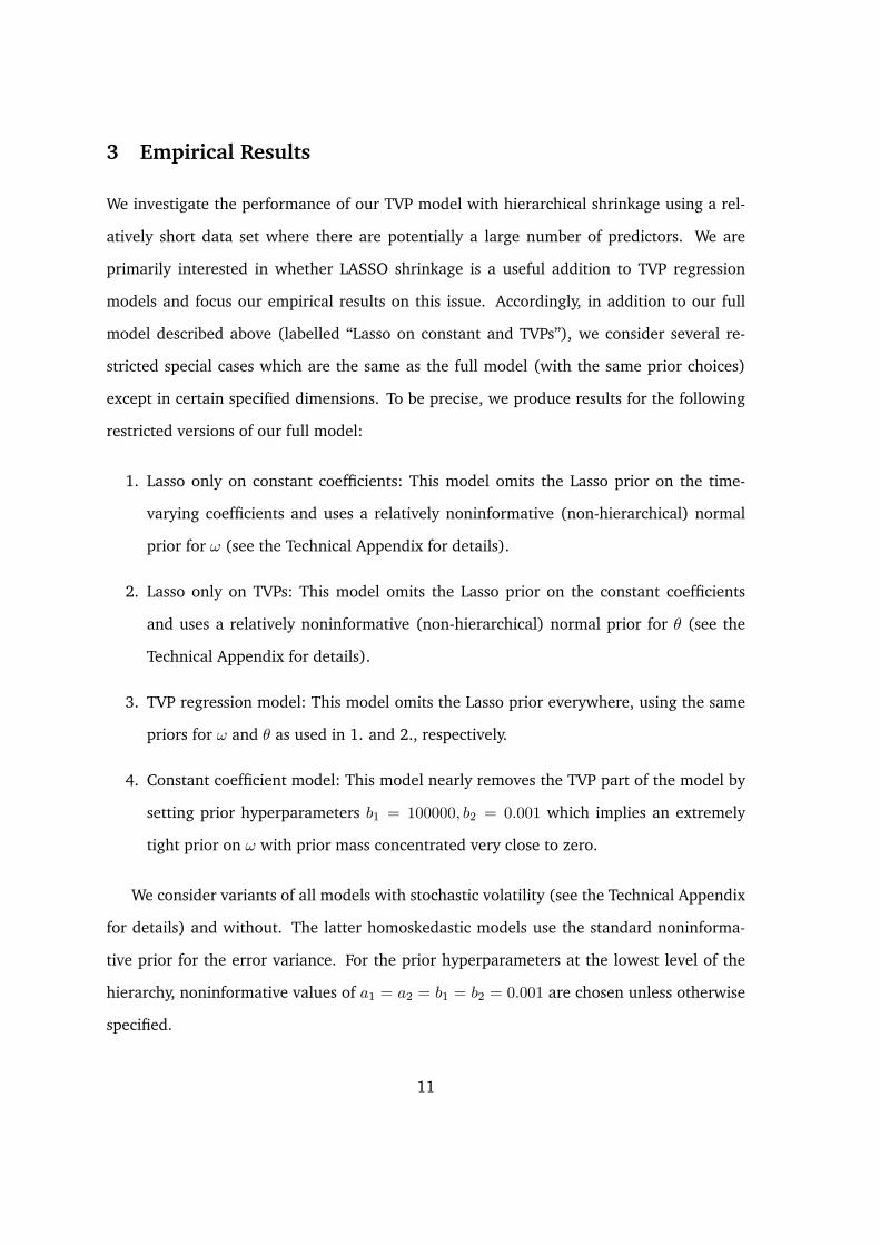
3 Empirical Results

We investigate the performance of our TVP model with hierarchical shrinkage using a rel-

atively short data set where there are potentially a large number of predictors. We are

primarily interested in whether LASSO shrinkage is a useful addition to TVP regression

models and focus our empirical results on this issue. Accordingly, in addition to our full

model described above (labelled “Lasso on constant and TVPs”), we consider several re-

stricted special cases which are the same as the full model (with the same prior choices)

except in certain specified dimensions. To be precise, we produce results for the following

restricted versions of our full model:

1. Lasso only on constant coefficients: This model omits the Lasso prior on the time-

varying coefficients and uses a relatively noninformative (non-hierarchical) normal

prior for ω (see the Technical Appendix for details).

2. Lasso only on TVPs: This model omits the Lasso prior on the constant coefficients

and uses a relatively noninformative (non-hierarchical) normal prior for θ (see the

Technical Appendix for details).

3. TVP regression model: This model omits the Lasso prior everywhere, using the same

priors for ω and θ as used in 1. and 2., respectively.

4. Constant coefficient model: This model nearly removes the TVP part of the model by

setting prior hyperparameters b1 = 100000, b2 = 0.001 which implies an extremely

tight prior on ω with prior mass concentrated very close to zero.

We consider variants of all models with stochastic volatility (see the Technical Appendix

for details) and without. The latter homoskedastic models use the standard noninforma-

tive prior for the error variance. For the prior hyperparameters at the lowest level of the

hierarchy, noninformative values of a1 = a2 = b1 = b2 = 0.001 are chosen unless otherwise

specified.

11

3.1 Data

We forecast overall and core inflation using a variety of predictors reflecting a range of

theoretical considerations. We use real-time data such that, at all points in time, we are

using the data that would have been available to the forecaster at that point in time.6 We

have monthly EU data from February 1994 through November, 2010. Precise definitions of

our variables follow.

Inflation is constructed as described after (2) based on the harmonized index of con-

sumer prices (HICP). We use overall inflation as well as core inflation (which excludes

energy and unprocessed food). Both measures are of interest to policymakers. Neither

measure of inflation is seasonally adjusted.

The following predictors are used:

1. I_1MO: 1-month Euribor (Euro interbank offered rate).

2. I_1YR: 1-year Euribor (Euro interbank offered rate).

3. SENT: Percentage change in economic sentiment indicator.

4. STOCK_1: Percentage change in equity index - Dow Jones, Euro Stoxx, Economic

sector index financial.

5. STOCK_2: Percentage change in equity index - Dow Jones Eurostoxx 50 index.

6. EXRATE: Percentage change in ECB real effective exchange rate (CPI deflated, broad

group of currencies against euro).

7. IP: Percentage change in industrial production index.

8. LOANS: Percentage change in loans (total maturity, all currencies combined).

9. M3: Annual percentage change in monetary aggregate M3.

6The data is obtained from the ECB’s Statistical Data warehouse with variables being updated in real timetaken from its Real Time Data base. Complete descriptions of all variables can be found on the ECB’s website.For some of the predictors complete real time data is only available from January 2001. For these variables weuse non-real time data before this time. Our forecast evaluations begin in January 2001.

12

10. CAR: Registrations of new passenger cars.

11. OIL: Percentage change in oil price (brent crude -1 month forward).

12. ORDER: Change in order-book levels.

13. UNEMP: Standardised unemployment rate (all ages, male & female).

In addition, p lags of the logged first difference of the price index are used as predictors,

as described after (2). All of the predictors are standardized to have mean zero and variance

one. The dependent variable is standardized to have variance one.7 Since our inflation

variables are not seasonally adjusted, we also include an intercept and monthly dummies

(omitting the January dummy). We forecast inflation a month ahead and a year ahead

(h = 1 and h = 12).

The results in the body of the paper always use an intercept, p = 12, 11 monthly dum-

mies and the 13 predictors listed above. Thus, we have 37 (possibly time-varying) coeffi-

cients to estimate with fewer than 18 years of data. In the Empirical Appendix, we present

results using various subsets of the 37 variables. These include the case where the 13 pre-

dictors are omitted, leading to TVP-AR models, as well the case where the 13 variables and

all lags are excluded from the model. This latter case leads to the unobserved components

stochastic volatility (UCSV) model of Stock and Watson (2007).8 Thus, we are investigate

the usefulness of hierarchical shrinkage in the context of several popular classes of forecast-

ing models.

3.2 Full Sample Results

Before comparing the forecast performance of the many models we consider, we present

some full sample parameter estimates using our model with Lasso priors on constant and

time-varying coefficients. For the sake of brevity, we present only results for core inflation.

7The standardization is re-done at each period in our recursive forecasting exercise using information avail-able at the time the forecast is being made.

8Although we always include the monthly dummies (with possibly time varying coefficients) so our modelsare not exactly equivalent to the TVP-AR or UCSV models.

13

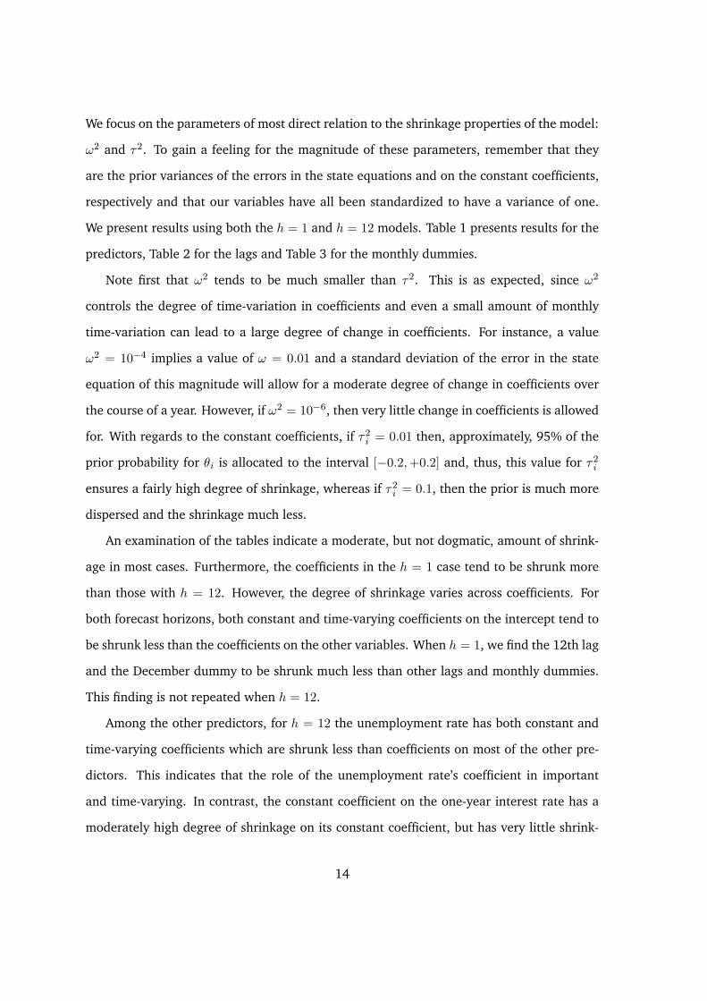
We focus on the parameters of most direct relation to the shrinkage properties of the model:

ω2 and τ2. To gain a feeling for the magnitude of these parameters, remember that they

are the prior variances of the errors in the state equations and on the constant coefficients,

respectively and that our variables have all been standardized to have a variance of one.

We present results using both the h = 1 and h = 12 models. Table 1 presents results for the

predictors, Table 2 for the lags and Table 3 for the monthly dummies.

Note first that ω2 tends to be much smaller than τ2. This is as expected, since ω2

controls the degree of time-variation in coefficients and even a small amount of monthly

time-variation can lead to a large degree of change in coefficients. For instance, a value

ω2 = 10−4 implies a value of ω = 0.01 and a standard deviation of the error in the state

equation of this magnitude will allow for a moderate degree of change in coefficients over

the course of a year. However, if ω2 = 10−6, then very little change in coefficients is allowed

for. With regards to the constant coefficients, if τ2i = 0.01 then, approximately, 95% of the

prior probability for θi is allocated to the interval [−0.2,+0.2] and, thus, this value for τ2i

ensures a fairly high degree of shrinkage, whereas if τ2i = 0.1, then the prior is much more

dispersed and the shrinkage much less.

An examination of the tables indicate a moderate, but not dogmatic, amount of shrink-

age in most cases. Furthermore, the coefficients in the h = 1 case tend to be shrunk more

than those with h = 12. However, the degree of shrinkage varies across coefficients. For

both forecast horizons, both constant and time-varying coefficients on the intercept tend to

be shrunk less than the coefficients on the other variables. When h = 1, we find the 12th lag

and the December dummy to be shrunk much less than other lags and monthly dummies.

This finding is not repeated when h = 12.

Among the other predictors, for h = 12 the unemployment rate has both constant and

time-varying coefficients which are shrunk less than coefficients on most of the other pre-

dictors. This indicates that the role of the unemployment rate’s coefficient in important

and time-varying. In contrast, the constant coefficient on the one-year interest rate has a

moderately high degree of shrinkage on its constant coefficient, but has very little shrink-

14

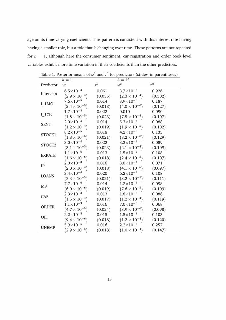
age on its time-varying coefficients. This pattern is consistent with this interest rate having

having a smaller role, but a role that is changing over time. These patterns are not repeated

for h = 1, although here the consumer sentiment, car registration and order book level

variables exhibit more time variation in their coefficients than the other predictors.

Table 1: Posterior means of ω2 and τ2 for predictors (st.dev. in parentheses)

h = 1 h = 12Predictor ω2 τ2 ω2 τ2

Intercept6.5×10−3(2.9× 10−4

) 0.061

(0.035)3.7×10−3(2.3× 10−4

) 0.926

(0.302)

I_1MO7.6×10−5(2.4× 10−5

) 0.014

(0.018)3.9×10−6(4.0× 10−6

) 0.187

(0.127)

I_1YR1.7×10−5(1.8× 10−5

) 0.022

(0.023)0.010(7.5× 10−4

) 0.090

(0.107)

SENT2.0×10−3(1.2× 10−4

) 0.014

(0.019)5.3×10−5(1.9× 10−5

) 0.088

(0.102)

STOCK18.2×10−5(1.8× 10−5

) 0.018

(0.021)4.2×10−5(8.2× 10−6

) 0.133

(0.129)

STOCK23.0×10−4(3.1× 10−5

) 0.022

(0.023)3.3×10−3(2.1× 10−4

) 0.089

(0.109)

EXRATE1.1×10−6(1.6× 10−6

) 0.013

(0.018)1.5×10−4(2.4× 10−5

) 0.108

(0.107)

IP2.0×10−3(2.0× 10−4

) 0.016

(0.018)3.0×10−4(4.1× 10−5

) 0.071

(0.097)

LOANS3.4×10−4(2.3× 10−5

) 0.020

(0.021)6.2×10−4(3.2× 10−5

) 0.108

(0.111)

M37.7×10−6(6.0× 10−6

) 0.014

(0.019)1.2×10−3(7.6× 10−5

) 0.098

(0.109)

CAR2.3×10−3(1.5× 10−4

) 0.013

(0.017)1.8×10−3(1.2× 10−4

) 0.086

(0.119)

ORDER1.1×10−3(4.7× 10−5

) 0.016

(0.024)7.0×10−6(3.9× 10−6

) 0.068

(0.098)

OIL2.2×10−5(9.4× 10−6

) 0.015

(0.018)1.5×10−3(1.2× 10−4

) 0.103

(0.120)

UNEMP5.9×10−5(2.9× 10−5

) 0.016

(0.018)2.2×10−3(1.0× 10−4

) 0.257

(0.147)

15

Table 2: Posterior means of ω2 and τ2 for lags (st. dev. in parentheses)

h = 1 h = 12Lag ω2 τ2 ω2 τ2

11.6×10−3(7.6× 10−5

) 0.019

(0.021)6.4×10−4(3.5× 10−5

) 0.109

(0.115)

23.9×10−4(9.5× 10−5

) 0.016

(0.018)6.2×10−3(2.6× 10−4

) 0.085

(0.116)

31.8×10−6(2.0× 10−6

) 0.029

(0.026)7.5×10−4(4.6× 10−5

) 0.104

(0.103)

43.5×10−5(7.1× 10−6

) 0.013

(0.018)4.0×10−4(5.0× 10−5

) 0.108

(0.112)

53.6×10−4(6.7× 10−5

) 0.013

(0.018)1.5×10−4(2.5× 10−5

) 0.108

(0.114)

61.8×10−4(5.3× 10−5

) 0.023

(0.020)9.2×10−5(2.3× 10−5

) 0.082

(0.100)

71.7×10−4(1.8× 10−5

) 0.020

(0.023)1.7×10−3(3.3× 10−4

) 0.075

(0.115)

81.2×10−5(5.8× 10−6

) 0.012

(0.015)2.2×10−4(5.3× 10−5

) 0.069

(0.107)

91.5×10−4(2.9× 10−5

) 0.012

(0.019)5.6×10−4(1.5× 10−4

) 0.097

(0.114)

101.0×10−4(1.0× 10−5

) 0.013

(0.018)6.6×10−5(3.2× 10−5

) 0.072

(0.102)

117.3×10−5(1.8× 10−5

) 0.019

(0.022)5.3×10−3(4.4× 10−4

) 0.094

(0.106)

125.1×10−5(8.5× 10−6

) 0.085

(0.040)1.4×10−4(3.2× 10−4

) 0.096

(0.114)

16

Table 3: Posterior means of ω2 and τ2 for dummies (st. dev. in parentheses)

h = 1 h = 12ω2 τ2 ω2 τ2

February6.7×10−4(1.1× 10−4

) 0.041

(0.028)1.2×10−3(3.1× 10−4

) 0.169

(0.146)

March1.4×10−3(4.5× 10−4

) 0.027

(0.024)1.4×10−3(4.2× 10−4

) 0.088

(0.104)

April8.9×10−5(4.1× 10−5

) 0.015

(0.020)2.8×10−4(2.9× 10−4

) 0.136

(0.122)

May1.4×10−5(1.5× 10−5

) 0.034

(0.026)8.5×10−6(1.6× 10−5

) 0.071

(0.112)

June3.8×10−5(4.5× 10−5

) 0.016

(0.020)4.3×10−5(3.6× 10−5

) 0.073

(0.094)

July3.6×10−5(2.9× 10−5

) 0.014

(0.020)2.2×10−5(3.6× 10−5

) 0.101

(0.114)

August1.7×10−4(2.2× 10−4

) 0.015

(0.020)4.5×10−4(1.4× 10−4

) 0.078

(0.100)

September1.1×10−4(9.8× 10−5

) 0.016

(0.020)4.3×10−5(5.0× 10−5

) 0.072

(0.088)

October1.4×10−4(5.9× 10−5

) 0.028

(0.023)5.1×10−4(2.0× 10−4

) 0.145

(0.133)

November1.6×10−3(1.4× 10−4

) 0.022

(0.020)2.4×10−4(1.5× 10−4

) 0.081

(0.099)

December1.5×10−4(1.4× 10−4

) 0.079

(0.036)5.1×10−4(1.1× 10−4

) 0.118

(0.126)

3.3 Forecasting Results

Most Bayesians prefer to use predictive likelihoods for evaluating forecast performance.

Our posterior and predictive simulation algorithm provides us with the predictive density

for forecasting yτ+h given information through time τ , which we denote by p (yτ+h|Dataτ ).

This predictive density is evaluated for τ = τ0, .., T − h where τ0 is January, 2001 and

h = 1 and 12. If we let yoτ+h be the observed value of yi,τ+h, then the predictive likelihood

is p(yτ+h = y

oτ+h|Dataτ

)and we use the mean of the log predictive likelihoods (MLPL) for

forecast evaluation:

MLPL =1

T − h− τ0 + 1

T−h∑

τ=τ0

log[p(yτ+h = y

oτ+h|Dataτ

)].

In the tables, MLPL results are presented relative to those produced by our full model

17

(i.e. the model with hierarchical shrinkage on both constant and time-varying coefficients

and which has stochastic volatility in the measurement equation). Since MLPL is measured

in log units, we take the difference between the MLPL for the full model and the restricted

model. Thus, positive numbers indicate our full model is forecasting better than the re-

stricted model.

We also present the mean of the squared forecast errors (MSFE) and the mean of the ab-

solute value of the forecast errors (MAFE). In contract to the predictive likelihoods, which

evaluate the performance of the entire predictive distribution, MSFEs and MAFE only eval-

uate the performance of the point forecast. We use the predictive median as our point

forecast. Again, we present results relative to the full model. The tables present MSFEs and

MAFEs for a restricted model divided by those for the full model. Thus, a number greater

than one indicates our full model is forecasting better, using MSFE or MAFE as a metric.

3.3.1 Results for Core Inflation

Tables 4 and 5 present results for core inflation. Consider first results for h = 1 (see Table

4). Regardless of whether we use MLPL, MSFE or MAFE to evaluate forecast performance,

we find evidence that the inclusion of stochastic volatility causes forecast performance to

deteriorate. The predictive likelihoods are substantially higher in the homoskedastic mod-

els suggesting that stochastic volatility may not be present in this data set.9 It is worth

noting that the TVP regression model with stochastic volatility (which could be a popular

benchmark for the researcher working in this literature, but not interested in adding shrink-

age) produces the worst forecasts. And our full model is the second best forecasting model

among the set of models with stochastic volatility. This suggests caution should be taken

when forecasting with TVP regression models without shrinkage and suggests the impor-

tance of shrinkage such as that provided by the Lasso. But beyond this we will say no more

about the models with stochastic volatility and focus on the better-forecasting homoskedas-

9Note that the product of predictive likelihoods over the entire sample is the marginal likelihood. Thus,MLPL can be used as a method of model selection and here indicates support for homoskedasticity.

18

tic models.

Among the homoskedastic models with h = 1, our model with Lasso prior on both

constant and time-varying coefficients forecasts the best when we use predictive likelihoods

to evaluate forecast performance. When we use MAFE or MSFE, the constant coefficient

model forecasts best. However, our model is a close second best in terms of the latter

forecast metrics. In this data set, at this forecast horizon, it appears that there is little

need for time-varying coefficients and, thus, our model is forecasting roughly as well as a

constant coefficient model. However, it is important to stress that our approach discovered

this fact automatically. That is, it allows the researcher to begin with a very flexible model,

allowing for features which might be important for forecasting (such as parameter change),

but then the statistical methodology decides which aspect is important and which is not.

Here our approach is shrinking the time-varying coefficients so as to mostly “turn off” this

part of the model. The standard TVP regression model does not do this and exhibits poorer

forecast performance. At the other extreme, a researcher who simply began with a constant

coefficient model might have been unknowingly working with a badly mis-specified model.

Our approach allows the data to decide whether the coefficients are time-varying and, if so,

by how much they vary.

The story at the annual forecast horizon (h = 12) is a bit different, but also indicates the

benefits of using the Lasso, especially on the TVPs. In terms of predictive likelihoods, our

full model (including Lasso prior on constant and time-varying coefficients and stochastic

volatility) forecasts best. In terms of MSFE and MAFE, our full model also forecasts well,

but it is the homoskedastic version of our model which does even better. In this case,

our different measures of forecast performance are telling a somewhat conflicting story

(especially with regards to the need for stochastic volatility). This is a point we will return

to below.

For h = 1, we found the simple constant coefficient model to forecast well. For h = 12,

this is not so. In this case, allowing to time-variation in coefficients is important in achieving

a good forecast performance. However, the TVP regression model does not forecast well.

19

It is allowing for too much time-variation in coefficients. The Lasso prior is allowing for

us to estimate the correct degree of time-variation in coefficients in order to obtain a good

forecast performance.

Table 4: Measures of Forecast Performance for Core Inflation (h = 1)

Constant Variance Stochastic Volatility

MLPL MSFE MAFE MLPL MSFE MAFE

Lasso on constant and TVPs -0.42 0.77 0.83 0.00 1.00 1.00

Lasso only on constant coeffs. -0.29 0.88 0.87 2.00 1.93 1.94

Lasso only on TVPs -0.37 0.85 0.86 0.30 1.59 1.11

TVP regression model 0.09 1.08 0.95 2.54 3.64 1.69

Constant coeff. model -0.40 0.66 0.78 0.01 0.91 0.94

Note: All results are relative to the benchmark model (Lasso on constant & TVPs)

Table 5: Measures of Forecast Performance for Core Inflation (h = 12)



Lasso on constant and TVPs 12.83 0.95 0.95 0.00 1.00 1.00

Lasso only on constant coeffs. 2.80 0.88 0.90 0.89 1.23 1.09

Lasso only on TVPs 11.64 1.18 1.02 0.19 1.31 1.14


Constant coeff. model 6.33 1.09 0.98 0.14 12.48 10.31


Tables 4 and 5 present evidence on average forecast performance. To investigate whether

forecast performance varies over time and to shed light on why the MLPL results conflict

with the MAFE and MSFE results in Table 5, we present Figures 1 and 2. These are pro-

duced using the model with Lasso prior on both constant and time-varying coefficients with

h = 12 (but similar patterns are found with the other models). Figure 1 plots the forecast

errors squared for the homoskedastic and heteroskedastic versions of the model. Figure 2

plots the logs of the predictive likelihood in the same format. Note first that forecast perfor-

mance does vary over time with a deterioration of forecast performance at the time of the

financial crisis and in 2001.

Looking at Figure 1, it can be seen that the homoskedastic and heteroskedastic versions

of our model are forecasting roughly as well as each other, in terms of their point forecasts.

A similar pattern holds for the predictive likelihoods (see Figure 2) for most of the time.

However, at the time of the financial crisis, the homoskedastic version of the model has

20

much lower predictive likelihoods and it is this time period which drives the inconsistency

between MLPL and MSFE noted in Table 5. What is happening is that the homoskedastic

version of the model is missing the large increase in volatility which began with the financial

crisis. This has little impact on the point forecasts and thus, the forecast errors squared do

not differ by much between the homoskedastic and heteroskedastic versions of the model.

However, the homoskedastic version of the model has an error variance which is much too

small. This makes it appear that the point forecast is far in the tails of the predictive density,

leading to a very small predictive likelihood. The heteroskedastic version of this model does

not run into this problem. Policymakers are increasingly interested in forecast uncertainty

and, hence, want more than just a point forecast. Figure 2 shows how the appropriate

modelling of the error variance can be crucial in obtaining reliable inference about forecast

uncertainty.

2001 2002 2003 2004 2005 2006 2007 2008 2009 20100

1

2

x 10-4 Forecast Errors Squared

stoch. vol .

homoskedastic

Figure 1: Forecast errors squared for models with Lasso prior on constant

and time-varying coefficients, h = 12

21

2001 2002 2003 2004 2005 2006 2007 2008 2009 2010-300

-250

-200

-150

-100

-50

0

50

Log Predictive Likelihoods

stoch. vol .

homoskedastic

Figure 2: Log predictive likelihoods for models with Lasso prior on constant

and time-varying coefficients, h = 12

3.3.2 Results for Overall Inflation

Tables 6 and 7 are the same as Tables 4 and 5, except that the former are for overall

inflation.

For h = 1, we are finding that homoskedastic models tend to do better than those with

stochastic volatility (although to a lesser extent than for core inflation). The homoskedastic

version of our model with Lasso prior on both time varying and constant coefficients exhibits

the best forecast performance regardless of whether one uses MLPL, MSFE or MAFE. Note

also that, to a greater extent than with core inflation, our model is forecasting better than

two popular benchmarks: the TVP regression model and the constant coefficient model.

For h = 12, Table 7 is showing a similar pattern to Table 5. That is, in terms of MLPL,

22

TVP models with stochastic volatility forecast best – but only if a Lasso prior is used on

the time-varying coefficients. However, if we look at MSFE or MAFE, models with constant

coefficients forecast best. This discrepancy between the MLPL and MSFE results is due to

the same reason discussed previously (and illustrated in Figures 1 and 2). However, it is

worth noting that, even if we use only MSFE and MAFE for forecast comparison, models

with Lasso priors on TVPs forecast much better than the unrestricted TVP regression model.

In summary, in cases where there is time-variation in coefficients, putting a Lasso prior

on these coefficients does lead to better forecast performance than unrestricted TVP mod-

els. The shrinkage is beneficial in keeping the time-varying coefficients from wandering

too widely. In cases where there is little evidence of time-varying coefficients (i.e. where

constant coefficient models forecast well), the Lasso prior can automatically discover this

lack of time-variation and lead to forecasting results that are almost as good as the constant

coefficient model. In these latter cases, unrestricted TVP models can forecast very poorly.

Table 6: Forecast Performance for Overall Inflation (h = 1)



Lasso on constant and TVPs -0.24 0.75 0.85 0.00 1.00 1.00



TVP regression model -0.04 1.00 1.04 1.99 1.56 1.27



Table 7: Forecast Performance for Overall Inflation (h = 12)



Lasso on constant and TVPs 26.75 0.85 0.95 0.00 1.00 1.00


Lasso only on TVPs 16.37 0.97 0.96 -0.08 1.02 1.01


Constant coeff. model 8.11 0.63 0.80 -0.05 0.76 0.89


23

3.3.3 Robustness to Different Specifications

Our empirical results are based on large set of explanatory variables. In the Empirical

Appendix we investigate the robustness of our results to changes in this set. The reader is

referred to the Empirical Appendix for details. We do find our results to be quite robust. We

briefly summarize our findings here.

If we omit the 13 predictors listed in Section 3.1, we still have a model with many

explanatory variables (an intercept, 11 monthly dummies and 12 lags) and, thus, Lasso-

type shrinkage is potentially useful. Table A.1 through A.4 in the Empirical Appendix shows

that it is indeed useful in a similar manner to what we found in Tables 4 through 7. This

indicates the usefulness of hierarchical shrinkage even in time-varying AR(p) models.

The Empirical Appendix also includes results for models where all predictors and all

lags are excluded. Hence, the models include only a (potentially time-varying) intercept

and monthly dummies. With the inclusion of stochastic volatility, we have models which

are similar to the popular UCSV model of Stock and Watson (2007). For these models, the

benefits of hierarchical shrinkage are smaller, but still evident.

4 Conclusions

The macroeconomist often has many variables which can be used in a forecasting exercise.

She may also wish to work with a model which allows for the parameter change which is

empirically evident in many macroeconomic data sets. These considerations can often lead

to models with many parameters, leading to over-fitting and poor forecast performance. In

regressions and VARs with constant coefficients, there have been many approaches which

try to overcome these problems by shrinking coefficients. However, with TVP models (where

we would expect the need for shrinkage to be even greater than in constant coefficient

models), few shrinkage approaches have been suggested. In this paper, we have developed

a new approach to shrinkage in TVP models based on the Lasso. We have extended Lasso

methods, which are popular with constant coefficient models, to TVP models and developed

24

Bayesian methods for posterior and predictive inference.

To investigate the performance of our approach, we use an EU data set which is rela-

tively short and involves many predictors. Our findings are moderately encouraging in that

use of the Lasso on the time-varying coefficients does lead to substantial improvements in

forecast performance relative to unrestricted TVP models. Relative to constant coefficient

models, a TVP model with Lasso shrinkage in some cases exhibits improved forecast per-

formance. But we find that an advantage of using a TVP model with Lasso shrinkage is

that it can automatically produce a model which is similar to a constant coefficient model

in the cases where a constant coefficient model is the appropriate forecasting model. Thus,

the researcher using the TVP model with Lasso prior can be confident that the risks of mis-

specification associated with constant coefficient models are avoided, while at the same

time avoid the risks of over-parameterization associated with unrestricted TVP models.

25

References

Banbura, M., Giannone, D. and Reichlin, L. (2010). “Large Bayesian Vector Auto Regres-

sions,” Journal of Applied Econometrics, 25, 71-92.

Carter, C. and Kohn, R. (1994). “On Gibbs sampling for state space models,” Biometrika,

81, 541–553.

Chipman, H., George, E. and McCulloch, R. (2001). “The practical implementation

of Bayesian model selection,” pages 65-134 in Institute of Mathematical Statistics Lecture

Notes - Monograph Series, Volume 38, edited by P. Lahiri.

Clements, M. and Hendry, D., 1998, Forecasting Economic Time Series. (Cambridge Uni-

versity Press: Cambridge).

Clements, M. and Hendry, D., 1999, Forecasting Non-stationary Economic Time Series.

(The MIT Press: Cambridge).

Cogley, T., Morozov, S. and Sargent, T. (2005). “Bayesian fan charts for U.K. inflation:

Forecasting and sources of uncertainty in an evolving monetary system,” Journal of Eco-

nomic Dynamics and Control, 29, 1893-1925.

Cogley, T. and Sargent, T. (2001). “Evolving post World War II inflation dynamics,”

NBER Macroeconomics Annual, 16, 331-373.

Cogley, T. and Sargent, T. (2005). “Drifts and volatilities: Monetary policies and out-

comes in the post WWII U.S.,” Review of Economic Dynamics, 8, 262-302.

D’Agostino, A., Gambetti, L. and Giannone, D. (2009). “Macroeconomic forecasting and

structural change,” ECARES working paper 2009-020.

De Mol, C., Giannone, D. and Reichlin, L. (2008). “Forecasting using a large number of

predictors: Is Bayesian shrinkage a valid alternative to principal components?” Journal of

Econometrics, 146, 318-328.

Frühwirth-Schnatter, S. and Wagner, H. (2010). “Stochastic model specification search

for Gaussian and partial non-Gaussian state space models,” Journal of Econometrics 154,

85-100.

26

George, E. and McCulloch, R. (1997). ”Approaches for Bayesian variable selection,”

Statistica Sinica, 7, 339-373.

Kim, S., Shephard, N. and Chib, S. (1998). “Stochastic volatility: likelihood inference

and comparison with ARCH models,” Review of Economic Studies, 65, 361-93.

Koop, G. and Korobilis, D. (2009). “Forecasting inflation using dynamic model averag-

ing,” RCFEA WP 09-34, Rimini Center for Economic Analysis.

Koop, G., Leon-Gonzalez, R., Strachan, R. (2009). “On the evolution of the monetary

policy transmission mechanism,” Journal of Economic Dynamics and Control 33 (2009), 997-

1017.

Park, T. and Casella, G. (2008). “The Bayesian Lasso,” Journal of the American Statistical

Association 103, 681-686.

Pesaran, M.H., Pettenuzzo, D. and Timmerman, A. (2006). “Forecasting time series

subject to multiple structural breaks,” Review of Economic Studies, 73, 1057–1084.

Primiceri. G. (2005). “Time varying structural vector autoregressions and monetary

policy,” Review of Economic Studies, 72, 821-852.

Sims, C. and Zha, T. (2006). “Were there regime switches in macroeconomic policy?”

American Economic Review, 96, 54-81.

Stock, J. and Watson, M. (1996). “Evidence on structural instability in macroeconomic

time series relations, ” Journal of Business and Economic Statistics, 14, 11-30.

Stock, J. and Watson, M. (2006). “Forecasting using many predictors,” pp. 515-554

in Handbook of Economic Forecasting, Volume 1, edited by G. Elliott, C. Granger and A.

Timmerman, Amsterdam: North Holland.

Stock, J. and Watson, M. (2007). “Why has U.S. inflation become harder to forecast?”

Journal of Monetary Credit and Banking 39, 3-33.

Stock, J. and Watson, M. (2011). “Generalized shrinkage methods for forecasting using

many predictors,” manuscript available at http://www.princeton.edu/~mwatson/papers/

stock_watson_generalized_shrinkage_February_2011.pdf.

27

Technical Appendix

Stochastic volatility

We use a standard stochastic volatility specification for the error variance in the mea-

surement equation. In particular, if ht = ln (σt), then:

ht+1 = ht + ut,

where ut is N (0,W ) and is independent over t and of εt and ηt. We use the algorithm of

Kim, Shephard and Chib (1998) to draw the volatilities. The prior for the initial volatility

is:

h0 ∼ N (−0.5, 0.5) .

Since the dependent variable is standardized to have a variance of one, this is only very

weakly informative, but is centered over a plausible value for h0. The prior for W−1 is

Gamma with prior mean of 104 and two prior degrees of freedom.

Priors for λ2 and κ2

Unless otherwise specified, our empirical results set a1 = a2 = b1 = b2 = 0.001 which

implies proper but very noninformative priors (i.e. the prior mean of these priors is one,

but the prior variance is 1000). One of our models almost totally removes the TVP part of

the model altogether by setting b1 = 100000. This value for b1 implies prior mean of 100

for κ (a value which ensures shrinkage of ω to very near zero) and the prior variance is 0.1

ensuring a tight prior around this value.

Priors when Lasso is not used

For models without the Lasso prior on the TVP coefficients, ξ2i and κ do not appear in

the model and we use a non-hierarchical prior for ω of the form:

ω ∼ N (0, I) .

28

For models without the Lasso prior on the constant coefficients, τ2i and λ do not appear

in the model and we use a non-hierarchical prior for θ of the form:

θ ∼ N (0, 9× I) .

29

Empirical Appendix

In this sub-section, we present results for a few additional specifications to show that the

results in the body of the paper are robust. Results are presented in the same format as

in Tables 4 through 7. That is forecast performance is measured relative to the full model

with the same explanatory variables. Tables A.1 and A.2 present results without any of

the predictors listed in Section 3.1 (i.e. simply using an intercept, the monthly dummies

and p = 12). It can be seen that the same patterns noted in Tables 4 through 7 hold.

For instance, Table A.1 shows that using the Lasso on the time-varying coefficients leads

to substantive forecast improvements over unrestricted TVP models for h = 1. It is worth

noting, however, that the MLPLs are roughly the same in Tables A.1 and A.2 as in Tables

4 through 7 and the MSFEs and MAFEs are in many cases, somewhat lower in the former

tables. This suggests that, in this application, the predictors are adding little. This re-

emphasizes the importance of shrinkage methods such as those introduced in this paper.

That is, if the researcher is working with a data set with many predictors, our TVP shrinkage

methods can, in an automatic fashion, uncover the fact that the predictors are adding little.

This may be preferable to a model selection strategy where the researcher seeks to find a

single parsimonious forecasting model.

Tables A.3 and A.4 repeat the analysis for models with only an intercept and monthly

dummies. Similar patterns to those noted previously are found, although in this relatively

parsimonious model, the benefits of Lasso-type shrinkage are smaller. Note, however, that

with core inflation, the constant coefficient model does quite poorly (especially when h = 1)

which contrasts with the results we found with more parameter-rich models.

30

Table A.1: Forecast Performance for Core Inflation: No Predictors



h = 1Lasso on constant and TVPs -0.46 0.67 0.77 0.00 1.00 1.00



TVP regression model -0.31 0.82 0.85 2.14 1.87 133

Constant coeff. model -0.46 0.56 0.74 -0.16 0.70 0.82

h = 12Lasso on constant and TVPs 50.29 1.15 1.10 0.00 1.00 1.00





Note: All results are relative to the benchmark model (Lasso on constant & TVPs) for each forecast horizon h

Table A.2: Forecast Performance for Overall Inflation: No Predictors





Lasso only on TVPs -0.52 0.63 0.79 -0.06 0.86 0.88







Constant coeff. model 0.26 0.58 0.76 -0.07 0.63 0.81


31

Table A.3: Forecast Performance for Core Inflation: No Predictors nor Lags









Lasso only on constant coeffs. 35.07 0.81 0.89 -0.71 0.81 0.88

Lasso only on TVPs 58.98 0.81 0.89 -0.13 0.87 0.91

TVP regression model 39.31 0.81 0.89 -0.75 0.83 0.90



Table A.4: Forecast Performance for Overall Inflation: No Predictors nor Lags









Lasso only on constant coeffs. 55.23 1.40 1.14 -0.20 1.37 1.13


TVP regression model 44.81 1.39 1.14 -0.08 1.38 1.13



32

Hierarchical Shrinkage in Time-Varying Parameter Models

Documents

Transcript of Hierarchical Shrinkage in Time-Varying Parameter Models