Varying constants entropic–ΛCDM cosmology

Mariusz P. Dabrowski∗

Institute of Physics, University of Szczecin, Wielkopolska 15, 70-451 Szczecin, Poland,National Centre for Nuclear Research, Andrzeja So ltana 7, 05-400 Otwock, Poland, andCopernicus Center for Interdisciplinary Studies, S lawkowska 17, 31-016 Krakow, Poland

H. Gohar† and Vincenzo Salzano‡

Institute of Physics, University of Szczecin, Wielkopolska 15, 70-451 Szczecin, Poland(Dated: February 24, 2016)

We formulate the basic framework of thermodynamical entropic force cosmology which allowsvariation of the gravitational constant G and the speed of light c. Three different approaches to theformulation of the field equations are presented. Some cosmological solutions for each framework aregiven and one of them is tested against combined observational data (supernovae, BAO, and CMB).From the fit of the data it is found that the Hawking temperature numerical coefficient γ is two tofour orders of magnitude less than usually assumed on the geometrical ground theoretical value ofO(1) and that it is also compatible with zero. Besides, in the entropic scenario we observationallytest that the fit of the data is allowed for the speed of light c growing and the gravitational constantG diminishing during the evolution of the universe. We also obtain a bound on the variation of cto be ∆c/c ∝ 10−5 > 0 which is at least one order of magnitude weaker than the quasar spectraobservational bound.

PACS numbers: 98.80.Jk; 95.36.+x; 04.50.Kd; 04.70.Dy

∗ mpdabfz@wmf.univ.szczecin.pl† hunzaie@wmf.univ.szczecin.pl‡ enzo@wmf.univ.szczecin.pl

2

I. INTRODUCTION

General Relativity is an established theory which explains the evolution of the universe on a large scale [1]. Althoughit is not complete because it contains singularities, it explains the dynamics of the universe in a consistent way.Furthermore, the current phase of accelerated evolution of the universe has been discovered [2, 3]. In order toobtain this accelerated expansion, one has to put an extra term, the cosmological constant Λ or dark energy intothe Einstein–Friedmann equations. The ΛCDM models that resulted [4–7] are consistent models to explain thisaccelerated expansion, but the observational value of Λ is over 120 orders of magnitude smaller than the valuecalculated in quantum field theory, where it is interpreted as vacuum energy. This motivates cosmologists to look foralternative models which can explain the effect [8, 9].

The relation between Einstein’s gravity and thermodynamics is a puzzle. In the 1970s, Bekenstein and Hawking[10–13] derived the laws of black hole thermodynamics which emerged to have similar properties as in standardthermodynamics. Jacobson [14] derived Einstein field equations from the first law of thermodynamics by assumingthe proportionality of the entropy and the horizon area. A more extensive work in this direction was made byVerlinde and Padmanabhan in [15–18]. Verlinde derived gravity as an entropic force, which originated in a systemby the statistical tendency to increase its entropy. He assumed the holographic principle [19], which stated that themicroscopic degrees of freedom can be represented holographically on the horizons, and this piece of information(or degrees of freedom) can be measured in terms of entropy. The approach got criticized on the base of neutronexperiments though [20].

Recently, the entropic cosmology based on the notion of the entropic force was developed in a series of papers[21–27] and it was especially compared with supernovae data in [28, 29]. However, supernovae tests are not verystrong and so the [28] got criticized on the basis of a galaxy formation problem (e.g., [30–33]). Basically, the idea ofentropic cosmology is to add extra entropic force terms into the Friedmann equation and the acceleration equation.This force is supposed to be responsible for the current acceleration as well as for an early exponential expansionof the universe. It is pertinent to mention that the entropic cosmology suggested in these references assumes thatgravity is still a fundamental force and that it includes extra driving force terms or boundary terms in the Einsteinfield equations. This is unlike Verlinde [15], who considers gravity as an entropic force, but not as a fundamentalforce (see also [34–44]). All frameworks were discussed in detail in [45] by Visser. Entropic cosmology is also relatedto dynamical vacuum energy models which have been discussed and confronted with data in [46–50].

In this paper, we expand entropic cosmology suggested in [21–29] for the theories with varying physical constants:the gravitational constant G and the speed of light c. Although [28] is problematic in the context galaxy formationtest, we use it as a starting point for further discussion. We discuss possible consequences of such variability ontothe entropic force terms and the boundary terms. As it has been known for the last fifteen years, varying constantscosmology [51–53] was proposed as an alternative to inflationary cosmology, because it can help to solve all thecosmological problems (horizon, flatness, and monopole). In the paper, we try three different approaches to formulatethe entropic cosmology with varying constants. In Section II, we present a consistent set of the field equationswhich describes varying constants entropic cosmology with general entropic force terms. In Section III, we derive thecontinuity equation from the first law of thermodynamics and fit general entropic terms to the field equations derivedin Section II using explitic definitions of Bekenstein entropy and Hawking temperature. We also discuss the constraintson the models which come from the second law of thermodynamics. In Section IV, we study single-fluid acceleratingcosmological solutions to the field equations derived in Section III. In Section V, we derive the entropic force forvarying constants, define appropriate entropic pressure, and modify the continuity and acceleration equations. Wealso determine the Friedmann equation and give single-fluid accelerating cosmological solutions. In Section VI, wederive gravitational Einstein field equations using the heat flow through the horizon to which Bekenstein entropy andthe Hawking temperature is assigned. Sections VII and VIII are devoted to observationally testing the many-fluidentropic force models with varying constants. Because of this, the data from supernovae, Baryon Acoustic Oscillations(BAO), and Cosmic Microwave Background (CMB) are used. In Section IX, we give our conclusions.

II. ENTROPIC FORCE FIELD EQUATIONS AND VARYING CONSTANTS

The main idea of our consideration is to follow [21–24, 28, 29] (assuming homogeneous Friedmann geometry) andgeneralize field equations which contain the entropic force terms f(t) and g(t) onto the case of varying speed of light cand varying Newton gravitational constant G theories. This can be done by making the entropic force field equationsas derived in [21–24, 28, 29] to have dynamical c and G. The method to obtain such equations is similar as forvarying c and G models of [51, 52, 54–57], which relies on Lorentz symmetry violation and, consequently, allowingsome preferred (minimally coupled or cosmological) frame. In this frame, one applies standard variational principles,and so neither new terms (involving the derivatives of a dynamical field) nor dynamical field equations appeared. We

3

follow this simple method as the first step towards perhaps more sophisticated ways of deriving the field equationsfrom variational principles with dynamical fields. The attempts to do so were made in [58]. More recently [59, 60], thespontaneous brake of the Lorentz symmetry SO(3, 1) into O(3)×R with a preferred frame allowing the cosmologicalco-moving time was considered. The symmetry breaking is due to an extra vector field Mexican hat type potential,which is included apart from the dynamical field for the speed of light c. Some non-minimally coupled dynamicalfields corresponding to c and G have been considered in [61].

In conclusion, our method just relies on having a preferred frame in which we vary the action which also contains theentropic force terms. This leads to a generalized entropic force Equations [21–24, 28, 29] with dynamical constantsi.e., the equations in which we made the replacement c→ c(t) and G→ G(t) as follows:(

a

a

)2

=8πG(t)

3ρ− kc2(t)

a2+ f (t) , (II.1)

a

a= −4πG(t)

3

[ρ+

3p

c2(t)

]+ g(t). (II.2)

In fact, the functions f(t) and g(t) in general play the role analogous to bulk viscosity with dissipative term (cf.[50–69] of the paper by Komatsu et al. [21]), and this is why from Equations (II.1) and (II.2), one obtains the modifiedcontinuity equation

ρ+ 3H

[ρ+

p

c2(t)

]+ ρ

G(t)

G(t)− 3

kc(t)c(t)

4πG(t)a2(t)=

3H

4πG(t)

[g(t)− f(t)− f(t)

2H

], (II.3)

which will further be used in our paper to various thermodynamical scenarios of the evolution of the universe. If thefunctions f(t) and g(t) are equal and have the value of the Λ-term modified by varying speed of light c(t) i.e.,

f(t) = g(t) =Λc2(t)

3, (II.4)

then they give modified varying c and G Einstein field equations with the continuity Equation as [53]

%+ 3a

a

(%+

p

c2(t)

)+ %

G(t)

G(t)=

(3k − Λa2

)4πG(t)a2

c(t)c(t), (II.5)

which finally reduce to the standard Λ-CDM equations for c and G constant. Another point is that the f(t) andg(t) terms can also be considered as time-dependent (dynamical) vacuum energy [46–50]. It is worth mentioning thatthere is a derivation of varying c models within the framework of Brans–Dicke theory [54–57], but then Equation (II.3)

does not allow for G-varying terms %G/G, and the set of equations is also appended by the dynamical Brans-Dickefield equation Φ ∝ 1/G.

III. GRAVITATIONAL THERMODYNAMICS AND VARYING CONSTANTS

In this section, we start with basic thermodynamics in order to get entropic force varying constants field equations.Please note that the first law of thermodynamics has been widely used to interlink different gravity theories withthermodynamics [34–40, 62]. Defining the temperature and entropy on the cosmological horizons, one can use thislaw of thermodynamics for the whole universe

dE + pdV = TdS, (III.6)

where dE, dV , and dS describe changes in the internal energy E, the volume V , and the entropy S, while T is thetemperature, and p is the pressure. The volume of the universe contained in a sphere of the proper radius r∗ = a(t)r(r is the comoving radius and a(t) is the scale factor) is

V (t) =4

3πa3r3 . (III.7)

We have

V (t) = 3V (t)a

a= 3V (t)H(t), (III.8)

4

where dot represents the derivative with respect to time, and the Hubble function is H(t) = a/a. The internal energyE and the energy density ε(t) of the universe are related by

E(t) = ε(t)V (t), ε(t) = ρ(t)c2(t), (III.9)

where ρ is the mass density of the universe.Now, we generalize the Hawking temperature T [13] and Bekenstein entropy S [10–12] of the (time-dependent)

Hubble horizon at r ≡ rh = rh(t) onto the varying c and G theories as follows (we have to correct the latex errorsbelow)

T =γc(t)

2πkBrh(t)(III.10)

S =kB4

[c3(t)A(t)

G (t)

]. (III.11)

Here, A(t) = 4πr2h(t) is the horizon area, is the Planck constant, kB is the Boltzmann constant, and γ is an

arbitrary, dimensionless, and non-negative theoretical parameter of the order of unity O(1) which is usually taken tobe 3

2π , 34π or 1

2 [21–24, 28, 29]. In fact, γ can be related to a corresponding screen or boundary of the universe todefine the temperature and the entropy on that preferred screen. Here, the screen will be the Hubble horizon i.e., thesphere of the radius rh. Dividing Equation (III.6) by time differential dt, we have

dE

dt+ p

dV

dt= T

dS

dt, (III.12)

which after applying Equations (III.7) and (III.9) gives

E + pV =

[ρ+ 2

c(t)

c(t)ρ+ 3

a

a

(ρ+

p

c2(t)

)]V c2(t). (III.13)

From Equations (III.10) and (III.11) we have

T S =γc4(t)

2G(t)rh

[3c(t)

c(t)+ 2

rhrh− G(t)

G(t)

]. (III.14)

By using Equations (III.12), (III.13), and (III.14) we get the modified continuity equation as follows

ρ+ 3H

[ρ+

p

c2(t)

]= −2

c(t)

c(t)ρ+

3γH2

8πG(t)

[(5c(t)

c(t)− G(t)

G(t)

)− 2

H

H

], (III.15)

where we have used the explicit definition of the Hubble horizon modified to varying speed of light models [28, 29]

rh(t) ≡ c(t)

H(t). (III.16)

If we introduced the non-zero spatial curvature k = ±1, then we would have to apply the entropy and the temper-ature of the apparent horizon which reads

rA =c(t)√

H2 + kc2(t)a2(t)

. (III.17)

Simple calculations give that

rArA

= −Hr2A

c2

(H − kc2

a2

)+c

c

(1− k

a2r2A

), (III.18)

which for k = 0 case reduces to

rhrh

=c(t)

c(t)− H

H. (III.19)

5

In this section, we restrict ourselves to k = 0 case in order to get the general functions f(t) and g(t).In order to constrain possible sets of varying constant models, we can apply the second law of thermodynamics

according to which the entropy of the universe remains constant (adiabatic expansion) or increases (non-adiabaticexpansion)

dS

dt≥ 0. (III.20)

In fact, Equation (III.14) gives the condition

3c(t)

c(t)− G(t)

G(t)≥ −2

rhrh

= −2

(c(t)

c(t)− H

H

)(III.21)

or

5c(t)

c(t)− G(t)

G(t)≥ 2

H

H= 2

(a

a− a

a

), (III.22)

which for c = G = 0 just says that the Hubble horizon must increase rh ≥ 0. For G(t) = 0, and by using Equations(III.16) and (III.21), we have

c (t) ≥ b1H25 , (III.23)

and for c(t) = 0, we have

G(t) ≤ b2H−2, (III.24)

where b1 and b2 are constants.

IV. GRAVITATIONAL THERMODYNAMICS—COSMOLOGICAL SOLUTIONS

Using the generalized continuity Equation (III.15), one is able to fit the functions f(t) and g(t) from a generalvarying constants entropic force continuity Equation (II.3) as follows

f(t) = γH2 (IV.25)

g(t) = γH2 +γ

2

(5c(t)

c(t)− G(t)

G(t)

)H +

4πG(t)

3H

(G(t)

G(t)− 2

c(t)

c(t)

)ρ (IV.26)

Having given f(t) and g(t), one is able to write down the Equations (II.1) and (II.2) as follows(a

a

)2

=8πG(t)

3ρ+ γH2, (IV.27)

a

a= γH2 − 4πG(t)

3

(ρ+

3p

c2(t)

)+

(7γ − 2

2

)c(t)

c(t)H +

(1− 2γ

2

)G(t)

G(t)H, (IV.28)

which form a consistent set together with Equation (III.15). While fitting the functions f(t) and g(t), we set k = 0.If we were to investigate k = ±1 models, then the the temperature T (III.10) and the entropy S (III.11) should bedefined on the apparent horizon (III.17). A different choice of f(t) and g(t) which is consistent with Equation (III.15)would be, for example, as follows

f(t) = 0, (IV.29)

g(t) = γH +γ

2

(5c(t)

c(t)− G(t)

G(t)

)H +

4πG(t)

3H

(G(t)

G(t)− 2

c(t)

c(t)

)ρ. (IV.30)

6

However, both choices (IV.25)–(IV.26) and (IV.29)–(IV.30) do not allow for a constant term like the cosmologicalconstant (unless one fine-tunes H = const.) so that an alternative choice which fulfills this requirement would be

f(t) = γH2 +K1, (IV.31)

g(t) = γH2 +K1 +γ

2

(5c(t)

c(t)− G(t)

G(t)

)H +

4πG(t)

3H

(G(t)

G(t)− 2

c(t)

c(t)

)ρ, (IV.32)

where K1 is a constant acting on the same footing as the cosmological Λ-term in standard Λ-CDM cosmology securingthe model with respect to structure formation tests (cf. [21–23, 30–33]).

There is a full analogy of varying constants generalized Equations (IV.27), (IV.28), and (III.15) with the entropicforce equation given in [28, 29] when one applies the specific ansatz for varying c and G:

c(t) = c0an and G(t) = G0a

q (IV.33)

with n, q = const. which gives c(t)/c(t) = nH or G(t)/G(t) = qH. It is worth emphasizing that our ansatz should bec(t) = c0(a/a0)n and G(t) = G0(a/a0)q [63], but the standard approach nowadays picks up a0 = 1 [64].

We note that the application of the ansatz (IV.33) to the growing entropy requirement (III.22) gives the boundthat

n ≥ −2/5 and q ≤ 2. (IV.34)

As we shall see in Section VIII (or Table I), these limits are in agreement with the observational values we haveobtained. They also allow the Newtonian limit c→∞ (n→∞) or G→ 0 (q → −∞) [65].

The cosmological solutions of the set of varying constants Equations (IV.27), (IV.28) and (III.15) are given below.

A. G Varying Models Only: G(t) = G0aq; q,G0 = const., c(t) = 0.

Defining the barotropic index equation of state parameter w by using the barotropic equation of state, p = wρc2

for varying G = G0aq, we can integrate the continuity Equation (III.15) to get

ρ = ρ0a3(1+w)

[(G(t)

G0

)(H

H0

)2] γγ−1

, (IV.35)

where ρ0 is a constant with the dimension of mass density, G0 the gravitational constant, andH0 the Hubble parameter.Using (IV.27) and (IV.28) and then multiplying (IV.27) by (1 + 3w) and (IV.28) by 2, we get

H =

(1− 2γ

2

)G

GH − 3

2(1 + w) (1− γ)H2 (IV.36)

or (using the fact that G/G = qH, a/a = H +H2) one has

H = −wH2, (IV.37)

where

w =1

2[3(w + 1) (1− γ)− (1− 2γ)q] . (IV.38)

Equation (IV.37) solves easily using a new variable N = ln a [22] i.e.,(dH

da

)a =

dH

dN=

(dH

dt

)dt

daa = −wH, (IV.39)

7

which integrates to give

H = H0a−w, (IV.40)

where H0 is constant. The solution of (IV.40) is

a (t) = w1w [H0 (t− t0)]

1w , (IV.41)

where t0 is constant. Bearing in mind the value of (IV.38), we can easily conclude that, without entropic terms, thesolution (IV.41) corresponds to a standard barotropic fluid Friedmann evolution a(t) ∝ (t− t0)(2/3(w+1)). The scalefactor for radiation, matter and vacuum (cosmological constant) dominated eras reads as

a(t) ∝

[H0(t− t0)]

2(4−q)+2γ(q−2) ;w = 1

3 , (radiation)

[H0(t− t0)]2

(3−q)+(2q−3)γ ;w = 0, (dust)

[H0(t− t0)]2

(2γ−1)q ;w = −1. (vacuum)

. (IV.42)

The solution (IV.42) shows that in varying G entropic cosmology even dust (w = 0) can drive acceleration of theuniverse provided

(3− q) + (2q − 3) γ ≤ 2 . (IV.43)

On the other hand, the solution which includes Λ−term (w = −1) drives acceleration for (2γ − 1) q ≤ 2. Thereis an interesting check of these formulas for the case when one takes the Hawking temperature parameter γ = 1; inall three cases (radiation, dust, vacuum), the conditions for accelerated expansion fall into one relation q ≤ 2. Infact, this limit is very special, which can be seen from Equation (IV.27) in which the terms involving H2 cancel andlead to empty universe (% = 0) so that it is no wonder that the acceleration does not depend on the barotropic indexparameter w. Finally, we conclude that, in all these cases, the entropic terms and the varying constants can play therole of dark energy.

One may also consider a more than one component model i.e., the models which allow matter, radiation as wellas other cosmological fluids of negative pressure like the cosmological constant which give a turning point of theevolution compatible with current observational data (early-time deceleration and late-time acceleration). We willconsider such models numerically in Section VIII, where we test these models with observational data.

B. c Varying Models Only: c(t) = c0an; c0, n = const., G(t) = 0

The solution of the continuity Equation (III.15) for varying c is

ρ = ρ0a3(1+w)

[(c(t)

c0

)7γ−2(H

H0

)−2γ] 1

1−γ

, (IV.44)

where again ρ0 is a constant with the dimension of mass density, c0 the velocity of light, and H0 the Hubble parameter.Applying (IV.27) and (IV.28), we have

H =7γ − 2

2

c

cH − 3

2(1− γ) (1 + w)H2, (IV.45)

or

H = −wH2, (IV.46)

where

w =1

2[3(1 + w) (1− γ)− n (7γ − 2)] . (IV.47)

The solution of (IV.46) is

H = H0a−w, (IV.48)

8

where H0 is constant. Finally, the solution of (IV.48) for the scale factor gives

a(t) = w1w [H0 (t− t0)]

1w , (IV.49)

where t0 is constant. For radiation, dust and vacuum we have, respectively

a(t) ∝

[H0(t− t0)]

2(4+2n)−(4+7n)γ ;w = 1

3 , (radiation)

[H0(t− t0)]2

(3+2n)−(3+7n)γ ;w = 0, (dust)

[H0(t− t0)]2

(2−7γ)n ;w = −1. (vacuum)

(IV.50)

For these three cases, one derives inflation provided

(4 + 2n)− (4 + 7n)γ ≤ 2, (radiation)

(3 + 2n)− (3 + 7n)γ ≤ 2, (dust)

(2− 7γ)n ≤ 2, (vacuum)

and the entropic force terms play the role of dark energy which can be responsible for the current acceleration of theuniverse. As in the previous subsection, here also after taking the Hawking temperature parameter γ = 1, in all threecases (radiation, dust, vacuum) the conditions for accelerated expansion fall into one relation n ≥ −2/5, but this isalso a special empty universe limit of Equation (IV.27).

As in the previous subsection, one may also consider a more than one component model—the matter we deal withnumerically in Section VIII. We would like to emphasize again that here we have presented one-component solutionsonly, while in Section VII, we will be studying multi-component models which allow the transition from decelerationto acceleration.

V. ENTROPIC PRESSURE MODIFIED EQUATIONS

In this section, we start with the formal definition of the entropic force as given in [21–24, 28, 29]. We assume thatthe temperature and entropy are given by (III.10) and (III.11) and use the definition of the entropic force

F = −T dSdr. (V.51)

We calculate the entropic force on the horizon r = rh(t) by taking

dS/drh = S/rh (V.52)

to obtain

F = −γc4(t)

2G(t)

5 c(t)c(t) −G(t)G(t) − 2 HH

c(t)c(t) −

HH

. (V.53)

For c = G = 0, this formula reduces to the value obtained in [22]: F = γ(c4/G) which is presumably the value ofmaximum tension in general relativity [66–68]. It has been shown in [69] that (V.53) may recover infinite tension thusviolating the so-called Maximum Tension Principle [66] in the framework of varying constants theories.

Now, we define the entropic pressure pE , as the entropic force per unit area A, and use (III.16) to get

pE = −γc2(t)H2

8πG(t)

5 c(t)c(t) −G(t)G(t) − 2 HH

c(t)c(t) −

HH

. (V.54)

Out of the set of initial Equations (II.1)–(II.3), only two of them are independent. On the other hand, only (II.2)(acceleration equation) and (II.3) (continuity equation) contain the pressure. This is why while having (V.54), wewill define the effective pressure

peff = p+ pE (V.55)

9

and then write down the continuity Equation (II.3) as

ρ+ 3H

(ρ+

peffc2(t)

)+G(t)

G(t)ρ = 0, (V.56)

or

ρ+ 3H

(ρ+

p

c2(t)

)+G(t)

G(t)ρ =

3γH3

8πG(t)

5 c(t)c(t) −G(t)G(t) − 2 HH

c(t)c(t) −

HH

, (V.57)

and the acceleration Equation (II.2) as

a

a= −4πG(t)

3

(ρ+

3peffc2(t)

)(V.58)

or

a

a= −4πG(t)

3

(ρ+

3p

c2(t)

)+γH2

2

5 c(t)c(t) −G(t)G(t) − 2 HH

c(t)c(t) −

HH

. (V.59)

In order to solve the continuity Equation (V.57) we have to put f(t) = 0 in the Friedmann equation. Alternatively,we see by comparing (V.57) and (II.3) for k = 0, that we need to put f(t) = 0. We then obtain the simplest form ofthe Friedmann equation to use

(a

a

)2

=8πG(t)

3ρ, (V.60)

By using (V.59) and (V.60), we get for varying c(t) = c0an and G(t) = G0a

q:(H)2

−(B1 + 2n

2

)HH2 −

(nB2 + qγ

2

)H4 = 0, (V.61)

where

B1 = −3(1 + w) + 2γ (V.62)

B2 = 3(1 + w)− 5γ (V.63)

The cosmological solutions are obtained below. We consider two cases.

A. G Varying Models Only: G(t) 6= 0 and c(t) = 0; q 6= 0, n = 0.

Equation (V.61) reduces to (H)2

−(B1

2

)HH2 −

(qγ2

)H4 = 0, (V.64)

or we can write

H − B1H2

4= ±

√(qγ

2+B2

1

16

)H2 (V.65)

or

H = −WH2, (V.66)

10

where

W = ∓

√(qγ

2+B2

1

16

)+B1

4(V.67)

Solving (V.66) for the Hubble parameter, we have

H = H0a−W , (V.68)

where H0 is a constant of integration. Solving (V.68) for the scale factor a(t), one gets

a(t) = W1W [H0(t− t0)]

1W . (V.69)

B. c Varying Models Only: G(t) = 0 and c(t) 6= 0; q = 0, n 6= 0

From (V.61) we obtain (H)2

−(B1 + 2n

2

)HH2 −

(nB2

2

)H4 = 0, (V.70)

Following the same procedure as in the subsection A, one can find the Hubble parameter and the scale factor forvarying c as:

H = H0a−X (V.71)

and

a(t) = X1X [H0(t− t0)]

1X , (V.72)

where, H0 and t0 are real constants and X is given by

X = −

(±

√(nB2

2+

(B1 + 2n)2

16

)+B1 + 2n

4

). (V.73)

Both of the above cases have the same non-varying constants limit (n→ 0 or G→ 0) of W = B1/2.

VI. GRAVITATIONAL THERMODYNAMICS—HORIZON HEAT FLOW

In this section, we use yet another approach to derive entropic cosmology which is based on the application ofthe idea that one can get gravitational Einstein field equations using the heat flow through the horizon to whichBekenstein entropy (III.11) and Hawking temperature (III.10) (with γ = 1) are assigned.

The heat flow dQ out through the horizon is given by the change of energy dE inside the apparent horizon andrelates to the flow of entropy TdS as follows [41–43]

dQ = TdS = −dE. (VI.74)

If the matter inside the horizon has the form of a perfect fluid and c is not varying, then the heat flow through thehorizon over the period of time dt is [42]

dQ

dt= T

dS

dt= A(%+

p

c2) = 4πr2

A(%+p

c2). (VI.75)

However, in our case, c is varying in time, and we have to take this into account while calculating the flow so that,bearing in mind that the rest mass element is dM , we have the energy through the horizon as

−dE = c2dM + 2Mcdc+ pdV. (VI.76)

The mass element flow is

dM = A(vdt)% = dV %, (VI.77)

11

where vdt = s is the distance travelled by the fluid element, v is the velocity of the volume element, and dV is thevolume element. The velocity of a fluid element can be related to the Hubble law of expansion

v = HrA (VI.78)

so that (VI.77) can be written down as

dM = AHrA%dt. (VI.79)

We assume that the speed of light is the function of the volume through the scale factor i.e., c = c(V ) and sincea ∝ V 1/3, then c = c(a) [70]. We have

dc

dV=

1

3

1

V 2/3

dc

da(VI.80)

and besides, by putting M = V % in (VI.76), we get

−dE = c2dV

(%+

p

c2+

2

3%a

c

dc

da

). (VI.81)

Using (VI.79), (VI.81) and (III.14) (replacing rh by rA) one has from (VI.74)

4πr2AH

(%+

p

c2+

2

3%a

c

dc

da

)=

c2

2G

(3c

c+ 2

rArA− G

G

), (VI.82)

or after explicitly using (III.17), we get a generalized acceleration equation

H = −4πG(ρ+p

c2) +

1

2

(5c

c− G

G

)H − 8πG

3

c

c

ρ

H+

1

2

kc2

a2H

(c

c− G

G+ 2H

), (VI.83)

which for c = G = 0 gives the Equation (A6) of [28].In order to get the Friedmann equation, we have to use the continuity Equation (VII.94) but for adiabatic expansion

(dS = 0) to obtain

H(ρ+

p

c2

)= − ρ

3− 2

3

c

cρ. (VI.84)

By using Equation (VI.83) in (VI.84), we have

HH =4πG(t)

3ρ+

1

2

(5c

c− G

G

)H2 +

1

2

kc2

a2H

(c

c− G

G+ 2H

). (VI.85)

After integrating (VI.85) one obtains a generalized Friedmann equation

H2 =8π

3

∫G(t)ρdt+

∫ (5c

c− G

G

)H2dt+

1

2

∫kc2

a2H

(c

c− G

G+ 2H

). (VI.86)

For k = 0 (rA → rh = c/H) by taking the ansatz of the form

c(t) = c0[H(t)]m, (VI.87)

c0 = const., m = const. (or c(t) = c0(H/H0)m, H0 = const.; similar ansatz c(t) = a(t) was used in [71]), for varying

c only (i.e., for G = 0), we have the following equations

H2 =8πG

3ρ+

5m

2H2 +K, (VI.88)

a

a= −4πG

3(ρ+

3p

c2) +

5m

2H2 + (

3m

2+

5m2

2)H +K +mK

H

H2, (VI.89)

12

ρ+ 3H

(ρ+

p

c2(t)

)+ 2m

H

Hρ = 0, (VI.90)

where solely K is the constant of integration which can be interpreted as the cosmological constant Λc2/3 [43] providedm = 0 (cf. the discussion in Section II and the formula (II.5)). For small m, one may expand c(t) given by (VI.87)in Taylor series

c(t) = c0 [H(t)]m

= c0

[1 +m lnH(t) +

m2

2(lnH(t))

2+ . . .

]and use numerical procedures to calculate the consequences of variability of the speed of light, but we keep this beyondthe scope of the paper.

Our set of Equations (VI.88)–(VI.90) contains two effects: the entropic force contribution K as well as many newterms related to variability of c (all the terms which involve the parameter m). In fact, there are as many as four suchlatter terms in Equation (VI.89) (including a cross-term with K) and each of them may play the role in acceleratingthe universe instead of K-term.

For the K = 0 case, one can easily solve for the Hubble parameter H and the scale factor a for varying c models as

H = H0a− 3(1+w)

2(1+m) , (VI.91)

and

a(t) ∝ [H0(t− t0)]2(1+m)3(1+w) . (VI.92)

where H0 is the constant of integration. Besides, the continuity equation solves by

ρ = ρ0a− 3(1+w)

1+m , (VI.93)

where ρ0 is a constant with the dimension of mass density. The solutions for K 6= 0 can be found numerically, butwe do not present them here.

VII. OBSERVATIONAL PARAMETERS

In this section, we will try to give some more quantitative information about our approach, by applying our modelto observational data. We will leave the single-fluid approach we have considered in past section, to move to themore realistic case of a multi-fluid scenario. We will take into account the components which make up the total massdensity ρ, i.e., radiation ρr, matter ρm, and some unknown vacuum energy component ρv (which can also be thecosmological constant). We take the model with f(t) and g(t) given by (IV.25) and (IV.26) which do not contain theconstant K1-term as in (IV.31) and (IV.32). However, we will get this constant term effectively as the energy densityof vacuum ρΛ = (Λc2)/(8πG). With these assumptions, we can write the continuity Equation (III.15) by applyingFriedmann Equation (IV.27) and putting ρ =

∑i ρi and p =

∑i pi as

∑i

ρi + 3H

[∑i

ρi +

∑i pi

c2(t)

]= −2

c

c

∑i

ρi +γ

1− γ∑i

ρi

[(5c(t)

c(t)− G(t)

G(t)

)− 2

H

H

], (VII.94)

where summation on i runs for radiation, matter and dark energy. From (VII.94), one can easily check that onecan separate the contribution of the three fluids obtaining the number of separate continuity equations. For eachindividual fluid with the barotropic parameter wi and barotropic equation of state pi = wi ρi, the continuity equationtakes the form:

ρi + 3Hρi (1 + wi) = −2c

cρi (VII.95)

+γ

1− γρi

[(5c(t)

c(t)− G(t)

G(t)

)− 2

H

H

],

where, of course, wi = 0 for matter, wi = 1/3 for radiation, and wi = −1 for vacuum. From them, it is easy to checkthat, on the one hand, no interaction term is present, in the way of exchanging energy among the fluids; however, on

13

the other hand, entropic forces and the varying constants influence the behavior of the fluids, by the same amountand separately. Thus, for each of them, a separate continuity equation holds, and we never have any violation of themass-energy conservation law.

The solution for each fluid from (VII.95) can be easily found; once we use our ansatz, c = c0an and G = G0a

q, wehave:

ρi =ρ0

H2γ

1−γ0

H2γ

1−γ afXi (γ,n,q), (VII.96)

where, as usual, H is the Hubble function, H0 the Hubble constant, a the scale factor, and fi(γ, n, q) are generalfunctions obtained by solving (VII.95). When considering only a varying c, these functions are:

f ci (γ, n) = −3

[1 + wi +

n(2− 7γ)

3(1− γ)

], (VII.97)

while for a varying G we have:

fGi (γ, q) = −3

[1 + wi +

qγ

3(1− γ)

], (VII.98)

and fully agree with our solutions (IV.35) and (IV.44). We can note down that the main changes to the equation ofstate parameters come for the varying constant assumptions: in the limit of n → 0 and q → 0, we recover the usualbehaviors, a−3 for matter, a−4 for radiation, and constancy for the vacuum. However, we still have some dynamical

effects on the densities from the entropic forces, through the H2γ

1−γ term. Thus, even in the case of no-varying constant,the entropic forces make the vacuum dynamical.

Starting from the Friedmann Equation (IV.27), after some simple algebra, we can write the Hubble function H,which we explicitly need for observational fitting. In the case of varying c it will be

E2 =

(H

H0

)2

=

[∑i

Ωi,01− γ

afci (γ, n)

] γ−12γ−1

, (VII.99)

while for varying G it will be

E2 =

(H

H0

)2

=

[aq∑i

Ωi,01− γ

afGi (γ, q)

] γ−12γ−1

. (VII.100)

We have defined the dimensionless density parameters as

Ωi,0 =8πG0ρi,0

3H20

, (VII.101)

where G0 is the current value of Newton’s gravitational constant. Finally, in order to check if our model (VII.94)allows a transition from deceleration to acceleration during the evolution of the universe at some redshift z in a similarway to a “pure” ΛCDM model, we have looked at the deceleration parameter, defined as:

q(z) =(1 + z)

2H2(z)

dH2(z)

dz− 1 , (VII.102)

where the cosmological redshift is given by 1 + z = 1/a.

VIII. DATA ANALYSIS

The analysis has involved the largest updated set of cosmological data available so far, and includes: Type IaSupernovae (SNeIa); Baryon Acoustic Oscillations (BAO); Cosmic Microwave Background (CMB); and a prior on theHubble constant parameter, H0.

14

A. Type Ia Supernovae

We used the SNeIa (Supernovae Type Ia) data from the JLA (Joint-Light-curve Analysis) compilation [72]. Thisset is made of 740 SNeIa obtained by the SDSS-II (Sloan Digital Sky Survey) and SNLS (Supenovae Legacy Survey)collaboration, covering a redshift range 0.01 < z < 1.39. The χ2

SN in this case is defined as

χ2SN = ∆FSN · C−1

SN · ∆FSN , (VIII.103)

with ∆FSN = FSNtheo−FSNobs , the difference between the observed and the theoretical value of the observable quantityFSN ; and CSN the total covariance matrix (for a discussion about all the terms involved in its derivation, see [72]).For JLA, the observed quantity will be the predicted distance modulus of the SNeIa, µ, given the cosmological modeland two other quantities, the stretch (a measure of the shape of the SNeIa light-curve) and the color. It will read

µ(θ) = 5 log10[DL(z,θc)]− αX1 + βC +MB , (VIII.104)

where DL is the luminosity distance

DL(z,θc) =c0H0

(1 + z)

∫ z

0

dz′

E(z′,θc), (VIII.105)

with H(z) ≡ H0E(z) (following [72], we assume H0 = 70 km/s·Mpc−1), c0 the speed of light here and now, and θcthe vector of cosmological parameters. The total vector θ will include θc and the other fitting parameters, which inthis case are: α and β, which characterize the stretch-luminosity and color-luminosity relationships; and the nuisanceparameter MB , expressed as a step function of two more parameters, M1

B and ∆m:

MB =

M1

B if Mstellar < 1010M,

M1B + ∆m otherwise.

(VIII.106)

Further details about this choice are given in [72]. The formula (VIII.107) stands for the constant c cases; when cis varying according to (IV.33), it is modified into [63, 73]

DL(z,θc) =c0H0

(1 + z)

∫ z

0

(1 + z′)−n

E(z′,θc)dz′ . (VIII.107)

B. Baryon Acoustic Oscillations

The χ2BAO for Baryon Acoustic Oscillations (BAO) is defined as

χ2BAO = ∆FBAO · C−1

BAO · ∆FBAO , (VIII.108)

where the quantity FBAO can be different depending on the considered survey. We used data from the WiggleZ DarkEnergy Survey [74], evaluated at redshifts z = 0.44, 0.6, 0.73, and given in Table 1 of [75]; in this case, the quantitiesto be considered are the acoustic parameter

A(z,θc) ≡ 100√

Ωm h2DV (z,θc)

c0 z, (VIII.109)

and the Alcock-Paczynski distortion parameter

F (z,θc) ≡ (1 + z)DA(z,θc)H(z,θc)

c0, (VIII.110)

where DA is the angular diameter distance

15

DA(z,θc) =c0H0

1

1 + z

∫ z

0

dz′

E(z′,θc), (VIII.111)

and DV is a combination of the physical angular-diameter distance DA (tangential separation) and Hubble parameterH(z) (radial separation) defined as

DV (z,θc) =

[(1 + z)2D2

A(z,θc)c0 z

H(z,θc)

]1/3

. (VIII.112)

When dealing with varying c, Equations (VIII.109)–(VIII.112) have to be changed into [63, 73]:

A(z,θc) ≡ 100√

Ωm h2DV (z,θc)

c0(1 + z)−n z, (VIII.113)

F (z,θc) ≡ (1 + z)DA(z,θc)H(z,θc)

c0(1 + z)−n, (VIII.114)

DA(z,θc) =c0H0

1

1 + z

∫ z

0

(1 + z′)−n

E(z′,θc)dz′ , (VIII.115)

DV (z,θc) =

[(1 + z)2D2

A(z,θc)c0(1 + z)−n z

H(z,θc)

]1/3

. (VIII.116)

We have also considered the data from SDSS-III Baryon Oscillation Spectroscopic Survey (BOSS) DR10-11, de-scribed in [76, 77]. Data are expressed as

DV (z = 0.32) = (1264± 25)rs(zd)

rfids (zd), (VIII.117)

and

DV (z = 0.57) = (2056± 20)rs(zd)

rfids (zd), (VIII.118)

where rs(zd) is the sound horizon evaluated at the dragging redshift zd, and rfids (zd) is the same sound horizon butcalculated for a given fiducial cosmological model used, being equal to 149.28 Mpc [76, 77]. The redshift of the dragepoch is well approximated by [78]

zd =1291(Ωm h

2)0.251

1 + 0.659(Ωm h2)0.828

[1 + b1(Ωb h

2)b2]

(VIII.119)

where

b1 = 0.313(Ωm h2)−0.419

[1 + 0.607(Ωm h

2)0.6748],

b2 = 0.238(Ωm h2)0.223. (VIII.120)

In addition, the sound horizon is defined as:

rs(z) =

∫ ∞z

cs(z′)

H(z′,θc)dz′ , (VIII.121)

16

with the sound speed

cs(z) =c0√

3(1 +Rb (1 + z)−1)(VIII.122)

and

Rb = 31500Ωb h2 (TCMB/2.7)

−4, (VIII.123)

with TCMB = 2.726 K.We have also added data points from Quasar–Lyman α Forest from SDSS-III BOSS DR11 [79]:

DA(z = 2.36)

rs(zd)= 10.8± 0.4

c0H(z = 2.36)rs(zd)

= 9.0± 0.3. (VIII.124)

When working with varying c models, of course, we will have to change DA and DV as described above, and alsothe sound horizon, through the definition of the sound speed, Equation (VIII.122), which now will be [63, 73]

cs(z) =c0(1 + z)−n√

3(1 +Rb (1 + z)−1). (VIII.125)

Thus, we will have three different contributions to χ2BAO, e.g., χ2

WiggleZ , χ2BOSS , χ

2Lyman, depending on the data

sets we consider.

C. Cosmic Microwave Background

The χ2CMB for Cosmic Microwave Background (CMB) is defined as

χ2CMB = ∆FCMB · C−1

CMB · ∆FCMB , (VIII.126)

where FCMB is a vector of quantities taken from [80], where Planck first data release is analyzed in order to give aset of quantities which efficiently summarize the information contained in the full power spectrum (at least, for thecosmological background), and can thus be used as an alternative to the latter [81]. The quantities are the CMB shiftparameters:

R(θc) ≡√

ΩmH20

r(z∗,θc)

c0

la(θc) ≡ π r(z∗,θc)

rs(z∗,θc), (VIII.127)

and the baryonic density parameter, Ωb h2. Again, rs is the comoving sound horizon, but evaluated at the photon-

decoupling redshift z∗, given by the fitting formula [82]:

z∗ = 1048[1 + 0.00124(Ωbh

2)−0.738] (

1 + g1(Ωmh2)g2

), (VIII.128)

with

g1 =0.0783(Ωbh

2)−0.238

1 + 39.5(Ωbh2)−0.763

g2 =0.560

1 + 21.1(Ωbh2)1.81, (VIII.129)

while r is the comoving distance defined as:

r(z,θc) =c0H0

∫ z

0

dz′

E(z′,θc)dz′ . (VIII.130)

17

When considering varying c models, again, the sound horizon will change as described above, and the comovingdistance will be [63, 73]

r(z,θc) =c0H0

∫ z

0

(1 + z′)−n

E(z′,θc)dz′ , (VIII.131)

and the shift parameter R will become

R(θc) ≡√

ΩmH20

r(z∗,θc)

c0(1 + z∗)−n(VIII.132)

Moreover, we have added a gaussian prior on the Hubble constant, H0

χ2H0

=(H0 − 69.6)2

0.072(VIII.133)

derived from [83].Thus, the total χ2

Tot will be the sum of: χ2SN , χ

2WiggleZ , χ

2BOSS , χ

2Lyman, χ

2CMB , χ

2H0

. We minimize χ2Tot using the

Markov Chain Monte Carlo (MCMC) method.Finally, we should make a few comments about the parameters which will be constrained. The total pa-

rameters vector θc will be equal to Ωm,Ωb, h, q, γ, α βM1B ,∆M when considering the varying G cases, and

Ωm,Ωb, h, n, γ, α βM1B ,∆M when considering the varying c ones. The actual observationally fitted components of

this vector are given in Table I.The parameter h is defined in a standard way by H0 ≡ 100h. The density parameters entering H(z) are Ωm,Ωr,Ωv;

assuming zero spatial curvature, we can express Ωv = 1−γ−Ωm−Ωr, in order to ensure the condition E(z = 0) = 1.Moreover, the radiation density parameter Ωr will be defined [84] as the sum of photons and relativistic neutrinos

Ωr = Ωγ(1 + 0.2271Neff ) , (VIII.134)

where Ωγ = 2.469 × 10−5 h−2 for TCMB = 2.726 K, and the number of relativistic neutrinos is assumed to beNeff = 3.046.

D. Results

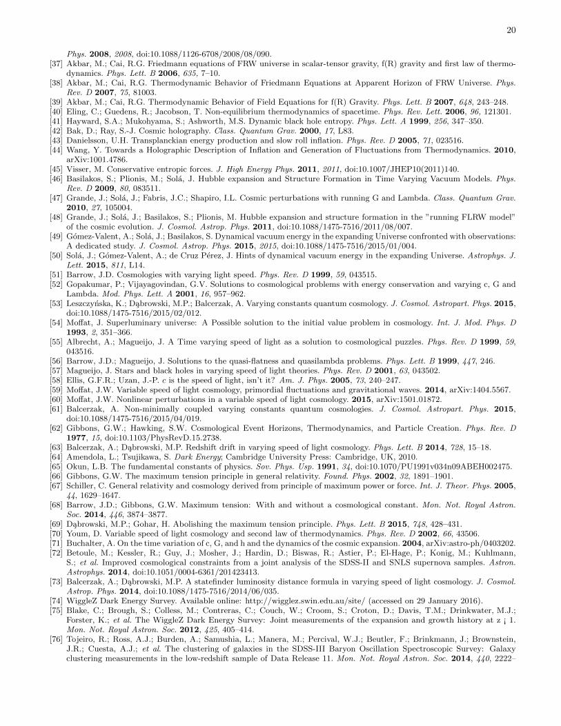
Our main result is presented in Figure 1. The first novelty is that we have found the observational bounds on theHawking temperature coefficient γ which (on the theoretical basis) was usually taken to the order of unity O(1). Ourevaluation gives that it should be of the order of 10−2 − 10−4. This difference is not unexpected, because the O(1)estimation was based on purely theoretical considerations, with no previous connection to data. Now, we show thatobservations are not consistent with such large values of γ. Instead, it is at least two orders of magnitude less. Thus,the entropic force in the model we have considered gives only a small contribution. Similar results were obtained in[46, 49]. Another novelty is the bound on the variability of the speed of light c and the gravitational constant G.According to them, in the entropic scenario we have investigated both G (Figure 1, left panel) and c (Figure 1, rightpanel) should be increasing with the evolution of the universe. Bearing in mind that the speed of light is related tothe inverse of the fine structure constant defined as

α =e2

~c, (VIII.135)

where e is the electron charge and ~ is the Planck constant, by using (IV.33) and (VIII.135) one has

∆c

c= −∆α

α= n

∆a

a∼ n

10, (VIII.136)

then one can derive from Table I and Figure 1 that the change in c and so in α (∆α/α0) from our fit is ∼ 10−5 in aredshift range [1; 2] (n = 4.9 × 10−4 > 0), while other observational bounds, in the same range (see Table II of [85]which is based on [86–89]), give ∆α/α0 ∼ 10−6. However, our estimation is still compatible with other cosmologicalconstraints, as the ones derived from CMB Planck first release (see [90]). Moreover, recent observations show thatboth positive and negative values of n are possible (the so-called α−dipole [91]). Similarly, we can evaluate the range ofchange of G. From Table I, we can also find the evaluation for q = 0.048, and this can be translated onto the constraintfrom the relation (IV.33) using the current value of the Hubble constant as (G/G)0 = qH0 ∼ 3.42× 10−12 year−1.

18

This is within the Solar System bound coming from Viking landers on Mars [92] (G/G)0 = (2± 4)× 10−12 year−1

though weaker than the bound from the Lunar laser ranging [93] (G/G)0 = (4±9)×10−13 year−1 (for a more detailedreview, see [94]).

Finally, we can enumerate some general conclusions as follows:

• the entropic scenario plus varying c and/or G is quite indistinguishable from a pure-ΛCDM model, that is whywe call it an entropic-ΛCDM model. Present data is still unable to differentiate between the two scenarios;

• the model obtained (entropic-ΛCDM cosmology) is a variation of the exchange of energy between vacuum andmatter model studied in [46, 48, 49].

• the best fit for the value of the Hawking temperature coefficient γ is quite different from the theoretical valuesused in literature, i.e., γ = 3/(2π) or 1/2; it should be pointed out that other considered entropic scenarios havethe values of O(1) (e.g., [25]);

• the model with small values of the parameter γ is equivalent to a dynamical vacuum model with small variationof the vacuum energy studied in [46, 49];

• the value for γ is compatible with zero since we were able to put only an upper limit to it. This would meanthat the Hawking temperature was zero for the models under study;

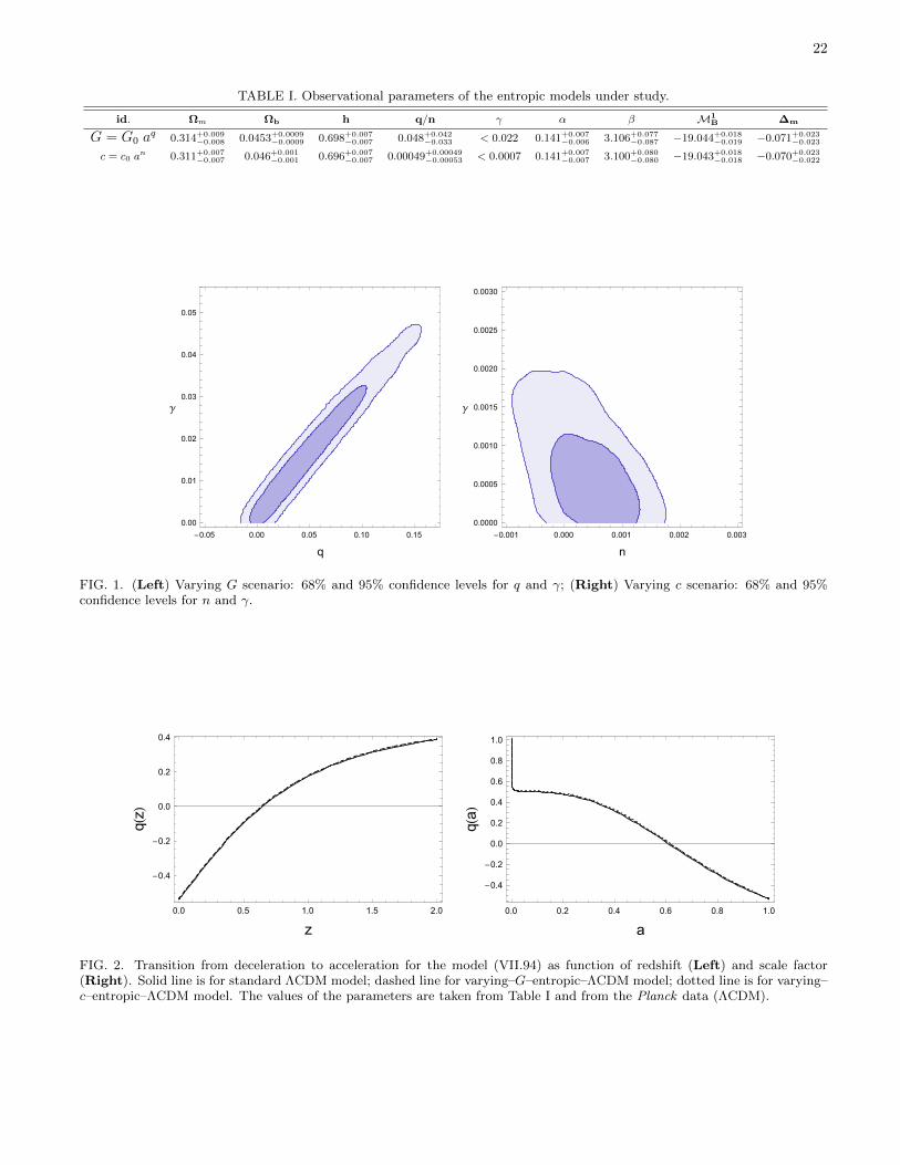
• it is also clear that we still have the deceleration-acceleration transition, as we show in the plot of the relationfor q(z) and also for q(a) in Figure 2, where our models are compared with a standard ΛCDM resulting in being,as said above, barely distinguishable.

The models we have studied here involve a mixture of matter and the dark energy fluid which is typically the energyof vacuums with small modifications due to the variability of c and G. This means that the discussion of the structureformation problem (perturbation equations, the formation of the structures, linear growth rate) is similar to those ofdynamical vacuum models given in [48], with γ parameter here being analogous to ν parameter of that reference. Infact, the models the models III and IV of [48] are indistinguishable from ΛCDM while the models I and II exhibitsome difference what can be seen from Figure 1 of [48], where the density contrast and the linear growth rate ofclustering are shown.

IX. CONCLUSIONS

In this paper, we extended the entropic cosmology onto the framework of the theories with varying gravitationalconstant G and varying speed of light c. We discussed the consequences of such variability onto the entropic forceterms and the boundary terms using three different approaches which possibly relate thermodynamics, cosmologicalhorizons and gravity. We started with a general set of the field equations which described varying constants’ entropiccosmology with a general form of the entropic terms. In the first approach, we derived the continuity equation fromthe first law of thermodynamics, Bekenstein entropy, as well as Hawking temperature to fit the general entropicterms to this continuity equation. We found appropriate single-fluid accelerating cosmological solutions to these fieldequations. We also discussed the constraints on the models which come from the second law of thermodynamics. Inthe second approach, we derived the entropic force for varying constants, defined the entropic pressure, and finallymodified the continuity and the acceleration equations. Then, we determined the Friedmann equation and gavesingle-fluid accelerating cosmological solutions as well. Finally, in the third approach, we got gravitational Einsteinfield equations using the heat flow through the horizon to which Bekenstein entropy and Hawking temperature wereassigned.

We have also examined some of the many-fluid (first accelerating and then decelerating) entropic models againstobservational data (supernovae, BAO, and CMB). We have used data from JLA compilation of SDSS-II and SNLScollaboration (supernovae), WiggleZ Dark Energy Survey and SDSS-III Baryon Oscillation Spectroscopic Survey(BOSS) as well as Planck data (CMB). We found that the observational bound on the Hawking temperature coefficientγ was much smaller (10−2 − 10−4) than it is usually assumed to be on the theoretical basis to be of order of unityO(1). We have also found that in our entropic models G should be diminishing while c should be increasing withthe evolution of the universe. Our bound on the variation of c being ∆c/c ∼ 10−5 is at least one order of magnitudeweaker than observational bound obtained from analysis of the quasar spectra.

19

ACKNOWLEDGMENTS

Acknowledgments: This project was financed by the Polish National Science Center Grant DEC-2012/06/A/ST2/00395.

[1] Ellis, G.F.R.; Maartens, R.; MacCallum, M.A.H. Relativistic Cosmology; Cambridge University Press: Cambridge, UK,2012.

[2] Perlmutter, S.; Aldering, G.; Goldhaber, G.; Knop, R.A.; Nugent, P.; Castro, P.G.; Deustua, S.; Fabbro, S.; Goobar, A.;Groom, D.E.; et al. Measurements of Omega and Lambda from 42 high redshift supernovae. Astrophys. J. 1999, 517,565–586.

[3] Riess, A.G.; Filippenko, A.V.; Challis, P.; Clocchiattia, A.; Diercks, A.; Garnavich, P.M.; Gilliland, R.L.; Hogan, C.J.; Jha,S.; Kirshner R.P.; et al. Observational evidence from supernovae for an accelerating universe and a cosmological constant.Astron. J. 1998, 116, 1009–1038.

[4] Peebles, P.J.E.Tests of cosmological models constrained by inflation. Astrophys. J. 1984, 284, 439–444.[5] Kofman, L.A.; Starobinsky, A.A. Effect of the cosmological constant on large-scale anisotropies in the microwave back-

ground. Sov. Astron. Lett. 1985, 11, 271–274.[6] Dabrowski, M.P.; Stelmach, J. Analytic Solutions of Friedman Equation for Spatially Opened Universes with Cosmological,

Constant and Radiation Pressure. J. Ann. Phys. 1986, 166, 422–442.[7] Weinberg, S. The cosmological constant problem. Rev. Mod. Phys. 1989, 61, doi:10.1103/RevModPhys.61.1.[8] Miao, L.; Dong, L.X.; Shuang, W.; Yi, W. Dark Energy. Commun. Theor. Phys. 2011, 56, 525–604.[9] Bamba, K.; Capozziello, S.; Nojiri, S.; Odintsov, S.D. Dark energy cosmology: The equivalent description via different

theoretical models and cosmography tests. Astrophys. Space Sci. 2012, 342, 155–228.[10] Bekenstein, J.D. Black holes and entropy. Phys. Rev. D 1973, 7, 2333–2346.[11] Bekenstein, J.D. Generalized second law of thermodynamics in black hole physics. Phys. Rev. D 1974, 9, 3292–3300.[12] Bekenstein, J.D. Statistical Black Hole Thermodynamics. Phys. Rev. D 1975, 12, 3077–3085.[13] Hawking, S.W. Black hole explosions. Nature 1974, 248, 30–31.[14] Jacobson, T. Thermodynamics of space-time: The Einstein equation of state. Phys. Rev. Lett. 1995, 75, 1260–1263.[15] Verlinde, E.J. On the Origin of Gravity and the Laws of Newton. J. High Energy Phys. 2011, 2011, 1–27.[16] Padmanabhan, T. Gravitational entropy of static space-times and microscopic density of states. Class. Quant. Grav. 2004,

21, 4485–4494.[17] Padmanabhan, T. Thermodynamical Aspects of Gravity: New Insights .Rep. Prog. Phys. 2010, 73, 046901.[18] Padmanabhan, T. Equipartition of energy in the horizon degrees of freedom and the emergence of gravity. Mod. Phys.

Lett. A 2010, 25, 1129–1136.[19] Hooft, G.’t Dimensional reduction in quantum gravity. 1993, arXiv:gr-qc/9310026.[20] Kobakhidze, A. Gravity is not an entropic force. Phys. Rev. D 2011, 83, 021502.[21] Komatsu, N.; Kimura, S. Non-adiabatic-like accelerated expansion of the late universe in entropic cosmology. Phys. Rev.

D 2013, 87, 043531.[22] Komatsu, N.; Kimura, S. Entropic cosmology for a generalized black-hole entropy. Phys. Rev. D 2014, 88, 083534.[23] Komatsu, N.; Kimura, S. Evolution of the universe in entropic cosmologies via different formulations. Phys. Rev. D 2014,

89, 123501.[24] Komatsu, N. Entropic cosmology from a thermodynamics viewpoint. In Proceedings of the 12th Asia Pacific Physics

Conference (APPC12), Kanazawa, Japan, 14–19 July 2013.[25] Cai, Y.F.; Liu, J.; Li, H. Entropic cosmology: A unified model of inflation and late-time acceleration. Phys. Lett. B 2010,

690, 213–219.[26] Cai, Y.F.; Saridakis, E.N. Inflation in Entropic Cosmology: Primordial Perturbations and non-Gaussianities. Phys. Lett.

B 2011, 697, 280–287.[27] Qiu, T.; Saridakis, E.N. Entropic Force Scenarios and Eternal Inflation. Phys. Rev. D 2012, 85, 043504.[28] Easson, D.A.; Frampton, P.H.; Smoot, G.F. Entropic Accelerating Universe. Phys. Lett. B 2011, 696, 273–277.[29] Easson, D.A.; Frampton, P.H.; Smoot, G.F. Entropic Inflation. Int. J. Mod. Phys. A 2012, 27, 125066.[30] Koivisto, T.S.; Mota, D.F.; Zumalacarrequi, M. Constraining entropic cosmology. J. Cosmol. Astrop. Phys. 2011, 2011,

27.[31] Basilakos, S.; Polarski, D.; Sola, J. Generalizing the running vacuum energy model and comparing with the entropic-force

models. Phys. Rev. D 2012, 86, 043010.[32] Basilakos, S.; Sola, J. Entropic-force dark energy reconsidered. Phys. Rev. D 2014, 90, 023008.[33] Gomez-Valent, A.; Sola, J. Vacuum models with a linear and a quadratic term in H: Structure formation and number

counts analysis. Mon. Not. Roy. Astron. Soc. 2015, 448, 2810–2821.[34] Cai, R.G.; Kim, S.P. First law of thermodynamics and Friedmann equations of Friedmann-Robertson-Walker universe. J.

High Energy Phys. 2005, doi:10.1088/1126-6708/2005/02/050.[35] Cai, R.G.; Cao, L.M. Unified first law and thermodynamics of apparent horizon in FRW universe. Phys. Rev. D 2007, 75,

064008.[36] Cai, R.G.; Cao, L.M.; Hu, Y.P. Corrected Entropy-Area Relation and Modified Friedmann Equations. J. High Energy

20

Phys. 2008, 2008, doi:10.1088/1126-6708/2008/08/090.[37] Akbar, M.; Cai, R.G. Friedmann equations of FRW universe in scalar-tensor gravity, f(R) gravity and first law of thermo-

dynamics. Phys. Lett. B 2006, 635, 7–10.[38] Akbar, M.; Cai, R.G. Thermodynamic Behavior of Friedmann Equations at Apparent Horizon of FRW Universe. Phys.

Rev. D 2007, 75, 81003.[39] Akbar, M.; Cai, R.G. Thermodynamic Behavior of Field Equations for f(R) Gravity. Phys. Lett. B 2007, 648, 243–248.[40] Eling, C.; Guedens, R.; Jacobson, T. Non-equilibrium thermodynamics of spacetime. Phys. Rev. Lett. 2006, 96, 121301.[41] Hayward, S.A.; Mukohyama, S.; Ashworth, M.S. Dynamic black hole entropy. Phys. Lett. A 1999, 256, 347–350.[42] Bak, D.; Ray, S.-J. Cosmic holography. Class. Quantum Grav. 2000, 17, L83.[43] Danielsson, U.H. Transplanckian energy production and slow roll inflation. Phys. Rev. D 2005, 71, 023516.[44] Wang, Y. Towards a Holographic Description of Inflation and Generation of Fluctuations from Thermodynamics. 2010,

arXiv:1001.4786.[45] Visser, M. Conservative entropic forces. J. High Energy Phys. 2011, 2011, doi:10.1007/JHEP10(2011)140.[46] Basilakos, S.; Plionis, M.; Sola, J. Hubble expansion and Structure Formation in Time Varying Vacuum Models. Phys.

Rev. D 2009, 80, 083511.[47] Grande, J.; Sola, J.; Fabris, J.C.; Shapiro, I.L. Cosmic perturbations with running G and Lambda. Class. Quantum Grav.

2010, 27, 105004.[48] Grande, J.; Sola, J.; Basilakos, S.; Plionis, M. Hubble expansion and structure formation in the ”running FLRW model”

of the cosmic evolution. J. Cosmol. Astrop. Phys. 2011, doi:10.1088/1475-7516/2011/08/007.[49] Gomez-Valent, A.; Sola, J.; Basilakos, S. Dynamical vacuum energy in the expanding Universe confronted with observations:

A dedicated study. J. Cosmol. Astrop. Phys. 2015, 2015, doi:10.1088/1475-7516/2015/01/004.[50] Sola, J.; Gomez-Valent, A.; de Cruz Perez, J. Hints of dynamical vacuum energy in the expanding Universe. Astrophys. J.

Lett. 2015, 811, L14.[51] Barrow, J.D. Cosmologies with varying light speed. Phys. Rev. D 1999, 59, 043515.[52] Gopakumar, P.; Vijayagovindan, G.V. Solutions to cosmological problems with energy conservation and varying c, G and

Lambda. Mod. Phys. Lett. A 2001, 16, 957–962.[53] Leszczynska, K.; Dabrowski, M.P.; Balcerzak, A. Varying constants quantum cosmology. J. Cosmol. Astropart. Phys. 2015,

doi:10.1088/1475-7516/2015/02/012.[54] Moffat, J. Superluminary universe: A Possible solution to the initial value problem in cosmology. Int. J. Mod. Phys. D

1993, 2, 351–366.[55] Albrecht, A.; Magueijo, J. A Time varying speed of light as a solution to cosmological puzzles. Phys. Rev. D 1999, 59,

043516.[56] Barrow, J.D.; Magueijo, J. Solutions to the quasi-flatness and quasilambda problems. Phys. Lett. B 1999, 447, 246.[57] Magueijo, J. Stars and black holes in varying speed of light theories. Phys. Rev. D 2001, 63, 043502.[58] Ellis, G.F.R.; Uzan, J.-P. c is the speed of light, isn’t it? Am. J. Phys. 2005, 73, 240–247.[59] Moffat, J.W. Variable speed of light cosmology, primordial fluctuations and gravitational waves. 2014, arXiv:1404.5567.[60] Moffat, J.W. Nonlinear perturbations in a variable speed of light cosmology. 2015, arXiv:1501.01872.[61] Balcerzak, A. Non-minimally coupled varying constants quantum cosmologies. J. Cosmol. Astropart. Phys. 2015,

doi:10.1088/1475-7516/2015/04/019.[62] Gibbons, G.W.; Hawking, S.W. Cosmological Event Horizons, Thermodynamics, and Particle Creation. Phys. Rev. D

1977, 15, doi:10.1103/PhysRevD.15.2738.[63] Balcerzak, A.; Dabrowski, M.P. Redshift drift in varying speed of light cosmology. Phys. Lett. B 2014, 728, 15–18.[64] Amendola, L.; Tsujikawa, S. Dark Energy; Cambridge University Press: Cambridge, UK, 2010.[65] Okun, L.B. The fundamental constants of physics. Sov. Phys. Usp. 1991, 34, doi:10.1070/PU1991v034n09ABEH002475.[66] Gibbons, G.W. The maximum tension principle in general relativity. Found. Phys. 2002, 32, 1891–1901.[67] Schiller, C. General relativity and cosmology derived from principle of maximum power or force. Int. J. Theor. Phys. 2005,

44, 1629–1647.[68] Barrow, J.D.; Gibbons, G.W. Maximum tension: With and without a cosmological constant. Mon. Not. Royal Astron.

Soc. 2014, 446, 3874–3877.[69] Dabrowski, M.P.; Gohar, H. Abolishing the maximum tension principle. Phys. Lett. B 2015, 748, 428–431.[70] Youm, D. Variable speed of light cosmology and second law of thermodynamics. Phys. Rev. D 2002, 66, 43506.[71] Buchalter, A. On the time variation of c, G, and h and the dynamics of the cosmic expansion. 2004, arXiv:astro-ph/0403202.[72] Betoule, M.; Kessler, R.; Guy, J.; Mosher, J.; Hardin, D.; Biswas, R.; Astier, P.; El-Hage, P.; Konig, M.; Kuhlmann,

S.; et al. Improved cosmological constraints from a joint analysis of the SDSS-II and SNLS supernova samples. Astron.Astrophys. 2014, doi:10.1051/0004-6361/201423413.

[73] Balcerzak, A.; Dabrowski, M.P. A statefinder luminosity distance formula in varying speed of light cosmology. J. Cosmol.Astrop. Phys. 2014, doi:10.1088/1475-7516/2014/06/035.

[74] WiggleZ Dark Energy Survey. Available online: http://wigglez.swin.edu.au/site/ (accessed on 29 January 2016).[75] Blake, C.; Brough, S.; Colless, M.; Contreras, C.; Couch, W.; Croom, S.; Croton, D.; Davis, T.M.; Drinkwater, M.J.;

Forster, K.; et al. The WiggleZ Dark Energy Survey: Joint measurements of the expansion and growth history at z ¡ 1.Mon. Not. Royal Astron. Soc. 2012, 425, 405–414.

[76] Tojeiro, R.; Ross, A.J.; Burden, A.; Samushia, L.; Manera, M.; Percival, W.J.; Beutler, F.; Brinkmann, J.; Brownstein,J.R.; Cuesta, A.J.; et al. The clustering of galaxies in the SDSS-III Baryon Oscillation Spectroscopic Survey: Galaxyclustering measurements in the low-redshift sample of Data Release 11. Mon. Not. Royal Astron. Soc. 2014, 440, 2222–

21

2237.[77] Anderson, L.; Aubourg, E.; Bailey, S.; Beutler, F.; Bhardwaj, V.; Blanton, M.; Bolton, A.S.; Brinkmann, J.; Brownstein,

J.R.; Burden, A.; et al. The clustering of galaxies in the SDSS-III Baryon Oscillation Spectroscopic Survey: Baryon acousticoscillations in the Data Releases 10 and 11 Galaxy samples. Mon. Not. Royal Astron. Soc. 2014, 441, 24–62.

[78] Eisenstein, D.; Hu, W. Baryonic Features in the Matter Transfer Function. Astrophys. J. 1998, 496, doi:10.1086/305424.[79] Font-Ribera, A.; Kirkby, D.; Busca, N.; Miralda-Escude, J.; Ross, N.P.; Slosar, A.; Rich, J.; Aubourg, E.; Bailey, S.;

Bhardwaj, V.; et al. Quasar-Lyman α forest cross-correlation from BOSS DR11: Baryon Acoustic Oscillations. J. Cosmol.Astropart. Phys. 2014, 2014, doi:10.1088/1475-7516/2014/05/027.

[80] Wang, Y.; Wang, S. Distance priors from Planck and dark energy constraints from current data. Phys. Rev. D 2013, 88,043522.

[81] Wang, Y.; Mukherjee, P. Observational constraints on dark energy and cosmic curvature. Phys. Rev. D 2007, 76,doi:10.1103/PhysRevD.76.103533.

[82] Hu, W.; Sugiyama, N. Small-Scale Cosmological Perturbations: An Analytic Approach. Astrophys. J. 1996, 471,doi:10.1086/177989.

[83] Bennett, C.L.; Larson, D.; Weiland, J.L.; Hinshaw, G. The 1% Concordance Hubble Constant. Astrophys. J. 2014, 794,doi:10.1088/0004-637X/794/2/135.

[84] Komatsu, E.; Dunkley, J.; Nolta, M.R.; Bennett, C.L.; Gold, B.; Hinshaw, G.; Jarosik, N.; Larson, D.; Limon, M.; Page, L.;et al. Five-Year Wilkinson Microwave Anisotropy Probe Observations: Cosmological Interpretation. Astrophys. J. Suppl.Ser. 2009, 180, 330–376.

[85] Dabrowski, M.P.; Denkiewicz, T.; Martins, C.J.A.P.; Vielzeuf, P. Variations of the fine-structure constant α in exoticsingularity models. Phys. Rev. D 2014, 89, 123512.

[86] Molaro, P.; Centurion, M.; Whitmore, J.B.; Evans, T.M.; Murphy, M.T.; Agafonova, I.I.: Bonifacio, P.; D’Odorico, S.;Levshakov, S.A.; Lopez, S.; et al. The UVES Large Program for Testing Fundamental Physics: I Bounds on a change inα towards quasar HE 2217–2818. Astron. Astrophys. 2013, doi:10.1051/0004-6361/201321351 .

[87] Molaro, P.; Reimers, D.; Agafonova, I.I.; Levshakov, S.A. Bounds on the fine structure constant variability from Fe IIabsorption lines in QSO spectra. Eur. Phys. J. Spec. Top. 2008, 163, 173–189.

[88] Chand, H.; Srianad, R.; Petitjean, P.; Aracil, B.; Quast, R.; Reimers, D. On the variation of the fine-structure constant:Very high resolution spectrum of QSO HE 0515-4414. Astron. Astrophys. 2006, 451, 45–56.

[89] Agafonova, I.I.; Molaro, P.; Levshakov, S.A. First measurement of Mg isotope abundances at high redshifts and accurateestimate of ∆α/α. Astron. Astrophys. 2011, doi:10.1051/0004-6361/201016194.

[90] O’Brian, J.; Smidt, J.; de Bernardis, F.; Cooray, A. Constraints on Spatial Variations in the Fine-Structure constantfrom Planck. Astrophys. J. 2015, doi:10.1088/0004-637X/798/1/18.

[91] Webb, J.K.; King, J.A.; Murphy, M.T.; Flambaum, V.V.; Carswell, R.F.; Bainbridge, M.B. Indications of a spatialvariation of the fine structure constant. Phys. Rev. Lett. 2011, 107, 191101.

[92] Hellings, R.W.; Adams, P.J.; Anderson, J.D.; Keesey, M.S.; Lau, E.L.; Standish, E.M.; Canuto,V.M.; Goldman, I. Experimental Test of the Variability of G Using Viking Lander Ranging Data. Phys. Rev. Lett. 1983,51, doi:10.1103/PhysRevLett.51.1609.

[93] Williams, J.G.; Turyshev, S.G.; Boggs, D.H. Progress in lunar laser ranging tests of relativistic gravity. Phys. Rev. Lett.2004, 93, 26101.

[94] Uzan, J.-P. Varying constants, gravitation, and cosmology. Liv. Rev. Rel. 2011, 14, doi:10.12942/lrr-2011-2.

22

TABLE I. Observational parameters of the entropic models under study.

id. Ωm Ωb h q/n γ α β M1B ∆m

G = G0 aq 0.314+0.009

−0.008 0.0453+0.0009−0.0009 0.698+0.007

−0.007 0.048+0.042−0.033 < 0.022 0.141+0.007

−0.006 3.106+0.077−0.087 −19.044+0.018

−0.019 −0.071+0.023−0.023

c = c0 an 0.311+0.007

−0.007 0.046+0.001−0.001 0.696+0.007

−0.007 0.00049+0.00049−0.00053 < 0.0007 0.141+0.007

−0.007 3.100+0.080−0.080 −19.043+0.018

−0.018 −0.070+0.023−0.022

-0.05 0.00 0.05 0.10 0.15

0.00

0.01

0.02

0.03

0.04

0.05

q

g

-0.001 0.000 0.001 0.002 0.003

0.0000

0.0005

0.0010

0.0015

0.0020

0.0025

0.0030

n

g

FIG. 1. (Left) Varying G scenario: 68% and 95% confidence levels for q and γ; (Right) Varying c scenario: 68% and 95%confidence levels for n and γ.

0.0 0.5 1.0 1.5 2.0

-0.4

-0.2

0.0

0.2

0.4

z

qHzL

0.0 0.2 0.4 0.6 0.8 1.0

-0.4

-0.2

0.0

0.2

0.4

0.6

0.8

1.0

a

qHaL

FIG. 2. Transition from deceleration to acceleration for the model (VII.94) as function of redshift (Left) and scale factor(Right). Solid line is for standard ΛCDM model; dashed line for varying–G–entropic–ΛCDM model; dotted line is for varying–c–entropic–ΛCDM model. The values of the parameters are taken from Table I and from the Planck data (ΛCDM).