Hierarchical Spatial Models

Ali Arab, Mevin B. Hooten, Christopher K. Wikle

Department of Statistics,

University of Missouri-Columbia

June 2006

Introduction

Methods for spatial and spatio-temporal modeling are becoming increasingly impor-

tant in environmental sciences and other sciences where data arise from a process

in an inherent spatial setting. Technological advances in remote sensing, monitor-

ing networks, and other methods of collecting spatial data in recent decades have

revolutionized scientific endeavor in fields such as agriculture, climatology, ecology,

economics, transportation, epidemiology and health management, as well as many

other areas. However, such technological advancements require a parallel effort in

the development of techniques that enable researchers to make rigorous statistical

inference given the wealth of new information at hand. Unfortunately, the applica-

tion of traditional covariance-based spatial statistical models is either inappropriate

or computationally inefficient in many cases. Moreover, conventional methods are

often incapable of allowing the researcher to quantify uncertainities corresponding to

the model parameters since the parameter space of most complex spatial and spatio-

temporal models is very large.

1

Hierarchical Models

A main goal in the rigorous characterization of natural phenomena is the estimation

and prediction of processes as well as the parameters governing processes. Thus a

flexible framework capable of accommodating complex relationships between data

and process models while incorporating various sources of uncertainty is necessary.

Traditional likelihood based approaches to modeling have allowed for scientifically

meaningful data structures, though, in complicated situations with heavily parame-

terized models and limited or missing data, estimation by likelihood maximization

is often problematic or infeasible (Hilborn and Mangel 1997). Developments in nu-

merical approximation methods have been useful in many cases, especially for high-

dimensional parameter spaces (e.g., Newton-Raphson and E-M methods, Givens and

Hoeting 2005), though can still be difficult or impossible to implement and have no

provision for accommodating uncertainty at multiple levels.

Hierarchical models, whereby a problem is decomposed into a series of levels linked

by simple rules of probability, assume a very flexible framework capable of accommo-

dating uncertainty and potential a priori scientific knowledge while retaining many

advantages of a strict likelihood approach (e.g., multiple sources of data and scientifi-

cally meaningful structure). The years after introduction of the Bayesian hierarchical

model and development of MCMC (i.e., Markov Chain Monte Carlo) have brought on

an explosion of research, both theoretical and applied, utilizing and (or) developing

hierarchical models.

Hierarchical modeling is based on a simple fact from probability that the joint

distribution of a collection of random variables can be decomposed into a series of

conditional models. For example, if a, b, c are random variables, then basic probability

allows the factorization:

[a, b, c] = [a|b, c][b|c][c] . (1)

2

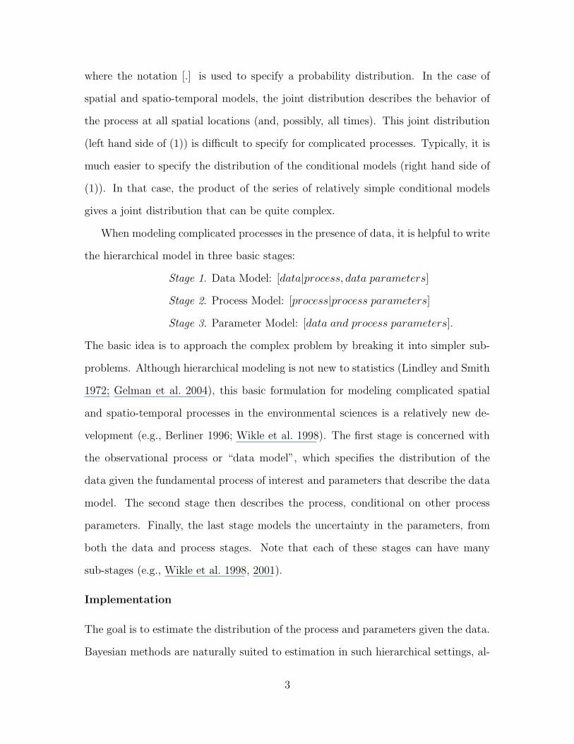
where the notation [.] is used to specify a probability distribution. In the case of

spatial and spatio-temporal models, the joint distribution describes the behavior of

the process at all spatial locations (and, possibly, all times). This joint distribution

(left hand side of (1)) is difficult to specify for complicated processes. Typically, it is

much easier to specify the distribution of the conditional models (right hand side of

(1)). In that case, the product of the series of relatively simple conditional models

gives a joint distribution that can be quite complex.

When modeling complicated processes in the presence of data, it is helpful to write

the hierarchical model in three basic stages:

Stage 1. Data Model: [data|process, data parameters]

Stage 2. Process Model: [process|process parameters]

Stage 3. Parameter Model: [data and process parameters].

The basic idea is to approach the complex problem by breaking it into simpler sub-

problems. Although hierarchical modeling is not new to statistics (Lindley and Smith

1972; Gelman et al. 2004), this basic formulation for modeling complicated spatial

and spatio-temporal processes in the environmental sciences is a relatively new de-

velopment (e.g., Berliner 1996; Wikle et al. 1998). The first stage is concerned with

the observational process or “data model”, which specifies the distribution of the

data given the fundamental process of interest and parameters that describe the data

model. The second stage then describes the process, conditional on other process

parameters. Finally, the last stage models the uncertainty in the parameters, from

both the data and process stages. Note that each of these stages can have many

sub-stages (e.g., Wikle et al. 1998, 2001).

Implementation

The goal is to estimate the distribution of the process and parameters given the data.

Bayesian methods are naturally suited to estimation in such hierarchical settings, al-

3

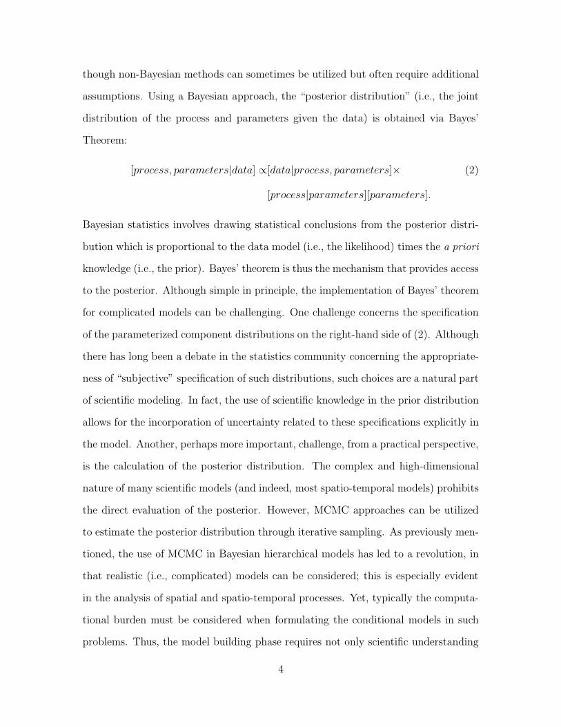
though non-Bayesian methods can sometimes be utilized but often require additional

assumptions. Using a Bayesian approach, the “posterior distribution” (i.e., the joint

distribution of the process and parameters given the data) is obtained via Bayes’

Theorem:

[process, parameters|data] ∝[data|process, parameters]× (2)

[process|parameters][parameters].

Bayesian statistics involves drawing statistical conclusions from the posterior distri-

bution which is proportional to the data model (i.e., the likelihood) times the a priori

knowledge (i.e., the prior). Bayes’ theorem is thus the mechanism that provides access

to the posterior. Although simple in principle, the implementation of Bayes’ theorem

for complicated models can be challenging. One challenge concerns the specification

of the parameterized component distributions on the right-hand side of (2). Although

there has long been a debate in the statistics community concerning the appropriate-

ness of “subjective” specification of such distributions, such choices are a natural part

of scientific modeling. In fact, the use of scientific knowledge in the prior distribution

allows for the incorporation of uncertainty related to these specifications explicitly in

the model. Another, perhaps more important, challenge, from a practical perspective,

is the calculation of the posterior distribution. The complex and high-dimensional

nature of many scientific models (and indeed, most spatio-temporal models) prohibits

the direct evaluation of the posterior. However, MCMC approaches can be utilized

to estimate the posterior distribution through iterative sampling. As previously men-

tioned, the use of MCMC in Bayesian hierarchical models has led to a revolution, in

that realistic (i.e., complicated) models can be considered; this is especially evident

in the analysis of spatial and spatio-temporal processes. Yet, typically the computa-

tional burden must be considered when formulating the conditional models in such

problems. Thus, the model building phase requires not only scientific understanding

4

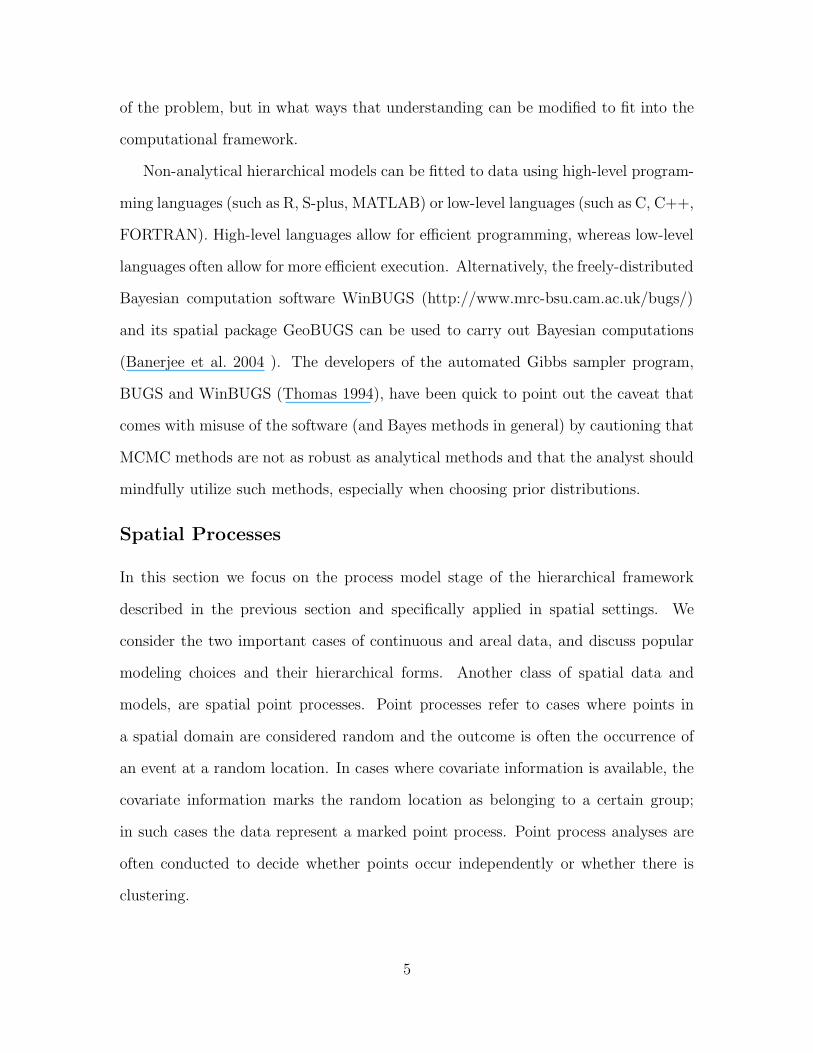
of the problem, but in what ways that understanding can be modified to fit into the

computational framework.

Non-analytical hierarchical models can be fitted to data using high-level program-

ming languages (such as R, S-plus, MATLAB) or low-level languages (such as C, C++,

FORTRAN). High-level languages allow for efficient programming, whereas low-level

languages often allow for more efficient execution. Alternatively, the freely-distributed

Bayesian computation software WinBUGS (http://www.mrc-bsu.cam.ac.uk/bugs/)

and its spatial package GeoBUGS can be used to carry out Bayesian computations

(Banerjee et al. 2004 ). The developers of the automated Gibbs sampler program,

BUGS and WinBUGS (Thomas 1994), have been quick to point out the caveat that

comes with misuse of the software (and Bayes methods in general) by cautioning that

MCMC methods are not as robust as analytical methods and that the analyst should

mindfully utilize such methods, especially when choosing prior distributions.

Spatial Processes

In this section we focus on the process model stage of the hierarchical framework

described in the previous section and specifically applied in spatial settings. We

consider the two important cases of continuous and areal data, and discuss popular

modeling choices and their hierarchical forms. Another class of spatial data and

models, are spatial point processes. Point processes refer to cases where points in

a spatial domain are considered random and the outcome is often the occurrence of

an event at a random location. In cases where covariate information is available, the

covariate information marks the random location as belonging to a certain group;

in such cases the data represent a marked point process. Point process analyses are

often conducted to decide whether points occur independently or whether there is

clustering.

5

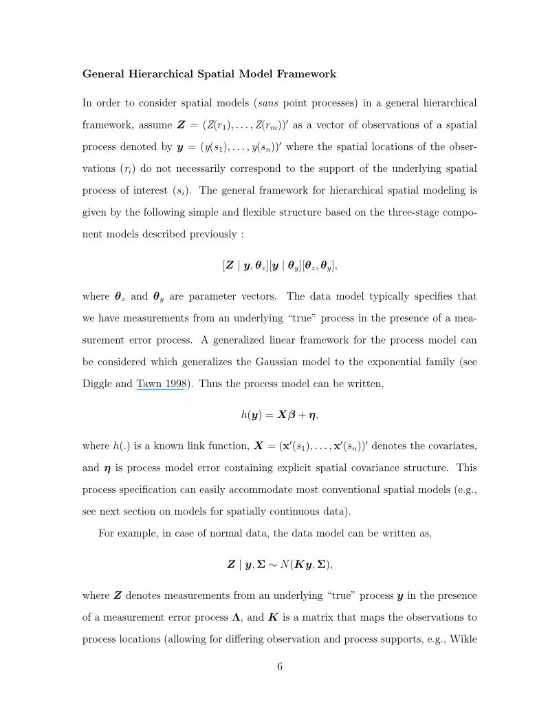
General Hierarchical Spatial Model Framework

In order to consider spatial models (sans point processes) in a general hierarchical

framework, assume Z = (Z(r1), . . . ,Z(rm))′ as a vector of observations of a spatial

process denoted by y = (y(s1), . . . , y(sn))′ where the spatial locations of the obser-

vations (ri) do not necessarily correspond to the support of the underlying spatial

process of interest (si). The general framework for hierarchical spatial modeling is

given by the following simple and flexible structure based on the three-stage compo-

nent models described previously :

[Z | y, θz][y | θy][θz, θy],

where θz and θy are parameter vectors. The data model typically specifies that

we have measurements from an underlying “true” process in the presence of a mea-

surement error process. A generalized linear framework for the process model can

be considered which generalizes the Gaussian model to the exponential family (see

Diggle and Tawn 1998). Thus the process model can be written,

h(y) = Xβ + η,

where h(.) is a known link function, X = (x′(s1), . . . ,x′(sn))′ denotes the covariates,

and η is process model error containing explicit spatial covariance structure. This

process specification can easily accommodate most conventional spatial models (e.g.,

see next section on models for spatially continuous data).

For example, in case of normal data, the data model can be written as,

Z | y,Σ ∼ N(Ky,Σ),

where Z denotes measurements from an underlying “true” process y in the presence

of a measurement error process Λ, and K is a matrix that maps the observations to

process locations (allowing for differing observation and process supports, e.g., Wikle

6

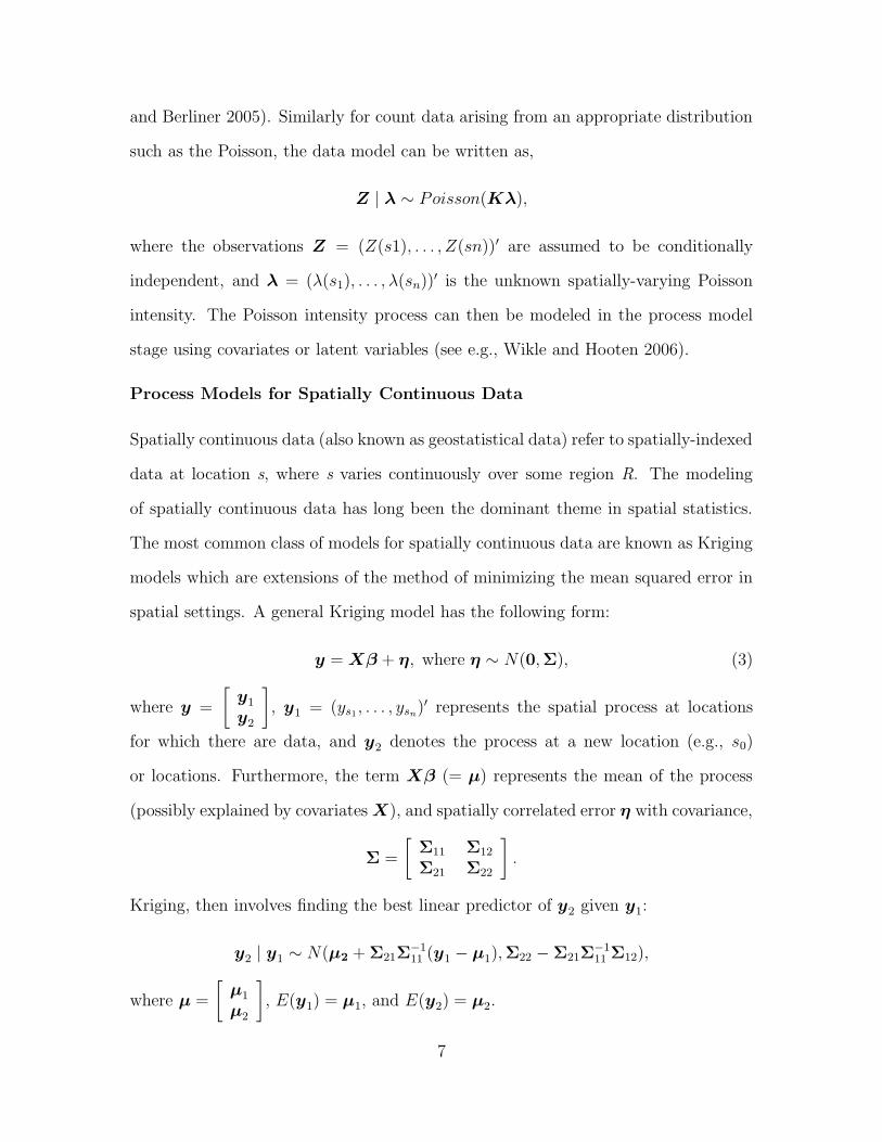
and Berliner 2005). Similarly for count data arising from an appropriate distribution

such as the Poisson, the data model can be written as,

Z | λ ∼ Poisson(Kλ),

where the observations Z = (Z(s1), . . . , Z(sn))′ are assumed to be conditionally

independent, and λ = (λ(s1), . . . , λ(sn))′ is the unknown spatially-varying Poisson

intensity. The Poisson intensity process can then be modeled in the process model

stage using covariates or latent variables (see e.g., Wikle and Hooten 2006).

Process Models for Spatially Continuous Data

Spatially continuous data (also known as geostatistical data) refer to spatially-indexed

data at location s, where s varies continuously over some region R. The modeling

of spatially continuous data has long been the dominant theme in spatial statistics.

The most common class of models for spatially continuous data are known as Kriging

models which are extensions of the method of minimizing the mean squared error in

spatial settings. A general Kriging model has the following form:

y = Xβ + η, where η ∼ N(0,Σ), (3)

where y =

[

y1

y2

]

, y1 = (ys1, . . . , ysn

)′ represents the spatial process at locations

for which there are data, and y2

denotes the process at a new location (e.g., s0)

or locations. Furthermore, the term Xβ (= µ) represents the mean of the process

(possibly explained by covariates X), and spatially correlated error η with covariance,

Σ =

[

Σ11 Σ12

Σ21 Σ22

]

.

Kriging, then involves finding the best linear predictor of y2

given y1:

y2| y

1∼ N(µ2 + Σ21Σ

−1

11(y

1− µ

1),Σ22 − Σ21Σ

−1

11Σ12),

where µ =

[

µ1

µ2

]

, E(y1) = µ1, and E(y2) = µ2.

7

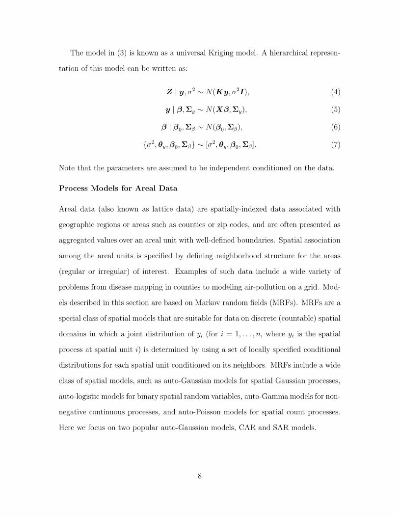
The model in (3) is known as a universal Kriging model. A hierarchical represen-

tation of this model can be written as:

Z | y, σ2 ∼ N(Ky, σ2I), (4)

y | β,Σy ∼ N(Xβ,Σy), (5)

β | β0,Σβ ∼ N(β

0,Σβ), (6)

{σ2, θy, β0,Σβ} ∼ [σ2, θy, β0

,Σβ]. (7)

Note that the parameters are assumed to be independent conditioned on the data.

Process Models for Areal Data

Areal data (also known as lattice data) are spatially-indexed data associated with

geographic regions or areas such as counties or zip codes, and are often presented as

aggregated values over an areal unit with well-defined boundaries. Spatial association

among the areal units is specified by defining neighborhood structure for the areas

(regular or irregular) of interest. Examples of such data include a wide variety of

problems from disease mapping in counties to modeling air-pollution on a grid. Mod-

els described in this section are based on Markov random fields (MRFs). MRFs are a

special class of spatial models that are suitable for data on discrete (countable) spatial

domains in which a joint distribution of yi (for i = 1, . . . , n, where yi is the spatial

process at spatial unit i) is determined by using a set of locally specified conditional

distributions for each spatial unit conditioned on its neighbors. MRFs include a wide

class of spatial models, such as auto-Gaussian models for spatial Gaussian processes,

auto-logistic models for binary spatial random variables, auto-Gamma models for non-

negative continuous processes, and auto-Poisson models for spatial count processes.

Here we focus on two popular auto-Gaussian models, CAR and SAR models.

8

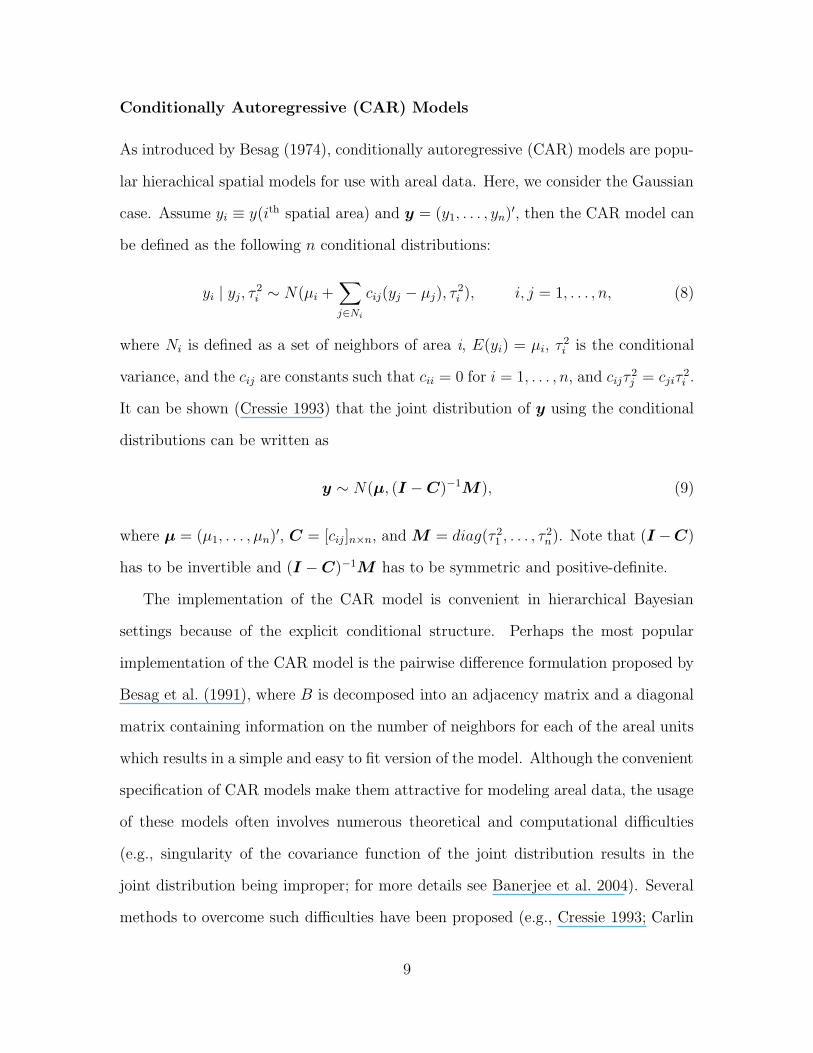
Conditionally Autoregressive (CAR) Models

As introduced by Besag (1974), conditionally autoregressive (CAR) models are popu-

lar hierachical spatial models for use with areal data. Here, we consider the Gaussian

case. Assume yi ≡ y(ith spatial area) and y = (y1, . . . , yn)′, then the CAR model can

be defined as the following n conditional distributions:

yi | yj, τ2

i ∼ N(µi +∑

j∈Ni

cij(yj − µj), τ2

i ), i, j = 1, . . . , n, (8)

where Ni is defined as a set of neighbors of area i, E(yi) = µi, τ 2

i is the conditional

variance, and the cij are constants such that cii = 0 for i = 1, . . . , n, and cijτ2

j = cjiτ2

i .

It can be shown (Cressie 1993) that the joint distribution of y using the conditional

distributions can be written as

y ∼ N(µ, (I − C)−1M ), (9)

where µ = (µ1, . . . , µn)′, C = [cij]n×n, and M = diag(τ 2

1, . . . , τ 2

n). Note that (I −C)

has to be invertible and (I − C)−1M has to be symmetric and positive-definite.

The implementation of the CAR model is convenient in hierarchical Bayesian

settings because of the explicit conditional structure. Perhaps the most popular

implementation of the CAR model is the pairwise difference formulation proposed by

Besag et al. (1991), where B is decomposed into an adjacency matrix and a diagonal

matrix containing information on the number of neighbors for each of the areal units

which results in a simple and easy to fit version of the model. Although the convenient

specification of CAR models make them attractive for modeling areal data, the usage

of these models often involves numerous theoretical and computational difficulties

(e.g., singularity of the covariance function of the joint distribution results in the

joint distribution being improper; for more details see Banerjee et al. 2004). Several

methods to overcome such difficulties have been proposed (e.g., Cressie 1993; Carlin

9

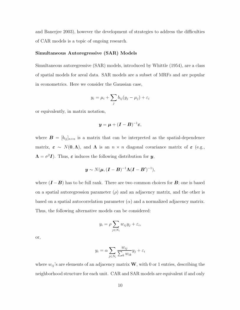
and Banerjee 2003), however the development of strategies to address the difficulties

of CAR models is a topic of ongoing research.

Simultaneous Autoregressive (SAR) Models

Simultaneous autoregressive (SAR) models, introduced by Whittle (1954), are a class

of spatial models for areal data. SAR models are a subset of MRFs and are popular

in econometrics. Here we consider the Gaussian case,

yi = µi +∑

j

bij(yj − µj) + εi

or equivalently, in matrix notation,

y = µ + (I − B)−1ε,

where B = [bij]n×n is a matrix that can be interpreted as the spatial-dependence

matrix, ε ∼ N(0,Λ), and Λ is an n × n diagonal covariance matrix of ε (e.g.,

Λ = σ2I). Thus, ε induces the following distribution for y,

y ∼ N(µ, (I − B)−1Λ(I − B ′)−1),

where (I −B) has to be full rank. There are two common choices for B; one is based

on a spatial autoregression parameter (ρ) and an adjacency matrix, and the other is

based on a spatial autocorrelation parameter (α) and a normalized adjacency matrix.

Thus, the following alternative models can be considered:

yi = ρ∑

j∈Ni

wijyj + εi,

or,

yi = α∑

j∈Ni

wij∑

k wik

yj + εi

where wij’s are elements of an adjacency matrix W, with 0 or 1 entries, describing the

neighborhood structure for each unit. CAR and SAR models are equivalent if and only

10

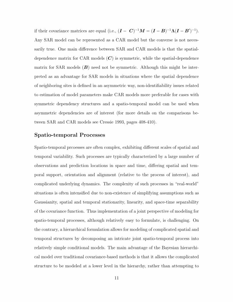
if their covariance matrices are equal (i.e., (I − C)−1M = (I − B)−1Λ(I − B′)−1).

Any SAR model can be represented as a CAR model but the converse is not neces-

sarily true. One main difference between SAR and CAR models is that the spatial-

dependence matrix for CAR models (C) is symmetric, while the spatial-dependence

matrix for SAR models (B) need not be symmetric. Although this might be inter-

preted as an advantage for SAR models in situations where the spatial dependence

of neighboring sites is defined in an asymmetric way, non-identifiability issues related

to estimation of model parameters make CAR models more preferable for cases with

symmetric dependency structures and a spatio-temporal model can be used when

asymmetric dependencies are of interest (for more details on the comparisons be-

tween SAR and CAR models see Cressie 1993, pages 408-410).

Spatio-temporal Processes

Spatio-temporal prcoesses are often complex, exhibiting different scales of spatial and

temporal variability. Such processes are typically characterized by a large number of

observations and prediction locations in space and time, differing spatial and tem-

poral support, orientation and alignment (relative to the process of interest), and

complicated underlying dynamics. The complexity of such processes in “real-world”

situations is often intensified due to non-existence of simplifying assumptions such as

Gaussianity, spatial and temporal stationarity, linearity, and space-time separability

of the covariance function. Thus implementation of a joint perspective of modeling for

spatio-temporal processes, although relatively easy to formulate, is challenging. On

the contrary, a hierarchical formulation allows for modeling of complicated spatial and

temporal structures by decomposing an intricate joint spatio-temporal process into

relatively simple conditional models. The main advantage of the Bayesian hierarchi-

cal model over traditional covariance-based methods is that it allows the complicated

structure to be modeled at a lower level in the hierarchy, rather than attempting to

11

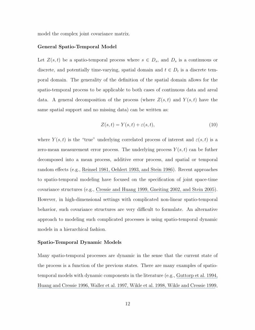
model the complex joint covariance matrix.

General Spatio-Temporal Model

Let Z(s, t) be a spatio-temporal process where s ∈ Ds, and Ds is a continuous or

discrete, and potentially time-varying, spatial domain and t ∈ Dt is a discrete tem-

poral domain. The generality of the definition of the spatial domain allows for the

spatio-temporal process to be applicable to both cases of continuous data and areal

data. A general decomposition of the process (where Z(s, t) and Y (s, t) have the

same spatial support and no missing data) can be written as:

Z(s, t) = Y (s, t) + ε(s, t), (10)

where Y (s, t) is the “true” underlying correlated process of interest and ε(s, t) is a

zero-mean measurement error process. The underlying process Y (s, t) can be futher

decomposed into a mean process, additive error process, and spatial or temporal

random effects (e.g., Reinsel 1981, Oehlert 1993, and Stein 1986). Recent approaches

to spatio-temporal modeling have focused on the specification of joint space-time

covariance structures (e.g., Cressie and Huang 1999, Gneiting 2002, and Stein 2005).

However, in high-dimensional settings with complicated non-linear spatio-temporal

behavior, such covariance structures are very difficult to formulate. An alternative

approach to modeling such complicated processes is using spatio-temporal dynamic

models in a hierarchical fashion.

Spatio-Temporal Dynamic Models

Many spatio-temporal processes are dynamic in the sense that the current state of

the process is a function of the previous states. There are many examples of spatio-

temporal models with dynamic components in the literature (e.g., Guttorp et al. 1994,

Huang and Cressie 1996, Waller et al. 1997, Wikle et al. 1998, Wikle and Cressie 1999,

12

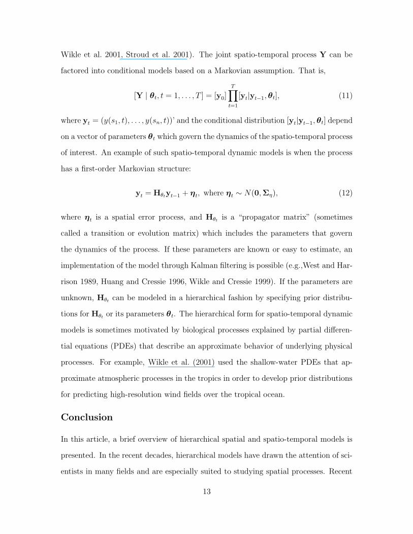
Wikle et al. 2001, Stroud et al. 2001). The joint spatio-temporal process Y can be

factored into conditional models based on a Markovian assumption. That is,

[Y | θt, t = 1, . . . , T ] = [y0]

T∏

t=1

[yt|yt−1, θt], (11)

where yt = (y(s1, t), . . . , y(sn, t))’ and the conditional distribution [yt|yt−1, θt] depend

on a vector of parameters θt which govern the dynamics of the spatio-temporal process

of interest. An example of such spatio-temporal dynamic models is when the process

has a first-order Markovian structure:

yt = Hθtyt−1

+ ηt, where ηt ∼ N(0,Ση), (12)

where ηt is a spatial error process, and Hθtis a “propagator matrix” (sometimes

called a transition or evolution matrix) which includes the parameters that govern

the dynamics of the process. If these parameters are known or easy to estimate, an

implementation of the model through Kalman filtering is possible (e.g.,West and Har-

rison 1989, Huang and Cressie 1996, Wikle and Cressie 1999). If the parameters are

unknown, Hθtcan be modeled in a hierarchical fashion by specifying prior distribu-

tions for Hθtor its parameters θt. The hierarchical form for spatio-temporal dynamic

models is sometimes motivated by biological processes explained by partial differen-

tial equations (PDEs) that describe an approximate behavior of underlying physical

processes. For example, Wikle et al. (2001) used the shallow-water PDEs that ap-

proximate atmospheric processes in the tropics in order to develop prior distributions

for predicting high-resolution wind fields over the tropical ocean.

Conclusion

In this article, a brief overview of hierarchical spatial and spatio-temporal models is

presented. In the recent decades, hierarchical models have drawn the attention of sci-

entists in many fields and are especially suited to studying spatial processes. Recent

13

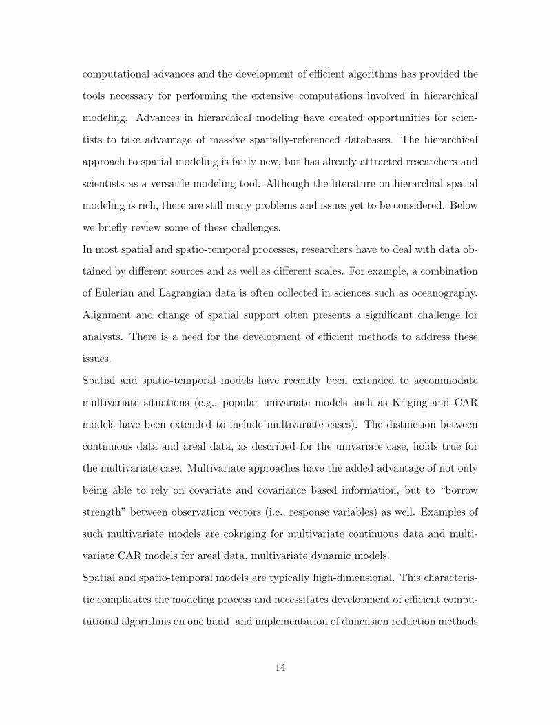
computational advances and the development of efficient algorithms has provided the

tools necessary for performing the extensive computations involved in hierarchical

modeling. Advances in hierarchical modeling have created opportunities for scien-

tists to take advantage of massive spatially-referenced databases. The hierarchical

approach to spatial modeling is fairly new, but has already attracted researchers and

scientists as a versatile modeling tool. Although the literature on hierarchial spatial

modeling is rich, there are still many problems and issues yet to be considered. Below

we briefly review some of these challenges.

In most spatial and spatio-temporal processes, researchers have to deal with data ob-

tained by different sources and as well as different scales. For example, a combination

of Eulerian and Lagrangian data is often collected in sciences such as oceanography.

Alignment and change of spatial support often presents a significant challenge for

analysts. There is a need for the development of efficient methods to address these

issues.

Spatial and spatio-temporal models have recently been extended to accommodate

multivariate situations (e.g., popular univariate models such as Kriging and CAR

models have been extended to include multivariate cases). The distinction between

continuous data and areal data, as described for the univariate case, holds true for

the multivariate case. Multivariate approaches have the added advantage of not only

being able to rely on covariate and covariance based information, but to “borrow

strength” between observation vectors (i.e., response variables) as well. Examples of

such multivariate models are cokriging for multivariate continuous data and multi-

variate CAR models for areal data, multivariate dynamic models.

Spatial and spatio-temporal models are typically high-dimensional. This characteris-

tic complicates the modeling process and necessitates development of efficient compu-

tational algorithms on one hand, and implementation of dimension reduction methods

14

( e.g., recasting the problem in a spectral context), on the other hand.

References

Banerjee, S., B. Carlin, and A. Gelfand. 2004. Hierarchical Modeling and Analysisfor Spatial Data. Chapman & Hall/CRC.

Berliner, L. In: Maximum Entropy and Bayesian Methods, chapter HierarchicalBayesian time series models, pages 15–22. Kluwer Academic Publishers, 1996.

Besag, J. 1974. Spatial interactions and the statistical analysis of lattice systems(with discussion). Journal of the Royal Statistical Society, Series B, 36:192–236.

Besag, J., J. York, and A. Mollie. 1991. Bayesian image restoration, with twoapplications in spatial statistics (with discussion). Annals of Institute of StatisticalMathematics, 43:1–59.

Carlin, B. and S. Banerjee. In: Bayesian Statistics 7, chapter Hierarchical multivari-ate CAR models for saptio-temporally correlated survival data (with discussion),pages 45–63. Oxford: Oxford University Press, 2003.

Cressie, N. 1993. Statistics for Spatial Data. Wiley & Sons.

Cressie, N. and H.-C. Huang. 1999. Classes of nonseparable spatio-temporal station-ary covariance functions. Journal of American Statistical Association, 94:1330–1340.

Diggle, P. and J. Tawn. 1998. Model-based geostatistics (with discussions). AppliedStatistics, 47(3):299–350.

Gelman, A., J. Carlin, H. Stern, and D. Rubin. 2004. Bayesian Data Analysis, SecondEdition. Chapman & Hall CRC, New York, USA.

Givens, G. and J. Hoeting. 2005. Computational Statistics. Wiley, New Jersey.

Gneiting, T. 2002. Nonseparable, stationary covariance functions for space-time data.Journal of American Statistical Association, 97:590–600.

Guttorp, P., W. Meiring, and P. Sampson. 1994. A space-time analysis of ground-levelozone data. Environmetrics, 5:241–254.

Hilborn, R. and M. Mangel. 1997. The Ecological Detective. Princeton UniversityPress, Princeton, New Jersey.

Huang, H.-C. and N. Cressie. 1996. Spatio-temporal prediction of snow water equiv-alent using the Kalman filter. Comp. Statist. Data Anal., 22:159–175.

Lindley, D. and A. Smith. 1972. Bayes estimates for the linear model. Journal of theRoyal Statistical Society, Series B, 34:1–41.

Oehlert, G. 1993. Regional trends in sulfate wet deposition. Journal of AmericanStatistical Association, 88:390–393.

15

Reinsel, G. 1981. Analysis of total ozone data for the detection of recent trends andthe effects of nuclear testing during the 1960’s. Geophysical Research Letters, 8:1227–1230.

Stein, M. 1986. A simple model for spatial-temporal processes. Water ResourcesResearch, 22:2107–2110.

Stein, M. 2005. Space-time covariance functions. Journal of American StatisticalAssociation, 100:320–321.

Stroud, J., P. Muller, and B. Sanso. 2001. Dynamic models for spatiotemporal data.Journal of the Royal Statistical Society, Series B, 63:673–689.

Thomas, A. 1994. Bugs: A statistical modelling package. RTA/BCS Modular Lan-guages Newsletter, 2:36–38.

Waller, L., B. P. Xia, and A. E. Gelfand. 1997. Hierarchical spatio-temporal mappingof disease rates. Journal of American Statistical Association, 92:607–617.

West, M. and J. Harrison. 1989. Bayesian Forecasting and Dynamic Models. SpringerVerlag, New York.

Whittle, P. 1954. On stationary processes in the plane. Biometrika, 41(3):434–449.

Wikle, C. and L. Berliner. 2005. Combining information across spatial scales. Tech-nometrics, 47:80–91.

Wikle, C., L. Berliner, and N. Cressie. 1998. Hierarchical Bayesian space-time models.J. Envr. Ecol. Stat., 5:117–154.

Wikle, C. and N. Cressie. 1999. A dimension-reduced approach to space-time kalmanfiltering. Biometrika, 86(4):815–829.

Wikle, C. and M. Hooten. In: Hierarchical Modelling for the Environmental Sciences,chapter Hierarchical Bayesian spatio-temporal models for population spread, pages145–169. Oxford: Oxford University Press, 2006.

Wikle, C., R. F. Millif, D. Nychka, and L. Berliner. 2001. Spatiotemporal hierarchicalBayesian modeling: Tropical ocean surface winds. Journal of American StatisticalAssociation, 96:382–397.

16