Using Hierarchical Growth Models to Monitor School Performance Over Time: Comparing NCE to Scale...

Using Hierarchical Growth Modelsto Monitor School Performance Over Time:

Comparing NCE to Scale Score Results

CSE Report 618

Pete Goldschmidt, Kilchan Choi, and Felipe MartinezCRESST/University of California, Los Angeles

January 2004

Center for the Study of EvaluationNational Center for Research on Evaluation,

Standards, and Student TestingGraduate School of Education & Information Studies

University of California, Los AngelesLos Angeles, CA 90095-1522

(310) 206-1532

Project 3.1 Methodologies for Assessing Student Progress, Strand 2Pete Goldschmidt, Project Director, CRESST/UCLA

Copyright © 2004 The Regents of the University of California

The work reported herein was supported under the Educational Research and Development CentersProgram, PR/Award Number R305B60002, as administered by the Institute of Education Sciences, U.S.Department of Education.

The findings and opinions expressed in this report do not reflect the positions or policies of the NationalInstitute on Student Achievement, Curriculum, and Assessment, the Institute of Education Sciences, orthe U.S. Department of Education.

1

USING HIERARCHICAL GROWTH MODELS

TO MONITOR SCHOOL PERFORMANCE OVER TIME:

COMPARING NCE TO SCALE SCORE RESULTS

Pete Goldschmidt, Kilchan Choi, and Felipe Martinez

CRESST/University of California, Los Angeles

Abstract

Monitoring school performance increasingly uses sophisticated analytical techniques and

we investigate whether one such method, hierarchical growth modeling, yieldsconsistent school performance results when different metrics are used as the outcome

variable. Specifically we examine whether statistical and substantive inferences arealtered when using normal curve equivalents (NCEs) vs. scale scores. The results indicate

that the effect of the metric depends upon the evaluation objective. NCEs significantlyunderestimate absolute growth, but NCEs and scale scores yield highly correlated (.9)

results based on mean initial status and growth estimates. Correlations between NCEand scale score rankings, based on fitted school initial status and growth values are

generally over .94. Further, statistical and substantive results, using NCEs and scalescores, pertaining to school-wide program effects are highly correlated (.95) as well.

NCEs and scale scores matched 99% of the time on whether or not the program indicatorvariable was statistically significant.

The use of longitudinal analysis of educational data encompasses a wide arrayof applications from individual growth curve modeling to program evaluation andschool performance modeling. We focus on the latter of these uses, especially as theypertain to the general issue of school accountability. These models are oftenconstrained by data availability, in terms of the number of time points available, thecompleteness of data, and the metric available for analysis. As school districtsbecome more sophisticated in record keeping ability, it is now more common andless problematic to acquire multiple years of data on students, who are linked with aunique identifier across years. Recent advances in multilevel modeling techniquesallow for the use of unbalanced data, make unequal timing of outcomes, andmissing data less of a barrier to analysis than repeated measures ANOVA oncepresented (Hox, 2002; Raudenbush & Bryk, 2002). Given the recent trend towardsaccountability that is based on outcomes (Hanushek & Raymond, 2001), it is relevant

2

to consider whether the metric used for the longitudinal analysis affects inferences.As Seltzer, Frank, and Bryk (1994) demonstrated, the metric matters whenattempting to model individual growth trajectories. Seltzer et al. concluded thatscale scores are the most appropriate metric for growth curve modeling.Theoretically, Item Response Theory (IRT)-based scale scores represent contentmastery on a continuum and may be used to measure absolute academic progressover time; whereas, NCEs represent a relative standing compared to a normingpopulation. Because NCEs represent a relative position from year to year, and not achange from the previous year, it cannot present a complete picture of studentacademic progress. Two issues give rise to this analysis: one, schools or schooldistricts are often unable to provide scale scores and are, at best, able to providenormal curve equivalents (NCEs).1 Two, school districts periodically change tests(publishers), but desire to conduct longitudinal evaluations across these differenttests. Test publishers use different methods to scale their tests, and rarely isinformation available equating scores from one test to another; NCEs may be morecomparable because they are relative scores. Within the longitudinal analysisframework, two questions arise: one, to what extent the metric matters when thefocus is school performance over time; and two, to what extent the metric matterswhen the focus is program evaluation.

While the properties of both scale scores and NCEs are understood, theempirical evidence against the use of NCEs for longitudinal models utilizingindividual student data to examine school performance over time is lacking. Hence,this analysis incorporates Monte Carlo methods and utilizes a three-levelhierarchical model to compare the results of growth models using scale scoresagainst growth models using NCEs on the same set of students. In general, the goalis to apply a three-level hierarchical linear model (HLM) with test scores nestedwithin students at level one, students nested within schools at level two, and schoolsat level three, to determine the effect of the metric on school-level estimates of initialstatus, growth, and a school program participation indicator variable.

Background

Methodologically advanced methods of examining school performance orevaluating program effectiveness take both the nature of the data into consideration,

1 Often districts report (understand) national percentile ranks (NPR), which can easily be convertedto NCEs.

3

and attempt to mitigate the effects of potential confounding factors (PCF). The short-comings of simply examining school means (Aitkin & Longford, 1986), ignoring thenested nature of educational data (Raudenbush & Bryk, 2002), or the differingmeaning of variables at different levels of aggregation (Burstein, 1980) are generallytaken into account in recent sound efforts to discern school effectiveness. The effectsof PCFs, in non-randomized, cross-sectional designs (Campbell & Stanley, 1963) andlimitations of pre-post designs (Bryk & Wesiburg, 1977; Raudenbush, 2001;Raudenbush & Bryk, 1987) in making inferences about school or program effects(i.e., change in student outcomes due to a hypothesized cause) leads us to considerthe advantages of examining growth trajectories to make inferences about change(Raudenbush & Bryk, 2002; Rogosa, Brandt, & Zimowski, 1982; Willet, Singer, &Martin, 1998). The usefulness of hierarchical longitudinal growth models thatexamine individual growth trajectories and make subsequent inferences aboutprogram effectiveness have been posited and applied for some time (Heck, 2000;Willms & Raudenbush, 1989); their use increasing with both computing power anddata availability (see for example Goldschmidt, 2002b; Heck, 2000; Ramirez, Yuen,Ramey, & Pasta, 1991). Specifying an adequate model that correctly captures thestructure of growth depends upon the nature of the data being modeled(Raudenbush, 2001).

Theoretical understanding of the optimum model is often confronted with theempirical realism of the data, however. The advantages of longitudinal growthmodels may be a mute point if proper data cannot be compiled. Assuming thatstudent records have been accurately matched, and that there are at least threemeasurement occasions, one can consider a longitudinal2 evaluation model. Thesemodels have examined diverse outcomes such as growth in mathematics gradeequivalents (GE), (Wilms & Jacobson, 1990) early child vocabulary growthHuttenlocher, Haight, Bryk, and Seltzer (1991), early reading achievement growth(Goldschmidt, 2002a), and feelings of isolation (Osgood & Smith, 1995). While thesemodels are often referred to as longitudinal growth models, they often, as in the caseof Osgood and Smith, for example, evaluate an outcome that is intended to change,though not necessarily grow.

The scale is important in drawing conclusions from individual growth curves(Yen, 1986). The key element is that the outcome must have constant meaning over

2 Which we differentiate from a pre-post, or simple gain score model.

4

time (Raudenbush, 2001). As Seltzer et al. (1994) demonstrated, the metric matterswhen looking at student progress over time. Seltzer et al. focused on the inadequacyof grade equivalents (GEs). Theoretically, the optimal metric to use when examiningchange is a vertically equated IRT based scale score because it is on an interval scaleand is comparable across grades (Hambleton & Swaminathan, 1987). Thus a changein a scale score from year to year is an absolute measure of academic progress,irrespective of grade. However, equating is generally designed to comparecontiguous grade pairs (Yen, 1986) and scales may be less meaningful as the gradespan increases. The NCE are based on national percentile ranks, but arestandardized to have a mean of 50 and a standard deviation of 21.06, and also havean equal interval scale (Worthen, White, Fan, & Sudweeks, 1999). As noted, NCEscannot adequately describe absolute achievement growth because it places studentsat a relative position at each test occasion. A change in this relative position does notnecessarily functionally correspond to absolute achievement gains. One argumentagainst the use of NCEs is that it places students on a relative position, whichguarantees “winners” and “losers.” But, it should be noted that both NCEs and IRTbased scale scores are based on a representative norming sample that is generallyconducted approximately every five to eight years. This implies that all scores arepotentially based on a fixed standard for some period of time.

The focus of this discussion has centered on the correct metric and ensuinginterpretation of individual student growth trajectories, but not on whether resultspertaining to school performance would be either statistically or substantivelyaltered by using NCE scores rather than scale scores. The questions that arise arewhether the results using NCEs or scale scores would substantively change theinferences made about school performance or program effectiveness, within thecontext of a hierarchical longitudinal evaluation. This is relevant in that schoolaccountability systems compare school performance, but accurate models do notsimply evaluate school aggregate performance because that suffers biases broughtabout due to aggregation (Aitkin & Longford, 1986), and incorrectly mixesinferences concerning student and school level variables (Burstein, 1980). Further,program evaluation may not simply consist of comparing two groups ofstudents—treatment vs. control—rather it may consist of evaluating the context inwhich students are placed (i.e., individual students are not assigned to a group,rather the entire school may be part of a reform effort). As in general schoolperformance modeling, the question of interest is to what extent the program school

5

performs better than non-program school, with the same notion of value added as inaccountability models. Given that NCE scores are available for analysis substantiallymore often than scale scores, it is important to compare school level results usingboth NCEs and scale scores.

Data

The data are from a large, racially integrated, urban school district that enrollsapproximately 65,000 students. We have four years of panel data beginning with the1997-98 (1998) school year and ending with the 2000-2001 (2001) school year. Theoutcome measures are reading and mathematics Stanford Achievement Test, v9,(SAT-9) scores, for which we have both NCEs and scale scores. In order to focus thisanalysis on the effect of the metric and not confound school-effect results with issuesof cross-classification (Rashbash & Goldstein, 1994; Raudenbush, 1993) we limit oursample to students who attended the same school between 1998 and 2001. Wefurther reduce our sample by excluding students with missing demographic oroutcome information (although these are certainly not requirements for longitudinalanalyses). Table 1 presents the SAT-9 reading and mathematics means for each ofthe years that we have data. Although not inherently comparable, both metricsdemonstrate an increase between 1998 and 2001 of between 12% and 15%. Simplezero-order correlations between students’ scores measured by NCEs and scale scoresindicate that they are only moderately correlated in each year (range r = .59 to .68).

Table 1

Means of NCEs and Scale Scores by Year

Reading Mathematics

Year NCE SS NCE SS

1998 38.5 561.2 43.3 560.8

(20.1) (40.7) (22.3) (41.0)

1999 40.8 595.1 49.2 596.7

(20.5) (44.4) (22.1) (43.8)

2000 41.2 619.7 47.0 617.6

(20.6) (42.1) (21.3) (41.3)

2001 43.2 640.6 48.7 644.3

(19.7) (37.8) (21.9) (40.6)

Note. N = 7,856 students; standard deviation in parentheses.

6

The final sample that we utilize consists of 7,856 students, representing 31,424test scores for each content area. Student demographic characteristics are presentedin Table 2. The sample that forms the basis for the simulation study (forming thepopulation from which we draw samples) matches fairly closely the district as awhole, but more importantly is a substantially diverse sample, intimating thatresults are not biased by an unrealistically homogeneous sample.

We utilize school context measures that are constructed from the aggregatestudent characteristics for each school. We also use an indicator variable thatidentifies whether schools participated in a school-wide school reform effort(program schools). Fifteen percent of schools are classified as program schools.

Methodology

We employ a Monte Carlo method to examine the consequences of using NCEscores instead of scaled scores when using a three level hierarchical growth model inmonitoring school performance. Comparing the key parameters of interest allows usto examine whether the results are statistically or substantively similar. Monte Carlotechniques allow us to simulate key factors of interest so that we can obtain moregeneral information about the differences between the results pertaining to each testmetric, when those measures are used for monitoring school performance over time.

Table 2

Student Characteristics

Proportion

Student characteristic District Sample

Female 0.50 0.49

African-American 0.21 0.21

Asian 0.17 0.13

Hispanic 0.41 0.45

Other 0.03 0.03

White 0.19 0.18

ELL 0.37 0.49

Free/reduced lunch 0.67 0.88

Special ed. 0.07 0.08

Note. N = 7,856 students

7

In general, the Monte Carlo method involves randomly generating data underspecific conditions. However, in this study, we consider the data described above asthe population from which we will sample repeatedly for a Monte Carlo study. Eachschool has an average sample size of 745 students. Given that the number ofstudents per school is extremely large, we can comfortably say that repeatedsamples hold the i.i.d assumption. The main factors of the Monte Carlo study are thefollowing: the number of students within schools, the number of schools, gradelevels, and content areas. Table 3 summarizes the conditions. In each of the samplingconditions, we sample the population data 2,000 times. We use SAS™ to sample andgenerate the datasets and HLM™ to run the hierarchical growth models.

Depending upon content area, the choice of NCE or scale scores might lead todifferent consequences in terms of inferences concerning school performance. Forexample, in a content area in which students show remarkable progress over time,scale scores may be a better metric in detecting progress than NCE scores, becauseNCE scores might wash out the magnitude of absolute growth over time.

In this study, we focus on the four key parameters estimated in a three-levelhierarchical model (described below) for measuring school performance over time:

1. school mean initial status for non-program schools;

2 . the difference between non-program schools and program schools in

initial status;

Table 3

Sampling Conditions for Monte Carlo Study

Total number Students sampled

of schools Percent Mean n

60 25% 31.3

60 50% 65.6

60 75% 98.5

60 100% 130.9

8

3. the school mean rate of change for non-program schools; and,

4. the difference between non-program and program schools in the mean

rate of change.

For each simulation condition, we estimate Pearson correlations between eachof the parameters based on NCE scores and the corresponding parameters based onscale scores (see Table 4). In addition, school rankings based on the magnitudes ofschool mean initial status and school mean rate of change3 are calculated for thecases of NCE and scale scores. We compare Spearman and Kendall’s Tau rank-ordercorrelations based on the estimated school rankings between the two metrics (seeTable 5).

Briefly, the three-level model is as follows:

Ytij = π 0ij + π 1ij_tij + etij, (1)

where Ytij is the outcome at time t for student i in school j with α as a time parameter

measured in school years. Since growth trajectories are assumed to vary acrossstudents, at level 2 for the initial status at time = 0:

π 0ij = _ 00j + _ 01jX1ij + … + _ 0PjXPij + r0ij , (2)

where there are p = 1 to P student-level predictors (e.g. student backgroundcharacteristics). Similarly, for the growth trajectories

π 1ij = _10j + _ 11jX1ij + … + _ 1PjXPij + r1ij, (3)

The effects of student characteristics (Xij’s) are assumed to vary across schools atlevel 3. For example, for mean initial status for school j:

_ 00j = _000 + _001Z1j + u00j, (5)

where Z is a 1/0 indicator variable denoting school program membership. Forstudent-level effects on initial status for school j:

_ 0pj = _0p0 + _0p1Z1j + u0pj. (6)

For the mean rate of change for school j:

_10j = _100 + _101Z1j + u10j, (7)

and for the student level effects on the student rate of change for school j:

3 That is based on the fitted values for school mean initial status and rate of change.

9

_1pj = _1p0 + _1pqZ1j + u1pj, (8)

Within each condition we run four models. Model one is the unconditionalmodel used to partition the unconditional variation in the outcome among time,students, and schools, and is used as a basis for comparing the fit of subsequentmore complex models (Raudenbush & Bryk, 2002). Model two includes only studentlevel covariates, as these are potentially associated with changes in achievement andaccount for between school differences in enrollment; thereby potentially reducingthe between school variation in the outcome. Model three includes the student levelcovariates at level two and the program indicator variable at level three. This modelattempts to capture differences between program and non-program schools,accounting for differences in student enrollment, but excluding other schoolcontextual factors. Model four includes all of the variables included in model three,

Table 4

Summary Parameter Estimates Compared

Question Scale scores NCEs

1) _000 vs. _000

2) _001 vs. _001

3) _100 vs. _100

4) _101 vs. _101

Note. NCE = normal curve equivalent.

Table 5

Fitted Values Generating School Ranks

School Scale scores NCEs

Initial status booj booj

Rate of change b10j b10j

Note. NCE = normal curve equivalent.

10

and additional school context variables to examine whether the program effect ismoderated by school context. The full model (model 4) is displayed in theAppendix.

Results

The results of the simulations demonstrate that the legitimacy of using NCEsinstead scale scores depends on the intended objective. The results for each of theconditions, models, and content areas are presented below. Comparisons thatinvolve the actual estimated coefficients are recast into effect sizes, given the obviousdifference in scale between NCEs and scale scores. Although not of primary interest,we briefly present the substantive results of the tested models. Tables 6 and 7summarize the results of the full model for each of the sampling conditions. Theestimated coefficients are presented in effect sizes that we define as the estimatedcoefficient divided by the outcome standard deviation (Cooper & Hedges, 1994).4

Generally the magnitude of the estimated effects, by content area are consistentbetween NCEs and scale scores—with one major exception, growth, which wediscuss in more detail below. Although we do not present detailed resultsconcerning the parameters estimates here, it is important to note that the estimateswere normally distributed with standard deviations decreasing as sample sizeincreased. The results in Table 8 give one indication of how well the modelsperform, in terms of reducing the unconditional between-school variation in growth.Overall, the full model accounts for approximately 43% to 52% of the variation in theReading growth rate and approximately 16% to 17% in the mathematics growth rate.The marginal impact of adding school context variables (after accounting for studentcovariates)—that is the variance reduction from model 2 to model 4—is much moretightly aligned between the NCE and scale score models; although they do differ bycontent area. The addition of school context has a consistent effect across samplingconditions and metric, within content area.

Except for the growth parameter estimates, within content area, the outcomemetric and the sampling condition would lead to consistent interpretations of theassociations of the covariates and their ability to reduce unconditional between-school variation. However, our focus is whether the results would lead to

4For indicator variables this is strictly correct given these are group differences. Subsequently we willutilize both the above definition for the effect size as well as another identified in Raudenbush andFeng (2001).

11

substantively consistent inferences about school and/or program performance,when comparing models using NCEs and scale scores.

Table 6

Summary of Results Describing SAT-9 Reading Achievement – in Effect Size

25% 50% 75%

SAT-9 Reading Achievement NCE SS NCE SS NCE SS

Mean Initial status (g000)

Student Predictors

Special Education (g010) -0.47 -0.44 -0.47 -0.44 -0.47 -0.44

Low SES (g020) -0.36 -0.40 -0.35 -0.40 -0.35 -0.39

LEP (g030) -0.34 -0.35 -0.33 -0.34 -0.32 -0.33

Minority (g040) -0.48 -0.54 -0.48 -0.54 -0.48 -0.53

Girl (g050) 0.10 0.10 0.10 0.10 0.10 0.10

School Predictors

LAAMP Effect (g001) 0.03 0.04 0.02 0.03 0.02 0.02

Minority (g002) -0.01 -0.01 -0.01 -0.01 -0.01 -0.01

Low (g003) 0.13 0.10 0.17 0.15 0.20 0.17

Mean Growth (g100) 0.07 0.64 0.07 0.63 0.07 0.63

Student Predictors

Special Education (g110) 0.00 -0.03 0.00 -0.03 0.00 -0.03

Low SES (g120) 0.05 0.06 0.05 0.06 0.05 0.06

LEP (g130) 0.07 0.07 0.07 0.07 0.07 0.07

Minority (g140) -0.03 -0.02 -0.03 -0.02 -0.03 -0.02

Girl (g150) 0.01 0.01 0.01 0.01 0.01 0.01

School Predictors

LAAMP Effect (g101) 0.01 0.01 0.01 0.01 0.01 0.01

Minority (g102) 0.11 0.14 0.12 0.15 0.12 0.16

Low (g103) -0.08 -0.08 -0.08 -0.08 -0.08 -0.08

Note. NCE = normal curve equivalent, SS = scale scores; SES = socio-economic status, LEP =limited English proficient, LAAMP = Los Angeles Annenberg Metropolitan Project.

12

Table 7

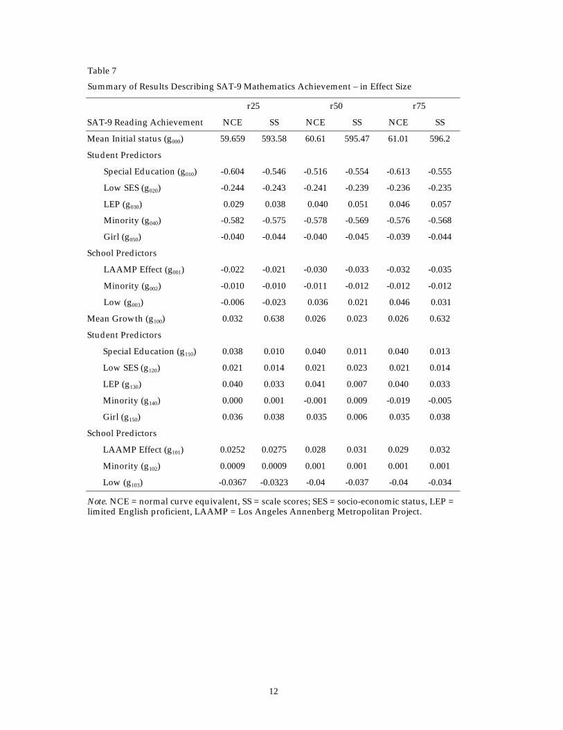
Summary of Results Describing SAT-9 Mathematics Achievement – in Effect Size

r25 r50 r75

SAT-9 Reading Achievement NCE SS NCE SS NCE SS

Mean Initial status (g000) 59.659 593.58 60.61 595.47 61.01 596.2

Student Predictors

Special Education (g010) -0.604 -0.546 -0.516 -0.554 -0.613 -0.555

Low SES (g020) -0.244 -0.243 -0.241 -0.239 -0.236 -0.235

LEP (g030) 0.029 0.038 0.040 0.051 0.046 0.057

Minority (g040) -0.582 -0.575 -0.578 -0.569 -0.576 -0.568

Girl (g050) -0.040 -0.044 -0.040 -0.045 -0.039 -0.044

School Predictors

LAAMP Effect (g001) -0.022 -0.021 -0.030 -0.033 -0.032 -0.035

Minority (g002) -0.010 -0.010 -0.011 -0.012 -0.012 -0.012

Low (g003) -0.006 -0.023 0.036 0.021 0.046 0.031

Mean Growth (g100) 0.032 0.638 0.026 0.023 0.026 0.632

Student Predictors

Special Education (g110) 0.038 0.010 0.040 0.011 0.040 0.013

Low SES (g120) 0.021 0.014 0.021 0.023 0.021 0.014

LEP (g130) 0.040 0.033 0.041 0.007 0.040 0.033

Minority (g140) 0.000 0.001 -0.001 0.009 -0.019 -0.005

Girl (g150) 0.036 0.038 0.035 0.006 0.035 0.038

School Predictors

LAAMP Effect (g101) 0.0252 0.0275 0.028 0.031 0.029 0.032

Minority (g102) 0.0009 0.0009 0.001 0.001 0.001 0.001

Low (g103) -0.0367 -0.0323 -0.04 -0.037 -0.04 -0.034

Note. NCE = normal curve equivalent, SS = scale scores; SES = socio-economic status, LEP =limited English proficient, LAAMP = Los Angeles Annenberg Metropolitan Project.

13

Table 8

Percent Reduction in Between School Variation in Growth

Sampling Reading Math

Condition NCE SS NCE SS

Model 2 to 4

25% 24.5 23.7 9.3 9.2

50% 24.4 25.5 9.6 9.7

75% 24.5 26.4 9.2 9.3

Model 1 to 4

25% 43.8 52.2 16.8 16.8

50% 42.7 51.9 16.4 16.5

75% 42.9 52.3 16.1 16.1

Note. NCE = normal curve equivalent, SS = scale scores.

Hence, we turn to the correlations between mean initial status and growth ratesfor models using scale scores vs. models using NCEs, the rank order correlationsamong the fitted values for mean school initial status and mean school rates ofchange for models using scale scores vs. models using NCEs, and the correlationsfor the estimated difference between program and non-program schools for modelsusing scale scores vs. models using NCEs. Tables 9a through 9d present thecorrelations for each of the models for each of the sampling conditions. We presentboth Spearman rank-order correlations and Kendall’s Tau, which are bothappropriate for use with ordinal ranks (Allen & Yen, 1979). The correlations rangefrom a low of about .75 to a high of about .98 and average about .9. The SpearmanCorrelations overall average is about .97 for initial status and .94 for growth. The

Table 9a

Correlations Between Estimated Coefficients – Model 1

Correlation Kendall (Tau) correlation

Sample Test type Initial status Growth Initial status Growth

R25 Read 0.988 0.936 0.925 0.806

Math 0.987 0.963 0.925 0.863

R50 Read 0.990 0.932 0.931 0.798

Math 0.988 0.964 0.929 0.870

R75 Read 0.991 0.932 0.935 0.798

Math 0.989 0.964 0.932 0.871

14

Table 9b




R25 Read 0.964 0.914 0.857 0.779

Math 0.975 0.955 0.887 0.849

R50 Read 0.970 0.910 0.872 0.775

Math 0.978 0.956 0.898 0.857

R75 Read 0.974 0.908 0.881 0.776

Math 0.981 0.955 0.905 0.857

Table 9c




R25 Read 0.963 0.916 0.856 0.781

Math 0.975 0.956 0.887 0.849

R50 Read 0.971 0.912 0.873 0.777

Math 0.978 0.958 0.897 0.858

R75 Read 0.974 0.910 0.882 0.776

Math 0.980 0.956 0.904 0.857

Table 9d




R25 Read 0.939 0.897 0.817 0.754

Math 0.969 0.954 0.873 0.847

R50 Read 0.942 0.895 0.821 0.750

Math 0.972 0.956 0.880 0.856

R75 Read 0.943 0.896 0.826 0.748

Math 0.973 0.955 0.878 0.858

Kendall Tau correlations are slightly lower, with an overall average of .89 for initialstatus and .82 for growth. The pattern across sampling conditions and models is

15

consistent for both correlation measures. That is, the correlations increase withsample size and decrease with model complexity. However, it should be noted thatthese changes are relatively small—generally about 4%, at the maximum, in eitherdirection. Figure 1 summarizes this relationship.5

Model 1Model 2

Model 3Model 4

R25

R50

R750.700.720.740.760.780.800.820.840.860.880.900.920.940.960.981.00

0.98-10.96-0.980.94-0.960.92-0.940.9-0.920.88-0.90.86-0.880.84-0.860.82-0.840.8-0.820.78-0.80.76-0.780.74-0.760.72-0.740.7-0.72

Figure 1. Correlation pattern between sampling condition and model – Reading SAT-9 growth.

We are, of course, most interested in the effects of the metric on growth asthis is the parameter estimate upon which the evaluation of school performance orprogram effectiveness will be based. Hence, we next turn to the correlations of thefitted values and effect sizes for growth. Tables 10a through 10d summarize theresults for each of the models and sampling conditions. The first column of Table 10presents the correlation of the fitted school mean growth rates estimated usingNCEs and scale scores. These range between about .89 and .96, with a mean of about.93. These correlations do not exhibit any pattern across sampling conditions ormodel. We generate two effect sizes to standardize annual growth.

5We present only one of the possible figures as an example. The remaining conditions are availablefrom the authors.

16

Table 10a

Summary of Correlations Among Fitted Values and Effect Sizes for Growth – Model 1

Sample Test type Correlation ES1 ES2

FV Raudenbush eff.size Ratio Difference Ratio Difference

R25 Read 0.936 0.812 0.113 -0.567 0.148 -8.792

Math 0.963 0.749 0.088 -0.596 0.095 -8.113

R50 Read 0.931 0.822 0.114 -0.568 0.147 -8.738

Math 0.964 0.736 0.089 -0.596 0.095 -7.970

R75 Read 0.932 0.823 0.114 -0.568 0.147 -8.725

Math 0.963 0.734 0.090 -0.596 0.096 -7.941

Note. FV = Fitted Value, ES = Effect Sizes.

Table 10b




R25 Read 0.914 0.788 0.116 -0.570 0.139 -11.388

Math 0.954 0.757 0.091 -0.595 0.098 -8.474

R50 Read 0.909 0.822 0.117 -0.570 0.139 -11.057

Math 0.956 0.743 0.092 -0.596 0.098 -8.277

R75 Read 0.908 0.859 2.023 0.672 2.413 18.419

Math 0.954 0.931 1.834 0.545 1.949 8.640


Table 10c




R25 Read 0.916 0.780 0.114 -0.571 0.138 -11.430

Math 0.955 0.749 0.088 -0.595 0.094 -8.518

R50 Read 0.911 0.811 0.115 -0.571 0.137 -11.085

Math 0.958 0.733 0.088 -0.595 0.094 -8.318

R75 Read 0.909 0.860 2.023 0.670 2.424 18.509

Math 0.956 0.931 1.834 0.543 1.950 8.653


17

Table 10d




R25 Read 0.896 0.703 0.160 -0.562 0.194 -12.761

Math 0.953 0.621 0.096 -0.593 0.103 -8.863

R50 Read 0.895 0.664 0.163 -0.563 0.193 -12.542

Math 0.955 0.635 0.099 -0.593 0.106 -8.678

R75 Read 0.895 0.685 0.164 -0.562 0.192 -12.574

Math 0.954 0.934 0.099 -0.593 0.105 -8.621


The first (ES1) is based on the general effect size presented in Cooper andHedges (1994), while the second (ES2) is based on Raudenbush and Feng (2001). Wedefine ES1 as the estimated growth parameter (γ100), divided by the sample standarddeviation of the outcome. ES2 is defined as the estimated growth parameter (γ100)divided by the standard deviation of true change (τ11

1/2) and has the advantage of

excluding the sampling variance (Raudenbush & Feng). The correlations of theseeffect sizes are presented in column two. These range from approximately .62 to .93,and average about .78. These correlations, while still high, are expectantly lower asthey are based on parameter estimates for growth and for the standard deviation ofgrowth, which vary with each of the 2,000 simulations for each condition. Theremaining four columns present the ratios and absolute differences for ES1 and ES2,respectively. We present both ratios and absolute differences as estimates near zerotend to disproportional effects on the ratio. The results in Tables 10a through 10dfurther corroborate the results presented above in terms of actual estimates ofachievement growth. That is, NCE scores significantly and consistently under-estimate annual growth. This result is consistent across sampling conditions andmodel. The ratios of effect sizes for both ES1 and ES2 clearly demonstrate that actualgrowth is under-estimated using NCEs. In fact we calculate an index of relative bias(RB), as in Krull and MacKinnon (2001). In this case we define

RB = (ES100NCE – ES100

ss)/ ES100ss,

18

where each ES (1 and 2) is calculated as noted above. This can be used to estimatethe proportional under/over estimate using NCEs vs. scale scores. Figure 26 presentsassociation between RB and the actual magnitude of annual growth (as measured byscale scores) in effect size units. We use this chart to demonstrate that the NCEmetric under-estimates growth by about 85% and that this proportion is inverselyrelated to the magnitude of growth. However, it is important to note that the rangeof growth and the corresponding range of RB are relatively small.

Hence, the metric does not change the substantive inferences made fromranking schools based on their fitted growth estimates, but matters when theinferences concern inferences about actual absolute growth.

Finally, we present the simulation results for evaluating school-wide programeffects. Tables 11a and 11b display the relevant results. The first two columnspresent the correlations among the IS and growth estimates using NCEs and scalescores. In every case these correlations were at least .94. The next four columnspresent the ratios and absolute differences in effect sizes. In general, the programeffect sizes were relatively small, which tends to make our comparison criteriatake on extreme values in some

6The results in Figures 2, 3, and 4 are based on model 4.

19

-0.89

-0.88

-0.87

-0.86

-0.85

-0.84

-0.83

-0.82

-0.81

-0.80

-0.79

0.62 0.63 0.64 0.65 0.66 0.67 0.68 0.69 0.70 0.71 0.72 0.73

Efect Size of Growth (scale scores)

Rel

ativ

e B

ias

in G

row

th

Figure 2. Comparison of relative bias to the effect size of growth – SAT-9 Reading (in scale scores).

Table 11aSummary of Program Effect Sizes for SAT-9 Achievement – Model 3

Correlation Effect size ratio Effect size difference

Sample Test type Initialstatus Growth Initial

status Growth Initialstatus Growth

Agreement(growth)

R25 Read 0.982 0.943 0.686 0.934 -0.016 0.006 0.993

Math 0.988 0.950 1.155 -0.267 -0.007 -0.001 0.998

R50 Read 0.982 0.941 0.843 1.417 -0.015 0.006 1.000

Math 0.989 0.943 0.884 0.891 -0.006 -0.002 1.000

R75 Read 0.984 0.942 0.873 2.220 -0.014 0.006 1.000

Math 0.990 0.939 0.910 0.904 -0.005 -0.002 1.000

20

Table 11b

Summary of Program Effect Sizes for SAT-9 Achievement – Model 4

Correlation Effect size ratio Effect size difference

Sample Test type Initialstatus Growth Initial

status Growth Initialstatus Growth

Agreement(growth)

R25 Read 0.988 0.954 1.149 0.348 -0.008 0.004 0.985

Math 0.982 0.940 0.793 0.812 0.000 -0.003 0.992

R50 Read 0.990 0.950 0.965 0.693 -0.004 0.003 0.994

Math 0.984 0.940 0.966 0.880 0.003 -0.004 0.999

R75 Read 0.985 0.940 0.265 1.146 -0.002 0.002 1.000

Math 0.990 0.948 0.710 0.878 0.004 -0.004 1.000

instances. That is estimated ES1’s that are very small may have small absolutedifferences, but have relatively large ratios. Substantively estimated ES1 that areclose to zero for NCEs are close to zero for scale scores as well—leading to the sameinferences regarding program effectiveness. Tables 11a and 11b, therefore, presentboth the ratio of ES1NCE to ES1SS, but also the mean differences. The tables alsodisplay the proportion of the time that there is agreement in statistical significanceprogram indicator variable between models using NCE and models using scalescores. The results indicate that the two metrics agree almost 100% of the time.

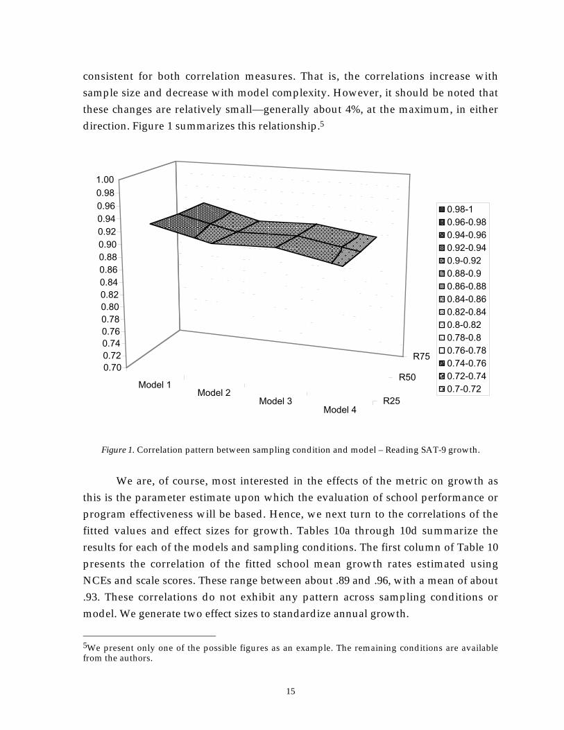
As noted, due to the relatively small ES1 for growth, we again use the RBmeasure. Figures 3 and 4 plot the relative bias as a function of the actual program

21

Program Effect Size for Initial Status (scale score)

.09.07.05.03.01-.01-.03-.05-.07-.09

Rel

ativ

e B

ias

for

Intia

l Sta

tus

5

4

3

2

1

0

-1

-2

-3

-4

-5

Figure 3. Relationship between relative bias in NCEs for initial status.

effect estimates, based on scale scores. These figures demonstrate two importantpoints. One, the RB is largest when the actual scale score effect is close to zero(which, as noted, often generates very small actual differences in effect sizes, butvery large ratios). And two, The RB decreases with the increase of the absolute valueof the program effect size. This result holds true for both initial status and growth.The correlation, for SAT-9 reading, between ES1NCE and ES1SS is .986 and .940 forinitial status and growth respectively

Hence, the simulations indicate that metric does not change inferences ofwhether or not a program is statistically or substantively significant. It is interestingto note that while NCEs significantly under estimate actual absolute growth, theyaccurately represent the difference between program and non-program schools inthat growth.

22

Program Effect Size for Growth (scale scores)

.03.02.010.00-.01

Rel

ativ

e B

ias

for

Gro

wth

5

4

3

2

1

0

-1

-2

-3

-4

-5

Figure 4. Relationship between relative bias in NCEs for growth.

Discussion

Recent legislation has increased the need to accurately evaluate schoolperformance. School accountability has moved beyond simply comparing schoolmeans in league tables to more advanced techniques, such as hierarchical lineargrowth models. Coinciding educationists’ increased focus on accountability isincreased public interest in accountability, as demonstrated by the growing demandfor school quality information. Given both the ubiquitousness of NCE scores and theease of interpretation, it is valuable to ascertain the sensitivity of school level resultsto the choice of the metric. Further, given the volatility in the use of tests, it isimportant to ascertain whether NCE scores produce estimates that result inconsistent policy implications compared to those derived using scale scores. The

23

simulation results indicate that the effect of the metric is tied to the evaluationobjective. We find that the correlation between mean initial status and growth ratesfor models using scale scores vs. models using NCEs is strong. The simulationresults also suggest that this relationship is affected, to a small, extent, by the samplesize and the complexity of the model used. The effect of model complexity isstronger than the effect of sample size. The results for the rank order correlationsbetween fitted values for mean school initial status and mean school rates of change,for models using scale scores vs. models using NCEs, are also consistently strong.These results are invariant across sample size and model complexity. Thisdemonstrates that if the objective of the evaluation is to rank schools then the choiceof NCE or scale score will not change the ensuing school ranking. NCEs canaccurately rank schools.

Further we find that the correlation of program effect sizes for models usingscale scores vs. NCEs are strong and consistent. This means that evaluations basedon NCEs and using hierarchical longitudinal models will be able to accuratelyestimate both initial differences among program and non-program schools, andwhether the program has an effect on growth—both in terms of statistical andsubstantive significance.

Still, it is important to reiterate that when estimating mean school growth,NCEs will yield misleading absolute achievement growth estimates. In fact thesimulation results indicate that using NCEs under-estimate growth by about 85%.Interpreting growth using NCEs, without additional information, is likely to bedifficult, despite the fact that students maintaining the same NCE score from oneyear to the next must have demonstrated some absolute growth in order to maintaintheir relative standing. Even with additional information, the estimated range ofgrowth in the scale score metric, derived from NCEs, will be imprecise. However,ranking schools by the amount of growth they exhibit does yield consistent results.

The results of this analysis provide some guidance in the planning ofevaluations or monitoring of school performance; this is particularly relevant forprogram evaluations or school performance systems that attempt to take advantageof longitudinal data sources, but are limited to conducting analyses with NCEscores. These results may be particularly relevant as school districts change tests, butdesire to conduct longitudinal evaluations across the different tests—as NCEs maybe more comparable across tests than IRT based scale scores. As Linn (2000)demonstrated there will clearly be effects from switching tests, but these can be

24

handled within the model (Goldschmidt & Swigert, 2001). The simulations alsodemonstrate that the results based on a 25% sample are very consistent with resultsbased on the full sample. This finding may be particularly relevant for longitudinalmethods that do not rely on panel data, such as HLM models for estimating schooleffects proposed by Willms and Raudenbush (1989). The effects of NCEs vs. scalescores in these types of models are unknown and warrant further research. Theseresults allow program evaluators and school accountability analysts more flexibilityin designing evaluations—especially when cost is an issue. While the results indicatethat schools can be ranked and programs evaluated consistently using longitudinalmethods and NCE scores, ranks should be interpreted carefully. Confidenceintervals of estimated effects generally overlap substantially, which means thatcaution should be exercised when comparing schools in this manner (Goldstein etal., 1993). Further, we are by no means advocating that using a single standardizedmeasure be the sole criteria upon which school or program quality ought to bejudged.

25

References

Aitkin, M., & Longford, N. (1986). Statistical modeling issues in school effectivenessstudies. Journal of the Royal Statistical Society, 149(1), 1-43.

Allen, M., & Yen, W. (1979). Introduction to measurement theory. Monterey, CA:Brooks/Cole Publishing.

Bryk, A. S., & Weisberg, H. I. (1977). Use of the nonequivalent control group designwhen subjects are growing. Psychological Bulletin, 84(5), 950-962.

Burstein, L. (1980). The analysis of multi-level data in educational research andevaluation. Review of Research in Education, 4, 158-233.

Campbell, D. T., & Stanley, J. C. (1963). Experimental and quasi-experimental designs forresearch. Boston: Houghton Mifflin.

Cooper, H., & Hedges, L. (1994). The handbook of research synthesis. New York: Sage.

Goldschmidt, P. (2002a). Evaluation of Alaska Beginning Literacy Institutes. LosAngeles: University of California, Center for the Study of Evaluation (CSE).

Goldschmidt, P. (2002b). A comparison of student achievement in LAAMP and Non-LAAMP schools in Los Angeles county: Longitudinal analysis results 1997-’98–1999-2000. Los Angeles: University of California, Center for the Study of Evaluation(CSE).

Goldschmidt P., & Swigert, S. (2001). Oxymoronic program evaluation: The short-termlongitudinal analysis dilemma. Paper presented at the annual meeting of theAmerican Educational Research Association, New Orleans, LA.

Goldstein, H., Rasbash, J., Yang, M., Woodhouse, G., Pan, H., Nuttall, D., et al.(1993). A multilevel analysis of school examination results. Oxford Review ofEducation, 19(4).

Hambleton, R. K., & Swaminathan, H. (1987). Item Response Theory: Principles andapplications, Boston, MA: Kluwer.

Hanushek, E. A., & Raymond, M. E. (2001, June). The confusing world ofeducational accountability. National Tax Journal, 54(2), 365-384.

Heck, R. H. (2000, October). Examining the impact of school quality on schooloutcomes and improvement: A value-added approach. EducationalAdministration Quarterly, 36(4), 513-552.

Hox, J. (2002). Multilevel analysis: Techniques and applications. Mahwah, New Jersey:Erlbaum.

26

Huttenlocher, J., Haight, W., Bryk, A., & Seltzer, M. (1991). Early vocabulary growth:Relation to language input and gender. Developmental Psychology, 27, pp. 236-248.

Krull, J., & MacKinnon, D. P. (2001). Multivariate modeling of individual and grouplevel mediated effects. Multivariate Behavioral Research, 36(2), 249-277.

Linn, R.L. (2000). Assessments and accountability. Educational Researcher, 20(2), 4-16.

Osgood, W. D., & Smith, G. (1995). Applying hierarchical linear modeling toextended longitudinal evaluations. Evaluation Review, 19(1), 3-39.

Ramirez, D., Yuen, R., Ramey, R., & Pasta, D. (1991). The immersion study (finalreport). Washington, DC, Office of Educational Research and Improvement.

Rasbash, J., & Goldstein, H. (1994). Efficient analysis of mixed hierarchical and cross-classified random structures using a multilevel model. Journal of Educational andBehavioral Statistics, 19(4), 337-350.

Raudenbush, S. (2001). Comparing personal trajectories and drawing causalinferences from longitudinal data. Annual Review of Psychology, 52, 501-525.

Raudenbush, S. (1993). A crossed random effects model for unbalanced data withapplications in cross-sectional and longitudinal research. Journal of EducationalStatistics, 18(4), 321-349.

Raudenbush, S. W., & Bryk, A. S. (2002). Hierarchical linear models: Applications anddata analysis methods (2nd ed.). Thousand Oaks, CA: Sage Publications.

Raudenbush, S. W., & Bryk, A. S. (1987). Application of hierarchical linear models toassessing change. Psychological Bulletin, 104(3), 396-404.

Raudenbush, S., & Xiao-Feng, L. (2001). Effects of study duration, frequency ofobservation, and sample size on power in studies of group differences inpolynomial change. Psychological Methods, 6(4), 387-401.

Rogosa, D. R., Brandt, D., & Zimowski, M. (1982). A growth curve approach to themeasurement of change. Psychological Bulletin, 92, 726-74.

Seltzer, M., Frank, K., & Bryk, A. (1994). The metric matters: The sensitivity ofconclusions about growth in student achievement to the choice of metric.Educational Evaluation and Policy Analysis, 16, 41-49.

Willett, J. B., Singer, J. D., & Martin, N. C. (1998). The design and analysis oflongitudinal studies of development and psychopathology in context:Statistical models and methodological recommendations. Development andPsychopathology, 10, 395-426.

27

Willms, J. D., & Jacobsen, S. (1990). Growth in mathematics skills during theintermediate years: Sex differences and school effects. International Journal ofEducational Research, 14, 157-174.

Willms, J. D., & Raudenbush, S. (1989). A longitudinal hierarchical linear model forestimating school effects and their stability. Journal of Educational Measurement,26(3), 209-232.

Worthen, B. R., White, K. R., Fan, X., & Sudweeks, R. R. (1999). Measurement andassessment in the schools (2nd ed.). New York: Longman.

Yen, W. M. (1986). The choice of scale for educational measurement: An IRTperspective. Journal of Educational Measurement, 23(4), 299-325.

28

Appendix

Level-1 Model

Y = P0 + P1*(TIME) + E

Level-2 Model

P0 = B00 + B01*(SPED1) + B02*(LOW1) + B03*(LEP1) + B04*(MINOR)

+ B05*(GIRL_1) + R0

P1 = B10 + B11*(SPED1) + B12*(LOW1) + B13*(LEP1) + B14*(MINOR)

+ B15*(GIRL_1) + R1

Level-3 Model

B00 = G000 + G001(MEDLAMP) + G002(MMINOR2) + G003(MLOW1) + U00

B01 = G010

B02 = G020

B03 = G030

B04 = G040

B05 = G050

B10 = G100 + G101(MEDLAMP) + G102(MMINOR2) + G103(MLOW1) + U10

B11 = G110

B12 = G120

B13 = G130

B14 = G140

B15 = G150

Where:

Time = years Coded as 0 = 1998, 1 = 1999….)

SPED1 = Special Education (0 = no 1 = yes)

LOW1 = (proxy is free/reduced lunch status) (0= no 1 = yes)

LEP1 = English Language Learner (0= no 1 = yes)

29

MINOR = Minority (i.e., non-White) (0= no 1 = yes)

GIRL = gender = female (0= no 1 = yes)

MEDLAAMP = school participated in school-wide reform (0= no 1 = yes)

MINOR2 = school mean percentage of MINOR

MLOW1 = school mean percentage of LOW1.

Using Hierarchical Growth Models to Monitor School Performance Over Time: Comparing NCE to Scale...

Documents

Transcript of Using Hierarchical Growth Models to Monitor School Performance Over Time: Comparing NCE to Scale...