GWmodel: an R Package for Exploring Spatial Heterogeneity using Geographically Weighted Models
43
arXiv:1306.0413v1 [stat.AP] 3 Jun 2013 GWmodel: an R Package for Exploring Spatial Heterogeneity Using Geographically Weighted Models Isabella Gollini University of Bristol, UK Binbin Lu NUI Maynooth, Ireland Martin Charlton NUI Maynooth, Ireland Christopher Brunsdon University of Liverpool, UK Paul Harris NUI Maynooth, Ireland Abstract Spatial statistics is a growing discipline providing important analytical techniques in a wide range of disciplines in the natural and social sciences. In the R package GW- model, we introduce techniques from a particular branch of spatial statistics, termed geographically weighted (GW) models. GW models suit situations when data are not described well by some global model, but where there are spatial regions where a suitably localised calibration provides a better description. The approach uses a moving window weighting technique, where localised models are found at target locations. Outputs are mapped to provide a useful exploratory tool into the nature of the data spatial hetero- geneity. GWmodel includes: GW summary statistics, GW principal components analysis, GW regression, GW regression with a local ridge compensation, and GW regression for prediction; some of which are provided in basic and robust forms. Keywords : geographically weighted regression, geographically weighted principal components analysis, spatial prediction, robust, R package. 1. Introduction Spatial statistics provides important analytical techniques for a wide range of disciplines in the natural and social sciences, where (often large) spatial data sets are routinely collected. Here we introduce techniques from a particular branch of non-stationary spatial statistics, termed geographically weighted (GW) models. GW models suit situations when spatial data are not described well by some universal or global model, but where there are spatial regions where a suitably localised model calibration provides a better description. The approach uses a moving window weighting technique, where localised models are found at target locations. Here, for an individual model at some target location, we weight all neighbouring observations according to some distance-decay kernel function and then locally apply the model to this weighted data. The size of the window over which this localised model might apply is controlled by the bandwidth. Small bandwidths lead to more rapid spatial variation in the results while large bandwidths yield results increasingly close to the universal model solution. When there exists some objective function (e.g. the model can predict), a bandwidth can be found optimally,
Transcript of GWmodel: an R Package for Exploring Spatial Heterogeneity using Geographically Weighted Models
arX
iv:1
306.
0413
v1 [
stat
.AP]
3 J
un 2
013
GWmodel: an R Package for Exploring Spatial
Heterogeneity Using Geographically Weighted
Models
Isabella Gollini
University of Bristol, UKBinbin Lu
NUI Maynooth, Ireland
Martin Charlton
NUI Maynooth, IrelandChristopher Brunsdon
University of Liverpool, UKPaul Harris
NUI Maynooth, Ireland
Abstract
Spatial statistics is a growing discipline providing important analytical techniques ina wide range of disciplines in the natural and social sciences. In the R package GW-
model, we introduce techniques from a particular branch of spatial statistics, termedgeographically weighted (GW) models. GW models suit situations when data are notdescribed well by some global model, but where there are spatial regions where a suitablylocalised calibration provides a better description. The approach uses a moving windowweighting technique, where localised models are found at target locations. Outputs aremapped to provide a useful exploratory tool into the nature of the data spatial hetero-geneity. GWmodel includes: GW summary statistics, GW principal components analysis,GW regression, GW regression with a local ridge compensation, and GW regression forprediction; some of which are provided in basic and robust forms.
Keywords: geographically weighted regression, geographically weighted principal componentsanalysis, spatial prediction, robust, R package.
1. Introduction
Spatial statistics provides important analytical techniques for a wide range of disciplines in thenatural and social sciences, where (often large) spatial data sets are routinely collected. Herewe introduce techniques from a particular branch of non-stationary spatial statistics, termedgeographically weighted (GW) models. GW models suit situations when spatial data are notdescribed well by some universal or global model, but where there are spatial regions where asuitably localised model calibration provides a better description. The approach uses a movingwindow weighting technique, where localised models are found at target locations. Here, for anindividual model at some target location, we weight all neighbouring observations accordingto some distance-decay kernel function and then locally apply the model to this weighteddata. The size of the window over which this localised model might apply is controlled by thebandwidth. Small bandwidths lead to more rapid spatial variation in the results while largebandwidths yield results increasingly close to the universal model solution. When there existssome objective function (e.g. the model can predict), a bandwidth can be found optimally,
2 GWmodel: Geographically Weighted Models
using cross-validation and related approaches.
The GW modelling paradigm has evolved to encompass many techniques; techniques thatare applicable when a certain heterogeneity or non-stationarity is suspected in the study’sspatial process. Commonly, outputs or parameters of the GW model are mapped to providea useful exploratory tool, which can often precede (and direct) a more traditional or sophisti-cated statistical analysis. Subsequent analyses can be non-spatial or spatial, where the lattercan incorporate stationary or non-stationary decisions. Notable advances in GW modellinginclude: GW summary statistics (Brunsdon, Fotheringham, and Charlton 2002); GW princi-pal components analysis (GW PCA) (Fotheringham, Brunsdon, and Charlton 2002; Harris,Brunsdon, and Charlton 2011a); GW regression (Brunsdon, Fotheringham, and Charlton1996, 1998, 1999; Leung, Mei, and Zhang 2000; Wheeler 2007); GW generalised linear mod-els (Fotheringham et al. 2002; Nakaya, Fotheringham, Brunsdon, and Charlton 2005); GWdiscriminant analysis (Brunsdon, Fotheringham, and Charlton 2007); GW variograms (Har-ris, Charlton, and Fotheringham 2010a); GW regression kriging hybrids (Harris and Juggins2011) and GW visualisation techniques (Dykes and Brunsdon 2007).
Many of these GW models are included in the R package GWmodel that we introduce inthis paper. Those that are not, will be incorporated at a later date. For the GW modelsthat are included, there is a clear emphasis on data exploration. Notably, GWmodel providesfunctions to a conduct: (i) a GW PCA; (ii) a GW regression with a local ridge compensa-tion (for addressing local collinearity); (iii) robust and outlier-resistant GW modelling; (iv)associated Monte Carlo significance tests; and (v) GW modelling with a wide selection ofdistance metric and kernel weighting options. These functions extend and enhance functionsfor: (a) GW summary statistics; (b) GW regression; and (c) GW generalised linear models -GW models that are also found in the spgwr R package. In this respect, GWmodel providesa more extensive set of GW modelling tools, within a single coherent framework (GWmodel
similarly extends or complements the gwrr R package with respect to GW regression andlocal collinearity issues). GWmodel also provides an advanced alternative to various exe-cutable software packages that have a focus on GW regression - such as GW regression v3.0(Charlton, Fotheringham, and Brunsdon 2003); the ArcGIS GW regression tool in the Spa-tial Statistics Toolbox (ESRI 2011); SAM for GW regression applications in macroecology(Rangel, Diniz-Filho, and Bini 2010); and SpaceStat for GW regression applications in health(Biomedware 2011).
The paper is structured as follows. Section 2 describes the example data sets that are availablein GWmodel. Section 3 describes the various distance metric and kernel weighting options.Section 4 describes modelling with basic and robust GW summary statistics. Section 5 de-scribes modelling with basic and robust GW PCA. Section 6 describes modelling with basicand robust GW regression. Section 7 describes ways to address local collinearity issues whenmodelling with GW regression. Section 8 describes how to use GW regression as a spatialpredictor. Section 9 concludes this work and indicates future work.
2. Data sets
The GWmodel package comes with four example data sets, these are: (i) Georgia, (ii)LondonHP, (iii) DubVoter and (iv) EWHP. The Georgia data consists of selected 1990 UScensus variables (with n = 159) for counties in the state of Georgia; and is fully described in

Isabella Gollini, Binbin Lu, Martin Charlton, Christopher Brunsdon, Paul Harris 3
Fotheringham, Brunsdon, and Charlton (2002). This data has been routinely used in a GWregression context for linking educational attainment with various contextual social variables(see also Griffith 2008). The data set is also available in the GW regression 3.0 executablesoftware package (Charlton et al. 2003) and the spgwr R package.
The LondonHP data is a house price data set for London, UK. This data set (with n = 372) issampled from a 2001 house price data set, provided by the Nationwide Building Society of theUK and is combined with various hedonic contextual variables (Fotheringham et al. 2002).The hedonic data reflect structural characteristics of the property, property constructiontime, property type and local household income conditions. Studies in house price marketswith respect to modelling hedonic relationships have been a common application of GWregression (e.g. Kestens, Theriault, and Rosiers 2006; Bitter, Mulligan, and Dall’Erba 2007;Paez, Long, and Farber 2008).
For this article’s presentation of GW models, we use as case studies, the DubVoter andEWHP data sets. The DubVoter data (with n = 322) is the main study data set and is usedthroughout sections 4 to 7, where key GW models are presented. This data is composed ofnine percentage variables1, measuring (a) voter turnout in the Irish 2004 Dail elections and(b) eight characteristics of social structure (census data); for 322 Electoral Divisions (EDs)of Greater Dublin. Kavanagh, Fotheringham, and Charlton (2006) modelled this data usingGW regression; with voter turnout (GenEl2004), the dependent variable (i.e. the percentageof the population in each ED who voted in the election). The eight independent variablesmeasure the percentage of the population in each ED, with respect to:
A. one year migrants (i.e. moved to a different address one year ago) (DiffAdd);
B. local authority renters (LARent);
C. social class one (high social class) (SC1);
D. unemployed (Unempl);
E. without any formal educational (LowEduc);
F. age group 18-24 (Age18_24);
G. age group 25-44 (Age25_44); and
H. age group 45-64 (Age45_64).
Thus the eight independent variables reflect measures of migration, public housing, high socialclass, unemployment, educational attainment, and three broad adult age groups.
The EWHP data (with n = 519) is a house price data set for England and Wales of the UK, thistime sampled from 1999, but again provided by the Nationwide Building Society and combinedwith various hedonic contextual variables. Here for a regression fit, the dependent variableis PurPrice (what the house sold for) and the nine independent variables are: BldIntWr,BldPostW, Bld60s, Bld70s, Bld80s, TypDetch, TypSemiD, TypFlat and FlrArea. All inde-pendent variables are indicator variables (1 or 0) except for FlrArea. Section 8 uses this data
1Observe that none of the DubVoter variables constitute a closed system (i.e. the full array of values sumto 100) and as such, we do not need to transform the data prior to a GW model calibration.
4 GWmodel: Geographically Weighted Models
when demonstrating GW regression as a spatial predictor. Here PurPrice is considered as afunction of FlrArea (floor area), only.
3. Distance matrix, kernels and bandwidth
A fundamental element in GWmodelling is the spatial weighting function (Fotheringham et al.2002) that quantifies (or sets) the spatial relationship or spatial dependency between the ob-served variables. Here W (ui, vi) is a n × n (with n the number of observations) diagonalmatrix denoting the geographical weighting of each observation point for model calibrationpoint i at location (ui, vi). We have a different diagonal matrix for each model calibrationpoint.There are three key elements in building this weighting matrix: (a) the type of distance, (b)the kernel function and (c) its bandwidth.
3.1. Selecting the distance function
Distance can be calculated in various ways and does not have to be Euclidean. An importantfamily of distance metrics is the Minkowski distance in Euclidean space. This family includesthe Euclidean distance having p = 2 and the Manhattan distance when p = 1. Another usefuldistance metric is the great circle distance, which finds the shortest distance between twopoints taking into consideration the natural curvature of the Earth.
3.2. Kernel functions and bandwidth
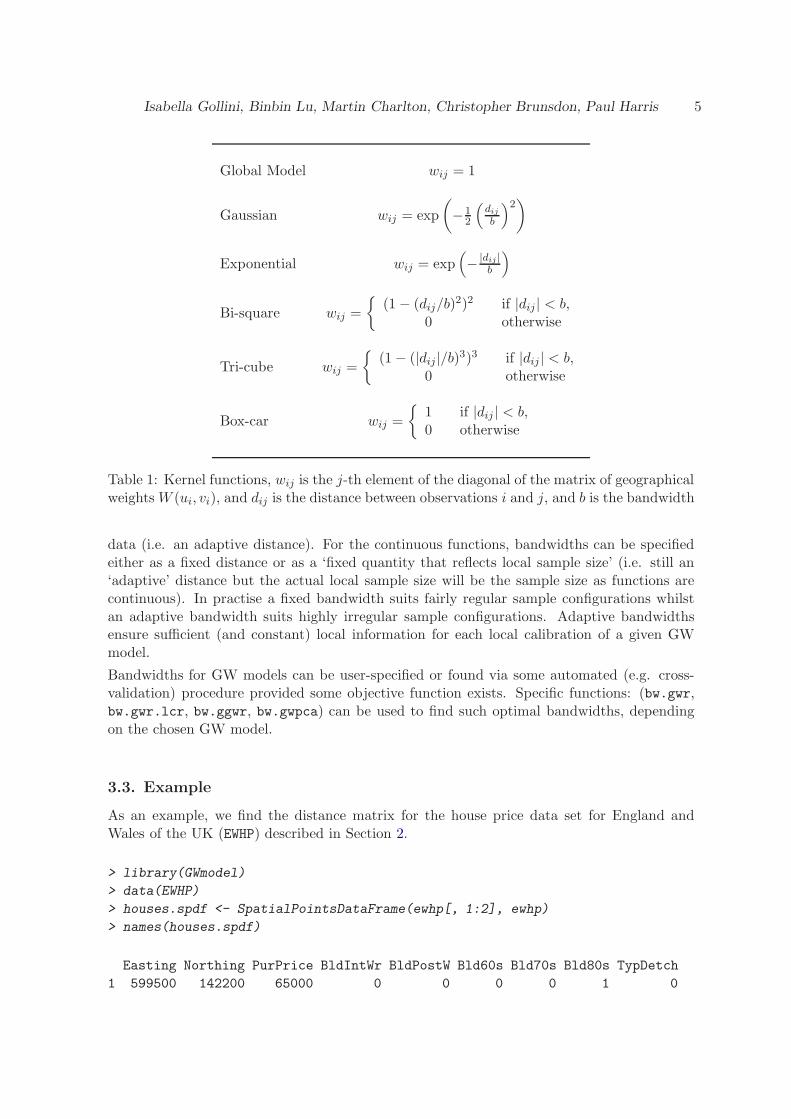
A set of commonly used kernel functions are shown in Table 1 and Figure 1; all of whichare available in GWmodel. The ‘Global Model’ kernel, that gives a unit weight to eachobservation, is included in order to show that a global model is a special case of its GWmodel.
The Gaussian and exponential kernels are continuous functions of the distance between twoobservation points (or an observation and calibration point). The weights will be a maximum(equal to 1) for an observation at a GW model calibration point, and will decrease accordingto a Gaussian or exponential curve as the distance between observation/calibration pointsincreases.
The box-car kernel is a simple discontinuous weighting function that excludes observationsthat are further than some distance b from the GW model calibration point. This is equivalentto setting their weights to zero at such distances. This kernel allows for efficient computation,since only a subset of the observation points need to be included in fitting the local modelat each GW model calibration point. This can be particularly useful when handling largedatasets.
The bi-square and tri-cube kernels are similarly discontinuous, giving null weights to obser-vations with a distance greater than b. However unlike a box-car kernel, they provide weightsthat decrease as the distance between observation/calibration points increase, up until thedistance b. Thus these are both distance-decay weighting kernels, as are Gaussian and expo-nential kernels.
The key controlling parameter in all kernel functions is the bandwidth b. For the discontinuousfunctions, bandwidths can be specified either as a fixed distance or as a fixed number of local
Isabella Gollini, Binbin Lu, Martin Charlton, Christopher Brunsdon, Paul Harris 5
Global Model wij = 1
Gaussian wij = exp
(
−12
(
dijb
)2)
Exponential wij = exp(
− |dij |b
)
Bi-square wij =
{
(1− (dij/b)2)2 if |dij | < b,
0 otherwise
Tri-cube wij =
{
(1− (|dij |/b)3)3 if |dij | < b,0 otherwise
Box-car wij =
{
1 if |dij | < b,0 otherwise
Table 1: Kernel functions, wij is the j-th element of the diagonal of the matrix of geographicalweights W (ui, vi), and dij is the distance between observations i and j, and b is the bandwidth
data (i.e. an adaptive distance). For the continuous functions, bandwidths can be specifiedeither as a fixed distance or as a ‘fixed quantity that reflects local sample size’ (i.e. still an‘adaptive’ distance but the actual local sample size will be the sample size as functions arecontinuous). In practise a fixed bandwidth suits fairly regular sample configurations whilstan adaptive bandwidth suits highly irregular sample configurations. Adaptive bandwidthsensure sufficient (and constant) local information for each local calibration of a given GWmodel.
Bandwidths for GW models can be user-specified or found via some automated (e.g. cross-validation) procedure provided some objective function exists. Specific functions: (bw.gwr,bw.gwr.lcr, bw.ggwr, bw.gwpca) can be used to find such optimal bandwidths, dependingon the chosen GW model.
3.3. Example
As an example, we find the distance matrix for the house price data set for England andWales of the UK (EWHP) described in Section 2.
> library(GWmodel)
> data(EWHP)
> houses.spdf <- SpatialPointsDataFrame(ewhp[, 1:2], ewhp)
> names(houses.spdf)
Easting Northing PurPrice BldIntWr BldPostW Bld60s Bld70s Bld80s TypDetch
1 599500 142200 65000 0 0 0 0 1 0

6 GWmodel: Geographically Weighted Models
−2000 −1000 0 1000 2000
0.0
0.4
0.8
Global b=1000
d
w
−2000 −1000 0 1000 2000
0.0
0.4
0.8
Gaussian b=1000
d
w
−2000 −1000 0 1000 2000
0.0
0.4
0.8
Exponential b=1000
d
w
−2000 −1000 0 1000 20000.
00.
40.
8
Bisquare b=1000
d
w
−2000 −1000 0 1000 2000
0.0
0.4
0.8
Tricube b=1000
d
w
−2000 −1000 0 1000 2000
0.0
0.4
0.8
Boxcar b=1000
d
w
Figure 1: Plot of the Kernel functions, with the bandwidth b = 1000, and where w is theweight, and d is the distance between two observations
2 575400 167200 45000 0 0 0 0 0 0
3 530300 177300 50000 1 0 0 0 0 0
4 524100 170300 105000 0 0 0 0 0 0
5 426900 514600 175000 0 0 0 0 1 1
6 508000 190400 250000 0 1 0 0 0 1
TypSemiD TypFlat FlrArea
1 1 0 78.94786
2 0 1 94.36591
3 0 0 41.33153
4 0 0 92.87983
5 0 0 200.52756
6 0 0 148.60773
In GWmodel, the distance matrix can be calculated: (i) within a function of a specific GWmodel or (ii) outside of the function and saved using the function gw.dist. This flexibilty isparticularly useful for saving computation time when fitting several different GW models.

Isabella Gollini, Binbin Lu, Martin Charlton, Christopher Brunsdon, Paul Harris 7
Observe that we have specified the Euclidean distance metric for this data set. Other dis-tance metrics could have been specified by: (a) modifying the parameter p, the power of theMinkowsky distance or (b) setting longlat=TRUE in order to have the great circle distance.The output of the function gw.dist is a matrix containing in each row the value of thediagonal of the distance matrix for each observation.
> DM <- gw.dist(dp.locat = coordinates(houses.spdf))
> DM[1:7,1:7]
[,1] [,2] [,3] [,4] [,5] [,6] [,7]
[1,] 0.00 34724.78 77592.848 80465.956 410454.0 103419.00 236725.0
[2,] 34724.78 0.00 46217.096 51393.579 377808.2 71281.13 202563.8
[3,] 77592.85 46217.10 0.000 9350.936 352792.9 25863.10 160741.1
[4,] 80465.96 51393.58 9350.936 0.000 357757.4 25753.06 160945.0
[5,] 410454.04 377808.17 352792.928 357757.362 0.0 334189.84 232275.4
[6,] 103419.00 71281.13 25863.101 25753.058 334189.8 0.00 135411.2
[7,] 236725.01 202563.77 160741.096 160945.022 232275.4 135411.23 0.0
4. GW summary statistics
This section presents the simplest form of GW modelling with GW summary statistics(Brunsdon, Fotheringham, and Charlton 2002; Fotheringham et al. 2002). Here, we describehow to calculate GW means, GW standard deviations and GW measures of skew; whichconstitute a set of basic GW summary statistics. To mitigate against any adverse of outlierson these local statistics, a set of robust alternatives are also described in GW medians, GWinter-quartile ranges and GW quantile imbalances. Such local univariate summary statisticsare detailed in Brunsdon et al. (2002). In addition, GW correlations are described in basicand robust forms (Pearson’s and Spearman’s, respectively); providing a set of local bivariatesummary statistics.
Although fairly simple to calculate and map, GW summary statistics are considered a vitalpre-cursor to an application of any subsequent GW model, such as GW PCA (section 5) orGW regression (sections 6 to 8). For example, GW standard deviations (or GW inter-quartileranges) will highlight areas of high variability for a given variable, areas where a subsequentapplication of a GW PCA or a GW regression may warrant close scrutiny. Basic and robustGW correlations provide a preliminary assessment of relationship non-stationarity betweenthe dependent and an independent variable of a GW regression (section 6). GW correlationsalso provide an assessment of local collinearity between two independent variables of a GWregression; which could then lead to the application of a locally compensated model (section 7).
4.1. Basic GW summary statistics
For attributes z and y at any location i where wij accords to some kernel function of section 3,definitions for a GW mean, a GW standard deviation, a GW measure of skew and a GW

8 GWmodel: Geographically Weighted Models
Pearson’s correlation coefficient are respectively:
m(zi) =
∑nj=1wijzj
∑nj=1wij
(1)
s(zi) =
√
√
√
√
∑nj=1wij (zj −m(zi))
2
∑nj=1wij
(2)
b(zi) =
[
3
√∑nj=1
wij(zj−m(zi))3
∑nj=1
wij
]
s(zi)(3)
and
ρ(zi, yi) =c(zi, yi)
s(zi)s(yi)(4)
with the GW covariance:
c(zi, yi) =
∑nj=1wij [(zj −m(zi)) (yj −m(yi))]
∑nj=1wij
(5)
4.2. Robust GW summary statistics
Definitions for a GW median, a GW inter-quartile range and a GW quantile imbalance,all require the calculation of GW quantiles at any location i ; the calculation of which arepresented in Brunsdon et al. (2002). Thus if we calculate GW quartiles, the GW median isthe second GW quartile; and the GW inter-quartile range is the third minus the first GWquartile. The GW quantile imbalance measures the symmetry of the middle part of the localdistribution and is based on the position of the GW median relative to the first and thirdGW quartiles. It ranges from -1 (when the median is very close to the first GW quartile) to1 (when the median is very close to the third GW quartile), and is zero if the median bisectsthe first and third GW quartiles. To find a GW Spearman’s correlation coefficient, the localdata for z and for y each need to be ranked using the same approach as that used to calculatethe GW quantiles. The locally ranked variables are then simply fed into expression (4).
4.3. Example
For a demonstration of basic and robust GW summary statistics, we use the Dublin voterturnout data. Here we investigate the local variability in voter turnout (GenEl2004), whichis the dependent variable in the regressions of sections 6 and 7. We also investigate thelocal relationships between: (i) turnout and LARent and (ii) LARent and Unempl (i.e. twoindependent variables in the regressions of sections 6 and 7).
For any GW model calibration, it is prudent to experiment with different kernel functions.Here for our chosen GW summary statistics, we specify box-car and bi-square kernels; wherethe former relates to an un-weighted moving window, whilst the latter relates to a weighted
Isabella Gollini, Binbin Lu, Martin Charlton, Christopher Brunsdon, Paul Harris 9
one (from section 3). GW models using box-car kernels are useful in that the identifica-tion of outlying relationships or structures are more likely (Lloyd and Shuttleworth 2005;Harris and Brunsdon 2010). Such calibrations more easily relate to the global model form(see section 7) and in turn, tend to provide an intuitive understanding of the degree of hetero-geneity in the process. Observe that it is always possible that the spatial process is essentiallyhomogeneous, and in such cases, the output of a GW model can confirm this.
The spatial arrangement of the EDs in Greater Dublin is not a tessellation of equally sizedzones, so it makes sense to specify an adaptive kernel bandwidth. For example if we specify abandwidth of N = 100 , the box-car and bi-square kernels will change in radius but will alwaysinclude the closest 100 EDs for each local summary statistic. Bandwidths for GW means ormedians could be found optimally using cross-validation (functions not yet incorporated inGWmodel), whereas for all other GW summary statistics, bandwidths can only be user-specified (as no objective function exists).
Commands to conduct our GW summary statistical analysis are as follows, where we use thefunction gwss with two different specifications to find our GW summary statistics. We specifybox-car and bi-square kernels, each with an adaptive bandwidth of N = 48 (approximately15% of the data). To find robust GW summary statistics based on quantiles, the gwss functionis specified with quantiles = TRUE (observe that we do not need to do this for our robustGW correlations).
> library(GWmodel)
> library(RColorBrewer)
> data(DubVoter)
> gw.ss.bx <- gwss(Dub.voter, vars = c("GenEl2004", "LARent", "Unempl"),
+ kernel = "boxcar", adaptive = TRUE, bw = 48, quantile = TRUE)
> gw.ss.bs <- gwss(Dub.voter,vars = c("GenEl2004", "LARent", "Unempl"),
+ kernel = "bisquare", adaptive = TRUE, bw = 48)
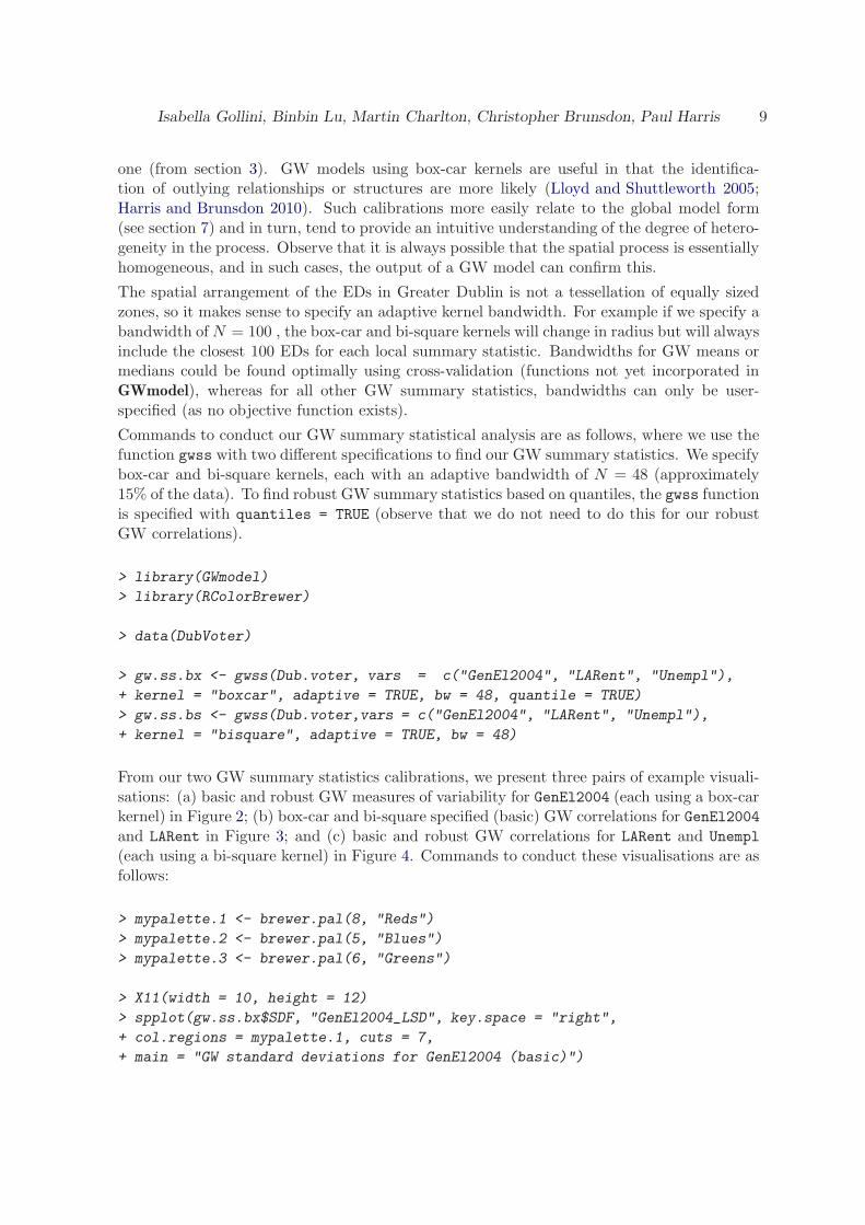
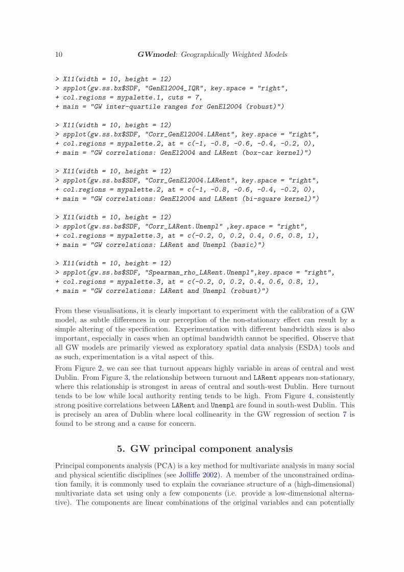
From our two GW summary statistics calibrations, we present three pairs of example visuali-sations: (a) basic and robust GW measures of variability for GenEl2004 (each using a box-carkernel) in Figure 2; (b) box-car and bi-square specified (basic) GW correlations for GenEl2004and LARent in Figure 3; and (c) basic and robust GW correlations for LARent and Unempl
(each using a bi-square kernel) in Figure 4. Commands to conduct these visualisations are asfollows:
> mypalette.1 <- brewer.pal(8, "Reds")
> mypalette.2 <- brewer.pal(5, "Blues")
> mypalette.3 <- brewer.pal(6, "Greens")
> X11(width = 10, height = 12)
> spplot(gw.ss.bx$SDF, "GenEl2004_LSD", key.space = "right",
+ col.regions = mypalette.1, cuts = 7,
+ main = "GW standard deviations for GenEl2004 (basic)")
10 GWmodel: Geographically Weighted Models
> X11(width = 10, height = 12)
> spplot(gw.ss.bx$SDF, "GenEl2004_IQR", key.space = "right",
+ col.regions = mypalette.1, cuts = 7,
+ main = "GW inter-quartile ranges for GenEl2004 (robust)")
> X11(width = 10, height = 12)
> spplot(gw.ss.bx$SDF, "Corr_GenEl2004.LARent", key.space = "right",
+ col.regions = mypalette.2, at = c(-1, -0.8, -0.6, -0.4, -0.2, 0),
+ main = "GW correlations: GenEl2004 and LARent (box-car kernel)")
> X11(width = 10, height = 12)
> spplot(gw.ss.bs$SDF, "Corr_GenEl2004.LARent", key.space = "right",
+ col.regions = mypalette.2, at = c(-1, -0.8, -0.6, -0.4, -0.2, 0),
+ main = "GW correlations: GenEl2004 and LARent (bi-square kernel)")
> X11(width = 10, height = 12)
> spplot(gw.ss.bs$SDF, "Corr_LARent.Unempl" ,key.space = "right",
+ col.regions = mypalette.3, at = c(-0.2, 0, 0.2, 0.4, 0.6, 0.8, 1),
+ main = "GW correlations: LARent and Unempl (basic)")
> X11(width = 10, height = 12)
> spplot(gw.ss.bs$SDF, "Spearman_rho_LARent.Unempl",key.space = "right",
+ col.regions = mypalette.3, at = c(-0.2, 0, 0.2, 0.4, 0.6, 0.8, 1),
+ main = "GW correlations: LARent and Unempl (robust)")
From these visualisations, it is clearly important to experiment with the calibration of a GWmodel, as subtle differences in our perception of the non-stationary effect can result by asimple altering of the specification. Experimentation with different bandwidth sizes is alsoimportant, especially in cases when an optimal bandwidth cannot be specified. Observe thatall GW models are primarily viewed as exploratory spatial data analysis (ESDA) tools andas such, experimentation is a vital aspect of this.
From Figure 2, we can see that turnout appears highly variable in areas of central and westDublin. From Figure 3, the relationship between turnout and LARent appears non-stationary,where this relationship is strongest in areas of central and south-west Dublin. Here turnouttends to be low while local authority renting tends to be high. From Figure 4, consistentlystrong positive correlations between LARent and Unempl are found in south-west Dublin. Thisis precisely an area of Dublin where local collinearity in the GW regression of section 7 isfound to be strong and a cause for concern.
5. GW principal component analysis
Principal components analysis (PCA) is a key method for multivariate analysis in many socialand physical scientific disciplines (see Jolliffe 2002). A member of the unconstrained ordina-tion family, it is commonly used to explain the covariance structure of a (high-dimensional)multivariate data set using only a few components (i.e. provide a low-dimensional alterna-tive). The components are linear combinations of the original variables and can potentially
Isabella Gollini, Binbin Lu, Martin Charlton, Christopher Brunsdon, Paul Harris 11
GW standard deviations for GenEl2004 (basic)
5
6
7
8
9
10
11
(a)
GW inter−quartile ranges for GenEl2004 (robust)
8
10
12
14
16
18
(b)
Figure 2: (a) Basic and (b) robust GW measures of variability for GenEl2004 (turnout).
GW correlations: GenEl2004 and LARent (box−car kernel)
−1.0
−0.8
−0.6
−0.4
−0.2
0.0
(a)
GW correlations: GenEl2004 and LARent (bi−square kernel)
−1.0
−0.8
−0.6
−0.4
−0.2
0.0
(b)
Figure 3: (a) Box-car and (b) bi-square specified GW correlations for GenEl2004 and LARent.

12 GWmodel: Geographically Weighted Models
GW correlations: LARent and Unempl (basic)
−0.2
0.0
0.2
0.4
0.6
0.8
1.0
(a)
GW correlations: LARent and Unempl (robust)
−0.2
0.0
0.2
0.4
0.6
0.8
1.0
(b)
Figure 4: (a) Basic and (b) robust GW correlations for LARent and Unempl.
provide a better understanding of differing sources of variation and structure in the data.These may be visualised and interpreted using associated graphics. In geographical settings,standard PCA, in which the components do not depend on location, may be replaced witha GW PCA (Harris, Brunsdon, and Charlton 2011a), to account for spatial heterogeneity inthe structure of the multivariate data. In doing so, GW PCA can identify regions whereassuming the same underlying structure in all locations is inappropriate or over-simplistic.GW PCA can assess: (a) how effective data dimensionality varies spatially and (b) how theoriginal variables influence the components vary spatially. In part, GW PCA resembles thebivariate GW correlations of section 4 in a multivariate sense, as both are unlike the multi-variate GW regressions of sections 6 to 8, since there is no distinction between dependent andindependent variables. Key challenges in GW PCA are: (i) finding the scale at which eachlocalised PCA should operate and (ii) visualising and interpreting the output that resultsfrom its application. As with any GW model, GW PCA is constructed using weighted datathat is controlled by the kernel function and its bandwidth (section 3).
5.1. GW PCA
More formally, for a vector of observed variables xi at spatial location i with coordinates(u, v), GW PCA involves regarding xi as conditional on u and v, and making the mean vectorµ and covariance matrix Σ, functions of u and v. That is, µ(u, v) and Σ(u, v) are the GWmean vector and the GW covariance matrix, respectively. To find the GW principal compo-nents, the decomposition of the GW covariance matrix provides the GW eigenvalues and GWeigenvectors. The product of the i-th row of the data matrix with the GW eigenvectors for
Isabella Gollini, Binbin Lu, Martin Charlton, Christopher Brunsdon, Paul Harris 13
the i-th location provides the i-th row of GW component scores. The GW covariance matrixis:
Σ(u, v) = XTW (u, v)X (6)
whereX is the data matrix (with n rows for the observations andm columns for the variables);and W (u, v) is a diagonal matrix of geographic weights. The GW principal components atlocation (ui, vi) can be written as:
L(ui, vi)V (ui, vi)L(ui, vi)T = Σ(ui, vi) (7)
where L(ui, vi) is a matrix of GW eigenvectors; V (ui, vi) is a diagonal matrix of GW eigen-values; and Σ(ui, vi) is the GW covariance matrix. Thus for a GW PCA with m variables,there are m components, m eigenvalues, m sets of component scores, and m sets of compo-nent loadings at each observed location. We can also obtain eigenvalues and their associatedeigenvectors at unobserved locations, although as no data exists for these locations, we cannotobtain component scores.
5.2. Robust GW PCA
A robust GW PCA can also be specified, so as to reduce the effect of anomalous observationson its outputs. Outliers can artificially increase local variability and mask key features in localdata structures. To provide a robust GW PCA, each local covariance matrix is estimatedusing the robust minimum covariance determinant (MCD) estimator (Rousseeuw 1985). TheMCD estimator searches for a subset of h data points that has the smallest determinantfor their basic sample covariance matrix. Crucial to the robustness and efficiency of thisestimator is h, and we specify a default value of h = 0.75n, following the recommendation of(Varmuza and Filzmoser 2009, p.43).
5.3. Example
For applications of (global) PCA and GW PCA, we again use the Dublin voter turnout data,this time focussing on the eight variables: DiffAdd, LARent, SC1, Unempl, LowEduc, Age18_24,Age25_44 and Age45_64 (i.e. the independent variables of the regression fits in sections 6 and7). Although measured on the same scale, the variables are not of a similar magnitude. Thus,we standardise the data and specify our PCA with the covariance matrix. The same (globally)standardised data is also used in our GW PCA calibrations, which are similarly specified with(local) covariance matrices. The effect of this standardisation is to make each variable haveequal importance in the subsequent analysis (at least for the global PCA case)2. The basicand robust PCA results are found using scale, princomp and covMcd functions, as follows:
> library(GWmodel)
> library(RColorBrewer)
> data(DubVoter)
> Data.scaled <- scale(as.matrix(Dub.voter@data[,4:11]))
2The use of un-standardised data, or the use of locally-standardised data with GW PCA is a subject ofcurrent investigation.

14 GWmodel: Geographically Weighted Models
> pca.basic <- princomp(Data.scaled, cor = F)
> (pca.basic$sdev^2 / sum(pca.basic$sdev^2))*100
Comp.1 Comp.2 Comp.3 Comp.4 Comp.5 Comp.6 Comp.7
36.084435 25.586984 11.919681 10.530373 6.890565 3.679812 3.111449
Comp.8
2.196701
> pca.basic$loadings
oadings:
Comp.1 Comp.2 Comp.3 Comp.4 Comp.5 Comp.6 Comp.7 Comp.8
DiffAdd 0.389 -0.444 -0.149 0.123 0.293 0.445 0.575
LARent 0.441 0.226 0.144 0.172 0.612 0.149 -0.539 0.132
SC1 -0.130 -0.576 -0.135 0.590 -0.343 -0.401
Unempl 0.361 0.462 0.189 0.197 0.670 -0.355
LowEduc 0.131 0.308 -0.362 -0.861
Age18_24 0.237 0.845 -0.359 -0.224 -0.200
Age25_44 0.436 -0.302 -0.317 -0.291 0.448 -0.177 -0.546
Age45_64 -0.493 0.118 0.179 -0.144 0.289 0.748 0.142 -0.164
> R.COV <- covMcd(Data.scaled, cor = F, alpha = 0.75)
> pca.robust <- princomp(Data.scaled, covmat = R.COV, cor = F)
> pca.robust$sdev^2 / sum(pca.robust$sdev^2)
Comp.1 Comp.2 Comp.3 Comp.4 Comp.5
0.419129445 0.326148321 0.117146840 0.055922308 0.043299600
Comp.6 Comp.7 Comp.8
0.017251964 0.014734597 0.006366926
> pca.robust$loadings
Loadings:
Comp.1 Comp.2 Comp.3 Comp.4 Comp.5 Comp.6 Comp.7 Comp.8
DiffAdd 0.512 -0.180 0.284 -0.431 0.659
LARent -0.139 0.310 0.119 -0.932
SC1 0.559 0.591 0.121 0.368 0.284 -0.324
Unempl -0.188 -0.394 0.691 -0.201 0.442 0.307
LowEduc -0.102 -0.186 0.359 -0.895 0.149
Age18_24 -0.937 0.330
Age25_44 0.480 -0.437 -0.211 -0.407 -0.598
Age45_64 -0.380 0.497 -0.264 0.178 -0.665 -0.241
From the ‘percentage of total variance’ (PTV) results, the first three components collectivelyaccount for 73.6% and 86.2% of the variation in the data, for the basic and robust PCA,
Isabella Gollini, Binbin Lu, Martin Charlton, Christopher Brunsdon, Paul Harris 15
respectively. From the tables of loadings, component one would appear to represent olderresidents (Age45_64) in the basic PCA or represent affluent residents (SC1) in the robustPCA. Component two, appears to represent affluent residents in both the basic and robustPCA. These are whole-map statistics (Openshaw, Charlton, Wymer, and Craft 1987) andinterpretations that represent a Dublin-wide average. However, it is possible that they do notrepresent local social structure particularly reliably aAS in the situation where variances andcovariances between the variables vary geographically. In this case, an application of GWPCA may be useful, which will now be demonstrated.
Kernel bandwidths for GW PCA can be found automatically using a cross-validation ap-proach, similar in nature to that used in GW regression (section 6). Details of this automatedprocedure are described in Harris et al. (2011a), where, a ‘leave-one-out’ cross-validation (CV)score is computed for all possible bandwidths and an optimal bandwidth relates to the small-est CV score found. With this procedure, it is currently necessary to decide a priori upon thenumber of components to retain (k, say), and a different optimal bandwidth results for eachk. The procedure does not yield an optimal bandwidth if all components are retained (i.e.m = k); in this case, the bandwidth must be user-specified. Thus, here an optimal adaptivebandwidth is found using the default, bi-square kernel, for both a basic and a robust GWPCA. Here, k = 3 is chosen on an a priori basis. With the GWmodel package, the bw.gwpcafunction is used in the following set of commands, where the standardised data is convertedto a spatial form via the SpatialPointsDataFrame function.
> Coords <- as.matrix(cbind(Dub.voter$X,Dub.voter$Y))
> Data.scaled.spdf <-
+ SpatialPointsDataFrame(Coords,as.data.frame(Data.scaled))
> bw.gwpca.basic <- bw.gwpca(Data.scaled.spdf,
+ vars = colnames(Data.scaled.spdf@data), k = 3, robust = FALSE,
+ adaptive = TRUE)
> bw.gwpca.basic
[1] 131
> bw.gwpca.robust <- bw.gwpca(Data.scaled.spdf,
+ vars=colnames(Data.scaled.spdf@data), k = 3, robust = TRUE, adaptive = TRUE)
> bw.gwpca.robust
[1] 130
Inspecting the values of bw.gwpca.basic and bw.gwpca.robust show that (very similar)optimal bandwidths of N = 131 and N = 130 will be used to calibrate the respective basicand robust GW PCA fits. Observe that we now specify all k = 8 components, but will focusour investigations on only the first three components. This specification ensures that thevariation locally accounted for by each component, is estimated correctly. The two GW PCAfits are found using the gwpca function as follows:
> gwpca.basic <- gwpca(Data.scaled.spdf,
+ vars = colnames(Data.scaled.spdf@data), bw = bw.gwpca.basic, k = 8,
16 GWmodel: Geographically Weighted Models
+ robust = FALSE, adaptive = TRUE)
> gwpca.robust <- gwpca(Data.scaled.spdf,
+ vars = colnames(Data.scaled.spdf@data), bw = bw.gwpca.robust, k = 8,
+ robust = TRUE, adaptive = TRUE)
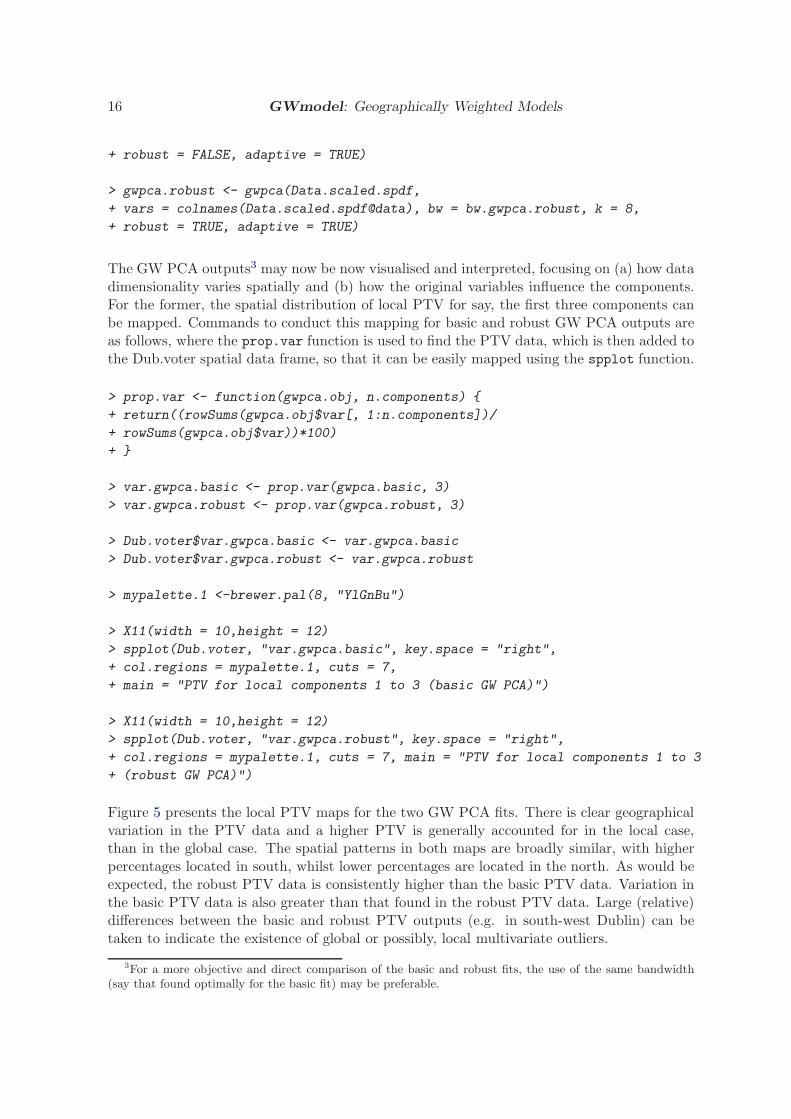
The GW PCA outputs3 may now be now visualised and interpreted, focusing on (a) how datadimensionality varies spatially and (b) how the original variables influence the components.For the former, the spatial distribution of local PTV for say, the first three components canbe mapped. Commands to conduct this mapping for basic and robust GW PCA outputs areas follows, where the prop.var function is used to find the PTV data, which is then added tothe Dub.voter spatial data frame, so that it can be easily mapped using the spplot function.
> prop.var <- function(gwpca.obj, n.components) {
+ return((rowSums(gwpca.obj$var[, 1:n.components])/
+ rowSums(gwpca.obj$var))*100)
+ }
> var.gwpca.basic <- prop.var(gwpca.basic, 3)
> var.gwpca.robust <- prop.var(gwpca.robust, 3)
> Dub.voter$var.gwpca.basic <- var.gwpca.basic
> Dub.voter$var.gwpca.robust <- var.gwpca.robust
> mypalette.1 <-brewer.pal(8, "YlGnBu")
> X11(width = 10,height = 12)
> spplot(Dub.voter, "var.gwpca.basic", key.space = "right",
+ col.regions = mypalette.1, cuts = 7,
+ main = "PTV for local components 1 to 3 (basic GW PCA)")
> X11(width = 10,height = 12)
> spplot(Dub.voter, "var.gwpca.robust", key.space = "right",
+ col.regions = mypalette.1, cuts = 7, main = "PTV for local components 1 to 3
+ (robust GW PCA)")
Figure 5 presents the local PTV maps for the two GW PCA fits. There is clear geographicalvariation in the PTV data and a higher PTV is generally accounted for in the local case,than in the global case. The spatial patterns in both maps are broadly similar, with higherpercentages located in south, whilst lower percentages are located in the north. As would beexpected, the robust PTV data is consistently higher than the basic PTV data. Variation inthe basic PTV data is also greater than that found in the robust PTV data. Large (relative)differences between the basic and robust PTV outputs (e.g. in south-west Dublin) can betaken to indicate the existence of global or possibly, local multivariate outliers.
3For a more objective and direct comparison of the basic and robust fits, the use of the same bandwidth(say that found optimally for the basic fit) may be preferable.
Isabella Gollini, Binbin Lu, Martin Charlton, Christopher Brunsdon, Paul Harris 17
PTV for local components 1 to 3 (basic GW PCA)
72
74
76
78
80
82
84
86
88
90
(a)
PTV for local components 1 to 3 (robust GW PCA)
92
93
94
95
96
97
98
(b)
Figure 5: (a) Basic and (b) robust PTV data for the first three local components.
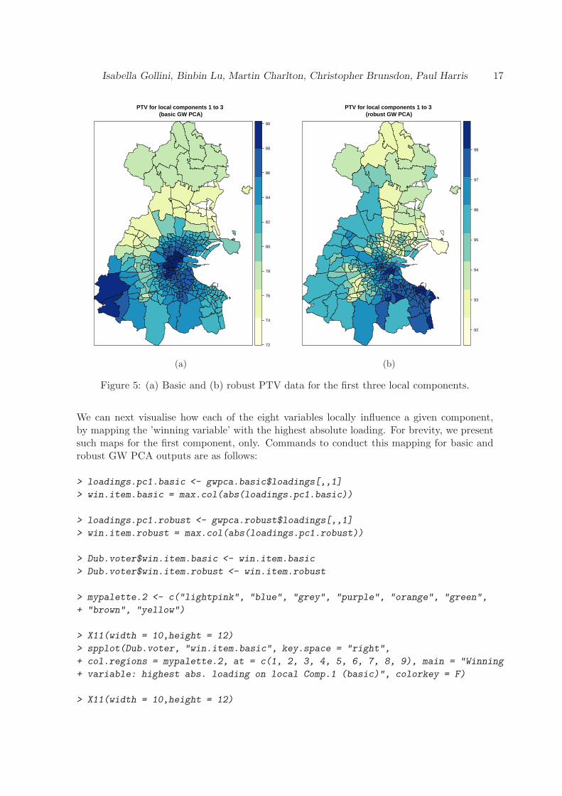
We can next visualise how each of the eight variables locally influence a given component,by mapping the ’winning variable’ with the highest absolute loading. For brevity, we presentsuch maps for the first component, only. Commands to conduct this mapping for basic androbust GW PCA outputs are as follows:
> loadings.pc1.basic <- gwpca.basic$loadings[,,1]
> win.item.basic = max.col(abs(loadings.pc1.basic))
> loadings.pc1.robust <- gwpca.robust$loadings[,,1]
> win.item.robust = max.col(abs(loadings.pc1.robust))
> Dub.voter$win.item.basic <- win.item.basic
> Dub.voter$win.item.robust <- win.item.robust
> mypalette.2 <- c("lightpink", "blue", "grey", "purple", "orange", "green",
+ "brown", "yellow")
> X11(width = 10,height = 12)
> spplot(Dub.voter, "win.item.basic", key.space = "right",
+ col.regions = mypalette.2, at = c(1, 2, 3, 4, 5, 6, 7, 8, 9), main = "Winning
+ variable: highest abs. loading on local Comp.1 (basic)", colorkey = F)
> X11(width = 10,height = 12)

18 GWmodel: Geographically Weighted Models
Winning variable: highest abs. loading on local Comp.1 (basic)
(a)
Winning variable: highest abs. loading on local Comp.1 (robust)
(b)
Figure 6: (a) Basic and (b) robust GW PCA results for the winning variable on the firstcomponent. Legend for both maps are as follows: DiffAdd - light pink; LARent - blue; SC1 -grey; Unempl - purple; LowEduc - orange; Age18_24 - green; Age25_44 - brown; and Age45_64
- yellow.
> spplot(Dub.voter, "win.item.robust", key.space = "right",
+ col.regions = mypalette.2, at = c(1, 2, 3, 4, 5, 6, 7, 8, 9), main = "Winning
+ variable: highest abs. loading on local Comp.1 (robust)", colorkey = F)
Figure 6 presents the ‘winning variable’ maps for the two GW PCA fits, where we can observeclear geographical variation in the influence of each variable on the first component. For basicGW PCA, low educational attainment (Low_Educ) dominates in the northern and south-western EDs, whilst public housing (LARent) dominates in the EDs of central Dublin. Thecorresponding global PCA ‘winning variable’ is Age45_64, which is clearly not dominantthroughout Dublin. Variation in the results from basic GW PCA is much greater than thatfound with robust GW PCA (reflecting analogous results to that found with the PTV data).For robust GW PCA, Age45_64 does in fact dominate in most areas, thus reflecting a closercorrespondence to the global case - but interestingly only the basic case, and not the robustcase.
6. GW regression
Isabella Gollini, Binbin Lu, Martin Charlton, Christopher Brunsdon, Paul Harris 19
6.1. Basic GW regression
The concept of GW modelling can be extended to a local regression form with GW regression(Brunsdon, Fotheringham, and Charlton 1996, 1998), where spatially-varying relationshipsare explored between the dependent and independent variables. Exploration commonly con-sists of mapping the resultant local regression coefficient estimates and associated t-values todetermine evidence of non-stationarity. The basic form of the GW regression model is:
yi = βi0 +
m∑
k=1
βikxik + ǫi (8)
where yi is the dependent variable at location i; xik is the value of the kth independentvariable at location i; m is the number of independent variables; βi0 is the intercept parameterat location i; βik is the local regression coefficient for the kth independent variable at locationi; and ǫi is the random error at location i.
As data are geographically weighted, nearer observations have more influence in estimatingthe local set of regression coefficients than observations farther away. The model measures theinherent relationships around each regression point i, where each set of regression coefficientsis estimated by a weighted least squares approach. The matrix expression for this estimationis:
βi =(
XTW (ui, vi)X)−1
XTW (ui, vi)y (9)
where X is the matrix of the independent variables with a column of 1s for the intercept; yis the dependent variable vector; βi = (βi0, . . . , βim)T is the vector of m + 1 local regressioncoefficients; and Wi is the diagonal matrix denoting the geographical weighting of each ob-served data for regression point i at location (ui, vi). This weighting is determined by somekernel function as described in section 3.
An optimum kernel bandwidth for GW regression can be found by minimising some model fitdiagnostic, such as a leave-one-out cross-validation (CV) score (Bowman 1984), which onlyaccounts for model prediction accuracy; or the Akaike Information Criterion (AIC) (Akaike1973), which accounts for model parsimony (i.e. a trade-off between prediction accuracy andcomplexity). In practice, a corrected version of the AIC is used, which unlike basic AIC is afunction of sample size (Hurvich and Simonoff 1998). Here model fits from smaller samplesreceive a higher penalty (i.e. are more complex) than those from larger samples. Thus for aGW regression with a bandwidth b, its AICc can be found from:
AICc(b) = 2n ln(σ) + n ln(2π) + n
{
n+ tr(S)
n− 2− tr(S)
}
(10)
where n is the (local) sample size (according to b); σ is the estimated standard deviationof the error term; and tr(S) denotes the trace of the hat matrix S. The hat matrix is theprojection matrix from the observed y to the fitted values, y.
6.2. Robust GW regression
To identify and reduce the effect of outliers in GW regression, various robust extensions havebeen proposed, two of which are described in Fotheringham et al. (2002). The first robust

20 GWmodel: Geographically Weighted Models
model re-fits a GW regression with a filtered dataset that has been found by removing obser-vations that correspond to large externally studentised residuals of an initial GW regressionfit. An externally studentised residual for each regression location i is defined as:
ri =ei
σ−i√qii
(11)
where ei is the residual at location i; σ−i is a leave-one-out estimate of σ; and qii is the ithelement of (I − S)(I − S)T . Observations are deemed outlying and filtered from the dataif they have |ri| > 3. The second robust model, iteratively down-weights observations thatcorrespond to large residuals. This (non-geographical) weighting function wr on the residualei is typically taken as:
wr(ei) =
1, if |ei| ≤ 2σ[
1− (|ei| − 2)2]2
, if 2σ < |ei| < 3σ
0 otherwise
(12)
Observe that both approaches have an element subjectivity, where the filtered data approachdepends on the chosen residual cut-off (in this case, 3) and the iterative (automatic) approachdepends on the chosen down-weighting function, with its associated cut-offs.
6.3. Example
We now demonstrate the fitting of the basic and robust GW regressions described, to theDublin voter turnout data. Here our GW regressions, together with the global OLS regression,attempt to predict the proportion of the electorate who turned out on voting night to casttheir vote in the 2004 General Election in Ireland. Thus the dependent variable is GenEl2004and the eight independent variables are DiffAdd, LARent, SC1, Unempl, LowEduc, Age18_24,Age25_44 and Age45_64.
A global correlation analysis suggests that turnout is negatively associated with the inde-pendent variables, except for social class (SC1) and older adults (Age45_64). Public renters(LARent) and unemployed (Unempl) have the highest correlations (both negative). The local(GW) correlation analysis from section 4 indicates that some of these relationships are non-stationary. The OLS regression fit to this data yields an R-squared value of 0.63 and detailsof this fit can be summarised as follows:
> library(GWmodel)
> library(RColorBrewer)
> data(DubVoter)
> lm.global <- lm(GenEl2004 ~ DiffAdd + LARent + SC1 + Unempl + LowEduc +
+ Age18_24 + Age25_44 + Age45_64, data = Dub.voter)
> summary(lm.global)
Coefficients:
Estimate Std. Error t value Pr(>|t|)
(Intercept) 77.70467 3.93928 19.726 < 2e-16 ***
DiffAdd -0.08583 0.08594 -0.999 0.3187
Isabella Gollini, Binbin Lu, Martin Charlton, Christopher Brunsdon, Paul Harris 21
LARent -0.09402 0.01765 -5.326 1.92e-07 ***
SC1 0.08637 0.07085 1.219 0.2238
Unempl -0.72162 0.09387 -7.687 1.96e-13 ***
LowEduc -0.13073 0.43022 -0.304 0.7614
Age18_24 -0.13992 0.05480 -2.554 0.0111 *
Age25_44 -0.35365 0.07450 -4.747 3.15e-06 ***
Age45_64 -0.09202 0.09023 -1.020 0.3086
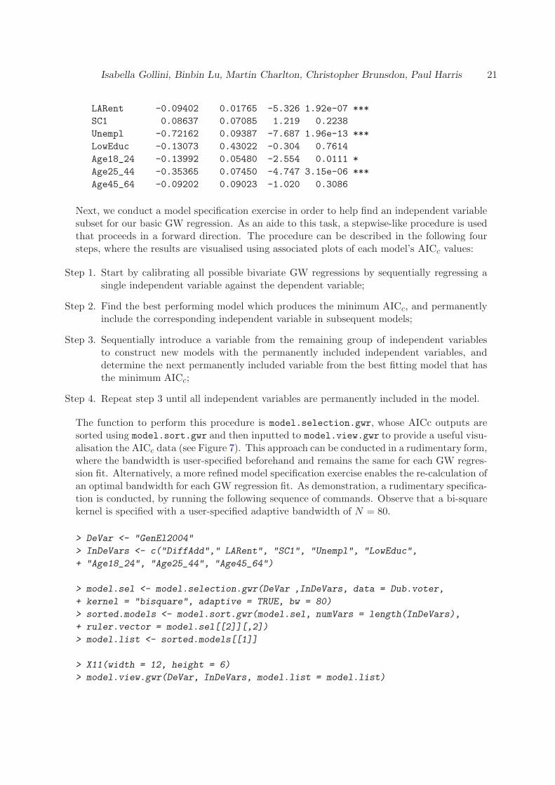
Next, we conduct a model specification exercise in order to help find an independent variablesubset for our basic GW regression. As an aide to this task, a stepwise-like procedure is usedthat proceeds in a forward direction. The procedure can be described in the following foursteps, where the results are visualised using associated plots of each model’s AICc values:
Step 1. Start by calibrating all possible bivariate GW regressions by sequentially regressing asingle independent variable against the dependent variable;
Step 2. Find the best performing model which produces the minimum AICc, and permanentlyinclude the corresponding independent variable in subsequent models;
Step 3. Sequentially introduce a variable from the remaining group of independent variablesto construct new models with the permanently included independent variables, anddetermine the next permanently included variable from the best fitting model that hasthe minimum AICc;
Step 4. Repeat step 3 until all independent variables are permanently included in the model.
The function to perform this procedure is model.selection.gwr, whose AICc outputs aresorted using model.sort.gwr and then inputted to model.view.gwr to provide a useful visu-alisation the AICc data (see Figure 7). This approach can be conducted in a rudimentary form,where the bandwidth is user-specified beforehand and remains the same for each GW regres-sion fit. Alternatively, a more refined model specification exercise enables the re-calculation ofan optimal bandwidth for each GW regression fit. As demonstration, a rudimentary specifica-tion is conducted, by running the following sequence of commands. Observe that a bi-squarekernel is specified with a user-specified adaptive bandwidth of N = 80.
> DeVar <- "GenEl2004"
> InDeVars <- c("DiffAdd"," LARent", "SC1", "Unempl", "LowEduc",
+ "Age18_24", "Age25_44", "Age45_64")
> model.sel <- model.selection.gwr(DeVar ,InDeVars, data = Dub.voter,
+ kernel = "bisquare", adaptive = TRUE, bw = 80)
> sorted.models <- model.sort.gwr(model.sel, numVars = length(InDeVars),
+ ruler.vector = model.sel[[2]][,2])
> model.list <- sorted.models[[1]]
> X11(width = 12, height = 6)
> model.view.gwr(DeVar, InDeVars, model.list = model.list)
22 GWmodel: Geographically Weighted Models
View of GWR model selection with different variables
12
34
56
78
910111213
141516
17
18
19
20
21
22
23
2425
26
27 28 2930 31
32
33
34
35
36
GenEl2004DiffAddLARentSC1UnemplLowEducAge18_24Age25_44Age45_64
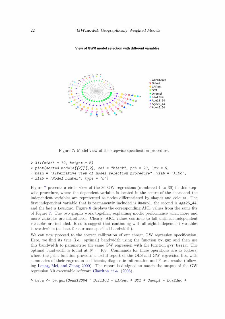
Figure 7: Model view of the stepwise specification procedure.
> X11(width = 12, height = 6)
> plot(sorted.models[[2]][,2], col = "black", pch = 20, lty = 5,
+ main = "Alternative view of model selection procedure", ylab = "AICc",
+ xlab = "Model number", type = "b")
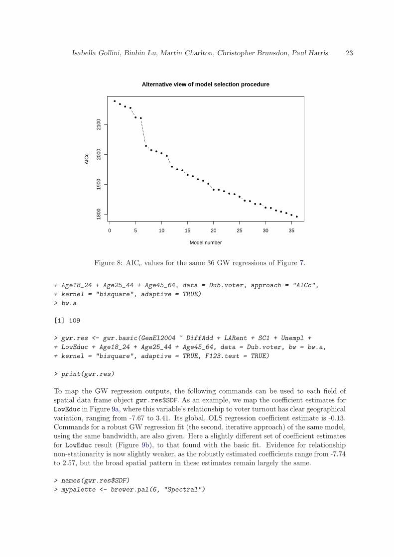
Figure 7 presents a circle view of the 36 GW regressions (numbered 1 to 36) in this step-wise procedure, where the dependent variable is located in the centre of the chart and theindependent variables are represented as nodes differentiated by shapes and colours. Thefirst independent variable that is permanently included is Unempl, the second is Age25_44,and the last is LowEduc. Figure 8 displays the corresponding AICc values from the same fitsof Figure 7. The two graphs work together, explaining model performance when more andmore variables are introduced. Clearly, AICc values continue to fall until all independentvariables are included. Results suggest that continuing with all eight independent variablesis worthwhile (at least for our user-specified bandwidth).
We can now proceed to the correct calibration of our chosen GW regression specification.Here, we find its true (i.e. optimal) bandwidth using the function bw.gwr and then usethis bandwidth to parametrise the same GW regression with the function gwr.basic. Theoptimal bandwidth is found at N = 109. Commands for these operations are as follows,where the print function provides a useful report of the OLS and GW regression fits, withsummaries of their regression coefficients, diagnostic information and F-test results (follow-ing Leung, Mei, and Zhang 2000). The report is designed to match the output of the GWregression 3.0 executable software Charlton et al. (2003).
> bw.a <- bw.gwr(GenEl2004 ~ DiffAdd + LARent + SC1 + Unempl + LowEduc +
Isabella Gollini, Binbin Lu, Martin Charlton, Christopher Brunsdon, Paul Harris 23
0 5 10 15 20 25 30 35
1800
1900
2000
2100
Alternative view of model selection procedure
Model number
AIC
c
Figure 8: AICc values for the same 36 GW regressions of Figure 7.
+ Age18_24 + Age25_44 + Age45_64, data = Dub.voter, approach = "AICc",
+ kernel = "bisquare", adaptive = TRUE)
> bw.a
[1] 109
> gwr.res <- gwr.basic(GenEl2004 ~ DiffAdd + LARent + SC1 + Unempl +
+ LowEduc + Age18_24 + Age25_44 + Age45_64, data = Dub.voter, bw = bw.a,
+ kernel = "bisquare", adaptive = TRUE, F123.test = TRUE)
> print(gwr.res)
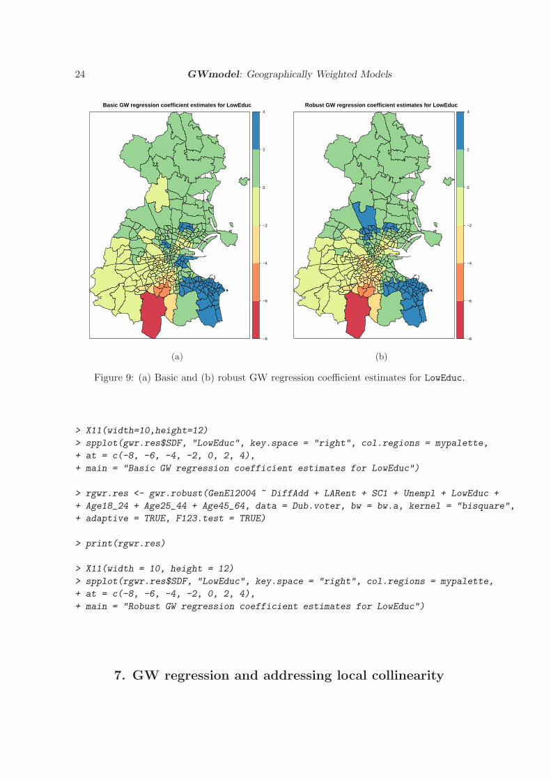
To map the GW regression outputs, the following commands can be used to each field ofspatial data frame object gwr.res$SDF. As an example, we map the coefficient estimates forLowEduc in Figure 9a, where this variable’s relationship to voter turnout has clear geographicalvariation, ranging from -7.67 to 3.41. Its global, OLS regression coefficient estimate is -0.13.Commands for a robust GW regression fit (the second, iterative approach) of the same model,using the same bandwidth, are also given. Here a slightly different set of coefficient estimatesfor LowEduc result (Figure 9b), to that found with the basic fit. Evidence for relationshipnon-stationarity is now slightly weaker, as the robustly estimated coefficients range from -7.74to 2.57, but the broad spatial pattern in these estimates remain largely the same.
> names(gwr.res$SDF)
> mypalette <- brewer.pal(6, "Spectral")
24 GWmodel: Geographically Weighted Models
Basic GW regression coefficient estimates for LowEduc
−8
−6
−4
−2
0
2
4
(a)
Robust GW regression coefficient estimates for LowEduc
−8
−6
−4
−2
0
2
4
(b)
Figure 9: (a) Basic and (b) robust GW regression coefficient estimates for LowEduc.
> X11(width=10,height=12)
> spplot(gwr.res$SDF, "LowEduc", key.space = "right", col.regions = mypalette,
+ at = c(-8, -6, -4, -2, 0, 2, 4),
+ main = "Basic GW regression coefficient estimates for LowEduc")
> rgwr.res <- gwr.robust(GenEl2004 ~ DiffAdd + LARent + SC1 + Unempl + LowEduc +
+ Age18_24 + Age25_44 + Age45_64, data = Dub.voter, bw = bw.a, kernel = "bisquare",
+ adaptive = TRUE, F123.test = TRUE)
> print(rgwr.res)
> X11(width = 10, height = 12)
> spplot(rgwr.res$SDF, "LowEduc", key.space = "right", col.regions = mypalette,
+ at = c(-8, -6, -4, -2, 0, 2, 4),
+ main = "Robust GW regression coefficient estimates for LowEduc")
7. GW regression and addressing local collinearity
Isabella Gollini, Binbin Lu, Martin Charlton, Christopher Brunsdon, Paul Harris 25
7.1. Collinearity
A problem which has long been acknowledged in regression modelling is that of collinearityamong the predictor (independent) variables. The effects of collinearity include a loss ofprecision and a loss of power in the coefficient estimates. Collinearity is potentially more ofan issue in GW regression because: (i) its effects can be more pronounced with the smallerspatial samples used in each local estimation and (ii) if the data are spatially heterogeneousin terms of its correlation structure, some localities may exhibit collinearity while others maynot. In both cases, collinearity may be a source of problems in GW regression even when noevidence is found for collinearity in the global model. A further complication is that in thecase of a variable which has little local spatial variation, the possibility of collinearity withthe intercept term is raised. Wheeler and Tiefelsdorf (2005) were the first to draw attentionto the effects of collinearity on GW regression estimation, and Wheeler (2007, 2009) has goneon to suggest modifications to the GW regression model which can cope with the effects ofcollinear predictors.
Collinearity can be identified through the use of the condition number of the cross-productmatrix (XTX) and variance inflation factors (VIFs). Both measurements can be made forlocal and global regressions. The condition number takes account of the predictor variablestaken together, whereas the VIFs consider each predictor in turn. Collinearity may be sus-pected if the condition number is greater than 30 or an individual VIF is greater than 10(Belsley, Kuh, and Welsch 1980; O’Brien 2007).
For a GW regression, a local condition number for the GW cross-product matrix that ex-ceeds 30 provides a warning that collinearity is affecting the corresponding local coefficientestimates. Although it will not indicate which variables are causing the problem, the localcondition number will indicate where the analyst should proceed with caution. Local versionsof the VIFs can also be used as a diagnostic. If the local VIFs are raised in some locations, thisprovides a warning that the corresponding local coefficient estimates may be suspect. Thereare several possible actions in the light of discovering levels of collinearity in the predictorsthat are a cause for concern. These include (i) doing nothing, (ii) removing the offendingvariables, (iii) transforming the predictors to some orthogonal form or (iv) using a differentestimator. However, although such actions may work globally, there is no guarantee, theywill similarly work locally. Thus to ensure that local collinearity is addressed, the appropriateremedy must also be local (i.e. taken at the same spatial scale).
7.2. Ridge regression
A method which to reduce the adverse effects of collinearity in the predictors of a linear modelis ridge regression (Hoerl 1962; Hoerl and Kennard 1970). Other methods include principalcomponents regression and partial least squares regression (Frank and Friedman 1993). Inridge regression the estimator is altered to include a small change to the values of the diagonalof the cross-product matrix aAS this is known as the ridge, indicated by λ in the followingequation:
β =(
XTX + λI)−1
XTY (13)
The effect of the ridge is to increase the difference between the diagonal elements of the matrixand the off-diagonal elements. As the off-diagonal elements represent the co-variation in thepredictors, the effect of the collinearity among the predictors in the estimation is lessened.
26 GWmodel: Geographically Weighted Models
The price of this is that β becomes biased, and the standard errors (and associated t-values)of the estimates are no longer available. Of interest is the value to be given to the ridgeparameter; Lee (1987) presents an algorithm to find a value which yields the best predictions.
7.3. GW regression with local compensation
There exists a link between the definition of the condition number for the cross-productmatrix and the ridge parameter based on the observation that if the eigenvalues of XTX areǫ1, ǫ2, . . . , ǫp then the eigenvalues of XTX + λI are ǫ1 + λ, ǫ2 + λ, . . . , ǫp + λ. The conditionnumber κ of a square matrix is defined as ǫ1/ǫp, so the condition number for the ridge-adjustedmatrix will be ǫ1 + λ/ǫp + λ. By re-arranging the terms, the ridge adjustment that will berequired to yield a particular condition number κ is λ = {(ǫ1 − ǫp)/(κ− 1)} − ǫp. Thusgiven the eigenvalues of the un-adjusted matrix, and the desired condition number, we candetermine the value of the ridge which is required to yield that condition number.
For GW regression, this can be applied to the GW cross-product matrix, which permits alocal compensation of each local regression model, so that the local condition number neverexceeds a specified value of κ. The condition numbers for the un-adjusted matrices may alsobe mapped to give an indication of where the analyst should take care in interpreting theresults, or the local ridge parameters may also be mapped. Collinearity is as much an issue inthe global OLS as the GW regression model; the local estimations will additionally indicatewhere the collinearity is a problem. The estimator for this locally compensated ridge (LCR)GW regression model is:
β(ui, vi) =(
XTW (ui, vi)X + λI(ui, vi))−1
XTW (ui, vi)Y (14)
where λI(ui, vi) is the locally compensated value of λ at location (ui, vi). Observe thatthe same approach to estimating the bandwidth in the basic GW regression (section 6) canbe applied to the locally-compensated GW regression model aAS for a CV approach, thebandwidth is optimised to yield the best predictions. Collinearity tends to affect the coefficientestimates rather than the predictions from the model, so nothing is lost when using the locally-compensated form of the model. Details on this and an alternative locally compensated GWregression can be found in Brunsdon, Charlton, and Harris (2012), where both models areperformance tested within a simulation experiment.
7.4. Example
We examine the use of local compensation with the same GW regression that is specifiedin section 6, where voter turnout is a function of the eight predictor variables of the Dublinelection data. For the corresponding OLS regression, the vif function in the car librarycomputes VIFs using the method outlined in Fox and Monette (1992). These global VIFs aregiven below and would suggest that weak collinearity exists within this data.
> library(GWmodel)
> library(car)
> library(RColorBrewer)
> data(DubVoter)

Isabella Gollini, Binbin Lu, Martin Charlton, Christopher Brunsdon, Paul Harris 27
> lm.global <- lm(GenEl2004 ~ DiffAdd + LARent + SC1 + Unempl +
+ LowEduc + Age18_24 + Age25_44 + Age45_64, data=Dub.voter)
> summary(lm.global)
> vif(lm.global)
DiffAdd LARent SC1 Unempl LowEduc Age18_24 Age25_44 Age45_64
3.170044 2.167172 2.161348 2.804576 1.113033 1.259760 2.879022 2.434470
In addition, the PCA from section 5 suggests collinearity between DiffAdd, LARent, Unempl,Age25_44, and Age45_64. As the first component accounts for some 36% of the variancein the data set, and of those components with eigenvalues greater than 1, the proportion ofvariance accounted for is 73.6%, we might consider removing variables with higher loadings.However for the purposes of illustration, we decide to keep the model as it is. Further globalfindings are of note, in that the correlation of turnout with Age45_64 is positive, but the signof the OLS regression coefficient is negative. Furthermore, only four of the OLS predictorsare significant. Unexpected sign changes and relatively few significant variables are bothindications of collinearity.
We can measure the condition number of the design matrix using the method outlined inBelsley et al. (1980). The method, termed BKW, requires that the columns of the matrixare scaled to have length 1; the condition number is the ratio of the largest to the smallestsingular value of this matrix. The following code implements the BKW computations, whereX is the design matrix consisting of the predictor variables and a column of 1s.
> X <- as.matrix(cbind(1,Dub.voter@data[,4:11]))
> BKWcn <- function(X) {
+ p <- dim(X)[2]
+ Xscale <- sweep(X, 2, sqrt(colSums(X^2)), "/")
+ Xsvd <- svd(Xscale)$d
+ Xsvd[1] / Xsvd[p]
+ }
> BKWcn(X)
[1] 41.06816
The BKW condition number is found to be 41.07 which is high, indicating that collinearityis at least, a global problem for this data. We can experiment by removing columns fromthe design matrix and test which variables appear to be the source of the collinearity. Forexample, entering:
> BKWcn(X[,c(-2,-8)])
[1] 18.69237
allows us to examine the effects of removing both DiffAdd and Age25_44 as sources ofcollinearity. The reduction of the BKW condition number to 18.69 suggests that removing

28 GWmodel: Geographically Weighted Models
these two variables is a useful start. However, for demonstration purposes, we will perseverewith the collinear (full specification) model, and now re-examine its GW regression fit, theone already fitted in section 6. The main function to perform this collinearity assessment isgwr.lcr, where we aim to compare the coefficient estimates for the unadjusted basic GWregression (of section 6) with those from a locally compensated ridge (LCR) GW regression.
In the first instance, we can use this function to find the global condition number (as thatfound with the OLS regression). This can be done simply by specifying a box-car kernel witha bandwidth equal to the sample size. This is equivalent to fitting n global models. Inspectionof the results from the spatial data frame show that the condition numbers are all equal to41.07, as hoped for. The same condition number is outputted by the ArcGIS Geographicallyweighted Regression tool in the Spatial Statistics Toolbox (ESRI 2011). Commands to conductthis check on the behaviour of the lcr.gwr function are as follows:
> nobs <- dim(Dub.voter)[1]
> lcrm1 <- gwr.lcr(GenEl2004 ~ DiffAdd + LARent + SC1 + Unempl + LowEduc +
+ Age18_24 + Age25_44 + Age45_64, data = Dub.voter, bw = nobs, kernel = "boxcar",
+ adaptive=TRUE)
> summary(lcrm1$SDF$Local_CN)
Min. 1st Qu. Median Mean 3rd Qu. Max.
41.07 41.07 41.07 41.07 41.07 41.07
To obtain local condition numbers for a basic GW regression without a local ridge compensa-tion, we use the bw.gwr.lcr function to optimally estimate the bandwidth, and then gwr.lcr
to estimate the local regression coefficients and the local condition numbers. To match that ofsection 6, we specify an adaptive bi-square kernel. Observe that the bandwidth for this modelcan be exactly the same as that obtained using bw.gwr, the basic bandwidth function. Witha ridge of zero and no local compensation, the cross-products matrices will be identical, butonly provided the same optimisation approach is specified. Here we specify a cross-validation(CV) approach, as the AICc approach is currently not an option in the bw.gwr.lcr function.Coincidently, for our basic GW regression of section 6, a bandwidth of N = 109 results forboth CV and AICc approaches. Commands to output the local condition numbers from abasic GW regression, and associated model comparisons are as follows:
> lcrm2.bw <- bw.gwr.lcr(GenEl2004 ~ DiffAdd + LARent + SC1 + Unempl + LowEduc +
+ Age18_24 + Age25_44 + Age45_64, data = Dub.voter, kernel = "bisquare",
+ adaptive=TRUE)
> lcrm2.bw
[1] 109
> lcrm2 <- gwr.lcr(GenEl2004 ~ DiffAdd + LARent + SC1 + Unempl + LowEduc +
+ Age18_24 + Age25_44 + Age45_64, data = Dub.voter, bw = lcrm2.bw,
+ kernel = "bisquare", adaptive = TRUE)
> summary(lcrm2$SDF$Local_CN)
Isabella Gollini, Binbin Lu, Martin Charlton, Christopher Brunsdon, Paul Harris 29
Min. 1st Qu. Median Mean 3rd Qu. Max.
32.88 52.75 59.47 59.28 64.85 107.50
> gwr.cv.bw <- bw.gwr(GenEl2004 ~ DiffAdd + LARent + SC1 + Unempl + LowEduc +
+ Age18_24 + Age25_44 + Age45_64, data = Dub.voter, approach = "CV",
+ kernel = "bisquare", adaptive = TRUE)
> gwr.cv.bw
[1] 109
> gwr.cv <- gwr.basic(GenEl2004 ~ DiffAdd + LARent + SC1 + Unempl + LowEduc +
+ Age18_24 + Age25_44 + Age45_64, data = Dub.voter, bw = gwr.cv.bw,
+ kernel = "bisquare", adaptive = TRUE)
> mypalette<-brewer.pal(8, "Reds")
> X11(width = 10, height = 12)
> spplot(lcrm2$SDF, "Local_CN", key.space = "right", col.regions = mypalette,
+ cuts=7, main="Local condition numbers from basic GW regression")
Thus the local condition numbers can range from 32.88 to 107.50, all worryingly large every-where. Whilst the local estimations are potentially more susceptible to collinearity than theglobal model, we might consider removing some of the variables which cause problems globally.The maps will show where the problem is worst, and where action should be concentrated.The local condition numbers for this estimation are shown in Figure 10a.
We can also use the local compensation to force the condition numbers not to exceed adesired threshold (taken as 30) by the application of local ridge adjustment to each localXTW (ui, vi)X matrix. The lambda.adjust = TRUE and cn.thresh = m parameters in thegwr.lcr function are used to invoke the local compensation process, as can be seen in followingcommands:
> lcrm3.bw <- bw.gwr.lcr(GenEl2004 ~ DiffAdd + LARent + SC1 + Unempl +
+ LowEduc + Age18_24 + Age25_44 + Age45_64, data = Dub.voter, kernel = "bisquare",
+ adaptive = TRUE, lambda.adjust = TRUE, cn.thresh = 30)
> lcrm3.bw
[1] 157
> lcrm3 <- gwr.lcr(GenEl2004 ~ DiffAdd + LARent + SC1+ Unempl + LowEduc +
+ Age18_24 + Age25_44 + Age45_64, data=Dub.voter, bw = lcrm3.bw,
+ kernel = "bisquare", adaptive = TRUE, lambda.adjust = TRUE, cn.thresh = 30)
> summary(lcrm3$SDF$Local_CN)
Min. 1st Qu. Median Mean 3rd Qu. Max.
34.34 47.08 53.84 52.81 58.66 73.72
> summary(lcrm3$SDF$Local_Lambda)
30 GWmodel: Geographically Weighted Models
Min. 1st Qu. Median Mean 3rd Qu. Max.
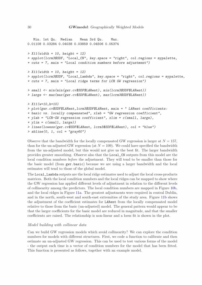
0.01108 0.03284 0.04038 0.03859 0.04506 0.05374
> X11(width = 10, height = 12)
> spplot(lcrm3$SDF, "Local_CN", key.space = "right", col.regions = mypalette,
+ cuts = 7, main = "Local condition numbers before adjustment")
> X11(width = 10, height = 12)
> spplot(lcrm3$SDF, "Local_Lambda", key.space = "right", col.regions = mypalette,
+ cuts = 7, main = "Local ridge terms for LCR GW regression")
> small <- min(min(gwr.cv$SDF$LARent), min(lcrm3$SDF$LARent))
> large <- max(max(gwr.cv$SDF$LARent), max(lcrm3$SDF$LARent))
> X11(w=10,h=10)
> plot(gwr.cv$SDF$LARent,lcrm3$SDF$LARent, main = " LARent coefficients:
+ basic vs. locally compensated", xlab = "GW regression coefficient",
+ ylab = "LCR-GW regression coefficient", xlim = c(small, large),
+ ylim = c(small, large))
> lines(lowess(gwr.cv$SDF$LARent, lcrm3$SDF$LARent), col = "blue")
> abline(0, 1, col = "gray60")
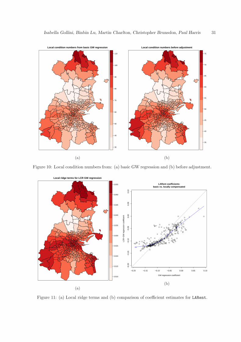
Observe that the bandwidth for the locally compensated GW regression is larger at N = 157,than for the un-adjusted GW regression (at N = 109). We could have specified the bandwidthfrom the un-adjusted model, but this would not give us the best fit. The larger bandwidthprovides greater smoothing. Observe also that the Local_CN outputs from this model are thelocal condition numbers before the adjustment. They will tend to be smaller than those forthe basic model (from gwr.basic) because we are using a larger bandwidth and the localestimates will tend to those of the global model.
The Local_Lambda outputs are the local ridge estimates used to adjust the local cross-productsmatrices. Both the local condition numbers and the local ridges can be mapped to show wherethe GW regression has applied different levels of adjustment in relation to the different levelsof collinearity among the predictors. The local condition numbers are mapped in Figure 10b,and the local ridges in Figure 11a. The greatest adjustments were required in central Dublin,and in the north, south-west and south-east extremities of the study area. Figure 11b showsthe adjustment of the coefficient estimates for LARent from the locally compensated modelrelative to those from the basic (un-adjusted) model. The general pattern would appear to bethat the larger coefficients for the basic model are reduced in magnitude, and that the smallercoefficients are raised. The relationship is non-linear and a loess fit is shown in the plot.
Model building with collinear data
Can we build GW regression models which avoid collinearity? We can explore the conditionnumbers for models with different structures. First, we code a function to calibrate and thenestimate an un-adjusted GW regression. This can be used to test various forms of the model- the output each time is a vector of condition numbers for the model that has been fitted.This function is presented as follows, together with an example model.
Isabella Gollini, Binbin Lu, Martin Charlton, Christopher Brunsdon, Paul Harris 31
Local condition numbers from basic GW regression
30
40
50
60
70
80
90
100
110
(a)
Local condition numbers before adjustment
35
40
45
50
55
60
65
70
75
(b)
Figure 10: Local condition numbers from: (a) basic GW regression and (b) before adjustment.
Local ridge terms for LCR GW regression
0.010
0.015
0.020
0.025
0.030
0.035
0.040
0.045
0.050
0.055
(a)
−0.20 −0.15 −0.10 −0.05 0.00 0.05 0.10
−0.
20−
0.15
−0.
10−
0.05
0.00
0.05
0.10
LARent coefficients: basic vs. locally compensated
GW regression coefficient
LCR
−G
W r
egre
ssio
n co
effic
ient
(b)
Figure 11: (a) Local ridge terms and (b) comparison of coefficient estimates for LARent.
32 GWmodel: Geographically Weighted Models
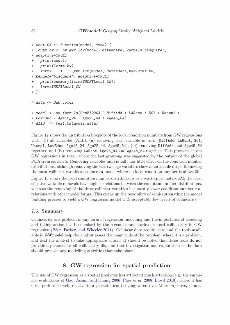
> test.CN <- function(model, data) {
+ lcrmx.bw <- bw.gwr.lcr(model, data=data, kernel="bisquare",
+ adaptive=TRUE)
+ print(model)
+ print(lcrmx.bw)
+ lcrmx <- gwr.lcr(model, data=data,bw=lcrmx.bw,
+ kernel="bisquare", adaptive=TRUE)
+ print(summary(lcrmx$SDF$Local_CN))
+ lcrmx$SDF$Local_CN
+ }
> data <- Dub.voter
> model <- as.formula(GenEl2004 ~ DiffAdd + LARent + SC1 + Unempl +
+ LowEduc + Age18_24 + Age25_44 + Age45_64)
> AllD <- test.CN(model,data)
Figure 12 shows the distribution boxplots of the local condition numbers from GW regressionswith: (i) all variables (ALL), (ii) removing each variable in turn (DiffAdd, LARent, SC1,Unempl, LowEduc, Age18_24, Age25_44, Age45_64), (iii) removing DiffAdd and Age45_64
together, and (iv) removing LARent, Age25_44 and Age45_64 together. This provides elevenGW regressions in total, where the last grouping was suggested by the output of the globalPCA from section 5. Removing variables individually has little effect on the condition numberdistributions, although removing the last two age variables show a noticeable drop. Removingthe most collinear variables produces a model where no local condition number is above 30.
Figure 13 shows the local condition number distributions as a scatterplot matrix aAS the leasteffective variable removals have high correlations between the condition number distributions,whereas the removing of the three collinear variables has mostly lower condition number cor-relations with other model forms. This opens up the possibility of semi-automating the modelbuilding process to yield a GW regression model with acceptably low levels of collinearity.
7.5. Summary
Collinearity is a problem in any form of regression modelling and the importance of assessingand taking action has been raised by the recent commentaries on local collinearity in GWregression (Paez, Farber, and Wheeler 2011). Collinear data require care and the tools avail-able in GWmodel help the analyst assess the magnitude of the problem, where it is a problem,and lead the analyst to take appropriate action. It should be noted that these tools do notprovide a panacea for all collinearity ills, and that investigation and exploration of the datashould precede any modelling activities that take place.
8. GW regression for spatial prediction
The use of GW regression as a spatial predictor has attracted much attention (e.g. the empir-ical evaluations of Gao, Asami, and Chung 2006; Paez et al. 2008; Lloyd 2010), where it hasoften performed well, relative to a geostatistical (kriging) alterative. More objective, simula-

Isabella Gollini, Binbin Lu, Martin Charlton, Christopher Brunsdon, Paul Harris 33
ALL DA LA SC Un LE A18 A25 A45 DA+1 LA+2
2040
6080
100
Distribution of local condition numbers from 11 different model specs.
Figure 12: Distribution of local condition numbers from 11 different GW regression fits.
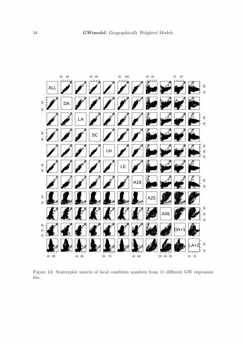
34 GWmodel: Geographically Weighted Models
ALL
30 60 40 80 40 100 20 35 15 30
4080
3060 DA
LA
4080
4080 SC
Un
3060
90
4080 LE
A18
4080
2035 A25
A45
2035
50
1525
35
DA+1
40 80 40 80 30 70 40 80 20 35 50 10 20
1020LA+2
Figure 13: Scatterplot matrix of local condition numbers from 11 different GW regressionfits.

Isabella Gollini, Binbin Lu, Martin Charlton, Christopher Brunsdon, Paul Harris 35
tion experiments can be found in Harris, Fotheringham, Crespo, and Charlton (2010b), wherekriging performed the best, but GW regression still performed with merit. Conceptual linksbetween GW regression and kriging are discussed in Harris, Brunsdon, and Fotheringham(2011b) and various hybrid predictors can be found in Lloyd (2010); Harris et al. (2010b);Harris and Juggins (2011), where GW regression can provide a useful trend component of akriging model.
Thus studies have demonstrated value in using GW regression as a spatial predictor and itsprediction at a location s can be found using:
yGWR(s) = x(s)T β(s) (15)
where x(s) and β(s) are each vectors of independent data values and parameter estimates,respectively. Following Leung et al. (2000), the corresponding GW regression prediction vari-ance at s can be estimated using:
σ2GWR(s) = VAR {y(s)− y(s)} = σ2 [1 + S(s)] (16)
where
S(s) = x(s)T[
XTW (s)X]−1
XTW 2(s)X[
XTW (s)X]−1
x(s) (17)
Here an unbiased estimate of the residual variance is taken as σ = RSS/(n − ENP), whereRSS is the residual sum of squares and ENP is the effective number of parameters of theGW regression model. Observe that the prediction variance for GW regression is for a singleobservation and not for the mean, and in doing so, is directly comparable with that foundwith kriging, in say, the gstat R package (Pebesma 2004).
8.1. Example
To demonstrate GW regression as spatial predictor, we use the EWHP data set. Here our aim isto predict the dependent variable, house price (PurPrice) using a subset of the nine indepen-dent variables described in section 2, each of which reflect some hedonic characteristic of theproperty. A correlation analysis reveals that FlrArea (floor area or the effective size of theproperty) provides the strongest correlation with house price at ρ = 0.65. For demonstrationpurposes, we choose to focus our prediction models using only this single hedonic variable.Four R libraries are required for this analysis section:
> library(GWmodel)
> library(RColorBrewer)
> library(ModelMap)
> library(gstat)
A GW correlation analysis between house price and our retained hedonic variable4 can be con-ducted using the gwss function, where GW correlations (and other GW summary statistics)are specified using an adaptive bi-square kernel with a bandwidth of N = 52 (approximately10% of the sample data). The quick.map function allows the GW correlations to be mapped.
4Observe that discarding hedonic variables that correlate weakly at the global scale does not directly entailsimilarly weak correlations, locally. As such, a comprehensive analysis would have locally investigated allrelationships with their respective GW correlations (see section 4).
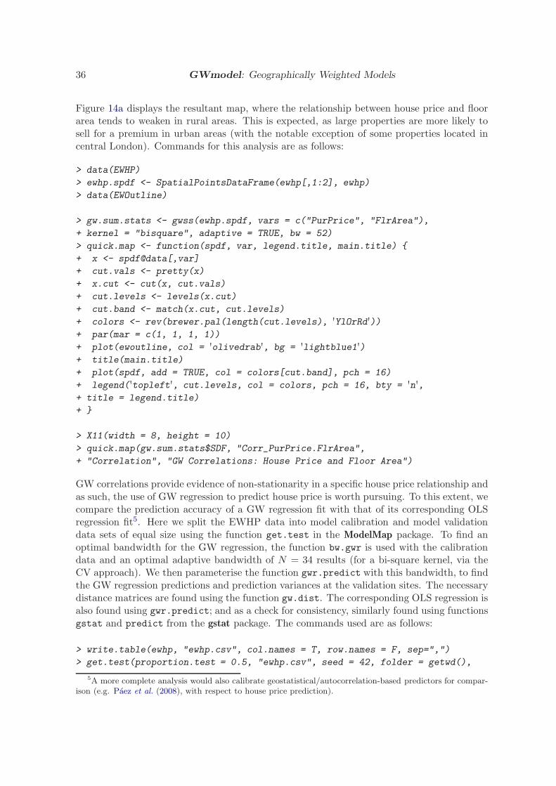
36 GWmodel: Geographically Weighted Models
Figure 14a displays the resultant map, where the relationship between house price and floorarea tends to weaken in rural areas. This is expected, as large properties are more likely tosell for a premium in urban areas (with the notable exception of some properties located incentral London). Commands for this analysis are as follows:
> data(EWHP)
> ewhp.spdf <- SpatialPointsDataFrame(ewhp[,1:2], ewhp)
> data(EWOutline)
> gw.sum.stats <- gwss(ewhp.spdf, vars = c("PurPrice", "FlrArea"),
+ kernel = "bisquare", adaptive = TRUE, bw = 52)
> quick.map <- function(spdf, var, legend.title, main.title) {
+ x <- spdf@data[,var]
+ cut.vals <- pretty(x)
+ x.cut <- cut(x, cut.vals)
+ cut.levels <- levels(x.cut)
+ cut.band <- match(x.cut, cut.levels)
+ colors <- rev(brewer.pal(length(cut.levels), 'YlOrRd'))
+ par(mar = c(1, 1, 1, 1))
+ plot(ewoutline, col = 'olivedrab', bg = 'lightblue1')
+ title(main.title)
+ plot(spdf, add = TRUE, col = colors[cut.band], pch = 16)
+ legend('topleft', cut.levels, col = colors, pch = 16, bty = 'n',
+ title = legend.title)
+ }
> X11(width = 8, height = 10)
> quick.map(gw.sum.stats$SDF, "Corr_PurPrice.FlrArea",
+ "Correlation", "GW Correlations: House Price and Floor Area")
GW correlations provide evidence of non-stationarity in a specific house price relationship andas such, the use of GW regression to predict house price is worth pursuing. To this extent, wecompare the prediction accuracy of a GW regression fit with that of its corresponding OLSregression fit5. Here we split the EWHP data into model calibration and model validationdata sets of equal size using the function get.test in the ModelMap package. To find anoptimal bandwidth for the GW regression, the function bw.gwr is used with the calibrationdata and an optimal adaptive bandwidth of N = 34 results (for a bi-square kernel, via theCV approach). We then parameterise the function gwr.predict with this bandwidth, to findthe GW regression predictions and prediction variances at the validation sites. The necessarydistance matrices are found using the function gw.dist. The corresponding OLS regression isalso found using gwr.predict; and as a check for consistency, similarly found using functionsgstat and predict from the gstat package. The commands used are as follows:
> write.table(ewhp, "ewhp.csv", col.names = T, row.names = F, sep=",")
> get.test(proportion.test = 0.5, "ewhp.csv", seed = 42, folder = getwd(),
5A more complete analysis would also calibrate geostatistical/autocorrelation-based predictors for compar-ison (e.g. Paez et al. (2008), with respect to house price prediction).
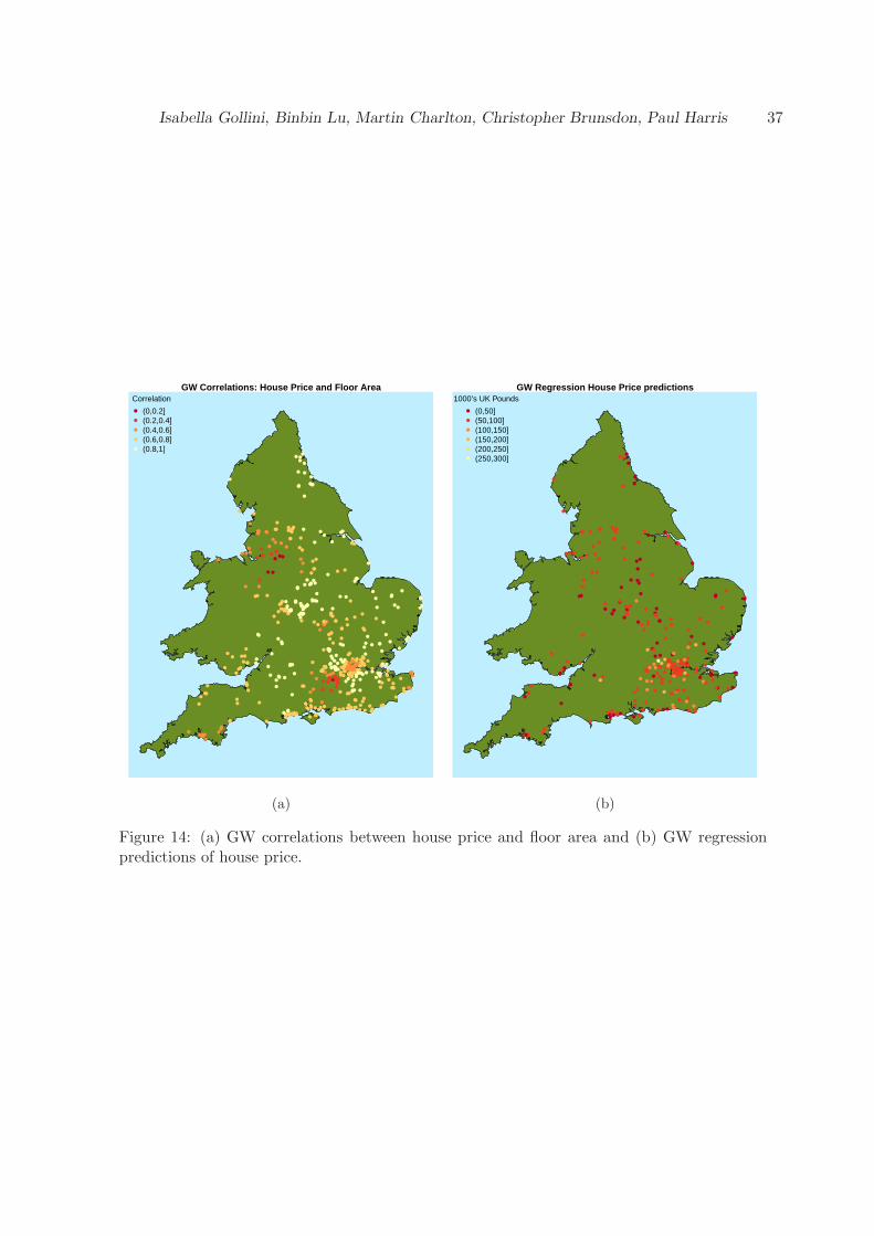
Isabella Gollini, Binbin Lu, Martin Charlton, Christopher Brunsdon, Paul Harris 37
GW Correlations: House Price and Floor AreaCorrelation
(0,0.2](0.2,0.4](0.4,0.6](0.6,0.8](0.8,1]
(a)
GW Regression House Price predictions1000’s UK Pounds
(0,50](50,100](100,150](150,200](200,250](250,300]
(b)
Figure 14: (a) GW correlations between house price and floor area and (b) GW regressionpredictions of house price.

38 GWmodel: Geographically Weighted Models
+ qdata.trainfn = "ewhp_calib.csv", qdata.testfn = "ewhp_valid.csv")
> ewhp_calib <- read.table("ewhp_calib.csv", header = T,sep = ",")
> attach(ewhp_calib)
> ewhp_calib.spdf <- SpatialPointsDataFrame(ewhp_calib[,1:2],
+ as.data.frame(ewhp_calib[c(3,12)]))
> dm.calib <- gw.dist(dp.locat = coordinates(ewhp_calib.spdf))
> gwr.bw.cv <-bw.gwr(PurPrice ~ FlrArea,data = ewhp_calib.spdf,
+ approach = "CV", kernel = "bisquare", adaptive = T, dMat = dm.calib)
> ewhp_valid <- read.table("ewhp_valid.csv", header = T, sep = ",")
> attach(ewhp_valid)
> ewhp_valid.spdf <- SpatialPointsDataFrame(ewhp_valid[,1:2],
+ as.data.frame(ewhp_valid[c(3,12)]))
> dm.valid <- gw.dist(dp.locat = coordinates(ewhp_calib.spdf),
+ rp.locat = coordinates(ewhp_valid.spdf))
> gwr.pred <- gwr.predict(PurPrice ~ FlrArea,data = ewhp_calib.spdf,
+ predictdata = ewhp_valid.spdf ,bw = gwr.bw.cv, kernel = "bisquare",
+ adaptive = T, dMat1 = dm.valid, dMat2 = dm.calib)
> ols.pred.gwmodel <- gwr.predict(PurPrice ~ FlrArea, data = ewhp_calib.spdf,
+ predictdata = ewhp_valid.spdf, bw = 519, kernel = "boxcar", adaptive = T,
+ dMat1 = dm.valid, dMat2 = dm.calib)
> ols <- gstat(id = "mlr",formula = PurPrice ~ FlrArea,loc=~Easting +
+ Northing, data = ewhp_calib)
> ols.pred.gstat <- predict(ols,newdata = ewhp_valid,BLUE = TRUE)
Performance results are reported in Table 1, in terms of prediction accuracy and predictionuncertainty accuracy. Prediction accuracy is measured by the root mean squared predictionerror (RMSPE) and the mean absolute prediction error (MAPE), both of which should tendto zero. Prediction uncertainty accuracy is measured by the mean and standard deviation(SD) of the prediction z-score data (mean.ZS and SD.ZS, respectively). These z-scores aredefined as:
z− scorepred(s) = (y(s)− y(s)) /σpred(s) (18)
where for unbiased prediction standard errors, the mean and SD of the z-scores should tendto zero and unity, respectively. As would be expected, GW regression provides the best setof results and there is near exact correspondence between two the OLS regression results.Finally, a map depicting the GW regression predictions is given in Figure 14b. Commands toconduct this model performance analysis, just for the GW regression model, are as follows:
> RMSPE.gwr <- (mean((ewhp_valid.spdf$PurPrice - gwr.pred$SDF$prediction)^2))^0.5
> MAPE.gwr <- mean(abs(ewhp_valid.spdf$PurPrice - gwr.pred$SDF$prediction))
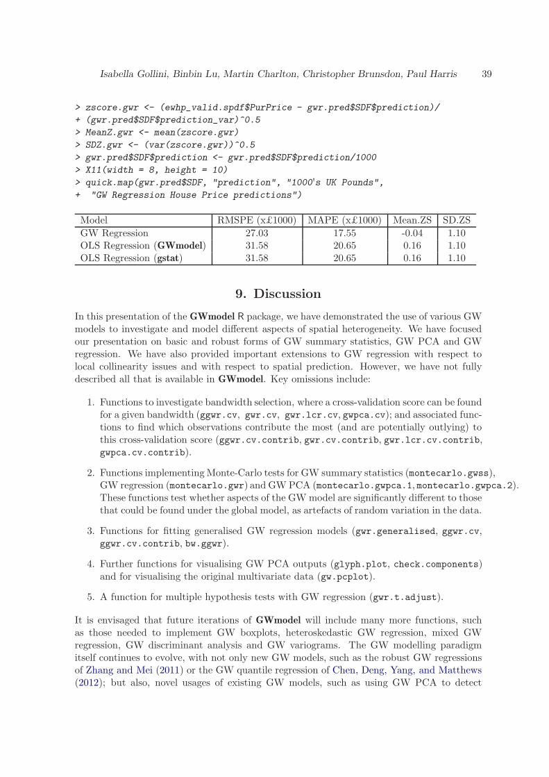
Isabella Gollini, Binbin Lu, Martin Charlton, Christopher Brunsdon, Paul Harris 39
> zscore.gwr <- (ewhp_valid.spdf$PurPrice - gwr.pred$SDF$prediction)/
+ (gwr.pred$SDF$prediction_var)^0.5
> MeanZ.gwr <- mean(zscore.gwr)
> SDZ.gwr <- (var(zscore.gwr))^0.5
> gwr.pred$SDF$prediction <- gwr.pred$SDF$prediction/1000
> X11(width = 8, height = 10)
> quick.map(gwr.pred$SDF, "prediction", "1000's UK Pounds",
+ "GW Regression House Price predictions")
Model RMSPE (x£1000) MAPE (x£1000) Mean.ZS SD.ZS
GW Regression 27.03 17.55 -0.04 1.10OLS Regression (GWmodel) 31.58 20.65 0.16 1.10OLS Regression (gstat) 31.58 20.65 0.16 1.10
9. Discussion
In this presentation of the GWmodel R package, we have demonstrated the use of various GWmodels to investigate and model different aspects of spatial heterogeneity. We have focusedour presentation on basic and robust forms of GW summary statistics, GW PCA and GWregression. We have also provided important extensions to GW regression with respect tolocal collinearity issues and with respect to spatial prediction. However, we have not fullydescribed all that is available in GWmodel. Key omissions include:
1. Functions to investigate bandwidth selection, where a cross-validation score can be foundfor a given bandwidth (ggwr.cv, gwr.cv, gwr.lcr.cv, gwpca.cv); and associated func-tions to find which observations contribute the most (and are potentially outlying) tothis cross-validation score (ggwr.cv.contrib, gwr.cv.contrib, gwr.lcr.cv.contrib,gwpca.cv.contrib).
2. Functions implementingMonte-Carlo tests for GW summary statistics (montecarlo.gwss),GW regression (montecarlo.gwr) and GWPCA (montecarlo.gwpca.1, montecarlo.gwpca.2).These functions test whether aspects of the GW model are significantly different to thosethat could be found under the global model, as artefacts of random variation in the data.
3. Functions for fitting generalised GW regression models (gwr.generalised, ggwr.cv,ggwr.cv.contrib, bw.ggwr).
4. Further functions for visualising GW PCA outputs (glyph.plot, check.components)and for visualising the original multivariate data (gw.pcplot).
5. A function for multiple hypothesis tests with GW regression (gwr.t.adjust).
It is envisaged that future iterations of GWmodel will include many more functions, suchas those needed to implement GW boxplots, heteroskedastic GW regression, mixed GWregression, GW discriminant analysis and GW variograms. The GW modelling paradigmitself continues to evolve, with not only new GW models, such as the robust GW regressionsof Zhang and Mei (2011) or the GW quantile regression of Chen, Deng, Yang, and Matthews(2012); but also, novel usages of existing GW models, such as using GW PCA to detect

40 GWmodel: Geographically Weighted Models
multivariate spatial outliers (Harris, Brunsdon, and Charlton 2012) or using GW PCA toaide sample re-design (Harris, Brunsdon, Charlton, Juggins, and Clarke 2013).
Acknowledgements
Research presented in this paper was funded by a Strategic Research Cluster grant (07/SRC/I1168)by Science Foundation Ireland under the National Development Plan. The authors gratefullyacknowledge this support.
References
Akaike H (1973). “Information Theory and an extension of the maximum likelihood princi-ple.” In B Petrov, F Csaki (eds.), 2nd Symposium on Information Theory, pp. 267–281.Akademiai Kiado, Budapest.
Belsley DA, Kuh E, Welsch RE (1980). Regression diagnostics: Identifying influential dataand sources of collinearity. John Wiley & Sons, Inc.
Bitter C, Mulligan G, Dall’Erba S (2007). “Incorporating spatial variation in housing at-tribute prices: a comparison of geographically weighted regression and the spatial expansionmethod.” Journal of Geographical Systems, 9(1), 7–27.
Bowman A (1984). “An Alternative Method of cross-validation for the smoothing of densityestimates.” Biometrika, 71, 353–360.
Brunsdon C, Charlton M, Harris P (2012). “Living with Collinearity in Local Regression Mod-els.” In In Proceedings of the 10th International Symposium on Spatial Accuracy Assessmentin Natural Resources and Environmental Sciences. Brasil.
Brunsdon C, Fotheringham AS, Charlton M (1996). “Geographically Weighted Regression:A Method for Exploring Spatial Nonstationarity.” Geographical Analysis, 28, 281–289.
Brunsdon C, Fotheringham AS, Charlton M (1998). “Geographically Weighted Regression.”Journal of the Royal Statistical Society: Series D (The Statistician), 47(3), 431–443.
Brunsdon C, Fotheringham AS, Charlton M (1999). “Some Notes on Parametric SignificanceTests for Geographically Weighted Regression.” Journal of Regional Science, 39(3), 497–524.
Brunsdon C, Fotheringham AS, Charlton M (2002). “Geographically Weighted SummaryStatistics - a Framework for Localised Exploratory Data Analysis.” Computers, Environ-ment and Urban Systems, 26(6), 501–524.
Brunsdon C, Fotheringham AS, Charlton M (2007). “Geographically Weighted DiscriminantAnalysis.” Geographical Analysis, 39(4), 376–396.
Charlton M, Fotheringham AS, Brunsdon C (2003). GWR 3: software for geographicallyweighted regression. National Centre for Geocomputation, National University of IrelandMaynooth.
Isabella Gollini, Binbin Lu, Martin Charlton, Christopher Brunsdon, Paul Harris 41
Chen VYJ, Deng WS, Yang TC, Matthews SA (2012). “Geographically Weighted Quan-tile Regression (GWQR): An Application to U.S. Mortality Data.” Geographical Analysis,44(2), 134–150.
Dykes J, Brunsdon C (2007). “Geographically Weighted Visualization: Interactive Graphicsfor Scale-Varying Exploratory Analysis.” IEEE Transactions on Visualization and Com-puter Graphics, 13(6), 1161–1168.
Fotheringham AS, Brunsdon C, Charlton M (2002). Geographically Weighted Regression: theAnalysis of Spatially Varying Relationships. Wiley, Chichester.
Fox J, Monette G (1992). “Generalized Collinearity Diagnostics.” Journal of the AmericanStatistical Association, 87(417), 178–183.
Frank IE, Friedman JH (1993). “A Statistical View of Some Chemometrics Regression Tools.”Technometrics, 35(2), 109–135.
Gao X, Asami Y, Chung CJF (2006). “An empirical evaluation of spatial regression models.”Computers & Geosciences, 32(8), 1040–1051.
Griffith DA (2008). “Spatial-filtering-based contributions to a critique of geographicallyweighted regression (GWR).” Environment and Planning A, 40(11), 2751–2769.
Harris P, Brunsdon C (2010). “Exploring spatial variation and spatial relationships in afreshwater acidification critical load data set for Great Britain using geographically weightedsummary statistics.” Computers & Geosciences, 36(1), 54 – 70.
Harris P, Brunsdon C, Charlton M (2011a). “Geographically Weighted Principal ComponentsAnalysis.” International Journal of Geographical Information Science, 25(10), 1717–1736.
Harris P, Brunsdon C, Charlton M (2012). “Multivariate spatial outlier detection: a compar-ison of techniques.” In geoENV 2012. Valencia, Spain.
Harris P, Brunsdon C, Charlton M, Juggins S, Clarke A (2013). “Robust geographicallyweighted principal components analysis and its use in sample re-design.” In GISRUK 2013.Liverpool, UK.
Harris P, Brunsdon C, Fotheringham AS (2011b). “Links, comparisons and extensions ofthe geographically weighted regression model when used as a spatial predictor.” Stochasticenvironmental Research and Risk assessment, 25(2), 123–138.
Harris P, Charlton M, Fotheringham AS (2010a). “Moving window kriging with geographicallyweighted variograms.” Stochastic Environmental Research and Risk Assessment, 24(8),1193–1209.
Harris P, Fotheringham A, Crespo R, Charlton M (2010b). “The use of geographicallyweighted regression for spatial prediction: an evaluation of models using simulated datasets.” Mathematical Geosciences, 42(6), 657–680.
Harris P, Juggins S (2011). “Estimating freshwater acidification critical load exceedance datafor Great Britain using space-varying relationship models.” Mathematical Geosciences,43(3), 265–292.
42 GWmodel: Geographically Weighted Models
Hoerl AE (1962). “Application of ridge analysis to regression problems.”Chemical EngineeringProgress, 58(3), 54–59.
Hoerl AE, Kennard RW (1970). “Ridge Regression: Biased Estimation for NonorthogonalProblems.” Technometrics, 12(1), 55–67.
Hurvich CM, Simonoff JS (1998). “Smoothing parameter selection in nonparametric regressionusing an improved Akaike information criterion.” Journal of the Royal Statistical Society,Series B, 60, 271–293.
Jolliffe IT (2002). Principal component analysis. 2 edition. Springer-Verlag, New York.
Kavanagh A, Fotheringham S, Charlton M (2006). “A geographically weighted regressionanalysis of the election specific turnout behaviour in the Republic of Ireland.” In Elections,Public Opinion and Parties Conference, Nottingham 8th to 10th September 2006.
Kestens Y, Theriault M, Rosiers FD (2006). “Heterogeneity in hedonic modelling of houseprices: looking at buyersaAZ household profiles.” Journal of Geographical Systems, 8(1),61–96.
Lee TS (1987). “Algorithm AS 223: Optimum Ridge Parameter Selection.” Journal of theRoyal Statistical Society. Series C (Applied Statistics), 36(1), pp. 112–118.
Leung Y, Mei C, Zhang WX (2000). “Statistical tests for spatial nonstationarity based ongeographically weighted regression.” Environment and Planning (A), 32, 9–32.
Lloyd C (2010). “Nonstationary models for exploring and mapping monthly precipitation inthe United Kingdom.” International Journal of Climatology, 30(3), 390–405.
Lloyd C, Shuttleworth I (2005). “Analysing commuting using local regression techniques:scale, sensitivity, and geographical patterning.” Environment and Planning A, 37, 81–103.
Nakaya T, Fotheringham AS, Brunsdon C, Charlton M (2005). “Geographically weightedPoisson regression for disease association mapping.” Statistics in Medicine, 24(17), 2695–2717.
O’Brien RM (2007). “A Caution Regarding Rules of Thumb for Variance Inflation Factors.”Quality & Quantity, 41(5), 673–690.
Openshaw S, Charlton M, Wymer C, Craft A (1987). “A mark 1 geographical analysis ma-chine for the automated analysis of point data sets.” International Journal of GeographicalInformation System, 1(4), 335–358.
Paez A, Farber S, Wheeler D (2011). “A simulation-based study of geographically weightedregression as a method for investigating spatially varying relationships.” Environment andPlanning-Part A, 43(12), 2992–3010.
Paez A, Long F, Farber S (2008). “Moving Window Approaches for Hedonic Price Estimation:An Empirical Comparison of Modelling Techniques.” Urban Studies, 45(8), 1565–1581.
Pebesma EJ (2004). “Multivariable geostatistics in S: the gstat package.” Computers &Geosciences, 30(7), 683–691.
Isabella Gollini, Binbin Lu, Martin Charlton, Christopher Brunsdon, Paul Harris 43
Rangel TF, Diniz-Filho JAF, Bini LM (2010). “SAM: a comprehensive application for SpatialAnalysis in Macroecology.” Ecography, 33(1), 46–50.
Rousseeuw PJ (1985). “Multivariate estimation with high breakdown point.” volume B, pp.283–297. Reidel Publishing, Dordrecht.
Varmuza K, Filzmoser P (2009). Introduction to multivariate statistical analysis in chemo-metrics. CRC press.
Wheeler D, Tiefelsdorf M (2005). “Multicollinearity and Correlation among Regression Co-efficients in Geographically weighted Regression.” Journal of Geographical Systems, 7(2),161–187.
Wheeler DC (2007). “Diagnostic tools and a remedial method for collinearity in geographicallyweighted regression.” Environment and Planning A, 39(10), 2464–2481.
Wheeler DC (2009). “Simultaneous coefficient penalization and model selection in geograph-ically weighted regression: the geographically weighted lasso.” Environment and planningA, 41(3), 722.
Zhang H, Mei C (2011). “Local least absolute deviation estimation of spatially varying coeffi-cient models: robust geographically weighted regression approaches.” International Journalof Geographical Information Science, 25(9), 1467–1489.
Affiliation:
Isabella GolliniDepartment of Civil EngineeringUniversity of BristolQueen’s BuildingBristol BS8 1TR, UKE-mail: [email protected]: http://www.bristol.ac.uk/engineering/people/isabella-gollini/