Package 'surveillance'

Package ‘surveillance’March 19, 2013

Title Temporal and Spatio-Temporal Modeling and Monitoring of Epidemic Phenomena

Version 1.5-2

Date 2013-03-15

Author M. Höhle, S. Meyer and M. Paul with contributions from T.Correa, L. Held, M. Hofmann, C. Lang, A. Riebler, D. SabanésBové, M. Salmon, S. Steiner, M. Virtanen, and V. Wimmer. A fewcode segments are modified versions of code by The R Core Team (available under GPL-2).

Depends R (>= 2.14.0), grDevices, graphics, stats, utils, xtable,methods, Rcpp, sp

Imports MASS, Matrix, spatstat (>= 1.17-0)

LinkingTo Rcpp

Suggests msm, spc, colorspace, animation, quadprog, mvtnorm, statmod,memoise, gpclib, map-tools, intervals, spdep, numDeriv, maxLik,RUnit, digest, coda, splancs, gamlss

Description A package implementing statistical methods for the modeling and change-point detec-tion in time series of counts,proportions and categorical data, as well as for the modelingof continuous-time epidemic phenomena, e.g. discrete-space setups such as the spatially enrichedSusceptible-Exposed-Infectious-Recovered (SEIR) models forsurveillance data, or continuous-space point process data suchas the occurrence of disease or earthquakes. Main focus is onoutbreak detection in count data time series originating frompublic health surveillance of infectious diseases, but applications could just as well origi-nate from environmetrics,reliability engineering, econometrics or social sciences.Currently the package contains implementations of typical outbreak detection proce-dures such as Stroup et. al (1989),Farrington et al (1996), Rossi et al (1999), Rogerson andYamada (2001), a Bayesian approach, negative binomial CUSUMmethods and a detector based on generalized likelihood ratios.Furthermore, inference methods for the retrospective infectiousdisease model in Held et al (2005), Held et al (2006), Paul etal (2008) and Paul and Held (2011) are provided. A novel CUSUMapproach combining logistic and multinomial logistic modellingis also included. Continuous self-exciting spatio-temporalpoint processes are modeled through additive-multiplicative

1

2 R topics documented:

conditional intensities as described in Höhle (2009)(‘‘twinSIR’’, discrete space) and Meyer et al (2012) (‘‘twinstim’’,continuous space). The pack-age contains several real-world datasets, the ability to simulate outbreak data, visualize theresults of the monitoring in temporal, spatial or spatio-temporal fashion.

Maintainer Michael Höhle <[email protected]>

License GPL-2

URL http://surveillance.r-forge.r-project.org/

ZipData no

Encoding latin1

NeedsCompilation yes

Repository CRAN

Date/Publication 2013-03-19 07:23:59

R topics documented:surveillance-package . . . . . . . . . . . . . . . . . . . . . . . . . . . . . . . . . . . . 5abattoir . . . . . . . . . . . . . . . . . . . . . . . . . . . . . . . . . . . . . . . . . . . 7addSeason2formula . . . . . . . . . . . . . . . . . . . . . . . . . . . . . . . . . . . . . 8aggregate-methods . . . . . . . . . . . . . . . . . . . . . . . . . . . . . . . . . . . . . 9aggregate.disProg . . . . . . . . . . . . . . . . . . . . . . . . . . . . . . . . . . . . . . 10algo.bayes . . . . . . . . . . . . . . . . . . . . . . . . . . . . . . . . . . . . . . . . . . 10algo.call . . . . . . . . . . . . . . . . . . . . . . . . . . . . . . . . . . . . . . . . . . . 12algo.cdc . . . . . . . . . . . . . . . . . . . . . . . . . . . . . . . . . . . . . . . . . . . 13algo.compare . . . . . . . . . . . . . . . . . . . . . . . . . . . . . . . . . . . . . . . . 15algo.cusum . . . . . . . . . . . . . . . . . . . . . . . . . . . . . . . . . . . . . . . . . 16algo.farrington . . . . . . . . . . . . . . . . . . . . . . . . . . . . . . . . . . . . . . . 18algo.farrington.assign.weights . . . . . . . . . . . . . . . . . . . . . . . . . . . . . . . 20algo.farrington.fitGLM . . . . . . . . . . . . . . . . . . . . . . . . . . . . . . . . . . . 21algo.farrington.threshold . . . . . . . . . . . . . . . . . . . . . . . . . . . . . . . . . . 22algo.glrnb . . . . . . . . . . . . . . . . . . . . . . . . . . . . . . . . . . . . . . . . . . 23algo.glrpois . . . . . . . . . . . . . . . . . . . . . . . . . . . . . . . . . . . . . . . . . 25algo.hhh . . . . . . . . . . . . . . . . . . . . . . . . . . . . . . . . . . . . . . . . . . . 28algo.hhh.grid . . . . . . . . . . . . . . . . . . . . . . . . . . . . . . . . . . . . . . . . 31algo.hmm . . . . . . . . . . . . . . . . . . . . . . . . . . . . . . . . . . . . . . . . . . 34algo.outbreakP . . . . . . . . . . . . . . . . . . . . . . . . . . . . . . . . . . . . . . . 37algo.quality . . . . . . . . . . . . . . . . . . . . . . . . . . . . . . . . . . . . . . . . . 39algo.rki . . . . . . . . . . . . . . . . . . . . . . . . . . . . . . . . . . . . . . . . . . . 40algo.rogerson . . . . . . . . . . . . . . . . . . . . . . . . . . . . . . . . . . . . . . . . 42algo.summary . . . . . . . . . . . . . . . . . . . . . . . . . . . . . . . . . . . . . . . . 44algo.twins . . . . . . . . . . . . . . . . . . . . . . . . . . . . . . . . . . . . . . . . . . 45animate . . . . . . . . . . . . . . . . . . . . . . . . . . . . . . . . . . . . . . . . . . . 47anscombe.residuals . . . . . . . . . . . . . . . . . . . . . . . . . . . . . . . . . . . . . 47arlCusum . . . . . . . . . . . . . . . . . . . . . . . . . . . . . . . . . . . . . . . . . . 48

http://surveillance.r-forge.r-project.org/

R topics documented: 3

backprojNP . . . . . . . . . . . . . . . . . . . . . . . . . . . . . . . . . . . . . . . . . 49bestCombination . . . . . . . . . . . . . . . . . . . . . . . . . . . . . . . . . . . . . . 53categoricalCUSUM . . . . . . . . . . . . . . . . . . . . . . . . . . . . . . . . . . . . . 54checkResidualProcess . . . . . . . . . . . . . . . . . . . . . . . . . . . . . . . . . . . . 56compMatrix.writeTable . . . . . . . . . . . . . . . . . . . . . . . . . . . . . . . . . . . 58correct53to52 . . . . . . . . . . . . . . . . . . . . . . . . . . . . . . . . . . . . . . . . 59create.disProg . . . . . . . . . . . . . . . . . . . . . . . . . . . . . . . . . . . . . . . . 60create.grid . . . . . . . . . . . . . . . . . . . . . . . . . . . . . . . . . . . . . . . . . . 61deleval . . . . . . . . . . . . . . . . . . . . . . . . . . . . . . . . . . . . . . . . . . . . 62discpoly . . . . . . . . . . . . . . . . . . . . . . . . . . . . . . . . . . . . . . . . . . . 63display-methods . . . . . . . . . . . . . . . . . . . . . . . . . . . . . . . . . . . . . . . 64disProg2sts . . . . . . . . . . . . . . . . . . . . . . . . . . . . . . . . . . . . . . . . . 66earsC . . . . . . . . . . . . . . . . . . . . . . . . . . . . . . . . . . . . . . . . . . . . 67enlargeData . . . . . . . . . . . . . . . . . . . . . . . . . . . . . . . . . . . . . . . . . 71estimateGLRNbHook . . . . . . . . . . . . . . . . . . . . . . . . . . . . . . . . . . . . 72estimateGLRPoisHook . . . . . . . . . . . . . . . . . . . . . . . . . . . . . . . . . . . 73find.kh . . . . . . . . . . . . . . . . . . . . . . . . . . . . . . . . . . . . . . . . . . . . 74findH . . . . . . . . . . . . . . . . . . . . . . . . . . . . . . . . . . . . . . . . . . . . 75findK . . . . . . . . . . . . . . . . . . . . . . . . . . . . . . . . . . . . . . . . . . . . 76fluBYBW . . . . . . . . . . . . . . . . . . . . . . . . . . . . . . . . . . . . . . . . . . 77formatPval . . . . . . . . . . . . . . . . . . . . . . . . . . . . . . . . . . . . . . . . . . 78gpc.poly,coerce-methods . . . . . . . . . . . . . . . . . . . . . . . . . . . . . . . . . . 78ha . . . . . . . . . . . . . . . . . . . . . . . . . . . . . . . . . . . . . . . . . . . . . . 79hagelloch . . . . . . . . . . . . . . . . . . . . . . . . . . . . . . . . . . . . . . . . . . 80hepatitisA . . . . . . . . . . . . . . . . . . . . . . . . . . . . . . . . . . . . . . . . . . 82hhh4 . . . . . . . . . . . . . . . . . . . . . . . . . . . . . . . . . . . . . . . . . . . . . 83hhh4_formula . . . . . . . . . . . . . . . . . . . . . . . . . . . . . . . . . . . . . . . . 89hhh4_methods . . . . . . . . . . . . . . . . . . . . . . . . . . . . . . . . . . . . . . . . 91hhh4_validation . . . . . . . . . . . . . . . . . . . . . . . . . . . . . . . . . . . . . . . 93imdepi . . . . . . . . . . . . . . . . . . . . . . . . . . . . . . . . . . . . . . . . . . . . 96influMen . . . . . . . . . . . . . . . . . . . . . . . . . . . . . . . . . . . . . . . . . . . 100inside.gpc.poly . . . . . . . . . . . . . . . . . . . . . . . . . . . . . . . . . . . . . . . 100intensityplot . . . . . . . . . . . . . . . . . . . . . . . . . . . . . . . . . . . . . . . . . 101isoWeekYear . . . . . . . . . . . . . . . . . . . . . . . . . . . . . . . . . . . . . . . . 102ks.plot.unif . . . . . . . . . . . . . . . . . . . . . . . . . . . . . . . . . . . . . . . . . 103linelist2sts . . . . . . . . . . . . . . . . . . . . . . . . . . . . . . . . . . . . . . . . . . 104LRCUSUM.runlength . . . . . . . . . . . . . . . . . . . . . . . . . . . . . . . . . . . . 105m1 . . . . . . . . . . . . . . . . . . . . . . . . . . . . . . . . . . . . . . . . . . . . . . 108magic.dim . . . . . . . . . . . . . . . . . . . . . . . . . . . . . . . . . . . . . . . . . . 109makePlot . . . . . . . . . . . . . . . . . . . . . . . . . . . . . . . . . . . . . . . . . . 110measles.weser . . . . . . . . . . . . . . . . . . . . . . . . . . . . . . . . . . . . . . . . 111measlesDE . . . . . . . . . . . . . . . . . . . . . . . . . . . . . . . . . . . . . . . . . 111meningo.age . . . . . . . . . . . . . . . . . . . . . . . . . . . . . . . . . . . . . . . . . 112MMRcoverageDE . . . . . . . . . . . . . . . . . . . . . . . . . . . . . . . . . . . . . . 113momo . . . . . . . . . . . . . . . . . . . . . . . . . . . . . . . . . . . . . . . . . . . . 114multiplicity . . . . . . . . . . . . . . . . . . . . . . . . . . . . . . . . . . . . . . . . . 115nbOrder . . . . . . . . . . . . . . . . . . . . . . . . . . . . . . . . . . . . . . . . . . . 116nowcast . . . . . . . . . . . . . . . . . . . . . . . . . . . . . . . . . . . . . . . . . . . 117

4 R topics documented:

pairedbinCUSUM . . . . . . . . . . . . . . . . . . . . . . . . . . . . . . . . . . . . . . 120plot.atwins . . . . . . . . . . . . . . . . . . . . . . . . . . . . . . . . . . . . . . . . . . 123plot.disProg . . . . . . . . . . . . . . . . . . . . . . . . . . . . . . . . . . . . . . . . . 124plot.survRes . . . . . . . . . . . . . . . . . . . . . . . . . . . . . . . . . . . . . . . . . 126polyCub . . . . . . . . . . . . . . . . . . . . . . . . . . . . . . . . . . . . . . . . . . . 128powerlaw . . . . . . . . . . . . . . . . . . . . . . . . . . . . . . . . . . . . . . . . . . 131predict.ah . . . . . . . . . . . . . . . . . . . . . . . . . . . . . . . . . . . . . . . . . . 131primeFactors . . . . . . . . . . . . . . . . . . . . . . . . . . . . . . . . . . . . . . . . 132print.algoQV . . . . . . . . . . . . . . . . . . . . . . . . . . . . . . . . . . . . . . . . 133qlomax . . . . . . . . . . . . . . . . . . . . . . . . . . . . . . . . . . . . . . . . . . . 133R0 . . . . . . . . . . . . . . . . . . . . . . . . . . . . . . . . . . . . . . . . . . . . . . 134readData . . . . . . . . . . . . . . . . . . . . . . . . . . . . . . . . . . . . . . . . . . . 136refvalIdxByDate . . . . . . . . . . . . . . . . . . . . . . . . . . . . . . . . . . . . . . . 137residuals.ah . . . . . . . . . . . . . . . . . . . . . . . . . . . . . . . . . . . . . . . . . 138residualsCT . . . . . . . . . . . . . . . . . . . . . . . . . . . . . . . . . . . . . . . . . 138runifdisc . . . . . . . . . . . . . . . . . . . . . . . . . . . . . . . . . . . . . . . . . . . 140salmonella.agona . . . . . . . . . . . . . . . . . . . . . . . . . . . . . . . . . . . . . . 141scale.gpc.poly . . . . . . . . . . . . . . . . . . . . . . . . . . . . . . . . . . . . . . . . 141shadar . . . . . . . . . . . . . . . . . . . . . . . . . . . . . . . . . . . . . . . . . . . . 142sim.pointSource . . . . . . . . . . . . . . . . . . . . . . . . . . . . . . . . . . . . . . . 142sim.seasonalNoise . . . . . . . . . . . . . . . . . . . . . . . . . . . . . . . . . . . . . . 144simHHH . . . . . . . . . . . . . . . . . . . . . . . . . . . . . . . . . . . . . . . . . . . 145simulate.ah4 . . . . . . . . . . . . . . . . . . . . . . . . . . . . . . . . . . . . . . . . . 147stcd . . . . . . . . . . . . . . . . . . . . . . . . . . . . . . . . . . . . . . . . . . . . . 148sts-class . . . . . . . . . . . . . . . . . . . . . . . . . . . . . . . . . . . . . . . . . . . 151stsBP-class . . . . . . . . . . . . . . . . . . . . . . . . . . . . . . . . . . . . . . . . . 153stsSlot-generics . . . . . . . . . . . . . . . . . . . . . . . . . . . . . . . . . . . . . . . 153surveillance.options . . . . . . . . . . . . . . . . . . . . . . . . . . . . . . . . . . . . . 154test . . . . . . . . . . . . . . . . . . . . . . . . . . . . . . . . . . . . . . . . . . . . . . 155testSim . . . . . . . . . . . . . . . . . . . . . . . . . . . . . . . . . . . . . . . . . . . 156toFileDisProg . . . . . . . . . . . . . . . . . . . . . . . . . . . . . . . . . . . . . . . . 157twinSIR . . . . . . . . . . . . . . . . . . . . . . . . . . . . . . . . . . . . . . . . . . . 158twinSIR_epidata . . . . . . . . . . . . . . . . . . . . . . . . . . . . . . . . . . . . . . 162twinSIR_epidata_animate . . . . . . . . . . . . . . . . . . . . . . . . . . . . . . . . . . 166twinSIR_epidata_intersperse . . . . . . . . . . . . . . . . . . . . . . . . . . . . . . . . 169twinSIR_epidata_plot . . . . . . . . . . . . . . . . . . . . . . . . . . . . . . . . . . . . 170twinSIR_epidata_summary . . . . . . . . . . . . . . . . . . . . . . . . . . . . . . . . . 172twinSIR_intensityplot . . . . . . . . . . . . . . . . . . . . . . . . . . . . . . . . . . . . 174twinSIR_methods . . . . . . . . . . . . . . . . . . . . . . . . . . . . . . . . . . . . . . 176twinSIR_profile . . . . . . . . . . . . . . . . . . . . . . . . . . . . . . . . . . . . . . . 179twinSIR_simulation . . . . . . . . . . . . . . . . . . . . . . . . . . . . . . . . . . . . . 180twinstim . . . . . . . . . . . . . . . . . . . . . . . . . . . . . . . . . . . . . . . . . . . 186twinstim_epidataCS . . . . . . . . . . . . . . . . . . . . . . . . . . . . . . . . . . . . . 193twinstim_epidataCS_animate . . . . . . . . . . . . . . . . . . . . . . . . . . . . . . . . 198twinstim_epidataCS_plot . . . . . . . . . . . . . . . . . . . . . . . . . . . . . . . . . . 201twinstim_epidataCS_update . . . . . . . . . . . . . . . . . . . . . . . . . . . . . . . . 203twinstim_iaf . . . . . . . . . . . . . . . . . . . . . . . . . . . . . . . . . . . . . . . . . 204twinstim_iafplot . . . . . . . . . . . . . . . . . . . . . . . . . . . . . . . . . . . . . . . 209

surveillance-package 5

twinstim_intensityplot . . . . . . . . . . . . . . . . . . . . . . . . . . . . . . . . . . . 211twinstim_methods . . . . . . . . . . . . . . . . . . . . . . . . . . . . . . . . . . . . . . 214twinstim_plot . . . . . . . . . . . . . . . . . . . . . . . . . . . . . . . . . . . . . . . . 216twinstim_profile . . . . . . . . . . . . . . . . . . . . . . . . . . . . . . . . . . . . . . . 217twinstim_simulation . . . . . . . . . . . . . . . . . . . . . . . . . . . . . . . . . . . . 219twinstim_step . . . . . . . . . . . . . . . . . . . . . . . . . . . . . . . . . . . . . . . . 223twinstim_update . . . . . . . . . . . . . . . . . . . . . . . . . . . . . . . . . . . . . . . 225untie . . . . . . . . . . . . . . . . . . . . . . . . . . . . . . . . . . . . . . . . . . . . . 226wrap.algo . . . . . . . . . . . . . . . . . . . . . . . . . . . . . . . . . . . . . . . . . . 228xtable.algoQV . . . . . . . . . . . . . . . . . . . . . . . . . . . . . . . . . . . . . . . . 229zetaweights . . . . . . . . . . . . . . . . . . . . . . . . . . . . . . . . . . . . . . . . . 230[,sts-methods . . . . . . . . . . . . . . . . . . . . . . . . . . . . . . . . . . . . . . . . 230

Index 231

surveillance-package Temporal and Spatio-Temporal Modeling and Monitoring of EpidemicPhenomena

Description

A package implementing statistical methods for the modeling and change-point detection in time se-ries of counts, proportions and categorical data, as well as for the modeling of continuous-time epi-demic phenomena, e.g. discrete-space setups such as the spatially enriched Susceptible-Exposed-Infectious-Recovered (SEIR) models for surveillance data, or continuous-space point process datasuch as the occurrence of disease or earthquakes. Main focus is on outbreak detection in count datatime series originating from public health surveillance of infectious diseases, but applications couldjust as well originate from environmetrics, reliability engineering, econometrics or social sciences.Currently the package contains implementations of typical outbreak detection procedures such asStroup et. al (1989), Farrington et al (1996), Rossi et al (1999), Rogerson and Yamada (2001), aBayesian approach, negative binomial CUSUM methods and a detector based on generalized likeli-hood ratios. Furthermore, inference methods for the retrospective infectious disease model in Heldet al (2005), Held et al (2006), Paul et al (2008) and Paul and Held (2011) are provided. A novelCUSUM approach combining logistic and multinomial logistic modelling is also included. Contin-uous self-exciting spatio-temporal point processes are modeled through additive-multiplicative con-ditional intensities as described in Höhle (2009) ("twinSIR", discrete space) and Meyer et al (2012)("twinstim", continuous space). The package contains several real-world datasets, the ability to sim-ulate outbreak data, visualize the results of the monitoring in temporal, spatial or spatio-temporalfashion.

Details

Package: surveillanceVersion: 1.4-3Date: 2012-10-01License: GPL version 2 (http://www.gnu.org/licenses/old-licenses/gpl-2.0.html)URL: http://surveillance.r-forge.r-project.org/

http://www.gnu.org/licenses/old-licenses/gpl-2.0.html

http://surveillance.r-forge.r-project.org/

6 surveillance-package

surveillance is an R package implementing statistical methods for the retrospective modeling andprospective change-point detection in time series of counts, proportions and categorical data. Themain application is in the detection of aberrations in routine collected public health data seen asunivariate and multivariate time series of counts or point-processes. However, applications couldjust as well originate from environmetrics, econometrics or social sciences. As many methods relyon statistical process control methodology, the package is thus also relevant to quality control andreliability engineering.

The fundamental data structure of the package is an S4 class sts wrapping observations, monitoringresults and date handling for multivariate time series. Currently the package contains implementa-tions typical outbreak detection procedures such as Stroup et al. (1989), Farrington et al., (1996),Rossi et al. (1999), Rogerson and Yamada (2001), a Bayesian approach (Höhle, 2007), negativebinomial CUSUM methods (Höhle and Mazick, 2009), and a detector based on generalized like-lihood ratios (Höhle and Paul, 2008). However, also CUSUMs for the prospective change-pointdetection in binomial, beta-binomial and multinomial time series is covered based on generalizedlinear modelling. This includes e.g. paired binary CUSUM described by Steiner et al. (1999) orpaired comparison Bradley-Terry modelling described in Höhle (2010). The package contains sev-eral real-world datasets, the ability to simulate outbreak data, visualize the results of the monitoringin temporal, spatial or spatio-temporal fashion.

Furthermore, inference methods for the retrospective infectious disease model in Held et al. (2005),Paul et al. (2008) ("algo.hhh") and Paul and Held (2011) ("hhh4") handling multivariate time seriesof counts. Furthermore, the fully Bayesian approach for univariate time series of counts fromHeld et al. (2006) ("twins") is also implemented Self-exciting spatio-temporal point processesare modeled through additive-multiplicative conditional intensities as described in Höhle (2009)("twinSIR") and Meyer et al (2012) ("twinstim").

Altogether, the package contains several real-world datasets, the ability to simulate outbreak data,visualize the results of the monitoring in temporal, spatial or spatio-temporal fashion.

Acknowledgements

T. Correa, L. Held, M. Hofmann, C. Lang, A. Riebler, D. Sabanés Bové, S. Steiner, M. Virtanen,and V. Wimmer made substantial contributions of code.

The authors would like to thank the following people for ideas, discussions, testing and feedback:Doris Altmann, Johannes Dreesman, Johannes Elias, Mayeul Kauffmann, Marc Geilhufe, Mar-cos Prates, Barry Rowlingson, Christopher W. Ryan, Klaus Stark, Yann Le Strat, André MichaelToschke, Achim Zeileis.

Author(s)

Michael Höhle, Sebastian Meyer, and Michaela Paul

Maintainer: Michael Höhle <[email protected]>

References

See citation(package="surveillance").

abattoir 7

Examples

#Code from an early survey article about the package: Hoehle (2007)#available from http://surveillance.r-forge.r-project.org/## Not run: demo(cost)#Code from a more recent book chapter about using the package for the#monitoring of Danish mortality data (Hoehle, 2009).## Not run: demo(biosurvbook)

abattoir Abattoir Data

Description

A synthetic dataset from the Danish meat inspection – useful for illustrating the beta-binomialCUSUM.

Usage

data(abattoir)

Details

The object of class sts contains an artificial data set inspired by meat inspection data used byDanish Pig Production, Denmark. For each week the number of pigs with positive audit reports isrecorded together with the total number of audits made that week.

References

Höhle, M. (2010), Changepoint detection in categorical time series, Book chapter to appear in T.Kneib and G. Tutz (Eds.), Statistical Modelling and Regression Structures, Springer.

See Also

categoricalCUSUM

Examples

data("abattoir")plot(abattoir,legend.opts=NULL)population(abattoir)

8 addSeason2formula

addSeason2formula Function that adds a sine-/cosine formula to an existing formula.

Description

This function helps to construct a formula object that can be used in a call to hhh4 to model seasonalvariation via a sum of sine and cosine terms.

Usage

addSeason2formula(f = ~1, S = 1, period = 52, timevar = "t")

Arguments

f formula that the seasonal terms should be added to, defaults to an intercept ~1.

S number of sine and cosine terms. If S is a vector, unit-specific seasonal termsare created.

period period of the season, defaults to 52 for weekly data.

timevar the time variable in the model. Defaults to "t".

Details

The function adds the seasonal terms

S∑s=1

γs sin(2πs

periodt) + δs cos(

2πs

periodt),

where γs and δs are the unknown parameters and t, t = 1, 2, . . . denotes the time variable timevar,to an existing formula f.

Note that the seasonal terms can also be expressed as

γs sin(2πs

periodt) + δs cos(

2πs

periodt) = As sin(

2πs

periodt+ εs)

with amplitude As =√γ2s + δ2s and phase difference tan(εs) = δs/γs.

Value

Returns a formula object with the seasonal terms. Note that to use the resulting formula in hhh4, atime variable named as specified by the argument timevar must be available.

Author(s)

M. Paul, with contributions by S. Meyer

See Also

hhh4, fe, ri

aggregate-methods 9

Examples

# add 2 sine/cosine terms to a model with intercept and linear trendaddSeason2formula(f = ~ 1 + t, S = 2)

# the same for monthly dataaddSeason2formula(f = ~ 1 + t, S = 2, period = 12)

# different number of seasons for a bivariate time seriesaddSeason2formula(f = ~ 1, S = c(3, 1), period = 52)

aggregate-methods Aggregate the the series of an sts object

Description

Method to aggregate the matrix slots of an sts object. Either the time series is aggregated so a newsampling frequency of nfreq units per time slot is obtained – i.e as in aggregate.ts. The otheroption is to aggregate over all ncol units.

Note: The function is not 100% consistent with what the generic function aggregate does.

Details

Warning: In case the aggregation is by unit the upperbound slot is set to NA. Furthermore the MAPobject is left as is, but the object cannot be plotted anymore.

Methods

x = "sts", by="time", nfreq="all",... x an object of class stsby a string being either "time" or "unit"nfreq new sampling frequency if by=="time". If nfreq=="all" then all time instances are

summed.... not usedreturns an object of class sts

See Also

aggregate

Examples

data("ha")has4 <- disProg2sts(ha)dim(has4)dim(aggregate(has4,by="unit"))dim(aggregate(has4,nfreq=13))

10 algo.bayes

aggregate.disProg Aggregate the observed counts

Description

Aggregates the observed counts for a multivariate disProgObj over the units. Future versions ofsurveillance will also allow for time aggregations etc.

Usage

## S3 method for class ’disProg’aggregate(x,...)

Arguments

x Object of class disProg

... not used at the moment

Value

x univariate disProg object with aggregated counts and respective states for eachtime point.

Examples

data(ha)plot(aggregate(ha))

algo.bayes The Bayes System

Description

Evaluation of timepoints with the Bayes subsystem 1,2 or 3 or a self defined Bayes subsystem.

Usage

algo.bayesLatestTimepoint(disProgObj, timePoint = NULL,control = list(b = 0, w = 6, actY = TRUE,alpha=0.05))

algo.bayes(disProgObj, control = list(range = range,b = 0, w = 6, actY = TRUE,alpha=0.05))

algo.bayes1(disProgObj, control = list(range = range))algo.bayes2(disProgObj, control = list(range = range))algo.bayes3(disProgObj, control = list(range = range))

algo.bayes 11

Arguments

disProgObj object of class disProg (including the observed and the state chain)timePoint time point which shoud be evaluated in algo.rkiLatestTimepoint. The de-

fault is to use the latest timepointcontrol control object: range determines the desired timepoints which should be eval-

uated, b describes the number of years to go back for the reference values, w isthe half window width for the reference values around the appropriate timepointand actY is a boolean to decide if the year of timePoint also spend w referencevalues of the past. The parameter alpha is the 1 − α-quantile to use in orderto calculate the upper threshold. As default b, w, actY are set for the Bayes 1system with alpha=0.05.

Details

Using the reference values for calculating an upper limit (threshold) via the negative binomial dis-tribution, alarm is given if the actual value is bigger or equal than this threshold. algo.bayes callsalgo.bayesLatestTimepoint for the values specified in range and for the system specified incontrol. algo.bayes1, algo.bayes2, algo.bayes3 call algo.bayesLatestTimepoint for thevalues specified in range for the Bayes 1 system, Bayes 2 system or Bayes 3 system.

• "Bayes 1" reference values from 6 weeks ago and alpha=0.05 fixed.• "Bayes 2" reference values from 6 weeks ago and 13 weeks of the year ago (symmetrical

around the comparable week). Alpha is fixed at 0.05.• "Bayes 3" 18 reference values. 9 from the year ago and 9 from two years ago (also symmet-

rical around the comparable week). Alpha is fixed at 0.05.

The procedure is now able to handle NA’s in the reference values. In the summation and whencounting the number of observed reference values these are simply not counted.

Value

survRes algo.bayesLatestTimepoint returns a list of class survRes (surveillance re-sult), which includes the alarm value for recognizing an outbreak (1 for alarm, 0for no alarm), the threshold value for recognizing the alarm and the input objectof class disProg. algo.bayes gives a list of class survRes which includes thevector of alarm values for every timepoint in range and the vector of thresholdvalues for every timepoint in range for the system specified by b, w and actY,the range and the input object of class disProg. algo.bayes1 returns the samefor the Bayes 1 system, algo.bayes2 for the Bayes 2 system and algo.bayes3for the Bayes 3 system.

Author(s)

M. Höhle, A. Riebler, C. Lang

Source

Riebler, A. (2004), Empirischer Vergleich von statistischen Methoden zur Ausbruchserkennung beiSurveillance Daten, Bachelor’s thesis.

12 algo.call

See Also

algo.call, algo.rkiLatestTimepoint and algo.rki for the RKI system.

Examples

disProg <- sim.pointSource(p = 0.99, r = 0.5, length = 208, A = 1,alpha = 1, beta = 0, phi = 0,frequency = 1, state = NULL, K = 1.7)

# Test for bayes 1 the latest timepointalgo.bayesLatestTimepoint(disProg)

# Test week 200 to 208 for outbreaks with a selfdefined bayesalgo.bayes(disProg, control = list(range = 200:208, b = 1,

w = 5, actY = TRUE,alpha=0.05))# The same for bayes 1 to bayes 3algo.bayes1(disProg, control = list(range = 200:208,alpha=0.05))algo.bayes2(disProg, control = list(range = 200:208,alpha=0.05))algo.bayes3(disProg, control = list(range = 200:208,alpha=0.05))

algo.call Query Transmission to Specified Surveillance Systems

Description

Transmission of a object of class disProg to the specified surveillance systems.

Usage

algo.call(disProgObj, control = list(list(funcName = "rki1", range = range),list(funcName = "rki", range = range,

b = 2, w = 4, actY = TRUE),list(funcName = "rki", range = range,

b = 2, w = 5, actY = TRUE)))

Arguments

disProgObj object of class disProg, which includes the state chain and the observed

control specifies which surveillance systems should be used with their parameters. Theparameter funcName and range must be specified where funcName must be theappropriate method function (without ’algo.’). range defines the timepoints tobe evaluated by the actual system. If control includes name this name is usedin the survRes Object as name.

Valuelist of survRes Objects

generated by the specified surveillance systems

algo.cdc 13

See Also

algo.rki, algo.bayes, algo.farrington

Examples

# Create a test objectdisProg <- sim.pointSource(p = 0.99, r = 0.5, length = 400, A = 1,

alpha = 1, beta = 0, phi = 0,frequency = 1, state = NULL, K = 1.7)

# Let this object be tested from any methods in range = 200:400range <- 200:400survRes <- algo.call(disProg,

control = list(list(funcName = "rki1", range = range),list(funcName = "rki2", range = range),list(funcName = "rki3", range = range),list(funcName = "rki", range = range,

b = 3, w = 2, actY = FALSE),list(funcName = "rki", range = range,

b = 2, w = 9, actY = TRUE),list(funcName = "bayes1", range = range),list(funcName = "bayes2", range = range),list(funcName = "bayes3", range = range),list(funcName = "bayes", name = "myBayes",

range = range, b = 1, w = 5, actY = TRUE,alpha=0.05)) )

# this are some survResObjectssurvRes[["rki(6,6,0)"]]survRes[["bayes(5,5,1)"]]

algo.cdc The CDC Algorithm

Description

Surveillance using the CDC Algorithm

Usage

algo.cdcLatestTimepoint(disProgObj, timePoint = NULL,control = list(b = 5, m = 1, alpha=0.025))

algo.cdc(disProgObj, control = list(range = range, b= 5, m=1,alpha = 0.025))

14 algo.cdc

Arguments

disProgObj object of class disProg (including the observed and the state chain).

timePoint time point which shoud be evaluated in algo.cdcLatestTimepoint. The de-fault is to use the latest timepoint.

control control object: range determines the desired timepoints which should be eval-uated, b describes the number of years to go back for the reference values, m isthe half window width for the reference values around the appropriate timepoint(see details). The standard definition is b=5 and m=1.

Details

Using the reference values for calculating an upper limit, alarm is given if the actual value is biggerthan a computed threshold. algo.cdc calls algo.cdcLatestTimepoint for the values specifiedin range and for the system specified in control. The threshold is calculated by the predictiveversion, i.e.

mean(x) + zα/2 ∗ sd(x) ∗√

(1 + 1/k),

which corresponds to Equation 8-1 in the Farrington and Andrews chapter.

Note that an aggregation into 4-week blocks occurs in algo.cdcLatestTimepoint and m denotesnumber of 4-week blocks (months) to use as reference values. This function currently does thesame for monthly data (not correct!)

Value

survRes algo.cdcLatestTimepoint returns a list of class survRes (surveillance result),which includes the alarm value (alarm = 1, no alarm = 0) for recognizing anoutbreak, the threshold value for recognizing the alarm and the input object ofclass disProg.algo.cdc gives a list of class survRes which includes the vector of alarm valuesfor every timepoint in range, the vector of threshold values for every timepointin range for the system specified by b, w, the range and the input object of classdisProg.

Author(s)

M. Höhle

Source

Stroup, D., G. Williamson, J. Herndon, and J. Karon (1989). Detection of aberrations in the oc-curence of notifiable diseases surveillance data. Statistics in Medicine 8, 323-329.

Farrington, C. and N. Andrews (2003). Monitoring the Health of Populations, Chapter OutbreakDetection: Application to Infectious Disease Surveillance, pp. 203-231. Oxford University Press.

See Also

algo.rkiLatestTimepoint,algo.bayesLatestTimepoint and algo.bayes for the Bayes sys-tem.

algo.compare 15

Examples

# Create a test objectdisProgObj <- sim.pointSource(p = 0.99, r = 0.5, length = 500,

A = 1,alpha = 1, beta = 0, phi = 0,frequency = 1, state = NULL, K = 1.7)

# Test week 200 to 208 for outbreaks with a selfdefined cdcalgo.cdc(disProgObj, control = list(range = 400:500,alpha=0.025))

algo.compare Comparison of Specified Surveillance Systems using Quality Values

Description

Comparison of specified surveillance systems using quality values.

Usage

algo.compare(survResList)

Arguments

survResList a list of survRes objects to compare via quality values.

Value

matrix Matrix with values from algo.quality, i.e. quality values for every surveil-lance system found in survResults.

See Also

algo.quality

Examples

# Create a test objectdisProgObj <- sim.pointSource(p = 0.99, r = 0.5, length = 400,

A = 1, alpha = 1, beta = 0, phi = 0,frequency = 1, state = NULL, K = 1.7)

# Let this object be tested from any methods in range = 200:400range <- 200:400survRes <- algo.call(disProgObj,

control = list(list(funcName = "rki1", range = range),list(funcName = "rki2", range = range),list(funcName = "rki3", range = range),list(funcName = "rki", range = range,

b = 3, w = 2, actY = FALSE),

16 algo.cusum

list(funcName = "rki", range = range,b = 2, w = 9, actY = TRUE),

list(funcName = "bayes1", range = range),list(funcName = "bayes2", range = range),list(funcName = "bayes3", range = range),list(funcName = "bayes", name = "myBayes",range = range, b = 1, w = 5, actY = TRUE,alpha=0.05)

) )algo.compare(survRes)

algo.cusum CUSUM method

Description

Approximate one-side CUSUM method for a Poisson variate based on the cumulative sum of thedeviation between a reference value k and the (standardized) observed values. An alarm is raised ifthe cumulative sum equals or exceeds a prespecified decision boundary h.

Usage

algo.cusum(disProgObj, control = list(range = range, k = 1.04, h = 2.26,m = NULL, trans = "standard", alpha = NULL))

Arguments

disProgObj object of class disProg (including the observed and the state chain)

control control object:

range determines the desired time points which should be evaluatedk is the reference valueh the decision boundarym how to determine the expected number of cases – the following arguments are

possiblenumeric a vector of values having the same length as range. If a single

numeric value is specified then this value is replicated length(range)times.

NULL A single value is estimated by taking the mean of all observationsprevious to the first range value.

"glm" A GLM of the form

log(mt) = α+ βt+

S∑s=1

(γs sin(ωst) + δs cos(ωst)),

where ωs = 2π52 s are the Fourier frequencies is fitted. Then this model

is used to predict the range values.

algo.cusum 17

trans one of the following transformations (warning: anscombe and negbintransformations are experimental)rossi compute standardized variables z3 as proposed by Rossistandard compute standardized variables z1 (based on asympotic normal-

ity)anscombe anscombe residuals – experimentalanscombe2nd anscombe residuals as in Pierce and Schafer (1986) based

on 2nd order approximation of E(X) – experimentalpearsonNegBin compute Pearson residuals for NegBin – experimentalanscombeNegBin anscombe residuals for NegBin – experimentalnone no transformation

alpha parameter of the negative binomial distribution, s.t. the variance is m+α ∗m2

Details

This implementation is still experimental

Value

survRes algo.cusum gives a list of class survRes which includes the vector of alarmvalues for every timepoint in range and the vector of cumulative sums for everytimepoint in range for the system specified by k and h, the range and the inputobject of class disProg.The upperbound entry shows for each time instance the number of diseased in-dividuals it would have taken the cusum to signal. Once the CUSUM signals noresetting is applied, i.e. signals occurs until the CUSUM statistic again returnsbelow the threshold.The control$m.glm entry contains the fitted glm object, if the original argumentwas "glm".

Author(s)

M. Paul and M. Höhle

References

G. Rossi, L. Lampugnani and M. Marchi (1999), An approximate CUSUM procedure for surveil-lance of health events, Statistics in Medicine, 18, 2111–2122

D. A. Pierce and D. W. Schafer (1986), Residuals in Generalized Linear Models, Journal of theAmerican Statistical Association, 81, 977–986

Examples

# Xi ~ Po(5), i=1,...,500disProgObj <- create.disProg(week=1:500, observed= rpois(500,lambda=5),

state=rep(0,500))

18 algo.farrington

# there should be no alarms as mean doesn’t changeres <- algo.cusum(disProgObj, control = list(range = 100:500,trans="anscombe"))plot(res)

# simulated datadisProgObj <- sim.pointSource(p = 1, r = 1, length = 250,

A = 0, alpha = log(5), beta = 0, phi = 10,frequency = 10, state = NULL, K = 0)

plot(disProgObj)

# Test week 200 to 250 for outbreakssurv <- algo.cusum(disProgObj, control = list(range = 200:250))plot(surv)

algo.farrington Surveillance for a count data time series using the Farrington method.

Description

The function takes range values of the surveillance time series disProgObj and for each time pointuses a GLM to predict the number of counts according to the procedure by Farrington et al. (1996).This is then compared to the observed number of counts. If the observation is above a specificquantile of the prediction interval, then an alarm is raised.

Usage

algo.farrington(disProgObj, control=list(range=NULL, b=3, w=3,reweight=TRUE,verbose=FALSE,alpha=0.01,trend=TRUE,limit54=c(5,4),powertrans="2/3",fitFun=c("algo.farrington.fitGLM.fast","algo.farrington.fitGLM",

"algo.farrington.fitGLM.populationOffset")))

Arguments

disProgObj object of class disProgObj (including the observed and the state time series.)

control Control object

range Specifies the index of all timepoints which should be tested. If range isNULL the maximum number of possible weeks is used.

b how many years back in time to include when forming the base counts.w windows size, i.e. number of weeks to include before and after the current

weekreweight Boolean specifying whether to perform reweight steptrend If true a trend is included and kept in case the conditions in the Far-

rington et. al. paper are met (see the results). If false then NO trend isfit.

verbose show extra debugging information

algo.farrington 19

plot shows the final GLM model fit graphically (use History|Recording to seeall pictures)

powertrans Power transformation to apply to the data. Use either "2/3" forskewness correction (Default), "1/2" for variance stabilizing transformationor "none" for no transformation

alpha An approximate (two-sided) (1− α)%\ prediction interval is calculatedlimit54 To avoid alarms in cases where the time series only has about 0-2

cases the algorithm uses the following heuristic criterion (see Section 3.8of the Farrington paper) to protect against low counts: no alarm is soundedif fewer than cases = 5 reports were received in the past period = 4weeks. limit54=c(cases,period) is a vector allowing the user to changethese numbers. Note: As of version 0.9-7 The term "last" period of weeksincludes the current week - otherwise no alarm is sounded for horrible largenumbers if the four weeks before that are too low.

fitFun String containing the name of the fit function to be used for fittingthe GLM. The options are algo.farrington.fitGLM.fast (default) andalgo.farrington.fitGLM or algo.farrington.fitGLM.populationOffset.See details of algo.farrington.fitGLM for more information.

Details

The following steps are perfomed according to the Farrington et al. (1996) paper.

1. fit of the initial model and initial estimation of mean and overdispersion.

2. calculation of the weights omega (correction for past outbreaks)

3. refitting of the model

4. revised estimation of overdispersion

5. rescaled model

6. omission of the trend, if it is not significant

7. repetition of the whole procedure

8. calculation of the threshold value

9. computation of exceedance score

Value

An object of class SurvRes.

Author(s)

M. Höhle

Source

A statistical algorithm for the early detection of outbreaks of infectious disease, Farrington, C.P.,Andrews, N.J, Beale A.D. and Catchpole, M.A. (1996), J. R. Statist. Soc. A, 159, 547-563.

20 algo.farrington.assign.weights

See Also

algo.farrington.fitGLM,algo.farrington.threshold

Examples

#Read Salmonella Agona datadata("salmonella.agona")

#Do surveillance for the last 100 weeks.n <- length(salmonella.agona$observed)#Set control parameters.control <- list(b=4,w=3,range=(n-100):n,reweight=TRUE, verbose=FALSE,alpha=0.01)res <- algo.farrington(salmonella.agona,control=control)#Plot the result.plot(res,disease="Salmonella Agona",method="Farrington")

## Not run:#Generate random data and convert into sts objectset.seed(123)x <- matrix(rpois(1000,lambda=1),ncol=1)sts <- new("sts", observed=x, epoch=1:nrow(x), state=x*0, freq=52)

#Compare timing of the two possible fitters for algo.farrington (here using S4)system.time( sts1 <- farrington(sts, control=list(range=c(500:1000),

fitFun="algo.farrington.fitGLM.fast")))system.time( sts2 <- farrington(sts, control=list(range=c(500:1000),

fitFun="algo.farrington.fitGLM")))

#Check if results are the samesum(upperbound(sts1) - upperbound(sts2))

## End(Not run)

algo.farrington.assign.weights

Assign weights to base counts

Description

Weights are assigned according to the Anscombe residuals

Usage

algo.farrington.assign.weights(s)

Arguments

s Vector of standardized Anscombe residuals

algo.farrington.fitGLM 21

Value

Weights according to the residuals

See Also

See Also as anscombe.residuals

algo.farrington.fitGLM

Fit the Poisson GLM of the Farrington procedure for a single timepoint

Description

The function fits a Poisson regression model (GLM) with mean predictor

logµt = α+ βwt

as specified by the Farrington procedure. That way we are able to predict the value c0. If requestedAnscombe residuals are computed based on an initial fit and a 2nd fit is made using weights, wherebase counts suspected to be caused by earlier outbreaks are downweighted.

Usage

algo.farrington.fitGLM(response, wtime, timeTrend = TRUE,reweight = TRUE, ...)

algo.farrington.fitGLM.fast(response, wtime, timeTrend = TRUE,reweight = TRUE, ...)

algo.farrington.fitGLM.populationOffset(response, wtime, population,timeTrend=TRUE,reweight=TRUE, ...)

Arguments

response The vector of observed base counts

wtime Vector of week numbers corresponding to response

timeTrend Boolean whether to fit the βt or not

reweight Fit twice – 2nd time with Anscombe residuals

population Population size. Possibly used as offset, i.e. in algo.farrington.fitGLM.populationOffsetthe value log(population) is used as offset in the linear predictor of the GLM:

logµt = log(population) + α+ βwt

This provides a way to adjust the Farrington procedure to the case of greatlyvarying populations. Note: This is an experimental implementation with method-ology not covered by the original paper.

... Used to catch additional arguments, currently not used.

22 algo.farrington.threshold

Details

Compute weights from an initial fit and rescale using Anscombe based residuals as described in theanscombe.residuals function.

Note that algo.farrington.fitGLM uses the glm routine for fitting. A faster alternative is providedby algo.farrington.fitGLM.fast which uses the glm.fit function directly (thanks to MikkoVirtanen). This saves computational overhead and increases speed for 500 monitored time pointsby a factor of approximately two. However, some of the routine glm functions might not work onthe output of this function. Which function is used for algo.farrington can be controlled by thecontrol$fitFun argument.

Value

An object of class GLM with additional fields wtime, response and phi. If the glm returns withoutconvergence NULL is returned.

See Also

anscombe.residuals,algo.farrington

algo.farrington.threshold

Compute prediction interval for a new observation

Description

Depending on the current transformation h(y) = {y,√y, y2/3},

V (h(y0)− h(µ0)) = V (h(y0)) + V (h(µ0))

is used to compute a prediction interval. The prediction variance consists of a component due to thevariance of having a single observation and a prediction variance.

Usage

algo.farrington.threshold(pred,phi,alpha=0.01,skewness.transform="none",y)

Arguments

pred A GLM prediction object

phi Current overdispersion parameter (superflous?)

alpha Quantile level in Gaussian based CI, i.e. an (1− α) · 100% confidence intervalis computed.

skewness.transform

Skewness correction, i.e. one of "none", "1/2", or "2/3".

y Observed number

algo.glrnb 23

Value

Vector of length four with lower and upper bounds of an (1−α)·100% confidence interval (first twoarguments) and corresponding quantile of observation y together with the median of the predictivedistribution.

algo.glrnb Cound data regression charts

Description

Count data regression charts for the monitoring of surveillance time series.

Usage

algo.glrnb(disProgObj,control = list(range=range,c.ARL=5,mu0=NULL, alpha=0, Mtilde=1, M=-1, change="intercept",theta=NULL,dir=c("inc","dec"),ret=c("cases","value")))

Arguments

disProgObj object of class disProg to do surveillance for

control A list controlling the behaviour of the algorithm

range vector of indices in the observed vector to monitor (should be consecu-tive)

mu0 A vector of in-control values of the mean of the negative binomial dis-tribution with the same length as range. If NULL the observed values in1:(min(range)-1) are used to estimate beta through a generalized linearmodel. To fine-tune the model one can instead specify mu0 as a list withtwo components:S number of harmonics to includetrend include a term t in the GLM model

alpha The (known) dispersion parameter of the negative binomial distribu-tion. If alpha=0 then the negative binomial distribution boils down tothe Poisson distribution and a call of algo.glrnb is equivalent to a callto algo.glrpois. If alpha=NULL the parameter is calculated as part of thein-control estimation.

c.ARL threshold in the GLR test, i.e. cγMtilde number of observations needed before we have a full rank the typical

setup for the "intercept" and "epi" charts is Mtilde=1M number of time instances back in time in the window-limited approach, i.e.

the last value considered is max 1, n−M . To always look back until thefirst observation use M=-1.

change a string specifying the type of the alternative. Currently the two choicesare intercept and epi. See the SFB Discussion Paper 500 for details.

24 algo.glrnb

theta if NULL then the GLR scheme is used. If not NULL the prespecified valuefor κ or λ is used in a recursive LR scheme, which is faster.

dir a string specifying the direction of testing in GLR scheme. With "inc"only increases in x are considered in the GLR-statistic, with "dec" de-creases are regarded.

ret a string specifying the type of upperbound-statistic that is returned. With"cases" the number of cases that would have been necessary to produce analarm or with "value" the glr-statistic is computed (see below).

Details

This function implements the seasonal cound data chart based on generalized likelihood ratio (GLR)as described in the Hoehle and Paul (2008) paper. A moving-window generalized likelihood ratiodetector is used, i.e. the detector has the form

N = inf

{n : max

1≤k≤n

[n∑t=k

log

{fθ1(xt|zt)fθ0(xt|zt)

}]≥ cγ

}

where instead of 1 ≤ k ≤ n the GLR statistic is computed for all k ∈ {n −M, . . . , n − M + 1}.To achieve the typical behaviour from 1 ≤ k ≤ n use Mtilde=1 and M=-1.

So N is the time point where the GLR statistic is above the threshold the first time: An alarm isgiven and the surveillance is resetted starting from time N + 1. Note that the same c.ARL as beforeis used, but if mu0 is different atN+1, N+2, . . . compared to time 1, 2, . . . the run length propertiesdiffer. Because c.ARL to obtain a specific ARL can only be obtained my Monte Carlo simulationthere is no good way to update c.ARL automatically at the moment. Also, FIR GLR-detectors mightbe worth considering.

At the moment, window limited “intercept” charts have not been extensively tested and are at themoment not supported. As speed is not an issue here this doesn’t bother too much. Therefore, avalue of M=-1 is always used in the intercept charts.

Value

survRes algo.glrnb returns a list of class survRes (surveillance result), which includesthe alarm value for recognizing an outbreak (1 for alarm, 0 for no alarm), thethreshold value for recognizing the alarm and the input object of class disProg.The upperbound slot of the object are filled with the current GLR(n) value orwith the number of cases that are necessary to produce an alarm at any timpoint<= n. Both lead to the same alarm timepoints, but "cases" has an obviousinterpretation.

Author(s)

M. Hoehle

Source

Count data regression charts for the monitoring of surveillance time series (2008), M. Höhle andM. Paul, Computational Statistics and Data Analysis, 52(9), pp. 4357–4368.

algo.glrpois 25

Poisson regression charts for the monitoring of surveillance time series (2006), Höhle, M., SFB386Discussion Paper 500.

See Also

algo.rkiLatestTimepoint

Examples

##Simulate data and apply the algorithmS <- 1 ; t <- 1:120 ; m <- length(t)beta <- c(1.5,0.6,0.6)omega <- 2*pi/52#log mu_{0,t}alpha <- 0.2base <- beta[1] + beta[2] * cos(omega*t) + beta[3] * sin(omega*t)#Generate example data with changepoint and tau=tautau <- 100kappa <- 0.4mu0 <- exp(base)mu1 <- exp(base + kappa)

#Generate dataset.seed(42)x <- rnbinom(length(t),mu=mu0*(exp(kappa)^(t>=tau)),size=1/alpha)s.ts <- create.disProg(week=1:length(t),observed=x,state=(t>=tau))

#Plot the dataplot(s.ts,legend=NULL,xaxis.years=FALSE)

#Run GLR based detectioncntrl = list(range=t,c.ARL=5, Mtilde=1, mu0=mu0, alpha=alpha,

change="intercept",ret="value",dir="inc")glr.ts <- algo.glrnb(s.ts,control=c(cntrl))plot(glr.ts,xaxis.years=FALSE)

#CUSUM LR detection with backcalculated number of casescntrl2 = list(range=t,c.ARL=5, Mtilde=1, mu0=mu0, alpha=alpha,

change="intercept",ret="cases",dir="inc",theta=1.2)glr.ts2 <- algo.glrnb(s.ts,control=c(cntrl2))plot(glr.ts2,xaxis.years=FALSE)

algo.glrpois Poisson regression charts

Description

Poisson regression charts for the monitoring of surveillance time series.

26 algo.glrpois

Usage

algo.glrpois(disProgObj,control = list(range=range,c.ARL=5,mu0=NULL, Mtilde=1, M=-1, change="intercept",theta=NULL,dir=c("inc","dec"),ret=c("cases","value")))

Arguments

disProgObj object of class disProg to do surveillance for


range vector of indices in the observed vector to monitor (should be consecu-tive)

mu0 A vector of in-control values of the Poisson distribution with the samelength as range. If NULL the observed values in 1:(min(range)-1) areused to estimate beta through a generalized linear model. To fine-tune themodel one can instead specify mu0 as a list with two components:S number of harmonics to includetrend include a term t in the GLM model

c.ARL threshold in the GLR test, i.e. cγMtilde number of observations needed before we have a full rank the typical

setup for the "intercept" and "epi" charts is Mtilde=1M number of time instances back in time in the window-limited approach, i.e.

the last value considered is max 1, n−M . To always look back until thefirst observation use M=-1.

change a string specifying the type of the alternative. Currently the two choicesare intercept and epi. See the SFB Discussion Paper 500 for details.

theta if NULL then the GLR scheme is used. If not NULL the prespecified valuefor κ or λ is used in a recursive LR scheme, which is faster.

dir a string specifying the direction of testing in GLR scheme. With "inc"only increases in x are considered in the GLR-statistic, with "dec" de-creases are regarded.

ret a string specifying the type of upperbound-statistic that is returned. With"cases" the number of cases that would have been necassary to produce analarm or with "value" the glr-statistic is computed (see below).

Details

This function implements the seasonal Poisson charts based on generalized likelihood ratio (GLR)as described in the SFB Discussion Paper 500. A moving-window generalized likelihood ratiodetector is used, i.e. the detector has the form

N = inf

{n : max

1≤k≤n

[n∑t=k

log

{fθ1(xt|zt)fθ0(xt|zt)

}]≥ cγ

}

where instead of 1 ≤ k ≤ n the GLR statistic is computed for all k ∈ {n −M, . . . , n − M + 1}.To achieve the typical behaviour from 1 ≤ k ≤ n use Mtilde=1 and M=-1.

algo.glrpois 27

So N is the time point where the GLR statistic is above the threshold the first time: An alarm isgiven and the surveillance is resetted starting from time N + 1. Note that the same c.ARL as beforeis used, but if mu0 is different atN+1, N+2, . . . compared to time 1, 2, . . . the run length propertiesdiffer. Because c.ARL to obtain a specific ARL can only be obtained my Monte Carlo simulationthere is no good way to update c.ARL automatically at the moment. Also, FIR GLR-detectors mightbe worth considering.

At the moment, window limited “intercept” charts have not been extensively tested and are at themoment not supported. As speed is not an issue here this doesn’t bother too much. Therefore, avalue of M=-1 is always used in the intercept charts.

Value

survRes algo.glrpois returns a list of class survRes (surveillance result), which in-cludes the alarm value for recognizing an outbreak (1 for alarm, 0 for no alarm),the threshold value for recognizing the alarm and the input object of class dis-Prog. The upperbound slot of the object are filled with the current GLR(n)value or with the number of cases that are necassary to produce an alarm at anytimpoint <= n. Both lead to the same alarm timepoints, but "cases" has anobvious interpretation.

Author(s)

M. Hoehle with contributions by V. Wimmer

Source

Poisson regression charts for the monitoring of surveillance time series (2006), Höhle, M., SFB386Discussion Paper 500.

See Also

algo.rkiLatestTimepoint

Examples

##Simulate data and apply the algorithmS <- 1 ; t <- 1:120 ; m <- length(t)beta <- c(1.5,0.6,0.6)omega <- 2*pi/52#log mu_{0,t}base <- beta[1] + beta[2] * cos(omega*t) + beta[3] * sin(omega*t)#Generate example data with changepoint and tau=tautau <- 100kappa <- 0.4mu0 <- exp(base)mu1 <- exp(base + kappa)

#Generate dataset.seed(42)x <- rpois(length(t),mu0*(exp(kappa)^(t>=tau)))s.ts <- create.disProg(week=1:length(t),observed=x,state=(t>=tau))

28 algo.hhh

#Plot the dataplot(s.ts,legend=NULL,xaxis.years=FALSE)

#Runcntrl = list(range=t,c.ARL=5, Mtilde=1, mu0=mu0,

change="intercept",ret="value",dir="inc")glr.ts <- algo.glrpois(s.ts,control=c(cntrl))lr.ts <- algo.glrpois(s.ts,control=c(cntrl,theta=0.4))

plot(glr.ts,xaxis.years=FALSE)plot(lr.ts,xaxis.years=FALSE)

algo.hhh Model fit based on the Held, Hoehle, Hofman paper

Description

Fits a Poisson/negative binomial model with mean µit (as described in Held/Höhle/Hofmann, 2005)to a multivariate time series of counts.

Usage

algo.hhh(disProgObj, control=list(lambda=TRUE, neighbours=FALSE,linear=FALSE, nseason = 0,negbin=c("none", "single", "multiple"),proportion=c("none", "single", "multiple"),lag.range=NULL),thetastart=NULL, verbose=TRUE)

Arguments

disProgObj object of class disProg


lambda If TRUE an autoregressive parameter λ is included, if lambda is a vectorof logicals, unit-specific parameters λi are included. By default, observa-tions yt−lag at the previous time points, i.e. lag = 1, are used for theautoregression. Other lags can be used by specifying lambda as a vector ofintegers, see Examples and Details.

neighbours If TRUE an autoregressive parameter for adjacent units φ is in-cluded, if neighbours is a vector of logicals, unit-specific parameters φiare included. By default, observations yt−lag at the previous time points,i.e. lag = 1, are used for the autoregression. Other lags can be used byspecifying neighbours as a vector of integers.

linear a logical (or a vector of logicals) indicating wether a linear trend β(or a linear trend βi for each unit) is included

algo.hhh 29

nseason Integer number of Fourier frequencies; if nseason is a vector of inte-gers, each unit i gets its own seasonal parameters

negbin if "single" negative binomial rather than poisson is used, if "multiple"unit-specific overdispersion parameters are used.

proportion see Detailslag.range determines which observations are used to fit the model

thetastart vector with starting values for all parameters specified in the control object (foroptim).

verbose if true information about convergence is printed

Details

This functions fits a model as specified in equations (1.2) and (1.1) in Held et al. (2005) to univariatetime series, and as specified in equations (3.3) and (3.2) (with extensions given in equations (2) and(4) in Paul et al., 2008) to multivariate time series.

For univariate time series, the mean structure of a Poisson or a negative binomial model is

µt = λyt−lag + νt

where

log(νt) = α+ βt+

S∑j=1

(γ2j−1 sin(ωjt) + γ2j cos(ωjt))

and ωj = 2πj/period are Fourier frequencies with known period, e.g. period=52 for weekly data.

Per default, the number of cases at time point t− 1, i.e. lag = 1, enter as autoregressive covariatesinto the model. Other lags can also be considered.

For multivariate time series the mean structure is

µit = λiyi,t−lag + φi∑j∼i

wjiyj,t−lag + nitνit

where

log(νit) = αi + βit+

Si∑j=1

(γi,2j−1 sin(ωjt) + γi,2j cos(ωjt))

and nit are standardized population counts. The weights wji are specified in the columns of theneighbourhood matrix disProgObj$neighbourhood.

Alternatively, the mean can be specified as

µit = λiπiyi,t−1 +∑j∼i

λj(1− πj)/|k ∼ j|yj,t−1 + nitνit

if proportion="single" ("multiple") in the control argument. Note that this model specificationis still experimental.

30 algo.hhh

Value

Returns an object of class ah with elements

coefficients estimated parameters

se estimated standard errors

cov covariance matrix

loglikelihood loglikelihood

convergence logical indicating whether optim converged or not

fitted.values fitted mean values µi,tcontrol specified control object

disProgObj specified disProg-object

lag which lag was used for the autoregressive parameters lambda and phi

nObs number of observations used for fitting the model

Note

For the time being this function is not a surveillance algorithm, but only a modelling approach asdescribed in the papers by Held et. al (2005) and Paul et. al (2008).

Author(s)

M. Paul, L. Held, M. Höhle

References

Held, L., Höhle, M., Hofmann, M. (2005) A statistical framework for the analysis of multivariateinfectious disease surveillance counts, Statistical Modelling, 5, 187–199.

Paul, M., Held, L. and Toschke, A. M. (2008) Multivariate modelling of infectious disease surveil-lance data, Statistics in Medicine, 27, 6250–6267.

See Also

algo.hhh.grid, hhh4

Examples

# univariate time series: salmonella agona casesdata(salmonella.agona)

model1 <- list(lambda=TRUE, linear=TRUE,nseason=1, negbin="single")

algo.hhh(salmonella.agona, control=model1)

# multivariate time series:# measles cases in Lower Saxony, Germany

algo.hhh.grid 31

data(measles.weser)

# same model as abovealgo.hhh(measles.weser, control=model1)

# include autoregressive parameter phi for adjacent "Kreise"# specifiy start values for thetamodel2 <- list(lambda = TRUE, neighbours = TRUE,

linear = FALSE, nseason = 1,negbin = "single")

algo.hhh(measles.weser, control = model2, thetastart = rep(0, 20) )

## weekly counts of influenza and meningococcal infections## in Germany, 2001-2006data(influMen)

# specify model with two autoregressive parameters lambda_i, overdispersion# parameters psi_i, an autoregressive parameter phi for meningococcal infections# (i.e. nu_flu,t = lambda_flu * y_flu,t-1# and nu_men,t = lambda_men * y_men,t-1 + phi_men*y_flu,t-1 )# and S=(3,1) Fourier frequenciesmodel <- list(lambda=c(TRUE,TRUE), neighbours=c(FALSE,TRUE),

linear=FALSE,nseason=c(3,1),negbin="multiple")

# run algo.hhhalgo.hhh(influMen, control=model)

# now meningococcal infections in the same week should enter as covariates# (i.e. nu_flu,t = lambda_flu * y_flu,t-1# and nu_men,t = lambda_men * y_men,t-1 + phi_men*y_flu,t )model2 <- list(lambda=c(1,1), neighbours=c(NA,0),


algo.hhh(influMen, control=model2)

algo.hhh.grid Function to try multiple starting values

Description

Tries multiple starting values in algo.hhh. Starting values are provided in a matrix with gridSizerows, the grid search is conducted until either all starting values are used or a time limit maxTime isexceeded. The result with the highest likelihood is returned.

Usage

algo.hhh.grid(disProgObj, control=list(lambda=TRUE, neighbours=FALSE,linear=FALSE, nseason=0,

32 algo.hhh.grid

negbin=c("none", "single", "multiple"),proportion=c("none", "single", "multiple"),lag.range=NULL),thetastartMatrix, maxTime=1800, verbose=FALSE)

Arguments



lambda If TRUE an autoregressive parameter λ is included, if lambda is a vectorof logicals, unit-specific parameters λi are included. By default, observa-tions yt−lag at the previous time points, i.e. lag = 1, are used for theautoregression. Other lags can be used by specifying lambda as a vector ofintegers, see Examples and algo.hhh for details.

neighbours If TRUE an autoregressive parameter for adjacent units φ is in-cluded, if neighbours is a vector of logicals, unit-specific parameters φiare included. By default, observations yt−lag at the previous time points,i.e. lag = 1, are used for the autoregression. Other lags can be used byspecifying neighbours as a vector of integers.

linear a logical (or a vector of logicals) indicating wether a linear trend β(or a linear trend βi for each unit) is included

nseason integer number of Fourier frequencies; if nseason is a vector of inte-gers, each unit i gets its own seasonal parameters

negbin if "single" negative binomial rather than poisson is used, if "multiple"unit-specific overdispersion parameters are used.

proportion see details in algo.hhh

lag.range determines which observations are used to fit the modelthetastartMatrix

matrix with initial values for all parameters specified in the control object asrows.

verbose if true progress information is printed

maxTime maximum of time (in seconds) to elapse until algorithm stopps.

Value

Returns an object of class ahg with elements

best result of a call to algo.hhh with highest likelihood

allLoglik values of loglikelihood for all starting values used

gridSize number of different starting values in thetastartMatrix

gridUsed number of used starting values

time elapsed time

convergence if false algo.hhh did not converge for all (used) starting values

Author(s)

M. Paul, L. Held

algo.hhh.grid 33

References



See Also

algo.hhh, create.grid

Examples

## Not run:## monthly counts of menigococcal infections in Francedata(meningo.age)

# specify model for algo.hhh.gridmodel1 <- list(lambda=TRUE)

# create grid of inital valuesgrid1 <- create.grid(meningo.age, model1,

params = list(epidemic=c(0.1,0.9,5)))

# try multiple starting values, print progress informationalgo.hhh.grid(meningo.age, control=model1, thetastartMatrix=grid1,

verbose=TRUE)

# specify modelmodel2 <- list(lambda=TRUE, neighbours=TRUE, negbin="single",

nseason=1)grid2 <- create.grid(meningo.age, model2,

params = list(epidemic=c(0.1,0.9,3),endemic=c(-0.5,0.5,3),negbin = c(0.3, 12, 10)))

# run algo.hhh.grid, search time is limited to 30 secalgo.hhh.grid(meningo.age, control=model2, thetastartMatrix=grid2,

maxTime=30)

## weekly counts of influenza and meningococcal infections in Germany, 2001-2006data(influMen)

# specify model with two autoregressive parameters lambda_i, overdispersion# parameters psi_i, an autoregressive parameter phi for meningococcal infections# (i.e. nu_flu,t = lambda_flu * y_flu,t-1# and nu_men,t = lambda_men * y_men,t-1 + phi_men*y_flu,t-1 )# and S=(3,1) Fourier frequenciesmodel <- list(lambda=c(TRUE,TRUE), neighbours=c(FALSE,TRUE),

linear=FALSE, nseason=c(3,1),negbin="multiple")

# create grid of initial values

34 algo.hmm

grid <- create.grid(influMen,model, list(epidemic=c(.1,.9,3),endemic=c(-.5,.5,3), negbin=c(.3,15,10)))

# run algo.hhh.grid, search time is limited to 30 secalgo.hhh.grid(influMen, control=model, thetastartMatrix=grid, maxTime=30)

# now meningococcal infections in the same week should enter as covariates# (i.e. nu_flu,t = lambda_flu * y_flu,t-1# and nu_men,t = lambda_men * y_men,t-1 + phi_men*y_flu,t )model2 <- list(lambda=c(1,1), neighbours=c(NA,0),


algo.hhh.grid(influMen, control=model2, thetastartMatrix=grid, maxTime=30)

## End(Not run)

algo.hmm Hidden Markov Model (HMM) method

Description

This function implements on-line HMM detection of outbreaks based on the retrospective proceduredescribed in Le Strat and Carret (1999). Using the function msm (from package msm) a specifiedHMM is estimated, the decoding problem, i.e. the most probable state configuration, is found by theViterbi algorithm and the most probable state of the last observation is recorded. On-line detectionis performed by sequentally repeating this procedure.

Warning: This function can be very slow - a more efficient implementation would be nice!

Usage

algo.hmm(disProgObj, control = list(range=range, Mtilde=-1,noStates=2, trend=TRUE, noHarmonics=1,covEffectEqual=FALSE, saveHMMs = FALSE, extraMSMargs=list()))

Arguments

disProgObj object of class disProg (including the observed and the state chain)


range determines the desired time points which should be evaluated. Notethat opposite to other surveillance methods an initial parameter estimationoccurs in the HMM. Note that range should be high enough to allow forenough reference values for estimating the HMM

Mtilde number of observations back in time to use for fitting the HMM (includ-ing the current observation). Reasonable values are a multiple of disProgObj$freq,the default is Mtilde=-1, which means to use all possible values - for longseries this might take very long time!

noStates number of hidden states in the HMM – the typical choice is 2. Theinitial rates are set such that the noStates’th state is the one having thehighest rate. In other words: this state is considered the outbreak state.

algo.hmm 35

trend Boolean stating whether a linear time trend exists, i.e. if TRUE (default)then βj 6= 0

noHarmonics number of harmonic waves to include in the linear predictor. De-fault is 1.

covEffectEqual see detailssaveHMMs Boolean, if TRUE then the result of the fitted HMMs is saved. With

this option the function can also be used to analyse data retrospectively.Default option is FALSE

extraMSMArgs A named list with additional arguments to send to the msm HMMfitting function. Note that the msm arguments formula, data, qmatrix,hmodel, hcovariates and hconstraint are automatically filled by algo.hmm,thus these should NOT be modified.

Details

For each time point t the reference values values are extracted. If the number of requested valuesis larger than the number of possible values the latter is used. Now the following happens on thesereference values:

A noState-State Hidden Markov Model (HMM) is used based on the Poisson distribution withlinear predictor on the log-link scale. I.e.

Yt|Xt = j ∼ Po(µjt ),

where

log(µjt ) = αj + βj · t+

nH∑i=1

γij cos(2iπ/freq · (t− 1)) + δij sin(2iπ/freq · (t− 1))

and nH =noHarmonics and freq = 12, 52 depending on the sampling frequency of the surveil-lance data. In the above t− 1 is used, because the first week is always saved as t=1, i.e. we want toensure that the first observation corresponds to cos(0) and sin(0).

If covEffectEqual then all covariate effects parameters are equal for the states, i.e. βj = β, γij =

γi, δij = δi for all j = 1, ..., noState.

In case more complicated HMM models are to be fitted it is possible to modify the msm code usedin this function. Using e.g. AIC one can select between different models (see the msm package forfurther details).

Using the Viterbi algorithms the most probable state configuration is obtained for the referencevalues and if the most probable configuration for the last reference value (i.e. time t) equalscontrol$noOfStates then an alarm is given.

Note: The HMM is re-fitted from scratch every time, sequential updating schemes of the HMMwould increase speed considerably! A major advantage of the approach is that outbreaks in thereference values are handled automatically.

Value

survRes algo.hmm gives a list of class survRes which includes the vector of alarm valuesfor every timepoint in range. No upperbound can be specified and is put equalto zero.

36 algo.hmm

The resulting object contains a slot control$hmm, which contains the msm objectwith the fitted HMM.

Author(s)

M. Höhle

References

Y. Le Strat and F. Carrat, Monitoring Epidemiologic Surveillance Data using Hidden Markov Mod-els (1999), Statistics in Medicine, 18, 3463–3478

I.L. MacDonald and W. Zucchini, Hidden Markov and Other Models for Discrete-valued TimeSeries, (1997), Chapman & Hall, Monographs on Statistics and applied Probability 70

See Also

msm

Examples

## Not run:library("msm")set.seed(123)#Simulate outbreak data from HMMcounts <- sim.pointSource(p = 0.98, r = 0.8, length = 3*52,


#Do surveillance using a two state HMM without trend component and#the effect of the harmonics being the same in both states. A sliding#window of two years is used to fit the HMMsurv <- algo.hmm(counts, control=list(range=(2*52):length(counts$observed),

Mtilde=2*52,noStates=2,trend=FALSE,covEffectsEqual=TRUE,extraMSMargs=list()))

plot(surv,legend=list(x="topright"))

#Retrospective use of the function, i.e. monitor only the last time point#but use option saveHMMs to store the output of the HMM fittingsurv <- algo.hmm(counts,control=list(range=length(counts$observed),Mtilde=-1,noStates=2,

trend=FALSE,covEffectsEqual=TRUE, saveHMMs=TRUE))

#Compute most probable state using the viterbi algorithm - 1 is "normal", 2 is "outbreak".viterbi.msm(surv$control$hmm[[1]])$fitted

#How often correct?tab <- cbind( truth=counts$state + 1 , hmm=viterbi.msm(surv$control$hmm[[1]])$fitted)table(tab[,1],tab[,2])

## End(Not run)

algo.outbreakP 37

algo.outbreakP Semiparametric surveillance of outbreaks

Description

Frisen and Andersson (2009) method for semiparametric surveillance of outbreaks

Usage

algo.outbreakP(disProgObj, control = list(range = range, k=100,ret=c("cases","value"),maxUpperboundCases=1e5))

Arguments



range determines the desired time-points which should be monitored. Notethat it is automatically assumed that ALL other values in disProgObj canbe used for the estimation, i.e. for a specific value i in range all valuesfrom 1 to i are used for estimation.

k The threshold value. Once the outbreak statistic is above this threshold k analarm is sounded.

ret a string specifying the type of upperbound-statistic that is returned. With"cases" the number of cases that would have been necessary to producean alarm (NNBA) or with "value" the outbreakP-statistic is computed (seebelow).

maxUpperboundCases Upperbound when numerically searching for NNBA. De-fault is 1e5.

Details

A generalized likelihood ratio test based on the Poisson distribution is implemented where themeans of the in-control and out-of-control states are computed by isotonic regression.

OutbreakP (s) =

s∏t=1

(µC1(t)

µD(t)

)x(t),

where µC1(t) is the estimated mean obtained by uni-modal regression under the assumption of onechange-point and µD(t) is the estimated result when there is no change-point (i.e. this is just themean of all observations). Note that the contrasted hypothesis assume all means are equal untilthe change-point, i.e. this detection method is especially suited for detecting a shift from a relativeconstant mean. Hence, this is less suited for detection in diseases with strong seasonal endemiccomponent. Onset of influenza detection is an example where this method works particular well.

In case control$ret == "cases" then a brute force numerical search for the number needed be-fore alarm (NNBA) is performed. That is, given the past observations, whats the minimum number

38 algo.outbreakP

which would have caused an alarm? Note: Computing this might take a while because the searchis done by sequentially increasing/decreasing the last observation by one for each time point incontrol$range and then calling the workhorse function of the algorithm again. The argumentcontrol$maxUpperboundCases controls the upper limit of this search (default is 1e5). Currently,even though the statistic has passed the threshold, the NNBA is still computed. After a few timeinstances what typically happens is that no matter the observed value we would have an alarm atthis time point. In this case the value of NNBA is set to NA. Furthermore, the first time point isalways NA, unless k<1.

Value

survRes algo.outbreakP gives a list of class survRes which includes the vector ofalarm values for every time-point in range, the vector of threshold values forevery time-point in range.

Author(s)

M. Höhle – based on Java code by Frisen and Schiöler

Source

The code is an extended R port of the Java code by Marianne Frisén and Linus Schiöler from theCASE project available under the GNU GPL License v3. See https://smisvn.smi.se/case/ for furtherdetails on the CASE project. A manual on how to use an Excel implementation of the method isavailable at http://www.hgu.gu.se/item.aspx?id=16857.

The R code contains e.g. the search for NNBA (see details).

References

Frisén, Andersson and Schiöler (2009), Robust outbreak surveillance of epidemics in Sweden,Statistics in Medicine, 28(3):476-493.

Frisén and Andersson (2009) Semiparametric Surveillance of Monotonic Changes, Sequential Anal-ysis 28(4):434-454.

Examples

#Use data from outbreakP manual (http://www.hgu.gu.se/item.aspx?id=16857)y <- matrix(c(1,0,3,1,2,3,5,4,7,3,5,8,16,23,33,34,48),ncol=1)

#Generate sts object with these observationsmysts <- new("sts", observed=y, epoch=1:length(y), alarm=y*0,

start=c(2000,1), freq=52)

#Run the algorithm and present results#Only the value of outbreakP statisticupperbound(outbreakP(mysts, control=list(range=1:length(y),k=100,

ret="value")))

#Graphical illustration with number-needed-before-alarm (NNBA) upperbound.res <- outbreakP(mysts, control=list(range=1:length(y),k=100,

http://www.hgu.gu.se/item.aspx?id=16857

algo.quality 39

ret="cases"))plot(res,dx.upperbound=0,lwd=c(1,1,3),legend.opts=list(legend=c("Infected",

"NNBA","Outbreak","Alarm"),horiz=TRUE))

algo.quality Computation of Quality Values for a Surveillance System Result

Description

Computation of the quality values for a surveillance System output.

Usage

algo.quality(survResObj, penalty = 20)

Arguments

survResObj object of class survRes, which includes the state chain and the computed alarmchain

penalty the maximal penalty for the lag

Details

The lag is defined as follows: In the state chain just the beginnings of an outbreak chain (outbreaksdirectly following each other) are considered. In the alarm chain, the range from the beginning ofan outbreak until min(nextoutbreakbeginning, penalty) timepoints is considered. The penaltytimepoints were chosen, to provide an upper bound on the penalty for not discovering an outbreak.Now the difference between the first alarm by the system and the defined beginning is denoted “thelag” Additionally outbreaks found by the system are not punished. At the end, the mean of the lagsfor every outbreak chain is returned as summary lag.

Valuelist of quality values

• TP: Number of correct found outbreaks.• FP: Number of false found outbreaks.• TN: Number of correct found non outbreaks.• FN: Number of false found non outbreaks.• sens: True positive rate, meaning TP/(FN + TP).• spec: True negative rate, meaning TN/(TN + FP).• dist: Euclidean distance between (1-spec, sens) to (0,1).• lag: Lag of the outbreak recognizing by the system.

See Also

algo.compare

40 algo.rki

Examples

# Create a test objectdisProgObj <- sim.pointSource(p = 0.99, r = 0.5, length = 200, A = 1,


# Let this object be tested from rki1survResObj <- algo.rki1(disProgObj, control = list(range = 50:200))

# Compute the quality valuesalgo.quality(survResObj)

algo.rki The system used at the RKI

Description

Evaluation of timepoints with the detection algorithms used by the RKI

Usage

algo.rkiLatestTimepoint(disProgObj, timePoint = NULL,control = list(b = 2, w = 4, actY = FALSE))

algo.rki(disProgObj, control = list(range = range,b = 2, w = 4, actY = FALSE))

algo.rki1(disProgObj, control = list(range = range))algo.rki2(disProgObj, control = list(range = range))algo.rki3(disProgObj, control = list(range = range))

Arguments


timePoint time point which shoud be evaluated in algo.rkiLatestTimepoint. The de-fault is to use the latest timepoint.

control control object: range determines the desired timepoints which should be eval-uated, b describes the number of years to go back for the reference values, w isthe half window width for the reference values around the appropriate timepointand actY is a boolean to decide if the year of timePoint also spend w referencevalues of the past. As default b, w, actY are set for the RKI 3 system.

Details

Using the reference values for calculating an upper limit (threshold), alarm is given if the actualvalue is bigger than a computed threshold. algo.rki calls algo.rkiLatestTimepoint for the val-ues specified in range and for the system specified in control. algo.rki1 calls algo.rkiLatestTimepointfor the values specified in range for the RKI 1 system. algo.rki2 calls algo.rkiLatestTimepointfor the values specified in range for the RKI 2 system. algo.rki3 calls algo.rkiLatestTimepointfor the values specified in range for the RKI 3 system.

algo.rki 41

• "RKI 1" reference values from 6 weeks ago

• "RKI 2" reference values from 6 weeks ago and 13 weeks of the year ago (symmetrical aroundthe comparable week).

• "RKI 3" 18 reference values. 9 from the year ago and 9 from two years ago (also symmetricalaround the comparable week).

Value

survRes algo.rkiLatestTimepoint returns a list of class survRes (surveillance result),which includes the alarm value (alarm = 1, no alarm = 0) for recognizing anoutbreak, the threshold value for recognizing the alarm and the input object ofclass disProg.

algo.rki gives a list of class survRes which includes the vector of alarm valuesfor every timepoint in range, the vector of threshold values for every timepointin range for the system specified by b, w and actY, the range and the input objectof class disProg. algo.rki1 returns the same for the RKI 1 system, algo.rki2for the RKI 2 system and algo.rki3 for the RKI 3 system.

Author(s)

M. Höhle, A. Riebler, Christian Lang

See Also

algo.bayesLatestTimepoint and algo.bayes for the Bayes system.

Examples



# Test week 200 to 208 for outbreaks with a selfdefined rkialgo.rki(disProgObj, control = list(range = 200:208, b = 1,

w = 5, actY = TRUE))# The same for rki 1 to rki 3algo.rki1(disProgObj, control = list(range = 200:208))algo.rki2(disProgObj, control = list(range = 200:208))algo.rki3(disProgObj, control = list(range = 200:208))

# Test for rki 1 the latest timepointalgo.rkiLatestTimepoint(disProgObj)

42 algo.rogerson

algo.rogerson Modified CUSUM method as proposed by Rogerson and Yamada(2004)

Description

Modified Poisson CUSUM method that allows for a time-varying in-control parameter θ0,t as pro-posed by Rogerson and Yamada (2004). The same approach can be applied to binomial data ifdistribution="binomial" is specified.

Usage

algo.rogerson(disProgObj, control = list(range = range,theta0t = NULL, ARL0 = NULL, s = NULL, hValues = NULL,distribution = c("poisson","binomial"), nt = NULL, FIR=FALSE,limit = NULL, digits = 1))

Arguments

disProgObj object of class disProg that includes a matrix with the observed number ofcounts

control list with elements

range vector of indices in the observed matrix of disProgObj to monitortheta0t matrix with in-control parameter, must be specifiedARL0 desired average run length γs change to detect, see findH for further detailshValues matrix with decision intervals h for a sequence of values θ0,t (in the

range of theta0t)distribution "poisson" or "binomial"nt optional matrix with varying sample sizes for the binomial CUSUM

FIR a FIR CUSUM with head start h2 is applied to the data if TRUE, otherwiseno head start is used; see details

limit numeric that determines the procedure after an alarm is given, see detailsdigits the reference value and decision interval are rounded to digits decimal

places. Defaults to 1 and should correspond to the number of digits used tocompute hValues

Details

The CUSUM for a sequence of Poisson or binomial variates xt is computed as

St = max{0, St−1 + ct(xt − kt)}, t = 1, 2, . . . ,

where S0 = 0 and ct = hht

; kt and ht are time-varying reference values and decision intervals. Analarm is given at time t if St ≥ h.

algo.rogerson 43

If FIR=TRUE, the CUSUM starts with a head start value S0 = h2 at time t = 0. After an alarm is

given, the FIR CUSUM starts again at this head start value.The procedure after the CUSUM gives an alarm can be determined by limit. Suppose that theCUSUM signals at time t, i.e. St ≥ h.For numeric values of limit, the CUSUM is bounded above after an alarm is given, i.e. St is set tomin{limit · h, St}.Using limit=0 corresponds to resetting St to zero after an alarm as proposed in the original formu-lation of the CUSUM. If FIR=TRUE, St is reset to h

2 (i.e. limit=h2 ). If limit=NULL, no resettingoccurs after an alarm is given.

Value

Returns an object of class survRes with elements

alarm indicates whether the CUSUM signaled at time t or not (1 = alarm, 0 = no alarm)upperbound CUSUM values StdisProgObj disProg objectcontrol list with the alarm threshold h and the specified control object

Note

algo.rogerson is a univariate CUSUM method. If the data are available in several regions (i.e.observed is a matrix), multiple univariate CUSUMs are applied to each region.

References

Rogerson, P. A. and Yamada, I. Approaches to Syndromic Surveillance When Data Consist of SmallRegional Counts. Morbidity and Mortality Weekly Report, 2004, 53/Supplement, 79-85

See Also

hValues

Examples

# simulate dataset.seed(123)data <- simHHH(control = list(coefs = list(alpha =-0.5, gamma = 0.4,

delta = 0.6)),length=300)

# extract mean used to generate the datalambda <- data$endemic

# determine a matrix with h valueshVals <- hValues(theta0 = 10:150/100, ARL0=500, s = 1, distr = "poisson")

# apply modified Poisson CUSUMres <- algo.rogerson(data$data,

control=c(hVals, list(theta0t=lambda,range=1:300)))plot(res)

44 algo.summary

algo.summary Summary Table Generation for Several Disease Chains

Description

Summary table generation for several disease chains.

Usage

algo.summary(compMatrices)

Arguments

compMatrices list of matrices constructed by algo.compare.

Details

As lag the mean of all single lags is returned. TP values, FN values, TN values and FP values aresummed up. dist, sens and spec are new computed on the basis of the new TP value, FN value,TN value and FP value.

Value

matrix summing up the singular input matrices

See Also

algo.compare, algo.quality

Examples

# Create a test objectdisProgObj1 <- sim.pointSource(p = 0.99, r = 0.5, length = 400,


disProgObj2 <- sim.pointSource(p = 0.99, r = 0.5, length = 400,A = 1, alpha = 1, beta = 0, phi = 0,frequency = 1, state = NULL, K = 5)


# Let this object be tested from any methods in range = 200:400range <- 200:400control <- list( list(funcName = "rki1", range = range),

list(funcName = "rki2", range = range),list(funcName = "rki3", range = range)

)

algo.twins 45

compMatrix1 <- algo.compare(algo.call(disProgObj1, control=control))compMatrix2 <- algo.compare(algo.call(disProgObj2, control=control))compMatrix3 <- algo.compare(algo.call(disProgObj3, control=control))

algo.summary( list(a=compMatrix1, b=compMatrix2, c=compMatrix3) )

algo.twins Model fit based on a two-component epidemic model

Description

Fits a negative binomial model (as described in Held et al. (2006) to an univariate time series ofcounts.

Usage

algo.twins(disProgObj, control=list(burnin=1000, filter=10,sampleSize=2500, noOfHarmonics=1, alpha_xi=10, beta_xi=10,psiRWSigma=0.25,alpha_psi=1, beta_psi=0.1, nu_trend=FALSE,logFile="twins.log"))

Arguments



burnin Number of burn in samples.filter Thinning parameter. If filter = 10 every 10th sample is after the

burn in is returned.sampleSize Number of returned samples. Total number of samples = burnin+filter*sampleSizenoOfHarmonics Number of harmonics to use in the modelling, i.e. L in (2.2)

of Held et al (2006).alpha_xi Parameter αξ of the hyperprior of the epidemic parameter λbeta_xi Parameter βξ of the hyperprior of the epidemic parameter λpsiRWSigma Starting value for the tuning of the variance of the random walk

proposal for the overdispersion parameter ψ.alpha_psi Parameter αψ of the prior of the overdispersion parameter ψbeta_psi Parameter βψ of the prior of the overdispersion parameter ψnu_trend Adjust for a linear trend in the endemic part? (default: FALSE)logFile Base file name for the output files. The function writes three output

files in your current working directory (i.e. getwd()). If logfile = "twins.log"the results are stored in the three files "twins.log", "twins.log2" and "twins.log.acc"."twins.log" containes the returned samples of the parameters ψ, γ0, γ1, γ2,K, ξλ λ1, ..., λn, the predictive distribution of the number of cases at timen + 1 and the deviance. "twins.log2" containes the sample means of thevariablesXt, Yt, ωt and the relative frequency of a changepoint at time t for

46 algo.twins

t=1,...,n and the relative frequency of a predicted changepoint at time n+1."twins.log.acc" contains the acceptance rates of ψ, the changepoints andthe endemic parameters γ0, γ1, γ2 in the third column and the variance ofthe random walk proposal for the update of the parameter ψ in the secondcolumn.

Details

Note that for the time being this function is not a surveillance algorithm, but only a modellingapproach as described in the Held et. al (2006) paper.

Note also that the function writes three logfiles in your current working directory (i.e. getwd()):twins.log, twins.log.acc and twins.log2 Thus you need to have write permissions in the currentgetwd() directory.

Value

Returns an object of class atwins with elements

control specified control object

disProgObj specified disProg-object

logFile containes the returned samples of the parameters ψ, γ0, γ1, γ2, K, ξλ λ1, ..., λn,the predictive distribution and the deviance.

logFile2 containes the sample means of the variablesXt, Yt, ωt and the relative frequencyof a changepoint at time t for t=1,...,n and the relative frequency of a predictedchangepoint at time n+1.

Author(s)

M. Hofmann and M. Höhle and D. Sabanés Bové

References

Held, L., Hofmann, M., Höhle, M. and Schmid V. (2006) A two-component model for counts ofinfectious diseases, Biostatistics, 7, pp. 422–437.

Examples

# Load the data used in the Held et al. (2006) paperdata("hepatitisA")

# Fix seed - this is used for the MCMC samplers in twinsset.seed(123)

# Call algorithm and save result (use short chain without filtering for speed)otwins <- algo.twins(hepatitisA,

control=list(burnin=500, filter=1, sampleSize=1000))

# This shows the entire output (use ask=TRUE for pause between plots)plot(otwins, ask=FALSE)

animate 47

# Direct access to MCMC outputhist(otwins$logFile$psi,xlab=expression(psi),main="")if (require("coda")) {

print(summary(mcmc(otwins$logFile[,c("psi","xipsi","K")])))}

animate Generic animation of spatio-temporal objects

Description

Generic function for animation of R objects.

Usage

animate(object, ...)

Arguments

object The object to animate.

... Arguments to be passed to methods, such as graphical parameters or time inter-val options for the snapshots.

See Also

The methods animate.epidata and animate.epidataCS for the animation of epidemics.

anscombe.residuals Compute Anscombe residuals

Description

The residuals of m are transformed to form Anscombe residuals. which makes them approximatelystandard normal distributed.

Usage

anscombe.residuals(m, phi)

Arguments

m m is a glm object of the fit

phi phi is the current estimated over-dispersion

Value

Standardized Anscombe residuals of m

48 arlCusum

References

McCullagh & Nelder, Generalized Linear Models, 1989

arlCusum Calculation of Average Run Length for discrete CUSUM schemes

Description

Calculates the average run length (ARL) for an upward CUSUM scheme for discrete distributions(i.e. Poisson and binomial) using the Markov chain approach.

Usage

arlCusum(h=10, k=3, theta=2.4, distr=c("poisson","binomial"),W=NULL, digits=1, ...)

Arguments

h decision interval

k reference value

theta distribution parameter for the cumulative distribution function (cdf) F , i.e. rateλ for Poisson variates or probability p for binomial variates

distr "poisson" or "binomial"

W Winsorizing value W for a robust CUSUM, to get a nonrobust CUSUM set W >k+h. If NULL, a nonrobust CUSUM is used.

digits k and h are rounded to digits decimal places

... further arguments for the distribution function, i.e. number of trials n for bino-mial cdf

Value

Returns a list with the ARL of the regular (zero-start) and the fast initial response (FIR) CUSUMscheme with reference value k, decision interval h forX ∼ F (θ), where F is the Poisson or binomialcdf

ARL one-sided ARL of the regular (zero-start) CUSUM scheme

FIR.ARL one-sided ARL of the FIR CUSUM scheme with head start h2

Source

Based on the FORTRAN code of

Hawkins, D. M. (1992). Evaluation of Average Run Lengths of Cumulative Sum Charts for anArbitrary Data Distribution. Communications in Statistics - Simulation and Computation, 21(4), p.1001-1020.

backprojNP 49

backprojNP Non-parametric back-projection of incidence cases to exposure casesusing a known incubation time as in Becker et al (1991).

Description

The function is an implementation of the non-parametric back-projection of incidence cases to ex-posure cases described in Becker et al. (1991). The method back-projects exposure times froma univariate time series containing the number of symptom onsets per time unit. Here, the delaybetween exposure and symptom onset for an individual is seen as a realization of a random vari-able governed by a known probability mass function. The back-projection function calculates theexpected number of exposures λt for each time unit under the assumption of a Poisson distribution,but without any parametric assumption on how the λt evolve in time.

Furthermore, the function contains a boostrap based procedure, as given in Yip et al (2011), whichallows an indication of uncertainty in the estimated λt. The procedure is equivalent to the suggestionin Becker and Marschner (1993). However, the present implementation in backprojNP allows onlya univariate time series, i.e. simulteneous age groups as in Becker and Marschner (1993) are notpossible.

The method in Becker et al. (1991) was originally developed for the back-projection of AIDSincidence, but it is equally useful for analysing the epidemic curve in outbreak situations of a dis-ease with long incubation time, e.g. in order to qualitatively investigate the effect of interventionmeasures.

Usage

backprojNP(sts, incu.pmf,control = list(k = 2,

eps = rep(0.005,2),iter.max=rep(250,2),Tmark = nrow(sts),B = -1,alpha = 0.05,verbose = FALSE,lambda0 = NULL,eq3a.method = c("R","C"),hookFun = function(stsbp) {}),

...)

Arguments

sts an object of class "sts" (or one that can be coerced to that class): contains theobserved number of symptom onsets as a time series.

incu.pmf Probability mass function (PMF) of the incubation time. The PMF is specifiedas a vector or matrix with the value of the PMF evaluated at 0, ..., dmax, i.e. notethat the support includes zero. The value of dmax is automatically calculatedas length(incu.pmf)-1 or nrow(incu.pmf)-1. Note that if the sts object has

50 backprojNP

more than one column, then for the backprojection the incubation time is eitherrecycled for all components or, if it is a matrix with the same number of columnsas the sts object, the k’th column of incu.pmf is used for the backprojection ofthe k’th series.

control A list with named arguments controlling the functionality of the non-parametricback-projection.k An integer representing the smoothing parameter to use in the smoothing step

of the EMS algorithm. Needs to be an even number.eps A vector of length two representing the convergence threshold ε of the EMS

algorithm, see Details for further information. The first value is the thresh-old to use in the k = 0 loop, which forms the values for the parametricbootstrap. The second value is the threshold to use in the actual fit andbootstrap fitting using the specified k. If k is only of length one, then thisnumber is replicated twice.

Tmark Numeric with T ′ ≤ T . Upper time limit on which to base convergence,i.e. only the values λ1, . . . , λT ′ are monitored for convergence. See details.

iter.max The maximum number of EM iterations to do before stopping.B Number of parametric bootstrap samples to perform from an initial k=0 fit.

For each sample a back projection is performed. See Becker and Marschner(1993) for details.

alpha (1-α)*100% confidence intervals are computed based on the percentilemethod.

verbose (boolean). If true show extra progress and debug information.lambda0 Start values for lambda. Vector needs to be of the length nrow(sts).eq3a.method A single character being either "R" or "C" depending on whether

the three nested loops of equation 3a in Becker et al. (1991) are to be exe-cuted as safe R code (can be extremely slow, however the implementation isnot optimized for speed) or a C code (can be more than 200 times faster!).However, the C implementation is experimental and can hang R if, e.g., thetime series does not go far enough back.

hookFun Hook function called for each iteration of the EM algorithm. Thefunction should take a single argument stsbp of class "stsBP" class. Itwill be have the lambda set to the current value of lambda. If no actiondesired just leave the function body empty (default). Additional argumentsare possible.

... Additional arguments are sent to the hook function.

Details

Becker et al. (1991) specify a non-parametric back-projection algorithm based on the Expectation-Maximization-Smoothing (EMS) algorithm.

In the present implementation the algorithm iterates until

||λ(k+1) − λ(k)||||λ(k)||

< ε

This is a slight adaptation of the proposals in Becker et al. (1991). If T is the length of λ then onecan avoid instability of the algorithm near the end by considering only the λ’s with index 1, . . . , T ′.

backprojNP 51

See the references for further information.

Value

backprojNP returns an object of "stsBP".

Note

The method is still experimental. A proper plot routine for stsBP objects is currently missing.

Author(s)

Michael Höhle

References

Becker NG, Watson LF and Carlin JB (1991), A method for non-parametric back-projection and itsapplication to AIDS data, Statistics in Medicine, 10:1527-1542.

Becker NG and Marschner IC (1993), A method for estimating the age-specific relative risk of HIVinfection from AIDS incidence data, Biometrika, 80(1):165-178.

Yip PSF, Lam KF, Xu Y, Chau PH, Xu J, Chang W, Peng Y, Liu Z, Xie X and Lau HY (2011), Re-construction of the Infection Curve for SARS Epidemic in Beijing, China Using a Back-ProjectionMethod, Communications in Statistics - Simulation and Computation, 37(2):425-433.

Examples

#Generate an artificial outbreak of size n starting at time t0 and being of lengthn <- 1e3 ; t0 <- 23 ; l <- 10

#PMF of the incubation time is an interval censored gamma distribution#with mean 15 truncated at 25.dmax <- 25inc.pmf <- c(0,(pgamma(1:dmax,15,1.4) - pgamma(0:(dmax-1),15,1.4))/pgamma(dmax,15,1.4))#Function to sample from the incubation timerincu <- function(n) {

sample(0:dmax, size=n, replace=TRUE, prob=inc.pmf)}#Sample time of exposure and length of incubation timeset.seed(123)exposureTimes <- t0 + sample(x=0:(l-1),size=n,replace=TRUE)symptomTimes <- exposureTimes + rincu(n)

#Time series of exposure (truth) and symptom onset (observed)X <- table( factor(exposureTimes,levels=1:(max(symptomTimes)+dmax)))Y <- table( factor(symptomTimes,levels=1:(max(symptomTimes)+dmax)))#Convert Y to an sts objectsts <- new("sts", epoch=1:length(Y),observed=matrix(Y,ncol=1))

#Plot the outbreakplot(sts,xaxis.years=FALSE,legend=NULL)#Add true number of exposures to the plot

52 backprojNP

lines(1:length(Y)+0.2,X,col="red",type="h",lty=2)

#Helper function to show the EM stepplotIt <- function(cur.sts) {

plot(cur.sts,xaxis.years=FALSE,legend=NULL,ylim=c(0,140))}

#Call non-parametric back-projection function with hook function but#without bootstrapped confidence intervalsbpnp.control <- list(k=0,eps=rep(0.005,2),iter.max=rep(250,2),B=-1,hookFun=plotIt,verbose=TRUE)

#Fast C version (use argument: eq3a.method="C")!system.time(sts.bp <- backprojNP(sts, incu.pmf=inc.pmf,

control=modifyList(bpnp.control,list(eq3a.method="C")), ylim=c(0,max(X,Y))))

#Show resultplot(sts.bp,xaxis.years=FALSE,legend=NULL,lwd=c(1,1,2),lty=c(1,1,1))lines(1:length(Y)+0.2,X,col="red",type="h",lty=2)

#Do the convolution for the expectationmu <- matrix(0,ncol=ncol(sts.bp),nrow=nrow(sts.bp))#Loop over all seriesfor (j in 1:ncol(sts.bp)) {

#Loop over all time pointsfor (t in 1:nrow(sts.bp)) {#Convolution, note support of inc.pmf starts at zero (move idx by 1)i <- seq_len(t)mu[t,j] <- sum(inc.pmf[t-i+1] * upperbound(sts.bp)[i,j],na.rm=TRUE)

}}#Show the fitlines(1:nrow(sts.bp)-0.5,mu[,1],col="green",type="s",lwd=3)

#Non-parametric back-projection including boostrap CIs. B=10 is only#used for illustration in the documentation example#In practice use a realistic value of B=1000 or more.bpnp.control2 <- modifyList(bpnp.control, list(hookFun=NULL,k=2,B=10,eq3a.method="C"))## Not run:bpnp.control2 <- modifyList(bpnp.control, list(hookFun=NULL,k=2,B=1000,eq3a.method="C"))

## End(Not run)sts.bp2 <- backprojNP(sts, incu.pmf=inc.pmf, control=bpnp.control2)

####################################################################### Plot the result. This is currently a manual routine.# ToDo: Need to specify a plot method for stsBP objects which also# shows the CI.## Parameters:# stsBP - object of class stsBP which is to be plotted.######################################################################

bestCombination 53

plot.stsBP <- function(stsBP) {maxy <- max(observed(stsBP),upperbound(stsBP),stsBP@ci,na.rm=TRUE)plot(upperbound(stsBP),type="n",ylim=c(0,maxy), ylab="Cases",xlab="time")if (!all(is.na(stsBP@ci))) {polygon( c(1:nrow(stsBP),rev(1:nrow(stsBP))),

c(stsBP@ci[2,,1],rev(stsBP@ci[1,,1])),col="lightgray")}lines(upperbound(stsBP),type="l",lwd=2)legend(x="topright",c(expression(lambda[t])),lty=c(1),col=c(1),fill=c(NA),border=c(NA),lwd=c(2))

invisible()}

#Plot the result of k=0 and add truth for comparison. No CIs availableplot.stsBP(sts.bp)lines(1:length(Y),X,col=2,type="h")#Same for k=2plot.stsBP(sts.bp2)lines(1:length(Y),X,col=2,type="h")

bestCombination Partition of a number into two factors

Description

Given a prime number factorization x, best combination partitions x into two groups, such thatthe product of the numbers in group one is as similar as possible to the product of the numbers ofgroup two. This is useful in magic.dim

Usage

bestCombination(x)

Arguments

x prime number factorization

Value

Returns a vector c(prod(set1),prod(set2))

54 categoricalCUSUM

categoricalCUSUM CUSUM detector for time-varying categorical time series

Description

Function to process sts object by binomial, beta-binomial or multinomial CUSUM. Logistic, multi-nomial logistic, proportional odds or Bradley-Terry regression models are used to specify in-controland out-of-control parameters.

Usage

categoricalCUSUM(stsObj,control = list(range=NULL,h=5,pi0=NULL,pi1=NULL, dfun=NULL, ret=c("cases","value")),...)

Arguments

stsObj Object of class sts containing the number of counts in each of the k categoriesof the response variable. Time varying number of counts nt is found in slotpopulationFrac.

control Control object containing several items

• rangeVector of length tmax with indices of the observed slot to monitor.• hThreshold to use for the monitoring. Once the CUSUM statistics is larger

or equal to h we have an alarm.• pi0(k−1)× tmax in-control probability vector for all categories except the

reference category.• mu1(k−1)×tmax out-of-control probability vector for all categories except

the reference category.• dfunThe probability mass function or density used to compute the likeli-

hood ratios of the CUSUM. In a negative binomial CUSUM this is dnbinom,in a binomial CUSUM dbinom and in a multinomial CUSUM dmultinom.The function must be able to handle the arguments y, size, mu and log. Asa consequence, one in the case of the beta-binomial distribution has to writea small wrapper function.

• retReturn the necessary proportion to sound an alarm in the slot upperboundor just the value of the CUSUM statistic. Thus, ret is one of tha values inc("cases","value").

... Additional arguments to send to dfun.

Details

The function allows the monitoring of categorical time series as described by regression models forbinomial, beta-binomial or multinomial data. The later includes e.g. multinomial logistic regressionmodels, proportional odds models or Bradley-Terry models for paired comparisons. See the Höhle(2010) reference for further details about the methodology.

Once an alarm is found the CUSUM scheme is resetted (to zero) and monitoring continues fromthere.

categoricalCUSUM 55

Value

An sts object with observed, alarm, etc. slots trimmed to the control$range indices.

Author(s)

M. Höhle

References

Höhle, M. (2010), Changepoint detection in categorical time series, Book chapter to appear in T.Kneib and G. Tutz (Eds.), Statistical Modelling and Regression Structures, Springer.

See Also

categoricalCUSUM

Examples

if (require("gamlss")) {############################################################################Beta-binomial CUSUM for a small example containing the time-varying#number of positive test out of a time-varying number of total#test.#######################################

#Load meat inspection datadata("abattoir")

#Use GAMLSS to fit beta-bin regression modelphase1 <- 1:(2*52)phase2 <- (max(phase1)+1) : nrow(abattoir)

#Fit beta-binomial model using GAMLSSabattoir.df <- as.data.frame(abattoir)colnames(abattoir.df) <- c("y","t","state","alarm","n")m.bbin <- gamlss( cbind(y,n-y) ~ 1 + t ++ sin(2*pi/52*t) + cos(2*pi/52*t) ++ sin(4*pi/52*t) + cos(4*pi/52*t), sigma.formula=~1,family=BB(sigma.link="log"),data=abattoir.df[phase1,c("n","y","t")])

#CUSUM parametersR <- 2 #detect a doubling of the odds for a test being positiveh <- 4 #threshold of the cusum

#Compute in-control and out of control meanpi0 <- predict(m.bbin,newdata=abattoir.df[phase2,c("n","y","t")],type="response")pi1 <- plogis(qlogis(pi0)+log(R))#Create matrix with in control and out of control proportions.#Categories are D=1 and D=0, where the latter is the reference categorypi0m <- rbind(pi0, 1-pi0)pi1m <- rbind(pi1, 1-pi1)

56 checkResidualProcess

####################################################################### Use the multinomial surveillance function. To this end it is necessary# to create a new abattoir object containing counts and proportion for# each of the k=2 categories. For binomial data this appears a bit# redundant, but generalizes easier to k>2 categories.######################################################################

abattoir2 <- new("sts",epoch=1:nrow(abattoir), start=c(2006,1),freq=52,observed=cbind(abattoir@observed,abattoir@populationFrac -abattoir@observed),populationFrac=cbind(abattoir@populationFrac,abattoir@populationFrac),state=matrix(0,nrow=nrow(abattoir),ncol=2),multinomialTS=TRUE)

#######################################################################Function to use as dfun in the categoricalCUSUM#(just a wrapper to the dBB function). Note that from v 3.0-1 the#first argument of dBB changed its name from "y" to "x"!######################################################################mydBB.cusum <- function(y, mu, sigma, size, log = FALSE) {

return(dBB(y[1,], mu = mu[1,], sigma = sigma, bd = size, log = log))}

#Create control object for multinom cusum and use the categoricalCUSUM#methodcontrol <- list(range=phase2,h=h,pi0=pi0m, pi1=pi1m, ret="cases",dfun=mydBB.cusum)surv <- categoricalCUSUM(abattoir2, control=control,sigma=exp(m.bbin$sigma.coef))

#Show resultsplot(surv[,1],legend.opts=NULL,dx.upperbound=0)lines(pi0,col="green")lines(pi1,col="red")

#Index of the alarmwhich.max(alarms(surv[,1]))

}

#ToDo: Compute run length using LRCUSUM.runlength

checkResidualProcess Check the residual process of a fitted twinSIR or twinstim

Description

Transform the residual process (cf. the residuals methods for classes "twinSIR" and "twinstim")such that the transformed residuals should be uniformly distributed if the fitted model well de-scribes the true conditional intensity function. Graphically check this using ks.plot.unif. The

checkResidualProcess 57

transformation for the residuals tau is 1 - exp(-diff(c(0,tau))) (cf. Ogata, 1988). Anotherplot inspects the serial correlation between the transformed residuals (scatterplot between u_i andu_i+1).

Usage

checkResidualProcess(object, plot = 1:2, mfrow = n2mfrow(length(plot)), ...)

Arguments

object an object of class "twinSIR" or "twinstim".

plot logical (or integer index) vector indicating if (which) plots of the transformedresiduals should be produced. The plot index 1 corresponds to a ks.plot.unifto check for deviations of the transformed residuals from the uniform distribu-tion. The plot index 2 corresponds to a scatterplot of ui vs. ui+1. By default(plot = 1:2), both plots are produced.

mfrow see par (and n2mfrow for the default choice).

... further arguments passed to ks.plot.unif.

Value

A list (returned invisibly, if plot = TRUE) with the following components:

tau the residual process obtained by residuals(object).

U the transformed residuals which should be distributed as U(0,1).

ks the result of the ks.test for the uniform distribution of U.

Author(s)

Sebastian Meyer

References

Ogata, Y. (1988) Statistical models for earthquake occurrences and residual analysis for point pro-cesses. Journal of the American Statistical Association, 83, 9-27

See Also

ks.plot.unif and the residuals-method for classes "twinSIR" and "twinstim".

Examples

## load the twinSIR() fitdata("foofit")checkResidualProcess(foofit)

58 compMatrix.writeTable

compMatrix.writeTable Latex Table Generation

Description

generates a latex table

Usage

compMatrix.writeTable(compMatrix)

Arguments

compMatrix Matrix which includes quality values for every surveillance system.

Value

xtable Latex table of the entered matrix.

Author(s)


Examples

### First creates some tables ###

# Create a test objectdisProgObj1 <- sim.pointSource(p = 0.99, r = 0.5, length = 400,




# Let this object be tested from any methods in range = 200:400range <- 200:400control <- list( list(funcName = "rki1", range = range),

list(funcName = "rki2", range = range),list(funcName = "rki3", range = range)

)

### This are single compMatricescompMatrix1 <- algo.compare(algo.call(disProgObj1, control=control))compMatrix2 <- algo.compare(algo.call(disProgObj2, control=control))compMatrix3 <- algo.compare(algo.call(disProgObj3, control=control))

correct53to52 59

### This is a summary compMatrixsumCompMatrix <- algo.summary( list(a=compMatrix1,

b=compMatrix2, c=compMatrix3) )

### Now show the latextable from the single compMatrix compMatrix1compMatrix.writeTable(compMatrix1)

### Now show the latextable from the summary compMatrixcompMatrix.writeTable(sumCompMatrix)

correct53to52 Data Correction from 53 to 52 weeks

Description

Correction of data from 53 to 52 weeks a year

Usage

correct53to52(disProgObj, firstweek = 1)

Arguments

disProgObj object of class disProg (including the observed and the state chain).firstweek the number of the first week in a year, default = 1 (if it starts with the beginning

of a year). Necessary, because the infected of week 53 and the infected of week52 must be added.

Details

readData reads data with 53 weeks a year, but normally one year is said to have 52 weeks.

Value

disProg a object disProg (disease progress) including a list of the observed and the statechain (corrected to 52 weeks instead of 53 weeks a year)

See Also

readData

Examples

#This call correct53to52 automaticallyobj <- readData("k1",week53to52=TRUE)correct53to52(obj) # first entry is the first week of the year

obj <- readData("n1",week53to52=FALSE)correct53to52(obj, firstweek = 5) # now it’s assumed that the fifth

# entry is the first week of the year

60 create.disProg

create.disProg Creating an object of class disProg

Description

Creates an object of class disProg from a vector with the weeknumber (week) and matrices withthe observed number of counts (observed) and the respective state chains (state), where each col-umn represents an individual time series. The matrices neighbourhood and populationFrac provideinformation about neighbouring units and population proportions.

Usage

create.disProg(week, observed, state, start=c(2001,1), freq=52,neighbourhood=NULL, populationFrac=NULL, epochAsDate=FALSE)

Arguments

week index in the matrix of observations, typically weeks

observed matrix with parallel time series of counts where rows are time points and columnsare the individual time series for unit/area i, i = 1, . . . ,m

state matrix with corresponding states

start vector of length two denoting the year and the sample number (week, month,etc.) of the first observation

freq sampling frequency per year, i.e. 52 for weekly data, 12 for monthly data, 13 if52 weeks are aggregated into 4 week blocks.

neighbourhood neighbourhood matrix N of dimension m×m with elements nij = 1 if units iand j are adjacent and 0 otherwise

populationFrac matrix with corresponding population proportions

epochAsDate interpret the integers in week as Dates. Default is FALSE

Value

disProg object of class disProg

Author(s)

M. Paul

Examples

# create an univariate disProg object# read in salmonella.agona datasalmonella <- read.table(system.file("extdata/salmonella.agona.txt",

package = "surveillance"), header = TRUE)# look at data.frame

create.grid 61

str(salmonella)

salmonellaDisProg <- create.disProg(week = 1:nrow(salmonella),observed = salmonella$observed,state = salmonella$state, start = c(1990, 1))

# look at disProg objectsalmonellaDisProg

create.grid Computes a matrix of initial values

Description

For a given model and a list of parameters specified as param = c(lower,upper,length), create.gridcreates a grid of initial values for algo.hhh.grid. The resulting matrix contains all combinationsof the supplied parameters which each are a sequence of length length from lower to upper. Notethat the autoregressive parameters λ, φ and the overdispersion parameter ψ must be positive. Onlyone sequence of initial values is considered for the autregressive, endemic and overdispersion pa-rameters to create the grid, e.g. initial values are the same for each one of the seasonal and trendparameters.

Usage

create.grid(disProgObj, control, params = list(epidemic = c(0.1, 0.9, 5),endemic=c(-0.5,0.5,3), negbin = c(0.3, 12, 10)))

Arguments


control specified model

params list of parameters: param=c(lower,upper,length)

• epidemic autoregressive parameters λ and φ.• endemic trend and seasonal parameters β, γj .• negbin overdispersion parameter for negative binomial model ψ.

Value

matrix matrix with gridSize starting values as rows

Author(s)

M. Paul

See Also

algo.hhh.grid

62 deleval

Examples

# simulate dataset.seed(123)disProgObj <- simHHH(control = list(coefs = list(alpha =-0.5, gamma = 0.4,

delta = 0.6)),length=300)$data

# consider the model specified in a control object for algo.hhh.gridcntrl1 <- list(lambda=TRUE, neighbours=TRUE,

linear=TRUE, nseason=1)cntrl2 <- list(lambda=TRUE, negbin="single")

# create a grid of initial values for respective parametersgrid1 <- create.grid(disProgObj, cntrl1,

params = list(epidemic=c(0.1,0.9,3),endemic=c(-1,1,3)))

grid2 <- create.grid(disProgObj, cntrl2,params = list(epidemic=c(0.1,0.9,5),

negbin=c(0.3,12,10)))

deleval Surgical failures data

Description

The dataset from Steiner et al. (1999) on A synthetic dataset from the Danish meat inspection –useful for illustrating the beta-binomial CUSUM.

Usage

data(abattoir)

Details

Steiner et al. (1999) use data from de Leval et al. (1994) to illustrate monitoring of failure rates ofa surgical procedure for a bivariate outcome.

Over a period of six years an arterial switch operation was performed on 104 newborn babies. Sincethe death rate from this surgery was relatively low the idea of surgical "near miss" was introduced.It is defined as the need to reinstitute cardiopulmonary bypass after a trial period of weaning. Theobject of class sts contains the recordings of near misses and deaths from the surgery for the 104newborn babies of the study.

The data could also be handled by a multinomial CUSUM model.

References

Steiner, S. H., Cook, R. J., and Farewell, V. T. (1999), Monitoring paired binary surgical outcomesusing cumulative sum charts, Statistics in Medicine, 18, pp. 69–86.

De Leval, Marc R., Franiois, K., Bull, C., Brawn, W. B. and Spiegelhalter, D. (1994), Analysis of acluster of surgical failures, Journal of Thoracic and Cardiovascular Surgery, March, pp. 914–924.

discpoly 63

See Also

pairedbinCUSUM

Examples

data("deleval")plot(deleval, xaxis.years=FALSE,ylab="Response",xlab="Patient number")

discpoly Generate a Polygon Representing a Disc/Circle (in Planar Coordi-nates)

Description

This functions generates a circle/disc represented as a polygon of one of three possible data classes:"gpc.poly", "owin", and "Polygon".

Usage

discpoly(center, r, npoly = 64, class = c("Polygon", "owin", "gpc.poly"),hole = FALSE)

Arguments

center numeric vector of length two. Center coordinates of the circle.

r numeric scalar. Radius of the circle.

npoly integer. Number of edges of the polygonal approximation to the circle.

class Which class of polygon should be generated? For spatstat’s "owin" class, thedisc function is used.

hole logical. hole flag of the polygon.

Value

Polygon of class class representing a circle/disc with npoly edges accuracy.

Author(s)

Sebastian Meyer

See Also

disc in package spatstat.

64 display-methods

Examples

# Construct circle with increasing accuracy and of different spatial classesdisc1 <- discpoly(c(0,0), 5, npoly=4, class = "owin")disc2 <- discpoly(c(0,0), 5, npoly=16, class = "Polygon")

library("spatstat")print(disc1)plot(disc1, axes=TRUE, main="", border=2)

print(disc2)lines(disc2, col=3)

if (require("gpclib")) {oopt <- surveillance.options(gpclib=TRUE)disc3 <- discpoly(c(0,0), 5, npoly=64, class = "gpc.poly")print(disc3)plot(disc3, add=TRUE, poly.args=list(border=4))surveillance.options(oopt)

}

# if one only wants to draw a circle without an object behindsymbols(0, 0, circles=5, inches=FALSE, add=TRUE, fg=5)

display-methods Display Methods for Surveillance Time-Series Objects

Description

Display methods for objects of class "sts".

Details

The plotting of time-series plots relies on two internal functions with plot.sts.time.one beingthe work-horse. Its arguments are (almost) similiar to plot.survRes. k is the column to plot.

plot.sts.time(x,type,method=x@control$name,disease=x@control$data,same.scale=TRUE,par.list=list(mfrow=magic.dim(nAreas),mar=par()$mar),...)

plot.sts.time.one <- function(x, k=1,domany=FALSE,ylim=NULL,xaxis.years=TRUE, xaxis.units=TRUE,epochsAsDate=x@epochAsDate, xlab="time", ylab="No. infected",main=NULL, type="s",lty=c(1,1,2),col=c(NA,1,4),lwd=c(1,1,1),outbreak.symbol = list(pch=3, col=3, cex=1),alarm.symbol=list(pch=24,col=2, cex=1),cex=1,legend.opts=list(x="top",legend=NULL,lty=NULL,pch=NULL,col=NULL),dx.upperbound=0.5,hookFunc=function() {},...)

display-methods 65

Note that the hookFunc is called after all the basic plotting has be done, i.e. it is not possible tocontrol formatting with this function.

For spacetime plots the following internal function does all the work:

plot.sts.spacetime(x,type,legend=NULL,opts.col=NULL,labels=TRUE,wait.ms=250,cex.lab=0.7,verbose=FALSE,dev.printer=NULL,...)

Alarmplot

plot.sts.alarm <- function(x, lvl=rep(1,nrow(x)),ylim=NULL,xaxis.years=TRUE, xaxis.units=TRUE,epochsAsDate=x@epochAsDate, xlab="time", main=NULL,type="hhs",lty=c(1,1,2),col=c(1,1,4), outbreak.symbol = list(pch=3,col=3, cex=1),alarm.symbol=list(pch=24, col=2,cex=1),cex=1,cex.yaxis=1,...)

print is the method for printing sts objects.

Value

The methods are called for their side-effects.

Usage

plot(x,y,type,...) print(x,...)

Arguments

x an object of class "sts"

y missing

type a formula specifying the plot type, several options are possible:

observed ~ time The observations in x are aggregated over units and the resulting univari-ate time-series is plotted. The plotting is done by the function plot.time.sts, whichtakes the same arguments as the plot.survRes function.

observed ~ time | unit shows dim(x) plots with each showing the time-series of oneobservational unit. The actual plotting is done by the function plot.time.sts.one

observed ~ 1 | unit for each unit the counts are aggregated over time and a map illustrat-ing the counts is shown. The column names of the x@observed object are used to labelthe entries of the x@map. Regions with an alarm are shaded.

observed ~ 1 | unit * time an animation consisting of nrow(x) frames is generated.Each frame contains the number of counts per region for the current row in the observedmatrix. It is possible to redirect the output into files, e.g. to generate an animated GIF.See the examples.

alarm ~ time Generates a so called alarmplot for a multivariate sts object. For each timepoint and each series it is shown whether there is an alarm. In case of hierarchical surveil-lance the user can pass an additional argument lvl, which is a vector of the same lengthas rows in x specifying for each time series its level.

66 disProg2sts

. . . further arguments passed to or from other methods: in case of plotting these are passed to plot,in case of printing these are passed to print.default

See Also

plot.survRes

Examples

data("ha.sts")print(ha.sts)plot(ha.sts, type= observed ~ time)plot(ha.sts, type= observed ~ time | unit)plot(ha.sts, type= observed ~ 1 | unit)plot(ha.sts[1:20,1:2], type= observed ~ 1 | unit)

## Not run:# space-time animationplot(aggregate(ha.sts,nfreq=13), type= observed ~ 1 | unit * time)

#Configure a png device printer to save the framesdev.printer <- list(device=png, extension=".png", width=640, height=480,

name=file.path(tempdir(),"berlin"))

#Do the animation (without extra sleeping time between frames)plot(aggregate(ha.sts,nfreq=13), type = observed ~ 1 | unit * time,

wait.ms=0, dev.printer=dev.printer)

#Use ImageMagick (you might have to adjust the path to ’convert’)system(paste("convert -delay 50 ",dev.printer$name,

"*.png ", dev.printer$name, "-animated.gif",sep=""))

## End(Not run)

disProg2sts Convert disProg object to sts and vice versa

Description

A small helper function to convert a disProg object to become an object of the S4 class sts andvice versa. In the future the sts should replace the disProg class, but for now this function allowsfor conversion between the two formats.

Usage

disProg2sts(disProgObj, map=NULL)sts2disProg(sts)

earsC 67

Arguments


map SpatialPolygonsDataFrame object containing the map visualization

sts Object of class sts to convert

Value

an object of class sts or disProg, respectively.

See Also

sts-class

Examples

data(ha)print(disProg2sts(ha))class(sts2disProg(disProg2sts(ha)))

earsC Surveillance for a count data time series using the EARS C1, C2 or C3method.

Description

The function takes range values of the surveillance time series sts and for each time point com-putes a threshold for the number of counts based on values from the recent past. This is thencompared to the observed number of counts. If the observation is above a specific quantile of theprediction interval, then an alarm is raised. This method is especially useful for data without manyreference values, since it only needs counts from the recent past.

Usage

earsC(sts, control = list(range = NULL, method = "C1",alpha = 0.001))

Arguments

sts object of class sts (including the observed and the state time series) , which isto be monitored.

control Control object

range Specifies the index of all timepoints which should be tested. If rangeis NULL the maximum number of possible timepoints is used. This numberdepends on the method chosen. For C1 all timepoints from timepoint 8 canbe assessed, for C2 from timepoint 10 and for C3 from timepoint 12.

68 earsC

method String indicating which method to use:"C1" for EARS C1-MILD method, "C2" for EARS C2-MEDIUM method,"C3" for EARS C3-HIGH method. By default if method is NULL C1 ischosen.

alpha An approximate (two-sided) (1− α) · 100% prediction interval is calcu-lated. By default if alpha is NULL 0.001 is assumed for C1 and C2 whereas0.025 is assumed for C3. These different choices are the one made at theCDC.

Details

The three methods are different in terms of baseline used for calculation of the expected value andin terms of method for calculating the expected value:

• in C1 and C2 the expected value is the moving average of counts over the sliding windowof the baseline and the prediction interval depends on the standard derivation of counts overthis window. They can be considered as Shewhart control charts with a small sample used forcalculations.

• in C3 the expected value is based on the sum over 3 timepoints (assessed timepoints and thetwo previous timepoints) of the discrepancy between observations and predictions, predictionsbeing calculated with C2 method. This method shares a common point with CUSUM method(adding discrepancies between predictions and observations over several timepoints) but is nota CUSUM (sum over 3 timepoints, not accumulation over a whole range), even if it sometimespresented as such.

Here is what the function does for each method:

1. For C1 the baseline are the 7 timepoints before the assessed timepoint t, t-7 to t-1. The ex-pected value is the mean of the baseline. An approximate (two-sided) (1−α)·100% predictioninterval is calculated based on the assumption that the difference between the expected valueand the observed value divided by the standard derivation of counts over the sliding window,called C1(t), follows a standard normal distribution in the absence of outbreaks:

C1(t) =Y (t)− Y1(t)

S1(t),

where

Y1(t) =1

7

t−7∑i=t−1

Y (i)

and

S21(t) =

1

6

t−7∑i=t−1

[Y (i)− Y1(i)]2.

Then under the null hypothesis of no outbreak,

C1(t)∼N(0, 1)

An alarm is raised ifC1(t) ≥ z1−α

earsC 69

with z1−α the (1− α)th quantile of the centered reduced normal law.

The upperbound U1(t) is then defined by:

U1(t) = Y1(t) + z1−αS1(t).

2. C2 is very close to C1 apart from a 2-day lag in the baseline definition. Indeed for C2 the base-line are 7 timepoints with a 2-day lag before the assessed timepoint t, t-9 to t-3. The expectedvalue is the mean of the baseline. An approximate (two-sided) (1 − α) · 100% predictioninterval is calculated based on the assumption that the difference between the expected valueand the observed value divided by the standard derivation of counts over the sliding window,called C2(t), follows a standard normal distribution in the absence of outbreaks:

C2(t) =Y (t)− Y2(t)

S2(t),

where

Y2(t) =1

7

t−9∑i=t−3

Y (i)

and

S22(t) =

1

6

t−9∑i=t−3

[Y (i)− Y2(i)]2.


C2(t)∼N(0, 1)

An alarm is raised ifC2(t) ≥ z1−α,



U2(t) = Y2(t) + z1−αS2(t).

3. C3 is quite different from the two other methods but it is based on C2. Indeed it uses C2(t)from timepoint t and the two previous timepoints. This means the baseline are timepoints t-11to t-3. The statistic C3(t) is the sum of discrepancies between observations and predictions.

C3(t) =

t−2∑i=t

max(0, C2(i)− 1)


C3(t)∼N(0, 1)

An alarm is raised ifC3(t) ≥ z1−α,

70 earsC



U3(t) = Y2(t) + S2(t)

(z1−α −

t−2∑i=t−1

max(0, C2(i)− 1)

).

Value

An object of class sts with the slots upperbound and alarm filled by the chosen method.

Author(s)

M. Salmon

Source

Fricker, R.D., Hegler, B.L, and Dunfee, D.A. (2008). Comparing syndromic surveillance detectionmethods: EARS versus a CUSUM-based methodology, 27:3407-3429, Statistics in medicine.

Examples

#Sim data and convert to sts objectdisProgObj <- sim.pointSource(p = 0.99, r = 0.5, length = 208, A = 1,


stsObj = disProg2sts( disProgObj)

#Call function and show resultres1 <- earsC(stsObj, control = list(range = 20:208,method="C1"))plot(res1,legend.opts=list(horiz=TRUE,x="topright"),dx.upperbound=0)

# compare upperbounds depending on alphares3 <- earsC(stsObj, control = list(range = 20:208,method="C3",alpha = 0.001))plot(res3@upperbound,t=’l’)res3 <- earsC(stsObj, control = list(range = 20:208,method="C3"))lines(res3@upperbound,col=’red’)

enlargeData 71

enlargeData Data Enlargement

Description

Enlargement of data which is too short for a surveillance method to evaluate.

Usage

enlargeData(disProgObj, range = 1:156, times = 1)

Arguments


range range of already existing data (state, observed) which should be used for en-largement.

times number of times to enlarge.

Details

observed and state are enlarged in the way that the part range of observed and state is repeatedtimes times in front of observed and state. Sometimes it’s useful to care for the cyclic propertyof the timeseries, so as default we enlarge observed and state once with the first three existing years,assuming a year has 52 weeks.

Value

disProg a object disProg (disease progress) including a list of the observed and the statechain (extended with cyclic data generation)

See Also

readData

Examples

obj <- readData("k1")

enlargeData(obj) # enlarge once with part 1:156enlargeData(obj, 33:36, 10) # enlarge 10 times with part 33:36

72 estimateGLRNbHook

estimateGLRNbHook Hook function for in-control mean estimation

Description

Allows the user to specify his own estimation routine for the in-control mean of algo.glrpoisNeeds to work for GLRNbHook

Usage

estimateGLRNbHook()

Details

This hook function allows the user to customize the behaviour of the algorithm.

Value

A list

mod resulting model of a call of glm.nb

range vector of length as range containing the predicted values

Author(s)

M. Hoehle

See Also

algo.glrnb and algo.glrpois

Examples

## Not run:estimateGLRNbHook <- function() {

#Fetch control object from parentcontrol <- parent.frame()$control#The periodp <- parent.frame()$disProgObj$freq#Current range to perform surveillance onrange <- parent.frame()$range

#Define training & test data set (the rest)train <- 1:(range[1]-1)test <- range

#Perform an estimation based on all observations before timePoint#Event better - don’t do this at all in the algorithm - force#user to do it himself - coz its a model selection problem

estimateGLRPoisHook 73

data <- data.frame(y=parent.frame()$disProgObj$observed[t],t=train)#Build the model equationformula <- "y ~ 1 "if (control$mu0Model$trend) { formula <- paste(formula," + t",sep="") }for (s in 1:control$mu0Model$S) {

formula <- paste(formula,"+cos(2*",s,"*pi/p*t)+ sin(2*",s,"*pi/p*t)",sep="")}#Fit the GLMm <- eval(substitute(glm.nb(form,data=data),

list(form=as.formula(formula))))

#Predict mu_{0,t}return(as.numeric(predict(m,newdata=data.frame(t=range),type="response")))

}

## End(Not run)

estimateGLRPoisHook Hook function for in-control mean estimation

Description

Allows the user to specify his own estimation routine for the in-control mean of algo.glrpois

Usage

estimateGLRPoisHook()

Details

This hook function allows the user to customize the behaviour of the algorithm.

Value

A vector of length as range containing the predicted values.

Author(s)

M. Hoehle

See Also

algo.glrpois

74 find.kh

Examples

## Not run:estimateGLRPoisHook <- function() {

#Fetch control object from parentcontrol <- parent.frame()$control#The periodp <- parent.frame()$disProgObj$freq#Current range to perform surveillance onrange <- parent.frame()$range

#Define training & test data set (the rest)train <- 1:(range[1]-1)test <- range

#Perform an estimation based on all observations before timePoint#Event better - don’t do this at all in the algorithm - force#user to do it himself - coz its a model selection problemdata <- data.frame(y=parent.frame()$disProgObj$observed[t],t=train)#Build the model equationformula <- "y ~ 1 "if (control$mu0Model$trend) { formula <- paste(formula," + t",sep="") }for (s in 1:control$mu0Model$S) {formula <- paste(formula,"+cos(2*",s,"*pi/p*t)+ sin(2*",s,"*pi/p*t)",sep="")

}#Fit the GLMm <- eval(substitute(glm(form,family=poisson(),data=data),list(form=as.formula(formula))))

#Predict mu_{0,t}return(as.numeric(predict(m,newdata=data.frame(t=range),type="response")))

}

## End(Not run)

find.kh Determine the k and h values in a standard normal setting

Description

Given a specification of the average run length in the (a)cceptance and (r)ejected setting determinethe k and h values in a standard normal setting.

Usage

find.kh(ARLa = 500, ARLr = 7, sided = "one", method = "BFGS", verbose=FALSE)

Arguments

ARLa average run length in acceptance setting, aka. in control state. Specifies thenumber of observations before false alarm.

findH 75

ARLr average run length in rejection state, aka. out of control state. Specifies thenumber of observations before an increase is detected (i.e. detection delay)

sided one-sided cusum scheme

method Which method to use in the function optim. Standard choice is BFGS, but insome situation Nelder-Mead can be advantageous.

verbose gives extra information about the root finding process

Details

Functions from the spc package are used in a simple univariate root finding problem.

Value

Returns a list with reference value k and decision interval h.

Examples

find.kh(ARLa=500,ARLr=7,sided="one")find.kh(ARLa=500,ARLr=3,sided="one")

findH Find decision interval for given in-control ARL and reference value

Description

Function to find a decision interval h* for given reference value k and desired ARL γ so that theaverage run length for a Poisson or Binomial CUSUM with in-control parameter θ0, reference valuek and is approximately γ, i.e.

∣∣∣ARL(h∗)−γγ

∣∣∣ < ε, or larger, i.e. ARL(h∗) > γ.

Usage

findH(ARL0, theta0, s = 1, rel.tol = 0.03, roundK = TRUE,distr = c("poisson", "binomial"), digits = 1, FIR = FALSE, ...)

hValues(theta0, ARL0, rel.tol=0.02, s = 1, roundK = TRUE, digits = 1,distr = c("poisson", "binomial"), FIR = FALSE, ...)

Arguments

ARL0 desired in-control ARL γ

theta0 in-control parameter θ0s change to detect, see details


76 findK

rel.tol relative tolerance, i.e. the search for h* is stopped if∣∣∣ARL(h∗)−γγ

∣∣∣ < rel.tol

digits the reference value k and the decision interval h are rounded to digits decimalplaces

roundK passed to findK

FIR if TRUE, the decision interval that leads to the desired ARL for a FIR CUSUMwith head start h2 is returned

... further arguments for the distribution function, i.e. number of trials n for bino-mial cdf

Details

The out-of-control parameter used to determine the reference value k is specified as:

θ1 = λ0 + s√λ0

for a Poisson variate X ∼ Po(λ)

θ1 =sπ0

1 + (s− 1)π0

for a Binomial variate X ∼ Bin(n, π)

Value

findH returns a vector and hValues returns a matrix with elements

theta0 in-control parameter

h decision interval

k reference value

ARL ARL for a CUSUM with parameters k and h

rel.tol corresponds to∣∣∣ARL(h)−γγ

∣∣∣

findK Find reference value

Description

Calculates the reference value k for a Poisson or binomial CUSUM designed to detect a shift fromθ0 to θ1

Usage

findK(theta0, theta1, distr = c("poisson", "binomial"),roundK = FALSE, digits = 1, ...)

fluBYBW 77

Arguments

theta0 in-control parameter

theta1 out-of-control parameter


digits the reference value k is rounded to digits decimal places

roundK For discrete data and rational reference value there is only a limited set of pos-sible values that the CUSUM can take (and therefore there is also only a limitedset of ARLs). If roundK=TRUE, integer multiples of 0.5 are avoided when round-ing the reference value k, i.e. the CUSUM can take more values.

... further arguments for the distribution function, i.e. number of trials n for thebinomial cdf.

Value

Returns reference value k.

fluBYBW Influenza in Southern Germany

Description

Weekly number of influenza A & B cases in the 140 districts of the two Southern German statesBavaria and Baden-Wuerttemberg, for years 2001 to 2008.

Usage

data(fluBYBW)

Format

An sts object containing 417× 140 observations starting from week 1 in 2001.

The population slot contains the population fractions of each district at 31.12.2001, obtained fromthe Federal Statistical Office of Germany.

The map slot contains an object of class SpatialPolygonsDataFrame.

Source

Robert Koch-Institut: SurvStat: http://www3.rki.de/SurvStat; Queried on 6 March 2009.

References

Paul, M. and Held, L. (2011) Predictive assessment of a non-linear random effects model for mul-tivariate time series of infectious disease counts. Statistics in Medicine, 30, 1118–1136.

http://www3.rki.de/SurvStat

78 gpc.poly,coerce-methods

Examples

data(fluBYBW)# Plot a map of the total number of cases in the year 2001plot(fluBYBW[year(fluBYBW) == 2001, ], type = observed ~ 1|unit,

labels = FALSE)

formatPval Pretty p-Value Formatting

Description

Just YAPF – yet another p-value formatter...

It is implemented as sapply(pv, function(p) format.pval(p, digits = if (p<10*eps) 1 else 2, eps = eps).

Usage

formatPval(pv, eps = 1e-4)

Arguments

pv a numeric vector (of p-values).eps a numerical tolerance, see format.pval.

Value

The character vector of formatted p-values.

Examples

formatPval(c(0.13567, 0.0432, 0.000546, 1e-8))

gpc.poly,coerce-methods

Some Additional Converters Between gpclib, sp, and spatstat

Description

The surveillance package defines some additional methods for conversion between "gpc.poly"(gpclib), "Polygons" (sp), and "owin" (spatstat).

Methods

signature(from = "gpc.poly", to = "Polygons")

signature(from = "owin", to = "gpc.poly")

signature(from = "Polygons", to = "gpc.poly")

signature(from = "SpatialPolygons", to = "gpc.poly")

ha 79

Details

Please note the varying polygon specifications in the packages:

sp: Repeat first vertex at the end (closed), anticlockwise order = hole, clockwise order = normalboundary

spatstat: do not repeat first vertex, anticlockwise order = normal boundary, clockwise order = hole

gpclib: not documented, but it seems that it is prefered to not repeat the first vertex and to haveclockwise vertex order for the normal boundary (and this is how we implemented the conver-sion here).

ha Hepatitis A in Berlin

Description

Number of Hepatitis A cases among adult male (age>18) in Berlin 2001-2006. An increase is seenduring 2006

Usage

data("ha")data("ha.sts")

Format

ha is a disProg object containing 290 × 12 observations starting from week 1 in 2001 to week 30in 2006. ha.sts is generated from ha by the converter function disProg2sts using a shape file ofBerlin, see the Example given in the help file for class "sts".

Source

Robert Koch-Institut: SurvStat: http://www3.rki.de/SurvStat; Queried on 25 August 2006.

Robert Koch Institut, Epidemiologisches Bulletin 33/2006, p.290.

Examples

data(ha)plot(aggregate(ha))


80 hagelloch

hagelloch 1861 measles epidemic in the city of Hagelloch, Germany

Description

Data on the 188 cases in the measles outbreak among children in the German city of Hagelloch (nearTübingen) 1861. The data were originally collected by Dr. Albert Pfeilsticker and re-analysed byDr. Heike Oesterle.

Usage

data("hagelloch")

Format

Loading the data in hagelloch gives two objects: hagelloch and hagelloch.df. The formeris an epidata object for use with twinSIR containing the entire process history of outbreak inthe population of 188 children. The latter is a simple data.frame containing a single line withindividual information of each infected child.

The covariate information in either hagelloch or hagelloch.df are as follows:

PN patient no.

NAME patient name

FN family name

HN House number.

AGE Age in years

SEX Sex of the individual (unknown,male,female)

PRO Date of prodromes, formatted as Date

ERU Date of rash, formatted as Date

CL Class (preschool, 1st class, 2nd class)

DEAD Date of death (as Date), if not available then NA

IFTO no. of patient who most likely insource of infection (0 = unknown)

SI serialinterval = no of days between dates of prodromes between infection source and infectedperson

C complications (no complicatons, bronchopneumonia, severe bronchitis, lobar pneumonia, pseu-docroup, cerebral edema)

PR duration of prodromes in days

CA number of cases in family

NI number of initial cases

GE generation number of case

TD day of max. fever (days after rush)

hagelloch 81

TM man fever (grad celsius)

HNX x coordinate of house (in meters). Scaling in metres is obtained by taking original datamultiplied by 2.5 (see details in Neal and Roberts (2004))

HNY y coordinate of house (in meters). See also the above description of HNX.

tS Time of symptoms (here: prodomes) in days after the start of the epidemic 30 Oct 1861. Thiscorresponds to the time of the "Exposed"->"Infectious" transition in an SEIR model.

tQ Time upon which the rash first appears.

tD Time of death, if available, in day after start of the epidemic.

tI Time at which individual becomes infected. This corresponds to the transition from state "Sus-ceptible" to "Exposed" in an "SEIR" model. Actually this time is unknown, but we use

Ii = Si − d1,

where d1 = 1 is the latency period. See Neal and Roberts (2004) for details.

tR Time at which the infectious period of the individual ends, i.e. time at which the individualmoves from "Infectious" to "Recovered". This unknown time is calculated as

Ri = minDi, Qi + d0,

where as in Section 3.1 of Neal and Roberts (2004) we use d0 = 3.

Note that the tS,tQ,tD,tI and tR entries are only available in the hagelloch object. They describethe transition of individual in an Susceptible-Exposed-Infectious-Revovered (SEIR) model. Notethat in order to avoid ties in the event times resulting from the daily interval censoring, a U(0, 1)distributed random variable has been subtracted from tS, tD and tQ in order to break ties.

Source

Thanks to Peter J. Neal, University of Manchester, for providing us with these data, which he againbecame from Niels Becker, Australian National University. To cite the data, the main references arePfeilsticker (1863) and Oesterle (1992).

References

Pfeilsticker, A. (1863). Beiträge zur Pathologie der Masern mit besonderer Berücksichtgung derstatistischen Verhältnisse, M.D. Thesis, Eberhard-Karls Universität, Tübingen. Available as http://www.archive.org/details/beitrgezurpatho00pfeigoog.

Oesterle, H. (1992). Statistische Reanalyse einer Masernepidemie 1861 in Hagelloch, M.D. Thesis,Eberhard-Karls Universitäat, Tübingen.

Neal, P. J. and Roberts, G. O (2004). Statistical inference and model selection for the 1861 Hagel-loch measles epidemic, Biostatistics 5(2):249-261

See Also

twinSIR, epidata

http://www.archive.org/details/beitrgezurpatho00pfeigoog

http://www.archive.org/details/beitrgezurpatho00pfeigoog

82 hepatitisA

Examples

data("hagelloch")#Data frame with the original data documented in Oesterle (1992)head(hagelloch.df)#Represented as epidata object(s <- summary(hagelloch))

### Use data.frame to illustrate the basics

#Show case locations as in Neal & Roberts (different scaling) using#the data.frame (promoted to a SpatialPointsDataFrame)coordinates(hagelloch.df) <- c("HNX","HNY")plot(hagelloch.df,xlab="x [m]",ylab="x [m]",pch=15,axes=TRUE,

cex=sqrt(multiplicity(hagelloch.df)))

#Epicurvehist(as.numeric(hagelloch.df$tS),xlab="Time (days)",ylab="Cases",main="")

### SIR model information for population & individuals

plot(s, col=c("green","red","darkgray"))stateplot(s, id=c("187"))

## Not run:#Show a dynamic illustration of the spread of the infectionanimate(hagelloch,time.spacing=0.1,legend.opts=list(x="topleft"),sleep=1/100)

## End(Not run)

hepatitisA Hepatitis A in Germany

Description

Weekly number of reported hepatitis A infections in Germany 2001-2004.

Usage

data(hepatitisA)

Format

A disProg object containing 208×1 observations starting from week 1 in 2001 to week 52 in 2004.

Source

Robert Koch-Institut: SurvStat: http://www3.rki.de/SurvStat; Queried on 11 01 2005.


hhh4 83

Examples

data(hepatitisA)plot(hepatitisA)

hhh4 Random effects HHH model fit as described in Paul and Held (2011)

Description

Fits a Poisson or negative binomial model with conditional mean

µit = λityi,t−1 + φit∑j 6=i

wjiyj,t−1 + eitνit

containing epidemic and endemic components to a multivariate time series of counts. In the case ofa negative binomial model, the conditional variance is µit(1 +ψµit) with overdispersion parameterψ. The three unknown quantities of the mean µit

• λit in the autoregressive (ar) component,

• φit in the neighbor-driven (ne) component, and

• νit in the endemic (end) component,

are decomposed additively on the log scale, wji are known weights, and eit is a (multiplicative)offset. The linear predictors may contain random effects.

Usage

hhh4(stsObj,control = list(

ar = list(f = ~ -1,lag = 1,weights = NULL,initial = NULL),

ne = list(f = ~ -1,lag = 1,weights = neighbourhood(stsObj),initial = NULL),

end = list(f = ~ 1,offset = 1,initial = NULL),

family = c("Poisson","NegBin1","NegBinM"),subset = 2:nrow(stsObj),optimizer = list(stop = list(tol=1e-5, niter=100),

regression = list(method="nlminb"),

84 hhh4

variance = list(method="nlminb")),verbose = FALSE,start = list(fixed=NULL, random=NULL, sd.corr=NULL),data = data.frame(t = epoch(stsObj)-1),keep.terms = FALSE),

check.analyticals = FALSE)

Arguments

stsObj object of class "sts" containing the multivariate count data time series

control control object, which is a list containing several components:

ar Model for the autoregressive component given as list with the followingcomponents:f = ~ -1 a formula specifying log(λit)

lag = 1 autoregression on yi,t−lag (currently only lag = 1 is possible)weights = NULL optional weights, only used if model is a contact matrix

(currently not implemented)initial = NULL vector with initial values for parameters if f = ~1 (not

really used ATM)ne Model for the neighbor-driven component given as list with the following

components:f = ~ -1 a formula specifying log(φit)

lag = 1 autoregression on yj,t−lag (currently only lag = 1 is possible)weights = neighbourhood(stsObj) weights wji. By default, the neigh-

bourhood matrix of stsObj is used.initial = NULL vector with initial values for parameter if f = ~1 (not re-

ally used ATM)end Model for the endemic component given as list with the following compo-

nentsf = ~ 1 a formula specifying log(νit)

offset = 1 optional multiplicative offset eitinitial = NULL vector with initial values for parameter if f = ~1 (not re-

ally used ATM)family Distributional family – either "Poisson", or the Negative Binomial dis-

tribution with one common overdispersion parameter for all units ("NegBin1")or an overdispersion parameter for each unit ("NegBinM").

subset Typically 2:nrow(obs) if model contains autoregressionoptimizer a list of three lists of control arguments. The "stop" list speci-

fies two criteria for the outer optimization of regression and variance pa-rameters: the relative tolerance for parameter change using the criterionmax(abs(x[i+1]-x[i])) / max(abs(x[i])), and the maximum numberniter of outer iterations. Control arguments for the single optimizers arespecified in the lists named "regression" and "variance". nlminb is the

hhh4 85

default method for both (taking advantage of the analytical Fisher informa-tion matrices), however, the methods specified in the method argument ofoptim may also be used (as well as nlm but that one is not recommendedhere). Especially for the variance updates, Nelder-Mead optimization is anattractive alternative.

verbose Logical if additional information is to be printed during the computa-tions

start List with initials, overrides any initial values in formulas (this is currentlythe only way to specify initial values)

data data.frame or named list with covariates that are specified in the formulasfor the 3 components

keep.terms Logical if the terms object used in the fit is to be returnedcheck.analyticals

logical (or a subset of c("numDeriv", "maxLik")), indicating if (how) theimplemented analytical score vector and Fisher information matrix should bechecked against numerical derivatives at the parameter starting values, using thepackages numDeriv and/or maxLik. If activated, hhh4 will return a list contain-ing the analytical and numerical derivatives for comparison (no ML estimationwill be performed). This is mainly intended for internal use by the packagedevelopers.

Details

For further details see vignette("hhh4") and the references.

Value

Returns an object of class ah4 with elements

coefficients named vector with estimated (regression) parameters of the model

se estimated standard errors (for regression parameters)

cov covariance matrix (for regression parameters)

Sigma estimated variance components for random effects

Sigma.orig estimated variance components on internal scale used for optimization

Sigma.cov inverse of (minus Hessian matrix) for variance components

call the matched call

dim vector with number of fixed and random effects in the model

loglikelihood (penalized) loglikelihood evaluated at the MLE

margll (approximate) log marginal likelihood should the model contain random effects

convergence logical. Did optimizer converge?

fitted.values fitted mean values µi,tcontrol control object of the fit

terms the terms object used in the fit if keep.terms = TRUE and NULL otherwise

stsObj the supplied stsObj

86 hhh4

lag specified lag of the autoregression, ATM always = 1

nObs number of observations used for fitting the model

nTime number of time points used for fitting the model

nUnit number of units (e.g. areas) used for fitting the model

Note

For the time being this function performs only modelling of the multivariate time series. No surveil-lance/monitoring functionality is available.

Author(s)

M. Paul and L. Held with contributions by S. Meyer

References



Paul, M. and Held, L. (2011) Predictive assessment of a non-linear random effects model for mul-tivariate time series of infectious disease counts. Statistics in Medicine, 30, 1118–1136

See Also

algo.hhh, fe, ri

Examples

###################################################################### Fit some models from ?algo.hhh#####################################################################

## univariate salmonella agona datadata(salmonella.agona)# convert to sts classsalmonella <- disProg2sts(salmonella.agona)

# generate formula for temporal and seasonal trendsf.end <- addSeason2formula(f = ~ 1 + t, S=1, period=52)model1 <- list(ar = list(f = ~ 1), end = list(f =f.end),

family = "NegBin1")# run modelres <- hhh4(salmonella, model1)summary(res, idx2Exp=1, amplitudeShift=TRUE)

## multivariate time series:# measles cases in Lower Saxony, Germanydata(measles.weser)measles <- disProg2sts(measles.weser)

hhh4 87

# same model as abovesummary(hhh4(measles, control=model1))

# now use region-specific intercepts in endemic componentf.end2 <- addSeason2formula(f = ~ -1 + fe(1, which=rep(TRUE, ncol(measles))) + t,

S = 1, period = 52)model2 <- list(ar = list(f = ~ 1),

end = list(f = f.end2, offset = population(measles)),family = "NegBin1")

# run modelsummary(hhh4(measles, control=model2), idx2Exp=1, amplitudeShift=TRUE)

# include autoregressive parameter phi for adjacent "Kreise"# no linear trend in endemic componentf.end3 <- addSeason2formula(f = ~ -1 + fe(1, which=rep(TRUE, ncol(measles))),

S = 1, period = 52)model3 <- list(ar = list(f = ~ 1),

ne = list(f = ~1),end = list(f = f.end3, offset= population(measles)),family = "NegBin1")

# run modelsummary(hhh4(measles, control=model3), idx2Exp=1:2, amplitudeShift=TRUE)

## Not run:####################################################################### Fit the models from the Paul & Held (2011) paper for the influenza data# from Bavaria and Baden-Wuerttemberg (this takes some time!)# For further documentation see also the vignette.######################################################################

data("fluBYBW")

################################################################# generate formula for temporal and seasonal trendsf.end <- addSeason2formula(f = ~ -1 + ri(type="iid", corr="all") +

I((t-208)/100), S=3, period=52)

## details for optimizeropt <- list(stop = list(tol=1e-5, niter=200),

regression = list(method="nlminb"),variance = list(method="nlminb"))

############################ models# A0cntrl_A0 <- list(ar = list(f = ~ -1),

end = list(f =f.end, offset = population(fluBYBW)),family = "NegBin1", optimizer = opt,verbose = 1, data = data.frame(t = epoch(fluBYBW)-1))

summary(res_A0 <- hhh4(fluBYBW,cntrl_A0))

# B0

88 hhh4

cntrl_B0 <- list(ar = list(f = ~ 1),end = list(f =f.end, offset = population(fluBYBW)),family = "NegBin1", optimizer = opt,verbose=1, data=data.frame(t=epoch(fluBYBW)-1))

res_B0 <- hhh4(fluBYBW,cntrl_B0)

# C0cntrl_C0 <- list(ar = list(f = ~ -1 + ri(type="iid", corr="all")),

end = list(f =f.end, offset = population(fluBYBW)),family = "NegBin1", optimizer = opt,verbose=1, data=data.frame(t=epoch(fluBYBW)-1))

res_C0 <- hhh4(fluBYBW,cntrl_C0)

#A1

# weight matrix w_ji = 1/(No. neighbors of j) if j ~ i, and 0 otherwisewji <- neighbourhood(fluBYBW)/rowSums(neighbourhood(fluBYBW))

cntrl_A1 <- list(ar = list(f = ~ -1),ne = list(f = ~ 1, weights = wji),end = list(f =f.end, offset = population(fluBYBW)),family = "NegBin1", optimizer = opt,verbose=1, data=data.frame(t=epoch(fluBYBW)-1))

res_A1 <- hhh4(fluBYBW,cntrl_A1)

# B1cntrl_B1 <- list(ar = list(f = ~ 1),

ne = list(f = ~ 1, weights = wji),end = list(f =f.end, offset = population(fluBYBW)),family = "NegBin1", optimizer = opt,verbose=1, data=data.frame(t=epoch(fluBYBW)-1))



ne = list(f = ~ 1, weights = wji),end = list(f =f.end, offset = population(fluBYBW)),family = "NegBin1", optimizer = opt,verbose=1, data=data.frame(t=epoch(fluBYBW)-1))

res_C1 <- hhh4(fluBYBW,cntrl_C1)

#A2cntrl_A2 <- list(ar = list(f = ~ -1),

ne = list(f = ~ -1 + ri(type="iid",corr="all"), weights=wji),end = list(f =f.end, offset = population(fluBYBW)),family = "NegBin1", optimizer = opt,verbose=1, data=data.frame(t=epoch(fluBYBW)-1))

res_A2 <- hhh4(fluBYBW,cntrl_A2)

hhh4_formula 89

# B2cntrl_B2 <- list(ar = list(f = ~ 1),

ne = list(f = ~ -1 + ri(type="iid",corr="all"), weights =wji),end = list(f =f.end, offset = population(fluBYBW)),family = "NegBin1", optimizer = opt,verbose=1, data=data.frame(t=epoch(fluBYBW)-1))



ne = list(f = ~ -1 + ri(type="iid",corr="all"), weights =wji),end = list(f =f.end, offset = population(fluBYBW)),family = "NegBin1", optimizer = opt,verbose=1, data=data.frame(t=epoch(fluBYBW)-1),start=list(fixed=fixef(res_B0),random=c(rep(0,140),

ranef(res_B0)), sd.corr=c(-.5,res_B0$Sigma.orig,0)))res_C2 <- hhh4(fluBYBW,cntrl_C2)

# Dcntrl_D <- list(ar = list(f = ~ 1),

ne = list(f = ~ -1 + ri(type="iid"), weights = wji),end = list(f =addSeason2formula(f = ~ -1 + ri(type="car") +

I((t-208)/100), S=3, period=52),offset = population(fluBYBW)),

family = "NegBin1", optimizer = opt,verbose=1, data=data.frame(t=epoch(fluBYBW)-1))

res_D <- hhh4(fluBYBW,cntrl_D)

## End(Not run)

hhh4_formula Specify Formulae in a Random Effects HHH Model

Description

The special functions fe and ri are used to specify (unit-specific) effects of covariates and a randomintercept term, respectively, in formulae used in the function hhh4.

Usage

fe(x, which = NULL, initial = NULL)

ri(type = c("iid","car")[1], corr = c("none", "all")[1],initial.var = NULL, initial.re = NULL)

90 hhh4_formula

Arguments

x an expression like sin(2*pi*t/52) involving the time variable t , or just 1 foran intercept.

which vector of logicals indicating which unit should get an unit-specific parameter. IfNULL, the effect of the covariate is assumbed to be the same for all units.

initial initial values (on internal scale!) for the fixed effects used for optimization. Notreally used ATM.

type random intercepts either follow an IID or a CAR model

corr logical switch indicating whether random effects in different components (suchas ar and end) should be correlated or not.

initial.var initial values (on internal scale!) for the variance components used for optimiza-tion. Not really used ATM.

initial.re initial values (on internal scale!) for the random effects used for optimization.Not really used ATM.

Note

This function should only be used in formula objects for hhh4, and is not intended for direct calling.

All covariates specified in fe must be available in the element data of the control argument ofhhh4.

If unit-specific or random intercepts are specified, an overall intercept must be excluded with -1.

See Also

addSeason2formula, usage of formulae in the vignette and in examples of hhh4.

Examples

## Not run:# some calls of the fitting function ’hhh4’:# see vignette("hhh4") for further details

## Ex: univariate time series of meningococcal infections in Germany# Negative binomial model with# endemic component: Intercept + S = 1 sine/cosine pair# autoregressive component: Intercept

f.S1 <- addSeason2formula(f = ~ 1, S = 1, period = 52)hhh4(meningo, control = list(ar = list(f = ~ 1),

end = list(f = f.S1),family = "NegBin1"))

## Ex: disease-specific intercept in influenza/meningococcal time series# Negative binomial model with# autoregressive component: disease-specific intercepts# neighbour-driven component: only intercept for flu -> men# endemic component: S=3 and S=1 sine/cosine pairs for flu and men, respectively

hhh4_methods 91

f.end <- addSeason2formula(f = ~ -1 + fe(1, which = c(TRUE, TRUE)),S = c(3, 1),period = 52)

m <- list(ar = list(f = ~ -1 + fe(1, which = c(TRUE, TRUE))),ne = list(f = ~ -1 + fe(1, which = c(FALSE, TRUE))),end = list(f = f.end),family = "NegBinM")

hhh4(fluMen, control = m)

## Ex: (correlated) random intercepts for influenza in Southern Germany# Negative binomial model with# autoregressive component: Intercept# neighbour-driven component: random intercepts# endemic component: random intercepts + trend + S = 3 sine/cosine pairs

f.end <- addSeason2formula(f = ~ -1 + ri(type = "iid", corr="all") +I((t-208)/100), S = 3, period = 52)

model.B2 <- list(ar = list(f = ~ 1),ne = list(f = ~ -1 + ri(type = "iid", corr="all"),

weights = wji),end = list(f = f.end, offset = population(flu)),family = "NegBin1")

hhh4(flu, model.B2)

## Ex: measles in Germany# Poisson model with# autoregressive component: Intercept + vaccination coverage info# endemic component: Intercept + S = 1 sine/cosine pair

f.end <- addSeason2formula(f = ~ 1, S = 1, period = 26)model.A0 <- list(ar = list(f = ~ 1 + logVac0),

end = list(f = f.end, offset = population(measles2w)),data = list(t = epoch(measles2w), logVac0 = log(vac0)))

hhh4(measles2w, model.A0)

## End(Not run)

hhh4_methods Print, Summary and Extraction Methods for "ah4" Objects

Description

Besides print and summary methods there are also some standard extraction methods defined forobjects of class "ah4" resulting from a call to hhh4.

92 hhh4_methods

Usage

## S3 method for class ’ah4’print(x, digits = max(3, getOption("digits") - 3),

reparamPsi = TRUE, ...)## S3 method for class ’ah4’summary(object, ...)

## S3 method for class ’ah4’coef(object, se = FALSE, reparamPsi = TRUE,

idx2Exp = NULL, amplitudeShift = FALSE, ...)## S3 method for class ’ah4’fixef(object, ...)## S3 method for class ’ah4’ranef(object, tomatrix = FALSE, ...)

## S3 method for class ’ah4’AIC(object, ..., k = 2)## S3 method for class ’ah4’logLik(object, ...)

## S3 method for class ’ah4’confint(object, parm, level = 0.95,

reparamPsi = TRUE, idx2Exp = NULL, amplitudeShift = FALSE, ...)

Arguments

x, object an object of class "ah4".

digits the number of significant digits to use when printing

reparamPsi logical. If TRUE, the overdispersion parameter from the negative binomial dis-tribution is transformed from internal (log-)scale to a user scale (where zerocorresponds to a Poisson distribution).

... For the summary, fixef and ranef methods: arguments passed to coef.For the remaining methods: unused (argument of the generic).

se logical switch indicating if standard errors are required

idx2Exp vector with integers idicating the parameters which should be returned on exp-scale.

amplitudeShift logical switch indicating whether the parameters for sine/cosine terms modellingseasonal patterns (see addSeason2formula) should be transformed to an ampli-tude/shift formulation.

tomatrix logical. If FALSE (default), the vector of all random effects is returned (as usedinternally). However, for random intercepts of type="car", the number of pa-rameters is one less than the number of regions and the individual parametersare not obviously linked to specific regions. Setting tomatrix to TRUE returns amore useful representation of random effects in a matrix with as many rows asthere are regions and as many columns as there are random effects. Here, anyCAR-effects are transformed to region-specific effects.

hhh4_validation 93

k numeric specifying the the penalty per parameter to be used; k = 2 is the clas-sical AIC.

parm a vector of numbers or names, specifying which parameters are to be givenconfidence intervals. If missing, all parameters are considered.

level the confidence level required.

Details

The function coef returns all estimated (regression) parameters from a model as propsed by Pauland Held (2011), see hhh4. If the model includes random effects, those can be extracted with ranef,whereas fixef returns the fixed parameters.

The function AIC returns the value of the AIC criterion only for models without random effects, andreturns NULL in the case of a random effects model where AIC is problematic.

The function logLik returns an object of class "logLik" in the case of a model without randomeffects, and the value of the penalized log-likelihood at the parameter estimates otherwise.

The function confint returns Wald-type confidence intervals (assuming asymptotic normality) forone or more parameters in the fitted model.

Value

See also the documentation for the generic functions coef, AIC, logLik and confint.

Author(s)

Michaela Paul

References

Paul, M. and Held, L. (2011) Predictive assessment of a non-linear random effects model for mul-tivariate time series of infectious disease counts. Statistics in Medicine, 30, 1118–1136.

hhh4_validation Predictive model assessment for a HHH4 model

Description

The function oneStepAhead computes successive one-step-ahead predictions for a (random effects)HHH model resulting from a call to hhh4.

The function scores computes a number of (strictly) proper scoring rules based on the one-step-ahead predictions.

See Paul and Held (2011) for further details.

Usage

oneStepAhead(result, tp, verbose = TRUE, keep.estimates = FALSE)

scores(object, unit = NULL, sign = FALSE, individual = FALSE)

94 hhh4_validation

Arguments

result Result of a call to hhh4.

tp One-step-ahead predictions are computed for time-points tp+1, . . . , nrow(result$stsObj).

verbose Logical if additional information is to be printed during the computations.

keep.estimates Logical if parameter estimates from the successive fits should be returned.

object Result of a call to oneStepAhead.

unit Integer specifying a specific unit for which the scores are computed. If null allunits are considered.

sign Logical indication if the sign of the difference between the observed counts andcorresponding predictions should be returned.

individual Logical indicating if individual scores for all units or a mean score over all unitsshould be returned.

Value

oneStepAhead returns a list with

mean matrix with one-step-ahead predictions

psi overdispersion parameter on log scale in case of a negative binomial model andNULL otherwise

x matrix with observed counts at time-points tp+1, . . . , nrow(result$stsObj)

allConverged Logical indicating if all successive fits converged

params matrix with estimated regression parameters from the successive fits if keep.estimates = TRUE,and NULL otherwise.

variances matrix with estimated variance components from the successive fits if the modelcontains random effects and keep.estimates = TRUE, and NULL otherwise.

scores returns a matrix with the computed logarithmic, ranked probability, squared error, Dawid-Sebastiani, and normalized squared error score as columns.

Author(s)

M. Paul

References

Czado, C., Gneiting, T. and Held, L. (2009) Predictive model assessment for count data. Biometrics,65, 1254–1261


See Also

See the vignette vignette{"hhh4"} and hhh4.

hhh4_validation 95

Examples

## univariate salmonella agona datadata(salmonella.agona)# convert to sts classsalmonella <- disProg2sts(salmonella.agona)

# generate formula for temporal and seasonal trendsf.end <- addSeason2formula(f = ~ 1 + t, S=1, period=52)model1 <- list(ar = list(f = ~ 1), end = list(f =f.end),

family = "NegBin1")# run modelresult <- hhh4(salmonella, model1)

# do one-step-ahead predictions for the last 5 weekspred <- oneStepAhead(result, nrow(salmonella)-5)

# compute mean scorescolMeans(scores(pred))

## Not run:####################################################################### Do one-step-ahead predictions for the models from the Paul & Held# (2011) paper for the influenza data from Bavaria and Baden-Wuerttemberg# (this takes some time!)######################################################################

## see ?hhh4 for a specification of the models

## do 1-step ahead predictions for the last two years

tp <- nrow(fluBYBW)-2*52

val_A0 <- oneStepAhead(res_A0,tp=tp)val_B0 <- oneStepAhead(res_B0,tp=tp)val_C0 <- oneStepAhead(res_C0,tp=tp)



val_D <- oneStepAhead(res_D,tp=tp)

#################################### compute scores################################

96 imdepi

#scoresvals <- ls(pattern="val_")

nam <- substring(vals,first=5,last=6)

uni <- NULLindiv <- TRUE

scores_i <- list()meanScores <- NULLfor(i in seq(along.with=vals)){

sc <- scores(get(vals[i]),unit=uni, individual=indiv)scores_i[[i]] <- scmeanScores <- rbind(meanScores,colMeans(sc))

}

names(scores_i) <- namrownames(meanScores) <- nam

##comparison with best model B2

compareWithBest <- function(best, whichModels, whichScores=1:3, nPermut=9999, seed=1234){set.seed(seed)pVals <- NULLfor(score in whichScores){p <- c()for(model in whichModels){

if(model==best) p <- c(p,NA)else p <- c(p,permutationTest(scores_i[[model]][,score],scores_i[[best]][,score],

plot=TRUE,nPermutation=nPermut)$pVal.permut)}pVals <- cbind(pVals,p)

}return(pVals)

}

pVals_flu <- compareWithBest(best=6, whichModels=1:10,seed=2059710987)rownames(pVals_flu) <- nam

## End(Not run)

imdepi Occurrence of Invasive Meningococcal Disease in Germany

Description

imdepi contains data on the spatio-temporal location of 636 cases of invasive meningococcal dis-ease caused by two specific meningococcal finetypes in Germany. imdepifit contains a model fit

imdepi 97

to the imdepi data.

Usage

data(imdepi)data(imdepifit)

Format

imdepi is an object of class "epidataCS" (a list with components events, stgrid, W and qmatrix).imdepifit is an object of class "twinstim".

Details

The dataset contains a slightly modified version of the data analyzed in Meyer et al. (2012) repre-sented as an "epidataCS" object, which is a list with components events, stgrid, W, and qmatrix.

The events entry is a "SpatialPointsDataFrame" object (ETSR89 projection, i.e. EPSG code3035, with unit ‘km’) containing 636 events, each with the following entries:

ID: Unique identifier of the case.

time: Time of the case occurrence measured in number of days since origin.

tile: Tile ID in the spatio-temporal grid (stgrid) of endemic covariates, where the event is con-tained in. This corresponds to one of the 413 districts of Germany.

type: Event type, a factor with levels "B" and "C".

eps.t: Maximum temporal interaction range for the event. Here set to 30 days.

eps.s: Maximum spatial interaction range for the event. Here set to 200 km.

sex: Sex of the case, i.e. a factor with levels "male" and "female".

agegrp: Factor giving the age group of the case, i.e. 0-2, 3-18 or >=19. Note: for a small numberof cases this information is not available (NA).

BLOCK, start: Block ID and start time (in days since origin) of the cell in the spatio-temporalendemic covariate grid, which the event belongs to.

popdensity: Population density at the location of the event (corresponds to population density ofthe district where the event is located).

There are further auxiliary columns attached to the events’ data the names of which begin with a .(dot): These are created during conversion to the "epidataCS" class and are necessary for fitting thedata with twinstim, see the description of the "epidataCS"-class. With coordinates(imdepi$events)one obtains the (x,y) locations of the events.

The identifier in tile is indexed according to the German official municipality key ( “AmtlicherGemeindeschlüssel”). See http://de.wikipedia.org/wiki/Amtlicher_Gemeindeschl%C3%BCsselfor details.

The data component stgrid contains the spatio-temporal grid of endemic covariate information. Inaddition to the usual bookkeeping variables this includes:

area: Area of the district tile in square kilometers.

http://de.wikipedia.org/wiki/Amtlicher_Gemeindeschl%C3%BCssel

98 imdepi

popdensity: Population density (inhabitants per square kilometer) computed from DESTATIS (Fed-eral Statistical Office) information (Date: 31.12.2008) on communities level (LAU2) aggre-gated to district level (NUTS3).

We have actually not included any time-dependent covariates here, we just established this gridwith a (reduced -> fast) temporal resolution of monthly intervals so that we can model endemictime trends and seasonality (in this discretized time).

The entry W contains the observation window as a SpatialPolygons object. In this case the bound-aries of Germany (simplified polygon to enhance speed).

The entry qmatrix is a 2 × 2 identity matrix indicating that no transmission between the twofinetypes can occur.

The code used to produce the imdepifit can be found at the end of the examples section below.

Source

National Reference Centre for Meningococci (NRZM) – hosted by the Department of Hygieneand Microbiology, Julius-Maximilians-Universität Würzburg, Germany. Thanks to Dr. JohannesElias and Prof. Dr. Ulrich Vogel from the NRZM for providing the IMD event data. See http://www.meningococcus.de/ and http://episcangis.hygiene.uni-wuerzburg.de/ for furtherdetails about the IMD event data.

References

Meyer, S., Elias, J. and Höhle, M. (2012): A space-time conditional intensity model for invasivemeningococcal disease occurrence. Biometrics, 68, 607-616.DOI-Link: http://dx.doi.org/10.1111/j.1541-0420.2011.01684.x

Meyer, S. (2010): Spatio-Temporal Infectious Disease Epidemiology based on Point Processes.Master’s Thesis, Ludwig-Maximilians-Universität München.Available as http://epub.ub.uni-muenchen.de/11703/

See Also

the data class "epidataCS", and function twinstim for model fitting.

Examples

data("imdepi")

# Basic informationprint(imdepi, n=5, digits=2)

# What is an epidataCS-object?str(imdepi, max.level=4)names(imdepi$events@data)# => events data.frame has hidden columnssapply(imdepi$events@data, class)# marks and print methods ignore these auxiliary columns

# look at the B type onlyimdepiB <- subset(imdepi, type == "B")

http://www.meningococcus.de/

http://www.meningococcus.de/

http://episcangis.hygiene.uni-wuerzburg.de/

http://dx.doi.org/10.1111/j.1541-0420.2011.01684.x

http://epub.ub.uni-muenchen.de/11703/

imdepi 99

#<- subsetting applies to the ’events’ componentimdepiB

# select only the last 10 eventstail(imdepi, n=10) # there is also a corresponding ’head’ method

# Access event marksstr(marks(imdepi))

# there is an update-method which assures that the object remains valid# when changing parameters like eps.s, eps.t or qmatrixupdate(imdepi, eps.t = 20)

# Summarys <- summary(imdepi)sstr(s)

# Step function of number of infectivesplot(s$counter, xlab = "Time [days]",

ylab = "Number of infectious individuals",main = "Time series of IMD assuming 30 days infectious period")

# distribution of number of potential sources of infectionopar <- par(mfrow=c(1,2), las=1)for (type in c("B","C")) {

plot(100*prop.table(table(s$nSources[s$eventTypes==type])),xlim=range(s$nSources), xlab = "Number of potential epidemic sources",ylab = "Proportion of events [%]")

}par(opar)

# a histogram of the number of events along time (using the# plot-method for the epidataCS-class, see ?plot.epidataCS)opar <- par(mfrow = c(2,1))plot(imdepi, aggregate = "time", subset = type == "B", main = "Finetype B")plot(imdepi, aggregate = "time", subset = type == "C", main = "Finetype C")par(opar)

# Plot the spatial distribution of the events in Wplot(imdepi$W)colTypes <- c("darkblue","indianred2")pch <- c(3,4)with(imdepi, {

plot(events,pch=pch[events$type],col=colTypes[events$type],add=TRUE)legend(x="topleft",levels(events$type),col=colTypes, pch=pch,title="Finetype")

})

# somehow easier: use the plot-method for the epidataCS classplot(imdepi, aggregate="space", axes=TRUE, colTypes=colTypes)title(xlab = "x [km]", ylab = "y [km]")

## Not run:

100 inside.gpc.poly

# Show a dynamic illustration of the spatio-temporal dynamics of the# spread during the first year of type B with a step size of 7 daysanimate(imdepiB, interval=c(0,365), time.spacing=7, sleep=0.1)

## End(Not run)

influMen Influenza and meningococcal infections in Germany, 2001-2006

Description

Weekly counts of new influenza and meningococcal infections in Germany 2001-2006.

Usage

data(influMen)

Format


Source

Robert Koch-Institut: SurvStat: http://www3.rki.de/SurvStat. Queried on 25 July 2007.

Examples

data(influMen)plot(influMen, as.one=FALSE, same.scale=FALSE)

inside.gpc.poly Test Whether Points are Inside a "gpc.poly" Polygon

Description

Same as, e.g., inside.owin from package spatstat and point.in.polygon from package sp, i.e.,test whether points lie inside or outside a given polygon. Actually, the method for "gpc.poly"documented here internally uses the point.in.polygon function.

Usage

inside.gpc.poly(x, y = NULL, polyregion, mode.checked = FALSE)


intensityplot 101

Arguments

x,y numeric vectors of coordinates of the points to be tested. The coordinates canbe supplied in any form accepted by xy.coords.

polyregion an object of class "gpc.poly". It is checked if the points specified through xand y fall into this polygonal region.

mode.checked passed to point.in.polygon.

Details

The nodes and edges of (non-hole) polygons are treated as being inside. Points that fall strictlyinside holes are treated as being outside of the polygon.

Value

Logical vector whose ith entry is TRUE if the corresponding point (x[i],y[i]) is inside polyregion.

Author(s)

Sebastian Meyer

Examples

if (require("gpclib")) {oopt <- surveillance.options(gpclib=TRUE)poly <- discpoly(c(0.5,0.5), 0.5, npoly=4, class="gpc.poly")surveillance.options(oopt)pts <- cbind(x=runif(50), y=runif(50))plot(poly)points(pts, col=1+inside.gpc.poly(pts, polyregion=poly))

}

intensityplot Plot Paths of Point Process Intensities

Description

Generic function for plotting paths of point process intensities. Methods currently defined in pack-age surveillance are for classes "twinSIR" and "simEpidata" (temporal), as well as "twinstim"and "simEpidataCS" (spatio-temporal).

Usage

intensityplot(x, ...)

Arguments

x An object for which an intensityplot method is defined.

... Arguments passed to the corresponding method.

102 isoWeekYear

See Also

The methods intensityplot.twinSIR and intensityplot.twinstim.

isoWeekYear Find ISO week and ISO year of a vector of Date objects

Description

This function extracts the ISO week and ISO year of a Date according to the ISO 8601 specification.Note that this function does nothing else than format.Date(x, "%G") and format.Date(x, "%V")would do on Mac/Unix computers. However, this is not implemented on Windows.

A small internal wrapper for format.Date (called formatDate) thus directs all calls having oneof these format strings to this function, if the sessionInfo()[[1]]$os information reveals a Win-dows system.

Usage

isoWeekYear(Y, M=NULL, D=NULL)

Arguments

Y Date object (POSIX) or the year. Can be a vector.

M month, NULL if Y is a Date object)

D day, NULL if Y is a Date object)

Details

The code is by Gustaf Rydevik <gustaf.rydevik_at_gmail.com> posted at http://tolstoy.newcastle.edu.au/R/e10/help/10/05/5588.html

Value

A list with entries ISOYear and ISOWeek containing the corresponding results.

Author(s)

Gustaf Rydevik

Examples

dates <- as.Date(c("2002-12-31","2003-01-01","2003-01-06"))isoWeekYear(dates)

ks.plot.unif 103

ks.plot.unif Plot the ECDF of a uniform sample with Kolmogorov-Smirnov bounds

Description

This plot function takes a univariate sample that should be tested for a U(0,1) distribution, plotsits empirical cumulative distribution function (ecdf), and adds a confidence band by inverting thecorresponding Kolmogorov-Smirnov test (ks.test). The uniform distribution is rejected if theECDF is not completely inside the confidence band.

Usage

ks.plot.unif(U, conf.level = 0.95, exact = NULL,col.conf = "gray", col.ref = "gray",xlab = expression(u[(i)]), ylab = "Cumulative distribution")

Arguments

U numeric vector containing the sample. Missing values are (silently) ignored.

conf.level confidence level for the K-S-test (defaults to 0.95), can also be a vector of mul-tiple levels.

exact see ks.test.

col.conf colour of the confidence lines.

col.ref colour of the diagonal reference line.

xlab, ylab axis labels.

Value

NULL (invisibly).

Author(s)

Michael Höhle and Sebastian Meyer. The code contains segments originating from the source ofthe ks.test function http://svn.r-project.org/R/trunk/src/library/stats/R/ks.test.R,which is Copyright (C) 1995-2012 The R Core Team available under GPL-2 (or later) and C func-tionality from http://svn.r-project.org/R/trunk/src/library/stats/src/ks.c, which iscopyright (C) 1999-2009 the R Core Team and available under GPL-2 (or later). Somewhat hid-den in their ‘ks.c’ file is a statement that part of their code is based on code published in GeorgeMarsaglia and Wai Wan Tsang and Jingbo Wang (2003), "Evaluating Kolmogorov’s distribution".Journal of Statistical Software, Volume 8, 2003, Issue 18. URL: http://www.jstatsoft.org/v08/i18/.

See Also

ks.test for the Kolmogorov-Smirnov test, as well as checkResidualProcess, which makes useof this plot function.

http://svn.r-project.org/R/trunk/src/library/stats/R/ks.test.R

http://svn.r-project.org/R/trunk/src/library/stats/src/ks.c

http://www.jstatsoft.org/v08/i18/

http://www.jstatsoft.org/v08/i18/

104 linelist2sts

Examples

samp <- runif(99)ks.plot.unif(samp, conf.level=c(0.95, 0.99), exact=TRUE)ks.plot.unif(samp, conf.level=c(0.95, 0.99), exact=FALSE)

linelist2sts Convert individual case information based on dates into an aggregatedtime series

Description

The function is used to convert an individual line list of cases to an aggregated time series based ondate information of the cases.

Usage

linelist2sts(linelist,dateCol,aggregate.by="1 week",dRange=NULL,startYearFormat=switch(aggregate.by,

"1 day"="%V","7 day"="%V","1 week"="%V","1 month"="%Y","3 month"="%Y"),startEpochFormat=switch(aggregate.by,

"1 day"="%j","7 day"="%V","1 week"="%V","1 month"="%m","3 month"="%Q"))

Arguments

linelist A data.frame containing the line list of cases.

dateCol A character string stating the column name in linelist which contain the casedata which are to be temporally aggregated.

aggregate.by Temporal aggregation level given as a string, see the by variable of the seq.Datefunction for further details.

dRange A vector containing the minimum and maximum data to use. If not specifiedthese dates are extracted automatically by taking range(D[,dateCol]).

startYearFormat

Strptime compatible format string to use for determining how the date string isgenerated. Usually the provided options are sufficient.

startEpochFormat

Strptime compatible format string to use for determining how the date string isgenerated. Usually the provided options are sufficient.

Details

In case aggregation occurs by week the date range is automatically extended such that the startingand ending dates are mondays. This might not be an appropriate way in all situations this functionis to be used.

LRCUSUM.runlength 105

Value

The function returns an object of class "sts". The freq slot might not be appropriate.

Note

This implementation is still experimental, changes might occur in the future.

Author(s)

Michael Höhle

See Also

See also seq.Date.

Examples

#Load simulated outbreak data.url <- paste("http://www.stat.uni-muenchen.de/~hoehle/",

"teaching/moid2011/tutorials/cast-backnow/outbreak.txt",sep="")D <- try(read.table(url,header=TRUE,colClasses=c("integer",rep("Date",3))))

if (!inherits(D, "try-error")) {#Convert line list to an sts objectsts <- linelist2sts(D, dateCol="dOnset", aggregate.by="1 day")

#Plot the resultplot(sts,xaxis.years=FALSE,legend.opts=NULL,xlab="time (days)")

}

LRCUSUM.runlength Run length computation of a CUSUM detector

Description

Compute run length for a count data or categorical CUSUM. The computations are based on aMarkov representation of the likelihood ratio based CUSUM.

Usage

LRCUSUM.runlength(mu,mu0,mu1,h,dfun, n, g=5,outcomeFun=NULL,...)

106 LRCUSUM.runlength

Arguments

mu k − 1 × T matrix with true proportions, i.e. equal to mu0 or mu1 if one wantsto compute e.g. ARL0 or ARL1.

mu0 k − 1× T matrix with in-control proportions

mu1 k − 1× T matrix with out-of-control proportion

h The threshold h which is used for the CUSUM.

dfun The probability mass function or density used to compute the likelihood ratiosof the CUSUM. In a negative binomial CUSUM this is dnbinom, in a binomialCUSUM dbinom and in a multinomial CUSUM dmultinom.

n Vector of length T containing the total number of experiments for each timepoint.

g The number of levels to cut the state space into when performing the Markovchain approximation. Sometimes also denoted M . Note that the quality of theapproximation depends very much on g. If T greater than, say, 50 its necessaryto increase the value of g.

outcomeFun A hook function to compute all possible outcome states to compute the likeli-hood ratio for. If NULL then the default function outcomeFunStandard(k,n) isused. This function uses the Cartesian product of 0:n for k components.

... Additional arguments to send to dfun.

Details

Brook and Evans (1972) formulated an approximate approach based on Markov chains to determinethe PMF of the run length of a time-constant CUSUM detector. They describe the dynamics of theCUSUM statistic by a Markov chain with a discretized state space of size g + 2. This is adoptedto the time varying case in Höhle (2010) and implemented in R using the . . . notation such that itworks for a very large class of distributions.

Value

A list with five components

P An array of g+2×g+2 transition matrices of the approximation Markov chain.

pmf Probability mass function (up to length T ) of the run length variable.

cdf Cumulative density function (up to length T ) of the run length variable.

arl If the model is time homogenous (i.e. if T == 1) then the ARL is computedbased on the stationary distribution of the Markov chain. See the eqns in the ref-erence for details. Note: If the model is not time homogeneous then the functionreturns NA and the ARL has to be approximated manually from the output. Onecould use sum(1:length(pmf) * pmf), which is an approximation because ofusing a finite support for a sum which should be from 1 to infinity.

Author(s)

M. Höhle

LRCUSUM.runlength 107

References

Höhle, M. (2010), Changepoint detection in categorical time series, Book chapter in T. Kneib andG. Tutz (Eds.), Statistical Modelling and Regression Structures - Festschrift in Honour of LudwigFahrmeir, Springer, pp. 377-397. Preprint available as http://www.stat.uni-muenchen.de/~hoehle/pubs/hoehle2010-preprint.pdf

Höhle, M. and Mazick, A. (2009), Aberration detection in R illustrated by Danish mortality moni-toring, Book chapter to appear in T. Kass-Hout and X. Zhang (Eds.) Biosurveillance: A Health Pro-tection Priority, CRCPress. Preprint available as http://www.stat.uni-muenchen.de/~hoehle/pubs/hoehle_mazick2009-preprint.pdf

Brook, D. and Evans, D. A. (1972), An approach to the probability distribution of Cusum run length,Biometrika, 59:3, pp. 539–549.

See Also

categoricalCUSUM

Examples

#######################################################Run length of a time constant negative binomial CUSUM######################################################

#In-control and out of control parametersmu0 <- 10alpha <- 1/2kappa <- 2

#Density for comparison in the negative binomial distributiondY <- function(y,mu,log=FALSE, alpha, ...) {

dnbinom(y, mu=mu, size=1/alpha, log=log)}

#In this case "n" is the maximum value to investigate the LLR for#It is assumed that beyond n the LLR is too unlikely to be worth#computing.LRCUSUM.runlength( mu=t(mu0), mu0=t(mu0), mu1=kappa*t(mu0), h=5,

dfun = dY, n=rep(100,length(mu0)), alpha=alpha)

h.grid <- seq(3,6,by=0.3)arls <- sapply(h.grid, function(h) {

LRCUSUM.runlength( mu=t(mu0), mu0=t(mu0), mu1=kappa*t(mu0), h=h,dfun = dY, n=rep(100,length(mu0)), alpha=alpha,g=20)$arl

})plot(h.grid, arls,type="l",xlab="threshold h",ylab=expression(ARL[0]))

if (surveillance.options("allExamples")){

#######################################################Run length of a time varying negative binomial CUSUM

108 m1

######################################################

mu0 <- matrix(5*sin(2*pi/52 * 1:200) + 10,ncol=1)

rl <- LRCUSUM.runlength( mu=t(mu0), mu0=t(mu0), mu1=kappa*t(mu0), h=2,dfun = dY, n=rep(100,length(mu0)), alpha=alpha,g=20)

plot(1:length(mu0),rl$pmf,type="l",xlab="t",ylab="PMF")plot(1:length(mu0),rl$cdf,type="l",xlab="t",ylab="CDF")

}

######################################################### Further examples contain the binomial, beta-binomial# and multinomial CUSUMs. Hopefully, these will be added# in the future.########################################################

m1 RKI SurvStat Data

Description

14 datasets for different diseases beginning in 2001 to the 3rd Quarter of 2004 including theirdefined outbreaks.

• m1 ’Masern’ in the ’Landkreis Nordfriesland’ (Germany, Schleswig-Holstein)

• m2 ’Masern’ in the ’Stadt- und Landkreis Coburg’ (Germany, Bayern)

• m3 ’Masern’ in the ’Kreis Leer’ (Germany, Niedersachsen)

• m4 ’Masern’ in the ’Stadt- und Landkreis Aachen’ (Germany, Nordrhein-Westfalen)

• m5 ’Masern’ in the ’Stadt Verden’ (Germany, Niedersachsen)

• q1_nrwh ’Q-Fieber’ in the ’Hochsauerlandkreis’ (Germany, Westfalen) and in the ’LandkreisWaldeck-Frankenberg’ (Germany, Hessen)

• q2 ’Q-Fieber’ in ’München’ (Germany, Bayern)

• s1 ’Salmonella Oranienburg’ in Germany

• s2 ’Salmonella Agona’ in 12 ’Bundesländern’ of Germany

• s3 ’Salmonella Anatum’ in Germany

• k1 ’Kryptosporidiose’ in Germany, ’Baden-Württemberg’

• n1 ’Norovirus’ in ’Stadtkreis Berlin Mitte’ (Germany, Berlin)

• n2 ’Norovirus’ in ’Torgau-Oschatz’ (Germany, Sachsen)

• h1_nrwrp ’Hepatitis A’ in ’Oberbergischer Kreis, Olpe, Rhein-Sieg-kreis’ (Germany, Nordrhein-Westfalen) and ’Siegenwittgenstein Altenkirchen’ (Germany, Rheinland-Pfalz)

Usage

data(m1)

magic.dim 109

Format

disProg objects each containing 209 observations (weekly on 52 weeks)

observed Number of counts in the corresponding week

state Boolean whether there was an outbreak.

Source

Robert Koch-Institut: SurvStat: http://www3.rki.de/SurvStat; m1 and m3 were queried on 10November 2004. The rest during September 2004.

See Also

readData

Examples

data(k1)survResObj <- algo.rki1(k1, control=list(range=27:192))plot(survResObj, "RKI 1", "k1", firstweek=27, startyear=2002)

magic.dim Returns a suitable k1 x k2 for plotting the disProgObj

Description

For a given number k magic.dim provides a vector containing two elements, the number of rows(k1) and columns (k2), respectively, which can be used to set the dimension of a single graphicdevice so that k1*k2 plots can be drawn by row (or by column) on the device.

Usage

magic.dim(k)

Arguments

k an integer

Value

vector with two elements

See Also

primeFactors and bestCombination which are internally used to complete the task.

n2mfrow is a similar function from package grDevices.


110 makePlot

makePlot Plot Generation

Description

Just a test method.

Usage

makePlot(outputpath, data = "k1", method = "rki1",name, disease, range = 157:339)

Arguments

outputpath path for the storage

data abbreviation of the disease-file

method method to be called

name name of the method

disease disease name

range range to plot

Details

makePlot reads the data given in data using the function readData, and the data are corrected to52 weeks, enlarged using enlargeData and sendt to the surveillance system given in method. Thesystem result is plotted and stored in outputpath.

Author(s)


See Also

readData, correct53to52, enlargeData, algo.call, plot.survRes

Examples

makePlot("./", "k1", "rki2", "RKI 2", "Kryptosporidiose")

measles.weser 111

measles.weser Measles epidemics in Lower Saxony in 2001-2002

Description

Weekly counts of new measles cases for each "Kreis" of the administrative district "Weser-Ems"in Lower Saxony, Germany, in 2001 and 2002. All in all there are 15 "Kreise", two "Kreise" havebeen omitted

Usage

data(measles.weser)

Format

An multivariate object of class disProg with 104 observations for each one of the 15 Kreise.

week Number of week.

observed Matrix with number of counts in the corresponding week and Kreis.

state Boolean whether there was an outbreak – dummy not implemented.

neighbourhood Neighbourhood matrix.

populationFrac Population fractions.

Examples

data(measles.weser)plot(measles.weser, as.one=FALSE)

measlesDE Measles in the 16 states of Germany

Description

Weekly number of measles cases in the 16 states (Bundeslaender) of Germany for years 2005 to2007.

Usage

data(measlesDE)

Format

An sts object containing 156× 16 observations starting from week 1 in 2005.

The population slot contains the population fractions of each state at 31.12.2006, obtained fromthe Federal Statistical Office of Germany.

112 meningo.age

Source

Robert Koch-Institut: SurvStat: http://www3.rki.de/SurvStat; Queried on 14 October 2009.

References

Herzog, S.A., Paul, M. and Held, L. (2011) Heterogeneity in vaccination coverage explains the sizeand occurrence of measles epidemics in German surveillance data. Epidemiology and Infection,139, 505–515.

See Also

MMRcoverageDE

Examples

data(measlesDE)plot(measlesDE)

meningo.age Meningococcal infections in France 1985-1995

Description

Monthly counts of meningococcal infections in France 1985-1995. Here, the data is split into 4 agegroups (<1, 1-5, 5-20, >20).

Usage

data(meningo.age)

Format

An multivariate object of class disProg with 156 observations in each one of 4 age groups.

week Number of monthobserved Matrix with number of counts in the corresponding month and age groupstate Boolean whether there was an outbreak – dummy not implementedneighbourhood Neighbourhood matrix, all age groups are adjacentpopulationFrac Population fractions

Source

??

Examples

data(meningo.age)plot(meningo.age, title="Meningococcal infections in France 1985-95")plot(meningo.age, as.one=FALSE)


MMRcoverageDE 113

MMRcoverageDE MMR coverage levels in the 16 states of Germany

Description

Coverage levels at school entry for the first and second dose of the combined measles-mumps-rubella (MMR) vaccine in 2006, estimated from children presenting vaccination documents atschool entry examinations.

Usage

data(MMRcoverageDE)

Format

A data.frame containing 19 rows and 5 columns with variables

state Names of states: first each of the 16 states (Bundeslaender, BL) is listed, followed by theTotal of Germany, as well as the total of West (alte BL) and East Germany (neue BL).

nOfexaminedChildren Number of children examined.

withVaccDocument Percentage of children who presented vaccination documents.

MMR1 Percentage of children with vaccination documents, who received at least 1 dose of MMRvaccine.

MMR2 Percentage of children with vaccination documents, who received at least 2 doses of MMRvaccine.

Coverage levels were derived from vaccination documents presented at medical examinations,which are conducted by local health authorities at school entry each year. Records include infor-mation about the receipt of 1st and 2nd doses of MMR, but no information about dates. Note thatinformation from children who did not present a vaccination document on the day of the medicalexamination, is not included in the estimated coverage.

Source

Robert Koch-Institut (2008) Zu den Impfquoten bei den Schuleingangsuntersuchungen in Deutsch-land 2006. Epidemiologisches Bulletin, 7, 55-57

References

Herzog, S.A., Paul, M. and Held, L. (2011) Heterogeneity in vaccination coverage explains the sizeand occurrence of measles epidemics in German surveillance data. Epidemiology and Infection,139, 505–515.

See Also

measlesDE

114 momo

Examples

data(MMRcoverageDE)

momo Danish 1994-2008 all cause mortality data for six age groups

Description

Weekly number of all cause mortality from 1994-2008 in each of the six age groups <1, 1-4, 5-14,15-44, 45-64, 65-74, 75-84 and 85 years.

Usage

data(momo)

Details

The object of class sts contains the number of all cause mortality from 1994-2008 in Denmark foreach of the six age groups <1, 1-4, 5-14, 15-44, 45-64, 65-74, 75-84 and 85 years. A special featureof such EuroMOMO data is that weeks are handled as defined by the ISO 8601 standard, which canbe handled by the sts class.

The population slot of the momo object contains the population size in each of the six age groups.These are yearly data obtained from the StatBank Denmark.

The aim of the EuroMOMO project is to develop and strengthen real-time monitoring of mortalityacross Europe; this will enhance the management of serious public health risks such as pandemicinfluenza, heat waves and cold snaps. For further details see the homepage of the EuroMOMOproject.

Source

Department of Epidemiology, Statens Serum Institute, Copenhagen, Denmark StatBank Denmark,Statistics Denmark, http://www.statistikbanken.dk/

References

Höhle, M. and A. Mazick, A. (2009) Aberration detection in R illustrated by Danish mortalitymonitoring, Book chapter to appear in T. Kass-Hout and X. Zhang (Eds.) Biosurveillance: AHealth Protection Priority, CRC Press.

EuroMOMO project page, http://www.euromomo.eu/, Last accessed: 13 Oct 2010.

Examples

data("momo")plot(momo,legend.opts=NULL)

http://www.statistikbanken.dk/

http://www.euromomo.eu/

multiplicity 115

multiplicity Count Number of Instances of Points

Description

The multiplicity S3-generic function defined in surveillance is intended as a simple auxiliaryfunction, which counts the number of instances of each row in a numeric matrix (or data.frame),or of each point in a Spatial object. Indeed, this just computes the distance matrix of the rows(points), and then counts the number of zeroes in each row.

Usage

multiplicity(x, ...)

## Default S3 method:multiplicity(x, ...)## S3 method for class ’Spatial’multiplicity(x, ...)

Arguments

x an object, for which a multiplicity method is defined, e.g. a numeric matrix(or anything coercible to it by as.matrix) or an object of class "SpatialPoints".

... currently unused.

Value

an integer vector containing the number of instances at each point of the object.

See Also

Examples of the hagelloch data for a specific use of this function.

Examples

foo <- matrix(c(1,2,3,2,3,4,1,2,3,4,5,6), byrow=TRUE, ncol=3)

multiplicity(foo)

# the following function determines the multiplicity of rows of a# numeric matrix and returns unique rows with appended multiplicitycountunique <- function (matrix) {

count <- multiplicity(matrix)unique(cbind(matrix, count))

}countunique(foo)

116 nbOrder

nbOrder Determine Neighbourhood Order Matrix from Binary Adjacency Ma-trix

Description

Given a square binary matrix indicating adjacencies, the function nbOrder determines the integermatrix of orders of neighbourhood using the function nblag from the spdep package. Hence thisfunction is essentially a wrapper around functionality of the spdep package.

Usage

nbOrder(neighbourhood, maxlag = 1)

Arguments

neighbourhood a square, numeric or logical, and usually symmetric matrix with finite entries(and usually zeros on the diagonal) which indicates first-order neighbourhood(interpreted as neighbourhood == 1, not >0).

maxlag positive scalar integer specifying an upper bound for the neighbourhood order.The default (1) just returns the input neighbourhood matrix (converted to binaryinteger mode). maxlag is automatically trimmed to one less than the numberof regions (there cannot be higher orders) and then converted to integer, thus,maxlag = Inf also works.

Value

An integer matrix of neighbourhood order. The dimnames of the input neighbourhood matrix arepreserved.

Note

By the end, the function issues a message informing about the range of maximum neighbourhoodorder by region.

Author(s)

Sebastian Meyer

See Also

nblag from the spdep package, on which this wrapper depends.

nowcast 117

Examples

## generate random adjancency matrixn <- 6adjmat <- matrix(0, n, n)adjmat[lower.tri(adjmat)] <- sample(0:1, n*(n-1)/2, replace=TRUE)adjmat <- adjmat + t(adjmat)

## determine neighbourhood order matrixif (require("spdep")) {

nbmat <- nbOrder(adjmat, maxlag=Inf)nbmat

}

nowcast Adjust observed epidemic curve for reporting delay of cases

Description

Nowcasting can help to obtain up-to-date information on epidemic trends during an outbreak situa-tion, when reports about important indicators (such as hospitalizations) only arrive with delay. Note:This function is experimental and currently does not deal with right-truncation of the observations.An improved version is to be expected.

Usage

nowcast(s, t, D, dEventCol = "dHospital", dReportCol = "dReport",method = c("freq.pi","bayes.nb","bayes.betapi","bayes.bnb","uniform"),aggregate.by="1 day",control = list(dRange = NULL,timeDelay = function(d1,d2) {as.numeric(d2-d1)},estimateF = NULL,alpha = 0.05,y.prior.max = 300,B = 1e5,score = FALSE, PMF=FALSE, sts.truth=FALSE))

Arguments

s an object of class Date denoting the day at which to do the nowcast

t a vector of Date objects denoting the day(s) for which the projections are to bedone. One needs to ensure t <= s.

D A data frame with one row per case – for each case on needs information on theday of the event (e.g. hospitalization) and the day of report of this event.

dEventCol The name of the column in D which contains the date of the event, e.g. hospital-ization. Default: "dHospital".

118 nowcast

dReportCol Name of the column in D containing the date at which the report arrives at therespective register. Default: "dReport".

method A vector of strings denoting the different methods to use. Note that resultsof the first name in this list are officially returned by the function. However,it is possible to specify several methods here, e.g. in order to compare scoreevaluations.

aggregate.by Time scale used for the temporal aggregation of the records in the data D. Seelinelist2sts and seq.Date for further information.

control A list with named arguments controlling the functionality of the nowcasting.dRange Default: NULL. In this case the dEventCol column is used to extract

the first and last available in D.timeDelay A function taking arguments d1 and d2 and which computes the time

span between them. Default: function(d1,d2) {as.numeric(d2-d1)}.However, more advanced function are imaginable. See examples.

estimateF Denotes the estimation procedure for the CDF of the delay distribu-tion. The function should have a header of the form function(Ds,s,dReportCol),where Ds is the linelist of all cases available at s and dReportCol denotesthe column containing the report data. If NULL (Default) then the empiricalCDF is computed each time based on all available data. Otherwise, one canspecify a function based on more complex modelling. Results needs to bea CDF, e.g. as a stepfunction.

alpha Equal tailed (1-α)*100% prediction intervals are calculated. Default:0.05.

y.prior.max Limit of the support of yt. The value needs to be high enough suchthat at this limit only little of the predictive distribution is right-truncated.Default: 300

B=1e5 Number of samples to use in the method "freq.pi". Default: 1e5score Compute scoring rules. Default: FALSE. The computed scores are found

in the control slot of the result.PMF Boolean whether to teturn the probability mass functions of the individual

forecasts (Default: FALSE). The result can be found in the control slot ofthe return object.

sts.truth Boolean whether to return an sts object containing the true number ofcounts (ignoring reporting delays). Result would be found in the controlslot.

Details

No details currently available.

Value

nowcast returns an object of "stsBP". The upperbound slot contains the median of the methodspecified at position one of the argument method.

Note

The methods and implementation is still experimental.

nowcast 119

Author(s)

Michael Höhle

References

Donker T, van Boven M, van Ballegooijen WM, Van’t Klooster TM, Wielders CC, Wallinga J.(2011), Nowcasting pandemic influenza A/H1N1 2009 hospitalizations in the Netherlands, Eur JEpidemiol. 2011 Mar;26(3):195-201. Epub 2011 Mar 18.

an der Heiden M, Wadl M, Höhle M (2011), Now-Casting during a huge outbreak of haemolytic-uremic syndrome in Germany 2011, Abstracts of the ESCAIDE conference, Stockholm, Sweden,6-8 Nov, 2011.

Examples

#Load simulated outbreak data.url <- paste("http://www.stat.uni-muenchen.de/~hoehle/",

"teaching/moid2011/tutorials/cast-backnow/outbreak.txt",sep="")D <- try(read.table(url,header=TRUE,colClasses=c("integer",rep("Date",3))))

if (!inherits(D, "try-error")) {s <- as.Date("2011-06-02") ;k <- 10 ; l <- 3t <- seq(s-k-l+1,s-l,by="1 day")dRange <- as.Date(c("2011-05-01","2011-07-10"))

#Perform the nowcastnc <- nowcast(s=s,t=t,D=D,dEventCol="dHospital",dReportCol="dRegister",

method="bayes.nb",aggregate.by="1 day",control=list(dRange=dRange))

#Show resultplot(nc,xaxis.years=FALSE,dx.upperbound=0,legend=NULL,lty=c(1,1,1),

lwd=c(1,1,2),ylab="Cases",xlab="Time (days)",main="",ylim=c(0,max(nc@ci,na.rm=TRUE)))

idx <- max(which(!is.na(upperbound(nc))))lines( c(idx-0.5,idx+0.5), rep(upperbound(nc)[idx,],2),lwd=2,col="blue")

##Show CIsfor (i in 1:nrow(nc)) {

points(i, upperbound(nc)[i,], col="indianred")lines( i+c(-0.3,0.3), rep(nc@ci[i,,1],2),lty=1,col="indianred2")lines( i+c(-0.3,0.3), rep(nc@ci[i,,2],2),lty=1,col="indianred2")lines( rep(i,each=2), nc@ci[i,,],lty=2,col="indianred2")

}#Add "now" on the x-axispoints( as.numeric(s-dRange[1])+1,0,pch=10,cex=1.5,col="red")

}

120 pairedbinCUSUM

pairedbinCUSUM Paired binary CUSUM and its run-length computation

Description

CUSUM for paired binary data as described in Steiner et al. (1999).

Usage

pairedbinCUSUM(stsObj, control = list(range=NULL,theta0,theta1,h1,h2,h11,h22))

pairedbinCUSUM.runlength(p,w1,w2,h1,h2,h11,h22, sparse=FALSE)

Arguments

stsObj Object of class sts containing the paired responses for each of the, say n, pa-tients. The observed slot of stsObj is thus a n× 2 matrix.

control Control object as a list containing several parameters.

• rangeVector of indices in the observed slot to monitor.• theta0In-control parameters of the paired binary CUSUM.• theta1Out-of-control parameters of the paired binary CUSUM.• h1Primary control limit (=threshold) of 1st CUSUM.• h2Primary control limit (=threshold) of 2nd CUSUM.• h11Secondary limit for 1st CUSUM.• h22Secondary limit for 2nd CUSUM.

p Vector giving the probability of the four different possibile states, i.e. c((death=0,near-miss=0),(death=1,near-miss=0), (death=0,near-miss=1),(death=1,near-miss=1)).

w1 The parameters w1 and w2 are the sample weights vectors for the two CUSUMs,see eqn. (2) in the paper. We have that w1 is equal to deaths

w2 As for w1

h1 decision barrier for 1st individual cusums

h2 decision barrier for 2nd cusums

h11 together with h22 this makes up the joing decision barriers

h22 together with h11 this makes up the joing decision barriers

sparse Boolean indicating whether to use sparse matrix computations from the Matrixlibrary (usually much faster!). Default: FALSE.

Details

For details about the method see the Steiner et al. (1999) reference listed below. Basically, twoindividual CUSUMs are run based on a logistic regression model. The combined CUSUM not onlysignals if one of its two individual CUSUMs signals, but also if the two CUSUMs simultaneouslycross the secondary limits.

pairedbinCUSUM 121

Value

An sts object with observed, alarm, etc. slots trimmed to the control$range indices.

Author(s)

S. Steiner and M. Höhle

References

Steiner, S. H., Cook, R. J., and Farewell, V. T. (1999), Monitoring paired binary surgical outcomesusing cumulative sum charts, Statistics in Medicine, 18, pp. 69–86.

See Also

categoricalCUSUM

Examples

#Set in-control and out-of-control parameters as in papertheta0 <- c(-2.3,-4.5,2.5)theta1 <- c(-1.7,-2.9,2.5)

#Small helper function to compute the paired-binary likelihood#of the length two vector yz when the true parameters are thetadPBin <- function(yz,theta) {

exp(dbinom(yz[1],size=1,prob=plogis(theta[1]),log=TRUE) +dbinom(yz[2],size=1,prob=plogis(theta[2]+theta[3]*yz[1]),log=TRUE))

}

#Likelihood ratio for all four possible configurationsp <- c(dPBin(c(0,0), theta=theta0), dPBin(c(0,1), theta=theta0),

dPBin(c(1,0), theta=theta0), dPBin(c(1,1), theta=theta0))

#Compute ARL using non-sparse matrix operations## Not run:pairedbinCUSUM.runlength(p,w1=c(-1,37,-9,29),w2=c(-1,7),h1=70,h2=32,h11=38,h22=17)

## End(Not run)

#Sparse computations don’t work on all machines (e.g. the next line#might lead to an error. If it works this call can be considerably (!) faster#than the non-sparse call.## Not run:pairedbinCUSUM.runlength(p,w1=c(-1,37,-9,29),w2=c(-1,7),h1=70,h2=32,

h11=38,h22=17,sparse=TRUE)

## End(Not run)

#Use paired binary CUSUM on the De Leval et al. (1994) arterial switch#operation data on 104 newborn babiesdata("deleval")

122 pairedbinCUSUM

#Switch between death and near missesobserved(deleval) <- observed(deleval)[,c(2,1)]

#Run paired-binary CUSUM without generating alarms.pb.surv <- pairedbinCUSUM(deleval,control=list(theta0=theta0,

theta1=theta1,h1=Inf,h2=Inf,h11=Inf,h22=Inf))

plot(pb.surv, xaxis.years=FALSE)

#######################################################################Scale the plots so they become comparable to the plots in Steiner et#al. (1999). To this end a small helper function is defined.######################################################################

#######################################################################Log LR for conditional specification of the paired model######################################################################LLR.pairedbin <- function(yz,theta0, theta1) {

#In controlalphay0 <- theta0[1] ; alphaz0 <- theta0[2] ; beta0 <- theta0[3]#Out of controlalphay1 <- theta1[1] ; alphaz1 <- theta1[2] ; beta1 <- theta1[3]#Likelihood ratiosllry <- (alphay1-alphay0)*yz[1]+log(1+exp(alphay0))-log(1+exp(alphay1))llrz <- (alphaz1-alphaz0)*yz[2]+log(1+exp(alphaz0+beta0*yz[1]))-

log(1+exp(alphaz1+beta1*yz[1]))return(c(llry=llry,llrz=llrz))

}

val <- expand.grid(0:1,0:1)table <- t(apply(val,1, LLR.pairedbin, theta0=theta0, theta1=theta1))w1 <- min(abs(table[,1]))w2 <- min(abs(table[,2]))S <- upperbound(pb.surv) / cbind(rep(w1,nrow(observed(pb.surv))),w2)

#Show resultspar(mfcol=c(2,1))plot(1:nrow(deleval),S[,1],type="l",main="Near Miss",xlab="Patient No.",

ylab="CUSUM Statistic")lines(c(0,1e99), c(32,32),lty=2,col=2)lines(c(0,1e99), c(17,17),lty=2,col=3)

plot(1:nrow(deleval),S[,2],type="l",main="Death",xlab="Patient No.",ylab="CUSUM Statistic")lines(c(0,1e99), c(70,70),lty=2,col=2)lines(c(0,1e99), c(38,38),lty=2,col=3)

####################################################################### Run the CUSUM with thresholds as in Steiner et al. (1999).# After each alarm the CUSUM statistic is set to zero and

plot.atwins 123

# monitoring continues from this point. Triangles indicate alarm# in the respective CUSUM (nearmiss or death). If in both# simultaneously then an alarm is caued by the secondary limits.######################################################################pb.surv2 <- pairedbinCUSUM(deleval,control=list(theta0=theta0,

theta1=theta1,h1=70*w1,h2=32*w2,h11=38*w1,h22=17*w2))

plot(pb.surv2, xaxis.years=FALSE)

plot.atwins Plot results of a twins model fit

Description

Plot results of fitting a twins model using MCMC output. Plots similar to those in the Held et al.(2006) paper are generated

Usage

## S3 method for class ’atwins’plot(x, which=c(1,4,6,7), ask=TRUE, ...)

Arguments

x An object of class atwins.

which a vector containing the different plot types to show

1 A plot of the observed time series Z is shown together with posterior meansfor the number of endemic cases (X) and number of epidemic cases (Y).

2 This plot shows trace plots of the gamma parameters over all MCMC samples.3 This shows a trace plot of psi, which controls the overdispersion in the model.4 Autocorrelation functions for K and psi are shown in order to judge whether

the MCMC sampler has converged.5 Shows a plot of the posterior mean of the seasonal model nu[t] together with

95% credibility intervals based on the quantiles of the posterior.6 Histograms illustrating the posterior density for K and psi. The first one cor-

responds to Fig. 4(f) in the paper.7 Histograms illustrating the predictive posterior density for the next observed

number of cases Z[n+1]. Compare with Fig.5 in the paper.

ask Boolean indicating whether to ask for a newline before showing the next plot.

... Additional control for the plots, which are currently ignored.

Details

For details see the plots in the paper. Basically MCMC output is visualized. This function istogether with algo.twins still experimental.

124 plot.disProg

Value

This function does not return anything.

Author(s)

M. Hofmann and M. Höhle

References

Held, L., Hofmann, M., Höhle, M. and Schmid V. (2006) A two-component model for counts ofinfectious diseases, Biostatistics, 7, pp. 422–437.

See Also

algo.twins

Examples

## Not run:#Apparently, the algo.atwins can crash on some LINUX systems#thus for now the example section is commented

#Load the data used in the Held et al. (2006) paperdata("hepatitisA")

#Fix seed - this is used for the MCMC samplers in twinsset.seed(123)

#Call algorithm and save resultotwins <- algo.twins(hepatitisA)

#This shows the entire outputplot(otwins,which=c(1,2),ask=FALSE)

## End(Not run)

plot.disProg Plot Generation of the Observed and the defined Outbreak States of a(multivariate) time series

Description

Plotting of a disProg object.

plot.disProg 125

Usage

## S3 method for class ’disProg’plot(x, title = "", xaxis.years=TRUE, startyear = x$start[1],

firstweek = x$start[2], as.one=TRUE, same.scale=TRUE, ...)## S3 method for class ’disProg.one’

plot(x, title = "", xaxis.years=TRUE, quarters=TRUE,startyear = x$start[1], firstweek = x$start[2], ylim=NULL, xlab="time",ylab="No. infected",type="hh",lty=c(1,1),col=c(1,1),outbreak.symbol = list(pch=3, col=3), legend.opts=list(x="top",legend=c("Infected", "Outbreak"), lty=NULL,pch=NULL,col=NULL), ...)

Arguments

x object of class disProg

title plot title

xaxis.years if TRUE, the x axis is labeled using years

quarters add quarters to the plot

startyear year to begin the axis labeling (the year where the oldest data come from). Thisarguments will be obsolete in sts.

firstweek number of the first week of January in the first year (just for axis labelinggrounds)

as.one if TRUE all individual time series are shown in one plot

same.scale if TRUE all plots have same scale

ylim range of y axis

xlab label of the x-axis

ylab label of the y-axis

type line type of the observed counts (should be hh)

lty line type of the observed counts

col color of the observed count linesoutbreak.symbol

list with entries pch and col specifying the plot symbol

legend.opts a list containing the entries to be sent to the legend function. If no legendis requested use legend.opts=NULL. Otherwise, the following arguments aredefault

x top

legend The names infected and outbreaklty If NULL the lty argument will be usedpch If NULL the pch argument is usedcol If NULL the col argument is used

An further arguments to the legend function are just provided as additionalelements of this list, e.g. horiz=TRUE.

... further arguments for the function matplot

126 plot.survRes

Value

a plot showing the number of infected and the defined alarm status for a time seriescreated by simulation or given in data either in one single plot or in several plotsfor each individual time series.

Author(s)

M. Höhle with contributions by A. Riebler and C. Lang

Examples

# Plotting of simulated datadisProgObj <- sim.pointSource(p = 0.99, r = 0.5, length = 208,

A = 1, alpha = 1, beta = 0, phi = 0,frequency = 1, state = NULL, K = 5)

# plot the simulated disease with the defined outbreaksplot(disProgObj)title <- "Number of Infected and Defined Outbreak Positions for Simulated Data"plot(disProgObj, title = title)plot(disProgObj, title = title, xaxis.years=TRUE,

startyear = 1999, firstweek = 13)plot(disProgObj, title = title, xaxis.years=TRUE,

startyear = 1999, firstweek = 14)

# Plotting of measles datadata(measles.weser)# one plotplot(measles.weser, title = "measles cases in the district Weser-Ems",

xaxis.years=TRUE, startyear= 2001, firstweek=1)# plot cases for each "Kreis"plot(measles.weser, same.scale=TRUE, as.one=FALSE)

plot.survRes Plot a survRes object

Description

Plotting of a (multivariate) survRes object. The function plot.survRes.one is used as a helperfunction to plot a univariate time series.

Usage

## S3 method for class ’survRes’plot(x, method=x$control$name, disease=x$control$data,xaxis.years=TRUE,startyear = 2001, firstweek = 1, same.scale=TRUE,...)## S3 method for class ’survRes.one’

plot(x, method=x$control$name, disease=x$control$data,domany=FALSE,ylim=NULL,xaxis.years=TRUE,startyear = 2001, firstweek = 1,

plot.survRes 127

xlab="time", ylab="No. infected", main=NULL, type="hhs",lty=c(1,1,2),col=c(1,1,4),outbreak.symbol = list(pch=3,col=3),alarm.symbol=list(pch=24,col=2),legend.opts=list(x="top",legend=c("Infected", "Upperbound", "Alarm", "Outbreak"),lty=NULL,col=NULL,pch=NULL), ...)

Arguments

x object of class survResmethod surveillance method to be used in titledisease name of disease in titlexaxis.years Boolean indicating whether to show a year based x-axis for weekly datadomany Boolean telling the function whether it is called for a multivariate (TRUE) or

univariate (FALSE) survRes object. In case of TRUE no titles are drawn.ylim range of y axisstartyear year to begin the axis labeling (the year where the oldest data come from)firstweek number of the first week of January in the first year (just for axis labeling rea-

sons)xlab label of the x-axisylab label of the y-axismain the title of the graphics is generated from the method and disease arguments if

not specified otherwisesame.scale plot all time series with the same ylim? Defaults to true.type line type of the observed counts (first two elements) and the upper bound (third

element)lty vector of size 3 speciying the line type of the observed counts (left, right) and

the upperbound linecol vector with three elements: color of left bar and color of top bar, color of right

bar, col of the upperbound line.outbreak.symbol

list with entries pch and col specifying the plot symbolalarm.symbol list with entries pch and col specifying the plot symbollegend.opts a list containing the entries to be sent to the legend function. If no legend

is requested use legend.opts=NULL. Otherwise, the following arguments aredefaultx top

legend The names infected and outbreak.lty If NULL the lty argument will be usedpch If NULL the pch argument is usedcol If NULL the col argument is usedAny further arguments to the legend function are just provided as additionalelements of this list, e.g. horiz=TRUE.

... further arguments for the function matplot. If e.g. xlab or main are providedthey overwrite the default values.

128 polyCub

Details

The plot.survRes.one is intended for internal use. At the moment none of the surveillance meth-ods support multivariate survRes objects. New versions of the packages currently under develop-ment will handle this.

Value

none. A plot showing the number of infected, the threshold for recognizing an outbreak, the alarmstatus and the outbreak status is generated.

Author(s)

M. Höhle

Examples

data(ha)ctrl <- list(range = 209:290, b = 2, w = 6, alpha = 0.005)plot(algo.bayes(aggregate(ha), control = ctrl))

polyCub Two-Dimensional Numerical Integration over a Polygonal Domain

Description

The functions documented here numerically integrate a two-dimensional function over a polygonaldomain. The first method uses the classical midpoint rule converting the polygons to binary pixelimages using the as.im.function method from package spatstat. The second one uses the moresophisticated product Gauss cubature proposed by Sommariva & Vianello (2007). The third oneis a quasi-exact method specific to the integration of the bivariate Gaussian density over polygonaldomains and is based on formulae from Chapter 26 of the famous Abramowitz & Stegun (1970)handbook, i.e. triangulation of the polygonal domain and appropriate evaluations of pmvnorm frompackage mvtnorm. See Section 3.2 of Meyer (2010) for a more detailed description and benchmarkexperiment of those three (among others).

Usage

polyCub(polyregion, f, method = c("SV", "midpoint", "exact.Gauss"), ...,plot = FALSE)

polyCub.midpoint(polyregion, f, ...,eps = NULL, dimyx = NULL, plot = FALSE)

polyCub.SV(polyregion, f, ...,nGQ = 20, alpha = NULL, rotation = FALSE, plot = FALSE)

polyCub.exact.Gauss(polyregion, mean = c(0,0), Sigma = diag(2),plot = FALSE)

polyCub 129

Arguments

polyregion a polygon representing the integration domain. For polyCub.midpoint, polyregioncan be anything coercible to the spatstat class "owin" (by as.owin). ThepolyCub.SV method allows for classes "owin", "gpc.poly", "SpatialPolygons","Polygons", and "Polygon".Finally, the polyCub.exact.Gauss method assumes polyregion to be any-thing coercible to a "gpc.poly" polygon.Unfortunately, it seems that there is no convention for the implementation ofpolygons of class "gpc.poly". Here we assume vertices ordered accordingto the sp convention, i.e. clockwise for normal boundaries and anticlockwisefor holes. However, in contrast to sp, the first vertex should not be repeated!The package surveillance offers methods to convert "SpatialPolygons" and"owin" objects to class "gpc.poly", which follow this convention. However,gpclib has a restricted license, which has to be accepted explicitly via settingsurveillance.options(gpclib=TRUE) prior to using polyCub.exact.Gauss.

f two-dimensional function to be integrated. As its first argument the functionmust take a coordinate matrix, i.e. a matrix with two columns. For the polyCub.exact.Gaussmethod, f is ignored since it is specific to the bivariate normal density.

method choose one of the implemented cubature methods (partial argument matching isapplied). Defaults to using the product Gauss cubature implemented in polyCub.SV.

... further arguments passed to f.

eps numeric scalar specifying the (approximate) width/height of the pixels for thegeneration of the image.

dimyx vector of length two specifying the number of subdivisions in each dimensionfor the generation of the image. See as.im.function and as.mask.

nGQ degree of the one-dimensional Gauss-Legendre quadrature rule (default: 20).See gauss.quad in package statmod, on which this function depends.

alpha base-line of the (rotated) polygon at x = alpha (see Sommariva & Vianello(2007) for an explication). If NULL (default), the midpoint of the x-range of thepolygon is chosen if no rotation is performed, and otherwise the x-coordinateof the rotated point "P". If f has its maximum value at the origin (0,0), which isthe case for the typical usage in this package (spatial interaction functions likesiaf.gaussian), alpha = 0 is a reasonable choice.

rotation logical (default: FALSE) or a list of points "P" and "Q" describing the preferreddirection. If TRUE, the polygon is rotated according to the vertices "P" and"Q", which are farthest apart (see Sommariva & Vianello, 2007). For convexpolygons, this rotation guarantees that all nodes fall inside the polygon.

mean, Sigma mean and covariance matrix of the bivariate normal density to be integrated.

plot logical indicating if an illustrative plot of the numerical integration should beproduced.

Value

The approximated value of the integral of f over polyregion.

For the polyCub.exact.Gauss method, two attributes are appended to the integral value:

130 polyCub

nEval number of triangles over which the standard bivariate normal density had to be integrated,i.e. number of calls to pmvnorm and pnorm, the former of which being the most time-consumingoperation.

error Approximate absolute integration error steming from the error introduced by the nEvalpmvnorm evaluations. For this reason, the cubature method is in fact only quasi-exact (asis the pmvnorm function).

Note

The R implementation of the product Gauss cubature in polycub.SV is based on the correspond-ing MATLAB code (polygauss) by Sommariva & Vianello (2007); but it only covers the case of“simple” polygons. The efficiency rotation also proposed by Sommariva & Vianello (2007) is notimplemented here since it does in general only apply to convex polygons.

Author(s)

Sebastian Meyer; the original MATLAB implementation on which the product Gauss cubature inpolyCub.SV is based, is due to Sommariva & Vianello (2007)

References

Abramowitz, M. and Stegun, I. A. (1970). Handbook of Mathematical Functions with Formulas,Graphs, and Mathematical Tables (9th ed.). New York: Dover Publications.


Sommariva, A. and Vianello, M. (2007): Product Gauss cubature over polygons based on Green’sintegration formula. Bit Numerical Mathematics, 47 (2), 441-453.

Examples

# two-dimensional function to integrate (here: isotropic Gaussian density with zero mean)f <- function (s, sigma = 5) exp(-rowSums(s^2)/2/sigma^2) / (2*pi*sigma^2)

# simple polygonal integration domaindisc.owin <- discpoly(c(3,2), 5, npoly=8, class="owin")

# plot image of the function and integration domaingr <- seq(-8,8,by=0.2)vals <- matrix(f(expand.grid(gr,gr)), nrow=length(gr))image(x=gr, y=gr, z=vals)library("spatstat")plot.owin(disc.owin, hatch=TRUE, add=TRUE)

# Two-dimensional midpoint ruletestmidpoint <- function (eps, main=paste("Two-dimensional midpoint rule with eps =",eps)){

image(x=gr, y=gr, z=vals, main=main)plot.owin(disc.owin, hatch=TRUE, add=TRUE)# add binary mask to plot


powerlaw 131

#plot(as.mask(disc.owin, eps=eps), add=TRUE, box=FALSE)# add evaluation points to plotwith(as.mask(disc.owin, eps=eps), points(expand.grid(xcol, yrow), col=m, pch=20))polyCub.midpoint(disc.owin, f, eps=eps)

}testmidpoint(5)testmidpoint(3)testmidpoint(0.5)testmidpoint(0.2)

# Product Gauss cubature by Sommariva & Vianello (2007)if (require("statmod")) {

for (nGQ in c(1:5,10,20,60)) {cat("nGQ =", sprintf("%2i",nGQ), ": ",

format(polyCub.SV(disc.owin, f, nGQ=nGQ), digits=16),"\n")

}}

# quasi-exact cubature by triangulation (gpclib) and using mvtnorm::pmvnorm()if (require("mvtnorm") && require("gpclib")) {

oopt <- surveillance.options(gpclib=TRUE)print(polyCub.exact.Gauss(disc.owin, mean=c(0,0), Sigma=5^2*diag(2),

plot=TRUE), digits=16)surveillance.options(oopt)

}

powerlaw Power-Law Neighbourhood Weight Structure for hhh4 Models

Description

Set up a power-law weight structure for the neighbourhood component of hhh4 models – STILLEXPERIMENTAL.

Author(s)

Sebastian Meyer

predict.ah Predictions from a HHH model

Description

Use a ah or ahg object for prediction.

132 primeFactors

Usage

## S3 method for class ’ah’predict(object,newdata=NULL,

type=c("response","endemic","epi.own","epi.neighbours"), ...)

Arguments

object object of class ah or ahg

newdata optionally, a disProgObject with which to predict; if omitted, the fitted mean isreturned.

type the type of prediction required. The default is on the scale of the response vari-able (endemic and epidemic part). The alternative "endemic" returns only theendemic part (i.e. nitνit), "epi.own" and "epi.neighbours" return the epidemicpart (i.e. λiyi,t and φi

∑j∼i yj,t−1 )

... not really used

Details

this function is still experimental

Value

matrix of values containing the mean µit for each region and time point.

primeFactors Prime number factorization

Description

Computes prime number factorization of an integer x.

Usage

primeFactors(x)

Arguments

x an integer

Value

vector with prime number factorization of x

print.algoQV 133

print.algoQV Print quality value object

Description

Print a single qualitity value object in a nicely formatted way

Usage

## S3 method for class ’algoQV’print(x,...)

Arguments

x Quality Values object generated with quality

... Further arguments (not reall used)

Examples




# Compute the quality values in a nice formatted wayalgo.quality(survResObj)

qlomax Quantile Function of the Lomax Distribution

Description

Quantile function of the Lomax distribution with positive scale parameter scale (often denoted asσ) and positive shape parameter shape (often denoted as α). This implementation does not includeany checks, but only the raw formula scale * ((1-p)^(-1/shape) - 1). Another implementa-tion can be found as qlomax in the package VGAM.

Usage

qlomax(p, scale, shape)

134 R0

Arguments

p vector of probabilities.

scale positive scale parameter.

shape positive shape parameter.

Value

Numeric vector of quantiles corresponding to the probabilities p.

Author(s)

Sebastian Meyer

See Also

Lomax in package VGAM.

Examples

qlomax(0.99, 1, 2)

R0 Computes basic reproduction numbers from fitted models

Description

The S3 generic function R0 defined in package surveillance is intended to compute basic repro-duction numbers from fitted epidemic models. The package currently defines a method for the"twinstim" class, which computes mean numbers of infections caused by infected individuals de-pending on the event type and marks attached to the individual, which contribute to the infectionpressure in the epidemic predictor of that class. There is also a method for simulated epidemics(internally just a wrapper for the "twinstim"-method).

Usage

R0(object, ...)

## S3 method for class ’twinstim’R0(object, newevents, trimmed = TRUE, ...)## S3 method for class ’simEpidataCS’R0(object, trimmed = TRUE, ...)

R0 135

Arguments

object A fitted epidemic model object for which an R0 method exists.

newevents an optional data.frame of events for which the basic reproduction numbersshould be calculated. If omitted, it is calculated for the original events from thefit. In this case, if trimmed = TRUE (the default), the result is just object$R0;however, if trimmed = FALSE, the model environment is required, i.e. objectmust have been fitted with model = TRUE.For the twinstim method, newevents must at least contain the following columns:the time of the events, the factor variable type, the interaction ranges eps.t andeps.s, as well as columns for the marks used in the epidemic component of thefitted twinstim object as stored in formula(object)$epidemic. The coding ofthe variables must of course be the same as used for fitting. For trimmed R0 val-ues, newevents must additionally contain the components .influenceRegionand, if using the Fcircle trick in the siaf specification, also .bdist (cf. thehidden columns in the events component of class "epidataCS").

trimmed logical indicating if the individual reproduction numbers should be calculated byintegrating the epidemic intensities over the observation period and region only(trimmed = TRUE) or over the whole time-space domain R+ x R^2 (trimmed = FALSE).By default, if newevents is missing, the trimmed R0 values stored in object arereturned. Trimming means that events near the (spatial or temporal) edges of theobservation domain have lower reproduction numbers (ceteris paribus) becauseevents outside the observation domain are not observed.

... additional arguments passed to methods. Currently unused for the twinstimmethod.

Details

For the "twinstim" class, the individual-specific mean number µj of infections caused by indi-vidual (event) j inside its theoretical (untrimmed) spatio-temporal range of interaction given by itseps.t (ε) and eps.s (δ) values is defined as follows (cf. Meyer et al, 2012):

µj = eηj ·∫ ε

0

g(t)dt ·∫b(0,δ)

f(s)ds.

Here, b(0, δ) denotes the disc centred at (0,0)’ with radius δ, ηj is the epidemic linear predictor,g(t) is the temporal interaction function, and f(s) is the spatial interaction function. Alternatively,the trimmed (observed) mean reproduction numbers are obtain by integrating over the observedinfectious domains of the individuals, i.e. integrate f over the intersection of the influence regionwith the observation region W (i.e. over {W ∩ b(sj , δ)} − sj) and g over the intersection of theobserved infectious period with the observation period (t0;T ] (i.e. over (0; min(T − tj , ε)]).(Numerical) Integration is performed exactly as during the fitting of object, for instance object$control.siafis queried if necessary.

Value

numeric vector of estimated basic reproduction numbers from the fitted model object correspond-ing to the rows of newevents (if supplied) or the original fitted events including events of theprehistory.

136 readData

Author(s)

Sebastian Meyer

References


Examples

# load the ’imdepi’ data and a model fitdata(imdepi)data(imdepifit)

R0s <- R0(imdepifit)tapply(R0s, imdepi$events@data[names(R0s), "type"], summary)

R0(imdepifit, newevents=marks(imdepi)[1,], trimmed=FALSE)

readData Reading of Disease Data

Description

Reading of disease data. In the package disease data are saved in a file <abb>.txt containing threecolumns – the weeknumber (week), the observed number of counts (observed) and a state (state).The data are read using read.table(...,header=T), hence the file has to contain a header.

Usage

readData(abb,week53to52=TRUE,sysPath=TRUE)

Arguments

abb abbreviation of the diseasename.

week53to52 Boolean indicating whether to convert RKI 53 Weeks System to 52 weeks a year

sysPath Boolean, if TRUE then R automatically looks in the data directory of the surveil-lance package.

Details

This function is only kept for backwards compability. As of 0.9-2 all data should be read with data.

Value

disProg a object disProg (disease progress) including a list of the observed and the statechain.

http://dx.doi.org/10.1111/j.1541-0420.2011.01684.x

refvalIdxByDate 137

See Also

m1, m2, m3, m4, m5, q1_nrwh, q2, s1, s2, s3, k1, n1, n2, h1_nrwrp

Examples

readData("m5")

#To bring a single vector of counts into a format, which can be#handled by readData. Assume ‘‘counts’’ is a vector of counts.counts <- rpois(100,20)counts <- data.frame("week"=1:length(counts),"observed"=counts,

"state"=rep(0,length(counts)))write(c("week","observed","state"),file="disease.txt",ncol=3)write(t(as.matrix(counts)),file="disease.txt",ncol=3,append=TRUE)disease <- readData("disease",week53to52=FALSE,sysPath=FALSE)

refvalIdxByDate Compute indices of reference value using Date class

Description

The reference values are formed base on computatations of seq for Date class arguments.

Usage

refvalIdxByDate(t0, b, w, epochStr, epochs)

Arguments

t0 A Date object describing the time point

b Number of years to go back in time

w Half width of window to include reference values for

epochStr One of "1 month", "1 week" or "1 day"

epochs Vector containing the epoch value of the sts/disProg object

Details

Using the Date class the reference values are formed as follows: Starting from t0 go i, i= 1,...,byears back in time. For each year, go w epochs back and include from here to w epochs after t0.

In case of weeks we always go back to the closest monday of this date. In case of months we alsogo back in time to closest 1st of month.

Value

a vector of indices in epochs which match

138 residualsCT

residuals.ah Residuals from a HHH model

Description

Extracts model residuals from a ah or ahg object.

Usage

## S3 method for class ’ah’residuals(object, type=c("deviance","pearson"), ...)

Arguments

object object of class ah or ahg

type the type of residuals which should be returned. The alternatives are "deviance"(default) and "pearson"

... not really used

Details

this function is still experimental

Value

matrix with residuals for each region and time point.

residualsCT Extract Cox-Snell-like Residuals of a Fitted Point Process

Description

Extract the “residual process” (cf. Ogata, 1988) of a fitted point process modell specified throughthe conditional intensity function, for instance a model of class "twinSIR" or "twinstim". Theresiduals are defined as the fitted cumulative intensities at the event times, and are generalizedresiduals similar to those discussed in Cox and Snell (1968).

Usage

## S3 method for class ’twinSIR’residuals(object, ...)## S3 method for class ’twinstim’residuals(object, ...)

residualsCT 139

Arguments

object an object of class "twinSIR" or "twinstim".

... unused (argument of the generic).

Details

For objects of class twinstim, the residuals may already be stored in the object as componentobject$tau if the model was fitted with cumCIF = TRUE. In this case, the residuals methodjust extracts these values. Otherwise, the residuals have to be calculated, which is only possiblewith access to the model environment, i.e. object must have been fitted with model = TRUE. Thecalulcated residuals are then also appended to object for future use. However, if cumCIF and modelwere both set to true in the object fit, then it is not possible to calculate the residuals and the methodreturns an error.

Value

Numeric vector of length the number of events of the corresponding point process fitted by object.This is the observed residual process.

Author(s)

Sebastian Meyer

References

Ogata, Y. (1988) Statistical models for earthquake occurrences and residual analysis for point pro-cesses. Journal of the American Statistical Association, 83, 9-27

Cox, D. R. & Snell, E. J. (1968) A general definition of residuals. Journal of the Royal StatisticalSociety. Series B (Methodological), 30, 248-275

See Also

checkResidualProcess to graphically check the goodness-of-fit of the underlying model.

Examples

## Load the twinSIR() fitdata("foofit")residuals(foofit)## these residuals are, e.g., used by checkResidualProcess()checkResidualProcess(foofit)

140 runifdisc

runifdisc Sample Points Uniformly on a Disc

Description

Sample n points uniformly on a disc of radius r in two-dimensional euclidean space via transfor-mation to polar coordinates: the angle is sampled uniformly from U(0, 2π), the length is sampleduniformly from

√U(0, r2). The sampled polar coordinates are then back-transformed to cartesian

coordinates.

Usage

runifdisc(n, r = 1)

Arguments

n integer size of the sample.

r numeric radius of the disc (centered at (0,0)).

Value

A two-column coordinate matrix of the sampled points.

Author(s)

Sebastian Meyer

See Also

runifdisc in package spatstat, which is slightly more flexible and integrated within the "ppp"class.

Examples

plot(surveillance:::runifdisc(1000, 3))

salmonella.agona 141

salmonella.agona Salmonella Agona cases in the UK 1990-1995

Description

Reported number of cases of the Salmonella Agona serovar in the UK 1990-1995. Note howeverthat the counts do not correspond exactly to the ones used by Farrington et. al (1996).

Usage

data(salmonella.agona)

Format

A disProg object with 312 observations starting from week 1 in 1990.

Source

A statistical algorithm for the early detection of outbreaks of infectious disease, Farrington, C.P.,Andrews, N.J, Beale A.D. and Catchpole, M.A. (1996). , J. R. Statist. Soc. A, 159, 547-563.

Examples

data(salmonella.agona)

scale.gpc.poly Centering and Scaling a "gpc.poly" Polygon

Description

This is a re-implementation of the corresponding method from package gpclib to also allow center-ing.

Usage

## S3 method for class ’gpc.poly’scale(x, center = c(0,0), scale = c(1,1))

Arguments

x an object of class "gpc.poly".

center numeric vector of length 2 (x,y), which will be subtracted from the respectivecoordinates of x.

scale numeric vector of length 2 (x,y), which serves as the divisor for the respectivecoordinates of x.

142 sim.pointSource

Value

A "gpc.poly", the shifted and/or scaled version of x.

shadar Salmonella Hadar cases in Germany 2001-2006

Description

Number of salmonella hadar cases in Germany 2001-2006. An increase is seen during 2006

Usage

data(shadar)

Format


Source

Robert Koch-Institut: SurvStat: http://www3.rki.de/SurvStat; Queried on September 2006.

Robert Koch Institut, Epidemiologisches Bulletin 31/2006.

Examples

data(shadar)plot(shadar)

sim.pointSource Generation of Simulated Point Source Epidemy

Description

Simulation of epidemies which were introduced by point sources. The basis of this proagramme isa combination of a Hidden Markov Modell (to get random timepoints for outbreaks) and a simplemodel (compare sim.seasonalNoise) to simulate the epidemy.

Usage

sim.pointSource(p = 0.99, r = 0.01, length = 400, A = 1,alpha = 1, beta = 0, phi = 0, frequency = 1, state = NULL, K)


sim.pointSource 143

Arguments

p probability to get a new epidemy at time i if there was one at time i-1, default0.99.

r probability to get no new epidemy at time i if there was none at time i-1, default0.01.

length number of weeks to model, default 400. length is ignored if state is given. Inthis case the length of state is used.

A amplitude (range of sinus), default = 1.

alpha parameter to move along the y-axis (negative values not allowed) with alpha >= A, default = 1.

beta regression coefficient, default = 0.

phi factor to create seasonal moves (moves the curve along the x-axis), default = 0.

frequency factor to determine the oscillation-frequency, default = 1.

state use a state chain to define the status at this timepoint (outbreak or not). If notgiven a Markov chain is generated by the programme, default NULL.

K additional weigth for an outbreak which influences the distribution parametermu, default = 0.

Value

disProg a object disProg (disease progress) including a list of the observed, the statechain and nearly all input parameters.

Author(s)


See Also

sim.seasonalNoise

Examples

# Plotting of simulated datadisProgObj <- sim.pointSource(p = 0.99, r = 0.5, length = 208,

A = 1, alpha = 1, beta = 0, phi = 0,frequency = 1, state = NULL, K = 2)

# plot the simulated disease with the defined outbreaksplot(disProgObj)

state <- rep(c(0,0,0,0,0,0,0,0,1,1), 20)disProgObj <- sim.pointSource(state = state, K = 1.2)plot(disProgObj)

144 sim.seasonalNoise

sim.seasonalNoise Generation of Background Noise for Simulated Timeseries

Description

Generation of a cyclic model of a Poisson distribution as background data for a simulated timevec-tor.

The mean of the Poisson distribution is modelled as:

µ = exp(A sin(frequency · ω · (t+ φ)) + α+ β ∗ t+K ∗ state)

Usage

sim.seasonalNoise(A = 1, alpha = 1, beta = 0, phi = 0,length, frequency = 1, state = NULL, K = 0)

Arguments

A amplitude (range of sinus), default = 1.

alpha parameter to move along the y-axis (negative values not allowed) with alpha >= A, default = 1.

beta regression coefficient, default = 0.

phi factor to create seasonal moves (moves the curve along the x-axis), default = 0.

length number of weeks to model.

frequency factor to determine the oscillation-frequency, default = 1.

state if a state chain is entered the outbreaks will be additional weighted by K.

K additional weigth for an outbreak which influences the distribution parametermu, default = 0.

Value

seasonNoise Object of class seasonNoise which includes the modelled timevector, the pa-rameter mu and all input parameters.

Author(s)


See Also

sim.pointSource

simHHH 145

Examples

season <- sim.seasonalNoise(length = 300)plot(season$seasonalBackground,type = "l")

# use a negative timetrend betaseason <- sim.seasonalNoise(beta = -0.003, length = 300)plot(season$seasonalBackground,type = "l")

simHHH Simulates data based on the model proposed by Held et. al (2005)

Description

Simulates a multivariate time series of counts based on the Poisson/Negative Binomial model asdescribed in Held et al. (2005).

Usage

## Default S3 method:simHHH(model=NULL, control = list(coefs = list(alpha=1, gamma = 0, delta = 0,

lambda = 0, phi = NULL, psi = NULL, period = 52),neighbourhood = NULL, population = NULL, start = NULL),

length)

## S3 method for class ’ah’simHHH(model, control = model$control, length)

Arguments

control list with

coefs list with the following parameters of the model - if not specified, thoseparameters are omittedalpha vector of length m with intercepts for m units or geographic areas

respectivelygamma vector with parameters for the "sine" part of νi,tdelta vector with parameters for the "cosine" part of νi,tlambda autoregressive parameterphi autoregressive parameter for adjacent unitspsi overdispersion parameter of the negative binomial model; NULL corre-

sponds to a Poisson modelperiod period of the seasonal component, defaults to 52 for weekly data

neighbourhood neighbourhood matrix of size m × m with element 1 if twounits are adjacent; the default NULL assumes that there are no neighbours

146 simHHH

population matrix with population proportions; the default NULL sets ni,t = 1

start if NULL, the means of the endemic part in the m units is used as initialvalues yi,0

model Result of a model fit with algo.hhh, the estimated parameters are used to sim-ulate data

length number of time points to simulate

Details

Simulates data from a Poisson or a Negative Binomial model with mean

µit = λyi,t−1 + φ∑j∼i

yj,t−1 + nitνit

where

log νit = αi +

S∑s=1

(γssin(ωst) + δscos(ωst))

ωs = 2sπ/period are Fourier frequencies and nit are possibly standardized population sizes.

Value

Returns a list with elements

data disProgObj of simulated data

mean matrix with mean µi,t that was used to simulate the data

endemic matrix with only the endemic part νi,t

coefs list with parameters of the model

Note

The model does not contain a linear trend.

Source

Held, L., Höhle, M., Hofmann, M. (2005). A statistical framework for the analysis of multivariateinfectious disease surveillance counts. Statistical Modelling, 5, p. 187-199.

simulate.ah4 147

simulate.ah4 Simulates data based on the model proposed by Paul and Held (2011)

Description

Simulates a multivariate time series of counts based on the Poisson/Negative Binomial model asdescribed in Paul and Held (2011).

Usage

## S3 method for class ’ah4’simulate(object, nsim = 1, seed = NULL, y.start = NULL, coefs = NULL, ...)

Arguments

object an object of class "ah4".

nsim number of time series to simulate. Defaults to 1.

seed an integer that will be used in the call to set.seed before simulating the timeseries.

y.start vector with starting counts for the epidemic components. If NULL, the observedmeans in the respective units of the data in object are used.

coefs if not NULL, these values (in the same order as coef(object)) are used to sim-ulate from the model specified in object.


Details

Simulates data from a Poisson or a Negative Binomial model with mean

µit = λityi,t−1 + φit∑j 6=i

wjiyj,t−1 + νit

where λit > 0, φit > 0, and νit > 0 are parameters which are modelled parametrically. Thefunction uses the model and parameter estimates of the fitted object to simulate the time series.

With the argument coefs it is possible to simulate from the model as specified in object, but withdifferent parameter values.

Value

An object of class "sts" in the case of nsim = 1, and a list of "sts" objects otherwise.

Author(s)

M. Paul

148 stcd

References


See Also

hhh4, simHHH

Examples

data(influMen)# convert to sts class and extract meningococcal disease time seriesmeningo <- disProg2sts(influMen)[,2]

# fit modelfit <- hhh4(meningo, control = list(ar = list(f = ~ 1),

end = list(f = addSeason2formula(S = 1, period = 52)),family = "NegBin1"))

plot(fit)

# simulate from modelset.seed(1234)simData <- simulate(fit)

# plot simulated dataplot(simData, main = "simulated data", legend.opts = NULL, xaxis.years = FALSE)

# consider a Poisson instead of a NegBin modelcoefs <- coef(fit)coefs["overdisp"] <- 0

simData2 <- simulate(fit, coefs = coefs)plot(simData2, main = "simulated data: Poisson model",

legend.opts = NULL, xaxis.years = FALSE)

# consider a model with higher autoregressive parametercoefs <- coef(fit)coefs[1] <- log(0.5)

simData3 <- simulate(fit, coefs = coefs)plot(simData3, main = "simulated data: lambda = 0.5",

legend.opts = NULL, xaxis.years = FALSE)

stcd Spatio-temporal cluster detection

stcd 149

Description

Shiryaev-Roberts based prospective spatio-temporal cluster detection as in Assuncao & Correa(2009).

Usage

stcd(x, y,t,radius,epsilon,areaA, areaAcapBk, threshold, cusum=FALSE)

Arguments

x Vector containing spatial x coordinate of the events.

y Vector containing spatial y coordinate of the events.

t Vector containing the time points of the events. It is assumed that the vector issorted (early->last).

radius Radius of the cluster to detect.

epsilon Relative change of event-intensity within the cluster to detect. See referencepaper for an explicit definition.

areaA Area of the observation region A (single number) – This argument is currentlyignored!

areaAcapBk Area of A \ B(s_k,rho) for all k=1,. . . ,n (vector). This argument is currentlyignored!

threshold Threshold limit for the alarm and should be equal to the desired Average-Run-Length (ARL) of the detector.

cusum (logical) If FALSE (default) then the Shiryaev-Roberts detector is used as inthe original article by Assuncao & Correa (2009), i.e. Rn =

∑nk=1 Λk,n,

where Λk,n denotes the likelihood ratio between the in-control and out-of con-trol model. If TRUE, CUSUM test statistic is used instead. Here,

Rn = max1≤k≤n

Λk,n

. Note that this has implications on what threshold will sound the alarm (CUSUMthreshold needs to be smaller).

Details

Shiryaev-Roberts based spatio-temporal cluster detection based on the work in Assuncao and Correa(2009). The implementation is based on C++ code originally written by Marcos Oliveira Prates,UFMG, Brazil and provided by Thais Correa, UFMG, Brazil during her research stay in Munich.This stay was financially supported by the Munich Center of Health Sciences.

Note that the vectors x, y and t need to be of the same length. Furthermore, the vector t needs tobe sorted (to improve speed, the latter is not verified within the function).

The current implementation uses a call to a C++ function to perform the actual computations ofthe test statistic. The function is currently experimental – data type and results may be subject tochanges.

150 stcd

Value

A list with three components

R A vector of the same length as the input containing the value of the test statisticfor each observation.

idxFA Index in the x,y,t vector causing a possible alarm. If no cluster was detected,then a value of -1 is returned here.

idxCC index in the x,y,t vector of the event containing the cluster. If no cluster wasdetected, then a value of -1 is returned here.

Author(s)

M. O. Prates, T. Correa and M. Höhle

References

Assuncao, R. and Correa, T. (2009), Surveillance to detect emerging space-time clusters, Computa-tional Statistics & Data Analysis, 53(8):2817-2830.

Examples

if (require("splancs")) {# load the data from package "splancs"data(burkitt, package="splancs")

# order the timesburkitt <- burkitt[order(burkitt$t), ]

#Parameters for the SR detectionepsilon <- 0.5 # relative change within the clusterradius <- 20 # radiusthreshold <- 161 # threshold limit

res <- stcd(x=burkitt$x,y=burkitt$y,t=burkitt$t,radius=radius,epsilon=epsilon,areaA=1,areaAcapBk=1,threshold=threshold)

#Index of the eventwhich.max(res$R >= threshold)

}

sts-class 151

sts-class Class "sts" – surveillance time series

Description

This is a leightweight S4 class to implement multivariate time series of counts used for public healthsurveillance data. The class captures the time series data as well as the spatial layout of the regions,where the data originate from.

Slots

epoch: Object of class numeric or specifying the time of observation. In old versions of the pack-age this used to be the week numbers. However, depending on the freq argument, it cannow be day or month as well. Furthermore, if epochAsDate=TRUE then it is the as.numericrepresentation of Date objects giving the exact date of the observation. Note: This slot usedto be called week in earlier versions of the package, but has now been renamed to reflect thegreater flexibility in the choice of observation time.

freq: If weekly data freq corresponds to 52, in case of monthly data freq is 12.

start: vector of length two denoting the year and the sample number (week, month, etc.) of thefirst observation

observed: A matrix of size length(week) times the number of regions containing the weekly/monthlynumber of counts in each region. The colnames of the matrix should match the ID values ofthe shapes in the map slot.

state: Matrix with the same dimension as observed containing booleans whether at the specifictime point there was an outbreak in the region

alarm: Matrix with the same dimension as observed specifying whether an outbreak detection al-gorithm declared a specific time point in the region as having an alarm. If the object containinsjust observations then this slot is null.

upperbound: Matrix with upper bound values

neighbourhood: Symmetric matrix of booleans size (numberofregions)2 stating the neighbour-hood matrix.

populationFrac: Object of class matrix.

map: Object of class SpatialPolygonsDataFrame providing a shape of the areas which are moni-tored.

control: Object of class list, thais is a rather free data type to be returned by the surveillancealgorithms.

epochAsDate: Object of class "logical" stating whether to use a ISO 8601 representation of theepoch/week slot using the Date class (epochAsDate=TRUE) or just to interpret the epochs/weeksas numerics (epochAsDate=FALSE).

multinomialTS: Object of class "logical" stating whether to interpret the object as observedout of population, i.e. a multinomial interpretation instead of a count interpretation.

152 sts-class

Methods

nrow signature(x = "sts"): extract number of rows of the observed matrix slot. The dimen-sion of the other matrix slots is similar.

ncol signature(x = "sts"): extract number of columns of the observed matrix slot.

dim signature(x = "sts"): extract matrix dimensions of observed using dim.

observed signature(x = "sts"): extract the observed slot of an sts object.

population signature(x = "sts"): extract the population slot of an sts object.

multinomialTS signature(x = "sts"): extract the multinomialTS slot of an sts object.

neighbourhood signature(x = "sts"): extract the neighbourhood slot of an sts object.

alarms signature(x = "sts"): extract the alarm slot of an sts object.

upperbound signature(x = "sts"): extract the upperbound slot of an sts object.

control signature(x = "sts"): extract the control slot of an sts object.

epoch signature(x = "sts"): extract the epoch slot of an sts object. If ISO dates are used thenthe returned object is of class Date.

epochInYear signature(x = "sts"): Returns the epoch number within the year of the epochslot.

colnames signature(x="sts",do.NULL="missing",prefix="missing"): extract colnames ofthe observed matrix.

initialize signature(x="sts"): the internal function init.sts is called, which assigns all slots.

aggregate signature(x="sts"): see aggregate,sts-method

year signature(x = "sts"): extracts the corresponding year of each observation of x

obsinyear signature(x = "sts"): extracts the corresponding week number within the year ofeach observation of x

as.data.frame signature(x = "sts"): converts the observed, week, state and alarm slots ofx into a data frame with column names matching the colnames of the respective slots. Usefulwhen one wants to fit a model based on the object

plot signature(x="sts",y="missing",function(x, y, type,...)...): this function is thesuccessor of the plot.disProg and plot.survRes functions. It takes (more or less) the samearguments as plot.survRes. The most important difference is the type of plot, which isspecified using type. See show,sts-method for details.

Author(s)

M. Höhle

Examples

if (require("maptools")) {# load disProg-object "ha" and convert to S4-class "sts"data("ha")shp <- system.file("shapes/berlin.shp",package="surveillance")ha.sts <- disProg2sts(ha, map=maptools::readShapePoly(shp,IDvar="SNAME"))

} else {

stsBP-class 153

# load pre-built sts-objectdata("ha.sts")# the only difference is that here German umlauts have been removed from# ’ha.sts@map@data$BEZIRK’ for compatibility reasons

}

plot(ha.sts, type=observed ~ 1 | unit)

stsBP-class Class "stsBP" – a class inheriting from class sts which allows theuser to store the results of back-projecting or nowcasting surveillancetime series

Description

A class inheriting from class sts, but with additional slots to store the result and associated confi-dence intervals from back projection of a sts object.

Slots

The slots are as for "sts". However, two additional slots exists.

ci: An array containing the upper and lower limit of the confidence interval.lambda: Back projection component

Methods

The methods are the same as for "sts".

• signature(from = "sts", to = "stsBP") Convert an object of class sts to class stsBP.

Author(s)

M. Höhle

stsSlot-generics Generic functions to access "sts" slots

Description

For almost every slot of the "sts" class, package surveillance defines a generic function of thesame name (except for the population method where the slot is actually called populationFrac,and alarms, where the slot is actually called alarm) as well as a replacement version (<-) to extractor set the corresponding slot of a sts object. (This documentation is not really valid yet.)

See Also

the "sts" class

154 surveillance.options

surveillance.options Options of the surveillance Package

Description

Query, set or reset options specific to the surveillance package, similar to what options does forglobal settings.

Usage

surveillance.options(...)reset.surveillance.options()

Arguments

... Either empty, or a sequence of option names (as strings), or a sequence ofname=value pairs, or a named list of options. Available options are:gpclib: Logical flag indicating whether gpclib, the General Polygon Clipping

Library for R, which has a restricted license, may be used. The defaultis FALSE, which means that gpclib is not used, and certain functions of thesurveillance package will not work, namely the generation of "epidataCS"objects by as.epidataCS or simEpidataCS (since they require the calcu-lation of polygon intersections). The licence for gpclib explicitly forbidscommercial use, thus "epidataCS" objects may not be generated for suchpurposes.

allExamples: Logical flag mainly for CRAN-compatibility, i.e. to prevent cum-bersome computations in help file examples from being run by CRANservers. This option defaults to TRUE unless the environment variable _R_CHECK_TIMINGS_is set when attaching the surveillance package.

Value

reset.surveillance.options reverts all options to their default values and (invisibly) returnsthese in a list.

For surveillance.options, the following holds:

• If no arguments are given, the current values of all package options are returned in a list.• If one option name is given, the current value of this option is returned (not in a list, just the

value).• If several option names are given, the current values of these options are returned in a list.• If name=value pairs are given, the named options are set to the given values, and the previous

values of these options are returned in a list.

Author(s)

Sebastian Meyer, inspired by the implementation of spatstat.options() in the spatstat packageby Adrian Baddeley and Rolf Turner.

test 155

Examples

surveillance.options()

test Print xtable for several diseases and the summary

Description

Just a test method

Usage

test(data = c("k1", "m5"), range = 157:339)

Arguments

data vector of abbreviations for the diseases

range timepoints to evaluate

Details

The specified datasets are readed, corrected, enlarged and sent to the RKI 1, RKI 2, RKI 3 and Bayessystem. The quality values are computed and printed for each diesease as latex table. Additonally asummary latex table for all diseases is printed

Value

xtable printed latex tables

Author(s)


Examples

test(c("m1", "m2", "m3", "m4", "m5", "q1_nrwh", "q2",

"s1", "s2", "s3", "k1", "n1", "n2", "h1_nrwrp"))

156 testSim

testSim Print xtable for a Simulated Disease and the Summary

Description

Just a test method.

Usage

testSim(p = 0.99, r = 0.01, length = 400, A = 1, alpha = 1,beta = 0, phi = 0, frequency = 1, state = NULL, K,range = 200:400)

Arguments

p probability to get a new epidemy at time i if there was one at time i-1, default0.99

r probability to get no new epidemy at time i if there was none at time i-1, default0.01

length number of weeks to model, default 400

A amplitude (range of sinus), default = 1

alpha parameter to move along the y-axis (negative values not allowed) with alpha >= A, default = 1

beta regression coefficient, default = 0

phi factor to create seasonal moves (moves the curve along the x-axis), default = 0

frequency factor to determine the oscillation-frequency, default = 1

state use a state chain to define the status at this timepoint (outbreak or not). If notgiven a Markov chain is generated by the programme, default NULL

K additional weigth for an outbreak which influences the distribution parametermu, default = 0

range range of timepoints to be evaluated by the RKI 1 system, default 200:400.

Details

A pointSource epidemy is generated and sent to the RKI 1 system, the quality values for the resultare computed and shown as a latex table. Additionally a plot of the result is generated.

Value

xtable one printed latex table and a result plot

Author(s)


toFileDisProg 157

See Also

sim.pointSource, algo.call, algo.compare, plot.survRes, compMatrix.writeTable

Examples

testSim(K = 2)testSim(r = 0.5, K = 5)

toFileDisProg Writing of Disease Data

Description

Writing of disease data (disProg object) into a file.

Usage

toFileDisProg(disProgObj, toFile)

Arguments

disProgObj The disProgObj to save in file

toFile The path and filename of the file to save

Details

Writing of disProg object into a file as illustrated in the example.

Value

file The file with the disease data

See Also

readData, sim.pointSource

Examples

disProgObj <- sim.pointSource(length=200, K=1)toFileDisProg(disProgObj, "./simulation.txt")mydisProgObj <- readData("./simulation",sysPath=FALSE)

158 twinSIR

twinSIR Spatio-Temporal Epidemic Modelling Using Additive-MultiplicativeIntensity Models

Description

twinSIR is used to fit additive-multiplicative intensity models for epidemics as described in Höhle(2009). Estimation is driven by (penalized) maximum likelihood in the point process frame work.Optimization (maximization) of the (penalized) likelihood function is performed by means of optim.

Usage

twinSIR(formula, data, weights, subset,knots = NULL, nIntervals = 1, lambda.smooth = 0, penalty = 1,optim.args = list(), model = TRUE, keep.data = FALSE)

Arguments

formula an object of class "formula" (or one that can be coerced to that class): a sym-bolic description of the intensity model to be estimated. The details of modelspecification are given under Details.

data an object inheriting from class "epidata".

weights an optional vector of weights to be used in the fitting process. Should be NULL(the default, i.e. all observations have unit weight) or a numeric vector.

subset an optional vector specifying a subset of observations to be used in the fittingprocess. The subset atRiskY == 1 is automatically chosen, because the likeli-hood only depends on those observations.

knots numeric vector or NULL (the default). Specification of the knots, where we sup-pose a step of the log-baseline. With the current implementation, these must beexisting "stop" time points in subset(data, atRiskY == 1). The intervalsof constant log-baseline hazard rate then are (minTime; knots1], (knots1; knots2],. . . , (knotsK ;maxTime]. By default, the knots are automatically chosen atthe quantiles of the infection time points such that nIntervals intervals result.Non-NULL knots take precedence over nIntervals.

nIntervals the number of intervals of constant log-baseline hazard. Defaults to 1, whichmeans an overall constant log-baseline hazard will be fitted.

lambda.smooth numeric, the smoothing parameter λ. By default it is 0 which leads to unpenal-ized likelihood inference. In case the value is specified as "-1" then the automaticsmoothing parameter selection based on a mixed model approach is used.

penalty either a single number denoting the order of the difference used to penalize thelog-baseline coefficients (defaults to 1), or a more specific penalty matrix Kfor the parameter sub-vector β. In case of non-equidistant knots – usually thecase when using quantile based knot locations – a 1st order differences penaltymatrix as in Fahrmeir and Lang (2001) is available. For non-equidistant knotshigher orders than one are not implemented.

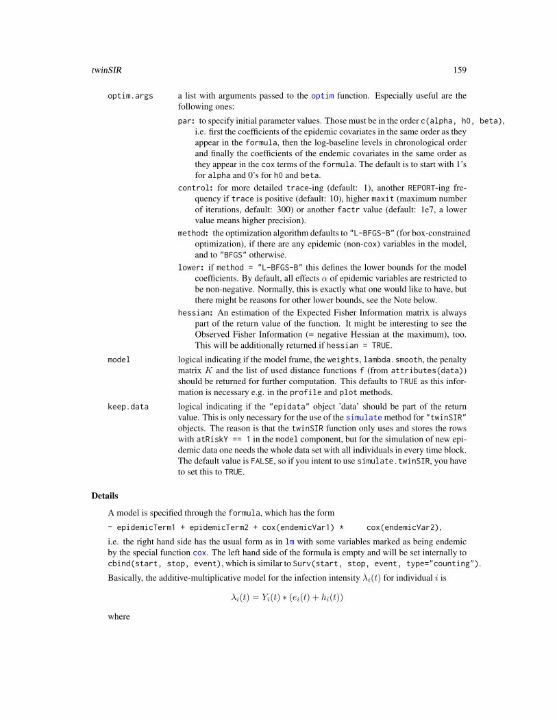
twinSIR 159

optim.args a list with arguments passed to the optim function. Especially useful are thefollowing ones:

par: to specify initial parameter values. Those must be in the order c(alpha, h0, beta),i.e. first the coefficients of the epidemic covariates in the same order as theyappear in the formula, then the log-baseline levels in chronological orderand finally the coefficients of the endemic covariates in the same order asthey appear in the cox terms of the formula. The default is to start with 1’sfor alpha and 0’s for h0 and beta.

control: for more detailed trace-ing (default: 1), another REPORT-ing fre-quency if trace is positive (default: 10), higher maxit (maximum numberof iterations, default: 300) or another factr value (default: 1e7, a lowervalue means higher precision).

method: the optimization algorithm defaults to "L-BFGS-B" (for box-constrainedoptimization), if there are any epidemic (non-cox) variables in the model,and to "BFGS" otherwise.

lower: if method = "L-BFGS-B" this defines the lower bounds for the modelcoefficients. By default, all effects α of epidemic variables are restricted tobe non-negative. Normally, this is exactly what one would like to have, butthere might be reasons for other lower bounds, see the Note below.

hessian: An estimation of the Expected Fisher Information matrix is alwayspart of the return value of the function. It might be interesting to see theObserved Fisher Information (= negative Hessian at the maximum), too.This will be additionally returned if hessian = TRUE.

model logical indicating if the model frame, the weights, lambda.smooth, the penaltymatrix K and the list of used distance functions f (from attributes(data))should be returned for further computation. This defaults to TRUE as this infor-mation is necessary e.g. in the profile and plot methods.

keep.data logical indicating if the "epidata" object ’data’ should be part of the returnvalue. This is only necessary for the use of the simulate method for "twinSIR"objects. The reason is that the twinSIR function only uses and stores the rowswith atRiskY == 1 in the model component, but for the simulation of new epi-demic data one needs the whole data set with all individuals in every time block.The default value is FALSE, so if you intent to use simulate.twinSIR, you haveto set this to TRUE.

Details

A model is specified through the formula, which has the form

~ epidemicTerm1 + epidemicTerm2 + cox(endemicVar1) * cox(endemicVar2),

i.e. the right hand side has the usual form as in lm with some variables marked as being endemicby the special function cox. The left hand side of the formula is empty and will be set internally tocbind(start, stop, event), which is similar to Surv(start, stop, event, type="counting").

Basically, the additive-multiplicative model for the infection intensity λi(t) for individual i is

λi(t) = Yi(t) ∗ (ei(t) + hi(t))

where

160 twinSIR

Y\_i(t) is the at-risk indicator, indicating if individual i is “at risk” of becoming infected at timepoint t. This variable is part of the event history data.

e\_i(t) is the epidemic component of the infection intensity, defined as

ei(t) =∑j∈I(t)

f(||si − sj ||)

where I(t) is the set of infectious individuals just before time point t, si is the coordinatevector of individual i and the function f is defined as

f(u) =

p∑m=1

αmBm(u)

with unknown transmission parameters α and known distance functions Bm. This set ofdistance functions results in the set of epidemic variables normally calculated by the converterfunction as.epidata, considering the equality

ei(t) =

p∑m=1

αmxim(t)

with xim(t) =∑j∈I(t)Bm(||si − sj ||) being the m’th epidemic variable for individual i.

h\_i(t) is the endemic (cox) component of the infection intensity, defined as

hi(t) = exp(h0(t) + zi(t)′β)

where h0(t) is the log-baseline hazard function, zi(t) is the vector of endemic covariates ofindividual i and β is the vector of unknown coefficients. To fit the model, the log-baseline haz-ard function is approximated by a piecewise constant function with known knots, but unknownlevels, which will be estimated. The approximation is specified by the arguments knots ornIntervals.

If a big number of knots (or nIntervals) is chosen, the corresponding log-baseline parameterscan be rendered identifiable by the use of penalized likelihood inference. At present, it is the job ofthe user to choose an adequate value of the smoothing parameter lambda.smooth. Alternatively, adata driven lambda.smooth smoothing parameter selection based on a mixed model representationof an equivalent truncated power spline is offered (see reference for further details). The followingtwo steps are iterated until converegence:

1. Given fixed smoothing parameter, the penalized likelihood is optimized for the regressioncomponents using a L-BFGS-B approach

2. Given fixed regression parameters, a Laplace approximation of the marginal likelihood for thesmoothing parameter is numerically optimized.

Depending on the data convergence might take a couple of iterations.

Note also that it is unwise to include endemic covariates with huge values, as they affect the in-tensities on the exponential scale after having been multiplied by the parameter vector β. With bigcovariates the optim method "L-BFGS-B" will likely terminate due to an infinite log-likelihood orscore function in some iteration.

twinSIR 161

Value

twinSIR returns an object of class "twinSIR". An object of this class is a list containing thefollowing components:

coefficients a named vector of coefficients.

loglik the maximum of the (penalized) log-likelihood function.

counts the number of log-likelihood and score function evaluations.

converged logical indicating convergence of the optimization algorithm.fisherinfo.observed

if requested, the negative Hessian from optim.

fisherinfo an estimation of the Expected Fisher Information matrix.

method the optimization algorithm used.

intervals a numeric vector (c(minTime, knots, maxTime)) representing the consecu-tive intervals of constant log-baseline.

nEvents a numeric vector containing the number of infections in each of the above intervals.

model if requested, the model information used. This is a list with components "survs"(data.frame with the id, start, stop and event columns), "X" (matrix of the epi-demic variables), "Z" (matrix of the endemic variables), "weights" (the speci-fied weights), "lambda.smooth" (the specified lambda.smooth), "K" (the penaltymatrix used) and "f" (the distance functions used). Be aware that the model onlycontains those rows with atRiskY == 1!

data if requested, the supplied "epidata" data.

call the matched call.

formula the specified formula.

terms the terms object used.

Note

There are some restrictions to modelling the infection intensity without a baseline hazard rate, i.e.without an intercept in the formula. Reason: At some point, the optimization algorithm L-BFGS-Btries to set all transmission parameters α to the boundary value 0 and to calculate the (penalized)score function with this set of parameters (all 0). The problem then is that the values of the infectionintensities lambdai(t) are 0 for all i and t and especially at observed event times, which is impossi-ble. Without a baseline, it is not allowed to have all alpha’s set to 0, because then we would not ob-serve any infections. Unfortunately, L-BFGS-B can not consider this restriction. Thus, if one wantsto fit a model without baseline hazard, the control parameter lower must be specified in optim.argsso that some alpha is strictly positive, e.g. optim.args = list(lower = c(0,0.001,0.001,0))and the initial parameter vector par must not be the zero vector.

Author(s)

Michael Höhle and Sebastian Meyer

162 twinSIR_epidata

References

Höhle, M. (2009), Additive-Multiplicative Regression Models for Spatio-Temporal Epidemics, Bio-metrical Journal, 51(6):961-978.

See Also

as.epidata for the necessary data input structure, plot.twinSIR for plotting the path of the infec-tion intensity, profile.twinSIR for profile likelihood estimation. and simulate.twinSIR for thesimulation of epidemics following the fitted model.

Furthermore, the standard extraction methods vcov, logLik, AIC and extractAIC are implementedfor objects of class "twinSIR".

Examples

data("fooepidata")summary(fooepidata)

# fit an overall constant baseline hazard ratefit1 <- twinSIR(~ B1 + B2 + cox(z2), data = fooepidata, keep.data = TRUE)fit1summary(fit1)

# fit a piecewise constant baseline hazard rate with 3 intervals using# _un_penalized ML and estimated coefs from fit1 as starting valuesfit2 <- twinSIR(~ B1 + B2 + cox(z2), data = fooepidata, nIntervals = 3,

optim.args = list(par=c(coef(fit1)[1:2],rep(coef(fit1)[3],3),coef(fit1)[4])))fit2summary(fit2)

# fit a piecewise constant baseline hazard rate with 9 intervals# using _penalized_ ML and estimated coefs from fit1 as starting valuesfit3 <- twinSIR(~ B1 + B2 + cox(z2), data = fooepidata, nIntervals = 9,

lambda.smooth = 0.1, penalty = 1, optim.args = list(par=c(coef(fit1)[1:2], rep(coef(fit1)[3],9), coef(fit1)[4])))

fit3summary(fit3)# plot of the 9 log-baseline levelsplot(x=fit3$intervals, y=coef(fit3)[c(3,3:11)], type="S")

### -> for more sophisticated intensity plots, see ’plot.twinSIR’plot(fit3)

twinSIR_epidata Class for Epidemic Data Discrete in Space and Continuous in Time

twinSIR_epidata 163

Description

The function as.epidata is used to generate objects of class "epidata". Objects of this classare specific data frames containing the event history of an epidemic together with some additionalattributes. These objects are the basis for fitting spatio-temporal epidemic intensity models with thefunction twinSIR. Note that the spatial information itself, i.e. the positions of the individuals, isassumed to be constant over time. Besides epidemics following the SIR compartmental model, alsodata from SI, SIRS and SIS epidemics may be supplied. Inference for the infectious process worksas usual and simulation of such epidemics is also possible.

Usage

as.epidata(data, ...)

## Default S3 method:as.epidata(data, id.col, start.col, stop.col, atRiskY.col,

event.col, Revent.col, coords.cols, f = list(), ...)## S3 method for class ’epidataCS’as.epidata(data, tileCentroids, eps = 0.001, ...)

## S3 method for class ’epidata’print(x, ...)## S3 method for class ’epidata’x[i, j, drop]

Arguments

data For the default method a matrix or a data.frame. It contains the observedevent history in a form similar to Surv(, type="counting") with additionalinformation (variables) along the process. It must not be sorted in any specificorder; this will be done automatically during conversion. The observation periodis splitted up into consecutive intervals of constant state - thus constant infectionintensities. The data frame consists of a block of N (number of individuals) rowsfor each of those time intervals (all rows in a block share the same start and stopvalues... therefore the name “block”), where there is one row per individualin the block. Each row describes the (fixed) state of the individual during theinterval given by the start and stop columns start.col and stop.col.Note that there may not be more than one event (infection or removal) in a singleblock. Thus, in a single block, only one entry in the event.col and Revent.colmay be 1, all others are 0. This rule follows the assumption that there are noconcurrent events (infections or removals).Alternatively, data may be an object of class "epidataCS", i.e. space-continuousepidemic data used in the twinstim context, which will be converted (aggre-gated) to an object of class "epidata" for use with twinSIR.

id.col single index of the id column in data. Can be numeric (by column number)or character (by column name). The id column identifies the individuals in thedata frame. It will be converted to a factor variable.

start.col single index of the start column in data. Can be numeric (by column number)or character (by column name). The start column contains the (numeric) time

164 twinSIR_epidata

points of the beginnings of the consecutive time intervals of the event history.The minimum value in this column, i.e. the start of the observation period shouldbe 0.

stop.col single index of the stop column in data. Can be numeric (by column number)or character (by column name). The stop column contains the (numeric) timepoints of the ends of the consecutive time intervals of the event history. The stopvalue must always be greater than the start value of a row.

atRiskY.col single index of the atRiskY column in data. Can be numeric (by column num-ber) or character (by column name). The atRiskY column indicates if the indi-vidual was “at-risk” of becoming infected during the time interval (start; stop].This variable must be logical or in 0/1-coding. Individuals with atRiskY == 0in the first time interval (normally the rows with start == 0) are taken as ini-tially infectious.

event.col single index of the event column in data. Can be numeric (by column number)or character (by column name). The event column indicates if the individualbecame infected at the stop time of the interval. This variable must be logicalor in 0/1-coding.

Revent.col single index of the Revent column in data. Can be numeric (by column num-ber) or character (by column name). The Revent column indicates if the indi-vidual was recovered at the stop time of the interval. This variable must belogical or in 0/1-coding.

coords.cols indexes of the coords columns in data. Can be a numeric (by column number)vector, a character (by column name) vector or NULL (in which case epidemiccovariates are not calculateable). These columns contain the coordinates of theindividuals. It must be emphasized that the functions related to twinSIR modelscurrently assume fixed positions of the individuals during the whole epidemic.Thus, an individual has the same coordinates in every block. For simplicity, thecoordinates are derived from the first time block only (normally the rows withstart == 0). The epidemic covariates are calculated based on the euclidiandistances between the individuals, see f.

f a named list of distance functions or list() (the default), if calculation of epi-demic covariates is not requested. The functions must interact elementwise ona (distance) matrix so that - for a matrix D - f[[m]](D) results in a matrix. Asimple example is function(u) {u <= 1}, which indicates if the euclidiandistance between the individuals is smaller than or equal to 1. To ensure thatan individual does not influence itself, the distance to itself is defined as Inf.Consequently, all of the distance functions must have the property f[[m]](Inf) =0. The names of the functions will be the names of the epidemic variables in theresulting data frame. The value of such a variable is computed as follows: I(t)denotes the set of infectious individuals just before time t and si the coordinatevector of individual i. For individual i at time t the epidemic component m hasthe value

∑j∈I(t) fm(||si − sj ||)

tileCentroids a coordinate matrix of the tile centroids the row names of which are the tilelevels. This will be the coordinates used for the population (i.e. the tiles from"epidataCS") in the discrete-space twinSIR modelling.

eps numeric scalar for breaking tied removal and infection times between differentindividuals (tiles), which might occur during conversion from "epidataCS" to

twinSIR_epidata 165

"epidata". Rather dumb, this is simply done by subtracting eps from each tiedremoval time. One should consider other ways of breaking the tied event times.

x an object of class "epidata".

... arguments passed to print.data.frame. Currently unused in as.epidata.

i,j,drop arguments passed to [.data.frame.

Details

The print method for objects of class "epidata" simply prints the data frame with a small headercontaining the time range of the observed epidemic and the number of infected individuals. Usually,the data frames are quite long, so the summary method summary.epidata might be useful. Also,indexing/subsetting "epidata" works exactly as for data.frames, but there is an own method,which assures consistency of the resulting "epidata" or drops this class, if necessary.

SIS epidemics are implemented as SIRS epidemics where the length of the removal period equals0. This means that an individual, which has an R-event will be at risk immediately afterwards, i.e.in the following time block. Therefore, data of SIS epidemics have to be provided in that formcontaining “pseudo-R-events”.

Some comments on the conversion from "epidataCS" to "epidata": the conversion results intoSIS epidemics only, i.e. the at-risk indicator is set to 1 immediately after recovery. The lengthsof the infectious periods are taken from data$events$eps.t. There will be no f columns in theresulting "epidata". These must be generated by a subsequent call to as.epidata with desired f.

Value

a data.frame with the columns "BLOCK", "id", "start", "stop", "atRiskY", "event", "Revent"and the coordinate columns (with the original names from data), which are all obligatory. Thesecolumns are followed by any remaining columns of the input data. Last but not least, the newlygenerated columns with epidemic variables corresponding to the functions in the list f are appended,if length(f) > 0.

The data.frame is given the additional attributes

"eventTimes" numeric vector of infection time points (sorted chronologically).

"timeRange" numeric vector of length 2: c(min(start), max(stop)).

"coords.cols" numeric vector containing the column indices of the coordinate columns in theresulting data frame.

"f" this equals the argument f.

Note

The column name "BLOCK" is a reserved name. This column will be added automatically at con-version and the resulting data frame will be sorted by this column and by id. Also the names "id","start", "stop", "atRiskY", "event" and "Revent" are reserved for the respective columns only.

Author(s)

Sebastian Meyer

166 twinSIR_epidata_animate

See Also

The plot and the summary method for class "epidata". Furthermore, the function animate.epidatafor the animation of epidemics.

Function twinSIR for fitting spatio-temporal epidemic intensity models to epidemic data.

Function simEpidata for the simulation of epidemic data.

Examples

# an artificial example of an event history from the packagedata("foodata")str(foodata)

# convert the data to an object of class "epidata",# also generating some epidemic covariatesmyEpidata <- as.epidata(foodata, id.col = 1, start.col = "start",

stop.col = "stop", atRiskY.col = "atrisk", event.col = "infected",Revent.col = "removed", coords.cols = c("x","y"),f = list(B1 = function(u) u<=1,

B2 = function(u) u>1 & is.finite(u)))# note the is.finite restriction in B2 to ensure that f[[i]](Inf) = 0, for all i

str(myEpidata)subset(myEpidata, BLOCK == 1)

summary(myEpidata) # see ’summary.epidata’plot(myEpidata) # see ’plot.epidata’ and also ’animate.epidata’stateplot(myEpidata, "15") # see ’stateplot’

## Not run: # works in interactive mode, but not in R CMD checkdata("fooepidata")stopifnot(identical(myEpidata, fooepidata))

## End(Not run)

twinSIR_epidata_animate

Spatio-Temporal Animation of an Epidemic

Description

Function for the animation of epidemic data, i.e. objects inheriting from class "epidata". Thisonly works with 1- or 2-dimensional coordinates and is not useful if some individuals share thesame coordinates (overlapping). There are two types of animation, see argument time.spacing.Besides the direct plotting in the R session, it is also possible to generate a sequence of graphicsfiles to create animations outside R.

twinSIR_epidata_animate 167

Usage

## S3 method for class ’summary.epidata’animate(object, main = "An animation of the epidemic",

pch = 19, col = c(3, 2, gray(0.6)), time.spacing = NULL,sleep = quote(5/.nTimes), legend.opts = list(), timer.opts = list(),end = NULL, generate.snapshots = NULL, ...)

## S3 method for class ’epidata’animate(object, ...)

Arguments

object an object inheriting from class "epidata" or "summary.epidata". In the for-mer case, its summary is calculated and the function continues as in the lattercase, passing all ... arguments to the summary.epidata method.

main a main title for the plot, see also title.

pch, col vectors of length 3 specifying the point symbols and colors for susceptible, in-fectious and removed individuals (in this order). The vectors are recycled ifnecessary. By default, susceptible individuals are marked as filled green circles,infectious individuals as filled red circles and removed individuals as filled graycircles. Note that the symbols are iteratively drawn (overlayed) in the same plot-ting region as time procedes. For information about the possible values of pchand col, see the help pages of points and par, respectively.

time.spacing time interval for the animation steps. If NULL (the default), the events are plot-ted one by one with pauses of sleep seconds. Thus, it is just the ordering ofthe events, which is shown. To plot the appearance of events proportionallyto the exact time line, time.spacing can be set to a numeric value indicat-ing the period of time between consecutive plots. Then, for each time point inseq(0, end, by = time.spacing) the current state of the epidemic can beseen and an additional timer indicates the current time (see timer.opts below).The argument sleep will be the artificial pause in seconds between two of thosetime points.

sleep time in seconds to Sys.sleep before the next plotting event. By default, eachartificial pause is of length 5/.nTimes seconds, where .nTimes is the numberof events (infections and removals) of the epidemic, which is evaluated in thefunction body. Thus, for time.spacing = NULL the animation has a duration ofapproximately 5 seconds. In the other case, sleep is the duration of the artificialpause between two time points.

legend.opts either a list of arguments passed to the legend function or NULL (or NA), in whichcase no legend will be plotted. All necessary arguments have sensible defaultsand need not be specified, i.e.

x: "topright"

legend: c("susceptible", "infectious", "removed")

pch: same as argument pch of the main functioncol: same as argument col of the main function

168 twinSIR_epidata_animate

timer.opts either a list of arguments passed to the legend function or NULL (or NA), in whichcase no timer will be plotted. All necessary arguments have sensible defaults andneed not be specified, i.e.

x: "bottomright"

title: "time"

box.lty: 0

adj: c(0.5,0.5)

inset: 0.01

bg: "white"

Note that the argument legend, which is the current time of the animation, cannot be modified.

end ending time of the animation in case of time.spacing not being NULL. By de-fault (NULL), time stops after the last event.

generate.snapshots

By default (NULL), the animation is not saved to image files but only shown onthe on-screen device. In order to do that, time.spacing must not be NULL, andthere are two options:If the framework of the animation package should be used, i.e. the animate-callis passed as the expr argument to one of the save* functions of the animationpackage, then set generate.snapshots = img.name, where img.name is thebase name for the generated images (the same as passed to the save* function).The path and format (type, width, height) for the generated images is derivedfrom ani.options. See the last example below.Alternatively, generate.snapshots may be a list of arguments passed to thefunction dev.print, which then is executed at each time point of the grid de-fined by time.spacing. Essentially, this is used for saving the produced snap-shots to files, e.g.generate.snapshots = list(device=pdf, file=quote(paste("epidemic_",sprintf(form,tp),".pdf", sep="")))

will store the animation steps in pdf-files in the current working directory, wherethe file names each end with the time point represented by the correspondingplot. Because the variables tp and form should only be evaluated inside thefunction the file argument is quoted. Alternatively, the file name could alsomake use of the internal plot index i, e.g., use file=quote(paste("epidemic",i,".pdf",sep="")).

... further graphical parameters passed to the basic call of plot, e.g. las, cex.axis(etc.) and mgp.

Author(s)

Sebastian Meyer

See Also

summary.epidata for the data, on which the plot is based. plot.epidata for plotting the evolutionof an epidemic by the numbers of susceptible, infectious and removed individuals.

The contributed R package animation.

twinSIR_epidata_intersperse 169

Examples

## Not run:data("fooepidata")(s <- summary(fooepidata))

# plot the ordering of the events onlyanimate(s, sleep=0.01) # or: animate(fooepidata)

# with timer (animate only up to t=10)animate(s, time.spacing=0.1, end=10, sleep=0.01)

# using features of the animation package:if (require("animation")) saveHTML(

animate(s, time.spacing = 1, sleep = 0, generate.snapshots = "epiani"),img.name = "epiani", use.dev = FALSE, ani.type = "png", width = 600

)

## End(Not run)

twinSIR_epidata_intersperse

Impute Blocks for Extra Stops in "epidata" Objects

Description

This function modifies an object inheriting from class "epidata" such that it features the specifiedstop time points. For this purpose, the time interval in the event history into which the new stopfalls will be splitted up into two parts, one block for the time period until the new stop – where noinfection or removal occurs – and the other block for the time period from the new stop to the endof the original interval.Main application is to enable the use of knots in twinSIR, which are not existing stop time pointsin the "epidata" object.

Usage

intersperse(epidata, stoptimes)

Arguments

epidata an object inheriting from class "epidata".stoptimes a numeric vector of time points inside the observation period of the epidata.

Value

an object of the same class as epidata with additional time blocks for any new stoptimes.

Author(s)

Sebastian Meyer

170 twinSIR_epidata_plot

Examples

data("fooepidata")subset(fooepidata, start < 25 & stop > 25, select = 1:7)nrow(fooepidata)moreStopsEpi <- intersperse(fooepidata, c(25,75))nrow(moreStopsEpi)subset(moreStopsEpi, stop == 25 | start == 25, select = 1:7)

twinSIR_epidata_plot Plotting the Evolution of an Epidemic

Description

Functions for plotting the evolution of epidemics. The plot methods for classes "epidata" and"summary.epidata" plots the numbers of susceptible, infectious and recovered (= removed) in-dividuals by step functions along the time axis. The function stateplot shows individual statechanges along the time axis.

Usage

## S3 method for class ’summary.epidata’plot(x, lty = c(2, 1, 3), lwd = 1, col = 1, col.hor = col,

col.vert = col, xlab = "Time", ylab = "Number of individuals",xlim = NULL, ylim = NULL, legend.opts = list(), do.axis4 = NULL,panel.first = grid(), rug.opts = list(),which.rug = c("infections", "removals", "susceptibility", "all"), ...)

## S3 method for class ’epidata’plot(x, ...)

stateplot(x, id, ...)

Arguments

x an object inheriting from class "epidata" or "summary.epidata". In the for-mer case, its summary is calculated and the function continues as in the lattercase. The plot method for class "epidata" is a simple wrapper for plot.summary.epidataimplemented as plot(summary(x, ...)).

lty, lwd vectors of length 3 containing the line types and widths, respectively, for thenumbers of susceptible, infectious and removed individuals (in this order). Bydefault, all lines have width 1 and the line types are dashed (susceptible), solid(infectious) and dotted (removed), respectively. To omit the drawing of a spe-cific line, just set the corresponding entry in lty to 0. The vectors are recycledif necessary. For information about the different lty and lwd codes, see the helppages of par.

twinSIR_epidata_plot 171

col, col.hor, col.vert

vectors of length 3 containing the line colors for the numbers of susceptible,infectious and removed individuals (in this order). col.hor defines the colorfor the horizontal parts of the step function, whilst col.vert defines the colorfor its vertical parts. The argument col is just short for col.hor = col andcol.vert = col. By default, all lines are completely drawn in black. Thevectors are recycled if necessary. For information about the possible values ofcol, see the help pages of par.

xlab, ylab axis labels, default to "Time" and "Number of individuals", respectively.

xlim, ylim the x and y limits of the plot in the form c(xmin, xmax) and c(ymin, ymax),respectively. By default, these are chosen adequately to fit the time range of theepidemic and the number of individuals.

legend.opts either a list of arguments passed to the legend function or NULL (or NA), in whichcase no legend will be plotted. All necessary arguments have sensible defaultsand need not be specified, i.e.

x: "topright"

legend: c("susceptible", "infectious", "removed")

lty: same as argument lty of the main functionlwd: same as argument lwd of the main functioncol: same as argument col.hor of the main functionbty: "n"

do.axis4 logical indicating if the final numbers of susceptible and removed individualsshould be indicated on the right axis. The default NULL means TRUE, if x rep-resents a SIR epidemic and FALSE otherwise, i.e. if the epidemic is SI, SIS orSIRS.

panel.first an expression to be evaluated after the plot axes are set up but before any plottingtakes place. By default, a standard grid is drawn.

rug.opts either a list of arguments passed to the function rug or NULL (or NA), in whichcase no rug will be plotted. By default, the argument ticksize is set to 0.02and quiet is set to TRUE. Note that the argument x, which contains the locationsfor the rug is fixed internally and can not be modified. The argument which.rug(see below) determines the locations to mark.

which.rug By default, tick marks are drawn at the time points of infections. Alternatively,one can choose to mark only "removals", "susceptibilities" (i.e. statechange from R to S) or "all" events.

id single character string or factor of length 1 specifying the individual for whichthe stateplot should be established.

... For plot.summary.epidata: further graphical parameters passed to plot, linesand axis, e.g. main, las, cex.axis (etc.) and mgp.For plot.epidata: arguments passed to plot.summary.epidata.For stateplot: arguments passed to plot.stepfun or plot.function (if idhad no events during the observation period). By default, xlab="time", ylab="state",xlim=attr(x,"timeRange"), xaxs="i" and do.points=FALSE.

172 twinSIR_epidata_summary

Value

plot.summary.epidata (and plot.epidata) invisibly returns the matrix used for plotting, whichcontains the evolution of the three counters.stateplot invisibly returns the function, which was plotted, typically of class "stepfun", butmaybe of class "function", if no events have been observed for the individual in question (thenthe function always returns the initial state). The vertical axis of stateplot can range from 1 to 3,where 1 corresponds to Suscepible, 2 to Infectious and 3 to Removed.

Author(s)

Sebastian Meyer

See Also

summary.epidata for the data, on which the plots are based. animate.epidata for the animationof epidemics.

Examples

data("fooepidata")s <- summary(fooepidata)

# evolution of the epidemicpar(las = 1)plot(s)

# stateplotstateplot(s, id = "15", main = "Some individual event paths")stateplot(s, id = "1", add = TRUE, col = 2)stateplot(s, id = "20", add = TRUE, col = 3)legend("topright", legend = c(15, 1, 20), title = "id", lty = 1, col = 1:3,

inset = 0.1)

twinSIR_epidata_summary

Summarizing an Epidemic

Description

The summary method for class "epidata" gives an overview of the epidemic. Its print methodshows the type of the epidemic, the time range, the total number of individuals, the initially andnever infected individuals and the size of the epidemic. An excerpt of the returned counters dataframe is also printed (see the Value section below).

twinSIR_epidata_summary 173

Usage

## S3 method for class ’epidata’summary(object, ...)

## S3 method for class ’summary.epidata’print(x, ...)

Arguments

object an object inheriting from class "epidata".

x an object inheriting from class "summary.epidata", i.e. an object returned bythe function summary.epidata.


Value

A list with the following components:

type character string. Compartmental type of the epidemic, i.e. one of "SIR", "SI","SIS" or "SIRS".

size integer. Size of the epidemic, i.e. the number of initially susceptible individuals,which became infected during the course of the epidemic.

initiallyInfected

factor (with the same levels as the id column in the "epidata" object). Set ofinitially infected individuals.

neverInfected factor (with the same levels as the id column in the "epidata" object). Set ofnever infected individuals, i.e. individuals, which were neither initially infectednor infected during the course of the epidemic.

coordinates numeric matrix of individual coordinates with as many rows as there are individ-uals and one column for each spatial dimension. The row names of the matrixare the ids of the individuals.

byID data frame with time points of infection and optionally removal and re-susceptibility(depending on the type of the epidemic) ordered by id. If an event was not ob-served, the corresponding entry is missing.

counters data frame containing all events (S, I and R) ordered by time. The columns aretime, type (of event), corresponding id and the three counters nSusceptible,nInfectious and nRemoved. The first row additionally shows the counters atthe beginning of the epidemic, where the type and id column contain missingvalues.

Author(s)

Sebastian Meyer

See Also

as.epidata for generating objects of class "epidata".

174 twinSIR_intensityplot

Examples

data("fooepidata")s <- summary(fooepidata)s # uses the print method for summary.epidatanames(s) # components of the list ’s’

# positions of the individualsplot(s$coordinates)

# events by idhead(s$byID)

twinSIR_intensityplot Plotting Paths of Infection Intensities for twinSIR Models

Description

intensityplot methods to plot the evolution of the total infection intensity, its epidemic proportionor its endemic proportion over time. The default plot method for objects of class "twinSIR" is justa wrapper for the intensityplot method.

Usage

## S3 method for class ’twinSIR’plot(x, which = c("epidemic proportion", "endemic proportion",

"total intensity"), ...)

## S3 method for class ’twinSIR’intensityplot(x, which = c("epidemic proportion", "endemic proportion",

"total intensity"), aggregate = TRUE, theta = NULL,plot = TRUE, add = FALSE, rug.opts = list(), ...)

## S3 method for class ’simEpidata’intensityplot(x, which = c("epidemic proportion", "endemic proportion",

"total intensity"), aggregate = TRUE, theta = NULL,plot = TRUE, add = FALSE, rug.opts = list(), ...)

Arguments

x an object of class "twinSIR" (fitted model) or "simEpidata" (simulated twinSIRepidemic), respectively.

which "epidemic proportion", "endemic proportion", or "total intensity".Partial matching is applied. Determines whether to plot the path of the totalintensity λ(t) or its epidemic or endemic proportions e(t)

λ(t) or h(t)λ(t) .

aggregate logical. Determines whether lines for all individual infection intensities shouldbe drawn (FALSE) or their sum only (TRUE, the default).

twinSIR_intensityplot 175

theta numeric vector of model coefficients. If x is of class "twinSIR", then theta = c(alpha, beta),where beta consists of the coefficients of the piecewise constant log-baselinefunction and the coefficients of the endemic (cox) predictor. If x is of class"simEpidata", then theta = c(alpha, 1, betarest), where 1 refers to the(true) log-baseline used in the simulation and betarest is the vector of the re-maining coefficients of the endemic (cox) predictor. The default (NULL) meansthat the fitted or true parameters, respectively, will be used.

plot logical indicating if a plot is desired, defaults to TRUE. Otherwise, only the dataof the plot will be returned. Especially with aggregate = FALSE and manyindividuals one might e.g. consider to plot a subset of the individual intensitypaths only or do some further calculations/analysis of the infection intensities.

add logical. If TRUE, paths are added to the current plot, using lines.

rug.opts either a list of arguments passed to the function rug, or NULL (or NA), in whichcase no rug will be plotted. By default, the argument ticksize is set to 0.02and quiet is set to TRUE. Note that the argument x of the rug() function, whichcontains the locations for the rug is fixed internally and can not be modified.The locations of the rug are the time points of infections.

... For the plot.twinSIR methode, arguments passed to intensityplot.twinSIR.For the intensityplot methods, further graphical parameters passed to thefunction matplot, e.g. lty, lwd, col, xlab, ylab and main. Note that thematplot arguments x, y, type and add are implicit and can not be specifiedhere.

Value

numeric matrix with the first column "stop" and as many rows as there are "stop" time points inthe event history x. The other columns depend on the argument aggregate: if TRUE, there is onlyone other column named which, which contains the values of which at the respective "stop" timepoints. Otherwise, if aggregate = FALSE, there is one column for each individual, each of themcontaining the individual which at the respective "stop" time points.

Author(s)

Sebastian Meyer

References


See Also

twinSIR or Höhle (2009) for a more detailed description of the intensity model. simulate.twinSIRfor the simulation of epidemic data according to a twinSIR specification.

176 twinSIR_methods

Examples

data("fooepidata")data("foofit")

# an overview of the evolution of the epidemicplot(fooepidata)

# overall total intensityplot(foofit, which="total")

# overall epidemic proportionepi <- plot(foofit, which="epidemic")

# look at returned valueshead(epi)

# add the inverse overall endemic proportion = 1 - epidemic proportionende <- plot(foofit, which="endemic", add=TRUE, col=2)legend("right", legend="endemic proportion \n(= 1 - epidemic proportion)",

lty=1, col=2, bty="n")

# individual intensitiestmp <- plot(foofit, which="total", aggregate=FALSE,

col=rgb(0,0,0,alpha=if(getRversion() < "2.7.0") 1 else 0.1),main=expression("Individual infection intensities " *

lambda[i](t) == Y[i](t) %.% (e[i](t) + h[i](t))))# return value: matrix of individual intensity pathsstr(tmp)

# plot intensity path only for individuals 3 and 99matplot(x=tmp[,1], y=tmp[,1+c(3,99)], type="S", ylab="Force of infection",

xlab="time", main=expression("Paths of the infection intensities " *lambda[3](t) * " and " * lambda[99](t)))

legend("topright", legend=paste("Individual", c(3,99)), col=c(1,2), lty=c(1,2))

twinSIR_methods Print, Summary and Extraction Methods for "twinSIR" Objects

Description

Besides print and summary methods there are also some standard extraction methods defined forobjects of class "twinSIR": vcov, logLik and especially AIC and extractAIC, which extractAkaike’s Information Criterion. Note that special care is needed, when fitting models with param-eter constraints such as the epidemic effects α in twinSIR models. Parameter constraints reducethe average increase in the maximized loglikelihood - thus the penalty for constrained parametersshould be smaller than the factor 2 used in the ordinary definition of AIC. To this end, these twomethods offer the calculation of the so-called one-sided AIC (OSAIC).

twinSIR_methods 177

Usage

## S3 method for class ’twinSIR’print(x, digits = max(3, getOption("digits") - 3), ...)## S3 method for class ’twinSIR’summary(object,

correlation = FALSE, symbolic.cor = FALSE, ...)

## S3 method for class ’twinSIR’AIC(object, ..., k = 2, one.sided = NULL, nsim = 1e3)## S3 method for class ’twinSIR’extractAIC(fit, scale = 0, k = 2, one.sided = NULL,

nsim = 1e3, ...)

## S3 method for class ’twinSIR’vcov(object, ...)## S3 method for class ’twinSIR’logLik(object, ...)

## S3 method for class ’summary.twinSIR’print(x,

digits = max(3, getOption("digits") - 3), symbolic.cor = x$symbolic.cor,signif.stars = getOption("show.signif.stars"), ...)

Arguments

x, object, fit an object of class "twinSIR".For the print method of the summary method, an object of class "summary.twinSIR".

digits integer, used for number formatting with signif(). Minimum number of sig-nificant digits to be printed in values.

correlation logical. if TRUE, the correlation matrix of the estimated parameters is returnedand printed.

symbolic.cor logical. If TRUE, print the correlations in a symbolic form (see symnum) ratherthan as numbers.

... For the summary method: arguments passed to extractAIC.twinSIR.For the AIC method, optionally more fitted model objects.For the print, extractAIC, vcov and logLik methods: unused (argument ofthe generic).

k numeric specifying the "weight" of the penalty to be used; in an unconstrainedfit k = 2 is the classical AIC.

one.sided logical or NULL (the default). Determines if the one-sided AIC should be cal-culated instead of using the classical penalty k*edf. The default value NULLchooses classical AIC in the case of an unconstrained fit and one-sided AIC inthe case of constraints. The type of the fit can be seen in object$method (orfit$method respectively), where "L-BFGS" means constrained optimization.

nsim number of simulations to use for determining the weights in the OSAIC formulawhen there are more than two epidemic covariates in the fit. Defaults to 1000samples.

178 twinSIR_methods

scale unused (argument of the generic).

signif.stars logical. If TRUE, “significance stars” are printed for each coefficient.

Details

The print and summary methods allow the compact or comprehensive representation of the fittingresults, respectively. The former only prints the original function call, the estimated coefficientsand the maximum log-likelihood value. The latter prints the whole coefficient matrix with standarderrors, z- and p-values (see printCoefmat), and additionally the number of infections per log-baseline interval, the (one-sided) AIC and the number of log-likelihood evaluations. They bothappend a big “WARNING”, if the optimization algorithm did not converge.

The estimated coefficients may be extracted by using the default coef-method from package stats.

The two AIC functions differ only in that AIC can take more than one fitted model object and thatextractAIC always returns the number of parameters in the model (AIC only does with more thanone fitted model object).

Concerning the choice of one-sided AIC: parameter constraints – such as the non-negative con-straints for the epidemic effects alpha in twinSIR models – reduce the average increase in themaximized loglikelihood. Thus, the penalty for constrained parameters should be smaller than thefactor 2 used in the ordinary definition of AIC. One-sided AIC (OSAIC) suggested by Hughes andKing (2003) is such a proposal when p out of k = p+ q parameters have non-negative constraints:

OSAIC = −2l(θ, τ) + 2

p∑g=0

w(p, g)(k − p+ g)

where w(p, g) are p-specific weights. For more details see Section 5.2 in Höhle (2009).

Value

The print methods return their first argument, invisibly, as they always should. The vcov andlogLik methods return the estimated variance-covariance matrix of the parameters (here, the inverseof the estimate of the expected Fisher information matrix), and the maximum log-likelihood valueof the model, respectively. The summary method returns a list containing some summary statisticsof the fitted model, which is nicely printed by the corresponding print method. For the AIC andextractAIC methods, see the documentation of the corresponding generic functions.

Author(s)

Michael Höhle and Sebastian Meyer

References

Hughes A, King M (2003) Model selection using AIC in the presence of one-sided information.Journal of Statistical Planning and Inference 115, pp. 397–411.


twinSIR_profile 179

Examples

data("foofit")

foofit

coef(foofit)vcov(foofit)logLik(foofit)

summary(foofit, correlation = TRUE, symbolic.cor = TRUE)

# AIC or OSAICAIC(foofit)AIC(foofit, one.sided = FALSE)extractAIC(foofit)extractAIC(foofit, one.sided = FALSE)

# with BIC-like penalty weightAIC(foofit, k = log(nlevels(foofit$model$survs$id)))

# just as a stupid example for the use of AIC with multiple fitsfoofit2 <- foofitAIC(foofit, foofit2) # 2nd column should actually be named "OSAIC" here

twinSIR_profile Profile Likelihood Computation and Confidence Intervals

Description

Function to compute estimated and profile likelihood based confidence intervals. Computationsmight be cumbersome!

Usage

## S3 method for class ’twinSIR’profile(fitted, profile, alpha = 0.05,

control = list(fnscale = -1, factr = 10, maxit = 100), ...)

Arguments

fitted an object of class "twinSIR".

profile a list with elements being numeric vectors of length 4. These vectors must havethe form c(index, lower, upper, gridsize).

index: index of the parameter to be profiled in the vector coef(fitted).lower, upper: lower/upper limit of the grid on which the profile log-likelihood

is evaluated. Can also be NA in which case lower/upper equals the lower/upperbound of the respective 0.3 % Wald confidence interval (+-3*se).

180 twinSIR_simulation

gridsize: grid size of the equally spaced grid between lower and upper. Canalso be 0 in which case the profile log-likelihood for this parameter is notevaluated on a grid.

alpha (1 − α)% profile likelihood based confidence intervals are computed. If alpha<= 0, then no confidence intervals are computed.

control control object to use in optim for the profile log-likelihood computations.


Value

list with profile log-likelihood evaluations on the grid and highest likelihood and wald confidenceintervals. The argument profile is also returned.

Author(s)

Michael Höhle

Examples

data("foofit")# the following call takes a while## Not run:prof <- profile(foofit, list(c(1,0,0.05,5), c(3,NA,NA,0), c(4, NA, NA, 10)))prof

## End(Not run)

twinSIR_simulation Simulation of Epidemic Data

Description

This function simulates the infection (and removal) times of an epidemic. Besides the classical SIRtype of epidemic, also SI, SIRS and SIS epidemics are supported. Simulation works via the condi-tional intensity of infection of an individual, given some (time varying) endemic covariates and/orsome distance functions (epidemic components) as well as the fixed positions of the individuals.The lengths of the infectious and removed periods are generated following a pre-specified function(can be deterministic).

The simulate method for objects of class "twinSIR" simulates new epidemic data using the modeland the parameter estimates of the fitted object.

twinSIR_simulation 181

Usage

simEpidata(formula, data, id.col, I0.col, coords.cols, subset,beta, h0, f = list(), alpha, infPeriod,remPeriod = function(ids) rep(Inf, length(ids)),end = Inf, trace = FALSE, .allocate = NULL)

## S3 method for class ’twinSIR’simulate(object, nsim = 1, seed = 1,

infPeriod = NULL, remPeriod = NULL,end = diff(range(object$intervals)), trace = FALSE, .allocate = NULL,data = object$data, ...)

Arguments

formula an object of class "formula" (or one that can be coerced to that class): a sym-bolic description of the intensity model to be estimated. The details of modelspecification are given under Details.

data a data.frame containing the variables in formula and the variables specified byid.col, I0.col and coords.col (see below). It represents the “history” of theendemic covariates to use for the simulation. The form is similar to and can be anobject of class "epidata". The simulation period is splitted up into consecutiveintervals of constant endemic covariables. The data-frame consists of a block ofN (number of individuals) rows for each of those time intervals (all rows in ablock share the same start and stop values... therefore the name “block”), wherethere is one row per individual in the block. Each row describes the (fixed) stateof the endemic covariates of the individual during the time interval given by thestart and stop columns (specified through the lhs of formula).For the simulate method of class "twinSIR" this should be the object of class"epidata" used for the fit. This is a part of the return value of the functiontwinSIR, if called with argument keep.data set to TRUE.

id.col only if data does not inherit from epidata: single index of the id column indata. Can be numeric (by column number) or character (by column name).The id column identifies the individuals in the data-frame. It will be convertedto a factor variable and its levels serve also to identify individuals as argumentto the infPeriod function.

I0.col only if data does not inherit from epidata: single index of the I0 column indata. Can be numeric (by column number), character (by column name) orNULL.The I0 column indicates if an individual is initially infectious, i.e. it is alreadyinfectious at the beginning of the first time block. Setting I0.col = NULL isshort for “there are no initially infectious individuals”. Otherwise, the variablemust be logical or in 0/1-coding. As this variable is constant over time theinitially infectious individuals are derived from the first time block only.

coords.cols only if data does not inherit from epidata: indexes of the coords columns indata. Can be a numeric (by column number), a character (by column name)vector or NULL.


These columns contain the coordinates of the individuals. It must be empha-sized that the functions in this package currently assume fixed positions of theindividuals during the whole epidemic. Thus, an individual has the same coor-dinates in every block. For simplicity, the coordinates are derived from the firsttime block only. The epidemic covariates are calculated based on the euclidiandistance between the individuals, see f.

subset an optional vector specifying a subset of the covariate history to be used in thesimulation.

beta numeric vector of length equal the number of endemic (cox) terms on the rhsof formula. It contains the effects of the endemic predictor (excluding the log-baseline h0, see below) in the same order as in the formula.

h0 either a single number to specify a constant baseline hazard (equal to exp(h0))or a list of functions named exact and upper. In the latter case, h0$exactis the true log-baseline hazard function and h0$upper is a piecewise constantupper bound for h0$exact. The function h0$upper must inherit from stepfunwith right=FALSE. Theoretically, the intensity function is left-continuous, thusright=TRUE would be adequate, but in the implementation, when we evaluatethe intensity at the knots (change points) of h0$upper we need its value for thesubsequent interval.

f a named list of distance functions or list() (the default), if no epidemic com-ponent is desired (if additionally infPeriod (see below) always returns Inf,then one simulates from the Cox model). The functions must interact element-wise on a (distance) matrix so that - for a matrix D - f[[m]](D) results in a matrix.A simple example is function(u) {u <= 1}, which indicates if the euclidiandistance between the individuals is smaller than or equal to 1. To ensure thatan individual does not influence itself, the distance to itself is defined as Inf.Consequently, all of the distance functions must have the property f[[m]](Inf)= 0. The names of the functions will be the names of the epidemic variablesin the resulting data-frame. So, the names should not coincident with names ofendemic variables. The value of such anepidemic variable is computed as follows: I(t) denotes the set of infectiousindividuals just before time t and si the coordinate vector of individual i. Forindividual i at time t the epidemic componentm has the value

∑j∈I(t) fm(||si−

sj ||)alpha numeric vector of length equal the number of epidemic terms, i.e. the number

of distance functions in f. It contains the effects of the epidemic predictor in thesame order as the distance functions in f or, if names are supplied, matching tothe distance functions will be done by name.

infPeriod a function generating lengths of infectious periods. It should take one parameter(e.g. ids), which is a character vector of id’s of individuals, and return appropri-ate infection periods for those individuals. Therefore, the value of the functionshould be of length length(ids). For example, for independent and identi-cally distributed infection periods following Exp(1), the generating function isfunction(ids) rexp(length(ids), rate=1). For a constant infectious pe-riod of length c, it is sufficient to set function (x) {c}.For the simulate method of class "twinSIR" only, this can also be NULL (the


default), which means that the observed infectious periods of infected individ-uals are re-used when simulating a new epidemic and individuals with missinginfectious periods (i.e. infection and recovery was not observed) are attributedto the mean observed infectious period.Note that it is even possible to simulate an SI-epidemic by settinginfPeriod = function (x) {Inf}

In other words: once an individual became infected it spreads the disease for-ever, i.e. it will never be removed.

remPeriod a function generating lengths of removal periods. Per default, once an individualwas removed it will stay in this state forever (Inf). Therefore, it will not becomeat-risk (S) again and re-infections are not possible. Alternatively, always return-ing 0 as length of the removal period corresponds to a SIS epidemic. Any othervalues correspond to SIRS.

end a single positive numeric value specifying the time point at which the simulationshould be forced to end. By default, this is Inf, i.e. the simulation continuesuntil there is no susceptible individual left.For the simulate method of class "twinSIR" the default is to have equal simu-lation and observation periods.

trace logical (or integer) indicating if (or how often) the sets of susceptible and in-fected individuals as well as the rejection indicator (of the rejection samplingstep) should be cated. Defaults to FALSE.

.allocate number of blocks to initially allocate for the event history (i.e. .allocate*Nrows). By default (NULL), this number is set to max(500, ceiling(nBlocks/100)*100),i.e. 500 but at least the number of blocks in data (rounded to the next multi-ple of 100). Each time the simulated epidemic exceeds the allocated space, theevent history will be enlarged by .allocate blocks.

object an object of class "twinSIR". This must contain the original data used for thefit (see data).

nsim number of epidemics to simulate. Defaults to 1.

seed an integer that will be used in the call to set.seed before simulating the epi-demics.


Details

A model is specified through the formula, which has the form

cbind(start, stop) ~ cox(endemicVar1) * cox(endemicVar2),

i.e. the right hand side has the usual form as in lm, but all variables are marked as being endemicby the special function cox. The effects of those predictor terms are specified by beta. The lefthand side of the formula denotes the start and stop columns in data. This can be omitted, if datainherits from class "epidata" in which case cbind(start, stop) will be used. The epidemicmodel component is specified by the parameter f (and by the epidemic effects alpha).

The simulation algorithm used is Ogata’s modified thinning. For details, see Höhle (2009), Section4.


Value

An object of class "simEpidata", which is a data.frame with the columns "id", "start", "stop","atRiskY", "event", "Revent" and the coordinate columns (with the original names from data),which are all obligatory. These columns are followed by all the variables appearing on the rhs ofthe formula. Last but not least, the generated columns with epidemic variables corresponding tothe functions in the list f are appended, if length(f) > 0.

Note that objects of class "simEpidata" also inherit from class "epidata", thus all "epidata"methods can be applied.

The data.frame is given the additional attributes

"eventTimes" numeric vector of infection time points (sorted chronologically).

"timeRange" numeric vector of length 2: c(min(start), max(stop)).

"coords.cols" numeric vector containing the column indices of the coordinate columns in theresulting data-frame.

"f" this equals the argument f.

"config" a list with elements h0 = h0$exact, beta and alpha.


terms the terms object used.

If nsim > 1 epidemics are simulated by the simulate-method for fitted "twinSIR" models, theseare returned in a list.

Author(s)

Sebastian Meyer and Michael Höhle

References


See Also

The plot.epidata and animate.epidata methods for plotting and animating (simulated) epi-demic data, respectively. The intensityplot.simEpidata method for plotting paths of infectionintensities.

Function twinSIR for fitting spatio-temporal epidemic intensity models to epidemic data.

Examples

## Generate a data frame containing a hypothetic population with 100 individualsset.seed(1234)n <- 100pos <- matrix(rnorm(n*2), ncol=2, dimnames=list(NULL, c("x", "y")))pop <- data.frame(id=1:n,x=pos[,1], y=pos[,2],

gender=sample(0:1, n, replace=TRUE),I0col=rep(0,n),start=rep(0,n),stop=rep(Inf,n))


## Simulate an epidemic in this populationset.seed(1)epi <- simEpidata(cbind(start,stop) ~ cox(gender),

data = pop,id = "id", I0.col = "I0col", coords.cols = c("x","y"),beta = c(-2), h0 = -1, alpha = c(B1 = 0.1),f = list(B1 = function(u) u <= 1),infPeriod = function(ids) rexp(length(ids), rate=1))

# Plot the numbers of susceptible, infectious and removed individualsplot(epi)


## load data of an artificial epidemicdata("fooepidata")summary(fooepidata)

## simulate a new evolution of the epidemicset.seed(1)simepi <- simEpidata(cbind(start, stop) ~ cox(z1) + cox(z1):cox(z2),

data = fooepidata,beta = c(1,0.5), h0 = -7, alpha = c(B2 = 0.01, B1 = 0.005),f = list(B1 = function(u) u<=1, B2 = function(u) u>1 & is.finite(u)),infPeriod = function(ids) rexp(length(ids), rate=0.2), trace = FALSE)

summary(simepi)plot(simepi)intensityplot(simepi)

}

## load a fitted model object, which must contain the original data## (use ’keep.data = TRUE’ in the call of ’twinSIR’)data("foofit")foofit# plot original epidemicplot(foofit$data)

## simulate a new epidemic using the model and parameter estimates of ’foofit’## and set simulation period = observation period# a) with observed infPeriods (i.e. fixed length 3 days):simfitepi1 <- simulate(foofit)plot(simfitepi1)# b) with new infPeriods (simuluated from the Exp(0.3) distribution):simfitepi2 <- simulate(foofit,

infPeriod=function(ids) rexp(length(ids), rate=0.3))plot(simfitepi2)intensityplot(simfitepi2, which="total", aggregate=FALSE,

col=rgb(0,0,0,alpha=if(getRversion() < "2.7.0") 1 else 0.1))

186 twinstim

twinstim Fit a Two-Component Spatio-Temporal Conditional Intensity Model

Description

A twinstim model as described in Meyer et al. (2012) is fitted to marked spatio-temporal pointprocess data. This constitutes a regression approach for conditional intensity function modelling.

Usage

twinstim(endemic, epidemic, siaf, tiaf, qmatrix = data$qmatrix, data,subset, t0 = data$stgrid$start[1], T = tail(data$stgrid$stop,1),na.action = na.fail, start = NULL, partial = FALSE,control.siaf = list(F = list(), Deriv = list()),optim.args = list(), finetune = FALSE,model = FALSE, cumCIF = TRUE, cumCIF.pb = TRUE, verbose = TRUE)

Arguments

endemic right-hand side formula for the exponential (Cox-like multiplicative) endemiccomponent. May contain offsets (to be marked by the special function offset).If omitted or ~0 there will be no endemic component in the model. A type-specific endemic intercept can be requested by including the term (1|type) inthe formula.

epidemic formula representing the epidemic model for the event-specific covariates (marks)determining infectivity. Offsets are not implemented here. If omitted or ~0 therewill be no epidemic component in the model.

siaf spatial interaction function. May be NULL or missing (corresponding to siaf.constant(),i.e. constant infectivity independent of the spatial distance from the host), a list(specifying a continuous kernel, as e.g., returned by the functions siaf.gaussianor siaf.powerlaw), or numeric (knots of a step function). If you run into “falseconvergence” with a non-constant siaf specification, the numerical accuracy ofthe cubature methods is most likely too low (see the control.siaf argument).

tiaf temporal interaction function. May be NULL (or missing, corresponding to con-stant infectivity independent of the temporal distance from the host), a list (spec-ifying a continuous function, as e.g., returned by tiaf.exponential), or nu-meric (knots of a step function).

qmatrix square indicator matrix (0/1 or FALSE/TRUE) for possible transmission betweenthe event types. The matrix will be internally converted to logical. Defaults tothe Q matrix specified in data.

data an object of class "epidataCS".

subset an optional vector evaluating to logical indicating a subset of data$events tokeep. Missing values are taken as FALSE. The expression is evaluated in the con-text of the data$events@data data.frame, i.e. columns of this data.framemay be referenced directly by name.

twinstim 187

t0, T events having occured during (-Inf;t0] are regarded as part of the prehistory H0

of the process. Only events that occured in the interval (t0; T] are considered inthe likelihood. The time point t0 (T) must be an element of data$stgrid$start(data$stgrid$stop). The default time range covers the whole spatio-temporalgrid of endemic covariates.

na.action how to deal with missing values in data$events? Do not use na.pass. Missingvalues in the spatio-temporal grid data$stgrid are not accepted.

start a named vector of initial values for (a subset of) the parameters. The names mustconform to the conventions of twinstim to be assigned to the correct modelterms. For instance, "h.(Intercept)" = endemic intercept, "h.I(start/365)"= coefficient of a linear time trend in the endemic component, "h.factorB" =coefficient of the level B of the factor variable factor in the endemic predictor,"e.(Intercept)" = epidemic intercept, "e.VAR" = coefficient of the epidemicterm VAR, "e.siaf.2" = second siaf parameter, "e.tiaf.1" = first tiaf pa-rameter. Elements which don’t match any of the model parameters are ignored.Alternatively, start may also be a named list with elements "endemic" or "h","epidemic" or "e", "siaf" or "e.siaf", and "tiaf" or "e.tiaf", each ofwhich containing a named numeric vector with the term labels as names (i.e.without the prefix "h.", "e.", etc). Thus, start=list(endemic=c("(Intercept)"=-10))is equivalent to start=c("h.(Intercept)"=-10).

partial logical indicating if a partial likelihood similar to the approach by Diggle etal. (2010) should be used (default is FALSE). Note that the partial likelihoodimplementation is not well tested.

control.siaf a list with elements "F" and "Deriv", which are lists of extra arguments passedto the functions siaf$F and siaf$Deriv, respectively.These arguments mainly determine the accuracy of the numerical cubature rulesinvolved in non-constant siaf specifications, e.g., the bandwidth of the midpointrule or the number of Gaussian quadrature points. For instance, siaf.gaussianby default uses the midpoint-cubature (see polyCub.midpoint) with an adap-tive bandwidth of adapt*sd to numerically integrate the kernel f(s) over polyg-onal domains. The adapt parameter defaults to 0.1, but may be modified viasetting control.siaf$F$adapt. In contrast, polyCub.SV with nGQ=20 is bydefault used to numerically integrate the derivative of f(s) wrt the kernel pa-rameters over polygonal domains. The number of cubature points may be mod-ified via setting control.siaf$Deriv$nGQ.This argument list is ignored in the case siaf=siaf.constant() (which is thedefault if siaf is unspecified).

optim.args an argument list passed to optim, or NULL, in which case no optimization will beperformed but the necessary functions will be returned in a list (similar to whatis returned if model = TRUE).Initial values for the parameters may be given as list element par in the order(endemic, epidemic, siaf, tiaf). If no initial values are provided, a crudeestimate for the endemic intercept will be used (see the Examples), but justzeroes for the remaining parameters. However, any initial values given in thestart argument take precedence over those in par.Note that optim receives the negative log-likelihood for minimization (thus, ifused, optim.args$control$fnscale should be positive). The hessian ar-

188 twinstim

gument defaults to TRUE and in the control list, traceing is enabled withREPORT=5 by default. By setting optim.args$control$trace = 0, all outputfrom the optimization routine is suppressed.

For the partial likelihood, the analytic score function and the Fisher informa-tion are not implemented and the default is to use robust method="Nelder-Mead"optimization.

There may be an extra component fixed in the optim.args list, which deter-mines which parameters should stick to their initial values. This can be specifiedby a logical vector of the same length as the par component, by an integer vectorindexing par or by a character vector following the twinstim naming conven-tions.

Importantly, the method argument in the optim.args list may also be "nlminb",in which case the nlminb optimizer is used. This is also the default for full like-lihood inference. In this case, not only the score function but also the expectedFisher information can be used during optimization (as estimated by what Mar-tinussen and Scheike (2006, p. 64) call the “optional variation process”, or seeRathbun (1996, equation (4.7))). In our experience this gives better conver-gence than optim’s methods. For method="nlminb", the following parametersof the optim.args$control list may be named like for optim and are renamedappropriatly: maxit (-> iter.max), REPORT (-> trace, default: 5), abstol (-> abs.tol), and reltol (-> rel.tol, default: 1e-6). For nlminb, a logicalhessian argument indicates if the negative expected Fisher information matrixshould be used as the Hessian during optimization (otherwise a numerical ap-proximation is used).

Similary, method="nlm" should also work but is not recommended here.

finetune logical indicating if a second maximisation should be performed with robustNelder-Mead optim using the resulting parameters from the first maximisationas starting point. This argument is only considered if partial = FALSE andthe default is to not conduct a second maximization (in most cases this does notimprove upon the MLE).

model logical. If TRUE the result contains an element functions with the log-likelihoodfunction (or partial log-likelihood function, if partial = TRUE), and option-ally the score and the expected Fisher information functions (not for the partiallikelihood, and only if siaf and tiaf provide the necessary derivatives). Theenvironment of those functions equals the evaluation environment of the fittingfunction, i.e. it is kept in the workspace and the necessary model frames arestill available when twinstim has finished. The environment is also set as anattribute of the twinstim result.

cumCIF logical (default: TRUE) indicating whether to calculate the fitted cumulativeground intensity at event times. This is the residual process, see residuals.twinstim.

cumCIF.pb logical indicating if a progress bar should be shown during the calculation ofcumCIF. Defaults to TRUE.

verbose logical indicating if information should be printed during execution. Defaults toTRUE.

twinstim 189

Details

The function performs maximum likelihood inference for the additive-multiplicative spatio-temporalintensity model described in Meyer et al. (2012). It uses nlminb as the default optimizer and returnsan object of class twinstim. Such objects have print, plot and summary methods. The output ofthe summary can be processed by the toLatex function. Furthermore, the usual model fit methodssuch as coef, vcov, logLik, residuals, and update are implemented. A specific add-on is the useof the functions R0 and simulate.

Value

Returns an S3 object of class "twinstim", which is a list with the following components:

coefficients vector containing the MLE.

loglik value of the log-likelihood function at the MLE with a logical attribute "partial"indicating if the partial likelihood was used.

counts number of log-likelihood and score evaluations during optimization.

control.siaf see the “Arguments” section above.

optim.args input optimizer arguments used to determine the MLE.

converged logical indicating if the optimizer converged.

fisherinfo expected Fisher information evaluated at the MLE. Only part of the output forfull likelihood inference (partial = FALSE) and if spatial and temporal inter-action functions are provided with their derivatives.

fisherinfo.observed

observed Fisher information matrix evaluated at the value of the MLE. Obtainedas the negative Hessian. This is only part of the result if optim.args$method isnot "nlminb" and if it was requested by setting hessian=TRUE in optim.args.

fitted fitted values of the conditional intensity function at the events.fittedComponents

two-column matrix with columns "h" and "e" containing the fitted values of theendemic and epidemic components, respectively.(Note that rowSums(fittedComponents) == fitted.)

tau fitted cumulative ground intensities at the event times. Only calculated andreturned if cumCIF = TRUE. This is the “residual process” of the model, seeresiduals.twinstim.

R0 estimated basic reproduction number for each event. This equals the spatio-temporal integral of the epidemic intensity over the observation domain (t0;T] xW for each event.

npars vector describing the lengths of the 5 parameter subvectors: endemic intercept(s)β0(κ), endemic coefficients β, epidemic coefficients γ, parameters of the siafkernel, and parameters of the tiaf kernel.

qmatrix the qmatrix associated with the epidemic data as supplied in the model call.

bbox the bounding box of data$W.

timeRange the time range used for fitting: c(t0,T).

190 twinstim

formula a list containing the four main parts of the model specification: endemic, epidemic,siaf, and tiaf.

functions if model=TRUE this is a list with components ll, sc and fi, which are func-tions evaluating the log-likelihood, the score function and the expected Fisherinformation for a parameter vector θ. The environment of these function is themodel environment, which is thus retained in the workspace if model=TRUE.


runtime contains the proc.time queried time taken to fit the model.

If model=TRUE, the model evaluation environment is assigned to this list and can thus be queried bycalling environment() on the result.

Note

twinstim makes use of the memoise package if it is available – and that is highly recommendedfor non-constant siaf specifications to speed up calculations. Specifically, the necessary numericalintegrations of the spatial interaction function will be cached such that they are only calculated oncefor every state of the siaf parameters during optimization.

Author(s)

Sebastian Meyer with documentation contributions by Michael Höhle and Mayeul Kauffmann.

References

Diggle, P. J., Kaimi, I. & Abellana, R. (2010): Partial-likelihood analysis of spatio-temporal point-process data. Biometrics, 66, 347-354.

Martinussen, T. and Scheike, T. H. (2006): Dynamic Regression Models for Survival Data. Springer.



Rathbun, S. L. (1996): Asymptotic properties of the maximum likelihood estimator for spatio-temporal point processes. Journal of Statistical Planning and Inference, 51, 55-74.

See Also

twinSIR for a discrete space alternative. There is also a simulate.twinstim method, which sim-ulates the point process based on the fitted twinstim.

Examples

# Load invasive meningococcal disease datadata("imdepi")

### first, fit a simple endemic-only model

http://dx.doi.org/10.1111/j.1541-0420.2011.01684.x


twinstim 191

## Calculate initial value for the endemic intercept (the crude estimate## which is used by default if no initial value is supplied).## Assume the model only had a single-cell endemic component## (rate of homogeneous Poisson process scaled for population density):popdensity.overall <- with(subset(imdepi$stgrid, BLOCK == 1),

weighted.mean(popdensity, area))popdensity.overall # pop. density in Germany is ~230 inhabitants/km^2W.area <- with(subset(imdepi$stgrid, BLOCK == 1), sum(area))W.area # area of Germany is about 357100 km^2# this should actually be the same assum(sapply(imdepi$W@polygons, slot, "area"))# which here is not exactly the case because of polygon simplification

## initial value for the endemic intercepth.intercept <- with(summary(imdepi),

log(nEvents/popdensity.overall/diff(timeRange)/W.area))

## fit the endemic-only modelm_noepi <- twinstim(

endemic = ~ 1 + offset(log(popdensity)) + I(start/365) +sin(start * 2 * pi/365) + cos(start * 2 * pi/365),

data = imdepi, subset = !is.na(agegrp),optim.args = list(par=c(h.intercept,rep(0,3)), # this is the default

method="nlminb", control = list(trace=1)),model = FALSE, cumCIF = FALSE # for reasons of speed

)

## look at the model summarysummary(m_noepi)


## type-dependent endemic intercept?m_noepi_type <- update(m_noepi, endemic = ~(1|type) + .)summary(m_noepi_type)

# LR-test for a type-dependent intercept in the endemic-only modelpchisq(2*(logLik(m_noepi_type)-logLik(m_noepi)), df=1, lower.tail=FALSE)

}

### add an epidemic component with just the intercept, i.e.### assuming uniform dispersal in time and space up to a distance of### eps.s = 200 km and eps.t = 30 days (see summary(imdepi))

m0 <- update(m_noepi, epidemic=~1, start=c("e.(Intercept)"=-18), model=TRUE)

## Not run:## NOTE: in contrast to using nlminb() optim’s BFGS would miss the## likelihood maximum wrt the epidemic intercept if starting at -10m0_BFGS <- update(m_noepi, epidemic=~1, start=c("e.(Intercept)"=-10),

192 twinstim

optim.args = list(method="BFGS"))format(cbind(coef(m0), coef(m0_BFGS)), digits=3, scientific=FALSE)m0_BFGS$fisherinfo # singular Fisher information matrix herem0$fisherinfologLik(m0_BFGS)logLik(m0)## nlminb is more powerful since we make use of the analytical fisherinfo## as estimated by the model during optimization, which optim cannot

## End(Not run)

## summarize the model fits <- summary(m0, correlation = TRUE, symbolic.cor = TRUE)s# output the table of coefficients as LaTeX codetoLatex(s, digits=2, withAIC=FALSE)

## the default confint-method can be used for Wald-CI’sconfint(m0, level=0.95)

## same R0 estimate for every event (epidemic intercept only)summary(R0(m0, trimmed=FALSE))

## plot the path of the fitted total intensityplot(m0, "total intensity", tgrid=500)


## extract "residual process" integrating over space (takes some seconds)res <- residuals(m0)# if the model describes the true CIF well _in the temporal dimension_,# then this residual process should behave like a stationary Poisson# process with intensity 1plot(res, type="l"); abline(h=c(0, length(res)), lty=2)# -> use the function checkResidualProcesscheckResidualProcess(m0)

## NB: the model fit environment is kept in the workspace with model=TRUEsort(sapply(environment(m0), object.size))# saving m0 to RData will include this model environment, thus might# consume quiet a lot of disk space (as it does use memory), mainly# depending on the size of "stgrid", the number of "events" and the# polygonal resolution of "W"

}


### try with spatially decreasing interaction kernel## Likelihood evaluation takes much longer than for constant spatial spread## Here we use the kernel of an isotropic bivariate Gaussian with same## standard deviation for both finetypes

twinstim_epidataCS 193

m1 <- update(m0,siaf = siaf.gaussian(1, F.adaptive = TRUE),start = c("e.siaf.1" = 2.8), # exp(2.8) = sigma = 16 kmoptim.args = list(fixed="e.siaf.1"),

# for reasons of speed of the example, the siaf# parameter log(sigma) is fixed to 2.8 here

control.siaf = list(F=list(adapt=0.25)) # use adaptive eps=sigma/4)

AIC(m_noepi, m0, m1) # further improvementsummary(m1, test.iaf=FALSE) # nonsense to test H0: log(sigma) = 0plot(m1, "siaf", xlim=c(0,200), types=1) # the same for types=2

### add epidemic covariates

m2 <- update(m1, epidemic = ~ 1 + type + agegrp)

AIC(m1, m2) # further improvementsummary(m2)

# look at estimated R0 values by event typetapply(R0(m2), imdepi$events@data[names(R0(m2)), "type"], summary)

}

twinstim_epidataCS Class for Representing Continuous Space-Time Point Process Data

Description

Data structure for (c)ontinuous (s)patio-temporal event data, typically cases of an infectious dis-ease. The data structure simultaneously contains a spatio-temporal grid of endemic covariates anda representation of the observation region.

The "epidataCS" class is the basis for fitting spatio-temporal epidemic intensity models with thefunction twinstim.

Usage

as.epidataCS(events, stgrid, W, qmatrix = diag(nTypes),nCircle2Poly = 32L, T = NULL)

## S3 method for class ’epidataCS’print(x, n = 6L, digits = getOption("digits"), ...)

## S3 method for class ’epidataCS’nobs(object, ...)## S3 method for class ’epidataCS’head(x, n = 6L, ...)## S3 method for class ’epidataCS’

194 twinstim_epidataCS

tail(x, n = 6L, ...)## S3 method for class ’epidataCS’x[i, j, drop = FALSE]## S3 method for class ’epidataCS’subset(x, subset, select, drop = FALSE, ...)

## S3 method for class ’epidataCS’marks(x, coords = TRUE, ...)

## S3 method for class ’epidataCS’summary(object, ...)## S3 method for class ’summary.epidataCS’print(x, ...)

Arguments

events "SpatialPointsDataFrame" of cases with the following obligatory columns(in the events@data data.frame):

time time point of event. Will be converted to a numeric variable by as.numeric.There should be no concurrent events and the event times must be coveredby stgrid, i.e. belong to the time interval (t0, T ], where t0 is min(stgrid$start)and T is described below.

tile reference to the spatial region (tile) in stgrid, where the event is located.type optional type of event in a marked twinstim model. Will be converted

to a factor variable dropping unused levels. If missing, all events will beattribute the single type "1".

eps.t maximum temporal influence radius (e.g. length of infectious period, timeto culling, etc.); must be positive and may be Inf.

eps.s maximum spatial influence radius (e.g. 100 [km]); must be positive andmay be Inf.

The data.frame may contain columns with further marks of the events, e.g.sex, age of infected individuals, which may be used as epidemic covariates in-fluencing infectiousness. Note that some auxiliary columns will be added atconversion whose names are reserved: "ID", ".obsInfLength", ".bdist",".influenceRegion", and ".sources", as well as "start", "BLOCK", and allendemic covariates’ names from stgrid.

stgrid data.frame describing endemic covariates on a full spatio-temporal region xinterval grid (e.g., district x week), which is a decomposition of the observationregion W and period t0, T . This means that for every combination of spatialregion and time interval there must be exactly one row in this data.frame, thatthe union of the spatial tiles equals W, the union of the time intervals equals t0, T ,and that regions (and intervals) are non-overlapping. There are the followingobligatory columns:

tile ID of the spatial region (e.g., district ID). It will be converted to a factorvariable (dropping unused levels if it already was one).

start, stop columns describing the consecutive temporal intervals (converted tonumeric variables by as.numeric). The start time of an interval must


be equal to the stop time of the previous interval. The stop column maybe missing, in which case it will be auto-generated from the set of startvalues and T.

area area of the spatial region (tile). Be aware that the unit of this area (e.g.,square km) must be consistent with the units of W and events (as specifiedin their proj4strings, if they have projected coordinates).

The remaining columns are endemic covariates. Note that the column name"BLOCK" is reserved (a column which will be added automatically for indexingthe time intervals of stgrid).

W an object of class "SpatialPolygons" indicating the observation region. Musthave the same proj4string as events and all events must be within W. Thefunction simplify.owin from the package spatstat may be useful if polygo-nal operations take too long or memory is limited (see also the “Note” sectionbelow).

qmatrix square indicator matrix (0/1 or FALSE/TRUE) for possible transmission betweenthe event types. The matrix will be internally converted to logical. Defaults toan independent spread of the event types, i.e. the identity matrix.

nCircle2Poly accuracy (number of edges) of the polygonal approximation of a circle.T end of observation period (i.e. last stop time of stgrid). Must be specified if

the start but not the stop times are supplied in stgrid (=> auto-generation ofstop times).

x an object of class "epidataCS" or "summary.epidataCS", respectively.n a single integer. If positive, the first (head, print) / last (tail) n events are

extracted. If negative, all but the n first/last events are extracted.digits minimum number of significant digits to be printed in values.i,j arguments passed to the [-method for SpatialPointDataFrames for subsetting

the events (not stgrid or W). Only epidemic covariates can be removed fromevents by the j index. The other components of x (stgrid, . . . ) are retained.

drop, ... unused (arguments of the generics). However, the print method for class"epidataCS" passes . . . to the print.data.frame method.

subset, select arguments used to subset the events from an "epidataCS" object like in subset.data.frame.coords logical indicating if the data frame of event marks returned by marks.epidataCS

should also include the event coordinates. This defaults to TRUE.object an object of class "epidataCS".

Details

The function as.epidataCS is used to generate objects of class "epidataCS", which is the datastructure that twinstim models work on.

The extraction method for class "epidataCS" ensures that the subsetted object will be valid, forinstance, it updates the auxiliary list of potential transmission paths stored in the object. This [-method is also the basis for the subset.epidataCS-method, which is implemented similar to thesubset.data.frame-method.

The print method for "epidataCS" prints some metadata of the epidemic, e.g., the observationperiod, the dimensions of the spatio-temporal grid, the types of events, and the total number ofevents. By default, it also prints the first n = 6 rows of the events.

196 twinstim_epidataCS

Value

An object of class "epidataCS" is a list containing the following components:

events see the description of the argument. The input events are checked for require-ments, sorted chronologically and attributed an ID. The columns are in the fol-lowing order: ID, obligatory event columns, event marks, the columns BLOCK,start and endemic covariates copied from stgrid, and finally, hidden auxiliarycolumns. The added auxiliary columns are:.obsInfLength observed length of the infectious period (being part [0,T]), i.e.

pmin(T-time, eps.t)..sources a list of numeric vectors of potential sources of infection (wrt the in-

teraction ranges eps.s and eps.t) for each event. Currently row numbers areused as index, not the ID’s.

.bdist minimal distance of the event locations to the polygonal boundary W.

.influenceRegion a list of influence regions represented by objects of the spat-stat class "owin". For each event, this is the intersection of W with a (polyg-onal) circle of radius eps.s centered at the event location. The list hasnCircle2Poly set as an attribute.

stgrid see the description of the argument. The spatio-temporal grid of endemic co-variates is sorted by time interval (indexed by the added variable BLOCK) andregion (tile). It is a full BLOCK x tile grid.

W observation region as SpatialPolygons (see the argument description).qmatrix see the description of the argument. The storage.mode of the indicator matrix

is set to logical and the dimnames are set to the levels of the event types.

The nobs-method returns the number of events.

The head and tail methods subset the epidemic data using the extraction method ([), i.e. theyreturn an object of class "epidataCS", which only contains (all but) the first/last n events.

For the "epidataCS" class, the method of the generic function marks defined by the spatstat pack-age returns a data.frame of the event marks (actually also including time and location of theevents), disregarding endemic covariates and the auxiliary columns from the events component ofthe "epidataCS" object.

The summary method (which has again a print method) returns a list of metadata, event data, thetables of tiles and types, a step function of the number of infectious individuals over time (counter),and the number of potential sources of transmission for each event (nSources) which is based onthe given maximum interaction ranges eps.t and eps.s.

Note

The more detailed the observation region W is the slower the operations will be. Often it can beadvantageous to sacrifice some detail for speed by reducing polygon complexity using, e.g., theDouglas and Peucker (1973) reduction method available at http://MapShaper.org (Harrower andBloch, 2006) or as function dp() in the (slightly outdated) package shapefiles, or by passing byspatstat’s simplify.owin procedure.

Note also that generation of "epidataCS" depends on the computation of polygon intersections viathe gpclib package, which has a restricted license. In order to use as.epidataCS, this license mustbe explicitly accepted by setting surveillance.options(gpclib=TRUE).

http://MapShaper.org


Author(s)

Sebastian Meyer with documentation contributions by Michael Höhle and Mayeul Kauffmann.

References

Douglas, D. H. and Peucker, T. K. (1973): Algorithms for the reduction of the number of pointsrequired to represent a digitized line or its caricature. Cartographica: The International Journal forGeographic Information and Geovisualization, 10, 112-122.

Harrower, M. and Bloch, M. (2006): MapShaper.org: A Map Generalization Web Service. IEEEComputer Graphics and Applications, 26(4), 22-27.DOI-Link: http://dx.doi.org/10.1109/MCG.2006.85



See Also

plot.epidataCS for plotting, and animate.epidataCS for the animation of such an epidemic.There is also an update method for the "epidataCS" class. Models for "epidataCS" can be fittedwith twinstim. It is also possible to convert the data to epidata objects (discrete space) for analysiswith twinSIR (see as.epidata.epidataCS).

Examples

## load "imdepi" example data (which is an object of class "epidataCS")data(imdepi)

## take a look at the data objectprint(imdepi, n=5, digits=2)s <- summary(imdepi)splot(s$counter, xlab = "Time [days]",

ylab="Number of infectious individuals",main=paste("Time series of the number of infectious individuals",

"assuming an infectious period of 30 days", sep="\n"))plot(table(s$nSources), xlab="Number of \"close\" infective individuals",

ylab="Number of events",main=paste("Distribution of the number of potential sources",

"assuming an interaction range of 200 km and 30 days",sep="\n"))

## the summary object contains further informationstr(s)

## see the help page on the ’imdepi’ dataset for more insight

## extraction methods subset the ’events’ component## (thereby taking care of the validity of the epidataCS object,

http://dx.doi.org/10.1109/MCG.2006.85

http://dx.doi.org/10.1111/j.1541-0420.2011.01684.x


198 twinstim_epidataCS_animate

## for instance the hidden auxiliary column .sources and qmatrix)imdepi[101:200, -match("sex", names(imdepi$events))]tail(imdepi, n=4) # reduce the epidemic to the last 4 eventssubset(imdepi, type=="B") # only consider event type B

### now reconstruct the object from its components

## (Simplified) observation region (as SpatialPolygons)W <- imdepi$Wsummary(W)

## eventsevents <- marks(imdepi)[,-1]coordinates(events) <- c("x", "y") # promote to a SpatialPointsDataFrameproj4string(events) <- proj4string(W) # ETRS89 projection (+units=km)summary(events)

## plot W with eventsplot(W, axes=TRUE)title(xlab="x [km]", ylab="y [km]")points(events, pch=unclass(events$type), cex=0.5, col=unclass(events$type))legend("topright", legend=levels(events$type), title="Type",

pch=1:2, col=1:2)## Not run:

# similar to using the convenient plot-method for "epidataCS"plot(imdepi, "space")

## End(Not run)

## endemic covariatesstgrid <- imdepi$stgrid[,-1]

## indicator matrix for possible transmission between event typesqmatrix <- imdepi$qmatrixqmatrix

## now construct an object of class "epidataCS" from these componentsif (require("gpclib")) {

oopt <- surveillance.options(gpclib=TRUE)myimdepi <- as.epidataCS(events, stgrid, W, qmatrix, nCircle2Poly=16)surveillance.options(oopt)

}

## take a look into the internal structure of an epidataCS-objectstr(imdepi, max.level=4)

twinstim_epidataCS_animate 199

twinstim_epidataCS_animate

Spatio-Temporal Animation of a Continuous-Time Continuous-SpaceEpidemic

Description

Function for the animation of continuous-time continuous-space epidemic data, i.e. objects inher-iting from class "epidataCS". There are three types of animation, see argument time.spacing.Besides the direct plotting in the R session, it is also possible to generate a sequence of graph-ics files to create animations outside R, since this function is compatible to the framework of thecontributed R package animation and respects the ani.options "interval" and "nmax" if thispackage is available.

Usage

## S3 method for class ’epidataCS’animate(object, interval = c(0,Inf), time.spacing = NULL,

nmax = NULL, sleep = NULL, legend.opts = list(), timer.opts = list(),pch = 15:18, col.current = "red", col.I = "#C16E41", col.R = "#B3B3B3",col.influence = "#FEE0D2", ...)

Arguments

object an object inheriting from class "epidataCS".

interval time range of the animation.

time.spacing time interval for the animation steps.If NULL (the default), the events are plotted one by one. Thus, it is just the or-dering of the events, which is shown.To plot the appearance of events proportionally to the exact time line, time.spacingcan be set to a numeric value indicating the period of time between consecutiveplots. Then, for each time point in seq(0, end, by = time.spacing) thecurrent state of the epidemic can be seen and an additional timer indicates thecurrent time (see timer.opts below).If time.spacing = NA, then the time spacing is automatically determined insuch a way that nmax snapshots result. In this case, nmax must be given a finitevalue.

nmax maximum number of snapshots to generate. The default NULL means to take thevalue from ani.options("nmax") if the animation package is available, andno limitation (Inf) otherwise.

sleep numeric scalar specyfing the artificial pause in seconds between two time points,or NULL (default), when this is taken from ani.options("interval") if theanimation package is available, or set to 0.1 otherwise. Thus, if generating ananimation inside animation’s saveHTML or similar, then this should be set to 0.

pch, col vectors of length equal to the number of event types specifying the point symbolsand colors for events to plot (in this order). The vectors are recycled if necessary.

200 twinstim_epidataCS_animate

legend.opts either a list of arguments passed to the legend function or NULL (or NA), in whichcase no legend will be plotted. All necessary arguments have sensible defaultsand need not be specified.

timer.opts either a list of arguments passed to the legend function or NULL (or NA), in whichcase no timer will be plotted. All necessary arguments have sensible defaults andneed not be specified, i.e.

x: "bottomright"

title: "time"

box.lty: 0

adj: c(0.5,0.5)

inset: 0.01

bg: "white"

Note that the argument legend, which is the current time of the animation, cannot be modified.

col.current color of events when occuring.

col.I color once infectious.

col.R color event has once “recovered”. If NA, then recovered events will not be shown.

col.influence color with which the influence region is drawn. Use NA if no influence regionsshould be drawn.

... further graphical parameters passed to the plot-method of the SpatialPolygons-class.

Author(s)

Sebastian Meyer with documentation contributions by Michael Höhle

See Also

plot.epidataCS for plotting the numbers of events by time (aggregated over space) or the locationsof the events in the observation region W (aggregated over time).

The contributed R package animation.

Examples

## Not run:data("imdepi")imdepiB <- subset(imdepi, type == "B")if (require("animation")) ani.options(interval = 0.1, nmax = 60)

# Animate the first year of type B with a step size of 7 daysanimate(imdepiB, interval=c(0,365), time.spacing=7)

# Animate the whole time range but with nmax=60 snapshots only and# omitting the painting of (quiet artificial) influence regionsanimate(imdepiB, time.spacing=NA, col.influence=NA, nmax=60)

# Sequential animation of eventsanimate(imdepiB, time.spacing=NULL, nmax=60)

twinstim_epidataCS_plot 201

# Such an animation can be saved in various ways using the tools of# the animation package, e.g., saveHTML()if (require("animation")) {

ani.options(outdir = tempdir())saveHTML(animate(imdepiB, interval=c(0,365), time.spacing=7),

img.name = "imdepi_year1", htmlfile = "imdepi_animation.html",autobrowse = TRUE, title = "Animation of the first year",description = c("Take a look into the first-year dynamics."))

}

## End(Not run)

twinstim_epidataCS_plot

Plotting the Events of an Epidemic over Time and Space

Description

The plot method for class "epidataCS" either plots the number of events along the time axis(aggregated over space) using hist(), or the locations of the events in the observation region W(aggregated over time).

Usage

## S3 method for class ’epidataCS’plot(x, aggregate = c("time", "space"), subset, ...)

Arguments

x an object of class "epidataCS".aggregate character, one of "time" and "space". If "time", the number of events over

time is plotted using the function hist (or hist.Date). Otherwise, the observa-tion region x$W and the locations of the events therein are plotted.

subset logical expression indicating a subset of events to consider for plotting: missingvalues are taken as false. Note that the expression is evaluated in the events dataframe x$events@data, which means that column names can be referred to byname (like in subset.data.frame).

... The following graphical parameters are available depending on the value ofaggregate.For plotting the number of events over time (aggregate = "time"):t0.Date the beginning of the observation period t0 = x$stgrid$start[1] as

a "Date" (or anything coercible by as.Date without further arguments),enabling a nice x-axis using hist.Date and sensible breaks of the his-togram (which must also be specified in this case, e.g., "months"). Theevent times then equal t0.Date + as.integer(x$events$time - t0),i.e. possible fractional parts of the event times are removed (which ensuresthat using breaks = "months" or other automatic types always works).

202 twinstim_epidataCS_plot

freq see hist, defaults to TRUE.col fill colour for the bars of the histogram, defaults to "white".add logical (FALSE) indicating if the histogram should be added to an existing

plot window.xlim,ylim NULL provides automatic axis limits.xlab,ylab axis labels (with sensible defaults).main main title of the plot, defaults to NULL.panel.first expression that should be evaluated after the plotting window has

been set up but before the histogram is plotted. Defaults to adding horizon-tal grid lines.

. . . further arguments passed to hist or hist.Date, respectively.

For plotting the locations of the events in the observation region (aggregate = "space"):

cex.fun function which takes a vector of counts of events at each unique loca-tion and returns a (vector of) cex value(s) for the sizes of the correspondingpoints. Defaults to the sqrt() function, which for the default circularpch=1 means that the area of each point is proportional to the number ofevents at its location.

points.args a list of further arguments passed to points. An argument cex(default: 0.5) in this list multiplies the sizes obtained from cex.fun.

colTypes colour vector for the different event types. Defaults to colours fromthe rainbow palette. They are only used if col is missing in points.args.

. . . further arguments passed to the plot-method for "SpatialPolygons", whichdraws the observation region x$W.

Value

For aggregate = "time" the data of the histogram (as returned by hist), for aggregate = "space"NULL, invisibly.

Author(s)

Sebastian Meyer

See Also

animate.epidataCS

Examples

data("imdepi")

## show the occurrence of events along the time axis (-> histogram)plot(imdepi, aggregate = "time", subset = type == "B",

main = "Time series of events of the serogroup B finetype")

## show the distribution in spaceplot(imdepi, aggregate = "space", colTypes = 1:2)

twinstim_epidataCS_update 203

twinstim_epidataCS_update

Update method for "epidataCS"

Description

The update method for the "epidataCS" class may be used to modify the hyperparameters ε(eps.t) and δ (eps.s), the indicator matrix qmatrix of possible ways of transmission between theevent types, and the numerical accuracy nCircle2Poly of the polygonal representation of a circle.The update method will also update the auxiliary information contained in an "epidataCS" objectaccordingly, e.g., the vector of potential sources of each event, or the polygonal representation ofthe influence region.

Usage

## S3 method for class ’epidataCS’update(object, eps.t, eps.s, qmatrix, nCircle2Poly, ...)

Arguments

object an object of class "epidataCS".

eps.t numeric vector of length the number of events in object$events. The eventdata column eps.t specifies the maximum temporal influence radius (e.g., lengthof infectious period, time to culling, etc.) of the events.

eps.s numeric vector of length the number of events in object$events. The eventdata column eps.s specifies the maximum spatial influence radius of the events.

qmatrix square indicator matrix (0/1 or TRUE/FALSE) for possible transmission be-tween the event types.

nCircle2Poly accuracy (number of edges) of the polygonal approximation of a circle.


Value

The updated "epidataCS" object.

Author(s)

Sebastian Meyer

See Also

class "epidataCS".

204 twinstim_iaf

Examples

data("imdepi")

if (require("gpclib")) {## assume different interaction ranges and simplify polygonsoopt <- surveillance.options(gpclib=TRUE)imdepi2 <- update(imdepi, eps.t = 20, eps.s = Inf, nCircle2Poly = 16)surveillance.options(oopt)

(s <- summary(imdepi))(s2 <- summary(imdepi2))## The update reduced the number of infectives (along time)## because the length of the infectious periods is reduced. It also## changed the set of potential sources of transmission for each## event, since the interaction is shorter in time but wider in space## (eps.s=Inf means interaction over the whole observation region).

}

twinstim_iaf Temporal and Spatial Interaction Functions for twinstim

Description

A twinstim model as described in Meyer et al. (2012) requires the specification of the spatial andtemporal interaction functions (f and g, respectively), i.e. how infectivity decays with increasingspatial and temporal distance from the source of infection. It is of course possible to define ownfunctions (which are implemented as list objects with required components described in the “Value”section below), but the package also predefines some dispersal kernels returned by the constructorfunctions documented here.

Usage

# predefined spatial interaction functionssiaf.constant()siaf.gaussian(nTypes = 1, logsd = TRUE, density = FALSE, F.adaptive = TRUE,

effRangeMult = 6, validpars = NULL)siaf.lomax(nTypes = 1, logpars = TRUE, density = FALSE,

effRangeProb = NULL, validpars = NULL)siaf.powerlaw(nTypes = 1, logpars = TRUE,

effRangeProb = NULL, validpars = NULL)

# predefined temporal interaction functionstiaf.constant()tiaf.exponential(nTypes = 1)

twinstim_iaf 205

Arguments

nTypes determines the number of parameters ((log-)scales or (log-)shapes) of the ker-nels. In a multitype epidemic, the different types may share the same spatialinteraction function, in which case nTypes=1. Otherwise nTypes should equalthe number of event types of the epidemic, in which case every type has its own(log-)scale or (log-)shape, respectively. Currently, the constructor function forthe Lomax and the power law kernels siaf.lomax and siaf.powerlaw, respec-tively, only allows a type-invariant kernel (nTypes=1).

logsd, logpars logical indicating if the kernel should be parametrized with the log-standard de-viation (or log(scale) and log(shape)) as the parameter(s) in question to enforcepositivity. This is the recommended default and avoids constrained optimisation(L-BFGS-B) or the use of validpars. The alternative (FALSE) is not imple-mented for siaf.lomax and siaf.powerlaw.

density logical. If TRUE, a density is used as the interaction function: for siaf.gaussian,the density of the bivariate, isotropic normal distribution, for siaf.lomax, f(||s||)is the density of the (univariate) Lomax distribution (f(s) is not a bivariate den-sity here). However, in this case, the magnitude of the interaction functiondepends on the parameters of the distribution, which interferes with the iden-tification of an epidemic intercept. Hence, the use of density = TRUE is notrecommended.For density = FALSE, siaf.gaussian uses the kernel of the bivariate normaldensity, and siaf.lomax is normalized to unity at the origin, i.e. f(s)/f(0) isused. However, the latter still has proportionality constants in the kernel, whichis why the use siaf.lomax is deprecated. The new siaf.powerlaw replacessiaf.lomax and uses the pure kernel of the Lomax density (see Details).

F.adaptive If F.adaptive = TRUE, then an adaptive bandwidth of adapt*sd will be usedin the midpoint-cubature (see polyCub.midpoint) of the Gaussian interactionkernel, where adapt is an extra parameter of the returned siaf$F function anddefaults to 0.1, but it may also be specified in the control.siaf$F argumentlist of twinstim.Otherwise, if F.adaptive = FALSE, a general cubature method (polyCub) isreturned as siaf$F component, where the method and accuracy (eps, dimyx, ornGQ, depending on the method) should then be specified in twinstim’s control.siaf$Fargument.

effRangeMult determines the effective range for numerical integration in terms of multiplesof the standard deviation σ of the Gaussian kernel, i.e. with effRangeMult=6numerical integration only considers the 6σ area around the event instead ofthe whole observation region W. Setting effRangeMult=NULL will disable theintegral approximation with an effective integration range.

effRangeProb numeric scalar in (0, 1), which determines the effective range for numerical in-tegration in terms of the corresponding quantile of the univariate Lomax distri-bution. May also be NULL (default), which disables the integral approximationwith an effective integration range.

validpars function taking one argument, the parameter vector, indicating if it is valid. Iflogsd=FALSE or logpars=FALSE and one prefers not to use method="L-BFGS-B"for fitting the twinstim, then validpars should be set to function (pars) pars > 0.

206 twinstim_iaf

Details

The readily available spatial interaction functions are defined as follows:

siaf.constant: f(s) = 1

siaf.gaussian: f(s|κ) = exp(−||s||/2/σ2κ)

If nTypes=1 (single-type epidemic or type-invariant siaf in multi-type epidemic), then σκ =σ for all types κ. If density=TRUE, then the kernel formula above is additionally divided by2πσ2

κ, yielding the density of the bivariate, isotropic Gaussian distribution with zero mean andcovariance matrix σ2

κI2.

siaf.lomax: f(s) = (σ/(||s||+ σ))α+1,which is the density of the univariate Lomax distribution scaled to 1 at the origin, i.e. dividedby α/σ. If density=TRUE, the original Lomax density is used. Due to potential identifiabilityissues with an epidemic intercept, siaf.lomax is deprecated and siaf.powerlaw should beused instead!

siaf.powerlaw: f(s) = (||s||+ σ)−d,which is the pure kernel of the Lomax density, i.e. without any proportionality constants.The parameters are optimized on the log-scale to ensure positivity, i.e. σ = exp(σ) andd = exp(d), where (σ, d) is the parameter vector.

Furthermore, there are two predefined temporal interaction functions:

tiaf.constant: g(t) = 1

tiaf.exponential: g(t|κ) = exp(−ακt),which is the kernel of the exponential distribution. If nTypes=1 (single-type epidemic ortype-invariant tiaf in multi-type epidemic), then ακ = α for all types κ.

Value

The specification of an interaction function, which is a list.

For spatial kernels, this list contains the following components:

f spatial interaction function (siaf). It must accept two arguments, the first onebeing a (2-column) coordinate matrix, the second one a parameter vector. Formarked twinstim, it must accept the type of the event (integer code) as its thirdargument (either a single type for all locations or separate types for each loca-tion).

F function computing the integral of f(s) (passed as second argument) over apolygonal "owin" domain (first argument). The third and fourth argument arethe parameter vector and the (single) type, respectively. There may be additionalarguments, which can then be specified in the control.siaf$F argument listof twinstim. If this function is missing, a general default (polyCub) will beused, with extra arguments method (default: "SV") and corresponding accuracyparameters.

Fcircle optional function for fast calculation of the (two-dimensional) integral of f(s)over a circle with radius r (first argument). Further arguments are as for f. Itmust not be vectorized (will always be called with single radius and a singletype). If this function is specified, integration of the siaf over the spatial influ-ence region of an event will be faster if the region is actually circular. This is

twinstim_iaf 207

the case if the event is located at least a distance eps.s from the border of theobservation region W, or if the distance to the border is larger than the effectiveintegration range (if specified, see effRange below).

effRange optional function returning the “effective” range of f(s) for the given set of pa-rameters (the first and only argument) such that the circle with radius effRangecontains the numerically essential proportion of the integral mass. For the Gaus-sian kernel the default is function (logsd) 6*exp(logsd). The return valuemust be a vector of length nTypes (effective range for each type). This functionis only used if Fcircle is also specified.

deriv optional derivative of f(s) with respect to the parameters. It takes the samearguments as f but returns a matrix with as many rows as there were coordinatesin the input and npars columns. This derivative is necessary for the calculationof the score function in twinstim(), which is advantageous for the numericallog-likelihood maximization.

Deriv function computing the integral of deriv (passed as second argument) over apolygonal "owin" domain (first argument). The third and fourth argument arethe parameter vector and the (single) type, respectively. There may be additionalarguments, which can then be specified in the control.siaf$Deriv argumentlist of twinstim. If this function is missing, a general default (polyCub) will beused, with extra arguments method (default: "SV") and corresponding accuracyparameters.

simulate optional function returning a sample drawn from the spatial kernel (only re-quired for the simulation of twinstim models). Its first argument is the sizeof the sample to generate, further arguments are as for f (but the optional thirdargument specifies a single event type only). The function must return a two-column matrix of the sampled locations. Note that the simulation method actu-ally samples only one location at a time, thus it is sufficient to have a workingfunction(n=1, pars, type). For siaf.constant(), the simulate compo-nent is NULL, but this will be handled specially by simEpidataCS.

npars the number of parameters of the spatial interaction function f (i.e. the length ofits second argument).

For temporal kernels, the components are:

g temporal interaction function (tiaf). It must accept two arguments, the first onebeing a vector of time points, the second one a parameter vector. For markedtwinstim, it must accept the type of the event (integer code) as its third argu-ment (either a single type for all locations or separate types for each location).

G a primitive of g(t) (with respect to time). It must accept the same arguments asg, for instance a vector of time points (not just a single one).

deriv optional derivative of g(t) with respect to the parameters. It takes the samearguments as g but returns a matrix with as many rows as there were time pointsin the input and npars columns. This derivative is necessary for the calculationof the score function in twinstim(), which is advantageous for the numericallog-likelihood maximization.

Deriv optional primitive of deriv (with respect to time). It must accept the samearguments as deriv, g and G and returns a matrix with as many rows as there

208 twinstim_iaf

were time points in the input and npars columns. The integrated derivative isnecessary for the score function in twinstim.

npars the number of parameters of the temporal interaction function g (i.e. the lengthof its second argument).

In both cases, there may be an additional component validpars as a way to specify parameterconstraints:

validpars optional function taking one argument, the parameter vector, indicating if it isvalid. This function is rarely needed in practice, because usual box-constrainedparameters can be taken into account by using L-BFGS-B as the optimizationmethod in twinstim (with arguments lower and upper), and positivity con-straints by using log-parametrizations. This component is not necessary (andignored) if npars == 0.

Author(s)

Sebastian Meyer

References



See Also

twinstim.

Examples

# constant temporal dispersaltiaf.constant()

# Type-dependent Gaussian spatial interaction function using an adaptive# two-dimensional midpoint-rule to integrate it over polygonal domainssiaf.gaussian(2, F.adaptive=TRUE)

# Type-independent power-law kernelsiaf.powerlaw() # siaf.lomax() is deprecated

http://dx.doi.org/10.1111/j.1541-0420.2011.01684.x


twinstim_iafplot 209

twinstim_iafplot Plot the spatial or temporal interaction function of a twimstim

Description

The function plots the fitted temporal or (isotropic) spatial interaction function of a twinstim object.

Usage

iafplot(object, which = c("siaf", "tiaf"),types = 1:nrow(object$qmatrix), scaled = FALSE,conf.type = if (length(pars) > 1) "bootstrap" else "parbounds",conf.level = 0.95, conf.B = 999,xgrid = 101, col.estimate = rainbow(length(types)), col.conf = col.estimate,alpha.B = 0.15, lwd = c(3,1), lty = c(1,2), xlim = NULL, ylim = NULL,add = FALSE, xlab = NULL, ylab = NULL, ...)

Arguments

object object of class "twinstim" containing the fitted model.

which argument indicating which of the two interaction functions to plot. Possiblevalues are "siaf" (default) for the spatial interaction function and "tiaf" forthe temporal interaction function.

types integer vector indicating for which event types the interaction function shouldbe plotted in case of a marked twinstim.

scaled logical indicating if the interaction function should be multiplied by the epi-demic intercept exp(γ0). This is required for the comparison of estimated inter-action functions from different models.

conf.type type of confidence interval to produce. If "bootstrap", conf.B parameter val-ues (vectors) are sampled from the asymptotic (multivariate) normal distribu-tion of the ML estimate(s) of the interaction function parameters; the interactionfunction is then evaluated on the xgrid (i.e. temporal or spatial distances fromthe host) for each parameter realization to obtain a conf.level confidence in-terval at each point of the xgrid. If "parbounds", the conf.level Wald con-fidence intervals for the interaction function parameters are calculated and theinteraction function is evaluated on the xgrid (distances from the host) for allcombinations of the bounds of the parameters and the point-wise extremes ofthose functions are plotted. This type of confidence interval is actually onlyvalid in the case of only one interaction function parameter, but could also beused as a rough indication if bootstrapping takes too long.

conf.level the confidence level required. For conf.type = "bootstrap" it may also bespecified as NA, in which case all conf.B bootstrapped functions will be plottedwith transparency value given by alpha.B.

conf.B number of samples for the "bootstrap" confidence interval.

210 twinstim_iafplot

xgrid either a numeric vector of x-values (distances from the host) where to evaluatewhich, or a scalar representing the desired number of evaluation points in theinterval c(0,xlim[2]).

col.estimate vector of colours to use for the function point estimates of the different types.

col.conf vector of colours to use for the confidence intervals of the different types.

alpha.B alpha transparency value (as relative opacity) used for the conf.B bootstrappedinteraction functions in case conf.level = NA

lwd, lty numeric vectors of length two specifying the line width and type of point esti-mates (first element) and confidence limits (second element), respectively.

xlim, ylim vectors of length two containing the x- and y-axis limit of the plot. The defaulty-axis ranges from 0 to 1 (or to exp(γ0), if scaled). The default x-axis rangesfrom 0 to the length of the observation period (which="tiaf") or the length ofthe diagonale of the bounding box of the observation region (which="siaf"),respectively, or to the maximum of xgrid if given as a vector of evaluationpoints.

add add to an existing plot?

xlab, ylab labels for the axes with NULL providing sensible defaults.

... additional arguments passed to the default plot method.

Value

A plot is created – see e.g. Figure 3(b) in Meyer et al. (2012). NULL is returned (invisibly).

Author(s)

Sebastian Meyer

References


See Also

plot.twinstim, which calls this function.

Examples

data(imdepifit)iafplot(imdepifit, "tiaf", types=1) # tiaf.constant(), not very excitingiafplot(imdepifit, "siaf", types=1, # same for types=2

xlim=c(0,200), col.estimate=1, lwd=c(2,1))

# bootstrap-CI (used if more than one parameter is affected)iafplot(imdepifit, "siaf", types=1, scaled=TRUE, xlim=c(0,200), xgrid=500,

conf.type="bootstrap", col.estimate=2)

http://dx.doi.org/10.1111/j.1541-0420.2011.01684.x

twinstim_intensityplot 211

twinstim_intensityplot

Plotting Intensities of Infection over Time or Space

Description

intensityplot method to plot the evolution of the total infection intensity, its epidemic propor-tion or its endemic proportion over time or space (integrated over the other dimension) of fittedtwinstim models (or simEpidataCS). The "simEpidataCS"-method is just a wrapper aroundintensityplot.twinstim by making the "simEpidataCS" object "twinstim"-compatible, i.e.enriching it by the required model components and environment.

The intensity.twinstim auxiliary function returns functions which calculate the endemic or epi-demic intensity at a specific time point or location (integrated over the other dimension).

Usage

## S3 method for class ’twinstim’intensityplot(x,

which = c("epidemic proportion", "endemic proportion", "total intensity"),aggregate = c("time", "space"), types = 1:nrow(x$qmatrix),tiles, tiles.idcol = NULL, plot = TRUE, add = FALSE,tgrid = 101, rug.opts = list(),sgrid = 128, polygons.args = list(), points.args = list(),cex.fun = sqrt, ...)

## S3 method for class ’simEpidataCS’intensityplot(x, ...)

intensity.twinstim(x,aggregate = c("time", "space"), types = 1:nrow(x$qmatrix),tiles, tiles.idcol = NULL)

Arguments

x an object of class "twinstim" or "simEpidataCS", respectively.

which "epidemic proportion", "endemic proportion", or "total intensity".Partial matching is applied. Determines whether to plot the path of the totalintensity or its epidemic or endemic proportions over time or space (which)aggregated over the other dimension and types.

aggregate One of "time" or "space". The former results in a plot of the evolution ofwhich as a function of time (integrated over the observation region W ), whereasthe latter produces a spplot of which over W (spanned by tiles). In bothcases, which is evaluated on a grid of values, given by tgrid or sgrid, respec-tively.

types event types to aggregate. By default, all types of events are aggregated, but onecould also be interested in only one specific type or a subset of event types.

212 twinstim_intensityplot

tiles object of class SpatialPolygons representing the decomposition of W intodifferent regions (as used in the corresponding stgrid of the "epidataCS".This is only needed for aggregate = "space".

tiles.idcol either a column index for tiles@data, or NULL (default), which refers to the"ID" slot of the polygons. The resulting ID’s must correspond to the ID’s usedin the tile column of the stgrid of the "epidataCS" on which x was fitted.

plot logical indicating if a plot is desired, which defaults to TRUE. Otherwise, a func-tion will be returned, which takes a vector of time points (if aggregate = "time")or a matrix of coordinates (if aggregate = "space"), and returns which on thisgrid.

add logical. If TRUE and aggregate = "time", paths are added to the current plot,using lines. This does not work for aggregate = "space".

tgrid either a numeric vector of time points when to evaluate which, or a scalar rep-resenting the desired number of evaluation points in the observation interval[t0, T ]. This argument is unused for aggregate = "space".

rug.opts if a list, its elements are passed as arguments to the function rug, which willmark the time points of the events if aggregate = "time" (it is unused in thespatial case); otherwise (e.g., NULL), no rug will be produced. By default, therug argument ticksize is set to 0.02 and quiet is set to TRUE. Note that theargument x of the rug function, which contains the locations for the rug is fixedinternally and can not be modified.

sgrid either an object of class "SpatialPixels" (or coercible to that class) repre-senting the locations where to evaluate which, or a scalar representing the totalnumber of points of a grid constructed on the bounding box of tiles (whichrequires the package maptools). sgrid is internally subsetted to contain onlypoints inside tiles. This argument is unused for aggregate = "time".

polygons.args if a list, its elements are passed as arguments to sp.polygons, which will addtiles to the plot if aggregate = "space" (it is unused for the temporal plot).By default, the fill colour of the tiles is set to "darkgrey".

points.args if a list, its elements are passed as arguments to sp.points, which will add theevent locations to the plot if aggregate = "space" (it is unused for the tempo-ral plot). By default, the plot symbol ist set to pch=1. The sizes of the points aredetermined as the product of the argument cex (default: 0.5) of this list and thesizes obtained from the function cex.fun which accounts for multiple events atthe same location.

cex.fun function which takes a vector of counts of events at each unique location andreturns a (vector of) cex value(s) for the sizes of the points at the event locationsused in points.args. Defaults to the sqrt() function, which for the defaultcircular pch=1 means that the area of each point is proportional to the numberof events at its location.

... further arguments passed to plot or lines (if aggregate = "time"), or tospplot (if aggregate = "space").For intensityplot.simEpidataCS, arguments passed to intensityplot.twinstim.

twinstim_intensityplot 213

Value

If plot = FALSE or aggregate = "time", a function is returned, which takes a vector of timepoints (if aggregate = "time") or a matrix of coordinates (if aggregate = "space"), and returnswhich on this grid.

If plot = TRUE and aggregate = "space", the trellis.object containg the spatial plot is re-turned.

Author(s)

Sebastian Meyer

See Also

plot.twinstim, which calls this function.

Examples


# for the intensityplot we need the model environment, which can be# easily added by the intelligent update method (no need to refit the model)imdepifit <- update(imdepifit, model=TRUE)

## path of the total intensityopar <- par(mfrow=c(2,1))intensityplot(imdepifit, which="total intensity",

aggregate="time", tgrid=500)plot(imdepi, breaks=100)par(opar)

## path of the proportion of the epidemic component by eventintensityplot(imdepifit, which="epidemic proportion",

aggregate="time", tgrid=500, types=1)intensityplot(imdepifit, which="epidemic proportion",

aggregate="time", tgrid=500, types=2, add=TRUE, col=2)legend("topright", legend=levels(imdepi$events$type), lty=1, col=1:2,

title = "event type")

if (surveillance.options("allExamples") && require("maptools")){

## spatial shape of the intensity (aggregated over time)# load borders of Germany’s districts (obtained from the# Bundesamt für Kartographie und Geodäsie, Frankfurt am Main, Germany,# www.geodatenzentrum.de), simplified by the "special" Visvalingam# algorithm (level=60%) using www.MapShaper.org:load(system.file("shapes", "districtsD.RData", package="surveillance"))

# total intensity (using a rather sparse ’sgrid’ for speed)intensityplot(imdepifit, which="total intensity",

aggregate="space", tiles=districtsD, sgrid=500)

214 twinstim_methods

# epidemic proportion by typemaps_epiprop <- lapply(1:2, function (type) {

intensityplot(imdepifit, which="epidemic", aggregate="space",types=type, tiles=districtsD, sgrid=1000,at=seq(0,1,by=0.1), col.regions=rev(heat.colors(20)))

})plot(maps_epiprop[[1]], split=c(1,1,2,1), more=TRUE)plot(maps_epiprop[[2]], split=c(2,1,2,1))

}

twinstim_methods Print, Summary and Extraction Methods for "twinstim" Objects

Description

Besides print and summary methods there are also some standard extraction methods defined forobjects of class "twinstim": vcov, logLik, and nobs. This also enables the use of, e.g., confintand AIC. The model summary can be exported to LaTeX by the corresponding toLatex method.

Usage

## S3 method for class ’twinstim’print(x, digits = max(3, getOption("digits") - 3), ...)## S3 method for class ’twinstim’summary(object, test.iaf = FALSE,

correlation = FALSE, symbolic.cor = FALSE, ...)

## S3 method for class ’twinstim’vcov(object, ...)## S3 method for class ’twinstim’logLik(object, ...)## S3 method for class ’twinstim’nobs(object, ...)

## S3 method for class ’summary.twinstim’print(x,

digits = max(3, getOption("digits") - 3), symbolic.cor = x$symbolic.cor,signif.stars = getOption("show.signif.stars"), ...)

## S3 method for class ’summary.twinstim’toLatex(object,

digits = max(3, getOption("digits") - 3), eps.Pvalue = 1e-4,align = "lrrrr", withAIC = FALSE, ...)

## S3 method for class ’summary.twinstim’xtable(x, caption = NULL, label = NULL,

align = c("l", "r", "r", "r"), digits = 3,display = c("s", "f", "s", "s"),

twinstim_methods 215

ci.level = 0.95, ci.fmt = "%4.2f", ci.to = "--",eps.pvalue = 1e-4, ...)

Arguments

x, object an object of class "twinstim" or "summary.twinstim", respectively.digits integer, used for number formatting with signif(). Minimum number of sig-

nificant digits to be printed in values.test.iaf logical indicating if the simple Wald z- and p-values should be calculated for pa-

rameters of the interaction functions siaf and tiaf. Because it is often invalidor meaningless to do so, the default is FALSE.

correlation logical. If TRUE, the correlation matrix of the estimated parameters is returnedand printed.

symbolic.cor logical. If TRUE, print the correlations in a symbolic form (see symnum) ratherthan as numbers.

signif.stars logical. If TRUE, “significance stars” are printed for each coefficient.eps.Pvalue see printCoefmat.withAIC logical indicating if the AIC and the log-likelihood of the model should be in-

cluded below the table of coefficients in the LaTeX tabular.caption,label,align,display

see xtable.ci.level,ci.fmt,ci.to

the confidence intervals are calculated at level ci.level and printed using sprintfwith format ci.fmt and seperator ci.to.

eps.pvalue argument passed to formatPval.... For print.summary.twinstim, arguments passed to printCoefmat.

For all other methods: unused (argument of the generic).

Details

The print and summary methods allow the compact or comprehensive representation of the fittingresults, respectively. The former only prints the original function call, the estimated coefficients andthe maximum log-likelihood value. The latter prints the whole coefficient matrix with standard er-rors, z- and p-values (see printCoefmat) – separately for the endemic and the epidemic component– and additionally the AIC, the number of log-likelihood and score evaluations, and the runtime.They both append a big “WARNING”, if the optimization algorithm did not converge.

The estimated coefficients may be extracted by using the default coef-method from package stats.

Value

The print methods return their first argument, invisibly, as they always should. The vcov, logLik,and nobs methods return the estimated variance-covariance matrix of the parameters (here, theinverse of the estimate of the expected Fisher information matrix), the maximum log-likelihoodvalue of the model, and the number of events (excluding events of the pre-history), respectively.The summary method returns a list containing some summary statistics of the model, which isnicely printed by the corresponding print method. The toLatex method returns a character vectorof class "Latex", each element containing one line of LaTeX code (see print.Latex).

216 twinstim_plot

Author(s)

Sebastian Meyer

Examples

# load a fit of the ’imdepi’ data, see the example in ?twinstimdata(imdepifit)

# print methodimdepifit

# extract point estimatescoef(imdepifit)

# variance-covariance matrix of endemic parameters# (inverse of expected Fisher information)unname(vcov(imdepifit)[1:4,1:4])

# the default confint() method may be used for Wald CI’sconfint(imdepifit, parm="e.typeC", level=0.95)

# log-likelihood and AIC of the fitted modellogLik(imdepifit)AIC(imdepifit)nobs(imdepifit)

# summary methodsummary(imdepifit, test.iaf=FALSE, correlation=TRUE, symbolic.cor=TRUE)

# create LaTeX code of coefficient tabletoLatex(summary(imdepifit), withAIC=FALSE)

twinstim_plot Plot methods for fitted twinstim’s

Description

The fitted conditional intensity function from twinstim may be visualized in at least two ways:iafplot plots the fitted interaction functions (as a function of the distance from the host), andintensityplot.twinstim plots the fitted intensity either aggregated over space (evolution overtime) or aggregated over time (spatial surface of the cumulated intensity). The plot method forclass "twinstim" is just a wrapper for these two functions.

Usage

## S3 method for class ’twinstim’plot(x, which, ...)

twinstim_profile 217

Arguments

x an object of class "twinstim".

which character. Which characteristic of the conditional intensity should be plotted?Possible values are the ones allowed in the functions iafplot and intensityplot.twinstim,e.g. "siaf", or "epidemic proportion". Partial matching is applied.

... further arguments passed to iafplot or intensityplot.twinstim.

Value

See the documentation of the respective plot functions, iafplot or intensityplot.twinstim.

Author(s)

Sebastian Meyer

Examples

# see the examples for iafplot() and intensityplot.twinstim()

twinstim_profile Profile Likelihood Computation and Confidence Intervals fortwinstim objects

Description

Function to compute estimated and profile likelihood based confidence intervals for twinstim ob-jects. Computations might be cumbersome!

Usage

## S3 method for class ’twinstim’profile(fitted, profile, alpha = 0.05,

control = list(fnscale = -1, factr = 10, maxit = 100),do.ltildeprofile=FALSE, ...)

Arguments

fitted an object of class "twinstim".

profile a list with elements being numeric vectors of length 4. These vectors must havethe form c(index, lower, upper, gridsize).

index: index of the parameter to be profiled in the vector coef(fitted).lower, upper: lower/upper limit of the grid on which the profile log-likelihood

is evaluated. Can also be NA in which case lower/upper equals the lower/upperbound of the respective 0.3 % Wald confidence interval (+-3*se).

218 twinstim_profile

gridsize: grid size of the equally spaced grid between lower and upper. Canalso be 0 in which case the profile log-likelihood for this parameter is notevaluated on a grid.

alpha (1 − α)% profile likelihood based confidence intervals are computed. If alpha<= 0, then no confidence intervals are computed.

control control object to use in optim for the profile log-likelihood computations. Itmight be necessary to control maxit or reltol in order to obtain results infinite time.

do.ltildeprofile

If TRUE calculate profile likelihood as well. This might take a while, since anoptimisation for all other parameters has to be performed. Useful for likelihoodbased confidence intervals. Default: FALSE.


Value

list with profile log-likelihood evaluations on the grid and highest likelihood and wald confidenceintervals. The argument profile is also returned.

Author(s)

Michael Höhle

Examples

# the following call takes a while## Not run:#Load the twinstim model fitted to the IMD datadata("imdepifit")

#Generate profiling object for a list of parameters for the new modelnames <- c("h.(Intercept)","e.typeC")coefList <- lapply(names, function(name) {

c(pmatch(name,names(coef(imdepi.fit))),NA,NA,11)})

#Profile object (necessary to specify a more loose convergence#criterion). Speed things up by using do.ltildeprofile=FALSE (the default)prof <- profile(imdepi.fit, coefList,control=list(fnscale=-1,maxit=50,

reltol=0.1,REPORT=1,trace=5),do.ltildeprofile=TRUE)

#Plot result for one variablepar(mfrow=c(1,2))for (name in names) {

with(as.data.frame(prof$lp[[name]]),matplot(grid,cbind(profile,estimated,wald),type="l",xlab=name,ylab="loglik"))

legend(x="bottomleft",c("profile","estimated","wald"),lty=1:3,col=1:3)}

## End(Not run)

twinstim_simulation 219

twinstim_simulation Simulation of a Self-Exciting Spatio-Temporal Point Process

Description

The function simEpidataCS simulates events of a self-exiciting spatio-temporal point process ofthe "twinstim" class. Simulation works via Ogata’s modified thinning of the conditional intensityas described in Meyer et al. (2012).

The simulate method for objects of class "twinstim" simulates new epidemic data using themodel and the parameter estimates of the fitted object.

Usage

simEpidataCS(endemic, epidemic, siaf, tiaf, qmatrix, rmarks,events, stgrid, tiles, beta0, beta, gamma, siafpars, tiafpars,t0 = stgrid$start[1], T = tail(stgrid$stop,1), nEvents = 1e5,control.siaf = list(F=list(), Deriv=list()),W = NULL, trace = 5, nCircle2Poly = 32, gmax = NULL, .allocate = 500,.skipChecks = FALSE, .onlyEvents = FALSE)

## S3 method for class ’twinstim’simulate(object, nsim = 1, seed = NULL, data, tiles,

rmarks = NULL, t0 = NULL, T = NULL, nEvents = 1e5,control.siaf = object$control.siaf,W = NULL, trace = FALSE, nCircle2Poly = NULL, gmax = NULL,.allocate = 500, simplify = TRUE, ...)

Arguments

endemic see twinstim. Note that type-specific endemic intercepts are specified by beta0here, not by the term (1|type).

epidemic see twinstim. Marks appearing in this formula must be returned by the gener-ating function rmarks.

siaf see twinstim. In addition to what is required for fitting with twinstim, thesiaf specification must also contain the element simulate, a function whichdraws random locations following the spatial kernel siaf$f. The first argumentof the function is the number of points to sample (say n), the second one is thevector of parameters siafpars, the third one is the type indicator (a characterstring matching a type name as specified by dimnames(qmatrix)). With thecurrent implementation there will always be simulated only one location at atime, i.e. n=1. The predefined siaf’s all provide simulation.

tiaf e.g. what is returned by the generating function tiaf.constant or tiaf.exponential.See also twinstim.

qmatrix see epidataCS. Note that this square matrix and its dimnames determine thenumber and names of the different event types. In the simplest case, there isonly a single type of event, i.e. qmatrix = diag(1).

220 twinstim_simulation

rmarks function of single time (1st arg) and location (2nd arg) returning a one-rowdata.frame of marks (named according to the variables in epidemic) for anevent at this point. This must include the columns eps.s and eps.t, i.e. the val-ues of the spatial and temporal interaction ranges at this point. Only "numeric"and "factor" columns are allowed. Assure that factor variables are codedequally (same levels and level order) for each new sample.For the simulate.twinstim method, the default (NULL) means sampling fromthe empirical distribution function of the (non-missing) marks in data in (t0;T].

events NULL or missing (default) in case of an empty prehistory, or a SpatialPointsDataFramecontaining events of the prehistory (-Inf;t0] of the process (required for the epi-demic to start in case of no endemic component in the model). The SpatialPointsDataFramemust have the same proj4string as tiles and W). The attached data.frame(data slot) must contain the typical columns as described in as.epidataCS(time, tile, eps.t, eps.s, and, for type-specific models, type) and all marksappearing in the epidemic specification. Note that some column names are re-served (see as.epidataCS). Only events up to time t0 are selected and taken asthe prehistory.

stgrid see as.epidataCS. Simulation only works inside the spatial and temporal rangeof stgrid.

tiles object inheriting from SpatialPolygons with row.names equal to the tilenames in stgrid and having the same proj4string as events and W. Thisis necessary to draw the spatial location of events generated by the endemiccomponent.

beta0,beta,gamma,siafpars,tiafpars

these are the parameter subvectors of the twinstim. beta and gamma must begiven in the same order as they appear in endemic and epidemic, respectively.beta0 is either a single endemic intercept or a vector of type-specific endemicintercepts in the same order as in qmatrix.

t0 events having occured during (-Inf;t0] are regarded as part of the prehistory H0

of the process. The time point t0 must be an element of stgrid$start. ForsimEpidataCS, by default, and also if t0=NULL, it is the earliest time point ofthe spatio-temporal grid stgrid. For the simulate.twinstim method, NULLmeans to use the same time range as for the fitting of the "twinstim" object.

T, nEvents simulate a maximum of nEvents events up to time T, then stop. For simEpidataCS,by default, and also if T=NULL, T equals the last stop time in stgrid (it cannot begreater) and nEvents is bounded above by 10000. For the simulate.twinstimmethod, T=NULL means to use the same same time range as for the fitting of the"twinstim" object.

W see as.epidataCS. Must have the same proj4string as events and tiles.If not specified (NULL), W is generated automatically by calculating the union ofthe tiles using unionSpatialPolygons from package maptools (if available).This automatic generation might take a while so it might be useful to create Win advance. It is important that W and tiles cover the same region, because onthe one hand offspring is sampled in the spatial influence region of the parentevent (which is the intersection of W and a circle of radius the eps.s of the parentevent), and on the other hand the tiles of the sampled coordinates are determinedby overlay with tiles.

twinstim_simulation 221

trace logical (or integer) indicating if (or how often) the current simulation statusshould be cated. For the simulate.twinstim method, trace currently onlyapplies to the first of the nsim simulations.

.allocate number of rows (events) to initially allocate for the event history; defaults to500. Each time the simulated epidemic exceeds the allocated space, the eventdata.frame will be enlarged by .allocate rows.

.skipChecks,.onlyEvents

these logical arguments are not meant to be set by the user. They are used by thesimulate-method for twinstim objects.

object an object of class "twinstim".

nsim number of epidemics (i.e. spatio-temporal point patterns inheriting from class"epidataCS") to simulate. Defaults to 1 when the result is a simple objectinheriting from class "simEpidataCS" (as if simEpidataCS would have beencalled directly). If nsim > 1, the result will be a list the structure of whichdepends on the argument simplify.

seed an object specifying if and how the random number generator should be ini-tialized (seeded). By default (NULL), the state of the random generator is notchanged and the value of .Random.seed prior to simulation is stored as attribute"seed" of the result.

data an object of class "epidataCS", usually the one to which the "twinstim" objectwas fitted.

simplify logical. It is strongly recommended to set simplify = TRUE (default) if nsimis large. This saves space and computation time, because for each simulatedepidemic only the events component is saved. All other components, which donot vary between simulations, are only stored from the first run. In this case, theruntime of each simulation is stored as an attribute "runtime" to each simulatedevents. See also the “Value” section below.

control.siaf see twinstim.

nCircle2Poly see as.epidataCS. For simulate.twinstim, NULL means to use the same valueas for data.

gmax maximum value the temporal interaction function tiaf$g can attain. If NULL,then it is assumed as the maximum value of the type-specific values at 0, i.e.max(tiaf$g(rep.int(0,nTypes), tiafpars, 1:nTypes)).

... unused (arguments of the generic).

Value

The function simEpidataCS returns a simulated epidemic of class "simEpidataCS", which en-hances the class "epidataCS" by the following additional components known from objects of class"twinstim": timeRange, formula, coefficients, npars, call, runtime.

The simulate.twinstim method has some additional attributes set on its result: call, seed,simplified, and runtime with their obvious meanings. Furthermore, if nsim > 1, it returnsan object of class "simEpidataCSlist", the form of which depends on the value of simplify:if simplify = FALSE, then the return value is just a list of sequential simulations, each of class"simEpidataCS". However, if simplify = TRUE, then the sequential simulations share all compo-nents but the simulated events, i.e. the result is a list with the same components as a single object

222 twinstim_simulation

of class "simEpidataCS", but with events replaced by an eventsList containing the eventsreturned by each of the simulations.

The stgrid component of the returned "simEpidataCS" will be truncated to the actual end of thesimulation, which might be < T , if the upper bound nEvents is reached during simulation.

CAVE: Currently, simplify=TRUE in simulate.twinstim ignores that multiple simulated epi-demics (nsim > 1) may have different stgrid time ranges. In a "simEpidataCSlist", the stgridshared by all of the simulated epidemics is just the stgrid returned by the first simulation.

Note

The more detailed the polygons in tiles are the slower the algorithm is. Often it can be advanta-geous to sacrifice some detail for speed by reducing polygon complexity using, e.g., the Douglasand Peucker (1973) reduction method available at http://MapShaper.org (Harrower and Bloch,2006) or as function dp() in the (slightly outdated) package shapefiles, or by passing by spatstat’ssimplify.owin procedure.

Note also that generation of "epidataCS" depends on the computation of polygon intersections viathe gpclib package, which has a restricted license. In order to use as.epidataCS, this license mustbe explicitly accepted by setting surveillance.options(gpclib=TRUE).

Author(s)

Sebastian Meyer, with contributions by Michael Höhle

References

Douglas, D. H. and Peucker, T. K. (1973): Algorithms for the reduction of the number of pointsrequired to represent a digitized line or its caricature. Cartographica: The International Journal forGeographic Information and Geovisualization, 10, 112-122

Harrower, M. and Bloch, M. (2006): MapShaper.org: A Map Generalization Web Service. IEEEComputer Graphics and Applications, 26(4), 22-27.DOI-Link: http://dx.doi.org/10.1109/MCG.2006.85



See Also

The plot.epidataCS and animate.epidataCS methods for plotting and animating continuous-space epidemic data, respectively, which also work for simulated epidemics (by inheritance).

Function twinstim for fitting spatio-temporal conditional intensity models to epidemic data.

http://MapShaper.org

http://dx.doi.org/10.1109/MCG.2006.85

http://dx.doi.org/10.1111/j.1541-0420.2011.01684.x


twinstim_step 223

Examples


## load borders of Germany’s districts (obtained from the## Bundesamt für Kartographie und Geodäsie, Frankfurt am Main, Germany,## www.geodatenzentrum.de), simplified by the "special" Visvalingam## algorithm (level=60%) using www.MapShaper.org:load(system.file("shapes", "districtsD.RData", package="surveillance"))

## map of Germany’s districtsplot(districtsD)plot(stateD, add=TRUE, border=2, lwd=2)# ’stateD’ is the union of the polygons in ’districtsD’# (created by maptools::unionSpatialPolygons)

if (require("gpclib")) {oopt <- surveillance.options(gpclib=TRUE)

## simulate 2 realizations (during a VERY short period -- for speed)## considering events from data(imdepi) before t=31 as pre-historymysims <- simulate(imdepifit, nsim=2, seed=1, data=imdepi,

tiles=districtsD, W=stateD, t0=31, T=61, trace=FALSE,nCircle2Poly=16, .allocate=100, simplify=TRUE)

## extract the first realization -> object of class simEpidataCSmysim1 <- mysims[[2]]summary(mysim1)plot(mysim1, aggregate="space")

## plot both epidemics using the plot-method for simEpidataCSlist’splot(mysims, aggregate="time", subset=type=="B")

surveillance.options(oopt)}

twinstim_step Stepwise Model Selection by AIC

Description

stepComponent is a wrapper around step to select a "twinstim" component’s model based on aninformation criterion in a stepwise algorithm.

There are also stand-alone single-step methods of add1 and drop1.

Usage

stepComponent(object, component = c("endemic", "epidemic"),scope = list(upper = object$formula[[component]]),

224 twinstim_step

direction = "both", trace = 2, verbose = FALSE, ...)

## S3 method for class ’twinstim’add1(object, scope, component = c("endemic", "epidemic"),

trace = 2, ...)## S3 method for class ’twinstim’drop1(object, scope, component = c("endemic", "epidemic"),

trace = 2, ...)

Arguments

object an object of class "twinstim".

component one of "endemic" or "epidemic" (partially matched), determining the modelcomponent where the algorithm should proceed.

scope,direction,trace

see step and add1, respectively.

verbose see twinstim.

... further arguments passed to step, add1.default, or drop1.default, respec-tively.

Value

See step and add1, respectively.

Author(s)

(of this wrapper around step) Sebastian Meyer

See Also

step, add1, drop1

Examples


## simple baseline modelm0 <- update(imdepifit, epidemic = ~1, siaf=NULL, cumCIF=FALSE,

start=c("e.(Intercept)"=-16))

## AIC-based step-wise backward selection of the endemic componentm0_step <- stepComponent(m0, "endemic", scope=list(lower=~I(start/365)))## nothing is dropped from the model

twinstim_update 225

twinstim_update update-method for "twinstim"

Description

Update and (by default) re-fit a "twinstim". This method is especially useful if one wants to addthe model environment (which is required for some methods) to a fitted model object a posteriori.

Usage

## S3 method for class ’twinstim’update(object, endemic, epidemic, optim.args, model,

..., use.estimates = TRUE, evaluate = TRUE)

Arguments

object a previous "twinstim" fit.

endemic, epidemic

changes to the formulae – see update.formula and twinstim.

optim.args see twinstim. If a list, it will modify the original optim.args using modifyList.

model see twinstim. If this is the only argument to update, re-fitting is cleverly cir-cumvented.

... Additional arguments to the call, or arguments with changed values.

use.estimates logical indicating if the estimates of object should be used as initial values forthe new fit (in the start argument of twinstim). Defaults to TRUE.

evaluate If TRUE (default), evaluate the new call else return the call.

Value

If evaluate = TRUE the re-fitted object, otherwise the updated call.

Author(s)

Sebastian Meyer

Inspiration and some pieces of code originate from update.default by the R Core Team.

See Also

update.default

226 untie

Examples



## enrich the fit by the model environmentimdepifit <- update(imdepifit, model=TRUE)## this enables, e.g., intensityplot()s and untrimmed R0 estimates

## add another epidemic covariateimdepifit2 <- update(imdepifit, epidemic = ~. + log(popdensity),optim.args=list(fixed="e.siaf.1"), cumCIF=FALSE) # for reasons of speed

## compare with AICAIC(imdepifit, imdepifit2)

}

untie Randomly Break Ties in Data

Description

This is a generic function intended to randomly break tied data in a way similar to what jitterdoes: tie-breaking is performed by shifting all data points by a random amount. The surveillancepackage defines methods for matrices, "epidataCS", and a default method for numeric vectors.

Usage

untie(x, amount, ...)

## S3 method for class ’epidataCS’untie(x, amount = list(t = NULL, s = NULL),

direction = "left", keep.sources = FALSE, ...)## S3 method for class ’matrix’untie(x, amount = NULL,

constraint = NULL, ...)## Default S3 method:untie(x, amount = NULL,

direction = c("symmetric", "left", "right"), sort = NULL, ...)

Arguments

x the data to be untied.

amount upperbound for the random amount by which data are shifted. NULL means to usea data-driven default, which equals the minimum separation of the data pointsfor the default method, and its half for the matrix method.

untie 227

For numeric vectors (default method), the jittered version is the same as forjitter(x, amount=amount) if direction="symmetric" (and amount is non-NULL), and x “+-” runif(length(x), 0, amount) (otherwise).For matrices, a vector uniformly drawn from the disc with radius amount isadded to each point (row).For "epidataCS", amount is a list stating the amounts for the temporal and/orspatial dimension, respectively. It then uses the specific methods with argumentsconstraint=x$W, direction, and sort=TRUE.

keep.sources logical (FALSE). If TRUE, the original list of possible event sources in x$events$.sourceswill be preserved. For instance, events observed at the same time did by defi-nition not trigger each other; however, after random tie-breaking one event willprecede the other and considered as a potential source of infection for the latter,although it could just as well be the other way round. Enabling keep.sourceswill use the .sources list from the original (tied) "epidataCS" object.

constraint an object of class "SpatialPolygons" representing the domain which the pointsof the matrix should belong to – before and after jittering.

direction one of "symmetric" (default), "left", or "right", indicating in which direc-tion vector elements should be shifted.

sort logical indicating if the jittered vector should be sorted. Defaults to doing so ifthe original vector was already sorted.

... currently unused.

Value

the untied (jittered) data.

Author(s)

Sebastian Meyer

See Also

jitter

Examples

# vector exampleset.seed(123)untie(c(rep(1,3), rep(1.2, 4), rep(3,3)), direction="left", sort=FALSE)

# spatial exampledata(imdepi)coords <- coordinates(imdepi$events)table(duplicated(coords))mult <- multiplicity(coords)plot(coords, cex=sqrt(mult))set.seed(1)coords_untied <- untie(coords)stopifnot(!anyDuplicated(coords_untied))points(coords_untied, col=2) # shifted by very small amount in this case

228 wrap.algo

wrap.algo Multivariate Surveillance through independent univariate algorithms

Description

This function takes an sts object and applies an univariate surveillance algorithm to the time seriesof each observational unit.

Usage

wrap.algo(sts, algo, control,control.hook=function(k)return(control),verbose=TRUE,...)

farrington(sts, control=list(range=NULL, b=3, w=3,reweight=TRUE,verbose=FALSE,alpha=0.01),...)

bayes(sts, control = list(range = range, b = 0, w = 6,actY = TRUE,alpha=0.05),...)

rki(sts, control = list(range = range, b = 2, w = 4,actY = FALSE),...)

cusum(sts, control = list(range=range, k=1.04, h=2.26,m=NULL, trans="standard",alpha=NULL),...)

glrpois(sts, control = list(range=range,c.ARL=5, S=1,beta=NULL,Mtilde=1, M=-1, change="intercept",theta=NULL),...)

glrnb(sts, control = list(range=range,c.ARL=5, mu0=NULL, alpha=0,Mtilde=1, M=-1, change="intercept",theta=NULL,dir=c("inc","dec"),ret=c("cases","value")),...)

outbreakP(sts, control=list(range = range, k=100,ret=c("cases","value"),maxUpperboundCases=1e5),...)

Arguments

sts Object of class sts

algo Character string giving the function name of the algorithm to call, e.g. "algo.farrington".Calling is done using do.call.

control Control object as list. Depends on each algorithm.

control.hook This is a function for handling multivariate objects. This argument is a functionfunction of integer k, which returns the appropriate control object for region k

verbose Boolean, if TRUE then textual information about the process is given

... Additional arguments sent to the algo function.

Value

An sts object with the alarm, upperbound, etc. slots filled with the results of independent andunivariate surveillance algorithm.

xtable.algoQV 229

Author(s)

M. Höhle

See Also

algo.rki, algo.farrington, algo.cusum, algo.glrpois, algo.glrnb, algo.outbreakP forthe exact form of the control object.

xtable.algoQV Xtable quality value object

Description

Xtable a single qualitity value object in a nicely formatted way

Usage

## S3 method for class ’algoQV’xtable(x,caption = NULL, label = NULL,

align = NULL, digits = NULL, display = NULL, ...)

Arguments

x Quality Values object generated with quality

caption See xtable

label See xtable

align See xtable

digits See xtable

display See xtable

... Further arguments (see xtable)

See Also

xtable

Examples




# Compute the quality values in a nice formatted wayxtable(algo.quality(survResObj))

230 [,sts-methods

zetaweights Derive Power-Law Weights from Neighbourhood Order

Description

STILL EXPERIMENTAL...

Author(s)

Sebastian Meyer

[,sts-methods Extraction and Subsetting of sts objects

Description

Methods for "[", i.e., extraction or subsetting of the "sts" class in package surveillance.

Note that [<--methods methods (i.e. subassigments) are currently not supported.

drop is always FALSE.

Methods

There are more than these:

x = "sts", i = "missing", j = "missing", drop= "ANY" ...

x = "sts", i = "numeric", j = "missing", drop= "missing" ...

x = "sts", i = "missing", j = "numeric", drop= "missing" ...

Examples

data("ha.sts")haagg <- aggregate(ha.sts, nfreq=13)

#A suite of of simple tests (inspired by the Matrix package)stopifnot(identical(ha.sts, ha.sts[]))

plot(haagg[, 3]) # Single seriesplot(haagg[1:30, 3]) # Somewhat shorter

#Counts at time 20plot(haagg[20, ], type = observed ~1 |unit)

Index

∗Topic aplottwinSIR_intensityplot, 174twinstim_iafplot, 209twinstim_intensityplot, 211

∗Topic array[,sts-methods, 230

∗Topic chronisoWeekYear, 102

∗Topic classessts-class, 151stsBP-class, 153twinSIR_epidata, 162twinstim_epidataCS, 193

∗Topic classifalgo.bayes, 10algo.call, 12algo.cdc, 13algo.compare, 15algo.cusum, 16algo.farrington, 18algo.glrnb, 23algo.glrpois, 25algo.hmm, 34algo.outbreakP, 37algo.rki, 40algo.rogerson, 42earsC, 67wrap.algo, 228

∗Topic clusterstcd, 148

∗Topic datagendiscpoly, 63runifdisc, 140sim.pointSource, 142sim.seasonalNoise, 144simHHH, 145simulate.ah4, 147twinSIR_simulation, 180twinstim_simulation, 219

∗Topic datasetsabattoir, 7deleval, 62fluBYBW, 77ha, 79hagelloch, 80hepatitisA, 82imdepi, 96influMen, 100m1, 108measles.weser, 111measlesDE, 111meningo.age, 112MMRcoverageDE, 113momo, 114salmonella.agona, 141shadar, 142

∗Topic distributionqlomax, 133runifdisc, 140

∗Topic dplotcheckResidualProcess, 56magic.dim, 109twinSIR_intensityplot, 174twinSIR_profile, 179twinstim_intensityplot, 211twinstim_profile, 217untie, 226

∗Topic dynamicanimate, 47twinSIR_epidata_animate, 166twinstim_epidataCS_animate, 199

∗Topic environmentsurveillance.options, 154

∗Topic filetoFileDisProg, 157

∗Topic hplotaggregate.disProg, 10animate, 47

231

232 INDEX

bestCombination, 53create.disProg, 60display-methods, 64intensityplot, 101ks.plot.unif, 103plot.disProg, 124plot.survRes, 126primeFactors, 132twinSIR_epidata_animate, 166twinSIR_epidata_plot, 170twinSIR_intensityplot, 174twinstim_epidataCS_animate, 199twinstim_epidataCS_plot, 201twinstim_iafplot, 209twinstim_intensityplot, 211twinstim_plot, 216

∗Topic htestcheckResidualProcess, 56ks.plot.unif, 103twinSIR_methods, 176twinSIR_profile, 179twinstim_methods, 214twinstim_profile, 217

∗Topic manipscale.gpc.poly, 141twinSIR_epidata, 162twinSIR_epidata_intersperse, 169twinstim_epidataCS, 193twinstim_epidataCS_update, 203untie, 226

∗Topic mathpolyCub, 128

∗Topic methods[,sts-methods, 230aggregate-methods, 9gpc.poly,coerce-methods, 78hhh4_methods, 91R0, 134residualsCT, 138scale.gpc.poly, 141stsSlot-generics, 153twinSIR_epidata_plot, 170twinSIR_epidata_summary, 172twinSIR_intensityplot, 174twinSIR_methods, 176twinSIR_profile, 179twinstim_epidataCS_plot, 201twinstim_epidataCS_update, 203

twinstim_intensityplot, 211twinstim_methods, 214twinstim_profile, 217twinstim_step, 223twinstim_update, 225

∗Topic miscalgo.quality, 39create.grid, 61makePlot, 110readData, 136test, 155testSim, 156

∗Topic modelsarlCusum, 48backprojNP, 49find.kh, 74findH, 75findK, 76linelist2sts, 104nowcast, 117powerlaw, 131predict.ah, 131residuals.ah, 138twinSIR, 158twinSIR_simulation, 180twinstim, 186twinstim_iaf, 204twinstim_simulation, 219twinstim_step, 223twinstim_update, 225

∗Topic optimizebackprojNP, 49linelist2sts, 104nowcast, 117twinSIR, 158twinSIR_profile, 179twinstim, 186twinstim_profile, 217

∗Topic packagesurveillance-package, 5

∗Topic printalgo.summary, 44compMatrix.writeTable, 58formatPval, 78hhh4_methods, 91print.algoQV, 133twinSIR_methods, 176twinstim_methods, 214

INDEX 233

xtable.algoQV, 229∗Topic regression

algo.farrington.assign.weights, 20algo.farrington.fitGLM, 21algo.farrington.threshold, 22algo.hhh, 28algo.hhh.grid, 31algo.twins, 45anscombe.residuals, 47categoricalCUSUM, 54estimateGLRNbHook, 72estimateGLRPoisHook, 73hhh4, 83hhh4_formula, 89hhh4_validation, 93LRCUSUM.runlength, 105pairedbinCUSUM, 120plot.atwins, 123refvalIdxByDate, 137

∗Topic spatialanimate, 47discpoly, 63gpc.poly,coerce-methods, 78inside.gpc.poly, 100multiplicity, 115nbOrder, 116polyCub, 128powerlaw, 131twinSIR_epidata, 162twinSIR_epidata_animate, 166twinSIR_epidata_intersperse, 169twinSIR_epidata_plot, 170twinstim_epidataCS, 193twinstim_epidataCS_animate, 199twinstim_epidataCS_plot, 201zetaweights, 230

∗Topic tsalgo.hhh, 28algo.hhh.grid, 31algo.twins, 45display-methods, 64hhh4, 83hhh4_validation, 93plot.atwins, 123

∗Topic univarR0, 134

∗Topic utilitiescorrect53to52, 59

disProg2sts, 66enlargeData, 71inside.gpc.poly, 100magic.dim, 109multiplicity, 115nbOrder, 116polyCub, 128powerlaw, 131twinstim_epidataCS_update, 203twinstim_iaf, 204untie, 226zetaweights, 230

[,sts,ANY,ANY,ANY-method([,sts-methods), 230

[,sts-method ([,sts-methods), 230[,sts-methods, 230[.data.frame, 165[.epidata (twinSIR_epidata), 162[.epidataCS (twinstim_epidataCS), 193

abattoir, 7add1, 223, 224add1.default, 224add1.twinstim (twinstim_step), 223addSeason2formula, 8, 90, 92aggregate, 9aggregate,sts,ANY,ANY-method

(aggregate-methods), 9aggregate,sts-method

(aggregate-methods), 9aggregate-methods, 9aggregate.disProg, 10aggregate.ts, 9AIC, 93, 162, 178, 214AIC.ah4 (hhh4_methods), 91AIC.twinSIR (twinSIR_methods), 176alarms (stsSlot-generics), 153alarms,sts-method (sts-class), 151alarms<- (stsSlot-generics), 153alarms<-,sts-method (sts-class), 151algo.bayes, 10, 13, 14, 41algo.bayes1 (algo.bayes), 10algo.bayes2 (algo.bayes), 10algo.bayes3 (algo.bayes), 10algo.bayesLatestTimepoint, 14, 41algo.bayesLatestTimepoint (algo.bayes),

10algo.call, 12, 12, 110, 157algo.cdc, 13

234 INDEX

algo.cdcLatestTimepoint (algo.cdc), 13algo.compare, 15, 39, 44, 157algo.cusum, 16, 229algo.farrington, 13, 18, 22, 229algo.farrington.assign.weights, 20algo.farrington.fitGLM, 19, 20, 21algo.farrington.threshold, 20, 22algo.glrnb, 23, 72, 229algo.glrpois, 25, 72, 73, 229algo.hhh, 28, 32, 33, 86, 146algo.hhh.grid, 30, 31, 61algo.hmm, 34algo.outbreakP, 37, 229algo.quality, 15, 39, 44algo.rki, 12, 13, 40, 229algo.rki1 (algo.rki), 40algo.rki2 (algo.rki), 40algo.rki3 (algo.rki), 40algo.rkiLatestTimepoint, 12, 14, 25, 27algo.rkiLatestTimepoint (algo.rki), 40algo.rogerson, 42algo.summary, 44algo.twins, 45, 124ani.options, 168, 199animate, 47animate.epidata, 47, 166, 172, 184animate.epidata

(twinSIR_epidata_animate), 166animate.epidataCS, 47, 197, 202, 222animate.epidataCS

(twinstim_epidataCS_animate),199

animate.summary.epidata(twinSIR_epidata_animate), 166

anscombe.residuals, 21, 22, 47arlCusum, 48as.data.frame,sts-method (sts-class),

151as.epidata, 160, 162, 173as.epidata (twinSIR_epidata), 162as.epidata.epidataCS, 197as.epidataCS, 220, 221as.epidataCS (twinstim_epidataCS), 193as.im.function, 128, 129as.mask, 129as.owin, 129

backprojNP, 49bayes (wrap.algo), 228

bestCombination, 53, 109

calc.outbreakP.statistic(algo.outbreakP), 37

catcusum.LLRcompute (categoricalCUSUM),54

categoricalCUSUM, 7, 54, 55, 107, 121checkResidualProcess, 56, 103, 139class, 161, 163, 170, 172coef, 93coef.ah (algo.hhh), 28coef.ah4 (hhh4_methods), 91coef.ahg (algo.hhh.grid), 31coerce,gpc.poly,Polygons-method

(gpc.poly,coerce-methods), 78coerce,owin,gpc.poly-method

(gpc.poly,coerce-methods), 78coerce,Polygons,gpc.poly-method

(gpc.poly,coerce-methods), 78coerce,SpatialPolygons,gpc.poly-method

(gpc.poly,coerce-methods), 78coerce,sts,stsBP-method (stsBP-class),

153colnames, 152colnames,sts,missing,missing-method

(sts-class), 151compMatrix.writeTable, 58, 157confint, 93, 214confint.ah4 (hhh4_methods), 91control (stsSlot-generics), 153control,sts-method (sts-class), 151control<- (stsSlot-generics), 153control<-,sts-method (sts-class), 151correct53to52, 59, 110cox, 159, 183create.disProg, 60create.grid, 33, 61cusum (wrap.algo), 228

data.frame, 163, 165Date, 201deleval, 62dev.print, 168dim, 152dim,sts-method (sts-class), 151disc, 63discpoly, 63display-methods, 64disProg2sts, 66, 79

INDEX 235

dist.median (nowcast), 117drop1, 223, 224drop1.default, 224drop1.twinstim (twinstim_step), 223

earsC, 67ecdf, 103em.step.becker (backprojNP), 49enlargeData, 71, 110epidata, 81, 158, 170, 172, 181, 184, 197epidata (twinSIR_epidata), 162epidataCS, 97, 98, 163–165, 186, 203, 212,

219epidataCS (twinstim_epidataCS), 193epoch (stsSlot-generics), 153epoch,sts-method (sts-class), 151epoch<- (stsSlot-generics), 153epoch<-,sts-method (sts-class), 151epochInYear (sts-class), 151epochInYear,sts-method (sts-class), 151estimateGLRNbHook, 72estimateGLRPoisHook, 73extractAIC, 162, 178extractAIC.twinSIR, 177extractAIC.twinSIR (twinSIR_methods),

176

farrington (wrap.algo), 228fe, 8, 86fe (hhh4_formula), 89find.kh, 74findH, 42, 75findK, 76fixef (hhh4_methods), 91fluBYBW, 77format.pval, 78formatPval, 78, 215formula, 8, 158, 181

gauss.quad, 129glrnb (wrap.algo), 228glrpois (wrap.algo), 228gpc.poly, 63, 78, 129gpc.poly,coerce-methods, 78

h1_nrwrp, 137h1_nrwrp (m1), 108ha, 79hagelloch, 80, 115

head.epidataCS (twinstim_epidataCS), 193hepatitisA, 82hhh4, 8, 30, 83, 89–91, 93, 94, 131, 148hhh4_formula, 89hhh4_methods, 91hhh4_validation, 93hist, 201, 202hist.Date, 201, 202hValues, 43hValues (findH), 75

iafplot, 216, 217iafplot (twinstim_iafplot), 209imdepi, 96imdepifit (imdepi), 96influMen, 100initialize,sts-method (sts-class), 151inside.gpc.poly, 100inside.owin, 100intensity.twinstim

(twinstim_intensityplot), 211intensityplot, 101, 174, 211intensityplot.simEpidata, 184intensityplot.simEpidata

(twinSIR_intensityplot), 174intensityplot.simEpidataCS

(twinstim_intensityplot), 211intensityplot.twinSIR, 102intensityplot.twinSIR

(twinSIR_intensityplot), 174intensityplot.twinstim, 102, 216, 217intensityplot.twinstim

(twinstim_intensityplot), 211intersperse

(twinSIR_epidata_intersperse),169

isoWeekYear, 102

jitter, 226, 227

k1, 137k1 (m1), 108knots, 182ks.plot.unif, 56, 57, 103ks.test, 103

legend, 125, 127, 167, 168, 171, 200linelist2sts, 104, 118LLR.fun (LRCUSUM.runlength), 105

236 INDEX

lm, 159, 183logLik, 93, 162, 214logLik.ah4 (hhh4_methods), 91logLik.twinSIR (twinSIR_methods), 176logLik.twinstim (twinstim_methods), 214logS (nowcast), 117Lomax, 134LRCUSUM.runlength, 105

m1, 108, 137m2, 137m2 (m1), 108m3, 137m3 (m1), 108m4, 137m4 (m1), 108m5, 137m5 (m1), 108magic.dim, 109makePlot, 110markformat.default

(twinstim_epidataCS), 193marks, 196marks (twinstim_epidataCS), 193matplot, 175matrix, 163measles.weser, 111measlesDE, 111, 113meningo.age, 112message, 116MMRcoverageDE, 112, 113modifyList, 225momo, 114msm, 34–36multinomialTS (stsSlot-generics), 153multinomialTS,sts-method (sts-class),

151multinomialTS<- (stsSlot-generics), 153multinomialTS<-,sts-method (sts-class),

151multiplicity, 115

n1, 137n1 (m1), 108n2, 137n2 (m1), 108n2mfrow, 57, 109na.pass, 187naninf2zero (backprojNP), 49

nblag, 116nbOrder, 116ncol,sts-method (sts-class), 151neighbourhood (stsSlot-generics), 153neighbourhood,sts-method (sts-class),

151neighbourhood<- (stsSlot-generics), 153neighbourhood<-,sts-method (sts-class),

151nlm, 85nlminb, 188, 189nobs, 214nobs.epidataCS (twinstim_epidataCS), 193nobs.twinstim (twinstim_methods), 214nowcast, 117nrow,sts-method (sts-class), 151

observed (stsSlot-generics), 153observed,sts-method (sts-class), 151observed<- (stsSlot-generics), 153observed<-,sts-method (sts-class), 151oneStepAhead (hhh4_validation), 93optim, 75, 85, 158, 159, 180, 187, 218options, 154outbreakP (wrap.algo), 228outcomeFunStandard (LRCUSUM.runlength),

105outside.ci (nowcast), 117owin, 63, 78, 129

pairedbinCUSUM, 63, 120par, 57, 167, 170, 171permutationTest (hhh4), 83pit (hhh4), 83plot, 66, 166, 170, 189plot,sts,missing-method

(display-methods), 64plot.ah4 (hhh4), 83plot.atwins, 123plot.disProg, 124, 152plot.epidata, 168, 184plot.epidata (twinSIR_epidata_plot), 170plot.epidataCS, 197, 200, 222plot.epidataCS

(twinstim_epidataCS_plot), 201plot.function, 171plot.stepfun, 171plot.sts.alarm (display-methods), 64plot.sts.spacetime (display-methods), 64

INDEX 237

plot.sts.time (display-methods), 64plot.summary.epidata

(twinSIR_epidata_plot), 170plot.survRes, 64–66, 110, 126, 152, 157plot.twinSIR, 162plot.twinSIR (twinSIR_intensityplot),

174plot.twinstim, 210, 213plot.twinstim (twinstim_plot), 216pmvnorm, 128, 130pnorm, 130point.in.polygon, 100, 101points, 167, 202polyCub, 128, 205polyCub.midpoint, 187, 205Polygon, 63, 129Polygons, 78, 129population (stsSlot-generics), 153population,sts-method (sts-class), 151population<- (stsSlot-generics), 153population<-,sts-method (sts-class), 151powerlaw, 131predefined siaf’s, 219predict.ah, 131predict.ah4 (hhh4), 83predict.ahg (predict.ah), 131primeFactors, 109, 132print, 172, 214print.ah (algo.hhh), 28print.ah4 (hhh4_methods), 91print.ahg (algo.hhh.grid), 31print.algoQV, 133print.data.frame, 165, 195print.default, 66print.disProg (create.disProg), 60print.epidata (twinSIR_epidata), 162print.epidataCS (twinstim_epidataCS),

193print.Latex, 215print.summary.ah4 (hhh4_methods), 91print.summary.epidata

(twinSIR_epidata_summary), 172print.summary.epidataCS

(twinstim_epidataCS), 193print.summary.twinSIR

(twinSIR_methods), 176print.summary.twinstim

(twinstim_methods), 214

print.twinSIR (twinSIR_methods), 176print.twinstim (twinstim_methods), 214printCoefmat, 178, 215proc.time, 190profile.twinSIR, 162profile.twinSIR (twinSIR_profile), 179profile.twinstim (twinstim_profile), 217proj4string, 195

q1_nrwh, 137q1_nrwh (m1), 108q2, 137q2 (m1), 108qlomax, 133, 133

R0, 134, 189rainbow, 202ranef (hhh4_methods), 91readData, 59, 71, 109, 110, 136, 157refvalIdxByDate, 137reset.surveillance.options

(surveillance.options), 154residuals, 56, 57, 189residuals.ah, 138residuals.ahg (residuals.ah), 138residuals.twinSIR (residualsCT), 138residuals.twinstim, 188, 189residuals.twinstim (residualsCT), 138residualsCT, 138ri, 8, 86ri (hhh4_formula), 89rki (wrap.algo), 228RPS (nowcast), 117rug, 171, 175, 212runifdisc, 140, 140

s1, 137s1 (m1), 108s2, 137s2 (m1), 108s3, 137s3 (m1), 108salmonella.agona, 141saveHTML, 199scale.gpc.poly, 141scores (hhh4_validation), 93seq.Date, 104, 105, 118set.seed, 147, 183shadar, 142

238 INDEX

show,sts-method (display-methods), 64siaf.constant (twinstim_iaf), 204siaf.gaussian, 129, 186, 187siaf.gaussian (twinstim_iaf), 204siaf.lomax (twinstim_iaf), 204siaf.powerlaw, 186siaf.powerlaw (twinstim_iaf), 204sim.pointSource, 142, 144, 157sim.seasonalNoise, 142, 143, 144simEpidata, 166, 174simEpidata (twinSIR_simulation), 180simEpidataCS, 211simEpidataCS (twinstim_simulation), 219simHHH, 145, 148simplify.owin, 195, 196, 222simulate, 159, 180, 189, 219simulate.ah4, 147simulate.twinSIR, 162, 175simulate.twinSIR (twinSIR_simulation),

180simulate.twinstim, 190simulate.twinstim

(twinstim_simulation), 219sp.points, 212sp.polygons, 212SpatialPixels, 212SpatialPoints, 115SpatialPointsDataFrame, 97, 194, 220SpatialPolygons, 98, 129, 195, 202, 212, 227spplot, 212sprintf, 215stateplot (twinSIR_epidata_plot), 170stcd, 148step, 223, 224stepComponent (twinstim_step), 223stepfun, 182storage.mode, 196sts, 49, 79, 84, 105, 153, 230sts-class, 151sts2disProg (disProg2sts), 66stsBP, 50, 51, 118stsBP-class, 153stsSlot-generics, 153subset.data.frame, 195, 201subset.epidataCS (twinstim_epidataCS),

193summary, 166, 172, 189, 214summary.ah4 (hhh4_methods), 91

summary.epidata, 165, 168, 172summary.epidata

(twinSIR_epidata_summary), 172summary.epidataCS (twinstim_epidataCS),

193summary.twinSIR (twinSIR_methods), 176summary.twinstim (twinstim_methods), 214surveillance (surveillance-package), 5surveillance-package, 5surveillance.options, 129, 154, 196, 222Sys.sleep, 167

tail.epidataCS (twinstim_epidataCS), 193test, 155testSim, 156tiaf.constant, 219tiaf.constant (twinstim_iaf), 204tiaf.exponential, 186, 219tiaf.exponential (twinstim_iaf), 204title, 167toFileDisProg, 157toLatex, 189, 214toLatex.summary.twinstim

(twinstim_methods), 214trellis.object, 213twinSIR, 57, 81, 138, 139, 158, 163, 164, 166,

174, 175, 180, 184, 190, 197twinSIR_epidata, 162twinSIR_epidata_animate, 166twinSIR_epidata_intersperse, 169twinSIR_epidata_plot, 170twinSIR_epidata_summary, 172twinSIR_intensityplot, 174twinSIR_methods, 176twinSIR_profile, 179twinSIR_simulation, 180twinstim, 57, 97, 98, 134, 135, 138, 139, 163,

186, 193, 195, 197, 208, 211, 216,219, 221–225

twinstim_epidataCS, 193twinstim_epidataCS_animate, 198twinstim_epidataCS_plot, 201twinstim_epidataCS_update, 203twinstim_iaf, 204twinstim_iafplot, 209twinstim_intensityplot, 211twinstim_methods, 214twinstim_plot, 216twinstim_profile, 217

INDEX 239

twinstim_simulation, 219twinstim_step, 223twinstim_update, 225

unionSpatialPolygons, 220untie, 226update, 197, 203update.default, 225update.epidataCS

(twinstim_epidataCS_update),203

update.formula, 225update.twinstim (twinstim_update), 225upperbound (stsSlot-generics), 153upperbound,sts-method (sts-class), 151upperbound<- (stsSlot-generics), 153upperbound<-,sts-method (sts-class), 151

vcov, 162, 214vcov.twinSIR (twinSIR_methods), 176vcov.twinstim (twinstim_methods), 214

wrap.algo, 228

xtable, 215, 229xtable.algoQV, 229xtable.summary.twinstim

(twinstim_methods), 214xy.coords, 101

year (sts-class), 151year,sts-method (sts-class), 151

zetaweights, 230

Package 'surveillance'

Documents

Transcript of Package 'surveillance'