This article was downloaded by: [Dr Yaoyang Yan]On: 02 July 2014, At: 08:10Publisher: Taylor & FrancisInforma Ltd Registered in England and Wales Registered Number: 1072954 Registeredoffice: Mortimer House, 37-41 Mortimer Street, London W1T 3JH, UK

GIScience & Remote SensingPublication details, including instructions for authors andsubscription information:http://www.tandfonline.com/loi/tgrs20

Geographically weighted spatialmodelling of sediment quality in LakeOkeechobee, FloridaYaoyang Yana, R. Thomas Jamesa, Fernando Miralles-Wilhelmb &Walter Tangc

a Applied Science Bureau, Water Resources Division, South FloridaWater Management District, West Palm Beach, FL 33406, USAb Department of Earth & Environment, Florida InternationalUniversity, Miami, FL 33199, USAc Department of Civil and Environmental Engineering, FloridaInternational University, Miami, FL 33174, USAPublished online: 30 Jun 2014.

To cite this article: Yaoyang Yan, R. Thomas James, Fernando Miralles-Wilhelm & Walter Tang(2014): Geographically weighted spatial modelling of sediment quality in Lake Okeechobee,Florida, GIScience & Remote Sensing

To link to this article: http://dx.doi.org/10.1080/15481603.2014.929258

PLEASE SCROLL DOWN FOR ARTICLE

Taylor & Francis makes every effort to ensure the accuracy of all the information (the“Content”) contained in the publications on our platform. However, Taylor & Francis,our agents, and our licensors make no representations or warranties whatsoever as tothe accuracy, completeness, or suitability for any purpose of the Content. Any opinionsand views expressed in this publication are the opinions and views of the authors,and are not the views of or endorsed by Taylor & Francis. The accuracy of the Contentshould not be relied upon and should be independently verified with primary sourcesof information. Taylor and Francis shall not be liable for any losses, actions, claims,proceedings, demands, costs, expenses, damages, and other liabilities whatsoever orhowsoever caused arising directly or indirectly in connection with, in relation to or arisingout of the use of the Content.

This article may be used for research, teaching, and private study purposes. Anysubstantial or systematic reproduction, redistribution, reselling, loan, sub-licensing,systematic supply, or distribution in any form to anyone is expressly forbidden. Terms &

Conditions of access and use can be found at http://www.tandfonline.com/page/terms-and-conditions

Dow

nloa

ded

by [

Dr

Yao

yang

Yan

] at

08:

10 0

2 Ju

ly 2

014

Geographically weighted spatial modelling of sediment quality in LakeOkeechobee, Florida

Yaoyang Yana*, R. Thomas Jamesa, Fernando Miralles-Wilhelmb and Walter Tangc

aApplied Science Bureau, Water Resources Division, South Florida Water Management District,West Palm Beach, FL 33406, USA; bDepartment of Earth & Environment, Florida InternationalUniversity, Miami, FL 33199, USA; cDepartment of Civil and Environmental Engineering, FloridaInternational University, Miami, FL 33174, USA

(Received 6 February 2014; accepted 12 May 2014)

Lake Okeechobee is a large shallow lake with over 44% (as of 2006) being underlainwith phosphorus-enriched mud sediments. Wind-induced sediment re-suspension mayplay a significant role in the nutrient cycling of this lake. It is critical to developoptimal models with low uncertainty to map the distribution and changes of totalphosphorus (TP) over time. Geographically Weighted Regression (GWR) is a powerfulspatial regression method that examines the details of relationship between the targetvariable and independent variables and their changes over space. The calibrated GWRmodels were applied to data sets of organic mud sediment from Lake Okeechobeecollected in 1988, 1998 and 2006. Three sets of ancillary data were also used in themodels: total iron (Fe), which was strongly and positively correlated to TP (0.69–0.72); mud thickness, which was moderately and positively correlated to TP (0.57–0.72); and site elevation, which was weakly but negatively correlated to TP (−0.46-−0.55). The GWR models were compared with Ordinary Kriging (OK), OrdinaryLeast-squares Regression (OLS) and Regression-Kriging (RK) to determine theiraccuracy. GWR models use both spatial auto-correlation and correlation between TPand independent variables to improve the model performance. The GWR models weresuperior to OK and RK models previously applied to these data sets. The GWR (totalFe) and GWR (mud thickness and site elevation) models were the most accurate basedon lower root mean square errors (RMSE). GWR (Fe) and GWR (Thickness andElevation) models were used to map TP concentrations and TP mass. Using TPconcentrations and mud volumes, TP mass in the lake sediments was estimated foreach sample set. The TP mass increased about 38–44% from 1988 to 1998 anddecreased about 30–34% from 1998 to 2006. TP mass was similar in 1988 and 2006.

Keywords: geographically weighted regression (GWR); Lake Okeechobee; modelaccuracy; ordinary kriging (OK); TP mass; total phosphorus (TP); spatial models

Introduction

Lake Okeechobee is a large shallow lake with over 44% of the lakebed containingphosphorus-enriched mud sediments (Yan and James 2007). Because of the strong linkbetween water quality and resuspended sediments (James and Zhang 2008), the distribu-tion of these sediments, their compositions and changes over time, sediment re-suspensionand interaction with water quality are of direct concern for lake management and restora-tion efforts to improve the lake’s environmental quality. In 1988, a comprehensive surveyreported that the upper 10 cm of mud sediments within the lake contained an estimated

*Corresponding author. Email: yyan@sfwmd.gov

GIScience & Remote Sensing, 2014http://dx.doi.org/10.1080/15481603.2014.929258

© 2014 Taylor & Francis

Dow

nloa

ded

by [

Dr

Yao

yang

Yan

] at

08:

10 0

2 Ju

ly 2

014

28,600 metric tons of P (Reddy, Sheng, and Jones 1995). A second survey in 1998produced similar estimates (Fisher, Reddy, and James 2001). Both studies indicated alarge variation (coefficient of variation greater than 28%) in these estimates.

In order to improve the estimates of P content and distribution of P in the sediments,generic and robust spatial modelling techniques can be used. Kriging and its variants havebeen widely recognized as primary spatial interpolation techniques from the 1950s. In the1990s, with the emergence of geographical information science (GIS) and remote-sensingtechnologies, exhaustively mapped ancillary variables (e.g. digital elevation terrain attri-butes), images and other derivatives (such as land-use data) are used to estimate soilparameters directly with linear regression models (Gessler et al. 1995; Moore et al. 1993).This approach is termed environmental correlation (McKenzie and Ryan 1999) sincequantitative environmental variables were used in the regression. In the last decade, anumber of ‘hybrid’ interpolation techniques, which combine kriging and ancillary vari-ables, have been developed and tested. Kriging combined with regression (McBratneyet al. 2000) is considered as one of the most popular methods with few estimated modelparameters (Knotters, Brusm, and Oude Voshaar 1995; Hengl 2009). Most recently, anoptimized regional regression (ORR) model was proposed to estimate house value and itproduced the most accurate predictions compared to four other regression methods (Luet al. 2013).

Pebesma (2004) selected models for spatial prediction based on three questions: (1) isa physical model defined; (2) do sampled variables correlate with environmental variablesand (3) do residuals show spatial autocorrelation? Four potential models can be chosendepending on how the questions are answered for the area of interest (Figure 1). If adeterministic model is not defined, and correlations exist between sampled variables andenvironmental factors, then a statistically significant regression model is defined. Theregression residuals are then examined for spatial autocorrelation. If no spatial autocorre-lation is identified with the residuals, the regression coefficients can be estimated usingordinary least squares (OLS). Otherwise, mixed models like regression-kriging (RK) andGeographically Weighted Regression (GWR) can be applied. If the data are not correlatedto environmental factors but do exhibit spatial autocorrelation, the variogram of the targetvariable (describing the degree of spatial dependence of the variable) can be analysed andOK and its variants can be used for estimation. Otherwise, a global mean is the bestestimate for the area of interest.

The objective of this study is to develop optimal spatial models for accurate estimatesof total phosphorus (TP) concentrations and mass in Lake Okeechobee sediments over

Yes

EnvironmentCorrelation?

Spatial Auto-correlation?

Yes

Yes

NO

No

Yes

OLS/GWR

Globalmean

OK/CK

OLS

RK/GWR

Variogramfitting

Residual SpatialAuto-correlation

No

Figure 1. Model selection processes for spatial prediction (OLS: ordinary least square, OK:ordinary kriging; RK: regression-kriging and GWR: geographically weighted regression).

2 Y. Yan et al.

Dow

nloa

ded

by [

Dr

Yao

yang

Yan

] at

08:

10 0

2 Ju

ly 2

014

time (1988–2006). Spatial changes also are examined to identify the potential effects ofextreme environmental forcing during 2004 and 2005 hurricane seasons. Several uniqueGWR models were calibrated and validated to describe the sediment characteristics, andthen the best models were used to calculate TP and the changes in TP from 1988 to 2006.

Materials and methodology

Study area and data

Lake Okeechobee is a large shallow lake with an area of approximately 1730 km2 and anaverage depth of 2.7 m (Figure 2). It is the largest freshwater lake in the southern UnitedStates. It is located in the southern peninsula of Florida with a subtropical climate.Average rainfall is 1.12 m (SFWMD 2014), evaporation is in excess of 1.3 m (Abtew2001) and water temperatures range from 10°C on rare occasions in winter to 32°C in

Figure 2. Bathymetry, zones and sample sites of Lake Okeechobee.

GIScience & Remote Sensing 3

Dow

nloa

ded

by [

Dr

Yao

yang

Yan

] at

08:

10 0

2 Ju

ly 2

014

summer. The lake experiences major storm events once or twice every decade (James andPollman 2011).

Lake Okeechobee is turbid and has experienced decades of excessive phosphorusloading, primarily from agricultural runoff. This excessive P load has accumulatedprimarily in mud sediments that comprise 44% of the lakebed (James and Pollman2011). While three major regions of the lake are easily defined – the pelagic, nearshoreand littoral (Figure 2) – there are distinct regions comprising different types of sediments.In addition to the mud sediments, three other sediment types have been found: (1) peat,primarily on the south rim of the lake; (2) sand, in the nearshore region on the west side ofthe lake and (3) marl/rock, along an outcrop just north of the peat region (Fisher, Reddy,and James 2001).

Sediment cores were obtained from Lake Okeechobee in 1988, 1998 (Fisher, Reddy,and James 2001) and 2006 (Balance Environmental Management (BEM) Systems andUniversity of Florida 2007; Yan and James 2012) at 170 sampling points (Figure 2). Thethickness of mud sediments at the top of each core was measured. Fisher, Reddy, andJames (2001) describe methods used to extract and analyse total nitrogen (TN), TP, iron(Fe), calcium (Ca) and carbon (TC) from the top 10 cm of each core (Table 1). Thesevalues along with their coordinate locations were used to create a number of geospatialmodels as described below.

In addition, the lake bottom elevation was surveyed during July–September 2008. The681,796 survey data points were integrated with a LiDAR (Light Detection and Ranging)survey data collected during 2007–2009 for the lakeshore areas. These data sets werecombined to develop an accurate digital elevation model (500 feet by 500 feet) for the

Table 1. Summary table of nutrients (mg/g), mud thickness (cm) and elevation (ft).

TC CA FE TN TP Thickness Elevation

1988 Min. 0.6 41 24 166 38.6 0 −1.271st Qu. 17.75 7297 643 1541 220.7 0 0.31Median 107.8 54,377 1700 8621 664 0 2.6Mean 118.93 53,799 2695 9094 670.5 12.47 4.323rd Qu. 151.8 85,154 4787 11,319 1076 18.88 8.14Max. 481.9 176,020 10,524 36,107 1708.1 66 15.44Skewness 1.46 0.48 0.61 1.38 0.16 1.26 0.66Kurtosis 1.89 −0.86 −0.56 1.68 −1.42 0.29 −0.91

1998 Min. 1.4 220 112 0 2.2 0 −1.271st Qu. 25.93 10,396 1449 400 165.7 0 0.31Median 143.6 51,325 3506 8000 474.7 0 2.78Mean 145.06 60,705 7060 9363 650.2 11.17 4.393rd Qu. 182.45 89,439 14,352 12,500 1149.8 13.75 8.15Max. 487.1 328,000 21,123 47,800 1793.3 74 15.44Skewness 1.06 1.47 0.60 1.47 0.30 1.49 0.61Kurtosis 0.35 2.46 −1.35 1.84 −1.48 0.99 −0.95

2006 Min. 1.15 114 39 70 16.64 0 −1.121st Qu. 25.69 6813 716 610 141.39 0 0Median 140.77 64,349 2013 8170 397.42 1 0.99Mean 139.09 64,217 3429 8926 566.22 8.27 3.163rd Qu. 175.81 94,162 6947 12,500 999.46 14.75 5.94Max. 490.55 347,790 8827 41,030 1285.31 51 14.58Skewness 1.10 1.68 0.38 1.15 0.13 1.28 1.06Kurtosis 0.69 3.83 −1.53 1.07 −1.71 0.65 −0.20

4 Y. Yan et al.

Dow

nloa

ded

by [

Dr

Yao

yang

Yan

] at

08:

10 0

2 Ju

ly 2

014

entire area of Lake Okeechobee (Figure 2). Elevation values for the 170 sample locationswere extracted from the integrated elevation raster to be used in geospatial models.

GWR models

There are a number of assumptions associated with spatial statistical prediction models.Variables of interest must be stationary, which means that the statistical properties of thevariables (e.g. mean, standard deviation and covariance) are the same over space and timefor the area of interest. However, spatial data exhibit two properties: spatial dependenceand spatial heterogeneity, and this makes it difficult to meet the assumptions and require-ments of traditional (non-spatial) statistical methods. For example, geographical propertiesvary from place to place. A local spatial model can estimate temperature values at un-sampled locations, better than a global model, based on the values at nearby locations andknown values of elevation (or other ancillary variables).

There are different strategies to deal with spatial autocorrelation in regression modelresiduals, such as re-sampling until the input variables no longer exhibit statisticallysignificant spatial autocorrelation, or isolating the spatial and non-spatial components ofeach input variable using a spatial filtering regression method. For the traditional non-spatial OLS models, regional variation (non-stationarity) can be eliminated by defining/reducing the size of the study area so that the processes within it are all stationary. A betterapproach is to use methods that incorporate regional variation into the regression modelsuch as GWR (Brunsdon, Fotheringham, and Charlton 2010; Fotheringham, Brunsdon,and Charlton 2002).

GWR is a spatial regression method developed by Brunsdon, Fotheringham, andCharlton (2010), Fotheringham, Brunsdon, and Charlton (2002), building on the worksof Hastie and Tibshirani (1990) and Loader (1999). It can calibrate a multiple regressionmodel that allows different relationships between the dependent and independent variablesto exist at different locations in space (non-stationarity). GWR is a local spatial regressionapproach based on the ‘First Law of Geography’: everything is related to everything else,but closer things are more related to each other (Tobler 1970). As a local analysistechnique, GWR tends to serve as a ‘microscope’ that amplifies details of the data thatare otherwise hidden. GWR provides a local model of the predicted variable or process byfitting a regression equation to every feature in the data set. When used properly, thesemethods are powerful and reliable statistics for examining linear relationships. With thesecharacteristics, GWR is recommended as an additional spatial interpolation technique thatmay increase interpolation accuracy. GWR assumes that relationships between the targetvariable and ancillary variables are not constant over space, and the error terms areindependent and identically distributed (i.i.d.) across space. Therefore, the coefficients(βks) vary from location to location; the interpolation can then be expressed as

yi ¼ β0 uivið Þ þXnk¼0

βk uivið Þxik uivið Þ þ εi (1)

where yi is the predicted value at the ith observation, β0 is the model intercept, βk isthe coefficient of the kth explanatory variable, n is the the number of available ancillaryvariables, xk = kth is the explanatory variable, k = 1, …, n, εi is the error associated withthe ith observation, (ui vi) are the coordinates of the ith observation in space and βk uivið Þ isa realization of the function βk u; vð Þ at point i.

GIScience & Remote Sensing 5

Dow

nloa

ded

by [

Dr

Yao

yang

Yan

] at

08:

10 0

2 Ju

ly 2

014

It is assumed that each prediction is generated through a Gaussian or Gaussian-likespatial process in which the strength of the correlation among observations declines asdistance increases. With such an assumption, it is possible to mimic the spatial process atany particular location in space, and generate a set of local predictions that are based onweighting of available observations according to the distance and the prediction location.The raster surfaces of model coefficient values created by GWR can be examined toevaluate regional variation in the model explanatory variables. The spatially consistent(stationary) relationships between the dependent variable and each explanatory variableand how they change across the study area can be evaluated as well as the coefficientdistribution that shows where and how much variation is present.

GWR also can be used for prediction when it is applied to sampled data. First, a dataset is specified with all of the explanatory variables for locations where the dependentvariable is unknown. GWR then calibrates the regression equation using known depen-dent variable values from the input feature class, and creates a new output feature classwith dependent variable estimates.

Weighting functions and bandwidth selection

The parameters estimated for a GWR model are dependent on the spatial weightingfunction and the bandwidth selected. The weighting function determines the importanceof a local observation based on its proximity to the sample point (Figure 3). Thebandwidth determines which nearby observations are considered when calibrating coeffi-cients for a sample point. Bandwidths may be constant (fixed kernel) or variable (adaptivekernel) that vary by the location of a data point.

The weighted function for parameter estimation was developed by Fotheringham,Brunsdon, and Charlton (2002):

β ui;; vi� � ¼ ðXTW ui;; vi

� �X�1XTW ui;; vi

� �Y (2)

where the bold symbols are matrices, β is an estimate of β and W ui;; vi� �

is an n by nmatrix whose off-diagonal elements are zero and whose diagonal elements denote thegeographic weighting of each of the n observed data for regression point i.

The weights are chosen such that those observations near the point in space where theparameter estimates are derived have more influence on the result than observationsfurther away. Two schemes are used for the weight calculation: bi-square and Gaussian.In the case of the Gaussian scheme, the weight for the ith observation wij is

wij ¼ exp �d2ijh2

2

24

35 (3)

In the bi-square function

wij ¼ 1� d2ijh2

" #2

ifdij<h

¼ 0 otherwise

(4)

6 Y. Yan et al.

Dow

nloa

ded

by [

Dr

Yao

yang

Yan

] at

08:

10 0

2 Ju

ly 2

014

where d is the Euclidean distance between the location of observation i and location j, andh is the bandwidth.

With the fixed kernel-weighting scheme, the same shape and magnitude of the selectedweighting functions are applied to every sample point over the space (Figure 3a). Fixedschemes might produce estimates with large variances where data are sparse, while maskingsubtle local variations where data are dense. Adaptive schemes adjust according to thedensity of data: shorter bandwidths are selected where data are dense and longer bandwidthsselected where data are sparse. Adaptive kernels are often used when data are not evenlydistributed (Figure 3b).

An optimal bandwidth (or nearest neighbours) can be selected by satisfying eitherleast cross-validation (CV) score (the difference between the observed value and the GWRcalibrated value), or least Akaike Information Criterion (AIC). Four GWR sub-models –Adaptive AICc, Adaptive CV, Fixed AICc and Fixed CV – are the different combinationsof weighting functions and optimization criteria. In GWR, a corrected AIC (AICc) wasused (Hurvich, Simonoff, and Tsai 1998), and it was first suggested for normal linear

Figure 3. GWR weighting schemes and bandwidths. (a) Fixed weighting scheme. (b) Adaptiveweighting schemes.

GIScience & Remote Sensing 7

Dow

nloa

ded

by [

Dr

Yao

yang

Yan

] at

08:

10 0

2 Ju

ly 2

014

regression by Sugiura (1978). Hurvich, Simonoff, and Tsai (1998) demonstrated thesmall-sample superiority of AICc over AIC, and justified the use of AICc in the frame-works of non-linear regression models and autoregressive models. The AICc can becalculated using the following equation:

AICc ¼ 2n loge σð Þ þ n loge 2πð Þ þ nf nþ tr Sð Þn� 2� tr Sð Þg (5)

where n is the number of observations in the data set, σ is the estimate of the standarddeviation of the residuals, S is the hat matrix and tr(S) is the trace of the hat matrix.

Cross-validation minimization can be used to search for an optimal bandwidth:

CV ¼Xni¼0

ðyi�yj�iÞ2 (6)

Model development

OLS models of observed data were first developed to find significant relationshipsbetween TP and other ancillary data. After one or more candidate regression models areidentified using the ArcGIS 9.3.1 OLS statistical regression tool, the GWR model isapplied for the selected regression models. The ArcGIS GWR statistical tool createscoefficient raster surfaces for the model intercept and each explanatory variable.

Corrected AICc was the measure chosen to determine goodness-of-fit. The AICc

compares models of the same target variable and it contains a penalty for the complexity(degrees of freedom) of the model. The AICc provides a measure of the informationdistance between the fitted model and the unknown ‘true’ model. This distance is not anabsolute measure but a relative measure known as the Kullback–Leibler informationdistance. AICc can compare the global OLS model with a local GWR model. Othermodel performance indicators were also calculated: the sum of the squared residuals(SSR), sigma (the estimated standard deviation for the residuals) and R2.

Training and validation data sets were created with the Geostatistical Analyst exten-sion of ArcGIS 9.3.1 by randomly selecting the 170 samples into a 75–25% split. ArcGISOLS tool and Stepwise regression tools of R software were used to select the ‘best’ subsetof predictors. Redundant (collinear) variables were removed using the variance inflationfactor (VIF < 7.5). Two measures of model accuracy and precision were determined forvalidation points:

● Mean prediction error (ME):

ME ¼ 1

l

Xl

i¼1

½zðsiÞ � Z�ðsiÞ�;EfMEg ¼ 0 (7)

● Root mean square prediction error (RMSE):

8 Y. Yan et al.

Dow

nloa

ded

by [

Dr

Yao

yang

Yan

] at

08:

10 0

2 Ju

ly 2

014

RMSE ¼ffiffiffiffiffiffiffiffiffiffiffiffiffiffiffiffiffiffiffiffiffiffiffiffiffiffiffiffiffiffiffiffiffiffiffiffiffiffiffiffiffiffiffi1

l

Xl

i¼1

½zðsiÞ � Z�ðsiÞ�2vuut ;EfRMSEg ¼ σ (8)

where l is the number of validation points, z ðsiÞ and z� sið Þare estimated and measuredvalues at validation points si, E is the expected value of the variable and σ is the variance.

In order to compare accuracy of prediction between variables of different types, theRMSE was normalized by the total variation. This is called the normalized root meansquared deviation or error (NRMSD or NRMSE):

NRMSE ¼ RMSE

Xmax � Xmin(9)

where Xmax and Xmin are the maximum and minimum predicted values in the valida-tion data points, respectively. Equation (9) determines the amount of global variationexplained by the model. A value of NRMSE that is close to 40% means a fairlysatisfactory accuracy of prediction (R-square = 85%). If NRMSE > 71%, then the modelaccounts for less than 50% of variability at the validation points (Hengl 2009). Thevalidation results were calculated through a series of GIS processes using theModelBuilder tool.

We also developed a histogram of errors at validation points and compared the errorsestimated by the model and the true mapping error at validation points. This can help usdetect outlier points where the errors are extreme compared to other locations. Scatterplots of predicted versus the measured values at validation points are used to derive acorrelation coefficient to test the model’s ability. For comparison, OK, OLS and RKmodels were also examined and their errors were calculated.

In this study, the best GWR models were selected based on AICc, SSR (or sigma) andthe adjusted R2. If at least two of the SSR, AIC and adjusted R2 values for Model A werebetter than those for Model B, while the remaining one (if any) was similar to that ofModel B, then Model A was considered better. The model output feature class tableincludes fields for observed and predicted y-values, condition number (cond), Local R2,residuals, explanatory variable coefficients and standard errors and can be examined forlocal errors and local collinearity.

Results

Mud thickness varied temporally and spatially. The maximum mud thickness for 1988,1998 and 2006 were 66, 74 and 51 cm, respectively. The mean thickness declined slightlyfrom 12.47 cm in 1988 to 11.17 cm in 1998, then dropped to 8.27 cm in 2006 (Table 1).The values of TP in sediments formed a bimodal distribution for each year sampled(Figure 4). TP varies in different zones, with the highest values in mud zones (>850 mg/kg), lower values in peat zones (250–450 mg/kg) and the lowest in sand and rocks zones(0–300 mg/kg) (Yan 2011). The 2006 TP values ranged from 17 to 999 mg/kg, with meanand median values of 566 and 397 mg/kg, respectively. The 1998 TP values ranged fromnear zero to over 1793 mg/kg, with mean and median values of 650 and 475 mg/kg,respectively. The 1988 TP ranged from 39 to 1708 mg/kg, with mean and median valuesof 670 and 664 mg/kg, respectively (Table 1). The TP concentrations of the three data sets

GIScience & Remote Sensing 9

Dow

nloa

ded

by [

Dr

Yao

yang

Yan

] at

08:

10 0

2 Ju

ly 2

014

show a second-order trend change along the north–south direction and relatively weaktrend (first-order trend) in the east–west direction.

Correlations (r) of the measured values show that TP is strongly and positivelycorrelated with Fe (0.79–0.94), moderately and positively correlated with mud thickness(0.57–0.72), and weakly and negatively correlated with site elevation (−0.47 to −0.55) inall three data sets. Other parameters were not significantly correlated to TP (Table 2).

Model selection and calibration

Two statistically significant OLS models with different independent variables wereselected for TP concentration: total Fe alone, and mud thickness (Th) & elevation(Elev) together, respectively (Table 3). Each parameter was significantly related to TPindependent of the others in the OLS models. The Global Moran’s I Index was used tocalculate the spatial autocorrelation of the residuals.

For all three data sets total Fe as a predictor alone explained over 70% of the modelvariation while mud thickness explained over 45% of the variation (Table 3). The modelresiduals were either clustered (1988 and 2006 data sets) or randomly distributed (1998)as shown by the Jarque–Bera (JB) statistic. Koenker’s Breusch–Pagan (BP) value K is notsignificant, indicating the correlation between TP and total Fe is stationary in the studyarea. Correlation analysis shows that both mud thickness and elevation are statisticallyindependent. The K (BP) statistic is not significant, indicating that the relationshipbetween TP and thickness and elevation are also stationary in the study area.

Figure 4. TP histograms (mg/kg) for 1988, 1998 and 2006.

10 Y. Yan et al.

Dow

nloa

ded

by [

Dr

Yao

yang

Yan

] at

08:

10 0

2 Ju

ly 2

014

GWR (TP vs. mud thickness and elevation) model

Four GWR sub-models (Adaptive AICc, Adaptive CV, Fixed AICc and Fixed CV) weredeveloped using mud thickness and elevation as independent predictors. For all data setsthe Fixed CV model had the best overall results (Table 4). For the 2006 data set, the FixedCV model has the lowest errors (SSR, Sigma), better model performance (lower AICc

value) and the model explained much of the variability (higher R2). This sub-model wasfurther evaluated in the validation process. Its residuals were dispersed based on theMoran Index value (Yan 2011). For the 1998 TP data, all the GWR sub-models performedsimilarly with small differences and weakly dispersed residuals.

Table 2. Correlation coefficients and their significances of sediment nutrients (mg/kg), mudthickness (cm) and elevation (ft).

Year Thickness Elevation TP TN CA FE TC

1988 Thickness 1Elevation −0.5276 1

<.0001TP 0.6046 −0.5472 1

<.0001 <.0001TN 0.1255 0.1959 0.3703 1

0.1222 0.0152 <.0001CA 0.4056 −0.6705 0.6460 0.1286 1

<.0001 <.0001 <.0001 0.113FE 0.6540 −0.6864 0.7936 0.1460 0.6031 1

<.0001 <.0001 <.0001 0.0718 <.0001TC 0.1583 0.1573 0.3382 0.9512 0.1187 0.1596 1

0.0506 0.0522 <.0001 <.0001 0.144 0.04881998 Thickness 1

Elevation −0.5982 1<.0001

TP 0.5715 −0.5474 1<.0001 <.0001

TN 0.0301 0.2789 0.3612 10.7131 0.0005 <.0001

CA 0.2387 −0.5161 0.2611 −0.1659 10.0031 <.0001 0.0012 0.0411

FE 0.6932 −0.7038 0.8492 0.1469 0.2876 1<.0001 <.0001 <.0001 0.0709 0.0003

TC 0.0675 0.1880 0.3533 0.9506 0.0286 0.1741 10.4085 0.0204 <.0001 <.0001 0.7268 0.0319

2006 Thickness 1Elevation −0.4678 1

<.0001TP 0.7159 −0.4552 1

<.0001 <.0001TN 0.1414 0.1452 0.37545 1

0.0793 0.0714 <.0001CA 0.2918 −0.4579 0.3774 −0.0662 1

0.0002 <.0001 <.0001 0.4134FE 0.7272 −0.4862 0.9374 0.3025 0.3603 1

<.0001 <.0001 <.0001 0.0001 <.0001TC 0.1098 0.0925 0.3332 0.9616 0.0514 0.2556 1

0.174 0.2522 <.0001 <.0001 0.5257 0.0013

Note: Upper values are the coefficients and bottom ones are the p values based on Pearson correlations.

GIScience & Remote Sensing 11

Dow

nloa

ded

by [

Dr

Yao

yang

Yan

] at

08:

10 0

2 Ju

ly 2

014

The model coefficient maps show very strong spatial gradients of the relationships toTP concentrations (Figure 5). In the 2006 data, mud thickness was positively correlatedwith TP, with a decreasing correlation from the eastern open water region of the lake tothe western littoral region of the lake (Figure 5); site elevation was negatively correlatedto TP in the central lake zone and positively correlated in most other regions of the lake.The 1988 and 1998 models had similar relationships (Figure 5).

Table 3. Statistically significant calibrated OLS models for Iron (Fe) and mud thickness andlakebed elevation (Th & Elev).

1988 1998 2006

Predictors Fe Th & Elev Fe Th & Elev Fe Th & Elev

AIC 1580.78 1657.35 1563.97 1686.89 1461.83 1617.15R2 0.72 0.46 0.81 0.46 0.89 0.58Adj R2 0.72 0.45 0.81 0.45 0.89 0.57F-Stat 287.33 47.38 489.51 47.69 907.33 76.11K(BP) 2.01 3.00 1.56 1.51 0.03 3.45K(BP)-Prob 0.16 0.22 0.21 0.47 0.86 0.18JB 22.71 10.30 447.17 29.77 40.41 8.42Sigma 246.07 342.80 228.58 390.23 146.04 287.40Neighbours 15,795 15,795 13,665 13,665 14,729 14,729Stationary Yes Yes Yes Yes Yes YesResiduals Clustered Clustered Random Random Random Clustered

Table 4. Analyses of the GWR calibration model (TP vs. Th & Elev).

Year GWR Models Adaptive AICc Adaptive CV Fixed AICc Fixed CV

2006 Neighbours 49 54 30,916 28,774Residual squares 4,738,304 4,895,445 4,211,677 4,010,590Effective number 17.73 16.03 25.51 28.09Sigma 221.85 223.54 218.17 216.068AICc 1569.80 1570.11 1571.12 1571.41R2 0.78 0.77 0.81 0.82R2 Adjusted 0.74 0.74 0.75 0.76

1998 Neighbours 66 66 44,943 42,884Residual squares 12,781,568 12,781,568 12,902,301 12,735,949Effective number 11.74 11.74 13.02 13.88Sigma 353.55 353.55 357.46 356.66AICc 1671.51 1671.51 1673.89 1673.93R2 0.59 0.59 0.59 0.59R2 adjusted 0.55 0.55 0.54 0.54

1988 Neighbours 32 27 30,777.37 21,021Residual squares 5,694,144 5,233,681 6,224,684 4,734,359Effective number 26.45 31.02 24.47 41.02Sigma 255.03 251.14 263.68 254.70AICc 1610.11 1611.91 1613.47 1625.79R2 0.76 0.78 0.74 0.80R2 adjusted 0.70 0.71 0.68 0.70

Note: In bold the most accurate models.

12 Y. Yan et al.

Dow

nloa

ded

by [

Dr

Yao

yang

Yan

] at

08:

10 0

2 Ju

ly 2

014

Figure 5. Coefficient maps of the GWR model (TP vs. Th & Elev) calibration for 1988, 1998 and2006.

GIScience & Remote Sensing 13

Dow

nloa

ded

by [

Dr

Yao

yang

Yan

] at

08:

10 0

2 Ju

ly 2

014

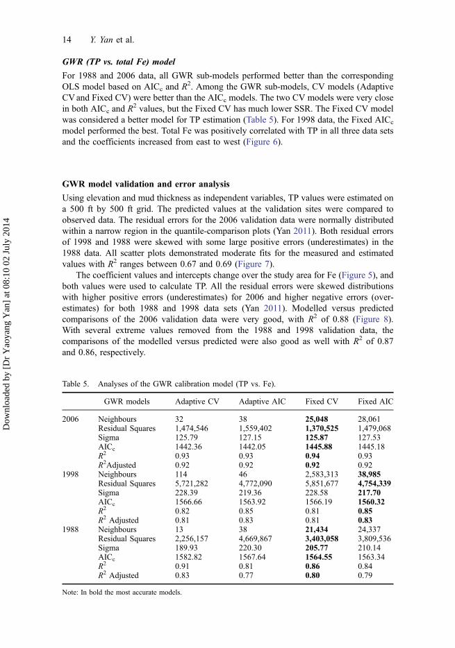
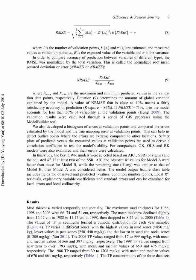
GWR (TP vs. total Fe) model

For 1988 and 2006 data, all GWR sub-models performed better than the correspondingOLS model based on AICc and R2. Among the GWR sub-models, CV models (AdaptiveCVand Fixed CV) were better than the AICc models. The two CV models were very closein both AICc and R2 values, but the Fixed CV has much lower SSR. The Fixed CV modelwas considered a better model for TP estimation (Table 5). For 1998 data, the Fixed AICc

model performed the best. Total Fe was positively correlated with TP in all three data setsand the coefficients increased from east to west (Figure 6).

GWR model validation and error analysis

Using elevation and mud thickness as independent variables, TP values were estimated ona 500 ft by 500 ft grid. The predicted values at the validation sites were compared toobserved data. The residual errors for the 2006 validation data were normally distributedwithin a narrow region in the quantile-comparison plots (Yan 2011). Both residual errorsof 1998 and 1988 were skewed with some large positive errors (underestimates) in the1988 data. All scatter plots demonstrated moderate fits for the measured and estimatedvalues with R2 ranges between 0.67 and 0.69 (Figure 7).

The coefficient values and intercepts change over the study area for Fe (Figure 5), andboth values were used to calculate TP. All the residual errors were skewed distributionswith higher positive errors (underestimates) for 2006 and higher negative errors (over-estimates) for both 1988 and 1998 data sets (Yan 2011). Modelled versus predictedcomparisons of the 2006 validation data were very good, with R2 of 0.88 (Figure 8).With several extreme values removed from the 1988 and 1998 validation data, thecomparisons of the modelled versus predicted were also good as well with R2 of 0.87and 0.86, respectively.

Table 5. Analyses of the GWR calibration model (TP vs. Fe).

GWR models Adaptive CV Adaptive AIC Fixed CV Fixed AIC

2006 Neighbours 32 38 25,048 28,061Residual Squares 1,474,546 1,559,402 1,370,525 1,479,068Sigma 125.79 127.15 125.87 127.53AICc 1442.36 1442.05 1445.88 1445.18R2 0.93 0.93 0.94 0.93R2Adjusted 0.92 0.92 0.92 0.92

1998 Neighbours 114 46 2,583,313 38,985Residual Squares 5,721,282 4,772,090 5,851,677 4,754,339Sigma 228.39 219.36 228.58 217.70AICc 1566.66 1563.92 1566.19 1560.32R2 0.82 0.85 0.81 0.85R2 Adjusted 0.81 0.83 0.81 0.83

1988 Neighbours 13 38 21,434 24,337Residual Squares 2,256,157 4,669,867 3,403,058 3,809,536Sigma 189.93 220.30 205.77 210.14AICc 1582.82 1567.64 1564.55 1563.34R2 0.91 0.81 0.86 0.84R2 Adjusted 0.83 0.77 0.80 0.79

Note: In bold the most accurate models.

14 Y. Yan et al.

Dow

nloa

ded

by [

Dr

Yao

yang

Yan

] at

08:

10 0

2 Ju

ly 2

014

Model comparison and TP mass calculations using optimal models

In addition to GWR models, errors of OK, OLS and RK models were determined (Table 6).For all models evaluated, the GWR models (TP vs. Fe and TP vs. Th & Elev) had lowerRMSE and the lowestME for TP 2006 and TP 1988 data sets (Table 6). For 1998 TP data, OKhas the lowest mean errors but higher RMSE than the OLS and GWR models.

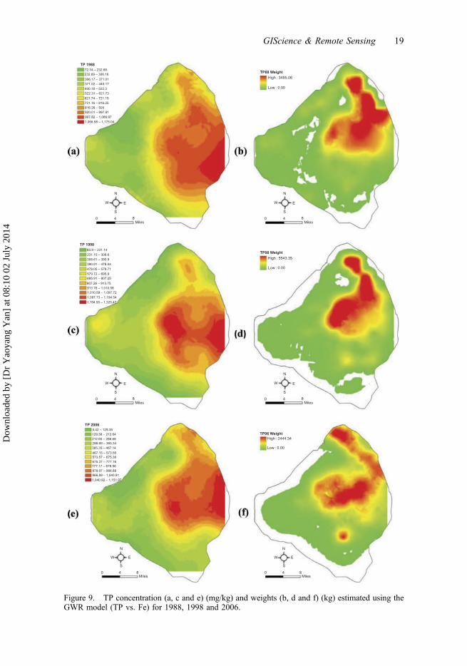
Based on model validation errors, the GWR (Fe) and GWR (Th and Elev) modelswere used for TP concentration prediction and mass calculation. For the GWR (TP vs. Fe)model, total Fe was estimated using OK for the whole lake bottom first. TP concentrations(a, c and e of Figure 9) and mass (b, d and f of Figure 9) were calculated using ArcGIStools. For the GWR (Th and Elev) model, the mud thickness raster and the lake bottom

Figure 6. Coefficient maps of the GWR model (TP vs. Fe) calibration for 1988, 1998 and 2006.

GIScience & Remote Sensing 15

Dow

nloa

ded

by [

Dr

Yao

yang

Yan

] at

08:

10 0

2 Ju

ly 2

014

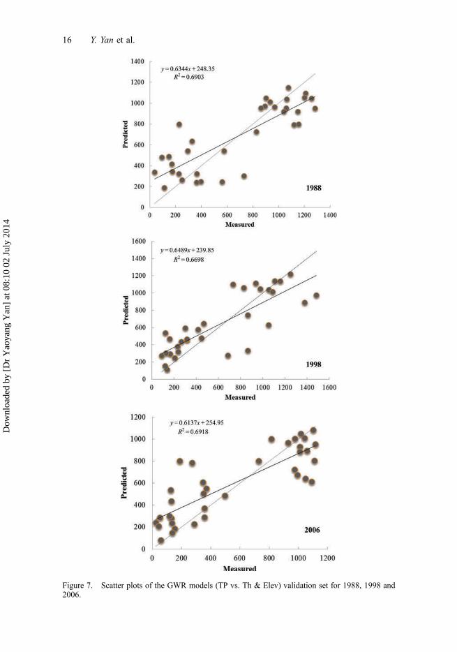
Figure 7. Scatter plots of the GWR models (TP vs. Th & Elev) validation set for 1988, 1998 and2006.

16 Y. Yan et al.

Dow

nloa

ded

by [

Dr

Yao

yang

Yan

] at

08:

10 0

2 Ju

ly 2

014

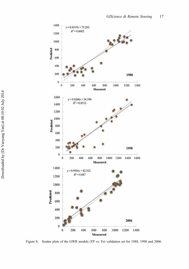
Figure 8. Scatter plots of the GWR models (TP vs. Fe) validation set for 1988, 1998 and 2006.

GIScience & Remote Sensing 17

Dow

nloa

ded

by [

Dr

Yao

yang

Yan

] at

08:

10 0

2 Ju

ly 2

014

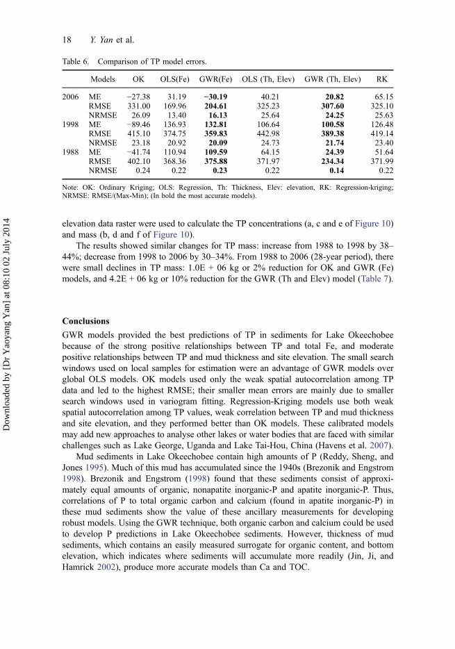
elevation data raster were used to calculate the TP concentrations (a, c and e of Figure 10)and mass (b, d and f of Figure 10).

The results showed similar changes for TP mass: increase from 1988 to 1998 by 38–44%; decrease from 1998 to 2006 by 30–34%. From 1988 to 2006 (28-year period), therewere small declines in TP mass: 1.0E + 06 kg or 2% reduction for OK and GWR (Fe)models, and 4.2E + 06 kg or 10% reduction for the GWR (Th and Elev) model (Table 7).

Conclusions

GWR models provided the best predictions of TP in sediments for Lake Okeechobeebecause of the strong positive relationships between TP and total Fe, and moderatepositive relationships between TP and mud thickness and site elevation. The small searchwindows used on local samples for estimation were an advantage of GWR models overglobal OLS models. OK models used only the weak spatial autocorrelation among TPdata and led to the highest RMSE; their smaller mean errors are mainly due to smallersearch windows used in variogram fitting. Regression-Kriging models use both weakspatial autocorrelation among TP values, weak correlation between TP and mud thicknessand site elevation, and they performed better than OK models. These calibrated modelsmay add new approaches to analyse other lakes or water bodies that are faced with similarchallenges such as Lake George, Uganda and Lake Tai-Hou, China (Havens et al. 2007).

Mud sediments in Lake Okeechobee contain high amounts of P (Reddy, Sheng, andJones 1995). Much of this mud has accumulated since the 1940s (Brezonik and Engstrom1998). Brezonik and Engstrom (1998) found that these sediments consist of approxi-mately equal amounts of organic, nonapatite inorganic-P and apatite inorganic-P. Thus,correlations of P to total organic carbon and calcium (found in apatite inorganic-P) inthese mud sediments show the value of these ancillary measurements for developingrobust models. Using the GWR technique, both organic carbon and calcium could be usedto develop P predictions in Lake Okeechobee sediments. However, thickness of mudsediments, which contains an easily measured surrogate for organic content, and bottomelevation, which indicates where sediments will accumulate more readily (Jin, Ji, andHamrick 2002), produce more accurate models than Ca and TOC.

Table 6. Comparison of TP model errors.

Models OK OLS(Fe) GWR(Fe) OLS (Th, Elev) GWR (Th, Elev) RK

2006 ME −27.38 31.19 −30.19 40.21 20.82 65.15RMSE 331.00 169.96 204.61 325.23 307.60 325.10NRMSE 26.09 13.40 16.13 25.64 24.25 25.63

1998 ME −89.46 136.93 132.81 106.64 100.58 126.48RMSE 415.10 374.75 359.83 442.98 389.38 419.14NRMSE 23.18 20.92 20.09 24.73 21.74 23.40

1988 ME −41.74 110.94 109.59 64.15 24.39 51.64RMSE 402.10 368.36 375.88 371.97 234.34 371.99NRMSE 0.24 0.22 0.23 0.22 0.14 0.22

Note: OK: Ordinary Kriging; OLS: Regression, Th: Thickness, Elev: elevation, RK: Regression-kriging;NRMSE: RMSE/(Max-Min); (In bold the most accurate models).

18 Y. Yan et al.

Dow

nloa

ded

by [

Dr

Yao

yang

Yan

] at

08:

10 0

2 Ju

ly 2

014

TP 1988

TP 1998

TP 2006

TP88 Weight72.74 – 232.68

85.9 – 231.14

4.42 – 129.35129.36 – 212.64212.65 – 286.68286.69 – 365.34365.35 – 467.14

467.15 – 573.56573.57 – 675.36675.37 – 777.16777.17 – 878.96878.97 – 966.88966.89 – 1,040.911,040.92 – 1,151.97

231.15 – 308.6308.61 – 390.9390.91 – 478.04478.05 – 579.71579.72 – 695.9695.91 – 807.25

807.26 – 913.75913.76 – 1,010.581,010.59 – 1,097.721,097.73 – 1,194.541,194.55 – 1,320.42

High : 3495.06

Low : 0.00

TP98 Weight

High : 5543.35

Low : 0.00

TP06 WeightHigh : 2444.34

Low : 0.00

N

W

S

E

0 4 8Miles

N

W

S

E

0 4 8Miles

N

W

S

E

0 4 8Miles

N

W

S

E

0 4 8Miles

N

W

S

E

0 4 8Miles

N

W

S

E

0 4 8Miles

232.69 – 306.16

306.17 – 371.01371.02 – 440.17440.18 – 522.3522.31 – 621.73621.74 – 721.15721.16 – 816.25816.26 – 920920.01 – 997.81997.82 – 1,066.971,066.98 – 1,175.04

Figure 9. TP concentration (a, c and e) (mg/kg) and weights (b, d and f) (kg) estimated using theGWR model (TP vs. Fe) for 1988, 1998 and 2006.

GIScience & Remote Sensing 19

Dow

nloa

ded

by [

Dr

Yao

yang

Yan

] at

08:

10 0

2 Ju

ly 2

014

TP 1988

TP 1998

TP 2006

TP88 Weight9.16 – 172.87

High : 4127.93

Low : 0.00

TP98 WeightHigh : 7163.74

Low : 0.00

TP06 WeightHigh : 3056.83

Low : 0.00

0 4 8

S

E

N

W

Miles

0 4 8

S

E

N

W

Miles0 4 8

S

E

N

W

Miles

0 4 8

S

E

N

W

Miles0 4 8

S

E

N

W

Miles

0 4 8

S

E

N

W

Miles

172.88 – 269.17269.18 – 346.21346.22 – 442.51442.52 – 548.44

6.33 – 161.74

5.29 – 130.39130.4 – 217.96217.97 – 293.02293.03 – 361.83361.84 – 455.66455.67 – 568.25568.26 – 674.58674.59 – 768.41768.42 – 862.24862.25 – 949.81949.82 – 1,024.871,024.88 – 1,149.97

161.75 – 275.7275.71 – 358.59358.6 – 451.83451.84 – 555.43555.44 – 690.12690.13 – 824.81824.82 – 949.13949.14 – 1,042.381,042.39 – 1,125.261,125.27 – 1,239.221,239.23 – 1,415.35

548.45 – 664664.01 – 789.19789.2 – 914.38914.39 – 1,010.681,010.69 – 1,078.091,078.1 – 1,145.51,145.51 – 1,521.07

Figure 10. TP concentration (a, c and e) (mg/kg) and weights (b, d and f) (kg) using the GWRmodel (TP vs. Th & Elev) for 1988, 1998 and 2006.

20 Y. Yan et al.

Dow

nloa

ded

by [

Dr

Yao

yang

Yan

] at

08:

10 0

2 Ju

ly 2

014

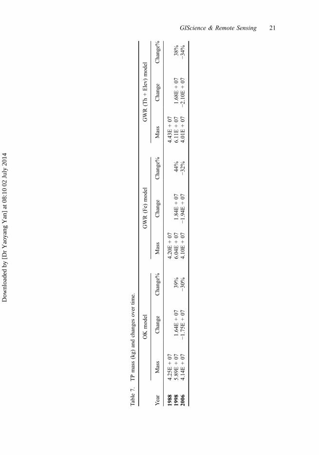
Table

7.TPmass(kg)

andchangesov

ertim

e.

OK

mod

elGWR

(Fe)

mod

elGWR

(Th+Elev)

mod

el

Year

Mass

Chang

eChang

e%Mass

Chang

eChang

e%Mass

Chang

eChang

e%

1988

4.25

E+07

4.20

E+07

4.43

E+07

1998

5.89

E+07

1.64

E+07

39%

6.04

E+07

1.84

E+07

44%

6.11E+07

1.68

E+07

38%

2006

4.14

E+07

−1.75

E+07

−30

%4.10

E+07

−1.94

E+07

−32

%4.01

E+07

−2.10

E+07

−34

%

GIScience & Remote Sensing 21

Dow

nloa

ded

by [

Dr

Yao

yang

Yan

] at

08:

10 0

2 Ju

ly 2

014

Discussion

Sediments accumulate in the central deep regions of Lake Okeechobee (Brezonik andEngstrom 1998). This is due primarily to the wind-driven gyres that are set up on the lakeand tend to deposit sediments in the deeper central areas of the Lake (Jin, Ji, and Hamrick2002). Over time this material has collected in these regions, and has been mostlyundisturbed as demonstrated from core dating using Pb210 (Brezonik and Engstrom1998) and the observance of sub-millimetre laminations in the mud sediments thatdisappeared only within the top few centimetres (Kirby, Hobbs, and Mehta 1994). Thedramatic changes in the thickness and elevation coefficients for the GWR model(Figure 5) between the 1998 and 2006 period are indicative of the three major hurricanes– Frances, Jeanne and Wilma – that passed close to the Lake on 5 September 2004, 26September 2004 and 24 October 2005, respectively. The hurricanes re-suspended a largeamount of sediment and redistributed it throughout the lake (Jin et al. 2011).

The strong positive relationship between TP and Fe is related to the binding of inorganicphosphorus to oxidized iron in the upper few centimetres of sediment (Moore et al. 1993).Moore et al. (1993) suggested that the abundance of iron in the Lake Okeechobee systemproduces conditions that control P exchange by precipitation and absorption in the upperoxic layer of sediment rather than diffusion from the anoxic sediments below. These authorsdemonstrated the process by incubating sediment cores under alternating oxic/anoxic watercolumn conditions. They found higher fluxes of P under anoxic conditions, suggesting thatoxidized Fe was controlling the rate of this flux. This indicates that more soluble P could besequestered under sediment layers with higher Fe. Because Fe is observed in regions withand without mud, it is a much better predictor than mud thickness. Fe also is better thanelevation in predicting P because it is mobile and it affects the geochemistry of P.

Moore and Reddy (1994) used a similar framework to investigate the role of pH on Pexchange from Lake Okeechobee sediments. They found that very acidic conditions (pH5.5) resulted in SRP release. However, Lake Okeechobee pH is somewhat basic (approxi-mately 8.2 – James, Smith, and Jones 1995) and the sediment pH is rather stable (7.0–7.5– Moore and Reddy 1994). Thus, pH was not a useful parameter in these GWR models.

Between 1988 and 1998 the lake received an estimated net load of phosphorus of2584 metric tons (Havens and James 2005); from 1999 to 2006 the estimated net load was1949 metric tons (James and Zhang 2008). The changes predicted by the models are muchgreater and variable than these numbers derived from nutrient budgets. The tremendousvariability among the sediment-sampled cores is also confounded by the small number ofsamples per area (less than 1 per square km). The large amount of error could account forthe differences between the net loads to the lake and net change observed in the models.By sampling more intensively in areas where large changes in TP and ancillary data occur,model accuracy could be improved and thus improve estimates of change.

Sediment–water interactions are important to the health of Lake Okeechobee. Re-suspension of the mud sediments, especially during high lake water levels, can lead toreduced submerged aquatic vegetation, which negatively affects fish recruitment (Havenset al. 2005). Diffusive phosphorus fluxes, primarily from the mud sediments, produce aninternal load that is equivalent to external loads (Fisher, Reddy, and James 2005). This canlead to delays of in-lake phosphorus in response to eternal loads (James and Pollman2011). Given a program that measures sediment content of TP and ancillary data, accurateGIS models can be developed to evaluate spatial variability on these lakes. Such informa-tion could be used to manage these lakes through targeted chemical or dredging techni-ques (Søndergaard, Jensen, and Jeppesen 2003).

22 Y. Yan et al.

Dow

nloa

ded

by [

Dr

Yao

yang

Yan

] at

08:

10 0

2 Ju

ly 2

014

AcknowledgementsThis research was supported by South Florida Water Management District. The authors wish tothank Susan Gray, Jun Han, David Unsell, Ming Chen, Kim O’Dell and Jenifer Barnes for theircomments and suggestions to the previous version of this manuscript. The authors also wish to thankthe three anonymous reviewers for their valuable comments and recommendations, which enhancedthe manuscript significantly.

ReferencesAbtew, W. 2001. “Evaporation Estimation for Lake Okeechobee in South Florida.” Journal of

Irrigation and Drainage Engineering 127: 140–147. doi:10.1061/(ASCE)0733-9437(2001)127:3(140).

BEM System, University of Florida. 2007. Lake Okeechobee Sediment Quality Final Report. WestPalm Beach: South Florida Water Management District.

Brezonik, P. L., and D. R. Engstrom. 1998. “Modern and Historic Accumulation Rates ofPhosphorus in Lake Okeechobee, Florida.” Journal of Paleolimnology 20: 31–46.doi:10.1023/A:1007939714301.

Brunsdon, C., A. S. Fotheringham, and M. E. Charlton. 2010. “Geographically WeightedRegression: A Method for Exploring Spatial Nonstationarity.” Geographical Analysis 28 (4):281–298. doi:10.1111/j.1538-4632.1996.tb00936.x.

Fisher, M. M., K. R. Reddy, and R. T. James. 2001. “Long-Term Changes in the SedimentChemistry of a Large Shallow Subtropical Lake.” Lake and Reservoir Management 17: 217–232. doi:10.1080/07438140109354132.

Fisher, M. M., K. R. Reddy, and R. T. James. 2005. “Internal Nutrient Loads from Sediments in aShallow, Subtropical Lake.” Lake and Reservoir Management 21: 338–349. doi:10.1080/07438140509354439.

Fotheringham, A. S., C. Brunsdon, and M. E. Charlton. 2002. Geographically Weighted Regression:The Analysis of Spatially Varying Relationships. Chichester: Wiley.

Gessler, P. E., I. D. Moore, N. J. McKenzie, and P. J. Ryan. 1995. “Soil-Landscape Modelling andSpatial Prediction of Soil Attributes.” International Journal of Geographical InformationSystems 9 (4): 421–432. doi:10.1080/02693799508902047.

Hastie, T. J., and R. J. Tibshirani. 1990. Generalized Additive Models. London: Chapman and Hall.Havens, K. E., D. Fox, S. Gornak, and C. Hanlon. 2005. “Aquatic Vegetation and Largemouth Bass

Population Responses to Water-Level Variations in Lake Okeechobee, Florida (USA).”Hydrobiologia 539: 225–237. doi:10.1007/s10750-004-4876-1.

Havens, K. E., and R. T. James. 2005. “The Phosphorus Mass Balance of Lake Okeechobee,Florida: Implications for Eutrophication Management.” Lake and Reservoir Management 21:139–148. doi:10.1080/07438140509354423.

Havens, K. E., K.-R. Jin, N. Iricanin, and R. T. James. 2007. “Phosphorus Dynamics at MultipleTime Scales in the Pelagic Zone of a Large Shallow Lake in Florida, USA.” Hydrobiologia 581:25–42. doi:10.1007/s10750-006-0502-8.

Hengl, T. 2009. A Practical Guide to Geostatistical Mapping. 2nd ed. Amsterdam: University ofAmsterdam.

Hurvich, C. M., J. S. Simonoff, and C. L. Tsai. 1998. “Smoothing Parameter Selection inNonparametric Regression Using an Improved Akaike Information Criterion.” Journal of theRoyal Statistical Society: Series B (Statistical Methodology) 60: 271–293. doi:10.1111/1467-9868.00125.

James, R. T., and C. D. Pollman. 2011. “Sediment and Nutrient Management Solutions to Improvethe Water Quality of Lake Okeechobee.” Lake and Reservoir Management 27 (1): 28–40.doi:10.1080/07438141.2010.536618.

James, R. T., V. H. Smith, and B. L. Jones. 1995. “Historical Trends in the Lake OkeechobeeEcosystem III. Water Quality.” Archives Hydrobiol Supplement 107: 49–69.

James, R. T., and J. Zhang. 2008. “Lake Okeechobee Protection Program – State of the Lake andWatershed.” In South Florida Environmental Report, Chapter 10, edited by G. W. Redfield andS. Efron, 10-11–10-102. West Palm Beach: South Florida Water Management District.

GIScience & Remote Sensing 23

Dow

nloa

ded

by [

Dr

Yao

yang

Yan

] at

08:

10 0

2 Ju

ly 2

014

Jin, K. R., N. B. Chang, Z. G. Ji, and R. T. James. 2011. “Hurricanes Affect the Sediment andEnvironment in Lake Okeechobee.” Critical Reviews in Environmental Science and Technology41 (sup1): 382–394. doi:10.1080/10643389.2010.531222.

Jin, K. R., Z. G. Ji, and J. H. Hamrick. 2002. “Modeling Winter Circulation in Lake Okeechobee,Florida.” Journal of Waterway, Port, Coastal, and Ocean Engineering 128: 114–125.doi:10.1061/(ASCE)0733-950X(2002)128:3(114).

Kirby, R., C. H. Hobbs, and A. J. Mehta. 1994. “Shallow Stratigraphy of Lake Okeechobee, Florida:A Preliminary Reconnaissance.” Journal of Coastal Research 10 (2): 339–350.

Knotters, M., D. Brusm, and J. Oude Voshaar. 1995. “A Comparison of Kriging, Co-Kriging andKriging Combined with Regression for Spatial Interpolation of Horizon Depth with CensoredObservations.” Geoderma 67 (3–4): 227–246. doi:10.1016/0016-7061(95)00011-C.

Loader, C. 1999. Local Regression and Likelihood. New York: Springer.Lu, Z. Y., J. Im, L. J. Quackenbush, and S. Yoo. 2013. “Remote Sensing-Based House Value

Estimation Using an Optimized Regional Regression Model.” Photogrammetric Engineering &Remote Sensing 79: 809–882.

McBratney, A. B., I. O. A. Odeh, T. F. A. Bishop, M. S. Dunbar, and T. M. Shatar. 2000. “AnOverview of Pedometric Techniques for Use in Soil Survey.” Geoderma 97: 293–327.doi:10.1016/S0016-7061(00)00043-4.

McKenzie, N. J., and P. J. Ryan. 1999. “Spatial Prediction of Soil Properties Using EnvironmentalCorrelation.” Geoderma 89 (1–2): 67–94. doi:10.1016/S0016-7061(98)00137-2.

Moore, I., P. Gessler, G. Nielsen, and G. Peterson. 1993. “Soil Attribute Prediction Using TerrainAnalysis.” Soil Science Society of America Journal 57 (2): 443. doi:10.2136/sssaj1993.03615995005700020026x.

Moore, P. A. J., and K. R. Reddy. 1994. “Role of Eh and pH on Phosphorus Geochemistry inSediments of Lake Okeechobee, Florida.” Journal of Environment Quality 23: 955.doi:10.2134/jeq1994.00472425002300050016x.

Pebesma, E. J. 2004. “Multivariable Geostatistics in S: The Gstat Package.” Computers &Geosciences 30 (7): 683–691. doi:10.1016/j.cageo.2004.03.012.

Reddy, K. R., Y. P. Sheng, and B. L. Jones 1995. “Lake Okeechobee Phosphorus Dynamics Study.”In Summary, 84. Final report submitted to the South Florida Water Management District, WestPalm Beach, Fl, Contract Number C91-2393.

SFWMD. 2014. “SFWMD Average Rainfall (30 Year: 1981-2010).” Accessed April 4, 2014. http://my.sfwmd.gov/portal/page/portal/xweb%20weather/rainfall%20historical%20%28normal%20florida%20annual%20rainfall%20map%29

Søndergaard, M., J. P. Jensen, and E. Jeppesen. 2003. “Role of Sediment and Internal Loading ofPhosphorus in Shallow Lakes.” Hydrobiologia 506–509: 135–145. doi:10.1023/B:HYDR.0000008611.12704.dd.

Sugiura, N. 1978. “Further Analysts of the Data by Akaike’s Information Criterion and the FiniteCorrections.” Communications in Statistics – Theory and Methods 7: 13–26. doi:10.1080/03610927808827599.

Tobler, W. 1970. “A Computer Movie Simulating Urban Growth in the Detroit Region.” EconomicGeography 46: 234. doi:10.2307/143141.

Yan, Y. Y. 2011. “Development of Methods for Spatial Modeling of Sediments Quality in LakeOkeechobee, Florida.” Diss., Florida International University, Miami, FL, 200.

Yan, Y. Y., and R. T. James 2007. “Spatial-Temporal Modeling of Sediments from 1988 to 2006,Lake Okeechobee, Florida.” ESRI User Conference, San Diego, CA, June 17–21.

Yan, Y. Y., and R. T. James. 2012. “Spatial Modeling of Mud Thickness and Mud WeightCalculation (1988-2006), Lake Okeechobee.” Florida Geography 43: 16–36.

24 Y. Yan et al.

Dow

nloa

ded

by [

Dr

Yao

yang

Yan

] at

08:

10 0

2 Ju

ly 2

014