Method of the Geographically Weighted Regression and an Example for its Application

ZSÓFIA FÁBIÁNa)1

Method of the Geographically Weighted Regression and an Example for its Application

Abstract

This research is concerned with a statistical method that has recently become widespread in the international literature; although, it is still limited in Hungarian research. The method is geographically weighted regression (GWR), which is demonstrated through an example of its application. GWR is a local model that is founded on the basis of regression, prominently taking into consideration the geographical distance. Since it does not calculate the global relations of the whole data, but concentrates on the relationship of the dependent and independent variables locally within a determined search area, it allows consideration of the spatially varying processes. Simply, GWR is a developed version of the global regression model, since, through its use, it is possible to take into account the local features that are hidden by the global approach.

Keywords: GWR model, local regression.

Introduction

The research is concerned with a statistical method, the geographically weighted regression (GWR) that has recently become widespread in the international literature; although, it is still limited in Hungarian research. The GWR is a local model that is founded on the basis of regression, prominently taking into consideration the geographical distance. In the first part of the study, the methodology is presented; then, the use of the method is demonstrated through an example of its application: an analysis of the local features of economic development with the help of territorial data series of GDP per capita.

Geographically weighted regression

Regression is one of the most widespread mathematical-statistical tools of social scientific researches. Its popularity is based on its essence, since this is a method which is suitable to explore the relationships between the phenomena being the key objective of research. Regression analysis means finding and describing the function that describes the stochastic relationship between two or more variables. It differs from correlation (which also examines the probability relationship between variables) insofar that correlation only indicates the existence of the relationship and does not give detailed information on it. For

a)1Hungarian Central Statistical Office, 1024 Budapest, Keleti Károly utca 5-7., Hungary, E-mail: [email protected]

REGIONAL STATISTICS, 2014, VOL 4, No 1: 61–75; DOI: 10.15196/RS04105

62 ZSÓFIA FÁBIÁN

further exploration of the relationship, another method must be used, which is in most cases regression analysis.

However, if this is applied for territorial data, it may result in a significant problem since regression examines phenomena as if they were constant over space. On the contrary, geographically weighted regression (GWA) is suitable, due to its methodology, to model spatial processes as variables, i.e. as opposed to simple regression; GWA can solve the problem of how continuous territorial processes can be examined with the help of discrete weighting (Figure 1).

The logic of GWR is most similar to that of the moving window regression. With the help of the moving window regression, the problem that processes do not end at the borders of territorial units can be solved. Its methodology is as follows: the first step is to stretch the grid of regression points for the study area. As a result, a region/window can be determined around each regression point, which is generally a square or a circle, although theoretically it could be any shape that is suitable to cover the space, i.e. to include all points examined. Depending on the problem examined, it is possible to determine what the certain region is (e.g. squares around a regression point). The regression model is based on the different data points in the regions created around the regression points, and the process is repeated in case of each regression point. By mapping the received local parameter estimates, the non-stationary assumption can be examined (Fotheringham–Brunsdon–Charlton 2002).

The main problem of this method is that spatial processes, which can be considered continuous, are not handled as continuous. Namely, it gives a weight of 1 for data points within the region/window and a weight of 0 for those outside the region/window, which may seem arbitrary in case of continuous phenomena. The result largely depends on the size of the region/window, and, due to the fewer regression points at the edges and in the lack of measures eliminating this problem, it is also biased. In the case of GWR, each data point within a defined distance has to be weighted with its distance from the regression point. Thus, data points nearer to the regression point will have a larger weight in the model than those which are farther away (Fotheringham–Brunsdon–Charlton 2002).

Figure 1

Spatial kernel

Source: Fotheringham–Brunsdon–Charlton 2002, p. 44.

Regression point Data point

x Regression point wij The weight of j data point in i regression point Data point dij The distance between I regression point and j data point


METHOD OF THE GEOGRAPHICALLY WEIGHTED REGRESSION AND AN EXAMPLE FOR ITS APPLICATION 63

It is possible to apply a fixed spatial kernel (Figure 2). In this case, regarding one regression point, the data point coinciding with the regression point will have the largest weight. This maximum weight is continuously decreasing by the increase in the distance between the two points (regression point and data point). With this method, the regression model will be local in a way such that the regression point is moving in the study area. Since the weight of the data point is different in each area, local calculations are completely different. Mapping these local calculations will provide the surface including parameter estimates. In most cases, the result of GWR is not sensitive to weighting, but is sensitive to the bandwidth/diameter used for weighting. Therefore, its optimal definition is especially important in case of each examination. When comparing this with the moving window regression, it can be said that, due to the difference in the kernels, GWR gives a less even picture and shows more local differences, thus, in case of continuous phenomena its application is more realistic (Fotheringham–Brunsdon–Charlton 2002).

Figure 2

GWR with fixed spatial kernel


This means in practice that points within a circle of a certain radius from the point examined are taken into account with a weight continuously decreasing the further they are from the starting point. The radius of the circle is determined by the scale of the examination, but more than one possibility is usually tested.

Also, in case of GWR with a fixed spatial kernel, the problem arises that there are some parts of the area where data points are much more sparsely located, and so, the local models estimated from them also have a greater random error. In extreme cases, the estimation of some parameters is impossible due to the low number of data. This problem can be solved by applying an adaptive kernel (Figure 3). Its distinctive feature is that its bandwidth can adapt to the number and density of data points, i.e. it will be narrower where the data are denser and wider where the data is sparse. In respect of the settlement network of Hungary, the difference between the settlement density of the Great Plain and Transdanubia is a good example for the necessity of applying the adaptive kernel. Comparing a map with a fixed kernel with that prepared with an adaptive kernel, the picture is very similar, with the difference that the map with an adaptive kernel is more even. The reason for this is that, in

x Regression point Data point


64 ZSÓFIA FÁBIÁN

case of local models calibrated from fewer points, greater variability is expected (Fotheringham–Brunsdon–Charlton 2002).

The simplest way of performing an examination with an adaptive kernel in practice is to setup the regression models on the basis of a certain number of nearest neighbours to the points.

Figure 3

GWR with adaptive kernel


This method can be imagined so that so many different regression equations/estimates are available as the number of territorial units. Namely, the regression model is set up for territorial units together with its nearest neighbours selected in a defined way, i.e. we do quasi-local calculations. GWR is a complex statistical process; some elements of autocorrelation, regression and spatial moving average calculations can be found in its application. The logic of the method is the same as that of spatial moving average: GWR with a fixed spatial kernel is similar to moving average with a constant radius, while GWR with an adaptive kernel to that with a varying radius (Dusek 2004).

Although this method was described for point-like units of observation, it can be applied for larger territorial units, which can be marked as a point; this has been shown by numerous examples in the scientific literature (e.g. Chasco–García–Vicéns 2007, Eckey–Kosfeld–Türck 2007, Yu 2005).

The equation of the geographically weighted regression (Fotheringham–Brunsdon–Charlton 2002) is:

yi = β0(ui,vi)+∑k βk(ui,vi) xik+εi where (ui,vi) is the geographical coordinates of point i and βk(ui,vi) is the calculated value of the continuous function βk(u,v) in point i.

The essence of GWR is that it handles the regression coefficient as a function of location and not as a fixed constant value (Yu 2005). GWR expands the framework of global regression so that it allows the local estimation of parameters (Bálint 2010).

x Regression point Data point



Weighting options

The weighting options of fixed kernels: the shape and the extension of the kernel is unchanged during the examination.

wij = 1 each i,j where j is a point in the space where the observation was made and i is a point in the space whose parameter was estimated (Fotheringham–Brunsdon–Charlton 1996).

This approach is used in the global model, as the weight of every element is the same. A possible shift towards taking into account locality is if, outside a certain distance

from the regression point, some elements are not taken into account. This is equivalent with the case if these have a weight of 0. This approach is used in case of moving window regression:

wij = 1 if dij < d wij = 0 otherwise

This weighting method makes the calculation simpler, since at the single regression points, the further calculation should be made only with the subset of the data points. The problem of this kind of weighting is that spatial processes, which can be considered continuous, are not handled as continuous ones. As the regression point changes, the coefficient may drastically change according to whether the data point moved into or out from the “window” (Charlton–Fotheringham–Brunsdon 1997).

A possible solution to this problem, i.e. that the weights are not continuous, is to determine a wij matrix which derives from the function of the continuous distance dij (between i point and j point):

wij = exp [–½(dij/b)2] where b is the bandwidth. If the i point and j point coincide, since the i point may also be a point of observation, the data will have a per unit weight at this point and the weight of the other data points will decrease according to the Gaussian Curve as the distance between i and j points is increasing (Fotheringham–Brunsdon–Charlton 1998).

Another possibility is that a kernel uses the function b2: wij = exp [1 – (dij/b)2]2 if dij < b

wij = 0 otherwise. This is useful since it is a continuous, near Gaussian weight function to distance b from

the regression point and has 0 weight at data points beyond b (Fotheringham–Brunsdon–Charlton 1998).

Turning to the presentation of adaptive kernels, there are further reasons for their use. First, where data points are densely located, it is possible to examine the changes of the relation within a relatively small distance, which would otherwise remain ignored in case of using a fixed kernel. In an area where data points are sparsely located, the value of estimated standard errors may be high when using fixed kernels since the number of used data points is low.

There are at least three types of adaptive kernels that can be applied for calculating GWR. According to the first one, the data points should be arranged in series depending on their distance from each i point:

wij = exp – (Rij/b),


66 ZSÓFIA FÁBIÁN

where Rij is the rank number of point j from point i, i.e. the distance of j from i. The weight of the data point nearest to i is 1, and the weights are decreasing by the increase in the rank number. This will automatically reduce the bandwidth of the kernel in areas where there are many data, since, by taking the 10 nearest data points, the distance will be smaller than in the case of a regression point in a region comprising only a few data points (Fotheringham–Brunsdon–Charlton 2002).

Another, more complicated way to create an adaptive kernel is to define that the sum of weights is constant, C at any i point. In areas where data points are densely located, the kernel has to be shrunk so that the sum of the weights is the defined C, while the kernel will be wider where there are fewer points.

Σj wij = C for each i With this method, to define optimal C may cause difficulty. Defining C can be done as

follows: first an optional value has to be defined; the weight function has to be created with this value and a goodness-of-fit test has to be run for the model. Then, another C value has to be chosen, the weight function has to be created, the goodness-of-fit test has to be run again and these two steps must be repeated until the optimally fitting C values are found (Fotheringham–Brunsdon–Charlton 2002).

As a third possibility, taking into account the N number of nearest neighbours can be considered.

wij = 1 if j is one of the N nearest neighbours of i wij = 0 otherwise

or wij = [1 - (dij/b)2]2 if j is one of the N nearest neighbours of i, and b is the distance of

the n nearest neighbour wij = 0 otherwise.

In this case, the calibration of the model also involves the definition of N. Namely, N means the number of those data points which are included in the calibration of the local model, and the weight function determines the weight of each point to N. The weights converge to 0 (Fotheringham–Brunsdon–Charlton 2002).

To define the optimal diameter of the kernel

One option is to minimize the value of z as follows: z = ∑ [yi - ŷi (b)]2

where ŷi is the estimated value of the dependent variable, by using b diameter. In order to get this estimated value, the estimation of the βk(ui,vi) values at each data point and the x values are needed. In a general case, the problem may arise that, if the value of b is too small, the value of the other points except for i will become negligible by the weighting. As a result, the estimated value will be very similar to the original one at the selected points, and so the equation will equal 0 as well. Therefore, the parameters of such a model cannot be determined in some cases, and the estimation will change in space so that there will be locally appropriate estimated values at each regression point (Fotheringham–Brunsdon–Charlton 2002).

In order to eliminate this, the extension of the above correlation is needed. The cross-validation applied also in case of local regressions is necessary:



CV = ∑ [yi - ŷ≠i (b)]2 where ŷ≠i is the estimated value of the dependent variable if i point is left out of the calibration. This is a good solution since, if the value of b is small, the model will be based on points close to point i and not on point i itself (Fotheringham–Brunsdon–Charlton 2002).

Another possibility to define the optimal diameter of the kernel is the application of the Akaike information criterion (AIC) and the Schwarz criterion (SC). The indicators combine the error of fitting with the complexity of the model. The more complex the model and the more explanatory variables it contains, the more it will be penalized. The smaller the value of indicators, the more the model will fit. Consequently, that kernel diameter is the optimal with the help of which the AIC and SC values calculated for the model are minimal (Bálint 2010, Fotheringham–Brunsdon–Charlton 2002).

GWR can be widely applied, as it is utilised in economic and geographical researches alike. This is illustrated in the following examples. In the study of Yu (2005), the regional development of the wider area of Beijing was examined with GWR in terms of spatial heterogeneity. Lin, Cromely and Yang (2011) used the method for solving interpolation problems. Fotheringham, Brunsdon and Charlton (2002) set up a GWR model for London house prices in order to explore local features. Eckey, Kosfeld and Türck (2007) analysed the regional convergence of the German labour market with the help of this method. Ridefelt, Etzelmüller, Boelhouwers and Jonasson (2011), when modelling mountain permafrost, studied the existence of stationarity with the help of geographically weighted regression.

According to some opinions, the GWR method is one of the most often used local regressions, and is considered an excellent visualisation tool to present spatially varying effects (Bálint 2010). Several criticisms were expressed in connection with the method, suggesting that it cannot be considered a model, since it has rather an illustrative role, and the emphasis is not on the estimations but on the regional pattern of parameter estimates. Another disadvantage of the method is that it is sensitive to outliers, additionally, the probability of problems coming from multicollinearity is also higher than in a global regression model (Lloyd 2007, Wheeler–Páez 2010).

Local analysis of the fragmentation of regional development in Europe

With the help of an example for the application, the paper presents in which aspects the use of the GWR method is better than the use of global regression.

Beginning with defining the regional framework: the calculations refer first of all to the EU member states including Macedonia from the candidate countries. In the interest of as complete an analysis as possible, Switzerland and Norway are also included. Due to their large distance from the continent, Cyprus, Malta, as well as the overseas regions of France, Portugal and Spain are left out.

Initially, the calculations were for the NUTS-2 regions, but, when interpreting the results, it became obvious that this approach is not detailed enough, since selecting the neighbours was often difficult due to the shape of Europe. Therefore, the decision made to carry out the examinations for regional units of lower level. In respect of the European regional structure, this would unambiguously mean the use of the NUTS-3 level. However,


68 ZSÓFIA FÁBIÁN

because of the heterogeneity of the NUTS structure, the mixed use of the NUTS-2 and NUTS-3 levels was decided on. In the case of Belgium, the United Kingdom, the Netherlands, Germany and Switzerland, the NUTS-2 level, while in the case of the other countries, the NUTS-3 level (793 regions) was used. Thus, more homogeneous data series were available and the dispersion deriving from the differences in size was also reduced.

Most of the data come from the Regio database of Eurostat. Some of the data missing from the data series were supplemented from the websites of the national statistical offices while others were estimated with the help of regression on the basis of longer data series.

Some words about the calculations: The model for GDP data measured in purchasing power parity per capita was set up in 2009. The computation was made with the Matlab program on the basis of the methodological study of Fotheringham–Brunsdon–Charlton titled Geographically Weighted Regression, the analysis of spatially varying relationships, and the study of LeSage titled The Theory and Practice of Spatial Econometrics presenting the computation of some statistical methods with this program.

The dependent variable: – GDP per capita. The independent variables: – rate of economically active people, – unemployment rate, – population density, – rate of people employed in the tertiary sector.12 When interpreting the results, it is worth taking into consideration several

opportunities. There is an opportunity to examine the standardised beta values of the different regression equations, utilising this, we get an answer as to which factors have a greater role in the evolution of the phenomenon at the different territorial units (Eckey–Kosfeld–Türck 2007).

By mapping the R2 values, it can be seen how reliable the model is for the different territorial units and what the spatial relevance of the models is (Xiaomin–Shuo-sheng 2011).

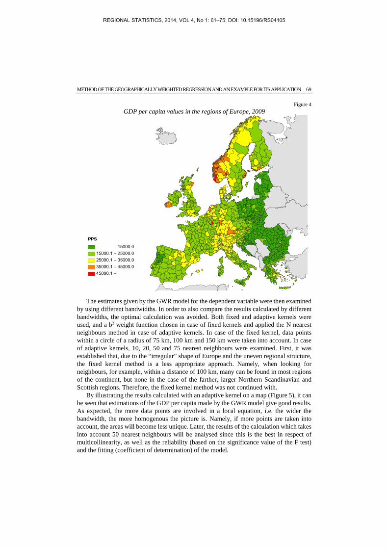
It is possible to compare the original values with the ones estimated with the equations. First, when examining the GDP per capita, the regions comprising the capitals or some

large cities are in a more favourable situation (Figure 4). In addition, a central area with high GDP/capita values is outlined, which comprises first of all regions in Southern Germany, Switzerland and Northern Italy. Furthermore, due to her significant revenue from petroleum and low-population number, Norway also has outstandingly high values. The most backward regions in this respect are those in the new member states that acceded to the EU in 2004 and 2007.

12As a starting point, an OLS model was set up in order to see which indicators have an influence on the GDP/capita. The computations carried out with the SPSS program, Regression/Stepwise method. This method was used, since, after defining the dependent and independent variables, the program creates the most optimal regression model.



Figure 4

GDP per capita values in the regions of Europe, 2009

The estimates given by the GWR model for the dependent variable were then examined by using different bandwidths. In order to also compare the results calculated by different bandwidths, the optimal calculation was avoided. Both fixed and adaptive kernels were used, and a b2 weight function chosen in case of fixed kernels and applied the N nearest neighbours method in case of adaptive kernels. In case of the fixed kernel, data points within a circle of a radius of 75 km, 100 km and 150 km were taken into account. In case of adaptive kernels, 10, 20, 50 and 75 nearest neighbours were examined. First, it was established that, due to the “irregular” shape of Europe and the uneven regional structure, the fixed kernel method is a less appropriate approach. Namely, when looking for neighbours, for example, within a distance of 100 km, many can be found in most regions of the continent, but none in the case of the farther, larger Northern Scandinavian and Scottish regions. Therefore, the fixed kernel method was not continued with.

By illustrating the results calculated with an adaptive kernel on a map (Figure 5), it can be seen that estimations of the GDP per capita made by the GWR model give good results. As expected, the more data points are involved in a local equation, i.e. the wider the bandwidth, the more homogenous the picture is. Namely, if more points are taken into account, the areas will become less unique. Later, the results of the calculation which takes into account 50 nearest neighbours will be analysed since this is the best in respect of multicollinearity, as well as the reliability (based on the significance value of the F test) and the fitting (coefficient of determination) of the model.

PPS – 15000.015000.1 – 25000.025000.1 – 35000.035000.1 – 45000.045000.1 –


70 ZSÓFIA FÁBIÁN

Multicollinearity was examined with the help of a Red indicator; the value of which can be between 0 and 1, and the closer it is to 0, the smaller the effect of multicollinearity is (Kovács 2008b). The Red indicator examines the considerable co-movement of the explanatory variables and the redundancy of data based on the dispersion of their eigenvalues. Its formula is:

Red = vλ /√(m – 1) where vλ is the relative dispersion of eigenvalues, m is the number of elements. In the case of maximum redundancy, the value of the indicator is 1, while in case of complete absence of redundancy it is 0 (its value can be given in percentage as well).

Figure 5

GDP per capita estimated by an adaptive kernel taking into account a certain number of neighbours defined by GWR

PPS – 15000.015000.1 – 25000.025000.1 – 35000.035000.1 – 45000.045000.1 –

75 neighbours 50 neighbours




Following this, the R2 values of the local equations were mapped in order to examine their geographical relevance (Figure 6). When analysing the maps, the first point to be established is that the explanatory power of the models decreased by the increase of the bandwidth. This is in line with the expected results since the more neighbours/elements are taken into account, the larger the number of those which are included in the model but have no actual effect on the GDP per capita of the initial region. The new elements quasi “ruin” the original model. Thus, the more territorial units are included, the more the local characteristics are neglected, and the global nature strengthens. On the other hand, the more neighbours the equations are based on, the more homogeneous the picture is. It can also be observed that, taking into account more and more neighbouring regions, correlations relating to territorial units in peripheral areas become less and less reliable. In respect of the R2 values of the calculation taking into account only 50 neighbours, in the case of regions in Southern Norway, Denmark, Romania, Greece, Southern Italy and some regions in Northern Germany and Spain, the explanatory force of the models is lower than in the case of other regions. This may result first of all from the fact that these territorial units are peripherally located. Thus, the regression equations were not setup on the basis of neighbours actually associated with them. In respect of the R2 values, it is important to mention that correlations between variables are not equally true for each region; in some of them, the correlation is closer to the trend throughout Europe, while in others, the fitting is more uncertain.

When setting up a global regression model, with the help of the standardised beta values, the strength of the effect of the different independent variables on the dependent variable is defined, i.e. which explanatory variable has the strongest impact on the result variable. This approach can also be applied in case of GWR models. However, in this case, since there are as many regression equations as the number of territorial units, we can say which variable has the greatest impact so that we select in each equation which indicator has the greatest role and combine them. This was examined in the present study (GWR taking into account 50 neighbours), and as opposed to the results expected on the basis of the global model (Table 1), in the local equations, not the rate of people employed in the tertiary sector but the unemployment rate influences the income per capita the most. The reason for the difference may be that the OLS estimation, in the absence of independence error structure, might have led to biased estimations (Moran I value is 0.380).

Seeing the results of the global regression (OLS) and the GWR, we can say that local relationships sometimes significantly differ from the global ones. Later, it will be obviously visible that, on a global level, the impact of an independent variable on the GDP per capita is only positive, while, on a local level, it can be positive or negative alike, i.e. the sign in the local model may differ from that in the global one (Shaoming–Huaqun 2010).


72 ZSÓFIA FÁBIÁN

Table 1

Results of the multivariable global regression (OLS)

Unstandardised coefficients Standardised coefficient

t Sig.

B standard error Beta

Constant –17838.8 1824.1 –9.8 0.0

Rate of people employed in the tertiary sector

383.3

16.7

0.536

23.0

0.0

Rate of economically actives 304.1 26.2 0.264 11.6 0.0

Unemployment rate –408.5 40.2 –0.230 –10.2 0.0

Population density 2.0 0.2 0.237 10.1 0.0

By mapping the beta and standardised beta values, we can examine the impact of the different explanatory variables on the dependent variable (Figure 7, due to the considerable similarity, it was thought sufficient to present only the maps of the beta values). Thus, the GWR coefficients show the regional pattern of the impact of different explanatory variables on the GDP per capita, with the difference that beta values show the direction and strength of the relationship between the dependent and the independent variable in the original unit of measurement, while standardised beta values show them in a standardised, i.e. comparable way (Shaoming–Huaqun 2010). Examining the different beta values, in general, in respect of explanatory variables, the values of peripheral areas were negative, while those of central areas were rather positive. This is mainly the opposite in case of the unemployment rate. The reason for this is that the meaning of changes in the unemployment rate is just the opposite of that of the others (any increase has a negative effect in the case of unemployment rate).

When separately examining the different regression coefficients, a quite homogeneous picture can be seen in the case of population density. At most territorial units, the GDP/capita changes in the same direction as the change in the value of population density except for some regions in Spain, Poland, Estonia and Greece. The impact of population density on the state of development is the strongest in the regions in Southern France, Eastern Spain and some regions of Norway and Sweden. In respect of the beta values of the unemployment rate, the values of some regions in Portugal, Spain, Southern France and Southern Greece show the same direction, while the central regions show an opposite one. The strongest influencing effect can be seen in North-western Spain, Southern Norway, Central Sweden and Central Germany. In the case of regression coefficients of economic activity, a co-movement of opposite direction can be observed in the Eastern peripheral regions, in regions in Portugal-Spain and the territory of the Benelux countries, with a co-movement of the same direction in the central areas. The impact on the state of development is the strongest in the regions in Ireland, Northern England, Central Spain, Southern France, Benelux and Central Italy. Differently from the former ones, the beta values of the rate of people employed in the tertiary sector are quite various, since the effect of the opposite direction is only partly characteristic of the peripheral regions, and it can be observed in the regions of Southern France and Northern Spain. The impact on the state of development is the strongest in the regions of Northern Spain, Northern France, Ireland,



Scotland, Benelux, the Czech Republic and Estonia. When examining the maps of the standardised beta values next to each other, it can be seen which of the four explanatory variables has a stronger impact on the state of development in a given region.

When comparing the values estimated by regression equations with the original ones, the models have rather underestimated than overestimated.

Figure 6

R2 values of calculation with adaptive kernel taking into account a certain number of neighbours

R2

– 0.2500.251 – 0.5000.501 – 0.7500.751 – 0.9000.901 –

10 neighbours


20 neighbours


74 ZSÓFIA FÁBIÁN

Figure 7

Beta values of GWR calculation with adaptive kernel taking into account 50 neighbours

Summary

GWR is a local model, since it does not calculate the global relations of the whole data, but concentrates on the relationship of the dependent and independent variables locally within a determined search area, and so is also suitable for the consideration of the spatially varying processes (Mitchell 2005). Fundamentally, the GWR is a developed version of the global regression model, since with the use of it, the local features remaining hidden by the global approach can be taken into account. In the author’s opinion, the overriding result of its use is that the R2 values of the different regions show that correlations between variables are not equally true for each region. In some of them, the correlation is closer to the trend throughout Europe, while in others, the fit is more uncertain. This also confirms that the global approach conceals or may conceal local features.

Unemployment rate – (-1500.1)-1500.0 – (-1000.1)-1000.0 – (-500.1) -500.0 – 0.0 0.1 –

Population density – 0.000.01 – 2.502.51 – 5.005.01 – 7.507.51 –

Rate of economicallyactive people

– 0.0 0.1 – 200.0200.1 – 400.0400.1 – 600.0600.1 –

Rate of peopleemployed in the tertiary sector

– 0.0 0.1 – 150.0150.1 – 300.0300.1 – 450.0450.1 –



REFERENCES

Bálint, L. (2010): A kistérségi életkilátások egy modellje A GWR alkalmazása hazai példán kézirat, MFT Vándorgyűlése, Pécs.

Charlton, M. E. – Fotheringham, A. S. – Brunsdon C. (1997): The geography of relationships: an investigation of spatial non-stationarity. In: Bocquet-Appel, J-P. – Courgeau, D. – Pumain D. (ed.): Spatial analysis of biodemographic data. pp. 23–47. John Libbey Eurotext, Montrouge.

Chasco, C. – García, I. – Vicéns, J. (2007): Modeling spatial variations in household disposable income with Geographically Weighted Regression. MPRA paper No. 9581, Madrid, Universidad Autónoma de Madrid.

Dusek, T. (2004): A területi elemzések alapjai ELTE Regionális Földrajzi Tanszék, Budapest. Eckey, H-E. – Kosfeld, R. – Türck, M. (2007): Regional Convergence in Germany: a Geographically Weighted

Regression Approach. Spatial Economic Analysis 2 (1): 45–64. Fotheringham, A. S. – Charlton, M. E. – Brunsdon, C. (1996): The geography of parameter space: an investigation

into spatial nonstationarity International Journal of GIS 10 (5): 605–627. Fotheringham, A. S. – Brunsdon, C. – Charlton, M. E. (1998): Geographically weighted regression: a natural

evolution of the expansion method for spatial data analysis. Environment and Planning A 30 (11): 1905–1927.

Fotheringham, A. S. – Brunsdon, C. – Charlton, M. E. (2002): Geographically Weighted Regression, the analysis of spatially varying relationships University of Newcastle, Newcastle.

Kovács, P. (2008): A multikollinearitás vizsgálata lineáris regressziós modellekben, A PETRES-féle Red-mutató vizsgálata Doktori értekezés, Szegedi Tudományegyetem Gazdaságtudományi Kar, Közgazdaságtudományi Doktori Iskola, Szeged.

LeSage, J. P. (1999): The Theory and Practice of Spatial Econometrics Department of Economics, University of Toledo, Toledo.

Lin, J. – Cromley, R. – Zhang, C. (2011): Using geographically weighted regression to solve the areal interpolation problem Annals of GIS 17 (1): 1–14.

Lloyd, C. D. (2007): Local Models for Spatial Analysis CRC Press, Taylor & Francis Group, London. Mitchell, A. (2005): The ESRI guide to GIS analysis 2. Spatial measurements and statistics, CA: ESRI Press,

Redlands. Ridefelt, H. – Etzelmüller, B. – Boelhouwers, J. – Jonasson, C. (2011): Statistic-empirical modelling of mountain

permafrost distribution in the Abisko region, sub-Arctic northern Sweden. Norwegian Journal of Geography 62 (4): 278–289.

Shaoming, C. –Huaqun, L. (2010): Spatially Varying Relationships of New Firm Formation in the United States Regional Studies 45 (6): 1–17.

Xiaomin, Q. – Shuo-sheng, W. (2011): Global and Local Regression Analysis of Factors of American College Test (ACT) Score for Public High Schools in the State of Missouri. Annals of the Association of American Geographers 101 (1): 63–83.

Yu, D. (2005): GIS and Spatial Modeling in Regional Development Studies: Case Study on the Greater Beijing Area. PhD dissertation. Milwaukee, Department of Geography University of Wisconsin. http://www4.uwm.edu/gis/research/upload/danlinyucompetition04.doc (downloaded: December, 2012.).

Wheeler, D. C. – Páez, A. (2010): Geographically Weighted Regression. In. Fischer, M. M. – Getis, A. (ed.): Handbook of Applied Spatial Analysis Software Tools, Methods and Applications. Springer-Verlag, Berlin.


Method of the Geographically Weighted Regression and an Example for its Application

Documents

Transcript of Method of the Geographically Weighted Regression and an Example for its Application